American Institute of Aeronautics and Astronautics

1

Fluorescence Visualization of Hypersonic Flow over Rapid Prototype Wind-Tunnel Models

D.W. Alderfer*, P.M. Danehy†, J.A. (Wilkes) Inman‡, K.T. Berger§, G.M. Buck** NASA Langley Research Center, Hampton VA, 23681-2199

R. J. Schwartz†† Swales Aerospace, Hampton VA, 23681-2199

Reentry models for use in hypersonic wind tunnel tests were fabricated using a stereolithography apparatus. These models were produced in one day or less, which is a significant time savings compared to the manufacture of ceramic or metal models. The models were tested in the NASA Langley Research Center 31-Inch Mach 10 Air Tunnel. Most of the models did not survive repeated tests in the tunnel, and several failure modes of the models were identified. Planar laser-induced fluorescence (PLIF) of nitric oxide (NO) was used to visualize the flowfields in the wakes of these models. Pure NO was either seeded through tubes plumbed into the model or via a tube attached to the strut holding the model, which provided localized addition of NO into the model’s wake through a porous metal cylinder attached to the end of the tube. Models included several 2-inch diameter Inflatable Reentry Vehicle Experiment (IRVE) models and 5-inch diameter Crew Exploration Vehicle (CEV) models. Various configurations were studied including different sting placements relative to the models, different model orientations and attachment angles, and different NO seeding methods. The angle of attack of the models was also varied and the location of the laser sheet was scanned to provide three-dimensional flowfield information. Virtual Diagnostics Interface technology, developed at NASA Langley, was used to visualize the data sets in post processing. The use of calibration “dotcards” was investigated to correct for camera perspective and lens distortions in the PLIF images. Lessons learned and recommendations for future experiments are discussed.

I. Introduction he use of stereo lithography to rapidly build wind-tunnel test articles can potentially shorten the design cycle for future hypersonic vehicles. Steel wind tunnel models are relatively expensive and typically take months to

manufacture. Ceramic wind tunnel models are generally less expensive but still typically take weeks to produce. Plastic models, by contrast, can be produced using stereolithography in one day or less. These models are typically used as templates for cast ceramic models, which are used in conjunction with the phosphor thermography method.1 However, if test durations are kept short, the plastic models themselves can be used for wind tunnel testing. A significant advantage of using these plastic models for tests requiring gas seeding is that they can be manufactured with internal plenums and ducting at no additional cost or delay. The internal ducting can be used to channel a tracer gas through the model and to the surface, allowing gas to be strategically seeded into the flowfield. This paper reports the results of testing several different models manufactured with internal ducting, and compares these results to those obtained for models requiring external seeding. During the tunnel runs, nitric oxide (NO) was injected into the flowfield, either through internal ducting, or via an externally mounted 1/8-inch stainless steel delivery tube. A portable planar laser-induced fluorescence (PLIF) system passed a laser sheet into the flowfield * Research Scientist, Advanced Sensing and Optical Measurement Branch, MS 493 † Research Scientist, Advanced Sensing and Optical Measurement Branch, MS 493, AIAA Associate Fellow. ‡ PhD Student, Department of Physics, College of William and Mary, Williamsburg ,VA and NASA Graduate Co-op Student, Advanced Sensing and Optical Measurement Branch, MS 493, AIAA Student Member. § Research Scientist, Aerothermodynamics Branch, MS 408A, AIAA Member. ** Research Scientist, Aerothermodynamics Branch, MS 408A. †† Senior Research Engineer, MS 493, NASA Langley Research Center

T

https://ntrs.nasa.gov/search.jsp?R=20070005163 2018-07-14T04:53:34+00:00Z

American Institute of Aeronautics and Astronautics

2

that excited fluorescence from the seeded NO. The fluorescence intensity was recorded by an intensified CCD camera. In the past, viewing wake flows behind wind tunnel test articles has proven very difficult—if not impossible—because the low density in such regions is not conducive to the use of schlieren (a more readily available flow visualization technique), owing to schlieren’s lack of sensitivity at these conditions. PLIF now provides a viable means of visualizing such wake flows. PLIF images provide two-dimensional visualization of planar regions of the flow in real time. By sweeping the laser sheet through the flow, three-dimensional visualizations can be obtained by post processing using Langley-developed Virtual Diagnostics Interface (ViDI) technology. In addition to using these rapid prototyping models, dotcards (flat imaging targets with a regular pattern of square dots) have been implemented in these experiments. The use of dotcards was suggested in previous work2,3 as a major potential improvement when applying PLIF to study hypersonic flows. The acquisition of dotcard images allowed perspective and lens distortions to be corrected and allowed the PLIF images to be accurately scaled. Another innovation of the current work is that flow streamlines could be visualized by seeding various ports in the model and sweeping the laser sheet.

II. Experimental Description The experiments were performed in the 31-Inch Mach 10 Air Tunnel at the NASA Langley Research Center.

The test apparatus consisted of three main components: the test articles, the wind tunnel facility and the PLIF system, each of which is detailed below.

A. Test Articles The test articles used in the present experiment were manufactured at NASA Langley Research Center in a

stereolithography apparatus (SLA). This machine uses a scanning laser beam to construct solid three-dimensional shapes from a liquid resin bath. The shapes can be arbitrary and are determined directly from CAD input files supplied by the model designer. Two different SLA materials were used in this experiment: a conventional material (Accura® SI 10 Material from 3D Systems) and a high-temperature nanocomposite material (NanoFormTM 15120 from DSM Somos). The Accura® SI 10 Material has a glass transition temperature of 62 °C (143 °F) and a heat deflection temperature of 56 !C at 0.455 MPa (133 !F at 66 psi).4 In contrast, NanoFormTM 15120 has a glass transition temperature of 80 !C (176 !F) and a heat deflection temperature of 269 !C at 0.455 MPa (517 !F at 66 psi).5 However, these yield temperatures are well below the typical 727 !C (1341 °F) stagnation temperature of the present wind tunnel, so short tunnel runs are required to avoid damage to the models. Since the SLA process does not result in a smooth polish, some hand working of the models is required prior to optional coating and use in the wind tunnels.

Various coatings were used on these models, though some were uncoated. Some were painted black using a high-temperature black paint from Krylon® which can withstand temperatures up to 649 !C (1200 !F) intermittently and up to 316 !C (600 !F) continuously, according to the manufacturer.6 Others were coated with graphite using Formkote T50 dry lubricant from E/M® Corporation which is rated for use up to 816 !C (1500 !F).7 Another coating applied was a high temperature boron nitride aerosol lubricoat from ZYP® Coatings, Inc, which is rated for use up to 1000 !C (1832 !F),8 which was applied either over a layer of graphite paint or straight onto the substrate. A main goal of applying these coatings was to prevent rapid oxidation of the model surface during tunnel runs.

(1) IRVE Models. The Inflatable Reentry Vehicle Experiment (IRVE) is a flight test that is designed to demonstrate various aspects of inflatable technology during Earth reentry. IRVE is expected to be launched from a sounding rocket at the NASA Wallops Flight Facility. In its inflated state, the vehicle forebody is a sphere-cone with a 60-degree half angle. It is designed to inflate to a diameter of 3.0 m near apogee and then reenter the atmosphere. The vehicle aft-body has a cylindrical instrument pod that extends out from the back of the heat shield into the wake flowfield. The IRVE wind tunnel models tested herein are roughly based on this design and have diameters of 50.8 mm (2.0 in). Several different variations of the IRVE shape were tested using two different substrates and three types of coatings (or lack thereof). Models were also constructed of the two different substrate materials described above. NO was supplied to visualize the wake flows using the two aforementioned methods. For the external seeding method, a 3.2 mm (1/8 in) diameter tube was attached to the sting and delivered NO to a 7.7 mm (0.3 in) diameter and 7.7 mm (0.3 in) length porous metal cylinder attached to the end of the tube using a high-temperature epoxy. The porous cylinder was tucked into the concave aft-body, as close to the front of the vehicle as possible. For the internal seeding method, two of the models tested had an internal plenum supplied with NO through a tube attached to the sting. The gas from the plenum exited through 41 holes, each having a diameter of 0.77 mm (0.030 in.). These holes were distributed in three concentric rings on the aft side of the heat shield, dispersing the NO evenly, so that seeding would be uniform, barring blocked passages, and flow perturbations

American Institute of Aeronautics and Astronautics

3

would be minimized. The model angle of attack (AOA) was varied from 0! to 10! for many of the runs, with the laser sheet positioned on the model centerline. For other runs, the model AOA was held constant, and the laser sheet was scanned spanwise across the model (towards or away from the camera) to provide, sliced, volumetric imaging of three-dimensional flow structures.

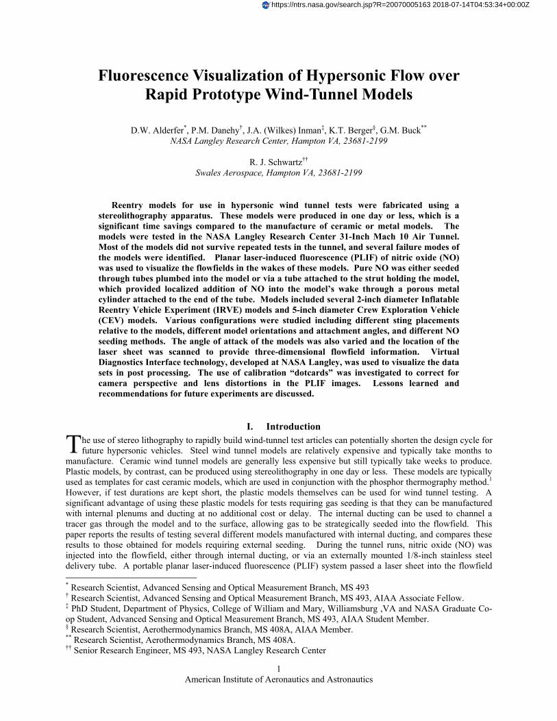
(2) CEV Models. Two different Crew Exploration Vehicle (CEV) Crew Module models were tested. The capsule shape was based on the Cycle I outer mold line (OML) of the CEV Crew Module, a blunt-body capsule with a diameter of 5.5 m (18.0 ft). During previous (unpublished) phosphor thermography testing, discrepancies were noted in the heating rates on the windward aft-body surfaces, depending on the sting placement geometry. Two 2.2% scale 127 mm (5 in) diameter models were fabricated for testing with the PLIF system to determine if PLIF could observe differences in the flowfields. The reference model OML and nominal model parameters are shown in Figure 1 and Table 1.

(a) (b) Figure 1. CEV Cycle I OML and model dimensions. The left figure (a) shows the two sting placement geometries while the right figure (b) shows the definition of terms used in the discussion.

The 5-inch diameter models were created using the rapid prototyping (SLA) process described previously. The

NanoFormTM substrate material was used because of its ability to withstand higher temperatures. The models were coated with the graphite coating described previously. The tests had a nominal AOA of 28º, the design angle of

reentry. The models were supported by 19 mm (0.75 in) diameter cylindrical stings in one of two base mounting techniques: (1) a straight sting mounted through the axis of symmetry and (2) a sting aligned 28° from the axis of symmetry in order to place the sting in the shadow of the flow (shown in Figure 1). These two sting configurations were identical to those in the previous heating test.

The straight sting model was built with 11 afterbody ports that could be seeded with NO. The 28° sting model was

Model Diameter

(in)

Base Diameter

(in)

Model Nose Radius

(in)

Sting Diameter

(in)

Base/Sting Diameter

M6 Sting Length/

Diameter

M10 Sting Length/

Diameter 5” Straight Sting 5 1.53 6.0 0.75 2.04 8.0 5.33 5” 28 deg Sting 5 1.53 6.0 0.75 2.04 8.0 8.0

Table 1. Model Reference Dimensions

10987

54

32 1

6

10

9

8 7 6

5

4

32

1

111098

765

43 2 1

11

10

9

8 7 6

5

4

32

1

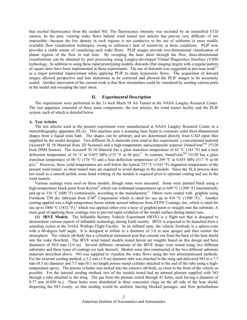
Figure 2. CEV sting configurations. (Left) The model is mounted to the sting at 28° such that the sting produces minimal interference on the windward-aft surface (ports 1 – 5). (Right) Straight sting configuration allows the addition of an eleventh seeding port. Black dots mark the location of seeding/pressure ports. Grey dots indicate the position of the seeding tubes (not shown in Fig. 1) as they enter the model.

Backshell Heat Shield

Windward

Leeward

Afterbody

Fore- Body

American Institute of Aeronautics and Astronautics

4

built with 10 afterbody ports in similar places as those on the straight sting model (one port was lost due to the location of the sting on the leeward afterbody surface). Neither model had any ports on the forebody heat shield surface. Each port was 1.5 mm (0.060 in.) in diameter at the model surface and 2.3 mm (0.090 in.) diameter at base for the NO feed lines. Each port had an individual path through the model to the base of the sting, allowing the ports to be controlled separately. Individual ports could be excluded and/or multiple NO seeding ports and mass flow rates could be utilized in a single run. For each of the models, the feed lines were located around the sting mounting location. During model installation, the NO feed lines were secured to the outside of the sting in order to minimize their effect on the base flow. Diagrams of NO port locations on the two models are shown in Fig. 2.

B. Wind Tunnel, Operating Conditions, Mass Flow Control and Data Acquisition Systems The 31-Inch Mach 10 Air Tunnel is an electrically-heated blowdown facility located at NASA Langley Research

Center in Hampton, Virginia, USA. Reference 9 details this facility, a summary of which is provided here. As the name implies, the facility has a nominal Mach number of 10 and a 31-inch square test section. The tunnel uses heated, dried, and filtered air as the test gas. The air flows from the high pressure heater, through the settling chamber, three-dimensional contoured nozzle, test section, second minimum, aftercooler and into vacuum spheres pumped by a steam ejector and/or conventional vacuum pumps. The test section is “closed,” as opposed to an “open jet” test section; large windows form three walls (including top and bottom) of the test section with the fourth wall formed by the model injection system. This window arrangement has advantages in the present experiment because the laser sheet can be directed into the test section through the top window and the NO fluorescence can be detected from the side window. Also, the ICCD camera can be placed very close to the test section windows, resulting in a working distance slightly larger than half of the test section width, allowing good magnification (~7 pixels/mm) PLIF images to be obtained without modification of the tunnel and without using exotic camera optics. Furthermore, the tunnel is equipped with windows composed of UV-grade fused silica, providing ~90% transmission at the 225 nm and higher wavelengths required for PLIF.

Test durations of up to two minutes are possible in this facility. However, for the current tests, run times were limited to avoid destroying the fragile models. The facility is capable of performing more than one run per hour, but, as will be discussed below, typically only a few runs were performed per day. The facility stagnation pressure P0 is typically varied from 2.41 MPa (350 psia) to 10.0 MPa (1450 psia) to simulate a range of Reynolds numbers.9 Two stagnation pressures were used in this experiment: 1.03 MPa (150 psia) and 2.41 MPa (350 psia), corresponding to freestream unit Reynolds numbers of 0.70 and 1.64 million per meter (0.21 and 0.5 million per foot), respectively. The test core size for the 2.41 MPa (350 psia) condition is stated to be 0.25 x 0.25 m (10 x 10 in.).9 Flow quality is considered to be worse, though it has not been fully characterized, with an even smaller test core size at the 1.03 MPa (150 psia) condition. This lower-pressure condition is not typically used in this facility. The nominal stagnation temperature was 1,000 K (1,800° Rankine) for the experiment described herein. The freestream temperatures are estimated to be 53 K (95° Rankine) for the 2.41 MPa (350 psia) condition.9 The freestream velocity is estimated to be about 1414 m/s (4640 ft/s).9 The freestream pressure was estimated to be 68 Pa (0.0099 psia) for the Po = 2.41 MPa (350 psia) condition.9

For this test, the facility was equipped with a vented and alarmed toxic gas cabinet for handling gas bottles containing nitric oxide. Our previously reported2,3 entry into this wind tunnel was considered a proof-of-concept study, so a safe but inefficient method was used to supply NO from small (~0.5 liter) cylinders. In the present study, the NO flowed from this gas cabinet through mass flow controllers and then through a stainless steel tube to the tunnel injection system where it branched into the various sting and model delivery tubing. The mass flow controllers used in this experiment had a maximum flowrate of 1 standard liter per minute (slpm) and an accuracy of ±0.75% of full scale of reading, or about 0.0075 slpm for the conditions used. Nominal flowrates used in this experiment were 0.150, 0.100, 0.075, 0.05 and 0.03 slpm. Facility and model temperatures, pressures, angles of attack, flowrates, etc. were recorded by a data acquisition system at a rate of 50 Hz.

The normal sequence of operation was to begin flowing the NO, begin the tunnel flow, and then wait until both flows stabilized. The data acquisition was then started, the model injected into the flow and the image acquisition initiated. An output signal from the intensified CCD indicated to the data acquisition system that the PLIF image acquisition had begun. A remote manual translation stage trigger could be used to start a sweep of the laser sheet across the model for three-dimensional flow visualizations.

American Institute of Aeronautics and Astronautics

5

C. Planar Laser-Induced Fluorescence (PLIF) Imaging System The PLIF system consists primarily of the laser system, beam forming optics and the detection system. The laser

system has three main components: a pump laser (Spectra Physics Pro-230-10), a tunable pulsed dye laser (Spectra Physics PDL-2), and a wavelength extender (Spectra Physics WEX). The injection-seeded Nd:YAG laser operates at 10 Hz and pumps the PDL, which contained a mixture of Rhodamine 590 and Rhodamine 610 laser dyes in a methanol solvent. The output of the dye laser and the residual infrared from the Nd:YAG are combined in a WEX, which contains both a doubling and a mixing crystal. The resulting output is tuned to a wavelength of 226.256 nm, chosen to excite the strongly fluorescing spectral lines of NO near the Q1 branch head.

A monitoring gas cell system is used to ensure that the laser is tuned to the correct spectral line of NO. The gas cell contains a low-pressure mixture of 5% NO in N2. A quartz window serves as a beam splitter and sends a small portion of the laser energy through windows on either side of the gas cell. A photomultiplier tube (PMT) monitors the fluorescence intensity through a third window at right angles to the path of the laser beam.

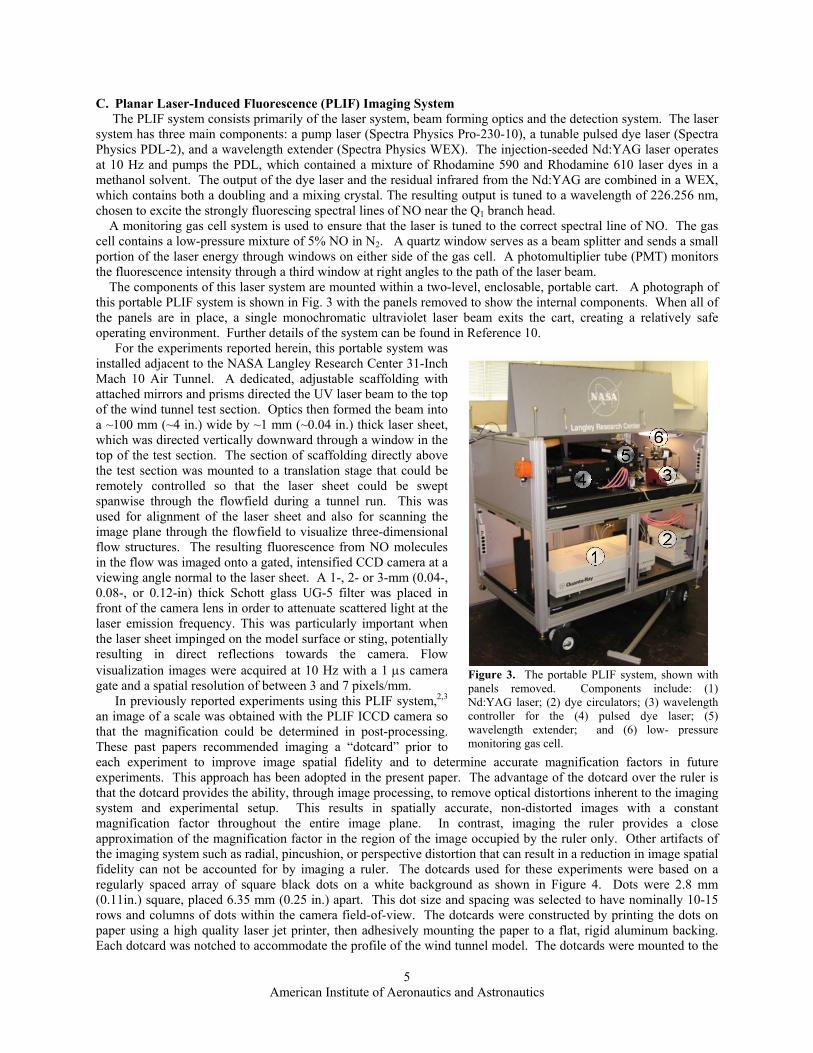
The components of this laser system are mounted within a two-level, enclosable, portable cart. A photograph of this portable PLIF system is shown in Fig. 3 with the panels removed to show the internal components. When all of the panels are in place, a single monochromatic ultraviolet laser beam exits the cart, creating a relatively safe operating environment. Further details of the system can be found in Reference 10.

For the experiments reported herein, this portable system was installed adjacent to the NASA Langley Research Center 31-Inch Mach 10 Air Tunnel. A dedicated, adjustable scaffolding with attached mirrors and prisms directed the UV laser beam to the top of the wind tunnel test section. Optics then formed the beam into a ~100 mm (~4 in.) wide by ~1 mm (~0.04 in.) thick laser sheet, which was directed vertically downward through a window in the top of the test section. The section of scaffolding directly above the test section was mounted to a translation stage that could be remotely controlled so that the laser sheet could be swept spanwise through the flowfield during a tunnel run. This was used for alignment of the laser sheet and also for scanning the image plane through the flowfield to visualize three-dimensional flow structures. The resulting fluorescence from NO molecules in the flow was imaged onto a gated, intensified CCD camera at a viewing angle normal to the laser sheet. A 1-, 2- or 3-mm (0.04-, 0.08-, or 0.12-in) thick Schott glass UG-5 filter was placed in front of the camera lens in order to attenuate scattered light at the laser emission frequency. This was particularly important when the laser sheet impinged on the model surface or sting, potentially resulting in direct reflections towards the camera. Flow visualization images were acquired at 10 Hz with a 1 "s camera gate and a spatial resolution of between 3 and 7 pixels/mm.

In previously reported experiments using this PLIF system,2,3 an image of a scale was obtained with the PLIF ICCD camera so that the magnification could be determined in post-processing. These past papers recommended imaging a “dotcard” prior to each experiment to improve image spatial fidelity and to determine accurate magnification factors in future experiments. This approach has been adopted in the present paper. The advantage of the dotcard over the ruler is that the dotcard provides the ability, through image processing, to remove optical distortions inherent to the imaging system and experimental setup. This results in spatially accurate, non-distorted images with a constant magnification factor throughout the entire image plane. In contrast, imaging the ruler provides a close approximation of the magnification factor in the region of the image occupied by the ruler only. Other artifacts of the imaging system such as radial, pincushion, or perspective distortion that can result in a reduction in image spatial fidelity can not be accounted for by imaging a ruler. The dotcards used for these experiments were based on a regularly spaced array of square black dots on a white background as shown in Figure 4. Dots were 2.8 mm (0.11in.) square, placed 6.35 mm (0.25 in.) apart. This dot size and spacing was selected to have nominally 10-15 rows and columns of dots within the camera field-of-view. The dotcards were constructed by printing the dots on paper using a high quality laser jet printer, then adhesively mounting the paper to a flat, rigid aluminum backing. Each dotcard was notched to accommodate the profile of the wind tunnel model. The dotcards were mounted to the

Figure 3. The portable PLIF system, shown with panels removed. Components include: (1) Nd:YAG laser; (2) dye circulators; (3) wavelength controller for the (4) pulsed dye laser; (5) wavelength extender; and (6) low- pressure monitoring gas cell.

American Institute of Aeronautics and Astronautics

6

sting using clamps, then carefully aligned using a precision level to ensure the dot rows were parallel to the nominal streamwise flow direction. Figure 4(a) shows a photograph of a dotcard during alignment and installation. Figure 4(b) shows the same dotcard after installation, as imaged by the PLIF camera. Care was taken to ensure the camera was not moved or otherwise physically adjusted after the dotcard images were obtained.

Acquisition of dotcard images after each model change and prior to the first test with a model has several

benefits. These are summarized in Table 2. By carefully attaching the dotcard so that it is square to the model and level in both the streamwise and spanwise directions, it can act as a reference plane for aligning the laser. Also, this allows alignment of the laser sheet with respect to a specific seeding orifice, though further fine tuning of the laser sheet position may be required for highly precise alignment. Dotcards can also be used in subsequent image processing to correct camera perspective distortion that occurs when the camera is not oriented perpendicularly to the laser sheet. This facilitates off-perpendicular camera alignments, which may be necessary to circumvent specular glints or flare caused by the laser impinging on the model or sting. Removal of perspective distortion, as well as other optical distortions inherent in the imaging system and experimental setup, is accomplished through computational “dewarping” of each dotcard image. Dewarping applies a conformal mapping to produce non-distorted images with a constant spatial resolution (e.g., mm/pixel) throughout the entire image plane. Such images are then suitable for import into the ViDI environment for further analysis and visualization. It was also hoped that the dotcards would allow accurate spatial registration of the PLIF images relative to the virtual wind tunnel models in the ViDI environment.

For tunnel runs where the laser sheet was to be scanned in the spanwise direction, dotcard images were obtained at multiple spanwise positions throughout the laser scanning range. When acquiring PLIF imagery in this mode of operation, images obtained different spanwise locations will have different spatial resolutions (higher spatial resolution when laser is closer to the camera, lower spatial resolution when laser is farther from the camera). Use of the dotcards allows for determination of, and compensation for, the different magnification. Since the dotcard was mounted to the model sting, positioning the dotcard in the spanwise direction was accomplished by advancing and retracting the model injection system to various spanwise positions within the test section. The spanwise model injection position (and hence dotcard position) was indicated by a precision position sensor on the injection system.

(a)

(b) Figure 4. Dotcard images. Image (a) was taken with a hand-held camera outside the tunnel and (b) was taken with the ICCD camera used for PLIF imaging, with the model injected into the tunnel, prior to a tunnel run. The dotcard was removed before the tunnel run.

Potential Benefit: Implemented In: Successful: Alignment of laser sheet and focus of camera

Experiment Yes

Perspective distortion Dewarping Yes Camera lens distortion Dewarping Yes Scale/magnification ViDI Yes Orientation of PLIF images relative to model

ViDI Yes

Position of PLIF images relative to model

ViDI Sometimes

Table 2. Five potential benefits of using dotcards in the present experiment.

American Institute of Aeronautics and Astronautics

7

A series of dotcard images were obtained and averaged at each dotcard location. The averaged dotcard images were then used in subsequent post-processing.

III. Analysis Methods

A. PLIF Flow Visualization Image Processing Single-shot PLIF images were processed using smoothing routines and by adding false color tables. Images

were corrected for spatial variations in laser sheet intensity, but neither the laser-sheet intensity nor spatial distribution was measured on a shot-to-shot basis. Rather, the average laser sheet spatial intensity variation has been measured by injecting NO into a near vacuum, resulting in uniform NO seeding, prior to the tunnel runs and acquiring an average of 100 PLIF images. Single-shot images were divided by this laser-sheet intensity image. To reduce noise, images were smoothed with a two-dimensional low-pass filter (MATLAB®’s “fspecial”, Gaussian or average filters) prior to additional processing. Averaged images were then sometimes created from single-shot images. In some cases, pixel values below a certain threshold were set to zero to reduce noise in the images in regions away from strong fluorescence intensity. The images were then made into bitmap images or movies for display on the model using ViDI technology as described below. To remove optical distortions due to aberrations in the camera lens and filters used, and perspective distortion due to the camera’s placement, a dewarping technology11 developed at the NASA Langley Research Center for various measurement technologies is used to process the dotcards and then the PLIF images. The dotcard processing began by defining the region of interest in the dotcard image that contained the pertinent data and the remainder of the image was masked out. Techniques such as image dilation or erosion and thresholding were used to create a binary form of the remaining dotcard image. Care was taken to ensure the geometric centroid of each dot was not altered. Since the dewarping algorithm used here required a rectangular grid of dots, it was necessary to fill in any region that was missing dots (see for example, near the model in Fig. 4) with new dots. Most regions of the image that were missing dots, such as the edges, did not contain valid flow field data. Adding dots in these regions was done using an extrapolation method. If a dot was added in a region that did contain data, care was taken to carefully place the dot, either by interpolation or extrapolation, though this did add some error into the spatial dewarping method.

When the rectangular grid of dots was complete, a centroid-finding process located the center of each of dot. The list of centroid locations was then used to dewarp the image. The images were adjusted so that each dot was equidistant from adjacent dots. Thus, a mapping from the distorted original image to a “dewarped”, non-distorted image could be computed. This was done in a bi-linear, piecewise fashion, operating on each block defined by four centroids. The end result was a file of mapping coordinates that contained the appropriate transformation coefficients for dewarping the PLIF image files.

The final step was applying the dewarping transformation to the individual PLIF images. Since the spacing of the dots on the dotcard is known, a calculation of the number of pixels per unit of distance can be computed. The data is also now appropriately formatted for inclusion into ViDI for further processing, as described in the next section. Note that in each case, the dewarping algorithm was determined from dotcards that had been placed on the model centerline (which also corresponds to the tunnel centerline). However, the dotcards obtained at different spanwise locations are dewarped as if they were PLIF images (that is, not processed as dotcard images) and were provided as inputs to the ViDI processing. These off-centerline dotcard images were used to correct for magnification changes during spanwise laser-sheet scans.

B. Virtual Diagnostics Interface (ViDI) The Virtual Diagnostics Interface (ViDI)12 is a software tool developed at NASA Langley Research Center that

provides unified data handling and interactive three-dimensional display of experimental data and computational predictions. It is a combination of custom-developed software applications and Autodesk® 3ds Max®, a commercially available, CAD-like software package for three-dimensional rendering and animation.13 Currently, ViDI technology is applied to three main areas: 1) pre-test planning and optimization; 2) visualization and analysis of experimental data and/or computational predictions; and 3) establishment of a central hub to visualize, store and retrieve experimental results.

For this experiment, ViDI was used for post-test visualization of the PLIF data. CAD (Computer Aided Design) files containing the geometry for each wind tunnel model tested were imported into the virtual environment along with the PLIF images and centerline dotcard images. The dewarped centerline dotcard images were scaled in absolute units (inches or mm) and placed adjacent to the virtual models according to the dimensions determined

American Institute of Aeronautics and Astronautics

8

from the color dotcard images taken with the hand-held camera. Then PLIF images were applied, sequentially at this same image location. In many cases, further minor spatial adjustments of the images were required to obtain realistic positions of the data relative to the wind tunnel models. To create the final output, a virtual camera was placed in the scene, and high resolution bitmaps were rendered. In addition, a series of PLIF images was imported to create animations of time-varying data.

For analysis of experiments where the laser sheet is swept spanwise across the model, additional steps are required. If no correction is applied, then images taken further from the camera have lower magnification than those obtained closer to the camera. Dotcard images obtained at the various spanwise positions are dewarped as described above, and are then imported into the program. They were placed at their correct locations as determined from the position sensor on the wind tunnel’s model-injection/retraction system, and are then scaled to absolute units at each image plane location. Finally, the software interpolates a continuous scaling between these images so that when the PLIF images are overlaid, they are correctly scaled.

IV. Results

A. Overview of the test campaign Data reported in this paper were obtained during a 26 calendar day interval in April and May 2006. This paper

reports results from about half of the days of operation. During this time, 20 tunnel runs were performed in 8 days of testing, averaging 2.5 runs per day of testing. The other calendar days or fractions of days were lost to weekends, model changes, facility maintenance, safety checks, etc. Testing in the 31-Inch Mach 10 Air Tunnel without the use of PLIF typically achieves ~6-8 runs per day during production testing, depending on the number of model changes and the operating conditions of the test. In our previous test entry using PLIF in the same facility, in which we used neither dotcards nor rapid prototyping models, we averaged 3.8 runs per day of testing.2,3 The use of PLIF decreased the efficiency of testing by nearly a factor of 2 in that test. The use of dotcards and rapid prototyping models with PLIF in the present test has further reduced this efficiency by a factor of 1.5. The lower operating rates are associated with additional time needed before and between runs. For example, waiting for the laser to warm up at the beginning of the day, changing the position and/or orientation of the laser sheet, attaching dotcard to the model and injecting it into the tunnel, focusing the camera, acquiring images, retracting the model and dotcard and removing the dotcard, etc. all add time to operations. The low durability of the rapid prototyping models required a model change (and a new dotcard image) after almost every run, severely decreasing productivity. In the discussion section below, several recommended changes that should improve run productivity are discussed.

Run No’s.

Description of Model Coating Stagnation Pressure

(psia)

Run Duration

(s)

Mode(s) of Failure

4 2” 60° IRVE (internally ducted) Accura® SLA

White 150 5.82 Coating separation; penetrating crack near stagnation point

5 2” 60° IRVE (internally ducted) Accura® SLA

Graphite 150 7.72 Surface crack vertically to right of stagnation point

9 2” 60° IRVE (porous cyl.) NanoformTM SLA Material

None 150 13.72 Burned/melted material and cracks stemming from stagnation point

10-12 2” 60° IRVE (porous cyl.). One model used over runs 10-12. NanoformTM SLA Material

Hi-temp. black paint

10) 150 11) 150 12) 350

6.64 7.08 11.58

Paint dulled at stagnation point Stress lines, increased dulling Burns & cracks at stagnation point

14-16 5” SLA CEV 28° sting mount NanoformTM SLA Material

Graphite 350 9.7 10.4 13.64

No visual damage No visual damage Cracked during cool down

37-39 5” SLA CEV Straight sting mount NanoformTM SLA Material

Graphite 350 11.48 11.36 13.82

No visible damage No visible damage No visible damage

Table 3: Summary of model failure modes. The run durations shown are for the individual runs if the model was used in several runs.

American Institute of Aeronautics and Astronautics

9

B. Model Survivability While the rapid prototype models are relatively inexpensive and easy to build, they are also relatively fragile and

are subject to cracking and/or burning under the high heating and pressure loading conditions experienced in hypersonic wind tunnels. Table 3 shows run conditions, models, coatings, and the associated model survival/failure mode for selected tunnel runs. In summary, most SLA models survived intact for run durations of 10 seconds or less at a stagnation pressure of 1.03 MPa (150 psia) (and higher in some cases) and total temperature of 1,000 K (1,800 °R). But when subject to multiple or long runs, most of the models either cracked, burned, melted, or shed their coating. A variety of different coatings and model substrates were used, with varying degrees of success.

The first three tunnel runs (Runs 1-3, not shown) used the boron nitride aerosol lubricoat coatings on solid IRVE

models made from the lower-temperature-rated Accura SLA material. All of these models showed bubbling or peeling of their coatings after single 6-10 sec. runs, particularly at the stagnation point, which is the location of maximum heating. Figure 5(a) shows a damaged 2-inch diameter IRVE model, with internal ducting, after a single

(a) (b) (c)

(d) (e) (f)

(g)

(h) (i)

Figure 5. Selected wind tunnel models used in the present experiment. Images (a)-(g) show IRVE models while (h) and (i) show the CEV model. Images (a) and (b) were obtained after Runs 4 and 5, respectively. Image (c) was obtained after Run 9. Image (d) was taken prior to Run 10, (e) was taken after Run 10, (f) was taken after Run 11 and (g) was taken after Run 12. Image (h) was obtained after Run 16. Image (i) shows a photo detail of the boxed region in (h).

American Institute of Aeronautics and Astronautics

10

tunnel run (Run 4). For this run, the white coating peeled off, revealing the underlying graphite coating. The model also suffered a penetration crack at the nose; the material at the nose was pushed into the plenum within the model, possibly by aerodynamic loading. Figure 5(b) shows an identically manufactured model, coated with graphite only, after Run 5. This model also suffered a large crack after a single run. In contrast with the damage to the Run 4 model, the material from the Run 5 model appears to have pushed away from the plenum. Since aerodynamic loads are unlikely to have caused such damage, this suggests that rapid or uneven cooling of the models may be a contributing factor to model structural failure. Alternately, the model may have failed because of a combination of aeroheating and high pressure in the plenum during the test. Figure 5(c) shows an uncoated model made of the NanoformTM material that survived intact but charred and cracked after a single, relatively long run. Since changes to the forebody such as those observed in this figure are undesirable, we decided to investigate protective coatings applied to this material.

Figure 5(d) shows an image of an IRVE model painted with high-temperature black paint, prior to Run 10. Figure 5(e) shows an image after Run 10. The nose of the 60° cone shows evidence of high temperature paint curing (dull colorization). There is also slight evidence of crack formation stemming from the tip of the nose. Figure 5(f) shows the model after Run 11. The image shows additional crack formation and more paint curing at the nose. Figure 5(g) shows the model after Run 12. This was this model’s third 10-second injection. The model experienced several radial cracks, making it unsuitable for further testing and lending uncertainty to the interpretation of the data obtained during this run. Note that variations in the color of the model in Figs. 5(d)-(g) are primarily due to changes in ambient lighting and camera flash used to obtain the photos.

Figure 5(h) shows the straight-sting CEV model after Run 16. This model survived three runs, but a crack formed on the outside edge of the model after the model had been retracted and exposed to room air after the third run. It is likely that this crack also formed because the model cooled too rapidly and nonuniformly. To remedy this, in the next series of runs, a wool cap was immediately placed over the new CEV models after retraction. This model survived three runs without damage.

At the end of the test program, the surviving CEV model was tested through a range of higher pressures and longer run times. The purpose of this was to test the material’s viability for aerothermodynamic, and if possible, longer-duration aerodynamic testing. Initially the model was tested at a stagnation pressure of 4.96 MPa (720 psia). Using the insulating wool cap, the model survived. Similarly, the model survived a 10 second run at a stagnation pressure of 8.96 MPa (1300 psia). This stagnation pressure represents the highest condition routinely tested using global phosphor thermography in the 31-Inch Mach 10 Air facility. Thus, the model survived the range of phosphor thermography conditions based on test duration, stagnation temperature and stagnation pressure.

The model was then tested at a condition and duration representative of an aerodynamic test. For such tests, durations of 60-90 seconds are common so that the angle of attack can be varied during the run. The test was completed at a pressure 2.4 MPa (350 psia) for 60 seconds at a single angle of attack. When the model was removed from the tunnel, it was immediately seen that the model had not survived these conditions. Cracks were seen on a large portion of the forebody surface, portions of the surface were melted and two small pieces of the forebody surface were missing.

C. Fluid Mechanical Results (1) IRVE Models: Wake Flowfield Visualization and Sting Interference Figure 6 shows the differences in two wake-flow visualizations of IRVE models mounted and plumbed in two

different configurations. The one on the left (Run 4) has 41 NO ports fabricated symmetrically into the leeside skin to distribute the NO uniformly. The one on the right has the single porous cylinder, with accompanying tube tucked tightly against a cylindrical peg, located on the back of the model, as shown in Fig. 4(a). In the IRVE flight vehicle, this peg is the payload, used to house instrumentation and communications equipment. The model in Fig. 6(a) was mounted with the sting directly below the model, hereafter called vertical mounting. The model shown next to it in Fig. 6(b) was mounted in a 90° clockwise orientation, when observing from the front, hereafter called horizontal mounting. The horizontal sting mounting configuration model had two advantages. First, it eliminated some scattered laser light that was problematic in the vertical sting mounting configuration. Secondly, but more importantly, it reduced the direct observation of sting interference at the bottom edge of the wake flowfield. This is evident by comparing Figs. 6(a) and (b). Figure 6(b) shows the expected smooth attachment of the lower and the upper shear layers of the wake flow to the heat shield. Furthermore, the outer edges of the shear layers on top (blue) and bottom (red) are symmetric. In Fig. 6(a), the flow on the bottom of the image is pulled towards the wake of the sting itself. Using the vertical sting mounting position highlights this effect while using the horizontal mounting minimizes observation of this effect because the sting wake is not probed by the laser sheet.

American Institute of Aeronautics and Astronautics

11

Also evident from these wake flowfields is the strikingly biased NO distribution in the wake shown in Fig. 6(b). This is in contrast to the relatively uniform top-to-bottom seeding in Fig. 6(a). The trapping of the NO gases in the lower half of the Fig. 6(b) wake is caused by recirculating gases flowing in the upstream direction along the model centerline, radially downward across the porous cylinder (where it mixes with the NO) to the edge of the model, where it meets and is entrained into the shear layer. Since the porous cylinder is located below the model centerline, the NO flows mostly below the model centerline. A small amount of NO mixes or diffuses around to the top half of the flow, thereby weakly visualizing the top wake region and shear layer as well.

Although not shown here, a comparison was made of two nearly identical, internally-plumbed models (Runs 4 and 5) to determine the effect of varying the NO flow rate on the wake flowfield. If too large of a flowrate is used, the wake flow could be significantly perturbed, evidenced by a widening of the wake flowfield. In Run 5, the flowrate was decreased by a factor of 3. The results showed mainly that there was no significant change in the flowfield, and that therefore, both flow rates were sufficiently non-perturbative.

In summary, the observation of sting wakes can be reduced by rotating the sting away from the plane of the laser sheet, i.e. locating the sting as far behind the model and laser sheet as possible. Sting effects will then be shifted to the backside of the wake flowfield, where the imaging camera will not observe their influence. Either sting orientation can be used in the future, depending on whether sting mounting effects are to be studied or whether the less-perturbed flowfield is to be studied.

(a) (b)

Figure 6: Comparison of an internally plumbed vs. an externally plumbed IRVE model: (a) shows an averaged image from Run 4, which used an internally-plumbed model that was mounted vertically; (b) shows a model in the horizontal configuration plumbed externally with tubing attached to a porous cylinder. The faded grey rectangular box shows the imaged region.

American Institute of Aeronautics and Astronautics

12

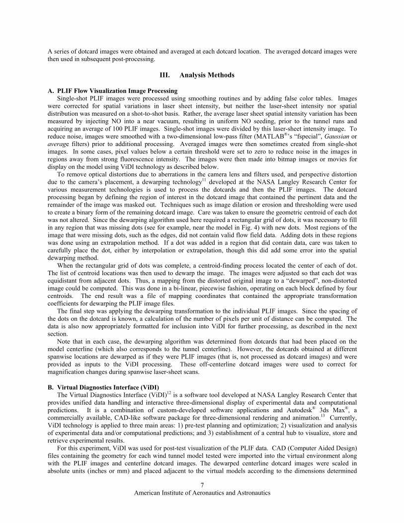
Figure 7 shows an angle-of-attack sweep using an IRVE model with seeding from the externally-plumbed porous cylinder and a horizontal sting mounting. These are single-shot images. Similar to Figure 6(b), the image acquired at a zero degree angle of attack (Fig. 7(a)) has brighter fluorescence on the bottom of this image, since the NO is seeded on the bottom half of the model. However, when the angle of attack changes by 2 degrees the brightest part of the image shifts to the center of the wake (Figs. 7(b) and (c)), indicating that the aft-body separated flow pattern has changed. Further changes in the angle of attack shift the NO to the top of the image (Figs. 7(e) and (f)). From these images, it is clear that the flow pattern in the wake has dramatically changed during this angle-of-attack sweep. Gas from the bottom of the wake is being swept up to the top of the wake. This is an advantage of pointwise-seeding of NO: it illustrates the flow direction. This is effectively a crude form of streamline visualization, though

(a) (b)

(c) (d)

(e) (f) Figure 7: ViDI rendering of selected images from the wake of an IRVE model during Run 12, in which the angle of attack was swept nominally from 0° to 10°. Seeding is through the porous cylinder which was located on the bottom half of the model. The angle of attack of the model in these images was (a) 0.1°, (b) 2.2°, (c) 3.9°, (d) 6.0°, (e) 8.1° and (f) 9.9°.

American Institute of Aeronautics and Astronautics

13

the NO distributes itself well enough in the wake that the full width of the wake is visualized as well. Curiously, the images show what appears to be a bifurcation in the downstream wake. This would be an interesting phenomenon to study with cross-plane imaging, where the laser sheet is rotated by 45 or 90 degrees relative to the current orientation. Alternatively, such flow structures can be studied with the laser sheet in its current orientation, by sweeping it spanwise through the flow, as described in Fig. 8.

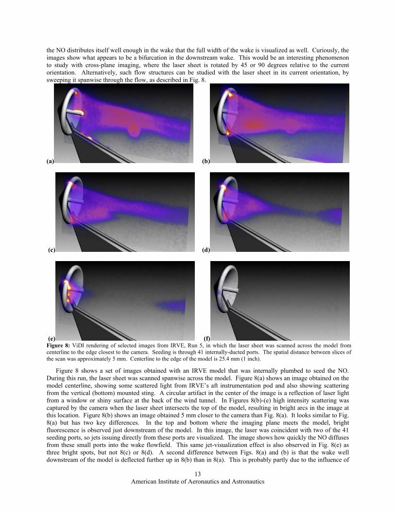
Figure 8 shows a set of images obtained with an IRVE model that was internally plumbed to seed the NO. During this run, the laser sheet was scanned spanwise across the model. Figure 8(a) shows an image obtained on the model centerline, showing some scattered light from IRVE’s aft instrumentation pod and also showing scattering from the vertical (bottom) mounted sting. A circular artifact in the center of the image is a reflection of laser light from a window or shiny surface at the back of the wind tunnel. In Figures 8(b)-(e) high intensity scattering was captured by the camera when the laser sheet intersects the top of the model, resulting in bright arcs in the image at this location. Figure 8(b) shows an image obtained 5 mm closer to the camera than Fig. 8(a). It looks similar to Fig. 8(a) but has two key differences. In the top and bottom where the imaging plane meets the model, bright fluorescence is observed just downstream of the model. In this image, the laser was coincident with two of the 41 seeding ports, so jets issuing directly from these ports are visualized. The image shows how quickly the NO diffuses from these small ports into the wake flowfield. This same jet-visualization effect is also observed in Fig. 8(e) as three bright spots, but not 8(c) or 8(d). A second difference between Figs. 8(a) and (b) is that the wake well downstream of the model is deflected further up in 8(b) than in 8(a). This is probably partly due to the influence of

(a) (b)

(c) (d)

(e) (f) Figure 8: ViDI rendering of selected images from IRVE, Run 5, in which the laser sheet was scanned across the model from centerline to the edge closest to the camera. Seeding is through 41 internally-ducted ports. The spatial distance between slices of the scan was approximately 5 mm. Centerline to the edge of the model is 25.4 mm (1 inch).

American Institute of Aeronautics and Astronautics

14

the sting, which was mounted on the bottom, and certainly caused, in part, by random flapping fluctuations in this wake flow. For Figs. 8(c)-(e), slices of the conical wake are shown, resulting in triangular flow structures. Figure 8(f) shows that when the laser sheet is nearly a full inch (25.4 mm) from the centerline, the wake flow is no longer visible at the right of the image.

(2) CEV Results: Streamline Visualization Figure 9 shows a ViDI rendering of several superimposed NO fluorescence images on the CEV model measured

using the straight-sting configuration. NO was seeded from 11 ports in the model and the laser sheet was scanned spatially across the model. Ports 1-5 were seeded using one mass flow controller and ports 6-11 were seeded using a second mass flow controller (each set to .075 slpm) so that similar amounts of gas would emanate from the various ports, despite the large pressure difference between the windward and leeward after-bodies. The fluorescence streaks across the images originate at ports in the model where NO was injected. Some streaks, such as that in Fig. 9(b) between ports 2 and 3 show that laser scatter from the model has been captured by the ICCD camera. The color tables for the PLIF images have been thresholded (low values of fluorescence set to zero) by an arbitrary value to deemphasize noise and scatter from the model while emphasizing regions of high NO concentration (high fluorescence intensity). Since the NO tracer gas is being swept up in the flowing gas, its fluorescence effectively visualizes flow streamlines.

In Fig. 9(a) the gas exiting port 6 is observed to sweep close to and tangent to the model surface and slightly downstream. This is in contrast to the flow emanating from ports 9 and 10, which immediately separate from the model surface and travel nearly parallel to the laser sheet. Note that only selected images have been displayed in this image, for clarity, so the fact that fluorescence does not originate exactly at port 9 in this image does not mean that PLIF was not observed there. Flow from port 10 identifies the top of the separated flow region aft of the model. Flow emanating from port 11 is particularly interesting: it flows towards port 10, which is opposite the main tunnel flow. This is clear visual evidence of flow separation on the leeward afterbody. In Fig. 9(a) no fluorescence is visible from ports 1-5, 7, and 8. The laser sheet entered from directly above the model so ports 1-5 were in the shadow of the laser sheet. Flow is not observed exiting ports 7 and 8 because the laser sheet width did not extend out to those ports.

In Fig. 9(b) the model was rotated by 90 degrees about the tunnel centerline, and the laser sheet was moved further upstream to illuminate ports 1-5. But all else was identical to the conditions of Fig. 9(a). Selected images were overlaid on the model showing NO fluorescence downstream of ports 1 and 2. Fluorescence was also observed

(a) (b) Figure 9: ViDI renderings of a laser sheet sweeps across the CEV model using the straight sting configuration. Flow conditions were identical for the two runs: (a) Run 37 and (b) Run 39. NO streams from all 11 ports which are numbered in (a) and which correspond to the port map shown in Figure 2. Only selected images are shown. Data for (a) was obtained with the model oriented vertically in the tunnel (laser sheet parallel to the plane of sting sweep) whereas (b) was obtained with the model oriented horizontally (laser sheet perpendicular to the plane of sting sweep). Both images are viewed from approximately the same perspective. The ports are numbered in (a); ports numbers (b) are identical but have been omitted for clarity. Flow is from left to right and the model is at an angle of attack of 28º with respect to the flow. The laser sheet scanned 38.1 mm (1.5 in) in (a) and 101.6 mm (4 in) in (b).

8

7

1

6

2

3

4

5

9

10

11

American Institute of Aeronautics and Astronautics

15

downstream of ports 3 and 4 (not shown) and 5. Careful examination of all PLIF images of the flow emanating from ports 1-5 show that the gas flows very close the model; that is, the flow is attached on this windward afterbody surface. Fluorescence images coinciding with ports 3 and 4 showed weak fluorescence along the model surface and strong scattered laser light from the model itself so they were omitted from this rendering. Weak fluorescence is observed downstream of port 8 and stronger fluorescence is observed downstream of ports 6 and 7. Again, the flow exiting port 6 is observed to track tangentially across the model, but the laser sheet is slicing across this flow at a steep angle, elongating this flow feature. Figure 9(b) also shows an oblique cross section of the flow exiting port 9. This jet of fluid appears to be an ellipse due to the orientation of the laser sheet relative to this streamline (jet of gas).

Comparing the streamlines from the two different sting mounting methods—straight sting and 28º sting mounting (not shown)—indicated that they were similar: no obvious differences were observed. This suggests that the position of the sting does not dramatically affect the afterbody flow.

V. Discussion Several new technologies were demonstrated in this work. Rapid prototype models were used in the 31-Inch

Mach 10 Air Tunnel exhibiting varying degrees of survivability. In several cases NO was successfully seeded through multiple ports in these models, demonstrating an effective means of uniformly seeding a separated wake flow or generating streamlines. The combination of PLIF with rapid prototype models was also demonstrated for the first time. PLIF was used to visualize streamlines in the flowfields in certain cases. Finally, dotcard images were used to process the PLIF images for the first time. In this section, these topics are discussed.

While several of the rapid prototype models did not survive even a single, short tunnel run, about half of them did. Generally speaking, models with thinner walls, such as those with an internal plenum, did not survive. Those made with high-temperature SLA material fared better than those that weren’t. The more durable of these small models were very quick to manufacture (~1 hour) and lasted for more than a few short runs, so their continued use should be explored, particularly if time and cost are factors. However, the present investigation of model survivability was performed in an ad hoc fashion since only a small number of models was available when the tests were performed. Furthermore, since the primary goal of the test was to study the PLIF flow visualization method, many variables were adjusted during the test in an uncontrolled way: a variety of tunnel conditions, run durations, model shapes, angles of attack and flow rates being used. It is difficult to make accurate comparisons between the different model substrates and coatings based on this test. If further testing of SLA models is required in the future, we recommend that a systematic investigation be undertaken to compare different materials and coatings. Several different types of models could be tested in a single run to minimize the number of runs that would need to be performed. Also a high-quality observation camera could view the model(s) during runs to determine when models start to fail. A potential concern with SLA models is shrinkage. If a careful study is undertaken, the models should be tested by quality assurance before and after the tests. The results of such a study could potentially provide a new paradigm for aeroheating tests.

Even though both of the internal-plenum IRVE models failed, this approach had significant advantages in terms of uniform seeding of NO, so it should not be abandoned. Instead, the plenums should be designed and built more robustly, with additional internal struts, and the plenums should be located further from the front surface of the model if possible.

A limitation of the current model construction method is that the models are not always mounted squarely to the sting. When the sting was at a zero degree angle of attack, the models sometimes were observed to have up to a 2.5 degree angle of attack. While this angle could be taken out using the yaw and angle-of-attack sweep systems, it would have been preferable if the model had been more accurately mounted to the sting in the first place. Development and use of a mechanical jig for this sting-attachment process would alleviate this problem.

SLA models should be easier to use in other wind tunnels that have lower stagnation temperatures, such as the NASA Langley 20-Inch Mach 6 Air Tunnel. Preliminary tests performed in this tunnel by one of the authors (GMB) showed that models tended to survive better in this environment than in the 31-Inch Mach 10 Air Tunnel.

The larger (5-in. diameter CEV) models took somewhat longer to manufacture (approximately a day) but they stood up to multiple runs of use at higher stagnation pressures. Insulating the model immediately after a run prevented crack formation due to thermal stresses caused by rapid cooling. NO was successfully plumbed through these larger CEV models, allowing partial visualization of streamlines with PLIF. If it is desired to extend the rapid prototyping model concept to longer run times an alternate approach could be pursued: a metal heatsink forebody capable of enduring higher heating loads could be adapted to an SLA afterbody, possibly using an insulating

American Institute of Aeronautics and Astronautics

16

material between the other two materials. Several such SLA afterbodies (possibly with different shapes) could be generated and adapted to a single metallic forebody.

The use of dotcard images in the present experiment had some notable benefits but also some drawbacks. During pre-run setup the dotcard allowed the laser sheet to be aligned vertically and oriented properly with respect to the model. Additionally, the camera could be focused on the dotcard. (UV flood lamps were used to illuminate the dotcard during camera focusing so that NO fluorescence would also be in focus; using visible light for camera focusing would have necessitated the removal of filters from in front of the camera in addition to resulting in out-of-focus fluorescence images.) The acquisition of dotcard images allowed perspective and lens distortions to be corrected in the images. Furthermore, they allowed the scale in the images to be accurately determined. The dotcards also allowed the orientation of the images to be determined relative to the model during the ViDI processing. However, the dotcard images did not always facilitate precise relative positioning of the PLIF images to the model during ViDI processing. For some runs, the camera evidently moved relative to the model between acquisition of dotcard images and acquisition of PLIF images during tunnel runs. This could be caused by the tunnel heating up and lengthening slightly prior to and during runs, while the camera is attached to the floor of the facility. This problem could be alleviated by attaching the camera directly to the wind tunnel. The relative positioning error could be also be caused by sting deflection under load during the tunnel run: aerodynamic loading is absent when dotcard images are being acquired.

There were several aspects of the use of dotcards that were not ideal. Most importantly, it slowed down operation of the tunnel. The number of runs per day was reduced from 3.8 to 2.5 in the current test – much of this being attributed to the use of dotcards, though some of the additional time was caused by frequent model changes. The use of the rapid prototyping models, which often lasted only a single run, compounded this problem because new dotcard images were acquired with each model change. Use of the dotcards, particularly when images needed to be acquired in multiple planes, required the model to be injected and retracted additional times – each time taking about 20 minutes.

Another problem with the use of dotcards in the present experiment was that when they were fabricated and attached to the model, dots near the model were physically cut out, as shown in Fig. 4. In order to use the available dewarping algorithm, these dots had to be added back into the raw dotcard images in post-processing. These dots were added either by eye or by mathematical interpolation or extrapolation. Dots are needed very near to the model surface so that images could be dewarped there. This post-processing was time consuming and added error. Finally, cutting custom dotcards for each model and affixing them to a solid, flat surface was time consuming.

An alternate dotcard-imaging method can be used in future tests that will alleviate most of these problems while retaining most of the advantages of dotcard imaging. A single, large, uniform dotcard image that fills the entire field of view of the camera should be used each time the camera is moved or adjusted, but not with each model change as in the present work. Using a large, rectangular dotcard will result in dots everywhere in the image, eliminating the need to hand-edit the dotcard images, i.e. adding dots where they are missing. This large dotcard could be attached to the sting at the same time as the model, perhaps mounted 6 in closer to the camera than the model. Then the model could be injected into the tunnel 6 in. from the centerline so that the dotcard would be positioned on the tunnel centerline. The laser sheet would be aligned to the dotcard as before, and the CCD camera would be focused on the dot pattern. Furthermore, the dotcard could be moved to various locations using the model injection system and multiple images could be obtained to prepare for spanwise laser-sheet scans. This new method should significantly improve productivity while achieving most of the goals of using dotcards. The only goal that cannot be achieved with this new method is the final goal shown in Table 2: positioning the PLIF images relative to the model. However, even in the current test where dotcards were custom-made for each model, this objective was not met. And white-light images of the model could also be obtained to facilitate overlaying PLIF images on the model during image processing. So, it is strongly recommended that this new approach be investigated.

VI. Conclusion The PLIF technique has been used to visualize the flow downstream of rapid prototype stereolithography IRVE

and CEV models. These models are relatively quick and inexpensive to fabricate, though they did not survive long duration runs in the NASA Langley 31-Inch Mach 10 Air Tunnel. Models that were more massive, as well as those which were made from a high-temperature material and coated with either high-temperature black paint or graphite survived better than other models.

PLIF was successfully implemented for the visualization of wake-flow structures as well as streamlines downstream of internally-plumbed NO-seeding ports. PLIF helped characterize the influence of sting placement on wake flows for both the IRVE and CEV models. In the case of the IRVE model, the sting was observed to perturb

American Institute of Aeronautics and Astronautics

17

the flow very close to the side-mounted sting and it also seemed to deflect the downstream wake. In the case of the CEV models, the images did not show a strong influence of sting placement on the aft-body streamlines. For wake flow visualizations, internally-plumbed models having many small seed ports on the leeside of the model produced uniform wake seeding. However, the structural integrity of these internal-plenum models was inadequate for withstanding the thermal and aerodynamics loads of this facility. If uniform seeding is desired, this is a good approach but an improved design will be required. The use of a porous cylinder attached to a tube for wake flow visualization was successful. The porous cylinder acted as a large point source of NO, thereby creating a crude streamline visualization, allowing identification of changes in separated wake-flow patterns. Finally, recommendations were made for improving the use of dotcards imaging and for improving the quality and quantity of data obtained in future tests.

Acknowledgments We wish to acknowledge the contribution to this project from the NASA Langley Research Center 31-Inch Mach

10 Air Tunnel technicians and engineers, including Kevin Hollingsworth, Paul Tucker Tony Robbins, Henry Fitzgerald, and Johnny Ellis. For model fabrication and coating we wish to acknowledge Gary Wainwright, Mike Powers, Pete Vasquez and Steve Nevins. This work was supported by the NASA Fundamental Aeronautics Hypersonics Program.

References

1 N. R. Merski, “Global Aeroheating Wind-Tunnel Measurements Using Improved Two-Color Phosphor Thermography Method,” Journal of Spacecraft and Rockets vol.36 no.2, pp. 160-170, 1999.

2 P. M. Danehy, J. A. Wilkes, G. Brauckmann, D. W. Alderfer, S. B. Jones, and D. Patry, “Visualization of a Capsule Entry Vehicle Reaction-Control System (RCS) Thruster” AIAA Paper 2006-1532 44th AIAA Aerospace Sciences Meeting and Exhibit, Reno, Nevada, Jan. 9-12, 2006.

3 P. M. Danehy, J. A. Wilkes, D. W. Alderfer, S. B. Jones, A. W. Robbins, D. P. Patry and R. J. Schwartz “Planar laser-induced fluorescence (PLIF) investigation of hypersonic flowfields in a Mach 10 wind tunnel” AIAA AMT-GT Technology Conference, San Francisco, AIAA-2006-3442 June, (2006).

4 3D Systems Accura® SI 10 Material Product Data Sheet, http://www.3dsystems.com/products/datafiles/accura/datasheets/ Accura_si_10_rev_081004.pdf, viewed Jan 2, 2006.

5 DSM Somos® NanoFormTM 15120 Product Data Sheet, http://www.dsm.com/en_US/html/dsms/pd_product_data_sheets.htm, viewed Jan 2, 2006.

6 Krylon® BBQ & Hi-Temp Paint, http://krylon.com/main/product_template.cfm?levelid=5&sub_levelid=26&productid=1726&content=product_details, viewed Jan 2, 2006.

7 Neely Industries E/M Products, http://www.neelyindustries.com/prod03.htm, viewed Jan 2, 2006. 8 ZYP BN Aerosol, ZYP® Coatings, http://www.zypcoatings.com/Datasheets/BnAerosol/BnAerosol.htm, viewed Jan 2, 2006. 9 J. R. Micol “Langley Aerothermodynamic Facilities Complex: Enhancements and Testing Capabilities,” AIAA Paper 98-

0147, 36th AIAA Aerospace Sciences Meeting & Exhibit, January 12-15, Reno, NV, 1998. 10 J. A. Wilkes, D. W. Alderfer, S. B. Jones, and P. M. Danehy, “Portable Fluorescence Imaging System for Hypersonic Flow

Facilities,” JANNAF Interagency Propulsion Committee Meeting, Colorado Springs, Colorado, December 2003. 11 J. F. Meyers, “Development of Doppler Global Velocimetry as a Flow Diagnostics Tool,” Meas. Sci. and Tech. v. 6, n. 6,

pp. 769-783 June, 1995. 12 R. J. Schwartz, "ViDI: Virtual Diagnostics Interface Volume 1-The Future of Wind Tunnel Testing" Contractor Report

NASA/CR-2003-212667, December 2003. 13 Autodesk 3ds Max Product Information, Autodesk Inc.,

http://usa.autodesk.com/adsk/servlet/index?id=5659302&siteID=123112, viewed Jan 2, 2006.