Fluid Power System Dynamics

William Durfee, Zongxuan Sunand James Van de Ven

Department of Mechanical EngineeringUniversity of Minnesota

A National Science FoundationEngineering Research Center

FLUID POWER SYSTEM DYNAMICS

Center for Compact and Efficient Fluid PowerUniversity of MinnesotaMinneapolis, USA

This book is available as a free, full-color PDF download fromsites.google.com/site/fluidpoweropencourseware/. The printed,bound version can be purchased at cost on lulu.com.

Copyright and DistributionCopyright is retained by the authors. Anyone may freely copy anddistribute this material for educational purposes, but may not sell thematerial for profit. For questions about this book contact Will Durfee,University of Minnesota, wkdurfee@umn.edu.

c©2015

Version: September 25, 2015

Contents

Preface 1

1. Introduction 21.1. Overview . . . . . . . . . . . . . . . . . . . . . . . . . . . . 21.2. Fluid Power Examples . . . . . . . . . . . . . . . . . . . . 31.3. Analyzing Fluid Power Systems . . . . . . . . . . . . . . 7

2. Basic Principles of Fluid Power 102.1. Pressure and Flow . . . . . . . . . . . . . . . . . . . . . . . 102.2. Power and Efficiency . . . . . . . . . . . . . . . . . . . . . 122.3. Hydraulic Fluids . . . . . . . . . . . . . . . . . . . . . . . 132.4. Fluid Behavior . . . . . . . . . . . . . . . . . . . . . . . . . 14

2.4.1. Viscosity . . . . . . . . . . . . . . . . . . . . . . . . 142.4.2. Bulk Modulus . . . . . . . . . . . . . . . . . . . . . 152.4.3. Pascal’s Law . . . . . . . . . . . . . . . . . . . . . . 172.4.4. High Forces . . . . . . . . . . . . . . . . . . . . . . 18

2.5. Conduit Flow . . . . . . . . . . . . . . . . . . . . . . . . . 202.5.1. Pressure Losses in Conduits . . . . . . . . . . . . . 22

2.6. Bends and Fittings . . . . . . . . . . . . . . . . . . . . . . 252.7. Orifice Flow . . . . . . . . . . . . . . . . . . . . . . . . . . 27

3. Fluid Power Components 293.1. Cylinders . . . . . . . . . . . . . . . . . . . . . . . . . . . . 293.2. Pumps and Motors . . . . . . . . . . . . . . . . . . . . . . 323.3. Control Valves . . . . . . . . . . . . . . . . . . . . . . . . . 34

3.3.1. Dynamic Models for Valves . . . . . . . . . . . . . 353.3.2. Valve Symbols . . . . . . . . . . . . . . . . . . . . . 36

3.4. Accumulators . . . . . . . . . . . . . . . . . . . . . . . . . 373.5. Filters . . . . . . . . . . . . . . . . . . . . . . . . . . . . . . 383.6. Reservoirs . . . . . . . . . . . . . . . . . . . . . . . . . . . 393.7. Hoses and Fittings . . . . . . . . . . . . . . . . . . . . . . 40

4. Hydraulic Circuit Analysis 414.1. Fluid Resistance . . . . . . . . . . . . . . . . . . . . . . . . 424.2. Fluid Capacitance . . . . . . . . . . . . . . . . . . . . . . . 434.3. Fluid Inertance . . . . . . . . . . . . . . . . . . . . . . . . 454.4. Connection Laws and States . . . . . . . . . . . . . . . . . 45

4.4.1. Connections . . . . . . . . . . . . . . . . . . . . . . 45

iii

iv Contents

4.4.2. State Variables . . . . . . . . . . . . . . . . . . . . . 454.5. Example Systems . . . . . . . . . . . . . . . . . . . . . . . 45

5. Bibliography 49

A. Fluid Power Symbols 50

Preface

This book was created because system dynamics courses in the stan-dard mechanical engineering curriculum do not cover fluid power, eventhough fluid power is essential to mechanical engineering and studentsentering the work force are likely to encounter fluid power systems intheir job. Most system dynamics textbooks have a chapter or part of achapter on fluid power but typically the chapter is thin and does notcover practical fluid power as is used in industry today. For example,many textbooks confine their discussion of fluid power to liquid tanksystems and never even mention hydraulic cylinders, the workhorse oftoday’s practical fluid power.

The material is intended for use in an introductory system dynamicscourse that would teach analysis of mechanical translational, mechan-ical rotary and electrical system using differential equations, transferfunctions and time and frequency response. The material should be in-troduced toward the end of the course after the other domains and mostof the analysis methods have been covered. It replaces or supplementsany coverage of fluid power in the course textbook. The instruction canpick and choose which sections will be covered in class or read by thestudent. At the University of Minnesota, the material is used in courseME 3281, System Dynamics and Control and in ME 4232, Fluid PowerControl Lab.

The book is a result of the Center for Compact and Efficient FluidPower (CCEFP) (www.ccefp.org), a National Science Foundation En-gineering Research Center founded in 2006. CCEFP conducts basic andapplied research in fluid power with three thrust areas: efficiency, com-pactness, and usability. CCEFP has over 50 industrial affiliates and itsresearch is ultimately intended to be used in next generation fluid powerproducts. To ensure the material in the book is current and relevant, itwas reviewed by industry representatives and academics affiliated withCCEFP.

Will DurfeeZongxuan SunJim Van de Ven

1

1. Introduction

1.1. Overview

Fluid power is the transmission of forces and motions using a confined,pressurized fluid. In hydraulic fluid power systems the fluid is oil, orless commonly water, while in pneumatic fluid power systems the fluidis air.

Fluid power is ideal for high speed, high force, high power applica-tions. Compared to all other actuation technologies, including electricmotors, fluid power is unsurpassed for force and power density and iscapable of generating extremely high forces with relatively lightweightcylinder actuators. Fluid power systems have a higher bandwidth thanelectric motors and can be used in applications that require fast starts,stops and reversals, or that require high frequency oscillations. Becauseoil has a high bulk modulus, hydraulic systems can be finely controlledfor precision motion applications. 1 Another major advantage of fluidpower is compactness and flexibility. Fluid power cylinders are rela-tively small and light for their weight and flexible hoses allows powerto be snaked around corners, over joints and through tubes leading tocompact packaging without sacrificing high force and high power. Agood example of this compact packaging are Jaws of Life rescue toolsfor ripping open automobile bodies to extract those trapped within.

Fluid power is not all good news. Hydraulic systems can leak oil atconnections and seals. Hydraulic power is not as easy to generate aselectric power and requires a heavy, noisy pump. Hydraulic fluids cancavitate and retain air resulting in spongy performance and loss of preci-sion. Hydraulic and pneumatic systems become contaminated with par-ticles and require careful filtering. The physics of fluid power is morecomplex than that of electric motors which makes modeling and con-trol more challenging. University and industry researchers are workinghard not only to overcome these challenges but also to open fluid powerto new applications, for example tiny robots and wearable power-assisttools.

1While conventional thinking was that pneumatics were not useful for precision con-trol, recent advances in pneumatic components and pneumatic control theory has openedup new opportunities for pneumatics in precision control.

2

1.2. Fluid Power Examples 3

Figure 1.1.: Caterpillar 797B mining truck. Source: Caterpillar

1.2. Fluid Power Examples

Fluid power is pervasive, from the gas spring that holds you up in theoffice chair you are sitting on, to the air drill used by dentists, to thebrakes in your car, to practically every large agriculture, constructionand mining machine including harvesters, drills and excavators.

The Caterpillar 797B mining truck is the largest truck in the world at3550 hp (Fig. 1.1). It carries 400 tons at 40 mph, uses 900 g of diesel per12 hr shift, costs about $6M and has tires that are about $60,000 each.It is used in large mining operations such as the Hull-Rust-MahoningOpen Pit Iron Mine, the world’s largest open pit iron mine, located inHibbing MN and the Muskeg River Mine in Alberta Canada.2 The 797Buses fluid power for many of its internal actuation systems, includinglifting the fully loaded bed.

Shultz Steel, an aerospace company in South Gate CA, has a 40,000-ton forging press that weighs over 5.2 million pounds (Fig. 1.2). It isthe largest press in the world and is powered by hydraulics operating at6,600 psi requiring 24 700 hp pumps.

The Multi-Axial Subassemblage Testing (MAST) Laboratory is locatedat the University of Minnesota and is used to conduct three-dimensional,quasi-static testing of large scale civil engineering structures, including

2”New Tech to Tap North America’s Vast Oil Reserves”, Popular Mechanics, March2007.

4 1. Introduction

Figure 1.2.: 40,000 ton forging press. Source: Shultz Steel.

buildings, to determine behavior during earthquakes (Fig. 1.3). TheMAST system, constructed by MTS Systems, has eight hydraulic actua-tors that can each push or pull with a force of 3910 kN.

The Caterpillar 345C L excavator is used in the construction industryfor large digging and lifting operations and has a 345 hp engine (Fig.1.4). The 345C L operates at a hydraulic pressure of 5,511 psi to generatea bucket digging force of 60,200 lbs and a lift force of up to 47,350 lbs.

A feller buncher is a large forestry machine that cuts trees in place(Fig. 1.5).

Some of the fastest roller coasters in the world get their initial launchfrom hydraulics and pneumatics. (Fig. 1.6). Hydraulic launch assist sys-tems pump hydraulic fluid into a bank of accumulators storing energyas a compressed gas. At launch, the energy is suddenly released into ahydraulic motor whose output shaft drives a cable drum with the cablerapidly bringing the train from rest to very high velocities. The KingdaKa at Six Flags Great Adventure uses this launch and reaches 128 mphin 3.5 s. The Hypersonic SLC at Kings Dominion ups the ante with acompressed air launch system that accelerates riders to 81 mph in 1.8 s.

Most automatic transmissions have hydraulically actuated clutchesand bands to control the gear ratios. Fluid is routed through internalpassageways in the transmission case rather than through hoses (Fig.1.7)

The dental drill is used to remove small volumes of decayed tooth

1.2. Fluid Power Examples 5

Figure 1.3.: MAST Laboratory for earthquake simulation. Source: MAST Lab.

Figure 1.4.: Caterpillar 345C L excavator. Source: Caterpillar.

6 1. Introduction

Figure 1.5.: Feller buncher. Souce: Wikipedia image.

Figure 1.6.: Hypersonic XLC roller coaster with hydraulic lanuch assist. Source:Wikipedia image.

1.3. Analyzing Fluid Power Systems 7

Figure 1.7.: Mercedes-Benz automatic transmission model.

prior to inserting a filling (Fig. 1.8). Modern drills rotate at up to 500,000rpm using an air turbine and use a burr bit for cutting. The hand piececan cost up to $800. Pneumatic drills are used because they are smaller,lighter and faster than electric motor drills. The compressor is locatedaway from the drill and pressurized air is piped to the actuator.

Hydraulic microdrives are used during surgery to position recordingelectrodes in the brain with micron accuracy (Fig. 1.9). Master and slavecylinders have a 1:1 ratio and are separated by three to four feet of fluidfilled cable.

1.3. Analyzing Fluid Power Systems

Analyzing the system dynamics of fluid power means using differen-tial equations and simulations to examine the pressures and flows incomponents of a fluid power circuit, and the forces and motions of themechanisms driven by the fluid power. For example, in an excavator,the engineer would be interested in determining the diameter and strokelength of the cylinder that is required to drive the excavator bucket andhow the force and velocity of the bucket changes with time as the valves

Figure 1.8.: A dental handpiece. Source: Wikipedia image.

8 1. Introduction

Figure 1.9.: Hydraulic microdrive for neural recording electrode placement.Source: Stoelting Co.

to the cylinder are actuated. Because fluid power systems change withtime and because fluid power systems have energy storage elements,a dynamic system analysis approach must be taken which means theuse of linear and nonlinear differential equations, linear and nonlinearsimulations, time responses, transfer functions and frequency analysis.

Fluid power is one domain within the field of system dynamics, justas mechanical translational, mechanical rotational and electronic net-works are system dynamic domains. Fluid power systems can be an-alyzed with the same mathematical tools used to describe spring-mass-damper or inductor-capacitor-resistor systems. Like the other domains,fluid power has fundamental power variables and system elements con-nected in networks. Unlike other domains many fluid power elementsare nonlinear which makes closed-form analysis somewhat more chal-lenging, but not difficult to simulate. Many concepts from transfer func-tions and basic closed loop control systems are used to analyze fluidpower circuits, for example the response of a servovalve used for preci-sion control of hydraulic pistons. 3

Like all system dynamics domains, fluid power is characterized bytwo power variables that when multiplied form power, and ideal lumpedelements including two energy storing elements, one energy dissipatingelement, a flow source element and a pressure source element. Table1.1 shows the analogies between fluid power elements and elements inother domains. Lumping fluid power systems into elements is useful

3See ”‘Transfer Functions for Mood Servovalves”’ available on-line in the technicaldocuments section of the Moog company web site.

1.3. Analyzing Fluid Power Systems 9

Table 1.1.: Element analogies in several domains.Domain Power Power Storage Storage Dissipative

Variable 1 Variable 2 Element 1 Element 2 Element

Translational Force, F Velocity, V Mass,M Spring,K Damper,BRotational Torque, T Velocity, ω Inertia, J Spring,K Damper,BElectrical Current, I Voltage, V Inductor, L Capacitor, C Resistor,RFluid Power Flow,Q Pressure, P Inertance, If Capacitor, Cf Resistance,Rf

when analyzing complex circuits.

2. Basic Principles of Fluid Power

2.1. Pressure and Flow

Fluid power is characterized by two main variables, pressure and flow,whose product is power. Pressure P is force per unit area and flow Qis volume per time. Because pneumatics uses compressible gas as thefluid, mass flow rate Qm is used for the flow variable when analyzingpneumatic systems. For hydraulics, the fluid is generally treated as in-compressible, which means ordinary volume flow Q can be used.

Pressure is reported several common units that include pounds persquare inch (common engineering unit in the U.S.), pascal (one newtonper square meter, the SI unit), megapascal and bar. Table 2.1 shows howpressure units are related. For engineering, it is best to do calculationsand simulations in SI units, but to report in SI and the conventionalengineering unit.

Pressure is an across type variable, which means that it is always mea-sured with respect to a reference just like voltage in an electrical system.As shown in Figure 2.1, one can talk about the pressure across a fluidpower element such as a pump or a valve, which is the pressure dif-ferential from one side to the other, but when describing the pressureat a point, for example the pressure of fluid at one point in a hose, it isalways with respect to a reference pressure. Reporting absolute pressuremeans that the pressure is measured with respect to a perfect vacuum.It is more common to measure and report gauge pressure, the pressurerelative to ambient atmospheric pressure (0.10132 mPA, 14.7 psi at sealevel). The distinction is critical when analyzing the dynamics of pneu-matic systems because the ideal gas law that models the behavior of airis based on absolute pressure.

Table 2.1.: Conversions between pressure units

pascal megapascal bar lbs-sq-in(Pa) (Mpa) (bar) (psi)

1 Pa 1 10−6 10−5 145.04× 10−6

1 Mpa 106 1 10 1451 bar 105 0.1 1 14.51 psi 6895 6.895× 10−3 0.06895 1

10

2.1. Pressure and Flow 11

Figure 2.1.: Pressure is measured with respect to a reference.

Pressure is measured with a mechanical dial type pressure gage orwith an electronic pressure transducer that outputs a voltage propor-tional to pressure (Fig. 2.2). Almost all pressure transducers reportgauge pressure because they expose their reference surface to atmo-sphere.

Volume flow rate is reported in gallons per minute, liters per minuteand cubic meters per second (SI unit). Table 2.2 shows how flow rateunits are related.

Flow is a through type variable, which means it is volume of fluid flow-ing through an imaginary plane at one location. Like current in an elec-trical system, there is no reference point. Flow is measured with a flowmeter placed in-line with the fluid circuit. One common type of flowmeter contains a turbine, vane or paddle wheel that spins with the flow.Another type has a narrowed passage or an orifice and flow is estimatedby measuring the differential pressure across the obstruction. A Pitottube estimates velocity by measuring the dynamic pressure, which isthe difference between the stagnation pressure and static pressure. Fig-ure 2.3 shows some common types of flow meters. Because flow metersrestrict the flow, they are used sparingly in systems where small pres-sure drops matter.

Figure 2.2.: Dial pressure gauge and electronic pressure transducer.

12 2. Basic Principles of Fluid Power

Table 2.2.: Conversions between volume flow rate units

gallon/minute liter/minute cubicmeter/second(gpm) (lpm) (m3/s)

1 gpm 1 3.785 6.31× 10−5

1 lpm 0.264 1 1.67× 10−5

1 m3/s 1.585× 104 6× 104 1

2.2. Power and Efficiency

The power available at any one point in a fluid power system is thepressure times the flow at that point

power = P ×Q (2.1)

For the power available in a conduit, the pressure in Equation 2.1 isthe pressure relative to the pressure in the system reservoir, which istypically at atmospheric pressure.

Example 2.2.1. The hose supplying the cylinder operating the bucket ofa large excavator has fluid at 1000 psi flowing at 5 gpm. What is theavailable power in the line?

Figure 2.3.: Types of flowmeters. Top row: turbine, digital paddle, variable area.Bottom row is a dual-rotor turbine flowmeter with a cutaway.

2.3. Hydraulic Fluids 13

Solution: For most engineering examples, the reported pressure is agage pressure, which means the hose is operating at 1000 psi above at-mospheric pressure, the pressure of the reservoir. To calculate the power

1000 psi × 6895 Pa/psi = 6.9×106 Pa5 gpm × 6.31×10−5 m3/s/gpm = 31.6×10−5 m3/s

Power = 6.9× 106 × 31.6× 10−5 = 2180 watts = 2.9 horsepower

Components such as cylinders, motors and pumps have input andoutput powers, which can be used to calculate the efficiency of the com-ponent. For example, pressured fluid flows into a cylinder and the cylin-der extends. The input power is the pressure of the fluid times its flowrate while the output power is the compression force in the cylinderrod times the rod extension velocity. Dividing output power by inputpower yields the efficiency of the component. The same can be done forcomponents such as an orifice. The efficiency of the orifice is the outputpressure divided by the input pressure because the flow rate is the sameon either side of the orifice.

2.3. Hydraulic Fluids

The main purpose of the fluid in a fluid power system is to transmitpower. There are other, practical considerations that dictate the specificfluids used in real hydraulic systems. The fluids must cool the systemby dissipation of heat in a radiator or reservoir, must help with sealingto prevent leaks, must lubricate sliding and rotating surfaces such asthose in motors and cylinders, must not corrode components and musthave a long life without chemical breakdown.

The earliest hydraulic systems used water for the fluid. While wa-ter is safe for humans and environment, cheap and readily available,it has significant disadvantages for hydraulic applications. Water pro-vides almost no lubrication, has low viscosity and leaks by seals, easilycavitates when subjected to negative pressures, has a narrow tempera-ture range between freezing and boiling (0 to 100 ◦ C), is corrosive to thesteels used extensively in hydraulic components and is a friendly envi-ronment for bacteria and algae growth, which is why swimming poolsare chlorinated.

Modern hydraulic system use petroleum based oils, with additivesto inhibit foaming and corrosion. Petroleum oils are inexpensive, pro-vide good lubricity and, with additives, have long life. The brake andautomatic transmission fluids in your car are examples.

14 2. Basic Principles of Fluid Power

Figure 2.4.: Viscosity related hydraulic system losses.

2.4. Fluid Behavior

2.4.1. Viscosity

All fluids, including oil and air have fundamental properties and fol-low basic fluid mechanics laws. The viscosity of a fluid is its resistanceto flow. Some fluids, like water, are thin and have low viscosity whileothers like honey are thick and have high viscosity. The fluids for hy-draulic systems are a compromise. If the viscosity is too low, fluid willleak by internal seals causing a volumetric loss of efficiency. If the vis-cosity is too high, the fluid is difficult to push through hoses, fittingsand valves causing a loss of mechanical efficiency. Figure 2.4 shows thistradeoff and indicates that a medium viscosity fluid is best for hydraulicapplications.

The dynamic viscosity (also known as the absolute viscosity) is theshearing resistance of the fluid and is measured by placing the fluidbetween two plates and shearing one plate with respect to the other.The symbol for dynamic viscosity is the Greek letter mu (µ). The SI unitfor dynamic viscosity is the pascal-second (Pa-s), but the more commonunit is the centipoise (cP), with 1 cP = 0.001 Pa-s. The dynamic viscosityof water at 20 ◦ C is 1.00 cP

It is easier to measure and more common to report the kinematic viscos-ity of a fluid, the ratio of the viscous forces to inertial forces. The symbolfor kinematic viscosity is the Greek letter nu (ν). Kinematic viscositycan be measured by the time it takes a volume of oil to flow through acapillary. The SI unit for kinematic viscosity is m2/s but the more com-

2.4. Fluid Behavior 15

Figure 2.5.: The viscosity of hydraulic oils varies with temperature.

mon unit is the centistoke (cSt) which is 1 mm2/s. The conversion is1m2/s = 106cSt = 104stokes

If ρ is the fluid density, the kinematic and dynamic viscosity are re-lated by

ν =µ

ρ(2.2)

The kinematic viscosity of water over a wide range of temperature is 1cSt while common hydraulic oils at 40 ◦ C are in the range of 20-70 cSt.Sometimes hydraulic oil kinematic viscosity is expressed in Saybolt Uni-versal Seconds (SUS), which comes from the oil properties being mea-sured on a Saybolt viscometer.

Viscosity changes with temperature; as fluid warms up it flows moreeasily. One reason your car is hard to start on a very cold morning isthat the engine oil thickened overnight in the cold. The viscosity indexVI expresses how much viscosity changes with temperature. Fluids witha high VI are desirable because they experience less change in viscositywith temperature. Figure 2.5 shows how viscostiy changes for typicalhydraulic fluids.

2.4.2. Bulk Modulus

In many engineering applications, liquids are assumed to be completelyincompressible even though all materials can be compressed to some

16 2. Basic Principles of Fluid Power

Figure 2.6.: Fluid bulk modulous. Liquids are nearly incompressible (left), ex-cept when there is trapped air, as shown on the right.

degree. In some hydraulic applications, the tiny compressibility of oilturns out to be important because the pressures are high, up to 5,000 psi.The bulk modulus of the fluid is the property that indicates the springi-ness of the fluid and is defined as the pressure needed to cause a givendecrease in volume. A typical oil will decrease about 0.5% in volume forevery 1000 psi increase in pressure. When the compressibility is signif-icant, it is modeled as a fluid capacitor (spring) and often is lumped inwith the fluid capacitance of the accumulator (see Section 3.4).

When air bubbles are entrained in the hydraulic oil, the bulk modulusdrops and the fluid becomes springy (Fig. 2.6). You may have experi-enced this when the brake pedal in your car felt spongy. The solutionwas to bleed the brake system, which releases the trapped air so that thebrake fluid becomes stiff again.

Another way that the fluid can change properties is if the pressure fallbelow the vapor pressure of the liquid causing the formation of vaporbubbles. When the bubbles collapse, a shock wave is produced that canerode nearby surfaces. Cavitation damage can be a problem for pro-pellers and for fluid power pumps with the erosion greatly shorteningthe lifetime of components.

The bulk modulus β is defined as

β =∆P

∆V/V(2.3)

where V is the original volume of liquid and ∆V is the change in volumeof the liquid when subjected to a pressure change of ∆P . Because ∆V/Vis dimensionless, the units of β are pressure. Water has a bulk modulusof 3.12 × 105 psi (2.15 GPa) while hydraulic oils have a bulk modulusbetween 2 × 105 and 3 × 105 psi (SAE 30 oil is 2.2 × 105 psi = 1.5 GPa),

2.4. Fluid Behavior 17

but can drop way down if air is entrained.

Example 2.4.1. A piston pushes down on a volume of SAE 30 oil trappedin a cylinder like the one shown in Figure 2.6. The cylinder bore is 5 in.and the height of the unstressed column of oil is 4 in. The oil has a bulkmodulus β = 2.2 × 105 psi. When a force of 10,000 lbs is applied to thepiston, how much does the piston displace?

Solution: Use Equation 2.3 to calculate the change in volume

∆V =∆PV

β=

(F/A)(Ah)

β=Fh

β

=(1× 104)× 4

2.2× 105

= .18 cu. in.

The change in height is

∆h =∆V

A

=.18

π(5/2)2

= 0.0092 in.

2.4.3. Pascal’s Law

Pascal’s Law states that in a confined fluid at rest, pressure acts equallyin all directions and acts perpendicular to the confining walls (Fig. 2.7).This means that all chambers, hoses and spaces in a fluid power systemthat have open passageways between them are at equal pressure so longas the fluid is not moving.

Pascal’s Law makes it easy to understand the operation of a simplehydraulic amplifier. Figure 2.8 shows how it works. The piston on theright is 25 times the area of the piston on the left. Pushing down with10 lbs on the left piston will lift a 250 lb load on the right because thepressure of 10 psi is the same everywhere.

18 2. Basic Principles of Fluid Power

Figure 2.7.: Pascal’ Law. Fluid at rest has same pressure everywhere and acts atright angles against the walls.

2.4.4. High Forces

The crowning glory of fluid power is the ability for small, light fluidpower cylinders to produce extremely large forces. Consider the Cater-pillar 345D hydraulic excavator shown in Figure 2.9. The bore (diam-eter) of the cylinder that drives the stick is 7.5 in. and the maximumworking pressure is 5511 psi. The peak force in the cylinder is therefore

F = P ×A = 5511× π × (7.5/2)2 = 243, 468 lbs

or over 120 tons! It is impossible to produce this force using electricmotors.

Force can be increased two ways, raising the pressure or increasingthe bore of the cylinder. Force is proportional to pressure but goes as thesquare of the bore, which means small increases in cylinder size results

Figure 2.8.: Hydraulic amplifier. Pushing down with 10 lbs on the left pistonraises the 250 lb. weight on the right piston.

2.4. Fluid Behavior 19

Figure 2.9.: A large excavator. Source: Caterpillar.

in large increases in force. For example, consider a small pneumaticcylinder with a 7/16 in. bore running at 60 psi. This cylinder can pushwith 9 lbs of force. But, as shown in Figure 2.10, force goes up as boresquared and a 4 in. bore cylinder at the same 60 psi can push with 754lbs of force.

Of course the extra force does not come free. A larger cylinder re-quires a greater volume of fluid to move the load than a smaller cylinder,the practical result of the requirement that power be conserved.

Figure 2.10.: Force in a cylinder acting at 60 psi. goes up with the square of thebore.

20 2. Basic Principles of Fluid Power

Figure 2.11.: Hoses on an excavator.

2.5. Conduit Flow

In electromechanical actuation systems, power is carried to motors throughappropriately sized, low-resistance wires with negligible power loss.This is not the case for fluid power systems where the flow of oil throughhydraulic hoses and pipes can result in energy losses due to internalfluid friction and the friction against the walls of the conduit (Fig. 2.11).Designers size the diameter and length of hydraulic hoses to minimizethese losses. The other cause of major losses in fluid power systems isthe orifice drag of valves and fittings. These will be discussed in Sec-tion 3 These loses are modeled as nonlinear resistances in the hydrauliccircuit.

Conduit flow properties can be analyzed using basic principles offluid mechanics. Typical flow patterns through pipes are shown in Fig-ure 2.12. At low velocities, the flow is smooth and uniform while athigher velocities the flow turns turbulent. Turbulent flow can also becaused by sudden changes in direction or when the area suddenly changes,conditions that are common in hydraulic systems. Turbulent flow hashigher friction, which results in greater heat losses and lower operatingefficiencies. This is a practical concern for designers of hydraulic sys-tems because every right angle fitting designed into the system lowersthe system efficiency.

The Reynolds number, the non-dimensional ratio of inertial to viscousforces, is commonly used to characterize the flow in pipes

Re =ρV Dh

µ=V Dh

ν(2.4)

where ρ is the density (kg/m2), V is the mean fluid velocity (m/s),Dh isthe hydraulic diameter (m), µ is the dynamic viscosity (Pa-s) and ν is the

2.5. Conduit Flow 21

Figure 2.12.: Laminar and turbulent flow through a pipe.

kinematic viscosity. For circular conduits, the hydraulic diameter is thesame as the pipe diameter. The more general formula, which accountsfor non-circular pipes and hoses is

Dh =4A

S(2.5)

where A is the cross-sectional area of the conduit and S is the perimeter.For a circle this formula reduces to diameter of the circle.

For fully developed pipe flow, if Re < 2100 the flow is laminar, if2100 < Re < 4000 the flow is in transition, neither laminar or turbulent,and if Re > 4000 the flow is turbulent. These are approximations asthe actual flow type will depend on local conditions and local geome-try, which is why you may find other sources using different Reynoldsnumber break points to define the flow type.

Example 2.5.1. A hydraulic hose with internal diameter of 1.0 in. iscarrying oil with kinematic viscosity 50 cSt at a flow rate of 20 gpm.Calculate the Reynolds number and determine if the flow is laminar orturbulent.

Solution: Convert to SI units.

Q = 20 gpm = .00126 cu-m/sD = 1.0 in. = .0254 m

ν = 50 cSt = 5.0× 10−5 m2/s

Find the average velocity

V =4Q

πD2=

(4)(.00126)

(3.142)(.0254)2= 2.49 m/s

Calculate the Reynolds number

Re =VD

ν=

(2.49)(.0254)

5.0× 10−5= 1265

22 2. Basic Principles of Fluid Power

Because Re is below 2000 the flow is laminar.

2.5.1. Pressure Losses in Conduits

The pressure losses in straight pipe and hoses contribute to the overallefficiency of a fluid power system. The losses can be estimated using theDarcy-Weisbach equation

∆P = fρL

2DV 2 (2.6)

where ∆P is the pressure drop, f is the friction factor, L is the pipelength, D is the pipe inside diameter and V 2 is the average flow veloc-ity. There are different formulas for the friction factor depending on theReynolds number and the surface roughness of the pipe or hose.

The experimental determination of friction factors are shown on theclassic Moody Diagram 1 (Fig. 2.13) that plots the friction factor as afunction of Reynolds number for a range of surface roughness of roundpipes. Surface roughness is defined as ε/D where ε is the mean heightof the roughness of the pipe. The diagram shows that for laminar flow,friction factor is independent of roughness. For turbulent flow, the fric-tion factor, and therefore pressure losses, depend both on the Reynoldsnumber and the roughness of the pipe, except at high Reynolds numberswhere losses depend only on the roughness. Once the Reynolds numberis determined, simple formulas can be used to calculate pressure dropthat avoid having to estimate numbers off the Moody Diagram.

Laminar Flow For laminar flow, the friction factor depends only on theReynolds number

f =64

Re(2.7)

Using this equation, Equation 2.6 and Equation 2.4 the pressure loss ina pipe with laminar flow can be calculated as

∆P =32µL

D2V (2.8)

Converting average velocity to the more convenient fluid flow rate (V =4Q/πD2) yields

∆P =128µL

πD4Q (2.9)

1Moody, L. F. (1944), ”Friction factors for pipe flow”, Transactions of the ASME 66 (8):671–684

2.5. Conduit Flow 23

Figure 2.13.: Moody Diagram showing the experimental friction factor for pipes.

This equation shows that for smooth flow, the pressure drop is propor-tional to the flow rate Q. This is analogous to a linear resistor in anelectrical system and to a linear damper in a mechanical system.

Turbulent Flow, Smooth Pipes For turbulent flow, the friction factordepends both on the Reynolds number and the surface roughness ofthe pipe, however, in most fluid power systems the pipes and hoseshave smooth interiors and the friction factor for smooth pipes can beused. Under these conditions, an empirical approximation, derived byBlasius and based on experimental data, can be used to calculate thefriction factor

f =0.316

Re0.25(2.10)

Combining with Equation 2.4 and converting from velocity to flow, thepressure loss in a smooth pipe with turbulent flow is

∆P = 0.214µ.25ρ.75L

D4.75Q1.75 (2.11)

The pressure loss is almost, but not quite, proportional to the squareof the flow rate, thus a pipe with turbulent flow acts like a nonlinear

24 2. Basic Principles of Fluid Power

resistor.

Turbulent Flow, Rough Pipes If needed, the turbulent friction factordata for rough piles in the Moody diagram can be modeled by the Cole-brook Equation 2

1√f

= −2 log10

(ε/Dh

3.7+

2.51

Re√f

)This equation must be solved iteratively for f , but a close-approximationdirect solution that can be used for hydraulic system modeling purposescomes from the Swamee-Jain Equation 3

f =0.25[

log10

(ε

3.7D + 5.74Re0.9

)]2

Example 2.5.2. Hydraulic oil ISO 68 is flowing through a hydraulic linewith inside diameter 2.0 in. at a rate of 200 gpm. Find the pressure dropin psi for a 10 ft length of hose.

Solution: Hydraulic oil ISO 68 has a density of 54.9 lb/cu-ft (880 kg/cu-m) and a kinematic viscosity ν of 68.0 cSt at 104 ◦ F and 10.2 cSt at 212 ◦

F. For this problem, assume the oil is at 104 ◦ F. First, convert to SI units.

Q =6.31× 10−5 cu-m/s

1 gpm× 200 gpm = .0126 cu-m/s

D =1 m

39.37 in.× 2.0 in. = .0504 m

L =1

3.281× 10 = 3.048 m

ν =1 m2/s106 cSt

× 68.0 = 6.8× 10−5 m2/s

ρ = 880 kg/cu-m

µ = ρν = (880)(6.8× 10−5) = .0598 Pa-s

Calculate the average velocity

V =4Q

πD2=

(4)(.0126)

(3.142)(.0504)2= 6.316 m/s

2Colebrook, C.F. (1938), ”Turbulent Flow in Pipes”, J Inst Civil Eng 11:133.3Swamee, P.K.; Jain, A.K. (1976). ”Explicit Equations for Pipe-Flow Problems”. Journal

of the Hydraulics Division, ASCE 102 (5): 657664

2.6. Bends and Fittings 25

Calculate the Reynolds number

Re =VD

ν=

(6.316)(.0504)

6.8× 10−5= 4681

This indicates turbulent flow. Using Equation 2.11 for turbulent flowand a smooth pipe gives the pressure drop

∆P = 0.214(.0598.25)(880.75)(3.048)

(.05044.75)(.01261.75)

= 35, 980 Pa

=1 psi

6895 Pa× 35, 980

= 5.2 psi

Because most hydraulic systems operate we above 500 psi, the 5.2 psidrop in the 10 ft. line is inconsequential. The pressure drop scales lin-early with line length so longer hoses, and certainly smaller hoses, couldimpact system efficiency.

Note: Calculations such as the one in the last example can be tediousand prone to errors because it is easy to lose track of units. If you findyourself doing these calculations often, consider developing a spread-sheet macro that takes care of the details. Software for hydraulic linecalculations is also available 4 and fluid power simulation software au-tomatically calculate line losses, a big plus if you are designing a largesystem.

2.6. Bends and Fittings

Flow through long straight pipes is not common in practical fluid powersystem as typically flow goes through right-angle fittings and short sec-tions of bent, flexible hose. For example, Figure 2.14 shows an SAE 90deg elbow fitting made to SAE/JIC standards. The pressure drops inthese pathways can be significant and must be estimated to analyze sys-tem efficiency. While fluid mechanics theory and computational fluiddynamics simulations can be used to generate precise values of pres-sure loss, the fluid power engineer generally uses tabulated values of

4For example, a free web-based calculator is atwww.efunda.com/formulae/fluids/calc pipe friction.cfm and a comprehensive hydraulicsizing software tool that includes line loss calculations is available for a small cost fromwww.CompuDraulic.com.

26 2. Basic Principles of Fluid Power

Figure 2.14.: SAE hydraulic elbow fitting.

dimensionless loss coefficients K for each component. The pressure dropacross the component is

∆P = Kρ

2V 2 = K

ρ

2A2Q2 (2.12)

where A is the area of the fitting. Note that the pressure drop is propor-tional to the flow squared. Inverting Equation 2.12 gives the flow as afunction of pressure

Q =A√K

√2

ρ∆P (2.13)

Loss coefficients can be found in vendor catalogs. Table 2.3 lists K forsome common fittings and flow path geometries. 5 For accurate model-ing, loss coefficients must be found experimentally.

Table 2.3.: Loss coefficients K for geometric elements

Fitting K

90 ◦ deg elbow 0.245 ◦ deg elbow 0.15

Tee fitting 0.9Sharp-edged entrance 0.5

Rounded entrance 0.05Sharp-edged exit 1.0

Rounded exit 1.0

5For a 45 and 90 deg elbows, the loss coefficients depend on the ratio of the radius ofthe bend to the diameter of the fitting. Texts such as [1] and [2] have reference information.

2.7. Orifice Flow 27

2.7. Orifice Flow

The third major pressure loss comes from the flow of fluid through therestricted orifices found in valves and some fittings. Here the classicorifice equation, valid for steady, incompressible flow with Re >> 1, isused to model the flow

Q = CdA

√2∆P

ρ(2.14)

or rewriting for the pressure drop

∆P =ρ

2A2C2d

Q2 (2.15)

whereA is is cross-section of the orifice andCd is the discharge (or valve)coefficient. The discharge coefficient can be a variable, changing withvalve position, however, an average value for Cd of 0.62 is often used tosimplify calculations leaving area A to change with valve position.

The fixed parameters can be lumped together to form a slightly dif-ferent version of the orifice loss equation

Q = Cv

√∆P

SG(2.16)

or∆P =

SG

C2v

Q2 (2.17)

where SG is the dimensionless specific gravity for the fluid (ratio of thedensity of the fluid to the density of water) and Cv is the valve coef-ficient. When U.S. manufacturers state a value for Cv in a valve datasheet, it assumes that Q is in gpm and ∆P is in psi and that the tem-perature and viscosity are fixed. Typical hydrocarbon based oils havespecific gravities between 0.85 and 0.95. In all cases, note that flow isproportional to the square root of the pressure drop across the valve,which makes it a nonlinear resistance.

Example 2.7.1. Find Cv for a Sun Hydraulics DAAA solenoid-operatedon-off valve when running hydraulic oil with a specific gravity of 0.864.

Solution: The Sun Hydraulics DAAA valve is a 2-position, 2-way car-tridge valve. When the solenoid is energized the valve switches fromblocking the flow to a fully open flow. The data sheet is at www.sunhydraulics.com.Some of the key valve specs are: Max flow = .25 gpm (1 L/m), Max

28 2. Basic Principles of Fluid Power

pressure = 5000 psi (350 bar), Response time = 30 ms. The figure belowshows a photo of the valve, the valve schematic and the experimentalpressure vs. flow characteristics for the valve in its open position. Theseare cartridge valves, designed to screw into a manifold with the solenoidon top.

The following approximate (gpm,psi) data points can be read off thegraph: (0,0), (0.3,50), (0.5,100), (1,410). With the help of a spreadsheetthe points were fit to an approximate parabola, psi = 400gpm2. UsingEquation 2.17

SG

C2v

= 400

Cv =

√SG

400

=

√.864

400

= 0.046

3. Fluid Power Components

This chapter describes the most common components found in typi-cal fluid power systems. Basic mathematical models for the constitu-tive properties of components are presented, which are the buildingblocks for understanding how to select components and for simulatingfluid power circuits. Standard symbols for the schematic representationof flud power components are also introduced. Fluid power symbolsare referenced in ISO standard 1219-1:2006, which is explained in Ap-pendix A. While this section will not make you an expert in practicalhydraulic and pneumatic systems, it will build your understanding ofthe fundamental principles underlying such systems.

3.1. Cylinders

Cylinders convert fluid power pressure and flow to mechanical transla-tional power force and velocity (Fig. 3.1). Cylinders are linear actuatorsthat can push and pull, and when mounted around a joint, for example,as is done in an excavator, can actuate rotary motion. Cylinders come insingle acting (push only), single acting with spring return and double-acting (push-pull). The rest of the section will focus on double actingcylinders, which are most common in hydraulic applications.

A cutaway illustration of a typical double-acting cylinder used for in-dustrial applications is shown in Figure 3.2 and the ISO symbol is shownin Figure 3.3

The end of the cylinder where the rod emerges is called the rod end

Figure 3.1.: Hydraulic cylinder.

29

30 3. Fluid Power Components

Figure 3.2.: Cut-away view of a welded body, industrial double-acting hydrauliccylinder. Source: Hyco International

and the other end is called the cap end. This distinction is importantfor modeling because the rod side of the piston within the cylinder hasless surface area than the cap side of the piston. For the same pressurea double-acting cylinder can push with much greater force than it canpull. Examination of the cylinder configuration in an excavator (e.g. Fig.1.4 shows how designers can take advantage of the larger pushing force.Cylinders have considerable friction, particularly around the piston be-cause of its large circumference with wrap-around seals. The rod sealtends to be even tighter than the piston seals to prevent leaking of hy-draulic oil, but because of the smaller circumference, rod seals play lessof a role in cylinder friction.

While the design of a cylinder is complex, the dynamic model usedfor most simulations simply captures the pressure-force transformationand sometimes includes the cylinder friction and leakage around thepiston seal. The defining equations for an ideal, friction-free, leaklesscylinder are

F = PA (3.1)V = Q/A (3.2)

The piston force depends on the difference in pressure across the piston,taking into account the area on each side. Referring to Figure 3.4 thepiston force is

FP = P1Acap − P2Arod (3.3)

where all pressures are gauge pressures with respect to atmospheric

Figure 3.3.: ISO schematic symbol for a double-acting cylinder.

3.1. Cylinders 31

Figure 3.4.: Forces on a cylinder.

pressure. 1 and the piston velocity is

V =Q1

Acap=

Q2

Arod(3.4)

The rod area is the piston annulus around the rod and is

Arod =π

4

(bore2 − roddia2

)Another consequence of the different areas on either side of the pistonis that the oil flow in one port will not be equal to the flow out the otherport. If the return line to the reservoir is long or the return line valve hassmall orifices then the pressure build up on the rod side of the cylinderwhen pushing can be significant and must be modeled.

The overall efficiency of a cylinder is given by the ratio of the outputmechanical power to the input fluid power

η =FV

PiQi(3.5)

wherePi andQi refer to either the cap or rod side depending on whetherthe piston is pushing or pulling. Cylinder efficiency can be split into twoparts, the force efficiency

ηf =F

PiAi(3.6)

and the volumetric efficiency

ηv =AiV

Qi(3.7)

1For pneumatic systems where compressible gas laws define cylinder behavior, pres-sures are absolute, which means that the defining force equation is

FP = P1Acap − (P2Aannulus + PatmAr)

where Aannulus is the area of the piston annulus around the rod and Ar is the area of thepiston rod.

32 3. Fluid Power Components

with the overall efficiency being the product η = ηfηv . Using theserelations, Equations 3.3 and 3.4 can be modified for a non-ideal cylinderwith friction and leakage

FP = (P1Acap − P2Arod) ηf (3.8)

V =Q1

Acapηv =

Q2

Arodηv (3.9)

3.2. Pumps and Motors

Hydraulic pumps supply energy to the system, converting the torqueand velocity of an input shaft to pressure and flow of the output fluid.Hydraulic motors are the rotary equivalent of cylinders. Pressurized oilflows through the motor and produces rotation of the output shaft. Oneway of looking at a motor is simply as a pump driven in reverse (fluidflow in, shaft rotation out versus shaft rotation in and fluid flow out)and indeed many devices can act both as a pump and a motor, muchthe same way that a DC permanent magnet motor can act both as amotor and a generator. The common types of pumps and motors aregear and vane pumps and motors and axial and radial piston pumpsand motors motors. Fixed displacement devices rotate a fixed amountfor a fixed volume of fluid. Variable displacement devices have a me-chanical or fluid power control port that can be used to vary the relationbetween fluid volume and shaft rotation, and are essentially a variabletransmission between fluid and mechanical rotary power. Pumps aregenerally driven by electric motors in industrial applications and dieselengines in mobile applications. 2 The symbols for fixed displacement,uni-directional pumps and motors are shown in Figure 3.5.

Ideal pumps and motors are defined by the relations between fluidpressure P and flow Q and shaft torque T and velocity ω. For an idealmotor, input and output power is conserved. If ∆P is the pressure dif-ference across the pump or motor, then the power balance for a pumpor motor is

Power = ∆PQ = Tω (3.10)

If the volumetric displacement of the motor or pump isDv , typically ex-pressed in cubic in./rad, then the relations relating fluid to mechanical

2For descriptions of how various pumps and motors are work and their applications,see these web resources:http://en.wikipedia.org/wiki/Hydraulic_pumphttp://www.hydraulicspneumatics.com/200/TechZone/HydraulicPumpsM/74

3.2. Pumps and Motors 33

Figure 3.5.: Pumps, motors and their schematic symbols. The difference be-tween the two symbols is the direction that the triangle is pointing;out for pumps, in for motors

are

T = Dv∆P (3.11)Q = Dvω (3.12)

The parameter Dv is the sole parameter that defines the operatingcharacteristics of an ideal pump or motor and in that respect is simi-lar to the torque constant of a DC motor. From the above equations,it can be seen that a pump can be a constant flow source if its shaft isrotated at constant velocity and a constant pressure source if the shafttorque is fixed. In practice, neither is the case as the shaft is rotated byan electric motor and the motor-pump combination results in pressure-flow performance curves. An example is shown in Figure 3.6.

Real pumps and motors are not 100% efficient and, like cylinders,have an overall efficiency η, which is made up of volumetric ηv andmechanical ηm efficiencies with

η = ηvηm (3.13)

Table 3.1 shows the equations for the various efficiencies for pumps andfor motors.

Table 3.1.: Efficiency equations for pumps and motors

Pump Motor

η = ∆PQ/Tω η = Tω/∆PQηv = Q/Dvω ηv = Dvω/Qηm = Dv∆P/T ηm = T/Dm∆P

34 3. Fluid Power Components

Figure 3.6.: A small, packaged hydraulic power supply containing a 115V ACelectric motor, hydraulic pump, relief valve, reservoir tank and fil-ter. The combined electric motor plus pump results in the outputpressure-flow characteristics shown in the data sheet to the right.Source: Oildyne.

3.3. Control Valves

Control valves are essential and appear in all fluid power systems. Valvesare sometimes categorized by function, which includes directional con-trol valves for directing fluid flow to one or the other side of a cylinderor motor, pressure control valves for controlling the fluid pressure at apoint and flow control valves for limiting the fluid flow rate in a line,which in turn limits the extension or retraction velocities of a piston.

Valves are also characterized by the number of ports on the valve forconnecting input and output lines and by the number of operating posi-tions that the valve can assume. For example, a 3-way, 2-position valvecommonly found in pneumatic systems has three ports for connectingsupply line, exhaust or reservoir line and output line to the cylinder andtwo positions. In one position the supply line connects to the cylinderline extending the piston. In the other position the exhaust line connectsto the cylinder retracting the piston, assuming the piston has a spring re-turn. On/off valves can only be in the states defined by their positionswhile proportional valves are continuously variable and can take on anyposition in their working range. A servo valve is a proportional valvewith an internal closed-loop feedback mechanism to maintain precisecontrol over the valve behavior. Example valves are shown in Figure 3.7

3.3. Control Valves 35

Figure 3.7.: Types of control valves. Left to right: hand-operated directionalvalve for a log splitter. On-off miniature, solenoid actuated pneu-matic valve. Precision proportional pneumatic valves. High preci-sion, flapper-nozzle hydraulic servo valve.

3.3.1. Dynamic Models for Valves

For dynamic modeling purposes, valves are fundamentally variable ori-fices where the area of the orifice depends on the valve position. Forexample, the core dynamic model of a solenoid proportional valve hasthe area of an orifice as a nonlinear function of the command signal tothe solenoid.

The basic equation for a valve is the orifice equation introduced inSection 2.7 and repeated here

Q = CdA

√2∆P

ρ(3.14)

where Cd is valve coefficient, A is the area of the valve opening and P isthe pressure drop across the valve. For valves with internal spools andrectangular orifice slots, the orifice opening area is proportional to thevalve position, A = wx.

To simplify analysis, the orifice equation can be linearized about anominal operating point at the x = 0 valve position with leakage flowQ0

Q = Q0 +Kqx+KcP (3.15)

The linearized valve is characterized by two parameters, the flow gaincoefficient

Kq =∂Q

∂x= Cd

√2P

ρ

∂A

∂x= Cdw

√2P

ρ(3.16)

and the flow pressure coefficient

Kc =∂Q

∂P=

ACd√2Pρ

=wxCd√

2Pρ(3.17)

36 3. Fluid Power Components

Figure 3.8.: Basic symbology for fluid power valves. The number of squares isthe number of valve positions. Image (a) represents a three-positionvalve and (b) represents a two-position valve. The number of con-nection points on the symbol is the number of ports (”‘ways”’) forthe valve. Image (c) represents a 3-way, 2-position valve or ”‘3/2valve”’ for short.

3.3.2. Valve Symbols

Because there are so many types of valves, their symbols can be com-plex. Some of the more basic symbols are covered in this section.

A valve has one square for each working position. The nominal orinitial valve position has connection points, or ways, to the valve ports.Thus a three-way two-position (3/2) valve would have three connectionports and two boxes as shown in Fig. 3.8. The ports are sometimeslabeled with letters with A,B,C, . . . indicating working lines, P indicatingthe pressurized supply line and T or R indicating the return (tank) lineconnected to the reservoir.

Lines with arrows inside the boxes indicate the path and directionof flow. Pneumatic systems are indicated with unfilled arrow heads.Examples are shown in Figure 3.9.

The icons on the side of the symbol indicate how the valve is actuated.Common methods include push button, lever, spring-return, solenoid(for computer-control) and pilot-pressure line. Examples are shown inFigures 3.10 and 3.11. Also shown in Figure 3.11 is an example of a

Figure 3.9.: A 4/2 valve with four connection points and two positions. In thenominal, unactuated state, supply line P connects to working lineA and working line B connects to return (tank) line T. In the actu-ated state, the valve slides to the right and supply line P connects toworking line B and working line A connects to return line T.

3.4. Accumulators 37

Figure 3.10.: Valve actuation symbols. Left to right: push-button, lever, spring-return, solenoid, pilot-line.

proportional valve that can take on any position. An infinite position,proportional valve is indicated by parallel lines on top and bottom ofthe symbol.

3.4. Accumulators

Hydraulic accumulators are used for temporarily storing pressurizedoil. The oil enters a chamber and acts against a piston or bladder to raisea weight, compress a spring or compress a gas. Accumulators are usedto supply transient peak power, which reduces the flow rate require-ment for the power supply and to act as shock absorbers for smooth-ing out pressure wave spikes. Accumulators are the equivalent to a ca-pacitor in an electrical system and to a spring in a mechanical system.Bladder type accumulators, precharged with nitrogen gas are the mostcommon type for hydraulic systems (Fig. 3.12).

The capacity of a fluid capacitor is defined by its change in volumedivided by its change in pressure

Cf =∆V

∆P(3.18)

Figure 3.11.: (a) Pushbutton hydraulic 4/2 valve. In the nominal position, thecylinder is held in the retracted position because supply line P isconnected to the rod side. When the button is pushed, the rod ex-tends because supply line P is now connected to the cap side. Whenthe button is released, the valve spring returns the valve to thenominal position, retracting the rod. (b) Solenoid 4/3 valve withcenter closed position and spring return to center. A computer cancontrol extension and retraction of the cylinder by actuating thevalve solenoids. (c) Same as b, but with a continuously variableproportional valve.

38 3. Fluid Power Components

Figure 3.12.: Accumulator and ISO symbol.

Change in volume per time is flow rate and change in pressure per timeis the derivative of pressure. This leads to the constituative law for alinear fluid capacitor

Q = Cf P (3.19)

For a gas-filled accumulator, the capacitance Cf will depend on the ac-cumulator pre-charge. The capacitance is the slope of the accumulatorvolume-pressure curve, which is sometimes given in the manufacturer’sdata sheet. If the curve is nonlinear, the slope at the operating pointshould be taken for Cf .

Another type of accumulator is a cylinder with the fluid pushing onone side of the piston against a stiff spring on the other side of piston.For these spring-loaded piston accumulators the capacitance is

Cf =A2

K(3.20)

where A is the area of the piston and K is the spring constant.

3.5. Filters

During use, hydraulic oil picks up contaminating particles from wear ofsliding metallic surface that add to residual contaminants from the oilmanufacturing process, rust from metal and polymer particles from sealwear. These dirt particles are tiny grit that cause additional abrasivewear. Clumps of particles can clog tiny clearances in precision valvesand cylinders and can lead to corrosion.

All practical hydraulic systems require a filter in the circuit (Fig. 3.13).In-line filters have a fine mesh media formed from wire, paper or glassfiber, formed to create a large surface area for the fluid to pass through.The oil filter in your car is an example of a hydraulic filter. Sometimesthe filter is included inside the reservoir or is part of an integrated powersupply unit along with the motor, pump and reservoir. Selecting a filter

3.6. Reservoirs 39

Figure 3.13.: Hydraulic filter and ISO symbol.

is a tradeoff between a media that traps fine contaminants and one thatpasses fluid with minimal resistance.

The dynamic model for a filter is a nonlinear resistance P = f(Q) thatcan be linearized about the nominal flow. If the pressure drop across thefilter is small compared to other pressure drops in the system, the effectsof the filter on the dynamic model can be ignored. Resistance values forsimulation models can be estimated from the manufacturer’s data sheetor from a filter characterization experiment.

3.6. Reservoirs

The main function of the reservoir is to provide a source of room temper-ature oil at atmospheric pressure (Fig. 3.14). The reservoir is equivalentto the ground in an electrical system. Conceptually, a reservoir is noth-ing more than an oil storage tank connected to atmosphere through abreather and having pump and return lines to deliver and accept oil. Inpractice, a reservoir has additional functions including de-aerating andacting as a heat exchanger. The dynamic model of a reservoir is to treatit as a ground, a source of zero pressure.

Figure 3.14.: Hydraulic reservoir and ISO symbol.

40 3. Fluid Power Components

Figure 3.15.: Symbols for fluid power lines. Left to right: lines joined, lines cross-ing, flexible line

3.7. Hoses and Fittings

The glue that connects the various components together are the hy-draulic hoses and fittings. As described in Sections 2.5, 2.6 and 2.7,they are modeled as fluid power resistors with with linear or non-linearpressure-flow characteristics. Symbols for pipes and hoses are shown inFigure 3.15

4. Hydraulic Circuit Analysis

A basic hydraulic circuit is shown in Figure 4.1. It contains a motor-driven, fixed-displacement hydraulic pump, a 4-way, 3-position, centeroff valve and a double-acting hydraulic cylinder. A pressure relief valveis stationed between the pump output and the return line. This valve isrequired because otherwise, with the valve shut and no place for thesupply fluid to move, the output pressure of the fixed displacementpump would quickly build up to dangerous levels. A typical settingfor the relief valve for a small system is 600 psi. The combination of thefixed displacement pump and the relief valve effectively turns the com-bination into a constant pressure supply, assuming the pump flow ratecan keep up with the load demands. While the pump plus relief valvecombination is common, it is not efficient because when the system isidling, the pump is wasting energy pushing flow through the pressurevalve drop back to the tank.

Hydraulic circuit static and dynamic analysis involves first develop-ing the appropriate mathematical models for each component in the cir-cuit and then using Pascal’s Law (pressure same at all points for fluidat rest) and conservation of flow to connect the components into a setof equations that describes the complete system. For a static analysis,the set of equations will be algebraic while a dynamic analysis a set ofdifferential equations.

For example, the circuit shown in Figure 4.1 could be modeled as a

Figure 4.1.: A basic hydraulic circuit with fixed-displacement pump, pressurerelief valve, 4/3 solenoid valve and cylinder.

41

42 4. Hydraulic Circuit Analysis

constant source of pressure feeding into the valve because of the com-bination of the positive displacement pump coupled to the relief valve.The pressure would be the setpoint of the relief valve, for example 600psi. The valve could be modeled as a nonlinear resistance whose valuedepends on the position of the valve spool as shown in Section 3.3.1.The pressure drop in the lines would also be modeled as a nonlinearresistor as described in Section 2.5.1. The cylinder is modeled as a trans-former that converts pressure and flow to force and velocity (Section3.1). Not shown is the mechanical load that the cylinder acts against,which would be some combination of inertia, friction, damping andspring. The return lines from the cylinder through the valve and backto the reservoir would be modeled as a resistors in series. If the filterintroduced significant pressure losses, it would also be modeled as a re-sistor. Because the pressures in typical hydraulic systems are so high(1000 to 3000 psi), small pressure drops in hoses and filters are often ne-glected or treated in rule-of-thumb tables when sizing power supplies.Accurate models are required, however, to understand efficiencies anddetailed system behavior.

A steady-state static analysis of the circuit would entail writing equa-tions for a network of nonlinear resistors and the force balance acrossthe piston. These equations can be solved to determine the pressuresand flows at various points in the circuit. A dynamic analysis with dif-ferential equations is needed if the cylinder pushed against a load withsprings or inertias, if there were an accumulator in the circuit or if fluidcapacitance were significant.

For dynamic analysis, particularly for the purpose of designing a highperformance hydraulic control system, the system is generally linearizedso that linear control design methods can be used. The process for lin-earizing a control valve was described in Section 3.3.1.

The rest of this section covers the building blocks needed to developdynamic models, resistance, capacitance, inertance and source elements,and presents several modeling examples.

4.1. Fluid Resistance

Fluid resistors are any component that resists flow. Another way oflooking at fluid resistors are any component that causes a pressure dropwhen fluid flows through the component. Fluid resistors include valves,filters, hoses, pipes and fittings. A generalized linear fluid resistor re-lates flow and pressure

P = RfQ (4.1)

orQ =

1

RfP (4.2)

4.2. Fluid Capacitance 43

Figure 4.2.: Symbol for a fixed (left) or variable (right) restrictor valve. This sym-bol is sometimes used to indicate a parasitic resistance, for examplethe flow resistance in a pipe.

As we saw in the sections on conduit, orifice and valve flow, real fluidresistors are nonlinear and typically relate flow to the square root ofpressure. The general form of resistance can be written as

P = fR(Q) (4.3)

orQ = f−1

r (P ) (4.4)

In fluid power schematics, sometimes a general resistance, for exam-ple to represent the flow resistance in a pipe, is indicated with the re-strictor valve symbol (Figure 4.2).

4.2. Fluid Capacitance

Fluid capacitors are one of two types of energy storing elements in fluidpower systems. Capacitance in a fluid power circuit comes from discreteaccumulators (Section 3.4 but also from the fluid itself if it is compliant.Fluid compliance is essential to consider in pneumatic systems, but gen-erally does not play a significant role in dynamic models of hydraulicsystems unless there is significant trapped air causing spongy behavior.

The capacitance of the fluid is captured by its bulk modulus property(Section 2.4.2. The capacitance of a trapped section of compliant fluidcan be determined as shown in the following example.

Example 4.2.1. Find the equivalent capacitance of the hydraulic ram forthe system described in Example 2.4.1

Solution: From the solution to Example 2.4.1 the fluid volume changed1.8 cu. in. for a pressure change of 10, 000/19.63 = 509 psi. The capaci-tance of the fluid trapped in the cylinder is

Cf =1.8

509= 3.54× 10−3

44 4. Hydraulic Circuit Analysis

The idea of capacitance of fluid trapped in a cylinder can be expandedto estimate the capacitance of a plug of fluid in a hose or pipe, whichin turn can be used in a dynamic model. One application of a dy-namic model involving fluid compression is to understand water ham-mer, which is impact loading cause by sudden changes in flow, such aswhen a valve is switched from on to off.

Equation 3.18 states that capacitance is the change in volume dividedby change in pressure while Equation 2.3 defines the bulk modulus βas the change in pressure divided by the normalized change in vol-ume. These can be combined into an expression for the capacitance of aknown volume of fluid, for example the fluid in a length of pipe.

Cf =∆V

∆P(4.5)

=V

β(4.6)

Example 4.2.2. Find the fluid capacitance of SAE 30 oil with bulk mod-ulus β = 2.2 × 105 psi. flowing through in a 20 inch length of 2 inchdiameter hose.

Solution: The volume of the fluid is

V =LπD2

4

Using Equation 4.6 the capacitance is

Cf =V

β=LπD2

4β

=(20)(3.14)(4)

(4)(2.2× 105)

= 2.85× 10−4

In a fluid power network, fluid capacitance that comes from an accu-mulator is referenced to ground (zero gauge pressure) while capacitancefrom compressibility of the fluid is referenced to the pressures at the twoends of the fluid plug.

4.3. Fluid Inertance 45

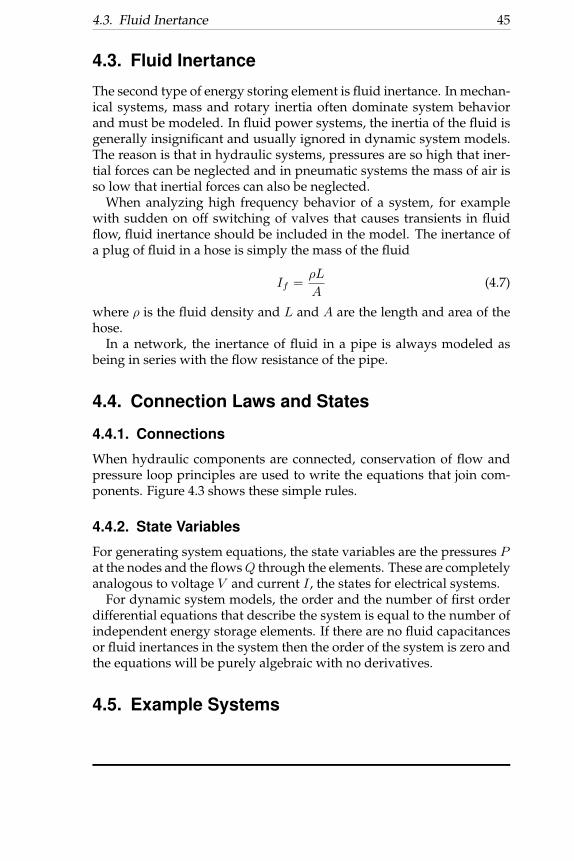
4.3. Fluid Inertance

The second type of energy storing element is fluid inertance. In mechan-ical systems, mass and rotary inertia often dominate system behaviorand must be modeled. In fluid power systems, the inertia of the fluid isgenerally insignificant and usually ignored in dynamic system models.The reason is that in hydraulic systems, pressures are so high that iner-tial forces can be neglected and in pneumatic systems the mass of air isso low that inertial forces can also be neglected.

When analyzing high frequency behavior of a system, for examplewith sudden on off switching of valves that causes transients in fluidflow, fluid inertance should be included in the model. The inertance ofa plug of fluid in a hose is simply the mass of the fluid

If =ρL

A(4.7)

where ρ is the fluid density and L and A are the length and area of thehose.

In a network, the inertance of fluid in a pipe is always modeled asbeing in series with the flow resistance of the pipe.

4.4. Connection Laws and States

4.4.1. Connections

When hydraulic components are connected, conservation of flow andpressure loop principles are used to write the equations that join com-ponents. Figure 4.3 shows these simple rules.

4.4.2. State Variables

For generating system equations, the state variables are the pressures Pat the nodes and the flowsQ through the elements. These are completelyanalogous to voltage V and current I , the states for electrical systems.

For dynamic system models, the order and the number of first orderdifferential equations that describe the system is equal to the number ofindependent energy storage elements. If there are no fluid capacitancesor fluid inertances in the system then the order of the system is zero andthe equations will be purely algebraic with no derivatives.

4.5. Example Systems

46 4. Hydraulic Circuit Analysis

Figure 4.3.: Flow and pressure connection laws. The flows into a node must sumto zero. The pressure drops around a loop must sum to zero. In thefigure on the right, Pi indicates the pressure drop across componenti.

Example 4.5.1. Write the state equations for the system shown in thefigure. There are two resistances, one is an orifice the other is the piperesistance. The output of interest is the pressure at the accumulator.

Solution: The pressure at the reservoir is 0 and the pump is modeledas a pressure source with output pressure PS . There is only one otherpressure in the system, PA, the pressure in the accumulator. Write theelement and connection equations.

Orifice The behavior of the orifice is described by Equation 2.14 orEquation 2.16. For this analysis, lump all constants into one paramterKo = Cv

√1/SG so that Q = Ko

√Porifice. From continuity, the flow

through the orifice is QS

Porifice = PS − PA

4.5. Example Systems 47

QS = Ko

√PS − PA (4.8)

Pipe Resistance Assume turbulent flow. The full expression for tur-bulent flow in a smooth pipe is given by Equation 2.11. For this analysis,make the approximation that the pressure loss is proportional to flowsquared rather than to flow to the 1.75 power. Use KP for the propor-tional constant. The flow through the pipe is the output flow Qo and thepressure across the pipe is P = PA − 0 = PA. Thus, the pipe resistanceis described by

Qo = KP

√PA (4.9)

Accumulator The accumulator is the only energy storage element inthe system and is described by Equation 3.19

QA = Cf PA (4.10)

where QA is the flow into the accumulator.Continuity Conservation of flow dictates that

QS = QA +Qo (4.11)

State Equation The goal is to find a set of state equations (for thisfirst-order example with one energy storage element there will be oneequation) with PA as the output and PS as the input. Using (4.10), (4.9)and (4.11) yields

Cf PA = QS −Qo = QS −KP

√PA (4.12)

Using (4.8) and (4.12)

Cf PA = Ko

√PS − PA −KP

√PA (4.13)

Dividing by Cf yields the state equation

PA =Ko

Cf

√PS − PA −

KP

Cf

√PA (4.14)

Because the state equation is nonlinear, it cannot be solved directlybut can be easily simulated numerically in a package such as Simulink.A Simulink block diagram for this example is shown below.

48 4. Hydraulic Circuit Analysis

5. Bibliography

[1] Herbert Merritt, Hydraulic Control Systems. Wiley, 1967.The classic text on hydraulic control systems. Still useful.

[2] Noah Manring, Hydraulic Control Systems. Wiley, 2005.A modern rewrite of Merritt’s text. Highly recommended.

[3] Eaton-Vickers, Industrial Hydraulics Manual. Eaton Corportation,2001.A standard text for training fluid power technicians. Containsgood,practical information. Used in the fluid power lab course at the Uni-versity of Minnesota.

[4] Arthur Akers, Max Gassman and Richard Smith, Hydraulic PowerSystem Analysis. Taylor & Francis, 2006.Good text on hydraulic system analysis.

[5] Lightning Reference Handbook. Berendsen Fluid Power Inc., 2001.Comprehensive reference information for hydraulics.

[6] Andrew Parr, Hydraulics and Pneumatics: A technician’s and engi-neer’s guide. Butterworth Heinemann, 1998.Good introductory overview of fluid power systems.

49

A. Fluid Power Symbols

Fluid power symbols are set by International Organization for Standard-ization (ISO) standards, ISO 1219-1:2006 for fluid power system andcomponent graphic symbols and ISO 1219-2:1995 for fluid power cir-cuits.

The following tables show the basic ISO/ANSI symbols for fluid powercomponents and systems. 1

Tables will appear in the next version. For now, lists of symbols can be foundat these web locations:

http://www.hydraulicsupermarket.com/upload/db_documents_doc_

19.pdf

http://www.patchn.com/index.php?option=com_content&task=view&

id=31&Itemid=31

http://www.hydraulic-gear-pumps.com/pdf/Hydraulic%20Symbols.

pdf

http://www.hydrastore.co.uk/products/Atos/P001.pdf

http://www.scribd.com/doc/2881790/Fluid-Power-Graphic-Symbols

1Microsoft VISIO has a library of symbols for generating fluid power schematics, al-though may not be in the latest ISO format.

50