ACTAUNIVERSITATIS

UPSALIENSISUPPSALA

2012

Digital Comprehensive Summaries of Uppsala Dissertationsfrom the Faculty of Science and Technology 998

Fluid Mechanics of Vertical AxisTurbines

Simulations and Model Development

ANDERS GOUDE

ISSN 1651-6214ISBN 978-91-554-8539-9urn:nbn:se:uu:diva-183794

Dissertation presented at Uppsala University to be publicly examined in Polhemssalen,Ångströmslaboratoriet, Lägerhyddsvägen 1, Uppsala, Friday, December 14, 2012 at 13:15 forthe degree of Doctor of Philosophy. The examination will be conducted in English.

AbstractGoude, A. 2012. Fluid Mechanics of Vertical Axis Turbines: Simulations and ModelDevelopment. Acta Universitatis Upsaliensis. Digital Comprehensive Summaries ofUppsala Dissertations from the Faculty of Science and Technology 998. 111 pp. Uppsala.ISBN 978-91-554-8539-9.

Two computationally fast fluid mechanical models for vertical axis turbines are the streamtubeand the vortex model. The streamtube model is the fastest, allowing three-dimensional modelingof the turbine, but lacks a proper time-dependent description of the flow through the turbine. Thevortex model used is two-dimensional, but gives a more complete time-dependent description ofthe flow. Effects of a velocity profile and the inclusion of struts have been investigated with thestreamtube model. Simulations with an inhomogeneous velocity profile predict that the powercoefficient of a vertical axis turbine is relatively insensitive to the velocity profile. For thestruts, structural mechanic loads have been computed and the calculations show that if turbinesare designed for high flow velocities, additional struts are required, reducing the efficiencyfor lower flow velocities.Turbines in channels and turbine arrays have been studied with thevortex model. The channel study shows that smaller channels give higher power coefficientsand convergence is obtained in fewer time steps. Simulations on a turbine array were performedon five turbines in a row and in a zigzag configuration, where better performance is predictedfor the row configuration. The row configuration was extended to ten turbines and it has beenshown that the turbine spacing needs to be increased if the misalignment in flow direction islarge.A control system for the turbine with only the rotational velocity as input has been studiedusing the vortex model coupled with an electrical model. According to simulations, this systemcan obtain power coefficients close to the theoretical peak values. This control system studyhas been extended to a turbine farm. Individual control of each turbine has been compared to aless costly control system where all turbines are connected to a mutual DC bus through passiverectifiers. The individual control performs best for aerodynamically independent turbines, butfor aerodynamically coupled turbines, the results show that a mutual DC bus can be a viableoption.Finally, an implementation of the fast multipole method has been made on a graphicsprocessing unit (GPU) and the performance gain from this platform is demonstrated.

Keywords: Wind power, Marine current power, Vertical axis turbine, Wind farm, Channelflow, Simulations, Vortex model, Streamtube model, Control system, Graphics processingunit, CUDA, Fast multipole method

Anders Goude, Uppsala University, Department of Engineering Sciences, Electricity,Box 534, SE-751 21 Uppsala, Sweden.

© Anders Goude 2012

ISSN 1651-6214ISBN 978-91-554-8539-9urn:nbn:se:uu:diva-183794 (http://urn.kb.se/resolve?urn=urn:nbn:se:uu:diva-183794)

To my family

List of papers

This thesis is based on the following papers, which are referred to in the textby their Roman numerals.

I Goude, A., Lundin, S., Leijon, M., “A parameter study of the influenceof struts on the performance of a vertical-axis marine current turbine”,In “Proceedings of the 8th European wave and tidal energy conference,EWTEC2009”, Uppsala, Sweden, pp. 477–483, September 2009.

II Goude, A., Lalander, E., Leijon, M., “Influence of a varying verticalvelocity profile on turbine efficiency for a Vertical Axis Marine CurrentTurbine”, In “Proceedings of the 28th International Conference onOffshore Mechanics and Arctic Engineering, OMAE 2009”, Honolulu,USA, May 2009.

III Grabbe, M., Yuen K., Goude, A., Lalander, E., Leijon, M., “Design ofan experimental setup for hydro-kinetic energy conversion”,International Journal on Hydropower & Dams, 15(5), pp. 112–116,2009.

IV Goude, A., Ågren, O., “Simulations of a vertical axis turbine in achannel”, Submitted to Renewable Energy, October 2012.

V Goude, A., Ågren, O., “Numerical simulation of a farm of vertical axismarine current turbines”, In “Proceedings of the 29th InternationalConference on Offshore Mechanics and Arctic Engineering, OMAE2010”, Shanghai, China, June 2010.

VI Dyachuk, E., Goude, A., Lalander, E., Bernhoff, H., “Influence ofincoming flow direction on spacing between vertical axis marinecurrent turbines placed in a row”, In “Proceedings of the 31thInternational Conference on Offshore Mechanics and ArcticEngineering, OMAE 2012”, Rio de Janeiro, Brazil, July 2012.

VII Goude, A., Bülow, F., “Robust VAWT control system evaluation bycoupled aerodynamic and electrical simulation”, Submitted toRenewable Energy, September 2012.

VIII Goude, A., Bülow, F., “Aerodynamic and electric evaluation of aVAWT farm control system with passive rectifiers and mutualDC-bus”, Submitted to Renewable Energy, November 2012.

IX Goude, A., Engblom, S., “Adaptive fast multipole methods on theGPU”, Journal of Supercomputing, DOI 10.1007/s11227-012-0836-0,In Press, October 2012.

Reprints were made with permission from the publishers.

The author has also contributed to the following paper, not included in thethesis:

A Yuen, K., Lundin, S., Grabbe, M., Lalander, E., Goude, A., Leijon,M., “The Söderfors Project: Construction of an Experimental Hydroki-netic Power Station”, In “Proceedings of the 9th European wave andtidal energy conference, EWTEC2011”, Southampton, United Kingdom,September 2011.

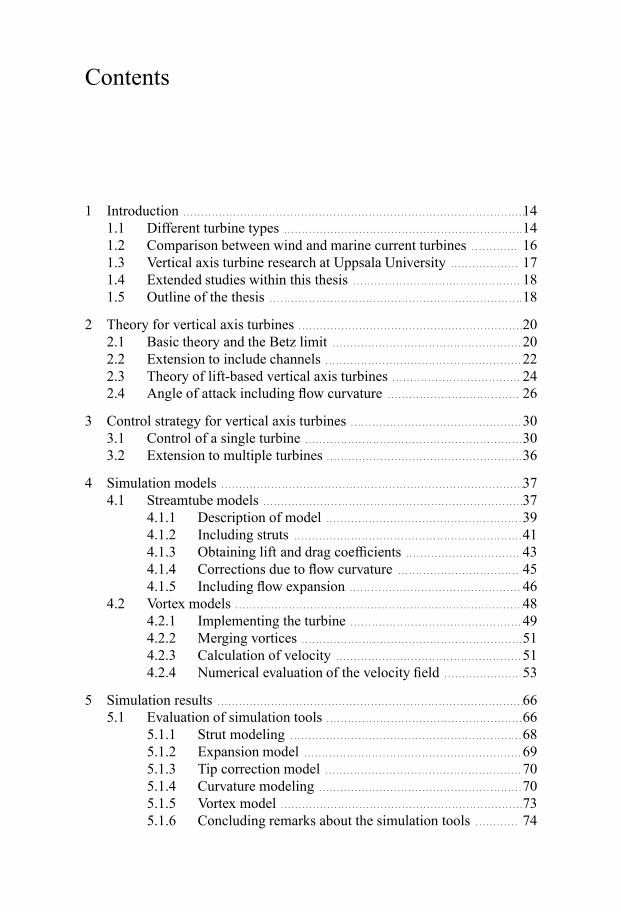
Contents

1 Introduction . . . . . . . . . . . . . . . . . . . . . . . . . . . . . . . . . . . . . . . . . . . . . . . . . . . . . . . . . . . . . . . . . . . . . . . . . . . . . . . . . . . . . . . . . . . . . . . .141.1 Different turbine types . . . . . . . . . . . . . . . . . . . . . . . . . . . . . . . . . . . . . . . . . . . . . . . . . . . . . . . . . . . . . . . . . . .141.2 Comparison between wind and marine current turbines . . . . . . . . . . . . . 161.3 Vertical axis turbine research at Uppsala University . . . . . . . . . . . . . . . . . . . 171.4 Extended studies within this thesis . . . . . . . . . . . . . . . . . . . . . . . . . . . . . . . . . . . . . . . . . . . . . . . 181.5 Outline of the thesis . . . . . . . . . . . . . . . . . . . . . . . . . . . . . . . . . . . . . . . . . . . . . . . . . . . . . . . . . . . . . . . . . . . . . . .18

2 Theory for vertical axis turbines . . . . . . . . . . . . . . . . . . . . . . . . . . . . . . . . . . . . . . . . . . . . . . . . . . . . . . . . . . . . . . .202.1 Basic theory and the Betz limit . . . . . . . . . . . . . . . . . . . . . . . . . . . . . . . . . . . . . . . . . . . . . . . . . . . . . 202.2 Extension to include channels . . . . . . . . . . . . . . . . . . . . . . . . . . . . . . . . . . . . . . . . . . . . . . . . . . . . . . . 222.3 Theory of lift-based vertical axis turbines . . . . . . . . . . . . . . . . . . . . . . . . . . . . . . . . . . . . 242.4 Angle of attack including flow curvature . . . . . . . . . . . . . . . . . . . . . . . . . . . . . . . . . . . . . 26

3 Control strategy for vertical axis turbines . . . . . . . . . . . . . . . . . . . . . . . . . . . . . . . . . . . . . . . . . . . . . . . . 303.1 Control of a single turbine . . . . . . . . . . . . . . . . . . . . . . . . . . . . . . . . . . . . . . . . . . . . . . . . . . . . . . . . . . . . .303.2 Extension to multiple turbines . . . . . . . . . . . . . . . . . . . . . . . . . . . . . . . . . . . . . . . . . . . . . . . . . . . . . . .36

4 Simulation models . . . . . . . . . . . . . . . . . . . . . . . . . . . . . . . . . . . . . . . . . . . . . . . . . . . . . . . . . . . . . . . . . . . . . . . . . . . . . . . . . . . . .374.1 Streamtube models . . . . . . . . . . . . . . . . . . . . . . . . . . . . . . . . . . . . . . . . . . . . . . . . . . . . . . . . . . . . . . . . . . . . . . . . .37

4.1.1 Description of model . . . . . . . . . . . . . . . . . . . . . . . . . . . . . . . . . . . . . . . . . . . . . . . . . . . . . . . 394.1.2 Including struts . . . . . . . . . . . . . . . . . . . . . . . . . . . . . . . . . . . . . . . . . . . . . . . . . . . . . . . . . . . . . . . . 414.1.3 Obtaining lift and drag coefficients . . . . . . . . . . . . . . . . . . . . . . . . . . . . . . . . 434.1.4 Corrections due to flow curvature . . . . . . . . . . . . . . . . . . . . . . . . . . . . . . . . . . 454.1.5 Including flow expansion . . . . . . . . . . . . . . . . . . . . . . . . . . . . . . . . . . . . . . . . . . . . . . . . 46

4.2 Vortex models . . . . . . . . . . . . . . . . . . . . . . . . . . . . . . . . . . . . . . . . . . . . . . . . . . . . . . . . . . . . . . . . . . . . . . . . . . . . . . . . .484.2.1 Implementing the turbine . . . . . . . . . . . . . . . . . . . . . . . . . . . . . . . . . . . . . . . . . . . . . . . . 494.2.2 Merging vortices . . . . . . . . . . . . . . . . . . . . . . . . . . . . . . . . . . . . . . . . . . . . . . . . . . . . . . . . . . . . . .514.2.3 Calculation of velocity . . . . . . . . . . . . . . . . . . . . . . . . . . . . . . . . . . . . . . . . . . . . . . . . . . . . 514.2.4 Numerical evaluation of the velocity field . . . . . . . . . . . . . . . . . . . . . 53

5 Simulation results . . . . . . . . . . . . . . . . . . . . . . . . . . . . . . . . . . . . . . . . . . . . . . . . . . . . . . . . . . . . . . . . . . . . . . . . . . . . . . . . . . . . . .665.1 Evaluation of simulation tools . . . . . . . . . . . . . . . . . . . . . . . . . . . . . . . . . . . . . . . . . . . . . . . . . . . . . . .66

5.1.1 Strut modeling . . . . . . . . . . . . . . . . . . . . . . . . . . . . . . . . . . . . . . . . . . . . . . . . . . . . . . . . . . . . . . . . . 685.1.2 Expansion model . . . . . . . . . . . . . . . . . . . . . . . . . . . . . . . . . . . . . . . . . . . . . . . . . . . . . . . . . . . . . 695.1.3 Tip correction model . . . . . . . . . . . . . . . . . . . . . . . . . . . . . . . . . . . . . . . . . . . . . . . . . . . . . . . 705.1.4 Curvature modeling . . . . . . . . . . . . . . . . . . . . . . . . . . . . . . . . . . . . . . . . . . . . . . . . . . . . . . . . . 705.1.5 Vortex model . . . . . . . . . . . . . . . . . . . . . . . . . . . . . . . . . . . . . . . . . . . . . . . . . . . . . . . . . . . . . . . . . . . .735.1.6 Concluding remarks about the simulation tools . . . . . . . . . . . . 74

5.2 Results from papers . . . . . . . . . . . . . . . . . . . . . . . . . . . . . . . . . . . . . . . . . . . . . . . . . . . . . . . . . . . . . . . . . . . . . . . .745.2.1 The effects of struts . . . . . . . . . . . . . . . . . . . . . . . . . . . . . . . . . . . . . . . . . . . . . . . . . . . . . . . . . 755.2.2 The effects of a velocity profile . . . . . . . . . . . . . . . . . . . . . . . . . . . . . . . . . . . . . . 775.2.3 Design of a turbine for use in a river . . . . . . . . . . . . . . . . . . . . . . . . . . . . . . 795.2.4 Turbines in channels . . . . . . . . . . . . . . . . . . . . . . . . . . . . . . . . . . . . . . . . . . . . . . . . . . . . . . . . 805.2.5 Turbines in an array . . . . . . . . . . . . . . . . . . . . . . . . . . . . . . . . . . . . . . . . . . . . . . . . . . . . . . . . . 835.2.6 Simulations of control systems . . . . . . . . . . . . . . . . . . . . . . . . . . . . . . . . . . . . . . . 875.2.7 Control of multiple turbines . . . . . . . . . . . . . . . . . . . . . . . . . . . . . . . . . . . . . . . . . . . . 90

6 Conclusions . . . . . . . . . . . . . . . . . . . . . . . . . . . . . . . . . . . . . . . . . . . . . . . . . . . . . . . . . . . . . . . . . . . . . . . . . . . . . . . . . . . . . . . . . . . . . . . .95

7 Suggestions for future work . . . . . . . . . . . . . . . . . . . . . . . . . . . . . . . . . . . . . . . . . . . . . . . . . . . . . . . . . . . . . . . . . . . . . .97

8 Summary of papers . . . . . . . . . . . . . . . . . . . . . . . . . . . . . . . . . . . . . . . . . . . . . . . . . . . . . . . . . . . . . . . . . . . . . . . . . . . . . . . . . . . .98

9 Errata for papers . . . . . . . . . . . . . . . . . . . . . . . . . . . . . . . . . . . . . . . . . . . . . . . . . . . . . . . . . . . . . . . . . . . . . . . . . . . . . . . . . . . . . .102

10 Acknowledgments . . . . . . . . . . . . . . . . . . . . . . . . . . . . . . . . . . . . . . . . . . . . . . . . . . . . . . . . . . . . . . . . . . . . . . . . . . . . . . . . . . .103

11 Summary in Swedish . . . . . . . . . . . . . . . . . . . . . . . . . . . . . . . . . . . . . . . . . . . . . . . . . . . . . . . . . . . . . . . . . . . . . . . . . . . . . . .104

References . . . . . . . . . . . . . . . . . . . . . . . . . . . . . . . . . . . . . . . . . . . . . . . . . . . . . . . . . . . . . . . . . . . . . . . . . . . . . . . . . . . . . . . . . . . . . . . . . . . . . .107

Nomenclature

A m2 Turbine cross-sectional areaA∞ m2 Asymptotic area of streamtube enclosing turbineAc m2 Cross-sectional area of a channelAd m2 Area of turbine discAe m2 Streamtube area far downstream/center of turbineAR − Aspect ratio of a bladeCD − Drag coefficientCDs − Drag coefficient for strutCD∞ − Drag coefficient for infinitely long bladeCL − Lift coefficientCLs − Lift coefficient for strutCL∞ − Lift coefficient for infinitely long bladeCN − Normal force coefficientCN0 − Normal force coefficient without curvature correctionsCNs − Normal force coefficient for strutCP − Power coefficientCPe − Power coefficient equivalent for extracted powerCPmax − Maximum power coefficient for a given flow velocityCT − Tangential force coefficientCTs − Tangential force coefficient for strutD m Turbine diameterF − Velocity correction factorFD N Drag forceFD0 N Drag force at zero angle of attackFL N Lift forceFN N Normal forceFNl N/m Normal force per meterFR N Force in radial directionFT N Tangential forceFTs N Tangential force on strutFx N Aerodynamic force from a blade on flow in a streamtubeFxs N Aerodynamic force from a strut on flow in a streamtubeH m Channel heightJ kgm2 Moment of intertiaL m Distance between strutsK N Constant to determine lift force

9

Ma − Mach numberN − Number of particles (FMM)Nb − Number of bladesNbox − Number of boxes (FMM)Nd − Number particles per box (FMM)Np − Number of panelsNs − Number of strutsNt − Number of turbinesNv − Number of vorticesNFi − Set of all boxes in near field of box i (FMM)P W Power absorbed by the turbinePe W Power extracted from the turbinePe,tot W Total power extracted from the turbines of a farmPtot W Power available in flowR m Turbine radius

Rinner m Strut inner attachment pointRouter m Strut outer attachment pointRe − Reynolds numberTs Nm Torque from strutV m/s Flow velocityV0 m/s Flow velocity far upstream of turbineV∞ m/s Asymptotic flow velocityVabs m/s Magnitude of incoming flow velocity at blade positionVb m/s Blade velocityVd m/s Flow velocity at turbine discVe m/s Flow velocity far downstream/center of turbine�Vi m/s Vortex velocityVr m/s Relative flow velocity for a blade (absolute value)Vrs m/s Relative flow velocity for a strut (absolute value)Vs m/s Flow velocity at strut positionVre f m/s Reference flow velocity for estimating angle of attackVrel m/s Relative flow velocity for bladeVrelz m/s Relative flow velocity for blade in its own reference frameVs m/s Far downstream velocity of flow passing outside turbineVs j m/s Flow velocity at strut segmentVω m/s Velocity due to vorticesW m2/s Complex velocity potentialWb m2/s Complex velocity potential for blade velocitya − Axial induction factorai − Multipole coefficient i (FMM)as − Slope of lift coefficient curve inCL/α plotb m Circle radius used for conformal mappingbi − Local coefficient i (FMM)

10

by∞ − Normalized asymptotic streamtube widthbye − Normalized streamtube width at the turbine centerbz∞ − Normalized asymptotic streamtube heightbze − Normalized streamtube height at the turbine centerc m Blade chordcs m Strut chordcsound m/s Speed of soundc0 m Reference chord for struts�g m/s2 Gravitational accelerationh m Turbine heightk1 kgm2 First control system constantk2 kgm2 Second control system constantk3 kgm2 Third control system constantkd1 − Constant for time estimate of direct evaluation (FMM)kd2 − Constant for time estimate of direct evaluation (FMM)l m Blade length in streamtubep − Number of multipole coefficients (FMM)p0 N/m2 Pressure far upstream of turbinepatm N/m2 Atmospheric pressurepd1 N/m2 Pressure directly in front of turbine discpd2 N/m2 Pressure directly after turbine discpe N/m2 Pressure far downstream of turbiner0 m Box center (FMM)rs m Radial position on a strut�r m Arbitrary position�ri m Vortex positions m Position on blade surface in transformed planet s Timetb m Blade thicknesstd s Time estimate for direct evaluation (FMM)u − Interference factorx m Position in the x-directionx0 m Blade attachment pointx0r − Normalized blade attachment pointy m Position in the y-directiony∞ m Asymptotic streamtube position in y-directionyd m Streamtube position at turbine disc in y-directionye m Streamtube position far downstream in y-directionΔy m Streamtube widthz m Position on blade surface in the blades reference framez0 m Position on blade surface in the turbines reference framezb m Blade positionΔz m Streamtube height

11

�Γp m3/s Circulation of three dimensional point vortexΓ m2/s Circulation of two dimensional vortexΔ m Cutoff radius used for vortex mergingΩ rad/s Turbine rotational velocityΩi rad/s Rotational velocity of turbine iΩ1 rad/s First control system rotational velocity constantΩ2 rad/s Second control system rotational velocity constantΩ3 rad/s Third control system rotational velocity constantα − Angle of attackαb − Corrected angle of attackαs − Angle of attack for strutβ − Direction of incoming windδ − Blade pitch angleε m Cutoff radius of Gaussian vortex kernelη − Angle of blade relative to the vertical axisηs − Angle of strut relative to the horizontal planeθ − Blade azimuthal position shifted 90 degreesθb − Blade azimuthal positionλ − Tip speed ratioλe − Equilibrium tip speed ratio

λmax − The tip speed ratio that gives highest power coefficientν m2/s Kinematic viscosityρ kg/m3 Density of fluidσ N/m2 Stressϕ − Angle of relative windφ m2/s Velocity potentialω 1/s Vorticity

12

Abbreviations

CPU Central processing unitCUDA Compute unified device architectureFEM Finite element methodFMM Fast multipole methodFVM Finite volume methodGPU Graphics processing unitL2L Local to local translationL2P Local to particle evaluationM2L Multipole to local translationM2M Multipole to multipole translationNACA National Advisory Committee for AeronauticsP2M Particle to multipole initializationP2P Particle to particle interaction (direct evaluation)RANS Reynolds-averaged Navier-Stokes equationsSIMD Single instruction multiple dataSSE Streaming SIMD Extensions

13

1. Introduction

A turbine is used to convert the energy from a moving fluid into rotational mo-tion, which in turn can drive an electric generator. The best suited turbine forthis energy conversion depends on the characteristics of the flow. One case,which is present in gas turbines and traditional hydro power plants, is flow con-strained by walls, such as flow within a pipe. Here, the turbine cross-sectionalarea usually covers the entire flow and the flow has a large pressure differencethat drives the turbine. A second case is the free flow, where no confiningwallsare present. This is the case for wind power and often a reasonable approxi-mation for tidal power in the ocean. In free flow, the fluid can pass around theturbine and the available energy is the kinetic energy in the flow. This thesismainly treat the free flow case, but also a hybrid case where there are confin-ing walls, but the turbine does not cover the whole cross-sectional area of theflow, is studied in this thesis. This situation occurs in a river, where the rivercross-sectional shape area usually prevents a turbine from covering the entirecross-section.

1.1 Different turbine typesThe typical turbine design for wind power is a horizontal axis turbine, wherethe rotational axis of the turbine is parallel to the flow direction [1, chapter 1].In this thesis, however, the vertical axis turbine will be investigated. Here, therotational axis is perpendicular to the flow direction. This kind of turbine issometimes called “cross-flow turbine”, as the turbine in principle also can betilted 90 degrees to have a horizontal axis while still having its rotational axisperpendicular to the flow. The traditional name “vertical axis turbine” will beused here, even for situations where the rotational axis is tilted, since this isthe most commonly used name.There are two different types of vertical axis turbines. The first type is

based on the drag force and is often called the Savonius rotor after the Finnishinventor Sigurd Johannes Savonius, despite that Savonius only patented an im-provement of older designs [2]. This improvement is neither implemented onall present drag-based turbines. Drag-based devices rely on variation of thedrag coefficient with respect to the orientation of the object. To create a rea-sonably efficient drag-based turbine, the drag coefficient should be high in onedirection and low in the opposite direction, which gives a torque on the tur-bine. Drag-based devices achieve lower power coefficients than the lift-based

14

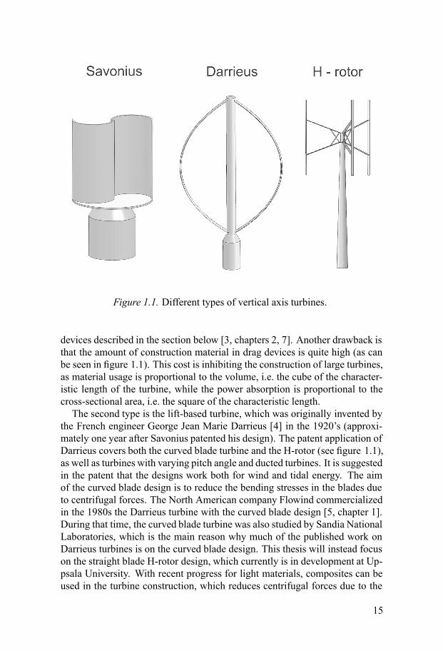
Figure 1.1. Different types of vertical axis turbines.

devices described in the section below [3, chapters 2, 7]. Another drawback isthat the amount of construction material in drag devices is quite high (as canbe seen in figure 1.1). This cost is inhibiting the construction of large turbines,as material usage is proportional to the volume, i.e. the cube of the character-istic length of the turbine, while the power absorption is proportional to thecross-sectional area, i.e. the square of the characteristic length.The second type is the lift-based turbine, which was originally invented by

the French engineer George Jean Marie Darrieus [4] in the 1920’s (approxi-mately one year after Savonius patented his design). The patent application ofDarrieus covers both the curved blade turbine and the H-rotor (see figure 1.1),as well as turbines with varying pitch angle and ducted turbines. It is suggestedin the patent that the designs work both for wind and tidal energy. The aimof the curved blade design is to reduce the bending stresses in the blades dueto centrifugal forces. The North American company Flowind commercializedin the 1980s the Darrieus turbine with the curved blade design [5, chapter 1].During that time, the curved blade turbine was also studied by Sandia NationalLaboratories, which is the main reason why much of the published work onDarrieus turbines is on the curved blade design. This thesis will instead focuson the straight blade H-rotor design, which currently is in development at Up-psala University. With recent progress for light materials, composites can beused in the turbine construction, which reduces centrifugal forces due to the

15

lighter structure. This makes the H-rotor design more feasible. The straightblade design has the advantages that straight blades are easier to manufactureand by attaching the blades with struts, it is possible to place the upper bear-ing much closer to the turbine center, reducing the bending moment on theaxis. In addition, the constant radius of the straight blade design gives a largercross-sectional area. Disadvantages compared to the curved blade design arethe addition of extra struts and the higher bending moments due to centrifugalforces.The main aerodynamic advantage of vertical axis turbines, compared to

standard horizontal axis turbines, is the independence of flow direction, re-moving the need for a yaw mechanism. For water flow, an additional advan-tage is that the cross-sectional area can be more flexibly chosen as both heightand diameter can be varied (and the diameter can vary with height). This canbe useful in shallow water where a turbine with a large width and small heightcan cover a larger area than a horizontal axis turbine, as the cross-sectionalarea of a horizontal axis turbine is circular. Disadvantages of the vertical axisturbines are the lower power coefficients and that the turbines are typically notself-starting.The vertical axis turbine can have its generator on the ground, which in

the wind power case simplifies maintenance, tower construction and makesthe weight of the generator less important. This is beneficial for direct drivengenerators, which typically have large diameters. The use of direct driven gen-erators further reduces the number of moving parts in the system. One majorconcern for vertical axis turbines is the cyclic blade forces in each revolution,which leads to torque oscillations and material fatigue. For further compar-isons between horizontal and vertical axis turbines (and also between curvedand straight blade turbines) see e.g. [6].

1.2 Comparison between wind and marine currentturbines

Even though wind turbines operate in air (gas) while marine current turbinesoperate in water (liquid), there are many similarities between the two. Tra-ditionally, water is considered an incompressible fluid and can therefore bemodeled with the incompressible Navier-Stokes equations. For air, it is typi-cally expected that compressibility effects can be neglected for Mach numbersMa within the range

Ma=Vrelcsound

< 0.3.

Here, Vrel is the relative flow velocity (measured in the blades rest frame) andcsound is the speed of sound in the fluid [7, chapter 9]. Note that the major con-tribution toVrel originates from the blades’ own motion for lift-based turbines.

16

The speed of the blades in a wind turbine is typically too low for the Machnumber to be above 0.3 and wind turbines can therefore also be modeled withincompressible aerodynamics. Although both wind andmarine turbines can bestudied with the incompressible Navier-Stokes equations, there are still somecharacteristic differences. One difference is that for marine current turbines,there is both a sea bed and a free surface that bounds the flow. Another dif-ference is the risk for cavitation at too high flow velocities. Cavitation wouldmodify the flow characteristics and can cause damage to the turbine [8].The energy absorbed by a turbine is proportional to the fluid density and

the cube of the flow velocity. As the density of water is 800 times higher thanthe density of air, comparatively low fluid velocities are adequate for marinecurrent power generation. For equal cross-sectional area, a wind speed of10 m/s has the same incoming kinetic power as a water flow speed of 1.1 m/s.However, as the forces only are proportional to the square of the flow velocity,the marine current turbine experiences approximately 9.3 times higher fluidmechanical forces than a wind turbine at the same conditions (assuming thatthe turbines are identical) and rotates 9.3 times slower. The increased forcesfor marine current turbines require both stronger blades and support structure.Many of the experimental vertical axis turbines for water have used relativelylarge blades and thereby low optimal tip speed ratios [9–12].One important parameter for the effectiveness of the turbine is the Reynolds

number, which for a blade is defined as

Re=cVν

,

whereV is the flow velocity, c is the blade chord and ν is the kinematic viscos-ity. A higher Reynolds number usually decreases the drag losses and increasesthe stall angle, which is beneficial for vertical axis turbines. For 20 ◦C, thekinematic viscosities are 15.1 μm2/s for air and 1.00 μm2/s for water [13, ap-pendix A]. Under the conditions of equal power extraction mentioned above(i.e. 9.3 times higher flow velocity for the wind turbine), this would give a63 % higher Reynolds number for the marine current turbine, which is withinthe same order of magnitude as the wind turbine.

1.3 Vertical axis turbine research at Uppsala UniversityAt the Division of Electricity at Uppsala University, three vertical axis windturbines have been built. The first turbine had a cross-sectional area of 6 m2and was later followed by a turbine with the cross-sectional area 30 m2 and therated power 12 kW [14–16]. This larger turbine is used for most of the experi-ments. A 10 kW turbine for telecom applications has also been built [17]. Fur-ther, a 200 kW turbine has been constructed by the spin-off company VerticalWind AB [18]. Additionally, a marine current turbine (described in paper III)is scheduled to be deployed by the end of 2012.

17

Several simulation tools for turbine simulations have previously been de-veloped at the division. A two-dimensional inviscid vortex model based onconformal mappings for the blades has been created by Deglaire et al. [19]. Inthe turbine implementation, each blade is solved independently [20], allowingfor coupling to an elastic method developed by Bouquerel et al., see paper IVin [21]. A multibody version for simulating turbines has been developed byÖsterberg et al., see [22] and paper III in [21]. Two streamtube models havealso been implemented by Deglaire and Bouquerel.

1.4 Extended studies within this thesisThis thesis focuses on the fluid mechanical modeling of the vertical axis tur-bine, and two different simulation tools have been developed. The first simu-lation tool uses the streamtube model and the development of this tool startedfrom the basic streamtube model implemented by Bouquerel, which is basedon the model of Paraschivoiu [3]. All additional modeling and code develop-ment have been developed within this thesis.The second simulation tool uses a vortex model, and this tool has been

developed from scratch within this work. This model is based on empiricaldata for lift and drag coefficients instead of the conformal mapping methodby Deglaire, which is based on inviscid theory. The computational speed iscrucial for the developed vortex model and large efforts have been put intothis. The existing implementation of the fast multipole method by Stefan Eng-blom [23] has been significantly improved and ported to a GPU (paper IX)Several studies have been carried out with the two simulation models. The

streamtube model has been used to study losses due to struts (paper I), theeffects of a velocity profile (Paper II) and to design a turbine for deploymentin a river (paper III). The more computationally demanding vortex model hasbeen used to study turbines in channels (paper IV) and turbine arrays (paper Vand VI). The vortex model is also coupled to an electrical model to study con-trol systems for a single turbine (paper VII) and extended simulations analyzecontrol systems for a turbine farm (paper VIII).

1.5 Outline of the thesisAfter the introduction, theory for vertical axis turbines is presented in chap-ter 2. This is followed by an introduction to control systems in chapter 3.The theory and implementation for the simulation models are then presentedin chapter 4, which also includes the GPU implementation of the fast multi-pole method. The results from the simulations are given in chapter 5, wherethe first part evaluates the accuracy of the simulation models and the secondpart summarizes the results from the articles. The thesis ends by conclusions,

18

suggestions for future work, summary of papers, errata for papers and ac-knowledgments.

19

2. Theory for vertical axis turbines

Given a cross-sectional area A perpendicular to a homogenous flow of a fluid,the kinetic power that passes through this area is given by

Ptot =12

ρAV 3, (2.1)

where ρ is the density and V is the flow velocity. If the flow is not confinedby any surrounding boundaries, the kinetic power is the available power for awind/current turbine. The efficiency (i.e. outgoing power divided by incomingpower) would be one possible measure of how good the energy conversionis. However, adding a turbine will change the velocity and force parts of theflow to pass outside the turbine area and thereby change the kinetic energythat passes through this area A. Moreover, some kinetic energy is left in theflow and can possibly be used later. Therefore, turbine performance is usuallymeasured with the power coefficient instead, which is defined as

CP =P

12ρAV 3∞

, (2.2)

where P is the power absorbed by the turbine and V∞ is the asymptotic up-stream flow velocity. With this expression, the absorbed power is comparedto the power that would have passed through the cross-sectional area, if theturbine would be absent, instead of compared to the power that actually passesthrough the area. Since this expression is normalized against an expressionthat does not change with the turbine characteristics, it is a better measure thanefficiency. Improving the power coefficient will give higher power absorption,which is not always the case with efficiency.

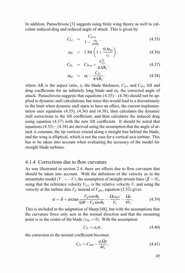
2.1 Basic theory and the Betz limitOne of the most basic approximations of a turbine is the one used in the tradi-tional Betz theory [24], where the turbine is approximated as a single flat discwith a constant pressure drop over the whole turbine surface. All flow passingthrough the disc is encapsulated in a streamtube that starts far ahead of theturbine and ends far behind. By making the assumption that the pressure atboth ends of the streamtube is the atmospheric pressure patm, and by using the

20

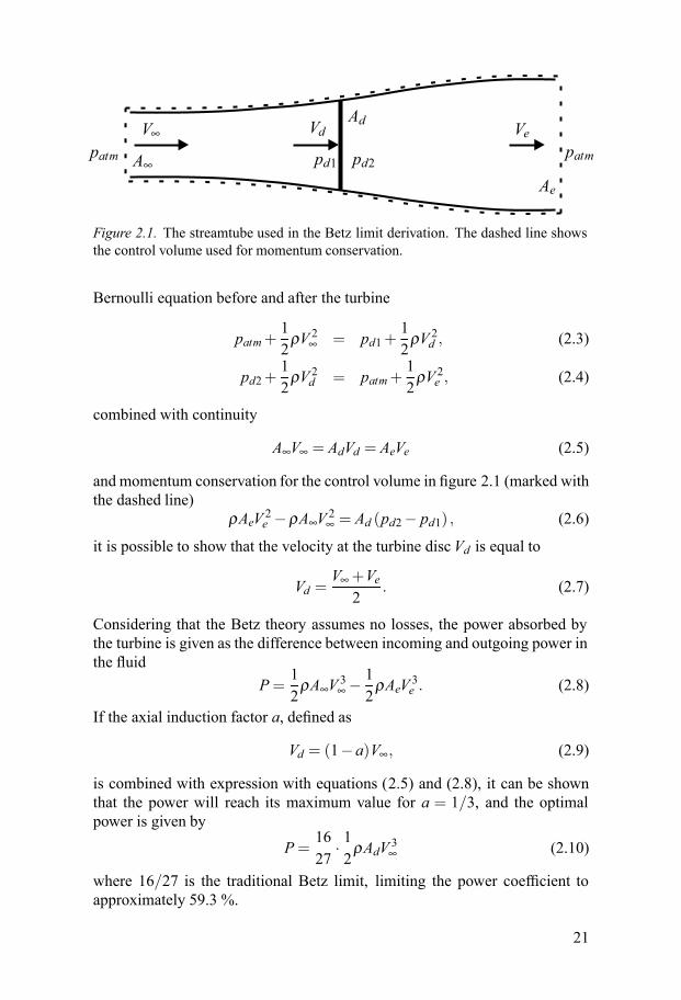
patmpatmV∞

A∞

Vd

pd1 pd2

Ve

Ae

Ad

Figure 2.1. The streamtube used in the Betz limit derivation. The dashed line showsthe control volume used for momentum conservation.

Bernoulli equation before and after the turbine

patm+12

ρV 2∞ = pd1+12

ρV 2d , (2.3)

pd2+12

ρV 2d = patm+12

ρV 2e , (2.4)

combined with continuity

A∞V∞ = AdVd = AeVe (2.5)

and momentum conservation for the control volume in figure 2.1 (marked withthe dashed line)

ρAeV 2e −ρA∞V 2∞ = Ad (pd2− pd1) , (2.6)

it is possible to show that the velocity at the turbine discVd is equal to

Vd =V∞ +Ve2

. (2.7)

Considering that the Betz theory assumes no losses, the power absorbed bythe turbine is given as the difference between incoming and outgoing power inthe fluid

P=12

ρA∞V 3∞ − 12

ρAeV 3e . (2.8)

If the axial induction factor a, defined as

Vd = (1−a)V∞, (2.9)

is combined with expression with equations (2.5) and (2.8), it can be shownthat the power will reach its maximum value for a = 1/3, and the optimalpower is given by

P=1627

· 12

ρAdV 3∞ (2.10)

where 16/27 is the traditional Betz limit, limiting the power coefficient toapproximately 59.3 %.

21

p0

p0V0

V0

V0

A0AcVdpd1 pd2

Ve

Ae

Adpe

Vs

Figure 2.2. Illustration of a streamtube confining the flow that passes through theturbine disc for a channel of cross-sectional area Ac.

2.2 Extension to include channelsThe Betz theory assumes no outer boundaries in the system. For a turbine op-erating in water, it is more common that boundaries are present. One exampleis a river, where the flow is limited by the width and depth. The outer wallsprevent the flow from expanding, pushing more flow through the turbine. Thisoccurs in a traditional hydro power plant, where the entire flow is forced topass through the turbine, which results in much higher power absorption thanthe Betz limit [25].To analyze this case analytically, assume that the flow upstream of the tur-

bine has constant velocity V0 and pressure p0 (see figure 2.2). Note that inthis case, the pressure upstream and the pressure downstream are not equal.Instead, there will be a drop in pressure, which, for open channel flow, wouldcorrespond to a drop in the surface level. Due to the continuity of the pressure,the pressure inside the streamtube and outside has to be the same downstream(pe) . The cross-sectional area of the channel is Ac and the cross-sectional areaof the turbine is Ad . In this case, the Bernoulli equation gives

p0+12

ρV 20 = pd1+12

ρV 2d , (2.11)

pd2+12

ρV 2d = pe+12

ρV 2e , (2.12)

p0+12

ρV 20 = pe+12

ρV 2s , (2.13)

the continuity equation gives

A0V0 = AdVd = AeVe, (2.14)

(Ac−A0)V0 = (Ac−Ae)Vs (2.15)

22

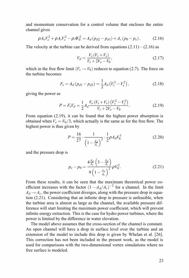
and momentum conservation for a control volume that encloses the entirechannel gives

ρAeV 2e +ρAsV 2s −ρAV 20 = Ad (pd2− pd1)+Ac (p0− pe) . (2.16)

The velocity at the turbine can be derived from equations (2.11) – (2.16) as

Vd =Ve (Vs+Ve)Vs+2Ve−V0 , (2.17)

which in the free flow limit (Vs →V0) reduces to equation (2.7). The force onthe turbine becomes

Fx = Ad (pd1− pd2) =12Ad

(V 2s −V 2e

), (2.18)

giving the power as

P= FxVd =12AdVe (Vs+Ve)

(V 2s −V 2e

)Vs+2Ve−V0 . (2.19)

From equation (2.19), it can be found that the highest power absorption isobtained when Ve =V0/3, which actually is the same as for the free flow. Thehighest power is thus given by

P=1627

· 1(1− Ad

Ac

)2 · 12ρAdV 30 (2.20)

and the pressure drop is

pe− p0 =4AdAc

(3− Ad

Ac

)9(1− Ad

Ac

)2 ρV 20 . (2.21)

From these results, it can be seen that the maximum theoretical power co-efficient increases with the factor (1−Ad/Ac)−2 for a channel. In the limitAd → Ac, the power coefficient diverges, along with the pressure drop in equa-tion (2.21). Considering that an infinite drop in pressure is unfeasible, whenthe turbine area is almost as large as the channel, the available pressure dif-ference will start limiting the maximum power coefficient, which will preventinfinite energy extraction. This is the case for hydro power turbines, where thepower is limited by the difference in water elevation.The model above assumes that the cross-section of the channel is constant.

An open channel will have a drop in surface level over the turbine and anextension of the model to include this drop is given by Whelan et al. [26].This correction has not been included in the present work, as the model isused for comparisons with the two-dimensional vortex simulations where nofree surface is modeled.

23

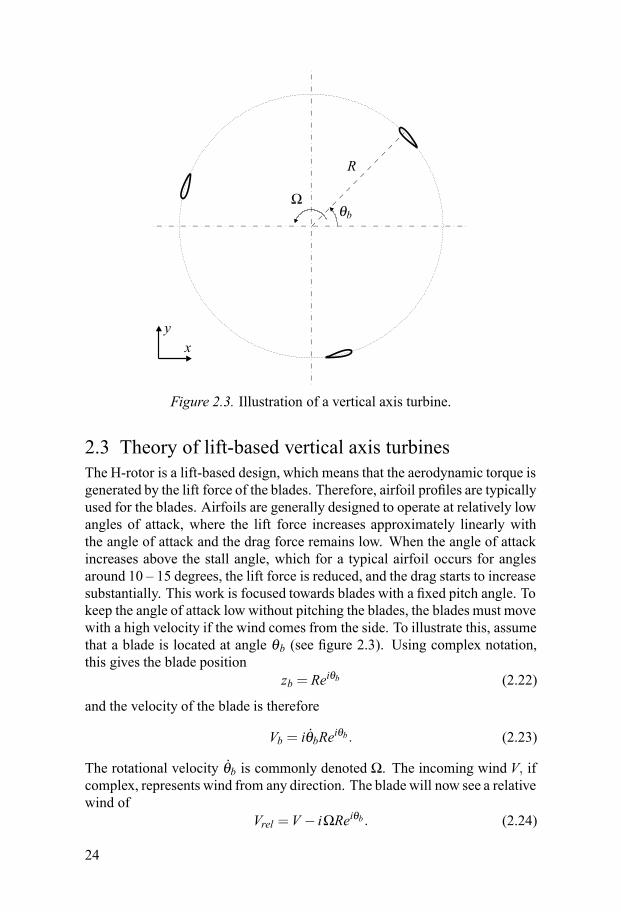
R

θbΩ

xy

Figure 2.3. Illustration of a vertical axis turbine.

2.3 Theory of lift-based vertical axis turbinesThe H-rotor is a lift-based design, which means that the aerodynamic torque isgenerated by the lift force of the blades. Therefore, airfoil profiles are typicallyused for the blades. Airfoils are generally designed to operate at relatively lowangles of attack, where the lift force increases approximately linearly withthe angle of attack and the drag force remains low. When the angle of attackincreases above the stall angle, which for a typical airfoil occurs for anglesaround 10 – 15 degrees, the lift force is reduced, and the drag starts to increasesubstantially. This work is focused towards blades with a fixed pitch angle. Tokeep the angle of attack low without pitching the blades, the blades must movewith a high velocity if the wind comes from the side. To illustrate this, assumethat a blade is located at angle θb (see figure 2.3). Using complex notation,this gives the blade position

zb = Reiθb (2.22)

and the velocity of the blade is therefore

Vb = iθbReiθb. (2.23)

The rotational velocity θb is commonly denoted Ω. The incoming wind V, ifcomplex, represents wind from any direction. The blade will now see a relativewind of

Vrel =V − iΩReiθb . (2.24)

24

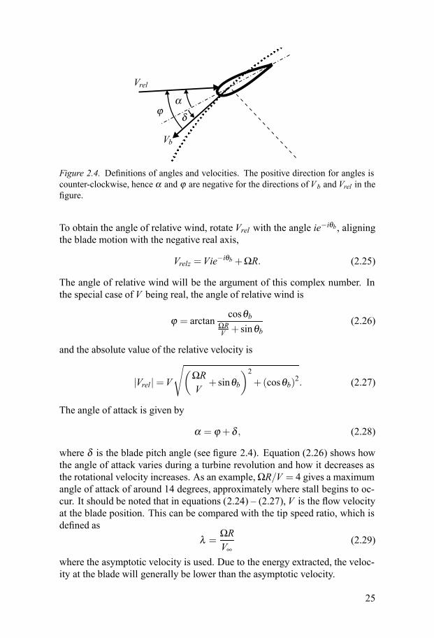
Vrelα

δϕ

Vb

Figure 2.4. Definitions of angles and velocities. The positive direction for angles iscounter-clockwise, hence α and ϕ are negative for the directions of Vb and Vrel in thefigure.

To obtain the angle of relative wind, rotate Vrel with the angle ie−iθb , aligningthe blade motion with the negative real axis,

Vrelz =Vie−iθb +ΩR. (2.25)

The angle of relative wind will be the argument of this complex number. Inthe special case of V being real, the angle of relative wind is

ϕ = arctancosθb

ΩRV + sinθb

(2.26)

and the absolute value of the relative velocity is

|Vrel | =V√(

ΩRV

+ sinθb)2

+(cosθb)2. (2.27)

The angle of attack is given by

α = ϕ +δ , (2.28)

where δ is the blade pitch angle (see figure 2.4). Equation (2.26) shows howthe angle of attack varies during a turbine revolution and how it decreases asthe rotational velocity increases. As an example,ΩR/V = 4 gives a maximumangle of attack of around 14 degrees, approximately where stall begins to oc-cur. It should be noted that in equations (2.24) – (2.27), V is the flow velocityat the blade position. This can be compared with the tip speed ratio, which isdefined as

λ =ΩRV∞

(2.29)

where the asymptotic velocity is used. Due to the energy extracted, the veloc-ity at the blade will generally be lower than the asymptotic velocity.

25

The turbine torque is calculated from the tangential force, which is givenby

FT = FL sinϕ −FD cosϕ . (2.30)When the angle of relative wind is low, the approximations sinϕ ≈ ϕ andcosϕ ≈ 1 can be applied. Assume that the pitch angle is zero, hence α =ϕ . For symmetric blades, the blade forces can be approximated as FL ≈ Kα ,where K is a constant, and FD ≈ FD0, where FD0 is a constant. The tangentialforce can therefore be estimated as

FT = Kϕ2−FD0, (2.31)

showing that when the angle of relative wind decreases, the drag force be-comes dominating. The conclusion is that for high tip speed ratios, drag willgive a more significant contribution, reducing the power coefficient. At toolow tip speed ratios, the turbine will enter stall, where lift decreases and dragincreases, which also should be avoided. For these reasons, the turbine shouldbe designed to operate with a tip speed ratio close to the stall limit in order toobtain the highest possible power coefficient.

2.4 Angle of attack including flow curvatureThe expression (2.26) is only valid for infinitely small symmetric blades. Theblade performs a rotational motion, which leads to additional curvature effects,changing the effective angle of attack. To conclude the theory section, a moreproper derivation will be performed using a rotating flat plate instead.By the use of conformal mappings, a circle can be transformed into a flat

plate with the Joukowski transformation. The s-plane represents the circlewith radius b and the z-plane a flat plate extending between −2b to 2b givingthe blade chord c as c = 4b. The blade coordinates z in its own frame ofreference is given by

z= s+b2

s. (2.32)

Using the same transformation as Deglaire [20], the z0 plane can be defined as

z0 =[(z+ x0)e−iδ + iR

]eiθ = (z+D)ei(θ−δ), (2.33)

where D = x0+ iReiδ . By assuming that the blade only rotates around thecenter, the blade velocity is given by

Vb = iθ[(z+ x0)e−iδ + iR

]eiθ = iΩz0 (2.34)

with Ω = θ . Introduce a complex velocity potentialW , with complex conju-gateW , such that

dWdz0

=V, (2.35)

26

hence the potential can be used to calculate the flow velocity V . Assume thatthe potential is given on the form

W (s) =Vabsei(−β+θ−δ)s+Vabse−i(−β+θ−δ) b2

s− iΓ2πlog(s)+W1(s), (2.36)

where Vabseiβ is the flow velocity at the blade position. Now, construct apotential such that

dWbdz0

= Vb, (2.37)

which givesdWbds

= Vbdz0ds

= −iΩz0 dz0ds = −iΩ(z+D

) dzds

. (2.38)

Note that on the boundary, z= z. Integrated, this is

Wb = −iΩ(12z2+Dz

)

= −iΩ[12

(s2+2b2+

b4

s2

)+D

(s+b2

s

)]. (2.39)

The no-penetration boundary condition states that the stream function shouldbe constant (possibly time-dependent) on the boundary. Given that the bound-ary is moving, the condition becomes

Im [W (s)−Wb (s)] =C. (2.40)

The first part ofW (s) already fulfills the condition, whileW1 (s) remains to bedetermined, hence

Im [W1 (s)−Wb (s)] =C. (2.41)The boundary condition at infinity states

dW1ds

∣∣∣∣s→∞

= 0, (2.42)

and on the boundary,

s=b2

s(2.43)

applies. Write equation (2.41) in terms of complex conjugates

iC = W1 (s)−W1(s)+ iΩ[12

(s2+2b2+

b4

s2

)+

12

(s2+2b2+

b4

s2

)+D

(s+b2

s

)+D

(s+b2

s

)]= W1 (s)−W1(s)+

iΩ(b4

s2+b4

s2+b2

sb+

b2

sD+

b2

sD+D

b2

s+2b2

). (2.44)

27

Note that constants can be excluded from the potential. Therefore,W1 (s) canbe identified as

W1 (s) = −iΩ[b2

s(D+D

)+b4

s2

]

= −iΩ{b2

s

[iR

(eiδ − e−iδ

)+2x0

]+b4

s2

}. (2.45)

The Kutta condition [27] states that the velocity has to be finite at s= b whereds/dz diverges, giving

dWds

∣∣∣∣s=b

= 0⇒

− iΓ2π1b

= −Vabsei(−β+θ−δ) +Vabse−i(−β+θ−δ)−

iΩ[iR

(eiδ − e−iδ

)+2x0+2b

]= −Vabs2isin(−β +θ −δ )−2iΩ(−Rsinδ + x0+b) .(2.46)

Use the reference case of a static wing

− iΓ2π1b

= Vre f 2isinα ⇒

sinα =−Vabs sin(−β +θ −δ )−Ω(−Rsinδ + x0+b)

Vre f, (2.47)

and that for small values of x0

Vre f ≈√

(Vabs cos(θ −β )+ΩR)2+V 2abs sin2 (θ −β ). (2.48)

Now, redefine x0 in terms of the chord as x0 = x0rc, which means that x0r =0.25 is the quarter chord position and use that 4b= c

sinα =−Vabs sin(θ −β −δ )−Ω

(−Rsinδ + x0rc+ c4)

Vre f

=(Vabs cos(θ −β )+ΩR)sinδ −Vabs cosδ sin(θ −β )

Vre f−

Ω(x0rc+ c

4)

Vre f

= sin[

δ + arctan−Vabs sin(θ −β )V0 cos(θ −β )+ΩR

]− Ω

(x0rc+ c

4)

Vre f. (2.49)

Assuming small angles of attack, one can approximate

arcsin(α +β ) ≈ α +β (2.50)

28

which gives the simplifications

α = δ + arctan−Vabs sin(θ −β )

Vabs cos(θ −β )+ΩR− Ωx0rcVre f

− Ωc4Vre f

. (2.51)

Note that at the position θ = 0, the blade is at the position θb = π/2. Thesubstitution θ = θb−π/2 gives

α = δ + arctanVabs cos(θb−β )

Vabs sin(θb−β )+ΩR− Ωx0rcVre f

− Ωc4Vre f

, (2.52)

which with β = 0 would correspond to equations (2.26) and (2.28), but in-cludes mounting position x0r and flow curvature. As an example, for a turbinewith chord 0.25m and radius 3 m (i.e. the experimental turbine inMarsta [16]),at very high rotational velocities

(Vre f ≈ ΩR

), the change in angle of attack

due to flow curvature is approximately -1.2 degrees. This gives higher anglesof attack upstream and lower downstream.

29

3. Control strategy for vertical axis turbines

Optimizing the power from a wind/marine current turbine does not only re-quire that the turbine is designed with the highest possible power coefficient.Another important factor is to make sure that the turbine actually runs at thetip speed ratio associated with the peak power coefficient. Therefore, a con-trol strategy which keeps the turbine tip speed ratio near this optimal value ispreferable.Wind turbines in general are either controlled by pitch or stall regulation,

where the most common design today is a horizontal axis turbine with pitchregulation [28]. The advantage with pitch control is that it introduces an ad-ditional parameter that can be controlled, allowing for a more flexible controlsystem. Pitch control is mainly used in the region above rated wind speed (seefigure 3.1) to keep a smoother power and reduce mechanical loads, as the pitchangle can be changed to reduce the blade forces [1, Chapter 8]. Stall regula-tion, instead, reduces the tip speed ratio, which increases the angle of attack.This will eventually cause stall, which reduces the lift force and increases thedrag force. This will be most prominent for the tangential force, and therebythe turbine torque, due to the significant increase in the drag force. Pitch con-trol has been used for vertical axis turbines, mainly to improve performance atlow tip speed ratios [29,30] where stall is avoided by actively altering the pitchangle to reduce the angle of attack. The angle of attack oscillates betweenpositive and negative values as the blade moves between the upstream anddownstream section of the turbine. Hence, reducing the angle of attack withactive pitch requires a change in pitch angle during each revolution. An activepitch mechanism would complicate the turbine further. No pitch mechanismsare included in the turbines studied here to reduce the sources of mechanicalfailure.Without a pitch mechanism, the remaining parameter to control is the ro-

tational velocity, where the turbine power is controlled by regulating the tipspeed ratio and thereby the power coefficient. Even with a pitch mechanisminstalled, it is common for horizontal axis wind turbines to use a fixed pitchangle in the variable rotational speed region illustrated in figure 3.1 [1, Chap-ter 8]. The following sections will focus on the variable rotational speed re-gion, where the aim is to maximize the extracted power.

3.1 Control of a single turbineOne way to control a turbine is to perform real time flow velocity measure-ments and adjust the tip speed ratio to optimal values. However, this would,

30

0 2 4 6 8 10 12 14 160

0.5

1

1.5

Fra

ction

ofra

ted

pow

er

Wind speed (m/s)

Cut in

Variable rotational speedregion, constant CP

Constantpower

Constantrotationalspeed Rated wind

speed

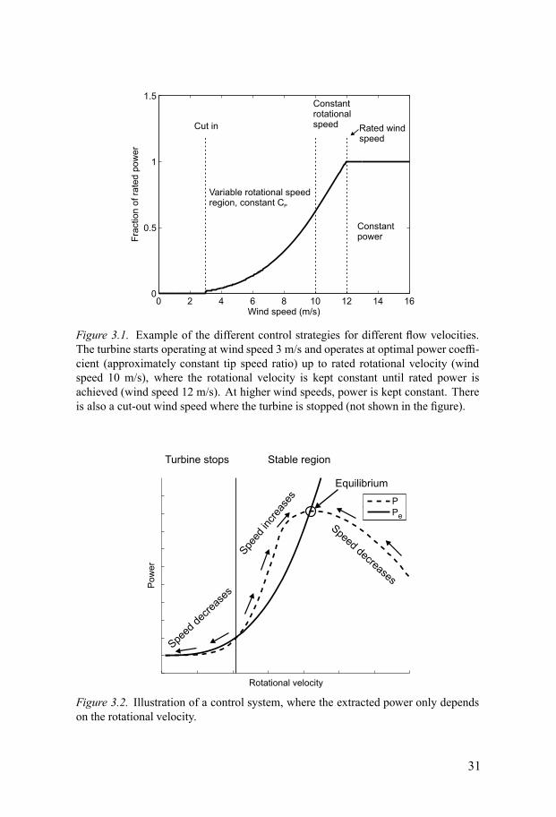
Figure 3.1. Example of the different control strategies for different flow velocities.The turbine starts operating at wind speed 3 m/s and operates at optimal power coeffi-cient (approximately constant tip speed ratio) up to rated rotational velocity (windspeed 10 m/s), where the rotational velocity is kept constant until rated power isachieved (wind speed 12 m/s). At higher wind speeds, power is kept constant. Thereis also a cut-out wind speed where the turbine is stopped (not shown in the figure).

Rotational velocity

Po

we

r

Spe

edin

crea

ses

Turbine stops Stable region

Equilibrium

PeP

Pe

Speeddecreases

Speed

decr

ease

s

Figure 3.2. Illustration of a control system, where the extracted power only dependson the rotational velocity.

31

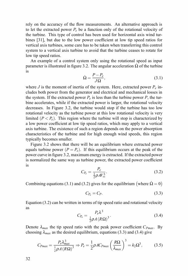
rely on the accuracy of the flow measurements. An alternative approach isto let the extracted power Pe be a function only of the rotational velocity ofthe turbine. This type of control has been used for horizontal axis wind tur-bines [31], but due to the low power coefficient at low tip speed ratios forvertical axis turbines, some care has to be taken when transferring this controlsystem to a vertical axis turbine to avoid that the turbine ceases to rotate forlow tip speed ratios.An example of a control system only using the rotational speed as input

parameter is illustrated in figure 3.2. The angular acceleration Ω of the turbineis

Ω =P−PeJΩ

, (3.1)

where J is the moment of inertia of the system. Here, extracted power Pe in-cludes both power from the generator and electrical and mechanical losses inthe system. If the extracted power Pe is less than the turbine power P, the tur-bine accelerates, while if the extracted power is larger, the rotational velocitydecreases. In Figure 3.2, the turbine would stop if the turbine has too lowrotational velocity as the turbine power at this low rotational velocity is verylimited (P< Pe). This region where the turbine will stop is characterized bya low power coefficient at low tip speed ratios, which may apply to a verticalaxis turbine. The existence of such a region depends on the power absorptioncharacteristics of the turbine and for high enough wind speeds, this regiontypically becomes smaller.Figure 3.2 shows that there will be an equilibrium where extracted power

equals turbine power (P= Pe). If this equilibrium occurs at the peak of thepower curve in figure 3.2, maximum energy is extracted. If the extracted poweris normalized the same way as turbine power, the extracted power coefficientis

CPe =Pe

12ρAV 3∞

. (3.2)

Combining equations (3.1) and (3.2) gives for the equilibrium(where Ω = 0

)CPe =CP. (3.3)

Equation (3.2) can be written in terms of tip speed ratio and rotational velocityas

CPe =Peλ 3

12ρA(RΩ)3

. (3.4)

Denote λmax the tip speed ratio with the peak power coefficient CPmax. Bychoosing λmax as the desired equilibrium, equations (3.3) and (3.4) give

CPmax =Peλ 3max

12ρA(RΩ)3

⇒ Pe =12

ρACPmax(RΩλmax

)3= k2Ω3, (3.5)

32

0 1 2 3 4 5 6 7 8-0.05

0

0.05

0.1

0.15

0.2

0.25

0.3

0.35

0.4

0.45

Tip speed ratio

Pow

er

coeffic

ient

C at 3 m/sP

C at 6 m/sP

C at 12 m/sP

CPe

Figure 3.3. The control strategy A from equation (3.5) illustrated for three differentflow velocities.

where the constant k2 is related to λmax andCPmax according to equation (3.5).Under the conditions thatCPmax and λmax are constants, maximum power willbe extracted if the extracted power is chosen to vary with the cube of the rota-tional velocity and the constant k2 is chosen according to equation (3.5). Thiscontrol strategy will be denoted “strategy A”. With CPmax and λmax constant,equation (3.5) is independent of flow velocity. However, due to the increasedReynolds number at higher flow velocities, the airfoil performance will in-crease, as drag is reduced and stall angle is increased. Therefore, the valuesfor λmax and CPmax have a small dependence on the Reynolds number, seefigure 3.3. The performance of the strategy in equation (3.5) is plotted in fig-ure 3.3 for three flow velocities (for specifications on the simulated turbine,see section 5.2.6). The change in power coefficient with respect to the flowvelocity causes the obtained equilibrium tip speed ratio λe to be slightly dis-tanced to λmax, although the obtained power coefficient is very similar toCPmax(see figure 3.3). For a flow velocity of 3 m/s, there is an unstable region for tipspeed ratios below 2.2, while for 6 m/s and 12 m/s, the strategy is stable in theentire interval as long as the turbine power is larger than the mechanical andelectrical losses. Even though the strategy is stable for 6 m/s and 12 m/s, thedifference between turbine power and extracted power is low at low tip speedratios, causing a slow acceleration, cf. equation (3.1).Twomodifications to the devised strategy in equation (3.5) have been made,

with the intention to increase the rotational velocity at low tip speed ratios in

33

0 1 2 3 4 5 6 7 8-0.05

0

0.05

0.1

0.15

0.2

0.25

0.3

0.35

0.4

0.45

Tip speed ratio

Po

we

rco

effic

ient

C at 3 m/sP

C at 6 m/sP

C at 12 m/sP

C at 3 m/sPe

C at 6 m/sPe

C at 12 m/sPe

Figure 3.4. Control strategy B from equation (3.6) illustrated for three different flowvelocities.

0 1 2 3 4 5 6 7 8-0.05

0

0.05

0.1

0.15

0.2

0.25

0.3

0.35

0.4

0.45

Tip speed ratio

Po

we

rco

effic

ient

C at 3 m/sP

C at 6 m/sP

C at 12 m/sP

C at 3 m/sPe

C at 6 m/sPe

C at 12 m/sPe

Figure 3.5. Control strategy C from equation (3.7) illustrated for three different flowvelocities.

34

order to create a more stable and faster control strategy. Strategy B is given as{Pe = 0 Ω ≤ Ω0,Pe = k1Ω2 (Ω−Ω0) Ω > Ω0,

(3.6)

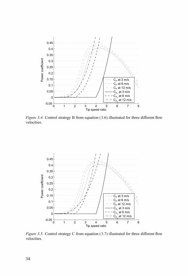
where the rotational velocityΩ0 is required before the strategy starts to extractenergy. This strategy obtains higher differences between extracted and turbinepower for low rotational velocities at the cost of having λe further distancedfrom λmax.Strategy C combines a higher torque at low rotational velocities with the

good performance of strategy A by dividing the rotational velocities in threeregions according to⎧⎪⎪⎪⎨

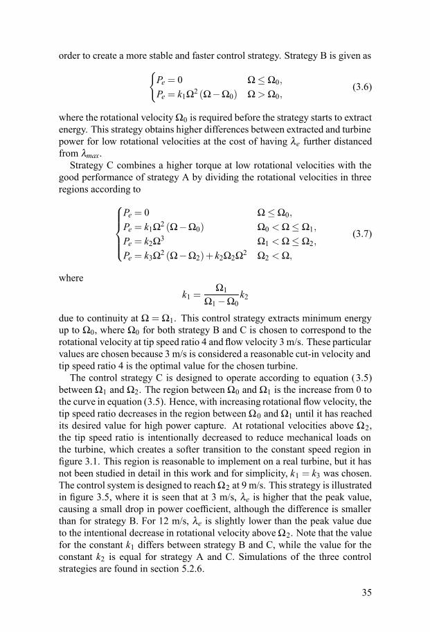
⎪⎪⎪⎩Pe = 0 Ω ≤ Ω0,Pe = k1Ω2 (Ω−Ω0) Ω0 < Ω ≤ Ω1,Pe = k2Ω3 Ω1 < Ω ≤ Ω2,Pe = k3Ω2 (Ω−Ω2)+ k2Ω2Ω2 Ω2 < Ω,

(3.7)

wherek1 =

Ω1Ω1−Ω0

k2

due to continuity at Ω = Ω1. This control strategy extracts minimum energyup to Ω0, where Ω0 for both strategy B and C is chosen to correspond to therotational velocity at tip speed ratio 4 and flow velocity 3 m/s. These particularvalues are chosen because 3 m/s is considered a reasonable cut-in velocity andtip speed ratio 4 is the optimal value for the chosen turbine.The control strategy C is designed to operate according to equation (3.5)

between Ω1 and Ω2. The region between Ω0 and Ω1 is the increase from 0 tothe curve in equation (3.5). Hence, with increasing rotational flow velocity, thetip speed ratio decreases in the region betweenΩ0 and Ω1 until it has reachedits desired value for high power capture. At rotational velocities above Ω2,the tip speed ratio is intentionally decreased to reduce mechanical loads onthe turbine, which creates a softer transition to the constant speed region infigure 3.1. This region is reasonable to implement on a real turbine, but it hasnot been studied in detail in this work and for simplicity, k1 = k3 was chosen.The control system is designed to reachΩ2 at 9 m/s. This strategy is illustratedin figure 3.5, where it is seen that at 3 m/s, λe is higher that the peak value,causing a small drop in power coefficient, although the difference is smallerthan for strategy B. For 12 m/s, λe is slightly lower than the peak value dueto the intentional decrease in rotational velocity aboveΩ2. Note that the valuefor the constant k1 differs between strategy B and C, while the value for theconstant k2 is equal for strategy A and C. Simulations of the three controlstrategies are found in section 5.2.6.

35

3.2 Extension to multiple turbinesIt is common to locate several turbines in close proximity to each other in afarm configuration, as this can give economical benefits due to synergy effects,since some parts of the system can be commonly used. Therefore, two differ-ent electrical topologies are suggested, where the second “mutual topology”is designed to reduce the number of electric components [32]. For additionalpossible topologies, see e.g. [33–35].One way to control multiple turbines is to apply the model described in sec-

tion 3.1 for each turbine in the farm. This can be accomplished by using anindividual electric system for each turbine, where each turbine has a passivediode rectifier and an inverter (“separate topology”). An alternative approachis to connect all turbines to the same inverter, but to obtain individual control.This would for a permanent magnet synchronous generator require some addi-tional electrical components such as an active rectifier or a DC-DC converter.One simplification is to connect all turbines to the same DC-bus with pas-

sive rectifiers, which makes the inverter the only parameter to control (“mutualtopology”). This reduces the number of electric components and it is thereforeof interest to study how performance is affected by this simplification.For the mutual topology, the total power extracted from the entire turbine

farm is chosen as

Pe,tot =Nt∑i=1Pe (Ωi) , (3.8)

where Pe (Ωi) is calculated according to one of the strategies A – C in sec-tion 3.1. With the total extracted power chosen according to equation (2.1),the separate and mutual topologies extract the same power if all turbines ex-perience identical flow velocities.Other studies have previously been performed for horizontal axis turbines,

with a global control strategy for the entire farm [36, 37]. Farm effects havebeen included in the control system in [38, 39] and a method for estimatingthe flow velocity within the farm with only rotational velocities and extractedpower as input parameters is presented in [40].

36

4. Simulation models

The flow through a turbine can be simulated by solving Navier-Stokes equa-tions coupled with the continuity equation. Navier-Stokes equations are validfor all Newtonian fluids, i.e. both air and water, although in water, cavitationwould require additional modeling. The validity of Navier-Stokes equationsis well established, and the most accurate simulation model would be a directsolution of these equations. However, Navier-Stokes equations are non-linearpartial differential equations and due to the computational complexity, accu-rate direct solutions of these equations are numerically very hard to obtain,even for the two-dimensional case. Considering that the fluid-flow in a largeturbine generally is turbulent, one common simplification is to model the tur-bulence by e.g. Reynolds-averaged Navier-Stokes equations (RANS), whichinclude additional turbulence models. This has been done by e.g. [41, 42].The most common methods to solve Navier-Stokes equations are the FiniteElement Method (FEM) and the Finite Volume Method (FVM), which areboth based on a mesh over the entire simulated volume. For this reason,these methods are suited for confined regions. There are commercial FEMand FVM simulation software available, but due to the long simulation times,other methods have been chosen in this work.Another method for solving Navier-Stokes equations is to use a vortex

method (see section 4.2). This method can also directly solve Navier-Stokesequations, and is designed for open flows with small boundaries, which is thecase for a vertical axis turbine. Directly solving Navier-Stokes equations withthis method requires much computational time, and has not been done in thiswork. An advantage of the vortex method is that there are many simplifica-tions available, and by including models of blade forces, the simulation timescan be reduced substantially. This simplification is used within this work.One even more simplified and very fast method is the streamtube model,

which assumes static flow, and does not give a full description of the flowthrough the turbine. Due to the high computational efficiency, this model canbe used to quickly perform many simulations, and it is one of the models usedin this work, even though the simplifications of the flow limit the applicabilityof the model.

4.1 Streamtube modelsStreamtube models are among the fastest models used for simulating verticalaxis turbines. The first application of streamtube models, usually credited to

37

V∞VdVe

Ad

R

θb

Δθ

Ω

c

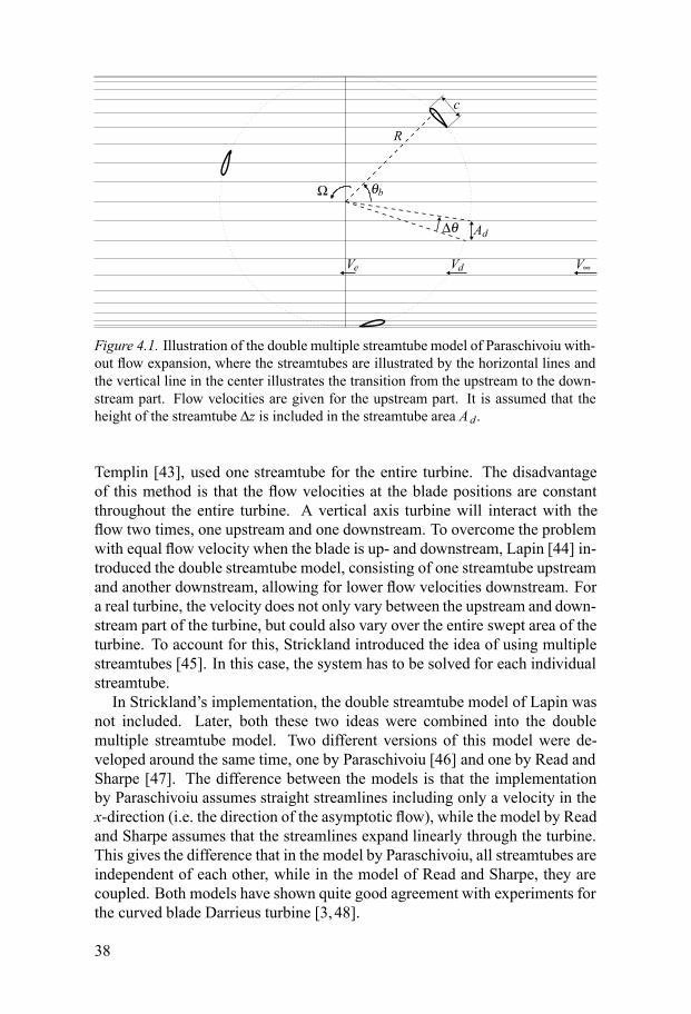
Figure 4.1. Illustration of the double multiple streamtube model of Paraschivoiu with-out flow expansion, where the streamtubes are illustrated by the horizontal lines andthe vertical line in the center illustrates the transition from the upstream to the down-stream part. Flow velocities are given for the upstream part. It is assumed that theheight of the streamtube Δz is included in the streamtube area Ad .

Templin [43], used one streamtube for the entire turbine. The disadvantageof this method is that the flow velocities at the blade positions are constantthroughout the entire turbine. A vertical axis turbine will interact with theflow two times, one upstream and one downstream. To overcome the problemwith equal flow velocity when the blade is up- and downstream, Lapin [44] in-troduced the double streamtube model, consisting of one streamtube upstreamand another downstream, allowing for lower flow velocities downstream. Fora real turbine, the velocity does not only vary between the upstream and down-stream part of the turbine, but could also vary over the entire swept area of theturbine. To account for this, Strickland introduced the idea of using multiplestreamtubes [45]. In this case, the system has to be solved for each individualstreamtube.In Strickland’s implementation, the double streamtube model of Lapin was

not included. Later, both these two ideas were combined into the doublemultiple streamtube model. Two different versions of this model were de-veloped around the same time, one by Paraschivoiu [46] and one by Read andSharpe [47]. The difference between the models is that the implementationby Paraschivoiu assumes straight streamlines including only a velocity in thex-direction (i.e. the direction of the asymptotic flow), while the model by Readand Sharpe assumes that the streamlines expand linearly through the turbine.This gives the difference that in the model by Paraschivoiu, all streamtubes areindependent of each other, while in the model of Read and Sharpe, they arecoupled. Both models have shown quite good agreement with experiments forthe curved blade Darrieus turbine [3, 48].

38

4.1.1 Description of modelThe double multiple streamtube model implementation used here is based onthe implementation of Paraschivoiu [3] and an illustration of this model isgiven in figure 4.1. In the double multiple streamtube model, the turbine isseparated into two discs, one upstream and one downstream. In the middle ofthe turbine, the pressure is assumed to be the same as the asymptotic pressure.With this assumption, the velocity at the upstream disc will be the average ofthe velocity at the middle and the asymptotic velocity, similar to equation (2.7)in the Betz theory. In the same way, the velocity at the downstream disc be-comes equal to the average of the velocity at the middle, and the velocity farbehind the turbine. In the implementation by Paraschivoiu, the upstream discis solved first, independently of the downstream disc. The downstream discuses the velocity in the middle of the turbine, calculated when solving theupstream disc, as input. Except from this calculation of velocity, both discsare solved in the same way, and most equations will only be presented for theupstream part of the system.This description will follow the same notation as Paraschivoiu for the direc-

tion of the flow velocity. Hence, the flow direction illustrated in figure 4.1 isconsidered positive direction. The definitions of the blade angle θb and the an-gle of attack α will still remain the same as in section 2.3. Therefore, negativeangles of attack will be obtained when the blades are upstream, while the de-scription by Paraschivoiu [3, Chapter 6] has positive angle of attack upstream.The difference in the definition of the flow direction is the reason why theexpressions for flow velocity and angle of attack are different in this section,compared to section 2.3.The main principle behind streamtube models is the use of momentum con-

servation in each streamtube. Similar to the Betz derivation, momentum con-servation gives

ρAeiV 2ei−ρA∞iV 2∞i = ρAdiVdi (Vei−V∞i) = Fxi, (4.1)

where A∞i, Adi and Aei are the cross-sectional areas of a streamtube and idenotes the streamtube index (cf. figure 2.1). The difference, compared tothe Betz theory, is that in this model, the force Fxi is calculated from bladesection data. If the streamtubes are discretized to give each streamtube thesame angular distance Δθ and height Δz, the size of each streamtube becomes

Adi = RiΔzΔθ |cosθbi| . (4.2)

To calculate the force, the first step is to obtain the lift and drag coefficients,which depend on the angle of attack and the Reynolds number. In the modelof Paraschivoiu, it is assumed that the direction of the flow does not change.This gives the relative velocity as

Vri =Vdi

√(RiΩVdi

− sinθbi)2

+ cos2θbi cos2ηi (4.3)

39

and the angle of attack as

αi = ϕi+δi = arctan

(cosθbi cosηisinθbi− RiΩ

Vdi

)+δi, (4.4)

where η is the angle of the blade relative to the vertical axis.When the coefficients have been determined from the empirical data, the

lift and drag forces are obtained from

FLi =12CLiρciliV 2ri , (4.5)

FDi =12CDiρciliV 2ri , (4.6)

where ci is the chord and li is the blade length in the streamtube. Generally,it is the normal and tangential forces that are of interest. These forces can bedetermined from the corresponding normal and tangential force coefficients

CNi = CLi cosϕi+CDi sinϕi, (4.7)CTi = CLi sinϕi−CDi cosϕi (4.8)

and therefore, the forces are

FNi =12CNiρciliV 2ri , (4.9)

FTi =12CTiρciliV 2ri. (4.10)

Note that by this definition, the normal force is perpendicular to the blade, andthe force in the radial direction is

FRi = FNi cosηi. (4.11)

To calculate how the velocity decreases in the streamtube, the forces in thex-direction (parallel to the flow) are of interest. These are obtained as

Fxi = FNi cosθbi cosηi−FTi sinθbi. (4.12)

Considering that there are Nb blades on the turbine, and that a streamtube onlyhave a blade inside it a fraction of the time, the mean force is given by

Fxi =NbΔθ2π

(FNi cosθbi cosηi−FTi sinθbi) . (4.13)

If the length of the blade in a streamtube li = Δz/cosηi is inserted into equa-tions (4.9) and (4.10), equation (4.13) becomes

Fxi =NbρciV 2riΔθ Δz

4π

(CNi cosθbi−CTi sinθbi

cosηi

). (4.14)

40

Vs VdiVei

cs

Δrs

Router

Rinner

θb

θ

Streamtube i

Ω

ηs

rs

Δz

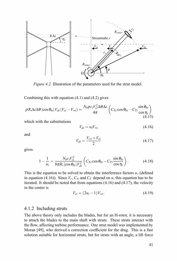
Figure 4.2. Illustration of the parameters used for the strut model.

Combining this with equation (4.1) and (4.2) gives

ρRiΔzΔθ |cosθbi|Vdi (Vei−V∞i) =NbρciV 2riΔθ Δz

4π

(CNi cosθbi−CTi sinθbi

cosηi

)(4.15)

which with the substitutionsVdi = uiV∞i (4.16)

andVdi =

V∞i+Vei2

(4.17)

gives

1− 1ui

=NbciV 2ri

8πRi |cosθbi|V 2di

(CNi cosθbi−CTi sinθbi

cosηi

). (4.18)

This is the equation to be solved to obtain the interference factors ui (definedin equation (4.16)). Since Vr, CN and CT depend on u, this equation has to beiterated. It should be noted that from equations (4.16) and (4.17), the velocityin the center is

Vei = (2ui−1)V∞i. (4.19)

4.1.2 Including strutsThe above theory only includes the blades, but for an H-rotor, it is necessaryto attach the blades to the main shaft with struts. These struts interact withthe flow, affecting turbine performance. One strut model was implemented byMoran [49], who derived a correction coefficient for the drag. This is a fastsolution suitable for horizontal struts, but for struts with an angle, a lift force

41

will also be generated. To increase the flexibility of the code, it was chosen tocalculate the forces directly from the lift and drag coefficients instead.To calculate the forces, the relative velocity has to be known. Let rs be a

position along the strutRinner < rs < Router, (4.20)

where the strut starts at Rinner and ends at Router, see figure 4.2. The strutsare discretized into Δr long segments in the radial direction. In the streamtubemodel, the velocity is only known at the turbine disc and at the center of theturbine. The simple approximation that the velocity varies linearly betweenthese positions gives the velocityVs j of strut segment j as

Vs j =Vei+Vdi−Vei√R2i − r2s j sin2θb

rs j cosθb. (4.21)

The position of the blade, to which the strut is attached, is given as θb. Thisexpression involves the velocity in streamtube i, in which the segment is lo-cated. To determine which streamtube this is, the corresponding angle at thecircumference of the turbine is given by

θi = arcsin(rs jR jsinθb

). (4.22)

In the vertical direction, the position of segment j will be equal to the verticalposition of the corresponding streamtube i. The relative velocity can be calcu-lated basically in the sameway as in equation (4.3), but since the discretizationis performed in the radial direction for the struts, the angle is to be given rel-ative this direction as well (the reason for not using vertical discretization forstruts is that Fxi in equation (4.14) would diverge for horizontal struts). Withthe strut angle given as ηs, the velocity is given by

Vrs j =Vs j

√(rs jΩVs j

− sinθb)2

+ cos2θb sin2ηs j (4.23)

and the angle attack αs for the strut is

αs j = arctancosθb sinηs jsinθb− rs jΩ

Vs j

, (4.24)

where zero pitch angle is assumed for the strut. By defining the chord of thestrut as cs and following the same derivation as with equations (4.7) – (4.14),the expression for the mean force in the flow direction for a section (Δrs,Δθ )of the strut is obtained as

Fxs j =Nbcs jρV 2rs j

4πΔθ Δrs

(CNs j cosθb tanηs j−CTs j sinθb

cosηs j

), (4.25)

42

where CNs j and CTs j are the normal and tangential force coefficients of thestrut, which are defined in a similar way as for the blades

CNs j = CLs j cosαs j+CDs j sinαs j, (4.26)CTs j = CLs j sinαs j−CDs j cosαs j. (4.27)

Here,CLs j andCDs j are the lift and drag coefficients for the struts. The differ-ences in equations (4.24) and (4.25), compared to equations (4.4) and (4.14),originate from the different definition of ηs j, and that the discretization is donein the radial direction.The interference factor ui can be calculated according to

1− 1ui

=1

2Ri |cosθb|V 2diρΔθ Δz

(Fxi+∑

j∈iFxs j

)(4.28)

where ∑ j∈i Fxs j is the sum of the forces from all points (rsi,θb) that corre-sponds to streamtube i. Similar expressions can be derived for the downwindpart of the turbine. The torque from the struts can be calculated in a similarway as for the blades in a curved blade Darrieus turbine

Ts (θb) = ∑jrs jFTs j (θb)cosη j

, (4.29)

whereFTs j (θb) =

12CTs j (θb)ρcs jΔrsVrs j (θb)2 .

4.1.3 Obtaining lift and drag coefficientsIn the streamtube model, it is necessary to have the lift and drag coefficientsfor a given angle of attack. Experimental data can be used to obtain these ifthe Reynolds number and angle of attack are known. For several symmetricalNACA profiles, such data can be obtained from [50], which has been used inthis work. The problem with this kind of data is that it usually is valid for verylong blades and a static angle of attack. For a vertical axis turbine, the bladeswill change their angles of attack during the revolution.When the angle of attack for a blade increases above the stall angle, the flow

will separate from the blade surface, which reduces the lift force and increasesthe drag. The flow separation takes time to develop and if the blade rapidlyincreases its angle of attack, the lift force can be higher than in the static casefor a short period of time. During this time, a vortex starts to form at thesurface of the blade and when this vortex detaches, the lift force is greatlyreduced. This phenomenon is called dynamic stall. When the turbine has alow tip speed ratio, the angles of attack become high enough for the blades toexperience this in each revolution. This occurs for tip speed ratios around 4.

43

Tomodel dynamic stall, the Gormont model has been used. This model wasoriginally developed by Gormont [51], later modified by Massé [52] and ad-justed by Berg [53]. The advantages of this model is that it only requires datafor lift and drag coefficients, flow velocity, blade thickness to chord ratio, an-gle of attack and rate of change of the angle of attack, making it easy to applyto any blade, which is the reason why this model was chosen. Other mod-els have been shown to give better results [3]. One example is the Beddoes-Leishman model [54,55], but it has more parameters that have to be calibrated,which makes it harder to apply the model to an arbitrary airfoil.

Tip effectsFor a blade to obtain a lift force, there has to be circulation around the blade(cf. Kutta Joukowski lift formula, equation (4.57)). Since the vorticity is di-vergence free

(ω = ∇×�V ⇒ ∇ ·

(∇×�V

)= 0

), there are vortices generated

from the blade tips with the same circulation as around the blade. These vor-tices are the source of induced drag, and the corresponding losses. It should benoted that the curved blade Darrieus turbine does not have any distinct bladetips (the blades are attached to the main axis). Here, the tip vortices haveto leave the blades more evenly distributed over the length of the blade, andin the model of Paraschivoiu, no tip losses are applied to curved blade Dar-rieus turbines. For straight blade turbines, one correction model, derived fromPrandtl’s theory for screw propellers, used by e.g. Sharpe [48], uses a velocitycorrection factor F , which for the upstream disc is

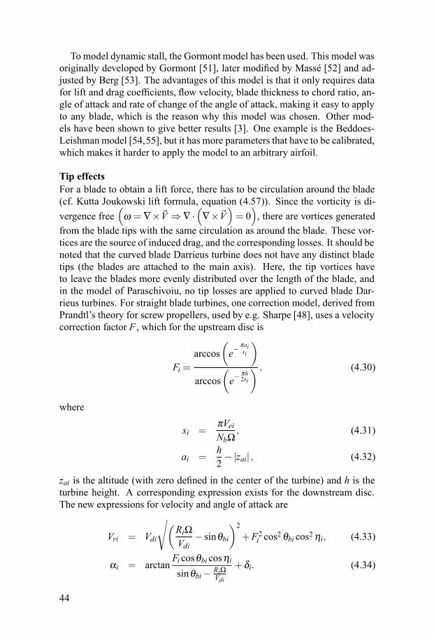
Fi =arccos

(e−

πaisi

)

arccos(e−

πh2si

) , (4.30)

where

si =πVeiNbΩ

, (4.31)

ai =h2−|zai| , (4.32)

zai is the altitude (with zero defined in the center of the turbine) and h is theturbine height. A corresponding expression exists for the downstream disc.The new expressions for velocity and angle of attack are

Vri = Vdi

√(RiΩVdi

− sinθbi)2

+F2i cos2θbi cos2ηi, (4.33)

αi = arctanFi cosθbi cosηisinθbi− RiΩ

Vdi

+δi. (4.34)

44

In addition, Paraschivoiu [3] suggests using finite wing theory as well to cal-culate induced drag and reduced angle of attack. This is given by

CLi =CL∞i

1− a0iπARi

, (4.35)

a0i = 1.8π(1+

0.8tbici

), (4.36)

CDi = CD∞i+C2Li

πARi, (4.37)

αbi = αi− CLiπARi

, (4.38)

where AR is the aspect ratio, tb the blade thickness, CL∞ and CD∞ lift anddrag coefficients for an infinitely long blade and αb the corrected angle ofattack. Paraschivoiu suggests that equations (4.35) – (4.38) should not be ap-plied to dynamic stall calculations, but since this would lead to a discontinuityin the limit when dynamic stall starts to have an effect, the current implemen-tation uses equations (4.35), (4.36) and (4.38), then calculates the dynamicstall corrections to the lift coefficient, and then calculates the induced dragusing equation (4.37) with the new lift coefficient. It should be noted thatequations (4.35) – (4.38) are derived using the assumption that the angle of at-tack is constant, the tip vortices extend along a straight line behind the blade,and the wing is elliptical, which is not the case for a vertical axis turbine. Thishas to be taken into account when evaluating the accuracy of the model forstraight blade turbines.

4.1.4 Corrections due to flow curvatureAs was illustrated in section 2.4, there are effects due to flow curvature thatshould be taken into account. With the definition of the velocity as in thestreamtube model (V →−V ), the assumption of straight stream lines (β = 0),using that the reference velocity Vre f is the relative velocity Vr and using thevelocity at the turbine disc Vd instead of Vabs, equation (2.52) gives

α = δ + arctanVd cosθb

ΩR−Vd sinθb− Ωx0rc

Vr− Ωc4Vr

. (4.39)

This is included in the adaptation of Sharp [48], but with the assumptions thatthe curvature force only acts in the normal direction and that the mountingpoint is in the center of the blade (x0r = 0). With the assumption

CN = asα , (4.40)

the correction to the normal coefficient becomes

CN =CN0− asΩc4Vr, (4.41)

45

z

y

ay∞ aye

a ze

a z∞

b ze

1

b z∞

by∞

1

bye

Figure 4.3. Illustration of the cross-section for a streamtube at the three positions: Farahead of turbine (black), at the upstream disc (white) and in the center (hatched).

whereCN0 is the original normal force without corrections.

4.1.5 Including flow expansionIn contrast with the model of Read and Sharpe [47], the model of Paraschi-voiu does not include streamtube expansion in the basic implementation. Onemethod for implementing the expansion was used by Paraschivoiu [56] wherethe streamtubes were allowed to expand, but the direction of the velocity wasnot changed. In this implementation, similar to the one by Read and Sharpe,it was assumed that streamtube expansion only occurs in the horizontal plane,and that the streamline that intersects the turbine center is unchanged. In thiswork, the assumption is instead that the flow can expand both in the verticaland the horizontal directions. It is assumed that the direction of the expansiondepends on the ratio between the width and height of the turbine. Assume thatthe streamtube size at the turbine disc is unity Ad = 1, at infinity A∞ = by∞bz∞and at the center Ae = byebze (see figure 4.3). By defining

ay∞ = 1−by∞ and aye = 1+bye (4.42)

46

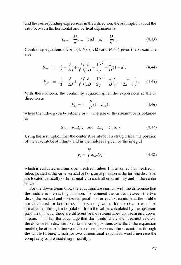
and the corresponding expressions in the z direction, the assumption about theratio between the horizontal and vertical expansion is

ay∞ =Dhaz∞ and aye =

Dhaze. (4.43)

Combining equations (4.16), (4.19), (4.42) and (4.43) gives the streamtubesize

by∞ =12− h2D

+

√(h2D

+12

)2− hD

(1−u), (4.44)

bye =12− h2D

+

√(h2D

+12

)2− hD

(1− u

2u−1)

. (4.45)

With these known, the continuity equation gives the expressions in the z-direction as

bzq = 1− hD

(1−byq) , (4.46)

where the index q can be either e or ∞. The size of the streamtube is obtainedas

Δyq = bzqΔyd and Δzq = bzqΔzd. (4.47)

Using the assumption that the center streamtube is a straight line, the positionof the streamtube at infinity and in the middle is given by the integral

yq =yd∫0

byqdyd, (4.48)

which is evaluated as a sum over the streamtubes. It is assumed that the stream-tubes located at the same vertical or horizontal position at the turbine disc, alsoare located vertically or horizontally to each other at infinity and in the centeras well.For the downstream disc, the equations are similar, with the difference that

the middle is the starting position. To connect the values between the twodiscs, the vertical and horizontal positions for each streamtube at the middleare calculated for both discs. The starting values for the downstream discare obtained through interpolation from the values calculated by the upstreampart. In this way, there are different sets of streamtubes upstream and down-stream. This has the advantage that the points where the streamtubes crossthe downstream disc are fixed to the same positions as without the expansionmodel (the other solution would have been to connect the streamtubes throughthe whole turbine, which for two-dimensional expansion would increase thecomplexity of the model significantly).

47

4.2 Vortex modelsTo describe the motion of a fluid, the continuity equation and Navier-Stokesequations are used. The continuity equation

∂ρ∂ t

+∇ ·(

ρ�V)

= 0 (4.49)

represents the conservation of mass. Due to the low flow velocities present forwind and marine current turbines, the flow can be considered incompressible.In this case, the continuity equation reduces to

∇ ·�V = 0. (4.50)

Navier-Stokes equations are derived from Newton’s second law and can in theincompressible case be written as

∂�V∂ t

+(�V ·∇

)�V = −∇p

ρ+�g+ν∇2�V , (4.51)

where �g is the acceleration of gravity and ν is the kinematic viscosity. Theseare non-linear partial differential equations, which only have closed form solu-tions in rare cases. Numerical solutions can be obtained with traditional finiteelement/volume methods, where these equations are solved on a grid with thevelocity as the unknown variable. An alternative method is to use the vortexformulation, where the vorticity

�ω = ∇×�V (4.52)

is used instead. The vorticity equation is obtained from the rotation of equation(4.51) according to

∂�ω∂ t

+(�V ·∇

)�ω = (�ω ·∇)�V +ν∇2�ω . (4.53)

The left hand side represents the convection of vorticity. The first term onthe right hand side is the vortex stretching, and the second is the diffusion ofvorticity. These equations show that the vorticity moves with the flow velocity.In the two-dimensional case, the vorticity is directed along the z-axis, whilethe flow occurs in the x - y plane. Due to orthogonality, vortex stretching doesnot apply in the two-dimensional case, and with �ω = ω z,

∂ω∂ t

+(�V ·∇

)ω = ν∇2ω . (4.54)

For vortex methods, it is more common to use a Lagrangian descriptionrather than an Eulerian (which is used in equations (4.51) – (4.54)) [57, chap-ter 1]. In the Lagrangian description, the vorticity is discretized into vortices,

48

which move with the flow. The use of these vortices removes the need for amesh (compared to e.g. the finite element method). The vortices are deter-mined by their positions�ri and their circulations Γi. If diffusion is included,equation (4.54) is solved in two steps, one convection step, which in the La-grangian description becomes

d�ridt

=�Vi, (4.55)

and one diffusion step, which could either change the position of the vor-tex (like random walk [58]) or the circulation (like the vortex redistributionmethod [59]). In this work, it is assumed that convection is much more im-portant than diffusion and when solving the time evaluation of the vortices,diffusion is ignored. This is expected to be a good approximation in the tur-bine neighborhood outside the boundary layer of the blades. The divergenceof the vorticity is

∇ ·�ω = ∇ ·(

∇×�V)

= 0, (4.56)

i.e. the vorticity is divergence free. For two-dimensional flow, this implies thatvortices are always created in pairs (or possibly higher order pairs). Kelvin’stheorem [57, chapter 2] states that without viscosity, the circulation inside thefluid is conserved for a vortex, and the implication is that vorticity can only becreated at the boundaries.

4.2.1 Implementing the turbineWith the vortex model, it is theoretically possible to calculate the lift and dragforces for an airfoil. However, this requires a full solution of Navier-Stokesequations, which is very time-consuming, and adds a large amount of vorticesto the flow at each time step. As a simplification, the same procedure as for thestreamtube models can be used, where experimental data and a dynamic stallmodel are used to calculate lift and drag forces. In this implementation, theexperimental data and the dynamic stall model are the same for the streamtubemodel and the vortex model. For the 3D corrections, the correction factor F inequation (4.30) cannot be applied because the vortex model is a 2D model, butequations (4.35) – (4.38) can be applied in the same way as for the streamtubemodel, described in section 4.1.3.The calculation of the angle of attack can either be performed by calculat-

ing the velocity at the turbine position and applying the corrections derived insection 2.4, or by solving the potential flow problem. In this implementation,the potential flow solution is chosen, because it can handle a varying velocityfield and flow curvature. Linear panels are used according to section 4.2.3 tocalculate the potential flow solution. These equations are not fully determinedwithout knowledge of the total circulation around the blade. As it is this cir-culation that is of interest for the lift force, closure is obtained by applying the

49

Kutta condition, which states that the velocity at the trailing edge of an airfoilshould be finite [27, chapter 3]. The potential flow solution gives an infinitevelocity at an edge, unless it is a stagnation point, which therefore is enforcedwith the Kutta condition. For a panel method, this can be achieved by forcingthe vorticity of the panels to be zero at the trailing edge. In the implementa-tion, the vorticity at the end of the panel on the upper side of the blade is set tothe same vorticity as the panel on the lower side. With this condition and theno-penetration boundary condition, the circulation can be calculated. To getthe angle of attack from the circulation, the method is calibrated by calculat-ing the circulation for a set of stationary airfoils with known angles of attack.These values are used to create an inverse function, which gives the angle ofattack from the circulation.By using the conservation of vorticity, one vortex has to be released be-

hind the trailing edge every time-step with a circulation corresponding to thechange in circulation for the blade. Since experimental data and a dynamicstall model are applied to get the lift and drag forces, the effective circulationwill not be the one calculated from the Kutta condition if the blade is stalled.To get the circulation, the same method as in Strickland [60] is used, wherethe Kutta-Joukowski lift formula

Γ =12CLcV (4.57)

gives the circulation from the lift coefficient. With the circulation known, thestrength of the released vortex can be calculated. By adding an additional vor-tex to the flow, the angle of attack changes slightly. As calculating the circula-tion from empirical data combined with the dynamic stall model is non-linear,the procedure to calculate the angle of attack with the Kutta condition andrecalculating the strength of the released vortex can be iterated. Consideringthat equation (4.57) is derived from potential theory, this approximation is bestsuited when the drag is low.For a turbine, it is often the case that the turbine blades are quite small com-

pared to the distance between them. The first simplification with this approxi-mation is that the circulation of each blade can be solved separately. Anotherapproximation is to assume that each blade can be represented with a singlepoint circulation during the vortex convection. With this approximation, thereis no need to calculate the velocity due to any panels on the blade surface. Be-cause it is more expensive to calculate the velocity of a panel, approximatingthe blade with a single point can significantly improve computational speedwhen calculating the vortex velocities. Further, as the Kutta condition is notsatisfied as the circulation is modified by the empirical data, the flow velocityat the trailing edge would be infinite if the panels were to be used, which isunphysical. The approximation with a single circulation does not suffer fromthis problem if a Gaussian vortex is used according to equation (4.64). Withinthis approximation, a vortex can theoretically end up inside a blade when us-

50

ing the Kutta condition. If this is the case, that vortex is ignored during thistime step.

4.2.2 Merging vorticesThe vortex method creates one vortex for each blade during each time step.For long simulations, this will cause a steady increase in computational timefor each time step. However, some of the vortices that have propagated topositions far behind the turbine can be merged without loosing any significantaccuracy.To properly merge two vortices, there are some conservation laws that

should be satisfied. First, the total circulation should be conserved

Γ1+Γ2 = const. (4.58)

Secondly, the center of vorticity should be conserved as well

x1Γ1+ x2Γ2 = const,y1Γ1+ y2Γ2 = const. (4.59)

By satisfying these equations, a new vortex can be created, which is a rea-sonable representation of the two old ones. This procedure can be performedfor all vortices, which are closer to each other than a cutoff radius Δ, wherethe value of Δ is increased with increasing distance behind the turbine. Themerging is only performed on vortices with the same sign for the circulation,where the merged vortex actually will be located somewhere in between theold ones.

4.2.3 Calculation of velocitySince the vortex method propagates the vortices with the flow according toequation (4.55), the velocity needs to be calculated. The velocity field is tra-ditionally divided into two parts (or more)

�V = ∇φ +�Vω , (4.60)

where the first part is the potential flow solution for the system (where∇×�V =0), and the second part is the contribution from all vortices.

Potential flow solutionIn the most simple case without any boundaries, the potential flow solutionwill be the asymptotic velocityV∞.Boundaries can be included, either by usingconformal mappings, as used by e.g. Deglaire [15], or by using panel methods.The panel method implemented is described in [61] and uses linear panels

51

with linearly varying vortex strengths. In this work, panels have been used toimplement the blades of the turbine in the calculation of the angle of attack,see section 4.2.1, and to implement channel walls in paper V.When using panels, one control point in the middle of each panel is chosen.

This is the point where the boundary condition is satisfied, which means thatthe boundary condition is only satisfied at N control points, where N is thenumber of panels. To solve the panel equations, the velocity contribution fromeach panel at each control point is used to create an N×N equation system. Itis usually desired to have a condition on the total circulation of all panels aswell (total source strength for source panels). Adding this condition leads to anover-determined equation system. This system can be solved approximatelywith the least square method, which gives a unique approximation. It shouldtherefore be noted that this method does not give an exact solution. The matrixsystem to be solved is of size N×N, which would take O (

N3)operations to

solve, but if the relative panel positions are constant, L-U decomposition canbe used, which requires O

(N3

)operations, but only has to be performed once

for each geometry. Thereafter, only O(N2

)operations are required for each

time step.In paper V, panels have been used to create channel walls for some of the

simulations. Here, the no penetration boundary condition (zero normal veloc-ity) is used for the side walls, while for the outflow, zero tangential velocityis chosen. For the inflow, the normal velocity is fixed to the asymptotic ve-locity, while the tangential velocity is set to zero. This is accomplished byusing both source and vortex strength for the inflow panels (the other panelshad only vortex strength). For channels, both the total circulation and the to-tal source strength of the panels that belong to the channel are set to zero. Inpaper IV, the channel walls have been included using the analytical expressionin equation (4.66), instead of using panels.

Vortex contributionAccording to the Biot-Savart Law, the velocity at position �r due to a pointvortex at�ri is

�Vω =14π

�Γp× (�r−�ri)|�r−�ri|3 , (4.61)

which in the two-dimensional case (note that a point in 2D is a line in 3D)with complex numbers simplifies to

Vω =iΓ2π

1(r− ri) . (4.62)

Here, r is a complex number representing the position in the x- and y-directionaccording to r = x+ iy and r denotes the complex conjugate of the position.This assumes point vortices, which have the vorticity

ω = Γδ (2) (r− ri) , (4.63)

52

where δ (2) is the two-dimensional Dirac delta function. Numerically, equa-tion (4.62) diverges when the distance approaches zero. To avoid these un-physical divergences in the velocity, a mollifier is usually applied to the vor-tices. Here, a Gaussian kernel has been applied, giving the vorticity

ω =Γ

πε2e−

|r−ri|2ε2 (4.64)

which, for a given number of vortices with strengths Γi at positions ri givesthe velocity

Vω(r) =Nv∑i=1

iΓi2π

1(r− ri)

(1− e−

|r−ri|2ε2

). (4.65)

The vortex contribution in a channelIf a wall is included in the simulation domain at Im(r) = 0 and the no pene-tration boundary condition applies at this wall, the method of images can beused to obtain the flow velocity from a vortex at position r j by adding an ad-ditional vortex at the mirror position r j with opposite strength. For a channelwith an additional wall at Im(r) = H , the solution will consist of an infiniteseries of mirror vortices. It has been shown in [62] that this series convergesto the analytical expression

Vω (r) =Nv∑i=1

iΓ j2π

(coth

( π2H

(r− r j))− coth

( π2H

(r− r j)))

. (4.66)

This equation requires that the channel height is constant. This method is usedin paper IV. Otherwise, the linear panel method can be used to create channelsof arbitrary shapes [61] and this method is used in paper V.

4.2.4 Numerical evaluation of the velocity fieldAt every time-step, the velocities at each vortex position, and at each controlpoint for the panels, have to be calculated. This can be accomplished by di-rect evaluation of equation 4.61. Assuming Nv vortices and Np panels, thiswould require O

(N2v

)+O(NvNp)+O

(N2p

)operations. The evaluation of the

velocity of a panel is much more expensive than the velocity of a point vortex.This is the reason why a speedup is obtained for the approximation that theblades are considered as single circulations during the convection phase of thevortices, although the infinite velocity at the trailing edge also warrants thisapproximation, see section 4.2.1. The velocity contributions from the panelsto the vortices are therefore only included in paper V, where panels are usedto model a channel.To efficiently evaluate the velocity, the fast multipole method [63] can be

used. The current implementation is based on the one described in [23], but

53

with multipole expansions of the linear panels included similar to the im-plementation in [61], which allows the total velocity to be evaluated withO(Nv+Np) operations instead. In the case of a channel (paper IV), a methodfor implementing equation (4.66) using the fast multipole method is givenin [62], which has been implemented in combinationwith the models from [23,61].

The fast multipole methodThe fast multipole method is a method for rapid evaluation of pairwise interac-tions between particles, originally developed by Greengard and Rhoklin [63].This method works by dividing the domain, where the interaction particles arelocated, into smaller and smaller boxes. The implementation used here splitseach box into four smaller boxes for each level and the number of levels isdecided from the amount of particles in the domain.For each box, a multipole expansion can be formed around the center of the

box r0 according to [63] as

V (r) = a0 log(r− r0)+∞

∑k=1

ak(r− r0)k

. (4.67)

Expanding the harmonic potential

V (r) = q j1

ri− r , (4.68)

whereqi =

iΓi2π

, (4.69)

results in a0 = 0. The coefficients ak are given by

ak = −Nd∑j=1q j (r j− r0)k−1 (4.70)

whereNd is the number of particles in the box and r0 is the box center. This ex-pansion can be used to calculate the velocity from the particles inside the boxfor any point located with sufficient distance from the box. Equation (4.67)is truncated to include coefficients up to ap. The required distance for con-vergence of the truncated version of equation (4.67) depends on the numberof multipole coefficients p in the expansion and the required tolerance of thealgorithm.Instead of expanding the particles of box m around the center of box m, the

expansion can instead be performed around the center of another box n, underthe condition that the distances from the center of box n to the points in box mare large enough. This local expansion is

V (r) =∞

∑l=0bl (r− r0)l , (4.71)

54

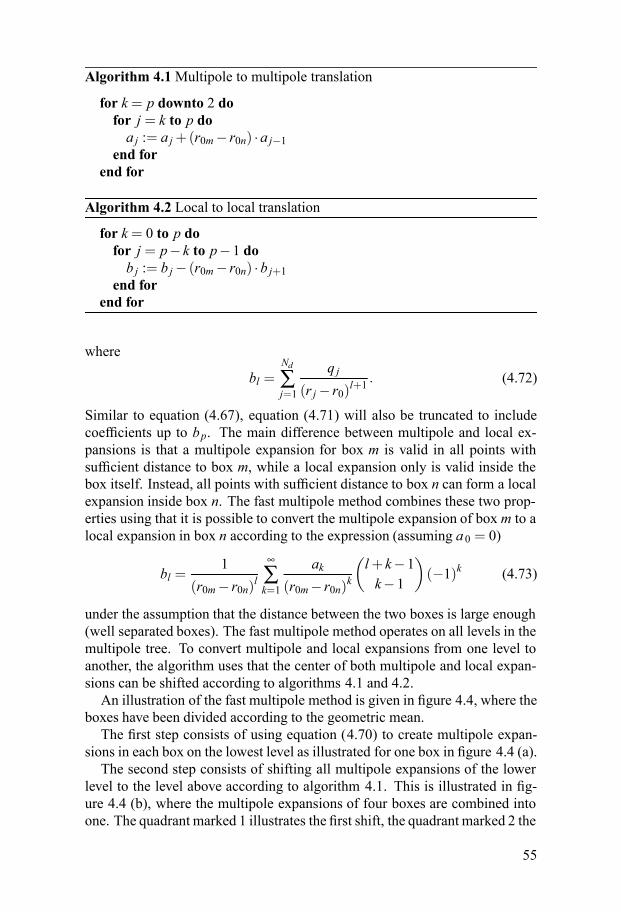
Algorithm 4.1Multipole to multipole translation

for k= p downto 2 dofor j = k to p doa j := a j+(r0m− r0n) ·a j−1

end forend for

Algorithm 4.2 Local to local translation

for k= 0 to p dofor j = p− k to p−1 dob j := b j− (r0m− r0n) ·b j+1

end forend for

where

bl =Nd∑j=1

q j(r j− r0)l+1

. (4.72)

Similar to equation (4.67), equation (4.71) will also be truncated to includecoefficients up to bp. The main difference between multipole and local ex-pansions is that a multipole expansion for box m is valid in all points withsufficient distance to box m, while a local expansion only is valid inside thebox itself. Instead, all points with sufficient distance to box n can form a localexpansion inside box n. The fast multipole method combines these two prop-erties using that it is possible to convert the multipole expansion of box m to alocal expansion in box n according to the expression (assuming a 0 = 0)

bl =1

(r0m− r0n)l∞

∑k=1

ak(r0m− r0n)k

(l+ k−1k−1

)(−1)k (4.73)

under the assumption that the distance between the two boxes is large enough(well separated boxes). The fast multipole method operates on all levels in themultipole tree. To convert multipole and local expansions from one level toanother, the algorithm uses that the center of both multipole and local expan-sions can be shifted according to algorithms 4.1 and 4.2.An illustration of the fast multipole method is given in figure 4.4, where the

boxes have been divided according to the geometric mean.The first step consists of using equation (4.70) to create multipole expan-

sions in each box on the lowest level as illustrated for one box in figure 4.4 (a).The second step consists of shifting all multipole expansions of the lower

level to the level above according to algorithm 4.1. This is illustrated in fig-ure 4.4 (b), where the multipole expansions of four boxes are combined intoone. The quadrant marked 1 illustrates the first shift, the quadrant marked 2 the

55

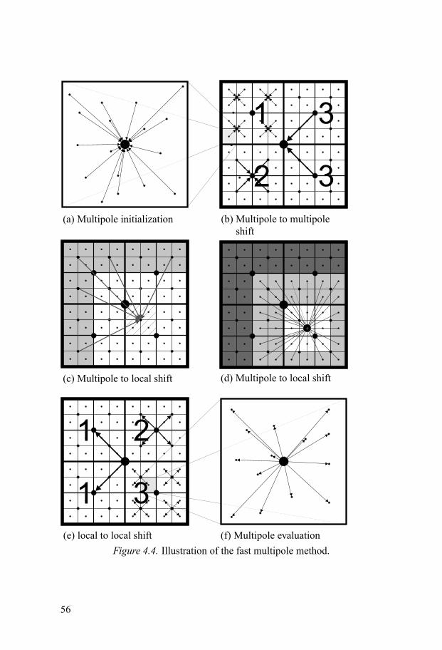
1

2 3

3

3

21

1

(a) Multipole initialization (b) Multipole to multipoleshift

(c) Multipole to local shift (d) Multipole to local shift

(e) local to local shift (f) Multipole evaluationFigure 4.4. Illustration of the fast multipole method.

56

second shift and the two quadrants marked 3 the third and final shift to the toplevel. After this shift, all boxes on all levels have their multipole expansions.The third step consists of converting multipole expansions to local expan-

sions according to equation (4.73), which is illustrated in figure 4.4 (c) and(d). This operation is performed for all boxes, but for simplicity, the operationis only illustrated for one box in figure 4.4. At each level, the neighboringboxes are divided between those in the near field and those in the far field.The boxes in the far field can be evaluated through a local expansion in thebox. The highest level only contains one box and in the homogeneous case infigure 4.4, the second level with only four boxes also has all boxes in the nearfield. As no multipole to local shifts are performed at these two levels, they areomitted from figure 4.4. At the third level, the boxes marked with grey in (c)are in the far field, hence local expansions of these boxes can be created in theselected box (the arrows in the figure represent these shifts). The white boxesrepresent the near field, which have to be handled at a lower level. The fourthlevel is illustrated in figure 4.4 (d). Here, those boxes that were shifted at theprevious level have been marked with dark grey as they have already com-pleted their interaction with the illustrated box. The other grey boxes interactwith the current box through equation (4.73).As the interactions with equation (4.73) occur at different levels, the local

expansions of the higher levels have to be shifted down to the lower levels,which is performed according to algorithm 4.2. This step is similar to themultipole to multipole shift, but here, the shift starts from the top level andmoves downward, as illustrated by the numbers in figure 4.4 (e). It can benoted that since there are no multipole to local shifts on the top two levels, boththe local to local shift and the multipole to multipole shifts of the two highestlevels could have been omitted, but were kept here for illustrative purposes.When all local expansions have been formed at the lowest level, the veloc-

ity can be evaluated at each evaluation point in the box according to equa-tion (4.71), giving the velocity contribution of all boxes in the far field. Whatremains is to calculate the contribution of the boxes still remaining in the nearfield at the lowest level, which is performed for each evaluation point in thebox using direct interaction with all particles in all boxes in the near field.To obtain maximum speed for the method, a suitable number of particles

in each box Nd at the lowest level needs to be determined. The computationaltime of the direct evaluation is

td = kd1Nbox∑i=1

∑j∈NFi

NdiNd j, (4.74)

where NFi is the set of all boxes in the near field of box i, Ndi and Nd j are thenumber of particles in boxes i and j respectively, Nbox is the number of boxesand kd1 is a constant. If the number of particles per box is approximately

57

constant, the expression simplifies to

td = kd2NNd, (4.75)

where N is the total number of particles, Nd the number of particles per boxand kd2 another constant (kd2 ≈ 9kd1 for the system i figure 4.4). If Nd is toohigh, an extra level can be added, reducing the Nd by four. The cost is thatthe number of multipole to local shifts for an additional level is approximatelyfour times higher than for the previous level. Hence, there will be an optimalNd that minimizes the total computational time.

The adaptive fast multipole methodThe homogeneous implementation of the fast multipole method, as illustratedin figure 4.4, works well for uniform particle distributions, where Nd is ap-proximately constant for all boxes. For less uniform particle distributions, Ndwill be different for different boxes as seen in figure 4.5 (a). If the particle den-sity is very high in a neighborhood, these boxes contain many particles, whichincreases the computational time according to equation (4.74). To account forthis problem, an adaptive method is necessary.There are two common ways of implementing an adaptive fast multipole

method. One method is based on using different number of levels at dif-ferent positions in the multipole tree (midpoint adaptivity), illustrated in fig-ure 4.5 (b) for two different particle distributions. This adaptivity splits eachbox that contains more than a given number of particles into four sub-boxes,hence preventing too many boxes in the near field. The advantage of thismethod is that all boxes still have a square shape, which is beneficial for theconvergence of the multipole and local expansions, hence keeping the numberof boxes in the near field relatively low. Fixed box sizes can also be beneficialfor the shift operations [64], as there are simplifications that can be made if thedistances of two shifts are the same. Disadvantages are that the Nd will varybetween the boxes as each split divides in four parts, and that the implemen-tations of the shift operators becomes more complicated as interactions occurbetween different levels.The second adaptive method, which is the one implemented in paper IX,

splits the boxes around the median point instead of the geometric midpoint.This is called asymmetric adaptivity and is illustrated in figure 4.5 (c). Thisadaptivity causes all boxes to have approximately equal Nd , which can bebeneficial when parallelizing the algorithm. While fixed rules can be applied todetermine the near field for the midpoint adaptivity, the asymmetric adaptivityis based on the θ - criterion, which states

Criterion 1. Let r0i and r0 j be centers of boxes containing the sets of elementsSi and S j respectively. Define ri ≡max‖Si− r0i‖ and r j ≡max

∥∥S j− r0 j∥∥. Letdb ≡

∥∥S j− r0 j∥∥, Rb ≡ max(ri,r j) and rb ≡ min(ri,r j). Then the two boxesare well separated if Rb+θ rb ≤ θdb, θ ∈ (0,1) .

58

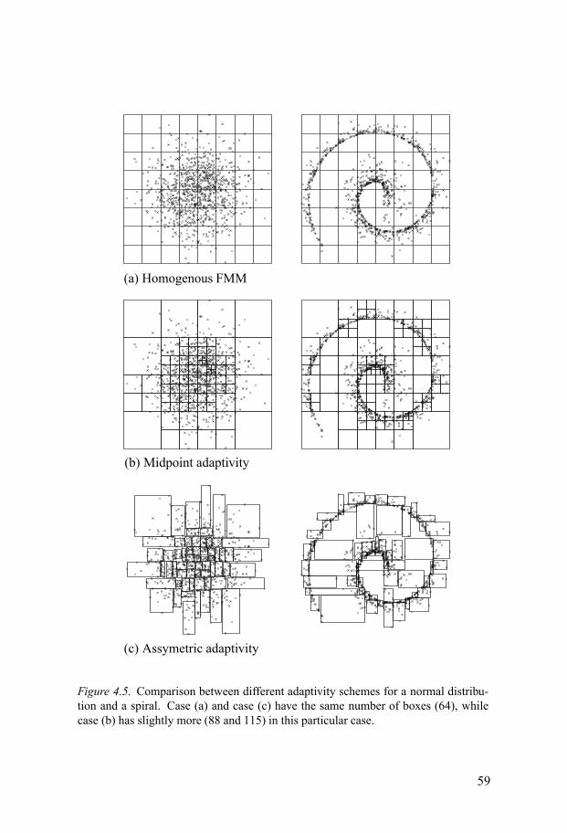
(a) Homogenous FMM

(b) Midpoint adaptivity

(c) Assymetric adaptivity

Figure 4.5. Comparison between different adaptivity schemes for a normal distribu-tion and a spiral. Case (a) and case (c) have the same number of boxes (64), whilecase (b) has slightly more (88 and 115) in this particular case.

59

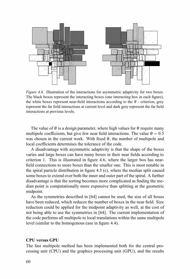
Figure 4.6. Illustration of the interactions for asymmetric adaptivity for two boxes.The black boxes represent the interacting boxes (one interacting box in each figure),the white boxes represent near-field interactions according to the θ - criterion, greyrepresent the far field interactions at current level and dark grey represent the far fieldinteractions at previous levels.

The value of θ is a design parameter, where high values for θ require manymultipole coefficients, but give few near field interactions. The value θ = 0.5was chosen in the current work. With fixed θ , the number of multipole andlocal coefficients determines the tolerance of the code.A disadvantage with asymmetric adaptivity is that the shape of the boxes

varies and large boxes can have many boxes in their near fields according tocriterion 1. This is illustrated in figure 4.6, where the larger box has near-field connections to more boxes than the smaller one. This is most notable inthe spiral particle distribution in figure 4.5 (c), where the median split causedsome boxes to extend over both the inner and outer part of the spiral. A furtherdisadvantage is that the sorting becomes more complicated as finding the me-dian point is computationally more expensive than splitting at the geometricmidpoint.As the symmetries described in [64] cannot be used, the size of all boxes

have been reduced, which reduces the number of boxes in the near field. Sizereduction could be applied for the midpoint adaptivity as well, at the cost ofnot being able to use the symmetries in [64]. The current implementation ofthe code performs all multipole to local translations within the same multipolelevel (similar to the homogenous case in figure 4.4).

CPU versus GPUThe fast multipole method has been implemented both for the central pro-cessing unit (CPU) and the graphics processing unit (GPU), and the results

60

for these architectures are analyzed in paper IX. A brief introduction to thedifferent systems is given here.The traditional CPU consists of a relatively small number of CPU cores,

where each core is relatively fast. This is to be compared to the GPU, wherethere are many slower computational cores. As the GPU used in Paper IX isa Nvidia Tesla C2075, this GPU (which is based on Nvidia’s CUDA architec-ture) will be in focus when describing the GPU architecture. This GPU has14 multiprocessors which each have 32 cores, giving a total of 448 cores. TheGPU has several threads grouped together into a warp (where the size of awarp is 32 threads). Within a warp, only one instruction can be executed atthe same time by all the threads in this warp, although all threads can oper-ate on different data. This is called single instruction multiple data (SIMD).If different threads within a warp have to perform different operations at thesame time, all instructions have to be serialized, where the CUDA cores of thethreads not executing the particular instruction become idle. If the number ofthreads within the warp is not equal to 32, it will also mean that the rest ofthe 32 CUDA cores become idle [65, chapter 4]. To fully use the GPU, thealgorithm has to be data parallel in a way that 32 identical instructions canbe executed all the time. To compare with the CPU case, most modern PCprocessors support streaming SIMD extensions (SSE), which allows for sim-ple algebraic operations to be performed on two double precision numbers (orfour single precision numbers) in one operation [66]. To get a good compari-son with the GPU code, the entire multipole evaluation phase was written withSSE instructions in the CPU case, which accelerated most parts with a factorclose to two.In the GPU computational model, functions (called kernels) are sent from

the CPU to the GPU. Each kernel contains a set of code to be executed andall threads execute this kernel. A kernel will be launched with a predefinednumber of threads, which are grouped together into blocks. Communicationbetween threads is typically only performed within the block, as there is cur-rently no synchronization method between different blocks, except for endingthe kernel and launching a new one, although some methods for sharing mem-ory between blocks have been developed, see e.g. [67, appendix A]. Com-munication between threads within a block is performed through a specialfast memory called shared memory, of which each multiprocessor has its own(48 kB on the Tesla C2075). For optimal performance, the number of threadsis usually a multiple of the warp size to avoid idle cores as all threads in a warpmust belong to the same block.The GPU programming model is based on launching a large number of

threads and each core will therefore run many threads. Several blocks can runon the same multiprocessor simultaneously to increase the number of activethreads. The GPU is very fast at switching between threads and the largenumber of threads per core is used to hide the time it takes to complete certaininstructions by issuing other instructions in the meantime. Too few threads

61

Part Time Part TimeDirect evaluation (P2P) 43 % Connectivity 1 %Sorting 30 % Multipole to multipoleMultipole to local shift (M2L) 11 % shift (M2M) < 1 %Multipole initialization (P2M) 5 % Local to local (L2L) < 1 %Multipole evaluation (L2P) 2 % Other 8 %

Table 4.1. Time distribution among different parts in the GPU implementation foroptimal Nd.

executing on a multiprocessor result in lower performance. One case wherethis could occur is if each thread requires too much shared memory, as the48 kB has to be enough for all threads together.

The FMM on the GPUThe implementation of the FMM on the GPU is given in paper IX and onlya brief description is given here, where more focus is given to the more com-putationally expensive parts. All parts of the code are implemented on theGPU.The sorting successively splits a box in two parts according to a chosen

pivot point. After each split, the part that does not contain the median willbe excluded for the next split until the median is found. This will requireO(logNd) steps to complete. For the CPU, a split can be performed in a singlepass by interchanging elements. The GPU uses a two pass algorithm, wherethe first step counts the elements (each thread has its on subset of elements).Then the cumulative sum is calculated between the threads and afterward, theelements can be inserted into a common array. The speed of the sorting codedepends on the number of particles in each box and if the number becomes toolow, all 32 threads of the warp will no longer be active, hence reducing speedfor small boxes. The connectivity (application of criterion 1) is determinedwith one thread per box making the code very similar to the CPU version.The multipole to local shift (M2L) uses one thread block to calculate the

interaction of one box (possibly two boxes if few interactions). Two threadsper box are used, where one thread shifts the real part and the other shifts theimaginary part. The algorithm will store the entire set of coefficients to shiftin shared memory as it is used several times during the shift. In other respects,the implementation is similar to the CPU implementation and as the operationcan perform shifts from two boxes within a block, it can often use most of the32 threads of the warp. Multipole to multipole (M2M) and local to local (L2L)shifts work similarly, but each level is evaluated in its own kernel launch as theshifts depend on the results from the shifts at the previous level, see figure 4.4.The number of shifts per box is fixed to 4, hence 4 boxes use 32 threads andall threads of the warp can be used.

62

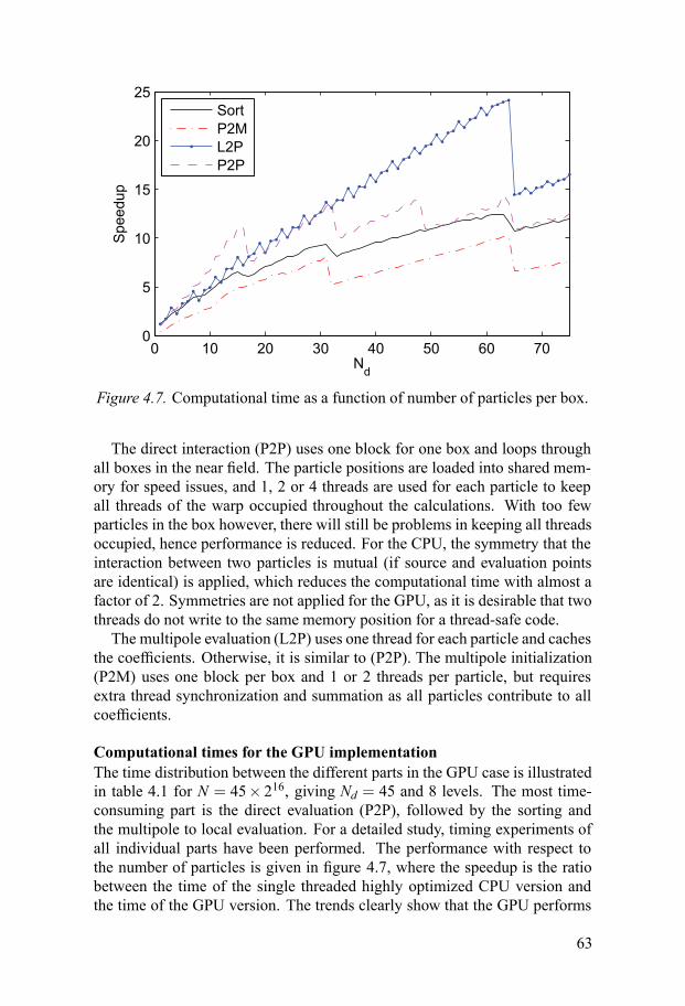
0 10 20 30 40 50 60 700

5

10

15

20

25

Nd

Spe

edup

SortP2ML2PP2P

Figure 4.7. Computational time as a function of number of particles per box.

The direct interaction (P2P) uses one block for one box and loops throughall boxes in the near field. The particle positions are loaded into shared mem-ory for speed issues, and 1, 2 or 4 threads are used for each particle to keepall threads of the warp occupied throughout the calculations. With too fewparticles in the box however, there will still be problems in keeping all threadsoccupied, hence performance is reduced. For the CPU, the symmetry that theinteraction between two particles is mutual (if source and evaluation pointsare identical) is applied, which reduces the computational time with almost afactor of 2. Symmetries are not applied for the GPU, as it is desirable that twothreads do not write to the same memory position for a thread-safe code.The multipole evaluation (L2P) uses one thread for each particle and caches

the coefficients. Otherwise, it is similar to (P2P). The multipole initialization(P2M) uses one block per box and 1 or 2 threads per particle, but requiresextra thread synchronization and summation as all particles contribute to allcoefficients.

Computational times for the GPU implementationThe time distribution between the different parts in the GPU case is illustratedin table 4.1 for N = 45× 216, giving Nd = 45 and 8 levels. The most time-consuming part is the direct evaluation (P2P), followed by the sorting andthe multipole to local evaluation. For a detailed study, timing experiments ofall individual parts have been performed. The performance with respect tothe number of particles is given in figure 4.7, where the speedup is the ratiobetween the time of the single threaded highly optimized CPU version andthe time of the GPU version. The trends clearly show that the GPU performs

63

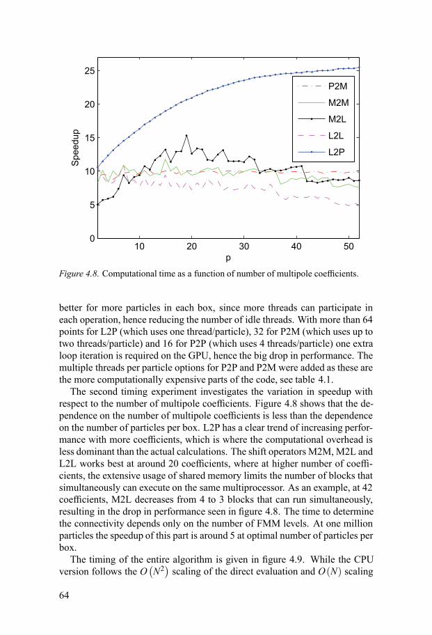
10 20 30 40 500

5

10

15

20

25

p

Spe

edup

P2M

M2M

M2L

L2L

L2P

Figure 4.8. Computational time as a function of number of multipole coefficients.

better for more particles in each box, since more threads can participate ineach operation, hence reducing the number of idle threads. With more than 64points for L2P (which uses one thread/particle), 32 for P2M (which uses up totwo threads/particle) and 16 for P2P (which uses 4 threads/particle) one extraloop iteration is required on the GPU, hence the big drop in performance. Themultiple threads per particle options for P2P and P2M were added as these arethe more computationally expensive parts of the code, see table 4.1.The second timing experiment investigates the variation in speedup with

respect to the number of multipole coefficients. Figure 4.8 shows that the de-pendence on the number of multipole coefficients is less than the dependenceon the number of particles per box. L2P has a clear trend of increasing perfor-mance with more coefficients, which is where the computational overhead isless dominant than the actual calculations. The shift operators M2M, M2L andL2L works best at around 20 coefficients, where at higher number of coeffi-cients, the extensive usage of shared memory limits the number of blocks thatsimultaneously can execute on the same multiprocessor. As an example, at 42coefficients, M2L decreases from 4 to 3 blocks that can run simultaneously,resulting in the drop in performance seen in figure 4.8. The time to determinethe connectivity depends only on the number of FMM levels. At one millionparticles the speedup of this part is around 5 at optimal number of particles perbox.The timing of the entire algorithm is given in figure 4.9. While the CPU

version follows the O(N2

)scaling of the direct evaluation and O(N) scaling

64

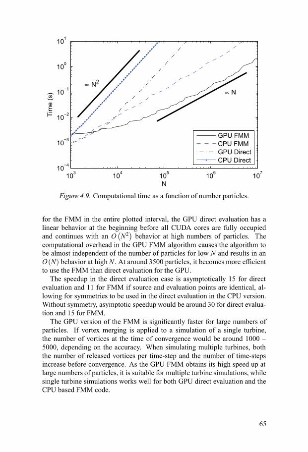
103 104 105 106 10710−4

10−3

10−2

10−1

100

101

N

Tim

e (s

)

∝ N2

∝ N

GPU FMMCPU FMMGPU DirectCPU Direct

Figure 4.9. Computational time as a function of number particles.

for the FMM in the entire plotted interval, the GPU direct evaluation has alinear behavior at the beginning before all CUDA cores are fully occupiedand continues with an O

(N2

)behavior at high numbers of particles. The

computational overhead in the GPU FMM algorithm causes the algorithm tobe almost independent of the number of particles for low N and results in anO(N) behavior at high N. At around 3500 particles, it becomes more efficientto use the FMM than direct evaluation for the GPU.The speedup in the direct evaluation case is asymptotically 15 for direct

evaluation and 11 for FMM if source and evaluation points are identical, al-lowing for symmetries to be used in the direct evaluation in the CPU version.Without symmetry, asymptotic speedup would be around 30 for direct evalua-tion and 15 for FMM.The GPU version of the FMM is significantly faster for large numbers of

particles. If vortex merging is applied to a simulation of a single turbine,the number of vortices at the time of convergence would be around 1000 –5000, depending on the accuracy. When simulating multiple turbines, boththe number of released vortices per time-step and the number of time-stepsincrease before convergence. As the GPU FMM obtains its high speed up atlarge numbers of particles, it is suitable for multiple turbine simulations, whilesingle turbine simulations works well for both GPU direct evaluation and theCPU based FMM code.

65

5. Simulation results

The simulation results are presented in two parts. The first part contains acomparison of the two different simulation models, and the different modifi-cations of them. This is to illustrate how the simulation model works, whichgenerally is not presented in articles, and this section will therefore consist ofunpublished work. The second part consists of the results from the publishedarticles that are included in this thesis.

5.1 Evaluation of simulation toolsIn this section, the experimental turbine located inMarsta outside Uppsala [16]will be used as a reference case. In the simulatedmodel, the turbine parameterscan be found in table 5.1. The struts are assumed to vary piecewise linearlyfrom the tip to the center, and from the center to the root. The trailing edge ofthe strut is blunt at the root, and the flat end is approximately 38 mm wideat the root (approximately 18 mm at the center, and sharp at the tip). Toaccount for this, a set of airfoils with blunt trailing edges was simulated inXFOIL [68], and the increase in drag due to the blunt trailing edge was addedas an additional drag term for the struts.As a comparison, the simulated curves are compared to experimental val-

ues, which were obtained according to [16]. The measurements were per-formed at a constant rotational velocity of around 6 rad/s, which means thatthe values for higher tip speed ratios were obtained from lower flow veloci-ties, where external losses (e.g. mechanical/electrical losses etc) are more sig-nificant. Considering that the power coefficient is expected to increase withincreasing flow velocity (increasing Reynolds number), which is illustrated infigure 5.1, the measured power coefficient will likely have its peak at a slightlylower tip speed ratio than it would if the measurements would have been per-formed with constant flow velocity. In all simulations where comparisons aremade, the simulations are therefore performed at constant rotational velocityas well.For the measured data, the accuracy is consistent at low tip speed ratios

where the flow velocity is high, but shows a more scattered behavior at highertip speed ratios (see figure 5.1). For high tip speed ratios, the power is lowerdue to the lower flow velocity, and uncertainties due to other losses, such asbearing friction and generator losses etc. are more prominent, further increas-ing the uncertainty in this region. Due to the cubic relation between flow ve-locity and power, a small measurement error in wind speed will give a much

66

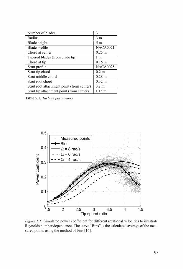
Number of blades 3Radius 3 mBlade height 5 mBlade profile NACA0021Chord at center 0.25 mTapered blades (from blade tip) 1 mChord at tip 0.15 mStrut profile NACA0025Strut tip chord 0.2 mStrut middle chord 0.28 mStrut root chord 0.32 mStrut root attachment point (from center) 0.2 mStrut tip attachment point (from center) 1.15 m

Table 5.1. Turbine parameters

1.5 2 2.5 3 3.5 4 4.50

0.1

0.2

0.3

0.4

0.5

Tip speed ratio

Pow

er c

oeffi

cien

t

Measured pointsBinsΩ = 8 rad/sΩ = 6 rad/sΩ = 4 rad/s

Figure 5.1. Simulated power coefficient for different rotational velocities to illustrateReynolds number dependence. The curve “Bins” is the calculated average of the mea-sured points using the method of bins [16].

67

1.5 2 2.5 3 3.5 4 4.50

0.1

0.2

0.3

0.4

0.5

Tip speed ratio

Pow

er c

oeffi

cien

tMeasured pointsBinsNo strutsNo flow correctionFlow correction

Figure 5.2. Simulated power coefficient with and without strut modeling compared tomeasured data.

larger contribution to the power coefficient and since the measurements are 10minute mean values, changes in flow velocity during the measurement periodalso contribute to the measurement error.

5.1.1 Strut modelingStruts can either be modeled as only giving drag (which was done in [49])using an equivalent drag for the all struts only varying with the rotational ve-locity, or the equations in section 4.1.2 can be used, which include lift forceon struts and corrections to the flow velocity. Lift force on struts occur if thestruts (or the flow velocity) are not horizontally aligned (in paper I of this the-sis, the struts are horizontally aligned, and only the drag terms are includedwithout the flow corrections). The differences between including struts withflow corrections or not can be seen in figure 5.2. In these simulations, curva-ture modeling with angle correction and all tip corrections are enabled, but noexpansion model. By comparing the three simulated figures, the strut model,including lift force on struts and flow corrections, obtains a higher power coef-ficient at low tip speed ratios, which is closer to the measurements. All modelsestimate a higher power coefficient than measurements at high tip speed ratios,but by using strut modeling, the values are closer to the measurements.

68

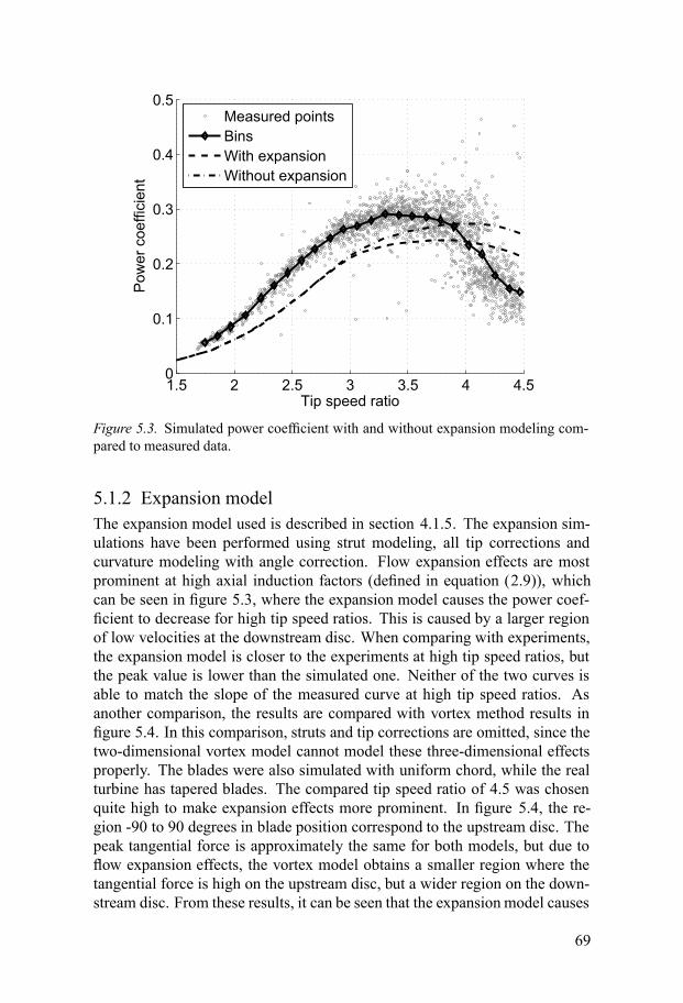
1.5 2 2.5 3 3.5 4 4.50

0.1

0.2

0.3

0.4

0.5

Tip speed ratio

Pow

er c

oeffi

cien

tMeasured pointsBinsWith expansionWithout expansion

Figure 5.3. Simulated power coefficient with and without expansion modeling com-pared to measured data.

5.1.2 Expansion modelThe expansion model used is described in section 4.1.5. The expansion sim-ulations have been performed using strut modeling, all tip corrections andcurvature modeling with angle correction. Flow expansion effects are mostprominent at high axial induction factors (defined in equation (2.9)), whichcan be seen in figure 5.3, where the expansion model causes the power coef-ficient to decrease for high tip speed ratios. This is caused by a larger regionof low velocities at the downstream disc. When comparing with experiments,the expansion model is closer to the experiments at high tip speed ratios, butthe peak value is lower than the simulated one. Neither of the two curves isable to match the slope of the measured curve at high tip speed ratios. Asanother comparison, the results are compared with vortex method results infigure 5.4. In this comparison, struts and tip corrections are omitted, since thetwo-dimensional vortex model cannot model these three-dimensional effectsproperly. The blades were also simulated with uniform chord, while the realturbine has tapered blades. The compared tip speed ratio of 4.5 was chosenquite high to make expansion effects more prominent. In figure 5.4, the re-gion -90 to 90 degrees in blade position correspond to the upstream disc. Thepeak tangential force is approximately the same for both models, but due toflow expansion effects, the vortex model obtains a smaller region where thetangential force is high on the upstream disc, but a wider region on the down-stream disc. From these results, it can be seen that the expansionmodel causes

69

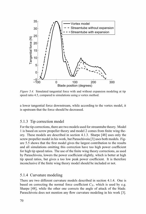
−100 0 100 200 300−5

0

5

10

15

20

25

30

35

Blade position (degrees)

Tang

entia

l for

ce (N

)

Vortex modelStreamtube without expansionStreamtube with expansion

Figure 5.4. Simulated tangential force with and without expansion modeling at tipspeed ratio 4.5, compared to simulations using a vortex method.

a lower tangential force downstream, while according to the vortex model, itis upstream that the force should be decreased.

5.1.3 Tip correction modelFor the tip corrections, there are twomodels used for streamtube theory. Model1 is based on screw propeller theory and model 2 comes from finite wing the-ory. These models are described in section 4.1.3. Sharpe [48] uses only thescrew propeller model in his work, but Paraschivoiu [3] uses both models. Fig-ure 5.5 shows that the first model gives the largest contribution to the resultsand all simulations omitting this correction have too high power coefficientfor high tip speed ratios. The use of the finite wing theory corrections, as usedby Paraschivoiu, lowers the power coefficient slightly, which is better at hightip speed ratios, but gives a too low peak power coefficient. It is thereforeinconclusive if the finite wing theory model should be included or not.

5.1.4 Curvature modelingThere are two different curvature models described in section 4.1.4. One isbased on correcting the normal force coefficient CN , which is used by e.g.Sharpe [48], while the other one corrects the angle of attack of the blade.Paraschivoiu does not mention any flow curvature modeling in his work [3].

70

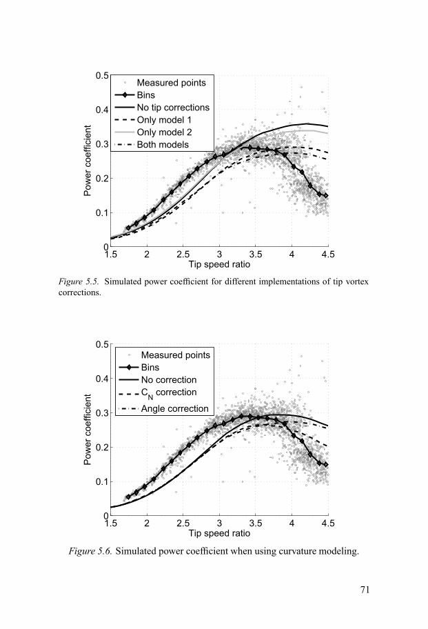
1.5 2 2.5 3 3.5 4 4.50

0.1

0.2

0.3

0.4

0.5

Tip speed ratio

Pow

er c

oeffi

cien

tMeasured pointsBinsNo tip correctionsOnly model 1Only model 2Both models

Figure 5.5. Simulated power coefficient for different implementations of tip vortexcorrections.

1.5 2 2.5 3 3.5 4 4.50

0.1

0.2

0.3

0.4

0.5

Tip speed ratio

Pow

er c

oeffi

cien

t

Measured pointsBinsNo correctionCN correction

Angle correction

Figure 5.6. Simulated power coefficient when using curvature modeling.

71

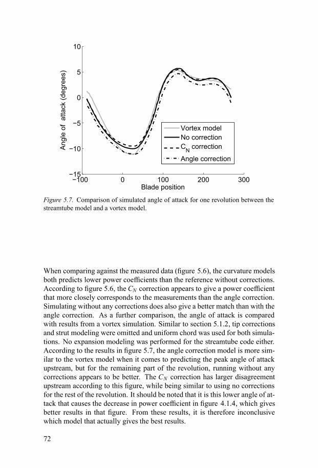
−100 0 100 200 300−15

−10

−5

0

5

10

Blade position

Ang

le o

f at

tack

(deg

rees

)

Vortex modelNo correctionCN correction

Angle correction

Figure 5.7. Comparison of simulated angle of attack for one revolution between thestreamtube model and a vortex model.

When comparing against the measured data (figure 5.6), the curvature modelsboth predicts lower power coefficients than the reference without corrections.According to figure 5.6, the CN correction appears to give a power coefficientthat more closely corresponds to the measurements than the angle correction.Simulating without any corrections does also give a better match than with theangle correction. As a further comparison, the angle of attack is comparedwith results from a vortex simulation. Similar to section 5.1.2, tip correctionsand strut modeling were omitted and uniform chord was used for both simula-tions. No expansion modeling was performed for the streamtube code either.According to the results in figure 5.7, the angle correction model is more sim-ilar to the vortex model when it comes to predicting the peak angle of attackupstream, but for the remaining part of the revolution, running without anycorrections appears to be better. The CN correction has larger disagreementupstream according to this figure, while being similar to using no correctionsfor the rest of the revolution. It should be noted that it is this lower angle of at-tack that causes the decrease in power coefficient in figure 4.1.4, which givesbetter results in that figure. From these results, it is therefore inconclusivewhich model that actually gives the best results.

72

1 2 3 4 5 60

0.1

0.2

0.3

0.4

0.5

Tip speed ratio

Pow

er c

oeffi

cien

t

Vortex modelStreamtube without expansionStreamtube with expansion

Figure 5.8. Simulated power coefficient using vortex model compared with thestreamtube model.

5.1.5 Vortex modelThe vortex model has the advantage that it actually solves the flow fromNavier-Stokes equations, instead of adding many correction models, whichis done for the streamtube models. The problem is that the current implemen-tation is a two-dimensional model, which cannot model struts and tip effects inthe same way as three-dimensional models such as the streamtube model. Toget a good comparison between the two models, all three-dimensional effectshave been omitted from the streamtube model. The results can be found infigure 5.8, where the vortex model is compared against the streamtube model,both with and without expansion modeling. In this figure, flow curvature ef-fects have been included in the streamtube model using the corrections to theangle of attack. At tip speed ratio 4.5, the angle of attack is plotted in fig-ure 5.7 and the tangential force in figure 5.4. The general results are that thestreamtube model predicts higher torque on the upstream disc and lower onthe downstream disc, due to flow expansion effects not properly being mod-eled in the streamtube theory. In this particular case, the vortex model shouldbe more accurate, but the streamtube model does currently show the ability tomodel three-dimensional effects more flexibly.

73

1.5 2 2.5 3 3.5 4 4.50

0.1

0.2

0.3

0.4

0.5

Tip speed ratio

Pow

er c

oeffi

cien

tMeasured pointsBinsSimulation

Figure 5.9. Closest matching power coefficient using streamtube model.

5.1.6 Concluding remarks about the simulation toolsFrom all the simulations performed, it can be concluded that the best fit to ex-perimental data would be obtained if strut modeling, the screw propeller partof the tip corrections, the CN correction for curvature effects and the expan-sion model are used. For this case, the simulated power coefficient is plottedin figure 5.9. Even though this seems good for the particular turbine, the com-parisons with the vortex model show for example that the expansion modeldoes not really match the vortex model solutions of Navier-Stokes equations.Neither do the curvature corrections show good results in the comparison withvortex theory. For the tip corrections, further studies are necessary to validatethe model, and the strut model also requires additional validation. Further, us-ing the power coefficient as validation is not the best method, as it cannot tellwhere during the revolution the torque was generated. It should therefore notbe concluded that the model configuration that created figure 5.9 really is thebest solution. Instead, additional, and more accurate, experimental results, ornumerical results using more advanced models, are necessary to validate themodel more properly.

5.2 Results from papersThis section contains a summary of the results from the papers included inthis thesis. Papers I – III use the streamtube model, while papers IV – VIII use

74

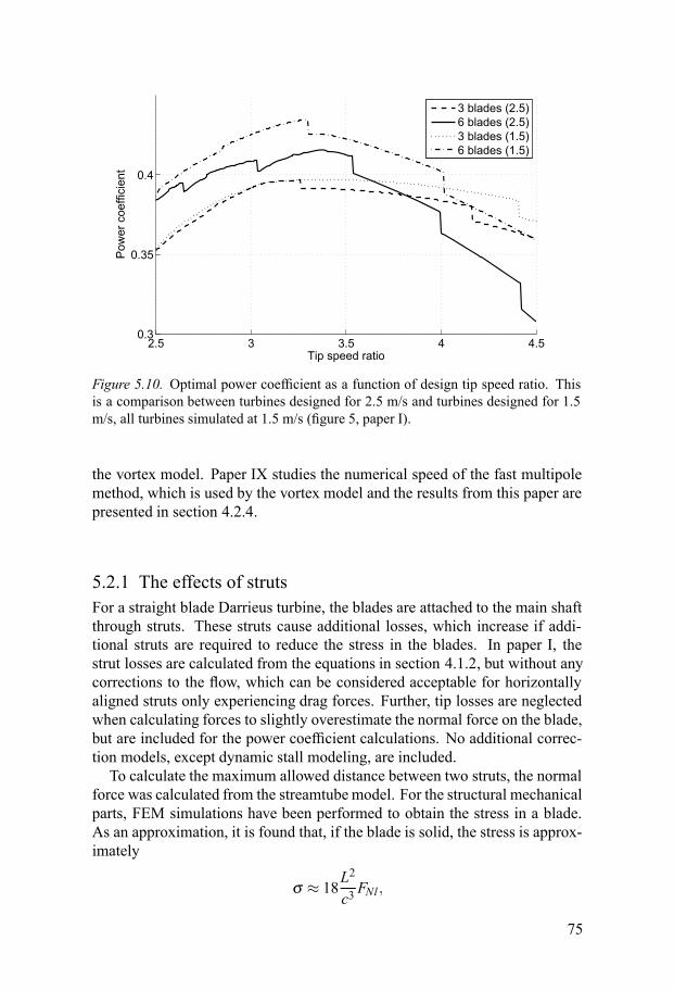
2.5 3 3.5 4 4.50.3

0.35

0.4

Tip speed ratio

Pow

er c

oeffi

cien

t3 blades (2.5)6 blades (2.5)3 blades (1.5)6 blades (1.5)

Figure 5.10. Optimal power coefficient as a function of design tip speed ratio. Thisis a comparison between turbines designed for 2.5 m/s and turbines designed for 1.5m/s, all turbines simulated at 1.5 m/s (figure 5, paper I).

the vortex model. Paper IX studies the numerical speed of the fast multipolemethod, which is used by the vortex model and the results from this paper arepresented in section 4.2.4.

5.2.1 The effects of strutsFor a straight blade Darrieus turbine, the blades are attached to the main shaftthrough struts. These struts cause additional losses, which increase if addi-tional struts are required to reduce the stress in the blades. In paper I, thestrut losses are calculated from the equations in section 4.1.2, but without anycorrections to the flow, which can be considered acceptable for horizontallyaligned struts only experiencing drag forces. Further, tip losses are neglectedwhen calculating forces to slightly overestimate the normal force on the blade,but are included for the power coefficient calculations. No additional correc-tion models, except dynamic stall modeling, are included.To calculate the maximum allowed distance between two struts, the normal

force was calculated from the streamtubemodel. For the structural mechanicalparts, FEM simulations have been performed to obtain the stress in a blade.As an approximation, it is found that, if the blade is solid, the stress is approx-imately

σ ≈ 18L2

c3FNl ,

75

where FNl is the normal force per meter, and L is the distance between thestruts. From this equation, the maximum allowed length between two strutscan be determined if the maximum allowed stress is given. In this study, theblades are assumed to be made of steel, and the maximum stress is set to100 MPa. From further FEM studies, it was found that the number of strutsapproximately can be given by the equation

Ns =hL

+0.2.

The number of strutsNs is set to be at least 2. The studied turbine is 5×5m andit is designed to run in water, where hydrodynamic forces are more prominentthan centrifugal forces (both forces are included in FNl). To determine thenecessary size of the struts, FEM studies have been performed for a bladewith chord c= 0.2 m. With this blade chord, a strut chord cs of 0.8c at the tip,and 1.2c at the root was determined to be sufficient to keep the strees withinthe limits. If the chord is increased, it is not necessary to increase the strutchord as much, and the equations

cs = 0.8√c0c tip,

cs = 1.2√c0c root,

give good results for the stress in the struts. Here, c0 is the chord used in theFEM studies, e.g. c0 = 0.2 m.Two different turbine configurations have been tested, one with 3 blades and

one with 6 blades. For each configuration, one is designed to run at optimaltip speed ratio at flow velocity of 1.5 m/s and one is designed to run at 2.5 m/s.Due to the higher forces at 2.5 m/s, additional struts are required, especiallyfor a turbine with 6 blades. Results from all four combinations are found infigure 5.10. The chord is adjusted to give the peak of the power coefficientcurve for each tip speed ratio in this figure. The sharp decreases in powercoefficient correspond to the positions where the chord is small enough toforce the addition of an additional strut. Figure 5.10 suggests that a turbinewith 6 blades can give higher power coefficients than a turbine with 3 blades,which is a result of the higher aspect ratio for the 6-bladed turbine due toits smaller chord. It can also be seen that the 6-bladed turbine needs morestruts due to its smaller chord. One interesting result is that if the turbine isdesigned for 2.5 m/s, the additional struts required for the 6-bladed turbinedecrease the power coefficient. Therefore, the turbine designed for 2.5 m/shas a lower power coefficient at 1.5 m/s than the turbine designed for only 1.5m/s. The implication is that if a turbine is designed for high flow velocities, theperformance at lower flow velocities can be reduced due to additional losses.Therefore, designing a turbine to run at high flow velocities can actually causea decrease in the total energy extraction if high flow velocities at the site arerare.

76

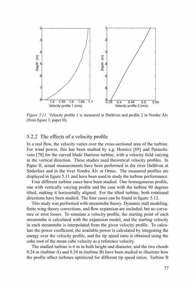
1.5 1.55 1.6 1.65 1.7

2

3

4

5

6

7

8

Velocity profile 1 (m/s)

De

pth

(m)

0.35 0.4 0.45 0.5 0.55

1

2

3

4

5

6

7

Velocity profile 2 (m/s)D

ep

th(m

)

Figure 5.11. Velocity profile 1 is measured in Dalälven and profile 2 in Nordre Älv(from figure 3, paper II).

5.2.2 The effects of a velocity profileIn a real flow, the velocity varies over the cross-sectional area of the turbine.For wind power, this has been studied by e.g. Homicz [69] and Paraschi-voiu [70] for the curved blade Darrieus turbine, with a velocity field varyingin the vertical direction. These studies used theoretical velocity profiles. InPaper II, actual measurements have been performed in the river Dalälven atSöderfors and in the river Nordre Älv at Ormo. The measured profiles aredisplayed in figure 5.11 and have been used to study the turbine performance.Four different turbine cases have been studied. One homogeneous profile,

one with vertically varying profile and the case with the turbine 90 degreestilted, making it horizontally aligned. For the tilted turbine, both rotationaldirections have been studied. The four cases can be found in figure 5.12.This study was performed with streamtube theory. Dynamic stall modeling,

finite wing theory corrections, and flow expansion are included, but no curva-ture or strut losses. To simulate a velocity profile, the starting point of eachstreamtube is calculated with the expansion model, and the starting velocityin each streamtube is interpolated from the given velocity profile. To calcu-late the power coefficient, the available power is calculated by integrating theenergy over the velocity profile, and the tip speed ratio is obtained using thecube root of the mean cube velocity as a reference velocity.The studied turbine is 6 m in both height and diameter, and the two chords

0.24 m (turbine A) and 0.34 m (turbine B) have been studied to illustrate howthe profile affect turbines optimized for different tip speed ratios. Turbine B

77

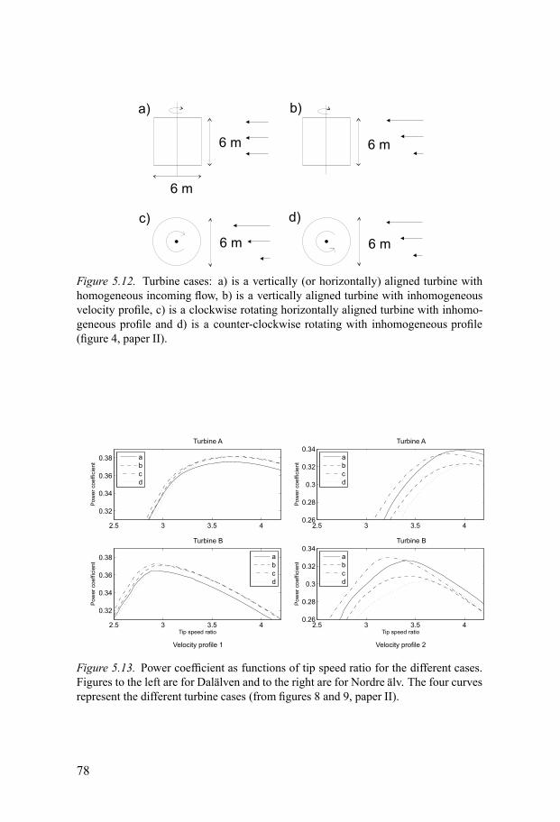
a) b)

c)

6 m 6 m

d)

6 m6 m

6 m

Figure 5.12. Turbine cases: a) is a vertically (or horizontally) aligned turbine withhomogeneous incoming flow, b) is a vertically aligned turbine with inhomogeneousvelocity profile, c) is a clockwise rotating horizontally aligned turbine with inhomo-geneous profile and d) is a counter-clockwise rotating with inhomogeneous profile(figure 4, paper II).

2.5 3 3.5 4

0.32

0.34

0.36

0.38

Turbine A

2.5 3 3.5 4

0.32

0.34

0.36

0.38

Tip speed ratio

Pow

er

coeffic

ient

Turbine B

a

b

c

d

a

b

c

d

2.5 3 3.5 40.26

0.28

0.3

0.32

0.34Turbine A

2.5 3 3.5 40.26

0.28

0.3

0.32

0.34Turbine B

a

b

c

d

a

b

c

d

Velocity profile 1 Velocity profile 2

Pow

er

coeffic

ient

Pow

er

coeffic

ient

Pow

er

coeffic

ient

Tip speed ratio

Figure 5.13. Power coefficient as functions of tip speed ratio for the different cases.Figures to the left are for Dalälven and to the right are for Nordre älv. The four curvesrepresent the different turbine cases (from figures 8 and 9, paper II).

78

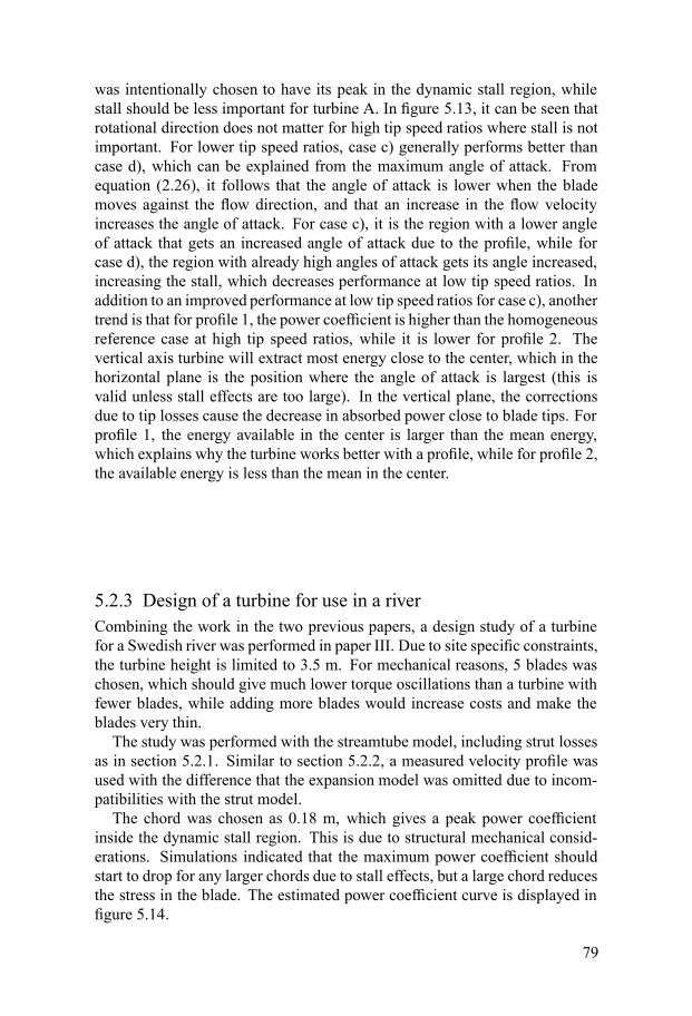
was intentionally chosen to have its peak in the dynamic stall region, whilestall should be less important for turbine A. In figure 5.13, it can be seen thatrotational direction does not matter for high tip speed ratios where stall is notimportant. For lower tip speed ratios, case c) generally performs better thancase d), which can be explained from the maximum angle of attack. Fromequation (2.26), it follows that the angle of attack is lower when the blademoves against the flow direction, and that an increase in the flow velocityincreases the angle of attack. For case c), it is the region with a lower angleof attack that gets an increased angle of attack due to the profile, while forcase d), the region with already high angles of attack gets its angle increased,increasing the stall, which decreases performance at low tip speed ratios. Inaddition to an improved performance at low tip speed ratios for case c), anothertrend is that for profile 1, the power coefficient is higher than the homogeneousreference case at high tip speed ratios, while it is lower for profile 2. Thevertical axis turbine will extract most energy close to the center, which in thehorizontal plane is the position where the angle of attack is largest (this isvalid unless stall effects are too large). In the vertical plane, the correctionsdue to tip losses cause the decrease in absorbed power close to blade tips. Forprofile 1, the energy available in the center is larger than the mean energy,which explains why the turbine works better with a profile, while for profile 2,the available energy is less than the mean in the center.

5.2.3 Design of a turbine for use in a riverCombining the work in the two previous papers, a design study of a turbinefor a Swedish river was performed in paper III. Due to site specific constraints,the turbine height is limited to 3.5 m. For mechanical reasons, 5 blades waschosen, which should give much lower torque oscillations than a turbine withfewer blades, while adding more blades would increase costs and make theblades very thin.The study was performed with the streamtube model, including strut losses

as in section 5.2.1. Similar to section 5.2.2, a measured velocity profile wasused with the difference that the expansion model was omitted due to incom-patibilities with the strut model.The chord was chosen as 0.18 m, which gives a peak power coefficient

inside the dynamic stall region. This is due to structural mechanical consid-erations. Simulations indicated that the maximum power coefficient shouldstart to drop for any larger chords due to stall effects, but a large chord reducesthe stress in the blade. The estimated power coefficient curve is displayed infigure 5.14.

79

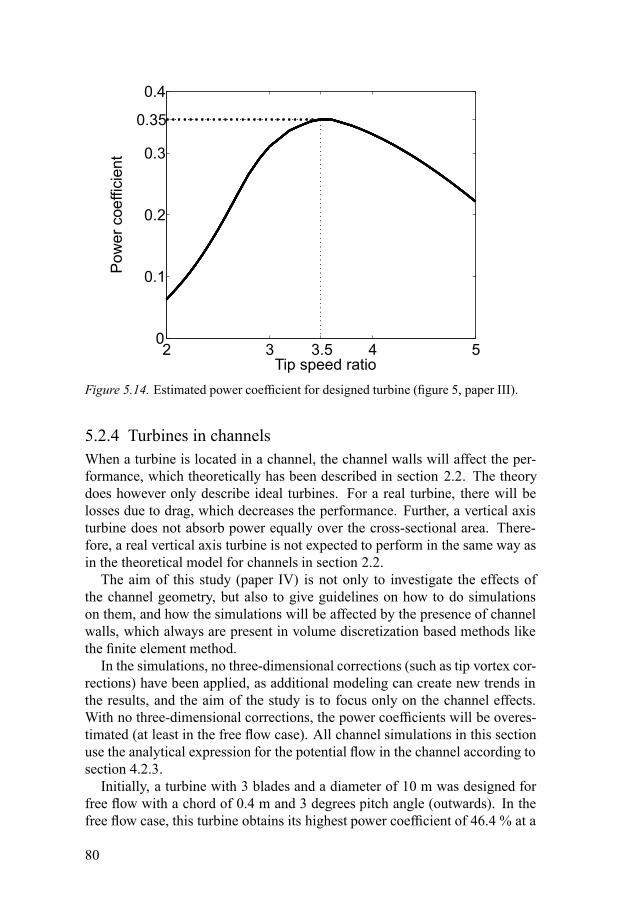
2 3 3.5 4 50

0.1

0.2

0.3

0.35

0.4

Tip speed ratio

Pow

er

coeffic

ient

Figure 5.14. Estimated power coefficient for designed turbine (figure 5, paper III).

5.2.4 Turbines in channelsWhen a turbine is located in a channel, the channel walls will affect the per-formance, which theoretically has been described in section 2.2. The theorydoes however only describe ideal turbines. For a real turbine, there will belosses due to drag, which decreases the performance. Further, a vertical axisturbine does not absorb power equally over the cross-sectional area. There-fore, a real vertical axis turbine is not expected to perform in the same way asin the theoretical model for channels in section 2.2.The aim of this study (paper IV) is not only to investigate the effects of

the channel geometry, but also to give guidelines on how to do simulationson them, and how the simulations will be affected by the presence of channelwalls, which always are present in volume discretization based methods likethe finite element method.In the simulations, no three-dimensional corrections (such as tip vortex cor-

rections) have been applied, as additional modeling can create new trends inthe results, and the aim of the study is to focus only on the channel effects.With no three-dimensional corrections, the power coefficients will be overes-timated (at least in the free flow case). All channel simulations in this sectionuse the analytical expression for the potential flow in the channel according tosection 4.2.3.Initially, a turbine with 3 blades and a diameter of 10 m was designed for

free flow with a chord of 0.4 m and 3 degrees pitch angle (outwards). In thefree flow case, this turbine obtains its highest power coefficient of 46.4 % at a

80

0 20 40 60 80 1000

20

40

60

80

100

120

Revolutions

Cha

nnel

wid

th

Figure 5.15. Number of revolutions until convergence as function of channel width.Channel width is measured in terms of turbine diameters (figure 4, paper IV).

tip speed ratio of 3.4. For this case, approximately 100 revolutions are requiredfor convergence. The necessary number of revolutions is a function of tipspeed ratio, and increases with increasing tip speed ratio. Simulations at hightip speed ratios show oscillatory behavior and with the chosen convergencecriterion that the power coefficient should remain within 0.001 of the finalvalue, these simulations do not show any good convergence at all.The primary numerical parameter investigated is the number of revolutions

required for a given channel width. Here, all simulations have been performedat the optimal tip speed ratio. Figure 5.15 shows that the necessary numberof revolutions increases with increasing channel width, where the increase atthe beginning is linear, while for increasing width, it approaches the free flowcase.The second part of the study shows how the turbine performance changes

due to the channel width. According to analytical predictions, the power co-efficient should increase with decreasing channel width, and this is indeed thecase (see figure 5.16), but the power coefficient increases slower than theorypredicts. When the power coefficient increases, the tip speed ratio, for whichthe peak occurs, increases as well, illustrated in figure 5.17. It is generally notoptimal to have the peak tip speed ratio too high, since drag losses are moredominating at high tip speed ratios, and for small channels, the power coeffi-cient can be improved by increasing the chord. As an example, for a channelof 4 turbine diameters, the turbine with chord 0.4 m obtains a 37 % increase

81

0 20 40 60 80 1000.4

0.5

0.6

0.7

0.8

0.9

1

Pow

er c

oeffi

cien

t

Channel width

SimulatedTheoreticalSimulated/Theoretical

Figure 5.16. Changes in Power coefficient due to the channel width. Theoretical val-ues are calculated from the theory in section 2.2. The dotted line is the ratio betweenthe two other curves (figure 6, paper IV).

0 20 40 60 80 1003

4

5

6

7

8

Tip

spee

d ra

tio

Channel width

Figure 5.17. Optimal the tip speed ratio as a function of channel width (figure 8,paper IV).

82

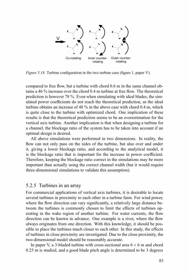
V

Co-rotating Inner counter-rotating

Outer counter-rotating

Figure 5.18. Turbine configuration in the two turbine case (figure 1, paper V).

compared to free flow, but a turbine with chord 0.6 m in the same channel ob-tains a 46 % increase over the chord 0.4 m turbine at free flow. The theoreticalprediction is however 78 %. Even when simulating with ideal blades, the sim-ulated power coefficients do not reach the theoretical prediction, as the idealturbine obtains an increase of 48 % in the above case with chord 0.4 m, whichis quite close to the turbine with optimized chord. One implication of theseresults is that the theoretical prediction seems to be an overestimation for thevertical axis turbine. Another implication is that when designing a turbine fora channel, the blockage ratio of the system has to be taken into account if anoptimal design is desired.All above simulations were performed in two dimensions. In reality, the

flow can not only pass on the sides of the turbine, but also over and underit, giving a lower blockage ratio, and according to the analytical model, itis the blockage ratio that is important for the increase in power coefficient.Therefore, keeping the blockage ratio correct in the simulations may be moreimportant than actually using the correct channel width (but it would requirethree-dimensional simulations to validate this assumption).

5.2.5 Turbines in an arrayFor commercial applications of vertical axis turbines, it is desirable to locateseveral turbines in proximity to each other in a turbine farm. For wind power,where the flow direction can vary significantly, a relatively large distance be-tween the turbines is commonly chosen to limit the effects of turbines op-erating in the wake region of another turbine. For water currents, the flowdirection can be known in advance. One example is a river, where the flowalways originates from one direction. With this knowledge, it should be pos-sible to place the turbines much closer to each other. In this study, the effectsof turbines in close proximity are investigated. Due to the close proximity, thetwo-dimensional model should be reasonably accurate.In paper V, a 3-bladed turbine with cross-sectional area 6× 6 m and chord

0.25 m is studied, and a good blade pitch angle is determined to be 3 degrees

83

3 3.5 4 4.5 5 5.50.25

0.3

0.35

0.4

0.45

Tip Speed Ratio

Pow

er C

oeffi

cien

t

Co−rotating turbine 1Co−rotating turbine 2Inner counter−rotatingOuter counter−rotatingSingle turbine

Figure 5.19. Simulation using two turbines. For the co-rotating case, the individualturbines are shown, while in the other two cases, both turbines give the same powercoefficient due to symmetry (figure 3, paper V).

8 m

8 m

1

2

3

4

5

Case 1 Case 2

V

8 m

Figure 5.20. Turbine configuration in the five turbine case (from figure 6, paper V).

84

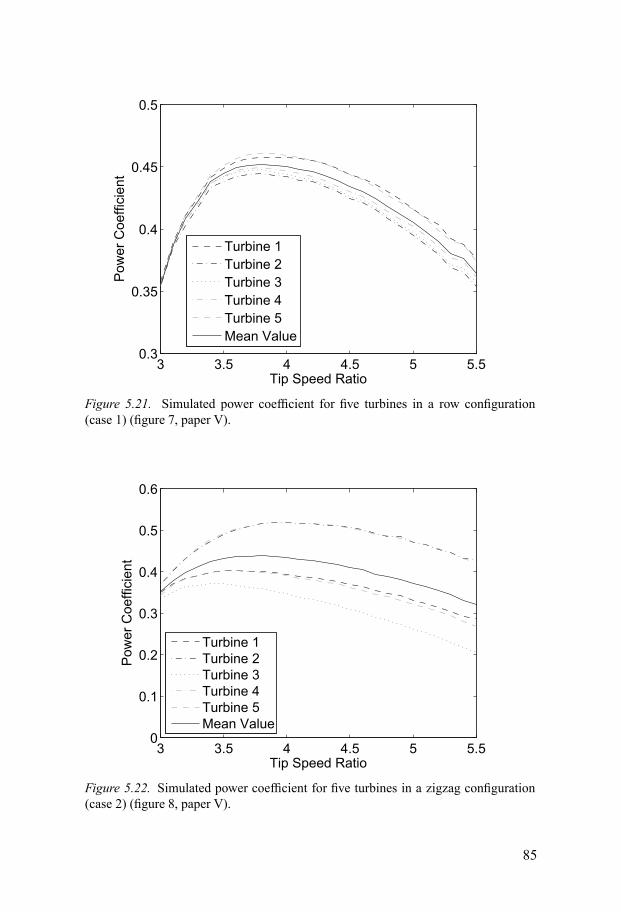
3 3.5 4 4.5 5 5.50.3

0.35

0.4

0.45

0.5

Tip Speed Ratio

Pow

er C

oeffi

cien

t

Turbine 1Turbine 2Turbine 3Turbine 4Turbine 5Mean Value

Figure 5.21. Simulated power coefficient for five turbines in a row configuration(case 1) (figure 7, paper V).

3 3.5 4 4.5 5 5.50

0.1

0.2

0.3

0.4

0.5

0.6

Tip Speed Ratio

Pow

er C

oeffi

cien

t

Turbine 1Turbine 2Turbine 3Turbine 4Turbine 5Mean Value

Figure 5.22. Simulated power coefficient for five turbines in a zigzag configuration(case 2) (figure 8, paper V).

85

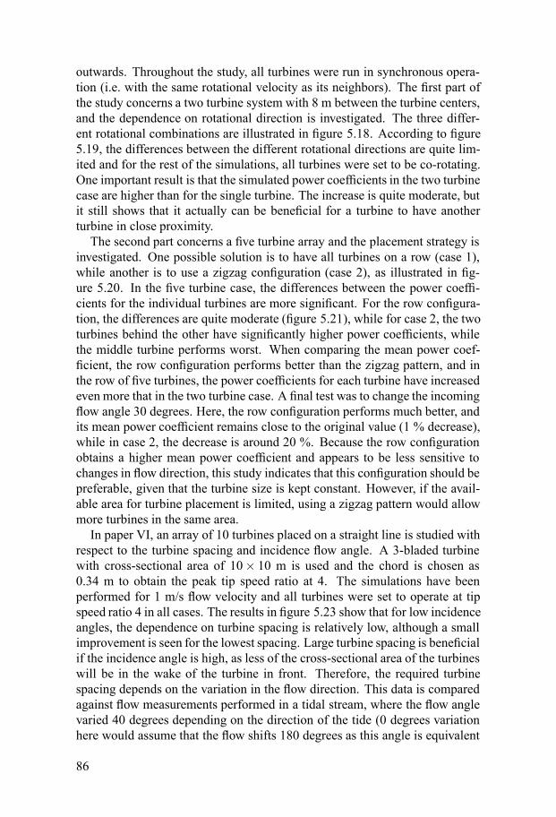
outwards. Throughout the study, all turbines were run in synchronous opera-tion (i.e. with the same rotational velocity as its neighbors). The first part ofthe study concerns a two turbine system with 8 m between the turbine centers,and the dependence on rotational direction is investigated. The three differ-ent rotational combinations are illustrated in figure 5.18. According to figure5.19, the differences between the different rotational directions are quite lim-ited and for the rest of the simulations, all turbines were set to be co-rotating.One important result is that the simulated power coefficients in the two turbinecase are higher than for the single turbine. The increase is quite moderate, butit still shows that it actually can be beneficial for a turbine to have anotherturbine in close proximity.The second part concerns a five turbine array and the placement strategy is

investigated. One possible solution is to have all turbines on a row (case 1),while another is to use a zigzag configuration (case 2), as illustrated in fig-ure 5.20. In the five turbine case, the differences between the power coeffi-cients for the individual turbines are more significant. For the row configura-tion, the differences are quite moderate (figure 5.21), while for case 2, the twoturbines behind the other have significantly higher power coefficients, whilethe middle turbine performs worst. When comparing the mean power coef-ficient, the row configuration performs better than the zigzag pattern, and inthe row of five turbines, the power coefficients for each turbine have increasedeven more that in the two turbine case. A final test was to change the incomingflow angle 30 degrees. Here, the row configuration performs much better, andits mean power coefficient remains close to the original value (1 % decrease),while in case 2, the decrease is around 20 %. Because the row configurationobtains a higher mean power coefficient and appears to be less sensitive tochanges in flow direction, this study indicates that this configuration should bepreferable, given that the turbine size is kept constant. However, if the avail-able area for turbine placement is limited, using a zigzag pattern would allowmore turbines in the same area.In paper VI, an array of 10 turbines placed on a straight line is studied with

respect to the turbine spacing and incidence flow angle. A 3-bladed turbinewith cross-sectional area of 10× 10 m is used and the chord is chosen as0.34 m to obtain the peak tip speed ratio at 4. The simulations have beenperformed for 1 m/s flow velocity and all turbines were set to operate at tipspeed ratio 4 in all cases. The results in figure 5.23 show that for low incidenceangles, the dependence on turbine spacing is relatively low, although a smallimprovement is seen for the lowest spacing. Large turbine spacing is beneficialif the incidence angle is high, as less of the cross-sectional area of the turbineswill be in the wake of the turbine in front. Therefore, the required turbinespacing depends on the variation in the flow direction. This data is comparedagainst flow measurements performed in a tidal stream, where the flow anglevaried 40 degrees depending on the direction of the tide (0 degrees variationhere would assume that the flow shifts 180 degrees as this angle is equivalent

86

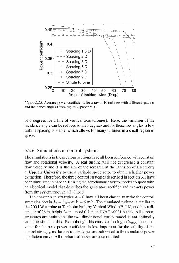
0 10 20 30 40 50 60 70 800.25

0.3

0.35

0.4

0.45

Angle of incident wind (Deg.)

Pow

er c

oeffi

cien

t

Spacing 1.5 DSpacing 2 DSpacing 3 DSpacing 5 DSpacing 7 DSpacing 9 DSingle turbine

Figure 5.23. Average power coefficients for array of 10 turbines with different spacingand incidence angles (from figure 2, paper VI).

of 0 degrees for a line of vertical axis turbines). Here, the variation of theincidence angle can be reduced to±20 degrees and for these low angles, a lowturbine spacing is viable, which allows for many turbines in a small region ofspace.

5.2.6 Simulations of control systemsThe simulations in the previous sections have all been performed with constantflow and rotational velocity. A real turbine will not experience a constantflow velocity and it is the aim of the research at the Division of Electricityat Uppsala University to use a variable speed rotor to obtain a higher powerextraction. Therefore, the three control strategies described in section 3.1 havebeen simulated in paper VII using the aerodynamic vortex model coupled withan electrical model that describes the generator, rectifier and extracts powerfrom the system through a DC load.The constants in strategies A – C have all been chosen to make the control

strategies obtain λe = λmax at V = 6 m/s. The simulated turbine is similar tothe 200 kW turbine at Torsholm built by Vertical Wind AB [18], and has a di-ameter of 26 m, height 24 m, chord 0.7 m and NACA0021 blades. All supportstructures are omitted as the two-dimensional vortex model is not optimallysuited to simulate this. Even though this causes a too high CPmax, the actualvalue for the peak power coefficient is less important for the validity of thecontrol strategy, as the control strategies are calibrated to this simulated powercoefficient curve. All mechanical losses are also omitted.

87

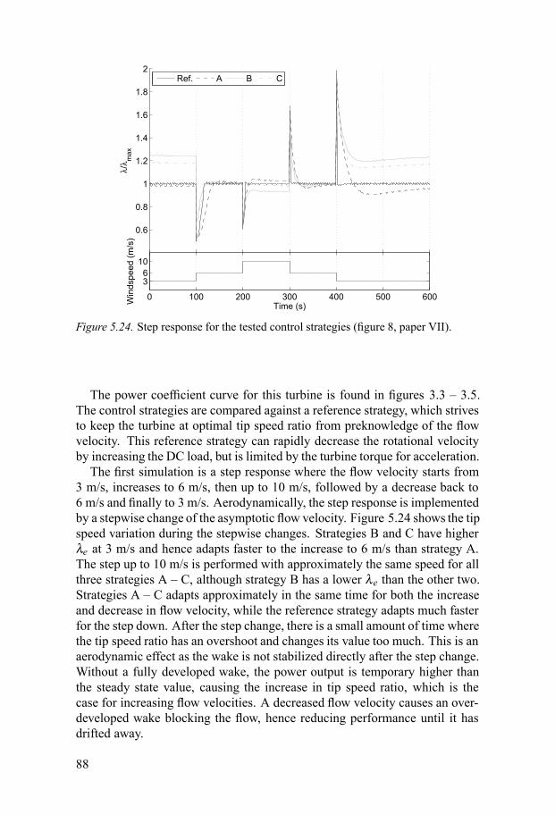
0.6

0.8

1

1.2

1.4

1.6

1.8

2

λ/λ m

ax

Ref. A B C

0 100 200 300 400 500 600

36

10

Win

dspe

ed (m

/s)

Time (s)

Figure 5.24. Step response for the tested control strategies (figure 8, paper VII).

The power coefficient curve for this turbine is found in figures 3.3 – 3.5.The control strategies are compared against a reference strategy, which strivesto keep the turbine at optimal tip speed ratio from preknowledge of the flowvelocity. This reference strategy can rapidly decrease the rotational velocityby increasing the DC load, but is limited by the turbine torque for acceleration.The first simulation is a step response where the flow velocity starts from

3 m/s, increases to 6 m/s, then up to 10 m/s, followed by a decrease back to6 m/s and finally to 3 m/s. Aerodynamically, the step response is implementedby a stepwise change of the asymptotic flow velocity. Figure 5.24 shows the tipspeed variation during the stepwise changes. Strategies B and C have higherλe at 3 m/s and hence adapts faster to the increase to 6 m/s than strategy A.The step up to 10 m/s is performed with approximately the same speed for allthree strategies A – C, although strategy B has a lower λe than the other two.Strategies A – C adapts approximately in the same time for both the increaseand decrease in flow velocity, while the reference strategy adapts much fasterfor the step down. After the step change, there is a small amount of time wherethe tip speed ratio has an overshoot and changes its value too much. This is anaerodynamic effect as the wake is not stabilized directly after the step change.Without a fully developed wake, the power output is temporary higher thanthe steady state value, causing the increase in tip speed ratio, which is thecase for increasing flow velocities. A decreased flow velocity causes an over-developed wake blocking the flow, hence reducing performance until it hasdrifted away.

88

0 0.005 0.01 0.015 0.02 0.025 0.03 0.035 0.041.6

1.8

2

2.2

2.4

2.6

2.8

3x 104

Wind frequency (Hz)

Del

iver

ed p

ower

(W)

Ref.Strategy AStrategy BStrategy C

Figure 5.25. Delivered power for oscillating wind field (figure 9, paper VII).

0 0.005 0.01 0.015 0.02 0.025 0.03 0.035 0.043.2

3.4

3.6

3.8

4

4.2

4.4

4.6

4.8

5

Wind frequency (Hz)

Tip

speed

ratio

Ref.

Strategy A

Strategy B

Strategy C

Figure 5.26. Mean tip speed ratio for oscillating wind field (figure 10, paper VII).

89

A second study evaluates the control strategy performance for oscillatingwind conditions (figure 5.25), where the wind is set to a sinusoidal oscillationbetween 3 m/s and 8 m/s. Among the three strategies A – C, strategy A hasthe highest performance for steady wind conditions, which is expected as itis the strategy that should operate closest to λmax. For unsteady conditions,strategy C extracts more energy than strategy A and for even faster wind os-cillations, strategy B is the best choice. The reference strategy works well forwind frequencies below 0.02 Hz and later starts to drop rapidly. The explana-tion is found in figure 5.26 where it is seen that the reference strategy drops intip speed ratio for higher wind frequencies, while strategies A – C obtains toohigh tip speed ratios. The reference strategy has the ability to rapidly decreaseflow velocity, but is limited to aerodynamic torque for acceleration. Whenthe aerodynamic torque becomes too small to accelerate the turbine to properspeed, the tip speed ratio drops. Strategies A – C have slightly higher accel-erations than retardations when operating close to λe with respect to changesin flow velocity and hence end up at a too high tip speed ratio instead. Thishigher tip speed ratio is advantageous as the turbine operates closer to λmax athigh flow velocities, which is where most energy is available.According to the simulations, all strategies A – C should be viable options

for controlling the turbine and the best choice depends on the flow character-istics. The reference strategy may obtain slightly higher performance in manycases, but such a strategy would be complicated to implement as it would re-quire full knowledge of the flow velocity through proper measurements, andflow measurement equipment would also introduce additional sources of fail-ure.

5.2.7 Control of multiple turbinesThis section contains an evaluation of the two different electric topologiesdescribed in section 3.2. The multiple turbine simulations with the separatetopology have been performed as four different electric simulations, while themutual topology simulations have been simulated as one combined electricalsimulation. Control strategy C was chosen for both topologies as it obtainedgood results in the previous section. All tests were performed on a farm offour turbines identical to the turbine tested in section 3.1.The first test to compare the separate and mutual topologies is a simulation

where all turbines are aerodynamically separated. The flow velocity was var-ied slowly according to figure 5.27. This velocity variation gives the rotationalvelocities for the different topologies shown in figure 5.28. For the separatetopology, the different regions for strategy C is seen, where the decrease inrotational velocity is reduced below V∞ = 4.5 m/s for turbine 4, while the in-crease in rotational velocity is less for turbine 1 above V∞ = 9 m/s. Aroundt = 1800 s for the mutual topology, turbine 4 stops delivering power and the

90

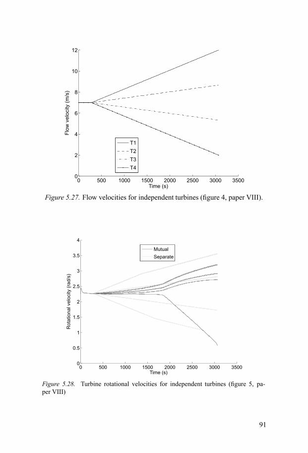
0 500 1000 1500 2000 2500 3000 35000

2

4

6

8

10

12

Flo

wve

locity

(m/s

)

Time (s)

T1

T2

T3

T4

Figure 5.27. Flow velocities for independent turbines (figure 4, paper VIII).

0 500 1000 1500 2000 2500 3000 35000

0.5

1

1.5

2

2.5

3

3.5

4

Ro

tatio

na

lve

locity

(ra

d/s

)

Time (s)

Mutual

Separate

Figure 5.28. Turbine rotational velocities for independent turbines (figure 5, pa-per VIII)

91

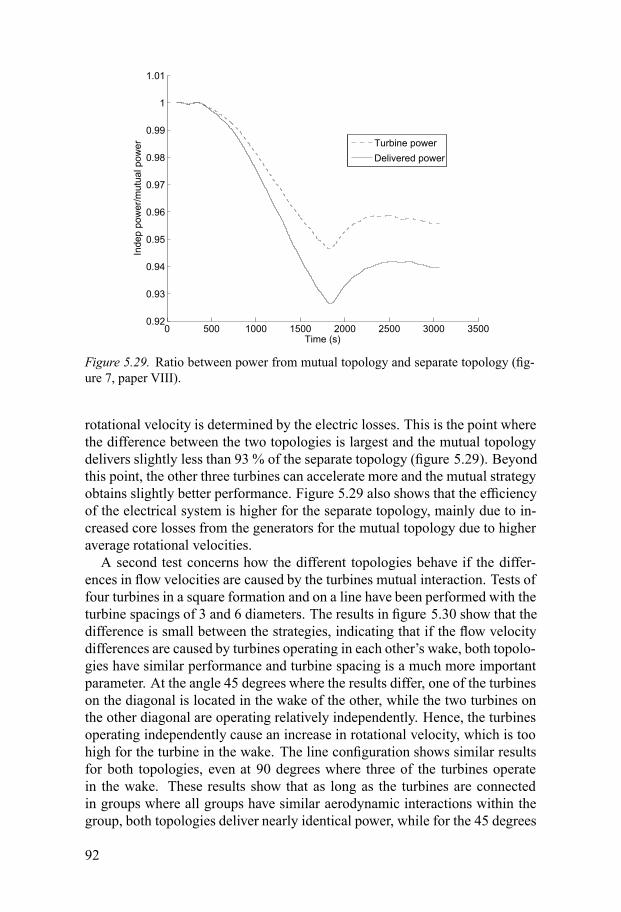
0 500 1000 1500 2000 2500 3000 35000.92

0.93

0.94

0.95

0.96

0.97

0.98

0.99

1

1.01

Time (s)

Inde

p po

wer

/mut

ual p

ower Turbine power

Delivered power

Figure 5.29. Ratio between power from mutual topology and separate topology (fig-ure 7, paper VIII).

rotational velocity is determined by the electric losses. This is the point wherethe difference between the two topologies is largest and the mutual topologydelivers slightly less than 93 % of the separate topology (figure 5.29). Beyondthis point, the other three turbines can accelerate more and the mutual strategyobtains slightly better performance. Figure 5.29 also shows that the efficiencyof the electrical system is higher for the separate topology, mainly due to in-creased core losses from the generators for the mutual topology due to higheraverage rotational velocities.A second test concerns how the different topologies behave if the differ-

ences in flow velocities are caused by the turbines mutual interaction. Tests offour turbines in a square formation and on a line have been performed with theturbine spacings of 3 and 6 diameters. The results in figure 5.30 show that thedifference is small between the strategies, indicating that if the flow velocitydifferences are caused by turbines operating in each other’s wake, both topolo-gies have similar performance and turbine spacing is a much more importantparameter. At the angle 45 degrees where the results differ, one of the turbineson the diagonal is located in the wake of the other, while the two turbines onthe other diagonal are operating relatively independently. Hence, the turbinesoperating independently cause an increase in rotational velocity, which is toohigh for the turbine in the wake. The line configuration shows similar resultsfor both topologies, even at 90 degrees where three of the turbines operatein the wake. These results show that as long as the turbines are connectedin groups where all groups have similar aerodynamic interactions within thegroup, both topologies deliver nearly identical power, while for the 45 degrees

92

0 10 20 30 40 50 60 70 80 90100

110

120

130

140

150

160

170

180

190

200

Angle of incident wind (Deg.)

De

live

red

po

we

r(k

W)

D=3, Mutual

D=6, Mutual

D=3, Separate

D=6, Separate

Figure 5.30. Total delivered power for a square formationwith four turbines (figure 11,paper VIII).

case for the square configuration where two turbines are approximately inde-pendent and two turbines are strongly coupled, the separate topology performsbetter.A final test was performed with vortices injected into the flow to cause a

fluctuating flow, which for the square formation is illustrated in figure 5.31.The line configuration had a similar velocity field, although not exactly thesame due to the different turbine positions. This test was performed for the3 diameter spacing with approximately 0 degrees incident flow angle. Theresults show that for the line configuration, the separate topology delivered1.7 % more power than the mutual topology between t = 200 s and 1400 s.With 0 degrees incident angle, the line configuration approximately has inde-pendent turbines and an improvement in performance is expected accordingto the first test (see figure 5.29). The square configuration has two turbinesoperating in the wake of the other two and for this configuration, the mutualtopology extracted 6.2 % between t = 200 s and 1400 s. These results showthat applying the separate topology with strategy C independently for eachturbine is not the best choice in case of strong aerodynamic coupling. Themutual strategy, which kept a more constant rotational velocity, handles thefluctuations in flow velocity better in this case.All three tests show that the more independent the turbines are, the more

beneficial it becomes to use the separate topology, while for strongly con-nected turbines, the mutual topology can be a viable option considering thesimplifications in the electric system.

93

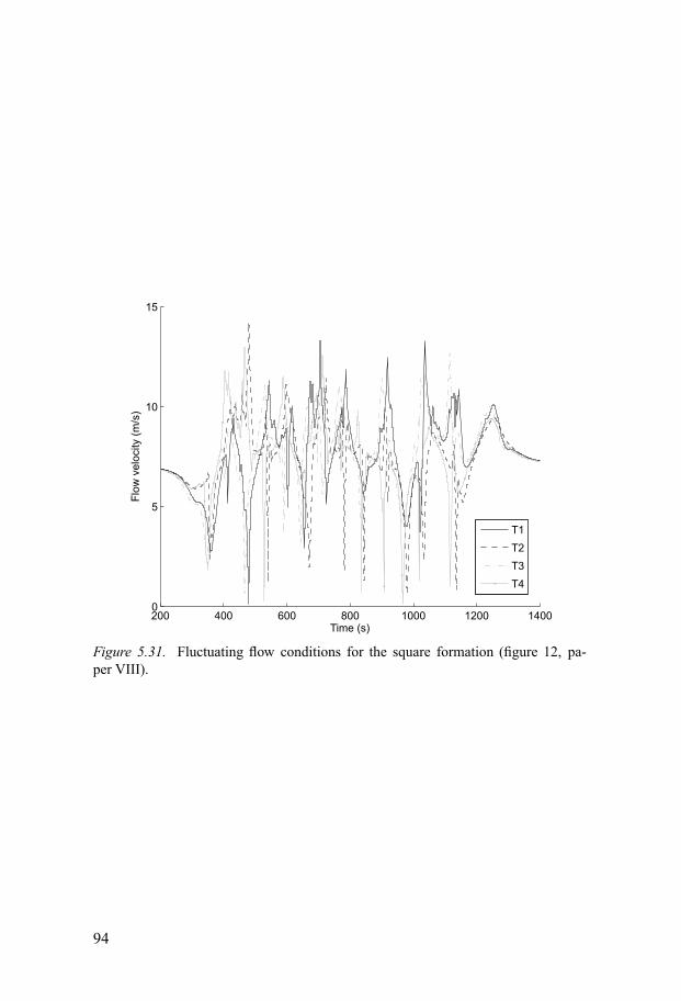
200 400 600 800 1000 1200 14000

5

10

15

Time (s)

Flo

wvelo

city

(m/s

)

T1

T2

T3

T4

Figure 5.31. Fluctuating flow conditions for the square formation (figure 12, pa-per VIII).

94

6. Conclusions

From the work included in this thesis, it can be concluded that:1. It is possible to simulate a turbine with some accuracy. Even though thesimulations do not perfectly match experimental results, the simulationcodes give results that agree reasonably well with experimental values.The simulation tools are therefore useful for designing vertical axis tur-bines. An uncertainty is the accuracy in the experimental data availablefor comparison.

2. If a turbine is designed to handle high flow velocities, the performanceof the turbine may decrease if additional struts are necessary to handlethe large forces.

3. The vertical axis turbine appears to be insensitive to the inflowing ve-locity profile, and in some cases, it is possible that the turbine absorbs alarger fraction of the available energy in the presence of a velocity pro-file. For a horizontally aligned rotational axis, it is preferable to let theblades move opposite to the flow direction at the side where the flowvelocity is highest.

4. If a turbine is located in a channel with constant flow, the power coef-ficient increases with higher blockage ratio. A turbine will also reachits peak performance at a higher tip speed ratio with higher blockage ra-tio. The best turbine design is a function of the blockage ratio, and forhigher blockage ratios, the optimal design is likely to have larger chordsor more blades.

5. If several turbines are located in close proximity in a row configuration,and the flow is perpendicular to the line intersecting the turbine centers,simulations predict an increase in power production from the individualturbines. If more turbines are used, placing all turbines in a row appearsto be better than placing them in a zigzag configuration. For the line con-figuration, a larger spacing is favorable if the variation in flow directionis large.

6. A control system that only measures the rotational velocity of the tur-bine has been shown to be a viable control strategy for vertical axis tur-bines. A cubic relation between extracted power and rotational velocitygives good accuracy in obtaining peak power coefficient for the steadystate case. A reduction of the extracted power at low rotational veloc-ities increases the response time of the control system and is thereforebeneficial for rapid flow variations.

95

7. Connecting all turbines through a mutual DC bus and only controllingthe total extracted power from a turbine farm can be a viable controlstrategy. The differences between this system and a separate control ofeach turbine are smaller in the coupled case than for aerodynamicallyindependent turbines.

8. The speed of the vortex simulations can be increased if graphics pro-cessing units (GPU) are used to evaluate the velocity field. The increasein computational speed is most prominent for large number of vortices.Thus a GPU is well suited for simulations of large turbine farms.

96

7. Suggestions for future work

The simulation codes need better validation. One way would be to performforce measurements on the blades of a turbine, which would give a much moredetailed description of the turbine than measurements of the power coefficient,especially since it is the force that is calculated by the simulation codes.The dynamic stall modeling should be updated to a more accurate model, as

the current model gives too low power coefficients at low tip speed ratios. Thecurrent code uses the Gormont model, while a Beddoes Leishman model [55]probably would be more accurate [3]. This would benefit both the vortex andthe streamtube model, since both models use the same dynamic stall model.The expansion code in the streamtube method could be extended to include

the change in flow direction, similar to the model by Read and Sharpe [47].This could make the streamtube results approach those of the vortex model.The corrections due to tip vortices need to be studied further to determine

model uncertainties. This could either be performed by comparing with three-dimensional simulations of turbines, or by measurements on a turbine withconstant diameter and chord, but with varying blade length.To simulate tip effects, struts, wake structure etc. in more detail, a three-

dimensional vortex code should be developed. Such a model would probablyrequire extensive computational time and may therefore not be suited for de-sign studies, but it could be used to create better correction models for thetwo-dimensional vortex model and the streamtube code.The current models are based on empirical data, thereby limiting the num-

ber of airfoils that can be conveniently modeled. A first principle model basedon Navier-Stokes equations would be more desirable. This requires a full so-lution of the boundary layer which is computationally demanding. Combiningthe vortex model with turbulence models or boundary layer theory could be away to achieve reasonably short computational times.

97

8. Summary of papers

This chapter contains a summary of all papers included in this thesis.

Paper IA parameter study of the influence of struts on the performance of avertical-axis marine current turbineA turbine for a marine current application is studied with focus on the losses

due to the struts. Hydrodynamically, a loss model for the struts is derivedwithin a streamtube model and empirical data is used for the drag coefficientof the struts. Mechanically, FEM simulations are used to calculate the stressesin the blades due to the hydrodynamic forces obtained from the streamtubemodel, and when the stresses are too high, additional struts are added. Twoturbines are studies, one with 3 blades and one with 6 blades. The 6-bladedturbine is predicted to obtain the highest power coefficient, but is also moresensitive to the flow velocity as it needs more struts. It is shown that designingthe turbine for too high flow velocities will give lower power coefficient atlower flow velocities due to the extra struts required. The author has beenresponsible for the theory development, software development and most of thehydrodynamic simulations as well as some FEM simulations and has writtenmore than half of the paper.

Paper IIInfluence of a varying vertical velocity profile on turbine efficiency for avertical axis marine current turbineMeasurements on the velocity profile at three different locations in Swedish

rivers are performed and a streamtube model is used to simulate the perfor-mance of a vertical axis turbine operating in these velocity profiles. The tradi-tional configuration with the axis vertical is compared to the tilted version witha horizontal axis. In this tilted case, both rotational directions are investigated.These three cases are compared against the reference case with homogeneousflow. Simulations show that the vertical axis turbine can obtain higher powercoefficients than the homogeneous case if the energy density is higher in thecenter of the turbine, compared to the mean value. Simulations also show that

98

for the tilted turbine, having the blade moving against the flow at the high ve-locity side of the turbine is beneficial at low tip speed ratios. The author hasbeen responsible for the theory development, software development and mostof the hydrodynamic simulations and writing more than half of the paper.

Paper IIIDesign of an experimental setup for hydro-kinetic energy conversionThe experimental setup that is intended to be located in Dalälven at Söder-

fors is covered in this paper. This begins with a characterization of the locationfor the turbine including measurements of the velocity profile and data for thepredicted flow velocities. It also includes the electrical design of the generatorand how the generator and turbine efficiencies are coupled together. The au-thor has been responsible for simulating and writing the hydrodynamic part inthe article, where a turbine is designed with the streamtube model to operateat the given location including simulations of the power coefficient versus thetip speed ratio, and how the maximum power coefficient is expected to varywith flow velocity.

Paper IVSimulations of a vertical axis turbine in a channelA turbine located in a channel where there are boundaries confining the flow

is studied with a vortex model. The paper is intended to show both the benefitsof having the flow confined and the errors that will be obtained from simula-tion models where confining boundaries are necessary. Flow confinement oc-curs when volume discretization is used. The first part of the paper covers thenumerical aspects of performing channel simulations with the vortex model,including the required number of revolutions required for convergence as afunction of channel width, which increases with increasing width. The secondpart of the paper covers the improvement in performance due to the channel.Here, the simulated power coefficient increases with decreasingwidth. The tipspeed ratio where the peak occurs also increases for a given turbine. The au-thor has written the simulation software, performed all simulations and writtenthe article.

Paper VNumerical simulation of a farm of vertical axis marine current turbinesSeveral turbines located in close proximity to each other are studied with

a vortex model. First, a two turbine system is simulated using all different

99

combinations of rotational directions and with different distances between theturbines. The contribution from the rotational direction is found to be small,and there is a slight increase in performance when the turbines are movedcloser to each other. Second, five turbine systems are studied. One case has allturbines on a row and the other two cases use a zigzag pattern, where the lastcase has larger turbines. With equal size of the turbines, the turbines on the rowperforms slightly better if the flow comes straight forward, while more powercan be extracted with the zigzag pattern when the turbine radius is increased.The row configuration is found to be less sensitive to small misalignments inthe flow direction. The author has written the simulation software, performedall simulations and written the article.

Paper VIInfluence of incoming flow direction on spacing between vertical axis ma-rine current turbines placed in a rowA line of ten turbines is simulated and the focus is on the turbine spacing

and how it affects the power production of the array with respect to differentincoming flow directions. The simulations are performed with a vortex modeland all turbines are simulated with constant rotational velocity independent onflow direction. The article shows how the spacing between the turbines needsto be increased for high power production if the direction of the incoming flowis increased. Finally, an example with measurement data for the velocity in atidal flow is used and the required turbine spacing in this case is found to bequite low. The author has written the simulation software and parts of thearticle.

Paper VIIRobust VAWT control system evaluation by coupled aerodynamic andelectrical simulationThree different control strategies, all based on the rotational velocity of the

turbine as only input parameter, are tested with respect to absorbed powerand response times to changes in flow velocity. The control strategies arealso compared against a reference strategy designed to operate at optimal tipspeed ratio. The strategies are evaluated with an aerodynamic vortex modelcoupled with an electrical model. First, the different strategies are tested for astep change in flow velocity and second, the behavior of the different controlstrategies is studied under sinusoidal variations in wind velocity. The resultsshow that the power absorption for the three tested strategies is close to thereference strategy. It is also shown that there is a trade off between accuracyin obtaining the optimal tip speed ratio and the speed of the control strategy,

100

where the faster strategies perform better for the high frequency oscillations.The author has been responsible for the aerodynamic part of the simulationmodel and has written more than half of the article.

Paper VIIIAerodynamic and electric evaluation of a VAWT farm control systemwithpassive rectifiers and mutual DC-busThe control of a farm of four turbines is simulated using a coupled aero-

dynamic electrical simulation model. The article focuses on the differencebetween controlling all turbines individually with the model described in pa-per VII and connecting all turbines to a mutual DC bus by passive rectifiers.The mutual DC bus limits the control system to set the extracted power forthe entire farm, instead of individually. For aerodynamically independent tur-bines, less power is extracted if the flow velocities differ, but if the turbinesare aerodynamically coupled, the differences are smaller. A line and a squareconfiguration of the farm are tested and for simulations with varying incom-ing flow velocity, the simulations give that if one turbine is in front of another,the mutual DC bus can actually be better than individually optimizing eachturbine. The author has been responsible for the aerodynamic part of the sim-ulation model and has written more than half of the article.

Paper IXAdaptive fast multipole methods on the GPUAn implementation of the adaptive fast multipole method for a GPU using

CUDA is described. The implementation is two-dimensional and uses asym-metric adaptivity. All individual parts of the algorithm have been ported to theGPU and the speedup gained from using a GPU is investigated for all indi-vidual parts of the algorithm. The comparison is made against an optimizedsingle threaded CPU version and the article shows a speedup of around 11when the number of particles is large. The results also show that asymmetricadaptivity performs well on the GPU as the non-uniform particle distributionsobtain a slightly higher speedup than the homogeneous distributions. The au-thor has implemented the GPU version, performed many optimizations for thesingle threaded CPU version and written more than half of the article.

101

9. Errata for papers

• In paper II, figure 4, the turbine diameter should be 6 m (instead of 8 m)• In paper V, equation (7) should read

CP =ΩR∑FT12ρAV 3∞

,

i.e. the radius R should be added and the power coefficient should benormalized against the asymptotic flow velocity

102

10. Acknowledgments

First of all, I would like to thank my supervisor Olov Ågren for his help withwriting the articles, this thesis and for all interesting discussions on many ar-bitrary subjects. I would also like to thank my co-supervisor and head of thisdivisionMats Leijon for givingme the opportunity to work within this interest-ing area of research and also Hans Bernhoff, for his support and for includingme in the wind power group.I would also like to thank Staffan Lundin, with whom I been sharing office

with during most of my time here, for all his help, especially for proof-readingseveral of my articles and for all his help with LATEX.I like to thank Marcus Berg, Staffan Lundin, Mårten Grabbe, Jon Kjellin,

Mikael Bergkvist, Johan Bladh, Katarina Yuen, Emilia Lalander, Linnea Sjök-vist, Fredrik Bülow, and Fredric Ottermo for proof-reading this thesis and allthe feedback you gave me.I would also like to thank the rest of the members of the marine current

group, Karin, Johan, Nicole and also Anders N, for all your help and interest-ing discussionsA special thanks goes also to Jon Kjellin for providing the experimental

results used to compare the simulations with in section 5.1. Also included isthe rest of the wind power group, Senad, Eduard, Stefan, Jon O, Per, Sandraand former member Kristian for all your support and also the former mem-bers Paul, Mathias and David, who made the foundations for the aerodynamicresearch at the division.The rest of the members of the Division of Electricity for being very nice

co-workers.My family and all my friends, thanks for all the support you have given me,

both before, and during my time at the division.Final thanks go to all financiers of this work, especially Uppsala University

for my salary, but also the rest of the financiers: The Swedish Research Coun-cil, The Swedish Energy Agency, Vinnova, Ångpanneföreningen’s Foundationfor Research and Development, The J. Gust. Richert Foundation for TechnicalScientific Research and CF’s Environmental Fund.

103

11. Summary in Swedish

Vid generering av elektricitet från flödande medium, t.ex. vind eller ström-mande vatten, används traditionellt horisontalaxlade propellerliknande turbi-ner. Ett alternativ till dessa är den vertikalaxlade turbinen, som har fördelenatt den är oberoende av flödesriktning, samt att den vertikala axeln möjliggöratt generatorn kan placeras på marken. Aerodynamiskt kännetecknas vertika-laxlade turbiner av att bladen, som rör sig runt i en cirkel, passerar flödet tvågånger per varv. Det medför att varje blad genererar vridmoment två gångerunder varvet. Däremellan finns två punkter där kraften är nästan noll, vilketger pulserande krafter.När aerodynamiken simuleras för de vertikalaxlade turbinerna används ge-

nerellt sett tre olika metoder, nämligen strömrörsmodeller, virvelmodeller ochfinita element-/volyms-metoden där endast de två förstnämnda har används idenna avhandling. Av dessa är strömrörsmodellen den snabbaste då den inteinnehåller något tidsberoende flöde samt att hela hastighetsfältet runt turbi-nen inte beräknas, utan endast approximeras vid turbinbladen. I denna snab-ba modell kan turbineproblemet lösas tredimensionellt. Det möjliggör studierav varierande hastighet över turbinarean och inkluderande av bärarmar, vilketmodellen har används till i denna avhandling.I fallet med varierande flödeshastighet undersöktes hur turbinens effekti-

vitet påverkas av att flödeshastigheten inte är konstant över turbinarean. Enmer realistisk fördelning med lägre hastighet närmare botten användes. Enligtsimuleringarna ska den vertikalaxlade turbinen fungera bra när flödeshastig-hetens variation har tagits som de uppmätta värdena från två svenska älvar.Simuleringarna visar också att om flödeshastigheten varierar vinkelrätt medturbinens rotationsaxel (vilket är fallet för liggande turbin) så bör turbinen blieffektivare om bladen rör sig motströms där hastigheten är som högst.För en strömkraftsturbin studerades hur många bärarmar som är nödvändi-

ga för att turbinen ska hålla vid olika flödeshastigheter. Detta kopplades sedantill de hydrodynamiska förlusterna som bärarmarna ger upphov till. Från des-sa resultat kan man se hur turbinens effektivitet sjunker när fler bärarmar ärnödvändiga. Detta leder till att om en turbin designas för att hålla för relativthöga flödeshastigheter tappas effektivitet vid de lägre hastigheterna. I sådanafall kan det vara bättre att konstruera turbinen för en lägre flödeshastighet ochstänga av den i de fåtal fall då flödeshastigheten är allt för hög.Strömrörsmodellen har begränsningar, t.ex. hur flödet modelleras, och fun-

gerar inte för alla problem. En mer avancerad metod är virvelmetoden somlöser hela flödesfältet tidsberoende, vilket ger en mer fullständig beskrivning

104

av turbinen. Virvelmetoderna är mer tidskrävande än strömrörsmodellen, ochendast tvådimensionella simuleringar har genomförts i denna avhandling.Med virvelmetoden har det studerats vilka effekter som uppkommer när

flödet kring en turbin innesluts av kanalväggar, vilket är fallet för t.ex. flo-der. Studien börjar med att undersöka hur snabbt simuleringarna konvergeraroch resultatet är att man behöver simulera ett större antal turbinvarv för bre-da kanaler innan konvergens uppnås. Sen studerades turbinen prestanda ochför kanaler ökar den erhållna effekten från turbinen när kanalens bredd mins-kar. Detta stämmer med strömrörsteori som förutspår en effektökning, men isimuleringarna ökar effekten inte lika snabbt som teorin förutspår. Samtidigtkan noteras att turbinen erhåller maximal effekt vid högre löptal när kanalensbredd minskar.Virvelmetoden har även använts för att studera hur flera turbiner växelver-

kar med varandra. Enligt simuleringarna kan man erhålla högre effekt hos en-skilda turbiner om de placeras nära varandra och flödet kommer rakt framifrån(vinkelrätt mot linjen som skär turbinernas centrum). En studie genomfördespå fem turbiner, där placering i rad eller i sicksackmönster jämfördes. När flö-det kom rakt framifrån gav radgeometrin aningen bättre prestanda. Däremotvar rad-geometrin väsentligt bättre vid 30 graders infallsvinkel. Utifrån dessasimuleringar kan slutsatsen dras att rad-geometrin är bättre om turbinerna är li-ka stora. Däremot finns utrymme för flera turbiner i ett sicksackmönster, vilketkan vara en fördel om tillgänglig yta för turbinplacering är begränsad. Utifråndessa resultat undersöktes rad-geometrin extra för en rad av 10 turbiner ochhur vinkeln på flödet relativt linjens riktning påverkar prestandan. Resultatetblev att avståndet mellan turbinerna i raden behöver ökas ifall vinkeln på flödetkan bli stor.Virvelmetoden kombinerades även med en elektrisk modell och denna

kopplade simuleringsmodell användes för att studera kontrollstrategier för hurman ska styra en turbin. Tre olika strategier, som alla endast använde rotations-hastigheten som indata och styrde genom att reglera uttagen effekt, undersök-tes och dessa strategier lyckades styra turbinen väl i avseendet att erhålla enhög elektrisk effekt från systemet. Resultatet blev även att de strategier somtog ut lite lägre effekt vid låga varvtal snabbare ställde in sig på angivet varvtaloch dessa kunde därmed bli fördelaktiga vid snabba förändringar i flödeshas-tigheten.Simuleringarna av kontrollsystem utökades sedan till att involvera en park

av 4 turbiner. Här studerades skillnaden mellan att styra varje turbin enskiltenligt ovanstående modell, och att med passiva likriktare koppla ihop elsyste-men via en gemensam DC-buss, vilket gör att man endast kan styra den totalaeffekten från hela parken. För aerodynamiskt åtskilda turbiner var det bättreatt styra varje turbin enskilt om det var stora variationer i hastighet mellanturbinerna. Om hastighetsvariationerna istället orsakades av att vissa turbinervar placerade bakom andra, som då redan absorberat större delen av energin,så blev skillnaderna mellan de olika systemen mindre. Detta visar att använ-

105

dandet av en en gemensam DC-buss kan vara ett alternativ, särskilt då detreducerar antalet elektriska komponenter.En studie genomfördes även på om man kan använda grafikkort för att

öka hastigheten vid beräkningen av flödeshastigheten för virvlarna, då dettaär den mest tidskrävande delen av virvelmetoden. I studien implementeradeshela snabba multipolmetoden (FMM) för grafikkortet och beräkningstidernajämfördes med en seriell implementation på en vanlig processor. Resultatetvisar att hastighetsökningen när man använder grafikkort är störst för ett stortantal virvlar. Därför är denna metod lämplig för tunga beräkningar, som t.ex.simulering av en stor park.

106

References

[1] J. F. Manwell, J. G. McGowan, and A. L. Rogers. Wind Energy Explained:Theory, Design and Application. John Wiley & Sons, 2009.

[2] S. J. Savonius. Rotor adapted to be driven by wind or flowing water. U.S. PatentNo. 1,697,574, January 1929.

[3] I. Paraschivoiu. Wind turbine design with emphasis on Darrieus concept.Polytechnic International Press, 2002.

[4] G. J. M. Darrieus. Turbine having its rotating shaft transverse to the flow of thecurrent. U.S. patent No. 1,835,018, December 1931.

[5] P. Gipe. Wind Energy Basics: A Guide to Home- And Community-Scale WindEnergy Systems. Chelsea Green Publishing Company, 2009.

[6] S. Eriksson, H. Bernhoff, and M. Leijon. Evaluation of different turbineconcepts for wind power. Renewable & Sustainable Energy Reviews,12(5):1419–1434, June 2008.

[7] F. M. White. Fluid Mechanics. McGraw-Hill Series in MechanicalEngineering. McGraw-Hill, 2008.

[8] G. Kuiper. Cavitation research and ship propeller design. Applied ScientificResearch, 58:33–50, 1997. 10.1023/A:1000754928962.

[9] M. Shiono, K. Suzuki, and S. Kiho. Output characteristics of Darrieus waterturbine with helical blades for tidal current generations. In Proceedings of theTwelfth (2002) International Offshore and Polar Engineering Conference,Kitatkyushu, Japan, May 2002.

[10] T. Maître, J.-L. Achard, L. Guittet, and C. Ploesteanu. Marine turbinedevelopment: numerical and experimental investigations. Scientific Bulletin ofthe Polytechnic University of Timisoara: Transactions on Mechanics,50(64):59–66, 2005.

[11] D. P. Coiro, A. De Marco, F. Nicolosi, S. Melone, and F. Montella. Dynamicbehaviour of the patented Kobold tidal turbine: numerical and experimentalaspects. Acta Polytechnica, 45(3):77–84, 2005.

[12] B. Kirke and L. Lazauskas. Variable pitch Darrieus water turbines. Journal ofFluid Science and Technology, 3(3):430–438, 2008.

[13] C. T. Crowe, D. F. Elger, J. A. Roberson, and B. C. Williams. EngineeringFluid Mechanics, 9th Edition Binder Ready. John Wiley & Sons, 2008.

[14] A. Solum, P. Deglaire, S. Eriksson, M. Stålberg, M. Leijon, and H. Bernhoff.Design of a 12kW vertical axis wind turbine equipped with a direct driven PMsynchronous generator. In Proceedings of EWEC 2006, European Wind EnergyConference & Exhibition, 2006.

[15] P. Deglaire, S. Eriksson, J. Kjellin, and H. Bernhoff. Experimental results froma 12 kW vertical axis wind turbine with a direct driven PM synchronousgenerator. In Proceedings of EWEC 2007, European Wind Energy Conference& Exhibition, Milan, Italy, 2007.

107

[16] J. Kjellin, F. Bülow, S. Eriksson, P. Deglaire, M. Leijon, and H. Bernhoff.Power coefficient measurement on a 12 kW straight bladed vertical axis windturbine. Renewable Energy, 36(11):3050 – 3053, 2011.

[17] F. Bülow, J. Kjellin, S. Eriksson, M. Bergkvist, P. Ström, and H. Bernhoff.Adapting a VAWT with PM generator to telecom applications. In Proceedingsof the European Wind Energy Conference & Exhibition 2010, April 2010.

[18] S. Eriksson, H. Bernhoff, and M. Leijon. A 225 kW direct driven PM generatoradapted to a vertical axis wind turbine. Advances in Power Electronics, 2011,2011. Article ID 239061.

[19] P. Deglaire, O. Ågren, H. Bernhoff, and M. Leijon. Conformal mapping andefficient boundary element method without boundary elements for fast vortexparticle simulations. European Journal of Mechanics, B/Fluids, 27(2):150–176,April 2008.

[20] P. Deglaire, S. Engblom, O. Ågren, and H. Bernhoff. Analytical solutions for asingle blade in vertical axis turbine motion in two-dimensions. EuropeanJournal of Mechanics, B/Fluids, 28:506–520, 2009.

[21] P. Deglaire. Analytical Aerodynamic Simulation Tools for Vertical Axis WindTurbines. PhD thesis, Uppsala University, Electricity, 2010.

[22] D. Österberg. Multi-body unsteady aerodynamics in 2D applied to avertical-axis wind turbine using a vortex method. Master’s thesis, UppsalaUniversity, 2010.

[23] S. Engblom. On well-separated sets and fast multipole methods. AppliedNumerical Mathematics, 61(10):1096 – 1102, October 2011.

[24] A. Betz. Das maximum der theoretisch möglichen ausnutzung des windes durchwindmotoren. Zeitschrift für das gesamte Turbinenwesen, September 1920.

[25] C. Garrett and P. Cummins. The efficiency of a turbine in a tidal channel.Journal of Fluid Mechanics, 588:243–251, October 2007.

[26] J. I. Whelan, J. M. R. Graham, and J. Peiró. A free-surface and blockagecorrection for tidal turbines. Journal of Fluid Mechanics, 624:281–291, 2009.

[27] I. H. Abbott and A. E. V. Doenhoff. Theory of wing sections: including asummary of airfoil data. Dover books on physics and chemistry. DoverPublications, 1959.

[28] J. H. Laks, L. Y. Pao, and A. D. Wright. Control of wind turbines: Past, present,and future. In American Control Conference, 2009. ACC ’09., pages 2096–2103, June 2009.

[29] L. Lazauskas. Three pitch control systems for vertical axis wind turbinescompared. Wind Engineering, 16(5):269–282, 1992.

[30] B. K. Kirke and L. Lazauskas. Limitations of fixed pitch Darrieus hydrokineticturbines and the challenge of variable pitch. Renewable Energy, 36:893–897,2011.

[31] E. A. Bossanyi. The design of closed loop controllers for wind turbines. WindEnergy, 3(3):149–163, 2000.

[32] M. Dahlgren, H. Frank, M. Leijon, F. Owman, and L. Walfridsson.WindformerTM. Wind power goes large-scale. ABB Review, pages 31–37, 2000.

[33] S. Lundberg. Performance comparison of wind park configurations. Technicalreport, Chalmers University of Technology, 2003. Technical Report No. 30R.

[34] D. Jovcic and N. Strachan. Offshore wind farm with centralised power

108

conversion and DC interconnection. Generation, Transmission Distribution,IET, 3(6):586 –595, June 2009.

[35] M. Parker and O. Anaya-Lara. An evaluation of collection network designswhich eliminate the turbine converter. In EWEA 2012 Scientific Proceedings,pages 32–36, April 2012. OMAE2012-83347.

[36] A. Kusiak and Z. Song. Design of wind farm layout for maximum wind energycapture. Renewable Energy, 35(3):685 – 694, 2010.

[37] A. Crespo, J. Hernández, and S. Frandsen. Survey of modelling methods forwind turbine wakes and wind farms. Wind Energy, 2(1):1–24, 1999.

[38] M. Soleimanzadeh and R. Wisniewski. Controller design for a wind farm,considering both power and load aspects. Mechatronics, 21(4):720 – 727, 2011.

[39] J. Shu, B. H. Zhang, and Z. Q. Bo. A wind farm coordinated controller forpower optimization. In Power and Energy Society General Meeting, 2011 IEEE,pages 1 –8, july 2011.

[40] T. Knudsen, T. Bak, and M. Soltani. Prediction models for wind speed atturbine locations in a wind farm. Wind Energy, 14(7):877–894, 2011.

[41] R. Howell, N. Quin, J. Edwards, and N. Durrani. Wind tunnel and numericalstudy of a small vertical axis wind turbine. Renewable Energy, 35(2):412–422,February 2010.

[42] O. Guerri, A. Sakout, and K. Bouhadef. Simulations of the fluid flow around arotating vertical axis wind turbine. Wind Engineering, 31(3):149–163,May2007.

[43] R. Templin. Aerodynamic performance theory for the NRC vertical-axis windturbine. Technical report, National Research Council of Canada, 1974.Laboratory technical report – LTR-LA-160.

[44] E. E. Lapin. Theoretical performance of vertical axis wind turbines. November1975. ASME Paper 75-WA/ENER-1.

[45] J. H. Strickland. The Darrieus turbine: A performance prediction model usingmultiple streamtubes. Technical Report SAND75-0431, Sandia NationalLaboratories, Albuquerque, New Mexico, October 1975.

[46] I. Paraschivoiu. Double-multiple streamtube model for Darrieus wind turbines.In Second DOE/NASA wind turbines dynamics workshop, pages 19–25,Cleveland, OH, February 1981. NASA CP-2186.

[47] S. Read and D. J. Sharpe. An extended multiple streamtube theory for verticalaxis wind turbines. 2nd BWEA workshop, Cranfield, UK, pages 65–72, April1980.

[48] D. J. Sharpe. Refinements and developments of the multiple streamtube theoryfor the aerodynamic performance of vertical axis wind turbines. In Proceedingsof the BWEA Wind Energy Conference, pages 146–159, 1984.

[49] W. A. Moran. Giromill wind tunnel test and analysis. Volume 2. Technicaldiscussion. Technical Report C00/2617-4/2, U.S. Energy Research andDevelopment Administration, October 1977.

[50] R. E. Sheldahl and P. C. Klimas. Aerodynamic characteristics of sevensymmetrical airfoil sections through 180-degree angle of attack for use inaerodynamic analysis of vertical axis wind turbines. Technical ReportSAND80-2114, Sandia National Laboratories, Albuquerque, New Mexico,March 1981.

109

[51] R. E. Gormont. A mathematical model of unsteady aerodynamics and radialflow for application to helicopter rotors. Technical report, USAAV Labs., May1973. TR 72-67.

[52] B. Massé. Description de deux programmes d’ordinateur pour le calcul desperformances et des charges aerodynamiques pour des eoliennes a’axe vertical.Report IREQ 2379, Institut de Recherche de L’Hydro–Quebec, Varennes,Quebec, July 1981.

[53] D. E. Berg. Improved double-multiple streamtube model for the Darrieus-typevertical axis wind turbine. In Presented at the Am. Solar Energy Soc. Meeting,Minneapolis, 1 Jun. 1983, volume 1, pages 231–238, June 1983.

[54] J. G. Leishman and T. S. Beddoes. A generalised model for airfoil unsteadyaerodynamic behaviour and dynamic stall using the indical method. InProceedings from the 42nd Annual Forum of the American Helicopter Society,pages 243–266, 1986.

[55] J. G. Leishman and T. S. Beddoes. A semi-empirical model for dynamic stall. J.Am. Helicopter Society, 34(3), July 1989.

[56] I. Paraschivoiu, P. Fraunié, and C. Béguier. Streamtube expansion effects on theDarrieus wind turbine. Journal of Propulsion and Power, 1:150–155,March-April 1985.

[57] G. H. Cottet and P. D. Koumoutsakos. Vortex Methods: Theory and Practice.Cambridge University Press, 2008.

[58] A. J. Chorin. Numerical study of slightly viscous flow. J. Fluid. Mech,57:785–796, 1973.

[59] S. Shankar and L. van Dommelen. A new diffusion procedure for vortexmethods. J. Comput. Phys., 127:88–109, August 1996.

[60] J. H. Strickland, B. T. Webster, and T. Nguyen. A vortex model of the Darrieusturbine: An analytical and experimental study. Journal of Fluids Engineering,101:500–505, December 1979.

[61] P. Ramachandran, S. C. Rajan, and M. Ramakrishna. A fast, two-dimensionalpanel method. SIAM Journal on Scientific Computing, 24(6):1864–1878, 2003.

[62] L. Greengard. Potential flow in channels. SIAM Journal on Scientific andStatistical Computing, 11(4):603–620, July 1990.

[63] L. Greengard and V. Rokhlin. A fast algorithm for particle simulations. Journalof Computational Physics, 73:325–348, December 1987.

[64] T. Hrycak and V. Rokhlin. An improved fast multipole algorithm for potentialfields. SIAM Journal on Scientific Computing, 19(6):1804–1826, 1998.

[65] R. Farber. CUDA Application Design and Development. Morgan KaufmannPublishers Inc., San Francisco, CA, USA, 1st edition, 2011.

[66] S. K. Raman, V. Pentkovski, and J. Keshava. Implementing streaming SIMDextensions on the pentium III processor. Micro, IEEE, 20(4):47 –57, jul/aug2000.

[67] J. Sanders and E. Kandrot. CUDA by Example: An Introduction toGeneral-Purpose GPU Programming. Addison-Wesley Professional, 1stedition, 2010.

[68] M. Drela. XFOIL: an analysis and design system for low Reynolds numberairfoils. In Conference on low Reynolds number Aerodynamics. University ofNotre Dame, 1989.

110

[69] G. F. Homicz. Numerical simulation of VAWT stochastic aerodynamic loadsproduced by atmospheric turbulence: VAWT-SAL code. Technical ReportSAND91-1124 UC-261, Sandia National Laboratories, Albuquerque, NewMexico, September 1991.

[70] I. Paraschivoiu. Aerodynamic models and experiments for studying Darrieuswind turbines. In Proceedings of the EWEC, pages 617–622, Herning,Denmark, 1988.

111

Acta Universitatis UpsaliensisDigital Comprehensive Summaries of Uppsala Dissertationsfrom the Faculty of Science and Technology 998

Editor: The Dean of the Faculty of Science and Technology

A doctoral dissertation from the Faculty of Science andTechnology, Uppsala University, is usually a summary of anumber of papers. A few copies of the complete dissertationare kept at major Swedish research libraries, while thesummary alone is distributed internationally throughthe series Digital Comprehensive Summaries of UppsalaDissertations from the Faculty of Science and Technology.

Distribution: publications.uu.seurn:nbn:se:uu:diva-183794

ACTAUNIVERSITATIS

UPSALIENSISUPPSALA

2012