Fluid Dynamics Lab Manual
47
1 EXPERIMENT No.1 FLOW MEASUREMENT BY ORIFICEMETER 1.1 AIM: To determine the co-efficient of discharge of the orifice meter 1.2 APPARATUS REQUIRED: Orifice meter test rig, Stopwatch 1.3 PREPARATION 1.3.1 THEORY An orifice plate is a device used for measuring the volumetric flow rate. It uses the same principle as a Venturi nozzle, namely Bernoulli's principle which states that there is a relationship between the pressure of the fluid and the velocity of the fluid. When the velocity increases, the pressure decreases and vice versa. An orifice plate is a thin plate with a hole in the middle. It is usually placed in a pipe in which fluid flows. When the fluid reaches the orifice plate, with the hole in the middle, the fluid is forced to converge to go through the small hole; the point of maximum convergence actually occurs shortly downstream of the physical orifice, at the so-called vena contracta point. As it does so, the velocity and the pressure changes. Beyond the vena contracta, the fluid expands and the velocity and pressure change once again. By measuring the difference in fluid pressure between the normal pipe section and at the vena contracta, the volumetric and mass flow rates can be obtained from Bernoulli's equation. Orifice plates are most commonly used for continuous measurement of fluid flow in pipes. Fig.1. Orifice Plate 1.3.2 PRE-LAB QUESTIONS 1. Write continuity equation for incompressible flow? Mass flow rate = Density x Flow Area x Velocity of flow ……… kg/s 2. What is meant by flow rate? Volume flow rate, Q = A V …………. m 3 /s 3. What is the use of orifice meter?
-
Upload
parthiban-parasuraman -
Category
Documents
-
view
58 -
download
4
description
In detailed description of fluid dynamics lab calculations
Transcript of Fluid Dynamics Lab Manual

1
EXPERIMENT No.1
FLOW MEASUREMENT BY ORIFICEMETER
1.1 AIM: To determine the co-efficient of discharge of the orifice meter
1.2 APPARATUS REQUIRED: Orifice meter test rig, Stopwatch
1.3 PREPARATION
1.3.1 THEORY
An orifice plate is a device used for measuring the volumetric flow rate. It uses the
same principle as a Venturi nozzle, namely Bernoulli's principle which states that there is a
relationship between the pressure of the fluid and the velocity of the fluid. When the velocity
increases, the pressure decreases and vice versa. An orifice plate is a thin plate with a hole in
the middle. It is usually placed in a pipe in which fluid flows. When the fluid reaches the
orifice plate, with the hole in the middle, the fluid is forced to converge to go through the small
hole; the point of maximum convergence actually occurs shortly downstream of the physical
orifice, at the so-called vena contracta point. As it does so, the velocity and the pressure
changes. Beyond the vena contracta, the fluid expands and the velocity and pressure change
once again. By measuring the difference in fluid pressure between the normal pipe section and
at the vena contracta, the volumetric and mass flow rates can be obtained from Bernoulli's
equation. Orifice plates are most commonly used for continuous measurement of fluid flow in
pipes.
Fig.1. Orifice Plate
1.3.2 PRE-LAB QUESTIONS
1. Write continuity equation for incompressible flow?
Mass flow rate = Density x Flow Area x Velocity of flow ……… kg/s
2. What is meant by flow rate?
Volume flow rate, Q = A V …………. m3/s
3. What is the use of orifice meter?

2
To measure the co-efficient of discharge and flow rate
4. What is the energy equation used in orifice meter?
Bernoulli‘s equation. Z1 + P1/ g +V12/2g= Z2 + P2/ g +V2
2/2g (Or)
1.4 PROCEDURE
N.B.: Avoid complete closing of supply valve (nearer to pump) or delivery valve
(nearer to collecting tank)
1. Switch on the power supply to the pump
2. Adjust the delivery flow control valve and note down manometer heads (h1, h2) and
time taken for collecting 10 cm rise of water in collecting tank (t). (i.e. Initially the
delivery side flow control valve to be kept fully open and then gradually closing.)
3. Repeat it for different flow rates.
4. Switch off the pump after completely opening the delivery valve.
1.5 OBSERVATIONS
1.5.1 FORMULAE / CALCULATIONS
The actual rate of flow, Qa = A x h / t (m3/sec)
Where A = Area of the collecting tank = lengh x breadth (m2
)
h = Height of water(10 cm) in collecting tank ( m),
t = Time taken for 10 cm rise of water (sec)
Qa = 0.009 / t ………… after using l, b and h.
The Theoretical discharge through orifice meter,
Qt = (a1 a2 2g H ) / (a12 – a2
2 ) m
3/sec
Where, H = Differential head of manometer in m of water = 12.6 x hm x 10 -2
(m)
g = Acceleration due to gravity (9.81m/sec2)
Inlet Area of orifice meter in m2 , a1 = d1
2/ 4 ,
Area of the throat or orifice in m2
, a2 = d22/ 4
Qt = 14.85 x 10⁻⁴
H …….. after using a1, a2 and g values.

3
The co-efficient of discharge, Cd = Actual discharge / Theoretical discharge = Qa/Qt
1.5.2 TABULATION
Size of Orificemeter : Inlet Dia. d1 = 25 mm , Orifice dia d2 = 18.77 mm,
Measuring area in collecting tank A = 0.3 x 0.3 m2
Sl.
No.
Manometer Reading
(cm)
Manomet
er Head
H
Time for
10 cm rise
t
Actual
Discharge
Qa
Theoretical
Discharge
Qt
Co-eff. of
discharge
Cd
h1 h2 hm =
h1 - h2
m sec m3/sec m
3/sec
1. 23 17.5 5.5 0.693 7.6 0.0012 0.0013 0.92
2. 25 15.5 9.5 1.19 8.9 0.0013 0.0016 0.81
3. 26.5 14 12.5 1.5 9.0 0.0015 0.0018 0.83
4. 27.5 13 14.5 1.82 9.2 0.0016 0.0020 0.80
5.
Average Cd value 0.84
1.5.3 GRAPH:
Qa Vs Qt .
Find Cd value from the graph and compare it with calculated Cd
1.6 POST-LAB QUESTIONS
1. How do you find actual discharge?
By calculating the time taken for the volume of water coming to the collecting tank
with the help of formula, Qa = A x h / t
2. How do you find theoretical discharge?
Based on the pressure head difference and the area of pipe and orifice.
3. What do you meant by co-efficient of discharge?
It is the ratio of actual discharge to theoretical discharge.
1.7 INFERENCES

4
Fig. 1. Orifice meter (Qa Vs Qt)
1.8 RESULT
The co-efficient of discharge of orifice meter = 0.84….…. From Calculation
The co-efficient of discharge of orifice meter = 0.60……. From Graph
5
2. FLOW MEASUREMENT BY VENTURIMETER
1.1 AIM: To determine the co-efficient of discharge of the venturimeter
1.2 APPARATUS REQUIRED: Venturimeter test rig, Stopwatch
1.3 PREPARATION
1.3.1 THEORY
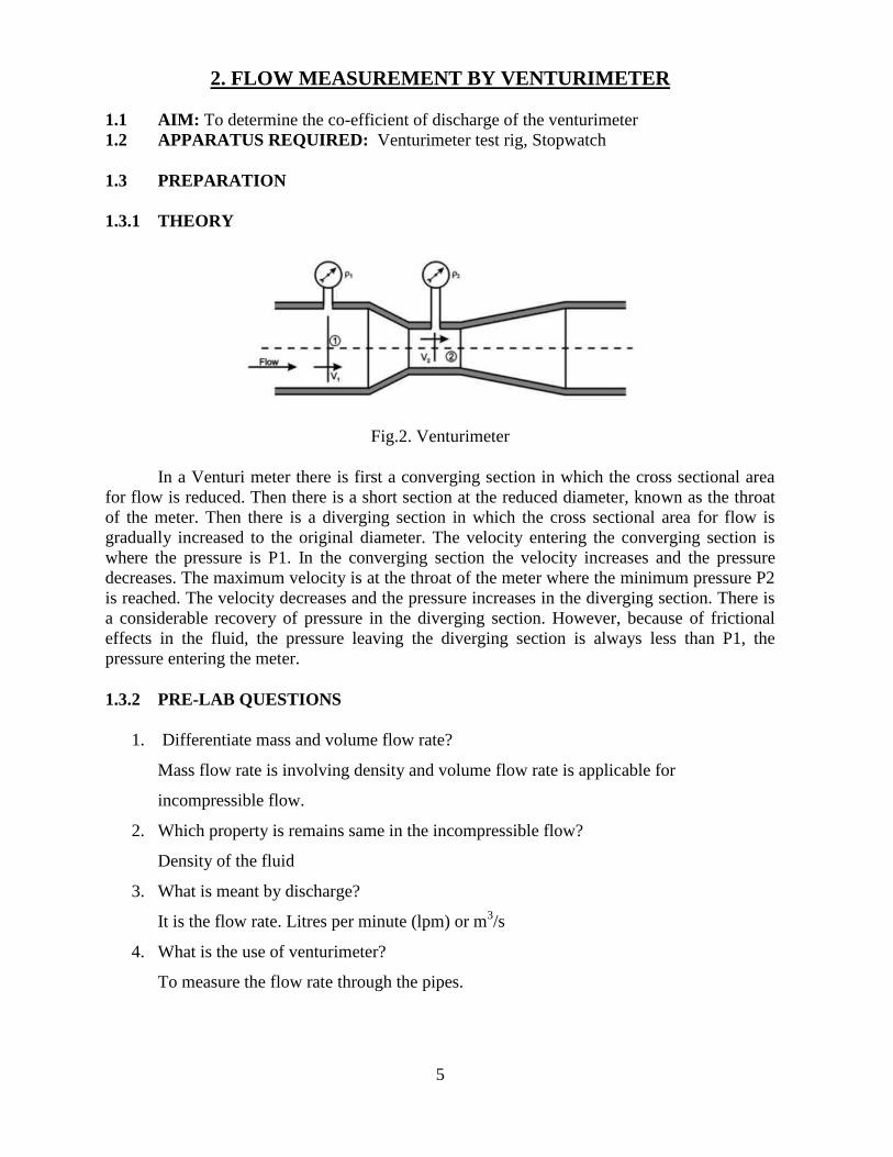
Fig.2. Venturimeter
In a Venturi meter there is first a converging section in which the cross sectional area
for flow is reduced. Then there is a short section at the reduced diameter, known as the throat
of the meter. Then there is a diverging section in which the cross sectional area for flow is
gradually increased to the original diameter. The velocity entering the converging section is
where the pressure is P1. In the converging section the velocity increases and the pressure
decreases. The maximum velocity is at the throat of the meter where the minimum pressure P2
is reached. The velocity decreases and the pressure increases in the diverging section. There is
a considerable recovery of pressure in the diverging section. However, because of frictional
effects in the fluid, the pressure leaving the diverging section is always less than P1, the
pressure entering the meter.
1.3.2 PRE-LAB QUESTIONS
1. Differentiate mass and volume flow rate?
Mass flow rate is involving density and volume flow rate is applicable for
incompressible flow.
2. Which property is remains same in the incompressible flow?
Density of the fluid
3. What is meant by discharge?
It is the flow rate. Litres per minute (lpm) or m3/s
4. What is the use of venturimeter?
To measure the flow rate through the pipes.

6
1.4 PROCEDURE:
N.B.: Avoid complete closing of supply valve (nearer to pump) or delivery valve
(nearer to collecting tank).
1. Switch on the power supply to the pump
2. Check any air bubbles inside the manometer tubes connected to the venturimeter.
(If air bubbles present means, open the top levers (cocks) of the manometer
Simultaneously and adjust the delivery valve in order to release the air. After the air
released, close the top levers simultaneously)
3. Adjust the delivery flow control valve and note down manometer heads (h1, h2) and
time taken for collecting 10 cm rise of water in collecting tank (t). (i.e. Initially the
delivery side flow control valve to be kept fully open and then gradually closing.)
4. Repeat it for different flow rates.
5. Switch off the pump after completely opening the delivery valve.
1.5 OBSERVATIONS
1.5.1 FORMULAE / CALCULATIONS
The actual rate of flow rate Qa = A x h (m3/sec)
t
Where A = Area of the collecting tank = lengh x breadth (m2
)
h = Height of water(10 cm) in collecting tank ( m),
t = Time taken for 10 cm rise of water (sec)
Qa = 0.009 / t ………… after using l, b and h.
The Theoretical flow rate or discharge through a venturimeter,
Qt = (a1 a2 2g H ) / (a12 – a2
2 ) m
3/sec
Where, H = Differential head of manometer in m of water = 12.6 x hm x 10 -2
(m)
g = Acceleration due to gravity (9.81m/sec2)
Inlet Area of Venture meter in m2 , a1 = d1
2/ 4 ,
Area of the throat in m2
, a2 = d22/ 4
Qt = 14.88 x 10⁻⁴
H …….. after using a1, a2 and g values.
The co-efficient of discharge, Cd = Actual discharge / Theoretical discharge = Qa/Qt
7
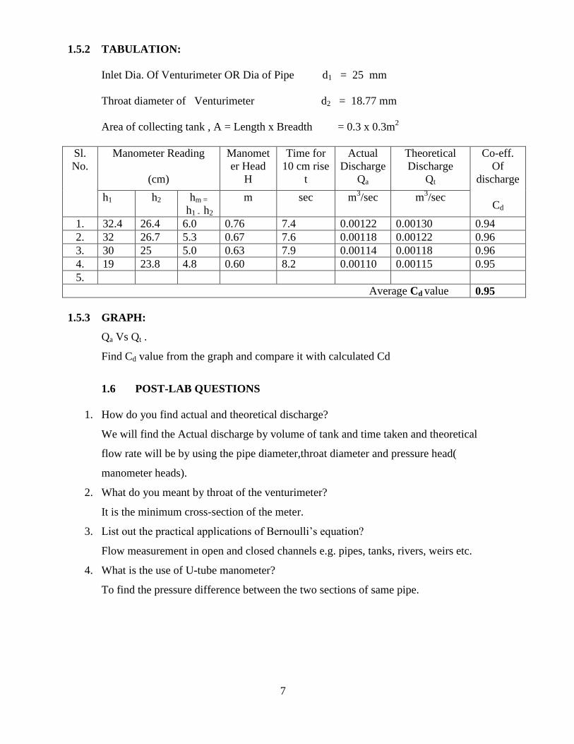
1.5.2 TABULATION:
Inlet Dia. Of Venturimeter OR Dia of Pipe d1 = 25 mm
Throat diameter of Venturimeter d2 = 18.77 mm
Area of collecting tank , A = Length x Breadth = 0.3 x 0.3m2
Sl.
No.
Manometer Reading
(cm)
Manomet
er Head
H
Time for
10 cm rise
t
Actual
Discharge
Qa
Theoretical
Discharge
Qt
Co-eff.
Of
discharge
Cd h1 h2 hm =
h1 - h2
m sec m3/sec m
3/sec
1. 32.4 26.4 6.0 0.76 7.4 0.00122 0.00130 0.94
2. 32 26.7 5.3 0.67 7.6 0.00118 0.00122 0.96
3. 30 25 5.0 0.63 7.9 0.00114 0.00118 0.96
4. 19 23.8 4.8 0.60 8.2 0.00110 0.00115 0.95
5.
Average Cd value 0.95
1.5.3 GRAPH:
Qa Vs Qt .
Find Cd value from the graph and compare it with calculated Cd
1.6 POST-LAB QUESTIONS
1. How do you find actual and theoretical discharge?
We will find the Actual discharge by volume of tank and time taken and theoretical
flow rate will be by using the pipe diameter,throat diameter and pressure head(
manometer heads).
2. What do you meant by throat of the venturimeter?
It is the minimum cross-section of the meter.
3. List out the practical applications of Bernoulli‘s equation?
Flow measurement in open and closed channels e.g. pipes, tanks, rivers, weirs etc.
4. What is the use of U-tube manometer?
To find the pressure difference between the two sections of same pipe.
8
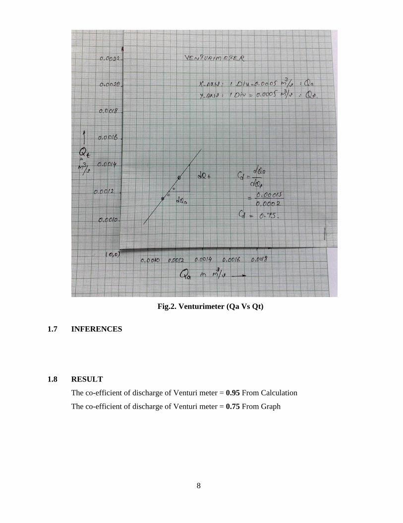
Fig.2. Venturimeter (Qa Vs Qt)
1.7 INFERENCES
1.8 RESULT
The co-efficient of discharge of Venturi meter = 0.95 From Calculation
The co-efficient of discharge of Venturi meter = 0.75 From Graph

9
3.VERIFICATION OF BERNOULLIS THEOREM
1.1 AIM: To verify the Bernoulli‘s theorem
1.2 APPARATUS REQUIRED: Bernoulli‘s Theorem test set-up, Stopwatch
1.3 PREPARATION
1.3.1 THEORY
Bernoulli’s Theorem
According to Bernoulli‘s Theorem, in a continuous fluid flow, the total head at any
point along the flow is the same. Z1 + P1/ g +V12/2g= Z2 + P2/ g +V2
2/2g , Since Z1 –Z2 = 0
for Horizontal flow, h1 +V12/2g= h2 +V2
2/2g ( Pr. Head, h = P1/ g ). Z is ignored for adding
in both sides of the equations due to same datum for all the positions. Bernoulli‘s equation is
based on Euler‘s equation of motion. It is applicable to flow of fluid through pipe and channel.
In Euler‘s equation the force of viscosity is neglected. Bernoulli‘s equation is required to be
modified if the flow is compressible and unsteady.
Apparatus
The apparatus is fitted with piezometer tubes and scales at 8 cross sectional points,
along the experimental duct at suitable intervals for measurement of pressure head. The area of
flow section (a) is written on each one of these 8 sections. The velocity of flow (V) can be
calculated at each of these sections from the flow rate(Q) obtained from the measuring tank
that is V = Q/a from this velocity head V2/2g can be calculated for each section.
For the verification of Bernoulli‘s theorem, the velocity head when superposed over the
hydraulic gradient gives the energy gradient must be a level line. However, in the flow of need
fluid, contain losses of energy is inevitable and this can be readily seen by plating energy
gradient.
1.3.2 PRE-LAB QUESTIONS
1. State Bernoulli‘s theorem?
Z1 + P1/ g +V12/2g= Z2 + P2/ g +V2
2/2g
2. What is continuity equation?
It is mass balance equation. M = ρ A V = ρ Q
3. What do you meant by potential head?
The head of energy due to position (height) from a reference level
1.4 PROCEDURE
1. Switch on the pump
2. Fix a steady flow rate by operating the appropriate supply and drain valves.
3. Note down the pressure heads (h1 – h8)
4. Note down the time taken for 10 cm rise of water in measuring (collecting) tank.
5. Switch off the power supply.
10
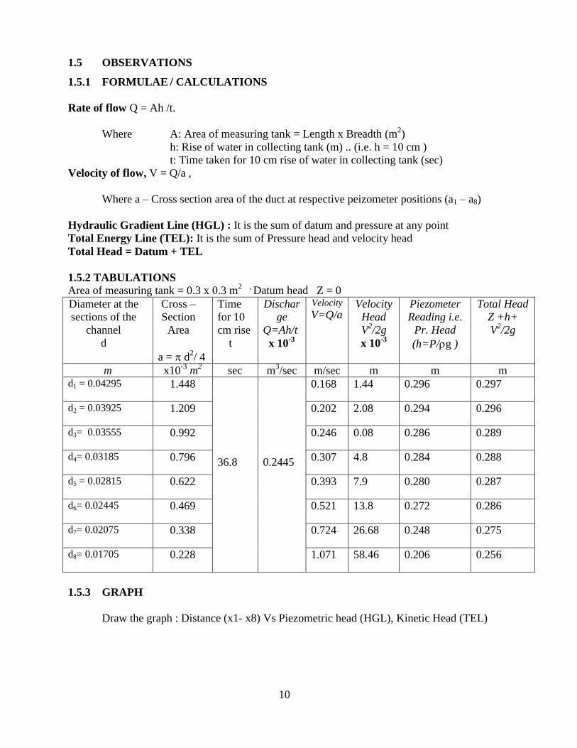
1.5 OBSERVATIONS
1.5.1 FORMULAE / CALCULATIONS
Rate of flow Q = Ah /t.
Where A: Area of measuring tank = Length x Breadth (m2)
h: Rise of water in collecting tank (m) .. (i.e. h = 10 cm )
t: Time taken for 10 cm rise of water in collecting tank (sec)
Velocity of flow, V = Q/a ,
Where a – Cross section area of the duct at respective peizometer positions (a1 – a8)
Hydraulic Gradient Line (HGL) : It is the sum of datum and pressure at any point
Total Energy Line (TEL): It is the sum of Pressure head and velocity head
Total Head = Datum + TEL
1.5.2 TABULATIONS
Area of measuring tank = 0.3 x 0.3 m2 ,
Datum head Z = 0
Diameter at the
sections of the
channel
d
Cross –
Section
Area
a = d2/ 4
Time
for 10
cm rise
t
Dischar
ge
Q=Ah/t
x 10-3
Velocity
V=Q/a Velocity
Head
V2/2g
x 10-3
Piezometer
Reading i.e.
Pr. Head
(h=P/g )
Total Head
Z +h+
V2/2g
m x10-3
m2 sec m
3/sec m/sec m m m
d1 = 0.04295
1.448
36.8
0.2445
0.168 1.44 0.296 0.297
d2 = 0.03925
1.209 0.202 2.08 0.294 0.296
d3= 0.03555
0.992 0.246 0.08 0.286 0.289
d4= 0.03185
0.796 0.307 4.8 0.284 0.288
d5 = 0.02815
0.622 0.393 7.9 0.280 0.287
d6= 0.02445
0.469 0.521 13.8 0.272 0.286
d7= 0.02075
0.338 0.724 26.68 0.248 0.275
d8= 0.01705
0.228 1.071 58.46 0.206 0.256
1.5.3 GRAPH
Draw the graph : Distance (x1- x8) Vs Piezometric head (HGL), Kinetic Head (TEL)

11
Fig.3. Bernoulli’s Theorem (Distance Vs TEL, HGL)

12
1.6 POST-LAB QUESTIONS
1. What do you meant by velocity head?
The head of energy due to pressure of the fluid in m
2. What do you meant by pressure head?
The head of energy due to K.E. (velocity) of the fluid in m
3. What do you meant by datum head?
The head of energy due to position (height) from a reference level
4. What is the use of piezometer? The tube used to show the pressure head in m. Its one
end is connected to the point where the pressure is to be measured and other end is
open to atmosphere.
5. Practically the total head of liquid at a point does not remain constant during the flow,
why? The total energy remains constant due to Bernoulli‘s theorem.
6. The liquid level in the piezometric tube connected to minimum c/s area is lowest,
Why? The pressure head is converted into kinetic or velocity head.
7. Why the water levels in the various piezometric tubes are different?
The pressure is decreasing due to the reduction in the cross section and the pressure
head is converted into KE (i.e. the velocity is increasing)
8. What do you mean by piezometric head?
It is the sum of the pressure head and datum head of the flow. (h+Z)
1.7 INFERENCES
The differences in the total head values are due to the loss of head due to friction,
fittings etc.
1.7 RESULT
The Bernoulli‘s theorem is verified.
13
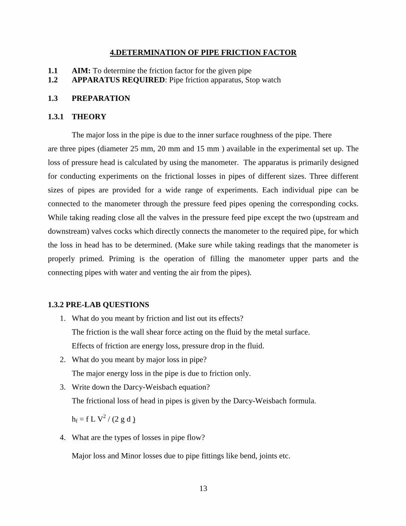
4.DETERMINATION OF PIPE FRICTION FACTOR
1.1 AIM: To determine the friction factor for the given pipe
1.2 APPARATUS REQUIRED: Pipe friction apparatus, Stop watch
1.3 PREPARATION
1.3.1 THEORY
The major loss in the pipe is due to the inner surface roughness of the pipe. There
are three pipes (diameter 25 mm, 20 mm and 15 mm ) available in the experimental set up. The
loss of pressure head is calculated by using the manometer. The apparatus is primarily designed
for conducting experiments on the frictional losses in pipes of different sizes. Three different
sizes of pipes are provided for a wide range of experiments. Each individual pipe can be
connected to the manometer through the pressure feed pipes opening the corresponding cocks.
While taking reading close all the valves in the pressure feed pipe except the two (upstream and
downstream) valves cocks which directly connects the manometer to the required pipe, for which
the loss in head has to be determined. (Make sure while taking readings that the manometer is
properly primed. Priming is the operation of filling the manometer upper parts and the
connecting pipes with water and venting the air from the pipes).
1.3.2 PRE-LAB QUESTIONS
1. What do you meant by friction and list out its effects?
The friction is the wall shear force acting on the fluid by the metal surface.
Effects of friction are energy loss, pressure drop in the fluid.
2. What do you meant by major loss in pipe?
The major energy loss in the pipe is due to friction only.
3. Write down the Darcy-Weisbach equation?
The frictional loss of head in pipes is given by the Darcy-Weisbach formula.
hf = f L V2 / (2 g d )
4. What are the types of losses in pipe flow?
Major loss and Minor losses due to pipe fittings like bend, joints etc.

14
1.4 PROCEDURE
1. Switch on the pump and choose any one of the pipe and open its corresponding
valves to the manometer.
2. Adjust the delivery control valve to a desired flow rate. (i.e. fully opened
Delivery valve position initially)
2. Take manometer readings and time taken for 10 cm rise of water in collecting
tank
3. Repeat the readings for various flow rates by adjusting the delivery valve. (i.e.
Gradually closing the delivery valve from complete opening)
4. Switch of the power supply after opening the valve completely at the end.
1.5 OBSERVATIONS
1.5.1 FORMULAE / CALCULATIONS
The actual rate of flow Q = A x h (m3/sec)
t
Where A = Area of the collecting tank = lengh x breadth (m2
)
h = Height of water(10 cm) in collecting tank ( m),
t = Time taken for 10 cm rise of water (sec)
The frictional loss of head in pipes is given by the formula.
hf = 4 f L V2
2 g d
Where f = Co-efficient of friction for the pipe (to be found)
L = Distance between two sections for which loss of head is measured = 3 m
V = Av. Velocity of flow = Q/a (m/s),
Area of pipe a= d2/ 4 (m
2),
d = Pipe dia = 0.015 m
g = Acceleration due to gravity = 9.81 m/sec2
hf = Loss of head in metres
= hm ( Sm – Sf)/ (Sf x 100) in m
= hm (13.6 – 1 ) x 10 -2
(m)
Where Sm = Sp. Gr. of manometric liquid , Hg =13.6 ,
Sf = Sp. Gr. of flowing liquid, H2O = 1
hm = Difference in manometric reading = (h1-h2) in cm
hf can be found by the above formula (data from the manometer). The rest of the factors except
‗hf‘ being known, the valve of ‗f‘ can be determined.
15
1.5.2 TABULATION
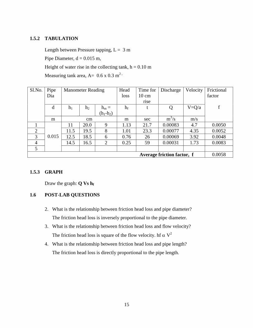
Length between Pressure tapping, L = 3 m
Pipe Diameter, d = 0.015 m,
Height of water rise in the collecting tank, h = 0.10 m
Measuring tank area, A= 0.6 x 0.3 m2 ,
Sl.No. Pipe
Dia
Manometer Reading Head
loss
Time for
10 cm
rise
Discharge Velocity Frictional
factor
f d h1 h2 hm =
(h1-h2)
hf t Q V=Q/a
m cm m sec m3/s m/s
1
0.015
11 20.0 9 1.13 21.7 0.00083 4.7 0.0050
2 11.5 19.5 8 1.01 23.3 0.00077 4.35 0.0052
3 12.5 18.5 6 0.76 26 0.00069 3.92 0.0048
4 14.5 16.5 2 0.25 59 0.00031 1.73 0.0083
5
Average friction factor, f 0.0058
1.5.3 GRAPH
Draw the graph: Q Vs hf
1.6 POST-LAB QUESTIONS
2. What is the relationship between friction head loss and pipe diameter?
The friction head loss is inversely proportional to the pipe diameter.
3. What is the relationship between friction head loss and flow velocity?
The friction head loss is square of the flow velocity. hf V2
4. What is the relationship between friction head loss and pipe length?
The friction head loss is directly proportional to the pipe length.

16
Fig.4. Major loss in pipes (Friction loss) (Q Vs hf)
1.7 INFERENCES
1.8 RESULT
The friction factor for the given pipe diameter of 0.015 m is = 0.0058

17
5. PERFORMANCE TEST ON GEAR PUMP
1.1 AIM: To study the performance of gear oil pump.
1.2 APPARATUS REQUIRED: Gear pump test rig, Stopwatch
1.3 PREPARATION
1.3.1 THEORY
A gear pump uses the meshing of gears to pump fluid by displacement. They are
one of the most common types of pumps for hydraulic fluid power applications. Gear
pumps are also widely used in chemical installations to pump fluid with a certain
viscosity. There are two main variations; external gear pumps which use two external
spur gears, and internal gear pumps which use an external and an internal spur gear. Gear
pumps are positive displacement (or fixed displacement), meaning they pump a constant
amount of fluid for each revolution. Some gear pumps are designed to function as either a
motor or a pump. The gear oil pump is works based on the squeezing action of the two
meshing gears (internal or external gears). The gear pump is one of the positive
displacement pump and the reduction in volume inside the pump results in increase in
pressure of fluid.
As the gears rotate they separate on the intake side of the
pump, creating a void and suction which is filled by fluid. The
fluid is carried by the gears to the discharge side of the pump,
where the meshing of the gears displaces the fluid. The
mechanical clearances are small— in the order of 10 μm. The
tight clearances, along with the speed of rotation, effectively
prevent the fluid from leaking backwards. The rigid design of
the gears and houses allow for very high pressures and the
ability to pump highly viscous fluids.
Fig.3. External Gear pump
1.3.2 PRE-LAB QUESTIONS
1. What is the purpose of gear pump?
Gear pump is a positive displacement pump and it is used to increase the pressure of high
viscous liquids.
2. What do you meant by internal and external gears?
The external gears the meshing teeth are only outer side of the driver and follower
whereas in the internal gears, one gear is having external teeth and other one is having
external teeth.
3. What are the applications of gear pump?
To pump the lubricating oil to a higher head ( to increase the pressure of oil)
18
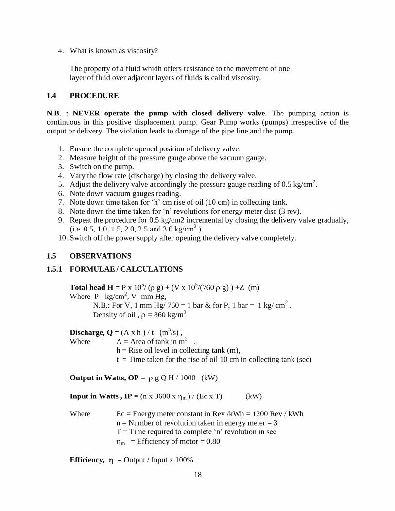
4. What is known as viscosity?
The property of a fluid whidh offers resistance to the movement of one
layer of fluid over adjacent layers of fluids is called viscosity.
1.4 PROCEDURE
N.B. : NEVER operate the pump with closed delivery valve. The pumping action is
continuous in this positive displacement pump. Gear Pump works (pumps) irrespective of the
output or delivery. The violation leads to damage of the pipe line and the pump.
1. Ensure the complete opened position of delivery valve.
2. Measure height of the pressure gauge above the vacuum gauge.
3. Switch on the pump.
4. Vary the flow rate (discharge) by closing the delivery valve.
5. Adjust the delivery valve accordingly the pressure gauge reading of 0.5 kg/cm2.
6. Note down vacuum gauges reading.
7. Note down time taken for ‗h‘ cm rise of oil (10 cm) in collecting tank.
8. Note down the time taken for ‗n‘ revolutions for energy meter disc (3 rev).
9. Repeat the procedure for 0.5 kg/cm2 incremental by closing the delivery valve gradually,
(i.e. 0.5, 1.0, 1.5, 2.0, 2.5 and 3.0 kg/cm2 ).
10. Switch off the power supply after opening the delivery valve completely.
1.5 OBSERVATIONS
1.5.1 FORMULAE / CALCULATIONS
Total head H = P x 105/ ( g) + (V x 10
5/(760 g) ) +Z (m)
Where P - kg/cm2, V- mm Hg,
N.B.: For V, 1 mm Hg/ 760 = 1 bar & for P, 1 bar = 1 kg/ cm2
.
Density of oil , = 860 kg/m3
Discharge, Q = (A x h ) / t (m3/s) ,
Where A = Area of tank in m2
,
h = Rise oil level in collecting tank (m),
t = Time taken for the rise of oil 10 cm in collecting tank (sec)
Output in Watts, OP = g Q H / 1000 (kW)
Input in Watts , IP = (n x 3600 x m ) / (Ec x T) (kW)
Where Ec = Energy meter constant in Rev /kWh = 1200 Rev / kWh
n = Number of revolution taken in energy meter = 3
T = Time required to complete ‗n‘ revolution in sec
m = Efficiency of motor = 0.80
Efficiency, = Output / Input x 100%

19
1.5.2 TABULATION
Measuring Area in collecting tank = 0.3x0.3m2
Datum head Z = 0.3 m
Sl.
No.
P
V
Z
H
Time
for
10cm
rise
(t)
Flow
rate
Q
Time for
3 rev of
Energy
meter
(T)
Input
IP
Output
OP
Effici
- ency
kg/cm2 mm
Hg
m m Sec m3/sec sec kW kW %
1 1.0 140
0.3
14.33 16.71 0.00054 32 0.23 0.065 28.31
2 1.5 140 20.26 17.13 0.00053 26 0.28 0.091 32.50
3 2.0 130 26.03 18.81 0.00048 22 0.33 0.105 31.82
4 2.5 110 31.64 19.13 0.00047 19 0.38 0.126 33.16
5 3.0 110 37.57 19.78 0.00046 17 0.42 0.146 34.76
6
1.5.3 GRAPH
Draw the graph: Discharge Vs Head, Output and Efficiency.
1.6 POST-LAB QUESTIONS
1. What is the squeezing in gear pumps?
The pressuring of fluid by passing through the reduced flow area and the
volume is reduced due to meshing of the gears.
2. What is the type of gears used in gear pumps? Spur gears
3. List out the different pressure heads used in gear pump?
Static head, Pressure and vacuum heads
4. What is mechanical efficiency of pump?
It is the ratio of hydraulic output power to motor shaft input power.

20
Fig.5. Performance of Gear oil pump ( Q vs H, OP, Efficiency)
1.7 INFERENCES
1.8 RESULT
The performance characteristics of the given gear oil pump are studied.

21
6. PERFORMANCE TEST ON SUBMERSIBLE PUMP
1.1 AIM: To study the performance of submersible pump at constant speed.
1.2 APPARATUS REQUIRED: Submersible pump test rig, Stop watch
1.3 PREPARATION
1.3.1 THEORY
A submersible pump (or electric submersible pump (ESP)) is a device which has a
hermetically sealed motor close-coupled to the pump body. The whole assembly is submerged in
the fluid to be pumped. The main advantage of this type of pump is that it prevents pump
cavitation, a problem associated with a high elevation difference between pump and the fluid
surface. Submersible pumps push fluid to the surface as opposed to jet pumps having to pull
fluids. Submersibles are more efficient than jet pumps
1.3.2 PRE-LAB QUESTIONS
1. What is the submersible pump?
2. What is the working principle of submersible pump?
3. What are applications of submersible pump?
1.4 PROCEDURE
1. Start the pump and run it at particular head on it.
2. Ensure the complete opening of the delivery valve provided.
3. The pressure gauge reading to be noted for the pressure of 0.5 kg/cm2.
4. The time is to be noted for collecting 10 cm rise of water in the collecting tank.
5. The time is to be noted for 3 revolution of Energy meter disc.
6. Repeat the procedure for 0.5, 1.0, 1.5, 2.0, 2.5, 3.0 kg/cm2 delivery pressures.
by closing the delivery valve.
7. Open the delivery valve completely and then Switch off the power supply.
1.5 OBSERVATIONS
1.5.1 FORMULAE / CALCULATIONS
Total Head, H = P x 105/ ( g) …… in m
Where P – Pressure gauge reading in kg/cm2,
g = Gravitational acceleration = 9.81 m2/s
= Density of fluid (water) = 1000 kg/m3
Discharge, Q = (A x h ) / t (m3/sec)
Where A = Area of tank in m2 A = l x b
h = Rise of water level in collecting tank = 0.10 m
t = Time taken for 10 cm rise of water in the collecting tank
22
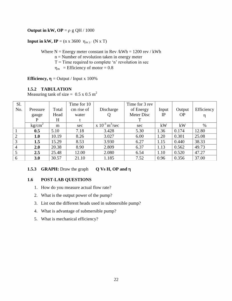
Output in kW, OP = g QH / 1000
Input in kW, IP = (n x 3600 m ) / (N x T)
Where N = Energy meter constant in Rev /kWh = 1200 rev / kWh
n = Number of revolution taken in energy meter
T = Time required to complete ‗n‘ revolution in sec
m = Efficiency of motor = 0.8
Efficiency, = Output / Input x 100%
1.5.2 TABULATION
Measuring tank of size = 0.5 x 0.5 m2
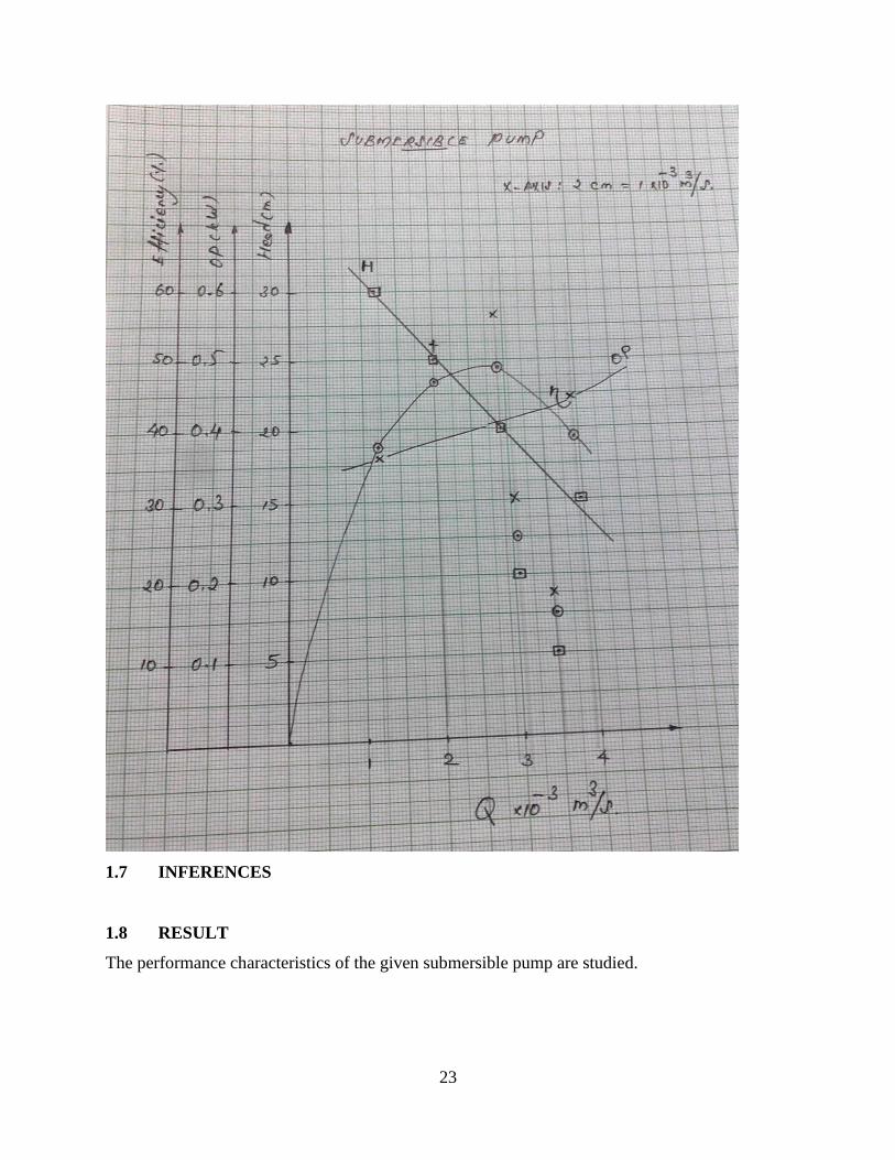
1.5.3 GRAPH: Draw the graph Q Vs H, OP and
1.6 POST-LAB QUESTIONS
1. How do you measure actual flow rate?
2. What is the output power of the pump?
3. List out the different heads used in submersible pump?
4. What is advantage of submersible pump?
5. What is mechanical efficiency?
Sl.
No.
Pressure
gauge
P
Total
Head
H
Time for 10
cm rise of
water
t
Discharge
Q
Time for 3 rev
of Energy
Meter Disc
T
Input
IP
Output
OP
Efficiency
kg/cm2 m sec x 10
-3 m
3/sec sec kW kW %
1 0.5 5.10 7.18 3.428 5.30 1.36 0.174 12.80
2 1.0 10.19 8.26 3.027 6.00 1.20 0.301 25.08
3 1.5 15.29 8.53 3.930 6.27 1.15 0.440 38.33
4 2.0 20.38 8.90 2.809 6.37 1.13 0.562 49.73
5 2.5 25.48 12.00 2.080 6.54 1.10 0.520 47.27
6 3.0 30.57 21.10 1.185 7.52 0.96 0.356 37.00
23
1.7 INFERENCES
1.8 RESULT
The performance characteristics of the given submersible pump are studied.

24
7.PERFORMANCE TEST ON RECIPROCATING PUMP
1.1 AIM: To study the performance of Reciprocating pump at constant speed.
1.2 APPARATUS REQUIRED: Reciprocating pump test rig, Stop watch
1.3 PREPARATION
1.3.1 THEORY
1.3.2 PRE-LAB QUESTIONS
1. What is the working principle of reciprocating pump?
2. What is type of suction and delivery valves in reciprocating pump?
3. What do you meant by slip in reciprocating pump?
4. What do you meant by single and double acting pump?
1.4 PROCEDURE
N.B. : NEVER operate the pump with closed delivery valve. The pumping action is
continuous in this positive displacement pump. Reciprocating Pump works (pumps)
irrespective of the output or delivery. The violation leads to damage of the pipe line and
the pump. Never operate the pump above the gauge pressure of 3 kg/cm2.
1. Start the pump and run it at particular head on it.
2. Ensure the complete opened position of delivery valve.
3. Vary the flow rate (discharge) by closing the delivery valve in order to maintain certain
pressure gauge reading i.e.0.5 kg/cm2.
4. Note down pressure gauge reading (0.5 kg/cm2) and vacuum gauges readings.
5. Measure height of the pressure gauge above the vacuum gauge (Datum level)
6. Note down time taken (t) for ‗h‘ cm rise of water (10 cm) in collecting tank.
7. Note down the time taken (T) for ‗n‘ revolutions for energy meter (3 rev) disc.
8. Repeat the procedure for 0.5, 1.0, 1.5, 2.0, 2.5 kg/cm2 in the Pressure gauge reading by
closing the delivery valve.
9. Switch off the power supply after opening the delivery valve completely.
1.5 OBSERVATIONS
1.5.1 FORMULAE / CALCULATIONS
1. Total head, H = [ P + (V/760) ] x 105 / ( g ) + Z (m)
Where P – Pressure gauge reading in kg/cm2,
V- Vacuum gauge reading in mm Hg,
Z – Datum level between Pressure gauge and Vacuum gauge
g = Gravitational acceleration = 9.81 m2/s
= Density of fluid (water) = 1000 kg/m3

25
N.B.: For V, 1 mm Hg/ 760 = 1 bar & for P, 1 bar = 1 kg/ cm2
2. Discharge, Q = (A h )/ t (m3/sec)
Where A- Collecting tank area = l x b in m2,
t - time for 10 cm rise of water level in the collecting tank (sec)
h – Rise of water level in the collecting tank = 0.10 m
3. Output in kW, OP = g QH / 1000
4. Input in kW, IP = (‗n‘ rev of energy meter x 3600 x Efficiency of motor) / (Energy
meter constant in Rev/kW-hr x Time for n revolutions)
= (n x 3600 x m ) / (Ec x T)
Where Ec = Energymeter constant in Rev /kW – hr = 1200 rev / kWh
n = Number of revolution taken in energymeter
T = Time required to complete ‗n‘ revolution in sec
m = Efficiency of motor = 0.8
5. Efficiency of Pump, = (Output / Input) x 100 %
1.5.3 TABULATION:
Area of Measuring tank A : 0.3 x 0.3 m2 , Motor Efficiency m : 0.8
Energymeter Constant : 1200 Rev/kW-hr Datum, Z =0.75 m
Sl.
No.
Pressure
Gauge
reading
P
Vacuum
Gauge
reading
V
Total
Head
H
Time
for
10 cm
rise
T
Discha
rge
Q
10-4
Time for
‗n‘ rev
of EM
disc
T
Input
Power
IP
Output
Power
OP
Efficie
ncy
kg/cm2 mm Hg metres Sec m
3/sec sec kW kW %
1. 0.5 170 8.13 31.88 2.82 23.24 0.23 0.023 10.00
2. 1 170 13.22 31.10 2.90 27.90 0.26 0.038 14.62
3. 1.5 165 18.25 37.08 2.43 24.93 0.29 0.044 15.17
4. 2 160 23.28 36.46 2.47 22.40 0.32 0.056 17.50
5. 2.5 160 28.37 33.56 2.68 19.50 0.37 0.075 20.27
6 3 160 33.47 33.38 2.70 17.09 0.42 0.089 21.20
1.5.3 GRAPH: Disharge Vs head, Output, Efficiency.
1.6 POST-LAB QUESTIONS
1. List out the different heads used in reciprocating pump?

26
2. What is the use of air vessel?
3. Why the delivery valve should be kept open always?
4. What do you meant by indicator diagram and its use?
5. What do you meant by percentage slip and negative slip?
1.7 INFERENCES
1.8 RESULT
The performance test on reciprocating pump is completed and the performance
characteristics are studied.

27
8.PERFORMANCE TEST ON CENTRIFUGAL PUMP
1.1 Aim: To study the performance of centrifugal pump at constant speed.
1.2 Apparatus Required: Centrifugal pump test rig, Stop watch
1.3 PREPARATION
1.3.1 THEORY
1.3.2 PRE-LAB QUESTIONS
1. What is the purpose of pump?
2. What do you meant by centrifugal force?
3. What is type of flow in centrifugal pump?
4. What is the use of volute casing?
5. What do you meant by priming?
1.4 PROCEDURE
N.B.: If the pump is not delivering water output , prime the pump and then start the
motor.
1. Ensure the complete opened position of delivery valve.
2. Vary the flow rate (discharge) by closing the delivery valve.
3. Note down pressure gauge reading for 0.5 kg/cm2 and vacuum gauges readings.
4. Measure height of the pressure gauge above the vacuum gauge. (Z)
5. Note down time taken (t) for ‗h‘ cm rise of water (10 cm) in collecting tank.
6. Note down the time taken (T) for ‗n‘ revolutions for energy meter(3 rev) disc.
7. Repeat the procedure for 0.5, 1.0, 1.5, 2.0, 2.5 kg/cm2 in the pressure gauge reading by
gradual closing of delivery valve.
8. Switch off the power supply after opening the delivery valve completely.
1.5 OBSERVATIONS
1.5.1 FORMULAE / CALCULATIONS
1. Total head, H = [ P + (V/760) ] x 105 / ( g ) + Z (m)
Where P – Pressure gauge reading in kg/cm2,
V- Vacuum gauge reading in mm Hg,
Z – Datum level between Pressure gauge and Vacuum gauge
g = Gravitational acceleration = 9.81 m2/s
= Density of fluid (water) = 1000 kg/m3
28
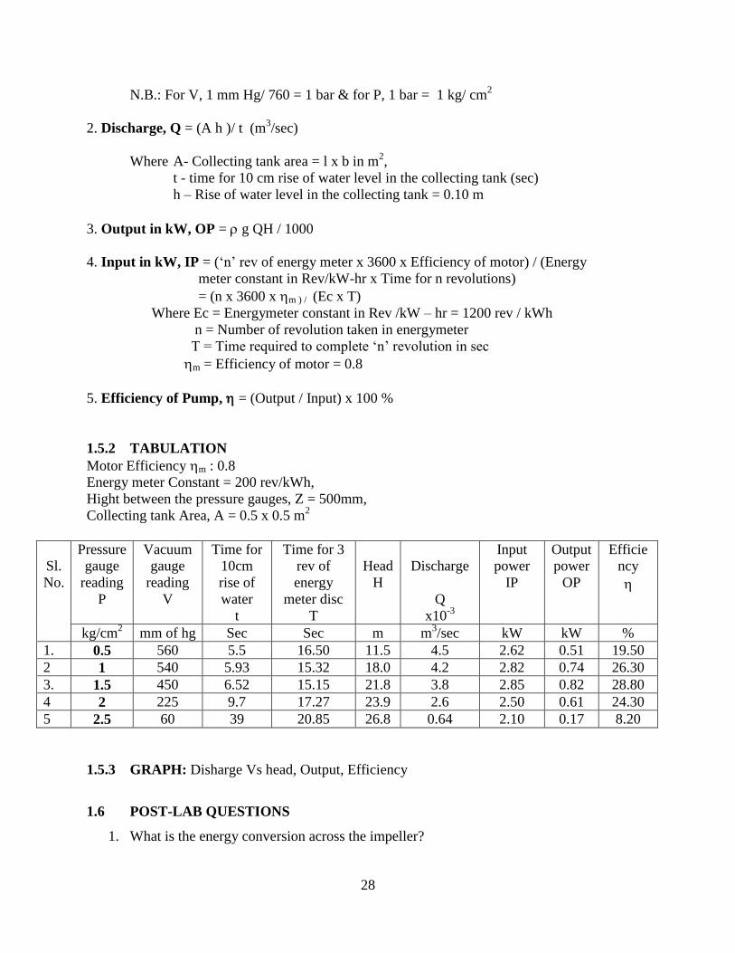
N.B.: For V, 1 mm Hg/ 760 = 1 bar & for P, 1 bar = 1 kg/ cm2
2. Discharge, Q = (A h )/ t (m3/sec)
Where A- Collecting tank area = l x b in m2,
t - time for 10 cm rise of water level in the collecting tank (sec)
h – Rise of water level in the collecting tank = 0.10 m
3. Output in kW, OP = g QH / 1000
4. Input in kW, IP = (‗n‘ rev of energy meter x 3600 x Efficiency of motor) / (Energy
meter constant in Rev/kW-hr x Time for n revolutions)
= (n x 3600 x m ) / (Ec x T)
Where Ec = Energymeter constant in Rev /kW – hr = 1200 rev / kWh
n = Number of revolution taken in energymeter
T = Time required to complete ‗n‘ revolution in sec
m = Efficiency of motor = 0.8
5. Efficiency of Pump, = (Output / Input) x 100 %
1.5.2 TABULATION
Motor Efficiency m : 0.8
Energy meter Constant = 200 rev/kWh,
Hight between the pressure gauges, Z = 500mm,
Collecting tank Area, A = 0.5 x 0.5 m2
Sl.
No.
Pressure
gauge
reading
P
Vacuum
gauge
reading
V
Time for
10cm
rise of
water
t
Time for 3
rev of
energy
meter disc
T
Head
H
Discharge
Q
x10-3
Input
power
IP
Output
power
OP
Efficie
ncy
kg/cm2 mm of hg Sec Sec m m
3/sec kW kW %
1. 0.5 560 5.5 16.50 11.5 4.5 2.62 0.51 19.50
2 1 540 5.93 15.32 18.0 4.2 2.82 0.74 26.30
3. 1.5 450 6.52 15.15 21.8 3.8 2.85 0.82 28.80
4 2 225 9.7 17.27 23.9 2.6 2.50 0.61 24.30
5 2.5 60 39 20.85 26.8 0.64 2.10 0.17 8.20
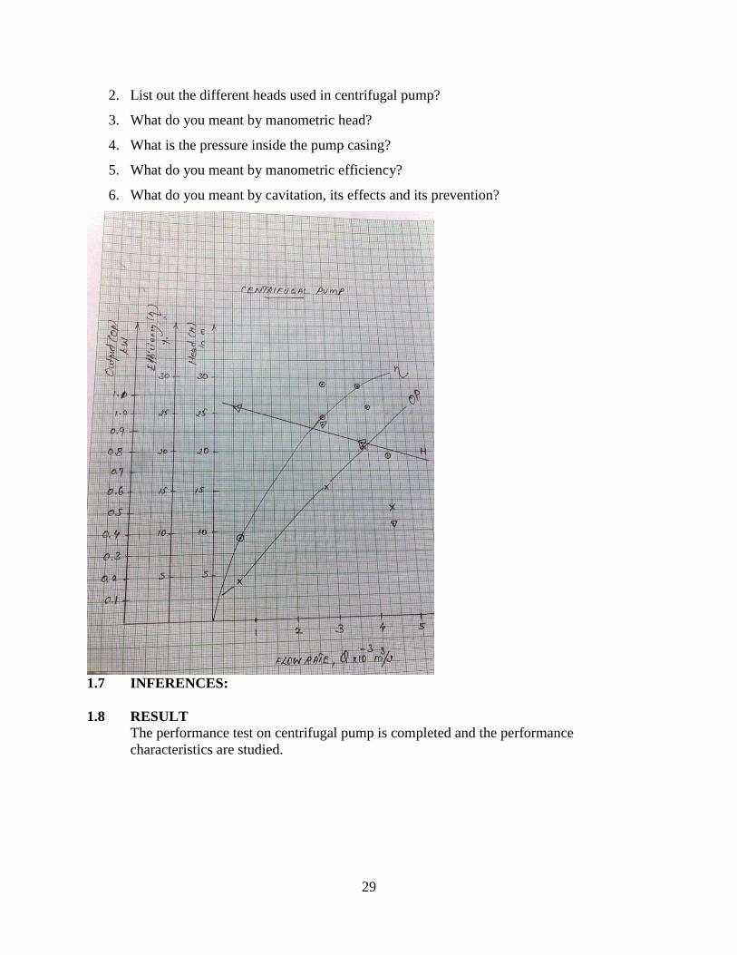
1.5.3 GRAPH: Disharge Vs head, Output, Efficiency
1.6 POST-LAB QUESTIONS
1. What is the energy conversion across the impeller?
29
2. List out the different heads used in centrifugal pump?
3. What do you meant by manometric head?
4. What is the pressure inside the pump casing?
5. What do you meant by manometric efficiency?
6. What do you meant by cavitation, its effects and its prevention?
1.7 INFERENCES:
1.8 RESULT
The performance test on centrifugal pump is completed and the performance
characteristics are studied.
30
9.DETERMINATION OF MINOR LOSSES DUE TO PIPE FITTINGS
1.1 AIM: To study the various losses due to the pipe fittings
1.2 APPARATUS REQUIRED: Minor losses test rig, Stopwatch
1.3 PREPARATION
1.3.2 THEORY
The various pipe fittings used in the piping applications are joints, bends, elbows,
entry, exit and sudden flow area changes (enlargement and contraction) etc. The energy
losses associated with these types of pipe fittings are termed as the minor losses due its
lesser values compared to the major loss (pipe friction) in the pipe. The loss of head is
indicated by the manometer connected across the respective pipe fitting.
1.3.2 PRE-LAB QUESTIONS
1. List out the various types of pipe fittings?
2. What do you meant by minor losses?
3. What are the types of losses in pipe flow?
1.4 PROCEDURE
1. Switch on the pump. Adjust the delivery valve to a desired steady flow rate.
2. Note down the time taken for 10 cm rise of water level in the collecting tank.
3. Choose any one of the pipe fittings (4 bends, one enlargement and one contraction). e.g.
Bend-1
4. Open the levers (cocks) of respective pipe fitting to the manometer. Ensure other fitting
levers should be closed. e.g. Open the entry and exit levers of Bend-1
5. Note down the manometer head levels (e.g. h1 & h2 for bend-1)
6. Now open the other two entry and exit levers of next pipe fitting. Then close the levers of
first chosen pipe fitting. (e.g. Open the levers for Bend-2 and close the levers of Bend-1)
7. Note down the manometer for the second pipe fitting. (e.g. h1 & h2 for bend-2)
8. Repeat this procedure by opening the respective levers of a particular fitting after closing
other levers.
9. Ensure the readings taken for all pipe fittings and then switch off the pump.
1.5 OBSERVATIONS
1.5.1 FORMULAE / CALCULATIONS
1. Discharge, Q = (A x h ) / t ….. (m3/s)
A = Area of tank in m2
,
h = 0.10 m // Rise water level in collecting tank (m),
t = Time taken for the 10 cm rise of water in collecting tank (sec)
31
2. Velocity, V = Discharge / Area of pipe = Q/A… (m/s)
A
Where A = d2/4 , d – Dia of pipe in m
3. Actual loss of head, hf = ( h1 – h2 ) x 12.6 x 10⁻²
… (m)
4. Velocity loss heads for pipe fittings
Velocity head for bend and elbow hv = V2
(2g)
Velocity head for sudden enlargement hv = ( V1 – V2 )2 / (2g)
Velocity head for sudden contraction hv = 0.5 (V2)2 / (2g)
Where V2= velocity of smaller pipe
5. Loss co-efficient K = Actual loss of head / Theoretical Velocity head = hf / hv
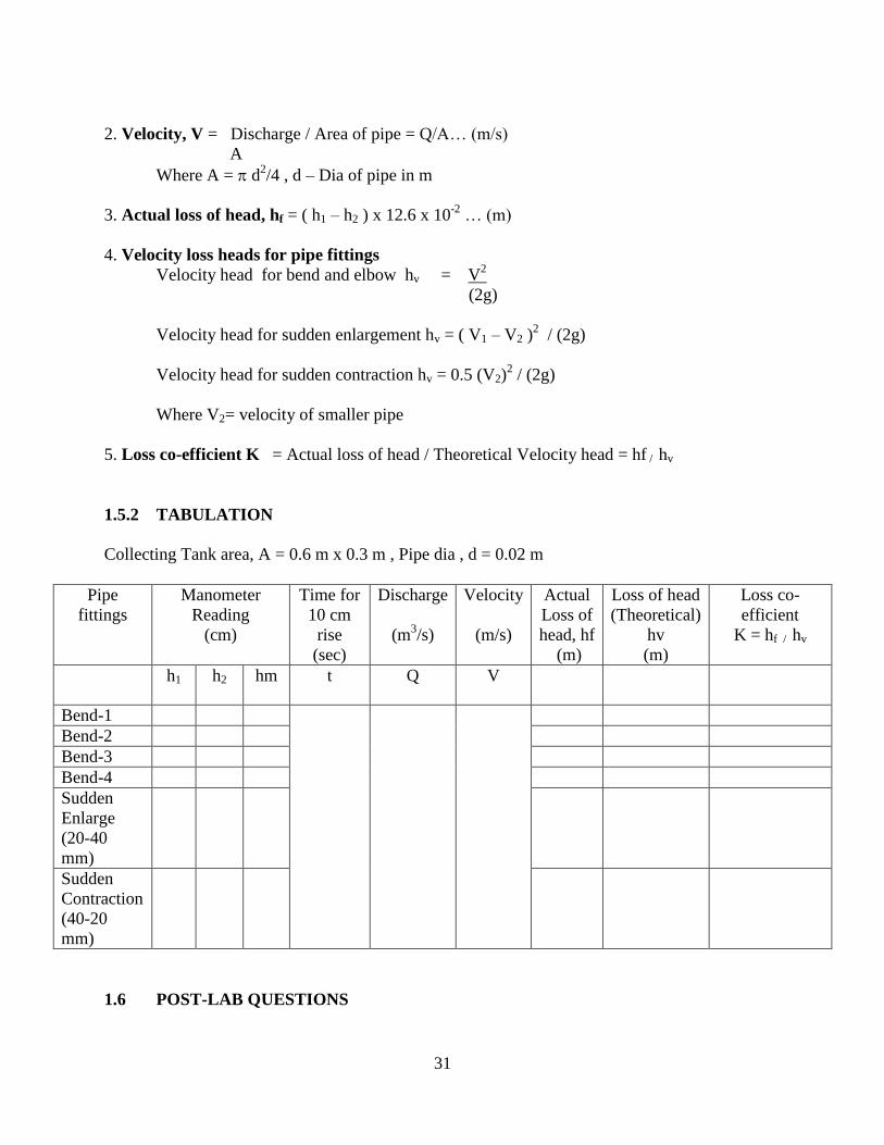
1.5.2 TABULATION
Collecting Tank area, A = 0.6 m x 0.3 m , Pipe dia , d = 0.02 m
Pipe
fittings
Manometer
Reading
(cm)
Time for
10 cm
rise
(sec)
Discharge
(m3/s)
Velocity
(m/s)
Actual
Loss of
head, hf
(m)
Loss of head
(Theoretical)
hv
(m)
Loss co-
efficient
K = hf / hv
h1 h2 hm t Q V
Bend-1
Bend-2
Bend-3
Bend-4
Sudden
Enlarge
(20-40
mm)
Sudden
Contraction
(40-20
mm)
1.6 POST-LAB QUESTIONS
32
1. What is the equation for head loss due to sudden enlargement?
2. What is the equation for head loss due to sudden contraction?
3. What is the equation for head loss due to bend?
4. What is the equation for head loss at entry of pipe?
5. What is the equation for head loss at exit of pipe?
1.7 INFERENCES
1.8. RESULT
The various losses in pipe fittings are determined.

33
10. PERFORMANCE TEST ON PELTON TURBINE
1.1 Aim: To study the performance of Pelton turbine.
1.2 Apparatus Required: Pelton Turbine test rig, Stop watch, Weights & Tachometer
1.3 PREPARATION
1.3.1 THEORY
1.3.2 PRE-LAB QUESTIONS
1. What are the types of hydraulic turbines?
2. What is the purpose of turbine?
3. What is the use of nozzle?
4. What is water hammer?
5. What is the purpose of surge tank?
1.4 PROCEDURE
1.4.1 SAFETY PRECAUTIONS
1. Remove any weights (loads) on the turbine shaft.
2. Ensure the closed position of the delivery valve.
3. After starting, check the functioning of cooling water supply to the turbine
4. Avoid running of turbine without cooling water to the brake drum on the shaft.
5. Keep away from the rotating shaft and avoid touching the shaft by hand or
Tachometer
6. Avoid pressure more than 2.5 kg/cm2 to the turbine for stability reasons.
7. Avoid any disturbances to the manometer tubes.
1.4.2 OPERATIONAL (PROCEDURAL) STEPS
1. Prime the pump and start it with closed gate valve. The spear in the turbine inlet and should
also be in the closed position while starting the pump in order to avoid sudden falling of water
and its impact on the turbine blades.
2. After starting the pump, Run the turbine at full spear opening by opening the spear gradually.
3. Load the turbine with the given 5 kg weights.
4. Vary the delivery pressure or pressure head acting on the turbine from 0.5 kg/cm2 to 2.5
kg/cm2 by gradual opening of the valve nearer to turbine. The incremental pressure is 0.5 kg/cm
2.

34
5. Note the following for the first Discharge pressures (P = 0.5 kg/cm2 ): Venturimeter pressure
heads (p1,p2), Turbine shaft speed (N) by torching on the turbine shaft sensor strip with the non
contact digital tachometer, Brake weight (Dead Weights plus hanger and rope weight) (W1 ) and
Spring balance reading(W2).
6. Increase the Discharge pressure by adjusting the delivery valve to 1 kg/cm2 and note down
(repeat the step-5)
7. First remove all the dead weights on the hanger. Close the delivery valve and stop the turbine.
Now switch off the power supply.
1.5 OBSERVATIONS
1.5.1 FORMULAE / CALCULATIONS
Input Power, IP = g Q H (W)
Where g = Specific weight of water = 9.81 kN/m3
Q = Discharge in m3/sec
Q = K √h = 3.183 x 10⁻³
√h (h in m )
Size of Venturimeter : 50mm and Throat Diameter : 29.58mm
Where ‗K‘ Value = (a1 a2 2g ) / (a12 – a2
2 = 3.183 x 10
-3
Where h = Venturimeter head in m of water
h = p x105/ g = (p1 – p2) x10
5/ (g) (m)
H = Supply head in m = Input total head in m
H = P x105/ (g )
Output (Brake) Power, OP = 2 N T / 60 (W)
Efficiency = (OP/IP ) x 100%
Where N = Turbine speed in RPM.,
T = W Re g = Torque in N-m
Brake drum dia D =0.2m ,
Rope dia d =0.015m
Effective radius of Brake Drum, Re = (D/2 )+d) = 0.115m
Weight of rope & hanger = 1kg.
Brake drum Net load W =(W1 + weight of rope hanger) –W2 kg = ( 5+1) – 2 = 4 kg

35
1.5.2 TABULATION
Sl
N
Pressure
gauge
reading
P
Pressure Gauge reading Venturi
-meter
Head
h
Discharg
e
Q
Weight
on
hanger
W1
Spring
balance
reading
W2
Net
Load
W
Speed
N
Inpu
t
IP
Output
OP
Effici
ency
p1
p2
P = p1-
p2
kg/cm2 kg/cm
2 m m
3/sec kg kg kg rpm W W %
1. 0.5 1.5 0.85 0.65 6.26 0.065 6 2 4 151 151 409 37
2. 1 1.4 0.8 0.6 6.12 0.062 6 2 4 487 487 787 62
3. 1.5 1.4 0.85 0.55 5.61 0.060 6 2 4 591 591 1130 52
4. 2 1.3 0.8 0.5 5.10 0.057 6 2 4 851 851 1436 59
5. 2.5 1.2 1.1 0.1 1.02 0.026 6 2 4 491 491 803 61
6.
1.5.3 GRAPH: Discharge Vs Speed, Output, Efficiency
1.6 POST-LAB QUESTIONS
1. What do you meant by impulse turbine?
2. How do you regulate the flow of water to the turbine?
3. What is the energy conversion from nozzle to turbine?
4. Why is braking jet used?
5. What is the spear and nozzle?
6. What is the pressure inside the turbine casing?
7. What is mechanical efficiency?
8. What do you meant by volumetric efficiency?

36
1.7 INFERENCES
1.8 RESULT: The performance of Pelton turbine is studied.

37
11.PERFORMANCE TEST ON FRANCIS TURBINE
Aim: To study the performance of Francis turbine.
Apparatus Required: Stop watch, Weights, tachometer
PROCEDURE
1. Prime the pump and start it with closed gate valve. The spear in the turbine inlet and should
also be in the closed position while starting the pump.
2. After starting and running the turbine at normal speed for some time, load the turbine and take
readings. Note the following: Net supply head, Discharge (pressure gauge readings), Turbine
shaft speed, Brake weight (Dead Weights plus hanger and rope weight) (1kg) and Spring balance
reading.
3. Before switching off the supply pump set, first remove all the dead weights on the hanger.
FORMULA
Input Power = g QH in kW
Where = Density of water = 1000 kg/m3
g = Acceleration due to gravity (9.81m/sec
2)
Q = Discharge in m
3/sec.
H = Supply head in meters.
2 NReW x 9.81
Brake Power =------------------- kW
60000
Output
Efficiency = ------------- x 100%
Input
Where N = Turbine speed in RPM.
T= Torque in kgm, (effective radius of the brake drum in meters (0.165m)
x The net brake load in kg.

38
FRANCIS TUBRINE
Orificemeter Head h in m of water h=(p1-p2)x 10m of water
Effective Radius of = (D/2 + t) Discharge Q = Kh (h in m of water)
Input power IP = x H x Q kW (H in m of water) Brake drum Re = 0.115m
Brake Drum net load W = (W1 + weight of rope & hanger) – W2 kg
Weight of rope & hanger = 1kg
Turbine output OP =(2 NWRe x 9.81)/ 60000 kW
Guide Vane opening = 0.5 Efficiency = (output / Input) x 100%
―K‖ value : 9.11 x10⁻³
Inlet diameter of Orificemeter: 80mm , Orificemeter diameter : 60 mm
Meter constant for Orificemeter: K=9.11 x10⁻³
h , h in m of water
Brake drum dia D=0.23m Rope Dia t = 0.015m
Input total head H in m of water = Pressure gauge reading in kg/cm2x 10
GRAPH: Discharge Vs Speed, output, Input, Efficiency
RESULT: The performance of Francis turbine is studied.
Sl.
No.
Pressu
re
gauge
readin
g
Pressure
Gauge
Reading
Orifice
meter
head
Disc
harg
e
Speed Wei
ght
on
hang
er
Sprin
g
balanc
e
readin
g
Net
load
Output
Input
Efficien
cy
P.S kg/cm2 h Q N W1 W2 W OP IP
kg/cm
2
P
1
p2 P m of
water
m3/s
ec
RPM kg kg kg kW kW %

39
FRANCIS TURBINE
Pre-Lab Questions
1. What are the types of hydraulic turbines?
2. What is the use of draft tube?
3. What is type of flow in reaction turbine?
4. What is the use of guide vanes?
Post-Lab Questions
1. What is the energy conversion across the turbine?
2. Differentiate stator and rotor vanes or blades?
3. What do you meant by runner?
4. What is the pressure inside the turbine casing?
5. What do you meant by reaction turbine?
6. List out different types of efficiency used?
7. What do you meant by brake power?
8. What do you meant by cavitation?
9. What are the methods to avoid cavitation?
40
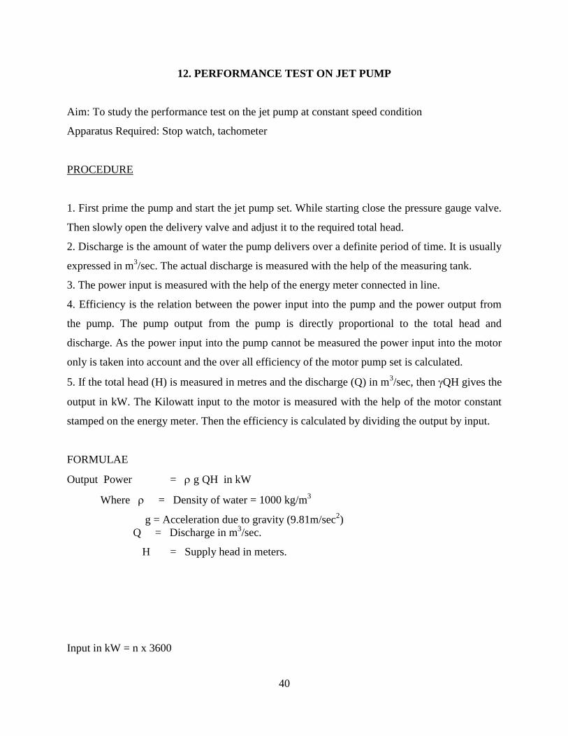
12. PERFORMANCE TEST ON JET PUMP
Aim: To study the performance test on the jet pump at constant speed condition
Apparatus Required: Stop watch, tachometer
PROCEDURE
1. First prime the pump and start the jet pump set. While starting close the pressure gauge valve.
Then slowly open the delivery valve and adjust it to the required total head.
2. Discharge is the amount of water the pump delivers over a definite period of time. It is usually
expressed in m3/sec. The actual discharge is measured with the help of the measuring tank.
3. The power input is measured with the help of the energy meter connected in line.
4. Efficiency is the relation between the power input into the pump and the power output from
the pump. The pump output from the pump is directly proportional to the total head and
discharge. As the power input into the pump cannot be measured the power input into the motor
only is taken into account and the over all efficiency of the motor pump set is calculated.
5. If the total head (H) is measured in metres and the discharge (Q) in m3/sec, then QH gives the
output in kW. The Kilowatt input to the motor is measured with the help of the motor constant
stamped on the energy meter. Then the efficiency is calculated by dividing the output by input.
FORMULAE
Output Power = g QH in kW
Where = Density of water = 1000 kg/m3
g = Acceleration due to gravity (9.81m/sec
2)
Q = Discharge in m
3/sec.
H = Supply head in meters.
Input in kW = n x 3600
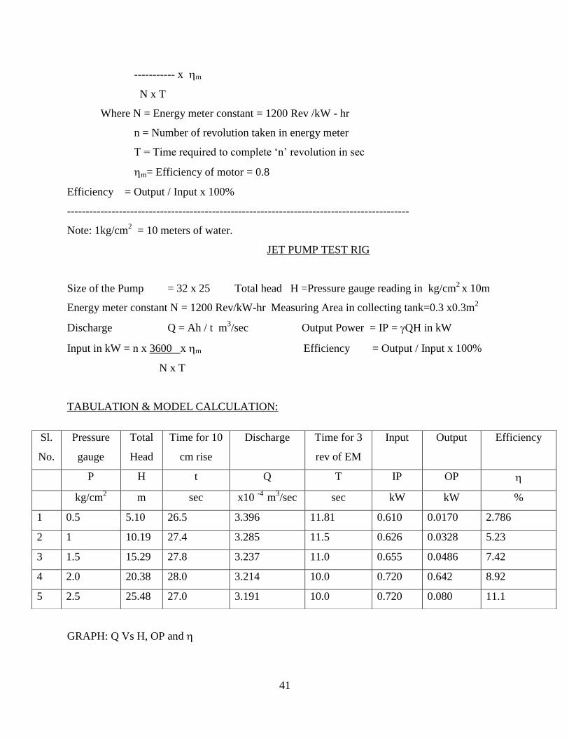
41
----------- x m
N x T
Where N = Energy meter constant = 1200 Rev /kW - hr
n = Number of revolution taken in energy meter
T = Time required to complete ‗n‘ revolution in sec
m= Efficiency of motor = 0.8
Efficiency = Output / Input x 100%
--------------------------------------------------------------------------------------------
Note: 1kg/cm2 = 10 meters of water.
JET PUMP TEST RIG
Size of the Pump = 32 x 25 Total head H =Pressure gauge reading in kg/cm2 x 10m
Energy meter constant N = 1200 Rev/kW-hr Measuring Area in collecting tank=0.3 x0.3m2
Discharge Q = Ah / t m3/sec Output Power = IP = QH in kW
Input in kW = n x 3600 x m Efficiency = Output / Input x 100%
N x T
TABULATION & MODEL CALCULATION:
GRAPH: Q Vs H, OP and
Sl.
No.
Pressure
gauge
Total
Head
Time for 10
cm rise
Discharge Time for 3
rev of EM
Input Output Efficiency
P H t Q T IP OP
kg/cm2 m sec x10
-4 m
3/sec sec kW kW %
1 0.5 5.10 26.5 3.396 11.81 0.610 0.0170 2.786
2 1 10.19 27.4 3.285 11.5 0.626 0.0328 5.23
3 1.5 15.29 27.8 3.237 11.0 0.655 0.0486 7.42
4 2.0 20.38 28.0 3.214 10.0 0.720 0.642 8.92
5 2.5 25.48 27.0 3.191 10.0 0.720 0.080 11.1

42
RESULT: The performance of the given jet pump is studied.
JET PUMP
Pre-Lab Questions
1. What is the purpose of jet pump?
2. What is the working principle of jet pump?
3. What are applications of jet pump?
Post-Lab Questions
1. How do you measure actual flow rate?
2. What is the output power of the pump?
3. List out the different pressure heads used in jet pump?
4. What is mechanical efficiency?
5. What is overall efficiency?
43
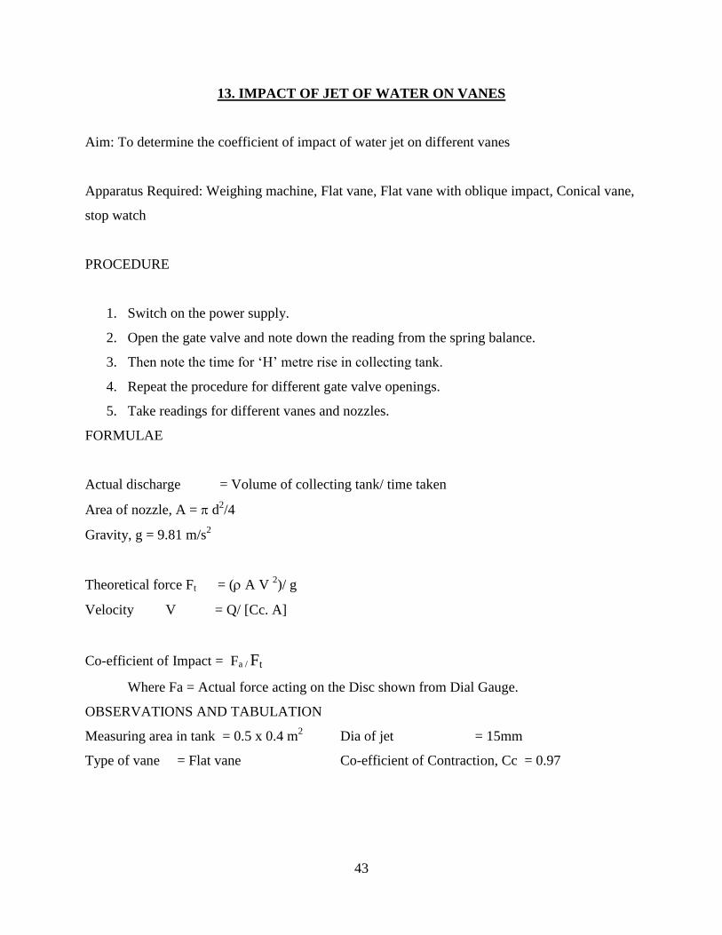
13. IMPACT OF JET OF WATER ON VANES
Aim: To determine the coefficient of impact of water jet on different vanes
Apparatus Required: Weighing machine, Flat vane, Flat vane with oblique impact, Conical vane,
stop watch
PROCEDURE
1. Switch on the power supply.
2. Open the gate valve and note down the reading from the spring balance.
3. Then note the time for ‗H‘ metre rise in collecting tank.
4. Repeat the procedure for different gate valve openings.
5. Take readings for different vanes and nozzles.
FORMULAE
Actual discharge = Volume of collecting tank/ time taken
Area of nozzle, A = d2/4
Gravity, g = 9.81 m/s2
Theoretical force Ft = ( A V 2)/ g
Velocity V = Q/ [Cc. A]
Co-efficient of Impact = Fa / Ft
Where Fa = Actual force acting on the Disc shown from Dial Gauge.
OBSERVATIONS AND TABULATION
Measuring area in tank = 0.5 x 0.4 m2
Dia of jet = 15mm
Type of vane = Flat vane Co-efficient of Contraction, Cc = 0.97

44
Sl.
No.
Type of Vane Time for 10 cm
rise of water
(sec)
Actual
force, Fa in
kg
Theoretical
Force, Ft in
kg
Co-efficient
of impact
1
2
3
RESULT: The co-efficient of impact of the given vane = ___________
JET ON VANE APPARATUS
Pre-Lab Questions
1. What is the water jet?
2. What is the effect of water jet on vanes?
3. What do you meant by impact?
4. List out different types of vanes?
Post-Lab Questions
1. How do you compare different vanes?
2. What do you meant by co-efficient of impact?
3. How do you measure the force of the jet?
4. How do you measure actual flow rate?

45
5. How do you measure theoretical flow rate?
14.FLOW VISUALIZATION - REYNOLDS APPARATUS
Aim: To demonstrate the flow visualization – laminar or turbulent flow.
Apparatus Required: Stop watch
THEORY
There are two different types of fluid flows laminar flow and Turbulent flow. The
velocity at which the flow changes laminar to Turbulent is called the ‗Critical Velocity‘.
REYNOLDS NUMBER(Re)
Reynolds number for pipe flow, Re = ( V D)/
Where V= Velocity of the fluid (m/s),
D= diameter of the pipe (m)
= Kinetic viscosity of the fluid (m2/s)
For water, = 1.01 x 10⁻⁶
m2/sec
Reynolds number determines whether any flow is laminar or Turbulent. Reynolds number
corresponding to transition from laminar to Turbulent flow is about 2,300.
PROCEDURE
1. Switch on the power supply. Adjust the water inflow slow by flow control valve.
2. Inject a filament of dye into the water stream by opening the value from dye tank.
3. When the flow is laminar, the colored stream of dye does not mix with the stream of water and
is apparent long the whole length of the pipe. Increase the velocity of the stream gradually by
46
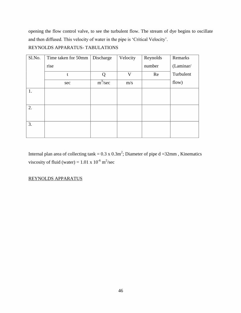
opening the flow control valve, to see the turbulent flow. The stream of dye begins to oscillate
and then diffused. This velocity of water in the pipe is ‗Critical Velocity‘.
REYNOLDS APPARATUS- TABULATIONS
Internal plan area of collecting tank = 0.3 x 0.3m2; Diameter of pipe d =32mm , Kinematics
viscosity of fluid (water) = 1.01 x 10⁻⁶
m2/sec
REYNOLDS APPARATUS
Sl.No. Time taken for 50mm
rise
Discharge Velocity Reynolds
number
Remarks
(Laminar/
Turbulent
flow)
t Q V Re
sec m3/sec m/s
1.
2.
3.

47
Pre-Lab Questions
1. What do you meant by fluid?
2. What are the types of flow?
3. Define Reynolds number?
4. What is laminar flow?
5. What is turbulent flow?
Post-Lab Questions
1. What do you meant by stream and streak lines?
2. Mention the Reynolds no for laminar and turbulent flow?
3. What do you meant by steady and unsteady flow?
4. What do you meant by path line?
5. What do you meant by uniform and non-uniform flow?
RESULT : The flow visualization test is conducted.