June 2002 ANL/TD/TM02-29

Flow of a Two-Dimensional Liquid Metal Jet in a

Strong Magnetic Field

S. Molokov, Coventry University

C.B. Reed, Argonne National Laboratory

Argonne National Laboratory 9700 South Cass Avenue

Argonne, IL 60439

Work supported by the Office of Fusion Energy Sciences

U.S. Department of Energy Under Contract W-31-109-ENG-38

2

Abstract

Steady, two-dimensional flow of a liquid metal jet pouring vertically down from a nozzle in the

presence of crossed magnetic and electric fields has been investigated. The magnetic field is

supposed to have a single component transverse to the flow. An asymptotic, high Hartmann

number model has been used to study a combined effect of surface tension, nonuniform magnetic

field, gravity and inertia. Relations have been obtained for a jet issuing from a duct, pouring into

a draining duct, pouring from one duct into another, and that in a liquid bridge. The results show

that the jet becomes thicker if the field increases along the flow and thinner if it decreases. It has

also been shown that for gradually varying fields characteristic for the divertor region of both

C-MOD and NSTX tokamaks, inertial effects are negligible for N > 10, where N is the interaction

parameter. Thus, provided the jet remains stable, the inertialess flow model is expected to give

good results even for relatively low magnetic fields and high jet velocity. Surface tension plays a

crucial role in shaping the jet profile at the nozzle. Partial flooding of the nozzle walls is

predicted. Finally, proposals have been made to investigate a possibility of using an axisymmetric

curtain along the perimeter of the bottom of a tokamak as an alternative to the film- or jet-

divertors, or to use a system of plane liquid metal sheets.

3

Contents

1. Introduction............................................................................................................... 4

2. Formulation.................………………………………………………….................. 5

3. Inertialess jet flow for high Ha................................................................................. 9

3.1 Cores C1, C2………………………………………………………..…….. 10

3.2 Steady flow……………………….………………………………………. 12

3.3 Parallel layer S at x = 0…………………………………………………… 14

3.4 Results…………………………………………………………………….. 15

3.4.1 Jet of constant thickness…………………………………………. 15

3.4.2 Negligible surface tension ( 0→λ )…………….………………. 15

3.4.3 Uniform magnetic field..………………………………………... 16

3.4.3.1 Linearized solution for β ~ 1…………………………… 18

3.4.3.2 Flow for arbitrary h, κ and β…………………………… 19

3.4.3.3 Discussion………………………………………………… 25

3.4.3.4 Jet pouring from a supplying into the draining duct……. 26

3.4.4 Nonuniform magnetic field..…………………………………… 27

3.4.5 Tailoring the jet…....……………………………………….…… 28

4. Slender inertial jet ……………................................................................................ 29

4.1 Cores C1, C2………………………………………………………..…….. 29

4.2 Results…………………………………………………………………….. 30

4.2.1 Jet of constant thickness………………………………………… 30

4.2.2 Uniform magnetic field…………………………………………. 30

4.2.2.1 Negligible surface tension ( 0→λ )…………….………. 30

4.2.2.2 Solution of a linearized equation for β ~ 1……………… 32

4.2.2.3 Flow for arbitrary h and β……………………………… 33

4.2.3 Nonuniform magnetic field..…………………………………… 33

5. Conclusions………………………………………………………………………… 34

Acknowledgment........................................................................................................... 37

References..................................................................................................................... 38

Figures........................................................................................................................... 40

4

1. Introduction

Liquid metal free-surface flows offer the potential to solve the lifetime issues limiting

solid surface designs for tokamak reactors by eliminating the problems of erosion and thermal

stresses [1], [2]. They also provide the possibility of absorbing impurities and possibly helium for

removal outside of the plasma chamber. In the US ALPS divertor concept this role is fulfilled by

a curtain of liquid metal jets [1].

One of the most important problems for the liquid-metal divertors is the

magnetohydrodynamic (MHD) interaction. When a liquid metal flows in a magnetic field,

electric currents are induced. These currents in turn interact with the magnetic field and the

resulting electromagnetic force induces a high MHD pressure drop and significant

nonuniformities of the velocity profile. Although some experimental and theoretical work on the

MHD jet flows has been performed, many issues still need to be resolved (see a review in [3]).

Among the most important ones are the effects of nonuniform magnetic fields, inertia, surface

tension, and gravity on both the jet cross-section and trajectory.

The main aim of this paper is to study a combined effect of surface tension, gravity,

inertia and a transverse nonuniform magnetic field on the steady jet flow. As an initial step a two-

dimensional flow is considered (Fig. 1). Thus the flow geometry may be thought of that of a

curtain, which is widely used in coating flows [4] (Fig. 2). The assumption of two-dimensionality

means that the flow is confined laterally by two perfectly conducting sidewalls. Away from the

immediate vicinity of the sidewalls the flow is two-dimensional (cf. [5]).

The flow also approximates that in an axisymmetric, vertical curtain in a radial, horizontal

magnetic field (Fig. 3), which may be placed along the perimeter of the bottom of a tokamak. If

the radius of such a curtain, R*, is much higher than the curtain thickness, a*, the effects of the

azimuthal curvature may be neglected and the flow in an azimuthal cross-section may be

considered two-dimensional.

It should be emphasized that as far as divertors for tokamaks are concerned, the jets are

likely to have a finite cross-section, and that all the solid walls are either insulating or have a

finite conductivity. Thus this particular model flow has its limitations in terms of direct

applicability to real divertor flows. In such flows, however, nonlinear effects are difficult to

analyse. In contrast, the geometry studied here presents a unique opportunity to get an assessment

5

of the importance of inertial and surface tension effects and to derive simple relations for the jet

velocity and thickness, which may be used to verify numerical methods being developed for more

realistic geometries.

Despite the limitations, curtain flow has several advantages with respect to a jet- or film-

flow, which are discussed in Conclusions, and which may be employed in the divertor design.

2. Formulation

Consider a flow of a viscous, electrically conducting, incompressible fluid in a jet (curtain)

pouring downward in the ∗x -direction (the direction of gravity) from an orifice (Fig. 1). Here

),,( ∗∗∗ zyx is the Cartesian co-ordinate system. Dimensional quantities are denoted by letters

with asterisks, while their dimensionless counterparts - with the same letters, but without the

asterisks. For ∗x < 0 the flow is between two parallel electrically insulating plates located at

2/∗∗ ±= ay , while for ∗x > 0 there is a free-surface flow. The location of the free surface is

defined as follows: ),( ∗∗∗∗ ±= txhy , where t* is time. The flow is supposed to be symmetric with

respect to ∗y , and therefore flow for ∗y > 0 only will be considered. Electrically insulating solid

plates at ∗x = 0, 2/|| ∗∗ = ay may also be present. In this case the fluid issues from a wall. If

these plates are absent, the flow will be referred to as “the nozzle problem”.

The flow occurs in the presence of a strong, transverse magnetic field yB ˆ)/2(0∗∗∗∗ = axBB ,

where ∗0B = constant is the induction of the magnetic field in the far upstream region. It should be

noted that the fact that B tends to 1 as −∞→∗x is not a necessary assumption; ∗0B may be a

magnitude of B* at any reference point within the flow region.

Laterally the flow is confined by perfectly conducting sidewalls located at ∗∗ ±= Lz (Fig. 1),

which are connected through a resistor, so that the resulting constant electric field ∗E is supposed

to be given (see the discussion below). In this case, sufficiently far from the sidewalls the electric

current flows in the ∗z -direction only, while the flow may be considered two-dimensional, in the

),( ∗∗ yx -plane [5]. The sidewalls are analogous to the edge guides in curtain flows (Fig. 2), which

support the jet (curtain) from contracting owing to surface tension [4].

6

The characteristic values of the length, the fluid velocity, time, the electric current density,

the electric field and the pressure are 2/∗a , ∗∗∗ = aQv /0 (average velocity in the duct region),

∗∗0/ va , ∗∗σ 00Bv , ∗∗

00Bv and 200∗∗∗σ Bva , respectively. In the above, σ, ρ, ν are the electrical

conductivity, density and kinematic viscosity of the fluid, ∗Q is the flow rate. Then the

dimensionless, two-dimensional, inductionless equations governing the flow are [3]:

∂∂+

∂∂+

∂∂+δ−

∂∂=−∇ −−

t

u

y

uv

x

uuN

x

pxBjuHa z

122 )( , (1a)

∂∂+

∂∂+

∂∂+

∂∂=∇ −−

t

v

y

vv

x

vuN

y

pvHa 122 , (1b)

)(xuBEjz += , (1c)

0=∂∂+

∂∂

y

v

x

u, (1d)

where u and v are the x- and y- components of the fluid velocity, respectively, p is the pressure, jz

is the electric current; 2/10 )/( ρνσ= ∗∗BaHa is the Hartmann number, which expresses the ratio of

the electromagnetic to the viscous force; ∗∗∗ ρσ= 02

0 / vBaN is the interaction parameter, which

expresses the ratio of the electromagnetic to the inertial force; parameter 200/ ∗∗σρ=δ Bvg =(FrN)-1

expresses the ratio of the gravitational to the electromagnetic force [3], where gavFr ∗∗= /20 is

the Froude number. Typical values of the dimensionless parameters are given in Table 1.

The values of ∗0B of 10T, 5T and 1T are characteristic for the conditions in large-scale

tokamaks (e.g. ITER), C-MOD and NSTX, respectively [3], [6]. From Table 1 follows that both

Ha and N are high in general. For NSTX, however, N may be ~1 or even lower in the regions of

lower field. For velocities ~ 10m/s it is unlikely that the flow in NSTX will be laminar (see Sec. 4

and Conclusions), and thus the theory presented here is expected to be valid for NSTX conditions

only for lower velocities.

In free-surface MHD flows parameter δ may be as low as ~ 10-4-10-6 (negligible gravity;

Table 1), or as high as ~1 (see Table 3.3 in [3]). Therefore, in the following it is treated as an

O(1) parameter.

7

The symmetry conditions are:

0/ =∂∂ yu , v = 0 at y = 0. (1e,f)

The boundary conditions at the duct wall are the no-slip- conditions:

u = v = 0 at y = 1, x < 0. (1g,h)

The boundary conditions at the free surface are the kinematic and the dynamic boundary

conditions [3], [4]:

x

huv

t

h

∂∂−=

∂∂

at y = h(x,t), (1i)

Table 1. Typical values of dimensionless parameters for Li divertors, for ma 005.0=∗ .

Thermophysical data for Li have been taken from [3].

∗0v 10m/s 1m/s

Fr 2039 20.39

Ca 0.0115 0.00115

∗0B 10T 5T 1T 10T 5T 1T

Ha 4308 2154 431 4308 2154 431

N 334 83.5 3.34 3340 835 33.4

N/Ha 0.078 0.039 0.0078 0.78 0.39 0.078

δ 61047.1 −⋅ 61087.5 −⋅ 41047.1 −⋅ 51047.1 −⋅ 51087.5 −⋅ 31047.1 −⋅

λ 61069.4 −⋅ 51087.1 −⋅ 41069.4 −⋅ 51069.4 −⋅ 41087.1 −⋅ 31069.4 −⋅

8

0142

=

∂∂+

∂∂

∂∂−+

∂∂

∂∂−

x

v

y

u

x

h

x

u

x

h at y = h(x,t), (1j)

κ=

∂∂

+∂∂

∂∂

−∂∂

−

∂∂

∂∂

++− −

−

1212

2 112 Cax

v

y

u

x

h

x

u

x

h

x

hpHa at y = h(x,t), (1k)

where

2/32

2

2

1

−

∂∂+

∂∂=κ

x

h

x

h (1l)

is the curvature of the free surface; γρν= ∗ /0vCa is the capillary number, which expresses the

ratio of viscous to surface tension terms in the dynamic boundary condition; γ is the surface

tension coefficient. Typical values of parameter Ca are shown in Table 1 above and in Table 2.2

in [3].

Far upstream the flow is fully developed, which requires

constant→∂∂ xp , 0/ →∂∂ xu as −∞→x . (1m,n)

Finally, the solution is normalized using the condition of a fixed flow rate:

∫ =1

0

1udy for x < 0. (1o)

If the flow is steady, then

∫ =h

udy0

1 for x > 0. (1p)

The constant electric field E is a parameter of the problem, which is determined by the

external circuit, and which is created by a fixed potential difference applied to the sides. Similar

to flows in ducts [7], [8], the present flow may be in the regime of either a brake, or a generator,

depending on the value of E.

Consider the duct region, x < 0. Integrating Eq. (1c) over the duct cross-section yields:

])([2)( ExBxI += . Suppose for an instant that B = 1 and thus I = constant. Then the flows may

be classified as follows. For E = -1 one gets I = 0 (an open electric circuit). This case is relevant

9

to ducts/jets of a finite cross-section. The case E = 0 corresponds to either short-circuited

sidewalls, or to an axisymmetric curtain shown in Fig. 3. In this case the current I is generated by

the flow. For E < -1 (current I < 0 is supplied to the system) the flow is accelerated, i.e. gravity is

artificially enhanced. For E = δ gravity is balanced by the term EB, and there is no flow. Values E

> δ are not relevant for the discussion here as a much stronger Lorentz force acts against gravity

and destroys the curtain. Thus, in the following we will consider E to be within the range

δ≤<∞− E .

If B is not a constant, then current I varies with x, so that different parts of the flow region

may function in different regimes, e.g. the current may be generated in one part and brake the

flow in another. Similar analysis holds for the jet region.

In the following the problem defined by Eqs. (1) is analysed for high values of parameter Ha.

First the inertialess flow is studied in Sec. 3 for an arbitrary jet thickness and curvature of the free

surface. Then in Sec. 4 slender inertial jet is studied, which requires 1/ <<∂∂ xh .

Although here we are interested in the steady flow, the unsteady, evolution equations are

derived first in the quasi-static approximation. These equations will be analysed in a subsequent

investigation.

3. Inertialess jet flow for high Ha

In this section the problem defined by Eqs. (1) is analysed for high values of Ha and for

∞→N . In the following all the flow variables denote their core values. Terms O(Ha-1) are

neglected.

In a sufficiently strong magnetic field the flow region splits into the following subregions

(Fig. 1): the cores C1, C2, the Hartmann layers H1, H2 of thickness O(Ha-1) at the walls y = ± 1

and the free surface, respectively, and the internal parallel layer S at x = 0 of thickness O(Ha-1/2).

There are also corner layers at x = 0, y = ±1 (being passive; not shown in the Fig. 1) with

dimensions )()( 11 −− × HaOHaO .

The analysis of the Hartmann layers is standard and thus is not presented here. The

Hartmann layers H1, H2 provide matching conditions for the variables in cores C1 and C2. In the

10

duct region (C1) this is the non-penetration condition (1h). In the jet region the Hartmann layer

H2 vanishes to O(1) [5], [9]. As a result for variables in the core C2 the kinematic condition (1i)

holds, while the normal component of the dynamic condition (1k) reduces to

p = - λκ at y = h(x,t). (2)

The constant pressure of the surrounding medium is set to zero. In the above parameter

)/()( 02

0212 ∗∗∗− σγ==λ vBaCaHa expresses the ratio of the surface tension and electromagnetic

forces, and thus depends neither on viscosity nor density of the fluid.

As λ varies in a wide range (~10-7-100) (see Table 1 above and Table 3.3 in [3]), it will be

treated as an O(1) parameter. If λ is low, the electromagnetic force dominates the surface tension.

This is despite the fact that the values of the capillary number for liquid metals are usually low.

Nevertheless, as will be shown below even if the value of λ is low, in general surface tension

cannot be neglected.

Another point of view on Eq. (2) is that in a two-dimensional MHD flow changes in pressure

O(λ) cause respective changes in curvature O(1).

The tangential component of the dynamic condition (Eq. (1j)) is taken into account in the

O(Ha-1) terms in the Hartmann layer. As will be shown later the x-component of the core velocity

is a function of x and t only, while the y-component is linear in y. As the core velocity does not

satisfy condition (1j), this leads to the O(Ha-1) flow in the Hartmann layer at the free surface.

Since we are interested here in the O(1) variables only, this secondary effect will not be analysed

(see the details of the analysis for a similar problem of the fully developed rivulet flow in [9]),

and thus Eq. (1j) is omitted.

3.1 Cores C1, C2

The analysis for both cores goes along the same lines. In the cores both viscous and inertial

terms in Eqs. (1a,b) are neglected. Now, for high values of N there are two time scales in the

problem. One is slow, O(1), which appears via the kinematic condition (1j). The other is fast,

O(N-1), as follows from Eqs. (1a,b). If one assumes that variations of the free surface are

sufficiently slow, derivatives with respect to time in Eqs. (1a,b) may be neglected, while that in

11

Eq. (1i) retained. The result is the so-called quasi-static approximation employed in the study of

slow motion of drops, jets and other flows in ordinary hydrodynamics (see reviews in [10], [11]).

Then Eqs. (1a,b) become:

δ−∂∂

=−x

pxBjz )( ,

y

p

∂∂=0 . (3a,b)

Substituting Eq. (1c) into Eq. (3a) and using Eq. (1d) gives the expressions for the

components of the core velocity as follows:

12),( −− −

∂∂−δ= EB

x

pBtxu , (4a)

x

uytyxv

∂∂−=),,( , (4b)

where p(x,t) is an unknown core pressure. These expressions are valid for both cores.

Now, in the duct region the non-penetration condition (1h) holds. Using Eqs. (4a,b) and

(1c,o) give the solution for the core C1 as follows:

u = 1, v = 0, jz = E + 1, { } dssBsBExtpxpx∫ ++δ+=0

0 )()()()( for x < 0, (5a-d)

where p0(t) is the unknown pressure at the duct exit x = 0. It follows that the Hartmann flow holds

up to the junction, while the pressure “absorbs” all variations of the field with x.

It should be noted that for δ = 0 and E = -1 the pressure gradient is O(Ha-1) (see e.g. [7], [8])

and thus is neglected as we are interested in O(1) terms only.

As 1)( →xB for −∞→x , the asymptotics for pressure far upstream in the duct is:

p(x) ~ (δ – E – 1)x. (6)

Now let us discuss the jet region. We note first that Eq. (2) yields the expression

)0()(0 =λκ−= xtp at the duct exit. As the pressure is continuous, any disturbance in the free-

surface curvature at x = 0 would modify the level of pressure in the duct (see Eq. (5d)). However,

as the steady term given by Eq. (6) dominates at large distances into the duct region, then

sufficiently far upstream from the orifice the importance of the possibly time-dependent surface

tension term diminishes.

12

Applying the kinematic condition (1i) to the core velocity (4) and using Eq. (2) gives:

)(uhxt

h

∂∂−=

∂∂

, (7)

12),( −− −

δ+

∂κ∂

λ= EBx

Btxu . (8)

This system may be reduced further to a single fourth-order evolution equation as follows:

[ ]{ }112 −−− δ−∂∂+

∂κ∂

∂∂λ−=

∂∂

BEhBxx

hBxt

h. (9)

Eq. (9) will be the subject of investigation of a separate study.

3.2 Steady flow

Our main interest here is in the steady flow. Neglecting time derivative in Eq. (7) and taking

into account Eq. (1p) gives:

u(x) = h-1(x). (10)

Substituting Eq. (10) into Eq. (8) gives the nonlinear third-order equation for function h(x) as

follows:

12' −+δ−=λκ hBEB , (11)

where ‘ = d/dx. This equation describes equilibrium solutions of Eq. (9) subject to condition (1p).

Once h is known, core flow variables are determined from Eqs. (2), (10), (1c) and (4b).

As there is a sharp corner at x = 0, y = 1, the fluid will tend to be attached to it [4], [12].

Therefore, we assume first that the so-called pinned-end conditions hold at this point. This gives:

h = 1 at x = 0, (12)

while the value of the angle, ))0('(tan 1 h−=θ (Fig. 1) is the result of the solution of the problem.

The wetting line will remain attached to the edge for a range of contact angles given by Gibbs’

inequality [4]:

13

1180 γ−+θ≤θ≤θ oAR , (13)

where θA, θR are the so-called advancing and receding angles for two different walls, and γ1 is the

included edge angle (Fig. 4). As far as we know there has been no measurements of the angles θA

and θR for MHD flows. Therefore, we treat θ being arbitrary, provided the steady solution exists.

The conditions far downstream from the jet exit depend on the asymptotics of B at infinity.

For ∞→ BB = constant as ∞→x , the boundary conditions compatible with Eq. (11) are:

β→h , 0'→h as ∞→x , (14a,b)

where

∞

∞

−δ=β

EB

B2

. (15)

In this case parameter β has a meaning of being half the constant jet thickness far downstream.

Therefore, the jet will expand if β > 1 and contract if β < 1.

More generally, parameter β-1 may be thought of as an efficient gravity modified by the

Lorentz force.

In the far downstream region the flow variables are:

12 −∞

−∞∞ −δ= EBBu , 0=∞v , 1−

∞∞ δ= Bjz , 0=∞p , (16a-d)

so that the fluid flows with a constant velocity in a jet of a uniform thickness determined by the

magnetic field in the downstream region.

If E = 0 (sidewalls short-circuited), then 2−∞∞ δ= Bu . In this case the dimensional jet

thickness, velocity and current are: gBvaah ρσ=β= ∗∞

∗∗∗∗∞ /2 2

0 , 2/ ∗∞

∗∞ σρ= Bgu , ∗

∞∗∞ ρ= Bgjz / ,

respectively. Thus, neither dimensional velocity nor current depend on either the average flow

velocity ∗0v or surface tension. For 2

∞<<δ B , sufficiently far downstream, the jet thickness is

expected to increase dramatically.

Eqs. (16) are in fact the exact solution of the problem defined by Eqs. (1) for an infinitely

long jet driven by gravity. In such a flow gravity is balanced by the Lorentz force, while variation

of pressure vanishes, and thus h = constant. In a corresponding hydrodynamic problem, vertical

14

jet flow with a uniform velocity is not possible [13], [14], as there is no body force to balance

gravity. This causes the fluid to accelerate and thus the jet to contract.

If δ = 0 (negligible gravity), then 1−∞∞ −= EBu , 0=∞zj . In this case the electric current

vanishes and ∞∞ Bh ~ .

If both δ = 0 and E = 0, no uniform flow is possible.

3.3 Parallel layer S at x = 0

The flow in the parallel layer is discussed here for B = 1 and for h’(0) = tan(θ) = O(1). As

both the core pressure and axial component of core velocity (cf. Eq (10)) are continuous across

x = 0, then in layer S the following expansions of the flow variables hold:

SuHau 2/11 −+= , Svv = , SpHapp 10

−+= . (17)

Here p0 = -λκ(0), while quantities with index S are the parallel-layer corrections to the core

variables. As the parallel layer does not disturb the core flow to O(1), it is passive.

Introducing the stretched co-ordinate xHa 2/1=ξ into Eqs. (1a,b,d) yields the equations

governing the flow in layer S as follows:

y

pv SS

∂∂=

ξ∂∂

2

2

, y

vp SS

∂∂=

ξ∂∂

2

2

, (18a,b)

while function uS is determined from the equation

ξ∂

∂−= S

S

pu . (18c)

As the Taylor’s expansion of function h at x = 0 is ...)0('1 ++= xhh , the geometry of the

vicinity of x = 0 in the layer is similar to that of a linearly expanding (β > 1) or contracting

(β < 1) duct [15]. Therefore, the boundary and matching conditions for the system of Eqs. (18a,b)

are (see [15] and Fig. 3):

0=Sv at y = 1, ξ < 0, (18d)

15

)0('hvS = at y = 1, ξ > 0, (18e)

0→Sv as −∞→ξ , (18f)

)0('yhvS → as ∞→ξ . (18g)

The solution to this system may be obtained in a similar way to that described in [15], and

thus is not discussed here.

3.4 Results

Before we proceed with a general discussion of the problem defined by Eqs. (11), (12), (14),

several limiting cases will be considered.

3.4.1 Jet of constant thickness

If B = 1, β = 1, the jet thickness is constant to O(1). The flow variables are: u = 1,

v = jz = p = 0.

3.4.2 Negligible surface tension ( 0→λ )

If 0→λ pressure in the jet vanishes, and the solution to the reduced version of Eq. (11) is:

)(

)()(ˆ

2

xEB

xBxh

−δ= , (19a)

and thus

)(

)()(ˆ 2 xB

xEBxu

−δ= . (19b)

In the above ^ denotes quantities obtained for λ = 0. With regard to Eqs. (19) the following

observations can be made:

(i) For δ << 1 (negligible gravity) one gets:

16

1)()(ˆ −−= ExBxh , )()(ˆ 1 xEBxu −−= . (20a,b)

The jet width is proportional to the induction of the field. The jet expands if B

increases or contract if B decreases along the flow. The fluid decelerates or

accelerates, respectively.

(ii) Function h is always non-zero. It becomes unbounded when δ = EB(x).

(iii) For E = 0 (sidewalls short-circuited) one gets

12 )()(ˆ −δ= xBxh , )()(ˆ 2 xBxu −δ= . (21a,b)

If B increases/decreases along the flow, the rate of expansion/contraction of the jet

becomes higher than in (i) because the electric currents are higher in this case than

for E ≠ 0. If in addition δ = 0 (negligible gravity), the solution fails to exist. In this

case the jet is diverted into the horizontal direction straight at the duct exit (see

discussion in Sec. 4.2.3).

(iv) Even if λ is small, surface tension is negligibly small in the whole domain only if

the solution h satisfies the boundary condition (12). This occurs for

B2(0) = δ – EB(0) only.

3.4.3 Uniform magnetic field

If λ ≠ 0 and B = 1, Eq. (11) becomes:

11' −− β−=λκ h . (22)

First of all let us consider what reductions of this equation are possible. Basically, two main

simplifications can be made.

If |h’| << 1, curvature may be linearized, i.e.

κ ≈ h’’. (23)

If h ~ 1, then the right-hand side of Eq. (22) may be linearized, which yields:

Hhh −∆≈β− −− 11 . (24)

17

Here H = 1 – h, and ∆h = β - 1 is the difference between the jet thickness far downstream and that

at the orifice.

A combination of these two cases, as well as the limit when 0→h leads to the following

five cases presented in Table 2.

It is worth noting that the reduced Eqs. IV and V from Table 2 belong to the following

family:

nfccf −+−= 21''' , (25)

where n is a real number and c1,2 are certain constants. For various values of n Eq. (25) describes

travelling-wave solutions for a spreading or a sliding drop, drawing down a vertical wall, Hele-

Shaw cell, porous media, etc. (see reviews in [10], [11], [16], [17]). However, Eq. (22) is more

general than Eq. (25) in that it involves full curvature and thus does not require the assumption

that a fluid volume be thin, which is employed while deriving Eq. (25) for the above-mentioned

flows.

Table 2. Particular types of Eq. (22) for various limiting cases. In the table xdd /'= .

Approximation Equation Notation

I |h – 1| << 1, |h’| << 1 hHH ∆=+λ ''' H = 1- h

II |h – 1| << 1,

h’ arbitrary hHH ∆=+λκ )(' H = 1- h, xx =

III 0→h , h’ arbitrary 1)(' −=κ ff f = h/λ, λ= /xx ,

IV 0→h , |h’| << 1 1''' −= ff f = h, xx 3/2λ=

V h arbitrary, |h’| << 1 1''' 1 −= −ff f = h/β, xx 3/12 )/( βλ=

18

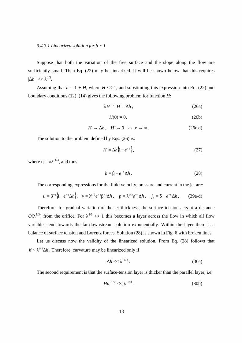
3.4.3.1 Linearized solution for β ~ 1

Suppose that both the variation of the free surface and the slope along the flow are

sufficiently small. Then Eq. (22) may be linearized. It will be shown below that this requires

|∆h| << λ1/3.

Assuming that h = 1 + H, where H << 1, and substituting this expression into Eq. (22) and

boundary conditions (12), (14) gives the following problem for function H:

hHH ∆=+λ ''' , (26a)

H(0) = 0, (26b)

hH ∆→ , 0'→H as ∞→x . (26c,d)

The solution to the problem defined by Eqs. (26) is:

{ }η−−∆= ehH 1 , (27)

where η = xλ-1/3, and thus

heh ∆−β= η− . (28)

The corresponding expressions for the fluid velocity, pressure and current in the jet are:

{ }heu ∆+β= η−− 11 , hev ∆βλ= −η− 13/1 , hep ∆λ= η−3/1 , hejz ∆+δ= η− . (29a-d)

Therefore, for gradual variation of the jet thickness, the surface tension acts at a distance

O(λ1/3) from the orifice. For λ1/3 << 1 this becomes a layer across the flow in which all flow

variables tend towards the far-downstream solution exponentially. Within the layer there is a

balance of surface tension and Lorentz forces. Solution (28) is shown in Fig. 6 with broken lines.

Let us discuss now the validity of the linearized solution. From Eq. (28) follows that

hh ∆λ 3/1~' . Therefore, curvature may be linearized only if

3/1−λ<<∆h . (30a)

The second requirement is that the surface-tension layer is thicker than the parallel layer, i.e.

3/12/1 −− λ<<Ha . (30b)

19

This is equivalent to Ca << Ha-1/2, which holds in most cases except for very high magnetic

fields. For Ca = O(Ha-1/2) the jet thickness varies within the parallel layer governed by viscous-

electromagnetic-surface tension interaction. The problem in the layer becomes nonlinear; it

requires a separate study.

3.4.3.2 Flow for arbitrary h, κ and β

If h is arbitrary, the boundary-value problem defined by Eqs. (22), (12), (14) is solved

numerically using three different methods for reasons described below.

Method 1 is as follows. A subroutine DBVPFD from IMSL library is used to solve the

boundary-value problem. The method employs a variable order, variable step size finite

difference method with deferred corrections. For low values of λ parameter continuation

technique is used. Method 1 is also applicable to flows in nonuniform magnetic fields discussed

in Sec. 3.4.4; neither Method 2 nor 3 is.

The results of calculations for λ = 10-4 and for several values of β are shown in Fig. 6.

Solutions of linearized Eq. (26) are also shown in the figure with broken lines. As the selected

values of β are sufficiently close to 1, solutions of Eq. (26) approximate the actual ones very

well.

However, when β has been increased above about 1.07 or decreased below about 0.94, a

problem appeared: the numerical solution diverged. Similar situation occurred for a fixed value

of β and for various values of λ (Fig. 7). For example, for 25.1=β decreasing parameter λ below

the value of 0.003 was not possible.

To clarify the reason for the divergence of the numerical method, calculations have been

performed for a fixed value of 25.1=β and for various values of λ using Method 2, which is

described below.

As the conditions far downstream are known, (h = β, h’ = 0, κ = 0), the solution is obtained

by integrating backwards using the function ode45 from MATLAB, which employs a fourth-

order Runge-Kutta method. Calculations start from a certain value of x = xend. As Eq. (22) is

invariant with respect to translation along the x-axis, the value of xend is arbitrary. When the value

20

of h reaches 1 at a certain point, this indicates the position of the orifice. However, we let

calculations run even belyond the level h = 1 until the solution terminates.

The results are shown in Fig. 8. It is seen that for λ = 1 (and higher) the solution exists for all

positive values of h. For λ below about 0.6 the solution curves terminate at certain points for

h > 0. At points of termination the absolute values of the first (and the second) derivatives

becomes very high (see Fig. 9). In fact we will show below that at these points ∞→'h ,

−∞→''h , while curvature remains finite. For λ < 0.003 the solution terminates above h = 1.

Therefore, for sufficiently low values of λ the steady flow obeying the boundary condition (12) is

not possible.

In calculations described above curvature κ has been nonlinear. If curvature is linearized, i.e.

Eq. V from Table 2 is solved instead of Eq. (22), the solution exists for all values of λ and β (see

Fig. 8, broken lines).

As follows from Figs. 9, 10, although curvature at the points of termination remains

moderate, the absolute values of both the first and the second derivatives of h become very high.

Therefore, there is a possibility that the solution terminates because of numerical errors. In order

to eliminate this possibility the following approach has been adopted (Method 3).

Since coefficients of Eq. (22) are constant, this third-order equation may be reduced to the

second-order one by means of the following substitution:

( ) 2/12'1−

+= hs , (31)

where 0 ≤ s ≤ 1 is an unknown function of h. The plane (h,s) is the phase plane for the original

flow.

The limiting values s = 0 and s = 1 correspond to ∞→|'| h and h’ = 0, respectively. Then

Eq. (22) yields:

22

2

11

s

sh

dh

sdh

−

−

β±=λ . (32)

The upper and lower signs in the above equation are taken for solutions with h’ > 0 (expanding

jet) and h’ < 0 (contracting jet), respectively. The expression for h’ in terms of s is:

ssh /)1(' 2/12−±= . It should also be noted that

ds/dh = -κ. (33)

21

Eq. (32) is solved as follows. As the value s = 1 (h’ = 0) is reached at h = β, this point

corresponds to ∞→x . Then Eq. (32) may be integrated numerically from h = β towards h = 1

using the initial conditions:

s = 1, ds/dh = 0 at h = β. (34)

The initial-value problem defined by Eqs. (32), (34) is solved by a fourth-order Runge-Kutta

method.

The advantage of this approach is that the derivatives of s remain bounded for all values of h,

which reduces possible numerical errors.

Calculations of the problem defined by Eqs. (32), (34) have been performed for various

values of parameters. The results of calculations on a phase plane (h,s) for β = 1.25 (expanding

jet) and for various values of λ are shown in Fig. 11. For sufficiently high values of λ (> 0.003)

function s is monotonic. The resulting value of s(1) decreases with decreasing λ (curves 1 - 4),

i.e. h’ remains finite. For λ = 0.003, the value s(1) becomes zero (curve 5), i.e. h’ tends to infinity

at h = 1. For λ < 0.003 it follows that 0→s for a certain h > 1 (curve 6). Therefore, a pass from

h = β to h = 1 becomes impossible.

The situation for which the solution breaks down first will be called critical, characterised by

critical values of parameters: λcr, ∆hcr (or βcr).

The results presented above are in full agreement with the results obtained by Methods 1 and

2. In fact, comparison of the numerical results obtained by the three methods are in perfect

agreement, i.e. numerical errors related to high values of h’ and h’’ do not alter the accuracy of

either Methods 1 or 2.

Finally, further decrease in λ leads to oscillating solutions of Eq. (32) (curves 7, 8 in

Fig. 11). The frequency of oscillations increases as λ decreases. It should be noted that negative

values of s have no physical meaning. However, branches of positive values of s, which start and

terminate at s = 0 do. We postpone the discussion of these branches until Sec. 3.4.3.3.

Variation of angle θ with λ for expanding jets is shown in Fig. 12. For any non-zero value of

∆h, as λ decreases the angle θ eventually becomes equal to either +90o or –90o, respectively

(critical solutions). Fig. 13 shows the results for |θ| in a log-log scale, from which follows that

3/12 )(|| λ∆−=θ π hc (35)

22

for virtually all values of λ. Here c is a coefficient of proportionality, which is a function of ∆h.

Now, the question is what happens if the values of parameters λ and ∆h are beyond critical,

i.e. we are interested in what happens if we slightly increase or decrease, say ∆h. There are

several possibilities: (i) the flow becomes unstable; (ii) the slope never becomes equal to π/2,

being adjusted in the parallel layer; (iii) pinned-end boundary condition is violated and a new

equilibrium state results.

Here we study scenario (iii), i.e. we are looking for steady, post-critical solutions of the

problem. As has been discussed in Sec. 3.2 the fluid tends to be attached to sharp corners, while

the angle θ results from the solution of the problem. If such a flow is not possible, a new steady

flow may result.

It is easy to predict what will happen if β < 1 (i.e. for the jet velocity higher than that in the

duct; contracting jet) and if we slightly decrease the ∆h below critical. If boundary condition (12)

is violated, the point of attachment will move upstream. At the solid walls a contact angle, θ0,

must be specified. If one assumes that this angle is static, then it is uniquely determined by the

material properties of the particular solid, liquid, and the surrounding medium. If wettability of

the walls is good (e.g. for In-Ga-Zn, which wets most materials), then θ0 < π/2, while for poor

wettability (e.g. Hg) θ0 > π/2 (Fig. 14).

Therefore, if wettability of walls at y = ±1 is poor (Fig. 14a), the duct will drain. Indeed, as

the contact angle θ0 > π/2, this corresponds to the angle θ defined in Fig. 1 being higher than

–π/2, i.e. above critical. However, for post-critical conditions such a flow is not permitted.

Therefore, the point of attachment will continuously move upstream until the whole duct drains.

As has been analysed in the above, for λ = 10-4 this will happen for ∆hcr = 0.075 (i.e. βcr = 0.93).

If wettability of walls at y = ±1 is good (θ0 < π/2), a new equilibrium is possible, as shown in

Fig. 14b. In this case regions of stagnant fluid (St) are formed. Indeed, in such a region there is a

“dead end” at the point of attachment, through which the fluid cannot flow. Since u is a function

of x only, recirculating flow in region St is not possible, and thus this region is stagnant.

The equation of equilibrium in regions St is:

1)(' −λβ−=κ , (36)

23

which represents a balance between the efficient gravity and surface tension. For E = 0 (pure

gravity) parameter Bo=λβ −1)( , where γρ= ∗ /2 gaBo is the Bond number, which expresses the

ratio of the gravitational and surface tension forces.

At points A in Fig. 14b the first derivative of h is infinite and changes the sign, while

curvature in region St matches that of a critical solution. The method of obtaining post-critical

solutions is described at the end of this section.

What exactly will happen for an expanding jet if we slightly increase the ∆h above critical

largely depends on the geometry of the flow at x = 0 and again on the wettability of the solid

walls. Several situations are possible as shown in Fig. 15.

In the first two cases (Figs. 15a,b) solid walls at x = 0 are present. Suppose now that λ is

fixed, and that ∆h is just below the value ∆hcr. If ∆h is increased slightly above ∆hcr, the point of

attachment will suddenly start moving along the wall x = 0 until a certain value of h(0+) is

reached, which corresponds to a given value of the contact angle θ0. An example of such a

scenario for λ = 10-4, ∆hcr = 0.075 is shown in Fig. 16, where two resulting post-jump jet profiles

are presented. These are for θ0 = 30o (good wettability) and 150o (poor wettability).

As there is now a jump in the value of h at x = 0, vertical velocity in the parallel layer will

increase by a factor of Ha1/2. The geometry in the vicinity of x = 0 will become that in a sudden

expansion studied in [18].

The transition from a sub- to a post- critical state is likely to be even more complicated,

because the hysteresis of the contact angle occurs not only for the angle θ, given by the Gibbs’

inequality, but for the contact angle θ0 as well. In dynamic problems θ0 is not necessarily static.

In fact, its value varies within a range

θ0R < θ0 < θ0A, (37)

where θ0A and θ0R are the advancing and receding contact angles for a particular wall [4]. Besides

other factors a particular value of θ0 depends on roughness of the wall and the presence of

surfactants. Therefore, new jumps may occur if θ0 fails to satisfy condition (37).

Ultimately, the dynamics of the transition and the post-critical flow itself will depend on

such experimental conditions as wall roughness, cleanness, etc. Therefore, experimental studies

of the dynamics contact angles in MHD flows are very important.

24

Consider further possibilities for post-critical flows. If there are no vertical walls at x = 0 (the

nozzle problem), several post-critical states are possible (Figs. 15c-h).

As the nozzle walls have a finite thickness, the point of attachment will first jump to the

upper corner of the wall, as shown in Fig. 15c. The fluid will stick to this corner until the flow

becomes critical again. If ∆h decreases further, the fluid will partially flood the nozzle wall as

shown in Figs. 15d,e. In both cases of good (Fig. 15d) and poor (Fig. 15e) wettability there will

be a zone St of stagnant fluid for x < 0.

If a nozzle protrudes from a wall over a certain distance (Fig. 15f-h), again several states are

possible. The fluid may stick to the inner corner as shown in Fig. 15f, or if this becomes

impossible (the third critical situation), will flood the vertical wall as shown in Figs. 15g,h.

Let us demonstrate how to obtain post-critical solutions for the flow of the type presented in

Figs. 15d,e, for which the following conditions hold:

h = 1, h’ = tanθ0 at x = -L, (38a,b)

where x = -L is the point of attachment.

Eq. (36) may be integrated twice to give, consequently:

)0(κ+λβ

−=κx

for x < 0, (39)

)('1

'2

xh

h Π=+

for x < 0, (40)

where 312

21 )0()()( cxxx +κ+λβ−=Π − , [ ] 2/12

3 )0('1)0('−

+= hhc . Expressing h’ in terms of Π(x)

and noting that h’ and Π must have the same sign (Eq. (40)), and thus be positive, one gets:

)(1

)('

2 x

xh

Π−

Π= for x < 0. (41)

From Eq. (41) follows the following restriction on the values of Π(x): -1 ≤ Π(x) < 1.

Next, integrating Eq. (41) and using the boundary condition (38a) yields:

∫− Π−

Π+=x

L t

dttxh

)(1

)(1)(

2 for x < 0. (42)

25

Now, in the region x > 0 the solution curves are shown in Fig. 8. Each curve in the figure,

which has been obtained for fixed values of β and λ, generates a family of solutions. Indeed, the

position x = 0 may be placed at any point along the curve. If we fix such a point, so that h(0) is

known, then both h’(0) and κ(0) are known as they are uniquely determined by the value of h(0).

Therefore, region x > 0 provides only one unknown value, h(0). The only other unknown value is

L. These two unknowns are determined from a system of nonlinear equations as follows:

∫− Π−

Π+=

0

2 )(1

)(1)0(

L t

dtth , (43)

)(sin 0 L−Π±=θ . (44)

The second equation follows from Eqs. (38b) and (40). The upper and lower signs in Eqs. (44) is

taken for θ0 < π/2 and θ0 > π/2, respectively.

For a given contact angle one needs to iterate between Eqs. (43), (44) and the numerical

solution of the problem in the region x > 0 to get the resulting post-critical flow.

3.4.3.3 Discussion

The preliminary conclusions that can be made at this point of the discussion is that surface

tension plays a crucial role in shaping the jet profile over a distance O(λ1/3) from the orifice. If

the value of λ is very low, the events take place in the vicinity of the orifice, so most of the jet

region will not be affected. However, sudden jumps of the point of attachment and restructuring

of the flow in the parallel layer may affect global flow stability. This requires a separate study.

We finally note that the effects described in this section are closely related to the so-called

“tea-pot effect” [19] in ordinary hydrodynamics of curtain flows. Several figures presented in

[19] and in [4] show various steady flows with partially “flooded” walls. In these flows strong

“tea-pot” effect occurs mainly at the backside of walls inclined to the gravity vector. In the

present MHD flow partial flooding of walls is the result of strong braking of the flow, which

cannot be held by the surface tension. Thus it occurs even for a vertical curtain studied here.

Flooding of walls transverse to the flow in various MHD free-surface film flows is also

common (see e.g. [20]). In the above we provide the mechanism for this effect.

26

3.4.3.4 Jets pouring from a supplying into the draining duct

We postponed the discussion of curve 8 in Fig. 8 until this section. For s ≥ 0 some branches

of this curve start and end up at s = 0. These and other similar curves have an important

interpretation: they correspond to flows for curtains pouring from one duct into the other, liquid

bridges, semi-infinite jets pouring into draining ducts, jets impinging on a layer of fluid, etc.

Let us consider two cases. The first case corresponds to a straight jet as −∞→x , pouring

into a draining duct. Since β→h , 0'→h , 0→κ as −∞→x , the starting point in the (h,s)

phase plane is β=h , and the initial conditions are given by Eq. (34). We solve Eq. (32), but now

we shoot in the direction h > β. The result of calculations of for β = 1.25, λ = 0.1 is shown in

Fig. 17. Again this curve generates a family of solutions. One could place a wall of the draining

duct along any point along the curve. Two examples are shown in Fig. 17. For the first one (thick

solid line), the edge of the draining duct is placed at the curve, which corresponds to pinned-end

conditions. For the second (thick broken line), the fluid goes into the duct, which corresponds to a

given contact angle.

Combining the solutions presented in Sec. 3.4.3.2 with the one discussed above gives a jet

pouring from a supplying duct, which becomes straight, and then pours into a draining duct.

If the distance between the two ducts is short, one gets a flow in a liquid bridge. To obtain a

solution for the bridge, one needs to perform calculations with the following initial conditions:

s = s0, ds/dh = -κ0 at h = 1, (45)

where s0 and κ0 are certain non-zero numbers. An example of a liquid bridge for β = 5,

λ = 0.0001, s0 = 0.1, κ0 = -120 is shown in Fig. 18.

The solutions which start and terminate at s = 0 (see e.g. curve 8 in Fig. 8) are the critical

solutions for liquid bridges/jets, for which |θ| = π/2 at both ends. These solutions by necessity

have an inflection point, which corresponds to a maximum of s along the curves.

27

3.4.4 Nonuniform magnetic field

We return now to the discussion of the jet flow pouring from the orifice.

If a nonuniform magnetic field is applied, Eq. (11), together with the boundary conditions

(12), (14) is solved using Method 1. Neither Methods 2 nor 3 are applicable, because coefficients

in Eq. (11) are functions of x.

In the following we will consider a family of step-like magnetic fields defined by the

following expression:

)(tanh)1(21

)1(21

0xxBBB −ζ−++= ∞∞ . (46)

The field magnitude equals 1 as −∞→x and ∞B as ∞→x . Parameter ζ defines the gradient of

the field; x0 defines the position where B is an average value of ∞B and 1. The results of

calculations for E = -1, δ = 0, and for various values of ∞B , λ, ζ and x0 are shown in Figs. 19, 20.

Fig. 19 shows the flow in a decreasing, high-gradient field, while Fig. 20 shows that in an

increasing, low-gradient field.

If point x0 is located far into the jet region, the jet profile at the orifice is a constant (Fig. 19,

curves 1-5 and Fig. 20, curve 1). As the change of the jet thickness occurs sufficiently far from

the orifice, for λ1/3 << 1 the surface tension plays a minor role. For λ = O(1) “wiggles” in the jet

profile are present. They occur near points where solution for λ ≠ 0 intersects function h , which

is the solution for λ = 0. This results in several inflection points in the jet profile.

If point x0 is within the duct or near x = 0, so that the jet is inside a magnetic field region

right from the orifice, then surface tension plays an important role (Fig. 19, curve 6 and Fig. 20,

curves 2,3).

Curve 6 in Fig. 19 shows the result for λ = 1. The gradient of h at x = 0 is higher than those

for smaller values of λ. If λ is increased further, Gibbs’ condition may be violated walls may be

flooded as a result. The effect is the opposite to that discussed in Sec. 3.4.3.2. For jet profiles

tending to uniform at infinity, a decrease in λ leads to wall flooding. For the flow studied in this

Section the cause of flooding is surface-tension induced wiggles owing to rapid decrease in the

field. The results shown in Fig. 19 are high field gradient and for x0 = 5.

28

If either field gradient or x0 are reduced, the wiggles become less pronounced, and the effect

reverses. Fig. 20 shows the results for a gradually varying field, over a distance of about 10

values of the characteristic length, which is characteristic to both C-MOD and NSTX conditions

[8]. No wiggles are observed if point x0 is far from the orifice.

For x0 = 0 the solution for λ = 0 given by Eq. (19a) does not satisfy the pinned-end condition

(12). Thus the jet profile with surface tension attempts to match that for λ = 0 (curve 4). Then at

x = 0 all the effects related to flooding and discussed in Sec. 3.4.3.2, which are now induced by

the jump |1ˆ| −h , apply. Curve 3 in Fig. 20 corresponds to a critical solution with λcr = 0.1.

3.4.5 Tailoring the jet

Nonuniform magnetic fields can be efficiently used to tailor the jet profile. Indeed, it is

possible to obtain profile of the jet with a desired thickness. Suppose y = h(x) is such a profile,

which satisfies the boundary condition. Solving Eq. (11) for B(x) gives:

{ })'(421

)( 22 κλ−δ++−= hhEEhxB . (47)

As an example consider a jet expanding linearly for δ = 0, E = -1, i.e.

h = 1+mx, u = (1+mx)-1, v = ym/(1+mx)2 , (48a-c)

where m = constant is the expansion ratio. Then the curvature vanishes identically, and Eq. (47)

gives:

B = 1+mx. (49)

Although in tokamaks the magnetic fields cannot be changed and there are other two field

components, one could try to select such a direction of the jet (with the use of the expressions of

the type (47)), for which the effects of the nonuniform magnetic fields are either minimized or

even exploited.

29

4. Slender inertial jet

Consider now the inertial flow for sufficiently high values of N. The restriction on N is

determined by the requirement that the flow remains laminar. Since no experimental data for

transition to turbulence in a jet exist, we base the restriction on N on the available data for the

duct flow. Therefore, we require that N/Ha > 0.004 [21].

As follows from Table 1 this condition holds for all the three values of the field and both

values of the characteristic velocity. For both C-MOD and large-scale tokamaks the values of

N/Ha are sufficiently higher than critical. Thus the flow in these reactors may be expected to be

laminar. It should be noted, however, that the condition is valid for fully developed duct flows in

a uniform field. It is based on the pressure drop measurements. This does not exclude the

presence of two-dimensional turbulence in the presumably laminar regime, which does not affect

the pressure drop. Thus concerning NSTX, for velocities ~ 10m/s the condition is likely to be

violated (see Conclusions). The interaction parameter in NSTX may be as low as 0.1, which

indicates a three-dimensional MHD turbulent flow regime.

4.1 Cores C1, C2

The analysis for both cores goes along the same lines as that for the inertialess flow. In the

cores the flow is inviscid. The inertial term xuuN ∂∂− /1 in Eq. (1a) is retained, while all other

inertial terms in Eqs. (1a,b) are neglected. This requires that the jet is slender (h’ << 1) [13].

Similar analysis to that in Sec. 3 yields a third-order ordinary differential equation for the jet

thickness as follows:

)()()(

3

22

3

3

xEBx

h

Nh

xB

h

xB

x

h −δ+∂∂−=

∂∂λ . (50)

This equation, together with the boundary conditions (12), (14), constitutes the problem for

the slender inertial jet.

The analysis of the flow in the inertial parallel layer is similar to that presented in [15] and is

not discussed here.

30

4.2 Results

4.2.1 Jet of constant thickness

If B = 1, β = 1, the jet thickness is h = 1, as for the inertialess flow.

4.2.2 Uniform magnetic field

4.2.2.1 Negligible surface tension ( 0→λ )

If 0→λ Eq. (50) reduces to the first-order ordinary differential equation of Abel type as

follows:

2231 )(' BhEBhhN +δ−=− , (51)

and if further B = 1, one gets:

2131 ' hhhN +β−= −− . (52)

This equation can be easily integrated. Taking into account the boundary condition (12) gives the

solution to Eq. (52) in an implicit form as follows:

{ }111111 1)1/()(ln −−−−−− −+β−β−β−= hhNx for x > 0. (53)

The interaction parameter simply scales the x-co-ordinate: the lower the N, the more gradual

variation of the jet profile is. From the discussion in Sec. 4.2.2.2 follows that the solution (53) is

valid for 3/1−λ<<N .

Variation of the jet thickness with xN for several values of β is shown in Fig. 21. For all

cases presented in Fig. 21, except for ∞→β , inertia acts over a distance of about 2N-1, which is

less than one value of the characteristic length for all the three values of the magnetic field

presented in Table 1.

For ∞→β (E = δ) gravity is fully compensated by the Lorentz force, and Eq. (52) yields:

[ ] 11)( −−= Nxxh , (54a)

31

which gives

Nxxu −= 1)( , v(x,y) = Ny. (54b,c)

This is a stagnation-point type flow, which indicates that the jet is completely diverted in the

±y-direction at a distance x = N-1 (curve 1 in Fig. 21). The solution is exactly the same as that for

a submerged two-dimensional jet studied in [22]. As the jet is supposed to be slender here,

solution (54) remains valid for h << N-1/2. For higher values of h other inertial terms in Eqs. (1a,b)

become important. For E = δ = 0 solution (54) becomes valid for nonuniform fields as well.

Solution (54) gives an indication of what will happen with an axisymmetric curtain presented

in Fig. 3. The fluid will be diverted into a horizontal direction and is likely to cover all the bottom

of the reactor. We believe that it is worth investigating this idea as an alternative to the either jet

or film divertor.

As N tends to infinity, the flow becomes inertialess, while the jet will be diverted in the

±y-direction right at the junction, in layer S.

If 0→β (high gravity or high |E|), then Eq. (52) reduces to

131 ' −− β−= hhN , (55)

the solution of which is:

2/1

12

−

+

β= Nx

h . (56)

The jet becomes thinner along the flow, so that 0→h as ∞→x (curve 7 in Fig. 21), while the

fluid accelerates. If E = 0, then β = δ-1 = NFr, so that N/β = Fr-1. Then the Eq. (56) gives the

classical solution for an ordinary hydrodynamic flow [13], [14].

For a small but finite β, when h3 becomes sufficiently small, the term h2 in Eq. (52) becomes

of the same order as the term –h3β-1. Therefore, the current will eventually brake the flow so that

jet thickness far downstream will tend to a constant (curve 6 in Fig. 21).

32

4.2.2.2 Solution of a linearized equation for β ~ 1

Suppose, as in Sec. 3.4.3.1, that both the variation of the free surface and the slope along the

flow are small. Assuming that h = 1 + H, where H << 1, and substituting this expression into

Eq. (52) and boundary conditions (12), (14) gives the following problem for function H:

hHd

dH

d

Hd ∆=+η

τ+η3

3

, (57a)

H(0) = 0, (57b)

hH ∆→ , 0'→H as ∞→x , (57c,d)

where η = xλ-1/3 and τ = λ-1/3N-1. The solution to problem defined by Eqs. (57) is:

{ }η−−∆= mehH 1 , (58)

where

3/1

3/2

612

r

rm

−τ= , 811212108 3 +τ+−=r .

Both parameters m and r are non-negative for all values of τ.

From Eq. (58) follows that surface tension acts over a distance O(λ1/3m). In this region there

is a balance between the electromagnetic, inertial and surface tension forces.

For 3/1−λ>>N one gets 0→τ , 1→m , i.e. the flow becomes inertialess. For a sufficiently

low N, 3/1−λ<<N , one gets ∞→τ , 1~ −τm , from which follows that Nxm ~η . In this case

inertia acts over a distance O(N-1).

The expressions for half the jet thickness, the fluid velocity, pressure and current are:

heh m ∆−β= η− , { }heu m ∆+β= η−− 11 , hmev m ∆βλ= −η− 13/1 , (59a-c)

hmep m ∆λ= η−3/1 , hej mz ∆+δ= η− . (59d,e)

33

4.2.2.3 Flow for arbitrary h and β

For a uniform field and for arbitrary values of h and b Eq. (50) yields:

1131 '''' −−−− β−+−=λ hhhNh . (60)

This third-order equation with constant coefficients can be easily reduced to the second-order

one, and then studied in a phase plane. As the slender-jet Eq. (60) assumes linearised curvature, it

will not be possible to obtain critical solutions. However, for appropriate values of the advancing

and receding contact angles (for which |h’(0)| remains small) solutions to the problem defined by

Eqs. (60), (12), (14) may violate the Gibbs’ inequality (13). Thus may describe solutions for

partially flooded walls.

Our main aim here is to investigate at what range of values of N the flow becomes

inertialess. The results of calculations for β = 1.25, λ = 0.004 and for various values of N using

Method 1 are shown in Fig. 22. Curve 1 in Fig. 22 corresponds to the inertialess solution shown

with curve 4 in Fig. 7. The jet profiles deviate from that for the inertialess flow only for N < 10

(curve 2, Fig. 22). Even then the deviation is significant only for N < 3 (curves 3,4, Fig. 22). Thus

the steady two-dimensional jet flow in both C-MOD and large-scale tokamaks will be inertialess.

It should be noted that for N = 1 the flow is close to the boundary of turbulent flow (Table 1), and

thus for this value of N the solution may be invalid.

4.2.3 Nonuniform magnetic field

Finally we consider the slender jet flow in a nonuniform field given by Eq. (46).

First the effect of inertia is studied for a high-gradient field, whose magnitude changes

sufficiently far from the orifice, and for λ = 1, E = -1, ∞B = 0.6, δ = 0, ζ = 1. The inertialess jet

profile for this set of parameters has been discussed in Sec. 3.4.4 and is shown in Fig. 19, curve 3,

which show surface-tension induced wiggles.

Fig. 23 shown the results for several values of N. As expected, with decreasing N the curves

are shifted downstream. Part of the curves following the maximum is smoothed by inertia. The

reason is that smaller values of h correspond to higher values of u. Thus, the effect of inertia is

34

higher at the centre of the jet. However, the wiggles at h = 1 remain. Moreover, with decreasing

N they increase in intensity. This may be explained in a similar way: at the local minimum inertia

is higher, which leads to local steepening of the jet profile.

Again, the flow may be considered to be inertialess for N > 10.

If the field is increasing, then h increases as well, which may lead to steepening of the

gradient of h and eventual breakdown of the steady solution. For gradually-varying fields,

however, characteristic for C-MOD and NSTX, this does not happen (Fig. 24). The solution is

locally fully developed; it follows the profile of the field almost exactly, and may be considered

to be inertialess for N > 1.

5. Conclusions

Steady, two-dimensional flow of a liquid metal jet pouring vertically down from a nozzle in

the presence of crossed magnetic (B) and electric (E) fields has been investigated. The magnetic

field is supposed to have a single component transverse to the flow. An asymptotic, high

Hartmann number model has been used to study a combined effect of surface tension,

nonuniform magnetic field, gravity and inertia. Relations have been obtained for a jet issuing

from a duct, pouring into a draining duct, pouring from one duct into another, and that in a liquid

bridge.

Let us discuss first the inertialess flows.

For a uniform magnetic field the jet thickness tends to a certain constant β sufficiently far

downstream. The value of β is determined by gravity, the electric and magnetic field only. In this

region the Lorentz force compensates gravity, while variations of pressure and thus surface

tension force vanish. Therefore in contrast to ordinary hydrodynamic flows it is possible to create

a curtain of a constant thickness.

The parameter characterising the importance of gravity is not Fr-1, as in ordinary

hydrodynamics, but (FrN)-1. It is expected to be very small in divertors (Table 1), but not always

small in liquid-metal MHD experiments [3]. For parameters presented in Table 1 gravity is

important only if the sidewalls are short-circuited (E = 0) or for an axisymmetric curtain shown in

Fig. 3.

35

Concerning the effect of surface tension, it acts over a distance O(λ1/3) from the orifice.

Parameter λ characterises the ratio of the surface tension and the electromagnetic forces. If λ is

small, as expected in divertor flows for both C-MOD and NSTX, surface tension acts in a narrow

region at the nozzle, where the flow is governed by the electromagnetic-surface tension balance.

The surface tension tends to smooth the jump |β-1| in the constant jet profile downstream and that

at the nozzle. As one moves from downstream region towards the nozzle, the absolute value of

curvature monotonically increases. If the jump to be smoothed is too high, the solution ceases to

exist. This situation is called critical.

Calculations show that for small values of λ sub-critical solutions exist only for a very

narrow range of the jump |β-1|. If the value of λ or |β-1| are beyond critical, partial flooding of the

nozzle walls, or draining of the supplying duct are expected. Various possible post-critical flows

have been shown in Figs. 14-16.

The critical solutions give the upper limit for the pinned-end condition to hold. If the

advancing or receding contact angles for a particular wall are not 0o or 180o, the Gibbs’ condition

will be violated for the values of parameters |β-1| and λ less than critical, so in reality the range of

existence of a sub-critical flow is even narrower.

If the magnetic field is non-uniform, the jet tends to expand if the field increases, and

contract if the field decreases; the jet thickness being proportional to B(x). Partial flooding of

walls is also expected. For high-gradient field surface-tension induced wiggles have been

observed in the jet profile, which increase in magnitude with increasing λ.

It has been shown that for the steady flow of a slender jet inertial effects are negligible for

N > 10. Even for N = 3 these effects are not very high. Inertial effects may be important for a

high-gradient magnetic field increasing along the flow. This may result in a flip-over of the jet

profile at some distance from the nozzle. For gradually varying fields this effect does not occur.

In C-MOD the fields vary gradually, over a distance of about 10-20 values of the

characteristic length. For these conditions the jet will develop in a locally fully developed

manner, following the profile of the field. Nozzle walls are expected to be partially flooded, as

the magnetic field is nonuniform in the whole flow domain, not only within jet region. If the flow

remains steady, inertia is not important. Similar conclusion could have been made about the flow

in NSTX. For this machine and for velocities ~10m/s, however, the flow is expected to be

36

turbulent. Thus the present theory does not apply (see the discussion in [23]). It may be

applicable for velocities ~ 1m/s.

Magnetic fields can be used to tailor the jet profile. One could pose an inverse problem and

attempt to find such a magnetic field that creates a jet of a desired thickness. It is very easy to do

it for the two-dimensional jet using the expressions, which we derived. In tokamaks the field is

fixed, but the jet trajectory is not. Thus there are reasons to believe that by choosing the right

trajectory it will be possible to shape a jet of a finite cross-section in a three-component field.

The analysis presented here is valid for a single-component field and for a two-dimensional

jet. The relations we derived can be used for testing numerical methods. For some flows the

CFX-based MHD code developed in [23] has already shown an excellent agreement with the

theory presented here. The work on jets of finite cross-section and flow stability is in progress.

We recommend to investigate further a possibility of using an axisymmetric curtain with no

dividing walls in the divertor region as an alternative to either films or jets (Fig. 25). If either the

outer or the inner walls of the annulus is extended to the bottom of the tokamak, the curtain is

diverted by the electromagnetic forces in the horizontal direction at a distance of about N –1,

which is very short. The fluid will flow either radially outwards, or inwards, respectively,

covering either the whole or a part of the bottom of a tokamak. Two curtains, one from the

outboard, and another from the inboard direction are also possible. The poloidal field component

is not expected to change the qualitative picture. Of course, the stability of such a curtain and the

effect of the nonuniform, though gradually varying, toroidal field need to be studied separately.

If an axisymmetric curtain turns out not to be suitable for heat extraction, or owing to other

issues, another possibility is to place a system of curtains (Fig. 26) along the perimeter of the

divertor area. The planes of the curtains should be strictly transverse to the direction of the three-

component field. As gravity is negligible, and the fluid velocity is high, the curtains could have

an arbitrary angle to the horizon, with the electric field creating an artificial gravity in any

direction. Therefore, qualitatively, the flow behaviour ought to be similar to that described above.

The advantage of this system is that (i) the field does not cross solid walls (in contrast to the

chute, where severe distortions of the film thickness are expected owing to a nonuniform

Hartmann braking); (ii) the sidewall electrodes may be actively used to control the curtain

thickness (this is not possible for jets of finite cross-section); (iii) the same concept could be used

at the top of a tokamak with fluid being pumped up by the electric field. This idea may be

37

especially attractive for test machines such as C-MOD or NSTX to study feasibility of the free-

surface liquid metal flows in tokamaks.

If electrodes are allowed in large-scale machines, one could try to extend this concept further

and consider the system of such curtains between curved electrodes going down (but not

touching) the walls the plasma chamber, and thus serve as an alternative to the liquid-wall

concept.

Acknowledgement

This work has been supported by the Office of Fusion Energy Sciences, U.S. Department of

Energy, under Contract No. W-31-109-ENG-38.

38

References

[1] R. Mattas et al. (2000) ALPS – advanced limiter-divertor plasma-facing systems, Fus.

Eng. Des. 49-50, 127-134.

[2] B.G. Karasev and A.V. Tananaev (1990) Liquid metal fusion reactor systems, Plasma

Devices and Operations 1, 11-30.

[3] S. Molokov and C.B. Reed (1999) Review of free-surface MHD experiments and

modelling, ANL Report No. ANL/TD/TM99-08.

[4] Liquid film coating (1997) Eds.: S.F.Kistler, P.M.Schweitzer, (Chapman& Hall: London),

1997.

[5] P.R. Hays and J.S. Walker (1984) Liquid-metal MHD open-channel flows, Trans. ASME.

E: J. Appl. Mech. 106, 13-18.

[6] M. Ulrickson (2001) Applications of free surface liquids for fusion plasma facing

components, Int. Seminar on Electromagnetic Control of Liquid Metal Processes, Coventry

University (UK), June 27-29, 2001.

[7] Moreau, R. (1990) Magnetohydrodynamics, (Kluwer: Amsterdam).

[8] U. Müller and L. Bühler (2001) Magnetofluiddynamics in channels and containers,

Springer, 2001.

[9] Molokov, S. & Reed, C.B. (2000) Fully developed magnetohydrodynamic flow in a

rivulet, Argonne National Laboratory Report, ANL/TD/TM00-12.

[10] Myers, T.G. (1998) Thin films with high surface tension, SIAM Rev. 40, 441-462.

[11] Leger, L. and Joanny, J.F. (1992) Liquid spreading, Rep. Prog. Phys., 431-468.

[12] Tuck, E.O. and Schwarz, L.W. (1991) Thin static drops with a free attachment boundary,

J. Fluid Mech. 223, 313-324.

39

[13] Brown, D.R. (1961) A study of the behaviour of a thin sheet of a moving fluid, J. Fluid

Mech. 10, 297-305.

[14] Ramos, J.I. (1996) Planar liquid sheets at low Reynolds numbers, Int. J. Numer. Meth.

Fluids 22, 961-978.

[15] Hunt, J.C.R. and Leibovich, S. (1967) Magnetohydrodynamic flow in channels of

variable cross-section with strong transverse magnetic fields, J. Fluid Mech 28, 241-260.

[16] Tuck, E.O. and Schwarz, L.W. (1990) A numerical study of some third-order ordinary

differential equations relevant to draining and coating flows, SIAM Rev. 32, 453-469.

[17] Boatto, S., Kadanoff, L.P. and Olla, P. (1993) Travelling-wave solutions to thin-film

equations, Phys. Rev. E 48, 4423-4431.

[18] Molokov, S. (2000) Two-dimensional parallel layers at high Ha, Re, and N, Proc. Fourth

Int. PAMIR Conf. "Magnetohydrodynamics at Dawn of Third Millennium", Presquile de

Giens, France, September 18-22, 2000, p. 573-578.

[19] Kistler, S.F. and Scriven, L.E. (1994) The teapot effect: sheet-forming flows with

deflection, wetting and hysteresis, J. Fluid Mech. 263, 19-62.

[20] Lebedev, M.E., Fokin, B.S. and Yakovlev, V.V. (1990) MHD free-surface flow in a

model of a contact divertor device, In: Liquid Metals in Thermonuclear Energetics, Trudi

TsKTI, No.264, 80-91. (In Russian)

[21] Murgatroyd, W. (1953) Experiments on magnetohydrodynamic channel flow, Phil. Mag.

44, 1348-1358.

[22] Moffatt, H.K. and Toomre, J. (1967) The annihilation of a two-dimensional jet by a

transverse magnetic field, J. Fluid Mech. 30, 65-82.

[23] Aleksandrova, S., Molokov, S. and Reed, C.B. (2002) Modelling of duct and free-surface

flows using CFX, Argonne National Laboratory Report, ANL/TD/TM02-30.

x

y

B

0

flow

g

1-1

y = h x,t( )

duct wallduct wall

jet

C1

C2

H1 H1

H2 H2

free surface

S

Fig. 1 Schematic diagram of the flow of a two-dimensional jetand flow subregions at high Hartmann number. The jet pourseither from a nozzle (thick solid lines at = ) or froma wall (thick solid lines followed by brokenlines at = 0, | | > 1). Dimensionless co-ordinates.

y

x yat =y

±1, < 0x±1, < 0x

xy

zB

sidewalls

jet/curtain

ductL

-L

θ

Fig. 2 Curtain flow with edge guides (from [4]).

Fig. 3 Schematic diagram of a vertical, axisymmetric liquid curtain.

B

x

y

z

solid walls

curtain

a*R*

v* v*

Fig. 4 Conditions for a wetting line to advance or retreat from an edge(from [4]).

1

y

ξ

0

1vS = 0

vS = 0vS = 0

v h’S = (0)

Fig. 5 Schematic diagram of the flow in the parallel layer for (0) = (1),= 1, and boundary conditions for .

h’ OB vS

x

0.0 0.2 0.4 0.6 0.8 1.0

h

0.92

0.94

0.96

0.98

1.00

1.02

1.04

1.06

1.08

Fig. 6 Flow in a uniform field. Variation of the jet thickness with x (solid lines) for β = 1.064 (1), 1.042 (2), 1.020 (3), 1.000 (4), 0.981 (5), 0.962 (6),

0.943 (7). Corresponding soltuion of linearized equations is shown

with broken lines. Here λ = 10-4.

1

2

3

4

5

6

7

x

0 2 4 6 8 10

h

1.00

1.05

1.10

1.15

1.20

1.25

1.30

1

23

4

Fig. 7 Flow in a uniform field. Variation of the jet thickness with x for β = 1.25 and for λ = 1 (1), 0.1 (2), 0.01 (3), 0.004 (4).

X

-40 -30 -20 -10 0

h

0.0

0.2

0.4

0.6

0.8

1.0

1.2

1.4

1 23

4 5 6

Fig. 8 Flow in a uniform field. Variation of the jet thickness with X = xend - x

(solid lines ) for β = 1.25 and for λ = 1 (1), 0.5 (2), 0.1 (3), 0.01 (4),

0.003 (5), 0.001 (6). Calculations for linearized curvature are shown

with dotted lines.

X

-40 -30 -20 -10 0

h'

10-9

10-8

10-7

10-6

10-5

10-4

10-3

10-2

10-1

100

101

102

103

104

105

106

1

23

4 5 6

Fig. 9 Flow in a uniform field. Variation of h' with X = xend - x

(solid lines ) for β = 1.25 and for λ = 1 (1), 0.5 (2), 0.1 (3), 0.01 (4),

0.003 (5), 0.001 (6). Calculations for linearized curvature are shown

with dotted lines.

X

-40 -30 -20 -10 0

-κ

10-9

10-8

10-7

10-6

10-5

10-4

10-3

10-2

10-1

100

101

102

103

1

23

4 5 6

Fig. 10 Flow in a uniform field. Variation of -κ with X = xend - x

(solid lines ) for β = 1.25 and for λ = 1 (1), 0.5 (2), 0.1 (3), 0.01 (4),

0.003 (5), 0.001 (6). Calculations for linearized curvature are shown

with dotted lines.

h

1.00 1.05 1.10 1.15 1.20 1.25

s

-1

0

1 1

2

3 4 5

67

8

Fig. 11 Flow in a uniform field. Variation of s with h for β = 1.25

and for λ = 1 (1), 0.1 (2), 0.01 (3), 0.004 (4),

0.003 (5), 0.001 (6), 0.0001 (7), 0.00001 (8).

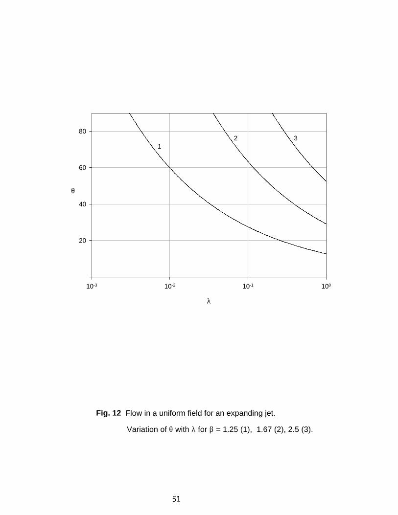
λ

10-3 10-2 10-1 100

θ

20

40

60

80

12 3

Fig. 12 Flow in a uniform field for an expanding jet.

Variation of θ with λ for β = 1.25 (1), 1.67 (2), 2.5 (3).

λ

10-3 10-2 10-1 100

θ

1

10

100

12 3

Fig. 13 Flow in a uniform field for an expanding jet.

Variation of θ with λ in a log-log scale for β = 1.25 (1),

1.67 (2), 2.5 (3).

θ0

θ0

0

0

1

1

x

x

y

y

a)

b)

A

St

Fig. 14 Schematic diagram of the post-critical profiles of a contracting jetfor poor (a) and good (b) wettability of the duct walls.

θ0

θ0

θθ0

θ0 θ0

θ

θ0

0

0

0

0 0

0

0

0

1

1

1

1 1

1

1

1

x

x

x

x x

x

x

x

y

y

y

y y

y

y

y

a)

d)

f)

g) h)

e)

c)

b)

St

St

St

St St

Fig. 15 Schematic diagram of the post-critical profiles for anexpanding jet.

gB

x

0.0 0.2 0.4 0.6 0.8 1.0

h

1.00

1.02

1.04

1.06

1.08

1.10

1.12

1.14

Fig. 16 Flow in a uniform field. Variation of the jet thickness with x

for a subcritical flow, β = 1.064 (1) and supercritical flows for

β = 1.07 and for θ0 = 150o (2) and 30o (3). Critical value of ∆h = 0.075

is shown with a straight line. Here λ = 10-4.

12

3

x

0 1 2 3 4 5

h

1.0

1.5

2.0

2.5

3.0

Fig. 17 Straight jet pouring into a draining duct in a uniform field.

Here λ = 0.1, β = 1.25. Pinned-end conditions (thick solid straight line);

given contact angle (thich broken straight line).

θ

θ0

x

-0.01 0.00 0.01 0.02 0.03 0.04

h

0.995

1.000

1.005

1.010

1.015

1.020

1.025

Fig. 18 Liquid bridge between two ducts of a slightly different size.

Here λ = 0.0001, β = 5.

wall

wall

bridge

fluid

x

0 5 10 15 20 25 30

h

0.5

0.6

0.7

0.8

0.9

1.0

1.1

Fig. 19 Flow in a step-like nonuniform field. Variation of the jet thickness with x

for x0 = 20, λ = 10-4 (1), x0 = 20, λ = 0.1 (2), x0 = 20, λ = 1 (3),

x0 = 5, λ = 10-4 (4), x0 = 5, λ = 0.1 (5), x0 = 5, λ = 1 (6). Here E = -1, Binf = 0.6,

ζ = 1, δ = 0. The curves for λ = 0 coincide with those for λ = 10-4.

1

23

4

56

x

0 10 20 30 40 50

h

0.9

1.0

1.1

1.2

1.3

1.4

1.5

Fig. 20 Flow in a step-like nonuniform field. Variation of the jet thickness with x

for x0 = 20, λ = 1, 0.2, 10-4 (1), x0 = 0, λ = 1 (2), x0 = 0, λ = 0.1 (3),

x0 = 0, λ = 0 (formula (18a)) (4). Here E = -1, Binf = 1.4, ζ = 0.2, δ = 0.

1

42

3

xN

0 1 2 3 4 5 6 7 8 9 10

h

0

1

2

3

4

Fig. 21 Slender inertial jet in a uniform field for λ = 0 and for β = infinity (1), 4 (2), 2 (3),

0.57 (4), 1 (5), 10 (6), and pure-gravity solution (Eq. (50)) for β = 10 (7).

12

3

4

5

6 7

x

0 2 4 6 8 10

h

1.00

1.05

1.10

1.15

1.20

1.25

1.30

12

3

4

Fig. 22 Inertial flow in a uniform field. Variation of the jet thickness with x

for β = 1.25, λ = 0.004 and N = infinity (1), 10 (2), 3 (3), 1 (4).

x

0 5 10 15 20 25 30 35 40 45 50

h

0.5

0.6

0.7

0.8

0.9

1.0

1.1

Fig. 23 Inertial flow in a step-like nonuniform field. Variation of the jet thickness with x

for x0 = 20, λ = 1 and for N = infinity (1), 10 (2), 3 (3), 1(4). Here E = -1, Binf = 0.6,

ζ = 1, δ = 0.

1

23 4

x

0 10 20 30 40 50

h

0.9

1.0

1.1

1.2

1.3

1.4

1.5

Fig. 24 Inertial flow in a step-like nonuniform field. Variation of the jet thickness with x

for x0 = 20, λ = 10-6 and for N = infinity (1), 1 (2).

Here E = -1, Binf = 1.4, ζ = 0.2, δ = 0.

1

2

curtain flow(radially inward)

~N-1

r

LM flow

Brad

outer chamber wall

Fig. 25 Part of a radial-poloidal cross-section of a tokamak.Schematic diagram of an axisymmetric curtain flowing radiallyinto the plasma chamber.

B

gB

tokamakperimeter

overlappingliquid curtains

electrodes

electrodes

Fig. 26 A system of overlapping liquid metal curtains covering the divertor area.Each curtain is transverse to a local three-component field. The curtainthickness may be controlled by the electrodes. If the field direction varies

significantly along the flow, the electrodes may be curved. The inclinationof a curtain to gravity plays no role as artificial gravity in the requireddirection is created by the electric field.