FLOW MODELING IN A MATRIX OF SPHERES

___________

A Thesis

Presented

to the Faculty of

California State University, Chico

___________

In Partial Fulfillment

of the Requirements for the Degree

Master of Science

in

Geosciences

Hydrology/Hydrogeology Option

___________

by

© Mark M. Menard 2004

Spring 2004

FLOW MODELING IN A MATRIX OF SPHERES

A Thesis

by

Mark M. Menard

Spring 2004

APPROVED BY THE DEAN OF THE SCHOOL OF GRADUATE, INTERNATIONAL, AND SPONSORED PROGRAMS:

Robert M. Jackson, Ph.D.

APPROVED BY THE GRADUATE ADVISORY COMMITTEE: Gregory Taylor, Ph.D. Gregory Taylor, Ph.D., Chair Graduate Coordinator K. R. Gina Johnston, Ph.D. Frank E. Burk, Ph.D.

ii

PUBLICATION RIGHTS

No portion of this thesis may be reprinted or reproduced in any

manner unacceptable to the usual copyright restrictions without the written

permission of the author.

iii

ACKNOWLEDGMENTS

Paratherm RI is a trademarked product of Paratherm Corporation,

Conshohocken, PA.

iv

TABLE OF CONTENTS

LIST OF TABLES viii

LIST OF FIGURES ix

ABSTRACT xi

CHAPTER I 1

INTRODUCTION 1

Background 1

Groundwater Flow Basics 4

The Navier-Stokes Equations and 6

the Continuity Equation 6

Hagen-Poiseuille Flow and Hydraulic Radius Theory 8

Reynolds Numbers 9

Flow and Pressure Loss in Porous Media 10

Flow Modeling 11

Purpose of the Study 12

CHAPTER II 13

LITERATURE REVIEW 13

Early Experiments 13

Later Experiments 17

Mathematical Characterization 23

Meta-studies 25

CHAPTER III 28

METHODS 28

v

Design and Construction of the 29

MIR-PTV Flow System 29

Design and Construction of the Flow Modules 35

Measurement of Mineral Oil 37

Physical Properties 37

Calibration of Pressure Transducers 42

Calibration of MIRFS Flow Rates 42

Particle Tracking 43

Summary of Methods 44

CHAPTER IV 45

RESULTS AND ANALYSIS 45

Flow Module Characteristics 45

Fluid Physical Properties 47

Pressure Transducer Calibrations 49

Flow Rate Pressure-loss Relationships 52

PTV Kinematics 57

Qualitative Flow Observations 58

Summary of Results and Analysis 61

CHAPTER V 62

MATHEMATICAL MODELING 62

Sphere Geometry 62

Matrix Algebra 66

An Analytic Approach 66

vi

Summary of Mathematical Modeling 69

Limitations of the Study 69

Conclusions 70

REFERENCES 72

APPENDIX A: PARATHERM RITM PHYSICAL PROPERTIES 77

APPENDIX B: OBSERVATION FLOW MODULE PHOTOGRAPH 79

APPENDIX C: DIFFERENTIAL PRESSURE TRANSDUCER CALIBRATION

TABLE 80

APPENDIX D: SX01 DD4 DIFFERENTIAL PRESSURE TRANSDUCER

TEMPERATURE-DEPENDENCE CURVE 82

vii

LIST OF TABLES

Table 1. Matrix Sphere Dimensional Properties..................................................46

viii

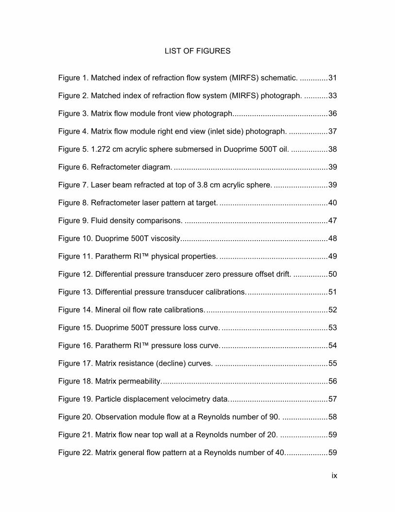
LIST OF FIGURES

Figure 1. Matched index of refraction flow system (MIRFS) schematic. .............31

Figure 2. Matched index of refraction flow system (MIRFS) photograph. ...........33

Figure 3. Matrix flow module front view photograph............................................36

Figure 4. Matrix flow module right end view (inlet side) photograph. ..................37

Figure 5. 1.272 cm acrylic sphere submersed in Duoprime 500T oil. .................38

Figure 6. Refractometer diagram. .......................................................................39

Figure 7. Laser beam refracted at top of 3.8 cm acrylic sphere. .........................39

Figure 8. Refractometer laser pattern at target. ..................................................40

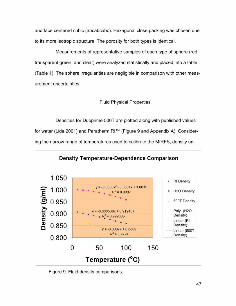
Figure 9. Fluid density comparisons. ..................................................................47

Figure 10. Duoprime 500T viscosity....................................................................48

Figure 11. Paratherm RI™ physical properties. ..................................................49

Figure 12. Differential pressure transducer zero pressure offset drift. ................50

Figure 13. Differential pressure transducer calibrations......................................51

Figure 14. Mineral oil flow rate calibrations.........................................................52

Figure 15. Duoprime 500T pressure loss curve. .................................................53

Figure 16. Paratherm RI™ pressure loss curve. .................................................54

Figure 17. Matrix resistance (decline) curves. ....................................................55

Figure 18. Matrix permeability.............................................................................56

Figure 19. Particle displacement velocimetry data..............................................57

Figure 20. Observation module flow at a Reynolds number of 90. .....................58

Figure 21. Matrix flow near top wall at a Reynolds number of 20. ......................59

Figure 22. Matrix general flow pattern at a Reynolds number of 40....................59

ix

Figure 23. Matrix flow near bottom wall at a Reynolds number of 40..................60

Figure 24. Matrix flow near bottom wall at a Reynolds number of 80..................60

Figure 25. Rhombohedral sphere packing 3-dimensional top view diagram.......63

Figure 26. Rhombohedral sphere packing 2-dimensional geometry diagram. ....63

Figure 27. Rhombohedral sphere packing 3-dimensional side view diagram. ....64

Figure 28. Rhombohedral sphere packing 2-dimensional aperture geometry

diagram........................................................................................................65

Figure 29. Flow geometry unit cell location diagram. ..........................................67

Figure 30. Flow geometry unit cell diagram. .......................................................68

x

ABSTRACT

FLOW MODELING IN A MATRIX OF SPHERES

by

© Mark M. Menard 2004

Master of Science in Geosciences

Hydrology/Hydrogeology Option

California State University, Chico

Spring 2004

This study of porous media fluid dynamics combines mathematical

characterization with physical modeling with a special focus on the fundamental

physics of pressure loss as a function of Reynolds numbers. Pressure loss

departure from linearity is shown to occur at a Reynolds number of eight,

apparently as a result of boundary layer growth and decay and narrowing flow

tubes. A matched index of refraction flow modeling system using mineral oil and

acrylic was combined with particle tracking velocimetry for quantitative and

qualitative analysis of porous media flow. A liquid/solid refractometer was

developed for refractive index matching. A falling liquid sphere viscometer was

also designed and employed to determine mineral oil viscosity. A mathematical

xi

approach based on the Navier-Stokes and continuity equations was proposed

and partially developed for rigorous treatment of pressure losses in ordered

porous media.

xii

CHAPTER I

INTRODUCTION

The following study is focused on the underlying mathematical and

physical principles responsible for pressure losses of fluid flow through porous

media.

Background

The fluid mechanical properties of single phase and multi-phase flow

through porous media are of primary importance in hydrogeology and many other

scientific disciplines. Hydrologists are concerned with fundamentals such as

pressure head losses as a function of Reynolds numbers (decline curves) and

aquifer media geometric properties. Environmental scientists are interested in

contaminant dispersion as it relates to flow in both the hydrosphere and the at-

mosphere. Soil scientists seek to understand basic hydrodynamic flow and

transport characteristics. Chemical engineers study filtration, thermodynamics,

chemical kinetics, and other phenomena as they relate to fluid flow through

porous media. Petroleum, mechanical, and civil engineers, along with nuclear

scientists, medical researchers, mathematicians, and many others also conduct

basic and applied research of fluid flow through porous media. Because of the

wide diversity of interest in the naturally complex nature of porous media fluid

mechanics (e.g., Bakhmmeteff and Feodoroff 1937; Bennethum and Georgi

1

1997; Borishanskii et al. 1980; Mori et al. 1999; Rose 1945; Schneebeli 1955; Tiu

1997; Wright 1968; Trussell and Chang 1999), relevant literature is widely scat-

tered and uncoordinated, resulting in duplicated efforts and a lack of general fo-

cus. Fortunately, with the advent of electronic publishing and online retrieval an

accelerated and more focused development in the realm of porous media hydro-

dynamics can be expected. The present inquiry includes a comprehensive litera-

ture review of experiments and theoretical underpinnings, including several meta-

studies of previous research.

Until the last two or three decades, the study of flow through porous

media has been obscured by the non-uniformity and opacity of materials and dif-

ficulties inherent in measuring fluid flow fields (Bear 1972; Scheidegger 1974).

Far more sophisticated flow modeling is now possible due to new technologies

and experimental designs such as matched index of refraction flow systems, dif-

ferential pressure transducers, and digital cinematography (e.g., Choi et al. 2001;

Moroni, Cushman, and Cenedese 2003; Northrup, Kulp, and Angel 1993;

Peurrung, Rashidi, and Kulp 1995). These new tools allow for the transition from

statistical, empirical, and dimensional analysis into the realm of rigorous and fun-

damental insights based on first principles. Thus the present study has been

designed to physically model an idealized aquifer media using state-of-the-art

equipment with a primary focus on decline curves and the fundamental mechan-

ics responsible for them.

Vagaries of porous media properties and model boundary conditions

often confound analysis of fluid flow fundamentals. Although numerous media

2

grain properties have been parameterized (e.g., Bakhmmeteff and Feodoroff

1937; Rose 1945; Rose and Rizk 1949; Wright 1968), including shape, rough-

ness, size distribution, and orientation, and packing, their exact mathematical

relationship to flow non-laminarity has remained elusive. Media field properties

have also been extensively treated—chiefly pore size, porosity, effective porosity,

tortuosity, isotropy, and homogeneity (Schneebeli 1955; Thiruvengadam and

Kumar 1997; War, 1939)—yet have largely escaped precise quantitative physics.

Boundary conditions, often minimized or ignored (Bakhmmeteff and Feodoroff

1937; Hamdan 1994; McWhirter, Crawford, and Klein 1997; Rose and Rizk 1949;

Ward 1939; Wright 1968), include fluid local accelerations (e.g. from pump ir-

regularities), wall effects, upstream and downstream flow instabilities (e.g. from

piping and media containment screens), and numerous other conditions. Under-

standably, study has been primarily limited to dimensional analysis and empiri-

cism (Borishanskii 1980; Sen 1989). Typical treatment (e.g. Rose and Rizk 1949;

Thiruvengadam and Kumar 1997) of media vagaries includes application of

Buckingham pi theorem (Buckingham 1914); one or more dimensionless pi terms

are assembled (each representing a media property), and given coefficients to

form a polynomial which best fits the data. Although this general methodology

does shed some light on the basic causes of non-laminar flow and non-linear

pressure losses, complete illumination of the intrinsic nature of energy dissipation

in non-laminar flow will require precise modeling with commensurately rigorous

mathematical treatment.

3

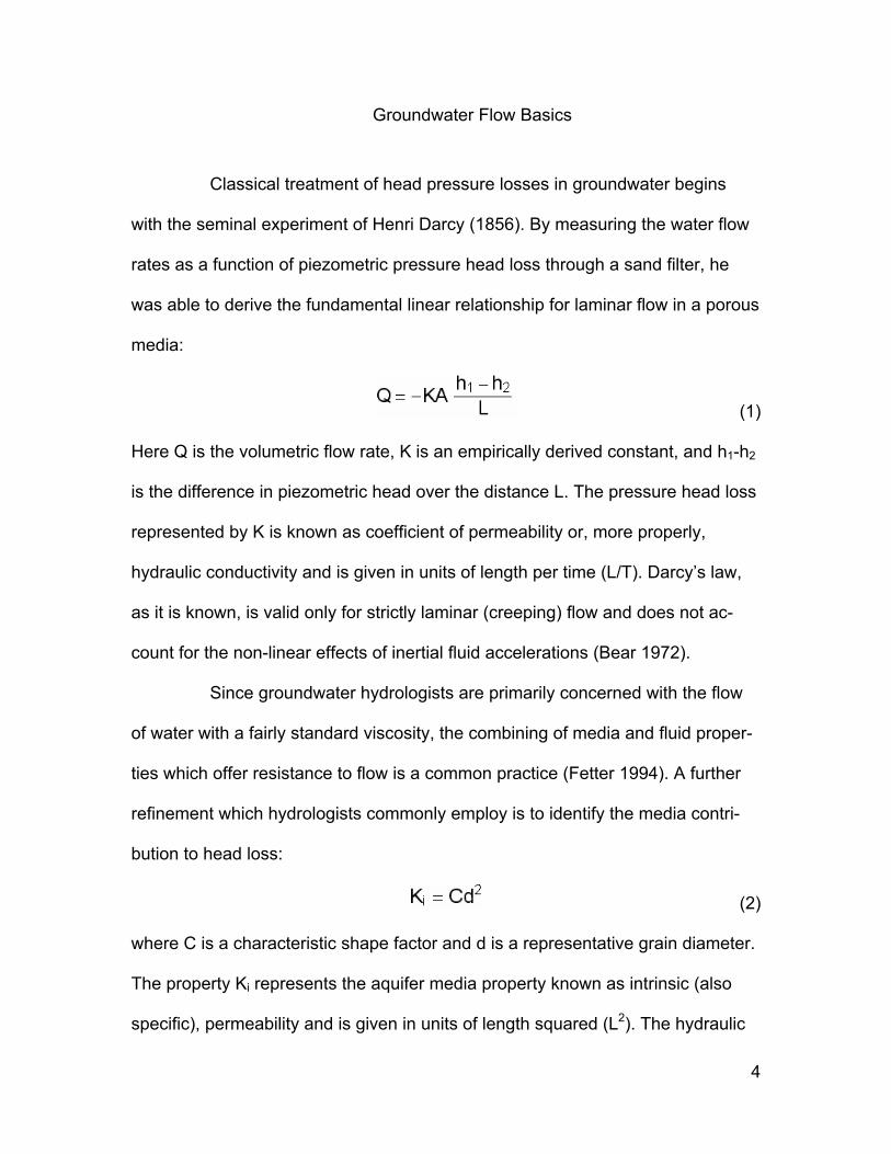
Groundwater Flow Basics

Classical treatment of head pressure losses in groundwater begins

with the seminal experiment of Henri Darcy (1856). By measuring the water flow

rates as a function of piezometric pressure head loss through a sand filter, he

was able to derive the fundamental linear relationship for laminar flow in a porous

media:

(1)

Here Q is the volumetric flow rate, K is an empirically derived constant, and h1-h2

is the difference in piezometric head over the distance L. The pressure head loss

represented by K is known as coefficient of permeability or, more properly,

hydraulic conductivity and is given in units of length per time (L/T). Darcy’s law,

as it is known, is valid only for strictly laminar (creeping) flow and does not ac-

count for the non-linear effects of inertial fluid accelerations (Bear 1972).

Since groundwater hydrologists are primarily concerned with the flow

of water with a fairly standard viscosity, the combining of media and fluid proper-

ties which offer resistance to flow is a common practice (Fetter 1994). A further

refinement which hydrologists commonly employ is to identify the media contri-

bution to head loss:

(2)

where C is a characteristic shape factor and d is a representative grain diameter.

The property Ki represents the aquifer media property known as intrinsic (also

specific), permeability and is given in units of length squared (L2). The hydraulic

4

force driving groundwater results from gravity acting on the mass of fluid (ρg) or

simply the specific weight (γ) of the fluid. The dynamic viscosity (µ) of ground-

water is the fluid property which resists this hydraulic force:

(3)

where µ has dimensions of mass per length and time (M/LT), τ is the fluid stress

and dU/dy is the rate of fluid strain. The relationship between hydraulic conduc-

tivity and the fluid and media properties may be given as:

(4)

Or, in terms of kinematic viscosity (see equation 16),

(5)

By combining equations 1, 2, and 4, Darcy’s Law may also be expressed as:

(6)

For a Newtonian fluid such as groundwater at a given temperature, pressure loss

as a function of fluid mean velocity simplifies to:

(7)

where ∆P is the pressure loss for a given bed length—equivalent to γ(h1-h2)/L, CS

is an empirical coefficient, UD is the superficial (Darcy) velocity (equal to dis-

charge divided by area normal to translational flow), and µ and d are as defined

earlier. Here it is evident that pressure loss is linearly related to the fluid velocity

and inversely proportional to the grain diameter squared.

5

Effective porosity is another aquifer property which hydrogologists treat

as an important variable in analysis of aquifer flow rates:

(8)

with ne representing the ratio of interconnected pore space volume to total media

volume. The basic effect of porosity is that, owing to conservation of mass flow

rates, the average pore velocity will equal the Darcy velocity divided by the po-

rosity. The ratio Vp/Vt is obviously a general measure of the cross-sectional area

available for fluid flow. Yet Vp/Vt is also a geometric property which is closely re-

lated to specific surface (M), the ratio of pore surface area (As) to total media

volume (Vt):

(9)

Both porosity and specific surface are reciprocally related to hydraulic radius, a

geometric parameter of significance in more advanced treatments of fluid flow.

The Navier-Stokes Equations and the Continuity Equation

The foregoing discussion of laminar groundwater flow, combining first

principles with empirically derived constants, is typical of groundwater hydrology

(e.g., Fetter 1994) and has very useful yet limited application. Further theoretical

development can be found in other disciplines that study flow in porous media

(e.g. Bear 1972; Dybbs and Edwards 1984; Perry and Green 1997; Scheidegger

1974) and draw upon numerous other facets of fluid mechanics. General under-

standing of the fluid dynamics in porous media is primarily based on inference

6

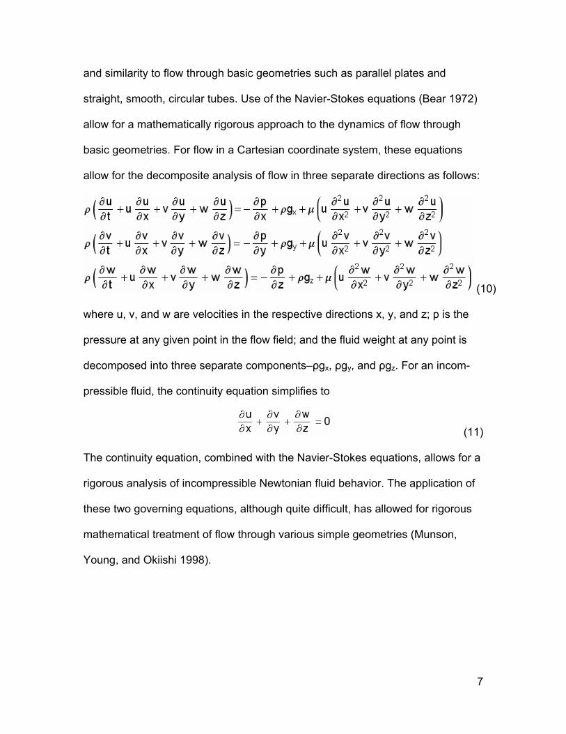
and similarity to flow through basic geometries such as parallel plates and

straight, smooth, circular tubes. Use of the Navier-Stokes equations (Bear 1972)

allow for a mathematically rigorous approach to the dynamics of flow through

basic geometries. For flow in a Cartesian coordinate system, these equations

allow for the decomposite analysis of flow in three separate directions as follows:

(10)

where u, v, and w are velocities in the respective directions x, y, and z; p is the

pressure at any given point in the flow field; and the fluid weight at any point is

decomposed into three separate components–ρgx, ρgy, and ρgz. For an incom-

pressible fluid, the continuity equation simplifies to

(11)

The continuity equation, combined with the Navier-Stokes equations, allows for a

rigorous analysis of incompressible Newtonian fluid behavior. The application of

these two governing equations, although quite difficult, has allowed for rigorous

mathematical treatment of flow through various simple geometries (Munson,

Young, and Okiishi 1998).

7

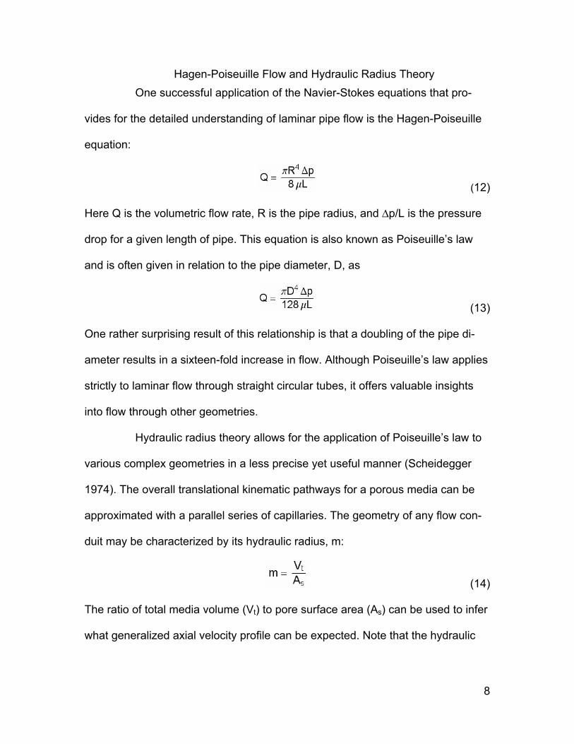
Hagen-Poiseuille Flow and Hydraulic Radius Theory One successful application of the Navier-Stokes equations that pro-

vides for the detailed understanding of laminar pipe flow is the Hagen-Poiseuille

equation:

(12)

Here Q is the volumetric flow rate, R is the pipe radius, and ∆p/L is the pressure

drop for a given length of pipe. This equation is also known as Poiseuille’s law

and is often given in relation to the pipe diameter, D, as

(13)

One rather surprising result of this relationship is that a doubling of the pipe di-

ameter results in a sixteen-fold increase in flow. Although Poiseuille’s law applies

strictly to laminar flow through straight circular tubes, it offers valuable insights

into flow through other geometries.

Hydraulic radius theory allows for the application of Poiseuille’s law to

various complex geometries in a less precise yet useful manner (Scheidegger

1974). The overall translational kinematic pathways for a porous media can be

approximated with a parallel series of capillaries. The geometry of any flow con-

duit may be characterized by its hydraulic radius, m:

(14)

The ratio of total media volume (Vt) to pore surface area (As) can be used to infer

what generalized axial velocity profile can be expected. Note that the hydraulic

8

radius is simply the reciprocal of specific surface. Here again, analysis is con-

fined to strictly laminar flow.

Reynolds Numbers

The transition from laminar to turbulent flow has been studied exten-

sively and has been observed visually by filming tracer dye injected into liquid

flowing through transparent pipes (Munson, Young, and Okiishi 1998). The

common mathematical characterization of transition to turbulence is based on

Osborne Reynolds’ (Perry and Green 1997) dimensional analysis of the ratio of

inertial to viscous forces given by

(15)

where Re is the Reynolds number, ρ is the fluid density, U is the tangential

velocity, d is a length parameter normal to the flow (e.g. pipe diameter), and µ is

the dynamic viscosity of the fluid. The kinematic viscosity ( ) is related to the dy-

namic (or absolute) viscosity and density

(16)

A more common means of expressing the Reynolds equation thus becomes

(17)

Transition from laminar to fully turbulent flow in smooth, straight pipes has been

observed at Reynolds numbers from 2100 to 4000 (Munson, Young, and Okiishi

1998). Because of the mixing inherent in non-laminar flow, transfer of momentum

9

and energy are much greater, resulting in significantly increased rates of disper-

sion, heat transfer, and pressure loss.

Flow and Pressure Loss in Porous Media

Although Darcy’s law is useful for predicting flow rates, pressure

losses, and other values in analysis of laminar flow, the empirical nature of this

widely used tool precludes in-depth understanding of flow through porous media.

Additionally, evaluation of fluid properties in higher inertial regimes requires the

integration of various mathematical tools. For example, study of porous media

laminar flow can be placed on a more basic footing by applying hydraulic radius

theory (Bear 1972; Scheidegger 1974) to homogeneous, isotropic matrix ge-

ometry such as uniformly sized, rhombohedrally packed spheres. Under laminar

conditions, hydraulic radius theory seems to meet the requirements of true

dynamic similarity, where logical prediction of pressure losses can be made and

transferred from one system to another. General empirical analysis of decline

curves can be evaluated in terms of Reynolds numbers and applying coefficients

and exponents as needed to fit data (Rose 1945; Rose and Rizk, 1949). The

Forchheimer equation (Camacho, Vasquez, and Padilla 1998; Pedras and de

Lemos 2001) is one such popular formulation:

(18)

Here α and β are coefficients empirically derived to adjust the viscous and inertial

terms to fit the observed pressure energy losses (Thiruvengadam and Kumar

1997). Many others (Sen 1989; Trussell and Chang 1999; Ward 1939) have of-

10

fered similar expressions to match observations; one popular variation is of the

following form:

(19)

with a and b again being empirical constants. More robust mathematical evalua-

tions (e.g., Antohe and Lage 1997; Lahbabi and Chang 1985; Macedo, Costa,

and Almeida 2001; Mohseni et al. 2003; Pedras and de Lemos 2001) of non-

laminar flow require the use of comprehensive flow equations (i.e., Navier-

Stokes) as well as similar geometric restrictions.

Flow Modeling

Flow modeling provides a means of studying phenomena not observ-

able in natural settings. Models may be physical or mathematical analogues

which satisfactorily measure or predict responses to given stimuli. Physical mod-

els often provide answers to questions that are mathematically intractable.

Mathematical models may provide rigorous characterization and precise predic-

tion of relationships not fully understood through physical observation alone.

Combining carefully designed and constructed physical models with mathemati-

cal modeling based on fully understood basic precepts provides the most com-

prehensive and meaningful approach to scientific enigmas such as non-laminar

flow and turbulence. Additionally, an ideal model should be cost-effective, pro-

vide precise and comprehensive data, and be amenable to dimensional analysis

or rigorous analytical mathematical treatment.

11

Purpose of the Study

The primary intent of this study is to further understanding of the basic

physics behind decline curves by means of thorough mathematical treatment and

model observations. An ideal physical model is geometrically, dynamically, and

kinematically similar to its prototype. True similarity allows for a model to operate

at a different scale than the prototype with identical responses to inputs (Munson,

Young, and Okiishi 1998). In the present study, the experimental model was de-

signed to parallel ideal groundwater flow; faithful adherence to Reynolds num-

bers combined with conservative treatment of boundary conditions was em-

ployed to this end. A careful approach to scaling and fluid observation using

macro and zoom lenses on a digital video camera to film suspended particle tra-

jectories has been used for qualitative and quantitative flow analysis. The appa-

ratus in this study was engineered and constructed to better understand the fluid

dynamics behind decline curves.

12

CHAPTER II

LITERATURE REVIEW

Porous media flow modeling has evolved considerably from Henry

Darcy’s basic water and sand constant-head permeameter experiments. One re-

cent experiment (Marulanda, Culligan, and Germaine 2000) examined two-phase

flow through disordered media using matched indexed of refraction (MIR) and

particle tracking velocimetry (PTV); air sparging was investigated via a small

charge-coupled device (CCD) camera mounted inside a centrifuge which video-

taped liquid/gas flow at varying centripetal accelerations. Computers can be em-

ployed to evaluate digital video images and generate three-dimensional velocity

vector fields (Haam and Brodkey 2000; Moroni, Cushman, and Cendese 2003). It

is now possible to precisely control flow over an extremely wide range of

Reynolds numbers—from less than 0.01 to greater than 100,000 (Rose and Rizk

1949). Precision control and measurement facilitates the transition from “black

box” empirical analysis to the application of governing flow equations and basic

mechanics to match observations.

Early Experiments

Henry Darcy is regarded as the original pioneer of modern analysis of

porous media flow (Fetter 1994). By measuring head pressure losses of water

flowing through a sand column, he was able to identify a linear relationship be-

13

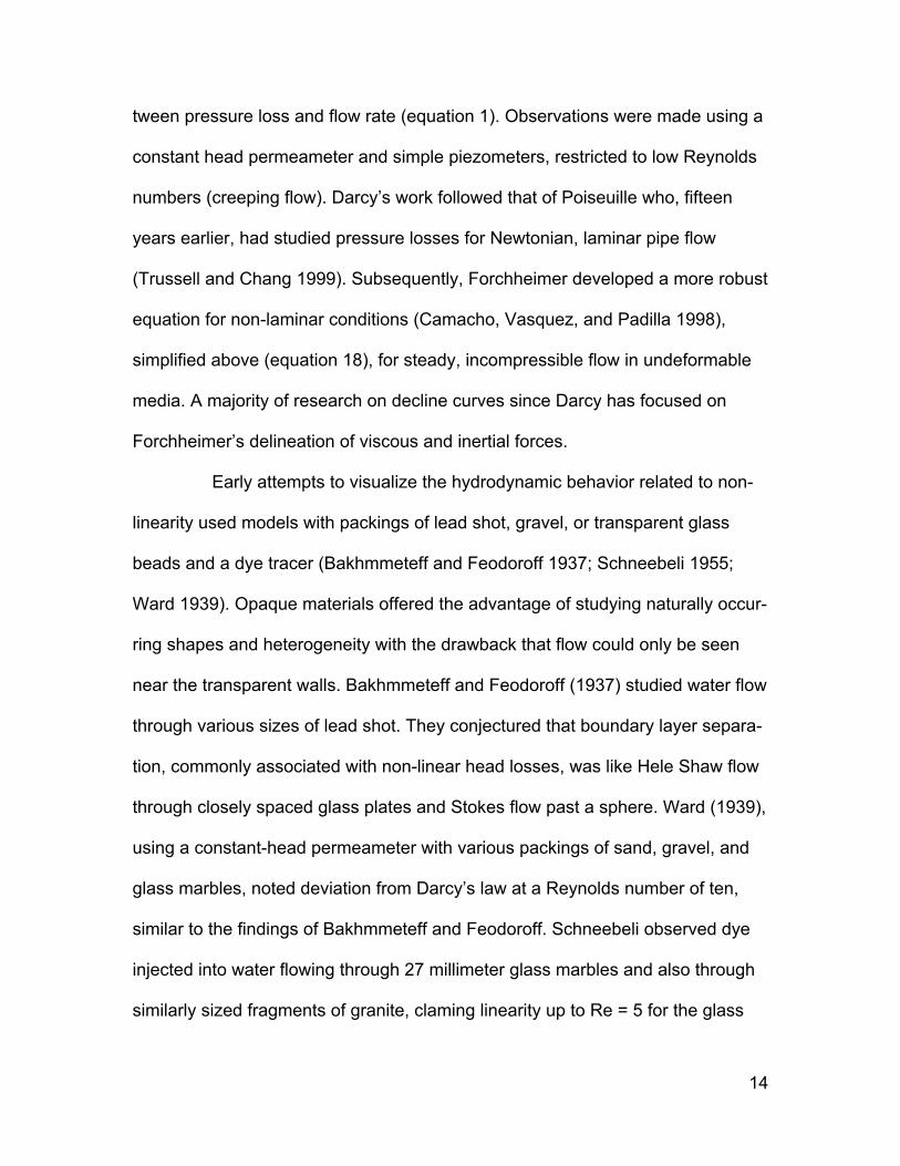
tween pressure loss and flow rate (equation 1). Observations were made using a

constant head permeameter and simple piezometers, restricted to low Reynolds

numbers (creeping flow). Darcy’s work followed that of Poiseuille who, fifteen

years earlier, had studied pressure losses for Newtonian, laminar pipe flow

(Trussell and Chang 1999). Subsequently, Forchheimer developed a more robust

equation for non-laminar conditions (Camacho, Vasquez, and Padilla 1998),

simplified above (equation 18), for steady, incompressible flow in undeformable

media. A majority of research on decline curves since Darcy has focused on

Forchheimer’s delineation of viscous and inertial forces.

Early attempts to visualize the hydrodynamic behavior related to non-

linearity used models with packings of lead shot, gravel, or transparent glass

beads and a dye tracer (Bakhmmeteff and Feodoroff 1937; Schneebeli 1955;

Ward 1939). Opaque materials offered the advantage of studying naturally occur-

ring shapes and heterogeneity with the drawback that flow could only be seen

near the transparent walls. Bakhmmeteff and Feodoroff (1937) studied water flow

through various sizes of lead shot. They conjectured that boundary layer separa-

tion, commonly associated with non-linear head losses, was like Hele Shaw flow

through closely spaced glass plates and Stokes flow past a sphere. Ward (1939),

using a constant-head permeameter with various packings of sand, gravel, and

glass marbles, noted deviation from Darcy’s law at a Reynolds number of ten,

similar to the findings of Bakhmmeteff and Feodoroff. Schneebeli observed dye

injected into water flowing through 27 millimeter glass marbles and also through

similarly sized fragments of granite, claming linearity up to Re = 5 for the glass

14

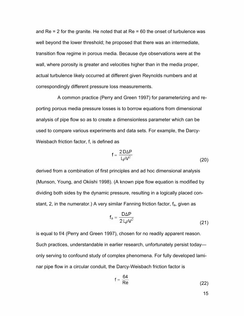
and Re = 2 for the granite. He noted that at Re = 60 the onset of turbulence was

well beyond the lower threshold; he proposed that there was an intermediate,

transition flow regime in porous media. Because dye observations were at the

wall, where porosity is greater and velocities higher than in the media proper,

actual turbulence likely occurred at different given Reynolds numbers and at

correspondingly different pressure loss measurements.

A common practice (Perry and Green 1997) for parameterizing and re-

porting porous media pressure losses is to borrow equations from dimensional

analysis of pipe flow so as to create a dimensionless parameter which can be

used to compare various experiments and data sets. For example, the Darcy-

Weisbach friction factor, f, is defined as

(20)

derived from a combination of first principles and ad hoc dimensional analysis

(Munson, Young, and Okiishi 1998). (A known pipe flow equation is modified by

dividing both sides by the dynamic pressure, resulting in a logically placed con-

stant, 2, in the numerator.) A very similar Fanning friction factor, fa, given as

(21)

is equal to f/4 (Perry and Green 1997), chosen for no readily apparent reason.

Such practices, understandable in earlier research, unfortunately persist today—

only serving to confound study of complex phenomena. For fully developed lami-

nar pipe flow in a circular conduit, the Darcy-Weisbach friction factor is

(22)

15

The value of f increases with non-laminar conditions, where it is also functionally

related to the conduit wall roughness. The use of properly standardized friction

factors is useful and perhaps necessary for comparison of different media per-

meabilities, though a basic understanding of the physics behind decline curves

perhaps may be better understood simply by examining pressure loss as a func-

tion of Reynolds numbers through an ordered, uniform geometry.

Two of the most thorough and oft-cited sets of investigations of porous

media pressure losses are those of Rose (1945) and Rose and Rizk (1949),

where decline curves were generated for a large variety of shapes and sizes over

a wide range of Reynolds numbers. In both studies water is forced through

opaque, undeformable porous media. Rose (1945) developed a dimensionless

equation with the head loss (divided by the grain diameter), given as a function of

eight independent parameters. Several are eliminated by experimental design

(e.g. smooth, spherical lead shot eliminates the roughness and shape fac-

tors).The remainder are controlled and varied so as allow for empirical evaluation

of data. Rose and Rizk (1949) examined flow through an interesting variety of

materials, from spheres and cubes to nails and oddly shaped electrical insula-

tors. Decline curve data are plotted on log-log coordinates along with data from

previous studies. Although there is apparently very good agreement amongst the

data, the use of log-log graphs tends to mask trends along specific narrow

ranges of interest (e.g., 0.1 < Re < 20). Thoughtful consideration of boundary

conditions is applied to bed length and to correct for wall-effect (the higher per-

meability at the walls).

16

Two additional studies (Barr 2001; Thiruvengadam and Kumar 1997)

are included with the early experiments owing to their relatively outdated meth-

ods. Thiruvengadam and Kumar (1997) generated decline curves for water flow

through glass spheres and crushed rock in a radial flow permeameter. They ap-

plied the Forchheimer equation to their measurements without any notable dis-

coveries. Barr’s (2001) analysis of experimental data which he collected for his

1949 master’s thesis offers little insight into decline curve physics. Pressure loss

as a function flow rate was made for water at various temperatures flowing

through several media, “lead pellets, sand, and taconite.” His discussion of the

“effective length of eddies,” is limited to ex post facto speculation regarding tur-

bulence. Here the turbulence was not actually measured but rather inferred from

decline curves.

Later Experiments

Modern experimental studies of decline curves (Dybbs and Edwards

1984; Johnston, Dybbs, and Edwards 1975; McFarland and Dranchuk 1976;

Wright 1968) capitalizing on new technology have provided improved imaging

and measurement of flow through porous media. Velocity vector fields, turbu-

lence intensities, boundary layer separations, and complex flow patterns deep

inside porous media have been visualized and quantified with varying degrees of

detail and precision. These new tools have also been applied to many other as-

pects of fluid mechanics, including free-surface flow (Roy et al. 1999; Weitbrecht,

Kuhn, and Jirka 2002), multi-phase flow (Choi et al. 2002; Haam, Brodkey,

17

Klaboch et al. 2000; Haam and Brodkey 2000), air sparging (Marulanda,

Culligan, and Germaine 2000), and flow through natural, opaque media

(Garrouch and Ali 2001; Mori et al. 1999; Zhou 2003).

Wright (1968) presents two differing sets of experiments. The first uses

an oscilloscope coupled with hot-wire anemometers to provide turbulence inten-

sity measurements of air flowing through course sand and crushed rock at fairly

high Reynolds numbers (51 < Re < 2080). Film photographs of oscilloscope

readings provide high temporal resolution quantification of turbulence trends at

several test bed locations. Maximum “turbulence intensity,” was stated to occur

at 300 < Re < 800, after which amplitude decreased and frequency increased

rapidly.

Wright’s (1968) second set of experiments were conducted using a ra-

dial (converging flow), permeameter constructed with transparent acrylic walls.

Pressure-loss of water flowing through two grades of well-rounded sand was

measured with mercury manometers connected to various points in the flow bed.

Flow was visualized via injection of process-black dye into the flow field. Wright

reported that dye filaments were well-intact at Re = 70 with vortices appearing

behind some grains at Re = 106. Yet deviation from Darcy’s law was ascertained

to occur at Re = 2, considerably lower than the onset of visibly non-laminar flow.

Wright postulated the existence of four fairly distinct flow regimes, given as,

“laminar, steady inertial, turbulent transition, and fully ‘turbulent’” (pp. 867-868).

McFarland and Dranchuk (1976) used streaming birefringence to

visualize the transition from laminar to turbulent flow in porous media. A colloidal

18

suspension of milling yellow dye was pumped up to a constant head reservoir

where it descended past a flow-control needle-valve into a flow module. The four

flow modules consisted of two arrangements, cubic and orthorhombic, of thinly

packed (n = 2) precision stainless steel ball bearings in two sizes. The spheres

were embedded half-way into the clear acrylic walls so as to eliminate the wall-

effect. Turbulence was reported at values ranging from Re = 123 to Re = 251.

However, the authors’ generalization of transition to turbulence as a discrete

function seems simplistic.

One of the more thoughtful investigations of decline curves is Dybbs

and Edwards (1984) matched index of refraction (MIR) flow modeling through

two different complex ordered geometries. One flow module, similar in many re-

spects to the matrix used in the present study, consisted of 485 rhombohedrally

packed 1.27 cm (1/2 inch) acrylic spheres. Alternating layers of 37 and 27

spheres were held fast by acrylic strips fabricated to hold the spheres inside a

clear conduit without the need for adhesives. They reported a void fraction of

0.394, defined by the following ratio

(23)

where ne is the effective porosity as defined earlier (equation 8). This translates

to a porosity of 0.283. Their measured intrinsic permeability, Ki, was given as 8.6

± 0.9 x 104 Darcys (8.5 ± 0.9 x 10-4 cm2). This same flow module was described

in greater detail in an earlier publication (Johnston, Dybbs, and Edwards 1975).

In the early paper, fluid flow equated to Re = 0.158 and point velocity profiles

were obtained using laser Doppler anemometry. Due to the wall effect, axial

19

velocities at the wall ranged up to five times the characteristic velocities in the

matrix proper. Although they claimed an, “average interstitial velocity [of] 0.100±

0.10 cm/sec, calculated from the volumetric flow rate,” all five velocity profile

transects revealed a much lower average velocity for the matrix proper, obviously

an artifact of preferential flow at the walls. Thus it would seem that the reported

Reynolds number is artificially high, and the true intrinsic permeability would be

somewhat lower for the matrix.

The primary focus of Dybbs and Edwards (1984) was centered on data

collected on the second flow module, a complex array of eighty-eight transparent

acrylic and glass solid cylinders. Although the array was ordered, the geometry

was fairly complex, with the rods arranged in four different orientations. The het-

erogeneous porosity of the matrix varied from 0.33 to 0.79. Two silicone oils were

mixed to closely match the refractive index of the Pyrex glass. Filming of dye in-

jected over a range of Reynolds numbers from creeping to turbulent permitted a

qualitative analysis of flow through porous media. Laser anemometry was used

to generate velocity profiles at flow rates corresponding to Re = 0.8, 7, and 28.

Velocity measurements were made in two directions and computed for the third

direction using an algorithm based on the continuity equation. Carefully con-

structed velocity profiles were used to quantitatively study flow inside a porous

medium.

Dybbs and Edwards’ rigorous approach to modeling enabled them to

see deviation form Darcy’s law in a new light. Fairly high temporal and spatial

resolution velocity profiles were used to show that, unlike the case with pipe flow,

20

boundary layer development cannot be treated as complete in porous media,

even in a steady, laminar flow regime. The authors argued that this is due to the

fact that boundary layer development must occur repeatedly in each pore, es-

sentially being destroyed at the end of each pore by convergent flow from

neighboring pores. In the authors’ words,

An important and interesting feature of the flow through the porous me-

dia studied is that there is no change in the flow structure at a given Reynolds

number from pore space to pore space as one goes downstream. But in any

given pore the velocity profiles are developing (for Re > 1). Hence at any position

in the porous medium the inertial effects are important since the boundary effects

have not penetrated the core flow. This pattern of flow development repeats itself

time and time again in the pores as one proceeds downstream.

Their significant discovery allowed them to reason, “the developing of

these ‘core’ flows outside the boundary layers is the reason for the non-linear re-

lationship between pressure drop and flow rate [at such low Reynolds numbers]”

(p. 251). Their finding may be attributed to a combination of careful study, good

modeling, and new technologies.

Particle tracking velocimentry (PTV) is a fairly recent technology which

has greatly advanced modeling in fluid mechanics (Medina, Sanchez, and

Redondo 2001; Roy et al. 1999; Weitbrecht, Kuhn, and Jirka, 2002). Recent

studies of flow through porous media have combined MIR with PTV (Choi et al.

2002; Marulanda, Culligan, and Germaine 2000; Northrup, Kulp, and Angel 1993;

Peurrung, Rashidi, and Kulp 1995). PTV is a general term applied to several

21

types of fluid flow visualization that involve filming of fine suspended particles. In

particle image velocimetry (PIV), two or more exposures per frame (provided by

a strobe or pulsed laser), provide a means of recording particle paths and veloci-

ties. Particle streak velocimetry (PSV) is designed so that exposure times are

long enough for particle trajectories to be filmed as streaks, thus providing quan-

tifiable point speed and direction for flow fields, similar to velocity vector fields,

but lacking explicit information pertaining to negative velocities. Particle dis-

placement velocimetry (PDV) uses shorter exposure times; particle movement is

tracked from frame to frame. All three methods generally can use a planar laser

beam to restrict imaging to a specific transect of the flow field. Digital video lends

itself better than film to computer analysis and velocity vector field generation.

Recent porous media modeling (Haam and Brodkey 2000; Moroni,

Cushman, and Cendese 2003) has advanced MIR-PTV technology to provide

three-dimensional imaging and velocity vector fields. Haam and Brodkey (2000)

used one digital video camera with an arrangement of four mirrors to produce

stereo images of dispersed acrylic beads. Moroni, Cushman, and Cendese

(2003) used two digital video cameras to provide stereo imaging of particle

dispersion in a porous media. Although both of these studies used sophisticated

applications of new technology to porous media flow modeling, their rather

particular topics of inquiry do not relate specifically to the objectives of this study;

rather, they serve as excellent models for future experimental design and study.

22

Mathematical Characterization

Dybbs and Edwards (1984) have identified three basic analytic ap-

proaches to modeling porous media flow. The first uses the basic governing

equations and applies them to simplified geometric approximations of porous

media, for example, the Navier-Stokes equations solved for a bundle of straight,

parallel tubes. The second approach relies on statistical analysis of a random

arrangement of two-dimensional, arbitrary shapes designed as a general repre-

sentation of a porous media. The third employs time-averaged forms of the rele-

vant differential equations; semi-empirical Reynolds stress terms are required for

closure (Perry and Green 1997). The second approach may hold promise as a

heuristic study of flow through both ordered and disordered media, but sheds lit-

tle light on the basic physics. The first and third methods have been used for both

rigorous symbolic treatment and also numerical analysis of porous media physics

(Antohe and Lage 1997; Lahbabi and Chang 1985; Macedo, Costa, and Almeida

2001; Masuoka and Takatsu 1996; Mohseni et al. 2003; Nield 2000; Pedras and

de Lemos 2001; Skjetne and Auriault 1999).

Computational Fluid Dynamics (CFD) has emerged in the previous

thirty years or so as advances in computer computational power have greatly

improved numerical problem solving of complex equations. Yet, as Mohseni et al.

(2003) have noted, numerical study of high Reynolds flow may remain elusive for

some time, as:

[T]he number of degrees of freedom for a three-dimensional Navier-Stokes flow grows rapidly with Reynolds number; namely, it is propor-tional to Re9/4. Consequently, increasing the Reynolds number by a

23

factor of 2 will increase the memory size by a factor of about 5 and the computational time by an order of magnitude. (p. 524)

Hence the motivation to use averaging techniques to reduce computational re-

quirements.

Strictly speaking, a true analytic solution may be more narrowly

defined as a mathematical solution to a natural phenomenon which applies gov-

erning equations without the benefit of averaging assumptions. When applied to

a wide range of Reynolds numbers, the Navier-Stokes equations (equation 10)

are non-linear, second-order, partial differential equations. An exact description

of flow through any geometry would, in principle, be possible by solving the

Navier-Stokes equations along with the continuity equation. Unfortunately, as

Munson, Young, and Okiishi (1998) dryly point out, “there are no known analyti-

cal solutions to (equation 10) for flow past any object such as a sphere, cube, or

airplane” (p. 372).

Nield (2000) has provided a useful mathematical study of pressure loss

in porous media based on an overview of fundamental equations. In considera-

tion of the basic thermodynamics, he explains that,

[T]he bottom line is that when fluid is forced to flow unidirectionally down a channel, whether occupied by a solid porous matrix or not, the work done by the applied pressure difference has to be matched by the thermal energy, because there is no other mechanism available to achieve the balance of total energy. (p. 351)

The focus of Nield’s article is the well known D’Alembert paradox. He states,

The explanation of the apparent paradox lies in the recognition that, as pointed out by Joseph et al. (1982) [a study in which Nield was a co-author], the Forchheimer drag term models essentially a form drag effect, and involves the separation of boundary layers and wake for-mation behind solid obstacles. (p. 352)

24

A rigorous treatment of pressure loss related to boundary layers is

provided by Skjetne and Auriault (1999). They model the fluid near grain

separation zones as a “triple deck,” consisting of three layers of fluid. In their

model, the triple deck scales energy dissipation as Re5/4 as Re reaches the

upper limit. Regarding flow tube narrowing, the authors note:

There are several nonidealities observed in porous media flow. One

effect which has been noticed in simulations is that the flow tubes narrow with

increasing Reynolds number. Thus, the local velocity in the flow tubes increases

faster than the average velocity.

Their observations are consistent with the physical modeling of both

Dybbs and Edwards (1984) and the present study. Skjetne and Auriault summa-

rize their findings:

We propose that the square pressure loss in the laminar Forchheimer equation is caused by development of strong localized dissipation zones around flow separation, that is, in the viscous boundary layer in triple decks. For turbulent flow, the resulting pressure loss due to aver-age dissipation is a power 2 term in velocity. (p. 131)

Their observations might help explain the gradual transition from first to second

order dependence of pressure loss on Reynolds numbers.

Meta-studies

Several reviews of decline curve studies have been offered in the

previous two decades. Perspectives are offered from thermal and chemical engi-

neering (Borishanskii et al. 1980), hydrogeology (Sen 1989), and environmental

engineering (Trussell and Chang 1999). Additionally, theoretical treatment of

25

common various porous media flow equations with an emphasis on flow entry

conditions is provided by Hamdan (1994).

Borishanskii et al. (1980) compare their data with similar studies of de-

cline curves for bed resistance to air flow. Decline curve data sets are plotted

together on log-log graphs in the common fashion of engineers. A qualitative dis-

cussion of flow entry and exit conditions is given along with an empirical analysis

of the relationship between porosity and resistance. The basic physics of flow are

not investigated. Their report ends with the questionable assertion that regular

packings of spheres, as compared with irregular packings, are anisotropic and

consequently, “[c]alculation of their resistances with allowances for mean volu-

metric porosity of the bed can lead to considerable error” (p. 53). It is likely that

the error to which they are referring is an artifact of the wall effect due to

orientation of a regular matrix geometry with respect to the general axis of flow.

Sen’s (1989) hydrogeology perspective provides a lucid comparison of

decline curve equations and critical Reynolds numbers published from 1878 to

1965. The mathematical nature of numerous nonlinear flow equations is pre-

sented in an informative table. Critical Reynolds numbers derived from eighteen

studies, primarily flow through packings of spheres, are also tabulated and dis-

cussed. Sen notes a Gaussian distribution of critical Reynolds numbers ranging

from one to ten, with a mean, median, and mode, “all equal approximately to 5.”

He does not delve into the basic physics of decline curves; the primary emphasis

of his study is the effect of non-linear flow conditions on Theis-type curves re-

lated to aquifer drawdown dynamics.

26

Trussell and Chang (1999) offer a concise, informative overview of the

history of porous media flow research and compare other several data sets for

head losses through three common filter media: crushed anthracite, crushed

sand, and glass beads. Although the authors claim to develop and analyze flow

equations based on first principles, their analysis is largely confined to hydraulic

radius theory which, as Scheidegger (1974) made clear, has serious limitations.

They note the importance of two types of acceleration in porous media—throttling

due to expansion and contraction in pore spaces and radial acceleration due to

curvilinear paths. Unfortunately, their review misses much of the groundbreaking

research of the previous two decades.

Hamdan (1994) provides a mathematician’s perspective of porous me-

dia flow and the importance of channel entry conditions. His terse review of the

constitutive equations of flow through porous media starts with Darcy’s law and

discusses various elaborations of the Forchheimer equation. He rather summarily

closes his discussion of the development of flow equations with the presentation

of an elaborate binary equation ostensibly derived from the combining of the

Navier-Stokes equations with the aforementioned elaborations. Hamdan’s

thoughtful treatment of channel entry conditions (corresponding to the inlet ve-

locity profiles in the present study), concludes with the observation that, “for fully-

developed flow in porous media possessing solid, impermeable boundaries, the

Poiseuille-type inlet condition that is employed in the Navier-Stokes flow also

serves as an inlet condition for flow in porous media” (p. 217).

27

CHAPTER III

METHODS

The following experiments were constructed and operated largely with-

out resources typically associated with fluid mechanical laboratories. Parameter

values (i.e. density, viscosity, and refractive index) not available through equip-

ment and chemical manufacturers and providers were obtained in the author’s

laboratory (Chapter 4). Design of the primary apparatus—the MIRFS—was

largely conducted prior to the publication or discovery of several similar experi-

ments. On one hand, certain shortcomings and limitations have compromised

this investigation. For example, the lack of a high temporal resolution electrical

multi-meter limited pressure fluctuation measurements to roughly one second

intervals, despite the digital pressure transducer’s published response time of

100µs. On the other hand, several new methods have been developed as a con-

sequence of such constraints. A simple, inexpensive refractometer was devel-

oped to obtain reasonably precise refractive index (RI) values for solid acrylic

spheres and several mineral oils at various temperatures, with the added value of

simultaneous polychromatic RI matching for acrylic/mineral oil combinations. The

overall outcome, as will be shown, has been the production of fairly robust data

sets and new qualitative observations of fluid flow through porous media.

28

Design and Construction of the MIR-PTV Flow System

Development of the MIR-PTV Flow System (or MIRFS for brevity),

came about as a developmental process starting with a basic design and subse-

quently modified through numerous refinements. Preliminary attempts to model

groundwater flow included a “bathtub model,” where tap water was pumped

through a random packing of approximately 200 clear, solid glass spheres. Red

food coloring was injected as a flow tracer and observed visually to study flow

patterns. Two shortcomings quickly became apparent. Firstly, the differences

between the refractive indexes of glass (n ≈ 1.53) and water (n = 1.33) created

such radical optical distortions as to make the apparent dye positions completely

different than the actual locations. Secondly, the slightly higher density of the dye

resulted in gravitational forces that introduced an artificial vertical velocity com-

ponent that significantly belied true streamlines and also introduced artificial flow

instabilities in an otherwise perfectly laminar flow field. Consequently, the need to

create a MIR system with a neutrally buoyant tracer became obvious.

The primary design requirement for the MIRFS was to maintain dy-

namic similitude with respect to groundwater flow in natural and pumped settings.

The lowest range of natural groundwater flow (Re << 1) deviates from Darcy’s

law due to various phenomena such as relatively large intermolecular forces

(Bear 1972). A somewhat arbitrary but reasonable rate of typical laminar flow

may be determined from the following example. Water at 20°C flowing through

coarse sand with a hydraulic conductivity of 0.05 cm/s under a hydraulic gradient

29

of 1/3 can be expected to produce a Darcy velocity of roughly 0.02 cm/s. For a

grain size of 0.01 cm and an effective porosity of 0.25, this translates to a Rey-

nolds value of 0.7 and an average pore velocity of 0.07 cm/s. The upper range of

interest may be associated with groundwater approaching large pump wellheads.

For example, a large municipal or agricultural, submersible, 112 kilowatt (150

horsepower) pump can produce 60 liters per second (1,000 gallons per minute).

Radial groundwater velocity approaching a cylindrical wellhead is proportional to

r-n, where r is the radius from the center of the well casing and n varies from 2 for

a horizontal slice to 3 for an (idealized) unconfined isotropic aquifer of unlimited

thickness. For an aquifer one meter in thickness at r = 1 meter, the expected

Darcy velocity is 2 cm/s. For a well-sorted 0.1 cm sand aquifer with a porosity of

0.4, this translates to Re = 50. The MIRFS was engineered to model at a range

inclusive of 0.7< Re < 50.

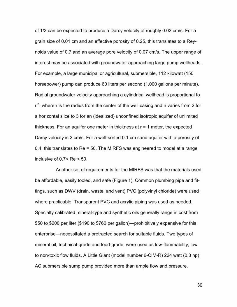
Another set of requirements for the MIRFS was that the materials used

be affordable, easily tooled, and safe (Figure 1). Common plumbing pipe and fit-

tings, such as DWV (drain, waste, and vent) PVC (polyvinyl chloride) were used

where practicable. Transparent PVC and acrylic piping was used as needed.

Specialty calibrated mineral-type and synthetic oils generally range in cost from

$50 to $200 per liter ($190 to $760 per gallon)—prohibitively expensive for this

enterprise—necessitated a protracted search for suitable fluids. Two types of

mineral oil, technical-grade and food-grade, were used as low-flammability, low

to non-toxic flow fluids. A Little Giant (model number 6-CIM-R) 224 watt (0.3 hp)

AC submersible sump pump provided more than ample flow and pressure.

30

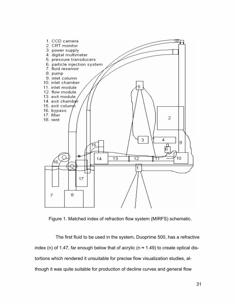
Figure 1. Matched index of refraction flow system (MIRFS) schematic.

The first fluid to be used in the system, Duoprime 500, has a refractive

index (n) of 1.47, far enough below that of acrylic (n ≈ 1.49) to create optical dis-

tortions which rendered it unsuitable for precise flow visualization studies, al-

though it was quite suitable for production of decline curves and general flow

31

observation. The second fluid, Paratherm RI, is a heat transfer mineral oil with a

refractive index that at 30°C closely matches that of the acrylic spheres used in

the experiments. Some fluid physical properties were given by the manufactur-

ers. Citgo provided values for viscosity and specific gravity at one temperature,

40°C. Little information for Duoprime 500 was available owing to the fact that it is

a technical grade paraffinic heavy mineral oil used primarily for lubrication of food

machinery and for dust suppression. Paratherm RI, on the other hand, is a

napthenic mineral oil heat transfer fluid specified by engineers. Shawn Stoner, a

chemical engineer with Paratherm Corporation, was instrumental in finding and

developing a suitable fluid for these experiments, and furnishing various samples

and extensive data obtained from independent laboratory analysis. Paratherm

Corporation furnished values for numerous parameters, including viscosity and

specific gravity over a wide range of temperatures (Appendix A). Fluid physical

properties not given were measured primarily with fabricated test equipment as

described in further sections.

The basic design was a closed-loop, transparent flow system where oil

was pumped up to a (fairly) constant-head inlet column, gravity-fed sequentially

through the inlet chamber, inlet module, flow module, exit module, exit chamber,

and exit column back to the reservoir (Figures 1 and 2). The system was pow-

ered by a centrifugal pump submersed in 57 liters of mineral oil. The transition

between the (6 cm diameter) cylindrical columns and the (5 x 4 x 23 cm) rectan-

gular prism modules was via two (15 cm) cubical inlet and exit chambers. In ad-

dition to providing a geometric transition, the inlet and exit chambers helped to

32

Figure 2. Matched index of refraction flow system (MIRFS) photograph.

stabilize flow and allow for monitoring of flow boundary conditions. Fine (~ 200

µm) white, polypropylene particles were suspended in a mixing chamber and in-

jected into the inlet module using an adjustable-position, streamlined injection

tube. A needle-valve located at the pump discharge permitted precise control of

the injection-system flow rate. Flow was recorded by a Sony TRV27 digital video

33

camera with a 10x optical zoom and fitted with 1x, 2x, and 4x macro lenses,

permitting observation at virtually any desired magnification via a CRT monitor.

Flow module pressure loss was measured by a basic electrical circuit in which

two (ICT model number SX01DD4 and SX15DD4), differential pressure trans-

ducers were fed by a regulated power supply and read by a microvolt-resolution

digital multimeter. Thermistors located near the top of the exit chamber, at the

pump housing, on the cooling coil inlet-side, and by the transducer circuit fed

digital thermometers. Thus the basic design facilitated careful control, viewing,

and measurement of fluid flow and important boundary conditions. The MIRFS

was modified several times as needed to correct problems such as air entrain-

ment and vibration and to operate correctly with the two different flow modules.

Operation of the MIRFS included filtering and control of mineral oil

temperature and flow rates. The highly temperature-dependent nature of mineral

oil physical properties such as density, viscosity, and refractive index necessi-

tated suitable temperature controls. Waste heat from the pump was great enough

to raise the reservoir temperature to over 40°C within 45 minutes of start-up.

Temperature was reduced to 36 ± 1°C by a submersed, 0.64 cm, open-loop

copper cooling coil fed by tap water and drained into a sink. A box-fan was also

used to cool the equipment and maintain stable laboratory air temperatures. Be-

cause an AC pump cannot be varied without an expensive control such as an AC

frequency regulator, fluid flow was governed by the use of throttling and bypass

valves immediately on the discharge side of the pump. Flow was also diverted

through a filter near this juncture to remove debris and unwanted injection

34

particles. (Electrical grounding of the filter housing was required to control static

electricity generated by oil flowing through the filtering system at higher velocities

—arcing of this current was seen [and felt!] across distances of approximately

1 cm.)

Additional minor MIRFS concerns were fluid leakage, entrainment of

fine air bubbles at higher velocities, and selection of tracer particles. Several

sealing products were successfully applied: Seal-All glue, Lock-Tite gel super-

glue, and acrylic cement. Fine-mesh (< 1 mm) polypropylene tulle was added to

the inlet and outlet columns to eliminate fluid free-fall while improving flow-

stability boundary conditions. Initially several sizes of glitter were used as injec-

tion particles. Glitter is multi-colored and could, in principle, display small-scale

fluid shear and vorticity. Unfortunately, a glitter particle changes from highly re-

flective and visible when normal to the line of sight to nearly invisible when par-

allel. Subsequently, Sephadex G-50 flow cytometry particles (50 µm < d < 150

µm) were used, but were expensive, tended to clump together, and too dense to

remain properly suspended. Finally, Behr #970 Non-Skid Floor Finish Additive

proved to be a remarkably inexpensive and effective tracer particle with a density

closely matching that of the Paratherm RI mineral oil chosen as the ideal flow

fluid.

Design and Construction of the Flow Modules

Two interchangeable flow modules were used in the MIRFS. The pri-

mary module consisted of a rhombohedral (hexagonal close packed) packing of

35

172 transparent acrylic commercial-grade spheres manufactured by Engineering

Laboratories, Incorporated. The published diameter of these spheres is given as

1.27 ± 0.010/0.013 cm (0.5 ± 0.004/0.005 inches) with a sphericity tolerance of

0.005 cm. A digital micrometer was used to measure representative samples of

the three sets used (Table 1). One set of four opaque red spheres was used to

provide evenly-spaced markers in the bottom rear row of the matrix (Figure 3).

Figure 3. Matrix flow module front view photograph.

Another set of 51 transparent green spheres was used to provide three rows

(n = 17) located toward the upper rear portion of the matrix for geometric refer-

encing (Figure 4). The remainder of the matrix was comprised of 217 clear acrylic

spheres. Four clear acrylic strips were fabricated to fill in the cavities at the walls.

Minimal amounts of acrylic cement were applied with a syringe to weld the

spheres together at either end of the matrix. The second flow module, designed

36

Figure 4. Matrix flow module right end view (inlet side) photograph.

for general observation and possible studies of critical lift-off and transport of

sediment, contained one 3.8 cm clear acrylic sphere on the left (discharge) side

and a rotatable, transparent, red acrylic vane on the right side (Appendix B). The

second module was used in the MIRFS for heuristic purposes.

Measurement of Mineral Oil

Physical Properties

Refractive index, density, and viscosity were measured as required for

proper application of the MIRFS. The refractive index of Duoprime 500T at room

temperature was obtained using an Abbey refractometer. With such a low refrac-

tive index of n = 1.47 (Figure 5), Duoprime 500T was only used in the MIRFS for

decline curve production and general observation. Attention was then redirected

toward finding an ideal fluid. Very little information was found pertaining to min-

eral oils with refractive indexes greater than 1.48. (See Cornellisen and

37

Waterman 1956 for a general overview.) What is known tends to be proprietary

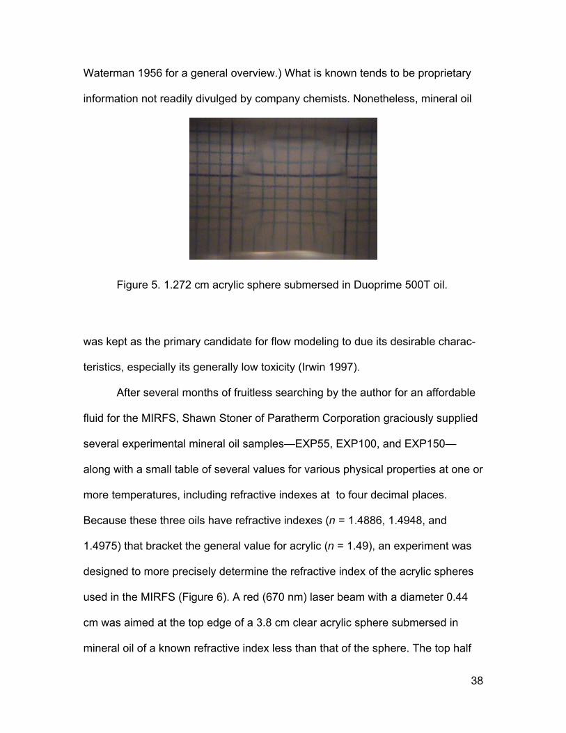
information not readily divulged by company chemists. Nonetheless, mineral oil

Figure 5. 1.272 cm acrylic sphere submersed in Duoprime 500T oil.

was kept as the primary candidate for flow modeling to due its desirable charac-

teristics, especially its generally low toxicity (Irwin 1997).

After several months of fruitless searching by the author for an affordable

fluid for the MIRFS, Shawn Stoner of Paratherm Corporation graciously supplied

several experimental mineral oil samples—EXP55, EXP100, and EXP150—

along with a small table of several values for various physical properties at one or

more temperatures, including refractive indexes at to four decimal places.

Because these three oils have refractive indexes (n = 1.4886, 1.4948, and

1.4975) that bracket the general value for acrylic (n = 1.49), an experiment was

designed to more precisely determine the refractive index of the acrylic spheres

used in the MIRFS (Figure 6). A red (670 nm) laser beam with a diameter 0.44

cm was aimed at the top edge of a 3.8 cm clear acrylic sphere submersed in

mineral oil of a known refractive index less than that of the sphere. The top half

38

of the beam passes just above the sphere onto a target 200 cm beyond. The

Figure 6. Refractometer diagram.

lower half of the beam is twice-refracted downward at the surface of the sphere

(Figure 7) and hits the target slightly below the upper half.

Figure 7. Laser beam refracted at top of 3.8 cm acrylic sphere.

The first mineral oil is then titrated with a second mineral oil which has a refrac-

tive index slightly higher than that of the acrylic sphere. The two spots of light at

the target become closer during the process and converge when the correct

mixture of the two oils matches the refractive index of the sphere (Figure 8). For

example, at room temperature, a correct mix of 31 ml EXP55 (n = 1.4886) and 85

39

ml EXP100 (n = 1.4948) translated to a determination of n = 1.4931 ± 0.0005 for

the 3.8 cm acrylic sphere.

Figure 8. Refractometer laser pattern at target.

Another set of similar experiments examined the temperature depend-

ence of the Paratherm samples by heating oil to 40°C and watching the target

spots converge as the fluid reached an ideal temperature. A good match was

obtained for EXP100 at 30°C. Thereupon 57 liters (15 gallons) of EXP100 was

ordered from Paratherm. They produced a much larger batch, named it

Paratherm RI™, and shipped the order along with extensive physical property

data obtained from an independent laboratory (Appendix A).

Another experiment was designed to find the viscosity of Duoprime

500 at various temperatures. Falling liquid sphere viscometry was employed with

Duoprime 500 at various temperatures. De-ionized water with a small amount

(< 5%) of red food coloring was introduced at the top of a transparent acrylic

container and measured with a digital micrometer. A Sony TRV27 digital video

camera operating at an interlaced rate of 30 frames per second was used to

40

capture images of the falling sphere against a ruled backdrop. Frame-by-frame

analysis provided data which were put into a spreadsheet to precisely determine

terminal velocities. The following formulas, adapted from Lommatzsch et al.

(2001), were used to obtain viscosity as a function of terminal velocity. First, ab-

solute viscosity as a function of velocity was determined from

(24)

where µopen is the absolute viscosity without correction for wall effect, g is the

gravitational constant, d is the diameter of the sphere, ρ1 is the density of the

(liquid) sphere, ρ2 is the density of the mineral oil, and U∞ is the terminal velocity

of the sphere. Corrections for the wall effect are given by

(25)

Here µ is the corrected viscosity and D is the diameter of the cylinder.

The density temperature-dependence of Duoprime 500 was deter-

mined simply by heating 500 ml of the oil in graduated glass cylinder and ob-

serving the height as the temperature decreased. The thermal expansion of the

Pyrex glass was neglected and the ratio of heights used to determine the density

of the fluid. Data thus obtained were plotted along with values provided by

Paratherm for Paratherm RI™ (Appendix A) and data for water given by Lide

(2001) for general understanding and to evaluate methods and uncertainties.

41

Calibration of Pressure Transducers

Calibration curves for two differential pressure transducers were

generated using an inverted U-tube manometer method. Microvolt outputs from

the individual Wheatstone bridge transducers were plotted as a function of the

pressure difference between atmospheric pressure and the pressure inferred

from manometer readings. De-ionized water with a small amount (< 5%) of red

food coloring was incrementally added to an inverted 4 meter length of 8 mm

diameter vinyl tubing and the height differential was used to ascertain head

pressure.

Calibration of MIRFS Flow Rates

Calibration of the MIRFS was done with the sphere matrix module in-

stalled. The first stage was a determination of flow rate as a function of column

height. One worker called out the height and temperature of the mineral oil in the

inlet column at one to three second intervals, depending on the flow rate, while a

second individual quickly inserted a graduated cylinder under the exit column

discharge. Both of these activities were recorded by the Sony TRV27 for subse-

quent frame-by-frame analysis. A spreadsheet was used to calculate flow rate as

a function of value-averaged column height. Graphical analysis revealed that for

the much higher Reynolds numbers associated with the Paratherm RI, there was

a typical Forchheimer relationship. Regression analysis provided equations that

related flow rates to column heights for the two oils.

42

Measurement of Pressure Loss as a

Function of Reynolds Numbers

MIRFS pressure loss curves were derived from videotaped images of

the digital multimeter positioned so as to remain alongside the inlet column fluid

level as it was varied in height synchronously with system flow rates which

spanned the full range from maximum to minimum. Data were manipulated in a

spreadsheet to determine pressures from transducer millivolt output readings,

flow rates from column heights, Reynolds numbers from flow rates and viscosi-

ties, and thence decline curves. Corrections were made for pressure transducer

air temperature dependency and mineral oil viscosity temperature dependency.

MIRFS decline curves (i.e., Darcy-Weisbach friction factor as a function of Rey-

nolds number), and permeability values were also calculated and presented

graphically (Chapter 4).

Particle Tracking

Particle Tracking Velocimetry was applied using both PSV and PDV.

The Sony TRV27 time-stamps each frame as it records, generally at the rate of

30 interlaced frames per second. Individual frames were reviewed on a 33 cm

(13 inch) diagonal CRT monitor, providing magnifications ranging from 0x to 20x.

PSV was used at higher flow rated, where particle streak lengths were apprecia-

ble. Individual streaks were selected and measured on the monitor screen with a

ruler and compared with the diameter of a sphere, also measured on the monitor

screen. The correctly scaled streak length divided by the interlaced frame speed

43

(1/30 s) thus provided true point velocity. Only the horizontal component was

measured so as to provide the true y-component of velocity. For PDV measure-

ments, individual particle trajectories were followed frame-by-frame on the CRT

across a known distance, usually, the width of one sphere. The path distance

divided by the time between first and final frames thus produced averaged

y-component velocities.

Summary of Methods

The fluid dynamics behind decline curves were studied using a

matched index of refraction flow system (MIRFS) and particle tracking veloci-

metry (PTV). A special-purpose liquid/solid laser refractometer was used to

eliminate optical distortions in the MIRFS. Falling liquid sphere viscometry was

used to determine mineral oil viscosities at various temperatures. An inverted-U

manometer was constructed to calibrate differential pressure transducers. MIRFS

flow rates were determined by measuring flow rates as a function of inlet column

heights. Pressure transducer microvolt outputs, converted to pressure loss

across the flow module, were measured as a function of inlet column heights.

Pressure loss as a function of flow rate (alternatively Reynolds number) data

were generated for decline curves and permeability determinations. Fine (≈ 200

µm) white particles were injected well upstream of the flow module and filmed

with a digital video camera coupled with a CRT monitor at various magnifications.

Frame-by-frame analysis, or particle tracking velocimetry (PTV), was used to ob-

serve and measure fluid motion through the MIRFS.

44

CHAPTER IV

RESULTS AND ANALYSIS

Results of this study include matrix dimensional properties; fluid physi-

cal properties; pressure transducer calibrations; MIRFS refractive index (see

Chapter 3 for data), flow rate, and pressure-loss relationships; PTV kinematics;

qualitative flow observations; and mathematical modeling. Data are generally

presented graphically, with data sets available in the appendices.

Flow Module Characteristics

The porosity of the sphere matrix is equal to the volume of the flow

module minus the volumes displaced by the spheres and wall filler strips (Figure

4). This was measured to be 0.321 ± 0.013, obtained by noting the amount of

water required to fill the module. The volume of the flow module (without filler

strips) minus the volume of the spheres based on dimensional considerations is

0.371. The volume of the flow module was determined with a digital micrometer

(4.39 cm x 4.89 cm x 21.6 cm = 464 cm3). The volume of the spheres was cal-

culated by multiplying the number of spheres (272) by the volume of an average

sphere (Table 1). The theoretical porosity of rhombohedrally packed spheres

roughly 0.260 (Sphere Geometry section for proof). There are two possible pat-

terns of layering in a rhombohedral packing, hexagonal close packed (ababab),

45

Table 1. Matrix Sphere Dimensional Properties

Matrix Spheres Dimensional Properties

num

ber

colo

r

min

imum

di

amet

er (m

m)

max

imum

di

amet

er (m

m)

indi

vidu

al

aver

age

diam

eter

(mm

)

diam

eter

ch

ange

(mm

)

indi

vidu

al

sphe

ricity

(±

1%

)

mea

n sp

heric

ity

per c

olor

(± 1

%)

mea

n di

amet

er

per c

olor

(mm

)

aver

age

diam

eter

de

viat

ion

per

colo

r (m

m)

1 clear 12.69 12.74 12.72 0.050 0.197 0.150 12.696 0.0320

2 clear 12.69 12.75 12.72 0.060 0.236

3 clear 12.64 12.68 12.66 0.040 0.158

4 clear 12.69 12.73 12.71 0.040 0.157

5 clear 12.65 12.69 12.67 0.040 0.158

6 clear 12.67 12.73 12.70 0.060 0.236

7 clear 12.63 12.65 12.64 0.020 0.079

8 clear 12.66 12.70 12.68 0.040 0.158

9 clear 12.79 12.80 12.80 0.010 0.039

10 clear 12.66 12.68 12.67 0.020 0.079

11 green 12.74 12.76 12.75 0.020 0.078 0.141 12.761 0.012

12 green 12.71 12.77 12.74 0.060 0.235

13 green 12.76 12.78 12.77 0.020 0.078

14 green 12.73 12.78 12.76 0.050 0.196

15 green 12.76 12.78 12.77 0.020 0.078

16 green 12.70 12.78 12.74 0.080 0.314

17 green 12.76 12.77 12.77 0.010 0.039

18 green 12.75 12.77 12.76 0.020 0.078

19 green 12.77 12.83 12.80 0.060 0.234

20 green 12.75 12.77 12.76 0.020 0.078

21 red 12.71 12.72 12.72 0.010 0.039 0.086 12.736 0.016

22 red 12.74 12.77 12.76 0.030 0.118

23 red 12.74 12.75 12.75 0.010 0.039

24 red 12.73 12.74 12.74 0.010 0.039

25 red 12.73 12.75 12.74 0.020 0.078

26 red 12.75 12.76 12.76 0.010 0.039

27 red 12.73 12.78 12.76 0.050 0.196

28 red 12.67 12.69 12.68 0.020 0.079

29 red 12.72 12.75 12.74 0.030 0.118

30 red 12.73 12.76 12.75 0.030 0.118

overall average diameter (mm) 12.73

overall average diameter deviation mm) 0.0321

overall average diameter deviation (± 1%) 0.25

overall mean sphericity (± 1%) 0.126

46

and face centered cubic (abcabcabc). Hexagonal close packing was chosen due

to its more isotropic structure. The porosity for both types is identical.

Measurements of representative samples of each type of sphere (red,

transparent green, and clear) were analyzed statistically and placed into a table

(Table 1). The sphere irregularities are negligible in comparison with other meas-

urement uncertainties.

Fluid Physical Properties

Densities for Duoprime 500T are plotted along with published values

for water (Lide 2001) and Paratherm RI™ (Figure 9 and Appendix A). Consider-

ing the narrow range of temperatures used to calibrate the MIRFS, density un-

Density Temperature-Dependence Comparison

y = -0.0000x2 - 0.0001x + 1.0015R2 = 0.9997

y = -0.000538x + 0.912467R2 = 0.999685

y = -0.0007x + 0.8809R2 = 0.9794

0.800

0.850

0.900

0.950

1.000

1.050

0 50 100 150

Temperature (oC)

Den

sity

(g/m

l)

RI Density

H2O Density

500T Density

Poly. (H2ODensity)Linear (RIDensity)Linear (500TDensity)

Figure 9. Fluid density comparisons.

47

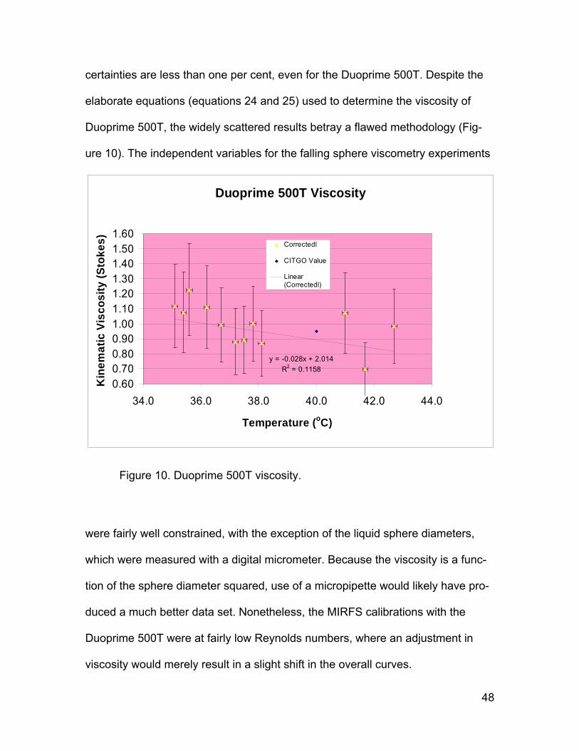
certainties are less than one per cent, even for the Duoprime 500T. Despite the

elaborate equations (equations 24 and 25) used to determine the viscosity of

Duoprime 500T, the widely scattered results betray a flawed methodology (Fig-

ure 10). The independent variables for the falling sphere viscometry experiments

Duoprime 500T Viscosity

y = -0.028x + 2.014R2 = 0.1158

0.600.700.800.901.001.101.201.301.401.501.60

34.0 36.0 38.0 40.0 42.0 44.0

Temperature (oC)

Kin

emat

ic V

isco

sity

(Sto

kes) Correctedl

CITGO Value

Linear(Correctedl)

Figure 10. Duoprime 500T viscosity.

were fairly well constrained, with the exception of the liquid sphere diameters,

which were measured with a digital micrometer. Because the viscosity is a func-

tion of the sphere diameter squared, use of a micropipette would likely have pro-

duced a much better data set. Nonetheless, the MIRFS calibrations with the

Duoprime 500T were at fairly low Reynolds numbers, where an adjustment in

viscosity would merely result in a slight shift in the overall curves.

48

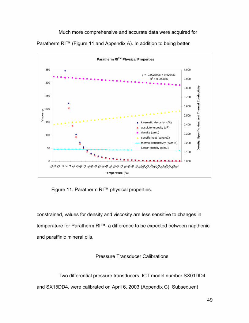
Much more comprehensive and accurate data were acquired for

Paratherm RI™ (Figure 11 and Appendix A). In addition to being better

Paratherm RITM Physical Properties

y = -0.002699x + 0.926123R2 = 0.999885

0

50

100

150

200

250

300

350

-20 -15 -10 -5 0 5 10 15 20 25 30 35 40 45 50 55 60 65 70 75 80 85 90 95 10010

511

011

512

012

513

013

514

014

515

0

Temperature (oC)

Visc

osity

0.000

0.100

0.200

0.300

0.400

0.500

0.600

0.700

0.800

0.900

1.000

Den

sity

, Spe

cific

Hea

t, an

d Th

erm

al C

ondu

ctiv

ity

kinematic viscosity (cSt)

absolute viscosity (cP)

density (g/mL)

specific heat (cal/g-oC)

thermal conductivity (W/m-K)

Linear (density (g/mL))

Figure 11. Paratherm RI™ physical properties.

constrained, values for density and viscosity are less sensitive to changes in

temperature for Paratherm RI™, a difference to be expected between napthenic

and paraffinic mineral oils.

Pressure Transducer Calibrations

Two differential pressure transducers, ICT model number SX01DD4

and SX15DD4, were calibrated on April 6, 2003 (Appendix C). Subsequent

49

conversation with Honeywell ICT technical support suggested that the

SSX01DD4 could be used at pressures higher than rated without significant error

or hysteresis. It was therefore decided to use only the SSX01DD4 for the MIRFS

over the next few months. After the MIRFS laboratory had been dismantled and

data were analyzed, a question arose as to the long term stability of the

SSX01DD4, mostly due to perceived discrepancies in data for the two oils used

in the MIRFS. Review of the lab notebook observations of zero pressure offset

values suggested serious drift over time (Figure 12). Uncertainties about what

SX01DD4 Zero Pressure Drift

20100202002030020400205002060020700

20 21 22 23 24 25 26 27

Temperature (oC)

Volta

ge (u

V)

3/23/2003 3/28/2003 3/30/20037/3/2003 4/6/2003 4/2/2003

Figure 12. Differential pressure transducer zero pressure offset drift.

was responsible for the drift motivated another round of calibrations for the

SSX01DD4. Separate analysis of dependences on input voltage and ambient air

temperature showed that temperature was fairly insignificant but that power sup-

ply drift might be a serious problem (Appendices D and E). A comparison of

50

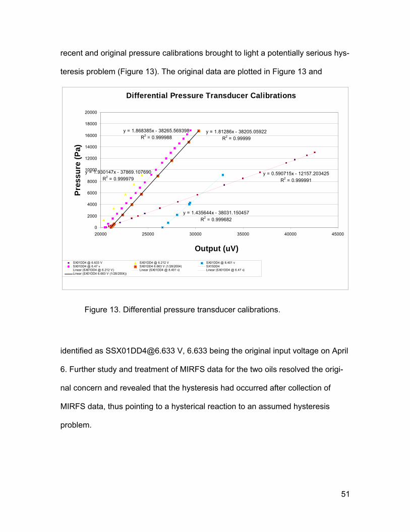
recent and original pressure calibrations brought to light a potentially serious hys-

teresis problem (Figure 13). The original data are plotted in Figure 13 and

Differential Pressure Transducer Calibrations

y = 0.590715x - 12157.203425R2 = 0.999991

y = 1.930147x - 37869.107690R2 = 0.999979

y = 1.435644x - 38031.150457R2 = 0.999682

y = 1.868385x - 38265.569398R2 = 0.999988

y = 1.81286x - 38205.05922R2 = 0.99999

0

2000

4000

6000

8000

10000

12000

14000

16000

18000

20000

20000 25000 30000 35000 40000 45000

Output (uV)

Pres

sure

(Pa)

SX01DD4 @ 6.633 V SX01DD4 @ 6.212 V SX01DD4 @ 8.401 vSX01DD4 @ 6.47 v SX01DD4 6.663 V (1/28/2004) SX15DD4Linear (SX01DD4 @ 6.212 V) Linear (SX01DD4 @ 8.401 v) Linear (SX01DD4 @ 6.47 v)Linear (SX01DD4 6.663 V (1/28/2004))

Figure 13. Differential pressure transducer calibrations.

identified as SSX01DD4@6.633 V, 6.633 being the original input voltage on April

6. Further study and treatment of MIRFS data for the two oils resolved the origi-

nal concern and revealed that the hysteresis had occurred after collection of

MIRFS data, thus pointing to a hysterical reaction to an assumed hysteresis

problem.

51

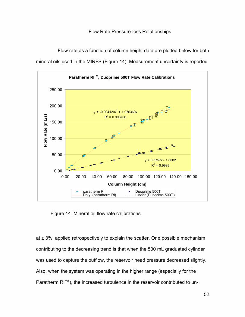
Flow Rate Pressure-loss Relationships

Flow rate as a function of column height data are plotted below for both

mineral oils used in the MIRFS (Figure 14). Measurement uncertainty is reported

Paratherm RITM, Duoprime 500T Flow Rate Calibrations

y = -0.004120x2 + 1.976369xR2 = 0.998706

y = 0.5757x - 1.6682R2 = 0.9989

0.00

50.00

100.00

150.00

200.00

250.00

0.00 20.00 40.00 60.00 80.00 100.00 120.00 140.00 160.00

Column Height (cm)

Flow

Rat

e (m

L/s)

paratherm RI Duoprime 500TPoly. (paratherm RI) Linear (Duoprime 500T)

Figure 14. Mineral oil flow rate calibrations.

er

tly.

at ± 3%, applied retrospectively to explain the scatter. One possible mechanism

contributing to the decreasing trend is that when the 500 mL graduated cylind

was used to capture the outflow, the reservoir head pressure decreased sligh

Also, when the system was operating in the higher range (especially for the

Paratherm RI™), the increased turbulence in the reservoir contributed to un-

52

steady flow and decreased flow rates. An unfortunate consequence of this

measurement error is that for the Paratherm RI™, the equation generated to fit

easing trend is expected at higher

ils

are plotted below separately because of the large difference in Reynolds number

ranges (Figures 15 and 16). For the Duoprime 500T, numerous regression

the observed data might have an artificially high leading coefficient for the non-

linear term. Because a non-linear decr

Reynolds numbers due to the Forchheimer effect, it would seem difficult to cor-

rect for this inherent calibration error.

Pressure loss as a function of Reynolds number data for the two o

Citgo Duoprime 500T Pressure Loss

y = -0.0158x2 + 681.29x + 32.595R2 = 0.9998

y = 5.1513x2 + 649.39x - 31.403R2 = 0.9988

0

2000

4000

6000

8000

10000

12000

0.0 2.0 4.0 6.0 8.0 10.0 12.0 14.0 16.0

Reynolds Number

Pres

sure

Dro

p (P

asca

ls)

low rangehigh rangePoly. (low range)Poly. (high range)

Figure 15. Duoprime 500T pressure loss curve.

53

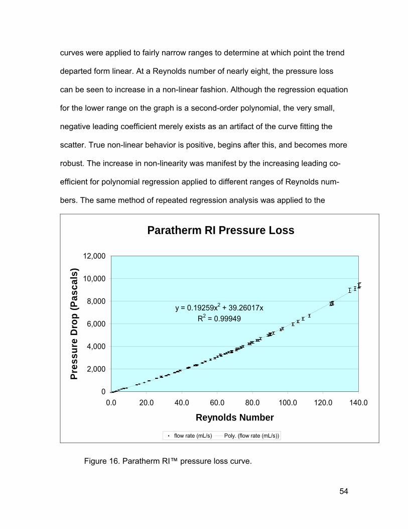
curves were applied to fairly narrow ranges to determine at which point the tren

departed form linear. At a Reynolds number of nearly eight, the pressure loss

d

ore

robust. The increase in non-linearity was manifest by the increasing leading co-

efficient for polynomial regression applied to different ranges of Reynolds num-

bers. The same method of repeated regression analysis was applied to the

can be seen to increase in a non-linear fashion. Although the regression equation

for the lower range on the graph is a second-order polynomial, the very small,

negative leading coefficient merely exists as an artifact of the curve fitting the

scatter. True non-linear behavior is positive, begins after this, and becomes m

Paratherm RI Pressure Loss

y = 0.19259x2 + 39.26017xR2 = 0.99949

0

2,000

4,000

6,000

8,000

10,000

12,000

0.0 20.0 40.0 60.0 80.0 100.0 120.0 140.0

Reynolds Number

Pres

sure

Dro

p (P

asca

ls)

flow rate (mL/s) Poly. (flow rate (mL/s))

Figure 16. Paratherm RI™ pressure loss curve.

54

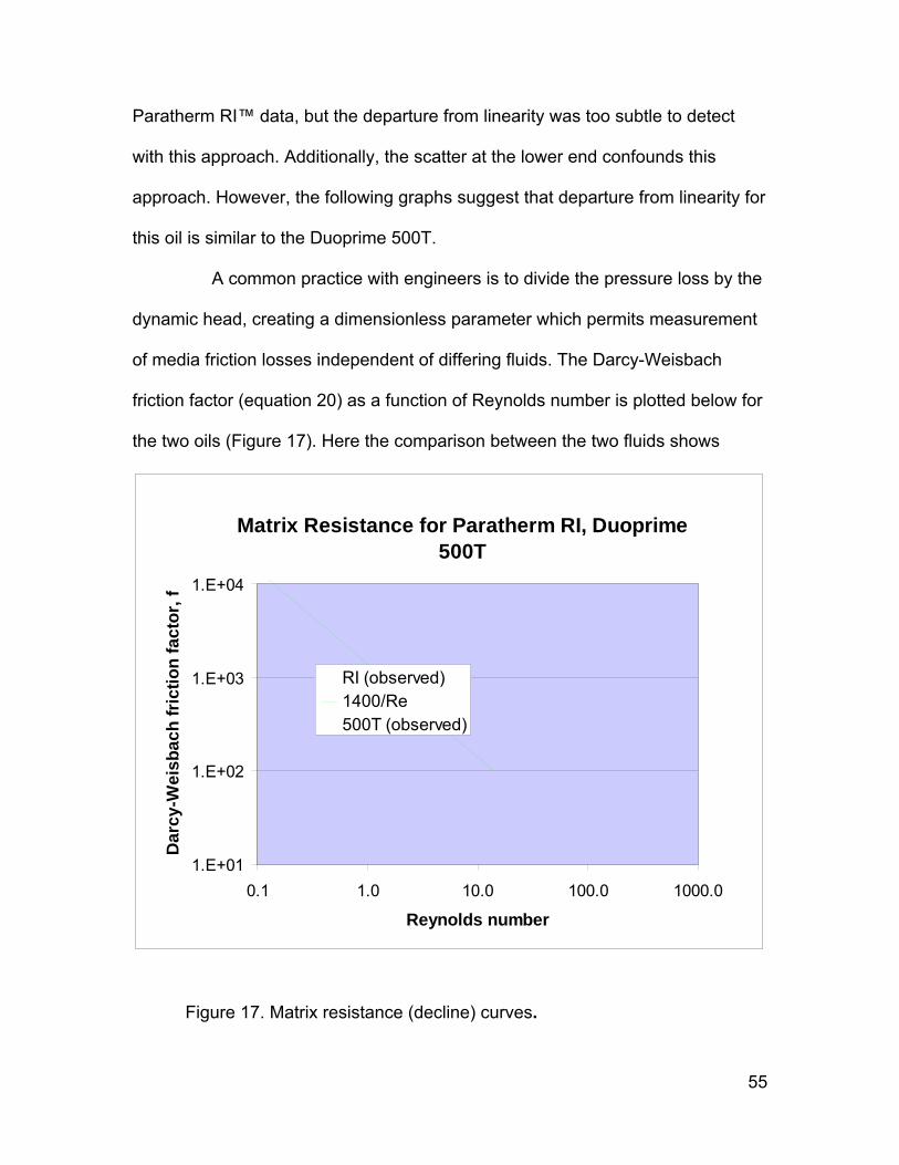
Paratherm RI™ data, but the departure from linearity was too subtle to detect

with this approach. Additionally, the scatter at the lower end confounds this

approach. However, the following graphs suggest that departure from linearity for

this oil is similar to the Duoprime 500T.

A common practice with engineers is to divide the pressure loss by

dynamic head, creating a dimensionless parameter which permits measurement

of media friction losses independent of differing fluids. The Darcy-Weisbach

the

friction factor (equation 20) as a function of Reynolds number is plotted below for

the two oils (Figure 17). Here the comparison between the two fluids shows

Matrix Resistance for Paratherm RI, Duoprime 500T

1.E+01

1.E+02

1.E+03

1.E+04

0.1 1.0 10.0 100.0 1000.0

Reynolds number

Dar

cy-W

eisb

ach

fric

tion

fact

or, f

RI (observed)1400/Re500T (observed)

Figure 17. Matrix resistance (decline) curves.

55

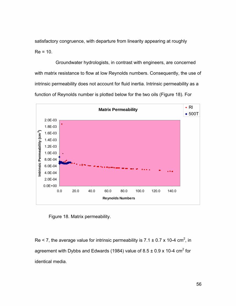
satisfactory congruence, with departure from linearity appearing at roughly

Re = 10.

Groundwater hydrologists, in contrast with engineers, are concerned

with matrix resistance to flow at low Reynolds numbers. Consequently, the use of

intrinsic permeability does not account for fluid inertia. Intrinsic permeability as a

function of Reynolds number is plotted below for the two oils (Figure 18). For

Matrix Permeability

0.0E+00

2.0E-04

4.0E-04

6.0E-04

8.0E-04

1.0E-03

1.2E-03

1.4E-03

1.6E-03

1.8E-03

2.0E-03

0.0 20.0 40.0 60.0 80.0 100.0 120.0 140.0

Reynolds Numbers

Intri

nsic

Per

mea

bilit

y (c

m2 )

RI500T

ge value for intrinsic permeability is 7.1 ± 0.7 x 10-4 cm2, in

greement with Dybbs and Edwards (1984) value of 8.5 ± 0.9 x 10-4 cm2 for

identical media.

Figure 18. Matrix permeability.

Re < 7, the avera

a

56

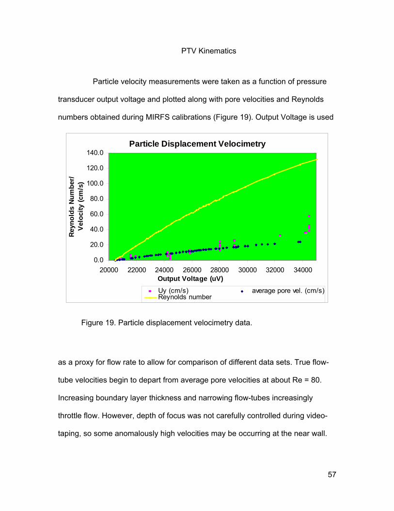
PTV Kinematics

Particle velocity measurements were taken as a function of pressure

transducer output voltage and plotted along with pore velocities and Reynolds

numbers obtained during MIRFS calibrations (Figure 19). Output Voltage is used

Particle Displacement Velocimetry

0.0

20.0

40.0

60.0

80.0

100.0

120.0

140.0

20000 22000 24000 26000 28000 30000 32000 34000Output Voltage (uV)

Rey

nold

s N

umbe

r/V

eloc

ity (c

m/s

)

Uy (cm/s) average pore vel. (cm/s)Reynolds number

Figure 19. Particle displacement velocimetry data.

ow-

rottle flow. However, depth of focus was not carefully controlled during video-

taping, so some anomalously g at the near wall.

as a proxy for flow rate to allow for comparison of different data sets. True fl

tube velocities begin to depart from average pore velocities at about Re = 80.

Increasing boundary layer thickness and narrowing flow-tubes increasingly

th

high velocities may be occurrin

57

Qualitative Flow Observations

Non-linear dynamical affects upon streamlines can result in much mor

chaotic flow paths than tortuous porous media pores. Consider the complex

e

streamlines evident in the simple, two-object array used in the observation flow

module shown below (Figure 20 and Appendix B). Here, at Re = 90, the interplay

Figure 20. Observation module flow at a Reynolds number of 90.

n

ctly laminar (Figure 21). The wide,

straight flow conduits at the top wall are not enough to induce non-laminar flow.

between the red vane and the transparent sphere downstream create sudde

flow reversals and strong angular accelerations. Yet, for the matrix of spheres, at

Re = 20 porous media flow seems perfe

58

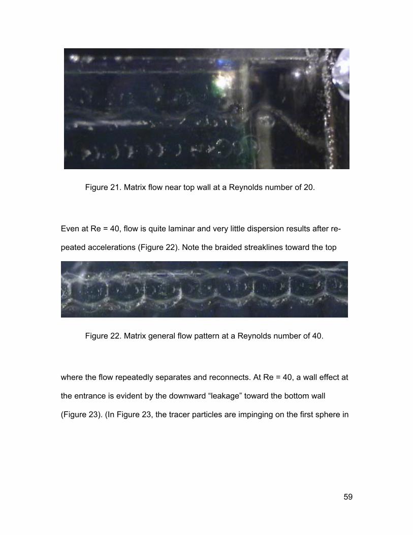
Figure 21. Matrix flow near top wall at a Reynolds number of 20.

Even at Re = 40, flow is quite laminar and very little dispersion results after re-

peated accelerations (Figure 22). Note the braided streaklines toward the top

Figure 22. Matrix general flow pattern at a Reynolds number of 40.

where the flow repeatedly separates and reconnects. At Re = 40, a wall effect at

the entrance is evident by the downward “leakage” toward the bottom wall

(Figure 23). (In Figure 23, the tracer particles are impinging on the first sphere in

59

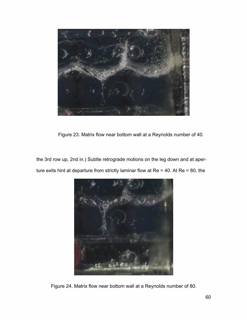
Figure 23. Matrix flow near bottom wall at a Reynolds number of 40.

the 3rd row up, 2nd in.) Subtle retrograde motions on the leg down and at aper-

ture exits hint at departure from strictly laminar flow at Re = 40. At Re = 80, the

Figure 24. Matrix flow near bottom wall at a Reynolds number of 80.

60

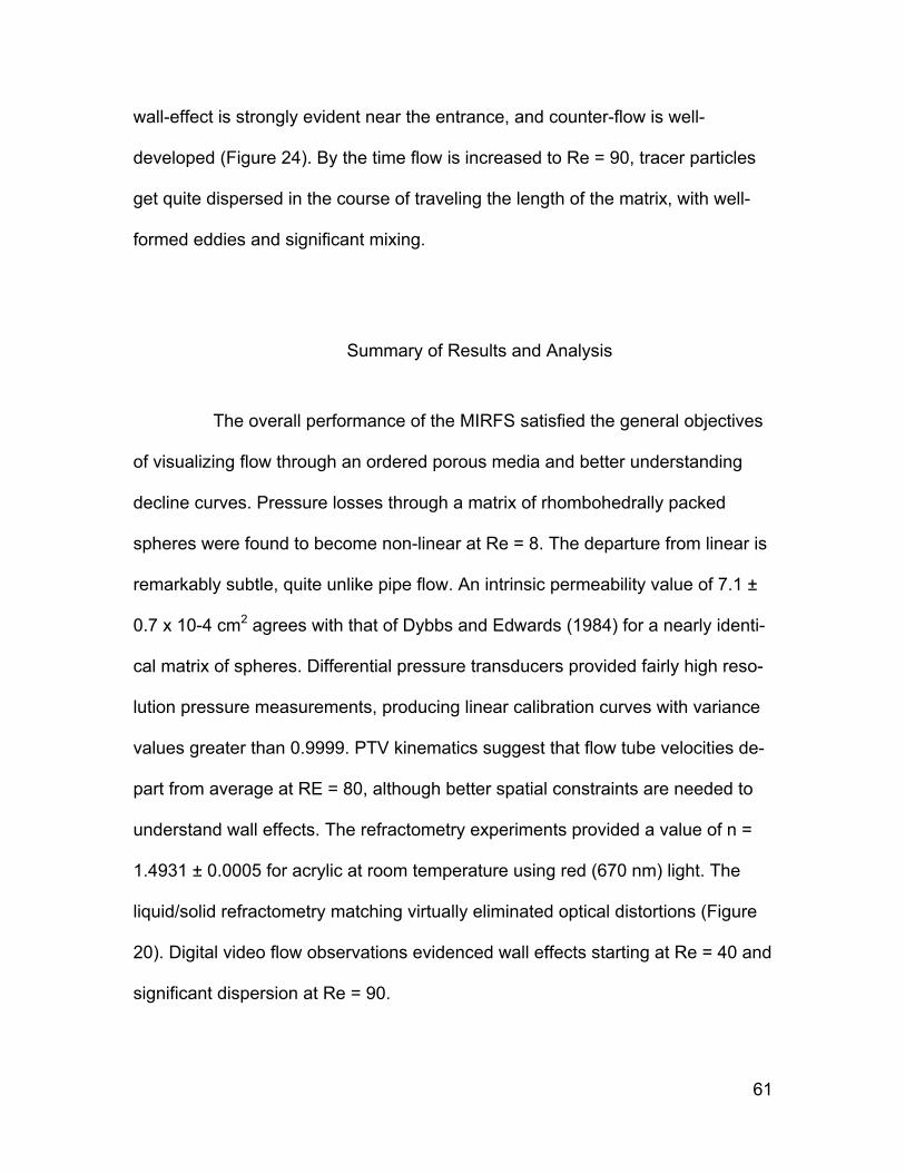
wall-effect is strongly evident near the entrance, and counter-flow is well-

developed (Figure 24). By the time flow is increased to Re = 90, tracer particles

get quite dispersed in the course of traveling the length of the matrix, with well-

formed eddies and significant mixing.

Summary of Results and Analysis

The overall performance of the MIRFS satisfied the general objectives

of visualizing flow through an ordered porous media and better understanding

decline curves. Pressure losses through a matrix of rhombohedrally packed

spheres were found to become non-linear at Re = 8. The departure from linear is

remarkably subtle, quite unlike pipe flow. An intrinsic permeability value of 7.1 ±

0.7 x 10-4 cm2 agrees with that of Dybbs and Edwards (1984) for a nearly identi-

cal matrix of spheres. Differential pressure transducers provided fairly high reso-

lution pressure measurements, producing linear calibration curves with variance

values greater than 0.9999. PTV kinematics suggest that flow tube velocities de-

part from average at RE = 80, although better spatial constraints are needed to

understand wall effects. The refractometry experiments provided a value of n =

1.4931 ± 0.0005 for acrylic at room temperature using red (670 nm) light. The

liquid/solid refractometry matching virtually eliminated optical distortions (Figure

20). Digital video flow observations evidenced wall effects starting at Re = 40 and

significant dispersion at Re = 90.

61

CHAPTER V

MATHEMATICAL MODELING A mathematically rigorous prediction of pressure losses for fluids pass-

ing through a matrix of rhombohedrally packed spheres first requires a mathe-

matical characterization of the overall geometry of the packed spheres. An alge-

braic parameterization of the pore and boundary surfaces is needed. An alge-

braic expression describing the kinematic pathways (or streamlines), through the

matrix is also necessary. The cross-sectional areas and geometric centers as

functions of translational position are required as well. These relationships might

then be combined to allow for rigorous determination of pressure loss at low

Reynolds numbers in a manner analogous to the methods that have been

successfully applied to Couette flow, Hagen-Pouiselle plane flow, and Hagen-

Pouiselle pipe flow.

Sphere Geometry

The following proof for porosity of rhombohedrally packed spheres,

derived as part of this study, illustrates the overall geometry of tightly packed

spheres (Figures 25-27). The triangle ABC can be seen as the left half of an

isosceles triangle with vertices at the centers of three first-tier spheres (Figure

26). With a sphere radius of one unit, the following line segment lengths can be

62

Figure 25. Rhombohedral sphere packing 3-dimensional top view

diagram.

easily deduced: AB = 1; AC = 2; BC = √3 (from the Pythagorean Theorem); and

Figure 26. Rhombohedral sphere packing 2-dimensional geometry

diagram.

63

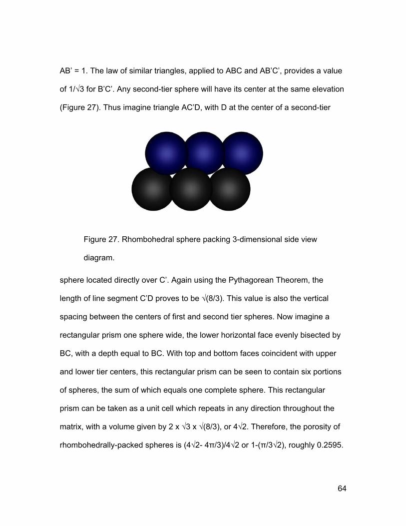
AB’ = 1. The law of similar triangles, applied to ABC and AB’C’, provides a value

of 1/√3 for B’C’. Any second-tier sphere will have its center at the same elevation

(Figure 27). Thus imagine triangle AC’D, with D at the center of a second-tier

Figure 27. Rhombohedral sphere packing 3-dimensional side view

diagram.

sphere located directly over C’. Again using the Pythagorean Theorem, the

length of line segment C’D proves to be √(8/3). This value is also the vertical

spacing between the centers of first and second tier spheres. Now imagine a

rectangular prism one sphere wide, the lower horizontal face evenly bisected by

BC, with a depth equal to BC. With top and bottom faces coincident with upper

and lower tier centers, this rectangular prism can be seen to contain six portions

of spheres, the sum of which equals one complete sphere. This rectangular

prism can be taken as a unit cell which repeats in any direction throughout the

matrix, with a volume given by 2 x √3 x √(8/3), or 4√2. Therefore, the porosity of

rhombohedrally-packed spheres is (4√2- 4π/3)/4√2 or 1-(π/3√2), roughly 0.2595.

64

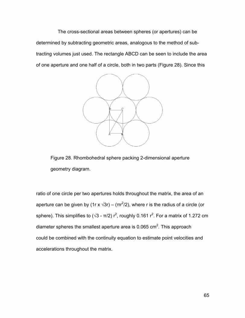
The cross-sectional areas between spheres (or apertures) can be

determined by subtracting geometric areas, analogous to the method of sub-

tracting volumes just used. The rectangle ABCD can be seen to include the area

of one aperture and one half of a circle, both in two parts (Figure 28). Since this

Figure 28. Rhombohedral sphere packing 2-dimensional aperture

geometry diagram.

ratio of one circle per two apertures holds throughout the matrix, the area of an

aperture can be given by (1r x √3r) – (πr2/2), where r is the radius of a circle (or

sphere). This simplifies to (√3 - π/2) r2, roughly 0.161 r2. For a matrix of 1.272 cm

diameter spheres the smallest aperture area is 0.065 cm2. This approach

could be combined with the continuity equation to estimate point velocities and

accelerations throughout the matrix.

65

Matrix Algebra

Algebraic expressions for the matrix surfaces were derived from the

basic equation of a sphere

(26)

where x, y, and z are right-hand Cartesian coordinates and r is the sphere radius.

The following four equations are based on the application of rhombohedral

sphere spacing to the previous equation:

(27)

(28)

(29)

(30)

Here a, b, and c represent consecutive integer values for the respective direc-

tions x, y, and z for the four types of rows. These four equations might conceiva-

bly be modified, constrained, and applied to a sphere matrix to provide analytic

solutions.

An Analytic Approach

By choosing the proper sphere radius and expressing the general flow

direction, y, in terms of x, and z within the bounds of the matrix, the basic flow

capillaries can be mathematically defined to permit flow field quantification. A

66

geometric proxy such as the running geometric center might be established as

the axial flow center, thus providing a kinematic path for the fastest streamline

(based on equations 27-30). The overall flow through the matrix used in the pre-

sent study is no more than a simple braided pattern where pairs of flow tubes

from small voids converge in large voids and then diverge back into small voids

symmetrically and repeatedly (Figure 22). Choosing a geometric unit cell which

repeats linearly throughout the flow matrix simplifies the task of applying rigorous

analytical methods to a large matrix (Figures 29 and 30).

Figure 29. Flow geometry unit cell location diagram.

By carefully examining the structure of sphere packing, it would seem

quite possible to quantify both non-local accelerations due to throttling and nor-

mal accelerations associated with radial forces. At low Reynolds numbers the

task of analytically determining pressure drop is greatly simplified.

67

Figure 30. Flow geometry unit cell diagram.

Although the general consensus amongst scientists, engineers, and

mathematicians holds that analytical solutions to porous media flow are unob-

tainable, perhaps there is a way out for the maverick who chooses to simplify in

many ways. Because mineral oil is very incompressible, it is likely that normal

stresses give rise to virtually adiabatic processes that do not result in significant

energy (pressure) losses at low Reynolds numbers. For steady flow, the time de-

rivative can be discarded. And the uniformity of gravitational forces dispenses of

the need for the gravity terms in the Navier-Stokes equations as well. After all the

editing one is left with pressure loss as a function of shear stresses, virtually the

same as with Hagen-Poiseuille flow. The remaining problems for this approach

lie in quantifying boundary layer growth and decay rates at solid surfaces and

determination of shear forces where flow tubes converge and diverge. Thus it

may be possible to find a rigorous analytic solution to steady, incompressible, low

Reynolds flow through an ordered porous media such as rhombohedrally packed

68

spheres. The predicted pressure losses could then be compared with experi-

mental data to check the assumptions.

Summary of Mathematical Modeling

A method of rigorous analytic treatment of laminar, incompressible,

Newtonian flow through an undeformable matrix of rhombohedrally packed

spheres was proposed and partially developed. This approach is based on the

premise that Hagen-Poiseuille flow (Equation 12) applies to a non-cylindrical flow

conduit at low Reynolds numbers, similar to hydraulic radius theory. However,

this method differs from the dimensional analysis approach of hydraulic radius

theory, which averages relationships between total media surface area and total

pore volume. Rather, by determining the shear stress for each cross-section

normal to the translational flow for discrete repeating unit volumes, total pressure

loss as a function of shear stress might be determined by integrating the losses

of these cross-sections. In this manner, pressure energy lost to friction (heat)

would be expressed as a fundamental relationship. Therefore, the first steps

were completed toward quantification of the geometric and algebraic properties

of a rhombohedral sphere matrix needed for this approach.

Limitations of the Study

Time and budget constraints have compromised data collection and

analysis in this study in several ways. The original apparatus was designed to

produce higher flow rates that would have enabled observation of fully turbulent

69

flow with Reynolds numbers up to 500 or more. A direct current pump would

have permitted much smoother throttling and less pump-induced flow instability.

More extensive and sophisticated use of clear PVC and acrylic piping would have

reduced air entrainment and supply flow instabilities. Laser-cutting of acrylic ma-

terials and placing portions of cut spheres on flow module walls would have vir-

tually eliminated wall-effect, a significant problem for rigorous analysis. The use

of two higher speed digital video cameras, (or one higher speed camera with the

proper configuration of mirrors), along with suitable computer hardware and soft-

ware could have provided high temporal and spatial resolution, three-dimensional

velocity vector fields. Insertion of miniature pressure transducers into strategic

locations in the flow matrix was specified in the original design but cut due to

budgetary limits. Nonetheless, flexibility and persistence permitted satisfactory

results.

Conclusions

Several conclusions can be drawn from the present study. The overall

picture suggests that porous media decline curves can be explained by boundary

layer growth and decay at the sphere walls and higher shear rates corresponding

to narrowing flow tubes at Reynolds numbers of about 5 to 10. Although Rey-

nolds numbers are a useful tool, a more rigorous relationship should be derived

to relate shear and normal stresses to kinematic viscosity on a unit volume basis.

Very recent research has focused on the scaling of inertial perturbations to lami-

nar flow on a volumetric basis (Fitzgerald, 2004). An MIR flow system utilizing

70

acrylic, mineral oil, and PTV can be a relatively inexpensive yet very effective

approach to qualitative and quantitative study of flow through porous media and

fluid mechanics in general. A system similar to the MIRFS without any wall

effects could be used to very precisely determine pressure losses through an

ordered geometry such as tightly packed spheres. The relationship obtained

could then be compared with analytic predictions to provide fundamental new

insights into porous media fluid dynamics.

71

REFERENCES

Antohe, B.V., and J.L. Lage. 1997. A general two-equation macroscopic turbu-lence model for incompressible flow in porous media. International Journal of Heat and Mass Transfer 40, no. 13: 3013-24.

Bakhmmeteff, B.A., and N.V. Feodoroff. 1937. Flow through granular media. Journal of Applied Mechanics 4A: 97-104.

Barr, D.W. 2001. Turbulent flow through porous media. Ground Water 39, no. 5: 646-50.

Bear, J. 1972. Dynamics of fluids in porous media. New York: American Elsevier.

Bennethum, L.S., and T. Georgi. 1997. Generalized Forchheimer equation for two-phase flow based on hybrid mixture theory. Transport in Porous Media 26, no. 3: 261-75.

Borishanskii, V.M., O.S. Vinogradov, I.P. Luzin, and I.P. Tigarev. 1980. Hydraulic resistance of beds of spherical particles. Thermal Engineering 27, no. 1: 51-4.

Brenner, H., and J. Happel. 1958. Slow viscous flow past a sphere in a cylindrical tube. Journal of Fluid Mechanics 4: 195-213.

Buckingham, E. 1914. On physically similar systems: Illustrations of the use of dimensional equations. Physical Review 4: 345-76.

Camacho, V.R.G., C.M.A. Vasquez, and S.R. Padilla. 1998. New results on de-cline curves considering non-Darcy flow effects. SPE Reservoir Evaluation & Engineering 1, no. 5: 457-66.

Choi, H.M., T. Kurihara, H. Monji, and G. Matsui. 2002. Measurement of particle/bubble motion and turbulence around it by hybrid PIV. Flow Measurement and Instrumentation 12: 421-28.

Cornellisen, J., and H.I. Waterman. 1956. Determination of carbon-type compo-sition and molecular weight of mineral oil fractions from viscosity, refrac-tive index, and density by means of nomograms. Analytica Chimica ACTA 15: 401-09.

Darcy, H. 1856. Les fountains publiques de la ville de Dijon. Paris: Dalmont.

72

Dybbs, A., and R.V. Edwards. 1984. A new look at porous media mechanics - Darcy to turbulent. In Fundamentals of transport phenomena in porous media, ed. Jacob Bear and M. Yavuz Corapcioglu, 199-256. The Hague: Martin Nijhoff.

Fetter, C.W. 1994. Applied hydrogeology. Upper Saddle River: Prentice Hall.

Fitzgerald, R. 2004. New experiments set the scale for the onset of turbulence in pipe flow. Physics Today 57, no. 2: 21-4.

Galloway, D., D.R. Jones, and S.E. Ingebritsen. 1999. Land subsidence in the United States. Reston: U.S. Geological Survey. Circular 1182.

Garrouch, A.A., and L. Ali. 2001. Predicting the onset of inertial effects in sand-stone rocks. Transport in Porous Media 44, no. 3: 487-505.

Green, R.T., F.T. Dodge, S.J. Svedeman, R.D. Manteufel, G. Rice, K.A. Meyer, and R.G. Baca. 1995. Thermally driven moisture redistribution in partially saturated porous media. Washington, D.C.: U.S. Nuclear Regulatory Commission.

Haam, S.J., and R.S. Brodkey. 2000. Laser Doppler anemometry measurements in an index of refraction matched column in the presence of dispersed beads, Part II. International Journal of Multiphase Flow 26, no. 9: 1419-438.

Haam, S.J., R.S. Brodkey, I. Fort, L. Klaboch, M. Placnik, and V. Vanecek. 2000. Laser Doppler anemometry measurements in an index of refraction matched column in the presence of dispersed beads, Part I. International Journal of Multiphase Flow 26, no. 3: 1401-418.

Hamdan, M.H. 1994. Single-phase flow through porous channels, A review of flow models and channel entry conditions. Applied Mathematics and Computation 62, no. 2-3: 203-23.

Irwin, R.J. 1997. Environmental contaminants encyclopedia. Fort Collins: National Parks Service Water Resources Divisions, Water Operations Branch.

Johnston, W., A. Dybbs, and R. Edwards. 1975. Measurement of fluid velocity inside a porous media with a laser anemometer. The Physics of Fluids 18, no. 7: 913-14.

Klinge, W. 1940. Was ist wasserwirtschaft? Die Wasserwirtschaft 4, no. 39: 70-2.

Lahbabi, A., and H. Chang. 1985. High Reynolds number flows through cubic arrays of spheres. Chemical Engineering Science 40, no. 3: 435-47.

73

Lide, D.R. 2001. CRC handbook of chemistry and physics. Boca Raton: CRC Press.

Lommatzsch, T., M. Megharfi, E. Mahe, and E. Devin. 2001. Conceptual study of an absolute falling-ball viscometer. Metrologia 38, no. 6: 531-34.

Macedo, H.H., U.M.S. Costa, and M.P. Almeida. 2001. Turbulent effects on fluid flow through disordered porous media. Physica A 299: 371-77.

Manoharan, V.N., M.T. Elsessar, and D.J. Pin. 2003. Dense packing and sym-metry in small clusters of microspheres. Science 301, no. 5632: 483-87.

Marulanda, C., P.J. Culligan, and J.T. Germaine. 2000. Centrifuge modeling of air sparging—A study of air flow through saturated porous media. Journal of Hazardous Materials 72: 179-215.

Masuoka, T., and Y. Takatsu. 1996. Turbulence model for flow through porous media. International Journal of Heat and Mass Transfer 39, no. 13: 2803-809.

McFarland, J.D., and P.M. Dranchuk. 1976. Visualization of the transition to tur-bulent flow in porous media. Recovery Technology 15, no. 2: 71-8.

McWhirter, J.D., M.E. Crawford, and D.E. Klein. 1997. Wall region porosity distri-butions for packed beds of uniform spheres with modified and unmodified walls. Transport in Porous Media 27, no. 1: 99-118.

Medina, P., M.A. Sanchez, and J.M. Redondo. 2001. Grid stirred turbulence: Applications to the initiation of sediment motion and lift-off studies. Physical Chemistry of the Earth (B) 26, no. 4: 299-304.

Mohseni, K., B. Kosovic, S. Shkoller, and J. Marsden. 2003. Numerical simulations of the Lagrangian averaged Navier-Stokes equations for homogenous isotropic turbulence. Physics of Fluids 15, no. 2: 524-44.

Mori, Y., K. Iwama, T. Maruyama, and T. Mitsuno. 1999. Discriminating the influence of soil texture and management-induced changes in macropore flow using soft x-rays. Soil Science 164, no. 7: 467-82.

Moroni, M., J.H. Cushman, and A. Cendese. 2003. A 3D-PTV two-projection study of pre-asymptotic dispersion in porous media which are heteroge-neous on the bench scale. International Journal of Engineering Science 41: 337-70.

Munson, B.R., D.F. Young, and T.H. Okiishi. 1998. Fundamentals of fluid mechanics. New York: John Wiley & Sons.

74

Nield, D.A. 2000. Resolution of a paradox involving viscous dissipation and nonlinear drag in a porous medium. Transport in Porous Media 41, no. 3: 349-57.

Northrup, M.A., T.J. Kulp, and S.M. Angel. 1993. Direct measurement of intersti-tial velocity field variations in a porous medium using fluorescent-particle image velocimetry. Chemical Engineering Science 48, no. 1: 13-21.

Pedras, M.H.J., and M.J.S. de Lemos. 2001. Macroscopic turbulence modeling for incompressible flow through undeformable porous media. International Journal of Heat and Mass Transfer 44: 1081-93.

Perry, R. H., and D.W. Green. 1997. Perry’s chemical engineers’ handbook. New York: McGraw-Hill.

Peurrung, L.M., M. Rashidi, and T.J. Kulp. 1995. Measurement of porous me-dium velocity fields and their volumetric averaging characteristics using particle tracking velocimetry. Chemical Engineering Science 50, no. 14: 243-253.

Rhoadarmer, T.A., and J.R.P. Angel. 2001. Low-cost broadband static phase plate for generating atmospheric-like turbulence. Applied Optics 40, no. 18: 2946-955.

Rose, H.E. 1945. An investigation into the laws of flow of fluids through beds of granular materials. Proceedings - Institution of Mechanical Engineers (Great Britain) 153:141-48.

Rose, H.E., and A.M.A. Rizk. 1949. Further researches into fluid flow through beds of granular material. Proceedings - Institution of Mechanical Engi-neers (Great Britain) 160: 493-511.

Roy, A.G., P.M. Biron, T. Buffin-Belanger, and M. Levasseur. 1999. Combined visual and quantitative techniques in the study of natural turbulent flows. Water Resources Research 35, no. 3: 871-77.

Scheidegger, A.E. 1974. The physics of flow through porous media. Toronto: U of Toronto P.

Schneebeli, G. 1955. Experiments on the range of validity of Darcy’s law and the appearance turbulence in a filtering flow. La Houille Blanche 5, no. 2: 141-50. Trans. Dr. Patricia E. Black, California State University, Chico.

Sen, Z. 1989. Nonlinear flow toward wells. Journal of Hydraulic Engineering 115, no. 2: 193-209.

Skjetne, E., and J. Auriault. 1999. High velocity laminar and turbulent flow in porous media. Transport in Porous Media 36, no. 2: 131-47.

75

Thiruvengadam, M., and G.N.P. Kumar. 1997. Validity of Forchheimer equation in radial flow through coarse granular media. Journal of Engineering Mechanics 123, no. 7: 696-705.

Tiu, C., J.Z.Q. Zhou, G. Nicolae, T.N. Fang, and R.P. Chhabra. 1997. Flow of visceolastic polymer solutions in mixed beds of particles. The Canadian Journal of Chemical Engineering 75: 843-50.

Trussell, R.R., and M. Chang. 1999. Review of flow through porous media as applied to head loss in water filters. Journal of Environmental Engineering 125, no. 11: 998-1006.

Viotti, P. 1997. Scaling properties of tracer trajectories in a saturated porous medium. Transport in Porous Media 27, no. 1: 1-16.

Ward, W.H. 1939. The flow of liquids through beds of granular solids. Engineer-ing 148: 435-38.

Weitbrecht, V., G. Kuhn, and G.H. Jirka. 2002. Large scale PIV-measurements at the surface of shallow water flows. Flow Measurement and Instrumen-tation 13: 237-45.

Wright, D.E. 1968. Nonlinear flow through granular media. Journal of the Hydrau-lics Division, Proceedings of the American Society of Civil Engineers. 94, no. HY4: 851-72.

Zhou, H.W., Z.Q. Yue, L.G. Tham, and H. Xie. 2003. The shape of moving boundary of fluid flow in sandstone: Video macroscopic investigation and stochastic modeling approach. Transport in Porous Media 50, no. 3: 343-70.

76

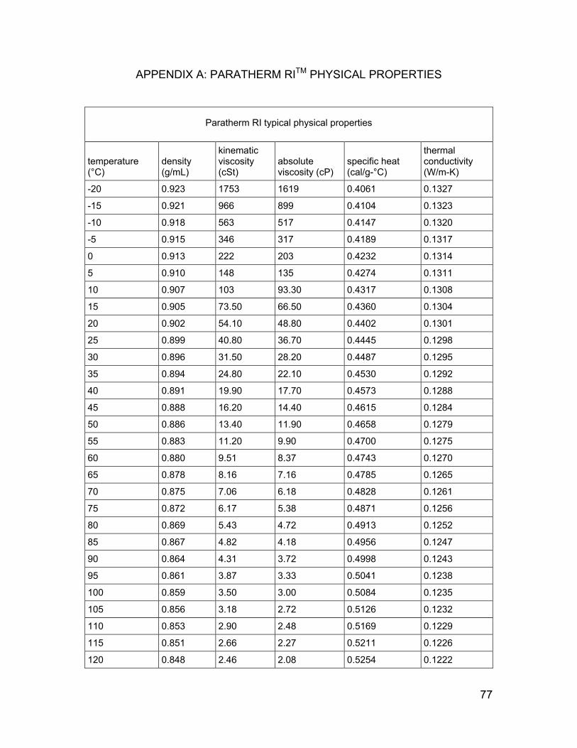
APPENDIX A: PARATHERM RITM PHYSICAL PROPERTIES

Paratherm RI typical physical properties

temperature (°C)

density (g/mL)

kinematic viscosity (cSt)

absolute viscosity (cP)

specific heat (cal/g-°C)

thermal conductivity (W/m-K)

-20 0.923 1753 1619 0.4061 0.1327

-15 0.921 966 899 0.4104 0.1323

-10 0.918 563 517 0.4147 0.1320

-5 0.915 346 317 0.4189 0.1317

0 0.913 222 203 0.4232 0.1314

5 0.910 148 135 0.4274 0.1311

10 0.907 103 93.30 0.4317 0.1308

15 0.905 73.50 66.50 0.4360 0.1304

20 0.902 54.10 48.80 0.4402 0.1301

25 0.899 40.80 36.70 0.4445 0.1298

30 0.896 31.50 28.20 0.4487 0.1295

35 0.894 24.80 22.10 0.4530 0.1292

40 0.891 19.90 17.70 0.4573 0.1288

45 0.888 16.20 14.40 0.4615 0.1284

50 0.886 13.40 11.90 0.4658 0.1279

55 0.883 11.20 9.90 0.4700 0.1275

60 0.880 9.51 8.37 0.4743 0.1270

65 0.878 8.16 7.16 0.4785 0.1265

70 0.875 7.06 6.18 0.4828 0.1261

75 0.872 6.17 5.38 0.4871 0.1256

80 0.869 5.43 4.72 0.4913 0.1252

85 0.867 4.82 4.18 0.4956 0.1247

90 0.864 4.31 3.72 0.4998 0.1243

95 0.861 3.87 3.33 0.5041 0.1238

100 0.859 3.50 3.00 0.5084 0.1235

105 0.856 3.18 2.72 0.5126 0.1232

110 0.853 2.90 2.48 0.5169 0.1229

115 0.851 2.66 2.27 0.5211 0.1226

120 0.848 2.46 2.08 0.5254 0.1222

77

125 0.845 2.27 1.92 0.5297 0.1219

130 0.842 2.11 1.78 0.5339 0.1216

135 0.840 1.96 1.65 0.5382 0.1213

140 0.837 1.84 1.54 0.5424 0.1210

145 0.834 1.72 1.44 0.5467 0.1206

150 0.832 1.62 1.35 0.5510 0.1202

78

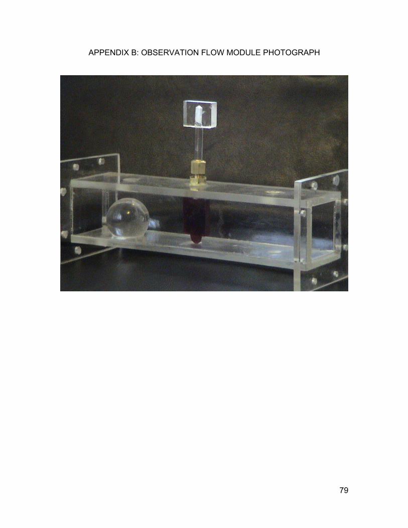
APPENDIX B: OBSERVATION FLOW MODULE PHOTOGRAPH

79

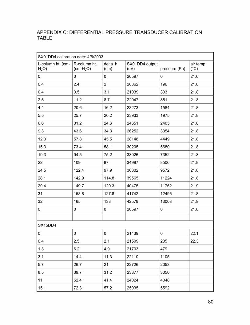
APPENDIX C: DIFFERENTIAL PRESSURE TRANSDUCER CALIBRATION TABLE

SX01DD4 calibration date: 4/6/2003

L-column ht. (cm-H2O)

R-column ht. (cm-H2O)

delta h (cm)

SX01DD4 output (uV) pressure (Pa)

air temp (°C)

0 0 0 20597 0 21.6

0.4 2.4 2 20862 196 21.8

0.4 3.5 3.1 21039 303 21.8

2.5 11.2 8.7 22047 851 21.8

4.4 20.6 16.2 23273 1584 21.8

5.5 25.7 20.2 23933 1975 21.8

6.6 31.2 24.6 24651 2405 21.8

9.3 43.6 34.3 26252 3354 21.8

12.3 57.8 45.5 28148 4449 21.8

15.3 73.4 58.1 30205 5680 21.8

19.3 94.5 75.2 33026 7352 21.8

22 109 87 34987 8506 21.8

24.5 122.4 97.9 36802 9572 21.8

28.1 142.9 114.8 39565 11224 21.8

29.4 149.7 120.3 40475 11762 21.9

31 158.8 127.8 41742 12495 21.8

32 165 133 42579 13003 21.8

0 0 0 20597 0 21.8

SX15DD4

0 0 0 21439 0 22.1

0.4 2.5 2.1 21509 205 22.3

1.3 6.2 4.9 21703 479

3.1 14.4 11.3 22110 1105

5.7 26.7 21 22726 2053

8.5 39.7 31.2 23377 3050

11 52.4 41.4 24024 4048

15.1 72.3 57.2 25035 5592

80

17.8 86.3 68.5 25752 6697

21 103 82 26599 8017 22.4

24.8 122.4 97.6 27609 9542

28.2 141.5 113.3 28612 11077

31.8 161.8 130 29691 12710 22.4

32 167 135 29999 13199 22.6

34.6 182.6 148 30815 14470

37.6 199.5 161.9 31696 15829

40.8 219 178.2 32751 17423

44.8 245.4 200.6 34111 19613 22.9

31.8 159.2 127.4 29551 12456 22.9

31.1 155.7 124.6 29368 12182

30.9 154.6 123.7 29311 12094

0 0 0 21442 0 22.9

81

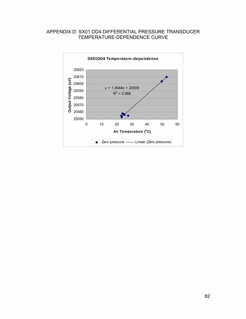
APPENDIX D: SX01 DD4 DIFFERENTIAL PRESSURE TRANSDUCER TEMPERATURE-DEPENDENCE CURVE

SX01DD4 Temperature-dependence

y = 1.9044x + 20509R2 = 0.986

20550

20560

20570

20580

20590

20600

20610

20620

0 10 20 30 40 50 60

Air Temperature (oC)

Out

put V

olta

ge (u

V)

Zero pressure Linear (Zero pressure)

82

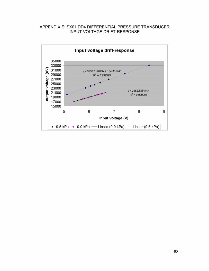
APPENDIX E: SX01 DD4 DIFFERENTIAL PRESSURE TRANSDUCER INPUT VOLTAGE DRIFT-RESPONSE

Input voltage drift-response

y = 3162.586444xR2 = 0.999991

y = 3937.119873x + 104.381440R2 = 0.999999

1500017000190002100023000250002700029000310003300035000

5 6 7 8 9

Input voltage (V)

outp

ut v

olta

ge (u

V)

9.5 kPa 0.0 kPa Linear (0.0 kPa) Linear (9.5 kPa)

83