1    

FLOW AND THERMAL ANALYSIS OF OIL BRUSH SEALS, AND INVESTIGATION OF SHEAR HEATING PHENOMENON

Mahmut F. Aksit, E. Tolga Duran

Sabanci University, Orhanli, Tuzla, Istanbul/TURKEY, 34956

Abstract Due to their superior performance and stable leakage characteristics, brush seal is one of the emerging seals to be used in oil and oil mist applications in aero-engines and turbines. The viscous medium between the high speed rotor surface and bearing surfaces formed by brush seal bristles generates a hydrodynamic lifting force that determines seal clearance and leakage rate in oil sealing applications. The analytical solution to bristle lifting force can be found by using Reynolds formulation. Following a short bearing approximation, a closed form solution of the lifting force has been previously presented. However, the solution suggests a strong dependence of hydrodynamic lift force and seal clearance on oil temperature and viscosity. This work presents an analytical solution to oil temperature rise due to shear heating. The hydrodynamic lift force relation has been expanded to include oil temperature variability due to rotor speed and lift clearance. Results are also compared with the experimental data obtained from the dynamic oil seal test rig.

Keywords: Brush Seal, Shear Heat Dissipation, Hydrodynamic Lift Clearance, Oil Pressure, Bearing Theory

1. Introduction

Owing to their excellent leakage performance, brush seals have been extensively used in secondary flow sealing in turbo machinery. Labyrinth seals, carbon seals or oil rings are other sealing elements that are commonly used around the bearings and oil sumps. Tighter clearances are required at these locations to avoid oil contamination of the downstream turbine components, to limit hot gas ingestion to oil sumps in adverse conditions, or to minimize oil consumption levels. In hydrogen cooled generator applications, these requirements are accentuated by the presence of explosive cooling gas.

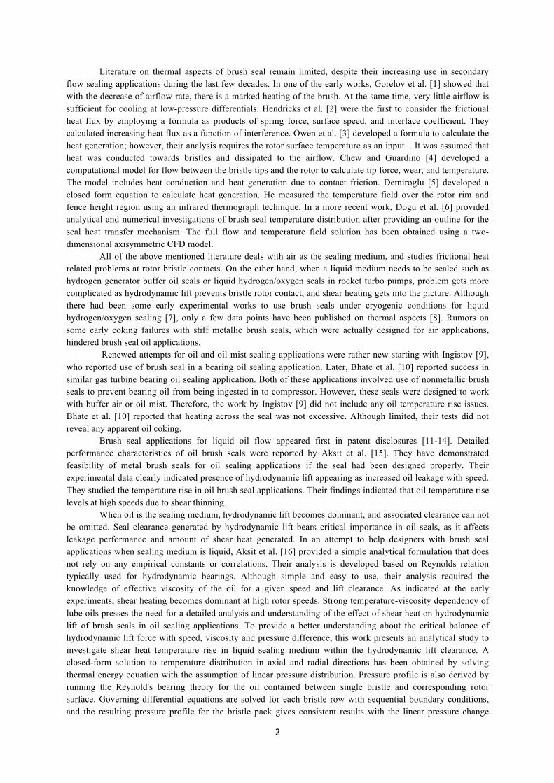
Recently, brush seal is emerging as a viable alternative in both oil and oil mist applications. As

illustrated in Fig. 1, a brush seal is a set of fine diameter metallic wires densely packed between retaining and backing plates. The bristles touch the rotor with an angle in the direction of the rotor rotation. Brush seals perform very well under rotor transients owing to the inherent compliance of bristles.

Fig. 1– Brush seal geometry.

2    

Literature on thermal aspects of brush seal remain limited, despite their increasing use in secondary flow sealing applications during the last few decades. In one of the early works, Gorelov et al. [1] showed that with the decrease of airflow rate, there is a marked heating of the brush. At the same time, very little airflow is sufficient for cooling at low-pressure differentials. Hendricks et al. [2] were the first to consider the frictional heat flux by employing a formula as products of spring force, surface speed, and interface coefficient. They calculated increasing heat flux as a function of interference. Owen et al. [3] developed a formula to calculate the heat generation; however, their analysis requires the rotor surface temperature as an input. . It was assumed that heat was conducted towards bristles and dissipated to the airflow. Chew and Guardino [4] developed a computational model for flow between the bristle tips and the rotor to calculate tip force, wear, and temperature. The model includes heat conduction and heat generation due to contact friction. Demiroglu [5] developed a closed form equation to calculate heat generation. He measured the temperature field over the rotor rim and fence height region using an infrared thermograph technique. In a more recent work, Dogu et al. [6] provided analytical and numerical investigations of brush seal temperature distribution after providing an outline for the seal heat transfer mechanism. The full flow and temperature field solution has been obtained using a two-dimensional axisymmetric CFD model.

All of the above mentioned literature deals with air as the sealing medium, and studies frictional heat related problems at rotor bristle contacts. On the other hand, when a liquid medium needs to be sealed such as hydrogen generator buffer oil seals or liquid hydrogen/oxygen seals in rocket turbo pumps, problem gets more complicated as hydrodynamic lift prevents bristle rotor contact, and shear heating gets into the picture. Although there had been some early experimental works to use brush seals under cryogenic conditions for liquid hydrogen/oxygen sealing [7], only a few data points have been published on thermal aspects [8]. Rumors on some early coking failures with stiff metallic brush seals, which were actually designed for air applications, hindered brush seal oil applications.

Renewed attempts for oil and oil mist sealing applications were rather new starting with Ingistov [9], who reported use of brush seal in a bearing oil sealing application. Later, Bhate et al. [10] reported success in similar gas turbine bearing oil sealing application. Both of these applications involved use of nonmetallic brush seals to prevent bearing oil from being ingested in to compressor. However, these seals were designed to work with buffer air or oil mist. Therefore, the work by Ingistov [9] did not include any oil temperature rise issues. Bhate et al. [10] reported that heating across the seal was not excessive. Although limited, their tests did not reveal any apparent oil coking.

Brush seal applications for liquid oil flow appeared first in patent disclosures [11-14]. Detailed performance characteristics of oil brush seals were reported by Aksit et al. [15]. They have demonstrated feasibility of metal brush seals for oil sealing applications if the seal had been designed properly. Their experimental data clearly indicated presence of hydrodynamic lift appearing as increased oil leakage with speed. They studied the temperature rise in oil brush seal applications. Their findings indicated that oil temperature rise levels at high speeds due to shear thinning.

When oil is the sealing medium, hydrodynamic lift becomes dominant, and associated clearance can not be omitted. Seal clearance generated by hydrodynamic lift bears critical importance in oil seals, as it affects leakage performance and amount of shear heat generated. In an attempt to help designers with brush seal applications when sealing medium is liquid, Aksit et al. [16] provided a simple analytical formulation that does not rely on any empirical constants or correlations. Their analysis is developed based on Reynolds relation typically used for hydrodynamic bearings. Although simple and easy to use, their analysis required the knowledge of effective viscosity of the oil for a given speed and lift clearance. As indicated at the early experiments, shear heating becomes dominant at high rotor speeds. Strong temperature-viscosity dependency of lube oils presses the need for a detailed analysis and understanding of the effect of shear heat on hydrodynamic lift of brush seals in oil sealing applications. To provide a better understanding about the critical balance of hydrodynamic lift force with speed, viscosity and pressure difference, this work presents an analytical study to investigate shear heat temperature rise in liquid sealing medium within the hydrodynamic lift clearance. A closed-form solution to temperature distribution in axial and radial directions has been obtained by solving thermal energy equation with the assumption of linear pressure distribution. Pressure profile is also derived by running the Reynold's bearing theory for the oil contained between single bristle and corresponding rotor surface. Governing differential equations are solved for each bristle row with sequential boundary conditions, and the resulting pressure profile for the bristle pack gives consistent results with the linear pressure change

3    

assumption of closed form thermal solution. Effective temperature has been calculated for different values of rotor surface speed, pressure difference and hydrodynamic lift clearance. Calculated speed dependent viscosity values have been adopted into the bearing theory to calculate hydrodynamic lifting force. Results have been compared with lifting force obtained by Aksit et al. [16] through beam and short bearing analyses.

2. Thermal Energy Equation for the Brush Seal

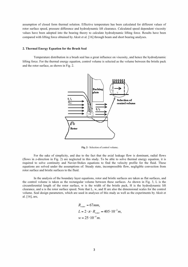
Temperature distribution in a brush seal has a great influence on viscosity, and hence the hydrodynamic lifting force. For the thermal energy equation, control volume is selected as the volume between the bristle pack and the rotor surface, as shown in Fig. 2.

Fig. 2– Selection of control volume.

For the sake of simplicity, and due to the fact that the axial leakage flow is dominant, radial flows (flows in z-direction in Fig. 2) are neglected in this study. To be able to solve thermal energy equation, it is required to solve continuity and Navier-Stokes equations to find the velocity profile for the fluid. These equations are solved under the assumptions of: Steady state, incompressible flow, negligible convection from rotor surface and bristle surfaces to the fluid.

In the analysis of the boundary layer equations, rotor and bristle surfaces are taken as flat surfaces, and the control volume is taken as the rectangular volume between these surfaces. As shown in Fig. 3, L is the circumferential length of the rotor surface, w is the width of the bristle pack, H is the hydrodynamic lift clearance, and u is the rotor surface speed. Note that L, w, and H are also the dimensional scales for the control volume. Seal design parameters, which are used in analyses of this study as well as the experiments by Aksit et al. [16], are,

.1025

,104052

,67

4

3

mwmRL

mmR

rotor

rotor

−

−

⋅=

⋅≈⋅⋅=

=

π

4    

Fig. 3– Unwrapped brush seal geometry.

Hydrodynamic lift clearance is a function of pressure difference and rotor speed. Based on the experimental data, amount of lift and the inlet temperature (for the initial steps of analysis) are taken as below. Density and the specific heat values for the oil at the upstream temperature are also specified.

./5.2030,/61.884

,50,1040

3

6

CkgJcmkg

CTmH

p

u

ο

ρ

=

=

=

⋅=°

−

Analysis of this study starts with the continuity and the Navier-Stokes equations, which will provide the required velocity and pressure profiles for the thermal analysis.

The leakage flow through the control volume is an internal flow, and the Reynolds number needs to be checked in order to decide the flow type. Hydrodynamic lift clearance is the characteristic length for the flow and control volume of interest.

Re f

H

Hρ υ

µ

⋅ ⋅= (1)

In Eq. (1), ρ is the density of the fluid, and υf is the mean fluid velocity. Viscosity of the oil at upstream temperature of 50oC is equal to 0.0195Pa.s, and the density of the oil at upstream temperature is 884.61kg/m3. Flow rate per circumferential length of the rotor is divided to hydrodynamic lift clearance to obtain the mean fluid velocity value. To match the available data, flow rate per circumferential length of the rotor is taken as

5    

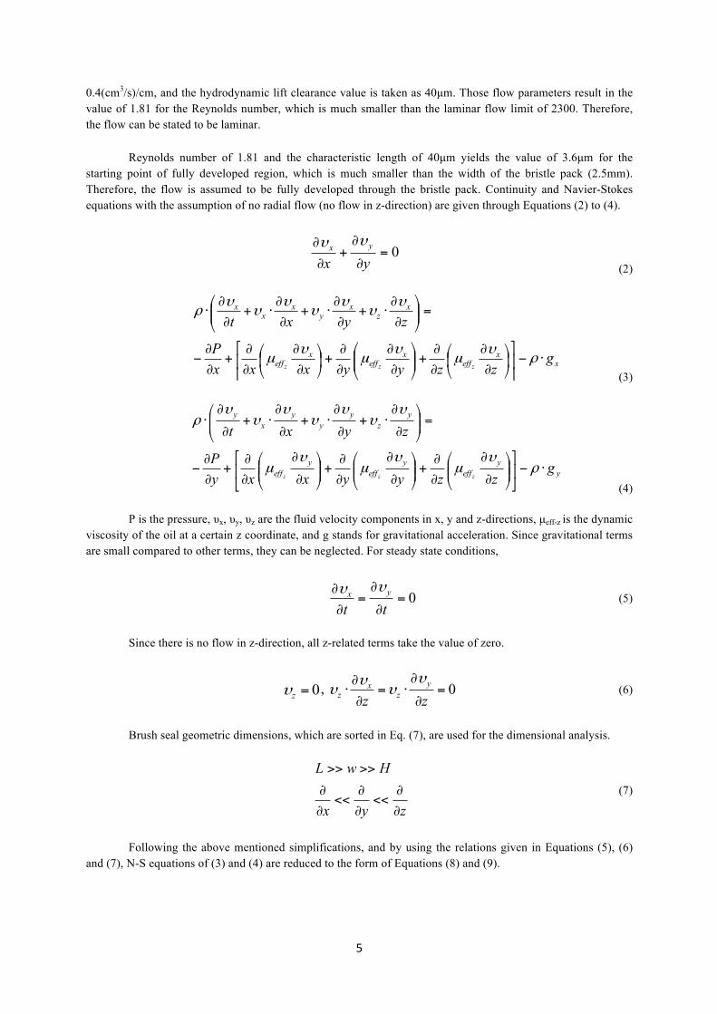
0.4(cm3/s)/cm, and the hydrodynamic lift clearance value is taken as 40µm. Those flow parameters result in the value of 1.81 for the Reynolds number, which is much smaller than the laminar flow limit of 2300. Therefore, the flow can be stated to be laminar.

Reynolds number of 1.81 and the characteristic length of 40µm yields the value of 3.6µm for the starting point of fully developed region, which is much smaller than the width of the bristle pack (2.5mm). Therefore, the flow is assumed to be fully developed through the bristle pack. Continuity and Navier-Stokes equations with the assumption of no radial flow (no flow in z-direction) are given through Equations (2) to (4).

0=∂

∂+

∂

∂

yxyx υυ

(2)

x

xeff

xeff

xeff

xz

xy

xx

x

gzzyyxxx

P

zyxt

zzz⋅−⎥

⎦

⎤⎢⎣

⎡⎟⎠

⎞⎜⎝

⎛∂

∂

∂

∂+⎟⎟⎠

⎞⎜⎜⎝

⎛

∂

∂

∂

∂+⎟⎠

⎞⎜⎝

⎛∂

∂

∂

∂+

∂

∂−

=⎟⎟⎠

⎞⎜⎜⎝

⎛

∂

∂⋅+

∂

∂⋅+

∂

∂⋅+

∂

∂⋅

ρυ

µυ

µυ

µ

υυ

υυ

υυ

υρ

(3)

y

yeff

yeff

yeff

yz

yy

yx

y

gzzyyxxy

P

zyxt

zzz⋅−⎥

⎦

⎤⎢⎣

⎡⎟⎟⎠

⎞⎜⎜⎝

⎛

∂

∂

∂

∂+⎟⎟⎠

⎞⎜⎜⎝

⎛

∂

∂

∂

∂+⎟⎟⎠

⎞⎜⎜⎝

⎛

∂

∂

∂

∂+

∂

∂−

=⎟⎟⎠

⎞⎜⎜⎝

⎛

∂

∂⋅+

∂

∂⋅+

∂

∂⋅+

∂

∂⋅

ρυ

µυ

µυ

µ

υυ

υυ

υυ

υρ

(4)

P is the pressure, υx, υy, υz are the fluid velocity components in x, y and z-directions, µeff-z is the dynamic viscosity of the oil at a certain z coordinate, and g stands for gravitational acceleration. Since gravitational terms are small compared to other terms, they can be neglected. For steady state conditions,

0=∂

∂=

∂

∂

ttyx υυ

(5)

Since there is no flow in z-direction, all z-related terms take the value of zero.

0=zυ , 0=∂

∂⋅=

∂

∂⋅

zzy

zx

z

υυ

υυ (6)

Brush seal geometric dimensions, which are sorted in Eq. (7), are used for the dimensional analysis.

zyx

HwL

∂

∂<<

∂

∂<<

∂

∂

>>>>

(7)

Following the above mentioned simplifications, and by using the relations given in Equations (5), (6) and (7), N-S equations of (3) and (4) are reduced to the form of Equations (8) and (9).

6    

2

2

zxP

yxx

effx

yx

x z ∂

∂⋅+

∂

∂−=⎟⎟

⎠

⎞⎜⎜⎝

⎛

∂

∂⋅+

∂

∂⋅⋅

υµ

υυ

υυρ

(8)

                                                                                                2

2

zyP

yxy

effy

yy

x z ∂

∂⋅+

∂

∂−=⎟⎟

⎠

⎞⎜⎜⎝

⎛

∂

∂⋅+

∂

∂⋅⋅

υµ

υυ

υυρ                                                                       (9)  

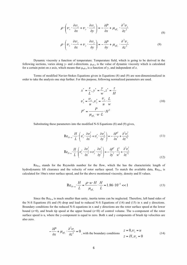
Dynamic viscosity a function of temperature. Temperature field, which is going to be derived in the following sections, varies along y- and z-directions. µeff-z is the value of dynamic viscosity which is calculated for a certain point on z axis, which means that µeff-z is a function of y, and independent of z.

Terms of modified Navier-Stokes Equations given in Equations (8) and (9) are non-dimensionalized in order to take the analysis one step further. For this purpose, following normalized parameters are used.

2*

**

***

,

,,

HLu

PP

wL

uu

Hzz

wyy

Lxx

zeff

yy

xx

⋅⋅⋅

=

⋅==

===

µ

υυ

υυ (10)

Substituting these parameters into the modified N-S Equations (8) and (9) gives,

* * 2 *** *

* * * *2Re x x xH u x y

H PL x y x z

υ υ υυ υ−

⎛ ⎞∂ ∂ ∂∂⋅ ⋅ ⋅ + ⋅ = − +⎜ ⎟∂ ∂ ∂ ∂⎝ ⎠

(11)

* * 2 ** 2* *

* * * 2 *2Re y y yH u x y

H P LL x y y w z

υ υ υυ υ−

⎛ ⎞∂ ∂ ∂∂⋅ ⋅ ⋅ + ⋅ = − ⋅ +⎜ ⎟⎜ ⎟∂ ∂ ∂ ∂⎝ ⎠ (12)

ReH-u stands for the Reynolds number for the flow, which the has the characteristic length of hydrodynamic lift clearance and the velocity of rotor surface speed. To match the available data, ReH-u is calculated for 10m/s rotor surface speed, and for the above mentioned viscosity, density and H values.

3Re 1.86 10 1z

H ueff

H u H HL L

ρµ

−−

⋅ ⋅⋅ = ⋅ ≈ ⋅ << (13)

Since the ReH-u is much smaller than unity, inertia terms can be neglected. Therefore, left hand sides of the N-S Equations (8) and (9) drop and lead to reduced N-S Equations of (14) and (15) in x and y directions. Boundary conditions for the reduced N-S equations in x and y directions are the rotor surface speed at the lower bound (z=0), and brush tip speed at the upper bound (z=H) of control volume. The x-component of the rotor surface speed is u, where the y-component is equal to zero. Both x and y components of brush tip velocities are also zero.

2

2 0z

xeff

Px z

υµ

∂∂− + ⋅ =∂ ∂ , with the boundary conditions

0,, 0x

x

z uz H

υ

υ

= =

= = (14)

7    

2

2 0z

yeff

Py z

υµ

∂∂− + ⋅ =∂ ∂ , with the boundary conditions

0, 0

, 0y

y

zz H

υ

υ

= =

= = (15)

Velocity profiles for the fluid in x and y directions are found by solving reduced N-S Equations (14) and (15) with the given boundary conditions respectively.

( ) ⎟⎠

⎞⎜⎝

⎛ −⋅+⋅−⋅∂

∂⋅=

HzuHzz

xP

zeffx 1

21 2

µυ (16)

( )HzzyP

zeffy ⋅−⋅

∂

∂⋅= 2

21µ

υ (17)

Substituting xυ and yυ into the continuity equation, Eq. (1), and making the necessary simplifications

yield,

033

=⎟⎟⎠

⎞⎜⎜⎝

⎛

∂

∂⋅

∂

∂+⎟⎟⎠

⎞⎜⎜⎝

⎛

∂

∂⋅

∂

∂

yPH

yxPH

xzz effeff µµ

(18)

Since L>>w, ∂ / x∂ <<∂ / y∂ , Eq. (18) reduces to,

03

=⎟⎟⎠

⎞⎜⎜⎝

⎛

∂

∂

∂

∂

yPH

yzeff

µ (19)

Eq. (19) is the governing differential equation for the variation of hydrodynamic pressure in axial (y) direction. The term µeff-z in Equation (19) depends on y, and cannot be taken out. However, for the sake of simplicity, and to be able to find a closed form solution to the temperature distribution, pressure gradient along y-axis is assumed to be constant. As stated by Bhate et al [10], axial pressure drop is almost linear. Therefore, Equation (19) reduces to,

1P Cy∂

=∂ , B.C’s:

0,,

u

d

y P Py w P P= =

= = (20)

Pressure profile can be found by solving the differential equation (20).

uPP y PwΔ

= − ⋅ +, where u dP P PΔ = − (21)

Pressure profile of Eq. (21) can be used to solve thermal energy equation for the flow. In its most general form, the 3-D thermal energy equation for an incompressible flow is as given below.

8    

'''p x y zT T T T T Tc k k k qx y z x x y y z z

ρ υ υ υ µ φ⎛ ⎞ ⎛ ⎞∂ ∂ ∂ ∂ ∂ ∂ ∂ ∂ ∂⎛ ⎞ ⎛ ⎞+ + = + + + ⋅ +⎜ ⎟ ⎜ ⎟⎜ ⎟ ⎜ ⎟∂ ∂ ∂ ∂ ∂ ∂ ∂ ∂ ∂⎝ ⎠ ⎝ ⎠⎝ ⎠ ⎝ ⎠

(22)

φ is the dissipation function which is defined as,

2 2 22 2

2 y y yx xz z

x y z y x y zυ υ υυ υυ υ

φ⎡ ⎤∂ ∂ ∂⎛ ⎞ ⎛ ⎞ ⎛ ⎞∂ ∂∂ ∂⎛ ⎞ ⎛ ⎞= + + + + + +⎢ ⎥⎜ ⎟ ⎜ ⎟ ⎜ ⎟⎜ ⎟⎜ ⎟∂ ∂ ∂ ∂ ∂ ∂ ∂⎝ ⎠⎝ ⎠⎢ ⎥⎝ ⎠ ⎝ ⎠ ⎝ ⎠⎣ ⎦ (23)

22 2

3yx xz z

z x x y zυυ υυ υ∂⎛ ⎞∂ ∂∂ ∂⎛ ⎞+ + − + +⎜ ⎟⎜ ⎟∂ ∂ ∂ ∂ ∂⎝ ⎠ ⎝ ⎠

.

In thermal energy equation (22), '''q stands for the heat input per volume and equals to zero for the control volume of interest. Since the circumferential length of the rotor (L) is much larger than the bristle pack width (w) and hydrodynamic lift clearance (H), temperature of the oil can be assumed to be lumped in x-direction. In addition to that, dissipation function terms, xυ∂ / x∂ , xυ∂ / y∂ drop out when compared to xυ∂ /

z∂ , and yυ∂ / x∂ , yυ∂ / y∂ drop out when compared to yυ∂ / z∂ . Since υz is zero, all z-related terms on the

left hand side of the thermal energy equation and in the dissipation function drop out. Assuming that there is no convection from the rotor and the bristle surfaces to the fluid, and neglecting the heat conduction, thermal energy equation reduces,

22yx

p yTcy z z

υυρ υ µ

⎛ ⎞∂⎛ ⎞∂∂ ⎛ ⎞⎜ ⎟= + ⎜ ⎟⎜ ⎟⎜ ⎟∂ ∂ ∂⎝ ⎠ ⎝ ⎠⎝ ⎠ (24)

Based on the experimental leakage data, flow rate in y-direction is around 0.4cm3/sec. Oil properties for the test conditions and the thermal conductivity coefficient of 0.145W/m-K result in the value of 495 for the Peclet number, which is the ratio of forced convection to heat conduction. Hence, it can be stated that the contribution of heat conduction to energy transfer is small in comparison with convection terms, and therefore conduction terms can be neglected for the control volume of interest.

3. Closed-form solution for the thermal energy equation

Thermal energy equation given in Eq. (24) is a first order differential equation, where the boundary condition is the upstream temperature; Tu. Density and specific heat of the fluid are assumed to be constant at their upstream temperature values.

The temperature dependent viscosity can be given by the formula;

( )00

T Te βµ µ − −= (25)

Taking z-derivatives of the velocity profiles in x and z-directions, which are given in Equations (16) and (17), with appropriate simplifications coming from scaling yields,

x uz Hυ∂

= −∂

(26)

9    

( )1 22

y P z Hz yυ

µ

∂ ∂= ⋅ ⋅ −

∂ ∂ (27)

Substituting 0T Tθ = − into the temperature dependent viscosity equation yields;

βθµµ −= e0 (28)

After substituting Equations (26), (27) and (28) into the thermal energy equation, Equation (24) takes the form of Equation (29).

( )( )22

2 22 2 220 0

21 1 02 4p

z Hu w Pe e yH P wc z zH

βθ βθθµ µρ

⎡ ⎤−⎛ ⎞ Δ⋅ ⋅∂ + ⋅ + ⋅ ∂ =⎢ ⎥⎜ ⎟

Δ− ⎢ ⎥⎝ ⎠ ⎣ ⎦,

B.C: uT T= at 0y = (29)

The oil of interest has the β value of 0.0294 and µ0 value of 0.028Pa.s for T0 = 37.78oC. The above governing differential equation can be re-written as:

( )( , ) , 0M y N y yθ θ θ⋅∂ + ⋅∂ =

, 0yM = , ( )

( )2 2, 22

0

224p

z HPN ewc z zH

βθθ

βµρ

−Δ= ⋅ ⋅ ⋅

− (30)

Since , yM does not equal to ,N θ , the differential equation is not an exact differential equation. An

integration factor must be found to make it exact. Assume an integration factor η , such as,

( )( )

2, ,

2

2y

p

N M z Hd P dyM wc z zH

θηβ

η ρ

− − Δ= = ⋅ ⋅ ⋅

⋅ ⋅ − (31)

Integrating the both sides of Eq. (31) yields,

( )( )

2

2

2

p

z Hd P dywc z zH

ηβ

η ρ

− Δ= ⋅ ⋅ ⋅

⋅ ⋅ −∫ ∫

( ) ( )( )

2

2

2ln

p

z H Py ywc z zH

η βρ

− Δ= ⋅ ⋅ ⋅⎡ ⎤⎣ ⎦ ⋅ ⋅ −

(32)

The below integration factor, which is a function of y, can be extracted from Eq. (32).

10    

( )( ) ⎥

⎥⎦

⎤

⎢⎢⎣

⎡⋅⋅

Δ⋅

−

−= y

wP

zHzcHzy

p

βρ

η 2

22exp)( (33)

An exact differential equation can be obtained by multiplying the Eq. (29) with the integration factor η(y). After multiplication, relations given in Equations (34), (35) and (36) can be obtained.

0,, =∂+∂=∂ yFFF yθθ (34)

( )( )

( )( )

⎥⎦

⎤⎢⎣

⎡ −⋅

Δ+

Δ⋅

−

⎥⎥⎦

⎤

⎢⎢⎣

⎡⋅⋅

Δ⋅

−

−

= βθ

µρ

βρ

220

2

2

2

2

2

2

, 42

2exp

eHzwP

PHwu

zHzc

ywP

zHzcHz

Fp

py (35)

( )( ) ⎥

⎥⎦

⎤

⎢⎢⎣

⎡⋅⋅

Δ⋅

−

−⋅⋅= y

wP

zHzcHzeF

p

βρµ

βθθ 2

22

20

,2exp

21

(36)

Taking the derivative of F(θ,y) with respect to θ , and equating it to Eq. (36), gives the value of zero for C(θ),θ, which means that C(θ)=C, which is a constant. Although solution to function F(θ,y) is found, it is required to find θ in order to find temperature. It is known from the differential equation (34) that F∂ equals to zero, which means F(θ,y) is a constant. As a result, solution to differential equation is obtained as,

( )( )

( )( ) 02exp

242

22

2

22

20

2

2

2

=+⎥⎥⎦

⎤

⎢⎢⎣

⎡⋅⋅

Δ⋅

−

−⋅

−Δ⋅⎥⎦

⎤⎢⎣

⎡ −⋅

Δ+

ΔCy

wP

zHzcHz

HzPweHz

wP

PHwu

p

βρβµ

βθ

(38)

C2 is a constant other than C. After applying temperature boundary condition, T = TU at y = 0, C2 is obtained as,

( )( )2

220

2

2

2

2 242

HzPweHz

wP

Pw

HuC u

−Δ⋅⎟⎟⎠

⎞⎜⎜⎝

⎛ −⋅

Δ+

Δ⋅−=

βµβθ (39)

After substituting C2 into the Eq. (38) while keeping in mind that 0T Tθ = − and 0TTuu −=θ ,

temperature distribution is reached as,

⎟⎟⎠

⎞⎜⎜⎝

⎛⋅++= 43

2

10 ln21 ff

ffTT

β (40)

where

11    

( )( )

( )( )

( )( )[ ]( )( ) 12exp

24

2exp

2exp

2

2

4

2

20

3

2

2

2

01

−⎥⎥⎦

⎤

⎢⎢⎣

⎡⋅⋅

Δ⋅

−

−−=

−⋅Δ⋅

⋅⋅=

⎥⎥⎦

⎤

⎢⎢⎣

⎡⋅⋅

Δ⋅

−

−=

−=

ywP

zHzcHzf

HzPHwuf

ywP

zHzcHzf

TTf

p

p

u

βρ

µ

βρ

β

(41)

Temperature distribution under the bristle pack along y and z axes is obtained as a function of pressure difference (ΔP), upstream temperature (Tu) rotor surface speed (u), hydrodynamic lift clearance (H), bristle pack width (w) and oil (properties (ρ, cp, µ0, β)). Pressure load and upstream temperature are design parameters and known. Oil properties are also known. Hydrodynamic lift clearance changes with the rotor surface speed and pressure difference. To compare the results with the hydrodynamic lift data provided by Aksit et al. [16], which are also given in Table 1 and Fig. 5, following seal parameters are used in the analyses,

Bristle radius, Rb = 0.051 mm

Elasticity modulus of the bristle, E = 2.07x1011 Pa

Cant angle, θ = 450

Viscosity constants for the fluid, β = 0.0294, µ0 = 0.028Pa.s for To = 37.78oC

Free bristle height, BH = 16mm.

As it can be seen from the temperature function given in Equations (40) and (41), it gives 0/0 uncertainty for value of H/2 for z. The uncertainty of the temperature function at z = H/2 is removed by applying L’Hopitals Rule. Temperature function at z = H/2 is obtained as given in Eq. (42).

( )[ ] ( )⎪⎭

⎪⎬⎫

⎪⎩

⎪⎨⎧

⋅⋅Δ⋅

⋅⋅⋅⋅+−⋅+=⎟

⎠

⎞⎜⎝

⎛ =⋅

4

2

001162expln

21

2,

HwPcywuTTTHzyT

p

ou ρ

βµβ

β (42)

Since convection from bristles and rotor surfaces is neglected, temperature distribution goes to infinity at both ends for z, which does not reflect the real case. Therefore, mean value of temperature with respect to z is used for temperature analysis.

( ) ( )0

1 ,mean z

H

T y T y z dzH−

= ⋅∫ (43)

Tmean-z is the mean temperature in z-axis. Numerical integration methods are used to evaluate the integral of temperature with respect to z. Trapezoid rule is employed as the numeric integration method.

( ) ( ) ( )1 1 20

( , ) , 2 , ... ,2

H lT y z dz T y z T y z l T y z⋅ = ⋅ + + + +⎡ ⎤⎣ ⎦∫ (44)

12    

l , the increment of z for each step, is taken as H/80, which is around 5x10-7 m. In Eq. (44), z1 takes the value of zero, and z2 stands for H, and temperature goes to infinity at that z-value. To be able to get over this problem, values of the temperature at both ends are evaluated at z-locations which have H/80 distance from these ends. After evaluating the integral, mean temperature value with respect to z at any y point can be derived by simply dividing it by H, as given in Eq. (43). A simple MATLAB code is written to compute the numeric integration and mean-z temperature values along y-axis. Mean-z temperature distribution along y-axis is given in Fig. 11 for different pressure loads and rotor surface speeds.

Table 1 – Hydrodynamic lift clearance data for different rotor surface speeds and pressure loads, based on experimental leakage data

Hydrodynamic lift clearance [mm]

Rotor surface speed [m/s] ΔP = 48.3 kPa ΔP = 89.6 kPa

0 0 0

6.2 0.044 0.038

12.3 0.052 0.044

20.5 0.048 0.044

Fig. 4– Hydrodynamic lift clearance versus rotor speed under different pressure loads, based on experimental leakage data Aksit et al. [16]

4. Hydrodynamic lift force theories in literature and shear heat effect included bearing theory

Hydrodynamic lift force acts to deflect bristles off the shaft surface. This force is balanced by a reaction force due to beam/bristle deflection and so called “blow-down” forces occurring due to radial pressure gradient

13    

within the bristle pack. In rotor operating conditions, hydrodynamic lift clearance is determined by the balance of the lift force and reaction forces. Therefore, it is logical to compare estimated hydrodynamic lift force with beam bristle/beam deflection forces, as well as the results of other works.

Equations (45) and (46) are used for the calculation of the reaction of a bristle with the beam bending theory [16, 17].

( )( )θ

π23

4

sin2

643

b

b

LHREW = (45)

)sin(θ

BHLb = (46)

θ=450 refers to bristle lay angle, and BH is the free bristle height, which is taken as 16mm for the brush seal of interest. Radial pressure gradients, which put an additional fluid force on bristles, are not taken into account in Equations (45) and (46). Bristle interlocking and frictional effects are also not included in beam theory, and therefore that theory underestimates the actual bristle tip force, which will balance the hydrodynamic lift.

Studies, which estimate the hydrodynamic lift force without including the shear heating effect, are available in the literature. Previous study by Aksit et al. [16] provides the lifting force for a single bristle as,

HR

uRW bbµ

π

26

= (47)

For steady state operation, lift force given by Eq. (47) is balanced by bristle reaction forces which will include beam deflection as well as the effects of blow-down and frictional forces. However, as the rotor surface speed increases, estimated lift force, which is calculated by using the bearing theory with constant viscosity, increases continuously. The continuously increasing trend of the bearing theory is due to the fact that the formulation does not include oil thinning effect, which is caused from shear heat dissipation. In engine applications, as the test data illustrate in Fig. 4, increase in rotor speed cause temperature to rise, which results in decrease of dynamic viscosity. This decrease in viscosity is the reason for high speed lift force stabilization.

To include the effect of shear heating into the bearing theory, effective temperature is calculated by using temperature distribution given by Equations (40) and (41). Effective temperature is calculated by using the mean values of the temperature distribution along y and z-axes. Mean value of the temperature along z-direction can be derived as,

( ) ∫ ⋅=−

H

zmean dzzyTH

yT0

),(1 (48)

Taking the mean value of the Eq. (48) along y-axis yields the effective temperature for the bearing as follows,

0

1 ( )w

eff mean zT T y dyw −= ⋅∫ (49)

Numerical integration methods are used again in order to calculate mean value of the temperature along z-direction and the effective temperature. Trapezoidal rule is preferred as the numerical integration method, which in turn yields the mean-z temperature and effective temperature as,

14    

( ) ( ) ( ) ( )1 1 20

1 1( , ) , 2 , ... ,2

H

mean zlT y T y z dz T y z T y z l T y z

H H−⎧ ⎫= ⋅ = ⋅ + + + +⎡ ⎤⎨ ⎬⎣ ⎦⎩ ⎭∫ (50)

( )0

1 w

eff mean zT T y dyw −= ⋅∫ ( ) ( ) ( )2

1 1 2 21 2 ...2 mean z mean z mean zl T y T y l T y

w − − −⎧ ⎫= ⋅ + + + +⎡ ⎤⎨ ⎬⎣ ⎦⎩ ⎭

(51)

Parameters l and l2 are the increment for each step of numeric integration for z and y respectively. l is taken as one eightieth of the hydrodynamic lifting clearance, H/80, and l2 is taken as w/2500. Integration steps are taken as small as possible in order to minimize the numerical integration errors. Effective temperature is calculated for the hydrodynamic lift clearance, which is obtained from experimental leakage data for different rotor speeds under various pressure loads. Evaluations of numeric integrals are performed by a code written in MATLAB.

Effect of shear heat dissipation is included into the bearing theory by means of the effective viscosity. Effective viscosity is obtained from the effective temperature as,

( )oeff TT

eff e −−⋅= βµµ 0 (52)

Values of µ0, T0 and β are provided in the previous sections. Substituting this effective viscosity into the lift force, which is previously derived with constant viscosity, yields a lift force formulation that includes the shear heating effect as,

62

beff b

RW uRH

πµ= (53)

5. Derivation of oil film pressure for each bristle and theoretical confirmation of linear pressure change for the brush seal pack

In the previous sections, control volume is selected as the oil between the rotor surface and the bristle pack. Pressure distribution is assumed to change linear in the rotor axial direction, and thermal analysis is done with that assumption. As stated by Bhate et. al. [10], experimental studies suggest almost constant pressure gradient in the rotor axial direction, which is consistent with the results of previous boundary layer analysis of this study.

In this section, pressure distribution is derived by selecting the control volume as the oil contained between a single bristle and corresponding rotor surface. Reynolds bearing theory is applied to find the pressure distribution for each bristle row in the rotor axial direction. Cyclic pressure is assumed for the rotor tangential direction (x-direction in Fig. 3). Pressure profiles under bristle packs are combined to obtain the pressure change under the brush pack.

5.1 Selection of the control volume  

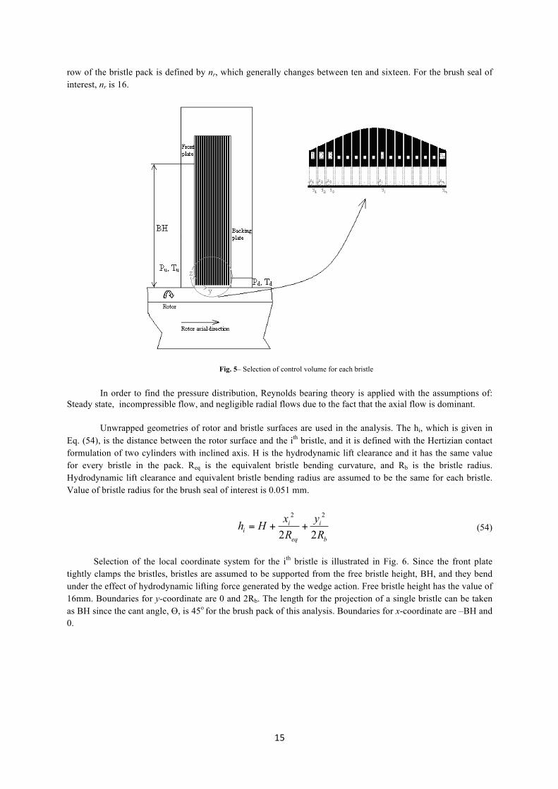
Selection of the control volume has crucial importance since it defines the valid region for the derived pressure distribution. Control volume for the hydrodynamic bearing theory is selected as the volume under each bristle, as showhn in Fig. 5. As it can be seen from the same figure, local coordinate system is defined for each control volume of interest. The subscripts in the local coordinate systems stand for the bristle numbers. First bristle is at the upstream side, and the last bristle is located at the downstream side. Number of bristles in one

15    

row of the bristle pack is defined by nr, which generally changes between ten and sixteen. For the brush seal of interest, nr is 16.

Fig. 5– Selection of control volume for each bristle

In order to find the pressure distribution, Reynolds bearing theory is applied with the assumptions of: Steady state, incompressible flow, and negligible radial flows due to the fact that the axial flow is dominant.

Unwrapped geometries of rotor and bristle surfaces are used in the analysis. The hi, which is given in Eq. (54), is the distance between the rotor surface and the ith bristle, and it is defined with the Hertizian contact formulation of two cylinders with inclined axis. H is the hydrodynamic lift clearance and it has the same value for every bristle in the pack. Req is the equivalent bristle bending curvature, and Rb is the bristle radius. Hydrodynamic lift clearance and equivalent bristle bending radius are assumed to be the same for each bristle. Value of bristle radius for the brush seal of interest is 0.051 mm.

2 2

2 2i i

ieq b

x yh HR R

= + + (54)

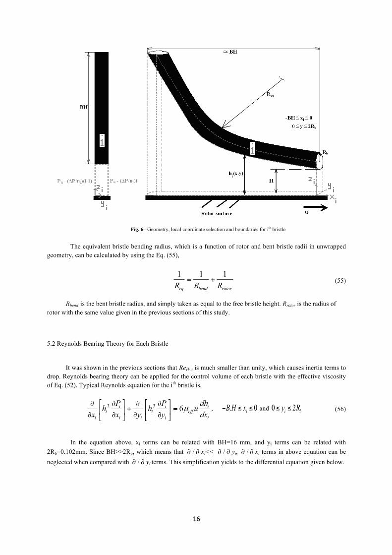
Selection of the local coordinate system for the ith bristle is illustrated in Fig. 6. Since the front plate tightly clamps the bristles, bristles are assumed to be supported from the free bristle height, BH, and they bend under the effect of hydrodynamic lifting force generated by the wedge action. Free bristle height has the value of 16mm. Boundaries for y-coordinate are 0 and 2Rb. The length for the projection of a single bristle can be taken as BH since the cant angle, Ө, is 45o for the brush pack of this analysis. Boundaries for x-coordinate are –BH and 0.

16    

Fig. 6– Geometry, local coordinate selection and boundaries for ith bristle

The equivalent bristle bending radius, which is a function of rotor and bent bristle radii in unwrapped geometry, can be calculated by using the Eq. (55),

1 1 1

eq bend rotorR R R= + (55)

Rbend is the bent bristle radius, and simply taken as equal to the free bristle height. Rrotor is the radius of rotor with the same value given in the previous sections of this study.

   

5.2 Reynolds Bearing Theory for Each Bristle

It was shown in the previous sections that ReH-u is much smaller than unity, which causes inertia terms to drop. Reynolds bearing theory can be applied for the control volume of each bristle with the effective viscosity of Eq. (52). Typical Reynolds equation for the ith bristle is,

3 3 6i i ii i eff

i i i i i

P P dhh h ux x y y dx

µ⎡ ⎤ ⎡ ⎤∂ ∂∂ ∂

+ =⎢ ⎥ ⎢ ⎥∂ ∂ ∂ ∂⎣ ⎦ ⎣ ⎦, . 0iB H x− ≤ ≤ and 0 2i by R≤ ≤ (56)

In the equation above, xi terms can be related with BH=16 mm, and yi terms can be related with 2Rb=0.102mm. Since BH>>2Rb, which means that ∂ /∂ xi<< ∂ /∂ yi, ∂ /∂ xi terms in above equation can be neglected when compared with ∂ /∂ yi terms. This simplification yields to the differential equation given below.

17    

3 6i ii eff

i i eq

P xh uy y R

µ⎡ ⎤∂∂

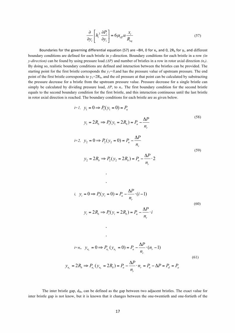
=⎢ ⎥∂ ∂⎣ ⎦ (57)

    Boundaries  for  the  governing  differential  equation  (57)  are  –BH,  0  for  xi,  and  0,  2Rb  for  yi,  and  different boundary conditions are defined for each bristle in y-direction. Boundary conditions for each bristle in a row (in y-direction) can be found by using pressure load (ΔP) and number of bristles in a row in rotor axial direction (nr). By doing so, realistic boundary conditions are defined and interaction between the bristles can be provided. The starting point for the first bristle corresponds the y1=0,and has the pressure value of upstream pressure. The end point of the first bristle corresponds to y1=2Rb, and the oil pressure at that point can be calculated by substracting the pressure decrease for a bristle from the upstream pressure value. Pressure decrease for a single bristle can simply be calculated by dividing pressure load, ΔP, to nr. The first boundary condition for the second bristle equals to the second boundary condition for the first bristle, and this interaction continuous until the last bristle in rotor axial direction is reached. The boundary conditions for each bristle are as given below.

i=1, 1 1 10 ( 0) uy P y P= ⇒ = =

1 1 12 ( 2 )b b ur

Py R P y R PnΔ

= ⇒ = = − (58)

i=2, 2 2 20 ( 0) ur

Py P y PnΔ

= ⇒ = = −

2 2 22 ( 2 ) 2b b ur

Py R P y R PnΔ

= ⇒ = = − ⋅

(59)

.

.

i, 0 ( 0) ( 1)i i i ur

Py P y P inΔ

= ⇒ = = − ⋅ −

2 ( 2 )i b i i b ur

Py R P y R P inΔ

= ⇒ = = − ⋅

(60)

.

.

i=nr, 0 ( 0) ( 1)r r rn n n u r

r

Py P y P nnΔ

= ⇒ = = − ⋅ −

2 ( 2 )r r rn b n n b u r u d a

r

Py R P y R P n P P P PnΔ

= ⇒ = = − ⋅ = −Δ = =

(61)

The inter bristle gap, dIb, can be defined as the gap between two adjacent bristles. The exact value for inter bristle gap is not know, but it is known that it changes between the one-twentieth and one-fortieth of the

18    

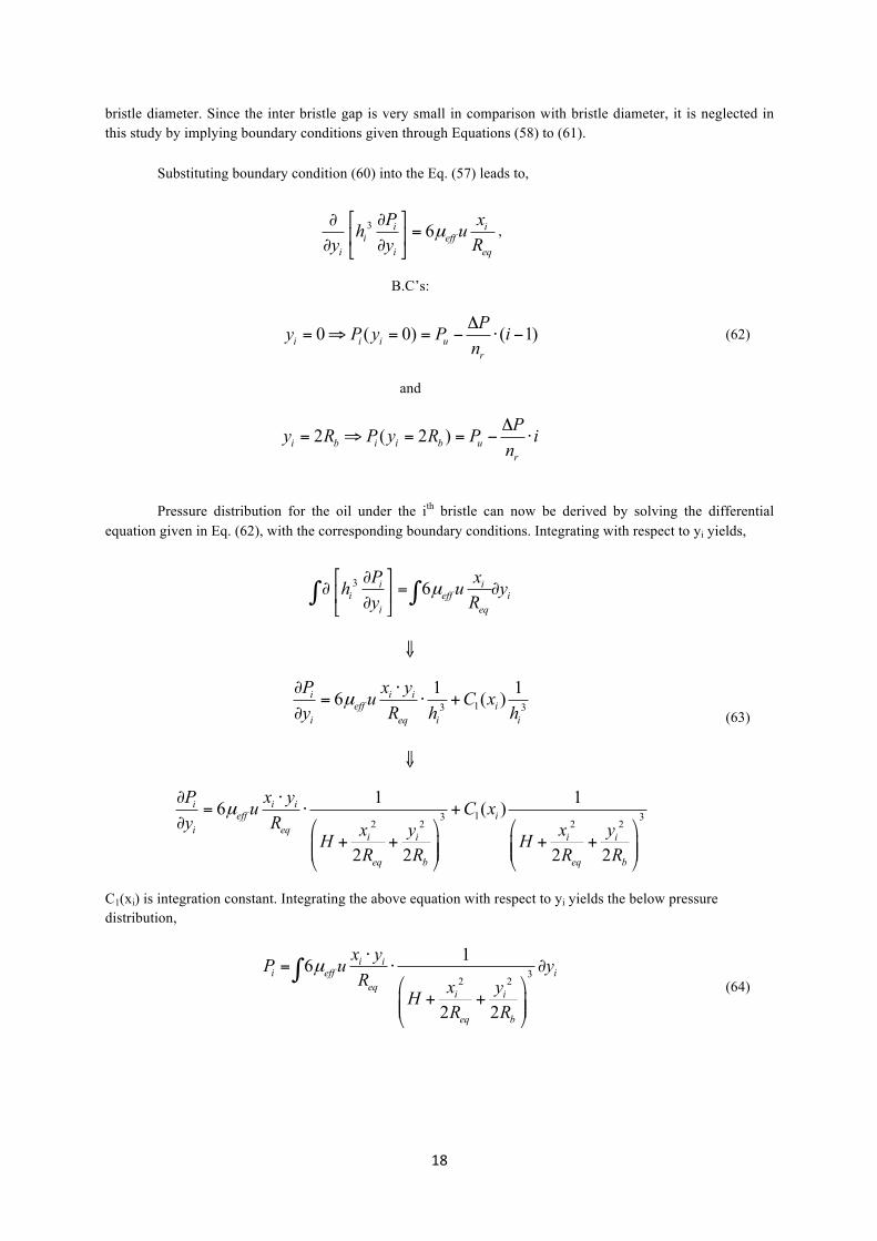
bristle diameter. Since the inter bristle gap is very small in comparison with bristle diameter, it is neglected in this study by implying boundary conditions given through Equations (58) to (61).

Substituting boundary condition (60) into the Eq. (57) leads to,

3 6i ii eff

i i eq

P xh uy y R

µ⎡ ⎤∂∂

=⎢ ⎥∂ ∂⎣ ⎦,

B.C’s:

0 ( 0) ( 1)i i i ur

Py P y P inΔ

= ⇒ = = − ⋅ −

and

2 ( 2 )i b i i b ur

Py R P y R P inΔ

= ⇒ = = − ⋅

(62)

Pressure distribution for the oil under the ith bristle can now be derived by solving the differential equation given in Eq. (62), with the corresponding boundary conditions. Integrating with respect to yi yields,

3 6i ii eff i

i eq

P xh u yy R

µ⎡ ⎤∂

∂ = ∂⎢ ⎥∂⎣ ⎦∫ ∫

⇓

13 3

1 16 ( )i i ieff i

i eq i i

P x yu C xy R h h

µ∂ ⋅

= ⋅ +∂

⇓

13 32 2 2 2

1 16 ( )

2 2 2 2

i i ieff i

i eqi i i i

eq b eq b

P x yu C xy R x y x yH H

R R R R

µ∂ ⋅

= ⋅ +∂ ⎛ ⎞ ⎛ ⎞

+ + + +⎜ ⎟ ⎜ ⎟⎜ ⎟ ⎜ ⎟⎝ ⎠ ⎝ ⎠

(63)

C1(xi) is integration constant. Integrating the above equation with respect to yi yields the below pressure distribution,

32 2

16

2 2

i ii eff i

eqi i

eq b

x yP u yR x yH

R R

µ⋅

= ⋅ ∂⎛ ⎞

+ +⎜ ⎟⎜ ⎟⎝ ⎠

∫ (64)

19    

1 232 2

1( ) ( )

2 2

i i i

i i

eq b

C x y C xx yHR R

+ ∂ +⎛ ⎞

+ +⎜ ⎟⎜ ⎟⎝ ⎠

∫

C2(xi) in Eq. (64) is another integration constant. Integral components of the Eq. (63) are evaluated to obtain below relations.

3 32 2 2 2

616

2 2 2 2

eff ii i ieff i i

eq eqi i i i

eq b eq b

u xx y yu dy dyR Rx y x yH H

R R R R

µµ

⋅ ⋅⋅⋅ =⎛ ⎞ ⎛ ⎞

+ + + +⎜ ⎟ ⎜ ⎟⎜ ⎟ ⎜ ⎟⎝ ⎠ ⎝ ⎠

∫ ∫

⇓ Use the method of substitution

2 2

2 2i i

i beq b

x yH y dy R dR R

γ γ+ + = ⇒ ⋅ = ⋅

⇓ Substitute

3 32 2

6 6

2 2

eff i eff ii bi

eq eqi i

eq b

u x u xy Rdy dR Rx yH

R R

µ µγ

γ

⋅ ⋅ ⋅ ⋅=

⎛ ⎞+ +⎜ ⎟⎜ ⎟

⎝ ⎠

∫ ∫

⇓ Integrate

3 22 2

6 6 12

2 2

eff i eff ii bi

eq eqi i

eq b

u x u xy RdyR Rx yH

R R

µ µ

γ

⋅ ⋅ ⋅ ⋅ −= ⋅ ⋅

⎛ ⎞+ +⎜ ⎟⎜ ⎟

⎝ ⎠

∫

⇓ Substitute γ function

3 22 2 2 2

6 6 12

2 2 2 2

eff i eff ii bi

eq eqi i i i

eq b eq b

u x u xy RdyR Rx y x yH H

R R R R

µ µ⋅ ⋅ ⋅ ⋅ −⎛ ⎞= ⋅ ⋅⎜ ⎟⎝ ⎠⎛ ⎞ ⎛ ⎞

+ + + +⎜ ⎟ ⎜ ⎟⎜ ⎟ ⎜ ⎟⎝ ⎠ ⎝ ⎠

∫

(65)

 

1 13 32 2 2

23

1( ) ( )12

2 2 2 8

ii i i

i i ib i

eq b eq b

dyC x dy C xx y xH H R yR R R R

= ⋅⎛ ⎞ ⎡ ⎤⎛ ⎞

+ + + ⋅ + ⋅⎜ ⎟ ⎢ ⎥⎜ ⎟⎜ ⎟ ⎜ ⎟⎢ ⎥⎝ ⎠ ⎝ ⎠⎣ ⎦

∫ ∫

⇓

20    

Define a function, 2

2 22i

i beq

xR HR

α⎛ ⎞

= ⋅ +⎜ ⎟⎜ ⎟⎝ ⎠

⇓

( )3

1 13 32 222

3

( ) ( ) 812

2 8

i ii i b

i iib i

eq b

dy dyC x C x RyxH R y

R Rα

⋅ = ⋅⎡ ⎤ +⎛ ⎞

+ ⋅ + ⋅⎢ ⎥⎜ ⎟⎜ ⎟⎢ ⎥⎝ ⎠⎣ ⎦

∫ ∫

⇓

Evaluate the integral

⇓

( ) ( ) ( )

33

1 13 2 222 2 2 2 2 2

2( ) 8 ( ) 3i b i ii b i

ii i i i i i

dy R y dyC x R C xy y yαα α α

⎡ ⎤⎢ ⎥⋅ = ⋅ ⋅ +⎢ ⎥+ + +⎣ ⎦

∫ ∫

⇓

( ) ( )

3

1 2 22 2 2 2 2

2( ) 3b i ii

i i i i i

R y dyC xy yα α α

⎡ ⎤⎢ ⎥⋅ ⋅ + =⎢ ⎥+ +⎣ ⎦

∫

( ) ( )

3

1 22 2 2 22 2

2 3 1( ) arctan2

b i i ii

i i i ii ii i

R y y yC xyyα α α ααα

⎧ ⎫⎡ ⎤⎛ ⎞⎪ ⎪⎢ ⎥⋅ ⋅ + +⎨ ⎬⎜ ⎟

+⎢ ⎥+ ⎝ ⎠⎪ ⎪⎣ ⎦⎩ ⎭

(66)

Oil pressure distribution for ith bristle can be found by substituting Equations (65) and (66) into the Eq. (64). After substitution, integration constants can be found by applying boundary conditions given in Eq. (62).

22 2

6 12

2 2

eff i bi

eqi i

eq b

u x RPR x yH

R R

µ ⋅ ⋅ −⎛ ⎞= ⋅ ⋅⎜ ⎟⎝ ⎠ ⎛ ⎞

+ +⎜ ⎟⎜ ⎟⎝ ⎠

( ) ( )3

1 222 2 2 22 2

2 3 1( ) arctan ( )2

b i i ii i

i i i ii ii i

R y y yC x C xyyα α α ααα

⎧ ⎫⎡ ⎤⎛ ⎞⎪ ⎪⎢ ⎥+ ⋅ ⋅ + + +⎨ ⎬⎜ ⎟

+⎢ ⎥+ ⎝ ⎠⎪ ⎪⎣ ⎦⎩ ⎭

B.C’s:

0 ( 0) ( 1)i i i ur

Py P y P inΔ

= ⇒ = = − ⋅ −

(67)

21    

and

2 ( 2 )i b i i b ur

Py R P y R P inΔ

= ⇒ = = − ⋅

⇓ Applying the first boundary condition yields C2(xi) as,

2 22

6 1( ) ( 1)2

2

eff bi u i

r eqi

eq

u RPC x P i xn R xH

R

µ

⎡ ⎤⎢ ⎥⎢ ⎥−Δ

= − ⋅ − − ⋅⎢ ⎥⎛ ⎞⎢ ⎥

+⎜ ⎟⎢ ⎥⎜ ⎟⎝ ⎠⎣ ⎦

⇓ Applying the first boundary condition yields C1(xi) as,

1 2 22 21

61 1 1( )2

12 2

eff bi i

r eqi i

eq eq

u RPC x xF n R x xH H

R R

µ

⎧ ⎫⎡ ⎤⎪ ⎪⎢ ⎥⎪ ⎪⎢ ⎥−Δ⎪ ⎪⎛ ⎞

= − −⎨ ⎬⎢ ⎥⎜ ⎟⎝ ⎠ ⎛ ⎞ ⎛ ⎞⎪ ⎪⎢ ⎥

+ + +⎜ ⎟ ⎜ ⎟⎪ ⎪⎢ ⎥⎜ ⎟ ⎜ ⎟⎝ ⎠ ⎝ ⎠⎪ ⎪⎣ ⎦⎩ ⎭

where

( ) ( )

3

1 2 2 2 22 2 2

2 2 2 23 1 arctan2 44

b b b b

i i b i ii i b

R R R RFRR α α α αα α

⎧ ⎫⎡ ⎤⎛ ⎞⎪ ⎪= + +⎨ ⎬⎢ ⎥⎜ ⎟

++ ⎝ ⎠⎣ ⎦⎪ ⎪⎩ ⎭

and

2

2 22i

i beq

xR HR

α⎛ ⎞

= ⋅ +⎜ ⎟⎜ ⎟⎝ ⎠

(68)

(69)

Substituting Equations (68) and (69) into the pressure equation (67) yields,

23 4 5

1i

FP F F FF

= + ⋅ + ,

( ) ( )

3

1 2 2 2 22 2 2

2 2 2 23 1 arctan2 44

b b b b

i i b i ii i b

R R R RFRR α α α αα α

⎧ ⎫⎡ ⎤⎛ ⎞⎪ ⎪= + +⎨ ⎬⎢ ⎥⎜ ⎟

++ ⎝ ⎠⎣ ⎦⎪ ⎪⎩ ⎭

(70)

22    

2 2 22 2

6 1 12

12 2

eff bi

r eqi i

eq eq

u RPF xn R x xH H

R R

µ

⎡ ⎤⎢ ⎥⎢ ⎥−Δ ⎛ ⎞

= − −⎢ ⎥⎜ ⎟⎝ ⎠ ⎛ ⎞ ⎛ ⎞⎢ ⎥

+ + +⎜ ⎟ ⎜ ⎟⎢ ⎥⎜ ⎟ ⎜ ⎟⎝ ⎠ ⎝ ⎠⎣ ⎦

,

3 22 2

6 12

2 2

eff i b

eqi i

eq b

u x RFR x yH

R R

µ ⋅ ⋅ −⎛ ⎞= ⋅ ⋅⎜ ⎟⎝ ⎠ ⎛ ⎞

+ +⎜ ⎟⎜ ⎟⎝ ⎠

,

( ) ( )

3

4 2 2 2 22 2 2

2 2 23 1 arctan2

b b b i

i i i i ii i i

R R R yFyy α α α αα α

⎧ ⎫⎡ ⎤⎛ ⎞⎪ ⎪= + +⎨ ⎬⎢ ⎥⎜ ⎟

++ ⎝ ⎠⎣ ⎦⎪ ⎪⎩ ⎭

,

5 22

6 1( 1)2

2

eff bu i

r eqi

eq

u RPF P i xn R xH

R

µ

⎡ ⎤⎢ ⎥⎢ ⎥−Δ

= − ⋅ − − ⋅⎢ ⎥⎛ ⎞⎢ ⎥

+⎜ ⎟⎢ ⎥⎜ ⎟⎝ ⎠⎣ ⎦

,

22 2

2i

i beq

xR HR

α⎛ ⎞

= ⋅ +⎜ ⎟⎜ ⎟⎝ ⎠

.

Pressure distribution for the ith bristle, Pi, includes the effect of shear heating since the term µeff appears in the pressure function. Pressure is a function of brush seal geometry (Rb, Req, nr), pressure load, ΔP, upstream pressure (Pu), rotor surface speed, u, and hydrodynamic lift clearance, H. Table 1 is used for the experimental hydrodynamic lift clearance values.

6. Results and discussion  

6.1 Pressure  

Pressure distribution of Eq. (70) is a function of both xi and yi coordinates. Pressure change for each bristle along xi direction is evaluated for yi=Rb (mid-point of the bristle, see Fig. 6),  ΔP=48.3kPa  and  for  6.2m/s  rotor   surface   speed, and given in Fig. 7. The oil pressure change along xi has similar character for different pressure loads and rotor surface speeds, where only difference is observed in the magnitude.

As it can be seen from Fig. 7, pressure change in xi direction shows similar change for each bristle. Plots have same character, but magnitudes are decreasing as going from upstream side to downstream side, which is an expected pressure drop behavior. The oil pressure value for the first bristle is around upstream pressure (Pu), whereas the pressure magnitude is around downstream pressure (Pd=Pa) for the oil under the last bristle. There is an evident change in oil pressure between -2mm and 0, which corresponds to the projected length of bristle

23    

portion at “Fence height, FH” onto the xi-axis. After that point, pressure change is almost zero until -7mm, and then the oil pressure remains constant. Considering the tighter clamping effect of the brush structure on bristles between free bristle height (BH) and fence height (FH) region, and resulting restriction in the oil flow, it is reasonable and consistent with real-life applications to obtain a constant pressure in xi direction after a certain distance from fence height projection on xi-axis.

Fig. 7– Oil pressure distributions along xi for each bristle, ΔP = 48.3 kPa, u = 6.2m/s

Fig. 8– Oil pressure change under each bristle along rotor axial and tangential directions

24    

As a representative example, oil pressure distribution along xi and yi axes for 89.6kPa pressure load and 20.5m/s rotor surface speed is presented in Fig. 8.

Local oil pressure functions of bristles are combined to obtain the pressure distribution under the brush pack for a row of bristles. As it can be observed from the Fig. 8, pressure change in rotor axial direction is almost linear. It takes the upstream pressure value for y = 0 (at the upstream side), and drops to the downstream pressure value for y = w (at the downstream side).

Oil pressure function, which is evaluated by selecting the control volume as the oil under each bristle, gives almost linear pressure change in rotor axial direction. Mean value of the oil pressure for each bristle with respect to xi coordinate is developed in order to make more clear comments on linear pressure change.

( )01 ( , )

mean xii i i i i iBH

P y P x y dxBH−

−

= ⋅∫ (71)

Pi is the oil pressure under each bristle. Trapezoid rule is applied for numeric integration, which is evaluated by writing a MATLAB code.

( )01 ( , )

mean xii i i i i iBH

P y P x y dxBH−

−

= ⋅∫

( ) ( )1 1 2

1 ( , ) 2 , ... ,2 i i i i i i i i il P x y P x l y P x y

BH⎧ ⎫⎡ ⎤= ⋅ + + + +⎨ ⎬⎣ ⎦⎩ ⎭

(72)

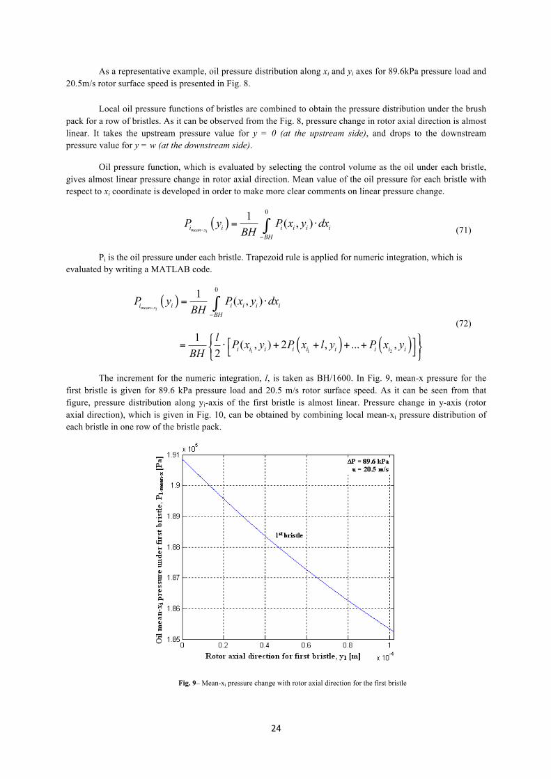
The increment for the numeric integration, l, is taken as BH/1600. In Fig. 9, mean-x pressure for the first bristle is given for 89.6 kPa pressure load and 20.5 m/s rotor surface speed. As it can be seen from that figure, pressure distribution along yi-axis of the first bristle is almost linear. Pressure change in y-axis (rotor axial direction), which is given in Fig. 10, can be obtained by combining local mean-xi pressure distribution of each bristle in one row of the bristle pack.

Fig. 9– Mean-xi pressure change with rotor axial direction for the first bristle

25    

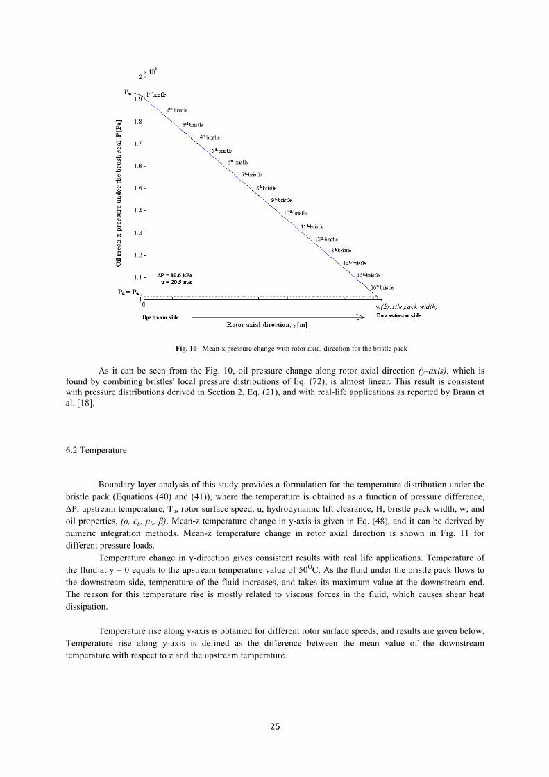
Fig. 10– Mean-x pressure change with rotor axial direction for the bristle pack

As it can be seen from the Fig. 10, oil pressure change along rotor axial direction (y-axis), which is found by combining bristles' local pressure distributions of Eq. (72), is almost linear. This result is consistent with pressure distributions derived in Section 2, Eq. (21), and with real-life applications as reported by Braun et al. [18].

6.2 Temperature  

Boundary layer analysis of this study provides a formulation for the temperature distribution under the bristle pack (Equations (40) and (41)), where the temperature is obtained as a function of pressure difference, ΔP, upstream temperature, Tu, rotor surface speed, u, hydrodynamic lift clearance, H, bristle pack width, w, and oil properties, (ρ, cp, µ0, β). Mean-z temperature change in y-axis is given in Eq. (48), and it can be derived by numeric integration methods. Mean-z temperature change in rotor axial direction is shown in Fig. 11 for different pressure loads. Temperature change in y-direction gives consistent results with real life applications. Temperature of the fluid at y = 0 equals to the upstream temperature value of 50OC. As the fluid under the bristle pack flows to the downstream side, temperature of the fluid increases, and takes its maximum value at the downstream end. The reason for this temperature rise is mostly related to viscous forces in the fluid, which causes shear heat dissipation. Temperature rise along y-axis is obtained for different rotor surface speeds, and results are given below. Temperature rise along y-axis is defined as the difference between the mean value of the downstream temperature with respect to z and the upstream temperature.

26    

( )0

1( ) ,mean z

H

d mean zT T y w T w z dzH− −= = = ⋅∫

mean zd uT T T−

Δ = − (73)

a)

b)

Fig. 11– Mean-z temperature, Tmean-z(y), distribution along y-axis (in the direction of leakage flow (rotor axial direction)) for different pressure loads and rotor surface speeds a) ΔP = 48.3 kPa, b) ΔP = 89.6 kPa

27    

The total temperature increase in the rotor axial direction is given in Table 2 for 48.3 and 89.6 kPa pressure loads. Comparison of the theoretical results with the experimental data and with the CFD results of Aksit and Dogu [16] is given in Fig.12.

Table 2 – Evaluated temperature rise along y-axis for rotor surface speeds and different pressure loads

ΔP = 48.3 kPa ΔP = 89.6 kPa

Rotor surface speed [m/s] Temperature rise along y-axis, ΔT Temperature rise along y-axis, ΔT

0 0 0

6.2 4.3 oC 4.2 oC

12.3 7.4 oC 7.7 oC

20.5 19 oC 15.4 oC

Fig. 12– Mean-z temperature, Tmean-z(y), distribution along y-axis (in the direction of leakage flow (rotor axial direction)) for different pressure loads and rotor surface speeds a) ΔP = 48.3 kPa, b) ΔP = 89.6 kPa

As shown in Fig. 12, the temperature function derived in this study gives consistent results with the experimental data and real life applications, whereas CFD model of Aksit et al underestimates the temperature rise for all rotor speeds. Temperature rise in the bristle pack increases with rotor surface speed due to the increasing effect of shear heating. At lower speeds, temperature rise is almost same for different pressure loads, whereas higher pressure loads give smaller temperature rise values at moderate speeds because of the increasing cooling effect of convective terms. Negative effect of pressure load on temperature rise can also be observed from the temperature function given in Equations (40) and (41). In those equations, pressure load appears in functions f2, f3 and f4, and the main negative effect of PΔ on temperature rise is coming from the function f3, where the square of PΔ appears in the denominator. The square of the rotor surface speed appears in the numerator of function f3, which makes this term dominant at high rotor speeds. This explains the increasing negative effect of the pressure load with rotor surface speed.

6.3 Shear heating effect included hydrodynamic lifting force  

Aksit et al. [16] estimates the lifting force by using the beam theory and the bearing theory without including shear heating effect. As given in Eq. (45), lifting force of the beam theory does not include the effect of friction and blow-down forces. The lifting force found by bearing theory is given in Eq. (47), and it does not

0

5

10

15

20

25

0 5 10 15 20 25Rotor speed [m/s]

Tem

per

atu

re r

ise

[C] 48.3 KPa

89.6 KPaExp (62.1 KPa)Aksit et al (CFD)

28    

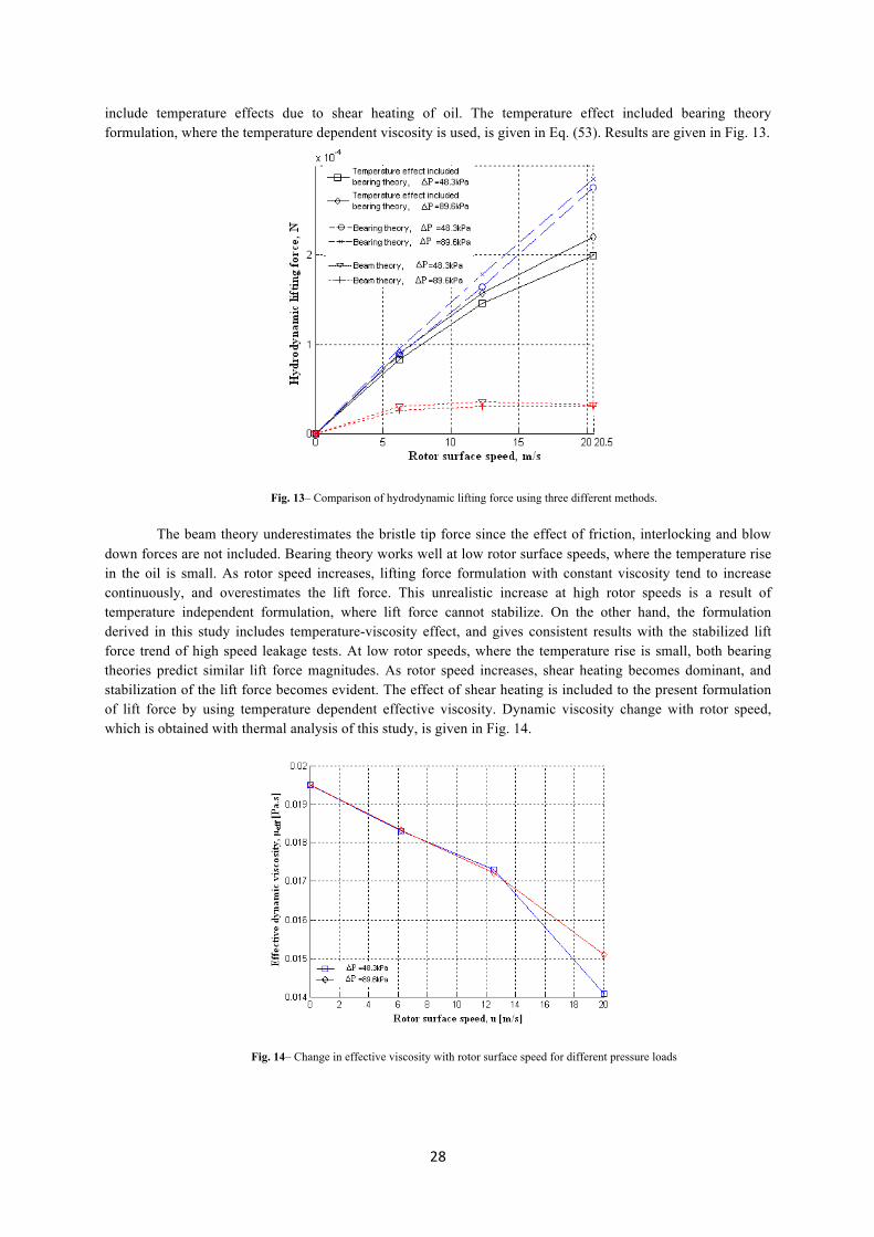
include temperature effects due to shear heating of oil. The temperature effect included bearing theory formulation, where the temperature dependent viscosity is used, is given in Eq. (53). Results are given in Fig. 13.

Fig. 13– Comparison of hydrodynamic lifting force using three different methods.

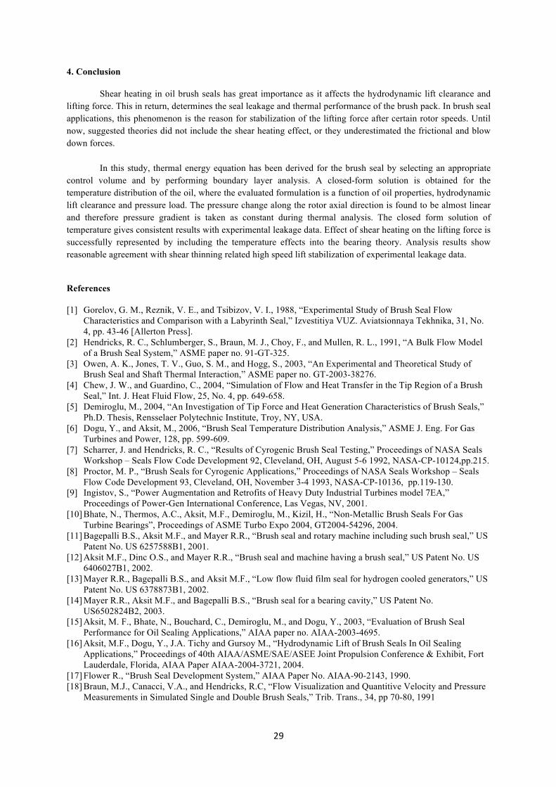
The beam theory underestimates the bristle tip force since the effect of friction, interlocking and blow down forces are not included. Bearing theory works well at low rotor surface speeds, where the temperature rise in the oil is small. As rotor speed increases, lifting force formulation with constant viscosity tend to increase continuously, and overestimates the lift force. This unrealistic increase at high rotor speeds is a result of temperature independent formulation, where lift force cannot stabilize. On the other hand, the formulation derived in this study includes temperature-viscosity effect, and gives consistent results with the stabilized lift force trend of high speed leakage tests. At low rotor speeds, where the temperature rise is small, both bearing theories predict similar lift force magnitudes. As rotor speed increases, shear heating becomes dominant, and stabilization of the lift force becomes evident. The effect of shear heating is included to the present formulation of lift force by using temperature dependent effective viscosity. Dynamic viscosity change with rotor speed, which is obtained with thermal analysis of this study, is given in Fig. 14.

Fig. 14– Change in effective viscosity with rotor surface speed for different pressure loads

29    

4. Conclusion

Shear heating in oil brush seals has great importance as it affects the hydrodynamic lift clearance and lifting force. This in return, determines the seal leakage and thermal performance of the brush pack. In brush seal applications, this phenomenon is the reason for stabilization of the lifting force after certain rotor speeds. Until now, suggested theories did not include the shear heating effect, or they underestimated the frictional and blow down forces.

In this study, thermal energy equation has been derived for the brush seal by selecting an appropriate

control volume and by performing boundary layer analysis. A closed-form solution is obtained for the temperature distribution of the oil, where the evaluated formulation is a function of oil properties, hydrodynamic lift clearance and pressure load. The pressure change along the rotor axial direction is found to be almost linear and therefore pressure gradient is taken as constant during thermal analysis. The closed form solution of temperature gives consistent results with experimental leakage data. Effect of shear heating on the lifting force is successfully represented by including the temperature effects into the bearing theory. Analysis results show reasonable agreement with shear thinning related high speed lift stabilization of experimental leakage data.

References [1] Gorelov, G. M., Reznik, V. E., and Tsibizov, V. I., 1988, “Experimental Study of Brush Seal Flow

Characteristics and Comparison with a Labyrinth Seal,” Izvestitiya VUZ. Aviatsionnaya Tekhnika, 31, No. 4, pp. 43-46 [Allerton Press].

[2] Hendricks, R. C., Schlumberger, S., Braun, M. J., Choy, F., and Mullen, R. L., 1991, “A Bulk Flow Model of a Brush Seal System,” ASME paper no. 91-GT-325.

[3] Owen, A. K., Jones, T. V., Guo, S. M., and Hogg, S., 2003, “An Experimental and Theoretical Study of Brush Seal and Shaft Thermal Interaction,” ASME paper no. GT-2003-38276.

[4] Chew, J. W., and Guardino, C., 2004, “Simulation of Flow and Heat Transfer in the Tip Region of a Brush Seal,” Int. J. Heat Fluid Flow, 25, No. 4, pp. 649-658.

[5] Demiroglu, M., 2004, “An Investigation of Tip Force and Heat Generation Characteristics of Brush Seals,” Ph.D. Thesis, Rensselaer Polytechnic Institute, Troy, NY, USA.

[6] Dogu, Y., and Aksit, M., 2006, “Brush Seal Temperature Distribution Analysis,” ASME J. Eng. For Gas Turbines and Power, 128, pp. 599-609.

[7] Scharrer, J. and Hendricks, R. C., “Results of Cyrogenic Brush Seal Testing,” Proceedings of NASA Seals Workshop – Seals Flow Code Development 92, Cleveland, OH, August 5-6 1992, NASA-CP-10124,pp.215.

[8] Proctor, M. P., “Brush Seals for Cyrogenic Applications,” Proceedings of NASA Seals Workshop – Seals Flow Code Development 93, Cleveland, OH, November 3-4 1993, NASA-CP-10136, pp.119-130.

[9] Ingistov, S., “Power Augmentation and Retrofits of Heavy Duty Industrial Turbines model 7EA,” Proceedings of Power-Gen International Conference, Las Vegas, NV, 2001.

[10] Bhate, N., Thermos, A.C., Aksit, M.F., Demiroglu, M., Kizil, H., “Non-Metallic Brush Seals For Gas Turbine Bearings”, Proceedings of ASME Turbo Expo 2004, GT2004-54296, 2004.

[11] Bagepalli B.S., Aksit M.F., and Mayer R.R., “Brush seal and rotary machine including such brush seal,” US Patent No. US 6257588B1, 2001.

[12] Aksit M.F., Dinc O.S., and Mayer R.R., “Brush seal and machine having a brush seal,” US Patent No. US 6406027B1, 2002.

[13] Mayer R.R., Bagepalli B.S., and Aksit M.F., “Low flow fluid film seal for hydrogen cooled generators,” US Patent No. US 6378873B1, 2002.

[14] Mayer R.R., Aksit M.F., and Bagepalli B.S., “Brush seal for a bearing cavity,” US Patent No. US6502824B2, 2003.

[15] Aksit, M. F., Bhate, N., Bouchard, C., Demiroglu, M., and Dogu, Y., 2003, “Evaluation of Brush Seal Performance for Oil Sealing Applications,” AIAA paper no. AIAA-2003-4695.

[16] Aksit, M.F., Dogu, Y., J.A. Tichy and Gursoy M., “Hydrodynamic Lift of Brush Seals In Oil Sealing Applications,” Proceedings of 40th AIAA/ASME/SAE/ASEE Joint Propulsion Conference & Exhibit, Fort Lauderdale, Florida, AIAA Paper AIAA-2004-3721, 2004.

[17] Flower R., “Brush Seal Development System,” AIAA Paper No. AIAA-90-2143, 1990. [18] Braun, M.J., Canacci, V.A., and Hendricks, R.C, “Flow Visualization and Quantitive Velocity and Pressure

Measurements in Simulated Single and Double Brush Seals,” Trib. Trans., 34, pp 70-80, 1991