Flow along a long thin cylinder - ePrints...
37
J. Fluid Mech. (2008), vol. 602, pp. 1–37. c 2008 Cambridge University Press doi:10.1017/S0022112008000542 Printed in the United Kingdom 1 Flow along a long thin cylinder O. R. TUTTY School of Engineering Sciences, University of Southampton, Highfield, Southampton SO17 1BJ, UK (Received 20 March 2007 and in revised form 11 January 2008) Two different approaches have been used to calculate turbulent flow along a long thin cylinder where the flow is aligned with the cylinder. A boundary-layer code is used to predict the mean flow for very long cylinders (length to radius ratio of up to O(10 6 )), with the effects of the turbulence estimated through a turbulence model. Detailed comparison with experimental results shows that the mean properties of the flow are predicted within experimental accuracy. The boundary-layer model predicts that, sufficiently far downstream, the surface shear stress will be (almost) constant. This is consistent with experimental results from long cylinders in the form of sonar arrays. A periodic Navier–Stokes problem is formulated, and solutions generated for Reynolds number from 300 to 5 × 10 4 . The results are in agreement with those from the boundary-layer model and experiments. Strongly turbulent flow occurs only near the surface of the cylinder, with relatively weak turbulence over most of the boundary layer. For a thick boundary layer with the boundary-layer thickness much larger than the cylinder radius, the mean flow is effectively constant near the surface, in both temporal and spatial frameworks, while the outer flow continues to develop in time or space. Calculations of the circumferentially averaged surface pressure spectrum show that, in physical terms, as the radius of the cylinder decreases, the surface noise from the turbulence increases, with the maximum noise at a Reynolds number of O(10 3 ). An increase in noise with a decrease in radius (Reynolds number) is consistent with experimental results. 1. Introduction Axial flow along a long cylinder is relevant to a number of applications, including the flow along wire or thread, drawing of optical fibres, and the flow along towed sonar arrays which are used for underwater sensing. A sonar array may have a very large ratio of length to radius, up to O(10 5 ), with a radius in the order of centimetres and a length of a kilometre or more. Currently there is a trend to develop smaller, more easily deployed devices, using, for example, optical fibres as sensors. However, the performance of towed arrays is usually limited by the noise generated by the turbulent fluctuations on the surface of the body (Knight 1996), and, for a given flow velocity (tow speed), decreasing the diameter of the array leads to an increase in the turbulent noise (Marschall et al. 1993; Potter et al. 2000). This process would not be expected to continue indefinitely, and one question addressed in this paper is how small the cylinder must be before the turbulent flow noise stops growing. The sensors on towed arrays are usually mounted along the axis of the cylinder, and measure averaged pressure in some form rather than point pressure, through a transfer function representing the transfer of the surface pressure fluctuations to the axis. The form of the transfer function will depend on the construction of the array and the configuration of the sensors, and will not be considered here (see Knight 1996
Transcript of Flow along a long thin cylinder - ePrints...

J. Fluid Mech. (2008), vol. 602, pp. 1–37. c© 2008 Cambridge University Press
doi:10.1017/S0022112008000542 Printed in the United Kingdom
1
Flow along a long thin cylinder
O. R. TUTTYSchool of Engineering Sciences, University of Southampton, Highfield, Southampton SO17 1BJ, UK
(Received 20 March 2007 and in revised form 11 January 2008)
Two different approaches have been used to calculate turbulent flow along a longthin cylinder where the flow is aligned with the cylinder. A boundary-layer code isused to predict the mean flow for very long cylinders (length to radius ratio of upto O(106)), with the effects of the turbulence estimated through a turbulence model.Detailed comparison with experimental results shows that the mean properties of theflow are predicted within experimental accuracy. The boundary-layer model predictsthat, sufficiently far downstream, the surface shear stress will be (almost) constant.This is consistent with experimental results from long cylinders in the form of sonararrays. A periodic Navier–Stokes problem is formulated, and solutions generated forReynolds number from 300 to 5 × 10⁴. The results are in agreement with those fromthe boundary-layer model and experiments. Strongly turbulent flow occurs only nearthe surface of the cylinder, with relatively weak turbulence over most of the boundarylayer. For a thick boundary layer with the boundary-layer thickness much larger thanthe cylinder radius, the mean flow is effectively constant near the surface, in bothtemporal and spatial frameworks, while the outer flow continues to develop in time orspace. Calculations of the circumferentially averaged surface pressure spectrum showthat, in physical terms, as the radius of the cylinder decreases, the surface noise fromthe turbulence increases, with the maximum noise at a Reynolds number of O(103).An increase in noise with a decrease in radius (Reynolds number) is consistent withexperimental results.
1. IntroductionAxial flow along a long cylinder is relevant to a number of applications, including
the flow along wire or thread, drawing of optical fibres, and the flow along towedsonar arrays which are used for underwater sensing. A sonar array may have a verylarge ratio of length to radius, up to O(105), with a radius in the order of centimetresand a length of a kilometre or more. Currently there is a trend to develop smaller,more easily deployed devices, using, for example, optical fibres as sensors. However,the performance of towed arrays is usually limited by the noise generated by theturbulent fluctuations on the surface of the body (Knight 1996), and, for a givenflow velocity (tow speed), decreasing the diameter of the array leads to an increasein the turbulent noise (Marschall et al. 1993; Potter et al. 2000). This process wouldnot be expected to continue indefinitely, and one question addressed in this paperis how small the cylinder must be before the turbulent flow noise stops growing.The sensors on towed arrays are usually mounted along the axis of the cylinder,and measure averaged pressure in some form rather than point pressure, through atransfer function representing the transfer of the surface pressure fluctuations to theaxis. The form of the transfer function will depend on the construction of the arrayand the configuration of the sensors, and will not be considered here (see Knight 1996

2 O. R. Tutty
for a theoretical study of this effect). The work presented here is concerned mainlywith behaviour quantities relevant to the performance of towed arrays. In particular,we will consider the variation of the wall mean shear stress and the circumferentiallyaveraged wall pressure spectra with the Reynolds number of the flow. However,in addition to the spectra for circumferentially averaged wall pressure, some pointspectra will be presented.
Flow along a cylinder has an additional length scale to that for a flat plate, thecylinder radius. If the boundary layer is thin compared to the radius, then the flowwill resemble that on a flat plate, with negligible effect from the curvature of thewall. However, once the boundary thickness becomes comparable with the size ofthe cylinder, effects of curvature will be significant. The flow also depends on theReynolds number, which is defined in terms of the cylinder radius a and free-streamvelocity U∞ so that Re = aU∞/ν, where ν is the kinematic viscosity of the fluid. We canalso define a+ = auτ/ν where uτ =(τw/ρ)1/2 is the friction velocity, with τw the shearstress at the wall and ρ the density of the fluid. a+ gives the radius of the cylinder inwall units. It is also the Reynolds number using the friction velocity as the referencevelocity. For y+ of O(a+) or greater, where y+ is the distance from the surface inwall units, the effects of the curvature of the wall will be important. Closer to thewall, the effects of curvature will be less important. If a+ is large, the boundary layernear the surface should resemble that for a flat plate, with the curvature significantonly in the outer part of the flow. For small a+, the effects of curvature will be feltcloser to the wall. In the laminar sublayer for a flat plate, we have u+ = y+, whereu+ = u/uτ , and u is the streamwise velocity. This reflects momentum equilibrium inthe sublayer, given by τ = τw . For the cylinder, as noted by Glauert & Lighthill (1955)among others, the equilibrium model is rτ = aτw . This gives
u+ = a+ log(1 + y+/a+). (1.1)
Hence if a+ is O(1), the effects of the wall curvature would extend right to the wall.For the laminar problem, Seban & Bond (1951) give the first three terms in a
series solution valid near the leading edge of the cylinder, giving expressions forthe shear stress on the surface and the displacement area. Stewartson (1955) givesa series solution for very large distances along the cylinder. Stewartson shows thatsufficiently far along the cylinder, the wall shear stress decays logarithmically withdistance, rather than algebraically as is usually found. Glauert & Lighthill (1955)considered the flow along the entire cylinder. They developed a similar series solutionto Stewartson for the flow far downstream. They produced a set of recommendedcurves for quantities such as the displacement area and the skin friction.
Tutty, Price & Parsons (2002) solved the problem of laminar boundary-layer flowon a cylinder numerically. They found good agreement with the predictions of Seban& Bond (1951) near the leading edge and Glauert & Lighthill (1955) far downstream.All these studies showed that there is an increase in the surface shear stress and adecrease in the boundary-layer thickness compared with those for a flat plate. Tuttyet al. (2002) also considered the linear normal mode stability of the flow. They foundthat for Reynolds numbers less than 1060 the flow is unconditionally stable. This isin marked contrast to the flat-plate boundary-layer problem where the flow alwaysbecomes unstable if far enough downstream. Further, for the cases investigated,above the critical Reynolds number the flow was unstable for a finite distance only,reverting to stability further downstream, with closure of the neutral stability curves.Also, unlike planar flows, the two-dimensional (axisymmetric) mode was not the least
Flow along a long thin cylinder 3
stable, but had only the fourth lowest critical Reynolds number. The mode with thelowest critical value was that with an azimuthal wavenumber of one.
The studies that exist for turbulent flow along a cylinder are mainly experimental,complemented by some attempts to obtain an appropriate form for a law of the wall.A substantial body of work comes from Lueptow and his colleagues (Lueptow, Leehey& Stellinger 1985; Lueptow & Haritonidis 1987; Lueptow 1988, 1990; Lueptow &Jackson 1991; Wietrzak & Lueptow 1994; Snarski & Lueptow 1995; Nepomuceno &Lueptow 1997; Bokde, Lueptow & Abraham 1999). These are experimental studies offlow with a Reynolds number of 3 × 10³ − 5 × 10³ with the boundary-layer thickness5–8 times the cylinder radius. Lueptow (1988) is a review of much of the experimentalwork to that point. Willmarth et al. (1976) measured the boundary layer on verticallymounted cylinders with Reynolds numbers from 482 to 92 310 with the boundary-layer thickness from 1.88 to 42.5 times the cylinder radius.
Luxton, Bull & Rajagopalan (1984) investigated cylinders for Reynolds numbersfrom 140 to 785. Although the flow was unsteady for all Reynolds numbers, Luxtonet al. (1984) observed that at the lowest Reynolds number, Re= 140, the high-frequency content of the flow was low, and argued that this flow was transitionalrather than fully turbulent. They also observed that the turbulence intensities overmost of the boundary layer were much lower than those expected on a flat plate,with peak values near the wall about twice that found on a flat plate. From this theysuggested that the flow contained two scales, a fine wall scale with a gross outer scaleforming most of the layer.
A series of experiments has been performed in a large towing tank (approximately900 m in length) using thin cylinders aligned with the flow, with diameters oforder 1 mm and lengths of order 100 m (Cippola & Keith 2003a; Furey, Cippola& Atsavappranee 2004) at relatively low Reynolds numbers (Re of O(103 − 104)). Aprimary measurement in this work is the mean drag on the cylinders as a functionof cylinder length, obtained by a direct measurement of the force on the body forcylinders of different lengths. From this, estimates of the momentum thickness at theends of the cylinders are calculated. Furey et al. (2004) plot the mean wall shear stressagainst length for a cylinder with radius 0.445 mm for tow speeds from 3.1 m s−1 to14.4 m s−1. As far as can be seen from the plot (figure 6, Furey et al. 2004), there isno decay in the wall shear stress with the length of the cylinder, which varies fromaround 8 m to 150 m long.
As for laminar flow, the experimental studies show that the turbulent boundarylayer on a cylinder has higher mean shear stress and is thinner that its counterpart ona flat plate. One observation is that the outer flow acts like a continuously regeneratedwake rather than a boundary layer attached to a wall (Denli & Landweber 1979;Luxton et al. 1984; Lueptow & Haritonidis 1987; Wietrzak & Lueptow 1994).
The only numerical studies related to turbulent axial flow on a cylinder thatwe are aware of are those by Neves, Moin & Moser (1994) and Neves & Moin(1994). This work is also reported in Neves et al. (1992) which contains more detail.Rather than a spatially developing boundary layer with zero pressure gradient, Neveset al. considered a model problem, periodic in the streamwise direction, with a fixedboundary-layer thickness, and with a ‘mild streamwise pressure gradient’ to suppressthe spatial growth of the boundary layer. We note that for a laminar flow, a non-zeropressure gradient can be introduced to suppress the boundary-layer growth, or moreprecisely, to fix the boundary-layer thickness. However, the streamwise velocity andpressure gradient cannot be constant, but must develop either spatially downstreamor in time.

4 O. R. Tutty
A number of studies consider the surface wall pressure spectra, although forrelatively thin boundary layers (2–11 times the cylinder radius). Also, usually thespectra are for pointwise pressure measurements rather than the circumferentiallyaveraged pressure found with towed sonar arrays. Willmarth & Yang (1970) giveexperimental spectra for a cylinder with Re= 115 000 and a boundary-layer thickness(δ) of approximately 2a, and Willmarth et al. (1976) a cylinder with Re = 36 800 andδ ≈ 4a. Bokde et al. (1999) give measurements for a cylinder with Re =3300 andδ =4.81a and Snarski & Lueptow (1995) measurements for a cylinder with Re= 3644and δ = 5a. Statistics on the pressure fluctuations from the numerical study by Neveset al. (1994) are presented in Neves & Moin (1994). They found that as the curvatureincreases (in effect, the Reynolds number and hence the size of the cylinder decreases)the root-mean-square (r.m.s.) pressure fluctuations decrease. This does not, as such,contradict the observation that the surface noise from the turbulence increases asthe Reynolds number decreases, since the Reynolds numbers used by Neves & Moin(1994) are two to three orders of magnitude less than those for sonar arrays.
Since a sonar array may have a length to radius ratio of up to O(105), it isnot possible to perform a full Navier–Stokes calculation for such a configuration.Instead, first we will investigate the axial flow along a cylinder using a boundary-layerapproach with the effects of the turbulence included through a turbulence model.This model will be validated by detailed comparison with experimental results. It willthen be used to investigate the far-downstream behaviour of the flow. The predictionsmade, including that of essentially constant wall shear stress, are shown to agree withexperimental results. Based on the results from the boundary-layer analysis, a modelproblem is then formulated. This problem is periodic in the streamwise direction,and can be solved numerically, using a Navier–Stokes solver for lower Reynoldsnumbers (5000 or below), and a large-eddy simulation (LES) approach for higherReynolds numbers (up to 5 × 10⁴). The results from these calculations agree withexperimental observations and the results from the boundary-layer model. The effectof the Reynolds number on the pressure spectra is then investigated.
2. Boundary-layer model2.1. Formulation
The flow takes the form of a boundary layer with zero pressure gradient so that thegoverning equations in polar coordinates (x, r), which are normalized by the cylinderradius a, are
∂u
∂x+
1
r
∂
∂r(rv) = 0, (2.1)
u∂u
∂x+ v
∂u
∂r=
1
Re
1
r
∂
∂r
(r∂u
∂r
)− 1
r
∂
∂r(ru′v′), (2.2)
where (u, v) are the streamwise and radial mean velocity components, (u′, v′) are theperturbation velocities, normalized by the free-stream velocity U∞. As a result of theassumption that the rate of change in the streamwise direction is much smaller thanthat in the transverse direction, only one of the Reynolds stresses, −u′v′, appears inthe governing equations.
We make the standard assumption that the Reynolds stress is proportional to therate of strain, that is
−u′v′ =1
Reµt
∂u
∂r, (2.3)

Flow along a long thin cylinder 5
where µt is the turbulent viscosity, which is normalized by the molecular viscosity µ.The boundary-layer equation (2.2) becomes
u∂u
∂x+ v
∂u
∂r=
1
Re
1
r
∂
∂r
(r(1 + µt )
∂u
∂r
). (2.4)
The turbulent viscosity is calculated using the Spalart–Allmaras model (Spalart &Allmaras 1994). This model uses a single transport equation for a modified turbulentviscosity, with terms representing the generation, convection and destruction of theturbulent viscosity. The model used in this study is as given in Spalart & Allmaras(1994), adapted for an axisymmetric attached boundary layer. No additional tuningwas performed, and the various damping functions and constants are as given bySpalart & Allmaras (1994).
A standard finite-difference scheme was used to solve the boundary-layer problem.Details of procedure used for the boundary-layer equations ((2.1) and (2.4)) can befound in Tutty et al. (2002). A Crank–Nicolson method was used for the turbulentviscosity equation.
The radial coordinate was scaled using
r =(1 + Re−1/2hz
), (2.5)
where h = x2/3. This scaling allows for the growth of the boundary layer. Note however,that this does not imply that the boundary layer grows as x2/3. The growth of theboundary layer will be discussed below.
The grid in z was non-uniform, with the points clustered near the surface. Thedegree of stretch was adjusted to ensure that the grid point closest to the wall hady+ significantly less than one. The grid step in x was taken either as a constant or asas x1/3∆ with ∆ usually taken as 0.005. The grid step in both directions was variedto check the accuracy of the solutions.
The flow near the leading edge was laminar and the boundary layer was tripped ata specified location. The position of the trip is not in itself important. Changing theposition of the trip simply moves the position of the turbulent boundary layer alongthe cylinder, and away from the trip, results can be overlaid by adjusting the virtualorigin of the turbulent flow.
Calculations were performed for a flat plate to verify that the code was producingthe expected results. These were compared with the results from Spalart & Allmaras(1994), with excellent agreement.
2.2. Comparison with experimental results
In this section, predictions made using the turbulence model will be compared withexperimental values found in the literature. Specifically, values taken from Willmarthet al. (1976) and Lueptow et al. (1985). Values for the experiments will be given in amixture of units, matching those used in the source papers.
Willmarth et al. (1976) used a wind tunnel with speeds between 96 and 204 ft s−1,with cylinders of radius ranging from 0.01 to 1.0 in. This gave Reynolds numbersfrom 482 to 92 310. The wind tunnel used was constructed specifically to study axialflow, with a vertical working section to avoid the sag which would be expected inexperiments with very long, thin cylinders mounted horizontally. Willmarth et al.(1976) obtained flows with a large degree of axisymmetry. They did not trip theboundary layer, nor did they measure the position of transition. In order to comparethe experimental results with the numerical values from the boundary-layer model,the calculations were terminated at the point where the boundary-layer thickness δ

6 O. R. Tutty
Case a U∞ Re δ δ1 θ uτ δ1n θn uτn
1 0.010 96 482 0.425 0.0735 0.0630 6.65 0.0716 0.0689 5.552 0.010 147 736 0.375 0.0692 0.0591 9.20 0.0626 0.0602 8.083 0.010 180 899 0.240 0.0429 0.0327 11.30 0.0417 0.0396 9.684 0.020 145 1439 0.540 0.0791 0.0752 8.40 0.0904 0.0864 7.405 0.0625 142 4330 1.000 0.1780 0.1530 6.50 0.1658 0.1567 6.506 0.125 104 6203 1.302 0.2418 0.2237 4.56 0.2181 0.2023 4.617 0.125 160 9494 1.181 0.2042 0.1896 6.55 0.1942 0.1799 6.838 0.125 198 11693 1.165 0.1779 0.1657 7.73 0.1896 0.1758 8.299 0.250 105 12790 1.380 0.2233 0.1994 4.22 0.2274 0.2039 4.40
10 0.250 159 19230 1.178 0.1767 0.1573 6.21 0.1898 0.1690 6.4411 0.250 192 23100 1.159 0.1703 0.1537 7.41 0.1847 0.1646 7.6512 0.500 155 36680 2.062 0.3460 0.3040 5.75 0.3201 0.2844 5.9513 1.000 158 74260 1.760 0.2770 0.2370 5.77 0.2629 0.2209 5.8714 1.000 204 92310 1.880 0.2940 0.2340 6.98 0.2764 0.2342 7.42
Table 1. Experimental and numerical values for turbulent boundary layers. The values withsubscript n are numerical, and the others are experimental from Willmarth et al. (1976).Lengths are in inches and velocities in ft s−1.
matched that from the experiments, and the other values from the numerical solutionat this point were compared with those measured by Willmarth et al. (1976). Theboundary-layer thickness δ is based on 0.99U∞.
Table 1 gives the test conditions for 13 different cases, as specified in Willmarth et al.(1976). Table 1 also gives the experimental values of the boundary-layer thicknessδ = aδ, and the experimental and numerical values of the displacement thicknessδ1 = aδ1, the momentum thickness θ = aθ , and the friction velocity uτ . Note that hereand below, a circumflex will denote a dimensional quantity. The displacement andmomentum thicknesses in non-dimensional form are defined as
(δ1 + 1)2 − 12 = 2
∫ 1+δ
1
(1 − u)r dr, (2.6)
(θ + 1)2 − 12 = 2
∫ 1+δ
1
u (1 − u) r dr, (2.7)
respectively. Note that for consistency with Willmarth et al. (1976), for the numericalvalues given in table 1, the upper limit on the integral is set to 1 + δ rather than ∞.
Percentage differences between the experimental and numerical values for δ1, θ anduτ are given in table 2. In Willmarth et al. (1976) the velocities were measured usinga mixture of hot wires with three different lengths (0.005 in for cases 1–5, 0.019 in forcases 6–8, and 0.040 in for cases 9–11) and a pressure probe (cases 12–14). Generally,the experimental and calculated values of the displacement and momentum thicknessshow good agreement for cases 5–14, with poorer agreement for cases 1–4. However,for cases 1–4 the length of the hot wire is comparable to the radius of the cylinder,so relatively large errors could occur. The same length hot wire was used in cases 5and 4. Unlike case 4, case 5 shows good agreement, but the cylinder in case 5 is morethan three times as large as that in case 4.
The wall shear stress is given by τw = ρu2τ , and hence the percentage difference
between the experimental and numerical values for τw is approximately twice thatgiven in table 2 for uτ . Willmarth et al. (1976) state that the accuracy of their valuesfor the wall shear stress is probably only ±10 or 15 %. Hence for cases 5–13 there

Flow along a long thin cylinder 7
Case δ1 θ uτ
1 −2.5 9.4 −16.52 −9.5 1.9 −12.23 −2.8 21.0 −14.34 14.2 14.9 −11.95 −6.8 2.4 0.06 −9.8 −9.5 1.17 −4.9 −5.1 4.28 6.6 6.1 7.29 1.8 2.2 4.2
10 7.4 7.4 3.711 8.4 7.1 3.212 −7.5 −6.4 3.413 −5.1 −6.8 1.714 −6.0 0.1 6.3
Table 2. Difference between experimental and numerical values as a percentage:100(fnum − fexp)/fexp.
is again good agreement between the experimental and calculated values of uτ . Theagreement is poorer for cases 1–4. However, it is not surprising that the agreement isnot as good for the smaller cylinders. The experimental values for uτ for cases 6–14were obtained by direct measurement of the wall shear stress, while the values forcases 1–5 were obtained by fitting to the measured velocity profiles and extrapolatingto the surface, assuming the velocity profile matched that for a planar boundarylayer. This procedure was also used to estimate the distance from the surface of themeasurement positions, since it was not possible to measure these with the accuracyrequired. The hot wires used to estimate the wall shear stress were very small, with theactive part approximately 0.004 in (100 µm) long and 0.00001 in (0.25 µm) in radius.Relatively large errors in measurement could occur, compounded by the fact that forthe very small cylinders the velocity profile differs from that for a flat plate, with noclear logarithmic region (see below). Also, Lueptow & Haritonidis (1987) performeda series of experiments for flow with Reynolds numbers from 1600 to 6400, wherethey measured the skin friction directly and estimated it using the same procedure asWillmarth et al. (1976). They found that Willmarth et al.’s method produced muchlarger values of the skin friction than those measured directly, especially at lowerReynolds numbers.
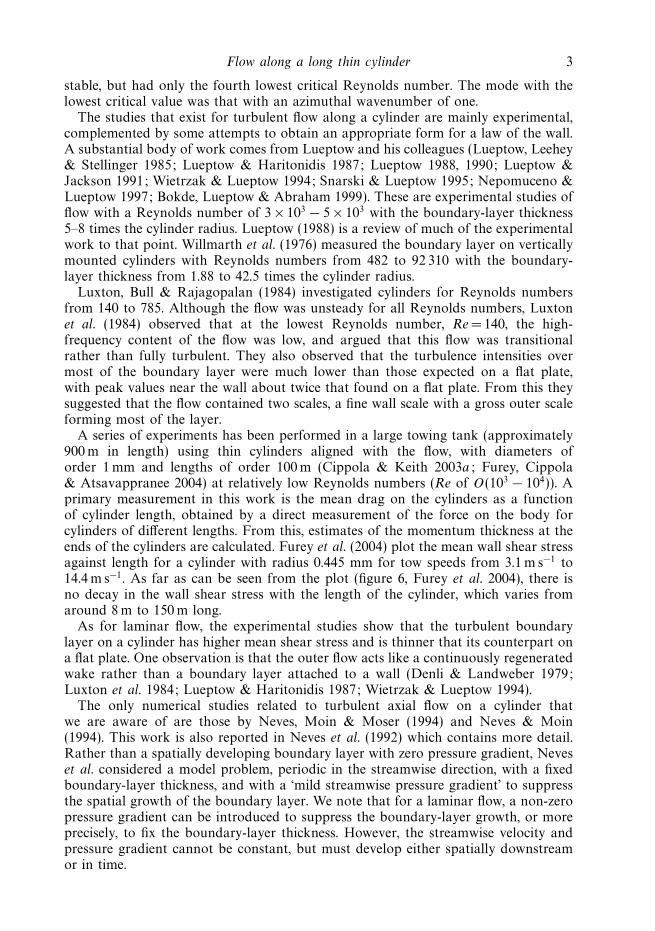
Figure 1 shows velocity profiles for cases 2, 5 and 13 along with experimentalvalues taken from Willmarth et al. (1976). Figure 1 uses wall units, i.e. showsu+ = u/uτ against y+ = (r − 1) a uτ /ν = y a+. There is excellent agreement betweenthe experimental and numerical results for cases 5 and 13. For case 2, figure 1 showsan apparently large difference. However, this is largely a reflection of the differencein the numerical and experimental values of uτ (see tables 1 and 2).
The experimental and numerical values for a+ and δ+ are given in table 3. Thepercentage difference in the values is the same as for uτ in table 2. From the valuesfor a+, it can be seen that for case 13, the effects of the wall curvature should berestricted to the outer part of the boundary layer, and a large portion of the boundarylayer should be similar to that for a flat plate. The velocity profile shown for case13 in figure 1 shows the expected pattern, with a clear logarithmic region. There isalso evidence for the loss of the shoulder in the far field characteristic of a planar
8 O. R. Tutty
0
5
10
15
20
25
30
35
100 101 102 103 104
y+
u+
Figure 1. Velocity profiles in wall coordinates (u+ = u/uτ against y+ = (r − 1) a uτ /ν). Linesare numerical and symbols experimental from Willmarth et al. (1976): lower, case 2; middle,case 5; top, case 13.
Case a+e a+
n δ+e δ+
n
1 33.4 27.9 1419 11842 46.1 40.5 1727 15173 56.4 48.3 1355 11604 83.4 73.4 2251 19835 198.2 198.2 3171 31716 272.0 275.0 2833 28647 388.7 405.3 3672 38298 456.5 489.6 4255 45639 513.6 536.0 2835 2959
10 751.2 778.9 3539 367011 891.4 920.4 4132 426712 1360.7 1408.0 5612 580713 2709.6 2758.9 4769 485614 3158.0 3357.6 5937 6312
Table 3. Values of a+ = auτ /ν: experimental, a+e , from Willmarth et al. (1976); numerical,
a+n . Also given are the corresponding values of δ+ = δ uτ /ν.
boundary layer. Experimental results (Lueptow et al. 1985) show that as a+ decreases,the velocity profile may have a logarithmic region, but the slope will be lower. Thenumerical solutions for the cases with the larger Reynolds numbers and values ofa+ (cases 9–14) showed this. For the lower Reynolds numbers, the values of a+ aresuch that the effects of curvature should be important in the region that normallycontains the logarithmic velocity profile. Both the numerical and experimental resultsreflect this, with initially a decrease in slope and then the loss of the logarithmic layer,as can be seen for cases 2 and 5 in figure 1. Luxton et al. (1984) studied the flowat low Reynolds number ranging from 140 to 785 and found that in this range thelogarithmic region had completely disappeared.

Flow along a long thin cylinder 9
0
2
4
6
8
10
12
400 800 1200 1600
δ
x – x0
Figure 2. Non-dimensional boundary-layer thickness δ against non-dimensional distancex − x0 (normalized on the radius a) for a cylinder with a = 0.2375 cm and U∞ = 20 m s−1.Line, numerical; symbols, experimental (Lueptow et al. 1985).
Lueptow et al. (1985) also performed experiments on a small circular cylinder,concentrating on the thick turbulent boundary layer where transverse curvature effectsshould be significant. They presented results for cylinders with Reynolds numbersfrom 103 to 5 × 10³, approximately. Here we will use the results for a cylinder of radius0.2375 cm with free-stream velocities of 20 or 30 m s−1, i.e. for Reynolds numbers from3 × 103 to 5 × 10³, approximately. The cylinder was mounted horizontally, and thesag at the midpoint was 1.2 radii. Whereas Willmarth et al. (1976) used different sizedcylinders and measured the boundary layer at the same point physically along thecylinder to obtain values for different regimes, Lueptow et al. (1985) measured it atdifferent points on the same cylinder. For the cases we will consider, Lueptow et al.tripped the boundary layer using an 0.08 cm radius O-ring. Also, Lueptow et al. statethat for this cylinder with a flow speed of 20 m s−1, there was a uniform streamwisepressure gradient of −10 Pa m−1 along the cylinder. This has been included in thenumerical results presented here.
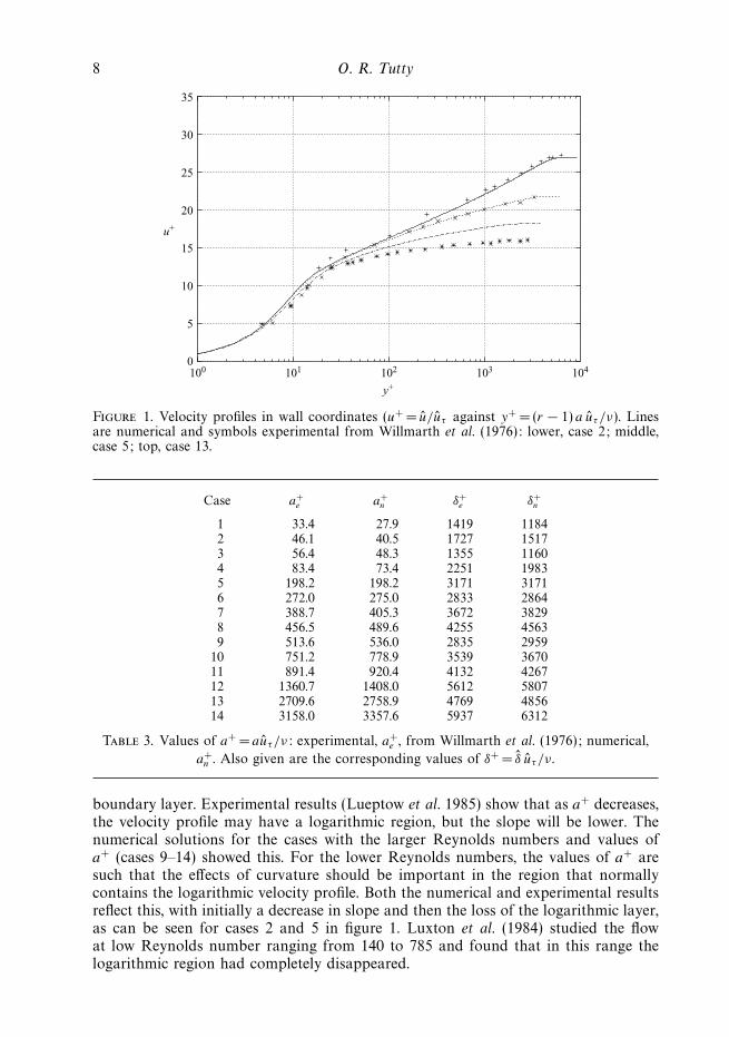
Figure 2 shows calculated and measured values for the boundary-layer thicknessalong the larger cylinder, and figure 3 the momentum thickness. In the experiments,x was measured as the distance from the trip. It is not possible to model directlythe effects of such a large trip using a boundary-layer formulation. Instead, a virtualorigin (x0) was used, estimated by approximately matching the apparent conditions atthe trip indicated in figure 2 in Lueptow et al. (1985). This was done in two ways. First,the laminar boundary layer was allowed to grow to an appropriate thickness before itwas tripped. Secondly, the boundary layer was tripped in the usual position, and theresults displaced by an appropriate amount. Both approaches produced essentiallythe same results.
Figures 2 and 3 show good agreement between the numerical and experimentalvalues except for those furthest downstream. However, in the experiments, thecylinder was mounted horizontally, and, as stated by Lueptow et al. (1985), thesag was sufficient to suggest that it may be modifying the boundary-layer thickness.
10 O. R. Tutty
1
2
0 400 800 1200 1600
θ
x – x0
Figure 3. Non-dimensional momentum thickness θ against non-dimensional distance x − x0
(normalized on the radius a) for a cylinder with a = 0.2375 cm and U∞ = 20 m s−1. Line,numerical; symbols, experimental (Lueptow et al. 1985).
0
0.001
0.002
2 4 6 8 10
Rey
nold
s st
ress
r – 1
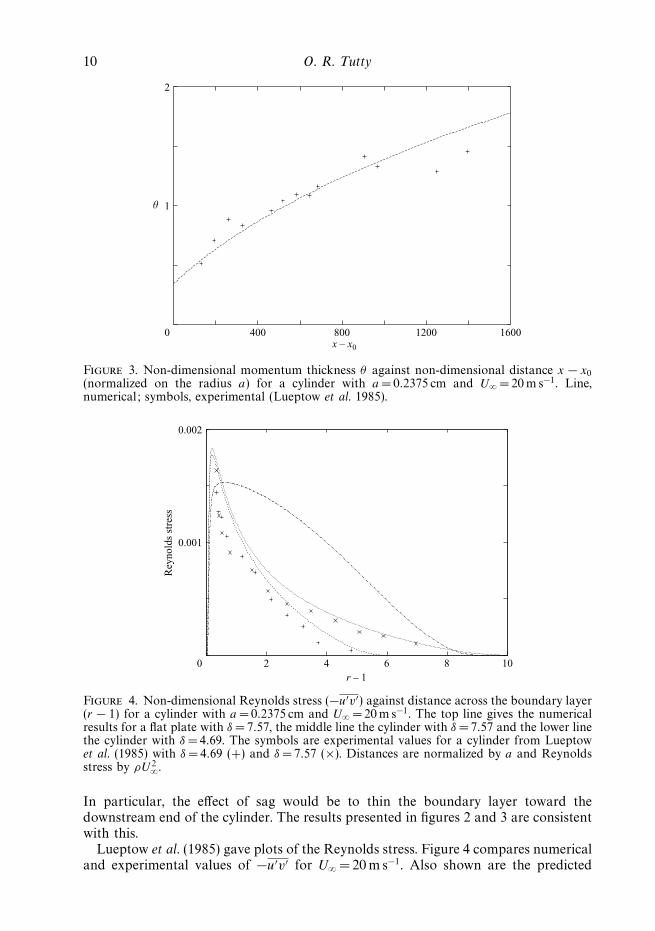
Figure 4. Non-dimensional Reynolds stress (−u′v′) against distance across the boundary layer(r − 1) for a cylinder with a = 0.2375 cm and U∞ = 20 m s−1. The top line gives the numericalresults for a flat plate with δ = 7.57, the middle line the cylinder with δ = 7.57 and the lower linethe cylinder with δ = 4.69. The symbols are experimental values for a cylinder from Lueptowet al. (1985) with δ = 4.69 (+) and δ = 7.57 (×). Distances are normalized by a and Reynoldsstress by ρU 2
∞.
In particular, the effect of sag would be to thin the boundary layer toward thedownstream end of the cylinder. The results presented in figures 2 and 3 are consistentwith this.
Lueptow et al. (1985) gave plots of the Reynolds stress. Figure 4 compares numericaland experimental values of −u′v′ for U∞ = 20 m s−1. Also shown are the predicted
Flow along a long thin cylinder 11
values of the Reynolds stress for an equivalent case on a flat plate, which areconsistent with flat-plate experimental values (see Lueptow et al. 1985). There is amarked difference in the Reynolds stress distribution between the cylinder and theplate, with larger values near the wall and a faster drop off away from the wall.The numerical and experimental distributions for the cylinder have the same shape,but the numerical predictions are, in general, higher than the experimental values.However, we note that Lueptow & Haritonidis (1987) state that the measurementsof the Reynolds stress reported in Lueptow et al. (1985) were made by a probe withpoor spatial resolution.
The experimental values collapse onto a single curve near the wall (r − 1 < 2), butseparate further away from the wall, reflecting the growth of the boundary layer.The numerical values also show this behaviour. A comparison was made between theexperimental and numerical values for U∞ = 30 m s−1, with similar results.
Lueptow et al. (1985) also give values for the friction velocity uτ obtained from acurve fit to the experimental results, and from matching the mean velocity profile tothat expected for a flat plate. There was a significant difference between the two sets ofvalues obtained in this way (up to 40 %). The values we predict show good agreementwith those obtained in Lueptow et al. (1985) by matching the velocity profile to the flat-plate one. With U∞ = 20 m s−1, the experimental values range between uτ /U∞ =0.053where δ =4.69 and 0.049 where δ = 8.11. The respective numerical values are 0.0488and 0.0496 (the slight increase with x is due to the effect of the favourable pressuregradient). At 30 m s−1, the experiments gave uτ /U∞ =0.048 at δ = 5.59 and 0.047 atδ = 8.53. The equivalent numerical values are 0.0460 and 0.0455.
The comparisons made above have shown that simulations using the Spalart–Allmaras turbulence model can faithfully reproduce the major features of a turbulentboundary layer along a cylinder, at least for the flow regimes for which detailedexperimental measurements are available. As well as reflecting the differences betweenthe boundary layer of a plate and a cylinder, given the uncertainty in experimentalvalues, there is a large measure of quantitative agreement between the numericaland experimental results. In the next section, the code will be used to investigate thebehaviour of the flow along cylinders with a range of Reynolds numbers.
2.3. Results
Numerical predictions for the non-dimensional wall shear stress,
τw =∂u
∂r(x, 1), (2.8)
near the leading edge of the cylinder with Re= 105 are shown in figure 5. Also shownin figure 5 are the numerical values for a flat plate with the same reference Reynoldsnumber. The boundary layer was tripped at x = 10. Upstream of this, as expected,there is little difference in the values for the cylinder and the flat plate. However, assoon as the boundary becomes turbulent the two sets of results diverge, with higherskin friction for the cylinder.
Figure 6 shows the boundary-layer thickness δ = δ/a against x for Re= 105. Oncethe flow is tripped, the boundary layer grows rapidly, and is of the same size as thecylinder before x = 80. By this stage, the effects of the transverse curvature will besignificant, as can be seen in figure 5. As for the laminar case, the boundary layer isthinner with higher wall shear stress than the equivalent flat-plate flow.
Figures 7 and 8 are similar to 5 and 6, but cover a much larger distance. Thedifference between the flat plate and cylinder flows increases downstream. Also, for

12 O. R. Tutty
20
40
60
80
100
120
140
160
180
200
0 20 40 60 80 100
Wal
l she
ar s
tres
s
x
Figure 5. Non-dimensional wall shear stress (in units of µU∞/a) versus distance (in units ofthe cylinder radius a) for Re =105. —, cylinder; - - -, flat plate.
0
0.2
0.4
0.6
0.8
1.0
1.2
1.4
20 40 60 80 100
δ
x
Figure 6. Boundary-layer thickness δ versus distance along the cylinder x (in units of thecylinder radius a) for Re= 105. —, cylinder; - - -, flat plate.
the cylinder, the wall shear stress appears to tend to a constant value. However, acalculation was performed for a much longer run, until x = 105, and there was stilla slow decay in the predicted value of the wall shear stress for the far downstreamportion of the cylinder. It was not possible to determine whether this decay wouldcontinue indefinitely, or whether the wall shear stress was tending asymptotically toa finite value. However, the decay was extremely slow; from x = 5 × 10⁴ to 105 it wasapproximately 0.3 %. Physically, in water, a non-dimensional length of 5 × 10⁴ withRe= 105 would represent a length of approximately 1 km for a cylinder with a radiusof 2 cm and a free-stream velocity of 5m s−1, a typical speed for a sonar array. In

Flow along a long thin cylinder 13
20
40
60
80
100
120
140
160
180
200
0 1000 2000 3000 4000 5000
Wal
l she
ar s
tres
s
x
Figure 7. Non-dimensional wall shear stress (in units of µU∞/a) versus distance (in units ofthe cylinder radius a) for Re= 105. —, cylinder; - - -, flat plate.
0
10
20
30
40
50
60
1000 2000 3000 4000 5000x
δ
Figure 8. Boundary-layer thickness δ versus distance along the cylinder x (in units of thecylinder radius a) for Re =105. —, cylinder; - - -, flat plate.
air, the length would be approximately 2.5 km for a 5 cm radius cylinder with a flowof 30 m s−1.
For all practical purposes, and within the limits of the expected accuracy of suchcalculations, for Re = 105 the boundary-layer model is predicting that the wall shearstress is constant, except near the leading edge. Calculations were performed for arange of Reynolds numbers from 1 to 106. The results were similar to those for 105,with a thinner boundary layer and higher surface wall shear stress for the cylinderthan for the flat plate, and with the wall shear stress tending to a constant, oralmost constant, wall shear stress far downstream. Lueptow & Haritonidis (1987)measured the wall shear stress along a cylinder for a number of flow speeds and

14 O. R. Tutty
used the data to produce a fit of the variation of τw with Rex , the Reynolds numberbased on the distance along the cylinder from the point the boundary layer wastripped. This gave a weak dependence on distance, with the friction coefficient givenby Cf = 0.0123 Re−0.08
x . However, for each of the three flow speeds used to producethis fit, the data could be interpreted as showing an initial drop in τw , followed byan extended region where there is little change (see Lueptow & Haritonidis (1987),figure 6), consistent with the pattern shown in figure 7.
Furey et al. (2004) investigated the effects of the cylinder length on the mean dragfor a cylinder of radius 0.445 mm and lengths from around 8 to 150 m by directmeasurement of the force exerted on the cylinders. They present results for four flowspeeds from 3.1 to 14.4 m s−1. An unexpected result is that there are fluctuations in thedrag rather than a decrease with length (this was also reported in Cippola & Keith(2003a) where similar results with fewer data points are presented). No explanationof this effect was given. Although the values fluctuate, there is no apparent overalldecay in the level of the wall shear stress for any of the flow rates in the data shownin Furey et al. (2004). The data for the largest flow rate (14.4 m s−1) was digitized anda linear regression analysis was performed. Within the accuracy of this procedure, theslope was zero. In fact, by dropping one value from the data set (the last one) theslope changed from a very small negative value to a small positive one. The meanvalue of the wall shear stress values shown in figure 6 of Furey et al. (2004) wasestimated as 430 Mm−2. By comparison, the estimate from the boundary-layer codewas 395 N m−12, within 10 %. There was a similar level of agreement for the otherflow speeds (the numerical values are 179 Nm−12 for U∞ = 9.3 m s−1, 63 Nm−12 forU∞ =5.2 and 25 Nm−12 for U∞ = 3.1).
Below, we will refer to a constant wall shear stress to refer to a representative valueof the wall shear stress in the region where there is little or no variation over a longdistance (much less than 1 % over a non-dimensional distance of at least 104). It isimportant to note, however, that there may still be some change, and that this is aprediction obtained using a turbulence model, although one that has been shown tobehave well for this particular application.
The Reynolds stress −u′v′ at x = 2 × 10⁴ (δ = 33.8) and x = 105 (δ = 88.3) forRe= 105 is shown in figure 9. There is little difference between the Reynolds stressdistribution at these two widely spaced points, except in the far field, reflecting thedownstream growth of the boundary layer. Over most of the boundary layer, thelevel of the Reynolds stress is low, indicating that strong turbulence is found only inthe near-wall region, and that the far field is behaving essentially as a laminar flow.Further, there is little if any spatial development of the flow near the wall. This effectcan also be seen in the velocity distribution across the boundary layer (see below forRe= 10).
For axisymmetric flow on a cylinder with zero pressure gradient, the momentumintegral equation becomes
d
dx
∫ ∞
1
u (1 − u) r dr =τw
Re. (2.9)
Hence, the wall shear stress tending to a constant implies that the momentum thicknesswill grow as x1/2 for large x. The boundary-layer thickness would also be expected togrow as x1/2. As can be seen from figure 10, the results from the numerical solutionsupport this.
Cippola & Keith (2003a) and Furey et al. (2004) used (2.9) with the experimentaldrag values to estimate the variation in momentum thickness with length of the

Flow along a long thin cylinder 15
0
0.0002
0.0004
0.0006
0.0008
0.0010
0.0012
0.0014
10–4 10–3 10–2 10–1 100 101 102 103
Rey
nold
s st
ress
r – 1
Figure 9. Reynolds stress −u′v′ (in units of U 2∞) against distance across the boundary layer
(normalized by a) for Re= 105. The dashed line is for x = 2 × 10⁴ and the solid line for x = 105.
0
500
1000
1500
2000
2500
3000
3500
10000 20000 30000 40000x
δ2
Figure 10. Boundary-layer thickness squared versus x (in units of a2 and a) for Re= 105.Also shown is a straight line which is asymptotic to δ2 for large x.
cylinder. There is little difference between the values obtained from (2.9) using themean value of the experimental results and those plotted by Furey et al. (2004)obtained using the distribution of wall shear stress as a function of x. Also, Cippola& Keith (2003a) plotted the estimated values of the momentum thickness non-dimensionalized by ν/uτ against the momentum thickness Reynolds number, andnoted that the apparent linear relationship could only be obtained if uτ was constant.
As noted above, the smaller the value of a+, the closer to the wall the effects ofcurvature will be felt. The smallest value of a+ for the data presented in Willmarthet al. (1976) or Lueptow et al. (1985) is 33.4 (table 3). This value is sufficiently large to

16 O. R. Tutty
0
5
10
15
20
25
5 10 15 20
u+
y+
Cylinderu = a log(1 + y/a)
Flat plateu = y
Figure 11. Velocity in wall units (u+ = u/uτ against y+ = (r − 1) a uτ /ν) close to the wall withRe= 482. This shows the numerical results for a cylinder (bottom curve) and a flat plate withthe same value of the wall shear stress (second from top), plus the corresponding theoreticalcurves for the laminar sublayer.
suggest that the laminar sublayer should be similar to that for a flat plate. Figure 11shows the numerical predictions for u+ against y+ for the cylinder for case 1 fromWillmarth et al. (1976), and for a flat plate with the same value of the wall shearstress. Also shown are the profiles from (1.1) and from u+ = y+. For very small valuesof y+ (2 or less) these all produce essentially the same velocity profile. However, byy+ = 5 there is a noticeable difference between the velocity for the cylinder and theflat plate, and it is clear that by this stage, which is significantly less than y+ = a+,(1.1) provides a better comparison with the numerically generated velocity profilethan the planar model.
Luxton et al. (1984) have performed experiments for flow with the Reynolds numberas low as 140, which has a+ of approximately 13. The boundary-layer model produceda value of a+ of approximately 11 with the same boundary-layer thickness. Given thelevel of uncertainty, this level of agreement is as good as could be expected. There is,however, no data available that we are aware of in the literature for flows with a+
less than 10, when the effects of curvature would be expected to be significant rightdown to the wall. A calculation was performed with a very low value of the Reynoldsnumber, Re =10, which gave a far downstream value of a+ of 1.49. Figure 12 showsthe wall shear stress. Again, τw appears to tend to a constant as x → ∞. Figure 13shows the velocity in wall units at x = 106 and 2 × 10⁶, and the predicted near-wall behaviour from (1.1). There is little difference between the velocity at the twopoints except a long way from the cylinder, with agreement up to y+ at least 103.The difference in the far field reflects the continuing growth in the thickness of theboundary layer. Note that since the scaling is the same for the two positions usedin figure 13, the velocity in physical terms matches up to the same point, which isapproximately 700 radii from the cylinder.
It can also be seen that (1.1) gives a good estimate for the velocity up to y+ ≈ 20,much further than would be expected for a flat plate or for a cylinder with a muchlarger value of a+. This is a reflection of the fact that the turbulence model does not

Flow along a long thin cylinder 17
0.20
0.22
0.24
0.26
0.28
0.30
0 5 10 15(× 105)
20
Wal
l she
ar s
tres
s
x
Figure 12. Non-dimensional wall shear stress (in units of µU∞/a) versus distance along thecylinder (scaled on the radius a) with Re= 10.
0
1
2
3
4
5
6
7
8
10–1 100 101 102 103 104 105
u+
y+
x = 2000000x = 1000000
u = a log(1 + y/a)
Figure 13. The velocity in wall units (u+ = u/uτ against y+ = (r −1)a uτ /ν) for a cylinder withRe =10. Numerical values are shown for x ≈ 106 (middle curve) and 2 × 10⁶ (lowest curve).Also shown is the theoretical curve u+ = a+ log(1 + y+/a+) (top curve).
produce a significant amount of turbulent viscosity in the near-wall region, with themodel predicting a laminar sublayer much larger than usual.
Luxton et al. (1984) considered the variation of the friction velocity with Reynoldsnumber from a number of different sets of experimental data. They produced a fitwhich can be written as
τw = 0.0121 Re0.8. (2.10)
18 O. R. Tutty
Wal
l she
ar s
tres
s
Re100
10–2
10–1
100
101
102
103
101 102 103 104 106105
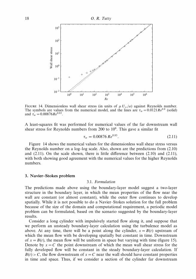
Figure 14. Dimensionless wall shear stress (in units of µU∞/a) against Reynolds number.The symbols are values from the numerical model, and the lines are τw = 0.0121Re0.8 (solid)and τw = 0.00876Re0.83.
A least-squares fit was performed for numerical values of the far downstream wallshear stress for Reynolds numbers from 200 to 106. This gave a similar fit
τw = 0.00876 Re0.83. (2.11)
Figure 14 shows the numerical values for the dimensionless wall shear stress versusthe Reynolds number on a log–log scale. Also, shown are the predictions from (2.10)and (2.11). On the scale shown, there is little difference between (2.10) and (2.11),with both showing good agreement with the numerical values for the higher Reynoldsnumbers.
3. Navier–Stokes problem3.1. Formulation
The predictions made above using the boundary-layer model suggest a two-layerstructure in the boundary layer, in which the mean properties of the flow near thewall are constant (or almost constant), while the outer flow continues to developspatially. While it is not possible to do a Navier–Stokes solution for the full problembecause of the size of the domain and computational requirement, a periodic modelproblem can be formulated, based on the scenario suggested by the boundary-layerresults.
Consider a long cylinder with impulsively started flow along it, and suppose thatwe perform an unsteady boundary-layer calculation using the turbulence model asabove. At any time, there will be a point along the cylinder, x = B(t) upstream ofwhich the mean flow with be developing spatially but constant in time. Downstreamof x = B(t), the mean flow will be uniform in space but varying with time (figure 15).Denote by x = C the point downstream of which the mean wall shear stress for thefully developed flow will be constant in the steady boundary-layer calculation. IfB(t) > C, the flow downstream of x = C near the wall should have constant propertiesin time and space. Thus, if we consider a section of the cylinder far downstream

Flow along a long thin cylinder 19
t = t1
t = t2
B(t1) C B(t2)
Figure 15. Development of the boundary layer, The point x = B(t) marks the transitionbetween spatial and temporal behaviour of the boundary layer. x = C is the point where thewall shear stress takes a constant value.
with x B(t) > C, the flow should be spatially periodic on the section, provided thesection is sufficiently long.
We will consider flow on a periodic domain, developing in time. If the modelpresented above is correct, the wall shear stress should settle on a value close tothat predicted by the boundary-layer model, and hence consistent with experimentalvalues. Also, near the surface, the mean velocity profile should be close to that givenby the boundary-layer model, as should the Reynolds stress −u′v′. These will providetests for the feasibility of the model.
Further, the boundary-layer model suggests that strong turbulence exists only nearthe wall, where there is little variation on the mean flow. Hence, the contribution tosurface pressure fluctuations from this part of the flow should not vary significantlywith time provided the boundary layer is thick enough, with the variation in thepressure spectra with time coming from the large-scale motions, affecting mainly thelow-frequency range (see Bull (1996) or Farabee & Casarella (1991) for a discussionof frequency ranges and their scalings in wall-bounded boundary layers).
Also, when using the turbulence model but with the flow developing in time anduniform in space, the value of the wall shear stress should settle on a value closeto that obtained from the spatial boundary-layer model. Figure 16 shows the resultof a time-dependent calculation with Re =103. There is excellent agreement with thespatial model.
The governing equations in non-dimensional form are the continuity equation
∂u
∂x+
∂v
∂r+
v
r+
1
r
∂w
∂φ= 0, (3.1)
and the Navier–Stokes equations
∂u
∂t+ wΩr − vΩφ = −∂P
∂x+
1
Re∇2u, (3.2)
∂v
∂t+ uΩφ − wΩx = −∂P
∂r+
1
Re
(∇2v − v
r2− 2
r2
∂w
∂φ
), (3.3)
∂w
∂t+ vΩx − uΩr = −1
r
∂P
∂φ+
1
Re
(∇2w − w
r2+
2
r2
∂v
∂φ
), (3.4)
where u = (u, v, w) is the velocity in polar coordinates (x, r, φ),
∇2 =∂2
∂x2+
∂2
∂r2+
1
r
∂
∂r+
1
r2
∂2
∂φ2

20 O. R. Tutty
0
1
2
3
2000 4000 6000 8000 10000
Wal
l she
ar s
tres
s
t
Figure 16. The wall shear stress (in units of µU∞/a) against time (in units of a/U∞)for a time-dependent but spatially uniform flow using the Spalart–Allmaras turbulencemodel. Re =103. The straight line gives the downstream value from the spatially developingboundary-layer model.
is the Laplacian,
(Ωx, Ωr, Ωφ) =
(1
r
∂(rw)
∂r− 1
r
∂v
∂φ,1
r
∂u
∂φ− ∂w
∂x,∂v
∂x− ∂u
∂r
)(3.5)
is the vorticity, and
P = p + 12
| u |2 (3.6)
is a modified pressure. The time is written in non-dimensional form as t = t U∞/a. Theinertial terms in the Navier–Stokes equations (3.2)–(3.4) have been written in vorticityform as this has better numerical characteristics than the standard convective form.
The flow is calculated on a cylinder of non-dimensional length L. The boundaryconditions are
u = 0 on r = 1, − 12L x 1
2L, (3.7)
u → (1, 0, 0) as r → ∞. (3.8)
Periodicity implies
u(
12L, r, φ, t
)= u
(− 1
2L, r, φ, t
). (3.9)
3.2. Numerical
The code developed for this study uses standard methods, and thus will be described inoutline only. Fourier series are used in the streamwise (x) and polar (φ) directions, anda second-order central difference method in the radial (r) direction. As is usual withsimulations of turbulent flow, a pseudospectral method is used, with the nonlinearterms handled explicitly and the linear terms implicitly. A second-order Adams–Bashforth method is used for the nonlinear terms, and a second-order backwarddifference formula is used for the time derivative. At each time step, the momentumequations are solved to obtain an intermediate velocity field. This velocity is thenupdated through a pressure correction substep which ensures that the continuityequation (3.1) is satisfied at each time step. As in Neves et al. (1992), to simplify the

Flow along a long thin cylinder 21
numerical procedure, the cross-coupling viscous terms in (3.3) and (3.4) were includedwith the nonlinear terms. This does not alter the formal accuracy of the scheme.
A staggered grid was used, with the radial velocity v defined on the grid pointsrj and the pressure and the other velocity components at the midpoints. Staggeringthe variables in this manner allows the discrete form of the continuity equation tobe satisfied within rounding error. The grid in r was stretched so that the points areclustered near the surface of the cylinder.
We denote the Fourier transform of f as f ∗j,m where j and m are the mode numbers
in x and φ, respectively. In the far field (r = rmax), the mean value of the streamwisevelocity u∗
0,0 is set to the free-stream value, and the radial derivative of the othermodes of u are set to zero. The modes of the azimuthal velocity w also have a zeroradial derivative, while from continuity (3.1)
∂
∂r(rv∗
j,m) = 0 at r = rmax.
The mean value of the pressure P ∗0,0 was set to zero in the far field, which provides
the necessary normalization of the pressure. Again, a zero derivative condition wasused for the other modes.
The scheme reduces the Navier–Stokes equations to a system of tridiagonalequations for the Fourier modes of the velocity and the pressure, second-orderin time and space, which are easily solved.
An updated version of the code uses a third-order Runge–Kutta time-steppingmethod (Nikitin 2006), in place of the second-order Adams–Bashforth backwarddifference scheme used in the original code. It was not practical to repeat all thecalculations described below. However, a test case was performed, using the samegrid with both codes and Re = 103. There was no significant difference in the results.Also, the computational effort was similar. The Runge–Kutta method was morestable, so that a larger time step could be used, but this only compensated for theincreased effort per time step.
An initial condition must also be specified. Initially, the streamwise velocity u wasgiven an exponential growth from zero at the surface to the free-stream value of1, plus a random disturbance added to all velocity components. This was sufficientto provoke transition provided the boundary layer was sufficiently thick. However,it took up to t = 2000 for the flow to undergo transition and for the turbulence tobecome established. To avoid this unproductive computational effort, for most runs,and for all those with fine grids, the results from an existing calculation where theflow was already turbulent were used to initialize the flow.
The numerical scheme described above can be used for a direct numerical solution(DNS) of the problem in which all scales are resolved. However, at the higher Reynoldsnumbers studied, such a calculation was impractical because of the computationaleffort required. Hence for these Reynolds numbers, a large eddy simulation (LES)approach was used. In this method, the larger scales are resolved, while the effectsof those that are too small to be represented on the grid are simulated by the useof a subgrid model. The subgrid model consists of an eddy viscosity term which isdesigned to act as a filter to provide an appropriate decay of the spectrum at higherwavenumbers.
The subgrid model used is the standard Smagorinsky model with Van Driestdamping to represent the reduced growth of the small scales near the surface. The

22 O. R. Tutty
subgrid viscosity µsg is given by
µsg = Re (c0∆)2D2 S (3.10)
where c0 = 0.05, S =(2SijSij )1/2, Sij is the rate of strain tensor, and ∆ =(r∆x∆r∆φ)1/3
gives the characteristic local grid step. D is a wall damping function given by
D = 1 − exp
(−y+
A
), (3.11)
where A= 26.The subgrid model is incorporated into the numerical scheme by multiplying the
viscous terms by a non-dimensional viscosity µ where
µ = 1 + µsg (3.12)
or
µ = max(1, µsg). (3.13)
An advantage of (3.13) over the usual model (3.12) is that, if the subgrid viscosityis sufficiently small, µ will be 1, and the calculation will be DNS. For the lowerReynolds numbers considered, 2000 or less, this was the case and the LES model wasnot used. Swapping between (3.12) and (3.13) provides a simple method of estimatingthe effect of the LES model.
When the LES method was used, at each time step, µsg was calculated for eachvalue of r by using the strain S averaged over x and φ, an approach used by Moin &Kim (1982). The LES model is easily incorporated into the numerical scheme usingthis method. Also, it is consistent with the expected behaviour of the flow, where theinner part of the boundary layer should tend to a constant state with a constant valueof the wall shear stress.
It is known that the Smagorinsky model is overly dissipative with regard to the largescales in the flow. Therefore, the subgrid model was applied only to high-frequencymodes, usually the top eighth, although this was varied to assess the effect of varyingthe LES model.
A number of tests were performed to check the code. These included analytic testsof the one-dimensional Helmholtz and Poisson solvers arising from the momentumand pressure equations, the use of known functions for the formation of the nonlinearterms, and solutions of Burgers equation to test the time stepping. Results from thecode operating in planar mode were compared with those from studies of channel flow,with excellent agreement. Also, the travelling-wave solutions of Wedin & Kerswell(2004), which are unsteady, nonlinear solutions of the Navier–Stokes equations, werecompared with solutions obtained from a version of the code developed for pipe flow.Again, there was good agreement.
One of the major aims of the work is to investigate the effect of the Reynoldsnumber of the noise generated at the surface of the cylinder by the turbulent pressurefluctuations procedure. This can be measured by the power spectrum (power spectraldensity) of the pressure. The pressure was circumferentially averaged at a specificvalue of x, the data were split into a number of samples, a Hanning window wasapplied to each sample, normalized to ensure that the variance of the windowed datamatched that of the original data, and the power spectrum was then calculated as theaverage over the samples.
Table 4 gives the parameters for the grids used in the Navier–Stokes calculations.This is not a complete list; other grids were used to verify the accuracy of the
Flow along a long thin cylinder 23
Re a+ J K M L L+ x+ φ+
300 18.5 512 100 64 96 1775 3.5 1.8500 28.7 512 100 64 96 2757 5.4 2.8103 52.8 512 120 256 96 5070 9.9 1.3
2 × 10³ 98.1 512 100 128 48 9416 9.2 4.85 × 10³ 223.4 256 120 64 48 10 721 41.9 21.95 × 10³ 223.4 512 120 256 24 5361 10.5 5.5
104 418.4 512 100 128 48 20 083 39.2 20.5104 418.4 512 100 256 24 10 042 19.6 10.3
5 × 10⁴ 1824.8 512 100 256 24 43 796 85.5 44.85 × 10⁴ 1824.8 1024 100 512 24 43 796 42.8 22.4
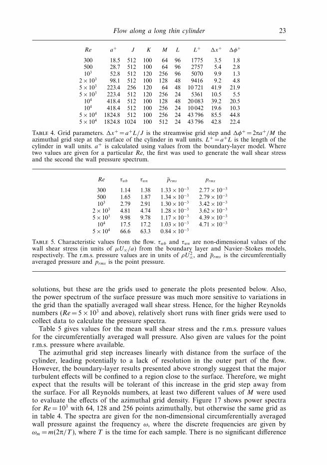
Table 4. Grid parameters. x+ = a+L/J is the streamwise grid step and φ+ = 2πa+/M theazimuthal grid step at the surface of the cylinder in wall units. L+ = a+L is the length of thecylinder in wall units. a+ is calculated using values from the boundary-layer model. Wheretwo values are given for a particular Re, the first was used to generate the wall shear stressand the second the wall pressure spectrum.
Re τwb τwn prms prms
300 1.14 1.38 1.33 × 10⁻³ 2.77 × 10⁻³
500 1.65 1.87 1.34 × 10⁻³ 2.79 × 10⁻³
103 2.79 2.91 1.30 × 10⁻³ 3.42 × 10⁻³
2 × 10³ 4.81 4.74 1.28 × 10⁻³ 3.62 × 10⁻³
5 × 10³ 9.98 9.78 1.17 × 10⁻³ 4.39 × 10⁻³
104 17.5 17.2 1.03 × 10⁻³ 4.71 × 10⁻³
5 × 10⁴ 66.6 63.3 0.84 × 10⁻³
Table 5. Characteristic values from the flow. τwb and τwn are non-dimensional values of thewall shear stress (in units of µU∞/a) from the boundary layer and Navier–Stokes models,respectively. The r.m.s. pressure values are in units of ρU 2
∞, and prms is the circumferentiallyaveraged pressure and prms is the point pressure.
solutions, but these are the grids used to generate the plots presented below. Also,the power spectrum of the surface pressure was much more sensitive to variations inthe grid than the spatially averaged wall shear stress. Hence, for the higher Reynoldsnumbers (Re = 5 × 10³ and above), relatively short runs with finer grids were used tocollect data to calculate the pressure spectra.
Table 5 gives values for the mean wall shear stress and the r.m.s. pressure valuesfor the circumferentially averaged wall pressure. Also given are values for the pointr.m.s. pressure where available.
The azimuthal grid step increases linearly with distance from the surface of thecylinder, leading potentially to a lack of resolution in the outer part of the flow.However, the boundary-layer results presented above strongly suggest that the majorturbulent effects will be confined to a region close to the surface. Therefore, we mightexpect that the results will be tolerant of this increase in the grid step away fromthe surface. For all Reynolds numbers, at least two different values of M were usedto evaluate the effects of the azimuthal grid density. Figure 17 shows power spectrafor Re = 103 with 64, 128 and 256 points azimuthally, but otherwise the same grid asin table 4. The spectra are given for the non-dimensional circumferentially averagedwall pressure against the frequency ω, where the discrete frequencies are given byωm = m(2π/T ), where T is the time for each sample. There is no significant difference

24 O. R. Tutty
10–4
10–5
10–6
10–7
10–8
10–9
10–10
10–11
10–12
10–13
10–1 100 101
Pow
er s
pect
ral d
ensi
ty
Frequency
Figure 17. Non-dimensional power spectra for the wall pressure (in units of aρ2U 3∞/2π)
against frequency (in units of U∞/a radians) for Re= 103. The bottom three lines are for thecircumferentially averaged pressure for M = 64, 128 and 256. The top line is for point pressurefor M = 256.
in the spectra. The behaviour of the wall shear stress was also unaffected by thevariation in M . The power spectrum for point wall pressure for M = 256 is alsoshown in figure 17.
A number of different factors must be taken into account when selecting the sizeof the domain. The boundary-layer thickness will grow with time. As the largeststructures in the flow would be expected to be the size of the boundary layer, theperiodic model will not be valid once the boundary-layer thickness approaches thelength of the domain. We are interested in thick boundary layers. In practice, thisrequires the non-dimensional boundary-layer thickness to be 10 or greater, whichsuggests that L should be at least 20. Examination of the solutions over a rangeof Reynolds numbers showed that once the boundary-layer thickness became muchgreater than half the length of the cylinder, large structures could be observed inthe far field which clearly would not be independent between periods. When thisoccurs, the effect is felt throughout the boundary layer. In particular, assuming thatthe boundary layer is thick enough for the inner part of the flow to have reacheda constant state, with the wall shear stress oscillating around a constant value, thelevel of wall shear stress will drop below this value when the boundary layer becomestoo thick. Usually, following this drop, the wall shear stress levelled off again arounda lower value. That this drop in the level of the wall shear stress was due to theshortness of the domain was demonstrated by performing calculations with differentdomain lengths, but all other parameters the same. In particular, if a solution inwhich the boundary-layer thickness was approaching half the length of the domain,but the wall shear stress had not dropped below its equilibrium level, was used toinitialize a calculation on a longer domain, this second calculation would continuewith its wall shear stress maintaining its value past the point where it would havedecreased on the shorter cylinder.

Flow along a long thin cylinder 25
In contrast, allowing the boundary layer to grow past half the length of the cylinderhad little effect on the power spectrum of the surface pressure.
For the lower Reynolds numbers, it was necessary for L to be considerably greaterthan 20 for two reasons. First, the cylinder must be long enough to accommodatethe near-wall structures in the turbulence. Secondly, we wish to investigate the effectof the size of the cylinder on the surface pressure fluctuations. This requires theReynolds number to be varied by fixing the free-stream velocity U∞ and varying thecylinder radius a. Since the time scale is a/U∞, the smaller the Reynolds number, thelonger the run required in non-dimensional terms to collect sufficient data in physicaltime to calculate the pressure spectrum. This implies a thicker boundary layer andhence a longer cylinder, particularly as the growth of the boundary layer with time islarger at lower Reynolds numbers. Integrating the streamwise momentum equationover the domain produces
d
dt
(δ21 + 2δ1
)=
2
Reτw, (3.14)
which with (2.10) or (2.11) implies that the growth rate of the displacement thicknesswill increase as Re decreases. This effect will be more pronounced at very low Reynoldsnumbers when (2.10)/(2.11) do not apply (see figure 14). The boundary-layer andmomentum thicknesses would be expected to behave in a similar manner to thedisplacement thickness.
The values of L given in table 4 are sufficient to satisfy these requirements. Theposition of the far field boundary (rmax) was chosen, depending on Reynolds number,to allow the boundary layer to grow sufficiently thick without wasted effort. Gridpoints were distributed radially so that there were sufficient points near the wall toresolve the inner part of the boundary layer where the turbulence is strongest. Anexample, for Re =103, of the radial grid can be seen in figure 20. In all cases, theradial grid was chosen so that the grid step at the wall was less than one in wall units.
3.3. Results: Re= 103
Calculations were performed for Re = 103 for a number of different grids and domainsizes. For this Reynolds number, a DNS calculation was performed with µsg = 0. Ingeneral, the results from the different runs were consistent, with the wall shear stresssettling on a value close to that predicted by the boundary-layer model. Figure 18shows the spatially averaged value of the wall shear stress for two runs, with differentgrids azimuthally and radially. The longer run has rmax = 75 and M = 64 and theshorter, rmax = 50 and M =256. Axially, both are as in table 4. There is no significantdifference in the behaviour of the wall shear stress for these two runs. Also, a longrun was performed with M = 128, which is not shown for clarity, with similar results.The pressure spectrum was the same for all three runs (figure 17).
If the boundary-layer model is accurately modelling the Navier–Stokes problem,then they should both have the same mean streamwise velocity profile, at leastnear the wall. Figure 19 shows the mean velocity profiles from the Navier–Stokescalculation (averaged in x and φ), and the predictions from the spatial boundary-layermodel, when the boundary-layer thickness is approximately 18.7. There is excellentagreement.
The Reynolds stress distribution should also match that from the boundary-layermodel. Figure 20 shows the values of −u′v′ against r (averaged in x, φ and t forthe Navier–Stokes calculations) when the boundary-layer thickness is approximately18.7. Again there is excellent agreement.

26 O. R. Tutty
2.6
2.7
2.8
2.9
3.0
3.1
3.2
3.3
0 1000 2000 3000 4000 5000 6000 7000 8000
Wal
l she
ar s
tres
s
t
Figure 18. The mean wall shear stress (in units of µU∞/a) against time (in units of a/U∞)for Re= 103. The solid line has M = 64 and the dashed line M = 256. The straight line givesthe downstream value from the boundary-layer model.
0
0.2
0.4
0.6
0.8
1.0
1.2
10–4 10–3 10–2 10–1 100 101 102
u
r – 1
Figure 19. Mean streamwise velocity u = u/U∞ across the boundary layer (normalized by the
cylinder radius a) for Re =103 when δ/a ≈ 18.7 The line is from the boundary-layer modeland the symbols from the Navier–Stokes calculation.
The agreement between the boundary-layer and Navier–Stokes results shown infigures 19 and 20 is typical of comparisons made using Navier–Stokes results from anumber of runs with different resolutions and with different boundary-layer thickness.Also, the variation in time of the streamwise velocity and the Reynolds stressdistribution is confined mainly to the outer part of the flow, reflecting the growth ofthe boundary layer, consistent with the predictions from the boundary-layer model.
Experimentally, in wall-bounded flows, structures in the flow are convected at avelocity somewhat below the free-stream velocity. There are a number of ways of
Flow along a long thin cylinder 27
0
0.0004
0.0008
0.0012
0.0016
5 10 15 20
Rey
nold
s st
ress
r
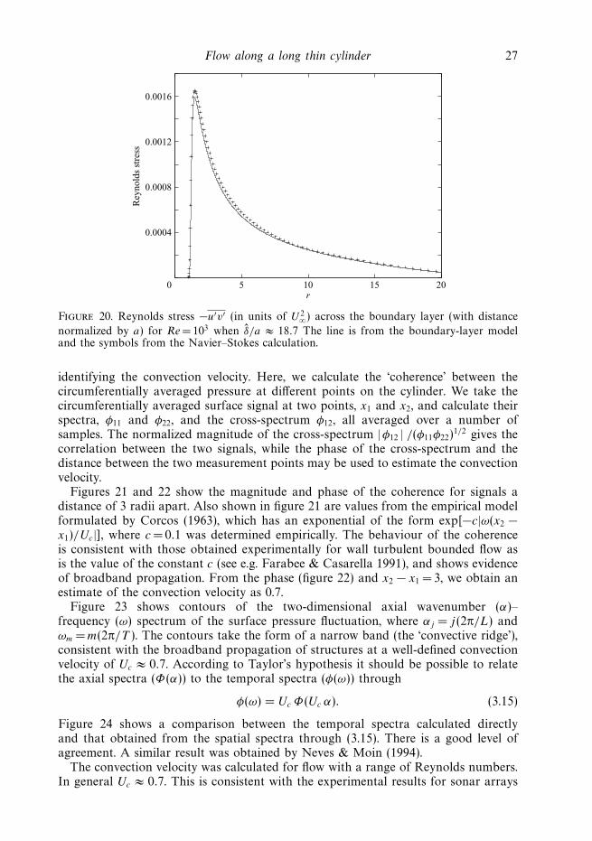
Figure 20. Reynolds stress −u′v′ (in units of U 2∞) across the boundary layer (with distance
normalized by a) for Re= 103 when δ/a ≈ 18.7 The line is from the boundary-layer modeland the symbols from the Navier–Stokes calculation.
identifying the convection velocity. Here, we calculate the ‘coherence’ between thecircumferentially averaged pressure at different points on the cylinder. We take thecircumferentially averaged surface signal at two points, x1 and x2, and calculate theirspectra, φ11 and φ22, and the cross-spectrum φ12, all averaged over a number ofsamples. The normalized magnitude of the cross-spectrum |φ12 | /(φ11φ22)
1/2 gives thecorrelation between the two signals, while the phase of the cross-spectrum and thedistance between the two measurement points may be used to estimate the convectionvelocity.
Figures 21 and 22 show the magnitude and phase of the coherence for signals adistance of 3 radii apart. Also shown in figure 21 are values from the empirical modelformulated by Corcos (1963), which has an exponential of the form exp[−c|ω(x2 −x1)/Uc|], where c =0.1 was determined empirically. The behaviour of the coherenceis consistent with those obtained experimentally for wall turbulent bounded flow asis the value of the constant c (see e.g. Farabee & Casarella 1991), and shows evidenceof broadband propagation. From the phase (figure 22) and x2 − x1 = 3, we obtain anestimate of the convection velocity as 0.7.
Figure 23 shows contours of the two-dimensional axial wavenumber (α)–frequency (ω) spectrum of the surface pressure fluctuation, where αj = j (2π/L) andωm = m(2π/T ). The contours take the form of a narrow band (the ‘convective ridge’),consistent with the broadband propagation of structures at a well-defined convectionvelocity of Uc ≈ 0.7. According to Taylor’s hypothesis it should be possible to relatethe axial spectra (Φ(α)) to the temporal spectra (φ(ω)) through
φ(ω) = Uc Φ(Uc α). (3.15)
Figure 24 shows a comparison between the temporal spectra calculated directlyand that obtained from the spatial spectra through (3.15). There is a good level ofagreement. A similar result was obtained by Neves & Moin (1994).
The convection velocity was calculated for flow with a range of Reynolds numbers.In general Uc ≈ 0.7. This is consistent with the experimental results for sonar arrays

28 O. R. Tutty
0
0.2
0.4
0.6
0.8
1.0
2 4 6 8 10
Mag
nitu
de
Frequency
Figure 21. The magnitude of the coherence of the circumferentially averaged wall pressureagainst frequency (in units of radians × U∞/a) for Re= 103. The dashed line is for the Corcosmodel (exp[−c|ω(x2 − x1)/Uc|]) with c = 0.1, x2 − x1 = 3 and Uc = 0.7.
–4
–2
0
2
4
0 2 4 6 8 10
Pha
se
Frequency
Figure 22. The phase of the coherence of the circumferentially averaged wall pressure (inradians) against frequency (in units of U∞/a) for Re= 103.
of a convection velocity of 0.7 to 0.8 of the tow speed. It is slightly higher than thevalue obtained by Neves & Moin (1994) of around 0.65.
3.4. Results: variation in Reynolds number
A detailed series of calculations were performed for Reynolds numbers from 300 to5 × 105. In all cases, a number of runs were performed with different grids to checkthe accuracy of the results. Figure 25 shows the spatially averaged wall shear stress forRe= 300, 500, 1000 and 2000, from Navier–Stokes calculations with no LES model,and the predictions from the boundary-layer model. For all three Reynolds numbers,

Flow along a long thin cylinder 29
–1.2 –1.0 –0.8 –0.6 –0.4 –0.2 0 0.20
0.4
0.8
1.2
1.6
ω
α
Figure 23. Contours of the two-dimensional axial wavenumber–frequency spectra for thecircumferentially averaged wall pressure (α − ω, in units of a−1 radians and U∞/a radians,respectively).
10–5
10–6
10–7
10–8
10–9
10–10
10–2 10–1 100 101
Pow
er s
pect
ral d
ensi
ty
Frequency
SpatialTemporal
Figure 24. Comparison between the temporal spectra and the estimated spectra using Taylor’shypothesis (3.15) with Uc =0.7. The spectra are for the circumferentially averaged wall pressure,and are in units of aρ2U 3
∞/2π with the frequency in units of U∞/a radians.
the wall shear stress eventually settles on a value close to that predicted from theboundary-layer model.
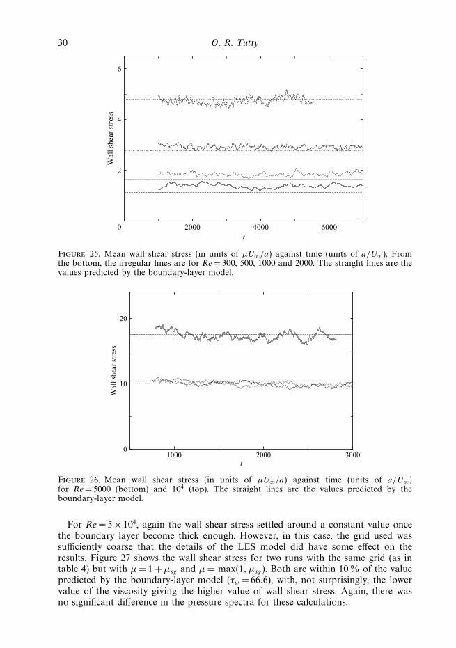
Figure 26 shows the wall shear stress for Re = 5000 and 104. For Re = 5000,calculations were performed in both DNS and LES mode with the same grid. Theresults from both calculations are shown in figure 26. There is no significant difference.Also, there was no significant difference in the circumferentially averaged pressurespectrum. In wall units, the grid for Re = 104 is similar to that for Re = 5 × 10³
(table 4), and a similar result was obtained. That is, the same level of wall shear stressand pressure spectra with and without the LES model, with good agreement with thelevel of wall shear stress predicted by the boundary-layer model.
30 O. R. Tutty
0
2
4
6
2000 4000 6000
Wal
l she
ar s
tres
s
t
Figure 25. Mean wall shear stress (in units of µU∞/a) against time (units of a/U∞). Fromthe bottom, the irregular lines are for Re= 300, 500, 1000 and 2000. The straight lines are thevalues predicted by the boundary-layer model.
0
10
20
1000 2000 3000
Wal
l she
ar s
tres
s
t
Figure 26. Mean wall shear stress (in units of µU∞/a) against time (units of a/U∞)for Re= 5000 (bottom) and 104 (top). The straight lines are the values predicted by theboundary-layer model.
For Re =5 × 10⁴, again the wall shear stress settled around a constant value oncethe boundary layer become thick enough. However, in this case, the grid used wassufficiently coarse that the details of the LES model did have some effect on theresults. Figure 27 shows the wall shear stress for two runs with the same grid (as intable 4) but with µ = 1 + µsg and µ = max(1, µsg). Both are within 10 % of the valuepredicted by the boundary-layer model (τw = 66.6), with, not surprisingly, the lowervalue of the viscosity giving the higher value of wall shear stress. Again, there wasno significant difference in the pressure spectra for these calculations.
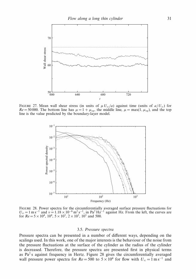
Flow along a long thin cylinder 31
50
60
70
600 640 680 720
Wal
l she
ar s
tres
s
t
Figure 27. Mean wall shear stress (in units of µU∞/a) against time (units of a/U∞) forRe =50 000. The bottom line has µ= 1 + µsg , the middle line, µ= max(1, µsg), and the topline is the value predicted by the boundary-layer model.
10–1
10–2
10–3
10–4
10–5
10–6
10–7
101 102 103
Pow
er s
pect
ral d
ensi
ty
Frequency (Hz)
Figure 28. Power spectra for the circumferentially averaged surface pressure fluctuations forU∞ = 1 m s−1 and ν = 1.18 × 10⁻⁶ m2 s−1, in Pa2 Hz−1 against Hz. From the left, the curves arefor Re =5 × 10⁴, 104, 5 × 10³, 2 × 10³, 103 and 500.
3.5. Pressure spectra
Pressure spectra can be presented in a number of different ways, depending on thescalings used. In this work, one of the major interests is the behaviour of the noise fromthe pressure fluctuations at the surface of the cylinder as the radius of the cylinderis decreased. Therefore, the pressure spectra are presented first in physical termsas Pa2 s against frequency in Hertz. Figure 28 gives the circumferentially averagedwall pressure power spectra for Re = 500 to 5 × 10⁴ for flow with U∞ =1ms−1 and

32 O. R. Tutty
a fluid with ν = 1.18 × 10⁻⁶ m2 s−1, typical of sea water. The spectra for Re= 5 × 10³
or greater were obtained with the finer grids given in table 4. For Re =5 × 10⁴, thestreamwise and azimuthal grid steps are still relatively crude (approximately 43 and22 in wall units, respectively), and from the results with smaller Reynolds number,where it was possible to use much finer grids in wall units, suggest that there wouldstill be some change with further refinement of the grid. However, the results fromlower Reynolds numbers also suggest that the spectrum with this resolution givesa reasonable approximation to the fully resolved spectrum, although the decay athigher frequencies may be too fast (this occurred with coarse grids at low Reynoldsnumbers).
As the Reynolds number/cylinder radius decreases, the pressure spectrum increasesin value over a wide frequency range, consistent with the observation that the surfacenoise from the turbulence varies inversely with the radius of the cylinder (Marschallet al. 1993; Potter et al. 2000).
The computational effort increases as the Reynolds number drops below 500because of the longer non-dimensional time that is required to provide data for thesame physical time when the flow velocity is held constant (the scale factor is a/U∞)and the larger domain required to cope with the thicker boundary layer arising fromthe increase in run time and the faster growth rate of the boundary layer. However,calculations were performed for Re= 300, although with a smaller number of samples,producing a spectrum with more noise than those shown in figure 28. The spectrumfor Re= 300 was similar to that for 500 and 1000, but has not been shown in figure 28for clarity.
The r.m.s. pressure values (non-dimensional in units of ρU 2∞) are given in table 5.
Consistent with figure 28, the r.m.s. values of the circumferentially averaged pressureincrease as Re decreases, until Re= 500. The value for Re =300 is almost the sameas that for 500.
When discussing pressure spectra, it is common to present them in non-dimensionalform using either outer (free-stream or convection velocity and a measure of theboundary-layer thickness) or inner (friction velocity and time) variables for thescaling (see e.g. Bull 1996; Farabee & Casarella 1991). Using the outer variablesdoes not provide any useful information as there is no significant variation in thespectra with time. In particular, for the longest run in non-dimensional terms, thatwith Re = 103 and M = 256, the boundary-layer thickness approximately doubled(from around 20 to 40), but there was no significant change in either the point orcircumferentially averaged pressure spectra between the first and second halves ofthe run. In contrast to the current situation, for wall-bounded flow, the pressurespectra for low frequencies commonly scales with the outer variables, in particulara measure of the boundary-layer thickness. One possible explanation for the lack ofdependence on the boundary-layer thickness lies in the distribution of the strengthof the turbulence. As shown in figures 4, 9 and 20, there is a pronounced peak in theReynolds stress near the wall, with a rapid drop in the outer region. This suggeststhat the large-scale structures may be correspondingly weak, and may have much lesseffect on the pressure spectrum than for flow with planar geometry where the decayis less severe (see figure 4).
The wall pressure spectra were scaled using inner variables based on the frictionvelocity (uτ ) and time (ν/u2
τ ). This involves multiplying the non-dimensional angularfrequency and spectrum (as shown in figure 17) by τ−1
w and Re2/τw , respectively.Equivalently, the dimensional frequency (in Hz) and spectra (figure 28) can bemultiplied by 2πν/u2
τ and u2τ /2πντ 2
w , respectively. Circumferentially averaged pressure

Flow along a long thin cylinder 33
101
100
10–1
10–2
10–3
10–4
10–5
10–2 10–1 100 101
Pow
er s
pect
ral d
ensi
ty
Frequency
Figure 29. Power spectra for the circumferentially averaged surface pressure fluctuations,non-dimensionalized on the inner variables. From the bottom at low frequencies the curvesare for Re= 300, 500, 103, 2 × 10³ and 104. The straight line has slope −9.
spectra scaled by the inner variables are shown in figure 29. At higher frequencies,the spectra for Re =103 to 104 collapse well (the curve for Re = 5 × 10³ is omittedfor clarity, but behaves in a similar manner). The curve for Re= 5 × 10⁴ does notmatch as well, perhaps reflecting a degree of under resolution (it is also omittedfor clarity). However, the curves for Re =300 and 500 do not match those for thehigher Reynolds numbers, despite a reasonably fine grid (table 4). However, forthese Reynolds numbers, the flow will not behave as typical wall-bounded flow; forRe = 500, the circumference of the cylinder is approximately 180 in wall units, andthe flow would not be expected to have the usual structure with a number of streaksaligned with the flow with a typical spacing of 100 wall units and length of 1000 wallunits. At small enough Reynolds number, the cylinder will interfere directly with thesmallest structures in the flow, and this could lead to a fundamental change in thebehaviour of the flow, and that of the wall pressure spectrum in particular.
Assume that for high frequencies the power spectra scaled on the inner variablesbehaves as ω−m
i where m > 0 and ωi is the frequency scaled on the inner variables(figure 28). If we also assume that the non-dimensional wall shear stress τw behavesas Ren where 0 <n< 1, as in (2.10) or (2.11), then
Φ = κ Uα∞ aβ f −m, (3.16)
where Φ is the dimensional power spectrum (Pa2 Hz−1), f is the frequency in Hz,α = (n + 1)(m + 1), β = (n − 1)(m + 1) and κ depends only on the fluid properties(ρ and µ). Since n< 1, (3.16) predicts that the turbulent noise as measured by thepower spectrum increases as the radius of the cylinder decreases with the flow velocityheld constant. Also, as expected, the turbulent noise increases as the flow velocityincreases. Taking values of m =9 (figure 29) and n= 0.8 (2.10 or 2.11) gives α =18and β = − 2. That is, with the same flow conditions, the high-frequency noise fromthe turbulence will vary as O(a−2) for Reynolds numbers of O(103) or greater.

34 O. R. Tutty
100
10–1
10–2
10–3
10–4
10–6
10–5
101 102 103
Pow
er s
pect
ral d
ensi
ty
Frequency (Hz)
Figure 30. Power spectra for the point surface pressure fluctuations for U∞ =1ms−1 andν = 1.18 × 10⁻⁶ m2 s−1, in Pa2 Hz−1 against Hz. From the bottom at low frequencies the curvesare for Re =300, 103 and 5 × 10³.
Figure 17 shows the point wall pressure spectra as well as the circumferentiallyaveraged spectra for Re= 103. The point spectrum is approximately an order ofmagnitude greater than that for the circumferentially averaged pressure. This isconsistent with the experimental estimates of the difference between point andaveraged pressure given by Bokde et al. (1999) for a flow with Re = 3300 andδ/a = 4.81. The point r.m.s. surface pressures are larger than the averaged valuesfor all Reynolds numbers (table 5). In contrast to the circumferentially averagedvalues, the point r.m.s. values increase monotonically with Reynolds number (table 5),although there is little difference between the values for Re = 300 and 500.
Figure 30 shows surface point pressure spectra in physical terms for Re= 300,103 and 5 × 10³. The curves collapse at high frequencies, but, at low frequencies, themagnitude of the spectra increases with Reynolds number. The point spectra forRe= 500, 2 × 10³ and 104 followed this pattern, which can also be seen in the r.m.s.pressure values given in table 5 (the lines for these Reynolds numbers are omittedfrom figure 30 for clarity). Scaling the data for the point spectra by the inner variablesseparates the curves at high frequency.
Neves & Moin (1994) calculated the flow along cylinders with Reynolds numbers311 and 674. They reported a smaller r.m.s. pressure fluctuation with the lowerReynolds number when scaled by the mean wall shear. Converting the values givenby Neves & Moin (1994) into non-dimensional values scaled by ρU 2
∞ gives 3.39 × 10⁻³
for Re = 674 and 2.83 × 10⁻³ for Re = 311. The values obtained in this study for ther.m.s. point wall pressure (table 5) closely match those of Neves & Moin (1994).Snarski & Lueptow (1995) and Bokde et al. (1999) performed experiments at similarReynolds numbers to those considered here. Snarski & Lueptow (1995) give a pointr.m.s. wall pressure measurement (scaled on ρU 2
0 ) of 4.32 × 10⁻³ for Re = 3644 forδ =5, and Bokde et al. (1999), 4.63 × 10⁻³ for Re= 3300 for δ = 4.81. These areconsistent with the values obtained here (table 5).

Flow along a long thin cylinder 35
4. ConclusionsCalculations have been performed for the zero mean pressure gradient turbulent
boundary layer on a long thin cylinder. The predictions using the Spalart–Allmarasturbulence model show good agreement with the experimental results over a widerange of Reynolds numbers. Both experimental and numerical results show that theboundary layer on a cylinder is thinner and has higher shear stress than for theequivalent flow on a flat plate. For all practical purposes, the shear stress on thesurface of the cylinder tends to a constant downstream with the boundary layergrowing in thickness as the square root of the distance. This is in marked contrastto the flow far downstream on a flat plate in which the shear continues to decay asdistance to the power 1/6 with the boundary layer growing as distance to the power5/6.
The transverse curvature of the cylinder affects the structure of the boundarylayer to an extent which depends on the Reynolds number, or equivalently, the far-downstream value of a+. For high-Reynolds-number flows (O(105) or greater), thetransverse curvature effects are restricted to the outer part of the boundary layer, andthere is a logarithmic layer with approximately the same slope as found for the flatplate. As the Reynolds number decreases, while the log layer may still be present,its slope decreases. For Reynolds numbers of O(103) or less, the log layer vanishes,although the inner part of the boundary layer may still resemble that for a flat plate.Eventually, however, as the Reynolds number decreases, the effects of the transversecurvature will be felt all the way to the surface of the cylinder. At this stage, thevelocity profile in the laminar sublayer will be logarithmic rather than linear.
The boundary-layer calculations suggest that when the boundary layer is sufficientlythick, the mean flow near the surface is constant (or almost constant), but continuesto develop away from the wall as the boundary layer thickens. This occurs in bothspatially and temporally growing flow, and is consistent with the structure suggestedby Luxton et al. (1984) with a fine wall scale and a gross outer scale forming mostof the layer. A periodic Navier–Stokes problem was formulated. The results fromthe Navier–Stokes/LES calculations were consistent with those of the boundary-layermodel and experiments. Both the boundary layer and Navier–Stokes models showthat the turbulence intensity peaks near the wall and drops off rapidly in the far field.Given the increase in area with distance away from the wall, this might be expected.
Circumferentially averaged pressure spectra were calculated from the Navier–Stokes results. These showed an increase in the surface noise from the turbulence asthe Reynolds number (cylinder radius) decreased, consistent with the behaviour ofsonar arrays. The results (figure 28 and table 5) indicate that the (circumferentiallyaveraged) turbulent noise on the surface of the cylinder stops increasing when theReynolds number is O(103), i.e. with small cylinders in physical terms. In sea water,Re = 103 corresponds to a cylinder with a radius of less than 1 mm in sea water whenU = 1 m s−1 or 0.1 mm when U = 10 m s−1. In air, the radius would be approximately1.6 mm with U = 30 m s−1.
The r.m.s. values for the circumferentially averaged surface pressure followed thepatterns of the spectra, increasing as the Reynolds number decreased (table 5). Incontrast, the r.m.s. values for the point pressure increased with an increase in theReynolds number.
In addition to the results presented above, some calculations were performed forReynolds numbers up to 2.5 × 10⁵ using the LES model. Although the grid usedin these calculations was crude, reasonable agreement (within 20 %) was obtained

36 O. R. Tutty
with the wall shear stress predicted by the boundary-layer model, and the predictedsurface noise from the circumferentially averaged pressure dropped significantly asthe Reynolds number increased.
Finally, we note that there was little variation in the wall pressure spectra with time,and hence with the boundary-layer thickness. The analogous result for a spatial flowdeveloping along the cylinder would be a flow showing little variation with distancedownstream.
REFERENCES
Bokde, A. L. W., Lueptow, R. M. & Abraham, B. 1999 Spanwise structure of wall pressure on acylinder in axial flow. Phys Fluids 11, 151–161.
Bull, M. K. 1996 Wall-pressure fluctuations beneath turbulent boundary layers: some relectionson forty years of research. J. Sound Vib. 190, 299–315.
Cippola, K. M. & Keith, W. L. 2003a High Reynolds number thick axisymmetric turbulentboundary layer measurements. Exps. Fluids 35, 477–485.
Cippola, K. M. & Keith, W. L. 2003b Momentum thickness measurements for thick turbulentaxisymmetric boundary layers. Trans. ASME I: J. Fluids Engng 125, 569–575.
Corcos, J. M. 1963 Resolution of pressure in turbulence. J. Accoust. Soc. Am. 35, 192–199.
Denli, N. & Landweber, L. 1979 Thick axisymmetric turbulent boundary layer on a circularcylinder. J. Hydronautics 13, 92–104.
Farabee, T. M. & Casarella, M. J. 1991 Spectral features of wall pressure fluctuations beneathturbulent boundary layers. Phys. Fluids A 10, 2410–2420.
Furey, D., Cippola, K. M. & Atsavappranee, P. 2004 Investigation of the turbulent boundary layerflow on a microfliament towed array. In Proc. 25th Symp. on Naval Hydrodynamics . St Johns,Canada.
Glauert, M. B. & Lighthill, M. J. 1955 The axisymmetric boundary layer on a long thin cylinder.Proc. R. Soc. Lond. A 224, 188–203.
Knight, A. 1996 Flow noise calculations for extened hydrophones in fluid and solid-filled arrays.J. Accoust. Soc. Am. 100, 245–251.
Lueptow, R. M. 1988 Turbulent boundary layer on a cylinder in axial flow. Tech. Rep. 8389. USNUSC Tech. Mem.
Lueptow, R. M. 1990 Turbulent boundary layer on a cylinder in axial flow. AIAA J. 28, 1706–1706.
Lueptow, R. M. & Haritonidis, J. H. 1987 The structure of the turbulent boundary layer on acylinder axial flow. Phys. Fluids 30, 2993–3005.
Lueptow, R. M. & Jackson, C. P. 1991 Near-wall streaky structure in a turbulent boundary layeron a cylinder. Phys Fluids 3, 2822–2824.
Lueptow, R. M., Leehey, P. & Stellinger, T. 1985 The thick, turbulent boundary layer on acylinder: mean and fluctuating velocities. Phys Fluids 28, 3495–3505.
Luxton, R. M., Bull, M. K. & Rajagopalan, S. 1984 The thick turbulent boundary layer on along fine cylinder in axial flow. Aero. J. 88, 186–199.
Marschall, R. A., Stinson, D. L., Pearce, R. E., Boyer, E. & Embury, B. 1993 The use of aninnovative solid towed array for exploring the Antartic marine environment. In Proc. Oceans93; Engineering in Harmony with Ocean , vol. 2, pp. II/35–II/40.
Moin, P. & Kim, J. 1982 Numerical investigation of turbulent channel flow. J. Fluid Mech. 118,341–377.
Nepomuceno, H. G. & Lueptow, R. M. 1997 Pressure and shear stress measurements at the wallin a turbulent boundary layer on a cylinder. Phys Fluids 9, 2732–2739.
Neves, J. C. & Moin, P. 1994 Effects of convex transverse curvature on wall bounded turbulence.Part 2. The pressure fluctuations. J. Fluid Mech 272, 383–406.
Neves, J. C., Moin, P. & Moser, R. D. 1992 Numerical study of axial turbulent flow over longcylinders. Tech. Rep. 54. Department of Mechanical Engineering, Stanford University.
Neves, J. C., Moin, P. & Moser, R. D. 1994 Effects of convex transverse curvature on wall boundedturbulence. Part 1. The velocity and vorticity. J. Fluid Mech 272, 349–381.

Flow along a long thin cylinder 37
Nikitin, N. 2006 Third-order accurate semi-implicit Runge–Kutta scheme of the incompressibleNavier–Stokes equations. Intl J. Numer. Meth. Fluids 51, 221–233.
Potter, J. R., Delory, E., Constantin, S. & Badiu, S. 2000 The ‘thinarray’; a lightweight, ultra-thin(8 mm OD) towed array for use with small vessels of opportunity. In Proc. Intl Symp. onUnderwater Technology , pp. 49–53. Tokyo.
Seban, R. A. & Bond, R. 1951 Skin-friction and heat-transfer characteristics of a laminar boundarylayer on a cylinder in axial compressible flow. J. Aero. Sci. 18, 671–675.
Snarski, S. R. & Lueptow, R. M. 1995 Wall pressure and coherent structures in a turbulentboundary layer on a cylinder in axial flow. J. Fluid Mech. 286, 137–171.
Spalart, P. R. & Allmaras, S. R. 1994 A one-equation turbulence model for aerodynamic flows.Recherche Aerospatiale 1, 5–21.
Stewartson, K. 1955 The asymptotic boundary layer on a circular cylinder in axial incompressibleflow. Q. Appl. Maths 13, 113–122.
Tutty, O. R., Price, W. G. & Parsons, A. T. 2002 Boundary layer flow on a long thin cylinder.Phys. Fluids 14, 628–637.
Wedin, H. & Kerswell, R. R. 2004 Exact coherent structures in pipe flow: travelling wave solutions.J. Fluid Mech. 508, 333–371.
Wietrzak, A. & Lueptow, R. M. 1994 Wall shear stress and velocity in a turbulent axisymmetricboundary layer. J. Fluid Mech. 259, 191–218.
Willmarth, W. W. & Yang, C. S. 1970 Wall-pressure fluctuations beneath turbulent boundarylayers on a flat plate and a cylinder. J. Fluid Mech. 41, 47–80.
Willmarth, W. W., Winkel, R. E., Sharma, L. K. & Bogar, T. J. 1976 Axially symmetric turbulentboundary layers on cylinders: mean velocity profiles and wall pressure fluctuations. J. FluidMech. 76, 35–64.