1

Flow: A Modular Learning Framework forMixed Autonomy Traffic

Cathy Wu∗, Abdul Rahman Kreidieh†, Kanaad Parvate‡, Eugene Vinitsky§, Alexandre M Bayen‡¶∗MIT, Laboratory for Information and Decision Systems;

MIT, Department of Civil and Environmental Engineering; MIT, Institute of Data, Systems & Society†UC Berkeley, Department of Civil and Environmental Engineering

‡UC Berkeley, Department of Electrical Engineering and Computer Sciences§UC Berkeley, Department of Mechanical Engineering¶UC Berkeley, Institute for Transportation Studies

Abstract— The rapid development of autonomous vehicles(AVs) holds vast potential for transportation systems throughimproved safety, efficiency, and access to mobility. However,due to numerous technical, political, and human factors chal-lenges, new methodologies are needed to design vehicles andtransportation systems for these positive outcomes. This articletackles technical challenges arising from the partial adoption ofautonomy: partial control, partial observation, complex multi-vehicle interactions, and the sheer variety of traffic settingsrepresented by real-world networks. The article presents a mod-ular learning framework which leverages deep ReinforcementLearning methods to address complex traffic dynamics. Modulesare composed to capture common traffic phenomena (traffic jams,lane changing, intersections). Learned control laws are found toexceed human driving performance by at least 40% with only5-10% adoption of AVs. In partially-observed single-lane traffic,a small neural network control law can eliminate stop-and-gotraffic – surpassing all known model-based controllers, achievingnear-optimal performance, and generalizing to out-of-distributiontraffic densities.

Index Terms—Deep Learning in Robotics and Automation;Automation Technologies for Smart Cities; Intelligent Trans-portation Systems; Deep Reinforcement Learning

I. INTRODUCTION

Autonomous vehicles (AVs) are projected to enter oursociety in the very near future, with full adoption in selectareas expected as early as 2050 [1]. A recent study furtherestimated that fuel consumption in the U.S. could decrease asmuch as 40% or increase as much as 100% once autonomousfleets of vehicles are rolled out onto the streets [1], potentiallyexacerbating the 28% of energy consumption that is alreadydue to transportation in the US [2]. These factors includeincorporation of platooning and eco-driving practices, vehicleright-sizing, induced demand, travel cost reduction, and newmobility user groups. As such, computational tools are neededwith which to design, study, and control these complex large-scale robotic systems.

Existing tools are largely limited to commonly studied caseswhere AVs are few enough to not affect the environment [3],[4], [5], such as the surrounding traffic dynamics, or so manyas to reduce the problem to primarily one of coordination

Corresponding author: Cathy Wu (cathywu@mit.edu)Email addresses: aboudy, kanaad, evinitsky, bayen@berkeley.edu

[6], [7], [8]. For clarity, we refer to these as the isolatedautonomy and full autonomy cases, respectively. At the sametime, the intermediate regime, which is the long and arduoustransition from no (or few) AVs to full adoption, is poorlyunderstood. We term this intermediate regime mixed auton-omy. The understanding of mixed autonomy is crucial for thedesign of suitable vehicle controllers, efficient transportationsystems, sustainable urban planning, and public policy in theadvent of AVs. This article focuses on autonomous vehicles,which we expect to be among the first of robotic systems toenter and widely affect existing societal systems. Additionalhighly anticipated robotic systems, which may benefit fromsimilar techniques as presented in this article, include aerialvehicles, household robotics, automated personal assistants,and additional infrastructure systems.

Motivated by the importance and uncertainty about thetransition in the adoption of AVs, this article deviates fromfocus in the literature on isolated and full autonomy settingsand proposes the mixed autonomy setting. The mixed au-tonomy setting exposes heightened complexities due to theinteractions of many human and robotics agents in highlyvaried contexts, for which the predominant model-based ap-proaches of the traffic community are largely unsuitable.Instead, we posit that model-free deep reinforcement learning(RL) allows us to de-couple mathematical modeling of thesystem dynamics and control law design, thereby overcomingthe limitations of classical approaches to autonomous vehiclecontrol in complex environments. Specifically, we proposea modular learning framework, in which environments rep-resenting complex control tasks are comprised of reusablecomponents. We validate the proposed methodology on widelystudied traffic benchmark exhibiting backward propagatingtraffic shockwaves in a partially-observed environment, andwe subsequently produce a control law which far exceedsall previous methods, generalizes to unseen traffic densities,and closely matches control theoretic performance bounds. Byappropriately composing the reusable components, we furtherdemonstrate the effectiveness of the methodology with pre-liminary results on more complex traffic scenarios for whichcontrol theoretic results are not known. In order to facilitatefuture research in mixed autonomy traffic, we developed and

arX

iv:1

710.

0546

5v3

[cs

.AI]

29

Dec

202

0

2

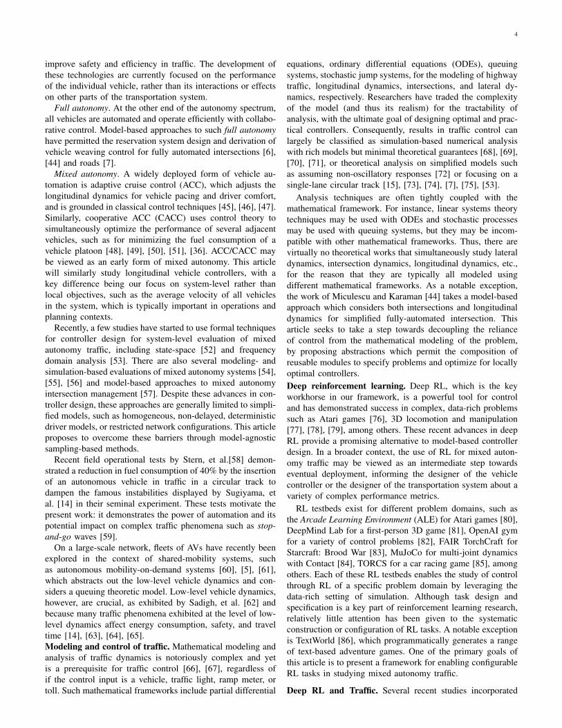
Fig. 1: Example network modules supported by the Flow framework. Top left: Single-lane circular track. Top middle: Multi-lane circular track. Top right:Figure-eight road network. Bottom left: Intersection network. Bottom middle: Closed loop merge network. Bottom right: Imported San Francisco network.In Flow, scenarios can be generated using OpenStreetMap (OSM) data and vehicle dynamics models from SUMO.

open-sourced the modular learning framework as Flow1, whichexposes design primitives for composing traffic control tasks.Our contributions aim to enable the community to studynot only mixed autonomy scenarios which are compositesof analytically tractable mathematical frameworks, but alsoarbitrary networks, or even full-blown traffic microsimulators,designed to simulate hundreds of thousands of agents incomplex environments (see examples in Figure 1).

The contributions of Flow to the research community aremulti-faceted. For the robotics community, Flow seeks toenable rich characterizations and empirical study of complex,large-scale, and realistic multi-robot control tasks. For themachine learning community, Flow seeks to expose to mod-ern reinforcement learning algorithms a class of challengingcontrol tasks derived from an important real-world domain.For the control community, Flow seeks to provide intuition,through successful learned control laws, for new provablecontrol techniques for traffic-related control tasks. Finally,for the transportation community, Flow seeks to provide anew pathway, through reusable traffic modules and modernreinforcement learning methods, to addressing new challenges

1Our modular learning framework called Flow is open-source and availableat https://github.com/flow-project/flow.

concerning AVs and long-standing challenges concerning traf-fic control.

The rest of the article is organized as follows: Section II in-troduces the problem of mixed autonomy. Section III presentsrelated work to place this article in the broader contextof automated vehicles, traffic flow modeling, and deep RL.Section IV summarizes requisite concepts from RL and traffic.Section V describes the modular learning framework for thescalable design and experimentation of traffic control tasks.This is followed by two experimental sections: Section VI,in which we validate the modular learning framework on acanonical traffic control task, and Section VII which presentsmore sophisticated applications of the framework to morecomplex traffic control tasks.

II. MIXED AUTONOMY

To make headway towards understanding the complex inte-gration of AVs into existing transportation and urban systems,this article introduces the problem of mixed autonomy to framethe study of partial adoption of autonomy into an existing sys-tem. Although mixed autonomy technically subsumes isolatedand full autonomy, both are still important and active areasof research and will often lead to more efficient algorithms

3

for specialized settings. However, we observe that there areimportant robotics problems that are not addressed by eitherbody of approaches, and thus formulate the problem of mixedautonomy traffic and propose a suitable methodology.

For a particular type of autonomy (e.g. AVs, traffic lights,roadway pricing), we define mixed autonomy as the in-termediate regime between a system with no adoption ofautonomy and a system where the autonomy is employedfully. For example, in the context of AVs, full autonomycorresponds to 100% vehicles being autonomously driven,so mixed autonomy corresponds to any fraction of vehiclesbeing autonomously driven. In the context of traffic lights, fullautonomy corresponds to all traffic lights having automatedsignal control, so mixed autonomy corresponds to any fractionof traffic lights being automated; the other lights could followsome different pre-programmed rules or could not be utilizedat all. As the examples allude, mixed autonomy must bedefined alongside its boundary conditions of no autonomy andfull autonomy as well as its system context. For example, thefull system context could be a segment of roadway, a fullroad, or a entire urban region. Mixed autonomy differs fromthe previously studied cases in two important ways.

First, the evaluation criteria for mixed autonomy settingswill typically be less clear than in studies of isolated autonomy.Studies in isolated autonomy are often evaluated with respectto known human or expert performance for a similar task.For example, the performance of a self-driving vehicle in theisolated autonomy context is typically measured against that ofa human driver [9], [10]. Similarly, expert demonstrations areoften considered the objective in robot learning for a variety oftasks, including locomotion, grasping, and manipulation [11],[12], [13]. In these cases, we may assume knowledge of agood control law and that it is feasible to attain, e.g. froma human or expert demonstrator. However, evaluating withrespect to human performance makes implicit assumptionsabout the capabilities of the autonomous system and theoptimality of human performance, both of which may beincorrect. For example, in the context of a mixed autonomytraffic system, evaluating with respect to the known humanperformance is restrictive; it is well known that human drivingbehavior induces (suboptimal) stop-and-go traffic in a wideregime of traffic scenarios [14], [15]. In mixed autonomysettings, we are instead interested evaluating autonomy withrespect to a different, possibly system-level objective, in orderto understand its potential effects on the system.

Second, the strict coupling between the mathematical mod-eling and the control law evaluation is a critical restriction forstudying mixed autonomy. Differently from isolated autonomy,full autonomy is indeed often evaluated with respect to asystem-level objective. However, its system dynamics are oftenmuch simpler than that of mixed autonomy. In full autonomysettings, all autonomous components are known and neednot be modeled, and uncertainty from human behavior islargely eliminated. Even so, full autonomy is far from solved;however, numerous full autonomy settings can be analyzedusing techniques from control theory, in particular when thesystem dynamics may be modeled within a number of pow-erful mathematical frameworks, including partial differential

equations [16], [17], [18], [19], ordinary differential equations[20], [21], [22], [23], queuing systems [24], [25], [26], etc.In a number of cases, control theoretic performance boundscan be analytically derived or an optimal controller may evenbe found directly. In contrast, mixed autonomy suffers fromadditional challenges including interactions with humans ofunknown or complex dynamics, partial observability fromsensing limitations, and partial controllability due to the lackof full autonomy. However, these control theoretic perfor-mance bounds be employed as reference points when evalu-ating mixed autonomy systems. For mixed autonomy settings,these aspects are often prohibitively complex to characterizewithin a single mathematical framework.

In this work, we propose and validate a new methodol-ogy for addressing mixed autonomy traffic. We posit thatsampling-based optimization allows us to de-couple mathe-matical modeling of the system dynamics and control lawdesign for arbitrary evaluation objectives, thereby overcomingthe limitations of studies in both isolated and full autonomy.In particular, we propose that model-free deep reinforcementlearning (RL) is a compelling and suitable framework forthe study of mixed autonomy. The decoupling allows thedesigner to specify arbitrary control objectives and systemdynamics to explore the effects of autonomy on complexsystems. For the system dynamics, the designer may model asystem of interest in whichever mathematical or computationalframework she wishes, and we require only that the modelis consistent with a (Partially Observed) Markov DecisionProcess, (PO)MDP, interface. For control law design, deepneural network architectures may be used for representinglarge and expressive control law (or policy) classes. Finally, theresulting framework employs model-free deep RL to enablethe designer to explore the effects of autonomy on a complexsystem, up to local optimality with respect to the control lawparameterization.

III. RELATED WORK

Control of automated vehicles. Automated and autonomousvehicles have been studied in a myriad of contexts, which weframe in the context of isolated, full, and mixed autonomy.

Isolated autonomy. Spurred by the US DARPA challengesin autonomous driving in 2005 and 2007 [27], [4], countlessefforts have demonstrated the increasing ability of vehiclesto operate autonomously on real roads and traffic condi-tions, without custom traffic infrastructure. These vehiclesinstead rely largely on sensors (LIDAR, radar, camera, GPS),computer vision, motion planning, mapping, and behaviorprediction, and are designed to obey traffic rules. Roboticshas continued to demonstrate tremendous potential in im-proving transportation systems through AVs research; highlyrelated problems include localization [28], [29], [30], pathplanning [31], [32], collision avoidance [33], and perception[34]. Considerable progress has also been made in recentdecades in vehicle automation, including anti-lock brakingsystems (ABS), adaptive cruise control (ACC), lane keeping,lane changing, parking, overtaking, etc. [35], [36], [37], [38],[39], [40], [41], [42], [43], which also have great potential to

4

improve safety and efficiency in traffic. The development ofthese technologies are currently focused on the performanceof the individual vehicle, rather than its interactions or effectson other parts of the transportation system.

Full autonomy. At the other end of the autonomy spectrum,all vehicles are automated and operate efficiently with collabo-rative control. Model-based approaches to such full autonomyhave permitted the reservation system design and derivation ofvehicle weaving control for fully automated intersections [6],[44] and roads [7].

Mixed autonomy. A widely deployed form of vehicle au-tomation is adaptive cruise control (ACC), which adjusts thelongitudinal dynamics for vehicle pacing and driver comfort,and is grounded in classical control techniques [45], [46], [47].Similarly, cooperative ACC (CACC) uses control theory tosimultaneously optimize the performance of several adjacentvehicles, such as for minimizing the fuel consumption of avehicle platoon [48], [49], [50], [51], [36]. ACC/CACC maybe viewed as an early form of mixed autonomy. This articlewill similarly study longitudinal vehicle controllers, with akey difference being our focus on system-level rather thanlocal objectives, such as the average velocity of all vehiclesin the system, which is typically important in operations andplanning contexts.

Recently, a few studies have started to use formal techniquesfor controller design for system-level evaluation of mixedautonomy traffic, including state-space [52] and frequencydomain analysis [53]. There are also several modeling- andsimulation-based evaluations of mixed autonomy systems [54],[55], [56] and model-based approaches to mixed autonomyintersection management [57]. Despite these advances in con-troller design, these approaches are generally limited to simpli-fied models, such as homogeneous, non-delayed, deterministicdriver models, or restricted network configurations. This articleproposes to overcome these barriers through model-agnosticsampling-based methods.

Recent field operational tests by Stern, et al.[58] demon-strated a reduction in fuel consumption of 40% by the insertionof an autonomous vehicle in traffic in a circular track todampen the famous instabilities displayed by Sugiyama, etal. [14] in their seminal experiment. These tests motivate thepresent work: it demonstrates the power of automation and itspotential impact on complex traffic phenomena such as stop-and-go waves [59].

On a large-scale network, fleets of AVs have recently beenexplored in the context of shared-mobility systems, suchas autonomous mobility-on-demand systems [60], [5], [61],which abstracts out the low-level vehicle dynamics and con-siders a queuing theoretic model. Low-level vehicle dynamics,however, are crucial, as exhibited by Sadigh, et al. [62] andbecause many traffic phenomena exhibited at the level of low-level dynamics affect energy consumption, safety, and traveltime [14], [63], [64], [65].Modeling and control of traffic. Mathematical modeling andanalysis of traffic dynamics is notoriously complex and yetis a prerequisite for traffic control [66], [67], regardless ofif the control input is a vehicle, traffic light, ramp meter, ortoll. Such mathematical frameworks include partial differential

equations, ordinary differential equations (ODEs), queuingsystems, stochastic jump systems, for the modeling of highwaytraffic, longitudinal dynamics, intersections, and lateral dy-namics, respectively. Researchers have traded the complexityof the model (and thus its realism) for the tractability ofanalysis, with the ultimate goal of designing optimal and prac-tical controllers. Consequently, results in traffic control canlargely be classified as simulation-based numerical analysiswith rich models but minimal theoretical guarantees [68], [69],[70], [71], or theoretical analysis on simplified models suchas assuming non-oscillatory responses [72] or focusing on asingle-lane circular track [15], [73], [74], [7], [75], [53].

Analysis techniques are often tightly coupled with themathematical framework. For instance, linear systems theorytechniques may be used with ODEs and stochastic processesmay be used with queuing systems, but they may be incom-patible with other mathematical frameworks. Thus, there arevirtually no theoretical works that simultaneously study lateraldynamics, intersection dynamics, longitudinal dynamics, etc.,for the reason that they are typically all modeled usingdifferent mathematical frameworks. As a notable exception,the work of Miculescu and Karaman [44] takes a model-basedapproach which considers both intersections and longitudinaldynamics for simplified fully-automated intersection. Thisarticle seeks to take a step towards decoupling the relianceof control from the mathematical modeling of the problem,by proposing abstractions which permit the composition ofreusable modules to specify problems and optimize for locallyoptimal controllers.Deep reinforcement learning. Deep RL, which is the keyworkhorse in our framework, is a powerful tool for controland has demonstrated success in complex, data-rich problemssuch as Atari games [76], 3D locomotion and manipulation[77], [78], [79], among others. These recent advances in deepRL provide a promising alternative to model-based controllerdesign. In a broader context, the use of RL for mixed auton-omy traffic may be viewed as an intermediate step towardseventual deployment, informing the designer of the vehiclecontroller or the designer of the transportation system about avariety of complex performance metrics.

RL testbeds exist for different problem domains, such asthe Arcade Learning Environment (ALE) for Atari games [80],DeepMind Lab for a first-person 3D game [81], OpenAI gymfor a variety of control problems [82], FAIR TorchCraft forStarcraft: Brood War [83], MuJoCo for multi-joint dynamicswith Contact [84], TORCS for a car racing game [85], amongothers. Each of these RL testbeds enables the study of controlthrough RL of a specific problem domain by leveraging thedata-rich setting of simulation. Although task design andspecification is a key part of reinforcement learning research,relatively little attention has been given to the systematicconstruction or configuration of RL tasks. A notable exceptionis TextWorld [86], which programmatically generates a rangeof text-based adventure games. One of the primary goals ofthis article is to present a framework for enabling configurableRL tasks in studying mixed autonomy traffic.

Deep RL and Traffic. Several recent studies incorporated

5

ideas from deep learning in traffic optimization. Deep RL hasbeen used for traffic prediction [87], [88] and control [89],[90], [91]. A deep RL architecture was used by Polson, etal. [87] to predict traffic flows, demonstrating success evenduring special events with nonlinear features; to learn featuresto represent states involving both space and time, Lv, et al.[88] additionally used hierarchical autoencoding for trafficflow prediction. Deep Q Networks (DQN) was employed forlearning traffic signal timings in Li, et al. [89]. A multi-agentdeep RL algorithm was introduced in Belletti, et al. [90] tolearn a control law for ramp metering. Wei, et al. [92], [91]employs reinforcement learning and graph attention networksfor control of traffic signals. For additional uses of deeplearning in traffic, we refer the reader to Karlaftis, et al. [93],which presents an overview comparing non-neural statisticalmethods and neural networks in transportation research. Theserecent results demonstrate that deep learning and deep RLare promising approaches to traffic problems. This article isthe first to employ deep RL to design controllers for AVsand assess their impacts in traffic. An early prototype ofthe implementation of Flow is published [94] and an earlierversion of this manuscript is available [95] (unpublished). Incomparison, this article provides substantive presentation ofthe learning framework, use cases, and experimental findingswhich contribute to the understanding of traffic dynamics andcontrol.

IV. PRELIMINARIES

In this section, we define the notation and key concepts usedin subsequent sections.

A. Markov Decision ProcessesThe system described in this article solves tasks which

conform to the standard interface of a finite-horizon discountedMarkov decision process (MDP) [96], [97], defined by thetuple (SS,A, P, r, ρ0, γ, T ), where SS is a (possibly infinite)set of states, A is a set of actions, P : SS ×A× SS → R≥0

is the transition probability distribution, r : SS × A → Ris the reward function, ρ0 : SS → R≥0 is the initial statedistribution, γ ∈ (0, 1] is the discount factor, and T is the timehorizon. For partially observable tasks, which conform to theinterface of a partially observable Markov decision process(POMDP), two more components are required, namely Ω, aset of observations, and O : SS × Ω→ R≥0, the observationprobability distribution.

Although traffic may be most naturally formulated as aninfinite horizon problem, traffic phenomena such as trafficjams are ephemeral or even periodic. Thus, we formulate finitehorizon MDPs. More generally, traffic has periodic patterns ona daily or weekly basis. Thus, the finite horizon problem canbe a suitable approximation of the infinite horizon problem,so long as the horizon sufficiently long to capture the transientor periodic behavior. For example, in the single-lane trackscenario (Section VI), the periods are around 40 sec. To enablethe formation of the periodic behavior, we select a fairly longhorizon length of 300 seconds (or 3000 simulation steps).Furthermore, we will select a fairly high discount factor (closeto 1) to approximate a non-discounted problem.

B. Reinforcement learning

RL studies the problem of how agents can learn to takeactions in its environment to maximize its cumulative reward.The article uses policy gradient methods [98], a class ofreinforcement learning algorithms which optimize a stochasticpolicy πθ : SS × A → R≥0, e.g. deep neural networks.Although commonly called a policy, we will generally referto π as a controller or control law in this article, to beconsistent with traffic control terminology. In a stochasticpolicy, both the mean and standard deviation are predicted bythe controller. Actions are then sampled from a correspondingGaussian distribution. During test time, the mean action istaken, corresponding to the maximum likelihood determin-istic controller. Policy gradient methods iteratively updatethe parameters of the control law by estimating a gradientfor the expected cumulative reward, using data samples (e.g.from a traffic simulator or model). Three control laws usedin this article are the Linear network, Multilayer Perceptron(MLP), and Gated Recurrent Unit (GRU). The Linear networkis a parameterized linear function. The MLP is a classicalartificial neural network with one or more hidden layers [99],consisting of linear weights and nonlinear activation functions(e.g. sigmoid, ReLU). The GRU is a recurrent neural networkcapable of storing memory on the previous states of the system[100]. GRUs make use of parameterized update and resetgates, which enable decision making based on both currentand past inputs. In all cases, the networks are trained usingbackpropagation to optimize its parameters.

C. Vehicle dynamics models

The environments studied in this article are traffic systems.Basic traffic dynamics on single-lane roads can be representedby ordinary differential equation (ODE) models known ascar following models (CFMs). These models describe thelongitudinal dynamics of human-driven vehicles, given onlyobservations about itself and the vehicle preceding it. CFMsvary in terms of model complexity, interpretability, and theirability to reproduce prevalent traffic phenomena, includingstop-and-go traffic waves. For modeling of more complextraffic dynamics, including lane changing, merging, drivingnear traffic lights, and city driving, we refer the reader to thetext of Treiber and Kesting [66] dedicated to this topic.

Standard CFMs are of the form:

ai = vi = f(hi, hi, vi), (1)

where the acceleration ai of car i is some typically nonlinearfunction of hi, hi, vi, which are the headway, relative velocity,and velocity for vehicle i, respectively. Though a generalmodel may include time delays from the input signals hi, hi, vito the resulting output acceleration ai, we will consider a non-delayed system, where all signals are measured at the sametime instant t. Example CFMs include the Intelligent DriverModel (IDM) [21] and the Optimal Velocity Model (OVM)[22], [23].

6

D. Intelligent Driver Model

The Intelligent Driver Model (IDM) is a car followingmodel capable of accurately representing realistic driver be-havior [21] and reproducing traffic waves, and is commonlyused in the transportation research community. We will employIDM in the numerical experiments of this article, and thereforeanalyze this specific model to compute the theoretical perfor-mance bounds of the overall traffic system. The accelerationfor a vehicle modeled by IDM is defined by its bumper-to-bumper headway h (distance to preceding vehicle), velocityv, and relative velocity h, via the following equation:

aIDM =dv

dt= a

[1−

(v

v0

)δ−(H(v, h)

h

)2](2)

where H(·) is the desired headway of the vehicle, denoted by:

H(v,∆v) = s0 + max

(0, vT +

vh

2√ab

)(3)

where h0, v0, T, δ, a, b are given parameters. Table I describesthe parameters of the model and provides typically used values[66].

Intelligent Driver Model (IDM)Parameter v0 T a b δ h0 noiseValue 30 m/s 1 s 1 m/s2 1.5 m/s2 4 2 m N (0, 2)

TABLE I: Parameters for car-following control law

E. Traffic, equilibria, and performance bounds

The overall traffic system is comprised of interconnecteddynamical models, including CFMs, representing the manyinteracting vehicles in the traffic system. An example of atraffic system which can be represented by only longitudinalvehicle dynamics is a circle of n vehicles, all driving clock-wise, and each of which is following the vehicle preceding it.The result is a dynamical system which consists of a cascade ofn potentially nonlinear and delayed vehicle dynamics models.This example will serve as our first numerical experiment(Section VI), as it is able to reproduce important trafficphenomena (traffic waves and traffic jams), and, despite itssimplicity, its optimal control problem in the mixed autonomysetting has remained an open research question.

Although the primary methodology explored in this articleis model-agnostic, we employ control theoretic model-basedanalysis to compute the performance bounds of the trafficsystem, so that we can adequately assess the performance ofthe learned control laws. In a homogeneous setting, whereall vehicles follow the same dynamics model, uniform flowdescribes the situations where all vehicles moves at some con-stant velocity v∗ and constant headway h∗, and corresponds toone of the equilibria of the traffic system. It can be representedin terms of the vehicle dynamics model by:

ai = 0 = f(h∗, 0, v∗). (4)

This equation defines the relationship between the two equi-librium quantities h∗, v∗ for a general car following model,and the specific relationship for IDM is displayed in Figure 3

(green curve). Uniform flow equilibria correspond to highvelocities, and are thus desirable, but these equilibria are alsounstable due to properties of human driving behavior [101].

It is intuitive to think of the equilibrium density (which isinversely related to the equilibrium headway h∗) as a trafficcondition. We will seek to evaluate our learned control lawsagainst a range of traffic conditions. Each traffic condition(density) has associated with it an optimal equilibrium velocityv∗. In practice, the equilibrium density can be approximatedby the local traffic density. In settings with heterogeneousvehicle types, the equilibrium can be numerically solved byconstraining the total headways to be the total road lengthand the velocities to be uniform. It is important to note thedifference between the equilibrium velocity v∗ and the targetvelocity v0 (free flow speed) of the vehicle models; v0 can bethought of as a speed limit for highway traffic [21]. On theother hand, v∗ is a control theoretic quantity jointly determinedby the traffic condition h∗, the target velocity v0, the systemdynamics, and various other parameters.

Another set of equilibria exhibited by the example trafficsystem corresponds to traffic waves (also called stop-and-gowaves). These traffic waves are stable limit cycles, that is,closed curves that trajectories tend towards (rather than away)[15]. In other words, the typical traffic system tends towardsexhibiting traffic waves. We view this as a performance lowerbound for the mixed autonomy setting because any control lawwhich yields worse performance could be replaced by a humandriver to yield a better outcome. Using IDM, the relationshipbetween density and the average velocity with traffic waves isdisplayed in Figure 3 (red curve).

Finally, we are concerned with steady-state performance ofthe traffic system, rather than any instantaneous performance.We thus take the uniform flow and traffic waves equilibria todescribe the upper and lower bounds, respectively, for steady-state performance of the overall traffic system. We note that,because we are analyzing the no autonomy setting, but evaluat-ing against a mixed autonomy setting, the performance boundspresented here should be viewed as close approximations tothe true performance bounds. For more detailed performancebounds, we refer the reader to related work [15], [102], [103].

V. FLOW: A MODULAR LEARNING FRAMEWORK

While the research community in deep RL focuses onsolving pre-defined tasks, relatively little emphasis is placedon flexible scenario creation (see Section III). In multi-agentsystems such as traffic, the flexibility to study a wide range ofscenarios is important due to their highly varied and complexnature, including different numbers and types of vehicles,heterogeneity of agents, network configurations, regional be-haviors and regulations, etc. To this end, this article contributesan approach that decomposes a scenario into modules whichcan be configured and composed to create new scenarios ofinterest. Flow is the resulting modular learning framework forenabling the creation, study, and control of complex trafficscenarios.

A note on terminology: We use the term scenario todescribe the full traffic setting, including all learning and non-learning components, and it conforms to a (PO)MDP interface

7

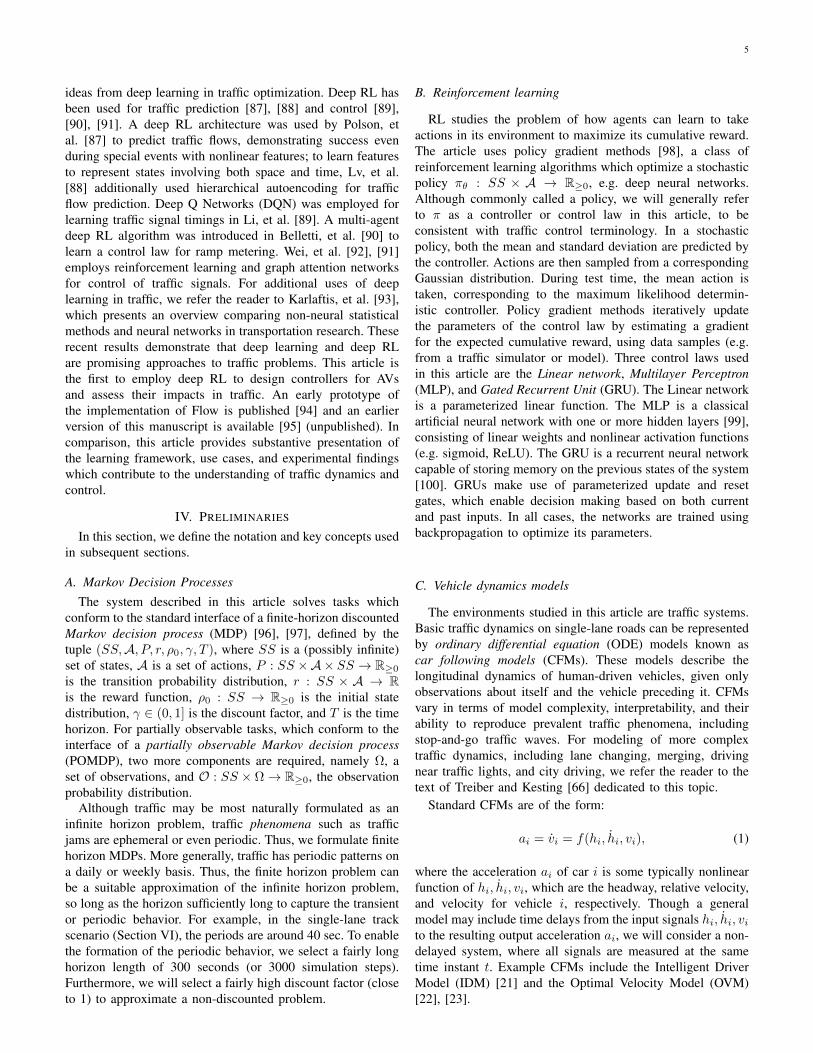
Fig. 2: Flow overview. Flow is a modular learning framework, which enables the study of diverse mixed autonomy traffic scenarios with deep reinforcementlearning (RL) methods. Scenarios are defined within the Markov Decision Process (MDP) framework. The workhorse of Flow is modules (rectangles) whichcan be composed to comprise scenarios, including networks, actors, observers, control laws, metrics, initializations, and additional dynamics. Actors mayrefer to vehicles or infrastructure, and may be learned or pre-specified. Additional dynamics may include vehicle fail-safes, right-of-way rules, and physicallimitations. Additional parameters (hexagons) may also be configured. Flow facilitates the composition of these modules to create new traffic scenarios ofinterest, which may then be studied as traffic control problems using deep RL methods. Flow invokes external libraries for training and simulation.

(see Section IV). In robotics, the term “task” is commonlyused; we prefer the word “scenario” to also capture settingswith no learning components or no goal to achieve (e.g.,situations with only human driver models).

A. Scenario modules

Flow is comprised of the following modules, which can beassembled to form scenarios of interest (see Figure 2).

Network: The network specifies the physical road layout, interms of roads, lanes, length, shape, roadway connections, andadditional attributes. Example include a two-lane circular trackwith circumference 200m, or the structure described by im-porting a map from OpenStreetMap (see Figure 1 for examplesof supported networks). Several of these examples will be usedin demonstrative experiments in Sections VI and VII. Moredetails about the specific networks are in Appendix A.

Actors: The actors describe the physical entities in the en-vironment which issue control signals to the environment.In contrast to isolated autonomy settings, in a traffic setting,there are typically many interacting physical entities. Due tothe focus on mixed autonomy, this article specifically studiesvehicles as its physical entities. Other possible actors mayinclude pedestrians, bicyclists, traffic lights, roadway signs,toll booths, as well as other transit modes and infrastructure.

Observer: The observer describes the mapping S → O andyields the function of the state that is observed by the actor(s).The output of the observer is taken as input to the control law,described below. For example, while the state may include theposition, lane, velocity, and accelerations of all vehicles in thesystem, the observer may restrict access to only informationabout local vehicles and aggregate statistics, such as averagespeed or length of queue at an intersection.

Control laws: Control laws dictate the behaviors of the actorsand are functions mapping observations to control inputsO → A. All actors require a control law, which may be pre-specified or learned. For instance, a control law may represent

a human driver, an autonomous vehicle, or even a set ofvehicles. That is, a single control law may be used to controlmultiple vehicles in a centralized control setting. Alternatively,a single control law may be used by multiple actors in a sharedparameter control setting.

Dynamics: The dynamics module consists of additional sub-modules which describe different aspects of the system evo-lution, including vehicle routes, demands, stochasticity, trafficrules (e.g., right-of-way), and safety constraints.

Metrics: The metrics describe pertinent aggregated statisticsof the environment. The reward signal for the learning agentis a function of these metrics. Examples include the overall(average) velocity of all vehicles and the number of (hard)braking events.

Initialization: The initialization describes the initial configu-ration of the environment at the start of an episode. Examplesinclude setting the position and velocity of vehicles accordingto different probability distributions.

Sections VI and VII demonstrate the potential of the frame-work. Whereas in a model-based framing, many modules aresimply not re-configurable due to differences in the mathe-matical descriptions (e.g. discrete versus continuous controlinputs, such as in the case of longitudinal and lateral control),in this model-agnostic framework, disparate dynamics maybe captured in the same scenario and effectively studiedusing sampling-based optimization techniques such as deepreinforcement learning.

B. Architecture and implementation

The implementation of Flow is open source and builds uponopen source software to promote access and extension. Theopen source approach further aims to support the further devel-opment of custom modules, to permit the study of richer andmore complex environments, agents, metrics, and algorithms.The implementation builds upon SUMO (Simulation of UrbanMObility) [104] for vehicle and traffic modeling, Ray RLlib

8

[105], [106] for reinforcement learning, and OpenAI gym [82]for the MDP.

SUMO is a microscopic traffic simulator, which explic-itly models vehicles, pedestrians, traffic lights, and publictransportation. It is capable of simulating urban-scale roadnetworks. SUMO has a rich Python API called TraCI (TrafficControl Interface). Ray RLlib are frameworks that enabletraining and evaluating of RL algorithms on a variety ofscenarios, from classic tasks such as cartpole balancing tomore complicated tasks such as 3D humanoid locomotion.OpenAI gym is an MDP interface for reinforcement learningtasks.

Flow is implemented as a lightweight architecture to con-nect and permit experimentation with the modules describedin the previous section. As typical in reinforcement learningstudies, an environment encodes the MDP. The environmentfacilitates the composition of dynamics and other modules,stepping through the simulation, retrieving the observations,sampling and applying actions, computing the metrics andreward, and resetting the simulation at the end of an episode.A generator produces network configuration files compati-ble with SUMO according to the network description. Thegenerator is invoked by the experiment upon initializationand, optionally, upon reset of the environment, allowing fora variety of initialization conditions, such as sampling froma distribution of vehicle densities. Flow then assigns controlinputs from the different control laws to the correspondingactors, according to an action assigner, and uses the TraCIlibrary to apply actions for each actor. Actions specified asaccelerations are converted into velocities, using numericalintegration and based on the timestep and current state of theexperiment.

Finally, Flow is designed to be inter-operable with classicalmodel-based control methods for evaluation purposes. That is,the learning component of Flow is optional, and this permitsthe fair comparison of diverse methods for traffic control.

VI. CONFIGURABLE MODULES FOR MIXED AUTONOMY

This section demonstrates that Flow can achieve high perfor-mance in a challenging and classic traffic congestion scenario.Specifically, this section studies the canonical traffic setupof Sugiyama, et al. [14], which consists of 22 human-drivenvehicles on a 230 m circular track. This seminal experimentshows that human drivers cause backward propagating trafficwaves, resulting in some vehicles to come to a complete stop(see left side of Figures 4 and 5). This is the case even inthe absence of typical sources of traffic perturbations, suchas lane changes, merges or stop lights. We adapt the setup tomixed autonomy traffic using the methodology presented inSection V-A.

A. Background

Although single-lane traffic has been studied over severaldecades, previous work has focused on modeling and optimiz-ing for local performance (e.g. comfort), rather than system-level performance (e.g. traffic congestion). Various modelingapproaches include closed networks [14], [15], [52], [103],

Experiment parameters Valuesimulation step 0.1 s/stepcircular track range (train) [220, 270] mcircular track range (test) [210, 290] mwarmup time 75 stime horizon 300 stotal number of vehicles 22number of AVs 1

TABLE II: Network and simulation parameters for mixed autonomy circulartrack (single-lane).

open networks [46], [68], [53], different human driving models[66], and different objectives [54], To the best of the authorsknowledge, no prior work has achieved an optimal controllerin the mixed autonomy setting for single-lane traffic conges-tion. While studies in eco-driving practices provide heuristicguidance to drivers to ease traffic congestion [107], [108], thecharacterization of optimality of these practices has receivedlimited attention.

The most closely related work includes Horn, et al. [7],Stern, et al. [58], and Wu, et al [102]. Horn, et al. [7] presentsa near-optimal controller but studies the setting where allvehicles are automated. The field experiment of Stern, etal. [58] presents two control laws for the mixed autonomysetting. These control laws are included in our experiments asbaseline methods and are detailed in Appendix B. Importantly,both works hand-designed a control law based on knowledgeof the environment, and thus we refer to them as model-based control laws. In contrast, the approach proposed by thiswork requires a significantly less “design supervision,” in theform of a reward function, which largely avoids explicitlyemploying domain knowledge or mathematical analysis. Inpreliminary work [102], we employed RL to learn a controllerin the single-lane mixed autonomy setting; however, our focuswas on characterizing the emergence of behaviors in mixedautonomy traffic, rather than on learning an optimal controller.

B. Experiment Modules

We design the following experiment composed of the mod-ules proposed in Section V-A. The network and simulation-specific parameters of our numerical experiments are summa-rized in Table II.Network: The training domain consists of single-lane cir-cular track networks, with uniformly sampled track lengthsL ∼ Unif([Lmin, Lmax]), as displayed in Figure 1 (top left),to represent a continuous and wide range of traffic densities.We take Lmin = 230 m and Lmax = 270 m. An alternativeapproach (not considered here) to represent a range of densitiesis to fix the track length and instead vary the number ofvehicles.Actors: There are n = 22 vehicles, each 5 m long.Observer: The state consists of the velocity and position of allvehicles, that is s = (x1, v1, x2, v2, . . . , xn, vn). It is practicalto consider an observer which restricts the observation to theinformation that can be directly sensed by the single learningagent, given as o = ( viv0 ,

hi

v0, hi

Lmax), where i is the index of the

learning agent, v0 is the speed limit, Lmax is the maximumlength of the track, headway hi = xi−1 − xi, and headway

9

differential hi = vi−1− vi. The observation can be viewed asnormalized inputs to a car following model.

Control laws: Of the 22 actors, 21 are modeled as humandrivers according to the Intelligent Driver Model (IDM) [66](see Section IV and Table I). For the single autonomousvehicle actor, we compare the following control laws. Recallthat actors partially observe the environment.

• Learned control laws. We consider control laws with andwithout memory.

– GRU control law (with memory): hidden layers (5,)and tanh non-linearity.

– MLP control law (no memory): diagonal GaussianMLP, two-layer network with hidden layer of shape(3,3) and tanh non-linearity.

– Linear control law (no memory).

• Model-based control laws

– Proportional Integral (PI) control law with satura-tion, given in Stern, et al. [58] and is included inSection B-2 for completeness.

– FollowerStopper control law, with desired velocityfixed at 4.15 m/s. The FollowerStopper control lawis introduced in Stern, et al. [58] and is also detailedin Section B-1. FollowerStopper requires an externaldesired velocity, so we selected the largest fixedvelocity which successfully mitigates stop-and-gowaves at a track length of 260 m; this is furtherdiscussed in the results.

– IDM: For a no autonomy baseline, we take IDM asthe control law. This results in a stop-and-go stablelimit cycle. Although not strictly a lower bound,we take this to be a practical lower bound, sinceany worse controller could default to human drivingbehavior.

Dynamics: The overall system dynamics consists of a cascadeof nonlinear dynamics models from n− 1 (homogeneous) ac-tors and 1 autonomous vehicle actor (learning agent). The n−1IDM dynamics models are additionally perturbed by Gaussianacceleration noise of N (0, 0.2), calibrated to match measuresof stochasticity to the IDM model presented by Treiber, etal. [109]. The traffic simulator enforces safety through built-in failsafe mechanisms. For the first 75 seconds of the 300second episode, the acceleration of the autonomous vehicle isoverridden by the IDM model to allow for randomization ofthe initial state and for the formation of stop-and-go waves.

Metrics: We consider two natural metrics: the average velocityof all vehicles in the network and a control cost, whichpenalizes acceleration. The reward function supplied to thelearning agent is a weighted combination of the two metrics.

r(s, a) =1

n

∑i

vi − α|a| (5)

where α = 0.1.

Initialization: The vehicles are evenly spaced around thecircular track, with an initial velocity of 0 m/s.

C. Learning setup

The AVs in our system execute controllers which are param-eterized control laws, trained using policy gradient methods.For all experiments in this article, we use the Trust Region Pol-icy Optimization (TRPO) [78] method for learning the controllaw, linear feature baselines as described in Duan, et al. [105],discount factor γ = 0.999, and step size 0.01. Each of theresults presented in this article was collected from numericalexperiments conducted on three Intel(R) Core(TM) i7-6600UCPU @ 2.60GHz processors for six hours. A total of 6,000,000samples were collected during the training procedure2.

D. Results

By studying mixed autonomy track, we demonstrate 1) thatFlow enables composing modules to study an open problem intraffic control and 2) that reliable controllers for complex prob-lems can be efficiently learned, which surpass the performanceof all known model-based controllers. This section details ourfindings, and videos and additional results are available athttps://sites.google.com/view/ieee-tro-flow.

1) Performance: Figure 3 shows several key findings. Thistraffic density versus velocity plot shows the performance ofthe different learned and model-based controllers. First, weobserve that GRU and MLP control laws match the optimalvelocity closely for traffic densities (train and test), therebypractically eliminating congestion. The PI with Saturation andFollowerStopper control, on the other hand, only dissipatestop-and-go traffic at densities less than or equal to their cal-ibration density (less congested settings). The Linear controllaw performs well but not as well as the MLP/GRU. Thisindicates that a linear function may be unable to expressthe equilibrium flow velocity, whereas a two-layer neuralnetwork can. Our learned controllers outperform all the model-based controllers, with the exception of the PI with saturationcontroller outperforming the Linear controller in low densitytraffic.

Figure 4 shows the velocity profiles for the different learnedand model-based control laws on the 260 m track. Althoughboth types of controllers eventually stabilize the system,the GRU control law reaches the uniform flow equilibriumvelocity fastest. The GRU and MLP control laws stabilize thesystem with less oscillatory behavior than the FollowerStopperand PI with Saturation control laws, as observed in the velocityprofiles. In addition, the FollowerStopper control law is theleast performant; the control law stabilizes a 260 m track toa speed of 4.15 m/s, well below the 4.82 m/s uniform flowvelocity.

Finally, Figure 5 shows the space-time curves for all vehi-cles in the system, using a variety of control laws. We observethat the PI with Saturation and FollowerStopper control lawleave much smaller openings in the network (smaller head-ways) than the MLP and GRU control laws. The MLP controllaw exhibits the largest openings, as can be seen by the largewhite portion of the MLP plot within Figure 5. If this wereinstead applied in a multi-lane circular track, then the smaller

2Further implementation details can be found at: https://github.com/flow-project/flow-lab/tree/master/flow-framework.

10

80 85 90 95 100

2

4

6

Vehicle density (veh/km)

Ave

rage

velo

city

(m/s

)Uniform flow unstable equilibrium (optimal)

GRU control law (ours)MLP control law (ours)

Linear control law (ours)PI with saturation control lawFollowerStopper control law

Calibration density for PI control lawStop-and-go stable limit cycle

Fig. 3: Comparison of control laws for single-lane mixed autonomy track.The performance of learned (GRU, MLP, and Linear) and model-based(FollowerStopper and PI Saturation) control laws are averaged over ten runsat each evaluated density. Also displayed are the performance upper and lowerbounds, derived from the unstable and stable system equilibria, respectively.The GRU and MLP control laws closely match the velocity upper boundclosely for all densities (train and test). The Linear control law performs wellbut not as well as the MLP/GRU. The PI with Saturation and FollowerStopperbaselines perform relatively well at their calibration density, but not as well asthe learned controllers. The PI with saturation controller generalizes well tolower density traffic. Remarkably, the GRU and MLP control laws are able togeneralize (to the gray region) and bring the system to near optimal velocitieseven at densities outside the training range (white region). Additionally, thelearned MLP control law demonstrates that memory is not necessary toachieve near optimal average velocity.

openings would have the benefit of preventing opportunisticlane changes, so this observation can lead to better rewarddesign for more complex mixed autonomy traffic studies.

2) Robustness: A strength of learned control laws is thatthey do not rely on external calibration of parameters thatare specific to a traffic setting, such as traffic density. Model-based controller baselines, on the other hand, often exhibitconsiderable sensitivity to the traffic setting. We found theperformance of the PI with Saturation control law to besensitive to parameters, even though in principle it can ad-just to different densities with its moving average filter (seeFigures 3-5). Using parameters calibrated for the 260 m track(as described in Stern, et al. [58]), the PI with Saturationcontrol law performs decently at 260 m; however, this controllaw’s performance quickly degrades at higher densities (morecongested settings), dropping close to the performance lowerbound (Figure 3).

Similarly, the FollowerStopper control law requires carefultuning before usage, which is beyond the scope of this work.Specifically, the desired velocity must be provided beforehand.Interestingly, we found experimentally that this control lawoften fails to stabilize the system if provided too high of adesired velocity, even if it is well below the uniform flowequilibrium velocity.

3) Generalization of the learned control law: Training witha range of vehicle densities encourages the learning of a morerobust control law. We found the control law to generalize evento densities outside of the training regime. Figure 3 shows theaverage velocity of all vehicles in the network achieve for thefinal 100 s of simulation time; the gray regions indicate thetest-time densities. Interestingly, even training in the absence

of noise in the human driver models, learned control laws stillsuccessfully stabilized settings with human model noise duringtest time.

4) Partial observability eases controller learning: At thisearly stage of autonomous vehicle development, we do not yethave a clear picture of what manufacturers will choose in termsof sensing infrastructure for the vehicles, what regulators willrequire, or what technology will enable (e.g. communicationtechnologies). Furthermore, we do not know how the observa-tion landscape of autonomous vehicles will change over time,as AVs are gradually adopted. Therefore, a methodology whichis modular and provides flexibility for the study of AVs iscrucial. By invoking the composible observation components,we could readily study a variety of possible scenarios.

As such, this study focuses on the partially-observed settingfor several reasons: 1) it is the more realistic setting fornear-term deployments of autonomous vehicles, and 2) itpermits a fair comparison with previously studied model-based controllers, which typically utilize partial observations.Finally, since our learned control laws already closely trackthe optimal velocity curve, we do not further explore the fullyobserved setting. However, in Section VII, we do explore avariety of additional settings, ranging from partially observedto fully observed settings.

Our partially observed experiments uncover several surpris-ing findings which warrant further investigation. First, con-trary to the classical view on partially observed control (e.g.POMDPs), these experiments suggest that partial observabilitymay ease training instead of making it more difficult; as com-pared to full observations, we found that partial observationsdecreased the training time required from around 24 hours to6 hours. Second, as seen in Figure 3, the results demonstratethat a near global optimum is achievable even under partialobservation. Finally, the MLP control law closely mirrors theGRU control law and the optimal velocity curve; despite thepartially observed setting, this suggests that memory is notnecessary to achieve near optimal velocity across the full rangeof vehicle densities with a single learned controller.

A possible explanation is that a neural network with fewerweights may require fewer samples and iterations to convergeto a local optimum, thus contributing to faster training. A morerigorous understanding of this phenomenon is left as a topicof future study, as well as questions concerning the situationsunder which partial observations still lead to a globally optimalsolution in a learning framework. These early results suggestthat deep RL methods may more efficiently utilize partialobservations when they are provided appropriately, avoidingthe need to learn to essentially ignore extraneous inputs.

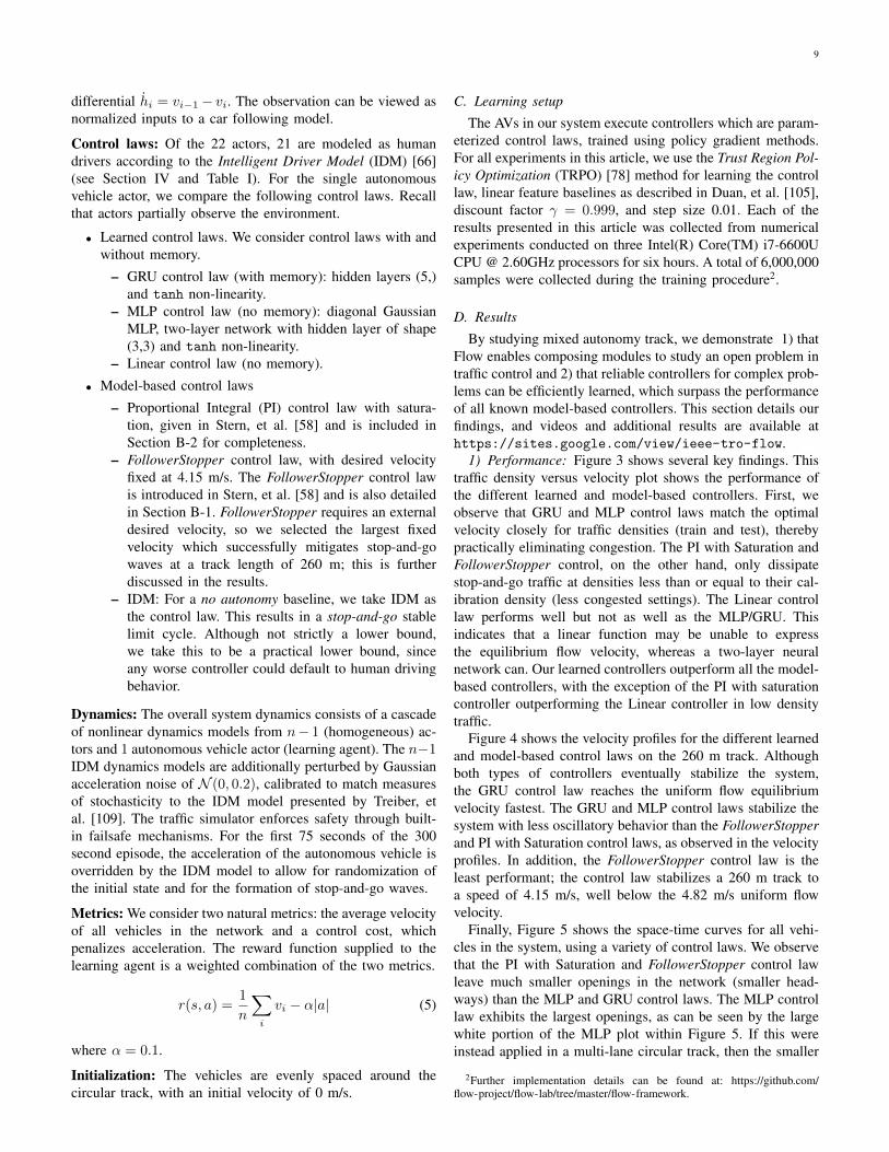
5) Interpreting the controllers: Yet another advantage ofthe partially observed setting is that the low dimensionality ofthe observation space lends itself to interpretation. In Figure 6,we illustrate differences between the learned controllers andIDM. We use a heatmap to show 2-dimensional slices ofthe controllers of 3-dimensional inputs, and the color ofthe heatmap represents the output (acceleration). From theheatmap, we can see that the MLP controller (left subfigure)generally speeds up when it is slower than its leader and slowsdown when it is faster. However, it will also increase its speed

11

0 50 100 150 200 250 300 350 400 450 500 550 600

0

5

10 no automation (stop-and-go waves) automation turned on (for velocity optimization)

velo

city

(m/s

)

Velocity Profile for Vehicles in a 260 m Circular Track for Different Control Laws

FollowerStopper

0 50 100 150 200 250 300 350 400 450 500 550 600

0

5

10

velo

city

(m/s

)

PI Saturation

0 50 100 150 200 250 300 350 400 450 500 550 600

0

5

10

velo

city

(m/s

)

MLP control law (ours)

0 50 100 150 200 250 300 350 400 450 500 550 600

0

5

10

time (s)

velo

city

(m/s

)

GRU control law (ours)

Fig. 4: All experiments start with 300 seconds with the autonomous vehicle following human driving behavior. As we can see from four different controllaws, a single autonomous vehicle in a partially observable circular track can stabilize the system. Both learned control laws stabilize the system close to the4.82 m/s uniform flow velocity, whereas the two model-based controllers fall short. The learned GRU control law allows the system to reach the uniformflow equilibrium velocity fastest.

when faster if it is far away. Notable for the MLP controlleris the “0.0” entry in the left heatmap; it corresponds closelyto the uniform flow equilibrium density. The controller can beinterpreted as regulating its speed and headway such that itsspeed (4.2 m/s) matches the speed of its leader (4.2 m/s) at aspecific density (corresponding to headway of 12 m).

On the other hand, the Linear controller is minimallyreactive (middle subfigure); across the board of speeds andheadways, the control law issues very small accelerations (anddecelerations). However, note that the Linear controller is stillnonlinear due to the failsafe mechanisms built into the trafficsimulator, which prevent vehicle crashes. That is, the controlleris overridden by the simulator whenever the AV’s headway istoo small. Without enabling failsafe mechanisms, we foundin separate experiments (not shown) that the Linear controllertypically converges to a controller with frequent collisions orsignificantly lower performance. Additionally, there may befurther sources of nonlinearity that are introduced through thelearning algorithm (e.g. observation and action clipping), andthis warrants further investigation. Our experiments indicatethat a Linear model, even with nonlinearities introduced byfailsafes and otherwise, may not be able to achieve the optimalvelocity for the mixed autonomy ring. The MLP controller(left), is similarly prone to exploiting the simulator failsafes,and thus for ease of interpretation, the heatmap is displaying

a controller trained without failsafes enabled.In comparison to both learned controllers, IDM (right

subfigure) is visibly more aggressive in its acceleration anddeceleration. Even when the ego vehicle is faster than itsleader, it continues to accelerate until its headway is verysmall. This behavior, sensibly, results in traffic jams.

VII. REUSABLE MODULES FOR MIXED AUTONOMY

The previous section showed that the modules presentedin Section V-A can be composed to study open problems intraffic control and to rigorously evaluate RL and model-basedapproaches. Additionally, the capacity of RL to optimallysolve the idealized circular track scenario in Section VI pro-vides motivation to build more complex traffic scenarios andstudy the mixed autonomy performance with RL. This sectiongoes beyond commonly studied scenarios and demonstratesthat the modules can be configured to create new scenarioswith important traffic characteristics, such as multiple AVsinteracting, lane changes, and intersections. While larger scalescenarios can also be composed, they are out of scope ofthis article, due to the sample efficiency limitations of currentdeep RL methods; this is an important direction of futurework. Instead, we present several scenarios to demonstrate therichness of composing simple modules and the insights thatcan be derived from training controllers therein.

12

Fig. 5: Prior to the activation of the single AV in the circular track, backward propagating waves are exhibited from stop-and-go traffic resulting fromhuman driving. At 300 seconds, the AV then employs different model-based and learned control laws. Top left: Time-space diagram for an AV employing aFollowerStopper control law (model-based). Top right: Time-space diagram for an AV employing a PI with Saturation control law (model-based). Bottomleft: Time-space diagram for an AV employing a learned MLP control law. Bottom right: Time-space diagram for an AV employing a learned GRU controllaw.

Network # vehicles # AVs % improvement (avg. speed)VII-A 22 3 4.07VII-A 22 11 27.07VII-B 44 6 6.09VII-C 14 1 57.45VII-C 14 14 150.49

TABLE III: AV performance results summary. For the VII-A and VII-Bexperiments, the average velocity improvement is calculated relative to theuniform flow equilibrium. For the VII-C experiment, the average velocityimprovement is calculated relative to the no-autonomy setting.

Notably, in contrast to typical model-based control ap-proaches to traffic control, RL requires limited domain knowl-edge or analysis for the study of these more complex trafficcontrol problems. In contrast to sophisticated mathematicalanalysis, we instead need to design a suitable reward function,which does require some degree of trial-and-error. Ultimately,we selected a sensible reward function as before, focusing onsystem velocity and a secondary control cost term. The controlcost will vary depending on the type of control action.

For brevity, we describe only the differences relative to themodules described in Section VI. All methods are comparedagainst a baseline of human performance (IDM), as thereare no known AV control laws for the following scenarios.Results are summarized in Table III. Based on the findingsof Section VI, these experiments use a memory-less diagonalGaussian MLP control law, with hidden layers (100, 50, 25)and tanh non-linearity.

A. Single-lane circular track with multiple autonomous vehi-cles

A simple extension to the previous experiment showsthat many variants to the same problem may be studiedin a scalable manner, without the need to adhere to strictmathematical frameworks for analysis. The following showsadditionally that even simple extensions can yield interestingand significant performance improvements. Here we describethe experimental modules, as they differ from the previousexperiment.Networks: The network is fixed at a circumference of L =230 m, as displayed in Figure 1 (top left).Observer: All vehicle positions and velocities, that is o = s =(x1, v1, x2, v2, . . . , xn, vn).Control laws: Three to eleven of the actors are dictated bya single (centralized) learned control law; that is, A = Rmwhere m ∈ 3, . . . , 11 and πθ : O×A → ∆m. The remainingactors are modeled as human drivers according to IDM.Metrics: The reward function is a weighted combination ofthe average velocity of all vehicles and a control cost.

r(s, a) =1

n

∑i

vi − α1

m

∑j∈[m]

|aj | (6)

where α = 0.1.Result: A string of consecutive AVs learns to proceed with asmaller headway than the human driver models (platooning),

13

8 10 12 14 15 17 19 21 23 24headway (m)

1.52.02.63.13.74.24.85.35.96.4

AV

spe

ed (m

/s)

0.5 0.5 0.5 0.5 0.6 0.6 0.6 0.6 0.7 0.7

0.4 0.4 0.4 0.4 0.5 0.5 0.5 0.5 0.6 0.6

0.2 0.3 0.3 0.3 0.4 0.4 0.4 0.4 0.5 0.5

0.1 0.2 0.2 0.2 0.3 0.3 0.3 0.3 0.4 0.4

0.0 0.1 0.1 0.1 0.1 0.2 0.2 0.2 0.3 0.3

-0.0 -0.0 0.0 0.0 0.1 0.1 0.1 0.1 0.2 0.2

-0.1 -0.1 -0.1 -0.1 -0.0 -0.0 0.0 0.0 0.1 0.1

-0.2 -0.2 -0.2 -0.2 -0.1 -0.1 -0.1 -0.1 -0.0 -0.0

-0.3 -0.3 -0.2 -0.2 -0.2 -0.2 -0.2 -0.1 -0.1 -0.1

-0.4 -0.3 -0.3 -0.3 -0.3 -0.3 -0.2 -0.2 -0.2 -0.2

Multilayer perceptron model

8 10 12 14 15 17 19 21 23 24headway (m)

1.52.02.63.13.74.24.85.35.96.4

AV

spe

ed (m

/s)

0.1 0.1 0.1 0.1 0.1 0.1 0.1 0.1 0.1 0.1

0.1 0.1 0.1 0.1 0.1 0.1 0.1 0.1 0.1 0.1

0.1 0.1 0.1 0.1 0.1 0.1 0.1 0.1 0.1 0.1

0.1 0.1 0.1 0.1 0.1 0.1 0.1 0.1 0.0 0.0

0.1 0.1 0.1 0.1 0.1 0.1 0.0 0.0 0.0 0.0

0.1 0.1 0.1 0.1 0.0 0.0 0.0 0.0 0.0 0.0

0.1 0.1 0.0 0.0 0.0 0.0 0.0 0.0 0.0 0.0

0.0 0.0 0.0 0.0 0.0 0.0 0.0 0.0 0.0 0.0

0.0 0.0 0.0 0.0 0.0 0.0 0.0 0.0 0.0 -0.0

0.0 0.0 0.0 0.0 0.0 0.0 0.0 -0.0 -0.0 -0.0

Linear model

8 10 12 14 15 17 19 21 23 24headway (m)

1.52.02.63.13.74.24.85.35.96.4

AV

spe

ed (m

/s)

0.9 1.0 1.0 1.0 1.0 1.0 1.0 1.0 1.0 1.0

0.9 0.9 1.0 1.0 1.0 1.0 1.0 1.0 1.0 1.0

0.9 0.9 0.9 1.0 1.0 1.0 1.0 1.0 1.0 1.0

0.8 0.8 0.9 0.9 0.9 0.9 1.0 1.0 1.0 1.0

0.6 0.7 0.8 0.9 0.9 0.9 0.9 0.9 0.9 0.9

0.4 0.6 0.7 0.8 0.8 0.8 0.9 0.9 0.9 0.9

0.0 0.3 0.5 0.6 0.7 0.7 0.8 0.8 0.8 0.8

-0.5 -0.0 0.2 0.4 0.5 0.6 0.7 0.7 0.7 0.8

-1.2 -0.5 -0.1 0.1 0.3 0.4 0.5 0.6 0.6 0.6

-2.2 -1.2 -0.6 -0.3 -0.0 0.2 0.3 0.4 0.4 0.5

Intelligent Driver Model

-1.0

-0.8

-0.5

-0.2

0.0

0.2

0.5

0.8

1.0

acce

lera

tion

(m/s

2 )

Fig. 6: Visualization of vehicle control laws. The heatmaps are 2-dimensional slices of the controllers (3-dimensional), and the color depicts the output(acceleration). The x-axis is a representative range of headways seen by vehicles during training. The y-axis is a representative range of vehicle speeds.Displayed is the slice of acceleration values of the model when the leader vehicle speed is fixed at 4.2 m/s (a typical speed for the 250 m track). The singlecolorbar is shared by all plots. Left: Learned MLP model, with failsafes disabled. Middle: Learned Linear model, with failsafes enabled. Right: IDM.

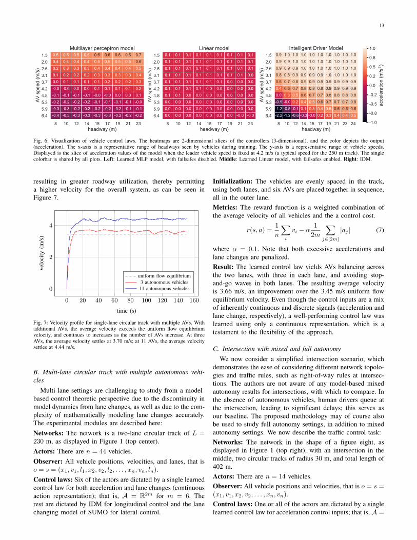
resulting in greater roadway utilization, thereby permittinga higher velocity for the overall system, as can be seen inFigure 7.

0 20 40 60 80 100 120 140 160

0

2

4

time (s)

velo

city

(m/s

)

uniform flow equilibrium3 autonomous vehicles

11 autonomous vehicles

Fig. 7: Velocity profile for single-lane circular track with multiple AVs. Withadditional AVs, the average velocity exceeds the uniform flow equilibriumvelocity, and continues to increases as the number of AVs increase. At threeAVs, the average velocity settles at 3.70 m/s; at 11 AVs, the average velocitysettles at 4.44 m/s.

B. Multi-lane circular track with multiple autonomous vehi-cles

Multi-lane settings are challenging to study from a model-based control theoretic perspective due to the discontinuity inmodel dynamics from lane changes, as well as due to the com-plexity of mathematically modeling lane changes accurately.The experimental modules are described here:Networks: The network is a two-lane circular track of L =230 m, as displayed in Figure 1 (top center).Actors: There are n = 44 vehicles.Observer: All vehicle positions, velocities, and lanes, that iso = s = (x1, v1, l1, x2, v2, l2, . . . , xn, vn, ln).Control laws: Six of the actors are dictated by a single learnedcontrol law for both acceleration and lane changes (continuousaction representation); that is, A = R2m for m = 6. Therest are dictated by IDM for longitudinal control and the lanechanging model of SUMO for lateral control.

Initialization: The vehicles are evenly spaced in the track,using both lanes, and six AVs are placed together in sequence,all in the outer lane.Metrics: The reward function is a weighted combination ofthe average velocity of all vehicles and the a control cost.

r(s, a) =1

n

∑i

vi − α1

2m

∑j∈[2m]

|aj | (7)

where α = 0.1. Note that both excessive accelerations andlane changes are penalized.Result: The learned control law yields AVs balancing acrossthe two lanes, with three in each lane, and avoiding stop-and-go waves in both lanes. The resulting average velocityis 3.66 m/s, an improvement over the 3.45 m/s uniform flowequilibrium velocity. Even though the control inputs are a mixof inherently continuous and discrete signals (acceleration andlane change, respectively), a well-performing control law waslearned using only a continuous representation, which is atestament to the flexibility of the approach.

C. Intersection with mixed and full autonomy

We now consider a simplified intersection scenario, whichdemonstrates the ease of considering different network topolo-gies and traffic rules, such as right-of-way rules at intersec-tions. The authors are not aware of any model-based mixedautonomy results for intersections, with which to compare. Inthe absence of autonomous vehicles, human drivers queue atthe intersection, leading to significant delays; this serves asour baseline. The proposed methodology may of course alsobe used to study full autonomy settings, in addition to mixedautonomy settings. We now describe the traffic control task:Networks: The network in the shape of a figure eight, asdisplayed in Figure 1 (top right), with an intersection in themiddle, two circular tracks of radius 30 m, and total length of402 m.Actors: There are n = 14 vehicles.Observer: All vehicle positions and velocities, that is o = s =(x1, v1, x2, v2, . . . , xn, vn).Control laws: One or all of the actors are dictated by a singlelearned control law for acceleration control inputs; that is, A =

14

R or A = Rm. The rest are dictated by IDM for longitudinalcontrol and intersection rules from SUMO.

Dynamics: There is no traffic light at the intersection; insteadvehicles crossing the intersection follow a right-of-way modelprovided by SUMO to enforce traffic rules and to preventcrashes.

Metrics: The reward function is a weighted combination ofthe average velocity of all vehicles and the a control cost.

r(s, a) =1

n

∑i

vi − α1

m

∑j∈[m]

|aj | (8)

where α = 0.1.

Result: With only one autonomous vehicle, the learned controllaw results in the vehicles moving on average 1.5 times faster.The full autonomy setting exhibits an improvement of almostthree times in average velocity. Figure 8 shows the averagevelocity of vehicles in the network for different levels ofautonomy.

0 20 40 60 80 100 120

0

5

10

15

time (s)

velo

city

(m/s

)

0 autonomous vehicles1 autonomous vehicles

14 autonomous vehicles

Fig. 8: Velocity profile for the intersection with different fractions ofautonomous vehicles. The performance of the network improves as thenumber of AVs improves; even one autonomous vehicle results in a velocityimprovement of 1.5x, and full autonomy almost triples the average velocityfrom 5 m/s (no autonomy) to 14 m/s.

Further study is needed to understand, interpret, and analyzethe above learned behaviors and control laws, and thereby takesteps towards a real-world deployment and policy analysis.Some preliminary investigations can be found in [102], [110].

VIII. CONCLUSION

The complex integration of autonomy into existing systemsintroduces new technical challenges beyond studying auton-omy in isolation or in full. This article aims to make progresson these upcoming challenges by studying how modern deepreinforcement learning can be leveraged to gain insights intocomplex mixed autonomy systems. In particular, we focus onthe integration of autonomous vehicles into urban systems, aswe expect these to be among the first of robotic systems toenter and affect existing systems. The article introduces Flow,a modular learning framework which eases the configurationand composition of modules, to enable learning control lawsfor AVs in complex traffic settings involving nonlinear ve-hicle dynamics and arbitrary network configurations. Several

experiments resulted in controllers which far exceeded state-of-the-art performance (in fact, achieving near-optimal perfor-mance) and demonstrated the generality of the methodologyfor disparate traffic dynamics. Since an early version of thismanuscript was made available online in 2017 [95], severalworks have employed this framework to achieve results in thedirections of transfer learning, bottleneck control, sim2real,the discovery of emergent behaviors in traffic, and the designof traffic control benchmarks [110], [111], [112], [102], [113].

Open directions of research include the study of mixedautonomy in larger and more complex traffic networks; study-ing different, more realistic, and regional objective functions;studying delayed vehicle models; devising new reinforcementlearning techniques for large-scale networked systems; study-ing scenarios with variable numbers of actors; incorporatingadvances in safe reinforcement learning; and incorporatingmulti-agent reinforcement learning for the study of variablenumbers of autonomous vehicles. Another open direction is tostudy fundamental limitations of this methodology; in partic-ular, 1) establishing when guarantees of global convergence,stability, robustness, and safety of classical approaches cannot be achieved with deep RL, and 2) quantifying the effectsof simulation model error or misspecification on trainingoutcomes. We additionally plan to extend Flow with modulessuitable for the study of other forms of automation in traffic,such as problems concerning traffic lights, road directionality,signage, roadway pricing, and infrastructure communication.Another interesting direction is whether an analogous designof reusable modules may be used for other robotics andtransportation-related scenarios, such as for motion planning,navigation, ridesharing, and land use planning.

ACKNOWLEDGMENTS

The authors would like to thank Professor Alexander Skabardonis forinsightful discussions about vehicle dynamics; Leah Dickstein and NathanMandi for early prototyping; Nishant Kheterpal, Kathy Jang, Saleh Albeaikand Ananth Kuchibhotla for helping to build out features; Jakob Erdmann forSUMO support; Rocky Duan and Alex Lee for rllab support, used in earlyexperiments; Philipp Moritz, Eric Liang, and Richard Liaw for Ray and RLlibsupport; and Zhongxia Yan for discussions and training framework support.The team is grateful to Professor Dan Work for technical conversations aboutthe circular track experiment, and to the inspirational work of the Piccoli-Seibold-Sprinkle-Work team. The authors would additionally like to thank theanonymous reviewers of early versions of the manuscript for their insightfuland constructive comments.

APPENDIX ANETWORKS

Flow currently supports learning policies on arbitrary (user-defined) networks. These include closed networks such assingle and multi-lane circular tracks, figure-eight networks,and loops with merge as well as open networks, such asintersections, and open networks with such as merge andhighway networks with pre-defined in-flows of vehicles intothe traffic system. See Figure 1 for various example networkssupported by Flow. In each of these networks, Flow can beused to study the design or learning of controllers which

15

optimize the system-level velocity or fuel consumption, in thepresence of different types of vehicles, model noise, etc.

Single-lane circular tracks: This network consists of acircular lane with a specified length, inspired by the 230mtrack studied by Sugiyama et al. [14]. This network hasbeen extensively studied and serves as an experimental andnumerical baseline for benchmarking.

Multi-lane circular tracks: Multi-lane circular tracks area natural extension to problems involving a single circulartrack. The inclusion of lane-changing behavior in this settingmakes studying such problems exceedingly difficult froman analytical perspective, thereby constraining most classicalcontrol techniques to the single-lane case. Many multi-lanemodels forgo longitudinal dynamics in order to encouragetractable analysis [114], [115], [116], [117]. Recent strideshave been made in developing simple stochastic models thatretain longitudinal dynamics while capturing lane-changingdynamics in a single lane setting [118]. Modern machinelearning methods, however, do not require a simplification ofthe dynamics for the problem to become tractable, as exploredin Section VII-B.

Figure-eight network: The figure-eight network is a simpleclosed network with an intersection. Two circular tracks,placed at opposite ends of the network, are connected bytwo perpendicular intersections. Vehicles that try to cross thisintersection from opposite ends are constrained by a right-of-way model provided by SUMO to prevent crashes.

Loops with merge network: This network permits the studyof merging behavior in closed loop networks. This networkconsists of two circular tracks which are connected together.Vehicles in the smaller track stay within this track, whilevehicles in the larger track try to merge into the smaller trackand then back out to the larger track. This typically results incongestion at the merge points.

Intersections: This network permits the study of intersectionmanagement in an open network. Vehicles arrive in the controlzone of the intersection according to a Poisson distribution. Atthe control zone, the system speeds or slows down vehiclesto either maximize average velocity or minimize experienceddelay. The building block can be used to build a generalschema for arbitrary maps such as the one shown in Figure 1(bottom right).

APPENDIX BMODEL-BASED LONGITUDINAL CONTROL LAWS

In this section, we detail the two state-of-the-art controllaws for the mixed autonomy circular track, against which webenchmark our learned policies generated using Flow.

1) FollowerStopper: Recent work by [58] presented twocontrol models that may be used by autonomous vehiclesto attenuate the emergence of stop-and-go waves in a trafficnetwork. The first of these models is the FollowerStopper. Thismodel commands the AVs to maintain a desired velocity U ,while ensuring that the vehicle does not crash into the vehicle

behind it. Following this model, the command velocity vcmd

of the autonomous vehicle is:

vcmd =

0 if ∆x ≤ ∆x1

v ∆x−∆x1

∆x2−∆x1if ∆x1 < ∆x ≤ ∆x2

v + (U − v) ∆x−∆x2

∆x3−∆x2if ∆x2 < ∆x ≤ ∆x3

U if ∆x3 < ∆x

(9)

where v = min(max(vlead, 0), U), vlead is the speed ofthe leading vehicles, ∆x is the headway of the autonomousvehicle, subject to boundaries defined as:

∆xk = ∆x0k +

1

2dk(∆v−)2, k = 1, 2, 3 (10)

The parameters of this model can be found in [58].2) PI with Saturation: In addition to the FollowerStopper

control law, [58] presents a model called the PI with Saturationcontrol law that attempts to estimate the average equilibriumvelocity U for vehicles on the network, and then drives at thatspeed. This average is computed as a temporal average fromits own history: U = 1

m

∑mj=1 v

AVj . The target velocity at any

given time is then defined as:

vtarget = U + vcatch ×min

(max

(∆x− glgu − gl

, 0

), 1

)(11)

Finally, the command velocity for the vehicle at time j+ 1,which also ensures that the vehicle does not crash, is:

vcmdj+1 = βj(αjv

targetj + (1− αj)vlead

j ) + (1− βj)vcmdj (12)

The values for all parameters in the model can be found in[58] and are also provided in Table I.

REFERENCES

[1] Z. Wadud, D. MacKenzie, and P. Leiby, “Help or hindrance? thetravel, energy and carbon impacts of highly automated vehicles,”Transportation Research Part A: Policy and Practice, vol. 86, pp. 1–18,2016.

[2] U. DOT, “National transportation statistics,” Bureau of TransportationStatistics, Washington, DC, 2016.

[3] S. Thrun, M. Montemerlo, H. Dahlkamp, D. Stavens, A. Aron,J. Diebel, P. Fong, J. Gale, M. Halpenny, G. Hoffmann et al., “Stanley:The robot that won the darpa grand challenge,” Journal of fieldRobotics, vol. 23, no. 9, pp. 661–692, 2006.

[4] M. Buehler, K. Iagnemma, and S. Singh, The DARPA urban challenge:autonomous vehicles in city traffic. Springer, 2009, vol. 56.

[5] K. Spieser, K. Treleaven, R. Zhang, E. Frazzoli, D. Morton, andM. Pavone, “Toward a systematic approach to the design and evaluationof automated mobility-on-demand systems: A case study in singapore,”in Road Vehicle Automation. Springer, 2014, pp. 229–245.

[6] K. Dresner and P. Stone, “A multiagent approach to autonomousintersection management,” Journal of artificial intelligence research,vol. 31, pp. 591–656, 2008.

[7] B. K. Horn, “Suppressing traffic flow instabilities,” in Intelligent Trans-portation Systems-(ITSC), 2013 16th International IEEE Conferenceon. IEEE, 2013, pp. 13–20.

[8] D. Miculescu and S. Karaman, “Polling-systems-based autonomousvehicle coordination in traffic intersections with no traffic signals,”arXiv preprint arXiv:1607.07896, 2016.

[9] M. Bojarski, D. Del Testa, D. Dworakowski, B. Firner, B. Flepp,P. Goyal, L. D. Jackel, M. Monfort, U. Muller, J. Zhang et al., “End toend learning for self-driving cars,” arXiv preprint arXiv:1604.07316,2016.

[10] S. Shalev-Shwartz, S. Shammah, and A. Shashua, “Safe, multi-agent, reinforcement learning for autonomous driving,” CoRR, vol.abs/1610.03295, 2016. [Online]. Available: http://arxiv.org/abs/1610.03295

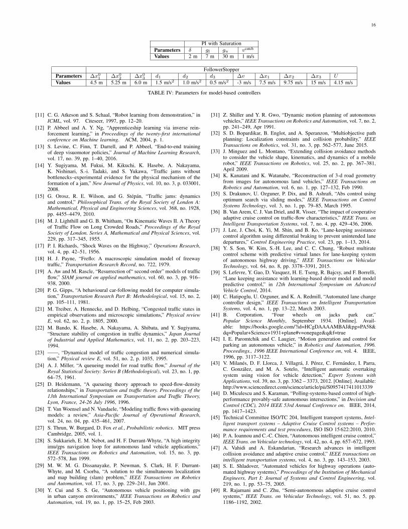
16

PI with SaturationParameters δ gl gu vcatch

Values 2 m 7 m 30 m 1 m/s

FollowerStopperParameters ∆x01 ∆x02 ∆x03 d1 d2 d3 ∆v ∆x1 ∆x2 ∆x3 UValues 4.5 m 5.25 m 6.0 m 1.5 m/s2 1.0 m/s2 0.5 m/s2 -3 m/s 7.5 m/s 9.75 m/s 15 m/s 4.15 m/s

TABLE IV: Parameters for model-based controllers

[11] C. G. Atkeson and S. Schaal, “Robot learning from demonstration,” inICML, vol. 97. Citeseer, 1997, pp. 12–20.

[12] P. Abbeel and A. Y. Ng, “Apprenticeship learning via inverse rein-forcement learning,” in Proceedings of the twenty-first internationalconference on Machine learning. ACM, 2004, p. 1.

[13] S. Levine, C. Finn, T. Darrell, and P. Abbeel, “End-to-end trainingof deep visuomotor policies,” Journal of Machine Learning Research,vol. 17, no. 39, pp. 1–40, 2016.

[14] Y. Sugiyama, M. Fukui, M. Kikuchi, K. Hasebe, A. Nakayama,K. Nishinari, S.-i. Tadaki, and S. Yukawa, “Traffic jams withoutbottlenecks–experimental evidence for the physical mechanism of theformation of a jam,” New Journal of Physics, vol. 10, no. 3, p. 033001,2008.

[15] G. Orosz, R. E. Wilson, and G. Stepan, “Traffic jams: dynamicsand control,” Philosophical Trans. of the Royal Society of London A:Mathematical, Physical and Engineering Sciences, vol. 368, no. 1928,pp. 4455–4479, 2010.

[16] M. J. Lighthill and G. B. Whitham, “On Kinematic Waves II. A Theoryof Traffic Flow on Long Crowded Roads,” Proceedings of the RoyalSociety of London. Series A, Mathematical and Physical Sciences, vol.229, pp. 317–345, 1955.

[17] P. I. Richards, “Shock Waves on the Highway,” Operations Research,vol. 4, pp. 42–51, 1956.

[18] H. J. Payne, “Freflo: A macroscopic simulation model of freewaytraffic,” Transportation Research Record, no. 722, 1979.

[19] A. Aw and M. Rascle, “Resurrection of“ second order” models of trafficflow,” SIAM journal on applied mathematics, vol. 60, no. 3, pp. 916–938, 2000.

[20] P. G. Gipps, “A behavioural car-following model for computer simula-tion,” Transportation Research Part B: Methodological, vol. 15, no. 2,pp. 105–111, 1981.

[21] M. Treiber, A. Hennecke, and D. Helbing, “Congested traffic states inempirical observations and microscopic simulations,” Physical reviewE, vol. 62, no. 2, p. 1805, 2000.

[22] M. Bando, K. Hasebe, A. Nakayama, A. Shibata, and Y. Sugiyama,“Structure stability of congestion in traffic dynamics,” Japan Journalof Industrial and Applied Mathematics, vol. 11, no. 2, pp. 203–223,1994.

[23] ——, “Dynamical model of traffic congestion and numerical simula-tion,” Physical review E, vol. 51, no. 2, p. 1035, 1995.

[24] A. J. Miller, “A queueing model for road traffic flow,” Journal of theRoyal Statistical Society: Series B (Methodological), vol. 23, no. 1, pp.64–75, 1961.

[25] D. Heidemann, “A queueing theory approach to speed-flow-densityrelationships,” in Transportation and traffic theory. Proceedings of the13th International Symposium on Transportation and Traffic Theory,Lyon, France, 24-26 July 1996, 1996.

[26] T. Van Woensel and N. Vandaele, “Modeling traffic flows with queueingmodels: a review,” Asia-Pacific Journal of Operational Research,vol. 24, no. 04, pp. 435–461, 2007.

[27] S. Thrun, W. Burgard, D. Fox et al., Probabilistic robotics. MIT pressCambridge, 2005, vol. 1.

[28] S. Sukkarieh, E. M. Nebot, and H. F. Durrant-Whyte, “A high integrityimu/gps navigation loop for autonomous land vehicle applications,”IEEE Transactions on Robotics and Automation, vol. 15, no. 3, pp.572–578, Jun 1999.

[29] M. W. M. G. Dissanayake, P. Newman, S. Clark, H. F. Durrant-Whyte, and M. Csorba, “A solution to the simultaneous localizationand map building (slam) problem,” IEEE Transactions on Roboticsand Automation, vol. 17, no. 3, pp. 229–241, Jun 2001.

[30] Y. Cui and S. S. Ge, “Autonomous vehicle positioning with gpsin urban canyon environments,” IEEE Transactions on Robotics andAutomation, vol. 19, no. 1, pp. 15–25, Feb 2003.

[31] Z. Shiller and Y. R. Gwo, “Dynamic motion planning of autonomousvehicles,” IEEE Transactions on Robotics and Automation, vol. 7, no. 2,pp. 241–249, Apr 1991.

[32] S. D. Bopardikar, B. Englot, and A. Speranzon, “Multiobjective pathplanning: Localization constraints and collision probability,” IEEETransactions on Robotics, vol. 31, no. 3, pp. 562–577, June 2015.

[33] J. Minguez and L. Montano, “Extending collision avoidance methodsto consider the vehicle shape, kinematics, and dynamics of a mobilerobot,” IEEE Transactions on Robotics, vol. 25, no. 2, pp. 367–381,April 2009.

[34] K. Kanatani and K. Watanabe, “Reconstruction of 3-d road geometryfrom images for autonomous land vehicles,” IEEE Transactions onRobotics and Automation, vol. 6, no. 1, pp. 127–132, Feb 1990.

[35] S. Drakunov, U. Ozguner, P. Dix, and B. Ashrafi, “Abs control usingoptimum search via sliding modes,” IEEE Transactions on ControlSystems Technology, vol. 3, no. 1, pp. 79–85, March 1995.

[36] B. Van Arem, C. J. Van Driel, and R. Visser, “The impact of cooperativeadaptive cruise control on traffic-flow characteristics,” IEEE Trans. onIntelligent Transportation Systems, vol. 7, no. 4, pp. 429–436, 2006.

[37] J. Lee, J. Choi, K. Yi, M. Shin, and B. Ko, “Lane-keeping assistancecontrol algorithm using differential braking to prevent unintended lanedepartures,” Control Engineering Practice, vol. 23, pp. 1–13, 2014.

[38] Y. S. Son, W. Kim, S.-H. Lee, and C. C. Chung, “Robust multiratecontrol scheme with predictive virtual lanes for lane-keeping systemof autonomous highway driving,” IEEE Transactions on VehicularTechnology, vol. 64, no. 8, pp. 3378–3391, 2015.

[39] S. Lefevre, Y. Gao, D. Vasquez, H. E. Tseng, R. Bajcsy, and F. Borrelli,“Lane keeping assistance with learning-based driver model and modelpredictive control,” in 12th International Symposium on AdvancedVehicle Control, 2014.

[40] C. Hatipoglu, U. Ozguner, and K. A. Redmill, “Automated lane changecontroller design,” IEEE Transactions on Intelligent TransportationSystems, vol. 4, no. 1, pp. 13–22, March 2003.

[41] B. Corporation, “Four wheels on jacks park car,”Popular Science Monthly, September 1934. [Online]. Avail-able: https://books.google.com/?id=HCgDAAAAMBAJ&pg=PA58&dq=Popular+Science+1931+plane#v=onepage&q&f=true

[42] I. E. Paromtchik and C. Laugier, “Motion generation and control forparking an autonomous vehicle,” in Robotics and Automation, 1996.Proceedings., 1996 IEEE International Conference on, vol. 4. IEEE,1996, pp. 3117–3122.

[43] V. Milanes, D. F. Llorca, J. Villagra, J. Perez, C. Fernandez, I. Parra,C. Gonzalez, and M. A. Sotelo, “Intelligent automatic overtakingsystem using vision for vehicle detection,” Expert Systems withApplications, vol. 39, no. 3, pp. 3362 – 3373, 2012. [Online]. Available:http://www.sciencedirect.com/science/article/pii/S0957417411013339

[44] D. Miculescu and S. Karaman, “Polling-systems-based control of high-performance provably-safe autonomous intersections,” in Decision andControl (CDC), 2014 IEEE 53rd Annual Conference on. IEEE, 2014,pp. 1417–1423.

[45] Technical Committee ISO/TC 204, Intelligent transport systems, Intel-ligent transport systems – Adaptive Cruise Control systems – Perfor-mance requirements and test procedures, ISO ISO 15 622:2010, 2010.

[46] P. A. Ioannou and C.-C. Chien, “Autonomous intelligent cruise control,”IEEE Trans. on Vehicular technology, vol. 42, no. 4, pp. 657–672, 1993.

[47] A. Vahidi and A. Eskandarian, “Research advances in intelligentcollision avoidance and adaptive cruise control,” IEEE transactions onintelligent transportation systems, vol. 4, no. 3, pp. 143–153, 2003.

[48] S. E. Shladover, “Automated vehicles for highway operations (auto-mated highway systems),” Proceedings of the Institution of MechanicalEngineers, Part I: Journal of Systems and Control Engineering, vol.219, no. 1, pp. 53–75, 2005.

[49] R. Rajamani and C. Zhu, “Semi-autonomous adaptive cruise controlsystems,” IEEE Trans. on Vehicular Technology, vol. 51, no. 5, pp.1186–1192, 2002.

17

[50] X. Lu, S. Shladover, and J. Hedrick, “Heavy-duty truck control: Shortinter-vehicle distance following,” in American Control Conference,2004. Proceedings of the 2004, vol. 5. IEEE, 2004, pp. 4722–4727.

[51] S. Sheikholeslam and C. A. Desoer, “A system level study of thelongitudinal control of a platoon of vehicles,” Journal of dynamicsystems, measurement, and control, vol. 114, no. 2, pp. 286–292, 1992.

[52] S. Cui, B. Seibold, R. Stern, and D. B. Work, “Stabilizing trafficflow via a single autonomous vehicle: Possibilities and limitations,”in Intelligent Vehicles Symposium (IV), 2017 IEEE. IEEE, 2017, pp.447–453.

[53] C. Wu, A. M. Bayen, and A. Mehta, “Stabilizing traffic withautonomous vehicles,” in 2018 IEEE International Conference onRobotics and Automation (ICRA). IEEE, 2018, pp. 1–7.

[54] A. Kesting et al., “Jam-avoiding adaptive cruise control (ACC) andits impact on traffic dynamics,” in Traffic and Granular Flow’05.Springer, 2007, pp. 633–643.

[55] Y.-M. Yuan, R. Jiang, M.-B. Hu, Q.-S. Wu, and R. Wang, “Traffic flowcharacteristics in a mixed traffic system consisting of acc vehicles andmanual vehicles: A hybrid modelling approach,” Physica A: StatisticalMechanics and its Applications, vol. 388, no. 12, pp. 2483–2491, 2009.

[56] T.-C. Au, S. Zhang, and P. Stone, “Semi-autonomous intersectionmanagement,” in Proceedings of the 2014 international conference onAutonomous agents and multi-agent systems. International Foundationfor Autonomous Agents and Multiagent Systems, 2014, pp. 1451–1452.

[57] G. Sharon and P. Stone, “A protocol for mixed autonomous and human-operated vehicles at intersections,” in International Conference onAutonomous Agents and Multiagent Systems. Springer, 2017, pp. 151–167.

[58] R. E. Stern, S. Cui, M. L. D. Monache, R. Bhadani, M. Bunting,M. Churchill, N. Hamilton, R. Haulcy, H. Pohlmann, F. Wu,B. Piccoli, B. Seibold, J. Sprinkle, and D. B. Work, “Dissipationof stop-and-go waves via control of autonomous vehicles: Fieldexperiments,” CoRR, vol. abs/1705.01693, 2017. [Online]. Available:http://arxiv.org/abs/1705.01693

[59] M. Garavello and B. Piccolli, Traffic flow on networks: ConservationLaws Models. Springfield, MO: American Institute of MathematicalSciences, 2006.

[60] M. Pavone, S. L. Smith, E. Frazzoli, and D. Rus, “Robotic loadbalancing for mobility-on-demand systems,” The International Journalof Robotics Research, vol. 31, no. 7, pp. 839–854, 2012.

[61] R. Zhang and M. Pavone, “Control of robotic mobility-on-demandsystems: a queueing-theoretical perspective,” 2014.

[62] D. Sadigh, S. Sastry, S. A. Seshia, and A. D. Dragan, “Planning forautonomous cars that leverage effects on human actions.” in Robotics:Science and Systems, 2016.

[63] J. Lee, M. Park, and H. Yeo, “A probability model for discretionarylane changes in highways,” KSCE Journal of Civil Engineering, vol. 20,no. 7, pp. 2938–2946, 2016.

[64] J. Rios-Torres and A. A. Malikopoulos, “A survey on the coordinationof connected and automated vehicles at intersections and merging athighway on-ramps,” IEEE Transactions on Intelligent TransportationSystems, vol. 18, no. 5, pp. 1066–1077, 2017.

[65] ——, “Automated and cooperative vehicle merging at highway on-ramps,” IEEE Transactions on Intelligent Transportation Systems,vol. 18, no. 4, pp. 780–789, 2017.

[66] M. Treiber and A. Kesting, “Traffic flow dynamics,” Traffic FlowDynamics: Data, Models and Simulation, Springer-Verlag Berlin Hei-delberg, 2013.

[67] M. Papageorgiou, C. Diakaki, V. Dinopoulou, A. Kotsialos, andY. Wang, “Review of road traffic control strategies,” Proceedings ofthe IEEE, vol. 91, no. 12, pp. 2043–2067, 2003.

[68] C.-Y. Liang and P. Huei, “String stability analysis of adaptive cruisecontrolled vehicles,” JSME International Journal Series C MechanicalSystems, Machine Elements and Manufacturing, vol. 43, no. 3, pp.671–677, 2000.

[69] A. Bose and P. A. Ioannou, “Analysis of traffic flow with mixed manualand semiautomated vehicles,” IEEE Trans. on Intelligent Transporta-tion Systems, vol. 4, no. 4, pp. 173–188, 2003.

[70] P. A. Ioannou and M. Stefanovic, “Evaluation of acc vehicles in mixedtraffic: Lane change effects and sensitivity analysis,” IEEE Transactionson Intelligent Transportation Systems, vol. 6, no. 1, pp. 79–89, 2005.

[71] M. A. S. Kamal, J.-i. Imura, T. Hayakawa, A. Ohata, and K. Aihara,“Smart driving of a vehicle using model predictive control for im-proving traffic flow,” IEEE Transactions on Intelligent TransportationSystems, vol. 15, no. 2, pp. 878–888, 2014.

[72] D. Swaroop, “String stability of interconnected systems: An applicationto platooning in automated highway systems,” California Partners forAdvanced Transit and Highways (PATH), 1997.

[73] G. Orosz, J. Moehlis, and F. Bullo, “Delayed car-following dynamicsfor human and robotic drivers,” in ASME 2011 International DesignEngineering Technical Conferences and Computers and Information inEngineering Conference. American Society of Mechanical Engineers,2011, pp. 529–538.

[74] I. G. Jin and G. Orosz, “Dynamics of connected vehicle systemswith delayed acceleration feedback,” Transportation Research Part C:Emerging Technologies, vol. 46, pp. 46–64, 2014.

[75] L. Wang, B. K. Horn, and G. Strang, “Eigenvalue and eigenvector anal-ysis of stability for a line of traffic,” Studies in Applied Mathematics,2016.

[76] V. Mnih, K. Kavukcuoglu, D. Silver, A. Graves, I. Antonoglou,D. Wierstra, and M. Riedmiller, “Playing atari with deep reinforcementlearning,” arXiv preprint arXiv:1312.5602, 2013.

[77] J. Schulman, P. Moritz, S. Levine, M. Jordan, and P. Abbeel, “High-dimensional continuous control using generalized advantage estima-tion,” in Proceedings of the International Conference on LearningRepresentations (ICLR), 2016.

[78] J. Schulman, S. Levine, P. Abbeel, M. I. Jordan, and P. Moritz, “Trustregion policy optimization,” in ICML, 2015, pp. 1889–1897.

[79] N. Heess, G. Wayne, D. Silver, T. Lillicrap, T. Erez, and Y. Tassa,“Learning continuous control policies by stochastic value gradients,” inAdvances in Neural Information Processing Systems, 2015, pp. 2944–2952.

[80] M. G. Bellemare, Y. Naddaf, J. Veness, and M. Bowling, “The arcadelearning environment: An evaluation platform for general agents,” J.Artif. Intell. Res.(JAIR), vol. 47, pp. 253–279, 2013.

[81] C. Beattie, J. Z. Leibo, D. Teplyashin, T. Ward, M. Wainwright,H. Kuttler, A. Lefrancq, S. Green, V. Valdes, A. Sadik et al., “Deep-mind lab,” arXiv preprint arXiv:1612.03801, 2016.

[82] G. Brockman, V. Cheung, L. Pettersson, J. Schneider, J. Schul-man, J. Tang, and W. Zaremba, “Openai gym,” arXiv preprintarXiv:1606.01540, 2016.

[83] G. Synnaeve, N. Nardelli, A. Auvolat, S. Chintala, T. Lacroix,Z. Lin, F. Richoux, and N. Usunier, “Torchcraft: a library for ma-chine learning research on real-time strategy games,” arXiv preprintarXiv:1611.00625, 2016.

[84] E. Todorov, T. Erez, and Y. Tassa, “Mujoco: A physics engine formodel-based control,” in Intelligent Robots and Systems (IROS), 2012IEEE/RSJ International Conference on. IEEE, 2012, pp. 5026–5033.

[85] B. Wymann, E. Espie, C. Guionneau, C. Dimitrakakis, R. Coulom, andA. Sumner, “Torcs, the open racing car simulator,” Software availableat http://torcs. sourceforge. net, 2000.

[86] M.-A. Cote, A. Kadar, X. Yuan, B. Kybartas, T. Barnes, E. Fine,J. Moore, M. Hausknecht, L. E. Asri, M. Adada et al., “Textworld:A learning environment for text-based games,” arXiv preprintarXiv:1806.11532, 2018.

[87] N. G. Polson and V. O. Sokolov, “Deep learning for short-termtraffic flow prediction,” Transportation Research Part C: EmergingTechnologies, vol. 79, pp. 1–17, 2017.

[88] Y. Lv, Y. Duan, W. Kang, Z. Li, and F.-Y. Wang, “Traffic flowprediction with big data: a deep learning approach,” IEEE Transactionson Intelligent Transportation Systems, vol. 16, no. 2, pp. 865–873,2015.

[89] L. Li, Y. Lv, and F. Wang, “Traffic signal timing via deep reinforcementlearning,” IEEE/CAA Journal of Automatica Sinica, vol. 3, no. 3, pp.247–254, July 2016.

[90] F. Belletti, D. Haziza, G. Gomes, and A. M. Bayen, “Expert levelcontrol of ramp metering based on multi-task deep reinforcementlearning,” IEEE Transactions on Intelligent Transportation Systems,vol. 19, no. 4, pp. 1198–1207, 2018.

[91] H. Wei, N. Xu, H. Zhang, G. Zheng, X. Zang, C. Chen, W. Zhang,Y. Zhu, K. Xu, and Z. Li, “Colight: Learning network-level cooperationfor traffic signal control,” arXiv preprint arXiv:1905.05717, 2019.

[92] H. Wei, G. Zheng, H. Yao, and Z. Li, “Intellilight: A reinforcementlearning approach for intelligent traffic light control,” in Proceedingsof the 24th ACM SIGKDD International Conference on KnowledgeDiscovery & Data Mining. ACM, 2018, pp. 2496–2505.

[93] M. G. Karlaftis and E. I. Vlahogianni, “Statistical methods versusneural networks in transportation research: Differences, similarities andsome insights,” Transportation Research Part C: Emerging Technolo-gies, vol. 19, no. 3, pp. 387–399, 2011.

[94] C. Wu, K. Parvate, N. Kheterpal, L. Dickstein, A. Mehta, E. Vinitsky,and A. M. Bayen, “Framework for control and deep reinforcement

18

learning in traffic,” in Intelligent Transportation Systems (ITSC), 2017IEEE 20th International Conference on, 2017.

[95] C. Wu, A. Kreidieh, K. Parvate, E. Vinitsky, and A. M. Bayen, “Flow:Architecture and benchmarking for reinforcement learning in trafficcontrol,” arXiv preprint arXiv:1710.05465, 2017.

[96] R. Bellman, “A markovian decision process,” DTIC Document, Tech.Rep., 1957.

[97] R. A. Howard, “Dynamic programming and markov processes,” 1964.[98] R. S. Sutton, D. A. McAllester, S. P. Singh, and Y. Mansour, “Policy

gradient methods for reinforcement learning with function approxima-tion,” in Advances in neural information processing systems, 2000, pp.1057–1063.

[99] S. Haykin, Neural networks: a comprehensive foundation. PrenticeHall PTR, 1994.

[100] J. Chung, C. Gulcehre, K. Cho, and Y. Bengio, “Gated feedbackrecurrent neural networks,” in International Conference on MachineLearning, 2015, pp. 2067–2075.

[101] M. Treiber, A. Kesting, and D. Helbing, “Multi-anticipative driving inmicroscopic traffic models,” Tech. Rep., 2004.

[102] C. Wu, A. Kreidieh, E. Vinitsky, and A. M. Bayen, “Emergentbehaviors in mixed-autonomy traffic,” in Proceedings of the 1stAnnual Conference on Robot Learning, ser. Proceedings of MachineLearning Research, S. Levine, V. Vanhoucke, and K. Goldberg, Eds.,vol. 78. PMLR, 13–15 Nov 2017, pp. 398–407. [Online]. Available:http://proceedings.mlr.press/v78/wu17a.html

[103] Y. Zheng, J. Wang, and K. Li, “Smoothing traffic flow via control ofautonomous vehicles,” arXiv preprint arXiv:1812.09544, 2018.

[104] D. Krajzewicz, J. Erdmann, M. Behrisch, and L. Bieker, “Recentdevelopment and applications of sumo-simulation of urban mobility,”International Journal On Advances in Systems and Measurements,vol. 5, no. 3&4, 2012.

[105] Y. Duan, X. Chen, R. Houthooft, J. Schulman, and P. Abbeel,“Benchmarking deep reinforcement learning for continuous control,”CoRR, vol. abs/1604.06778, 2016. [Online]. Available: http://arxiv.org/abs/1604.06778

[106] E. Liang, R. Liaw, R. Nishihara, P. Moritz, R. Fox, J. Gonzalez,K. Goldberg, and I. Stoica, “Ray rllib: A composable and scalable re-inforcement learning library,” arXiv preprint arXiv:1712.09381, 2017.

[107] CIECA, “Internal project on eco-driving in category b driver training& the driving test,” 2007.

[108] M. Barth and K. Boriboonsomsin, “Energy and emissions impacts of afreeway-based dynamic eco-driving system,” Transportation ResearchPart D: Transport and Environment, vol. 14, no. 6, pp. 400 – 410,2009, the interaction of environmental and traffic safety policies.[Online]. Available: http://www.sciencedirect.com/science/article/pii/S1361920909000121

[109] M. Treiber and A. Kesting, “The intelligent driver model withstochasticity-new insights into traffic flow oscillations,” TransportationResearch Procedia, vol. 23, pp. 174–187, 2017.

[110] A. R. Kreidieh, C. Wu, and A. M. Bayen, “Dissipating stop-and-gowaves in closed and open networks via deep reinforcement learning,”in 2018 21st International Conference on Intelligent TransportationSystems (ITSC). IEEE, 2018, pp. 1475–1480.

[111] E. Vinitsky, K. Parvate, A. Kreidieh, C. Wu, and A. Bayen, “Lagrangiancontrol through deep-rl: Applications to bottleneck decongestion,”in 2018 21st International Conference on Intelligent TransportationSystems (ITSC). IEEE, 2018, pp. 759–765.

[112] K. Jang, E. Vinitsky, B. Chalaki, B. Remer, L. Beaver, A. A. Ma-likopoulos, and A. Bayen, “Simulation to scaled city: zero-shot policytransfer for traffic control via autonomous vehicles,” in Proceedingsof the 10th ACM/IEEE International Conference on Cyber-PhysicalSystems. ACM, 2019, pp. 291–300.

[113] E. Vinitsky, A. Kreidieh, L. Le Flem, N. Kheterpal, K. Jang, F. Wu,R. Liaw, E. Liang, and A. M. Bayen, “Benchmarks for reinforcementlearning in mixed-autonomy traffic,” in Conference on Robot Learning,2018, pp. 399–409.

[114] P. G. Michalopoulos, D. E. Beskos, and Y. Yamauchi, “Multilane traf-fic flow dynamics: some macroscopic considerations,” TransportationResearch Part B: Methodological, vol. 18, no. 4, pp. 377–395, 1984.

[115] A. Klar and R. Wegener, “A hierarchy of models for multilane vehiculartraffic i: Modeling,” SIAM Journal on Applied Mathematics, vol. 59,no. 3, pp. 983–1001, 1998.

[116] A. Sasoh and T. Ohara, “Shock wave relation containing lane changesource term for two-lane traffic flow,” Journal of the Physical Societyof Japan, vol. 71, no. 9, pp. 2339–2347, 2002.

[117] C. F. Daganzo, “A behavioral theory of multi-lane traffic flow. part i:Long homogeneous freeway sections,” Transportation Research PartB: Methodological, vol. 36, no. 2, pp. 131–158, 2002.

[118] C. Wu, A. Kreidieh, E. Vinitsky, and A. M. Bayen, “Multi-lanereduction: A stochastic single-lane model for lane changing,” in In-telligent Transportation Systems (ITSC), 2017 IEEE 20th InternationalConference on, 2017.