Florida VAM Methodology - Florida Administrative Register

FloridaVAMMethodology

Incorporated in Rule 6A‐5.0411, Calculations of Student Learning Growth for Use in School Personnel Evaluations

Effective August 2015

TableofContents

THE FLORIDA VALUE‐ADDED MODEL (VAM) .................................................................................................................1

EXECUTIVE SUMMARY ...................................................................................................................................................1

SECTION 1: DATA ..........................................................................................................................................................1

Assessment Scores ....................................................................................................................................................2

Student/Teacher/Course Data ..................................................................................................................................2

Other Covariates .......................................................................................................................................................3

Reference File ...........................................................................................................................................................5 Table 1. Exclusions and deletions ....................................................................................................................6

SECTION 2: DESCRIPTION OF THE STATISTICAL MODEL AND ITS IMPLEMENTATION ...................................................9

Covariate Adjustment Model ....................................................................................................................................9

Accounting for Measurement Error in the Prior Scores ......................................................................................... 11 Observed Values for ′ 1 .................................................................................................................. 12

Computing the Value‐Added Model ...................................................................................................................... 13 Standard Errors of Fixed and Random Effects .............................................................................................. 13

Construction of Z matrix ........................................................................................................................................ 15 Table 2. Rules for constructing the Z matrix ................................................................................................. 15

Construction of W matrix ....................................................................................................................................... 16

Standard Errors of Measurement (SEMs) at the Highest (HOSS) and Lowest (LOSS) Observed Scale Scores ....... 16

SECTION 3: FINAL ESTIMATES OF THE TEACHER VALUE‐ADDED SCORE ..................................................................... 17

SECTION 4: AGGREGATING SCORES ACROSS SUBJECTS AND YEARS .......................................................................... 17

Teacher Files .......................................................................................................................................................... 18 Create and Standardize Teacher VAM Scores and Their Variances .............................................................. 19 Standardize Scores ........................................................................................................................................ 19 Create Weights ............................................................................................................................................. 20 Aggregate Scores .......................................................................................................................................... 20 Compute Variance of Aggregated Scores ..................................................................................................... 21 Share of Students Meeting Expectations ...................................................................................................... 21

School Files ............................................................................................................................................................. 21

District Files ............................................................................................................................................................ 23

APPENDIX A – VARIABLES IN THE REFERENCE FILES ................................................................................................... 25

Table A‐1. Variables included from the original data file ............................................................................. 25 Table A‐2. Variables computed in the reference files ................................................................................... 27

TheFloridaValue‐AddedModel(VAM)

Value‐added analysis is a statistical method that estimates the effectiveness of a teacher by seeking to isolate the

contribution of the teacher to student learning. Conceptually, a portion of the difference between a student’s actual

score on an assessment and the score they were expected to achieve is the estimated “value” that the teacher added

during the year to the teacher’s students’ learning growth with respect to the content tested. A student’s expected

score is based on the student’s prior test score history and measured characteristics, as well as how other students in

the state actually performed on the assessment.

The value‐added models implemented for the State of Florida are covariate adjustment models that include up to two

prior assessment scores (except in the grade 4 statewide, standardized assessment models, where only one prior

assessment is available) and a set of measured characteristics for students. The models use error‐in‐variables regression

to account for the measurement error in the covariates used.

ExecutiveSummary

This document contains a technical description of the data sources, formula, covariates, and methodology for calculating

VAM scores. It should be read in conjunction with the main rule text provided in Rule 6A‐5.0411, F.A.C. It uses the

definitions provided in the main rule text. Section 1: Data, describes the processes districts use to submit data to the

Department for use in VAM calculations. It requires the Department to establish a schedule by which the Department

will extract and process data related to students, courses, and teachers, and includes opportunities for districts to revise

and correct information provided to the Department. It also includes a list and description of the variables, referred to

as covariates, controlled for in the model to help ensure that the diversity of students is taken into account when

assigning scores to teachers using the model. These include, for example, student disabilities and the percentage of

days a student was in attendance. Section 2 describes the statistical models for VAM, including the differences between

the models used for ELA and mathematics and the model used for Algebra I. It includes a description of how the model

takes measurement error in test scores for prior assessments into account. It also describes the processes used to derive

fixed and random effects model coefficients used to generate student expected scores and how model converge issues

are resolved. Section 3 describes the process used to create final value added model scores for teachers by grade and

subject. Section 4 describes how value added model scores for different grades, subjects and years are aggregated into

final scores across multiple grades, subjects and years. It also describes the files and data elements delivered to districts

containing information produced by the value added model. Appendix A describes the processes and data elements

used to create the reference files.

Section1:Data

To measure student growth and to attribute that growth to educators, at least two sources of data are required: student

assessment scores that can be observed over time and information describing how students are linked to schools,

teachers, and courses (i.e., identifying which teachers teach which students for which tested subjects and which

school[s] those students attended). In addition, Florida’s value‐added models also use other information, such as

student characteristics and attendance data. The following sections describe the data used for model estimation in

more detail.

AssessmentScoresFlorida’s value‐added models draw on data from statewide assessment programs in Grades 3–10 in ELA, Grades 3‐8 in

Mathematics and on Algebra 1 End‐of‐Course scores. Models are estimated separately by grade and subject using

scores from each grade/subject (e.g., Grade 5 mathematics) as the outcome, with additional covariates as described in

the “Other Covariates” section.

Up to two prior years of achievement scores are included for each student. This covariate is used to control for effects

related to a student’s prior test scores with content aligned to the statewide standardized assessment (English/Language

Arts or Mathematics) being modeled. The variables used are the developmental scale score on the prior year subject‐

relevant assessment and, when available, the developmental scale score on the subject‐relevant assessment from two

years prior. When the subject‐relevant developmental scale score from two years prior is not available, a dichotomous

missing value indicator variable is used.

Student/Teacher/CourseDataCourse enrollment data used in the VAM calculations are drawn from the Student/Teacher/Course File, which is compiled through the following process:

1. Survey 2. School districts submit Survey 2 data to the Department’s Student Information System and Staff Information System, pursuant to Rule 6A‐1.0014, F.A.C. (Comprehensive Management Information System) and Rule 6A‐1.0451, F.A.C. (Florida Education Finance Program Student Membership Surveys).

2. Roster Verification for Survey 2. School districts shall verify Survey 2 class rosters for use in the VAM calculations, in accordance with s. 1012.34, F.S. Districts may choose to use the Department’s roster verification tool for this purpose. Districts utilizing the Department’s roster verification tool must submit Survey 2 data by the first Survey 2 draw down date established by the Department. After the first Survey 2 draw down date, the Department will populate the roster verification tool with course enrollment data submitted by school districts in Survey 2. Districts that do not use the Department’s roster verification tool, but use an independent District roster verification process must submit verified course enrollment data in Survey 2. Districts shall have at least four weeks from the date the roster verification tool is opened to verify the roster data.

3. Survey 3. School districts submit Survey 3 data to the Department’s Student Information System and Staff Information System, pursuant to Rule 6A‐1.0014, F.A.C. (Comprehensive Management Information System) and Rule 6A‐1.0451, F.A.C. (Florida Education Finance Program Student Membership Surveys).

4. Roster Verification for Survey 3. School districts shall verify Survey 3 class rosters for use in the VAM calculations, in accordance with s. 1012.34, F.S. Districts may choose to use the Department’s roster verification tool for this purpose. Districts utilizing the Department’s roster verification tool must submit Survey 3 data by the first Survey 3 draw down date established by the Department. After the first Survey 3 draw down date, the Department will populate the roster verification tool with course enrollment data submitted by school districts in Survey 3. Districts that do not use the Department’s roster verification tool, but use an independent District roster verification process must submit verified course enrollment data in Survey 3. Districts shall have at least four weeks from the date the roster verification data tool is opened to verify the roster data.

5. Survey 2 and 3 Match. Districts are permitted to make local decisions to exclude students from a teacher’s VAM

calculation if he or she changed schools or left the district between survey periods. After the final draw down dates established for Surveys 2 and 3 established by the Department, the Department matches students across both surveys and identifies if each student was present at the same district or at the same school, and provides the results of these matches back to districts. Districts shall make final corrections to the student/teacher/course files and submit back to the Department final files for both surveys for the inclusion in the VAM analysis. Districts shall have at least two weeks from the date the Survey 2 and 3 match files are provided by the Department to make final corrections.

6. Final Student/Teacher/Course Files. The final student/teacher/course files are compiled from the Survey 2 and 3 Match, if the District opts for such a match, or if not, from the post‐verification roster data described above.

Teachers and students associated with the courses shown in the document “Florida VAM Course List” are included in

analyses. See the section on “Construction of Z matrix” for more information on how student/teacher/course data are

used in models.

OtherCovariatesBoth student and classroom characteristics are statistically controlled for in Florida’s value‐added models. Using these characteristics in the value‐added model is intended to help ensure fair comparisons across teachers of diverse groups of students. Following is a list of factors (beyond prior assessment scores described earlier) included in each model and a description of how they are derived. The number of subject‐relevant courses in which the student is enrolled: The number of subject‐relevant courses in

which a student is enrolled. Relevant courses are listed in the document “Florida VAM Course List”. This covariate is

used to control for the effects related to the amount of instruction in the subject the student received during the year. It

counts, for each student, the number of courses in which he or she was enrolled during either Survey 2 or Survey 3 of

the most recent school year that are associated with the statewide standardized assessment being modeled

(English/Language Arts or Mathematics). The variables that make up this covariate are three binary variables indicating

whether the student was enrolled in 2 or more, 3 or more, and 4 or more subject‐relevant courses as reported by school

districts via the course number and period data elements contained within the student course and teacher course

reporting formats of the student information and staff information systems.

A student’s disabilities: This covariate is used to control for effects related to which disabilities, if any, the student has. It

is measured using an array of ten binary variables, each indicating the presence or absence of a specific exceptionality as

reported by school districts via the primary exceptionality and/or other exceptionality data elements contained within

the exceptional student reporting format of the student information system during survey 2 or 3. The exceptionalities

used within the model are limited to language impaired; deaf or hard of hearing; visually impaired;

emotional/behavioral disabilities; specific learning disability; dual sensory impaired; autistic; traumatic brain injured;

other health impaired; and other intellectual disability.

A student’s English Language Learner (ELL) status: This covariate is used to control for effects related to whether a

student has limited English proficiency. It is based on whether a student has been identified as an ELL and is enrolled in a

program or receiving services that are specifically designed to meet the instructional needs of ELL students. These data

are reported by school districts via the ELL indicator in the student demographic format, and the English Language

Learners entry date contained within the English language learners format, of the student information system. It is

measured using four binary variables indicating whether the student has been an ELL for less than two years; at least

two years but less than 4 years; at least 4 years but less than 6 years; or at least 6 years or longer.

Gifted status: This covariate is used to control for effects related to whether or not the student is gifted. It is measured

using a binary variable, indicating the presence or absence of a the gifted exceptionality as reported by school districts

via the primary exceptionality and other exceptionality data elements contained within the exceptional student

reporting format of the student information system during Survey 2 or 3.

Student attendance: This covariate is used to control for effects related to student attendance. It is measured by a

continuous variable that indicates the percentage of days a student was enrolled that the student was in attendance

during the school year as reported by school districts in the student information system via the days present and days

absent data elements from the prior school status/attendance format of the student information system during Survey 2

and 3. The variable is computed as the ratio of the sum of the days present to the sum of the days present plus days

absent across all schools and surveys for the year for the student.

Student mobility: This covariate is used to control for effects related to changing schools during the school year. It is

measured by a continuous variable that is a count of the number of schools beyond the first one that reported the

student via the count of the unique combinations of district, school, student, entry date and withdrawal dates, as

reported via the prior school and student attendance format during Survey 2 and 3.

Difference from modal age in grade: This covariate is used to control for effects related to differences in a student’s age

from the most common age for students enrolled in the same grade across the state and is included as an indicator of

retention or acceleration. It is measured by a continuous variable that computes the difference, in years, between the

student’s age on September 1 of the school year and the modal age of all students in the same grade as reported by

school districts in the student information system via the date of birth data element from the student demographic

format of the student information system during Survey 2 or 3.

Class size: This covariate is used to control for effects related to the number of students in a class. It is measured by a

group of up to 6 continuous variables representing the subject‐relevant courses in which the student is enrolled. Each

variable represents a different class and is the sum of students enrolled in the same class as reported by school districts

in the student information system via the course number and period data elements contained within the student course

and teacher course reporting formats of the student information and staff information systems during Survey 2 and 3.

Homogeneity of students’ entering test scores in the class: This covariate is used to control for the variation in student

proficiency within a classroom at the beginning of the year. It is measured by a group of continuous variables that

represent each of up to 6 subject‐relevant classes in which the student is enrolled. Each of these variables computes the

difference between developmental scale scores located at the 25th percentile and 75th percentile of students assigned

to the teacher who are enrolled in the same class on the prior year’s assessment. When the student is enrolled in fewer

than 6 subject‐relevant classes, a binary missing value indicator variable is used for each class beyond the first one for

which there is no data for the student.

In addition to the variables listed above, the Algebra I EOC models include the following covariates:

Mean prior test score: This covariate is used to control for the effect of the overall incoming proficiency level of

students in the class. It is measured by a group of continuous variables that represent each of up to 6 subject‐relevant

classes the student is enrolled in. For each of these classes, it is the average of the most recent prior score on the

statewide, standardized assessment in Mathematics for all students within the class. When the student is enrolled in

fewer than 6 subject‐relevant classes, a binary missing value indicator variable is used for each class beyond the first one

for which there is no data for the student.

Percent gifted: This covariate is used to control for the effect of the overall proportion of the class that is gifted. It is

measured by a group of continuous variables that represent each of up to 6 subject‐relevant classes the student is

enrolled in. For each of these classes, it is the percentage of students in the class identified as gifted as reported by

school districts via the primary exceptionality and/or other exceptionality data elements contained within the

exceptional student reporting format of the student information system during Survey 2 or 3. When the student is

enrolled in fewer than 6 subject‐relevant classes, a binary missing value indicator variable is used for each class beyond

the first one for which there is no data for the student.

Percent at modal age in grade: This covariate is used to control for the effect of differences in age from the most

common age for students in the grade among the students enrolled in the class as an indicator of what proportion of

students in the class may be accelerated or retained students. It is measured by a group of continuous variables that

represent each of up to 6 subject‐relevant classes the student is enrolled in. For each of these classes it is the percentage

of students whose age on September 1 of the school year is the same as the modal age of all students in the same grade

as reported by school districts in the student information system via the date of birth data element from the student

demographic format of the student information system during Survey 2 or 3. When the student is enrolled in fewer

than 6 subject‐relevant classes, a binary missing value indicator variable is used for each class beyond the first one for

which there is no data for the student.

ReferenceFileIn preparation for the analysis, a single student‐level data file, called the Reference File, is created for each grade/subject combination (i.e., 6th grade ELA, 6th grade Mathematics). These files are compiled from the following data sources:

Relevant course lists (Located in the document “Florida VAM Course List”)

Student/Teacher/Course File

Surveys 2 and 3 (extracted from survey data after the final Survey 2/3 down dates):

o Student demographic information

o Student attendance information

o Student ELL status information

o Student exceptionality information

Assessment data

Staff demographics

School Information

Within the model year, the relevant course list is used for subsetting both the Teacher Course File and the Student

Course File for the relevant courses for each subject. Summer courses are excluded. The Student Course Files are subset

for the relevant courses, and then unique records according to Student_Unique_ID, Year, Survey, District_ID, School_ID,

Period, Section_Number, Course_Number are kept in the file. The Teacher Course File is subset for the relevant courses,

and then unique records according to Teacher_ID, Year, Survey, District_ID, School_ID, Period, Section_Number,

Course_Number are kept in the file. Then the Teacher Course File and the Student Course Files are joined by Year,

Survey, District, School, Period, Section_Number, Course_Number.

The student demographic file is sorted by Year, Student_Unique_ID, Survey, District_enroll, School_enroll, District_ID,

gender, birthyear, and the last record within each year for each student is retained. The attendance records are sorted

by Student_Unique_ID, District ID, School ID. The days present and days absent across all records for a student are

accumulated across districts and schools, and the last student record is retained. ELL information is sorted by

Student_Unique_ID, survey, and the last record is retained. Student exceptionality data are sorted by

Student_Unique_ID, Survey, district, school. Exceptionality flags are accumulated across all surveys, districts, and schools

for the student, and the last record is retained. These four files (demographic, attendance, ELL, and exceptionality) are

then merged by Student_Unique_ID.

Up to four years of student assessment data are merged together by Student_Unique_ID. Merges are verified using the

Levenshtein distance test based on first and last names.. Data are then reshaped from a long dataset (one observation

per student/teacher/course/period) to a wide dataset (one observation per student). Assessment data are then merged

to student data by Student_Unique_ID. Merges are again verified using the Levenshtein test. When a student has no

current assessment information or the student has no prior assessment data in the most recent year used among the

covariates (immediate prior year for ELA and Mathematics, but can be up to 2 years earlier than the current year for

Algebra) then the student is removed from the analysis.

Classes are defined as the unique combination of variables district/school/teacher/course/period and reported in the

data as ClassID. For each student/subject/year, N unique ClassID combinations are retained for the analysis. Analyses are

limited to a maximum of 6 subject relevant courses.

Appendix A contains a list of the variables, source files, and code values used to generate the reference file.

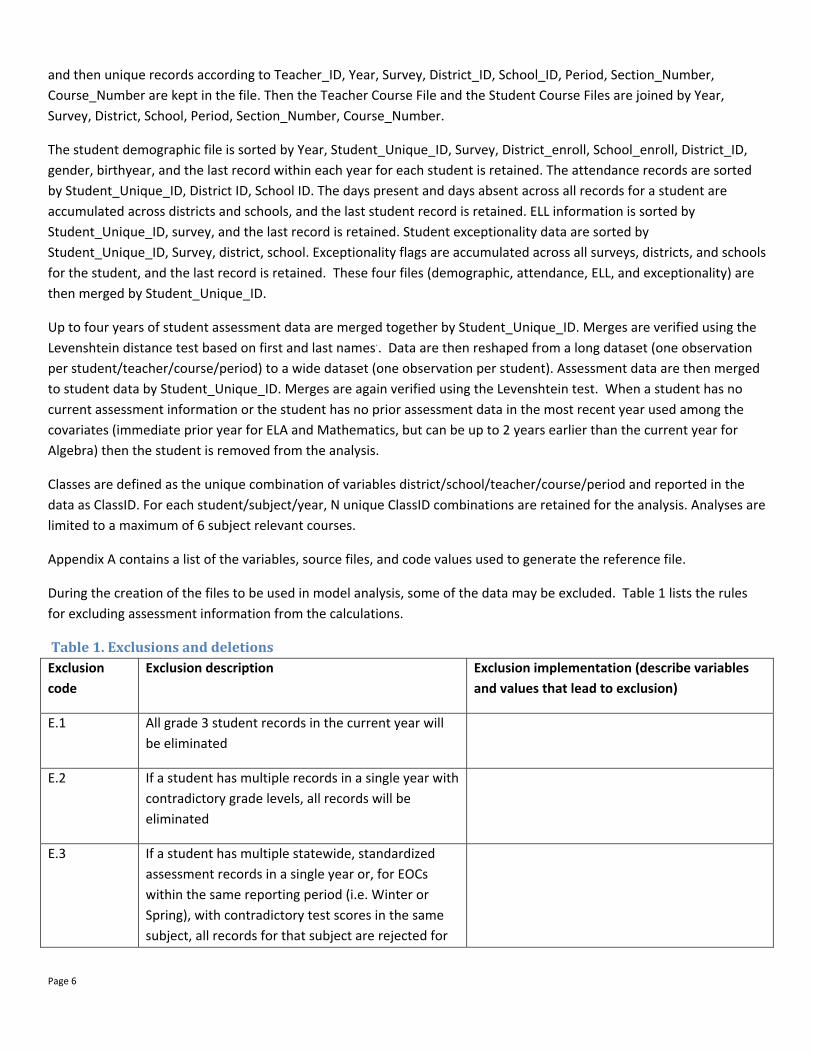
During the creation of the files to be used in model analysis, some of the data may be excluded. Table 1 lists the rules

for excluding assessment information from the calculations.

Table1.ExclusionsanddeletionsExclusion

code

Exclusion description Exclusion implementation (describe variables

and values that lead to exclusion)

E.1 All grade 3 student records in the current year will

be eliminated

E.2 If a student has multiple records in a single year with

contradictory grade levels, all records will be

eliminated

E.3 If a student has multiple statewide, standardized

assessment records in a single year or, for EOCs

within the same reporting period (i.e. Winter or

Spring), with contradictory test scores in the same

subject, all records for that subject are rejected for

the purposes of the analysis.

However, for EOCs within the same year but

different periods, the best score is retained and the

others excluded.

E.4 Student records with missing, or invalidated test

scores are removed

E.5 All grade 9 and 10 student records for the

Mathematics statewide, standardized assessment

for all years will be eliminated

E.6 In the ELA and Mathematics models, exclude

students without both current and immediate prior

year assessment data for the state standard

assessments.

Eliminate records missing the prior year test

score.

If ScaleScore_<yy‐1> missing then delete record

from analysis.

E.7 If a student’s current tested grade is lower than the

student’s prior tested grade, eliminate the record

If tested grade in the current year is less than the

tested grade in the prior year, exclude the

record from analysis.

If Testedgrade yy < Testedgrade yy‐1, exclude

the record. If Testedgrade yy‐1 < Testedgrade

yy‐2, exclude the record

E.8 For EOCs, students must have at least one

immediate prior grade.

Students in grade 8 must have 1st or 2nd prior

year 7th grade (M_1_7 or M_2_7). Students in

grade 9 must have 1st or 2nd prior year 8th grade

(M_1_8 or M_2_8).

E.9 Prior attendance records from survey 3 with “Y” or

“S” codes are not used for the record

These students are summer term students and

should not be in the analysis

TimelineforDataSubmissionandExtraction

No later than September 30 of each year, the Department will post the timeline of data submission and extraction

activities associated with the VAM calculation on its website at (http://www.fldoe.org/teaching/performance‐

evaluation) and shall notify districts of these dates. The timeline shall provide a schedule for the following activities:

Survey 2 first draw down date Complete Roster Verification for Survey 2 (for Districts using the Department’s roster verification tool) Complete Roster Verification for Survey 2 (for Districts not using the Department’s roster verification tool) Survey 3 first draw down date Complete Roster Verification for Survey 3 (for Districts using the Department’s roster verification tool) Complete Roster Verification for Survey 3 (for Districts not using the Department’s roster verification tool) Final Survey 2/3 draw down date District submission of Survey 2/3 Match Requests District final corrections of Survey 2/3 match data

Section2:DescriptionoftheStatisticalModelandItsImplementation

This section provides the technical description of Florida’s value‐added models and their computational implementation.

CovariateAdjustmentModelThe statistical value‐added model implemented for the State of Florida is a covariate adjustment model, as the current

year observed score is conditioned on prior levels of student achievement as well as other covariates that may be

related to the student or classroom characteristics.

Models are run separately by grade, subject, and year. In its most general form, the model can be represented as

follows:

y y , y ,

where the terms in the model are defined as follows:

is the observed score at time t for student i.

is the matrix for the student and classroom demographic variables for student i.

is a vector of coefficients capturing the effect of any covariates included in the model except prior test score.

, is the prior test score at time t‐r ( ∈ 1,2 .

is the coefficient capturing the effects of the most recent prior test score.

is the coefficient capturing the effects of the second prior test score. Elsewhere in this document, and

are concatenated such that ′ , is the coefficient vector capturing the effects of up to two prior test

scores.

is a design matrix with one column for each teacher and one row for each student record in the data file. The

entries in the matrix indicate the association between the student record represented in the row and the

teacher represented in the column.

is the vector of teacher random effects.

is a design matrix with one column for each school and one row for each student record in the data file. The

entries in the matrix indicate the association between the student record represented in the row and the school

represented in the column. Elsewhere in this document, and are concatenated such that , .

is the vector of school random effects. Corresponding to , , define ′ , .

captures all residual student‐level factors contributing to student achievement.

Because Florida’s VAM model treats these vectors of effects as random and independent from each other, it is assumed

that the distributions of teacher and school effects are approximately normal about a mean of 0 ( ~ 0, for

each level of q where ∈ 1,2 , with 1 referencing teacher and 2 referencing school. In the subsequent sections, the

notation ′ ′, ′ is used to refer to the covariate coefficient vectors collectively, and , , is used to

refer to the covariate values collectively in order to simplify computation and explanation.

The statistical model applied to the statewide, standardized assessment and EOC data decomposes total variation in

achievement into three orthogonal components: variance between schools (the school component), variance between

teachers (the teacher component), variance among residual student‐level factors.

While all parameters are estimated simultaneously, conceptually it is helpful to consider the levels separately. First,

student‐level prior assessment data and other covariates are used to establish a statewide conditional expectation,

called an expected score. The expected score is based on the student’s prior test score history and measured

characteristics, as well as how other students in the state actually performed on the assessment.

However, schools exhibit differential amounts of growth. The school component refers to how much higher or lower

the school’s students scored, on average, compared to other students in the same grade and subject in the state after

adjusting for the covariates. Similarly, the teacher component refers to how much higher or lower the teacher’s

students scored, on average, compared to other students within the school after adjusting for the covariates.

If the school component were excluded and the model included only the teacher component, then legitimate differences

between teachers could be exaggerated, as the model would ignore any variation in effectiveness among schools. In

other words, some teachers could appear to have higher (or lower) value‐added scores because their estimated scores

would include things common to all students in a school and may not be due to teachers, such as principal leadership.

In contrast, when the school component is included, then some of the legitimate differences between teachers could be

minimized. For example, if all teachers at a school are highly effective, the school component would capture this

common effectiveness and attributed it to the school, rather than the individual teachers.

As a result, when estimating a value‐added model, it needs to be determined whether the model should:

estimate the common school component, thus potentially removing some legitimate differences between

teachers;

ignore the common school component and assume that any difference in learning across classes is entirely a

function of classroom instruction; or

estimate the common school component, and then attribute some portion of this back to teachers—i.e., find

some middle ground where teacher value‐added scores include some but not all of the common school

component.

Adding none of the school component (0%) to teachers’ value‐added scores essentially creates a model with different

growth expectations for otherwise similar students who attend different schools. A teacher whose students exhibit high

growth in a school where high growth is typical could earn a lower value‐added score than a second teacher whose

students exhibit less growth than the first teacher, but who teaches at a school where lower growth is typical. In

contrast, adding the entire school component (100%) to teachers’ value‐added scores creates a model with the same

statistical expectations for student outcomes, regardless of the school the student attends. Teachers with high student

growth in high‐growth schools will earn higher value‐added scores than teachers with lower growth at low‐growth

schools, regardless of how each teacher performed relative to the other teachers at the school.

The Student Growth Implementation Committee (SGIC), the statewide committee tasked with providing direction on

value‐added model implementation, recommended that 50 percent of the school component should be added to the

teacher component. Teacher value‐added scores from the statewide, standardized assessment models result from the

following calculation:

Teacher Value‐Added Score = Unique Teacher Component + .50 * Common School Component

This formula recognizes that some of the school component is a result of teacher actions within their schools, and

therefore teachers should receive some credit for the typical growth of students in their school in their overall value‐

added scores.

For the Algebra I EOC models, the SGIC determined that none of the school component should be attributed back to

teachers. The SGIC made this decision because more than one‐third of schools have only one or two Algebra I teachers

teaching grade 9 students, and more than half of schools have only one or two Algebra I teachers teaching grade 8

students. In these situations, it is difficult to distinguish between teacher effects and the common school component,

and so the SGIC decided that attributing the school component back to the teacher effect was unnecessary.

AccountingforMeasurementErrorinthePriorScoresFlorida’s value‐added models account for measurement error in test scores through an error‐in‐variables approach.

Accounting for measurement error is important because otherwise bias will still remain, even if multiple scores are used.

To describe how the model accounts for measurement error, we stack the rows for all students in a grade, subject, and

year, drop the i subscript from the model described previously, and re‐express the true score regression equation as

follows:

∗ ∗ ∗

We use * to denote the variables without measurement error. For convenience, define the matrices

, , , ∗ , ∗ , ∗ , and ′ ′, ′ . Let N be the number of students included in the model and

be the number of columns in , so that ∗ has N rows and 2 columns.

Label the matrix of measurement errors associated with , by . Define , where is an

matrix with elements of 0, so that has the same dimension as , but only the final 2 columns of are non‐

zero, so ∗ . If those measurement errors were observed, the parameters ′, ′ can be estimated by solving

the following mixed model equations:

∗′ ∗ ∗′′ ∗

′ ∗

′ ∗

Let be a diagonal matrix of dimension N with diagonal elements , , , , , where , , and , ,

are the known measurement variance of the 2 prior test scores and and are the coefficients on those prior scores.

The matrix is made up of 2 diagonal blocks, one for teachers and one for schools. Each diagonal is constructed as σ

where is an identity matrix with dimension equal to the number of units at level q, and σ is the estimated variance of

the random effects among units at level q. When concatenated diagonally, the square matrix has dimension, where is the number of units at level q.

Two complications intervene. First, we cannot observe , and second, the unobservable nature of this term, along with

the heterogeneous measurement variance in the dependent variable, renders this estimator inefficient.

Addressing the first issue, upon expansion we see that:

∗ ∗ ∗ ∗ ∗ ∗

Taking expectation over the measurement error distributions and treating the true score matrix, ∗, as fixed , we have

E E ∗ ∗ ∗ ∗ E

And then rearranging terms gives

∗ ∗ E E

We also have ′ ∗ E with the expectation taken over the measurement error distributions associated

with observed , and ′ ∗

′ ∗ E′′

with the expectation taken over the measurement error

distributions associated with observed .

As described earlier, is a diagonal matrix of dimension N with diagonal elements , , , , , where

, , and , , are the known measurement variance of the 2 prior test scores and and are the coefficients on

those prior scores. Because the measurement error of the prior score varies depending on the value of the prior score,

, , and , , vary across students. With the above, we can define the mixed model equations as:

E E EE ′

E′′

Using observed scores and measurement error variance, the mixed model equations are redefined as:

E′

′′

ObservedValuesfor

As indicated, is unobserved, and so solving the mixed model equation cannot be computed unless is replaced with

some observed values. First, the mixed model equations are redefined as:

′′′

where now stands in place of E and is subsequently defined as a diagonal “correction” matrix with

dimensions p × p accounting for measurement variance in the predictor variables

Recall that we previously defined as diag , , … , and the matrix of unobserved disturbances is:

where is a matrix with elements of 0, and:

⋮ ⋮

The theoretical result of the matrix operation yields the following symmetric matrix:

1 1

1 1

The theoretical result is limited only because we do not observe and , since they are latent. However,

and , where and are taken as the conditional standard errors of measurement,

which depend on the value of the prior scores, for student i. The theoretical result also simplifies because variances of

measurement on different variables are by expectation uncorrelated, i.e. 0.

Because the conditional standard error of measurement varies for each student i and the off‐diagonals can be ignored,

let the matrix be:

diag 0,… 0,1

, , ,1

, , ,

where σ σ , , , , , , , denotes the measurement variance for the first prior score, and , ,

denotes the measurement variance for the second prior score.

ComputingtheValue‐AddedModelThe implementation of the value‐added model uses the Expectation‐Maximization (EM) algorithm to solve the mixed

model equations. The solutions for the fixed effects and predictions for the random effects are obtained using the

Expectation‐Maximization (EM) algorithm via the following steps:

1. Construct starting values for the variances of the random effects including and for all levels of q.

These are used in the matrices and D, respectively. Typical starting values are 10,000; 1,000; and 1,000 for

residual, teacher, and school variance respectively.

2. Solve the linear system for and .

3. Update the values of the variances of the random effects including and using the methods described

above.

4. Iterate between steps 2 and 3 until 1e‐5 ∀ p, where indexes the iterations.

StandardErrorsofFixedandRandomEffectsThe standard errors of the fixed and random effects can be computed as:

Var ′′

′′

′′

Note that

=

Let and . Then

′ , ′ and

′ ′ .

In order to compute the standard errors of the random effects, it is assumed that teachers teach in only one district,

that students do not move across districts within a school year, and that therefore is block diagonal. Under this

assumption can be computed efficiently and the other computations also become tractable even for very large data

sets. If there are some students who were in two or more districts during the current year, a few entries in the matrix

will not be in the block diagonal, but these will simply be ignored for the purposes of computing the variance terms.

Now

ar

The standard errors of the fixed effects are computed as:

ar

The variances of the random effects are then computed as follows. We first compute the following matrix:

1

,

Where , is the estimate of from the previous iteration and is the identity matrix with dimensions equal to the

model matrix for the random effects and all other matrices are as defined in the prior section.

We then compute

,′ 1

, , , ,

and

Where , are the predictions of the random effects for the level q at iteration 1, are the

number of units (teachers or schools) at level q, and is the trace of the matrix , which is the block of the matrix

corresponding to the qth level.

ConstructionofZmatrixConstruction of the matrix determines how expectations are determined for each teacher. For this section, let i index

students, j index teachers, and k index schools. The table below summarizes how is constructed to achieve the

expectation of effects intended by the business rules.

Table2.RulesforconstructingtheZmatrixRule Summary Example

A.1 If a student is in a single subject‐relevant course with

a single teacher

Teacher j in school k teaches student i in a single

course, 1

A.2 Students enrolled in the same course in multiple

periods with the same teacher treated as a single

student in a single course

Teacher j in school k teaches student i in multiple

periods of a single course, 1

A.3 Students enrolled in different courses with same

teacher, the growth expectation is based on the

number of courses and 100 percent attribution is

made to the teacher for each course

Teacher j in school k teaches student i in two

different courses, 2. If it is 3 different

courses, 3.

A.4 Students enrolled in different courses with different

teachers, the growth expectations is based on the

number of courses and 100 percent attribution is

made to each teacher for each course

Teachers j and j’ each teach student i in one course

(but different course codes) in school k, 1

and 1

A.5 Students taking the same course under multiple

teachers (e.g. coteaching) will be treated as if each

teacher taught the course on their own

Ifeachers j={1,2,…J} teach student i in a single

course (same course number) in school k, 1

for each teacher. If the student takes additional

courses with the teacher, will be augmented

per A.2.

Note that teachers with only a single student within a subject are eliminated from the dataset, and when two teachers

teach exactly the same set of students only one is retained in data used for analysis. The same teacher value‐added

score is then assigned to the teacher that was dropped. Each corresponds to a unique student/teacher/school

combination. These elements are normalized to sum one for each student, so that ∑ ∑

. These

elements are summed within teachers across schools to create the elements of the matrix, and the elements are

summed within schools across teachers to create the elements of the matrix.

ConstructionofWmatrixThe model matrix W consists of the following:

A constant (The expected value of y when all W=0)

Up to two prior years of achievement scores

A missing score indicator for the second prior score

Up to 14 Students with Disabilities (SWD) status indicators

Gifted status

4 English Language Learner (ELL) status indicators (time as ELL)

Attendance (percent of days present)

Number of transitions between schools

Difference from modal age in grade

Number‐of‐course indicators

Homogeneity of entering test scores in the first class in which the student is enrolled. This variable is always

based on the immediate (see table defining prior grades) prior Mathematics scores for entering students

Compute interquartile range based on all entering scores simultaneously

Homogeneity of entering test scores in each additional class in which the student is enrolled, up to 6

Missing indicator(s) for the course homogeneity covariates

Class size of the first course in which the student is enrolled

Class size of each additional class in which the student is enrolled, up to 6

Missing indicator(s) for the class‐size covariates.

For the Algebra EOC Model this also includes:

Percent at modal grade in the first course in which the student is enrolled

Percent at modal grade in each additional class in which the student is enrolled, up to 6

Missing indicator(s) for percent‐at‐modal‐grade covariates

Percent gifted in the first course in which the student is enrolled

Percent gifted in each additional class in which the student is enrolled, up to 6

Missing indicator(s) for the percent gifted indicators

Mean prior test score for the first course in which the student is enrolled

Mean prior test score for each additional class in which the student is enrolled, up to 6

Missing indicator(s) for mean prior test score covariates

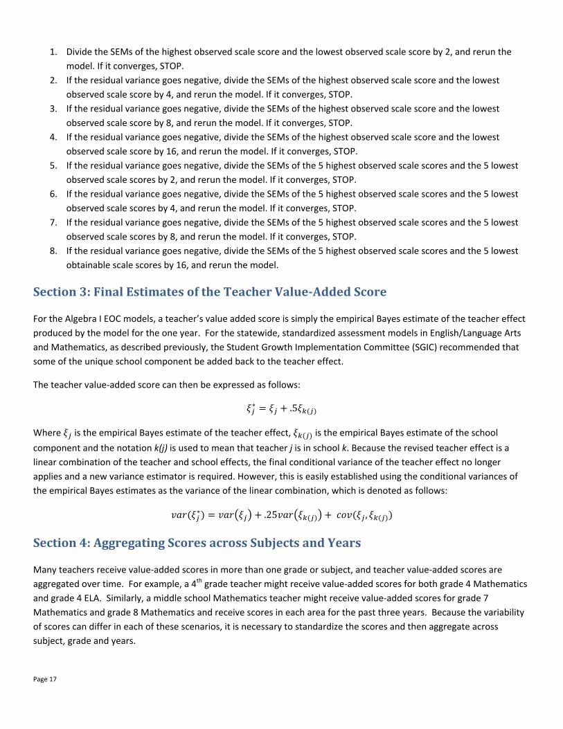
StandardErrorsofMeasurement(SEMs)attheHighest(HOSS)andLowest(LOSS)ObservedScaleScoresThe initial model runs use no adjustment to the standard errors of measurement (SEMs) at the highest and lowest

observed scale scores (HOSS/LOSS). If the model converges successfully no adjustments are needed to address the issue

surrounding the observation of negative variance. If the residual variance becomes negative, the starting values of the

variance components are increased. If the residual variance remains negative, the SEMs of all prior scores for some

records at the extreme ends of the distribution are modified. The following rules regarding adjusting for these outliers

are as follows:

1. Divide the SEMs of the highest observed scale score and the lowest observed scale score by 2, and rerun the

model. If it converges, STOP.

2. If the residual variance goes negative, divide the SEMs of the highest observed scale score and the lowest

observed scale score by 4, and rerun the model. If it converges, STOP.





5. If the residual variance goes negative, divide the SEMs of the 5 highest observed scale scores and the 5 lowest

observed scale scores by 2, and rerun the model. If it converges, STOP.






obtainable scale scores by 16, and rerun the model.

Section3:FinalEstimatesoftheTeacherValue‐AddedScore

For the Algebra I EOC models, a teacher’s value added score is simply the empirical Bayes estimate of the teacher effect

produced by the model for the one year. For the statewide, standardized assessment models in English/Language Arts

and Mathematics, as described previously, the Student Growth Implementation Committee (SGIC) recommended that

some of the unique school component be added back to the teacher effect.

The teacher value‐added score can then be expressed as follows:

∗ .5

Where is the empirical Bayes estimate of the teacher effect, is the empirical Bayes estimate of the school

component and the notation k(j) is used to mean that teacher j is in school k. Because the revised teacher effect is a

linear combination of the teacher and school effects, the final conditional variance of the teacher effect no longer

applies and a new variance estimator is required. However, this is easily established using the conditional variances of

the empirical Bayes estimates as the variance of the linear combination, which is denoted as follows:

∗ .25 ,

Section4:AggregatingScoresacrossSubjectsandYears

Many teachers receive value‐added scores in more than one grade or subject, and teacher value‐added scores are

aggregated over time. For example, a 4th grade teacher might receive value‐added scores for both grade 4 Mathematics

and grade 4 ELA. Similarly, a middle school Mathematics teacher might receive value‐added scores for grade 7

Mathematics and grade 8 Mathematics and receive scores in each area for the past three years. Because the variability

of scores can differ in each of these scenarios, it is necessary to standardize the scores and then aggregate across

subject, grade and years.

These specifications for collecting results focus on the aggregation of teacher and school value‐added scores and

standard errors across grades, subjects, and, in the case of teachers, schools.

TeacherFilesEight separate teacher files are created:

1‐year aggregate

2‐year aggregate

3‐year aggregate

1‐year aggregate by grade


3‐year aggregates by grade

1‐year ELA file

1 ‐year Mathematics file

The aggregate and by‐grade aggregate teacher files include the following:

Teacher name and ID

School name and ID

District name and ID

Number of student scores contributing to the teacher’s ELA score

The teacher’s ELA VAM score and its standard error

Number of student scores contributing to the teacher’s Mathematics score

The teacher’s Mathematics VAM score and its standard error

Number of student scores contributing to the teacher’s combined score

The teacher’s combined VAM score and its standard error

Number of unique students whose scores contributed to the teacher composite VAM score

Binary flags for the years (ex. 2013‐14, 2012‐13, and 2011‐12) to indicate the years a teacher’s score is

aggregated across.

Grade‐level files also include a grade variable.

The ELA and Mathematics 1‐year teacher files include the following:

Teacher name and ID

School name and ID


Subject

Grade

Teacher component estimate and its standard error

School component estimate and its standard error

Teacher VAM score and its standard error

Number of students with scores linked to that teacher

The number and percent of students with scores linked to that teacher meeting expectations

Race

Highest degree attained

Gender

Years of experience

CreateandStandardizeTeacherVAMScoresandTheirVariancesDefinition of Terms:

Let j index teachers, k index schools, g index grades, s index subjects, and t index years.

Let be the teacher component.

Let be the school component.

Let be the average growth (difference between scores at times t and t‐1) for all students in grade g, subject

s, and year t.

Before standardizing across grades and subjects, we first combine the teacher and school components to create the

teacher VAM score as follows:

∗ 0.5

The variance of ∗ is then computed as follows:

∗ 0.25 ∗ ,

StandardizeScoresThe values of ∗ and ∗ must be standardized before they can be aggregated because growth along the

vertically aligned developmental scale is not constant from one grade level to the next. Teacher VAM scores are

standardized as follows:

∗

The variance of a ratio with two random variables is determined from the first‐order Taylor series expansion:

∗ ,

∗ ∗ , ∗ , ∗ ,

The required derivatives are as follows:

∗1

∗

We also need the variance of the average growth:

2 ∗ 1

Where is the number of students in grade g and subject s with current‐year test scores. Substituting these into the

method above and expanding gives the following:

∗ ∗ 2 ∗ , ∗

Except in very small samples the covariance term will be trivial (because any teacher j’s contribution to the state average

is very small), and therefore can be ignored. Because the number of students in the model is large, can

reasonably be approximated to equal zero. Because the covariance term and are assumed to equal zero, we

are essentially treating as fixed, rather than random.

CreateWeightsTeachers who teach multiple grades, multiple subjects, and/or over multiple years will have multiple values of .

Moreover, in most cases teachers teaching during different years, in different subjects, or in different grades will have

different numbers of students or more or less variation within their different classes. These differences lead to

differences in the precision of the estimates. The estimate of overall teacher value‐added can be improved by

accounting for these differences through a weighted average.

Define student weights as follows:

∑ ∑ ∑ ∑

Where is the number of students taught by teacher j, in school k, in grade g, subject s, and year t. The weights for

an individual teacher will always sum to 1. The weights for an individual teacher will likely be different for different

levels of aggregation due to different values in the denominators. For example, the weights used when aggregating a

single year’s worth of scores will be different than the weights used when aggregating several years’ worth of scores.

To strike a balance between precision and simplicity we perform this calculation in two parts. First we look at

aggregations within subjects, and then look at the aggregation of Mathematics and ELA. When aggregating within

subjects, certain covariance terms become ignorably small, which may not be the case across subjects. The covariance

terms depend on the number of students shared across estimates, and students taking a course in a subject generally do

that only within one grade. Across subjects, however, teachers more often teach the same students. Most apparently,

elementary teachers commonly teach all subjects to their students. Therefore, when aggregating across subjects we do

not ignore the covariance term.

AggregateScoresThe aggregated teacher estimate is calculated as follows:

Subject‐, year‐, grade‐, subject‐by‐grade‐, subject‐by‐year‐, grade‐by‐year‐, and subject‐by‐grade‐by‐year‐specific scores

are calculated using analogous formulas.

ComputeVarianceofAggregatedScoresThe variance of the estimate is a function of the weights, the variances of the component estimates, and the

sampling covariance among the estimates. Sampling covariances may be non‐zero when the estimates are based, at

least in part, on common students. In general, teachers rarely teach the same students across grades (students are only

in one grade at a time) or over time; however, many elementary teachers teach the same students across subjects.

Hence, while the cross‐time, cross‐grade covariances may be small enough to ignore, it unlikely that the same is true for

cross‐subject covariances:

2 ,

The sampling covariance between ELA and Mathematics estimates arises because shared students induce dependence

between samples. A simple and accurate approximation can capture this covariance.

First, define as the residual for student i in grade g at time t in subject s (actual value less the expected value less

the estimated school and teacher components). Recall that the estimates have been scaled by dividing by the average

growth (difference between scores at times t and t‐1) for all students in grade g, subject s, and year t. To place the

residuals on the same scale divide them by :

Also, define

, where is the number of students taught both Mathematics and

ELA by teacher j during year t in grade g. This can be calculated by subtracting the number of unique students from the

sum of students taught in Mathematics and ELA separately.

With these in hand, we can approximate

, , , where the final covariance term is the Pearson’s

correlation between the scaled Mathematics and ELA residuals.

ShareofStudentsMeetingExpectationsFor each teacher, calculate and report the share of students who meet expectations. A student meets expectations if

either of the following is true:

The student’s outcome score is greater than or equal to the student’s expected score. The student’s expected

score is calculated using the fixed effects but not the random effects ( ).

The student’s outcome score is at the highest observed scale score.

SchoolFilesEight separate school files are created:

1‐year aggregate

2‐year aggregate

3‐year aggregate




1‐year ELA file


The aggregate and by‐grade aggregate school files include the following:

School name and ID


Number of student scores contributing to the school’s ELA score

A weighted average of the ELA VAM scores of teachers at the school

The standard error of that average ELA score

Number of student scores contributing to the average ELA score

A weighted average of the Mathematics VAM scores of teachers at the school

The standard error of that average Mathematics score

Number of student scores contributing to the average Mathematics score

A weighted average of the combined VAM scores of teachers at the school

The standard error of that average combined score

Number of student scores contributing to the average combined score

The number of unique students with scores linked to that school


aggregated across.


The ELA and Mathematics 1‐year school files include the following:

School name and ID


Subject

Grade

Number of teachers linked to the school in that subject

The school component and its standard error

A weighted average of the teacher components of teachers linked to that school

The standard error of that average teacher component

A weighted average of the VAM scores of teachers linked to that school

The standard error of that average VAM score

Number of students meeting expectations

Percent of students meeting expectations

Number of students

VAM scores of teachers at the 5th, 10th, 25th, 50th, 75th, 90th, and 95th percentile in that district.

Percent of students at that school qualifying for free‐ or reduced‐price meals

Percent of students at that school who are non‐white

A binary variable indicating whether the school is a Title I school.

Weighted averages are student‐weighted averages. These averages and their standard errors are calculated using

formulae analogous to those used to calculate aggregate teacher scores and their standard errors.

∑

DistrictFilesEight separate district files are created:

1‐year aggregate

2‐year aggregate

3‐year aggregate




1‐year ELA file


The aggregate and by‐grade aggregate district files include the following:


Number of student scores contributing to the district’s ELA score

A weighted average of the ELA VAM scores of teachers at the district

The standard error of that average ELA score

Number of student scores contributing to the average ELA score

A weighted average of the Mathematics VAM scores of teachers at the district

The standard error of that average Mathematics score

Number of student scores contributing to the average Mathematics score

A weighted average of the combined VAM scores of teachers at the district

The standard error of that average combined score

Number of student scores contributing to the average combined score

The number of unique students with scores linked to that district


aggregated across.


The ELA and Mathematics 1‐year district files include the following:


Subject

Grade

Number of schools in the district

A weighted average of the school components linked to that district

The standard error of that weighted average

A weighted average of the VAM scores of teachers linked to that district

The standard error of that average VAM score

Number of students meeting expectations

Percent of students meeting expectations

Number of students

VAM scores of teachers at the 5th, 10th, 25th, 50th, 75th, 90th, and 95th percentile in that district.

AppendixA–VariablesintheReferenceFiles

The Reference Files are compiled as follows. Table A‐1 lists the variables to be retained from the original data files and

the data files from which they are retained. New variables that need to be created from these original variables are

listed in Table A‐2.

TableA‐1.VariablesincludedfromtheoriginaldatafileThe total number of ClassIDs for a student will dictate the iteration of the subscript i for each of the subscripted

variables in the table. Note that ‘yy’ represents the year for which data are being reported. For example, using three

years of data, we would expect (yy=14, yy=13, yy=12). If a given student has N unique ClassIDs in which he/she is

enrolled, the subscript i would iterate (i=1 to N) in the table.

Original variable name Variable name in reference file Source file

Description of variable

Student_Unique_ID SSID Multiple Unique Student Identifier

Year _yy_Year Multiple Year

Survey _yy_NewSurvey Multiple 1 if Full Year, 2 if only Survey 2, 3 if

Only Survey 3

District_ID _yy_District_ID_i Multiple District ID

School_ID _yy_School_ID_i Multiple School ID

FirstName _yy_FirstName Student

Demographic

Student first name

LastName _yy_LastName Student

Demographic

Student last name

SBday _yy_S_Bday Student

Demographic

Calendar day of birth

S_Bmonth _yy_S_Bmonth Student

Demographic

Month of birth

S_Byear _yy_S_Byear Student

Demographic

Year of birth

S_EconDisadvantaged _yy_S_EconDisadvantaged Student

Demographic

Binary indicator {0, 1}

S_Gender _yy_S_Gender Student

Demographic

Categorical

S_Race _yy_S_Race Student

Demographic

Categorical

S_LEP _yy_S_LEP Student

Demographic

Limited English Proficiency

Entry_Date _yy_ELL_Entry_Date Student ELL ELL Entry date

EXCEPTIONALITYx _yy_SWD Student

Exceptionality

Binary variable indicating the

student has at least one of the 14

SWD exceptionalities listed below.

The individual _yy_SWDx variables

are also binary indicators. Note that

a student with a gifted

exceptionality is only SWD if the

student has one of the other

exceptionality codes as well.

Present_Days_NBR _yy_Present_Days_NBR Student

Attendance

Number of days the student

attended school

Absent_Days_NBR _yy_Absent_Days_NBR Student

Attendance

Number of days the student was

absent from school

Course_Number _yy_Course_Number_i Student Course

Linkage, Teacher

Course Linkage

Course Number

Period _yy_Period_i Student Course

Linkage, Teacher

Course Linkage,

Course Period

Teacher_ID _yy_Teacher_ID_i Teacher Course

Linkage

Teacher ID

ScaleScore _yy_ScaleScore Assessment Scale score for year yy

ScaleScore_SEM _yy_Scale_Score_SEM Assessment Standard Error of Measure (SEM) of

that scale score for year yy

Grade _yy_TestedGrade Assessment Tested grade of that scale score for

year yy

ScaleScore _yy‐1_ScaleScore Assessment Scale score for year yy‐1

ScaleScore_SEM _yy‐1_Scale_Score_SEM Assessment SEM of that scale score for year yy‐1

Grade _yy‐1_TestedGrade Assessment Tested grade of that scale score for

year yy‐1

ScaleScore _yy‐2_ScaleScore Assessment Scale score for year yy‐2

ScaleScore_SEM _yy‐2_Scale_Score_SEM Assessment SEM of that scale score for year yy‐2

Grade _yy‐2_TestedGrade Assessment Tested grade of that scale score for

year yy‐2

TableA‐2.VariablescomputedinthereferencefilesVariable name in reference

file

Description

Subject Mathematics or ELA

_yy_ELL_LY Student is an English language learner. _yy_ELL_LY = 1 if and only if S_LEP = LY, and zero

otherwise

_yy_ELL_LY_1 For the current year, using the S_LEP variable, create a new variable, ELL_LY_1, which is 1

if and only if S_LEP=LY and the testing date minus the entry date is less than two years.

Otherwise, ELL_LY_1 = 0.

_yy_ELL_LY _2 For the current year, using the S_LEP variable, create a new variable, ELL_LY_2, which is 1

if and only if S_LEP=LY and the testing date minus the entry date is at least two years but

less than four years.



if and only if S_LEP=LY and the testing date minus the entry date is at least four years but

less than six years.



if and only if S_LEP=LY and the testing date minus the entry date is equal to or greater

than six years.


_yy_S_Gifted Set value to 1 if and only if EXCEPTIONALITY = L (indicating Gifted). Otherwise, set value to

0.

_yy_SWD1 Set value to 1 if and only if EXCEPTIONALITY = A (indicating Intellectual Disability)

(Collapsed into Code W in 2008‐09). Otherwise, set value to 0

_yy_SWD2 Set value to 1 if and only if EXCEPTIONALITY = B (indicating Intellectual

Disability)(Collapsed into Code W in 2008‐09). Otherwise, set value to 0.

_yy_SWD3 Set value to 1 if and only if EXCEPTIONALITY = G (indicating Language Impaired).

Otherwise, set value to 0.

_yy_SWD4 Set value to 1 if and only if EXCEPTIONALITY = H (indicating Deaf or Hard of Hearing).


_yy_SWD5 Set value to 1 if and only if EXCEPTIONALITY = I (indicating Visually Impaired). Otherwise,

set value to 0.

_yy_SWD6 Set value to 1 if and only if EXCEPTIONALITY = J (indicating Emotional/Behavioral

Disability. Otherwise, set value to 0.

_yy_SWD7 Set value to 1 if and only if EXCEPTIONALITY = K (indicating Specific Learning Disability).


_yy_SWD8 Set value to 1 if and only if EXCEPTIONALITY = N (indicating Intellectual Disability)

(Collapsed into Code W in 2008‐09). Otherwise, set value to 0.

_yy_SWD9 Set value to 1 if and only if EXCEPTIONALITY = O (indicating Dual‐Sensory Impaired.


_yy_SWD10 Set value to 1 if and only if EXCEPTIONALITY = P (indicating Autism Spectrum Disorder.


_yy_SWD11 Set value to 1 if and only if EXCEPTIONALITY = Q (indicating Emotional / Behavioral

Disability (Collapsed into Code J in 2007‐08). Otherwise, set value to 0.

_yy_SWD12 Set value to 1 if and only if EXCEPTIONALITY = S (indicating Traumatic Brain Injured.


_yy_SWD13 Set value to 1 if and only if EXCEPTIONALITY = V (indicating Other Health Impaired.


_yy_SWD14 Set value to 1 if and only if EXCEPTIONALITY = W (indicating Intellectual Disability.


_yy_Bdate Birthdate (SAS Date value)

_yy_Age Student age is calculated as the age in years as of September 1 of the academic year.

_yy_ModalAge Modal age in grade, where age is calculated as the age in years as of September 1 of the

academic year.

_yy_DeltaAge Difference from modal age in grade: yy_Age – yy_ModalAge

_yy_Present_Days_Prop Across all schools, sum the number of days in attendance. If the sum is greater than 180

days, set equal to 180 days.

Across all schools, sum the number of days in attendance and the number of days absent

to create the total number of days enrolled. If the sum is greater than 180 days, set equal

to 180 days.

Divide by the total days in attendance by the total days enrolled to obtain the share of

days in attendance.

_yy_Teacher_Effect_i Attribution of the teacher effect. The weight for a teacher divided by the sum of the

weights of all teachers for the specific student: ∑

. The weight of 1 would be

assigned to a teacher if they were the only teacher the student was assigned; while a

weight of 0.5 would be assigned if the student had two different teachers.

_yy_Num_Trans Sort the attendance file by year, SSID, and entry date. If the student has only one record

within the current school year, he/she has 0 transitions. For each change of school, within

the year, count one transition. If a student has two entry dates for the same school, count

as one transition only if the second entry date is more than 21 days after the previous

withdrawal date.

_yy_NumberCourses Total number of subject relevant courses in which the student is enrolled.

Courses_x_or_more A vector of binary variables indicating the number of courses in which the student is

enrolled. 2 or more, 3 or more, 4 or more, 5 or more.

_yy_Class_Size_i The count of students who are enrolled in the same course with the same teacher during

the same period at the same school in the same district.

_yy_Homogeneity_i The interquartile range of year yy‐1 test scores among all students who are enrolled in

the same course with the same teacher during the same period at the same school in the

same district.

_yy_Mean_Prior_i Mean prior assessment score among all students in class.

_yy_Pct_Gifted_i Percent of students in class who are gifted.

_yy_Pct_AtModalGrade_i Percent of students in class who are at the modal grade.

Florida VAM Methodology - Florida Administrative Register

Documents

Transcript of Florida VAM Methodology - Florida Administrative Register