ARTICLE IN PRESS

Deep-Sea Research I 57 (2010) 835–846

Contents lists available at ScienceDirect

Deep-Sea Research I

0967-06

doi:10.1

n Corr

E-m

Molly.B

(R.F. Ga1 Te2 Te

journal homepage: www.elsevier.com/locate/dsri

Florida Current transport variability: An analysis of annual andlonger-period signals

Christopher S. Meinen a,n, Molly O. Baringer a,1, Rigoberto F. Garcia b,2

a NOAA/AOML, PHOD, 4301 Rickenbacker Causeway, Miami, FL 33149, USAb UM/CIMAS, 4600 Rickenbacker Causeway, Miami, FL 33149, USA

a r t i c l e i n f o

Article history:

Received 23 June 2009

Received in revised form

9 December 2009

Accepted 7 April 2010Available online 24 April 2010

Keywords:

Florida Current

Gulf Stream

Transport

Time series

Cable

Float

37/$ - see front matter Published by Elsevier

016/j.dsr.2010.04.001

esponding author. Tel.: +1 305 361 4355; fax

ail addresses: Christopher.Meinen@noaa.gov (

aringer@noaa.gov (M.O. Baringer), Rigoberto.

rcia).

l.: +1 305 361 4345.

l.: +1 305 361 4348.

a b s t r a c t

More than forty years of Florida Current transport estimates are combined to study annual and longer-

term variability in this important component of the MOC and subtropical gyre. A detailed analysis with

error estimates illustrates the difficulties in extracting annual and longer time scale variability given the

strong higher frequency energy present. The annual cycle represents less than 10% of the total Florida

Current transport variance in a 16 yr segment of the record, while interannual (13–42 month)

variability represents only 13% of the total and periods longer than 42 months represents less than 10%

of the total. Given the observed high frequency variability of the Florida Current, in order to get a

monthly mean that is accurate to within 0.5 Sv (one standard error level) more than 20 daily

observations are needed. To obtain an estimate of the annual climatology that is ‘‘accurate’’ to within

20% of its own standard deviation, at least 24 yr of data is needed. More than 40 observations spread

throughout a year are required to obtain an annual mean that is accurate to within 0.5 Sv. Despite these

daunting data requirements, there is sufficient data now to evaluate both the annual cycle of the Florida

Current transport with a high degree of accuracy and to begin to determine the longer period transport

variability. Comparison of the Florida Current, NAO and wind stress curl records shows that a recently

described Sverdrup-based mechanism explains a significant fraction of the long-period variability

primarily during the 1986–1998 time window, with other mechanisms clearly dominating before

and after.

Published by Elsevier Ltd.

1. Introduction

The North Atlantic subtropical gyre is distinguished from othersubtropical gyres because the horizontal gyre is embedded within(or embeds) a climatically important full-water-column verticalgyre, the meridional overturning circulation (MOC). Decadalvariations in the MOC, and the associated changes in oceanproperties such as sea-surface temperature, have been tied tovariations in precipitation over the neighboring continents andother socially important quantities (e.g. Alvarez-Garcia et al.,2008). Improved understanding of the variability in the MOC, andthe role of the high frequency variability in extracting theseannual and longer period variations from the MOC, is a key issuefor long-term predictability (e.g. von Storch and Haak, 2008).

Off the east coast of Florida the bulk of both the warm surfacelimb of the vertical MOC and the majority of the western

Ltd.

: +1 305 361 4412.

C.S. Meinen),

Garcia@noaa.gov

boundary component of the horizontal subtropical gyre arecarried within the Florida Current as it passes through the Straitsof Florida. Observations and estimations of the Florida Currenthave been made over a surprisingly long period of time, startingas early as the late 1880s (Pillsbury, 1887,1890). The importanceof the Florida Current to the dynamical ocean–atmosphere systemand as a flow with a significant history of observations has longbeen understood, leading to the establishment in 1982 of a nearlycontinuously program to provide long-term monitoring of theFlorida Current (e.g. Larsen and Sanford, 1985; Molinari et al.,1985a; Leaman et al., 1987; Larsen, 1992). Among other things,the studies based on these measurements have demonstrated asmall but significant annual cycle (e.g. Leaman et al., 1987) as wellas higher frequency (3–10 day periods) variations that appear tobe locally or near-locally forced coastally trapped waves (e.g.Mooers et al., 2005). Baringer and Larsen (2001) evaluated theannual cycle using 16 years of time-series data and they found anapparent shift in the annual cycle of Florida Current transportbetween the first and second half of their study period. Baringerand Larsen also showed that over the period 1982–1998 thelow-frequency Florida Current transport variability (at periodsgreater than 2 years) appears to have a negative correlationwith the atmospheric North Atlantic Oscillation (NAO), which has

ARTICLE IN PRESS

C.S. Meinen et al. / Deep-Sea Research I 57 (2010) 835–846836

well-documented correlations with a multitude of other climati-cally important variations around the Atlantic basin. A subsequentstudy by DiNezio et al. (in press) developed a plausiblemechanism to explain this anti-correlation based on fast propa-gation of first baroclinic mode Rossby waves forced by basininterior wind stress curl variability. The 16 yr time series studiedby Baringer and Larsen (2001) included, however, less than twocomplete cycles of the low-frequency (roughly 12 yr) anti-correlated fluctuation and the authors noted that the significanceof the anti-correlation was marginal. It has been observed that inthe most recent few years this anti-correlation appears lesscertain (Baringer and Meinen, 2006; Beal et al. 2008), leading toquestions about the robustness of the interannual/decadalmechanisms proposed to date to explain the observed FloridaCurrent variability. In addition to the modern data used in most ofthese studies, there is a significant amount of older data thatcould also be used to test the relationships such as that betweenNAO and Florida Current proposed by DiNezio et al. (in press).Doing so, however, requires a careful review of temporalsampling, spatial sampling locations, and other issues with thesedata sets.

The purpose of this article is to review the available historicalobservations, compare them with the updated modern observa-tions, and to use both types of data to evaluate the variations ofthe Florida Current over the full length of time during whichobservations have been made. The paper presents, for the firsttime, the data processing methods used on many of themeasurements undertaken since 2000. The paper is organized asfollows. First the data types available throughout the Straits willbe reviewed, along with their strengths and weaknesses. Next, aconsistent forty-year time series centered along 271N within theFlorida Straits will be compiled taking into account the appro-priate offsets for the different instrument types. This is followedby a careful presentation of statistical tests using both simulatedand actual data to estimate the errors associated with temporalundersampling, focusing first on the annual cycle and then on theinterannual and longer variability. Finally the resulting time serieswill be compared to the NAO index and long-period wind stresscurl forcing mechanisms and conclusions will be presented.

82°W 80°W 78°W 76°W 74°W 72°W25°N

26°N

27°N

28°N

29°N

30°NDropsonde/Pegasus stationNova Univ. linePresent day cableSanford (1982) cable

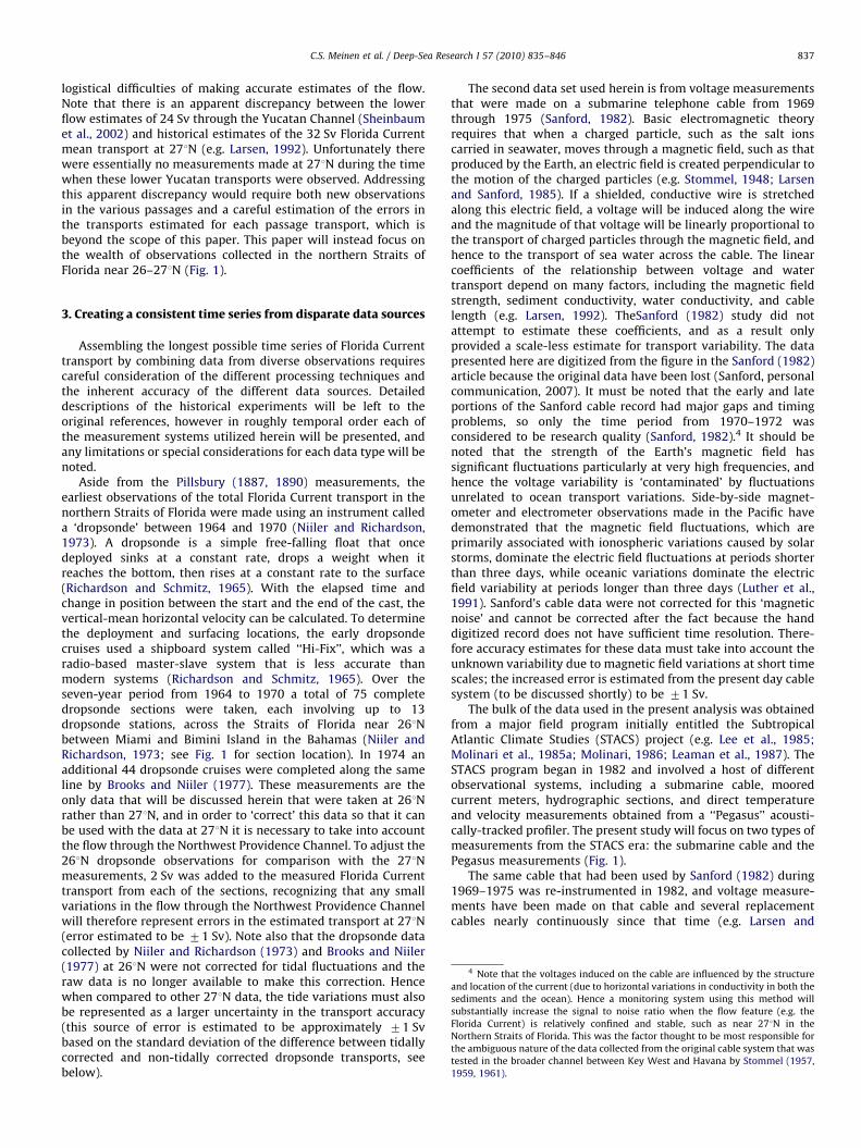
Fig. 1. Location of the observations collected in the Florida Current near 26–271N.

Dropsonde/Pegasus locations at 271N have been essentially the same since 1982;

2. Summary of observations with the Florida Straits

Some of the very first ocean transport observations obtainedanywhere in the world were made in the Florida Current/GulfStream in the 1880s (Pillsbury, 1887, 1890). Using extremelyinnovative techniques for the time, Pillsbury was able to estimatea transport of about 26 Sv (converting from his more archaicunits) for the Florida Current near 261N using velocity measure-ments made within the upper �200 m over several months froman anchored ship.3 Considering the probable accuracy of thoseearly methods this transport estimate is surprisingly close tomore accurate estimates made at 261N 70–80 years later, such asthe 30 Sv obtained for the period of 1964–1970 (Niiler andRichardson, 1973) and 33 Sv obtained during 1974 (Brooks andNiiler, 1977).

Since these pioneering observations, a host of differentobservational techniques have been applied to measuring theFlorida Current transport ranging from geostrophic estimates(relative to an assumed level of no motion, e.g. Montgomery,1941; Broida, 1969) to free-falling floats (e.g. Richardson and

3 The assumption of zero flow at the bottom in the Pillsbury studies resulted

in an underestimation of the total transport of the Florida Current. A subsequent

reanalysis of the Pillsbury data resulted in a revised estimate of about 29 Sv

(Schmitz and Richardson, 1968).

Schmitz, 1965; Brooks and Niiler, 1975) to a creative use ofsubmarine telephone cables (e.g. Stommel, 1948, 1957; Broida,1962, 1963). The latter measurements were in essence the earliesttime series measurements of the Florida Current transport, andthey were made in the southern Straits of Florida using asubmarine cable that stretched from Key West, Florida to Havana,Cuba (Wertheim, 1954; Stommel 1957, 1959, 1961, Broida, 1962,1963). However, interpretation of those early cable measure-ments is ambiguous due to difficulties with the application of theelectromagnetic technique in an environment where the FloridaCurrent could meander widely over different sediments (Schmitzand Richardson, 1968; Wunsch et al., 1969; Larsen, 1992). Therewere a number of estimates of the transport of the Florida Currentduring the 1960s using sea-level differences (e.g. Wunsch et al.,1969). The next in situ estimates that were made started in themid-1960s near 261N between Miami, Florida and Bimini,Bahamas (Niiler and Richardson, 1973; Brooks and Niiler, 1977).Subsequent to the work in the mid 1960s to mid 1970s, most ofthe observations were made a bit further north at 271N betweenWest Palm Beach, Florida and Grand Bahama Island. The morerecent measurements have been taken at a location to the Northof any inflow into the straits from passages opening to theAtlantic Ocean and where the Florida straits geometry tightlyconstricts the flow to a fairly shallow and narrow current wheresubstantial meandering (as a percentage of the Florida Currentwidth) is not possible.

The flow of the Florida Current at 271N is fed through threeprimary sources. The largest is the flow through the YucatanChannel, where transport estimates have ranged from 24 to 28 Sv(Johns et al., 2002; Sheinbaum et al., 2002). The next-largestinflow is through the Northwest Providence Channel, a narrowgap through the Bahamas bank centered at about 26.41N (Fig. 1).Previous work in this area has found that the top-to-bottomwestward transport through the Northwest Providence Channelranges from about 1.2 to 2.5 Sv (Richardson and Finlen, 1967;Leaman et al., 1995; Johns et al., 1999). The only other passagefeeding into the Florida Straits is the Old Bahamas Channelbetween Cuba and the Southern Bahamas Islands. This channel isextremely shallow but very broad. Estimates of the transportthrough the Old Bahama Channel have been about 2 Sv (Hamiltonet al., 2005), however this value is highly uncertain given the

the dropsonde casts collected by Niiler and Richardson (1973) and Brooks and

Niiler (1977) were collected along the ‘Nova Univ. line’. Both the cable used since

1993 (red) and the previous cable used from 1970–1972 and 1982–1993

(magenta) are shown. Gray-shading denotes the bottom topography (Smith and

Sandwell, 1997) with 500 m contour levels; the Northwest Providence Channel

enters the straits of Florida just south of the present-day cable location.

ARTICLE IN PRESS

C.S. Meinen et al. / Deep-Sea Research I 57 (2010) 835–846 837

logistical difficulties of making accurate estimates of the flow.Note that there is an apparent discrepancy between the lowerflow estimates of 24 Sv through the Yucatan Channel (Sheinbaumet al., 2002) and historical estimates of the 32 Sv Florida Currentmean transport at 271N (e.g. Larsen, 1992). Unfortunately therewere essentially no measurements made at 271N during the timewhen these lower Yucatan transports were observed. Addressingthis apparent discrepancy would require both new observationsin the various passages and a careful estimation of the errors inthe transports estimated for each passage transport, which isbeyond the scope of this paper. This paper will instead focus onthe wealth of observations collected in the northern Straits ofFlorida near 26–271N (Fig. 1).

4 Note that the voltages induced on the cable are influenced by the structure

and location of the current (due to horizontal variations in conductivity in both the

sediments and the ocean). Hence a monitoring system using this method will

substantially increase the signal to noise ratio when the flow feature (e.g. the

Florida Current) is relatively confined and stable, such as near 271N in the

Northern Straits of Florida. This was the factor thought to be most responsible for

the ambiguous nature of the data collected from the original cable system that was

tested in the broader channel between Key West and Havana by Stommel (1957,

1959, 1961).

3. Creating a consistent time series from disparate data sources

Assembling the longest possible time series of Florida Currenttransport by combining data from diverse observations requirescareful consideration of the different processing techniques andthe inherent accuracy of the different data sources. Detaileddescriptions of the historical experiments will be left to theoriginal references, however in roughly temporal order each ofthe measurement systems utilized herein will be presented, andany limitations or special considerations for each data type will benoted.

Aside from the Pillsbury (1887, 1890) measurements, theearliest observations of the total Florida Current transport in thenorthern Straits of Florida were made using an instrument calleda ‘dropsonde’ between 1964 and 1970 (Niiler and Richardson,1973). A dropsonde is a simple free-falling float that oncedeployed sinks at a constant rate, drops a weight when itreaches the bottom, then rises at a constant rate to the surface(Richardson and Schmitz, 1965). With the elapsed time andchange in position between the start and the end of the cast, thevertical-mean horizontal velocity can be calculated. To determinethe deployment and surfacing locations, the early dropsondecruises used a shipboard system called ‘‘Hi-Fix’’, which was aradio-based master-slave system that is less accurate thanmodern systems (Richardson and Schmitz, 1965). Over theseven-year period from 1964 to 1970 a total of 75 completedropsonde sections were taken, each involving up to 13dropsonde stations, across the Straits of Florida near 261Nbetween Miami and Bimini Island in the Bahamas (Niiler andRichardson, 1973; see Fig. 1 for section location). In 1974 anadditional 44 dropsonde cruises were completed along the sameline by Brooks and Niiler (1977). These measurements are theonly data that will be discussed herein that were taken at 261Nrather than 271N, and in order to ‘correct’ this data so that it canbe used with the data at 271N it is necessary to take into accountthe flow through the Northwest Providence Channel. To adjust the261N dropsonde observations for comparison with the 271Nmeasurements, 2 Sv was added to the measured Florida Currenttransport from each of the sections, recognizing that any smallvariations in the flow through the Northwest Providence Channelwill therefore represent errors in the estimated transport at 271N(error estimated to be 71 Sv). Note also that the dropsonde datacollected by Niiler and Richardson (1973) and Brooks and Niiler(1977) at 261N were not corrected for tidal fluctuations and theraw data is no longer available to make this correction. Hencewhen compared to other 271N data, the tide variations must alsobe represented as a larger uncertainty in the transport accuracy(this source of error is estimated to be approximately 71 Svbased on the standard deviation of the difference between tidallycorrected and non-tidally corrected dropsonde transports, seebelow).

The second data set used herein is from voltage measurementsthat were made on a submarine telephone cable from 1969through 1975 (Sanford, 1982). Basic electromagnetic theoryrequires that when a charged particle, such as the salt ionscarried in seawater, moves through a magnetic field, such as thatproduced by the Earth, an electric field is created perpendicular tothe motion of the charged particles (e.g. Stommel, 1948; Larsenand Sanford, 1985). If a shielded, conductive wire is stretchedalong this electric field, a voltage will be induced along the wireand the magnitude of that voltage will be linearly proportional tothe transport of charged particles through the magnetic field, andhence to the transport of sea water across the cable. The linearcoefficients of the relationship between voltage and watertransport depend on many factors, including the magnetic fieldstrength, sediment conductivity, water conductivity, and cablelength (e.g. Larsen, 1992). TheSanford (1982) study did notattempt to estimate these coefficients, and as a result onlyprovided a scale-less estimate for transport variability. The datapresented here are digitized from the figure in the Sanford (1982)article because the original data have been lost (Sanford, personalcommunication, 2007). It must be noted that the early and lateportions of the Sanford cable record had major gaps and timingproblems, so only the time period from 1970–1972 wasconsidered to be research quality (Sanford, 1982).4 It should benoted that the strength of the Earth’s magnetic field hassignificant fluctuations particularly at very high frequencies, andhence the voltage variability is ‘contaminated’ by fluctuationsunrelated to ocean transport variations. Side-by-side magnet-ometer and electrometer observations made in the Pacific havedemonstrated that the magnetic field fluctuations, which areprimarily associated with ionospheric variations caused by solarstorms, dominate the electric field fluctuations at periods shorterthan three days, while oceanic variations dominate the electricfield variability at periods longer than three days (Luther et al.,1991). Sanford’s cable data were not corrected for this ‘magneticnoise’ and cannot be corrected after the fact because the handdigitized record does not have sufficient time resolution. There-fore accuracy estimates for these data must take into account theunknown variability due to magnetic field variations at short timescales; the increased error is estimated from the present day cablesystem (to be discussed shortly) to be 71 Sv.

The bulk of the data used in the present analysis was obtainedfrom a major field program initially entitled the SubtropicalAtlantic Climate Studies (STACS) project (e.g. Lee et al., 1985;Molinari et al., 1985a; Molinari, 1986; Leaman et al., 1987). TheSTACS program began in 1982 and involved a host of differentobservational systems, including a submarine cable, mooredcurrent meters, hydrographic sections, and direct temperatureand velocity measurements obtained from a ‘‘Pegasus’’ acousti-cally-tracked profiler. The present study will focus on two types ofmeasurements from the STACS era: the submarine cable and thePegasus measurements (Fig. 1).

The same cable that had been used by Sanford (1982) during1969–1975 was re-instrumented in 1982, and voltage measure-ments have been made on that cable and several replacementcables nearly continuously since that time (e.g. Larsen and

ARTICLE IN PRESS

1982 1984 1986 1988 1990 1992 1994 1996 1998 2000 2002 2004 2006 200815

20

25

30

35

40

45

50

Flor

ida

Cur

rent

tran

spor

t [ S

v ]

100101102103

0

1

2

3

4

5

6

Freq

uenc

y tim

es P

SD

[ S

v2 ]

Period [ days ]

1982−19901991−19982000−2007

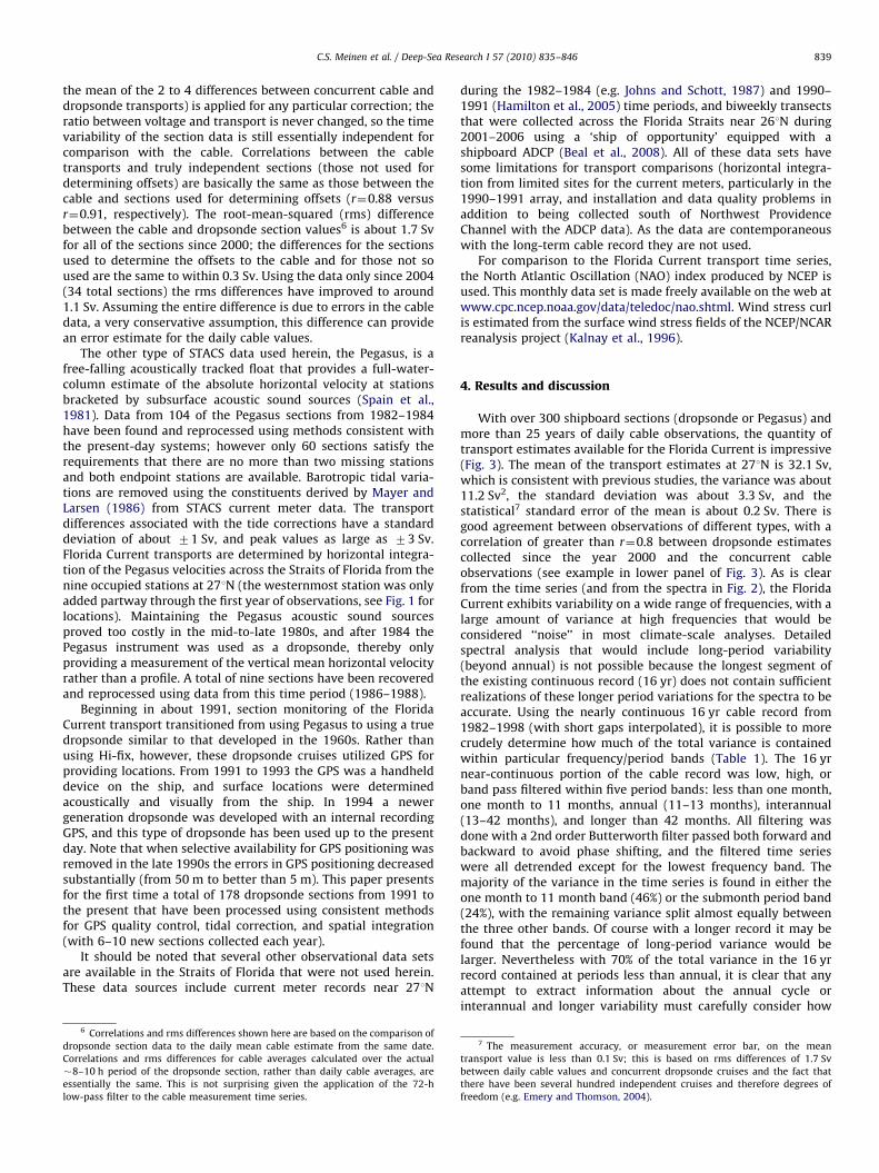
Fig. 2. Variance-preserving spectra of the Florida Current transport record from the submarine cable. The upper panel shows the color-coded segments of the cable record,

while the lower panel shows the spectra for the similarly colored segments. Cable record is broken into three segments, the first two segments were both processed by

Jimmy Larsen at PMEL using the methods described in Larsen (1992). The third segment was processed using the new automated system described in the text.

C.S. Meinen et al. / Deep-Sea Research I 57 (2010) 835–846838

Sanford, 1985; Larsen, 1992; Baringer and Larsen, 2001). The onlylarge gap occurred between 1998 and 2000 when funding for theproject was temporarily cut and the building where the recordingequipment was housed in West Palm Beach was closed. Thesecond largest gap occurred in September–October 2004 whenthe building housing the recording system at Eight Mile Rock wasseverely damaged by Hurricanes Frances and Jeanne. During thefirst 16 yr of this cable project the recording system transitionedfrom a paper tape recorder to a computer based recorder, and thedata were processed in a ‘research-mode’ that involved consider-able hand-editing to try to remove the tides as well as the largestof the magnetic-field fluctuations using magnetic observatorydata (Larsen, 1992). In the modern era (2000-present) the cable isnow part of the NOAA Western Boundary Time Series program,and the system has transitioned to a real-time system thatinvolves a computerized volt-meter that makes a measurementevery minute and an automated processing system involving athree-day lowpass filter with a 2nd order Butterworth filterpassed both forward and back for the removal of tides and themagnetic field variations. Both the ‘research-mode’ and ‘real-time’processing methods make a daily average of the minute data aspart of their processing. Comparison of the spectra of the dailycable data in eight year segments shows that differences in theresulting spectra between the modern (2000–2007) data and theearlier (1982–1998) data are smaller than the differencesbetween the spectra of the first and second half of the original16 yr record (Fig. 2)5. This suggests that the different processing

5 Note that the spectra for 1991–1998 demonstrates more high-frequency

energy (less than 10 days) than the periods before and after. The raw voltage data

from this time period has been lost (J. Larsen, personal communication), however

methods for different cable periods are not resulting inparticularly different spectra. Both the early records and themodern data have been daily averaged to provide means centeredon noon UTC. During the original STACS period the calibrationfactors for the linear relationship between voltage and transportfor this cable were determined using a series of 100+ Pegasusvelocity sections (see details below and Larsen, 1992), and thesecoefficients are used essentially ‘as is’ for evaluating both theolder Sanford (1982) data and for the modern era data.

It should also be noted that routine section validation isrequired for monitoring the performance and stability of the cablerecording equipment. The cable measurements are subject tospurious drifts and offsets when electrodes and wires decay andfail and when the recording systems have problems. Since 2000there has been roughly one problem with the system per year, allresulting in voltage step offsets except for one that was a voltagedrift due to a tiny break in a wire over two months. Each drift/offset problem has been traceable to a specific hardware problem.Many of these changes have been due to a failure in the recordingsystem itself (such as when it was destroyed by hurricanes in2004), and when these systems have been replaced small voltageoffsets (biases) have been observed. These offsets are caused bysmall but important differences from one voltmeter to the next,and the offsets are corrected using section data. Typically only thefirst 2–4 sections after any system change are used to determinethe offset. It must be stressed that only a constant offset (based on

(footnote continued)

it is known that during much of the 1991–1998 time period the cable being used

was simultaneously the active phone line and the telephone company was

applying an active voltage that previous research has indicated causes extra noise

in the voltage-to-transport conversion (Larsen, 1991).

ARTICLE IN PRESS

C.S. Meinen et al. / Deep-Sea Research I 57 (2010) 835–846 839

the mean of the 2 to 4 differences between concurrent cable anddropsonde transports) is applied for any particular correction; theratio between voltage and transport is never changed, so the timevariability of the section data is still essentially independent forcomparison with the cable. Correlations between the cabletransports and truly independent sections (those not used fordetermining offsets) are basically the same as those between thecable and sections used for determining offsets (r¼0.88 versusr¼0.91, respectively). The root-mean-squared (rms) differencebetween the cable and dropsonde section values6 is about 1.7 Svfor all of the sections since 2000; the differences for the sectionsused to determine the offsets to the cable and for those not soused are the same to within 0.3 Sv. Using the data only since 2004(34 total sections) the rms differences have improved to around1.1 Sv. Assuming the entire difference is due to errors in the cabledata, a very conservative assumption, this difference can providean error estimate for the daily cable values.

The other type of STACS data used herein, the Pegasus, is afree-falling acoustically tracked float that provides a full-water-column estimate of the absolute horizontal velocity at stationsbracketed by subsurface acoustic sound sources (Spain et al.,1981). Data from 104 of the Pegasus sections from 1982–1984have been found and reprocessed using methods consistent withthe present-day systems; however only 60 sections satisfy therequirements that there are no more than two missing stationsand both endpoint stations are available. Barotropic tidal varia-tions are removed using the constituents derived by Mayer andLarsen (1986) from STACS current meter data. The transportdifferences associated with the tide corrections have a standarddeviation of about 71 Sv, and peak values as large as 73 Sv.Florida Current transports are determined by horizontal integra-tion of the Pegasus velocities across the Straits of Florida from thenine occupied stations at 271N (the westernmost station was onlyadded partway through the first year of observations, see Fig. 1 forlocations). Maintaining the Pegasus acoustic sound sourcesproved too costly in the mid-to-late 1980s, and after 1984 thePegasus instrument was used as a dropsonde, thereby onlyproviding a measurement of the vertical mean horizontal velocityrather than a profile. A total of nine sections have been recoveredand reprocessed using data from this time period (1986–1988).

Beginning in about 1991, section monitoring of the FloridaCurrent transport transitioned from using Pegasus to using a truedropsonde similar to that developed in the 1960s. Rather thanusing Hi-fix, however, these dropsonde cruises utilized GPS forproviding locations. From 1991 to 1993 the GPS was a handhelddevice on the ship, and surface locations were determinedacoustically and visually from the ship. In 1994 a newergeneration dropsonde was developed with an internal recordingGPS, and this type of dropsonde has been used up to the presentday. Note that when selective availability for GPS positioning wasremoved in the late 1990s the errors in GPS positioning decreasedsubstantially (from 50 m to better than 5 m). This paper presentsfor the first time a total of 178 dropsonde sections from 1991 tothe present that have been processed using consistent methodsfor GPS quality control, tidal correction, and spatial integration(with 6–10 new sections collected each year).

It should be noted that several other observational data setsare available in the Straits of Florida that were not used herein.These data sources include current meter records near 271N

6 Correlations and rms differences shown here are based on the comparison of

dropsonde section data to the daily mean cable estimate from the same date.

Correlations and rms differences for cable averages calculated over the actual

�8–10 h period of the dropsonde section, rather than daily cable averages, are

essentially the same. This is not surprising given the application of the 72-h

low-pass filter to the cable measurement time series.

during the 1982–1984 (e.g. Johns and Schott, 1987) and 1990–1991 (Hamilton et al., 2005) time periods, and biweekly transectsthat were collected across the Florida Straits near 261N during2001–2006 using a ‘ship of opportunity’ equipped with ashipboard ADCP (Beal et al., 2008). All of these data sets havesome limitations for transport comparisons (horizontal integra-tion from limited sites for the current meters, particularly in the1990–1991 array, and installation and data quality problems inaddition to being collected south of Northwest ProvidenceChannel with the ADCP data). As the data are contemporaneouswith the long-term cable record they are not used.

For comparison to the Florida Current transport time series,the North Atlantic Oscillation (NAO) index produced by NCEP isused. This monthly data set is made freely available on the web atwww.cpc.ncep.noaa.gov/data/teledoc/nao.shtml. Wind stress curlis estimated from the surface wind stress fields of the NCEP/NCARreanalysis project (Kalnay et al., 1996).

4. Results and discussion

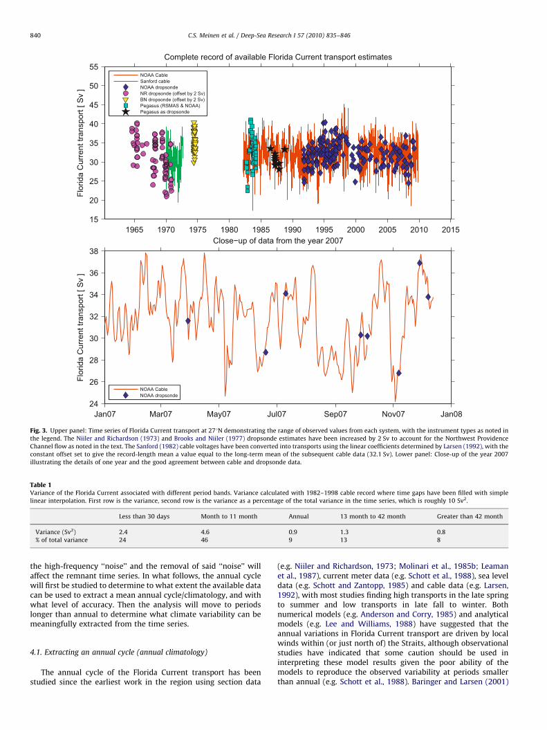
With over 300 shipboard sections (dropsonde or Pegasus) andmore than 25 years of daily cable observations, the quantity oftransport estimates available for the Florida Current is impressive(Fig. 3). The mean of the transport estimates at 271N is 32.1 Sv,which is consistent with previous studies, the variance was about11.2 Sv2, the standard deviation was about 3.3 Sv, and thestatistical7 standard error of the mean is about 0.2 Sv. There isgood agreement between observations of different types, with acorrelation of greater than r¼0.8 between dropsonde estimatescollected since the year 2000 and the concurrent cableobservations (see example in lower panel of Fig. 3). As is clearfrom the time series (and from the spectra in Fig. 2), the FloridaCurrent exhibits variability on a wide range of frequencies, with alarge amount of variance at high frequencies that would beconsidered ‘‘noise’’ in most climate-scale analyses. Detailedspectral analysis that would include long-period variability(beyond annual) is not possible because the longest segment ofthe existing continuous record (16 yr) does not contain sufficientrealizations of these longer period variations for the spectra to beaccurate. Using the nearly continuous 16 yr cable record from1982–1998 (with short gaps interpolated), it is possible to morecrudely determine how much of the total variance is containedwithin particular frequency/period bands (Table 1). The 16 yrnear-continuous portion of the cable record was low, high, orband pass filtered within five period bands: less than one month,one month to 11 months, annual (11–13 months), interannual(13–42 months), and longer than 42 months. All filtering wasdone with a 2nd order Butterworth filter passed both forward andbackward to avoid phase shifting, and the filtered time serieswere all detrended except for the lowest frequency band. Themajority of the variance in the time series is found in either theone month to 11 month band (46%) or the submonth period band(24%), with the remaining variance split almost equally betweenthe three other bands. Of course with a longer record it may befound that the percentage of long-period variance would belarger. Nevertheless with 70% of the total variance in the 16 yrrecord contained at periods less than annual, it is clear that anyattempt to extract information about the annual cycle orinterannual and longer variability must carefully consider how

7 The measurement accuracy, or measurement error bar, on the mean

transport value is less than 0.1 Sv; this is based on rms differences of 1.7 Sv

between daily cable values and concurrent dropsonde cruises and the fact that

there have been several hundred independent cruises and therefore degrees of

freedom (e.g. Emery and Thomson, 2004).

ARTICLE IN PRESS

1965 1970 1975 1980 1985 1990 1995 2000 2005 2010 2015

Flor

ida

Cur

rent

tran

spor

t [ S

v ]

Complete record of available Florida Current transport estimates

NOAA CableSanford cableNOAA dropsondeNR dropsonde (offset by 2 Sv)BN dropsonde (offset by 2 Sv)Pegasus (RSMAS & NOAA)Pegasus as dropsonde

Jan07 Mar07 May07 Jul07 Sep07 Nov07 Jan08

15

20

25

30

35

40

45

50

55

24

26

28

30

32

34

36

38

Flor

ida

Cur

rent

tran

spor

t [ S

v ]

Close−up of data from the year 2007

NOAA CableNOAA dropsonde

Fig. 3. Upper panel: Time series of Florida Current transport at 271N demonstrating the range of observed values from each system, with the instrument types as noted in

the legend. The Niiler and Richardson (1973) and Brooks and Niiler (1977) dropsonde estimates have been increased by 2 Sv to account for the Northwest Providence

Channel flow as noted in the text. The Sanford (1982) cable voltages have been converted into transports using the linear coefficients determined by Larsen (1992), with the

constant offset set to give the record-length mean a value equal to the long-term mean of the subsequent cable data (32.1 Sv). Lower panel: Close-up of the year 2007

illustrating the details of one year and the good agreement between cable and dropsonde data.

Table 1Variance of the Florida Current associated with different period bands. Variance calculated with 1982–1998 cable record where time gaps have been filled with simple

linear interpolation. First row is the variance, second row is the variance as a percentage of the total variance in the time series, which is roughly 10 Sv2.

Less than 30 days Month to 11 month Annual 13 month to 42 month Greater than 42 month

Variance (Sv2) 2.4 4.6 0.9 1.3 0.8

% of total variance 24 46 9 13 8

C.S. Meinen et al. / Deep-Sea Research I 57 (2010) 835–846840

the high-frequency ‘‘noise’’ and the removal of said ‘‘noise’’ willaffect the remnant time series. In what follows, the annual cyclewill first be studied to determine to what extent the available datacan be used to extract a mean annual cycle/climatology, and withwhat level of accuracy. Then the analysis will move to periodslonger than annual to determine what climate variability can bemeaningfully extracted from the time series.

4.1. Extracting an annual cycle (annual climatology)

The annual cycle of the Florida Current transport has beenstudied since the earliest work in the region using section data

(e.g. Niiler and Richardson, 1973; Molinari et al., 1985b; Leamanet al., 1987), current meter data (e.g. Schott et al., 1988), sea leveldata (e.g. Schott and Zantopp, 1985) and cable data (e.g. Larsen,1992), with most studies finding high transports in the late springto summer and low transports in late fall to winter. Bothnumerical models (e.g. Anderson and Corry, 1985) and analyticalmodels (e.g. Lee and Williams, 1988) have suggested that theannual variations in Florida Current transport are driven by localwinds within (or just north of) the Straits, although observationalstudies have indicated that some caution should be used ininterpreting these model results given the poor ability of themodels to reproduce the observed variability at periods smallerthan annual (e.g. Schott et al., 1988). Baringer and Larsen (2001)

ARTICLE IN PRESS

0 50 100 150 200 250 300 350 400−3

−2

−1

0

1

2

3

Yearday

Flor

ida

Cur

rent

tran

spor

t [ S

v ]

Annual cycle of the Florida Current transport during different periods

1982−20071982−19901991−19982000−2007

Fig. 4. Mean annual cycle/climatology of Florida Current transport determined

over different years as noted in the legend. Plotted values are daily averages for the

years noted (e.g. an average of all of the January 1st values, the January 2nd values,

etc., where the averaged daily values have been subsequently smoothed with a 30

day low-pass filter to remove the highest frequency ‘‘noise’’. Measurement error

bars on the 8 yr means would be about 0.2 Sv for reasonable estimates of the

integral time scale and 0.1 Sv for the 25 yr mean; statistical error bars will be

discussed shortly.

C.S. Meinen et al. / Deep-Sea Research I 57 (2010) 835–846 841

used cable observations of the Florida Current over the period1982–1998 to evaluate the stability of the annual cycle intransport. They found that there was a marked difference betweenthe annual cycle in the first half of the 16 yr window, when theFlorida Current appeared to exhibit a clear annual cycle, and thelatter half of the 16 yr window when the current variability wascharacterized more as a semi-annual cycle. Now that an additional8 yr of cable observations are available from 2000–2007 thepicture becomes even more confused, with the latter periodshowing a mean annual cycle that shows only a weak semi-annualcomponent and has the highest transport occurring 30–50 daysearlier than during the 1982–1990 window (Fig. 4). Since solarinput at the top of the atmosphere, the only significant externalforcing to the ocean–atmosphere system at the annual cycle, hasnot changed appreciably during this 25 year window, thesesignificant variations in mean annual cycle lead to questionsabout possible mechanisms which could be modulating theobserved annual cycle in Florida Current transport. Usingobservations and the results of a numerical model, a recentstudy has hypothesized that the variations in the form and phaseof the annual cycle may be related to changes in the North AtlanticOscillation and the associated wind pattern changes that go with it(Peng et al., 2009). Given the rather small measurement error barsthat would be associated with these 8 yr mean values8 it is clearthat the largest uncertainties in the various estimated annual cyclewould be the statistical accuracy (analogous to determining thestatistical standard error of the mean). Therefore before investingtoo much into a discussion of the mechanisms behind thesechanges, it is important to evaluate the statistical significance ofthis variability given the high percentage of the total variance that

8 The 1.1–1.7 Sv daily error bar discussed earlier would be reduced both due

to the 30-day lowpass filter applied to the annual climatologies and due to the

8–25 years that are averaged together. Based on some reasonable integral time

scale estimates of 3–10 days determined from the zeros in the autocorrelation

function (following the methods of Emery and Thomson, 2004) this yields

measurement accuracies of roughly 0.2 Sv for 8-year means and 0.1 Sv for 25-year

means.

exists at periods other than annual which may be aliased into anymean annual cycle/climatology determined from the data.

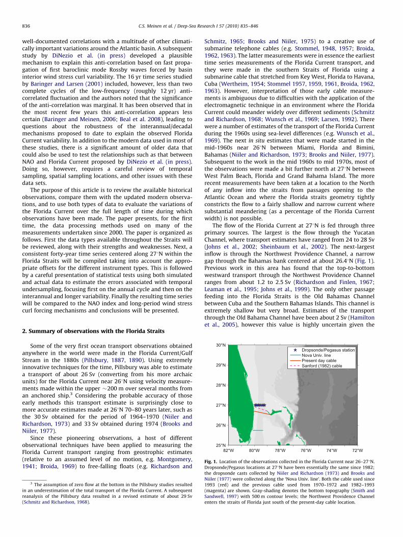
As noted earlier, about 70% of the total variance in the FloridaCurrent is found to have periods shorter than annual (coastallytrapped waves, etc.; e.g. Mooers et al., 2005), with about a quarterof the variance occurring at periods shorter than a month(Table 1). Baringer and Larsen (2001) showed that the strongestinterannual or longer transport variations that can be identified inthe 1982–1998 cable record have a period of roughly 10–12 years.Both this interannual-decadal variability and the high frequencyvariability (shorter than annual) can influence the accuracy withwhich the annual cycle can be determined. To evaluate the extentto which these other frequencies will pollute an estimate of theannual cycle/climatology, a Monte Carlo style approach was used.A simulated 100 year daily transport record was created as thesum of two sine waves (with annual and 12 year periods) andrandom noise. The amplitudes (standard deviation) of thesimulated annual cycle and the simulated 12 yr cycle were bothset to 1.0 Sv, consistent with the amplitudes determined from thereal cable observations. The amplitude of the random noise wasthen selected so that the standard deviation of the simulatedrecord equaled that of the true daily cable record (3.3 Sv). Therandom noise was added on a day-by-day basis, i.e. it has notemporal length scale beyond an individual day. Different spectraldistributions of the noise, ranging from white noise to progres-sively redder-spectra (spreading the noise evenly across 1–10days, 1–50 days, and 1–500 days), were tested; the effects weregenerally small, with wider spreads of noise generally havingerrors that were 0.05–0.30 Sv larger than those for the white noiseused in the simulated record.

The Monte Carlo style evaluation was done as follows. Take, forexample, the estimate for the statistical errors inherent indetermining a mean annual cycle using four years of data. Fouryears would be randomly selected from the 100 yr simulatedrecord, and a mean daily value for each day of the year would becalculated from the four years worth of ‘‘data’’. The differencesbetween the resulting mean daily values and the ‘true’ simulatedannual cycle (sine wave) was then calculated for the ‘‘raw’’ dailyvalues as well as for daily values that have been smoothed usingeither a 30 or 60 day low pass filter. These differences were thensaved and another random selection of four years was made andthe process was repeated. A total of 10,000 random subsets of fouryears would be made, and once this was done the root meansquared (rms) value of the complete data set of daily differenceswould be calculated for the raw, 30 day low pass filtered, and 60day low pass filtered annual mean records. This process wascompleted for random selections of one, two, four, six, eight, 10,15, 20, 25, and 30 years (Fig. 5). This analysis indicates that anannual cycle/climatology determined using roughly 8 years (aswas done by Baringer and Larsen, 2001), would have a statisticalerror bar of 0.4 Sv on each daily value simply due to the statistical‘‘noise’’ from the higher and lower frequencies in the record (thesevalues are nearly a factor of 2 larger than the measurement errorbars). For a roughly 25 yr record, the daily statistical error bar is0.2 Sv (again roughly a factor of 2 larger than the measurementerror bars). While these seem like fairly small values, keep inmind that the standard deviation of the simulated annual cycle(which is based on the true cable-derived annual cycle) is onlyabout 1.0 Sv, so a statistical error bar of 0.4 Sv is a 40% error bar onan annual climatology determined using only eight years of data.Applying these error bars to the annual cycles shown in Fig. 4 andlooking at the observed differences, it is found that about 32% ofthe daily values in the annual climatologies determined usingonly eight years of data are further than ‘‘one standard error’’ level(or a 67% confidence limit) from the annual cycle determinedusing 25 years of data. Therefore these statistical estimations

ARTICLE IN PRESS

0 5 10 15 20 25 30 35 40 45 50 55 60 65 70 75 80 85 90 95 100−10

−8

−6

−4

−2

0

2

4

6

8

10

Tran

spor

t [ S

v ]

Time [ years ]

Simulated 100−year time series of transport

Simulated time series: STD=3.4 SvAnnual component: STD=1.0 SvInterannual component: STD=1.0 Sv

0 5 10 15 20 25 30 35 40 45 50 55 60 65 70 75 80 85 90 95 1000

0.5

1

1.5

2

2.5

3

3.5

Number of years of data used in creating estimated annual mean

RM

S e

rror

[ S

v ]

Monte Carlo 100 repeat sample: RMS error between estimated and true annual means

Error using raw daily valuesError using 30−day lowpass filterError using 60−day lowpass filter

Fig. 5. Simulated 100 yr record in transport used in the Monte Carlo style estimation of the errors inherent in determining a mean annual cycle/climatology from a record

where the annual variance is a small percentage of the total. Upper panel shows the simulated cable record (black) along with the annual (blue) and interannual/decadal

(red) cycles upon which the simulated record was built. Lower panel shows the root-mean-squared (RMS) difference between the true daily annual mean values and those

estimated using the indicated number of years worth of data from the simulated cable record. The different colors and symbols in the lower panel denote either the raw,

30 day, or 60 day low pass filtering that was applied to the data before determining the differences from the true annual cycle.

C.S. Meinen et al. / Deep-Sea Research I 57 (2010) 835–846842

suggest that the differences in the annual cycles over the 1982–1990, 1991–1998, and 2000–2007 time periods are not differentfrom one another in a statistically meaningful way. This of coursedoes not mean that there is not a modulation of the annual cycleoccurring as was suggested by Baringer and Larsen, (2001) andPeng et al. (2009), only that given the limited data presentlyavailable the differences between the annual cycles determinedusing subsets of the past 25 years are of marginal statisticalsignificance and will require additional data for confirmation.

4.2. Extracting longer time scales from the data

Recalling that the percentage of variance at periods less than42 months is more than 90%, aliasing of the other frequencies intothe decadal band is also a problem given the short record. Asnoted previously, the largest fluctuation that can be identified atperiods beyond a year or two is a quasi-decadal fluctuation with aperiod of roughly 12 years observed by Baringer and Larsen(2001) from the 1982–1998 cable data that was shown to be anti-correlated to variations in the North Atlantic Oscillation (NAO).DiNezio et al. (in press) further illustrated this anti-correlationusing wavelet analyses over the period 1982–2007 and showedthat the wind stress curl and the NAO were out of phase.9 They

9 Note that although not expanded upon in detail in that study, the results of

DiNezio et al. (2009) agree with previous research by Baringer and Meinen (2006)

proposed a physical mechanism using faster-than-linear wavepropagation speeds for first baroclinic Rossby waves that couldexplain a significant fraction of the variability in the FloridaCurrent on these time scales (DiNezio et al., 2009). The challengeof analyzing the Florida Current variability at these timescales, however, as was noted in earlier studies such as Sturgesand Hong (1995), is that even with a roughly 25 year record,at most two realizations of the cycle would be captured in thenear-continuous record.

In order to expand the available time series beyond the near-continuous daily time period (1982–2007), most studies ofinterannual to decadal variability have focused on using monthly,annual or biannual mean transports for the Florida Current (e.g.Baringer and Larsen, 2001). As with the annual cycle studies, it isimportant to analyze the accuracy to which these means can becalculated with sparse data when the continuous cable recordsare not available (e.g. see 1964–1982 and 1998–2000 in Fig. 3).This Monte Carlo style analysis was done similarly to that used forthe annual cycle, however the actual cable data from the nearlycontinuous 1982–1998 period was used for estimating the errorsin monthly, annual, three-year and five-year means rather than asimulated time series. For the monthly averaging, a randommonth of data was selected from the cable record, and then a

(footnote continued)

and Beal et al. (2008) showing that the relationship between the NAO and the

Florida Current transport is less evident in the most recent few years.

ARTICLE IN PRESS

0 20 40 60 80 100 120 140 160 180 2000

0.20.40.60.8

11.21.41.61.8

22.22.42.62.8

33.23.4

Number of days averaged

RM

S tr

ansp

ort e

rror

[ S

v ]

Monte Carlo 10000−sample simulation

Monthly transport errorYearly transport error3−year transport error5−year transport error

Fig. 6. Monte Carlo style estimates of the root-mean-square (RMS) error in

estimating monthly, annual, three-year, and five-year means with only the

indicated number of samples. Monthly estimates were made for one, two, five,

eight, 10, and 20 days from the month, while annual, three-year, and five-year

estimates were made with one, two, five, eight, 10, 20, 30, 40, 50, 100, and 200

days from each time window. The Monte Carlo style simulation was run for 10,000

random selections at each sample level. Note this error bar assumes a random

distribution of days throughout the time window; errors would be larger if the

distribution is not random (e.g. all data were collected in January and February

when trying to estimate an annual mean).

C.S. Meinen et al. / Deep-Sea Research I 57 (2010) 835–846 843

randomly selected number of daily observations from that month(ranging from one to 20) were averaged and the differencebetween that average and the ‘true’ average of the complete set ofdaily values from that month was determined. The analogousprocedure was used for annual, three and five year means. Theresults (shown in Fig. 6) suggest that in order to obtain a monthlymean value that is accurate to better than 0.5 Sv (one standarderror, or 67% confidence level) at least 20 daily values from thatmonth are required. In order to obtain an estimate of the annualmean transport of the Florida Current that is accurate to betterthan 0.5 Sv more than 40 observations are required in that year.Furthermore, these results presume that the observations wererandomly spread throughout the year. If observations wereclustered within one part of the annual cycle (as often occurredin the early portion of the record, e.g. all of the 1974 observationsare in May–August when the annual cycle is nearing its peak)then the difference between the mean of those observations andthe true annual mean could be larger because the annual cyclewill be inadequately sampled by the observations.

This analysis does not suggest that the sparser data sets suchas the dropsonde data in the 1960s and early 1970s cannot beused, it simply illustrates that monthly, annual, and multi-yearmean estimates from the sparser data must be accompanied bylarger error bars associated with the undersampling of the higherfrequency variability in the Florida Current transport. For thestudy presented here, when annual means were based onobservations that spanned less than six months of a particularyear, the error bar on that annual mean was increased by thestandard deviation of the annual cycle (1.0 Sv) in a square-root ofthe sum of the squares manner (i.e. the annual cycle error and the

undersampling error are treated as independent of one another).For three and five year means, a similar sort of error can resultdepending on how many of the three or five years were sampled(for example, if a three-year average of 1981–1983 is desired butno data is available for 1981, then this three-year average willhave an error associated with this). This final source of error wasalso evaluated using a similar Monte Carlo style technique and theassociated errors were included in this analysis.

4.3. Relating Florida Current transport variations to other climate

variability

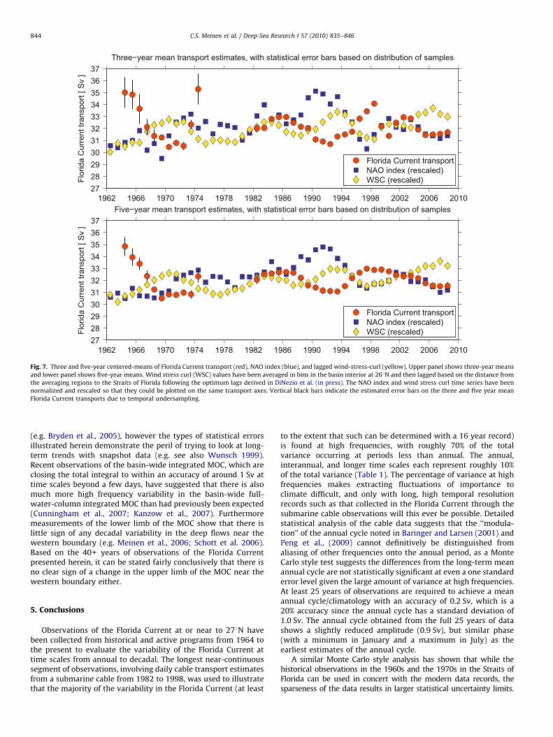
The anti-correlation between the NAO index and the FloridaCurrent transport discussed by Baringer and Larsen (2001) basedon the 1982–1998 record can be seen by focusing in particular onthe 1986–1998 time period in the three and five year meanrecords (Fig. 7). The maximum correlation between FloridaCurrent transport and NAO index over the 1982–1998window is a negative correlation with the NAO leading theFlorida Current by one year; for the three (five) year centeredmeans the peak correlation is roughly –0.5 (–0.6), howeverthe lag-correlation peak is fairly broad. This lag between the NAOand the Florida Current is similar to some earlier resultsdownstream of the Straits of Florida showing that the NAOleads Gulf Stream meridional shifts (the latter estimated fromTOPEX altimetry data) by about a year during the similar periodfrom 1992–1998 (Frankignoul et al. 2001), although a longerrepeat bathythermograph dataset evaluated by Molinari (2004)showed little evidence for a lag between NAO and Gulf Streammeridional position over the longer 1950–2003 time period.During the 1982–1998 period the wind stress curl time series,which has been lagged from three boxes in the interior near271N based on the faster-than-linear group speeds derived byDiNezio et al. (2009), shows a high degree of positive correlationwith variations in the NAO. The basic mechanism is that NAOvariations cause changes to the interior basin wind stress curlfield, and these wind stress curl variations force Rossby wavesthat propagate westward and result in changes in the FloridaCurrent transport. The DiNezio et al. (2009) study demonstratedthat the observations during 1982–2007 are consistent with thisbasic mechanism (although the relationship is weaker after 2000)and they determined that the necessary increase in first baroclinicmode group speeds required to explain the observed variability isconsistent with previous observations from altimetry and in situobservations.

Looking outside the 1982–1998 window the marginallysignificant anti-correlation between Florida Current transportand the NAO does not appear to hold. As noted by Baringer andMeinen (2006) and Beal et al. (2008) there is little evidence of ananti-correlation in the most recent years, and before about 1984(Fig. 7) even considering the large error bars it is clear from thedata presented herein that there little sign that the NAO andFlorida Current transport are correlated. The lack of correlationbetween the NAO and the Florida Current in the time periodsoutside 1984–1998, and the lack of correlation between the windstress curl and the NAO, suggests that the anti-correlation foundby Baringer and Larsen (2001) may have simply been fortuitousand that the mechanism proposed by DiNezio et al. (in press) maybe only one of several mechanisms that can result in interannualand longer variability in the Florida Current.

The Meridional Overturning Circulation (MOC) upper limb isflowing through the Florida Current, so it is logical to expect thatdecadal variability in the MOC may also be impacting the FloridaCurrent. There has been some speculation that the MOC isundergoing significant variability over the past few decades

ARTICLE IN PRESS

1962 1966 1970 1974 1978 1982 1986 1990 1994 1998 2002 2006 2010

Flor

ida

Cur

rent

tran

spor

t [ S

v ]

Three−year mean transport estimates, with statistical error bars based on distribution of samples

Florida Current transportNAO index (rescaled)WSC (rescaled)

1962 1966 1970 1974 1978 1982 1986 1990 1994 1998 2002 2006 2010

2728293031323334353637

2728293031323334353637

Flor

ida

Cur

rent

tran

spor

t [ S

v ]

Five−year mean transport estimates, with statistical error bars based on distribution of samples

Florida Current transportNAO index (rescaled)WSC (rescaled)

Fig. 7. Three and five-year centered-means of Florida Current transport (red), NAO index (blue), and lagged wind-stress-curl (yellow). Upper panel shows three-year means

and lower panel shows five-year means. Wind stress curl (WSC) values have been averaged in bins in the basin interior at 261N and then lagged based on the distance from

the averaging regions to the Straits of Florida following the optimum lags derived in DiNezio et al. (in press). The NAO index and wind stress curl time series have been

normalized and rescaled so that they could be plotted on the same transport axes. Vertical black bars indicate the estimated error bars on the three and five year mean

Florida Current transports due to temporal undersampling.

C.S. Meinen et al. / Deep-Sea Research I 57 (2010) 835–846844

(e.g. Bryden et al., 2005), however the types of statistical errorsillustrated herein demonstrate the peril of trying to look at long-term trends with snapshot data (e.g. see also Wunsch 1999).Recent observations of the basin-wide integrated MOC, which areclosing the total integral to within an accuracy of around 1 Sv attime scales beyond a few days, have suggested that there is alsomuch more high frequency variability in the basin-wide full-water-column integrated MOC than had previously been expected(Cunningham et al., 2007; Kanzow et al., 2007). Furthermoremeasurements of the lower limb of the MOC show that there islittle sign of any decadal variability in the deep flows near thewestern boundary (e.g. Meinen et al., 2006; Schott et al. 2006).Based on the 40+ years of observations of the Florida Currentpresented herein, it can be stated fairly conclusively that there isno clear sign of a change in the upper limb of the MOC near thewestern boundary either.

5. Conclusions

Observations of the Florida Current at or near to 271N havebeen collected from historical and active programs from 1964 tothe present to evaluate the variability of the Florida Current attime scales from annual to decadal. The longest near-continuoussegment of observations, involving daily cable transport estimatesfrom a submarine cable from 1982 to 1998, was used to illustratethat the majority of the variability in the Florida Current (at least

to the extent that such can be determined with a 16 year record)is found at high frequencies, with roughly 70% of the totalvariance occurring at periods less than annual. The annual,interannual, and longer time scales each represent roughly 10%of the total variance (Table 1). The percentage of variance at highfrequencies makes extracting fluctuations of importance toclimate difficult, and only with long, high temporal resolutionrecords such as that collected in the Florida Current through thesubmarine cable observations will this ever be possible. Detailedstatistical analysis of the cable data suggests that the ‘‘modula-tion’’ of the annual cycle noted in Baringer and Larsen (2001) andPeng et al., (2009) cannot definitively be distinguished fromaliasing of other frequencies onto the annual period, as a MonteCarlo style test suggests the differences from the long-term meanannual cycle are not statistically significant at even a one standarderror level given the large amount of variance at high frequencies.At least 25 years of observations are required to achieve a meanannual cycle/climatology with an accuracy of 0.2 Sv, which is a20% accuracy since the annual cycle has a standard deviation of1.0 Sv. The annual cycle obtained from the full 25 years of datashows a slightly reduced amplitude (0.9 Sv), but similar phase(with a minimum in January and a maximum in July) as theearliest estimates of the annual cycle.

A similar Monte Carlo style analysis has shown that while thehistorical observations in the 1960s and the 1970s in the Straits ofFlorida can be used in concert with the modern data records, thesparseness of the data results in larger statistical uncertainty limits.

ARTICLE IN PRESS

C.S. Meinen et al. / Deep-Sea Research I 57 (2010) 835–846 845

To achieve an annual mean estimate of the Florida Current transportthat is accurate to within 0.5 Sv more than 40 daily estimates arerequired. Similar numbers of observations are needed to determinethree and five year means of the Florida Current transport. Note all ofthese estimates presume that the observations are randomly spreadthroughout the year (or 3-year span, or 5-year span). If theobservations are clustered in a small subset of the averaging windowthe errors can be considerably larger. Nevertheless, despite the largeerror bars which must be placed on the early data records, it can beshown that the relationship between the North Atlantic Oscillationand the Florida Current first discussed in Baringer and Larsen (2001)and expanded upon by Peng et al. (2009) is not consistent over time.During the time window from 1984 to 1998 there is an anti-correlation between the two time series, but outside of that windowthere is no such clear relation.10 The sporadic nature of therelationship between the North Atlantic Oscillation, the wind stressfields and the Florida Current transport likely reflects the fact that theFlorida Current plays a role both in the wind driven horizontal‘‘Sverdrup’’ gyre and the thermohaline vertical gyre associated withthe Meridional Overturning Circulation. The data shown hereinprovide no evidence for a long-term trend in the Florida Currenttransport, and the variability that does exist on decadal time scales isgenerally quite small (order 1 Sv during 1982–2007). Perhaps themost interesting inference from this analysis, however, is that thereis an absolute necessity for measuring the components of the MOCboth continuously in time (i.e. not with snapshot sections) and forlong periods of time (i.e. not for just a few years) if there is any hopeof extracting the true long-period variability of the ocean circulation.

Acknowledgements

The authors of this paper want to point out that research suchas that discussed herein can only be done through the good willand dedicated work of many generations of scientists. As such, wewould like to share our thanks with the many fine researcherswho collected, processed, and published this data over the past40+ years. Particular thanks are made to Jimmy Larsen, RobertMolinari and Fritz Schott, who provided significant help in findingand making sense of historical data sets from the Florida Straits.Helpful conversations with Bill Johns, Tom Sanford, and TonySturges on these topics are also gratefully acknowledged. RobertMolinari and the anonymous reviewers also provided a number ofvery helpful suggestions for improving an earlier draft of thismanuscript. This work is supported through the WesternBoundary Time Series project, which is funded through the NOAAOffice of Climate Observations. The Florida Current data are madefreely available by AOML Physical Oceanography Division atwww.aoml.noaa.gov/phod/floridacurrent through funding fromthe NOAA Office of Climate Observations.

References

Alvarez-Garcia, F., Latif, M., Biastoch, A., 2008. On multidecadal and quasi-decadalNorth Atlantic variability. J. Clim. 21 (14), 3433–3452, doi:10.1175/2007JCLI1800.1.

Anderson, D.L.T., Corry, R.A., 1985. Seasonal transport variations in the FloridaStraits: a model study. J. Phys. Oceanogr. 15 (6), 773–786.

Baringer, M.O., Larsen, J.C., 2001. Sixteen years of Florida Current transport at271N. Geophys. Res. Lett. 28 (16), 3179–3182.

Baringer, M.O., Meinen, C.S., 2006. Thermohaline circulation, in State of theClimate in 2005Bull. Am. Met. Soc. 87 (6), s1–s102, doi:10.1175/BAMS-87-6-shein.

10 This is also evident in the most recent few years in the wavelet analyses of

DiNezio et al., 2009, although they did not evaluate the signals before 1982. The

lack of correlation in recent years was also noted by Baringer and Meinen (2006)

and by Beal et al. (2008).

Beal, L.M., Hummon, J.M., Williams, E., Brown, O., Baringer, W., Kearns, E., 2008.Five years of Florida Current structure and transport from the royal caribbeancruise ship Explorer of the Seas. J. Geophys. Res., doi:10.1029/2007JC004154.

Broida, S., 1962. Florida Straits transports: April 1960–January 1961. Bull. Mar. Sci.Gulf Carib. 12, 168.

Broida, S., 1963. Florida Straits transports: May 1961–September 1961. Bull. Mar.Sci. Gulf Carib. 13, 58.

Broida, S., 1969. Geostrophy and direct measurements in the Straits of Florida.J. Mar. Res. 27 (3), 278–292.

Brooks, I.H., Niiler, P.P., 1975. The Florida Current at Key West: summer 1972.J. Mar. Res. 33 (1), 83–92.

Brooks, I.H., Niiler, P.P., 1977. Energetics of the Florida Current. J. Mar. Res. 35 (1),163–191.

Bryden, H.L., Longworth, H.R., Cunningham, S.A., 2005. Slowing of the AtlanticMeridional Overturning Circulation at 251N. Nature 438, 655–657.

Cunningham, S.A., Kanzow, T., Rayner, D., Baringer, M.O., Johns, W.E., Marotzke, J.,Longworth, H.R., Grant, E.M., Hirschi, J.J.-M., Beal, L.M., Meinen, C.S.,Bryden, H.L., 2007. Temporal variability of the Atlantic Meridional OverturningCirculation at 26.51N. Science 317, 935, doi:10.1126/science.1141304.

DiNezio, P.N., Gramer, L.J., Johns, W.E., Meinen, C.S., Baringer, M.O., 2009. Observedinterannual variability of the Florida Current: wind forcing and the NorthAtlantic Oscillation, J. Phys. Oceanogr. 39 (3), 721–736, doi: 10.1175/2008JPO4001.1.

Emery, W.J., Thomson, R.E., 2004. Data Analysis Methods in Physical Oceano-graphy. Elsevier, Amsterdam 638pp.

Frankignoul, C., de Coetlogon, G., Joyce, T.M., Dong, S., 2001. Gulf Stream variabilityand ocean–atmosphere interactions. J. Phys. Oceanogr. 31 (12), 3516–3529.

Hamilton, P., Larsen, J.C., Leaman, K.D., Lee, T.N., Waddell, E., 2005. Transportsthrough the Straits of Florida. J. Phys. Oceanogr. 35 (3), 308–322.

Johns, E., Wilson, W.D., Molinari, R.L., 1999. Direct observations of velocity andtransport in the passages between the Intra-Americas Sea and the AtlanticOcean, 1984–1996. J. Geophys. Res. 104 (C11), 25805–25820.

Johns, W.E., Schott, F., 1987. Meandering and transport variations of the FloridaCurrent. J. Phys. Oceanogr. 17 (8), 1128–1147.

Johns, W.E., Townsend, T.L., Fratantoni, D.M., Wilson, W.D., 2002. On the Atlanticinflow to the Caribbean Sea. Deep Sea Res. I 49, 211–243.

Kanzow, T., Cunningham, S.A., Rayner, D., Hirschi, J.J.-M., Johns, W.E., Baringer,M.O., Bryden, H.L., Beal, L.M., Meinen, C.S., Marotzke, J., 2007. Observed flowcompensation associated with the meridional overturning at 26.51N in theAtlantic. Science 317, 938, doi:10.1126/science.1141293.

Kalnay, E., Kanamitsu, M., Kistler, R., Collins, W., Deaven, D., Gandin, L., Iredell, M.,Saha, S., White, G., Woollen, J., Zhu, Y., Leetmaa, A., Reynolds, B., Chelliah, M.,Ebisuzaki, W., Higgins, W., Janowiak, J., Mo, K.C., Ropelewski, C., Wang, J.,Jenne, R., Joseph, D., 1996. The NCEP/NCAR 40-year reanalysis project. Bull.Am. Meteor. Soc. 77 (3), 437–470.

Larsen, J.C., Sanford, T.B., 1985. Florida Current volume transports from voltagemeasurements. Science 227, 302–304.

Larsen, J.C., 1991. Transport measurements from in-service undersea telephonecables. IEEE J. Oceanic Eng. 16 (4), 313–318.

Larsen, J.C., 1992. Transport and heat flux of the Florida Current at 271N derivedfrom cross-stream voltages and profiling data: theory and observations. Phil.Trans. R. Soc. Lond. A 338, 169–236.

Leaman, K.D., Molinari, R.L., Vertes, P.S., 1987. Structure and variability of theFlorida Current at 271N: April 1982–July 1984. J. Phys. Oceanogr. 17 (5),565–583.

Leaman, K.D., Vertes, P.S., Atkinson, L.P., Lee, T.N., Hamilton, P., Waddell, E., 1995.Transport, potential vorticity, and current/temperature structure acrossNorthwest Providence and Santaren Channels and the Florida Current offCay Sal Bank. J. Geophys. Res. 100 (C5), 8561–8569.

Lee, T.N., Schott, F.A., Zantopp, R., 1985. Florida Current: low-frequency variabilityas observed with moored current meters during April 1982 to June 1983.Science 227, 298–302.

Lee, T.N., Williams, E., 1988. Wind-forced transport fluctuations of the FloridaCurrent. J. Phys. Oceanogr. 18 (7), 937–946.

Luther, D.S., Filloux, J.H., Chave, A.D., 1991. Low-frequency, motionally inducedelectromagnetic fields in the ocean 2. Electric field and Eulerian currentcomparison. J. Geophys. Res. 96 (C7), 12797–12814.

Mayer, D.A., Larsen, J.C., 1986. Tidal transport in the Florida Currentand its relationship to tidal heights and cable voltages. J. Phys. Oceanogr. 16,2199–2202.

Meinen, C.S., Baringer, M.O., Garzoli, S.L., 2006. Variability in Deep WesternBoundary Current transports: preliminary results from 26.51N in the Atlantic.Geophys. Res. Lett. 33, L17610, doi:10.1029/2006GL026965.

Molinari, R.L., Maul, G.A., Chew, F., Wilson, W.D., Bushnell, M., Mayer, D., Leaman,K., Schott, F., Lee, T., Zantopp, R., Larsen, J.C., Sanford, T.B., 1985a. SubtropicalAtlantic Climate studies: introduction. Science 227, 292–295.

Molinari, R.L., Wilson, W.D., Leaman, K., 1985b. Volume and heat transportsof the Florida Current: April 1982 through August 1983. Science 227,295–297.

Molinari, R.L., 1986. Subtropical Atlantic climate studies (STACS) revisited. EOS 67(5), 59–60.

Molinari, R.L., 2004. Annual and decadal variability in the western subtropicalNorth Atlantic: signal characteristics and sampling methodologies. Prog.Oceanogr. 62, 33–66.

Montgomery, R.B., 1941. Transport of the Florida Current off habana. J. Mar. Res. 4(3), 198–220.

ARTICLE IN PRESS

C.S. Meinen et al. / Deep-Sea Research I 57 (2010) 835–846846

Mooers, C.N.K., Meinen, C.S., Baringer, M.O., Bang, I., Rhodes, R., Barron, C.N., Bub,F., 2005. Cross validating ocean prediction and monitoring systems. EOS 86(29), 272–273.

Niiler, P.P., Richardson, W.S., 1973. Seasonal variability of the Florida Current.J. Mar. Res. 31, 144–167.

Peng, G., Garraffo, Z., Halliwell, G.R., Smedstad, O.-M., Meinen, C.S., Kourafalou, V.,Hogan, P., 2009. Temporal variability of the Florida Current transport at 271N.In: Columbus, F. (Ed.), Ocean Circulation and El Nino: The New Research.NOVA Science Publishers, Hauppauge, NY in press.

Pillsbury, J.E., 1887. Gulf Stream Explorations – Observations of Currents – 1887.Rept. Supt., US Coast Geod. Surv., Appendix 8, 173–184.

Pillsbury, J.E., 1890. The Gulf Stream—a description of the methods employed inthe investigation, and the results of the research. Rept. Supt., US Coast Geod.Surv., Appendix 10, 461–620.

Richardson, W.S., Finlen, J.R., 1967. The transport of Northwest ProvidenceChannel. Deep Sea Res. 14, 361–367.

Richardson, W.S., Schmitz Jr., W.J., 1965. A technique for the direct measurementof transport with application to the Straits of Florida. J. Mar. Res. 23,172–185.

Sanford, T.B., 1982. Temperature transport and motional induction in the FloridaCurrent. J. Mar. Res. 40 (Suppl.), 621–639.

Schmitz Jr., W.J., Richardson, W.S., 1968. On the transport of the Florida Current.Deep Sea Res. 15, 679–693.

Schott, F., Zantopp, R., 1985. Florida Current: seasonal and interannual variability.Science 227 (4684), 308–311.

Schott, F.A., Lee, T.N., Zantopp, R., 1988. Variability of structure and transport ofthe Florida Current in the period range of days to seasonal. J. Phys. Oceanogr.18 (9), 1209–1230.

Schott, F.A., Fischer, J., Dengler, M., Zantopp, R., 2006. Variability of the deepwestern boundary current east of the grand banks. Geophys. Res. Lett. 33,L21S07, doi:10.1029/2006GL026563.

Sheinbaum, J., Candela, J., Badan, A., Ochoa, J., 2002. Flow structure and transportin the Yucatan Channel. Geophys. Res. Lett. 29 (3), 1040, doi:10.1029/2001GL013990.

Smith, W.H.F., Sandwell, D.T., 1997. Global Sea floor topography from satellitealtimetry and ship depth soundings. Science 277 (5334), 1956–1962.

Spain, P.F., Dorson, D.L., Rossby, H.T., 1981. PEGASUS: a simple, acousticallytracked, velocity profiler. Deep Sea Res. 28A, 1553–1567.

Stommel, H., 1948. The theory of the electric field induced in deep ocean currents.J. Mar. Res. 7, 386–392.

Stommel, H., 1957. Florida Straits transports: 1952–1956. Bull. Mar. Sci. Gulf Carib.7, 252–254.

Stommel, H., 1959. Florida Straits transports: June 1956–July 1958. Bull. Mar. Sci.Gulf Carib. 9, 222–223.

Stommel, H., 1961. Florida straits transports: July 1958–March 1959. Bull. Mar. Sci.Gulf Carib. 11, 318.

Sturges, W., Hong, B.G., 1995. Wind forcing of the Atlantic thermocline along 321Nat low frequencies. J. Phys. Oceanogr. 25, 1706–1715.

von Storch, J.-S., and H. Haak, Impact of daily fluctuations on long-termpredictability of the Atlantic Meridional Overturning Circulation, Geophys.Res. Lett., 35, L01609, 10.1029/2007GL032385, 2008.

Wertheim, G.K., 1954. Studies of the electric potential between Key West, Florida,and Havana, Cuba. Trans. Am. Geophys. U. 35, 872–882.

Wunsch, C., Hansen, D.V., Zetler, B.D., 1969. Fluctuations of the Florida Currentinferred from sea level records. Deep Sea Res., Suppl. 16, 447–470.

Wunsch, C., 1999. The interpretation of short climate records, with comments on theNorth Atlantic and Southern Oscillations. Bull. Am. Met. Soc. 80 (2), 245–255.