FloEFDTM for CATIA - Mentor Graphicss3.mentor.com/mechanical/floefd-demoguide.pdf · FloEFD is a...
98
Rev. 09032013 FloEFD TM for CATIA Demonstration Version Guide Software Version 13 © 2013 Mentor Graphics Corporation All rights reserved. This document contains information that is proprietary to Mentor Graphics Corporation. The original recipient of this document may duplicate this document in whole or in part for internal business purposes only, provided that this entire notice appears in all copies. In duplicating any part of this document, the recipient agrees to make every reasonable effort to prevent the unauthorized use and distribution of the proprietary information.
Transcript of FloEFDTM for CATIA - Mentor Graphicss3.mentor.com/mechanical/floefd-demoguide.pdf · FloEFD is a...

Rev. 09032013
FloEFDTM for CATIADemonstration Version Guide
Software Version 13
© 2013 Mentor Graphics CorporationAll rights reserved.
This document contains information that is proprietary to Mentor Graphics Corporation. The original recipient of thisdocument may duplicate this document in whole or in part for internal business purposes only, provided that this entirenotice appears in all copies. In duplicating any part of this document, the recipient agrees to make every reasonable effortto prevent the unauthorized use and distribution of the proprietary information.

This document is for information and instruction purposes. Mentor Graphics reserves the right to make changes in specifications and other information contained in this publication without prior notice, and the reader should, in all cases, consult Mentor Graphics to determine whether any changes have been made.
The terms and conditions governing the sale and licensing of Mentor Graphics products are set forth in written agreements between Mentor Graphics and its customers. No representation or other affirmation of fact contained in this publication shall be deemed to be a warranty or give rise to any liability of Mentor Graphics whatsoever.
MENTOR GRAPHICS MAKES NO WARRANTY OF ANY KIND WITH REGARD TO THIS MATERIAL INCLUDING, BUT NOT LIMITED TO, THE IMPLIED WARRANTIES OF MERCHANTABILITY AND FITNESS FOR A PARTICULAR PURPOSE.
MENTOR GRAPHICS SHALL NOT BE LIABLE FOR ANY INCIDENTAL, INDIRECT, SPECIAL, OR CONSEQUENTIAL DAMAGES WHATSOEVER (INCLUDING BUT NOT LIMITED TO LOST PROFITS) ARISING OUT OF OR RELATED TO THIS PUBLICATION OR THE INFORMATION CONTAINED IN IT, EVEN IF MENTOR GRAPHICS CORPORATION HAS BEEN ADVISED OF THE POSSIBILITY OF SUCH DAMAGES.
RESTRICTED RIGHTS LEGEND 03/97
U.S. Government Restricted Rights. The SOFTWARE and documentation have been developed entirely at private expense and are commercial computer software provided with restricted rights. Use, duplication or disclosure by the U.S. Government or a U.S. Government subcontractor is subject to the restrictions set forth in the license agreement provided with the software pursuant to DFARS 227.7202-3(a) or as set forth in subparagraph (c)(1) and (2) of the Commercial Computer Software - Restricted Rights clause at FAR 52.227-19, as applicable.
Contractor/manufacturer is:Mentor Graphics Corporation
8005 S.W. Boeckman Road, Wilsonville, Oregon 97070-7777.Telephone: 503.685.7000
Toll-Free Telephone: 800.592.2210Website: www.mentor.com
SupportNet: supportnet.mentor.com/Send Feedback on Documentation: supportnet.mentor.com/doc_feedback_form
TRADEMARKS: The trademarks, logos and service marks ("Marks") used herein are the property of Mentor Graphics Corporation or other third parties. No one is permitted to use these Marks without the prior written consent of Mentor Graphics or the respective third-party owner. The use herein of a third-party Mark is not an attempt to indicate Mentor Graphics as a source of a product, but is intended to indicate a product from, or associated with, a particular third party. A current list of Mentor Graphics’ trademarks may be viewed at: www.mentor.com/trademarks.

Contents
Overview . . . . . . . . . . . . . . . . . . . . . . . . . . . . . . . . . . . . . . . . . . . . . 1-1
Limitations of the Demonstration Version . . . . . . . . . . . . . . . . . . . . . 2-1
Tutorial 1 - Gate Valve . . . . . . . . . . . . . . . . . . . . . . . . . . . . . . . . . . . . . 3-1
Opening the Model . . . . . . . . . . . . . . . . . . . . . . . . . . . . . . . . . . . . . . . . . . . . . . . . . . 3-1
Creating the Project . . . . . . . . . . . . . . . . . . . . . . . . . . . . . . . . . . . . . . . . . . . . . . . . . 3-2
Specifying Boundary Conditions . . . . . . . . . . . . . . . . . . . . . . . . . . . . . . . . . . . . . . . 3-5
Specifying Engineering Goals . . . . . . . . . . . . . . . . . . . . . . . . . . . . . . . . . . . . . . . . . 3-9
Running the Calculation . . . . . . . . . . . . . . . . . . . . . . . . . . . . . . . . . . . . . . . . . . . . . 3-10
Viewing the Goals. . . . . . . . . . . . . . . . . . . . . . . . . . . . . . . . . . . . . . . . . . . . . . . . . . 3-11
Viewing Cut Plots . . . . . . . . . . . . . . . . . . . . . . . . . . . . . . . . . . . . . . . . . . . . . . . . . . 3-12
Viewing Surface Plots. . . . . . . . . . . . . . . . . . . . . . . . . . . . . . . . . . . . . . . . . . . . . . . 3-18
Viewing Flow Trajectories . . . . . . . . . . . . . . . . . . . . . . . . . . . . . . . . . . . . . . . . . . . 3-19
Viewing X-Y Plot . . . . . . . . . . . . . . . . . . . . . . . . . . . . . . . . . . . . . . . . . . . . . . . . . . 3-20
Case 2: Gate Valve in the Half-Closed Position . . . . . . . . . . . . . . . . . . . . . . . . . . . 3-21
FloEFD FEV13 for CATIA Demonstration Version Guide i

Tutorial 2 - Heat Exchanger . . . . . . . . . . . . . . . . . . . . . . . . . . . . . . . . 4-1
Opening the Model . . . . . . . . . . . . . . . . . . . . . . . . . . . . . . . . . . . . . . . . . . . . . . . . . . 4-2
Creating the Project . . . . . . . . . . . . . . . . . . . . . . . . . . . . . . . . . . . . . . . . . . . . . . . . . . 4-2
Specifying Fluid Subdomain. . . . . . . . . . . . . . . . . . . . . . . . . . . . . . . . . . . . . . . . . . . 4-4
Specifying Boundary Conditions . . . . . . . . . . . . . . . . . . . . . . . . . . . . . . . . . . . . . . . 4-6
Specifying Solid Materials . . . . . . . . . . . . . . . . . . . . . . . . . . . . . . . . . . . . . . . . . . . . 4-8
Specifying Engineering Goals. . . . . . . . . . . . . . . . . . . . . . . . . . . . . . . . . . . . . . . . . . 4-8
Cloning the Project . . . . . . . . . . . . . . . . . . . . . . . . . . . . . . . . . . . . . . . . . . . . . . . . . . 4-9
Running the Calculation . . . . . . . . . . . . . . . . . . . . . . . . . . . . . . . . . . . . . . . . . . . . . . 4-9
Loading Results. . . . . . . . . . . . . . . . . . . . . . . . . . . . . . . . . . . . . . . . . . . . . . . . . . . . 4-10
Viewing Surface Plots . . . . . . . . . . . . . . . . . . . . . . . . . . . . . . . . . . . . . . . . . . . . . . . 4-10
Getting Surface Parameters . . . . . . . . . . . . . . . . . . . . . . . . . . . . . . . . . . . . . . . . . . . 4-12
Viewing the Animation . . . . . . . . . . . . . . . . . . . . . . . . . . . . . . . . . . . . . . . . . . . . . . 4-13
Tutorial 3 - T-Mixer. . . . . . . . . . . . . . . . . . . . . . . . . . . . . . . . . . . . . . . . 5-1
Opening the Model . . . . . . . . . . . . . . . . . . . . . . . . . . . . . . . . . . . . . . . . . . . . . . . . . . 5-2
Creating the Project . . . . . . . . . . . . . . . . . . . . . . . . . . . . . . . . . . . . . . . . . . . . . . . . . . 5-2
Using Component Control . . . . . . . . . . . . . . . . . . . . . . . . . . . . . . . . . . . . . . . . . . . . 5-4
Specifying Boundary Conditions . . . . . . . . . . . . . . . . . . . . . . . . . . . . . . . . . . . . . . . 5-5
Specifying Engineering Goals. . . . . . . . . . . . . . . . . . . . . . . . . . . . . . . . . . . . . . . . . . 5-7
Cloning the Project . . . . . . . . . . . . . . . . . . . . . . . . . . . . . . . . . . . . . . . . . . . . . . . . . . 5-8
Running the Calculation . . . . . . . . . . . . . . . . . . . . . . . . . . . . . . . . . . . . . . . . . . . . . . 5-8
Loading Results. . . . . . . . . . . . . . . . . . . . . . . . . . . . . . . . . . . . . . . . . . . . . . . . . . . . . 5-9
Viewing the Goals . . . . . . . . . . . . . . . . . . . . . . . . . . . . . . . . . . . . . . . . . . . . . . . . . . . 5-9
Viewing Cut Plots . . . . . . . . . . . . . . . . . . . . . . . . . . . . . . . . . . . . . . . . . . . . . . . . . . 5-10
Viewing Isosurfaces . . . . . . . . . . . . . . . . . . . . . . . . . . . . . . . . . . . . . . . . . . . . . . . . 5-11
Viewing Surface Plots . . . . . . . . . . . . . . . . . . . . . . . . . . . . . . . . . . . . . . . . . . . . . . . 5-13
Getting Surface Parameters . . . . . . . . . . . . . . . . . . . . . . . . . . . . . . . . . . . . . . . . . . . 5-14
ii FloEFD FEV13 for CATIA Demonstration Version Guide

Tutorial 4 - Flow over the Roof-Mounted Figure . . . . . . . . . . . . . . . . 6-1
Opening the Model. . . . . . . . . . . . . . . . . . . . . . . . . . . . . . . . . . . . . . . . . . . . . . . . . . .6-2
Creating the Project . . . . . . . . . . . . . . . . . . . . . . . . . . . . . . . . . . . . . . . . . . . . . . . . . .6-2
Specifying the Size of the Computational Domain . . . . . . . . . . . . . . . . . . . . . . . . . .6-4
Specifying Boundary Conditions . . . . . . . . . . . . . . . . . . . . . . . . . . . . . . . . . . . . . . . .6-5
Specifying Engineering Goals . . . . . . . . . . . . . . . . . . . . . . . . . . . . . . . . . . . . . . . . . .6-6
Cloning the Project. . . . . . . . . . . . . . . . . . . . . . . . . . . . . . . . . . . . . . . . . . . . . . . . . . .6-6
Running the Calculation. . . . . . . . . . . . . . . . . . . . . . . . . . . . . . . . . . . . . . . . . . . . . . .6-8
Loading Results . . . . . . . . . . . . . . . . . . . . . . . . . . . . . . . . . . . . . . . . . . . . . . . . . . . . .6-8
Viewing the Goals . . . . . . . . . . . . . . . . . . . . . . . . . . . . . . . . . . . . . . . . . . . . . . . . . . .6-9
Viewing Surface Plots . . . . . . . . . . . . . . . . . . . . . . . . . . . . . . . . . . . . . . . . . . . . . . .6-10
Viewing Cut Plots. . . . . . . . . . . . . . . . . . . . . . . . . . . . . . . . . . . . . . . . . . . . . . . . . . .6-11
Tutorial 5 - Exhaust Manifold . . . . . . . . . . . . . . . . . . . . . . . . . . . . . . . 7-1
Opening the Model. . . . . . . . . . . . . . . . . . . . . . . . . . . . . . . . . . . . . . . . . . . . . . . . . . .7-2
Creating the Project . . . . . . . . . . . . . . . . . . . . . . . . . . . . . . . . . . . . . . . . . . . . . . . . . .7-2
Specifying Boundary Conditions . . . . . . . . . . . . . . . . . . . . . . . . . . . . . . . . . . . . . . . .7-4
Specifying Engineering Goals . . . . . . . . . . . . . . . . . . . . . . . . . . . . . . . . . . . . . . . . . .7-7
Running the Calculation. . . . . . . . . . . . . . . . . . . . . . . . . . . . . . . . . . . . . . . . . . . . . . .7-8
Loading Results . . . . . . . . . . . . . . . . . . . . . . . . . . . . . . . . . . . . . . . . . . . . . . . . . . . . .7-8
Viewing Goal Plots. . . . . . . . . . . . . . . . . . . . . . . . . . . . . . . . . . . . . . . . . . . . . . . . . . .7-8
Viewing the Animation . . . . . . . . . . . . . . . . . . . . . . . . . . . . . . . . . . . . . . . . . . . . . . .7-9
FloEFD FEV13 for CATIA Demonstration Version Guide iii

iv FloEFD FEV13 for CATIA Demonstration Version Guide

Overview
FloEFD is a fluid flow and heat transfer analysis software that is fully integrated in CATIA V5 and is based on the proved computational fluid dynamics (CFD) technology. Unlike other CFD software, FloEFD works directly with native CATIA V5 geometry in order to keep pace with on-going design changes. It has the same “look and feel” as CATIA V5 itself, so you can focus on solving the problem instead of learning a new software environment. FloEFD can reduce simulation time by as much as 65 to 75 percent in comparison to traditional CFD tools due to its adoption of Concurrent CFD technology and enables users to optimize product performance and reliability while reducing physical prototyping and development costs without time or material penalties.
Designed by engineers for engineers, FloEFD is widely used in many industries and for various applications, where design optimization and performance analysis are extremely important, such as valves and regulators, hydraulic and pneumatic components, heat exchangers, automotive parts, electronics and many others.
To perform an analysis, you just need to open your model and go through the following steps:
1 Create a FloEFD project describing the most important features and parameters of the problem. You can use the Wizard to create the project in a simple step-by-step process.
2 Specify all necessary Input Data for the project.
3 Run the calculation. During this process, you can view the calculation progress on the Solver Monitor.
4 Analyze the obtained Results with powerful results processing tools available in FloEFD.
FloEFD FEV13 for CATIA Demonstration Version Guide 1-1

Overview
The FloEFD interface consists of the following main elements:
• FloEFD Analysis Tab divided into two panes: the upper FloEFD Projects Tree that provides convenience and flexibility in managing projects and configurations and the bottom FloEFD Analysis Tree that provides an easy way to define a project, check and modify its properties at any time, and access the results analysis tools.
• FloEFD toolbars that provide quick access to the functions of FloEFD in a manner familiar for most users;
• FloEFD menu, integrated to the CATIA V5 menu bar and providing access to all functionality of FloEFD, arranged in a hierarchical order;
In the geometry area you can see the visual representation of the specified input data and obtained results, as well as adjust the results visualization settings.
FloEFD Analysis Tree
FloEFD Toolbars
Geometry AreaColor Bar
1-2 FloEFD FEV13 for CATIA Demonstration Version Guide

Limitations of the Demonstration Version
The demonstration version of FloEFD will introduce you to the FloEFD interface and its ease of use. As such this demonstration version allows you to run five tutorial examples that are supplied with this package. The geometry files for these tutorials are located in:
install_dir\FloEFD FEV13 Demonstration Version\examples\Demonstration Examples
(e.g. C:\Program Files\MentorGraphics\FloEFD FEV13 Demonstration Version \examples\Demonstration Examples)
To run a calculation in this demonstration version, you will need to switch to the project that has a name ending with ’Pre-Defined’, where the calculation function is unlocked. These projects already include the FloEFD project defined in accordance with the tutorial and cannot be further modified. Alternatively, if you select the other project name, you can still create and modify your own FloEFD project, however the calculation function for these projects will be locked.
For the model geometry, not relevant to these tutorials, FloEFD is disabled.
FloEFD FEV13 for CATIA Demonstration Version Guide 2-1

Overview
2-2 FloEFD FEV13 for CATIA Demonstration Version Guide
Tutorial 1 - Gate Valve
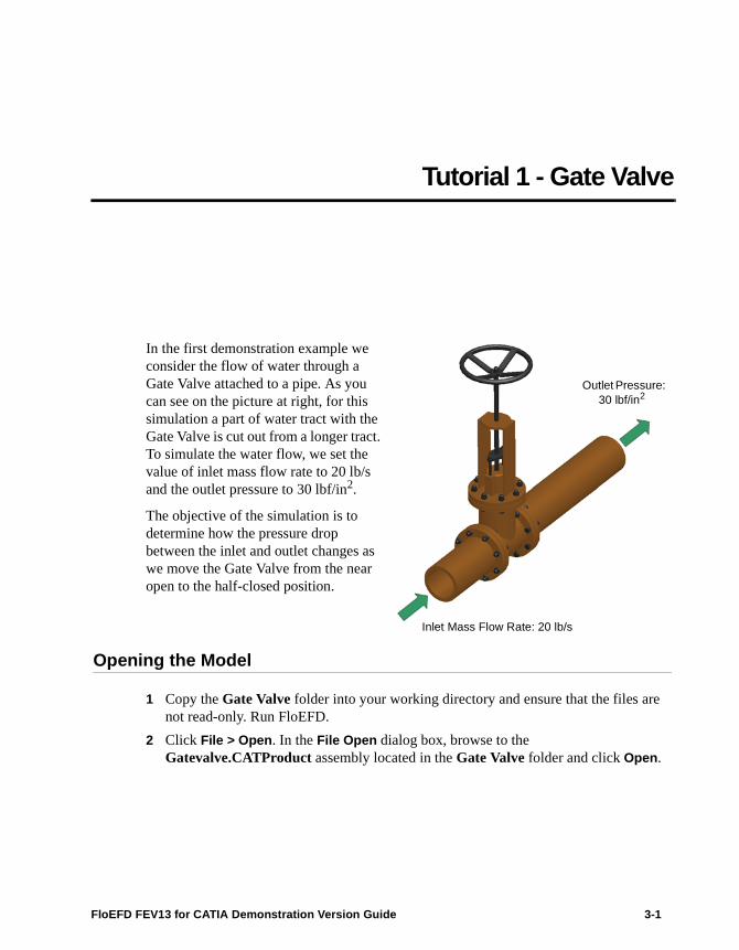
In the first demonstration example we consider the flow of water through a Gate Valve attached to a pipe. As you can see on the picture at right, for this simulation a part of water tract with the Gate Valve is cut out from a longer tract. To simulate the water flow, we set the value of inlet mass flow rate to 20 lb/s and the outlet pressure to 30 lbf/in2.
The objective of the simulation is to determine how the pressure drop between the inlet and outlet changes as we move the Gate Valve from the near open to the half-closed position.
Opening the Model
1 Copy the Gate Valve folder into your working directory and ensure that the files are not read-only. Run FloEFD.
2 Click File > Open. In the File Open dialog box, browse to the Gatevalve.CATProduct assembly located in the Gate Valve folder and click Open.
Outlet Pressure: 30 lbf/in2
Inlet Mass Flow Rate: 20 lb/s
FloEFD FEV13 for CATIA Demonstration Version Guide 3-1
Overview
You may notice that the model inlet and outlet are closed with cylindrical lids. These lids are necessary to enclose the internal space of the model allowing FloEFD to determine the fluid region properly. Each time you analyze a flow inside a model, you need to close all model openings with lids.
When analyzing an external flow around the model or flow both around and through the model, you do not have to close the model openings with lids.
FloEFD contains a lid creation tool that can relieve you from creating the lids manually. This tool (available by clicking Tools > Create Lids) can automatically create lids by closing all openings in the selected planar face of the model.
Creating the Project
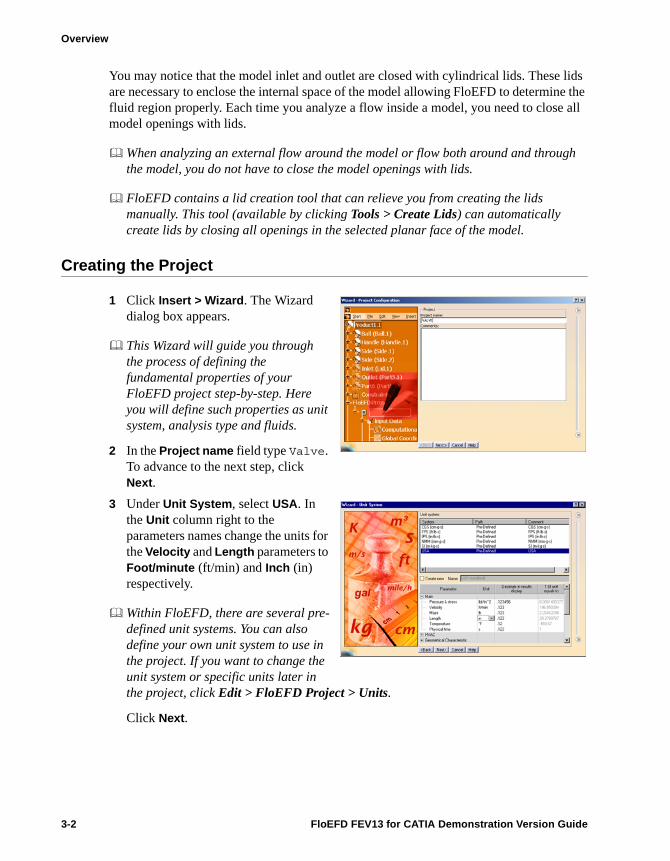
1 Click Insert > Wizard. The Wizard dialog box appears.
This Wizard will guide you through the process of defining the fundamental properties of your FloEFD project step-by-step. Here you will define such properties as unit system, analysis type and fluids.
2 In the Project name field type Valve. To advance to the next step, click Next.
3 Under Unit System, select USA. In the Unit column right to the parameters names change the units for the Velocity and Length parameters to Foot/minute (ft/min) and Inch (in) respectively.
Within FloEFD, there are several pre-defined unit systems. You can also define your own unit system to use in the project. If you want to change the unit system or specific units later in the project, click Edit > FloEFD Project > Units.
Click Next.
3-2 FloEFD FEV13 for CATIA Demonstration Version Guide
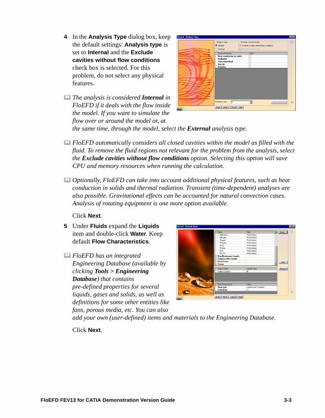
4 In the Analysis Type dialog box, keep the default settings: Analysis type is set to Internal and the Exclude cavities without flow conditions check box is selected. For this problem, do not select any physical features.
The analysis is considered Internal in FloEFD if it deals with the flow inside the model. If you want to simulate the flow over or around the model or, at the same time, through the model, select the External analysis type.
FloEFD automatically considers all closed cavities within the model as filled with the fluid. To remove the fluid regions not relevant for the problem from the analysis, select the Exclude cavities without flow conditions option. Selecting this option will save CPU and memory resources when running the calculation.
Optionally, FloEFD can take into account additional physical features, such as heat conduction in solids and thermal radiation. Transient (time-dependent) analyses are also possible. Gravitational effects can be accounted for natural convection cases. Analysis of rotating equipment is one more option available.
Click Next.
5 Under Fluids expand the Liquids item and double-click Water. Keep default Flow Characteristics.
FloEFD has an integrated Engineering Database (available by clicking Tools > Engineering Database) that contains pre-defined properties for several liquids, gases and solids, as well as definitions for some other entities like fans, porous media, etc. You can also add your own (user-defined) items and materials to the Engineering Database.
Click Next.
FloEFD FEV13 for CATIA Demonstration Version Guide 3-3
Overview
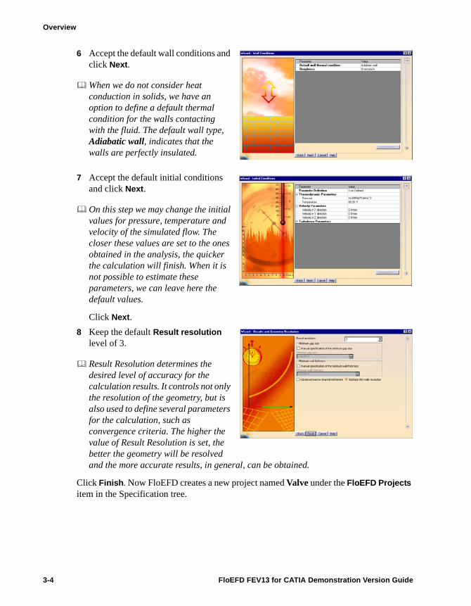
6 Accept the default wall conditions and click Next.
When we do not consider heat conduction in solids, we have an option to define a default thermal condition for the walls contacting with the fluid. The default wall type, Adiabatic wall, indicates that the walls are perfectly insulated.
7 Accept the default initial conditions and click Next.
On this step we may change the initial values for pressure, temperature and velocity of the simulated flow. The closer these values are set to the ones obtained in the analysis, the quicker the calculation will finish. When it is not possible to estimate these parameters, we can leave here the default values.
Click Next.
8 Keep the default Result resolution level of 3.
Result Resolution determines the desired level of accuracy for the calculation results. It controls not only the resolution of the geometry, but is also used to define several parameters for the calculation, such as convergence criteria. The higher the value of Result Resolution is set, the better the geometry will be resolved and the more accurate results, in general, can be obtained.
Click Finish. Now FloEFD creates a new project named Valve under the FloEFD Projects item in the Specification tree.
3-4 FloEFD FEV13 for CATIA Demonstration Version Guide

Expand Valve, then expand the Input Data and Results items. Features available under these two items together make the FloEFD Analysis tree.
We will use FloEFD Analysis tree to define our project in the same way as you use the Specification tree to create and manage your models. The analysis project is defined using features available under Input Data.
The exact list of the Input Data items depends on the physical features selected during definition of the project in the Wizard. However, the Analysis Tree is fully customizable and you can select which input data features should always be visible.
The results processing tools are available under Results. The set of results processing tools is independent on the selected physical features, but it is also fully customizable.
The FloEFD Analysis Tree can be customized by right-clicking at the project name at the top of the tree and selecting Customize Tree for the project object.
Specifying Boundary Conditions
A boundary condition is used to define flows of fluid entering or exiting the model through the openings by specifying pressure, mass or volume flow rate or velocity on the faces of corresponding lids closing the model openings.
Boundary conditions are also used to define various conditions on the model walls, such as thermal conditions, roughness or moving wall conditions.
In a typical internal analysis boundary conditions must be specified at all lids closing the model openings.
1 In the FloEFD Analysis tree, expand the Input Data item.
2 Right-click the Boundary conditions item and select Boundary Conditions object > New Boundary Condition.
FloEFD FEV13 for CATIA Demonstration Version Guide 3-5
Overview
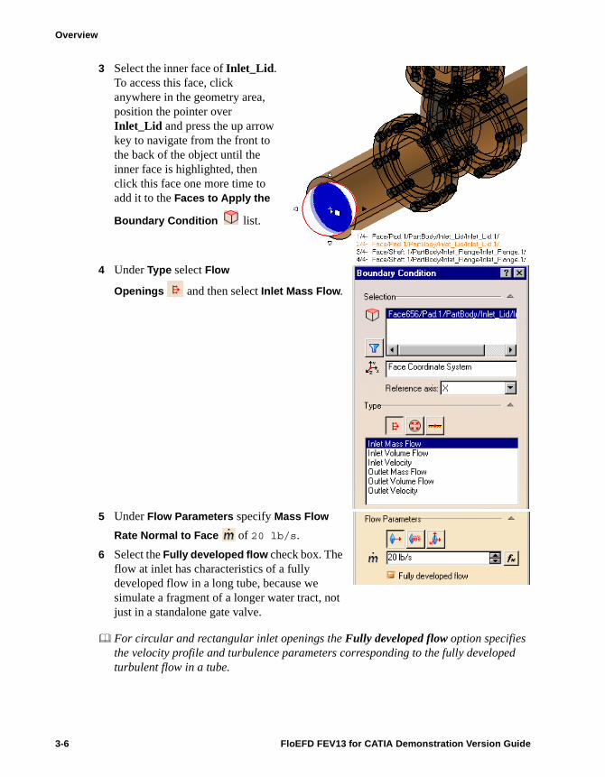
3 Select the inner face of Inlet_Lid. To access this face, click anywhere in the geometry area, position the pointer over Inlet_Lid and press the up arrow key to navigate from the front to the back of the object until the inner face is highlighted, then click this face one more time to add it to the Faces to Apply the
Boundary Condition list.
4 Under Type select Flow
Openings and then select Inlet Mass Flow.
5 Under Flow Parameters specify Mass Flow
Rate Normal to Face of 20 lb/s.
6 Select the Fully developed flow check box. The flow at inlet has characteristics of a fully developed flow in a long tube, because we simulate a fragment of a longer water tract, not just in a standalone gate valve.
For circular and rectangular inlet openings the Fully developed flow option specifies the velocity profile and turbulence parameters corresponding to the fully developed turbulent flow in a tube.
3-6 FloEFD FEV13 for CATIA Demonstration Version Guide

7 Click OK. The new Inlet Mass Flow 1 item defining the inlet flow appears in the FloEFD Analysis tree.
8 To define the outlet flow, right-click the Boundary conditions item and select Boundary Conditions object > New Boundary Condition.
9 Select the inner face of Outlet_Lid in the same way as you selected the inner face of Inlet_Lid.
10 Under Type select Pressure
Openings and then select Static Pressure.
11 Under Thermodynamic Parameters, specify
the value of Static Pressure equal to 30 lbf/in^2.
12 Click OK to close the dialog box.
FloEFD FEV13 for CATIA Demonstration Version Guide 3-7
Overview
Specifying Engineering Goals
FloEFD uses the concept of Engineering Goals that allows you to specify which parameters are of interest for you in the analysis. These can be, for example, average outlet flow velocity, maximum temperature of a wall or force applied to a surface. When you specify some variable as a goal, you tell FloEFD to focus on it when determining if the appropriate accuracy of the solution is reached during the calculation. You can run the calculation without any goals defined in the project, but it usually takes more time and resources to finish.
Goals can be set throughout the entire domain (Global Goals), within a selected volume (Volume Goals), on a selected surface area (Surface Goals), or at given point (Point Goals).
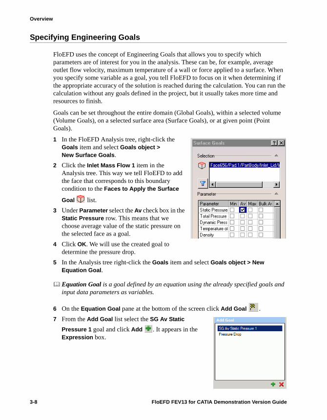
1 In the FloEFD Analysis tree, right-click the Goals item and select Goals object > New Surface Goals.
2 Click the Inlet Mass Flow 1 item in the Analysis tree. This way we tell FloEFD to add the face that corresponds to this boundary condition to the Faces to Apply the Surface
Goal list.
3 Under Parameter select the Av check box in the Static Pressure row. This means that we choose average value of the static pressure on the selected face as a goal.
4 Click OK. We will use the created goal to determine the pressure drop.
5 In the Analysis tree right-click the Goals item and select Goals object > New Equation Goal.
Equation Goal is a goal defined by an equation using the already specified goals and input data parameters as variables.
6 On the Equation Goal pane at the bottom of the screen click Add Goal .
7 From the Add Goal list select the SG Av Static
Pressure 1 goal and click Add . It appears in the Expression box.
3-8 FloEFD FEV13 for CATIA Demonstration Version Guide
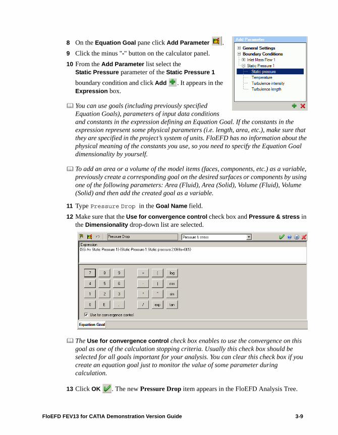
8 On the Equation Goal pane click Add Parameter .
9 Click the minus "-" button on the calculator panel.
10 From the Add Parameter list select the Static Pressure parameter of the Static Pressure 1
boundary condition and click Add . It appears in the Expression box.
You can use goals (including previously specified Equation Goals), parameters of input data conditions and constants in the expression defining an Equation Goal. If the constants in the expression represent some physical parameters (i.e. length, area, etc.), make sure that they are specified in the project’s system of units. FloEFD has no information about the physical meaning of the constants you use, so you need to specify the Equation Goal dimensionality by yourself.
To add an area or a volume of the model items (faces, components, etc.) as a variable, previously create a corresponding goal on the desired surfaces or components by using one of the following parameters: Area (Fluid), Area (Solid), Volume (Fluid), Volume (Solid) and then add the created goal as a variable.
11 Type Pressure Drop in the Goal Name field.
12 Make sure that the Use for convergence control check box and Pressure & stress in the Dimensionality drop-down list are selected.
The Use for convergence control check box enables to use the convergence on this goal as one of the calculation stopping criteria. Usually this check box should be selected for all goals important for your analysis. You can clear this check box if you create an equation goal just to monitor the value of some parameter during calculation.
13 Click OK . The new Pressure Drop item appears in the FloEFD Analysis Tree.
FloEFD FEV13 for CATIA Demonstration Version Guide 3-9

Overview
At this stage, the FloEFD project is fully defined and ready for calculation. To run the calculation in this demonstration version, you need to switch to the VALVE _PRE-DEFINE project, for which the calculation function is unlocked.
Running the Calculation
1 Double-click the VALVE_PRE-DEFINED item in the Specification tree to activate the pre-defined project, then right-click it and select VALVE_PRE-DEFINED object > Run Active FloEFD Project.
2 In the Run dialog box you can optionally select the number of CPUs in your PC that will be used for this calculation.
3 Click Run to start the calculation. In the opened Solver dialog box you can monitor the status of the calculation.
4 After the calculation has started, click the Suspend button on the Solver toolbar.
We employ the Suspend option only due to extreme simplicity of the current example, which otherwise could be calculated too fast, leaving you not enough time to perform the subsequent steps of results monitoring. Normally you can use the monitoring tools without suspending the calculation.
5 Click Insert Goal Plot on the Solver toolbar. The Add/Remove Goals dialog box appears.
6 Select Pressure Drop in the Select goals list and click OK. The goal plot appears.
In the Goal plot box you can see the current value and the graph for each of the selected goals as well as the current estimated progress towards achieving the appropriate accuracy, given as a percentage.
3-10 FloEFD FEV13 for CATIA Demonstration Version Guide

To see how the flow field changes during calculation, you can click Insert Preview . The preview parameter and other settings can be changed by right-clicking at the preview and selecting Settings.
7 Click the Suspend button again to continue calculation.
When the calculation is finished, close the monitor by clicking File > Close.
Viewing the Goals
1 In the FloEFD Analysis tree, under Results, right-click the Goal Plots icon and select Goal Plots object > Goal Plot.
2 In the Goals dialog box, select Pressure Drop.
3 Click OK.
An Excel spreadsheet with the goal results will open. On the first sheet there is a table summarizing the selected goals.
Gatevalve.CATProduct [VALVE_PRE-DEFINED]Goal Name Unit Value Averaged Value Minimum Value Maximum Value Progress [%] Use In ConvergencePressure Drop [lbf/in 2̂] 0,010507607 0,010159535 0,008692917 0,010956326 100 Yes
FloEFD FEV13 for CATIA Demonstration Version Guide 3-11
Overview
A more detailed analysis of the obtained solution can be performed by using various FloEFD results processing tools.
Viewing Cut Plots
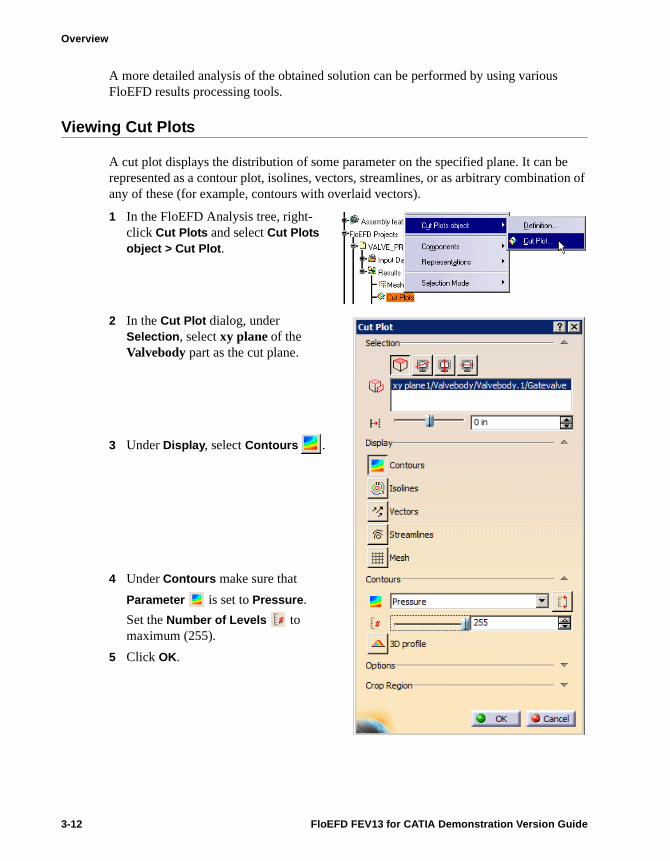
A cut plot displays the distribution of some parameter on the specified plane. It can be represented as a contour plot, isolines, vectors, streamlines, or as arbitrary combination of any of these (for example, contours with overlaid vectors).
1 In the FloEFD Analysis tree, right-click Cut Plots and select Cut Plots object > Cut Plot.
2 In the Cut Plot dialog, under Selection, select xy plane of the Valvebody part as the cut plane.
3 Under Display, select Contours .
4 Under Contours make sure that
Parameter is set to Pressure.
Set the Number of Levels to maximum (255).
5 Click OK.
3-12 FloEFD FEV13 for CATIA Demonstration Version Guide
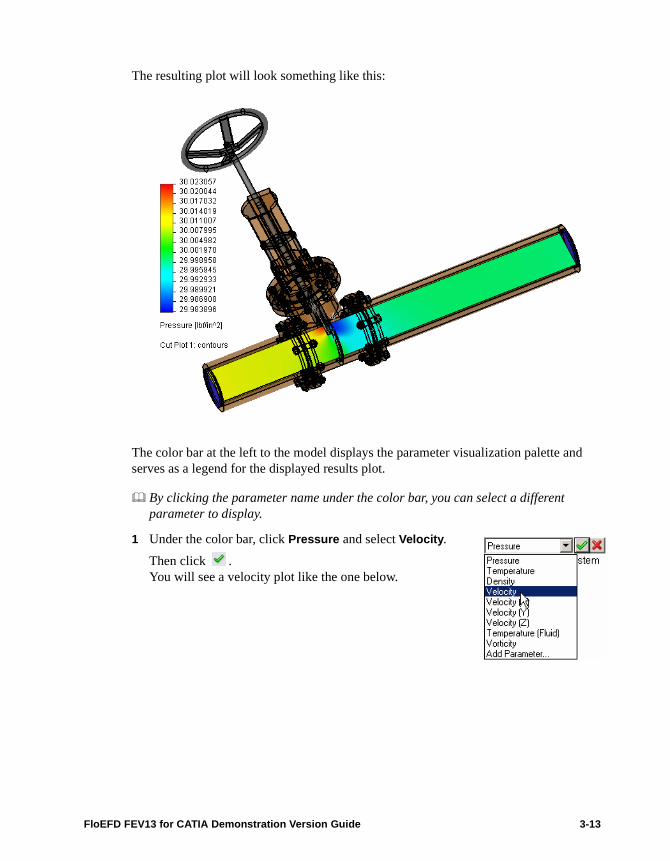
The resulting plot will look something like this:
The color bar at the left to the model displays the parameter visualization palette and serves as a legend for the displayed results plot.
By clicking the parameter name under the color bar, you can select a different parameter to display.
1 Under the color bar, click Pressure and select Velocity.
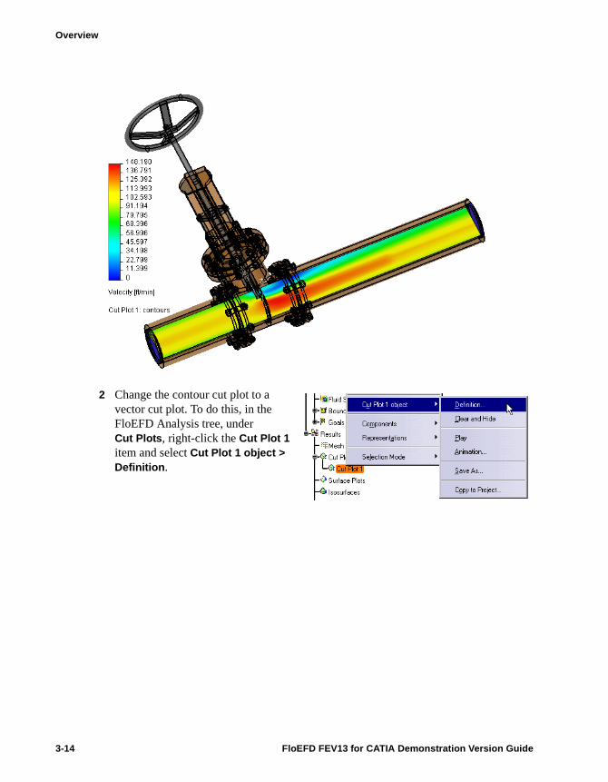
Then click . You will see a velocity plot like the one below.
FloEFD FEV13 for CATIA Demonstration Version Guide 3-13
Overview
2 Change the contour cut plot to a vector cut plot. To do this, in the FloEFD Analysis tree, under Cut Plots, right-click the Cut Plot 1 item and select Cut Plot 1 object > Definition.
3-14 FloEFD FEV13 for CATIA Demonstration Version Guide

3 Under Display clear Contours and
select Vectors .
4 Under Vectors set Spacing to 0.5 in
and Arrow Size to 0.9 in.
5 Click Adjust Minimum and Maximum
and change the Maximum velocity value to 50 ft/min, then click OK.
Under Vectors, you can switch to the
Dynamic Vectors mode to update the velocity distribution in real time as you manipulate the model, even as you zoom-in on local areas.
A portion of the resulting vector plot is shown below:
FloEFD FEV13 for CATIA Demonstration Version Guide 3-15

Overview
Viewing Surface Plots
1 In the FloEFD Analysis tree right-click the Cut Plot 1 item and select Hide/Show.
2 Right-click Surface Plots and select Surface Plots object > Surface Plot.
3 Under Selection select the Use all faces check box, then click Apply.
4 Under Contours set the Parameter to Pressure.
5 To adjust the color range of the plot, click
Adjust Minimum and Maximum and
change the Minimum and Maximum values to 29.98 and 30.02 lbf/in^2 respectively.
6 Click OK.
This plot shows the Pressure distribution on all faces that are in contact with the fluid (including inlet and outlet ones).To view the Surface Plot on a particular surface, clear the Use all faces check box and then select the surface of interest.
3-16 FloEFD FEV13 for CATIA Demonstration Version Guide

Viewing Flow Trajectories
1 In the FloEFD Analysis tree right-click the Surface Plot 1 item and select Hide/Show.
2 Right-click Flow Trajectories and select Flow Trajectories object > Flow Trajectories.
3 Click the Static Pressure 1 boundary condition to select its face.
4 Make sure that Pattern is selected under Starting Points.
5 Set the Number of Points to 16, then click OK.
FloEFD FEV13 for CATIA Demonstration Version Guide 3-17

Overview
By default, Flow Trajectories, like any new plot, are colored by parameter selected for the previous plot. You can select a different parameter or just set a fixed color.
3-18 FloEFD FEV13 for CATIA Demonstration Version Guide

Viewing X-Y Plot
This feature is used to show how the value of some parameter changes along the specified sketch. The resulting plot is exported to Microsoft® Excel®.
1 In the FloEFD Analysis tree right-click the Flow Trajectories 1 item and select Hide/Show.
2 Right-click XY Plots and select XY Plots object > XY Plot.
3 Under Parameters select Velocity (X).
4 In the geometry area click the sketch line along which we will create the XY Plot. This line belongs to Sketch 1.
5 Click OK.
This is the plot you will see:
-90
-40
10
60
110
160
0 1 2 3 4 5 6 7
Velocity (X) (ft/m in)
Length (in)
Gatevalve .CATProduct [VALVE_ PRE-DEFINED ]
E dge/ Sketch.1 /Pa rt Bod y/ Sketch 1 /Pa rt 1.2_ 1
FloEFD FEV13 for CATIA Demonstration Version Guide 3-19

Overview
Case 2: Gate Valve in the Half-Closed Position
With the FloEFD project defined for one Gate Valve position, we can easily define similar project for the other Gate Valve position by cloning the existing project and attaching it to the Design Table configuration that corresponds to this position.
1 In the main menu click Edit > FloEFD Project > Clone Project.
2 In the Project Name, type VALVE_HALF-CLOSED.
3 Click OK.
4 Click Edit > FloEFD Project > Design Table Connection.
5 Select Connect project with the active Design Table and in the Attach to configuration list select the configuration 2, then click OK.
6 As the selected configuration loads, you will get the following message:
This message occurs when you modify the model geometry (or project settings) so that the maximum or minimum X, Y or Z coordinates of the analyzed region become different from their values specified in the Computational Domain settings.
Click Yes.
7 As the computational domain is now modified, the following message suggests you to reset mesh settings for it.
3-20 FloEFD FEV13 for CATIA Demonstration Version Guide

Click Yes.
As you can see, FloEFD tracks geometry changes and suggests you to adjust the project automatically. Together with the ability to clone projects with all the specified input data and results plots settings, it makes FloEFD a very flexible and easy-to-use tool for analyzing multiple design variants. In our case we use these capabilities to analyze the Gate Valve performance at the various positions of the disk.
Now, the FloEFD project for the half-closed Gate Valve position is ready. To calculate the project for this Gate Valve position, switch to the VALVE_HALF-CLOSED_PRE-DEFINED project and repeat the steps described in the Running the Calculation section. When loading the Goal Plot, you will see a table as shown below:
According to this table, the value of pressure drop increased about 5 times comparing to the Gate Valve at the near open position. You can use FloEFD results processing tools to see how the change in Gate Valve position influences the overall flow field.
Gatevalve.CATProduct [VALVE_HALF-CLOSED_PRE-DEFINED]Goal Name Unit Value Averaged Value Minimum Value Maximum Value Progress [%] Use In ConvergencePressure Drop [lbf/in 2̂] 0,052077345 0,050795213 0,049410011 0,05255636 100 Yes
FloEFD FEV13 for CATIA Demonstration Version Guide 3-21

Overview
3-22 FloEFD FEV13 for CATIA Demonstration Version Guide
Tutorial 2 - Heat Exchanger
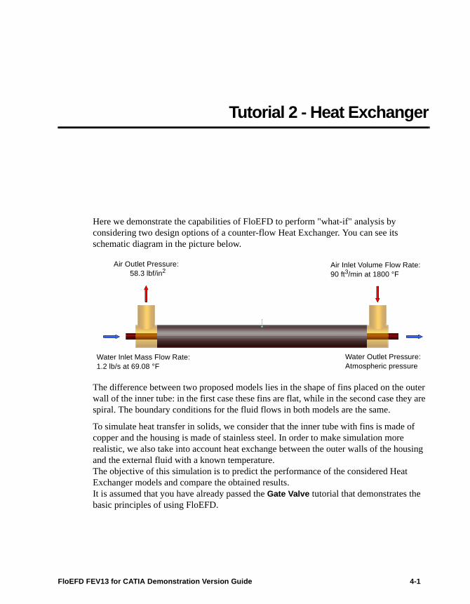
Here we demonstrate the capabilities of FloEFD to perform "what-if" analysis by considering two design options of a counter-flow Heat Exchanger. You can see its schematic diagram in the picture below.
The difference between two proposed models lies in the shape of fins placed on the outer wall of the inner tube: in the first case these fins are flat, while in the second case they are spiral. The boundary conditions for the fluid flows in both models are the same.
To simulate heat transfer in solids, we consider that the inner tube with fins is made of copper and the housing is made of stainless steel. In order to make simulation more realistic, we also take into account heat exchange between the outer walls of the housing and the external fluid with a known temperature. The objective of this simulation is to predict the performance of the considered Heat Exchanger models and compare the obtained results.It is assumed that you have already passed the Gate Valve tutorial that demonstrates the basic principles of using FloEFD.
Air Inlet Volume Flow Rate:90 ft3/min at 1800 °F
Water Inlet Mass Flow Rate:1.2 lb/s at 69.08 °F
Water Outlet Pressure:Atmospheric pressure
Air Outlet Pressure:58.3 lbf/in2
FloEFD FEV13 for CATIA Demonstration Version Guide 4-1

Tutorial 2 - Heat Exchanger
Opening the Model
1 Copy the Heat Exchanger folder into your working directory and ensure that the files are not read-only. Run FloEFD.
2 Click File, Open. In the File Open dialog box, browse to the Heat_Exchanger.CATProduct assembly located in the Heat Exchanger folder and click Open.
Creating the Project
1 Click Insert > Wizard.
2 In the Project name field type Flat fins.To advance to the next step, click Next.
3 Under Unit System, select USA.
Click Next.
4 In the Analysis Type dialog box keep Internal as the Analysis type. Under Physical Features, select the Heat conduction in solids check box.
By default, FloEFD considers heat conduction only within the fluid. To calculate a problem that includes heat transfer in solid parts, select the Heat conduction in solids option.
Click Next.
4-2 FloEFD FEV13 for CATIA Demonstration Version Guide
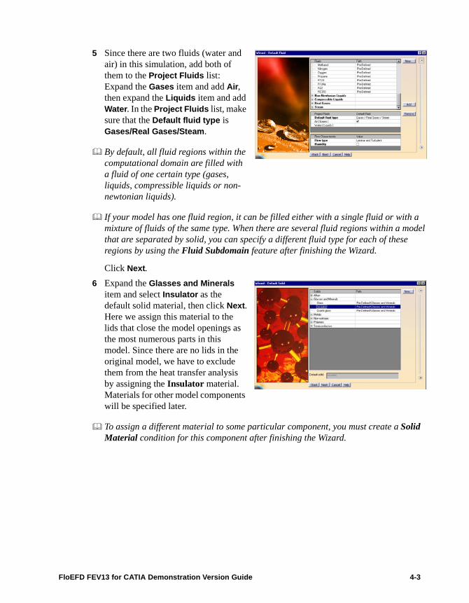
5 Since there are two fluids (water and air) in this simulation, add both of them to the Project Fluids list: Expand the Gases item and add Air, then expand the Liquids item and add Water. In the Project Fluids list, make sure that the Default fluid type is Gases/Real Gases/Steam.
By default, all fluid regions within the computational domain are filled with a fluid of one certain type (gases, liquids, compressible liquids or non-newtonian liquids).
If your model has one fluid region, it can be filled either with a single fluid or with a mixture of fluids of the same type. When there are several fluid regions within a model that are separated by solid, you can specify a different fluid type for each of these regions by using the Fluid Subdomain feature after finishing the Wizard.
Click Next.
6 Expand the Glasses and Minerals item and select Insulator as the default solid material, then click Next.Here we assign this material to the lids that close the model openings as the most numerous parts in this model. Since there are no lids in the original model, we have to exclude them from the heat transfer analysis by assigning the Insulator material. Materials for other model components will be specified later.
To assign a different material to some particular component, you must create a Solid Material condition for this component after finishing the Wizard.
FloEFD FEV13 for CATIA Demonstration Version Guide 4-3

Tutorial 2 - Heat Exchanger
7 In the Wall Conditions dialog box select Heat transfer coefficient in the Default outer wall thermal condition list. Change the value of Heat transfer coefficient to 5.5 W/m^2/K. The entered value is automatically converted to the selected system of units.
Click Next.
8 In the Initial Conditions dialog box, under Thermodynamic Parameters specify the values of Pressure and Temperature equal to 58.3 lbf/in^2 and 1800 °F respectively. These values are taken from the problem statement. Accept the default values for other conditions and click Next.
9 Keep the default Result resolution level of 3 and click Finish.
Now FloEFD creates a new project with the FloEFD data attached.
At the same time, a computational domain appears in the geometry area as a wireframe box.
In the Analysis tree, expand the Input Data item, then right-click the Computational Domain icon and select Hide/Show.
4-4 FloEFD FEV13 for CATIA Demonstration Version Guide

Specifying Fluid Subdomain
By default, FloEFD considers that all fluid regions in the project have the same Default fluid type. To specify a different fluid type and the exact set of fluids within a closed fluid region, you have to use the Fluid Subdomain feature.
Since we selected Gases/Real Gases/Steam as the Default fluid type and Air as the Default Fluid for this project in the Wizard, we need to specify a separate Fluid Subdomain for Water (Liquids type).
1 Click Insert > FloEFD Features > New Fluid Subdomain.
2 Select the inner face of the Inlet_Lid_Water. To access this face, click anywhere in the geometry area, position the pointer over Inlet_Lid_Water and press the up arrow key to navigate from the front to the back of the object until the inner face is highlighted, and then click this face one more time to add it to the Faces to Apply
the Fluid Subdomain list. After you add this face, you will see a preview of the detected subdomain that is shown as a blue body in the geometry area.
To define a fluid subdomain, you need to select a face contacting the fluid region.
3 Under Fluids, in the Fluid type list, select Liquids. Make sure that Water (Liquids) is selected.
4 Under Thermodynamic Parameters specify
the values of Pressure and
Temperature equal to 14.7 lbf/in^2 and 68 °F respectively.
FloEFD FEV13 for CATIA Demonstration Version Guide 4-5
Tutorial 2 - Heat Exchanger
5 Click OK. The new Fluid Subdomain 1 item appears in the Analysis tree. Right-click its name and select Properties, then change the Feature Name to Water Subdomain.
Specifying Boundary Conditions
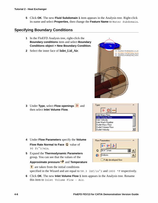
1 In the FloEFD Analysis tree, right-click the Boundary conditions item and select Boundary Conditions object > New Boundary Condition.
2 Select the inner face of Inlet_Lid_Air.
3 Under Type, select Flow openings and then select Inlet Volume Flow.
4 Under Flow Parameters specify the Volume
Flow Rate Normal to Face value of 90 ft^3/min.
5 Expand the Thermodynamic Parameters group. You can see that the values of the
Approximate pressure and Temperature
are taken from the initial conditions specified in the Wizard and are equal to 58.3 lbf/in^2 and 1800 °F respectively.
6 Click OK. The new Inlet Volume Flow 1 item appears in the Analysis tree. Rename this item to Inlet Volume Flow - Air.
4-6 FloEFD FEV13 for CATIA Demonstration Version Guide

7 Specify the same way inlet water flow (Inlet Mass Flow - Water) on the inner face of Inlet_Lid_Water. Under Flow Parameters specify the value of the
Mass Flow Rate Normal to Face equal to 1.2 lb/s.
8 Specify the boundary conditions for the outlet flows as shown in the table below:
The Environment Pressure is a special boundary condition type that is interpreted as static pressure for outlet flows and total pressure for inlet flows. Specifying this condition on a face, where fluid may flow in both directions (i.e. a vortex may occur), usually can lead to a better solution.
The Temperature value specified in the boundary condition applies only to the incoming flow, if such flow occurs.
Specifying Solid Materials
1 Click Insert > New Solid Material. The Solid Material dialog appears.
Air Water
Faces to apply inner face of Outlet_Lid_Air
inner face of Outlet_Lid_Water
Basic set of boundary conditions Pressure Openings Pressure Openings
Type of boundary condition
Environment Pressure Static Pressure
Thermodynamic Parameters
Default, the pressure and temperature values are taken from the Initial Conditions and equal to 58.3 lbf/in^2 and 1800 °F respectively
Default, the pressure and temperature values are taken from the Fluid Subdomain settings and equal to 14.7 lbf/in^2 and 68 °F respectively
FloEFD FEV13 for CATIA Demonstration Version Guide 4-7

Tutorial 2 - Heat Exchanger
2 In the Specification tree select the component Central_Part and both Side_Part components. All three components appear in the
Components to Apply the Solid Material list.
3 In the Solid group expand the Pre-Defined item and under Alloys select the Steel Stainless 321 solid material, then click OK.
4 The new Steel Stainless 321 Solid Material 1 item appears in the Analysis tree under Solid Materials. Rename it to Housing - Steel Stainless 321.
5 In the same way specify the Copper solid material (available under Pre-Defined > Metals) for the Core component. Rename the created item to Core - Copper.
Click anywhere in the geometry area to clear the selection.
Specifying Engineering Goals
1 In the FloEFD Analysis tree, right-click the Goals item and select Goals object > New Surface Goals.
2 In the Analysis tree, select the Environment Pressure 1 item. This selects the face at which the condition is specified. The face appears in the Faces
to Apply the Surface Goal list.
3 In the Parameter table, select Av for Temperature (Fluid). Make sure that the Use for Conv. check box for this parameter is selected.
4 Change the Name template to: Av Outlet Temperature of Air.
5 Click OK.
6 Repeat the same steps to create a surface goal of the average temperature of water at outlet. Select the Static Pressure 1 boundary condition to specify the face for the surface goal. When editing the Name template, type: Av Outlet Temperature of Water.
4-8 FloEFD FEV13 for CATIA Demonstration Version Guide

Cloning the Project
The FloEFD project for the Heat Exchanger model with flat fins is now fully defined. It is obvious that the project for the second Heat Exchanger modification (with spiral fins) will be basically the same. Thus, we can simply clone the current project and attach it to the corresponding Design Table configuration.
1 Click Edit > FloEFD Project > Clone Project.
2 In the Project Name, type Spiral fins.
3 Click OK.
4 Click Edit > FloEFD Project > Design Table Connection.
5 Select Connect project with the active Design Table and in the Attach to configuration list select the configuration 2, then click OK.
6 As the selected configuration loads, you will get a message that asks you if you want to reset mesh settings for the modified geometry. Click Yes.
At this stage, both FloEFD projects are fully defined and are ready for calculation. To run the calculation in this demonstration version, you need to use the pre-defined projects, for which the calculation function is unlocked. Then we will run the calculation of both pre-defined projects in the batch mode.
Running the Calculation
1 Click Edit > FloEFD Project > Batch Run.
2 In the Batch Run dialog box, select the Solve check box for both "Pre-Defined" projects and clear all check boxes for two other projects.
3 Click Run.
Wait while solver calculates both projects.
In the solver monitor window you can notice the Goal plot and Preview windows with the messages asking you to select goals and check the plot settings. You can ignore or close them.
FloEFD FEV13 for CATIA Demonstration Version Guide 4-9

Tutorial 2 - Heat Exchanger
The layout and settings of the solver monitor windows are stored when you close the solver monitor. The solver monitor layout stored from the previous calculation automatically applies when you start a new calculation. It is very convenient if you perform a series of calculations to analyze similar projects having some variations, which is typical for design optimization. In our case, the goal plot and preview settings from the previous calculation are not applicable, because the goals and model geometry in the heat exchanger project are completely different from the first example or any other example in the tutorial.
After the calculation is finished, close both monitor windows by clicking File, Close.
Loading Results
1 In the Specification tree double-click the FLAT_FINS_PRE-DEFINED project to activate it, then right-click Results and select Results object > Load Results.
2 In the Load Results dialog box, keep the default project results file name and click Open.
Once you calculate several FloEFD projects using Batch Run, you have to load the results manually.
3 Activate the other calculated project and repeat steps 1-2. Now, both result files are loaded in memory.
When analyzing the obtained results using the FloEFD post-processing tools, we assume that you are working with a single project, however you can switch to the other project anytime and repeat the same steps.
Viewing Surface Plots
Here we use Surface Plot to get a 3D view of the temperature distribution on the surface of the housing.
1 In the FloEFD Analysis tree, right-click Surface Plots and select Surface Plots object > Surface Plot.
2 In the analysis tree, select the Housing - Steel Stainless 321 item. All the faces of the components belonging to this solid material condition will be added to the Surfaces
list.
4-10 FloEFD FEV13 for CATIA Demonstration Version Guide

3 Under Contours set the Parameter to Temperature (Solid).
4 Click Adjust Minimum and Maximum and
change the Minimum and Maximum values to 150 and 1800 °F respectively.
5 Click OK. You will see a plot that looks something like the one shown below. Optionally, you can change the Model Display to Wireframe in order to get a more detailed view of this plot.
Getting Surface Parameters
This tool is used to determine minimum, maximum and average values of parameters in fluid and solid as well as calculate some integral parameters, such as mass flow rate or heat transfer rate, on the selected surfaces. For this problem, we use this tool to summarize the outlet air flow data and calculate the heat transfer rate from the inner tube walls to the water
1 In the FloEFD Analysis tree, right-click Surface Parameters and select Surface Parameters object > Surface Parameters.
FloEFD FEV13 for CATIA Demonstration Version Guide 4-11
Tutorial 2 - Heat Exchanger
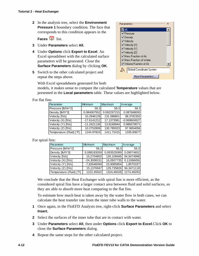
2 In the analysis tree, select the Environment Pressure 1 boundary condition. The face that corresponds to this condition appears in the
Faces list.
3 Under Parameters select All.
4 Under Options click Export to Excel. An Excel spreadsheet with the calculated surface parameters will be generated. Close the Surface Parameters dialog by clicking OK.
5 Switch to the other calculated project and repeat the steps above.
With Excel spreadsheets generated for both models, it makes sense to compare the calculated Temperature values that are presented in the Local parameters table. These values are highlighted below.
For flat fins:
For spiral fins:
We conclude that the Heat Exchanger with spiral fins is more efficient, as the considered spiral fins have a larger contact area between fluid and solid surfaces, so they are able to absorb more heat comparing to the flat fins.
To estimate how much heat is taken away by the water flow in both cases, we can calculate the heat transfer rate from the inner tube walls to the water.
1 Once again, in the FloEFD Analysis tree, right-click Surface Parameters and select Insert.
2 Select the surfaces of the inner tube that are in contact with water.
3 Under Parameters select All, then under Options click Export to Excel.Click OK to close the Surface Parameters dialog.
4 Repeat the same steps for the other calculated project.
Parameter Minimum Maximum AveragePressure [lbf/in^2] 58.3 58.3 58.3Density [lb/f t^3] 0.084067552 0.092297215 0.087668093Velocity [f t/s] 10.2946128 131.088601 98.3782353Velocity (X) [ft/s] -17.6141212 17.1373581 -0.069604527Velocity (Y) [f t/s] -11.2421136 13.8168944 0.986079071Velocity (Z) [ft/s] 10.2752806 130.789323 97.9654056Temperature (Fluid) [°F] 1244.97824 1411.72415 1335.83677
Parameter Minimum Maximum AveragePressure [lbf /in^2] 58,3 58,3 58,3Density [lb/f t^3] 0,088183059 0,093525089 0,09074652Velocity [f t/s] 15,2704802 130,108465 94,9474998Velocity (X) [f t/s] -24,3008151 16,0507735 0,11068456Velocity (Y) [f t/s] -7,82648394 23,9085804 1,8570337Velocity (Z) [f t/s] 15,1376947 129,735826 94,3471118Temperature (Fluid) [°F] 1222,45922 1324,46028 1274,49293
4-12 FloEFD FEV13 for CATIA Demonstration Version Guide

In the generated Excel spreadsheets, the value of Heat Transfer Rate that is of interest is presented in the Integral parameters table. Comparing these values, we see that about 15% more heat can be taken away by the water flow when considering the inner tube with spiral fins (under the given flow conditions).
Viewing the Animation
We will use the Animation tool to view how the fluid temperature changes on the cross-section plane as this plane moves along the flow axis.
1 In the FloEFD Analysis tree, right-click Cut Plots and select Cut Plots object > Cut Plot.
2 In the Cut Plot dialog, make sure that the selected Section Plane or Planar Face is zx plane of the Central_Part component.
3 Under Contours set the Parameter
to Temperature (Fluid).
4 Click Adjust Minimum and
Maximum and change the
Minimum and Maximum values to 150 and 1800 °F respectively.
5 Click OK. This way we created a reference plot.Set the Render Style to Wireframe and choose the appropriate model orientation in the graphic area.
6 In the FloEFD Analysis tree, right-click Cut Plot 1 and select Cut Plot 1 object > Animation.
7 In the Animation 1 dialog box click Expand .
FloEFD FEV13 for CATIA Demonstration Version Guide 4-13

Tutorial 2 - Heat Exchanger
8 Right-click the track that corresponds to the created Cut Plot 1 and select Properties.
9 Select Move. Change the Start position and Finish position values to 0.8 ft and -0.8 ft respectively.
10 Click OK.
11 To play the animation, click the button. Optionally, you can save the animation to
an AVI file by clicking the button. The file will be saved in the project results directory
Feel free to experiment with this and other FloEFD results processing tools on your own.
4-14 FloEFD FEV13 for CATIA Demonstration Version Guide

Tutorial 3 - T-Mixer
In this tutorial example we study the flow of water and ethanol as they mix together in the channel of a T-Mixer. Here, two models of T-Mixer are considered. The first model is a typical one, while the second model is expected to provide more uniform mixing. The difference between these two models is highlighted on the picture below.
To simulate the flow of water and ethanol entering through the pipes (as shown above), we set the values of their inlet mass flow rates both equal to 0.02 kg/s. The resulting mixture exits the T-mixer at the pressure of 1 atm.
Ethanol Inlet Mass Flow Rate: 0.02 kg/s
Water Inlet Mass Flow Rate: 0.02 kg/s
Outlet Pressure: 1 atm
T-Mixer Model 1 (original)
T-Mixer Model 2 (modified)
FloEFD FEV13 for CATIA Demonstration Version Guide 5-1

Tutorial 3 - T-Mixer
The objective of the simulation is to investigate how the proposed design change influences the mixing. In order to obtain some quantitative information about the mixing performance in both models, we will focus our attention on the distribution of Ethanol mass fraction near the outlet.
Such analysis may help an engineer to make a decision: whether the proposed modification improves the performance or not.
It is assumed that you have already passed at least the Gate Valve tutorial that demonstrates the basic principles of using FloEFD.
Opening the Model
1 Copy the Mixing Armature folder into your working directory and ensure that the files are not read-only. Run FloEFD.
2 Click File > Open. In the File Open dialog box, browse to the T-Mixer_Main.CATProduct assembly located in the Mixing Armature folder and click Open.
Creating the Project
1 Click Insert > Wizard.
1 In the Project name field type T-mixer original.
Click Next.
2 Under Unit System, keep the default International System (SI).
When specifying parameters in the FloEFD project, you can use any appropriate units that can be different from the default unit system. However the values you type will be converted to the units of the default unit system.
Click Next.
5-2 FloEFD FEV13 for CATIA Demonstration Version Guide
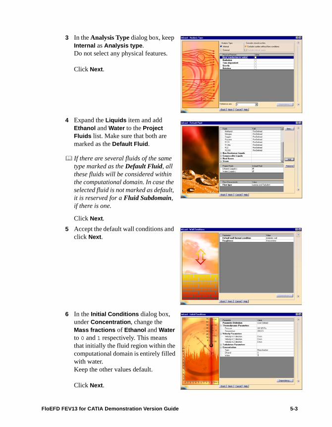
3 In the Analysis Type dialog box, keep Internal as Analysis type. Do not select any physical features.
Click Next.
4 Expand the Liquids item and add Ethanol and Water to the Project Fluids list. Make sure that both are marked as the Default Fluid.
If there are several fluids of the same type marked as the Default Fluid, all these fluids will be considered within the computational domain. In case the selected fluid is not marked as default, it is reserved for a Fluid Subdomain, if there is one.
Click Next.
5 Accept the default wall conditions and click Next.
6 In the Initial Conditions dialog box, under Concentration, change the Mass fractions of Ethanol and Water to 0 and 1 respectively. This means that initially the fluid region within the computational domain is entirely filled with water. Keep the other values default.
Click Next.
FloEFD FEV13 for CATIA Demonstration Version Guide 5-3

Tutorial 3 - T-Mixer
Set the Result resolution level to 5. Select Manual specification of the minimum wall thickness. Type the value of Minimum wall thickness equal to 0.002 m.
Click Finish.
In the geometry area, you will see a preview of the automatically generated computational domain.
Using Component Control
When examining the list of components in this assembly, you can notice the Measure assembly that consists of four components placed near the outlet lid. They are added here to be used when estimating the distribution of mass fraction (or more precisely, its average values) of Ethanol over the outlet. By setting the corresponding goals on the ring-shaped faces of these additional components, we can get a detailed statistics about the distribution of Ethanol in different flow regions (from the near-wall to the flow core) in the same cross-section.
To set goals on the Measure components, first we have to configure them so that they do not influence the fluid flow during the calculation, i.e. we make them "transparent" for the flow.
1 Click Edit > FloEFD Project > Component Control.
2 In the Component Control dialog box deselect the Measure assembly.
3 Click OK.
In case the disabled component is in contact with the computational domain boundary, it is recommended to reset the default size of the computational domain.
4 In the FloEFD Analysis tree right-click Computational Domain and select Computational Domain object > Definition.
5-4 FloEFD FEV13 for CATIA Demonstration Version Guide

5 Under Size and Conditions click Reset.
6 Click OK.
Specifying Boundary Conditions
1 In the FloEFD Analysis tree, right-click the Boundary conditions item and select Boundary Conditions object > New Boundary Condition.
2 Select the inner face of Inlet_Lid_Water.
3 Under Type select Flow openings and then select Inlet Mass Flow.
4 Under Flow Parameters specify the Mass
Flow Rate Normal to Face value of 0.02 kg/s.
5 Expand the Substance Concentrations group and make sure that the Mass fractions of Ethanol and Water are set to 0 and 1 respectively.
The default values of Substance Concentrations and Thermodynamic Parameters are set using Initial conditions specified in the Wizard.
FloEFD FEV13 for CATIA Demonstration Version Guide 5-5

Tutorial 3 - T-Mixer
6 Click OK. The new Inlet Mass Flow 1 item appears in the Analysis tree. Rename it to Inlet Mass Flow - Water.
7 Specify the same way the Inlet Mass Flow - Ethanol boundary condition on the inner face of the Inlet_Lid_Ethanol with the same Mass Flow Rate Normal to Face
value of 0.02 kg/s. As opposed to the previous boundary condition, under Substance Concentrations set the values of Ethanol and Water mass fractions to 1 and 0 respectively.
8 Specify the Environment Pressure boundary condition with the default values on the inner face of Outlet_Lid. To make the selection of the face easier, you can hide the Measure assembly.
5-6 FloEFD FEV13 for CATIA Demonstration Version Guide
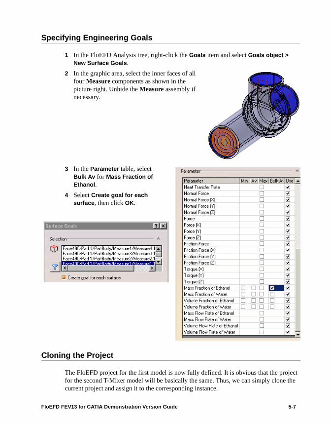
Specifying Engineering Goals
1 In the FloEFD Analysis tree, right-click the Goals item and select Goals object > New Surface Goals.
2 In the graphic area, select the inner faces of all four Measure components as shown in the picture right. Unhide the Measure assembly if necessary.
3 In the Parameter table, select Bulk Av for Mass Fraction of Ethanol.
4 Select Create goal for each surface, then click OK.
Cloning the Project
The FloEFD project for the first model is now fully defined. It is obvious that the project for the second T-Mixer model will be basically the same. Thus, we can simply clone the current project and assign it to the corresponding instance.
FloEFD FEV13 for CATIA Demonstration Version Guide 5-7

Tutorial 3 - T-Mixer
1 Click Edit > FloEFD Project > Clone Project.
2 In the Project Name, type T-mixer modified.
3 Click OK.
4 Click Edit > FloEFD Project > Design Table Connection.
5 Select Connect project with the active Design Table and in the Attach to configuration list select the configuration 2, then click OK.
6 When asked to reset the Computational Domain / Mesh Settings, click Yes.
At this stage, both FloEFD projects are fully defined and are ready for calculation. To run the calculation in this demonstration version, you need to use the pre-defined projects, for which the calculation function is unlocked. Then we will run the calculation of both pre-defined projects in the batch mode.
Running the Calculation
1 Click Edit > FloEFD Project > Batch Run.
2 In the Batch Run dialog box, select the Solve check box for both "Pre-Defined" projects and clear all check boxes for two other projects.
3 Click Run.
Wait while solver calculates both projects.
After the calculation is finished, close both monitor windows by clicking File > Close.
Loading Results
1 In the Specification tree double-click the T-MIXER_ORIGINAL_PRE-DEFINED project to activate it, then right-click Results and select Results object > Load Results.
2 In the Load Results dialog box, keep the default project results file name and click Open.
3 Activate the other calculated project and repeat steps 1-2. Now, both result files are loaded in memory.
5-8 FloEFD FEV13 for CATIA Demonstration Version Guide
When analyzing the obtained results by using the FloEFD post-processing tools, we assume that you are working with a single project, however you can switch to the other project anytime and repeat the same steps.
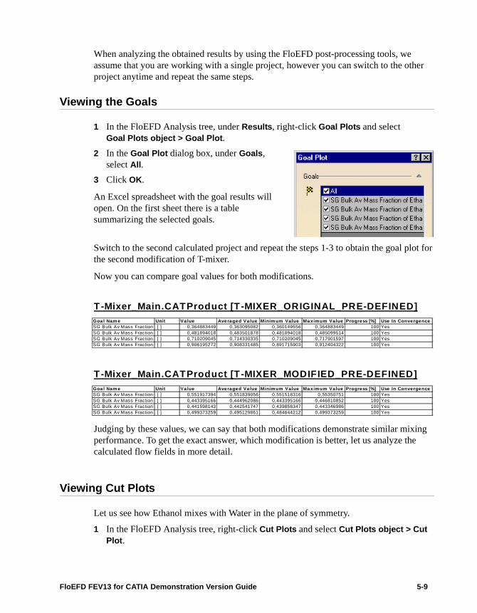
Viewing the Goals
1 In the FloEFD Analysis tree, under Results, right-click Goal Plots and select Goal Plots object > Goal Plot.
2 In the Goal Plot dialog box, under Goals, select All.
3 Click OK.
An Excel spreadsheet with the goal results will open. On the first sheet there is a table summarizing the selected goals.
Switch to the second calculated project and repeat the steps 1-3 to obtain the goal plot for the second modification of T-mixer.
Now you can compare goal values for both modifications.
Judging by these values, we can say that both modifications demonstrate similar mixing performance. To get the exact answer, which modification is better, let us analyze the calculated flow fields in more detail.
Viewing Cut Plots
Let us see how Ethanol mixes with Water in the plane of symmetry.
1 In the FloEFD Analysis tree, right-click Cut Plots and select Cut Plots object > Cut Plot.
T-Mixer_Main.CATProduct [T -MIXER_ORIGINAL_PRE-DEFINED]Goa l Nam e Unit Va lue Ave raged Va lue Minimum Value Ma ximum Value Progress [%] Use In ConvergenceSG Bulk Av Mass Fraction [ ] 0,364883449 0,363095082 0,360149556 0,364883449 100 YesSG Bulk Av Mass Fraction [ ] 0,481894018 0,483501878 0,481894018 0,485099514 100 YesSG Bulk Av Mass Fraction [ ] 0,710209045 0,714330335 0,710209045 0,717901597 100 YesSG Bulk Av Mass Fraction [ ] 0,906195272 0,908331485 0,891715903 0,912404322 100 Yes
T-Mixer_Main.CATProduct [T -MIXER_MODIFIED_PRE-DEFINED]Goa l Nam e Unit Va lue Ave raged Va lue Minimum Value Ma ximum Value Progress [%] Use In ConvergenceSG Bulk Av Mass Fraction [ ] 0,551917394 0,551839056 0,551518316 0,55350751 100 YesSG Bulk Av Mass Fraction [ ] 0,443395166 0,444962086 0,443395166 0,446810852 100 YesSG Bulk Av Mass Fraction [ ] 0,441598143 0,442541747 0,439858347 0,443346986 100 YesSG Bulk Av Mass Fraction [ ] 0,499373259 0,495129861 0,484644212 0,499373259 100 Yes
FloEFD FEV13 for CATIA Demonstration Version Guide 5-9
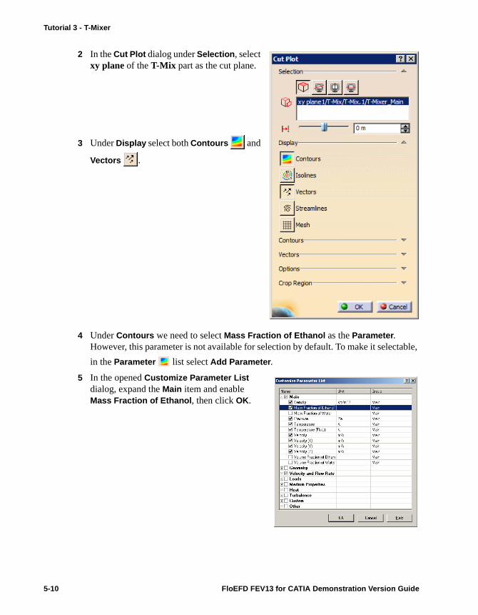
Tutorial 3 - T-Mixer
2 In the Cut Plot dialog under Selection, select xy plane of the T-Mix part as the cut plane.
3 Under Display select both Contours and
Vectors .
4 Under Contours we need to select Mass Fraction of Ethanol as the Parameter. However, this parameter is not available for selection by default. To make it selectable,
in the Parameter list select Add Parameter.
5 In the opened Customize Parameter List dialog, expand the Main item and enable Mass Fraction of Ethanol, then click OK.
5-10 FloEFD FEV13 for CATIA Demonstration Version Guide

6 In the Cut Plot dialog, under Contours, now select Ethanol Mass Fraction as the
Parameter , then click Adjust
Minimum and Maximum and
change the Minimum and
Maximum values to 0 and 1 respectively.
7 Set the Number of Levels to maximum (255) and click OK.
Repeat the steps 1-7 for the second calculated project. The resulting plots will look something like this:
Judging by these plots, we can say that the modified T-Mixer provides better penetration of Ethanol to the bottom side of the Water flow.
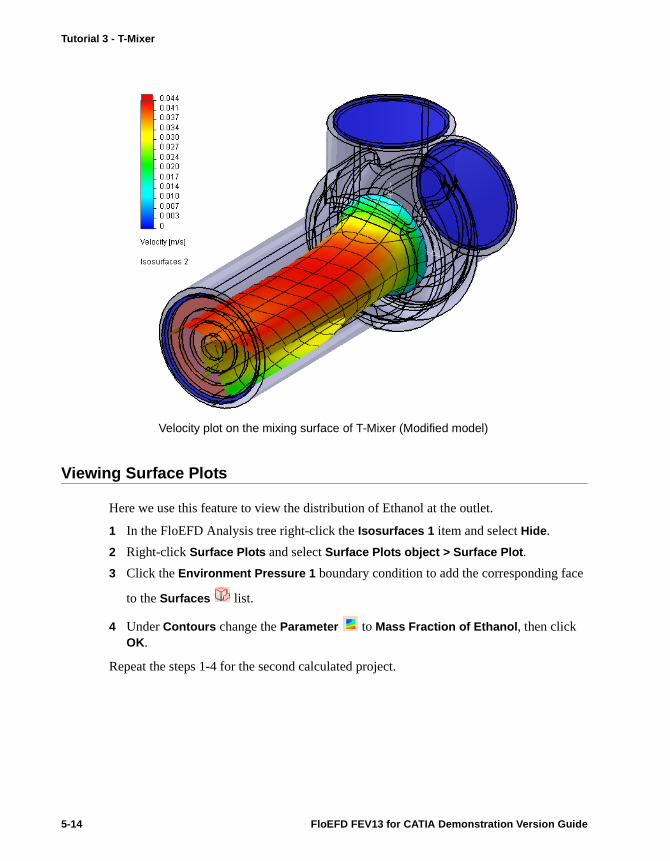
Viewing Isosurfaces
Using this feature, you can plot a 3D surface at which the selected parameter has some constant value. We will use it to view a mixing surface (i.e. the surface, where the Mass Fraction of Ethanol takes a value of 0.5).
1 In the FloEFD Analysis tree, right-click the Cut Plot 1 item and select Hide/Show.
2 Right-click Isosurfaces 1 and select Show. By default, FloEFD draws isosurface, where the pressure takes a value of 1 atm. We need to change this.
FloEFD FEV13 for CATIA Demonstration Version Guide 5-11

Tutorial 3 - T-Mixer
3 Right-click Isosurfaces 1 again and select Isosurfaces 1 object > Definition.
4 Change the Parameter to Mass Fraction of Ethanol.
5 Under Value 1 set the Value to 0.5.
6 Under Appearance, in the Color by
Parameter list, select Velocity.
7 Click Adjust Minimum and
Maximum and set the Number
of Levels to maximum (255), then click OK.
You can select Grid under Appearance to show grid lines at the isosurface.
Repeat the steps 1-7 for the second calculated project. Set the same Maximum value for the Velocity parameter as in the first project.
5-12 FloEFD FEV13 for CATIA Demonstration Version Guide

Now we can see, how a certain parameter (Velocity, in our case) changes along the mixing surface.
Velocity plot on the mixing surface of T-Mixer (Original model)
FloEFD FEV13 for CATIA Demonstration Version Guide 5-13
Tutorial 3 - T-Mixer
Viewing Surface Plots
Here we use this feature to view the distribution of Ethanol at the outlet.
1 In the FloEFD Analysis tree right-click the Isosurfaces 1 item and select Hide.
2 Right-click Surface Plots and select Surface Plots object > Surface Plot.
3 Click the Environment Pressure 1 boundary condition to add the corresponding face
to the Surfaces list.
4 Under Contours change the Parameter to Mass Fraction of Ethanol, then click OK.
Repeat the steps 1-4 for the second calculated project.
Velocity plot on the mixing surface of T-Mixer (Modified model)
5-14 FloEFD FEV13 for CATIA Demonstration Version Guide
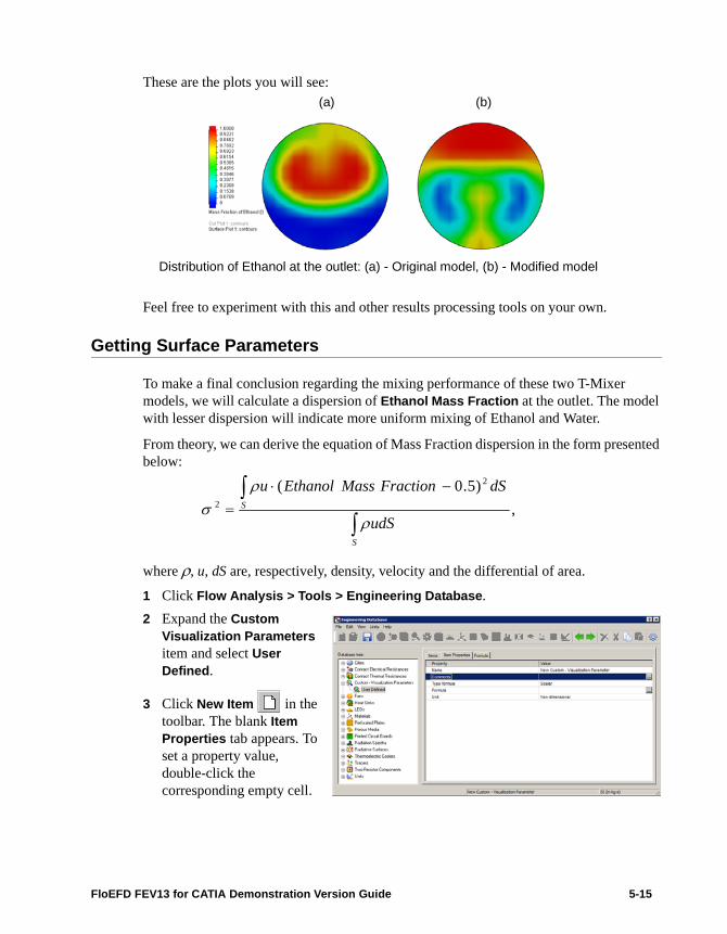
These are the plots you will see:
Feel free to experiment with this and other results processing tools on your own.
Getting Surface Parameters
To make a final conclusion regarding the mixing performance of these two T-Mixer models, we will calculate a dispersion of Ethanol Mass Fraction at the outlet. The model with lesser dispersion will indicate more uniform mixing of Ethanol and Water.
From theory, we can derive the equation of Mass Fraction dispersion in the form presented below:
where , u, dS are, respectively, density, velocity and the differential of area.
1 Click Flow Analysis > Tools > Engineering Database.
2 Expand the Custom Visualization Parameters item and select User Defined.
3 Click New Item in the toolbar. The blank Item Properties tab appears. To set a property value, double-click the corresponding empty cell.
Distribution of Ethanol at the outlet: (a) - Original model, (b) - Modified model
(a) (b)
,
)5.0( 2
2
S
S
udS
dSFractionMassEthanolu
FloEFD FEV13 for CATIA Demonstration Version Guide 5-15

Tutorial 3 - T-Mixer
4 Fill the table as shown below:
In this FloEFD project, Mass Fraction 1 corresponds to the Mass Fraction of Ethanol
5 Click Save in the toolbar and click File > Exit.
6 In the FloEFD Analysis tree right-click Surface Parameters and select Surface Parameters object > Surface Parameters.
7 In the analysis tree, select the Environment Pressure 1 boundary condition. The face
that corresponds to this condition appears in the Faces list.
8 Under Parameters we need to select newly created Dispersion parameter. However, this parameter is not available for selection by default. To make it selectable click More Parameters. In the opened Customize Parameter List window, expand the Custom item and enable the newly created Dispersion parameter, then click OK.Under Parameters select All.
9 Under Options click Export to Excel. An Excel spreadsheet with the calculated surface parameters will be generated. Close the Surface Parameters dialog by clicking OK.
Switch to the other calculated project and repeat the steps 6-10.
With Excel spreadsheets generated for both models, we have to compare the bulk average values of the calculated Dispersion that are presented in the Local parameters table.
Original model:
Modified model:
Comparing these values, we can conclude that the Original model actually provides more uniform mixing.
Name Dispersion
Type formula Scalar
Formula ({Mass Fraction 1}-0.5)^2
Unit Non-dimensional
Parameter Minimum Maximum Average Bulk AverageDispersion [ ] 0,001564181 0,248678497 0,145777072 0,14928345
Parameter Minimum Max imum A v erage Bulk A v erageDis pers ion [ ] 1,4365E-06 0,249748268 0,099661165 0,093751073
5-16 FloEFD FEV13 for CATIA Demonstration Version Guide
Tutorial 4 - Flow over the Roof-Mounted Figure
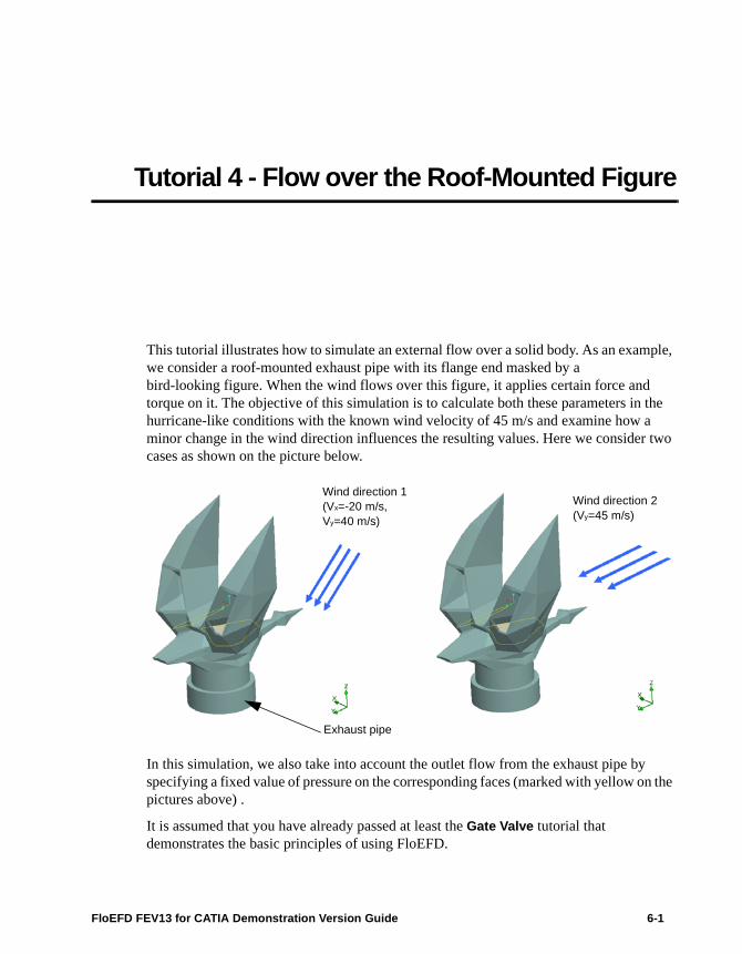
This tutorial illustrates how to simulate an external flow over a solid body. As an example, we consider a roof-mounted exhaust pipe with its flange end masked by a bird-looking figure. When the wind flows over this figure, it applies certain force and torque on it. The objective of this simulation is to calculate both these parameters in the hurricane-like conditions with the known wind velocity of 45 m/s and examine how a minor change in the wind direction influences the resulting values. Here we consider two cases as shown on the picture below.
In this simulation, we also take into account the outlet flow from the exhaust pipe by specifying a fixed value of pressure on the corresponding faces (marked with yellow on the pictures above) .
It is assumed that you have already passed at least the Gate Valve tutorial that demonstrates the basic principles of using FloEFD.
Wind direction 1 (Vx=-20 m/s,Vy=40 m/s)
Wind direction 2 (Vy=45 m/s)
Exhaust pipe
FloEFD FEV13 for CATIA Demonstration Version Guide 6-1
Tutorial 4 - Flow over the Roof-Mounted Figure
Opening the Model
1 Copy the Roof-Mounted Figure folder into your working directory and ensure that the files are not read-only. Run FloEFD.
2 Click File > Open. In the File Open dialog box, browse to the Bird_Shaped-Exhaust.CATProduct assembly located in the Roof-Mounted Figure folder and click Open.
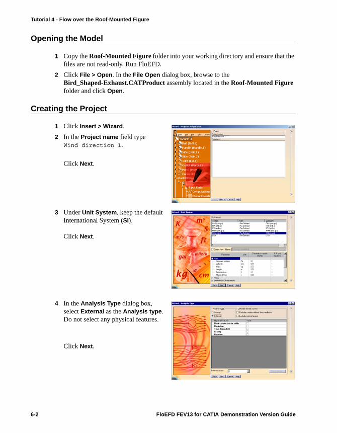
Creating the Project
1 Click Insert > Wizard.
2 In the Project name field type Wind direction 1.
Click Next.
3 Under Unit System, keep the default International System (SI).
Click Next.
4 In the Analysis Type dialog box, select External as the Analysis type. Do not select any physical features.
Click Next.
6-2 FloEFD FEV13 for CATIA Demonstration Version Guide

5 Expand the Gases item and add Air to the Project Fluids list.
Click Next.
6 Accept the default wall conditions and click Next.
7 In the Initial and Ambient Conditions dialog box, under Velocity Parameters, keep the default 3D Vector as the Defined by and change the Velocity in X direction and Velocity in Y direction to -20 m/s and 40 m/s respectively.Keep the other values default.
Alternatively, you can specify the velocity magnitude and the vector direction in terms of the aerodynamic angles. Under Velocity Parameters, select the Aerodynamic angles as the Defined by and specify the Velocity of
FloEFD FEV13 for CATIA Demonstration Version Guide 6-3
Tutorial 4 - Flow over the Roof-Mounted Figure
45 m/s, select YZ as the Longitudinal plane and Y as the Longitudinal axis, keep the default Angle of attack of 0° and set the Angle of sideslip to 30°.
The specified Initial and Ambient conditions for the External type of analysis are treated both as Initial conditions within the computational domain and as Boundary conditions on its bounding faces that make up a parallelepiped. The specified velocity and temperature values are maintained on the computational domain boundaries where the fluid flows into the computational domain , while the pressure values are maintained on the boundaries where the fluids flows out of the computational domain. Once you finish the Wizard, you can preview this domain in the graphic area and modify it to the appropriate size.
Click Next.
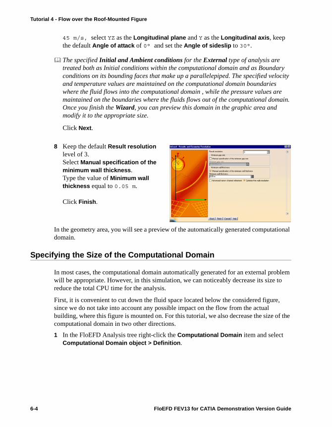
8 Keep the default Result resolution level of 3. Select Manual specification of the minimum wall thickness. Type the value of Minimum wall thickness equal to 0.05 m.
Click Finish.
In the geometry area, you will see a preview of the automatically generated computational domain.
Specifying the Size of the Computational Domain
In most cases, the computational domain automatically generated for an external problem will be appropriate. However, in this simulation, we can noticeably decrease its size to reduce the total CPU time for the analysis.
First, it is convenient to cut down the fluid space located below the considered figure, since we do not take into account any possible impact on the flow from the actual building, where this figure is mounted on. For this tutorial, we also decrease the size of the computational domain in two other directions.
1 In the FloEFD Analysis tree right-click the Computational Domain item and select Computational Domain object > Definition.
6-4 FloEFD FEV13 for CATIA Demonstration Version Guide
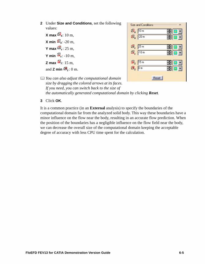
2 Under Size and Conditions, set the following values:
X max : 10 m,
X min : -20 m,
Y max : 25 m,
Y min : -10 m,
Z max : 15 m,
and Z min : 0 m.
You can also adjust the computational domain size by dragging the colored arrows at its faces. If you need, you can switch back to the size of the automatically generated computational domain by clicking Reset.
3 Click OK.
It is a common practice (in an External analysis) to specify the boundaries of the computational domain far from the analyzed solid body. This way these boundaries have a minor influence on the flow near the body, resulting in an accurate flow prediction. When the position of the boundaries has a negligible influence on the flow field near the body, we can decrease the overall size of the computational domain keeping the acceptable degree of accuracy with less CPU time spent for the calculation.
FloEFD FEV13 for CATIA Demonstration Version Guide 6-5
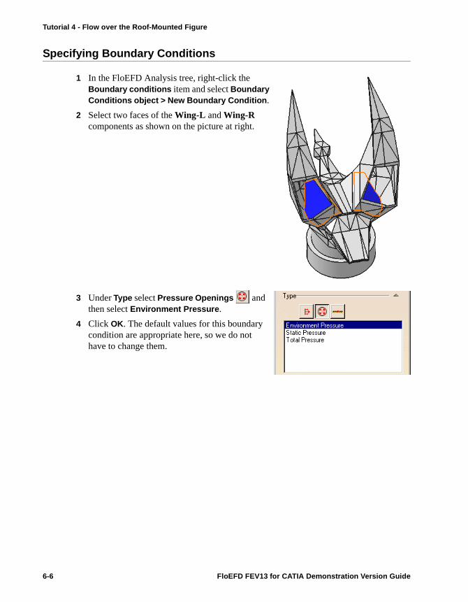
Tutorial 4 - Flow over the Roof-Mounted Figure
Specifying Boundary Conditions
1 In the FloEFD Analysis tree, right-click the Boundary conditions item and select Boundary Conditions object > New Boundary Condition.
2 Select two faces of the Wing-L and Wing-R components as shown on the picture at right.
3 Under Type select Pressure Openings and then select Environment Pressure.
4 Click OK. The default values for this boundary condition are appropriate here, so we do not have to change them.
6-6 FloEFD FEV13 for CATIA Demonstration Version Guide

Specifying Engineering Goals
1 In the FloEFD Analysis tree, right-click the Goals item and select Goals object > New Global Goals.
2 In the Parameter table, select Force, Force (X), Force (Y) and Torque (Z).
3 Make sure that the Global Coordinate System is selected, so that the goals will be calculated with respect to this system.
4 Click OK.
Cloning the Project
The FloEFD project for the first case is now fully defined. For the second case, the model geometry remains the same. The only difference is that we have to change the wind direction.
1 Click Edit > FloEFD Project > Clone Project.
2 In the Project Name, type Wind direction 2.
3 Click OK.This will create a new project.
FloEFD FEV13 for CATIA Demonstration Version Guide 6-7
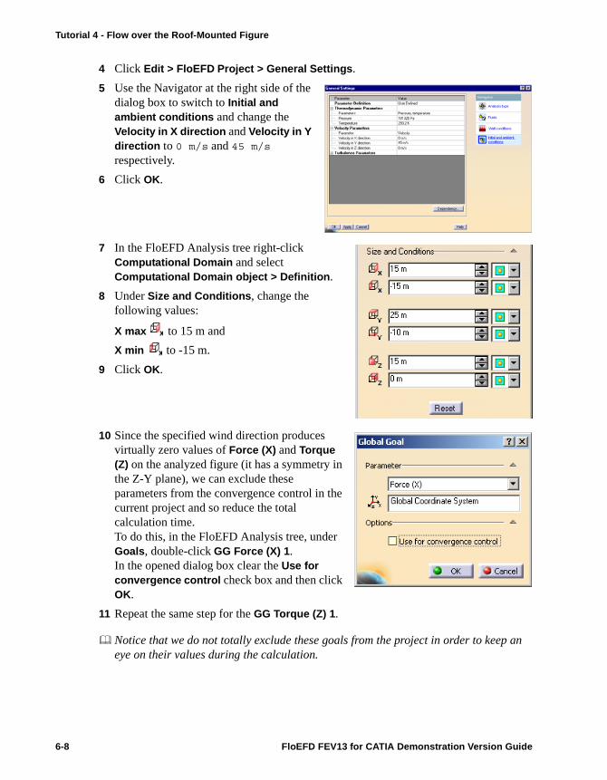
Tutorial 4 - Flow over the Roof-Mounted Figure
4 Click Edit > FloEFD Project > General Settings.
5 Use the Navigator at the right side of the dialog box to switch to Initial and ambient conditions and change the Velocity in X direction and Velocity in Y direction to 0 m/s and 45 m/s respectively.
6 Click OK.
7 In the FloEFD Analysis tree right-click Computational Domain and select Computational Domain object > Definition.
8 Under Size and Conditions, change the following values:
X max to 15 m and
X min to -15 m.
9 Click OK.
10 Since the specified wind direction produces virtually zero values of Force (X) and Torque (Z) on the analyzed figure (it has a symmetry in the Z-Y plane), we can exclude these parameters from the convergence control in the current project and so reduce the total calculation time. To do this, in the FloEFD Analysis tree, under Goals, double-click GG Force (X) 1. In the opened dialog box clear the Use for convergence control check box and then click OK.
11 Repeat the same step for the GG Torque (Z) 1.
Notice that we do not totally exclude these goals from the project in order to keep an eye on their values during the calculation.
6-8 FloEFD FEV13 for CATIA Demonstration Version Guide

At this stage, both FloEFD projects are fully defined and are ready for calculation. To run the calculation in this demonstration version, you need to use the pre-defined projects, for which the calculation function is unlocked. Then we will run the calculation of both pre-defined projects in the batch mode.
Running the Calculation
1 Click Edit > FloEFD Project > Batch Run.
2 In the Batch Run dialog box, select the Solve check box for both "Pre-Defined" projects and clear all check boxes for two other projects.
3 Click Run.
Wait while solver calculates both projects.
After the calculation is finished, close both monitor dialog boxes by clicking File > Close.
Loading Results
1 In the Specification tree double-click the WIND_DIRECTION_1_PRE-DEFINED project to activate it, then right-click Results and select Results object > Load Results.
2 In the Load Results dialog box, keep the default project results file name and click Open.
3 Activate the other calculated project and repeat steps 1-2.
When analyzing the obtained results by using the FloEFD post-processing tools, we assume that you are working with a single project, however you can switch to the other project anytime and repeat the same steps.
FloEFD FEV13 for CATIA Demonstration Version Guide 6-9

Tutorial 4 - Flow over the Roof-Mounted Figure
Viewing the Goals
1 In the FloEFD Analysis tree, under Results, right-click Goal Plots and select Goal Plots object > Goal Plot.
2 In the Goal Plot dialog, under Goals, select All.
3 Click OK.
An Excel spreadsheet with the goal results will open. On the first sheet there is a table summarizing the selected goals.
Switch to the second calculated project and repeat the steps 1-4 to obtain the goal plot for the second wind direction.
For the first case, we get:
And for the second case:
Analyzing these results, we can say that for the first case, when the wind has X-Velocity component two times smaller than Y-Velocity component, we get the X-Component of Force that is about twice as bigger as Y-Component of Force obtained on both cases. So, when designing such figure, it is obligatory to consider the wind blowing in several directions.
bird_shaped-exhaust.catproduct [WIND_DIRECTION_1_PRE-DEFINGoal Name Unit Value Averaged Value Minimum Value Maximum Value Progress [%] Use In ConvergenceGG Force 1 [N] 24119,5782 24064,45302 23926,18208 24146,30431 100 YesGG Force (X) 1 [N] -20428,30337 -20362,02112 -20474,04502 -20192,5319 100 YesGG Force (Y) 1 [N] 12457,64289 12467,45514 12437,26059 12516,32295 100 YesGG Torque (Z) 1 [N*m] -19401,31093 -19416,86071 -19547,58277 -19301,7136 100 Yes
bird_shaped-exhaust.catproduct [WIND_DIRECTION_2_PRE-DEFINGoal Name Unit Value Averaged Value Minimum Value Maximum Value Progress [%] Use In ConvergenceGG Force 1 [N] 11352,47641 11477,96749 11336,25881 11563,24645 100 YesGG Force (X) 1 [N] -1424,204204 -641,2317864 -1451,75379 16,96754095 0 NoGG Force (Y) 1 [N] 10747,01698 10746,25033 10622,73474 10807,65364 100 YesGG Torque (Z) 1 [N*m] 322,1471952 -63,89155448 -306,555822 322,1471952 0 No
6-10 FloEFD FEV13 for CATIA Demonstration Version Guide

Viewing Surface Plots
Here we use this feature to see how the pressure changes on the surface of the figure.
1 In the FloEFD Analysis tree, right-click Surface Plots and select Surface Plots object > Surface Plot.
2 In the Selection group, select the Use all faces check box.
3 Under Contours set the Parameter to Pressure.
4 Click Adjust Minimum and Maximum and
change the Minimum and Maximum values to 99000 Pa and 102000 Pa respectively. Set the Number of Levels to maximum (255) and then click OK.
The resulting plots for both cases will look like these:
Wind direction 1 Wind direction 2
FloEFD FEV13 for CATIA Demonstration Version Guide 6-11
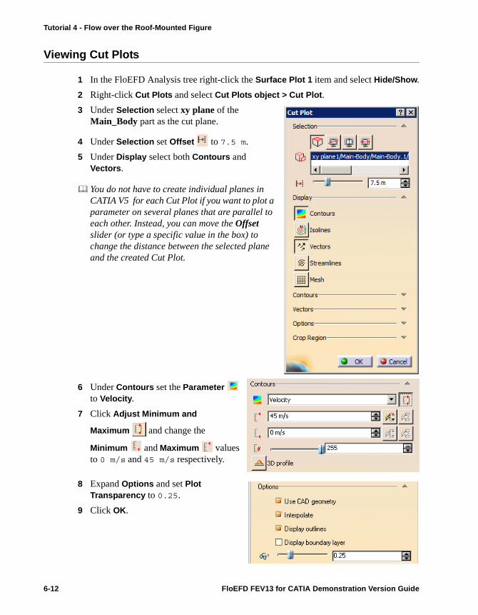
Tutorial 4 - Flow over the Roof-Mounted Figure
Viewing Cut Plots
1 In the FloEFD Analysis tree right-click the Surface Plot 1 item and select Hide/Show.
2 Right-click Cut Plots and select Cut Plots object > Cut Plot.
3 Under Selection select xy plane of the Main_Body part as the cut plane.
4 Under Selection set Offset to 7.5 m.
5 Under Display select both Contours and Vectors.
You do not have to create individual planes in CATIA V5 for each Cut Plot if you want to plot a parameter on several planes that are parallel to each other. Instead, you can move the Offset slider (or type a specific value in the box) to change the distance between the selected plane and the created Cut Plot.
6 Under Contours set the Parameter to Velocity.
7 Click Adjust Minimum and
Maximum and change the
Minimum and Maximum values to 0 m/s and 45 m/s respectively.
8 Expand Options and set Plot Transparency to 0.25.
9 Click OK.
6-12 FloEFD FEV13 for CATIA Demonstration Version Guide
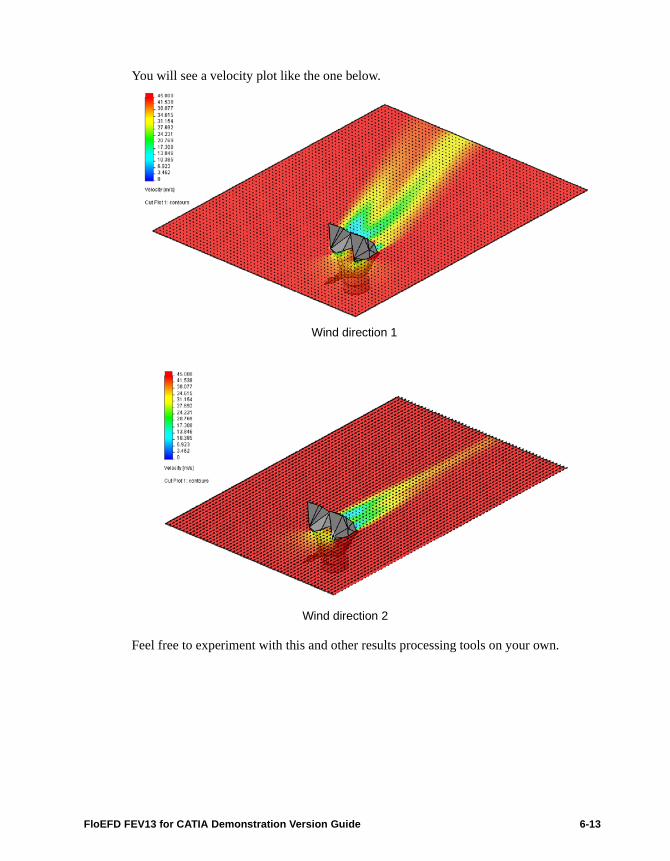
You will see a velocity plot like the one below.
Feel free to experiment with this and other results processing tools on your own.
Wind direction 1
Wind direction 2
FloEFD FEV13 for CATIA Demonstration Version Guide 6-13

Tutorial 4 - Flow over the Roof-Mounted Figure
6-14 FloEFD FEV13 for CATIA Demonstration Version Guide

Tutorial 5 - Exhaust Manifold
This tutorial demonstrates the capability of FloEFD to solve unsteady (time-dependent) problems. As an example, we study a flow of exhaust gas in the Exhaust Manifold of a 2 liter 4-cylinder engine.
In order to evacuate the combustion products from a cylinder during the exhaust stroke, each cylinder is equipped by a valve that operates in a periodic mode. During a quarter of one time period (a cycle), each valve is kept in the opened position and then moves to the closed position. The duration of this time period depends on the engine speed, so in order to define its value for the simulation, let us consider two typical engine regimes: 3000 RPM (nominal) and 1000 RPM (idle). The corresponding values of the time period will be: 20 ms for the nominal speed and 60 ms for the idle speed.
Case 1 (engine speed of 3000 RPM):Inlet Volume Flow Rate = 100 l/s, T = 1500 K
Case 2 (engine speed of 1000 RPM):Inlet Volume Flow Rate = 33.3 l/s, T = 1000 K
Exhaust Gases
FloEFD FEV13 for CATIA Demonstration Version Guide 7-1
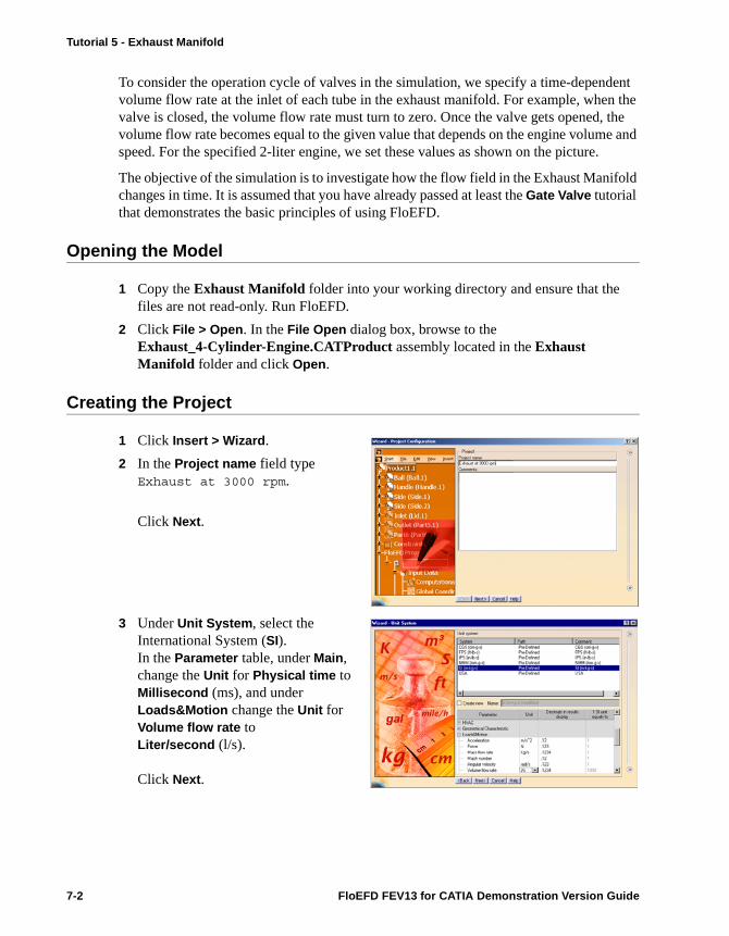
Tutorial 5 - Exhaust Manifold
To consider the operation cycle of valves in the simulation, we specify a time-dependent volume flow rate at the inlet of each tube in the exhaust manifold. For example, when the valve is closed, the volume flow rate must turn to zero. Once the valve gets opened, the volume flow rate becomes equal to the given value that depends on the engine volume and speed. For the specified 2-liter engine, we set these values as shown on the picture.
The objective of the simulation is to investigate how the flow field in the Exhaust Manifold changes in time. It is assumed that you have already passed at least the Gate Valve tutorial that demonstrates the basic principles of using FloEFD.
Opening the Model
1 Copy the Exhaust Manifold folder into your working directory and ensure that the files are not read-only. Run FloEFD.
2 Click File > Open. In the File Open dialog box, browse to the Exhaust_4-Cylinder-Engine.CATProduct assembly located in the Exhaust Manifold folder and click Open.
Creating the Project
1 Click Insert > Wizard.
2 In the Project name field type Exhaust at 3000 rpm.
Click Next.
3 Under Unit System, select the International System (SI). In the Parameter table, under Main, change the Unit for Physical time to Millisecond (ms), and under Loads&Motion change the Unit for Volume flow rate to Liter/second (l/s).
Click Next.
7-2 FloEFD FEV13 for CATIA Demonstration Version Guide

4 In the Analysis Type dialog box, select Internal as the Analysis type. Under Physical Features, select the Time-dependent check box. Change the Total analysis time to 20 ms and Output time step to 0.5 ms. The latter means that FloEFD will store the data obtained at each half of the millisecond of the specified total analysis time.
Click Next.
5 Expand the Gases item and add Air to the Project Fluids list. Here, we will use the properties of air to simulate the exhaust gas.
Click Next.
6 Accept the default wall conditions and click Next.
FloEFD FEV13 for CATIA Demonstration Version Guide 7-3

Tutorial 5 - Exhaust Manifold
7 In the Initial Conditions dialog box, under Thermodynamic Parameters, change the Temperature to 1500 K, then click Next.
8 Keep the default Result resolution level of 3.
Click Finish.
Specifying Boundary Conditions
1 In the FloEFD Analysis tree, right-click the Boundary conditions item and select Boundary Conditions object, New Boundary Condition.
2 Select the inner face of Inlet-Lid1.
3 Under Type select Flow openings and then select Inlet Volume Flow.
4 Expand the Thermodynamic Parameters group and make sure that the value of
Temperature is equal to 1500 K.
7-4 FloEFD FEV13 for CATIA Demonstration Version Guide

5 Under Flow Parameters click
Dependency to the right of the Volume
flow rate normal to face field.
6 In the Dependency dialog box, in the Dependency type list select F(time) - table. Fill the table as shown at the picture below. You can preview the resulting dependency by selecting Preview Chart.
7 After finishing, click OK, then click OK in the Boundary Condition dialog.
8 Repeat the steps 1-7 for the second inlet, where the volume flow rate is non-zero during the second time interval (5 ms - 10 ms). Specify it on the inner face of Inlet-Lid2 in the same way and fill the table as shown on the picture below.
FloEFD FEV13 for CATIA Demonstration Version Guide 7-5

Tutorial 5 - Exhaust Manifold
9 Repeat the same steps for the Inlet-Lid3 and Inlet-Lid4 and fill the tables for volume flow rate dependency as shown below. Notice that the non-zero volume flow rate on the third time interval (10 ms - 15 ms) is set on the Inlet-Lid4.Inlet-Lid3:
Inlet-Lid4:
10 Specify the Environment Pressure boundary condition with the default values on the inner face of both Outlet-Lid1 and Outlet-Lid2.
Specifying Engineering Goals
1 In the FloEFD Analysis tree, right-click the Goals item and select Goals object > New Surface Goals.
7-6 FloEFD FEV13 for CATIA Demonstration Version Guide

2 In the FloEFD Analysis tree select the Environment Pressure 1 condition to select the inner faces of the Outlet-Lid1 and Outlet-Lid2 components.
3 In the Parameter table, select Volume Flow Rate.
4 Select Create goal for each surface, then click OK.
The first FloEFD project is now fully defined. The second project will differ in the values of the inlet volume flow rate and temperature. Also, with a different period length (60 ms), all the time intervals specified at each inlet are three times longer. To save your time, we will not ask you to pass all these steps.
To run the calculation in this demonstration version, you need to use the pre-defined projects, for which the calculation function is unlocked.
Running the Calculation
1 Click Edit > FloEFD Project > Batch Run.
2 In the Batch Run dialog box, select the Solve check box for both "Pre-Defined" projects and clear all check boxes for the project defined by you.
3 Click Run.
Wait while solver calculates both projects.
After the calculation is finished, close both monitor dialog boxes by clicking File > Close.
Loading Results
1 In the Specification tree double-click the EXHAUST_AT_3000RPM_PRE-DEFINED project to activate it, then right-click Results and select Results object > Load Results.
2 In the Load Results dialog box, keep the default project results file name and click Open.
3 Activate the other calculated project and repeat steps 1-2.
FloEFD FEV13 for CATIA Demonstration Version Guide 7-7

Tutorial 5 - Exhaust Manifold
When analyzing the obtained results by using the FloEFD post-processing tools, we assume that you are working with a single project, however you can switch to the other project anytime and repeat the same steps.
Viewing Goal Plots
Let us see how the volume flow rate at the outlet changes in time.
1 In the FloEFD Analysis tree, under Results, right-click Goal Plots and select Goal Plots object > Goal Plot.
2 In the Goal Plot dialog box, under Goals, select All.
3 Change the Abscissa to Physical time.
4 Click OK.
An Excel spreadsheet with the goal results will open. Switch to the second Excel sheet (Volume Flow Rate).
This is the plot you will see.
-1 20
-1 00
-8 0
-6 0
-4 0
-2 0
0
2 0
0 5 10 15 2 0 2 5
Volume Flow Rate [l/s]
Physical time (ms)
Exhaust_4-Cylinder-Engine.CATProduct [EXHAUST_AT_3000RPM ]
SG Vo lu me Flow Rate 1
SG Vo lu me Flow Rate 2
7-8 FloEFD FEV13 for CATIA Demonstration Version Guide
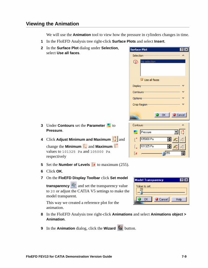
Viewing the Animation
We will use the Animation tool to view how the pressure in cylinders changes in time.
1 In the FloEFD Analysis tree right-click Surface Plots and select Insert.
2 In the Surface Plot dialog under Selection, select Use all faces.
3 Under Contours set the Parameter to Pressure.
4 Click Adjust Minimum and Maximum and
change the Minimum and Maximum values to 101325 Pa and 105000 Pa respectively
5 Set the Number of Levels to maximum (255).
6 Click OK.
7 On the FloEFD Display Toolbar click Set model
transparency and set the transparency value to 20 or adjust the CATIA V5 settings to make the model transparent.
This way we created a reference plot for the animation.
8 In the FloEFD Analysis tree right-click Animations and select Animations object > Animation.
9 In the Animation dialog, click the Wizard button.
FloEFD FEV13 for CATIA Demonstration Version Guide 7-9

Tutorial 5 - Exhaust Manifold
10 In the Animation Wizard dialog box, select Delete all existing tracks.
Click Next twice, skipping the Rotate Model step.
11 Select Scenario as the type of animation.
Click Next.
12 Keep the Uniform distribution and click Finish.
13 Double-click the track that corresponds to the created Surface Plot 1 and move the rhomb to the 00:10 position.
14 To play the resulting animation, click the button. Optionally, you can save the
animation to AVI file by clicking the button. The file will be saved in the project’s results directory.
7-10 FloEFD FEV13 for CATIA Demonstration Version Guide
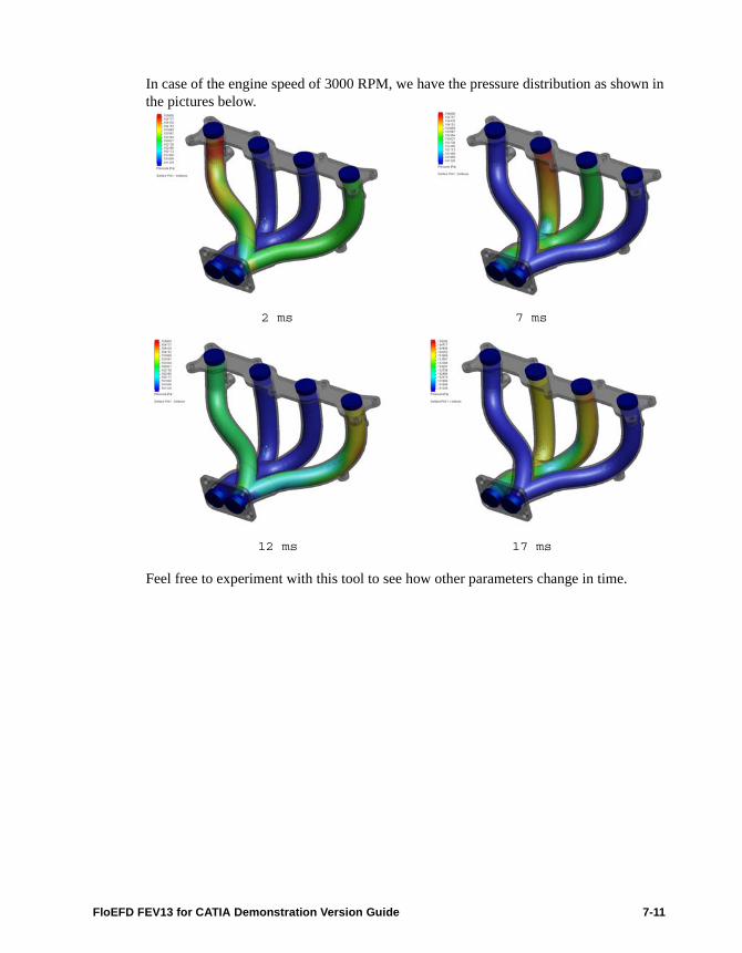
In case of the engine speed of 3000 RPM, we have the pressure distribution as shown in the pictures below.
Feel free to experiment with this tool to see how other parameters change in time.
2 ms 7 ms
12 ms 17 ms
FloEFD FEV13 for CATIA Demonstration Version Guide 7-11

Tutorial 5 - Exhaust Manifold
7-12 FloEFD FEV13 for CATIA Demonstration Version Guide

End-User License Agreement
The latest version of the End-User License Agreement is available on-line at:www.mentor.com/eula
END-USER LICENSE AGREEMENT (“Agreement”)
This is a legal agreement concerning the use of Software (as defined in Section 2) andhardware (collectively “Products”) between the company acquiring the Products(“Customer”), and the Mentor Graphics entity that issued the corresponding quotation or, ifno quotation was issued, the applicable local Mentor Graphics entity (“Mentor Graphics”).Except for license agreements related to the subject matter of this license agreement whichare physically signed by Customer and an authorized representative of Mentor Graphics, thisAgreement and the applicable quotation contain the parties’ entire understanding relating tothe subject matter and supersede all prior or contemporaneous agreements. If Customer doesnot agree to these terms and conditions, promptly return or, in the case of Software receivedelectronically, certify destruction of Software and all accompanying items within five daysafter receipt of Software and receive a full refund of any license fee paid.
1. ORDERS, FEES AND PAYMENT.
1.1. To the extent Customer (or if agreed by Mentor Graphics, Customer’s appointed third partybuying agent) places and Mentor Graphics accepts purchase orders pursuant to this Agreement(“Order(s)”), each Order will constitute a contract between Customer and Mentor Graphics,which shall be governed solely and exclusively by the terms and conditions of this Agreement,any applicable addenda and the applicable quotation, whether or not these documents arereferenced on the Order. Any additional or conflicting terms and conditions appearing on anOrder or presented via any electronic portal or other automated order management system willnot be effective unless agreed in writing by an authorized representative of Customer andMentor Graphics.
1.2. Amounts invoiced will be paid, in the currency specified on the applicable invoice, within 30days from the date of such invoice. Any past due invoices will be subject to the imposition ofinterest charges in the amount of one and one-half percent per month or the applicable legalrate currently in effect, whichever is lower. Prices do not include freight, insurance, customsduties, taxes or other similar charges, which Mentor Graphics will state separately in theapplicable invoice(s). Unless timely provided with a valid certificate of exemption or otherevidence that items are not taxable, Mentor Graphics will invoice Customer for all applicabletaxes including, but not limited to, VAT, GST, sales tax, consumption tax and service tax.Customer will make all payments free and clear of, and without reduction for, any withholdingor other taxes; any such taxes imposed on payments by Customer hereunder will beCustomer’s sole responsibility. If Customer appoints a third party to place purchase ordersand/or make payments on Customer’s behalf, Customer shall be liable for payment underOrders placed by such third party in the event of default.
IIMPORTANT INFORMATION
USE OF ALL SOFTWARE IS SUBJECT TO LICENSE RESTRICTIONS. CAREFULLY READ THIS LICENSE AGREEMENT BEFORE USING THE PRODUCTS. USE OF
SOFTWARE INDICATES CUSTOMER’S COMPLETE AND UNCONDITIONAL ACCEPTANCE OF THE TERMS AND CONDITIONS SET FORTH IN THIS
AGREEMENT. ANY ADDITIONAL OR DIFFERENT PURCHASE ORDER TERMS AND CONDITIONS SHALL NOT APPLY.
1.3. All Products are delivered FCA factory (Incoterms 2010), freight prepaid and invoiced toCustomer, except Software delivered electronically, which shall be deemed delivered whenmade available to Customer for download. Mentor Graphics retains a security interest in allProducts delivered under this Agreement, to secure payment of the purchase price of suchProducts, and Customer agrees to sign any documents that Mentor Graphics determines to benecessary or convenient for use in filing or perfecting such security interest. Mentor Graphics’delivery of Software by electronic means is subject to Customer’s provision of both a primaryand an alternate e-mail address.
2. GRANT OF LICENSE. The software installed, downloaded, or otherwise acquired by Customerunder this Agreement, including any updates, modifications, revisions, copies, documentation anddesign data (“Software”) are copyrighted, trade secret and confidential information of MentorGraphics or its licensors, who maintain exclusive title to all Software and retain all rights notexpressly granted by this Agreement. Mentor Graphics grants to Customer, subject to payment ofapplicable license fees, a nontransferable, nonexclusive license to use Software solely: (a) inmachine-readable, object-code form (except as provided in Subsection 5.2); (b) for Customer’sinternal business purposes; (c) for the term of the license; and (d) on the computer hardware and atthe site authorized by Mentor Graphics. A site is restricted to a one-half mile (800 meter) radius.Customer may have Software temporarily used by an employee for telecommuting purposes fromlocations other than a Customer office, such as the employee’s residence, an airport or hotel,provided that such employee’s primary place of employment is the site where the Software isauthorized for use. Mentor Graphics’ standard policies and programs, which vary depending onSoftware, license fees paid or services purchased, apply to the following: (a) relocation of Software;(b) use of Software, which may be limited, for example, to execution of a single session by a singleuser on the authorized hardware or for a restricted period of time (such limitations may betechnically implemented through the use of authorization codes or similar devices); and (c) supportservices provided, including eligibility to receive telephone support, updates, modifications, andrevisions. For the avoidance of doubt, if Customer provides any feedback or requests any change orenhancement to Products, whether in the course of receiving support or consulting services,evaluating Products, performing beta testing or otherwise, any inventions, product improvements,modifications or developments made by Mentor Graphics (at Mentor Graphics’ sole discretion) willbe the exclusive property of Mentor Graphics.
3. ESC SOFTWARE. If Customer purchases a license to use development or prototyping tools ofMentor Graphics’ Embedded Software Channel (“ESC”), Mentor Graphics grants to Customer anontransferable, nonexclusive license to reproduce and distribute executable files created usingESC compilers, including the ESC run-time libraries distributed with ESC C and C++ compilerSoftware that are linked into a composite program as an integral part of Customer’s compiledcomputer program, provided that Customer distributes these files only in conjunction withCustomer’s compiled computer program. Mentor Graphics does NOT grant Customer any right toduplicate, incorporate or embed copies of Mentor Graphics’ real-time operating systems or otherembedded software products into Customer’s products or applications without first signing orotherwise agreeing to a separate agreement with Mentor Graphics for such purpose.
4. BETA CODE.
4.1. Portions or all of certain Software may contain code for experimental testing and evaluation(which may be either alpha or beta, collectively “Beta Code”), which may not be used withoutMentor Graphics’ explicit authorization. Upon Mentor Graphics’ authorization, MentorGraphics grants to Customer a temporary, nontransferable, nonexclusive license forexperimental use to test and evaluate the Beta Code without charge for a limited period of timespecified by Mentor Graphics. This grant and Customer’s use of the Beta Code shall not beconstrued as marketing or offering to sell a license to the Beta Code, which Mentor Graphicsmay choose not to release commercially in any form.
4.2. If Mentor Graphics authorizes Customer to use the Beta Code, Customer agrees to evaluateand test the Beta Code under normal conditions as directed by Mentor Graphics. Customer willcontact Mentor Graphics periodically during Customer’s use of the Beta Code to discuss anymalfunctions or suggested improvements. Upon completion of Customer’s evaluation andtesting, Customer will send to Mentor Graphics a written evaluation of the Beta Code,including its strengths, weaknesses and recommended improvements.
4.3. Customer agrees to maintain Beta Code in confidence and shall restrict access to the BetaCode, including the methods and concepts utilized therein, solely to those employees andCustomer location(s) authorized by Mentor Graphics to perform beta testing. Customer agreesthat any written evaluations and all inventions, product improvements, modifications ordevelopments that Mentor Graphics conceived or made during or subsequent to thisAgreement, including those based partly or wholly on Customer’s feedback, will be theexclusive property of Mentor Graphics. Mentor Graphics will have exclusive rights, title andinterest in all such property. The provisions of this Subsection 4.3 shall survive termination ofthis Agreement.
5. RESTRICTIONS ON USE.
5.1. Customer may copy Software only as reasonably necessary to support the authorized use. Eachcopy must include all notices and legends embedded in Software and affixed to its medium andcontainer as received from Mentor Graphics. All copies shall remain the property of MentorGraphics or its licensors. Customer shall maintain a record of the number and primary locationof all copies of Software, including copies merged with other software, and shall make thoserecords available to Mentor Graphics upon request. Customer shall not make Productsavailable in any form to any person other than Customer’s employees and on-site contractors,excluding Mentor Graphics competitors, whose job performance requires access and who areunder obligations of confidentiality. Customer shall take appropriate action to protect theconfidentiality of Products and ensure that any person permitted access does not disclose oruse Products except as permitted by this Agreement. Customer shall give Mentor Graphicswritten notice of any unauthorized disclosure or use of the Products as soon as Customerbecomes aware of such unauthorized disclosure or use. Except as otherwise permitted forpurposes of interoperability as specified by applicable and mandatory local law, Customershall not reverse-assemble, reverse-compile, reverse-engineer or in any way derive any sourcecode from Software. Log files, data files, rule files and script files generated by or for theSoftware (collectively “Files”), including without limitation files containing StandardVerification Rule Format (“SVRF”) and Tcl Verification Format (“TVF”) which are MentorGraphics’ proprietary syntaxes for expressing process rules, constitute or include confidentialinformation of Mentor Graphics. Customer may share Files with third parties, excludingMentor Graphics competitors, provided that the confidentiality of such Files is protected bywritten agreement at least as well as Customer protects other information of a similar nature orimportance, but in any case with at least reasonable care. Customer may use Files containingSVRF or TVF only with Mentor Graphics products. Under no circumstances shall Customeruse Software or Files or allow their use for the purpose of developing, enhancing or marketingany product that is in any way competitive with Software, or disclose to any third party theresults of, or information pertaining to, any benchmark.
5.2. If any Software or portions thereof are provided in source code form, Customer will use thesource code only to correct software errors and enhance or modify the Software for theauthorized use. Customer shall not disclose or permit disclosure of source code, in whole or inpart, including any of its methods or concepts, to anyone except Customer’s employees or on-site contractors, excluding Mentor Graphics competitors, with a need to know. Customer shallnot copy or compile source code in any manner except to support this authorized use.
5.3. Customer may not assign this Agreement or the rights and duties under it, or relocate,sublicense or otherwise transfer the Products, whether by operation of law or otherwise(“Attempted Transfer”), without Mentor Graphics’ prior written consent and payment of
Mentor Graphics’ then-current applicable relocation and/or transfer fees. Any AttemptedTransfer without Mentor Graphics’ prior written consent shall be a material breach of thisAgreement and may, at Mentor Graphics’ option, result in the immediate termination of theAgreement and/or the licenses granted under this Agreement. The terms of this Agreement,including without limitation the licensing and assignment provisions, shall be binding uponCustomer’s permitted successors in interest and assigns.
5.4. The provisions of this Section 5 shall survive the termination of this Agreement.
6. SUPPORT SERVICES. To the extent Customer purchases support services, Mentor Graphics willprovide Customer with updates and technical support for the Products, at the Customer site(s) forwhich support is purchased, in accordance with Mentor Graphics’ then current End-User SupportTerms located at http://supportnet.mentor.com/about/legal/.
7. LIMITED WARRANTY.
7.1. Mentor Graphics warrants that during the warranty period its standard, generally supportedProducts, when properly installed, will substantially conform to the functional specificationsset forth in the applicable user manual. Mentor Graphics does not warrant that Products willmeet Customer’s requirements or that operation of Products will be uninterrupted or error free.The warranty period is 90 days starting on the 15th day after delivery or upon installation,whichever first occurs. Customer must notify Mentor Graphics in writing of anynonconformity within the warranty period. For the avoidance of doubt, this warranty appliesonly to the initial shipment of Software under an Order and does not renew or reset, forexample, with the delivery of (a) Software updates or (b) authorization codes or alternateSoftware under a transaction involving Software re-mix. This warranty shall not be valid ifProducts have been subject to misuse, unauthorized modification, improper installation orCustomer is not in compliance with this Agreement. MENTOR GRAPHICS’ ENTIRELIABILITY AND CUSTOMER’S EXCLUSIVE REMEDY SHALL BE, AT MENTORGRAPHICS’ OPTION, EITHER (A) REFUND OF THE PRICE PAID UPON RETURN OFTHE PRODUCTS TO MENTOR GRAPHICS OR (B) MODIFICATION ORREPLACEMENT OF THE PRODUCTS THAT DO NOT MEET THIS LIMITEDWARRANTY. MENTOR GRAPHICS MAKES NO WARRANTIES WITH RESPECT TO:(A) SERVICES; (B) PRODUCTS PROVIDED AT NO CHARGE; OR (C) BETA CODE;ALL OF WHICH ARE PROVIDED “AS IS.”
7.2. THE WARRANTIES SET FORTH IN THIS SECTION 7 ARE EXCLUSIVE. NEITHERMENTOR GRAPHICS NOR ITS LICENSORS MAKE ANY OTHER WARRANTIESEXPRESS, IMPLIED OR STATUTORY, WITH RESPECT TO PRODUCTS PROVIDEDUNDER THIS AGREEMENT. MENTOR GRAPHICS AND ITS LICENSORSSPECIFICALLY DISCLAIM ALL IMPLIED WARRANTIES OF MERCHANTABILITY,FITNESS FOR A PARTICULAR PURPOSE AND NON-INFRINGEMENT OFINTELLECTUAL PROPERTY.
8. LIMITATION OF LIABILITY. EXCEPT WHERE THIS EXCLUSION OR RESTRICTION OFLIABILITY WOULD BE VOID OR INEFFECTIVE UNDER APPLICABLE LAW, IN NOEVENT SHALL MENTOR GRAPHICS OR ITS LICENSORS BE LIABLE FOR INDIRECT,SPECIAL, INCIDENTAL, OR CONSEQUENTIAL DAMAGES (INCLUDING LOST PROFITSOR SAVINGS) WHETHER BASED ON CONTRACT, TORT OR ANY OTHER LEGALTHEORY, EVEN IF MENTOR GRAPHICS OR ITS LICENSORS HAVE BEEN ADVISED OFTHE POSSIBILITY OF SUCH DAMAGES. IN NO EVENT SHALL MENTOR GRAPHICS’ ORITS LICENSORS’ LIABILITY UNDER THIS AGREEMENT EXCEED THE AMOUNTRECEIVED FROM CUSTOMER FOR THE HARDWARE, SOFTWARE LICENSE ORSERVICE GIVING RISE TO THE CLAIM. IN THE CASE WHERE NO AMOUNT WAS PAID,MENTOR GRAPHICS AND ITS LICENSORS SHALL HAVE NO LIABILITY FOR ANYDAMAGES WHATSOEVER. THE PROVISIONS OF THIS SECTION 8 SHALL SURVIVE

THE TERMINATION OF THIS AGREEMENT.
9. HAZARDOUS APPLICATIONS. CUSTOMER ACKNOWLEDGES IT IS SOLELYRESPONSIBLE FOR TESTING ITS PRODUCTS USED IN APPLICATIONS WHERE THEFAILURE OR INACCURACY OF ITS PRODUCTS MIGHT RESULT IN DEATH ORPERSONAL INJURY (“HAZARDOUS APPLICATIONS”). EXCEPT TO THE EXTENT THISEXCLUSION OR RESTRICTION OF LIABILITY WOULD BE VOID OR INEFFECTIVEUNDER APPLICABLE LAW, IN NO EVENT SHALL MENTOR GRAPHICS OR ITSLICENSORS BE LIABLE FOR ANY DAMAGES RESULTING FROM OR IN CONNECTIONWITH THE USE OF MENTOR GRAPHICS PRODUCTS IN OR FOR HAZARDOUSAPPLICATIONS. THE PROVISIONS OF THIS SECTION 9 SHALL SURVIVE THETERMINATION OF THIS AGREEMENT.
10. INDEMNIFICATION. CUSTOMER AGREES TO INDEMNIFY AND HOLD HARMLESSMENTOR GRAPHICS AND ITS LICENSORS FROM ANY CLAIMS, LOSS, COST, DAMAGE,EXPENSE OR LIABILITY, INCLUDING ATTORNEYS’ FEES, ARISING OUT OF OR INCONNECTION WITH THE USE OF MENTOR GRAPHICS PRODUCTS IN OR FORHAZARDOUS APPLICATIONS. THE PROVISIONS OF THIS SECTION 10 SHALL SURVIVETHE TERMINATION OF THIS AGREEMENT.
11. INFRINGEMENT.
11.1. Mentor Graphics will defend or settle, at its option and expense, any action brought againstCustomer in the United States, Canada, Japan, or member state of the European Union whichalleges that any standard, generally supported Product acquired by Customer hereunderinfringes a patent or copyright or misappropriates a trade secret in such jurisdiction. MentorGraphics will pay costs and damages finally awarded against Customer that are attributable tosuch action. Customer understands and agrees that as conditions to Mentor Graphics’obligations under this section Customer must: (a) notify Mentor Graphics promptly in writingof the action; (b) provide Mentor Graphics all reasonable information and assistance to settleor defend the action; and (c) grant Mentor Graphics sole authority and control of the defense orsettlement of the action.
11.2. If a claim is made under Subsection 11.1 Mentor Graphics may, at its option and expense: (a)replace or modify the Product so that it becomes noninfringing; (b) procure for Customer theright to continue using the Product; or (c) require the return of the Product and refund toCustomer any purchase price or license fee paid, less a reasonable allowance for use.
11.3. Mentor Graphics has no liability to Customer if the action is based upon: (a) the combinationof Software or hardware with any product not furnished by Mentor Graphics; (b) themodification of the Product other than by Mentor Graphics; (c) the use of other than a currentunaltered release of Software; (d) the use of the Product as part of an infringing process; (e) aproduct that Customer makes, uses, or sells; (f) any Beta Code or Product provided at nocharge; (g) any software provided by Mentor Graphics’ licensors who do not provide suchindemnification to Mentor Graphics’ customers; or (h) infringement by Customer that isdeemed willful. In the case of (h), Customer shall reimburse Mentor Graphics for itsreasonable attorney fees and other costs related to the action.
11.4. THIS SECTION 11 IS SUBJECT TO SECTION 8 ABOVE AND STATES THE ENTIRELIABILITY OF MENTOR GRAPHICS AND ITS LICENSORS, AND CUSTOMER’S SOLEAND EXCLUSIVE REMEDY, FOR DEFENSE, SETTLEMENT AND DAMAGES, WITHRESPECT TO ANY ALLEGED PATENT OR COPYRIGHT INFRINGEMENT OR TRADESECRET MISAPPROPRIATION BY ANY PRODUCT PROVIDED UNDER THISAGREEMENT.
12. TERMINATION AND EFFECT OF TERMINATION.

12.1. If a Software license was provided for limited term use, such license will automaticallyterminate at the end of the authorized term. Mentor Graphics may terminate this Agreementand/or any license granted under this Agreement immediately upon written notice if Customer:(a) exceeds the scope of the license or otherwise fails to comply with the licensing orconfidentiality provisions of this Agreement, or (b) becomes insolvent, files a bankruptcypetition, institutes proceedings for liquidation or winding up or enters into an agreement toassign its assets for the benefit of creditors. For any other material breach of any provision ofthis Agreement, Mentor Graphics may terminate this Agreement and/or any license grantedunder this Agreement upon 30 days written notice if Customer fails to cure the breach withinthe 30 day notice period. Termination of this Agreement or any license granted hereunder willnot affect Customer’s obligation to pay for Products shipped or licenses granted prior to thetermination, which amounts shall be payable immediately upon the date of termination.
12.2. Upon termination of this Agreement, the rights and obligations of the parties shall cease exceptas expressly set forth in this Agreement. Upon termination, Customer shall ensure that all useof the affected Products ceases, and shall return hardware and either return to Mentor Graphicsor destroy Software in Customer’s possession, including all copies and documentation, andcertify in writing to Mentor Graphics within ten business days of the termination date thatCustomer no longer possesses any of the affected Products or copies of Software in any form.
13. EXPORT. The Products provided hereunder are subject to regulation by local laws and UnitedStates (“U.S.”) government agencies, which prohibit export, re-export or diversion of certainproducts, information about the products, and direct or indirect products thereof, to certain countriesand certain persons. Customer agrees that it will not export or re-export Products in any mannerwithout first obtaining all necessary approval from appropriate local and U.S. government agencies.If Customer wishes to disclose any information to Mentor Graphics that is subject to any U.S. orother applicable export restrictions, including without limitation the U.S. International Traffic inArms Regulations (ITAR) or special controls under the Export Administration Regulations (EAR),Customer will notify Mentor Graphics personnel, in advance of each instance of disclosure, thatsuch information is subject to such export restrictions.
14. U.S. GOVERNMENT LICENSE RIGHTS. Software was developed entirely at private expense.The parties agree that all Software is commercial computer software within the meaning of theapplicable acquisition regulations. Accordingly, pursuant to U.S. FAR 48 CFR 12.212 and DFAR48 CFR 227.7202, use, duplication and disclosure of the Software by or for the U.S. government ora U.S. government subcontractor is subject solely to the terms and conditions set forth in thisAgreement, which shall supersede any conflicting terms or conditions in any government orderdocument, except for provisions which are contrary to applicable mandatory federal laws.
15. THIRD PARTY BENEFICIARY. Mentor Graphics Corporation, Mentor Graphics (Ireland)Limited, Microsoft Corporation and other licensors may be third party beneficiaries of thisAgreement with the right to enforce the obligations set forth herein.
16. REVIEW OF LICENSE USAGE. Customer will monitor the access to and use of Software. Withprior written notice and during Customer’s normal business hours, Mentor Graphics may engage aninternationally recognized accounting firm to review Customer’s software monitoring system andrecords deemed relevant by the internationally recognized accounting firm to confirm Customer’scompliance with the terms of this Agreement or U.S. or other local export laws. Such review mayinclude FlexNet (or successor product) report log files that Customer shall capture and provide atMentor Graphics’ request. Customer shall make records available in electronic format and shallfully cooperate with data gathering to support the license review. Mentor Graphics shall bear theexpense of any such review unless a material non-compliance is revealed. Mentor Graphics shalltreat as confidential information all information gained as a result of any request or review and shallonly use or disclose such information as required by law or to enforce its rights under thisAgreement. The provisions of this Section 16 shall survive the termination of this Agreement.
17. CONTROLLING LAW, JURISDICTION AND DISPUTE RESOLUTION. The owners ofcertain Mentor Graphics intellectual property licensed under this Agreement are located in Irelandand the U.S. To promote consistency around the world, disputes shall be resolved as follows:excluding conflict of laws rules, this Agreement shall be governed by and construed under the lawsof the State of Oregon, U.S., if Customer is located in North or South America, and the laws ofIreland if Customer is located outside of North or South America. All disputes arising out of or inrelation to this Agreement shall be submitted to the exclusive jurisdiction of the courts of Portland,Oregon when the laws of Oregon apply, or Dublin, Ireland when the laws of Ireland apply.Notwithstanding the foregoing, all disputes in Asia arising out of or in relation to this Agreementshall be resolved by arbitration in Singapore before a single arbitrator to be appointed by thechairman of the Singapore International Arbitration Centre (“SIAC”) to be conducted in the Englishlanguage, in accordance with the Arbitration Rules of the SIAC in effect at the time of the dispute,which rules are deemed to be incorporated by reference in this section. Nothing in this section shallrestrict Mentor Graphics’ right to bring an action (including for example a motion for injunctiverelief) against Customer in the jurisdiction where Customer’s place of business is located. TheUnited Nations Convention on Contracts for the International Sale of Goods does not apply to thisAgreement.
18. SEVERABILITY. If any provision of this Agreement is held by a court of competent jurisdictionto be void, invalid, unenforceable or illegal, such provision shall be severed from this Agreementand the remaining provisions will remain in full force and effect.
19. MISCELLANEOUS. This Agreement contains the parties’ entire understanding relating to itssubject matter and supersedes all prior or contemporaneous agreements. Some Software maycontain code distributed under a third party license agreement that may provide additional rights toCustomer. Please see the applicable Software documentation for details. This Agreement may onlybe modified in writing, signed by an authorized representative of each party. Waiver of terms orexcuse of breach must be in writing and shall not constitute subsequent consent, waiver or excuse.
Rev. 130502, Part No. 255853


Corporate HeadquartersMentor Graphics Corporation8005 SW Boeckman RoadWilsonville, Oregon 97070-7777United States of America503-685-7000
Sales and Product Information800-547-3000 or 503-685-8000
North American Support Center800-547-4303
For support locations outside of the US, please refer to the followingwebsite: http://www.mentor.com/supportnet/support-offices.html
www.mentor.com/supportnet