
FLOATING OFFSHORE STRUCTURES MARK DAMIAN RICHARDSON · DYNAMICALLY INSTALLED ANCHORS FOR FLOATING...
402
DYNAMICALLY INSTALLED ANCHORS FOR FLOATING OFFSHORE STRUCTURES by MARK DAMIAN RICHARDSON B.E. (Hons), B.Com. This thesis is presented for the degree of DOCTOR OF PHILOSOPHY at THE UNIVERSITY OF WESTERN AUSTRALIA Centre for Offshore Foundation Systems School of Civil and Resource Engineering September 2008
Transcript of FLOATING OFFSHORE STRUCTURES MARK DAMIAN RICHARDSON · DYNAMICALLY INSTALLED ANCHORS FOR FLOATING...
DYNAMICALLY INSTALLED ANCHORS FOR
FLOATING OFFSHORE STRUCTURES
by
MARK DAMIAN RICHARDSON
B.E. (Hons), B.Com.
This thesis is presented for the degree of
DOCTOR OF PHILOSOPHY
at
THE UNIVERSITY OF WESTERN AUSTRALIA
Centre for Offshore Foundation Systems
School of Civil and Resource Engineering
September 2008

i
ABSTRACT
The gradual depletion of shallow water hydrocarbon deposits has forced the offshore oil
and gas industry to develop reserves in deeper waters. Dynamically installed anchors
have been proposed as a cost-effective anchoring solution for floating offshore
structures in deep water environments. The rocket or torpedo shaped anchor is released
from a designated drop height above the seafloor and allowed to penetrate the seabed
via the kinetic energy gained during free-fall and the anchor’s self weight. Dynamic
anchors can be deployed in any water depth and the relatively simple fabrication and
installation procedures provide a significant cost saving over conventional deepwater
anchoring systems.
Despite use in a number of offshore applications, information regarding the
geotechnical performance of dynamically installed anchors is scarce. Consequently, this
research has focused on establishing an extensive test database through the modelling of
the dynamic anchor installation process in the geotechnical centrifuge. The tests were
aimed at assessing the embedment depth and subsequent dynamic anchor holding
capacity under various loading conditions. Analytical design tools, verified against the
experimental database, were developed for the prediction of the embedment depth and
holding capacity.
Test results in normally consolidated clay indicated zero fluke anchor tip embedment
depths of up to 3 times the anchor length for impact velocities approaching 30 m/s. The
anchor embedment depth was found to depend on both the impact velocity and the
anchor geometry, and resulted in holding capacities of up to 4 times the anchor dry
weight. Given the dependence of holding capacity on penetration depth, optimisation of
the anchor impact velocity suggests the potential for considerably higher capacities.
Long-term sustained and cyclic loading did not significantly influence the holding
capacity, although an increase in the load duration under either sustained or cyclic
loading conditions led to a slight reduction in the anchor capacity. An apparent
threshold sustained loading level was identified, above which the anchor capacity may
be detrimentally affected.
ii
In normally consolidated clay, the dynamic anchor holding capacity increased with time
following installation due to setup. The short-term capacity immediately after
installation depended on the rate of installation, with an increase in the impact velocity
resulting in a comparative reduction in the short-term capacity. Cavity expansion
solutions for the radial consolidation of soil around a solid driven pile provided
reasonable estimates of the increase in capacity of dynamic anchors following
installation.
The centrifuge tests indicated that whilst dynamic anchors were suitable for use in
calcareous soils, extremely low embedment depths (less than the anchor length)
prevented their use in silica sands. Impact velocities of up to 30 m/s resulted in
penetration depths of up to 1.5 times the anchor length in uncemented calcareous sand
samples, corresponding to vertical monotonic holding capacities of 1 – 2 times the
anchor’s dry weight. Given the dependence of embedment depth on impact velocity and
the subsequent dependence of holding capacity on embedment depth, optimisation of
the dynamic anchor impact velocity suggests the potential for higher holding capacities
than were achieved here.
An analytical method based on conventional bearing and frictional resistance theory and
incorporating provisions for viscous enhanced shearing resistance and inertial drag
resistance during penetration was adopted for predicting the dynamic anchor
embedment depth. Similarly a conventional pile capacity calculation technique was
adapted for determining the vertical monotonic holding capacity of dynamic anchors.
Validation of these methods against the test database indicated that they were capable of
providing reasonable estimates of the embedment and holding capacity performance of
dynamically installed anchors in both normally consolidated clay and uncemented
calcareous sand deposits. Combining the embedment and capacity prediction methods
enabled the generation of dynamic anchor design charts.

iii
ACKNOWLEDGEMENTS
First and foremost I would like to take this opportunity to express my sincere gratitude
to Dr Conleth O’Loughlin for encouraging me to pursue this research. Con was always
available to discuss various aspects of the project and remained an important source of
guidance even after leaving the university. A special thank you also to Professor Mark
Randolph; it has been a great privilege to work with Mark and his guidance and advice
have proved invaluable. Thanks also to Dr Christophe Gaudin for helping out in Con’s
absence; Christophe’s input, particularly with the centrifuge tests was greatly
appreciated.
This research would not have been possible without the important contributions of Don
Herley and Bart Thompson. Don and Bart provided immeasurable assistance with the
experimental aspects of the project and lightened the mood with endless stories about
past sporting glories. Thanks also to the workshop, electronics and technical staff who
assisted with the project, especially John Breen, Tuarn Brown, Shane De Catania, Phil
Hortin, Gary Davies, Dave Jones, Frank Tan, Neil McIntosh, Alex Duff and Wayne
Galbraith. In addition, the support provided by Monica Mackman, Wenge Liu and the
rest of the administrative staff is gratefully acknowledged.
I would also like to acknowledge the financial support I received during my
candidature, which consisted of an Australian Postgraduate Award through a linkage
project with Woodside Energy Ltd, a postgraduate top-up scholarship through the
Western Australia Energy Research Alliance (WA:ERA) and an Ad-Hoc scholarship
through the Centre for Offshore Foundation Systems.
It would be remiss of me not to thank my friends. To my friends within the school,
thank you for providing valuable discussion on many of the issues arising during the
project. Thank you also to my friends outside of the university for the often much
needed distraction; but don’t pretend that you are ever going to read this.
A special thank you also to my family, particularly my parents, your guidance,
encouragement, love and understanding, not only over the past few years but throughout
my life has been an inspiration.

iv
Finally, to Rebecca (and Normie and Scoobie), your unwavering love and support has
been a source of strength and encouragement. This work is dedicated to you.
I certify that, except where specific reference is made in the text to the work of others,
the contents of this thesis are original and have not been submitted to any other
university.
Mark Richardson
September 2008

v
TABLE OF CONTENTS
ABSTRACT i
ACKNOWLEDGEMENTS iii
TABLE OF CONTENTS v
NOTATION xiv
CHAPTER 1 - INTRODUCTION 1
1.1 THE OFFSHORE OIL AND GAS INDUSTRY 1
1.2 OFFSHORE DEVELOPMENT SYSTEMS 2
1.2.1 Fixed Platform 2
1.2.2 Compliant Tower 2
1.2.3 Tension Leg Platform (TLP) 3
1.2.4 Semi-Submersible 3
1.2.5 Spar Platform 3
1.2.6 Floating Production Storage and Offloading (FPSO) Facility 4
1.2.7 Subsea System 4
1.2.8 Hybrid Systems 4
1.3 MOORING SYSTEMS 5
1.4 ANCHORING SYSTEMS 6
1.4.1 Anchor Piles 6
1.4.2 Suction Caissons 7
1.4.3 Drag Embedment Anchors 7
1.4.4 Drag-In Plate Anchors 8
1.4.5 Direct Embedment Anchors 8
1.4.6 Dynamically Installed Anchors 9
1.5 RESEARCH OBJECTIVES 10
1.6 THESIS STRUCTURE 12

vi
CHAPTER 2 - LITERATURE REVIEW 15
2.1 INTRODUCTION 15
2.2 SEABED PENETRATION 15
2.2.1 Seabed Strength Characterisation 16
2.2.1.1 Marine Sediment Penetrometer 16
2.2.1.2 Marine Impact Penetrometer 17
2.2.1.3 Doppler Penetrometer 18
2.2.1.4 Free Fall Cone Penetrometer 19
2.2.1.5 Expendable Bottom Penetrometer 19
2.2.2 Nuclear Waste Disposal 20
2.2.3 Embedment Prediction Methods 23
2.2.3.1 Strain Rate Effects 23
2.2.3.2 Inertial Drag 26
2.2.3.3 Young's Method 27
2.2.3.4 True's Method 29
2.2.3.5 Ove Arup and Partners Method 33
2.3 PULLOUT CAPACITY 35
2.3.1 American Petroleum Institute Method 35
2.3.2 Marine Technology Directorate Method 36
2.3.3 Consolidation Effects 38
2.3.4 Long-Term Sustained Loading 40
2.3.5 Cyclic Loading 41
2.4 DYNAMICALLY INSTALLED ANCHORS 42
2.4.1 Torpedo Anchor 42
2.4.2 Deep Penetrating Anchor 44
2.4.3 SPEAR Anchor 46
2.4.4 Physical Modelling 46
2.4.5 Analytical and Numerical Modelling 48
2.5 SUMMARY 49

vii
CHAPTER 3 - EXPERIMENTAL METHODS AND MODELLING 53
3.1 INTRODUCTION 53
3.2 CENTRIFUGE MODELLING 53
3.3 CENTRIFUGE FACILITIES 56
3.3.1 Beam Centrifuge 56
3.3.1.1 Sample Strong-Box 56
3.3.1.2 Actuators 56
3.3.1.3 STOMPI 57
3.3.2 Drum Centrifuge 57
3.3.2.1 Sample Channel 58
3.3.2.2 Tool Table Actuator 58
3.4 SOIL SAMPLES 58
3.4.1 Soil Properties 58
3.4.1.1 Kaolin Clay 58
3.4.1.2 Calcareous Sand 59
3.4.1.3 Silica Flour 60
3.4.2 Sample Preparation 60
3.4.2.1 Kaolin Clay 60
3.4.2.2 Calcareous Sand 62
3.4.2.3 Silica Flour 62
3.5 PENETROMETER DEVICES 63
3.5.1 T-bar Penetrometer 63
3.5.2 Cone Penetrometer 64
3.5.2.1 Calcareous Sand 64
3.5.2.2 Silica Flour 65
3.6 MODEL ANCHORS 65
3.6.1 Zero Fluke Model Anchors 65
3.6.2 Four Fluke Model Anchors 66
3.6.3 Model Anchors with Different Tip Shapes 67

viii
3.6.4 Instrumented Anchor 68
3.6.5 Model Anchors with Different Aspect Ratios 70
3.6.6 Anchor Chain and Release Cord 71
3.7 EXPERIMENTAL APPARATUS 71
3.7.1 Installation Guide 71
3.7.2 Release Mechanism 73
3.7.3 Load Cell 73
3.8 TESTING PROCEDURE 74
3.8.1 Beam Centrifuge 74
3.8.1.1 Dynamic Installation 74
3.8.1.2 Vertical Monotonic Extraction 75
3.8.1.3 Sustained Loading Tests 75
3.8.1.4 Cyclic Loading Tests 76
3.8.1.5 Static Installation 77
3.8.1.6 Monotonic Extraction Following Static Installation 77
3.8.2 Drum Centrifuge 78
3.8.2.1 Dynamic Installation 78
3.8.2.2 Vertical Monotonic Extraction 79
3.9 EXPERIMENTAL PROGRAMME 79
CHAPTER 4 - ANALYTICAL AND NUMERICAL METHODS 81
4.1 INTRODUCTION 81
4.2 DRAG COEFFICIENT 81
4.2.1 Factors Influencing the Drag Coefficient 82
4.2.2 Computational Fluid Dynamics 84
4.2.3 Inertial Drag in Soil 87
4.3 IMPACT VELOCITY 89
4.3.1 Uniform Acceleration Field 89
4.3.2 Centrifuge Acceleration Field 90

ix
4.3.3 Energy Losses 91
4.4 EMBEDMENT DEPTH 91
4.4.1 Calculation Procedure 92
4.4.2 Parameter Values 95
4.5 HOLDING CAPACITY 97
4.5.1 Calculation Procedure 98
4.5.2 Parameter Values 99
4.5.3 Normalised Capacity 101
4.5.4 Anchor Efficiency 101
4.6 CALCAREOUS SAND 101
4.6.1 Embedment Depth 102
4.6.1.1 Calculation Procedure 102
4.6.1.2 Parameter Values 103
4.6.2 Holding Capacity 104
4.6.2.1 Calculation Procedure 104
4.6.2.2 Parameter Values 105
CHAPTER 5 - EXPERIMENTAL RESULTS FOR DYNAMIC
ANCHOR TESTING IN NORMALLY CONSOLIDATED CLAY 107
5.1 INTRODUCTION 107
5.2 BEAM CENTRIFUGE 108
5.2.1 Strength Characterisation Tests 108
5.2.2 Impact Velocity 112
5.2.3 Embedment Depth 114
5.2.3.1 Influence of Impact Velocity 115
5.2.3.2 Influence of Anchor Geometry 116
5.2.3.3 Influence of Surface Water 118
5.2.3.4 Verticality 119
5.2.4 Load Displacement Response 119
5.2.5 Vertical Monotonic Holding Capacity 121

x
5.2.5.1 Influence of Embedment Depth 122
5.2.5.2 Influence of Anchor Geometry 123
5.2.6 Long-Term Sustained Loading 123
5.2.6.1 Normalised Capacity Ratio 125
5.2.6.2 Influence of Load Magnitude 126
5.2.6.3 Influence of Load Duration 128
5.2.7 Cyclic Loading 128
5.2.7.1 Normalised Capacity Ratio 130
5.2.7.2 Influence of Load Magnitude / Amplitude 130
5.2.7.3 Influence of Number of Cycles 132
5.2.8 Static Push Tests 133
5.2.8.1 Static Installation 133
5.2.8.2 Monotonic Extraction Following Static Installation 134
5.2.9 Summary 134
5.3 DRUM CENTRIFUGE 136
5.3.1 Strength Characterisation Tests 136
5.3.2 Impact Velocity 138
5.3.3 Embedment Depth 139
5.3.3.1 Influence of Impact Velocity 140
5.3.3.2 Influence of Anchor Aspect Ratio 141
5.3.3.3 Influence of Anchor Mass 141
5.3.3.4 Combined Influence of Aspect Ratio and Mass 142
5.3.4 Load-Displacement Response 142
5.3.5 Vertical Monotonic Holding Capacity 143
5.3.5.1 Influence of Embedment Depth 144
5.3.5.2 Influence of Anchor Aspect Ratio 144
5.3.6 Setup and Consolidation 145
5.3.6.1 Short-Term Anchor Capacity 147
5.3.6.2 Capacity Increase with Time 148
5.3.6.3 t50 and t90 149
5.3.7 Summary 150
5.4 CONCLUSIONS 152

xi
CHAPTER 6 - EXPERIMENTAL RESULTS FOR DYNAMIC
ANCHOR TESTING IN SILICA AND CALCAREOUS SAND 155
6.1 INTRODUCTION 155
6.2 SILICA SAND 155
6.2.1 Strength Characterisation Tests 156
6.2.2 Impact Velocity 156
6.2.3 Embedment Depth 156
6.3 CALCAREOUS SAND 157
6.3.1 Strength Characterisation Tests 158
6.3.2 Impact Velocity 158
6.3.3 Embedment Depth 159
6.3.4 Load-Displacement Response 160
6.3.5 Holding Capacity 161
6.3.6 Static Push Tests 161
6.4 CONCLUSIONS 161
CHAPTER 7 - COMPARISON OF EXPERIMENTAL AND
THEORETICAL RESULTS 163
7.1 INTRODUCTION 163
7.2 CLAY - BEAM CENTRIFUGE 163
7.2.1 Impact Velocity 163
7.2.2 Embedment Depth 164
7.2.2.1 Back-Calculated Strain Parameter 164
7.2.2.2 Predicted Embedment Depth 166
7.2.2.3 Sensitivity Analysis 167
7.2.3 Holding Capacity 168
7.2.3.1 Predicted Vertical Monotonic Holding Capacity 168
7.2.3.2 Sensitivity Analysis 170
7.2.4 Summary 171
xii
7.3 CLAY - DRUM CENTRIFUGE 172
7.3.1 Impact Velocity 172
7.3.2 Embedment Depth 173
7.3.2.1 Back-Calculated Strain Rate Parameter 173
7.3.2.2 Predicted Embedment Depth 174
7.3.3 Holding Capacity 176
7.3.3.1 Predicted Vertical Monotonic Holding Capacity 176
7.3.3.2 Consolidation Solutions 178
7.3.4 Summary 180
7.4 CALCAREOUS SAND – BEAM CENTRIFUGE 181
7.4.1 Impact Velocity 181
7.4.2 Embedment Depth 182
7.4.2.1 Back-Calculated Strain Rate Parameter 182
7.4.2.2 Predicted Embedment Depth 183
7.4.2.3 Sensitivity Analysis 183
7.4.3 Holding Capacity 184
7.4.3.1 Predicted Vertical Monotonic Holding Capacity 185
7.4.3.2 Sensitivity Analysis 185
7.4.4 Summary 187
7.5 DYNAMIC ANCHOR DESIGN CHARTS 188
7.5.1 0FA – Normally Consolidated Clay 188
7.5.2 4FA – Normally Consolidated Clay 189
7.5.3 0FA – Calcareous Sand 189
7.5.4 Design Example 190
7.6 CONCLUSIONS 191
CHAPTER 8 - CONCLUSIONS AND FURTHER RESEARCH 195
8.1 INTRODUCTION 195
8.2 MAIN FINDINGS 195
8.2.1 Experimental Modelling in Normally Consolidated Clay 195
xiii
8.2.2 Experimental Modelling in Silica and Calcareous Sand 196
8.2.3 Analytical Methods and Design Tools 197
8.3 APPLICATION TO INDUSTRY 198
8.4 RECOMMENDATIONS FOR FURTHER RESEARCH 199
REFERENCES 201
TABLES 215
FIGURES 231

xiv
NOTATION
Roman
a acceleration
Ap projected / cross-sectional area
Apf projected fluke area
As surface area
Asf fluke surface area
B diameter / width
ch horizontal coefficient of consolidation
cv vertical coefficient of consolidation
Cc compression index
CD drag coefficient
CDe effective drag coefficient
CDf drag coefficient in fluid
CD,N drag coefficient in Newtonian fluid
CDs drag coefficient in soil
Ce strain rate coefficient
Co strain rate constant
Cs swelling index
d50 average grain size
D diameter
Deq equivalent diameter
e void ratio
Ef anchor efficiency
Ek kinetic energy
Ep potential energy
f degree of hole closure
fh frequency received at hydrophone
fr frequency
F force / load
Fb bearing resistance force
Fbf bearing resistance force - anchor flukes
Fd inertial drag resistance force
xv
FN normalised capacity
Fr reverse end bearing resistance force
Frf reverse end bearing resistance force - anchor flukes
Fs side friction resistance force
Fsf side friction resistance force – anchor flukes
Fsus sustained load
Fv vertical capacity
g gravitational acceleration
G shear modulus
Gs specific gravity
h distance from pile tip
hd drop height
hd,eq equivalent prototype drop height
hs height above sample surface
hsample sample height
H Hedstrom number
ID relative density (density index)
Ir rigidity index
k undrained shear strength gradient with depth
kp permeability
Kc earth pressure coefficient after equalisation
KL soil viscosity coefficient
Ks lightweight projectile correction factor
L length
Lfluke1 length of fluke segment 1
Lfluke2 length of fluke segment 2
Lfluke3 length of fluke segment 3
Lshaft shaft length
Ltip tip length
LL liquid limit
m mass
Ma Mach number
n gravitational acceleration level
N nose performance coefficient
Nc bearing capacity factor
Ncd dynamic nose bearing capacity factor

xvi
Ncf fluke bearing capacity factor
Nchd dynamic tail bearing capacity factor
NCR normalised capacity ratio
Ned dynamic nose and tail bearing capacity factor
Neq equivalent number of cycles
Nq bearing capacity factor in calcareous sand
Nt nose resistance factor
NT-bar T-bar bearing capacity factor
PL plastic limit
q net bearing resistance
qc cone tip resistance
qcd dynamic cone tip resistance
r radius
Re Reynolds number
Reff effective radius
R0 radius to base of sample
Rf strain rate function
su undrained shear strength
su,ave undrained shear strength averaged over embedded shaft length
su,bf undrained shear strength at the bottom of the flukes
su,pad undrained shear strength at the padeye
su,r remoulded shear strength
su,ref undrained shear strength at reference strain rate
su,sea undrained shear strength at the seabed
su,sf average undrained shear strength over the embedded fluke length
su,tf undrained shear strength at the top of the flukes
su,tip undrained shear strength at the projectile tip
su0 undrained shear strength at the threshold strain rate
S target penetrability constant
Se strain rate factor
Se* maximum strain rate factor
St soil sensitivity
t time
tfluke fluke thickness
T non-dimensional time factor
v velocity

xvii
vave average velocity
vb velocity at the beginning of radius increment
ve velocity at the end of radius increment
vf velocity of sound in fluid
vi impact velocity
vm measured velocity
vref reference velocity
vs ‘static’ penetration velocity
vt terminal velocity
v0 velocity at threshold strain rate
V non-dimensional velocity
wfluke fluke width
W dry weight
Ws submerged weight
YSR yield stress ratio
z depth / displacement
zchain chain length
ze embedment depth
zLC height of load cell above sample surface
zslack anchor chain slack length
Greek
α adhesion factor
αd dynamic side adhesion factor
αfluke fluke adhesion factor
αshaft shaft adhesion factor
β strain rate parameter (power law)
βCALC ratio of shaft friction to effective overburden stress (adhesion factor)
γd dry unit weight
γsat saturated unit weight
γ΄ effective unit weight
γ& strain rate
refγ& reference strain rate
0γ& threshold strain rate
δ pile-soil interface friction angle
∆Ivy relative voids index
xviii
∆r radius increment
∆t interrupt time / time increment
∆u excess pore pressure
∆v velocity increment
∆z depth increment
η porosity
λ strain rate parameter (semi-logarithmic law)
λ΄ strain rate parameter (inverse hyperbolic sine law)
µ absolute viscosity
µp plastic viscosity
ν kinematic viscosity
ρ density
σ΄hc horizontal effective stress after installation and equalization
σ΄hf horizontal effective stress at failure
σ΄v vertical effective stress
σ΄vy vertical effective stress at yield
σ΄v0 in situ vertical effective stress
σ΄v0,ave average in situ vertical effective stress over embedded shaft length
σ΄v0,pad in situ vertical effective stress at padeye
τsf local shear stress at failure
sfτ average shear stress
τy shear stress at yield
φ friction angle
φcv critical state friction angle
φ΄ angle of internal friction
ψ dilation angle
ω angular rotation
Subscripts / Superscripts
ave average
cyc cyclic
m model
max maximum
min minimum
mon monotonic
p prototype

xix
sus sustained
0 original
Abbreviations
API American Petroleum Institute
BRE Building Research Establishment
CFD Computational Fluid Dynamics
CPT Cone Penetration Test
DOIR Department of Industry and Resources
DOMP Deep Ocean Model Penetrator
DPA Deep Penetrating Anchor
EPW Earth Penetrating Weapon
ESP European Standard Penetrometer
FFCPT Free Fall Cone Penetrometer
FLAC Fast Lagrangian Analysis of Continua
FPSO Floating, Production, Storage and Offloading
GME Great Meteor East
IEA International Energy Agency
ISSMGE International Society for Soil Mechanics and Geotechnical Engineering
MCF Multi-Column Floater
MIP Marine Impact Penetrometer
MODU Mobile Offshore Drilling Unit
MSP Marine Sediment Penetrometer
MTD Marine Technology Directorate
NAP Nares Abyssal Plain
NCEL Naval Civil Engineering Laboratory
NEA Nuclear Energy Agency
NNLA Near Normal Load Anchor
OECD Organisation for Economic Cooperation and Development
PERP Photoemitter-Receiver Pair
PVC Polyvinyl Chloride
RGD Rijks Geologische Dienst
SEPLA Suction Embedded Plate Anchor
SPEAR Self-Penetrating Embedment Attachment Rotation
SNL Sandia National Laboratories
STOMPI Sub-Terrain Oil Impregnated Multiple Pressure Instrument

xx
TLP Tension Leg Platform
UWA University of Western Australia
VLA Vertically Loaded Anchor
XBP Expendable Bottom Penetrometer
0FA Zero Fluke Anchor
3FA Three Fluke Anchor
4FA Four Fluke Anchor
1
CHAPTER 1 - INTRODUCTION
1.1 THE OFFSHORE OIL AND GAS INDUSTRY
Global oil demand is expected to increase by 2.5 % to 88.2 mb/d (million barrels per
day) during 2008 (IEA 2007), with long-term forecasts predicting a 40 % increase in
demand by 2030 (Mortished 2006). However oil and gas production from shallow water
sources has decreased significantly over the past 10 years. During this time deepwater
oil production has increased to such a level that it now exceeds shallow water
production in the Gulf of Mexico (Figure 1.1). Figure 1.1 suggests the emergence of a
similar trend for Gulf of Mexico gas production. The shortfall in supply generated by
increased worldwide demand and decreased shallow water production is placing
increased dependence on the discovery and development of deepwater oil and gas
reserves.
The definition of deepwater has evolved with technology, but today, water depths less
than 500 m are typically considered shallow, with depths of 500 – 1500 m representing
deep water and depths greater than 1500 m classified as ultra deep (Colliat 2002). The
first offshore platform, Superior, was installed in 1947 in the Gulf of Mexico in just 6 m
of water. Since this time the oil and gas industry has been continuously moving into
ever increasing water depths, with the Independence Hub semi-submersible production
facility installed in a record 2440 m of water during February 2007 (Offshore Engineer
2007c). Deepwater activity is currently dominated by developments in the Gulf of
Mexico, West Africa and Brazil, although deepwater exploration and production in the
Asia-Pacific region is also proceeding rapidly. Australia recently became a deepwater
producer when the Enfield development came onstream during 2006 in 600 m of water.
With additional significant natural gas discoveries in water depths of up to 1400 m, such
as the Io, Geryon and Jansz fields (DOIR 2007), further deepwater development in
Australia appears certain.
2
The transition from shallow to deep water has been made possible by advances in
platform and foundation technology. However as the water depths have increased, so to
have the installation and procurement costs, with traditional platforms fixed to the
seabed replaced by floating structures attached to the seabed by mooring lines.
Anchoring systems for these floating structures pose a number of financial and technical
challenges. Hence the current focus is on the development of cost effective and reliable
deepwater mooring techniques.
1.2 OFFSHORE DEVELOPMENT SYSTEMS
Selection of the appropriate development strategy for offshore hydrocarbon deposits is
influenced by a number of factors including water depth, reserve size, proximity to
existing infrastructure, well numbers, operating considerations, economic factors and
anticipated well intervention frequency (French et al. 2006). Offshore structures can be
broadly categorised as fixed platforms, compliant towers, floating structures and subsea
systems. Figure 1.2 shows the various types of offshore development systems currently
in use.
1.2.1 Fixed Platform
Fixed platforms may include tubular steel jackets or concrete gravity structures. Steel
jackets are primarily pile supported, whilst concrete gravity structures achieve stability
by virtue of their immense structural weight and large diameter base. Additional
stability may be provided by the use of base skirts which penetrate several metres into
the seabed. Economic considerations limit the installation of fixed platforms to water
depths approaching 600 m. In Australia, the North Rankin A platform is an example of
a steel jacket fixed platform whilst the Wandoo structure is an example of a fixed
concrete platform.
1.2.2 Compliant Tower
A compliant tower is a slender steel space-frame tower with a piled foundation, which is
very flexible in bending relative to a conventional fixed platform. This flexibility means
that the platform can withstand significant lateral loads by sustaining large lateral
3
deflections. Compliant towers are typically applicable in water depths ranging from 300
– 600 m. The Petronius compliant tower stands in 535 m of water, making it one of the
highest freestanding structures ever built (Chevron 2000).
1.2.3 Tension Leg Platform (TLP)
A TLP consists of a semi-submersible platform moored by vertical tendons connected to
the seafloor (Figure 1.3). The excess buoyancy provided by various hull components
maintains the tension in the mooring system even during storm loading conditions.
TLPs are capable of deployment in water depths of up to 2000 m. In May 2007, the hull
of the Neptune TLP was towed out for installation in approximately 1310 m of water
(Offshore Engineer 2007d).
1.2.4 Semi-Submersible
A semi-submersible production unit typically comprises parallel pontoons connected to
the topside by numerous vertical columns (Figure 1.4). The pontoons and columns can
be filled with water to alter the buoyancy of the system for improved stability under
wave and wind loading. Semi-submersibles can be deployed in a wide range of water
depths for both temporary and permanent operations. The Atlantis semi-submersible
was installed during November 2006 in the Gulf of Mexico in approximately 1870 m of
water (Offshore Engineer 2007a).
1.2.5 Spar Platform
A spar consists of a large diameter, truncated, vertical, cylindrical hull which supports
the platform by means of excess buoyancy (Figure 1.5). Buoyancy chambers located
within the hull enable the buoyancy of the structure to be controlled thereby maintaining
the platform stability. In addition, strakes fitted to the hull minimise lateral movement
due to vortex shedding, improving lateral stability. The spar can be anchored to the
seabed by vertical tethers but more commonly by catenary or taut mooring lines. The
Holstein truss spar was established in 1324 m of water (French et al. 2006), although
SPARs are theoretically capable of being deployed in water depths of up to 3000 m.
4
1.2.6 Floating Production Storage and Offloading (FPSO) Facility
FPSOs comprise a large tanker type vessel fitted with production and storage facilities
(Figure 1.6). The storage capabilities of the FPSO mean that it may be suitable for
marginally economic fields located in remote areas in which pipeline infrastructure does
not exist. Smaller shuttle tankers may be used to transport the hydrocarbons to an
onshore processing facility. FPSOs can be fixed in position or comprise multiple
mooring lines meeting at a single point. The single point mooring allows the tanker to
weathervane to achieve an optimal orientation with regard to the prevailing
environmental conditions. The key advantages of FPSOs relate to their ability to operate
on short term or permanent developments in water depths up to and exceeding 3000 m
(French et al. 2006). The P-50 FPSO is moored in approximately 1240 m of water in the
Albacora Leste field in the deepwater Campos Basin, Brazil (Brandão et al. 2006).
1.2.7 Subsea System
Subsea systems typically comprise either a single subsea well producing to a nearby
platform, or multiple wells producing through a manifold and pipeline system to a
distant production facility. Multi-component seabed facilities such as subsea wells,
manifolds, control umbilicals and flowlines allow subsea systems to recover
hydrocarbons in water depths and conditions that would normally preclude the
installation of a conventional fixed or floating platform. Subsea systems are capable of
operation in any water depth.
1.2.8 Hybrid Systems
Technical innovation in deepwater oil and gas exploration and production has seen the
evolution of hybrid development systems combining the characteristics of traditional
floating production installations. Several different hybrid systems have emerged,
including the MinDOC3 design which is a cross between a semi-submersible and a truss
spar and the MCF (multi-column floater) which is a combination of a semi-submersible
and a cell spar (Offshore Engineer 2007e). The MinDOC3 comprises three vertical
columns arranged in a triangular shape connected to pontoons. The structure appears to
be a semi-submersible but in fact behaves much like a spar in terms of stability. The
MCF is a deep draft semi-submersible with longer columns than conventional semi-

5
submersibles and each column is made up of four smaller diameter, closely spaced
tubular columns similar to those of a cell spar. In addition the development of
cylindrical mono-column floating structures known as MPSOs is challenging the
tradition of converting existing tankers into FPSOs. Hybrid systems continue to emerge
as the industry continues to explore and develop in ever increasing water depths.
1.3 MOORING SYSTEMS
Floating facilities can be anchored to the seabed by catenary, taut-leg or vertical
mooring systems. Vertical moorings are applicable only to TLPs (see Section 1.2.3), in
which the tendons from the TLP arrive vertically at the seabed. Catenary moorings on
the other hand arrive horizontally at the seabed, transmitting predominantly horizontal
loads to the anchoring system whilst taut-leg (or semi-taut leg) moorings arrive at
angles as high as 40° to 50° transmitting both horizontal and vertical load components
(Figure 1.7). The design of taut-leg moorings is therefore governed by the vertical
holding capacity of the anchoring system as opposed to the lateral capacity for catenary
moorings (Ehlers et al. 2004). In a catenary system, the restoring forces are provided by
the self-weight of the mooring lines and the pretension. In a taut-leg system however,
these restoring forces are provided by the elasticity of the mooring lines. Therefore the
use of taut-leg mooring systems is restricted to water depths that are sufficient to ensure
that the mooring line length is capable of providing the required elasticity.
Oil and gas exploration in shallow water has traditionally employed a chain or wire rope
catenary mooring line configuration. However in deepwater operations the weight and
length of the mooring line become limiting factors in the design of the platform (Vryhof
1999). Therefore the move towards deeper waters has seen an associated shift away
from catenary moorings towards taut-leg and vertical mooring systems. Taut-leg and
vertical configurations significantly reduce the mooring footprint (Figure 1.7) resulting
in a substantial decrease in the possibility of the mooring lines encroaching on adjacent
tracts, crossing mooring lines from adjacent facilities or encountering undersea
pipelines (Aubeny et al. 2001). The reduced mooring line length also results in
significant installation cost savings. The increased prevalence of taut-leg and vertical

6
mooring systems has subsequently resulted in the need for cost effective anchoring
systems that can resist high components of vertical load.
1.4 ANCHORING SYSTEMS
Floating facilities can be anchored to the seabed using a number of methods. The choice
of method depends on the size and nature of the facility (i.e. short, medium or long
term), environmental conditions, the mooring system (i.e. catenary or taut-leg), the
geotechnical properties of the seabed and any financial or installation limitations that
may exist. This section provides a brief description of each of the available anchoring
methods.
1.4.1 Anchor Piles
Anchor piles typically comprise a hollow steel tube with a mooring line attached at
some point below the mudline (Figure 1.8). Anchor piles may also be used to anchor
TLP tendons, in which case the TLP tendon attaches to a receptacle at the top of the
pile. Installation may involve vibration or driving by a pile hammer or the pile may be
drilled and grouted into position depending on the site characteristics. Resistance to
applied loads is predominantly provided by the frictional resistance developed between
the pile surface and the surrounding soil. Anchor piles can be accurately installed in a
wide range of seabed soil conditions and are capable of withstanding both horizontal
and vertical loads, making them suitable for catenary and taut-leg as well as vertical
mooring configurations.
Installation costs for anchor piles are extremely high due to the large crane barges and
pile driving equipment required. These installation costs increase dramatically with
increasing water depth. Current technology also limits the operating depth of pile
hammers to approximately 1500 m, with the Constitution spar holding the current depth
record for driven piles at 1564 m (Offshore Engineer 2007b).

7
1.4.2 Suction Caissons
Suction caissons consist of a large diameter, stiffened cylindrical shell with a cover
plate at the top and an open bottom (Figure 1.9). Installation is achieved by a pressure
differential (suction) established within the caisson after initial penetration under the
anchor’s self weight. The pressure differential established by pumping water out from
the caisson’s interior results in a downward force on the top of the caisson, which
slowly pushes the caisson further into the seabed. Suction caissons can be installed
relatively quickly and accurately in either single or multicell units for both fixed and
floating structures. The ability of suction caissons to resist both horizontal and vertical
loads means they can be employed in catenary, taut-leg and vertical mooring systems.
The nature of the suction caisson installation process may make it difficult for the
caisson to penetrate hard layers within the seabed. Furthermore, in stratigraphies
comprising clay overlying sand, the relatively high suction pressure required to
penetrate the sand may cause failure of the soil plug within the anchor (Watson et al.
2006). It is also possible that a thin-walled caisson may buckle due to excessive
underpressure. The large anchor size may require a considerable amount of deck space
during transport and the use of a heavy lift vessel during installation, resulting in higher
installation costs.
1.4.3 Drag Embedment Anchors
A drag anchor comprises a bearing plate (fluke) rigidly attached to a shank which is
designed to self embed when dragged along the seabed by a wire rope or chain (Figure
1.10). The anchor derives its capacity from the bearing resistance of the plate and the
frictional resistance developed along the anchor shank and embedded portion of the
mooring line. Drag anchors exhibit high efficiencies (ratio of capacity to dry weight)
and can be easily removed following installation making them suitable for short to
medium term applications.
Uncertainty exists, however, over the trajectory and final embedment depth of the
anchor during installation. Since the optimal anchor configuration (fluke angle) is
dependent on the soil conditions, layered soil profiles can lead to further installation
uncertainty. Drag embedment anchors are not capable of withstanding vertical loads and
8
as such they are only applicable for catenary mooring line configurations. Furthermore,
significant anchor drag distances may be required to achieve the final embedment depth
in certain soil conditions, resulting in greater site investigation costs and the increased
possibility of interference with existing mooring lines and subsea pipelines.
1.4.4 Drag-In Plate Anchors
Drag-in plate anchors, or vertically loaded anchors (VLAs) were introduced as an
alternative to conventional drag embedment anchors for use in taut-leg mooring
systems. VLAs consist of thin plates and smaller shanks than traditional drag anchors
(Figure 1.11); however a similar installation process is employed. When the fluke has
penetrated to the target depth the shank or bridle is triggered allowing the anchor to
rotate such that the fluke becomes normal to the applied load. The process by which the
anchor orientation changes to this normal configuration is known as keying. VLAs are
capable of withstanding high components of vertical load, making them suitable for use
in taut-leg mooring systems. As with drag embedment anchors, VLAs offer high weight
efficiencies and can easily be retrieved following installation.
Upon keying, VLAs are situated at their maximum possible embedment depth and
during loading can subsequently only experience a decrease in embedment and
therefore capacity. The near normal load anchor (NNLA) provides holding capacities of
up to 95 % of a VLA but is capable of embedding deeper or dragging horizontally at a
constant load without pulling out (Bruce 2007). The installation procedure is similar to
that of the VLA, but upon triggering the NNLA achieves a final fluke angle of
approximately 80° (near normal), thereby enabling the NNLA to embed further and thus
achieve higher capacities when overloaded.
VLAs and NNLAs offer the same disadvantages as conventional drag anchors in terms
of the uncertainty with the installation process and the soil conditions which they are
suited for. Furthermore, there is an additional degree of uncertainty regarding the
triggering process and the final anchor orientation.
1.4.5 Direct Embedment Anchors
Direct embedment anchors comprise a bearing plate attached to a mooring line installed
at the end of a follower either by driving, vibration or suction. The plate anchor is
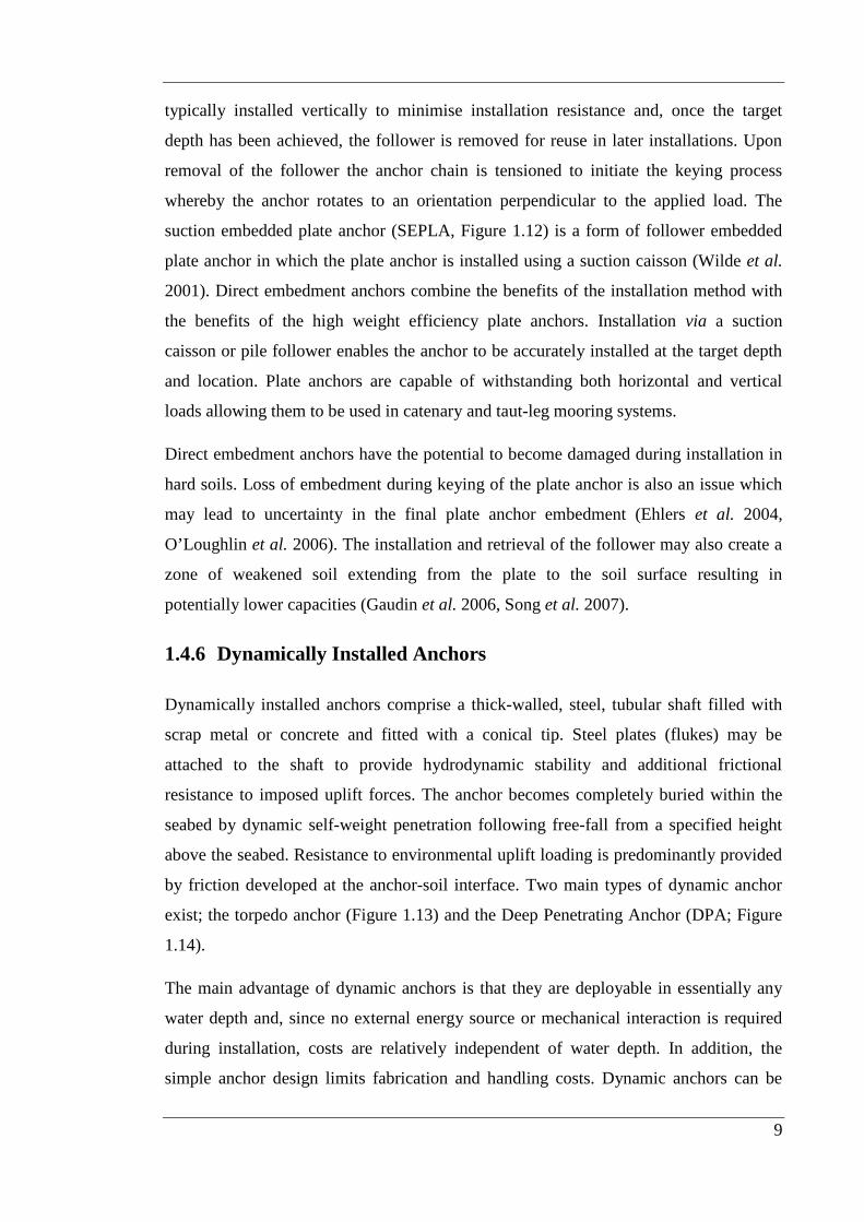
9
typically installed vertically to minimise installation resistance and, once the target
depth has been achieved, the follower is removed for reuse in later installations. Upon
removal of the follower the anchor chain is tensioned to initiate the keying process
whereby the anchor rotates to an orientation perpendicular to the applied load. The
suction embedded plate anchor (SEPLA, Figure 1.12) is a form of follower embedded
plate anchor in which the plate anchor is installed using a suction caisson (Wilde et al.
2001). Direct embedment anchors combine the benefits of the installation method with
the benefits of the high weight efficiency plate anchors. Installation via a suction
caisson or pile follower enables the anchor to be accurately installed at the target depth
and location. Plate anchors are capable of withstanding both horizontal and vertical
loads allowing them to be used in catenary and taut-leg mooring systems.
Direct embedment anchors have the potential to become damaged during installation in
hard soils. Loss of embedment during keying of the plate anchor is also an issue which
may lead to uncertainty in the final plate anchor embedment (Ehlers et al. 2004,
O’Loughlin et al. 2006). The installation and retrieval of the follower may also create a
zone of weakened soil extending from the plate to the soil surface resulting in
potentially lower capacities (Gaudin et al. 2006, Song et al. 2007).
1.4.6 Dynamically Installed Anchors
Dynamically installed anchors comprise a thick-walled, steel, tubular shaft filled with
scrap metal or concrete and fitted with a conical tip. Steel plates (flukes) may be
attached to the shaft to provide hydrodynamic stability and additional frictional
resistance to imposed uplift forces. The anchor becomes completely buried within the
seabed by dynamic self-weight penetration following free-fall from a specified height
above the seabed. Resistance to environmental uplift loading is predominantly provided
by friction developed at the anchor-soil interface. Two main types of dynamic anchor
exist; the torpedo anchor (Figure 1.13) and the Deep Penetrating Anchor (DPA; Figure
1.14).
The main advantage of dynamic anchors is that they are deployable in essentially any
water depth and, since no external energy source or mechanical interaction is required
during installation, costs are relatively independent of water depth. In addition, the
simple anchor design limits fabrication and handling costs. Dynamic anchors can be

10
accurately deployed and their performance is less dependent on accurate assessment of
the soil shear strength since lower seabed shear strengths permit greater penetration
depths and vice versa. Once installed, dynamic anchors behave in a similar manner to
anchor piles and as such are capable of withstanding both horizontal and vertical load
components, enabling their use in both catenary and taut-leg mooring systems.
Despite the economic advantages afforded by dynamic anchors, a degree of uncertainty
exists in relation to predicting the embedment depth and subsequent capacity. There is
also some concern with verifying the anchor’s verticality following installation. In
addition, this type of anchor may not be suitable for use in sandy soils.
1.5 RESEARCH OBJECTIVES
The need for cost effective deepwater anchoring solutions capable of withstanding both
horizontal and vertical loading components is clear. Conventional anchoring methods
such as anchor piles, suction caissons and drag embedment anchors become relatively
expensive as the water depth increases and as such developmental anchors such as the
dynamically installed anchor are being actively pursued. Dynamically installed anchors
appear to offer the most potential economic benefit of the current anchor concepts due
to the simplicity of the anchor design and the installation method, resulting in the need
for smaller marine vessels and reduced vessel time together with less complex marine
operations (Ehlers et al. 2004). With the exception of a number of field trials, (which
have not been published in detail) very little dynamic anchor performance data exists.
Increased understanding of the geotechnical behaviour of these anchors in varying soil
and loading conditions would evidently lead to increased industry confidence in the
potential of dynamically installed anchors.
Given the lack of performance data currently available and the potential economic
benefit of dynamic anchors to the industry, there exists a clear need for an experimental
study to address the basic issues of predicting the embedment depth and subsequent
holding capacity for a given anchor geometry, anchor drop height and seabed strength
profile. This project therefore aimed to investigate the geotechnical performance of
dynamically installed anchors in normally consolidated clay, calcareous sand and silica
sand. Two main challenges arise concerning the geotechnical performance of dynamic

11
anchors: firstly, determination of the anchor embedment depth for a given drop height
and seabed strength profile; secondly, determination of the subsequent anchor capacity
under various loading conditions. These challenges were addressed in two distinct
phases.
Considering the scarcity of dynamic anchor experimental data, Phase 1 involved the
development of an experimental database through an extensive suite of reduced scale
centrifuge tests on model dynamic anchors. Specifically this was aimed at:
• Investigating the parameters that govern anchor embedment depth, i.e. impact
velocity, anchor shaft length/diameter ratio, anchor fluke geometry, anchor tip
geometry, anchor mass and soil shear strength profile.
• Examining the effect of anchor embedment on anchor capacity under monotonic,
sustained and cyclic loading conditions.
• Quantifying the contribution of consolidation time (duration between anchor
installation and loading) to anchor capacity.
Phase 2 focused on the development of a design tool for the prediction of anchor
embedment depth and subsequent capacity. This design model was based on an
analytical approach validated against the experimental database established in Phase 1.
The specific aims of Phase 2 were to:
• Develop an analytical approach for anchor penetration. The anchor penetration
model is based upon conventional bearing and frictional capacity theory but with
provisions for viscous enhanced shearing resistance and fluid mechanics drag
resistance.
• Apply conventional pile capacity calculation techniques, incorporating end
bearing and shaft friction resistance terms, to the prediction of the vertical
anchor capacity. In this context, the effect of consolidation time on anchor
capacity was also considered.
The outcomes of the project include the attainment of experimental data that has been
used to identify expected dynamic anchor penetrations and capacities as well as the
development of robust and versatile design tools that can be used in routine offshore
engineering practice.

12
1.6 THESIS STRUCTURE
This thesis is presented in 8 chapters, as outlined below:
Chapter 2 reviews the literature relating to dynamically installed anchors. The review
commences with a discussion of seabed penetration research in terms of seabed disposal
of nuclear waste and the assessment of seabed strength properties using free-fall
penetrometers. In the context of dynamic seabed penetration, the strain rate effects on
soil shear strength are also examined. The chapter concludes with a summary of
experimental and numerical work relating to the use of free-fall projectiles as a form of
anchoring system.
Chapter 3 summarises the details of the dynamic anchor experimental programme. The
centrifuge facilities and test apparatus are outlined and the soil properties and sample
preparation procedures are presented. A discussion of the apparatus developed
specifically for the research project is provided with particular focus on the various
model anchors developed.
Chapter 4 details the analytical and numerical techniques adopted in the dynamic anchor
design model. The analytical approach adopted for predicting anchor embedment and
subsequent capacity, based on conventional bearing and frictional capacity theory, is
presented. Consideration of the effects of strain rate and inertial drag during anchor
installation is also provided. Simplified pile capacity calculation techniques are
presented for use in predicting the vertical anchor capacity following installation. The
techniques are subsequently adapted for use in calcareous soil.
Chapter 5 presents the results of the model anchor tests conducted in clay. The
experimental results are presented in terms of impact velocity, embedment depth and
holding capacity. The tests provide information regarding the influence of the aspect
ratio, mass, tip geometry, flukes, consolidation time and cyclic and sustained loading on
the performance of dynamically installed anchors. The test results are compared with
the results of dynamic anchor field trials and previous laboratory and centrifuge model
tests.

13
Chapter 6 presents the results of the model anchor tests conducted in silica and
calcareous sand. The test results are presented in terms of impact velocity, embedment
depth and holding capacity. The experimental results are compared with the results of
known field trials.
Chapter 7 provides a comparison of the experimental data presented in Chapters 5 and 6
with the analytical solutions for the dynamic anchor impact velocity, embedment depth
and holding capacity derived in Chapter 4 for both normally consolidated clay and
calcareous sand. The experimental results are used to validate the proposed methods and
to develop user friendly design tools
Chapter 8 summarises the major research findings and discusses the implications of
these findings with regard to the practical implementation of dynamic anchors in
industry. The chapter also presents recommendations for future work arising from the
outcomes of the research project.


15
CHAPTER 2 - LITERATURE REVIEW
2.1 INTRODUCTION
Literature regarding the behaviour of dynamically installed anchors is limited.
Dynamically installed anchors emerged during the late 1990s from the need of the oil
and gas industry for a reliable and cost effective deepwater anchoring system. However,
the potential application of dynamically embedded objects for anchoring purposes was
recognised as early as the 1970s (True 1974). Dynamic anchor behaviour is typically
considered in two distinct phases: (i) dynamic installation and (ii) loading and
extraction. The penetration of objects into the seabed has previously been considered in
the measurement of seabed shear strengths and for the disposal of high-level radioactive
waste. Likewise the capacity of anchor piles for offshore foundations has been
extensively investigated. This literature provides a basis for assessing the geotechnical
performance of dynamically installed anchors in both phases of its operation, as is
discussed further below.
2.2 SEABED PENETRATION
Investigation of the penetration of objects into the seabed is not new. Dynamic seabed
penetration has been studied for in situ strength measurement and nuclear waste
disposal purposes since the 1960s. For typical seabed soils in which the shear strength
increases with depth, dynamically installed anchors rely upon the depth of penetration
achieved during installation to achieve their capacity. Accurate prediction of the
dynamic anchor penetration depth is therefore an important consideration in evaluating
the subsequent anchor capacity and hence relative merit of the concept. Embedment
depth prediction methods exist, from earlier work on earth penetrating weapons and
nuclear waste disposal penetrometers, but uncertainty regarding strain rate effects and
inertial drag resistance limit their reliability.

16
2.2.1 Seabed Strength Characterisation
Foundations for offshore structures require detailed information about seabed soil
properties to enable safe and effective design. Seabed sampling is expensive and current
sampling techniques are known to cause significant sample disturbance. Likewise quasi-
static penetration tests for assessing soil strength, such as the Cone Penetration Test
(CPT), are expensive, especially in deep water. During the Earth Penetrating Weapon
(EPW) programme conducted by Sandia National Laboratories (SNL) during the 1960s,
the idea emerged of estimating the strength of the target material by instrumenting
projectiles and recording their deceleration during penetration (Thompson and Colp
1970, Colp et al. 1975). Since that time various penetrometer designs and analysis
techniques have been proposed for the in situ measurement of seabed strength
properties.
2.2.1.1 Marine Sediment Penetrometer
During the 1970s and 80s, SNL in association with Texas A and M University
undertook a seabed strength characterisation research programme resulting in the
development of a Marine Sediment Penetrometer (MSP; Colp et al. 1975; see Figure
2.1). Linked via an umbilical to a surface vessel, onboard accelerometers measured the
MSP deceleration during penetration of the soft seabed sediments. An approximate
method for determining the soil shear strength from penetrometer deceleration
measurements was subsequently proposed (McNeill 1981). The method was based on
the suggestion that there is an apparent constant, which when multiplied by the
deceleration at a given depth yields a close estimate of the soil shear strength at that
depth. Based on the results of field and laboratory tests the relationship between the soil
shear strength and deceleration was defined as:
agLA4
WDs
pu
≈ (2.1)
where su is the soil shear strength, W is the penetrometer weight, D is the penetrometer
diameter, g is the local gravitational acceleration, L is the penetrometer length, Ap is the
projected cross-sectional area of the penetrometer and a is the measured deceleration.

17
This approximate method is limited in its application due to its failure to account for
inertial effects during penetration. In addition no consideration has been given to the
strain rate dependence of soil shear strength, resulting in a discrepancy between the
derived dynamic shear strength profile and the shear strength profile based on low strain
rate laboratory tests. Hence it was recommended that this method not be used for
strength measurements for final design, but rather as a useful tool for the simple and
efficient assessment of soil stratigraphy and the relative strengths of adjacent soil layers
(McNeill 1981).
2.2.1.2 Marine Impact Penetrometer
Dayal and Allen (1973) described the development of an instrumented cone
penetrometer for the direct measurement of in situ strength properties of a soil target.
The Marine Impact Penetrometer (MIP; Figure 2.2) featured an accelerometer and tip
and sleeve load cells for measuring the acceleration/deceleration and tip and side
friction resistances during installation, with data transferred to a surface vessel via an
umbilical. Laboratory and preliminary field tests indicated that the ‘dynamic’ shear
strength profile and the soil stratigraphy could be evaluated directly during MIP
penetration of soft seabed sediments (Dayal et al. 1975). An empirical relationship was
proposed for calculating the static cone pressure and therefore static shear strength from
the dynamic cone pressure values obtained in MIP tests, by applying a correction for
penetration rate effects (Dayal et al. 1975)
=−
sL
c
ccd
v
vlogK
q
qq (2.2)
where qcd is the dynamic cone resistance, qc is the ‘static’ cone resistance, KL is a soil
viscosity coefficient, v is the penetrometer velocity and vs is the ‘static’ penetration
velocity. Values of the soil viscosity coefficient were established experimentally from a
limited number of tests and were found to vary from 0.03 – 1.5, indicating an increase
in the cone resistance per log cycle increase in velocity of 3 – 150 % (Dayal et al.
1975). Subsequent sea trials demonstrated the usefulness of the MIP and the analysis
method for obtaining in situ soil strength profiles in depths of up to 4 m below the
seabed (Dayal 1980). Further field and laboratory tests were recommended to validate
18
the accuracy of this method particularly with regard to values of the soil viscosity
coefficient.
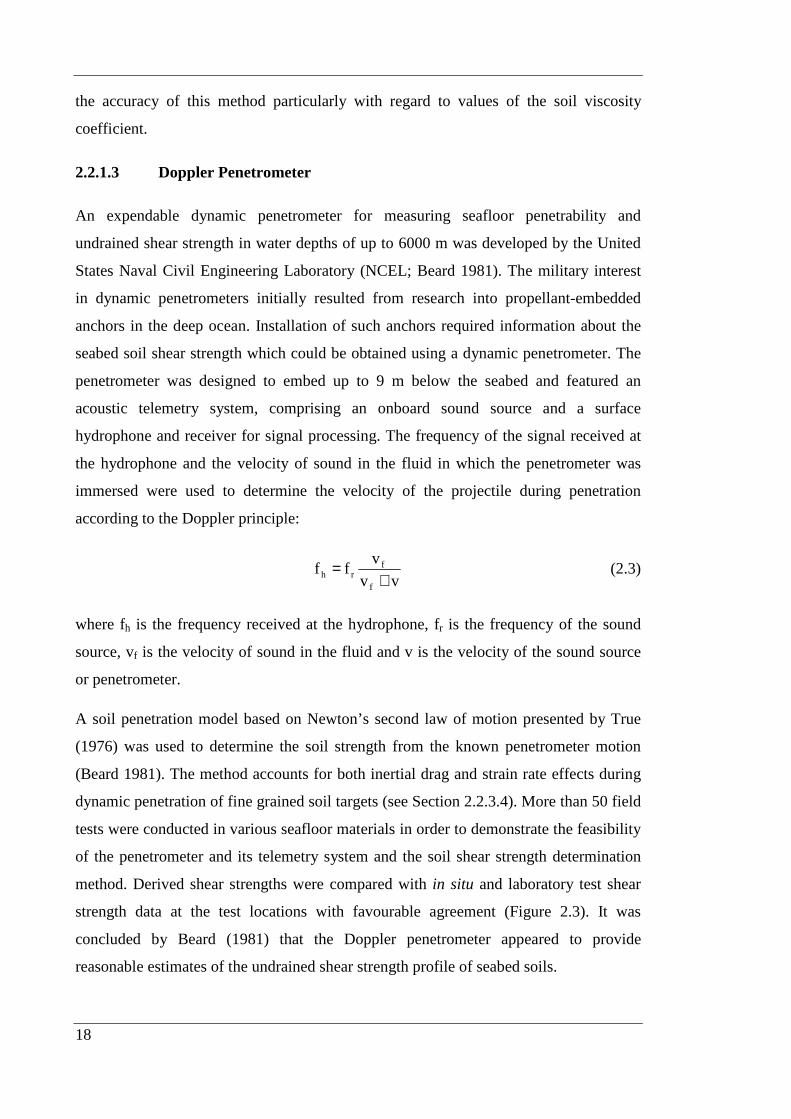
2.2.1.3 Doppler Penetrometer
An expendable dynamic penetrometer for measuring seafloor penetrability and
undrained shear strength in water depths of up to 6000 m was developed by the United
States Naval Civil Engineering Laboratory (NCEL; Beard 1981). The military interest
in dynamic penetrometers initially resulted from research into propellant-embedded
anchors in the deep ocean. Installation of such anchors required information about the
seabed soil shear strength which could be obtained using a dynamic penetrometer. The
penetrometer was designed to embed up to 9 m below the seabed and featured an
acoustic telemetry system, comprising an onboard sound source and a surface
hydrophone and receiver for signal processing. The frequency of the signal received at
the hydrophone and the velocity of sound in the fluid in which the penetrometer was
immersed were used to determine the velocity of the projectile during penetration
according to the Doppler principle:
vv
vff
f
frh +
= (2.3)
where fh is the frequency received at the hydrophone, fr is the frequency of the sound
source, vf is the velocity of sound in the fluid and v is the velocity of the sound source
or penetrometer.
A soil penetration model based on Newton’s second law of motion presented by True
(1976) was used to determine the soil strength from the known penetrometer motion
(Beard 1981). The method accounts for both inertial drag and strain rate effects during
dynamic penetration of fine grained soil targets (see Section 2.2.3.4). More than 50 field
tests were conducted in various seafloor materials in order to demonstrate the feasibility
of the penetrometer and its telemetry system and the soil shear strength determination
method. Derived shear strengths were compared with in situ and laboratory test shear
strength data at the test locations with favourable agreement (Figure 2.3). It was
concluded by Beard (1981) that the Doppler penetrometer appeared to provide
reasonable estimates of the undrained shear strength profile of seabed soils.

19
2.2.1.4 Free Fall Cone Penetrometer
The Free Fall Cone Penetrometer (FFCPT), shown in Figure 2.4 was developed by
Brooke Ocean Technology Ltd. and Christian Situ Geosciences Inc. to obtain
geotechnical and geophysical data from the seabed for a range of different applications
(Brooke Ocean Technology 2007). Onboard acceleration and pressure sensors in
conjunction with a high speed data acquisition system provide continuous data profiles
during penetration. A computer data logger fitted within the instrumentation section of
the penetrometer eliminates the need for an umbilical cord or acoustic data transmission
to the surface. The FFCPT provides information on layering within the sediments and
the undrained shear strength and it is also claimed to provide shear modulus and shear
wave velocity data. Pressure transducers provide the FFCPT with the ability to measure
pore pressures during and after penetration, enabling the consolidation properties of the
soil to be investigated. The use of this type of device is particularly suited to
investigations of pipeline or cable route surveys over large distances as the device is
quick and simple to install.
2.2.1.5 Expendable Bottom Penetrometer
The eXpendable Bottom Penetrometer (XBP) represents the most recent seabed
penetrometer for the measurement of in situ seabed soil strength properties. The XBP is
approximately 215 mm long, 51 mm in diameter and is designed to reach a terminal
velocity of approximately 7 m/s (Aubeny and Shi 2006; Figure 2.5). The penetrometer
is fitted with an accelerometer and decelerations measured upon impact with the seabed
provide a basis for estimating the sediment shear strength. The XBP provides an
advantage over previously devised seabed strength characterisation penetrometers in
that it can be deployed from a moving vessel, making it well suited to seabed
investigations over large survey areas.
Aubeny and Shi (2006) proposed a framework for assessing the soil shear strength from
interpreted XBP deceleration profiles in soft clay. Using static bearing capacity factors
derived from finite element analyses and by accounting for viscous strain rate effects
during penetration, a dynamic bearing capacity factor was determined:
20
λ+=
0ccd v
vlog1NN (2.4)
where Ncd is the dynamic bearing capacity factor, Nc is the static bearing capacity
factor, λ is the strain rate parameter, v is the penetrometer velocity and v0 is the velocity
corresponding to the threshold strain rate. Comparisons of interpreted XBP shear
strength profiles to reference miniature vane shear strength profiles of samples
recovered from Gulf of Mexico test sites indicate that the XBP overestimates the
strength during the initial stages of penetration, possibly because the data interpretation
technique ignores inertial drag effects which may be significant during the early stages
of penetration (Figure 2.6). Additionally the XBP strength decreases rapidly in the final
stages of penetration possibly due to elastic rebound of the soil as the velocity reduces
to zero. Overall it was concluded that the XBP is capable of providing first order
estimates of the strength of soft clay materials, although uncertainty with regard to the
strain rate effects precludes improved accuracy from being obtained (Aubeny and Shi
2006).
2.2.2 Nuclear Waste Disposal
During the late 1970s it was recognised that the world was facing a growing problem
with the management of high-level radioactive waste, with increased waste production
from both commercial and military sources. A coordinated research programme was
established by the Organisation for Economic Co-operation and Development (OECD)
Nuclear Energy Agency (NEA) through the International Seabed Working Group,
investigating the feasibility and safety of disposing of high-level radioactive waste in
deep ocean abyssal plain formations (Murray 1988). One waste disposal option
considered involved the free-fall installation of nuclear waste containers into the
seafloor. Vitrified nuclear waste was to be placed within streamlined projectiles and
released from a vessel and allowed to penetrate the soft seabed sediments (Valent and
Lee 1976). A key consideration in evaluating the feasibility of this concept was ensuring
adequate penetration of the projectiles into the ocean bottom. During the 1980s
extensive analytical and experimental research efforts were directed towards assessing
the technical feasibility of the penetrometer nuclear waste disposal method, both in
terms of hydrodynamic performance and seabed penetrability.

21
In 1981 the Building Research Establishment (BRE) representing the Department of the
Environment commissioned Ove Arup and Partners to carry out a feasibility study of
the seabed penetrometer method for the disposal of high-level nuclear waste (Ove Arup
and Partners 1982). This feasibility study proposed a method for predicting the
penetrometer embedment depth using simplifying assumptions about the free-fall
through water and the penetration resistance of the seabed sediments (see Section
2.2.3.5). Supplementary studies considered the seabed soil properties, ocean bed
seismology, penetrometer collision with seabed objects and the penetrometer path
during embedment. It was found that within the limitations of the embedment prediction
model, free-fall penetrometers could reasonably be expected to achieve the necessary
embedment to be considered for the disposal of radioactive waste.
In March 1983 a collaborative experiment between the BRE, the Commission of
European Communities Joint Research Centre and the Institute of Oceanographic
Sciences at Wormley was conducted in the Great Meteor East (GME) radioactive waste
disposal study area in the eastern Atlantic Ocean (Figure 2.7; Freeman et al. 1984). The
experiments involved the free-fall installation of four, similar Deep Ocean Model
Penetrators (DOMP), commonly referred to as European Standard Penetrators (ESP).
The design of the solid steel 3.25 m long, 0.325 m diameter, 1800 kg projectiles (Figure
2.8) was based on hydrodynamic analysis and indicated likely terminal velocities of
approximately 50 m/s. During the field trials, which later became known as the DOMP I
experiments, the penetrometer velocity was monitored using an acoustic telemetry
system incorporating a transmitter in the projectile and a surface hydrophone. The test
results indicated that in the soft calcareous ooze at the GME test site, tip penetrations of
approximately 30 – 35 m were achievable with ESPs impacting the seabed at 46 – 51
m/s (Freeman et al. 1984).
The DOMP II tests were performed in March 1984 at the Nares Abyssal Plain (NAP)
test site in the western Atlantic Ocean (Figure 2.7) by BRE in collaboration with the
Joint Research Centre, SNL and the Rijks Geologische Dienst (RGD). A total of
seventeen tests were conducted with eight different penetrometer designs, including the
ESP (Freeman and Burdett 1986; Figure 2.9). Several different instrumentation and
telemetry systems were also trialled during the test programme. The test results

22
indicated impact velocities of 45 – 56 m/s resulting in penetration depths of 21 – 35 m
in the soft seabed sediments at the NAP site.
A further fifteen tests were conducted at GME in 1986 with three different penetrometer
designs, including a Type X penetrometer, similar to the ESP (Freeman et al. 1988).
The tests were partially aimed at assessing the influence of the weight and surface finish
of the Type X penetrometers on their penetration performance. Impact velocities of 30 –
68 m/s resulted in tip penetration depths of approximately 29 – 58 m. The surface finish
was found to affect the impact velocity but did not result in destabilising hydrodynamic
forces on the penetrometer during free-fall.
Additional field tests were conducted in late 1986 off the coast of Antibes in the
Mediterranean Sea. A total of nine tests were conducted with five different
penetrometers in soil considerably stiffer and stronger than the sediments encountered at
the GME and NAP test sites. The increased seabed strength resulted in reduced tip
penetrations of only 9 – 15 m (Audibert et al. 2006).
In conjunction with the field trials, the Department of the Environment also
commissioned a series of centrifuge tests to model the free-fall option for nuclear waste
disposal. The tests were conducted at 1:100 scale, with 60 mm long, 6 mm diameter, 13
gram model projectiles representing 6 m long, 0.6 m diameter, 13 tonne prototype
projectiles (Poorooshasb and James 1989). The tests were conducted in kaolin clay to
assess the penetration depth, deformation pattern and degree of hole closure associated
with dynamic projectile penetration. The results indicated that nose penetrations of at
least 305 mm (30.5 m at prototype scale) were achievable with blunt nosed model
penetrometers impacting a normally consolidated clay sample at 40 m/s at 100 g. These
penetrations were in agreement with penetrations observed in the earlier field trials. It
was also found that the simple semi-empirical depth prediction model suggested by Ove
Arup and Partners (1982) (see Section 2.2.3.5) adequately predicted the projectile
penetration depth in the centrifuge tests.
Despite extensive developmental work which established the concept feasibility, seabed
penetrometers were never utilised in the disposal of high-level radioactive waste.
Disposal of nuclear waste in the sea was subsequently banned and as a result research
efforts in the area ceased. However the methods developed to predict penetrometer
23
embedment may be useful in determining the likely penetration depth of dynamic
anchors in soft seabed sediments.
2.2.3 Embedment Prediction Methods
For typical seabed strength profiles in which the shear strength increases with depth, the
dynamic anchor capacity is heavily dependent upon the depth of penetration achieved
during installation. Hence in order to predict the anchor capacity it is first necessary to
be able to predict the anchor embedment depth reliably. Arising from the seabed
strength characterisation and nuclear waste disposal penetrometer studies, several
methods for predicting the penetration depth of objects into soft seafloor sediments have
been proposed. However, dynamic penetration of fine grained soils is believed to
generate viscous strain rate effects and inertial drag resistance forces which are often
difficult to quantify. These methods adopt various approaches towards accounting for
strain rate and inertial drag effects during soil penetration.
2.2.3.1 Strain Rate Effects
It is generally observed that, under undrained conditions, an increase in the strain rate
results in an increase in the shear strength (Casagrande and Wilson 1951, Graham et al.
1983, Sheahan et al. 1996). The dependence of shear strength on the applied rate of
strain has long been recognised and is supported by a large database of vane shear
(Biscontin and Pestana 2001) and triaxial compression tests (Sheahan et al. 1996). The
effect of shear strain rate ( )γ& on the undrained shear strength of clay (su) may be
expressed using a semi-logarithmic function given by:
γγλ+=ref
ref,uu log1ss&
& (2.5)
where su,ref is the undrained shear strength at the reference strain rate (refγ& ) and λ is a
strain rate parameter representing the increase in shear strength per log cycle increase in
strain rate (Graham et al. 1983). There are arguments however, both from physical
principles (Mitchell 1993) and to avoid problems at low strain rates for the use of an
alternative inverse hyperbolic sine function, expressed as

24
γγλ′+= −
0
10uu sinh1ss
&
& (2.6)
Adopting λ’ = λ / ln(10), this expression reverts closely to Equation 2.5 for strain rates
greater than the threshold strain rate (0γ& ), but leads to rapidly decaying strain rate
effects below the threshold rate (Einav and Randolph 2006). Sheahan et al. (1996) noted
the concept of a threshold strain rate below which the rate effect disappears; the
subscript ‘0’ has been used to emphasise that su0 is a true minimum shear strength at
very low strain rates.
The variation in shear strength with strain rate can alternatively be represented by a
power law expression (Biscontin and Pestana 2001):
β
γγ=ref
ref,uu ss&
& (2.7)
The semi-logarithmic function is the most commonly adopted model for analysing rate
effects in clay. Sheahan et al. (1996) reported values of λ from a database of triaxial
compression tests of up to 0.17 for strain rates ranging from 0.0014 – 670 %/hr, while
Biscontin and Pestana (2001) gave values of λ from 0.01 – 0.60 for a database of vane
shear tests conducted at rotation rates of 0.06 – 3000 °/min.
Strain rate effects are an important consideration in assessing the penetration of objects
into the seabed, as they dictate the mobilised shear strength and therefore resistance to
penetration. Whilst the shear strength is known to increase with strain rate, assuming the
deformation pattern remains constant during penetration, it is reasonable to assume that
the strain rate is proportional to the velocity (True 1976). True (1974) was the first to
account for strain rate effects in predicting the penetration of objects into the seabed,
using an empirical approach to determine the strain rate effects from model
penetrometer tests in soft clay (see Section 2.2.3.4). The semi-logarithmic formulation
in Equation 2.5 has since been adopted in centrifuge model tests of dynamic anchors in
kaolin clay (Lisle 2001, Wemmie 2003, Richardson 2003, O'Loughlin et al. 2004b).
Back-calculated values of λ from the centrifuge tests indicate an increase in shear
strength ranging from 3 – 36 % per log cycle increase in anchor velocity. The wide

25
range of back-calculated strain rate parameter values highlights the difficulties
associated with determining strain rate effects in clay.
Strain rates relevant for in situ tests, laboratory tests and operational conditions cover an
extremely wide range, typically 6 to 8 orders of magnitude. Typical strain rates in
triaxial compression tests of 1 %/hr (3 × 10⁻⁶ s-1) are generally several orders of
magnitude lower than strain rates for in situ vane tests of approximately 2 × 10⁻³ s-1
(Einav and Randolph 2006). Strain rates associated with the dynamic installation of
seabed penetrometers may be considered proportional to v/D. Hence for a dynamic
anchor with a diameter of 1.2 m, an average strain rate during installation in the order of
10 s-1 is likely. This represents four and seven fold increases in the order of magnitude
over strain rates for triaxial compression and vane shear tests respectively. It is therefore
difficult to extrapolate potential strain rate effects from laboratory tests for use in
predicting the embedment depth of projectiles in fine grained seabed sediments unless
comparable strain rates are achieved.
Evidence suggests that strain rate effects are not constant for a given material but
actually increase with increasing strain rate. It has been shown that for vane tests
conducted at different rotation rates, the semi-logarithmic function in Equation 2.5 with
λ ≈ 0.1 adequately captures the shear strength rate dependence in the vicinity of the
conventional rotation rate of 0.1 °/s; at higher rates, however, the rate effect increased to
λ ≈ 0.2 (Biscontin and Pestana 2001). An increase in the strain rate effect with
increasing strain rate was also observed in model penetrometer tests by True (1976).
Biscontin and Pestana (2001) noted that the power law rate formulation in Equation 2.7
provided a better fit to their vane data over several log cycles of rotation rate.
Through seabed MIP tests (Section 2.2.1.2), Dayal and Allen (1975) found that the rate
effect for the skin friction component of penetrometer resistance was greater than the
rate effect for the nose bearing resistance component. Therefore it is acknowledged that
separate rate dependent functions for the bearing and frictional resistance during seabed
penetration may be more appropriate than the use of a single rate function for both
resistance components. However it is difficult to differentiate the rate dependence of
each component and as such the bearing and frictional rate effects are typically
combined in a single rate function (O’Loughlin et al. 2004b).
26
2.2.3.2 Inertial Drag
During the seabed penetration of projectiles, soil is displaced from the path of the
advancing projectile. Soil elements are accelerated from rest to a velocity sufficient to
move them out of the path of the projectile. The force required to accelerate the soil
elements is known as an inertial force. The reaction to the inertial force produces a
resistance force on the projectile. Inertial drag resistance in soil is analogous to the
hydrodynamic drag experienced by an object passing through water. Considering the
very soft, viscous clay typically present at the seabed surface it seems reasonable to
assume that an inertial drag force exists during penetration, despite a lack of
experimental justification.
Inertial drag resistance terms have been included in penetration analyses by True (1976)
and Ove Arup and Partners (1983). In each case the inertial drag resistance has been
evaluated using the expression:
2pD2
1d vACF ρ= (2.8)
where CD is the drag coefficient and ρ is the soil density. The most important
consideration in assessing the inertial drag resistance force acting on a projectile during
penetration is the drag coefficient. The drag coefficient is essentially a function of the
projectile geometry and surface roughness (True 1976); however, it is also dependent on
the Reynolds number (Re) of the associated flow.
ν
= vDRe (2.9)
where D is the projectile diameter and ν is the kinematic viscosity of the fluid.
During the transition of a seabed penetrometer from the water into the soil, the viscosity
of the medium through which the projectile is passing will change and as such there will
be an associated change in the Reynolds number. This suggests that there should be
separate drag coefficients for projectile motion through the water and the soil. However
the same drag coefficient is typically adopted for projectiles passing through both
media. This is a reasonable assumption provided the change in Reynolds number is
minimal and given the fact that the inertial drag resistance is expected to account only
for a relatively minor proportion of the total penetration resistance. For a range of

27
projectile velocities and geometries, True (1976) recommended a drag coefficient of 0.7
to account for both soil and water inertia effects. Hydrodynamic studies conducted on
nuclear waste disposal penetrometers during the 1980s indicated considerably smaller
drag coefficients in the order of 0.15 – 0.18 for the ESP (Freeman et al. 1984), whilst
similar studies on Deep Penetrating Anchors (DPAs) indicate a drag coefficient of 0.63
for a four fluke steel anchor in water (Øye 2000).
2.2.3.3 Young's Method
In the early 1960s SNL commenced an earth penetration research programme with the
objective of developing the technology to permit the design of a nuclear earth
penetrating weapon (EPW). As part of this project, empirical equations were developed
to predict the depth of penetration of projectiles into concrete and natural earth
materials. The development of the empirical equations was based on an extensive
database of full scale earth penetration tests and an assumed form of the depth
prediction equation, including assumptions as to which parameters influenced
penetration.
The basic equations first published by Young (1969) have varied little over the past 40
years, although the test database has been expanded and new target materials considered
such as ice, frozen soil and weathered rock. Revised empirical penetration equations
were published by Young (1981) and then later revised again by Young (1997). A
number of assumptions apply to the application of these equations:
• The projectile remains intact during penetration.
• The projectile follows a stable trajectory, i.e. no tumbling or large changes in
direction.
• The impact velocity is less than 4000 ft/s (1219 m/s).
• The equations may not be accurate for penetrations less than approximately three
projectile diameters.
• The equations are not valid for water or air penetration.
• The equations are not valid for armour penetration.
28
• The minimum projectile mass is approximately 5 lbs (2.3 kg) for soil and 10 lbs
(4.6 kg) for rock, concrete, ice and frozen soil targets.
For a uniform layer of soil, the penetration depth can be predicted using Equations 2.10
and 2.11 (Young 1997). For vi < 200 ft/s (61 m/s)
( )2i
5
7.0
ps v1021ln
A
mSNK3.0z −×+
= (2.10)
and for vi ≥ 200 ft/s (61 m/s)
( )100vA
mSNK00178.0z i
7.0
ps −
= (2.11)
where z is the penetration depth in ft, S is the target penetrability constant (see Table
2.1), N is a nose performance coefficient (see Equations 2.13 and 2.14), vi is the impact
velocity in ft/s, m is the projectile mass in lbs, Ap is the cross-sectional area of the
projectile in ft2 and Ks is a correction factor for lightweight projectiles, which for m <
60 lbs (27 kg) is given by:
4.0s m2.0K = (2.12)
For all other projectiles, Ks = 1.
Values of the nose performance coefficient were developed based on soil penetration
test data (Young 1997). For ogive shaped noses
56.0D
L18.0N tip += (2.13)
and for conical shaped noses
56.0D
L25.0N tip += (2.14)
where Ltip is the length of the projectile nose or tip in ft.
A major criticism of the Young penetration equations is that the target or soil
penetrability constant (S) has no physical relevance in terms of standard soil properties.

29
Whilst an extensive database of soil penetration tests exists, it was found to be more
difficult to estimate S for soil media than for rock or concrete. The accuracy of the
proposed empirical equations is heavily dependent on the accuracy with which the value
of S can be determined (Young 1969). Soil penetrability values for a number of typical
soil types are provided in Table 2.1. The value of S is assumed constant for a given
target material despite the fact that the strength of certain materials varies with depth
and strain rate. The Young penetration equations also fail to account for the length of
the projectile, which determines the surface area of the object available to provide
frictional resistance to penetration. Increasing the projectile length would be expected to
increase the frictional resistance and ultimately lead to lower penetration depths.
Consequently this method has rarely been used in predicting the embedment depth of
seabed penetrometers.
Target Material Description S
Dense, dry, cemented sand 2 - 4
Sand without cementation, very stiff and dry clay 4 - 6
Moderately dense to loose sand, no cementation 6 - 9
Soil fill material, various levels of compaction 8 - 10
Silt and clay, low to medium moisture content 5 - 10
Silt and clay, moist to wet 10 - 20
Very soft, saturated clay - very low shear strength 20 - 30
Clay marine sediments - Gulf of Mexico 30 - 60
Table 2.1 Soil penetrability of typical soil types (after Young 1997)
2.2.3.4 True's Method
During the 1970s the NCEL commenced a programme of research investigating the
penetration of projectiles into the seafloor with a view to establishing a new anchoring
technique (True 1974). It was recognised that the phenomenon of penetration into soils
was directly relevant to the performance of direct embedment anchors and that whilst
methods existed for predicting projectile embedment, these relationships were not
necessarily directly applicable to this problem. Accurate depth predictions were found
to be essential in evaluating the holding capacities attainable. A technique was
presented for determining the penetration of projectiles into the seafloor by considering
Newton's second law of motion and the forces acting on the projectile during

30
penetration (NCEL 1985). Early versions of this method (Schmid 1969, Migliore and
Lee 1971) were modified by True (1976) to adapt the technique to velocities up to 400
ft/s (122 m/s). The method considered the static forces resisting projectile penetration
and also accounted for strain rate effects on the soil shear strength, remoulding of the
soil on the sides of the projectile and inertial drag effects as the projectile passed
through the soil (NCEL 1985). The method was considered applicable for objects
impacting the seabed at velocities greater than 3 ft/s (0.9 m/s). At lower velocities,
dynamic effects were considered negligible and static penetration techniques were
recommended.
True’s method, as published in the NCEL Handbook for Marine Geotechnical
Engineering (NCEL 1985), defined the net downward force (F) on the projectile as the
difference between the submerged weight of the projectile (Ws) and the combined soil
resistance terms
dsbs FFFWF −−−= (2.15)
where Fb is the tip or nose bearing resistance, Fs is the side friction or adhesion
resistance and Fd is the inertial drag resistance.
The tip bearing resistance is obtained from:
ptetip,ub ANSsF = (2.16)
where su,tip is the undrained soil shear strength at a depth of D/2 below the projectile tip,
Se is the strain rate factor, Ap is the cross-sectional area of the projectile and Nt is a
dimensionless nose resistance factor given by:
10D
z2.01
L
D2.015Nt ≤
+
+= (2.17)
Assuming no separation between the soil and the side of the projectile during
penetration, the side friction or adhesion resistance is obtained from:
set
ave,us AS
S
sF
= (2.18)
31
where su,ave is the undrained soil shear strength averaged over the length of the projectile
in contact with the soil, St is the soil sensitivity (i.e. the ratio of the undisturbed
undrained shear strength to the remoulded shear strength) and As is the side surface area
of the projectile. True (1976) accounted for separation between the projectile and the
soil by including a side adhesion factor at high penetration velocities. This factor was
not included in the version published by NCEL (1985).
The undrained shear strength of fine grained soils is known to increase with an increase
in strain rate. True (1976) derived an empirical expression for the strain rate factor from
penetration test data
( )[ ]1
CDsvC
11
SS
5.0oeque
*e
e ≥
++
= (2.19)
where Se* is the maximum strain rate factor, Ce is an empirical strain rate coefficient, v
is the velocity of the projectile at the start of the increment (in ft/s), su is the undrained
soil shear strength (in lbf/ft2) equal to su,tip or su,ave depending on whether the expression
is modifying the bearing or frictional resistance, Deq = (4 Ap/π)0.5 is the equivalent
projectile diameter (in ft) and Co is an empirical strain rate constant. For long cylindrical
penetrometers, Se* = 4, Ce = 4 lbf.s/ft2 and Co = 0.11 (NCEL 1985)
The inertial drag force during penetration is given by Equation 2.8.
As the major forces resisting penetration are depth or velocity dependent, an iterative
procedure is used to solve for the projectile penetration. Consequently True’s method
provides an advantage over Young’s empirical method in that a complete velocity
profile with depth is obtained rather than just a final embedment value.
Modifying Newton's second law to eliminate the time term, the net downward force on
the projectile can be related to the deceleration
=dz
dvmvF (2.20)
where m is the penetrometer mass and dv/dz is the instantaneous change in velocity
with depth. Selecting an appropriate depth increment (∆z), the change in velocity can be
determined as:

32
∆=∆i
ii v
F
m
zv (2.21)
The velocity for the (i+1)th increment is therefore estimated as
i1i1i v2vv ∆+= −+ (2.22)
However, in order to commence the iterative calculation procedure, the velocity of the
projectile at the end of the first increment (v1) must be approximated as:
( )
−−−
∆
+= 1d1s1b1s
001 FFFW
m
z
v
1vv (2.23)
where v0 is the impact velocity of the penetrometer and Ws1, Fb1, Fs1 and Fd1 are the
submerged weight, bearing resistance, side friction resistance and inertial drag
resistance values for the first penetration increment. This approximation is then used to
calculate the inertial drag force and the first iteration can be completed. The process
continues until a negative velocity is obtained, in which case the penetration depth is
calculated by interpolating between the last two velocity values.
−∆+=
+1ii
ii vv
vzzz (2.24)
A flow chart outlining the calculation procedure for this method is shown in Figure
2.10.
True’s method was subsequently modified to include the semi-logarithmic rate function
(Lisle 2001, Wemmie 2003, Richardson 2003, O'Loughlin et al. 2004b, Cunningham
2005, Aubeny and Dunlap 2003, Shi 2005, Aubeny and Shi 2006) presented in Section
2.2.3.1 and expressed as:
( ) dsbfs2
2
FFFRWdt
zdm −+−= (2.25)
where Rf is the strain rate function in terms of penetration velocity given by
λ+=
reff v
vlog1R (2.26)

33
where vref is the velocity at which the reference penetration resistance was assessed.
In both the original formulation (NCEL 1985) and the modified version (Lisle 2001,
Wemmie 2003, Richardson 2003, O'Loughlin et al. 2004b, Cunningham 2005), the
strain rate parameter was back-analysed from penetrometer test data. However,
significant variation in the strain rate parameter was identified across test series,
demonstrating the uncertainty associated with strain rate effects in fine grained soils.
This uncertainty, particularly at very high strain rates, ultimately results in uncertainty
in the prediction of penetrometer embedment depths. Strain rate effects have been
discussed in more detail in Section 2.2.3.1.
2.2.3.5 Ove Arup and Partners Method
A method for calculating penetrometer embedment was proposed as part of the
feasibility study commissioned by the Department of the Environment investigating the
use of free-fall penetrometers for the disposal of high-level radioactive waste in seabed
sediments (Ove Arup and Partners 1982). The method involved the development of
separate equations for partial and full embedment. Upon full embedment the
accelerating force acting on the projectile can be related to semi-empirical soil
parameters, through the governing differential equation:
222
2
BzAdt
zdm +=− (2.27)
where t is the time after installation and A2 and B2 are given by:
ded
2
2 DLkkN4
DA απ+π= (2.28)
( )( ) ssea,udsea,ued
2
2 W2
LksDLkLsN
4
DB −
+απ++π= (2.29)
and
t
chdcded S
NNN += (2.30)
where Ned is a dynamic nose and tail bearing capacity factor, Ncd is a dynamic nose
bearing capacity factor, Nchd is a dynamic tail resistance factor, St is the soil sensitivity,
34
αd is the dynamic side adhesion factor, su,sea is the undrained shear strength at the seabed
and k is the undrained shear strength gradient such that the undrained shear strength at
any depth, z, below the seabed is given by
kzss sea,uu += (2.31)
Ove Arup and Partners (1982) adopted closed-form solutions of the differential equation
(Equation 2.27) to predict the final penetrometer embedment depth; however,
Poorooshasb and James (1989) present the predicted penetration depth with time after
installation as:
( )( ) ( )KtsinK
v1Ktcos
A
Bz i
2
2 +−= (2.32)
where
m
AK 22 = (2.33)
The projectile velocity can be determined by differentiating Equation 2.32 with respect
to time, which when combined with the displacement data provides a complete
penetration velocity profile with depth given by
( ) ( )KtcosvKtsinKA
Bv i
2
2 +
−= (2.34)
This method attempts to account for the soil strength dependence on strain rate by
utilising empirically derived dynamic bearing resistance and side adhesion factors. The
side adhesion factor was shown to vary with velocity, approaching very low values at
high velocities, indicating a certain degree of separation between the soil and projectile
(Poorooshasb and James 1989). No consideration of inertial drag effects during
penetration of the soil was provided. Many of these shortcomings were detailed in a
follow up report by Ove Arup and Partners (1983).
35
2.3 PULLOUT CAPACITY
Dynamic seabed penetrometers for in situ strength measurement and nuclear waste
disposal purposes were largely expendable in nature. Consequently very little
information exists regarding the pullout capacity of objects penetrating the seabed
following free-fall installation. However, geometric similarities between dynamically
installed anchors and driven piles suggest that the anchor capacity may be assessed
using conventional pile capacity techniques. Despite discrepancies in the rate of
installation between dynamic anchors and driven piles, these techniques provide a basis
for considering the expected anchor capacity and the effects of the installation rate on
this capacity. Two methods are in common use for predicting the capacity of offshore
piles in clay:
1. American Petroleum Institute (API) method (API 2000)
2. Marine Technology Directorate (MTD) method (Jardine and Chow 1996)
For both methods the ultimate vertical tensile capacity (Fv) is calculated as the sum of
the submerged weight of the pile (Ws) and the end bearing (Fb) and shaft friction (Fs)
resistances:
sbsv FFWF ++= (2.35)
For piles in tension the tip bearing resistance is often ignored, providing conservative
capacity estimates; however a reverse end bearing mechanism may generate
considerable short-term resistance to tension loading and should be considered in the
analysis. Consolidation following installation and long-term sustained and cyclic
loading conditions are also likely to affect the capacity. These effects are important
considerations in the accurate prediction of capacity, and at present are not wholly
addressed by either the API or MTD method.
2.3.1 American Petroleum Institute Method
According to API recommended guidelines for pile capacity in cohesive soils (API
2000), the tip bearing resistance is given by
36
ptip,ucb AsNF = (2.36)
where Nc = 9 is the tip bearing capacity factor, su,tip is the undrained shear strength at the
pile tip and Ap is the projected area of the pile.
In addition, the shaft friction resistance generated by a pile is given by
save,us AsF α= (2.37)
where su,ave is the average shear strength over the embedded pile shaft length, As is the
embedded surface area of the pile and α has been determined from empirical
correlations with an extensive database of pile test results compiled by Randolph and
Murphy (1985) and can be expressed as
For 1s
v
u ≤σ′
1s
5.05.0
v
u ≤
σ′=α
−
(2.38)
For 1s
v
u >σ′
1s
5.025.0
v
u ≤
σ′=α
−
(2.39)
where σ′v is the vertical effective stress.
The API design method is simple to apply, and as such remains widely used in the
offshore industry.
2.3.2 Marine Technology Directorate Method
The MTD method (Jardine and Chow 1996) was devised to address some of the
reported weaknesses of the API method and is currently becoming more widely used in
Europe. The penetration of closed ended piles is analogous to the penetration of a cone
penetrometer. Hence it appears logical that the unit base resistance for a pile will be
linked to the unit cone tip resistance. The MTD load test database suggests that for
undrained loading, the pile bearing resistance should be estimated as:
pcb Aq8.0F = (2.40)

37
where qc is the unit cone tip resistance. It should be noted that the value of qc adopted in
Equation 2.40 should be the cone tip resistance averaged over 1.5 pile diameters above
and below the pile tip.
The MTD method uses empirical correlations based on soil properties derived from high
pressure oedometer tests to determine the shaft friction resistance. The horizontal
effective stress after installation and equalisation (σ′hc) is given by:
0vchc K σ′=σ′ (2.41)
where σ′v0 is the in situ vertical effective stress and Kc is given by
[ ]20.0
42.0vyc r
hYSRI870.0YSR016.02.2K
−
∆−+= (2.42)
where h is the vertical distance from the pile tip, r is the pile radius and YSR is the yield
stress ratio given by
0v
vyYSRσ′σ′
= (2.43)
where σ′vy is the yield stress and
( )tvy SlogI =∆ (2.44)
A lower limit of h/r = 8 should be used in Equation 2.42, with the shaft resistance
assumed constant for a vertical distance of four diameters from the pile tip. Load tests
indicate that the horizontal effective stress typically drops by approximately 20 %
during loading; hence the horizontal effective stress at failure (σ′hf) is given by
hchf 8.0 σ′=σ′ (2.45)
The local shear stress (τsf) is then estimated as
δσ′=τ tanhfsf (2.46)
where δ is the interface friction angle, which can be determined from interface ring
shear tests. Ultimately the shaft friction resistance can be expressed as

38
ssfs AF τ= (2.47)
where sfτ is the average shear stress along the embedded shaft length.
The MTD method is more difficult to apply than the API method since it requires the
use of more sophisticated soil properties. However, the design correlations reflect the
processes governing pile capacity more closely. In particular the effects of friction
fatigue are captured by the decay of Kc in Equation 2.42 with increasing h/r. The
influence of the yield stress ratio and soil sensitivity is captured by empirical
correlations. The MTD method was calibrated against a large database of recent load
tests, and is therefore likely to give more accurate estimates of pile capacity than the
API method, if information regarding the appropriate input parameters is available.
2.3.3 Consolidation Effects
The capacity of piles in fine grained soils is known to increase with time following
installation (Soderberg 1962). During pile (and dynamic anchor) installation, significant
excess pore pressures are generated in the soil in the vicinity of the pile due to the
combined effects of changes in mean effective stress due to shearing and increases in
total stress as soil is forced outwards to accommodate the volume of the pile (Randolph
2003). The low effective stress in the soil leads to low frictional resistance in the short
term. Subsequent to installation however, the excess pore pressures gradually dissipate
and the shear strength of the soil increases due to the combined effects of thixotropy and
consolidation. This time dependent increase in capacity is known as setup.
Evidence suggests that generally, the capacity of piles in clay immediately following
driving ranges from approximately 25 – 45 % of the ultimate pile capacity (Esrig et al.
1977, Bogard and Matlock 1990). However, Seed and Reese (1957) (as cited in Fleming
et al. 1985) reported much lower short-term capacities of approximately 10 % of the
long-term pile capacity (see Figure 2.11). Observations made in laboratory tests on
dynamic anchors indicate short-term capacities of approximately 30 % of the anchor
capacity after complete consolidation (Figure 2.12; Audibert et al. 2006).
Soderberg (1962) showed that the consolidation time was proportional to the square of
the horizontal dimension of the foundation (D) and inversely proportional to the

39
horizontal coefficient of consolidation (ch). Hence the consolidation time (t) is often
expressed in terms of a non-dimensional time factor (T) given by:
2
h
D
tcT = (2.48)
It is generally recognised that for large offshore piles, setup times to achieve full
capacity may be of the order of 1 – 2 years in fine grained seabed soils (Mirza 1999).
By contrast, Jeanjean (2006) has reported 90 % consolidation times for suction caissons
of approximately 30 days. Randolph (2003) showed that dissipation times for open
ended piles and suction caissons are one to two orders of magnitude shorter than for a
closed-ended pile of the same diameter, since the key dimension is the ‘equivalent
diameter’, determined by the volume of steel per unit length of pile. Pipe piles of 2 to 3
m diameter and with a wall thickness of 2.5 % of the diameter have an equivalent
diameter of 0.7 to 1 m. Suction caissons of 5 to 8 m diameter, with wall thicknesses of
0.5 to 1 % of the diameter, have similar equivalent diameters (0.7 – 1.6 m). It appears
therefore that the time required for a dynamic anchor to develop its ultimate capacity
will be significantly longer than that required for a thin-walled suction caisson.
Analytical studies of DPAs conducted by Lieng et al. (1999) reported times for 90 %
consolidation for the anchor shank (shaft) of approximately 180 days (see Figure 2.13),
corresponding to a non-dimensional time factor of T90 = 1.89 with ch = 5.5 m2/yr and D
= 1.2 m. In soil with a similar coefficient of consolidation, 90 % consolidation times of
approximately 30 days for suction caissons with equivalent diameters of 0.7 – 1.6 m,
result in significantly lower T90 values of between 0.18 and 0.92.
Cavity expansion theory describes changes in stresses, pore pressures and displacements
caused by the expansion and contraction of cylindrical or spherical cavities in soil (Yu
2000). Modelling pile installation as the undrained expansion of a cylindrical cavity, the
effective and total stress changes during both the expansion of the cavity and
subsequent consolidation of the soil around the pile, can be estimated (Randolph et al.
1979). Randolph and Wroth (1979) presented a closed form solution for the radial
consolidation of soil around a driven pile, leading to the development of a realistic
method for modelling the dissipation of excess pore pressures following installation.
The dissipation of the excess pore pressures is governed by the extent of the pore
pressure zone surrounding the pile which is quantified by the rigidity index, Ir = G/su

40
(where G is the shear modulus of the soil). Theoretical consolidation curves for a solid
driven pile at typical values of Ir ranging from 50 to 500 (Randolph 2003) are presented
in Figure 2.14. These indicate non-dimensional consolidation times for 50%
consolidation of T50 = 0.42 to 2 and 90% consolidation of T90 = 6 to 32. The range of
T90 values is significantly higher than the back-calculated value of T90 = 1.89 from the
analytical studies of DPA consolidation, suggesting that even longer consolidation times
are likely for dynamic anchors than have been reported by Lieng et al. (1999).
The effects of setup in offshore foundation design are well recognised but often not
adequately accounted for. Both the short-term capacity and the time required for
capacity regain are important considerations in assessing the performance of the
anchoring system. Information regarding setup following the seabed penetration of
projectiles is limited and as such experience with piles and other offshore foundations
should be utilised to provide a better understanding of the effects of setup on the
capacity of dynamically installed anchors.
2.3.4 Long-Term Sustained Loading
Offshore foundations are subjected to sustained loading, which may govern the design
in deepwater, particularly in the Gulf of Mexico where loop currents may continue for
periods of several days or even weeks (Eltaher et al. 2003, Clukey et al. 2004). Apart
from loop currents, anchor piles may also be subjected to sustained loading in the form
of pre-tension in TLP tendons (see Section 1.2.3). It has been reported that sustained
tensile loading of 30 % of the ultimate pile capacity may be sufficient to induce a creep
related pile failure (Edil and Muchtar 1988).
Sustained loading may lead to a reduction in the foundation capacity due to the adverse
effects of creep on the soil shear strength. Conversely, longer duration loading may lead
to further consolidation of the soil surrounding the foundation resulting in higher shear
strengths and therefore higher capacities. Hence any examination of the influence of
sustained loading on the capacity of dynamically installed anchors should consider the
effects of both creep and consolidation. Analysis of the response of suction caissons in
clay to sustained axial tensile loading indicates a reduction in the caisson capacity
(Huang et al. 2003, Clukey et al. 2004, Chen 2005), which may be attributed partly to
creep and partly to a reduction in the passive suction, developed from the upward
41
motion of the caisson under tensile loading, due to the dissipation of negative excess
pore pressures (Huang et al. 2003).
Very little information exists regarding the behaviour of dynamically installed
projectiles under long-term sustained loading. Lieng et al. (1999) state that in order for
DPAs to be a viable concept the anchor must be capable of withstanding long-term
static loads of up to 3 MN, as opposed to 4 - 5 MN under short-term loading. A single
long-term sustained loading test conducted on a model dynamic anchor in the centrifuge
indicated a 19 % increase in capacity for sustained loads of up to 95 % of the short-term
capacity (Lisle 2001). It is recognised however that this increase in capacity may be due
to post-installation consolidation effects, and as such it is difficult to conclude what
effect the sustained loading had on the ultimate anchor capacity. It is clearly evident that
further research examining the effects of long-term sustained loading on dynamically
installed anchor capacity is necessary.
2.3.5 Cyclic Loading
Floating offshore structures will also be subjected to cyclic loads due to the influence of
wind, waves, and currents. Under extreme storm conditions these loads are significant
and may lead to failure of the foundation system. Cyclic environmental loads may result
in two potentially compensating effects: cyclic degradation of soil shear strength due to
the accumulation of excess pore pressures (Sangrey 1977, Eltaher et al. 2003, Huang et
al. 2003) and soil strength increase due to loading rate effects (Huang et al. 2003,
Poulos 1988). In field tests on piles in clay, Bjerrum (1973) and Bea (1980) indicated
that the rate of load application has a significant impact on the pile capacity; the higher
the loading rate, the greater the pile capacity. In situations where relatively rapid cyclic
loading is being applied to a pile, the beneficial effects of the high loading rate may
offset the effects of cyclic degradation. Hence simultaneous consideration of the effects
of both cyclic degradation and rate of loading are necessary in order to assess the
response of piles to cyclic loading.
Bea et al. (1982) suggested that cyclic loading results in a maximum of only 10 – 20 %
reduction in axial pile load capacity, but with a definite trend of increasing pile head
settlement with increasing number of cycles and level of cyclic loading. It is also
recognised that two-way cyclic loading (compression and tension) is likely to have a

42
more significant impact on pile capacity and stiffness than one-way cyclic loading
(tension only). Small-scale laboratory and field tests on piles in clay suggest that
reductions in capacity significantly greater than 20 % may occur, particularly in piles
subjected to two-way cyclic loading (Holmquist and Matlock 1976, Steenfelt et al.
1981).
Despite substantial research into the cyclic response of anchor piles, no previous studies
investigating the behaviour of dynamically installed anchors or seabed penetrometers to
cyclic loading have been undertaken. Given the requirements for offshore structures to
withstand extreme cyclic loading events, an evaluation of the performance of dynamic
anchors under cyclic loading conditions is considered essential.
2.4 DYNAMICALLY INSTALLED ANCHORS
Commercial development of dynamic seabed penetrometers as an offshore anchoring
system commenced in the late 1990s, as a direct result of the oil and gas industry need
for a cost effective deepwater anchor. Dynamically installed anchors have since been
identified as the most promising, present day, deepwater anchoring concept in terms of
the cost and complexity of installation (Ehlers et al. 2004). Several different forms of
dynamically installed anchor have been devised, the most notable of which are the
torpedo anchor, which has seen widespread use offshore Brazil, and the Deep
Penetrating Anchor, which has been the subject of field trials in Norwegian waters.
Although the torpedo anchor and Deep Penetrating Anchor are essentially identical
concepts, their respective developments in Brazil and Europe are addressed separately
below.
2.4.1 Torpedo Anchor
The torpedo anchor originated in 1996 (Medeiros 2001, 2002) as a cost effective
anchoring system for flexible risers and floating structures in soft seabed sediments.
Torpedo anchors feature a tubular steel pile, with or without vertical steel fins, fitted
with a conical tip and filled with scrap chain or concrete (Medeiros 2001, 2002; Figure
2.15). The anchor becomes completely buried within the seabed sediments by self
weight dynamic penetration following free-fall through the water column from drop
43
heights of up to 150 m. Loads are applied to the anchor via a mooring line attached to a
padeye located at the top of the anchor, with resistance predominantly provided by
friction developed at the anchor-soil interface.
Full scale field tests (Figure 2.16) were performed in the Campos Basin, offshore Brazil
in water depths of up to 1000 m to analyse the penetration performance and holding
capacity of torpedo anchors (Medeiros 2001, 2002). From a drop height of 30 m above
the seabed, finless 762 mm diameter, 12 m long torpedo anchors with a dry weight of
400 kN achieved average tip penetrations of:
• 29 m in normally consolidated clay;
• 13.5 m in overconsolidated clay;
• 15 m in uncemented calcareous sand;
• 22 m in 13 m of fine sand overlying normally consolidated clay.
The average embedment depth measured in the sand overlying clay is somewhat
surprising given the embedments measured in the other soil types.
Full scale load tests in normally consolidated clay indicate that for an average tip
embedment of 20 m, horizontal loading at the seabed of 762 mm diameter, 12 m long,
240 kN dry weight torpedo anchors resulted in capacities of 3.7 – 4.6 times the anchor
dry weight immediately following installation, increasing by a factor of approximately 2
after ten days consolidation (Medeiros 2001, 2002). For an average tip embedment of
29 m, 45° loading of 1.07 m diameter, 12 m long, 620 kN dry weight torpedo anchors
resulted in capacities of 3.1 – 3.4 times the dry weight immediately after installation,
with a setup factor of approximately 2 after eighteen days. Vertical pullout tests of the
620 kN dry weight torpedo anchor indicated an average capacity of 1.3 times the dry
weight immediately after installation, with a setup factor of 2.5 – 2.75 after ten days.
Following the results of these load tests, torpedo anchors were certified for use on
floating platforms in soft clay.
Medeiros (2001, 2002) reported the first application of torpedo anchors for the
anchoring of flexible risers using 762 mm diameter, 12 m long finless torpedo anchors.
The use of torpedo anchors for flexible risers significantly reduces flexible flowline
length, since without anchoring the floating facility movement must be resisted by

44
friction developed between the flowline and the soil. Reduced flowline length results in
considerable cost savings and may actually lead to the financial viability of previously
unexploitable fields. Medeiros (2002) reported significant cost savings from the
installation of more than 90 torpedo anchors for flexible riser applications. Similar
anchors have also been used successfully to anchor mono-buoys and ships in shallow
water. In addition, a larger torpedo anchor with four vertical fins was produced for
anchoring mobile offshore drilling units (MODUs) and a 1.07 m diameter, 15 m long,
950 kN torpedo anchor with larger fins was developed for use on floating production
systems. Recently, the P-50 FPSO became the first floating facility to be permanently
moored using torpedo anchors. P-50 is situated in 1240 m of water in the Albacora
Leste field in the Campos Basin and adopted a specifically designed and tested 960 kN
torpedo anchor (Brandão et al. 2006).
Limited torpedo anchor test data and analysis is available in the public domain. It is
likely that this is due to intellectual property issues. The little information that is
available is difficult to assess due to a lack of detail in the published geotechnical soil
properties at each test site. Torpedo anchors represent the only current, full scale,
commercial application of dynamic seabed penetrometers for anchoring purposes, with
extensive use in Brazilian waters.
2.4.2 Deep Penetrating Anchor
Deep Penetrating Anchors (DPAs) were first proposed in 1999 as a simple and cost
effective alternative to conventional deepwater anchoring systems for floating structures
(Lieng et al. 1999). Conceptually similar to the torpedo anchor, the DPA features a dart-
shaped, thick-walled steel cylinder with flat plates (flukes) attached to its upper section
(Figure 2.17). At prototype scale the DPA is 10 – 15 m long, with a diameter of
approximately 1.2 m and weighing in the order of 50 – 100 tonnes. The anchor is
lowered to a predetermined height above the seabed and then released and allowed to
free-fall (Figure 2.18). The anchor subsequently penetrates the seabed sediments via self
weight and the kinetic energy gained during free-fall. Once installed the majority of the
uplift resistance is provided by the friction developed at the anchor-soil interface.
Lieng et al. (1999) employed the semi-empirical method proposed by True (1974) to
evaluate the potential embedment depth of DPAs in soft clay seabed sediments (Section
45
2.2.3.4). The anchor capacity was estimated using the American Petroleum Institute
(API 2000) guidelines for pile capacity (Section 2.3.1) and these predictions were
compared with results from three dimensional finite element analyses (Lieng et al.
2000). Associated hydrodynamic studies investigated the drag, terminal velocity and
hydrodynamic stability of the DPA during free-fall through the water column (Øye
1999). The results of the feasibility study indicated that the DPA was a viable solution
for the deepwater mooring of floating offshore structures, concluding that (Ehlers et al.
2004):
• The DPA is deployable in practically any water depth.
• The DPA is applicable for taut-leg mooring, because long-term loading of the
anchor does not reduce the short-term undrained capacity.
• The anchor/soil system shows greater ductility to loading than anchor solutions
that are situated near the mudline, which may experience sudden failure and
anchor pullout due to loss of suction from consolidation effects.
• The anchor chain does not alter the behaviour of the anchor during descent and
the anchor velocity is not noticeably reduced due to chain drag.
During 2004 several 1:3 reduced scale model DPA field tests were conducted in
Trondheim Fjord, Norway in over 300 m of water (Figure 2.19). Instrumented and
‘dummy’ DPAs, 4.4 m long, 0.4 m in diameter and weighing 27 kN were installed and
left for various periods of time prior to extraction. The instrumented DPA contained
devices for measuring the anchor inclination, acceleration and soil pore pressures. The
results of these tests are yet to be published.
The DPA concept is currently limited in its application due to a lack of field and
laboratory data. Consequently, uncertainty exists regarding the installation behaviour of
the DPA, both in terms of the depth of penetration and the final anchor orientation.
Ultimately this lack of data prevents the calibration of theoretical embedment and
capacity models, thereby further restricting the commercial development of the concept.

46
2.4.3 SPEAR Anchor
Zimmerman and Spikula (2005) proposed a dynamically installed anchor design,
identified as the self-penetrating embedment attachment rotation (SPEAR) anchor (also
known as a MIG anchor). The SPEAR anchor is arrow shaped with a padeye located at
approximately half the anchor height that is capable of rotating 360° around the shaft to
orient itself with the direction of loading. The anchor is fitted with retractable fluke fins
(Figure 2.20) allowing the anchor to be adjusted to rotate into the soil and begin diving
at a preferred tension level (Zimmerman 2007). Upon the application of a significant
tensile load, the anchor begins to rotate until the lateral resistance of the lower fins
becomes equal to the lateral resistance of the upper fins. At this stage the anchor
performance is governed by the axial capacity and the anchor dives deeper into the soil.
Under extreme loading the anchor will continue to dive until the required capacity is
achieved.
A full scale field test conducted in the Gulf of Mexico in soft to medium clay using a 9
m long, 3 m fin span anchor with a dry mass of 34,019 kg was recently undertaken
(Zimmerman 2007). The results of the test demonstrated the stability of the anchor
during free-fall.
2.4.4 Physical Modelling
An initial attempt at physically modelling the dynamic anchor installation process was
undertaken by Massey (2000) in kaolin clay at 1 g. Although not able to replicate
prototype impact velocities of 20 – 25 m/s (Lieng et al. 1999) with 1:200 scale model
anchors (based on the idealised DPA design by Lieng et al. 1999), an understanding of
the relationship between anchor impact velocity, penetration depth and holding capacity
was obtained and provided a means of assessing the feasibility of the concept.
A system for centrifuge modelling was then developed (Lisle 2001) allowing prototype
stresses and velocities to be replicated using zero, three and four fluke 1:200 scale
model anchors (Figure 2.21) in the beam centrifuge at The University of Western
Australia (Wemmie 2003, Richardson 2003, O'Loughlin et al. 2004a, O'Loughlin et al.
2004b). These centrifuge tests indicated an approximately linear increase in embedment
with impact velocity and an increase in embedment with decreasing anchor surface area

47
(i.e. number of flukes; Figure 2.22). Somewhat surprisingly, however, the three fluke
model anchors demonstrated higher capacities, normalised by the anchor’s projected
area and the average undrained shear strength over the embedded anchor length, than
the four fluke anchors despite a lower available surface area (Wemmie 2003). Sample
size restrictions in the beam centrifuge limited the number of tests which could be
performed in any one sample. The testing apparatus was therefore adapted for use in the
drum centrifuge, which afforded a sample plan area almost four times larger than that
available in the beam centrifuge (Cunningham 2005). The drum centrifuge apparatus
was used to perform a parametric study on the influence of anchor geometry (diameter
and aspect ratio, i.e. anchor length to diameter ratio) and mass on the geotechnical
performance of dynamically installed anchors (Figure 2.23; Cunningham 2005,
Richardson et al. 2006). The tests highlighted the importance of the anchor mass on the
penetration depth and subsequent holding capacity.
Laboratory testing of DPAs has also been undertaken at the University of Dundee. The
1:200 scale model 1 g tests focused primarily on assessing the relationship between the
kinetic energy of the anchor and the embedment depth with particular attention paid to
the influence of anchor geometry and mass (Nelson 2004, O'Baxter 2005, Small 2007).
Supplementary studies investigated the pullout behaviour of model DPAs under
inclined loading conditions. A series of 1 g experiments conducted in kaolin clay at The
University of Texas at Austin also investigated the influence of anchor geometry and
mass on the embedment and capacity performance of torpedo piles (Audibert et al.
2006). As part of the study the effects of setup following installation were investigated
and indicate a capacity immediately after installation of approximately 30 % of the
ultimate anchor capacity (Figure 2.12).
Given the expense of full scale field trials, physical modelling of dynamic anchor
processes, particularly in the centrifuge, provides a cost effective method for evaluating
anchor performance and the applicability of proposed embedment and capacity
prediction models. To date, however, a relatively small database of model tests exists
and consequently uncertainty remains regarding the geotechnical behaviour of
dynamically installed anchors.

48
2.4.5 Analytical and Numerical Modelling
Much of the dynamically installed anchor research to date has been experimental in
nature. However, in several studies the anchor performance has also been evaluated
using analytical and numerical techniques. In most instances, the anchor embedment
depth has been assessed using True’s method (Section 2.2.3.4) or slight variations on
this (Lieng et al. 1999, Medeiros 2001, Lisle 2001, Medeiros 2002, Wemmie 2003,
Richardson 2003, Araujo et al. 2004, O’Loughlin et al. 2004b, Cunningham 2005,
Audibert et al. 2006, Small 2007). Accounting for both strain rate effects and inertial
drag has been found to be the most reliable embedment prediction method for
dynamically installed anchors. With regard to the anchor capacity, API (2000)
recommended guidelines for pile capacity (Section 2.3.1) have typically been used
(Lieng et al. 1999, Lisle 2001, Wemmie 2003, Richardson 2003, O’Loughlin et al.
2004b, Cunningham 2005, Audibert et al. 2006). The anchor capacity has also been
assessed using three dimensional finite element analyses (Lieng et al. 2000, Medeiros
2001, Medeiros 2002). A potential drawback of the analytical and finite element
capacity prediction methods, however, is that they fail to account for the effects of the
dynamic anchor installation process on the soil and therefore the anchor capacity.
Despite this, these methods have been found to provide reasonable predictions of the
anchor capacity when compared with the results of field and laboratory tests.
Einav et al. (2004) presented numerical analysis of the complete penetration process of
an anchor through the soil stratum. The finite difference approach (implemented in
FLAC; Itasca 2000) incorporated a contact interface formulation in an explicit time-
marching large strain Lagrangean analysis and incorporated a separate equation of
motion to solve for the incremental changes in anchor velocity. The rate-dependent
model assumed a logarithmic increase in soil shear strength due to strain rate effects
(Section 2.2.3.1) whilst the effects of inertial drag were ignored. The numerical results
were validated against experimental data from centrifuge model tests presented in a
companion paper (O'Loughlin et al. 2004a). Somewhat unexpectedly the numerical
analysis indicated that immediately following the cessation of anchor movement within
the soil, negative excess pore pressures exist around the upper portion of the anchor.
Such an effect may detrimentally influence the anchor capacity during consolidation.
49
Unlike the analytical penetration prediction methods presented in Section 2.2.3, which
only produce a velocity profile with depth during penetration, a recently developed
computational fluid dynamics (CFD) approach also provides information about the
pressure and shear distributions along the anchor (Raie and Tassoulas 2006). The CFD
method is capable of modelling the complete installation event including the release and
free-fall through the water column, the transition from the water into the seabed and the
subsequent motion of the anchor through the soil. Utilising a non-Newtonian Bingham
plastic fluid model with a non-zero shear stress at zero strain rate, good agreement was
obtained between the CFD method of Raie and Tassoulas (2006) and the results of
model penetration tests reported by True (1976).
Analytical and numerical methods provide a useful and necessary tool in the
development of the dynamically installed anchor concept. However, calibration of these
methods against experimental field and laboratory test data is necessary. Hence
extending the database of dynamic anchor field and laboratory tests will complement
the development and validation of such analytical techniques.
2.5 SUMMARY
Despite recent research efforts, the concept of dynamically installed anchors is still in its
relative infancy. Dynamically installed anchors have started to be used as anchoring
systems for flexible risers, ships, MODUs and even FPSOs, building on experience
gained with seabed penetrometers for in situ seabed strength measurement and also
studies for the disposal of high-level radioactive waste. With an installation process
which is relatively independent of water depth, they provide a comparative advantage
over conventional deepwater anchoring techniques. However, further development of
the concept, particularly in relation to the application of embedment and capacity
prediction techniques, is required before dynamic anchors achieve widespread
application. This chapter has presented the literature relevant to the development and
implementation of dynamically installed anchors for floating offshore structures,
highlighting shortcomings in current understanding in relation to the objectives of the
current research project.
50
Seabed penetration of projectiles has been considered in various contexts since the
1960s. Much of the earlier available literature is concerned with the development of
instrumented marine penetrometers for the assessment of in situ soil strength properties
or with the use of seabed penetrometers for the disposal of high-level radioactive waste.
Field and laboratory tests of this nature brought about the development of semi-
empirical methods for predicting the penetration depth of streamlined objects into the
seafloor. These methods have demonstrated the importance of considering strain rate
effects and inertial drag resistance during penetration of fine grained seabed soils.
Various methods that account for these effects have since been proposed, mostly based
on empirical fits to experimental test results. A better understanding of the influence of
these effects on the penetration depth of seabed penetrometers is required.
Literature concerning the pullout capacity of seabed penetrometers is scarce. Hence pile
capacity techniques have been adopted to evaluate the capacity of projectiles following
dynamic installation. Based on empirically derived parameters from extensive pile test
databases these methods provide reasonable estimates of the capacity of dynamically
installed anchors at model scale. It is important, however, to consider the effects of
setup due to consolidation and cyclic and sustained loading. These effects are likely to
have a significant impact on anchor capacity.
Two main forms of dynamic anchor exist: the torpedo anchor and the Deep Penetrating
Anchor. Originating at approximately the same time, the main difference between the
two is in the detailed anchor geometry. Torpedo anchors either have no fins or adopt
narrow vertical fins that extend most of the length of the anchor shaft; DPAs on the
other hand incorporate wider fins extending to approximately half the anchor length.
They also differ in terms of the stage of development. Extensive field trials of torpedo
anchors have been carried out, leading to their implementation in a wide variety of
applications as anchors for flexible risers, ships and FPSOs. DPA development,
however, has been limited to analytical studies and a small number of reduced scale
field trials. The cost of field trials has resulted in a move towards physical modelling of
dynamic anchors, both in the laboratory and in the centrifuge. These studies have
investigated the relationship between impact velocity, embedment depth and holding
capacity and sought to optimise the anchor design through consideration of the effects
of anchor mass and geometry. With the aim of providing a reliable design tool, the

51
experimental aspects of dynamic anchor research have been complemented by the
application of analytical embedment and capacity prediction techniques developed for
seabed penetrometers and piles. However, the relatively small amount of data available
has thus far limited the calibration of these methods.
This literature review has highlighted several potential shortcomings in the conceptual
development of dynamically installed anchors:
• A lack of experimental data, both from field and laboratory tests, has resulted in
limited understanding of the soil mechanics processes involved in dynamic
anchor installation.
• A lack of experimental data has restricted the calibration and application of
embedment and capacity prediction models.
• Quantifying and formulating the strain rate dependence of undrained shear
strength in the context of dynamic anchor penetration prediction models is not
straightforward, particularly in view of the several orders of magnitude
difference in strain rate between dynamic anchor installation and standard
laboratory and in situ tests.
• Greater understanding of the inertial drag effects in soil is required to enable
accurate prediction of the anchor embedment depth.
• Setup effects due to post-installation consolidation require examination to permit
accurate prediction of anchor capacity.
• Assessment of the dynamic anchor capacity under cyclic and long-term
sustained loading is essential for further development of the concept.
Dynamically installed anchors have been identified as an attractive option for the
mooring of floating structures in deepwater environments. However, a general lack of
data regarding their performance means that further research is required before
widespread application can be achieved.
53
CHAPTER 3 - EXPERIMENTAL METHODS AND
MODELLING
3.1 INTRODUCTION
Given the lack of available dynamically installed anchor data, a major objective of the
present research was to establish a database of dynamic anchor centrifuge model tests.
The test results would then be used to develop design methods for dynamically installed
anchors. This chapter describes the experimental equipment and methodology adopted
in compiling this database. The chapter introduces the basic principles and scaling laws
of centrifuge modelling and describes the centrifuge facilities used throughout the study.
The soil properties and sample preparation procedures are presented and the
experimental apparatus detailed. A summary of the various model anchors is provided
and the test procedures in both the beam and drum centrifuges are outlined. The chapter
concludes with an overview of the tests conducted during the experimental programme.
3.2 CENTRIFUGE MODELLING
Full scale field testing in offshore geotechnical engineering is often prohibitively
expensive and model tests performed at laboratory scale may be misleading as the
stresses due to self weight may be one or two orders of magnitude lower than those at
prototype scale. As geotechnical behaviour is in many instances dictated by stress level
and stress history (Taylor 1995), it is important to replicate the in situ stresses in the
laboratory model. Geotechnical centrifuge modelling provides a convenient and
economical method for achieving stress and strain similitude between the model and
prototype.
The fundamental principle of centrifuge modelling involves the accurate replication of
prototype body forces and stress conditions in a reduced scale laboratory model, by
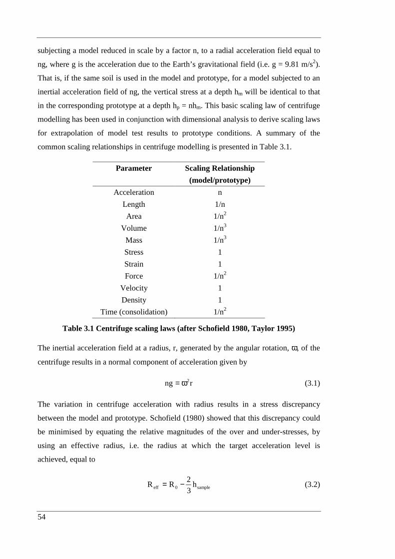
54
subjecting a model reduced in scale by a factor n, to a radial acceleration field equal to
ng, where g is the acceleration due to the Earth’s gravitational field (i.e. g = 9.81 m/s2).
That is, if the same soil is used in the model and prototype, for a model subjected to an
inertial acceleration field of ng, the vertical stress at a depth hm will be identical to that
in the corresponding prototype at a depth hp = nhm. This basic scaling law of centrifuge
modelling has been used in conjunction with dimensional analysis to derive scaling laws
for extrapolation of model test results to prototype conditions. A summary of the
common scaling relationships in centrifuge modelling is presented in Table 3.1.
Parameter Scaling Relationship
(model/prototype)
Acceleration n
Length 1/n
Area 1/n2
Volume 1/n3
Mass 1/n3
Stress 1
Strain 1
Force 1/n2
Velocity 1
Density 1
Time (consolidation) 1/n2
Table 3.1 Centrifuge scaling laws (after Schofield 1980, Taylor 1995)
The inertial acceleration field at a radius, r, generated by the angular rotation, ω, of the
centrifuge results in a normal component of acceleration given by
rng 2ω= (3.1)
The variation in centrifuge acceleration with radius results in a stress discrepancy
between the model and prototype. Schofield (1980) showed that this discrepancy could
be minimised by equating the relative magnitudes of the over and under-stresses, by
using an effective radius, i.e. the radius at which the target acceleration level is
achieved, equal to
sample0eff h3
2RR −= (3.2)

55
where Reff is the effective radius, R0 is the radius to the base of the sample and hsample is
the sample height.
Figure 3.1 shows a comparison of the stress variation with depth for the centrifuge
model and the corresponding prototype. It should be noted that the non-linear variation
in stress in the model is exaggerated for clarity. The maximum error in the vertical
stress is given by hsample/6Reff (Taylor 1995). For a sample height of 230 mm and an
effective radius of 1607 mm in the University of Western Australia (UWA) beam
centrifuge, the maximum error is 2.4 %. Similarly for a sample height of 165 mm and
an effective radius of 530 mm in the UWA drum centrifuge, the maximum stress
variation is 5.2 %. Hence the error in the stress profile is relatively minor in both
centrifuges.
The inertial radial acceleration is directed towards the axis of rotation of the centrifuge
and consequently in the horizontal plane, there is a change in its direction relative to
vertical across the width of the model, resulting in a lateral component of acceleration
(Taylor 1995). This lateral component of acceleration can become significant if testing
is conducted near a side wall of the model container. For this reason, in the beam
centrifuge, dynamic anchor test events were restricted to the centreline of the sample. In
the drum centrifuge, each point on the sample surface is normal to the axis of rotation
and hence no lateral acceleration component exists.
In order to achieve homologous stresses and strains in the model and prototype, model
tests are generally conducted in soil that is similar in grain size to the prototype soil.
Relative to the size of the foundation being modelled, the grain size of the model soil
will therefore be a factor of n greater than in the prototype. Grain size effects are
generally not observed provided that the ratio of the smallest significant dimension of
the problem (B) to the average grain size (d50) is greater than 35, i.e. B/d50 > 35
(ISSMGE TC2 2007). For tests in clays, silts and fine sands the model is usually large
enough relative to the soil particle size that no effect exists. However, for coarser
grained materials, particle size effects may become significant.

56
3.3 CENTRIFUGE FACILITIES
3.3.1 Beam Centrifuge
The fixed beam Acutronic Model 661 geotechnical beam centrifuge at The University
of Western Australia (UWA) was installed in 1989 and features a swinging platform
with a radius of 1.8 m. The centrifuge, shown in Figure 3.2, is rated to a capacity of 40
g-tonnes, with a maximum payload of 200 kg at the maximum acceleration level of 200
g. Test packages placed on the swinging platform are balanced by a movable counter
weight at the opposite end of the beam. The centrifuge is housed in a specially
constructed circular reinforced concrete chamber. The chamber is air conditioned to
maintain a constant temperature and to avoid seasonal variations. This facility is
described in detail by Randolph et al. (1991).
Since its installation, the beam centrifuge at UWA has undergone a number of upgrades,
particularly in relation to the control software and data acquisition systems. The control
software was written in-house and enables efficient operation of the centrifuge and
actuators. The test package is monitored in-flight by an onboard flight computer,
incorporating a 16 bit data acquisition system and data is transferred to the centrifuge
control room via a wireless network connection. This allows real time monitoring of test
and centrifuge performance data.
3.3.1.1 Sample Strong-Box
Beam centrifuge soil samples were contained within rectangular, aluminium strong-
boxes with internal dimensions measuring 650 mm long, 390 mm wide and 325 mm
high (Figure 3.3). Drainage holes at the base of the box allowed drainage or saturation
of the sample in-flight and an external standpipe enabled the sample water level to be
maintained during testing.
3.3.1.2 Actuators
The test programme was undertaken using electronic actuators (Figure 3.4) with two
degrees of freedom (horizontal and vertical). Powered by 30 V DC variable speed
servo-motors, the actuators have maximum horizontal and vertical strokes of 180 mm
57
and 250 mm respectively. Both axes have a maximum velocity of 3 mm/s and
displacements are monitored using high resolution optical encoders. The actuators
provide loading capabilities of 2 kN horizontally and 6.5 kN vertically. Control software
enables the actuators to perform both monotonic and cyclic loading under either
displacement or load control conditions.
3.3.1.3 STOMPI
During self weight consolidation in the beam centrifuge, the sample pore pressures were
monitored using the Sub-Terrain Oil impregnated Multiple Pressure Instrument
(STOMPI). STOMPI features five individual pore pressure transducers located at 50
mm intervals along a stainless steel shaft. The device was placed within the sample and
secured to the top flange of the strongbox, providing measurements of the pore
pressures at various sample depths. STOMPI is shown in Figure 3.5.
3.3.2 Drum Centrifuge
The drum centrifuge facility at UWA was established in 1997 (Figure 3.6). The
centrifuge has a diameter of 1.2 m and is capable of achieving a maximum rotational
speed of 850 rpm, representing a maximum acceleration level of 485 g at the bottom of
the channel. Two concentric shafts connected to a precision servo motor enable the
central tool table to be rotated differentially from the sample channel. The tool table
actuator is also capable of being stopped while the channel remains spinning,
eliminating the need for reconsolidation time between tests. A detailed description of
the drum centrifuge facility is provided by Stewart et al. (1998).
The drum centrifuge is fitted with two onboard data acquisition systems: one on both
the channel and tool table. Digital signals from each computer are transferred to a single
data acquisition computer in the control room, where the data is stored and transferred
to a second computer for real time graphics display. Rotation of the channel is computer
controlled and monitored and the tool table features a second onboard computer for
actuator control.

58
3.3.2.1 Sample Channel
The sample containment channel shown in Figure 3.7 has a diameter of 1.2 m and is 300
mm wide (vertically) and 200 mm deep (radially). The channel is driven by a 15.5 kW
440 V AC motor via a drive belt. Transducers located 50, 75 and 100 mm from the base
of the channel enable pore pressures to be monitored in-flight.
3.3.2.2 Tool Table Actuator
The central tool table actuator (Figure 3.8) is capable of vertical, radial and
circumferential actuation. The vertical and radial axes are driven by lead screws
powered by 60 V DC brushless servo motors fitted with 88:1 harmonic drive gearboxes
and have a continuous load rating of 10 kN. The circumferential axis is controlled by a
7.5 kW Dynaserv servo motor and has a torque rating of 500 Nm. The vertical and
radial velocities are limited to 3 mm/s with maximum strokes within the test zone of
156 mm and 227 mm respectively.
3.4 SOIL SAMPLES
Centrifuge model tests were conducted primarily in kaolin clay samples although
dynamic anchor performance was also assessed in uncemented calcareous sand and
silica flour samples. The following sections summarise the geotechnical properties and
sample preparation procedure for each soil type.
3.4.1 Soil Properties
3.4.1.1 Kaolin Clay
Kaolin clay is often used in centrifuge modelling due to its isotropic nature and
relatively short consolidation time. The properties of UWA kaolin clay have previously
been characterised by Stewart (1992). These properties have been combined with the
results of a standard Rowe cell test, conducted by the author, in Table 3.2.
The coefficient of consolidation depends on the stiffness and permeability of the soil
and hence varies with the effective stress level and void ratio. The variation in the
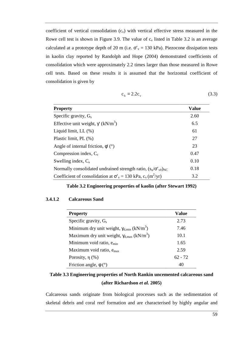
59
coefficient of vertical consolidation (cv) with vertical effective stress measured in the
Rowe cell test is shown in Figure 3.9. The value of cv listed in Table 3.2 is an average
calculated at a prototype depth of 20 m (i.e. σ′v = 130 kPa). Piezocone dissipation tests
in kaolin clay reported by Randolph and Hope (2004) demonstrated coefficients of
consolidation which were approximately 2.2 times larger than those measured in Rowe
cell tests. Based on these results it is assumed that the horizontal coefficient of
consolidation is given by
vh c2.2c = (3.3)
Property Value
Specific gravity, Gs 2.60
Effective unit weight, γ' (kN/m3) 6.5
Liquid limit, LL (%) 61
Plastic limit, PL (%) 27
Angle of internal friction, φ' (°) 23
Compression index, Cc 0.47
Swelling index, Cs 0.10
Normally consolidated undrained strength ratio, (su/σ′v0)NC 0.18
Coefficient of consolidation at σ′v = 130 kPa, cv (m2/yr) 3.2
Table 3.2 Engineering properties of kaolin (after Stewart 1992)
3.4.1.2 Calcareous Sand
Property Value
Specific gravity, Gs 2.73
Minimum dry unit weight, γd,min (kN/m3) 7.46
Maximum dry unit weight, γd,max (kN/m3) 10.1
Minimum void ratio, emin 1.65
Maximum void ratio, emax 2.59
Porosity, η (%) 62 - 72
Friction angle, φ (°) 40
Table 3.3 Engineering properties of North Rankin uncemented calcareous sand
(after Richardson et al. 2005)
Calcareous sands originate from biological processes such as the sedimentation of
skeletal debris and coral reef formation and are characterised by highly angular and
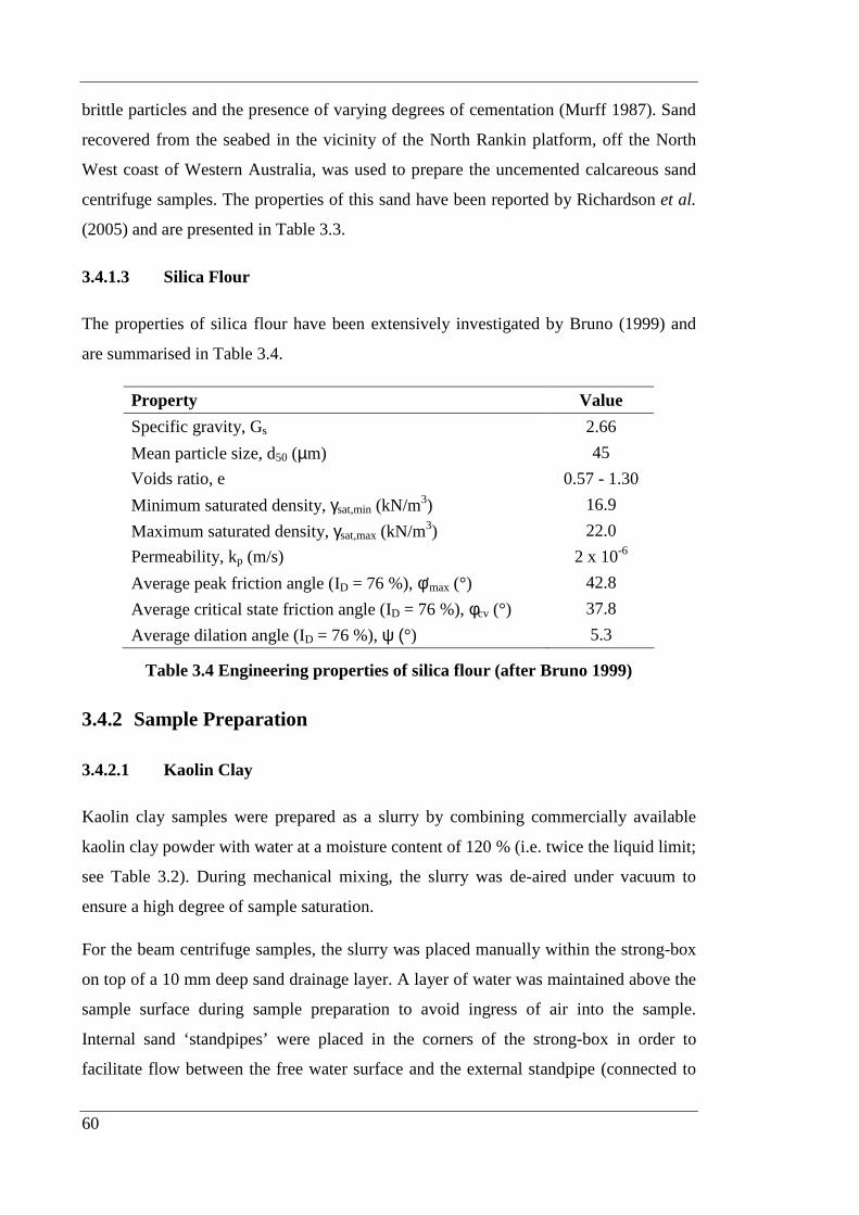
60
brittle particles and the presence of varying degrees of cementation (Murff 1987). Sand
recovered from the seabed in the vicinity of the North Rankin platform, off the North
West coast of Western Australia, was used to prepare the uncemented calcareous sand
centrifuge samples. The properties of this sand have been reported by Richardson et al.
(2005) and are presented in Table 3.3.
3.4.1.3 Silica Flour
The properties of silica flour have been extensively investigated by Bruno (1999) and
are summarised in Table 3.4.
Property Value
Specific gravity, Gs 2.66
Mean particle size, d50 (µm) 45
Voids ratio, e 0.57 - 1.30
Minimum saturated density, γsat,min (kN/m3) 16.9
Maximum saturated density, γsat,max (kN/m3) 22.0
Permeability, kp (m/s) 2 x 10⁻⁶
Average peak friction angle (ID = 76 %), φ'max (°) 42.8
Average critical state friction angle (ID = 76 %), φcv (°) 37.8
Average dilation angle (ID = 76 %), ψ (°) 5.3
Table 3.4 Engineering properties of silica flour (after Bruno 1999)
3.4.2 Sample Preparation
3.4.2.1 Kaolin Clay
Kaolin clay samples were prepared as a slurry by combining commercially available
kaolin clay powder with water at a moisture content of 120 % (i.e. twice the liquid limit;
see Table 3.2). During mechanical mixing, the slurry was de-aired under vacuum to
ensure a high degree of sample saturation.
For the beam centrifuge samples, the slurry was placed manually within the strong-box
on top of a 10 mm deep sand drainage layer. A layer of water was maintained above the
sample surface during sample preparation to avoid ingress of air into the sample.
Internal sand ‘standpipes’ were placed in the corners of the strong-box in order to
facilitate flow between the free water surface and the external standpipe (connected to
61
the base drainage layer), thereby avoiding an increase in pore pressure beneath the low
permeability clay layer. Water was added to the sample in-flight to compensate for
losses due to evaporation.
For the drum centrifuge samples, the mixed and de-aired slurry was transferred to a
hopper and positioned above the centrifuge (Figure 3.10). The hopper was connected by
a hose and rotating coupling to a PVC nozzle attached to the actuator (Figure 3.11).
Prior to placement of the slurry a 10 mm deep sand drainage layer was placed at the
bottom of the channel. Due to the orientation of the sample containment channel the
slurry was placed with the channel spinning at 20 g in order to prevent the slurry from
spilling out. The nozzle was rotated relative to the channel at a rate of 3 °/s such that the
slurry was distributed uniformly within the channel. The centrifugal force ensured the
slurry formed a level sample surface as it was poured. A layer of water was maintained
above the sample surface to prevent ingress of air during sample placement and water
was added to the sample in-flight to compensate for evaporation losses.
Normally consolidated samples were prepared by self weight consolidation in the
centrifuge at an average acceleration level of 200 g. In the beam centrifuge STOMPI
(Section 3.3.1.3) was used to monitor the progression of consolidation through the
dissipation of excess pore pressures, whilst in the drum centrifuge this information was
provided by pore pressure transducers situated in the channel (Section 3.3.2.1).
In order to achieve a sufficient sample height it was necessary to ‘top-up’ the sample
with slurry, following consolidation of the previous layer. Typically two top-ups were
required to achieve the target consolidated sample height of 230 mm in the beam
centrifuge and 165 mm in the drum centrifuge.
Note that beam centrifuge sample, Box 6 was prepared according to the method
proposed by Chen (2005) for the production of a clay sample with an artificially high
sensitivity. The sensitivity (St) is defined as the ratio of the undisturbed shear strength
(su) to the fully remoulded shear strength (su,r), St = su / su,r. Kaolin clay typically
exhibits sensitivities of approximately 2 – 2.5, however Chen (2005) demonstrated
sensitivities measured using cyclic T-bar tests of approximately 4 – 5. The sample was
prepared by dissolving a dispersing agent (sodium polymetaphosphate) in water for 24
hours at a concentration of 15 g/L. The kaolin slurry was then prepared at a moisture
62
content of 70 % using the hydrated sodium polymetaphosphate. Unfortunately the
sample preparation procedure did not produce a sample with increased sensitivity (see
Section 5.2.1).
3.4.2.2 Calcareous Sand
The preparation of uncemented calcareous sand samples for the beam centrifuge is
outlined in Richardson et al. (2005). Calcareous sand recovered from the seabed near
the North Rankin platform was dried and sieved to remove particles larger than 0.3 mm.
The sieved material was then dry mixed to ensure a uniform distribution of particles
throughout the sample. Following mixing the sand was loosely placed in a centrifuge
strong-box and saturated via the drainage holes in the bottom of the box. The strong-box
was then placed on a vibrating table at a low speed setting for approximately 1 hour.
Drainage at the bottom of the sample was provided via a woven, felt drainage blanket
overlying a 10 mm deep layer of coarse sand.
A total of three uncemented calcareous sand samples were produced. In order to save
sample preparation time the second calcareous sand sample (Box 8) was prepared by
reconstituting the original sample (Box 7). This was achieved by carefully hand mixing
the sample under water to avoid ingress of air. The sample was then placed back on the
vibrating table for approximately 30 minutes. However, due to inconsistencies between
cone penetration test (CPT) profiles in the original and reconstituted samples, the
reconstitution method was not deemed effective and consequently the test results from
Box 8 have been excluded from the analysis (see Section 6.3.1).
3.4.2.3 Silica Flour
The single silica flour beam centrifuge sample was prepared by loosely placing
commercially available silica flour in a strong-box over 10 mm layers of coarse and fine
sand. Following placement of the silica flour, the sample was saturated via the drainage
holes in the bottom of the box. The sample was then placed on a vibrating table at low
speed for approximately half an hour.

63
3.5 PENETROMETER DEVICES
3.5.1 T-bar Penetrometer
Soil characterisation tests in kaolin clay were conducted using a T-bar penetrometer
(Stewart and Randolph 1991). T-bar penetrometer tests were conducted in-flight and
provided a continuous profile of shear strength with depth. The major advantage of the
T-bar over other penetrometers such as the cone, is that the soil is allowed to flow
around and over the T-bar during penetration, therefore the soil overburden pressure is
equilibrated above and below the bar and as such the need for corrections is largely
avoided (Stewart and Randolph 1994).
The T-bar used in the beam centrifuge tests is shown in Figure 3.12. It comprises a 5
mm diameter, 20 mm long cylinder attached at right angles to the end of a vertical shaft.
A load cell at the tip of the shaft measures the T-bar penetration resistance. A similar T-
bar penetrometer was used in the drum centrifuge tests.
T-bar tests were carried out before and after dynamic anchor tests in each sample to
monitor any change in the sample strength with time. The T-bar was installed at a rate
of 1 mm/s, ensuring undrained conditions. The transition from partially drained to
undrained conditions has been shown to occur at a non-dimensional velocity (V) of
approximately 30 (Finnie and Randolph 1994), where
vc
vDV = (3.4)
where v is the penetration velocity, D is the penetrometer diameter (i.e. 5 mm) and cv is
the coefficient of consolidation. House et al. (2001), however, suggested a lower
undrained non-dimensional velocity limit of 10 from T-bar penetrometer tests. Hence
for a penetration velocity of 1 mm/s and an average coefficient of consolidation of 3.2
m2/yr (0.10 mm2/s; Table 3.2), the non-dimensional velocity is approximately 50, which
is greater than the lower bound value of 10 required for undrained conditions.
The net bearing resistance, q, during T-bar penetration can be correlated to the
undrained shear strength, su, by a T-bar bearing capacity factor, NT-bar, where

64
ubarT sNq −= (3.5)
The analytical value of NT-bar depends on the roughness of the T-bar. Plasticity solutions
for the limiting pressure acting on a cylinder displaced laterally in fine grained soil give
a value of approximately 12 for a rough bar, and a value of 9 for a smooth bar
(Randolph and Houlsby 1984). Stewart and Randolph (1991) recommend a T-bar factor
of 10.5, representing an average of the rough and smooth cases.
Cyclic T-bar tests have been used to measure the sensitivity of clay (Watson et al. 2000,
Chen 2005). The cyclic T-bar tests were conducted by monotonically installing the T-
bar to a depth of approximately two-thirds the sample height at a rate of 1 mm/s. An
average measurement of the maximum undisturbed shear strength (su) was made during
the initial penetration stroke of the test, however it should be noted that the actual
undisturbed shear strength is mobilised ahead of the penetrometer with the soil
softening towards a partially remoulded strength behind the T-bar (Yafrate and DeJong
2005). Subsequent vertical cycles of the T-bar over an interval of 30 mm were
considered sufficient to cause remoulding of the soil. Full remoulding in the cycling
zone typically occurred within 10 cycles, however, a total of 25 cycles were performed
in each test. Following cycling, the T-bar was monotonically installed to its final depth
before monotonic extraction at a rate of 1 mm/s. The cyclic T-bar profile is often
asymmetrical and this can have a significant impact on the calculated sensitivity. This
has been accounted for by taking the zero strength as the mid-point between the
penetration and extraction loops in the final cycle of the test. In addition, by assessing
the sensitivity at the mid depth of the cycling interval the influence of limit variations
was minimised.
3.5.2 Cone Penetrometer
3.5.2.1 Calcareous Sand
Cone penetrometer tests (CPTs) were used to assess the variation in cone tip resistance
with depth in the uncemented calcareous sand samples. The 60° cone angle, 10 mm
diameter model cone penetrometer used in the beam centrifuge tests is shown in Figure
3.13. Due to the brittle and collapsible nature of the calcareous sand a cone
penetrometer with a relatively low tip resistance capacity of 25 MPa was selected in
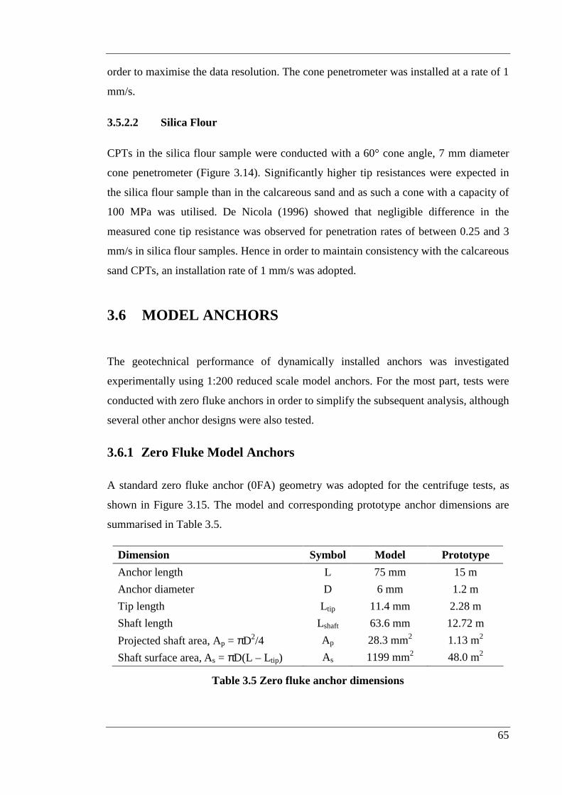
65
order to maximise the data resolution. The cone penetrometer was installed at a rate of 1
mm/s.
3.5.2.2 Silica Flour
CPTs in the silica flour sample were conducted with a 60° cone angle, 7 mm diameter
cone penetrometer (Figure 3.14). Significantly higher tip resistances were expected in
the silica flour sample than in the calcareous sand and as such a cone with a capacity of
100 MPa was utilised. De Nicola (1996) showed that negligible difference in the
measured cone tip resistance was observed for penetration rates of between 0.25 and 3
mm/s in silica flour samples. Hence in order to maintain consistency with the calcareous
sand CPTs, an installation rate of 1 mm/s was adopted.
3.6 MODEL ANCHORS
The geotechnical performance of dynamically installed anchors was investigated
experimentally using 1:200 reduced scale model anchors. For the most part, tests were
conducted with zero fluke anchors in order to simplify the subsequent analysis, although
several other anchor designs were also tested.
3.6.1 Zero Fluke Model Anchors
A standard zero fluke anchor (0FA) geometry was adopted for the centrifuge tests, as
shown in Figure 3.15. The model and corresponding prototype anchor dimensions are
summarised in Table 3.5.
Dimension Symbol Model Prototype
Anchor length L 75 mm 15 m
Anchor diameter D 6 mm 1.2 m
Tip length Ltip 11.4 mm 2.28 m
Shaft length Lshaft 63.6 mm 12.72 m
Projected shaft area, Ap = πD2/4 Ap 28.3 mm2 1.13 m2
Shaft surface area, As = πD(L – Ltip) As 1199 mm2 48.0 m2
Table 3.5 Zero fluke anchor dimensions
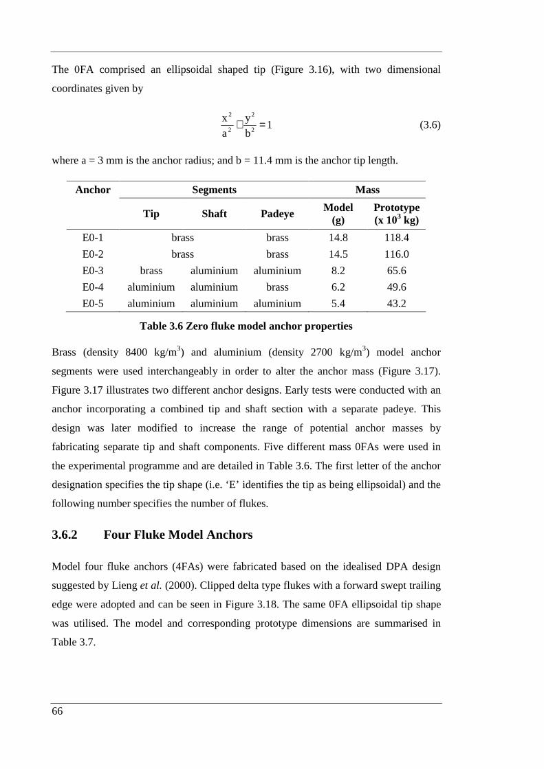
66
The 0FA comprised an ellipsoidal shaped tip (Figure 3.16), with two dimensional
coordinates given by
1b
y
a
x2
2
2
2
=+ (3.6)
where a = 3 mm is the anchor radius; and b = 11.4 mm is the anchor tip length.
Anchor Segments Mass
Tip Shaft Padeye Model (g)
Prototype (x 103 kg)
E0-1 brass brass 14.8 118.4
E0-2 brass brass 14.5 116.0
E0-3 brass aluminium aluminium 8.2 65.6
E0-4 aluminium aluminium brass 6.2 49.6
E0-5 aluminium aluminium aluminium 5.4 43.2
Table 3.6 Zero fluke model anchor properties
Brass (density 8400 kg/m3) and aluminium (density 2700 kg/m3) model anchor
segments were used interchangeably in order to alter the anchor mass (Figure 3.17).
Figure 3.17 illustrates two different anchor designs. Early tests were conducted with an
anchor incorporating a combined tip and shaft section with a separate padeye. This
design was later modified to increase the range of potential anchor masses by
fabricating separate tip and shaft components. Five different mass 0FAs were used in
the experimental programme and are detailed in Table 3.6. The first letter of the anchor
designation specifies the tip shape (i.e. ‘E’ identifies the tip as being ellipsoidal) and the
following number specifies the number of flukes.
3.6.2 Four Fluke Model Anchors
Model four fluke anchors (4FAs) were fabricated based on the idealised DPA design
suggested by Lieng et al. (2000). Clipped delta type flukes with a forward swept trailing
edge were adopted and can be seen in Figure 3.18. The same 0FA ellipsoidal tip shape
was utilised. The model and corresponding prototype dimensions are summarised in
Table 3.7.
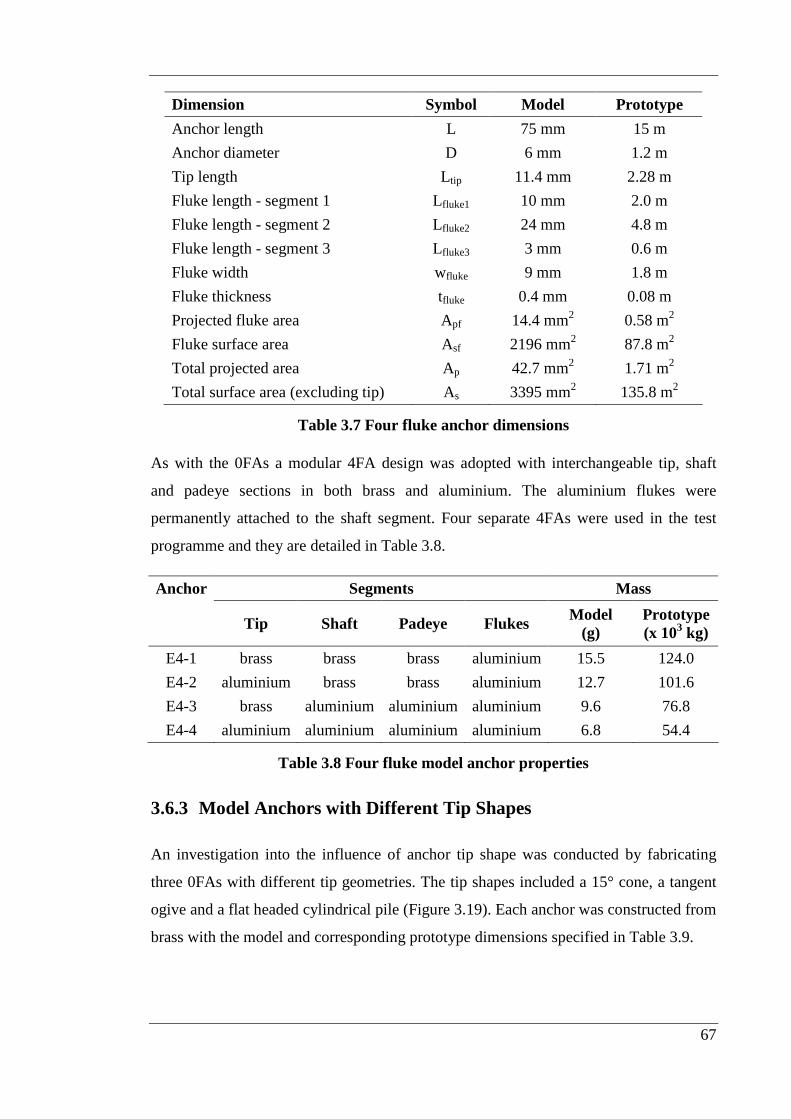
67
Dimension Symbol Model Prototype
Anchor length L 75 mm 15 m
Anchor diameter D 6 mm 1.2 m
Tip length Ltip 11.4 mm 2.28 m
Fluke length - segment 1 Lfluke1 10 mm 2.0 m
Fluke length - segment 2 Lfluke2 24 mm 4.8 m
Fluke length - segment 3 Lfluke3 3 mm 0.6 m
Fluke width wfluke 9 mm 1.8 m
Fluke thickness tfluke 0.4 mm 0.08 m
Projected fluke area Apf 14.4 mm2 0.58 m2
Fluke surface area Asf 2196 mm2 87.8 m2
Total projected area Ap 42.7 mm2 1.71 m2
Total surface area (excluding tip) As 3395 mm2 135.8 m2
Table 3.7 Four fluke anchor dimensions
As with the 0FAs a modular 4FA design was adopted with interchangeable tip, shaft
and padeye sections in both brass and aluminium. The aluminium flukes were
permanently attached to the shaft segment. Four separate 4FAs were used in the test
programme and they are detailed in Table 3.8.
Anchor Segments Mass
Tip Shaft Padeye Flukes Model (g)
Prototype (x 103 kg)
E4-1 brass brass brass aluminium 15.5 124.0
E4-2 aluminium brass brass aluminium 12.7 101.6
E4-3 brass aluminium aluminium aluminium 9.6 76.8
E4-4 aluminium aluminium aluminium aluminium 6.8 54.4
Table 3.8 Four fluke model anchor properties
3.6.3 Model Anchors with Different Tip Shapes
An investigation into the influence of anchor tip shape was conducted by fabricating
three 0FAs with different tip geometries. The tip shapes included a 15° cone, a tangent
ogive and a flat headed cylindrical pile (Figure 3.19). Each anchor was constructed from
brass with the model and corresponding prototype dimensions specified in Table 3.9.

68
Dimension Symbol Model Prototype
Anchor length L 75 mm 15 m
Anchor diameter D 6 mm 1.2 m
Tip length - cone Ltip 22.8 mm 4.6 m
Tip length - ogive Ltip 22.8 mm 4.6 m
Tip length - flat Ltip 0 mm 0 m
Shaft surface area - cone, As = πD(L – Ltip) As 984 mm2 39.4 m2
Shaft surface area - ogive, As = πD(L – Ltip) As 984 mm2 39.4 m2
Shaft surface area - flat, As = πD(L – Ltip) As 1414 mm2 56.5 m2
Projected shaft area Ap 28.3 mm2 1.13 m2
Table 3.9 Dimensions of anchors with varying tip geometry
The anchor masses are presented in Table 3.10. Every effort was made to ensure
equivalent anchor masses with the reference anchor E0-1 (see Table 3.6). Unfortunately
it was not possible to reduce the mass of the flat tipped anchor in line with the other
anchors, without exceeding safe wall thickness limits. The anchors in Table 3.10 are
designated as ‘C’ for the conical tip, ‘O’ for the ogive tip and ‘F’ for the flat tip.
Anchor Segments Mass
Tip Shaft Padeye Model (g)
Prototype (x 103 kg)
C0-1 brass brass 14.7 117.6 O0-1 brass brass 14.8 118.4 F0-1 brass brass 15.5 124.0
Table 3.10 Properties of model anchors with varying tip geometry
3.6.4 Instrumented Anchor
An instrumented model zero fluke anchor was designed and developed to measure the
anchor deceleration during penetration experiments in the centrifuge. Two identical
instrumented anchors were fabricated, incorporating a tip load cell and a miniature
accelerometer. The instrumented anchors were of similar design to the 0FAs described
in Section 3.6.1 and comprised the same ellipsoidal shaped tip (Figure 3.20). A slight
discrepancy in mass between the two instrumented anchors was identified (Table 3.11).
The ‘I’ in the anchor designation specifies that the anchors are instrumented.

69
The instrumentation was contained within a small section of the anchor just behind the
tip (Figure 3.20). Strain gauges placed on the walls of this section acted as an axial tip
load cell. A miniature piezoelectric accelerometer was installed inside the hollow strain
gauged section. Piezoelectric accelerometers rely on a property exhibited by certain
materials where a voltage is generated across the material when it is stressed. Therefore
when exposed to an acceleration, a test mass stresses the piezoelectric material by a
force, F = ma, resulting in a voltage being developed across the material. Measuring this
voltage provides a measurement of the acceleration. The instrumented anchor
accelerometer was designed to withstand accelerations of up to 1000 g.
Anchor Segments Mass
Tip Shaft Padeye Model (g)
Prototype (x 103 kg)
IE0-1 brass brass 14.3 114.4 IE0-2 brass brass 14.8 118.4
Table 3.11 Model instrumented anchor properties
The shaft of the model anchor was bored out to allow a single instrumentation cable
incorporating the data signals from both the load cell and accelerometer to pass up
through the middle of the anchor, exiting at the padeye. A small metal loop soldered to
the end of the anchor acted as a padeye for attachment of the anchor chain and release
cord. Strain relief for the instrumentation cable was provided with a grub screw located
near the padeye.
The instrumented anchor was designed and developed with the ultimate objective of
measuring the deceleration of model anchors during dynamic installation in the
centrifuge. Measurement of the deceleration would allow a velocity profile to be
obtained, which would subsequently aid calibration of theoretical resistance models
during anchor penetration. Unfortunately the high noise environment in the centrifuge
and damage to the instrumentation prevented any usable data from being obtained from
the instrumented model anchors. As such, no discussion or analysis of the data
measured by the instrumentation will be presented. However since the impact velocity,
embedment depth and holding capacity are measured independently of the anchor
instrumentation, the external data recorded for the instrumented model anchor tests will
be incorporated in the analysis presented in later chapters.

70
3.6.5 Model Anchors with Different Aspect Ratios
The influence of the aspect ratio (length to diameter ratio, L/D) on the performance of
dynamic anchors was assessed via a series of tests with 6, 9 and 12 mm diameter, zero
fluke model anchors with aspect ratios ranging from 1 – 14 (see Figure 3.21). Details of
the anchors are summarised in Table 3.12. In order to provide a smooth transition
between L/D = 1 and higher aspect ratios, both the anchor tip and padeye were
hemispherical in shape (see Figure 3.22). Consequently, the anchors in Table 3.12 have
been designated as ‘H’ for their hemispherical tip shape. The model anchors were
fabricated with interchangeable tip and padeye sections, such that the aspect ratio could
be altered simply by changing the central shaft section. The limited sample depth in the
drum centrifuge prevented all of the model anchors from being fabricated from brass
(density = 8400 kg/m3). In order to investigate anchors with higher aspect ratios,
without embedments exceeding the sample depth, a number of anchors were fabricated
from aluminium with a density of approximately 2700 kg/m3.
The influence of the aspect ratio was objectively assessed by comparing the
performance of two pairs of anchors with identical masses but different aspect ratios:
• Anchors H0-5 (L/D = 4) and H0-13 (L/D = 12) with a mass of 4.7 grams
• Anchors H0-15 (L/D = 1) and H0-18 (L/D = 3) with a mass of 3.0 grams
The anchor mass was varied by drilling out material from the middle of the central shaft
section of the anchor.
The use of brass and aluminium also allowed the behaviour of anchors with identical
aspect ratios but different masses to be compared, thereby providing an assessment of
the influence of anchor density on the dynamic anchor performance. Accordingly, four
individual groups of anchors were developed:
• Anchors H0-5 (m = 4.7 g) and H0-7 (m = 1.4 g) with L/D = 4
• Anchors H0-6 (m = 7.4 g), H0-8 (m = 2.3 g) and H0-9 (m = 1.9 g) with L/D = 6
• Anchors H0-12 (m = 5.0 g) and H0-13 (m = 4.7 g) with L/D = 12
• Anchors H0-17 (m = 11.4 g) and H0-18 (m = 3.0 g) with L/D = 3
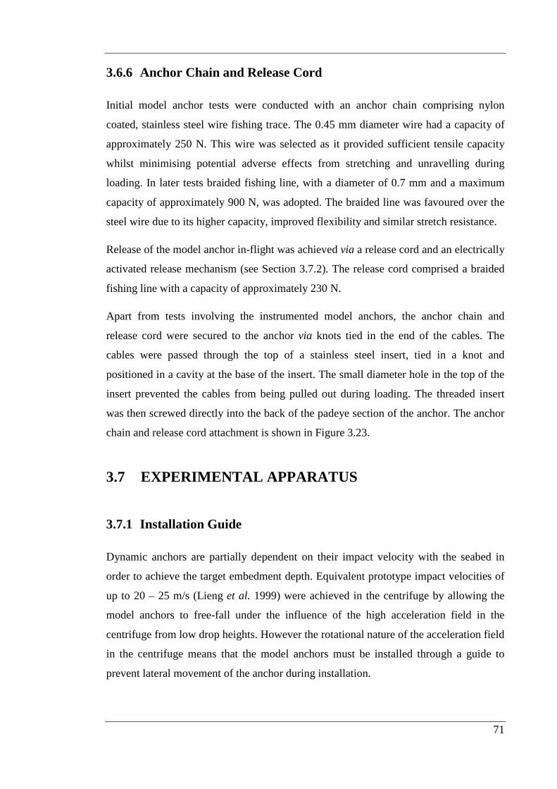
71
3.6.6 Anchor Chain and Release Cord
Initial model anchor tests were conducted with an anchor chain comprising nylon
coated, stainless steel wire fishing trace. The 0.45 mm diameter wire had a capacity of
approximately 250 N. This wire was selected as it provided sufficient tensile capacity
whilst minimising potential adverse effects from stretching and unravelling during
loading. In later tests braided fishing line, with a diameter of 0.7 mm and a maximum
capacity of approximately 900 N, was adopted. The braided line was favoured over the
steel wire due to its higher capacity, improved flexibility and similar stretch resistance.
Release of the model anchor in-flight was achieved via a release cord and an electrically
activated release mechanism (see Section 3.7.2). The release cord comprised a braided
fishing line with a capacity of approximately 230 N.
Apart from tests involving the instrumented model anchors, the anchor chain and
release cord were secured to the anchor via knots tied in the end of the cables. The
cables were passed through the top of a stainless steel insert, tied in a knot and
positioned in a cavity at the base of the insert. The small diameter hole in the top of the
insert prevented the cables from being pulled out during loading. The threaded insert
was then screwed directly into the back of the padeye section of the anchor. The anchor
chain and release cord attachment is shown in Figure 3.23.
3.7 EXPERIMENTAL APPARATUS
3.7.1 Installation Guide
Dynamic anchors are partially dependent on their impact velocity with the seabed in
order to achieve the target embedment depth. Equivalent prototype impact velocities of
up to 20 – 25 m/s (Lieng et al. 1999) were achieved in the centrifuge by allowing the
model anchors to free-fall under the influence of the high acceleration field in the
centrifuge from low drop heights. However the rotational nature of the acceleration field
in the centrifuge means that the model anchors must be installed through a guide to
prevent lateral movement of the anchor during installation.

72
Separate guides were fabricated for the 0FAs and the 4FAs. The slotted cylindrical
installation guide for the 0FAs was manufactured from aluminium with an internal
diameter of 6.5 mm, thereby providing nominal clearance to the 6 mm diameter model
anchor. The open slot along the entire 375 mm length of the guide allowed continuous
access for the model anchor chain. The 0FA guide is shown in Figure 3.24. Similar
guides were also fabricated for the 9 and 12 mm diameter anchors described in Section
3.6.5.
The 4FAs were installed using a guide fabricated from PVC incorporating a 0.85 mm
wide slot and a 6 mm diameter groove machined into the centre of the front face of the
guide. The anchor was positioned with a fluke in the slot and the shaft against the
groove. To prevent the anchor from falling away from the guide two PVC rails were
attached to the guide with brackets. These rails did not interfere with the anchor chain or
the movement of the anchor down the guide. The 4FA guide is shown in Figure 3.25.
Measurement of the model anchor velocity at the point of impact with the sample
surface is important in terms of the test analysis. Early tests utilised a single
PhotoEmitter-Receiver Pair (PERP; see the left side of Figure 3.26a) located one anchor
length back from the tip of the guide to measure the anchor velocity. As an object
passes the PERP and breaks the light beam passing between the emitter on one side of
the guide and the receiver on the other side of the guide, a voltage is recorded. The
duration of this voltage increase, known as the interrupt time, ∆t, can be used in
conjunction with the length of the object passing the PERP, L, to determine an average
velocity, vave.
t
Lvave ∆
= (3.7)
For the 0FAs the interrupt time was measured for the entire anchor length. However for
the 4FAs, since the beam was broken by the anchor fluke in the guide slot, the known
fluke length passing the PERP was used to determine the anchor velocity. The PERP
output for a typical model anchor drop test in the centrifuge is shown on the left side of
Figure 3.26b.
Use of a single PERP, however, was not deemed to provide sufficient accuracy for the
velocity calculated by Equation 3.7. Consequently an installation guide comprising
73
multiple PERPs positioned at 10 mm intervals along the guide was developed (see right
side of Figure 3.26a). The anchor velocity was calculated by measuring the time
required for both the anchor tip and padeye to pass consecutive PERPs. Coupled with
the fixed PERP spacing this information could be used to calculate multiple velocities
during the installation of the model anchor. Not only did the reduction in distance over
which the velocity was calculated lead to improved accuracy, but the multiple velocities
allowed a partial anchor velocity profile to be generated as opposed to a single velocity
point for the single PERP guide. A comparison of the velocities derived from the single
and multiple PERP guides is shown in Figure 3.26c.
Figure 3.26c shows that for two separate tests conducted from the same drop height of
250 mm, the single PERP guide records a velocity of 21.2 m/s. With the PERP located
100 mm above the sample surface the velocity is therefore representative of the anchor
velocity at an average height of 62.5 mm above the sample surface, based on an anchor
length of 75 mm (Table 3.5). At a similar height above the sample surface the multiple
PERP guide provides a slightly higher velocity of 22.3 m/s. However, the multiple
PERP guide suggests an interpolated impact velocity of 26.3 m/s, which is 24 % higher
than the single PERP velocity, demonstrating the inaccuracy associated with measuring
the impact velocity with the single PERP guide configuration.
3.7.2 Release Mechanism
Release of the model anchors in-flight was achieved with a release mechanism
developed by Wemmie (2003) (Figure 3.27). Prior to the test, the release cord was
positioned over a 30 Ω resistor and clamped in place to prevent premature movement of
the anchor in the centrifuge acceleration field. Activation of the release mechanism
resulted in a voltage being supplied to the resistor. This voltage was sufficient to cause
the resistor to burn through the release cord, thereby effecting release. The release
mechanism was attached to the top of the installation guide.
3.7.3 Load Cell
The load displacement response of the model anchors during extraction was measured
using a 1.7 kN load cell mounted in-line with the vertical axis of the actuator in the
beam centrifuge and the radial axis of the actuator in the drum centrifuge. The anchor

74
chain passed over a metal loop which was attached to the load cell by a connecting
screw (Figure 3.28).
3.8 TESTING PROCEDURE
The experimental programme predominantly comprised model anchor drop tests. These
tests were conducted in two distinct phases; installation and extraction. Typically
extraction involved vertical monotonic loading of the anchor to failure, although in
some instances this also involved vertical cyclic or sustained loading. Dynamic anchors
are expected to be subjected to predominantly inclined loading and not only vertical
loading as is the case here. However, results from finite element studies reported by
Lieng et al. (1999) suggest that dynamic anchors have ample horizontal capacity and
failure is governed by the vertical capacity. In addition to the drop tests a small number
of static installation tests were conducted. Each test in this study was performed at a
centrifuge acceleration level of 200 g.
3.8.1 Beam Centrifuge
3.8.1.1 Dynamic Installation
The test arrangement in the beam centrifuge is shown in Figure 3.29, with the
installation guide bolted to the actuator tower and the release mechanism attached via a
bracket to the top of the guide. The model anchor was fitted with both an anchor chain
and a release cord and positioned within the installation guide with the anchor tip at the
required drop height above the sample surface. The anchor chain was then connected to
the load cell and the release cord clamped over the resistor in the release mechanism.
The impact velocity of the anchor could be altered by adjusting the initial vertical
position of the anchor within the guide prior to release.
At the required centrifuge acceleration level, the release mechanism was activated from
the control room and after several seconds the anchor was released. Fast-logging data
acquisition software enabled the data from the PERPs to be logged at rates of up to 100
kHz during installation. The software was automatically activated when the anchor

75
passed a designated trigger PERP. A pre-trigger incorporated in the software enabled
the recording of data for a specified time prior to the trigger point.
To minimise interaction effects between adjacent test sites, a spacing of 5 anchor
diameters was adopted, corresponding to 30 mm for the 6 mm diameter 0FA. Similarly
in order to avoid interaction effects with the strong-box boundaries a minimum spacing
of 10 anchor diameters was adopted.
3.8.1.2 Vertical Monotonic Extraction
To allow consolidation of the soil surrounding the embedded anchor, various soak
periods were permitted following installation. Then, before extraction took place, the
actuator was driven horizontally 43 mm to account for the offset between the
installation guide and the vertical axis of the load cell. Extraction of the anchor was
initiated by driving the actuator vertically upwards away from the sample surface at a
constant rate sufficient to ensure undrained conditions. Undrained conditions occur
when the non-dimensional velocity (V) is greater than 10 (House et al. 2001), where V
is given by Equation 3.4. For D = 6 mm (Table 3.5) and cv = 3.2 m2/yr (0.10 mm2/s;
Table 3.2) an extraction rate greater than 0.17 mm/s is sufficient to ensure undrained
conditions, hence a rate of 0.3 mm/s was adopted in all model anchor tests.
The anchor embedment depth, ze, was determined from the initial vertical position of
the load cell above the sample surface, zLC, the length of the anchor chain, zchain, the
amount of slack removed from the anchor chain prior to the onset of a significant tensile
load, zslack, and the model anchor length, L (Figure 3.30), as
Lzzzz slackLCchaine +−−= (3.8)
The reliability of this method was verified by comparison with several direct
measurements.
3.8.1.3 Sustained Loading Tests
Long-term sustained loading of the model anchors was performed under load control
conditions. Following installation and consolidation, vertical sustained loads were
applied with a magnitude equal to a proportion of the maximum capacity measured in
the reference monotonic loading test. The load magnitude and duration were varied
76
between tests. If failure was not observed under the sustained loading sequence, the
anchor was loaded monotonically to failure at a rate of 0.3 mm/s in displacement
control. Failure was identified as excessive vertical displacement under the applied
sustained load.
3.8.1.4 Cyclic Loading Tests
Cyclic loading tests were also performed under load control conditions. Following
installation and consolidation, vertical cyclic loading sequences were applied with the
minimum and maximum cyclic loads specified as proportions of the maximum capacity
measured in the reference monotonic loading test. The load magnitude, duration and
frequency were varied between tests. Since mooring lines for floating offshore
structures are not capable of transmitting compression loads to the foundation system,
the model anchors were subjected to one-way cyclic tensile loading only. The cyclic
loading was applied using a sinusoidal wave form.
Floating structures such as semi-submersibles have natural periods of vibration of the
order of 100 seconds or more in deepwater (El-Gharbawy and Olson 1999). Low
frequency cyclic loads are often applied to these structures by the wind, current, wave
drift and tide, although higher frequency environmental loads from wave and storm
loading may result in cyclic loading frequencies of 5 to 20 times the natural frequency
of the structure. Therefore cyclic loading periods of between 5 and 100 sec can be
expected for floating offshore structures in deepwater. In the centrifuge, time
(consolidation) is scaled by a factor n2 to be representative of prototype conditions
(Table 3.1). Hence prototype cycling periods of 5 – 100 sec represent model periods of
0.000125 – 0.0025 sec, corresponding to frequencies of 400 – 8000 Hz at the test
acceleration level of 200 g. However the centrifuge actuator is limited to a maximum
displacement rate of 3 mm/s. Therefore in order to achieve these test frequencies, the
cyclic load magnitude would need to be realised over a displacement of 0.000375 –
0.0075 mm, which is not physically possible. However, providing the model frequency
is sufficient to ensure undrained conditions, exact replication of the prototype cyclic
loading frequencies is not required.
For nominally undrained conditions, elapsed times for equivalent cyclic loading events
should be less than the time required for approximately 20 % consolidation, i.e. t ≤ t20.

77
Assuming a horizontal coefficient of consolidation of ch = 0.17 mm2/s (ch = 5.5 m2/yr;
see Section 3.4.1.1) and an anchor diameter of D = 6 mm (Table 3.5), cavity expansion
solutions for the consolidation of soil around a solid driven pile in clay indicate a time
for 20 % consolidation of t20 ~ 24 sec (Randolph and Wroth 1979), based on a non-
dimensional time factor of T20 ~ 0.12, where
2
h
D
tcT = (3.9)
For a typical number of equivalent cycles for a cyclic loading sequence, Neq = 10,
undrained conditions will therefore be achieved if the cyclic loading frequency is
greater than 0.42 Hz (i.e. fr ≥ Neq/t20). The actual frequency achievable is somewhat
dependent on the stiffness of the load displacement response of the model anchor.
Cyclic loading frequencies achieved in the centrifuge ranged from 0.3 to 1.5 Hz. Hence
in the tests conducted at frequencies lower than 0.42 Hz, partially drained conditions
may be experienced.
If failure was not observed under the cyclic loading sequence, the model anchor was
subsequently loaded monotonically to failure under displacement control conditions at a
rate of 0.3 mm/s.
3.8.1.5 Static Installation
Static installation tests were conducted in order to assess the static penetration resistance
during dynamic anchor installation. The ‘T’ piece was removed from the T-bar
penetrometer (Section 3.5.1) and the model anchor padeye was screwed directly on to
the T-bar shaft. The anchor was then installed quasi-statically in-flight at a rate of 1
mm/s. Upon reaching the required depth, the anchor was then extracted at the same rate
without any setup period between anchor installation and extraction.
3.8.1.6 Monotonic Extraction Following Static Installation
A single test was conducted in which the model anchor was extracted monotonically
following static installation. The test was aimed at assessing the extraction load
displacement response of a dynamic anchor following static installation. An adaptor was
manufactured which attached to the T-bar shaft (Figure 3.31). The anchor was
positioned within the adaptor with the anchor chain passing through a hole in the top of

78
the adaptor. The anchor was then pushed into the sample at a rate of 1 mm/s with the
centrifuge stationary. When the required anchor penetration was achieved, the adaptor
connected to the T-bar shaft was removed, leaving the model anchor in place within the
sample. The anchor chain was connected to the load cell and the centrifuge ramped up.
Following reconsolidation vertical monotonic extraction of the anchor was performed at
a rate of 0.3 mm/s.
3.8.2 Drum Centrifuge
3.8.2.1 Dynamic Installation
The test arrangement in the drum centrifuge is shown in Figure 3.32. The installation
guide and load cell were mounted on an aluminium plate attached to the centrifuge
actuator tool connection. The model anchor was positioned in the installation guide at
the required drop height and the release cord and anchor chain were attached to the
release mechanism and load cell respectively. In the drum centrifuge, the model anchor
was positioned with the actuator stationary and raised but the channel still spinning.
Following positioning of the anchor the actuator was lowered (vertically) and ramped
up to the channel speed before being positioned circumferentially at the test site. The
actuator was then driven out to its radial test limit. This radial displacement was taken
into account when positioning the model anchor at the required drop height in the
installation guide.
Subsequent activation of the release mechanism resulted in release of the anchor in-
flight. The fast logging software in the drum centrifuge enabled the PERP data to be
recorded at a maximum rate of 22.5 kHz. Combined with a manual software trigger, the
lower capabilities of the drum centrifuge software, compared with the beam centrifuge,
resulted in decreased velocity accuracy and increased possibility that the installation
PERP data would be missed. As in the beam centrifuge tests, various soak periods were
provided following installation. Once again, a test spacing of 5 anchor diameters was
adopted, resulting in 30 mm and 120 mm between adjacent test sites for the 0 and 4FAs
respectively.
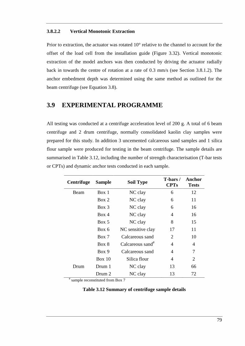
79
3.8.2.2 Vertical Monotonic Extraction
Prior to extraction, the actuator was rotated 10° relative to the channel to account for the
offset of the load cell from the installation guide (Figure 3.32). Vertical monotonic
extraction of the model anchors was then conducted by driving the actuator radially
back in towards the centre of rotation at a rate of 0.3 mm/s (see Section 3.8.1.2). The
anchor embedment depth was determined using the same method as outlined for the
beam centrifuge (see Equation 3.8).
3.9 EXPERIMENTAL PROGRAMME
All testing was conducted at a centrifuge acceleration level of 200 g. A total of 6 beam
centrifuge and 2 drum centrifuge, normally consolidated kaolin clay samples were
prepared for this study. In addition 3 uncemented calcareous sand samples and 1 silica
flour sample were produced for testing in the beam centrifuge. The sample details are
summarised in Table 3.12, including the number of strength characterisation (T-bar tests
or CPTs) and dynamic anchor tests conducted in each sample.
Centrifuge Sample Soil Type T-bars / CPTs
Anchor Tests
Beam Box 1 NC clay 6 12
Box 2 NC clay 6 11
Box 3 NC clay 6 16
Box 4 NC clay 4 16
Box 5 NC clay 8 15
Box 6 NC sensitive clay 17 11
Box 7 Calcareous sand 2 10
Box 8 Calcareous sand# 4 4
Box 9 Calcareous sand 4 7
Box 10 Silica flour 4 2
Drum Drum 1 NC clay 13 66
Drum 2 NC clay 13 72 # sample reconstituted from Box 7
Table 3.12 Summary of centrifuge sample details

81
CHAPTER 4 - ANALYTICAL AND NUMERICAL
METHODS
4.1 INTRODUCTION
The extensive dynamic anchor test database established during the experimental
programme has been complemented by the application of associated analytical and
numerical techniques. This chapter details the methods adopted in the evaluation of
dynamic anchor impact velocities, embedment depths and holding capacities in both
normally consolidated clay and calcareous sand. Accurate prediction of the anchor
embedment depth and holding capacity are of particular importance in the assessment of
the performance of dynamically installed anchors.
4.2 DRAG COEFFICIENT
Any object moving through a fluid will experience drag, i.e. a net force in the direction
of flow due to the pressure and shear forces on the surface of the object (Young et al.
1997). The drag force comprises a pressure drag component due to the pressure
exhibited on the front and back faces of the object and a friction drag component due to
the shear stresses acting along the walls of the object. Generally the effects of pressure
and friction drag are combined and an overall drag coefficient (CD) is defined as:
2p2
1
dD vA
FC
ρ= (4.1)
where Fd is the combined pressure and friction drag resistance force, ρ is the fluid
density, Ap is the projected cross-sectional area of the object and v is the velocity.
Previous studies of seabed penetrometers have identified a range of drag coefficient
values; as follows

82
• True (1976) CD = 0.7, for cylindrical penetrometers with a pointed nose;
• Freeman et al. (1984) CD = 0.15 – 0.18, for European Standard Penetrators
(ESP) at velocities of 10 – 50 m/s;
• Freeman and Hollister (1988) CD = 0.030 + 0.0085 L/D, lower bound to nuclear
waste disposal test data;
• Øye (2000) CD = 0.63, for four fluke DPAs;
• Fernandes et al. (2005) CD = 0.33, for torpedo anchors.
Discrepancies between the drag coefficients determined in these studies are not
unexpected as the drag coefficient is a function of the object shape, surface roughness,
Reynolds number and fluid compressibility.
4.2.1 Factors Influencing the Drag Coefficient
The drag coefficient of an object is dependent on its shape; the blunter the object, the
larger the drag coefficient. Conversely streamlined bodies exhibit smaller drag
coefficients. Figure 4.1 shows the difference in drag coefficient between a blunt
cylinder and a streamlined object, in an axial flow regime. The cylinder has a drag
coefficient which is approximately three times larger than that of the streamlined object
across the complete range of aspect ratios considered. Figure 4.1 also indicates a
decrease in drag coefficient with increasing aspect ratio (L/D), up to approximately L/D
= 2 – 3. Subsequently the drag coefficient becomes relatively constant at higher aspect
ratios, increasing slightly due to increased frictional drag resistance.
Generally, the drag on streamlined projectiles increases with increasing surface
roughness. However, for extremely blunt bodies the drag is independent of the surface
roughness, since the shear stress is not in the upstream flow direction and contributes
nothing to the drag. For blunt bodies like a cylinder or sphere, an increase in surface
roughness can actually lead to a decrease in drag as the increased roughness may cause
the boundary layer to become turbulent, resulting in a considerable drop in pressure
drag and only a slight increase in friction drag (Young et al. 1997).
The Reynolds number (Re) reflects the ratio of inertia to viscous effects and can be
defined as
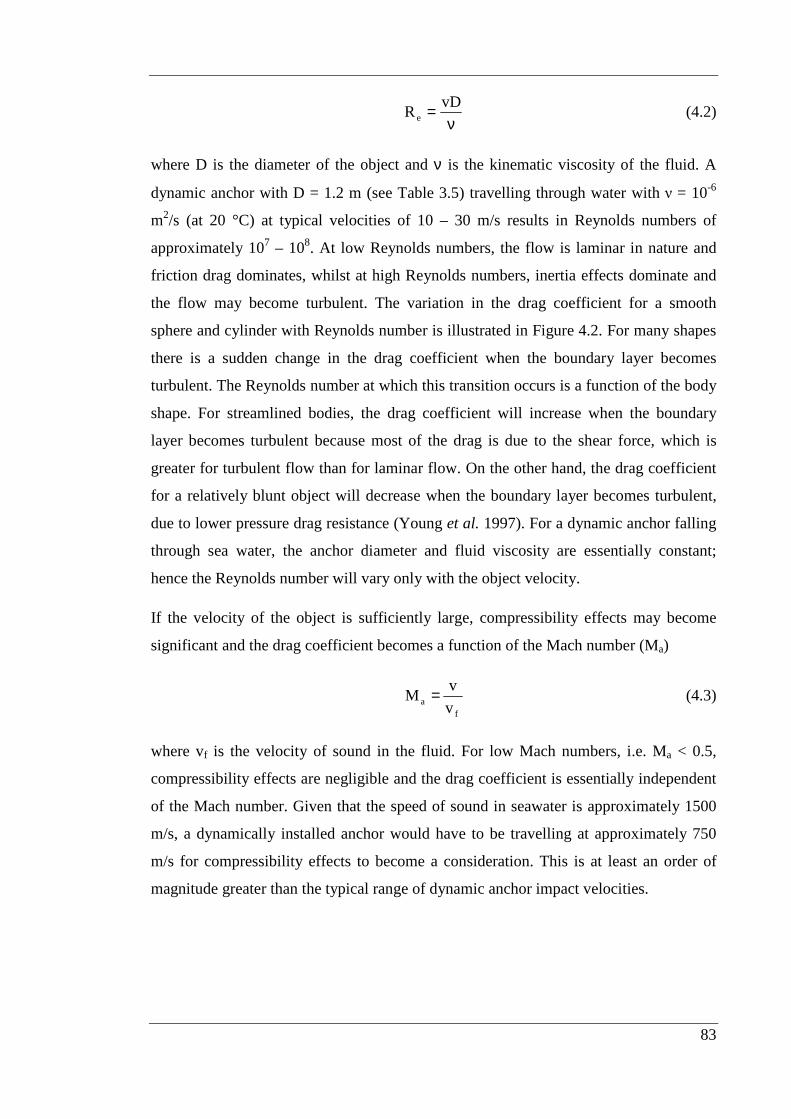
83
ν
= vDRe (4.2)
where D is the diameter of the object and ν is the kinematic viscosity of the fluid. A
dynamic anchor with D = 1.2 m (see Table 3.5) travelling through water with ν = 10-6
m2/s (at 20 °C) at typical velocities of 10 – 30 m/s results in Reynolds numbers of
approximately 107 – 108. At low Reynolds numbers, the flow is laminar in nature and
friction drag dominates, whilst at high Reynolds numbers, inertia effects dominate and
the flow may become turbulent. The variation in the drag coefficient for a smooth
sphere and cylinder with Reynolds number is illustrated in Figure 4.2. For many shapes
there is a sudden change in the drag coefficient when the boundary layer becomes
turbulent. The Reynolds number at which this transition occurs is a function of the body
shape. For streamlined bodies, the drag coefficient will increase when the boundary
layer becomes turbulent because most of the drag is due to the shear force, which is
greater for turbulent flow than for laminar flow. On the other hand, the drag coefficient
for a relatively blunt object will decrease when the boundary layer becomes turbulent,
due to lower pressure drag resistance (Young et al. 1997). For a dynamic anchor falling
through sea water, the anchor diameter and fluid viscosity are essentially constant;
hence the Reynolds number will vary only with the object velocity.
If the velocity of the object is sufficiently large, compressibility effects may become
significant and the drag coefficient becomes a function of the Mach number (Ma)
f
a v
vM = (4.3)
where vf is the velocity of sound in the fluid. For low Mach numbers, i.e. Ma < 0.5,
compressibility effects are negligible and the drag coefficient is essentially independent
of the Mach number. Given that the speed of sound in seawater is approximately 1500
m/s, a dynamically installed anchor would have to be travelling at approximately 750
m/s for compressibility effects to become a consideration. This is at least an order of
magnitude greater than the typical range of dynamic anchor impact velocities.

84
4.2.2 Computational Fluid Dynamics
The drag coefficients for the zero fluke model anchors described in Section 3.6 were
determined using the Computational Fluid Dynamics (CFD) package, FLUENT. The
problem geometry and mesh were first created using GAMBIT and then loaded into the
FLUENT solver for analysis. Using FLUENT’s segregated solver and a laminar viscous
model, the drag coefficient was first calculated for a two dimensional, smooth, axis-
symmetric sphere. This permitted verification of the FLUENT results against the
theoretical solutions shown in Figure 4.2. The fluid was modelled as water with a
density of ρ = 998.2 kg/m3 and a viscosity of µ = 0.001003 kg/m.s. The problem domain
extended five diameters in the upstream direction, 20 diameters downstream and 10
diameters laterally (see Figure 4.3), and was meshed using a quad pave mesh. The
upstream boundary condition was set as a velocity inlet whilst downstream the
boundary was specified as an outflow. The analysis was conducted at a range of flow
velocities to evaluate the variation in drag coefficient with Reynolds number. The drag
coefficient for the smooth sphere obtained from the FLUENT analysis (according to
Equation 4.1) is shown in Figure 4.4 together with the theoretical drag coefficient
values from Figure 4.3. Good agreement is achieved between the calculated and
theoretical drag coefficient for Reynolds number values approaching 105. At this stage,
the flow undergoes a transition from laminar to turbulent flow. It should be noted that it
was not possible to model the transition to turbulence in FLUENT and as such it was
not possible to capture the theoretical change in the drag coefficient during this
transition. However, for typical dynamic anchor velocities of 10 – 30 m/s, the
approximate corresponding Reynolds number values of Re = 107 – 108 indicate that,
according to Figure 4.2, the flow will be fully turbulent and no longer undergoing
transition. Figure 4.2 indicates that the fully turbulent drag coefficient is similar to the
drag coefficient prior to the transition. Hence the FLUENT analysis was deemed to
provide a reliable method for calculating the drag coefficient of the dynamic anchors.
Upon verification of the drag coefficient for the case of the smooth sphere, the problem
geometry was altered to represent the four different zero fluke model anchor shapes, i.e.
ellipsoid nose, conical nose, ogive nose and flat nose (Figure 4.5). Again the problem
was defined in a two dimensional, axis-symmetric manner, with similar mesh
characteristics and domain extents as adopted for the case of the smooth sphere. The

85
model anchor drag coefficients were determined assuming a smooth anchor surface, i.e.
the effects of surface roughness were ignored. Flow velocities of up to 60 m/s were
selected in order to capture the likely range of velocities encountered during the free-fall
of dynamically installed anchors through the water column. The drag coefficients from
the FLUENT analysis for each of the model anchors are shown in Table 4.1, for flow
velocities of 1 – 60 m/s representing Reynolds number values of approximately 1 × 10⁶
to 7 × 10⁷.
CD
Anchor Tip 1 m/s 10 m/s 20 m/s 30 m/s 60 m/s Average
E0 ellipsoid 0.24 0.24 0.24 0.24 0.24 0.24
C0 cone 0.23 0.22 0.22 0.22 0.22 0.22
O0 ogive 0.22 0.22 0.22 0.22 0.22 0.22
F0 flat 0.88 0.88 0.88 0.88 0.88 0.88
Table 4.1 Zero fluke anchor drag coefficients
The calculated drag coefficients for the ellipsoid and flat nosed model anchors compare
favourably with the drag coefficients of the cylinder and streamlined object presented
by Hoerner (1965) in Figure 4.1. At the dynamic anchor aspect ratio of 12.5, Figure 4.1
indicates drag coefficients of approximately 0.25 and 0.83 for the streamlined object
and cylinder respectively, compared with 0.24 and 0.88 from the FLUENT analysis. Not
surprisingly, the blunt shape of the flat nosed anchor results in a significantly higher
drag coefficient when compared with the other three anchor shapes. This difference is
observable in the velocity contours presented in Figures 4.6 – 4.9, where at higher
velocities the flat nosed anchor develops a larger wake zone. The velocity contours also
support the results presented in Table 4.1 which suggest very similar drag coefficients
for the ellipsoid, conical and ogive shaped noses.
Table 4.1 also demonstrates that, for each of the anchors, the drag coefficient is
essentially constant for velocities in the range of 1 – 60 m/s. However, Figure 4.10
shows significantly higher drag coefficients for velocities below 1 m/s. The change in
the drag coefficient at lower velocities is highlighted by the change in the velocity
contours presented in Figures 4.6 – 4.9. At low velocities, the flow is viscous and
essentially no wake forms behind the anchor. As the velocity increases, a wake begins
to develop and with further increases in velocity this wake narrows and the drag
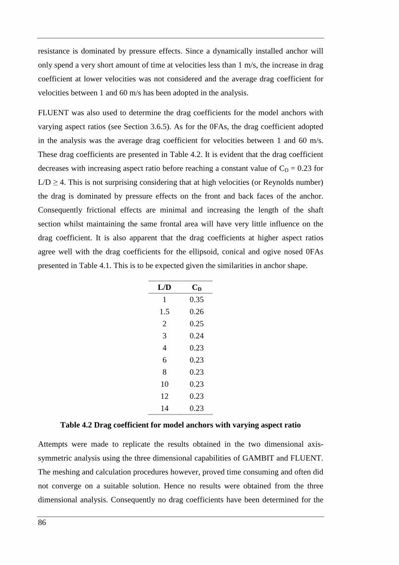
86
resistance is dominated by pressure effects. Since a dynamically installed anchor will
only spend a very short amount of time at velocities less than 1 m/s, the increase in drag
coefficient at lower velocities was not considered and the average drag coefficient for
velocities between 1 and 60 m/s has been adopted in the analysis.
FLUENT was also used to determine the drag coefficients for the model anchors with
varying aspect ratios (see Section 3.6.5). As for the 0FAs, the drag coefficient adopted
in the analysis was the average drag coefficient for velocities between 1 and 60 m/s.
These drag coefficients are presented in Table 4.2. It is evident that the drag coefficient
decreases with increasing aspect ratio before reaching a constant value of CD = 0.23 for
L/D ≥ 4. This is not surprising considering that at high velocities (or Reynolds number)
the drag is dominated by pressure effects on the front and back faces of the anchor.
Consequently frictional effects are minimal and increasing the length of the shaft
section whilst maintaining the same frontal area will have very little influence on the
drag coefficient. It is also apparent that the drag coefficients at higher aspect ratios
agree well with the drag coefficients for the ellipsoid, conical and ogive nosed 0FAs
presented in Table 4.1. This is to be expected given the similarities in anchor shape.
L/D CD
1 0.35
1.5 0.26
2 0.25
3 0.24
4 0.23
6 0.23
8 0.23
10 0.23
12 0.23
14 0.23
Table 4.2 Drag coefficient for model anchors with varying aspect ratio
Attempts were made to replicate the results obtained in the two dimensional axis-
symmetric analysis using the three dimensional capabilities of GAMBIT and FLUENT.
The meshing and calculation procedures however, proved time consuming and often did
not converge on a suitable solution. Hence no results were obtained from the three
dimensional analysis. Consequently no drag coefficients have been determined for the

87
four fluke model anchor and as such a value of CD = 0.63 has been adopted in
subsequent analysis, based on the results of similar CFD studies on DPAs (Øye 2000).
It should also be noted that no attempt was made to model the additional drag resistance
contributed by the anchor chain.
4.2.3 Inertial Drag in Soil
Despite a lack of experimental evidence supporting the existence of inertial drag
resistance in soil, True (1976), Freeman and Burdett (1986), Ove Arup and Partners
(1983), Lisle (2001), Wemmie (2003), Richardson (2003) and O’Loughlin et al.
(2004b) adopt an inertial drag resistance term (Fd) to predict the penetration depth of
objects into the seabed. In each case the inertial drag resistance has been formulated in a
similar manner as the hydrodynamic drag resistance
2pD2
1d vACF ρ= (4.4)
The inclusion of a drag term may be considered appropriate in view of the very soft
viscous clay often encountered at the surface of the seabed (O’Loughlin et al. 2004b).
However, in contrast to the vast amount of information regarding common fluids like
water, very little is known about the inertial forces experienced by objects moving
through soft seabed soil materials. These seafloor materials may exhibit non-Newtonian
behaviour; in fact, clay-water mixtures have been found to behave as Bingham plastics
(Houwink 1952, Pazwash and Robertson 1969, Pazwash 1970, Robertson and Pazwash
1971), defined by a non-zero yield stress and a plastic viscosity. Objects passing
through a Bingham plastic material may experience drag forces that are considerably
higher than those experienced when moving through a Newtonian fluid such as water.
Robertson and Pazwash (1971) define the drag coefficient of an object passing through
a Bingham plastic material as being of the form
2e
N,DDR
HKCC += (4.5)
where CD,N is the drag coefficient of the object in a Newtonian fluid at a Reynolds
number Re, K is an empirically derived coefficient dependent on the object shape and H
is the Hedstrom number defined as
88
2p
2yLH
µρτ
= (4.6)
where ρ is the fluid density, τy is the yield stress of the material, L is the object length
parallel to the flow direction and µp is the plastic viscosity. Consequently separate drag
coefficients may be necessary to account for the drag resistance to dynamic anchor
motion through the water column and through the seabed sediments. True (1976)
acknowledged the notion of separate drag coefficients for projectile motion through
fluid and soil materials by defining an effective drag coefficient (CDe)
fDsDf
DsDe v11
CCCC
+−+= (4.7)
where CDs and CDf are the drag coefficient in the soil and fluid respectively and vf is
given by
δ+
ρ=
pt
sceu
2De2
1f
AS
ANSs
vCv (4.8)
where su is the undrained shear strength, Se is the strain rate factor (see Section 2.2.3.4),
Nc is the bearing capacity factor for the projectile tip, δ is a side adhesion factor, As is
the surface area of the projectile, St is the soil sensitivity and Ap is the projected area of
the projectile.
Since CDe appears on both sides of Equation 4.7, an iterative procedure or algebraic
manipulation is required to derive the effective drag coefficient explicitly. The function
describing CDe provides an approximation for the transition between the geotechnical
and inertial effects. At low velocities, the soil drag coefficient dominates as the inertia
forces are small and the soil deformations follow typical bearing capacity mechanisms.
By contrast, at high velocities, the inertia forces are large and soil deformations tend
towards a pattern of fluid flow. The function assumes values of CDs and CDf for the
extreme cases of static and rapid penetration respectively but is limited in its
applicability in that both geotechnical and inertial effects are combined in a single
expression. True (1976) subsequently adopted an effective drag coefficient of 0.7 for the
analysis of cylindrical penetrometers. Whilst it is possible to model Bingham plastic
89
materials in FLUENT, this analysis has not yet been undertaken. Hence the analysis
presented in later chapters assumes that the drag coefficients for dynamic anchors
moving through soil are equivalent to the drag coefficients of these anchors moving
through water, i.e. CDs = CDf. It is acknowledged that this may create some inaccuracies
in the embedment depth analysis. However inertial drag effects are expected to
comprise only a relatively small proportion of the total resistance to penetration and
therefore this is not likely to have a substantial influence on the calculated embedment
depths.
4.3 IMPACT VELOCITY
The dynamic anchor velocity at impact with the seabed has a substantial influence on
the depth of penetration achieved. As the impact velocity was measured during the
centrifuge tests, accurate prediction of the impact velocity was not necessary. It is
interesting to note, however, the variation in impact velocity due to the non-uniform
acceleration field in the centrifuge and to compare the theoretical impact velocities with
the velocities measured in the experimental programme.
4.3.1 Uniform Acceleration Field
In a uniform acceleration field, the theory of conservation of energy can be used to
estimate the velocity of a dynamic anchor at the point of impact with the seabed. Prior
to release, the anchor possesses potential energy (Ep) based upon its height above the
seabed (hd), given by
dp mghE = (4.9)
where m is the anchor mass and g is the gravitational acceleration. Following release,
this potential energy is converted into kinetic energy (Ek), with
22
1k mvE = (4.10)
where v is the anchor velocity. According to the conservation of energy, assuming there
are no energy losses from the system, at the point of impact, all the potential energy
prior to release will have been converted into kinetic energy. Therefore the idealised

90
dynamic anchor impact velocity (vi) can be found by equating the potential energy to
the kinetic energy and rearranging to give:
di gh2v = (4.11)
The variation in impact velocity with drop height for a uniform acceleration field is
shown in Figure 4.11a.
4.3.2 Centrifuge Acceleration Field
In the centrifuge, the acceleration field is not uniform (see Section 3.2). During free-fall,
the model anchor experiences a gravitational acceleration (a) which increases with
radius (r) from the rotational axis of the centrifuge, expressed as:
ra 2ω= (4.12)
where ω is the rotational velocity of the centrifuge. Therefore, an incremental approach
is adopted whereby the acceleration is assumed constant over small radius intervals
(∆r). A linear equation of motion can then be used to determine the anchor velocity at
the end of each increment (ve)
ra2vv 2be ∆+= (4.13)
where vb is the velocity at the beginning of the increment. This incremental approach is
continued until the anchor reaches the sample surface, thereby providing an idealised
impact velocity.
Given the different radii of the beam and drum centrifuges, the relationship between the
drop height and idealised impact velocity will be different for each centrifuge. The
variation in impact velocity with drop height for the beam and drum centrifuges is
shown in Figure 4.11a. It should be noted that these theoretical impact velocities have
been obtained at an acceleration level of 200 g with an average sample height of 230
mm in the beam centrifuge and 165 mm in the drum centrifuge. Similarly effective radii
of 1607 mm and 530 mm were adopted for the beam and drum centrifuge calculations
respectively.
91
In Figure 4.11a the prototype drop heights are a factor of 200 times (i.e. gravitational
acceleration level, n) larger than the model drop heights, as given by the centrifuge
scaling laws in Section 3.2. However, due to the non-uniform acceleration field in the
centrifuge, an anchor installed from a prototype drop height of hd,p will achieve a higher
impact velocity than an anchor installed in the centrifuge from a drop height of hd,m =
hd,p/n. Hence the impact velocity analysis in the following chapters has been presented
in terms of equivalent prototype drop heights. These represent the drop height, at
prototype scale (i.e. uniform acceleration field), required for a dynamic anchor to
achieve the same impact velocity as a model anchor installed from a given drop height
in the centrifuge. Due to the different centrifuge radii the equivalent prototype drop
heights in the beam and drum centrifuges will be different (see Figure 4.11b).
4.3.3 Energy Losses
The above calculations are based on the assumption that no energy losses occur during
free-fall, i.e. all of the potential energy prior to release is converted into kinetic energy.
Hence they represent idealised impact velocities. Any external force acting on the
anchor during free-fall will cause an energy loss. During installation at prototype scale
the major external force acting on the anchor will be hydrodynamic drag. The energy
dissipated by this drag force will result in lower impact velocities than predicted by
Equation 4.11. In the centrifuge, only a nominal water layer exists on top of the soil
sample and as such the effects of hydrodynamic drag are expected to be minimal.
Instead, the anchor will experience a small amount of aerodynamic drag and frictional
resistance between the anchor and the installation guide (Section 3.7.1). Therefore
energy will also be dissipated during the free-fall stage of installation in the centrifuge
resulting in lower impact velocities than those predicted using the method outlined in
Section 4.3.2.
4.4 EMBEDMENT DEPTH
The holding capacity of dynamically installed anchors, in soil in which the shear
strength increases with depth, is directly dependent on the depth of penetration achieved
during installation. Hence in order to be able to accurately predict the anchor holding
92
capacity it is first necessary to be able to predict the expected embedment depth. From
studies investigating the penetration of objects into earth media (Young 1969, True
1976) it is apparent that the major factors influencing the embedment depth of an object
are the:
• shape (tip shape, aspect ratio, etc.)
• mass (density)
• impact velocity
• strength characteristics of the soil.
In Section 2.2.3, several methods were outlined for predicting the penetration depth of
objects into the seabed. In this study a modified version of True’s method (see Section
2.2.3.4) has been adopted for calculating the penetration depth of model dynamic
anchors in the centrifuge.
4.4.1 Calculation Procedure
True’s method is based on Newton’s second law of motion through consideration of the
forces acting on the anchor during penetration. The differential equation governing the
motion of the anchor through the soil is given by:
( ) dsbfs2
2
FFFRWdt
zdm −+−= (4.14)
where m is the anchor mass, z is the penetration depth below the seabed, t is the time
after impact with the seabed, Ws is the submerged weight of the anchor in soil, Rf is the
rate function, Fb is the end bearing resistance, Fs is the frictional resistance and Fd is the
inertial drag resistance.
It should be noted that the anchor embedment depth has been calculated assuming the
anchor remains vertical during installation. In addition, the cavity created by the passage
of the anchor through the soil is assumed to remain largely open following installation.
Poorooshasb and James (1989) used radiographs to show that cylindrical projectiles
consistently left open pathways when installed dynamically in kaolin clay in the
centrifuge, despite closed entrance craters. The radiographs showed that in some cases
the pathway extended continuously from the rear of the anchor to the sample surface,
whilst in other cases the pathway consisted of interconnected or discrete voids. Based

93
on these observations it has been assumed that during dynamic anchor installation in the
centrifuge, partial hole closure exists (see Figure 4.12b) despite a closed entrance crater.
Hence no reverse end bearing term is included in Equation 4.14 with the additional
resistance created by any hole closure accounted for by the inertial drag resistance term.
Figure 4.13 shows the forces acting on the anchor during penetration. The end bearing
resistance has been formulated as:
ptip,ucb AsNF = (4.15)
where Nc is the tip bearing capacity factor, su,tip is the undrained shear strength at the
anchor tip and Ap is the projected cross-sectional area of the anchor tip. In addition the
frictional resistance has been expressed as:
save,us AsF α= (4.16)
where α is the shaft adhesion factor, su,ave is the undrained shear strength averaged over
the embedded shaft length and As is the surface area of the embedded anchor shaft.
When considering the embedment depth of anchors with flukes, additional bearing and
frictional resistance terms should be included to account for their contribution to the
total penetration resistance (Figure 4.14). It is expected that full closure will occur
behind the anchor flukes due to their relatively small thickness and the apparent plane
strain conditions encountered. Hence a reverse end bearing term should be included to
account for the resistance generated by the topside of the anchor flukes (Frf), given by:
pftf,ucfrf AsNF = (4.17)
where Ncf is the bearing capacity factor of the flukes, su,tf is the undrained shear strength
at the top of the anchor flukes and Apf is the total projected area of the flukes. The
bearing resistance generated by the underside of the anchor flukes (Fbf) can be
expressed as:
pfbf,ucfbf AsNF = (4.18)
where su,bf is the undrained shear strength at the bottom of the flukes. The contribution
of the anchor flukes to the frictional resistance (Fsf) is given by:

94
sfsf,usf AsF α= (4.19)
where su,sf is the average shear strength over the embedded fluke length and Asf is the
embedded fluke surface area.
The inertial drag resistance of the soil to the penetration of dynamically installed
anchors has been formulated using Equation 4.4.
The strain rate dependence of the soil shear strength has been accounted for by adopting
either the semi-logarithmic rate function (see Section 2.2.3.1) given by:
γγλ+=ref
f log1R&
& (4.20)
or the power rate function (see Section 2.2.3.1) expressed as:
β
γγ=ref
fR&
& (4.21)
where λ and β are the strain rate parameters for the respective formulations, γ& is the
strain rate and refγ& is the strain rate at which the reference (‘static’) undrained shear
strength was determined. The strain rate is assumed to be proportional to v/D, where v
is the penetration velocity and D the diameter. Hence the reference strain rate from the
T-bar penetrometer tests (v = 1 mm/s and D = 5 mm, see Section 3.5.1) is refγ& = 0.2 s-1.
A finite difference approach was adopted to solve Equation 4.14, thereby producing a
velocity profile with penetration depth. The incremental acceleration (ai) can be
calculated as:
( )
m
FFFRWa disibifs
i
−+−= (4.22)
where Fbi, Fsi and Fdi are the incremental values of the bearing, frictional and inertial
resistance forces. From this, the incremental penetration depth can be determined using
a central difference solution:
1iii2
1i zz2atz −+ −+∆= (4.23)
95
where ∆t is the specified time increment. Calculation of the penetration depth at the end
of the first increment (z1) using Equation 4.23 requires an estimate of the depth one time
increment prior to impact (z-1). This depth has been calculated assuming a constant
velocity, i.e. z-1 = -∆t v0. Subsequently, the velocity at the end of the first increment can
be determined as:
( )
t
zzv i1i
1i ∆−= +
+ (4.24)
Further time increments are taken until the velocity becomes negative, at which point
the final embedment depth (z) can be calculated by interpolating between the final two
embedment depth values:
( )
−−−=
++
1ii
i1iii vv
vzzzz (4.25)
A flow chart outlining the calculation procedure is presented in Figure 4.15.
4.4.2 Parameter Values
Accurate prediction of the embedment depth of dynamic anchors relies heavily upon the
determination of several parameters, namely, the bearing capacity factor, the shaft
adhesion factor and the strain rate parameter. The selection of values for these
parameters is discussed below.
It has been shown that for a circular foundation deeply embedded within saturated clay,
Nc = 9 (Skempton 1951 as cited in Skempton 1959). Consequently Richardson (2003)
adopted a value of Nc = 9 in determining the tip bearing resistance to dynamic anchor
penetration. However, as illustrated in Figure 4.16, the bearing capacity factor increases
with depth, up to embedments of four diameters, at which point the free surface no
longer influences the bearing mechanism. The increase in bearing capacity factor with
depth, for both circular and strip foundations has been formulated as (Skempton 1951 as
cited in Whitlow 2001):
+
+=D
z053.01
L
D2.0114.5Nc (4.26)
96
where D is the foundation diameter or width, L is the foundation length and z is the
embedment. Maximum values of the bearing capacity factor occur when z/D ≥ 4, with:
• Nc = 9 for circular or square footings (D/L = 1)
• Nc = 7.5 for strip footings (D/L = 0)
Since dynamically installed anchors typically embed up to 2 – 3 times the anchor length
(O’Loughlin et al. 2004b), the variation in bearing capacity factor over the first few
diameters of embedment is not expected to have a significant influence on the
calculated embedment depth, particularly as the surface soils are typically very weak.
Generally, the nose of a dynamically installed anchor is not simply circular but rather
elongated or pointed. Therefore bearing capacity factors derived from cone penetration
tests may be more appropriate for determining the anchor’s bearing resistance. Bearing
capacity factors derived both experimentally and theoretically for cone penetration tests,
however, cover a wide range of values, typically approximately 8 – 20 (Lunne et al.
1997). Based on appropriate bearing capacity factors for cone penetration tests,
O’Loughlin et al. (2004b) adopted an average bearing capacity factor of Nc = 12 for
calculating the penetration depth of dynamically installed anchors. In addition, the
bearing area of the anchor flukes is analogous to a strip footing. For a deeply embedded
strip footing, Nc = 7.5 (Skempton 1951 as cited in Whitlow 2001). Therefore bearing
capacity factors of Nc = 12 and Ncf = 7.5 have been adopted in the analysis for the
anchor nose and flukes respectively. For the hemispherically nosed anchors with
varying aspect ratios, it seems appropriate to adopt the bearing capacity factor for a ball
penetrometer. Chung (2005) reports bearing capacity factors for ball penetrometers
ranging from approximately 7 – 13. Consequently an average bearing capacity factor of
Nc = 10 has been adopted in the analysis for the model anchors with hemispherical
noses.
Typically, during installation, the frictional resistance generated along the wall of the
foundation is close to the remoulded shear strength of the clay. The ratio of the
frictional resistance to the undisturbed shear strength is defined as the adhesion factor
(α) and is often expressed as:
u
r,u
t s
s
S
1 =≅α (4.27)
97
where St is the soil sensitivity, su,r is the remoulded shear strength and su is the
undisturbed shear strength. In accounting for the frictional resistance during penetration
of cylindrical projectiles, True (1976) included a parameter to account for separation
between the anchor and the soil during dynamic penetration of the soil. However, there
is no experimental evidence justifying the existence of separation between projectiles
and the soil during installation. Consequently, it has been assumed in the analysis
adopted in this study that no separation occurs during penetration. Chen and Randolph
(2007) report installation friction ratios of α = 0.38 for suction caissons in kaolin clay.
This agrees well with typical sensitivities for kaolin clay of St = 2 – 2.5. Similarly,
adopting a tip bearing capacity factor of Nc = 12, a best fit value of α = 0.4 was reported
for dynamic anchor constant rate of penetration tests in the centrifuge (O’Loughlin et al.
2004b). Hence unless otherwise specified a shaft adhesion factor of α = 0.4 has been
adopted in the embedment depth analysis. In all calculations, the fluke adhesion factor
has been assumed to be equal to the shaft adhesion factor, i.e. αshaft = αfluke = 0.4.
The greatest uncertainty in the calculation of dynamic anchor embedment depths is the
determination of the strain rate parameter. Typically, the strain rate parameter has been
back-calculated from measured experimental data (Lisle 2001, Wemmie 2003,
Richardson 2003, O’Loughlin et al. 2004b). O’Loughlin et al. (2004b) reported strain
rate parameter values of 19 – 33 % (i.e. λ = 0.19 – 0.33) for dynamic anchor tests
conducted in the centrifuge in kaolin cay. Due to the degree of uncertainty surrounding
the strain rate effects in fine grained soils, particularly at the very high strain rates
encountered during dynamic anchor installation, the strain rate parameter values in this
study have again been back-calculated from the results of the experimental programme.
Further details are provided in Chapter 7.
4.5 HOLDING CAPACITY
In Section 2.3 two simplified analytical methods for determining the capacity of piles
were outlined. The relative infancy of the dynamic anchor concept has ensured that very
little capacity data exists for the validation of either method in relation to the dynamic
anchor capacity. This combined with the uncertainty surrounding the influence of the
dynamic anchor installation process on the anchor capacity and the added complexities
98
of the anchor geometry relative to standard piles suggest the use of a simple capacity
calculation technique. The API method is the simpler of the two methods, expressing
the bearing resistance in terms of standard bearing capacity factors and the shaft friction
as a proportion of the undrained shear strength. By contrast, the MTD method requires
the use of more sophisticated soil properties, thereby adding to the complexity of the
calculation. Hence the API method has been used to evaluate the vertical, monotonic
holding capacity of the model dynamic anchors.
4.5.1 Calculation Procedure
Based on the API method (see Section 2.3.1, API 2000), the capacity of a zero fluke
dynamic anchor under tension loading (Fv) can be expressed as:
srbsv FFFWF +++= (4.28)
where Fb is the bearing resistance at the anchor padeye, Fr is the reverse end bearing
resistance at the anchor tip and Fs is the frictional resistance (see Figure 4.17).
It should be noted that, as for the embedment depth analysis, calculation of the anchor
capacity assumes anchor verticality and partial closure of the cavity created by the
passage of the anchor through the soil. Consequently the bearing resistance at the
anchor padeye has been calculated with a factored bearing capacity factor to reflect the
degree of hole closure. The bearing resistance at the anchor padeye is defined as:
ppad,ucb AsfNF = (4.29)
where f is the degree of hole closure (i.e. f = 0 for fully open cavity and f = 1 for fully
closed cavity), su,pad is the undrained shear strength at the anchor padeye and Ap is the
projected area of the anchor. A nominal value of f = 0.1 has been adopted, reflecting 10
% hole closure. The value of f is not expected to have a significant influence on the
anchor capacity as the relatively small anchor padeye embedments result in the
mobilisation of low shear strengths and hence small padeye bearing resistances.
The reverse end bearing at the anchor tip is expressed as:
ptip,ucr AsNF = (4.30)

99
where su,tip is the undrained shear strength at the anchor tip. In addition the frictional
resistance is given by:
save,us AsF α= (4.31)
As for the embedment depth analysis in Section 4.4, for anchors with flukes, the
additional bearing and frictional resistances to vertical uplift loading need to be
considered (see Figure 4.18). The bearing resistance generated on the upper portion of
the anchor flukes can be expressed as:
pftf,ucfbf AsNF = (4.32)
where su,tf is the undrained shear strength at the top of the anchor flukes. Likewise the
reverse end bearing at the bottom of the anchor flukes is given by:
pfbf,ucfrf AsNF = (4.33)
where su,bf is the undrained shear strength at the bottom of the anchor flukes. Finally the
frictional contribution of the anchor flukes to the holding capacity of the anchor is
defined as:
sfsf,usf AsF α= (4.34)
where su,sf is the average undrained shear strength over the embedded length of the
flukes.
4.5.2 Parameter Values
The bearing capacity factor adopted for the anchor tip in the embedment analysis, Nc =
12, was derived from the results of cone penetration tests (see Section 4.4.2). Hence it
seems appropriate that the same bearing capacity factor be adopted in the holding
capacity analysis. However, Watson et al. (2000) and Chung (2005) present cone
extraction profiles which demonstrate a much more gradual development of the tip
extraction resistance compared with the tip resistance during penetration. This tends to
suggest a reduction in the mobilisation rates of the tip bearing resistance between cone
penetration and extraction. These findings support the observations of Lehane (1992)
who through a series of pile load tests showed a much softer pile response under tension

100
rather than compression. Therefore due to the similarities between dynamic anchors and
cone penetrometers it could be expected that the full bearing resistance at the anchor tip
may not be mobilised until the anchor has undergone significant vertical displacement.
This would likely manifest itself in non-simultaneous mobilisation of the anchor bearing
and frictional resistance, as discussed by Jeanjean et al. (2006) for suction caissons.
Since the API method is based on the simultaneous mobilisation of full bearing and
frictional resistance, the calculation procedure may result in a slight over prediction of
the anchor capacity. Hence it may be appropriate to use a reduced bearing capacity
factor to account for this difference in mobilisation rates. However, since the reverse
end bearing resistance typically comprises only 15 – 20 % of the total anchor uplift
resistance, a reduction in the tip bearing capacity factor from Nc = 12 to 9 will have a
relatively minor influence on the anchor capacity. Consequently, the calculation
procedure has been simplified by adopting a bearing capacity factor of Nc = 12.
Similarly, the fluke bearing capacity factor (Ncf = 7.5) and the bearing capacity factor
for the hemispherically shaped tip (Nc = 10) adopted in the holding capacity analysis
have been assumed to be the same as those adopted in the embedment analysis (see
Section 4.4.2).
Unlike the elongated tip, the dynamic anchor padeye is flat and circular, suggesting the
use of a bearing capacity factor for a deep circular foundation, Nc = 9 (Skempton 1951
as cited in Skempton 1959). However as discussed in Section 4.4.2 the bearing capacity
factor for circular foundations varies with depth, up to four times the anchor diameter.
With typical dynamic anchor tip embedments ranging from 2 – 3 times the anchor
length (O’Loughlin et al. 2004b) and corresponding padeye embedments of 1 – 2 times
the anchor length or 12.5 – 25 times the anchor diameter, it is unlikely that the soil
surface will influence the bearing mechanism at the anchor padeye until well after
realisation of the ultimate anchor capacity. Hence a bearing capacity factor of Nc = 9
has been adopted for the anchor padeye in the holding capacity analysis. Since the
anchors fitted with hemispherical tips also feature hemispherical padeye sections, the
same bearing capacity factor has been adopted for the padeye as the anchor tip, i.e. Nc =
10.
American Petroleum Institute guidelines (API 2000) define the shaft adhesion factor
during loading as:

101
For 1s
v
u ≤σ′
1s
5.05.0
v
u ≤
σ′=α
−
(4.35)
For 1s
v
u >σ′
1s
5.025.0
v
u ≤
σ′=α
−
(4.36)
where σv′ is the vertical effective stress.
4.5.3 Normalised Capacity
Anchor capacities measured during testing in the centrifuge were adjusted to account for
the submerged weight of the anchor (Ws) and then normalised by the average undrained
shear strength over the embedded anchor length (su,ave) and the anchor’s projected area
(Ap):
pave,u
svN As
WFF
−= (4.37)
where FN is the normalised anchor capacity. Normalisation in this manner allows direct
comparison of capacities, taking into account differences in anchor and soil properties
and the anchor’s embedment depth.
4.5.4 Anchor Efficiency
The anchor capacities measured in the experimental programme have also been
compared in terms of the anchor efficiency. The anchor efficiency (Ef) represents the
ratio of the holding capacity (FV) to the anchor’s dry weight (W):
W
FE v
f = (4.38)
4.6 CALCAREOUS SAND
Calcareous sands are defined as sands comprising calcium carbonate and they originate
from biological processes such as sedimentation of skeletal debris, coral reef formation
or chemical precipitation (Murff 1987). Unexpected difficulties have been encountered

102
with offshore foundations situated on high carbonate content soils (i.e. > 50 %). The
engineering properties of these materials are quite different to those of silica sands and
clays due to the presence of varying amounts of cementation and the high angularity of
the particles which results in high in situ void ratios. The high void ratios result in low
densities and low ratios of horizontal to vertical stress as well as high compressibility.
The highly variable nature of calcareous soils has led to uncertainty in pile capacity
predictions (Murff 1987, Randolph 1988). Despite this, conventional pile capacity
theory has been applied to predict the embedment depth and holding capacity of
dynamic anchors in reconstituted calcareous sediments.
4.6.1 Embedment Depth
4.6.1.1 Calculation Procedure
The embedment depth of dynamically installed anchors in calcareous sand has been
calculated using a similar method to that adopted for determining anchor embedment in
clay (see Section 4.4). The differential equation linking the forces acting on the anchor
to the acceleration is given by:
( ) dsbfs2
2
FFFRWdt
zdm −+−= (4.39)
Equation 4.39 is identical to Equation 4.14 for anchor embedment in clay; however the
differences in soil properties ensure that the bearing and frictional resistance terms are
calculated differently. In silica sands, the end bearing capacity is generally expressed in
terms of a bearing capacity factor (Nq) and the in situ overburden pressure (0vσ′ ). A
similar approach has been adopted for calcareous sand, with the bearing resistance
given by
p0vqb ANF σ′= (4.40)
The shaft friction resistance has also been linked to the overburden pressure and is given
by
save,0vCALCs AF σ′β= (4.41)

103
where βCALC represents the ratio of shaft friction to the effective overburden stress and
ave,0vσ′ is the average effective stress over the embedded shaft length.
The inertial drag resistance of the soil to the penetration of dynamically installed
anchors has been formulated using Equation 4.4.
Since no tests were conducted in calcareous sand using the four fluke model anchors, it
was not necessary to consider the additional resistance contributed by the flukes during
penetration.
The rate dependence of the strength of the calcareous sand has been formulated using
either Equation 4.20 or 4.21.
Once the forces resisting penetration were determined, the same time stepping approach
adopted for the normally consolidated clay was used to calculate the incremental
acceleration, given by
( )
m
FFFRWa disibifs
i
−+−= (4.42)
The incremental displacement and velocity were then calculated using Equations 4.23
and 4.24, with the time stepping approach continuing until a negative velocity was
obtained, in which case the final embedment was found by interpolating between the
last two embedment values using Equation 4.25.
4.6.1.2 Parameter Values
The determination of the values of Nq and βCALC is notoriously difficult in calcareous
sands. Experimental evidence shows that the value of Nq decreases significantly as the
stress level rises, due to decreasing peak friction angles with increasing stress and the
increased compressibility of the soil (Randolph 1988). At a given stress level the high
friction angles and high compressibility of calcareous sediments result in substantially
lower bearing capacities compared with silica sand (Randolph 1988). Poulos and Chua
(1985) reported bearing capacity values for calcareous sand that were approximately 40
% of the corresponding bearing capacities in silica sand (see Figure 4.19).
Consequently, an average value of Nq = 32 derived from CPTs conducted during the
experimental programme has been used in the embedment depth analysis.
104
It is known that as piles are driven deeper into silica sands, the ratio, βCALC, decreases
rapidly with distance from the pile tip due to a reduction in the friction angle at
increasing stress levels and the lower lateral effective stresses generated around the pile
due to the increasing compressibility of the soil (Randolph 1988). The compressibility
of calcareous soils is generally an order of magnitude greater than for silica sands at the
same stress level. Nauroy and Le Tirant (1983) showed that for model tests the net
change in lateral stress due to pile installation becomes negative in calcareous sands.
This reduction may be attributed to crushing and compaction of the sand due to
shearing, both ahead of the advancing pile tip, and also along the shaft of the pile as it
continues to penetrate the soil. The degree of cementation may also affect the skin
friction; however the cementation will be broken down locally as the pile tip advances
during installation. Abbs et al. (1988) presented a summary of βCALC values obtained
from field tests plotted against the length of the test section in calcareous sand (see
Figure 4.20). Note that to avoid confusion with the strain rate parameter for the power
rate law (see Section 2.2.3.1), βCALC has been used in place of β. For short piles (L ≤ 20
m), βCALC values of up to 0.4 are evident, whilst for longer piles Figure 4.20 shows that
values of up to approximately 0.05 are likely. In the dynamic anchor tests, the value of
βCALC has been determined from static penetration tests, with a bearing capacity factor
of Nq = 32, giving an average value of βCALC = 0.42. Considering the relatively short
dynamic anchor length (L = 15 m), this is relatively consistent with the βCALC values for
short piles reported by Abbs et al. (1988).
The strain rate parameter was back-calculated from the experimental data and is
discussed further in Section 7.4.2.1.
4.6.2 Holding Capacity
4.6.2.1 Calculation Procedure
The ultimate vertical holding capacity (Fv) of dynamically installed anchors was
determined as the sum of the submerged weight in soil (Ws) and the end bearing (Fb)
and shaft friction resistances (Fs):
sbsv FFWF ++= (4.43)
105
It should be noted that as the vertical anchor extraction in calcareous sand was
conducted under drained conditions, no reverse end bearing term at the anchor tip is
included in the capacity analysis. The bearing resistance at the anchor padeye is
expressed as:
ppad,0vqb AfNF σ′= (4.44)
where Nq is the bearing capacity factor of the anchor padeye and pad,0vσ′ is the vertical
effective stress at the anchor padeye. Note that full closure of the anchor’s entry
pathway has been assumed in calcareous sand, i.e. f = 1. The frictional resistance to
anchor pullout is then determined as:
save,0vCALCs AF σ′β= (4.45)
4.6.2.2 Parameter Values
The measured embedments during dynamic anchor tests in calcareous sand are
considerably lower than the corresponding embedments in clay (see Section 6.3.3).
Consequently, the anchor padeye is often close to the soil surface following installation
in calcareous sand. As such the bearing resistance of the anchor padeye is analogous to
the bearing resistance of a shallow embedded circular plate anchor (see Figure 4.21).
Rowe and Davis (1982) present bearing capacity factors for vertically loaded plate
anchors in sand, for embedment depths normalised by the anchor diameter (see Figure
4.22). At the friction angle of φ = 40° for the calcareous sand used in the test
programme (Table 3.3) it is therefore possible to use Figure 4.22 to determine a bearing
capacity factor for the anchor padeye during vertical loading. Rowe and Davis (1982)
consider bearing capacity factors of up to 7 for normalised embedments of 8 or less. No
similar studies are available for plate anchors in calcareous sands and as such the Rowe
and Davis (1982) results for silica sand have been used as a basis for the assessment of
the bearing capacity at the anchor padeye in calcareous sand.
The values of βCALC used in the holding capacity analysis have been back-calculated
from the holding capacities measured in the experimental program, assuming bearing
capacity factors as determined above.


107
CHAPTER 5 - EXPERIMENTAL RESULTS FOR
DYNAMIC ANCHOR TESTING IN NORMALLY
CONSOLIDATED CLAY
5.1 INTRODUCTION
The key objective of the research programme was to establish a database of dynamic
anchor performance from centrifuge model tests, to investigate the relationship between
anchor impact velocity, embedment depth and holding capacity. Since dynamic anchors
have been proposed as an alternative deepwater anchoring solution, and deepwater
environments are typically characterised by soft clay deposits, this chapter presents the
results of the dynamic anchor centrifuge tests conducted in normally consolidated clay.
These tests accounted for over 90 % of the total dynamic anchor tests conducted in the
experimental programme and investigated the influence of anchor density, anchor
geometry, consolidation time, monotonic loading, sustained loading and cyclic loading
on the performance of dynamically installed anchors in clay. Tests were conducted in
both the beam and drum centrifuges. The beam centrifuge provided greater sample
depths, allowing heavier anchors and / or larger drop heights to be investigated. The
drum centrifuge on the other hand provided a sample plan area almost four times larger
than that in the beam centrifuge, allowing significantly more tests to be conducted in a
single sample, with the added benefit of in-flight changeover between tests thereby
avoiding the need for reconsolidation time. The results of the tests conducted in both the
beam and drum centrifuges have been considered separately and the test results have
been compared with the results of dynamic anchor field trials and previous laboratory
and centrifuge model tests.
When referring to individual tests the first letter of the test identifier indicates whether
the test was conducted in the beam (B) or drum (D) centrifuge, with the following
number referring to the sample number in that particular centrifuge. The subsequent
letter(s) specify the type of test.
108
• D – dynamic anchor drop test, vertical monotonic extraction
• SUS – dynamic anchor drop test, vertical sustained loading
• CYC – dynamic anchor drop test, vertical one-way cyclic loading
The final number represents the number of that particular type of test in the sample. For
example ‘B5SUS3’ identifies the third sustained loading test conducted in beam
centrifuge sample number 5, whilst ‘D2D9’ represents the ninth vertical monotonic
extraction test in drum centrifuge sample number 2. The dynamic anchor installation
process is summarised in Sections 3.8.1.1 and 3.8.2.1 for the beam and drum centrifuges
respectively, whilst the vertical monotonic extraction procedure is detailed in Section
3.8.1.2 for the beam centrifuge and 3.8.2.2 for the drum centrifuge. Long-term sustained
loading and cyclic loading are described in Sections 3.8.1.3 and 3.8.1.4 respectively.
5.2 BEAM CENTRIFUGE
The experimental programme in the beam centrifuge comprised a number of tests aimed
at establishing the general relationships between impact velocity, embedment depth and
holding capacity as well as investigating the influence of the anchor tip geometry on
these relationships and evaluating the performance of dynamic anchors under cyclic and
sustained loading. The tests assessing the general performance of dynamic anchors were
conducted with ellipsoid nosed zero fluke model anchors (i.e. anchors E0-1, E0-2, IE0-1
and IE0-2), which have been detailed previously in Sections 3.6.1 and 3.6.4. Similarly,
the influence of the anchor tip shape was investigated using zero fluke model anchors
with ellipsoid, conical, ogive and flat noses (i.e. anchors E0-1, C0-1, O0-1 and F0-1; see
Sections 3.6.1 and 3.6.3). Finally, the cyclic and sustained loading tests were conducted
with a single ellipsoid nosed zero fluke model anchor (E0-2; see Section 3.6.1).
5.2.1 Strength Characterisation Tests
Profiles of undrained shear strength with depth were obtained for the beam centrifuge
samples using the T-bar penetrometer described in Section 3.5.1, with the undrained
shear strength expressed as:

109
barT
u N
qs
−
= (5.1)
where q is the average bearing pressure and NT-bar is a T-bar factor. The analytical value
of NT-bar depends on the roughness of the T-bar. Plasticity solutions give a value of
approximately 12 for a rough bar, and a value of 9 for a smooth bar. Stewart and
Randolph (1991) recommended a T-bar factor of 10.5, representing an average of the
rough and smooth cases. Consequently, the shear strengths have been calculated using
NT-bar = 10.5.
Figure 5.1 shows the undrained shear strength profile with depth for a typical T-bar
penetrometer test conducted in normally consolidated clay. The test indicates an
approximately linear increase in shear strength with depth, such that:
kzsu = (5.2)
where k is the shear strength gradient and z is the penetration depth. However,
centrifuge shear strength data tend to deviate slightly from a linear profile at greater
depths, due to the increase in radial acceleration with increasing radius and slight
underconsolidation of the body of the soil sample. Therefore the undrained shear
strength profile is often better described using a polynomial expression of the form:
bzazs 2u += (5.3)
where ‘a’ and ‘b’ are coefficients. Both linear and polynomial idealised shear strength
profiles are shown in Figure 5.1 and it is apparent that the polynomial formulation in
Equation 5.3 provides better agreement with the experimental data, particularly at
depths greater than 100 mm (20 m at prototype scale). Table 5.1 presents the
polynomial coefficient values for the average undrained shear strength profiles in each
of the beam centrifuge samples. The polynomial functions provided improved accuracy
in the calculation of undrained shear strengths at particular anchor embedment depths.
Also included in Table 5.1 are the gradients for the best fit linear profile over the first 20
m of penetration for each sample.
T-bar tests were conducted prior to and at the conclusion of dynamic anchor testing in
each sample. The average undrained shear strength profiles are shown in Figures 5.2 –
5.7. The measured profiles are typical for normally consolidated reconstituted kaolin,

110
with approximate shear strength gradients of between 1 and 1.2 kPa/m and indicating a
slight increase in strength during the course of testing. Box 2 however, demonstrated a
lower shear strength gradient of approximately 0.8 kPa/m, possibly due to incomplete
consolidation of the sample. In addition, Box 6 demonstrated a higher shear strength
gradient of approximately 1.4 kPa/m, which can be attributed to the modified sample
preparation procedure adopted (see Section 3.4.2.1). Consequently the average shear
strength coefficients calculated at the bottom of Table 5.1 exclude the values
determined for Boxes 2 and 6. Figure 5.8 provides a comparison of the average
undrained shear strength profiles in each sample. It can be seen that apart from Boxes 2
and 6, the measured shear strengths are relatively consistent.
Sample a b k
(kPa/m2) (kPa/m) (kPa/m)
Box 1 0.012 0.973 1.17
Box 2 0.016 0.592 0.83
Box 3 0.018 0.797 1.09
Box 4 0.007 0.888 1.00
Box 5 0.013 0.822 1.03
Box 6 0.007 1.296 1.45
Average 0.013 0.870 1.07
Table 5.1 Polynomial and linear undrained shear strength coefficients
The shear strength profiles described by the coefficients presented in Table 5.1
represent the average shear strength profile for each sample. However the increase in
shear strength during the course of testing warrants the adoption of separate shear
strength profiles for each dynamic anchor test. Table 5.10 (see the Tables section)
provides values of the polynomial shear strength coefficients for individual dynamic
anchor tests derived from interpolation between T-bar tests conducted before and after
each test. These interpolated shear strength profiles have been used in the subsequent
analysis.
The undrained shear strength ratio, 0vu /s σ′ , was determined with the in situ vertical
effective stress calculated as:
zn0v γ ′=σ′ (5.4)
111
where n is the gravitational acceleration level, γ′ = 6.5 kN/m3 is the effective soil unit
weight (see Table 3.2) and z is the depth (at model scale). The average undrained shear
strength ratios in the beam centrifuge samples are presented in Table 5.2. The overall
average undrained shear strength ratio (excluding Boxes 2 and 6) compares favourably
with the value of 0.18 reported by Stewart (1992) for normally consolidated kaolin clay
(see Table 3.2).
Sample su / σ v0 k
(kPa/m)
Box 1 0.18 1.17
Box 2 0.13 0.83
Box 3 0.17 1.09
Box 4 0.15 1.00
Box 5 0.16 1.03
Box 6 0.22 1.45
Average 0.17 1.07
Table 5.2 Undrained shear strength ratio
Figure 5.9 shows an example of one of four cyclic T-bar tests conducted in Box 6 to
quantify the sensitivity of the clay (see Section 3.5.1). The development of sensitivity
with increasing number of cycles is shown in Figure 5.10. The steady state sensitivities
in Figure 5.10 indicate full remoulding of the soil after approximately 10 cycles. The
results of each of the four cyclic T-bar tests are relatively consistent and indicate a
sensitivity of approximately 2.5, which is in good agreement with sensitivity values for
normally consolidated kaolin clay of 2 – 2.8 reported by Watson et al. (2000). However,
the purpose of the modified sample preparation procedure outlined in Section 3.4.2.1
was to develop a clay sample with a higher than normal sensitivity; clearly it was not
successful in doing so. As a result of the addition of the dispersing agent and the lower
than normal moisture content, the exact soil properties of the sample are unclear.
Consequently the embedment and capacity results derived from dynamic anchor tests in
Box 6 have not been considered in the analysis. It should be noted that sensitivities
determined from cyclic T-bar tests are likely to under predict the actual soil sensitivity
as the undisturbed shear strength is mobilised ahead of the penetrometer with the soil
softening towards a partially remoulded strength behind the T-bar (Yafrate and DeJong

112
2005). As such cyclic T-bar tests are considered to provide a broad indication of the
sample sensitivity only.
5.2.2 Impact Velocity
The penetration depth achieved by dynamically installed anchors is dependent on the
velocity of the anchor at the point of impact with the seabed. The impact velocity is in
turn dependent on the drop height and the gravitational acceleration (see Section 4.3).
The velocities measured in the beam centrifuge tests are presented in Table 5.10.
A single PERP installation guide was used to measure the velocity in Boxes 1, 2 and 3.
As mentioned in Section 3.7.1, the single PERP velocity measurement system provides
a lower level of accuracy than the multiple PERP system adopted in Boxes 4, 5 and 6.
Figure 5.11 shows the variation in the measured velocity with drop height for the single
PERP tests. As expected the test results indicate an increase in velocity with increasing
drop height. Also included in Figure 5.11 are the results of similar centrifuge tests
conducted by Lisle (2001), Wemmie (2003) and Richardson (2003) using a single PERP
system. The current test data demonstrate good agreement with the results of the
previous centrifuge tests. It should be noted that the drop heights shown in Figure 5.11
are equivalent prototype drop heights, i.e. the drop height (at prototype scale) required
to achieve the same velocity as a dynamic anchor installed from a given drop height at
model scale in the centrifuge (see Section 4.3.2). Hence a model drop height of 300 mm
represents an equivalent prototype drop height of 51.5 m (assuming a sample height of
230 mm and an effective radius of 1.607 m). Both the model and corresponding
equivalent prototype drop heights are presented in Table 5.10.
A comparison of the velocities measured in the single and multiple PERP tests is
provided in Figure 5.12. The multiple PERP velocities are much more consistent and,
on average, approximately 30 % higher than the single PERP velocities over the range
of drop heights considered. In order to account for the apparent under estimation of
impact velocity in the single PERP tests, the measured single PERP velocities were
adjusted. The data were adjusted such that the best-fit line for the multiple PERP data
represented an approximate best-fit for the single PERP data. In order to achieve this, an
additional 6 m/s was added to each of the measured single PERP velocities (excluding
the situation of a zero drop height). It should be noted that for cases in which the drop
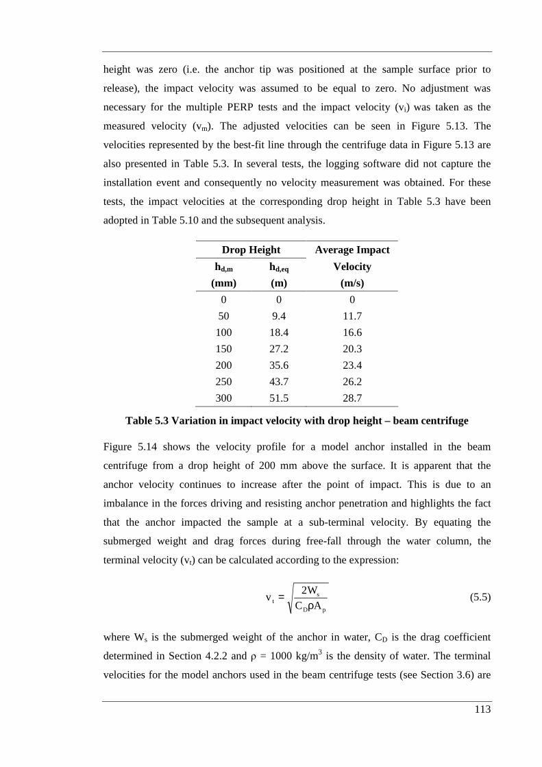
113
height was zero (i.e. the anchor tip was positioned at the sample surface prior to
release), the impact velocity was assumed to be equal to zero. No adjustment was
necessary for the multiple PERP tests and the impact velocity (vi) was taken as the
measured velocity (vm). The adjusted velocities can be seen in Figure 5.13. The
velocities represented by the best-fit line through the centrifuge data in Figure 5.13 are
also presented in Table 5.3. In several tests, the logging software did not capture the
installation event and consequently no velocity measurement was obtained. For these
tests, the impact velocities at the corresponding drop height in Table 5.3 have been
adopted in Table 5.10 and the subsequent analysis.
Drop Height Average Impact
hd,m hd,eq Velocity
(mm) (m) (m/s)
0 0 0
50 9.4 11.7
100 18.4 16.6
150 27.2 20.3
200 35.6 23.4
250 43.7 26.2
300 51.5 28.7
Table 5.3 Variation in impact velocity with drop height – beam centrifuge
Figure 5.14 shows the velocity profile for a model anchor installed in the beam
centrifuge from a drop height of 200 mm above the surface. It is apparent that the
anchor velocity continues to increase after the point of impact. This is due to an
imbalance in the forces driving and resisting anchor penetration and highlights the fact
that the anchor impacted the sample at a sub-terminal velocity. By equating the
submerged weight and drag forces during free-fall through the water column, the
terminal velocity (vt) can be calculated according to the expression:
pD
st AC
W2v
ρ= (5.5)
where Ws is the submerged weight of the anchor in water, CD is the drag coefficient
determined in Section 4.2.2 and ρ = 1000 kg/m3 is the density of water. The terminal
velocities for the model anchors used in the beam centrifuge tests (see Section 3.6) are

114
presented in Table 5.4. Restrictions in both drop height and sample depth, however,
limited the centrifuge tests to maximum velocities in the order of 30 m/s (see Table
5.10). These velocities are, on average, approximately 60 % lower than the terminal
velocities presented in Table 5.4 and approximately 40 % lower than impact velocities
recorded in field trials of nuclear waste disposal penetrometers (Freeman et al. 1984,
Freeman and Burdett 1986). It is therefore apparent that scope exists for substantial
increases in dynamic anchor impact velocity above those achievable in the beam
centrifuge. Given the dependence of embedment depth on impact velocity this also
suggests the potential for greater embedment depths and ultimately higher anchor
holding capacities.
Anchor CD vt
(m/s)
E0-1 0.24 86.0
E0-2 0.24 85.0
C0-1 0.22 90.6
O0-1 0.22 90.5
F0-1 0.88 45.9
IE0-1 0.24 84.3
IE0-2 0.24 86.0
Table 5.4 Model anchor terminal velocities
5.2.3 Embedment Depth
As the undrained shear strength of typical offshore clay deposits increases with depth
below the seabed, higher holding capacities can be mobilised by maximising the anchor
embedment depth. The embedment depth of dynamically installed anchors is dependent
on a number of factors, including impact velocity, anchor mass, anchor geometry and
soil strength characteristics. Anchor tip embedment depths measured in the beam
centrifuge tests ranged from 157 – 216 mm at model scale, representing 31.4 – 43.2 m
at prototype scale or 2.1 – 2.9 times the anchor length (see Table 5.10). These results are
in good agreement with torpedo anchor embedments of 2.4 times the anchor length
measured in field trials in normally consolidated clay (Medeiros 2001, 2002).
The anchor penetration depths were determined according to the method outlined in
Section 3.8.1.2. This method relies upon the measurement of the slack in the anchor

115
chain during extraction, prior to the onset of a tensile load. By examining the load
versus displacement response during extraction, the slack in the anchor chain can be
determined. Figure 5.15 shows a typical load displacement plot for a model dynamic
anchor test, illustrating the anchor chain slack length.
In certain tests, the penetration depth was either difficult to determine or misleading due
to twisting of the anchor chain (resulting in uncertainty over the point of load onset),
accidental premature installation of the anchor prior to the realisation of the target
acceleration level, or installation of the anchor in a previously disturbed test site. It
should be noted that although these embedment depths have been included in Table
5.10, they have not been considered in the analysis presented in this or following
chapters.
The embedment depths presented here and considered in the analysis refer to the
embedment of the anchor tip unless otherwise stated.
5.2.3.1 Influence of Impact Velocity
Figure 5.16 summarises the dependence of the dynamic anchor embedment depth on
impact velocity for the zero fluke ellipsoid nosed anchors in the beam centrifuge. The
data indicates an approximately linear increase in embedment depth with impact
velocity, such that from impact velocities of 0 – 30 m/s there is an approximate 30 %
increase in embedment. Despite very few data points at low velocities, Figure 5.16
suggests that the apparently linear relationship between impact velocity and embedment
depth is limited to a lower threshold impact velocity of approximately 10 m/s. These
observations are consistent with the findings of previous dynamic anchor centrifuge
studies by Lisle (2001), Wemmie (2003), Richardson (2003) and O’Loughlin et al.
(2004b). Interestingly, the relatively high embedment depths measured in the tests
installed from the sample surface, i.e. vi = 0 m/s, suggest a strong embedment depth
dependence on anchor mass.
Given the potential for higher dynamic anchor impact velocities (see Section 5.2.2)
there is also the potential for higher penetration depths. It should be noted, however,
that the samples in the beam centrifuge strongbox were approximately 230 mm deep
(including a 10 mm deep sand drainage layer), and as such tip penetrations were limited
to approximately 220 mm (44 m at prototype scale). Having said that, extrapolation of
116
the embedment data to impact velocities approaching terminal velocity (see Table 5.4)
indicate the potential for embedment depths in the order of 300 mm (60 m at prototype
scale) or 4 times the anchor length (see Figure 5.17). Such embedments are
considerably larger than those recorded in field trials of nuclear waste disposal
penetrometers (Freeman et al. 1984, Freeman and Burdett 1986), although the waste
disposal tests were conducted in sites with higher shear strengths (i.e. k = 1.5 kPa/m).
5.2.3.2 Influence of Anchor Geometry
O'Loughlin et al. (2004b) identified a significant discrepancy between the measured
penetration depths of two zero fluke model dynamic anchors with slightly different tip
shapes (Figure 5.18). The anchor with the ‘sharp’ tip exhibited penetration depths that
were on average over 20 % higher than the measured embedments for the ‘blunt’
anchor, suggesting a strong embedment depth dependency on anchor tip shape.
Consequently the tests in beam centrifuge Box 1 were used to investigate the influence
of tip shape on the penetration performance of dynamically installed anchors. Four
different tip shapes were assessed, a standard ellipsoid tip, a conical tip with a 15° cone
angle, a tangent ogive tip and a blunt or flat tip analogous to the head of a closed-ended
cylindrical pile (see Section 3.6.3). The ellipsoid, cone and ogive anchors were all
fabricated with approximately the same mass in order to eliminate the influence of the
anchor mass on the embedment depth. However, it was not possible to reduce the mass
of the flat nosed anchor further without exceeding safe wall thickness limits and as such
its final mass was slightly greater than the other three anchors (see Table 3.10).
Each of the four model anchors was installed three times from a drop height of 300 mm;
the measured embedment depths are shown in Figure 5.19 against the penetration
depths for the other ellipsoid nosed anchor tests conducted in the beam centrifuge. It can
be seen that the ellipsoid nosed anchor penetrations are consistent between individual
samples. It can also be seen that each of the other anchor tip shapes result in slightly
higher penetration depths. In fact the results indicate average prototype embedment
depths of 39.0 m, 42.7 m, 40.3 m and 42.3 m for the ellipsoid, cone, ogive and flat
nosed anchors respectively. Hence by selecting the conical anchor over the ellipsoid,
ogive and flat nosed anchors it was possible to achieve increases in embedment of 8.7
%, 5.6 % and 0.9 % respectively. Compared with a 30 % increase in embedment by
increasing the velocity from 0 – 30 m/s (see Section 5.2.3.1), it is therefore possible to

117
achieve a relatively high increase in embedment by selecting an appropriate anchor tip
shape. Interestingly, the flat nosed anchor provided similar embedment depths to the
conical anchor, although the differences in mass made it difficult to draw conclusions
about the influence of the tip geometry. However, by plotting the embedment depth as a
function of the kinetic energy at the point of impact, rather than the impact velocity, it
was possible to eliminate the effect of the anchor mass and thereby independently
evaluate the influence of the anchor tip shape. The kinetic energy (Ek) is dependent on
both the velocity of the anchor (v) and the anchor mass (m) and can be expressed as:
22
1k mvE = (5.6)
Figure 5.20 shows the variation in embedment depth with the kinetic energy at impact
for the four different anchor tip shapes. Similar to the impact velocity results in Figure
5.19, the ellipsoid nosed anchor recorded the lowest average embedment at an
equivalent kinetic energy, followed by the ogive, flat and conical anchors respectively.
It is apparent that at similar kinetic energies, the conical and flat nosed anchors provide
comparable embedment depths. This can be attributed to the fact that the bearing
capacity mechanism for a deep circular foundation is typically characterised by a central
soil wedge beneath the foundation, which remains in an elastic state of equilibrium and
acts as part of the foundation (Meyerhof 1951; see Figure 5.21). Hence during the
penetration of the flat nosed model anchor it is likely that a conical wedge of soil forms
beneath the circular anchor tip, with the wedge effectively acting as a conical tip. In this
regard it is not surprising that the flat nosed anchor and conical anchor achieved similar
embedment depths.
No four fluke anchor tests were conducted in the beam centrifuge experimental
programme. However, in order to assess the influence of the anchor flukes on
embedment, the results of the zero fluke anchor (0FA) tests have been compared with
the results of three (3FA) and four fluke anchor (4FA) tests conducted by Lisle (2001)
and Wemmie (2003) (see Figure 5.22). The results indicate an increase in embedment
with decreasing total surface area (i.e. number of flukes), with the 3FA embedding on
average approximately 9 % further than the 4FA and the 0FA approximately 20 %
further than the 3FA. This is not surprising considering that the higher surface area
afforded by the additional flukes will result in a higher frictional resistance to
penetration. Although this finding could be undermined somewhat by the higher mass
118
of the 0FAs, which in any case should promote an increase in embedment depth, it is
upheld by the observed increase in embedment of the 3FAs over the 4FAs, both of
which had the same mass (O’Loughlin et al. 2004b). Additionally, by plotting the
embedment against the kinetic energy at impact it is possible to eliminate the influence
of the anchor mass and thereby directly compare the influence of the anchor flukes on
the penetration depth (Figure 5.23). Just as for the impact velocity, the variation of
embedment with kinetic energy indicates an increase in embedment with decreasing
total anchor surface area.
5.2.3.3 Influence of Surface Water
Whilst the penetration results have not been considered directly in the analysis, several
tests conducted in Box 6 demonstrated interesting results. Typically, during the beam
centrifuge tests a nominal layer of surface water was maintained above the sample
surface in order to ensure complete saturation of the sample. For four tests conducted in
Box 6 (indicated by the superscript ‘w’ in Table 5.10), this surface water layer was
removed. The penetration depths recorded in these tests are compared in Figure 5.24
with the results of tests conducted in the same sample with the surface water layer
present. At corresponding impact velocities, the embedments measured in the tests in
which the surface water was removed are, on average, 20 % lower than those for the
tests in which the surface water was present.
Whilst it is acknowledged that during offshore installation of dynamic anchors, water
will always be present, these results highlight an important consideration which may
influence the short-term anchor capacity. The results tend to suggest that water may be
entrained in a boundary layer close to the anchor during penetration, thereby reducing
the effective stresses in the soil surrounding the anchor and allowing greater penetration
depths, but also resulting in lower short-term capacities prior to the dissipation of the
excess pore pressures generated in the boundary layer. Tika and Hutchinson (1999)
have commented on the reduction in strength observed in fast rate ring shear tests, in
which water was allowed to penetrate the shear zone. The short-term anchor capacity
and dissipation of excess pore pressures following dynamic anchor installation will be
discussed in greater detail in Section 5.3.6.
119
5.2.3.4 Verticality
Coriolis effects in the centrifuge mean that during installation, relative to the sample,
the model anchor will experience an apparent tangential component of acceleration,
unless otherwise restrained. Prior to impact with the sample surface, the anchor is
restrained by the rigid installation guide; however, once the anchor begins to penetrate
the deformable soil sample, the tangential acceleration component will tend to cause the
anchor to follow a curved trajectory through the sample. The only way to assess the
extent of this curved trajectory during penetration was to excavate the soil surrounding
the anchor following installation and to check the verticality of the anchor at its final
location. Three tests in two beam centrifuge samples were conducted in which the
embedded anchor was subsequently examined for verticality. Figure 5.25 shows a
photograph of an excavated beam centrifuge clay sample illustrating the inclination to
the vertical of a model dynamic anchor in one of these tests. Only a relatively minor
inclination (i.e. less than 3°) can be observed and hence the anchor is considered to
remain vertical during dynamic installation in the beam centrifuge. It was important,
however, to ensure that the tip of the installation guide remained as close as possible to
the sample surface to prevent rotation of the anchor prior to impact as an inclined
impact is likely to increase the inclination of the anchor during embedment.
5.2.4 Load Displacement Response
A typical load displacement plot following the onset of tensile load during the vertical
monotonic extraction of a dynamically installed anchor in the beam centrifuge is
presented in Figure 5.26. The response is characterised by a sharp increase in load
towards an initial maximum capacity (Peak 1) followed by a sudden drop in load and a
subsequent increase towards a secondary maximum capacity (Peak 2), generally of
lower magnitude than Peak 1. The initial maximum capacity at Peak 1 and rapid
softening is not wholly understood but appears to be due to high (and brittle) frictional
resistance, with the rise to Peak 2 indicating a more gradual mobilisation of bearing
resistance. Jeanjean et al. (2006) commented on the different mobilisation rates of
frictional and bearing resistance for suction caissons. Both the Peak 1 and Peak 2
capacities (Fv1 and Fv2), as well as the displacements required to mobilise each of these
capacities (z1 and z2), are presented in Table 5.10.

120
Previous dynamic anchor testing in the beam centrifuge reported by Lisle (2001),
Wemmie (2003), Richardson (2003) and O’Loughlin et al. (2004b) describe only the
overall maximum capacity, which generally corresponded to the Peak 1 capacity.
However, typical load displacement plots from Lisle (2001), Wemmie (2003) and
Richardson (2003) demonstrate the same Peak 1 and Peak 2 behaviour as shown in
Figure 5.26.
In Box 5 a single static installation, vertical monotonic extraction test (see Section
3.8.1.6) was conducted in order to assess the influence of the dynamic anchor
installation process on the observed load displacement behaviour during extraction. The
anchor was installed manually, via an adaptor fitted to the end of the T-bar shaft, at 1 g
with the centrifuge stationary. Following installation the adaptor was removed from the
sample leaving the anchor in place, the anchor chain was connected to the load cell and
the centrifuge ramped up to the test acceleration level of 200 g. The anchor was then
extracted vertically at a constant rate of 0.3 mm/s. The load displacement response
during the extraction of the model anchor is shown in Figure 5.27 and indicates the
same Peak 1 and Peak 2 behaviour. These observations suggest that the unusual load
displacement response is not attributable to the rate of installation of the model anchor.
The vast majority of tests conducted in the beam centrifuge utilised the standard
ellipsoidal shaped anchor tip described in Section 3.6.1. However, as discussed in
Section 5.2.3.2, the influence of the tip shape on the anchor performance was
investigated in Box 1. Figure 5.28 shows typical load displacement plots for each of the
model anchor nose shapes. It is apparent that, whilst the flat nosed anchor exhibits
similar load displacement behaviour up to Peak 1 and even in the subsequent rapid
softening, following this the flat nosed anchor capacity does not increase to a secondary
Peak 2 capacity but continues to decrease with increasing displacement. This behaviour
was observed in several tests with the flat nosed anchor and is unlike the load
displacement response observed for each of the other anchor tip shapes. This suggests
that the tip shape may influence the extraction behaviour of dynamically installed
anchors, possibly by altering the rate of mobilisation of the reverse end bearing
resistance.

121
5.2.5 Vertical Monotonic Holding Capacity
Over the range of embedment depths in the beam centrifuge, the undrained vertical
monotonic holding capacity ranged from 41.2 to 95.4 N (1.6 – 3.8 MN at prototype
scale) for Peak 1 and 34.5 to 72.7 N (1.4 - 2.9 MN at prototype scale) for Peak 2.
Typically, the anchor capacity was determined after approximately 13 minutes (1 year
at prototype scale) of reconsolidation following installation, although accurate
reconsolidation periods were not recorded in a large number of tests. The Peak 1 and
Peak 2 capacities measured in the beam centrifuge tests are shown in Figures 5.29 and
5.30 respectively, compared with the results of previous 0FA beam centrifuge tests
reported by O’Loughlin et al. (2004b) and the results of torpedo anchor field trials
conducted in normally consolidated clay reported by Medeiros (2001). It can be seen
that the agreement between the Peak 1 capacities and the previous centrifuge data is
noticeably better than that for the Peak 2 capacities. This is not surprising considering
that the capacities reported by O’Loughlin et al. (2004b) correspond to the Peak 1
capacity. Both the Peak 1 and Peak 2 data, however, agree well with the torpedo anchor
field test data. Despite differences in anchor geometry and mass and variations in the
soil strength characteristics, the relative agreement between the measured field and
centrifuge capacities is encouraging and demonstrates the suitability of centrifuge
modelling for assessing the performance of dynamic anchors.
Both the Peak 1 and Peak 2 capacities measured in the beam centrifuge tests have been
normalised according to Equation 4.37 (Section 4.5.3). With the undrained shear
strength known to increase with depth, normalisation in this manner not only accounts
for variations in the shear strength profile but also variations in the anchor embedment
depth. The normalised Peak 1 and Peak 2 capacities are shown in Figures 5.31 and 5.32
respectively and are also presented in Table 5.10 (FN1 and FN2). For comparison, the
normalised capacities from the torpedo anchor field trials (Medeiros 2001) and the
previous 0FA centrifuge tests (O’Loughlin et al. 2004b) are also provided. It should be
noted that the normalised capacities from the field tests are only approximate as the
calculations were based on the limited anchor and soil property information available.
Figure 5.31, in particular, shows very good agreement between the normalised Peak 1
capacities and both the previous centrifuge data and the torpedo anchor field test data.
Having taken into account the dry weight of the anchor and differences in the undrained

122
shear strength and embedment depth, the normalised centrifuge capacities compare
favourably with the results of the torpedo anchor field trials. Somewhat surprisingly
however, the normalised capacities presented in Figures 5.31 and 5.32 cover an
extremely wide range from approximately 40 – 70 for Peak 1 and 30 – 50 for Peak 2 at
embedment depths of approximately 2.3 – 2.9 times the anchor length. Despite slight
differences in the normalisation procedure significant scatter in the normalised capacity
of dynamic anchors at similar penetration depths was also reported by O’Loughlin et al.
(2004b).
Anchor efficiency is often used as an assessment of anchor performance (see Section
4.5.4). For the centrifuge tests reported here, Peak 1 efficiencies ranged from 1.4 – 3.2,
whilst Peak 2 efficiencies ranged from 1.2 – 2.4. In comparison, the efficiencies from
the torpedo anchor field trials ranged from approximately 3.2 – 3.5 (Medeiros 2001),
whilst the efficiencies for the previous 0FA centrifuge tests varied from 1.7 – 3.6
(O’Loughlin et al. 2004b). The torpedo anchor efficiencies appear slightly higher than
those in the centrifuge tests, although good agreement is achieved between the current
and previous centrifuge test data, particularly for Peak 1. Whilst these efficiencies are
significantly lower than those offered by conventional drag anchors (e.g. Vryhof 1999),
the measured anchor efficiencies are a function of the anchor capacity which varies with
embedment depth, with higher embedment depths yielding higher anchor efficiencies.
Hence given the potential for higher anchor embedment depths (see Section 5.2.3.1),
higher anchor efficiencies are also likely. That said, the concept of efficiency for these
anchors is not considered particularly useful, partly because fabrication and installation
costs are much lower than for a conventional drag anchor (so comparable efficiencies
do not reflect comparable cost) but also because the holding capacity is directly related
to the drop height and resulting embedment depth (O’Loughlin et al. 2004b).
5.2.5.1 Influence of Embedment Depth
Due to the increase in shear strength with depth observed in the beam centrifuge
samples (Section 5.2.1), it is expected that the anchor capacity will increase with
increasing embedment depth. The variation in vertical monotonic capacity with depth
for Peak 1 and Peak 2 is shown in Figures 5.29 and 5.30 respectively. It is apparent that
both the Peak 1 and Peak 2 capacities increase with embedment depth, due to the
mobilisation of higher shear strengths. However, care should be taken in this

123
assessment, as although consolidation times of approximately 13 minutes (1 year at
prototype scale) were provided following installation in the majority of tests, accurate
consolidation times were not recorded for approximately half of the beam centrifuge
tests. The capacity of dynamically installed anchors is expected to increase with time
following installation due to the effects of consolidation. This is discussed in Section
5.3.6.
5.2.5.2 Influence of Anchor Geometry
The normalised Peak 1 and Peak 2 capacities for the different anchor tip shapes are
shown in Figures 5.33 and 5.34 respectively. Focusing on the Peak 1 capacities, it is
noticeable that, on average, the normalised capacity of the flat nosed anchor is lower
than the capacities of the three other nose types. This is somewhat surprising
considering the greater overall surface area of the flat nosed anchor; however, once
again, care should be taken in drawing conclusions from these results as no accurate
consolidation times were recorded for any of the tests with different anchor tip shapes.
Hence the differences in capacity may in fact be attributable to slight variations in
consolidation time (see Section 5.3.6). It should be noted that no Peak 2 capacities were
obtained for the flat nosed anchor tests.
Figure 5.35 compares the 0FA efficiencies from the current test series with the
efficiencies calculated from the capacities of 3 and 4FAs reported by Wemmie (2003).
It was expected that a decrease in the total anchor surface area (i.e. number of flukes)
should result in a decrease in the anchor capacity. Hence at similar penetration depths,
the 4FA should demonstrate the highest efficiency followed by the 3FA and the 0FA. It
can be seen that, on average, the 0FA efficiencies are lower than the efficiencies of both
the 3 and 4FAs, with the 0FA required to penetrate to a depth of approximately 200 mm
(40 m at prototype scale) to achieve a similar efficiency as the 3 and 4FAs at a depth of
150 mm (30 m at prototype scale). Somewhat surprisingly however, the 3FAs provide
similar, if not slightly higher efficiencies, at comparable embedment depths as the 4FAs
despite the 3FA having a lower total surface area.
5.2.6 Long-Term Sustained Loading
The design of offshore foundations may be governed by the capacity of the foundation
under long-term sustained loading. Five sustained loading tests were conducted in Box
124
5 in order to assess the behaviour of dynamically installed anchors under sustained
loading conditions. Specifically, the effects of the sustained load magnitude and
duration were considered. The sustained loading tests were detailed in Section 3.8.1.3.
In each test the model anchor was installed from a drop height of 150 mm such that
similar embedment depths were achieved between tests. For the five sustained loading
tests, the variation in the measured embedment depth was approximately ± 3 % (see
Table 5.10). Following installation, the soil surrounding the anchor was allowed to
consolidate for 1 hour (4.5 years at prototype scale) prior to the application of the
sustained loading sequence (see Table 5.5). The sustained load magnitude in Table 5.5
has been specified as a proportion of the maximum Peak 1 capacity in a reference
vertical monotonic extraction test (B5D1), which was installed from the same drop
height and provided with the same consolidation period (see Section 3.8.1.3). If failure,
identified as excessive vertical displacement, was not observed during the sustained
loading sequence, the anchor was subsequently loaded monotonically to failure and
extracted under displacement control conditions at a rate of 0.3 mm/s. In tests B5SUS4
and B5SUS5, the model anchor was subjected to four consecutive sustained loading
stages of increasing load magnitude.
It should be noted that the results of test B5SUS1 have been excluded from the analysis
due to an error in the sustained loading sequence. The variations in load relative to the
Peak 1 capacity in B5D1 and displacement with time for each of the four successful
sustained loading tests are presented in Figures 5.36 – 5.39. It can be seen from these
figures that the sustained load actually fluctuated slightly with time, effectively
representing a very small amplitude cyclic loading sequence. This was attributed to the
resolution of the load cell, since sustained loads of less than 100 N were imposed on the
model anchors using the feedback from a load cell with a capacity of 1.7 kN. This was
not expected to have a significant influence on the test results. The point at which
failure occurred has been identified for each test. Figure 5.38 shows that during test
B5SUS4, the actuator control system overshot the desired sustained load. In the
transition from stage 1 to 2 the overshoot was approximately 14 %, whilst between
stages 2 and 3 the overshoot was approximately 9 %. The overshoot during the
transition from stage 2 to 3 was sufficient to cause instantaneous failure. Test B5SUS4
was subsequently repeated in test B5SUS5.
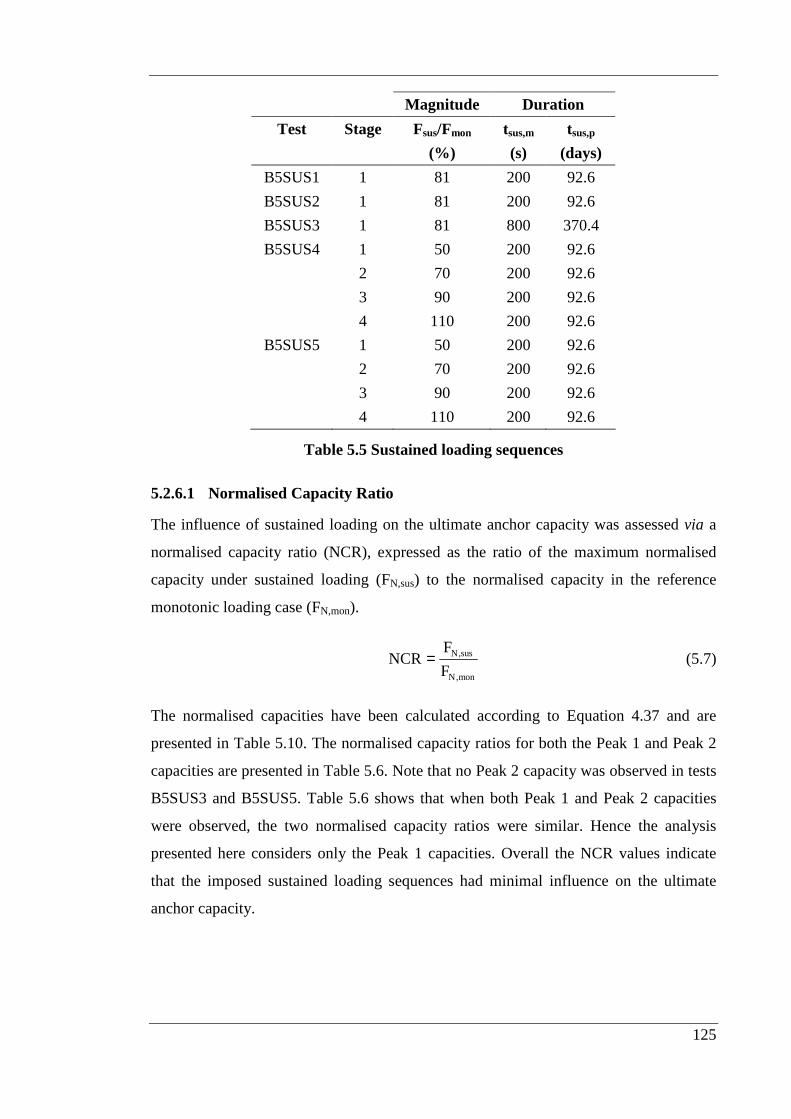
125
Magnitude Duration
Test Stage Fsus/Fmon tsus,m tsus,p
(%) (s) (days)
B5SUS1 1 81 200 92.6
B5SUS2 1 81 200 92.6
B5SUS3 1 81 800 370.4
B5SUS4 1 50 200 92.6
2 70 200 92.6
3 90 200 92.6
4 110 200 92.6
B5SUS5 1 50 200 92.6
2 70 200 92.6
3 90 200 92.6
4 110 200 92.6
Table 5.5 Sustained loading sequences
5.2.6.1 Normalised Capacity Ratio
The influence of sustained loading on the ultimate anchor capacity was assessed via a
normalised capacity ratio (NCR), expressed as the ratio of the maximum normalised
capacity under sustained loading (FN,sus) to the normalised capacity in the reference
monotonic loading case (FN,mon).
mon,N
sus,N
F
FNCR = (5.7)
The normalised capacities have been calculated according to Equation 4.37 and are
presented in Table 5.10. The normalised capacity ratios for both the Peak 1 and Peak 2
capacities are presented in Table 5.6. Note that no Peak 2 capacity was observed in tests
B5SUS3 and B5SUS5. Table 5.6 shows that when both Peak 1 and Peak 2 capacities
were observed, the two normalised capacity ratios were similar. Hence the analysis
presented here considers only the Peak 1 capacities. Overall the NCR values indicate
that the imposed sustained loading sequences had minimal influence on the ultimate
anchor capacity.

126
Test FN1 z1/D FN2 z2/D NCR1 NCR2
B5SUS2 63.0 1.67 40.7 1.88 1.03 1.06
B5SUS3 59.8 1.50 0.98
B5SUS4 57.4 1.37 36.9 1.70 0.94 0.96
B5SUS5 52.0 1.42 0.85
Table 5.6 Summary of normalised capacities from sustained loading tests
5.2.6.2 Influence of Load Magnitude
Sustained loading may lead to a reduction in the foundation capacity due to the adverse
effects of creep on the soil shear strength (Edil and Muchtar 1988). Evidence from
suction caisson tests in clay suggests that a threshold sustained loading level exists,
below which the sustained loading has very little influence on capacity. However, for
loads in excess of this threshold the caisson capacity may be significantly degraded.
Allersma et al. (2000) and Clukey et al. (2004) suggest threshold sustained loading
levels of approximately 80 - 85 % of the monotonic capacity. That said, an important
difference between suction caissons and dynamic anchors is that under sustained
loading, the suction caisson capacity may be reduced by the dissipation of negative
excess pore pressures at the bottom of the caisson and the corresponding reduction in
the reverse end bearing resistance.
The influence of the sustained load magnitude on the dynamic anchor capacity was
evaluated by comparing the results of tests B5SUS2, B5SUS4 and B5SUS5. In
B5SUS2, the model anchor was subjected to a 200 s duration sustained load with a
magnitude of approximately 80 % of the reference monotonic capacity. In contrast, the
initial stage of tests B5SUS4 and B5SUS5 were conducted with a 50 % load of similar
duration. Figure 5.40 shows the normalised load displacement response during the three
sustained loading tests, whilst Figure 5.41 shows the normalised displacements
measured during the sustained loading sequence. The normalised capacity ratio based
on the Peak 1 monotonic capacity is also shown in Figure 5.40. It can be seen that the
displacements under sustained loading develop in a similar manner in each test, with the
excellent agreement between tests B5SUS4 and B5SUS5 demonstrating good test
repeatability. It should be noted that due to the adjustment of the capacity by the
anchor’s submerged weight and the non-instantaneous mobilisation of the submerged
127
weight upon the onset of a tensile load in the anchor chain, the initial normalised load is
negative and has not been shown in Figure 5.40.
Figure 5.41 indicates that the displacements developed under an 80 % sustained load are
approximately 40 % higher than the displacements under a 50 % sustained load of
similar duration. Consequently, the greater creep displacements under the higher
magnitude sustained load would be expected to result in a lower anchor capacity.
However, Table 5.6 shows that for B5SUS2, NCR = 1.03 indicating no apparent
reduction in capacity from the reference monotonic case. Tests B5SUS4 and B5SUS5
indicate lower NCR values of 0.94 and 0.85 respectively, although the model anchor in
these tests was subjected to subsequent 70 % and 90 % sustained loading stages. An
additional 110 % loading stage was planned (see Table 5.5), however, failure in each
case was observed at the 90 % loading level. This failure could potentially be attributed
to the accumulated creep displacements under each of the sustained loading stages;
however it should also be considered that the duration of these subsequent stages
provides additional time for consolidation of the clay ahead of the anchor, thereby
increasing the bearing resistance. It may also be the case that a threshold loading level
of between 80 and 90 % exists, such that by increasing the sustained load to 90 % of the
monotonic capacity the threshold is exceeded and subsequent failure is observed. A
threshold loading level of 80 – 90 % agrees with threshold levels reported for sustained
loading tests of suction caissons (Allersma et al. 2000, Clukey et al. 2004). Based on
the results of the centrifuge tests, there is no evidence to suggest that sustained loading
levels of up to 80 % of the reference monotonic capacity influence the dynamic anchor
holding capacity.
In order to assess the influence of sustained loading on the load displacement response
of dynamic anchors in the centrifuge (see Section 5.2.4), tests B5SUS2 and B5SUS3
were conducted with sustained loads of similar magnitude to the Peak 2 capacity in the
reference monotonic case (B5D1). It was thought that by applying a sustained load of
equal or greater magnitude than the Peak 2 capacity, the Peak 1 behaviour could be
eliminated by initiating failure at the lower capacity. It is evident from Figure 5.42
however, that the same load spike at Peak 1 was observed in both sustained loading
tests. Hence it can be concluded that sustained loading at a level equivalent to the Peak
2 capacity was not sufficient to induce failure at this lower capacity.

128
5.2.6.3 Influence of Load Duration
In assessing the influence of the sustained load duration on the ultimate dynamic anchor
capacity, the effects of both creep and consolidation should be considered. As
mentioned previously, sustained loading may reduce the anchor capacity due to the
accumulation of creep displacements. Conversely, longer duration loading may lead to
further consolidation of the soil surrounding the anchor resulting in higher shear
strengths and therefore higher capacities.
The effect of sustained load duration on the ultimate anchor capacity was assessed in
tests B5SUS2 and B5SUS3, with a four fold difference in load duration at the same load
magnitude (see Table 5.5). The normalised load displacement response for both of these
tests is shown in Figure 5.42 with the normalised displacements under the sustained
loading sequences shown in Figure 5.43. It is evident that the normalised displacements
in each test are almost identical after 200 s, but the longer sustained load duration in
B5SUS3 results in total creep displacements after 800 s that are approximately 40 %
higher than those in B5SUS2 after 200 s. These higher creep displacements are likely to
result in a reduction in the anchor capacity, although, considering the additional
consolidation time, it is also likely that the shear strength will increase over the course
of the 800 s test, leading to an increase in the anchor capacity and thereby offsetting the
decrease in capacity due to creep.
Failure was not observed during the sustained loading sequence in either test and the
anchor was subsequently loaded monotonically to failure. The NCR values in Table 5.6
indicate a slight decrease in anchor capacity with increasing load duration from 103 %
of the monotonic capacity after 200 s to 98 % after 800 s. Hence whilst an increase in
the load duration appears to result in a slight decrease in anchor capacity, the difference
in capacity is not large enough for this to be considered conclusive.
5.2.7 Cyclic Loading
Offshore structures are continuously subjected to cyclic loads in the form of wind,
waves and currents. These loads are subsequently transmitted to the foundations and
may lead to failure of the anchoring system under extreme storm conditions. Seven
cyclic loading tests were conducted in Box 5 with the aim of assessing the behaviour of
dynamically installed anchors under cyclic loading conditions. In particular, the
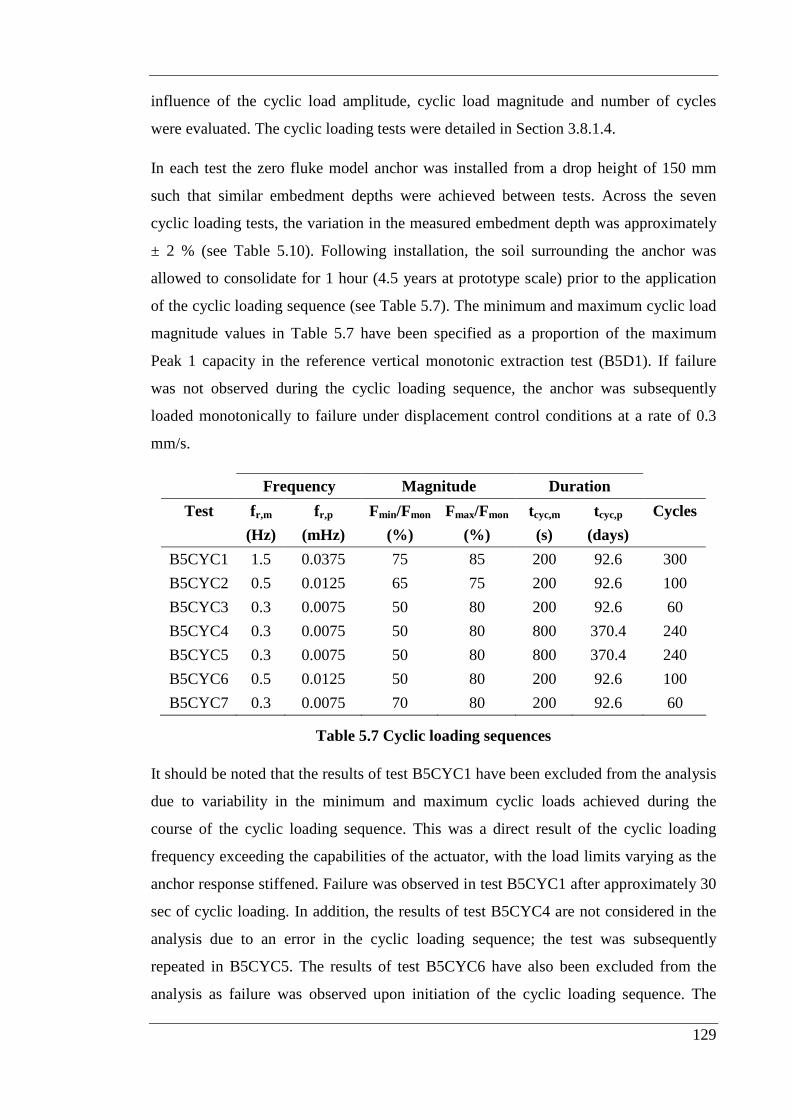
129
influence of the cyclic load amplitude, cyclic load magnitude and number of cycles
were evaluated. The cyclic loading tests were detailed in Section 3.8.1.4.
In each test the zero fluke model anchor was installed from a drop height of 150 mm
such that similar embedment depths were achieved between tests. Across the seven
cyclic loading tests, the variation in the measured embedment depth was approximately
± 2 % (see Table 5.10). Following installation, the soil surrounding the anchor was
allowed to consolidate for 1 hour (4.5 years at prototype scale) prior to the application
of the cyclic loading sequence (see Table 5.7). The minimum and maximum cyclic load
magnitude values in Table 5.7 have been specified as a proportion of the maximum
Peak 1 capacity in the reference vertical monotonic extraction test (B5D1). If failure
was not observed during the cyclic loading sequence, the anchor was subsequently
loaded monotonically to failure under displacement control conditions at a rate of 0.3
mm/s.
Frequency Magnitude Duration
Test fr,m fr,p Fmin/Fmon Fmax/Fmon tcyc,m tcyc,p Cycles
(Hz) (mHz) (%) (%) (s) (days)
B5CYC1 1.5 0.0375 75 85 200 92.6 300
B5CYC2 0.5 0.0125 65 75 200 92.6 100
B5CYC3 0.3 0.0075 50 80 200 92.6 60
B5CYC4 0.3 0.0075 50 80 800 370.4 240
B5CYC5 0.3 0.0075 50 80 800 370.4 240
B5CYC6 0.5 0.0125 50 80 200 92.6 100
B5CYC7 0.3 0.0075 70 80 200 92.6 60
Table 5.7 Cyclic loading sequences
It should be noted that the results of test B5CYC1 have been excluded from the analysis
due to variability in the minimum and maximum cyclic loads achieved during the
course of the cyclic loading sequence. This was a direct result of the cyclic loading
frequency exceeding the capabilities of the actuator, with the load limits varying as the
anchor response stiffened. Failure was observed in test B5CYC1 after approximately 30
sec of cyclic loading. In addition, the results of test B5CYC4 are not considered in the
analysis due to an error in the cyclic loading sequence; the test was subsequently
repeated in B5CYC5. The results of test B5CYC6 have also been excluded from the
analysis as failure was observed upon initiation of the cyclic loading sequence. The
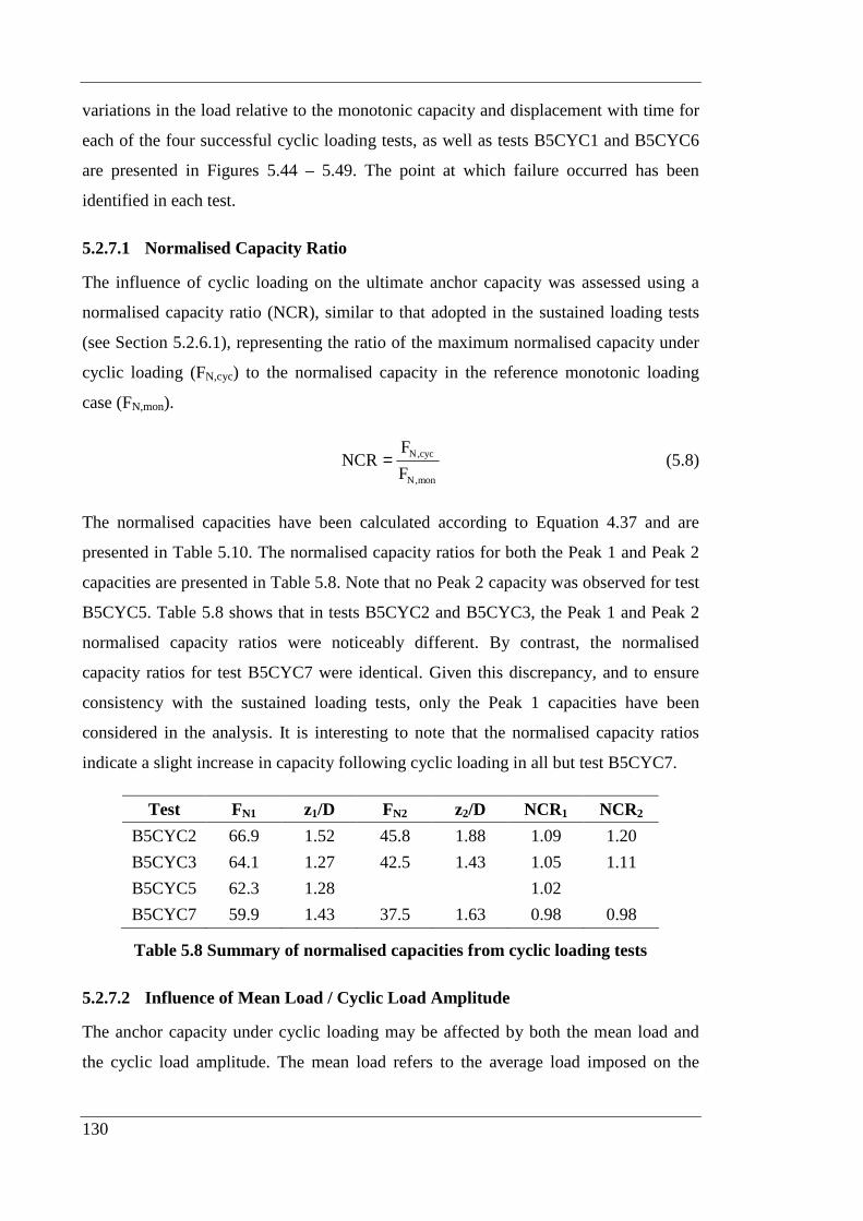
130
variations in the load relative to the monotonic capacity and displacement with time for
each of the four successful cyclic loading tests, as well as tests B5CYC1 and B5CYC6
are presented in Figures 5.44 – 5.49. The point at which failure occurred has been
identified in each test.
5.2.7.1 Normalised Capacity Ratio
The influence of cyclic loading on the ultimate anchor capacity was assessed using a
normalised capacity ratio (NCR), similar to that adopted in the sustained loading tests
(see Section 5.2.6.1), representing the ratio of the maximum normalised capacity under
cyclic loading (FN,cyc) to the normalised capacity in the reference monotonic loading
case (FN,mon).
mon,N
cyc,N
F
FNCR = (5.8)
The normalised capacities have been calculated according to Equation 4.37 and are
presented in Table 5.10. The normalised capacity ratios for both the Peak 1 and Peak 2
capacities are presented in Table 5.8. Note that no Peak 2 capacity was observed for test
B5CYC5. Table 5.8 shows that in tests B5CYC2 and B5CYC3, the Peak 1 and Peak 2
normalised capacity ratios were noticeably different. By contrast, the normalised
capacity ratios for test B5CYC7 were identical. Given this discrepancy, and to ensure
consistency with the sustained loading tests, only the Peak 1 capacities have been
considered in the analysis. It is interesting to note that the normalised capacity ratios
indicate a slight increase in capacity following cyclic loading in all but test B5CYC7.
Test FN1 z1/D FN2 z2/D NCR1 NCR2
B5CYC2 66.9 1.52 45.8 1.88 1.09 1.20
B5CYC3 64.1 1.27 42.5 1.43 1.05 1.11
B5CYC5 62.3 1.28 1.02
B5CYC7 59.9 1.43 37.5 1.63 0.98 0.98
Table 5.8 Summary of normalised capacities from cyclic loading tests
5.2.7.2 Influence of Mean Load / Cyclic Load Amplitude
The anchor capacity under cyclic loading may be affected by both the mean load and
the cyclic load amplitude. The mean load refers to the average load imposed on the
131
anchor during the cyclic loading sequence, whilst the cyclic load amplitude is defined as
the maximum variation from this average load (see Figure 5.50).
From the limited number of successful cyclic loading tests, it is not possible to separate
the individual effects of mean load and cyclic load amplitude. However, tests B5CYC3
and B5CYC7 provide an indication of their combined influence on the dynamic anchor
holding capacity. In B5CYC3, the model anchor was subjected to a cyclic loading
sequence with an average magnitude of 65 % of the reference monotonic capacity and a
cyclic load amplitude of 15 % of the reference monotonic capacity. By contrast, in
B5CYC7, the anchor was subjected to cyclic loading with an average of 75 % of the
monotonic capacity and an amplitude of only 5 % of the monotonic capacity. Figure
5.51 shows the normalised load displacement response for both tests. It can be seen that
despite a lower cyclic load amplitude, test B5CYC7 mobilises a lower capacity than
B5CYC3. This is likely to be due to the higher average load experienced by the anchor
during test B5CYC7. NCR values of 1.05 and 0.98 for tests B5CYC3 and B5CYC7
respectively (see Table 5.8), suggest that an increase in the mean load has a greater
influence on the anchor capacity than an increase in the cyclic load amplitude.
However, the difference in capacity is not large enough for this to be considered
conclusive.
Figure 5.52 shows the normalised displacements accumulated under the cyclic loading
sequences in B5CYC3 and B5CYC7. It is evident that the displacements in each test
develop similarly, with an increase in stiffness with continued cyclic loading.
Interestingly, this trend is similar to that observed in the sustained loading tests
discussed in Section 5.2.6 (see Figure 5.53). The average displacement at the end of the
cyclic loading sequence in B5CYC3 is only 13.8 % higher than the average
displacement at the end of the cyclic loading sequence in B5CYC7. This suggests that
the difference in capacity is not likely to be due to discrepancies in the accumulated
displacements, but rather differences in the excess pore pressures generated during the
cyclic loading sequence. The higher load magnitude in test B5CYC7 will result in the
development of higher excess pore pressures leading to lower effective stresses and
ultimately lower anchor capacities.
In a similar manner as the sustained loading tests, the influence of cyclic loading on the
dynamic anchor load displacement response (Section 5.2.4) was considered. In test

132
B5CYC7, an average cyclic load approximately equal to the Peak 2 capacity in the
reference monotonic case was applied to the model anchor. It was thought that by
applying cyclic loading at a magnitude equal to or greater than the Peak 2 capacity,
failure could be initiated at this lower capacity, thereby eliminating the somewhat
unusual Peak 1 behaviour observed. However, as Figure 5.54 shows, the load
displacement response in test B5CYC7 is typical of that observed in the beam
centrifuge tests. Hence it is apparent that cyclic loading at a level equivalent to the Peak
2 capacity was not sufficient to induce failure at this capacity.
5.2.7.3 Influence of Number of Cycles
The number of cycles or the duration of a cyclic loading sequence will influence the
dynamic anchor capacity due to consolidation and excess pore pressure development as
well as the accumulation of cyclic displacements. Excess pore pressures and
displacements generated during the cyclic loading of the model anchors will
detrimentally affect the anchor holding capacity. By contrast, the increased duration of
loading provides additional time for the excess pore pressures generated during dynamic
anchor installation to be dissipated, resulting in the mobilisation of higher shear
strengths and therefore higher anchor capacities. These opposing effects should be
considered when examining the influence of the number of cycles on the anchor holding
capacity.
Cyclic loading tests B5CYC3 and B5CYC5 have been used to assess the influence of
the number cycles on the dynamic anchor holding capacity. Test B5CYC3 was
conducted between load limits of 50 and 80 % of the reference monotonic holding
capacity at a frequency of 0.3 Hz for 60 cycles or 200 sec duration. Test B5CYC5 was
conducted at the same frequency and with the same load limits but with four times as
many cycles. The normalised load displacement response for both of these tests is
presented in Figure 5.55 with the normalised displacements under the cyclic loading
sequences shown in Figure 5.56. It is evident from Figure 5.55 and Table 5.8 that
similar maximum capacities are obtained in both tests. Similarly, comparison of the
normalised displacements in Figure 5.56 shows almost identical development of anchor
displacements under the cyclic loading sequence. However, the longer duration of the
cyclic loading in test B5CYC5 results in average accumulated displacements that are
approximately 31 % higher than the average displacements accumulated under the

133
shorter duration cyclic loading sequence in B5CYC3. The higher accumulated
displacements are likely to result in a reduction in the anchor capacity. However, the
increase in capacity due to the additional consolidation time provided by the longer
duration test may offset these negative effects.
Failure was not observed during the cyclic loading sequence in either test and the
anchor was subsequently loaded monotonically to failure. The NCR values in Table 5.8
indicate that neither cyclic loading sequence has a significant effect on the ultimate
anchor capacity with capacities of 105 % and 102 % of the monotonic capacity for tests
B5CYC3 and B5CYC5 respectively. Hence, whilst increasing the number of cycles may
decrease the anchor capacity, the influence on the ultimate anchor capacity over the
range of cycles considered was negligible.
5.2.8 Static Push Tests
5.2.8.1 Static Installation
The static penetration resistance of the model dynamic anchors was assessed via static
installation tests (see Section 3.8.1.5) in Box 1. Tests were conducted with each of the
four different anchor tip shapes (see Sections 3.6.1 and 3.6.3). The model anchors were
installed at a rate of 1 mm/s to depths of approximately 180 mm (36 m at prototype
scale). The average static resistance profiles with depth for each of the anchor tip shapes
are presented in Figure 5.57. Each of the model anchors exhibited static resistance
profiles that increase approximately linearly with depth, with a change of gradient at
approximately 70 mm (14 m at prototype scale) embedment, corresponding to the point
at which the model anchor becomes completely embedded within the sample. The
ellipsoid nosed anchors provided the highest static resistance, whilst somewhat
surprisingly the flat nosed anchor recorded the lowest resistance, with a maximum
penetration resistance almost 50 % lower than that for the ellipsoid anchor. These
observations support the findings of the dynamic anchor tests discussed in Section
5.2.3.2, in which the ellipsoid anchor recorded the lowest embedments and the flat
nosed anchor the highest embedments (comparable to the conical anchor).
134
5.2.8.2 Monotonic Extraction Following Static Installation
The dynamic anchor load displacement response following static installation was
assessed in a single test conducted in Box 5 in which the model anchor was installed
manually at 1 g via an adaptor fitted to the end of the T-bar shaft (see Section 3.8.1.6).
Following installation the anchor was extracted monotonically via the anchor chain
upon achievement of the target centrifuge acceleration level. The test was aimed at
evaluating the influence of the installation method on the dynamic anchor load
displacement response, considering the unusual behaviour described in Section 5.2.4.
The results of this test have been discussed previously in Section 5.2.4, with the
extraction load displacement response presented in Figure 5.27. It was concluded that
the dynamic anchor load displacement response was not attributable to the dynamic
installation process.
5.2.9 Summary
A total of 81 dynamic anchor drop tests were conducted in 6 beam centrifuge clay
samples during the experimental programme. These tests were aimed at assessing the
performance of zero fluke dynamic anchors in normally consolidated clay, both in terms
of embedment depth and holding capacity. In general the sample strength characteristics
were typical of normally consolidated kaolin clay samples in the beam centrifuge with
an average shear strength gradient of approximately 1 kPa/m, increasing to 1.2 kPa/m
during the course of testing.
Impact velocities of up to 30 m/s were recorded in the dynamic anchor tests for drop
heights ranging from 0 – 300 mm. The multiple PERP velocity system adopted in later
tests was successful in improving the accuracy of the impact velocity measurements
from the original single PERP system. The dependence of impact velocity on drop
height was clearly demonstrated and is in good agreement with the results of previous
dynamic anchor centrifuge tests.
Anchor tip embedments of 2.1 – 2.9 times the anchor length were recorded in the
experimental programme. The embedments are in agreement with the results of torpedo
anchor field trials conducted in normally consolidated clay. The test results indicate an
approximately linear increase in embedment with impact velocity for velocities greater
than 10 m/s. In addition, the anchor tip shape was shown to influence the anchor

135
embedment depth by as much as 9 %. It was interesting to note, however, that after
accounting for the effects of anchor mass, the flat nosed anchor proved comparable to
the anchor with the conical nose in terms of embedment efficiency. Although no three
or four fluke anchor tests were conducted in the beam centrifuge test programme,
comparison of the results of the zero fluke anchor tests with the results of three and four
fluke anchor tests in previous studies confirmed the assumption that an increase in total
anchor surface area (number of flukes) results in a decrease in embedment at a given
impact velocity. Excavation of the soil surrounding model anchors indicated that the
model anchors remained relatively vertical during installation.
The majority of the dynamic anchor tests conducted in the beam centrifuge exhibited
unusual load displacement behaviour, characterised by an initial maximum capacity,
followed by rapid softening and the realisation of a secondary maximum capacity. It is
thought that this behaviour may be attributable to the non-simultaneous mobilisation of
the end bearing and frictional resistance. Extraction of a dynamic anchor installed
statically at 1 g indicated that the dual capacity behaviour was not a result of the
dynamic anchor installation process. In addition, cyclic and sustained loading were not
sufficient to induce failure at the secondary capacity level.
Vertical monotonic holding capacities representing 1.4 – 3.2 times the anchor dry
weight were recorded for Peak 1, with Peak 2 capacities representing 1.2 – 2.4 times the
anchor dry weight. Due to the mobilisation of higher shear strengths at greater depths,
the vertical anchor capacity was found to increase with penetration depth. Sustained
loading tests suggest the existence of a threshold loading level of approximately 80 – 90
% of the monotonic capacity, below which continued sustained loading had little
influence on the anchor capacity. At higher sustained loads, the anchor capacity may be
negatively impacted by as much as 15 %. After accounting for the effects of additional
consolidation, an increase in the sustained loading duration resulted in a reduction in the
anchor capacity due to the adverse effects of creep. Ultimately, however, the imposed
sustained loading sequences had minimal influence on the dynamic anchor capacity.
The results of the cyclic loading tests conducted in the beam centrifuge tend to suggest
that the mean load rather than the cyclic load amplitude has a greater influence on the
dynamic anchor holding capacity. It was difficult, however, to separate the individual
influences of the mean load and cyclic amplitude in the limited number of cyclic

136
loading tests conducted. In addition, just as for the sustained loading tests, by increasing
the cyclic loading duration (number of cycles) the anchor capacity was reduced. Once
again, however, the overall impact of cyclic loading on the anchor capacity was
minimal.
5.3 DRUM CENTRIFUGE
The drum centrifuge tests focused primarily on evaluating the effects of soil setup on
the dynamic anchor holding capacity but were also used to investigate the influence of
the anchor aspect ratio and density on the performance of dynamically installed anchors
in normally consolidated clay. The setup tests utilised both zero fluke anchors (i.e.
anchors E0-3, E0-4 and E0-5) and four fluke anchors (i.e. anchors E4-1, E4-2, E4-3 and
E4-4), the details of which have been provided previously in Sections 3.6.1 and 3.6.2.
The parametric study investigating the influence of dynamic anchor aspect ratio and
density was conducted using a series of twenty model anchors with aspect ratios ranging
from 1 – 14 and diameters of 6, 9 and 12 mm (i.e. anchors H0-1 to H0-20; see Section
3.6.5).
The results of the tests conducted in Drum 1 have previously been published by
Cunningham (2005) and Richardson et al. (2006), whilst the results of the tests in Drum
2 have been published by Richardson et al. (2008).
5.3.1 Strength Characterisation Tests
Profiles of undrained shear strength with depth were obtained for the drum centrifuge
samples using the T-bar penetrometer described in Section 3.5.1. The shear strength was
determined from the average bearing pressure according to Equation 5.1, with a T-bar
factor of 10.5 (see Section 5.2.1).
A total of thirteen T-bar penetrometer tests were conducted in each of the drum
centrifuge samples. In Drum 1, all of the T-bar tests were affected by high unbalance
between the drum centrifuge channel and the tool table actuator. High levels of
unbalance cause vibration of the channel relative to the actuator resulting in vibration of
the T-bar relative to the soil during penetration. The vibration of the T-bar causes
softening of the soil ahead of the advancing penetrometer, leading to a reduction in the
137
local shear strength. Figure 5.58 presents the shear strength profiles obtained from
several tests in Drum 1 at various unbalance levels. It is evident that, as the unbalance
increases, the strength derived from the T-bar measurements decreases, with reductions
in the maximum shear strength of approximately 60 % and 73 % when the unbalance is
increased from 0.43 g to 0.57 g and 0.72 g respectively. Unfortunately it was not
possible to improve the unbalance in Drum 1 and as such no usable shear strength
profiles were obtained from the T-bar penetrometer tests.
Similar observations were made in Drum 2. A single test was conducted at a high
unbalance level of 0.6 g, with all but one of the remaining T-bar penetrometer tests
conducted at unbalance levels between 0.35 and 0.4 g. The other test was conducted
immediately upon conclusion of the dynamic anchor test programme with the centrifuge
stationary, thereby eliminating any unbalance effects between the channel and tool
table. Figure 5.59 shows the undrained shear strength profile derived from this test
compared with the average shear strength profile for the tests conducted at unbalance
levels between 0.35 and 0.4 g and the profile obtained in the high unbalance test. Once
again a substantial decrease in shear strength was observed with increasing centrifuge
vibration. Given that the shear strength in the zero unbalance test was, on average,
approximately 20 % higher than that in the moderate unbalance level tests (0.35 – 0.4
g), only the shear strength profile in the 1 g test has been adopted in the analysis. Note
that in the beam centrifuge, the actuator was mounted on top of the sample strongbox;
hence unbalance effects do not need to be considered.
The zero unbalance T-bar test represented an average shear strength gradient of 1.03
kPa/m (see Figure 5.60) and an undrained shear strength ratio of su/σ΄v0 = 0.16 (with γ' =
6.5 kN/m3), both of which are at the lower end of typical in situ values for normally
consolidated clay deposits. As for the beam centrifuge tests, the undrained shear
strength profile was described using a polynomial expression of the form presented in
Equation 5.3, with coefficient values of a = 0.0037 kPa/m2 and b = 0.9590 kPa/m (see
Figure 5.60). The shear strength coefficients for the zero unbalance test have been
adopted for each of the individual dynamic anchor tests in Drum 2 (see Table 5.11).

138
5.3.2 Impact Velocity
For each of the dynamic anchor tests conducted in the drum centrifuge, the velocity was
measured using a multiple PERP system (see Section 3.7.1). Evidence from the beam
centrifuge tests indicated that such a method provides improved accuracy over the
single PERP system (see Section 5.2.2). The velocities measured in the drum centrifuge
tests are presented in Table 5.11 and vary from approximately 0 – 20 m/s for drop
heights of 0 – 250 mm, representing equivalent prototype drop heights of up to 29.2 m.
Note that as the acceleration fields in the beam and drum centrifuges are different, the
equivalent prototype drop heights in the drum centrifuge do not correspond to
equivalent prototype drop heights in the beam centrifuge (see Section 4.3.2).
The variations in impact velocity with equivalent prototype drop height for the 0 and
4FA tests in the drum centrifuge are presented in Figures 5.61 and 5.62 respectively.
Similarly, the impact velocities for the hemispherically tipped anchors with L/D < 7 and
L/D > 7 (see Section 3.6.5) are presented in Figures 5.63 and 5.64 respectively. Figure
5.65 shows the best-fit lines through the experimental data for the 0FAs and the
hemispherically tipped anchors. It is evident that whilst the impact velocity in each case
increases with drop height, the rate of increase in impact velocity is somewhat
dependent on the anchor type. This observation suggests differences in the energy losses
experienced by the different model anchor types during installation. The most likely
source of these energy losses during dynamic anchor installation in the centrifuge is
friction between the anchor and the installation guide. Therefore the greater the surface
area of the anchor in contact with the installation guide, the higher the potential for
frictional energy losses and hence the greater the likelihood of lower impact velocities.
As expected, Figure 5.65 shows that the anchors with the lowest surface area (i.e. L/D <
7) exhibited the highest impact velocities for a given drop height. By contrast the 0FAs,
which on average have the largest surface area, demonstrated the lowest impact
velocities. It should be noted that the velocities of the 4FAs have not been included in
Figure 5.65 as a different guide was used during installation.
The velocities representing the best-fit line through the experimental data for each of the
four different anchor types are presented in Table 5.9. For the tests in which the logging

139
software failed to record the installation event, the average best-fit velocity for the
corresponding drop height in Table 5.9 has been adopted in the analysis.
Drop Height Average Impact Velocity
hd,m hd,eq 0FA 4FA L/D > 7 L/D < 7
(mm) (m) (m/s) (m/s) (m/s) (m/s)
0 0 0 0 0 0
50 7.7 8.9 9.0 10.5 10.1
100 14.5 11.3 11.9 14.1 12.9
150 20.4 12.8 13.8 16.5 14.7
200 25.3 13.9 15.1 18.2 16.0
250 29.2 14.6 16.1 19.4 16.9
Table 5.9 Variation in impact velocity with drop height – drum centrifuge
The average maximum impact velocity achieved in the drum centrifuge tests was 19.4
m/s, which is approximately 32 % lower than the average maximum impact velocity of
28.7 m/s measured in the beam centrifuge (see Table 5.3). This is largely due to
differences in the respective acceleration fields of the two centrifuges, but can also be
attributed to the drop height being restricted to 250 mm in the drum centrifuge. The
maximum velocities in Table 5.9 are also over 50 % lower than impact velocities of
approximately 45 – 55 m/s achieved in high level radioactive waste disposal field trials
(Freeman et al. 1984, Freeman and Burdett 1986). However, the drum centrifuge
velocities agree relatively well with torpedo anchor velocities of 10 – 22 m/s reported
by Medeiros (2001). The restrictions on drop height in the drum centrifuge limit the
impact velocities obtainable. However, just as for the beam centrifuge tests, there is the
potential for dynamic anchors to achieve much higher impact velocities and thereby
penetrate to much greater embedment depths than those measured in the current
experimental programme.
5.3.3 Embedment Depth
Embedment depths measured in the drum centrifuge tests ranged from 39 – 128 mm,
representing 7.8 – 25.6 m at prototype scale. Considering the different anchor lengths,
the normalised embedments ranged from approximately 0.9 – 7.7 times the anchor
length. The tip embedments measured in the drum centrifuge tests are presented in
Table 5.11.

140
The anchor penetration depths were determined in accordance with the method outlined
in Section 3.8.1.2. In a number of tests, the penetration depth was either difficult to
determine or misleading. This includes a number of tests that were inadvertently
conducted in previously disturbed test sites. These tests have been labelled accordingly
in Table 5.11 and are not included in the analysis.
5.3.3.1 Influence of Impact Velocity
The dependence of embedment depth on impact velocity in the drum centrifuge, for the
0FAs, 4FAs and a selection of anchors with various aspect ratios is presented in Figures
5.66 – 5.68. It is evident, particularly in the 0FA tests, that the embedment depth varies
with impact velocity in a manner similar to that observed in the beam centrifuge tests.
The results tend to suggest that for velocities greater than approximately 5 m/s, the
embedment depth increases approximately linearly with impact velocity. It should be
noted that while the results from only a small selection of anchors with different aspect
ratios have been presented, an approximately linear increase in embedment with impact
velocity was observed for each of the other anchors in the experimental programme.
The trend of increasing embedment with impact velocity is also consistent with the
findings of previous dynamic anchor centrifuge studies reported by Lisle (2001),
Wemmie (2003), Richardson (2003) and O’Loughlin et al. (2004b).
The experimental data suggest that by maximising the anchor impact velocity, the
embedment depth may be increased significantly. Figure 5.69 shows the results of the
0FA drum centrifuge tests relative to the results of field trials of nuclear waste disposal
penetrometers reported by Freeman et al. (1984) and Freeman and Burdett (1986). It is
apparent that the penetration depths achieved in the centrifuge tests are much lower than
those in the field trials, despite the higher shear strength gradients at the penetrometer
test sites and comparable projectile densities and aspect ratios. However, the centrifuge
data relate to impact velocities that are approximately 25 % of those in the waste
disposal trials. Consequently linear extrapolation of the centrifuge data to the terminal
velocities presented in Table 5.4 suggests similar embedment depths to the waste
disposal penetrometers at comparable impact velocities and likely zero fluke dynamic
anchor embedments of approximately 200 mm (40 m at prototype scale) at velocities
approaching 80 m/s. It should be noted, however, that the samples in the drum
centrifuge were approximately 165 mm deep (including a 10 mm deep sand drainage

141
layer) and as such tip penetrations greater than 155 mm (31 m at prototype scale) were
not possible.
5.3.3.2 Influence of Anchor Aspect Ratio
The anchor geometry has been identified as a key parameter influencing the penetration
depth of dynamically installed anchors. A major component of the anchor geometry is
the aspect ratio or length to diameter ratio (L/D). An increase in aspect ratio represents
an increase in the anchor surface area, which is likely to result in the generation of a
higher frictional resistance to penetration and subsequently lower embedment depths.
Several anchors were fabricated with similar masses but different aspect ratios in order
to investigate the influence of aspect ratio on dynamic anchor performance (see Section
3.6.5):
1. Anchor H0-5 (L/D = 4) and H0-13 (L/D = 12)
2. Anchor H0-15 (L/D = 1) and H0-18 (L/D = 3)
The relative penetration depths for the two pairs of anchors are presented in Figures
5.70 and 5.71. For comparison purposes, both the tip and padeye embedments have
been shown. In both cases, the anchor with the lower aspect ratio demonstrated higher
embedment depths across the range of impact velocities considered. For a three fold
increase in aspect ratio, a decrease in tip embedment of approximately 13 – 17 % was
measured.
5.3.3.3 Influence of Anchor Density
Considering the submerged weight is the driving force responsible for the penetration of
dynamic anchors into the seabed, an increase in the anchor density should result in a
corresponding increase in penetration. The influence of anchor density on the dynamic
anchor embedment depth was evaluated by comparing the embedments of several
groups of anchors with the same geometry but different mass (see Sections 3.6.1 and
3.6.5). These included:
1. Anchor E0-3 (m = 8.2 g), E0-4 (m = 6.2 g) and E0-5 (m = 5.4 g)
2. Anchor H0-5 (m = 4.7 g) and H0-7 (m = 1.4 g)
3. Anchor H0-6 (m = 7.4 g) and H0-8 (m = 2.3 g)
142
It should be noted that these anchors represent only a selection of the anchors available
for assessing the influence of the anchor density on penetration depth. The relative
penetration depths for the three groups of anchors are presented in Figures 5.66, 5.72
and 5.73 respectively. As expected, in each case an increase in density resulted in an
increase in penetration depth. Even a relatively small, 15 % increase in density (i.e.
anchor E0-5 to E0-4) resulted in an approximate 16 % increase in embedment. A greater
than three fold increase in density resulted in an increase in embedment of over 100 %.
5.3.3.4 Combined Influence of Aspect Ratio and Mass
Typically an increase in aspect ratio leads to both an increase in projectile mass and
shaft surface area. Section 5.3.3.2 showed that an increase in aspect ratio at a constant
mass lead to a reduction in the embedment depth. Conversely, Section 5.3.3.3 showed
an increase in embedment depth when the density was increased at a constant aspect
ratio. Anchors H0-1, H0-4 and H0-6 were each fabricated from brass with the anchor
mass increasing naturally with aspect ratio, from 0.9 grams at L/D = 1 to 7.4 grams for
L/D = 6. The combined effects of increasing the aspect ratio and projectile mass are
shown in Figure 5.74. It can be seen that the natural progression of mass with aspect
ratio results in increased tip embedments, with the mass effects dominating the
additional resistance created by the increased projectile surface area. Consequently for a
given material density, maximising the aspect ratio, and therefore mass, will maximise
the anchor embedment depth.
5.3.4 Load-Displacement Response
Figure 5.75 presents the load displacement response for four individual tests conducted
with anchor E4-3 (see Section 3.6.2) following various periods of consolidation prior to
extraction. It is apparent that the Peak 1 capacities in each case develop similarly, with
the Peak 1 magnitude and the displacement required to mobilise this capacity increasing
with consolidation time. Figure 5.75 also shows that the Peak 2 capacity, particularly in
the two tests with the lowest consolidation times, occurs after approximately the same
displacement despite different load magnitudes. The combined result of these two
effects is the merging of the Peak 1 and Peak 2 capacities into a single maximum
capacity with increasing consolidation time. In addition the post-peak softening
observed after longer consolidation times was much more gradual than was observed in
143
the short consolidation time tests. These observations reinforce the assertion that the
observed Peak 1 and Peak 2 load displacement behaviour can be attributed to
differences in the mobilisation rates of the frictional and end bearing resistances (see
Section 5.2.4). Hence with increasing consolidation time the displacement required to
mobilise the high frictional resistance responsible for Peak 1 increases to the point
where it coincides with the displacement required to mobilise the maximum bearing
resistance, resulting in a single maximum capacity.
Figure 5.76 demonstrates the influence of the aspect ratio on the dynamic anchor load
displacement response. Despite low data logging rates, it is evident that at low aspect
ratios a single maximum capacity develops, whilst at larger aspect ratios dual maximum
capacities are observed. The results in Figure 5.76 tend to suggest a transition between
single and multiple maximum capacity behaviour at an aspect ratio of approximately 6 -
8. In Section 5.2.4 it was suggested that the initial Peak 1 capacity and subsequent rapid
softening were due to high (and brittle) frictional resistance. Consequently, at low
aspect ratios, the anchor surface area may not be sufficient to develop a significant level
of frictional resistance and hence the more gradual development of the bearing
resistance dominates the load displacement response, resulting in a single maximum
capacity value. At higher aspect ratios, however, the anchor surface area is considerably
larger and as such a substantial increase in the frictional resistance develops, with this
frictional resistance dominating the end bearing effects and resulting in two separate
capacity values. It should be noted that all of the dynamic anchor aspect ratio tests were
conducted following approximately 800 s of consolidation (1 year at prototype scale)
and as such consolidation effects were not considered.
5.3.5 Vertical Monotonic Holding Capacity
Vertical monotonic holding capacities in the drum centrifuge ranged from 2.0 – 93.2 N
(0.1 – 3.7 MN at prototype scale) for Peak 1 and 4.0 – 56.4 N (0.2 – 2.3 MN at
prototype scale) for Peak 2, bearing in mind that Peak 2 capacities were not observed in
all tests. The Peak 1 and Peak 2 capacities are presented in Table 5.11 and represent
efficiencies of approximately 1 - 4 times the dry weight. Whilst these efficiencies are
somewhat lower than those offered by conventional drag anchors (Vryhof 1999), they
are comparable with the results of the beam centrifuge tests (see Section 5.2.5), previous
144
centrifuge tests (O’Loughlin et al. 2004b) and torpedo anchor field trials (Medeiros
2001). It should be noted that the results of several tests have been excluded from the
analysis either due to disturbance of the sample or problems with the data acquisition
system. These tests have been labelled accordingly in Table 5.11.
5.3.5.1 Influence of Embedment Depth
The beam centrifuge tests indicated an increase in the vertical monotonic holding
capacity with depth due to the mobilisation of higher shear strengths. The dependence
of holding capacity on embedment depth for the 0FAs in the drum centrifuge tests is
shown in Figures 5.77 and 5.78 for Peak 1 and Peak 2 respectively. Only the results of
tests with similar reconsolidation times have been considered. As for the beam
centrifuge tests, the results demonstrate an increase in holding capacity with increasing
embedment depth for both the Peak 1 and Peak 2 capacities. Hence in order to maximise
the anchor holding capacity it is necessary to maximise the embedment depth.
5.3.5.2 Influence of Anchor Aspect Ratio
The influence of aspect ratio on the dynamic anchor holding capacity was assessed by
considering the holding capacities of the two anchor pairs identified in Section 5.3.3.2,
i.e. anchors H0-5 and H0-13, and anchors H0-15 and H0-18. Since Peak 2 capacities
were not recorded for all of these tests only the Peak 1 capacities have been considered.
Figures 5.79 and 5.80 show the variation in holding capacity with embedment for the
two pairs of anchors. A higher aspect ratio provides a greater anchor surface area and is
therefore likely to result in higher anchor capacities due to the increased frictional
resistance generated along the anchor shaft. However, for a given tip penetration, higher
aspect ratios also mean lower padeye embedment depths, resulting in the mobilisation
of lower shear strengths at the anchor padeye and a possible change in the bearing
mechanism from a flow-round type mechanism for low aspect ratios to a shear failure
mechanism to the surface at higher aspect ratios. Given that the bearing capacity factor
increases with depth up to z/D = 4 (see Section 4.4.2), padeye embedments less than 4
anchor diameters may result in significant reductions in the padeye bearing resistance.
Hence when considering the influence of aspect ratio on the dynamic anchor holding
capacity, the effects of both the increased frictional resistance and reduced padeye
bearing resistance should be considered.
145
This is apparent in Figure 5.79, where the capacity for L/D = 12 is lower than that for
L/D = 4, at low padeye embedments. At slightly higher padeye embedments, the
capacity of the higher aspect ratio anchor exceeds that of the lower aspect ratio anchor.
With an anchor diameter of 6 mm, padeye embedments less than 24 mm would likely
result in significant reductions in the padeye bearing resistance. In the case of L/D = 12,
the maximum padeye embedment is 15 mm (2.5D) and hence the anchor capacity may
be significantly influenced by the reduction in capacity at the anchor padeye. In Figure
5.80 the anchor with the lower aspect ratio provides a higher holding capacity. In this
case the anchor diameter is 9 mm and as such padeye embedments less than 36 mm may
result in significant reductions in the padeye bearing resistance. The maximum padeye
embedment for L/D = 3 is 25 mm which is still well within this zone of influence.
Hence the reduction in bearing resistance at the anchor padeye may have offset the
increased frictional resistance to result in a lower overall capacity.
5.3.6 Setup and Consolidation
A number of tests in Drum 2 were conducted with the aim of assessing the influence of
setup on the dynamic anchor holding capacity. Setup refers to the gradual recovery of
the shear strength of the soil in the vicinity of the anchor following disturbance and
remoulding during installation. During installation, significant excess pore pressures are
generated in the soil surrounding the anchor, resulting in low effective stresses and
consequently low short-term frictional resistance. With time, the excess pore pressures
dissipate and the shear strength of the soil increases due to the combined effects of
thixotropy and consolidation. In soils in which the effective stresses are increasing,
separating the effects of thixotropy and consolidation is difficult. However, Skempton
and Northey (1952) showed that thixotropic effects in kaolin clay are negligible and as
such, the effects of thixotropy in this study have been ignored.
Field measurements of excess pore pressure distributions around driven piles show that
the major pore pressure gradients are radial (Bjerrum and Johannessen 1961, Koizumi
and Ito 1967, Lo and Stermac 1965 as cited by Randolph and Wroth 1979). Hence
consolidation of the soil surrounding dynamic anchors, following installation, is
assumed to proceed with the radial dissipation of excess pore pressures. As the soil
consolidates, the water content decreases and an increase in mean effective stress is
146
observed resulting in higher shear strengths and consequently higher anchor capacities.
Soderberg (1962) indicates that the timescale of this increase in capacity is proportional
to the square of the foundation diameter and inversely proportional to the coefficient of
consolidation. Since the major excess pore pressure gradients during consolidation are
assumed to be radial rather than vertical, the horizontal coefficient of consolidation (ch)
rather than the vertical coefficient of consolidation (cv) becomes the relevant
consolidation parameter. The Rowe cell test discussed in Section 3.4.1.1 resulted in cv
values in the range 1 – 6 m2/yr at vertical effective stresses of up to 500 kPa. Based on
the results of this test and the results of piezocone dissipation tests reported by
Randolph and Hope (2004) which showed that ch = 2.2cv, ch is assumed to vary from 3.6
– 7.3 m2/yr over the range of dynamic anchor embedments considered. The average
vertical effective stress at the mid-depth of the anchors following installation was
approximately 80 kPa and as such a value of ch = 5.5 m2/yr has been adopted in
normalising the consolidation times.
Two 0FAs (E0-3 and E0-4) and two 4FAs (E4-2 and E4-3) were specifically designed
with masses that would achieve similar penetration depths from different drop heights
(see Table 3.6 and Table 3.8). The lighter of the two anchors was dynamically installed
from a drop height of 200 mm, whilst the heavier anchor was installed quasi-statically
by release from the sample surface. This resulted in an average tip embedment depth of
106 mm (21.2 m at prototype scale) and allowed the effects of quasi-static and dynamic
installation on the time-dependent capacity of dynamic anchors to be compared
objectively. Following installation, reconsolidation periods of 40 seconds to 50 hours
(18 days to 228 years at prototype scale) were permitted prior to vertical monotonic
extraction.
Figure 5.81 presents the variation in Peak 1 capacities with consolidation time for each
of the four model anchors. Note that the analysis focuses on the Peak 1 capacities,
although the Peak 2 capacities exhibit a similar increase in capacity with time. In order
to correct for variations in anchor mass and embedment depth between tests, the Peak 1
capacities have been normalised according to Equation 4.37. These normalised
capacities are given in Table 5.11 and are plotted in Figure 5.82 against the non-
dimensional time factor, T = cht/d2. For anchors E0-3, E0-4 and E4-3, the final anchor
test was carried out about 15 hours after installation (T ~ 260, or prototype time of ~70
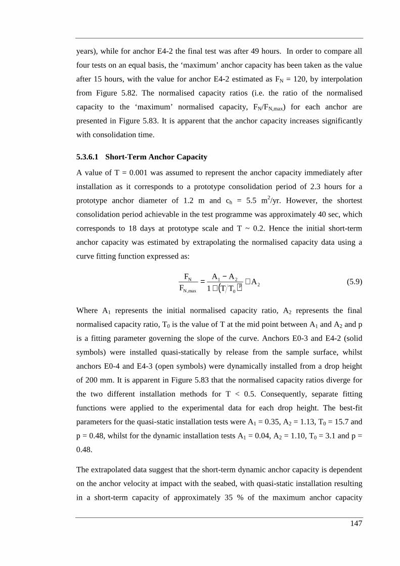
147
years), while for anchor E4-2 the final test was after 49 hours. In order to compare all
four tests on an equal basis, the ‘maximum’ anchor capacity has been taken as the value
after 15 hours, with the value for anchor E4-2 estimated as FN = 120, by interpolation
from Figure 5.82. The normalised capacity ratios (i.e. the ratio of the normalised
capacity to the ‘maximum’ normalised capacity, FN/FN,max) for each anchor are
presented in Figure 5.83. It is apparent that the anchor capacity increases significantly
with consolidation time.
5.3.6.1 Short-Term Anchor Capacity
A value of T = 0.001 was assumed to represent the anchor capacity immediately after
installation as it corresponds to a prototype consolidation period of 2.3 hours for a
prototype anchor diameter of 1.2 m and ch = 5.5 m2/yr. However, the shortest
consolidation period achievable in the test programme was approximately 40 sec, which
corresponds to 18 days at prototype scale and T ~ 0.2. Hence the initial short-term
anchor capacity was estimated by extrapolating the normalised capacity data using a
curve fitting function expressed as:
( ) 2p0
21
max,N
N ATT1
AA
F
F ++
−= (5.9)
Where A1 represents the initial normalised capacity ratio, A2 represents the final
normalised capacity ratio, T0 is the value of T at the mid point between A1 and A2 and p
is a fitting parameter governing the slope of the curve. Anchors E0-3 and E4-2 (solid
symbols) were installed quasi-statically by release from the sample surface, whilst
anchors E0-4 and E4-3 (open symbols) were dynamically installed from a drop height
of 200 mm. It is apparent in Figure 5.83 that the normalised capacity ratios diverge for
the two different installation methods for T < 0.5. Consequently, separate fitting
functions were applied to the experimental data for each drop height. The best-fit
parameters for the quasi-static installation tests were A1 = 0.35, A2 = 1.13, T0 = 15.7 and
p = 0.48, whilst for the dynamic installation tests A1 = 0.04, A2 = 1.10, T0 = 3.1 and p =
0.48.
The extrapolated data suggest that the short-term dynamic anchor capacity is dependent
on the anchor velocity at impact with the seabed, with quasi-static installation resulting
in a short-term capacity of approximately 35 % of the maximum anchor capacity

148
compared with 6 % for dynamic installation. This can be interpreted as resulting from
lower effective stresses around the dynamically installed anchor, possibly due to
entrainment of water in a boundary layer close to the anchor. Tika and Hutchinson
(1999) have commented on the reduction in strength observed in fast rate ring shear
tests, in which water is allowed to penetrate the shear zone. The results of several beam
centrifuge tests seem to support this assertion with the presence of surface water
resulting in greater dynamic anchor penetration depths (see Section 5.2.3.3).
Alternatively Vardoulakis (2002) suggested that strength softening at high strain rates
may in fact be due to thermal softening through the dissipation of mechanical energy
resulting in vaporisation of the pore water within the shear zone and consequently
higher pore pressures.
Pile installation is considered a quasi-static event since it occurs at relatively low
penetration velocities when compared to dynamic anchor impact velocities of 15 m/s in
the centrifuge tests and 25 – 30 m/s expected in the field. Typical short-term pile
capacities in clay range from approximately 25 – 45 % of the maximum pile capacity
(Esrig et al. 1977, Bogard and Matlock 1990), although Seed and Reese (1957) (as cited
in Fleming et al. 1985) reported short-term capacities of only approximately 10 % of the
long-term pile capacity. For UWA kaolin, Chen and Randolph (2007) reported typical
suction caisson installation friction ratios of 0.38, which assuming the short-term
capacity is governed solely by the remoulded shear strength during caisson installation
suggests a capacity immediately after installation of 38 % of the long-term capacity.
Similarly, laboratory tests of torpedo anchors quasi-statically installed in clay
demonstrated capacities immediately after installation of approximately 30 % of the
ultimate anchor capacity (Audibert et al. 2006). By comparison, the extrapolated quasi-
static short-term anchor capacity (FN,0/FN,max = 35 %) reported here is relatively
consistent with the short-term capacities for quasi-statically installed piles, suction
caissons and torpedo anchors.
5.3.6.2 Capacity Increase with Time
The degree of consolidation can be assessed by examining the relative increase in
anchor capacity with time from tests conducted at various time intervals following
installation. The relative increase in anchor capacity was determined through
consideration of the normalized capacity (FN) relative to the immediate capacity (FN,0)

149
and the ultimate long-term capacity (FN,max), and assumed linked to the degree of
consolidation by:
max0,Nmax,N
0,NN
u
u1
FF
FF
∆∆−≈
−−
(5.10)
where ∆u is the excess pore pressure adjacent to the anchor and ∆umax is the maximum
value of ∆u immediately after installation of the anchor. The assumption that the regain
in anchor capacity is proportional to the degree of consolidation may not necessarily be
valid due to stress relaxation effects and changes in radial effective stress during loading
(Randolph 2003). However, Equation 5.10 is considered to be a reasonable approach,
and has been used effectively for suction caissons (Jeanjean 2006). Figure 5.84 shows
the degree of consolidation with time after installation. In general, it can be seen that
consolidation proceeds slightly faster for the dynamically installed anchors (E0-4 and
E4-3).
Also shown in Figure 5.84 are the results of the torpedo anchor laboratory tests reported
by Audibert et al. (2006). Whilst the rate of increase in consolidation and therefore
anchor capacity appears slightly steeper for the torpedo anchor data, there is generally
relatively good agreement with the centrifuge test results. It should be noted that the
tests by Audibert et al. (2006) were conducted in kaolin clay, although the coefficient of
consolidation has not been reported. Consequently, the non-dimensional time factor (T)
for the data presented in Figure 5.84 has been calculated assuming ch = 5.5 m2/yr, as has
been adopted in the centrifuge tests. Given the lower effective stress level of the torpedo
anchor tests, the data should possibly be shifted towards lower values of T, reflecting a
lower ch (see Figure 3.9).
5.3.6.3 t50 and t90
The time required for a dynamically installed anchor to attain its operational capacity
can be evaluated by considering the times for 50 % (t50) and 90 % (t90) consolidation.
The consolidation data for dynamic anchors presented in Figure 5.84 suggests t50 values
of approximately 35 – 350 days for a prototype dynamic anchor with a diameter of 1.2
m and typical values of ch = 3 – 30 m2/yr. Likewise the data indicate t90 values of
approximately 2.4 – 24 years.
150
The consolidation times for high values of the coefficient of consolidation agree with
periods of 1 – 2 years for relatively large offshore piles to achieve their full capacity
(Mirza 1999). However, the dynamic anchor values are much greater than 90 %
consolidation times for suction caissons of around 90 days or less (Jeanjean 2006).
Randolph (2003) showed that dissipation times for open ended piles and suction
caissons are one to two orders of magnitude shorter than for closed ended piles of the
same diameter, since the key dimension is the ‘equivalent diameter’. It is not surprising
therefore that solid dynamic anchors record much larger consolidation times than thin
walled suction caissons. From a practical perspective, however, it is not feasible for an
anchoring system to require several years of consolidation prior to achieving its design
capacity. It is therefore apparent that dynamic anchors should be installed in soils in
which consolidation proceeds sufficiently quickly so as to ensure excessive
consolidation times are avoided. Alternatively, the anchoring system should be designed
such that the anchor is only required to develop a relatively small proportion of its
ultimate capacity prior to loading.
5.3.7 Summary
A total of 138 dynamic anchor drop tests were conducted in the 2 drum centrifuge clay
samples. The tests focused on assessing the influence of the anchor geometry on the
embedment depth and holding capacity performance of dynamically installed anchors
and the effects of consolidation following installation on the dynamic anchor holding
capacity. Unfortunately no usable shear strength information was obtained from Drum 1
due to severe unbalance effects between the drum centrifuge channel and tool table
actuator. In Drum 2, a T-bar test conducted at 1 g indicated a shear strength gradient of
approximately 1.03 kPa/m and an average undrained shear strength ratio of 0.16, both of
which are slightly lower than is typically expected for normally consolidated kaolin clay
samples in the centrifuge.
Impact velocities of up to 20 m/s were recorded using the multiple PERP velocity
measurement system, for dynamic anchor drop heights ranging from 0 – 250 mm. Just
as for the beam centrifuge tests, the impact velocity was found to be heavily dependent
on the drop height. Differences in the frictional losses between the model anchor and
151
installation guide resulted in slight variations in the impact velocity drop height
relationship for the different anchor types.
Considering the range of lengths of the model anchors tested in the drum centrifuge,
normalised tip embedments of 0.9 – 7.7 times the anchor length were observed. In
accordance with the results of the beam centrifuge tests and the results of previous
dynamic anchor centrifuge studies, the data for each individual anchor indicated an
approximately linear increase in embedment with impact velocity. Given this
dependence of embedment depth on impact velocity and the potential for higher anchor
impact velocities, the potential exists for dynamic anchors to achieve much higher
embedment depths than have been measured in the centrifuge tests. Additionally, as
expected, an increase in aspect ratio at a constant mass lead to a reduction in anchor
penetration, and an increase in density at a constant aspect ratio resulted in an increase
in embedment. However, when the density was held constant, so that the mass increased
linearly with aspect ratio, higher penetrations were observed, suggesting that the mass
tends to dominate the influence of the additional frictional resistance provided by the
increased surface area at higher anchor aspect ratios.
Interestingly, the load displacement response observed during the vertical monotonic
extraction of dynamic anchors in the centrifuge was found to be dependent on the
consolidation time provided prior to extraction. Higher consolidation times resulted in
the merging of the Peak 1 and Peak 2 capacities into a single maximum capacity,
suggesting that the dynamic anchor load displacement behaviour can be explained in
terms of the different mobilisation rates of the frictional and end bearing uplift
resistance components. The anchor aspect ratio was also found to influence the load
displacement response, with low aspect ratios resulting in a single maximum capacity
and higher aspect ratios demonstrating the typical dual capacity behaviour. The
transition between these effects was found to occur at aspect ratios of between 6 and 8.
The Peak 1 and Peak 2 holding capacities measured in the drum centrifuge tests
represented efficiencies of 1 – 4 times the anchor dry weight. Predictably, the capacity
of each of the model anchors increased with increasing penetration depth. An increase
in the anchor aspect ratio may lead to an increase in holding capacity due to the
increased frictional resistance over the larger anchor surface area. However, it may also
lead to a reduction in capacity due to the decreased bearing resistance at the anchor
152
padeye. Generally in the drum centrifuge tests, a lower aspect ratio resulted in higher
holding capacities at comparable tip embedment depths.
The results of the tests investigating the influence of post-installation consolidation time
on the dynamic anchor holding capacity indicated that the short-term capacity
immediately after installation was dependent on the rate at which the anchor was
installed. Model anchors quasi-statically installed from the sample surface were found
to provide short-term capacities, relative to the ultimate capacity, which were
comparable to the results of load tests on piles and laboratory tests of torpedo anchors.
In addition, it was found that the regain in anchor capacity following installation could
be linked to the degree of consolidation. Although recorded consolidation times were
significantly lower than have been reported for open-ended piles and thin-walled
suction caissons, consolidation times to attain the maximum dynamic anchor holding
capacity of 1 – 2 years were achieved.
5.4 CONCLUSIONS
Tables 5.10 and 5.11 present the results of over 200 individual centrifuge model tests
forming the dynamic anchor experimental database on which this research is based. The
tests have addressed issues concerning the relationship between impact velocity,
embedment depth and holding capacity and the influences of factors such as the soil
strength characteristics, anchor geometry and loading conditions on these relationships.
The conclusions for this portion of the experimental programme are summarised below:
1. Undrained shear strength measurements from T-bar penetrometer tests in the
drum centrifuge are highly sensitive to vibrations caused by unbalance between
the centrifuge channel and tool table actuator.
2. Due to drop height and sample depth restrictions, dynamic anchor impact
velocities were limited to approximately 30 m/s in the beam centrifuge and 20
m/s in the drum centrifuge. Drag coefficients for zero fluke anchors suggest that
significantly higher impact velocities are possible.
3. For all of the anchors tested, the embedment depth was shown to increase
approximately linearly with impact velocity. This linear relationship was limited

153
to lower threshold velocities of approximately 5 – 10 m/s and is consistent with
behaviour observed in previous dynamic anchor centrifuge tests.
4. Tip embedment depths of up to 3 times the anchor length were recorded for
typical dynamic anchor geometries, representing approximately 45 m at
prototype scale. Embedments of up to almost 8 times the anchor length were
measured for anchors with lower aspect ratios. Given the dependence of
embedment depth on impact velocity, considerably higher embedment depths
are possible by increasing the impact velocity to terminal values in water.
5. The load displacement response of dynamic anchors during vertical monotonic
extraction in the centrifuge was typically characterised by a sharp increase in
load towards an initial maximum capacity followed by a sudden drop in load and
a subsequent increase towards a secondary maximum capacity, generally of
lower magnitude than the initial maximum. The apparent merging of these two
maximum capacities following longer consolidation times and the absence of the
initial maximum capacity for low anchor aspect ratios, support the assumption
that this dual maximum capacity behaviour can be attributed to differential
mobilisation rates of the shaft friction and end bearing resistances during uplift.
6. Vertical monotonic holding capacities of up to 4 times the anchor’s dry weight
were measured. The holding capacity was also found to be dependent on the
penetration depth, with higher shear strengths mobilised at greater embedment
depths. Considering the potential increases in embedment, higher dynamic
anchor holding capacities are also possible.
7. Variations in the anchor tip shape were found to influence the penetration depth
and holding capacity. Reductions in the total anchor surface area, through a
reduction in the number of flukes, resulted in higher penetrations, but also lower
capacities at comparable embedment depths. Higher anchor aspect ratios were
found to result in lower embedment depths; however when the density was held
constant and the mass allowed to increase linearly with aspect ratio, the increase
in embedment due to the increase in anchor mass was greater than the reduction
in embedment due to the increased frictional resistance such that the overall
effect was an increase in penetration depth.

154
8. Long-term sustained loading was found to have minimal influence on the
dynamic anchor holding capacity. A threshold sustained loading level of
between 80 and 90 % of the reference monotonic capacity was observed, below
which the sustained loading was not sufficient to cause failure. An increase in
the sustained loading duration was found to result in a slight reduction in anchor
capacity.
9. Cyclic loading was also found to have minimal influence on the dynamic anchor
holding capacity. However, the average load was found to have a greater
influence on the anchor capacity than the cyclic load amplitude. An increase in
the load duration (number of cycles) resulted in a slight reduction in the anchor
capacity.
10. The dynamic anchor capacity increased with time following installation due to
setup effects. The short-term anchor capacity was found to be dependent on the
rate of anchor installation. The degree of consolidation was assessed by
examining the relative time-scale of the increase in anchor capacity. The tests
indicated that consolidation times for the realisation of 90 % of the ultimate
anchor capacity of approximately 2 years are possible.
155
CHAPTER 6 - EXPERIMENTAL RESULTS FOR
DYNAMIC ANCHOR TESTING IN SILICA AND
CALCAREOUS SAND
6.1 INTRODUCTION
Chapter 5 presented the experimental data from the dynamic anchor tests in normally
consolidated clay. However, substantial oil and gas deposits exist in areas of the world
where the seabed is characterised by silica or calcareous sand sediments. This chapter
presents the experimental results of dynamic anchor tests conducted in the beam
centrifuge in both silica and calcareous sand samples. Evaluation of the behaviour of
dynamically installed anchors in various seabed soil conditions is a significant aspect of
the research project and an important consideration in the commercial application of this
technology.
6.2 SILICA SAND
A single silica sand sample was prepared for the dynamic anchor beam centrifuge tests,
according to the procedure outlined in Section 3.4.2.3. Due to grain size effects in the
centrifuge, the sample was prepared from silica flour, the geotechnical properties of
which have been presented in Table 3.4. In the silica sand sample (Box 10) a total of
two anchor drop tests were conducted to assess both the penetration and holding
capacity performance of dynamically installed anchors in silica sand. The results of the
two anchor drop tests are presented in Table 6.1.
The extremely low penetration depths prevented capacity measurements from being
obtained and consequently the planned test programme was abandoned. The test results
are discussed in more detail below.
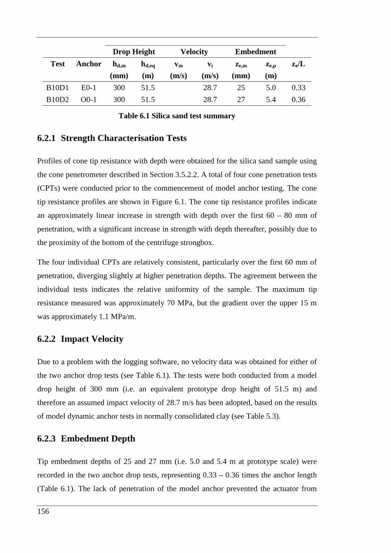
156
Drop Height Velocity Embedment
Test Anchor hd,m hd,eq vm vi ze,m ze,p ze/L
(mm) (m) (m/s) (m/s) (mm) (m)
B10D1 E0-1 300 51.5 28.7 25 5.0 0.33
B10D2 O0-1 300 51.5 28.7 27 5.4 0.36
Table 6.1 Silica sand test summary
6.2.1 Strength Characterisation Tests
Profiles of cone tip resistance with depth were obtained for the silica sand sample using
the cone penetrometer described in Section 3.5.2.2. A total of four cone penetration tests
(CPTs) were conducted prior to the commencement of model anchor testing. The cone
tip resistance profiles are shown in Figure 6.1. The cone tip resistance profiles indicate
an approximately linear increase in strength with depth over the first 60 – 80 mm of
penetration, with a significant increase in strength with depth thereafter, possibly due to
the proximity of the bottom of the centrifuge strongbox.
The four individual CPTs are relatively consistent, particularly over the first 60 mm of
penetration, diverging slightly at higher penetration depths. The agreement between the
individual tests indicates the relative uniformity of the sample. The maximum tip
resistance measured was approximately 70 MPa, but the gradient over the upper 15 m
was approximately 1.1 MPa/m.
6.2.2 Impact Velocity
Due to a problem with the logging software, no velocity data was obtained for either of
the two anchor drop tests (see Table 6.1). The tests were both conducted from a model
drop height of 300 mm (i.e. an equivalent prototype drop height of 51.5 m) and
therefore an assumed impact velocity of 28.7 m/s has been adopted, based on the results
of model dynamic anchor tests in normally consolidated clay (see Table 5.3).
6.2.3 Embedment Depth
Tip embedment depths of 25 and 27 mm (i.e. 5.0 and 5.4 m at prototype scale) were
recorded in the two anchor drop tests, representing 0.33 – 0.36 times the anchor length
(Table 6.1). The lack of penetration of the model anchor prevented the actuator from
157
being moved horizontally the required 43 mm (see Section 3.8.1.2) to enable vertical
extraction of the anchor. Consequently, no vertical extraction test was performed in
either case and the anchor embedment was obtained via direct measurement of the
length of anchor protruding from the sample surface (see Figure 6.2).
Figure 6.3 shows a comparison of the embedment depths achieved in silica sand and
normally consolidated clay. It is apparent that the penetration depths in silica sand are
considerably lower than those achieved with the same anchors at similar impact
velocities in normally consolidated clay. In fact, the measured tip embedments in silica
sand are, on average, only 13.5 % of the embedment depths recorded in the normally
consolidated clay tests. This can be largely attributed to the strength of the silica sand
sample. The high cone tip resistance measured in the CPTs discussed in Section 6.2.1
indicates a relatively large anchor tip bearing resistance to penetration which is likely to
lead to lower anchor embedments.
The low embedment depths may also be partially explained by the undrained conditions
encountered during dynamic anchor installation. Dilatant materials, such as silica flour,
become stronger when they are sheared at a constant volume (i.e. under undrained
conditions). At a constant volume, the soil is not free to dilate and hence negative
excess pore pressures are generated resulting in higher effective stresses and an increase
in the penetration bearing resistance.
As a result of the dilatant nature of silica flour and the relatively high cone tip
resistances encountered, dynamically installed anchors are not likely to achieve
sufficient embedment depths in silica sand to provide an adequate holding capacity.
Hence they are not deemed suitable for use in silica sand sediments.
6.3 CALCAREOUS SAND
The performance of dynamically installed anchors in calcareous sand was investigated
in the beam centrifuge using reconstituted uncemented calcareous sand recovered from
the seabed in the vicinity of the North Rankin platform off the North West coast of
Western Australia. A total of three calcareous sand samples were prepared, although as
mentioned in Section 3.4.2.2, Box 8 was unsuccessfully reconstituted from the sample

158
in Box 7 and has subsequently been excluded from the analysis. The results of the
anchor drop tests conducted in Boxes 7 and 9 are presented in Table 6.2 (see Tables
section). The results of the centrifuge tests in calcareous sand have previously been
reported by Richardson et al. (2005).
6.3.1 Strength Characterisation Tests
Profiles of cone tip resistance with depth were obtained with the cone penetrometer
described in Section 3.5.2.1. The average tip resistance profiles for each sample are
presented in Figure 6.4. Apart from the upper 20 – 40 mm, average cone resistance
profiles in Boxes 7 and 9 (before dynamic anchor testing) indicate a relatively uniform
increase in tip resistance with sample depth.
Box 8 was prepared by reconstituting the sample in Box 7 (see Section 3.4.2.2). The
average cone resistance profile for Box 8 indicates relatively high tip resistances within
the upper 40 mm of the sample compared with Boxes 7 and 9. At greater depths the
measured tip resistance remains relatively constant with depth. This suggests some form
of segregation or non-uniformity within the sample and implies that the reconstitution
method adopted was not effective in producing a sample consistent with those in Boxes
7 and 9. Consequently, the model anchor test results in Box 8 have been excluded from
the analysis.
In Box 9, CPTs were conducted both prior to and at the conclusion of the dynamic
anchor test programme. Figure 6.4 indicates an increase in tip resistance during the
course of testing, with the CPTs conducted after the dynamic anchor test programme
recording higher tip resistances than those conducted before the dynamic anchor tests.
This may be attributed to the sample ‘settling’ to a certain degree due to ramping up and
down of the centrifuge, leading to a maximum density and strength condition after
several ramp up/down cycles.
6.3.2 Impact Velocity
A single PERP installation guide (see Section 3.7.1) was used in the measurement of the
anchor velocities in the calcareous sand tests. These velocities are presented in Table
6.2 and in Figure 6.5 against the equivalent prototype drop height (see Section 4.3.2).
Also included in Figure 6.5 are the velocities measured in the normally consolidated

159
clay tests. As the velocity is independent of the soil properties it is not surprising that
the single PERP velocities measured in the calcareous sand tests agree well with the
single PERP velocities determined for model anchor tests in normally consolidated clay.
However, as mentioned in Section 5.2.2, the single PERP velocities under predict the
expected impact velocity and as such the measured velocities need to be adjusted. The
measured velocities have been adjusted in a similar manner as the single PERP
velocities in the normally consolidated clay tests, with the multiple PERP data
representing an approximate best fit of the single PERP velocities. The adjusted impact
velocities are shown in both Table 6.2 and Figure 6.6.
For the tests in Table 6.2 in which no velocity was measured, the average impact
velocity for the corresponding drop height in Table 5.3 has been adopted. For model
drop heights ranging from 0 to 300 mm, representing equivalent prototype drop heights
of 0 to 51.5 m, impact velocities of up to approximately 30 m/s were determined.
6.3.3 Embedment Depth
The tip embedment depths measured in the calcareous sand tests are presented in Table
6.2. The variation in penetration depth with impact velocity is shown in Figure 6.7.
Over the range of impact velocities considered, tip embedments ranging from
approximately 50 – 110 mm (10 – 22 m prototype) were observed, corresponding to
approximately 0.7 – 1.5 times the anchor length. Medeiros (2001, 2002) report average
tip penetrations for torpedo anchors in uncemented calcareous sand of 15 m,
corresponding to 1.25 times the anchor length and hence indicating good agreement
with the centrifuge test data. The test results in Figure 6.7 indicate a similar trend of
increasing embedment with impact velocity as observed in the normally consolidated
clay tests (see Section 5.2.3.1). Hence, given the potential for dynamic anchor terminal
velocities of approximately 80 m/s (see Section 5.2.2), embedment depths in the order
of 180 mm (36 m at prototype scale) are possible (see Figure 6.8).
It is evident that, at similar impact velocities, the tip embedments in calcareous sand are,
on average, approximately 50 % of the embedment depths measured in normally
consolidated clay and over three times larger than those measured in silica sand. In
calcareous sands, which are characterised by high friction angles and high
compressibility, the end bearing resistance has been shown to be significantly lower at a

160
given stress level than for silica sands (Poulos and Chua 1985). The difference in
bearing resistance is also apparent when comparing the cone tip resistance profiles in
the CPTs conducted in both silica and calcareous sand (Figures 6.1 and 6.4). The silica
sand sample exhibited cone tip resistances that were at least an order of magnitude
greater than those measured in the calcareous sand tests. Hence the lower bearing
resistance should be reflected in higher calcareous sand dynamic anchor embedment
depths.
It is also known that for piles in calcareous sands, very low shaft friction resistances are
common (Randolph 1988). It is generally accepted that these low values of shaft friction
are due to low normal effective stresses acting on the pile shaft as a result of the high
compressibility of the soil. The high soil compressibility may be attributed to crushing
of the highly angular and brittle soil particles during anchor penetration. Hence in
addition to lower end bearing resistances, when compared with silica sands, calcareous
sands also exhibit lower shaft friction resistances, ultimately resulting in higher
embedment depths.
Calcareous sands are also characterised by varying degrees of cementation. This
cementation may enhance the soil strength, although the penetration of the anchor may
also break down the cementation resulting in lower penetration resistances and therefore
higher embedments than in uncemented calcareous sand of identical cone resistance.
6.3.4 Load-Displacement Response
A typical load versus displacement plot during the vertical extraction of a model
dynamic anchor in the beam centrifuge in calcareous sand is presented in Figure 6.9.
Unlike the load displacement response observed during extraction of the model anchors
in normally consolidated clay (see Section 5.2.4), only a single maximum capacity is
recorded. No load spike at Peak 1 is encountered or any subsequent rapid softening;
rather the load steadily builds to a relatively smooth maximum before reducing
gradually with increased vertical displacement. Hence Table 6.2 includes only a single
maximum capacity value and a single displacement value required to mobilise this
capacity.
161
6.3.5 Holding Capacity
The maximum vertical holding capacities measured in the dynamic anchor tests in
calcareous sand ranged from approximately 30 – 55 N (i.e. 1.2 – 2.2 MN at prototype
scale) representing approximately 1 – 2 times the anchor’s dry weight. The dependence
of the ultimate vertical capacity on the embedment depth is shown in Figure 6.10. For
comparison, Figure 6.10 also shows both the Peak 1 and Peak 2 holding capacities
measured in the normally consolidated clay tests. Evidently, the shallower embedment
depths in calcareous sand result in capacities that are generally lower than the Peak 1
capacities in normally consolidated clay. However, it is apparent that the capacities in
calcareous sand are on average approximately 70 – 80 % of the Peak 2 capacities
measured in normally consolidated clay, despite the obvious differences in penetration.
Unfortunately, no field capacity data exists to verify these capacities.
6.3.6 Static Push Tests
Two static installation tests were conducted in Box 9 in order to assess the static
resistance to dynamic anchor penetration. Figure 6.11 shows the variation in static
resistance with penetration depth in both of the static penetration tests. It can be seen
that the static resistance force increases approximately linearly with depth, with good
agreement between the tests over the first 50 mm (10 m at prototype scale) of
penetration. At depths greater than 50 mm, the static resistances diverge slightly,
possibly due to local non-uniformities in the sample, reaching maximum resistances of
approximately 175 N and 225 N (7 MN and 9 MN at prototype scale) at the maximum
penetration depth of approximately 175 mm (35 m at prototype scale).
6.4 CONCLUSIONS
The results of the centrifuge tests in silica and calcareous sands formed a small but
important component of the dynamic anchor centrifuge test database. As in the tests in
normally consolidated clay presented in Chapter 5, these tests assessed the relationship
between impact velocity, embedment depth and holding capacity, but in soils with
vastly different properties. The conclusions derived from the dynamically installed
anchor tests in silica and calcareous sand are summarised below:
162
1. Dynamic anchors are not suitable for use in silica sand sediments. High cone tip
resistances and the dilatant nature of the soil resulted in extremely low
embedment depths which were not sufficient to develop adequate holding
capacities.
2. Dynamic anchors were found to be suitable for use in calcareous sediments. For
impact velocities of up to 30 m/s, tip embedments of up to 1.5 times the anchor
length were recorded. These embedments were significantly lower than the
corresponding embedments in normally consolidated clay, but over three times
larger than those in silica sand. The measured embedment depths span the value
reported from torpedo anchor field trials in uncemented calcareous sand
conducted in Brazilian waters.
3. The embedment depth in calcareous sand increased approximately linearly with
impact velocity in a similar manner to the normally consolidated clay tests.
Given the potential for higher dynamic anchor impact velocities, embedment
depths in the order of 2.4 times the anchor length are considered possible.
4. In calcareous sand, the load displacement response was characterised by only a
single maximum capacity. The dual capacity and rapid softening behaviour
observed in the normally consolidated clay tests was not evident in calcareous
sand.
5. The dynamic anchor holding capacity in calcareous sand was found to be
dependent on the embedment depth, with anchor capacities of 1 – 2 times the
anchor dry weight measured. Considering the potential for higher embedment
depths due to the maximisation of the impact velocity, considerably higher
holding capacities than were measured in the centrifuge tests are possible.

163
CHAPTER 7 - COMPARISON OF EXPERIMENTAL
AND THEORETICAL RESULTS
7.1 INTRODUCTION
In Chapter 4, analytical methods were introduced for evaluating the performance of
dynamically installed anchors, in terms of their impact velocity, embedment depth and
holding capacity. Subsequently Chapters 5 and 6 presented the results of the dynamic
anchor centrifuge tests forming the experimental database for the validation of these
analytical methods. This chapter summarises the comparison between the analytical
methods in Chapter 4 and the test results detailed in Chapters 5 and 6. In particular the
chapter focuses on evaluating the accuracy of the analytical embedment and holding
capacity solutions in both normally consolidated clay and calcareous sand. Successful
calibration of the analytical design models against the centrifuge database resulted in the
development of design charts summarising the potential performance of both zero and
four fluke dynamic anchors at prototype scale. The chapter concludes with a design
example demonstrating the use of the design charts.
7.2 CLAY - BEAM CENTRIFUGE
7.2.1 Impact Velocity
Figure 7.1 shows the comparison between the impact velocities reported in the beam
centrifuge tests in Section 5.2.2 and the theoretical impact velocities described in
Section 4.3.2, accounting for the non-uniform acceleration field in the centrifuge. The
theoretical velocities over predict the measured impact velocities by approximately 12
% over the range of drop heights considered. This can be attributed to frictional energy
losses between the anchor and guide during installation. Similar observations have been
made in previous dynamic anchor centrifuge tests reported by Lisle (2001), Wemmie
(2003), Richardson (2003) and O’Loughlin et al. (2004b).

164
7.2.2 Embedment Depth
The theoretical embedment depth following dynamic anchor installation in normally
consolidated clay in the beam centrifuge was determined according to the method
detailed in Section 4.4.1. For a specific impact velocity and a given set of anchor and
soil properties, this method produced a profile showing the variation in anchor velocity
with depth below the sample surface. The final embedment depth was assessed by
determining the depth at which the anchor velocity became zero. Figure 7.2 shows
example velocity profiles for a model zero fluke anchor (0FA; L/D = 12.5, m = 15
grams, Nc = 12, α = 0.4, CD = 0.24) impacting the sample (su = 1 kPa/m) at velocities of
0, 10, 20 and 30 m/s. Interestingly, in each case the anchor velocity increased during the
early stages of penetration.
7.2.2.1 Back-Calculated Strain Rate Parameter
Uncertainty surrounding strain rate effects during dynamic anchor penetration in fine
grained soils required the strain rate parameter (λ or β) in Equations 4.20 and 4.21 to be
back-calculated from the experimental data. The value of the strain rate parameter was
varied until the embedment depth measured in the beam centrifuge tests matched the
calculated embedment depth, assuming Nc = 12 and α = 0.4 (see Section 4.4.2). The
strain rate parameter values back-calculated from the 0FA embedment data for both the
semi-logarithmic and power rate laws are shown in Figure 7.3. It is evident that for both
rate laws, the back-calculated strain rate parameter values increase with increasing
impact velocity. However, if the strain rate parameter increases with impact velocity,
the embedment depth dependence on velocity is effectively considered twice. Hence the
embedment depth calculations should be performed with a constant strain rate
parameter. Whilst True (1976) and Biscontin and Pestana (2001) reported increases in
the strain rate parameter with increasing strain rate (see Section 2.2.3.1), the apparent
dependence of the strain rate parameter on impact velocity suggests that neither the
semi-logarithmic nor power rate law adequately reflect the soil response during
dynamic anchor installation. The inability of the embedment prediction method to fully
capture the soil behaviour may also be attributed to differences in the flow mechanism
or shear band thickness during penetration, or even changes in the inertial resistance at
high strain rates.

165
The values of λ in Figure 7.3a suggest increases in the undrained shear strength of
approximately 30 – 80 % per log cycle increase in strain rate (v/D). By comparison,
Sheahan et al. (1996) reported λ values of up to 17 % for triaxial compression tests at
strain rates of 0.0014 – 670 %/hr, while Biscontin and Pestana (2001) reported values of
1 – 60 % for vane shear tests conducted at rates of 0.06 – 3000 °/min. Similarly, typical
λ values for field and centrifuge penetrometer tests range from approximately 12 – 20 %
for installation rates of up to 200 mm/s (Boylan et al. 2007, Lehane et al. 2008). On
average, the semi-logarithmic strain rate parameter values determined from the dynamic
anchor tests are considerably higher than those reported in the laboratory and field tests.
This discrepancy may be attributed to the limitations of the semi-logarithmic law,
particularly when considering strain rates which cover several orders of magnitude. For
instance, in the centrifuge, a 6 mm diameter anchor impacting the sample at 30 m/s will
result in strain rates of v/D = 5000 s-1, which are 25000 times larger than the reference
strain rate (v/D = 0.2 s-1, 5 mm diameter T-bar installed at 1 mm/s). By comparison, the
laboratory and field tests mentioned above were typically conducted at strain rates
covering a much smaller range of values.
The limitations of the semi-logarithmic method can be seen by comparing the
normalised shear strength (su/su,ref) due to strain rate effects for both the semi-
logarithmic and power rate laws (see Figure 7.4). At low strain rates, good agreement is
obtained between the semi-logarithmic law with λ ≈ 0.2 and the power law with β = 0.1.
However at a normalised strain rate of γ& / γ& ref = 25000 (i.e. 5000/0.2), a value of λ = 0.4
is required to achieve the same normalised shear strength as the power law with β = 0.1.
Therefore the λ values of 0.3 – 0.8 back-calculated from the experimental data represent
some form of ‘secant’ fit to a power law model. Hence for strain rates covering several
orders of magnitude, the power law rate function is likely to provide improved accuracy
over the semi-logarithmic model. Given the limitations of the logarithmic model and the
apparent improvements afforded by the power law model, the predicted embedments
presented in Section 7.2.2.2 have been evaluated using the power law rate model with
an average value of β = 0.12.
The λ values in Figure 7.3a are also somewhat higher than values of 3 – 36 % reported
by Lisle (2001), Wemmie (2003), Richardson (2003) and O’Loughlin et al. (2004b) for
previous dynamic anchor centrifuge tests. These differences can be attributed to

166
improvements made to the embedment prediction model, including the use of a strain
rate rather than velocity rate dependence formulation and accounting for the variation in
the anchor weight as the anchor moves through the gravitational acceleration field. In
addition, the current calculations have been made using multiple PERP or adjusted
single PERP velocities (see Section 5.2.2), which are higher and more accurate than the
single PERP velocities utilised in these previous studies.
7.2.2.2 Predicted Embedment Depth
The theoretical embedment depth of the 0FAs in the beam centrifuge was calculated
using the power law rate model given in Equation 4.21, with an average value of β =
0.12. The calculations were based on an ellipsoid nosed anchor (see Table 3.5 for
anchor dimensions) with an average mass of 14.5 grams and a normally consolidated
clay sample with an average shear strength gradient of approximately 1.07 kPa/m (see
Table 5.1). Note that the calculations were actually performed using the average
polynomial shear strength profile given by Equation 5.3, with a = 0.013 kPa/m2 and b =
0.870 kPa/m, which correspond to the average linear shear strength gradient of 1.07
kPa/m (see Table 5.1). Figure 7.5 shows the measured and predicted embedment depths
for impact velocities of up to 35 m/s. For comparison, the embedment depths calculated
assuming average lower and upper bound values of β = 0.08 and 0.14 respectively, have
also been shown. It is apparent that whilst β = 0.12 provides relatively good agreement
with the experimental data for impact velocities between 15 and 30 m/s, at lower impact
velocities the embedment depth is underestimated by as much as 24 %. This
underestimation at low impact velocities highlights the limitations of the model in
predicting embedments over a wide range of potential strain rates. However, it is
difficult to make conclusive statements regarding the accuracy of these predictions
given the lack of centrifuge test data at velocities below 15 m/s. That said, field
installations of dynamic anchors will typically occur at velocities greater than 15 m/s, as
maximisation of the impact velocity has been shown to lead to higher embedment
depths and therefore higher holding capacities. Hence, the need for accurate embedment
predictions at lower impact velocities is not as critical as at moderate to high impact
velocities.
The experimental data presented in Section 5.2.3.1 demonstrated that the dynamic
anchor embedment depth depended on the velocity of the anchor at the point of impact
167
with the sample surface. Hence, given the potential for 0FAs to achieve theoretical
terminal velocities in the order of 80 m/s (see Section 5.2.2), extrapolation of the
experimental data suggested embedment depths in the order of 300 mm (60 m at
prototype scale). Figure 7.6 shows that by extending the embedment predictions to
similar impact velocities, potential embedment depths of approximately 360 mm (72 m
at prototype scale) are possible, assuming β = 0.12. Therefore following optimisation of
the impact velocity, dynamic anchors appear capable of achieving normalised
embedments of up to 4.8 times the anchor length.
It should be noted that as the strain rates encountered during dynamic anchor
installation in the centrifuge are n times larger than those encountered at prototype
scale, the penetration strain rate effects in the field will be less than those experienced in
the centrifuge (assuming a constant strain rate parameter). Consequently, higher
penetration depths should be expected in the field when compared with the centrifuge
test data.
7.2.2.3 Sensitivity Analysis
The influence of the tip bearing capacity factor, shaft adhesion factor, shear strength
gradient and drag coefficient on the calculated embedment depth were assessed via
sensitivity analysis. The calculations in Section 7.2.2.2 were based on the following
assumptions:
• Nc = 12
• α = 0.4
• k = 1.07 kPa/m (a = 0.013 kPa/m2, b = 0.870 kPa/m)
• CD = 0.24
For the sensitivity analysis, values of Nc were assumed to range from 8 – 20 based on
the results of cone penetration tests (Lunne et al. 1997). In addition, the shaft adhesion
factor was varied from 0 (no shaft friction) to 1 (undisturbed shear strength mobilised
along anchor shaft), whilst typical shear strength gradients for normally consolidated
clay in the centrifuge range from 1 to 1.5 kPa/m. The drag coefficient was assumed to
vary from 0 (no inertial drag resistance) to 0.7 (drag coefficient of cylindrical projectiles
reported by True 1976). A summary of the embedment depth sensitivities is provided in
Table 7.1 and Figures 7.7 – 7.10.
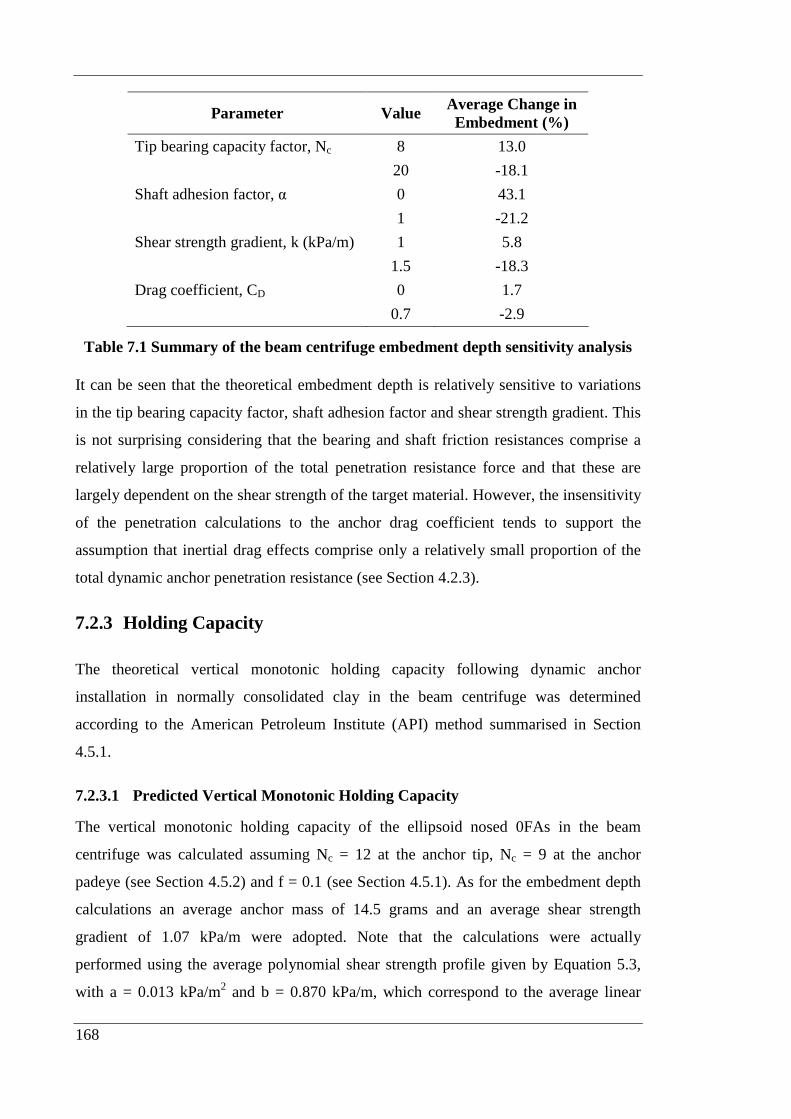
168
Parameter Value Average Change in Embedment (%)
Tip bearing capacity factor, Nc 8 13.0
20 -18.1
Shaft adhesion factor, α 0 43.1
1 -21.2
Shear strength gradient, k (kPa/m) 1 5.8
1.5 -18.3
Drag coefficient, CD 0 1.7
0.7 -2.9
Table 7.1 Summary of the beam centrifuge embedment depth sensitivity analysis
It can be seen that the theoretical embedment depth is relatively sensitive to variations
in the tip bearing capacity factor, shaft adhesion factor and shear strength gradient. This
is not surprising considering that the bearing and shaft friction resistances comprise a
relatively large proportion of the total penetration resistance force and that these are
largely dependent on the shear strength of the target material. However, the insensitivity
of the penetration calculations to the anchor drag coefficient tends to support the
assumption that inertial drag effects comprise only a relatively small proportion of the
total dynamic anchor penetration resistance (see Section 4.2.3).
7.2.3 Holding Capacity
The theoretical vertical monotonic holding capacity following dynamic anchor
installation in normally consolidated clay in the beam centrifuge was determined
according to the American Petroleum Institute (API) method summarised in Section
4.5.1.
7.2.3.1 Predicted Vertical Monotonic Holding Capacity
The vertical monotonic holding capacity of the ellipsoid nosed 0FAs in the beam
centrifuge was calculated assuming Nc = 12 at the anchor tip, Nc = 9 at the anchor
padeye (see Section 4.5.2) and f = 0.1 (see Section 4.5.1). As for the embedment depth
calculations an average anchor mass of 14.5 grams and an average shear strength
gradient of 1.07 kPa/m were adopted. Note that the calculations were actually
performed using the average polynomial shear strength profile given by Equation 5.3,
with a = 0.013 kPa/m2 and b = 0.870 kPa/m, which correspond to the average linear

169
shear strength gradient of 1.07 kPa/m (see Table 5.1). The shaft adhesion factor was
determined according to Equations 4.35 and 4.36, resulting in α = 1. Given the dual
maximum capacity behaviour observed in the beam centrifuge tests (see Section 5.2.4),
the measured Peak 1 and Peak 2 capacities have been compared with the theoretical
holding capacities in Figures 7.11 and 7.12 respectively. It is apparent that the predicted
capacity, assuming α = 1, provides reasonable agreement with the Peak 1 data, but
noticeably over predicts the Peak 2 holding capacities. Better agreement with the
experimental data is obtained with α = 0.8 and 0.5 for the Peak 1 and Peak 2 holding
capacities respectively (see Figures 7.11 and 7.12). A shaft adhesion factor of 0.8 agrees
with the findings of dynamic anchor centrifuge model tests reported by O’Loughlin et
al. (2004b).
Despite the satisfactory agreement obtained between the measured and predicted
capacities, a significant degree of variability exists amongst the measured capacities. It
is likely that these discrepancies can be attributed to variations in the consolidation time
permitted following installation, differences in the anchor mass or slight variations in
the undrained shear strength between samples. Section 5.3.6 showed that the anchor
capacity increases with consolidation time following installation, due to setup. Whilst
every effort was made to ensure similar consolidation times in each of the beam
centrifuge tests (i.e. approximately 13 min or 1 year at prototype scale), accurate times
were not recorded in a large number of cases. In addition, whilst the average shear
strength gradients in each of the beam centrifuge samples were similar, slight variations
between samples and even variations within individual samples between tests conducted
at the beginning and at the end of the test programme may have introduced
inconsistencies in the measured capacity data. Taking into account these potential
differences, the API framework is seen to provide a satisfactory method for predicting
the range of dynamic anchor holding capacities measured in the beam centrifuge tests.
In Section 5.2.5.1, the anchor capacities measured in the beam centrifuge tests were
found to increase with increasing embedment depth, due to the mobilisation of higher
undrained shear strengths. The predicted capacities shown in Figures 7.11 and 7.12
support these observations, indicating that in soils where the shear strength increases
with depth, the anchor capacity also increases with increasing penetration depth. This
highlights the importance of accurately predicting the dynamic anchor embedment
170
depth in order to be able to accurately predict the subsequent holding capacity. Given
the potential for the zero fluke dynamic anchors to achieve penetration depths in the
order of 360 mm (72 m at prototype scale; see Section 7.2.2.2), extending the holding
capacity predictions to similar depths indicates potential vertical monotonic holding
capacities in the order of 135 – 200 N (5.4 – 8.0 MN at prototype scale) for shaft
adhesion factors ranging from α = 0.5 – 1 (see Figure 7.13). These capacities represent
efficiencies of approximately 4.7 – 7.0 times the anchor dry weight.
7.2.3.2 Sensitivity Analysis
Just as for the embedment depth predictions, sensitivity analyses were also performed
on the predicted holding capacity. The calculations in Section 7.2.3.1 assumed:
• Nc = 12 at the anchor tip
• Nc = 9 at the padeye
• f = 0.1
• α = 0.8
• k = 1.07 kPa/m (a = 0.013 kPa/m2, b = 0.870 kPa/m)
For the sensitivity analysis, the bearing capacity factor at the anchor tip was assumed to
range from 8 – 20. The influence of the padeye bearing capacity factor was found to
depend on the degree of hole closure. Therefore the effects of both the padeye bearing
capacity factor and degree of hole closure were combined, with the limiting cases
defined as either no hole closure (f = 0) in which case no padeye bearing resistance is
generated, i.e. f.Nc = 0 and full hole closure (f = 1), in which case the maximum bearing
capacity factor for a circular foundation is assumed, i.e. f.Nc = 9. Similar to Section
7.2.2.3, the shaft adhesion factor was assumed to vary from 0 to 1 and the shear strength
gradient from 1 to 1.5 kPa/m. A summary of the holding capacity sensitivities is
provided in Table 7.2 and Figures 7.14 – 7.17. Note that for comparison, Figures 7.14 –
7.17 include the Peak 1 capacities from the 0FA centrifuge tests.
It is apparent that the theoretical holding capacity is relatively sensitive to variations in
the tip bearing capacity factor, shaft adhesion factor and shear strength gradient.
However, as a result of relatively low padeye embedment depths, the holding capacity is
insensitive to variations in the padeye bearing resistance.

171
Parameter Value Average Change in Capacity (%)
Tip bearing capacity factor, Nc 8 -6.2
20 12.5
Padeye bearing resistance, f.Nc 0 -0.6
9 5.4
Shaft adhesion factor, α 0 -33.9
1 8.5
Shear strength gradient, k (kPa/m) 1 -11.3
1.5 9.7
Table 7.2 Summary of beam centrifuge holding capacity sensitivity analysis
One of the key arguments proposed for dynamic anchors is that their performance is less
dependent on accurate assessment of the seabed shear strength profile, since lower shear
strengths permit greater penetrations, and vice versa. Hence, given the holding capacity
dependence on embedment depth, the capacity is effectively a function of the energy of
the anchor at impact (i.e. impact velocity and mass). Section 7.2.2.3 demonstrated that
the predicted embedment depth was relatively sensitive to variations in the undrained
shear strength gradient, with Table 7.2 showing a similar sensitivity for the predicted
holding capacity. These relative sensitivities have been combined in Figure 7.18, with
the holding capacity plotted against impact velocity for the limiting undrained shear
strength gradients of 1 and 1.5 kPa/m. It is evident that the predicted holding capacity is
relatively insensitive to variations in the shear strength gradient, particularly at low
impact velocities; although at higher impact velocities an increase in the undrained
shear strength gradient provided higher holding capacities.
7.2.4 Summary
Due to frictional effects, the theoretical impact velocity in the beam centrifuge over
predicted the measured impact velocities by approximately 12 %, over the range of drop
heights considered.
Back-calculated values of the strain rate parameter increased with impact velocity,
indicating potential limitations of the embedment depth prediction method and in
particular the semi-logarithmic and power law rate functions. Theoretical embedment
depths calculated using the power law rate model, assuming a constant strain rate

172
parameter, provided adequate agreement with the measured centrifuge data at velocities
above 15 m/s. However, for impact velocities below 15 m/s, the embedment depth was
under estimated by as much as 24 %. Given the dependence of penetration depth on
impact velocity, the calculations indicated that embedments of up to 4.8 times the
anchor length were possible at 0FA terminal velocities approaching 80 m/s. The
theoretical embedment depth was found to be sensitive to variations in the bearing
capacity factor, shaft adhesion factor and undrained shear strength gradient.
The API method with α = 0.8 and 0.5 provided reasonable predictions of the measured
Peak 1 and Peak 2 capacities respectively. The calculations supported the experimental
observations of an increase in holding capacity with embedment depth. Given the
potential for 0FA embedment depths of up to 4.8 times the anchor length, the
calculations suggested that capacities approaching 7.0 times the anchor dry weight were
possible. The theoretical holding capacity was found to be sensitive to the selection of
the tip bearing capacity factor, shaft adhesion factor and variations in the undrained
shear strength gradient. However, the shear strength gradient influences both the
embedment depth and holding capacity, with lower shear strengths resulting in lower
capacities but higher embedments and vice versa. The resulting relative insensitivity of
the anchor performance to accurate assessment of the undrained shear strength profile
represents a key advantage of dynamically installed anchors.
7.3 CLAY - DRUM CENTRIFUGE
7.3.1 Impact Velocity
The impact velocities measured in the drum centrifuge tests for the 0FAs, four fluke
anchors (4FAs) and hemispherically tipped anchors with L/D < 7 and L/D > 7 are
presented in Figure 7.19 compared with the theoretical impact velocity determined
according to the method outlined in Section 4.3.2. As in the beam centrifuge tests, it is
apparent that the theoretical impact velocity over predicts the measured velocities.
Again, this can be attributed to friction developed between the anchor and the
installation guide. As mentioned in Section 5.3.2, the various anchor types generated
different levels of friction depending on the anchor geometry and the installation guide
used, resulting in differences in the accuracy of the impact velocity calculations.

173
However, on average, the theoretical impact velocity over predicted the measured
velocity by approximately 36 %.
7.3.2 Embedment Depth
The theoretical embedment depths in the drum centrifuge were calculated using the
method outlined in Section 4.4.1.
7.3.2.1 Back-Calculated Strain Rate Parameter
Once again, the strain rate parameter values were back-calculated from the measured
embedment depth data. Since no accurate shear strength information was available for
Drum 1, strain rate parameter values have only been calculated based on the results of
tests conducted in Drum 2. For the 0FA tests, the strain rate parameter was calculated
assuming Nc = 12 and α = 0.4 (see Section 4.4.2). The strain rate parameter values back-
calculated from the 0FA embedment data for both the semi-logarithmic and power rate
laws are shown in Figure 7.20. As in the beam centrifuge tests (see Section 7.2.2.1), the
strain rate parameter values for both rate laws increased with increasing impact velocity.
These results once again highlight the limitations of the rate laws in describing the soil
response during dynamic anchor installation. Somewhat surprisingly however, the λ
values of 0.15 – 0.3, are lower than values of 0.3 – 0.8 reported in the beam centrifuge
tests (see Section 7.2.2.1), although good agreement is obtained with back-calculated λ
values of 0.03 – 0.36 from previous dynamic anchor centrifuge tests reported by Lisle
(2001), Wemmie (2003), Richardson (2003) and O’Loughlin et al. (2004b). This
discrepancy may be partially attributed to the lower impact velocities in the drum
centrifuge. In the 0FA tests in the drum centrifuge, a maximum impact velocity of
approximately 15 m/s corresponded to λ = 0.3. At a similar impact velocity, the beam
centrifuge tests indicated an average value of λ = 0.4, which considering the variability
of the back-calculated strain rate parameter values is relatively comparable. Given the
advantages of the power law model (see Section 7.2.2.1), the predicted embedment
depths for the 0FAs in Section 7.3.2.2 have been calculated assuming an overall average
strain rate parameter value of β = 0.06.
For the 4FA tests, the strain rate parameter was calculated assuming Nc = 12, Ncf = 7.5
and α = 0.4 (see Section 4.4.2). Figure 7.21 shows the back-calculated strain rate
parameter values for both the semi-logarithmic and power rate laws. Note that only a

174
limited number of 4FA tests were conducted in the drum centrifuge, many of which
were conducted at impact velocities of 0 m/s. However, the overall best-fit to the 4FA
data indicates an apparent increase in the strain rate parameter with increasing impact
velocity. In addition, the λ values in Figure 7.21a are consistent with the values of λ
determined for the 0FA tests. The 4FA embedment calculations presented in Section
7.3.2.2 are based on the power rate law with an average value of β = 0.08.
Strain rate parameters were also calculated for the tests conducted in Drum 2 with
anchors H0-3, H0-5, H0-9 and H0-13 (see Section 3.6.5), assuming Nc = 10 and α = 0.4
(see Section 4.4.2). The mass and aspect ratio of each of these anchors is summarised in
Table 7.3 and the back-calculated strain rate parameters from these tests are presented in
Figure 7.22. For all but anchor H0-5, the strain rate parameter appeared to increase with
impact velocity, although only a limited number of tests were conducted with each
anchor. Interestingly, the magnitude of the back-calculated strain rate parameter seemed
to vary with the anchor type (aspect ratio). This goes further to suggest that the
embedment depth prediction model does not completely reflect the soil behaviour
during dynamic anchor penetration. That said, the embedment predictions presented in
Section 7.3.2.2 are based on the power law rate model using individual average strain
parameters for each anchor type (see Table 7.3). The average β value of 0.07 compares
favourably with the average values from the 0 and 4FA tests. Hence the overall average
β value for the drum centrifuge tests was also 0.07.
Anchor L/D Mass Average β
(g)
H0-3 2 2.0 0.09
H0-5 4 4.7 0.11
H0-9 6 1.9 0.03
H0-13 12 4.7 0.06
Average 0.07
Table 7.3 Power law strain rate parameters for hemispherically tipped anchors
7.3.2.2 Predicted Embedment Depth
The theoretical embedment depths for the 0FAs in the drum centrifuge were calculated
using the power law rate model with β = 0.06. Figure 7.23 shows the measured and
predicted embedment depths for anchor E0-3. For comparison, the embedment depths

175
calculated assuming the overall average strain rate parameter value of β = 0.07 have
also been shown. Similar predictions for anchors E0-4 and E0-5 are provided in Figures
7.24 and 7.25 respectively. It is apparent that the embedment depths calculated using
both the average 0FA strain rate parameter (β = 0.06) and the overall drum centrifuge
average strain rate parameter (β = 0.07) provide reasonable agreement with
experimental data for each individual anchor. Despite this, at low impact velocities, the
embedments for anchors E0-3 and E0-5 are slightly under estimated.
For the 4FAs, the theoretical embedment depths were calculated assuming β = 0.08 as
discussed in Section 7.3.2.1. Figure 7.26 shows the measured and predicted embedment
depths for anchor E4-2. For comparison, the embedment depths calculated assuming the
overall average strain rate parameter value of β = 0.07 have also been provided. Similar
predictions for anchor E4-3 are provided in Figure 7.27. The theoretical embedment
depths calculated assuming both strain rate parameter values provide good agreement
with the experimental data for each anchor, despite a relatively small number of tests.
Figures 7.28, 7.29, 7.30 and 7.31 show the measured and theoretical embedment depths
for anchors H0-3, H0-5, H0-9 and H0-13 respectively. The embedment depths have
been calculated assuming the average strain rate parameter values given in Table 7.3.
For comparison, the embedment depths calculated assuming the overall average strain
rate parameter value of β = 0.07 have also been shown. As expected, the anchor specific
strain rate parameters provided the best agreement with the experimental data, although
for all but anchor H0-13, the embedment depths calculated using the overall average
strain rate parameter varied noticeably from the centrifuge test data. It should be noted
that anchor H0-13 had an aspect ratio of 12, which is very close to the aspect ratio of the
0 and 4FAs (i.e. L/D = 12.5), suggesting that the strain rate parameter may also depend
on the anchor aspect ratio. Such an observation indicates another potential limitation of
the embedment prediction model.
Since the calculation procedure adopted for the drum centrifuge tests was similar to that
used for the beam centrifuge, further sensitivity analyses were not undertaken.

176
7.3.3 Holding Capacity
The theoretical vertical monotonic holding capacities for the model anchors in the drum
centrifuge were determined using the API method outlined in Section 4.5.1.
7.3.3.1 Predicted Vertical Monotonic Holding Capacity
The holding capacities of the 0FAs in the drum centrifuge were calculated assuming Nc
= 12 for the anchor tip, Nc = 9 at the anchor padeye (see Section 4.5.2) and f = 0.1 (see
Section 4.5.1). The shaft adhesion factor was calculated according to Equations 4.35
and 4.36 resulting in α = 1. Figure 7.32 shows the comparison between the theoretical
capacity and the measured Peak 1 and Peak 2 holding capacities for anchor E0-3 in the
drum centrifuge. Figures 7.33 and 7.34 show similar comparisons for anchors E0-4 and
E0-5 respectively. It is apparent that for both anchors E0-3 and E0-4, the Peak 1
capacities in particular, vary significantly at comparable embedment depths. This can be
attributed to setup effects, with longer consolidation times resulting in higher anchor
capacities (see Section 5.3.6). The predicted capacity with α = 0.8 provided reasonable
estimates of the Peak 1 capacities for anchors E0-3 and E0-4 following consolidation
periods of approximately 14 min (1.1 years at prototype scale). However, for tests
conducted with longer consolidation times (i.e. up to approximately 15 hours or 68
years at prototype scale), the theoretical capacity under predicted the measured capacity
by approximately 40 %. The increase in capacity due to consolidation is discussed
further in Section 7.3.3.2. For anchor E0-5, with an average consolidation time of
approximately 16 min (1.2 years at prototype scale), α = 0.6 provided good agreement
with the measured Peak 1 capacities. The theoretical capacity assuming α = 0.5 – 0.6
provided good agreement with the Peak 2 capacity data for each of the model anchors
across the range of consolidation times considered. These adhesion factor values are
consistent with α = 0.8 and 0.5 for the Peak 1 and Peak 2 capacities in the beam
centrifuge tests (see Section 7.2.3.1).
For the 4FAs, the theoretical holding capacity was calculated assuming Nc = 12 at the
anchor tip, Nc = 9 at the anchor padeye, Ncf = 7.5 for the anchor flukes (see Section
4.5.2) and f = 0.1. It should be noted that complete closure of the entry pathway behind
the anchor flukes was assumed. The shaft adhesion factor was calculated according to
Equations 4.35 and 4.36 resulting in α = 1. Note also that the same adhesion factor was
177
assumed for both the anchor shaft and flukes. Figures 7.35 and 7.36 show the measured
and theoretical holding capacities for anchors E4-2 and E4-3 respectively. Just as in the
0FA tests, the measured holding capacities varied with consolidation time at comparable
embedment depths. The theoretical capacity assuming α = 1 provided good agreement
with the measured Peak 1 capacity data for anchor E4-2 following approximately 5 min
(0.4 years at prototype scale) of consolidation. However, following approximately 49
hours (224 years at prototype scale) of consolidation the holding capacity was under
predicted by approximately 30 %. For anchor E4-3, the theoretical capacity assuming α
= 0.7 provided good agreement with the Peak 1 capacity following approximately 7 min
(0.5 years at prototype scale) of consolidation, although the capacity following 15 hours
(68 years at prototype scale) of consolidation was under predicted by approximately 40
% with the same adhesion factor. The influence of consolidation is considered further in
Section 7.3.3.2. Shaft adhesion factors of α = 0.7 and α = 0.4 provided the best
agreement with the Peak 2 capacity data for anchors E4-2 and E4-3 respectively.
The theoretical holding capacities of the model anchors with different aspect ratios were
evaluated assuming Nc = 10 at both the anchor tip and padeye (hemispherical ends; see
Section 4.5.2), α = 1 and f = 0.1. Figures 7.37, 7.38, 7.39 and 7.40 show the measured
and theoretical holding capacities for anchors H0-3, H0-5, H0-9 and H0-13 respectively.
It should be noted that due to the lack of shear strength data from Drum 1, only the test
results from Drum 2 have been considered. In addition, only anchor H0-13 exhibited
Peak 2 capacities. Each of the anchors was extracted following approximately 14 min
(1.1 years at prototype scale) of consolidation. For anchors H0-3 and H0-5, the
theoretical capacities assuming α = 0.8 provide good agreement with the measured
capacities, with α = 0.7 providing a better fit to the experimental data for anchor H0-13.
These shaft adhesion factors are consistent with the values determined for the 0 and
4FAs. Somewhat surprisingly however, α = 0.4 was required to match the measured
capacities for anchor H0-9.
As the same method was used to predict the dynamic anchor capacity in both the beam
and drum centrifuge tests, it was not considered necessary to reconsider the sensitivity
of the calculation procedure to changes in the various parameter values.

178
7.3.3.2 Consolidation Solutions
Section 5.3.6 showed that the dynamic anchor capacity increases with time following
installation in fine grained soils due to setup. Since thixotropic effects in kaolin clay are
considered negligible (Skempton and Northey 1952), the time dependent increase in
anchor capacity was attributed to consolidation of the soil in the vicinity of the anchor.
Randolph and Wroth (1979) presented a closed form solution for the radial
consolidation of soil around a driven pile, leading to the development of a realistic
method for modelling the dissipation of excess pore pressures following pile installation
(Cavity Expansion Method; see Section 2.3.3). The method assumes that the initial pore
pressure distribution is a function of the rigidity index, Ir = G/su of the soil, with typical
values of Ir ranging from 50 – 500 (Randolph 2003). The change in the degree of
consolidation with non-dimensional time (T) for anchors E0-3, E0-4, E4-2 and E4-3 in
the drum centrifuge (see Section 5.3.6.2) is shown in Figure 7.41 along with the degree
of consolidation predicted by the Cavity Expansion Method (CEM) for Ir = 50 and 500.
For comparison, the results of torpedo anchor laboratory tests reported by Audibert et
al. (2006) have also been shown. It can be seen that the theoretical solution for the
upper bound value of Ir = 500 provides a relatively accurate representation of the
measured increase in capacity for the anchors which were installed dynamically
(anchors E0-4 and E4-3), but overestimates the anchor capacity regain for the quasi-
statically installed anchors (anchors E0-3 and E4-2). For T > 10, Ir = 500 agrees well
with the torpedo anchor data, whilst for T ≤ 10 a lower degree of consolidation is
observed. The extent of the conformity between the analytical solution and the
experimental data, particularly for the dynamic installation tests, suggests that cavity
expansion techniques may be appropriate for determining the consolidation behaviour
and therefore capacity regain with time following dynamic anchor installation.
Kehoe (1989), as reported by Bullock et al. (2005), indicated that setup following pile
driving is dominated by the regain in shaft frictional resistance. Hence it was assumed
that the time dependent regain in dynamic anchor capacity was due entirely to the
recovery of shaft and fluke friction and that any time changes in bearing resistance were
assumed to have negligible impact on setup. Section 7.3.3.1 demonstrated that the API
method (see Section 4.5.1) provided reasonable predictions of the Peak 1 anchor
capacity for consolidation times of up to approximately 1 year at prototype scale, with
179
adhesion factor values of up to α = 1. However, for consolidation times greater than 1
year, the capacity predictions assuming α = 1 significantly under predicted the measured
capacity for both the 0 and 4FAs. Assuming Nc = 12 for the anchor tip, Nc = 9 for the
anchor padeye and Ncf = 7.5 for the anchor flukes, adhesion factor values required to
achieve the measured holding capacities were back-calculated for the various time
intervals following installation (see Figure 7.42). An expected increase in α with
increasing consolidation time was observed, reflecting the increase in soil shear strength
with dissipation of the excess pore pressures. A value of α = 1 indicates that the shear
strength mobilised along the anchor shaft and flukes during vertical extraction is
equivalent to the undisturbed soil shear strength. However, as can be seen in Figure
7.42, for T > 4, i.e. after approximately 1 year of consolidation (assuming ch = 5.5 m2/yr
and D = 1.2 m), back-calculated values of α exceed 1, indicating an increase in the shear
strength above the intact strength. The assumption of constant bearing factors for the
anchor tip and edges of the flukes contributes to the high long-term α values shown in
Figure 7.42. There is little data in the literature as guidance for estimating any increase
in the bearing resistance, but if it were assumed that the bearing resistance increased by
50 % in the long-term the final α values would be reduced by ~15 %, from around 2
down to ~1.7. This is still significantly greater than unity.
With the adhesion factor limited to α = 1, according to API guidelines (see Section 4.5),
shear strength gradients of up to 1.7 kPa/m were required for agreement between the
measured and predicted capacities. This is considerably higher than the shear strength
gradient of 1.03 kPa/m measured in the T-bar penetrometer test (see Section 5.3.1) and
higher than typical shear strength gradients for normally consolidated kaolin clay in the
centrifuge of 1 – 1.5 kPa/m. Whilst the results may be complicated somewhat by the
unusual load displacement response observed during extraction (see Section 5.3.4), the
results tend to suggest that following long periods of post-installation consolidation,
undrained shear strengths higher than the initial undisturbed shear strength can be
mobilised by dynamic anchors to resist uplift loading. It should be noted that this
analysis has focused on the Peak 1 capacity, although back-calculated adhesion factor
values for Peak 2 would be some 25 to 50 % lower than those determined for Peak 1.
180
Based on the information in Figure 7.42 it was possible to develop an alternative
expression for the adhesion factor to account for the apparent increase in shear strength
with increasing consolidation time. The expression was obtained by fitting a curve to
the back-calculated α data, of the form:
( ) 2p0
21
TT1α+
+α−α=α (7.1)
where α1 represents the initial adhesion factor, α2 represents the final adhesion factor, T0
is the value of T at the mid point between α1 and α2 and p is a fitting parameter
governing the slope of the curve. It should be noted that due to the difficulty associated
with determining an appropriate cut-off velocity between quasi-static and dynamic
installation, a single curve has been fitted to the adhesion factor data in Figure 7.42
despite an apparent divergence between the values of α for quasi-static and dynamic
installation for T < 1. The best-fit parameters for the experimental data were α1 = 0.04,
α2 = 2.2, T0 = 9.5 and p = 0.42. Figure 7.43 shows the measured Peak 1 capacity data
for anchor E0-3 compared with the predicted capacities for revised adhesion factor
values of α = 0.4 and α = 1.8, representing the values following the minimum and
maximum consolidation times respectively. It can be seen that the modified adhesion
factors provide reasonable agreement with both the minimum and maximum holding
capacities for anchor E0-3.
7.3.4 Summary
On average, the theoretical impact velocity in the drum centrifuge over predicted the
impact velocities of the various model anchors by 36 %. The discrepancy between the
measured and theoretical impact velocity was attributed to friction, with differences in
the anchor geometry and installation guide leading to slight variations in the accuracy of
the calculations for the different anchor types.
Back-calculated strain rate parameter values were found to increase with impact
velocity, reinforcing the potential limitations of the semi-logarithmic and power rate
laws identified in the beam centrifuge analysis. Strain rate parameter values from the
drum centrifuge were generally lower than the values determined in the beam centrifuge
and provided reasonable agreement with the results of previous dynamic anchor
181
centrifuge tests. The 0 and 4FA theoretical embedment depths calculated using the
power law rate model, with an average strain rate parameter provided reasonable
agreement with the experimental data, although the embedment depths at low impact
velocities were slightly under predicted. For the anchors with varying aspect ratios,
anchor specific strain rate parameter values provided better agreement with the
centrifuge data, indicating further potential inadequacies in the embedment prediction
method.
Theoretical holding capacities calculated according to the API method with adhesion
factor values between 0.8 and 1 provided reasonable predictions of the dynamic anchor
holding capacity for post-installation consolidation times of up to approximately 1 year
at prototype scale. Agreement between the measured and theoretical holding capacities
following longer periods of consolidation required adhesion factor values considerably
higher than α = 1, suggesting the mobilisation of shear strengths higher than the
undisturbed strength. Cavity expansion solutions for radial consolidation around solid
driven piles provided a reasonable approximation of the dynamic anchor post-
installation consolidation behaviour.
7.4 CALCAREOUS SAND – BEAM CENTRIFUGE
7.4.1 Impact Velocity
The dynamic anchor impact velocity is independent of the soil properties, hence the
theoretical impact velocity for the calcareous sand tests was identical to the velocity for
the normally consolidated clay tests in the beam centrifuge (see Sections 4.3.2 and
7.2.1). Figure 7.44 shows the comparison between the predicted and adjusted impact
velocities for the 0FA tests in calcareous sand. Friction between the anchor and the
guide during installation resulted in the theoretical impact velocity over predicting the
measured velocities by approximately 17 %. This is consistent with the degree of
accuracy obtained in the normally consolidated clay tests in the beam centrifuge.

182
7.4.2 Embedment Depth
The theoretical embedment depth following dynamic anchor installation in calcareous
sand in the beam centrifuge was determined according to the method outlined in Section
4.6.1.
7.4.2.1 Back-Calculated Strain Rate Parameter
The strain rate parameter (λ or β) in Equations 4.20 and 4.21 was back-calculated from
the measured experimental data assuming Nq = 32, from cone penetration tests (CPTs)
conducted during the experimental programme (see Section 4.6.1.2), and βCALC = 0.42
from static penetration tests (see Section 6.3.6). The in situ vertical effective stress was
calculated assuming an average effective soil unit weight of 5.2 kN/m3 (Richardson et
al. 2005). Figure 7.45 shows the strain rate parameter values back-calculated from the
experimental data for both the semi-logarithmic and power rate laws. The strain rate
parameter values appear to increase with increasing impact velocity, although a
significant degree of variability exists, with several tests indicating a negative strain rate
parameter, i.e. a reduction in strength with increasing strain rate, which is physically
unlikely. The values of λ in Figure 7.45a indicate increases in the undrained shear
strength of up to approximately 25 % per log cycle increase in strain rate. This is
comparable to the average value of λ = 0.26 back-calculated from dynamic anchor
centrifuge tests in normally consolidated clay reported by O’Loughlin et al. (2004b).
However, the average value of λ = 0.09 for the calcareous sand tests, suggests lower
strain rate effects than in normally consolidated clay. In fact, Figure 7.45 indicates
negligible strain rate effects at low impact velocities. This is consistent with the reported
findings of CPTs conducted at rates of 0.2 – 1 mm/s in slightly cemented calcareous
sand (Joer et al. 1998). However, Figure 7.45 also indicates considerably higher strain
rate effects at higher impact velocities. This behaviour could possibly be attributed to
more complex phenomena than purely viscous effects, such as dilation, or it could also
reflect the limitations of the rate models in analysing the behaviour of dynamic anchors
during penetration of calcareous sediments. The strain rate parameter values in Figure
7.45a are also somewhat higher than the values reported by Richardson et al. (2005)
based on analysis of the same test data. The discrepancy can be attributed to
improvements in the embedment depth prediction model and the use of adjusted single

183
PERP impact velocities (see Section 6.3.2) as opposed to the non-adjusted velocities
reported by Richardson et al. (2005).
Considering the advantages of the power law rate model over the semi-logarithmic
model, and to ensure consistency with the normally consolidated clay tests, the
embedment depths in Section 7.4.2.2 have been calculated using the power law rate
model with an average strain rate parameter of β = 0.03.
7.4.2.2 Predicted Embedment Depth
The theoretical embedment depth for the 0FAs in calcareous sand was calculated
assuming β = 0.03 as described in Section 7.4.2.1. Since several different 0FAs were
used in the calcareous sand tests, the calculations were based on an anchor with an
average mass of 14.7 grams. Figure 7.46 shows the measured and theoretical
embedment depths for the 0FA calcareous sand tests. Whilst the calculations under
estimate the embedment depth at vi = 0 m/s by approximately 20 %, in general, the
theoretical embedment depths provide good agreement with the experimental data.
However, due to the variability of the measured embedment depths, the embedment
predictions in calcareous sand were not as accurate as those in normally consolidated
clay.
Terminal velocities of approximately 80 m/s were determined for the 0FAs (see Section
5.2.2); however, sample depth and drop height restrictions in the centrifuge limited the
impact velocity to approximately 30 m/s. Therefore, given the dependence of the
embedment depth on impact velocity, considerably higher embedments are likely
following maximisation of the anchor impact velocity. Extending the embedment depth
predictions to impact velocities of 80 m/s indicates potential embedment depths of up to
3.1 times the anchor length in calcareous sand (see Figure 7.47).
7.4.2.3 Sensitivity Analysis
The influence of the tip bearing capacity factor, adhesion factor and effective soil unit
weight on the calculated embedment depth in calcareous sand was assessed via
sensitivity analysis. The calculations in Section 7.4.2.2 were based on the following
assumptions:
• Nq = 32

184
• βCALC = 0.42
• γ΄ = 5.2 kN/m3
For the sensitivity analysis, values of Nq were assumed to range from 20 – 50 based on
the variation in the back-calculated bearing capacity factor during the CPTs.
Determination of appropriate bearing capacity factors in calcareous sand is notoriously
difficult, given that Nq decreases significantly as the stress level increases, due to
decreasing peak friction angles and the increased compressibility of the soil (Randolph
1988). The adhesion factor (βCALC) was assumed to vary from 0 – 0.5, based on values
reported by Abbs et al. (1988) for piles in calcareous sand. According to the soil
properties in Table 3.3, minimum and maximum values of the effective soil unit weight
were 4.3 kN/m3 and 6.8 kN/m3 respectively. A summary of the embedment depth
sensitivities is provided in Table 7.4 and Figures 7.48 – 7.50.
Parameter Value Average Change in Embedment (%)
Tip bearing capacity factor, Nq 20 33.8
50 -26.4
Adhesion factor, βCALC 0 6.0
0.5 -0.9
Effective unit weight, γ΄ (kN/m3) 4.3 14.9
6.8 -17.7
Table 7.4 Summary of calcareous sand embedment depth sensitivity analysis
The results suggest that the theoretical embedment depth in calcareous sand is relatively
sensitive to variations in the tip bearing capacity factor and the effective unit weight of
the soil. However, the calculated embedment is also relatively insensitive to variations
in the adhesion factor, suggesting that the shaft friction comprises a relatively small
proportion of the total penetration resistance.
7.4.3 Holding Capacity
The holding capacity of the dynamic anchors installed in calcareous sand was calculated
according to the method described in Section 4.6.2.
185
7.4.3.1 Predicted Vertical Monotonic Holding Capacity
The vertical monotonic holding capacity of the 0FAs in calcareous sand was evaluated
assuming a bearing capacity factor at the anchor padeye given by the bearing capacity
factors of flat plates in silica sand (see Section 4.6.2.2). For a friction angle of 40° (see
Table 3.3), the padeye bearing capacity factors taken from Figure 4.21 ranged from 2.0
– 5.3 for the range of measured embedment depths. Using these bearing capacity
factors, the adhesion factor was back-calculated by varying βCALC until the theoretical
capacity matched the capacity measured in the centrifuge tests. Note that no reverse end
bearing resistance was considered as the extraction was assumed to take place under
drained conditions. Interestingly, an average back-calculated value of βCALC = 0.42 was
determined from the measured capacity data. Encouragingly, this was identical to the
value of βCALC obtained from the static penetration tests adopted in the embedment
analysis (see Section 7.4.2.1). The theoretical holding capacity calculated assuming an
average bearing capacity factor of Nq = 3.3 and βCALC = 0.42 is presented in Figure 7.51
together with the holding capacities measured in the centrifuge tests. It is apparent that
the predicted capacity provides good agreement with the experimental capacity data.
Embedment depth predictions in Section 7.4.2.2 indicated potential embedment depths
for 0FAs in calcareous sand of approximately 230 mm (46 m at prototype scale). Given
the increase in capacity with embedment depth, theoretical holding capacities of up to
approximately 140 N (5.6 MN at prototype scale) have been calculated, representing
efficiencies of approximately 5 times the anchor dry weight (see Figure 7.51). These
efficiencies are comparable to the lower end extrapolated efficiencies determined for the
0FAs in normally consolidated clay (see Section 7.2.3.1) and highlight the potential for
the use of dynamic anchors in calcareous sediments.
7.4.3.2 Sensitivity Analysis
Just as for the embedment depth predictions, sensitivity analyses were also performed
on the theoretical holding capacity. The calculations in Section 7.4.3.1 were based on
the following assumptions:
• Nq = 3.3
• f = 1
• βCALC = 0.42

186
• γ΄ = 5.2 kN/m3
For the sensitivity analysis, the bearing capacity factor at the anchor padeye was
assumed to range from 2.0 – 5.3 based on the bearing capacity factors for flat plate
anchors in silica sand. Full hole closure was assumed in the calculations, although
potential values of f range from 0 to 1. The combined effects of the degree of hole
closure and the padeye bearing capacity factor gave limiting cases of the padeye bearing
resistance of f.Nq = 0 (assuming no hole closure) and f.Nq = 5.3 (full hole closure with
the maximum bearing capacity factor). As mentioned in Section 7.4.2.3, the adhesion
factor was assumed to range from 0 – 0.5, whilst the effective unit weight of the soil
varied from 4.3 – 6.8 kN/m3. A summary of the holding capacity sensitivities is
provided in Table 7.5 and Figures 7.52 – 7.54.
Parameter Value Average Change in Capacity (%)
Padeye bearing resistance, f.Nq 0 -6.6
5.3 4.0
Adhesion factor, β 0 -53.0
0.5 10.1
Effective unit weight, γ΄ (kN/m3) 4.3 -9.9
6.8 17.6
Table 7.5 Summary of calcareous sand holding capacity sensitivity analysis
It can be seen that the theoretical holding capacity in calcareous sand is sensitive to
variations in both the adhesion factor and effective soil unit weight. However, the
calculations are also relatively insensitive to variations in the padeye bearing resistance,
largely as a result of the low padeye embedments encountered in calcareous sand. In the
normally consolidated clay tests, it was shown that the overall holding capacity
performance of dynamic anchors was relatively insensitive to variations in the
undrained shear strength profile since lower shear strengths permitted greater
penetrations, and vice versa. Similarly in calcareous sand, both the embedment depth
and holding capacity predictions are relatively sensitive to variations in the effective soil
unit weight. Combining these relative sensitivities by plotting the holding capacity
against impact velocity for the limiting effective soil unit weights of 4.3 and 6.8 kN/m3
allows the overall sensitivity of dynamically installed anchors to the effective soil unit
weight to be evaluated (see Figure 7.55). It is evident that the predicted holding capacity

187
is relatively insensitive to variations in the effective unit weight, hence dynamic anchors
provide a significant advantage over other conventional anchoring systems in that
accurate assessment of the seabed strength properties is not required prior to
installation.
7.4.4 Summary
The theoretical impact velocity for the calcareous sand tests over predicted the
measured impact velocities by approximately 17 %. The accuracy of the theoretical
velocity was comparable to that determined in the normally consolidated clay tests in
the beam centrifuge.
Despite a significant degree of variability, back-calculated values of the strain rate
parameter appeared to increase with impact velocity. In general, the magnitude of the
strain rate effects was lower than observed in normally consolidated clay. At low strain
rates, the rate effects were found to be negligible, although at higher strain rates, back-
calculated values of the strain rate parameter were, in some instances, similar to those
reported in previous dynamic anchor studies. These findings highlight the limitations of
the semi-logarithmic and power rate laws in assessing the embedment depth of dynamic
anchors, with the variability and high magnitude of the strain rate parameter at high
strain rates potentially reflecting more complicated phenomena than purely viscous
effects. Despite this, theoretical embedment depths calculated using the power rate law
with an average strain rate parameter value provided good estimates of the measured
centrifuge embedment data in calcareous sand. The calculations indicated that following
maximisation of the dynamic anchor impact velocity, embedment depths of up to 3.1
times the anchor length are possible, compared with 4.8 times the anchor length in
normally consolidated clay.
Adhesion factor values back-calculated from the holding capacity data indicated an
average value which coincided with the adhesion factor adopted in the embedment
analysis. The theoretical holding capacity provided good agreement with the capacities
measured in the centrifuge tests. Given potential embedment depths of up to 3.1 times
the anchor length at terminal velocities approaching 80 m/s, the theoretical holding
capacity calculations indicated possible vertical monotonic holding capacities of up to 5
times the anchor weight, compared with 4.7 – 7.0 in normally consolidated clay. The

188
holding capacity performance of dynamically installed anchors was found to be
relatively insensitive to variations in the effective unit weight of the target material,
thereby providing dynamic anchors with a significant advantage over conventional
anchoring systems.
7.5 DYNAMIC ANCHOR DESIGN CHARTS
Two major research objectives were outlined in Section 1.5. The first of these objectives
was the establishment of an extensive centrifuge database to investigate the
geotechnical performance of dynamically installed anchors (see Chapters 5 and 6). The
second objective focused on the development of analytical design tools for predicting
the penetration and holding capacity behaviour of dynamic anchors. The earlier sections
of this chapter summarised the comparison of the individual embedment and capacity
prediction models with the experimental data and indicated that reasonable predictions
of both the penetration depth and holding capacity could be made using these methods.
However, from a practical perspective, and to improve the usability of these techniques,
the analyses have been combined in the form of dynamic anchor design charts for 0 and
4FAs in both normally consolidated clay and calcareous sand. Note that these design
charts have been presented in prototype units only, despite the analytical methods used
being calibrated from centrifuge model test data.
7.5.1 0FA – Normally Consolidated Clay
The embedment depth and holding capacity design charts for the standard 0FA (see
Table 3.5 and Figure 3.15) in normally consolidated clay are presented in Figures 7.56
and 7.57. The results have been presented for 50, 75, 100 and 125 tonne anchor masses
between shear strength gradient limits of 1 – 1.5 kPa/m. Figure 7.58 shows the variation
in capacity of a 100 tonne 0FA for limiting coefficient of consolidation values of ch = 3
– 30 m2/yr at a shear strength gradient of 1 kPa/m. The calculations were based on the
following assumptions:
• Nc = 12 at the anchor tip and Nc = 9 at the anchor padeye
• α = 0.4 during installation
• During extraction α given by Equation 7.1
189
• Figures 7.56 and 7.57 based on 1 year of consolidation with ch = 5.5 m2/yr
• CD = 0.24
• Power rate law with β = 0.09 (average of beam, β = 0.12 and drum, β = 0.06)
• 10 % closure of entry pathway, i.e. f = 0.1
• Vertical monotonic loading – undrained conditions
7.5.2 4FA – Normally Consolidated Clay
The embedment depth and holding capacity design charts for the standard 4FA (see
Table 3.7 and Figure 3.18) in normally consolidated clay are presented in Figures 7.59
and 7.60. The results have been presented for 50, 75, 100 and 125 tonne anchor masses
between shear strength gradient limits of 1 – 1.5 kPa/m. Figure 7.61 shows the variation
in capacity of a 100 tonne 4FA for limiting coefficient of consolidation values of ch = 3
– 30 m2/yr at a shear strength gradient of 1 kPa/m. The calculations were based on the
following assumptions:
• Nc = 12 at the anchor tip, Nc = 9 at the anchor padeye and Ncf = 7.5 for the
anchor flukes
• α = 0.4 during installation
• During extraction α given by Equation 7.1
• Figures 7.59 and 7.60 based on 1 year of consolidation with ch = 5.5 m2/yr
• CD = 0.63
• Power rate law with β = 0.08
• 10 % closure of entry pathway behind anchor shaft (i.e. f = 0.1), full closure
behind anchor flukes
• Vertical monotonic loading – undrained conditions
7.5.3 0FA – Calcareous Sand
The embedment depth and holding capacity design charts for the standard 0FA (see
Table 3.5 and Figure 3.15) in calcareous sand are presented in Figures 7.62 and 7.63.
The results have been presented for 50, 75, 100 and 125 tonne anchor masses between
effective soil unit weight limits of 4.3 – 6.8 kN/m3. The calculations were based on the
following assumptions:

190
• Nq = 32 at the anchor tip and Nq = 3.3 at the anchor padeye
• βCALC = 0.42 during both installation and extraction
• CD = 0.24
• Power rate law with β = 0.03
• Full closure of entry pathway, i.e. f = 1
• Vertical monotonic loading – drained conditions
7.5.4 Design Example
As an example, the design charts have been used in the analysis of a hypothetical design
problem. The site proposed for the anchoring of a MODU is characterised by soft
normally consolidated clay with a shear strength gradient of 1 kPa/m and coefficient of
consolidation of ch = 5.5 m2/yr. If an uplift capacity of 3.0 MN is required following 1
year of consolidation, what dynamic anchor options are available? See Figure 7.64.
0FA 4FA
m vi,min m vi,min
(tonnes) (m/s) (tonnes) (m/s)
50 70 50 48
75 44 75 26
100 28 100 12
125 14 125 0
Table 7.6 Design example – dynamic anchor options Stage I
If strong lateral ocean currents restrict the drop height such that a maximum impact
velocity of only 40 m/s is possible, what options remain available?
0FA 4FA
m vi,min m vi,min
(tonnes) (m/s) (tonnes) (m/s)
100 28 75 26
125 14 100 12
125 0
Table 7.7 Design example – dynamic anchor options Stage II
How far will the anchor penetrate at these velocities? See Figure 7.65.

191
0FA 4FA
m vi,min ze,min m vi,min ze,min
(tonnes) (m/s) (m) (tonnes) (m/s) (m)
100 28 46 75 26 27
125 14 42 100 12 25
125 0 26
Table 7.8 Design example – dynamic anchor options Stage III
If the 100 tonne 0FA was the selected option and it was decided that an impact velocity
of 30 m/s would be targeted, what is the ultimate anchor capacity and how long would it
take to achieve 50 % and 90 % of this capacity, considering subsequent soil analysis
actually indicated ch = 3 m2/yr.
According to Figure 7.66, the ultimate anchor capacity is approximately 5 MN, t50 = 0.3
years and t90 = 60 years.
7.6 CONCLUSIONS
This chapter has presented the comparison of analytical impact velocity, embedment
depth and holding capacity design methods with the results of centrifuge model tests for
the validation of these techniques and the development of dynamic anchor design tools.
In general, the techniques adopted proved successful in predicting the performance of
dynamically installed anchors in both normally consolidated clay and calcareous sand
soil conditions. The main findings are summarised below:
1. On average, the theoretical impact velocity over predicted the measured impact
velocity by approximately 15 % in the beam centrifuge and 36 % in the drum
centrifuge. The over prediction was attributed to friction between the anchor and
the installation guide.
2. Back-calculated strain rate parameter values increased with increasing impact
velocity in both the normally consolidated clay and calcareous sand samples,
indicating potential limitations of the semi-logarithmic and power rate functions
in assessing dynamic anchor embedment depths. The power law model, with a
constant strain rate parameter, was expected to provide improved accuracy over

192
the semi-logarithmic formulation, particularly over a wide range of strain rates.
The strain rate parameter values determined from the drum centrifuge tests were
typically lower than those from the beam centrifuge tests. Strain rate effects in
calcareous sand were found to be negligible at low impact velocities.
3. In normally consolidated clay, the embedment depth predicted using the power
law model with an average strain rate parameter value provided reasonable
agreement with the zero and four fluke anchor data in both the beam and drum
centrifuges, although the embedment depth at low impact velocities was under
estimated by as much as 24 %. For the anchors with lower aspect ratios, anchor
specific strain rate parameters provided improved agreement. The embedment
depth predicted using the average back-calculated strain rate parameter for
calcareous sand compared favourably with the experimental data.
4. The simplified API pile capacity method was found to provide reasonable
predictions of the vertical monotonic holding capacity of dynamic anchors in
normally consolidated clay for post-installation consolidation times of up to 1
year. For longer consolidation times an apparent increase in the soil shear
strength above the undisturbed strength was required for agreement between the
measured and theoretical capacities. A modified adhesion factor was adopted to
reflect the increase in frictional resistance with time after installation. Cavity
expansion solutions for the radial consolidation of soil around a driven pile
provided a reasonable approximation of the consolidation behaviour of dynamic
anchors following installation. The theoretical capacity calculated in calcareous
sand provided good agreement with the measured capacity data.
5. Given the potential for dynamic anchors to attain higher impact velocities than
were achievable in the centrifuge, the theoretical calculations indicate potential
embedment depths of up to 4.8 times the anchor length in normally consolidated
clay and 3.1 times the anchor length in calcareous sand. These embedments
correspond to vertical monotonic holding capacities of up to 7 and 5 times the
dry weight of the anchor in normally consolidated clay and calcareous sand
respectively.
6. Dynamic anchor embedment depths and holding capacities are both relatively
sensitive to variations in the soil strength characteristics. However, the
193
dependence of the capacity on embedment depth effectively results in an overall
insensitivity of the holding capacity performance to the soil strength. Lower
strengths result in lower capacities, but also higher embedments and vice versa.
Advantageously dynamic anchors therefore do not require precise knowledge of
the strength characteristics of the seabed material prior to installation.
7. Ultimately, both the embedment and holding capacity methods adopted were
found to provide acceptable predictions of the geotechnical behaviour of zero
and four fluke dynamic anchors. The successful calibration of these methods
against the centrifuge database resulted in the subsequent production of dynamic
anchor design charts for both normally consolidated clay and calcareous sand
soil conditions.


195
CHAPTER 8 - CONCLUSIONS AND FURTHER
RESEARCH
8.1 INTRODUCTION
Dynamically installed anchors have been proposed as a cost-effective alternative to
conventional anchoring systems for offshore structures in deepwater environments. This
dissertation has focused on investigating the geotechnical performance of dynamic
anchors through the calibration of analytical techniques against an extensive centrifuge
test database. The penetration and holding capacity performance of dynamic anchors
was evaluated experimentally in normally consolidated clay and silica and calcareous
sand samples, under monotonic, sustained and cyclic loading conditions. The centrifuge
test data were compared with the results of analytical embedment and capacity
prediction methods for the development of robust and versatile dynamic anchor design
tools. This chapter presents the major research findings, the implications of these
findings for the offshore industry and recommendations for further research.
8.2 MAIN FINDINGS
8.2.1 Experimental Modelling in Normally Consolidated Clay
The installation and subsequent loading of model dynamic anchors in normally
consolidated clay was successfully carried out in both the beam and drum centrifuges.
For impact velocities exceeding a lower threshold of 5 – 10 m/s the dynamic anchor
embedment depth was found to increase approximately linearly with impact velocity.
Relatively high embedment depths at velocities below this threshold indicated a strong
embedment depth dependence on the anchor mass with the anchor continuing to
accelerate initially within the soft upper sediments. Penetration depths measured in the
centrifuge tests were also found to depend on the anchor geometry, including the tip
shape, aspect ratio and fluke configuration.
196
The load displacement response of the model dynamic anchors during vertical
monotonic extraction in the centrifuge was typically characterised by a sharp increase in
load to an initial maximum capacity followed by a sudden drop in load and a subsequent
increase to a secondary maximum. This behaviour appears to be a result of non-
simultaneous mobilisation of the bearing and frictional resistance during extraction,
with the initial maximum capacity and rapid softening attributed to high (and brittle)
frictional resistance and the secondary peak indicating a more gradual mobilisation of
the bearing resistance. This is supported by experimental data indicating a merging of
the two capacities following longer consolidation times and the absence of the initial
maximum capacity at low anchor aspect ratios. It was shown that the dual capacity
behaviour was not caused by the dynamic anchor installation process.
With the soil shear strength increasing with depth, dynamic anchor capacities under
vertical monotonic loading were found to depend markedly on the penetration depth of
the anchor. Holding capacities were also found to vary with time following installation
due to consolidation effects. Short-term anchor capacities immediately following
installation depended on the impact velocity and the degree of consolidation was
quantified through analysis of the relative time-scale of the regain in anchor capacity.
Cyclic and long-term sustained loading of dynamically installed anchors in the
centrifuge had minimal influence on the ultimate anchor holding capacity. However,
sustained loading indicated a potential threshold loading level of between 80 and 90 %
of the reference monotonic capacity above which sustained loading may lead to a
reduction in the anchor capacity. Under cyclic loading, the influence of the mean load
on the anchor capacity appeared to override the effect of the cyclic load amplitude.
Increases in the duration of loading under both cyclic and sustained loading conditions
led to a slight reduction in anchor capacity.
8.2.2 Experimental Modelling in Silica and Calcareous Sand
Centrifuge testing of model dynamic anchors indicated that they were not suitable for
use in silica sand. This was attributed to the failure of the anchors to embed beyond 40
% of the anchor length, preventing the generation of capacities considered sufficient for
offshore applications.
197
Similar tests in uncemented calcareous sand demonstrated the potential of dynamic
anchors for use in carbonate soils. Despite penetration depths considerably lower than
those in normally consolidated clay, the embedment depths were sufficient for the
model dynamic anchors to achieve vertical monotonic holding capacities of up to 70 %
of the average capacity measured in the normally consolidated clay tests. The test
results also indicated an approximately linear increase in embedment with impact
velocity and an increase in holding capacity with embedment depth. Given the potential
for higher impact velocities, higher embedment depths, and consequently higher holding
capacities, are likely.
8.2.3 Analytical Methods and Design Tools
An analytical prediction method for the embedment depth was developed, based on
conventional bearing and frictional resistance theory but incorporating allowances for
viscous enhanced shearing resistance and inertial drag resistance. Strain rate parameters
back-calculated from the experimental data increased with impact velocity, suggesting
that the semi-logarithmic and power law functions used in quantifying the viscous strain
rate effects were not capable of fully capturing the soil response during dynamic anchor
installation. The power law, with a constant strain rate parameter was found to provide
improved accuracy over the semi-logarithmic law, particularly over strain rates covering
several orders of magnitude. In normally consolidated clay, the back-calculated strain
rate parameter values, particularly at low impact velocities, were in general agreement
with values reported in previous dynamic anchor centrifuge tests. In calcareous sand,
strain rate effects at low impact velocities were negligible. Embedment depths predicted
using the power law model with an average strain rate parameter were found to provide
good agreement with the zero and four fluke anchor data, although the calculations
tended to under estimate the embedment at low impact velocities. The calculations also
indicate the potential for considerably higher embedment depths at higher impact
velocities.
An existing simplified pile capacity technique was successfully implemented to predict
the vertical monotonic holding capacity of dynamically installed anchors in normally
consolidated clay for prototype consolidation times of up to approximately 1 year. For
longer consolidation times a modified adhesion factor, based on back-calculated values
198
from the centrifuge tests, was adopted to account for the apparent increase in shaft
friction above the original shear strength of the soil. A similar pile capacity method was
found to provide accurate predictions of the holding capacity of dynamic anchors in
calcareous sand.
The successful calibration of the embedment depth and holding capacity prediction
methods against the experimental data in both normally consolidated clay and
calcareous sand highlighted the suitability of these methods as dynamic anchor design
tools. Combining the individual embedment and capacity models enabled the
development of dynamic anchor design charts relating the impact velocity to the
penetration depth and holding capacity for zero and four fluke dynamic anchors. The
design charts are intended to be indicative of the potential anchor performance, at
prototype scale, in order to increase the understanding of the geotechnical behaviour of
dynamically installed anchors and thereby improve industry confidence in the concept.
8.3 APPLICATION TO INDUSTRY
With installation and procurement costs for conventional foundation technologies
increasing rapidly with water depth, dynamically installed anchors represent a
financially attractive development for the offshore oil and gas industry. Despite this
their use is scarce. Improved industry confidence in the geotechnical performance and
reliability of dynamic anchors is required before widespread implementation can be
achieved. From a practical point of view, this section details likely performance data for
typical dynamic anchors with the aim of highlighting aspects of the study relevant to the
industry.
Dynamic anchor impact velocities in the centrifuge were limited to approximately 30
m/s. However, terminal velocity calculations indicate potential impact velocities in the
field of up to 80 m/s for zero fluke anchors and 40 m/s for four fluke anchors. Given the
embedment depth dependence on impact velocity, a typical 15 m long, 1.2 m diameter,
100 tonne dynamic anchor would therefore be likely to achieve embedment depths in
normally consolidated clay of up to 90 m and 57 m in the zero and four fluke
configurations respectively. Further optimisation of the anchor geometry has the
199
potential of delivering additional increases in impact velocity, which in turn should
translate to higher penetration depths in the field.
Following installation, the short-term anchor capacity in normally consolidated clay is
expected to range from approximately 5 – 35 % of the ultimate long-term capacity,
indicating setup factors of approximately 3 – 20. For long-term capacities of up to 7 MN
(assuming a shear strength gradient of 1 kPa/m), these suggest vertical monotonic
holding capacities immediately after installation of up to approximately 2.5 MN.
Assuming typical values of ch = 3 – 30 m2/yr, the increase in anchor capacity with time
is reflected in consolidation times of 35 – 350 days for 50 % consolidation and 2.4 – 24
years for 90 % consolidation. Cyclic and sustained loading of dynamically installed
anchors is not expected to reduce the anchor capacity by more than 15 %. Given the
dependence of holding capacity on embedment depth, optimisation of the anchor impact
velocity will also translate into higher anchor capacities.
In uncemented calcareous sand, a typical zero fluke dynamic anchor, impacting the
seabed at a velocity of up to 80 m/s, will penetrate to a maximum embedment depth of
approximately 45 m. At this depth, the anchor is expected to achieve a vertical
monotonic holding capacity of up to 4.5 MN. Just as in normally consolidated clay,
optimisation of the anchor geometry has the potential of further increasing the
embedment depth and holding capacity of dynamic anchors in calcareous sand.
8.4 RECOMMENDATIONS FOR FURTHER RESEARCH
A degree of uncertainty remains regarding strain rate and inertia effects during dynamic
anchor installation. Direct measurement of the anchor velocity and displacement during
installation would assist in quantifying these effects and thereby aid in the calibration of
the embedment prediction model. Additional experimental data are required to
investigate the influence of the anchor geometry on the penetration performance of
dynamic anchors, in order to facilitate verification of the embedment model for different
anchor types.
A limited number of cyclic and sustained loading tests were undertaken in this study. It
is recommended that further experimental modelling should focus on increasing the

200
understanding of the behaviour of dynamic anchors under cyclic and sustained loading
conditions. Specifically this should be aimed at addressing the influence of the load
frequency, magnitude and amplitude on the holding capacity of the anchor. In addition,
dynamic anchors installed in offshore environments are subjected to inclined rather than
purely vertical loads. Hence any testing undertaken should also investigate the ability of
dynamic anchors to withstand monotonic, sustained or cyclic loads with inclined
orientations.
The test programme described in this research evaluated the performance of
dynamically installed anchors in normally consolidated clay, silica sand and calcareous
sand samples. However, offshore sites are often also characterised by higher sensitivity
or overconsolidated clays or layered soil stratigraphies. Therefore experimental testing
should be undertaken to assess the behaviour of dynamic anchors under a range of soil
conditions.
Field tests, even at a reduced scale, would prove invaluable in evaluating the
embedment depth and holding capacity of dynamic anchors. Not only would field
testing provide information for verification of the experimental results obtained in the
centrifuge model tests, but it would also allow further calibration of the design models
without the added complexities of centrifuge modelling. Given the relative infancy of
the concept, field testing is considered an essential component of any further research
on dynamically installed anchors.
201
REFERENCES
Abbs, A. F., Waterton, C., Bell, R. Khorshid, M. S. and Jewell, R. J. (1988). Evaluation
of pile friction from conductor tests. Proc. International Conference on Calcareous
Sediments, Vol. 2, 607-616.
Allersma, H. G. B., Kierstein, A. A. and Maes, D. (2000). Centrifuge modelling on
suction piles under cyclic and long term vertical loading. Proc. International
Offshore and Polar Engineering Conference, Seattle, USA, Vol. 2, 334-341.
American Petroleum Institute (2000). Recommended practice for planning, designing
and constructing fixed offshore platforms – working stress design, RP2A-WSD, 21st
Edition, Washington, 55-58.
Araujo, J. B., Machado, R. D. and Medeiros, C. J. (2004). High holding power torpedo
pile – results from the first long term application. Proc. International Conference on
Offshore Mechanics and Arctic Engineering, Vancouver, OMAE2004-51201.
Aubeny, C. P., Murff, J. D. and Roesset, J. M. (2001). Geotechnical issues in deep and
ultra deep waters. International Journal of Geomechanics, Vol. 1, No. 2, 225-247.
Aubeny, C. P. and Dunlap, W. (2003). Penetration of cylindrical objects in soft mud.
Proc. IEEE Oceans 2003, Vol. 4, 2068-2073.
Aubeny, C. P. and Shi, H. (2006). Interpretation of impact penetration measurements in
soft clays. Journal of Geotechnical and Geoenvironmental Engineering, ASCE,
Vol. 132, No. 6, 770-777.
Audibert, J. M. E., Movant, M. N., Won, J-Y. and Gilbert, R. B. (2006). Torpedo piles:
Laboratory and field research. Proc. International Polar and Offshore Engineering
Conference, San Francisco, California, 462-468.
Bea, R. G. (1980). Dynamic response of piles in offshore platforms. Proc. Dynamic
Response of Pile Foundations: Analytical aspects, ASCE, 80-109.
Bea, R. G., Nour-Omid, S. and Coull, T. B. (1982). Design for dynamic loadings. Proc.
Behaviour of Offshore Structures, Boston, USA.
202
Beard, R. M. (1981). A penetrometer for deep ocean seafloor exploration. Proc. IEEE
Oceans '81, Vol. 13, 668-673.
Biscontin, G. and Pestana, J. M. (2001). Influence of peripheral velocity on vane shear
strength of an artificial clay. ASTM Geotechnical Testing Journal, Vol. 24, No. 4,
423-429.
Bjerrum, L. and Johannessen, I. (1961). Pore pressure resulting from driving piles in
soft clay, in Pore Pressure and Suction in Soil, Butterworth, London.
Bjerrum, L. (1973). Problems of soil mechanics and construction on soft clays: state-of-
the-art report. Proc. International Conference on Soil Mechanics and Foundation
Engineering, Moscow, Vol. 3, 109-159.
Bogard, D. and Matlock, H. (1990). Application of model pile tests to axial pile design.
Proc. Offshore Technology Conference, Houston, Texas, OTC 6376.
Boylan, N., Long, M., Ward, D., Barwise, A. and Georgious, B. (2007). Full-flow
penetrometer testing in Bothkennar clay. Proc. International Offshore Site
Investigation and Geotechnics Conference, London, 177-186.
Brandão, F. E. N., Henriques, C. C. D., Araújo, J. B., Ferreira, O. C. G. and Amaral, C.
D. S. (2006). Albacora Leste field development - FPSO P-50 mooring system
concept and installation. Proc. Offshore Technology Conference, Houston, Texas,
OTC 18243.
Brooke Ocean Technology (2007). Free-fall cone penetrometer. Accessed 23 May 2007
from Brooke Offshore Technology at http://www.brooke-ocean.com.
Bruce (2007). Drag embedment near normal load anchor. Accessed 22 August 2007
from Bruce Anchor Group at http://www.bruceanchor.co.uk/
Bruno, D. (1999). Dynamic and static load testing of driven piles in sand. PhD thesis,
The University of Western Australia.
Bullock, P. J., Schmertmann, J. H., McVay, M. C. and Townsend, F. C. (2005). Side
shear setup I: Test piles driven in Florida. Journal of Geotechnical and
Geoenvironmental Engineering, ASCE, Vol. 131, No. 3, 292-300.
203
Casagrande, A. and Wilson, S. D. (1951). Effect of rate of loading on the strength of
clays and shales at constant water content. Géotechnique, Vol. 2, No. 3, 251-263.
Chen, W. (2005). Uniaxial behaviour of suction caissons in soft deposits in deepwater.
PhD thesis, The University of Western Australia.
Chen, W. and Randolph, M. F. (2007). External radial stress changes and axial capacity
for suction caissons in soft clay. Géotechnique, Vol. 57, No. 6, 499-511.
Chevron (2000). Texaco's Petronius platform installation completed in Gulf of Mexico.
Accessed 20 July 2007 from Chevron Texaco at http://www.chevron.com/news/
Chung, S. F. (2005). Characterisation of soft soils for deep water developments. PhD
thesis, The University of Western Australia.
Clukey, E. C., Templeton, J. S., Randolph, M. F. and Phillips, R. (2004). Suction
caisson response under sustained loop current loads. Proc. Offshore Technology
Conference, Houston, Texas, OTC 16843.
Colliat, J.-L. (2002). Anchors for deepwater to ultradeepwater moorings. Proc. Offshore
Technology Conference, Houston, Texas, OTC 14306.
Colp, J. L., Caudle, W. N. and Schuster, C. L. (1975). Penetrometer system for
measuring in situ properties of marine sediment. Proc. IEEE Ocean '75, 405-411.
Cunningham, T. J. (2005). Deep Penetrating Anchors. Honour's thesis, The University
of Western Australia.
Dayal, U. and Allen, J. H. (1973). Instrumented impact cone penetrometer. Canadian
Geotechnical Journal, Vol. 10, 397-409.
Dayal, U. and Allen, J. H. (1975). The effect of penetration rate on the strength of
remolded clay and sand samples. Canadian Geotechnical Journal, Vol. 12, No. 3,
336-348.
Dayal, U., Allen, J. H. and Jones, J. M. (1975). Use of an instrumented penetrometer for
the evaluation of the in-situ strength of marine sediments. Marine Geotechnology,
Vol. 1, No. 2, 73-89.

204
Dayal, U. (1980). Free-fall penetrometer: A performance evaluation. Applied Ocean
Research, Vol. 2, No. 1, 39-43.
De Nicola, A. (1996). The performance of pipe piles in sand. PhD thesis, The
University of Western Australia.
DOIR (2007). Western Australian Oil and Gas Review, Department of Industry and
Resources - Western Australia, Revised Edition, February 2007.
Edil, T. B. and Muchtar, I. B. (1988). Creep response of model piles in clay. Journal of
Geotechnical Engineering, ASCE, Vol. 114, No. 11, 1245-1260.
Ehlers, C. J., Young, A. G. and Chen, W. (2004). Technology assessment of deepwater
anchors. Proc. Offshore Technology Conference, Houston, Texas, OTC 16840.
Einav, I., Klar, A., O'Loughlin, C. D. and Randolph, M. F. (2004). Numerical modelling
of Deep Penetrating Anchors. Proc. Australian and New Zealand Conference on
Geomechanics, Auckland, Vol. 2, 818-824.
Einav, I. and Randolph, M. F. (2006). Effect of strain rate on mobilised strength and
thickness of curved shear bands. Géotechnique, Vol. 56, No. 7, 501-504.
El-Gharbawy, S. and Olson, R. (1999). The cyclic pullout capacity of suction caisson
foundations. Proc. International Offshore and Polar Engineering Conference,
Brest, France, 660-667.
Eltaher, A., Rajapaksa, Y. and Chang, K. (2003). Industry trends for design of
anchoring systems for deepwater offshore structures. Proc. Offshore Technology
Conference, Houston, Texas, OTC 15265.
Esrig, M. I., Kirby, R. C., Bea, R. G. and Murphy, B. S. (1977). Initial development of a
general effective stress method for the prediction of axial capacity for driven piles
in clay. Proc. Offshore Technology Conference, Houston, Texas, OTC 2943.
Fernandes, A. C., dos Santos, M. F., Araujo, J. B., Almeida, J. C. L., Diniz, R. and
Matos, V. (2005). Hydrodynamic aspects of the torpedo anchor installation. Proc.
International Conference on Offshore Mechanics and Arctic Engineering,
Halkidiki, Greece, OMAE2005-67201.

205
Finnie, I. M. S. and Randolph, M. F. (1994). Punch-through and liquefaction induced
failure of shallow foundations on calcareous sediments. Proc. International
Conference on Behaviour of Offshore Structures, BOSS ′94, Boston, 217-230.
Fleming, W. G. K., Weltman, A. J., Randolph, M. F. and Elson, W. K. (1985). Piling
Engineering. John Wiley and Sons, New York.
Freeman, T. J., Murray, C. N., Francis, T. J. G., McPhail, S. D. and Schultheiss, P. J.
(1984). Modelling radioactive waste disposal by penetrator experiments in the
abyssal Atlantic Ocean. Letters to Nature, Vol. 310, 130-133.
Freeman, T. J. and Burdett, J. R. F. (1986). Deep ocean model penetrator experiments.
Final report to Commission of European Communities, Report No. EUR 10502.
Freeman, T. J., Murray, C. N. and Schuttenhelm, R. T. E. (1988). The Tyro 86
penetrator experiments at Great Meteor East. Advances in Underwater Technology,
Ocean Science and Offshore Engineering, Vol. 16, Oceanology '88, 217-226.
Freeman, T. J. and Hollister, C. D. (1988). Modelling waste emplacement and the
physical changes to the sediment barrier. Proc. International Conference on the
Disposal of Radioactive Waste in Seabed Sediments, Oxford, 199-219.
French, L. S., Richardson, G. E., Kazanis, E. G., Montgomery, T. M., Bohannon, C. M.
and Gravois, M. P. (2006). Deepwater Gulf of Mexico 2006: America's expanding
frontier. U.S. Department of Interior, Minerals Management Service, Report No.
MMS 2006-022.
Gaudin, C., O'Loughlin, C. D., Randolph, M. F. and Lowmass, A. (2006). Influence of
the installation process on the performance of suction embedded plate anchors.
Géotechnique, Vol. 56, No. 6, 381-391.
Graham, J., Crooks, J. H. A. and Bell, A. L. (1983). Time effects on the stress-strain
behaviour of natural soft clays. Géotechnique, Vol. 33, No. 3, 327-340.
Hoerner, S. F. (1965). Fluid-dynamic drag: Practical information on aerodynamic drag
and hydrodynamic resistance. Midland Park, NJ.

206
Holmquist, D. V. and Matlock, H. (1976). Resistance-displacement relationships for
axially loaded piles in soft clay. Proc. Offshore Technology Conference, Houston,
Texas, OTC 2474.
House, A. R., Oliveira, J. R. M. S. and Randolph, M. F. (2001). Evaluating the
coefficient of consolidation using penetration tests. International Journal of
Physical Modelling in Geotechnics, Vol. 1, No. 3, 17-25.
Houwink, R. (1952). Elasticity, plasticity and structure of matter. Second edition,
Cambridge University Press.
Huang, J., Cao, J. and Audibert, J. M. E. (2003). Geotechnical design of suction caisson
in clay. Proc. International Offshore and Polar Engineering Conference, Honolulu,
Hawaii, 770-779.
IEA (2007). Oil Market Report. Accessed 19 July 2007 from International Energy
Agency at http://www.oilmarketreport.org
ISSMGE TC2 (2007). Catalogue of scaling laws and similitude questions in centrifuge
modelling. International Society for Soil Mechanics and Geotechnical Engineering,
Technical Committee 2 – Physical Modelling in Geotechnics. Accessed 13
November 2007 from http://www.tc2.civil.uwa.edu.au/
Itasca (2000). FLAC (Fast Lagrangian Analysis of Continua) Ver. 4.0 User's Manual,
Itasca Consulting Group, Minneapolis, Minnesota.
Jardine, R. J. and Chow, F. C. (1996). New design methods for offshore piles. MTD
Publication 96/103. London: Marine Technology Directorate.
Jeanjean, P. (2006). Set-up characteristics of suction anchors for soft Gulf of Mexico
clays: Experience from field installation and retrieval. Proc. Offshore Technology
Conference, Houston, Texas, OTC 18005.
Jeanjean, P., Znidarcic, D., Phillips, R., Ko, H.-Y., Pfister, S., Cinicioglu, O. and
Schroeder, K. (2006). Centrifuge testing of suction anchors: Double-wall, over-
consolidated clay, and layered soil profile. Proc. Offshore Technology Conference,
Houston, USA, OTC 18007.

207
Joer, H. A., Jewell, R. J. and Randolph, M. F. (1998). Cone penetrometer testing in
calcareous sediments, Proc. International Conference on Offshore Mechanics and
Arctic Engineering, Lisbon, Portugal.
Kehoe, S. P. (1989). An analysis of time effects on the bearing capacity of driven piles.
Master’s Report, University of Florida, Gainesville.
Koizumi, Y. and Ito, K. (1967). Field tests with regard to pile driving and bearing
capacity of piled foundations. Soils and Foundations (Japan), Vol. 7, No. 3.
Lehane, B. M. (1992). Experimental investigations of pile behaviour using instrumented
field piles. PhD thesis, University of London, Imperial College of Science,
Technology and Medicine.
Lehane, B. M., O’Loughlin, C. D., Gaudin, C. and Randolph, M. F. (2008). Rate effects
on penetrometer resistance in kaolin. Géotechnique, submitted.
Lieng, J. T., Hove, F. and Tjelta, T. I. (1999). Deep Penetrating Anchor: Subseabed
deepwater anchor concept for floaters and other installations. Proc. International
Offshore and Polar Engineering Conference, Brest, France, 613-619.
Lieng, J. T., Kavli, A., Hove, F. and Tjelta, T. I. (2000). Deep Penetrating Anchor:
Further development, optimization and capacity clarification. Proc. International
Offshore and Polar Engineering Conference, Seattle, 410-416.
Lisle, T. E. (2001). Rocket anchors – A deep water mooring solution. Honour's thesis,
The University of Western Australia.
Lo, K. Y. and Stermac, A. G. (1965). Induced pore pressures during pile driving
operations. Proc. International Conference on Soil Mechanics and Foundation
Engineering, Montreal.
Lunne, T., Robertson, P. K. and Powell, J. J. M. (1997). Cone penetration testing in
geotechnical engineering. Blackie Academic and Professional, London.
Massey, S. J. (2000). Feasibility study of a new concept for the anchorage of offshore
floating production platforms. Honour's thesis, Curtin University of Technology.

208
McNeill, R. L. (1981). Approximate method for estimating the strengths of cohesive
materials from penetrator decelerations. Proc. IEEE Oceans '81, 688-693.
Medeiros, C. J. (2001). Torpedo anchor for deep water. Proc. Deepwater Offshore
Technology Conference, Rio de Janeiro.
Medeiros, C. J. (2002). Low cost anchor system for flexible risers in deep waters. Proc.
Offshore Technology Conference, Houston, Texas, OTC 14151.
Meyerhof, G. G. (1951). The ultimate bearing capacity of foundations. Géotechnique,
Vol. 2, No. 4, 301-332.
Migliore, H. J. and Lee, H. J. (1971). Seafloor penetration tests: Presentation and
analysis of results. Technical Note N-1178, Port Hueneme, California.
Mirza, U. A. A. (1999). Pile short-term capacity in clays. Proc. International Offshore
and Polar Engineering Conference, Brest, France, 693-699.
Mitchell, J. K. (1993). Fundamentals of soil behavior. 2nd edition. Wiley, New York.
Mortished, C. (2006). World 'cannot meet oil demand'. Accessed 18 July 2007 from The
Times at http://business.timesonline.co.uk
Murff, J. D. (1987). Pile capacity in calcareous sands: State of the art. Journal of
Geotechnical Engineering, ASCE, Vol. 113, No. 5, 490-507.
Murray, C. N. (1988). The disposal of heat-generating nuclear waste in deep ocean
geological formation: A feasible option. Advances in Underwater Technology,
Ocean Science and Offshore Engineering, Vol. 16, Oceanology '88, 227-233.
Nauroy, J. F. and Le Tirant, P. (1983). Model tests on piles in calcareous sands. Proc.
Conference on Geotechnical Practice in Offshore Engineering, 356-369.
Naval Civil Engineering Laboratory (1985). Handbook for marine geotechnical
engineering. Port Hueneme, California.
Nelson, S. A. (2004). Deep Penetrating Anchor. Masters of Research thesis. The
University of Dundee.

209
O'Baxter, R. (2005). Investigation of Deep Penetrating Anchors with applications
offshore. Masters of Research thesis. The University of Dundee.
Offshore Engineer (2007a). Deepwater roundup. Offshore Engineer, April 2007, Vol.
32, No. 4, 94.
Offshore Engineer (2007b). Deck space shortage no barrier to deepwater pile
installation. Offshore Engineer, April 2007, Vol. 32, No. 4, 141-146.
Offshore Engineer (2007c). Independence Day. Offshore Engineer, June 2007, Vol. 32,
No. 6, 29-34.
Offshore Engineer (2007d). Neptune reigns in the Gulf. Offshore Engineer, June 2007,
Vol. 32, No. 6, 46-47.
Offshore Engineer (2007e). Hybrid designs float to the fore. Offshore Engineer, July
2007, Vol. 32, No. 7, 51-54.
O'Loughlin, C. D., Randolph, M. F. and Einav, I. (2004a). Physical modelling of Deep
Penetrating Anchors. Proc. Australian and New Zealand Conference on
Geomechanics, Auckland, Vol. 2, 710-716.
O'Loughlin, C. D., Randolph, M. F. and Richardson, M. D. (2004b). Experimental and
theoretical studies of Deep Penetrating Anchors. Proc. Offshore Technology
Conference, Houston, Texas, OTC 16841.
O'Loughlin, C. D., Lowmass, A., Gaudin, C. and Randolph, M. F. (2006). Physical
modelling to assess keying characteristics of plate anchors. Proc. International
Conference on Physical Modelling in Geotechnics, Hong Kong, 659-665.
Ove Arup and Partners (1982). Ocean disposal of high level radioactive waste:
Penetrator option – Studies relevant to emplacement in deep ocean sediments.
Department of the Environment, Report No. DOE/RW/82.102.
Ove Arup and Partners (1983). Ocean disposal of high level radioactive waste:
Penetrator option – Information note on development of mathematical models.
Department of the Environment, Report No. DOE/RW/83/ - Information Note.

210
Øye, I. (1999). Hydrodynamic analysis of a new deep penetrating anchor. CFD
Norway, Report No. 219:1999.
Øye, I. (2000). Simulation of trajectories for a deep penetrating anchor. CFD Norway,
Report No. 250:2000.
Pazwash, H. and Robertson, J. M. (1969). Fluid-dynamic consideration of bottom
materials. Proc. ASCE Conference on Ocean Engineering.
Pazwash, H. (1970). Drag forces on bodies moving through aqueous clay suspensions.
PhD thesis, University of Illinois at Urbana-Champaign.
Poorooshasb, F. and James, R. G. (1989). Centrifuge modelling of heat-generating
waste disposal. Canadian Geotechnical Journal, Vol. 26, 640-652.
Poulos, H. G. and Chua, E. W. (1985). Bearing capacity of foundations on calcareous
sand. Proc. International Conference on Soil Mechanics and Foundation
Engineering, San Francisco, Vol. 3, 1619-1622.
Poulos, H. G. (1988). Marine Geotechnics. Unwin Hyman Ltd (London).
Raie, M. and Tassoulas, J. L. (2006). Numerical modelling of torpedo anchors. Final
project report – Phase I, Minerals Management Service, Project No. 557.
Randolph, M. F., Carter, J. P. and Wroth, C. P. (1979). Driven piles in clay – The
effects of installation and subsequent consolidation. Géotechnique, Vol. 29, No. 4,
361-393.
Randolph, M. F. and Wroth, C. P. (1979). An analytical solution for the consolidation
around a driven pile. International Journal of Numerical and Analytical Methods in
Geomechanics, Vol. 3, 217-229.
Randolph, M. F. and Houlsby, G. T. (1984). The limiting pressure on a circular pile
loaded laterally in cohesive soil. Géotechnique, Vol. 34, No. 4, 613-623.
Randolph, M. F. and Murphy, B. S. (1985). Shaft capacity of driven piles in clay. Proc.
Offshore Technology Conference, Houston, Texas, OTC 4883.
211
Randolph, M. F. (1988). The axial capacity of deep foundations in calcareous soil. Proc.
International Conference on Calcareous Sediments, Perth, Australia, Vol. 2, 837-
857.
Randolph, M. F., Jewell, R. J., Stone, K. J. L. and Brown, T. A. (1991). Establishing a
new centrifuge facility. Proc. International Conference Centrifuge '91, Boulder,
Colorado.
Randolph, M. F. (2003). Science and empiricism in pile foundation design.
Géotechnique, Vol. 53, No. 10, 847-875.
Randolph, M. F. and Hope, S. (2004). Effect of cone velocity on cone resistance and
excess pore pressures. Proc. International Symposium on Engineering Practice and
Performance of Soft Deposits, Osaka, Japan, 147-152.
Richardson, M. D. (2003). Deep Penetrating Anchors. Honour's thesis, The University
of Western Australia.
Richardson, M. D., O'Loughlin, C. D. and Randolph, M. F. (2005). The geotechnical
performance of Deep Penetrating Anchors in calcareous sand. Proc. International
Symposium on Frontiers in Offshore Geotechnics, Perth, Australia, 357-363.
Richardson, M. D., O’Loughlin, C. D., Randolph, M. F. and Cunningham, T. J. (2006).
Drum centrifuge modelling of dynamically penetrating anchors, Proc. International
Conference on Physical Modelling in Geotechnics, Hong Kong, Vol. 1, 673-678.
Richardson, M. D., O’Loughlin, C. D., Randolph, M. F. and Gaudin, C. (2008). Setup
following installation of dynamic anchors in normally consolidated clay. Journal of
Geotechnical and Geoenvironmental Engineering, ASCE, submitted.
Robertson, J. M. and Pazwash, H. (1971). Forces on bodies in bottom-like materials.
Ocean Engineering, Vol. 2, 75-81.
Rowe, R. K. and Davis, E. H. (1982). The behaviour of anchor plates in sand.
Géotechnique, Vol. 32, No. 1, 25-41.
Sangrey, D. A. (1977). Response of offshore piles to cyclic loading. Proc. Offshore
Technology Conference, Houston, Texas, OTC 2944.
212
Schmid, W. E. (1969). The penetration of objects into the ocean bottom. Civil
Engineering in the Oceans II, 167-208.
Schofield, A. N. (1980). Cambridge geotechnical centrifuge operations. Géotechnique,
Vol. 30, No. 3, 227-268.
Seed, H. B. and Reese, L. C. (1957). The action of soft clay along friction piles.
Transactions of the American Society of Civil Engineers, Vol. 122, 731-753.
Sheahan, T. C., Ladd, C. C. and Germaine, J. T. (1996). Rate-dependent undrained
shear behavior of saturated clay. Journal of Geotechnical Engineering, ASCE, Vol.
122, No. 2, 99-108.
Shi, H. (2005). Numerical simulations and predictive models of undrained penetration
in soft soils. PhD thesis, Texas A and M University.
Skempton, A. W. (1951). The bearing capacity of clays. Proc. Building Research
Congress, Vol. 1, 180-189.
Skempton, A. W. and Northey, R. D. (1952). The sensitivity of clays. Géotechnique,
Vol. 3, No. 1, 30-53.
Skempton, A. W. (1959). Cast in-situ bored piles in London clay. Géotechnique, Vol. 9,
No. 4, 153-173.
Small, A. A. (2007). Development of novel Deep Penetrating Anchors (DPA) for
offshore applications. Masters of Research thesis. The University of Dundee.
Soderberg, L. O. (1962). Consolidation theory applied to foundation pile time effects.
Géotechnique, Vol. 12, No. 3, 217-225.
Song, Z., Hu, Y. and Gaudin, C. (2007). The influence of disturbed zone on capacity of
suction embedded plate anchors. Proc. International Offshore and Polar
Engineering Conference, Lisbon, Portugal, 1340-1346.
Steenfelt, J. S., Randolph, M. F. and Wroth, C. P. (1981). Model tests on instrumented
piles jacked into clay. Proc. International Conference on Soil Mechanics and
Foundation Engineering, Stockholm, Vol. 2, 857-864.
213
Stewart, D. P. and Randolph, M. F. (1991). A new site investigation tool for the
centrifuge. Proc. International Conference Centrifuge '91, Boulder, Colorado.
Stewart, D. P. (1992). Lateral loading of piled bridge abutments due to embankment
construction. PhD thesis, The University of Western Australia.
Stewart, D. P. and Randolph, M. F. (1994). T-bar penetration testing in soft clay.
Journal of Geotechnical Engineering, Vol. 120, No. 12, 2230-2235.
Stewart, D. P., Boyle, R. S. and Randolph, M. F. (1998). Experience with a new drum
centrifuge. Proc. International Conference Centrifuge '98, Tokyo, Japan.
Taylor, R. N. (1995). Centrifuges in modelling: Principles and scale effects.
Geotechnical Centrifuge Technology, Blackie Academic and Professional, 19-33.
Tika, Th. E. and Hutchinson, J. N. (1999). Ring shear tests on soil from the Vaiont
landslide slip surface. Géotechnique, Vol. 49, No. 1, 59-74.
Thompson, L. J. and Colp, J. L. (1970). Application of earth penetration technology to
ocean bottom penetration. Proc. Offshore Technology Conference, Houston, Texas,
OTC 1203.
True, D. G. (1974). Rapid penetration into seafloor soils. Proc. Offshore Technology
Conference, Houston, Texas, OTC 2095.
True, D. G. (1976). Undrained vertical penetration into ocean bottom soils. PhD thesis,
University of California, Berkeley.
Valent, P. J. and Lee, H. J. (1976). Feasibility of subseafloor emplacement of nuclear
waste. Marine Geotechnology, Vol. 1, No. 4, 267-293.
Vardoulakis, I. (2002). Dynamic thermo-poro-mechanical analysis of catastrophic
landslides. Géotechnique, Vol. 52, No. 3, 157-171.
Vryhof (1999). Anchor Manual 2000. Vryhof Anchors, Krimpen ad Yssel, The
Netherlands.
Watson, P. G., Suemasa, N. and Randolph, M. F. (2000). Evaluating undrained shear
strength using the vane shear apparatus. Proc. International Offshore and Polar
Engineering Conference, Seattle, USA, Vol. 2, 485-493.

214
Watson, P. G., Gaudin, C., Senders, M. and Randolph, M. F. (2006). Installation of
suction caissons in layered soil. Proc. International Conference on Physical
Modelling in Geotechnics, Hong Kong, 685-691.
Wemmie, A. (2003). Experimental investigations of a new offshore anchoring system –
Deep Penetrating Anchors. Diploma thesis, Hamburg University of Applied
Science.
Whitlow, R. (2001). Basic soil mechanics. 4th Edition. Pearson Education Ltd., England.
Wilde, B., Treu, H. and Fulton, T. (2001). Field testing of suction embedded plate
anchors. Proc. International Offshore and Polar Engineering Conference,
Stavanger, Norway, Vol. 2, 544-551.
Yafrate, N. J. and DeJong, J. T. (2005). Considerations in evaluating the remoulded
undrained shear strength from full flow penetrometer cycling. Proc. International
Symposium on Frontiers in Offshore Geotechnics, Perth, Australia, 991-997.
Young, C. W. (1969). Depth prediction for earth-penetrating projectiles. Journal of the
Soil Mechanics and Foundations Division, ASCE, Vol. 95, No. SM3, 803-817.
Young, C. W. (1981). An empirical equation for predicting penetration depth into soft
sediments. Proc. IEEE Oceans '81, 674-677.
Young, C. W. (1997). Penetration equations. Contractor Report SAND97-2426, Sandia
National Laboratories, Albuquerque, New Mexico, October 1997.
Young, D. F., Munson, B. R. and Okiishi, T. H. (1997). A brief introduction to fluid
mechanics. John Wiley and Sons, New York.
Yu, H. S. (2000). Cavity expansion methods in geomechanics. Kluwer Academic
Publishers, The Netherlands.
Zimmerman, E. H. and Spikula, D. (2005). A new direction for subsea anchoring and
foundations. Accessed 25 August 2007 from Society of Naval and Marine
Engineering at http://www.sname.org/sections/texas/Meetings/Presentations.
Zimmerman, E. H. (2007). New gravity installed anchor requires less soil penetration.
Offshore, Vol. 67, No. 1, 70-71.

215
TABLES


Anc
hor
Mat
eria
l L/
D
Leng
th
Dia
met
er
Tip
Len
gth
Pad
eye
Leng
th
Mas
s P
roje
cted
Are
a S
haft
Are
a
Lm
Lp
Dm
Dp
Ltip
,m
Ltip
,p
Lpa
d,m
Lpa
d,p
mm
mp
Ap,
m
Ap,
p A
s,m
As,
p
(mm
) (m
) (m
m)
(m)
(mm
) (m
) (m
m)
(m)
(g)
(x 1
03 kg)
(m
m2 )
(m2 )
(mm
2 ) (m
2 ) H
0-1
bras
s 1
6 1.
2 6
1.2
3 0.
6 3
0.6
0.9
7.2
28.3
1.
13
0 0
H0-
2 br
ass
1.5
9 1.
8 6
1.2
3 0.
6 3
0.6
1.8
14.4
28
.3
1.13
56
.5
2.26
H0-
3 br
ass
2 12
2.
4 6
1.2
3 0.
6 3
0.6
2.0
16.0
28
.3
1.13
11
3.1
4.52
H0-
4 br
ass
3 18
3.
6 6
1.2
3 0.
6 3
0.6
3.0
24.0
28
.3
1.13
22
6.2
9.05
H0-
5 br
ass
4 24
4.
8 6
1.2
3 0.
6 3
0.6
4.7
37.6
28
.3
1.13
33
9.3
13.5
7
H0-
6 br
ass
6 36
7.
2 6
1.2
3 0.
6 3
0.6
7.4
59.2
28
.3
1.13
56
5.5
22.6
2
H0-
7 al
umin
ium
4
24
4.8
6 1.
2 3
0.6
3 0.
6 1.
4 11
.2
28.3
1.
13
339.
3 13
.57
H0-
8 al
umin
ium
6
36
7.2
6 1.
2 3
0.6
3 0.
6 2.
3 18
.4
28.3
1.
13
565.
5 22
.62
H0-
9 al
umin
ium
6
36
7.2
6 1.
2 3
0.6
3 0.
6 1.
9 15
.2
28.3
1.
13
565.
5 22
.62
H0-
10
alum
iniu
m
8 48
9.
6 6
1.2
3 0.
6 3
0.6
3.2
25.6
28
.3
1.13
79
1.7
31.6
7
H0-
11
alum
iniu
m
10
60
12
6 1.
2 3
0.6
3 0.
6 4.
2 33
.6
28.3
1.
13
1017
.9
40.7
2
H0-
12
alum
iniu
m
12
72
14.4
6
1.2
3 0.
6 3
0.6
5.0
40.0
28
.3
1.13
12
44.1
49
.76
H0-
13
alum
iniu
m
12
72
14.4
6
1.2
3 0.
6 3
0.6
4.7
37.6
28
.3
1.13
12
44.1
49
.76
H0-
14
alum
iniu
m
14
84
16.8
6
1.2
3 0.
6 3
0.6
6.0
48.0
28
.3
1.13
14
70.3
58
.81
H
0-15
br
ass
1 9
1.8
9 1.
8 4.
5 0.
9 4.
5 0.
9 3.
0 24
.0
63.6
2.
54
0 0
H0-
16
bras
s 2
18
3.6
9 1.
8 4.
5 0.
9 4.
5 0.
9 7.
1 56
.8
63.6
2.
54
254.
5 10
.18
H0-
17
bras
s 3
27
5.4
9 1.
8 4.
5 0.
9 4.
5 0.
9 11
.4
91.2
63
.6
2.54
50
8.9
20.3
6
H0-
18
alum
iniu
m
3 27
5.
4 9
1.8
4.5
0.9
4.5
0.9
3.0
24.0
63
.6
2.54
50
8.9
20.3
6
H0-
19
bras
s 1
12
2.4
12
2.4
6 1.
2 6
1.2
7.2
57.6
11
3.1
4.52
0
0
H0-
20
alum
iniu
m
2 24
4.
8 12
2.
4 6
1.2
6 1.
2 18
.0
144.
0 11
3.1
4.52
45
2.4
18.1
0
Tab
le 3
.13
Pro
pert
ies
of m
odel
anc
hors
with
diff
eren
t asp
ect r
atio
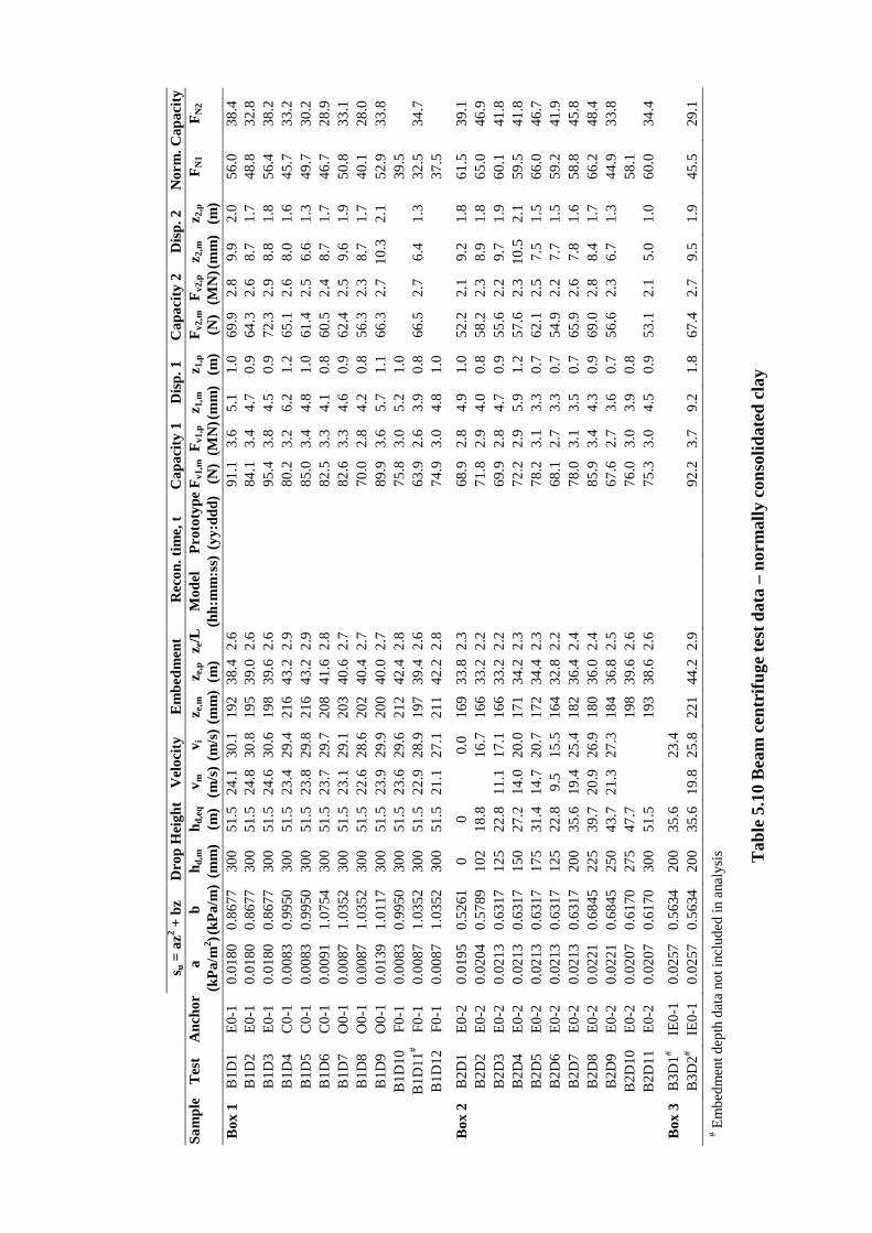
s u
= a
z2 + b
z D
rop
Hei
ght
Vel
ocity
E
mbe
dmen
t R
econ
. tim
e, t
Cap
acity
1 D
isp.
1
Cap
acity
2 D
isp.
2
Nor
m. C
apac
ity
Sam
ple
Tes
t A
ncho
r a
b h d
,m
h d,e
q v m
v i
z e
,m
z e,p
z e/L
M
odel
P
roto
type
Fv1
,m F
v1,p
z 1,m
z 1
,p
Fv2
,m
Fv2
,p
z 2,m
z 2
,p
FN
1 F
N2
(k
Pa/
m2 ) (
kPa/
m)
(mm
) (m
) (m
/s) (
m/s
) (m
m)
(m)
(h
h:m
m:s
s) (
yy:d
dd)
(N)
(MN
) (m
m)
(m)
(N)
(MN
) (m
m)
(m)
Box
1
B1D
1 E
0-1
0.01
80
0.86
77
300
51.5
24
.1
30.1
19
2 38
.4
2.6
91.1
3.
6 5.
1 1.
0 69
.9
2.8
9.9
2.0
56.0
38
.4
B
1D2
E0-
1 0.
0180
0.
8677
30
0 51
.5
24.8
30
.8
195
39.0
2.
6
84
.1
3.4
4.7
0.9
64.3
2.
6 8.
7 1.
7 48
.8
32.8
B1D
3 E
0-1
0.01
80
0.86
77
300
51.5
24
.6
30.6
19
8 39
.6
2.6
95.4
3.
8 4.
5 0.
9 72
.3
2.9
8.8
1.8
56.4
38
.2
B
1D4
C0-
1 0.
0083
0.
9950
30
0 51
.5
23.4
29
.4
216
43.2
2.
9
80
.2
3.2
6.2
1.2
65.1
2.
6 8.
0 1.
6 45
.7
33.2
B1D
5 C
0-1
0.00
83
0.99
50
300
51.5
23
.8
29.8
21
6 43
.2
2.9
85.0
3.
4 4.
8 1.
0 61
.4
2.5
6.6
1.3
49.7
30
.2
B
1D6
C0-
1 0.
0091
1.
0754
30
0 51
.5
23.7
29
.7
208
41.6
2.
8
82
.5
3.3
4.1
0.8
60.5
2.
4 8.
7 1.
7 46
.7
28.9
B1D
7 O
0-1
0.00
87
1.03
52
300
51.5
23
.1
29.1
20
3 40
.6
2.7
82.6
3.
3 4.
6 0.
9 62
.4
2.5
9.6
1.9
50.8
33
.1
B
1D8
O0-
1 0.
0087
1.
0352
30
0 51
.5
22.6
28
.6
202
40.4
2.
7
70
.0
2.8
4.2
0.8
56.3
2.
3 8.
7 1.
7 40
.1
28.0
B1D
9 O
0-1
0.01
39
1.01
17
300
51.5
23
.9
29.9
20
0 40
.0
2.7
89.9
3.
6 5.
7 1.
1 66
.3
2.7
10.3
2.
1 52
.9
33.8
B1D
10
F0-1
0.
0083
0.
9950
30
0 51
.5
23.6
29
.6
212
42.4
2.
8
75
.8
3.0
5.2
1.0
39.5
B
1D11
# F0
-1
0.00
87
1.03
52
300
51.5
22
.9
28.9
19
7 39
.4
2.6
63.9
2.
6 3.
9 0.
8 66
.5
2.7
6.4
1.3
32.5
34
.7
B
1D12
F0
-1
0.00
87
1.03
52
300
51.5
21
.1
27.1
21
1 42
.2
2.8
74.9
3.
0 4.
8 1.
0
37
.5
B
ox 2
B
2D1
E0-
2 0.
0195
0.
5261
0
0
0.0
169
33.8
2.
3
68
.9
2.8
4.9
1.0
52.2
2.
1 9.
2 1.
8 61
.5
39.1
B2D
2 E
0-2
0.02
04
0.57
89
102
18.8
16.7
16
6 33
.2
2.2
71.8
2.
9 4.
0 0.
8 58
.2
2.3
8.9
1.8
65.0
46
.9
B
2D3
E0-
2 0.
0213
0.
6317
12
5 22
.8
11.1
17
.1
166
33.2
2.
2
69
.9
2.8
4.7
0.9
55.6
2.
2 9.
7 1.
9 60
.1
41.8
B2D
4 E
0-2
0.02
13
0.63
17
150
27.2
14
.0
20.0
17
1 34
.2
2.3
72.2
2.
9 5.
9 1.
2 57
.6
2.3
10.5
2.
1 59
.5
41.8
B2D
5 E
0-2
0.02
13
0.63
17
175
31.4
14
.7
20.7
17
2 34
.4
2.3
78.2
3.
1 3.
3 0.
7 62
.1
2.5
7.5
1.5
66.0
46
.7
B
2D6
E0-
2 0.
0213
0.
6317
12
5 22
.8
9.5
15.5
16
4 32
.8
2.2
68.1
2.
7 3.
3 0.
7 54
.9
2.2
7.7
1.5
59.2
41
.9
B
2D7
E0-
2 0.
0213
0.
6317
20
0 35
.6
19.4
25
.4
182
36.4
2.
4
78
.0
3.1
3.5
0.7
65.9
2.
6 7.
8 1.
6 58
.8
45.8
B2D
8 E
0-2
0.02
21
0.68
45
225
39.7
20
.9
26.9
18
0 36
.0
2.4
85.9
3.
4 4.
3 0.
9 69
.0
2.8
8.4
1.7
66.2
48
.4
B
2D9
E0-
2 0.
0221
0.
6845
25
0 43
.7
21.3
27
.3
184
36.8
2.
5
67
.6
2.7
3.6
0.7
56.6
2.
3 6.
7 1.
3 44
.9
33.8
B2D
10
E0-
2 0.
0207
0.
6170
27
5 47
.7
198
39.6
2.
6
76
.0
3.0
3.9
0.8
58.1
B
2D11
E
0-2
0.02
07
0.61
70
300
51.5
19
3 38
.6
2.6
75.3
3.
0 4.
5 0.
9 53
.1
2.1
5.0
1.0
60.0
34
.4
Box
3
B3D
1# IE
0-1
0.02
57
0.56
34
200
35.6
23.4
B
3D2#
IE0-
1 0.
0257
0.
5634
20
0 35
.6
19.8
25
.8
221
44.2
2.
9
92
.2
3.7
9.2
1.8
67.4
2.
7 9.
5 1.
9 45
.5
29.1
# E
mbe
dmen
t dep
th d
ata
not i
nclu
ded
in a
naly
sis Tab
le 5
.10
Bea
m c
entr
ifuge
test
dat
a –
norm
ally
con
solid
ated
cla
y
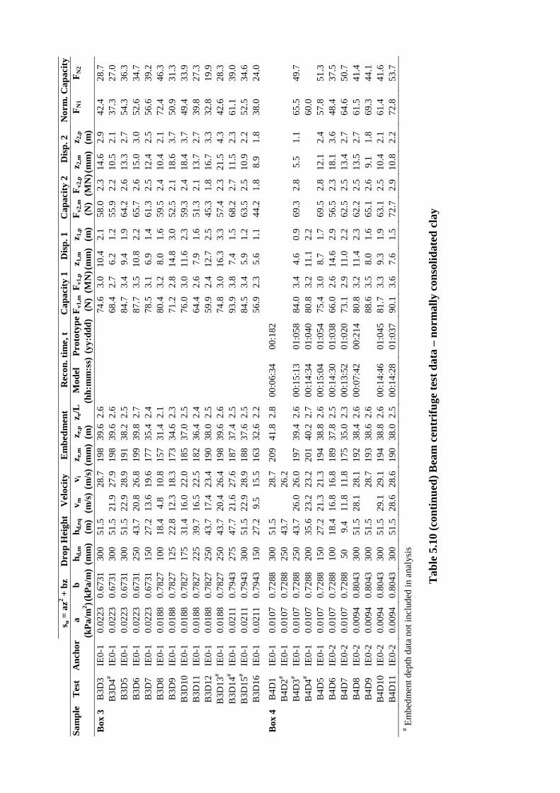
s u
= a
z2 + b
z D
rop
Hei
ght
Vel
ocity
E
mbe
dmen
t R
econ
. tim
e, t
Cap
acity
1 D
isp.
1
Cap
acity
2 D
isp.
2
Nor
m. C
apac
ity
Sam
ple
Tes
t A
ncho
r a
b h d
,m
h d,e
q v m
v i
z e
,m
z e,p
z e/L
M
odel
P
roto
type
Fv1
,m F
v1,p
z 1,m
z 1
,p
Fv2
,m
Fv2
,p
z 2,m
z 2
,p
FN
1 F
N2
(k
Pa/
m2 ) (
kPa/
m)
(mm
) (m
) (m
/s) (
m/s
) (m
m)
(m)
(h
h:m
m:s
s) (
yy:d
dd)
(N)
(MN
) (m
m)
(m)
(N)
(MN
) (m
m)
(m)
Box
3
B3D
3 IE
0-1
0.02
23
0.67
31
300
51.5
28.7
19
8 39
.6
2.6
74.6
3.
0 10
.4
2.1
58.0
2.
3 14
.6
2.9
42.4
28
.7
B
3D4#
IE0-
1 0.
0223
0.
6731
30
0 51
.5
21.9
27
.9
198
39.6
2.
6
68
.4
2.7
6.2
1.2
55.9
2.
2 10
.5
2.1
37.3
27
.0
B
3D5
IE0-
1 0.
0223
0.
6731
30
0 51
.5
22.9
28
.9
191
38.2
2.
5
84
.7
3.4
9.4
1.9
64.2
2.
6 13
.3
2.7
54.3
36
.3
B
3D6
IE0-
1 0.
0223
0.
6731
25
0 43
.7
20.8
26
.8
199
39.8
2.
7
87
.7
3.5
10.8
2.
2 65
.7
2.6
15.0
3.
0 52
.6
34.7
B3D
7 IE
0-1
0.02
23
0.67
31
150
27.2
13
.6
19.6
17
7 35
.4
2.4
78.5
3.
1 6.
9 1.
4 61
.3
2.5
12.4
2.
5 56
.6
39.2
B3D
8 IE
0-1
0.01
88
0.78
27
100
18.4
4.
8 10
.8
157
31.4
2.
1
80
.4
3.2
8.0
1.6
59.5
2.
4 10
.4
2.1
72.4
46
.3
B
3D9
IE0-
1 0.
0188
0.
7827
12
5 22
.8
12.3
18
.3
173
34.6
2.
3
71
.2
2.8
14.8
3.
0 52
.5
2.1
18.6
3.
7 50
.9
31.3
B3D
10
IE0-
1 0.
0188
0.
7827
17
5 31
.4
16.0
22
.0
185
37.0
2.
5
76
.0
3.0
11.6
2.
3 59
.3
2.4
18.4
3.
7 49
.4
33.9
B3D
11
IE0-
1 0.
0188
0.
7827
22
5 39
.7
16.5
22
.5
182
36.4
2.
4
64
.4
2.6
7.9
1.6
51.3
2.
1 13
.7
2.7
39.8
27
.3
B
3D12
IE
0-1
0.01
88
0.78
27
250
43.7
17
.4
23.4
19
0 38
.0
2.5
59.9
2.
4 12
.7
2.5
45.3
1.
8 16
.7
3.3
32.8
19
.9
B
3D13
# IE
0-1
0.01
88
0.78
27
250
43.7
20
.4
26.4
19
8 39
.6
2.6
74.8
3.
0 16
.3
3.3
57.4
2.
3 21
.5
4.3
42.6
28
.3
B
3D14
# IE
0-1
0.02
11
0.79
43
275
47.7
21
.6
27.6
18
7 37
.4
2.5
93.9
3.
8 7.
4 1.
5 68
.2
2.7
11.5
2.
3 61
.1
39.0
B3D
15#
IE0-
1 0.
0211
0.
7943
30
0 51
.5
22.9
28
.9
188
37.6
2.
5
84
.5
3.4
5.9
1.2
63.5
2.
5 10
.9
2.2
52.5
34
.6
B
3D16
IE
0-1
0.02
11
0.79
43
150
27.2
9.
5 15
.5
163
32.6
2.
2
56
.9
2.3
5.6
1.1
44.2
1.
8 8.
9 1.
8 38
.0
24.0
B
ox 4
B
4D1
IE0-
1 0.
0107
0.
7288
30
0 51
.5
28
.7
209
41.8
2.
8 00
:06:
34
00:1
82
B
4D2#
IE0-
1 0.
0107
0.
7288
25
0 43
.7
26
.2
B4D
3# IE
0-1
0.01
07
0.72
88
250
43.7
26
.0
26.0
19
7 39
.4
2.6
00:1
5:13
01
:058
84
.0
3.4
4.6
0.9
69.3
2.
8 5.
5 1.
1 65
.5
49.7
B4D
4# IE
0-1
0.01
07
0.72
88
200
35.6
23
.2
23.2
20
1 40
.2
2.7
00:1
4:34
01
:040
80
.8
3.2
11.1
2.
2
60
.0
B4D
5 IE
0-1
0.01
07
0.72
88
150
27.2
21
.3
21.3
19
4 38
.8
2.6
00:1
5:04
01
:054
75
.4
3.0
8.7
1.7
69.5
2.
8 12
.1
2.4
57.8
51
.3
B
4D6
IE0-
2 0.
0107
0.
7288
10
0 18
.4
16.8
16
.8
189
37.8
2.
5 00
:14:
30
01:0
38
66.0
2.
6 14
.6
2.9
56.5
2.
3 18
.1
3.6
48.4
37
.5
B
4D7
IE0-
2 0.
0107
0.
7288
50
9.
4 11
.8
11.8
17
5 35
.0
2.3
00:1
3:52
01
:020
73
.1
2.9
11.0
2.
2 62
.5
2.5
13.4
2.
7 64
.6
50.7
B4D
8 IE
0-2
0.00
94
0.80
43
300
51.5
28
.1
28.1
19
2 38
.4
2.6
00:0
7:42
00
:214
80
.8
3.2
11.4
2.
3 62
.2
2.5
13.5
2.
7 61
.5
41.4
B4D
9 IE
0-2
0.00
94
0.80
43
300
51.5
28.7
19
3 38
.6
2.6
88.6
3.
5 8.
0 1.
6 65
.1
2.6
9.1
1.8
69.3
44
.1
B
4D10
IE
0-2
0.00
94
0.80
43
300
51.5
29
.1
29.1
19
4 38
.8
2.6
00:1
4:46
01
:045
81
.7
3.3
9.3
1.9
63.1
2.
5 10
.4
2.1
61.4
41
.6
B
4D11
IE
0-2
0.00
94
0.80
43
300
51.5
28
.6
28.6
19
0 38
.0
2.5
00:1
4:28
01
:037
90
.1
3.6
7.6
1.5
72.7
2.
9 10
.8
2.2
72.8
53
.7
# Em
bedm
ent d
epth
dat
a no
t inc
lude
d in
ana
lysi
s
Tab
le 5
.10
(con
tinue
d) B
eam
cen
trifu
ge te
st d
ata
– no
rmal
ly c
onso
lidat
ed c
lay

s u
= a
z2 + b
z D
rop
Hei
ght
Vel
ocity
E
mbe
dmen
t R
econ
. tim
e, t
Cap
acity
1 D
isp.
1
Cap
acity
2 D
isp.
2
Nor
m. C
apac
ity
Sam
ple
Tes
t A
ncho
r a
b h d
,m
h d,e
q v m
v i
z e
,m
z e,p
z e/L
M
odel
P
roto
type
Fv1
,m F
v1,p
z 1,m
z 1
,p
Fv2
,m
Fv2
,p
z 2,m
z 2
,p
FN
1 F
N2
(k
Pa/
m2 )
(kP
a/m
) (m
m)
(m)
(m/s
) (m
/s) (
mm
) (m
)
(hh:
mm
:ss)
(yy
:ddd
) (N
) (M
N) (
mm
) (m
) (N
) (M
N) (
mm
) (m
)
Box
4
B4D
12
IE0-
2 0.
0094
0.
8043
20
0 35
.6
23.9
23
.9
194
38.8
2.
6 00
:14:
48
01:0
46
78.6
3.
1 7.
4 1.
5 58
.8
2.4
9.7
1.9
58.1
37
.0
B
4D13
# IE
0-2
0.00
58
1.03
10
200
35.6
23
.9
23.9
17
9 35
.8
2.4
00:0
6:58
00
:194
66
.5
2.7
4.8
1.0
55.3
2.
2 8.
5 1.
7 46
.5
34.3
B4D
14#
IE0-
2 0.
0058
1.
0310
15
0 27
.2
20.7
20
.7
179
35.8
2.
4 00
:26:
59
02:0
20
78.8
3.
2 9.
7 1.
9 66
.1
2.6
12.9
2.
6 59
.9
46.0
B4D
15#
IE0-
2 0.
0058
1.
0310
15
0 27
.2
20
.3
178
35.6
2.
4
63
.7
2.5
7.1
1.4
55.8
2.
2 12
.9
2.6
43.8
35
.1
B
4D16
IE
0-2
0.00
58
1.03
10
0 0
0.
0 15
7 31
.4
2.1
00:0
5:45
00
:160
41
.2
1.6
6.5
1.3
34.5
1.
4 8.
7 1.
7 23
.5
14.6
B
ox 5
B
5D1
E0-
2 0.
0119
0.
8110
15
0 27
.2
20.4
20
.4
184
36.8
2.
5 00
:59:
40
04:1
97
79.7
3.
2 8.
6 1.
7 58
.6
2.3
12.8
2.
6 61
.1
38.3
B5D
2 E
0-2
0.01
60
0.85
52
150
27.2
20
.7
20.7
18
0 36
.0
2.4
00:5
9:57
04
:205
79
.5
3.2
6.0
1.2
55.4
B
5D3
E0-
2 0.
0160
0.
8552
15
0 27
.2
20.3
20
.3
176
35.2
2.
3 00
:01:
57
00:0
54
64.1
2.
6 4.
9 1.
0 56
.5
2.3
11.3
2.
3 41
.9
34.1
B5S
US1
E
0-2
0.01
60
0.85
52
150
27.2
20
.6
20.6
18
8 37
.6
2.5
01:0
0:32
04
:221
B5S
US2
E
0-2
0.01
72
0.79
93
150
27.2
21
.2
21.2
18
4 36
.8
2.5
01:0
0:11
04
:212
88
.8
3.6
10.0
2.
0 65
.6
2.6
11.3
2.
3 63
.0
40.7
B5S
US3
E
0-2
0.01
72
0.79
93
150
27.2
21
.1
21.1
18
2 36
.4
2.4
00:5
9:58
04
:206
84
.3
3.4
9.0
1.8
59.8
B
5SU
S4
E0-
2 0.
0184
0.
7433
15
0 27
.2
21.2
21
.2
178
35.6
2.
4 01
:00:
22
04:2
17
78.6
3.
1 8.
2 1.
6 58
.8
2.4
10.2
2.
0 57
.4
36.9
B5S
US5
E
0-2
0.01
84
0.74
33
150
27.2
21
.2
21.2
18
1 36
.2
2.4
00:5
9:51
04
:202
74
.9
3.0
8.5
1.7
52.0
B
5CY
C1
E0-
2 0.
0184
0.
7433
15
0 27
.2
20.9
20
.9
182
36.4
2.
4 00
:59:
51
04:2
02
73.0
2.
9 7.
2 1.
4
49
.5
B5C
YC
2 E
0-2
0.01
84
0.74
33
150
27.2
21
.0
21.0
17
8 35
.6
2.4
01:0
0:08
04
:210
87
.7
3.5
9.1
1.8
67.4
2.
7 11
.3
2.3
66.9
45
.8
B
5CY
C3
E0-
2 0.
0179
0.
8285
15
0 27
.2
20.6
20
.6
178
35.6
2.
4 01
:00:
05
04:2
09
88.4
3.
5 7.
6 1.
5 66
.4
2.7
8.6
1.7
64.1
42
.5
B
5CY
C4
E0-
2 0.
0179
0.
8285
15
0 27
.2
20.3
20
.3
180
36.0
2.
4 00
:59:
57
04:2
05
B
5CY
C5
E0-
2 0.
0179
0.
8285
15
0 27
.2
20.9
20
.9
179
35.8
2.
4 01
:00:
02
04:2
08
87.2
3.
5 7.
7 1.
5
62
.3
B5C
YC
6 E
0-2
0.01
79
0.82
85
150
27.2
20
.4
20.4
17
9 35
.8
2.4
01:0
0:03
04
:208
68
.9
2.8
7.6
1.5
44.5
B
5CY
C7
E0-
2 0.
0173
0.
9137
15
0 27
.2
20.3
20
.3
175
35.0
2.
3 01
:00:
10
04:2
11
85.4
3.
4 8.
6 1.
7 62
.1
2.5
9.8
2.0
59.9
37
.5
Box
6*
B6D
1 E
0-2
0.01
58
1.08
17
0 0
0.
0 66
13
.2
0.9
01:0
6:50
05
:031
42
.2
1.7
4.9
1.0
106.
9
B
6D2
E0-
2 0.
0158
1.
0817
10
0 18
.4
16.4
16
.4
93
18.6
1.
2 01
:01:
31
04:2
49
51.0
2.
0 6.
7 1.
3
79
.4
B6D
3 E
0-2
0.01
58
1.08
17
200
35.6
23
.3
23.3
10
9 21
.8
1.5
01:0
1:08
04
:238
59
.6
2.4
6.3
1.3
75.4
B
6D4
E0-
2 0.
0088
1.
3792
30
0 51
.5
27.6
27
.6
117
23.4
1.
6 01
:01:
49
04:2
57
71.6
2.
9 6.
3 1.
3
77
.2
B6D
5w
E0-
2 0.
0088
1.
3792
30
0 51
.5
27.7
27
.7
90
18.0
1.
2 00
:04:
38
00:1
29
63.9
2.
6 4.
4 0.
9
10
6.0
# E
mbe
dmen
t dep
th d
ata
not i
nclu
ded
in a
naly
sis;
* Box
6 e
mbe
dmen
t and
cap
acit
y da
ta n
ot in
clud
ed in
ana
lysi
s; w
No
surf
ace
wat
er la
yer
pres
ent d
urin
g te
st
Tab
le 5
.10
(con
tinue
d) B
eam
cen
trifu
ge te
st d
ata
– no
rmal
ly c
onso
lidat
ed c
lay

s u
= a
z2 + b
z D
rop
Hei
ght
Vel
ocity
E
mbe
dmen
t R
econ
. tim
e, t
Cap
acity
1 D
isp.
1
Cap
acity
2 D
isp.
2
Nor
m. C
apac
ity
Sam
ple
Tes
t A
ncho
r a
b h d
,m
h d,e
q v m
v i
z e
,m
z e,p
z e/L
M
odel
P
roto
type
Fv1
,m F
v1,p
z 1,m
z 1
,p
Fv2
,m
Fv2
,p
z 2,m
z 2
,p
FN
1 F
N2
(k
Pa/
m2 )
(kP
a/m
) (m
m)
(m)
(m/s
) (m
/s) (
mm
) (m
)
(hh:
mm
:ss)
(yy
:ddd
) (N
) (M
N) (
mm
) (m
) (N
) (M
N) (
mm
) (m
)
B
ox 6
* B
6D6w
E
0-2
0.00
88
1.37
92
300
51.5
28
.7
28.7
81
16
.2
1.1
00:0
2:34
00
:071
40
.2
1.6
4.4
0.9
57.9
B
6D7
E0-
2 0.
0057
1.
3349
25
0 43
.7
26.2
26
.2
93
18.6
1.
2 00
:15:
43
01:0
72
49.9
2.
0 5.
5 1.
1
70
.3
B6D
8w
E0-
2 0.
0057
1.
3349
10
0 18
.4
16.3
16
.3
77
15.4
1.
0 00
:15:
59
01:0
79
B
6D9w
E
0-2
0.00
57
1.33
49
100
18.4
16
.8
16.8
69
13
.8
0.9
00:1
3:24
01
:007
32
.5
1.3
5.8
1.2
48.0
B
6D10
E
0-2
0.00
57
1.33
49
150
27.2
20
.4
20.4
96
19
.2
1.3
00:1
4:32
01
:039
46
.9
1.9
4.7
0.9
59.0
B
6D11
E
0-2
0.00
57
1.33
49
250
43.7
26
.4
26.4
10
8 21
.6
1.4
# Em
bedm
ent d
epth
dat
a no
t inc
lude
d in
ana
lysi
s; * B
ox 6
em
bedm
ent a
nd c
apac
ity
data
not
incl
uded
in a
naly
sis;
w N
o su
rfac
e w
ater
laye
r pr
esen
t dur
ing
test
Tab
le 5
.10
(con
tinue
d) B
eam
cen
trifu
ge te
st d
ata
– no
rmal
ly c
onso
lidat
ed c
lay
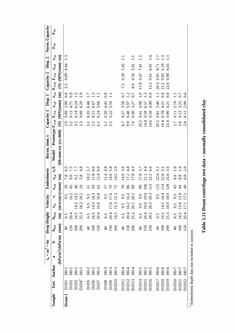
s u
= a
z2 + b
z D
rop
Hei
ght
Vel
ocity
E
mbe
dmen
t R
econ
. tim
e, t
Cap
acity
1 D
isp.
1
Cap
acity
2 D
isp.
2
Nor
m. C
apac
ity
Sam
ple
Tes
t A
ncho
r a
b h d
,m
h d,e
q v m
v i
z e
,m
z e,p
z e/L
M
odel
P
roto
type
Fv1
,m F
v1,p
z 1,m
z 1
,p
Fv2
,m F
v2,p
z 2,m
z 2
,p
FN
1 F
N2
(k
Pa/
m2 ) (
kPa/
m)
(mm
) (m
) (m
/s) (
m/s
) (m
m)
(m)
(h
h:m
m:s
s) (
yy:d
dd)
(N)
(MN
) (m
m)
(m)
(N)
(MN
) (m
m)
(m)
Dru
m 1
D
1D1
H0-
1
40
6.
3
9.5
39
7.8
6.5
2.0
0.08
3.
99
0.8
2.2
0.09
6.
44
1.3
D
1D2
H0-
1
15
0 20
.4
16
.2
45
9.0
7.5
3.2
0.13
4.
71
0.9
D
1D3
H0-
1
10
0 14
.5
14.2
14
.2
46
9.2
7.7
3.5
0.14
6.
24
1.2
D
1D4#
H0-
1
20
0 25
.3
18.2
18
.2
29
5.8
4.8
2.3
0.09
9.
29
1.9
D
1D5
H0-
2
40
6.
3 9.
3 9.
3 51
10
.2
5.7
5.1
0.20
8.
48
1.7
D
1D6
H0-
2
10
0 14
.5
14.3
14
.3
59
11.8
6.
6
5.
2 0.
21
6.67
1.
3
D1D
7 H
0-2
150
20.4
16
.8
16.8
62
12
.4
6.9
6.1
0.24
5.
66
1.1
D
1D8
H0-
3
40
6.
3
9.5
57
11.4
4.
8
5.
1 0.
20
4.45
0.
9
D1D
9 H
0-3
150
20.4
17
.6
17.6
70
14
.0
5.8
5.5
0.22
5.
59
1.1
D
1D10
H
0-3
100
14.5
15
.3
15.3
71
14
.2
5.9
D
1D11
H
0-4
40
6.3
9.5
9.5
70
14.0
3.
9
6.
7 0.
27
3.58
0.
7 7.
5 0.
30
5.42
1.
1
D1D
12
H0-
4
15
0 20
.4
16.2
16
.2
86
17.2
4.
8
9.
9 0.
40
5.97
1.
2
D1D
13
H0-
4
20
0 25
.3
20.1
20
.1
89
17.8
4.
9
7.
6 0.
30
3.27
0.
7 8.
9 0.
36
5.41
1.
1
D1D
14
H0-
5
40
6.
3 9.
9 9.
9 89
17
.8
3.7
10.2
0.
41
4.99
1.
0 11
.8
0.47
7.
41
1.5
D
1D15
H
0-5
150
20.4
19
.0
19.0
10
6 21
.2
4.4
14.4
0.
58
6.57
1.
3
D1D
16
H0-
5
25
0 29
.2
20.3
20
.3
111
22.2
4.
6
14
.6
0.58
4.
49
0.9
15.2
0.
61
6.91
1.
4
D1D
17
H0-
6
40
6.
3
9.5
112
22.4
3.
1
20
.2
0.81
5.
40
1.1
20.3
0.
81
8.71
1.
7
D1D
18
H0-
6
10
0 14
.5
14.1
14
.4
114
22.8
3.
2
19
.4
0.78
4.
21
0.8
21.2
0.
85
6.59
1.
3
D1D
19
H0-
6
20
0 25
.3
18.0
18
.0
128
25.6
3.
6
22
.4
0.90
4.
21
0.8
22.6
0.
90
6.65
1.
3
D1D
20
H0-
7
40
6.
3 9.
5 9.
5 43
8.
6 1.
8
2.
7 0.
11
5.74
1.
1
D1D
21
H0-
7
10
0 14
.5
13.9
13
.9
44
8.8
1.8
3.0
0.12
3.
25
0.7
D
1D22
H
0-7
150
20.4
17
.1
17.1
49
9.
8 2.
0
2.
8 0.
11
2.99
0.
6
# E
mbe
dmen
t dep
th d
ata
not i
nclu
ded
in a
naly
sis Tab
le 5
.11
Dru
m c
entr
ifuge
test
dat
a –
norm
ally
con
solid
ated
cla
y
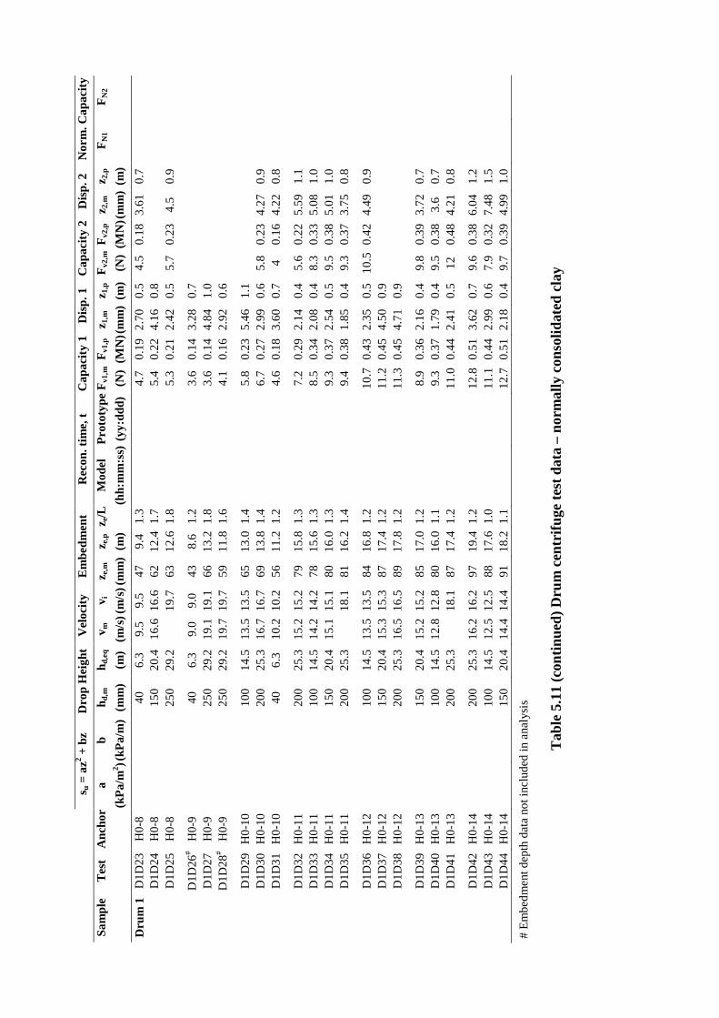
s u
= a
z2 + b
z D
rop
Hei
ght
Vel
ocity
E
mbe
dmen
t R
econ
. tim
e, t
Cap
acity
1 D
isp.
1
Cap
acity
2 D
isp.
2
Nor
m. C
apac
ity
Sam
ple
Tes
t A
ncho
r a
b h d
,m
h d,e
q v m
v i
z e
,m
z e,p
z e/L
M
odel
P
roto
type
Fv1
,m F
v1,p
z 1,m
z 1
,p
Fv2
,m F
v2,p
z 2,m
z 2
,p
FN
1 F
N2
(k
Pa/
m2 ) (
kPa/
m)
(mm
) (m
) (m
/s) (
m/s
) (m
m)
(m)
(h
h:m
m:s
s) (
yy:d
dd)
(N)
(MN
) (m
m)
(m)
(N)
(MN
) (m
m)
(m)
Dru
m 1
D
1D23
H
0-8
40
6.3
9.5
9.5
47
9.4
1.3
4.7
0.19
2.
70
0.5
4.5
0.18
3.
61
0.7
D
1D24
H
0-8
150
20.4
16
.6
16.6
62
12
.4
1.7
5.4
0.22
4.
16
0.8
D
1D25
H
0-8
250
29.2
19.7
63
12
.6
1.8
5.3
0.21
2.
42
0.5
5.7
0.23
4.
5 0.
9
D1D
26#
H0-
9
40
6.
3 9.
0 9.
0 43
8.
6 1.
2
3.
6 0.
14
3.28
0.
7
D1D
27
H0-
9
25
0 29
.2
19.1
19
.1
66
13.2
1.
8
3.
6 0.
14
4.84
1.
0
D1D
28#
H0-
9
25
0 29
.2
19.7
19
.7
59
11.8
1.
6
4.
1 0.
16
2.92
0.
6
D1D
29
H0-
10
100
14.5
13
.5
13.5
65
13
.0
1.4
5.8
0.23
5.
46
1.1
D
1D30
H
0-10
20
0 25
.3
16.7
16
.7
69
13.8
1.
4
6.
7 0.
27
2.99
0.
6 5.
8 0.
23
4.27
0.
9
D1D
31
H0-
10
40
6.3
10.2
10
.2
56
11.2
1.
2
4.
6 0.
18
3.60
0.
7 4
0.16
4.
22
0.8
D
1D32
H
0-11
20
0 25
.3
15.2
15
.2
79
15.8
1.
3
7.
2 0.
29
2.14
0.
4 5.
6 0.
22
5.59
1.
1
D1D
33
H0-
11
100
14.5
14
.2
14.2
78
15
.6
1.3
8.5
0.34
2.
08
0.4
8.3
0.33
5.
08
1.0
D
1D34
H
0-11
15
0 20
.4
15.1
15
.1
80
16.0
1.
3
9.
3 0.
37
2.54
0.
5 9.
5 0.
38
5.01
1.
0
D1D
35
H0-
11
200
25.3
18.1
81
16
.2
1.4
9.4
0.38
1.
85
0.4
9.3
0.37
3.
75
0.8
D
1D36
H
0-12
10
0 14
.5
13.5
13
.5
84
16.8
1.
2
10
.7
0.43
2.
35
0.5
10.5
0.
42
4.49
0.
9
D1D
37
H0-
12
150
20.4
15
.3
15.3
87
17
.4
1.2
11.2
0.
45
4.50
0.
9
D1D
38
H0-
12
200
25.3
16
.5
16.5
89
17
.8
1.2
11.3
0.
45
4.71
0.
9
D1D
39
H0-
13
150
20.4
15
.2
15.2
85
17
.0
1.2
8.9
0.36
2.
16
0.4
9.8
0.39
3.
72
0.7
D
1D40
H
0-13
10
0 14
.5
12.8
12
.8
80
16.0
1.
1
9.
3 0.
37
1.79
0.
4 9.
5 0.
38
3.6
0.7
D
1D41
H
0-13
20
0 25
.3
18
.1
87
17.4
1.
2
11
.0
0.44
2.
41
0.5
12
0.48
4.
21
0.8
D
1D42
H
0-14
20
0 25
.3
16.2
16
.2
97
19.4
1.
2
12
.8
0.51
3.
62
0.7
9.6
0.38
6.
04
1.2
D
1D43
H
0-14
10
0 14
.5
12.5
12
.5
88
17.6
1.
0
11
.1
0.44
2.
99
0.6
7.9
0.32
7.
48
1.5
D
1D44
H
0-14
15
0 20
.4
14.4
14
.4
91
18.2
1.
1
12
.7
0.51
2.
18
0.4
9.7
0.39
4.
99
1.0
# E
mbe
dmen
t dep
th d
ata
not i
nclu
ded
in a
naly
sis
Tab
le 5
.11
(con
tinue
d) D
rum
cen
trifu
ge te
st d
ata
– no
rmal
ly c
onso
lidat
ed c
lay

s u
= a
z2 + b
z D
rop
Hei
ght
Vel
ocity
E
mbe
dmen
t R
econ
. tim
e, t
Cap
acity
1 D
isp.
1
Cap
acity
2 D
isp.
2
Nor
m. C
apac
ity
Sam
ple
Tes
t A
ncho
r a
b h d
,m
h d,e
q v m
v i
z e
,m
z e,p
z e/L
M
odel
P
roto
type
Fv1
,m F
v1,p
z 1,m
z 1
,p
Fv2
,m F
v2,p
z 2,m
z 2
,p
FN
1 F
N2
(k
Pa/
m2 ) (
kPa/
m)
(mm
) (m
) (m
/s) (
m/s
) (m
m)
(m)
(h
h:m
m:s
s) (
yy:d
dd)
(N)
(MN
) (m
m)
(m)
(N)
(MN
) (m
m)
(m)
Dru
m 1
D
1D45
H
0-15
40
6.
3 8.
5 8.
5 48
9.
6 5.
3
10
.4
0.42
8.
43
1.7
D
1D46
H
0-15
10
0 14
.5
14.3
14
.3
61
12.2
6.
8
14
.1
0.56
7.
51
1.5
D
1D47
H
0-16
40
6.
3 9.
5 9.
5 76
15
.2
4.2
22.4
0.
90
8.59
1.
7
D1D
48
H0-
16
100
14.5
15
.2
15.2
89
17
.8
4.9
29.2
1.
17
9.51
1.
9
D1D
49
H0-
17
40
6.3
9.7
9.7
96
19.2
3.
6
33
.4
1.34
9.
57
1.9
D
1D50
H
0-17
10
0 14
.5
15.0
15
.0
114
22.8
4.
2
47
.5
1.90
7.
81
1.6
D
1D51
H
0-18
40
6.
3 10
.0
10.0
43
8.
6 1.
6
7.
9 0.
32
5.66
1.
1
D1D
52
H0-
18
100
14.5
14
.7
14.7
52
10
.4
1.9
8.1
0.32
4.
41
0.9
D
1D53
H
0-19
40
6.
3 9.
2 9.
2 64
12
.8
5.3
24.9
1.
00 1
2.19
2.
4
D1D
54
H0-
19
100
14.5
15
.5
15.5
73
14
.6
6.1
29.2
1.
17
9.31
1.
9
D1D
55
H0-
20
40
6.3
9.0
9.0
103
20.6
4.
3
54
.5
2.18
14.
12
2.8
D
1D56
H
0-20
10
0 14
.5
15.5
15
.5
115
23.0
4.
8
69
.1
2.76
9.
50
1.9
D
1D57
E
4-1
0 0
0.0
0.0
116
23.2
1.
5
54
.5
2.18
13.
22
2.6
D
1D58
# E
4-1
50
7.7
9.
3 98
19
.6
1.3
42.2
1.
69
6.62
1.
3
D1D
59#
E4-
1
10
0 14
.5
11
.8
102
20.4
1.
4
28
.1
1.12
6.
91
1.4
D
1D60
# E
4-1
100
14.5
11.8
10
5 21
.0
1.4
22.4
0.
90
6.93
1.
4
D1D
61
E4-
1
0
0 0.
0 0.
0 10
8 21
.6
1.4
57.8
2.
31
4.50
0.
9 47
.6
1.90
6.
03
1.2
D
1D62
E
4-1
0 0
0.0
0.0
110
22.0
1.
5
61
.9
2.48
6.
33
1.3
51.4
2.
06
8.14
1.
6
D1D
63
E4-
1
0
0 0.
0 0.
0 12
4 24
.8
1.7
55.9
2.
24
8.14
1.
6 46
.2
1.85
10.
28
2.1
D
1D64
# E
4-1
0 0
0.0
0.0
142
28.4
1.
9
53
.0
2.12
16.
47
3.3
44.7
1.
79 1
8.59
3.
7
D1D
65
E4-
1
0
0 0.
0 0.
0 11
2 22
.4
1.5
62.0
2.
48
5.64
1.
1 52
.6
2.10
7.
16
1.4
D
1D66
# E
4-1
0 0
0.0
0.0
140
28.0
1.
9
65
.1
2.60
14.
62
2.9
55.6
2.
22 1
6.39
3.
3
# E
mbe
dmen
t dep
th d
ata
not i
nclu
ded
in a
naly
sis
Tab
le 5
.11
(con
tinue
d) D
rum
cen
trifu
ge te
st d
ata
– no
rmal
ly c
onso
lidat
ed c
lay
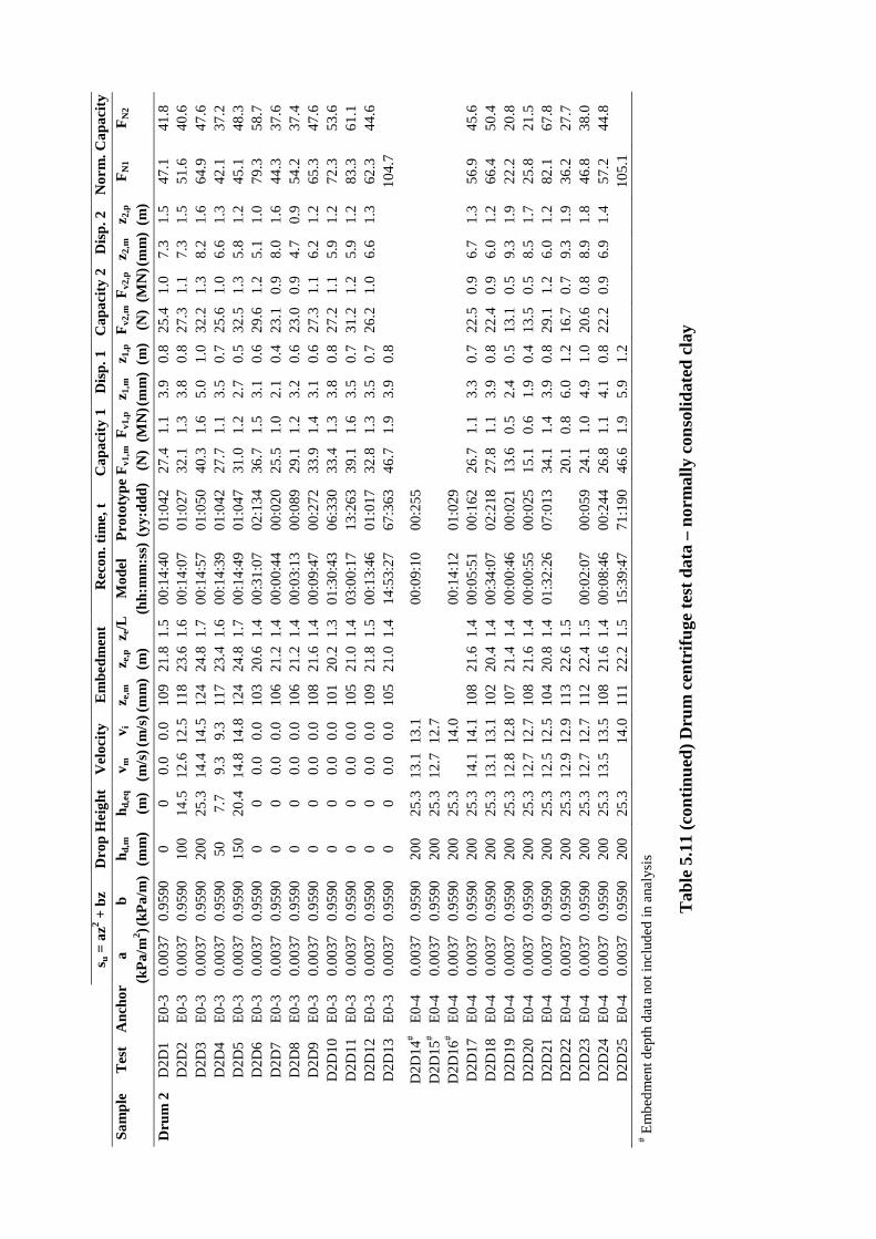
s u
= a
z2 + b
z D
rop
Hei
ght
Vel
ocity
E
mbe
dmen
t R
econ
. tim
e, t
Cap
acity
1 D
isp.
1
Cap
acity
2 D
isp.
2
Nor
m. C
apac
ity
Sam
ple
Tes
t A
ncho
r a
b h d
,m
h d,e
q v m
v i
z e
,m
z e,p
z e/L
M
odel
P
roto
type
Fv1
,m F
v1,p
z 1,m
z 1
,p
Fv2
,m F
v2,p
z 2,m
z 2
,p
FN
1 F
N2
(k
Pa/
m2 ) (
kPa/
m)
(mm
) (m
) (m
/s) (
m/s
) (m
m)
(m)
(h
h:m
m:s
s) (
yy:d
dd)
(N)
(MN
) (m
m)
(m)
(N)
(MN
) (m
m)
(m)
Dru
m 2
D
2D1
E0-
3 0.
0037
0.
9590
0
0 0.
0 0.
0 10
9 21
.8
1.5
00:1
4:40
01
:042
27
.4
1.1
3.9
0.8
25.4
1.
0 7.
3 1.
5 47
.1
41.8
D2D
2 E
0-3
0.00
37
0.95
90
100
14.5
12
.6
12.5
11
8 23
.6
1.6
00:1
4:07
01
:027
32
.1
1.3
3.8
0.8
27.3
1.
1 7.
3 1.
5 51
.6
40.6
D2D
3 E
0-3
0.00
37
0.95
90
200
25.3
14
.4
14.5
12
4 24
.8
1.7
00:1
4:57
01
:050
40
.3
1.6
5.0
1.0
32.2
1.
3 8.
2 1.
6 64
.9
47.6
D2D
4 E
0-3
0.00
37
0.95
90
50
7.7
9.3
9.3
117
23.4
1.
6 00
:14:
39
01:0
42
27.7
1.
1 3.
5 0.
7 25
.6
1.0
6.6
1.3
42.1
37
.2
D
2D5
E0-
3 0.
0037
0.
9590
15
0 20
.4
14.8
14
.8
124
24.8
1.
7 00
:14:
49
01:0
47
31.0
1.
2 2.
7 0.
5 32
.5
1.3
5.8
1.2
45.1
48
.3
D
2D6
E0-
3 0.
0037
0.
9590
0
0 0.
0 0.
0 10
3 20
.6
1.4
00:3
1:07
02
:134
36
.7
1.5
3.1
0.6
29.6
1.
2 5.
1 1.
0 79
.3
58.7
D2D
7 E
0-3
0.00
37
0.95
90
0 0
0.0
0.0
106
21.2
1.
4 00
:00:
44
00:0
20
25.5
1.
0 2.
1 0.
4 23
.1
0.9
8.0
1.6
44.3
37
.6
D
2D8
E0-
3 0.
0037
0.
9590
0
0 0.
0 0.
0 10
6 21
.2
1.4
00:0
3:13
00
:089
29
.1
1.2
3.2
0.6
23.0
0.
9 4.
7 0.
9 54
.2
37.4
D2D
9 E
0-3
0.00
37
0.95
90
0 0
0.0
0.0
108
21.6
1.
4 00
:09:
47
00:2
72
33.9
1.
4 3.
1 0.
6 27
.3
1.1
6.2
1.2
65.3
47
.6
D
2D10
E
0-3
0.00
37
0.95
90
0 0
0.0
0.0
101
20.2
1.
3 01
:30:
43
06:3
30
33.4
1.
3 3.
8 0.
8 27
.2
1.1
5.9
1.2
72.3
53
.6
D
2D11
E
0-3
0.00
37
0.95
90
0 0
0.0
0.0
105
21.0
1.
4 03
:00:
17
13:2
63
39.1
1.
6 3.
5 0.
7 31
.2
1.2
5.9
1.2
83.3
61
.1
D
2D12
E
0-3
0.00
37
0.95
90
0 0
0.0
0.0
109
21.8
1.
5 00
:13:
46
01:0
17
32.8
1.
3 3.
5 0.
7 26
.2
1.0
6.6
1.3
62.3
44
.6
D
2D13
E
0-3
0.00
37
0.95
90
0 0
0.0
0.0
105
21.0
1.
4 14
:53:
27
67:3
63
46.7
1.
9 3.
9 0.
8
10
4.7
D2D
14#
E0-
4 0.
0037
0.
9590
20
0 25
.3
13.1
13
.1
00
:09:
10
00:2
55
D
2D15
# E
0-4
0.00
37
0.95
90
200
25.3
12
.7
12.7
D
2D16
# E
0-4
0.00
37
0.95
90
200
25.3
14.0
00:1
4:12
01
:029
D2D
17
E0-
4 0.
0037
0.
9590
20
0 25
.3
14.1
14
.1
108
21.6
1.
4 00
:05:
51
00:1
62
26.7
1.
1 3.
3 0.
7 22
.5
0.9
6.7
1.3
56.9
45
.6
D
2D18
E
0-4
0.00
37
0.95
90
200
25.3
13
.1
13.1
10
2 20
.4
1.4
00:3
4:07
02
:218
27
.8
1.1
3.9
0.8
22.4
0.
9 6.
0 1.
2 66
.4
50.4
D2D
19
E0-
4 0.
0037
0.
9590
20
0 25
.3
12.8
12
.8
107
21.4
1.
4 00
:00:
46
00:0
21
13.6
0.
5 2.
4 0.
5 13
.1
0.5
9.3
1.9
22.2
20
.8
D
2D20
E
0-4
0.00
37
0.95
90
200
25.3
12
.7
12.7
10
8 21
.6
1.4
00:0
0:55
00
:025
15
.1
0.6
1.9
0.4
13.5
0.
5 8.
5 1.
7 25
.8
21.5
D2D
21
E0-
4 0.
0037
0.
9590
20
0 25
.3
12.5
12
.5
104
20.8
1.
4 01
:32:
26
07:0
13
34.1
1.
4 3.
9 0.
8 29
.1
1.2
6.0
1.2
82.1
67
.8
D
2D22
E
0-4
0.00
37
0.95
90
200
25.3
12
.9
12.9
11
3 22
.6
1.5
20.1
0.
8 6.
0 1.
2 16
.7
0.7
9.3
1.9
36.2
27
.7
D
2D23
E
0-4
0.00
37
0.95
90
200
25.3
12
.7
12.7
11
2 22
.4
1.5
00:0
2:07
00
:059
24
.1
1.0
4.9
1.0
20.6
0.
8 8.
9 1.
8 46
.8
38.0
D2D
24
E0-
4 0.
0037
0.
9590
20
0 25
.3
13.5
13
.5
108
21.6
1.
4 00
:08:
46
00:2
44
26.8
1.
1 4.
1 0.
8 22
.2
0.9
6.9
1.4
57.2
44
.8
D
2D25
E
0-4
0.00
37
0.95
90
200
25.3
14.0
11
1 22
.2
1.5
15:3
9:47
71
:190
46
.6
1.9
5.9
1.2
105.
1
# Em
bedm
ent d
epth
dat
a no
t inc
lude
d in
ana
lysi
s
Tab
le 5
.11
(con
tinue
d) D
rum
cen
trifu
ge te
st d
ata
– no
rmal
ly c
onso
lidat
ed c
lay

s u
= a
z2 + b
z D
rop
Hei
ght
Vel
ocity
E
mbe
dmen
t R
econ
. tim
e, t
Cap
acity
1 D
isp.
1
Cap
acity
2 D
isp.
2
Nor
m. C
apac
ity
Sam
ple
Tes
t A
ncho
r a
b h d
,m
h d,e
q v m
v i
z e
,m
z e,p
z e/L
M
odel
P
roto
type
Fv1
,m F
v1,p
z 1,m
z 1
,p
Fv2
,m F
v2,p
z 2,m
z 2
,p
FN
1 F
N2
(k
Pa/
m2 ) (
kPa/
m)
(mm
) (m
) (m
/s) (
m/s
) (m
m)
(m)
(h
h:m
m:s
s) (
yy:d
dd)
(N)
(MN
) (m
m)
(m)
(N)
(MN
) (m
m)
(m)
Dru
m 2
D
2D26
E
0-4
0.00
37
0.95
90
200
25.3
12
.7
12.7
10
2 20
.4
1.4
00:1
4:08
01
:028
28
.6
1.1
3.5
0.7
23.8
1.
0 5.
7 1.
1 68
.7
54.5
D2D
27
E0-
4 0.
0037
0.
9590
50
7.
7 8.
5 8.
5 96
19
.2
1.3
00:1
3:15
01
:003
23
.2
0.9
4.3
0.9
19.6
0.
8 7.
0 1.
4 59
.1
47.2
D2D
28
E0-
4 0.
0037
0.
9590
50
7.
7 8.
7 8.
7 88
17
.6
1.2
00:1
4:28
01
:037
21
.2
0.8
2.6
0.5
17.5
0.
7 4.
6 0.
9 62
.4
47.9
D2D
29#d
E
0-4
0.00
37
0.95
90
150
20.4
11
.9
11.9
96
19
.2
1.3
00:1
3:30
01
:010
28
.1
1.1
3.3
0.7
19.2
0.
8 5.
2 1.
0 75
.3
45.9
D2D
30#d
E
0-4
0.00
37
0.95
90
50
7.7
8.
7 83
16
.6
1.1
00:1
3:10
01
:001
17
.6
0.7
2.2
0.4
17.0
0.
7 4.
8 1.
0 54
.7
52.1
D2D
31#d
E
0-4
0.00
37
0.95
90
100
14.5
10
.6
10.6
94
18
.8
1.3
00:1
3:33
01
:011
24
.2
1.0
2.5
0.5
18.9
0.
8 5.
0 1.
0 65
.0
46.8
D2D
32#d
E
0-4
0.00
37
0.95
90
0 0
0.0
0.0
75
15.0
1.
0 00
:14:
01
01:0
24
17.6
0.
7 2.
2 0.
4 14
.2
0.6
5.2
1.0
69.1
50
.3
D
2D33
#d
E0-
4 0.
0037
0.
9590
20
0 25
.3
12.9
12
.9
93
18.6
1.
2 00
:13:
46
01:0
17
19.6
0.
8 2.
5 0.
5 17
.6
0.7
5.1
1.0
50.2
43
.2
D
2D34
#d
E0-
4 0.
0037
0.
9590
75
11
.3
9.4
9.4
91
18.2
1.
2 00
:13:
45
01:0
17
20.6
0.
8 2.
3 0.
5 17
.1
0.7
5.1
1.0
56.1
43
.3
D
2D35
#d
E0-
4 0.
0037
0.
9590
12
5 17
.6
12.2
12
.2
101
20.2
1.
3 00
:12:
29
00:3
47
26.0
1.
0 2.
8 0.
6 19
.8
0.8
5.7
1.1
62.1
43
.5
D
2D36
E
0-5
0.00
37
0.95
90
0 0
0 0.
0 69
13
.8
0.9
00:1
9:55
01
:188
12
.4
0.5
2.8
0.6
12.3
0.
5 4.
9 1.
0 51
.7
51.1
D2D
37
E0-
5 0.
0037
0.
9590
10
0 14
.5
12.4
12
.4
95
19.0
1.
3 00
:15:
41
01:0
71
17.0
0.
7 3.
1 0.
6 16
.4
0.7
6.2
1.2
43.8
41
.8
D
2D38
E
0-5
0.00
37
0.95
90
50
7.7
9.9
9.9
87
17.4
1.
2 00
:17:
18
01:1
16
13.9
0.
6 5.
6 1.
1
39
.9
D2D
39
E0-
5 0.
0037
0.
9590
20
0 25
.3
13.6
13
.6
93
18.6
1.
2 00
:16:
05
01:0
82
22.6
0.
9 2.
8 0.
6 19
.7
0.8
5.3
1.1
65.4
55
.2
D
2D40
E
0-5
0.00
37
0.95
90
150
20.4
13
.0
13.0
98
19
.6
1.3
00:1
7:35
01
:123
18
.7
0.7
3.2
0.6
15.3
0.
6 5.
8 1.
2 46
.7
35.9
D2D
41#d
E
0-5
0.00
37
0.95
90
0 0
0.0
0.0
69
13.8
0.
9 00
:13:
19
01:0
05
17.9
0.
7 2.
7 0.
5 13
.7
0.5
4.9
1.0
85.4
59
.7
D
2D42
E
4-1
0.00
37
0.95
90
0 0
0.0
0.0
121
24.2
1.
6 00
:15:
09
01:0
56
78.6
3.
1 6.
4 1.
3 63
.2
2.5
8.9
1.8
82.9
60
.3
D
2D43
#d
E4-
1 0.
0037
0.
9590
50
7.
7 8.
7 8.
7 12
2 24
.4
1.6
00:1
4:05
01
:026
72
.3
2.9
6.4
1.3
59.3
2.
4 8.
9 1.
8 72
.6
53.8
D2D
44#d
E
4-1
0.00
37
0.95
90
100
14.5
12
.0
12.0
12
0 24
.0
1.6
00:1
4:31
01
:038
72
.6
2.9
6.1
1.2
58.4
2.
3 7.
7 1.
5 75
.2
54.0
D2D
45#d
E
4-1
0.00
37
0.95
90
200
25.3
15
.0
15.0
13
0 26
.0
1.7
00:1
3:59
01
:023
88
.9
3.6
6.3
1.3
74.6
3.
0 8.
9 1.
8 86
.8
68.1
D2D
46#d
E
4-2
0.00
37
0.95
90
0 0
0.0
0.0
103
20.6
1.
4 00
:14:
53
01:0
48
56.8
2.
3 6.
8 1.
4 45
.6
1.8
9.5
1.9
78.7
57
.1
D
2D47
#d
E4-
2 0.
0037
0.
9590
0
0 0.
0 0.
0 10
4 20
.8
1.4
00:0
0:52
00
:024
43
.9
1.8
4.8
1.0
41.0
1.
6 9.
2 1.
8 52
.8
47.4
D2D
48
E4-
2 0.
0037
0.
9590
0
0 0.
0 0.
0 10
3 20
.6
1.4
00:0
5:05
00
:141
52
.5
2.1
4.9
1.0
42.1
1.
7 5.
5 1.
1 70
.4
50.4
D2D
49
E4-
2 0.
0037
0.
9590
0
0 0.
0 0.
0 10
3 20
.6
1.4
02:0
2:02
09
:105
68
.5
2.7
6.2
1.2
56.4
2.
3 8.
4 1.
7 10
1.3
77.9
# E
mbe
dmen
t dep
th d
ata
not i
nclu
ded
in a
naly
sis;
d Tes
t con
duct
ed in
pre
viou
sly
dist
urbe
d si
te
Tab
le 5
.11
(con
tinue
d) D
rum
cen
trifu
ge te
st d
ata
– no
rmal
ly c
onso
lidat
ed c
lay
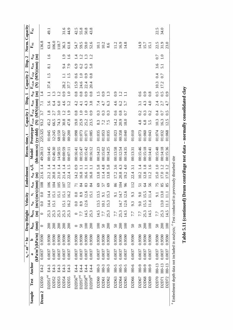
s u
= a
z2 + b
z D
rop
Hei
ght
Vel
ocity
E
mbe
dmen
t R
econ
. tim
e, t
Cap
acity
1 D
isp.
1
Cap
acity
2 D
isp.
2
Nor
m. C
apac
ity
Sam
ple
Tes
t A
ncho
r a
b h d
,m
h d,e
q v m
v i
z e
,m
z e,p
z e/L
M
odel
P
roto
type
Fv1
,m F
v1,p
z 1,m
z 1
,p
Fv2
,m F
v2,p
z 2,m
z 2
,p
FN
1 F
N2
(k
Pa/
m2 ) (
kPa/
m)
(mm
) (m
) (m
/s) (
m/s
) (m
m)
(m)
(h
h:m
m:s
s) (
yy:d
dd)
(N)
(MN
) (m
m)
(m)
(N)
(MN
) (m
m)
(m)
Dru
m 2
D
2D50
E
4-2
0.00
37
0.95
90
0 0
0.0
0.0
108
21.6
1.
4 49
:28:
13
225:
325
93.2
3.
7 7.
1 1.
4
13
6.8
D2D
51#d
E
4-3
0.00
37
0.95
90
200
25.3
14
.4
14.4
10
6 21
.2
1.4
00:1
4:45
01
:045
45
.2
1.8
5.6
1.1
37.4
1.
5 8.
1 1.
6 63
.4
49.1
D2D
52
E4-
3 0.
0037
0.
9590
20
0 25
.3
15.1
15
.1
104
20.8
1.
4 02
:46:
30
12:2
45
66.5
2.
7 6.
4 1.
3
10
6.0
D2D
53
E4-
3 0.
0037
0.
9590
20
0 25
.3
15
.1
105
21.0
1.
4 14
:58:
55
68:1
50
74.3
3.
0 6.
0 1.
2
11
8.7
D2D
54
E4-
3 0.
0037
0.
9590
20
0 25
.3
15.1
15
.1
107
21.4
1.
4 00
:00:
59
00:0
27
30.8
1.
2 4.
6 0.
9 28
.2
1.1
9.4
1.9
36.3
31
.6
D
2D55
E
4-3
0.00
37
0.95
90
200
25.3
16
.2
16.2
11
2 22
.4
1.5
00:0
7:11
00
:200
47
.8
1.9
5.2
1.0
37.7
1.
5 7.
9 1.
6 61
.8
44.9
D2D
56#d
E
4-4
0.00
37
0.95
90
0 0
0.0
0.0
71
14.2
0.
9 00
:16:
41
01:0
98
19.0
0.
8 4.
2 0.
8 15
.9
0.6
6.9
1.4
54.7
42
.5
D
2D57
#d
E4-
4 0.
0037
0.
9590
50
7.
7 8.
9 8.
9 84
16
.8
1.1
00:1
5:47
01
:073
25
.9
1.0
4.1
0.8
24.6
1.
0 6.
2 1.
2 59
.5
55.8
D2D
58#d
E
4-4
0.00
37
0.95
90
100
14.5
12
.6
12.6
83
16
.6
1.1
00:1
5:42
01
:071
25
.2
1.0
4.3
0.9
22.4
0.
9 6.
3 1.
3 59
.0
50.8
D2D
59#d
E
4-4
0.00
37
0.95
90
200
25.3
15.1
84
16
.8
1.1
00:1
6:12
01
:085
23
.5
0.9
3.8
0.8
20.4
0.
8 5.
8 1.
2 52
.6
43.8
D2D
60
H0-
3 0.
0037
0.
9590
10
0 14
.5
13.5
13
.5
69
13.8
5.
8 00
:14:
23
01:0
35
8.3
0.3
7.4
1.5
10.1
D
2D61
H
0-3
0.00
37
0.95
90
50
7.7
10.1
9.
1 57
11
.4
4.8
00:1
5:02
01
:053
7.
2 0.
3 4.
7 0.
9
10
.2
D2D
62
H0-
3 0.
0037
0.
9590
20
0 25
.3
15.3
15
.3
69
13.8
5.
8 00
:14:
25
01:0
35
7.5
0.3
6.3
1.3
8.6
D2D
63
H0-
5 0.
0037
0.
9590
50
7.
7
9.1
86
17.2
3.
6 00
:13:
58
01:0
23
14.2
0.
6 4.
6 0.
9
11
.2
D2D
64
H0-
5 0.
0037
0.
9590
20
0 25
.3
14.7
14
.7
104
20.8
4.
3 00
:12:
54
00:3
58
20.9
0.
8 6.
2 1.
2
16
.9
D2D
65
H0-
5 0.
0037
0.
9590
10
0 14
.5
12.6
12
.6
96
19.2
4.
0 00
:14:
35
01:0
40
18.0
0.
7 5.
7 1.
1
14
.8
D2D
66
H0-
6 0.
0037
0.
9590
50
7.
7 9.
3 9.
3 11
2 22
.4
3.1
00:1
3:31
01
:010
D2D
67
H0-
9 0.
0037
0.
9590
50
7.
7 9.
0 9.
0 51
10
.2
1.4
00:1
5:46
01
:073
4.
8 0.
2 3.
1 0.
6
14
.9
D2D
68
H0-
9 0.
0037
0.
9590
20
0 25
.3
15.5
15
.5
64
12.8
1.
8 00
:15:
18
01:0
60
6.8
0.3
4.3
0.9
15.7
D
2D69
H
0-9
0.00
37
0.95
90
100
14.5
11
.4
11.4
56
11
.2
1.6
00:1
4:41
01
:043
5.
5 0.
2 4.
0 0.
8
15
.1
D2D
70
H0-
13
0.00
37
0.95
90
50
7.7
9.
1 75
15
.0
1.0
00:1
5:48
01
:074
10
.3
0.4
2.4
0.5
10.3
0.
4 3.
6 0.
7 22
.5
22.5
D2D
71
H0-
13
0.00
37
0.95
90
200
25.3
13
.0
13.0
85
17
.0
1.2
00:1
4:18
01
:032
16
.3
0.7
2.7
0.5
17.2
0.
7 5.
1 1.
0 31
.9
34.0
D2D
72
H0-
13
0.00
37
0.95
90
100
14.5
11
.1
11.1
85
17
.0
1.2
00:1
5:36
01
:068
12
.5
0.5
4.7
0.9
23.0
# Em
bedm
ent d
epth
dat
a no
t inc
lude
d in
ana
lysi
s; d T
est c
ondu
cted
in p
revi
ousl
y di
stur
bed
site
Tab
le 5
.11
(con
tinue
d) D
rum
cen
trifu
ge te
st d
ata
– no
rmal
ly c
onso
lidat
ed c
lay
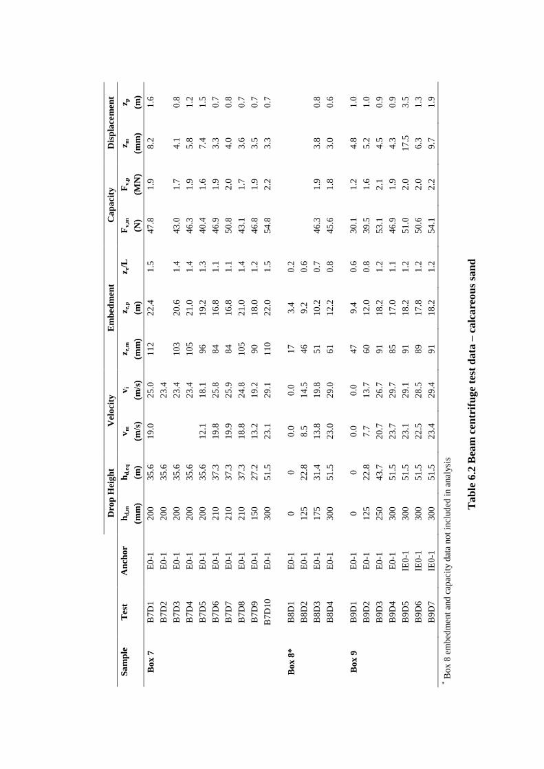
D
rop
Hei
ght
Vel
ocity
E
mbe
dmen
t C
apac
ity
Dis
plac
emen
t
Sam
ple
Tes
t A
ncho
r h d,
m
h d,e
q v m
v i
z e
,m
z e,p
z e/L
F
v,m
Fv,
p z m
z p
(mm
) (m
) (m
/s)
(m/s
) (m
m)
(m)
(N
) (M
N)
(mm
) (m
)
Box
7
B7D
1 E
0-1
200
35.6
19
.0
25.0
11
2 22
.4
1.5
47.8
1.
9 8.
2 1.
6
B
7D2
E0-
1 20
0 35
.6
23
.4
B
7D3
E0-
1 20
0 35
.6
23
.4
103
20.6
1.
4 43
.0
1.7
4.1
0.8
B
7D4
E0-
1 20
0 35
.6
23
.4
105
21.0
1.
4 46
.3
1.9
5.8
1.2
B
7D5
E0-
1 20
0 35
.6
12.1
18
.1
96
19.2
1.
3 40
.4
1.6
7.4
1.5
B
7D6
E0-
1 21
0 37
.3
19.8
25
.8
84
16.8
1.
1 46
.9
1.9
3.3
0.7
B
7D7
E0-
1 21
0 37
.3
19.9
25
.9
84
16.8
1.
1 50
.8
2.0
4.0
0.8
B
7D8
E0-
1 21
0 37
.3
18.8
24
.8
105
21.0
1.
4 43
.1
1.7
3.6
0.7
B
7D9
E0-
1 15
0 27
.2
13.2
19
.2
90
18.0
1.
2 46
.8
1.9
3.5
0.7
B
7D10
E
0-1
300
51.5
23
.1
29.1
11
0 22
.0
1.5
54.8
2.
2 3.
3 0.
7
B
ox 8
* B
8D1
E0-
1 0
0 0.
0 0.
0 17
3.
4 0.
2
B
8D2
E0-
1 12
5 22
.8
8.5
14.5
46
9.
2 0.
6
B
8D3
E0-
1 17
5 31
.4
13.8
19
.8
51
10.2
0.
7 46
.3
1.9
3.8
0.8
B
8D4
E0-
1 30
0 51
.5
23.0
29
.0
61
12.2
0.
8 45
.6
1.8
3.0
0.6
Box
9
B9D
1 E
0-1
0 0
0.0
0.0
47
9.4
0.6
30.1
1.
2 4.
8 1.
0
B
9D2
E0-
1 12
5 22
.8
7.7
13.7
60
12
.0
0.8
39.5
1.
6 5.
2 1.
0
B
9D3
E0-
1 25
0 43
.7
20.7
26
.7
91
18.2
1.
2 53
.1
2.1
4.5
0.9
B
9D4
E0-
1 30
0 51
.5
23.7
29
.7
85
17.0
1.
1 46
.9
1.9
4.3
0.9
B
9D5
IE0-
1 30
0 51
.5
23.1
29
.1
91
18.2
1.
2 51
.0
2.0
17.5
3.
5
B
9D6
IE0-
1 30
0 51
.5
22.5
28
.5
89
17.8
1.
2 50
.6
2.0
6.3
1.3
B
9D7
IE0-
1 30
0 51
.5
23.4
29
.4
91
18.2
1.
2 54
.1
2.2
9.7
1.9
* Box
8 e
mbe
dmen
t and
cap
acit
y da
ta n
ot in
clud
ed in
ana
lysi
s
Tab
le 6
.2 B
eam
cen
trifu
ge te
st d
ata
– ca
lcar
eous
san
d


231
FIGURES

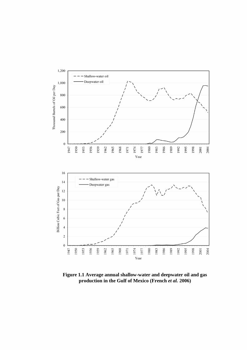
Figure 1.1 Average annual shallow-water and deepwater oil and gas production in the Gulf of Mexico (French et al.2006)

Figure 1.2 Offshore development systems(http://www.gomr.mms.gov)

Figure 1.3 Tension leg platform(http://www.offshore-technology.com)
Figure 1.4 Semi-submersible(http://www.offshore-technology.com)
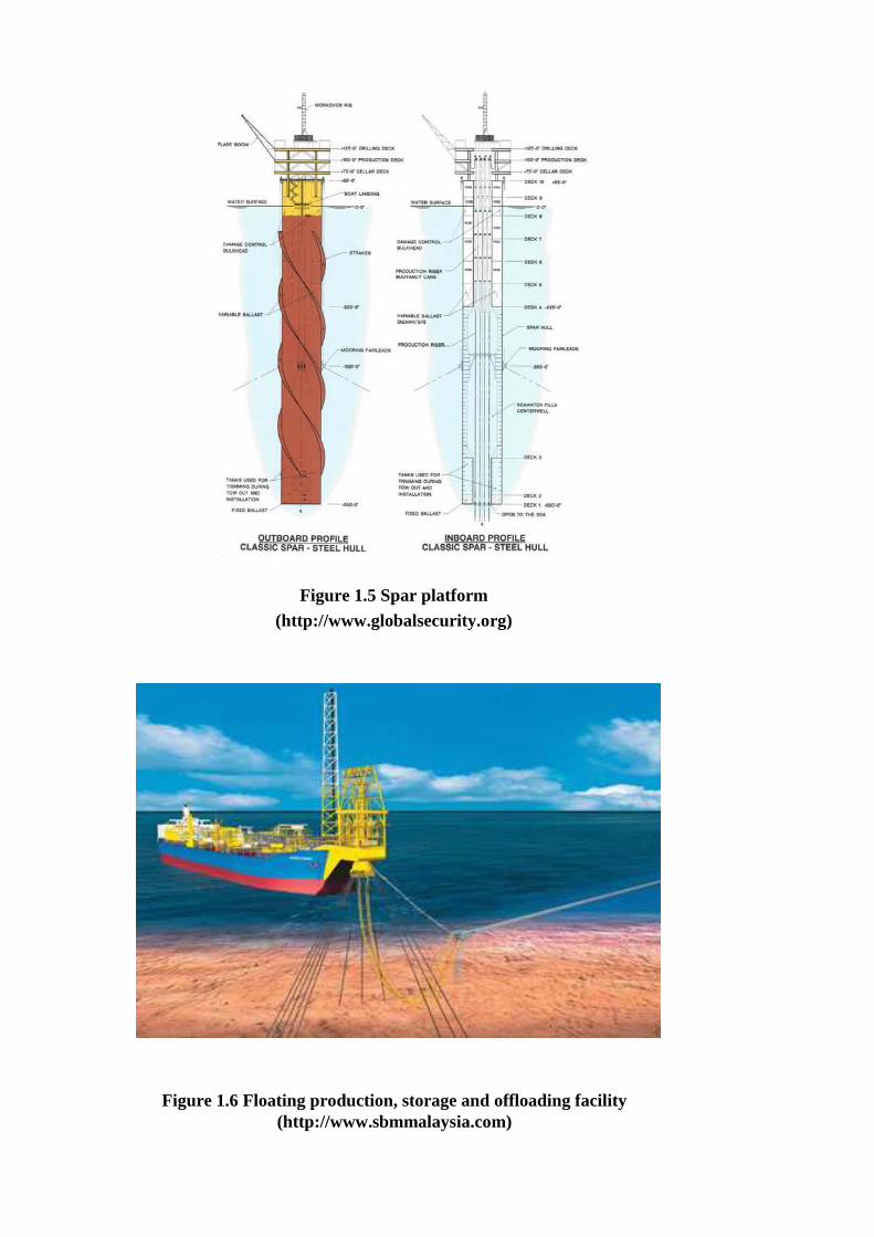
Figure 1.5 Spar platform(http://www.globalsecurity.org)
Figure 1.6 Floating production, storage and offloading facility (http://www.sbmmalaysia.com)
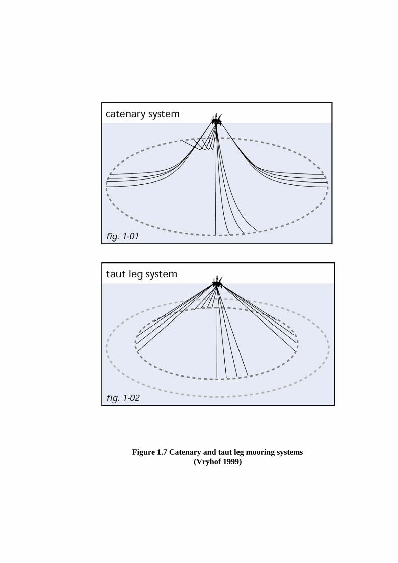
Figure 1.7 Catenary and taut leg mooring systems (Vryhof 1999)
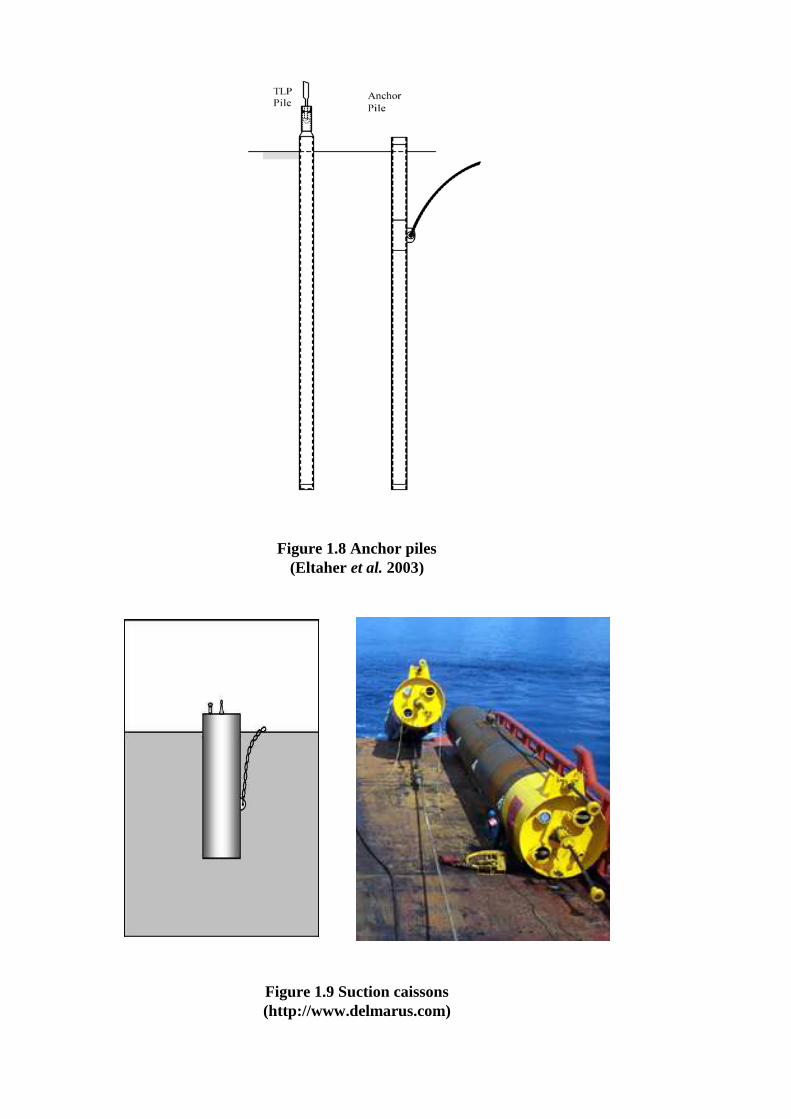
Figure 1.8 Anchor piles (Eltaher et al. 2003)
Figure 1.9 Suction caissons(http://www.delmarus.com)
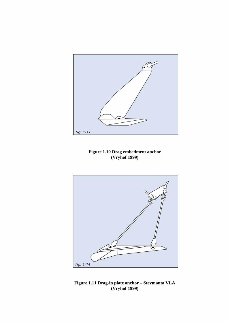
Figure 1.10 Drag embedment anchor (Vryhof 1999)
Figure 1.11 Drag-in plate anchor – Stevmanta VLA (Vryhof 1999)
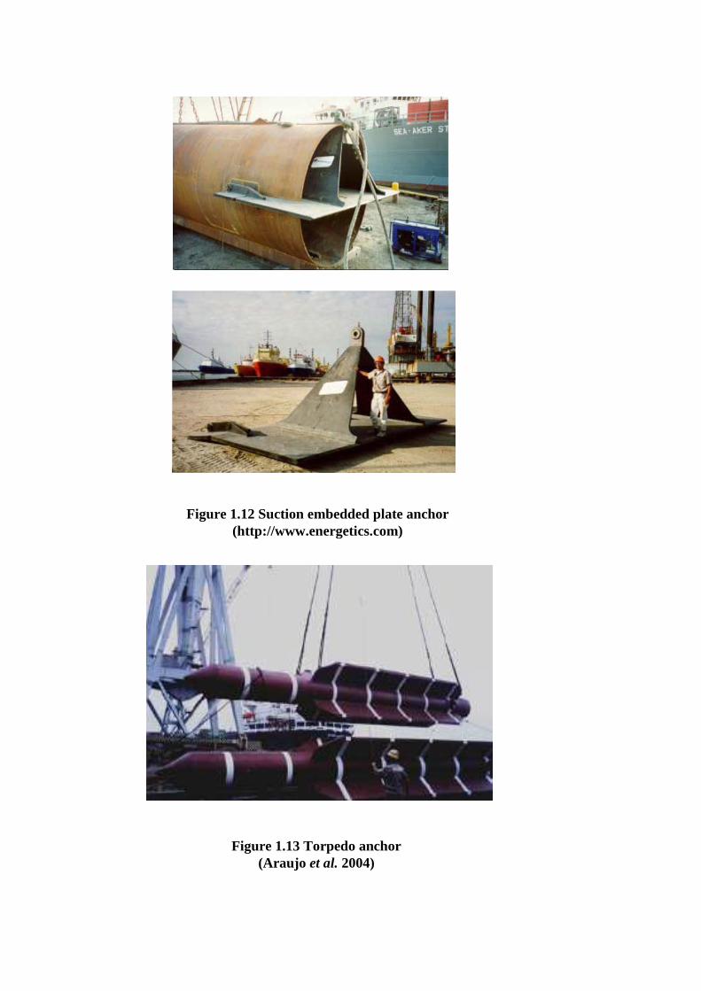
Figure 1.12 Suction embedded plate anchor (http://www.energetics.com)
Figure 1.13 Torpedo anchor (Araujo et al. 2004)

Figure 1.14 Deep Penetrating Anchor (Lieng et al. 1999)


Figure 2.1 Marine sediment penetrometer (after Colp et al. 1975)
Figure 2.2 Laboratory scale Marine impact penetrometer (after Dayal & Allen 1973)

Figure 2.3 Undrained shear strength profiles from Doppler penetrometer tests in normally consolidated terrigenous clayey silt
(after Beard 1981)

Figure 2.4 Free fall cone penetrometer (after Brooke Ocean Technology 2007)
Figure 2.5 Expendable Bottom Penetrometer (after Shi 2005)

Figure 2.6 Interpreted XBP and miniature vane shear strength profiles (after Aubeny & Shi 2006)
Figure 2.7 Great Meteor East and Nares Abyssal Plain test sites in the Atlantic Ocean (after Freeman & Burdett 1986)
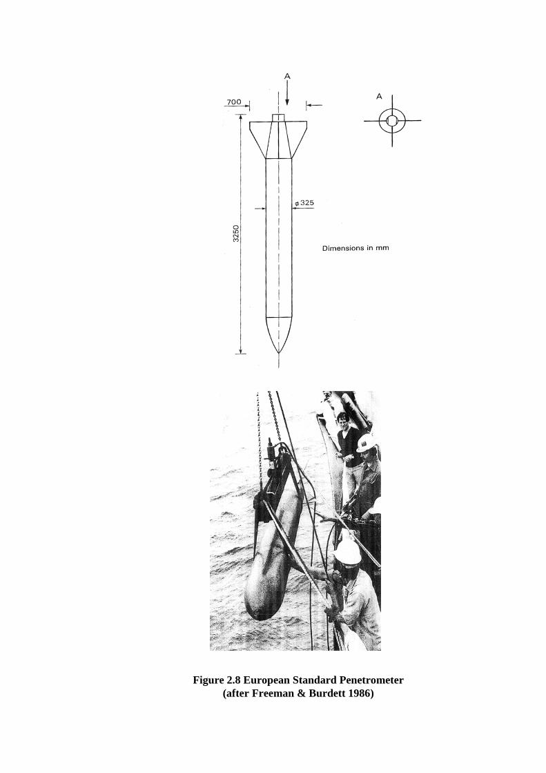
Figure 2.8 European Standard Penetrometer (after Freeman & Burdett 1986)

Figure 2.9 DOMP II penetrometer designs (after Freeman & Burdett 1986)

Figure 2.10 True’s Method – calculation procedure flow chart (NCEL 1985)
Is
vi > 3 ft/s
Determine object characteristics
L, D, Deq, Ap, As, Ws, m, CD
Yes
Use static penetration
method
Obtain soil parameters
su, St, ρ, Se*, Ce, Co
No
Select depth increment
∆z
Initialise iterative values
i = 0, z = 0, v0 = v
i = i + 1
zi = i(∆z)
Calculate
Ws
Calculate
Fbi, sui(nose), Sei, Nti
Calculate
Fsi, sui(side), Sti, Sei
Does
i = 1?
Estimate Fdiusing v0
Yes
Estimate v1
Calculate
Fdi
No
Calculate
Fi
Calculate
vi+1
Is
vi+1 < 0?
Penetrate one more
depth increment
No
Calculate final embedment
z
Yes
Equations 2.16, 2.17 & 2.19
Equations 2.18 & 2.19
Equation 2.8
Equation 2.15
Equation 2.22
Equation 2.24
Equation 2.8
Equation 2.23

Figure 2.11 Dependence of pile capacity on time after installation (after Fleming et al. 1985)
Figure 2.12 Dependence of torpedo anchor capacity on time after installation (after Audibert et al. 2006)
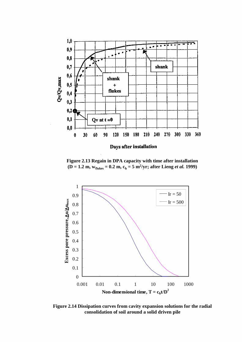
Figure 2.13 Regain in DPA capacity with time after installation (D = 1.2 m, wflukes = 0.2 m, ch = 5 m2/yr; after Lieng et al. 1999)
Figure 2.14 Dissipation curves from cavity expansion solutions for the radial consolidation of soil around a solid driven pile
0
0.1
0.2
0.3
0.4
0.5
0.6
0.7
0.8
0.9
1
0.001 0.01 0.1 1 10 100 1000
Non-dimensional time, T = cht/D2
Exc
ess
pore
pre
ssur
e, ∆∆ ∆∆u/
∆∆ ∆∆u m
ax
Ir = 50
Ir = 500

Figure 2.15 Torpedo anchors (a) after Medeiros (2001) (b) after Araujo et al. (2004)
(a)
(b)
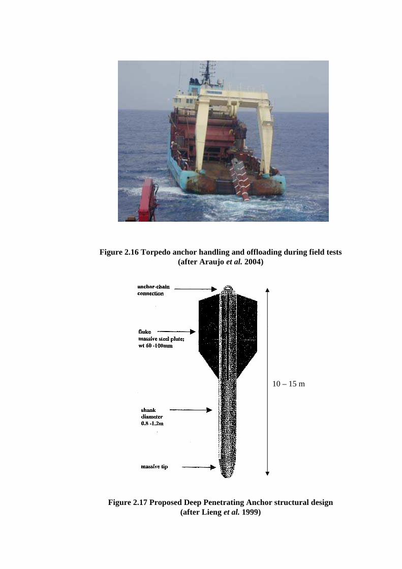
Figure 2.16 Torpedo anchor handling and offloading during field tests (after Araujo et al. 2004)
Figure 2.17 Proposed Deep Penetrating Anchor structural design (after Lieng et al. 1999)
10 – 15 m
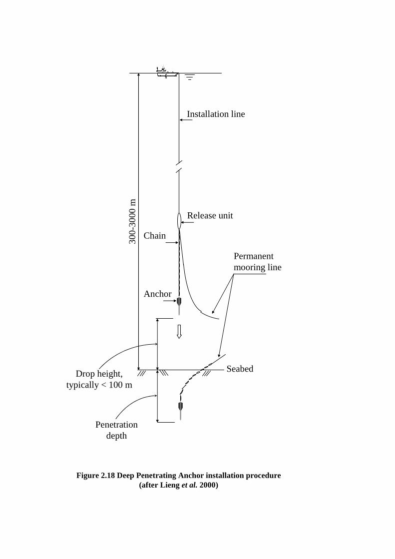
Figure 2.18 Deep Penetrating Anchor installation procedure (after Lieng et al. 2000)
Permanent mooring line
Installation line
Release unit
300
-30
00 m
Penetration depth
Anchor
Seabed
Chain
Drop height, typically < 100 m
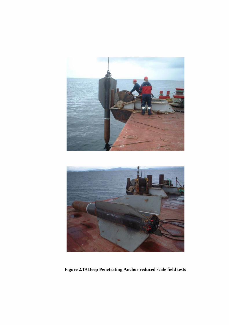
Figure 2.19 Deep Penetrating Anchor reduced scale field tests
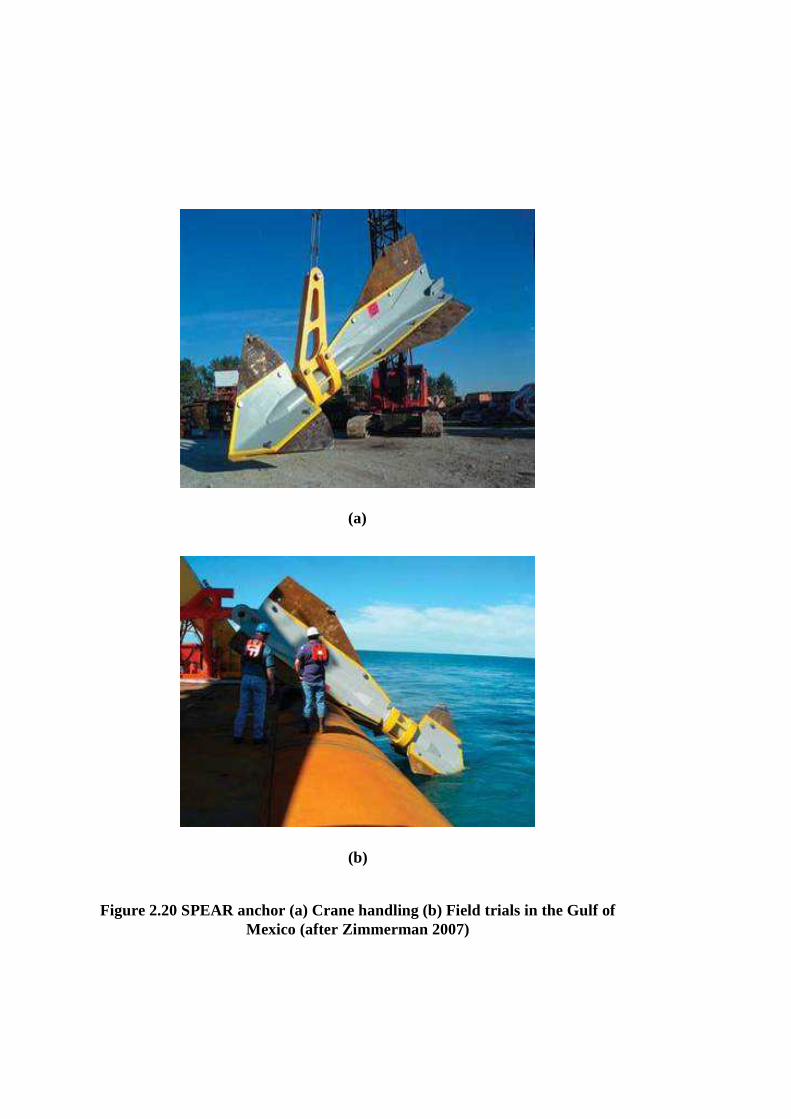
Figure 2.20 SPEAR anchor (a) Crane handling (b) Field trials in the Gulf of Mexico (after Zimmerman 2007)
(a)
(b)
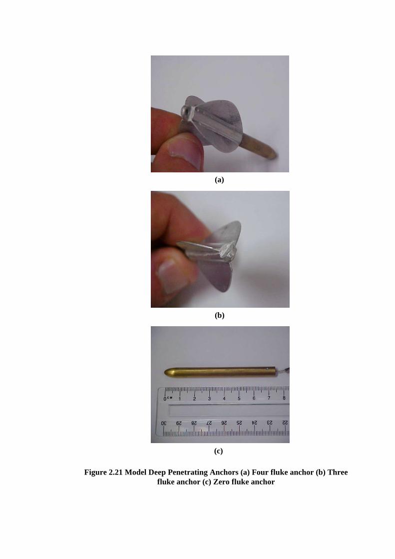
Figure 2.21 Model Deep Penetrating Anchors (a) Four fluke anchor (b) Three fluke anchor (c) Zero fluke anchor
(a)
(b)
(c)
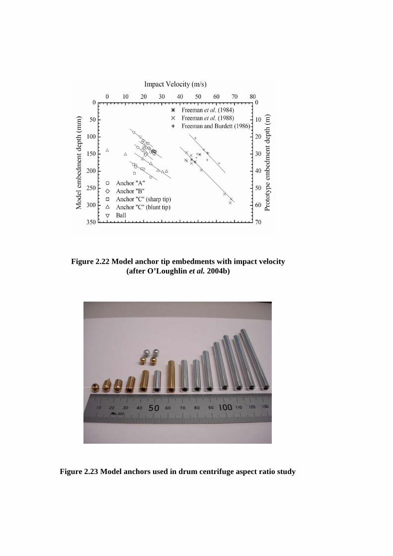
Figure 2.22 Model anchor tip embedments with impact velocity (after O’Loughlin et al. 2004b)
Figure 2.23 Model anchors used in drum centrifuge aspect ratio study

0
0.1
0.2
0.3
0.4
0.5
0.6
0.7
0.8
0.9
1
Stress
No
rma
lised
dep
th,
z/h sa
mpl
ePrototype
Model
Under stress
Over stress
Stress similitude
Figure 3.1 Stress variation with depth (model and prototype)
Swinging Platform
Counter Weight
Strong-box
Flight Computer
Figure 3.2 Beam centrifuge
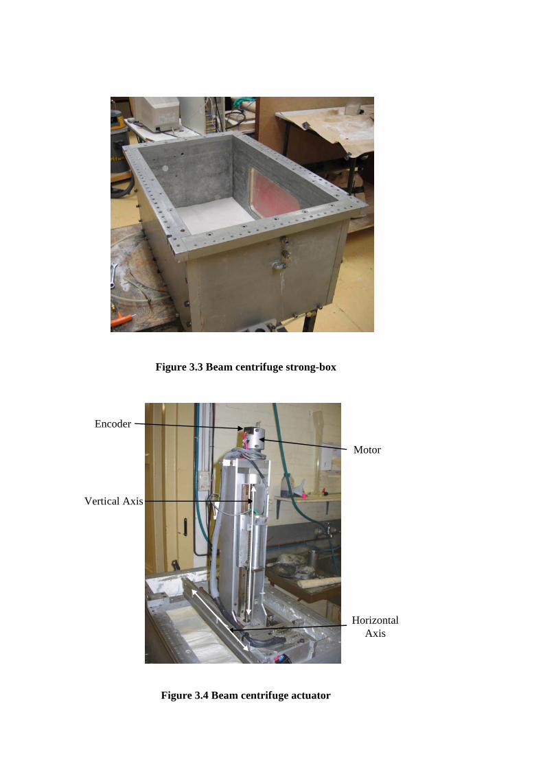
Figure 3.3 Beam centrifuge strong-box
Figure 3.4 Beam centrifuge actuator
Horizontal Axis
Vertical Axis
Motor
Encoder

50 mm
Pore pressure transducer
Figure 3.5 Sub-Terrain Oil impregnated Multiple Pressure Instrument (STOMPI)
Sample Channel Tool Table Actuator
Figure 3.6 Drum centrifuge (with cover removed)
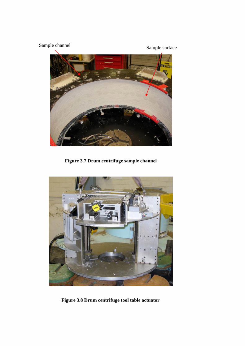
Figure 3.7 Drum centrifuge sample channel
Sample channel Sample surface
Figure 3.8 Drum centrifuge tool table actuator

Figure 3.9 Rowe cell test - coefficient of vertical consolidation
0 100 200 300 400 500 6000
1
2
3
4
5
6
7
Coe
ffici
ent o
f Con
solid
atio
n, c v (
m2 /y
r)
Vertical Effective Stress, σ'v (kPa)
Figure 3.10 Hopper positioned above drum centrifuge
Hopper
Clamshell
Cover
Coupling

Figure 3.11 Rotating coupling and slurry placement nozzle
Hose
Rotating coupling
HoseNozzle
Tool table actuator
20
5
SIDE VIEW END VIEW
Figure 3.12 T-bar penetrometer
Load cell Shaft
T-bar

Figure 3.13 25 MPa, 10 mm diameter cone penetrometer
Load cell
Cone tip
Shaft
Figure 3.14 100 MPa, 7 mm diameter cone penetrometer
Load cell
Cone tip
Shaft

Figure 3.15 Zero fluke model anchor
Ltip
Lshaft
D
L
0
2
4
6
8
10
12
-8 -6 -4 -2 0 2 4 6 8x (mm)
y (m
m)
a
b
Figure 3.16 Ellipsoid anchor tip shape

Figure 3.17 Interchangeable zero fluke model anchor segments
Tip & shaft
Padeye
Tip
Shaft
Padeye
Figure 3.18 Four fluke model anchor
L
D
Ltip
Lfluke1
Lfluke2
Lfluke3
wfluke

(a)
(b)
Figure 3.19 Model anchors – varying tip geometry (a) Conical tip (b) Ogive tip (c) Flat tip
(c)
Ltip
L
D
D
Lshaft
Ltip
Lshaft
L
D
L

Figure 3.20 Instrumented model anchor
Piezoelectric material
Test massStrain gauged
section
Figure 3.21 Model anchors – varying aspect ratio
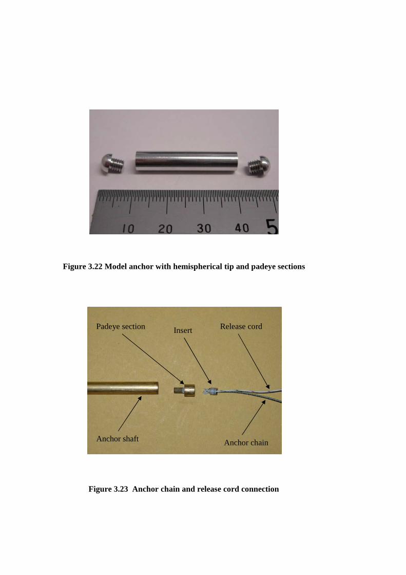
Figure 3.22 Model anchor with hemispherical tip and padeye sections
Anchor shaft
Padeye section Insert
Anchor chain
Release cord
Figure 3.23 Anchor chain and release cord connection
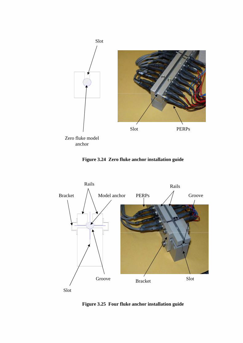
Figure 3.24 Zero fluke anchor installation guide
Slot
Zero fluke model anchor
Slot PERPs
Rails
Bracket
Slot
Model anchor
Groove
Figure 3.25 Four fluke anchor installation guide
Slot
Groove
Rails
Bracket
PERPs
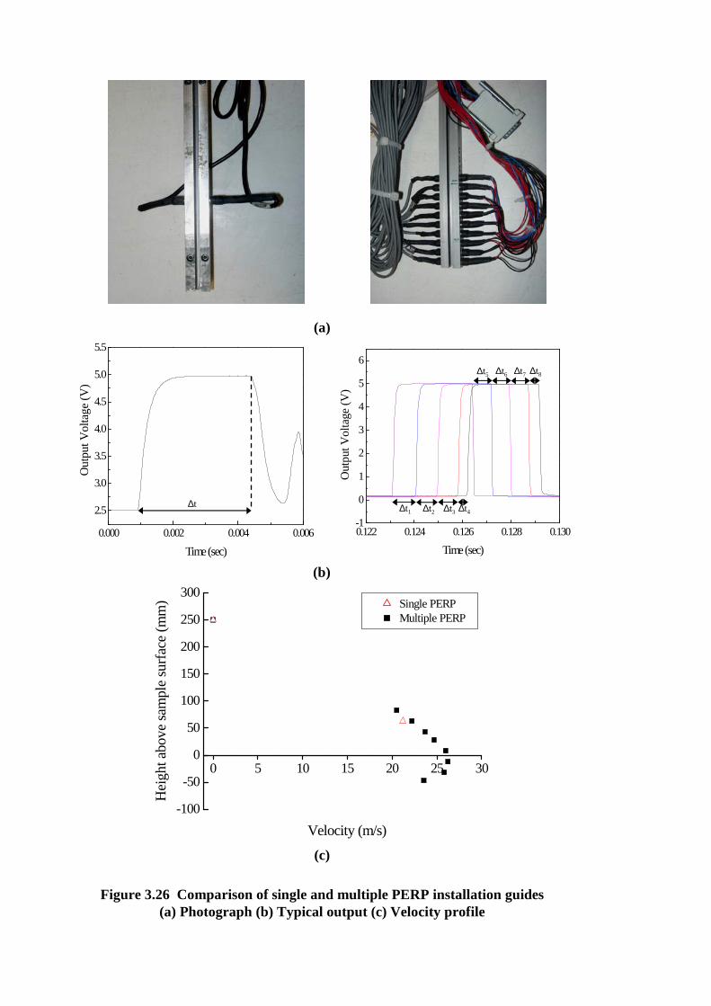
Figure 3.26 Comparison of single and multiple PERP installation guides (a) Photograph (b) Typical output (c) Velocity profile
(a)
(b)
(c)
0 5 10 15 20 25 30
-100
-50
0
50
100
150
200
250
300Single PERPMultiple PERP
Hei
ght a
bove
sam
ple
surf
ace
(mm
)
Velocity (m/s)
0.000 0.002 0.004 0.006
2.5
3.0
3.5
4.0
4.5
5.0
5.5
Out
put V
olta
ge (
V)
Time (sec)
∆t ∆t1 ∆t2 ∆t3 ∆t4
∆t5 ∆t6 ∆t7 ∆t8
0.122 0.124 0.126 0.128 0.130-1
0
1
2
3
4
5
6
O
utpu
t Vol
tage
(V
)
Time (sec)

Figure 3.27 Release mechanism
Release cord
Resistor
Clamp
Anchor chain
Load cell
Connecting screw
Figure 3.28 Load cell
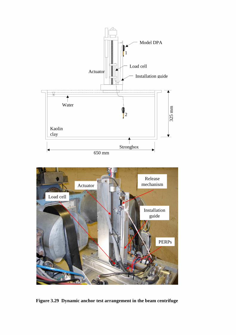
Water
650 mm
325
mm
1
2
Installation guide
Model DPA
Load cell Actuator
Kaolin clay
Strongbox
Load cell
Release mechanism
Installation guide
PERPs
Actuator
Figure 3.29 Dynamic anchor test arrangement in the beam centrifuge
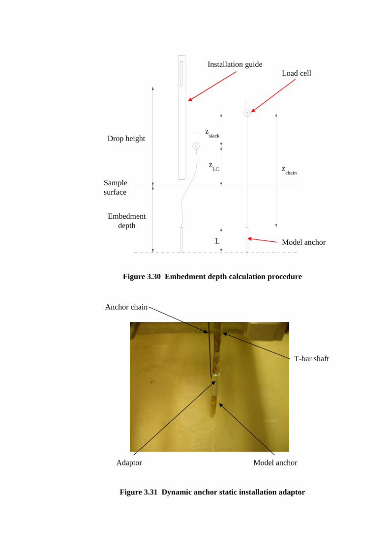
Figure 3.30 Embedment depth calculation procedure
Drop height
Embedment depth
Load cell
zslack
zchain
L
zLC
Sample surface
Installation guide
Model anchor
Figure 3.31 Dynamic anchor static installation adaptor
Model anchor
Anchor chain
Adaptor
T-bar shaft

Load cell
Installation guide
Sample surface
Figure 3.32 Dynamic anchor test arrangement in the drum centrifuge
Installation guide
Load cell
Sample surface
10°
PERPs
Anchor chain

Figure 4.1 Drag coefficient dependence on object shape (after Hoerner 1965)
Figure 4.2 Drag coefficient as a function of Reynolds number for a smooth sphere and a smooth cylinder (after Young et al. 1997)
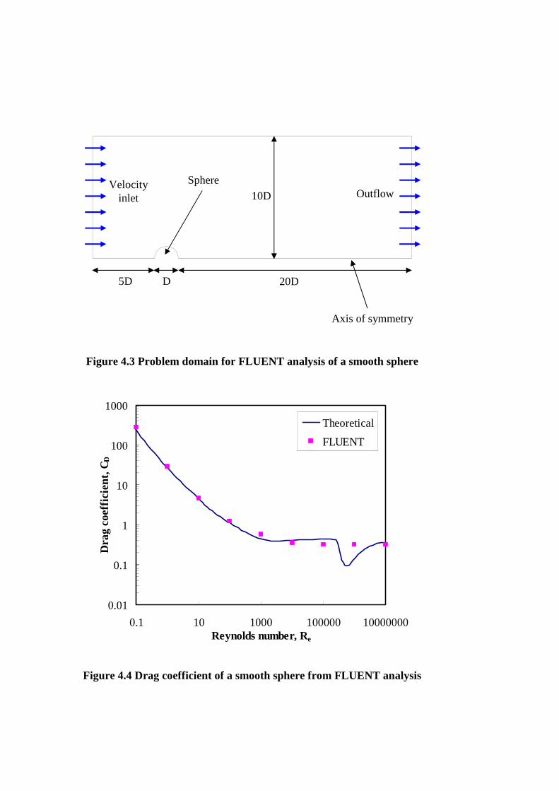
5D 20DD
10D
Figure 4.3 Problem domain for FLUENT analysis of a smooth sphere
Axis of symmetry
SphereVelocity inlet Outflow
Figure 4.4 Drag coefficient of a smooth sphere from FLUENT analysis
0.01
0.1
1
10
100
1000
0.1 10 1000 100000 10000000Reynolds number, Re
Dra
g co
effic
ient
, CD
Theoretical
FLUENT
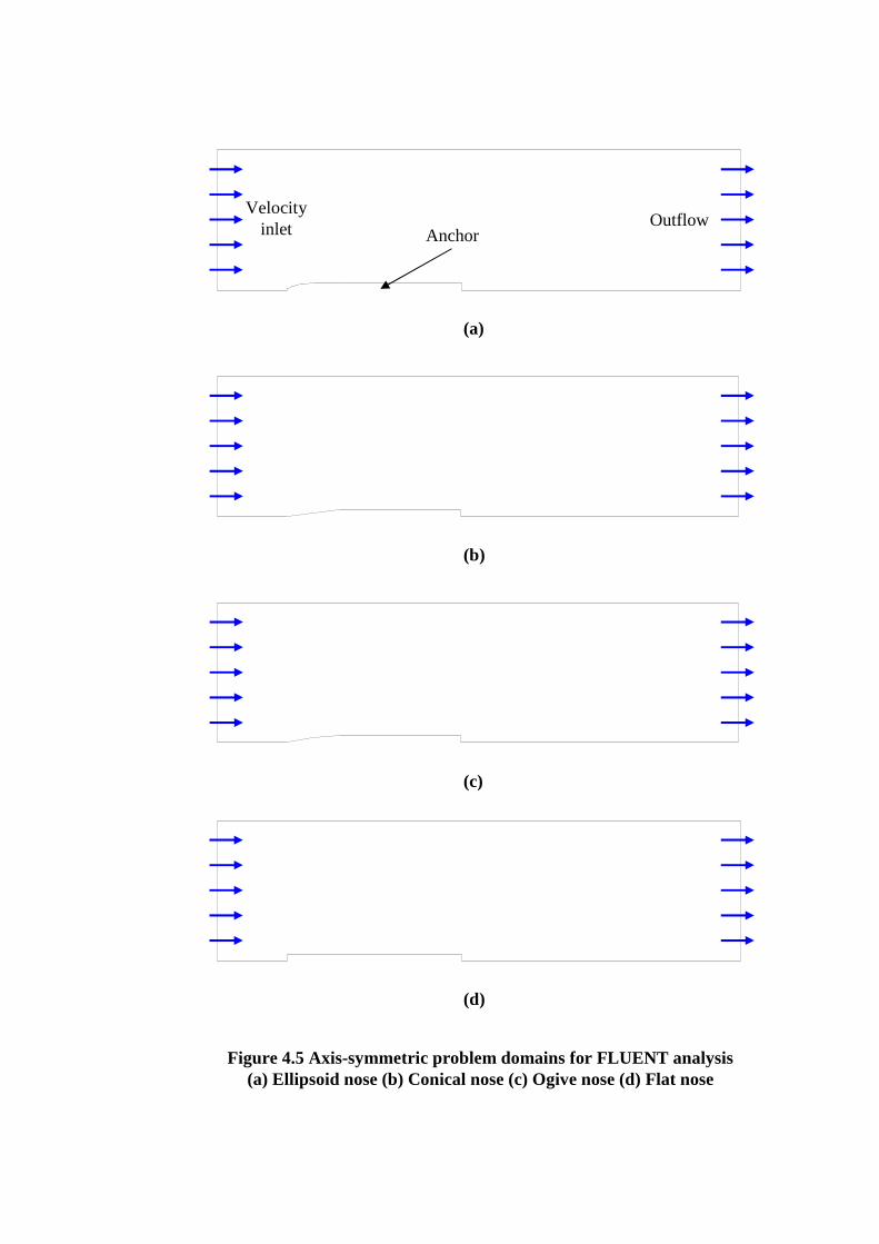
(a)
(b)
(c)
(d)
Figure 4.5 Axis-symmetric problem domains for FLUENT analysis (a) Ellipsoid nose (b) Conical nose (c) Ogive nose (d) Flat nose
Velocity inlet Outflow
Anchor
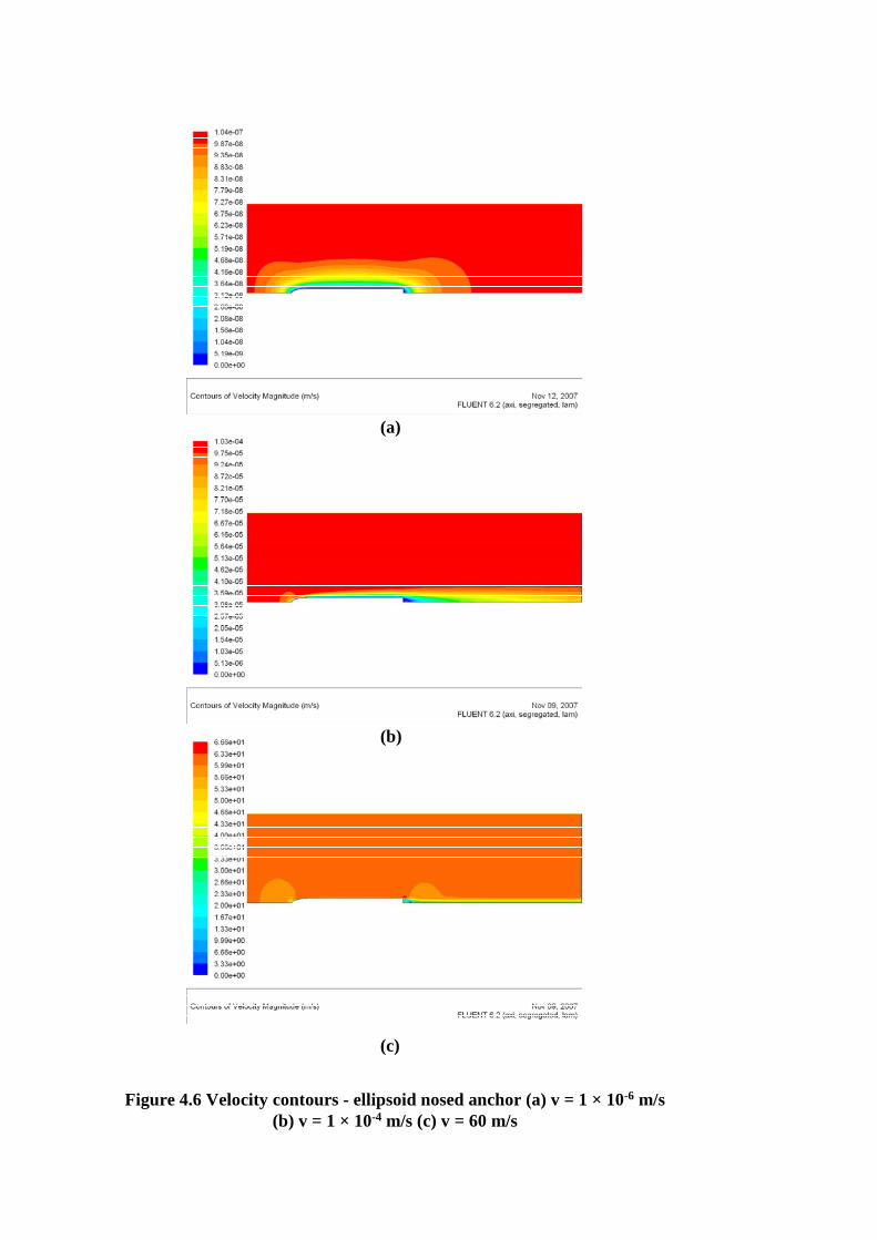
(a)
(b)
(c)
Figure 4.6 Velocity contours - ellipsoid nosed anchor (a) v = 1 × 10⁻⁶ m/s(b) v = 1 × 10⁻⁴ m/s (c) v = 60 m/s

(a)
(b)
(c)
Figure 4.7 Velocity contours - conical nosed anchor (a) v = 1 × 10⁻⁶ m/s(b) v = 1 × 10⁻⁴ m/s (c) v = 60 m/s

(a)
(b)
(c)
Figure 4.8 Velocity contours - ogive nosed anchor (a) v = 1 × 10⁻⁶ m/s(b) v = 1 × 10⁻⁴ m/s (c) v = 60 m/s
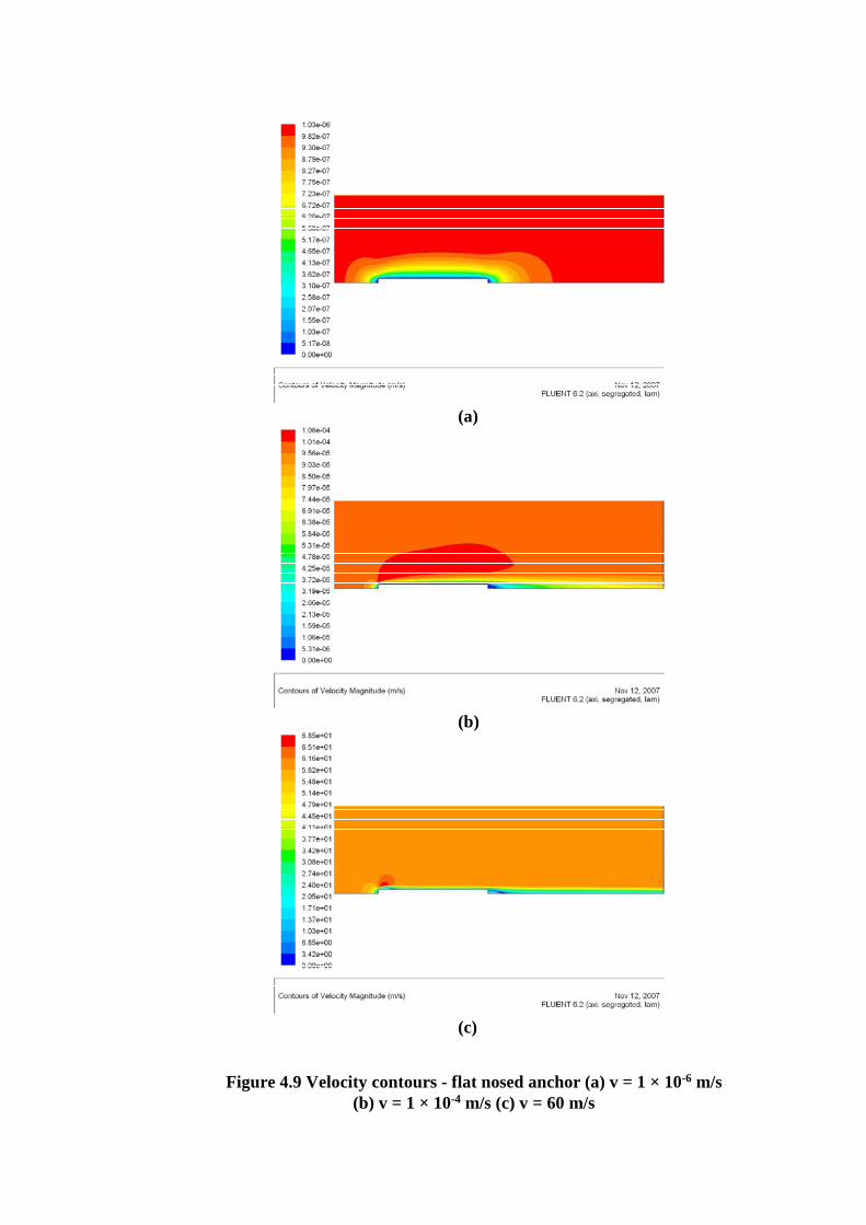
(a)
(b)
(c)
Figure 4.9 Velocity contours - flat nosed anchor (a) v = 1 × 10⁻⁶ m/s(b) v = 1 × 10⁻⁴ m/s (c) v = 60 m/s
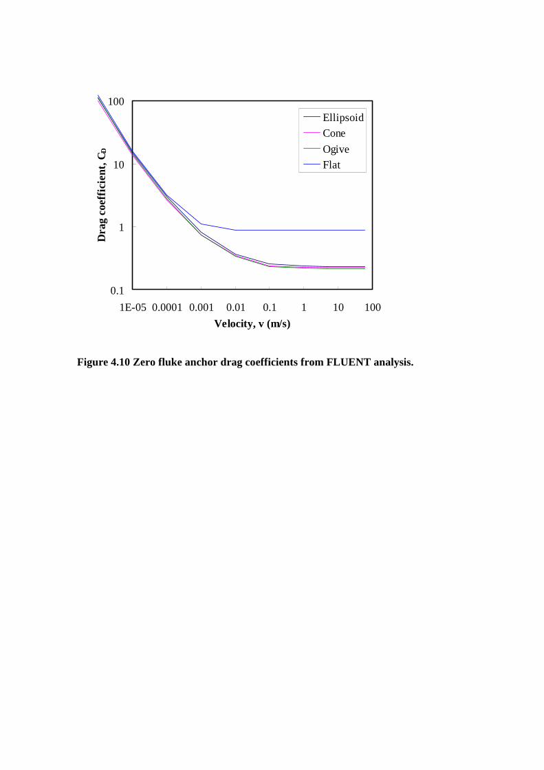
Figure 4.10 Zero fluke anchor drag coefficients from FLUENT analysis.
0.1
1
10
100
1E-05 0.0001 0.001 0.01 0.1 1 10 100
Velocity, v (m/s)
Dra
g co
effic
ient
, CD
Ellipsoid
Cone
Ogive
Flat

Figure 4.11 (a) Dependence of impact velocity on drop height
0
5
10
15
20
25
30
35
40
0 50 100 150 200 250 300Model drop height, hd,m (mm)
Impa
ct v
eloc
ity,
vi (
m/s
)
0 10 20 30 40 50 60Nominal prototype drop height, hd,p (m)
Uniform g field
Beam g field
Drum g field
0
10
20
30
40
50
60
0 50 100 150 200 250 300Model drop height, hd,m (mm)
Equ
ival
ent
prot
otyp
e dr
op h
eigh
t, h
d,e
q (m
)
Uniform g field
Beam g field
Drum g field
Figure 4.11 (b) Equivalent prototype drop heights

Sha
ft fr
ictio
n (F
s)
Iner
tial d
rag
(F d)
End
be
arin
g (F b
)
(a)
Com
plet
e ho
le c
losu
re(b
) P
artia
l hol
e cl
osur
e(c
) N
o ho
le c
losu
re
Sub
mer
ged
wei
ght (
W s)
Rev
ers
e en
d be
arin
g (F r
)
Fig
ure
4.12
Hol
e cl
osur
e be
hind
adv
anci
ng a
ncho
r du
ring
inst
alla
tion

Figure 4.13 Forces acting on a zero fluke dynamic anchor during installation
Shaft friction (Fs)
Submerged weight (Ws)
Inertial drag (Fd)
End bearing (Fb)
Figure 4.14 Forces acting on a four fluke dynamic anchor during installation
End bearing (Fb)
Inertial drag (Fd)
Submerged weight (Ws)
Shaft friction (Fs)
Fluke bearing (Fbf)
Fluke friction (Fsf)
Fluke reverse end bearing (Frf)

Figure 4.15 Flow chart showing calculation procedure for embedment prediction method
Determine object characteristics
L, Ltip, D, Ap, As, m, W, CD, vi, Nc
Determine soil properties
su, k, ρ, λ, β, α
Select time increment
∆t
Initialise iterative values
i = 0, z = 0, v = vi
i = i + 1
zi = i(∆z)
Calculate
Ws
Calculate
Fb, su,tip
Calculate
Fs, su,ave
Calculate
Fd
Calculate
F
Calculate
zi+1
Is
vi+1 < 0?
Penetrate another
increment
No
Calculate final embedment
z
Yes
Equation 4.16
Equation 4.20 or 4.21
Equation 4.22
Equation 4.23
Equation 4.24
Equation 4.25
ti-1 = -∆t
zi-1 = -∆t(vi)
Calculate
Rf
Calculate
a
Calculate
vi+1
Equation 4.15
Equation 4.4

Figure 4.16 Variation in bearing capacity factor with depth (after Skempton 1951 as cited by Whitlow 2001)
0
1
2
3
4
5
6
7
8
9
10
0 1 2 3 4 5Normalised depth, z/D
Bea
ring
ca
paci
ty fa
cto
r, N
c
Circle
Strip
Figure 4.17 Forces acting on a zero fluke dynamic anchor during extraction
Reverse end bearing (Fr)
Submerged weight (Ws)
Shaft friction (Fs)
Padeye bearing (Fb)
Cable tension (Fv)
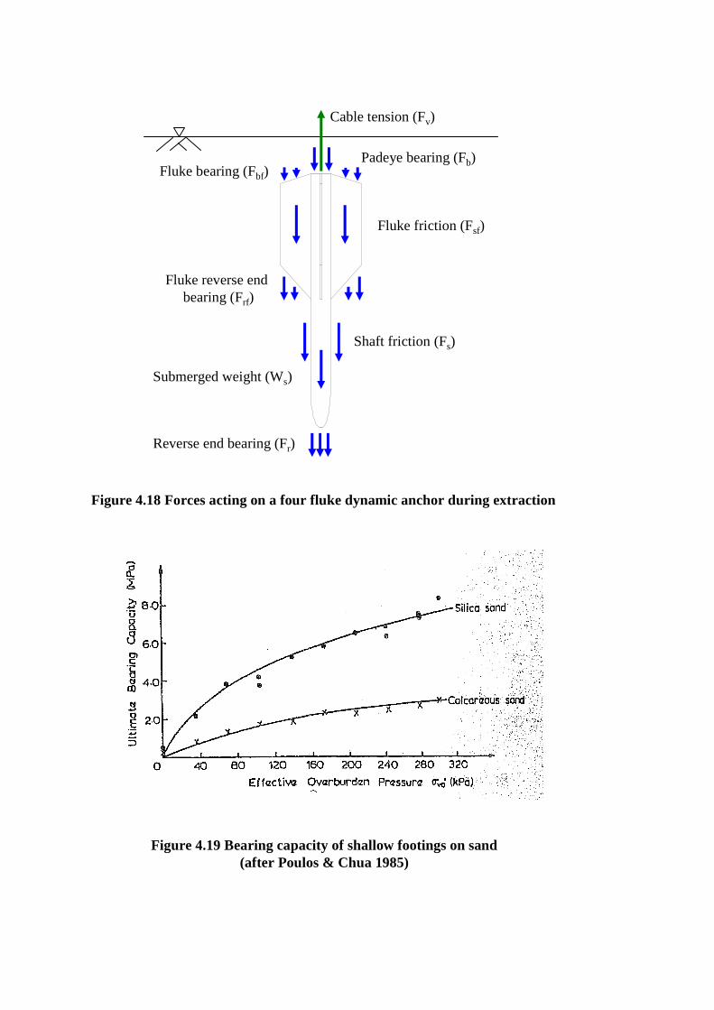
Figure 4.18 Forces acting on a four fluke dynamic anchor during extraction
Cable tension (Fv)
Padeye bearing (Fb)
Fluke reverse end bearing (Frf)
Fluke bearing (Fbf)
Fluke friction (Fsf)
Reverse end bearing (Fr)
Shaft friction (Fs)
Submerged weight (Ws)
Figure 4.19 Bearing capacity of shallow footings on sand (after Poulos & Chua 1985)
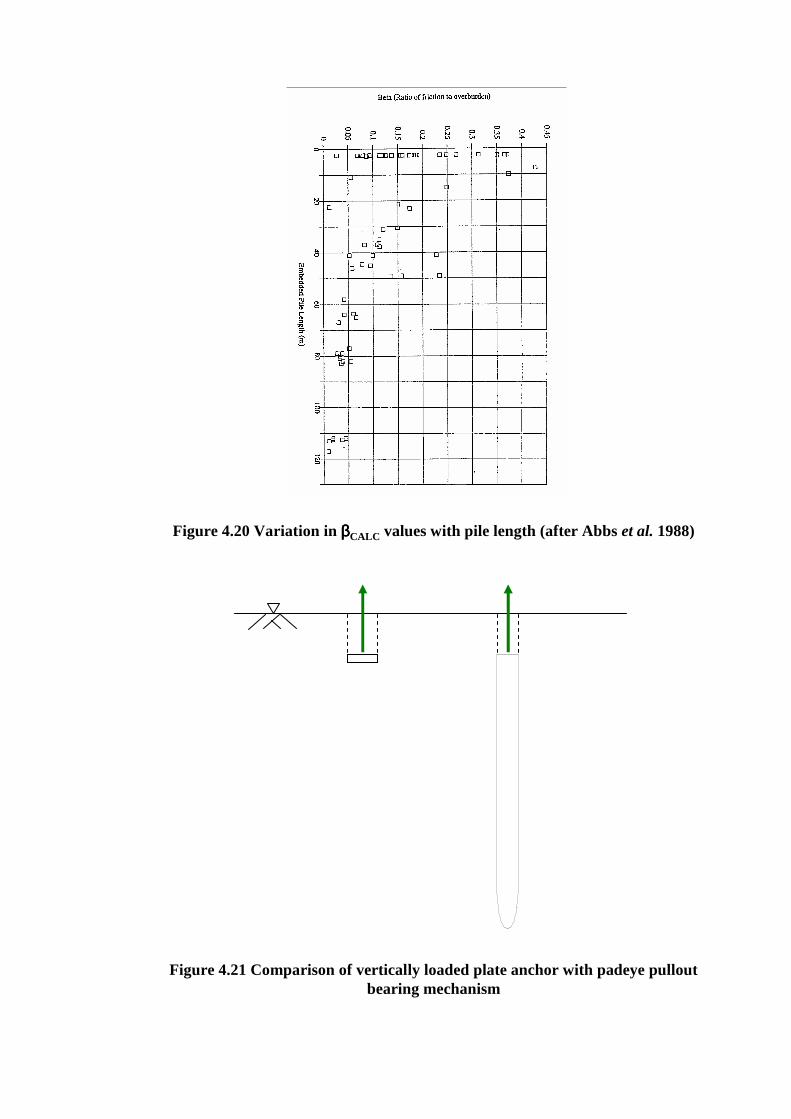
Figure 4.20 Variation in ββββCALC values with pile length (after Abbs et al. 1988)
Figure 4.21 Comparison of vertically loaded plate anchor with padeye pullout bearing mechanism
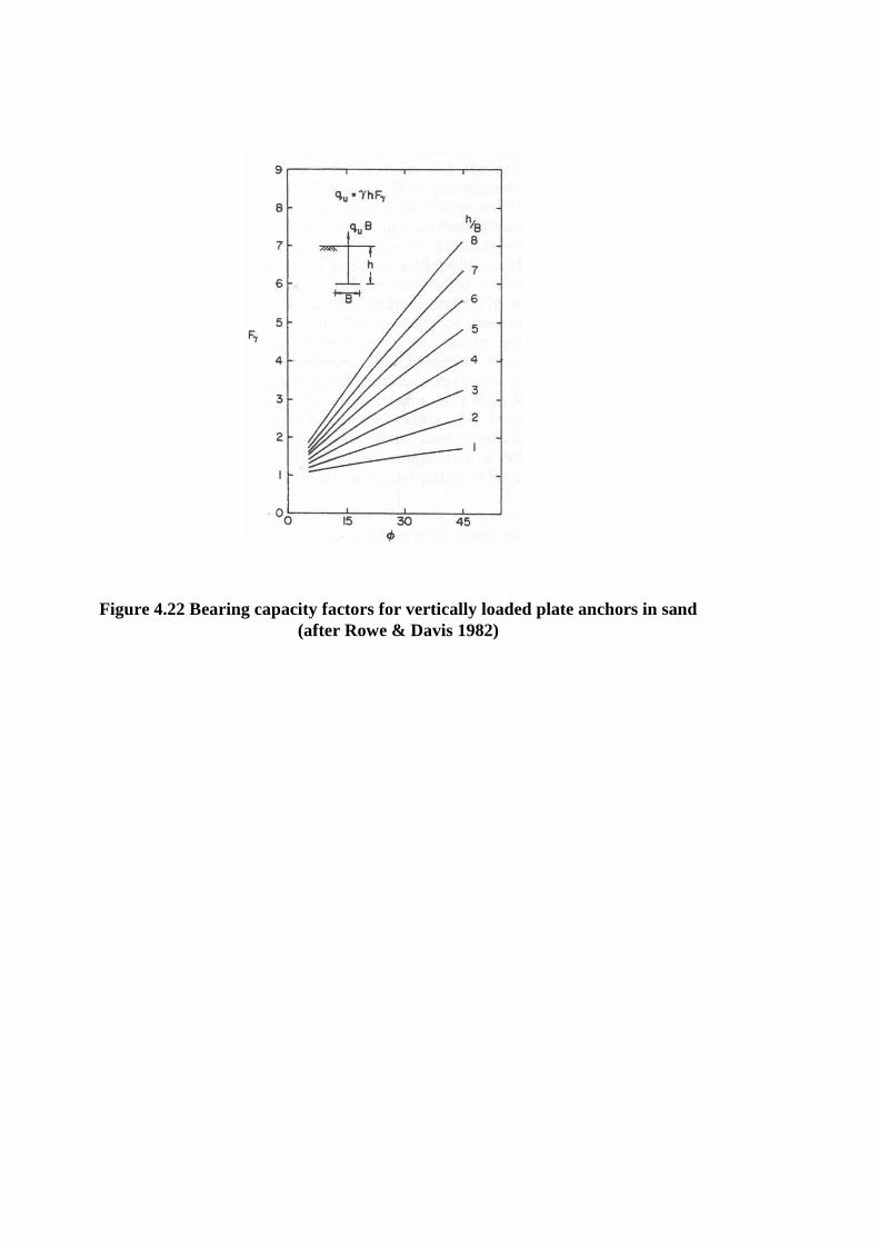
Figure 4.22 Bearing capacity factors for vertically loaded plate anchors in sand (after Rowe & Davis 1982)

Figure 5.1 Linear and polynomial approximations of a typical undrained shear strength profile
Figure 5.2 Undrained shear strength profiles in Box 1
0
4
8
12
16
20
24
28
32
36
0 10 20 30 40Undrained shear strength, su (kPa)
Pro
toty
pe d
epth
, zp (
m)
0
20
40
60
80
100
120
140
160
180
Mod
el d
epth
, zm (
mm
)
Measured
Linear
Polynomial
0
4
8
12
16
20
24
28
32
36
0 10 20 30 40 50 60Undrained shear strength, su (kPa)
Pro
toty
pe d
epth
, zp
(m)
0
20
40
60
80
100
120
140
160
180
Mod
el d
epth
, zm (
mm
)BeforeAfterAverage
k = 1.17 kPa/m
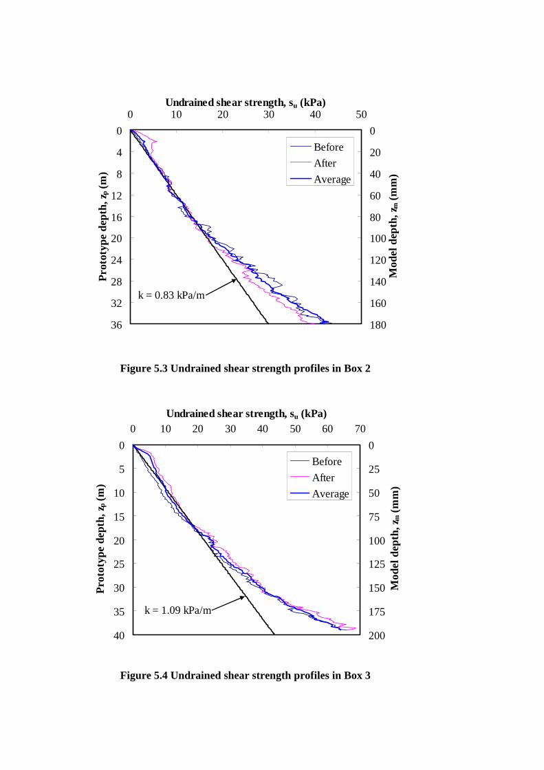
Figure 5.3 Undrained shear strength profiles in Box 2
Figure 5.4 Undrained shear strength profiles in Box 3
0
4
8
12
16
20
24
28
32
36
0 10 20 30 40 50Undrained shear strength, su (kPa)
Pro
toty
pe d
epth
, zp
(m)
0
20
40
60
80
100
120
140
160
180
Mod
el d
epth
, zm (
mm
)
Before
After
Average
k = 0.83 kPa/m
0
5
10
15
20
25
30
35
40
0 10 20 30 40 50 60 70Undrained shear strength, su (kPa)
Pro
toty
pe d
epth
, zp
(m)
0
25
50
75
100
125
150
175
200
Mod
el d
epth
, zm (
mm
)
Before
After
Average
k = 1.09 kPa/m
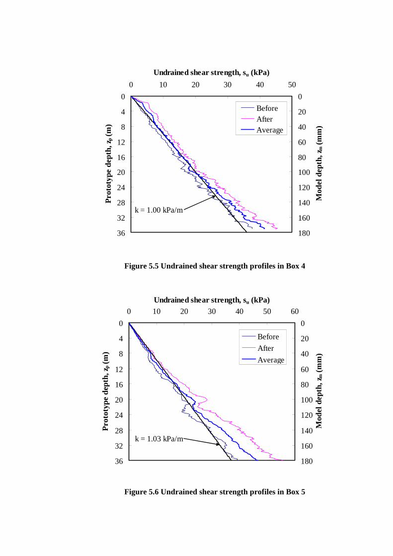
Figure 5.5 Undrained shear strength profiles in Box 4
Figure 5.6 Undrained shear strength profiles in Box 5
0
4
8
12
16
20
24
28
32
36
0 10 20 30 40 50
Undrained shear strength, su (kPa)
Pro
toty
pe d
epth
, zp
(m)
0
20
40
60
80
100
120
140
160
180
Mod
el d
epth
, zm (
mm
)
BeforeAfterAverage
k = 1.00 kPa/m
0
4
8
12
16
20
24
28
32
36
0 10 20 30 40 50 60
Undrained shear strength, su (kPa)
Pro
toty
pe d
epth
, zp
(m)
0
20
40
60
80
100
120
140
160
180
Mod
el d
epth
, zm (
mm
)
Before
After
Average
k = 1.03 kPa/m

Figure 5.7 Undrained shear strength profiles in Box 6
Figure 5.8 Average undrained shear strength profiles for the beam centrifuge samples
0
4
8
12
16
20
24
28
32
36
0 10 20 30 40 50 60 70Undrained shear strength, su (kPa)
Pro
toty
pe d
epth
, zp
(m)
0
20
40
60
80
100
120
140
160
180
Mod
el d
epth
, zm (
mm
)
BeforeAfterAverage
k = 1.45 kPa/m
0
4
8
12
16
20
24
28
32
36
0 10 20 30 40 50 60Undrained shear strength, su (kPa)
Pro
toty
pe d
epth
, zp
(m)
0
20
40
60
80
100
120
140
160
180
Mod
el d
epth
, zm (
mm
)
Box 1
Box 2Box 3
Box 4Box 5
Box 6
k = 1.07 kPa/m

Figure 5.10 Sensitivities from cyclic T-bar tests in Box 6
Figure 5.9 Cyclic T-bar test in Box 6
0
0.5
1
1.5
2
2.5
3
0 5 10 15 20 25
Number of cycles
Sen
sitiv
ity,
S t
Test 1
Test 2
Test 3
Test 4
0
40
80
120
160
200
-80 -60 -40 -20 0 20 40 60 80Undrained shear strength, su (kPa)
Mo
del
dep
th, z
m (
mm
)
Extraction
Installation
Cycling
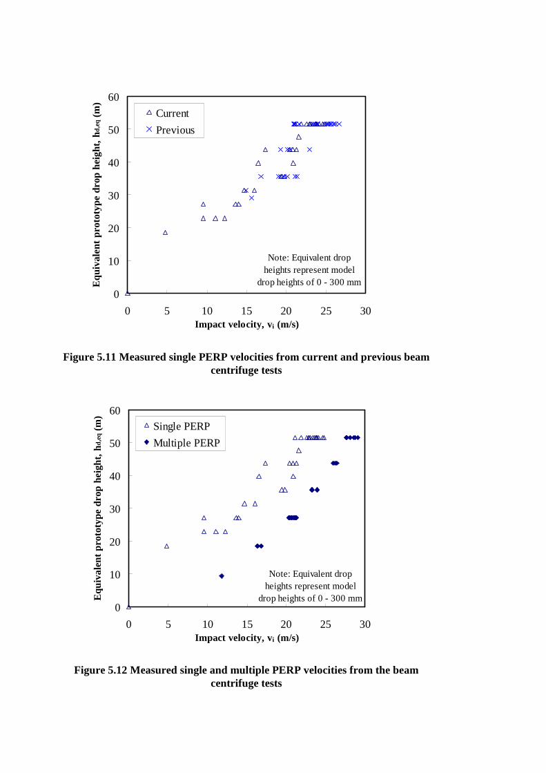
Figure 5.11 Measured single PERP velocities from current and previous beam centrifuge tests
Figure 5.12 Measured single and multiple PERP velocities from the beam centrifuge tests
0
10
20
30
40
50
60
0 5 10 15 20 25 30Impact velocity, vi (m/s)
Equ
ival
ent
prot
otyp
e dr
op h
eigh
t, h
d,e
q (m
)
Current
Previous
Note: Equivalent drop heights represent model
drop heights of 0 - 300 mm
0
10
20
30
40
50
60
0 5 10 15 20 25 30Impact velocity, vi (m/s)
Equ
ival
ent
prot
otyp
e dr
op h
eigh
t, h
d,e
q (m
)
Single PERP
Multiple PERP
Note: Equivalent drop heights represent model
drop heights of 0 - 300 mm

-50
0
50
100
150
200
250
0 10 20 30
Velocity, v (m/s)
Hei
gh
t abo
ve s
am
ple
surfa
ce,
h s (m
m)
Point of impact
Figure 5.13 Adjusted impact velocities from beam centrifuge tests
Figure 5.14 Typical velocity profile for a dynamic anchor test conducted from a drop height of 200 mm in the beam centrifuge
0
10
20
30
40
50
60
0 5 10 15 20 25 30 35Impact velocity, vi (m/s)
Equ
ival
ent
prot
otyp
e dr
op h
eigh
t, h
d,e
q (m
)
Multiple PERP
Single PERP
Note: Equivalent drop heights represent model
drop heights of 0 - 300 mm

Figure 5.15 Anchor chain slack length from load displacement curve
Figure 5.16 Dependence of embedment depth on impact velocity for 0FA tests in the beam centrifuge
0
10
20
30
40
50
60
70
0 50 100 150Vertical displacement (mm)
Loa
d (
N)
Slack length
Point of load onset
Maximum capacity
0
5
10
15
20
25
30
35
40
45
50
0 5 10 15 20 25 30 35Impact velocity, vi (m/s)
Pro
toty
pe
embe
dm
ent,
z e,p (
m)
0
25
50
75
100
125
150
175
200
225
250
Mo
del e
mb
edm
ent,
z e,m (
mm
)
Ellipsoid nose 0FA
mave = 14.5 g
L = 75 mmD = 6 mm
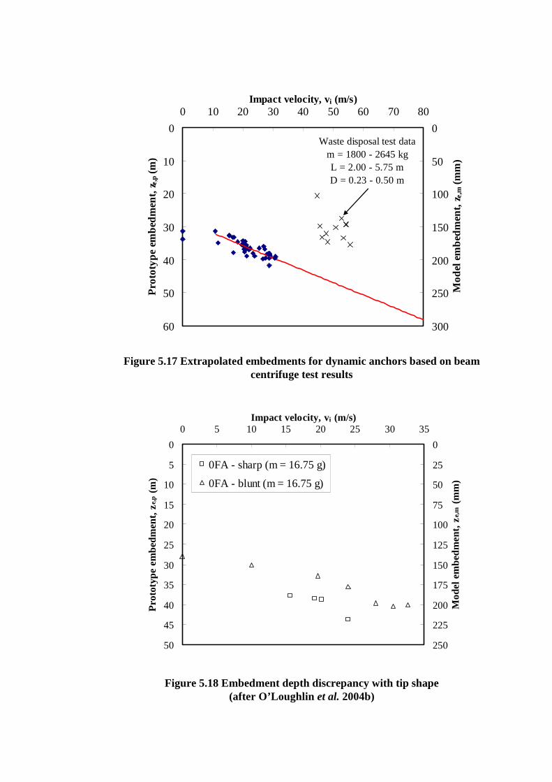
Figure 5.17 Extrapolated embedments for dynamic anchors based on beam centrifuge test results
Figure 5.18 Embedment depth discrepancy with tip shape (after O’Loughlin et al. 2004b)
0
10
20
30
40
50
60
0 10 20 30 40 50 60 70 80Impact velocity, vi (m/s)
Pro
toty
pe e
mb
edm
ent,
z e,p (
m)
0
50
100
150
200
250
300
Mo
del
em
bed
men
t, z e,m
(m
m)
Waste disposal test datam = 1800 - 2645 kgL = 2.00 - 5.75 mD = 0.23 - 0.50 m
0
5
10
15
20
25
30
35
40
45
50
0 5 10 15 20 25 30 35Impact velocity, vi (m/s)
Pro
toty
pe e
mbe
dmen
t, ze
,p (
m)
0
25
50
75
100
125
150
175
200
225
250
Mod
el e
mbe
dmen
t, ze
,m (
mm
)0FA - sharp (m = 16.75 g)
0FA - blunt (m = 16.75 g)
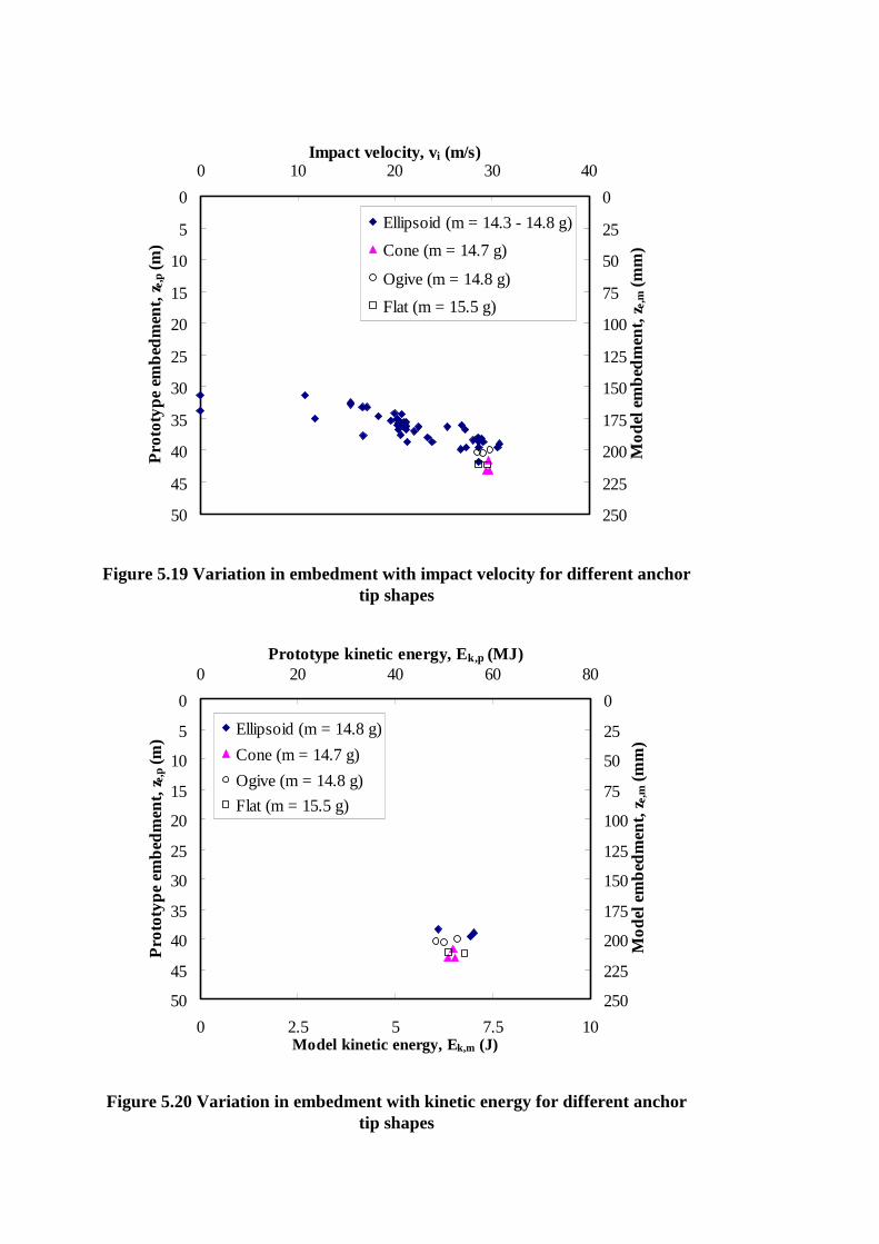
Figure 5.19 Variation in embedment with impact velocity for different anchor tip shapes
Figure 5.20 Variation in embedment with kinetic energy for different anchor tip shapes
0
5
10
15
20
25
30
35
40
45
50
0 10 20 30 40Impact velocity, vi (m/s)
Pro
toty
pe e
mb
edm
ent,
z e,p (
m)
0
25
50
75
100
125
150
175
200
225
250
Mo
del e
mb
edm
ent,
z e,m (
mm
)
Ellipsoid (m = 14.3 - 14.8 g)
Cone (m = 14.7 g)
Ogive (m = 14.8 g)
Flat (m = 15.5 g)
0
5
10
15
20
25
30
35
40
45
50
0 20 40 60 80Prototype kinetic energy, Ek,p (MJ)
Pro
toty
pe
emb
edm
ent,
z e,p (
m)
0
25
50
75
100
125
150
175
200
225
250
0 2.5 5 7.5 10Model kinetic energy, Ek,m (J)
Mo
del e
mb
edm
ent,
z e,m (
mm
)
Ellipsoid (m = 14.8 g)
Cone (m = 14.7 g)
Ogive (m = 14.8 g)
Flat (m = 15.5 g)

Figure 5.21 Bearing mechanism beneath a deep circular foundation(after Meyerhof 1951)
Figure 5.22 Dependence of embedment depth on the presence of anchor flukes (impact velocity)
0
5
10
15
20
25
30
35
40
45
50
0 5 10 15 20 25 30 35Impact velocity, vi (m/s)
Pro
toty
pe
embe
dmen
t, z e,p
(m
)
0
25
50
75
100
125
150
175
200
225
250
Mo
del
em
bed
men
t, z e,m
(m
m)
0FA (m = 14.5 g)
3FA (m = 12.5 g)
4FA (m = 12.5 g)
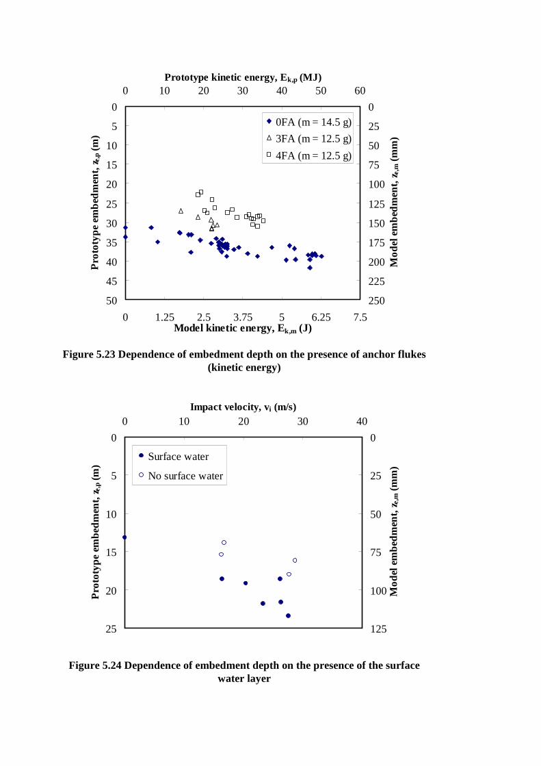
Figure 5.24 Dependence of embedment depth on the presence of the surface water layer
Figure 5.23 Dependence of embedment depth on the presence of anchor flukes (kinetic energy)
0
5
10
15
20
25
0 10 20 30 40Impact velocity, vi (m/s)
Pro
toty
pe e
mbe
dmen
t, z e,p
(m
)
0
25
50
75
100
125
Mo
del e
mbe
dmen
t, z e,m
(m
m)
Surface water
No surface water
0
5
10
15
20
25
30
35
40
45
50
0 10 20 30 40 50 60Prototype kinetic energy, Ek,p (MJ)
Pro
toty
pe
emb
edm
ent,
z e,p (
m)
0
25
50
75
100
125
150
175
200
225
250
0 1.25 2.5 3.75 5 6.25 7.5Model kinetic energy, Ek,m (J)
Mo
del e
mb
edm
ent,
z e,m (
mm
)
0FA (m = 14.5 g)
3FA (m = 12.5 g)
4FA (m = 12.5 g)
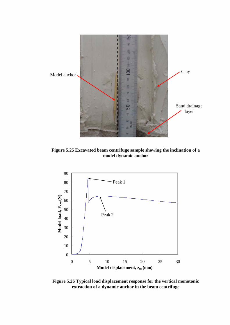
Figure 5.25 Excavated beam centrifuge sample showing the inclination of a model dynamic anchor
Figure 5.26 Typical load displacement response for the vertical monotonic extraction of a dynamic anchor in the beam centrifuge
Model anchor
Sand drainagelayer
Clay
0
10
20
30
40
50
60
70
80
90
0 5 10 15 20 25 30Model displacement, zm (mm)
Mo
del l
oa
d,
F v,m
(N
)
Peak 1
Peak 2
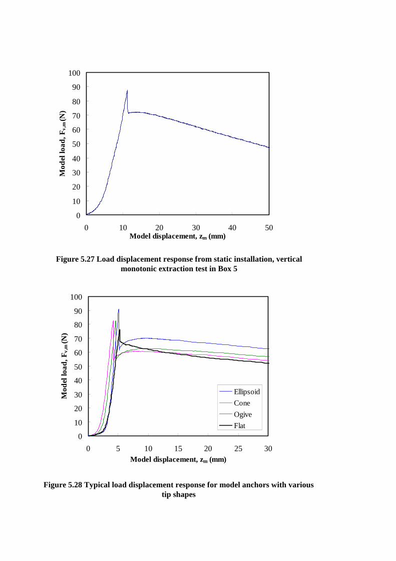
Figure 5.27 Load displacement response from static installation, vertical monotonic extraction test in Box 5
Figure 5.28 Typical load displacement response for model anchors with various tip shapes
0
10
20
30
40
50
60
70
80
90
100
0 10 20 30 40 50Model displacement, zm (mm)
Mo
del
loa
d, F
v,m (
N)
0
10
20
30
40
50
60
70
80
90
100
0 5 10 15 20 25 30Model displacement, zm (mm)
Mo
del
loa
d, F
v,m (
N)
Ellipsoid
Cone
Ogive
Flat

Figure 5.29 Measured 0FA Peak 1 vertical monotonic holding capacities
0
5
10
15
20
25
30
35
40
45
50
0 1 2 3 4 5Prototype capacity, Fv,p (MN)
Pro
toty
pe e
mbe
dmen
t, ze
,p (
m)
0
25
50
75
100
125
150
175
200
225
250
0 25 50 75 100 125Model capacity, Fv,m (N)
Mod
el e
mbe
dmen
t, ze
,m (
mm
)
Current 0FA (m = 14.5 g)
Previous 0FA (m = 16.75 g)
Torpedo anchor (m = 63200 kg, L = 12 m, D = 1.07 m)
Figure 5.30 Measured 0FA Peak 2 vertical monotonic holding capacities
0
5
10
15
20
25
30
35
40
45
50
0 1 2 3 4 5Prototype capacity, Fv,p (MN)
Pro
toty
pe e
mbe
dmen
t, ze
,p (
m)
0
25
50
75
100
125
150
175
200
225
250
0 25 50 75 100 125Model capacity, Fv,m (N)
Mod
el e
mbe
dmen
t, ze
,m (
mm
)Current 0FA - Peak 2 (m = 14.5 g)
Previous 0FA - Peak 1 (m = 16.75 g)
Torpedo anchor (m = 63200 kg,L = 12 m, D = 1.07 m)
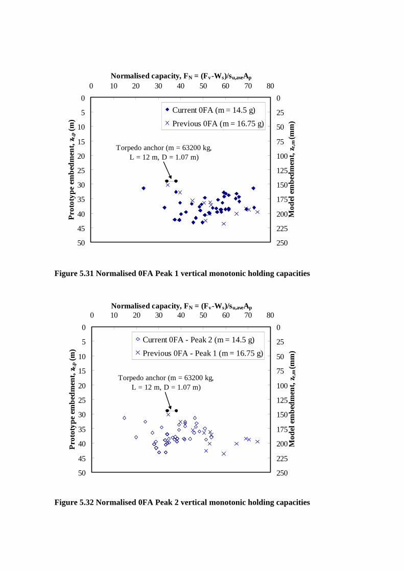
Figure 5.32 Normalised 0FA Peak 2 vertical monotonic holding capacities
Figure 5.31 Normalised 0FA Peak 1 vertical monotonic holding capacities
0
5
10
15
20
25
30
35
40
45
50
0 10 20 30 40 50 60 70 80Normalised capacity, FN = (Fv -Ws)/su,aveAp
Pro
toty
pe e
mb
edm
ent,
z e,p (
m)
0
25
50
75
100
125
150
175
200
225
250
Mo
del
em
bedm
ent,
z e,m (m
m)
Current 0FA (m = 14.5 g)
Previous 0FA (m = 16.75 g)
Torpedo anchor (m = 63200 kg,L = 12 m, D = 1.07 m)
0
5
10
15
20
25
30
35
40
45
50
0 10 20 30 40 50 60 70 80Normalised capacity, FN = (Fv -Ws)/su,aveAp
Pro
toty
pe e
mb
edm
ent,
z e,p (
m)
0
25
50
75
100
125
150
175
200
225
250
Mo
del
em
bed
men
t, z e,m
(mm
)
Current 0FA - Peak 2 (m = 14.5 g)
Previous 0FA - Peak 1 (m = 16.75 g)
Torpedo anchor (m = 63200 kg,L = 12 m, D = 1.07 m)

Figure 5.33 Variation in normalised Peak 1 capacity with anchor tip shape
Figure 5.34 Variation in normalised Peak 2 capacity with anchor tip shape
25
30
35
40
45
50
0 10 20 30 40 50 60 70Normalised capacity, FN = (Fv -Ws)/su,aveAp
Pro
toty
pe e
mb
edm
ent,
z e,p (
m)
125
150
175
200
225
250
Mo
del
em
bed
men
t, z e,m
(m
m)
Ellipsoid (m = 14.8 g)
Cone (m = 14.7 g)
Ogive (m = 14.8 g)
Flat (m = 15.5 g)
25
30
35
40
45
50
0 10 20 30 40 50
Normalised capacity, FN = (Fv -Ws)/su,aveAp
Pro
toty
pe e
mbe
dmen
t, ze
,p (
m)
125
150
175
200
225
250
Mod
el e
mbe
dmen
t, ze
,m (
mm
)
Ellipsoid (m = 14.8 g)
Cone (m = 14.7 g)
Ogive (m = 14.8 g)
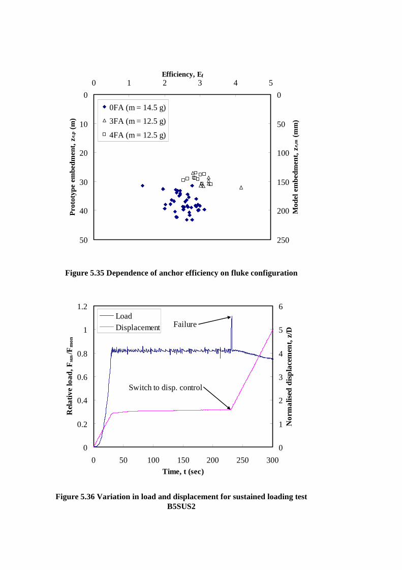
Figure 5.36 Variation in load and displacement for sustained loading test B5SUS2
Figure 5.35 Dependence of anchor efficiency on fluke configuration
0
10
20
30
40
50
0 1 2 3 4 5Efficiency, Ef
Pro
toty
pe e
mbe
dmen
t, ze
,p (
m)
0
50
100
150
200
250
Mod
el e
mbe
dmen
t, ze
,m (
mm
)
0FA (m = 14.5 g)
3FA (m = 12.5 g)
4FA (m = 12.5 g)
0
0.2
0.4
0.6
0.8
1
1.2
0 50 100 150 200 250 300Time, t (sec)
Rel
ativ
e lo
ad
, F s
us/F
mo
n
0
1
2
3
4
5
6
No
rma
lised
dis
pla
cem
ent,
z/D
Load
Displacement Failure
Switch to disp. control
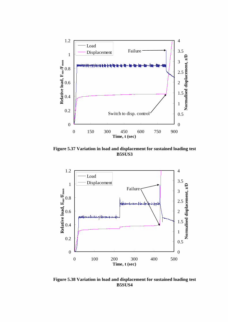
Figure 5.37 Variation in load and displacement for sustained loading test B5SUS3
Figure 5.38 Variation in load and displacement for sustained loading test B5SUS4
0
0.2
0.4
0.6
0.8
1
1.2
0 150 300 450 600 750 900Time, t (sec)
Rel
ativ
e lo
ad
, F s
us/F
mo
n
0
0.5
1
1.5
2
2.5
3
3.5
4
No
rma
lised
dis
pla
cem
ent,
z/D
Load
Displacement Failure
Switch to disp. control
0
0.2
0.4
0.6
0.8
1
1.2
0 100 200 300 400 500Time, t (sec)
Rel
ativ
e lo
ad, F
sus/
F mo
n
0
0.5
1
1.5
2
2.5
3
3.5
4
No
rma
lised
dis
pla
cem
ent,
z/D
Load
DisplacementFailure

Figure 5.39 Variation in load and displacement for sustained loading test B5SUS5
Figure 5.40 Normalised load displacement response for sustained loading tests B5SUS2, B5SUS4 and B5SUS5
0
0.1
0.2
0.3
0.4
0.5
0.6
0.7
0.8
0.9
1
0 100 200 300 400 500 600Time, t (sec)
Rel
ativ
e lo
ad,
Fsu
s/Fm
on
0
0.5
1
1.5
2
2.5
3
3.5
4
No
rma
lised
dis
pla
cem
ent,
z/D
Load
Displacement
Failure
0
10
20
30
40
50
60
70
0 1 2 3 4 5Normalised displacement, z/D
Nor
mal
ised
load
, FN
=(Fv
-Ws )
/su
,aveA
p
0
0.2
0.4
0.6
0.8
1
No
rma
lised
ca
paci
ty r
atio
, N
CR 1
B5SUS2
B5SUS4
B5SUS5
Fsus/Fmon = 50 %
70 %
90 %
80 %
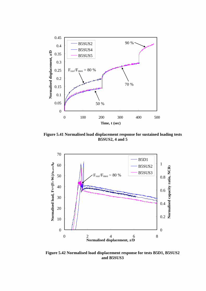
Figure 5.41 Normalised load displacement response for sustained loading tests B5SUS2, 4 and 5
Figure 5.42 Normalised load displacement response for tests B5D1, B5SUS2 and B5SUS3
0
0.05
0.1
0.15
0.2
0.25
0.3
0.35
0.4
0.45
0 100 200 300 400 500
Time, t (sec)
Nor
mal
ised
dis
plac
emen
t, z
/D
B5SUS2
B5SUS4
B5SUS5
Fsus/Fmon = 80 %
50 %
70 %
90 %
0
10
20
30
40
50
60
70
0 2 4 6 8Normalised displacement, z/D
Nor
mal
ised
load
, FN
=(Fv
-Ws )
/su
,ave
Ap
0
0.2
0.4
0.6
0.8
1N
orm
alis
ed c
apac
ity r
atio
, N
CR1
B5D1
B5SUS2
B5SUS3Fsus/Fmon ~ 80 %
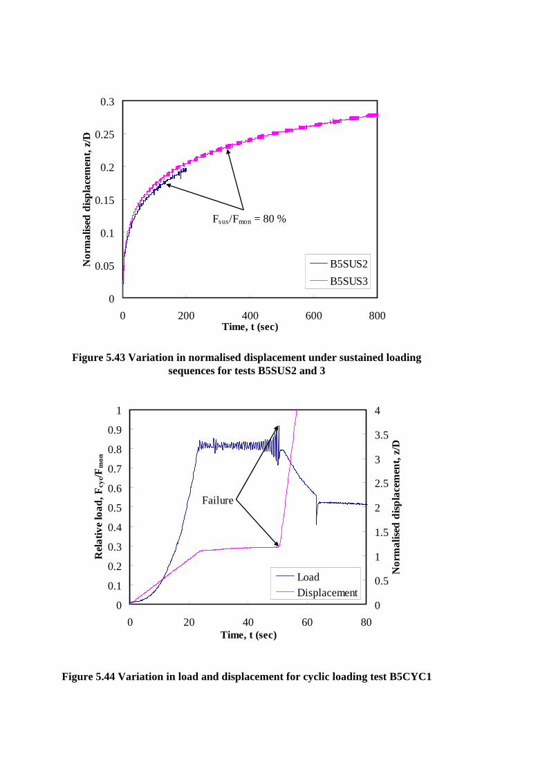
Figure 5.43 Variation in normalised displacement under sustained loading sequences for tests B5SUS2 and 3
Figure 5.44 Variation in load and displacement for cyclic loading test B5CYC1
0
0.05
0.1
0.15
0.2
0.25
0.3
0 200 400 600 800Time, t (sec)
No
rma
lised
dis
pla
cem
ent,
z/D
B5SUS2
B5SUS3
Fsus/Fmon = 80 %
0
0.1
0.2
0.3
0.4
0.5
0.6
0.7
0.8
0.9
1
0 20 40 60 80Time, t (sec)
Rel
ativ
e lo
ad
, F c
yc/F
mo
n
0
0.5
1
1.5
2
2.5
3
3.5
4N
orm
alis
ed d
isp
lace
men
t, z/
D
Load
Displacement
Failure
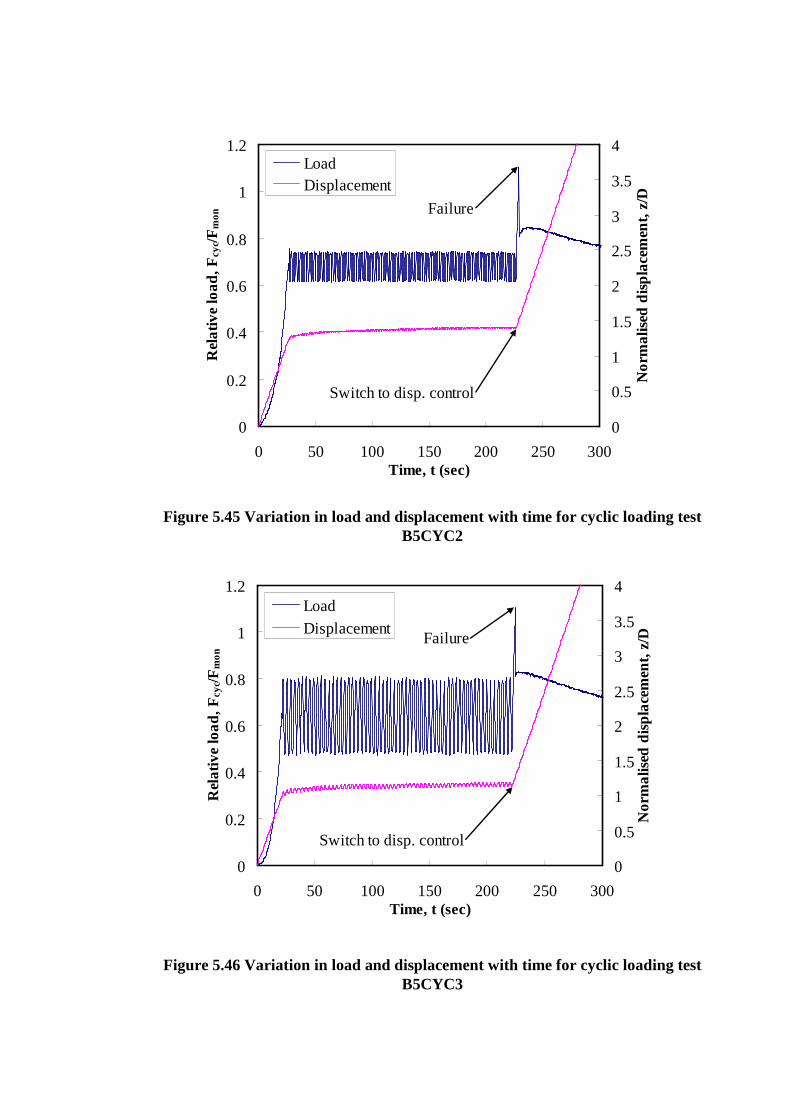
Figure 5.45 Variation in load and displacement with time for cyclic loading test B5CYC2
Figure 5.46 Variation in load and displacement with time for cyclic loading test B5CYC3
0
0.2
0.4
0.6
0.8
1
1.2
0 50 100 150 200 250 300Time, t (sec)
Rel
ativ
e lo
ad
, F c
yc/F
mo
n
0
0.5
1
1.5
2
2.5
3
3.5
4
No
rma
lised
dis
pla
cem
ent,
z/D
LoadDisplacement
Failure
Switch to disp. control
0
0.2
0.4
0.6
0.8
1
1.2
0 50 100 150 200 250 300Time, t (sec)
Rel
ativ
e lo
ad,
Fcy
c/Fm
on
0
0.5
1
1.5
2
2.5
3
3.5
4
No
rma
lised
dis
pla
cem
ent,
z/D
Load
DisplacementFailure
Switch to disp. control

Figure 5.47 Variation in load and displacement with time for cyclic loading test B5CYC5
Figure 5.48 Variation in load and displacement with time for cyclic loading test B5CYC6
0
0.2
0.4
0.6
0.8
1
1.2
0 200 400 600 800 1000Time, t (sec)
Rel
ativ
e lo
ad
, F c
yc/F
mo
n
0
0.5
1
1.5
2
2.5
3
3.5
4
No
rma
lised
dis
pla
cem
ent,
z/D
Load
DisplacementFailure
Switch to disp. control
0
0.1
0.2
0.3
0.4
0.5
0.6
0.7
0.8
0.9
1
0 20 40 60 80Time, t (sec)
Rel
ativ
e lo
ad
, F c
yc/F
mo
n
0
0.5
1
1.5
2
2.5
3
3.5
4
No
rma
lised
dis
pla
cem
ent,
z/D
Load
Displacement
Failure

Figure 5.49 Variation in load and displacement with time for cyclic loading test B5CYC7
Figure 5.50 Mean load and cyclic load amplitude
0
0.2
0.4
0.6
0.8
1
1.2
0 50 100 150 200 250 300Time, t (sec)
Rel
ativ
e lo
ad,
Fcy
c/Fm
on
0
0.5
1
1.5
2
2.5
3
3.5
4
No
rma
lised
dis
pla
cem
ent,
z/D
Load
DisplacementFailure
Switch to disp. control
Time
Lo
ad
Mean load
Cyclic load amplitude

Figure 5.51 Normalised load displacement response for cyclic loading tests B5CYC3 and B5CYC7
Figure 5.52 Variation in normalised displacements under cyclic loading sequences for tests B5CYC3 and B5CYC7
0
10
20
30
40
50
60
70
0 2 4 6 8Normalised displacement, z/D
Nor
mal
ised
load
, FN
=(Fv
-Ws )
/su
,aveA
p
0
0.2
0.4
0.6
0.8
1
Nor
mal
ised
cap
acity
rat
io,
NC
R1
B5CYC3
B5CYC7
Fcyc/Fmon = 50 - 80 %
70 - 80 %
0
0.05
0.1
0.15
0.2
0.25
0 50 100 150 200Time, t (sec)
Nor
mal
ised
dis
plac
emen
t, z
/D
B5CYC3
B5CYC7
Fcyc/Fmon = 50 - 80 %
70 - 80 %
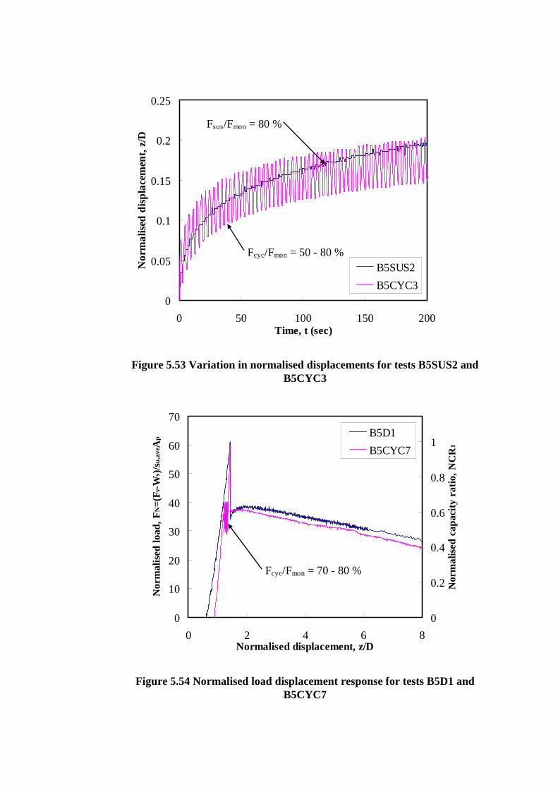
Figure 5.53 Variation in normalised displacements for tests B5SUS2 and B5CYC3
Figure 5.54 Normalised load displacement response for tests B5D1 and B5CYC7
0
0.05
0.1
0.15
0.2
0.25
0 50 100 150 200Time, t (sec)
No
rma
lised
dis
pla
cem
ent,
z/D
B5SUS2
B5CYC3
Fsus/Fmon = 80 %
Fcyc/Fmon = 50 - 80 %
0
10
20
30
40
50
60
70
0 2 4 6 8Normalised displacement, z/D
Nor
mal
ised
load
, FN
=(Fv
-Ws )
/su
,ave
Ap
0
0.2
0.4
0.6
0.8
1N
orm
alis
ed c
apac
ity r
atio
, N
CR1
B5D1
B5CYC7
Fcyc/Fmon = 70 - 80 %
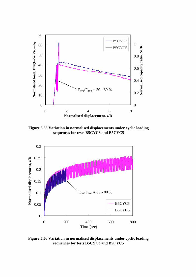
Figure 5.55 Variation in normalised displacements under cyclic loading sequences for tests B5CYC3 and B5CYC5
Figure 5.56 Variation in normalised displacements under cyclic loading sequences for tests B5CYC3 and B5CYC5
0
10
20
30
40
50
60
70
0 2 4 6 8Normalised displacement, z/D
Nor
mal
ised
load
, FN
=(Fv
-Ws )
/su
,aveA
p
0
0.2
0.4
0.6
0.8
1
Nor
mal
ised
cap
acity
rat
io,
NC
R1
B5CYC3
B5CYC5
Fcyc/Fmon = 50 - 80 %
0
0.05
0.1
0.15
0.2
0.25
0.3
0 200 400 600 800Time (sec)
No
rma
lised
dis
pla
cem
ent,
z/D
B5CYC5
B5CYC3
Fcyc/Fmon = 50 - 80 %

Figure 5.57 Variation in static penetration resistance with anchor tip shape
Figure 5.58 Undrained shear strength profiles with depth from Drum 1 showing the influence of unbalance
0
4
8
12
16
20
24
28
32
36
0 0.4 0.8 1.2 1.6 2 2.4Prototype static resistance, Fs,p (MN)
Pro
toty
pe
dep
th,
z p (m
)
0
20
40
60
80
100
120
140
160
180
0 10 20 30 40 50 60Model static resistance, Fs,m (N)
Mo
del
dep
th,
z m (
mm
)
Ellipsoid
Cone
Ogive
Flat
0
4
8
12
16
20
24
28
0 10 20 30 40Undrained shear strength, su (kPa)
Pro
toty
pe d
epth
, zp
(m
)
0
20
40
60
80
100
120
140
Mod
el d
epth
, zm
(m
m)
Unbalance = 0.43 g
Unbalance = 0.57 g
Unbalance = 0.72 g
k = 1 kPa/m
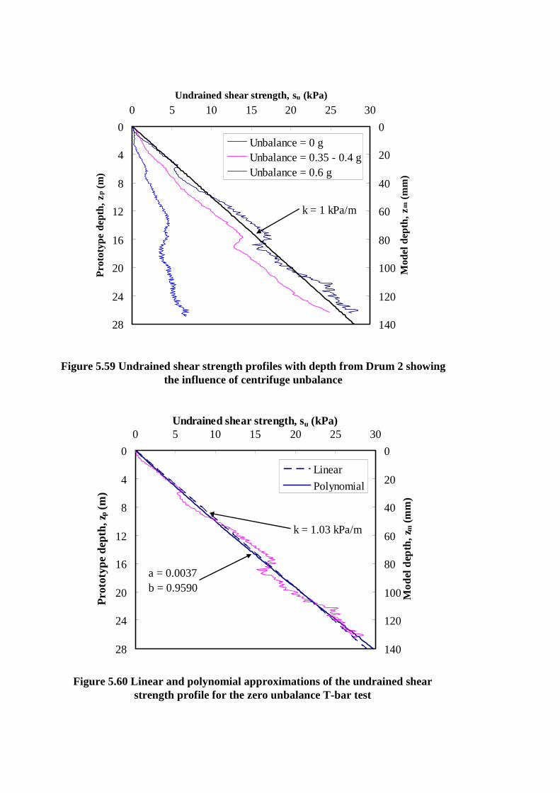
Figure 5.59 Undrained shear strength profiles with depth from Drum 2 showing the influence of centrifuge unbalance
Figure 5.60 Linear and polynomial approximations of the undrained shear strength profile for the zero unbalance T-bar test
0
4
8
12
16
20
24
28
0 5 10 15 20 25 30Undrained shear strength, su (kPa)
Pro
toty
pe d
epth
, zp
(m)
0
20
40
60
80
100
120
140
Mo
del d
epth
, z m
(m
m)
Linear
Polynomial
k = 1.03 kPa/m
a = 0.0037b = 0.9590
0
4
8
12
16
20
24
28
0 5 10 15 20 25 30Undrained shear strength, su (kPa)
Pro
toty
pe d
epth
, zp
(m
)
0
20
40
60
80
100
120
140
Mod
el d
epth
, zm
(m
m)
Unbalance = 0 gUnbalance = 0.35 - 0.4 gUnbalance = 0.6 g
k = 1 kPa/m
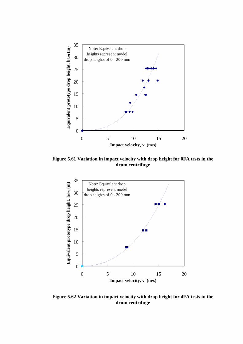
Figure 5.61 Variation in impact velocity with drop height for 0FA tests in the drum centrifuge
Figure 5.62 Variation in impact velocity with drop height for 4FA tests in the drum centrifuge
0
5
10
15
20
25
30
35
0 5 10 15 20Impact velocity, vi (m/s)
Equ
ival
ent
prot
otyp
e dr
op h
eigh
t, h
d,e
q (m
) Note: Equivalent drop heights represent model
drop heights of 0 - 200 mm
0
5
10
15
20
25
30
35
0 5 10 15 20Impact velocity, vi (m/s)
Equ
ival
ent
prot
otyp
e dr
op h
eigh
t, h
d,e
q (m
) Note: Equivalent drop heights represent model
drop heights of 0 - 200 mm
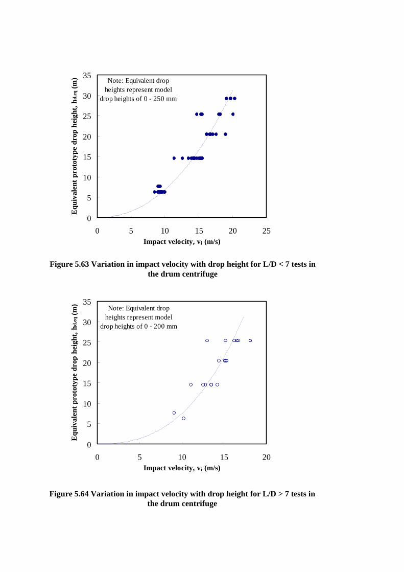
Figure 5.63 Variation in impact velocity with drop height for L/D < 7 tests in the drum centrifuge
Figure 5.64 Variation in impact velocity with drop height for L/D > 7 tests in the drum centrifuge
0
5
10
15
20
25
30
35
0 5 10 15 20 25Impact velocity, vi (m/s)
Equ
ival
ent
prot
otyp
e dr
op h
eigh
t, h
d,e
q (m
) Note: Equivalent drop heights represent model
drop heights of 0 - 250 mm
0
5
10
15
20
25
30
35
0 5 10 15 20Impact velocity, vi (m/s)
Equ
ival
ent
prot
otyp
e dr
op h
eigh
t, h
d,e
q (m
)
Note: Equivalent drop heights represent model
drop heights of 0 - 200 mm
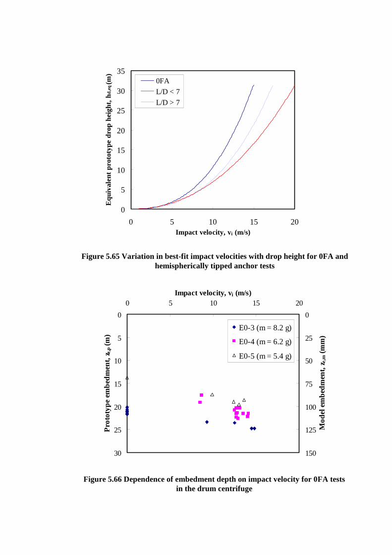
Figure 5.66 Dependence of embedment depth on impact velocity for 0FA tests in the drum centrifuge
Figure 5.65 Variation in best-fit impact velocities with drop height for 0FA and hemispherically tipped anchor tests
0
5
10
15
20
25
30
35
0 5 10 15 20Impact velocity, vi (m/s)
Equ
ival
ent
prot
otyp
e dr
op h
eigh
t, h
d,e
q (m
)
0FA
L/D < 7
L/D > 7
0
5
10
15
20
25
30
0 5 10 15 20Impact velocity, vi (m/s)
Pro
toty
pe
emb
edm
ent,
z e,p (
m)
0
25
50
75
100
125
150
Mo
del e
mb
edm
ent,
z e,m (
mm
)E0-3 (m = 8.2 g)
E0-4 (m = 6.2 g)
E0-5 (m = 5.4 g)
0
5
10
15
20
25
30
35
0 5 10 15 20Impact velocity, vi (m/s)
Equ
ival
ent
prot
otyp
e dr
op h
eigh
t, h
d,e
q (m
)
0FA
L/D < 7
L/D > 7
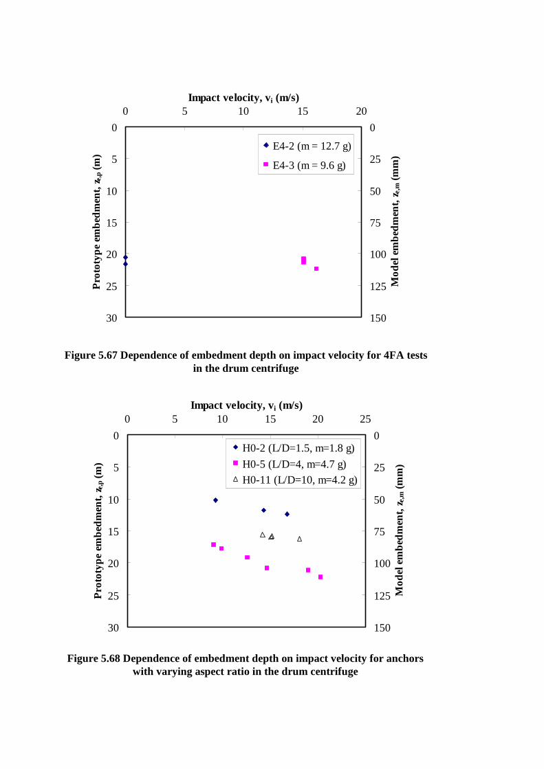
Figure 5.68 Dependence of embedment depth on impact velocity for anchors with varying aspect ratio in the drum centrifuge
0
5
10
15
20
25
30
0 5 10 15 20Impact velocity, vi (m/s)
Pro
toty
pe
emb
edm
ent,
z e,p (
m)
0
25
50
75
100
125
150
Mo
del e
mb
edm
ent,
z e,m (
mm
)
E4-2 (m = 12.7 g)
E4-3 (m = 9.6 g)
Figure 5.67 Dependence of embedment depth on impact velocity for 4FA tests in the drum centrifuge
0
5
10
15
20
25
30
0 5 10 15 20 25Impact velocity, vi (m/s)
Pro
toty
pe
emb
edm
ent,
z e,p (
m)
0
25
50
75
100
125
150
Mo
del
em
bed
men
t, z e,m
(m
m)
H0-2 (L/D=1.5, m=1.8 g)
H0-5 (L/D=4, m=4.7 g)
H0-11 (L/D=10, m=4.2 g)
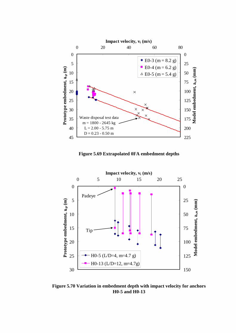
Figure 5.69 Extrapolated 0FA embedment depths
Figure 5.70 Variation in embedment depth with impact velocity for anchors H0-5 and H0-13
0
5
10
15
20
25
30
35
40
45
0 20 40 60 80Impact velocity, vi (m/s)
Pro
toty
pe
emb
edm
ent,
z e,p (
m)
0
25
50
75
100
125
150
175
200
225
Mo
del e
mb
edm
ent,
z e,m (
mm
)
E0-3 (m = 8.2 g)
E0-4 (m = 6.2 g)
E0-5 (m = 5.4 g)
Waste disposal test datam = 1800 - 2645 kgL = 2.00 - 5.75 mD = 0.23 - 0.50 m
0
5
10
15
20
25
30
0 5 10 15 20 25Impact velocity, vi (m/s)
Pro
toty
pe
emb
edm
ent,
z e,p (
m)
0
25
50
75
100
125
150
Mo
del
em
bed
men
t, z e,m
(m
m)
H0-5 (L/D=4, m=4.7 g)
H0-13 (L/D=12, m=4.7g)
Tip
Padeye
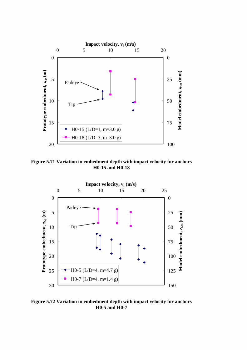
Figure 5.71 Variation in embedment depth with impact velocity for anchors H0-15 and H0-18
Figure 5.72 Variation in embedment depth with impact velocity for anchors H0-5 and H0-7
0
5
10
15
20
25
30
0 5 10 15 20 25Impact velocity, vi (m/s)
Pro
toty
pe
emb
edm
ent,
z e,p (
m)
0
25
50
75
100
125
150
Mo
del
em
bed
men
t, z e,m
(m
m)
H0-5 (L/D=4, m=4.7 g)
H0-7 (L/D=4, m=1.4 g)
Tip
Padeye
0
5
10
15
20
0 5 10 15 20Impact velocity, vi (m/s)
Pro
toty
pe
emb
edm
ent,
z e,p (
m)
0
25
50
75
100
Mo
del e
mb
edm
ent,
z e,m (
mm
)
H0-15 (L/D=1, m=3.0 g)
H0-18 (L/D=3, m=3.0 g)
Tip
Padeye

Figure 5.73 Variation in embedment depth with impact velocity for anchors H0-6 and H0-8
Figure 5.74 Variation in embedment depth with impact velocity for anchors H0-1, H0-4 and H0-6
0
5
10
15
20
25
30
35
0 5 10 15 20 25Impact velocity, vi (m/s)
Pro
toty
pe
emb
edm
ent,
z e,p (
m)
0
25
50
75
100
125
150
175
Mo
del
em
bed
men
t, z e,m
(m
m)
H0-6 (L/D=6, m=7.4 g)
H0-8 (L/D=6, m=2.3 g)
Tip
Padeye
0
5
10
15
20
25
30
35
0 5 10 15 20 25Impact velocity, vi (m/s)
Pro
toty
pe
emb
edm
ent,
z e,p (
m)
0
25
50
75
100
125
150
175
Mo
del e
mb
edm
ent,
z e,m (
mm
)
H0-1 (L/D=1, m=0.9 g)H0-4 (L/D=3, m=3.0 g)H0-6 (L/D=6, m=7.4 g)
Tip
Padeye

Figure 5.75 Influence of consolidation time on the load displacement response for anchor E4-3
Figure 5.76 Influence of the anchor aspect ratio on the load displacement response
0
10
20
30
40
50
60
70
80
0 10 20 30 40Model displacement, zm (mm)
Mo
del l
oa
d,
F v,m
(N
)
t = 59 s
t = 431 s
t = 9990 s
t = 53935 s
0
2
4
6
8
10
12
0 10 20 30 40Model displacement, zm (mm)
Mo
del
loa
d, F
v,m (
N)
L/D = 2
L/D = 6L/D = 8
L/D = 12
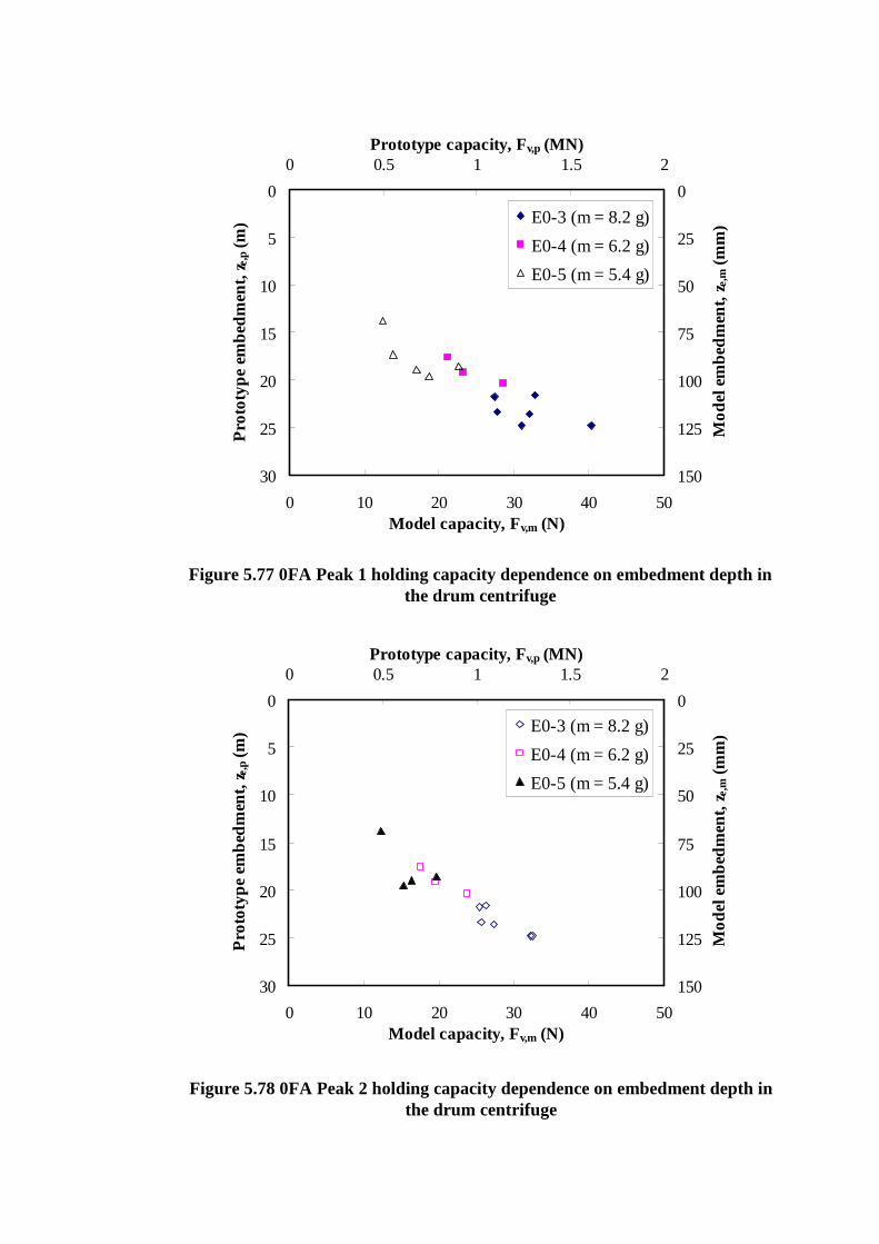
Figure 5.77 0FA Peak 1 holding capacity dependence on embedment depth in the drum centrifuge
Figure 5.78 0FA Peak 2 holding capacity dependence on embedment depth in the drum centrifuge
0
5
10
15
20
25
30
0 0.5 1 1.5 2Prototype capacity, Fv,p (MN)
Pro
toty
pe
embe
dmen
t, z e,p
(m
)
0
25
50
75
100
125
150
0 10 20 30 40 50Model capacity, Fv,m (N)
Mo
del e
mbe
dmen
t, z e,m
(m
m)E0-3 (m = 8.2 g)
E0-4 (m = 6.2 g)
E0-5 (m = 5.4 g)
0
5
10
15
20
25
30
0 0.5 1 1.5 2Prototype capacity, Fv,p (MN)
Pro
toty
pe
emb
edm
ent,
z e,p (
m)
0
25
50
75
100
125
150
0 10 20 30 40 50Model capacity, Fv,m (N)
Mo
del e
mb
edm
ent,
z e,m (
mm
)E0-3 (m = 8.2 g)
E0-4 (m = 6.2 g)
E0-5 (m = 5.4 g)
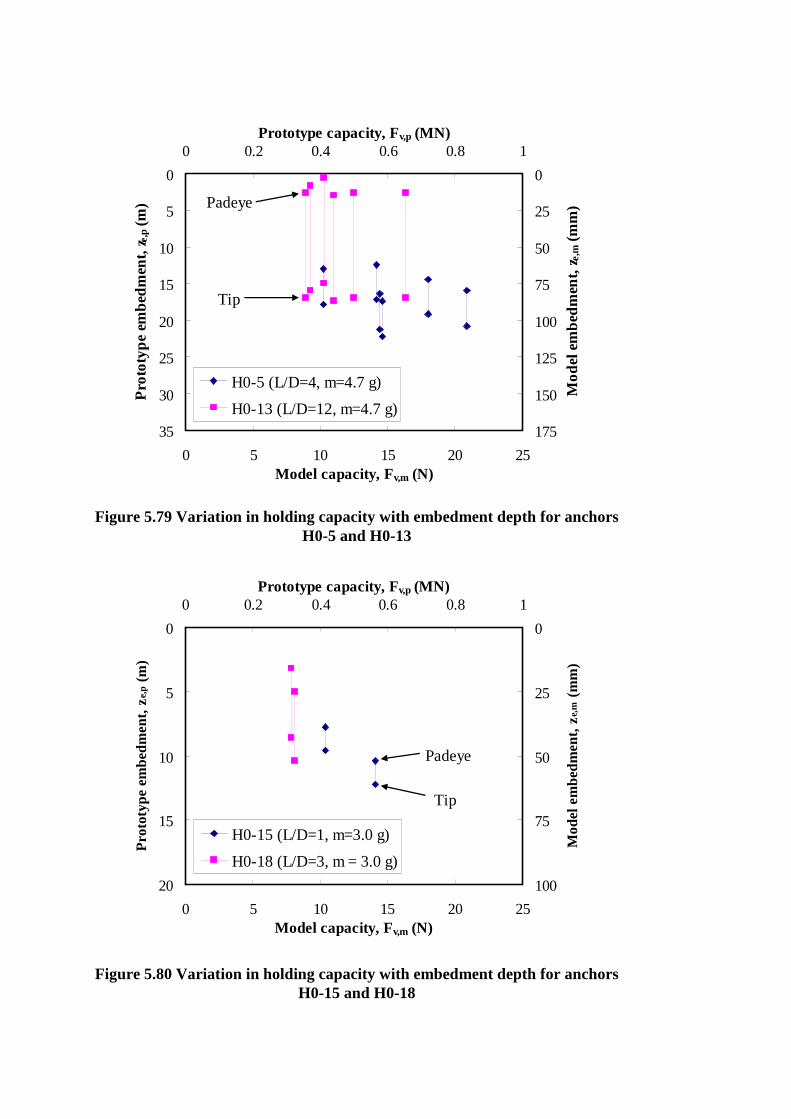
Figure 5.79 Variation in holding capacity with embedment depth for anchors H0-5 and H0-13
Figure 5.80 Variation in holding capacity with embedment depth for anchors H0-15 and H0-18
0
5
10
15
20
25
30
35
0 0.2 0.4 0.6 0.8 1Prototype capacity, Fv,p (MN)
Pro
toty
pe
embe
dmen
t, z e,p
(m
)
0
25
50
75
100
125
150
175
0 5 10 15 20 25Model capacity, Fv,m (N)
Mo
del e
mbe
dmen
t, z e,m
(m
m)
H0-5 (L/D=4, m=4.7 g)
H0-13 (L/D=12, m=4.7 g)
Tip
Padeye
0
5
10
15
20
0 0.2 0.4 0.6 0.8 1Prototype capacity, Fv,p (MN)
Pro
toty
pe e
mbe
dmen
t, ze
,p (
m)
0
25
50
75
100
0 5 10 15 20 25Model capacity, Fv,m (N)
Mod
el e
mbe
dmen
t, ze
,m (
mm
)
H0-15 (L/D=1, m=3.0 g)
H0-18 (L/D=3, m = 3.0 g)
Tip
Padeye
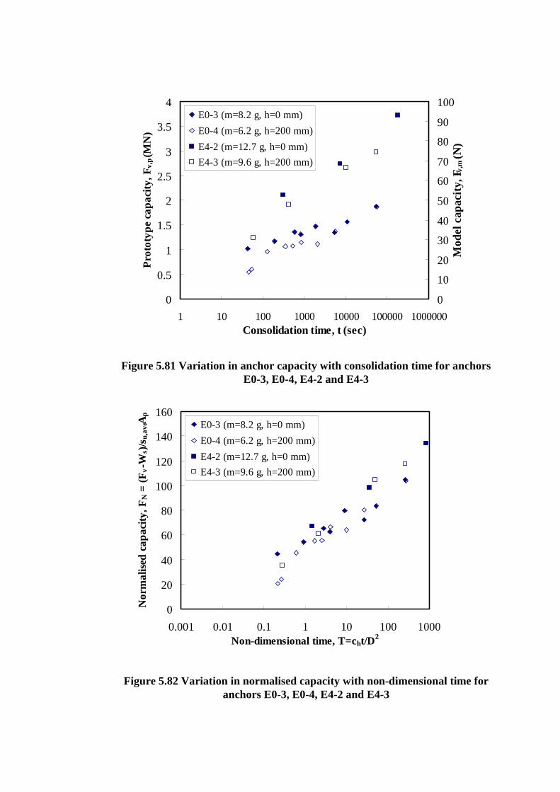
0
0.5
1
1.5
2
2.5
3
3.5
4
1 10 100 1000 10000 100000 1000000Consolidation time, t (sec)
Pro
toty
pe c
apa
city
, F v
,p (M
N)
0
10
20
30
40
50
60
70
80
90
100
Mod
el c
apac
ity, F
v,m (
N)
E0-3 (m=8.2 g, h=0 mm)
E0-4 (m=6.2 g, h=200 mm)
E4-2 (m=12.7 g, h=0 mm)
E4-3 (m=9.6 g, h=200 mm)
Figure 5.81 Variation in anchor capacity with consolidation time for anchors E0-3, E0-4, E4-2 and E4-3
Figure 5.82 Variation in normalised capacity with non-dimensional time for anchors E0-3, E0-4, E4-2 and E4-3
0
20
40
60
80
100
120
140
160
0.001 0.01 0.1 1 10 100 1000Non-dimensional time, T=cht/D
2
No
rma
lised
ca
pa
city
, FN =
(F v
-Ws)
/su,
aveA
p
E0-3 (m=8.2 g, h=0 mm)
E0-4 (m=6.2 g, h=200 mm)
E4-2 (m=12.7 g, h=0 mm)
E4-3 (m=9.6 g, h=200 mm)

0
0.2
0.4
0.6
0.8
1
1.2
0.001 0.01 0.1 1 10 100 1000Non-dimensional time, T=cht/D
2
Deg
ree
of C
onso
lidat
ion
E0-3 (m=8.2 g, h=0 mm)
E0-4 (m=6.2 g, h=200 mm)
E4-2 (m=12.7 g, h=0 mm)
E4-3 (m=9.6 g, h=200 mm)
Torpedo (m=0.6 kg, L/D=12)
Figure 5.83 Variation in normalised capacity ratio with non-dimensional time for anchors E0-3, E0-4, E4-2 and E4-3
Figure 5.84 Degree of consolidation for anchors E0-3, E0-4, E4-2 and E4-3
0
0.2
0.4
0.6
0.8
1
1.2
0.001 0.01 0.1 1 10 100 1000Non-dimensional time, T=cht/D
2
No
rma
lised
ca
paci
ty r
atio
, F N
/FN
,ma
x E0-3 (m=8.2 g, h=0 mm)
E0-4 (m=6.2 g, h=200 mm)
E4-2 (m=12.7 g, h=0 mm)
E4-3 (m=9.6 g, h=200 mm)
Dynamic
Quasi-static

Figure 6.1 Silica sand cone resistance profiles with depth
Figure 6.2 Zero fluke model anchor embedded in silica sand sample
0
4
8
12
16
20
24
28
32
0 20 40 60 80Cone tip resistance, qc (MPa)
Pro
toty
pe d
epth
, zp
(m
)0
20
40
60
80
100
120
140
160
Mod
el d
epth
, zm
(m
m)
CPT 1
CPT 2
CPT 3
CPT 4
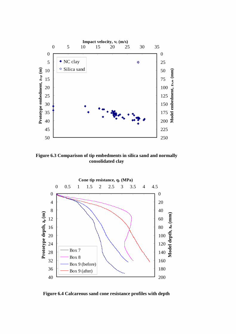
Figure 6.3 Comparison of tip embedments in silica sand and normally consolidated clay
Figure 6.4 Calcareous sand cone resistance profiles with depth
0
5
10
15
20
25
30
35
40
45
50
0 5 10 15 20 25 30 35Impact velocity, vi (m/s)
Pro
toty
pe e
mbe
dmen
t, ze
,p (
m)
0
25
50
75
100
125
150
175
200
225
250
Mod
el e
mbe
dmen
t, ze
,m (
mm
)
NC clay
Silica sand
0
4
8
12
16
20
24
28
32
36
40
0 0.5 1 1.5 2 2.5 3 3.5 4 4.5
Cone tip resistance, qc (MPa)
Pro
toty
pe d
epth
, zp
(m)
0
20
40
60
80
100
120
140
160
180
200
Mod
el d
epth
, zm (
mm
)
Box 7
Box 8
Box 9 (before)
Box 9 (after)

Figure 6.5 Variation in measured velocity with drop height
Figure 6.6 Variation in adjusted impact velocity with drop height
0
10
20
30
40
50
60
0 5 10 15 20 25 30 35Impact velocity, vi (m/s)
Equ
ival
ent
prot
otyp
e dr
op h
eigh
t, h
d,eq
(m
)
Multiple PERP
Single PERP
Calcareous sand
Note: Equivalent dropheights represent model
drop heights of 0 - 300 mm
0
10
20
30
40
50
60
0 5 10 15 20 25 30 35Impact velocity, vi (m/s)
Equ
ival
ent
prot
otyp
e dr
op h
eigh
t, h
d,eq
(m
)
Multiple PERP
Single PERP
Calcareous sand
Note: Equivalent dropheights represent model
drop heights of 0 - 300 mm
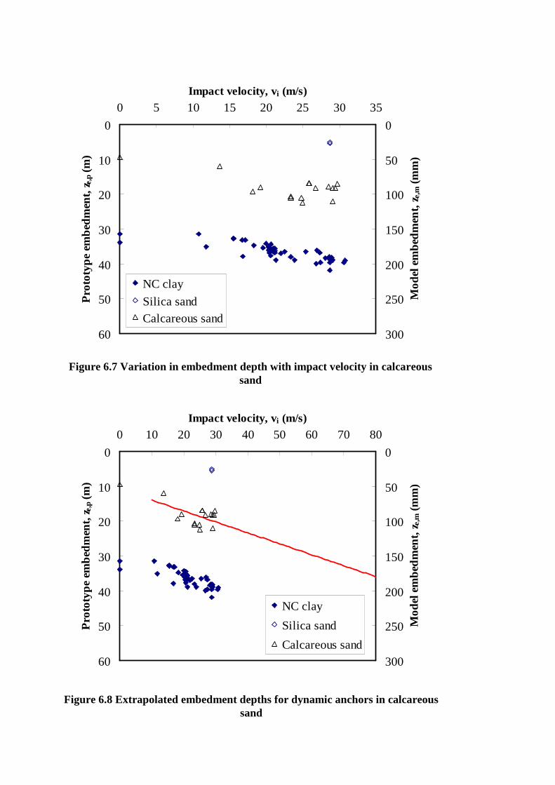
Figure 6.7 Variation in embedment depth with impact velocity in calcareous sand
0
10
20
30
40
50
60
0 5 10 15 20 25 30 35Impact velocity, vi (m/s)
Pro
toty
pe
emb
edm
ent,
z e,p (
m)
0
50
100
150
200
250
300
Mo
del e
mbe
dm
ent,
z e,m (
mm
)
NC clay
Silica sand
Calcareous sand
Figure 6.8 Extrapolated embedment depths for dynamic anchors in calcareous sand
0
10
20
30
40
50
60
0 10 20 30 40 50 60 70 80Impact velocity, vi (m/s)
Pro
toty
pe
emb
edm
ent,
z e,p (
m)
0
50
100
150
200
250
300
Mo
del e
mbe
dm
ent,
z e,m (
mm
)
NC clay
Silica sand
Calcareous sand

Figure 6.10 Comparison of vertical capacities for calcareous sand and normally consolidated clay
Figure 6.9 Typical load displacement plot in calcareous sand
0
5
10
15
20
25
30
35
40
45
50
0 5 10 15 20Vertical displacement, z (mm)
Mo
del
loa
d,
F v,m
(N
)
0
10
20
30
40
50
0 1 2 3 4 5Prototype capacity, Fv,p (MN)
Pro
toty
pe e
mbe
dmen
t, z e,p
(m
)
0
50
100
150
200
250
0 25 50 75 100 125Model capacity, Fv,m (N)
Mod
el e
mbe
dmen
t, z e,
m (
mm
)Calcareous sandNC clay - Peak 1NC clay - Peak 2

Figure 6.11 Static resistance force from static penetration tests in calcareous sand
0
5
10
15
20
25
30
35
40
0 2 4 6 8 10Prototype resistance, Fp (MN)
Pro
toty
pe d
epth
, zp
(m)
0
25
50
75
100
125
150
175
200
0 50 100 150 200 250Model resistance, Fm (N)
Mod
el d
epth
, zm (
mm
)
Test 1
Test 2
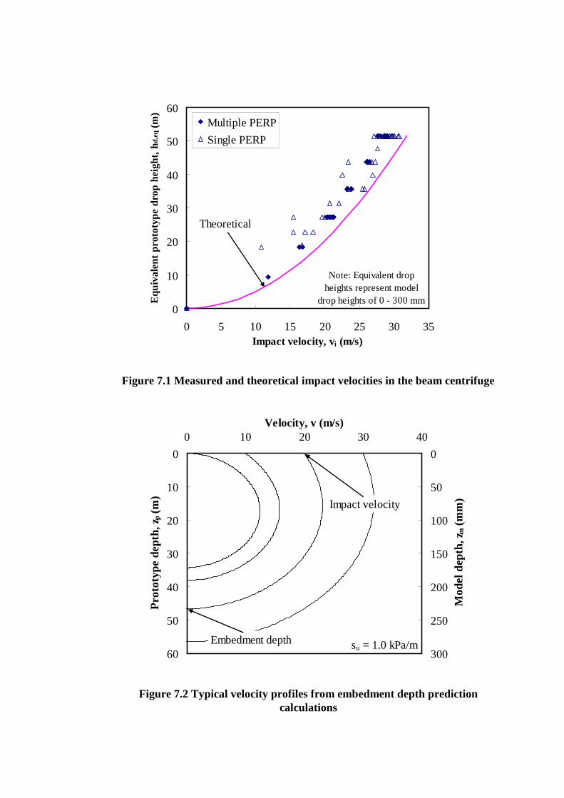
Figure 7.1 Measured and theoretical impact velocities in the beam centrifuge
Figure 7.2 Typical velocity profiles from embedment depth prediction calculations
0
10
20
30
40
50
60
0 5 10 15 20 25 30 35Impact velocity, vi (m/s)
Equ
ival
ent
prot
otyp
e dr
op h
eigh
t, h
d,e
q (m
)
Multiple PERP
Single PERP
Theoretical
Note: Equivalent dropheights represent model
drop heights of 0 - 300 mm
0
10
20
30
40
50
60
0 10 20 30 40Velocity, v (m/s)
Pro
toty
pe d
epth
, zp
(m)
0
50
100
150
200
250
300
Mod
el d
epth
, zm (
mm
)Impact velocity
Embedment depth su = 1.0 kPa/m
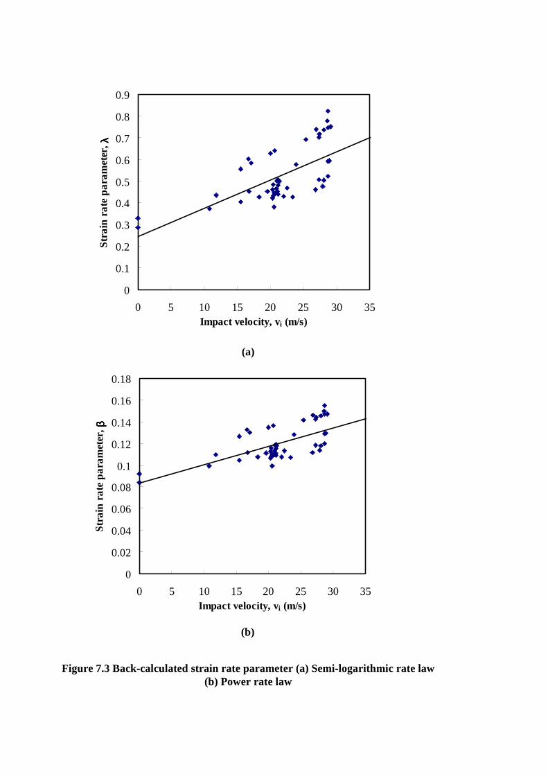
(a)
Figure 7.3 Back-calculated strain rate parameter (a) Semi-logarithmic rate law (b) Power rate law
(b)
0
0.02
0.04
0.06
0.08
0.1
0.12
0.14
0.16
0.18
0 5 10 15 20 25 30 35Impact velocity, vi (m/s)
Stra
in r
ate
pa
ram
eter
, ββ ββ
0
0.1
0.2
0.3
0.4
0.5
0.6
0.7
0.8
0.9
0 5 10 15 20 25 30 35Impact velocity, vi (m/s)
Stra
in r
ate
pa
ram
eter
, λλ λλ

Figure 7.5 Measured and predicted embedment depths for the 0FA in the beam centrifuge
0
5
10
15
20
25
30
35
40
45
50
0 5 10 15 20 25 30 35
Impact velocity, vi (m/s)
Pro
toty
pe
emb
edm
ent,
z e,p (
m)
0
25
50
75
100
125
150
175
200
225
250
Mo
del e
mb
edm
ent,
z e,m (
mm
)
β = 0.08
β = 0.14
βave = 0.12
0
0.5
1
1.5
2
2.5
3
3.5
4
1 10 100 1000 10000 100000Normalised strain rate, γγγγ/γγγγref
No
rma
lised
res
ista
nce
, s u/
s u,r
ef
Log - λ = 0.2
Log - λ = 0.4
Power - β = 0.1
Figure 7.4 Strain rate effects for semi-logarithmic and power rate laws

Figure 7.7 Sensitivity of embedment depth predictions to bearing capacity factor
0
10
20
30
40
50
60
0 5 10 15 20 25 30 35
Impact velocity, vi (m/s)
Pro
toty
pe
emb
edm
ent,
z e,p (
m)
0
50
100
150
200
250
300
Mo
del e
mb
edm
ent,
z e,m (
mm
)
Nc = 8
Nc = 20
Nc = 12
Figure 7.6 Embedment depth predictions for impact velocities of up to 80 m/s
0
10
20
30
40
50
60
70
80
0 10 20 30 40 50 60 70 80
Impact velocity, vi (m/s)P
roto
type
em
bed
men
t, z e,p
(m
)
0
50
100
150
200
250
300
350
400
Mo
del
em
bed
men
t, z e,m
(m
m)
β = 0.12
Figure 7.9 Sensitivity of embedment depth predictions to undrained shear strength gradient
0
10
20
30
40
50
60
0 5 10 15 20 25 30 35
Impact velocity, vi (m/s)
Pro
toty
pe
emb
edm
ent,
z e,p (
m)
0
50
100
150
200
250
300
Mo
del e
mb
edm
ent,
z e,m (
mm
)
k = 1 kPa/m
k = 1.5 kPa/m
k = 1.07 kPa/m(a = 0.013, b = 0.870)
Figure 7.8 Sensitivity of embedment depth predictions to shaft adhesion factor
0
10
20
30
40
50
60
0 5 10 15 20 25 30 35
Impact velocity, vi (m/s)
Pro
toty
pe
emb
edm
ent,
z e,p (
m)
0
50
100
150
200
250
300
Mo
del e
mb
edm
ent,
z e,m (
mm
)
α = 0
α = 1
α = 0.4
Figure 7.11 Measured and predicted Peak 1 vertical monotonic holding capacities
0
5
10
15
20
25
30
35
40
45
50
0 1 2 3 4 5Prototype capacity, Fv,p (MN)
Pro
toty
pe e
mbe
dmen
t, ze
,p (
m)
0
25
50
75
100
125
150
175
200
225
250
0 25 50 75 100 125Model capacity, Fv,m (N)
Mod
el e
mbe
dmen
t, ze
,m (
mm
)
α = 1
α = 0.8
Figure 7.10 Sensitivity of embedment depth predictions to drag coefficient
0
10
20
30
40
50
60
0 5 10 15 20 25 30 35
Impact velocity, vi (m/s)P
roto
typ
e em
bed
men
t, z e,p
(m
)
0
50
100
150
200
250
300
Mo
del e
mb
edm
ent,
z e,m (
mm
)
CD = 0
CD = 0.7
CD = 0.24

Figure 7.13 Holding capacity predictions for embedment depths of up to 360 mm (72 m at prototype scale)
0
10
20
30
40
50
60
70
80
0 1 2 3 4 5 6 7 8Prototype capacity, Fv,p (MN)
Pro
toty
pe e
mbe
dmen
t, ze
,p (
m)
0
50
100
150
200
250
300
350
400
0 25 50 75 100 125 150 175 200Model capacity, Fv,m (N)
Mod
el e
mbe
dmen
t, ze
,m (
mm
)
α = 1
α = 0.5
Figure 7.12 Measured and predicted Peak 2 vertical monotonic holding capacities
0
5
10
15
20
25
30
35
40
45
50
0 1 2 3 4 5Prototype capacity, Fv,p (MN)
Pro
toty
pe e
mbe
dmen
t, ze
,p (
m)
0
25
50
75
100
125
150
175
200
225
250
0 25 50 75 100 125Model capacity, Fv,m (N)
Mod
el e
mbe
dmen
t, ze
,m (
mm
)
α = 0.5α = 1
Figure 7.15 Sensitivity of holding capacity predictions to padeye bearing resistance
0
10
20
30
40
50
0 1 2 3 4 5Prototype capacity, Fv,p (MN)
Pro
toty
pe
emb
edm
ent,
z e,p (
m)
0
50
100
150
200
250
0 25 50 75 100 125Model capacity, Fv,m (N)
Mo
del e
mb
edm
ent,
z e,m (m
m)
f.Nc = 0.9
(f = 0.1, Nc = 9)
f.Nc = 9
f.Nc = 0
Figure 7.14 Sensitivity of holding capacity predictions to tip bearing capacity factor
0
10
20
30
40
50
0 1 2 3 4 5Prototype capacity, Fv,p (MN)
Pro
toty
pe
emb
edm
ent,
z e,p (
m)
0
50
100
150
200
250
0 25 50 75 100 125Model capacity, Fv,m (N)
Mo
del e
mb
edm
ent,
z e,m (m
m)
Nc = 20
Nc = 8
Nc = 12
Figure 7.17 Sensitivity of holding capacity predictions to undrained shear strength gradient
0
10
20
30
40
50
0 1 2 3 4 5Prototype capacity, Fv,p (MN)
Pro
toty
pe
emb
edm
ent,
z e,p (
m)
0
50
100
150
200
250
0 25 50 75 100 125Model capacity, Fv,m (N)
Mo
del e
mb
edm
ent,
z e,m (m
m)
k = 1 kPa/m
k = 1.5 kPa/m
k = 1.07 kPa/m(a = 0.013, b = 0.870)
Figure 7.16 Sensitivity of holding capacity predictions to shaft adhesion factor
0
10
20
30
40
50
0 1 2 3 4 5Prototype capacity, Fv,p (MN)
Pro
toty
pe
emb
edm
ent,
z e,p (
m)
0
50
100
150
200
250
0 25 50 75 100 125Model capacity, Fv,m (N)
Mo
del e
mb
edm
ent,
z e,m (m
m)
α = 0
α = 1
α = 0.8

Figure 7.19 Measured and theoretical impact velocities in the drum centrifuge
Figure 7.18 Variation in holding capacity predictions with impact velocity for shear strength gradients of 1 and 1.5 kPa/m
0
1
2
3
4
5
0 5 10 15 20 25 30 35Impact velocity, vi (m/s)
Pro
toty
pe c
apac
ity,
Fv,p (
MN
)
0
25
50
75
100
125
Mod
el c
apac
ity,
Fv,m
(N
)
k = 1 kPa/m
k = 1.5 kPa/m
0
5
10
15
20
25
30
35
0 5 10 15 20 25Impact velocity, vi (m/s)
Equ
ival
ent
prot
otyp
e dr
op h
eigh
t, h
d,e
q (m
)
0FA
4FA
L/D < 7
L/D > 7
TheoreticalNote: Equivalent drop
heights represent modeldrop heights of 0 - 250 mm
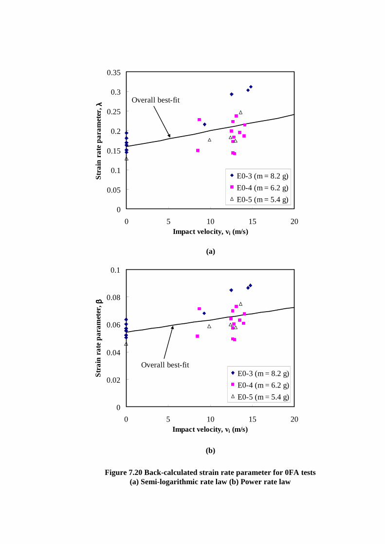
Figure 7.20 Back-calculated strain rate parameter for 0FA tests (a) Semi-logarithmic rate law (b) Power rate law
(a)
(b)
0
0.05
0.1
0.15
0.2
0.25
0.3
0.35
0 5 10 15 20Impact velocity, vi (m/s)
Stra
in r
ate
pa
ram
eter
, λλ λλ
E0-3 (m = 8.2 g)
E0-4 (m = 6.2 g)
E0-5 (m = 5.4 g)
Overall best-fit
0
0.02
0.04
0.06
0.08
0.1
0 5 10 15 20Impact velocity, vi (m/s)
Stra
in r
ate
pa
ram
eter
, ββ ββ
E0-3 (m = 8.2 g)
E0-4 (m = 6.2 g)
E0-5 (m = 5.4 g)
Overall best-fit

Figure 7.21 Back-calculated strain rate parameter for 4FA tests (a) Semi-logarithmic rate law (b) Power rate law
(a)
(b)
0
0.05
0.1
0.15
0.2
0.25
0.3
0.35
0 5 10 15 20Impact velocity, vi (m/s)
Stra
in r
ate
pa
ram
eter
, λλ λλ
E4-1 (m = 15.5 g)
E4-2 (m = 12.7 g)
E4-3 (m = 9.6 g)
Overall best-fit
0
0.02
0.04
0.06
0.08
0.1
0 5 10 15 20Impact velocity, vi (m/s)
Stra
in r
ate
pa
ram
eter
, ββ ββ
E4-1 (m = 15.5 g)
E4-2 (m = 12.7 g)
E4-3 (m = 9.6 g)
Overall best-fit
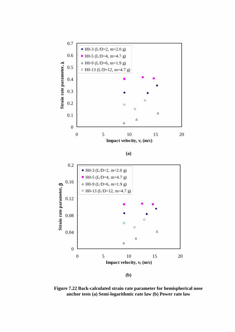
Figure 7.22 Back-calculated strain rate parameter for hemispherical nose anchor tests (a) Semi-logarithmic rate law (b) Power rate law
(a)
(b)
0
0.1
0.2
0.3
0.4
0.5
0.6
0.7
0 5 10 15 20Impact velocity, vi (m/s)
Stra
in r
ate
pa
ram
eter
, λλ λλ
H0-3 (L/D=2, m=2.0 g)
H0-5 (L/D=4, m=4.7 g)
H0-9 (L/D=6, m=1.9 g)
H0-13 (L/D=12, m=4.7 g)
0
0.04
0.08
0.12
0.16
0.2
0 5 10 15 20Impact velocity, vi (m/s)
Stra
in r
ate
pa
ram
eter
, ββ ββ
H0-3 (L/D=2, m=2.0 g)
H0-5 (L/D=4, m=4.7 g)
H0-9 (L/D=6, m=1.9 g)
H0-13 (L/D=12, m=4.7 g)

Figure 7.23 Measured and theoretical embedment depths for anchor E0-3
Figure 7.24 Measured and theoretical embedment depths for anchor E0-4
0
5
10
15
20
25
30
35
40
0 5 10 15 20 25
Impact velocity, vi (m/s)
Pro
toty
pe
emb
edm
ent,
z e,p (
m)
0
25
50
75
100
125
150
175
200
Mo
del e
mb
edm
ent,
z e,m (
mm
)
0FA
Overallβ = 0.07
β = 0.06
0
5
10
15
20
25
30
35
40
0 5 10 15 20 25
Impact velocity, vi (m/s)P
roto
typ
e em
bed
men
t, z e,p
(m
)
0
25
50
75
100
125
150
175
200
Mo
del e
mb
edm
ent,
z e,m (
mm
)
0FA
Overall
β = 0.07
β = 0.06
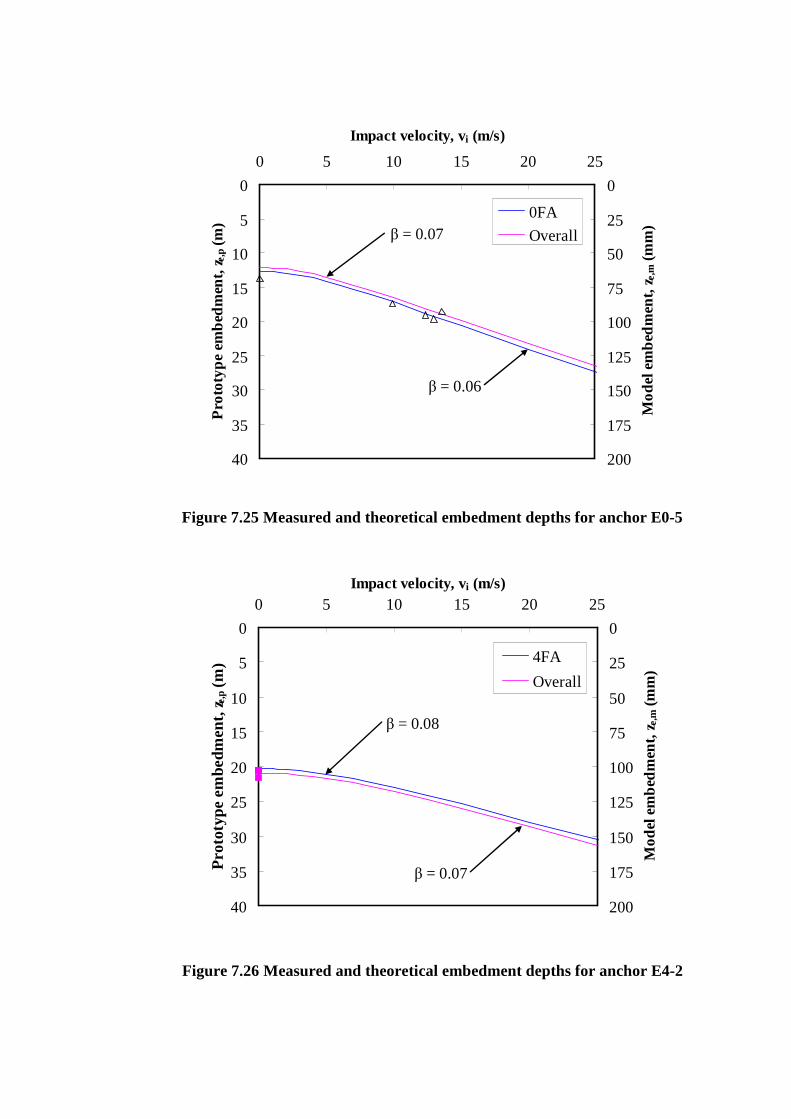
Figure 7.25 Measured and theoretical embedment depths for anchor E0-5
Figure 7.26 Measured and theoretical embedment depths for anchor E4-2
0
5
10
15
20
25
30
35
40
0 5 10 15 20 25
Impact velocity, vi (m/s)
Pro
toty
pe
emb
edm
ent,
z e,p (
m)
0
25
50
75
100
125
150
175
200
Mo
del e
mb
edm
ent,
z e,m (
mm
)
0FA
Overallβ = 0.07
β = 0.06
0
5
10
15
20
25
30
35
40
0 5 10 15 20 25Impact velocity, vi (m/s)
Pro
toty
pe e
mbe
dmen
t, z e,p
(m
)
0
25
50
75
100
125
150
175
200
Mo
del
em
bed
men
t, z e,m
(m
m)
4FA
Overall
β = 0.07
β = 0.08

Figure 7.27 Measured and theoretical embedment depths for anchor E4-3
Figure 7.28 Measured and theoretical embedment depths for anchor H0-3
0
5
10
15
20
25
30
35
40
0 5 10 15 20 25Impact velocity, vi (m/s)
Pro
toty
pe
embe
dmen
t, z e,p
(m
)
0
25
50
75
100
125
150
175
200
Mo
del
em
bed
men
t, z e,m
(m
m)
4FA
Overall
β = 0.07
β = 0.08
0
5
10
15
20
25
30
0 5 10 15 20 25Impact velocity, vi (m/s)
Pro
toty
pe
embe
dmen
t, z e,p
(m
)
0
25
50
75
100
125
150
Mo
del
em
bed
men
t, z e,m
(m
m)
H0-3
Overall
β = 0.07
β = 0.09
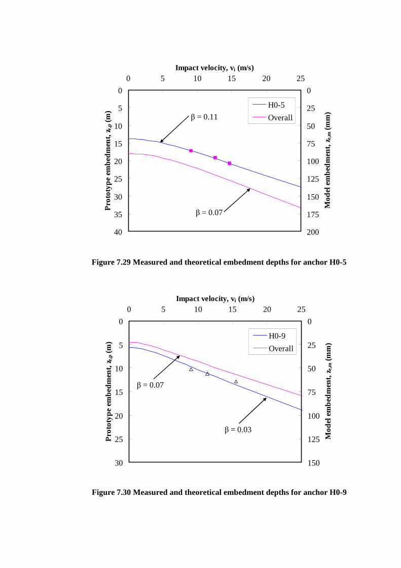
Figure 7.29 Measured and theoretical embedment depths for anchor H0-5
Figure 7.30 Measured and theoretical embedment depths for anchor H0-9
0
5
10
15
20
25
30
35
40
0 5 10 15 20 25Impact velocity, vi (m/s)
Pro
toty
pe
embe
dmen
t, z e,p
(m
)
0
25
50
75
100
125
150
175
200
Mo
del
em
bed
men
t, z e,m
(m
m)
H0-5
Overall
β = 0.07
β = 0.11
0
5
10
15
20
25
30
0 5 10 15 20 25Impact velocity, vi (m/s)
Pro
toty
pe
embe
dmen
t, z e,p
(m
)
0
25
50
75
100
125
150
Mo
del
em
bed
men
t, z e,m
(m
m)
H0-9
Overall
β = 0.07
β = 0.03
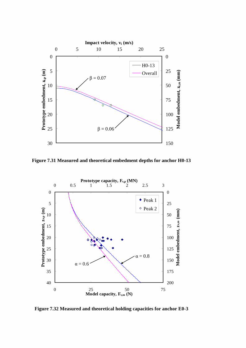
Figure 7.31 Measured and theoretical embedment depths for anchor H0-13
Figure 7.32 Measured and theoretical holding capacities for anchor E0-3
0
5
10
15
20
25
30
0 5 10 15 20 25Impact velocity, vi (m/s)
Pro
toty
pe
embe
dmen
t, z e,p
(m
)
0
25
50
75
100
125
150
Mo
del
em
bed
men
t, z e,m
(m
m)
H0-13
Overallβ = 0.07
β = 0.06
0
5
10
15
20
25
30
35
40
0 0.5 1 1.5 2 2.5 3Prototype capacity, Fv,p (MN)
Pro
toty
pe e
mbe
dmen
t, ze
,p (
m)
0
25
50
75
100
125
150
175
200
0 25 50 75Model capacity, Fv,m (N)
Mod
el e
mbe
dmen
t, ze
,m (
mm
)
Peak 1
Peak 2
α = 0.8
α = 0.6

Figure 7.33 Measured and theoretical holding capacities for anchor E0-4
Figure 7.34 Measured and theoretical holding capacities for anchor E0-5
0
5
10
15
20
25
30
35
40
0 0.5 1 1.5 2 2.5 3Prototype capacity, Fv,p (MN)
Pro
toty
pe e
mbe
dmen
t, ze
,p (
m)
0
25
50
75
100
125
150
175
200
0 25 50 75Model capacity, Fv,m (N)
Mod
el e
mbe
dmen
t, ze
,m (
mm
)
Peak 1
Peak 2
α = 0.8α = 0.5
0
5
10
15
20
25
30
35
40
0 0.5 1 1.5 2 2.5 3Prototype capacity, Fv,p (MN)
Pro
toty
pe e
mbe
dmen
t, ze
,p (
m)
0
25
50
75
100
125
150
175
200
0 25 50 75Model capacity, Fv,m (N)
Mod
el e
mbe
dmen
t, ze
,m (
mm
)Peak 1
Peak 2
α = 0.6
α = 0.5

Figure 7.35 Measured and theoretical holding capacities for anchor E4-2
Figure 7.36 Measured and theoretical holding capacities for anchor E4-3
0
5
10
15
20
25
30
35
40
0 1 2 3 4 5Prototype capacity, Fv,p (MN)
Pro
toty
pe
emb
edm
ent,
z e,p (
m)
0
25
50
75
100
125
150
175
200
0 25 50 75 100 125Model capacity, Fv,m (N)
Mo
del e
mb
edm
ent,
z e,m (
mm
)
Peak 1
Peak 2α = 1
α = 0.7
0
5
10
15
20
25
30
35
40
0 1 2 3 4 5Prototype capacity, Fv,p (MN)
Pro
toty
pe
emb
edm
ent,
z e,p (
m)
0
25
50
75
100
125
150
175
200
0 25 50 75 100 125Model capacity, Fv,m (N)
Mo
del e
mb
edm
ent,
z e,m (
mm
)
Peak 1
Peak 2α = 1
α = 0.4
α = 0.7

Figure 7.37 Measured and theoretical holding capacities for anchor H0-3
Figure 7.38 Measured and theoretical holding capacities for anchor H0-5
0
5
10
15
20
25
30
0 0.5 1 1.5Prototype capacity, Fv,p (MN)
Pro
toty
pe
emb
edm
ent,
z e,p (
m)
0
25
50
75
100
125
150
0 10 20 30Model capacity, Fv,m (N)
Mo
del e
mb
edm
ent,
z e,m (
mm
)
α = 1
α = 0.8
0
5
10
15
20
25
30
0 0.5 1 1.5Prototype capacity, Fv,p (MN)
Pro
toty
pe
emb
edm
ent,
z e,p (
m)
0
25
50
75
100
125
150
0 10 20 30Model capacity, Fv,m (N)
Mo
del e
mb
edm
ent,
z e,m (
mm
)
α = 1
α = 0.8

Figure 7.39 Measured and theoretical holding capacities for anchor H0-9
Figure 7.40 Measured and theoretical holding capacities for anchor H0-13
0
5
10
15
20
25
30
0 0.5 1 1.5Prototype capacity, Fv,p (MN)
Pro
toty
pe
emb
edm
ent,
z e,p (
m)
0
25
50
75
100
125
150
0 10 20 30Model capacity, Fv,m (N)
Mo
del e
mb
edm
ent,
z e,m (
mm
)
α = 1
α = 0.4
0
5
10
15
20
25
30
0 0.5 1 1.5Prototype capacity, Fv,p (MN)
Pro
toty
pe
emb
edm
ent,
z e,p (
m)
0
25
50
75
100
125
150
0 10 20 30Model capacity, Fv,m (N)
Mo
del e
mb
edm
ent,
z e,m (
mm
)
Peak 1
Peak 2
α = 0.7
α = 0.5
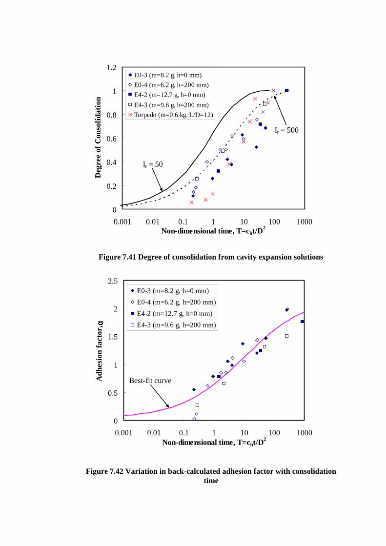
0
0.2
0.4
0.6
0.8
1
1.2
0.001 0.01 0.1 1 10 100 1000Non-dimensional time, T=cht/D
2
Deg
ree
of C
onso
lidat
ion
E0-3 (m=8.2 g, h=0 mm)
E0-4 (m=6.2 g, h=200 mm)
E4-2 (m=12.7 g, h=0 mm)
E4-3 (m=9.6 g, h=200 mm)
Torpedo (m=0.6 kg, L/D=12)
Ir = 50
Ir = 500
Figure 7.41 Degree of consolidation from cavity expansion solutions
Figure 7.42 Variation in back-calculated adhesion factor with consolidation time
0
0.5
1
1.5
2
2.5
0.001 0.01 0.1 1 10 100 1000Non-dimensional time, T=cht/D
2
Adh
esio
n fa
ctor
, αα αα
E0-3 (m=8.2 g, h=0 mm)
E0-4 (m=6.2 g, h=200 mm)
E4-2 (m=12.7 g, h=0 mm)
E4-3 (m=9.6 g, h=200 mm)
Best-fit curve
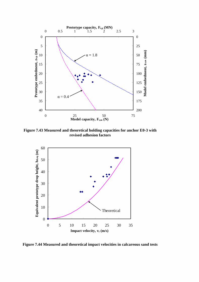
Figure 7.43 Measured and theoretical holding capacities for anchor E0-3 with revised adhesion factors
Figure 7.44 Measured and theoretical impact velocities in calcareous sand tests
0
5
10
15
20
25
30
35
40
0 0.5 1 1.5 2 2.5 3Prototype capacity, Fv,p (MN)
Pro
toty
pe e
mbe
dmen
t, ze
,p (
m)
0
25
50
75
100
125
150
175
200
0 25 50 75Model capacity, Fv,m (N)
Mod
el e
mbe
dmen
t, ze
,m (
mm
)
α = 1.8
α = 0.4
0
10
20
30
40
50
60
0 5 10 15 20 25 30 35Impact velocity, vi (m/s)
Equ
ival
ent
prot
otyp
e dr
op h
eigh
t, h
d,e
q (m
)
Theoretical
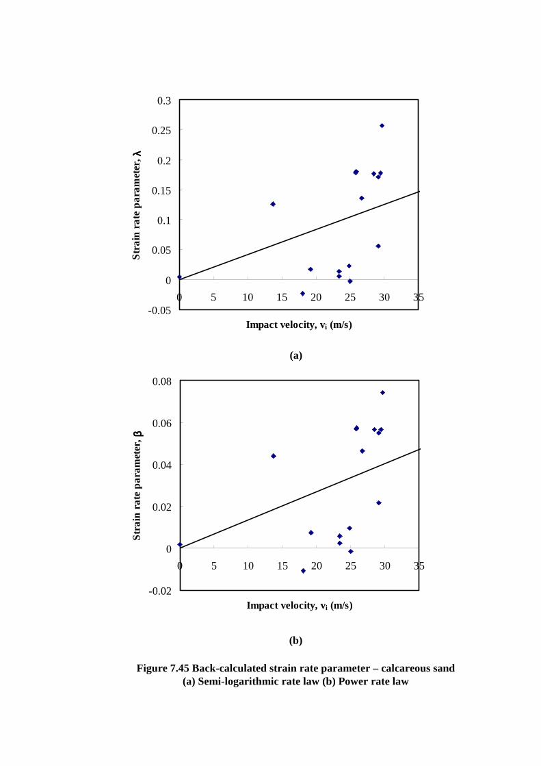
Figure 7.45 Back-calculated strain rate parameter – calcareous sand (a) Semi-logarithmic rate law (b) Power rate law
(a)
(b)
-0.05
0
0.05
0.1
0.15
0.2
0.25
0.3
0 5 10 15 20 25 30 35
Impact velocity, vi (m/s)
Stra
in r
ate
pa
ram
eter
, λλ λλ
-0.02
0
0.02
0.04
0.06
0.08
0 5 10 15 20 25 30 35
Impact velocity, vi (m/s)
Stra
in r
ate
pa
ram
eter
, ββ ββ

Figure 7.46 Measured and theoretical embedment depth - calcareous sand
Figure 7.47 Embedment depth predictions for impact velocities of up to 80 m/s -calcareous sand
0
5
10
15
20
25
30
0 5 10 15 20 25 30 35Impact velocity, vi (m/s)
Pro
toty
pe
embe
dmen
t, z e,p
(m
)
0
25
50
75
100
125
150
Mo
del
em
bed
men
t, z e,m
(m
m)
β = 0.03
0
10
20
30
40
50
0 10 20 30 40 50 60 70 80Impact velocity, vi (m/s)
Pro
toty
pe
embe
dmen
t, z e,p
(m
)
0
50
100
150
200
250
Mo
del
em
bed
men
t, z e,m
(m
m)
β = 0.03

Figure 7.48 Sensitivity of calcareous sand embedment predictions to bearing capacity factor
Figure 7.49 Sensitivity of calcareous sand embedment predictions to adhesion factor
0
5
10
15
20
25
30
0 5 10 15 20 25 30 35Impact velocity, vi (m/s)
Pro
toty
pe
embe
dmen
t, z e,p
(m
)
0
25
50
75
100
125
150
Mo
del
em
bed
men
t, z e,m
(m
m)
Nq = 50
Nq = 20
Nq = 32
0
5
10
15
20
25
30
0 5 10 15 20 25 30 35Impact velocity, vi (m/s)
Pro
toty
pe
embe
dmen
t, z e,p
(m
)
0
25
50
75
100
125
150
Mo
del
em
bed
men
t, z e,m
(m
m)
βCALC = 0.42
βCALC = 0
βCALC = 0.5
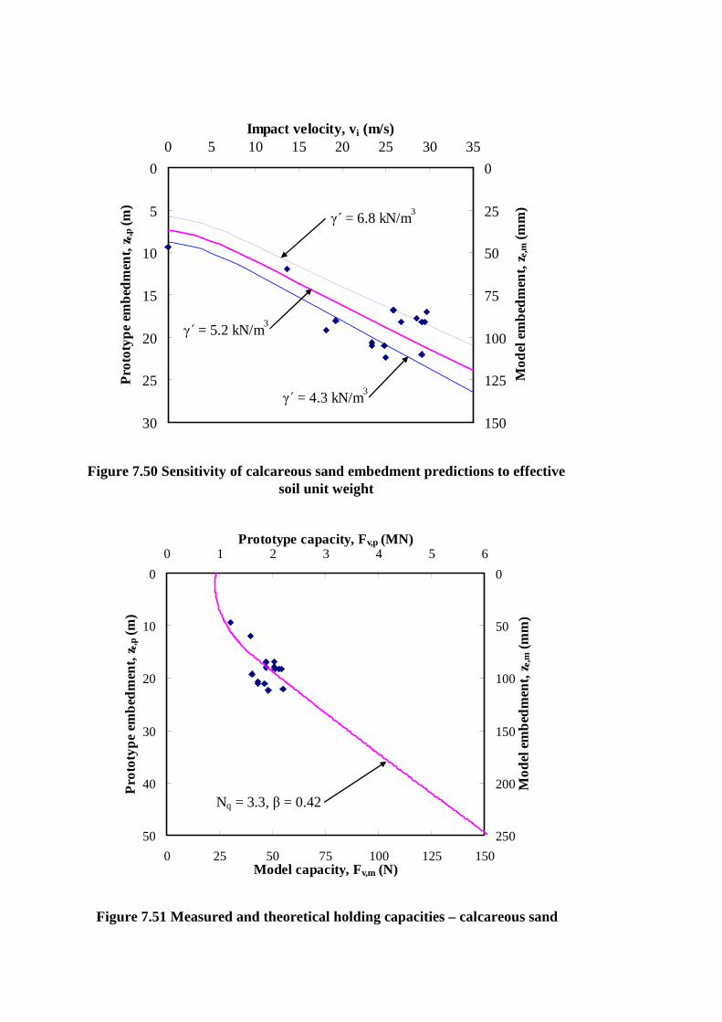
Figure 7.50 Sensitivity of calcareous sand embedment predictions to effective soil unit weight
Figure 7.51 Measured and theoretical holding capacities – calcareous sand
0
5
10
15
20
25
30
0 5 10 15 20 25 30 35Impact velocity, vi (m/s)
Pro
toty
pe
embe
dmen
t, z e,p
(m
)
0
25
50
75
100
125
150
Mo
del
em
bed
men
t, z e,m
(m
m)
γ΄ = 6.8 kN/m3
γ΄ = 4.3 kN/m3
γ΄ = 5.2 kN/m3
0
10
20
30
40
50
0 1 2 3 4 5 6Prototype capacity, Fv,p (MN)
Pro
toty
pe
emb
edm
ent,
z e,p (
m)
0
50
100
150
200
250
0 25 50 75 100 125 150Model capacity, Fv,m (N)
Mo
del e
mb
edm
ent,
z e,m (
mm
)
Nq = 3.3, β = 0.42
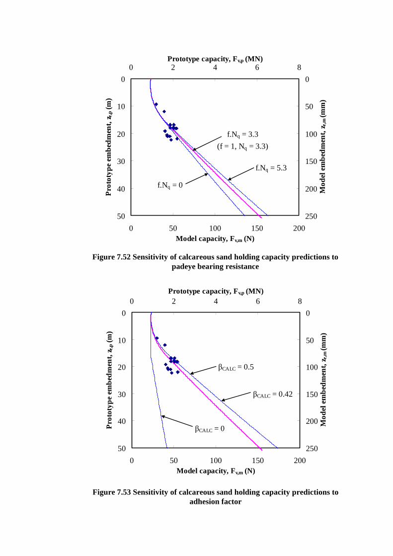
Figure 7.52 Sensitivity of calcareous sand holding capacity predictions to padeye bearing resistance
Figure 7.53 Sensitivity of calcareous sand holding capacity predictions to adhesion factor
0
10
20
30
40
50
0 2 4 6 8Prototype capacity, Fv,p (MN)
Pro
toty
pe
embe
dmen
t, z e,p
(m
)
0
50
100
150
200
250
0 50 100 150 200Model capacity, Fv,m (N)
Mo
del e
mb
edm
ent,
z e,m (m
m)
f.Nq = 5.3
f.Nq = 0
f.Nq = 3.3
(f = 1, Nq = 3.3)
0
10
20
30
40
50
0 2 4 6 8Prototype capacity, Fv,p (MN)
Pro
toty
pe
emb
edm
ent,
z e,p (
m)
0
50
100
150
200
250
0 50 100 150 200Model capacity, Fv,m (N)
Mo
del e
mb
edm
ent,
z e,m (m
m)
βCALC = 0.5
βCALC = 0
βCALC = 0.42

Figure 7.54 Sensitivity of calcareous sand holding capacity predictions to effective soil unit weight
Figure 7.55 Variation in holding capacity predictions with impact velocity for effective soil unit weights of 4.3 and 6.8 kN/m3
0
10
20
30
40
50
0 2 4 6 8Prototype capacity, Fv,p (MN)
Pro
toty
pe
emb
edm
ent,
z e,p (
m)
0
50
100
150
200
250
0 50 100 150 200Model capacity, Fv,m (N)
Mo
del e
mb
edm
ent,
z e,m (m
m)
γ΄ = 6.8 kN/m3
γ΄ = 4.3 kN/m3
γ΄ = 5.2 kN/m3
0
0.5
1
1.5
2
2.5
3
0 5 10 15 20 25 30 35
Impact velocity, vi (m/s)
Pro
toty
pe
cap
aci
ty,
F v,p
(MN
)
0
12.5
25
37.5
50
62.5
75
Mo
del c
apa
city
, F v
,m (N
)
γ΄ = 4.3 kN/m3
γ΄ = 6.8 kN/m3
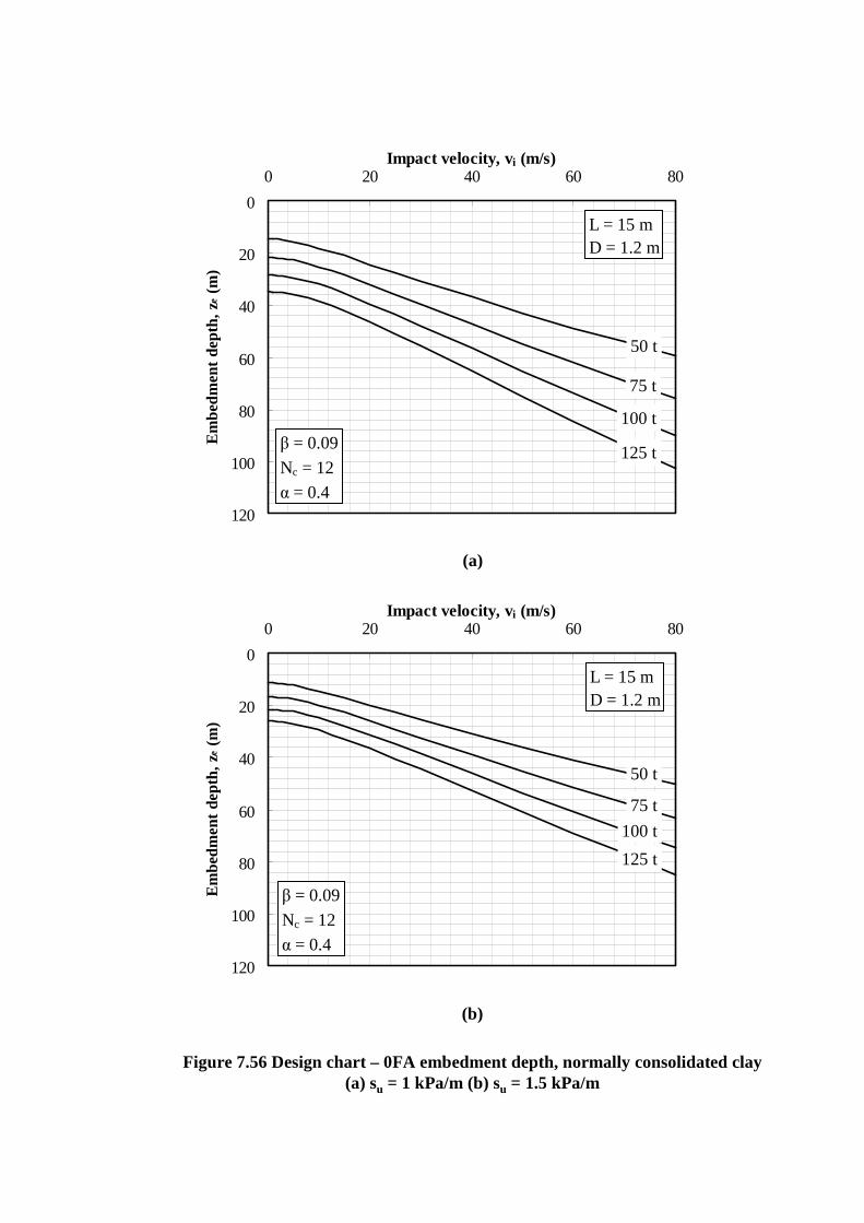
Figure 7.56 Design chart – 0FA embedment depth, normally consolidated clay (a) su = 1 kPa/m (b) su = 1.5 kPa/m
(a)
(b)
0
20
40
60
80
100
120
0 20 40 60 80Impact velocity, vi (m/s)
Em
bedm
ent
dept
h, ze
(m
)
50 t
75 t
100 t
125 tβ = 0.09
Nc = 12
α = 0.4
L = 15 mD = 1.2 m
0
20
40
60
80
100
120
0 20 40 60 80Impact velocity, vi (m/s)
Em
bedm
ent
dept
h, ze
(m
)
50 t
75 t
100 t
125 t
β = 0.09
Nc = 12
α = 0.4
L = 15 mD = 1.2 m
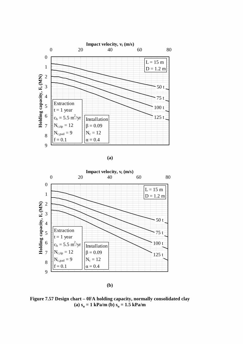
(a)
(b)
Figure 7.57 Design chart – 0FA holding capacity, normally consolidated clay (a) su = 1 kPa/m (b) su = 1.5 kPa/m
0
1
2
3
4
5
6
7
8
9
0 20 40 60 80Impact velocity, vi (m/s)
Ho
ldin
g c
ap
aci
ty,
F v (
MN
)
50 t
75 t
100 t
125 t
L = 15 mD = 1.2 m
Extractiont = 1 year
ch = 5.5 m2/yr
Nc,tip = 12
Nc,pad = 9f = 0.1
Installationβ = 0.09
Nc = 12α = 0.4
0
1
2
3
4
5
6
7
8
9
0 20 40 60 80Impact velocity, vi (m/s)
Ho
ldin
g c
apa
city
, F v
(M
N)
50 t
75 t
100 t
125 t
L = 15 mD = 1.2 m
Extractiont = 1 year
ch = 5.5 m2/yr
Nc,tip = 12
Nc,pad = 9
f = 0.1
Installationβ = 0.09
Nc = 12
α = 0.4
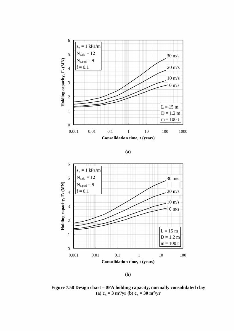
(a)
(b)
Figure 7.58 Design chart – 0FA holding capacity, normally consolidated clay (a) ch = 3 m2/yr (b) ch = 30 m2/yr
0
1
2
3
4
5
6
0.001 0.01 0.1 1 10 100 1000
Consolidation time, t (years)
Hol
ding
cap
acity
, Fv
(M
N)
30 m/s
20 m/s
10 m/s
0 m/s
L = 15 mD = 1.2 mm = 100 t
su = 1 kPa/m
Nc,tip = 12
Nc,pad = 9
f = 0.1
0
1
2
3
4
5
6
0.001 0.01 0.1 1 10 100
Consolidation time, t (years)
Hol
ding
cap
acity
, Fv
(M
N)
30 m/s
20 m/s
10 m/s
0 m/s
L = 15 mD = 1.2 mm = 100 t
su = 1 kPa/m
Nc,tip = 12
Nc,pad = 9
f = 0.1

Figure 7.59 Design chart – 4FA embedment depth, normally consolidated clay (a) su = 1 kPa/m (b) su = 1.5 kPa/m
(a)
(b)
0
10
20
30
40
50
60
70
0 20 40 60 80Impact velocity, vi (m/s)
Em
bedm
ent
dept
h, ze
(m
)
50 t
75 t
100 t
125 t
β = 0.08
Nc = 12
Ncf = 7.5
α = 0.4
L = 15 mD = 1.2 m
0
10
20
30
40
50
60
70
0 20 40 60 80Impact velocity, vi (m/s)
Em
bedm
ent
dept
h, ze
(m
)
50 t
75 t
100 t
125 t
L = 15 mD = 1.2 m
β = 0.08
Nc = 12
Ncf = 7.5
α = 0.4

(a)
(b)
Figure 7.60 Design chart – 4FA holding capacity, normally consolidated clay (a) su = 1 kPa/m (b) su = 1.5 kPa/m
0
2
4
6
8
10
12
0 20 40 60 80Impact velocity, vi (m/s)
Ho
ldin
g c
apa
city
, F v
(M
N)
50 t
75 t
100 t
125 t
L = 15 mD = 1.2 m
Extractiont = 1 year
ch = 5.5 m2/yr
Nc,tip = 12
Nc,pad = 9
Ncf = 7.5
f = 0.1
Installationβ = 0.12
Nc = 12
Ncf = 7.5
α = 0.4
0
2
4
6
8
10
12
0 20 40 60 80Impact velocity, vi (m/s)
Ho
ldin
g c
apa
city
, F v
(M
N)
50 t
75 t
100 t
125 t
L = 15 mD = 1.2 m
Extractiont = 1 year
ch = 5.5 m2/yr
Nc,tip = 12
Nc,pad = 9
Ncf = 7.5
f = 0.1
Installationβ = 0.12
Nc = 12
Ncf = 7.5
α = 0.4
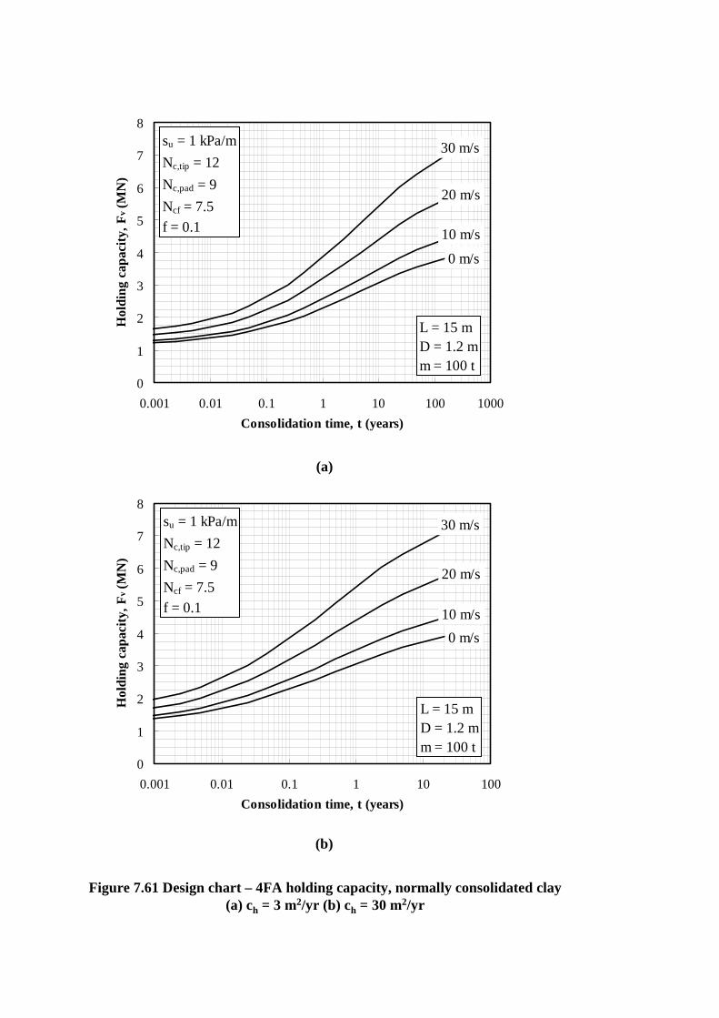
(a)
(b)
Figure 7.61 Design chart – 4FA holding capacity, normally consolidated clay (a) ch = 3 m2/yr (b) ch = 30 m2/yr
0
1
2
3
4
5
6
7
8
0.001 0.01 0.1 1 10 100 1000
Consolidation time, t (years)
Hol
ding
cap
acity
, Fv
(M
N)
30 m/s
20 m/s
10 m/s
0 m/s
L = 15 mD = 1.2 mm = 100 t
su = 1 kPa/m
Nc,tip = 12
Nc,pad = 9
Ncf = 7.5
f = 0.1
0
1
2
3
4
5
6
7
8
0.001 0.01 0.1 1 10 100
Consolidation time, t (years)
Hol
ding
cap
acity
, Fv
(M
N)
30 m/s
20 m/s
10 m/s
0 m/s
L = 15 mD = 1.2 mm = 100 t
su = 1 kPa/m
Nc,tip = 12
Nc,pad = 9
Ncf = 7.5
f = 0.1
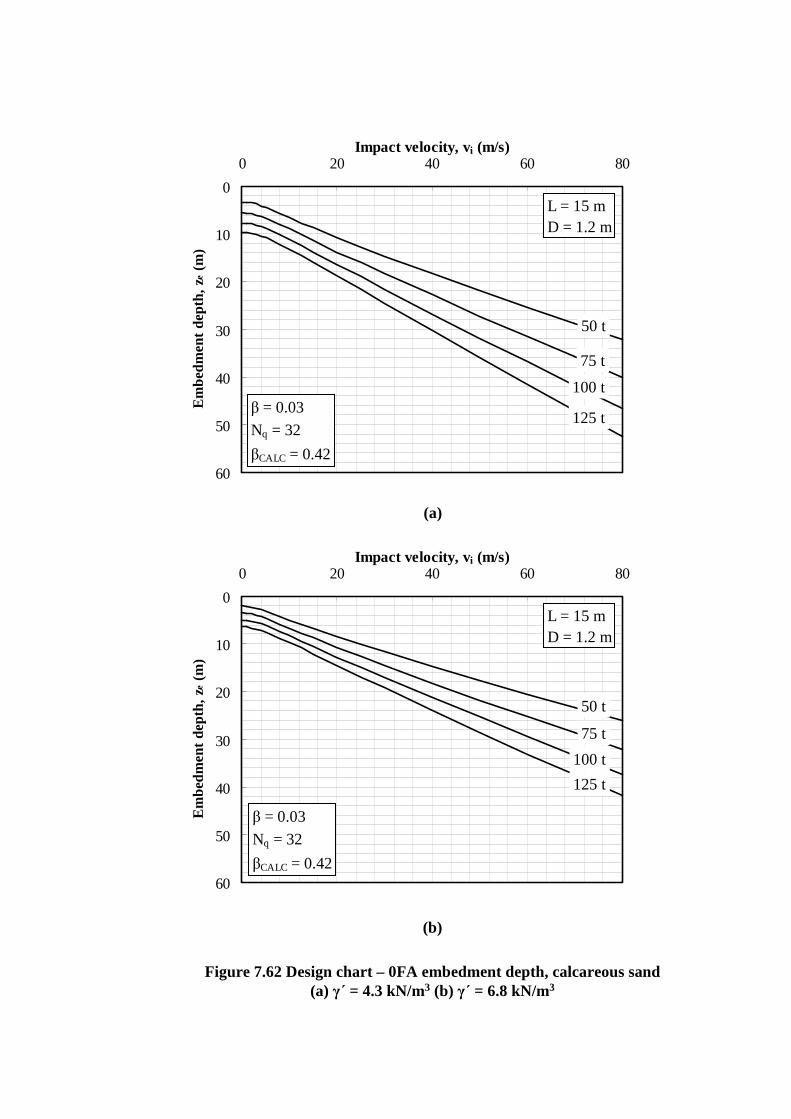
(a)
(b)
Figure 7.62 Design chart – 0FA embedment depth, calcareous sand(a) γ΄ = 4.3 kN/m3 (b) γ΄ = 6.8 kN/m3
0
10
20
30
40
50
60
0 20 40 60 80Impact velocity, vi (m/s)
Em
bedm
ent
dept
h, ze
(m
)
50 t
75 t
100 t
125 tβ = 0.03
Nq = 32
βCALC = 0.42
L = 15 mD = 1.2 m
0
10
20
30
40
50
60
0 20 40 60 80Impact velocity, vi (m/s)
Em
bedm
ent
dept
h, ze
(m
)
50 t
75 t
100 t
125 t
L = 15 mD = 1.2 m
β = 0.03
Nq = 32
βCALC = 0.42

Figure 7.63 Design chart – 0FA holding capacity, calcareous sand (a) γ΄ = 4.3 kN/m3 (b) γ΄ = 6.8 kN/m3
(a)
(b)
0
1
2
3
4
5
6
7
0 20 40 60 80Impact velocity, vi (m/s)
Ho
ldin
g c
ap
aci
ty,
F v (
MN
)
50 t
75 t
100 t
125 t
L = 15 mD = 1.2 m
Extraction
βCALC = 0.42
Nq = 3.3f = 1
Installationβ = 0.03Nq = 32
βCALC = 0.42
0
1
2
3
4
5
6
7
0 20 40 60 80Impact velocity, vi (m/s)
Ho
ldin
g c
apa
city
, F v
(M
N)
50 t
75 t
100 t
125 t
L = 15 mD = 1.2 m
Extraction
βCALC = 0.42
Nq = 3.3
f = 1
Installationβ = 0.03
Nq = 32
βCALC = 0.42
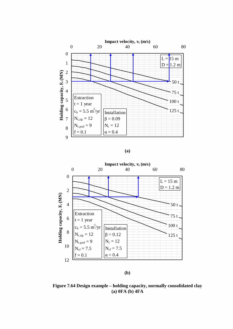
(a)
(b)
Figure 7.64 Design example – holding capacity, normally consolidated clay(a) 0FA (b) 4FA
0
1
2
3
4
5
6
7
8
9
0 20 40 60 80Impact velocity, vi (m/s)
Ho
ldin
g c
apa
city
, F v
(M
N)
50 t
75 t
100 t
125 t
L = 15 mD = 1.2 m
Extractiont = 1 year
ch = 5.5 m2/yr
Nc,tip = 12
Nc,pad = 9
f = 0.1
Installationβ = 0.09
Nc = 12
α = 0.4
0
2
4
6
8
10
12
0 20 40 60 80Impact velocity, vi (m/s)
Ho
ldin
g c
apa
city
, F v
(M
N)
50 t
75 t
100 t
125 t
L = 15 mD = 1.2 m
Extractiont = 1 year
ch = 5.5 m2/yr
Nc,tip = 12
Nc,pad = 9
Ncf = 7.5
f = 0.1
Installationβ = 0.12
Nc = 12
Ncf = 7.5
α = 0.4

(a)
(b)
Figure 7.65 Design example – embedment depth, normally consolidated clay(a) 0FA (b) 4FA
0
20
40
60
80
100
120
0 20 40 60 80Impact velocity, vi (m/s)
Em
bedm
ent
dept
h, ze
(m
)
50 t
75 t
100 t
125 tβ = 0.09
Nc = 12
α = 0.4
L = 15 mD = 1.2 m
0
10
20
30
40
50
60
70
0 20 40 60 80Impact velocity, vi (m/s)
Em
bedm
ent
dept
h, ze
(m
)
50 t
75 t
100 t
125 t
β = 0.08
Nc = 12
Ncf = 7.5
α = 0.4
L = 15 mD = 1.2 m

Figure 7.66 Design example – consolidation time, normally consolidated clay
0
1
2
3
4
5
6
0.001 0.01 0.1 1 10 100 1000
Consolidation time, t (years)
Hol
ding
cap
acity
, Fv
(M
N)
20 m/s
10 m/s
0 m/s
30 m/s
su = 1 kPa/m
Nc,tip = 12
Nc,pad = 9
f = 0.1
L = 15 mD = 1.2 mm = 100 t