Flight Recorder Localization Following at-Sea PlaneCrashes

Andre Filipe Pereira RochaInstituto Superior Tecnico

Av. Rovisco Pais, 1049-001 Lisboa, Portugalandre.p.rocha@ist.utl.pt

Abstract—Recent aircraft disasters over oceans and seas un-veiled critical deficiencies in the existing methods of submerged-aircraft localization and recovery. The current localization proce-dures rely on an acoustic transmitter, denominated UnderwaterLocator Beacon (ULB), which is attached to the aircraft’s ”blackbox” and emitting sinusoid-shaped acoustic signals with thepurpose of being detected and eventually located by a setof conveniently positioned hydrophones. This paper aims toquantify the precision gains in aircraft localization when somespecifications of the currently used beacons are modified, namelyits operating frequency, transmitted signal waveform and acousticpower. Moreover, we intend to compare two different sourcelocalization algorithms – TOA (Time Of Arrival) and TDOA(Time-Difference Of Arrival) – when applied to this kind ofsituations. This study is carried out in a simulation environment.

I. INTRODUCTION

The 2009 Air France (AF) flight 447 linking Rio deJaneiro to Paris crashed in the North Atlantic area. French,Brazilian and U.S. authorities took over the wreckage’s searchcampaigns, which proved unsuccessful as far as finding theaircraft’s Flight Data Recorders (FDR, also known as ”blackboxes”) is concerned. The search region was repeatedlyacoustically explored in the attempt of detecting the ULB’stransmitted signal, which never happened. It was only in May2011, almost two years after the crash, that the ULBs werefound thanks to the Remora 6000 ROV (Remotely OperatedVehicle).The ULB is an acoustic transmitter periodically emitting soundwaves, as outlined in Fig. 1. Following a crash of an aircraftat the ocean, a search area is laid out based on the informationavailable on the aircraft’s Last Known Position (LKP), whichmay be derived through flight plan, GPS or radar data. Thus,a set of hydrophone arrays are spread around the aircraft’sexpected position, as depicted in Fig. 2.

Fig. 1. Periodic sequence of pulses to be transmitted.

Fig. 2. ULB localization framework.

The AF 447 accident exposed the shortcomings of thecurrent ULB technology. Consequently, we suggest:

1) Increasing the autonomy of the ULBs. The current ULBbatteries have an operating life of 30 days; increasing itto 90 days would enable longer periods of searchingactivity, making it more likely to recover the ULBs;

2) That the ULBs start transmitting only when interrogated,instead of being water activated. In this sense, the ULBswould be functioning as transponders which could beinterrogated by a reference receiver [1], [2], [3]. Again,this would improve the ULBs’ autonomy, as well asallow the determination of the signal’s Round TripTime (RTT), which in turn yields the ULB-hydrophonesdistances, essential for the TOA algorithm;

3) Decreasing the ULB transmitted signal’s frequency. Theattenuation losses induced by the Underwater AcousticChannel (UAC) are highly dependent on frequency, andincrease proportionally to its cube. Hence, reducingthe current 37.5 kHz to a reasonable 10 kHz has thepotential to greatly enhance the maximum depth andrange for which the ULB signal can be detected. Thedownside of this solution is that the physical size of thebeacon would have to increase;

4) Substituting the currently used CW (Continuous Wave)sine wave by signals having richer frequency content

and better auto-correlation properties, such as a chirpor a QAM (Quadrature Amplitude Modulation) signal.Thus, the harmful frequency imprecision inherent tothe sinusoid tonal is no longer an issue, as broadbandsignals are easier to reproduce and frequency tune thantheir CW counterparts. The sine wave’s frequency mayindeed vary within the 36.5−38.5 kHz interval, albeit itsbandwidth is only the inverse of the pulse length (10ms)– 100Hz;

5) Incorporating in the ULB transmitted signal a digitalmessage conveying valuable data such as the FDRrecords or the ULB depth, which would greatly aid thesearch efforts.

This paper is structured as follows. Section II presents themain features of the UAC and its signal distorting agents, andits subsections address the Bellhop simulator and the oceano-graphic databases used in this work. Section III deals with thesignal processing chain, both at the transmitting ULB and thereceiving hydrophones, which leads to the determination ofthe signal’s RTT. Section IV addresses the source localizationalgorithms TOA and TDOA, whereas section V presents thesimulation results obtained.Remark: The material exposition is made to handle discrete-time signals. The Nyquist theorem states that there is no lossof information when converting a continuous-time signal todiscrete-time if the sampling rate is sufficiently high.

II. UNDERWATER ACOUSTIC CHANNEL

Conceptually, the underwater communication problem isdescribed in Fig. 3:

Fig. 3. Underwater communication problem.

The ocean is an acoustic waveguide limited above by thesea surface and below by the sea floor. Sound waves at middleand high frequencies (> 5 kHz) can be fairly modelled aspropagating along paths or rays through the ocean. In an idealhomogeneous environment the ray paths would follow straightlines radiating from the source and eventually reaching thereceiver [5]; in the real ocean environment, the ray pathsfollow curvilinear lines due to the high variability of theSound Speed Profile (SSP), which induces a bending of thesound rays towards regions of low sound speed (refraction).Additionally, it is verified that the acoustic beams are reflectedat both the sea surface and the sea bottom.

Scattering Loss: The reflection of sound at both oceaninterfaces causes a partial loss in its acoustic energy. Thus, theenergy that is scattered in a direction other than the directionof the receiver is effectively lost. Furthermore, the field scat-tered away from the specular direction and, in particular, thebackscattered field (reverberation) acts as negative interferencefor the main field.

Absorption Loss: Seawater and sea floor absorption isa sound attenuating mechanism consisting of the conversionof the acoustic energy of sound waves into another formof energy, which is then retained by the lossy agent. Seafloor sound-absorption occurs because the reflection of energyis incomplete, and sound penetrates into the bottom. Theabsorption of sound by the water is highly dependent onfrequency, meaning that high frequency signals are far moreattenuated that low frequency ones, as evidenced by (1), whereαw denotes the seawater attenuation.

αw = 3.3×10−3+0.11f2

1 + f2+

44f2

4100f + f2+3×10−4f2 (1)

Spreading Loss: The spreading loss is simply a measureof the signal weakening as it propagates outward from thesource. In regions close from the emitter, the acoustic wave-front radiates spherically, and the signal intensity is inverselyproportional to the surface of the sphere: I ∝ 1

4πR2 , where Ris the sphere radius. The spherical spreading in the nearfield isfollowed by a transition region towards cylindrical spreadingin the farfield, where the sound intensity becomes inverselyproportional to the surface of a cylinder of radius R and depthD: I ∝ 1

2πRD .Multipath propagation is a very critical aspect of soundpropagation in the ocean, which results in acoustic signalstravelling from the transmitter to the receivers by two or moredifferent paths (hundreds even), as exemplified in Fig. 4.

Fig. 4. Multipath propagation. A – direct path; B – surface-reflected path;C – bottom-reflected path; D – bottom-reflected surface-reflected path.

The multipath phenomenon is characterized by the inputdelay-spread function g, which reflects not only the energylosses endured by each path connecting the emitter to thereceiver, but also the delay-spread pattern obtained at thereceiver. Fig. 5 presents the signal arrival profile at eachreceiver for the situation of Fig. 4. From Fig. 5 it is immediateto understand that g resembles a train of Dirac impulses:

g[n] =

L∑l=1

alδ(n−Nl) , (2)

where L is the number of incoming rays at the receiver,al is the lth ray amplitude and Nl is the corresponding time

Fig. 5. Delay-spread pattern for the situation depicted in Fig. 4.

delay (in discrete-time). The ray amplitudes al are a measureof the absorption, scattering and spreading losses of the oceanenvironment.In underwater acoustic communications, ambient noise is alsoan issue because it masks the signal of interest. The severaldifferent sources of noise in the ocean are generally groupedinto four categories: turbulence (t), waves (w), thermal (th)and shipping noise (s). The ocean noise is then characterizedas a Gaussian variable having a Power Spectral Density (PSD)resulting from four different contributions:

N(f) = Nt(f) +Nw(f) +Nth(f) +Ns(f) , (3)

where

10 log10Nt(f) = 17− 30 log10 f (4)

10 log10Nw(f) = 50 + 7.5w12 + 20 log10 f−

40 log10(f + 0.4)(5)

10 log10Nth(f) = −15 + 20 log10 f (6)

10 log10Ns(f) = 40 + 20(s− 0.5) + 26 log10 f−60 log10(f + 0.03) .

(7)

These formulas were taken from [7] and present the noisepower N in dB re 1µPaHz−1 as a function of the acousticfrequency f in kHz. Along these lines, the received signal ycan be decomposed in two terms, one denoting the contribu-tion of the multipath attenuating effects (ym) and the otherexpressing the influence of underwater noise (yn):

y[n] = ym[n] + yn[n] , (8)

where

ym[n] = x[n] ? g[n] = g[n] ? x[n] =∑∞k=−∞

[∑Ll=1 alδ(k −Nl)

]x(n− k) . (9)

The term ym[n] is a time-delayed and amplitude-attenuatedversion of the transmitted signal x[n].

A. Bellhop

Bellhop is a freely distributed ray-tracing code incorporatedin the Acoustic Toolbox (check [11]). An exhaustive descrip-tion of this acoustic model, including a detailed theoreticalstudy of the wave theory behind it, is presented in [8]. Bellhopis designed in order to perform two-dimensional acoustic raytracing for a given SSP or a given sound speed field, inocean waveguides with flat or variable absorbing boundaries[12]. Output options include ray coordinates, travel time,amplitude, eigenrays, acoustic pressure or transmission loss(either coherent, incoherent or semi-coherent).Thus, we use Bellhop to simulate the time-delaying andamplitude-attenuating effects of the UAC on the transmittedsignal x. Three input files are required: a main environmen-tal file setting the simulation scenario for the localizationproblem (source depth, receivers’ depths and ranges, signalfrequency, etc.), a file describing the bathymetric profile, anda bottom reflection coefficient file generated through a Bouncerun. Bounce is a program also incorporated in the AcousticToolbox, and computes the reflection coefficient if given anadequate input.

B. Geoacoustic Database

A geoacoustic database is needed in this work to obtain thedata which serves as input to Bellhop’s (and Bounce’s) simu-lations. Thus, we resort to the GEBCO (General BathymetricChart of the Oceans) bathymetric database of the world’soceans, adopt the World Ocean Atlas 2009 material on SSPs,and utilize the DECK 41 bottom sediments database.

III. DELAY ESTIMATION

The state-of-the-art system depends on the directionality ofthe receiving hydrophones to estimate the ULB’s position viaa combination of AOA (Angle Of Arrival) and RSS (ReceivedSignal Strength) algorithms. In this work we have to estimatethe ULB-hydrophones distances to apply our methods ofinterest – TOA and TDOA. Thus, the reference receiver in-terrogates the transponder-acting ULB to synchronize clocks,setting the reference time origin. Once interrogated, the ULBstarts transmitting the acoustic signal to be detected and treatedby the hydrophones to determine its RTT, which in turn yieldsthe emitter-receiver distances.

A. Transmitter

The transmitter architecture is depicted in Fig. 6.The generator produces the wave signal in baseband, defin-

ing all the significant signal characteristics, such as its wave-form, nominal frequency or bandwidth Bs. In this study, we

Fig. 6. Transmitter block.

employ four different types of signals: the state-of-the-art highuncertain frequency sine wave and, on the other hand, sinusoid,chirp and QAM-4 signals with lower carrier frequency.Then, the baseband signal s is frequency-shifted by a mod-ulating carrier of frequency fc, creating the passband signalx, in accordance with (10), where ωc is the carrier’s angularfrequency and φ is the phase offset of the transmitter’s carrier.In this way, if we want to transmit a signal with frequency f0,the generated signal s must have a frequency f0 − fc so thatwhen modulated its frequency becomes (f0 − fc) + fc = f0.This frequency spectrum shift is exemplified in Fig. 7.

x[n] = s[n]Re{ej(ωcn+φ)} (10)

Fig. 7. Frequency spectrum shift resulting from the modulation process. Thebaseband signal presents lower frequencies than the passband signal.

After exiting the modulator, the discrete-time signal x[n]goes through the D/C converter where it is transformed intoits continuous-time equivalent x(t), at a sampling frequencyfs. Thereafter, the amplifier amplifies the continuous-timemodulated signal and drives the transducer to produce soundwaves, which are subsequently broadcast through the UAC.The discrete-time sinusoid transmitted signal is defined as

xs[n] = A sin(2πf0n+ ϕ) , (11)

where A is the amplitude and ϕ is the initial phase, or phaseoffset, in radians.The discrete-time chirp transmitted signal is

xc[n] = A cos((ω0 +

1

2βn)n+ ϕ

), (12)

where β is the frequency variation rate.The discrete-time QAM-4 transmitted signal is defined as

xqam[n] = I[n] cos(2πfcn) +Q[n] sin(2πfcn) . (13)

The QAM digital modulation architecture conveys twodigital symbol streams by changing the amplitudes of twocarrier waves using the ASK/PSK scheme. The two carriersinusoids are out of phase with each other by 90 ◦ and arethereby quadrature carriers of quadrature components. Themodulated waves are summed and the resulting waveform isa combination of both the PSK (Phase Shift-Keying) and theASK (Amplitude Shift-Keying) modulations. I[n] and Q[n]are the two symbol streams to be transmitted. The in-phasesymbol stream is obtained as

I[n] =∑k

akp(n− kN) , (14)

where ak is the amplitude of symbol k, p is the shape of thesignalling pulses (root-raised-cosine [13], in this case), and Nis the number of samples per symbol interval. The quadraturesequence Q[n] is generated similarly. In the case of a digitalquaternary modulation, as QAM-4, each symbol is constitutedby a combination of 4 bits (24 [bits] encode 1 of 16 [symbols]).The most significant parameters of each of the interest signalsare gathered next:

Sine Chirp QAM-4 SA sinePulse length τ (ms) 50 50 50 10Pulse repetition periodTp (s) 1.0 1.0 1.0 1.0

Signal frequency f0(kHz) 10 10 10 37.5

Signal bandwidth Bs1τ

2 kHz 2 kHz 1τ

Carrier frequency fc(kHz) 10 10 10 37.5

Sampling frequency fs(kHz) 50 50 50 85

TABLE ICHARACTERISTICS OF EACH OF THE POSSIBLE TRANSMITTED SIGNALS:

SINE, CHIRP, QAM AND STATE-OF-THE-ART SINE.

B. Receiver

The state-of-the-art system’s receiver is pictured in Fig. 8,whereas the proposed receiver structure is outlined in Fig. 9.

Fig. 8. Receiver configuration when the state-of-the-art signal (sine) istransmitted.

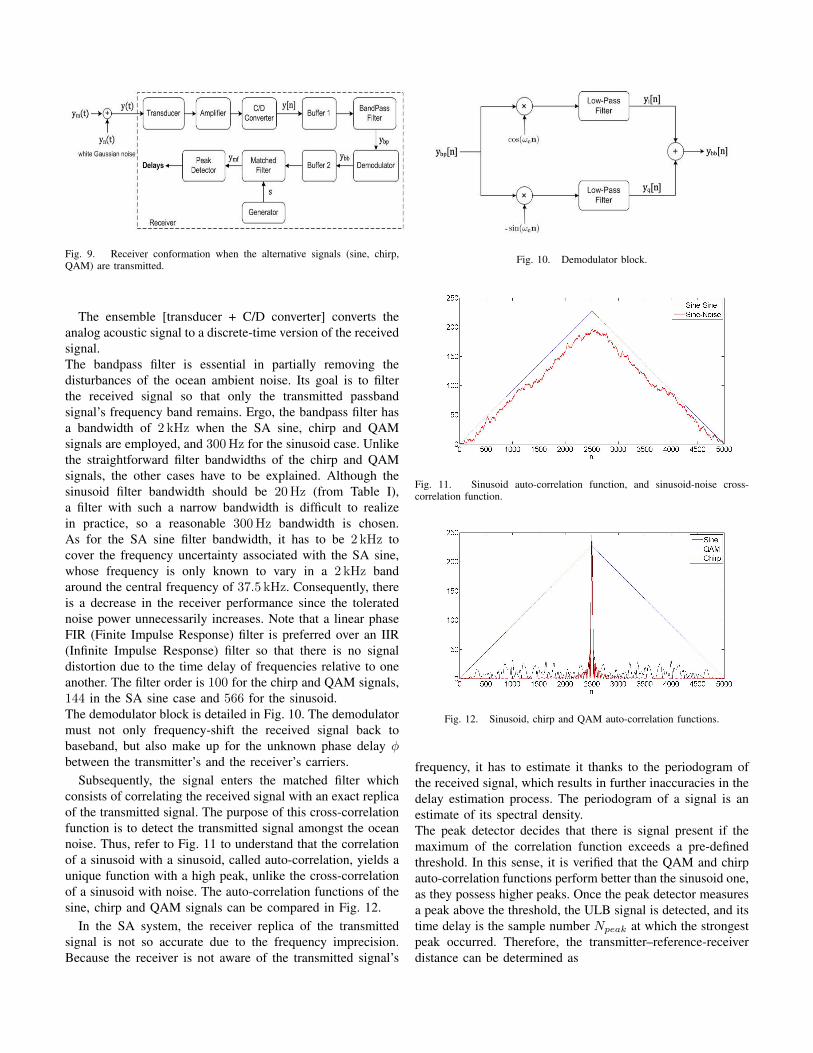
Fig. 9. Receiver conformation when the alternative signals (sine, chirp,QAM) are transmitted.

The ensemble [transducer + C/D converter] converts theanalog acoustic signal to a discrete-time version of the receivedsignal.The bandpass filter is essential in partially removing thedisturbances of the ocean ambient noise. Its goal is to filterthe received signal so that only the transmitted passbandsignal’s frequency band remains. Ergo, the bandpass filter hasa bandwidth of 2 kHz when the SA sine, chirp and QAMsignals are employed, and 300Hz for the sinusoid case. Unlikethe straightforward filter bandwidths of the chirp and QAMsignals, the other cases have to be explained. Although thesinusoid filter bandwidth should be 20Hz (from Table I),a filter with such a narrow bandwidth is difficult to realizein practice, so a reasonable 300Hz bandwidth is chosen.As for the SA sine filter bandwidth, it has to be 2 kHz tocover the frequency uncertainty associated with the SA sine,whose frequency is only known to vary in a 2 kHz bandaround the central frequency of 37.5 kHz. Consequently, thereis a decrease in the receiver performance since the toleratednoise power unnecessarily increases. Note that a linear phaseFIR (Finite Impulse Response) filter is preferred over an IIR(Infinite Impulse Response) filter so that there is no signaldistortion due to the time delay of frequencies relative to oneanother. The filter order is 100 for the chirp and QAM signals,144 in the SA sine case and 566 for the sinusoid.The demodulator block is detailed in Fig. 10. The demodulatormust not only frequency-shift the received signal back tobaseband, but also make up for the unknown phase delay φbetween the transmitter’s and the receiver’s carriers.

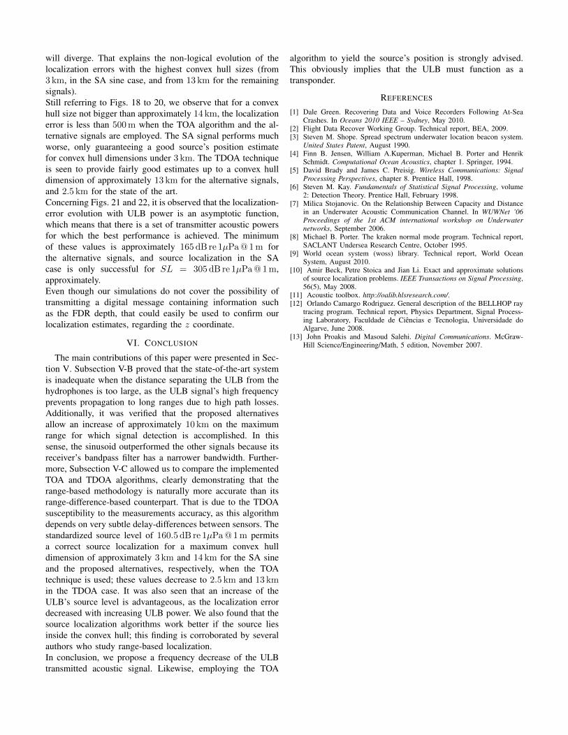
Subsequently, the signal enters the matched filter whichconsists of correlating the received signal with an exact replicaof the transmitted signal. The purpose of this cross-correlationfunction is to detect the transmitted signal amongst the oceannoise. Thus, refer to Fig. 11 to understand that the correlationof a sinusoid with a sinusoid, called auto-correlation, yields aunique function with a high peak, unlike the cross-correlationof a sinusoid with noise. The auto-correlation functions of thesine, chirp and QAM signals can be compared in Fig. 12.

In the SA system, the receiver replica of the transmittedsignal is not so accurate due to the frequency imprecision.Because the receiver is not aware of the transmitted signal’s

Fig. 10. Demodulator block.

Fig. 11. Sinusoid auto-correlation function, and sinusoid-noise cross-correlation function.

Fig. 12. Sinusoid, chirp and QAM auto-correlation functions.

frequency, it has to estimate it thanks to the periodogram ofthe received signal, which results in further inaccuracies in thedelay estimation process. The periodogram of a signal is anestimate of its spectral density.The peak detector decides that there is signal present if themaximum of the correlation function exceeds a pre-definedthreshold. In this sense, it is verified that the QAM and chirpauto-correlation functions perform better than the sinusoid one,as they possess higher peaks. Once the peak detector measuresa peak above the threshold, the ULB signal is detected, and itstime delay is the sample number Npeak at which the strongestpeak occurred. Therefore, the transmitter–reference-receiverdistance can be determined as

rref =tpeakref

2c =

Npeakref2fs

c , (15)

whereas the remaining transmitter-receivers distances arecomputed as

r =tpeak −

tpeakref

2

2c =

Npeak −Npeakref

2

2fsc . (16)

IV. SOURCE LOCALIZATION

Before presenting the localization algorithms, it is conve-nient to clarify the notation for this section: scalar values arerepresented by lowercase letters (example: x), vectors are rep-resented by boldface lowercase letters (example: x), matricesare represented by boldface uppercase letters (example: A),the identity matrix of order n is denoted by In, the all-zeromatrix of order n × k is designated by 0n×k, the transposeof a matrix H is referred to as HT , and the inverse of amatrix H is denoted by H−1. Moreover, given a positivedefinite n×n matrix B and a symmetric n×n matrix A, thegeneralized eigenvalues of the matrix pair (A,B) are denotedby λi, i = 1, . . . , n.Fig. 2 illustrates the source localization problems framework.The unknown source’s coordinate vector is x = [x y z]T ,and coordinates of the ith receiver are expressed as ai= [xi yi zi]

T , i = 1, . . . ,m, where m is the number ofreceivers distributed by k arrays. The next subsections presentthe work in [10].

A. TOA Algorithm

The TOA source localization algorithm consists of estimat-ing x from the measured source-receiver distances ri, whichcan be expressed as

ri = ‖x− ai‖+ εi, i = 1, . . . ,m , (17)

where εi stands for the error between the true source-receiver distance and the measured one at the ith receiver.We resort to the SR-LS (Squared-Range-based Least Squares)methodology to estimate the source’s position. Thus, we wantto minimize the following cost function:

minimize∑mi=1

(‖x− ai‖2 − ri2

)2.

x(18)

Although it is nonconvex, the SR-LS cost function is shownto have a global optimal solution that can be efficientlycomputed. First, let us transform (18) into a constrainedminimization problem:

minimize

{∑mi=1

(α− ai

Tx+ ‖ai‖2 − ri2)2

:

x ∈ Rn, α ∈ R

‖x‖2 = α

}.

(19)

In (19) n is the dimension of the ambient space, naturally3 in this case. Using y = [xT , α]T , (19) can be rewritten inmatrix form as

minimize{‖Ay − b‖2 : yTDy + 2fTy = 0

},

y ∈ Rn+1(20)

where

A =

−2a1T 1

......

−2amT 1

(21)

b =

r12 − ‖a1‖2

...rm

2 − ‖am‖2

(22)

D =

[In 0n×1

01×n 0

](23)

f =

[0n×10.5

]. (24)

The cost function of (20) fits the Generalized Trust Re-gion Subproblems (GTRS) description, since it consists ofminimizing a quadratic function subject to a single quadraticconstraint. In [10] and the references therein it is shown thatthe optimal solution of (20) is y ∈ Rn+1 such that

y(λ) = (ATA+ λD)−1(AT b− λf) , (25)

where λ is obtained through

ϕ(λ) ≡ y(λ)TDy(λ) + 2fT y(λ) = 0, λ ∈ I . (26)

The interval I consists of all λ for which ATA + λD ispositive definite, which immediately implies that

I =

(− 1

λ1(D,ATA),∞). (27)

The SR-LS estimate of the source’s position is given by thefirst n components of the solution vector y in (25).

B. TDOA Algorithm

The TDOA method estimates the source’s position based onthe receivers’ positions and the distance-difference measure-ments, which can be written as

di = ‖x− a′i‖ − ‖x‖, i = 1, . . . ,m , (28)

which, when squared, yields the following equation in thevector x:

−2di‖x‖ − 2a′iTx = di

2 − ‖a′i‖2, i = 1, . . . ,m , (29)

where a′i denotes the ith receiver position in the reference-

receiver-centred coordinate frame (reference receiver located

at the origin). Thus, a reasonable way to estimate x is viathe minimization of the SRD-LS (Squared-Range-Difference-based Least Squares) criterion

minimize∑mi=1

(− 2a′

iTx− 2di‖x‖ − gi

)2,

x ∈ Rn(30)

where gi = di2 − ‖a′

i‖2. Reformulating (30) as a con-strained LS problem with y = [xT , ‖x‖]T :

minimize{‖By − g‖2 : yTCy = 0, yn+1 ≥ 0

},

y ∈ Rn+1 (31)

where

B =

−2a′1T −2d1

......

−2a′mT −2dm

(32)

C =

[In 0n×1

01×n −1

]. (33)

It is proved in [10] that z ∈ Rn+1 is an optimal solution of(31):

z ≡ y(λ) = (BTB + λC)−1BTg , (34)

where λ is determined as

yTCy = 0 . (35)

If z satisfies the condition zn+1 ≥ 0, then z is a globaloptimal solution of (31). Otherwise, one needs to find all rootsλ1, . . . , λp of

yT (λ)Cy(λ) = 0, λ ∈ I0 ∪ I2 (36)

for which the (n + 1)th component of y(λi) is non-negative.The intervals are found by

I0 = (α0,∞) (37)

I2 = (α2, α1) , (38)

where

αi = −1

λi(C,BTB)

i = 1, . . . , n (39)

α0 = − 1

λn+1(C,BTB)

. (40)

Then, the solution of the SRD-LS problem are the firstn components of z, which is the vector with the smallestobjective function among the vectors 0, y(λ1), . . . , y(λp).

V. SIMULATION RESULTS

A. Scenarios

The simulation results were obtained for three differentlocalization setups. These localization scenarios are ratherdeterministic instead of being random or stochastic. This isinherently due to the nature of the crashed-aircraft localizationissue: there is a well-defined search radius and coordinatedoperation of search vessels around the wreckage’s expectedposition.Along these lines, three topologies are defined:

1) Scenario 1: 4 receiving arrays, each composed by10 hydrophones, are symmetrically spread around thesource, as sketched in Fig. 13;

2) Scenario 2: 4 receiving arrays, each composed by 10hydrophones, are spread around the source in a non-symmetrical fashion, as laid out in Fig. 14;

3) Scenario 3: 4 receiving arrays, each composed by 10hydrophones, are spread in a non-efficient way since thesource does not lie inside the convex hull, as depictedin Fig. 15.

All of these cases are characterized by a high depth discrep-ancy between the source and the receivers as they are locatedat the sea floor and the sea surface, respectively.

Fig. 13. Localization scenario 1.

B. Range Estimation

The range estimation algorithms are evaluated resortingto the localization scenario 1. In this manner, it is easy tocheck how the transmitter-hydrophone distance affects theobservations. As the transmitter-receiver distances vary, thesignal-to-noise ratio at the receivers vary accordingly, ergo themeasured distances evolution with the SNR at the receiver isinherently obtained.

The errors presented in Figs. 16 and 17 are the mean ofthe resulting errors for the 4 arrays, and are given in absoluteand relative values, respectively. The estimated ranges deviatefrom the real transmitter-receiver distances due to two reasons:

Fig. 14. Localization scenario 2.

Fig. 15. Localization scenario 3.

Fig. 16. Range estimation error as a function of the ULB-hydrophonedistance.

1) The ray paths do not follow straight lines from the emit-ter to the receiver – the curvilinear ray trajectories arelonger than the rectilinear transmitter-receiver distance;

2) The receiving apparatus is not perfect, and therefore thenoise introduced by the UAC will cause the receivers

Fig. 17. Range estimation error as a function of the SNR at the receiver.

to calculate the distances with a certain imprecision.In fact, it is verified that the distance pattern measuredwithin an array is non-coherent; an example of this non-coherence is a deeper hydrophone measuring a higherdistance than a shallower one.

In this fashion, it is easy to understand the presented graphs.The range-error increases with increasing range because thedistance-difference between the curvilinear and the rectilinearlines connecting the ULB to the hydrophones increases, andthe signal-to-noise ratio decreases. Furthermore, it is seen thatthere is a threshold transmitter-receiver distance and signal-to-noise ratio up to which the ranges are reasonably estimated.Once that threshold is crossed, the error quickly increases withthe ULB-hydrophone distance.Naturally, the state-of-the-art system performs much worsethan the alternatives: increasing the transmitter-receiver dis-tance past 3 km severely deteriorates the estimated ranges’precision for the SA sine, whereas this threshold is approxi-mately 13 km for the remaining signals. Thus, the maximumULB-hydrophone range for which detection is accomplishedis enhanced by 10 km.Based on Fig. 17, acknowledge that the error evolution withthe SNR is approximately equal for all the signals. Thus, it isverified that the SNR decreases much faster with the emitter-receiver range when the SA sine is employed, due to its highfrequency. On the other hand, the sinusoid performance withthe ULB-hydrophone distance is better than the other signals’because of its bandpass filter’s narrow bandwidth (300Hz),contrasting with the 2 kHz bandwidth of the chirp and QAMsignals. Hence, the sinusoid’s bandpass filter best limits thereceived noise power.

C. Source Localization

Topologies 2 and 3 were chosen to perform the sourcelocalization study because they are in theory more complicatedthan scenario 1. Therefore, if the localization algorithms showa good behavior for these scenarios, then topology 1 shouldbe no problem. The localization errors in the graphics of Figs.18 to 22 are the norm of the absolute error vector.The localization scenario 2 is used to compute the localizationerror versus the size of the convex hull. That is the maximumarray-source range in a given situation. The arrays’ distances

to the ULB differ 800m between consecutive arrays; referringto Fig. 14, this means that if range 1 equals e.g. 6 km, thenrange 2 is 5.2 km, range 3 is 4.4 km and range 4 equals 3.6 km.When the dimension of the convex hull increases, it means thatthe farthest array’s distance to the emitter increases, and theother arrays’ ranges increase accordingly.Topology 3 is used to evaluate the influence of the ULB sourcelevel on the localization error. In this problem, the arrays arefixed at coordinates ai = [13500 2500 zi]

T , i = 1, . . . , 10(array 1), ai = [7500 8500 zi]

T , i = 11, . . . , 20 (array2), ai = [1500 2500 zi]

T , i = 21, . . . , 30 (array 3) andai = [7500 − 3500 zi]

T , i = 31, . . . , 40 (array 4). Recallthat the source is placed at x = [0 0 2296]T , and the depthszi vary between 6m and 42m. Array 1 is the farthest fromthe source, being located at approximately 14 km from it.

Fig. 18. TOA source localization error as a function of the dimension of thereceiving convex hull (topology 2). There is an increase of the TOA sourcelocalization error with increasing convex hull size.

Fig. 19. TDOA source localization error as a function of the dimension ofthe receiving convex hull (topology 2). There is an increase of the TDOAsource localization error with increasing convex hull size.

Foremost, it is clear that the localization error increaseswith increasing transmitter-receiver distance, as well as withdecreasing ULB power. This is due to the increasing rangeestimation error, which subsequently affects the computedsource position. Another straightforward observation is thatthe TOA method offers much greater accuracy than its TDOAequivalent. This is well patented by the y axis scale in Fig. 19.It is ergo the recommended source localization methodology

Fig. 20. TDOA source localization error as a function of the dimensionof the receiving convex hull (topology 2), zoomed at the lower convex hullsizes for which the TDOA source localization error is very small when thealternative signals are employed.

Fig. 21. TOA source localization error as a function of the transmitter’ssource level (topology 3). There is a decrease of the TOA source localizationerror with increasing ULB power.

Fig. 22. TDOA source localization error as a function of the transmitter’ssource level (topology 3). There is a decrease of the TDOA source localizationerror with increasing ULB power.

for this type of problems, if transmit schedules are perfectlyknown.Regarding Figs. 18 to 20, once the ocean noise begins domi-nating the range estimation process, the localization algorithmsbecome erratic. That is, since they are given very noisy rangeestimates, their output is also nearly random. Hence, if weperform the same simulation repeatedly, with all the sameconditions, the output of the TOA and the TDOA algorithms

will diverge. That explains the non-logical evolution of thelocalization errors with the highest convex hull sizes (from3 km, in the SA sine case, and from 13 km for the remainingsignals).Still referring to Figs. 18 to 20, we observe that for a convexhull size not bigger than approximately 14 km, the localizationerror is less than 500m when the TOA algorithm and the al-ternative signals are employed. The SA signal performs muchworse, only guaranteeing a good source’s position estimatefor convex hull dimensions under 3 km. The TDOA techniqueis seen to provide fairly good estimates up to a convex hulldimension of approximately 13 km for the alternative signals,and 2.5 km for the state of the art.Concerning Figs. 21 and 22, it is observed that the localization-error evolution with ULB power is an asymptotic function,which means that there is a set of transmitter acoustic powersfor which the best performance is achieved. The minimumof these values is approximately 165 dB re 1µPa@1m forthe alternative signals, and source localization in the SAcase is only successful for SL = 305 dB re 1µPa@1m,approximately.Even though our simulations do not cover the possibility oftransmitting a digital message containing information suchas the FDR depth, that could easily be used to confirm ourlocalization estimates, regarding the z coordinate.

VI. CONCLUSION

The main contributions of this paper were presented in Sec-tion V. Subsection V-B proved that the state-of-the-art systemis inadequate when the distance separating the ULB from thehydrophones is too large, as the ULB signal’s high frequencyprevents propagation to long ranges due to high path losses.Additionally, it was verified that the proposed alternativesallow an increase of approximately 10 km on the maximumrange for which signal detection is accomplished. In thissense, the sinusoid outperformed the other signals because itsreceiver’s bandpass filter has a narrower bandwidth. Further-more, Subsection V-C allowed us to compare the implementedTOA and TDOA algorithms, clearly demonstrating that therange-based methodology is naturally more accurate than itsrange-difference-based counterpart. That is due to the TDOAsusceptibility to the measurements accuracy, as this algorithmdepends on very subtle delay-differences between sensors. Thestandardized source level of 160.5 dB re 1µPa@1m permitsa correct source localization for a maximum convex hulldimension of approximately 3 km and 14 km for the SA sineand the proposed alternatives, respectively, when the TOAtechnique is used; these values decrease to 2.5 km and 13 kmin the TDOA case. It was also seen that an increase of theULB’s source level is advantageous, as the localization errordecreased with increasing ULB power. We also found that thesource localization algorithms work better if the source liesinside the convex hull; this finding is corroborated by severalauthors who study range-based localization.In conclusion, we propose a frequency decrease of the ULBtransmitted acoustic signal. Likewise, employing the TOA

algorithm to yield the source’s position is strongly advised.This obviously implies that the ULB must function as atransponder.

REFERENCES

[1] Dale Green. Recovering Data and Voice Recorders Following At-SeaCrashes. In Oceans 2010 IEEE – Sydney, May 2010.

[2] Flight Data Recover Working Group. Technical report, BEA, 2009.[3] Steven M. Shope. Spread spectrum underwater location beacon system.

United States Patent, August 1990.[4] Finn B. Jensen, William A.Kuperman, Michael B. Porter and Henrik

Schmidt. Computational Ocean Acoustics, chapter 1. Springer, 1994.[5] David Brady and James C. Preisig. Wireless Communications: Signal

Processing Perspectives, chapter 8. Prentice Hall, 1998.[6] Steven M. Kay. Fundamentals of Statistical Signal Processing, volume

2: Detection Theory. Prentice Hall, February 1998.[7] Milica Stojanovic. On the Relationship Between Capacity and Distance

in an Underwater Acoustic Communication Channel. In WUWNet ’06Proceedings of the 1st ACM international workshop on Underwaternetworks, September 2006.

[8] Michael B. Porter. The kraken normal mode program. Technical report,SACLANT Undersea Research Centre, October 1995.

[9] World ocean system (woss) library. Technical report, World OceanSystem, August 2010.

[10] Amir Beck, Petre Stoica and Jian Li. Exact and approximate solutionsof source localization problems. IEEE Transactions on Signal Processing,56(5), May 2008.

[11] Acoustic toolbox. http://oalib.hlsresearch.com/.[12] Orlando Camargo Rodriguez. General description of the BELLHOP ray

tracing program. Technical report, Physics Department, Signal Process-ing Laboratory, Faculdade de Ciencias e Tecnologia, Universidade doAlgarve, June 2008.

[13] John Proakis and Masoud Salehi. Digital Communications. McGraw-Hill Science/Engineering/Math, 5 edition, November 2007.