Flight Maneuver Automation for System

Analysis of Small Fixed-Wing UAVs

Simon Yu

Senior Thesis in Computer Engineering

University of Illinois at Urbana-Champaign

Advisor: Professor Marco Caccamo

May 2019

Abstract

The application of Unmanned Aerial Vehicles (UAVs) has become increasingly versatile, creating

new opportunities in the diverse fields of technology and business. However, this increase in variety

also results in progressively challenging and complex flight maneuver sequences for UAVs to per-

form. In order to simplify such process, this work presents a software framework that automates

and streamlines the sequential executions of independent flight maneuvers. The flight maneu-

ver automation framework consists of several software modules, ranging from maneuver planning,

condition managing, and flight analysis, to graphical user interface (GUI) and user configurations.

Traditional global planning in an aircraft autopilot framework provides simple, position-based tra-

jectory planning. A typical unmanned mission consists of position trajectories generated from

several way-points. When executed, the position-based definition of the pre-generated paths limits

the capabilities of the UAVs. Thus, this work describes an automated flight maneuver planning

which provides a robust, condition-based framework that augments the conventional mission plan-

ning. Instead of generating fixed paths from position way-points, the automated framework creates

autonomous maneuvers in terms of any states of the aircraft, such as position, velocity, attitude,

and so on, and sequentially transitions to the next maneuver based on the states of the aircraft.

The flight maneuver automation framework is implemented in the modular uavAP autopilot de-

ployed on a fixed-wing UAV test-bed and validated using the real-time uavEE emulation environ-

ment. Finally, this work describes the application of the flight maneuver framework for automating

flight testing processes and streamlining system identification and analysis for small UAVs. In

addition, the framework also provides a platform for the implementation and the validation for a

robust kinematic model and an advanced geofencing algorithm for fixed-wing aircraft that tackle

the primary concern of keeping the UAVs inside a designated geofencing region.

Subject Keywords: Unmanned Aerial Vehicle (UAV); Automation; Flight Testing; Flight Control;

Mission Planning; Software Engineering

ii

Acknowledgments

While working with Professor Caccamo and his graduate students for the past few years, I have

enhanced and improved my broad knowledge and skill sets more than ever. As a result, I would like

to thank Professor Caccamo for providing me with the opportunities to work on this project with

his motivating and inspiring graduate students. Secondly, I would like to thank my wife, Maxine

He, for providing me with unconditional love and eternal spiritual supports during my hardest

and most difficult moments. Furthermore, I would like to thank Mirco Theile for his inspiration,

guidance, and support on this project, as well as providing me with his incredible uavAP autopilot

and uavEE emulation framework as the implementation platform. Besides, I would like to thank Or

Dantsker for his work on the aircraft and avionics systems used for the flight testing and evaluation

of this project. Lastly, I would like to thank Richard Nai for his contribution to the ground station.

The material presented in this thesis is based upon work supported by the National Science Foun-

dation (NSF) under grant number CNS-1646383. Any opinions, findings, and conclusions or rec-

ommendations expressed in this publication are those of the authors and do not necessarily reflect

the views of the NSF.

iii

Contents

List of Figures vi

List of Tables viii

List of Abbreviations ix

1 Introduction 1

2 Mission Control 4

2.1 Maneuver Planner . . . . . . . . . . . . . . . . . . . . . . . . . . . . . . . . . . . . . 4

2.1.1 Override . . . . . . . . . . . . . . . . . . . . . . . . . . . . . . . . . . . . . . . 5

2.1.2 Maneuver Set . . . . . . . . . . . . . . . . . . . . . . . . . . . . . . . . . . . . 5

2.2 Condition Manager . . . . . . . . . . . . . . . . . . . . . . . . . . . . . . . . . . . . . 7

2.2.1 Activation . . . . . . . . . . . . . . . . . . . . . . . . . . . . . . . . . . . . . . 7

2.2.2 Tool . . . . . . . . . . . . . . . . . . . . . . . . . . . . . . . . . . . . . . . . . 8

2.3 Condition Object . . . . . . . . . . . . . . . . . . . . . . . . . . . . . . . . . . . . . . 9

2.3.1 Duration . . . . . . . . . . . . . . . . . . . . . . . . . . . . . . . . . . . . . . 9

2.3.2 Rectanguloid . . . . . . . . . . . . . . . . . . . . . . . . . . . . . . . . . . . . 9

2.3.3 Sensor Data . . . . . . . . . . . . . . . . . . . . . . . . . . . . . . . . . . . . . 10

2.3.4 Steady State . . . . . . . . . . . . . . . . . . . . . . . . . . . . . . . . . . . . 10

3 Flight Analysis 11

3.1 Maneuver Analysis . . . . . . . . . . . . . . . . . . . . . . . . . . . . . . . . . . . . . 11

3.1.1 Collection Stage . . . . . . . . . . . . . . . . . . . . . . . . . . . . . . . . . . 11

3.1.2 Configurable Collection . . . . . . . . . . . . . . . . . . . . . . . . . . . . . . 12

3.2 Steady State Analysis . . . . . . . . . . . . . . . . . . . . . . . . . . . . . . . . . . . 13

3.2.1 Metrics . . . . . . . . . . . . . . . . . . . . . . . . . . . . . . . . . . . . . . . 13

3.2.2 Overshoot . . . . . . . . . . . . . . . . . . . . . . . . . . . . . . . . . . . . . . 14

3.2.3 Rise Time . . . . . . . . . . . . . . . . . . . . . . . . . . . . . . . . . . . . . . 14

3.2.4 Settling Time . . . . . . . . . . . . . . . . . . . . . . . . . . . . . . . . . . . . 15

3.3 Trim Analysis . . . . . . . . . . . . . . . . . . . . . . . . . . . . . . . . . . . . . . . . 15

3.3.1 Analysis Stage . . . . . . . . . . . . . . . . . . . . . . . . . . . . . . . . . . . 15

4 User Interaction 17

4.1 Object Configuration . . . . . . . . . . . . . . . . . . . . . . . . . . . . . . . . . . . . 17

4.1.1 Override . . . . . . . . . . . . . . . . . . . . . . . . . . . . . . . . . . . . . . . 18

4.1.2 Condition . . . . . . . . . . . . . . . . . . . . . . . . . . . . . . . . . . . . . . 18

4.2 Ground Station Widget . . . . . . . . . . . . . . . . . . . . . . . . . . . . . . . . . . 19

4.2.1 Maneuver Planner . . . . . . . . . . . . . . . . . . . . . . . . . . . . . . . . . 20

4.2.2 Steady State Analysis . . . . . . . . . . . . . . . . . . . . . . . . . . . . . . . 21

4.2.3 Trim Analysis . . . . . . . . . . . . . . . . . . . . . . . . . . . . . . . . . . . . 22

4.2.4 Advanced Control . . . . . . . . . . . . . . . . . . . . . . . . . . . . . . . . . 22

iv

5 Evaluation 235.1 Hardware . . . . . . . . . . . . . . . . . . . . . . . . . . . . . . . . . . . . . . . . . . 23

5.1.1 Aircraft . . . . . . . . . . . . . . . . . . . . . . . . . . . . . . . . . . . . . . . 235.1.2 Avionics . . . . . . . . . . . . . . . . . . . . . . . . . . . . . . . . . . . . . . . 24

5.2 Flight Testing . . . . . . . . . . . . . . . . . . . . . . . . . . . . . . . . . . . . . . . . 245.3 Geofencing . . . . . . . . . . . . . . . . . . . . . . . . . . . . . . . . . . . . . . . . . 30

6 Conclusion and Future Work 326.1 Conclusion . . . . . . . . . . . . . . . . . . . . . . . . . . . . . . . . . . . . . . . . . 326.2 Future Work . . . . . . . . . . . . . . . . . . . . . . . . . . . . . . . . . . . . . . . . 33

References 34

v

List of Figures

1 A fixed path with ascent and descent maneuvers to characterize aircraft efficiency

with advanced control configurations (flaps, spoilers, camber control, landing gear). . 1

2 The maneuver planner and the uavAP planning and control stack. The Override

objects generated by the maneuver planner are published through the inter-process

communication in uavAP core framework, and are subscribed by the control stack

for maneuver override execution. . . . . . . . . . . . . . . . . . . . . . . . . . . . . . 5

3 The Override object and its members. . . . . . . . . . . . . . . . . . . . . . . . . . . 6

4 The Maneuver object, containing the Override object, the Condition object refer-

ence, and other members. . . . . . . . . . . . . . . . . . . . . . . . . . . . . . . . . . 6

5 The ManeuverSet queue, containing a series of Maneuver objects connected by their

transitioning conditions. . . . . . . . . . . . . . . . . . . . . . . . . . . . . . . . . . . 7

6 The abstraction between the maneuver planner and the Condition objects, provided

by the condition manager. . . . . . . . . . . . . . . . . . . . . . . . . . . . . . . . . . 8

7 The data collection stages of the maneuver analysis, represented by a three-state

finite state machine. . . . . . . . . . . . . . . . . . . . . . . . . . . . . . . . . . . . . 12

8 An example controller response, illustrating the determination of rise time and set-

tling time in steady state analysis. The settling time resets each time the controller

response exits and re-enters the settling time tolerance. . . . . . . . . . . . . . . . . 14

9 Two examples of object configurations used for maneuver set generation. The exam-

ples illustrate the configuration sub-trees for the Override object, the Condition

object, and other members in the Maneuver object. Each of the example maneuver

set only contains one Maneuver for simple illustration. In practice, several Maneuver

can be added sub-trees of the same ManeuverSet. . . . . . . . . . . . . . . . . . . . . 18

10 The ground station widget for the maneuver planner, including automated maneuver

set selection, the manual and immediate maneuver construction, as well as other

configurations. Note that not all members in the Override object are shown due to

the limited vertical space. . . . . . . . . . . . . . . . . . . . . . . . . . . . . . . . . . 20

11 An example of the steady state analysis widget in the ground station. The velocity

controller response starts from 50 m/s, shown in green, with a target step input of

30 m/s, shown in red. The three pictures, from left to right, show the determination

of overshoot, rise time, and settling time metrics of the controller response. . . . . . 21

12 The left and the middle show the ground station widget for the control surface trim

analysis. The left shows the zero trim while the middle shows an example trim for

the Cessna 172 in X-Plane R© 11. The right shows the ground station widget for the

advanced control with an example advanced control configuration of full flaps down. 22

13 Completed flight-ready aircraft. . . . . . . . . . . . . . . . . . . . . . . . . . . . . . . 23

vi

14 The stall maneuver manually executed on the Cessna 172 in X-Plane R© 11 by a

human pilot. The attitude of the aircraft is visualized by the tilting of the aircraft

icons in the plot. The z-axis of the plot is offset by −50 meters from the actual range

which goes from 50 to 200 meters. . . . . . . . . . . . . . . . . . . . . . . . . . . . . 27

15 The stall maneuver automatically executed on the Cessna 172 in X-Plane R© 11 by

the flight maneuver automation framework. The attitude of the aircraft is visualized

by the tilting of the aircraft icons in the plot. The z-axis of the plot is offset by −50

meters from the actual range which goes from 50 to 200 meters. . . . . . . . . . . . . 27

16 The visualizations of data automatically collected by the maneuver analysis during

the manually executed stall maneuver. The left column, from the top to bottom,

shows the positions, body frame accelerations, body frame velocities, and motor

RPM of the aircraft during the maneuver. The right column, from the top to bottom,

shows the attitudes, attitude rates, alpha (AoA) and beta angles, and the control

surface deflections of the aircraft during the maneuver. . . . . . . . . . . . . . . . . . 28

17 The visualizations of data automatically collected by the maneuver analysis during

the automatically executed stall maneuver. The left column, from the top to bottom,

shows the positions, body frame accelerations, body frame velocities, and motor

RPM of the aircraft during the maneuver. The right column, from the top to bottom,

shows the attitudes, attitude rates, alpha (AoA) and beta angles, and the control

surface deflections of the aircraft during the maneuver. . . . . . . . . . . . . . . . . . 29

18 Root-mean-square deviation of the trajectory predictions of the three approaches for

three 30 second maneuvering sequences, comparing in two flight simulators, Avistar

in FS One R© and Cessna 172 in X-Plane R© 11; Note the different scale of the y-axis. 30

19 The left shows two automated roll maneuver sequences recorded using maneuver

analysis and compared to the three prediction approaches; the orange arrow shows

the initial position and heading. The right show a real-life flight path of the Avis-

tar deployed with the uavAP autopilot and the flight maneuver automation frame-

work; Red shows the geo-fence. Blue shows the evasive maneuvers labeled from 1-4.

Boundary slack value is 5 meters and velocity is 20 m/s. . . . . . . . . . . . . . . . . 31

vii

List of Tables

1 Avistar aircraft physical specifications. . . . . . . . . . . . . . . . . . . . . . . . . . . 24

2 Component specifications of the instrumentation. . . . . . . . . . . . . . . . . . . . . 24

viii

List of Abbreviations

AoA Angle of Attack

ASL Above Sea Level

GUI Graphical User Interface

IMU Inertial Measurement Unit

IPC Inter-Process Communication

JSON JavaScript Object Notation

PID Proportional-Integral-Derivative

RPM Revolution Per Minute

UAV Unmanned Aerial Vehicle

ix

1 Introduction

Lately, we have seen a steadily increasing trend in the variety of UAV applications for objectives

including but not limit to aerial photography and imaging, precision agriculture and irrigation

monitoring, infrastructure inspection and maintenance, remote landscape mapping and surveying,

cargo and delivery transportation, safety and emergency response, and more. All the above ap-

plications and scenarios require the aircraft to perform various flight maneuvers by itself in order

to achieve certain missions and goals. As a result, a flight maneuver automation framework is

needed for unmanned aircraft to automatically perform certain applications such as streamlining

the determination of the aerodynamic parameters of the UAVs and constraining the UAVs inside

a pre-defined geo-fence for safe interactions with surrounding humans, environments, and aircraft.

The traditional application for small size UAVs is to capture data on the aircraft, stream it to

the ground through a high power data-link, process it remotely (potentially off-line), perform

analysis, and then relay commands back to the aircraft as needed [1–4]. The automated flight

testing maneuvers, on the other hand, enable the aircraft to automatically fly through a set of

pre-determined flight maneuvers, induce certain aircraft motions and states, perform all necessary

analysis and data recording on the aircraft without active connections to the ground, and allow for

aerodynamic parameters to be easily obtained with minimal off-line post-processing. For example,

the aircraft is flown through a fixed flight path with automatic altitude maneuvers as can be

seen in Figure 1 for determining the efficiency parameters of an aircraft. The parameters include

the power requirements for the aircraft in different advanced control configurations, such as flaps,

spoilers, camber control, landing gear, and so on, to maintain level flight, turn, ascend, descend,

and any combination of the aforementioned. Furthermore, several other examples, such as the

determination of the aircraft system parameters as well as its control derivatives, have benefited

from this technique.

0

100

200

300

400

500

600

0

100

200

300

400

500

600

100

120

140

160

− Experimental − Simulated

Northing (m)Easting (m)

Alt

itu

de

(m)

Start

End

Figure 1: A fixed path with ascent and descent maneuvers to characterize aircraft efficiency withadvanced control configurations (flaps, spoilers, camber control, landing gear).

1

Automating the flight testing maneuvers [5], as opposed to the current mainstream approach of

manually piloting UAVs through the testing maneuvers to collect aerodynamics parameters [6–13],

allows for the aircraft parametrization and modeling process to be performed systematically with

minimal trial-and-error, which more importantly, reduces the flight time and power consumption

required. For example, by automating the flight testing maneuvers, aircraft inertial state variables

such as pitch, roll, and velocity can be set and maintained by controllers during the flight with

greater accuracy, consistency, and repeatability than manual piloting. It is important to note that

the pilots controlling UAVs are often highly disadvantaged compared to the full-scale aircraft pilots

because the UAV pilots often observe small aircraft from the sideline of the runway rather than

from inside of the aircraft (or from a ground control station). UAV pilots are often distant from

the aircraft, and thus cannot easily observe the attitude and velocity of the aircraft without relying

on telemetry or an assistant for such information.

As the industry of small unmanned aerial vehicles becomes increasingly popular, the safety and

regulation for these small aircraft are also becoming more and more essential and inalienable for

their applications and deployment. One of the useful and practical methods of executing the safety

regulations on those small aircraft is to require them to have mandatory and built-in geofencing

systems that provide constraints to vehicle’s behaviors and missions. The idea of geofencing for

small UAVs serves as one of the crucial parts of many safety regulations. For instance, it is

prohibited and dangerous for small airplanes to enter the range of any commercial airports and to

interfere with and threaten the operations and safety of the larger passenger aircraft. Moreover,

regulations that restrict small UAVs from entering prohibited areas are already in place but are

hard to execute due to the size and mobility of the smaller-sized planes. As a result, it would be

an ideal solution to have a built-in geofencing system on board of each small UAV that monitors

and regulates the missions and maneuvers of the aircraft.

Therefore, the flight maneuver automation framework, together with a robust and precise kine-

matic model derived in [14], forms an advanced geo-fencing system for UAVs to perform trajectory

modeling, boundary checking, and evasive maneuvering. Sensor data, such as position, heading,

etc., are collected and processed by the automation framework in real time during flights. By

providing it with geofencing information, such as the boundaries of an area across the map, the

kinematic model and the automation framework predict the future trajectory of the aircraft and

monitor the available distances between the trajectory and the geo-fence. If the kinematic model

shows that the aircraft is in danger of violating any part of the geo-fence, an automatic evasion ma-

neuver is executed using the flight maneuver automation framework to keep the aircraft inside the

geo-fencing area. The geo-fencing system allows the aircraft to predict its future paths, to use the

information to determine the critical points that represent potential violations of the pre-defined

geo-fencing boundaries, and, more importantly, to automatically perform evasive maneuvers to

enforce the geo-fence. In conclusion, the geo-fencing system helps to achieve the goal of geofencing

2

and facilitates the execution of the active safety regulations.

The proposed flight maneuver automation framework is designed and implemented in the uavAP

autopilot which is based on a modular and configurable design, allowing for easy integration of

various planning and control modules. The uavAP autopilot framework consists of several modules

in the planning and control stack, including a mission control module for high-level mission and

trajectory planning, a flight control module for low-level control planning and generation of con-

trol outputs, and so on. The autopilot framework also includes a useful core framework including

inter-process communication (IPC), synchronous runner, process scheduler, and more for modular

and distributed framework designs. Furthermore, the user interaction of the maneuver automa-

tion framework, as well as its evaluation, is also implemented and performed in a real-time UAV

Emulation Environment, uavEE [15]. The emulation environment includes a user-friendly ground

station GUI for monitoring and controlling, and the environment is primarily served as a commu-

nication broker managing interactions among the ground station, the uavAP autopilot framework,

as well as high-fidelity simulation programs such as FS One R© [16, 17] and X-Plane R© 11 [18]. For

more detailed information about uavAP or uavEE, the interested reader is directed to the GitHub

pages [19,20].

The primary contributions of this work include the following:

1. An extended mission control module enabling automatic maneuver executions and transitions.

2. A flight analysis module for providing mission control with various aircraft states analysis.

3. A set of ground station widgets for users to control and observe the maneuver executions.

4. An evaluation of the automation framework using high-fidelity simulators and real-flight data.

The thesis is structured as follows: Chapter 2 presents the design of the augmented mission con-

trol module containing a maneuver planner, a condition manager, and various condition objects.

Chapter 3 includes details of an automatic flight analysis module for maneuver, controller steady

state, as well as control surface trim analysis. Chapter 4 demonstrates the interactions between

users and the framework through the object configurations as well as through the ground station

widgets. In Chapter 5, the flight maneuver automation framework is evaluated in simulations as

well as in real flights. Finally, Chapter 6 concludes the thesis and outlines future work.

3

2 Mission Control

The mission control module in the uavAP autopilot framework provides high-level mission planning

and global plan generation. The traditional global planner in the mission control module takes

mission way-points as input parameters and generates a position-based global plan as its output.

The generated global plan usually consists of position-based flight trajectories and is then passed

to the flight control module for local planning and controller target generation. During the process,

the flight maneuvers are only generated by the local planner as the controller targets and are only

used for keeping the aircraft flying on the trajectories.

The traditional global planning is useful for simple and fixed-path missions such as a race track

flight path for surveying and power modeling. However, the conventional missions limit the UAVs

to fixed, position-based trajectories, preventing the aircraft from performing additional maneuvers

other than the ones for paths keeping. Therefore, in order to achieve more advanced autonomous

UAV applications such as automating flight testing maneuvers and geo-fencing, a more robust and

versatile mission planner is needed for planning and sequencing immediate and customizable flight

maneuvers.

2.1 Maneuver Planner

To accomplish customizable and robust mission planning, the maneuver planner extends and aug-

ments the typical planning and control stack of the uavAP autopilot framework, which consists of

global planning, local planning, and controlling. Specifically, the planner directly generates flight

maneuvers from user configurations in the forms of local plans, controller targets, controller out-

puts and more, and passes the maneuvers to the respective modules for execution as illustrated

by Figure 2. By this design, the maneuver planner is able to provide the aircraft with versatile

free-trajectory capabilities in terms of the states of the aircraft. For instance, if a 45 degrees right-

rolling maneuver is needed for a particular application, the maneuver planner simply executes a

flight maneuver which includes a roll controller target of 45 degrees.

When such maneuver is executed, the aircraft would simply roll right at 45 degrees from its current

state in a free-trajectory manner. Furthermore, the maneuver planner also concatenates multiple

individual flight maneuvers into a maneuver set and sequentially transitions between maneuvers

under certain conditions. In practice, however, it is difficult to operate the UAVs with the complete

absence of the traditional, fixed-path missions. As a result, the maneuver planner is designed to

fully or partially override the existing conventional missions and resumes at the end of the maneuver

set executions.

4

User Configuration Global Planner

Maneuver Set Generation

Maneuver Set

Override Objects

Local Planner

Controller

Aircraft

Inter-Process Communication

Maneuver Planner Planning and Control Stack

Local Plan

Controller Target

Controller Output

Override

Override

Figure 2: The maneuver planner and the uavAP planning and control stack. The Override

objects generated by the maneuver planner are published through the inter-process communicationin uavAP core framework, and are subscribed by the control stack for maneuver override execution.

2.1.1 Override

The core of each flight maneuver handled by the maneuver planner is represented by an Override

object. To execute the flight maneuver, the maneuver planner first populates the Override ob-

ject with user-specified target values including but not limited to local planner targets, controller

targets, Proportional-Integral-Derivative (PID) controller cascade targets, controller outputs, con-

troller constraints, and custom overrides as presented in Figure 3. Then, the planner publishes the

Override object via IPC for all other control stack modules, such as the local planner and con-

troller, to receive, shown in Figure 2. Once the override is received, each module within the control

stack parses the Override object for its corresponding override values and replaces its current

targets, which are generated by the traditional global planner, to the override values, effectively

overriding the current traditional missions.

2.1.2 Maneuver Set

Beside the override values, more information is needed for the maneuver planner to autonomously,

sequentially, and conditionally execute advanced flight maneuvers. Therefore, the Override object

is one of the many other items in a Maneuver object that constructively specifies and defines a

single, individual maneuver illustrated in Figure 4. The Maneuver object contains a Condition

5

Local PlannerTarget

Override

ControllerTarget

Override

Controller Constraint Override

Controller Output

Override

PID Cascade Target

Override

Custom Override

Override Object

Figure 3: The Override object and its members.

OverrideObject

Advanced Control Object

Trim Analysis

Command

Maneuver Analysis

Command

Condition Object

Reference

Maneuver Object

Figure 4: The Maneuver object, containing the Override object, the Condition object reference,and other members.

object reference, which is created during the maneuver configuration and informs the condition

manager about the type of the condition under which the maneuver planner needs to transition to

the next maneuver. More details about the Condition object are discussed in Section 2.3.

In addition, other items shown in Figure 4 such as the AdvancedControl object are used for

special controls of the aircraft, including camber, throws, and flap control, achieved by overriding

the default servo mapping of the UAV. Furthermore, each Maneuver object also contains analysis

commands, such as analyzeManeuver and analyzeTrim, for the flight analysis module discussed

in Chapter 3. Finally, each individual Maneuver object is sequentially stored into a ManeuverSet

queue which then represents a maneuver set as presented in Figure 5.

6

Maneuver 1

Maneuver 3

Maneuver 2

Maneuver Set

…

Condition 1 Condition 3

Condition 2

Figure 5: The ManeuverSet queue, containing a series of Maneuver objects connected by theirtransitioning conditions.

2.2 Condition Manager

The condition manager serves as an interface between the maneuver planner and the Condition

objects. When the ManeuverSet queue is populated, various types of Condition objects are created

by the maneuver planner from user-specified configurations and stored in the queue. The maneuver

planner, however, does not need to know the exact details about the Condition objects and is only

in charge of activating the condition when the associated maneuver is active.

In other words, the condition manager provides an abstraction of the Condition objects to the

maneuver planner and provides necessary interfaces for activating and deactivating the conditions

as illustrated in Figure 6. In addition, the condition manager also manages the Condition objects

by providing them with necessary tools such as a time-keeping tool and an aircraft-state observing

tool for determining if the specified conditions are met.

2.2.1 Activation

When the maneuver planner transitions from one maneuver to the next, the Condition object

associated with the next maneuver needs to be activated using condition manager. When activating

the Condition objects via the condition manager interface, the maneuver planner passes a condition

trigger to the Condition objects via the interface, and the condition trigger is called when the

conditions are determined to be satisfied.

For example, during the routine maneuver transitioning setup, the maneuver planner passes a

condition trigger, which activates the next maneuver when called, to the condition manager, to

7

Maneuver Planner

Condition Manager

Mission Control

Activation

Duration

Rectanguloid

Sensor Data

Condition Object

…

Trigger

Reference

Activation

Trigger

Tool

Figure 6: The abstraction between the maneuver planner and the Condition objects, provided bythe condition manager.

which it then passes to the associated Condition object. In other setups such as essential boundary

keeping, the maneuver planner can pass a trigger which deactivates all active maneuvers and

resumes to traditional missions when called, effectively achieving some level of boundary checking

during flight maneuver executions.

2.2.2 Tool

The Condition object requires information about the aircraft and other useful tools to decide

whether the conditions are met. Most of the Condition objects require either a time-keeping tool

or a tool for observing the state of the aircraft in order to determine the transition condition, and

the interface for the tools are provided by the condition manager which can be seen in Figure 6.

The manager provides not only an abstraction for the maneuver planner about the Condition

objects but also an abstraction for Condition objects for tools and information retrieval.

The condition manager subscribes on IPC to receive information such as the aircraft sensor data,

the controller steady state analysis from the flight analysis module discussed in Chapter 3, and so

on. When new data is received, the condition manager signals the corresponding Condition object

to retrieve the latest information from the manager. Tools such as a process scheduler are also

provided by the manager to the objects. For example, the DurationCondition object retrieves a

scheduler from the manager to schedule its condition trigger for a certain period in order to achieve

the effective duration condition.

8

2.3 Condition Object

The transition conditions between the maneuvers in a maneuver set are represented by various

Condition objects as shown in Figure 5. Depending on the nature of applications, different types

of conditions can be used to construct a maneuver set in order to achieve the goal. For instance, if a

specific application requires the aircraft to fly at 200 meters above sea level (ASL) for 10 seconds and

then descent to 100 meters ASL, a time duration condition in between the two altitude maneuvers

will be sufficient for the application.

Each Condition object can be activated or deactivated. When it is first instantiated, the object

is deactivated by default. When it is activated, the object signals observes the time or the state

of the aircraft, calls the condition trigger provided by the condition manager when the specified

condition is met, and deactivates itself immediately after.

2.3.1 Duration

The duration condition is useful when the transition condition between two maneuvers are defined

by a time interval. When activated, the DurationCondition object delays the calling of its con-

dition trigger by scheduling it for the given time interval condition using a scheduler. As a result,

when the duration condition is activated, the condition trigger is called by the scheduler only after

the time condition, thus effectively achieving the duration conditioning.

2.3.2 Rectanguloid

The rectanguloid condition is a position-based condition and only triggers when the aircraft is either

inside or outside a given rectanguloid-shaped boundary, depending on the user specifications. When

activated, the RectanguloidCondition object actively observes the position of the aircraft using

the sensor data retrieved from the condition manager and continuously determines whether the

aircraft is inside or outside the boundary.

Note that the rectanguloid condition does not achieve geo-fencing as it is mainly used by maneuver

planner to abort all active maneuvers and resume to traditional missions when the aircraft is inside

or outside the boundary. The rectanguloid condition cannot actively evade the boundary, and thus

cannot be considered as geo-fencing capable.

9

2.3.3 Sensor Data

The sensor data condition is the most powerful and versatile condition among all the others as it is

capable of conditioning on any available aircraft sensor data, effectively allowing the transition of

the maneuver to be based on any state of the aircraft. When activated, the SensorDataCondition

object observes the sensor data from the condition manager and calls the trigger when the observing

sensor data meets the condition.

In practice, however, it is almost impossible for certain sensor data to ever match the condition

perfectly due to real-life disturbances such as the wind, sensor noise, and so on. As a result,

several extra measures are implemented for the SensorDataCondition object to counteract the

disturbances. In order to minimize the effect of sensor noise and external disturbances, the data

from the condition manager can be optionally filtered using a low-pass filter.

In addition, as it is difficult for real-life sensor data to converge to steady, fixed values, the

SensorDataCondition object contains tolerances and relational operators for accepting a range

of sensor data values as opposed to a single one. For instance, if the given condition for the ASL

altitude of the aircraft to equal 100 meters and the condition tolerance is set to 5, then the condi-

tion is triggered as soon as the ASL altitude falls in the range of [95, 105]. More details about the

configuration of the SensorDataCondition object can be found in Section 4.1.2.

2.3.4 Steady State

The steady state condition is applied when the transition between the maneuvers depends on

the current status of the controllers. When activated, the SteadyStateCondition object actively

monitors whether the controller is in steady state by retrieving the steady state analysis from

the condition manager. If the controllers are in or out of steady state, depending on the user

configuration, the SteadyStateCondition object calls its condition trigger for maneuver transition.

The steady state condition is particularly useful for starting a maneuver set. For example, when

starting a brand-new maneuver set, the aircraft usually needs to deviate from its current mission

and perform the maneuvers. During the deviation, however, the controllers require some time to

rise to their targets and enter the steady state. As a result, it is useful to have steady state condition

as the first transition condition in a maneuver set to bring the aircraft to the desired state and

have all the controllers settled in steady state before proceeding to the other maneuvers.

10

3 Flight Analysis

The flight analysis module provides an analysis of various aspects of the aircraft during the flight.

The data and information generated by the flight analysis are used either during the flight or

during the post-processing stage after the aircraft has landed. For example, during the execution

of the autonomous maneuver set using the maneuver planner, the state of the aircraft is useful for

post-processing, graphical visualization, scientific research and validation, and so on. As a result,

a maneuver analyzing mechanism is needed for recording various states of the aircraft during the

executions of the maneuver sets.

Moreover, modules such as the maneuver planner and the Condition objects require more specific

status of the aircraft during the flight such as the steady state of the controllers, the trim of

the control surfaces, and so on. Therefore, additional analysis mechanisms are required for the

framework to achieve advanced, automatic, and precise executions of the maneuver sets.

3.1 Maneuver Analysis

The maneuver analysis captures the state of the aircraft and compiles the data into various log

files when a maneuver set is activated by the maneuver planner. Most of the avionics systems

on the current aircraft hardware provide flight logging and recording. However, those systems

usually record the entire flight, including less helpful sections such as idling, take-off, and landing.

As a result, the recorded data is generally lengthy and filled with useless information for most

applications, resulting in more inefficiency and time consumption during the post-processing stage.

The maneuver analysis, on the other hand, starts the recording of the aircraft state only when the

maneuvers are activated by the maneuver planner. When a maneuver is activated, the maneuver

planner sends the activation command to the maneuver analysis, signaling the start of the ma-

neuver. The maneuver analysis then starts the recording process and stops when the maneuver

is ended. In addition, users can also specify whether a particular maneuver should be recorded

by setting the analyzeManeuver command in each Maneuver object and each maneuver is only

recorded when its associated analyzeManeuver is true.

3.1.1 Collection Stage

The data collection of the maneuver analysis is separated into three different stages. The first stage,

collectStateInit, usually contains information such as the name of the maneuver, the time at

which the maneuver is executed, the header of the log describing each column of the data, as well

as the first batch of the data. The second stage of the maneuver analysis, collectStateNormal,

11

Init Norm Finalanalyze !analyze

analyze

!analyze

!analyze

analyze

Figure 7: The data collection stages of the maneuver analysis, represented by a three-state finitestate machine.

contains a continuous stream of data batches, representing the regular record operation for the

maneuver. The last stage, collectStateFinal, records the last batch of the data and stops the

analysis when the maneuver is ended.

The transition between the recording stages can be represented by a simple, three-state finite

state machine as presented in Figure 7. When the analysis command received from the maneu-

ver planner is true, indicating the start of the maneuver, but the maneuver analysis is not in

collectStateInit, then the maneuver analysis stops all current jobs and starts a new recording

in collectStateInit. When the analysis command is true, and the maneuver analysis has finished

collectStateInit, then the maneuver analysis enters collectStateNormal and starts the normal

recording operation. Lastly, when analysis command becomes false, and the maneuver analysis has

finished collectStateInit, then the maneuver analysis enters and stays at collectStateFinal.

3.1.2 Configurable Collection

Unlike most of the other avionics systems, the recording behavior of each stage in the maneuver

analysis is fully customizable and configurable and can be selected from a pool of different pre-

defined recording behaviors via configuration files before the take-off. For example, data such as

the controller outputs and the airspeed of the aircraft are needed for post-processing of the flight

testing maneuvers but not for that of the geo-fencing maneuvers. In such case, two sets of the

collection stages can be implemented in the analysis framework tailored to each type of maneuvers

and can be selected in the configuration files during the pre-flight phase.

12

3.2 Steady State Analysis

The steady state analysis provides insights on the step response metrics of the controllers of the

aircraft. When transitioning between different maneuvers, it is sometimes essential to know whether

the controllers have settled or entered the steady state for the current maneuver before transitioning

to the next. For instance, if a 45 degrees right-rolling maneuver is followed by a 45 degrees

left-rolling maneuver, it would be insufficient to use simple transitioning conditions such as the

DurationCondition since the controller may require longer duration for rising and settling to 45

degrees right roll. If the duration in the DurationCondition is too short, the maneuver planner

will transition to the left roll before the right roll is even properly executed. As a result, a steady

state analysis is necessary for the above situations to ensure the proper execution of the maneuvers

by the controllers.

The controller currently used in the uavAP autopilot framework is a series of cascaded PID con-

trollers. In addition, the override targets in each maneuver are currently fixed and invariant values.

As a result, each maneuver set can be modeled as a series of step inputs into the corresponding PID

controllers with various amplitudes, periods, duty cycles, and so on. Therefore, the step response

metrics are useful for measuring the performance and the status of the controllers.

3.2.1 Metrics

Traditionally, the step response metrics of a controller consist of overshoot (Mp), rise time (tr),

and settling time (ts). The overshoot of the controller is defined as the maximum deviation of the

step response of the controller from the step input. The rise time of the controller is defined as the

time it takes for the controller to rise from 10% to 90% of the target step input. The settling time

of the controller is defined as the time it takes for the controller to enter the ±5% range around

the target step input.

In practice, however, the above fixed percentages are mostly unfeasible due to disturbances such

as sensor noises, wind, control surface imperfections, and so on. For example, the internal inertial

measurement unit (IMU) installed on the current UAV hardware produces extremely noisy and

oscillating results, making the controllers nearly impossible to achieve the traditional step response

metrics under such influences. As a result, the steady state analysis is designed to accept a tolerance

value to replace the conventional percentage criterion for each controller in the cascaded design.

13

Upper Rise Time Tolerance

Upper Settling Time Tolerance

Lower Rise Time Tolerance

Lower Settling Time Tolerance

Target Step Input / Controller Response

Rise Time

First Settling Time

Second Settling Time

Final Settling Time

Figure 8: An example controller response, illustrating the determination of rise time and settlingtime in steady state analysis. The settling time resets each time the controller response exits andre-enters the settling time tolerance.

3.2.2 Overshoot

The overshoot of the controller is currently calculated using the traditional step response metrics

criterion and is helpful for tuning the PID controllers in the simulation environment. Although the

current design of the steady state analysis does not utilize the controller overshoot during the flight,

it is possible and useful to integrate the overshoot such that the steady state analysis has the ability

to produce warnings or action commands when the controller overshoot becomes exceedingly high.

3.2.3 Rise Time

Straying from the traditional metrics criterion, the rise time calculation in the steady state analysis

utilizes the user-specified, configurable tolerance values to accommodate the real-life disturbances

as seen in Figure 8. The clock for the rise time resets and starts running every time the maneuver

planner executes a new maneuver, and the clock stops when the controller response due to the new

maneuver first enters the ±tolerance range around the target step input, and the stopped clock

value is the rise time of the controller. The tolerance values can be configured depending on the

controller response.

14

3.2.4 Settling Time

Similar to the rise time calculation, the settling time calculation is designed to have its own tolerance

values similar to those in the rise time calculation. The clock for the settling time resets and starts

running every time the maneuver planner executes a new maneuver, and the clock is noted as a

time stamp when the controller response has first entered ±tolerance range around the target step

input. If the controller response has stayed in the ±tolerance range around the target step input

for a certain time interval, the controller is considered to be in steady state, and the noted time

stamp is the settling time. When the controller response exits the tolerance range before the end

of the time interval, similar to the example in Figure 8, the recorded timestamp is discarded, and

the new timestamp will be noted when the response re-enters the tolerance range again.

When the controller response appears to be noisy around the step input, it is difficult for the

response to stay in a fixed, confined range around the input such as the traditional ±5% range for

an extended period of time. As a result, it is necessary to have the ability to vary the tolerance

range shown in Figure 8 in order to analysis the steady state of a controller with noises. Moreover,

the current design considers the controller to be in a steady state when its control response has

stayed in tolerance for a certain time period. As a result, the ability to adjust the time period

before the controller is considered to be in the steady state is also designed to be configurable in

the steady state analysis to accommodate some particularly noisy controllers.

3.3 Trim Analysis

The trim analysis is used for determining the trim of the control surfaces of the aircraft. Due to

the inevitable imperfections in the real-life hardware, zero deflection of a control surface usually

does not translate to absolute zero control effort from the surface. For instance, if a zero pitch

maneuver is executed by the maneuver planner, i.e., theoretical zero deflection of the elevator, the

aircraft, in an ideal situation, should fly perfectly level with no vertical speed. In practice, however,

the elevator might still be deflected a bit from its zero position even though the controller output

is zero, causing the aircraft to pitch up or down. As a result, it is useful to analyze the trim of the

aircraft control surfaces in order to compensate the undesired deflections from the control surface

hardware.

3.3.1 Analysis Stage

To analyze the trim of the control surfaces, the aircraft executes the first maneuver which puts all

rotational controllers in steady state around zero, i.e., zero roll angle, zero pitch angle, zero yaw

15

angle, and a constant throttle output, which can be achieved using the SteadyStateCondition

for the first maneuver. In the ideal world, all the controllers at this point should output zero.

However, due to noises, imperfect hardware, and so on, the controllers need to output some small

corrective values in order to counteract the imperfections and to keep all the rotational attitudes

of the aircraft to zero. The trim analysis obeys the analyzeTrim command from the maneuver

planner and starts analyzing the trims at the rising edge of the command.

To obtain the trims, the trim analysis utilizes a three-stage analysis design similar to that of the

maneuver analysis shown in Figure 7. In the first stage, analysisInit, the trim analysis resets

the existing trim values to zeros. In the next stage, analysisNormal, the trim analysis obtains the

controller outputs via the IPC and starts accumulating the output values as well as denoting the

number of samples accumulated so far. In the final stage, analysisFinal, the trim analysis finds

the average trims of the control surfaces by dividing the accumulated outputs with the number of

samples and then publishes the obtained average trims to the IPC for other modules to receive.

16

4 User Interaction

The flight maneuver automation framework is designed to allow the users to interact with the

configuration and the operation of the framework in many different ways. The maneuver sets

can be fully customized and tailored from scratch for various application purposes. To build the

maneuver sets before the flight, the users can first conceptualize the design, i.e., determining each

maneuver in the maneuver set as well as the transition conditions between the maneuvers. Then, the

users can materialize the design by creating object configuration files and populating the designed

details into corresponding fields. The design of the uavAP autopilot framework utilizes the popular

and light-weight JavaScript Object Notation (JSON) data-exchange format for user configurations.

As a result, the maneuver set configurations can also be generated by user-friendly programs, which

will be addressed in future work.

In addition to the automated flight maneuver sets specified by the JSON configuration files, the

maneuvers can also be manually constructed and sent up to the aircraft during the flight via the

maneuver planner ground station widget as the immediate maneuver overrides. This design is

particularly helpful when some custom maneuvers besides the ones in the automated maneuver set

are needed when the aircraft is already in the air. Besides the maneuver planner widget, users

can also interact with the framework using the steady state analysis widget, in which the step

response metrics of the controller together with a graphical visualization of the controller response

are displayed during the executions of the maneuver sets. Furthermore, widgets such as the trim

analysis and the advanced control widgets enable users to send manual controller output offsets as

well as custom advanced control configurations.

4.1 Object Configuration

The object configuration for the maneuver set follows the vector and the object hierarchy of the

JSON format [21]. When loaded the JSON configuration file, the object configuration function

of the maneuver planner looks for an object tree named maneuver which contains all the user-

constructed maneuver sets. Descending into the maneuver tree, the configuration function creates

a ManeuverSet object for every sub-tree which represents each user-constructed maneuver set.

Each maneuver set sub-tree contains a vector of independent maneuvers, each of which contains

sub-trees for the Override object, the Condition object as well as commands for flight analysis

such as analyzeManeuver and analyzeTrim. The maneuver can also contain an advanced control

sub-tree for the advanced control overrides which can be seen in Figure 9.

17

Figure 9: Two examples of object configurations used for maneuver set generation. The examplesillustrate the configuration sub-trees for the Override object, the Condition object, and othermembers in the Maneuver object. Each of the example maneuver set only contains one Maneuver forsimple illustration. In practice, several Maneuver can be added sub-trees of the same ManeuverSet.

4.1.1 Override

The override sub-tree contains the user-specified override target values for the control stack mod-

ules. The maneuver planner loads the sub-tree, creates the Override object, and populates the

object with the values in the sub-trees. In order to save spaces, each entry in the override sub-tree

follows the format "module/channel": value, and the values for each entry corresponds to the

override target value for the particular channel.

For example, if one needs to construct a maneuver that brings the aircraft to 1000 meters ASL

similar to the one in Figure 9, the override entry for the maneuver can be something similar to

"local planner/position z": 1000. Moreover, if one wants the aircraft to have a zero roll angle,

the override entry can be similar to "pids/roll": 0. By following the above format, the override

target values for the maneuvers can be easily constructed in a fully customized fashion.

4.1.2 Condition

One of the other crucial components of the automated maneuver sets is the transition condition.

The condition sub-tree in the object configuration file specifies the type of the Condition object

for the associated maneuver in its first entry. For instance, if a maneuver requires the transition con-

18

dition to be a DurationCondition, the first entry of the condition would be "type": "duration".

The other entries in the sub-tree, however, vary depending on the type of the condition. For in-

stance, a DurationCondition requires a second entry to specify the duration of the condition in

milliseconds, such as "duration": 1000 as demonstrated in Figure 9. SteadyStateCondition,

similarly, requires the second entry to specify whether to transition to the next maneuver when the

controller is in or out of the steady state, such as "steady state": true for transitioning when it

is in steady state.

SensorDataCondition, on the other hand, requires many additional entries due to its tolerance,

relational operation, and data filtering features. When constructing the condition sub-tree for

SensorDataCondition, one first needs to specify the sensor or channel that the Condition object

needs to observe, such as "sensor": "position z" for observing altitude. Secondly, the condi-

tion also requires relational, tolerance, and the actual threshold specifications. For example, if the

condition requires the altitude to be less than 100 meters with a tolerance of 5 meters, the configu-

ration should include "relational": "<", "threshold": 100, and "tolerance": 5. Lastly, the

SensorDataCondition are also capable of filtering the data from the specified sensor or channel.

To enable filtering, one can create a data filter sub-tree under the condition sub-tree similar

to the one in Figure 9 for the low-pass filter and its smoothing constant alpha.

4.2 Ground Station Widget

Besides constructing maneuver sets using the object configurations for automatic executions, users

are able to further interact with the flight maneuver automation framework using the graphical

user interface in the uavEE emulation environment, the ground station widgets. The maneuver

planner widget not only provides users with the interface for selecting automated maneuver sets for

execution but also allows them to construct immediate maneuvers within the widget and to send

the maneuvers to the flying aircraft via radio communications.

In addition to the flight maneuvering widget, the steady state analysis widget provides users with

intuitive visualization of the step response metrics of the controllers involved in the active maneu-

vers. The trim analysis widget displays the currently obtained trims for all the control surfaces,

and the widget also allows users to specify the offset to the trim values and to send the offsets to

aircraft during the flight. Lastly, the advanced control widget enables users to specify and send

special controls of the aircraft such as the camber, throws, flap control, and their associated values

over the air.

19

Figure 10: The ground station widget for the maneuver planner, including automated maneuverset selection, the manual and immediate maneuver construction, as well as other configurations.Note that not all members in the Override object are shown due to the limited vertical space.

4.2.1 Maneuver Planner

The maneuver planner widget, shown in Figure 10, allows users to control the operation of the

flight maneuver automation framework. To send a configured maneuver set, the users simply select

the intended maneuver set from the drop-down menu next to the Auto Maneuver item and click

Send Auto Maneuver to transmit the maneuver command to the maneuver planner running on the

aircraft. In addition, users can also construct immediate, custom maneuvers during the flight by

populating the override target values for each channel in the widget.

For instance, if one requires the aircraft to immediately climb to 1000 meters and no maneuver set

has been constructed for this maneuver before the flight, the user can simply enter 1000 into the

position z field, as shown in Figure 10, and click Send Manual Maneuver button to transmit the

immediate maneuver. If the situation or the application requires the aircraft to stop all current

maneuvers and resume to the traditional mission, the user can abort all maneuvers, automated or

immediate, by clicking the Abort Maneuver button.

20

Figure 11: An example of the steady state analysis widget in the ground station. The velocitycontroller response starts from 50 m/s, shown in green, with a target step input of 30 m/s, shownin red. The three pictures, from left to right, show the determination of overshoot, rise time, andsettling time metrics of the controller response.

4.2.2 Steady State Analysis

The steady state analysis widget, presented in Figure 11, helps users visualize and understand the

performance and the status of the controllers during automated maneuvers. When a maneuver

is activated, the response of controllers associated with the overridden channels specified by the

current maneuver is actively observed and analyzed by the steady state analysis widget. The users

are able to select a controller for metrics inspection by selecting it from the drop-down menu. When

the intended controller is selected, its step response metrics, as well as the configured tolerance,

are actively displayed on the widget.

Moreover, the widget also show the analysis results from the flight analysis module, such as whether

the controller response is in tolerance or in steady state. Lastly, the widget includes a controller

response plotting display as presented in the example in Figure 11 which shows the continuous

curve of the controller response in green and the target step input in red. In this design, the users

are able to visualize the quality and characteristics of the controller response intuitively.

21

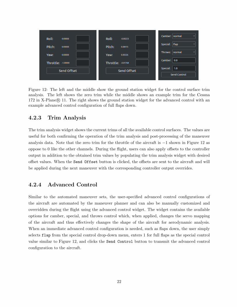
Figure 12: The left and the middle show the ground station widget for the control surface trimanalysis. The left shows the zero trim while the middle shows an example trim for the Cessna172 in X-Plane R© 11. The right shows the ground station widget for the advanced control with anexample advanced control configuration of full flaps down.

4.2.3 Trim Analysis

The trim analysis widget shows the current trims of all the available control surfaces. The values are

useful for both confirming the operation of the trim analysis and post-processing of the maneuver

analysis data. Note that the zero trim for the throttle of the aircraft is −1 shown in Figure 12 as

oppose to 0 like the other channels. During the flight, users can also apply offsets to the controller

output in addition to the obtained trim values by populating the trim analysis widget with desired

offset values. When the Send Offset button is clicked, the offsets are sent to the aircraft and will

be applied during the next maneuver with the corresponding controller output overrides.

4.2.4 Advanced Control

Similar to the automated maneuver sets, the user-specified advanced control configurations of

the aircraft are automated by the maneuver planner and can also be manually customized and

overridden during the flight using the advanced control widget. The widget contains the available

options for camber, special, and throws control which, when applied, changes the servo mapping

of the aircraft and thus effectively changes the shape of the aircraft for aerodynamic analysis.

When an immediate advanced control configuration is needed, such as flaps down, the user simply

selects flap from the special control drop-down menu, enters 1 for full flaps as the special control

value similar to Figure 12, and clicks the Send Control button to transmit the advanced control

configuration to the aircraft.

22

5 Evaluation

The flight maneuver automation framework, written in C++, is implemented and integrated into

the uavAP autopilot framework. The automation framework is deployed and assessed for flight

testing maneuver automation for aircraft and aerodynamic system analysis and identification. To

evaluate the framework, the flight testing maneuver for identifying the aircraft stall speed, discussed

in [22], is automated and simulated. Moreover, to show the advantage of the automation framework

in consistency and repeatability, the simulated results of the automated stall maneuver is compared

to those of the manually operated stall maneuver in the identical simulation configurations.

Furthermore, to achieve robust and predictive geo-fencing for small fixed-wing UAVs, a precise

kinematic model, the Beta-Trajectory, is developed for trajectory prediction and evasive maneu-

vering. The full derivation of the Beta-Trajectory can be found in this technical report [14]. In

order to evaluate the implementation of the geo-fencing system using the flight maneuver automa-

tion framework and the kinematic model, evaluations using multiple flights in simulations as well

as a geo-fenced flight in real-life are conducted.

5.1 Hardware

5.1.1 Aircraft

A fixed-wing trainer-type radio control aircraft, which was built for previous avionics develop-

ment [23–25], was used for the evaluation. The aircraft built was a Great Planes Avistar Elite [26],

which has a 1.59 m wingspan and a mass of 3.92 kg. The aircraft has the following control surfaces:

two ailerons (roll), two flaps, one elevator (pitch), and one rudder (yaw). The completed flight-

ready aircraft is shown in Figure 13 and its physical specifications are given in Table 1. Component

specifications can be found in [24].

Figure 13: Completed flight-ready aircraft.

23

Table 1: Avistar aircraft physical specifications.Geometric Properties

Overall Length 1395 mm (55.0 in)

Wing Span 1590 mm (62.5 in)

Wing Area 43.3 dm2 (672 in2)

Aspect Ratio 6.62

Inertial Properties

Mass/Weight 3.92 kg (8.63 lb)

Wing Loading 90.5 gr/dm2 (29.6 oz/ft2)

Table 2: Component specifications of the instrumentation.Instrumentation system Al Volo FC+DAQ 400 Hz system

Sensors

Inertial XSens MTi-G-700 AHRS with GPS

Airspeed Al Volo pitot-static airspeed sensor

Motor-Power Al Volo Castle ESC sensor

5.1.2 Avionics

The aircraft was instrumented with an Al Volo FC+DAQ flight computer and data acquisition

system [27], which incorporated the open source uavAP autopilot [19]. The specifications of the

instrumentation used for flight testing are given in Table 2.

5.2 Flight Testing

According to the analysis in [22], the stall speed is one of the most essential and critical aerodynamic

parameters of an aircraft in flight testing and system analysis. Many other flight testing maneuvers

and criteria often have a partial or complete dependency on the stall speed or its multiples. For

instance, knowing the stall speed of the Cessna 172 in X-Plane R© 11 is useful as it can be used as a

baseline or a reference velocity for other flight testing maneuvers such as the idle descent, singlet,

doublet, and so on. More importantly, knowing the stall speed of an aircraft is critical for safe

operation and handling during the flight. As a result, the aircraft stall speed is among one of the

first system parameters to be determined by flight testing maneuvers for aircraft system analysis.

To obtain the stall speed of the Cessna 172, an automated maneuver set is designed and constructed

for the flight maneuver automation framework. The methods for obtaining the stall speed discussed

in [22] is intended for real-life aircraft. However, the stall theory presented by [22], which states

that the stall of the aircraft exists due to the excessive increase in the aircraft’s angle of attack

(AoA) causing the airflow to split from the top of the wing, is general to fixed-wing aircraft of

24

various sizes. In a nutshell, the aircraft can be stalled by cutting its engine throttle entirely while

trying to maintain the original altitude by gradually deflecting its elevator. Therefore, the first

maneuver in the maneuver set is designed to set up and bring the Cessna to following initial states:

1. Maintain an ASL altitude of 200 meters.

2. Maintain a total body frame velocity of 40 m/s.

3. Maintain a yaw angle or heading of 0 degrees.

The flaps of the aircraft are up during the whole maneuver set. The condition for transitioning from

the state setup maneuver is a SteadyStateCondition with an in-steady-state transition, meaning

that the setup maneuver transitions to the next maneuver when all the overridden controllers above

are in the steady state according to the steady state analysis. The second maneuver is the most

important one since it performs the stalling of the aircraft, and the maneuver is designed as follows:

1. Maintain an ASL altitude of 200 meters.

2. Maintain a roll angle of 0 degrees.

3. Maintain an engine throttle controller output of 0.

The second maneuver completely cuts off the engine throttle of the aircraft, thus resulting in a

decrease in total body frame velocity and the lift generated by the wing of the aircraft. Meanwhile,

although not possible due to lack of throttle, the controller will try to maintain the ASL altitude of

the aircraft, resulting in gradual upward deflection in the elevator and increase in the AoA of the

aircraft, thus effectively stalling the plane. When it stalls, the aircraft results in a rapid pitch-down

with a remarkable rise of magnitude in its pitch rate. Therefore, the transitioning condition of the

second maneuver can be based on the pitch rate of the aircraft during the stalling process.

Since the setup maneuver removes all initial rotational movements of the aircraft, and the elevator

deflection during the stall is a gradual process, the pitch rate of the aircraft should be relatively

small. Hence, the aircraft transitions to the next maneuver when the magnitude of the pitch rate

of the aircraft during the stall is greater than 15 degrees per second, which can be achieved using

SensorDataCondition. Finally, the last maneuver recovers the aircraft from the stall. To recover

the stalled aircraft, the maneuver releases control from all control surfaces, i.e., centering them,

while still maintaining a zero throttle. In this way, the aircraft will naturally glide down, re-gain

the airspeed, and thus recover from the stall. The recover maneuver is designed as follows:

1. Maintain a roll controller output of 0.

2. Maintain a pitch controller output of 0.

3. Maintain a yaw controller output of 0.

4. Maintain an engine throttle controller output of 0.

25

After the controls are released, the aircraft will glide down and gain velocity. However, the aircraft

will lose the ASL altitude due to the release of control and the lack of throttle. As a result, the

recovery maneuver is set to end under the condition where the aircraft’s ASL altitude is less than

50 meters, which can be achieved using SensorDataCondition. After the condition is met, the

whole stall maneuver set is ended, and the aircraft resumes to its traditional mission.

In addition to the automated stall maneuver set, a manually operated stall maneuver set with

identical setup and configuration is performed by a human pilot using digital joysticks. The results

of the manual flight are then compared with the results of the automated maneuver set. Before

the executions of both automated and manual maneuver set, the control surfaces of the Cessna is

trimmed such the all the controls are centered with zero input. In the automated maneuver set,

the trim of the aircraft is automatically analyzed and applied by the trim analysis. In the manual

maneuver set, the trim is done by adjusting the trim configuration of the X-Plane R© 11 using the

digital joystick. The executions of both of the maneuver sets are automatically recorded by the

maneuver analysis for efficient post-processing and analysis of the maneuver set executions.

The results of both the automated and the manually operated stall maneuver sets are presented in

Figure 14, 15, 16, and 17. After examining the obtained results, it can be seen that the magnitude

of the pitch rate of the aircraft is small or close to zero with a noticeable spike at around 24 to 26

seconds for both flights since the beginning of the stall maneuver set. As a result, the Cessna has

stalled during the 24-to-26-second interval, and its stall speed can thus be observed to be around

25 to 27 m/s from the total body frame velocity data, which is consistent with the stall speed

specification of the full-scale Cessna 172 provided by its manufacturer [28].

Furthermore, the elevator deflection of the aircraft also peaks during the same time interval, in-

dicating the stall of the aircraft, and drops back to near-zero deflection afterward, indicating the

recovery of the aircraft. More importantly, it can also be observed that the AoA of the aircraft in

both flights peaks at around 15 degrees when the aircraft has stalled. Since the wing of an aircraft

provides almost all the lift during the flight, its stall point is indicative to the stall point of the

aircraft. The simulated Cessna 172 in X-Plane R© 11 models the identical, full-scale Cessna 172 in

real life, which has the NACA 2412 wing airfoil according to [29]. From the system analysis and

wind tunnel testing results performed on the NACA 2412 wing airfoil in [30], its lift coefficient, CL,

peaks at around 15 degrees of AoA with no flaps. According to [31, 32], the maximization of CL

causes the airfoil to stop producing lift, thus stalling the aircraft. As a result, results from both

automated and manual flights are consistent with the parameters of the full-scale Cessna 172.

The manually operated stall maneuver set, however, shows signs of noise, random variations, and

amplitude oscillations in the obtained data, especially in body frame accelerations, attitude rates,

AoA and beta angles, control surface deflections and so on, compared to those of the automated

stall maneuver set. Since both flights have identical setup and configuration, it is evident that the

26

disturbance in the manual flight is contributed to the unstable control input of the human operator

as it is difficult for a human pilot to manually control the ASL altitude, the roll and heading angle,

as well as the total body frame velocity of the aircraft all at once consistently and precisely. This

random nature of the human control input in the manually controlled flight further contributes to

inconsistent and non-repeatable results in multiple manual trials. The automation framework, in

contrast, shows precise executions of the maneuvers with high robustness and repeatability.

0

100

200

300

400

500

600

700

x (m)

800

900

100020100

y (m)

0

140

120

20

40

60

80

100

z (m

)

Figure 14: The stall maneuver manually executed on the Cessna 172 in X-Plane R© 11 by a humanpilot. The attitude of the aircraft is visualized by the tilting of the aircraft icons in the plot. Thez-axis of the plot is offset by −50 meters from the actual range which goes from 50 to 200 meters.

0

100

200

300

400

500

600

700

x (m)

800

900

1000

0-10-20

y (m)

-30

150

0

50

100

z (m

)

Figure 15: The stall maneuver automatically executed on the Cessna 172 in X-Plane R© 11 by theflight maneuver automation framework. The attitude of the aircraft is visualized by the tilting ofthe aircraft icons in the plot. The z-axis of the plot is offset by −50 meters from the actual rangewhich goes from 50 to 200 meters.

27

Time (s)0 2 4 6 8 10 12 14 16 18 20 22 24 26 28 30 32

Posi

tion

(m)

0

50

100

150

200

NorthingEasting (1/10)Altitude

Time (s)0 2 4 6 8 10 12 14 16 18 20 22 24 26 28 30 32

Eule

r Ang

le (d

eg)

-60

-45

-30

-15

0

15

30

45

60

? (Roll)3 (Pitch)A (Heading)

Time (s)0 2 4 6 8 10 12 14 16 18 20 22 24 26 28 30 32

Acce

lera

tion

(m/s

2 )

-20

-10

0

10

20

xyzTot

Time (s)0 2 4 6 8 10 12 14 16 18 20 22 24 26 28 30 32

Rot

atio

n R

ate

(deg

/s)

-45

-30

-15

0

15

30

45

pqr

Time (s)0 2 4 6 8 10 12 14 16 18 20 22 24 26 28 30 32

Body

Vel

ocity

(m/s

)

-40

-20

0

20

40

uvwV

Time (s)0 2 4 6 8 10 12 14 16 18 20 22 24 26 28 30 32

Rot

atio

n R

ate

(RPM

)

0

250

500

750

1000

1250

1500

1750

2000

Rotation Rate (RPM)

Time (s)0 2 4 6 8 10 12 14 16 18 20 22 24 26 28 30 32

Angl

e of

Atta

ck (d

eg)

-20

-15

-10

-5

0

5

10

15

20

,

-

Time (s)0 2 4 6 8 10 12 14 16 18 20 22 24 26 28 30 32

Con

trol D

efle

ctio

n (d

eg)

-45

-30

-15

0

15

30

45

AileronElevatorRudder

Figure 16: The visualizations of data automatically collected by the maneuver analysis during themanually executed stall maneuver. The left column, from the top to bottom, shows the positions,body frame accelerations, body frame velocities, and motor RPM of the aircraft during the maneu-ver. The right column, from the top to bottom, shows the attitudes, attitude rates, alpha (AoA)and beta angles, and the control surface deflections of the aircraft during the maneuver.

28

Time (s)2 4 6 8 10 12 14 16 18 20 22 24 26 28 30 32

Posi

tion

(m)

0

50

100

150

200

NorthingEasting (1/10)Altitude

Time (s)2 4 6 8 10 12 14 16 18 20 22 24 26 28 30 32

Eule

r Ang

le (d

eg)

-60

-45

-30

-15

0

15

30

45

60

? (Roll)3 (Pitch)A (Heading)

Time (s)2 4 6 8 10 12 14 16 18 20 22 24 26 28 30 32

Acce

lera

tion

(m/s

2 )

-20

-10

0

10

20

xyzTot

Time (s)2 4 6 8 10 12 14 16 18 20 22 24 26 28 30 32

Rot

atio

n R

ate

(deg

/s)

-45

-30

-15

0

15

30

45

pqr

Time (s)2 4 6 8 10 12 14 16 18 20 22 24 26 28 30 32

Body

Vel

ocity

(m/s

)

-40

-20

0

20

40

uvwV

Time (s)2 4 6 8 10 12 14 16 18 20 22 24 26 28 30 32

Rot

atio

n R

ate

(RPM

)

0

250

500

750

1000

1250

1500

1750

2000

Rotation Rate (RPM)

Time (s)2 4 6 8 10 12 14 16 18 20 22 24 26 28 30 32

Angl

e of

Atta

ck (d

eg)

-20

-15

-10

-5

0

5

10

15

20

,

-

Time (s)2 4 6 8 10 12 14 16 18 20 22 24 26 28 30 32

Con

trol D

efle

ctio

n (d

eg)

-45

-30

-15

0

15

30

45

AileronElevatorRudder

Figure 17: The visualizations of data automatically collected by the maneuver analysis duringthe automatically executed stall maneuver. The left column, from the top to bottom, shows thepositions, body frame accelerations, body frame velocities, and motor RPM of the aircraft duringthe maneuver. The right column, from the top to bottom, shows the attitudes, attitude rates, alpha(AoA) and beta angles, and the control surface deflections of the aircraft during the maneuver.

29

5.3 Geofencing

To evaluate the performance and the preciseness of the Beta-Trajectory, we compare it to the

Dubin’s-Curve in [33] as well as the Continuous Curvature Convected Dubin’s-Curve (CCC-Dubin)

in [34]. The flight maneuver automation framework automatically executes sequences of roll maneu-

vers in two different flight simulation programs, the high-fidelity FS One R© [16,17] and X-Plane R©11 [18] flight simulators. The aircraft used are the Avistar Elite in FS One R© and the Cessna 172

in X-Plane R© 11. The simulators are connected through the uavEE emulation environment. The

geo-fencing system is evaluated by flying an aircraft inside a defined geo-fence.

For evaluating the prediction accuracy of the Beta-Trajectory, the flight maneuver automation

framework automatically executes a sequence of roll maneuvers, alternating from right to left,

under 30 seconds of DurationCondition in total. The trajectory is recorded and compared to

a prediction using the three approaches. The predictions are based on the roll sequences, the

aircraft velocity, and the estimated roll rate. The performance of the respective approaches is

evaluated based on the deviation to the simulated trajectory. The deviation is calculated as the

root-mean-square (RMS) distance of the trajectories. Figure 18 shows the deviation for three

different sequences executed with the Avistar and the Cessna 172. While sequence 1 and sequence

2 used roll targets from the whole spectrum of roll angles (−45◦ to 45◦), sequence 3 is constrained

to angles from only −30◦ to 30◦. This is to show that the deviation in CCC-Dubin’s curves arises

from the linearization of the tan(). It can be seen that both the CCC-Dubin approach as well as

the Beta-Trajectory outperform the Dubin’s approach in the sequences. In sequences 1 and 2, the

Beta-Trajectory performs better than the CCC-Dubin approach while they show equal performance

in sequence 3.

Sequence 1

Avistar Cessna0

10

20

30

40

50

60

70

80

90

RM

SD

[m]

Sequence 3

Avistar Cessna0

5

10

15

20

25

30

35

40

DubinCCC-DubinBeta-Trajectory

Sequence 2

Avistar Cessna0

10

20

30

40

50

60

70

Figure 18: Root-mean-square deviation of the trajectory predictions of the three approaches forthree 30 second maneuvering sequences, comparing in two flight simulators, Avistar in FS One R©and Cessna 172 in X-Plane R© 11; Note the different scale of the y-axis.

30

�300 �200 �100 0 100 200 300

Distance X [m]

�300

�200

�100

0

100

200

300

Dista

nce

Y[m

]

1

2

3

4

Flight

Takeo↵ and Landing

Evasive Maneuver

0 50 100 150 200 250 300 350 400Position East [m]

0

50

100

150

200

Posi

tion

Nor

th [m

]

Sequence 3 - Avistar

0 200 400 600 800 1000Position East [m]

0

100

200

300

400

500Po

sitio

n N

orth

[m]

Sequence 2 - Cessna

SimulationDubinCCC-DubinBeta-Trajectory

Figure 19: The left shows two automated roll maneuver sequences recorded using maneuver analysisand compared to the three prediction approaches; the orange arrow shows the initial position andheading. The right show a real-life flight path of the Avistar deployed with the uavAP autopilotand the flight maneuver automation framework; Red shows the geo-fence. Blue shows the evasivemaneuvers labeled from 1-4. Boundary slack value is 5 meters and velocity is 20 m/s.

Figure 19 shows two examples from the sequences, first the sequence 2 using the Cessna 172 and

second the sequence 3 using the Avistar. Due to the low roll angles in sequence 3, the CCC-Dubin

and Beta-Trajectory give equal predictions. In sequence 2, however, a significant drift towards the

end of the trajectory can be observed in the CCC-Dubin prediction. The Dubin approach deviates

immediately and demonstrates that it is not suitable for short, horizon predictions.

Since it predicts the simulator path with high accuracy, the Beta-Trajectory is incorporated into

the geo-fencing system and deployed it onto a real aircraft. The autopilot on the aircraft was

instructed to fly out of the designated area defined by the geo-fence. The higher level geo-fencing

system observes the flight and intervenes the current flight path when necessary. The result can

be seen in Figure 19. The geo-fencing boundary slack was set low to emphasize the effect. The

aircraft is kept inside the geo-fence with two prominent deviations. The first deviation is reflected

by evasive maneuver 4 where the aircraft slightly overshoots the fence. The second deviation is in

evasive maneuver 1 which has a greater safety margin than the others. These two deviations can be

attributed to the effects of wind. As the initial assumption of the kinematic model sets the effects

of wind to zero, deviations due to winds and gusts are expected. However, these slight deviations

show the system’s ability to perform well in windy situations despite a low value for the slack.

31

6 Conclusion and Future Work

6.1 Conclusion

This work presents an augmented mission control module in the uavAP autopilot framework.

The maneuver planner implemented in the mission control module generates the maneuver sets

from the user-constructed object configuration files and executes the maneuver sets automatically

according to the user commands. More importantly, the automated flight maneuver framework

enables minimal trial-and-error during the flight testing maneuvers for aircraft system analysis and

increases the consistency in the testing results compared to human UAV operators.

The condition framework allows for advanced and sophisticated condition-based transitions between

flight maneuvers, making the maneuver framework more versatile and capable in real-life applica-

tions. The variety in condition objects allows the conditioning framework to handle and cover

most of the advanced real-life problems such as aircraft geofencing evasive maneuvers, flight testing

maneuvers for obtaining aircraft aerodynamic parameters for control system modeling, design, and

much more.

The maneuver analysis framework provides precise, efficient, and fully customizable flight maneuver

recording and analysis during the flight. Following the command from the maneuver planner, the

maneuver analysis is able to begin and stop the recording precisely at the start and the end of

the maneuver, excluding unwanted data and allowing for more precise and time-efficient data post-

processing. Additionally, customizable data collection behaviors enable flexibility and simplicity in

various real-life application.

The steady state analysis provides users with intuitive visualization and metrics for the controller

responses, allowing them to tune the PID controllers systematically and precisely. The well-tuned

controllers thus yield better aircraft stability and performance, resulting in better flight testing

data and aircraft models, and thus facilitating even better designs for the controllers.

The trim analysis enables aircraft to obtain control surface trims over the air and spontaneous

adjustments of the control surface deflection using the obtained trims for better controlling of the

aircraft. The ground station widgets allow for simple and intuitive interactions between the users

and the automation framework, providing users with the ability to construct custom and immediate

maneuvers, and advanced in-flight adjustments to the aircraft configuration such as the advanced

control configuration and controller output offsets.

32

6.2 Future Work

The flight maneuver automation framework will be extensively applied in the near future for au-

tomating the flight testing maneuvers in real-life flights for performing system identification and

analysis and obtaining aerodynamic parameters of small fixed-wing aircraft [5]. Aside from the

stalling maneuver, other standard flight testing maneuvers discussed in [22] such as phugoid, idle

descent, spin, singlet, doublet, and so on will be adapted and constructed into maneuver sets and

automatically executed in the simulation programs as well as on our small fixed-wing UAV test-bed.

With the benefits from the maneuver analysis, the aircraft parameters of our fixed-wing UAV will

be determined more systematically, efficiently, and precisely.

The framework can also be fitted for many other types of aircraft such as the quad-copter, helicopter,

and more. Due to the high-level and flexible design of the framework, minimal changes, such as

small variance in control surface configuration and sensor data, are required to adapt the framework

for those aircraft. Specific flight testing maneuvers can also be designed, developed, and constructed

into automated maneuver sets tailored to each type of the aircraft for obtaining their aerodynamic

characteristics. The geofencing of the rotary aircraft can also be implemented using the flight

maneuver framework as they have the ability to hover with low to zero total velocity.

An independent graphical user interface can also be developed for more intuitive and accessible

construction of the maneuver sets. Instead of creating the maneuvers directly inside the JSON

files, a user interface can be introduced to have visual representations of the maneuvers as well as

the transitioning condition. For example, each maneuver in the maneuver set can be represented

as a block with the override targets and other details available for customization within the block,

and each condition can be represented as an arrow. To design a maneuver set, the user can simply

create, configure, and order and blocks and the arrows in the user interface, and JSON configuration

containing the resulting maneuver set can be generated with one click of a button.

33

References

[1] Altavian, “Products - Altavian,” http://www.altavian.com/Products.

[2] Precision Hawk, “Precision Agriculture, Commercial UAV and Farm Drones For Sale,”

http://precisionhawk.com/.

[3] MicroPilot, “MicroPilot - MP-Vision,” http://www.micropilot.com/products-mp-visione.htm.

[4] Trigger Composites, “Pteryx UAV,” http://www.trigger.pl/pteryx/index.php.

[5] O. Dantsker, S. Yu, M. Vahora, and M. Caccamo, “Flight testing automation to characterize

uav aerodynamics,” Accepted to the AIAA Flight Testing Conference 2019, Dallas, TX.

[6] B. Johnson and R. Lind, “Characterizing wing rock with variations in size and configuration

of vertical tail,” Journal of Aircraft, vol. 47, no. 2, pp. 567–576, 2010.

[7] J. Perry, A. Mohamed, B. Johnson, and R. Lind, “Estimating angle of attack and sideslip

under high dynamics on small uavs,” Proceedings of the ION-GNSS Conference, Savannah,

Georgia, 2008.

[8] D. Uhlig, A. Sareen, P. Sukumar, A. H. Rao, and M. S. Selig, “Determining aerodynamic

characteristics of a micro air vehicle using motion tracking,” AIAA Paper 2010-8416, AIAA

Guidance, Navigation, and Control Conference, Toronto, Ontario, Canada, Aug. 2010.

[9] O. D. Dantsker, G. K. Ananda, and M. S. Selig, “GA-USTAR Phase 1: Development and

Flight Testing of the Baseline Upset and Stall Research Aircraft,” AIAA Paper 2017-4078,

AIAA Applied Aerodynamics Conference, Denver, Colorado, June 2017.

[10] A. M. Ragheb, O. D. Dantsker, and M. S. Selig, “Stall/spin flight testing with a subscale

aerobatic aircraft,” AIAA Paper 2013-2806, AIAA Applied Aerodynamics Conference, San

Diego, California, June 2013.

[11] R. A. Bunge, F. M. Savino, and I. M. Kroo, “Approaches to automatic stall/spin detection

based on small-scale uav flight testing,” AIAA Paper 2015-2235, AIAA Atmospheric Flight

Mechanics Conference, Dallas, Texas, Jun. 2015.

[12] C. D. Regan and B. R. Taylor, “maewing1: Design, build, test - invited,” AIAA Paper 2016-

1747, AIAA Atmospheric Flight Mechanics Conference, San Diego, California, Jun. 2016.

[13] R. A. Bunge, A. E. Alkurdi, E. Alfaris, and I. M. Kroo, “In-flight measurement of wing surface

pressures on a small-scale uav during stall/spin maneuvers,” AIAA Paper 2016-3652, AIAA

Flight Testing Conference, Washington, D.C., Jun. 2016.

34

[14] M. Theile and S. Yu, “Kinematic Model for Fixed-Wing Aircraft with Constrained Roll-Rate,”

University of Illinois at Urbana-Champaign, Department of Computer Science, Tech. Rep., Sep

2018.

[15] M. Theile, O. D. Dantsker, R. Nai, and M. Caccamo, “uavEE: A modular, power-aware emu-

lation environment for rapid prototyping and testing of uavs,” IEEE International Conference

on Embedded and Real-Time Computing Systems and Applications, Hakodate, Japan, Aug.

2018.

[16] M. S. Selig, “Real-time flight simulation of highly maneuverable unmanned aerial vehicles,”

Journal of Aircraft, vol. 51, no. 6, pp. 1705–1725, Nov.-Dec. 2014.

[17] M. Selig, “Modeling propeller aerodynamics and slipstream effects on small uavs in realtime,”

AIAA Atmospheric Flight Mechanics Conference, Toronto, Ontario, Canada, Aug. 2010.

[18] Laminar Research, “X-Plane 11,” http://www.x-plane.com/.

[19] Mirco Theile, “uavAP: A Modular Autopilot for Unmanned Aerial Vehicles,”

https://github.com/theilem/uavAP, Accessed Apr. 2019.

[20] Mirco Theile, “uavEE: A Modular Emulation Environment for Rapid Development and Testing

of Unmanned Aerial Vehicles,” https://github.com/theilem/uavEE, Accessed Apr. 2019.

[21] Douglas Crockford, “Introducing JSON,” https://www.json.org, Accessed Apr. 2019.

[22] R. D. Kimberlin, Flight Testing of Fixed-Wing Aircraft, ser. AIAA Education Series. AIAA,

Reston, VA, 2003.

[23] R. Mancuso, O. D. Dantsker, M. Caccamo, and M. S. Selig, “A low-power architecture for

high frequency sensor acquisition in many-DOF UAVs,” in Cyber-Physical Systems (ICCPS),

2014 ACM/IEEE International Conference on, April 2014, pp. 103–114.

[24] O. D. Dantsker, R. Mancuso, M. S. Selig, and M. Caccamo, “High-frequency sensor data

acquisition system (sdac) for flight control and aerodynamic data collection research on small

to mid-sized uavs,” in AIAA Applied Aerodynamics Conference, Atlanta, Georgia, June 2014.

[25] O. D. Dantsker, A. V. Loius, R. Mancuso, M. Caccamo, and M. S. Selig, “Sdac-uas: A sensor

data acquisition unmanned aerial system for flight control and aerodynamic data collection,”

in AIAA Infotech@Aerospace Conference, Kissimee, Florida, Jan 2015.

[26] Hobbico, Inc., “Great planes avistar elite .46 advanced trainer rtf,”

http://www.greatplanes.com/airplanes/gpma1605.html.

[27] Al Volo LLC, “Al Volo: Flight Systems,” http://www.alvolo.us.

35

[28] Cessna Skyhawk Information Manual, Model 172S. Cessna Aircraft Company, Wichita,

Kansas, 1998.

[29] M. S. Selig, “UIUC Airfoil Data Site, Department of Aerospace Engineering,” https://m-

selig.ae.illinois.edu/ads.html, Accessed Apr. 2019.

[30] I. H. Abbott, A. E. Von Doenhoff, and L. Stivers Jr, “Summary of airfoil data,” National

Advisory Committee for Aeronautics. Langley Aeronautical Lab.; Langley Field, VA, Tech.

Rep. NACA-TR-824, 1945.

[31] J. D. Anderson, Introduction to Flight, 8th Edition. McGraw-Hill Education, New York City,

NY, 2016.

[32] B. W. McCormick, Aerodynamics, Aeronautics, and Flight Mechanics, 2nd Edition. John

Wiley & Sons, Inc., Hoboken, NJ, 1994.

[33] M. Shanmugavel, A. Tsourdos, B. White, and R. Zbikowski, “Co-operative path

planning of multiple uavs using dubins paths with clothoid arcs,” Control Engineering

Practice, vol. 18, no. 9, pp. 1084 – 1092, 2010. [Online]. Available: http:

//www.sciencedirect.com/science/article/pii/S0967066109000379

[34] L. Techy, C. A. Woolsey, and K. A. Morgansen, “Planar path planning for flight vehicles in

wind with turn rate and acceleration bounds,” in 2010 IEEE International Conference on

Robotics and Automation. IEEE, 2010, pp. 3240–3245.

36