Preliminary Please do not quote or cite.

Financing Major Investments: Information about Capital Structure Decisions

Ralf Elsas a

Mark J. Flannery b

Jon A. Garfinkel c

December 2006 May 31, 2008

Abstract

We study how 1,455 firms paid for 2,027 very large investments during the period 1989-2005. Compustat Flow of Funds data indicate that major investments are mostly externally financed. An initial reliance on heavy debt financing is reversed following the event year, as firms adjust toward target leverage ratios. Small firms issue a surprisingly large amount of equity in this process. Peck-ing order and market timing effects appear during the event year, but weaken in the course of com-pleting the financing process. JEL Classification: G14, G31, G32

Keywords: firm financing, firm investments

a Institute for Finance and Banking, LMU München, elsas@bwl.uni-muenchen.de. b Department of Finance, University of Florida, flannery@ufl.edu. c Department of Finance, University of Iowa, jon-garfinkel@uiowa.edu.

1. Introduction

The study of corporate finance basically concerns the choice of new investments and decisions

about how to finance those investments. It is therefore somewhat surprising that researchers have

generally studied these two decisions separately from one another. Perhaps this dichotomy traces to

Modigliani and Miller’s (1958) classic analysis, which took a firm’s asset composition as fixed and

evaluated the impact of financing choices on firm value. The recent resurgence of empirical interest

in capital structure has likewise concentrated on the liability side of firms’ balance sheets. However,

focusing on the liabilities alone may overlook potentially important influences. Some firms may be

financing large new investments while others are more static. Some firms may have substantial inter-

nal cash flows, while others are cash constrained. Firms probably confront at least some fixed costs

of adjusting their leverage (Leary and Roberts (2005)). Hovakimian et al. [2004] therefore argue that

firms should be closest to their desired capital structure shortly after they have completed a major re-

capitalization.. Harford et al. (2006) argue that capital structure adjustments also may be relatively

inexpensive when firms choose how to finance large acquisitions, which often require them to raise

substantial external funds.1 Likewise, marginal leverage-adjustment costs may be less important

when a firm must raise new external funds -- such as when it must finance major investment expendi-

tures (Mayer and Sussman (2005)). New investments must be paid for and the need to finance large

investment may reveal information about how firms prefer to manage their capital structure.

In this paper, we assemble a sample of firms making large investments and study their financ-

ing decisions. We screen all Compustat firms to identify those with “major” real investments during

the period 1989-2005. We separately identify major “built” investments (Compustat item #128,

“capital expenditures”) and investments “acquired” from outside the firm (Compustat item #129, “ac-

quisitions”). We then use Compustat’s Statement of Cash Flows to infer how these major invest-

ments were financed. It is tempting to limit our analysis to the year in which a the major event oc-

1 Hovakimian et al. (2004) likewise argue that capital structure preferences will be most apparent when firms undertake substantial debt-for-equity re-capitalizations.

2

curs. However, Mayer and Sussmann [2005] point out that a firm’s ultimate financing choices need

not be manifested during the investment year. For example, suppose that a firm’s cash flow state-

ments indicate a large decline in working capital during the year a large capital expenditure occurred.

This could mean that the firm financed its investment through accumulated retained earnings – or it

may reflect a stock or bond issuance in year (t-1) that was intended to finance this investment. For

acquisitions, one financing arrangement might “get the job done quickly” but subsequent re-

financings offset or even eliminate the initial choice.

The firms in our sample finance the majority of their major investment expenditures by rais-

ing new, external funds. In fiscal years with a large investment, new debt provides at least half the

required funds. About 15 - 20% of the typical large investment is proximately financed by the sale of

equity, with internal funds supplying most of the remainder. However, multi-year financing adjust-

ments are important and systematic. When finance and investment decisions are aggregated over

two- (or three-) year intervals, a firm’s external securities issuance tends to move it toward a target

debt ratio computed from the usual combination of firm features. Some financing choices reflect

pecking order or market timing effects. Financing choices vary with firm size, but the nature of these

variations is quite noteworthy: smaller firms rely more on external equity funds, which seems incon-

sistent with the pecking order theory of capital structure (Frank and Goyal [2003], Fama and French

[2003]).

The rest of this paper is organized as follows. Section 2 sets the stage for our analysis with a

short literature review. Section 3 explains how we identify “major” investments, and describes the

features of our resulting sample firms. Financing patterns for these investments are evaluated in Sec-

tion 4, and the next section reports some robustness results. The paper concludes with a summary and

a discussion of the implications for further research.

3

2. Literature Review

Finance theory has long hypothesized that a firm’s capital structure affects its market value,

but the empirical evidence remains unclear about the specifics.

The dynamic trade-off hypothesis about capital structure asserts that a firm’s characteristics

determine its optimal capital ratio. Harris and Raviv [1991] provide a list of variables likely to affect

a firm’s preferred capital structure: fixed assets, nondebt tax shields, investment opportunities, firm

size, earnings volatility, advertising expenditure, the probability of bankruptcy, profitability and

uniqueness of the product. Many researchers have used these variables in estimating an “optimal

capital structure” model, producing considerable evidence that a firm’s characteristics systematically

determine its optimal leverage. Moreover, a change in characteristics elicits a change in preferred

leverage. Many of these studies estimate a simple cross-sectional regression, which implicitly as-

sumes that the typical firm has attained its desired capital structure. However, adjustment costs may

keep firms away from their optimal capital ratios, at least in the short run (Leary and Roberts [2005]).

Flannery and Rangan [2006] show that failing to account for partial adjustment introduces an omitted

variables bias that may be quite serious. They also show that including firm fixed effects in a model

of capital structure adjustment substantially increases the estimated adjustment speed.2 Lemmon et

al. [forthcoming] also emphasize the importance of firm-specific effects, which they contend are more

important than specific firm characteristics like fixed assets or investment opportunities. The dy-

namic panel models required to test the trade-off theory involve some unresolved, econometric issues

(Baltagi (2005)). These estimation problems raise the value of testing the trade-off model in a differ-

ent way, as we do here.

2 A very slow adjustment speed suggests that tradeoff considerations do not importantly affect firm’s capital decisions (e.g. Fama and French [2002]).

4

Myers (1984) challenges the tradeoff model of capital structure by contending that asymmet-

ric information imposes losses on existing shareholders when their firm sells new shares to the public.

According to this “pecking order” hypothesis, firms generally prefer to finance investments with in-

ternally generated funds. When external funding is required, firms strongly prefer debt to equity.

Shaym-Sunder and Myers [1999] present empirical support for the pecking order hypothesis in a

sample of large, long-lived firms. Chirinko and Singha (2000) challenge the statistical power of their

tests, and Frank and Goyal [2003] show that their model does not apply to a broader sample of

Compustat firms. Frank and Goyal [2003] also report that small firms quite often issue equity, con-

tradicting the pecking order’s prediction that firms with information asymmetries are reluctant to sell

equity.

A third capital structure hypothesis contends that managers can identify when their firm’s

market value deviates from fundamentals. In raising external funds, managers choose between debt

and equity on the basis of their relative valuation errors. When investors are overly bullish, the man-

agers issue shares; bearish investors lead managers to issue debt. A firm’s leverage at any point in

time therefore reflects the pattern of historical seecurity mis-pricings when new investment opportu-

nities occurred (e.g. Baker and Wurgler (2002), Ritter and Huang [2007]). However, these results

have also been challenged on econometric grounds (e.g. Hovakimian, [2004], Kayhan and Titman

[2007]). Once again, methodological problems limit our ability to reach firm conclusions about capi-

tal structure.

Hovakimian et al. [2004] study a set of firms that have chosen to revise their capital struc-

tures. If fixed adjustment costs are important, these firms should be closer to their desired leverage

than they typical firm. They identify 1,689 firms that issued or redeemed both debt and equity ex-

ceeding 5% of the prior year’s book asset value in the same fiscal year. They find more evidence for

tradeoff behaviour and less pecking-order behavior in the dual-issuer sample than in the set of passive

(non-issuing) firms. A potential problem with this result is that the authors cannot adjust for endoge-

5

neity. That is, their results may be affected by some unobserved debt or equity price characteristic

that caused the decision to re-capitalize.

Like Hovakimian et al. [2004] we approach the capital structure question outside the dynamic

panel framework. Following Mayer and Sussman [2005], we collect a sample of firms that made

large investment expenditures and examine how those investments were financed.3 We identify large

investment events differently from Mayer and Sussman (2005), and undertake a more extensive mul-

tivariate analysis of financing decisions. We also most strictly separate Built investments from Ac-

quisitions and find some interesting differences in their financing patterns.4

3. Sample Selection

Our research design requires a set of “major” investment events, but theory provides no clear

method for identifying such events. We therefore proceed with one plausible rule, that an investment

is “major” if

• it exceeds 200% of the firm’s past three years’ average investment level (its “benchmark” investment), and

• it is at least 30% of the firm’s prior year-end total assets. 5

Compustat reports data on two sorts of investment: capital expenditures (Item 128) and acquired as-

sets (Item 129). We compute separate investment levels for each firm-year’s built and acquired capi-

3 Our sample is also selected on the basis of an endogenous decision, but it is not so specifically tied to securities (mis?)valuation. If our conclusions tend to confirm Hovakimian et al.’s, we can have greater confidence in the truth of the supported hypotheses. 4 Mayer and Sussman (2005) selected all Compustat firms showing a large investment “spike” – one large investment year, preceded and succeeded by stable, lower investment expenditures. Examining the time series of investments associated with our major events (not reported here) suggests that the “spike” nature of Mayer and Sussman’s filter rule probably identifies more acquisitions than built investments, so their results may apply more directly to acquisitions. 5 Analysis based on a less restrictive, alternative rule (100% of trailing investment and only 20% of total assets) yields very similar results.

6

tal expenditures. We refer to internal investment projects (pure capital expenditures) as built invest-

ments, and to external investments as acquired investments or acquisitions.

Before identifying firms with major investments, we trimmed the universe of CRSP-

Compustat firms. We excluded firms from the sample for any year in which:

• The firm’s book value of equity is negative in the current or the previous year.

• A firm is missing data for capital expenditures and acquisitions (items #128 and #129), or for income before extraordinary items (item #123, used to calculate cash-flows).

We also exclude firms from regulated industries or industries with unusual capital structures: two-

digit NAICS industry codes equal to 22 (utilities), 52 (finance and insurance), 55 (management of

companies and enterprises), or exceeding 90 (public administration). Compustat’s flow-of-funds

data, which we use to identify financing patterns, become available only in 1988. We therefore focus

on investment events that occurred between 1989 and 2005. These screens leave 76,448 annual ob-

servations for 11,090 firms, which we search for major investment events.

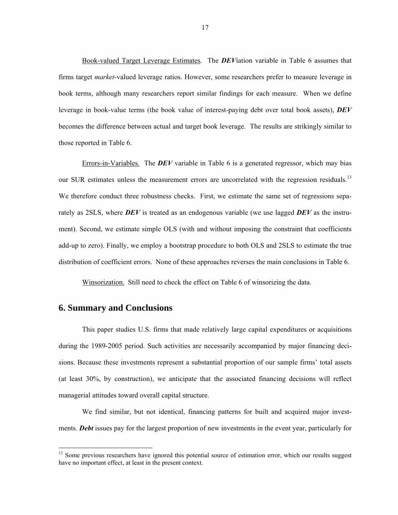
Table 1 describes our sample event firms. We identify 769 firms with major built investments

and 820 firms with major acquisitions. Because some firms have multiple events, the full sample in-

cludes 1,159 built events and 1,046 acquisitions. In order to evaluate built and acquired events sepa-

rately, we omit 67 firms with both built and acquired major investments during the 1989-2005 sample

period. This yields 1,066 built events and 961 acquired events for our main testing sample. Table 2

compares our Built and Acquired sample firms to the industrial concentrations of all Compustat firms.

Large investments over this time period were relatively common in the manufacturing (NAICS = 32,

33) and Information (NAICS = 51) industries, while Transportation (40), Health Care (62) and Ac-

commodations (72) undertook relatively few major investments. Although some industries are pro-

portionally over- (or under-) represented, no single industry dominates our sample.

Table 3 reports some financial aspects of the event firms. Many of the relevant variables are

ratios, which can take extreme values for a small number of observations. We therefore exclude the

7

0.5% highest and 0.5% lowest observations from our reported means and medians, and we concen-

trate our discussion on the median values.6 Panel A of Table 3 compares the built vs. acquiring firms’

median values for the year preceding the investment event. These two groups differ significantly in

almost all measured characteristics. Most notably, the acquiring firms are far larger and more profit-

able than firms with built investments and exhibit a significantly higher median debt ratio (19.9%

versus 14.2%). For both groups, the median market-to-book ratio for equity is fairly high (around

2.6), indicating that the market had been anticipating growth for firms making major investments. The

two groups’ recent asset growth rates are high and statistically indistinguishable.

The direct comparison between Built and Acquired investments in Panel A may be inappro-

priate if each sort of investment was concentrated in time. Panel B therefore compares each event

firm to the set of non-event firms available on Compustat at the same point in time. Both sample

groups (Built and Acquired) median characteristics differ from the contemporary non-event firms.

Consistent with Panel A, non-parametric tests confirm that the Built and Acquired sub-samples were

differentially different from their non-event contemporaries in nearly all measured dimensions. With

the event firm sample, Built firms are substantially smaller, less profitable, less leveraged and better

endowed with investment opportunities (M/B ratio) than the Acquiring firms.

4. Capital Structure (Financing) Decisions

By construction, our sample firms are very likely to be raising external funds. The literature

on capital structure provides a multitude of factors that might influence their financing choice. Our

data can indicate the extent to which sample firms’ behaviour is consistent with the pecking order

hypothesis, the trade-off hypothesis, or the market-timing hypothesis.

6 The sample is truncated only when reporting the statistics in Table 3. We use all observations when identifying event firms and conducting tests of financing.

8

Compustat’s Flow of Funds data permits each firm’s annual cash-flows to be aggregated into

four exhaustive financing sources for any time interval:

Debtj is the jth firm’s net change in long-term and short term debt (Compustat items 111 plus 114 less 301). Equityj is the jth firm’s dollar value of (net) common and preferred share sales (Compustat items 108 + 115). Cashflowj is jth firm’s operating cash-flows, defined as after-tax income before extraordinary items plus depreciation and amortization less cash dividends (Compustat items 123 + 125 - 127). Otherj is the aggregate of all jth firm’s other funds flow categories, including statistical dis-crepancies.

The following identity must hold for each firm over any time interval:

Invest j = Debtj + Equityj + Cashflowj + Otherj (1)

where Investj is the sum of firm j’s Built and Acquired capital expenditures. Obviously, an increase

in Debt or Equity affects firm leverage. Leverage is also affected –- it falls -- when new investment

is finance by Cashflow or Other. To the extent that operating cash flows are not paid out as divi-

dends, the firm’s equity account increases relative to outstanding debt. (i.e. leverage falls). Because

Other does not include changes in long-term debt, financing new investment from Other sources does

not affect leverage as we define it in equation (3) below.7

Although the identity (1) must hold within each accounting period, contemporaneous changes

in the RHS values of (1) may not reveal the ultimate financing source (Mayer and Sussman (2005)).

For example:

1) A firm might have issued Equity shares in τ = -1, planning to use the proceeds to fund in-vestment during year τ = 0. Until the investment occurs, however, the firm might pay down its line of credit, which can then be drawn to purchase new assets in τ = 0. The event-year values in (1) would mistakenly indicate a Debt-financed investment.

7 The capital structure literature represents “leverage” empirically in two different ways: as the ratio of debt to total assets and as the ratio of debt to (debt plus equity). We use the latter definition, which we believe is more common in the literature.

9

2) Suppose a firm issued Debt in τ = -1, invested the proceeds in short-term financial assets, and then sold off those liquid assets to fund investments at τ = 0. The event-year values in (1) would mistakenly indicate financing from Other, which includes cash and equiva-lents (# 274).

3) A firm might pay for investment by both drawing down a line of credit and reducing its portfolio of liquid assets, but plan to repay the line with the proceeds of an equity issue the following year. The event-year values in (1) would indicate financing from Debt and Other, rather than Equity and Other.

Other examples are readily constructed. The point is that a firm might make advance arrangements to

fund a planned, large investment, or it might use a temporary source of funds while planning to obtain

permanent financing later. In order to permit these possibilities, we examine the flow of funds rela-

tion (1) over longer periods than just the event year. In addition to considering the investment year’s

cash flows (τ = 0), we also evaluate the sum of years 0 and 1, and the sum of years -1 through +1. By

examining financing sources over several event windows, we hope to identify any systematic dynam-

ics in firm financing decisions.

4.1. Financing Decisions: Univariate Results

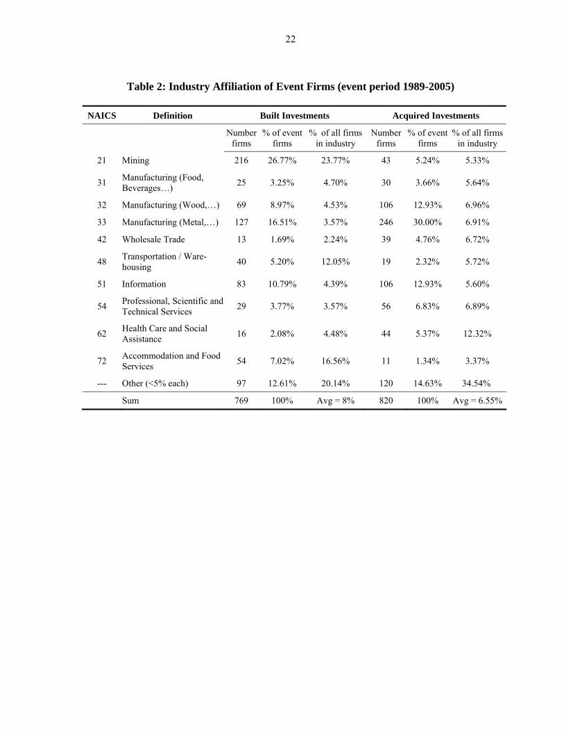
Table 4 reports the average investment’s size and financing proportions for three different

time intervals: the event year itself (τ = 0), the two year window starting in the event year (τ = [0,

+1]), and the three-year interval centered on the event year (τ = [-1, +1]). The Table’s last four rows

describe each financing source's relative contribution to investment spending. Because the mean of a

ratio can be substantially influenced by a few extreme values, we follow Loughran and Ritter [1997]

and Fama and French [2003] in reporting these percentages as ratios of averages instead of the aver-

ages of firms’ individual ratios. That is, we compute the contribution of new Equity to Built invest-

ment financing (22.63% for the event year alone (τ = 0)) as the ratio of all sample firms’ new equity

issues to their total investment expenditures. The proportions for Debt, Cashflow, and Other are

computed analogously. The accuracy of the Compustat Flow of Funds data is confirmed in the last

row, where all the financing proportions are shown to sum almost exactly to unity.

10

The left half of Table 4 indicates that firms with Built major investments finance themselves

primarily by raising new external funds.8 During the event year, firms issue new debt equal to

41.60% of their total investment expenditures and new equity shares for another 22.63%. Cashflow

contribute 32.51%. These "snapshot" results are not entirely consistent with the pecking order hy-

pothesis, but we do see that Debt provides the largest portion of total financing for new investments

in the event year. However, over the [-1,+1] event window the combined proportions of Cashflow

and Other funding rise about 7%, from 35.59% to 46.51%. The relative importance of Debt declines

by about the same proportion, from 41.60% to about 33.57%. The right half of Table 4 describes ma-

jor Acquisitions, which are substantially larger (in dollar terms) than Built investments. Acquisitions

are also financed initially by external funds (74.73%) in the event year, with Debt providing an even

larger proportion (61.52%) than it does for Built investments. However, acquiring firms exhibit the

same dynamic feature as Built firms: Debt financing falls to 44% of investments over the [-1, +1] pe-

riod, with Cashflow contributions rising to replace borrowed funds. In other words, the event year’s

cash flow statistics probably overstate the importance of debt financing, particularly following acqui-

sitions. Mayer and Sussman (2005) report a similar reduction in Debt, although they find that Equity

issuances replace the Debt, while our data indicate a larger role for Cashflow funds. The same broad

pattern emerges from (unreported) comparisons of firms’ median financing choices.

Table 4 implies a reasonable pattern of investment financing dynamics. Debt is initially the

main external claim sold, but the initial leverage effects of large investments are systematically re-

versed as profitable firms subsequently retain earnings.

8 The conventional wisdom is often said to indicate that most corporate investment is financed with internal funds (retained earnings). Our conclusion that major investments are funded primarily with external funds is not necessarily inconsistent with this conventional wisdom, since the major invest-ments in our sample represent only a subset of all investment activity.

11

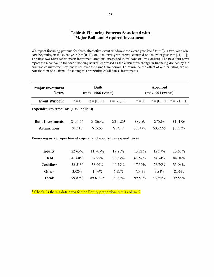
Previous writers have found that securities issuance activities and leverage vary substantially

with firm size. Table 5 therefore presents median values for three size-classes of sample firms.9 The

results clearly indicate that the investment type and firm size matter. Acquisitions are most promi-

nently financed by Debt, although the event year’s high debt is subsequently reduced in all segments

of Table 5. Over the broadest [-1, +1] window, the Large Firms use the greatest Debt proportion and

rely least on Equity. Medium Firms finance the largest proportion of their Built investments with

Cashflow funds (38.81%), while Small Firms’ largest financing source for Built investments is Eq-

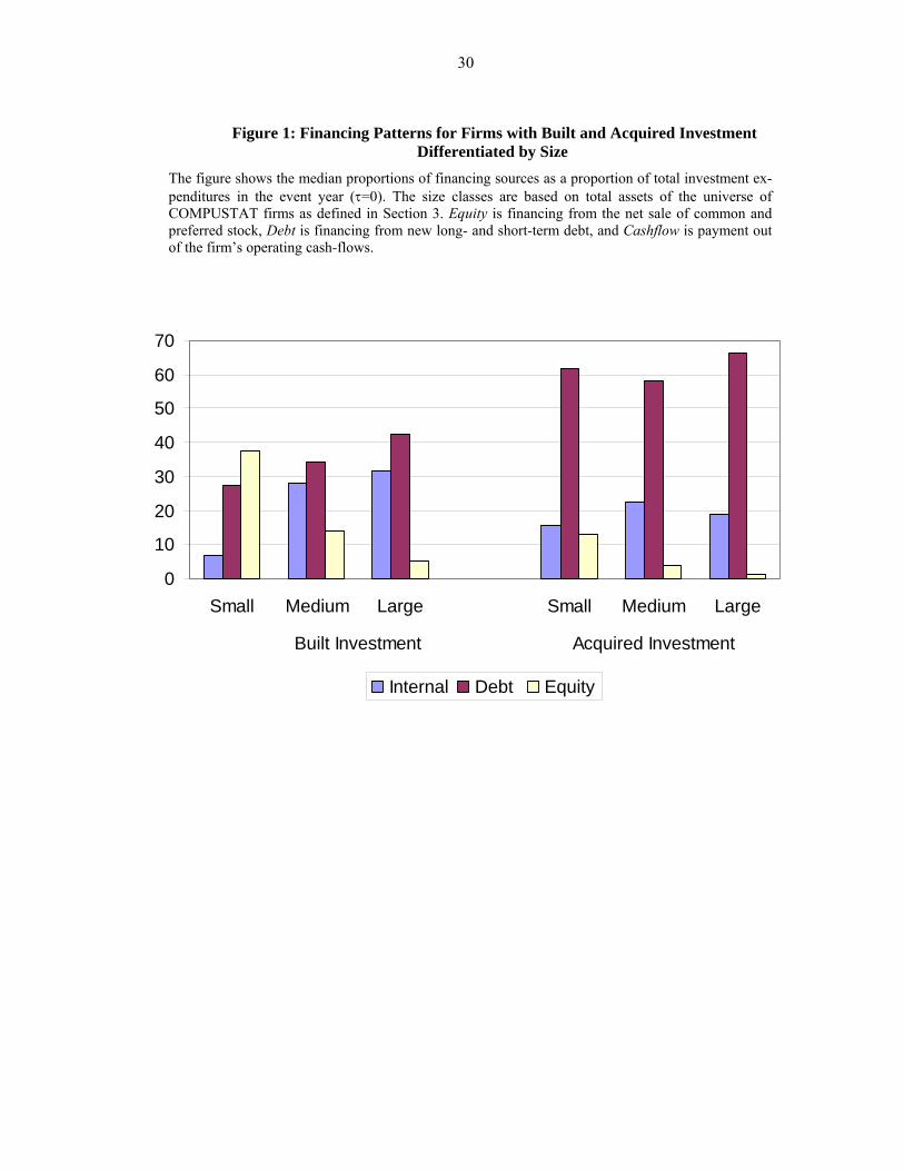
uity (40%). The extent to which financing choices differ with firm size is further illustrated in Figure

1, which plots median financing patterns during the event year (τ = 0) for different-sized firms. Debt

provides the largest proportion of investment funds for both investment types and for all firm size

groups. Debt is more important for larger firms, and when financing acquisitions.10 Table 5 again

indicates that financing patterns change as we widen the event window. Over time, firms replace

some of the Debt issued in year 0 with Cashflow and new Equity.

4.2. Financing Decisions: Multivatiate Results

Financing for the large investments described in Tables 4 and 5 may reflect the nature and

scale of the investment, the firm’s current market opportunities, or the existing deviation from some

type of target leverage ratio. We capture the multiple determinants of financing behavior via the re-

gression

Fijt = α + β1 DEVj, t-1 + β2 Profitj, t-1 + β3 ln(Sizej, t-1) + β4 INV_TAj, t-1 (2)

+ β5 FA_TAj, t-1 +β6 Runupj, t-1 + β7 Q j, t-1 + ijtε~ where Fijτ = the proportion of firm j’s net new investment financed by the ith funding source: i = Eq-

uity, Debt, Cashflow, and Other).

9 For each fiscal year, we sort the universe of Compustat firms that were searched for major invest-ments into three equal-sized groups on the basis of their book assets. Our event firms are then placed into the “Small”, “Medium”, or “Large” grouping. The results are qualitatively similar when we form size groupings on the basis of equity market value instead of book assets. 10 Equity is more important for funding smaller firms, as shown by Frank and Goyal [2003].

12

α represents a complete set of year dummy variables, 1989-2005.

DEVj, t-1 = the deviation from target leverage: the firm’s estimated target debt ratio (com-

puted from its t -1 characteristics as in Flannery and Rangan [2006]) less its actual debt ra-tio.

Profit j, t-1 = net annual income before extraordinary items, as a proportion of yearend total as-

sets

ln(Sizej, t-1) = log of the firm's yearend book assets. Table 5 indicates a substantial effect of size on financing choices.

INV_TA j, t-1 = the ratio of investments (built plus acquired) during the event window to book

total assets at the yearend preceding the event window. Larger investments may be fi-nanced differently.

FA_TA j, t-1 = the firm's yearend book value of fixed assets as a proportion of total assets; a measure of “debt capacity”.

Runup j, t-1 = the stock's excess return, relative to the market, during the 12-month period through the end of period t-1.11 Firms tend to issue stock following a Runup in the price (Korajczyk, Lucas and MacDonald [1991]).

Q j, t-1 = the ratio of the firm's market value (market value of equity plus book value of debt) to the book value of assets at the yearend preceding the event window. Q measures the firm’s investment opportunity set.

We specify a regression of the form (2) for each of the four funding sources. The Compustat Flow of

Funds accounting identity (1) indicates that all investment expenditures must be financed by a combi-

nation of Debt, Equity, Cashflow, or Other sources. This implies a cross-equation constraint: the

slope coefficients in (2) measure the impact of the associated regressors on each type of financing,

and the coefficients on each regressor must therefore sum to zero for any time interval.

The firm's deviation from target leverage (DEV) bears particular discussion because it forms

the basis for our tests of the trade-off model of capital structure. We define leverage as

titi

titi ED

DLEV

,,

,, += , (3)

11 For windows beginning in year 0, this return is computed over the months [-17,-6] relative to the end of the event year. For the event window [-1, +1], this excess return is computed over the months [-29,-18] relative to the end of the event year.

13

where Di,t denotes the book value of firm i’s interest-bearing debt (the sum of Compustat items 9 plus

34) at time t, and the firm’s equity value (Ei,t) can be measured alternately in book or market terms.

Flannery and Rangan [2006] fit a partial-adjustment model to the set of all industrial firms:

LEVi,t – LEVi, t-1 = λ (LEVi,1* -LEVi, t-1) + ti,~δ (4)

According to this specification, the typical firm annually closes a proportion λ of the deviation

(“DEV”) between its actual (LEVt-1) and its desired leverage (LEVt*). Specifying the desired (target)

leverage as a linear combination of firm characteristics gives the estimable model

LEVi, t = (λ β) Xi,t-1 + (1-λ)LEV i,t-1 + ti,~δ . (5)

X is a vector of variables commonly used to proxy for a firm's target debt ratio (earnings, deprecia-

tion, fixed assets and R&D expenditures (all as a proportion of total book assets), the assets' market to

book ratio, the log of (real) total assets, the firm's industry median LEV value, a dummy variable in-

dicating whether the firm has a credit rating, and firm fixed effects. We re-estimate Flannery and

Rangan's "base model" (their Table 2, column 7) and use the estimated coefficients (λ, β in (5)) to fit

a target debt ratio for each firm at the start of each year.12 We then compute each firm’s DEViation

from its estimated target:

1,1,1,*,

ˆ−−− −=−= titititiit LEVXLEVLEVDEV β (6)

The trade-off theory of capital structure implies that new investments should be funded dispropor-

tionately with Debt when DEV > 0. Conversely, a firm with DEV < 0 is "over leveraged" and should

issue equity to reduce its leverage. Merging these target debt ratios with the other data on investing

firms leaves 751 Built large investments and 757 Acquired large investments with complete data for

estimating our equations (2).

12 We thank Kasturi Rangan for computing the estimated target values.

14

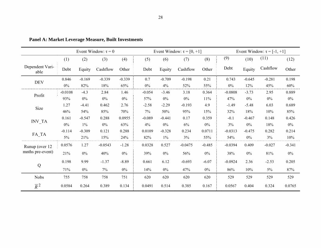
Table 6 presents the results of estimating (2) separately for Built and Acquired investments,

using both market and book measures of firm capital structure. Because the Flow of Funds data

should obey the financing constraint (1), our main results come from four single-equation, OLS re-

gressions. We confirmed that the accounting identity holds (almost) perfectly by estimating the four

variants of (2) as seemingly unrelated regressions and testing the restriction that the β estimates on

each independent variable sum to unity. In virtually all cases, we cannot reject this hypothesis; even

the statistically significant deviations from this theoretical condition are very small in magnitude.

More broadly, the results in Table 6 (derived from single-equation estimates) are virtually identical to

the results we get from estimating the equations via SUR, with or without imposing the cross-

equation restrictions.

Each panel of Table 6 includes twelve columns: four financing proportions (Debt, Equity,

Cashflow, or Other) for each of three event windows (τ = 0, [0,+1], and [-1,+1]). Panel A describes

market-valued leverage DEV for firms with Built investments. Consider first the event-year (τ = 0)

financing pattern in columns (1) through (4) of Panel A. Consistent with presence of a target leverage

ratio, DEViations from our estimated targets positively affect the proportion of new investments fi-

nanced with Debt. DEV also reduces the firm’s reliance on Equity and Cashflow, although these co-

efficients are highly insignificant. Coefficients in the second row indicate that more Profitable firms

issue significantly less Equity, making up the difference in Cashflow or Other financing. Many em-

pirical studies have found a negative relationship between profits and leverage, and inferred support

for the pecking order hypothesis. Here, however, we see a substitution largely between retained earn-

ings (Cashflow) and Equity issuance, which does not affect leverage. Somewhat surprisingly, given

the univariate results in Table 5, firm Size has no significant effect on financing decisions. The scale

of new investments (INV_TA) has a positive effect on leverage during the event year. The coeffi-

cients on tangible assets (FA_TA) indicate that firms with more PP&E finance new investments with

significantly less Debt, perhaps because their existing debt capacity has already been utilized. The

15

coefficients on Runup indicate that firms with larger recent stock price increases use more Equity,

consistent with the hypothesis that managers actively sell overpriced equity. This increased reliance

on equity is significantly, and nearly exactly, offset by the use of less Other funds. Finally, firms

with high growth opportunities (Q) use much more equity, again offset by a reduction in Other funds.

Some of these initial financing arrangements tend to change as time passes. The middle four

columns of Panel A show that Debt and Equity both respond appropriately to DEViations from target

leverage. The τ=0 reliance on Debt for larger investments is now reversed: INV_TA carries a sig-

nificantly negative coefficient for both Debt and Equity over the window τ = [0,+1], with the balance

being made up by Other funding. This suggests that larger investments are part of a broader plan to

revise a firm’s asset portfolio. The impact of FA_TA in the event year is also reversed with the wider

window: tangible assets have no effect on Debt issuance, but reduce Equity and raise Cashflow by

similar, significant amounts. The net effect of FA_TA on leverage is thus approximately zero after

capital structure adjustments have been completed. The Runup and Q effects from τ=0 persist over

the wider event window.

Columns (9) – (12) of Panel A indicate that financing decisions over a [-1, +1] event window

closely resemble those over the [0,+1] window. In other words, pre-investment financing does not

appear to have a major impact on how firms pay for their large investments; adjustments to the event

year decisions are generally made after the investments are in place. The only notable change be-

tween these two windows is that the effect of Q on Equity tend sto moderate and become (at best)

marginally significant.

Several important conclusions emerge from Panel A of Table 6.

• Financing decisions for Built investments are dynamic and change in important ways subse-quent to the event year. Researchers should examine an appropriately lengthy adjustment pe-riod in order to connect financing conclusively with leverage adjustments.

• Target leverage DEViations significantly influence Debt financing as firm use debt issues to move toward their target leverage.

16

• Firms with high Profits avoid issuing new Equity by financing new investments largely out of internal Cashflow, with a limited net effect on leverage.

• Larger investments are funded with less security issuance and more retained earnings (Cash-flow) or Other adjustments to the balance sheet.

• Firms finance investments more heavily with new Equity issuances when their stock price has been rising. This is consistent with the suggestions of both Baker and Wurgler (2002) and Carlson et al. (2004).

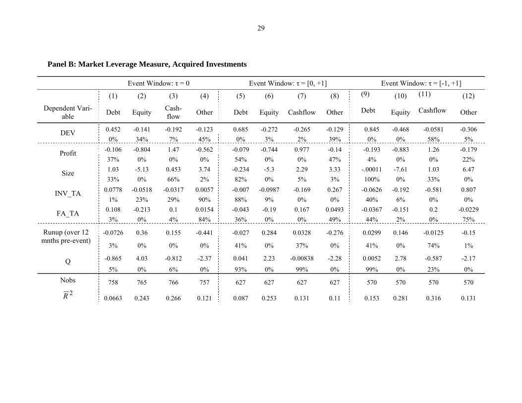
Panel B of Table 6 presents financing results for firms making for large Acquisitions. Per-

haps most noteworthy are the strong target-adjustment effects manifested for all event windows.

Both Debt and Equity/Cashflow uses tend to close the gap between current and target leverage, con-

sistent with the results of Harford et al. (2006). The effects of Profit, asset tangibility (FA_TA) and

Runup on Acquisition financing resemble those for Built investments, but differences appear for sev-

eral important variables. Firm size now affects financing: larger firms rely significantly less on Eq-

uity and more on Other. These findings conflict with the univariate results in Table 5. Investment

size (INV_TA) also presents surprising results, indicating that relatively large investments are initially

financed with debt, but eventually funded out of Other funds. The effects of Q manifested for Built

investments – more Equity, less Other – are slightly stronger for Acquisitions.

5. Robustness

In addition to the results reported in Table 6, we conducted a series of robustness tests with

respect to applied sample selection and methodology. All of these exercises yielded qualitatively the

same results as those reported in the previous sections.

Identifying the Event Firms. Our definition of “major” firm investments is essentially arbi-

trary. For the results reported above, we selected firms whose absolute capital/acquisition expendi-

tures exceed 200% of a trailing (3-year) average investment ratio and 30% of the prior year’s total

assets. We replicated our long-run performance analysis with a sample in which “major” investments

exceeded only 20% of the firm’s prior year-end assets. The main conclusions are unchanged.

17

Book-valued Target Leverage Estimates. The DEViation variable in Table 6 assumes that

firms target market-valued leverage ratios. However, some researchers prefer to measure leverage in

book terms, although many researchers report similar findings for each measure. When we define

leverage in book-value terms (the book value of interest-paying debt over total book assets), DEV

becomes the difference between actual and target book leverage. The results are strikingly similar to

those reported in Table 6.

Errors-in-Variables. The DEV variable in Table 6 is a generated regressor, which may bias

our SUR estimates unless the measurement errors are uncorrelated with the regression residuals.13

We therefore conduct three robustness checks. First, we estimate the same set of regressions sepa-

rately as 2SLS, where DEV is treated as an endogenous variable (we use lagged DEV as the instru-

ment). Second, we estimate simple OLS (with and without imposing the constraint that coefficients

add-up to zero). Finally, we employ a bootstrap procedure to both OLS and 2SLS to estimate the true

distribution of coefficient errors. None of these approaches reverses the main conclusions in Table 6.

Winsorization. Still need to check the effect on Table 6 of winsorizing the data.

6. Summary and Conclusions

This paper studies U.S. firms that made relatively large capital expenditures or acquisitions

during the 1989-2005 period. Such activities are necessarily accompanied by major financing deci-

sions. Because these investments represent a substantial proportion of our sample firms’ total assets

(at least 30%, by construction), we anticipate that the associated financing decisions will reflect

managerial attitudes toward overall capital structure.

We find similar, but not identical, financing patterns for built and acquired major invest-

ments. Debt issues pay for the largest proportion of new investments in the event year, particularly for

13 Some previous researchers have ignored this potential source of estimation error, which our results suggest have no important effect, at least in the present context.

18

large firms. Equity has a relatively small role. This initial pattern seems consistent with a pecking

order view of capital structure. Over time, however, firms systematically supplement newly-issued

debt with equity funds. Relative to large firms, small firms rely more on issuing new equity to replace

debt, while medium-sized firms tend to use internal cash flow. This seems inconsistent with the peck-

ing order theory of capital structure, because smaller firms are often said to confront higher informa-

tion costs in selling their shares (Frank and Goyal [2003]). Moreover, we find that high profits do not

reduce significantly debt issuance, but primarily replace new shares. Relatively larger investments

tend to be funded eventually with internal funds. The leverage effect of profitability is therefore ques-

tionable. Furthermore, our regression analysis indicates that firms choose financing vehicles that

move them toward a target debt ratio, although “market timing” effects also appear in the data.

Our analysis suggests at least one important area for further research. Compustat’s flow of funds data

do not permit us to distinguish between private (“bank”) debt and publicly issued bonds or commer-

cial paper. Because private debt involves better (“inside”) information and monitoring incentives,

and more complex covenants (Sufi [2005]), understanding how private debt is used in financing large

investments may yield important further insights about corporate finance.

19

References

Baker, Malcolm and Jeffrey Wurgler (2002): Market timing and capital structure, Journal of Finance 55, pp. 2219-2257.

Baltagi, Badi H., 2005, Econometric Analysis of Panel Data (John Wiley and Sons) 1 edn.

Carlson, Murray, Adlai Fisher, Ron Giammarino (2004), Corporate Investment and Asset Price Dynamics: Implications for the Cross-section of Returns, The Journal of Finance 59 (6), 2577–2603.

Chirinko, Robert S. and Anuja R. Singha Testing static tradeoff against pecking order models of capital structure: a critical comment Journal of Financial Economics Volume 58, Issue 3, December 2000, Pages 417-425

Fama, Eugene and Kenneth French (1993): Common risk factors in the returns on stock and bonds, Journal of Financial Economics, 33, 3-56.

Fama, E., French, K., 2002, Testing trade-off and pecking order predictions about dividends and debt. Review of Financial Studies 15, 1–34.

Fama, Eugene and Kenneth French (2004), Financing decisions: who issues stock?, CRSP Working Paper No. 549, University of Chicago.

Flannery, Mark J., and Kasturi P. Rangan (2006), Partial Adjustment toward Target Capital Structures, Journal of Financial Economics, 79(3), 469–506

Frank, Murray Z. and Vidhan K. Goyal (2003): Testing the pecking-order theory of capital structure, Journal of Financial Economics 67, pp. 217-248.

Franks, Julian, Robert Harris, Sheridan Titman (1991): The postmerger share-price performance of acquiring firms, Journal of Financial Economics 29, pp. 81-96.

Harford, Jarrad, Sandy Klasa, and Nathan Walcott, “Do firms have leverage targets? Evidence from acquisitions,” University of Washington working paper (October 2006).

Hovakimian, Armen, "The Role of Target Leverage in Security Issues and Repurchases," Journal of Business, October 2004, volume 77, No. 4.

Hovakimian, Armen, Tim Opler, and Sheridan Titman (2001): The debt-equity choice, Journal of Financial and Quantitative Analysis 36, 1-24.

Hovakimian, Armen, G. Hovakimian and H. Tehranian (2004): “Determinants of Target Capital Structure: The case of Combined Debt and Equity Financing,’ Journal of Financial Economics 71(3), 517-540.

20

Huang, Rongbing, and Jay Ritter, 2007, Journal of Financial and Quantitative Analysis

Kayhan, Ayla and Sheridan Titman “Firms’ histories and their capital structures,” Journal of Financial Economics (83) 1, January 2007, Pages 1-32

Korajczyk, Robert, Deborah Lucas, Robert McDonald (1991): The Effect of Information

Releases on the Pricing and Timing of Equity Issues, Review of Financial Studies 4, 4 (1991): 685-708.

Leary, Mark T. and Michael Roberts, Do Firms Rebalance Their Capital Structures?, Journal of Finance, 2005, 60: 2575-2619

Lemmon, Michael L., Michael Roberts and Jaime F. Zender, Back to the Beginning: Persistence and the Cross-Section of Corporate Capital Structure, Journal of Finance (forthcoming)

Loughran, Tim, and Jay Ritter (1997): The operating performance of firms conducting sea-soned equity offerings, Journal of Finance 52, pp. 1823-1850.

Mayer, Colin, and Oren Sussman (May 2005): A new test of capital structure, Working Pa-per, Said Business School, Oxford.

Modigliani, Franco and Merton H. Miller (1958): The cost of capital, corporation finance, and the theory of investment, American Economic Review 48, 261-297.

Myers, Stewart C. (1984): The Capital Structure Puzzle, The Journal of Finance 39(3), 575-92.

Rajan, Raghuram G. and Luigi Zingales (1995), What Do We Know about Capital Structure? Some Evidence from International Data, The Journal of Finance, Vol. 50, No. 5. (Dec., 1995), pp. 1421-1460.

Ritter, Jay (1991): The long-run performance of IPOs, Journal of Finance 46, pp. 3-28.

Ritter, Jay (2003): Investment Banking and Securities Issuance, in: Constantinides, G.M., Harris, M. and Stulz, R. (eds.): Handbook of the Economics of Finance, Elsevier , pp. 254-304.

Shyam-Sunder, Lakshmi and Stewart C. Myers (1999): Testing the static tradeoff against pecking order models of capital structure, Journal of Financial Economics 51, pp. 219-244.

Sufi, Amir (2005): “Bank Lines of Credit in Corporate Finance: An Empirical Analysis,” University of Chicago Working Paper, October 24, 2005.

This draft: EFG-I_d8.doc

21

Table 1: Frequency Distribution of Major Investment Events 1989-2005

Type of Firm Number of Firms Events

Initial Sample

With major built investment 769 1159

With major acquisition 820 1046

Overlap: Firms with both built and acquired investment 67 93 (Built) / 85 (Acquired)

Final Sample

With only major built investment(s) 702 1066

With only major acquisition(s) 753 961

22

Table 2: Industry Affiliation of Event Firms (event period 1989-2005)

NAICS Definition Built Investments Acquired Investments

Number firms

% of event firms

% of all firms in industry

Number firms

% of event firms

% of all firms in industry

21 Mining 216 26.77% 23.77% 43 5.24% 5.33%

31 Manufacturing (Food, Beverages…) 25 3.25% 4.70% 30 3.66% 5.64%

32 Manufacturing (Wood,…) 69 8.97% 4.53% 106 12.93% 6.96%

33 Manufacturing (Metal,…) 127 16.51% 3.57% 246 30.00% 6.91%

42 Wholesale Trade 13 1.69% 2.24% 39 4.76% 6.72%

48 Transportation / Ware-housing 40 5.20% 12.05% 19 2.32% 5.72%

51 Information 83 10.79% 4.39% 106 12.93% 5.60%

54 Professional, Scientific and Technical Services 29 3.77% 3.57% 56 6.83% 6.89%

62 Health Care and Social Assistance 16 2.08% 4.48% 44 5.37% 12.32%

72 Accommodation and Food Services 54 7.02% 16.56% 11 1.34% 3.37%

--- Other (<5% each) 97 12.61% 20.14% 120 14.63% 34.54%

Sum 769 100% Avg = 8% 820 100% Avg = 6.55%

23

Table 3: Descriptive Statistics for Event Firms Summary statistics for event firms in the year preceding the investment event (event period: 1989-2005). Calcu-lations are based on the sample of firms that had either built or acquired investments, but not both. Ratios have been multiplied by 100. The number of observations for each statistic may differ from the maximum number because of missing values and subsequent events. The test of “Medians, Built = Acquired” refers to a non-parametric Mann/Whitney rank sum test on differences in medians. *, *** denotes significance at the 10% and 1% significance-level, respectively.

Variable Definition Compustat Size [Million $, 1983] Total Assets, expressed in 1983 dollars #6, deflated by the CPI

Profit [%] Income before extraordinary items over total assets #123 / #6

Debt Ratio [%] Long-term debt and current debt over total assets (#9+#34) / (#6)

M/B Ratio Market Value Equity / Book Value Equity #199/(#60/#125)

Growth [%] Percentage change in total assets. (#6-#6[t-1]) / (#6[t-1] )

Equity Ratio [%] Common and preferred equity over total assets (#60+#130) / #6

Liabilities (other) [%] Other Liabilities which are not long-term debt or debt in current liabilities (e.g. accounts payable, deferred taxes, etc.)

(#181-#9-#34) / #6

Investment Ratio [%] Capital expenditures over total assets [t-1] #128/ (#6[t-1])

Acquisition Ratio [%] Acquisition expenditures over total assets [t-1] #129/ (#6[t-1])

R&D [%] R&D expenditures over total assets #46 / #6 (continued…)

24

Firms with Built Investment

(max. 1066 events) Firms with Acquisitions

( max. 961 events) Panel A: Firms with Built vs. Acquired Major Investments, raw ratios Data taken from the yearend preceding the event. Dollar magnitudes expressed in 1983 dollars.

Median Mean Std.Dev Medians, Built =

Acquired? Median Mean Std.Dev Size [Million $, 1983] 31.81 171.72 529.95 *** 124.19 514.16 1235.15

Profit [%] 3.25 -7.98 48.9 *** 5.77 3.4 16.78

M/B Ratio 2.7 4.54 24.6 * 2.55 4.36 11.97

Growth [%] 14.8 35.04 141.73 11.9 45.28 348.18

Equity Ratio [%] 60.44 60.02 21.94 *** 52.22 52.65 20.14

Debt Ratio [%] 14.23 19.28 19.28 *** 19.92 22.55 18.48

Liabilities (other) [%] 18.18 20.63 13 *** 23.79 24.82 11.82

Investment Ratio [%] 16.06 20.29 23.01 *** 4.9 8.02 15.13

Acquisition Ratio [%] 0 1.96 11.83 *** 2.8 13.34 77.78

R&D [%] 0 4.05 14.36 *** 0 2.58 6.21

Panel B: Differential Medians Between Each Sample and the Contemporaneous, Non-event Firm Population Data taken from the yearend preceding the event. Dollar magnitudes expressed in 1983 dollars. Entries measure the difference between sample firms’ median and the median non-event firm in the same year.

Median a Mean Std.Dev Median deviations, Built = Acquired? Medianb Mean Std.Dev

Size [Million $, 1983] -22.73 116.43 574.08 *** 57.65 452.12 1277.88

Profit [%] 0.41 -10.79 50.31 *** 3.52 1.48 16.6

M/B Ratio 0.67 2.36 27.63 *** 0.44 2.19 12.74

Growth [%] 11.19 31 151.35 7.56 30.33 103.8

Equity Ratio [%] 6.88 6.52 21.96 *** -1.5 -1.41 20.38

Debt Ratio [%] -2.08 2.59 19.63 *** 3.87 6.7 18.57

Liabilities (other) [%] -4.99 -2.73 12.9 *** 0.39 1.48 11.74

Investment Ratio [%] 11.64 16.24 24.34 *** 0.42 2.06 6.32

Acquisition Ratio [%] 0 1.05 10.42 *** 2.87 11.43 26.73

R&D [%] 0 4.32 15.62 *** 0 2.36 5.62

a The Built firms’ and non-event firms’ median values of the reported variables differ significantly at the 5% confidence level or better.

b Except for the equity ratio, the Acquiring firms’ and non-event firms’ median values of the re-ported variables differ significantly at the 5% confidence level or better. *, **, *** The underlying statistic is significant at the 10%, 5%, or 1% level respectively.

25

Table 4: Financing Patterns Associated with Major Built and Acquired Investments

We report financing patterns for three alternative event windows: the event year itself (τ = 0), a two-year win-dow beginning in the event year (τ = [0, 1]), and the three-year interval centered on the event year (τ = [-1, +1]). The first two rows report mean investment amounts, measured in millions of 1983 dollars. The next four rows report the mean value for each financing source, expressed as the cumulative change in financing divided by the cumulative investment expenditures over the same time period. To minimize the effect of outlier ratios, we re-port the sum of all firms’ financing as a proportion of all firms’ investments.

Major Investment Type:

Built (max. 1066 events)

Acquired (max. 961 events)

Event Window: τ = 0 τ = [0, +1] τ = [-1, +1] τ = 0 τ = [0, +1] τ = [-1, +1]

Expenditures Amounts (1983 dollars)

Built Investments $131.54 $186.42 $211.89 $39.59 $75.63 $101.06

Acquisitions $12.18 $15.53 $17.17 $304.00 $332.65 $353.27

Financing as a proportion of capital and acquisition expenditures

Equity 22.63% 11.907% 19.80% 13.21% 12.57% 13.52%

Debt 41.60% 37.95% 33.57% 61.52% 54.74% 44.04%

Cashflow 32.51% 38.09% 40.29% 17.30% 26.70% 33.96%

Other 3.08% 1.66% 6.22% 7.54% 5.54% 8.06%

Total: 99.82% 89.61% * 99.88% 99.57% 99.55% 99.58% * Check. Is there a data error for the Equity proportion in this column?

26

Table 5: Financing Patterns by Firm Size

Numbers provided are median ratios of funds raised by the respective source to total investment expenditures per firm over the corresponding event window. The size classification is based on total assets of the population of Compustat firms, as defined in Section 3, and updated yearly. The median financing ratios for built and acquired investments were compared using a non-parametric Mann/Whitney rank sum test. *, **, and *** denote that the median ratios for Built vs. Ac-quiring firms differ at the 10%, 5% and 1%-level, respectively.

Built Acquired

Type of Financing τ = 0 τ = [0, 1] τ = [-1, +1] τ = 0 τ = [0, 1] τ = [-1, +1]

Panel A: Small Firms [N(Built) = 367 / N(Acquired) = 86]

Debt 27.26% 24.55% 23.96% 61.67% *** 46.86%** 42.20% ***

Equity 37.65% 45.03% 47.51% 12.98%*** 22.57%** 22.89%***

Cashflow 6.89% 5.58% 7.87% 15.73% 19.67%* 25.92%**

Other 8.67% 11.18% 8.71% -0.19% 0.26% -11.18%

Panel B: Medium Firms [N(Built) = 399 / N(Acquired) = 359]

Debt 34.41% 28.93% 26.50% 58.09% *** 46.63%*** 42.43%***

Equity 14.06% 16.88% 19.75% 3.73% ** 7.53%* 11.85%**

Cashflow 28.32% 32.88% 38.81% 22.44% *** 28.46% 33.43%

Other 0% 2.42% 1.77% -0.29% -1.98%* -4.22%

Panel C: Large Firms [N(Built) = 300 / N(Acquired) = 516]

Debt 42.44% 37.57% 35.00% 66.18% *** 52.69%*** 48.14% ***

Equity 5.00% 10.23% 15.98% 1.12% *** 2.30%*** 3.33% ***

Cashflow 31.71% 37.30% 40.49% 18.98% *** 30.11%** 36.29%

Other 3.70% 6.08% 5.29% 1.64% 3.27% 2.54%

27

Table 6: Seemingly unrelated regression estimates of four equations of the form:

Fijt = α + β1 DEVj, t-1 + β2 Profitj, t-1 + β3 ln(Sizej, t-1) + β4 INV_TAj, t-1 + β5 FA_TAj, t-1 +β6 Runupj, t-1 + β7 Q j, t-1 + ijtε~ (2) where α represents a complete set of year dummy variables.

Fit = the proportion of the net new investment financed by each of the four funding sources: i = Equity, Debt, Cashflow, and Other) dur-ing the event window t. DEV = the deviation from target leverage: the firm’s estimated target debt ratio (from Flannery and Rangan [forthcoming]) less its actual market debt ratio at t = -1. Profit = net annual income as a proportion of yearend total assets

ln(Size-1) = log of the firm's yearend book assets. Table 5 indicates the effect of size on financing choices.

INV_TA = the ratio of investments (built plus acquired) during the event window to book total assets at the yearend preceding the event window. Larger investments may be financed differently. FA_TA = the firm's yearend book value of fixed assets as a proportion of total assets; a measure of “debt capacity”. Runup = the stock's excess return, relative to the market, measured with 6 month distance to the event window over 12 months. Hence, if the event window starts at τ=0, Runup is measured over the months [-17,-6]; if it starts at τ=-1, Runup is measured over the months [-29, -18]. Firms tend to issue stock following a runup in the price (Korajczyk, Lucas and MacDonald [1991]). Q = the ratio of the firm's market value (market value of equity plus book value of debt) to the book value of assets at the yearend preced-ing the event window. Q measures the firm’s investment opportunity set.

Note that all explanatory variables are measured at the fiscal year-end preceding the event window. Within each event window, each regression is estimated separately, although an accounting identity should make each independent variable's four coefficients sum to zero across the four equa-tions. A p-value for equality with zero is reported in percentage format below each of the estimated coefficients.

28

Panel A: Market Leverage Measure, Built Investments

Event Window: τ = 0 Event Window: τ = [0, +1] Event Window: τ = [-1, +1]

(1) (2) (3) (4) (5) (6) (7) (8) (9) (10) (11) (12)

Dependent Vari-able Debt Equity Cashflow Other Debt Equity Cashflow Other Debt Equity Cashflow Other

0.846 -0.169 -0.339 -0.339 0.7 -0.709 -0.198 0.21 0.743 -0.645 -0.281 0.198 DEV

0% 82% 18% 65% 0% 4% 52% 55% 0% 12% 45% 60% -0.0108 -4.3 2.84 1.46 -0.054 -3.46 3.18 0.364 -0.0808 -3.73 2.95 0.889

Profit 93% 0% 0% 0% 57% 0% 0% 11% 47% 0% 0% 0% 1.27 -4.41 0.462 2.76 -2.58 -2.29 -0.193 4.9 -1.49 -5.48 6.03 0.689

Size 46% 54% 85% 70% 7% 50% 95% 15% 32% 18% 10% 85% 0.161 -0.547 0.288 0.0955 -0.089 -0.441 0.17 0.359 -0.1 -0.467 0.148 0.426

INV_TA 0% 1% 0% 63% 4% 0% 6% 0% 3% 0% 18% 0%

-0.114 -0.309 0.121 0.288 0.0109 -0.328 0.234 0.0711 -0.0313 -0.475 0.282 0.214 FA_TA

5% 21% 15% 24% 82% 1% 3% 55% 54% 0% 3% 10%

0.0576 1.27 -0.0543 -1.28 0.0328 0.527 -0.0475 -0.485 -0.0394 0.409 -0.027 -0.341 Runup (over 12 mnths pre-event) 21% 0% 40% 0% 39% 0% 56% 0% 38% 0% 81% 0%

0.198 9.99 -1.37 -8.89 0.661 6.12 -0.693 -6.07 -0.0924 2.36 -2.53 0.205 Q

71% 0% 7% 0% 14% 0% 47% 0% 86% 10% 5% 87%

Nobs 755 758 758 751 620 620 620 620 529 529 529 529

2R 0.0584 0.264 0.389 0.134 0.0491 0.514 0.385 0.167 0.0567 0.404 0.324 0.0765

29

Panel B: Market Leverage Measure, Acquired Investments

Event Window: τ = 0 Event Window: τ = [0, +1] Event Window: τ = [-1, +1]

(1) (2) (3) (4) (5) (6) (7) (8) (9) (10) (11) (12)

Dependent Vari-able Debt Equity Cash-

flow Other Debt Equity Cashflow Other Debt Equity Cashflow Other

0.452 -0.141 -0.192 -0.123 0.685 -0.272 -0.265 -0.129 0.845 -0.468 -0.0581 -0.306 DEV 0% 34% 7% 45% 0% 3% 2% 39% 0% 0% 58% 5%

-0.106 -0.804 1.47 -0.562 -0.079 -0.744 0.977 -0.14 -0.193 -0.883 1.26 -0.179 Profit 37% 0% 0% 0% 54% 0% 0% 47% 4% 0% 0% 22% 1.03 -5.13 0.453 3.74 -0.234 -5.3 2.29 3.33 -.00011 -7.61 1.03 6.47 Size 33% 0% 66% 2% 82% 0% 5% 3% 100% 0% 33% 0%

0.0778 -0.0518 -0.0317 0.0057 -0.007 -0.0987 -0.169 0.267 -0.0626 -0.192 -0.581 0.807 INV_TA 1% 23% 29% 90% 88% 9% 0% 0% 40% 6% 0% 0%

0.108 -0.213 0.1 0.0154 -0.043 -0.19 0.167 0.0493 -0.0367 -0.151 0.2 -0.0229 FA_TA 3% 0% 4% 84% 36% 0% 0% 49% 44% 2% 0% 75%

-0.0726 0.36 0.155 -0.441 -0.027 0.284 0.0328 -0.276 0.0299 0.146 -0.0125 -0.15 Runup (over 12 mnths pre-event)

3% 0% 0% 0% 41% 0% 37% 0% 41% 0% 74% 1%

-0.865 4.03 -0.812 -2.37 0.041 2.23 -0.00838 -2.28 0.0052 2.78 -0.587 -2.17 Q 5% 0% 6% 0% 93% 0% 99% 0% 99% 0% 23% 0%

Nobs 758 765 766 757 627 627 627 627 570 570 570 570 2R 0.0663 0.243 0.266 0.121 0.087 0.253 0.131 0.11 0.153 0.281 0.316 0.131

30

Figure 1: Financing Patterns for Firms with Built and Acquired Investment

Differentiated by Size The figure shows the median proportions of financing sources as a proportion of total investment ex-penditures in the event year (τ=0). The size classes are based on total assets of the universe of COMPUSTAT firms as defined in Section 3. Equity is financing from the net sale of common and preferred stock, Debt is financing from new long- and short-term debt, and Cashflow is payment out of the firm’s operating cash-flows.

0

10

20

30

40

50

60

70

Small Medium Large Small Medium Large

Built Investment Acquired Investment

Internal Debt Equity

31

Appendix: Construction of Cash-Flow Financing Measures

The following table shows the exact definition of our financing measures. The scheme is based on Compustat’s “Statement of Cash Flows,” chapter 4 of the 2001 User’s Manual, pp. 15-16. Following Mayer and Sussman [2005], we assign zero values for missing data when a more aggregated item is present. For example, if there is a missing value for change in inventories (item 303), but the higher aggregate of operating activities – net cash flow (item 308) has a non-missing value, then we infer a zero value for change in inventories.

Sign Definition Compustat Data Item

Invest

+ ?? Capital expenditures (“Built”) 128

+ ?? Acquisitions (“Acquired”) 129

Debt

+ Issuance of long-term debt 111

- Retirement of long-term debt 114

+ Change in current debt 301

Equity

+ Sale of equity 108

- Purchase of equity 115

INTERNAL Cashflow (from operations)

+ After tax income before extraordinary items 123

+ Depreciation and amortization 125

- Cash dividends 127

Other

+ Sale of property, plant, equipment (book value) 107

+ Loss (gain) in sale of PPE and investments 213

Continued …

32

+ Change in account payables and accrued liabilities 304

+ Change in accrued income taxes 305

+ Equity in net loss (earnings) 106

+ Extraordinary items 124

+ Other funds from operations 217

+ Exchange rate effect 314

+ Change in receivables 302

+ Deferred tax 126

+ Change in other assets and liabilities 307

+ Other financing 312

+ Other investment 310

- Increase in investment 113

+ Sale of investment 109

+ Increase in short-term investment 309

- Change in cash and equivalent 274

+ Change in inventory 303