Flagger Operations: Investigating Their … Their Effectiveness in Capturing ... Flagger Operations:...
107
Flagger Operaons: Invesgang Their Effecveness in Capturing Driver Aenon Kathleen Harder, Principal Invesgator Center for Design in Health University of Minnesota February 2017 Research Project Final Report 2017-07 • mndot.gov/research
Transcript of Flagger Operations: Investigating Their … Their Effectiveness in Capturing ... Flagger Operations:...
Flagger Operations: Investigating Their Effectiveness in Capturing Driver AttentionKathleen Harder, Principal InvestigatorCenter for Design in HealthUniversity of Minnesota
February 2017
Research ProjectFinal Report 2017-07
• mndot.gov/research

To request this document in an alternative format, such as braille or large print, call 651-366-4718 or 1-
800-657-3774 (Greater Minnesota) or email your request to [email protected]. Please
request at least one week in advance.
Technical Report Documentation Page
1. Report No. 2. 3. Recipients Accession No.
MN/RC 2017-07
4. Title and Subtitle
Flagger Operations: Investigating Their Effectiveness in
Capturing Driver Attention
7. Author(s)
Kathleen Harder, John Hourdos
5. Report Date
February 2017
6.
8. Performing Organization Report No.
9. Performing Organization Name and Address 10. Project/Task/Work Unit No.
Center for Design in Health University of Minnesota 103 Nolte Center 315 Pillsbury Drive SE Minneapolis, MN 55455 Minnesota Traffic Observatory Department of Civil, Environmental, and Geo- Engineering University of Minnesota
CTS #2014002
11. Contract (C) or Grant (G) No.
(c) 99008 (wo) 90
12. Sponsoring Organization Name and Address 13. Type of Report and Period Covered
Minnesota Local Road Research Board Minnesota Department of Transportation Research Services & Library 395 John Ireland Boulevard, MS 330 St. Paul, Minnesota 55155-1899
Final Report
14. Sponsoring Agency Code
15. Supplementary Notes
http:// mndot.gov/research/reports/2017/201707.pdf
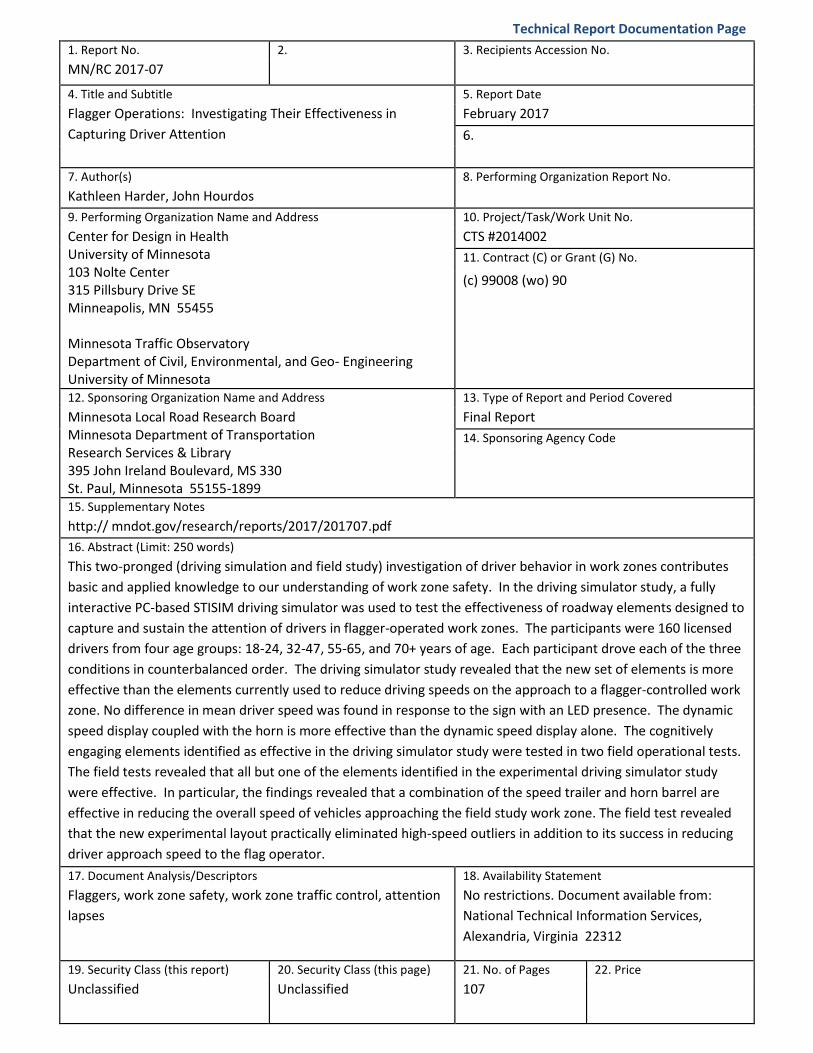
16. Abstract (Limit: 250 words)
This two-pronged (driving simulation and field study) investigation of driver behavior in work zones contributes
basic and applied knowledge to our understanding of work zone safety. In the driving simulator study, a fully
interactive PC-based STISIM driving simulator was used to test the effectiveness of roadway elements designed to
capture and sustain the attention of drivers in flagger-operated work zones. The participants were 160 licensed
drivers from four age groups: 18-24, 32-47, 55-65, and 70+ years of age. Each participant drove each of the three
conditions in counterbalanced order. The driving simulator study revealed that the new set of elements is more
effective than the elements currently used to reduce driving speeds on the approach to a flagger-controlled work
zone. No difference in mean driver speed was found in response to the sign with an LED presence. The dynamic
speed display coupled with the horn is more effective than the dynamic speed display alone. The cognitively
engaging elements identified as effective in the driving simulator study were tested in two field operational tests.
The field tests revealed that all but one of the elements identified in the experimental driving simulator study
were effective. In particular, the findings revealed that a combination of the speed trailer and horn barrel are
effective in reducing the overall speed of vehicles approaching the field study work zone. The field test revealed
that the new experimental layout practically eliminated high-speed outliers in addition to its success in reducing
driver approach speed to the flag operator.
17. Document Analysis/Descriptors 18. Availability Statement
Flaggers, work zone safety, work zone traffic control, attention
lapses
No restrictions. Document available from:
National Technical Information Services,
Alexandria, Virginia 22312
19. Security Class (this report) 20. Security Class (this page) 21. No. of Pages 22. Price
Unclassified Unclassified 107
FLAGGER OPERATIONS: INVESTIGATING THEIR EFFECTIVENESS IN
CAPTURING DRIVER ATTENTION
FINAL REPORT
Prepared by:
Kathleen Harder
Center for Design in Health
University of Minnesota
John Hourdos
Minnesota Traffic Observatory
Department of Civil, Environmental, and Geo- Engineering
University of Minnesota
FEBRUARY 2017
Published by:
Minnesota Local Road Research Board
Minnesota Department of Transportation
Research Services & Library
395 John Ireland Boulevard, MS 330
St. Paul, Minnesota 55155-1899
This report represents the results of research conducted by the authors and does not necessarily represent the views or policies
of the Minnesota Department of Transportation or the University of Minnesota or the Minnesota Local Road Research Board.
This report does not contain a standard or specified technique.
The authors and the Minnesota Department of Transportation and the University of Minnesota and the Minnesota Local Road
Research Board do not endorse products or manufacturers. Trade or manufacturers’ names appear herein solely because they
are considered essential to this report because they are considered essential to this report.

ACKNOWLEDGEMENTS
The authors would like to thank the following individuals and organizations for their contributions to this
project.
Robert Vasek, Minnesota Department of Transportation
Sue Lorentz, Retired from the Minnesota Department of Transportation
Dan Warzala, Minnesota Department of Transportation
Elizabeth Andrews, Center for Transportation Studies, University of Minnesota
Ronald Gregg, Fillmore County Engineer
Rochester Sand & Gravel
Max Rindels, University of Minnesota

TABLE OF CONTENTS
CHAPTER 1: INTRODUCTION ...............................................................................................................1
1.1 Objective ............................................................................................................................................. 1
1.2 Introduction ........................................................................................................................................ 1
1.3 Organization of this Report ................................................................................................................ 2
CHAPTER 2: DRIVING SIMULATION EXPERIMENT AND SURVEY ............................................................3
2.1 Method of Driving Simulation Experiment ......................................................................................... 3
2.1.1 Participants .................................................................................................................................. 3
2.1.2 Driving Simulator ......................................................................................................................... 3
2.1.3 Experimental Design.................................................................................................................... 4
2.2 Results of Driving Simulation Experiment .......................................................................................... 6
2.2.1 Driving Speed Data ...................................................................................................................... 6
2.3 Survey Data ....................................................................................................................................... 15
2.4 Summary Findings ............................................................................................................................ 15
CHAPTER 3: FIELD STUDY .................................................................................................................. 16
3.1 Introduction ...................................................................................................................................... 16
3.2 Base Deployment .............................................................................................................................. 16
3.2.1 Layout ........................................................................................................................................ 17
3.2.2 Flagger Location (1) ................................................................................................................... 17
3.2.3 Flagger Icon Sign (2) .................................................................................................................. 18
3.2.4 One Lane Road Ahead (3) .......................................................................................................... 18
3.2.5 Road Work Ahead (4) ................................................................................................................ 18
3.3 Experimental Deployment ................................................................................................................ 19
3.3.1 Layout ........................................................................................................................................ 19
3.3.2 Flagger (1) .................................................................................................................................. 21
3.3.3 Rumble Strips (2) ....................................................................................................................... 22
3.3.4 Be Prepared to Stop (3) ............................................................................................................. 23
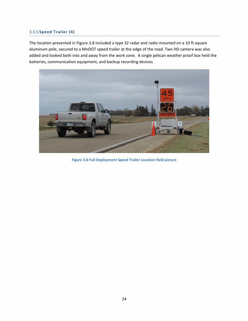
3.3.5 Speed Trailer (4) ........................................................................................................................ 24
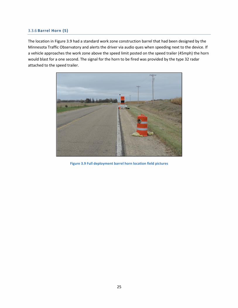
3.3.6 Barrel Horn (5) ........................................................................................................................... 25
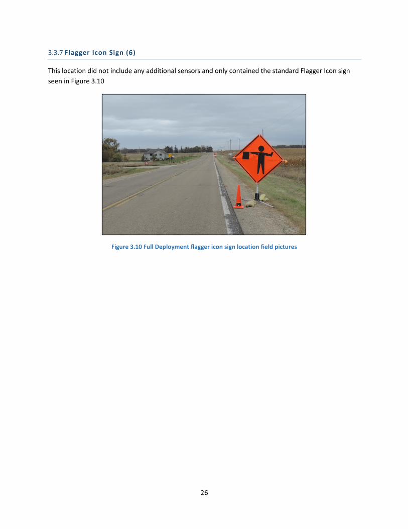
3.3.7 Flagger Icon Sign (6) .................................................................................................................. 26
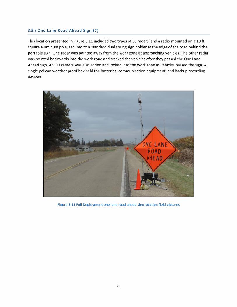
3.3.8 One Lane Road Ahead Sign (7) .................................................................................................. 27
3.4 Radar Data Collection and Extraction ............................................................................................... 28
3.5 Data Description ............................................................................................................................... 28
3.6 Data Collected .................................................................................................................................. 29
3.7 Data Errors ........................................................................................................................................ 30
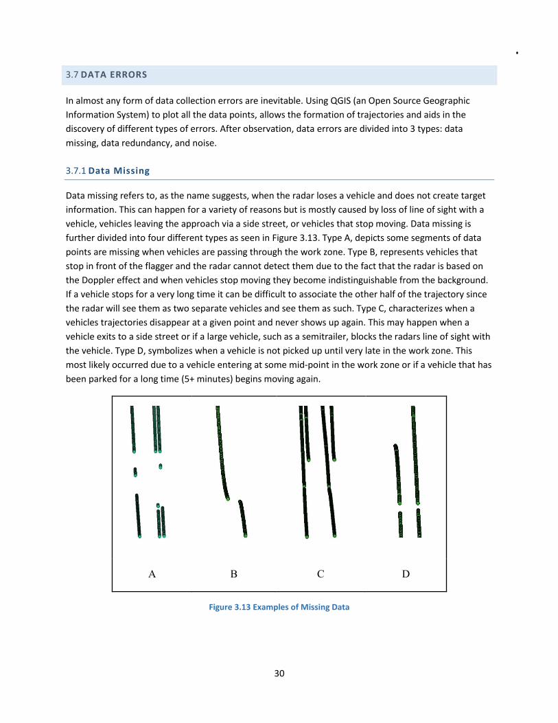
3.7.1 Data Missing .............................................................................................................................. 30
3.7.2 Data Redundancy ...................................................................................................................... 31
3.7.3 Noise .......................................................................................................................................... 31
3.8 Data Extraction ................................................................................................................................. 32
3.8.1 - Markers Creation .................................................................................................................... 32
3.8.2 Manual Trajectory Extraction .................................................................................................... 34
3.9 Individual Example Trajectories ........................................................................................................ 36
3.10 Data Analysis and Observations ..................................................................................................... 42
3.10.1 Work Zone Data Processing and Analysis ............................................................................... 42
3.10.2 Speed Distribution vs Distance Analysis .................................................................................. 43
3.11 Speed Adaptation Comparisons ..................................................................................................... 50
3.12 Field Study Conclusions .................................................................................................................. 67
CHAPTER 4: CONCLUSIONS ............................................................................................................... 68
4.1 Summary Findings and Conclusions of the Driving Simulator Experiment ...................................... 68
4.2 Summary Findings and Conclusions of the Field Study .................................................................... 68
4.3 Overall Summary .............................................................................................................................. 69
REFERENCES .................................................................................................................................... 70
APPENDIX A
APPENDIX B
APPENDIX C
LIST OF FIGURES
Figure 2.1 Layout of work zone area control condition ................................................................................ 5
Figure 2.2 Effect of condition on the average speed .................................................................................... 9
Figure 2.3 Average speed on approach to and after the LED and Non-LED signs ...................................... 10
Figure 2.4 Mean speed on the approach before and after the dynamic speed limit sign in horn and non-
horn conditions ........................................................................................................................................... 11
Figure 2.5 Effect of age on the average speed ........................................................................................... 13
Figure 2.6 Effect of gender on the average speed ...................................................................................... 14
Figure 3.1 Base deployment layout (not to scale) ...................................................................................... 17
Figure 3.2 Base deployment flagger location field picture ......................................................................... 18
Figure 3.3 Base deployment entire approach field picture ........................................................................ 19
Figure 3.4 Full deployment layout (not to scale) ........................................................................................ 20
Figure 3.5 Full deployment flagger location field picture ........................................................................... 21
Figure 3.6 Full deployment rumble strip location field picture .................................................................. 22
Figure 3.7 Full deployment be prepared to stop sign location field pictures ............................................. 23
Figure 3.8 Full Deployment Speed Trailer Location field picture................................................................ 24
Figure 3.9 Full deployment barrel horn location field pictures .................................................................. 25
Figure 3.10 Full Deployment flagger icon sign location field pictures ........................................................ 26
Figure 3.11 Full Deployment one lane road ahead sign location field pictures ......................................... 27
Figure 3.12 CSV File Format Example ......................................................................................................... 28
Figure 3.13 Examples of Missing Data ........................................................................................................ 30
Figure 3.14 Example of redundant data ..................................................................................................... 31
Figure 3.15 Examples of noise .................................................................................................................... 32
Figure 3.16 Window for data collection...................................................................................................... 33
Figure 3.17 Time-headway threshold verification ...................................................................................... 33
Figure 3.18 Manual trajectory extraction example .................................................................................... 35
Figure 3.19 Example (Experiment Deployment) of trajectories marked by the algorithm and ready for
manual extraction ....................................................................................................................................... 36
Figure 3.20 Example Trajectory of a Vehicle During the Experimental Layout That Did Not Stop at The
Flagger ......................................................................................................................................................... 38
Figure 3.21 Example trajectory of a vehicle during the experimental layout that did stop at the flagger 39
Figure 3.22 Example trajectory of a vehicle during the base layout that did not stop at the flagger ........ 40
Figure 3.23 Example trajectory of a vehicle during the base layout that did stop at the flagger .............. 41
Figure 3.24 Speed distributions at first sign seen by driver ........................................................................ 43
Figure 3.25 Speed distributions at 2,600 ft upstream of flag operator (first sign of Base layout) ............. 44
Figure 3.26 Speed distributions at first and second sign under experimental layout ................................ 45
Figure 3.27 Speed distributions at 1,800 ft upstream of flag operator ...................................................... 46
Figure 3.28 Speed distributions at first and second sign under base layout .............................................. 46
Figure 3.29 Speed distributions at 1,400 ft upstream of flag operator ...................................................... 47
Figure 3.30 Speed distributions at first sign, base layout (left), experimental layout (right) ..................... 47
Figure 3.31 Speed distributions at second sign, base layout (left), experimental layout (right) ................ 48
Figure 3.32 Speed distributions at third sign, base layout (left), experimental layout (right) ................... 48
Figure 3.33 Speed distributions at fourth sign, base layout (left), experimental layout (right) ................. 49
Figure 3.34 Speed distributions at 500 ft upstream of flag operator ......................................................... 49
Figure 3.35 Speed distributions vs distance under the base and experimental layouts ............................ 51
Figure 3.36 Distribution of speeds vs distance under base layout ............................................................. 53
Figure 3.37 Distribution of speeds vs distance under experimental layout ............................................... 54
Figure 3.38 Speed distributions vs distance under experimental layout. Speeders vs normal drivers. ..... 55
Figure 3.39 Distribution of speeds vs distance for vehicles experiencing the horn (speeders) ................. 56
Figure 3.40 Distribution of speeds vs distance for vehicles that did not activate horn (normal) .............. 57
Figure 3.41 Speed distributions vs Distance. Vehicles that didn’t have to stop at flag operator. .............. 58
Figure 3.42 Distribution of speeds vs distance of vehicles not stopping at flag operator under base layout
.................................................................................................................................................................... 59
Figure 3.43 Distribution of speeds vs distance of vehicles not stopping at flag operator under
experimental layout .................................................................................................................................... 60
Figure 3.44 Speed distributions vs distance. Vehicles that had to stop at flag operator. .......................... 61
Figure 3.45 Distribution of speeds vs distance of vehicles that stopped at flag operator under base layout
.................................................................................................................................................................... 62
Figure 3.46 Distribution of speeds vs distance of vehicles that stopped at flag operator under
experimental layout .................................................................................................................................... 63
Figure 3.47 Speed distributions vs distance. All vehicles at 2014 (original) field experiment. .................. 65
Figure 3.48 Speed distributions vs distance. Leader vehicles at 2014 (original) field experiment ............ 66

LIST OF TABLES
Table 2.1 Breakdown of participants by age and gender ............................................................................. 3
Table 2.2 Segments over which the driving speed was averaged on the approach to the four warning
signs and the flagger. .................................................................................................................................... 6
Table 2.3 P-values obtained in the five ANOVAs performed on average driving speed on the approach to
the four warning signs and the flagger. ........................................................................................................ 7
Table 2.4 Mean speed and standard deviation on the approach to the four warning signs and the flagger
as a function of the driving condition ........................................................................................................... 8
Table 2.5 The F-statistics and p-values of the LED effect on the average speed over each segment .......... 9
Table 2.6 The F-statistics and p-values of the horn effect on average speed for each segment ............... 10
Table 2.7 Average speed on approach to the warning signs and the flagger as a function of the age of
the participants ........................................................................................................................................... 12
Table 2.8 Average speed on approach to the warning signs and the flagger as a function of the gender 13
Table 2.9 Average speed on approach to the warning signs and the flagger as a function of the highway
segment ...................................................................................................................................................... 14
Table 3.1 Data collected from Experiment deployment ............................................................................. 29
Table 3.2 Data collected from base deployment ........................................................................................ 29
Table 3.3 Algorithm Created Markers ......................................................................................................... 34
EXECUTIVE SUMMARY
INTRODUCTION
The objective of the current study was to (1) use a driving simulator to test simulated roadway elements
to determine their effectiveness in capturing driver attention and fostering compliance in work zones
and then (2) in a field test evaluate the on-road effectiveness of the elements identified in the driving
simulation study. This two-pronged (driving simulation and field study) investigation of driver behavior
in work zones contributes basic and applied knowledge to our understanding of work zone safety.
DRIVING SIMULATION EXPERIMENT
Method
One hundred and sixty licensed drivers from four distinct age groups participated in the driving
simulation study. There were 40 participants in each of the four age groups—younger (18 to 24 year
olds), middle age (32 to 47 year olds), older (55 to 65 year olds), and seniors (70 years or older). There
were 20 males and 20 females within each age group. All 160 participants were licensed drivers. The
four age groups included drivers from the metro and non-metro regions and each was paid $50 for his
or her participation.
In the driving simulation portion of this study, we used a fully interactive PC-based STISIM driving
simulator with an automative-style seat that faced a bank of three 21-inch monitors. Three PCs
generated the virtual environment presented on the monitors. Participants drove 10 miles on a two-
lane bidirectional highway before they encountered the first warning sign in each of the three drives
(conditions). The layout of the control condition is shown in Figure 1. The layout of the work zone area
and the distance between the warning signs was the same for each of the three conditions; however,
the type or content of the warning signs was changed.
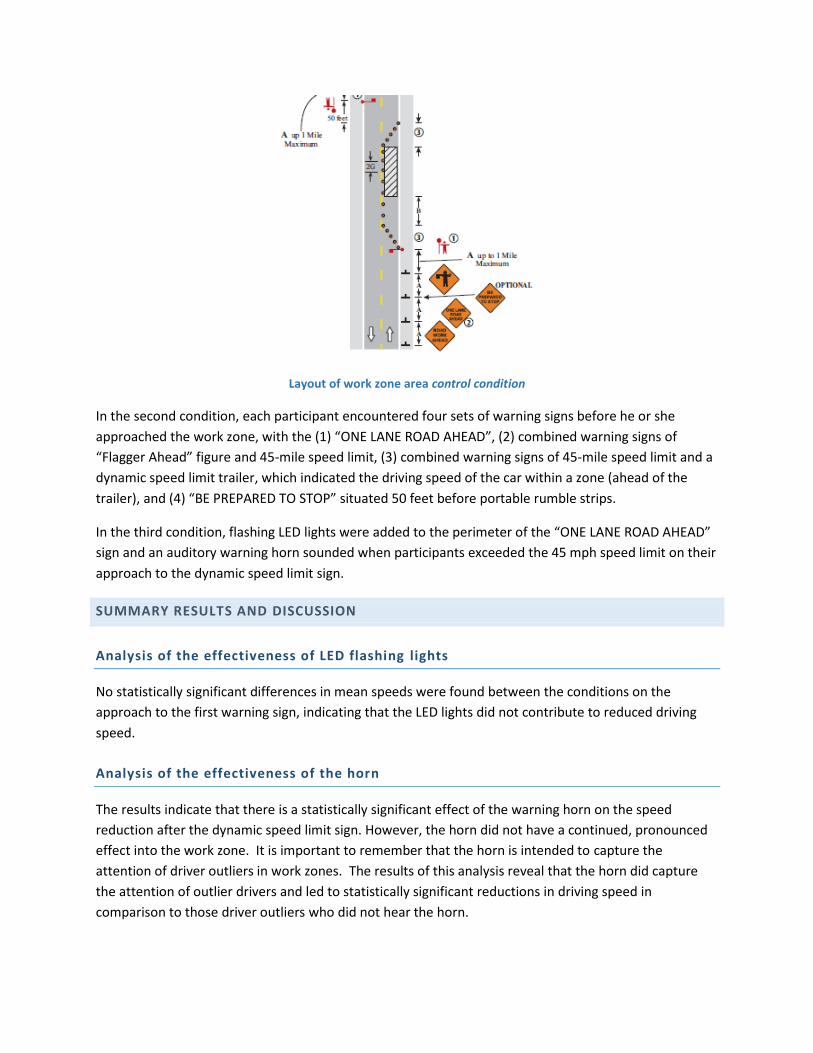
Layout of work zone area control condition
In the second condition, each participant encountered four sets of warning signs before he or she
approached the work zone, with the (1) “ONE LANE ROAD AHEAD”, (2) combined warning signs of
“Flagger Ahead” figure and 45-mile speed limit, (3) combined warning signs of 45-mile speed limit and a
dynamic speed limit trailer, which indicated the driving speed of the car within a zone (ahead of the
trailer), and (4) “BE PREPARED TO STOP” situated 50 feet before portable rumble strips.
In the third condition, flashing LED lights were added to the perimeter of the “ONE LANE ROAD AHEAD”
sign and an auditory warning horn sounded when participants exceeded the 45 mph speed limit on their
approach to the dynamic speed limit sign.
SUMMARY RESULTS AND DISCUSSION
Analysis of the effectiveness of LED flashing lights
No statistically significant differences in mean speeds were found between the conditions on the
approach to the first warning sign, indicating that the LED lights did not contribute to reduced driving
speed.
Analysis of the effectiveness of the horn
The results indicate that there is a statistically significant effect of the warning horn on the speed
reduction after the dynamic speed limit sign. However, the horn did not have a continued, pronounced
effect into the work zone. It is important to remember that the horn is intended to capture the
attention of driver outliers in work zones. The results of this analysis reveal that the horn did capture
the attention of outlier drivers and led to statistically significant reductions in driving speed in
comparison to those driver outliers who did not hear the horn.
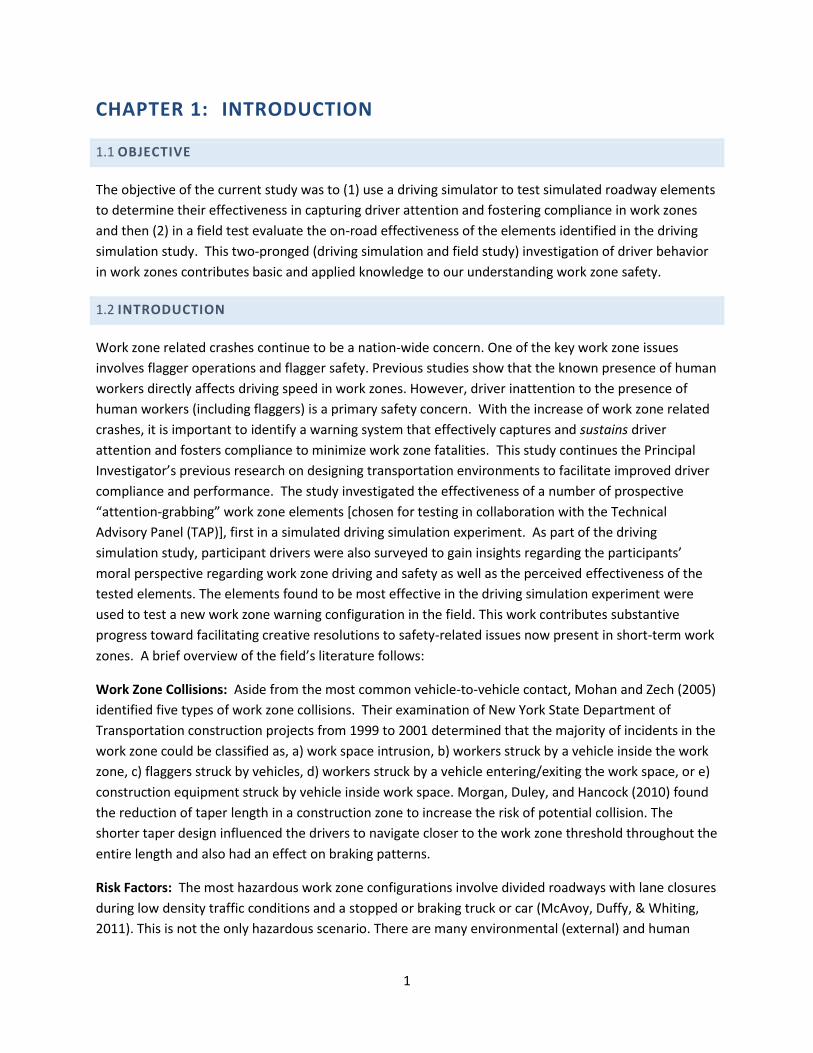
The effect of in-lane transverse rumble strips on driver behavior
The results indicate that nine participants left their lane to avoid experiencing the rumble strips for at
least one of the conditions. Of the nine, three participants left their lane to avoid the rumble strips in
both conditions, while the other six left the lane to avoid the rumble strips only once. If the opposing
lane is closed to oncoming traffic, it is not dangerous for drivers to leave their lane in a flagger-
controlled work zone. If, however, the opposing lane is not closed to oncoming traffic, then in-lane
transverse rumble strips could foster unsafe driving behavior. While this research reveals that rumble
strips capture driver attention, the data also reveal that some drivers engage in potentially unsafe
driving behavior to avoid the rumble strips.
In summary, we found that the new set of elements is more effective than the elements currently used
to reduce driving speeds on the approach to a flagger-controlled work zone. We found no difference in
mean driver speed in response to the sign with an LED presence. We found that the dynamic speed
display coupled with the horn is more effective than the dynamic speed display alone.
FIELD STUDY
The cognitively engaging elements identified as effective in the driving simulator study were tested in a
field operational test.
One field test of the cognitively engaging/attention-grabbing devices in an active work zone was
conducted in Spring Valley, MN on CSAH 8. The work zone was managed by Rochester Sand and Gravel
which was performing a full-depth reclamation and resurfacing of 4.1 miles of CSAH 8 north of Spring
Valley. Data were collected over an eight-day period. During that time, the research team set up and
deployed two different work zone layouts alongside the active work zone on one approach. The first,
referred to as base, was the minimum standard setup following Minnesota Manual on Uniform Traffic
Control Devices (MN MUTCD) guidelines. This setup was supplemented with additional radar sensors,
manufactured by Smartmicro, to gather data from the approaching vehicles during the base conditions.
The second setup deployed, referred to as the experimental layout in this report, included additional
signs and attention getting devices (Horn, Rumble Strips, Speed Trailer) identified as effective during the
driving simulator experiment. This layout was also instrumented with additional radar sensors and
cameras to gather data on the approaching vehicles.
An earlier field test of the new proposed work zone layout in an active work zone was conducted in Pine
City, MN on State Highway 70. The work zone was active over the course of four days. Unfortunately, a
combination of short work zone working periods as well as low traffic volumes did not allow for the
collection of a statistically secure sample of speeds. Interestingly, the results from the two tests are very
comparable. This finding reinforces the observations collected and conclusions reached because the
two sites were located very far from one other, the data were collected over a different time period,
and the sites were operated by completely different work zone crews.
In summary, the field test revealed that all but one of the elements identified in the experimental
driving simulator study were effective. In particular, the findings revealed that a combination of the

speed trailer and horn barrel is effective in reducing the overall speed of vehicles approaching the work
zone.
The portable rumble strips, however, did not generate any significant speed reduction, although a
definitive evaluation of the portable rumble strips would have required a test of the strips in isolation
and not when placed downstream of the speed trailer. Unfortunately, such an experiment was not in
the scope of this study.
Apart from the portable rumble strips, the field test revealed that the new experimental layout
practically eliminated high-speed outliers in addition to its success in reducing driver approach speed to
the flag operator.
1
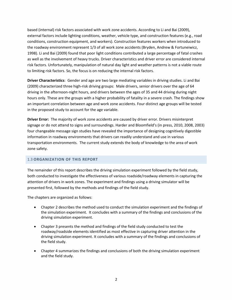
CHAPTER 1: INTRODUCTION
1.1 OBJECTIVE
The objective of the current study was to (1) use a driving simulator to test simulated roadway elements
to determine their effectiveness in capturing driver attention and fostering compliance in work zones
and then (2) in a field test evaluate the on-road effectiveness of the elements identified in the driving
simulation study. This two-pronged (driving simulation and field study) investigation of driver behavior
in work zones contributes basic and applied knowledge to our understanding work zone safety.
1.2 INTRODUCTION
Work zone related crashes continue to be a nation-wide concern. One of the key work zone issues
involves flagger operations and flagger safety. Previous studies show that the known presence of human
workers directly affects driving speed in work zones. However, driver inattention to the presence of
human workers (including flaggers) is a primary safety concern. With the increase of work zone related
crashes, it is important to identify a warning system that effectively captures and sustains driver
attention and fosters compliance to minimize work zone fatalities. This study continues the Principal
Investigator’s previous research on designing transportation environments to facilitate improved driver
compliance and performance. The study investigated the effectiveness of a number of prospective
“attention-grabbing” work zone elements [chosen for testing in collaboration with the Technical
Advisory Panel (TAP)], first in a simulated driving simulation experiment. As part of the driving
simulation study, participant drivers were also surveyed to gain insights regarding the participants’
moral perspective regarding work zone driving and safety as well as the perceived effectiveness of the
tested elements. The elements found to be most effective in the driving simulation experiment were
used to test a new work zone warning configuration in the field. This work contributes substantive
progress toward facilitating creative resolutions to safety-related issues now present in short-term work
zones. A brief overview of the field’s literature follows:
Work Zone Collisions: Aside from the most common vehicle-to-vehicle contact, Mohan and Zech (2005)
identified five types of work zone collisions. Their examination of New York State Department of
Transportation construction projects from 1999 to 2001 determined that the majority of incidents in the
work zone could be classified as, a) work space intrusion, b) workers struck by a vehicle inside the work
zone, c) flaggers struck by vehicles, d) workers struck by a vehicle entering/exiting the work space, or e)
construction equipment struck by vehicle inside work space. Morgan, Duley, and Hancock (2010) found
the reduction of taper length in a construction zone to increase the risk of potential collision. The
shorter taper design influenced the drivers to navigate closer to the work zone threshold throughout the
entire length and also had an effect on braking patterns.
Risk Factors: The most hazardous work zone configurations involve divided roadways with lane closures
during low density traffic conditions and a stopped or braking truck or car (McAvoy, Duffy, & Whiting,
2011). This is not the only hazardous scenario. There are many environmental (external) and human
2
based (internal) risk factors associated with work zone accidents. According to Li and Bai (2009),
external factors include lighting conditions, weather, vehicle type, and construction features (e.g., road
conditions, construction equipment, and workers). Construction features workers when introduced to
the roadway environment represent 1/3 of all work zone accidents (Bryden, Andrew & Fortuneiwicz,
1998). Li and Bai (2009) found that poor light conditions contributed a large percentage of fatal crashes
as well as the involvement of heavy trucks. Driver characteristics and driver error are considered internal
risk factors. Unfortunately, manipulation of natural day light and weather patterns is not a viable route
to limiting risk factors. So, the focus is on reducing the internal risk factors.
Driver Characteristics: Gender and age are two large mediating variables in driving studies. Li and Bai
(2009) characterized three high-risk driving groups: Male drivers, senior drivers over the age of 64
driving in the afternoon-night hours, and drivers between the ages of 35 and 44 driving during night
hours only. These are the groups with a higher probability of fatality in a severe crash. The findings show
an important correlation between age and work zone accidents. Four distinct age groups will be tested
in the proposed study to account for the age variable.
Driver Error: The majority of work zone accidents are caused by driver error. Drivers misinterpret
signage or do not attend to signs and surroundings. Harder and Bloomfield’s (in press, 2010, 2008, 2003)
four changeable message sign studies have revealed the importance of designing cognitively digestible
information in roadway environments that drivers can readily understand and use in various
transportation environments. The current study extends the body of knowledge to the area of work
zone safety.
1.3 ORGANIZATION OF THIS REPORT
The remainder of this report describes the driving simulation experiment followed by the field study,
both conducted to investigate the effectiveness of various roadside/roadway elements in capturing the
attention of drivers in work zones. The experiment and findings using a driving simulator will be
presented first, followed by the methods and findings of the field study.
The chapters are organized as follows:
Chapter 2 describes the method used to conduct the simulation experiment and the findings of the simulation experiment. It concludes with a summary of the findings and conclusions of the driving simulation experiment.
Chapter 3 presents the method and findings of the field study conducted to test the roadway/roadside elements identified as most effective in capturing driver attention in the driving simulation experiment. It concludes with a summary of the findings and conclusions of the field study.
Chapter 4 summarizes the findings and conclusions of both the driving simulation experiment and the field study.
3
CHAPTER 2: DRIVING SIMULATION EXPERIMENT AND SURVEY Method and Findings
Kathleen A. Harder, PhD
University of Minnesota
2.1 METHOD OF DRIVING SIMULATION EXPERIMENT
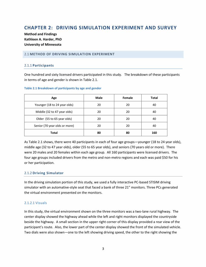
2.1.1 Participants
One hundred and sixty licensed drivers participated in this study. The breakdown of these participants
in terms of age and gender is shown in Table 2.1.
Table 2.1 Breakdown of participants by age and gender
Age Male Female Total
Younger (18 to 24 year olds) 20 20 40
Middle (32 to 47 year olds) 20 20 40
Older (55 to 65 year olds) 20 20 40
Senior (70 year olds or more) 20 20 40
Total 80 80 160
As Table 2.1 shows, there were 40 participants in each of four age groups—younger (18 to 24 year olds),
middle age (32 to 47 year olds), older (55 to 65 year olds), and seniors (70 years old or more). There
were 20 males and 20 females within each age group. All 160 participants were licensed drivers. The
four age groups included drivers from the metro and non-metro regions and each was paid $50 for his
or her participation.
2.1.2 Driving Simulator
In the driving simulation portion of this study, we used a fully interactive PC-based STISIM driving
simulator with an automative-style seat that faced a bank of three 21” monitors. Three PCs generated
the virtual environment presented on the monitors.
2.1.2.1 Visuals
In this study, the virtual environment shown on the three monitors was a two-lane rural highway. The
center display showed the highway ahead while the left and right monitors displayed the countryside
beside the highway. A small section in the upper right corner of this display provided a rear view of the
participant’s route. Also, the lower part of the center display showed the front of the simulated vehicle.
Two dials were also shown—one to the left showing driving speed, the other to the right showing the
4
RPM rate. On the monitors to the left and right, two small sections simulated side-view mirrors that
also provided rear views of the route.
2.1.2.2 Sound
Two small speakers located on each side of the monitors generated the simulator’s engine noise. The
speakers were approximately at the shoulder height of the participants. A subwoofer positioned on the
floor beneath the driver’s seat provided low-frequency sound.
2.1.2.3 Controls
Each participant controlled the simulator with a steering wheel, an accelerator pedal, and a brake pedal.
The simulator PCs registered inputs to these controls and adjusted speed and direction accordingly. The
steering wheel was linked to a torque motor, which provided forced-feedback, in order to add realism to
the “feel” of the steering.
2.1.2.4 Scenario Development
The driving scenario used in this study was developed using STISIM’s Scenario Definition Language (SDL).
Additional modifications were made to the experimental scenario so that when drivers crossed the
rumble strips, the effect was felt in the steering wheel.
2.1.3 Experimental Design
2.1.3.1 Procedure
Prior to the experiment, potential participants were contacted by phone. They were asked their age and
whether or not they drove a car. They were recruited if they were in one of the four age groups,
currently drove a vehicle, and (1) had not experienced motion sickness in automobiles or in airplanes,
(2) had not been sick on any amusement park rides, (3) had not felt queasy at IMAX presentations, and
(4) had not had migraines or severe tension headaches.
When each participant arrived at the lab housing the driving simulator, the experimenter examined his
or her driver’s license to ensure it was valid and to verify the participant’s age. Then, the participant
read and signed the consent form. The participant was told that he or she would drive in the simulator
and then would be asked to complete a brief survey. They were told that the session would be
approximately one hour long.
A brief training session followed. In the training session, the participant drove on a simulated six-lane
divided highway for approximately six or seven minutes. During the session, which began with the
simulator vehicle in the center lane, the participant was asked to accelerate, to reduce speed, and to
change lanes. The session continued until the participant felt comfortable driving the simulator vehicle.
Then, the experimenter answered any questions that the participant had.
5
Before each experimental trial the participants were told that they would be driving on a two-lane
bidirectional highway. They were asked to “Please drive as you normally would if you were driving on
an actual roadway.”
To control for possible effects of stimuli presentation order, the 160 participants were randomly
assigned to a counterbalanced driving order of the three conditions.
After driving the three drives, the participants left the simulator and moved to a table in the lab. There,
they were asked to complete a brief survey. After completing the survey, the participant was debriefed.
The debriefing was as follows:
“In this study, we’re interested in driving behavior in various roadway environments. We’d like you
to keep the information about this study confidential. Please do not discuss the study with anyone.
We don’t want anyone who might take part in the study to know anything about it beforehand.”
After the debriefing, the participant was paid $50. The experimental session lasted approximately one
hour.
2.1.3.2 Conditions
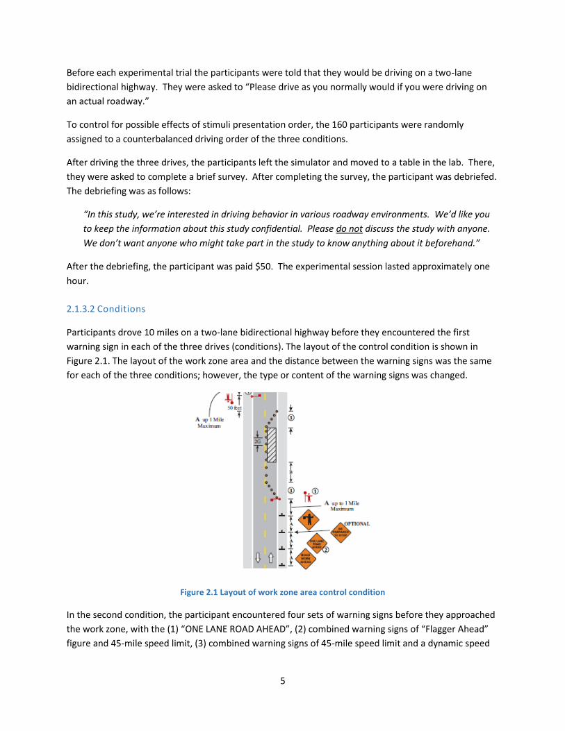
Participants drove 10 miles on a two-lane bidirectional highway before they encountered the first
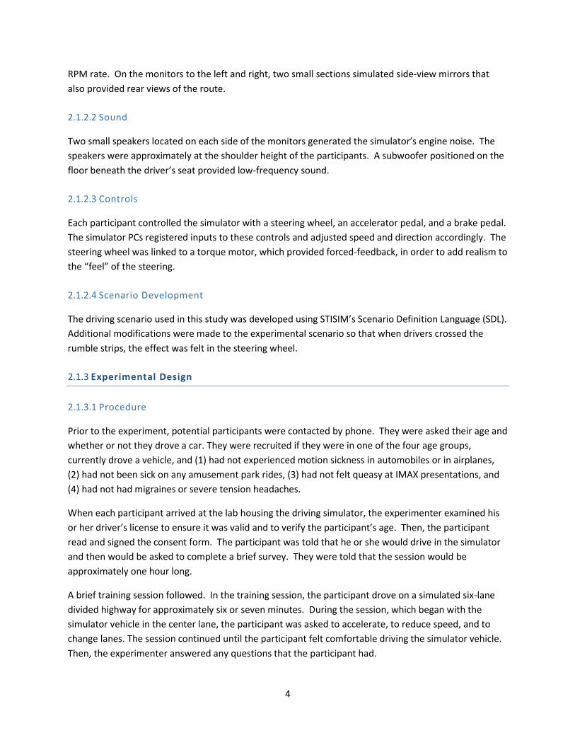
warning sign in each of the three drives (conditions). The layout of the control condition is shown in
Figure 2.1. The layout of the work zone area and the distance between the warning signs was the same
for each of the three conditions; however, the type or content of the warning signs was changed.
Figure 2.1 Layout of work zone area control condition
In the second condition, the participant encountered four sets of warning signs before they approached
the work zone, with the (1) “ONE LANE ROAD AHEAD”, (2) combined warning signs of “Flagger Ahead”
figure and 45-mile speed limit, (3) combined warning signs of 45-mile speed limit and a dynamic speed
6
limit trailer which indicated the driving speed of the car within a zone ( ahead of the trailer, and (4) “BE
PREPARED TO STOP” situated 50 feet before portable rumble strips.
In the third condition, flashing LED lights were added to the perimeter of the “ONE LANE ROAD AHEAD”
sign and an auditory warning horn sounded when participants exceeded the 45 mph speed limit on their
approach to the dynamic speed limit sign.
2.2 RESULTS OF DRIVING SIMULATION EXPERIMENT
2.2.1 Driving Speed Data
2.2.1.1 Analysis of Driving Speed
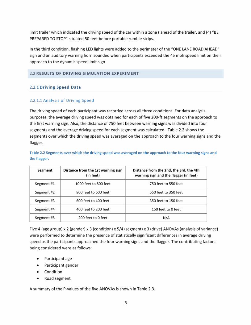
The driving speed of each participant was recorded across all three conditions. For data analysis
purposes, the average driving speed was obtained for each of five 200-ft segments on the approach to
the first warning sign. Also, the distance of 750 feet between warning signs was divided into four
segments and the average driving speed for each segment was calculated. Table 2.2 shows the
segments over which the driving speed was averaged on the approach to the four warning signs and the
flagger.
Table 2.2 Segments over which the driving speed was averaged on the approach to the four warning signs and
the flagger.
Segment Distance from the 1st warning sign (in feet)
Distance from the 2nd, the 3rd, the 4th warning sign and the flagger (in feet)
Segment #1 1000 feet to 800 feet 750 feet to 550 feet
Segment #2 800 feet to 600 feet 550 feet to 350 feet
Segment #3 600 feet to 400 feet 350 feet to 150 feet
Segment #4 400 feet to 200 feet 150 feet to 0 feet
Segment #5 200 feet to 0 feet N/A
Five 4 (age group) x 2 (gender) x 3 (condition) x 5/4 (segment) x 3 (drive) ANOVAs (analysis of variance)
were performed to determine the presence of statistically significant differences in average driving
speed as the participants approached the four warning signs and the flagger. The contributing factors
being considered were as follows:
Participant age
Participant gender
Condition
Road segment
A summary of the P-values of the five ANOVAs is shown in Table 2.3.
7
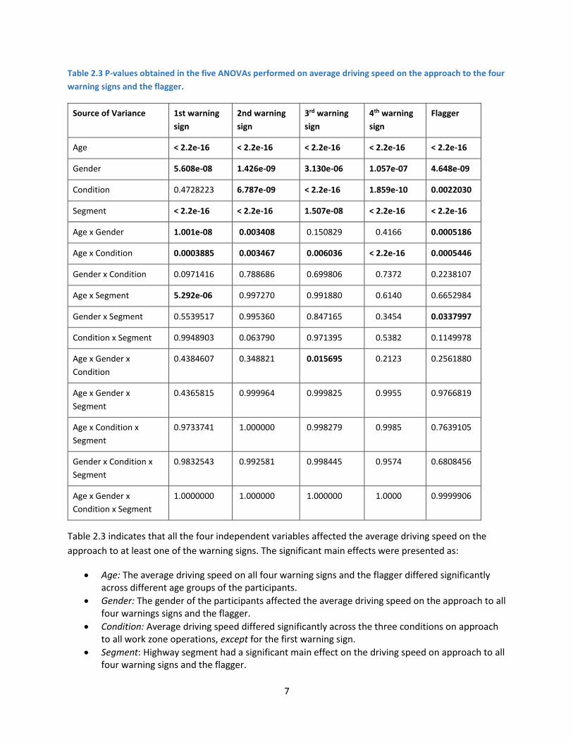
Table 2.3 P-values obtained in the five ANOVAs performed on average driving speed on the approach to the four
warning signs and the flagger.
Source of Variance 1st warning
sign
2nd warning
sign
3rd warning
sign
4th warning
sign
Flagger
Age < 2.2e-16 < 2.2e-16 < 2.2e-16 < 2.2e-16 < 2.2e-16
Gender 5.608e-08 1.426e-09 3.130e-06 1.057e-07 4.648e-09
Condition 0.4728223 6.787e-09 < 2.2e-16 1.859e-10 0.0022030
Segment < 2.2e-16 < 2.2e-16 1.507e-08 < 2.2e-16 < 2.2e-16
Age x Gender 1.001e-08 0.003408 0.150829 0.4166 0.0005186
Age x Condition 0.0003885 0.003467 0.006036 < 2.2e-16 0.0005446
Gender x Condition 0.0971416 0.788686 0.699806 0.7372 0.2238107
Age x Segment 5.292e-06 0.997270 0.991880 0.6140 0.6652984
Gender x Segment 0.5539517 0.995360 0.847165 0.3454 0.0337997
Condition x Segment 0.9948903 0.063790 0.971395 0.5382 0.1149978
Age x Gender x
Condition
0.4384607 0.348821 0.015695 0.2123 0.2561880
Age x Gender x
Segment
0.4365815 0.999964 0.999825 0.9955 0.9766819
Age x Condition x
Segment
0.9733741 1.000000 0.998279 0.9985 0.7639105
Gender x Condition x
Segment
0.9832543 0.992581 0.998445 0.9574 0.6808456
Age x Gender x
Condition x Segment
1.0000000 1.000000 1.000000 1.0000 0.9999906
Table 2.3 indicates that all the four independent variables affected the average driving speed on the
approach to at least one of the warning signs. The significant main effects were presented as:
Age: The average driving speed on all four warning signs and the flagger differed significantly across different age groups of the participants.
Gender: The gender of the participants affected the average driving speed on the approach to all four warnings signs and the flagger.
Condition: Average driving speed differed significantly across the three conditions on approach to all work zone operations, except for the first warning sign.
Segment: Highway segment had a significant main effect on the driving speed on approach to all four warning signs and the flagger.
8
Significant interaction effects can also been found from Table 2.3. Although statistically significant, the
magnitude of the average speed differences associated with the interactions was relatively small
compared to the main effects. A detailed presentation of the interactions is shown in Appendix A.
To identify the most effective work zone operation, the average speed of the approach to the warning
signs and the flagger is presented as a function of the experimental condition. Moreover, analysis was
conducted on the effectiveness of the warning horn for participants who drove beyond the speed limit
in both of the LED/horn condition and Non-LED/horn condition. Then, we also examined the differences
of the average driving speed on approach to the warning signs and the flagger depending on other
variables.
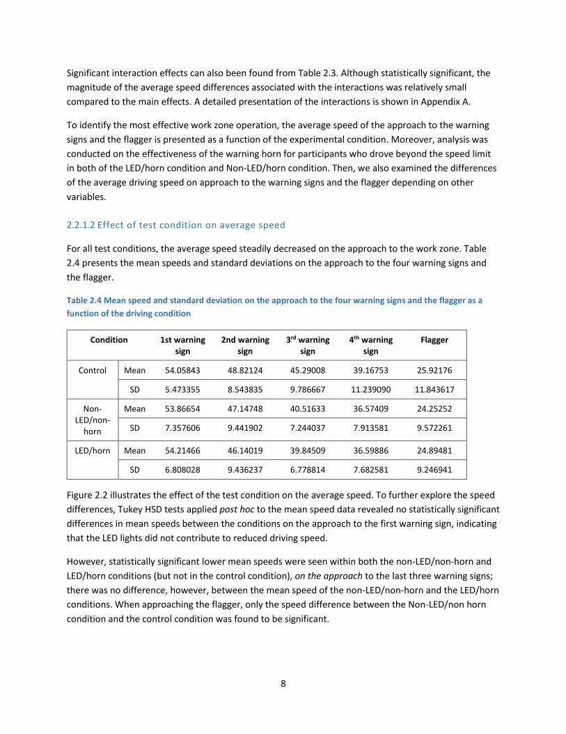
2.2.1.2 Effect of test condition on average speed
For all test conditions, the average speed steadily decreased on the approach to the work zone. Table
2.4 presents the mean speeds and standard deviations on the approach to the four warning signs and
the flagger.
Table 2.4 Mean speed and standard deviation on the approach to the four warning signs and the flagger as a
function of the driving condition
Condition 1st warning sign
2nd warning sign
3rd warning sign
4th warning sign
Flagger
Control Mean 54.05843 48.82124 45.29008 39.16753 25.92176
SD 5.473355 8.543835 9.786667 11.239090 11.843617
Non-LED/non-
horn
Mean 53.86654 47.14748 40.51633 36.57409 24.25252
SD 7.357606 9.441902 7.244037 7.913581 9.572261
LED/horn Mean 54.21466 46.14019 39.84509 36.59886 24.89481
SD 6.808028 9.436237 6.778814 7.682581 9.246941
Figure 2.2 illustrates the effect of the test condition on the average speed. To further explore the speed
differences, Tukey HSD tests applied post hoc to the mean speed data revealed no statistically significant
differences in mean speeds between the conditions on the approach to the first warning sign, indicating
that the LED lights did not contribute to reduced driving speed.
However, statistically significant lower mean speeds were seen within both the non-LED/non-horn and
LED/horn conditions (but not in the control condition), on the approach to the last three warning signs;
there was no difference, however, between the mean speed of the non-LED/non-horn and the LED/horn
conditions. When approaching the flagger, only the speed difference between the Non-LED/non horn
condition and the control condition was found to be significant.
9
Figure 2.2 Effect of condition on the average speed
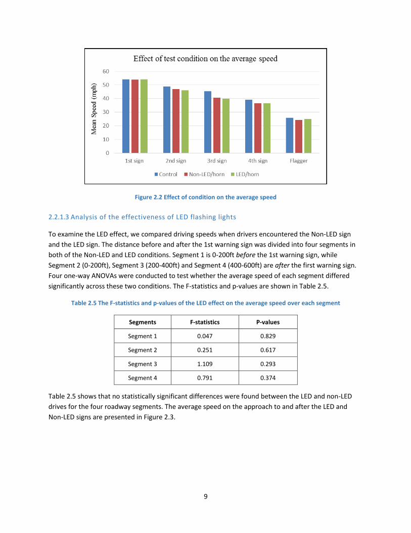
2.2.1.3 Analysis of the effectiveness of LED flashing lights
To examine the LED effect, we compared driving speeds when drivers encountered the Non-LED sign
and the LED sign. The distance before and after the 1st warning sign was divided into four segments in
both of the Non-LED and LED conditions. Segment 1 is 0-200ft before the 1st warning sign, while
Segment 2 (0-200ft), Segment 3 (200-400ft) and Segment 4 (400-600ft) are after the first warning sign.
Four one-way ANOVAs were conducted to test whether the average speed of each segment differed
significantly across these two conditions. The F-statistics and p-values are shown in Table 2.5.
Table 2.5 The F-statistics and p-values of the LED effect on the average speed over each segment
Segments F-statistics P-values
Segment 1 0.047 0.829
Segment 2 0.251 0.617
Segment 3 1.109 0.293
Segment 4 0.791 0.374
Table 2.5 shows that no statistically significant differences were found between the LED and non-LED
drives for the four roadway segments. The average speed on the approach to and after the LED and
Non-LED signs are presented in Figure 2.3.
10
Figure 2.3 Average speed on approach to and after the LED and Non-LED signs
2.2.1.4 Analysis of the effectiveness of the horn
The trigger region of the auditory warning horn was 150 feet before the dynamic speed limit sign for
those drivers exceeding 45 mph. The eighteen drivers in the LED/horn condition who exceeded 45 mph
in the zone of the dynamic speed limit sign experienced the auditory warning horn.
For purposes of comparison we also extracted the driving speed data for the 19 participants who
exceeded the 45 mph speed limit in the equivalent zone of the dynamic speed limit sign in the non-horn
condition.
To examine how the horn affected speed reduction, the roadway surrounding the dynamic speed limit
sign was divided into 4 segments. Segment 1 is 0-150ft before the dynamic speed limit sign, while
Segment 2 (0-200ft), Segment 3 (200-400ft) and Segment 4 (400-600ft) are after the dynamic speed
limit sign. The speed of those who heard the horn in the LED/horn condition and those who exceeded
the 45 mph speed limit in the non-horn condition was averaged over each segment. A one-way ANOVA
was conducted for each segment to examine the effect of the horn on average driving speed. The F-
statistics and P-values are presented in Table 2.6.
Table 2.6 The F-statistics and p-values of the horn effect on average speed for each segment
Segments F-statistics P-values
Segment 1 3.422 0.0728
Segment 2 4.301 0.0455
Segment 3 4.4 0.0432
Segment 4 1.552 0.221
11
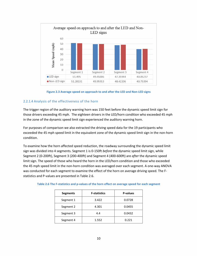
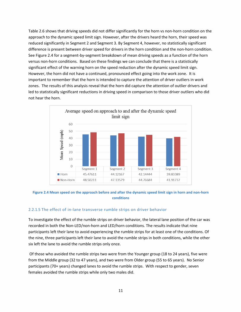
Table 2.6 shows that driving speeds did not differ significantly for the horn vs non-horn condition on the
approach to the dynamic speed limit sign. However, after the drivers heard the horn, their speed was
reduced significantly in Segment 2 and Segment 3. By Segment 4, however, no statistically significant
difference is present between driver speed for drivers in the horn condition and the non-horn condition.
See Figure 2.4 for a segment-by-segment breakdown of mean driving speeds as a function of the horn
versus non-horn conditions. Based on these findings we can conclude that there is a statistically
significant effect of the warning horn on the speed reduction after the dynamic speed limit sign.
However, the horn did not have a continued, pronounced effect going into the work zone. It is
important to remember that the horn is intended to capture the attention of driver outliers in work
zones. The results of this analysis reveal that the horn did capture the attention of outlier drivers and
led to statistically significant reductions in driving speed in comparison to those driver outliers who did
not hear the horn.
Figure 2.4 Mean speed on the approach before and after the dynamic speed limit sign in horn and non-horn
conditions
2.2.1.5 The effect of in-lane transverse rumble strips on driver behavior
To investigate the effect of the rumble strips on driver behavior, the lateral lane position of the car was
recorded in both the Non-LED/non-horn and LED/horn conditions. The results indicate that nine
participants left their lane to avoid experiencing the rumble strips for at least one of the conditions. Of
the nine, three participants left their lane to avoid the rumble strips in both conditions, while the other
six left the lane to avoid the rumble strips only once.
Of those who avoided the rumble strips two were from the Younger group (18 to 24 years), five were
from the Middle group (32 to 47 years), and two were from Older group (55 to 65 years). No Senior
participants (70+ years) changed lanes to avoid the rumble strips. With respect to gender, seven
females avoided the rumble strips while only two males did.
12
Please note: It is not dangerous for drivers to leave their lane in a flagger-controlled work zone because
the opposing lane is closed to oncoming traffic. The intent of this research is to generate driving
contexts that capture driver attention. The data show that rumble strips facilitate this intent.
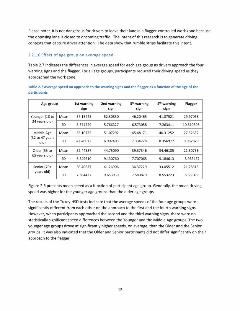
2.2.1.6 Effect of age group on average speed
Table 2.7 indicates the differences in average speed for each age group as drivers approach the four
warning signs and the flagger. For all age groups, participants reduced their driving speed as they
approached the work zone.
Table 2.7 Average speed on approach to the warning signs and the flagger as a function of the age of the
participants
Age group 1st warning sign
2nd warning sign
3rd warning sign
4th warning sign
Flagger
Younger (18 to 24 years old)
Mean 57.15425 52.30850 46.20465 41.87521 29.97058
SD 5.574729 5.766327 6.573058 7.263411 10.519595
Middle Age (32 to 47 years
old)
Mean 56.10735 51.07292 45.48171 40.31252 27.52652
SD 4.046072 6.907403 7.334728 8.356977 9.962879
Older (55 to 65 years old)
Mean 52.44587 44.75090 39.37346 34.46185 21.30756
SD 6.549610 9.130760 7.707065 9.184613 8.983437
Senior (70+ years old)
Mean 50.40637 41.26906 36.37229 33.05512 21.28515
SD 7.384437 9.653939 7.589879 8.553223 8.663483
Figure 2.5 presents mean speed as a function of participant age group. Generally, the mean driving
speed was higher for the younger age groups than the older age groups.
The results of the Tukey HSD tests indicate that the average speeds of the four age groups were
significantly different from each other on the approach to the first and the fourth warning signs.
However, when participants approached the second and the third warning signs, there were no
statistically significant speed differences between the Younger and the Middle Age groups. The two
younger age groups drove at significantly higher speeds, on average, than the Older and the Senior
groups. It was also indicated that the Older and Senior participants did not differ significantly on their
approach to the flagger.

13
Figure 2.5 Effect of age on the average speed
2.2.1.7 Effect of gender on average speed
Table 2.8 presents the means and standard deviations of driving speed as a function of gender and
roadway elements. For both males and females, the average speed decreased from the first warning
sign to the flagger.
Table 2.8 Average speed on approach to the warning signs and the flagger as a function of the gender
Gender 1st warning sign
2nd warning sign
3rd warning sign
4th warning sign
Flagger
Female Mean 53.38567 46.27796 41.11780 36.46930 23.90211
SD 6.516387 9.811168 9.069157 9.566229 10.17433
Male Mean 54.67125 48.42273 42.59825 38.38305 26.14279
SD 6.630059 8.438196 7.597822 8.637237 10.29128
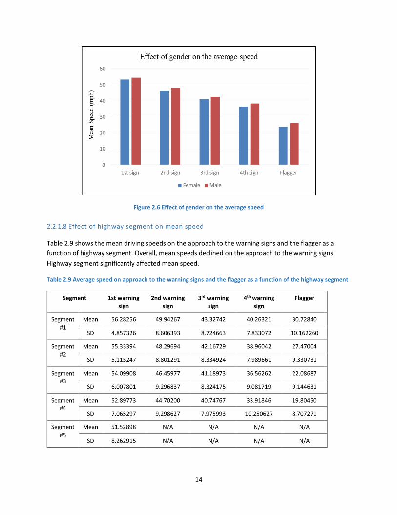
Figure 2.6 presents the effect of gender on mean speed. Males drove at a higher speed on average than
females.
14
Figure 2.6 Effect of gender on the average speed
2.2.1.8 Effect of highway segment on mean speed
Table 2.9 shows the mean driving speeds on the approach to the warning signs and the flagger as a
function of highway segment. Overall, mean speeds declined on the approach to the warning signs.
Highway segment significantly affected mean speed.
Table 2.9 Average speed on approach to the warning signs and the flagger as a function of the highway segment
Segment 1st warning sign
2nd warning sign
3rd warning sign
4th warning sign
Flagger
Segment #1
Mean 56.28256 49.94267 43.32742 40.26321 30.72840
SD 4.857326 8.606393 8.724663 7.833072 10.162260
Segment #2
Mean 55.33394 48.29694 42.16729 38.96042 27.47004
SD 5.115247 8.801291 8.334924 7.989661 9.330731
Segment #3
Mean 54.09908 46.45977 41.18973 36.56262 22.08687
SD 6.007801 9.296837 8.324175 9.081719 9.144631
Segment #4
Mean 52.89773 44.70200 40.74767 33.91846 19.80450
SD 7.065297 9.298627 7.975993 10.250627 8.707271
Segment #5
Mean 51.52898 N/A N/A N/A N/A
SD 8.262915 N/A N/A N/A N/A

15
The driving speed trajectories of each segment on approach to the warning signs and the flagger are
presented in Appendix B. The figures reveal that the mean speeds consistently declined on the
approach to the work zone.
2.3 SURVEY DATA
After completing the three drives, the 160 participants were asked to respond to six survey questions
pertaining to, for example, the extent to which they demonstrate consideration for other drivers,
pedestrians, and bicyclists. The participants were also queried about awareness of road conditions
while driving and whether they text while driving. Though the survey was not the focal point of our
research, and thus an extensive statistical analysis was not performed, the survey questions and
descriptive statistics are presented in Appendix C.
2.4 SUMMARY FINDINGS
In this exeriment, we used a driving simulator to identify elements that capture and sustain driver
attention in flagger-controlled work zones. We obtained lane position data and driving speed data from
the 160 participants who drove the simulated rural highway three times. We were particularly
interested in determining whether flashing LED lights mounted on the first warning sign of an approach
to a flagger-controlled work zone contributed to more significant reductions in speed than the same sign
without the flashing LED lights. We are also particularly interested in whether a horn blast emitted for
drivers exceeding 45 mph on their approach to an intelligent speed limit display effectively captured the
attention of outlier drivers. And we were interested in determining the effectiveness of transverse
rumble strips as an attention-grabbing device in a simulated flagger-controlled work zone.
Our main findings are the following:
The new set of elements is more effective than the elements currently used to reduce driving
speeds on the approach to the flagger-controlled work zone;
We found no difference in mean driver speed in response to the sign with an LED presence;
The dynamic speed display coupled with the horn is more effective than the dynamic speed
display alone;
Survey responses provide helpful self-reported information from drivers.
16
CHAPTER 3: FIELD STUDY Method and Findings
John Hourdos, PhD
University of Minnesota
3.1 INTRODUCTION
The second pilot test of the attention getting devices in an active work zone was conducted in Spring
Valley, MN on CSAH 8. The work zone was being managed by Rochester Sand and Gravel who were
performing a full depth reclamation and resurfacing of 4.1 miles of CSAH 8 north of Spring Valley. The
team was deployed from 10/8/15 – 10/17/15 and collected data on 8 days within that time period.
During that time, the research team setup and deployed two different work zone layouts alongside the
active work zone on one approach. The first, referred to as base, was the minimum standard setup
following Minnesota Manual on Uniform Traffic Control Devices (MN MUTCD) guidelines. This setup was
supplemented with additional radar sensors, manufactured by Smartmicro, to gather data from the
approaching vehicles during the base conditions. The second setup deployed, referred to as the
experimental in this report, included additional signs and attention getting devices (Horn, Rumble Strips,
Speed Trailer). This layout was also instrumented with additional radar sensors and cameras to gather
data on the approaching vehicles.
The first field test of the new proposed work zone layout in an active work zone was conducted in Pine
City, MN on State Highway 70. The work zone was active over the course of 4 days ranging from
10/06/2014 – 10/09/2014. Unfortunately, a combination of short work zone working periods as well as
low traffic volumes did not allow for the collection of a statistically secure sample of speeds. Even so,
the results from the two tests are very comparable, a fact that reinforces the observations collected and
conclusions reached since the two sites were very far from each other, on a different time period, and
operated by completely different work zone crews.
In summary, we observed that the combination Speed Trailer and Horn Barrel succeeded in reducing the
overall speed of vehicles approaching the work zone. In contrast, the portable rumble strips did not
generate any significant speed reduction.
3.2 BASE DEPLOYMENT
The base setup consisted of signs laid out according to the Minnesota Manual on Uniform Traffic Control
Devices (MN MUTCD). The only additions made to the setup were the data collection sensors hidden
behind each sign, which include 5 radar sensors and 4 HD cameras. Due to the activity of the work zone
the locations of the equipment changed daily, however the layout and distance between stations
remained the same.
17
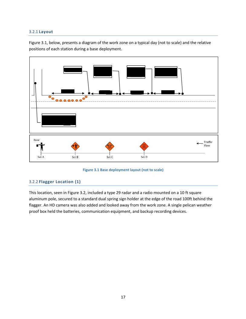
3.2.1 Layout
Figure 3.1, below, presents a diagram of the work zone on a typical day (not to scale) and the relative
positions of each station during a base deployment.
Figure 3.1 Base deployment layout (not to scale)
3.2.2 Flagger Location (1)
This location, seen in Figure 3.2, included a type 29 radar and a radio mounted on a 10 ft square
aluminum pole, secured to a standard dual spring sign holder at the edge of the road 100ft behind the
flagger. An HD camera was also added and looked away from the work zone. A single pelican weather
proof box held the batteries, communication equipment, and backup recording devices.

18
Figure 3.2 Base deployment flagger location field picture
3.2.3 Flagger Icon Sign (2)
This location, seen in the background of figure 3.3, included a type 32 radar and a radio on a 10ft square
aluminum pole, secured to a standard dual spring sign holder at the edge of the road behind the
portable sign. A single pelican weather proof box held the batteries, communication equipment, and
backup recording devices.
3.2.4 One Lane Road Ahead (3)
This location, seen in the middle of figure 3.3, included a type 32 radar and a radio on a 10 ft square
aluminum pole, secured to a standard dual spring sign holder at the edge of the road behind the
portable sign. Two HD cameras were also added and looked both into and away from the work zone. A
single pelican weather proof box held the batteries, communication equipment, and backup recording
devices.
3.2.5 Road Work Ahead (4)
This location, seen in the foreground of figure 3.3, included two type 30 radars and a radio mounted on
a 10 ft square aluminum pole, secured to a standard dual spring sign holder at the edge of the road
behind the portable sign. One radar was pointed away from the work zone at approaching vehicles. The
other radar was pointed backwards into the work zone and tracked the vehicles after they passed the
Road Work Ahead sign. An HD camera was also added and looked into the work zone as vehicles passed
the sign. A single pelican weather proof box held the batteries, communication equipment, and backup
recording devices.

19
Figure 3.3 Base deployment entire approach field picture
3.3 EXPERIMENTAL DEPLOYMENT
The experimental deployment setup used signs found in the Minnesota Manual on Uniform Traffic
Control Devices (MN MUTCD). In addition, alternative attention getting devices were deployed including
portable rumple strip, a speed trailer (with a 45mph construction zone speed limit displayed), and a
custom barrel horn designed by the Minnesota Traffic Observatory that alerts the driver via audio ques
when speeding next to the device. To collect information on vehicles in the work zone data collection
sensors were hidden behind each sign, which include 5 radar sensors and 4 HD cameras. Due to the
activity of the work zone the locations of the equipment changed daily, however the layout and distance
between stations remained the same.
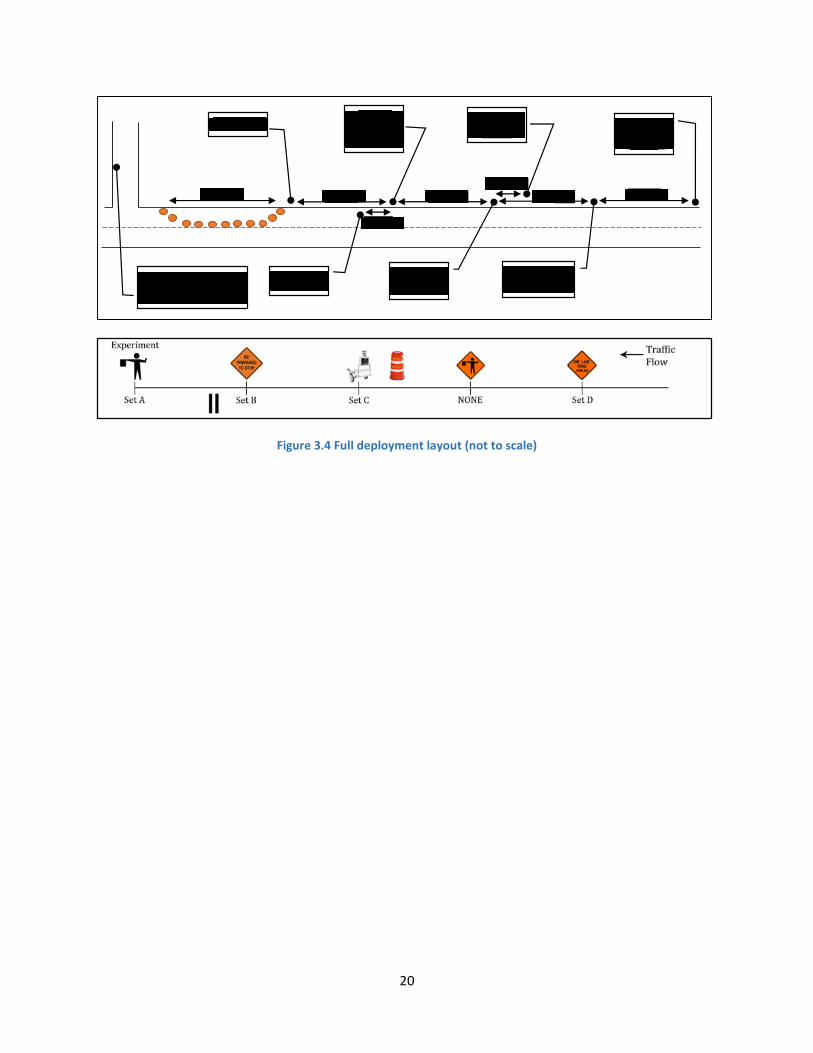
3.3.1 Layout
Figure 3.4, below, shows a diagram of the work zone on a typical day (not to scale) and the relative
positions of each station during an experimental deployment.
20
Figure 3.4 Full deployment layout (not to scale)
21
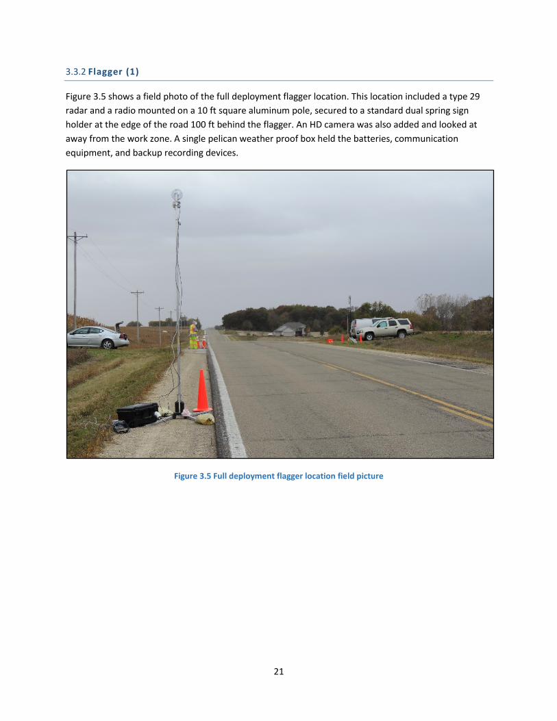
3.3.2 Flagger (1)
Figure 3.5 shows a field photo of the full deployment flagger location. This location included a type 29
radar and a radio mounted on a 10 ft square aluminum pole, secured to a standard dual spring sign
holder at the edge of the road 100 ft behind the flagger. An HD camera was also added and looked at
away from the work zone. A single pelican weather proof box held the batteries, communication
equipment, and backup recording devices.
Figure 3.5 Full deployment flagger location field picture
22
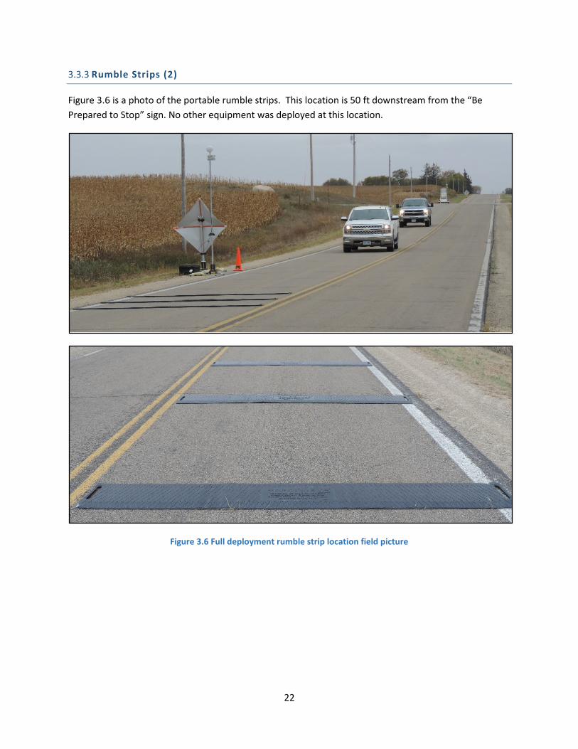
3.3.3 Rumble Strips (2)
Figure 3.6 is a photo of the portable rumble strips. This location is 50 ft downstream from the “Be
Prepared to Stop” sign. No other equipment was deployed at this location.
Figure 3.6 Full deployment rumble strip location field picture
23
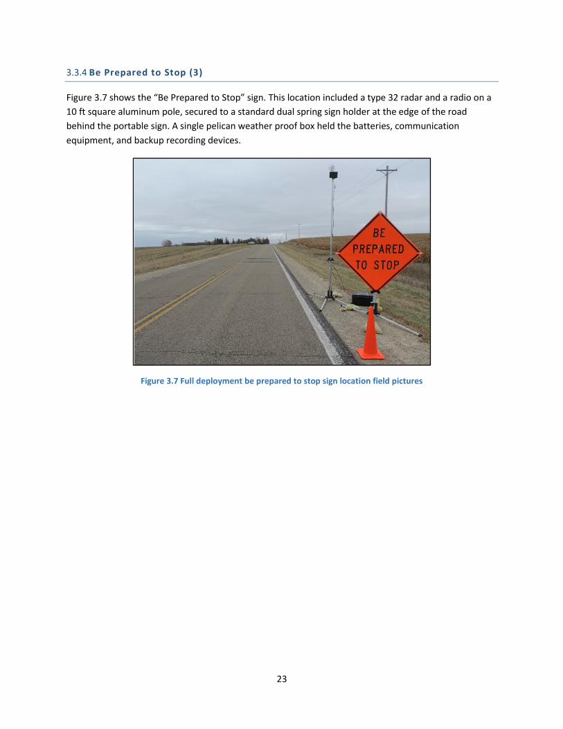
3.3.4 Be Prepared to Stop (3)
Figure 3.7 shows the “Be Prepared to Stop” sign. This location included a type 32 radar and a radio on a
10 ft square aluminum pole, secured to a standard dual spring sign holder at the edge of the road
behind the portable sign. A single pelican weather proof box held the batteries, communication
equipment, and backup recording devices.
Figure 3.7 Full deployment be prepared to stop sign location field pictures
24
3.3.5 Speed Trailer (4)
The location presented in Figure 3.8 included a type 32 radar and radio mounted on a 10 ft square
aluminum pole, secured to a MnDOT speed trailer at the edge of the road. Two HD camera was also
added and looked both into and away from the work zone. A single pelican weather proof box held the
batteries, communication equipment, and backup recording devices.
Figure 3.8 Full Deployment Speed Trailer Location field picture
25
3.3.6 Barrel Horn (5)
The location in Figure 3.9 had a standard work zone construction barrel that had been designed by the
Minnesota Traffic Observatory and alerts the driver via audio ques when speeding next to the device. If
a vehicle approaches the work zone above the speed limit posted on the speed trailer (45mph) the horn
would blast for a one second. The signal for the horn to be fired was provided by the type 32 radar
attached to the speed trailer.
Figure 3.9 Full deployment barrel horn location field pictures
26
3.3.7 Flagger Icon Sign (6)
This location did not include any additional sensors and only contained the standard Flagger Icon sign
seen in Figure 3.10
Figure 3.10 Full Deployment flagger icon sign location field pictures
27
3.3.8 One Lane Road Ahead Sign (7)
This location presented in Figure 3.11 included two types of 30 radars’ and a radio mounted on a 10 ft
square aluminum pole, secured to a standard dual spring sign holder at the edge of the road behind the
portable sign. One radar was pointed away from the work zone at approaching vehicles. The other radar
was pointed backwards into the work zone and tracked the vehicles after they passed the One Lane
Ahead sign. An HD camera was also added and looked into the work zone as vehicles passed the sign. A
single pelican weather proof box held the batteries, communication equipment, and backup recording
devices.
Figure 3.11 Full Deployment one lane road ahead sign location field pictures

28
3.4 RADAR DATA COLLECTION AND EXTRACTION
Data collected from the radar is extremely abundant due to the fact that they transmit a data “message”
every 1/20th of a second. This data needed to be read and stored in real time during the work zone
experiment. After the work zone the data was decoded from its binary message format and specific data
from each message was extracted and converted into a common CSV for additional analysis. This
chapter outlines the format of the CSV files, the data collected, and the method for extracting the
individual vehicle trajectories.
3.5 DATA DESCRIPTION
Each radar sensor produces a “message” every 1/20th of a second (50 milliseconds) while powered. Each
of these messages contains all the information about the sensor, its targets, and additional data. Most of
this data is not necessary for our analysis but was saved in the raw binary format in case it would be
needed later. After data collection was completed the binary data went through post processing and
only the data of interest was saved into comma-separated values (CSV) files.
Each CSV file, one for each day, contains a table with a variable number of rows and 8 columns. Each
row, as seen in Figure 5.12, represents a single target from a single sensor and therefore multiple rows
can have the same timestamp. For example, if a radar sensor sees three targets in its view the CSV file
would contain three separate rows with the same time stamp and sensor ID but different target values.
Figure 3.12 CSV File Format Example
The first column in the CSV file is “time”, which is represented as UNIX time (the numbers of seconds
since Jan 01 1970 (UTC)). The second column is the “sensor_id”, each sensor deployed in the work zone
had a unique ID from 0 to 4 (5 total). The third column is the “object_id”, which is a unique value given
to each target by the radar. These id’s range from 0 to 63, and once id 63 is used the radar begins again
at id 0. Therefore, in the range of each radar sensor every vehicle tracked will be given a unique id as
long as the radar does not lose its target. However, as a vehicle traverses the work zone and enters the
range of each sensor, unique targets will be created in each radar sensor and are more often than not
given different object ids by each radar sensor. The fourth and fifth columns represent x and y
coordinates of each target respectively. These positions are represented, in meters, as the distance
away from the recorded position of the flagger. The sixth and seventh columns represent lateral speed
and longitudinal speed in meters/second. Finally, the last column represents the radars calculated
29
lengths of vehicles in meters. For the purposes of this study the y coordinate and longitudinal speed
were omitted.
3.6 DATA COLLECTED
During the deployment in the active work zone each radar had to be calibrated for the current setup,
whether base or experiment, and physical location on each day. This process generally took 30 minutes
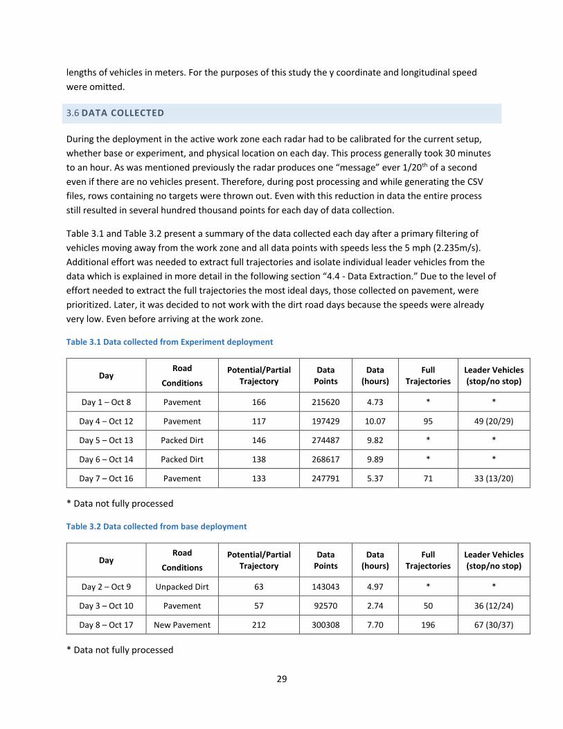
to an hour. As was mentioned previously the radar produces one “message” ever 1/20th of a second
even if there are no vehicles present. Therefore, during post processing and while generating the CSV
files, rows containing no targets were thrown out. Even with this reduction in data the entire process
still resulted in several hundred thousand points for each day of data collection.
Table 3.1 and Table 3.2 present a summary of the data collected each day after a primary filtering of
vehicles moving away from the work zone and all data points with speeds less the 5 mph (2.235m/s).
Additional effort was needed to extract full trajectories and isolate individual leader vehicles from the
data which is explained in more detail in the following section “4.4 - Data Extraction.” Due to the level of
effort needed to extract the full trajectories the most ideal days, those collected on pavement, were
prioritized. Later, it was decided to not work with the dirt road days because the speeds were already
very low. Even before arriving at the work zone.
Table 3.1 Data collected from Experiment deployment
Day Road
Conditions
Potential/Partial Trajectory
Data Points
Data (hours)
Full Trajectories
Leader Vehicles (stop/no stop)
Day 1 – Oct 8 Pavement 166 215620 4.73 * *
Day 4 – Oct 12 Pavement 117 197429 10.07 95 49 (20/29)
Day 5 – Oct 13 Packed Dirt 146 274487 9.82 * *
Day 6 – Oct 14 Packed Dirt 138 268617 9.89 * *
Day 7 – Oct 16 Pavement 133 247791 5.37 71 33 (13/20)
* Data not fully processed
Table 3.2 Data collected from base deployment
Day Road
Conditions
Potential/Partial Trajectory
Data Points
Data (hours)
Full Trajectories
Leader Vehicles (stop/no stop)
Day 2 – Oct 9 Unpacked Dirt 63 143043 4.97 * *
Day 3 – Oct 10 Pavement 57 92570 2.74 50 36 (12/24)
Day 8 – Oct 17 New Pavement 212 300308 7.70 196 67 (30/37)
* Data not fully processed
30
3.7 DATA ERRORS
In almost any form of data collection errors are inevitable. Using QGIS (an Open Source Geographic
Information System) to plot all the data points, allows the formation of trajectories and aids in the
discovery of different types of errors. After observation, data errors are divided into 3 types: data
missing, data redundancy, and noise.
3.7.1 Data Missing
Data missing refers to, as the name suggests, when the radar loses a vehicle and does not create target
information. This can happen for a variety of reasons but is mostly caused by loss of line of sight with a
vehicle, vehicles leaving the approach via a side street, or vehicles that stop moving. Data missing is
further divided into four different types as seen in Figure 3.13. Type A, depicts some segments of data
points are missing when vehicles are passing through the work zone. Type B, represents vehicles that
stop in front of the flagger and the radar cannot detect them due to the fact that the radar is based on
the Doppler effect and when vehicles stop moving they become indistinguishable from the background.
If a vehicle stops for a very long time it can be difficult to associate the other half of the trajectory since
the radar will see them as two separate vehicles and see them as such. Type C, characterizes when a
vehicles trajectories disappear at a given point and never shows up again. This may happen when a
vehicle exits to a side street or if a large vehicle, such as a semitrailer, blocks the radars line of sight with
the vehicle. Type D, symbolizes when a vehicle is not picked up until very late in the work zone. This
most likely occurred due to a vehicle entering at some mid-point in the work zone or if a vehicle that has
been parked for a long time (5+ minutes) begins moving again.
A B C D
Figure 3.13 Examples of Missing Data
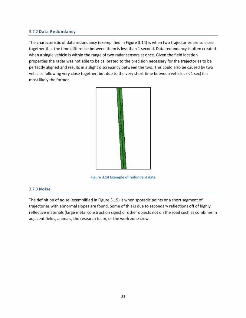
31
3.7.2 Data Redundancy
The characteristic of data redundancy (exemplified in Figure 3.14) is when two trajectories are so close
together that the time difference between them is less than 1 second. Data redundancy is often created
when a single vehicle is within the range of two radar sensors at once. Given the field location
properties the radar was not able to be calibrated to the precision necessary for the trajectories to be
perfectly aligned and results in a slight discrepancy between the two. This could also be caused by two
vehicles following very close together, but due to the very short time between vehicles (< 1 sec) it is
most likely the former.
Figure 3.14 Example of redundant data
3.7.3 Noise
The definition of noise (exemplified in Figure 3.15) is when sporadic points or a short segment of
trajectories with abnormal slopes are found. Some of this is due to secondary reflections off of highly
reflective materials (large metal construction signs) or other objects not on the road such as combines in
adjacent fields, animals, the research team, or the work zone crew.
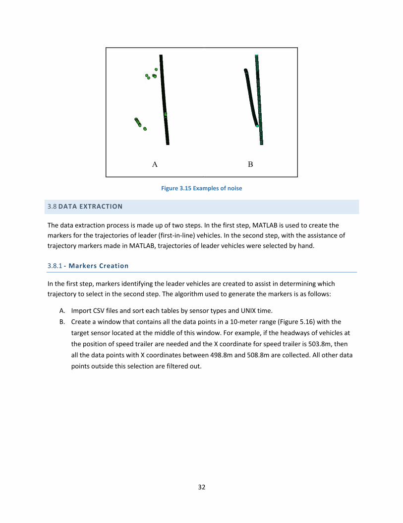
32
A B
Figure 3.15 Examples of noise
3.8 DATA EXTRACTION
The data extraction process is made up of two steps. In the first step, MATLAB is used to create the
markers for the trajectories of leader (first-in-line) vehicles. In the second step, with the assistance of
trajectory markers made in MATLAB, trajectories of leader vehicles were selected by hand.
3.8.1 - Markers Creation
In the first step, markers identifying the leader vehicles are created to assist in determining which
trajectory to select in the second step. The algorithm used to generate the markers is as follows:
A. Import CSV files and sort each tables by sensor types and UNIX time.
B. Create a window that contains all the data points in a 10-meter range (Figure 5.16) with the
target sensor located at the middle of this window. For example, if the headways of vehicles at
the position of speed trailer are needed and the X coordinate for speed trailer is 503.8m, then
all the data points with X coordinates between 498.8m and 508.8m are collected. All other data
points outside this selection are filtered out.
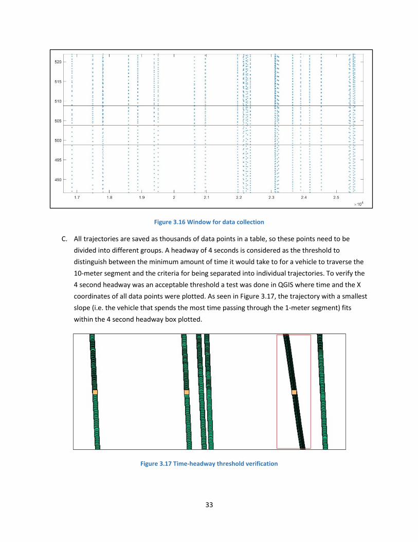
33
Figure 3.16 Window for data collection
C. All trajectories are saved as thousands of data points in a table, so these points need to be
divided into different groups. A headway of 4 seconds is considered as the threshold to
distinguish between the minimum amount of time it would take to for a vehicle to traverse the
10-meter segment and the criteria for being separated into individual trajectories. To verify the
4 second headway was an acceptable threshold a test was done in QGIS where time and the X
coordinates of all data points were plotted. As seen in Figure 3.17, the trajectory with a smallest
slope (i.e. the vehicle that spends the most time passing through the 1-meter segment) fits
within the 4 second headway box plotted.
Figure 3.17 Time-headway threshold verification
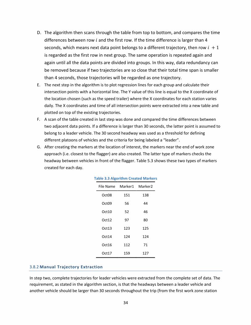
34
D. The algorithm then scans through the table from top to bottom, and compares the time
differences between row 𝑖 and the first row. If the time difference is larger than 4
seconds, which means next data point belongs to a different trajectory, then row 𝑖 + 1
is regarded as the first row in next group. The same operation is repeated again and
again until all the data points are divided into groups. In this way, data redundancy can
be removed because if two trajectories are so close that their total time span is smaller
than 4 seconds, those trajectories will be regarded as one trajectory.
E. The next step in the algorithm is to plot regression lines for each group and calculate their
intersection points with a horizontal line. The Y value of this line is equal to the X coordinate of
the location chosen (such as the speed trailer) where the X coordinates for each station varies
daily. The X coordinates and time of all intersection points were extracted into a new table and
plotted on top of the existing trajectories.
F. A scan of the table created in last step was done and compared the time differences between
two adjacent data points. If a difference is larger than 30 seconds, the latter point is assumed to
belong to a leader vehicle. The 30 second headway was used as a threshold for defining
different platoons of vehicles and the criteria for being labeled a “leader”.
G. After creating the markers at the location of interest, the markers near the end of work zone
approach (i.e. closest to the flagger) are also created. The latter type of markers checks the
headway between vehicles in front of the flagger. Table 5.3 shows these two types of markers
created for each day.
Table 3.3 Algorithm Created Markers
File Name Marker1 Marker2
Oct08 151 138
Oct09 56 44
Oct10 52 46
Oct12 97 80
Oct13 123 125
Oct14 124 124
Oct16 112 71
Oct17 159 127
3.8.2 Manual Trajectory Extraction
In step two, complete trajectories for leader vehicles were extracted from the complete set of data. The
requirement, as stated in the algorithm section, is that the headways between a leader vehicle and
another vehicle should be larger than 30 seconds throughout the trip (from the first work zone station
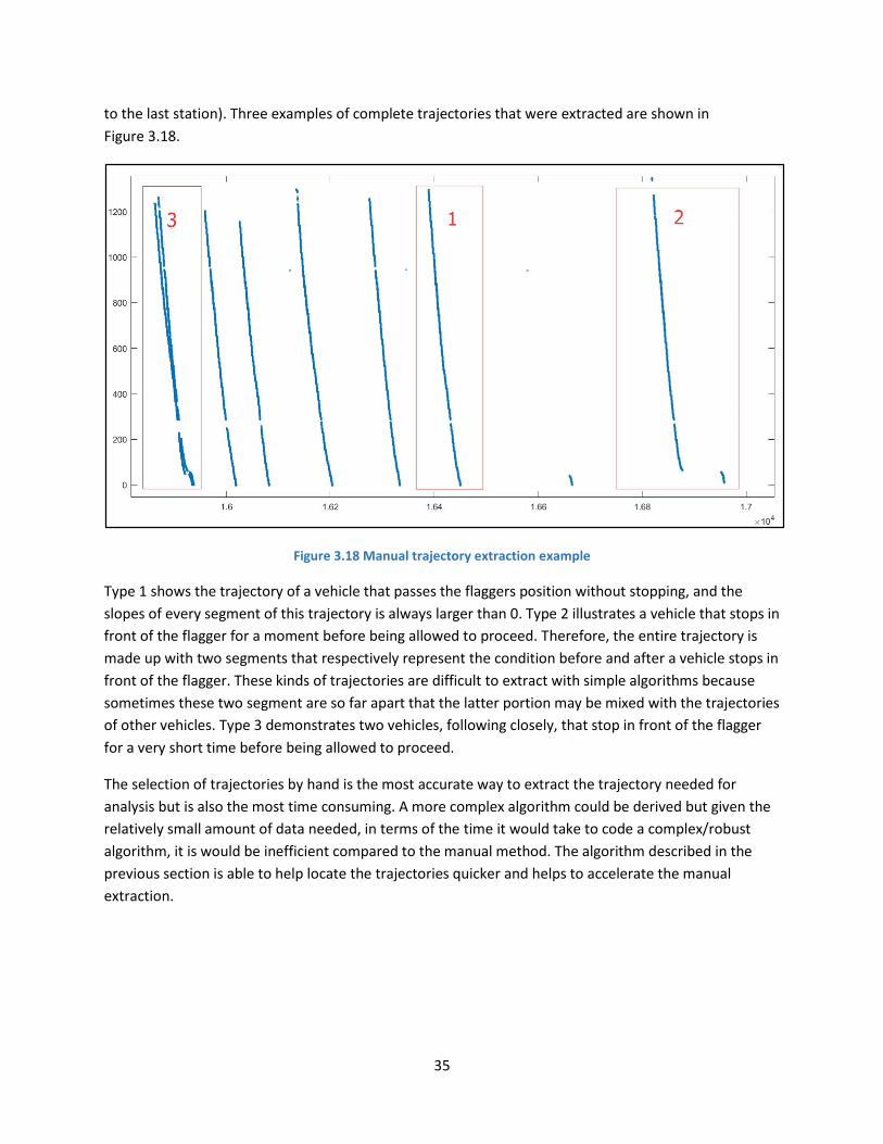
35
to the last station). Three examples of complete trajectories that were extracted are shown in
Figure 3.18.
Figure 3.18 Manual trajectory extraction example
Type 1 shows the trajectory of a vehicle that passes the flaggers position without stopping, and the
slopes of every segment of this trajectory is always larger than 0. Type 2 illustrates a vehicle that stops in
front of the flagger for a moment before being allowed to proceed. Therefore, the entire trajectory is
made up with two segments that respectively represent the condition before and after a vehicle stops in
front of the flagger. These kinds of trajectories are difficult to extract with simple algorithms because
sometimes these two segment are so far apart that the latter portion may be mixed with the trajectories
of other vehicles. Type 3 demonstrates two vehicles, following closely, that stop in front of the flagger
for a very short time before being allowed to proceed.
The selection of trajectories by hand is the most accurate way to extract the trajectory needed for
analysis but is also the most time consuming. A more complex algorithm could be derived but given the
relatively small amount of data needed, in terms of the time it would take to code a complex/robust
algorithm, it is would be inefficient compared to the manual method. The algorithm described in the
previous section is able to help locate the trajectories quicker and helps to accelerate the manual
extraction.

36
Figure 3.19 Example (Experiment Deployment) of trajectories marked by the algorithm and ready for manual
extraction
As Figure 3.19 shows, on an experimental deployment day, orange squares mark those trajectories
which meet the 30 second headway requirement when passing the speed trailer. Red squares mark
those trajectories which meet the requirement when approaching the flagger. Therefore, if a trajectory
is marked by both orange and red squires, it can be regarded as a leader trajectory throughout the trip.
Once identified tools in QGIS allow the selection of those points, using polylines, and saving them to a
new layer separate from the other data. The final product produces a layer that contains only
trajectories that are complete and contain leader vehicles.
3.9 INDIVIDUAL EXAMPLE TRAJECTORIES
Figures 3.20 to 3.23 reveal a preliminary look at the data. These figures depict a single vehicle from one
of the 4 main scenarios:
1. Experimental deployment with no stop at flagger
2. Experimental deployment with a stop at flagger
3. Base deployment with no stop at flagger
4. Base deployment with a stop at flagger
The graphs are marked with vertical lines that correspond to location of the radar sensors during the
different layouts. The distances marked on the x axis are the number of feet from an arbitrary point
upstream to the position of the flagger radar sensor at 4000 ft. The exact position of the flagger is
roughly 150 ft upstream of the radar sensor (i.e. 3850 ft).
This work zone was conducted on a road with a low enough volume that many vehicles approaching the
work zone did not have to stop for the flagger and instead were allowed to proceed directly into the
work zone as directed by the flagger. This represents a distinct change in behavior since as a vehicle
approaches the flagger instead of seeing the stop sign they would see the orange slow sign as well as
motions from the flagger guiding them to the correct lane. This can be seen in Figure 3.20 and Figure
3.22 where the vehicle never went less then 25mph.
Figure 3.20 shows a vehicle traversing the work zone during an experimental deployment. The vehicle
enters the work zone approach at around 60mph and shows a slight decrease in speed as the vehicle
37
approaches the first sign (one lane ahead.) It then maintains a speed around 55mph as it passes the
flagger icon sign before decelerating rapidly in around 500ft in front of the speed trailer to a final speed
of about 38mph at the speed trailer. After that the vehicle then accelerates up to around 45mph in the
first 400ft after the trailer before decelerating again at a fairly constant speed past the “be prepared to
stop” sign. The vehicle reaches a final speed of around 25mph as it is passing the flagger.
Figure 3.21 displays a vehicle traversing the work zone during an experimental deployment. The vehicle
enters the work zone at around 65mph and decreases at a fairly constant rate for the first 2000ft of the
approach and passing the first and second sign settling at a speed of about 58mph. At a distance of
around 300ft from the speed trailer the vehicle shows a rapid decrease in speed from 58mph to around
45mph just after the speed trailer. It then maintains a fairly constant deceleration rate while
approaching the be prepared to stop arriving at a speed of around 42mph as it passes. The vehicle finally
decelerates to a stop from around 40mph to a stop in the final 500ft before the flagger. After a moment
the vehicle is released and accelerates into the work zone.
Figure 3.22 illustrates a vehicle traversing the work zone during a base deployment. The vehicle entered
the work zone at a speed of around 55mph and continued through the approach with only a slight
decrease in speed as it passed the first and second sign. It settled at around 45mph between the one
lane road ahead and the flagger icon sign with only a small increase in speed between the two. At
around 100 ft in front of the flagger icon sign the vehicle began a deceleration to 35 mph over the next
800 ft until the flagger. At this point the vehicle was given permission to enter the work zone and
proceeded through without stopping.
Figure 3.23 depicts a vehicle traversing the work zone during a base deployment. The vehicle entered
the work zone with a speed of around 63mph and maintained that speed until the first sign (road work
ahead.) At this point it started to decelerate at a fairly constant rate over the next 800 ft and arrived at a
speed of about 45mph about 100 ft behind the one lane road sign. The vehicle the accelerated slightly
before decelerating again about 300ft in front of the flagger icon sign. About 600 ft in front of the
flagger the vehicle began decelerating to a stop from 35 mph. After a moment the vehicle is released
and accelerates into the work zone.

38
Figure 3.20 Example Trajectory of a Vehicle During the Experimental Layout That Did Not Stop at The Flagger
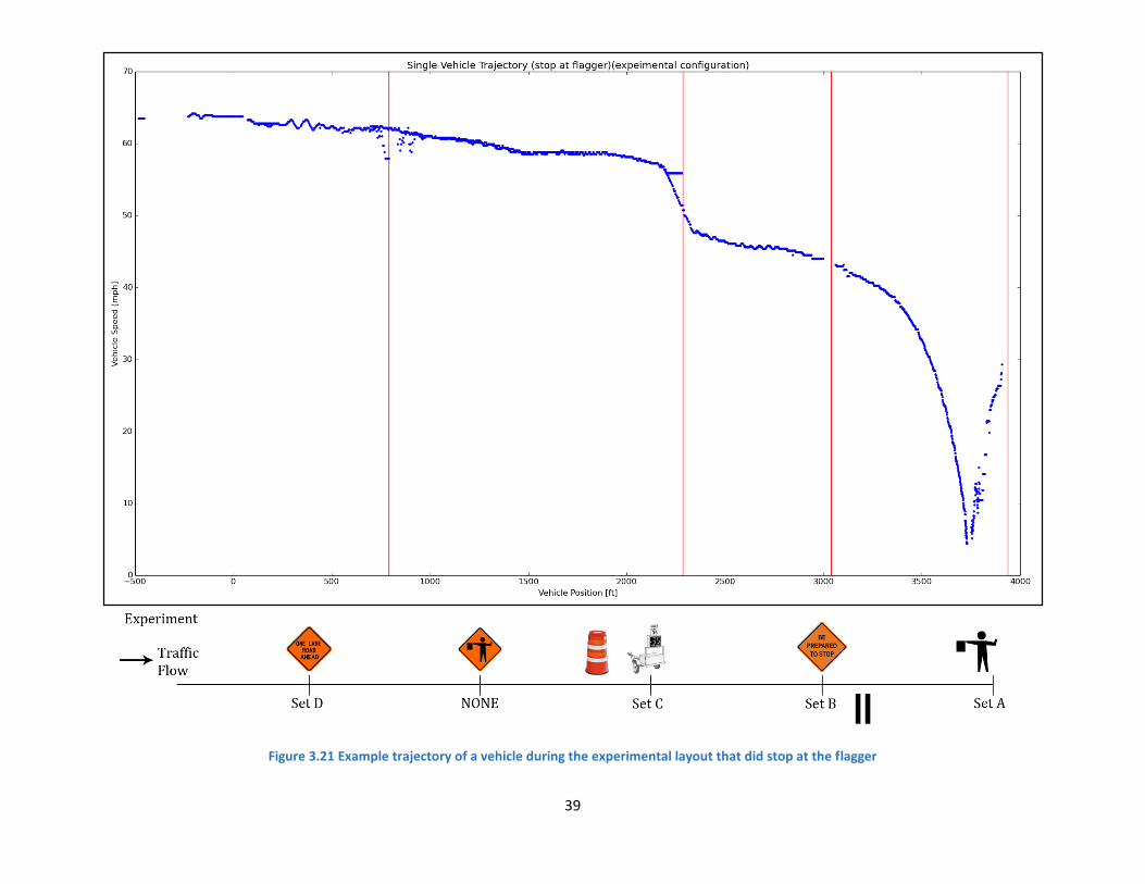
39
Figure 3.21 Example trajectory of a vehicle during the experimental layout that did stop at the flagger
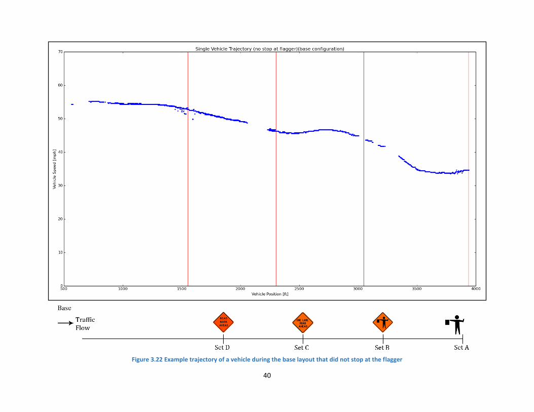
40
Figure 3.22 Example trajectory of a vehicle during the base layout that did not stop at the flagger
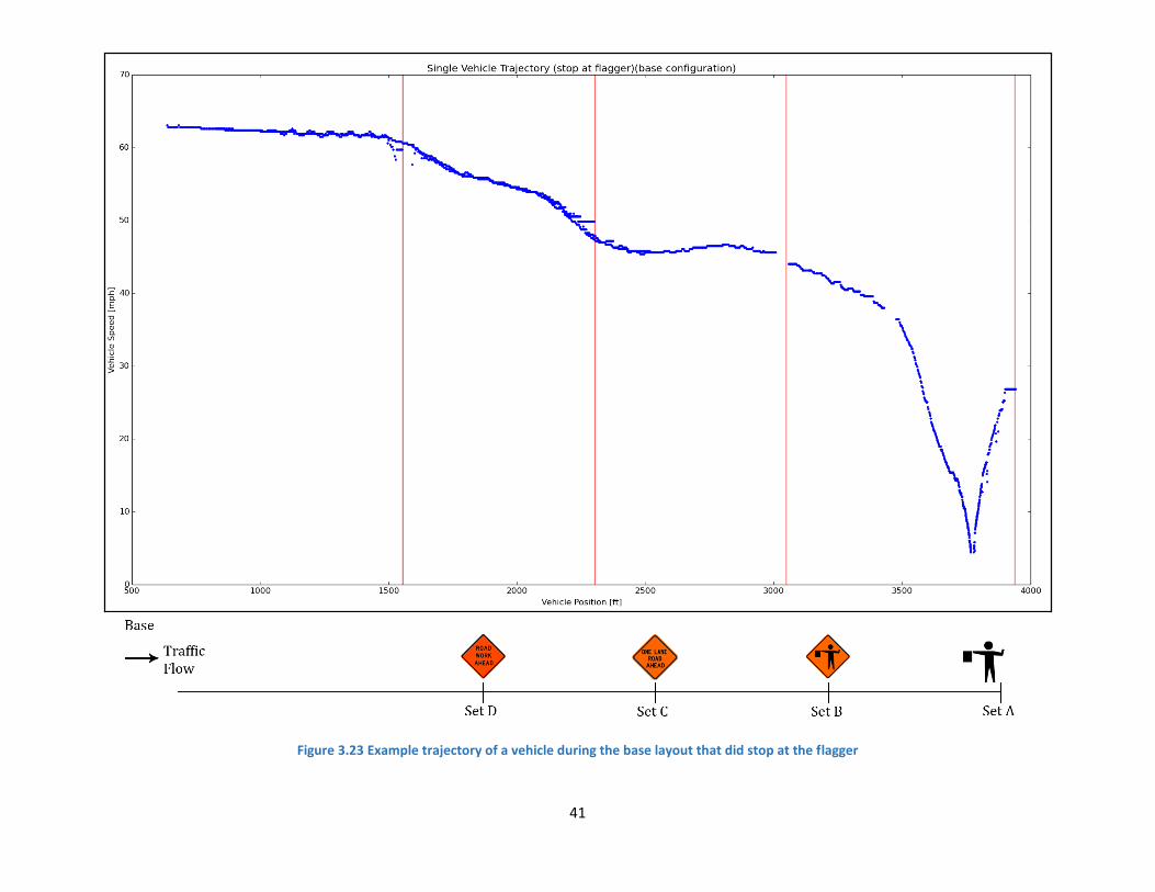
41
Figure 3.23 Example trajectory of a vehicle during the base layout that did stop at the flagger
42
3.10 DATA ANALYSIS AND OBSERVATIONS
3.10.1 Work Zone Data Processing and Analysis
This section outlines the steps followed to process the raw radar data and analyze the results for the
2015 Spring Valley work zone field experiment.
Data Collection: Radar data was collected in the field using a single computer running the software
required to interface with the sensors and parse their raw message streams. This data was stored in an
IPC dump file which stores the data efficiently in binary format. Data from individual sensors were all
stored together in single dump files. Additionally, in these files, vehicle trajectory and position data was
stored in each radar’s individual coordinate frame.
Data Processing: Processing was performed to convert the raw collected data into a format that
combines all the data from each sensor into a single, global coordinate frame. This involved performing
transformations on the data from each sensor based on knowledge about that sensor’s position and
orientation within the work zone coordinate frame.
This data was further processed to extract individual vehicle trajectories. This was conducted by plotting
all the trajectory data in GIS software and then selecting and extracting the points corresponding to a
single vehicle trajectory. Vehicle trajectories were selected such that a selected vehicle represented a
leader vehicle (i.e. any vehicle traveling in the work zone at least 30 seconds after another vehicle). This
was done to ensure independence between selected vehicle trajectories.
Each vehicle trajectory was labeled to identify the following attributes:
Road condition: pavement or gravel
Signage condition: base layout or experimental layout
Flagger behavior: stopping at flagger or not stopping at flagger (per flagger’s signals)
Vehicle type: heavy truck (semi) or automobile (cars, vans, light trucks)
Horn warning deployment: speeds exceeding horn trigger limit or speeds under limit
This resulted in the segmentation of individual vehicles that could then be used in the analysis of driver
behavior in the work zone.
Data analysis: The goal of the data analysis was to determine the effects that the different signage
conditions had on driver speeds through the work zone. The analysis represents the driver speed
behavior as aggregated by distance from the flagger. The work zone is split into 100 feet bins in which
vehicle speed statistics are calculated for the vehicles traveling through those areas.
Statistics are aggregated by identifying the portion of each individual vehicle trajectory contained by a
particular bin. The vehicle’s speed for that bin is then reported as the mean of all speeds recorded for
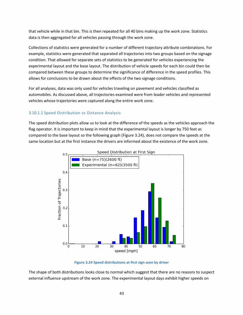
43
that vehicle while in that bin. This is then repeated for all 40 bins making up the work zone. Statistics
data is then aggregated for all vehicles passing through the work zone.
Collections of statistics were generated for a number of different trajectory attribute combinations. For
example, statistics were generated that separated all trajectories into two groups based on the signage
condition. That allowed for separate sets of statistics to be generated for vehicles experiencing the
experimental layout and the base layout. The distribution of vehicle speeds for each bin could then be
compared between these groups to determine the significance of difference in the speed profiles. This
allows for conclusions to be drawn about the effects of the two signage conditions.
For all analyses, data was only used for vehicles traveling on pavement and vehicles classified as
automobiles. As discussed above, all trajectories examined were from leader vehicles and represented
vehicles whose trajectories were captured along the entire work zone.
3.10.1.1 Speed Distribution vs Distance Analysis
The speed distribution plots allow us to look at the difference of the speeds as the vehicles approach the
flag operator. It is important to keep in mind that the experimental layout is longer by 750 feet as
compared to the base layout so the following graph (Figure 3.24), does not compare the speeds at the
same location but at the first instance the drivers are informed about the existence of the work zone.
Figure 3.24 Speed distributions at first sign seen by driver
The shape of both distributions looks close to normal which suggest that there are no reasons to suspect
external influence upstream of the work zone. The experimental layout days exhibit higher speeds on

44
the approach to the work zone which can be an effect of the local road environment. This location in the
experimental days (750 feet upstream of the equivalent location on the base layout) is upstream of a
vertical curve that restricts visibility to the work zone. Noteworthy is that during the base condition days
the drivers had no visibility of the work zone until they were close to the location of the first sign on the
experimental layout. One would think that having earlier warning about a work zone would had caused
the experimental days to exhibit lower speeds and not higher. This suggests that far upstream the work
zone where only the color and location of the first sign is visible the drivers feel no interest in changing
their speed.
Figure 3.25 shows the distribution of speeds 2,600 feet upstream of the flag operator. This is the
location of the first sign on the base layout and the second sign on the experimental layout. As we can
see, speeds are similar with a minor reduction during the experimental days. The distribution of speed
under the experimental layout has lost its normal distribution form suggesting that some of the subjects
have been affected from the message carried over by the first sign. This difference can be seen in the
double Figure 3.26 in which the right chart shows drivers clearly favoring slower speeds as compared to
their earlier condition.
Figure 3.25 Speed distributions at 2,600 ft upstream of flag operator (first sign of Base layout)
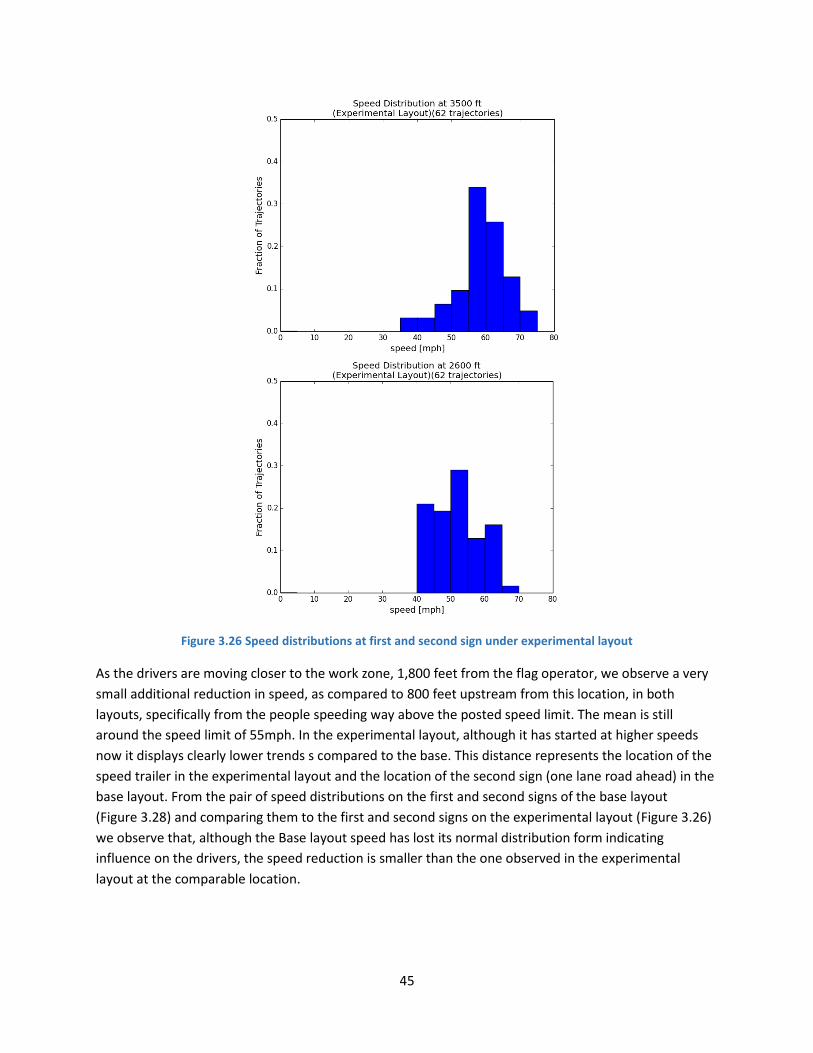
45
Figure 3.26 Speed distributions at first and second sign under experimental layout
As the drivers are moving closer to the work zone, 1,800 feet from the flag operator, we observe a very
small additional reduction in speed, as compared to 800 feet upstream from this location, in both
layouts, specifically from the people speeding way above the posted speed limit. The mean is still
around the speed limit of 55mph. In the experimental layout, although it has started at higher speeds
now it displays clearly lower trends s compared to the base. This distance represents the location of the
speed trailer in the experimental layout and the location of the second sign (one lane road ahead) in the
base layout. From the pair of speed distributions on the first and second signs of the base layout
(Figure 3.28) and comparing them to the first and second signs on the experimental layout (Figure 3.26)
we observe that, although the Base layout speed has lost its normal distribution form indicating
influence on the drivers, the speed reduction is smaller than the one observed in the experimental
layout at the comparable location.
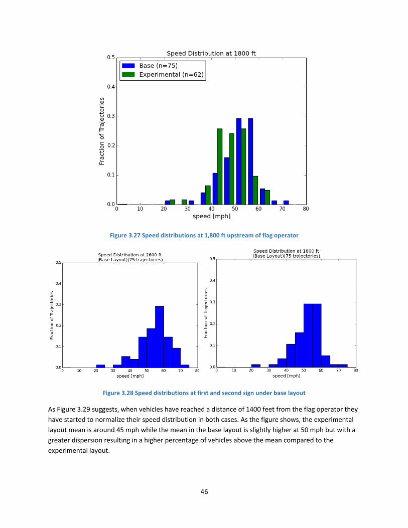
46
Figure 3.27 Speed distributions at 1,800 ft upstream of flag operator
Figure 3.28 Speed distributions at first and second sign under base layout
As Figure 3.29 suggests, when vehicles have reached a distance of 1400 feet from the flag operator they
have started to normalize their speed distribution in both cases. As the figure shows, the experimental
layout mean is around 45 mph while the mean in the base layout is slightly higher at 50 mph but with a
greater dispersion resulting in a higher percentage of vehicles above the mean compared to the
experimental layout.
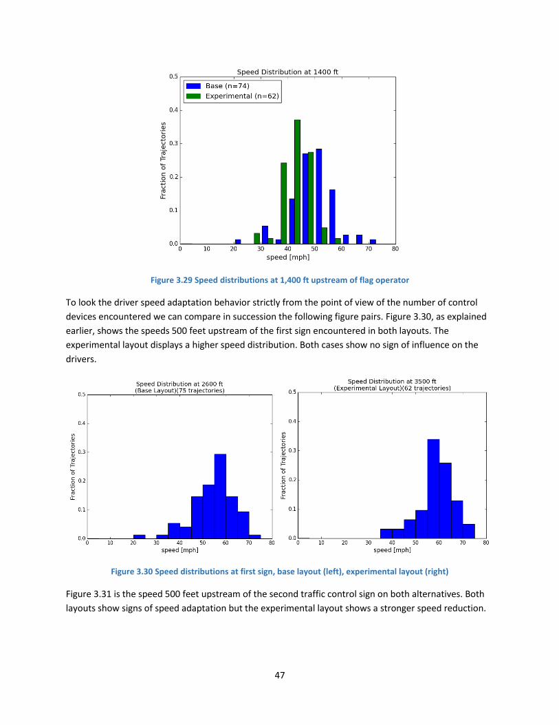
47
Figure 3.30 Speed distributions at first sign, base layout (left), experimental layout (right)
Figure 3.29 Speed distributions at 1,400 ft upstream of flag operator
To look the driver speed adaptation behavior strictly from the point of view of the number of control
devices encountered we can compare in succession the following figure pairs. Figure 3.30, as explained
earlier, shows the speeds 500 feet upstream of the first sign encountered in both layouts. The
experimental layout displays a higher speed distribution. Both cases show no sign of influence on the
drivers.
Figure 3.31 is the speed 500 feet upstream of the second traffic control sign on both alternatives. Both
layouts show signs of speed adaptation but the experimental layout shows a stronger speed reduction.
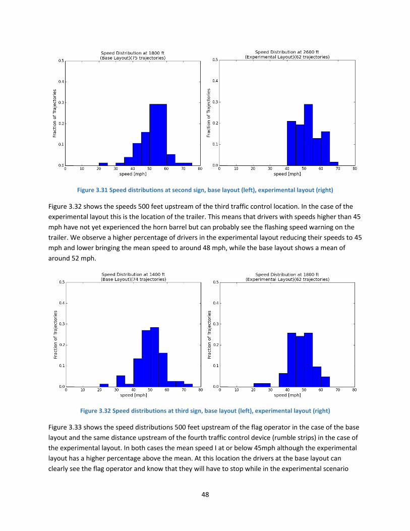
48
Figure 3.31 Speed distributions at second sign, base layout (left), experimental layout (right)
Figure 3.32 Speed distributions at third sign, base layout (left), experimental layout (right)
Figure 3.32 shows the speeds 500 feet upstream of the third traffic control location. In the case of the
experimental layout this is the location of the trailer. This means that drivers with speeds higher than 45
mph have not yet experienced the horn barrel but can probably see the flashing speed warning on the
trailer. We observe a higher percentage of drivers in the experimental layout reducing their speeds to 45
mph and lower bringing the mean speed to around 48 mph, while the base layout shows a mean of
around 52 mph.
Figure 3.33 shows the speed distributions 500 feet upstream of the flag operator in the case of the base
layout and the same distance upstream of the fourth traffic control device (rumble strips) in the case of
the experimental layout. In both cases the mean speed I at or below 45mph although the experimental
layout has a higher percentage above the mean. At this location the drivers at the base layout can
clearly see the flag operator and know that they will have to stop while in the experimental scenario
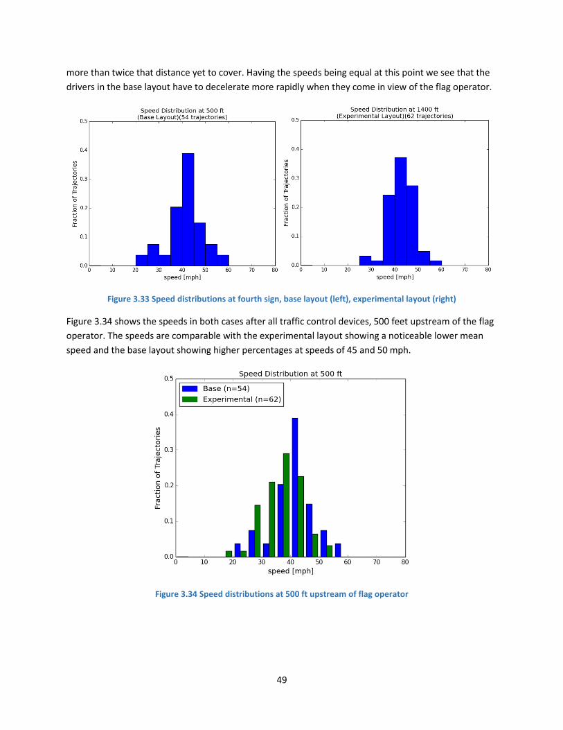
49
more than twice that distance yet to cover. Having the speeds being equal at this point we see that the
drivers in the base layout have to decelerate more rapidly when they come in view of the flag operator.
Figure 3.33 Speed distributions at fourth sign, base layout (left), experimental layout (right)
Figure 3.34 shows the speeds in both cases after all traffic control devices, 500 feet upstream of the flag
operator. The speeds are comparable with the experimental layout showing a noticeable lower mean
speed and the base layout showing higher percentages at speeds of 45 and 50 mph.
Figure 3.34 Speed distributions at 500 ft upstream of flag operator

50
3.11 SPEED ADAPTATION COMPARISONS
The following section contains the comparison of the speeds drivers selected in their approach to the
work zone under the experimental and base layouts during the 2015 field experiment. These figures are
the results of a statistical analysis of the collected data grouped in various ways in an attempt to
uncover the underlying driver behavior. Each combination graph contains a line representing the
median speed over distance. The shadowed area around each line marks the 75th and 25th percentile
speeds in each location. The black box contains the range of speeds/distances where the two work zone
layouts have produced speed differences that are statistically significant. The respective layouts are also
shown in the figures. For completeness the results from the 2014 field experiment are also included.
Figure 3.35 presents the speeds collected from all leading vehicles under the two work zone traffic
control alternatives. The experimental layout in general produced lower speeds but the speeds of the
vehicles substantially differ from the base layout case as the drivers approach the speed trailer and horn
barrel. While under the base layout we note a steady deceleration up until the last sign before the flag
operator, under the experimental layout we note a more complex behavior. Experimental layout drivers
start their deceleration earlier than their counterparts under the base layout. This is logical since the
experimental layout starts 750 feet upstream of the base layout. Until approximately 400 feet upstream
of the speed trailer the experimental layout drivers follow a similar steady deceleration. As they
approach the speed trailer, approximately at the location of the horn, the drivers apply a greater
deceleration. It is interesting to note that this greater deceleration brings the median speed below
45mph after the speed trailer at which point the drivers under the experimental layout accelerate
slightly to reach 45mph. The aforementioned acceleration last until approximately 400 feet upstream of
the rumble strips at which point the experimental layout drivers start a stronger deceleration in order to
stop at the flag operator. Although there is strong evidence that the speed trailer causes the drivers to
decelerate at a higher rate, there are no evidence that the rumble strips have any effect on speed
selection. In general, we can confidently say that the experimental layout produces slower speeds in the
approach to the work zone and, at least in the case of the speed trailer, and in extends we can be
certain that it succeeds in attracting the attention of the drivers.
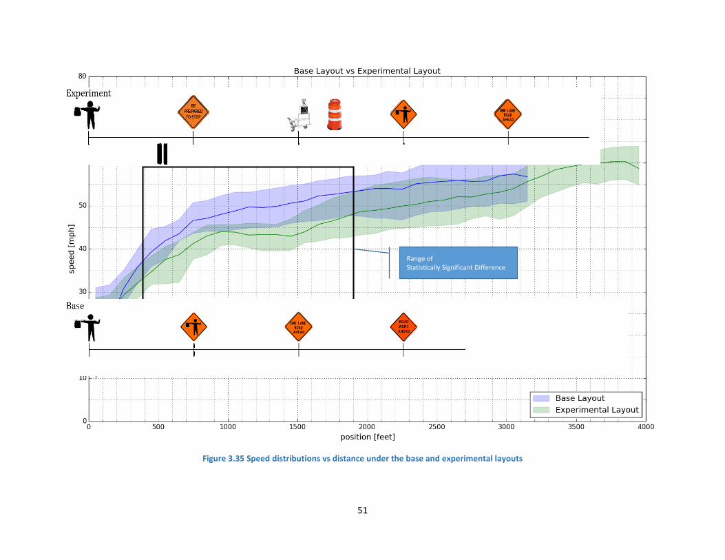
51
Figure 3.35 Speed distributions vs distance under the base and experimental layouts
Range of Statistically Significant Difference

52
Figure 3.36 and Figure 3.37 present the distributions of speed under the base and the experimental
layouts respectively. In comparing the two results it is worth noting that under the base layout the
dispersion of speeds is considerably higher and includes a few high speed outliers while the dispersion
of speed, as expressed by the 75th and 25th percentile bounds, is narrower and presents no high speed
outliers. The two are comparable at the earliest points upstream of the work zone which suggest that
there was minimal influence of exogenous factors other than the work zone layout.
Figure 3.39 attempts to separate the drivers under the experimental layout that experienced the horn vs
the ones that did not. Naturally, the ones that experienced the horn are the ones that were speeding so
the difference in speed levels is not informative but the deceleration patterns is telling of drivers’
reaction to the horn and the trailer. In both cases the drivers reach a speed lower than 45mph after the
trailer and accelerate slightly. This suggest that the trailer has an effect on driver behavior regardless of
the horn. Although both populations initially have similar speeds, speeders are displaying a much lower
deceleration as they enter the work zone boundary; still having speeds well above the speed limit.
Although non-speeders employ a steady deceleration between the first warning sign and before the
rumble strips, speeders display a very low, practically zero, deceleration till they reach the horn and be
in view of the trailer at which point they decelerate sharply to bring themselves below or at the work
zone speed limit. Clearly, although speeders have been informed of the work zone existence, they do
not show signs of speed compliance until the more dynamic warnings of the horn and the trailer. A
hypothesis is that they comply because they realize that their speed is monitored. From Figure 3.40 we
see that speeders under the experimental layout are also well below the speeding drivers under the
base layout and reach legal speeds well upstream of the flag operator.
Figure 3.41 shows the statistics of the driver population that did not have to stop at the flag operator
because either were the only vehicles on the scene (both ways) or they were the next vehicle after that
direction was given the right-of-way. Again we see a statistically significant lower speed pattern under
the experimental layout as compared to the base one although both populations reach similar speeds,
around 30mph, at the flag operator.
Figure 3.44 shows the speed adaptation of the driver population that had to stop at the flag operator.
Note that these are the first vehicles in line and no other vehicles were in queue at the flag post. Speeds
between these two groups are lower under the experimental layout but only statistically significantly
different right after the trailer and before the rumble strips.
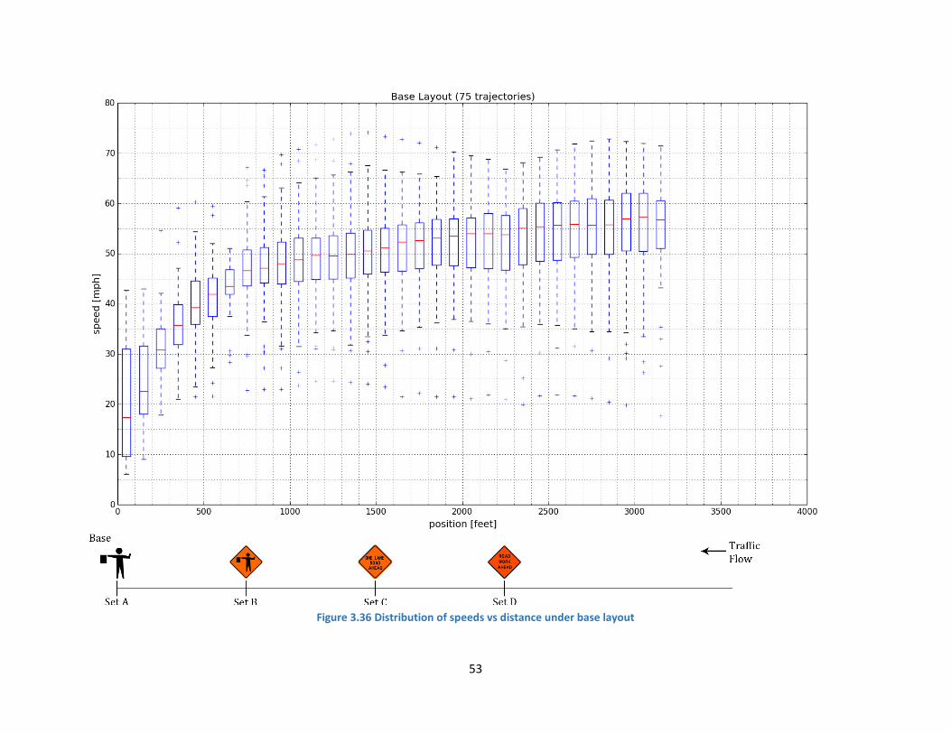
53
Figure 3.36 Distribution of speeds vs distance under base layout
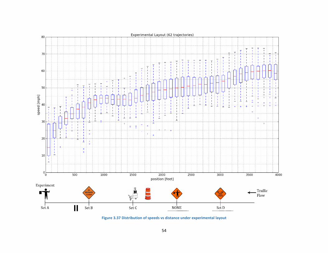
54
Figure 3.37 Distribution of speeds vs distance under experimental layout

55
Figure 3.38 Speed distributions vs distance under experimental layout. Speeders vs normal drivers.
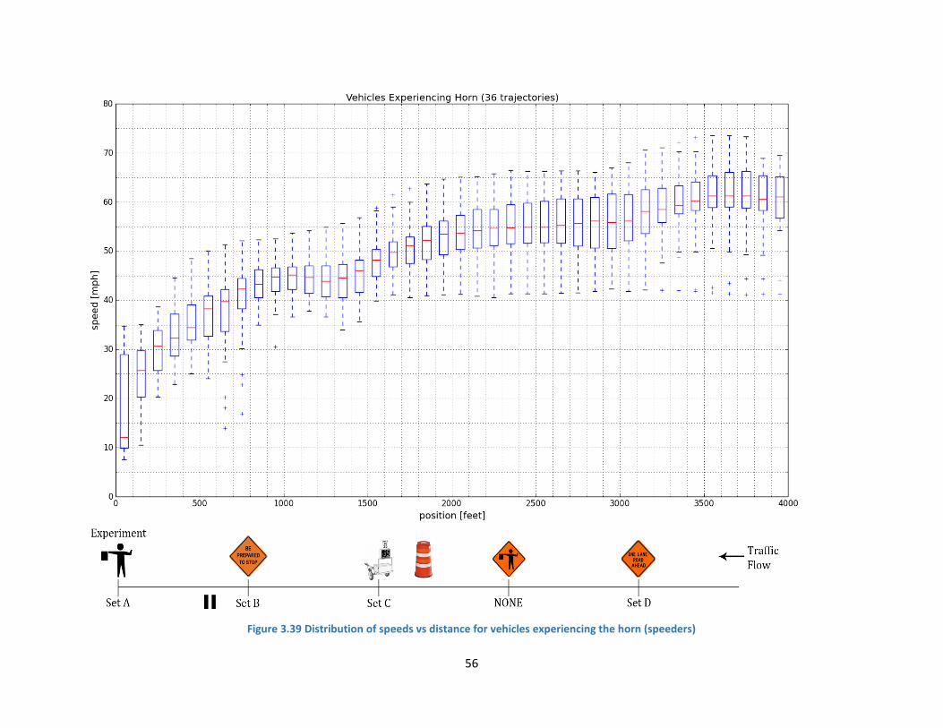
56
Figure 3.39 Distribution of speeds vs distance for vehicles experiencing the horn (speeders)
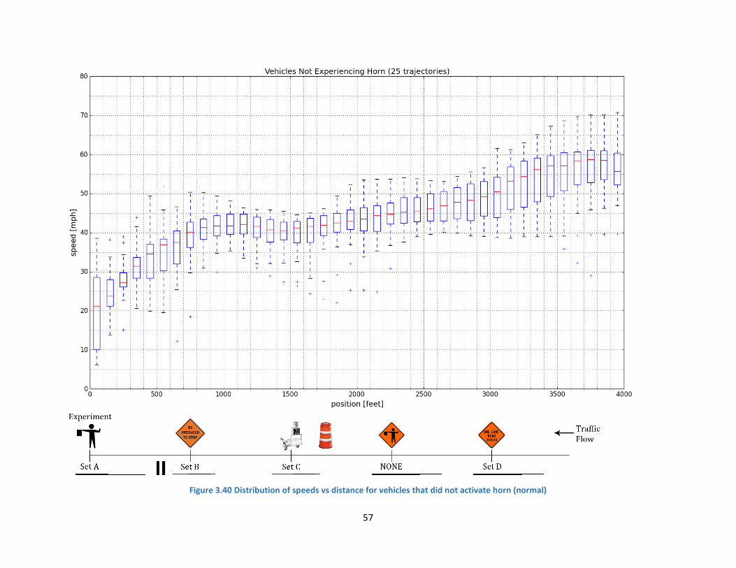
57
Figure 3.40 Distribution of speeds vs distance for vehicles that did not activate horn (normal)

58
Figure 3.41 Speed distributions vs Distance. Vehicles that didn’t have to stop at flag operator.
Range of
Statistically Significant Difference
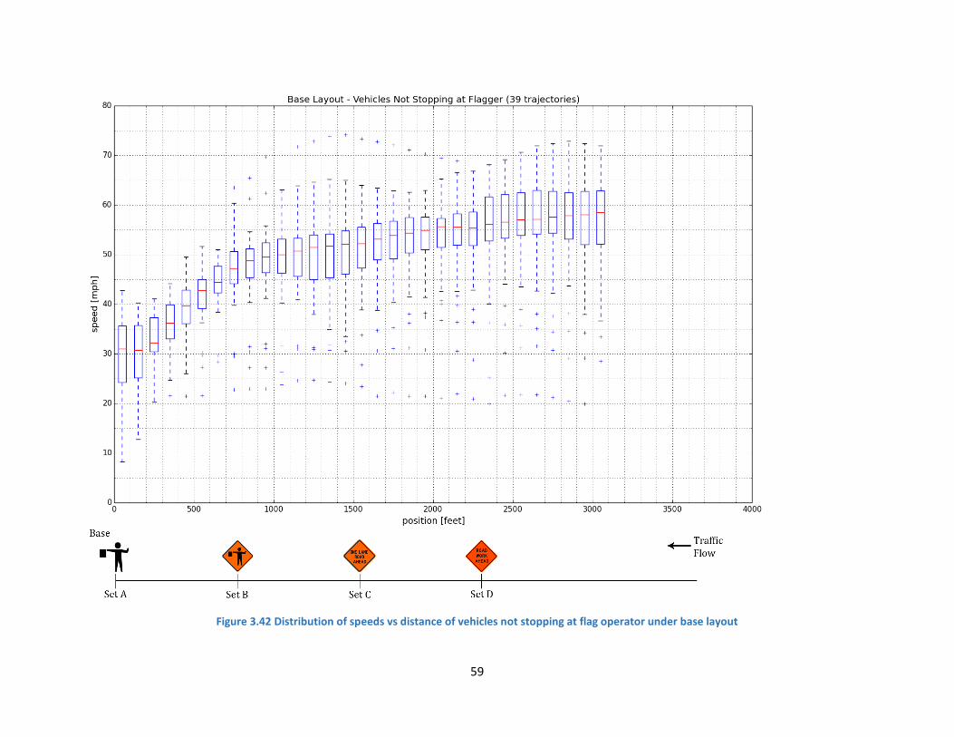
59
Figure 3.42 Distribution of speeds vs distance of vehicles not stopping at flag operator under base layout
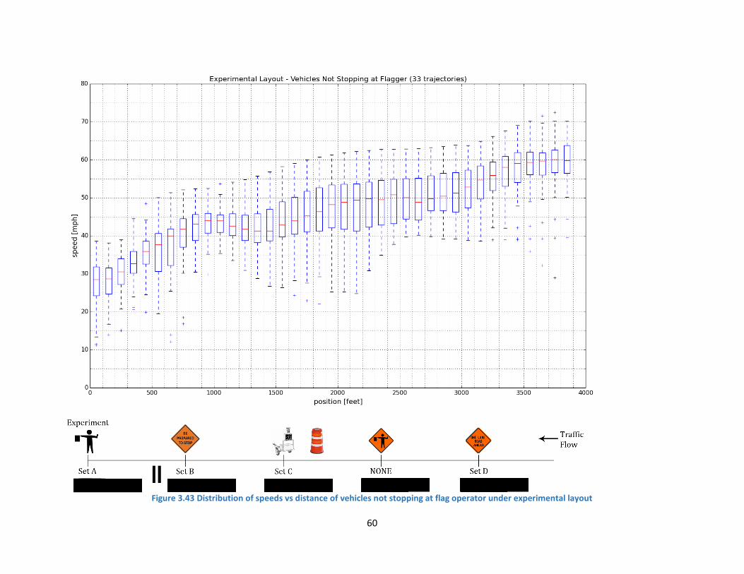
60
Figure 3.43 Distribution of speeds vs distance of vehicles not stopping at flag operator under experimental layout
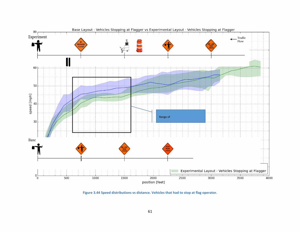
61
Figure 3.44 Speed distributions vs distance. Vehicles that had to stop at flag operator.
Range of
Statistically Significant Difference
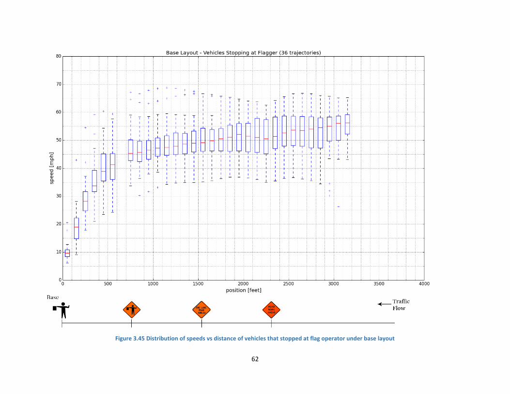
62
Figure 3.45 Distribution of speeds vs distance of vehicles that stopped at flag operator under base layout
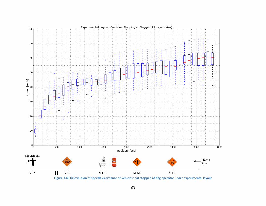
63
Figure 3.46 Distribution of speeds vs distance of vehicles that stopped at flag operator under experimental layout

64
Figure 3.47 and Figure 3.48 show the results from the 2014 field experiment and are included here for
completeness. In the earlier discussion and figures all data were from leader vehicles so the more
appropriate discussion can be based on Figure 3.48. Although the population in 2014 was considerably
smaller than the population captured in 2015, we still see the same behavior in terms of speed
adaptation.
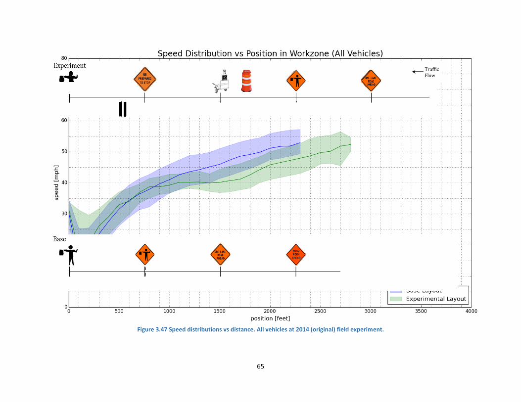
65
Figure 3.47 Speed distributions vs distance. All vehicles at 2014 (original) field experiment.
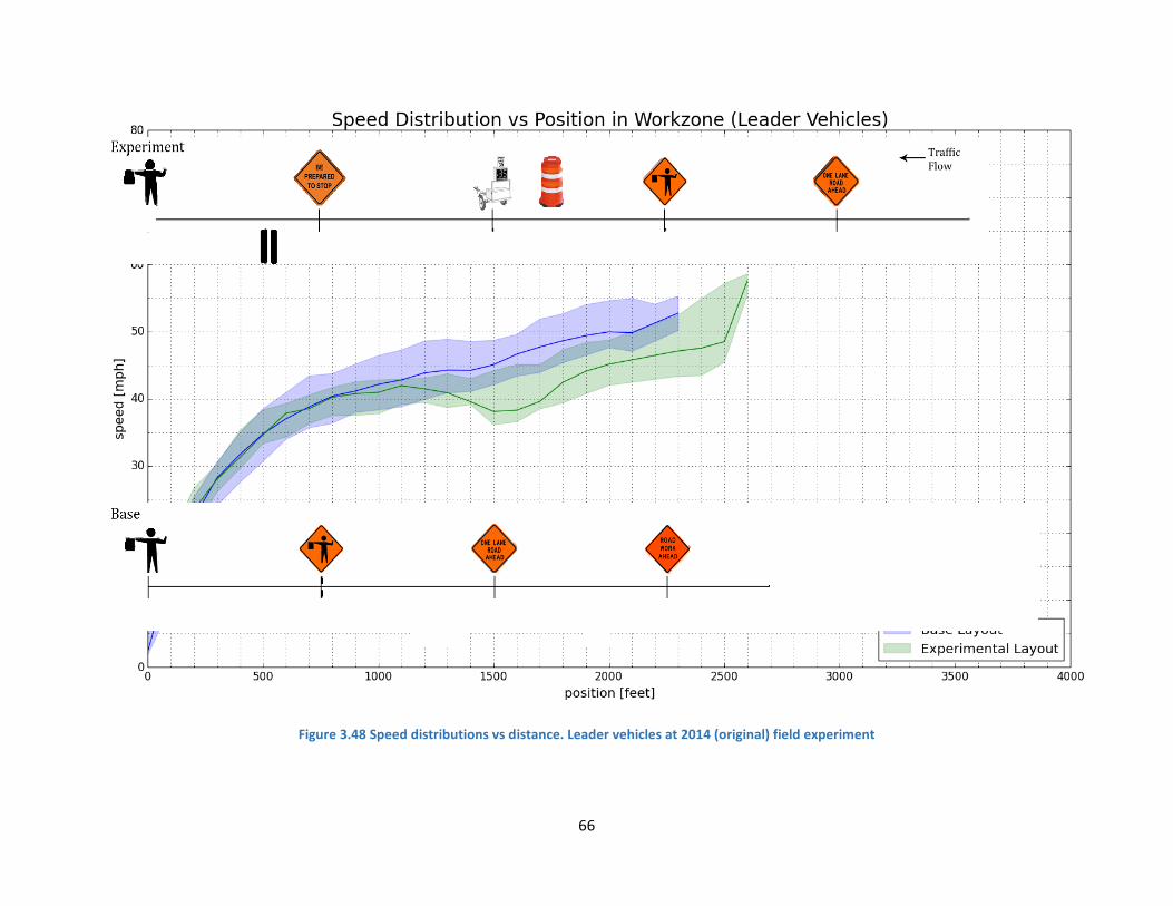
66
Figure 3.48 Speed distributions vs distance. Leader vehicles at 2014 (original) field experiment
67
3.12 FIELD STUDY CONCLUSIONS
The two field deployments of the experimentally identified new proposed traffic control layout in
flagger-controlled work zones revealed that the speed trailer + horn successfully influenced drivers to
reduce speeds, but the portable rumble strips did not. It is important to note, however, that an
independent assessment of portable rumble strips was not within the scope of this study. Rather the
portable rumble strips were included in a set of new treatments and were located downstream from the
speed trailer + horn so drivers remained under the influence of the speed trailer + horn as they
approached the rumble strips.
Because the combination speed trailer + horn spatially preceded the rumble strips the influence of the
speed trailer + horn can be evaluated. Our findings reveal that the speed trailer + horn have a significant
influence on a reduction in driver speed as well as the spread of the speed samples. As discussed earlier
in this document, the experimental layout practically eliminated high speed outliers in addition to
succeeding in reducing the approach speed to the flag operator.
68
CHAPTER 4: CONCLUSIONS
4.1 SUMMARY FINDINGS AND CONCLUSIONS OF THE DRIVING SIMULATOR EXPERIMENT
In this exeriment, we used a driving simulator to identify elements that capture and sustain driver
attention in flagger-controlled work zones. We obtained lane position data and driving speed data from
the 160 participants who drove the simulated rural highway three times. We were particularly
interested in determining whether flashing LED lights mounted on the first warning sign of an approach
to a flagger-controlled work zone contributed to more significant reductions in speed than the same sign
without the flashing LED lights. We are also particularly interested in whether a horn blast emitted for
drivers exceeding 45 mph on their approach to an intelligent speed limit display effectively captured the
attention of outlier drivers. And we were interested in determining the effectiveness of transverse
rumble strips as an attention-grabbing device in a simulated flagger-controlled work zone.
Our main findings are the following:
The new set of elements is more effective than the elements currently used to reduce driving
speeds on the approach to the flagger-controlled work zone;
We found no difference in mean driver speed in response to the sign with an LED presence;
The dynamic speed display coupled with the horn is more effective than the dynamic speed
display alone;
• Survey responses provide helpful self-reported information from drivers.
4.2 SUMMARY FINDINGS AND CONCLUSIONS OF THE FIELD STUDY
The two field deployments of the new experimentally identified proposed traffic control layout in
flagger-controlled work zones revealed that the speed trailer + horn successfully influenced drivers to
reduce speeds, but the portable rumble strips did not. It is important to note, however, that an
independent assessment of portable rumble strips was not within the scope of this study. Rather the
portable rumble strips were included in the set of new treatments and were located downstream from
the speed trailer + horn so drivers may have remained under the influence of the speed trailer + horn as
they approached the rumble strips.
Because the combination speed trailer + horn spatially preceded the rumble strips the influence of the
speed trailer + horn can be evaluated. Our findings reveal that the speed trailer + horn had a significant
influence on driver speed as well as the spread of the speed samples. As discussed earlier in this
document, the experimental layout practically eliminated high-speed outliers in addition to succeeding
in reducing the approach speed to the flag operator.

69
4.3 OVERALL SUMMARY
The elements identified as effective in capturing and sustaining driver attention in flagger controlled
work zones in the laboratory were then tested in a field study. The field study confirmed the findings of
the driving simulator study. As noted above, our findings clearly indicate that the experimental layout
was highly successful in practically eliminating high-speed outliers as well as in reducing the approach
speed to the flag operator.
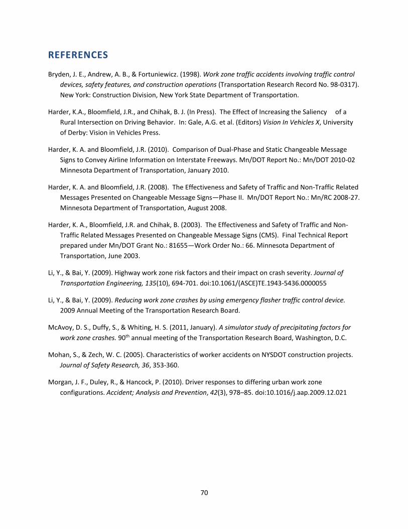
70
REFERENCES
Bryden, J. E., Andrew, A. B., & Fortuniewicz. (1998). Work zone traffic accidents involving traffic control
devices, safety features, and construction operations (Transportation Research Record No. 98-0317).
New York: Construction Division, New York State Department of Transportation.
Harder, K.A., Bloomfield, J.R., and Chihak, B. J. (In Press). The Effect of Increasing the Saliency of a
Rural Intersection on Driving Behavior. In: Gale, A.G. et al. (Editors) Vision In Vehicles X, University
of Derby: Vision in Vehicles Press.
Harder, K. A. and Bloomfield, J.R. (2010). Comparison of Dual-Phase and Static Changeable Message
Signs to Convey Airline Information on Interstate Freeways. Mn/DOT Report No.: Mn/DOT 2010-02
Minnesota Department of Transportation, January 2010.
Harder, K. A. and Bloomfield, J.R. (2008). The Effectiveness and Safety of Traffic and Non-Traffic Related
Messages Presented on Changeable Message Signs—Phase II. Mn/DOT Report No.: Mn/RC 2008-27.
Minnesota Department of Transportation, August 2008.
Harder, K. A., Bloomfield, J.R. and Chihak, B. (2003). The Effectiveness and Safety of Traffic and Non-
Traffic Related Messages Presented on Changeable Message Signs (CMS). Final Technical Report
prepared under Mn/DOT Grant No.: 81655—Work Order No.: 66. Minnesota Department of
Transportation, June 2003.
Li, Y., & Bai, Y. (2009). Highway work zone risk factors and their impact on crash severity. Journal of
Transportation Engineering, 135(10), 694-701. doi:10.1061/(ASCE)TE.1943-5436.0000055
Li, Y., & Bai, Y. (2009). Reducing work zone crashes by using emergency flasher traffic control device.
2009 Annual Meeting of the Transportation Research Board.
McAvoy, D. S., Duffy, S., & Whiting, H. S. (2011, January). A simulator study of precipitating factors for
work zone crashes. 90th annual meeting of the Transportation Research Board, Washington, D.C.
Mohan, S., & Zech, W. C. (2005). Characteristics of worker accidents on NYSDOT construction projects.
Journal of Safety Research, 36, 353-360.
Morgan, J. F., Duley, R., & Hancock, P. (2010). Driver responses to differing urban work zone
configurations. Accident; Analysis and Prevention, 42(3), 978–85. doi:10.1016/j.aap.2009.12.021

APPENDIX A
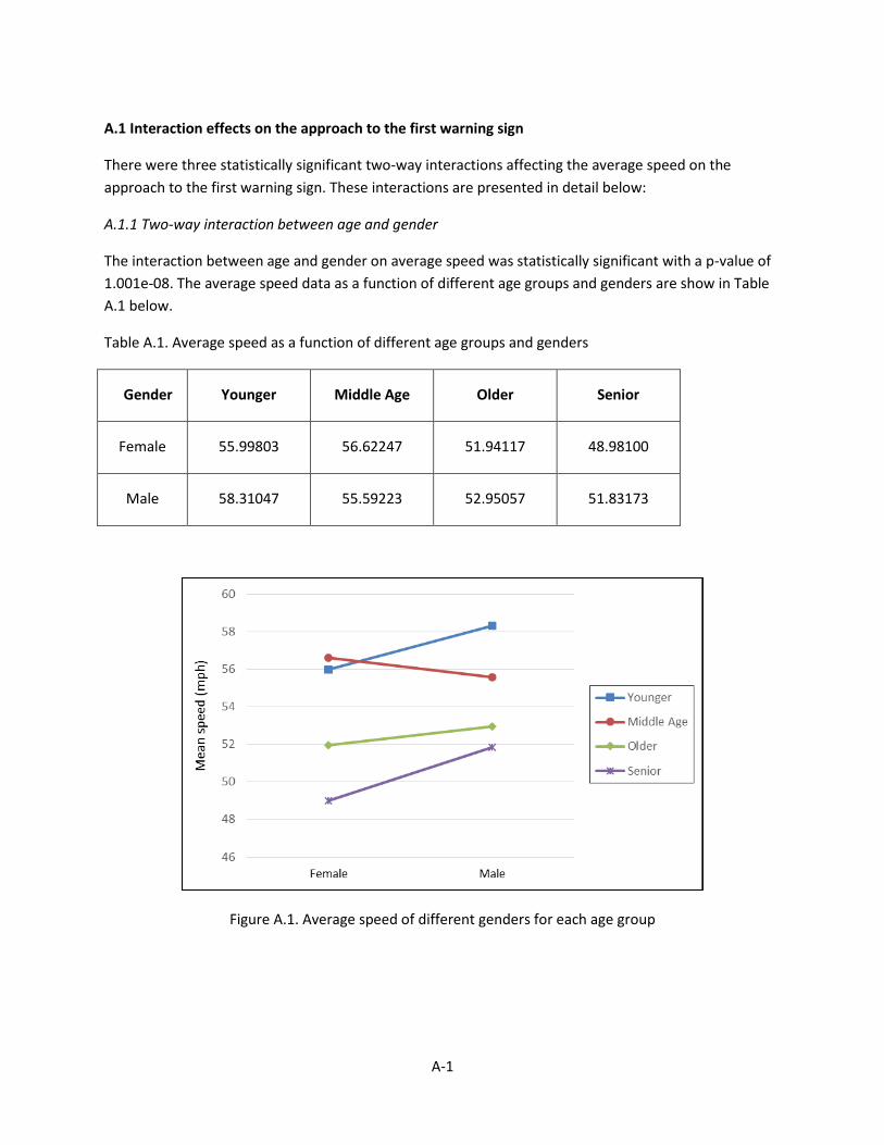
A-1
A.1 Interaction effects on the approach to the first warning sign
There were three statistically significant two-way interactions affecting the average speed on the
approach to the first warning sign. These interactions are presented in detail below:
A.1.1 Two-way interaction between age and gender
The interaction between age and gender on average speed was statistically significant with a p-value of
1.001e-08. The average speed data as a function of different age groups and genders are show in Table
A.1 below.
Table A.1. Average speed as a function of different age groups and genders
Gender Younger Middle Age Older Senior
Female 55.99803 56.62247 51.94117 48.98100
Male 58.31047 55.59223 52.95057 51.83173
Figure A.1. Average speed of different genders for each age group
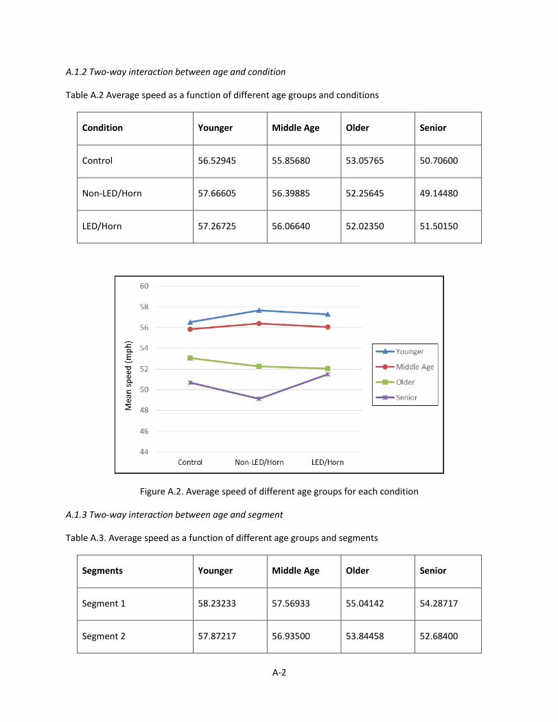
A-2
A.1.2 Two-way interaction between age and condition
Table A.2 Average speed as a function of different age groups and conditions
Condition Younger Middle Age Older Senior
Control 56.52945 55.85680 53.05765 50.70600
Non-LED/Horn 57.66605 56.39885 52.25645 49.14480
LED/Horn 57.26725 56.06640 52.02350 51.50150
Figure A.2. Average speed of different age groups for each condition
A.1.3 Two-way interaction between age and segment
Table A.3. Average speed as a function of different age groups and segments
Segments Younger Middle Age Older Senior
Segment 1 58.23233 57.56933 55.04142 54.28717
Segment 2 57.87217 56.93500 53.84458 52.68400
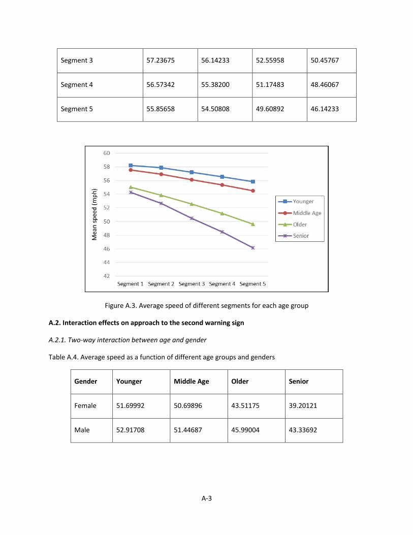
A-3
Segment 3 57.23675 56.14233 52.55958 50.45767
Segment 4 56.57342 55.38200 51.17483 48.46067
Segment 5 55.85658 54.50808 49.60892 46.14233
Figure A.3. Average speed of different segments for each age group
A.2. Interaction effects on approach to the second warning sign
A.2.1. Two-way interaction between age and gender
Table A.4. Average speed as a function of different age groups and genders
Gender Younger Middle Age Older Senior
Female 51.69992 50.69896 43.51175 39.20121
Male 52.91708 51.44687 45.99004 43.33692
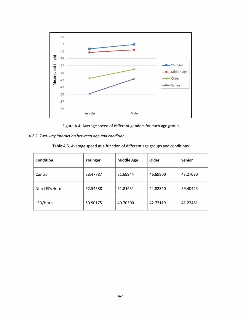
A-4
Figure A.4. Average speed of different genders for each age group
A.2.2. Two-way interaction between age and condition
Table A.5. Average speed as a function of different age groups and conditions
Condition Younger Middle Age Older Senior
Control 53.47787 51.69944 46.69800 43.27090
Non-LED/Horn 52.54588 51.81631 44.82350 39.40425
LED/Horn 50.90175 49.70300 42.73119 41.22481
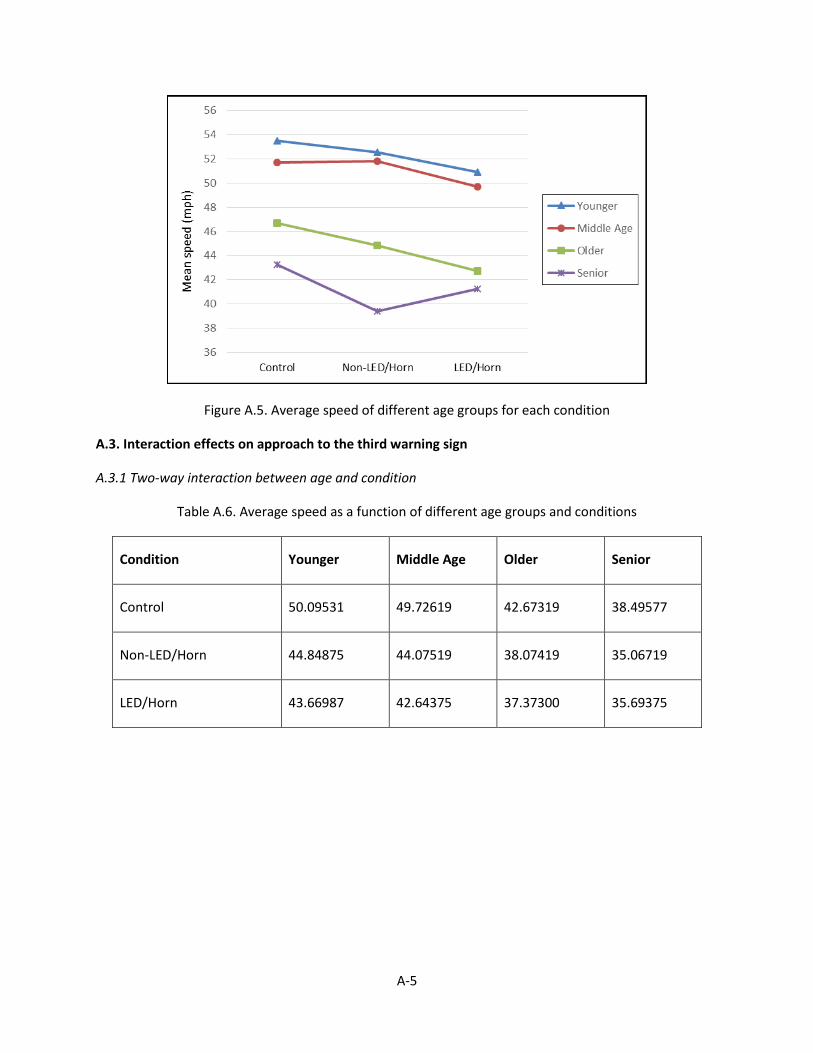
A-5
Figure A.5. Average speed of different age groups for each condition
A.3. Interaction effects on approach to the third warning sign
A.3.1 Two-way interaction between age and condition
Table A.6. Average speed as a function of different age groups and conditions
Condition Younger Middle Age Older Senior
Control 50.09531 49.72619 42.67319 38.49577
Non-LED/Horn 44.84875 44.07519 38.07419 35.06719
LED/Horn 43.66987 42.64375 37.37300 35.69375
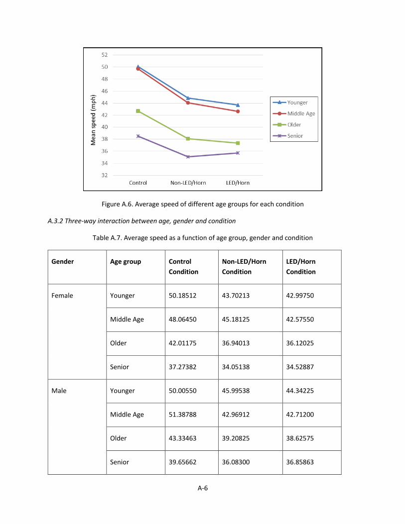
A-6
Figure A.6. Average speed of different age groups for each condition
A.3.2 Three-way interaction between age, gender and condition
Table A.7. Average speed as a function of age group, gender and condition
Gender Age group Control
Condition
Non-LED/Horn
Condition
LED/Horn
Condition
Female Younger 50.18512 43.70213 42.99750
Middle Age 48.06450 45.18125 42.57550
Older 42.01175 36.94013 36.12025
Senior 37.27382 34.05138 34.52887
Male Younger 50.00550 45.99538 44.34225
Middle Age 51.38788 42.96912 42.71200
Older 43.33463 39.20825 38.62575
Senior 39.65662 36.08300 36.85863
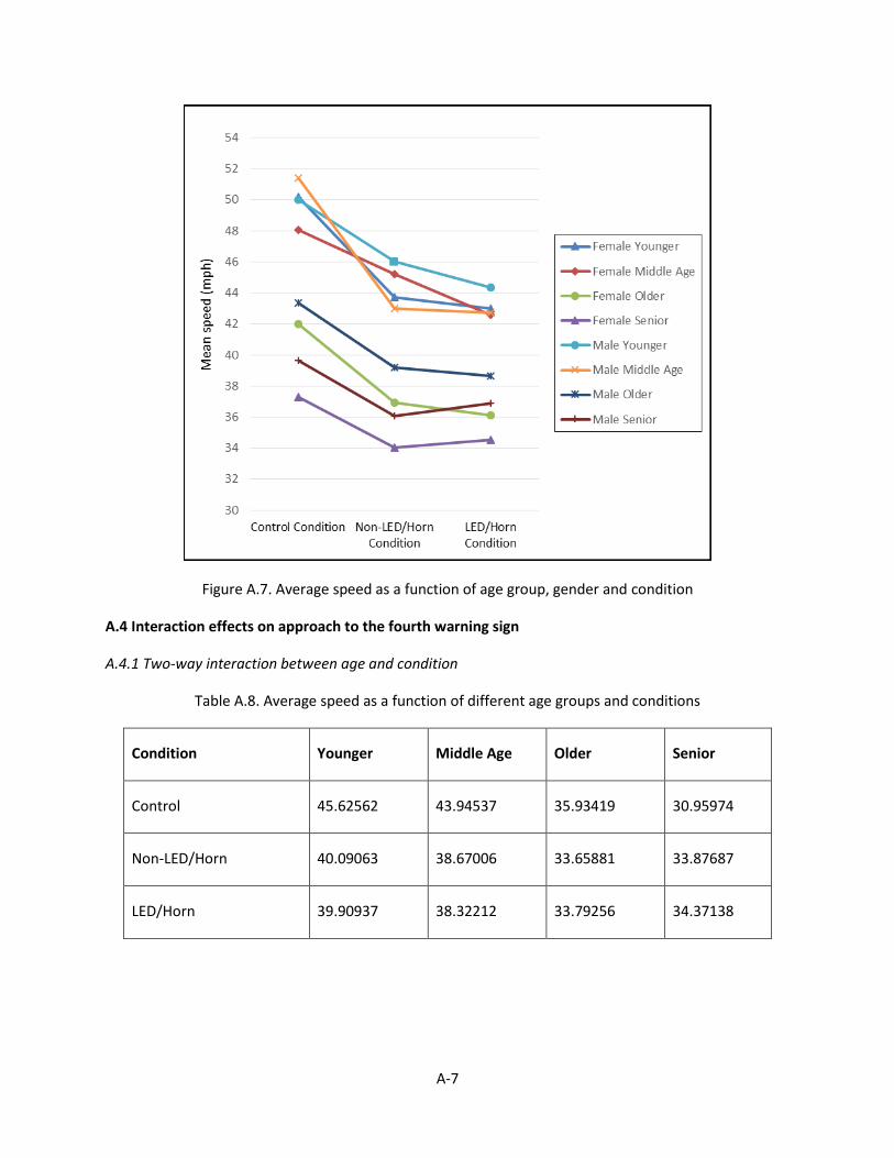
A-7
Figure A.7. Average speed as a function of age group, gender and condition
A.4 Interaction effects on approach to the fourth warning sign
A.4.1 Two-way interaction between age and condition
Table A.8. Average speed as a function of different age groups and conditions
Condition Younger Middle Age Older Senior
Control 45.62562 43.94537 35.93419 30.95974
Non-LED/Horn 40.09063 38.67006 33.65881 33.87687
LED/Horn 39.90937 38.32212 33.79256 34.37138
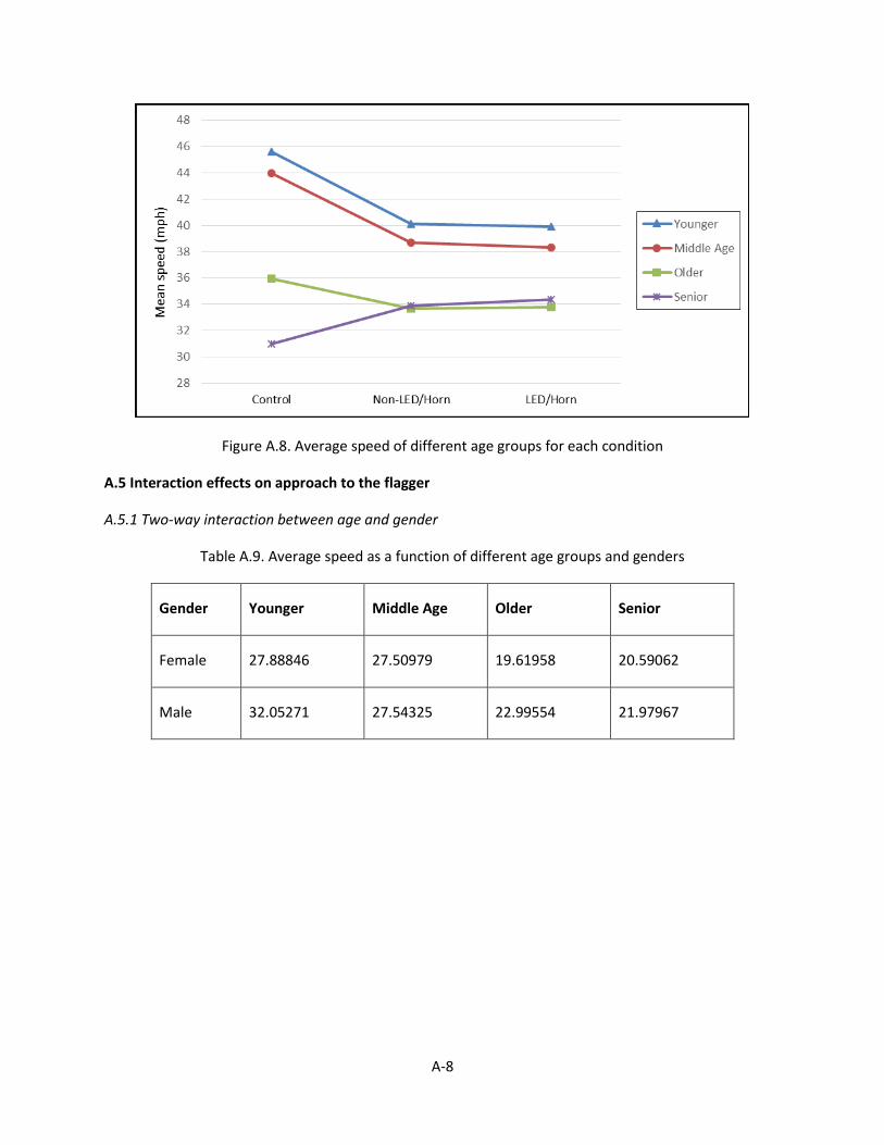
A-8
Figure A.8. Average speed of different age groups for each condition
A.5 Interaction effects on approach to the flagger
A.5.1 Two-way interaction between age and gender
Table A.9. Average speed as a function of different age groups and genders
Gender Younger Middle Age Older Senior
Female 27.88846 27.50979 19.61958 20.59062
Male 32.05271 27.54325 22.99554 21.97967
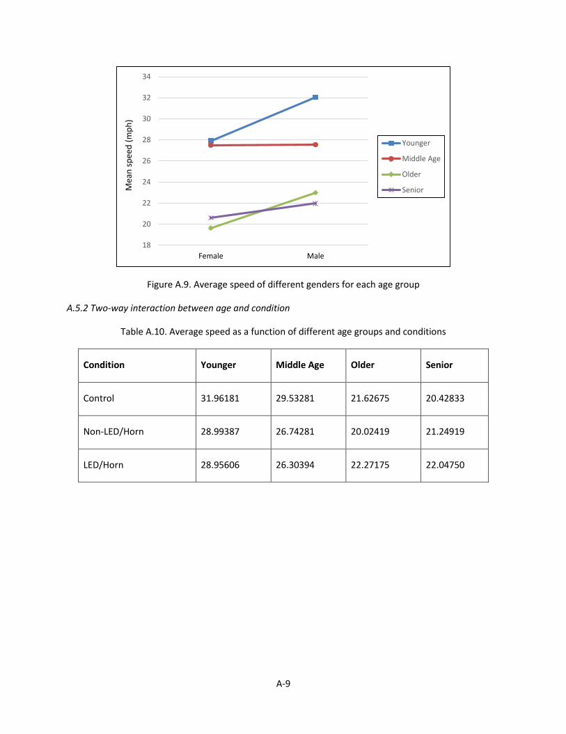
A-9
Figure A.9. Average speed of different genders for each age group
18
20
22
24
26
28
30
32
34
Female Male
Mea
n s
pee
d (
mp
h)
Younger
Middle Age
Older
Senior
A.5.2 Two-way interaction between age and condition
Table A.10. Average speed as a function of different age groups and conditions
Condition Younger Middle Age Older Senior
Control 31.96181 29.53281 21.62675 20.42833
Non-LED/Horn 28.99387 26.74281 20.02419 21.24919
LED/Horn 28.95606 26.30394 22.27175 22.04750

A-10
Figure A.10. Average speed of different age groups for each condition
A.5.3 Two-way interaction between gender and segment
Table A.11. Average speed as a function of gender and segment
Segments Female Male
Segment 1 28.86054 32.59625
Segment 2 26.11812 28.82196
Segment 3 21.13625 23.03750
Segment 4 19.49354 20.11546
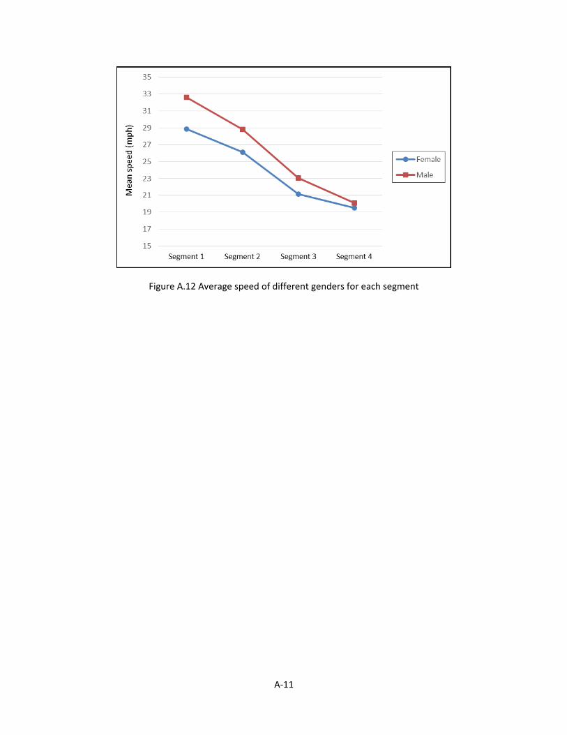
A-11
Figure A.12 Average speed of different genders for each segment

APPENDIX B
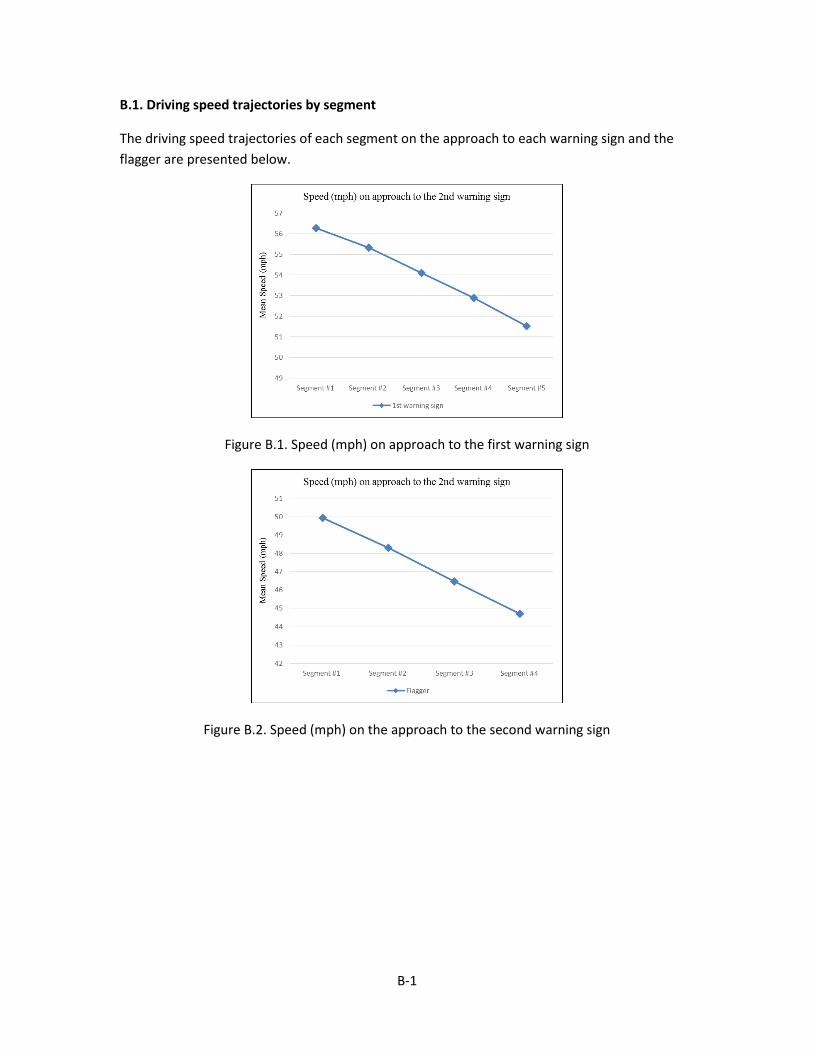
B-1
B.1. Driving speed trajectories by segment
The driving speed trajectories of each segment on the approach to each warning sign and the
flagger are presented below.
Figure B.1. Speed (mph) on approach to the first warning sign
Figure B.2. Speed (mph) on the approach to the second warning sign

B-2
Figure B.3. Speed (mph) on the approach to the third warning sign
Figure B.4. Speed (mph) on the approach to the fourth warning sign
Figure B.5. Speed (mph) on the approach to the flagger

APPENDIX C
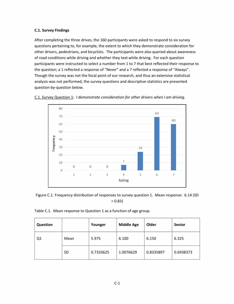
C-1
C.1. Survey Findings
After completing the three drives, the 160 participants were asked to respond to six survey
questions pertaining to, for example, the extent to which they demonstrate consideration for
other drivers, pedestrians, and bicyclists. The participants were also queried about awareness
of road conditions while driving and whether they text while driving. For each question
participants were instructed to select a number from 1 to 7 that best reflected their response to
the question; a 1 reflected a response of “Never” and a 7 reflected a response of “Always”.
Though the survey was not the focal point of our research, and thus an extensive statistical
analysis was not performed, the survey questions and descriptive statistics are presented
question-by-question below.
C.1. Survey Question 1: I demonstrate consideration for other drivers when I am driving.
Figure C.1. Frequency distribution of responses to survey question 1. Mean response: 6.14 (SD
= 0.83)
Table C.1. Mean response to Question 1 as a function of age group.
Question Younger Middle Age Older Senior
Q1 Mean 5.975 6.100 6.150 6.325
SD 0.7333625 1.0076629 0.8335897 0.6938373
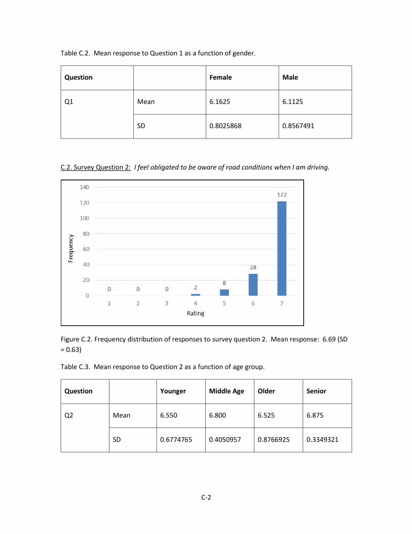
C-2
Table C.2. Mean response to Question 1 as a function of gender.
Question Female Male
Q1 Mean 6.1625 6.1125
SD 0.8025868 0.8567491
C.2. Survey Question 2: I feel obligated to be aware of road conditions when I am driving.
Figure C.2. Frequency distribution of responses to survey question 2. Mean response: 6.69 (SD
= 0.63)
Table C.3. Mean response to Question 2 as a function of age group.
Question Younger Middle Age Older Senior
Q2 Mean 6.550 6.800 6.525 6.875
SD 0.6774765 0.4050957 0.8766925 0.3349321
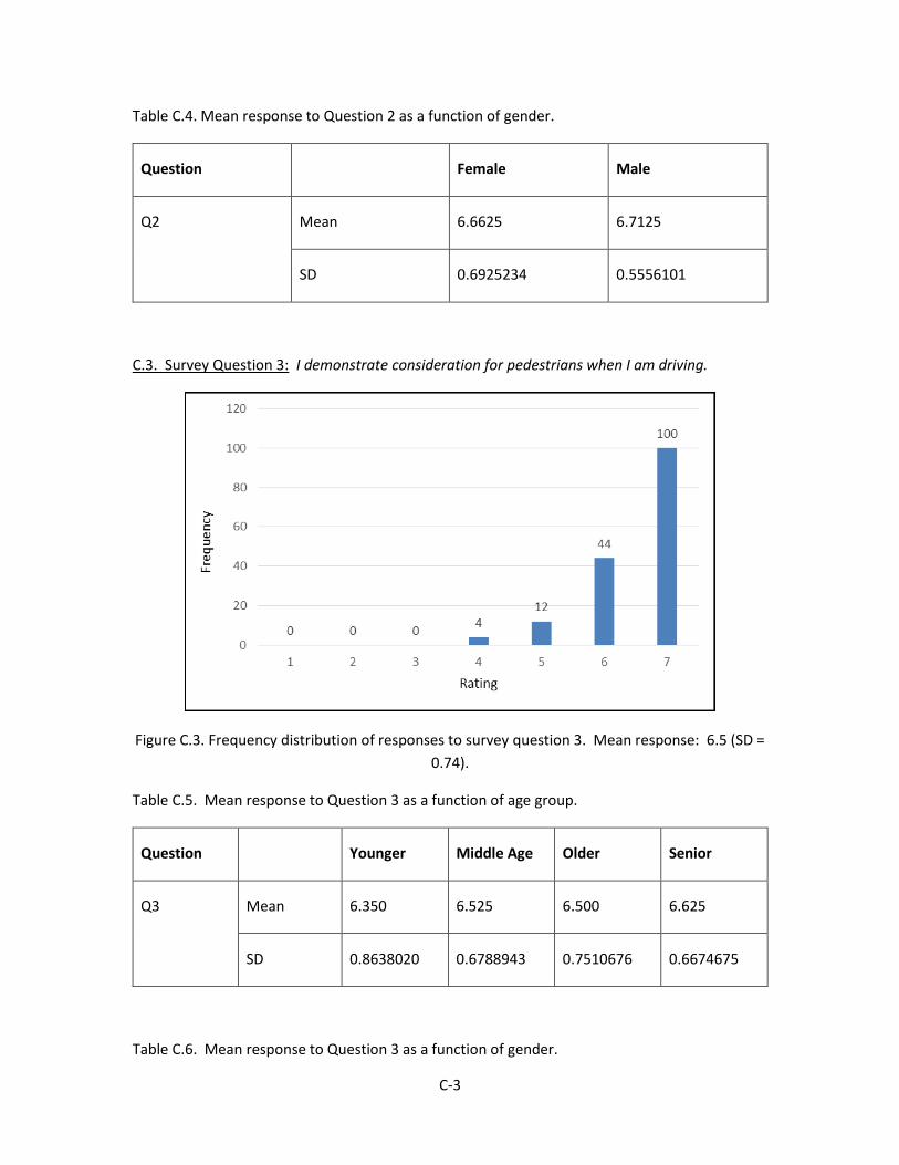
C-3
Table C.4. Mean response to Question 2 as a function of gender.
Question Female Male
Q2 Mean 6.6625 6.7125
SD 0.6925234 0.5556101
C.3. Survey Question 3: I demonstrate consideration for pedestrians when I am driving.
Figure C.3. Frequency distribution of responses to survey question 3. Mean response: 6.5 (SD =
0.74).
Table C.5. Mean response to Question 3 as a function of age group.
Question Younger Middle Age Older Senior
Q3 Mean 6.350 6.525 6.500 6.625
SD 0.8638020 0.6788943 0.7510676 0.6674675
Table C.6. Mean response to Question 3 as a function of gender.
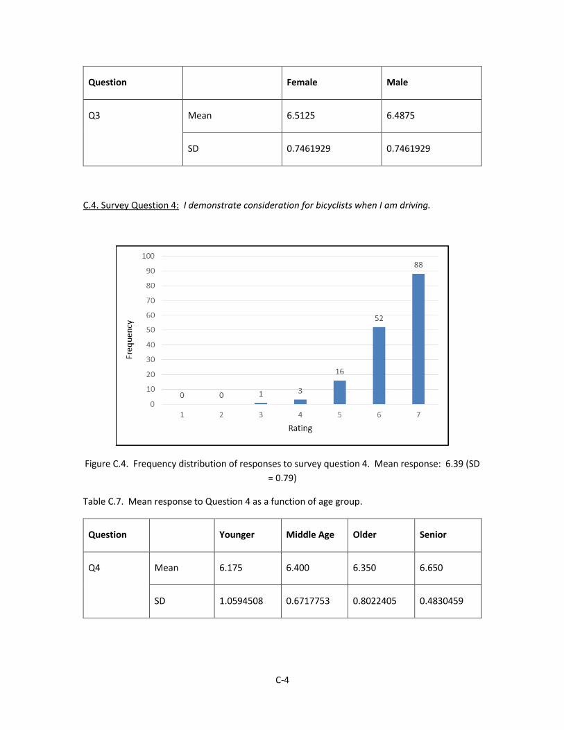
C-4
Question Female Male
Q3 Mean 6.5125 6.4875
SD 0.7461929 0.7461929
C.4. Survey Question 4: I demonstrate consideration for bicyclists when I am driving.
Figure C.4. Frequency distribution of responses to survey question 4. Mean response: 6.39 (SD
= 0.79)
Table C.7. Mean response to Question 4 as a function of age group.
Question Younger Middle Age Older Senior
Q4 Mean 6.175 6.400 6.350 6.650
SD 1.0594508 0.6717753 0.8022405 0.4830459
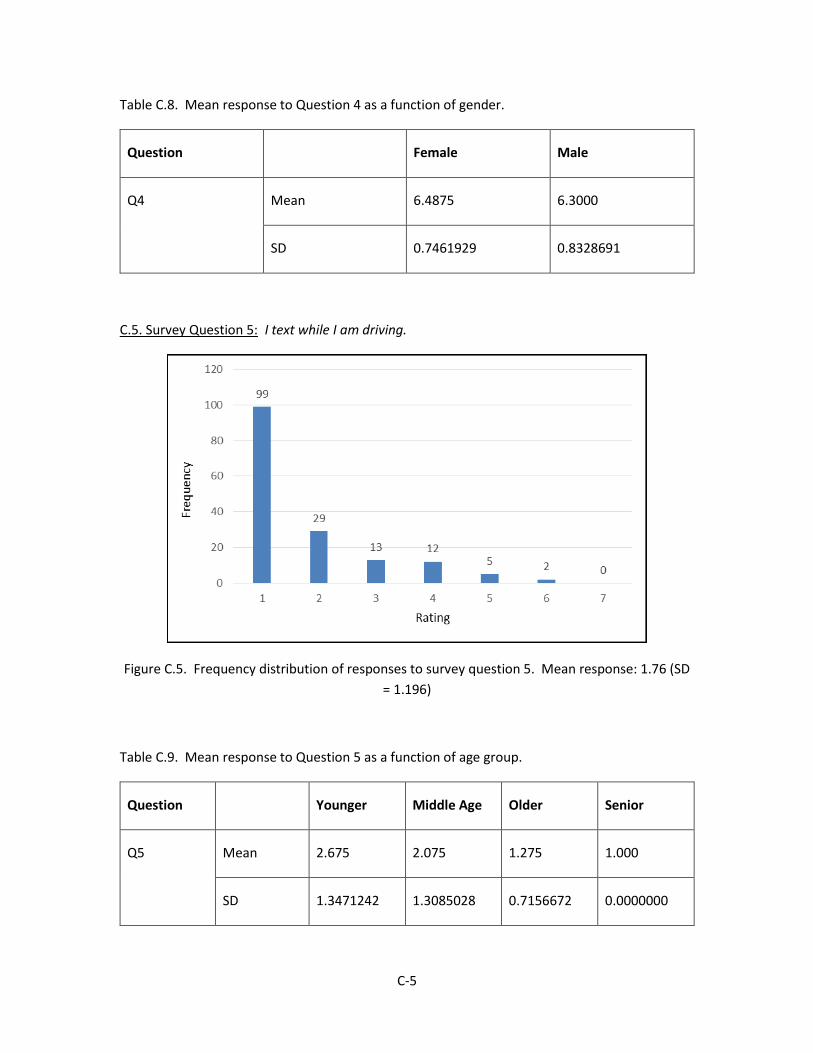
C-5
Table C.8. Mean response to Question 4 as a function of gender.
Question Female Male
Q4 Mean 6.4875 6.3000
SD 0.7461929 0.8328691
C.5. Survey Question 5: I text while I am driving.
Figure C.5. Frequency distribution of responses to survey question 5. Mean response: 1.76 (SD
= 1.196)
Table C.9. Mean response to Question 5 as a function of age group.
Question Younger Middle Age Older Senior
Q5 Mean 2.675 2.075 1.275 1.000
SD 1.3471242 1.3085028 0.7156672 0.0000000
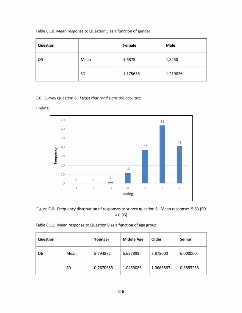
C-6
Table C.10. Mean response to Question 5 as a function of gender.
Question Female Male
Q5 Mean 1.6875 1.8250
SD 1.175636 1.219826
C.6. Survey Question 6: I trust that road signs are accurate.
Finding:
Figure C.6. Frequency distribution of responses to survey question 6. Mean response: 5.83 (SD
= 0.95)
Table C.11. Mean response to Question 6 as a function of age group.
Question Younger Middle Age Older Senior
Q6 Mean 5.794872 5.657895 5.875000 6.000000
SD 0.7670685 1.0469083 1.0666867 0.8885233

C-7
Table C.12. Mean response to Question 6 as a function of gender.
Question Female Male
Q6 Mean 5.936709 5.727273
SD 0.8964570 0.9952038