Fixed Wireless Access in Fiber Operator Context: A ...

Frank Rayal, Riad HartaniPartnersXona Partners

Fixed Wireless Access in Fiber Operator Context: A performance and spend analysis

SPONSORED BY:

Sudheer Dharanikota, Luc AbsillisDirectorsDuke Tech Solutions Inc.

© 2020 SCTE•ISBE, CableLabs & NCTA. All rights reserved. | scte.org • isbe.org 3

▪ Millimeter wave fixed wireless access technical analysis

▪ How can cable operators work with fixed wireless?

▪ Total cost of ownership analysis

▪ Rural morphologies considerations

▪ Conclusions and observations

There are many misconceptions on what can Fixed Wireless Access (FWA) do and what they cannot. Our goal is to provide an unbiased technical and financial analysis on FWA using mmWave technology for Cable operators

Presentation outline


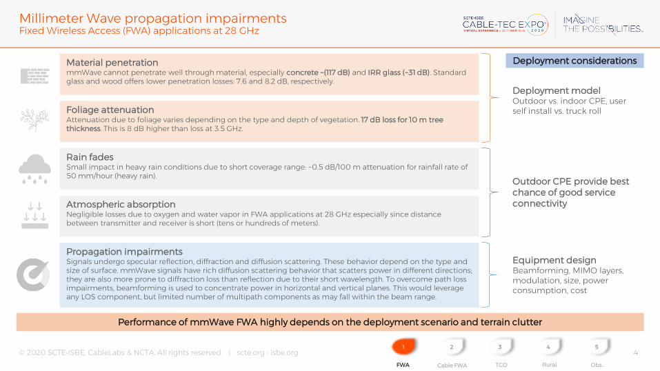
Millimeter Wave propagation impairmentsFixed Wireless Access (FWA) applications at 28 GHz

Material penetrationmmWave cannot penetrate well through material, especially concrete ~(117 dB) and IRR glass (~31 dB). Standard glass and wood offers lower penetration losses: 7.6 and 8.2 dB, respectively.

Foliage attenuationAttenuation due to foliage varies depending on the type and depth of vegetation. 17 dB loss for 10 m tree thickness. This is 8 dB higher than loss at 3.5 GHz.

Atmospheric absorptionNegligible losses due to oxygen and water vapor in FWA applications at 28 GHz especially since distance between transmitter and receiver is short (tens or hundreds of meters).

Rain fadesSmall impact in heavy rain conditions due to short coverage range: ~0.5 dB/100 m attenuation for rainfall rate of 50 mm/hour (heavy rain).

Propagation impairmentsSignals undergo specular reflection, diffraction and diffusion scattering. These behavior depend on the type and size of surface. mmWave signals have rich diffusion scattering behavior that scatters power in different directions; they are also more prone to diffraction loss than reflection due to their short wavelength. To overcome path loss impairments, beamforming is used to concentrate power in horizontal and vertical planes. This would leverage any LOS component, but limited number of multipath components as may fall within the beam range.

1

FWA

2

Cable FWA

3

TCO

4

Rural

5

Obs..

Equipment design Beamforming, MIMO layers, modulation, size, power consumption, cost

Deployment model Outdoor vs. indoor CPE, user self install vs. truck roll

Outdoor CPE provide best chance of good service connectivity

Performance of mmWave FWA highly depends on the deployment scenario and terrain clutter

Deployment considerations


80

90

100

110

120

130

140

150

160

10 100 1000

Pat

h L

oss

(d

B)

Distance (m)

Path Loss for Millimeter Wave Signals at 28 GHz(3GPP Urban Macrocell Model)

huT = 1.5 m

huT = 5 m

huT = 10 m

Short range and high throughput for mmWave FWA lead to selective and targeted deployments

1

FWA

2

Cable FWA

3

TCO

4

Rural

5

Obs..

d2D

d3D

hUT

hBS

Signal Strength Attenuation vs. Distance Throughput vs. Distance

Performance of mmWave fixed wireless access

▪ 141 dB MAPL leading to maximum 400 m cell range in outdoor FWA deployment with best of breed equipment parameters

▪ Including fade and interference margins; excludes glass penetration losses (up to 36 dB) for outdoor deployment

▪ Peak 1.55 Gbps/825 Mbps average throughput per 400 MHz channel and 1-layer MIMO; Frame structure 31 (6:1 DL/UL ratio)

▪ Average 1650 Mbps for 2 MIMO layer used in current deployments


Different Wireline and Wireless access technology evolution

0.1

1

10

100

1000

10000

100000

1995 2000 2005 2010 2015 2020 2025

FTTH, DSL, DOCSIS and Wireless Technology EvolutionDownstream Capacity in Mbps

PON DOCSIS Wireless DSL

1G EPON

2.5G GPON

10G EPON

100G PON

40G GPON

DOCSIS 1.0

DOCSIS 1.1

DOCSIS 2.0

DOCSIS 3.04DS Channels

DOCSIS 3.024DS Channels

DOCSIS 3.12x192 MHz Ch.

DOCSIS 3.1Full Duplex

2G/GPRS/EDGE

4G LTE Rel 8

4G LTE Adv Rel 10

4G LTE Adv Rel 13

5G Rel 15

ADSL

ADSL2

ADSL2+

VDSLVDSL2

G.fast

~10X

~10X

Today3G UMTS

3G HSPA

5G Rel 16

3G HSDPA

Downstream capacity wise, PON offers ~10x more than DSL or DOCSIS, and ~100x more than wireless

1

FWA

2

Cable FWA

3

TCO

4

Rural

5

Obs..


Comparing capacity of different access technologies

Category Fixed Wireless DOCSIS Fiber To The Home

Technology mmWave DOCSIS 3.1 with High split XGSPON

Spectrum block (Downlink/Uplink) 400 MHz 3 x 192 MHz/ 200 MHz NA

QAM (Downlink/Uplink) 64/16 256/64 NA

Peak capacity (Downlink/Uplink) 2.8 Gbps/0.34 Gbps 4.5 Gbps/1.3 Gbps 10 Gbps/10 Gbps

Non-Overhead 100%* 88% 90%

Oversubscription 20 20 20

Maximum subs (assuming 100% take rate) 200** 600 32

Avg. sellable bandwidth per sub*** (Downlink/Uplink) 142 Mbps/23 Mbps 132 Mbps/38 Mbps 5.6 Gbps/5.6 Gbps

Maximum distance to the customer 400 Meters ~5 Km 20 Km

(*) Overhead is already considered in the capacity calculation for 2 MIMO layers (**) A maximum of 200 homes covered per sector is considered in this analysis(***) Average sellable bandwidth per sub = Capacity * Non-Overhead * Over subscription / Maximum subs

XGSPON based FTTH solution offers the highest per sub bandwidth and the longest distance from to the end of line

1

FWA

2

Cable FWA

3

TCO

4

Rural

5

Obs..


FWA and FTTH deployments for a suburban topology

1

FWA

2

Cable FWA

3

TCO

4

Rural

5

Obs..

We used a Greenfield suburban topology for this analysis

▪ Assumes:

▪ 3-sectored cells; 25 m tower

▪ User terminal at 5 m (50% self-install)

▪ Cell area 0.136 sq. km (r = 390 m)

▪ 1 cell site covers ~600 houses (50x100’ lots)

Fixed wireless access deployment

Fiber To The Home access deployment

▪ Suburban greenfield area

▪ Primarily single-family residential community

▪ 600 home community

▪ North America cost and price structure

▪ Assumes:

▪ XGSPON as the deployment technology

▪ Hardened outside plant deployment

▪ 1:32 split per PON with 16 PON port OLT

16 PONs

512 Homes Passed

CriticalFacility

OLT

Splitter Cabinet


Fixed wireless access technology TCO analysis

Based on a 7-year RAN TCO

High sensitivity to cell radius and cell loading (no. of subs): FWA susceptible to competition from wireline service providers**

1

FWA

2

Cable FWA

3

TCO

4

Rural

5

Obs..

▪ Revenue per subscriber: $75▪ Leased infrastructure (site, backhaul)▪ 284/46 Mbps; 20 oversubscription* (residential subscriber)▪ 400 m cell radius▪ Does not include spectrum acquisition costs▪ 3-Sectors / site; 5 Gbps backhaul▪ 50% market penetration▪ 50% self-install CPEs

FWA TCO scenario parameters and results Houses covered per cell size and cost per covered house for typical North American suburban area

7-Year TCO Analysis Results

Subscribers per site 300

Houses covered 600

Market penetration rate 50%

Cost/house covered $ 607

Cost/sub/mo $ 23

Profit (Loss) / sub / mo $ 47

Months to breakeven 22

(*) Business subscriber requires lower oversubscription – e.g. 1-5 – leading to different parameters and results(**) Cost of CPE, % of self-install, cost of backhaul and cost of site lease are other important factors for positive business case


Fiber To The Home access technology TCO analysis

1

FWA

2

Cable FWA

3

TCO

4

Rural

5

Obs..

A typical greenfield FTTH deployment costs ~$850/HHP with a $53/year/HP OpEx cost, leading to a one year breakeven

Parameters that influence the FTTH financial analysis FTTH cost and revenue analysis

▪ Cost and revenue related▪ Revenue per subscriber: $75 per month

▪ Assumes 1 mile of aerial and 3 miles of underground construction

▪ Assumes $53/year/homes passed* operational expense

▪ Deployment considerations▪ No RFOG (All IP solution), centralized splitter

▪ 100 feet drops

▪ 50% take rate

▪ Difference between FWA and FTTH deployments▪ All homes are connected due to franchise agreements

▪ Leasing equipment or fiber is not considered (not applicable)

▪ Conduit sharing (join trenching) is not considered in this analysis

Note: XGSPON offers significantly higher capacity per sub leading to longer lifetime from product offering capability point of view

$850

$908

$150

$1,125

Mo. 1 2 3 4 5 6 7 8 9 10 11 12 13 14 Mo. 15

Per HHP FTTH TCO versus Revenue

Cum. TCO Cum. Revenue

(*) Refer to “Operational Expense Comparison in Access Networks,” Fiber Broadband Association


Comparing mmWave FWA and FTTH TCO analysis

1

FWA

2

Cable FWA

3

TCO

4

Rural

5

Obs..

Fixed wireless access could be considered more tactical and complementary to fiber which is more strategic

Category mmWave Fixed Wireless Fiber To The Home

Pros Cons Pros Cons

Deployment Quick access to marketCould be deployed quickly

Propagation characteristics (foliage, material, clutter) impact on range

Can be deployed in any terrain Requires advanced planning, permitting

Quality of Experience Variable depending on location Constant & predictable

Throughput Decreases proportionally to distance, varies depending on obstructions in signal path

Constant & predictable; ~100x more capability than FWA

Availability Depends on distance and location of user terminal; foliage and IRR glass reduce

availability

Constant & predictable

Number of users

Cell densification to increase capacity; Roadmap to support greater throughput/# of users

Variable depending on deployment scenario in addition to other factors

Linearly scalable

Financial Structure Lower CapEx (scenario specific), quick access to market

High OpEx (scenario specific) Low OpEx Initial CapExinvestment heavy

TCO 22 Months to breakeven (case dependent)

1. Small coverage range or low sub penetration lead to poor biz case

2. Actual breakeven is longer when factoring cost of core network and

spectrum

~ 12 mo. breakeven; Better product offers


Fixed Wireless Access

▪ mmWave offers shorter range especially in areas of high foliage

▪ Lower density drives negative business case

▪ Sub 6 GHz 5G solutions (e.g. 3.5 GHz) offer a better option▪ When spectrum available use 100 MHz carrier with option for carrier agg.

▪ Low spectrum price $0.01 - $0.4 / MHz-PoP depending on market (CBRS offers 80 MHz of unlicensed spectrum with potential to use up to 150 MHz)

▪ 64T64R massive MIMO antennas with multiple MIMO layers to reach gigabit throughput

Fiber To The Home Access

▪ Expensive & rocky terrains make the fiber construction not viable

▪ Operator may have a different price structure for rural customers

▪ Low density ➔ Longer distribution and drop ➔ higher costs leading to worse than wireless business case

▪ Recommend to use targeted deployments and cost sharing with customer

Access networks for rural morphologies

1

FWA

2

Cable FWA

3

TCO

4

Rural

5

Obs..

Rural morphologies have certain twists Impact of rural on the access deployments

Rural morphologies presents different set of problems for FWA and wireline access – navigate them accordingly

Density

Terrain

Vegetation

Product Offers

Revenue

Low population density leading to longer construction distribution/drops and lower subs per sector

Different cost/mile, permitting etc. that change the economics for wirelineOpen terrain helps extend wireless coverage

Foliage and seasonality significantly impact wireless performance

Product needs and hence the offers in the rural locations are different than that in the urban morphologies

Different revenue opportunities from urban areas leading to potentially longer breakeven


Our observations and conclusions

1

FWA

2

Cable FWA

3

TCO

4

Rural

5

Obs..

FWA could be deployed quickly and selectively but offers limited QoE depending on location and deployment scenario

Several FWA and FTTH service models are possible: own vs. lease; wholesale vs. retail; residential vs. business, greenfield vs. brownfield, hybrid wireless/fiber, shared vs. dedicated, etc.

FTTH technologies have been offering constantly 100x better throughput than FWA and offers product headroom

The scenario analyzed in this paper shows FTTH is CapEx intensive compared to FWA’s OpEx intensive nature

FWA - Quick to deploy but limited QoE

FTTH 100x Better

High ROI variability CapEx or OpEx

Frank RayalPartnerXona [email protected]

Thank You!Sudheer DharanikotaManaging DirectorDuke Tech Solutions [email protected]


Link budget and expected range performance

1

FWA

2

Cable FWA

3

TCO

4

Rural

5

Recos..

▪ Link budget maximizes the equipment performance

▪ 60 dBm gNB EiRP; 28 dB antenna gain including

beamforming

▪ Typically 55 – 60 dBm EiRP

▪ 39 dBm CPE EiRP including 19 dB antenna gain

▪ 400 MHz bandwidth (4x100 MHz carriers)

▪ Up to 8x100 MHz carriers is possible

▪ For window-mounted CPE, up to 36 dB additional loss may be

incurred (IRR glass)

▪ Expected range: 390 m

▪ Uplink limited 141 dB path loss

▪ Range for glass mounted CPE: 42 m

▪ 36 dB glass penetration loss

General parameters Downlink UplinkBandwidth per carrier 100 100 MHzOccupied channel BW 95.04 95.04 MHzCarriers 4 4Total BW 400 400 MHzPRB per carrier 66 66Transmitter parametersTx Power (all carriers) 32 20 dBmTx antenna gain 28 19 dBEiRP 60 39 dBmEiRP per carrier 54 33 dBmReceiver parameters

Thermal noise density -174 -174 dBm/HzReceiver noise figure 7 6 dBEffective noise power -87.2 -88.2 dBmMCS QPSK QPSKSNR -0.9 -0.9 dBReceiver sensitivity -88.1 -89.1 dBmRx antenna gain 19 28 dBRx power -107 -117 dBmPath loss 167.1 156.1 dBMarginsImplementation margin 2 2 dBInterference margin 6 2.5 dBLognormal fading 10 10 dBMAPL - Outdoor 149.1 141.6 dB


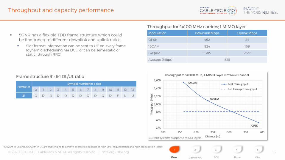
Throughput and capacity performance

1

FWA

2

Cable FWA

3

TCO

4

Rural

5

Obs..

▪ 5GNR has a flexible TDD frame structure which could be fine-tuned to different downlink and uplink ratios▪ Slot format information can be sent to UE on every frame

(dynamic scheduling, via DCI), or can be semi-static or static (through RRC)

Format #Symbol number in a slot

0 1 2 3 4 5 6 7 8 9 10 11 12 13

31 D D D D D D D D D D D F U U

Frame structure 31: 6:1 DL/UL ratio

Modulation Downlink Mbps Uplink Mbps

QPSK 462 84

16QAM 924 169

64QAM 1,385 253*

Average (Mbps) 825

Throughput for 4x100 MHz carriers; 1 MIMO layer

* 64QAM in UL and 256 QAM in DL are challenging to achieve in practice because of high SINR requirements and high propagation losses

Current systems support 2 MIMO layers


Spectrum allocations and pricing

1

FWA

2

Cable FWA

3

TCO

4

Rural

5

Obs..

▪ Low demand for mmWave spectrum expect in the US

▪ Valuation at fraction of a cent/MHz-PoP

▪ US price increased by ~3x since 1998 LMDS auction: $0.00262/MHz-PoP [$0.004112 in 2019 dollars]

▪ 3.5 GHz CBRS auction national average price $0.21/MHz-PoP: ~20x higher than mmWave


Different equipment used for the Fixed Wireless Access

1

FWA

2

Cable FWA

3

TCO

4

Rural

5

Obs..

Equipment▪ 3 sector gNB @25m

▪ 2 or 4 sectors also used in actual deployments

▪ CPE height = 5 m

▪ Outdoor typically

▪ Indoor: glass mounted

Nokia Airscale 28 GHz radio (AEUB)60 dBm EiRP44 lbs23.6x12x4.7”2x2 MIMO2x256 antenna elements420 W

Samsung 28 GHz gNB (AT1K01)50 dBm EiRP33 lbs19.41x9.57x6.89”8 CC x 100 MHz4x256 antenna elements525 W (10.9 A; -48 VDC)

Wistron 4G/5G CPE 5G: 37 – 40 GHz / 27.50 –28.35 GHz4G B2/B4/B5/B13/B666x3x3”2x2 MIMO5G 1x4 antenna elements (3x modules)60 W (PoE)

Samsung 310 5G CPE39 dBm EiRP

2.6 lbs7.8x7.4x1.5”

8 CC x 100 MHz2x2 MIMO

2x32 antenna elements20 W


Parameters that have high impact on the mmWave TCO model:

▪ Revenues▪ Subscribers per cell site: Range

▪ Up to 400 m (200 m encountered often in practice)

▪ Up to 600 houses in suburban area

▪ Up to 300 subscriber: 50% penetration

▪ Revenue per subscriber▪ $50-$90 / subscriber

▪ Costs ▪ Backhaul for 5 Gbps/site

▪ Site lease: 3 sectors typical (2 or 4 also common)

▪ CPE & CPE installation: 50% of total▪ Leverage LTE ecosystem to reduce cost

▪ Minimize truck roll: e.g. window mount CPEs

▪ 7-Year TCO RAN Scenario Outline▪ 3 sectors per cell site

▪ Leased site; backhaul leased from 3rd party

▪ Core network; OSS/BSS; spectrum costs not included

Key parameters of the mmWave Fixed Access TCO

1

FWA

2

Cable FWA

3

TCO

4

Rural

5

Obs..


Scenario: Leased Site

▪ 300 subscribers / site

▪ $75/month RPU (revenue per user)

▪ $600/month site lease

▪ $1,500/month backhaul

Notes on the TCO analysis

▪ Cost of spectrum is not factored into the TCO analysis; it would be additive and amortized over the number of sites in a market

▪ The cost of core network, OSS and BSS are included. They would be additive amortized over the number of base stations and subscribers.

Sensitivity of mmWave FWA To Key Parameters

1

FWA

2

Cable FWA

3

TCO

4

Rural

5

Obs..

High sensitivity to subscriber penetration and revenue per subscriber

Low sensitivity to cost of CPE and installation services

• ~1 month impact on breakeven per $100


Sensitivity to Backhaul and Site Lease Costs

1

FWA

2

Cable FWA

3

TCO

4

Rural

5

Obs..

Monte Carlo Analysis N = 5,000 for cost of backhaul

▪ Cost of backhaul with normal distribution; mean = $1,500/month; std. dev. = 300; $1,000 low bound

▪ $75/month revenue per user

▪ Coverage range▪ Careful analysis of service area

▪ Selective market entry▪ Open areas more likely to be profitable

▪ Wooded areas present a challenge

▪ Subscriber acquisition and retention

▪ Quality of service to minimize subscriber churn▪ Today’s FWA also leverage LTE networks

▪ Control infrastructure costs

▪ Leverage existing assets to minimize new site construction

▪ Leverage existing backhaul/fiber plant

Critical paramters for business case success


mmWave Fixed Access TCO scenario outcomes

1

FWA

2

Cable FWA

3

TCO

4

Rural

5

Obs..

Leased Site

Low Mid High

Subs per site 180 240 300

Revenue ($/month/Sub) 50 70 90

Site lease per month ($/mo) 150 600 1,200

Backhaul per site ($/mo) 500 1,500 2,000Throughput DL:UL (Mbps) 200:33 200:33 200:33


Months to breakeven 37 26 20

Own Site

Low Mid High

Subs per site 180 240 300

Revenue ($/month/Sub) 50 70 90

Site lease per month ($/mo) 0 0 0

Backhaul per site ($/mo) 0 0 0

Throughput (Mbps) 200:33 200:33 200:33


Months to breakeven 48 29 22

Site Type: Leased

▪ Penetration and revenue is critical to overcome expenses and get a positive business case. ▪ Low revenue and penetration cannot make business case valid even if costs are low.

Site Type: Owned [New Construction]

Fixed Wireless Access in Fiber Operator Context: A ...

Documents

Transcript of Fixed Wireless Access in Fiber Operator Context: A ...