Fixed-Parameter Algorithms for

Kemeny Rankings 1

Nadja Betzler a,2,∗ Michael R. Fellows b,3 Jiong Guo a,4

Rolf Niedermeier a Frances A. Rosamond b,5

a Institut fur Informatik, Friedrich-Schiller-Universitat JenaErnst-Abbe-Platz 2, D-07743 Jena, Germany

b PC Research Unit, Office of DVC (Research), University of Newcastle,Callaghan, NSW 2308, Australia.

Abstract

The computation of Kemeny rankings is central to many applications in the contextof rank aggregation. Given a set of permutations (votes) over a set of candidates,one searches for a “consensus permutation” that is “closest” to the given set ofpermutations. Unfortunately, the problem is NP-hard. We provide a broad study ofthe parameterized complexity for computing optimal Kemeny rankings. Beside thethree obvious parameters “number of votes”, “number of candidates”, and solutionsize (called Kemeny score), we consider further structural parameterizations. Morespecifically, we show that the Kemeny score (and a corresponding Kemeny ranking)of an election can be computed efficiently whenever the average pairwise distancebetween two input votes is not too large. In other words, Kemeny Score is fixed-parameter tractable with respect to the parameter “average pairwise Kendall-Taudistance da”. We describe a fixed-parameter algorithm with running time 16⌈da⌉ ·poly. Moreover, we extend our studies to the parameters “maximum range” and“average range” of positions a candidate takes in the input votes. Whereas Kemeny

Score remains fixed-parameter tractable with respect to the parameter “maximumrange”, it becomes NP-complete in case of an average range of two. This excludesfixed-parameter tractability with respect to the parameter “average range” unlessP=NP. Finally, we extend some of our results to votes with ties and incompletevotes, where in both cases one no longer has permutations as input.

Key words: computational social choice, voting systems, winner determination,rank aggregation, consensus finding, fixed-parameter tractability.

Preprint submitted to Elsevier 1 September 2009

1 Introduction

To aggregate inconsistent information not only appears in classical voting sce-narios but also in the context of meta search engines and a number of otherapplication contexts [1,10,13,16,17]. In some sense, herein one deals with con-sensus problems where one wants to find a solution to various “input demands”such that these demands are met as well as possible. Naturally, contradictingdemands cannot be fulfilled at the same time. Hence, the consensus solutionhas to provide a balance between opposing requirements. The concept of Ke-meny consensus is among the most classical and important research topics inthis context. In this paper, we study new algorithmic approaches based on pa-rameterized complexity analysis [15,19,29] for computing Kemeny scores and,thus, optimal Kemeny rankings. We start with introducing Kemeny elections.

Kemeny’s voting scheme goes back to the year 1959 [23] and was later specifiedby Levenglick [27]. It can be described as follows. An election (V, C) consists ofa set V of n votes and a set C of m candidates. A vote is a preference list of thecandidates, that is, each vote orders the candidates according to preference.For instance, in case of three candidates a, b, c, the order c > b > a wouldmean that candidate c is the best-liked one and candidate a is the least-likedone for this vote. 6 A “Kemeny consensus” is a preference list that is “closest”to the preference lists of the votes: For each pair of votes v, w, the so-called

∗ Corresponding author.Email addresses: nadja.betzler@uni-jena.de (Nadja Betzler),

michael.fellows@newcastle.edu.au (Michael R. Fellows),jiong.guo@uni-jena.de (Jiong Guo), rolf.niedermeier@uni-jena.de(Rolf Niedermeier), frances.rosamond@newcastle.edu.au(Frances A. Rosamond).1 This paper combines results from the two conference papers “Fixed-parameteralgorithms for Kemeny scores” (Proceedings of the 4th International Conferenceon Algorithmic Aspects in Information and Management (AAIM 2008), Springer,LNCS 5034, pages 60-71) and “How similarity helps to efficiently compute Kemenyrankings” (Proceedings of the 5th International Conference on Autonomous Agentsand Multiagent Systems (AAMAS 2009)).2 Supported by the Deutsche Forschungsgemeinschaft, Emmy Noether researchgroup PIAF (fixed-parameter algorithms, NI 369/4) and project DARE (data re-duction and problem kernels, GU 1023/1).3 Supported by the Australian Research Council. Work done while staying in Jenaas a recipient of a Humboldt Research Award of the Alexander von Humboldtfoundation, Bonn, Germany.4 Partially supported by the Deutsche Forschungsgemeinschaft, Emmy Noether re-search group PIAF (fixed-parameter algorithms, NI 369/4).5 Supported by the Australian Research Council.6 Some definitions also allow ties between candidates—we deal with this later inthe paper.

2

Kendall-Tau distance (KT-distance for short) between v and w, also knownas the number of inversions between two permutations, is defined as

dist(v, w) =∑

{c,d}⊆C

dv,w(c, d),

where the sum is taken over all unordered pairs {c, d} of candidates, anddv,w(c, d) is set to 0 if v and w rank c and d in the same order, and is setto 1, otherwise. Using divide and conquer, the KT-distance can be computedin O(m·logm) time (see, e.g., [25]). The score of a preference list l with respectto an election (V, C) is defined as

∑

v∈V dist(l, v). A preference list l with theminimum score is called Kemeny consensus (or Kemeny ranking) of (V, C) andits score

∑

v∈V dist(l, v) is the Kemeny score of (V, C). The central problemconsidered in this work is as follows: 7

Kemeny Score

Input: An election (V, C) and a positive integer k.Question: Is the Kemeny score of (V, C) at most k?

Clearly, in applications we are mostly interested in computing a Kemeny con-sensus of a given election. All our algorithms that decide the Kemeny Score

problem actually provide a corresponding Kemeny consensus, which gives thedesired ranking.

Known results. Bartholdi III et al. [2] showed that Kemeny Score isNP-complete, and it remains so even when restricted to instances with onlyfour votes [16,17]. Given the computational hardness of Kemeny Score onthe one hand and its practical relevance on the other hand, polynomial-timeapproximation algorithms have been studied. The Kemeny score can be ap-proximated to a factor of 8/5 by a deterministic algorithm [34] and to a factorof 11/7 by a randomized algorithm [1]. Recently, a polynomial-time approx-imation scheme (PTAS) has been developed [24]. However, its running timeis completely impractical. Conitzer, Davenport, and Kalagnanam [13,10] per-formed computational studies for the efficient exact computation of a Kemenyconsensus, using heuristic approaches such as greedy and branch-and-bound.Their experimental results encourage the search for practically relevant, effi-ciently solvable special cases, thus motivating parameterized complexity stud-ies. These experimental investigations focus on computing strong admissiblebounds for speeding up search-based heuristic algorithms. In contrast, our fo-cus is on exact algorithms with provable asymptotic running time bounds forthe developed algorithms. Recently, a further experimental study for differ-ent approximation algorithms for Kemeny rankings has been presented [32].

7 Note that for the sake of simplicity we formulate the decision problem here.

3

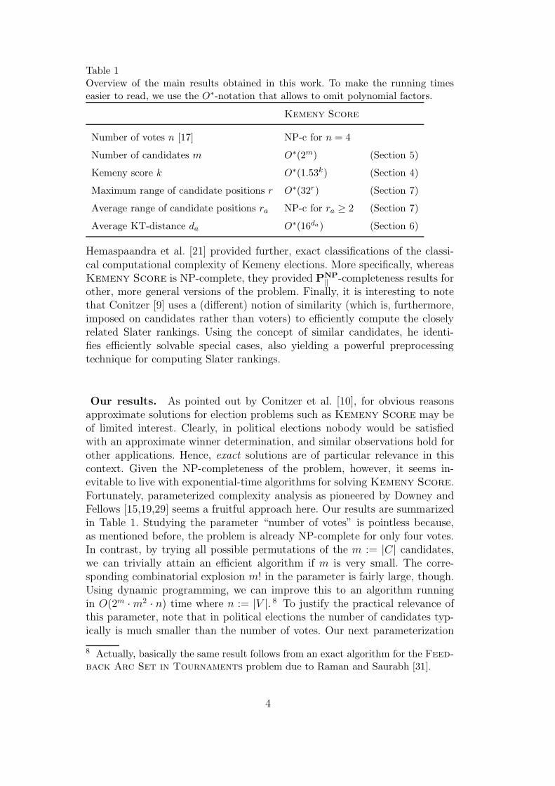
Table 1Overview of the main results obtained in this work. To make the running timeseasier to read, we use the O∗-notation that allows to omit polynomial factors.

Kemeny Score

Number of votes n [17] NP-c for n = 4

Number of candidates m O∗(2m) (Section 5)

Kemeny score k O∗(1.53k) (Section 4)

Maximum range of candidate positions r O∗(32r) (Section 7)

Average range of candidate positions ra NP-c for ra ≥ 2 (Section 7)

Average KT-distance da O∗(16da) (Section 6)

Hemaspaandra et al. [21] provided further, exact classifications of the classi-cal computational complexity of Kemeny elections. More specifically, whereasKemeny Score is NP-complete, they provided PNP

‖ -completeness results forother, more general versions of the problem. Finally, it is interesting to notethat Conitzer [9] uses a (different) notion of similarity (which is, furthermore,imposed on candidates rather than voters) to efficiently compute the closelyrelated Slater rankings. Using the concept of similar candidates, he identi-fies efficiently solvable special cases, also yielding a powerful preprocessingtechnique for computing Slater rankings.

Our results. As pointed out by Conitzer et al. [10], for obvious reasonsapproximate solutions for election problems such as Kemeny Score may beof limited interest. Clearly, in political elections nobody would be satisfiedwith an approximate winner determination, and similar observations hold forother applications. Hence, exact solutions are of particular relevance in thiscontext. Given the NP-completeness of the problem, however, it seems in-evitable to live with exponential-time algorithms for solving Kemeny Score.Fortunately, parameterized complexity analysis as pioneered by Downey andFellows [15,19,29] seems a fruitful approach here. Our results are summarizedin Table 1. Studying the parameter “number of votes” is pointless because,as mentioned before, the problem is already NP-complete for only four votes.In contrast, by trying all possible permutations of the m := |C| candidates,we can trivially attain an efficient algorithm if m is very small. The corre-sponding combinatorial explosion m! in the parameter is fairly large, though.Using dynamic programming, we can improve this to an algorithm runningin O(2m · m2 · n) time where n := |V |. 8 To justify the practical relevance ofthis parameter, note that in political elections the number of candidates typ-ically is much smaller than the number of votes. Our next parameterization

8 Actually, basically the same result follows from an exact algorithm for the Feed-

back Arc Set in Tournaments problem due to Raman and Saurabh [31].

4

uses the Kemeny score k as the parameter to derive an algorithm solving Ke-

meny Score in O(1.53k + m2n) time. This algorithm is based on a problemkernelization and a depth-bounded search tree. This may be considered asthe “canonical parameterization” because the parameter measures the “solu-tion size”—however, it is conceivable that in many applications the value of kmay not be small, rendering the corresponding fixed-parameter algorithms im-practical. Next, we introduce a structural parameterization by studying theparameter “maximum range rmax of positions that a candidate can have inany two of the input votes”. We show that Kemeny Score can be solved inO(32rmax·(r2

max·m+rmax·m2 log m·n)+n2·m log m) time by a dynamic program-

ming approach. Interestingly, if we study the parameter average range insteadof maximum range, Kemeny Score turns NP-complete already for constantparameter values. By way of contrast, developing our main technical result, weagain achieve fixed-parameter tractability when replacing the “range measure”by measuring the average pairwise distance between votes. More specifically,we show that with respect to the parameter “average KT-distance da” over allpairs of votes an exponential worst-case running time factor of 16da is possible.This is practically meaningful because this parameterization shows that theconsensus ranking can be computed efficiently whenever the votes are similarenough on average. Thus, it can cope with “outlier votes”. Finally, we extendsome of our findings to the cases where ties within votes are allowed and to in-complete votes where not all candidates are ranked, achieving fixed-parametertractability as well as computational hardness results.

2 Preliminaries

We refer to the introductory section for some basic definitions concerning(Kemeny) elections. Almost all further concepts are introduced where needed.Here we restrict ourselves to some central concepts.

The following notion of “dirtiness” is of particular relevance for some of ouralgorithms.

Definition 1 Let (V, C) be an election. Two candidates a, b ∈ C, a 6= b, forma dirty pair if there exists one vote in V with a > b and there exists anothervote in V with b > a. A candidate is called dirty if he is part of a dirty pair,otherwise he is called non-dirty. 9

Let the position of a candidate a in a vote v be the number of candidates thatare better than a in v. That is, the leftmost (and best) candidate in v has

9 For the sake of simplicity (and saving one letter), all candidates here are referredto by male sex.

5

position 0 and the rightmost has position m − 1. Then posv(a) denotes theposition of candidate a in v. For an election (V, C) and a candidate c ∈ C, theaverage position pa(c) of c is defined as

pa(c) :=1

n·

∑

v∈V

v(c).

For an election (V, C), the average KT-distance da is defined as 10

da :=1

n(n − 1)·

∑

u,v∈V,u 6=v

dist(u, v).

Note that an equivalent definition is given by

da :=1

n(n − 1)·

∑

a,b∈C

#v(a > b) · #v(b > a),

where for two candidates a and b the number of votes in which a is rankedbetter than b is denoted by #v(a > b). The latter definition is useful if theinput is provided by the outcomes of the pairwise elections of the candidatesincluding the margins of victory.

Furthermore, for an election (V, C) and for a candidate c ∈ C, the range r(c)of c is defined as

r(c) := maxv,w∈V

{|v(c) − w(c)|} + 1.

The maximum range rmax of an election is given by rmax := maxc∈C r(c) andthe average range ra is defined as

ra :=1

m

∑

c∈C

r(c).

Finally, we briefly introduce the relevant notions of parameterized complexitytheory [15,19,29]. Parameterized algorithmics aims at a multivariate complex-ity analysis of problems. This is done by studying relevant problem parametersand their influence on the computational complexity of problems. The hopelies in accepting the seemingly inevitable combinatorial explosion for NP-hardproblems, but confining it to the parameter. Thus, the decisive question iswhether a given parameterized problem is fixed-parameter tractable (FPT)

10 To simplify the presentation, the following definition counts the pair (u, v) as wellas the pair (v, u), thus having to divide by n(n − 1) to obtain the correct averagedistance value.

6

with respect to the parameter. In other words, for an input instance I to-gether with the parameter k, we ask for the existence of a solving algorithmwith running time f(k) · poly(|I|) for some computable function f .

A core tool in the development of fixed-parameter algorithms is polynomial-time preprocessing by data reduction rules, often yielding a reduction to aproblem kernel, kernelization for short (also see [20] for a survey). Herein,the goal is, given any problem instance x with parameter k, to transformit in polynomial time into a new instance x′ with parameter k′ such thatthe size of x′ is bounded from above by some function only depending on k,k′ ≤ k, and (x, k) is a yes-instance if and only if (x′, k′) is a yes-instance. Wecall a data reduction rule sound if the new instance after an application ofthis rule is a yes-instance iff the original instance is a yes-instance. We alsoemploy search trees for our fixed-parameter algorithms. Search tree algorithmswork in a recursive manner. The number of recursion calls is the number ofnodes in the according tree. This number is governed by linear recurrenceswith constant coefficients. These can be solved by standard mathematicalmethods [29]. If the algorithm solves a problem instance of size s and calls itselfrecursively for problem instances of sizes s− d1, . . . , s− di, then (d1, . . . , di) iscalled the branching vector of this recursion. It corresponds to the recurrenceTs = Ts−d1

+ · · ·+ Ts−difor the asymptotic size Ts of the overall search tree.

3 On Range and Distance Parameterizations of Kemeny Score

This section discusses the “art” of finding different, practically relevant param-eterizations of Kemeny Score. 11 Besides the considerations for the threeobvious parameters “number of votes”, “number of candidates”, and “Kemenyscore”, our paper focusses on structural parameterizations, that is, structuralproperties of input instances that may be exploited to develop efficient solvingalgorithms for Kemeny Score. To this end, among others in this work, weinvestigate the realistic scenario (which, to some extent, is also motivated byprevious experimental results [13,10]) that the given preference lists of thevoters show some form of similarity. More specifically, we consider the pa-rameters “average KT-distance” between the input votes, “maximum rangeof candidate positions”, and “average range of candidate positions”. Clearly,the maximum value is always an upper bound for the average value. The pa-rameter “average KT-distance” reflects the situation that in an ideal worldall votes would be the same, and differences occur to some (limited) form of

11 Generally speaking, parameterized complexity analysis aims at “deconstructingintractability”; the corresponding systematic approach towards parameter identi-fication has been recently discussed in more detail with respect to an NP-hardproblem occurring in bioinformatics [26].

7

v1 : a > b > c > d > e > f > . . ....

vi : a > b > c > d > e > f > . . .

vi+1 : b > a > d > c > f > e > . . ....

v2i : b > a > d > c > f > e > . . .

Fig. 1. Small maximum range but large average KT-distance.

noise which makes the actual votes different from each other (see [14,12,11]).With average KT-distance as parameter, we can affirmatively answer the ques-tion whether a consensus list that is closest to the input votes can efficientlybe found. By way of contrast, the parameterization by position range ratherreflects the situation that whereas voters can be more or less decided concern-ing groups of candidates (e.g., political parties), they may be quite undecidedand, thus, unpredictable, concerning the ranking within these groups. If thesegroups are small this can also imply small range values, thus making the questfor a fixed-parameter algorithm in terms of range parameterization attractive.

It is not hard to see, however, that the parameterizations by “average KT-distance” and by “range of position” can significantly differ. As describedin the following, there are input instances of Kemeny Score that have asmall range value and a large average KT-distance, and vice versa. This jus-tifies separate investigations for both parameterizations; these are performedin Sections 6 and 7, respectively. We end this section with some concrete ex-amples that exhibit the announced differences between our notions of votesimilarity, that is, our parameters under investigation. First, we provide anexample where one can observe a small maximum candidate range whereasone has a large average KT-distance, see Figure 1. The election in Figure 1consists of n = 2i votes such that there are two groups of i identical votes.The votes of the second group are obtained from the first group by swappingneighboring pairs of candidates. Clearly, the maximum range of candidatesis 2. However, for m candidates the average KT-distance da is

da =2 · (n/2)2 · (m/2)

n(n − 1)> m/4

and, thus, da is unbounded for an unbounded number of candidates.

Second, we present an example where the average KT-distance is small butthe maximum range of candidates is large, see Figure 2. In the election ofFigure 2 all votes are equal except that candidate a is at the last position inthe second vote, but on the first position in all other votes. Thus, the maximum

8

v1 : a > b > c > d > e > f > . . .

v2 : b > c > d > e > f > . . . > a

v′1 : a > b > c > d > e > f > . . .

...

Fig. 2. Small average KT-distance but large maximum range.

range equals the range of candidate a which equals the number of candidates,whereas by adding more copies of the first vote the average KT-distance canbe made smaller than one.

Finally, we have a somewhat more complicated example displaying a casewhere one observes small average KT-distance but large average range of can-didates. 12 To this end, we make use of the following construction based onan election with m candidates. Let Vm be a set of m votes such that everycandidate is in one of the votes at the first and in one of the votes at thelast position; the remaining positions can be filled arbitrarily. Then, for someN > m3, add N further votes VN in which all candidates have the same arbi-trary order. Let D(Vm) (D(VN)) be the average KT-distance within the votesof Vm (VN) and D(VN , Vm) be the average KT-distance between pairs of voteswith one vote from VN and the other vote from Vm. Since m2 is an upperbound for the pairwise (and average) KT-distance between any two votes, itholds that D(Vm) ≤ m2, D(VN) = 1, and D(VN , Vm) ≤ m2. Moreover, we havem · (m− 1) ordered pairs of votes within Vm, N ·m pairs between VN and Vm,and N · (N − 1) pairs within VN . Since N > m3 it follows that

da ≤m(m − 1) · m2 + Nm · m2 + N(N − 1) · 1

N(N − 1)≤ 3.

In contrast, the range of every candidate is m, thus the average range is m.

4 Parameterization by the Kemeny Score

In this section, we show that Kemeny Score is fixed-parameter tractablewith respect to the Kemeny score k of the given election (V, C). More precisely,we present a kernelization and a search tree algorithm for this problem. Thefollowing natural lemma, whose correctness directly follows from the extendedCondorcet criterion [33], is useful for deriving the problem kernel and thesearch tree.

12 Clearly, this example also exhibits the situation of a large maximum candidaterange with a small average KT-distance. We chose nevertheless to present the ex-ample from Figure 2 because of its simplicity.

9

Lemma 1 Let a and b be two candidates in C. If a > b in all votes v ∈ V ,then every Kemeny consensus has a > b.

4.1 Problem Kernel

When applied to an input instance of Kemeny Score, the following polynomial-time executable data reduction rules yield an “equivalent” election with atmost 2k candidates and at most 2k votes with k being the Kemeny score.In what follows, if we use a preference list over a subset of the candidates todescribe a vote, then we mean that the remaining candidates are positionedarbitrarily in this vote. We first describe a reduction rule reducing the numberof candidates and then we present a reduction rule reducing the number ofvotes.

The number of candidates. We apply the following data reduction ruleto shrink the number of candidates in a given election (V, C).

Rule 1. Delete all candidates that are in no dirty pair.

Lemma 2 Rule 1 is sound and can be carried out in O(m2n) time.

PROOF. If a candidate c is not dirty, then there exists a partition of theremaining candidates into two subsets C1 and C2 such that in all votes allcandidates c1 ∈ C1 are positioned better than c and all candidates c2 ∈ C2

are positioned worse than c. Thus, due to Lemma 1, the position of c in everyKemeny consensus is already determined and the removal of c does not affectthe Kemeny score. The running time O(m2n) of this rule is easy to see: Foreach candidate c, we construct an n × (m − 1) binary matrix M . Each rowcorresponds to a vote and each column corresponds to a candidate c′ 6= c. If c′

has a better position than c in vote v, then the entry of row v and column c′

of M has a value 1; otherwise, it is 0. Candidate c is a dirty candidate iffthe rows of M are not identical. The matrix M can clearly be constructedin O(mn) time. 2

Lemma 3 After having exhaustively applied Rule 1, in a yes-instance ((V, C), k)of Kemeny Score there are at most 2k candidates.

PROOF. By Rule 1, we know that there are only dirty candidates in a re-duced election instance. If there are more than 2k dirty candidates, then they

10

must form more than k dirty pairs. For each dirty pair, there are two possi-bilities to position the candidates of this pair in any preference list. For bothpossibilities, the score of this preference list is increased by at least one, im-plying that, with more than k dirty pairs, there is no preference list with ascore at most k. 2

The number of votes. We apply a second simple data reduction rule toget rid of too many identical votes.

Rule 2. If there are more than k votes in V identical to a preference list l,then return “yes” if the score of l is at most k; otherwise, return “no”.

In other words, the preference list l according to Rule 2 then is the onlypossible solution for the Kemeny consensus.

Lemma 4 Rule 2 is sound and can be carried out in O(mn) time.

PROOF. Regarding the soundness, assume that we have a Kemeny consen-sus that is not identical to l. Then, the KT-distance between l and this Kemenyconsensus is at least 1. Since we have more than k copies of l the Kemeny scoreexceeds k, a contradiction. The running time can be obtained using the samematrix as in the proof of Lemma 2. 2

The bound on the number of votes is achieved as follows.

Lemma 5 After having exhaustively applied Rule 1 and Rule 2, in a yes-instance ((V, C), k) of Kemeny Score there are at most 2k votes.

PROOF. Between two distinct preference lists, the KT-distance is at least 1.By Rule 2, we know that a preference list has at most k “copies” in V . There-fore, if |V | > 2k, then the score of every preference list is at least k + 1in (V, C). 2

In summary, we achieve the following result.

Theorem 1 Kemeny Score admits a problem kernel with at most 2k votesover at most 2k candidates. It can be computed in O(m2n) time.

11

4.2 Search Tree Algorithm

It is easy to achieve an algorithm with search tree size O(2k) by branchingon dirty pairs: At each search tree node we can branch into the two possiblerelative orders of a dirty pair and in each case we can decrease the parameterby one. For all non-dirty candidates their relative order with respect to allother candidates is already fixed due to Lemma 1. For the description of animproved search tree algorithm, we need the following definition.

Definition 2 A dirty triple consists of three candidates such that at least twopairs of them are dirty pairs.

The basic idea behind our algorithm is as follows. The search tree algorithmfirst enumerates all dirty pairs of the given election (V, C) and then branchesaccording to the dirty triples. At a search tree node, in each case of the branch-ing, an order of the candidates involved in the dirty triples processed at thisnode is fixed and maintained in a set. This order represents the relative po-sitions of these candidates in the Kemeny consensus sought for. Then, theparameter is decreased according to this order. Since every order of two can-didates in a dirty pair decreases the parameter at least by one, the height ofthe search tree is upper-bounded by the parameter.

Next, we describe the details of the branching strategy. At each node of thesearch tree, we store two types of information:

• The dirty pairs that have not been processed so far by ancestor nodes arestored in a set D.

• The information about the orders of candidates that have already beendetermined when reaching the node is stored in a set L. That is, for everypair of candidates whose order is already fixed we store this order in L.

For any pair of candidates a and b, the order a > b is implied by L if there is asubset of ordered pairs {(a > c1), (c1 > c2), (c2 > c3), . . . , (ci−1 > ci), (ci > b)}in L. To add the order of a “new” pair of candidates, for example a > b,to L, we must check if this is consistent with L, that is, L does not alreadyimply b > a.

At the root of the search tree, D contains all dirty pairs occurring in (V, C).For all non-dirty pairs, their relative order in an optimal Kemeny ranking canbe determined using Lemma 1. These orders are stored in L. At a search treenode, we distinguish three cases:

Case 1. If there is a dirty triple {a, b, c} forming three dirty pairs containedin D, namely, {a, b}, {b, c}, {a, c} ∈ D, then remove these three pairs from D.Branch into all six possible orders of a, b, and c. In each subcase, if the

12

a > b > c b > a > c

3 4 4

b > c > a c > b > a

655vote 1: a > b > c

vote 2: a > c > b

vote 3: b > c > aa > c > b c > a > b

Fig. 3. An illustration of the branching for the dirty triple {a, b, c} in the electiongiven by votes 1, 2, and 3. For the six orders of the three candidates a, b, and c wecan reduce the Kemeny score at the search tree node by the amount depicted nextto the corresponding arrow.

corresponding order is not consistent with L, discard this subcase, otherwise,add the corresponding order to L and decrease the parameter according tothis subcase. The branching vector of this case is (3, 4, 4, 5, 5, 6), giving thebranching number 1.52. To see this, note that we only consider instances withat least three votes, since Kemeny Score is trivially solvable for only twovotes. Thus, for every dirty pair {c, c′}, if there is only one vote with c > c′

(or c′ > c), then there are at least two votes with c′ > c (or c > c′). A simplecalculation then gives the branching vector. An example for a branching inthis case is given in Fig. 3. For instance, the value 3 occurs because for theorder a > b > c we have three inversions, one with vote 2 and two with vote 3.

Case 2. If Case 1 does not apply and there is a dirty triple {a, b, c}, then a, b, cform exactly two dirty pairs contained in D, say {a, b} ∈ D and {b, c} ∈ D.Remove {a, b} and {b, c} from D. As {a, c} is not a dirty pair, its order isdetermined by L. Hence, we have to distinguish the following two subcases.

If a > c is in L, then branch into three further subcases, namely,

• b > a > c,• a > b > c, and• a > c > b.

For each of these subcases, we add the pairwise orders induced by them to Lif they are consistent for all three pairs and discard the subcase, otherwise.The branching vector here is (3, 3, 2), giving the branching number 1.53.

If c > a is in L, then we also get the branching vector (3, 3, 2) by branchinginto the following three further subcases:

• b > c > a,• c > b > a, and• c > a > b.

Case 3. If there is no dirty triple but at least one dirty pair (a, b) in D, thencheck whether there exists some relative order between a and b implied by L.If L implies no order between a and b, then do not branch: Instead, add anorder between a and b to L that occurs in at least half of the given votes;otherwise, we add the implied order to L. Finally, decrease the parameter k

13

according to the number of votes having a and b oppositely ordered comparedto the order added to L.

The search tree algorithm outputs “yes” if it arrives at a node with D = ∅ anda parameter value k ≥ 0; otherwise, it outputs “no”. Observe that a Kemenyconsensus is then the full order implied by L at a node with D = ∅.

Combining this search tree algorithm with the kernelization given in Sec-tion 4.1, we arrive at the main theorem of this section.

Theorem 2 Kemeny Score can be solved in O(1.53k + m2n) time.

PROOF. First, we show that the above search tree algorithm solves Kemeny

Score correctly. At the root of the search tree, we compute the set of dirtypairs, which is clearly doable in O(m2n) time. Here, exemplarily we only givea correctness proof for Case 3. The other two cases can be shown in a similarbut much simpler way. The branching vectors in these two cases are also easyto verify.

In Case 3, we reach a node v in the search tree with no dirty triple but atleast one dirty pair {a, b}. If there is an order of a and b implied by L, thenwe have to obey this order, since it is fixed by v’s ancestors in the search tree.Otherwise, without loss of generality, assume that at least half of the votesorder a before b. It remains to show that, with the orders implied by L, therealways exists a Kemeny consensus with a > b.

Consider a Kemeny consensus l obeying all orders from L and having b > a.Then, we switch the positions of a and b in l, getting another preference list l′.In the following, we show that the score s(l′) of l′ is at most the score s(l) of l.Since l and l′ differ only in the positions of a and b, the difference between s(l)and s(l′) can only come from the candidate pairs consisting of at least oneof a and b. For the candidate pair {a, b}, switching the positions of a and bclearly does not increase s(l′) in comparison with s(l). Here, we only considerthe candidate pair {a, c} with c 6= b. The case for the candidate pair {b, c} canbe handled similarly. If c > b or a > c in l, then the position switch does notaffect s(l) − s(l′) with respect to c. Therefore, it suffices to show that thereis no candidate c /∈ {a, b} such that l induces b > c > a. Due to Lemma 1,such a candidate c can exist only if there are some votes with b > c and somevotes with c > a. If all votes have b > c, then the order b > c has alreadybeen added to the set L at the root of the search tree, since this order canbe determined based on Lemma 1. If not all votes have b > c, then {b, c} is adirty pair. By the precondition of Case 3, {b, c} /∈ D and, thus, L contains theorder b > c. Thus, in both cases, L contains b > c. Again, by the preconditionof Case 3, (a, c) is not a dirty pair in D and, hence, there must be an orderbetween a and c in L. The order c > a cannot be in L; otherwise, b > a would

14

be implied by L, a contradiction. Further, a > c in L contradicts the fact that lobeys the fixed orders in L. Therefore, there is no candidate c with c /∈ {a, b}such that l has b > c > a. This completes the proof of the correctness ofCase 3 and the algorithm.

Concerning the running time, we use standard interleaving techniques [30,29]for kernelization and search trees, that is, at each node of the search treewe exhaustively apply our data reduction rules. In this way, we arrive at therunning time of O(1.53k + m2n). 2

The above search tree algorithm also works for instances in which the votes areweighted by positive integers. More specifically, one can use exactly the samesearch tree, but may gain some further (heuristic) speed-up by decreasing theparameter value according to the weights.

5 Parameterization by the Number of Candidates

As already mentioned in the introductory section, simply trying all permuta-tions of candidates already leads to the fixed-parameter tractability of Ke-

meny Score with respect to the number m of candidates. However, the re-sulting algorithm has a running time of O(m!·nm log m). Here, by means of dy-namic programming, we improve this to an algorithm running in O(2m ·m2 ·n)time.

Theorem 3 Kemeny Score can be solved in O(2m · m2 · n) time. 13

PROOF. The dynamic programming algorithm goes like this: For each sub-set C ′ ⊆ C compute the Kemeny score of the given election system (V, C)restricted to C ′. The recurrence for a given subset C ′ is to consider every sub-set C ′′ ⊆ C ′ where C ′′ is obtained by deleting a single candidate c from C ′.Let l′′ be a Kemeny consensus for the election system restricted to C ′′. Com-pute the score of the permutation l′ of C ′ obtained from l′′ by putting c in thefirst position. Take the minimum score over all l′ obtained from subsets of C ′.The correctness of this algorithm follows from the following claim.

Claim: A permutation l′ of minimum score obtained as described above is aKemeny consensus of the election system restricted to C ′.

13 We give a direct proof here. Basically the same result also follows from a reduc-tion to Feedback Arc Set on Tournaments [17] and a corresponding exactalgorithm [31].

15

Proof of Claim: Let k′ be a Kemeny consensus of the election system restrictedto C ′, and suppose that candidate c is on the first position of k′. Consider C ′′ =C ′\{c}, and let k′′ be the length-|C ′′| tail of k′. The score of k′ is t+u, where uis the score of k′′ for the votes that are the restriction of V to C ′′, and t is the“cost” of putting c into the first position: Herein, the cost is the sum over thevotes (restricted to C ′) of the distance of c from the first position in each vote.Now suppose that l′′ is a Kemeny consensus of the election system restrictedto C ′′. Compared with the score of k′, augmenting l′′ to l′ by putting c in thefirst position increases the score of l′ by exactly t. The score of l′′ is at most u(since it is a Kemeny consensus for the election system restricted to C ′′), andso the score of l′ is at most t + u, so it is a Kemeny consensus for the electionsystem restricted to C ′. This completes the proof of the claim.

For each of the subsets of C, the algorithm computes a Kemeny score. Herein,a minimum is taken from at most m values and the computation of each ofthese values needs O(m ·n) time. As there are 2m candidate subsets of C, thetotal running time is O(2m · m2 · n). 2

6 Parameterization by the Average KT-Distance

In this section, we further extend the range of parameterizations by givinga fixed-parameter algorithm with respect to the parameter “average KT-distance”. We start with showing how the average KT-distance can be usedto upper-bound the range of positions that a candidate can take in any opti-mal Kemeny consensus. Based on this crucial observation, we then state thealgorithm. Within this section, let d := ⌈da⌉.

6.1 A Crucial Observation

Our fixed-parameter tractability result with respect to the average KT-distanceof the votes is based on the following lemma.

Lemma 6 Let da be the average KT-distance of an election (V, C) and d =⌈da⌉. Then, in every optimal Kemeny consensus l, for every candidate c ∈ Cwith respect to its average position pa(c) we have pa(c)−d < l(c) < pa(c)+d.

PROOF. The proof is by contradiction and consists of two claims: First, weshow that we can find a vote with Kemeny score less than d · n, that is, theKemeny score of the instance is less than d · n. Second, we show that in everyKemeny consensus every candidate is in the claimed range. More specifically,

16

we prove that every consensus in which the position of a candidate is not ina “range d of its average position” has a Kemeny score greater than d · n, acontradiction to the first claim.

Claim 1: K-score(V, C) < d · n.

Proof of Claim 1: To prove Claim 1, we show that there is a vote v ∈ Vwith

∑

w∈V dist(v, w) < d·n, implying this upper bound for an optimal Kemenyconsensus as well. By definition,

da =1

n(n − 1)·

∑

v,w∈V,v 6=w

dist(v, w) (1)

⇒ ∃v ∈ V with da ≥1

n(n − 1)· n ·

∑

w∈V,v 6=w

dist(v, w) (2)

=1

n − 1·

∑

w∈V,v 6=w

dist(v, w) (3)

⇒ ∃v ∈ V with da · n >∑

w∈V,v 6=w

dist(v, w). (4)

Since we have d = ⌈da⌉, Claim 1 follows directly from Inequality (4).

The next claim shows the given bound on the range of possible candidatespositions.

Claim 2: In every optimal Kemeny consensus l, every candidate c ∈ C fulfillspa(c) − d < l(c) < pa(c) + d.

Proof of Claim 2: We start by showing that, for every candidate c ∈ C,we have

K-score(V, C) ≥∑

v∈V

|l(c) − v(c)|. (5)

Note that, for every candidate c ∈ C, for two votes v, w we must havedist(v, w) ≥ |v(c)−w(c)|. Without loss of generality, assume that v(c) > w(c).Then, there must be at least v(c)−w(c) candidates that have a smaller posi-tion than c in v and that have a greater position than c in w. Further, eachof these candidates increases the value of dist(v, w) by one. Based on this, In-equality (5) directly follows as, by definition, K-score(V, C) =

∑

v∈V dist(v, l).

17

To simplify the proof of Claim 2, in the following, we shift the positions in lsuch that l(c) = 0. Accordingly, we shift the positions in all votes in V , thatis, for every v ∈ V and every a ∈ C, we decrease v(a) by the original valueof l(c). Clearly, shifting all positions does not affect the relative differences ofpositions between two candidates. Then, let the set of votes in which c hasa nonnegative position be V + and let V − denote the remaining set of votes,that is, V − := V \V +.

Now, we show that if candidate c is placed outside of the given range in anoptimal Kemeny consensus l, then K-score(V, C) > d · n. The proof is bycontradiction. We distinguish two cases:

Case 1: l(c) ≥ pa(c) + d.

As l(c) = 0, in this case pa(c) becomes negative. Then,

0 ≥ pa(c) + d ⇔ −pa(c) ≥ d.

It follows that |pa(c)| ≥ d. The following shows that Claim 2 holds for thiscase.

∑

v∈V

|l(c) − v(c)| =∑

v∈V

|v(c)| (6)

=∑

v∈V +

|v(c)| +∑

v∈V −

|v(c)|. (7)

Next, replace the term∑

v∈V − |v(c)| in (7) by an equivalent term that de-pends on |pa(c)| and

∑

v∈V + |v(c)|. For this, use the following, derived fromthe definition of pa(c):

n · pa(c) =∑

v∈V +

|v(c)| −∑

v∈V −

|v(c)|

⇔∑

v∈V −

|v(c)| = n · (−pa(c)) +∑

v∈V +

|v(c)|

= n · |pa(c)| +∑

v∈V +

|v(c)|.

The replacement results in

∑

v∈V

|l(c) − v(c)| = 2 ·∑

v∈V +

|v(c)| + n · |pa(c)|

≥ n · |pa(c)| ≥ n · d.

18

This says that K-score(V, C) ≥ n · d, a contradiction to Claim 1.

Case 2: l(c) ≤ pa(c) − d.

Since l(c) = 0, the condition is equivalent to 0 ≤ pa(c) − d ⇔ d ≤ pa(c), andwe have that pa(c) is nonnegative. Now, we show that Claim 2 also holds forthis case.

∑

v∈V

|l(c) − v(c)| =∑

v∈V

|v(c)| =∑

v∈V +

|v(c)| +∑

v∈V −

|v(c)|

≥∑

v∈V +

v(c) +∑

v∈V −

v(c) = pa(c) · n ≥ d · n.

Thus, also in this case, K-score(V, C) ≥ n · d, a contradiction to Claim 1. 2

Based on Lemma 6, for every position we can define the set of candidatesthat can take this position in an optimal Kemeny consensus. The subsequentdefinition will be useful for the formulation of the algorithm.

Definition 3 Let (V, C) be an election. For every integer i ∈ {0, . . . , m− 1},let Pi denote the set of candidates that can assume the position i in an optimalKemeny consensus, that is, Pi := {c ∈ C | pa(c) − d < i < pa(c) + d}.

Using Lemma 6, we can easily show the following.

Lemma 7 For every position i, |Pi| ≤ 4d.

PROOF. The proof is by contradiction. Assume that there is a position i with|Pi| > 4d. Due to Lemma 6, for every candidate c ∈ Pi the positions which cmay assume in an optimal Kemeny consensus can differ by at most 2d − 1.This is true because, otherwise, candidate c could not be in the given rangearound its average position. Then, in a Kemeny consensus, each of the at least4d + 1 candidates must hold a position that differs at most by 2d − 1 fromposition i. As there are only 4d−1 such positions (2d−1 on the left and 2d−1on the right of i), one obtains a contradiction. 2

6.2 Basic Idea of the Algorithm

In Subsection 6.4, we will present a dynamic programming algorithm for Ke-

meny Score. It exploits the fact that every candidate can only appear in

19

a fixed range of positions in an optimal Kemeny consensus. The algorithm“generates” a Kemeny consensus from the left to the right. It tries out allpossibilities for ordering the candidates locally and then combines these localsolutions to yield an optimal Kemeny consensus. More specifically, accordingto Lemma 7, the number of candidates that can take a position i in an optimalKemeny consensus for any 0 ≤ i ≤ m − 1 is at most 4d. Thus, for position i,we can test all possible candidates. Having chosen a candidate for position i,the remaining candidates that could also assume i must either be left or rightof i in a Kemeny consensus. Thus, we test all possible two-partitionings ofthis subset of candidates and compute a “partial” Kemeny score for everypossibility. For the computation of the partial Kemeny scores at position i wemake use of the partial solutions computed for the position i − 1.

6.3 Definitions for the Algorithm

To state the dynamic programming algorithm, we need some further defini-tions. For i ∈ {0, . . . , m − 1}, let I(i) denote the set of candidates that couldbe “inserted” at position i for the first time, that is,

I(i) := {c ∈ C | c ∈ Pi and c /∈ Pi−1}.

Let F (i) denote the set of candidates that must be “forgotten” at latest atposition i, that is,

F (i) := {c ∈ C | c /∈ Pi and c ∈ Pi−1}.

For our algorithm, it is essential to subdivide the overall Kemeny score intopartial Kemeny scores (pK). More precisely, for a candidate c and a subset Rof candidates with c /∈ R, we set

pK(c, R) :=∑

c′∈R

∑

v∈V

dRv (c, c′),

where for c /∈ R and c′ ∈ R we have dRv (c, c′) := 0 if in v we have c > c′,

and dRv (c, c′) := 1, otherwise. Intuitively, the partial Kemeny score denotes

the score that is “induced” by candidate c and the candidate subset R if thecandidates of R have greater positions than c in an optimal Kemeny consen-sus. 14 Then, for a Kemeny consensus l := c0 > c1 > · · · > cm−1, the overall

14 By convention and somewhat counterintuitively, we say that a candidate c has agreater position than a candidate c′ in a vote if c′ > c.

20

Kemeny score can be expressed by partial Kemeny scores as follows.

K-score(V, C) =m−2∑

i=0

m−1∑

j=i+1

∑

v∈V

dv,l(ci, cj) (8)

=m−2∑

i=0

∑

c′∈R

∑

v∈V

dRv (ci, c

′) for R := {cj | i < j < m} (9)

=m−2∑

i=0

pK(ci, {cj | i < j < m}). (10)

Next, consider the corresponding three-dimensional dynamic programming ta-ble T . Roughly speaking, define an entry for every position i, every candidate cthat can assume i, and every candidate subset C ′ ⊆ Pi\{c}. The entry storesthe “minimum partial Kemeny score” over all possible orders of the candidatesof C ′ under the condition that c takes position i and all candidates of C ′ takepositions smaller than i. To define the dynamic programming table formally,we need some further notation.

Let Π(C ′) denote the set of all possible orders of the candidates in C ′, whereC ′ ⊆ C. Further, consider a Kemeny consensus in which every candidate of C ′

has a position smaller than every candidate in C\C ′. Then, the minimumpartial Kemeny score restricted to C ′ is defined as

min(d1>d2>···>dx)∈Π(C′)

{

x∑

s=1

pK (ds, {dj | s < j < m} ∪ (C\C ′))

}

with x := |C ′|. That is, it denotes the minimum partial Kemeny score over allorders of C ′. We define an entry of the dynamic programming table T for aposition i, a candidate c ∈ Pi, and a candidate subset P ′

i ⊆ Pi with c /∈ P ′i .

For this, we define L :=⋃

j≤i F (j)∪P ′i . Then, an entry T (i, c, P ′

i ) denotes theminimum partial Kemeny score restricted to the candidates in L ∪ {c} underthe assumptions that c is at position i in a Kemeny consensus, all candidatesof L have positions smaller than i, and all other candidates have positionsgreater than i. That is, for |L| = i − 1, define

T (i, c, P ′i ) := min

(d1>···>di−1)∈Π(L)

{

i−1∑

s=0

pK(ds, C\{dj | j ≤ s})

}

+ pK(c, C\(L ∪ {c})).

21

Input: An election (V, C) and, for every 0 ≤ i < m, the set Pi of candidatesthat can assume position i in an optimal Kemeny consensus.Output: The Kemeny score of (V, C).Initialization:01 for i = 0, . . . , m − 102 for all c ∈ Pi

03 for all P ′i ⊆ Pi\{c}

04 T (i, c, P ′i ) := +∞

05 for all c ∈ P0

06 T (0, c, ∅) := pK(c, C\{c})Update:07 for i = 1, . . . , m − 108 for all c ∈ Pi

09 for all P ′i ⊆ Pi\{c}

10 if |P ′i ∪

⋃

j≤i F (j)| = i − 1and T (i − 1, c′, (P ′

i ∪ F (i))\{c′}) is defined then

11T (i, c, P ′

i ) = minc′∈P ′

i∪F (i)

T (i − 1, c′, (P ′i ∪ F (i))\{c′})

+ pK(c, (Pi ∪⋃

i<j<m

I(j))\(P ′i ∪ {c}))

Output :12 K-score = minc∈Pm−1

T (m − 1, c, Pm−1\{c})

Fig. 4. Dynamic programming algorithm for Kemeny Score exploiting the averageKT-distance parameter.

6.4 Dynamic Programming Algorithm

The algorithm is displayed in Figure 4. It is easy to modify the algorithmsuch that it outputs an optimal Kemeny consensus: for every entry T (i, c, P ′

i ),one additionally has to store a candidate c′ that minimizes T (i − 1, c′, (P ′

i ∪F (i))\{c′}) in line 11. Then, starting with a minimum entry for position m−1,one reconstructs an optimal Kemeny consensus by iteratively adding the “pre-decessor” candidate. The asymptotic running time remains unchanged. More-over, in several applications, it is useful to compute not just one optimal Ke-meny consensus but to enumerate all of them. At the expense of an increasedrunning time, which clearly depends on the number of possible optimal consen-sus rankings, our algorithm can be extended to provide such an enumerationby storing all possible predecessor candidates.

Lemma 8 The algorithm in Figure 4 correctly computes Kemeny Score.

PROOF. For the correctness, we have to show two points:

22

First, all table entries are well-defined, that is, for an entry T (i, c, P ′i ) con-

cerning position i there must be exactly i − 1 candidates that have positionssmaller than i. This condition is assured by line 10 of the algorithm. 15

Second, we must ensure that our algorithm finds an optimal solution. Dueto Equality (10), we know that the Kemeny score can be decomposed intopartial Kemeny scores. Thus, it remains to show that the algorithm consid-ers a decomposition that leads to an optimal solution. For every position,the algorithm tries all candidates in Pi. According to Lemma 6, one of thesecandidates must be the “correct” candidate c for this position. Further, for cwe can observe that the algorithm tries a sufficient number of possibilities topartition all remaining candidates C\{c} such that they have either smalleror greater positions than i. More precisely, every candidate from C\{c} mustbe in exactly one of the following three subsets:

(1) The set F of candidates that have already been forgotten, that is, F :=⋃

0≤j≤i F (j).(2) The set of candidates that can assume position i, that is, Pi\{c}.(3) The set I of candidates that are not inserted yet, that is, I :=

⋃

i<j<m I(j).

Due to Lemma 6 and the definition of F (j), we know that a candidate from Fcannot take a position greater than i − 1 in an optimal Kemeny consensus.Thus, it is sufficient to explore only those partitions in which the candidatesfrom F have positions smaller than i. Analogously, one can argue that forall candidates in I, it is sufficient to consider partitions in which they havepositions greater than i. Thus, it remains to try all possibilities for partitioningthe candidates from Pi. This is done in line 09 of the algorithm. Thus, thealgorithm returns an optimal Kemeny score. 2

Theorem 4 Kemeny Score can be solved in O(16d · (d2 ·m + d ·m2 log m ·n)+n2 ·m log m) time with average KT-distance da and d = ⌈da⌉. The size ofthe dynamic programming table is O(16d · d · m).

PROOF. The dynamic programming procedure requires the set of candi-dates Pi for 0 ≤ i < m as input. To determine Pi for all 0 ≤ i < m, oneneeds the average positions of all candidates and the average KT-distance da

of (V, C). To determine da, compute the pairwise distances of all pairs of votes.As there are O(n2) pairs and the pairwise KT-distance can be computed inO(m log m) time [25], this takes O(n2 ·m log m) time. The average positions of

15 It can still happen that a candidate takes a position outside of the required rangearound its average position. Since such an entry cannot lead to an optimal solutionaccording to Lemma 6, this does not affect the correctness of the algorithm. Toimprove the running time it would be convenient to “cut away” such possibilities.We leave considerations in this direction to future work.

23

all candidates can be computed in O(n ·m) time by iterating once over everyvote and adding the position of every candidate to a counter variable for thiscandidate. Thus, the input for the dynamic programming algorithm can becomputed in O(n2 · m log m) time.

Concerning the dynamic programming algorithm itself, due to Lemma 7,for 0 ≤ i < m, the size of Pi is upper-bounded by 4d. Then, for the ini-tialization as well as for the update, the algorithm iterates over m positions,4d candidates, and 24d subsets of candidates. Whereas the initialization in theinnermost instruction (line 04) can be done in constant time, in every inner-most instruction of the update phase (line 11) one has to look for a minimumentry and one has to compute a pK-score. To find the minimum, one has to con-sider all candidates from P ′

i ∪F (i). As P ′i ∪F (i) is a subset of Pi−1, it can con-

tain at most 4d candidates. Further, the required pK-score can be computedin O(n · m log m) time. Thus, for the dynamic programming we arrive at therunning time of O(m·4d·24d·(4d+n·m log m)) = O(16d·(d2·m+d·m2 log m·n)).

Concerning the size of the dynamic programming table, there are m positionsand any position can be assumed by at most 4d candidates. The number ofconsidered subsets is bounded from above by 24d. Hence, the size of the table Tis O(16d · d · m). 2

7 Parameterization by the Candidate Range

In this section, we consider two further parameterizations, namely “maxi-mum range” and “average range” of candidates. As exhibited in Section 3,the parameterizations by the maximum and average range in general are “or-thogonal” to the parameterization by the average KT-distances dealt within Section 6. Whereas for the parameter “maximum range” we can obtainfixed-parameter tractability by using the dynamic programming algorithmdescribed in Subsection 6.4, Figure 4, the Kemeny Score problem becomesNP-complete already in case of an average range of two.

7.1 Parameter Maximum Range

In the following, we show how to bound the number of candidates that canassume a position in an optimal Kemeny consensus by a function of the max-imum range. This enables the application of the algorithm from Figure 4.

Lemma 9 Let rmax be the maximum range of an election (V, C). Then, forevery candidate its relative order in an optimal consensus with respect to all

24

but at most 3rmax candidates can be computed in O(n · m2) time.

PROOF. According to Lemma 1, the following holds: If for two candidates b, c ∈C we have v(b) > v(c) for all v ∈ V , then in every Kemeny consensus l itholds that l(b) > l(c). Thus, it follows that for b, c ∈ C with maxv∈V v(b) <minv∈V v(c), in an optimal Kemeny consensus l we have l(b) < l(c). That is,for two candidates with “non-overlapping range” their relative order in anoptimal Kemeny consensus can be determined using this observation. Clearly,all these candidate pairs can be computed in O(n · m2) time.

Next, we show that for every candidate c there are at most 3rmax candidateswhose range overlaps with the range of c. The proof is by contradiction. Letthe range of c go from position i to j, with i < j. Further, assume that thereis a subset of candidates S ⊆ C with |S| ≥ 3rmax + 1 such that for everycandidate s ∈ S there is a vote v ∈ V with i ≤ v(s) ≤ j. Now, consider anarbitrary input vote v ∈ V . Since there are at most 3rmax positions p withi−rmax ≤ p ≤ j+rmax for one candidate s ∈ S it must hold that v(s) < i−rmax

or v(s) > j + rmax. Thus, the range of s is greater than rmax, a contradiction.Hence, there can be at most 3rmax candidates that have a position in therange of c in a vote v ∈ V . As described above, for all other candidates we cancompute the relative order in O(n · m2) time. Hence, the lemma follows. 2

As a direct consequence of Lemma 9, we conclude that every candidate canassume one of at most 3rmax consecutive positions in an optimal Kemenyconsensus. Recall that for a position i the set of candidates that can assume iin an optimal consensus is denoted by Pi (see Definition 3). Then, using thesame argument as in Lemma 7, one obtains the following.

Lemma 10 For every position i, |Pi| ≤ 6rmax.

In complete analogy to Theorem 4, one arrives at the following.

Theorem 5 Kemeny Score can be solved in O(32rmax · (r2max · m + rmax ·

m2 log m · n) + n2 · m log m) time with maximum range rmax. The size of thedynamic programming table is O(32rmax · rmax · m).

7.2 Parameter Average Range

Theorem 6 Kemeny Score is NP-complete for elections with average rangetwo.

25

PROOF. The proof uses a reduction from an arbitrary instance ((V, C), k)of Kemeny Score to a Kemeny Score-instance ((V ′, C ′), k) with averagerange less than two. The construction of the election (V ′, C ′) is given in thefollowing. To this end, let ai, 1 ≤ i ≤ |C|2, be new candidates not occurringin C.

• C ′ := C ⊎ {ai | 1 ≤ i ≤ |C|2}.• For every vote v = c1 > c2 > · · · > cm in V , put the vote v′ := c1 > c2 >· · · > cm > a1 > a2 > · · · > am2 into V ′.

It follows from Lemma 1 that if a pair of candidates has the same order inall votes, it must have this order in a Kemeny consensus as well. Thus, in aKemeny consensus it holds that ai > aj for i > j and, therefore, adding thecandidates from C ′\C does not increase the Kemeny score. Hence, an optimalKemeny consensus of size k for (V ′, C ′) can be transformed into an optimalKemeny consensus of size k for (V, C) by deleting the candidates of C ′\C. Theaverage range of (V ′, C ′) is bounded as follows:

ra =1

m + m2·

∑

c∈C′

r(c)

=1

m + m2·

∑

c∈C

r(c) +∑

c∈C′\C

r(c)

≤1

m + m2· (m2 + m2) < 2.

Clearly, the reduction can be easily modified to work for every constant valueof at least two by choosing a C ′ of appropriate size. 2

8 Ties and Incomplete Votes

In the following, we investigate two generalizations of Kemeny Score. First,we allow for ties, that is, in a vote several candidates may be ranked equally,and, second, we consider the realistic scenario that one has only incompleteinformation. Whereas all our results can be transferred to the problem variantwith ties, the Kemeny score problem behaves in a significantly differentway in the case of incomplete information. Note that the algorithm from Sec-tion 5 regarding the parameter “number of candidates” directly applies toboth generalizations.

26

8.1 Kemeny Score with Ties

Introducing ties, we follow the definition of Hemaspaandra et al. [21]: Eachvote consists of a ranking of candidates that can contain ties between candi-dates and the Kemeny consensus can contain ties as well. In the definition ofthe KT-distance, we then replace dv,w(c, d) by

tv,w(c, d) :=

0 if v and w agree on c and d,

1 if v has a preference among c and d and w does not,

2 if v and w strictly disagree on c and d.

In the following, we also work with weighted candidates, because we willuse a dynamic programming algorithm that works on preprocessed instanceswith weighted candidates. Thus, in addition, we extend the KT-distance toweighted candidates.

Altogether, given a weight function s : C → N+, the KT-distance dist(v, w)between two votes v, w is defined as

dist(v, w) =∑

{c,d}⊆C

s(c) · s(d) · tv,w(c, d).

In what follows, we state our results for Kemeny Score with Ties.

8.1.1 Parameterization by the Kemeny Score

Clearly, by increasing the Kemeny score by two if two votes strictly disagreeon two candidates, the overall score becomes larger.

Theorem 7 Kemeny Score with Ties admits a problem kernel with alinear number of votes and a linear number of candidates with respect to k. Itcan be solved in O(1.76k + m2n) time.

PROOF. To prove the theorem, we extend the notion of dirty pairs suchthat two candidates a and b also form a dirty pair if we have a = b in onevote and a > b or a < b in another vote. Then, we can obtain a problemkernelization in complete analogy to the case without ties (see Section 4).Concerning the search tree, by branching for a dirty pair {a, b} into the threecases a > b, a = b, and a < b, we already achieve the branching vector (1, 2, 4)and, hence, the branching number 1.76. For example, having three votes inwhich candidates a and b tie in two of the votes and we have a < b in the

27

remaining vote, by branching into the case “a = b” we have one inversion thatcounts one, branching into “a < b” we have two inversions that count one, andbranching into “a > b” we have two inversions counting one and one inversioncounting two. Altogether, this gives the branching vector (1, 2, 4). 2

8.1.2 Structural Parameterizations

For Kemeny Score without ties, the algorithm used for showing fixed-parameter tractability for the average KT-distance strongly relies on the cru-cial observation that is described in Subsection 6.1. However, it is not obvioushow to transfer this result to the case with ties. The same is true for the pa-rameterization by the maximum range: Here it is not obvious that Lemma 9can be transferred to the case with ties.

However, for the parameters “maximum range” and “maximum KT-distance”,we still can obtain fixed-parameter tractability by using a dynamic program-ming given for the parameterization by the “maximum KT-distance” for thecase without ties in our conference paper [3]. For the case without ties, thisalgorithm has a worse running time than the algorithm given in Section 6 andis omitted here. In contrast to the algorithm given in Section 6 that makes useof the fact that every candidate can only assume a certain range of positions inan optimal Kemeny consensus, the dynamic programming algorithm as givenin our conference paper [3], does not need any “knowledge” about the con-sensus but explores the fact that every candidate only appears in a boundedrange in all of the votes. Basically, the corresponding dynamic programmingtable stores all possible orders of the candidates of a given subset of candi-dates, resulting in a running time of O∗((3dmax + 1)!) (or O∗((3rmax + 1)!),respectively) [3].

Now, let us describe the results for ties. To deal with the two structural pa-rameters “maximum range of candidate position” rmax and “maximum KT-distance” dmax, we need to extend the notion of position and range.

For a vote v ∈ V and a candidate c ∈ C, let

Tv(c) := {c′ ∈ C | c and c′ tie in v}.

Furthermore, for a vote v we define the minimum and maximum positionwhich c can assume. That is, posmin

v (c) is the number of candidates that arebetter than c in v and posmax

v (c) := posminv (c) + |Tv(c)|. Then, we can define

the range of a candidate as

r(c) := maxv,w∈V

{| posmaxv (c) − posmin

v (c)|}.

The overall maximum range of an election is defined as the maximum of all

28

candidate ranges. Then, by arguing in analogy to our conference paper [3] wecan state the following theorem. 16

Theorem 8 Kemeny Score with Ties can be solved in O((3rmax + 1)! ·23rmax+1 · rmax log rmax · nm) time with rmax being the maximum position rangeof a candidate.

With some more effort, we can also show that Kemeny Score with Ties

is fixed-parameter tractable with respect to the parameter maximum KT-distance. To this end, we prove that the range of every candidate is at mosttwo times the maximum KT-distance and then make use of Theorem 8. Inorder to achieve this, we employ a preprocessing step, which is based on thefollowing lemma:

Lemma 11 Let dmax denote the maximum KT-distance of an input instance.If there is a vote in which at least dmax + 2 candidates c1, . . . , cdmax+2 are tied,then the candidates c1, . . . , cdmax+2 are tied in all votes.

PROOF. We show the lemma by contradiction. Assume that dmax + 2 can-didates c1 = c2 = · · · = cdmax+2 are tied within a vote v. If there is a vote w inwhich not all candidates from C ′ := {c1, . . . , cdmax+2} are tied, then there mustbe a non-empty subset D ( C ′ containing candidates that are positioned in wbetter or worse than the remaining candidates C ′\D.

Then, to compute the KT-distance between v and w, for every candidatefrom D we have to increase the KT-distance by x := |C ′| − |D|; in total, wehave to increase the score by |D| · x. It is easy to verify that the minimumvalue that |D| · x may take is dmax + 1, a contradiction to the fact that theKT-distance between two votes is at most dmax. 2

Now, we can state the following data reduction rule:

Rule 3. If there are dmax + i candidates for any integer i ≥ 2 that are tiedin some vote, then replace them in all votes by one candidate whose weight isthe sum of the weights of the replaced candidates.

The correctness of Rule 3 follows from Lemma 11 and it is easy to see that itcan be carried out in O(nm) time. Moreover, the dynamic programming proce-dure from our conference paper [3, Section 4] can be adapted in a straightfor-

16 The additional factor of 23rmax+1 in the running time is due to the fact that forevery possible permutation of 3r+1 candidates the algorithm checks all possibilitiesto set = or > between any two consecutive candidates in this permutation. Thisfactor is missing in [3] due to a incorrect analysis of the running time.

29

ward way to deal with candidate weights. Note that, since Rule 3 can decreasethe position range of a candidate, it also makes sense to combine Rule 3 withthe dynamic programming algorithm exploiting this parameter.

Lemma 12 In a candidate-weighted instance with maximum KT-distance dmax

obtained after exhaustively applying Rule 3, the range of a candidate is atmost 2dmax.

PROOF. Consider a candidate a and two votes v and w. Assume that posminv (a) =

p and posmaxw (a) ≥ p + 2dmax + 1. As after exhaustive application of Rule 3

in w at most dmax candidates can be tied with a, there are at least p + dcandidates that are better than a. In v there are at most p − 1 candidatesthat are better than a. Therefore, there are at least dmax + 1 candidates thatare ranked higher than a in w and lower than a in v. As a consequence, theKT-distance between v and w is at least dmax + 1, a contradiction. 2

Combining Lemma 12 and Theorem 8 one directly obtains the following.

Theorem 9 Kemeny Score with Ties can be solved in O((6dmax + 2)! ·26dmax+2 · dmax · log dmax · n · m) time with d being the maximum KT-distancebetween two input votes.

8.2 Incomplete Votes

Finally, we consider the problem Kemeny Score with Incomplete Votes,which was introduced by Dwork et al. [16]. Here, the given votes are not re-quired to be permutations of the entire candidate set, but only of candidatesubsets, while the Kemeny consensus sought for should be a permutation ofall candidates. In the definition of the KT-distance, we then replace dv,w(c, d)by

d′v,w(c, d) :=

0 if {c, d} 6⊆ Cv or {c, d} 6⊆ Cw or v and w agree on c and d,

1 otherwise,

where Cv contains the candidates occurring in vote v.

For incomplete votes we cannot apply the kernelization and the branchingapproach of Section 4. This is due to the fact that we can have non-trivialinstances without dirty pairs. An easy example is given by the following threevotes over candidates a, b, and c:

• v1 : a > b,

30

• v2 : b > c,• v3 : a > c.

Here, although there is no dirty pair, a Kemeny consensus nevertheless is notobvious. However, using another approach, we can show that, parameterizedby the Kemeny score k, also Kemeny Score with Incomplete Votes isfixed-parameter tractable.

Theorem 10 Kemeny Score with Incomplete Votes is solvable in O(nm2+2k · nm2 + k!4k · m4k3).

PROOF. Let ((V, C), k) be the given Kemeny Score instance. The fixed-parameter algorithm consists of three steps. First, transform the given elec-tion (V, C) system into one where each vote contains only two candidates. Forexample, a vote a > b > c is replaced by threes votes: a > b, b > c, and a > c.Second, find all dirty pairs and, for each of them, branch into two cases suchthat in each case an order between the two candidates of this pair is fixed andthe parameter k is decreased accordingly. Further, the votes corresponding tothe dirty pair are removed. Third, after having processed all dirty pairs, weconstruct an edge-weighted directed graph for each of the election systems gen-erated by the second step. The vertices of this graph one-to-one correspond tothe candidates. There is an arc (c, c′) from vertex c to vertex c′ iff there is a voteof the form c > c′, and a weight equal to the number of the “c > c′”-votes isassigned to this arc. For each pair of candidates c and c′ where the second stephas already fixed an order c > c′, add an arc (c, c′) and assign a weight equalto k + 1 to this arc. Observe that solving Kemeny Score on the instancesgenerated by the first two steps is now equivalent to solving the Weighted

Feedback Arc Set problems on the constructed edge-weighted directedgraphs. Feedback Arc Set is the special case of Weighted Feedback

Arc Set with unit edge weights. The fixed-parameter algorithm by Chen etal. [7] for Feedback Arc Set can also handle Weighted Feedback Arc

Set with integer edge weights [6]. Therefore, applying this algorithm in thethird step gives a running time of O(k!4k ·m4k3). Since the first step (transfor-mation of the voting system) can be done in O(m2n) time and the branchingis doable in 2k · nm2 time, we arrive at the claimed running time 2

In incomplete votes the position of a candidate in a vote cannot be defined.Therefore, we cannot parameterize by the maximum range of candidate posi-tions.

Finally, we turn our attention to the parameter “maximum KT-distance”.A simple reduction from the NP-complete Feedback Arc Set problemto Kemeny Score with Incomplete Votes shows that, in contrast to

31

Kemeny Score with complete votes, the parameterization by the maximumKT-distance does not lead to fixed-parameter tractability for Kemeny Score

with Incomplete Votes:

Theorem 11 Kemeny Score with Incomplete Votes is NP-completeeven if the maximum KT-distance between two input votes is zero.

PROOF. The problem is obviously contained in NP. To show the NP-hardness,we employ a straightforward reduction from Feedback Arc Set where,given a directed graph G = (V, E) and a non-negative integer k, one asks foran arc set E ′ ⊆ E with |E ′| ≤ k such that the removal of E ′ leaves an acyclicgraph. This reduction is also described by Dwork et al. [16]. Let (G = (V, E), k)be an instance of Feedback Arc Set. Set C := V and, for each arc (u, v) ∈E, add a vote u > v. Clearly, every feedback arc set E ′ with |E ′| ≤ k of Gcorresponds to the existence of a Kemeny consensus having a score of k. Sincethe maximum KT-distance between two votes is zero in the constructed votinginstance, we arrive at the claimed result. 2

We remark that Theorem 11 clearly implies the NP-completeness for the av-erage KT-distance parameterization as well.

9 Conclusion

We initiated a parameterized complexity analysis of Kemeny Score andsome of its variants. An overview of our results is given in Table 2. Similarstudies have been undertaken for Dodgson and Young elections in a compan-ion paper [4]. Clearly, this work means only a first step. There are numerouspossibilities for future studies. For instance, further (structural) parameter-izations may be explored in order to extend the range of computationallytractable Kemeny Score instances. Clearly, it is also desirable to signifi-cantly improve on the running times of our fixed-parameter algorithms. Forinstance, one may try to refine the search tree strategy or provide furtherdata reduction rules concerning the parameterization by the score value. Inthis context, above guarantee parameterization as introduced by Mahajan andRaman [28] seems to be a promising field of research. The point here is thatL :=

∑

{a,b}⊆C min{π(a, b), π(b, a)}, where π(a, b) denotes the number of votesin V that rank a higher than b, is an obvious lower bound for the Kemeny

Score. Hence, it is interesting to parameterize above the guaranteed lowerbound [28]. Also see Table 2 for few theoretical open questions, indicated bythe question marks. Our positive algorithmic results encourage experimentalstudies for the developed algorithms to evaluate their practical usefulness.

32

Table 2Parameterized complexity of Kemeny Score and two of its generalizations. TheNP-hardness results for a constant number of votes are from Dwork et al. [16,17].The remaining results are obtained in this work. All algorithms also provide acorresponding optimal Kemeny ranking. Note that due to space constraints withinthe table the maximum range (distance) is denoted by r (d) instead of rmax (dmax).

Kemeny Score with Ties Incomplete Votes

# votes n NP-h for n = 4 NP-h for n = 4 NP-h for n = 4

# candidates m O∗(2m) O∗(2m) O∗(2m)

Kemeny score k kernelization kernelization ?

O∗(1.53k) O∗(1.76k) O∗(k! · 4k)

max. range r O∗(32r) O∗((3r + 1)! · 23r+1) —

avg. range ra NP-h for ra ≥ 2 NP-h for ra ≥ 2 —

max. KT-dist. d O∗(16d) O∗((6d + 2)! · 26d+2) NP-h for d = 0

avg. KT-dist. da O∗(16da) ? NP-h for da = 0

Here, perhaps synergies with the more heuristic approaches [10,13] may arise.Considering previous success stories with practical implementations of fixed-parameter algorithms [22], this line of research seems prospective. Notably,except for the parameter “Kemeny score”, all other parameter values can beefficiently computed in advance from the input. Hence, implementing our al-gorithms, one can easily combine them into a “meta-algorithm” which firstquickly computes all parameter values from the given input instance and thenchooses which fixed-parameter algorithm(s) to apply (based on their predictedrunning time behavior, see Table 2). Finally, we want to advocate parameter-ized algorithmics [15,19,29] as a very helpful tool for better understandingand exploiting the numerous natural parameters occurring in voting scenarioswith associated NP-hard combinatorial problems. Only few investigations inthis direction have been performed so far, see, for instance [4,5,8,18].

Acknowledgements. We are grateful to anonymous referees of AAIM 2008,COMSOC 2008, AAMAS 2009, and Theoretical Computer Science whose con-structive feedback significantly helped to improve the quality of the paper.

References

[1] N. Ailon, M. Charikar, and A. Newman. Aggregating inconsistent information:ranking and clustering. Journal of the ACM, 55(5), 2008. Article 23 (October

33

2008). 2, 3

[2] J. Bartholdi III, C. A. Tovey, and M. A. Trick. Voting schemes for which it canbe difficult to tell who won the election. Social Choice and Welfare, 6:157–165,1989. 3

[3] N. Betzler, M. R. Fellows, J. Guo, R. Niedermeier, and F. A. Rosamond. Fixed-parameter algorithms for Kemeny scores. In Proc. of 4th AAIM, volume 5034of LNCS, pages 60–71. Springer, 2008. 28, 29

[4] N. Betzler, J. Guo, and R. Niedermeier. Parameterized computationalcomplexity of Dodgson and Young elections. In Proc. of 11th SWAT, volume5124 of LNCS, pages 402–413. Springer, 2008. 32, 33

[5] N. Betzler and J. Uhlmann. Parameterized complexity of candidate control inelections and related digraph problems. In Proc. of 2nd COCOA ’08, volume5165 of LNCS, pages 43–53. Springer, 2008. 33

[6] J. Chen. Personal communication. December 2007. 31

[7] J. Chen, Y. Liu, S. Lu, B. O’Sullivan, and I. Razgon. A fixed-parameteralgorithm for the directed feedback vertex set problem. Journal of the ACM,55(5), 2008. Article No. 21. 31

[8] R. Christian, M. R. Fellows, F. A. Rosamond, and A. Slinko. On complexityof lobbying in multiple referenda. Review of Economic Design, 11(3):217–224,2007. 33

[9] V. Conitzer. Computing Slater rankings using similarities among candidates.In Proc. of 21st AAAI, pages 613–619. AAAI Press, 2006. 4

[10] V. Conitzer, A. Davenport, and J. Kalagnanam. Improved bounds forcomputing Kemeny rankings. In Proc. of 21st AAAI, pages 620–626. AAAIPress, 2006. 2, 3, 4, 7, 33

[11] V. Conitzer, M. Rognlie, and L. Xia. Preference functions that score rankingsand maximun likelihood estimation. In Proc. of 21st IJCAI, 2009. To appear.8

[12] V. Conitzer and T. Sandholm. Common voting rules as maximum likelihoodestimators. In Proc. of 21st UAI, pages 145–152. AUAI Press, 2005. 8

[13] A. Davenport and J. Kalagnanam. A computational study of the Kemeny rulefor preference aggregation. In Proc. of 19th AAAI, pages 697–702. AAAI Press,2004. 2, 3, 7, 33

[14] M. J. A. N. de Caritat (Marquis de Condorcet). Essai sur l’application del’analyse a la probabilite des decisions redues a la pluralite des voix. Paris:L’Imprimerie Royal, 1785. 8

[15] R. G. Downey and M. R. Fellows. Parameterized Complexity. Springer, 1999.2, 4, 6, 33

34

[16] C. Dwork, R. Kumar, M. Naor, and D. Sivakumar. Rank aggregation methodsfor the Web. In Proc. of 10th WWW, pages 613–622, 2001. 2, 3, 30, 32, 33

[17] C. Dwork, R. Kumar, M. Naor, and D. Sivakumar. Rank aggregation revisited,2001. Manuscript. 2, 3, 15, 33

[18] P. Faliszewski, E. Hemaspaandra, L. A. Hemaspaandra, and J. Rothe. Llull andCopeland voting broadly resist bribery and control. In Proc. of 22nd AAAI,pages 724–730. AAAI Press, 2007. 33

[19] J. Flum and M. Grohe. Parameterized Complexity Theory. Springer, 2006. 2,4, 6, 33

[20] J. Guo and R. Niedermeier. Invitation to data reduction and problemkernelization. ACM SIGACT News, 38(1):31–45, 2007. 7

[21] E. Hemaspaandra, H. Spakowski, and J. Vogel. The complexity of Kemenyelections. Theoretical Computer Science, 349:382–391, 2005. 4, 27

[22] F. Huffner, R. Niedermeier, and S. Wernicke. Techniques for practical fixed-parameter algorithms. The Computer Journal, 51(1):7–25, 2008. 33

[23] J. Kemeny. Mathematics without numbers. Daedalus, 88:571–591, 1959. 2

[24] C. Kenyon-Mathieu and W. Schudy. How to rank with few errors. In Proc. of39th STOC, pages 95–103. ACM, 2007. 3

[25] J. Kleinberg and E. Tardos. Algorithm Design. Addison Wesley, 2006. 3, 23

[26] C. Komusiewicz, R. Niedermeier, and J. Uhlmann. Deconstructingintractability—a case study for Interval Constrained Coloring. In Proc. of 20thCPM, 2009. To appear. 7

[27] A. Levenglick. Fair and reasonable election systems. Behavioral Science,20(1):34–46, 1975. 2

[28] M. Mahajan and V. Raman. Parameterizing about guaranteed values: MaxSatand MaxCut. Journal of Algorithms, 31(2):335–354, 1999. 32

[29] R. Niedermeier. Invitation to Fixed-Parameter Algorithms. Oxford UniversityPress, 2006. 2, 4, 6, 7, 15, 33

[30] R. Niedermeier and P. Rossmanith. A general method to speed up fixed-parameter-tractable algorithms. Information Processing Letters, 73:125–129,2000. 15

[31] V. Raman and S. Saurabh. Improved fixed parameter tractable algorithmsfor two “edge” problems: MAXCUT and MAXDAG. Information ProcessingLetters, 104(2):65–72, 2007. 4, 15

[32] F. Schalekamp and A. van Zuylen. Rank aggregation: Together we’re strong.In Proc. of 11th ALENEX, pages 38–51. SIAM, 2009. 3

35

[33] M. Truchon. An extension of the Condorcet criterion and Kemeny orders.Technical report, cahier 98-15 du Centre de Recherche en Economie et FinanceAppliquees, Universite Laval, Quebec, Candada, 1998. 9

[34] A. van Zuylen and D. P. Williamson. Deterministic algorithms for rankaggregation and other ranking and clustering problems. In Proc. of 5th WAOA,volume 4927 of LNCS, pages 260–273. Springer, 2007. 3

36