
Fixed - income investments 2
425
Workshop of structured query language in terms of SQL Both databases are servers that you construct and you can import the data in Excel in terms of pivot table, pivot chart and spreadsheet. To import the data, select data and, then, select import external data and then new SQL server connection or connect to new data source in case of Oracle database. Press open, then, write the name of the server, then, click on the user name and password and input the login and password. Thus, the whole procedure in Excel takes place in the data connection wizard. In addition, you can use the Query wizard to form a SQL query. In this case, you select data, and then import external data. Then, you form new query data. You have the options to choose columns, to filter data, and to sort or order the data in ascending or descending order. Then, by pressing import, you select existing data or data from a new worksheet. In the Query wizard, you have the option to apply multiple filters to sort your data in addition to string operators. It is a function that links Excel reports to SQL query. For example, we create an Excel file with futures contracts for different individuals and companies with monthly, annual returns and profit and loss position. Then, we export this file through new SQL server connection to form and filter different queries in order to form management reports. We then return the data to Excel reports by limiting or extracting the transactions that took place in the futures contract the last 6 months. String operators are used in terms of equals, does not equal, is greater then, is greater than or equal to, is lee than, is less than or equal to. These strings are used as filter value in the drop – down field. These, reports facilitate the derivatives portfolio management. Another example is JP Morgan investment bank that keeps data warehouses of client and company accounts and their related balance. Information related to portfolio management is used as a business intelligence tool in the Query wizard. The Query wizard is a very useful and intermediary tool between Excel and a database for applicants with limited SQL knowledge, as it provides a selection of existing 1
-
Upload
dr-michel-zaki-guirguis -
Category
Documents
-
view
72 -
download
0
Transcript of Fixed - income investments 2
Workshop of structured query language in terms of SQL
Both databases are servers that you construct and you can import the data in Excel in terms of pivot table, pivot chart and spreadsheet. To import the data, select data and, then, select import external data and then new SQL server connection or connect to new data source in case of Oracle database. Press open, then, write the name of the server, then, click on the user name and password and input the login and password. Thus, the whole procedure in Excel takes place in the data connection wizard. In addition, you can use the Query wizard to form a SQL query. In this case, you select data, and then import external data. Then, you form new query data. You have the options to choose columns, to filter data, and to sort or order the data in ascending or descending order. Then, by pressing import, you select existing data or data from a new worksheet. In the Query wizard, you have the option to apply multiple filters to sort your data in addition to string operators. It is a function that links Excel reports to SQL query. For example, we create an Excel file with futures contracts for different individuals and companies with monthly, annual returns and profit and loss position. Then, we export this file through new SQL server connection to form and filter different queries in order to form management reports. We then return the data to Excel reports by limiting or extracting the transactions that took place in the futures contract the last 6 months. String operators are used in terms of equals, does not equal, is greater then, is greater than or equal to, is lee than, is less than or equal to. These strings are used as filter value in the drop – down field. These, reports facilitate the derivatives portfolio management. Another example is JP Morgan investment bank that keeps data warehouses of client and company accounts and their related balance. Information related to portfolio management is used as a business intelligence tool in the Query wizard. The Query wizard is a very useful and intermediary tool between Excel and a database for applicants with limited SQL knowledge, as it provides a selection of existing database tables, views, formula creations, and applications of filter conditions.
To install the SQL server 5.0 edition, please check the web site www.mysql.com.Please download the software program MySQL through the set up wizard. Then, choose typical and then install it. Select the standard configuration. Then, select from the start up programs MySQL command line client. This procedure is for more advanced applicants that will insert the code and the syntax to construct the tables, the rows from scratch. In addition, please, download the driver Open Database Connectivity, (ODBC) and then WinSQL from the website www.mysql.com. Select zipped EXE and download it. The trader will get a setup wizard named My SQL connector / ODBC 3.51. Repeat again the same procedure of software installation by clicking on typical and then install it. The WinSQL is not a database server. It is a program to enter statements. It is not our main focus. We are focusing on creating Excel files and then exporting through Query wizard to form a SQL query and then returning back to Excel. For example, the trader would like to construct a Table 1 in a database format with the following information:
Column 1 2 3 4
1
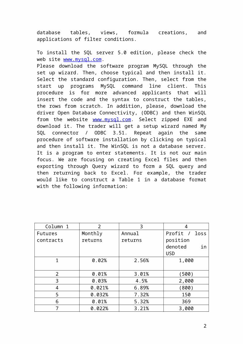
Futures contracts Monthly returns Annual returns Profit / loss position denoted in USD
1 0.02% 2.56% 1,000
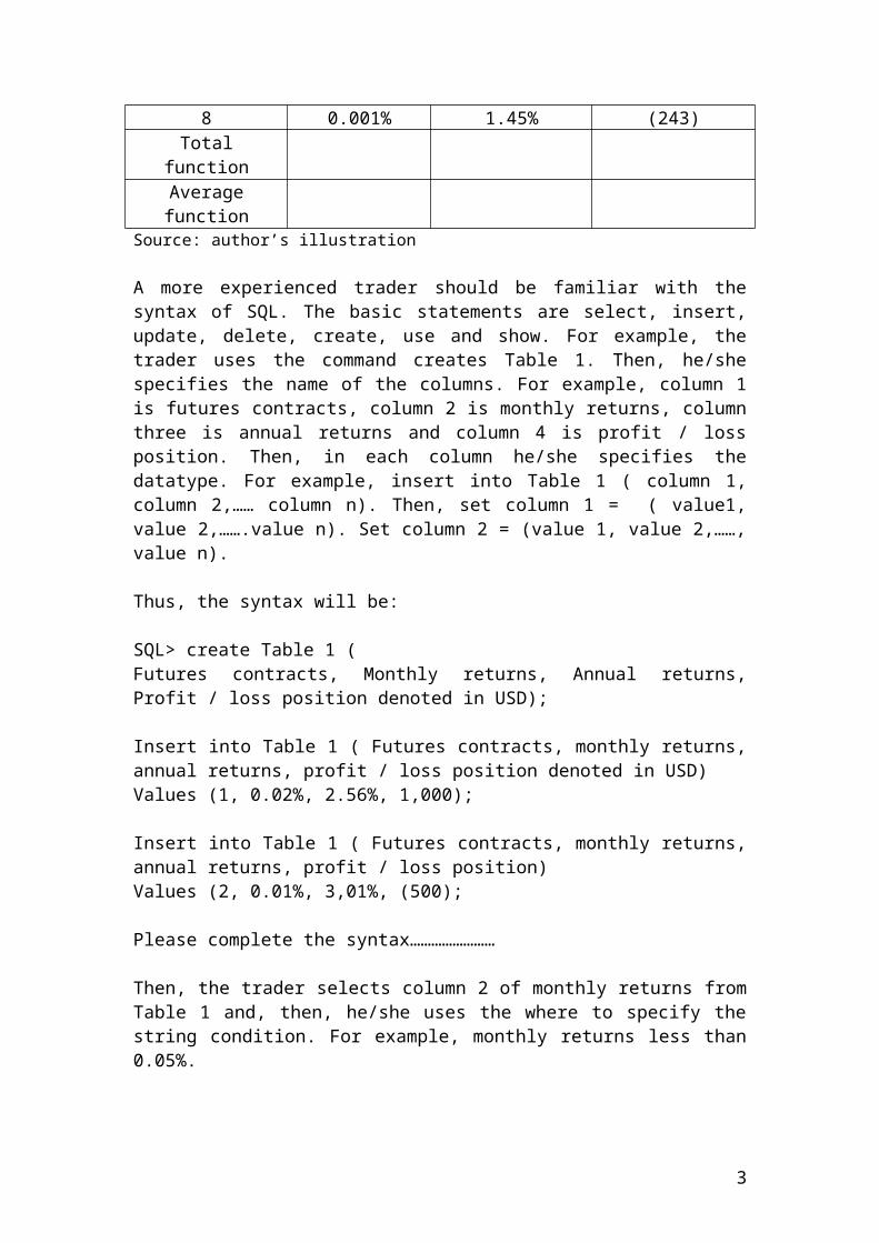
2 0.01% 3.01% (500)3 0.03% 4.5% 2,0004 0.021% 6.89% (800)5 0.032% 7.32% 1506 0.01% 5.32% 3697 0.022% 3.21% 3,0008 0.001% 1.45% (243)
Total functionAverage function
Source: author’s illustration
A more experienced trader should be familiar with the syntax of SQL. The basic statements are select, insert, update, delete, create, use and show. For example, the trader uses the command creates Table 1. Then, he/she specifies the name of the columns. For example, column 1 is futures contracts, column 2 is monthly returns, column three is annual returns and column 4 is profit / loss position. Then, in each column he/she specifies the datatype. For example, insert into Table 1 ( column 1, column 2,…… column n). Then, set column 1 = ( value1, value 2,…….value n). Set column 2 = (value 1, value 2,……, value n).
Thus, the syntax will be:
SQL> create Table 1 ( Futures contracts, Monthly returns, Annual returns, Profit / loss position denoted in USD);
Insert into Table 1 ( Futures contracts, monthly returns, annual returns, profit / loss position denoted in USD)Values (1, 0.02%, 2.56%, 1,000);
Insert into Table 1 ( Futures contracts, monthly returns, annual returns, profit / loss position)Values (2, 0.01%, 3,01%, (500);
Please complete the syntax……………………
Then, the trader selects column 2 of monthly returns from Table 1 and, then, he/she uses the where to specify the string condition. For example, monthly returns less than 0.05%.
Then, the trader has the option to perform various functions based on the table. For example, he/she could use the SQL count function, max function, average function, sum function, SQRT function, etc…
As an example, we will show the syntax of the total and average function. The average and total function for monthly returns will be as following:
2
SQL> SELECT AVG( monthly returns)-> FROM Table 1;
SQL> SELECT SUM( monthly returns)-> FROM Table 1;
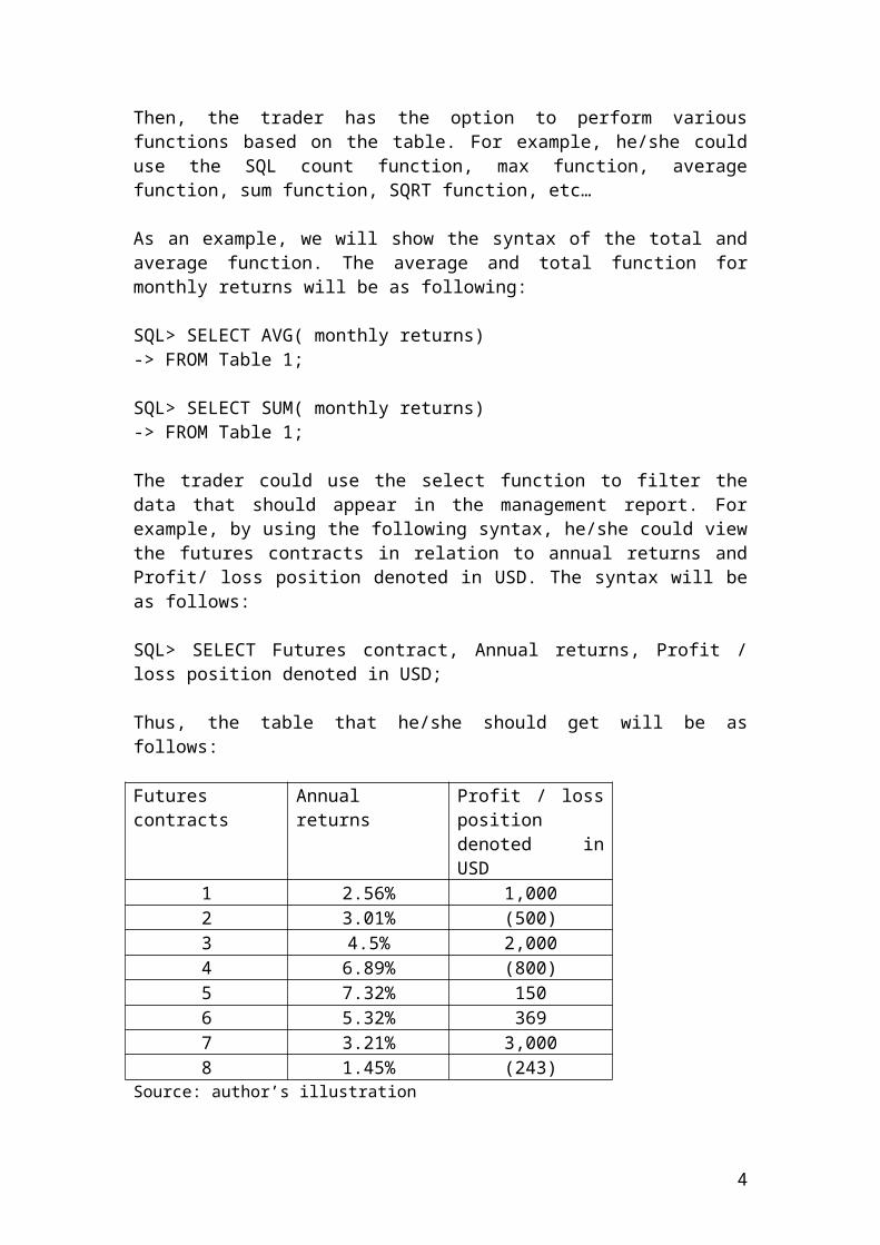
The trader could use the select function to filter the data that should appear in the management report. For example, by using the following syntax, he/she could view the futures contracts in relation to annual returns and Profit/ loss position denoted in USD. The syntax will be as follows:
SQL> SELECT Futures contract, Annual returns, Profit / loss position denoted in USD;
Thus, the table that he/she should get will be as follows:
Futures contracts Annual returns Profit / loss position denoted in USD
1 2.56% 1,0002 3.01% (500)3 4.5% 2,0004 6.89% (800)5 7.32% 1506 5.32% 3697 3.21% 3,0008 1.45% (243)
Source: author’s illustration
3
Workshop of language programming in terms of Python 3.4.1
Python version 3.4.1 Shell is very useful language programming for modeling financial derivatives. You can download and donate for the software by visiting the site www.python.org
The Python organization provides free download for the standard package version 3.4.1 Shell for windows or 3.5.
Python includes a math and a statistical library to import functions and perform basic calculations. Part of Python is the scientific Python package IPython. Components of IPyhton are scipy and Numpy. Scipy is used to calculate the cumulative normal distribution and generate random numbers. Numpy is used to construct array in matrix format which are used in statistics, econometrics and data analysis. We will focus on financial derivatives examples. IPython could be downloaded through the continuum analytics Anaconda website. www.continuum.io/downloads
Anaconda includes the standard Python software and the related libraries of IPython. You can download it for Windows, Linux and Macintosh. Please check for compatibility. version and memory space for fitness with your PC.
Please visit the site www.python.org and check the source code for mathematical statistics functions and the math library.
We will focus mainly on Python version 3.4.1 for doing simple calculations. We will use also the scientific Python package IPython to calculate call, put options and their related Greeks.
I have included basic examples that I have used in the Python version 3.4.1 Shell.
Variable names are written with underscore followed by the equal sign. For example,
>>> interest_rate = 0.03Variable names could also be written with small letters adjacent to each other. For example, interestrate = 0.03
It is better to use underscore to separate them and be able to read them clearly.
Another example that we can mention is if we have two variable values such as:>>> c = 5>>> d = 3>>> c+d 8>>> c*d15
4
I have included another example that shows the multiplication of two interest rates. Then, I have added to the result the second interest rate by using the function >>>interest_rate2+_. Then, I have rounded the final figure to two decimal places.
>>> interest_rate1 = 0.02>>> interest_rate2 = 0.03>>> interest_rate1*interest_rate20.0006>>> interest_rate2+_0.0306>>> round(_,2)0.03
Powers are performed by using twice the symbol**. For example, >>>3**5 243
If you would like to add comments, then, use the symbol # in front of the variable name.The operator # is used to write comments. For example,
>>>sigma = 0.5 # volatility.
Please distinguish between the integer numbers, (int), such as (1,3,4,5,7) and the fractional ones such as (2.0, 1.3) that are float.
Division is performed using the sign / to get a float result. Use the symbol // to get an integer result without fractional part. For example,>>> 7.0 / 3.0 2.33333
In contrast, >>> 7 // 3 2
Lists could be written as numbers separated by commas in brackets. As an example, please consider the following:
>>> squares = [1,2,4,5]>>> squares[1, 2, 4, 5]
Strings should be enclosed in single or double quotes.
5
For example, ‘ volatility’
Use the function range to include numbers from 1 to 10. The function is as follows:
>>> range(1,10)[1, 2, 3, 4, 5, 6, 7, 8, 9]
It is worth to mention the headings that should be included in Python version 3.4.1 Shell and IPython.
The headings are as follows:
>>>from statistics import mean, median, variance, or stdev OR
>>>from statistics import*
>>>data = [1.2,3.4]>>> mean(data)>>>2.3>>> median(data)etc…..
If you want to round then use the function round(_,2)
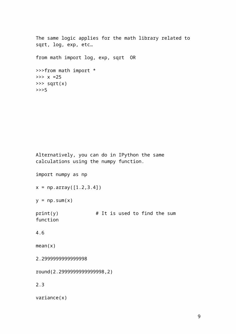
The same logic applies for the math library related to sqrt, log, exp, etc…
from math import log, exp, sqrt OR
>>>from math import *>>> x =25>>> sqrt(x)>>>5
Alternatively, you can do in IPython the same calculations using the numpy function.
import numpy as np
x = np.array([1.2,3.4])
y = np.sum(x)
6
print(y) # It is used to find the sum function
4.6
mean(x)
2.2999999999999998
round(2.2999999999999998,2)
2.3
variance(x)
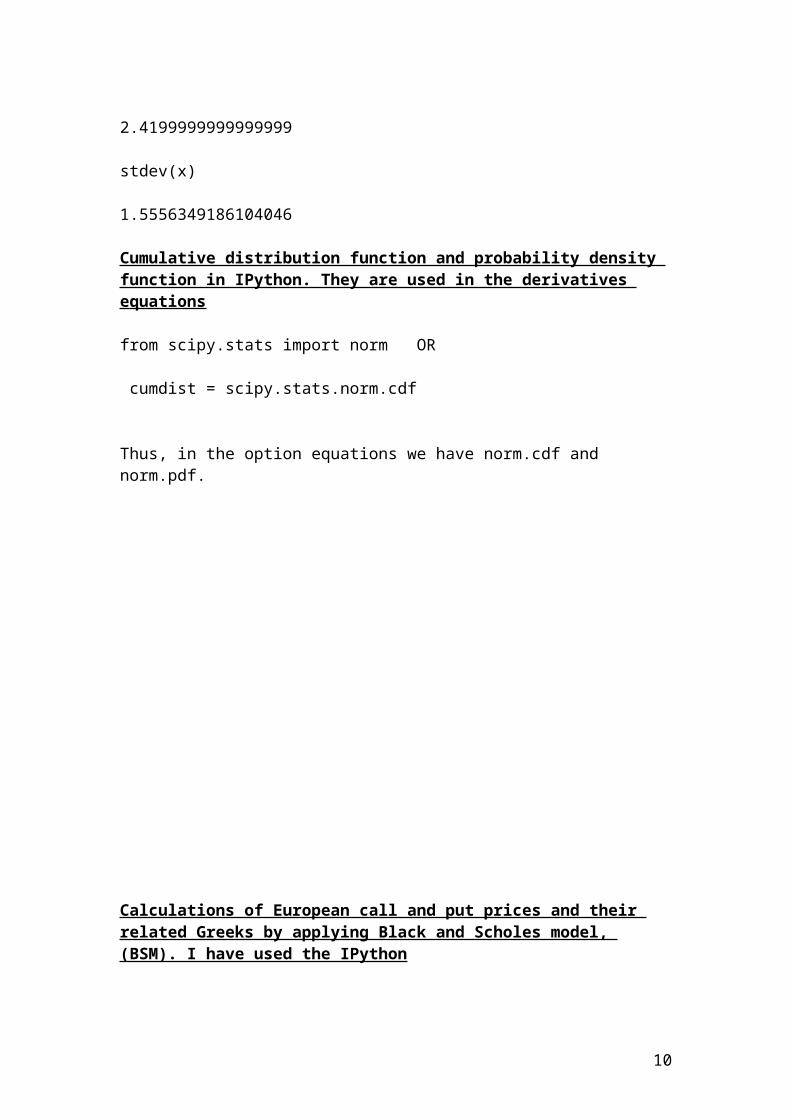
2.4199999999999999
stdev(x)
1.5556349186104046
Cumulative distribution function and probability density function in IPython. They are used in the derivatives equations
from scipy.stats import norm OR
cumdist = scipy.stats.norm.cdf
Thus, in the option equations we have norm.cdf and norm.pdf.
7
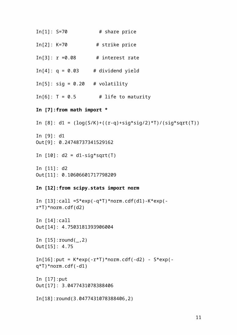
Calculations of European call and put prices and their related Greeks by applying Black and Scholes model, (BSM). I have used the IPython
In[1]: S=70 # share price
In[2]: K=70 # strike price
In[3]: r =0.08 # interest rate
In[4]: q = 0.03 # dividend yield
In[5]: sig = 0.20 # volatility
In[6]: T = 0.5 # life to maturity
In [7]:from math import *
In [8]: d1 = (log(S/K)+((r-q)+sig*sig/2)*T)/(sig*sqrt(T))
In [9]: d1Out[9]: 0.24748737341529162
In [10]: d2 = d1-sig*sqrt(T)
In [11]: d2Out[11]: 0.10606601717798209
In [12]:from scipy.stats import norm
In [13]:call =S*exp(-q*T)*norm.cdf(d1)-K*exp(-r*T)*norm.cdf(d2)
In [14]:callOut[14]: 4.7503181393906004
In [15]:round(_,2)Out[15]: 4.75
In[16]:put = K*exp(-r*T)*norm.cdf(-d2) - S*exp(-q*T)*norm.cdf(-d1)
In [17]:putOut[17]: 3.0477431078388406
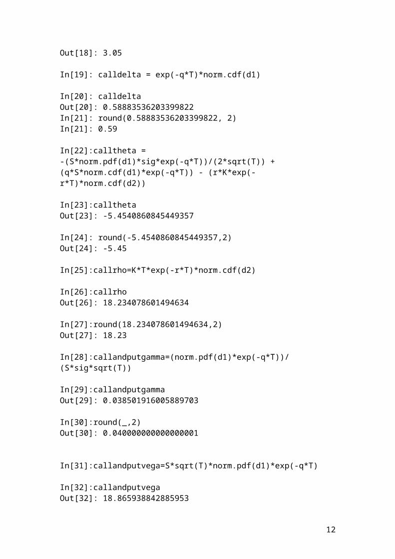
In[18]:round(3.0477431078388406,2)Out[18]: 3.05
In[19]: calldelta = exp(-q*T)*norm.cdf(d1)
In[20]: calldeltaOut[20]: 0.58883536203399822
8
In[21]: round(0.58883536203399822, 2)In[21]: 0.59
In[22]:calltheta = -(S*norm.pdf(d1)*sig*exp(-q*T))/(2*sqrt(T)) +(q*S*norm.cdf(d1)*exp(-q*T)) - (r*K*exp(-r*T)*norm.cdf(d2))
In[23]:callthetaOut[23]: -5.4540860845449357
In[24]: round(-5.4540860845449357,2)Out[24]: -5.45
In[25]:callrho=K*T*exp(-r*T)*norm.cdf(d2)
In[26]:callrhoOut[26]: 18.234078601494634
In[27]:round(18.234078601494634,2)Out[27]: 18.23
In[28]:callandputgamma=(norm.pdf(d1)*exp(-q*T))/(S*sig*sqrt(T))
In[29]:callandputgammaOut[29]: 0.038501916005889703
In[30]:round(_,2)Out[30]: 0.040000000000000001
In[31]:callandputvega=S*sqrt(T)*norm.pdf(d1)*exp(-q*T)
In[32]:callandputvegaOut[32]: 18.865938842885953
In[33]:round(_,2)Out[33]: 18.870000000000001
In[34]:putdelta = exp(-q*T)*(norm.cdf(d1)-1)
In[35]:putdeltaOut[35]: -0.39627657756906448
In[36]:round(_,2)Out[36]: -0.40000000000000002
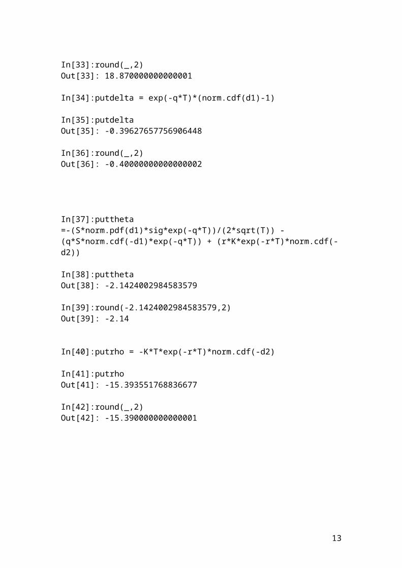
In[37]:puttheta =-(S*norm.pdf(d1)*sig*exp(-q*T))/(2*sqrt(T)) - (q*S*norm.cdf(-d1)*exp(-q*T)) + (r*K*exp(-r*T)*norm.cdf(-d2))
9
In[38]:putthetaOut[38]: -2.1424002984583579
In[39]:round(-2.1424002984583579,2)Out[39]: -2.14
In[40]:putrho = -K*T*exp(-r*T)*norm.cdf(-d2)
In[41]:putrhoOut[41]: -15.393551768836677
In[42]:round(_,2)Out[42]: -15.390000000000001
10
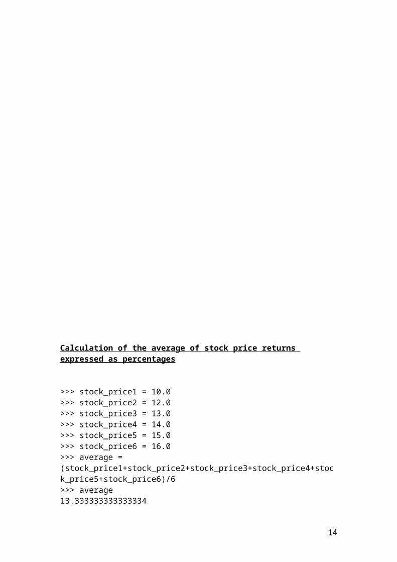
Calculation of the average of stock price returns expressed as percentages
>>> stock_price1 = 10.0>>> stock_price2 = 12.0>>> stock_price3 = 13.0>>> stock_price4 = 14.0>>> stock_price5 = 15.0>>> stock_price6 = 16.0>>> average = (stock_price1+stock_price2+stock_price3+stock_price4+stock_price5+stock_price6)/6>>> average13.333333333333334
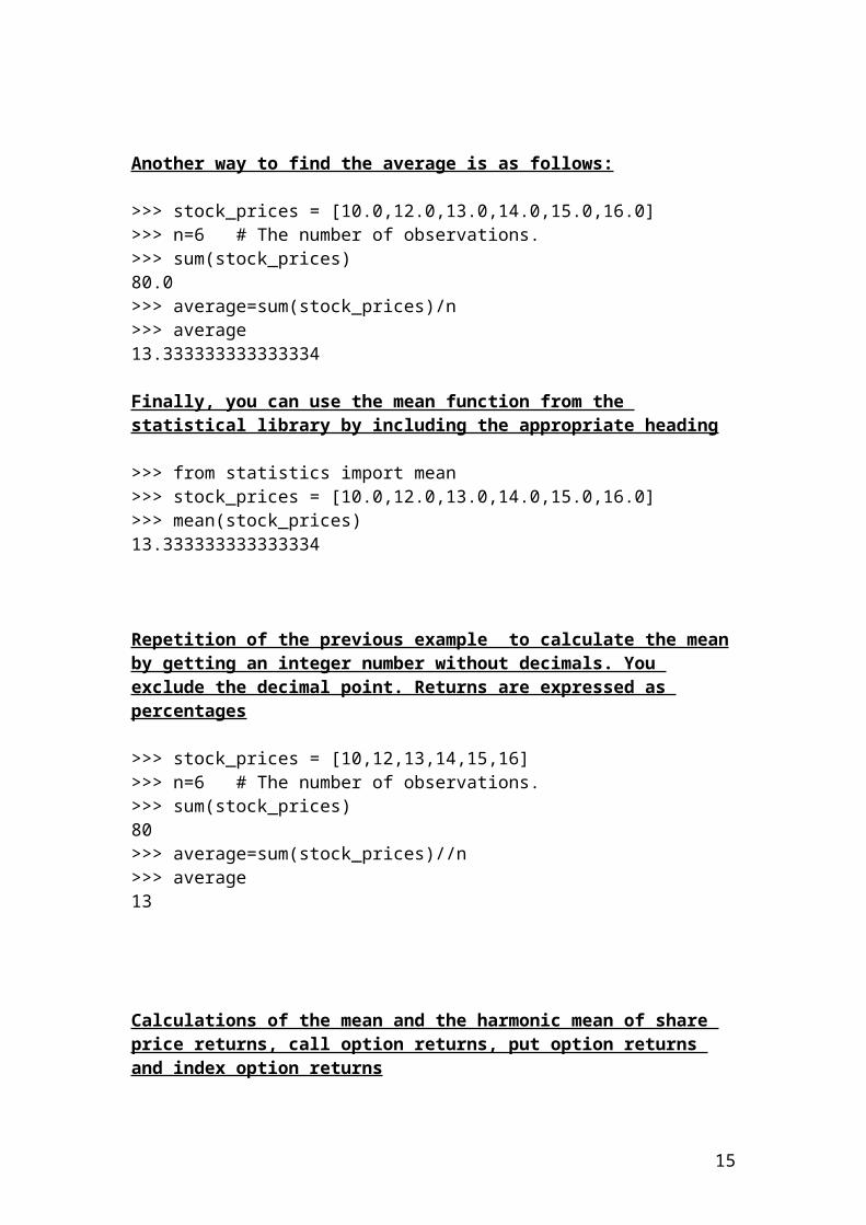
Another way to find the average is as follows:
>>> stock_prices = [10.0,12.0,13.0,14.0,15.0,16.0]>>> n=6 # The number of observations.>>> sum(stock_prices)80.0>>> average=sum(stock_prices)/n>>> average13.333333333333334
Finally, you can use the mean function from the statistical library by including the appropriate heading
>>> from statistics import mean>>> stock_prices = [10.0,12.0,13.0,14.0,15.0,16.0]>>> mean(stock_prices)13.333333333333334
Repetition of the previous example to calculate the mean by getting an integer number without decimals. You exclude the decimal point. Returns are expressed as percentages
>>> stock_prices = [10,12,13,14,15,16]>>> n=6 # The number of observations.>>> sum(stock_prices)80>>> average=sum(stock_prices)//n>>> average13
11
Calculations of the mean and the harmonic mean of share price returns, call option returns, put option returns and index option returns
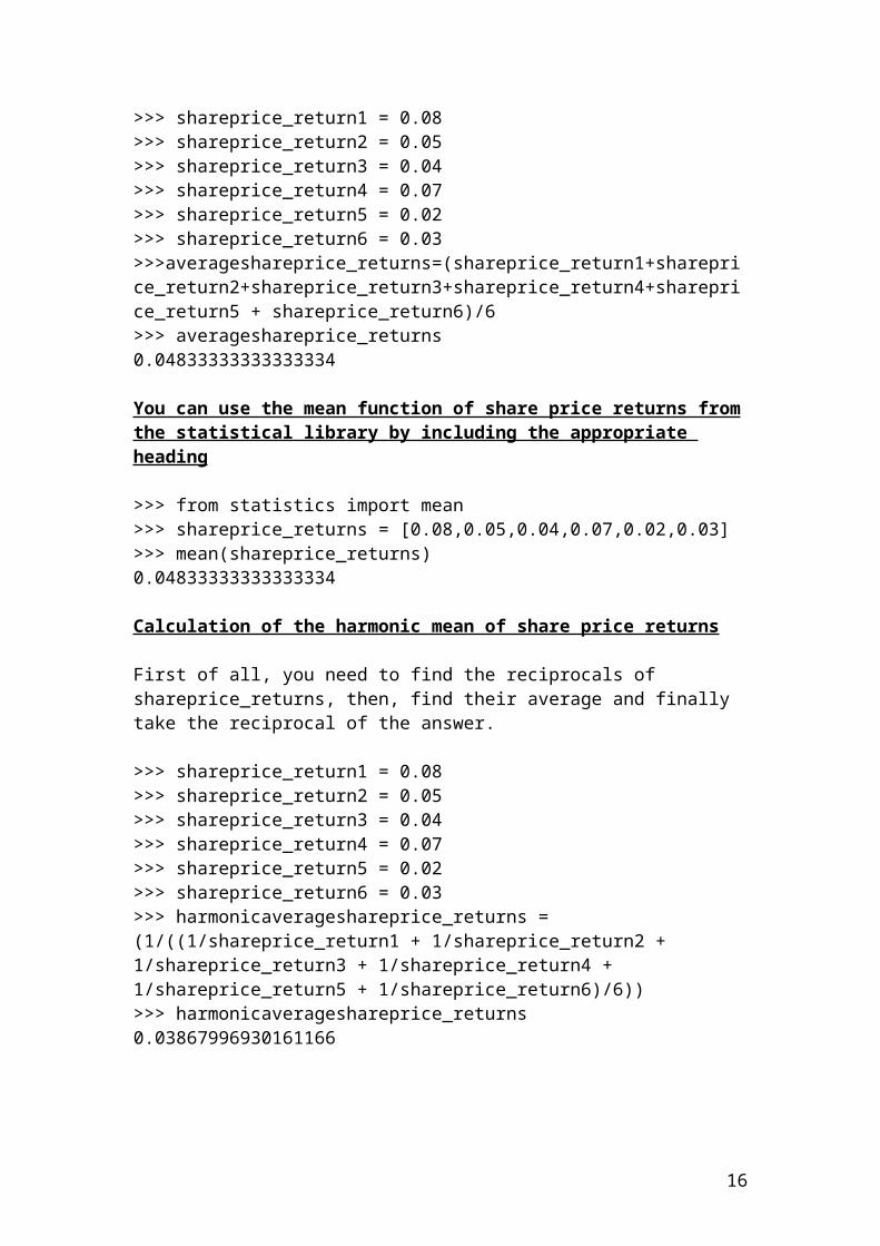
>>> shareprice_return1 = 0.08>>> shareprice_return2 = 0.05>>> shareprice_return3 = 0.04>>> shareprice_return4 = 0.07>>> shareprice_return5 = 0.02>>> shareprice_return6 = 0.03>>>averageshareprice_returns=(shareprice_return1+shareprice_return2+shareprice_return3+shareprice_return4+shareprice_return5 + shareprice_return6)/6>>> averageshareprice_returns0.04833333333333334
You can use the mean function of share price returns from the statistical library by including the appropriate heading
>>> from statistics import mean>>> shareprice_returns = [0.08,0.05,0.04,0.07,0.02,0.03]>>> mean(shareprice_returns)0.04833333333333334
Calculation of the harmonic mean of share price returns
First of all, you need to find the reciprocals of shareprice_returns, then, find their average and finally take the reciprocal of the answer.
>>> shareprice_return1 = 0.08>>> shareprice_return2 = 0.05>>> shareprice_return3 = 0.04>>> shareprice_return4 = 0.07>>> shareprice_return5 = 0.02>>> shareprice_return6 = 0.03>>> harmonicaverageshareprice_returns = (1/((1/shareprice_return1 + 1/shareprice_return2 + 1/shareprice_return3 + 1/shareprice_return4 + 1/shareprice_return5 + 1/shareprice_return6)/6))>>> harmonicaverageshareprice_returns0.03867996930161166
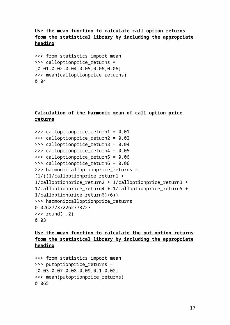
Use the mean function to calculate call option returns from the statistical library by including the appropriate heading
>>> from statistics import mean>>> calloptionprice_returns = [0.01,0.02,0.04,0.05,0.06,0.06]>>> mean(calloptionprice_returns)0.04
12
Calculation of the harmonic mean of call option price returns
>>> calloptionprice_return1 = 0.01>>> calloptionprice_return2 = 0.02>>> calloptionprice_return3 = 0.04>>> calloptionprice_return4 = 0.05>>> calloptionprice_return5 = 0.06>>> calloptionprice_return6 = 0.06>>> harmoniccalloptionprice_returns = (1/((1/calloptionprice_return1 + 1/calloptionprice_return2 + 1/calloptionprice_return3 + 1/calloptionprice_return4 + 1/calloptionprice_return5 + 1/calloptionprice_return6)/6))>>> harmoniccalloptionprice_returns0.026277372262773727>>> round(_,2)0.03
Use the mean function to calculate the put option returns from the statistical library by including the appropriate heading
>>> from statistics import mean>>> putoptionprice_returns = [0.03,0.07,0.08,0.09,0.1,0.02]>>> mean(putoptionprice_returns)0.065
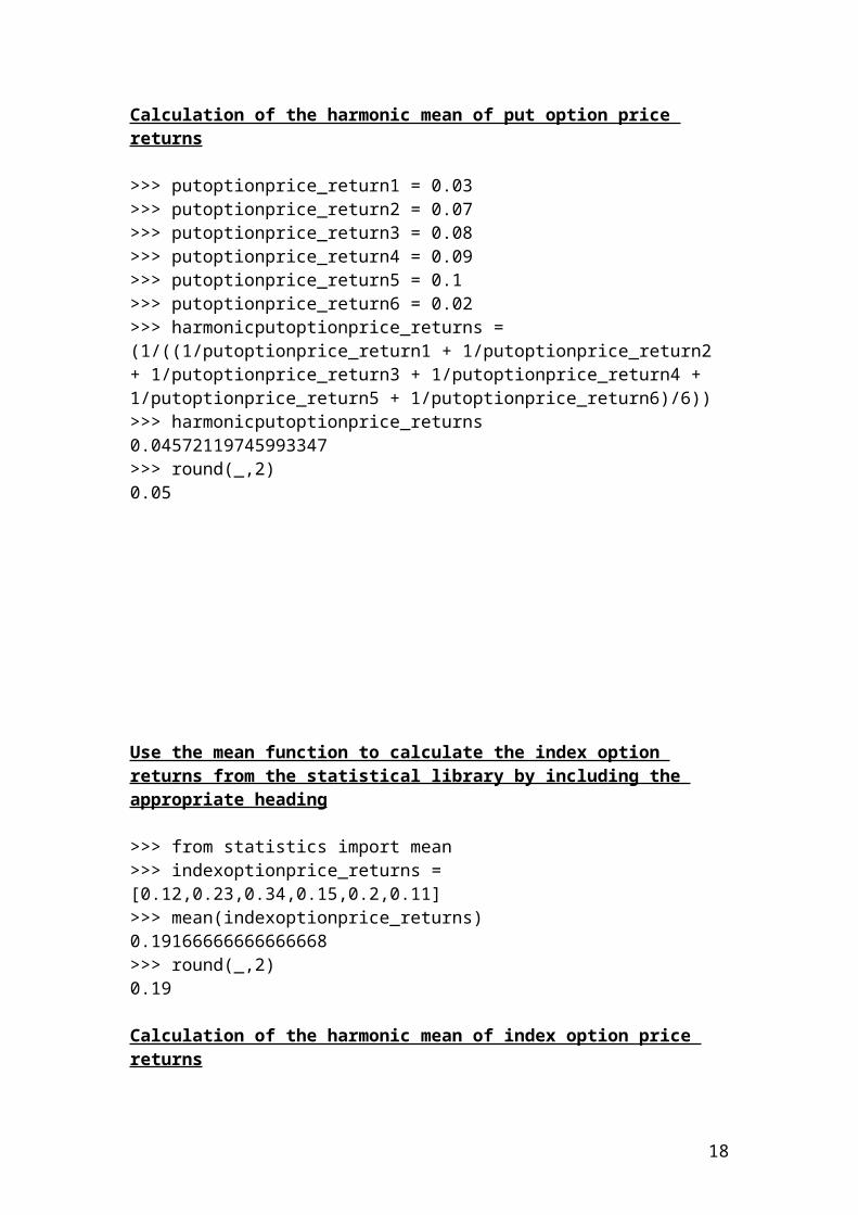
Calculation of the harmonic mean of put option price returns
>>> putoptionprice_return1 = 0.03>>> putoptionprice_return2 = 0.07>>> putoptionprice_return3 = 0.08>>> putoptionprice_return4 = 0.09>>> putoptionprice_return5 = 0.1>>> putoptionprice_return6 = 0.02>>> harmonicputoptionprice_returns = (1/((1/putoptionprice_return1 + 1/putoptionprice_return2 + 1/putoptionprice_return3 + 1/putoptionprice_return4 + 1/putoptionprice_return5 + 1/putoptionprice_return6)/6))>>> harmonicputoptionprice_returns0.04572119745993347>>> round(_,2)0.05
13
Use the mean function to calculate the index option returns from the statistical library by including the appropriate heading
>>> from statistics import mean>>> indexoptionprice_returns = [0.12,0.23,0.34,0.15,0.2,0.11]>>> mean(indexoptionprice_returns)0.19166666666666668>>> round(_,2)0.19
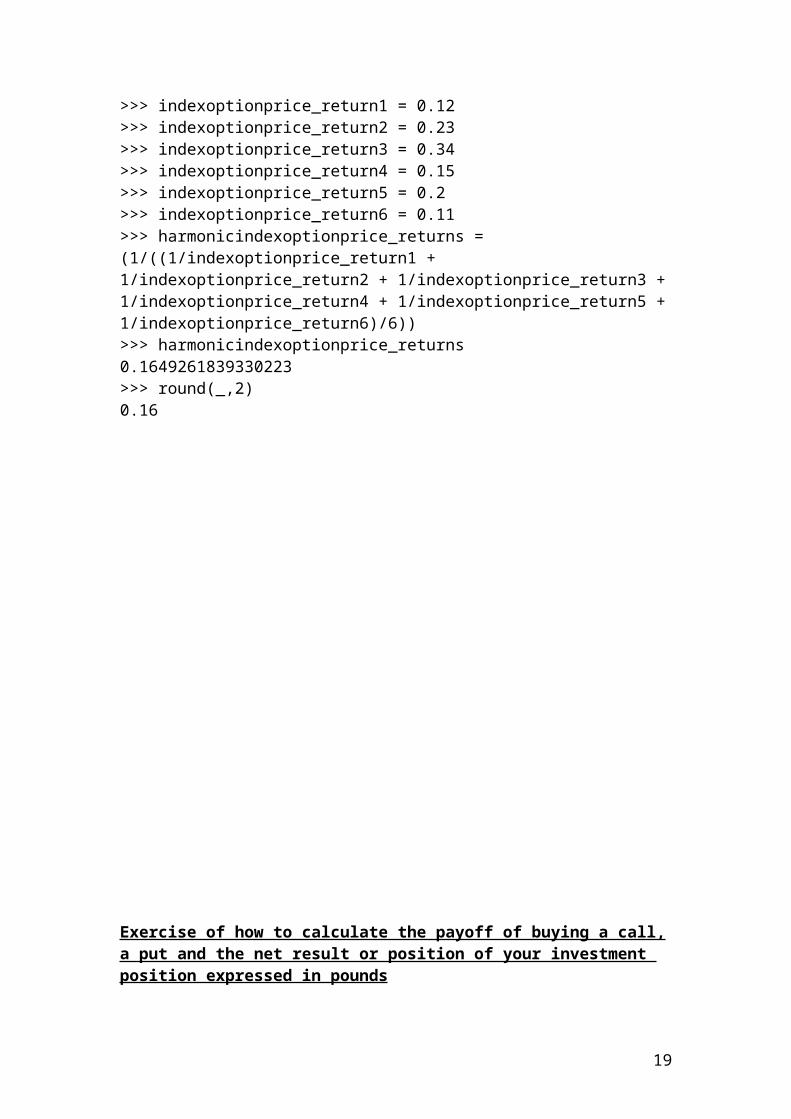
Calculation of the harmonic mean of index option price returns
>>> indexoptionprice_return1 = 0.12>>> indexoptionprice_return2 = 0.23>>> indexoptionprice_return3 = 0.34>>> indexoptionprice_return4 = 0.15>>> indexoptionprice_return5 = 0.2>>> indexoptionprice_return6 = 0.11>>> harmonicindexoptionprice_returns = (1/((1/indexoptionprice_return1 + 1/indexoptionprice_return2 + 1/indexoptionprice_return3 + 1/indexoptionprice_return4 + 1/indexoptionprice_return5 + 1/indexoptionprice_return6)/6))>>> harmonicindexoptionprice_returns0.1649261839330223>>> round(_,2)0.16
14
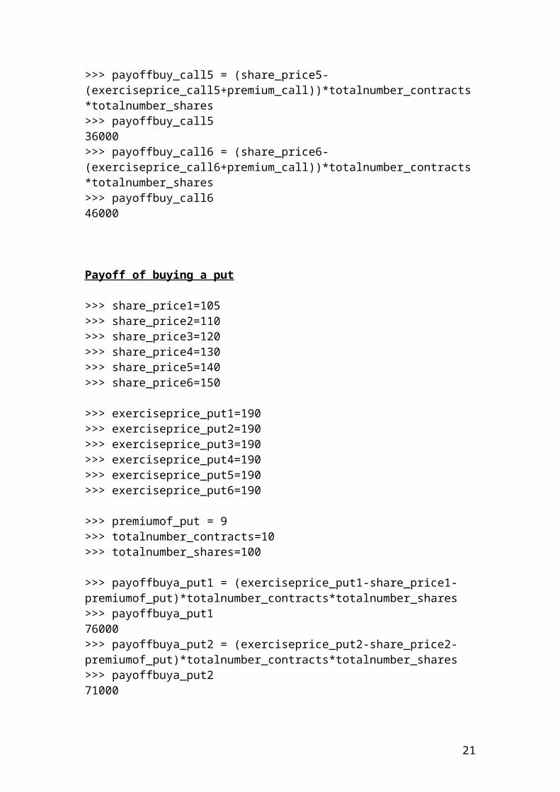
Exercise of how to calculate the payoff of buying a call, a put and the net result or position of your investment position expressed in pounds
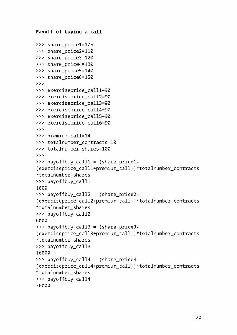
Payoff of buying a call
>>> share_price1=105>>> share_price2=110>>> share_price3=120>>> share_price4=130>>> share_price5=140>>> share_price6=150>>> >>> exerciseprice_call1=90>>> exerciseprice_call2=90>>> exerciseprice_call3=90>>> exerciseprice_call4=90>>> exerciseprice_call5=90>>> exerciseprice_call6=90>>> >>> premium_call=14>>> totalnumber_contracts=10>>> totalnumber_shares=100>>> >>> payoffbuy_call1 = (share_price1-(exerciseprice_call1+premium_call))*totalnumber_contracts*totalnumber_shares>>> payoffbuy_call11000>>> payoffbuy_call2 = (share_price2-(exerciseprice_call2+premium_call))*totalnumber_contracts*totalnumber_shares>>> payoffbuy_call26000>>> payoffbuy_call3 = (share_price3-(exerciseprice_call3+premium_call))*totalnumber_contracts*totalnumber_shares>>> payoffbuy_call316000>>> payoffbuy_call4 = (share_price4-(exerciseprice_call4+premium_call))*totalnumber_contracts*totalnumber_shares>>> payoffbuy_call426000>>> payoffbuy_call5 = (share_price5-(exerciseprice_call5+premium_call))*totalnumber_contracts*totalnumber_shares>>> payoffbuy_call536000>>> payoffbuy_call6 = (share_price6-(exerciseprice_call6+premium_call))*totalnumber_contracts*totalnumber_shares>>> payoffbuy_call646000
15
Payoff of buying a put
>>> share_price1=105>>> share_price2=110>>> share_price3=120>>> share_price4=130>>> share_price5=140>>> share_price6=150
>>> exerciseprice_put1=190>>> exerciseprice_put2=190>>> exerciseprice_put3=190>>> exerciseprice_put4=190>>> exerciseprice_put5=190>>> exerciseprice_put6=190
>>> premiumof_put = 9>>> totalnumber_contracts=10>>> totalnumber_shares=100
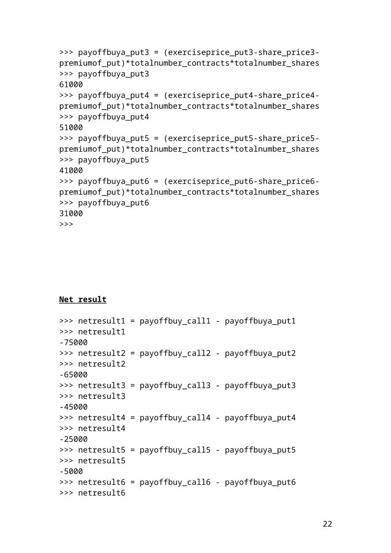
>>> payoffbuya_put1 = (exerciseprice_put1-share_price1-premiumof_put)*totalnumber_contracts*totalnumber_shares>>> payoffbuya_put176000>>> payoffbuya_put2 = (exerciseprice_put2-share_price2-premiumof_put)*totalnumber_contracts*totalnumber_shares>>> payoffbuya_put271000>>> payoffbuya_put3 = (exerciseprice_put3-share_price3-premiumof_put)*totalnumber_contracts*totalnumber_shares>>> payoffbuya_put361000>>> payoffbuya_put4 = (exerciseprice_put4-share_price4-premiumof_put)*totalnumber_contracts*totalnumber_shares>>> payoffbuya_put451000>>> payoffbuya_put5 = (exerciseprice_put5-share_price5-premiumof_put)*totalnumber_contracts*totalnumber_shares>>> payoffbuya_put541000>>> payoffbuya_put6 = (exerciseprice_put6-share_price6-premiumof_put)*totalnumber_contracts*totalnumber_shares>>> payoffbuya_put631000>>>
16
Net result
>>> netresult1 = payoffbuy_call1 - payoffbuya_put1>>> netresult1-75000>>> netresult2 = payoffbuy_call2 - payoffbuya_put2>>> netresult2-65000>>> netresult3 = payoffbuy_call3 - payoffbuya_put3>>> netresult3-45000>>> netresult4 = payoffbuy_call4 - payoffbuya_put4>>> netresult4-25000>>> netresult5 = payoffbuy_call5 - payoffbuya_put5>>> netresult5-5000>>> netresult6 = payoffbuy_call6 - payoffbuya_put6>>> netresult615000>>>
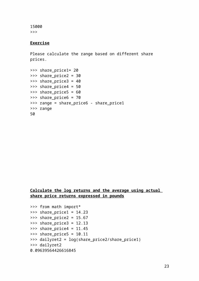
Exercise
Please calculate the range based on different share prices.
>>> share_price1= 20>>> share_price2 = 30>>> share_price3 = 40>>> share_price4 = 50>>> share_price5 = 60>>> share_price6 = 70>>> range = share_price6 - share_price1>>> range50
17
Calculate the log returns and the average using actual share price returns expressed in pounds
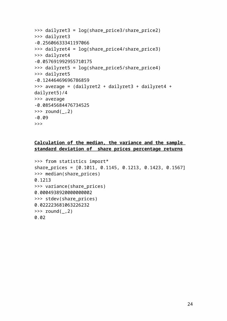
>>> from math import*>>> share_price1 = 14.23>>> share_price2 = 15.67>>> share_price3 = 12.13>>> share_price4 = 11.45>>> share_price5 = 10.11>>> dailyret2 = log(share_price2/share_price1)>>> dailyret20.09639564426616845>>> dailyret3 = log(share_price3/share_price2)>>> dailyret3-0.25606633341197066>>> dailyret4 = log(share_price4/share_price3)>>> dailyret4-0.057691992955710175>>> dailyret5 = log(share_price5/share_price4)>>> dailyret5-0.12446469696786859>>> average = (dailyret2 + dailyret3 + dailyret4 + dailyret5)/4>>> average-0.08545684476734525>>> round(_,2)-0.09>>>
Calculation of the median, the variance and the sample standard deviation of share prices percentage returns
>>> from statistics import*share_prices = [0.1011, 0.1145, 0.1213, 0.1423, 0.1567]>>> median(share_prices)0.1213>>> variance(share_prices)0.0004938920000000002>>> stdev(share_prices)0.022223681063226232>>> round(_,2)0.02
18
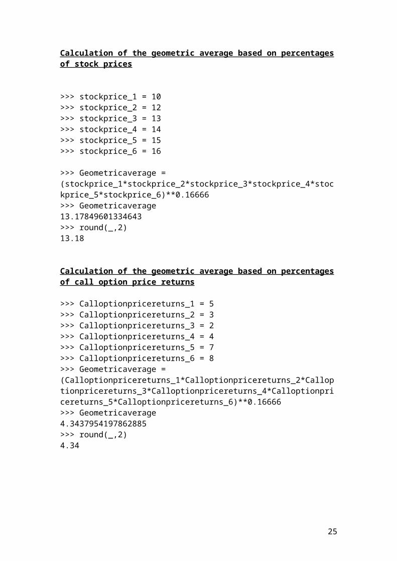
Calculation of the geometric average based on percentages of stock prices
>>> stockprice_1 = 10>>> stockprice_2 = 12>>> stockprice_3 = 13>>> stockprice_4 = 14>>> stockprice_5 = 15>>> stockprice_6 = 16
>>> Geometricaverage = (stockprice_1*stockprice_2*stockprice_3*stockprice_4*stockprice_5*stockprice_6)**0.16666>>> Geometricaverage13.17849601334643>>> round(_,2)13.18
Calculation of the geometric average based on percentages of call option price returns
>>> Calloptionpricereturns_1 = 5>>> Calloptionpricereturns_2 = 3>>> Calloptionpricereturns_3 = 2>>> Calloptionpricereturns_4 = 4>>> Calloptionpricereturns_5 = 7>>> Calloptionpricereturns_6 = 8>>> Geometricaverage = (Calloptionpricereturns_1*Calloptionpricereturns_2*Calloptionpricereturns_3*Calloptionpricereturns_4*Calloptionpricereturns_5*Calloptionpricereturns_6)**0.16666>>> Geometricaverage4.3437954197862885>>> round(_,2)4.34
19
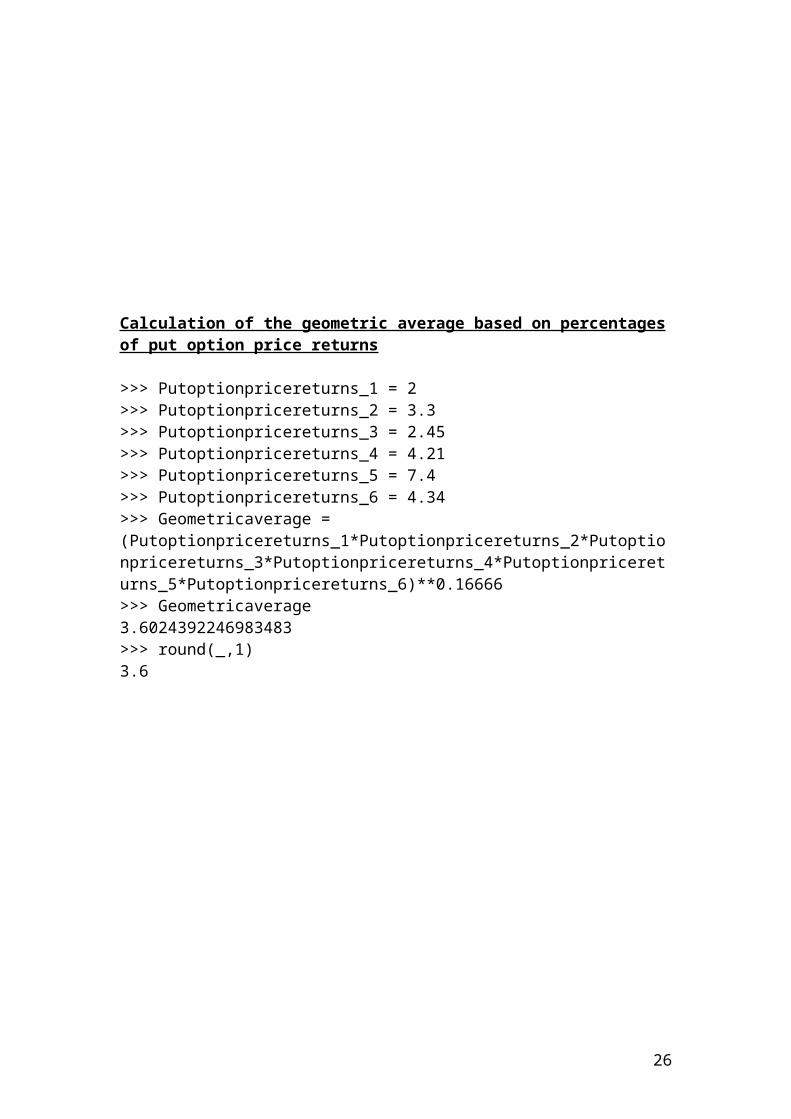
Calculation of the geometric average based on percentages of put option price returns
>>> Putoptionpricereturns_1 = 2>>> Putoptionpricereturns_2 = 3.3>>> Putoptionpricereturns_3 = 2.45>>> Putoptionpricereturns_4 = 4.21>>> Putoptionpricereturns_5 = 7.4>>> Putoptionpricereturns_6 = 4.34>>> Geometricaverage = (Putoptionpricereturns_1*Putoptionpricereturns_2*Putoptionpricereturns_3*Putoptionpricereturns_4*Putoptionpricereturns_5*Putoptionpricereturns_6)**0.16666>>> Geometricaverage3.6024392246983483>>> round(_,1)3.6
20
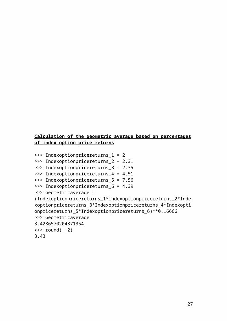
Calculation of the geometric average based on percentages of index option price returns
>>> Indexoptionpricereturns_1 = 2>>> Indexoptionpricereturns_2 = 2.31>>> Indexoptionpricereturns_3 = 2.35>>> Indexoptionpricereturns_4 = 4.51>>> Indexoptionpricereturns_5 = 7.56>>> Indexoptionpricereturns_6 = 4.39>>> Geometricaverage = (Indexoptionpricereturns_1*Indexoptionpricereturns_2*Indexoptionpricereturns_3*Indexoptionpricereturns_4*Indexoptionpricereturns_5*Indexoptionpricereturns_6)**0.16666>>> Geometricaverage3.4286570204871354>>> round(_,2)3.43
21
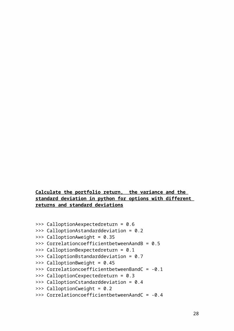
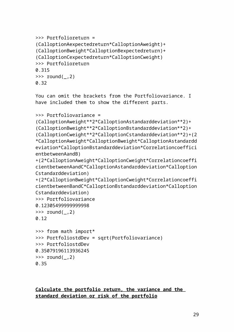
Calculate the portfolio return, the variance and the standard deviation in python for options with different returns and standard deviations
>>> CalloptionAexpectedreturn = 0.6>>> CalloptionAstandarddeviation = 0.2>>> CalloptionAweight = 0.35>>> CorrelationcoefficientbetweenAandB = 0.5>>> CalloptionBexpectedreturn = 0.1>>> CalloptionBstandarddeviation = 0.7>>> CalloptionBweight = 0.45>>> CorrelationcoefficientbetweenBandC = -0.1>>> CalloptionCexpectedreturn = 0.3>>> CalloptionCstandarddeviation = 0.4>>> CalloptionCweight = 0.2>>> CorrelationcoefficientbetweenAandC = -0.4
>>> Portfolioreturn = (CalloptionAexpectedreturn*CalloptionAweight)+(CalloptionBweight*CalloptionBexpectedreturn)+(CalloptionCexpectedreturn*CalloptionCweight)>>> Portfolioreturn0.315>>> round(_,2)0.32
You can omit the brackets from the Portfoliovariance. I have included them to show the different parts.
>>> Portfoliovariance = (CalloptionAweight**2*CalloptionAstandarddeviation**2)+ (CalloptionBweight**2*CalloptionBstandarddeviation**2)+(CalloptionCweight**2*CalloptionCstandarddeviation**2)+(2*CalloptionAweight*CalloptionBweight*CalloptionAstandarddeviation*CalloptionBstandarddeviation*CorrelationcoefficientbetweenAandB)+(2*CalloptionAweight*CalloptionCweight*CorrelationcoefficientbetweenAandC*CalloptionAstandarddeviation*CalloptionCstandarddeviation)+(2*CalloptionBweight*CalloptionCweight*CorrelationcoefficientbetweenBandC*CalloptionBstandarddeviation*CalloptionCstandarddeviation)>>> Portfoliovariance0.12305499999999998>>> round(_,2)0.12
>>> from math import*>>> PortfoliostdDev = sqrt(Portfoliovariance)>>> PortfoliostdDev0.35079196113936245>>> round(_,2)0.35
22
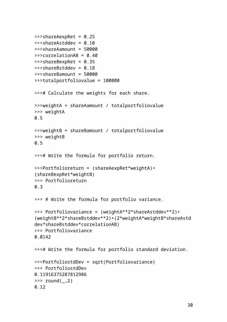
Calculate the portfolio return, the variance and the standard deviation or risk of the portfolio
>>>shareAexpRet = 0.25>>>shareAstddev = 0.10>>>shareAamount = 50000>>>correlationAB = 0.40>>>shareBexpRet = 0.35>>>shareBstddev = 0.18>>>shareBamount = 50000>>>totalportfoliovalue = 100000
>>># Calculate the weights for each share.
>>>weightA = shareAamount / totalportfoliovalue>>> weightA0.5
>>>weightB = shareBamount / totalportfoliovalue>>> weightB0.5
>>># Write the formula for portfolio return.
>>>Portfolioreturn = (shareAexpRet*weightA)+(shareBexpRet*weightB)>>> Portfolioreturn0.3
>>> # Write the formula for portfolio variance.
>>> Portfoliovariance = (weightA**2*shareAstddev**2)+(weightB**2*shareBstddev**2)+(2*weightA*weightB*shareAstddev*shareBstddev*correlationAB)>>> Portfoliovariance0.0142
>>># Write the formula for portfolio standard deviation.
>>>PortfoliostdDev = sqrt(Portfoliovariance)>>> PortfoliostdDev0.11916375287812986>>> round(_,2)0.12
23
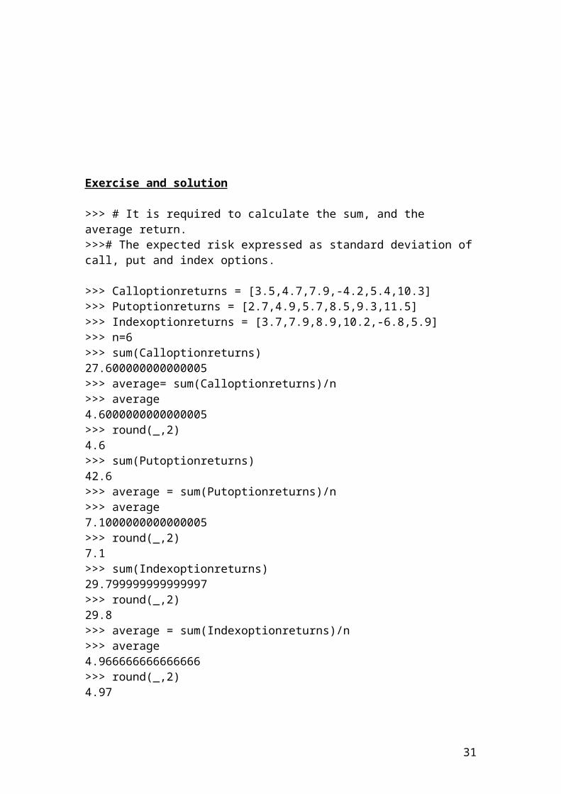
Exercise and solution
>>> # It is required to calculate the sum, and the average return.>>># The expected risk expressed as standard deviation of call, put and index options.
>>> Calloptionreturns = [3.5,4.7,7.9,-4.2,5.4,10.3]>>> Putoptionreturns = [2.7,4.9,5.7,8.5,9.3,11.5]>>> Indexoptionreturns = [3.7,7.9,8.9,10.2,-6.8,5.9]>>> n=6>>> sum(Calloptionreturns)27.600000000000005>>> average= sum(Calloptionreturns)/n>>> average4.6000000000000005>>> round(_,2)4.6>>> sum(Putoptionreturns)42.6>>> average = sum(Putoptionreturns)/n>>> average7.1000000000000005>>> round(_,2)7.1>>> sum(Indexoptionreturns)29.799999999999997>>> round(_,2)29.8>>> average = sum(Indexoptionreturns)/n>>> average4.966666666666666>>> round(_,2)4.97
>>> from statistics import stdev>>> stdev(Calloptionreturns)4.953382682571578>>> round(_,2)4.95>>> stdev(Putoptionreturns)3.234810659064917>>> round(_,2)3.23>>> stdev(Indexoptionreturns)6.203117495797308>>> round(_,2)6.2
24
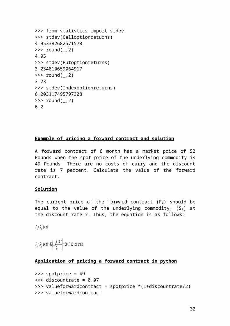
Example of pricing a forward contract and solution
A forward contract of 6 month has a market price of 52 Pounds when the spot price of the underlying commodity is 49 Pounds. There are no costs of carry and the discount rate is 7 percent. Calculate the value of the forward contract.
Solution
The current price of the forward contract (F0) should be equal to the value of the underlying commodity, (S0) at the discount rate r. Thus, the equation is as follows:
F0=S0(1+r )
F0=S0(1+r )=49(1+0 . 072 )=50 . 715 pounds
Application of pricing a forward contract in python
>>> spotprice = 49>>> discountrate = 0.07>>> valueforwardcontract = spotprice *(1+discountrate/2)>>> valueforwardcontract50.714999999999996>>> round(_,2)50.71 # Pounds
25
Example of interest rate payment and solution
A trader wants to calculate the interest amount that he / she will receive in three months from a forward contract of a Euribor deposit paying a Euro deposit rate of 3.55%. The principal amount is 300,000
The mathematical formula is as follows:
Interest payment = principal x [interest rate x (tdays / 360)]
Interest payment = 300,000 x [0.0355 x (90/360)]Interest payment = 2662.5 Euro.
Application of interest payment in python
>>> principal = 300000>>> interest_rate = 0.0355>>> days = 90>>> interestpayment = principal*(interest_rate *days/360)>>> interestpayment2662.4999999999995>>> round(_,2)2662.5 # Euro
26
Example and solution of calculating profits and losses on futures contracts
An investor buys 8 S&P 500 futures contracts at $2189. He has closed the futures contract position with a price of $2236. The multiplier for S&P 500 futures contracts is 250 dollars. Did he record a profit or a loss?
Solution
The mathematical formula is as follows:
Pr ofit /Loss=|number of contracts x contract size x ( f T− f 0 )|
Where: fT is the final contract price. f0 is the initial contract price.
Gain=8 x 250 x (2236−2189 )=94000 USD
When the prices move up, the investor will gain in long positions. When prices move down, the investor will gain in short positions.
Application of calculating profits and losses on futures contracts in python
>>> numberof_contracts = 8>>> buying_price = 2189>>> selling_price = 2236>>> multiplier = 250>>> profitorloss = numberof_contracts*multiplier*(selling_price - buying_price)>>> profitorloss94000 # USD
27
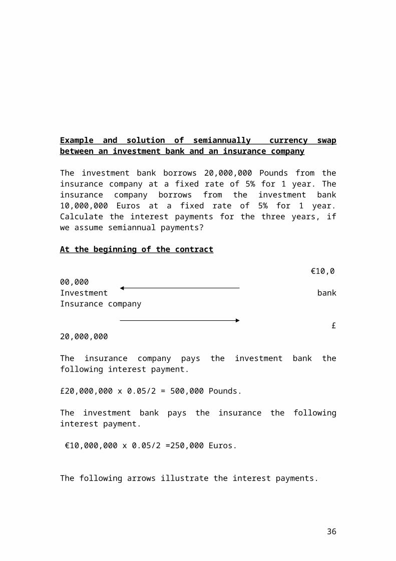
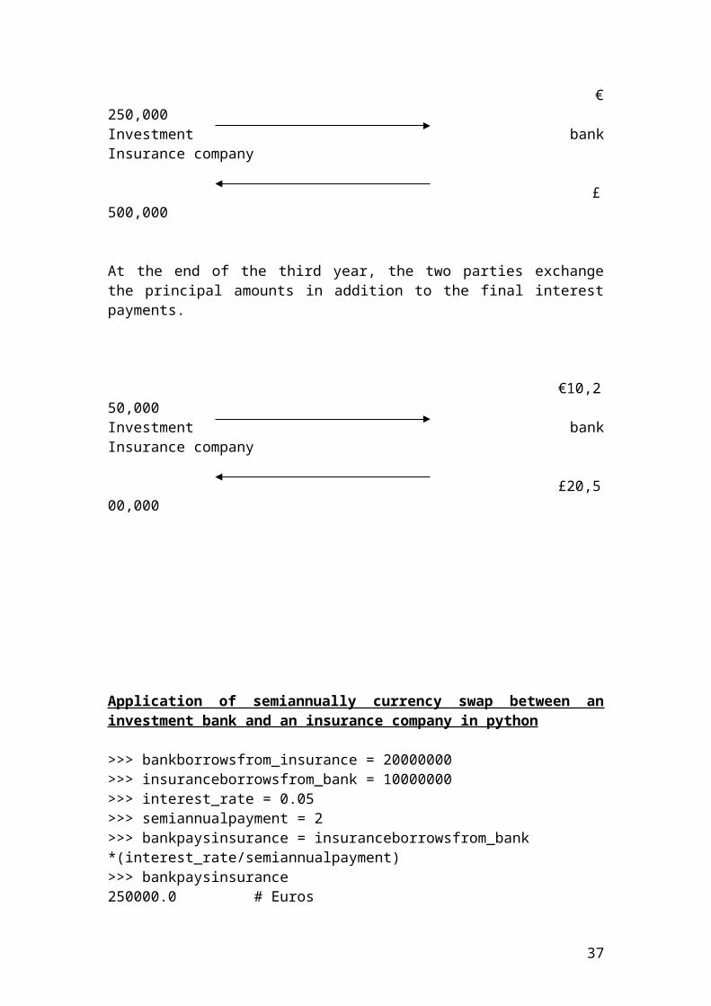
Example and solution of semiannually currency swap between an investment bank and an insurance company
The investment bank borrows 20,000,000 Pounds from the insurance company at a fixed rate of 5% for 1 year. The insurance company borrows from the investment bank 10,000,000 Euros at a fixed rate of 5% for 1 year. Calculate the interest payments for the three years, if we assume semiannual payments?
At the beginning of the contract
€10,000,000Investment bank Insurance company
£ 20,000,000
The insurance company pays the investment bank the following interest payment.
£20,000,000 x 0.05/2 = 500,000 Pounds.
The investment bank pays the insurance the following interest payment.
€10,000,000 x 0.05/2 =250,000 Euros.
The following arrows illustrate the interest payments.
€ 250,000Investment bank Insurance company
£ 500,000
At the end of the third year, the two parties exchange the principal amounts in addition to the final interest payments.
€10,250,000Investment bank Insurance company
£20,500,000
28
Application of semiannually currency swap between an investment bank and an insurance company in python
>>> bankborrowsfrom_insurance = 20000000>>> insuranceborrowsfrom_bank = 10000000>>> interest_rate = 0.05>>> semiannualpayment = 2>>> bankpaysinsurance = insuranceborrowsfrom_bank *(interest_rate/semiannualpayment)>>> bankpaysinsurance250000.0 # Euros>>> insurancepaysbank = bankborrowsfrom_insurance *(interest_rate/semiannualpayment)>>> insurancepaysbank500000.0 # Pounds
29
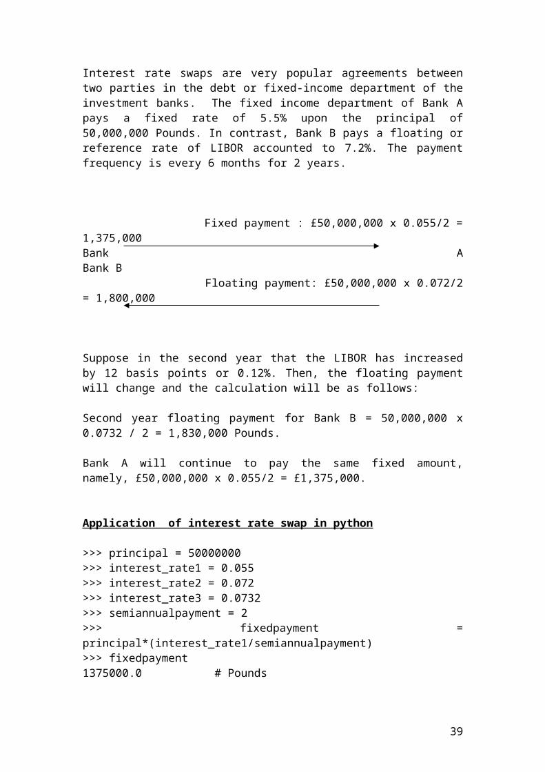
Example and solution of interest rate swap
Interest rate swaps are very popular agreements between two parties in the debt or fixed-income department of the investment banks. The fixed income department of Bank A pays a fixed rate of 5.5% upon the principal of 50,000,000 Pounds. In contrast, Bank B pays a floating or reference rate of LIBOR accounted to 7.2%. The payment frequency is every 6 months for 2 years.
Fixed payment : £50,000,000 x 0.055/2 = 1,375,000 Bank A Bank B Floating payment: £50,000,000 x 0.072/2 = 1,800,000
Suppose in the second year that the LIBOR has increased by 12 basis points or 0.12%. Then, the floating payment will change and the calculation will be as follows:
Second year floating payment for Bank B = 50,000,000 x 0.0732 / 2 = 1,830,000 Pounds.
Bank A will continue to pay the same fixed amount, namely, £50,000,000 x 0.055/2 = £1,375,000.
Application of interest rate swap in python
>>> principal = 50000000>>> interest_rate1 = 0.055>>> interest_rate2 = 0.072>>> interest_rate3 = 0.0732>>> semiannualpayment = 2>>> fixedpayment = principal*(interest_rate1/semiannualpayment)>>> fixedpayment1375000.0 # Pounds>>> floatingpayment1 = principal*(interest_rate2/semiannualpayment)>>> floatingpayment11799999.9999999998>>> round(_,2)1800000.0 # Pounds>>> floatingpayment2 = principal*(interest_rate3/semiannualpayment)>>> floatingpayment21830000.0 # Pounds
30
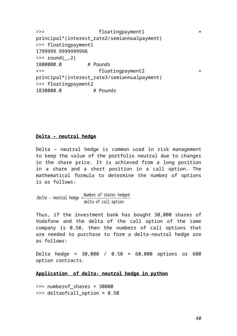
Delta – neutral hedge
Delta – neutral hedge is common used in risk management to keep the value of the portfolio neutral due to changes in the share price. It is achieved from a long position in a share and a short position in a call option. The mathematical formula to determine the number of options is as follows:
Delta - neutral hedge =Number of shares hedgeddelta of call option
Thus, if the investment bank has bought 30,000 shares of Vodafone and the delta of the call option of the same company is 0.50, then the numbers of call options that are needed to purchase to form a delta-neutral hedge are as follows:
Delta hedge = 30,000 / 0.50 = 60,000 options or 600 option contracts.
Application of delta- neutral hedge in python
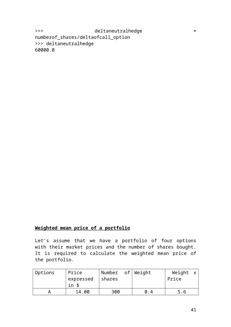
>>> numberof_shares = 30000>>> deltaofcall_option = 0.50>>> deltaneutralhedge = numberof_shares/deltaofcall_option>>> deltaneutralhedge60000.0
31
Weighted mean price of a portfolio
Let’s assume that we have a portfolio of four options with their market prices and the number of shares bought. It is required to calculate the weighted mean price of the portfolio.
Options Price expressed in $
Number of shares
Weight Weight x Price
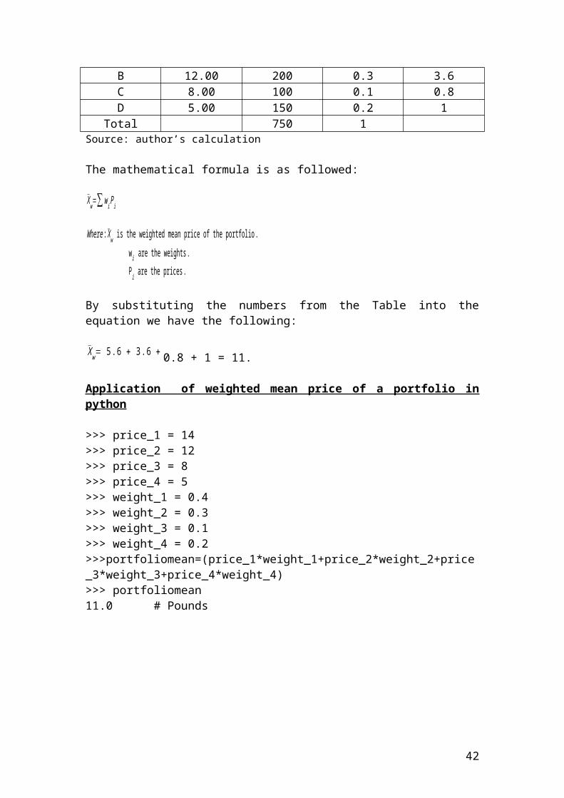
A 14.00 300 0.4 5.6B 12.00 200 0.3 3.6C 8.00 100 0.1 0.8D 5.00 150 0.2 1
Total 750 1Source: author’s calculation
The mathematical formula is as followed:
X̄ w=∑ w i Pi
Where : X̄ w is the weighted mean price of the portfolio . w i are the weights . Pi are the prices .
By substituting the numbers from the Table into the equation we have the following:
X̄ w= 5 . 6 + 3. 6 + 0.8 + 1 = 11.
Application of weighted mean price of a portfolio in python
>>> price_1 = 14>>> price_2 = 12>>> price_3 = 8>>> price_4 = 5>>> weight_1 = 0.4>>> weight_2 = 0.3>>> weight_3 = 0.1>>> weight_4 = 0.2>>>portfoliomean=(price_1*weight_1+price_2*weight_2+price_3*weight_3+price_4*weight_4)>>> portfoliomean11.0 # Pounds
32
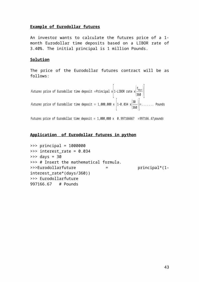
Example of Eurodollar futures
An investor wants to calculate the futures price of a 1-month Eurodollar time deposits based on a LIBOR rate of 3.40%. The initial principal is 1 million Pounds.
Solution
The price of the Eurodollar futures contract will be as follows:
Futures price of Eurodollar time deposit =Principal x[1-LIBOR rate x (tdays
360 )]
Futures price of Eurodollar time deposit = 1,000,000 x [1-0 . 034 x (30360 )]=. . .. .. . Pounds
Futures price of Eurodollar time deposit = 1,000,000 x 0 .997166667 =997166 .67 pounds
Application of Eurodollar futures in python
>>> principal = 1000000>>> interest_rate = 0.034>>> days = 30>>> # Insert the mathematical formula.>>>Eurodollarfuture = principal*(1- interest_rate*(days/360))>>> Eurodollarfuture997166.67 # Pounds
33
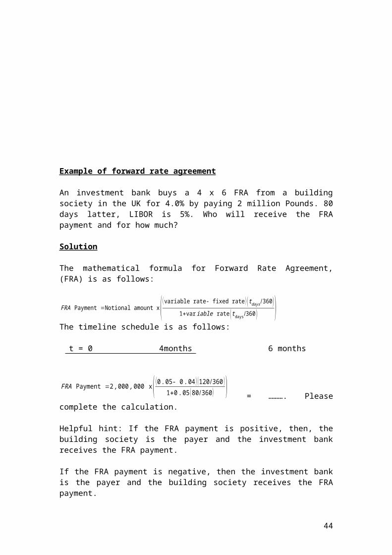
Example of forward rate agreement
An investment bank buys a 4 x 6 FRA from a building society in the UK for 4.0% by paying 2 million Pounds. 80 days latter, LIBOR is 5%. Who will receive the FRA payment and for how much?
Solution
The mathematical formula for Forward Rate Agreement, (FRA) is as follows:
FRA Payment =Notional amount x( ( variable rate- fixed rate ) (t days /360 )1+var iable rate ( tdays/360 ) )
The timeline schedule is as follows:
t = 0 4months 6 months
FRA Payment =2, 000 , 000 x( (0 . 05- 0 . 04 ) (120/360 )1+0 . 05 (80/360 ) )
= ………. Please complete the calculation.
Helpful hint: If the FRA payment is positive, then, the building society is the payer and the investment bank receives the FRA payment.
If the FRA payment is negative, then the investment bank is the payer and the building society receives the FRA payment.
Application of forward rate agreement in python
>>> principal = 2000000>>> variable_rate = 0.05>>> fixed_rate = 0.04>>> FRApayment= principal*(variablerate - fixedrate)*0.333333333/1.011111111>>> FRApayment6593.4 # Pounds
34
Example of futures on Treasury bills
An investor wants to calculate the futures price of a 3-month Treasury bills. Treasury bills are short-term notes of limited period of 1- month, and 3 - month respectively. The initial principal is 5 million Pounds and the discount rate is 3.50%.
Solution
The price of the Treasury bill futures will be as follows:
Futures price Treasury Bill = Principal x [1-discount rate x (t days
360 )]
Please complete the calculation …….
Application of futures on Treasury bills in python
>>> principal = 5000000>>> discount_rate = 0.035>>> days = 90>>> futurestreasurybills = principal*(1- discount_rate *days/360)>>> futurestreasurybills4956250 or 4.95625 e+006 # Pounds
35
Example of stock index futures
For example, if you bought 10 contracts of the Dow Jones Industrial index at 10,000 and you expected an aggressive bull market that reaches the value of 16,000, then, the 6000 points increase are multiplied by the standardized value of 250. If the initial principal of investment is $100,000, the mathematical formula for the gains will be as follows:
10 x 100,000 x 6000 x 250 = 1.5 x 10¹² Dollars
Application of stock index futures in python
>>> principal = 100000>>> points_increase = 6000>>> multiplier = 250>>> number_of_contracts = 10>>> gains = principal*points_increase*multiplier>>> gains1.5 x 1012 # USD
36
Example of currency futures
A manufacturer wants to calculate the currency futures price of EURO/USD traded in Frankfurt derivative market. For example, in August the contract is quoted as 1.35 EURO /USD and the contract size is 20,000. The principal is 300,000 Euro.
Solution
The contract price of 1 contract is as follows:
Futures price of currency future EURO/USD = principal* contract size x August quoted price = . .. . . Euro
Please complete the calculation . .. .
Application of currency futures in python
>>> principal = 300000>>> quote = 1.35>>> contract_size = 20000>>> futurespriceofcurrency = principal*quote*contract_size>>> futurespriceofcurrency8100000000.0 # Euro
37
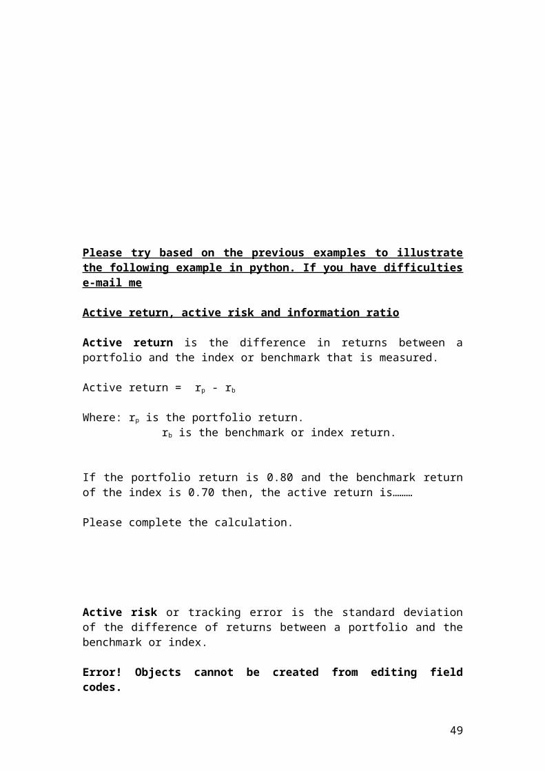
Please try based on the previous examples to illustrate the following example in python. If you have difficulties e-mail me
Active return, active risk and information ratio
Active return is the difference in returns between a portfolio and the index or benchmark that is measured.
Active return = rp - rb
Where: rp is the portfolio return. rb is the benchmark or index return.
If the portfolio return is 0.80 and the benchmark return of the index is 0.70 then, the active return is………
Please complete the calculation.
Active risk or tracking error is the standard deviation of the difference of returns between a portfolio and the benchmark or index.
Error! Objects cannot be created from editing field codes.
If the portfolio return is 0.80, the number of assets is 10 and the benchmark return of the index is 0.40 then, the active risk is………
Please complete the calculation.
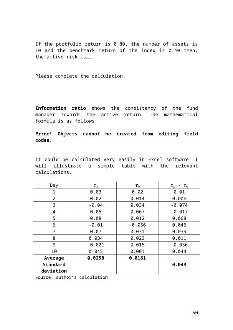
Information ratio shows the consistency of the fund manager towards the active return. The mathematical formula is as follows:
Error! Objects cannot be created from editing field codes.
It could be calculated very easily in Excel software. I will illustrate a simple table with the relevant calculations.
Day rp rb rp - rb
1 0.03 0.02 0.01
38
2 0.02 0.014 0.0063 -0.04 0.034 -0.0744 0.05 0.067 -0.0175 0.08 0.012 0.0686 -0.01 -0.056 0.0467 0.07 0.031 0.0398 0.034 0.023 0.0119 -0.021 0.015 -0.03610 0.045 0.001 0.044
Average 0.0258 0.0161Standard deviation
0.043
Source: author’s calculation
By substituting the values that we have found in terms of rp =0.0258, rb = 0.0161 and standard deviation = 0.043 in the following equation we have:
Error! Objects cannot be created from editing field codes.
Error! Objects cannot be created from editing field codes.
But what is the interpretation of the information ratio of 0.23. It means that the fund manager gained around 23 basis points of active return per unit of active risk. The higher is this number, the better the manager is performing in relation to active risk.
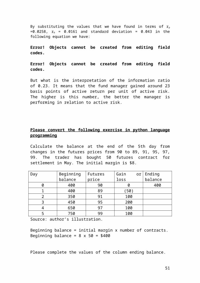
Please convert the following exercise in python language programming
Calculate the balance at the end of the 5th day from changes in the futures prices from 90 to 89, 91, 95, 97, 99. The trader has bought 50 futures contract for settlement in May. The initial margin is $8.
Day Beginning balance
Futures price Gain or loss Ending balance
0 400 90 0 4001 400 89 (50)2 350 91 1003 450 95 2004 650 97 1005 750 99 100
Source: author’s illustration.
Beginning balance = initial margin x number of contracts.Beginning balance = 8 x 50 = $400
Please complete the values of the column ending balance.
39
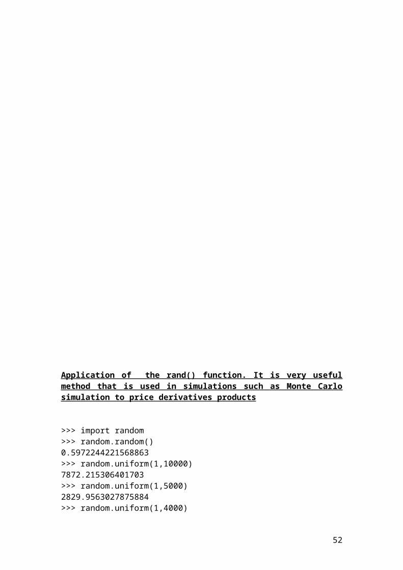
Application of the rand() function. It is very useful method that is used in simulations such as Monte Carlo simulation to price derivatives products
>>> import random>>> random.random()0.5972244221568863>>> random.uniform(1,10000)7872.215306401703>>> random.uniform(1,5000)2829.9563027875884>>> random.uniform(1,4000)2475.3647035985528
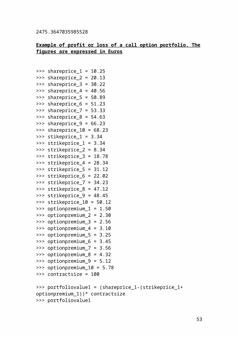
Example of profit or loss of a call option portfolio. The figures are expressed in Euros
>>> shareprice_1 = 10.25>>> shareprice_2 = 20.13>>> shareprice_3 = 30.22>>> shareprice_4 = 40.56
40
>>> shareprice_5 = 50.89>>> shareprice_6 = 51.23>>> shareprice_7 = 53.33>>> shareprice_8 = 54.63>>> shareprice_9 = 66.23>>> shareprice_10 = 68.23>>> stikeprice_1 = 3.34>>> strikeprice_1 = 3.34>>> strikeprice_2 = 8.34>>> strikeprice_3 = 18.78>>> strikeprice_4 = 28.34>>> strikeprice_5 = 31.12>>> strikeprice_6 = 22.02>>> strikeprice_7 = 34.23>>> strikeprice_8 = 47.12>>> strikeprice_9 = 48.45>>> strikeprice_10 = 50.12>>> optionpremium_1 = 1.50>>> optionpremium_2 = 2.30>>> optionpremium_3 = 2.56>>> optionpremium_4 = 3.10>>> optionpremium_5 = 3.25>>> optionpremium_6 = 3.45>>> optionpremium_7 = 3.56>>> optionpremium_8 = 4.32>>> optionpremium_9 = 5.12>>> optionpremium_10 = 5.78>>> contractsize = 100
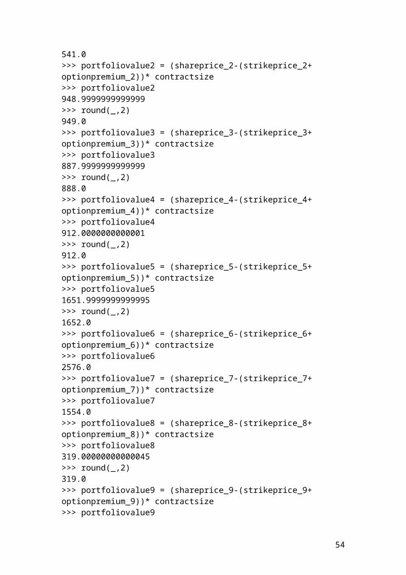
>>> portfoliovalue1 = (shareprice_1-(strikeprice_1+ optionpremium_1))* contractsize>>> portfoliovalue1541.0>>> portfoliovalue2 = (shareprice_2-(strikeprice_2+ optionpremium_2))* contractsize>>> portfoliovalue2948.9999999999999>>> round(_,2)949.0>>> portfoliovalue3 = (shareprice_3-(strikeprice_3+ optionpremium_3))* contractsize>>> portfoliovalue3887.9999999999999>>> round(_,2)888.0>>> portfoliovalue4 = (shareprice_4-(strikeprice_4+ optionpremium_4))* contractsize>>> portfoliovalue4912.0000000000001>>> round(_,2)
41
912.0>>> portfoliovalue5 = (shareprice_5-(strikeprice_5+ optionpremium_5))* contractsize>>> portfoliovalue51651.9999999999995>>> round(_,2)1652.0>>> portfoliovalue6 = (shareprice_6-(strikeprice_6+ optionpremium_6))* contractsize>>> portfoliovalue62576.0>>> portfoliovalue7 = (shareprice_7-(strikeprice_7+ optionpremium_7))* contractsize>>> portfoliovalue71554.0>>> portfoliovalue8 = (shareprice_8-(strikeprice_8+ optionpremium_8))* contractsize>>> portfoliovalue8319.00000000000045>>> round(_,2)319.0>>> portfoliovalue9 = (shareprice_9-(strikeprice_9+ optionpremium_9))* contractsize>>> portfoliovalue91266.0000000000005>>> round(_,2)1266.0>>> portfoliovalue10 = (shareprice_10-(strikeprice_10+ optionpremium_10))* contractsize>>> portfoliovalue101233.0000000000005>>> round(_,2)1233.0
42
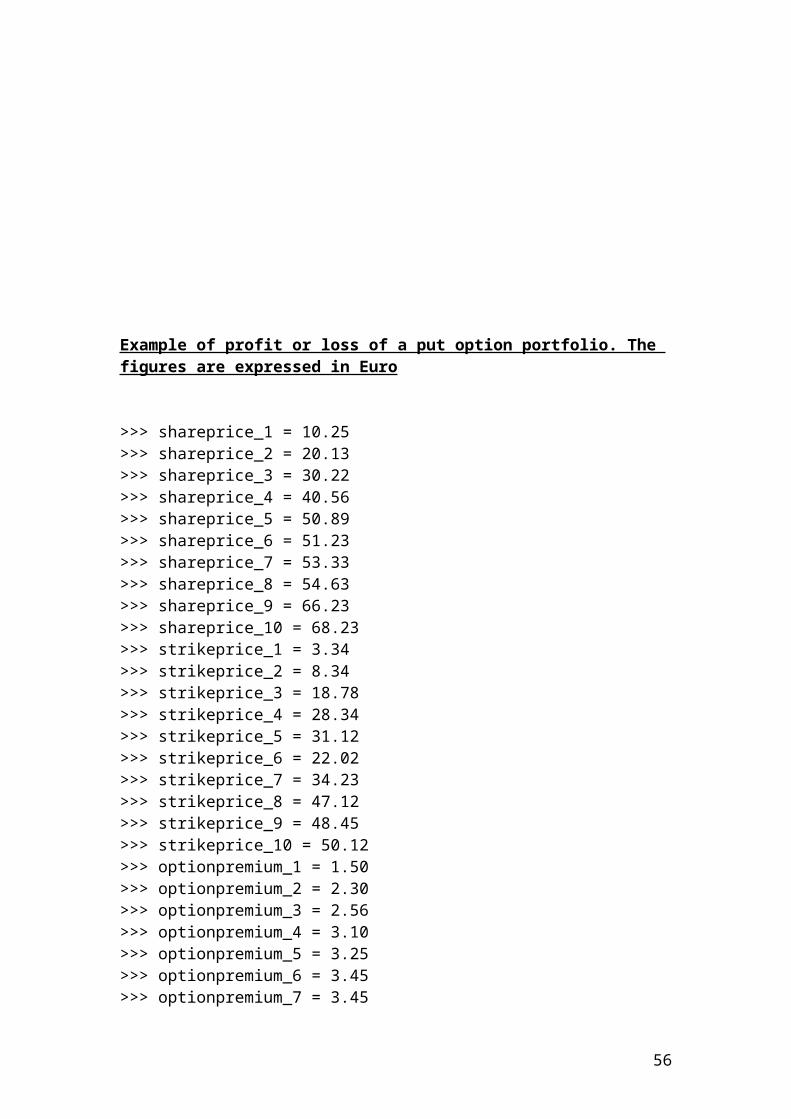
Example of profit or loss of a put option portfolio. The figures are expressed in Euro
>>> shareprice_1 = 10.25>>> shareprice_2 = 20.13>>> shareprice_3 = 30.22>>> shareprice_4 = 40.56>>> shareprice_5 = 50.89>>> shareprice_6 = 51.23>>> shareprice_7 = 53.33>>> shareprice_8 = 54.63>>> shareprice_9 = 66.23>>> shareprice_10 = 68.23>>> strikeprice_1 = 3.34>>> strikeprice_2 = 8.34>>> strikeprice_3 = 18.78>>> strikeprice_4 = 28.34>>> strikeprice_5 = 31.12>>> strikeprice_6 = 22.02>>> strikeprice_7 = 34.23>>> strikeprice_8 = 47.12>>> strikeprice_9 = 48.45
43
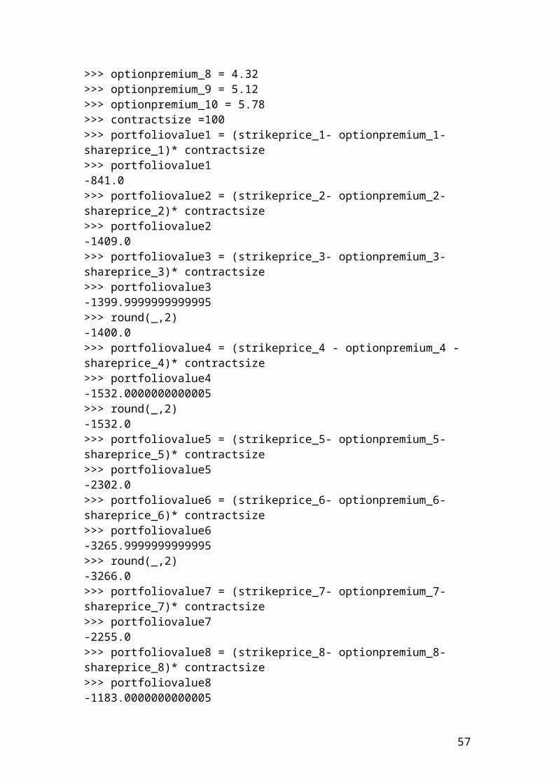
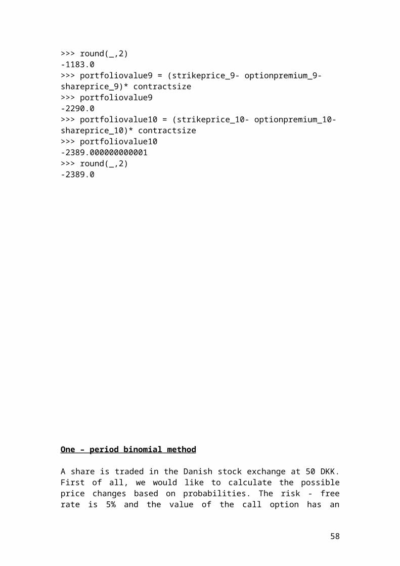
>>> strikeprice_10 = 50.12>>> optionpremium_1 = 1.50>>> optionpremium_2 = 2.30>>> optionpremium_3 = 2.56>>> optionpremium_4 = 3.10>>> optionpremium_5 = 3.25>>> optionpremium_6 = 3.45>>> optionpremium_7 = 3.45>>> optionpremium_8 = 4.32>>> optionpremium_9 = 5.12>>> optionpremium_10 = 5.78>>> contractsize =100>>> portfoliovalue1 = (strikeprice_1- optionpremium_1-shareprice_1)* contractsize>>> portfoliovalue1-841.0>>> portfoliovalue2 = (strikeprice_2- optionpremium_2- shareprice_2)* contractsize>>> portfoliovalue2-1409.0>>> portfoliovalue3 = (strikeprice_3- optionpremium_3- shareprice_3)* contractsize>>> portfoliovalue3-1399.9999999999995>>> round(_,2)-1400.0>>> portfoliovalue4 = (strikeprice_4 - optionpremium_4 - shareprice_4)* contractsize>>> portfoliovalue4-1532.0000000000005>>> round(_,2)-1532.0>>> portfoliovalue5 = (strikeprice_5- optionpremium_5- shareprice_5)* contractsize>>> portfoliovalue5-2302.0>>> portfoliovalue6 = (strikeprice_6- optionpremium_6- shareprice_6)* contractsize>>> portfoliovalue6-3265.9999999999995>>> round(_,2)-3266.0>>> portfoliovalue7 = (strikeprice_7- optionpremium_7- shareprice_7)* contractsize>>> portfoliovalue7-2255.0>>> portfoliovalue8 = (strikeprice_8- optionpremium_8- shareprice_8)* contractsize>>> portfoliovalue8-1183.0000000000005>>> round(_,2)-1183.0>>> portfoliovalue9 = (strikeprice_9- optionpremium_9- shareprice_9)* contractsize>>> portfoliovalue9-2290.0>>> portfoliovalue10 = (strikeprice_10- optionpremium_10- shareprice_10)* contractsize>>> portfoliovalue10
44
-2389.000000000001>>> round(_,2)-2389.0
One – period binomial method
A share is traded in the Danish stock exchange at 50 DKK. First of all, we would like to calculate the possible price changes based on probabilities. The risk - free rate is 5% and the value of the call option has an exercise price of 50 DKK. It is required to calculate the expected value of the option at t =1. In addition, it is required to calculate the value of the option today discounted at the given risk-free rate.
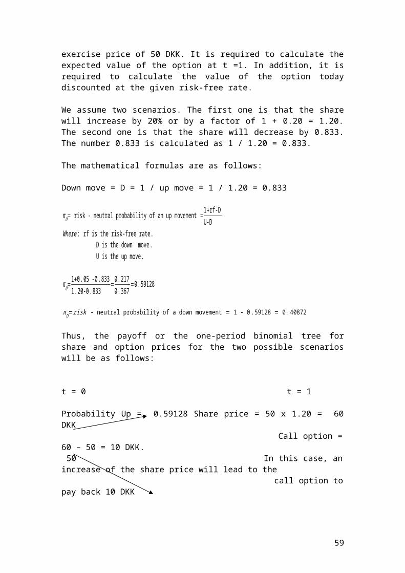
We assume two scenarios. The first one is that the share will increase by 20% or by a factor of 1 + 0.20 = 1.20. The second one is that the share will decrease by 0.833. The number 0.833 is calculated as 1 / 1.20 = 0.833.
The mathematical formulas are as follows:
Down move = D = 1 / up move = 1 / 1.20 = 0.833
45
πU= risk - neutral probability of an up movement =1+ rf-DU-D
Where : rf is the risk-free rate . D is the down move . U is the up move.
πU=1+0 . 05 -0 .8331 .20-0 .833
=0 .2170 .367
=0 .59128
π D=risk - neutral probability of a down movement = 1 - 0 .59128 = 0 . 40872
Thus, the payoff or the one-period binomial tree for share and option prices for the two possible scenarios will be as follows:
t = 0 t = 1
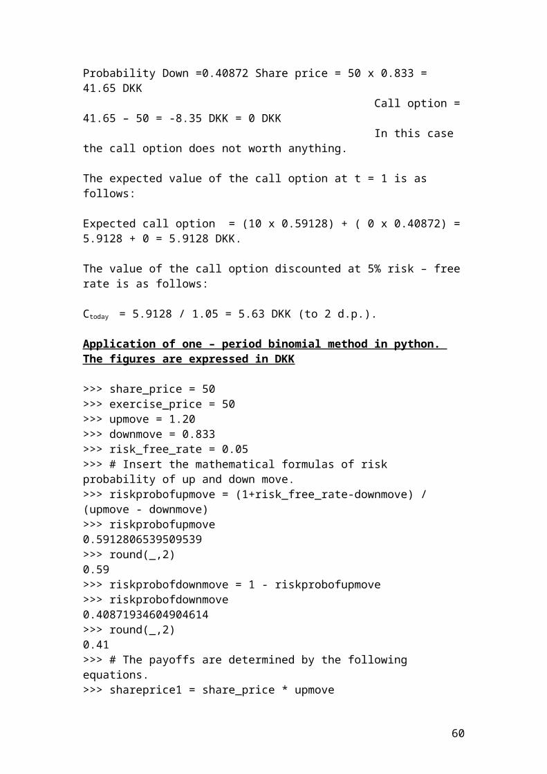
Probability Up = 0.59128 Share price = 50 x 1.20 = 60 DKK Call option = 60 – 50 = 10 DKK. 50 In this case, an increase of the share price will lead to the call option to pay back 10 DKK Probability Down =0.40872 Share price = 50 x 0.833 = 41.65 DKK Call option = 41.65 – 50 = -8.35 DKK = 0 DKK In this case the call option does not worth anything.
The expected value of the call option at t = 1 is as follows:
Expected call option = (10 x 0.59128) + ( 0 x 0.40872) = 5.9128 + 0 = 5.9128 DKK.
The value of the call option discounted at 5% risk – free rate is as follows:
Ctoday = 5.9128 / 1.05 = 5.63 DKK (to 2 d.p.).
Application of one – period binomial method in python. The figures are expressed in DKK
>>> share_price = 50>>> exercise_price = 50>>> upmove = 1.20>>> downmove = 0.833>>> risk_free_rate = 0.05>>> # Insert the mathematical formulas of risk probability of up and down move.>>> riskprobofupmove = (1+risk_free_rate-downmove) / (upmove - downmove)>>> riskprobofupmove0.5912806539509539>>> round(_,2)
46
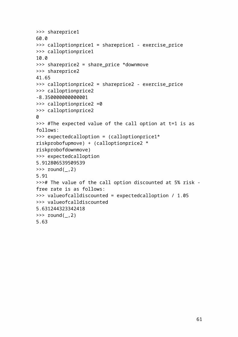
0.59>>> riskprobofdownmove = 1 - riskprobofupmove>>> riskprobofdownmove0.40871934604904614>>> round(_,2)0.41>>> # The payoffs are determined by the following equations.>>> shareprice1 = share_price * upmove>>> shareprice160.0>>> calloptionprice1 = shareprice1 - exercise_price>>> calloptionprice110.0>>> shareprice2 = share_price *downmove>>> shareprice241.65>>> calloptionprice2 = shareprice2 - exercise_price>>> calloptionprice2-8.350000000000001>>> calloptionprice2 =0>>> calloptionprice20>>> #The expected value of the call option at t=1 is as follows:>>> expectedcalloption = (calloptionprice1* riskprobofupmove) + (calloptionprice2 * riskprobofdownmove)>>> expectedcalloption5.912806539509539>>> round(_,2)5.91>>># The value of the call option discounted at 5% risk - free rate is as follows:>>> valueofcalldiscounted = expectedcalloption / 1.05>>> valueofcalldiscounted5.631244323342418>>> round(_,2)5.63
47
Two – period binomial method
This method is based on the one – period binomial method, but it is extended to include a second period, t = 2. Thus, we have three periods. t = 0, t =1 and t =2. We use the same example of the previous section but extended to an additional period.
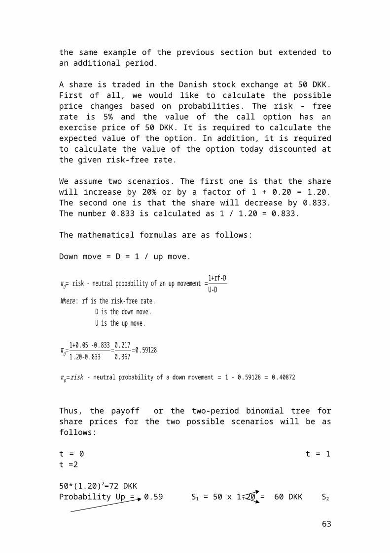
A share is traded in the Danish stock exchange at 50 DKK. First of all, we would like to calculate the possible price changes based on probabilities. The risk - free rate is 5% and the value of the call option has an exercise price of 50 DKK. It is required to calculate the expected value of the option. In addition, it is required to calculate the value of the option today discounted at the given risk-free rate.
We assume two scenarios. The first one is that the share will increase by 20% or by a factor of 1 + 0.20 = 1.20. The second one is that the share will decrease by 0.833. The number 0.833 is calculated as 1 / 1.20 = 0.833.
48
The mathematical formulas are as follows:
Down move = D = 1 / up move.
πU= risk - neutral probability of an up movement =1+ rf-DU-D
Where : rf is the risk-free rate . D is the down move . U is the up move.
πU=1+0 . 05 -0 .8331 .20-0 .833
=0 . 2170 . 367
=0 .59128
π D=risk - neutral probability of a down movement = 1 - 0 .59128 = 0 . 40872
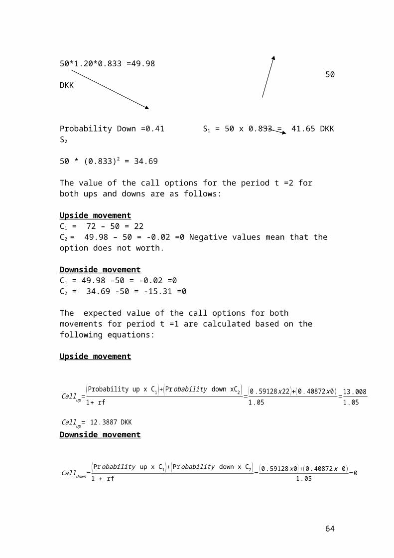
Thus, the payoff or the two-period binomial tree for share prices for the two possible scenarios will be as follows:
t = 0 t = 1 t =2 50*(1.20)2=72 DKKProbability Up = 0.59 S1 = 50 x 1.20 = 60 DKK S2 50*1.20*0.833 =49.98 50 DKK Probability Down =0.41 S1 = 50 x 0.833 = 41.65 DKK S2
50 * (0.833)2 = 34.69
The value of the call options for the period t =2 for both ups and downs are as follows:
Upside movementC1 = 72 – 50 = 22C2 = 49.98 – 50 = -0.02 =0 Negative values mean that the option does not worth.
Downside movementC1 = 49.98 -50 = -0.02 =0C2 = 34.69 -50 = -15.31 =0
The expected value of the call options for both movements for period t =1 are calculated based on the following equations:
Upside movement
49
Callup=( Probability up x C1 )+( Probability down xC2 )1+ rf
=(0 .59128 x 22 )+(0 . 40872 x 0)1. 05
=13 .0081. 05
Callup= 12 .3887 DKKDownside movement
Calldown=( Pr obability up x C1 )+( Probability down x C2 )1 + rf
=(0 .59128 x0 )+(0 .40872 x 0)
1 .05=0
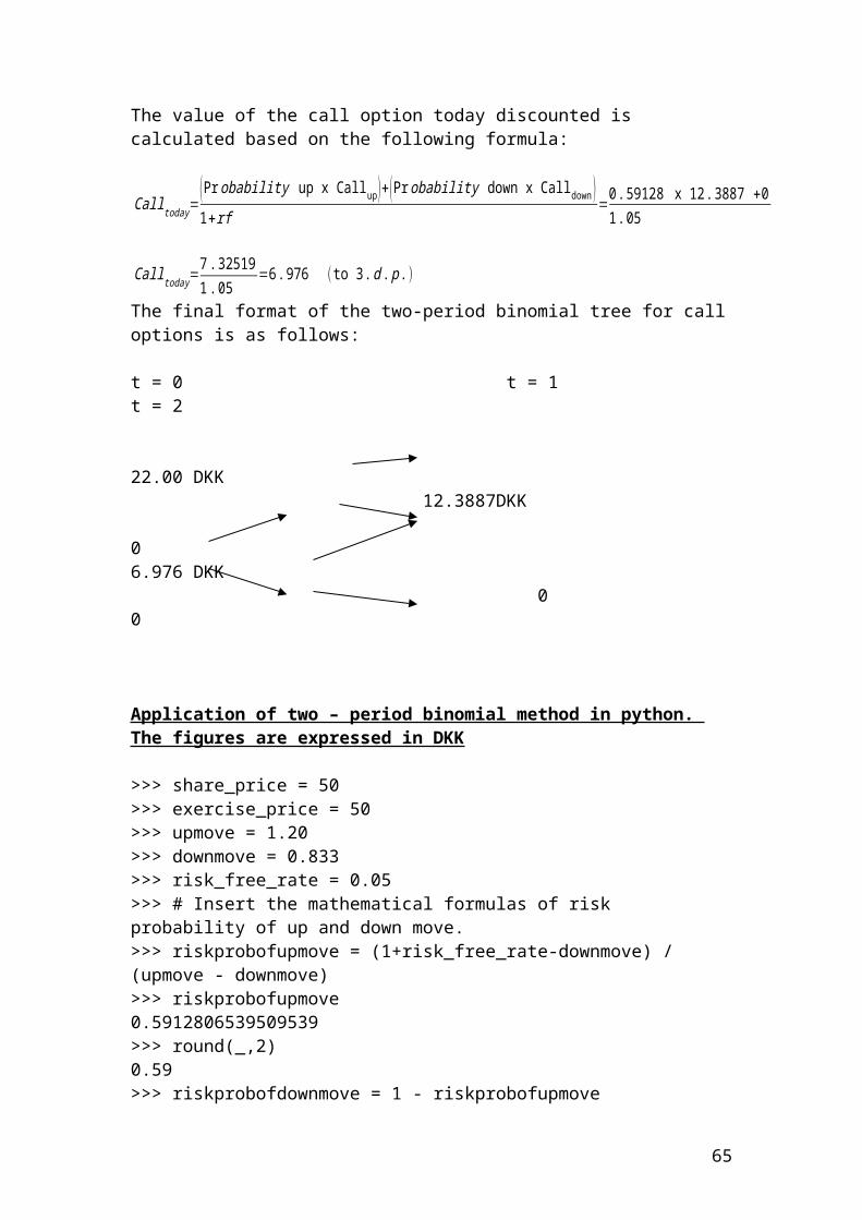
The value of the call option today discounted is calculated based on the following formula:
Calltoday=(Pr obability up x Callup )+( Pr obability down x Calldown )1+rf
=0. 59128 x 12 . 3887 +01 . 05
Calltoday=7 .325191. 05
=6 .976 ( to 3 . d . p .)
The final format of the two-period binomial tree for call options is as follows:
t = 0 t = 1 t = 2
22.00 DKK 12.3887DKK 06.976 DKK 0 0
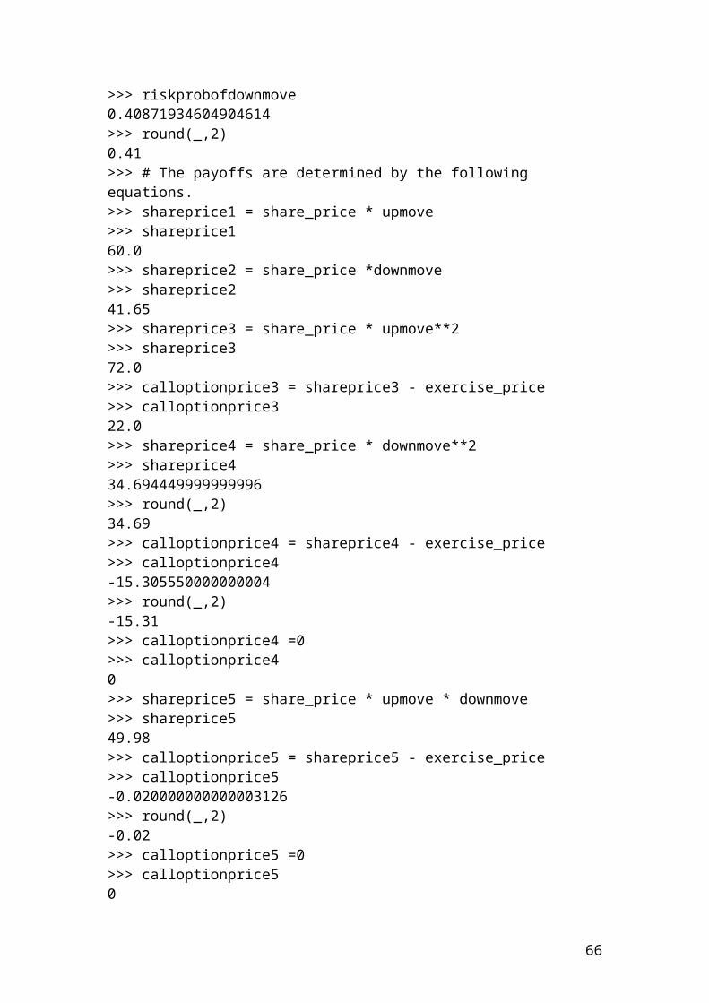
Application of two – period binomial method in python. The figures are expressed in DKK
>>> share_price = 50>>> exercise_price = 50>>> upmove = 1.20>>> downmove = 0.833>>> risk_free_rate = 0.05>>> # Insert the mathematical formulas of risk probability of up and down move.>>> riskprobofupmove = (1+risk_free_rate-downmove) / (upmove - downmove)>>> riskprobofupmove0.5912806539509539>>> round(_,2)0.59>>> riskprobofdownmove = 1 - riskprobofupmove>>> riskprobofdownmove0.40871934604904614>>> round(_,2)
50
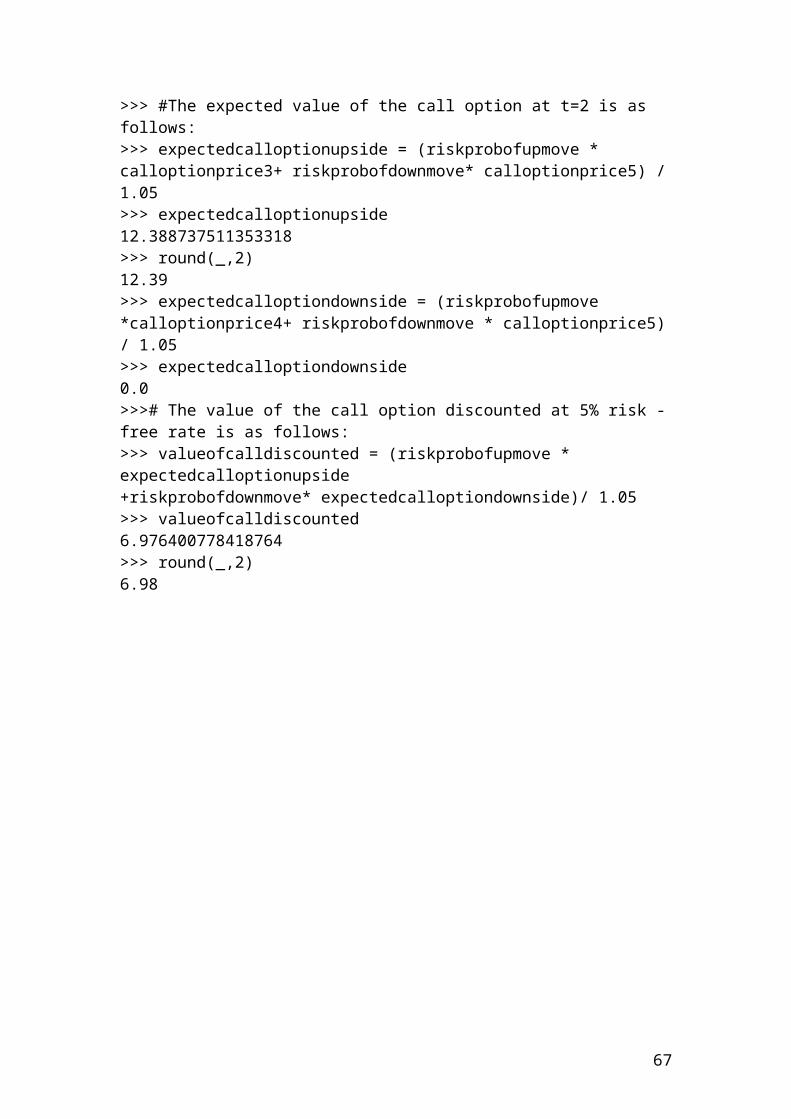
0.41>>> # The payoffs are determined by the following equations.>>> shareprice1 = share_price * upmove>>> shareprice160.0>>> shareprice2 = share_price *downmove>>> shareprice241.65>>> shareprice3 = share_price * upmove**2>>> shareprice372.0>>> calloptionprice3 = shareprice3 - exercise_price>>> calloptionprice322.0>>> shareprice4 = share_price * downmove**2>>> shareprice434.694449999999996>>> round(_,2)34.69>>> calloptionprice4 = shareprice4 - exercise_price>>> calloptionprice4-15.305550000000004>>> round(_,2)-15.31>>> calloptionprice4 =0>>> calloptionprice40>>> shareprice5 = share_price * upmove * downmove>>> shareprice549.98>>> calloptionprice5 = shareprice5 - exercise_price>>> calloptionprice5-0.020000000000003126>>> round(_,2)-0.02>>> calloptionprice5 =0>>> calloptionprice50>>> #The expected value of the call option at t=2 is as follows:>>> expectedcalloptionupside = (riskprobofupmove * calloptionprice3+ riskprobofdownmove* calloptionprice5) / 1.05>>> expectedcalloptionupside12.388737511353318>>> round(_,2)12.39>>> expectedcalloptiondownside = (riskprobofupmove *calloptionprice4+ riskprobofdownmove * calloptionprice5) / 1.05>>> expectedcalloptiondownside0.0>>># The value of the call option discounted at 5% risk - free rate is as follows:
51
>>> valueofcalldiscounted = (riskprobofupmove * expectedcalloptionupside+riskprobofdownmove* expectedcalloptiondownside)/ 1.05>>> valueofcalldiscounted6.976400778418764>>> round(_,2)6.98
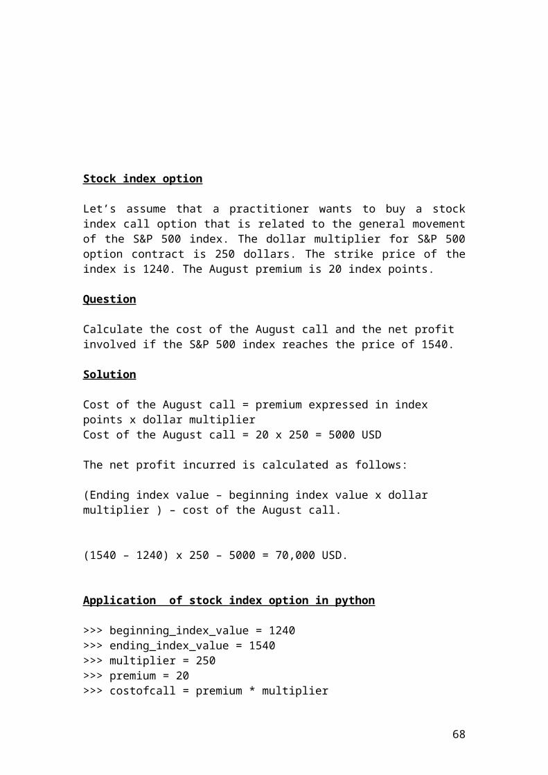
Stock index option
Let’s assume that a practitioner wants to buy a stock index call option that is related to the general movement of the S&P 500 index. The dollar multiplier for S&P 500 option contract is 250 dollars. The strike price of the index is 1240. The August premium is 20 index points.
Question
Calculate the cost of the August call and the net profit involved if the S&P 500 index reaches the price of 1540.
Solution
Cost of the August call = premium expressed in index points x dollar multiplier Cost of the August call = 20 x 250 = 5000 USD
The net profit incurred is calculated as follows:
52
(Ending index value – beginning index value x dollar multiplier ) – cost of the August call.
(1540 – 1240) x 250 – 5000 = 70,000 USD.
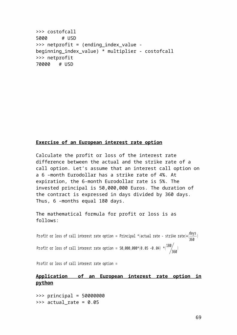
Application of stock index option in python
>>> beginning_index_value = 1240>>> ending_index_value = 1540>>> multiplier = 250>>> premium = 20>>> costofcall = premium * multiplier>>> costofcall5000 # USD>>> netprofit = (ending_index_value - beginning_index_value) * multiplier - costofcall>>> netprofit70000 # USD
Exercise of an European interest rate option
Calculate the profit or loss of the interest rate difference between the actual and the strike rate of a call option. Let’s assume that an interest call option on a 6 –month Eurodollar has a strike rate of 4%. At expiration, the 6-month Eurodollar rate is 5%. The invested principal is 50,000,000 Euros. The duration of the contract is expressed in days divided by 360 days. Thus, 6 –months equal 180 days.
The mathematical formula for profit or loss is as follows:
Pr ofit or loss of call interest rate option = Principal * (actual rate - strike rate)∗(days360
)
Pr ofit or loss of call interest rate option = 50,000,000*(0 .05 -0 .04 ) *(180360)
Pr ofit or loss of call interest rate option =
53
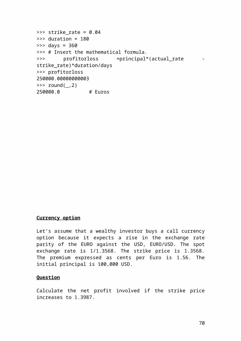
Application of an European interest rate option in python
>>> principal = 50000000>>> actual_rate = 0.05>>> strike_rate = 0.04>>> duration = 180>>> days = 360>>> # Insert the mathematical formula.>>> profitorloss =principal*(actual_rate - strike_rate)*duration/days>>> profitorloss250000.00000000003>>> round(_,2)250000.0 # Euros
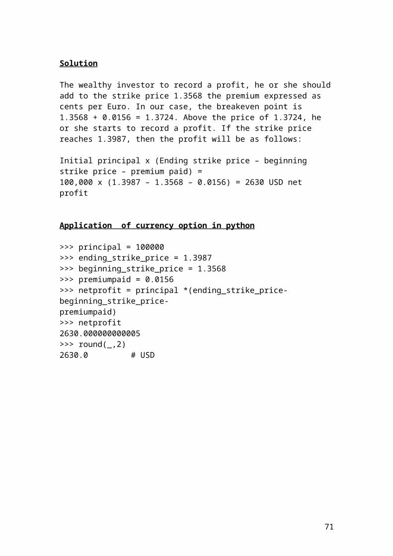
Currency option
Let’s assume that a wealthy investor buys a call currency option because it expects a rise in the exchange rate parity of the EURO against the USD, EURO/USD. The spot exchange rate is 1/1.3568. The strike price is 1.3568. The premium expressed as cents per Euro is 1.56. The initial principal is 100,000 USD.
Question
Calculate the net profit involved if the strike price increases to 1.3987.
Solution
The wealthy investor to record a profit, he or she should add to the strike price 1.3568 the premium expressed as cents per Euro. In our case, the breakeven point is1.3568 + 0.0156 = 1.3724. Above the price of 1.3724, he or she starts to record a profit. If the strike price reaches 1.3987, then the profit will be as follows:
54

Initial principal x (Ending strike price – beginning strike price – premium paid) =100,000 x (1.3987 – 1.3568 – 0.0156) = 2630 USD net profit
Application of currency option in python
>>> principal = 100000>>> ending_strike_price = 1.3987>>> beginning_strike_price = 1.3568>>> premiumpaid = 0.0156>>> netprofit = principal *(ending_strike_price-beginning_strike_price-premiumpaid)>>> netprofit2630.000000000005>>> round(_,2)2630.0 # USD
Example of calculating the payments of an interest rate cap based on different LIBOR rates
Interest rate cap is an agreement between two parties where one party pay the other at a specified period of time in which the interest rate or London interbank offered rate ,LIBOR, exceeds the strike price. It is used this contract to hedge against interest rate fluctuations. Let’s assume that an interest cap has a value of 5.5% and the LIBOR prices for the next three years are 7.5%, 8.3% and 4.65%. The principal is $50,000,000 and the payments take place semiannually.
The mathematical formula that is used to calculate the payments of each year is as follows:
Interest rate payment =[ principal x (LIBOR rate – cap rate)/0.5]
Therefore, the first year interest rate payment is as follows:
Year 1
55
Interest rate payment = [50,000,000 x (0.075 – 0.055)/2] = $ ………
Application of payments of an interest rate cap based on different LIBOR rates in python
>>> principal = 50000000>>> liborrate_1 = 0.075>>> liborrate_2 = 0.083>>> caprate = 0.055>>> duration = 2>>> interestpay1 = principal *(liborrate_1 - caprate) /duration>>> interestpay1499999.99999999994>>> round(_,2)500000.0 # USD>>> interestpay2 = principal *(liborrate_2 - caprate) / duration>>> interestpay2700000.0000000001>>> round(_,2)700000.0 # USD
A six month interest rate cap has a rate of 0.08 and the principal is 20,000,000 USD. The settlements is done quarterly. The first quarter the 3 –month libor rate is 0.096 and the second quarter the rate is 0.087. Calculate the payoff for the cap the first and the second quarter?
Solution
Payoff the first quarter = 20,000,000 * (0 . 096−0. 08 )/4 = 80000 USD
Payoff the second quarter = 20,000,000 * (0 .087−0. 08 )/4=35000 USD
Application of payoff of interest rate cap in python
>>> principal = 20000000>>> caprate = 0.08>>> liborrate_1 = 0.096>>> liborrate_2 = 0.087
56
>>> period = 4>>> # Insert the mathematical formulas.>>> payoff1 = (principal*(liborrate_1-caprate)/period)>>> payoff180000.0 # USD>>> payoff2 = (principal*(liborrate_2-caprate)/period)>>> payoff234999.99999999996>>> round(_,2)35000.0 # USD
Swaption
An investor purchased a 1 year European swaption with exercise price 7.50%. The principal is 30,000,000USD. The floating rate payments are based on LIBOR. The 90, 180, 270, and 360 day annualized LIBOR rates and present value factors are as follows:
LIBOR Rate Present value factors90 day LIBOR 4% 0.990099180 day LIBOR 5.5% 0.973236270 day LIBOR 6% 0.956938360 day LIBOR 7% 0.934579
Calculate the semi-annual and annualized swap rate?Calculate the net cash flow at each payment and the value of swaption at maturity.
Solution
57
The present value factors are calculated as follows:
PV 90 days = Error! Objects cannot be created from editing field codes.0.990099
PV 180 days = Error! Objects cannot be created from editing field codes.0.973236
PV 270 days = Error! Objects cannot be created from editing field codes.0.956938
PV 360 days = Error! Objects cannot be created from editing field codes.0.934579
Semi - annual swap rate =
Error! Objects cannot be created from editing field codes.
Annulaized swap rate = Error! Objects cannot be created from editing field codes.
The swaption is in the money because the exercise price 7.50% is greater than the market annualized swap rate 6.788%.
The net cash flow is as follows:
netCashFlow = (0.075 – 0.06788)*90/360 * 30000000 = 53400 USD
The value of swaption at maturity is as follows:
valueSwaption = 53400 *(Error! Objects cannot be created from editing field codes.) = 205,849.1 USD
Application of swaption in python
>>> principal = 30000000>>> exercise_rate = 0.075>>> rate90 = 0.04>>> rate180 = 0.055>>> rate270 = 0.06>>> rate360 = 0.07>>> # Insert the mathematical formulas.>>> PV90 = 1 /(1+(rate90 * 90/360))>>> PV900.9900990099009901>>> PV180 = 1/(1+(rate180 * 180/360))>>> PV1800.97323600973236>>> PV270 = 1/(1+(rate270 * 270/360))
58
>>> PV2700.9569377990430623>>> PV360 = 1/(1+(rate360* 360/360))>>> PV3600.9345794392523364>>> semiAnnualRate = (1-PV360)/(PV90 +PV180 +PV270 +PV360)>>> semiAnnualRate0.01697096448070222>>> round(_,5)0.01697>>> annualizedSwapRate = semiAnnualRate * (360/90)>>> annualizedSwapRate0.06788385792280888>>> round(_,5)0.06788
Please repeat the above swaption problem in python and calculate the net cash flow and the value of swaption at maturity.
Put –call parity
The put – call parity shows the relationship between a call and a put option with the same expiration, strike and share prices. The mathematical formula is as follows:
Error! Objects cannot be created from editing field codes.
Example
Calculate the price of a call if the price of a put is 5.34 Pounds, the share price is 94, the strike price is 97, the risk-free rate is 4% and the time to maturity, T=0.5. By rearranging formula (20) and solving for the price of a call, we have the following results:
C=P+S− X(1+rf )T
=5 . 34+94−97(1.04 )0 .5
C=4 .22 Pounds
Application of put - call parity in python
>>> put = 5.34>>> share_price = 94>>> strike_price = 97>>> disriskfreerate = 1.04>>> maturity = 0.5>>> # Insert the mathematical formula.>>> call = put + share_price - strike_price /(disriskfreerate**maturity)
59
>>> call4.223674457980749>>> round(_,2)4.22 # Pounds
Example of margin payments in the clearinghouse
An investor open a margin account with a minimum initial margin of 5,200 dollars per contract. The maintenance margin is 1,500 dollars per contract. He/she buys 7 July wheat futures contracts with a standard contract size of 200 bushels priced at 230 dollars per bushel. The July contract size in the next 2 days recorded the prices of 220 and 210 dollars per bushel. Show the cash flows, gains and losses for the buyer and the seller?
Solution
Initial margin = 7 x 5,200 = 36,400 dollars
Maintenance margin = 7 x 1,500 = 10,500 dollars
The cash flows, gains and losses for the next two days will be as follows:
Day 1
Cash flows for the buyer’s: 36,400 + 14,000 = 50,400 dollars. The investor’s recorded a gain.
Cash flows for the seller’s: 36,400 – 14,000 = 22,400 dollars. The investor’s recorded a loss.
Helpful hint: the amount of 14,000 is calculated from the difference of the bushel prices, (fT-f0) x number of contracts x standard contract size. Thus, we have: (220-230) x 7 x 200 = (14,000 dollars). The same principle applies for the second day but with different bushel prices. Thus, we have: (210 – 230) x 7 x 200 = (28000 dollars). Gains or losses depends if you are the buyer or seller.
Day 2
Please do the calculations for the second day.
This is why I am stressing the importance that the investors should buy or sell ONLY when the market is aggressively increasing or falling. If he/she gets trapped in a market that is not strong bull or bear, then, he/she will have to compensate regularly for the losses or he/she will experience a very small profit. If the amounts as the days
60
passes is below the maintenance margin, then, the investor’s will receive a margin call and he/she should add the capital required to proceed with the contract. If the investor’s is short of money, then, the position is closed with the incurred losses.
Application of margin payments in the clearinghouse in python
>>> initialmargin = 5200>>> maintenancemargin = 1500>>> contractnumber = 7>>> bushelcontractsize = 200>>> bushelprice_1 = 230>>> bushelprice_2 = 220>>> # Insert the mathematical formulas.>>> initialmarginwithcontract = initialmargin * contractnumber>>> initialmarginwithcontract36400 # USD>>> maintenancemarginwithcontract = maintenancemargin * contractnumber>>> maintenancemarginwithcontract10500 # USD>>> bushelcontract = (bushelprice_1-bushelprice_2) * bushelcontractsize * contractnumber>>> bushelcontract14000 # USD>>> cashflowbuyer = initialmarginwithcontract + bushelcontract>>> cashflowbuyer50400 # USD>>> cashflowseller = initialmarginwithcontract - bushelcontract>>> cashflowseller22400 # USD
Please continue the calculations for the second day….
61
Example of calculating a margin call due to changes of price futures
An investor has opened a short position of 20 Soybean futures contract. The initial margin was 500 Pounds and the maintenance margin was 430 Pounds per contract. The price change that will create a margin call is as follows:
Solution
Margin call created at a price =initial margin - maintenance margincontract size
=500 -43020
=3.5
Pounds
Application of margin call in python
>>> initial_margin = 500>>> maintenance_margin = 430>>> futures_contract = 20>>> # Insert the mathematical formula.>>> margincall =(initial_margin-maintenance_margin) / futures_contract>>> margincall3.5 # Pounds
62
Solution of the above examples
Active return, active risk and information ratio
Active return is the difference in returns between a portfolio and the index or benchmark that is measured.
Active return = rp - rb
Where: rp is the portfolio return. rb is the benchmark or index return.
If the portfolio return is 0.80 and the benchmark return of the index is 0.70 then, the active return is………
Please complete the calculation.
Application of active return in python
>>> portfolio_return = 0.8>>> benchmark_return = 0.7>>> active_return = portfolio_return - benchmark_return>>> active_return0.10000000000000009>>> round(_,2)0.1
63
Active risk or tracking error is the standard deviation of the difference of returns between a portfolio and the benchmark or index.
Active risk =√∑ (r p−r b )2
n−1
Where : rp is portfolio return . rb is portfolio benchmark return . It could be for example an index . n is the number of assets or observations .
If the portfolio return is 0.80, the number of observations is 10 and the benchmark return of the index is 0.40 then, the active risk is………
Please complete the calculation.
Application of active risk in python
>>> portfolio_return = 0.80>>> benchmark_return = 0.40>>> n =10>>> # Insert the mathematical formula.>>> active_risk = sqrt((portfolio_return - benchmark_return)**2/9)>>> active_risk0.13333333333333336>>> round(_,2)0.13
64
Information ratio shows the consistency of the fund manager towards the active return. The mathematical formula is as follows:
Error! Objects cannot be created from editing field codes.
It could be calculated very easily in Excel software. I will illustrate a simple table with the relevant calculations.
Day rp rb rp - rb
1 0.03 0.02 0.012 0.02 0.014 0.0063 -0.04 0.034 -0.0744 0.05 0.067 -0.0175 0.08 0.012 0.0686 -0.01 -0.056 0.0467 0.07 0.031 0.0398 0.034 0.023 0.0119 -0.021 0.015 -0.03610 0.045 0.001 0.044
Average 0.0258 0.0161Standard deviation
0.043
Source: author’s calculation
By substituting the values that we have found in terms of rp =0.0258, rb = 0.0161 and standard deviation = 0.043 in the following equation we have:
Error! Objects cannot be created from editing field codes.
Error! Objects cannot be created from editing field codes.
But what is the interpretation of the information ratio of 0.23. It means that the fund manager gained around 23 basis points of active return per unit of active risk. The higher is this number, the better the manager is performing in relation to active risk.
Application of information ratio in python
>>> portfolio_return1 = 0.03
65
>>> portfolio_return2 = 0.02>>> portfolio_return3 = -0.04>>> portfolio_return4 = 0.05>>> portfolio_return5 = 0.08>>> portfolio_return6 = -0.01>>> portfolio_return7 = 0.07>>> portfolio_return8 = 0.034>>> portfolio_return9 = -0.021>>> portfolio_return10 = 0.045>>> # Insert the mathematical formula.>>> average_1 = (portfolio_return1 + portfolio_return2 + portfolio_return3 + portfolio_return4 + portfolio_return5 + portfolio_return6+ portfolio_return7 + portfolio_return8 + portfolio_return9+ portfolio_return10)/10>>> average_10.0258>>> benchmark_return1 = 0.02>>> benchmark_return2 = 0.014>>> benchmark_return3 = 0.034>>> benchmark_return4 = 0.067>>> benchmark_return5 = 0.012>>> benchmark_return6 = -0.056>>> benchmark_return7 = 0.031>>> benchmark_return8 = 0.023>>> benchmark_return9 = 0.015>>> benchmark_return10 = 0.001>>> average_2 = (benchmark_return1 + benchmark_return2 + benchmark_return3 + benchmark_return4 + benchmark_return5 + benchmark_return6 + benchmark_return7 + benchmark_return8 + benchmark_return9+ benchmark_return10)/10>>> average_20.016100000000000003>>># Insert the mathematical formulas to calculate the differences between the portfolioand benchmark return and then square it.>> diff1 = portfolio_return1 - benchmark_return1>>> diff10.009999999999999998>>> diff2 = portfolio_return2 - benchmark_return2>>> diff20.006>>> diff3 = portfolio_return3 - benchmark_return3>>> diff3-0.07400000000000001>>> diff4 = portfolio_return4 - benchmark_return4>>> diff4-0.017>>> diff5 = portfolio_return5 - benchmark_return5>>> diff50.068>>> diff6 = portfolio_return6 - benchmark_return6>>> diff60.046
66
>>> diff7 = portfolio_return7 - benchmark_return7>>> diff70.03900000000000001>>> diff8 = portfolio_return8 - benchmark_return8>>> diff80.011000000000000003>>> diff9 = portfolio_return9 - benchmark_return9>>> diff9-0.036000000000000004>>> diff10 = portfolio_return10 - benchmark_return10>>> diff100.044>>> #Find the sum from the differences.>>> sumDiff = diff1 + diff2 + diff3 + diff4 + diff5 + diff6 + diff7 + diff8 +diff9 +diff10>>> sumDiff0.09699999999999999>>># Find the average from the differences.>>> average3 = sumDiff /10>>> average30.009699999999999999
Please complete the exercise……. If you have questions, then, please let me know.
Please convert the following exercise in python language programming
Calculate the balance at the end of the 5th day from changes in the futures prices from 90 to 89, 91, 95, 97, 99. The trader has bought 50 futures contract for settlement in May. The initial margin is $8.
Day Beginning Futures price Gain or loss Ending balance
67
balance0 400 90 0 4001 400 89 (50)2 350 91 1003 450 95 2004 650 97 1005 750 99 100
Source: author’s illustration.
Beginning balance = initial margin x number of contracts.Beginning balance = 8 x 50 = $400
Please complete the values of the column ending balance.
Solution
Day Beginning balance
Futures price Gain or loss Ending balance
0 400 90 0 4001 400 89 (50) 3502 350 91 100 4503 450 95 200 6504 650 97 100 7505 750 99 100 850
The ending balance at the 5th day in the margin account will be 850 USD.
Calculate the caplet option payments based on different interest rates using a binomial 2 steps tree. The figures are expressed in pounds
>>> # Calculate the caplet values based on an interest rate cap using a binomial 2 steps tree. It is a similar example of a call option on interest rates. The payment is based on the difference between the current interest rate and the cap rate multiplied by
68
the principal and divided by the discounted current interest rate. The buyer receives a payment when the current interest rate exceeds the cap strike price.
>>> strike = 0.02>>> principal = 30000000>>> maturity = 0.5>>> sigma = 0.3>>> interest_rate = 0.04>>> n =2>>> p=0.5>>> # Insert the mathematical formulas.>>> dt = maturity/n # steps expressed in years.>>> dt0.25>>> from math import*>>> u = exp(sigma*sqrt(dt)) # multiplier of upmove.>>> u1.161834242728283>>> d = 1/u # multiplier of downmove.>>> d0.8607079764250578>>># Identify the interest rates in each node.>>> interest_0 = 0.04>>> interest_1i = 0.0465>>> interest_1ii = 0.0344>>> interest_2i = 0.054>>> interest_2ii = 0.04>>> interest_2iii = 0.0296>>># Identify the discounted interest rates.>>> disinterest_0 = 1.04>>> disinterest_1i = 1.0465>>> disinterest_1ii = 1.0344>>> disinterest_2i = 1.054>>> disinterest_2ii = 1.04>>> disinterest_2iii = 1.0296>>># Insert the mathematical formulas. It is a backward induction methodology.>>> capletPrice2i = (principal*(interest_2i-strike)/disinterest_2i)>>> capletPrice2i967741.935483871>>> capletPrice2ii = (principal*(interest_2ii-strike)/disinterest_2ii)>>> capletPrice2ii576923.0769230769>>> capletPrice2iii = (principal*(interest_2iii-strike)/disinterest_2iii)>>> capletPrice2iii279720.2797202797>>> capletPrice1i = (((capletPrice2i*p)+(capletPrice2ii*p))/disinterest_1i)>>> capletPrice1i738014.8172035108>>> capletPrice1ii = (((capletPrice2ii*p)+(capletPrice2iii*p))/disinterest_1ii)
69
>>> capletPrice1ii414077.415237508>>> capletPrice0 = (((capletPrice1i*p)+(capletPrice1ii*p))/disinterest_0)>>> capletPrice0553890.4963658744>>> round(_,2)553890.5
Calculate the floorlet option payments based on different interest rates using a binomial 2 steps tree. The figures are expressed in pounds
>>> # Calculate the floorlet values based on an interest rate floor using a binomial 2 steps tree. It is a similar example of a put option on interest rates. It protects the holder from declining interest rates. The payment is based on the difference between
70
the floor rate and the current interest rate multiplied by the principal and divided by the discounted current interest rate.
>>> strike = 0.02>>> principal = 30000000>>> maturity = 0.5>>> sigma = 0.3>>> interest_rate = 0.04>>> n =2>>> p=0.5>>> # Insert the mathematical formulas.>>> dt = maturity/n # steps expressed in years.>>> dt0.25>>> from math import*>>> u = exp(sigma*sqrt(dt)) # multiplier of upmove.>>> u1.161834242728283>>> d = 1/u # multiplier of downmove.>>> d0.8607079764250578>>># Identify the interest rates in each node.>>> interest_0 = 0.04>>> interest_1i = 0.0465>>> interest_1ii = 0.0344>>> interest_2i = 0.054>>> interest_2ii = 0.04>>> interest_2iii = 0.0296
>>># Identify the discounted interest rates.>>> disinterest_0 = 1.04>>> disinterest_1i = 1.0465>>> disinterest_1ii = 1.0344>>> disinterest_2i = 1.054>>> disinterest_2ii = 1.04>>> disinterest_2iii = 1.0296
>>># Insert the mathematical formulas. It is a backward induction methodology.>>> floorletPrice2i = (principal*(strike - interest_2i)/disinterest_2i)>>> floorletPrice2i56925.99620493363>>> floorletPrice2ii = (principal*(strike - interest_2ii)/disinterest_2ii)>>> floorletPrice2ii461538.4615384615>>> floorletPrice2iii = (principal*(strike - interest_2iii)/disinterest_2iii)>>> floorletPrice2iii769230.7692307691>>> floorletPrice1i = (((floorletPrice2i*p)+(floorletPrice2ii*p))/disinterest_1i)>>> floorletPrice1i247713.5488501649
71
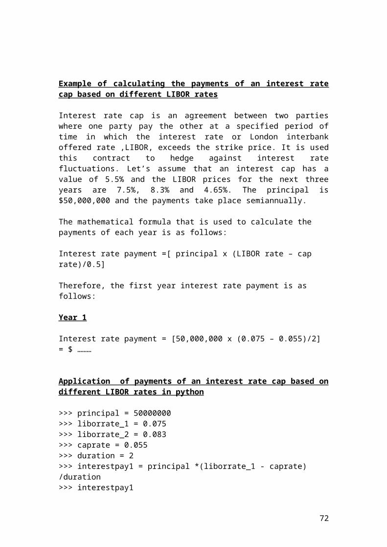
>>> floorletPrice1ii = (((floorletPrice2ii*p)+(floorletPrice2iii*p))/disinterest_1ii)>>> floorletPrice1ii594919.3884228686>>> floorletPrice0 = (((floorletPrice1i*p)+(floorletPrice1ii*p))/disinterest_0)>>> floorletPrice0405111.9890735737>>> round(_,2)405111.99
Calculate the bond put option prices based on different interest rates using a binomial 2 steps tree
>>> bond_price = 100>>> strike = 102
72
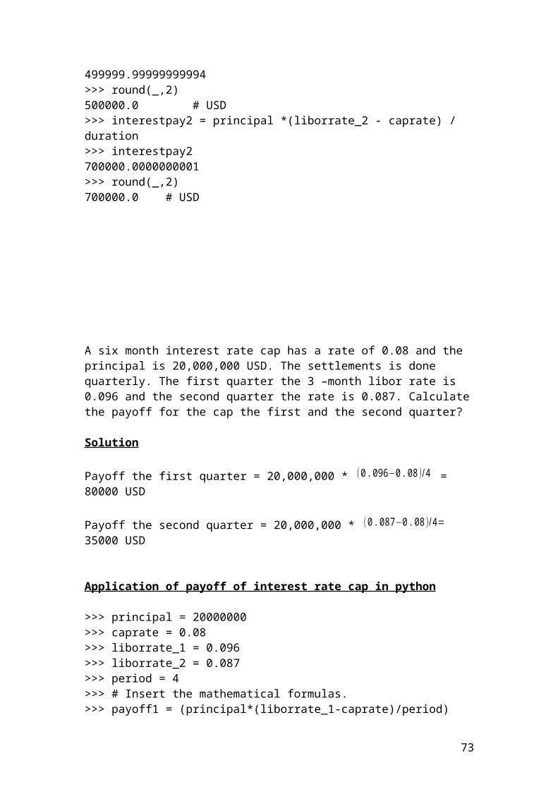
>>> annual_coupon = 7>>> maturity = 0.5>>> sigma = 0.3>>> interest_rate = 4>>> n =2>>> p = 0.5>>> dt = maturity/n # steps expressed in years.>>> dt0.25>>> from math import*>>> u = exp(sigma*sqrt(dt)) # multiplier of upmove.>>> u1.161834242728283>>> d = 1/u # multiplier of downmove.>>> d0.8607079764250578>>># Insert the mathematical formulas. It is a backward induction methodology.>>> bondPrice2i = (bond_price+annual_coupon)*(1/disinterest_2i)>>> bondPrice2i101.5180265654649>>> bondPrice2ii=(bond_price+annual_coupon)*(1/disinterest_2ii)>>> bondPrice2ii102.88461538461537>>> bondPrice2iii = (bond_price+annual_coupon)*(1/disinterest_2iii)>>> bondPrice2iii103.92385392385391>>> bondPrice1i = ((((bondPrice2i+annual_coupon)*p)+(bondPrice2ii+annual_coupon)*p)/disinterest_1i)>>> bondPrice1i104.3490883660202>>> bondPrice1ii = ((((bondPrice2ii+annual_coupon)*p)+(bondPrice2iii+annual_coupon)*p)/disinterest_1ii)>>> bondPrice1ii106.73263210966226>>> bondPrice0 = ((((bondPrice1i+ annual_coupon)*p)+(bondPrice1ii+ annual_coupon)*p)/disinterest_0)>>> bondPrice0108.21236561330888
>>> putPriceUpmovestep2i = strike - bondPrice2i>>> putPriceUpmovestep2i0.48197343453510655>>> putPriceUpdownmovestep2ii = strike - bondPrice2ii>>> putPriceUpdownmovestep2ii-0.8846153846153726
73
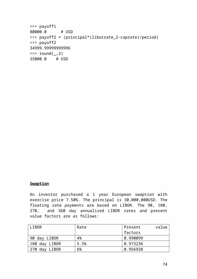
>>> putPriceUpdownmovestep2ii = 0>>> putPriceUpdownmovestep2ii0>>> putPriceDownmovestep2iii = strike - bondPrice2iii>>> putPriceDownmovestep2iii-1.9238539238539119>>> putPriceDownmovestep2iii =0>>> putPriceDownmovestep2iii0>>> putPriceUpmovestep1i= (((putPriceUpmovestep2i*p)+(putPriceUpdownmovestep2ii*p))/disinterest_1i)>>> putPriceUpmovestep1i0.2302787551529415>>> putPriceDownmovestep1ii= (((putPriceUpdownmovestep2ii*p)+(putPriceDownmovestep2iii*p))/disinterest_1ii)>>> putPriceDownmovestep1ii0.0>>> putPricestep0= (((putPriceUpmovestep1i*p)+(putPriceDownmovestep1ii*p))/disinterest_0)>>> putPricestep00.11071093997737572
Calculate the bond call option prices based on different interest rates using a binomial 2 steps tree. The figures are expressed in pounds
>>> bond_price = 100>>> strike = 100>>> annual_coupon = 7
74
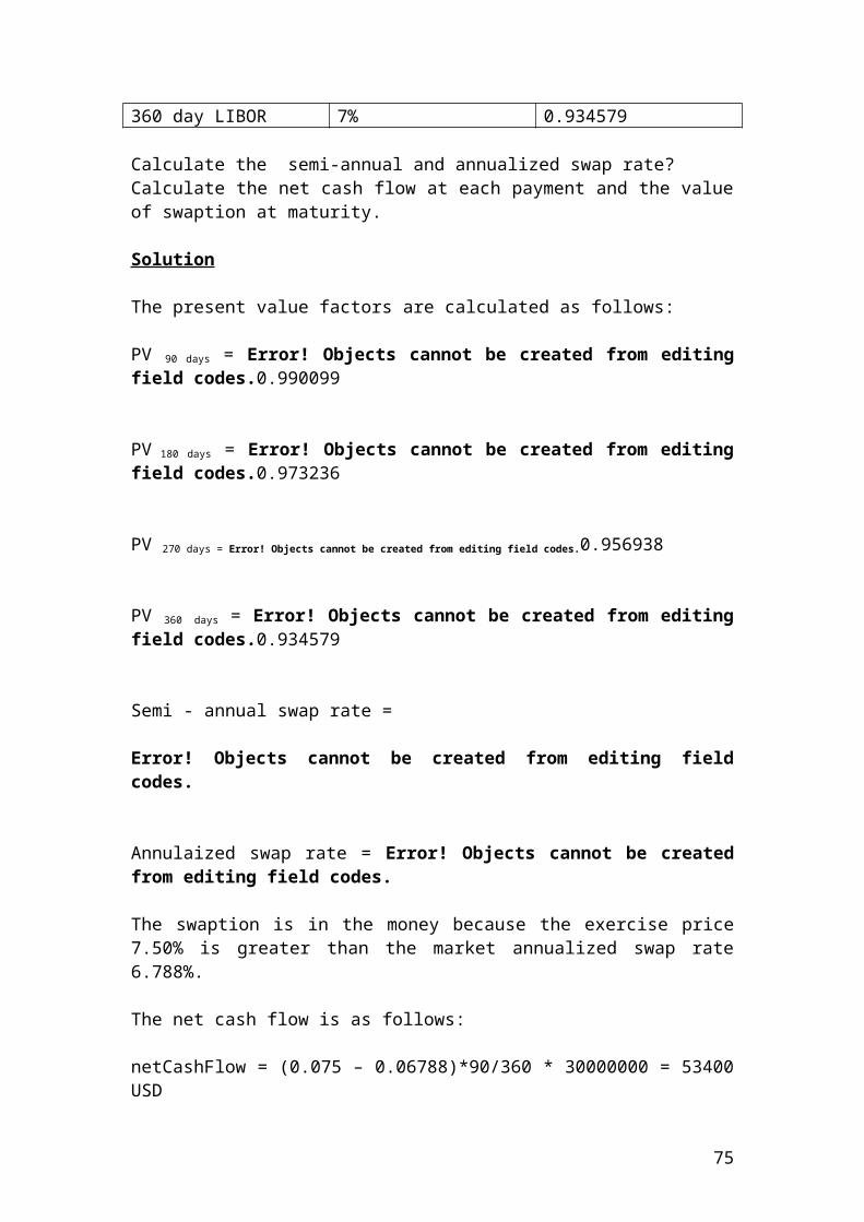
>>> maturity = 0.5>>> sigma = 0.3>>> interest_rate = 4>>> n =2>>> p = 0.5>>> dt = maturity/n # steps expressed in years.>>> dt0.25>>> from math import*>>> u = exp(sigma*sqrt(dt)) # multiplier of upmove.>>> u1.161834242728283>>> d = 1/u # multiplier of downmove.>>> d0.8607079764250578
>>> #Identify the discounted interest rates.>>> disinterest_0 = 1.04>>> disinterest_1i = 1.0465>>> disinterest_1ii = 1.0344>>> disinterest_2i = 1.054>>> disinterest_2ii = 1.04>>> disinterest_2iii = 1.0296>>># Insert the mathematical formulas. It is a backward induction methodology.>>> bondPrice2i = (bond_price+annual_coupon)*(1/disinterest_2i)>>> bondPrice2i101.5180265654649>>> bondPrice2ii=(bond_price+annual_coupon)*(1/disinterest_2ii)>>> bondPrice2ii102.88461538461537>>> bondPrice2iii = (bond_price+annual_coupon)*(1/disinterest_2iii)>>> bondPrice2iii103.92385392385391>>> bondPrice1i = ((((bondPrice2i+annual_coupon)*p)+(bondPrice2ii+annual_coupon)*p)/disinterest_1i)>>> bondPrice1i104.3490883660202>>> bondPrice1ii = ((((bondPrice2ii+annual_coupon)*p)+(bondPrice2iii+annual_coupon)*p)/disinterest_1ii)>>> bondPrice1ii106.73263210966226>>> bondPrice0 = ((((bondPrice1i+ annual_coupon)*p)+(bondPrice1ii+ annual_coupon)*p)/disinterest_0)>>> bondPrice0108.21236561330888>>> callPriceUpmovestep2i = bondPrice2i - strike>>> callPriceUpmovestep2i1.5180265654648935>>> round(_,2)1.52
75
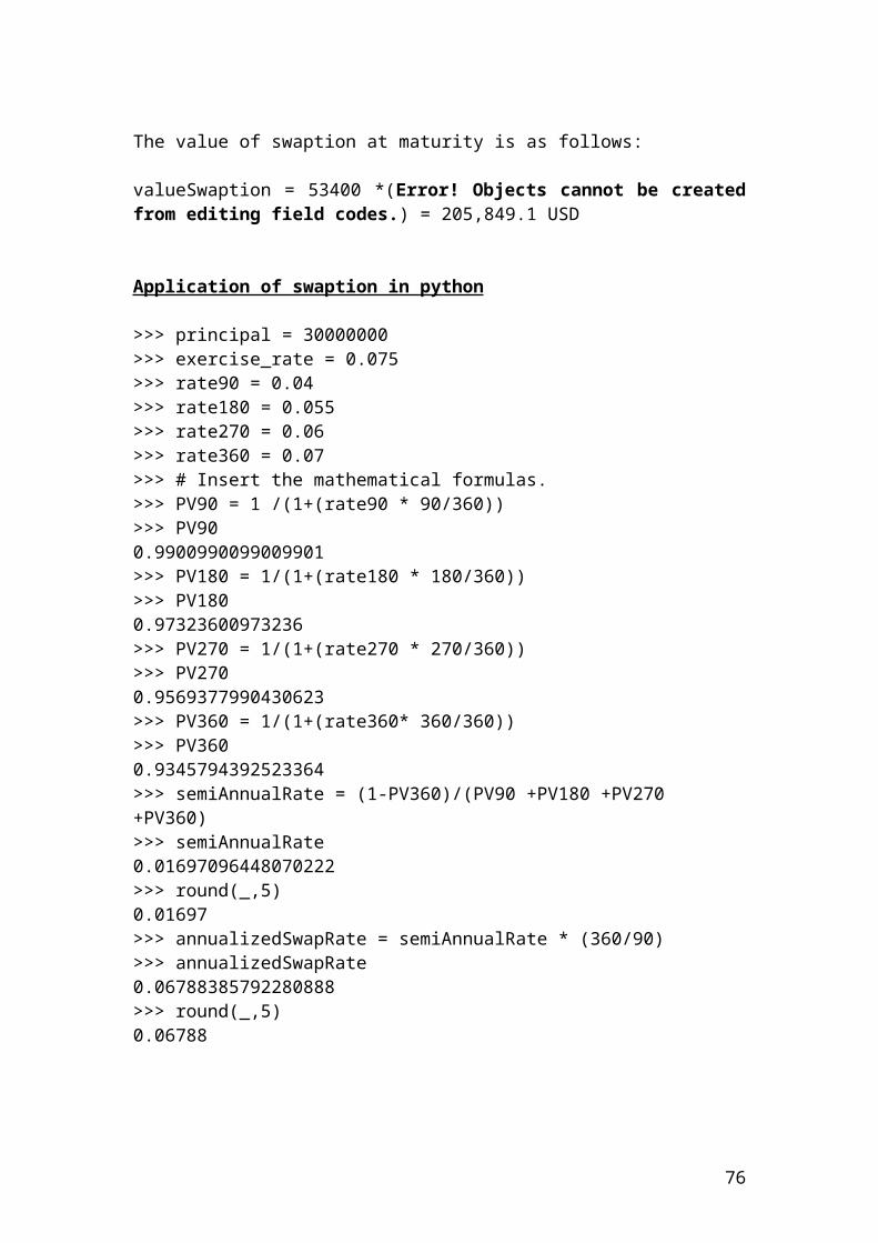
>>> callPriceUpdownmovestep2ii = bondPrice2ii - strike>>> callPriceUpdownmovestep2ii2.8846153846153726>>> callPriceDownmovestep2iii = bondPrice2iii - strike>>> callPriceDownmovestep2iii3.923853923853912>>> callPriceUpmovestep1i= (((callPriceUpmovestep2i*p)+(callPriceUpdownmovestep2ii*p))/disinterest_1i)>>> callPriceUpmovestep1i2.103507859570122>>> callPriceDownmovestep1ii= (((callPriceUpdownmovestep2ii*p)+(callPriceDownmovestep2iii*p))/disinterest_1ii)>>> callPriceDownmovestep1ii3.291023447635965>>> callPricestep0= (((callPriceUpmovestep1i*p)+(callPriceDownmovestep1ii*p))/disinterest_0)>>> callPricestep02.5935246669260033>>> round(_,2)2.59
Calculate the bond prices of an option based on different interest rates using a binomial 2 steps tree. The figures are expressed in pounds
>>> bond_price = 100>>> strike = 100>>> annual_coupon = 7>>> maturity = 0.5>>> sigma = 0.3>>> interest_rate = 4>>> n =2
76
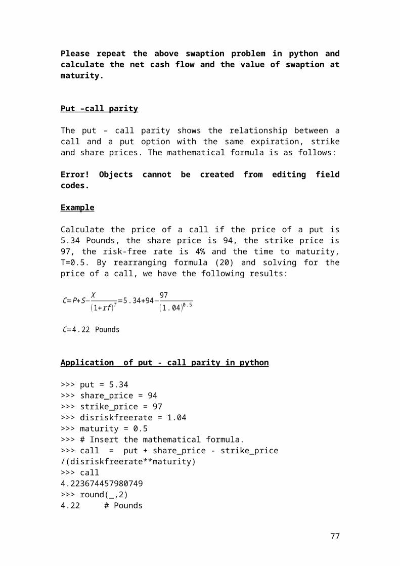
>>> p = 0.5>>> dt = maturity/n # steps expressed in years.>>> dt0.25>>> from math import*>>> u = exp(sigma*sqrt(dt)) # multiplier of upmove.>>> u1.161834242728283>>> d = 1/u # multiplier of downmove.>>> d0.8607079764250578
>>> #Identify the discounted interest rates.>>> disinterest_0 = 1.04>>> disinterest_1i = 1.0465>>> disinterest_1ii = 1.0344>>> disinterest_2i = 1.054>>> disinterest_2ii = 1.04>>> disinterest_2iii = 1.0296
>>># Insert the mathematical formulas. It is a backward induction methodology.>>> bondPrice2i = (bond_price+annual_coupon)*(1/disinterest_2i)>>> bondPrice2i101.5180265654649>>> bondPrice2ii=(bond_price+annual_coupon)*(1/disinterest_2ii)>>> bondPrice2ii102.88461538461537>>> bondPrice2iii = (bond_price+annual_coupon)*(1/disinterest_2iii)>>> bondPrice2iii103.92385392385391>>> bondPrice1i = ((((bondPrice2i+annual_coupon)*p)+(bondPrice2ii+annual_coupon)*p)/disinterest_1i)>>> bondPrice1i104.3490883660202>>> bondPrice1ii = ((((bondPrice2ii+annual_coupon)*p)+(bondPrice2iii+annual_coupon)*p)/disinterest_1ii)>>> bondPrice1ii106.73263210966226>>> bondPrice0 = ((((bondPrice1i+ annual_coupon)*p)+(bondPrice1ii+ annual_coupon)*p)/disinterest_0)>>> bondPrice0108.21236561330888
77
Calculate the interest rates of an option bond based on a two – period binomial tree. The risk – neutral probability of an up and down move in the interest rate tree is always 50% or 0.5. The figures are expressed in percentages
>>> bond_price =100>>> strike = 100>>> annual_coupon = 7>>> maturity = 0.5>>> volatility = 0.3>>> interest_rate = 4>>> p=0.5>>> n=2
78
>>>interestrate0 = 4>>> interestrate1i = interest_rate * u>>> interestrate1i4.647336970913132>>> interestrate1ii = interest_rate * d>>> interestrate1ii3.4428319057002312>>> interestrate2i = interest_rate * u**2>>> interestrate2i5.399435230304012>>> interestrate2ii= interest_rate*u*d>>> interestrate2ii4.0>>> interestrate2iii= interest_rate* d**2>>> interestrate2iii2.9632728827268715>>> round(_,2)2.96
Calculate the share prices of a call option using a Cox, Ross, Rubinstein,(CRR) binomial 3 steps tree using a vector. The multipliers of up and down move depend on volatility and length of steps. The figures are expressed in pounds
S = 60 # share price K = 50 # strike price r = 0.05 # interest rateq = 0.02 # dividend yieldT = 0.5 # maturitysig = 0.3 # volatilityn = 3>>> dt = T/n
79
>>> dt0.16666666666666666>>> u = exp(sig*sqrt(dt))>>> u1.1302902827674572>>> d = 1/u>>> d0.8847284766100544>>> share_price0 = S>>> share_price060>>> share_price_1upmove = S*u>>> share_price167.81741696604743>>> round(_,2)67.82>>> share_price_1downmove = S *d>>> share_price_1downmove53.083708596603266>>> round(_,2)53.08>>> share_price2upmove = S *u**2>>> share_price2upmove76.6533673991123>>> round(_,2)76.65>>> share_price2downmove = S*d**2>>> share_price2downmove46.96466863948485>>> round(_,2)46.96>>> share_price2upanddownmove = S*u*d>>> share_price2upanddownmove60.0>>> share_price3downmove = S*d**3>>> share_price3downmove41.55097973990743>>> round(_,2)41.55>>> share_price3upmove = S*u**3>>> share_price3upmove86.64055631262043>>> round(_,2)86.64>>> share_price3updowndown = S*u*d*d>>> share_price3updowndown53.083708596603266>>> round(_,2)53.08>>> share_price3upandupdown = S*u*u*d
80
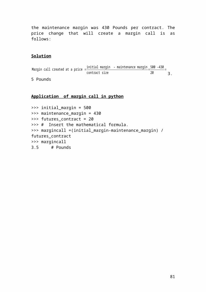
>>> share_price3upandupdown67.81741696604743>>> round(_,2)67.82
Calculate the call option prices using a Cox, Ross, Rubinstein,(CRR) binomial 3 steps tree. The figures are expressed in pounds
S = 60 # share price K = 50 # strike price r = 0.05 # interest rateq = 0.02 # dividend yieldT = 0.5 # maturitysig = 0.3 # volatilityn = 3>>> dt = T/n>>> dt
81
0.16666666666666666>>> from math import*>>> u = exp(sig*sqrt(dt))>>> u1.1302902827674572>>> d = 1/u>>> d0.8847284766100544>>> disfact = exp(-r*dt)>>> disfact0.991701292638876>>> riskprobofupmove = (exp((r-q)*dt)-d)/(u-d)>>> riskprobofupmove0.48983205544695174>> #The option prices are calculated backwards.>>> callpayoffupmovestep3 = S*u**3-K>>> callpayoffupmovestep336.64055631262043>>> callpayoff3i = S * u**2 * d -K>>> callpayoff3i17.817416966047432>>> callpayoff3ii =S * d**2*u-K>>> callpayoff3ii3.083708596603259>>> callpayoffdownmovestep3 = S*d**3-K>>> callpayoffdownmovestep3-8.449020260092567>>> callpayoffdownmovestep3 =0>>> callpayoffdownmovestep30>>> callpriceupmovestep2 = (disfact*(riskprobofupmove*callpayoffupmovestep3)+(1-riskprobofupmove)*callpayoff3i)>>> callpriceupmovestep226.88865113426896>>> callpriceupdownmovestep2 =(disfact*(riskprobofupmove*callpayoff3i)+(1-riskprobofupmove)*callpayoff3ii)>>> callpriceupdownmovestep210.228323934729657>>> callpricedownmovestep2 =(disfact*(riskprobofupmove*callpayoff3ii)+(1-riskprobofupmove)*callpayoffdownmovestep3)>>> callpricedownmovestep21.4979641284454819>>> callpriceupmovestep1 = (disfact*(riskprobofupmove*callpriceupmovestep2)+(1-riskprobofupmove)*callpriceupdownmovestep2)>>> callpriceupmovestep118.279784613543832>>> callpricedownmovestep1=(disfact*(riskprobofupmove*callpriceupdownmovestep2)+(1-riskprobofupmove)*callpricedownmovestep2)>>> callpricedownmovestep1
82
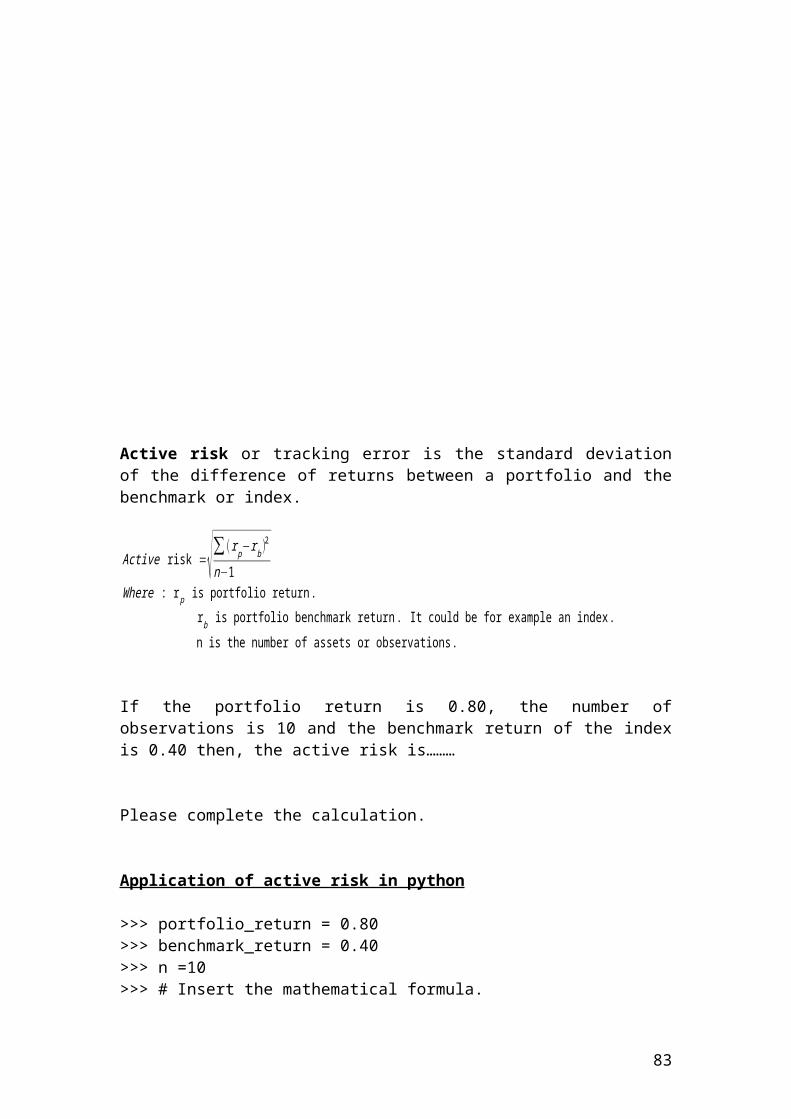
5.732796357703088>>> callpricestep0= (disfact*(riskprobofupmove*callpriceupmovestep1)+(1-riskprobofupmove)*callpricedownmovestep1)>>> callpricestep011.804406575946299>>> round(_,2)11.8
Calculate the put option prices using a Cox, Ross, Rubinstein,(CRR) binomial 3 steps tree. The figures are expressed in USD
>>> S = 60 # share price>>> K = 70 # strike price>>> r = 0.02 # interest rate>>> q = 0.03 # dividend yield>>> T = 0.5 # maturity>>> sig = 0.2 # volatility>>> n = 3>>> dt = T/n
83
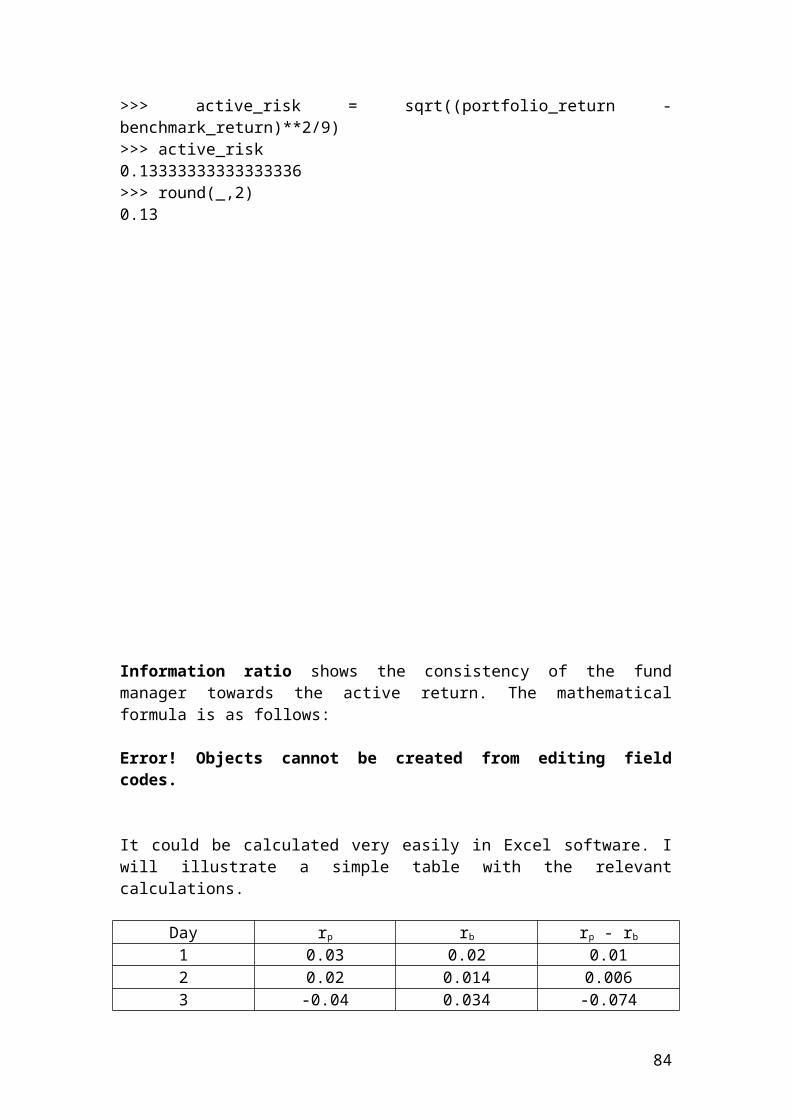
>>> dt0.16666666666666666>>> from math import*>>> u = exp(sig*sqrt(dt))>>> u1.0850755957772693>>> d = 1/u>>> d0.9215947754162443>>> disfact = exp(-r*dt)>>> disfact0.9966722160545233>>> riskprobofupmove = (exp((r-q)*dt)-d)/(u-d)>>> riskprobofupmove0.46941253331873867>>> #The option prices are calculated backwards.>>> putpayoffupmovestep3 = K-S*u**3>>> putpayoffupmovestep3-6.653367399112284>>> putpayoffupmovestep3=0>>> putpayoffupmovestep30>>> putpayoff3i = K- S * u**2 * d>>> putpayoff3i4.895464253363841>>> putpayoff3ii =K- S * d**2*u>>> putpayoff3ii14.704313475025337>>> putpayoffdownmovestep3 = K - S*d**3>>> putpayoffdownmovestep323.035331360515137>>> putpriceupmovestep2 = (disfact*(riskprobofupmove*putpayoffupmovestep3)+(1-riskprobofupmove)*putpayoff3i)>>> putpriceupmovestep22.5974719764209926>>> putpriceupdownmovestep2 =(disfact*(riskprobofupmove*putpayoff3i)+(1-riskprobofupmove)*putpayoff3ii)>>> putpriceupdownmovestep210.092269491137635>>> putpricedownmovestep2 =(disfact*(riskprobofupmove*putpayoff3ii)+(1-riskprobofupmove)*putpayoffdownmovestep3)>>> putpricedownmovestep219.101677490334147>>> putpriceupmovestep1 = (disfact*(riskprobofupmove*putpriceupmovestep2)+(1-riskprobofupmove)*putpriceupdownmovestep2)>>> putpriceupmovestep16.5700600829982925
84
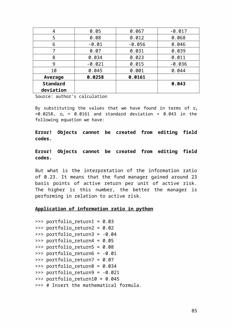
>>> putpricedownmovestep1=(disfact*(riskprobofupmove*putpriceupdownmovestep2)+(1-riskprobofupmove)*putpricedownmovestep2)>>> putpricedownmovestep114.85678328831304>>> putpricestep0= (disfact*(riskprobofupmove*putpriceupmovestep1)+(1-riskprobofupmove)*putpricedownmovestep1)>>> putpricestep010.956628441795559>>> round(_,2)10.96
Calculation of a Monte Carlo put option using antithetic variables. The purpose of using antithetic variables is to improve the estimation results by reducing the standard error of the simulation results. The figures are expressed in USD
>>> number_of_simulation = 199999>>> max_size = 200000>>> initial_share_price = 80>>> strike_price = 110>>> interest_rate = 0.07>>> dividend_yield = 0.02
85
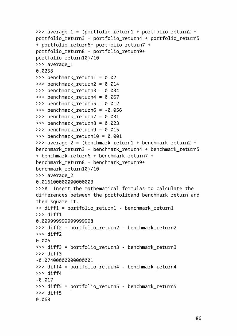
>>> volatility = 0.10>>> maturity = 0.5>>> from math import*>>> normsamp = [i]>>> i =0>>> i<=number_of_simulationTrue>>> random.number = (30000+3000)/300>>> random.number110.0>>> sharePrice = initial_share_price *exp((interest_rate-dividend_yield-0.5*volatility*volatility)*maturity+normsamp[i]*random.number*volatility *sqrt(maturity))>>> sharePrice81.82040273315567>>> round(_,2)81.82>>> sharePrice = initial_share_price *exp((interest_rate-dividend_yield-0.5*volatility*volatility)*maturity-normsamp[i]*random.number*volatility *sqrt(maturity))>>> sharePrice>>> payoff += value*strike*sharePrice*sharePrice>>> payoff35460314.4509055>>> optPrice = (payoff * exp(-r*T))/ Number_of_simulation/2>>> optPrice87.7691349127051>>> round(_,2)87.77
Calculate the put option prices using a Cox, Ross, Rubinstein,(CRR) binomial 3 steps tree. The figures are expressed in USD
>>> S = 60 # share price>>> K = 70 # strike price>>> r = 0.02 # interest rate>>> q = 0.03 # dividend yield>>> T = 0.5 # maturity>>> sig = 0.2 # volatility>>> n = 3
86
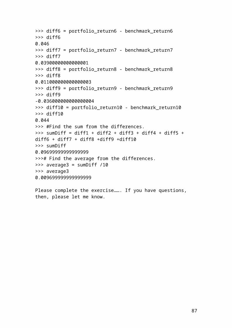
>>> dt = T/n>>> dt0.16666666666666666>>> from math import*>>> u = exp(sig*sqrt(dt))>>> u1.0850755957772693>>> d = 1/u>>> d0.9215947754162443>>> disfact = exp(-r*dt)>>> disfact0.9966722160545233>>> riskprobofupmove = (exp((r-q)*dt)-d)/(u-d)>>> riskprobofupmove0.46941253331873867>>> #The option prices are calculated backwards.>>> putpayoffupmovestep3 = K-S*u**3>>> putpayoffupmovestep3-6.653367399112284>>> putpayoffupmovestep3=0>>> putpayoffupmovestep30>>> putpayoff3i = K- S * u**2 * d>>> putpayoff3i4.895464253363841>>> putpayoff3ii =K- S * d**2*u>>> putpayoff3ii14.704313475025337>>> putpayoffdownmovestep3 = K - S*d**3>>> putpayoffdownmovestep323.035331360515137>>> putpriceupmovestep2 = (disfact*(riskprobofupmove*putpayoffupmovestep3)+(1-riskprobofupmove)*putpayoff3i)>>> putpriceupmovestep22.5974719764209926>>> putpriceupdownmovestep2 =(disfact*(riskprobofupmove*putpayoff3i)+(1-riskprobofupmove)*putpayoff3ii)>>> putpriceupdownmovestep210.092269491137635>>> putpricedownmovestep2 =(disfact*(riskprobofupmove*putpayoff3ii)+(1-riskprobofupmove)*putpayoffdownmovestep3)>>> putpricedownmovestep219.101677490334147>>> putpriceupmovestep1 = (disfact*(riskprobofupmove*putpriceupmovestep2)+(1-riskprobofupmove)*putpriceupdownmovestep2)>>> putpriceupmovestep16.5700600829982925
87
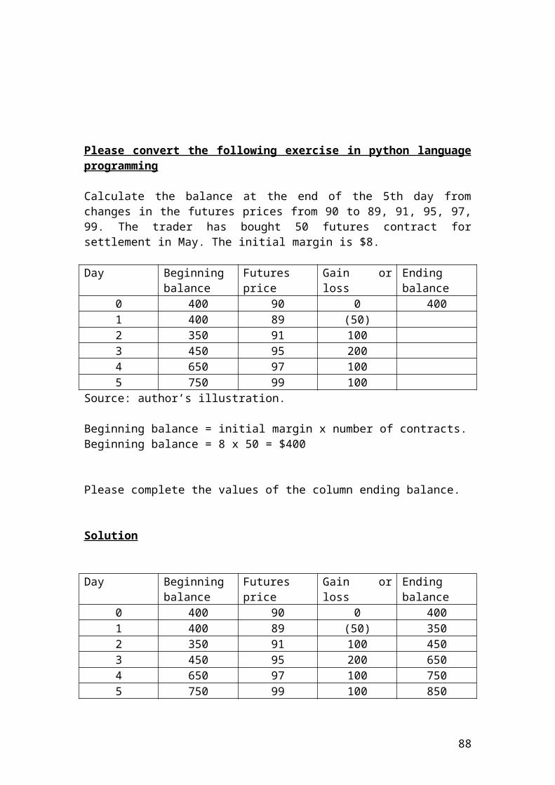
>>> putpricedownmovestep1=(disfact*(riskprobofupmove*putpriceupdownmovestep2)+(1-riskprobofupmove)*putpricedownmovestep2)>>> putpricedownmovestep114.85678328831304>>> putpricestep0= (disfact*(riskprobofupmove*putpriceupmovestep1)+(1-riskprobofupmove)*putpricedownmovestep1)>>> putpricestep010.956628441795559>>>>>> round(_,2)10.96
Calculation of a Monte Carlo call option using antithetic variables. The purpose of using antithetic variables is to improve the estimation results by reducing the standard error of the simulation results
>>> number_of_simulation = 199999>>> max_size = 200000>>> initial_share_price = 120>>> strike_price = 90>>> interest_rate = 0.07
88
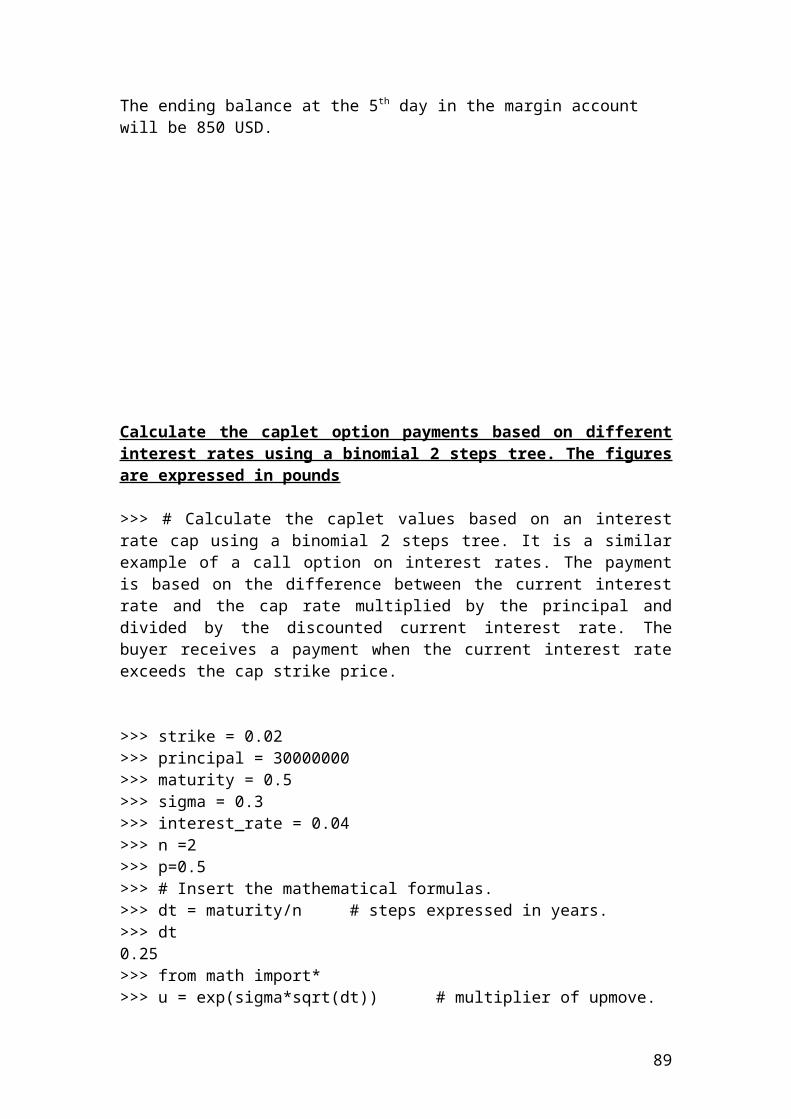
>>> dividend_yield = 0.02>>> volatility = 0.10>>> maturity = 0.5>>> from math import*>>> i =0>>> i<=number_of_simulationTrue>>> normsamp = [i]>>> random = (30000+3000)/300>>> random110.0>>> sharePrice = initial_share_price *exp((interest_rate-dividend_yield-0.5*volatility*volatility)*maturity+normsamp[i]*random*volatility *sqrt(maturity))>>> sharePrice122.73060409973353>>> round(_,2)122.73>>> sharePrice = initial_share_price *exp((interest_rate-dividend_yield-0.5*volatility*volatility)*maturity-normsamp[i]*random*volatility *sqrt(maturity))>>> sharePrice>>> value = initial_share_price – strike_price>>> value>>>30>>> payoff += value*strike*sharePrice*sharePrice>>> payoff
>>> optPrice = (payoff * exp(-r*T))/ Number_of_simulation/2>>> optPrice
Please continue the calculations related to payoff and optPrice….
Calculate the call option prices using a Jarrow – Rudd, (JR), binomial 3 steps tree. The key difference between the Cox, Ross, Rubinstein,(CRR) binomial tree and the Jarrow – Rudd, (JR), binomila tree is in defining the parmeters of the multiplier of up and down move. The figures are expressed in pounds
>>> S = 90 # share price>>> K = 85 # strike price>>> r = 0.04 # interest rate>>> q = 0.03 # dividend yield
89
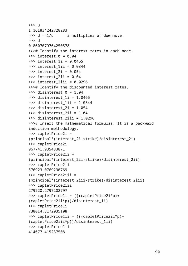
>>> T = 0.5 # maturity>>> sig = 0.2 # volatility>>> n = 3>>> from math import*>>> dt = T/n>>> dt = T/n # steps expressed in years.>>> dt0.16666666666666666>>> u = (exp((r-q -0.5*sig*sig)*dt + sig*sqrt(dt))) # multiplier of upmove.>>> u1.0832686426635116 >>> d = (exp((r-q -0.5*sig*sig)*dt - sig*sqrt(dt))) # multiplier of downmove.>>> d0.9200600634058166>>> disfact = exp(-r*dt) # discount factor.>>> disfact0.9933555062550344>>> riskprobofupmove = (exp((r-q)*dt)-d)/(u-d) # risk neutral probability of upmove.>>> riskprobofupmove0.5000226905523886>>> callpayoffupmovestep3 = S*u**3-K>>> callpayoffupmovestep329.406585701387428>>> callpayoff3i = S * u**2 * d -K>>> callpayoff3i12.169738279923607>>> callpayoff3ii =S*d**2*u-K>>> callpayoff3ii-2.470152793185349>>> callpayoff3ii =0>>> callpayoff3ii0>>> callpayoffdownmovestep3 = S*d**3-K>>> callpayoffdownmovestep3-14.904352933845047>>> callpayoffdownmovestep3 =0>>> callpayoffdownmovestep30>>> callpriceupmovestep2 = (disfact*(riskprobofupmove*callpayoffupmovestep3)+(1-riskprobofupmove)*callpayoff3i)>>> callpriceupmovestep220.690852733318547>>> callpriceupdownmovestep2 =(disfact*(riskprobofupmove*callpayoff3i)+(1-riskprobofupmove)*callpayoff3ii)>>> callpriceupdownmovestep26.044712568308618>>> callpricedownmovestep2 =(disfact*(riskprobofupmove*callpayoff3ii)+(1-riskprobofupmove)*callpayoffdownmovestep3)>>> callpricedownmovestep2
90

0.0>>> callpriceupmovestep1 = (disfact*(riskprobofupmove*callpriceupmovestep2)+(1-riskprobofupmove)*callpriceupdownmovestep2)>>> callpriceupmovestep113.299371739539392>>> callpricedownmovestep1=(disfact*(riskprobofupmove*callpriceupdownmovestep2)+(1-riskprobofupmove)*callpricedownmovestep2)>>> callpricedownmovestep13.0024105032518027>>> callpricestep0= (disfact*(riskprobofupmove*callpriceupmovestep1)+(1-riskprobofupmove)*callpricedownmovestep1)>>> callpricestep08.10693896385682>>> round(_,2)8.11
Calculate the share prices of a call option using a Jarrow – Rudd, (JR), binomial 3 steps tree. The prices are expressed in Euros
>>> S = 90>>> K = 85>>> r = 0.04>>> q = 0.03>>> T = 0.5>>> sig = 0.2
91
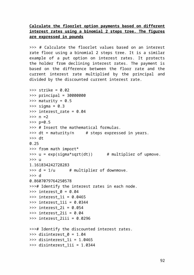
>>> n =3>>> dt = T/n>>> dt0.16666666666666666>>> from math import*>>> u = (exp((r-q -0.5*sig*sig)*dt + sig*sqrt(dt)))>>> u1.0832686426635116>>> d = (exp((r-q -0.5*sig*sig)*dt - sig*sqrt(dt)))>>> d0.9200600634058166>>> share_price0 = S>>> share_price090>>> share_priceupmove1 = S*u>>> share_priceupmove97.49417783971604>>> round(_,2)97.49>>> share_pricedownmove1 = S*d>>> share_pricedownmove182.80540570652349>>> round(_,2)82.81>>> share_priceupmove2 = S*u**2>>> share_priceupmove2105.61238569602422>>> round(_,2)105.61>>> share_priceupmovedownmove = S*u*d>>> share_priceupmovedownmove89.70049944490711>>> round(_,2)89.7>>> share_pricedownmove2 = S*d**2>>> share_pricedownmove276.18594682468837>>> round(_,2)76.19>>> share_priceupmove3 = S*u**3>>> share_priceupmove3114.40658570138743>>> round(_,2)114.41
Please complete the remaining calculations……
92
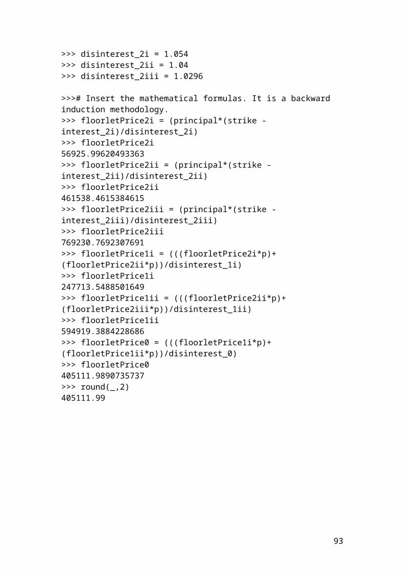
Example of simulating share prices by showing different price scenarios. The figure is expressed in pounds
>>> number_of_simulation = 6>>> max_size = 8>>> S0 = 60>>> r = 0.03>>> q = 0.02>>> sig = 0.20
93
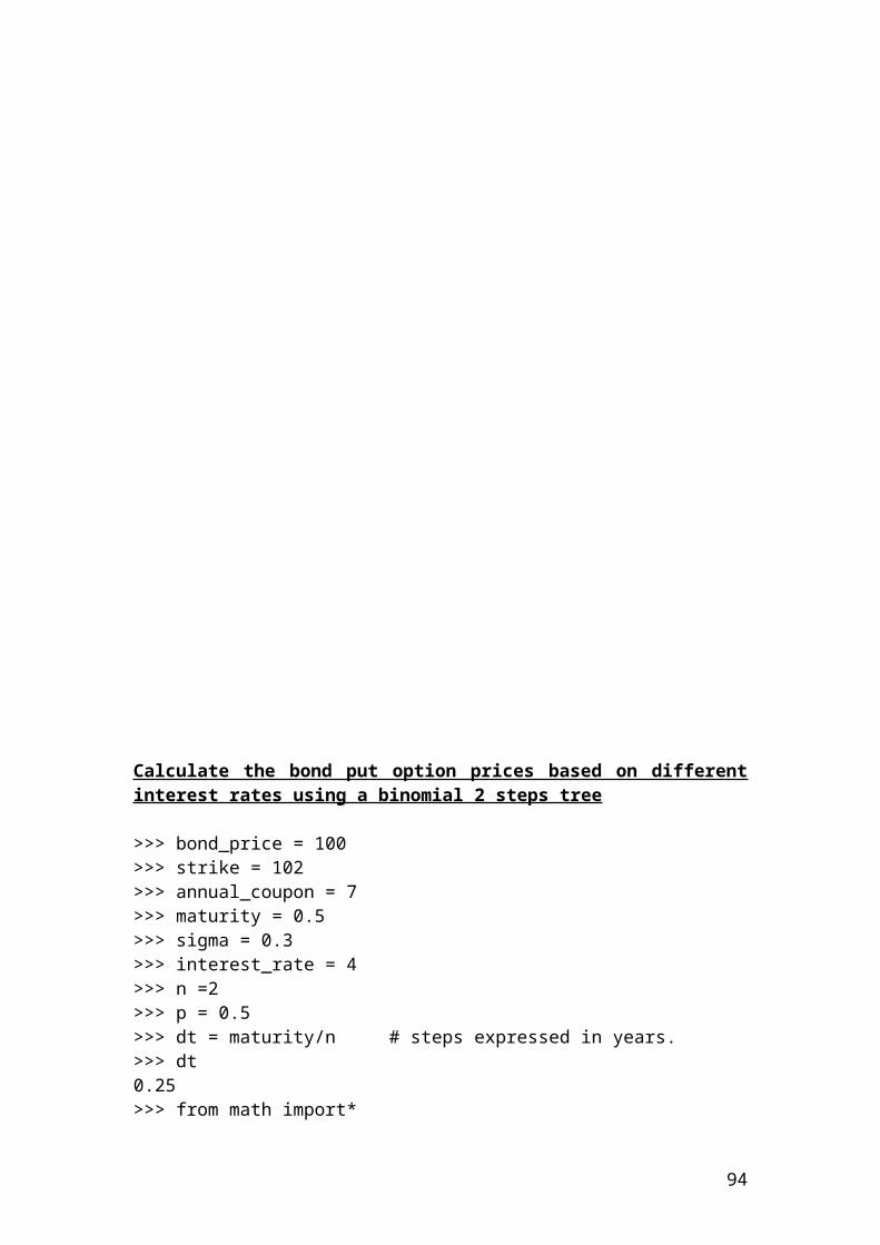
>>> dt = 1/250>>> dt0.004>>> from math import*>>> normsamp = [i]>>> i = 0>>> normsamp=[i]>>> i<=number_of_simulationTrue>>> random.number = (30000+3000)/300>>> random.number110.0>>> sharePrice=S0*exp((r-q-0.5*sig*sig)*dt+normsamp[i]*random.number*sig*sqrt(dt))>>> sharePrice59.99760004799936
Please complete the calculations to get different share prices….
A manufacturing company sold a FRA contract expiring in 50 days with a principal of 30,000,000 USD. The underlying is 180 days LIBOR. The agreed rate on this FRA is 7%. At expiration, 90 days later, the actual rate on 180 days LIBOR is 8%. How much is the payoff of the manufacturing company at expiration?
Solution
94
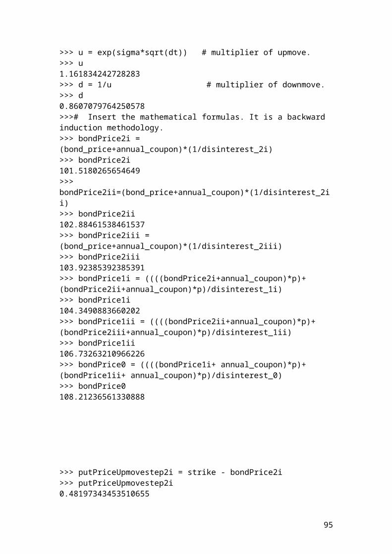
The mathematical formula for Forward Rate Agreement, (FRA) is as follows:
FRA Payment =Notional amount x( (actualrate - agreed rate ) (t days /360 )1+actual rate (tdays /360 ) )
FRA Payment = 30,000,000* ((0.08 – 0.07)*(180/360) / 1 + 0.08*(180/360)
FRA Payment = 30,000,000 * 0.005 / 1.04
FRA Payment = 144230.77 USD
Application of FRA payment in python
>>> principal = 30000000>>> actual_rate = 0.08>>> agreed_rate = 0.07>>> days_1underlying = 180>>> days_2expiration = 180
Please complete the calculations using python ……..
Currency futures
Futures Price = contract size * exchange rate
If the contract size is 20,000 USD and the quoted price is 1.573 USD, then, the futures price is as follows:
Futures Price = 20,000 * 1.573 = 31460 USD
95
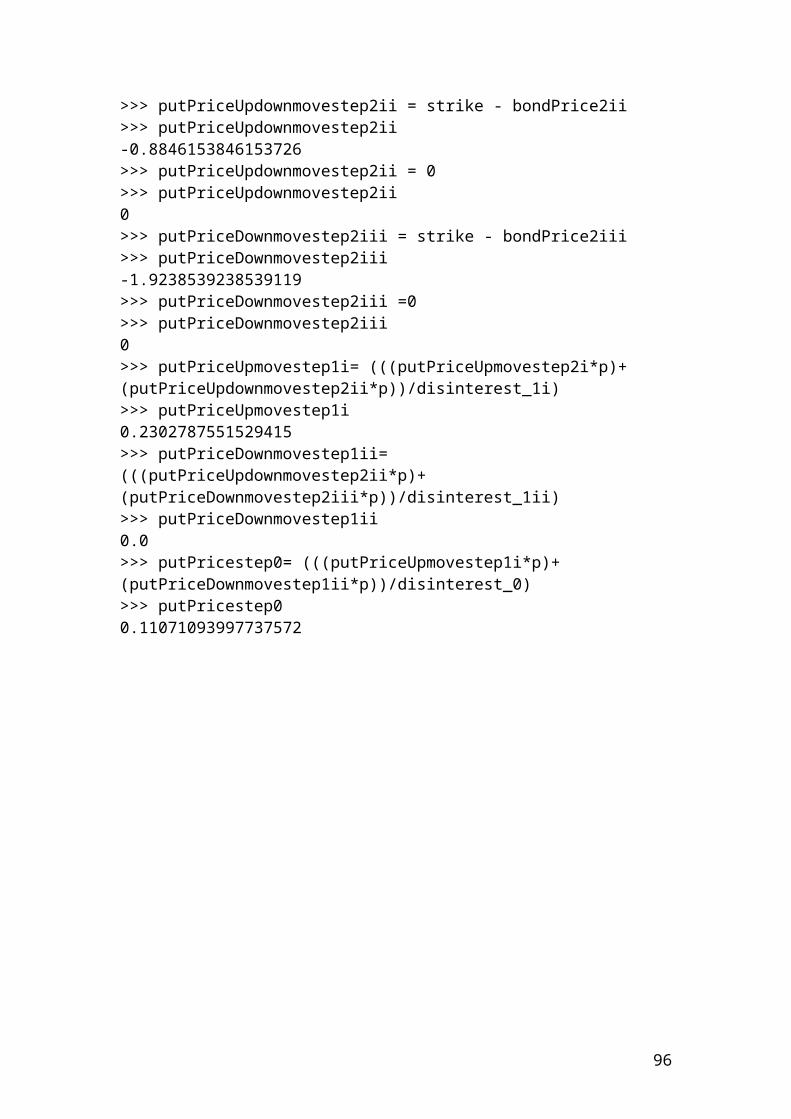
Application of currency futures in python
>>> contract_size = 20000>>> quoted_price = 1.573>>> FuturesPrice = contract_size * quoted_price>>> FuturesPrice31460.0 # USD>>>
Minimum price required for a margin call
It is very important to check the maintenance margin level. The initial margin per contract for a gold futures contract is 1,500 USD. The maintenance margin per contract is 800 USD. The contract size is 5,000 ounces.
Solution
96
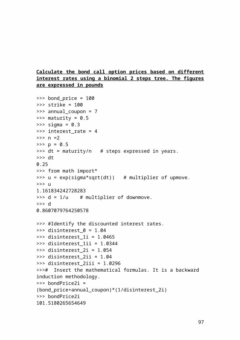
Minimum price required for a margin call = initial margin – maintenance margin / contract size
Minimum price required for a margin call = 1500 – 800 / 5000 = 0.14 USD.
Application of minimum price required for a margin call in python
>>> initial_margin_of_gold_futures = 1500>>> maintenance_margin_percontract = 800>>> contract_size = 5000>>> minimum_price_required_for_a_margin_call = (initial_margin_of_gold_futures - maintenance_margin_percontract) / contract_size>>> minimum_price_required_for_a_margin_call0.14 # USD
Loss on the futures position
Please consider a bond related to Eurodollar futures. The settlement price of the bond is 95.70 in December 2015. The principal is 2,000,000 Euros. The investor has adopted a long position of 100 contracts. The bond price has fallen to 90.15. Calculate the loss on the futures position.
97
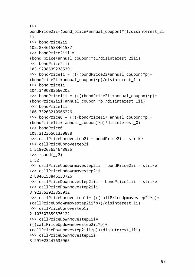
Solution
Insert the mathematical formula.
Loss on the futures position = (settlement price – current price) / 100 * 100 contracts * 2,000,000
Loss on the futures position = (95.70 – 90.15) / 100 * 100 * 2,000,000 =
Loss on the futures position = 5.55 / 100 * 100 * 2000000 = 11,100,000 Euros.
Application of loss on the futures position in python
>>> settlement_price = 95.70>>> current_price = 90.15>>> principal = 2000000>>> contract_size = 100>>> Loss_on_the_futures_position =(settlement_price - current_price)/100*contract_size*principal>>> Loss_on_the_futures_position11099999.999999994>>> round(_,2)11100000.0 # Euros
Variation margin call
The amount of variation margin call is used in futures when the price of the asset price falls below a certain amount. For example, consider the bond price of Eurodollar futures.
98
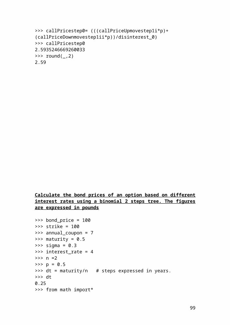
Consider a trader that has bought a Eurodollar bond futures with a principal of 10,000,000 Euros. The settlement price is 97.14. The long position includes 100 contracts. The price of the bond has fallen to 95.78. The maintenance price is 96.45. The price of the bond has fallen below the maintenance price.
Variation margin = (settlement price – current price) / 100 * 100 contracts * 10,000,000
Variation margin = (97.14 – 95.78) / 100 * 100 *10,000,000 =
Variation margin = 1.36 / 100 * 100 * 10,000,000 = 13,600,000 Euros.
Application of variation margin call in python
>>> settlement_price = 97.14>>> current_price = 95.78>>> principal = 10000000>>> contract_size = 100>>> variation_margin =(settlement_price-current_price)/100*contract_size*10000000>>> variation_margin13599999.999999994>>> round(_,2)13600000.0 # Euros
Calculate the volume and the open interest position in the July FTSE 100 index
Please consider 5 investors with the following short/long contract position.
99
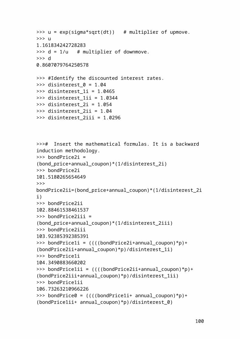
First investor buys 3 contracts to open a long position.Second investor buys 5 contracts to open a long position.Third investor buys 2 contracts to open a long position.Fourth investor sells 7 contracts to close a long position.Fifth investor sells 4 contracts to close a long position.
If we assume that the initial open interest before the trades was 30 contracts. Calculate the volume and ending open interest.
Solution
Total volume = 3 + 5 + 2 + 7 + 4 = 21 contracts.
Ending open interest = initial open interest + opened positions - closed positions
Ending open interest = 30 + 3 + 5 + 2 - 7 – 4 = 29
Application of calculation the volume and the open interest position in the July FTSE 100 index in python
>>> first_investor_buys_3contracts = 3>>> second_investor_buys_5contracts = 5>>> third_investor_buys_2contracts = 2>>> fourth_investor_sells_7contracts = 7>>> fifth_investor_sells_4contracts = 4>>> initial_open_interest = 30>>> Total_volume = 3+5+2+7+4>>> Total_volume21 # contracts>>> ending_open_interest = 30 + 3 + 5 + 2 - 7 -4>>> ending_open_interest29 # ending open interest>>>
Calculation of the minimum price per ounce before a margin call
Please consider the following terms of the silver contract:
Initial margin = $ 3,500 per contract.
100

Maintenance margin = $ 2,500 per contract.20 silver contracts sold at a price equals $700 per ounce.Contract size = 100 ounces.
Solution
The initial margin = 3,500 * 20 = 70,000 USD. The maintenance margin = 2,500 * 20 = 50,000 USD.The difference between the initial and maintenance margin is the amount recorded before a margin call take place. Thus, 70,000 – 50,000 = 20,000 USD.
The price is 20,000 / 20*100 = 10 USD per ounce. This is the price before a margin call take place.
Application of calculating the minimum up or down ounce price before a margin call in python
>>> initial_margin = 3500>>> maintenance_margin = 2500>>> silver_contracts = 20>>> contract_size = 100>>> minimum_price_required_for_a_margincall = (3500 - 2500) / 100>>> minimum_price_required_for_a_margincall10.0 # USD per ounce.
Calculate the intrinsic value of call share traded in Frankfurt stock exchange
The VW share is traded at 140 Euro in the Frankfurt stock exchange. The strike price is 130 Euro and the option market price is 7.70 Euro. The intrinsic value of the VW call is as calculate as follows:
101
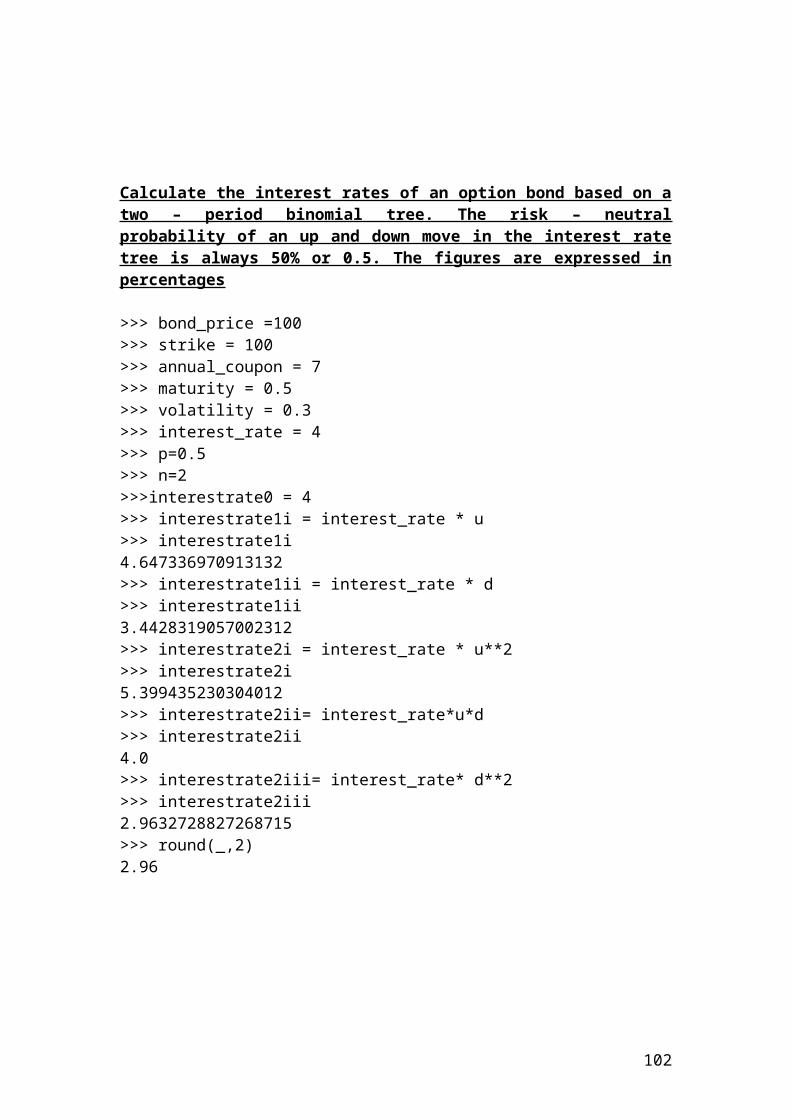
Solution
The intrinsic value of the VW call is = Share price – strike price = 140 – 130 = 10 Euro.
Application of calculating the intrinsic value of call share traded in Frankfurt stock exchange
>>> share_price = 140>>> strike_price = 130>>> intrinsic_value = share_price - strike_price>>> intrinsic_value10 # Euro.>>>
Workshop and detailed explanation of Matlab
Matlab is a powerful mathematical and statistical package that covers Financial Derivatives. Once you open Matlab, you get a launch pad that includes Financial Derivatievs toolbox. By clicking on it you have a help and a demo function. By clicking on the demo function and selection Financial toolbox, you get a variety of financial functions and quantitative analysis options. You could select options as follows:
102
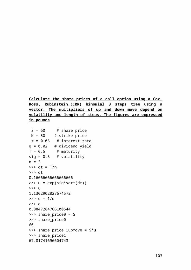
Equity options Portfolio optimization Capital allocation GARCH estimation Time series Financial charting Mean – Variance efficient frontier Call option sensitivity measures 1 Call option sensitivity measures 2
In this workshop, we will focus on capital allocation, call option sensitivity measures 1 and call option sensitivity measures 2.
By clicking on capital allocation, you have the option the change the inputs such as risk free rate, borrowing rate, and risk aversion coefficient. Once you input the numbers, you are provided with a chart that displays the expected return in relation to the risk or standard deviation. The chart shows the optimal overall portfolio and the optimal risky portfolio.
By clicking on capital option sensitivity measures 1 and 2, you are provided with a graph that shows the sensitivity of the Greek letter Gamma of the share option in relation to the time expressed in months. (gamma), measures the change in an option’s delta for a small change in the share price. , (delta), means the change that will occur in the option price for a small change in the share price, when all other factors are constant.
Once you have prepared the Excel datasheet with all the variables that you will describe and analyse, you then import the data in the Matalab software. For example, you have recorded the closing price, the open price the high and low of a future index contract for the last 5 years. You press file and then import data and then select the file type. The, select create vectors from each column using column names. Then, press workspace to work on your data individually or in aggregate format. By clicking on the variable or the group of variables, you are provided with graph selection. You have the option to use plot, surf, 2-Dgraphics and 3-D graphics. Once you have your chart, you press tools and you are provided with the option of basic fitting and data statistics. By clicking on the basic fitting, you have the option to click the shape that your data will take. For example, it will be linear, quadratic, cubic, etc… Thus, you have the option to explore different polynomials that fit your data. For example, you can try a linear or cubic polynomial to the data. You have also the option to select the equation and to plot the residuals. By plotting the residuals, you can evaluate the goodness of fit. You have also the option to interpolate or extrapolate the fit and shows the results. I have included an example of a Danske call equity option that is traded in the OMX Copenhagen 20 stock exchange index.
103
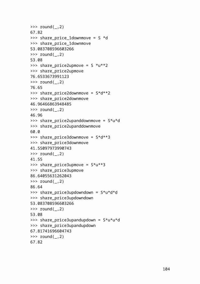
Source: author’s calculation
In this workshop we will cover in detail the following topics:
The command window of matrix algebra. Excel link used to exchange data between Matlab and Excel Microsoft. Financial Toolbox. Financial Time Series toolbox is used to analyze time series data. GARCH toolbox used to test the Generalized Autoregressive Conditional
Heteroskedasticity, (GARCH) volatility modelling. Matlab compiler is used to convert Matlab M-files to C++ computer language
programming. Statistics toolbox is used to analyze statistical historical data, model systems
and develop statistical algorithms. Financial derivatives toolbox is used to analyze options, futures and swaps. Quotes from the Gospel that are integrated in a Fuzzy logic function through a
spiritual advisor. Introduction to spectral analysis by using the covariance method, wavelet and
Fourier analysis. Introduction to Simulink.
Matrix algebra
In the command window, you have the options to calculate matrix algebra by inputting the correct syntax of Matlab command. For example, you want to construct a 3 x 3 matrix of a variable X. You write the following formula in the command window:
104
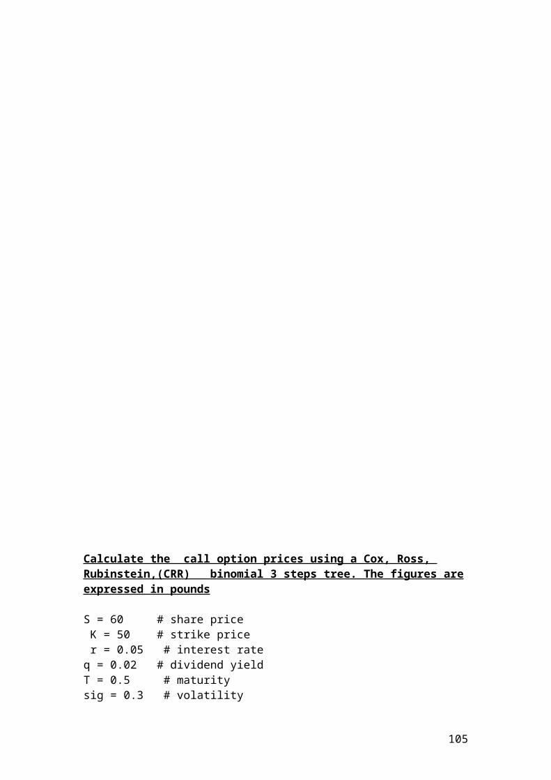
>>X = [2 4 5; 7 9 10; 3 5 8] Then, press enter in the command window. Matlab will arrange the numbers in a matrix format as follows:
X =
2 4 5 7 9 10 3 5 8
Now if you want to create a new variable Y = X + 3. Then, write the formula in the command window and press enter. Matlab will do the additions in the matrix as follows:
>>Y = X + 3
Y =
5 7 8 10 12 13 6 8 11
If you want to multiply the above matrices and create a new one, then use the formula as follows:
>>Z = X*Y
Z =
80 102 123 185 237 283 113 145 177
If you want to calculate the inverse function of Z, then type the formula as follows:Matlab will make the following calculation.
>>M = inv(Z).
M =
2.2850 -0.5475 -0.7125 -1.9150 0.6525 0.2875 0.1100 -0.1850 0.2250If you want to calculate the eigenvalue of M. Type the command eig(M). Matlab will do the following calculation.
>> eig(M)
105
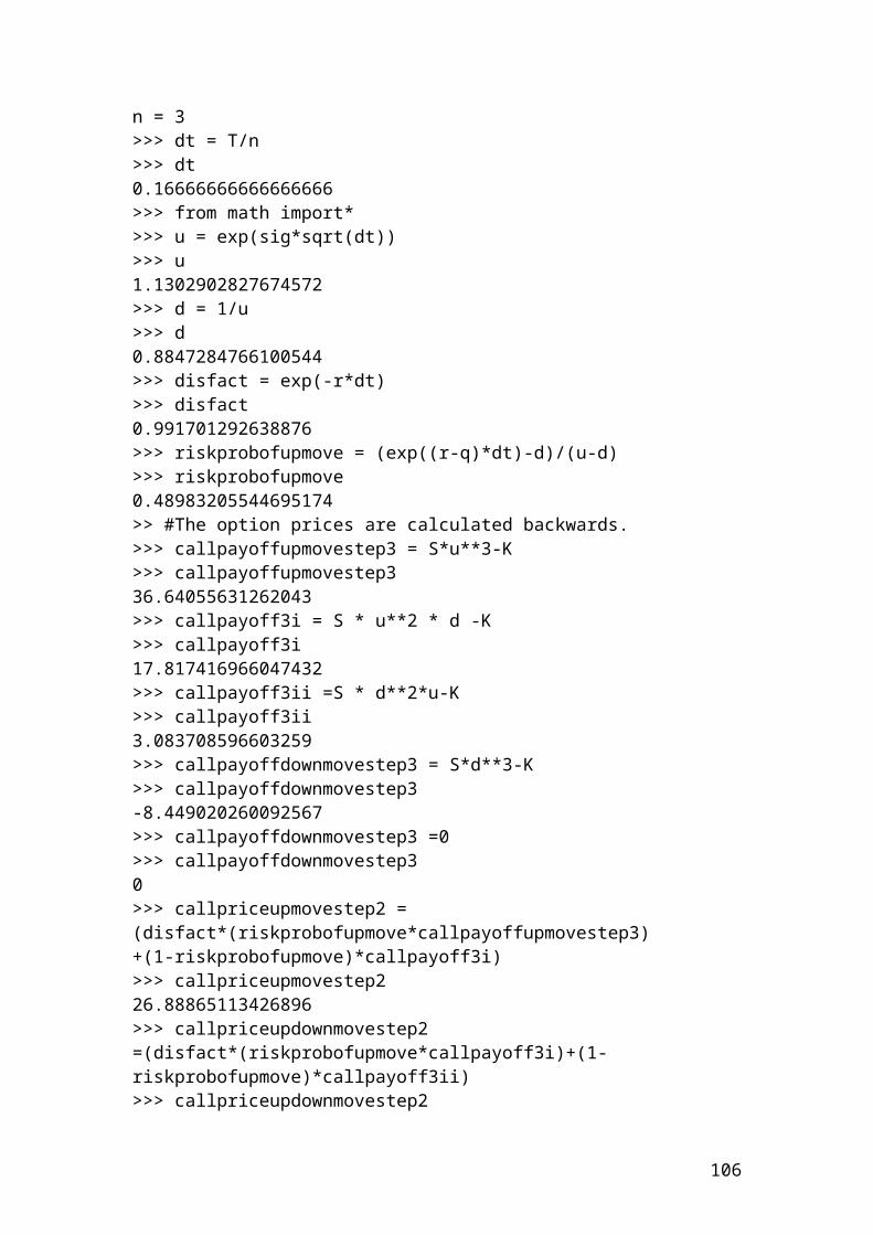
ans =
2.7065 0.0020 0.4539
If you want to calculate the singular value decomposition of M. Type the command svd(M). Matlab will do the following calculation.
>>svd(M)
ans =
3.1837 0.4062 0.0019
You could calculate the poly function of M. It generates a vector containing the coefficients of the characteristic polynomial. Type the command P=round(poly(M)). Matlab will do the following calculation.
>> P=round(poly(M))
P =
1 -3 1 0
If you want to calculate the roots function of a polynomial. Type the command roots(P). Matlab will do the following calculation.
>> roots(P)
ans =
0 2.6180 0.3820
Excel link used to exchange data between Matlab and Excel Microsoft
To achieve a linkage between Excel and Matlab you have to do the following:
Start Microsoft Excel. Select Tools menu. Select Add-Ins and click Browse.
106
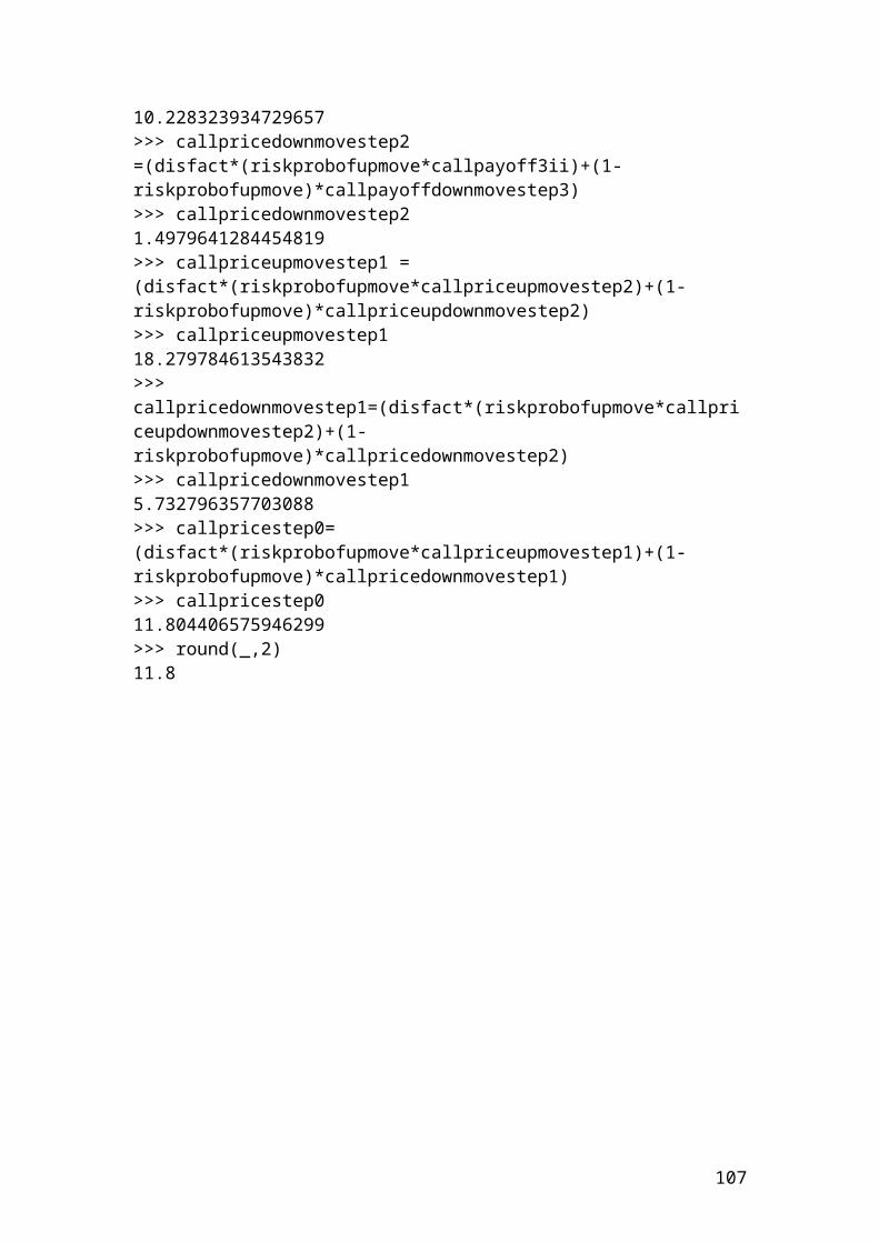
Find and select the Excel Link add-in excllink.xla under matlab/toolbox/exlink.
Press OK.
The function matlabinit start the Excel link in relation to the Matlab software. The function MLAutoStart start Matlab. The function MLClose stops Matlab from running. The function MLOpen initiate matlab software.
You can combine both softwares, namely, Excel and Matlab to build and solve financial derivatives problems.
For example, we want to calculate the expected risk expressed as a standard deviation based on historical return data that was collected from Metastock technical analysis for buying or going long on a call, put and index options. Then, we want to design the efficient frontier and decide which investment strategy is the most appropriate. Is it better to hold a call, a put or index options portfolio?
1 (A) Date (B) Call option return of Danske bank
( C) Put option return of
Danske bank
(D) Index option return
of OMX Copenhagen stockmarket
(E) Risk expressed
as standard deviation,
(STDEVA)
(F)Average returns for call, put and index
options2 2009 3.5% 2.7% 3.7%3 2010 4.7% 4.9% 7.9%4 2011 7.9% 5.7% 8.9%5 2012 -4.2% 8.5% 10.2%6 2013 5.4% 9.3% -6.8%7 2014 10.3% 11.5% 5.9%
Source: author’s calculation.
The first thing is to input the above data in a visual basic application, (VBA) format and then use Matlab syntax to transfer and exchange the data between the two softwares. The name of the Excel file is VBA for options.
Please complete the table ……………………………
VBA code illustration of the above example
Sub test1()
'Question
107
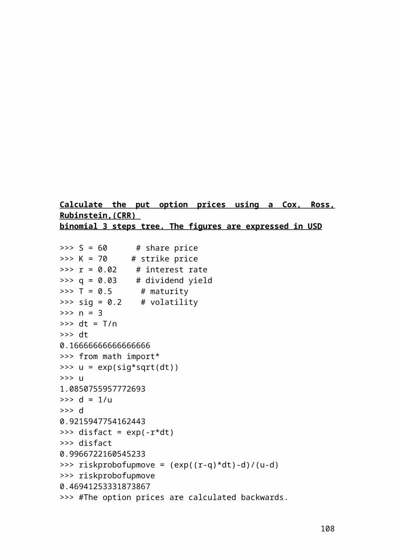
'It is required to calculate the expected risk expressed as a standard deviation based on historical return data that was collected from Metastock technical analysis for call, put and index options. The risk will be calculated for the three bands of investment for each year.
'Draw an efficient frontier and decide which investment strategy is the most suitable?
'********************************************************************'Data provided'********************************************************************
'Call option return of Danske bank = 3.5%, 4.7%, 7.9%, -4.2%, 5.4%, 10.3%'Put option return of Danske bank = 2.7%, 4.9%, 5.7%, 8.5%, 9.3%, 11.5%'Index option return of OMX Copenhagen stockmarket = 3.7%, 7.9%, 8.9%, 10.2%, -6.8%, 5.9%'********************************************************************'Variables name that are used in the worksheet VBA for options'********************************************************************Dim D 'DateDim COR 'Call option returnDim POR 'Put option returnDim IndexOptR 'Index option returnDim STDEVA 'Standard deviationDim Average 'Average return for call, put and index options
Application.Workbooks("VBA for options1").Worksheets("sheet1").Range("A1") = "Date"Application.Workbooks("VBA for options1").Worksheets("sheet1").Range("B1") = "Call option return"Application.Workbooks("VBA for options1").Worksheets("sheet1").Range("C1") = "Put option return"Application.Workbooks("VBA for options1").Worksheets("sheet1").Range("D1") = "Index option return"Application.Workbooks("VBA for options1").Worksheets("sheet1").Range("E1") = "Risk expressed as standard deviation"Application.Workbooks("VBA for options1").Worksheets("sheet1").Range("F1") = "Average return for call, put and index options"
'********************************************************************'Input data'********************************************************************
Application.Workbooks("VBA for options1").Worksheets("sheet1").Range("A2").Value = 2009Application.Workbooks("VBA for options1").Worksheets("sheet1").Range("A3").Value = 2010Application.Workbooks("VBA for options1").Worksheets("sheet1").Range("A4").Value = 2011
108
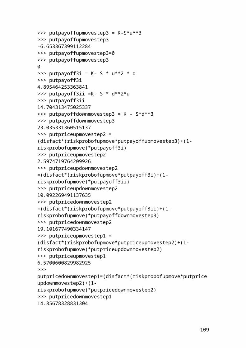
Application.Workbooks("VBA for options1").Worksheets("sheet1").Range("A5").Value = 2012Application.Workbooks("VBA for options1").Worksheets("sheet1").Range("A6").Value = 2013Application.Workbooks("VBA for options1").Worksheets("sheet1").Range("A7").Value = 2014
Application.Workbooks("VBA for options1").Worksheets("sheet1").Range("B2").Value = 0.035Application.Workbooks("VBA for options1").Worksheets("sheet1").Range("B3").Value = 0.047Application.Workbooks("VBA for options1").Worksheets("sheet1").Range("B4").Value = 0.079Application.Workbooks("VBA for options1").Worksheets("sheet1").Range("B5").Value = -0.042Application.Workbooks("VBA for options1").Worksheets("sheet1").Range("B6").Value = 0.054Application.Workbooks("VBA for options1").Worksheets("sheet1").Range("B7").Value = 0.103
Application.Workbooks("VBA for options1").Worksheets("sheet1").Range("C2").Value = 0.027Application.Workbooks("VBA for options1").Worksheets("sheet1").Range("C3").Value = 0.049Application.Workbooks("VBA for options1").Worksheets("sheet1").Range("C4").Value = 0.057Application.Workbooks("VBA for options1").Worksheets("sheet1").Range("C5").Value = 0.085Application.Workbooks("VBA for options1").Worksheets("sheet1").Range("C6").Value = 0.093Application.Workbooks("VBA for options1").Worksheets("sheet1").Range("C7").Value = 0.115
Application.Workbooks("VBA for options1").Worksheets("sheet1").Range("D2").Value = 0.037Application.Workbooks("VBA for options1").Worksheets("sheet1").Range("D3").Value = 0.079Application.Workbooks("VBA for options1").Worksheets("sheet1").Range("D4").Value = 0.089Application.Workbooks("VBA for options1").Worksheets("sheet1").Range("D5").Value = 0.102Application.Workbooks("VBA for options1").Worksheets("sheet1").Range("D6").Value = -0.068Application.Workbooks("VBA for options1").Worksheets("sheet1").Range("D7").Value = 0.059
'********************************************************************' Formula calculations'********************************************************************
109
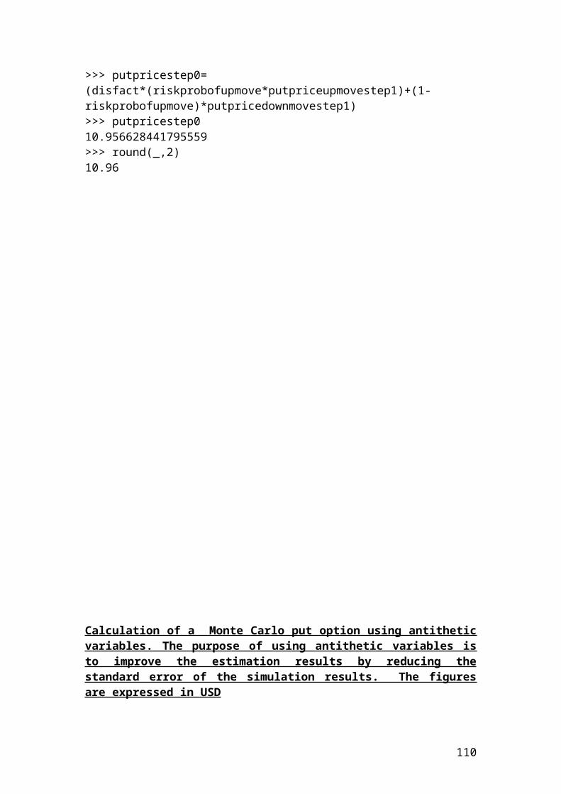
Application.Workbooks("VBA for options1").Worksheets("sheet1").Range("E2").Formula = "=SQRT(((3*((B2)^2+(C2)^2+(D2)^2))-((B2+C2+D2)^2))/(3*(3-1))) "Application.Workbooks("VBA for options1").Worksheets("sheet1").Range("E3").Formula = "= SQRT(((3*((B3)^2+(C3)^2+(D3)^2))-((B3+C3+D3)^2))/(3*(3-1)))"Application.Workbooks("VBA for options1").Worksheets("sheet1").Range("E4").Formula = "= SQRT(((3*((B4)^2+(C4)^2+(D4)^2))-((B4+C4+D4)^2))/(3*(3-1)))"Application.Workbooks("VBA for options1").Worksheets("sheet1").Range("E5").Formula = "= SQRT(((3*((B5)^2+(C5)^2+(D5)^2))-((B5+C5+D5)^2))/(3*(3-1)))"Application.Workbooks("VBA for options1").Worksheets("sheet1").Range("E6").Formula = "= SQRT(((3*((B6)^2+(C6)^2+(D6)^2))-((B6+C6+D6)^2))/(3*(3-1)))"Application.Workbooks("VBA for options1").Worksheets("sheet1").Range("E7").Formula = "= SQRT(((3*((B7)^2+(C7)^2+(D7)^2))-((B7+C7+D7)^2))/(3*(3-1)))"
Application.Workbooks("VBA for options1").Worksheets("sheet1").Range("F2").Formula = "= (B2+C2+D2)/3"Application.Workbooks("VBA for options1").Worksheets("sheet1").Range("F3").Formula = "= (B3+C3+D3)/3"Application.Workbooks("VBA for options1").Worksheets("sheet1").Range("F4").Formula = "= (B4+C4+D4)/3"Application.Workbooks("VBA for options1").Worksheets("sheet1").Range("F5").Formula = "= (B5+C5+D5)/3"Application.Workbooks("VBA for options1").Worksheets("sheet1").Range("F6").Formula = "= (B6+C6+D6)/3"Application.Workbooks("VBA for options1").Worksheets("sheet1").Range("F7").Formula = "= (B7+C7+D7)/3"
End Sub'********************************************************************Sub createchart1()
Dim Chart1 As ChartSet Chart1 = Charts.AddChart1.SetSourceData Source:=Worksheets("sheet2").Range("A2").CurrentRegion, PlotBy:=xlColumnsChart1.ChartType = xl3DBarStackedEnd Sub'********************************************************************Sub createchart2()
Dim Chart1 As ChartSet Chart1 = Charts.AddChart1.SetSourceData Source:=Worksheets("sheet2").Range("A2").CurrentRegion, PlotBy:=xlColumns
110
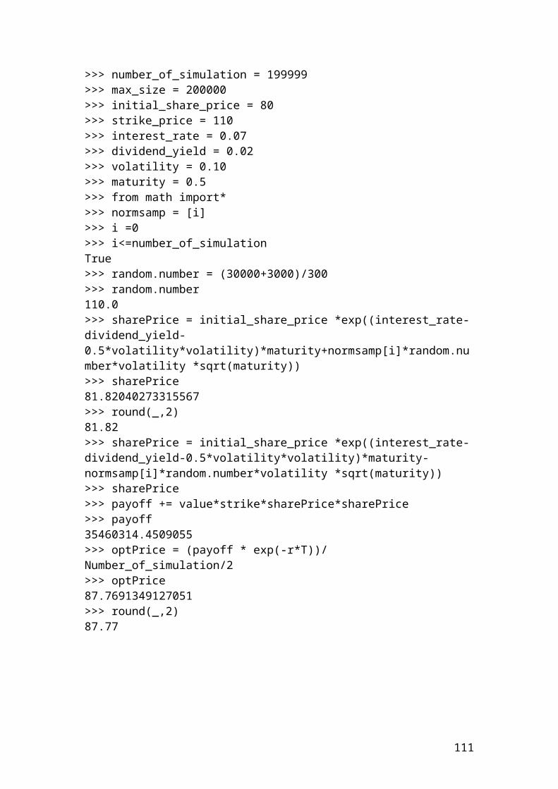
Chart1.ChartType = xlLine
End Sub
Sub createchart3()Dim Chart As ChartSet Chart = Charts.AddChart.SetSourceData Source:=Sheet2.Range("A2:B7").CurrentRegion, PlotBy:=xlColumnsChart.ChartType = xlLineActiveChart.HasTitle = TrueActiveChart.ChartTitle.Font.Bold = TrueActiveChart.ChartTitle.Font.Size = 12ActiveChart.ChartTitle.Text = "Risk and average returns of options"ActiveChart.Axes(xlCategory, xlPrimary).HasTitle = TrueActiveChart.Axes(xlCategory, xlPrimary).AxisTitle.Text = "Risk expressed as standard deviation"ActiveChart.Axes(xlValue, xlPrimary).HasTitle = TrueActiveChart.Axes(xlValue, xlPrimary).AxisTitle.Text = "Average return for call, put and index options"
End Sub*********************************************************************Sub MsgBox_Test()Averagereturn = 0.05msgReply = MsgBox("The company expects increase of the average returns above 0.05")End Sub
Link functions between Excel and Matlab
A) After finishing with writing the VBA code and the Excel file is ready, then, you can transfer the data to Matlab.
= MLPutMatrix("retseries", B2:D7) <== MLPutMatrix("retseries", B2:D7)
B) Use Matlab Financial toolbox functions.
= MLEvalString("[ret, cov]= ewstats(retseries)") <== MLEvalString("[ret, cov] = ewstats(retseries)")
<== MLEvalString("[risk] = portopt(ret, cov, 6)")
C) Transfer the resulting output to Excel.
=MLGetMatrix("risk", "F2")<== MLGetMatrix("risk", "F2")
D) Draw the efficient frontier.
111
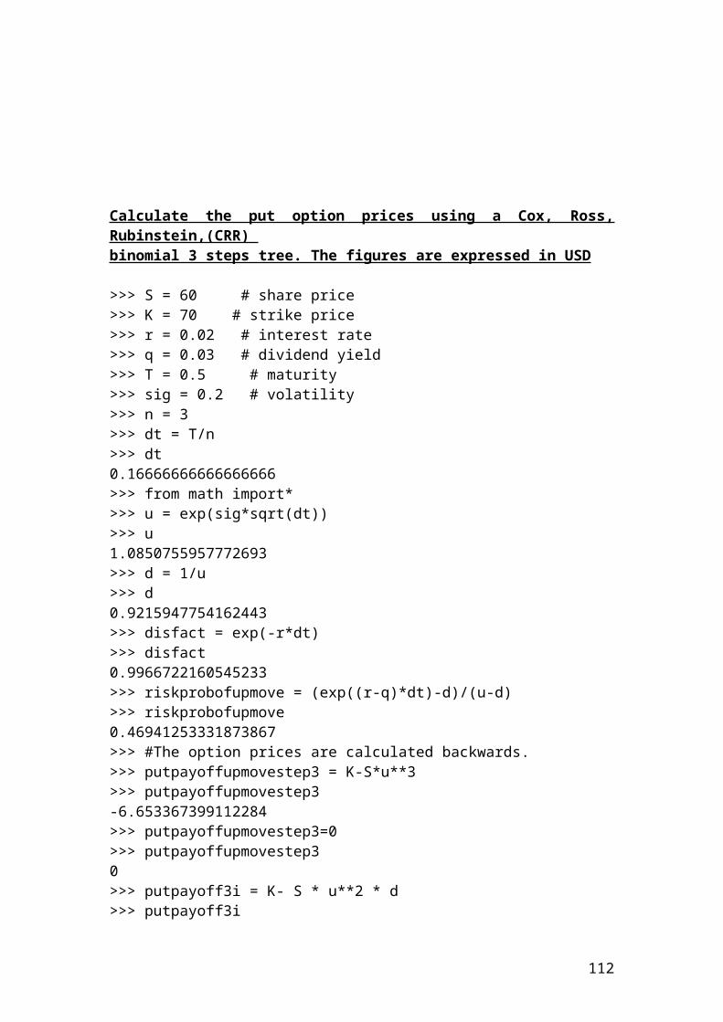
=MLEvalString("portopt (ret, cov, 6); grid on; xlabel('Risk'); ylabel('Return')") <== MLEvalString("portopt (ret, cov, 6); grid on; xlabel('Risk'); ylabel('Return')")
Financial Toolbox
In Matlab, Financial toolbox is very useful to perform mathematical and statistical analysis. It is used to display cash flows. It is used to compute, analyze, manage portfolios, measure risk and compute yields and sensitivities for the derivatives products.
The cash flows in the command window of Matlab could be displayed as follows:
>> Cash = [-2000 3000 5000 6000]
Cash =
-2000 3000 5000 6000
To transpose a matrix of cash flows, please use the following syntax:
>> Cash = [-2000 3000 5000 6000]'
Cash =
-2000 3000 5000 6000
Another example is if you have two portfolios of shares and you would like to calculate the NewPortfolios as an addition of portfolios A and B.
>> Portfolios_A = [400 300 200 400 200 250];
Portfolios_B = [375 425 400 300 100 400];
NewPortfolios = Portfolios_A + Portfolios_B
NewPortfolios =
775 725 600 700 300 650
112
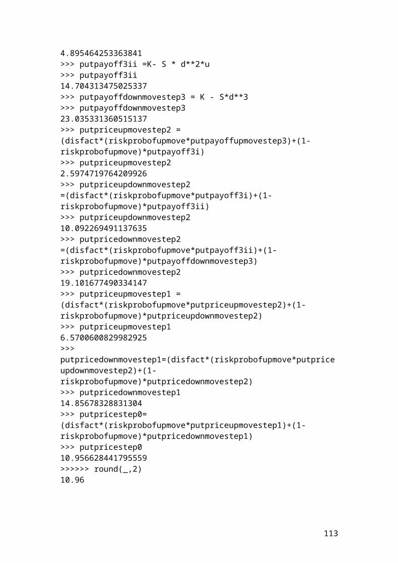
Another example that is used in portfolio management is to multiply closing prices with numbers of shares. The syntax of the closing prices for three shares and the number of shares of equity derivatives in the command window is as follows:
ClosePrices = [50 37 40]
NumShares = [200 300 400]
The portfolio total value is the multiplication of the vectors of ClosePrices and NumShares.
PortfValue = ClosePrices * NumShares
ClosePrices =
50 37 40
NumShares =
200 300 400
PortfValue =
37100
Solving simultaneous equations is another example. Let’s assume that we have two matrices.
A = [2 2 4 -3];
B = [12 -14];
X = A \ B
X =
0.5714 5.4286
Another example, it is how to calculate yields based on dividends and prices.
113
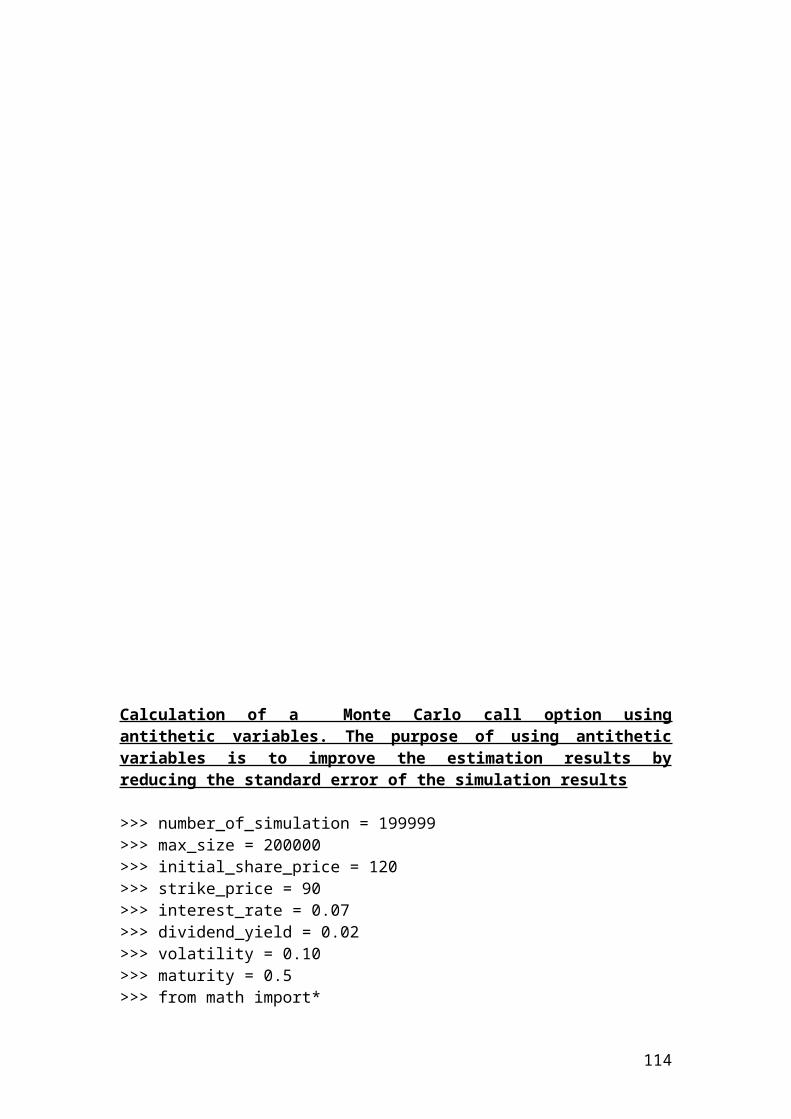
Dividends = [2.40 0.67 2.30 3.20];Prices = [30.14 12.89 16.78 54.20];Yields = Dividends ./ Prices
Yields =
0.0796 0.0520 0.1371 0.0590
Let’s assume that the initial capital that an investor has is 200 USD. The amount has been invested with a fixed rate and the investor received annual cash receipts of 30 USD, 50 USD, 60 USD, 75 USD, and 85 USD. Calculate the internal rate of return based on the cash flows. The transposed cash flows could be displayed in Matlab with the followed syntax:
>> CashFlows = [-200 30 50 60 75 85]'
CashFlows =
-200 30 50 60 75 85
>> Rate = irr(CashFlows)
Rate =
0.1290
>> Rate = 0.1290 * 100
Rate =
12.9 % . The internal rate of return based on the above cash flows is 12.9%
Financial Time Series toolbox is used to analyze time series data
Compute the Bollinger bands for Danisco share. It is a technical analysis indicator that is used to decide whether to buy or sell a call option. I have included the syntax that will be used in the command window and a figure that shows the three bands of the Bollinger indicator.
114
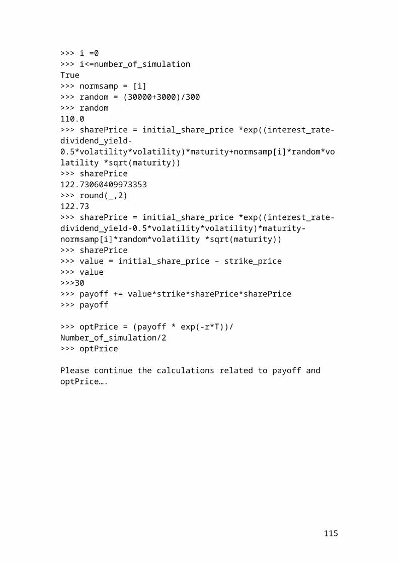
>> load danisco.mat[danisco_Mid,danisco_Uppr,danisco_Lowr]= bollinger(danisco);danisco_CloseBolling = [danisco_Mid, danisco_Uppr danisco_Lowr];plot (danisco_CloseBolling);title('Bollinger Bands for Danisco Closing Prices')
Source: author’s illustration.
GARCH toolbox used to test the Generalized Autoregressive Conditional Heteroskedasticity, (GARCH) volatility modelling
GARCH models are very important and show the volatility of asset returns by taking into consideration excess kurtosis or fat tails and volatility clustering. It provides timely forecasts of time varying conditional variances and covariances. They are important models for risk and portfolio managers who are involved in financial derivatives, portfolio management and asset allocation. They are also very important in designing successful strategies for short and long-term interest rate futures, currency options, and value-at-risk, (VaR) calculations. Thus, it is a useful tool that you can compare a Gaussian distribution with a distribution with excess kurtosis and spot the variations.
Suppose that we have the following autoregressive moving average, ARMA(2,2) model.
115
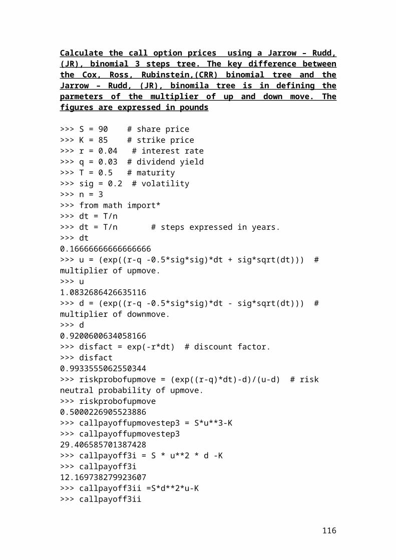
y t=0 . 4 y t−1−0 . 6 y t−2+εt−0. 3 ε t−1+0.5 εt−1
Use the function garchar to convert finite-order ARMA models to 5 infinite order auto-regressive (AR) models. The syntax in the command window of Matlab is as follows:
PI' or InfiniteAR = garchar(AR, MA, NumLags)
Where: garchar convert finite-order ARMA models to infinite order auto-regressive (AR) models.AR are autoregressive coefficients such as yt-1 and yt-2.
MA are moving average coefficients such as ε t−1 and ε t-2.NumLags is an integer scalar and determines the length of the infinite-order AR output vector. If it is not specified, the default is 10.
AR = [0.4 -0.6] MA = [-0.3 0.5]
PI = garchar([0.4 -0.6], [-0.3 0.5], 5);PI'
ans =
0.1000 -0.0700 -0.0710 0.0137 0.0396
Use the function garchma to convert finite-order ARMA models to 10 infinite order moving average (MA) models. The syntax in the command window of Matlab is as follows:
PI' or InfiniteMA = garchma(AR, MA, NumLags)
Where: garchma convert finite-order ARMA models to infinite order moving average (MA) models.AR are autoregressive coefficients such as yt-1 and yt-2.
MA are moving average coefficients such as ε t−1 and ε t-2.NumLags is an integer scalar and determines the length of the infinite-order AR output vector. If it is not specified, the default is 10.
116
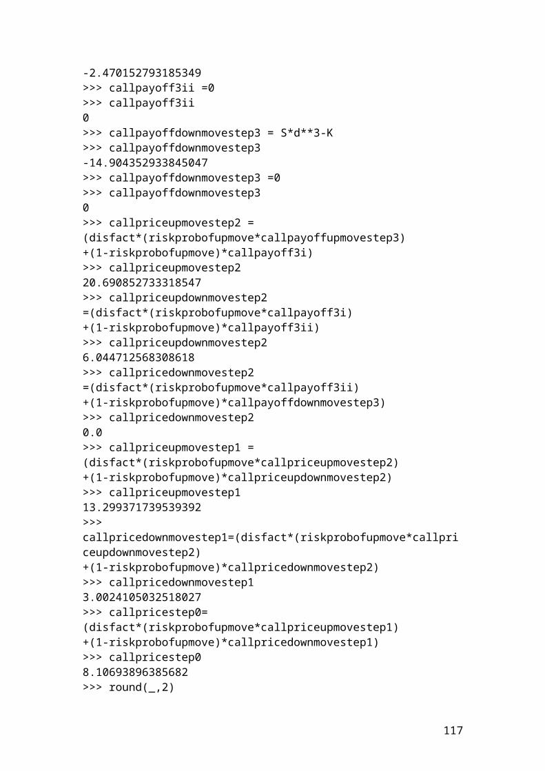
Suppose that we have the following autoregressive moving average, ARMA(2,2) model.
y t=0 . 4 y t−1−0 . 6 y t−2+εt−0. 3 ε t−1+0.5 εt−1
AR = [0.4 -0.6] MA = [-0.3 0.5]
PI = garchma([0.4 -0.6], [-0.3 0.5], 10);PI'
ans =
0.1000 -0.0600 -0.0840 0.0024 0.0514 0.0191 -0.0232 -0.0207 0.0056 0.0147
Matlab compiler is used to convert Matlab mat-files to C++ computer language programming
Programming in C++ differs from programming in MATLAB in terms of syntax. Expression such as and ' is not valid syntax for C++. The mathematical symbols.*, .\, ./, .^ and \ are not valid C++ operators. The {} cell array indexing operator is unavailable. In Matlab, the syntax for the logical function is logical (). It could be a logical scalar or a variety of arrays of logical values. In C++, logical values are defined only as scalars.
Statistics toolbox is used to analyze statistical historical data and model systems
Statistical process control, (SPC) is very important tools that are used in Six Sigma analysis in order to improve the efficiency of the derivative product that is offered to the customer. I have included the syntax that is used in the command window and the xbar chart with 95% confidence level.
load partsconf = 0.95;spec = [-0.5 0.5];xbarplot(runout,conf,spec)
117
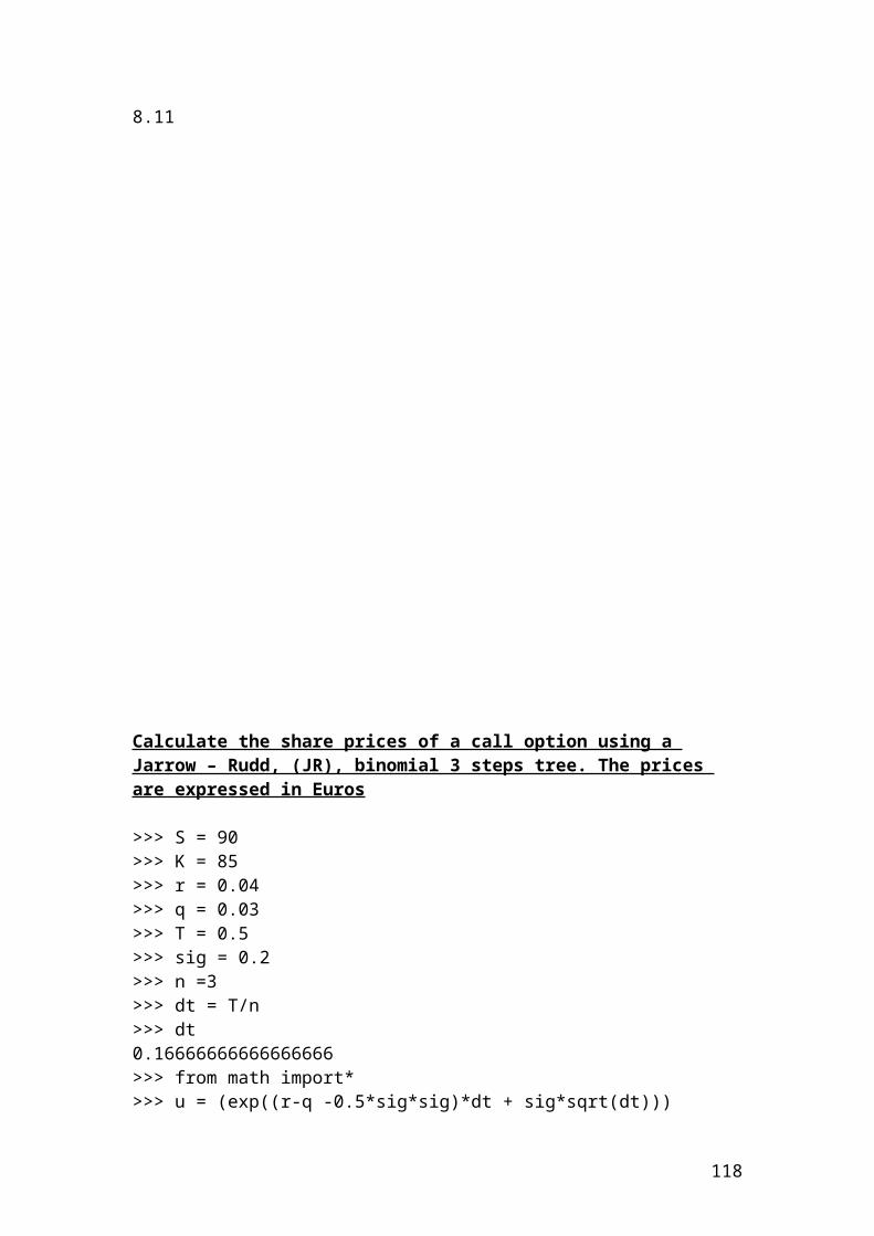
Source: author’s illustration.
I have included the syntax that is used in the command window for the exponentially weighted moving average, (EWMA), chart with 95% confidence level.
ewmaplot(runout,0.5,0.01,spec)
118
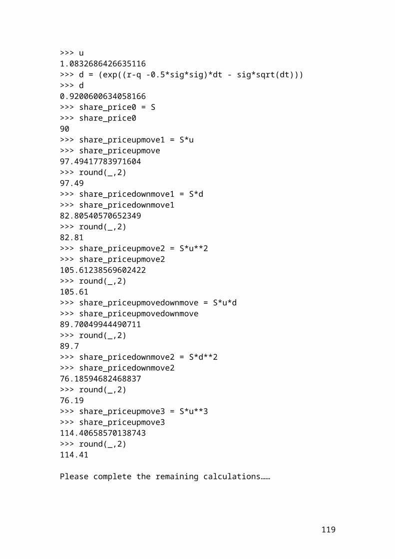
Source: author’s illustration.
I have included the syntax that is used in the command window for the distribution plots, quantile - quantile plot.
x = poissrnd(15,40,1);y = poissrnd(5,100,1);qqplot(x,y);
119

Source: author’s illustration.
I have included the syntax that is used in the command window for the normal distribution plots.
x = normrnd(15,1,35,1);normplot(x)
120
Source: author’s illustration.
I have included the syntax that is used in the command window for the box plot and analysis of variance, (ANOVA).
load data>> data
data =
203.6000 257.1000 181.0000 230.7000 279.5000 192.2000 235.9000 280.1000 197.5000 232.5000 262.8000 191.8000 235.6000 270.2000 193.8000 241.3000 273.1000 196.4000 [p,tbl,stats] = anova1(data);pp =
121
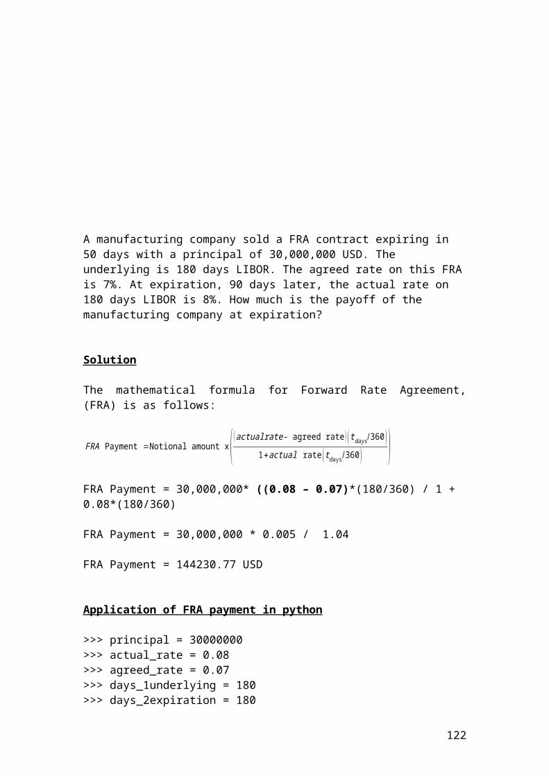
Source: author’s illustration.
Source: author’s illustration.
I have included the syntax that is used in the command window to calculate the mean.
>> A = [1 2 4 4 3 4 6 8];mean(A)ans =
122
4
I have included the syntax that is used in the command window to calculate the geometric mean.
>> m = geomean(A)
m =
3.4135
I have included the syntax that is used in the command window to calculate the range. It calculates the difference between the maximum and the minimum value of a data sample such as A = [1 2 4 4 3 4 6 8];
>> y = range(A)
y =
7
I have included the syntax that is used in the command window to calculate the interquartile range. It calculates the difference between the 75th and the 25th
percentiles of a data sample such as A = [1 2 4 4 3 4 6 8];
>>
y = iqr(A)
y =
2.5000
I have included the syntax that is used in the command window to calculate the variance as a measure of dispersion by using a data sample such as A = [1 2 4 4 3 4 6 8];
>> var(A)
ans =
4.8571
Financial derivatives toolbox is used to analyze options, futures and swaps
123
Let’s consider a portfolio of options and future. Let’s consider a future contract that is traded in Frankfurt with a delivery date of 20-08-2014. The quoted price is $200.45. The layout of displaying the data in Matlab is as follows:
Type Strike Price Call Put Option 97 88 13.7 4.9 Option 102 97 8.2 7.9 Option 108 98 7.8 9.4 Type Delivery F Future 20-Aug-2014 200.45
Strike = (97;102;108); Price = (88;97;98);Call = [13.7; 8.2; 7.8];Put = [4.9; 7.9; 9.4]; Future = {20-Aug-2014; 200.45};
InstSet = instaddfield{Option;97;88;13.7;4.9};InstSet = instaddfield{Option;102;97;8.2;7.9};InstSet = instaddfield{Option;108;98;7.8;9.4};InstSet = instaddfield{future;20-Aug-2014;200.45};
Where:InstSet is a variable that contains a collection of data. The above data are expressed as a row vector.
Instaddfield is used to create or customize a portfolio of investment products according to the needs of the clients. For example, a portfolio of options and future.
The syntax for a swap contract is as follows:
InstSet = instswap(InstSet, LegRate, Settle, Maturity, LegReset, Basis, Principal, LegType)
Where:
InstSet is a function used when adding a swap to an existing portfolio set with other investment products.
LegRate is defined as [couponrate ;spread], where couponrate is the decimal annual rate and spread is the number of basis points.
Settle is the settlement date.
Maturity represents the maturity date for the swap contract.
124
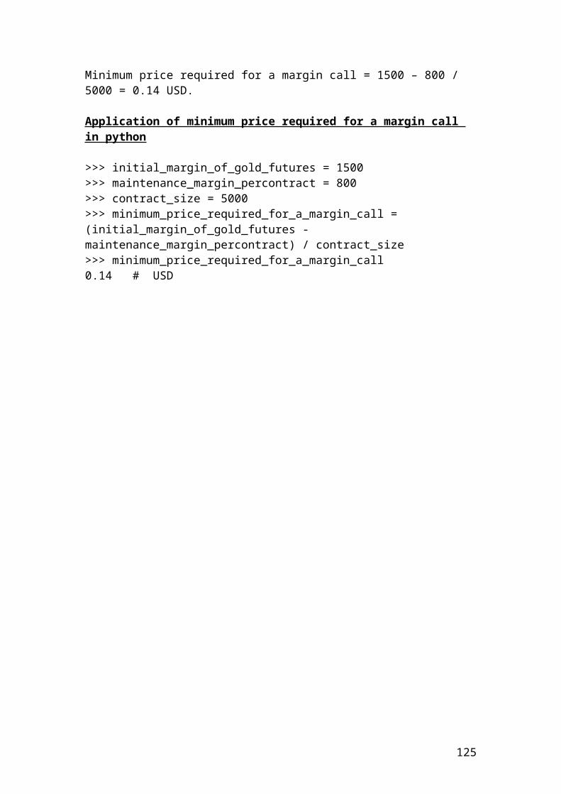
LegReset is optional and represents the frequency per year for each swap. The default function is default =[1 1].
Basis is optional and the Default = 0 (actual/actual).
Principal is optional and the Default = 100.
LegType is optional. It represents a matrix and each column indicates if thecorresponding leg is fixed (1) or floating (0). Default is [1,0] for each swap contract.
The syntax for a bond option is as follows:
InstSet = instoptbnd(InstSet, BondIndex, OptSpec, Strike, ExerciseDates, AmericanOpt or EuropenOpt )
Where:
InstSet is a function used when adding a bond option to an existing portfolio set with other investment products.
BondIndex is used to specify bond data.
OptSpec is used to specify if the option is a call or a put. The definition of the strike and exercise date depend if the option is American or European. If AmericanOpt = 1.
Strike shows the exercise price for each bond option.
ExerciseDates. There is only one exercise date, the option expiry date for an European option.
Sensitivity Measures or Greeks used in option pricing
The most common Greeks that are used in option pricing are:
Delta is the rate of change of its price relative to the price of the underlying asset. When delta is large, the derivative is sensitive to small changes in the price.
Gamma is the rate of change of delta relative to the price of the underlying asset. When gamma is small, the change in delta is small.
Lambda represents the percentage change in the price of an option. Rho is the rate of change in option price relative to the risk free rate. Theta is the rate of change in the price of the derivative instrument relative to
time. The value is small or negative as it reaches maturity. Vega is the rate of change in the price of the derivative instrument relative to
the volatility of the underlying security. Implied volatility helps the trader to determine the volatility of the stock and
according to the variance to hedge by using different strategies.
125
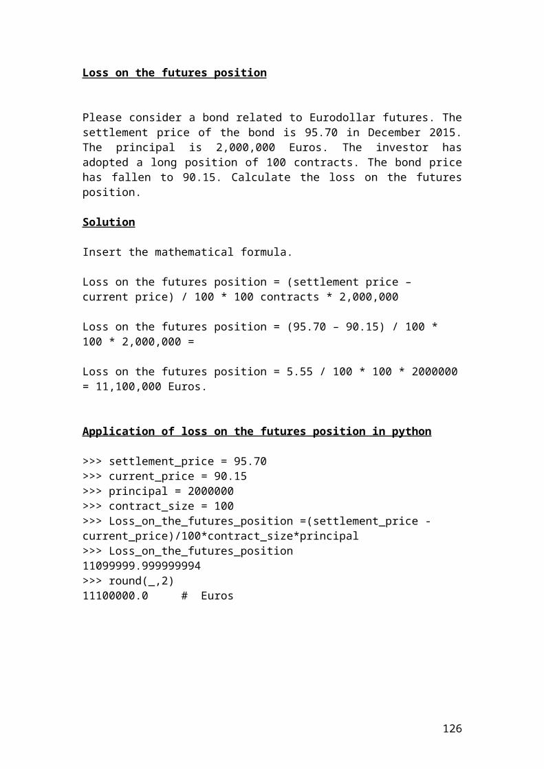
Let’s illustrate an example of a call European option and its delta, gamma, lambda, and implied volatility calculations. The asset price is 200 USD. The exercise price is150 USD. The risk-free rate is 8% and the time to maturity is 0.2 years, the volatility is 0.40, and the dividend rate is 0. By using the syntax in the command window of Matlab, we have the followed functions:
[CallPrice, PutPrice] = blsprice(200, 150, 0.08, 0.2, 0.40, 0)CallPrice; PutPrice =
CallPrice =
52.9446
PutPrice =
0.5637
[CallDelta, PutDelta] = blsdelta(200, 150, 0.08, 0.2, 0.40, 0)CallDelta; PutDelta =
CallDelta =
0.9630
PutDelta =
-0.0370
Gamma = blsgamma(200, 150, 0.08, 0.2, 0.40, 0)Gamma =
Gamma =
0.0023
[CallEl, PutEl] = blslambda(200, 150, 0.08, 0.2, 0.40, 0)CallEl; Put El =
CallEl =
3.6379
PutEl =
-13.1151
126
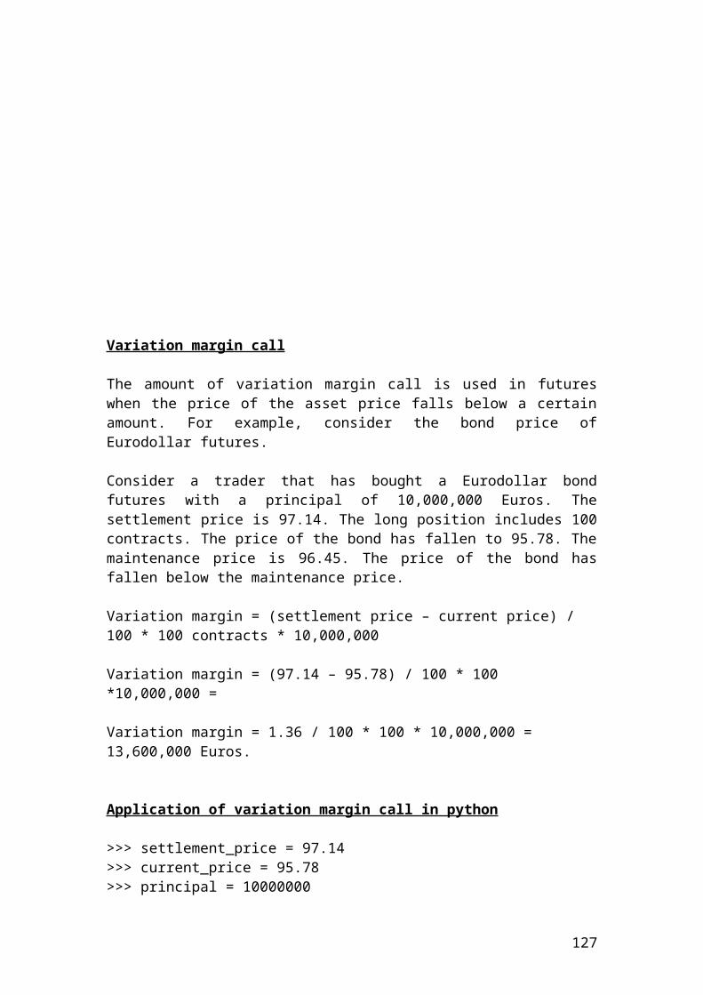
[CallRho, PutRho] = blsrho(200, 150, 0.08, 0.2, 0.40, 0)CallRho; PutRho =
CallRho =
27.9326
PutRho =
-1.5912
[CallTheta, PutTheta] = blstheta(200, 150, 0.08, 0.2, 0.40, 0)CallTheta; PutTheta =
CallTheta =
-18.4001
PutTheta =
-6.5906
Vega = blsvega(200, 150, 0.08, 0.2, 0.40, 0)Vega =
Vega =
7.2271
Quotes from the Gospel that are integrated in a Fuzzy logic function through a spiritual advisor
I have included two statements as follows:
“Wealth is not eternal and stable, but as a dream will disappear one day”.
“The spirit of the individual is strengthened from the Holy Spirit and not from the mammon or the money”.
Fuzzy logic is used to show the link between an input and an output space to find the best decision. The difference with the Christian Orthodox approach is that the best decision is offered from the strong faith that the individual has towards the Holy Trinity and the interaction with the Orthodox principles. Thus, the best decision is associated with the Holy gifts that he/she received from the Holy Trinity with always the help of the Virgin Mary.
127
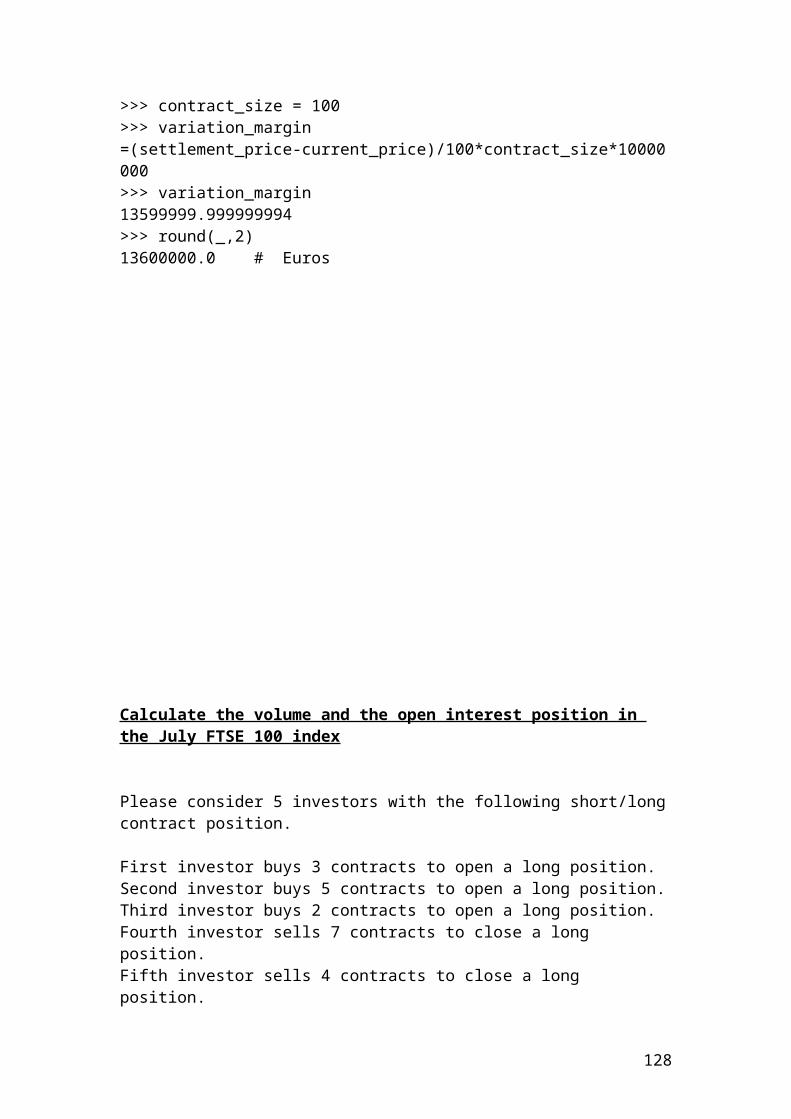
As an example of application of Fuzzy logic, we could mention the degree of wealth that an individual could dispose. The trend line starts from the extremely poor to reach the super rich. The amount that represents the different classes are expressed in Euros per month. The variables that sustain the Greek Christian Orthodox theology are expressed in a Likert scale from very weak to very strong. It is worth to mention that in practice these variables are sustained and increased according to the following parameters:
The faith. The good actions. The purity of the heart and the thoughts that the individual has towards
himself/herself and towards the fellow-persons.For example, Saint Nektarios metropolitan of pentapolis in Aegina has received all the spiritual gifts from heaven by keeping purity and maximum spiritual integrity in all his life. Aegina is an island situated in the Saronic Gulf of Greece. It is worth to visit the monastery and get blessing.
/ / / / / / Extremely poor Very Very poor Very poor Lower class Middle class Upper class
% Establish constantsextremely poor =200 ; very very poor=250 ; very poor=300; lower class=400; middle class=700; upper class=1000;Wealthrange =upper class - extremelypoor
Faith towards the Holy Trinityvery weak =0; weak=1; medium=2.5; strong=4; verystrong=5;faith towards the holy trinity=verystrong - veryweak
Repentancevery weak =0; weak=1; medium=2.5; strong=4; verystrong=5;repentance= verystrong - veryweak
Confessionvery weak =0; weak=1; medium=2.5; strong=4; verystrong=5;confession= verystrong - veryweak
HolyCommunionvery weak =0; weak=1; medium=2.5; strong=4; verystrong=5;holy communion= verystrong - veryweak
Prayervery weak =0; weak=1; medium=2.5; strong=4; verystrong=5;prayer= verystrong - veryweak
Fastveryweak =0; weak=1; medium=2.5; strong=4; verystrong=5;
128
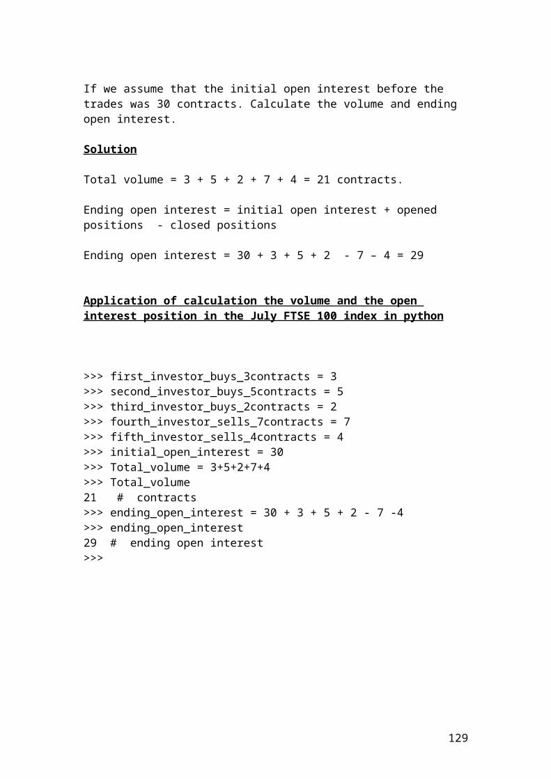
fast= verystrong - veryweak
Prostrationsveryweak =0; weak=1; medium=2.5; strong=4; verystrong=5;prostrations= verystrong - veryweak
Vigilveryweak =0; weak=1; medium=2.5; strong=4; verystrong=5;vigil= verystrong - veryweak
Almsgivingveryweak =0; weak=1; medium=2.5; strong=4; verystrong=5;almsgiving= verystrong - veryweak
Rejection of personal willveryweak =0; weak=1; medium=2.5; strong=4; verystrong=5;rejection of personal will= verystrong - veryweak
Appreciate Byzantine musicveryweak =0; weak=1; medium=2.5; strong=4; verystrong=5;appreciate byzantine music= verystrong – veryweak
Humilityveryweak =0; weak=1; medium=2.5; strong=4; verystrong=5;humility= verystrong – veryweak
Strong believe that Jesus Christ was resurrectedveryweak =0; weak=1; medium=2.5; strong=4; verystrong=5;strong believe that Jesus Christ was resurrected= verystrong - veryweak
% Wealth is not eternal and stable but as a dream will disappear one day.% The spiritual advisor suggest to focus on the spirit until the government finds a solution with the financial part.% He suggests that the spirit of the individual is strengthened from the Holy Spirit and not from the mammon or the money.Safeguard the spiritual integrity = faith towards the Holy Trinity* repentance* confession* Holy Communion* prayer* fast* prostrations* vigil* almsgiving* rejection of personal will* appreciate Byzantine music*humility* strong believe that Jesus Christ was resurrected
The result of the above or the gifts of the Holy Spirit after lifting a personal cross for all your life and the cross of the other person, if possible, is as follows:
1) Love plenty of honesty and free from hypocrisy. 2) Happiness.3) To be patient and control your temper in a way that reflects the Christian Orthodox principles. To love yourself, the other person and put yourself in his/her position.4) Control the desire of the body and strengthen the spiritual integrity.2) Sustainable faith towards the Holy Trinity and the help of Virgin Mary.
129
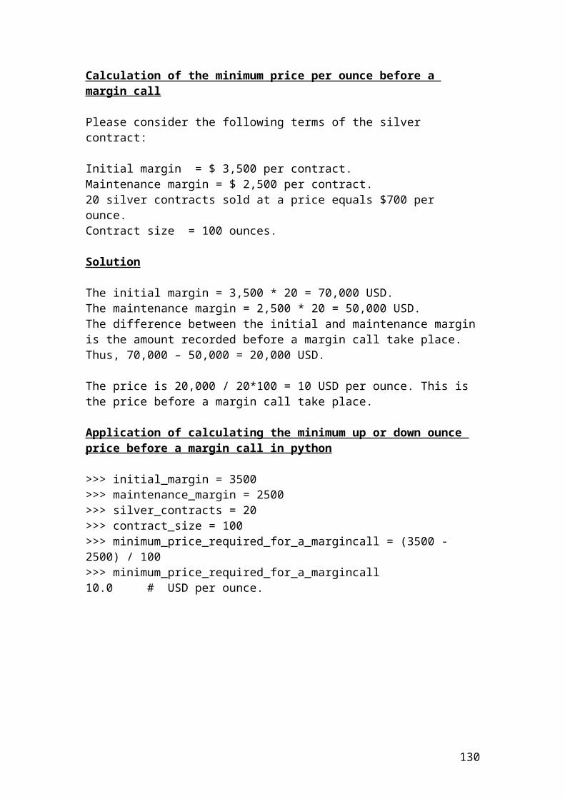
3) Solidarity to take care about the other person as yourself.4) Inner peace with yourself, the neighbor and the enemy.5) Virtuosity.6) Salvation of the soul.7) Gentleness
The above model should be combined with the letter to Galatas, Chapter E, pages 760-763 and verses 22-26.
end
Introduction to spectral analysis by using the covariance method, wavelet and Fourier analysis
The signal processing toolbox is used for spectral analysis to estimate random signals that can be used in investment for buying or selling derivatives instrument. To open the signal processing toolbox, type the syntax SPtool in the command window.
To open the Spectrum Viewer and create a power spectral density, (PSD) estimate from the SPTool is done as follows:
Select a signal from the Signal list box in SPTool. Press the Create button in the Spectra list. Press the Apply button in the Spectrum Viewer.
To select signals that display the volatility of the option or the future press shift and click on the noise and blnoise signals in the signals list of SPtool to select both signals. Then, press the View button under the signals list.
The purpose of spectral analysis is to describe and analyze the trend of the distribution of the equity option based on different signals that are extracted from a set of data. The power spectral density function is based on the covariance method. It represents a signal by using an autoregressive model. It is used to show the trend line in relation to an autoregressive filter function that isolates the buying from the selling signals. The power spectral density is calculated in units of power per radians per sample. For example, a first order autoregressive model defined as, (1,c) for returns of an equity option is as follows:
c = [1 -3.5678 4.5278 -1.4267 5.1267]; % AR filter coefficientsfreqz(1,c) % AR filter frequency responsetitle('AR System Frequency Response')
130
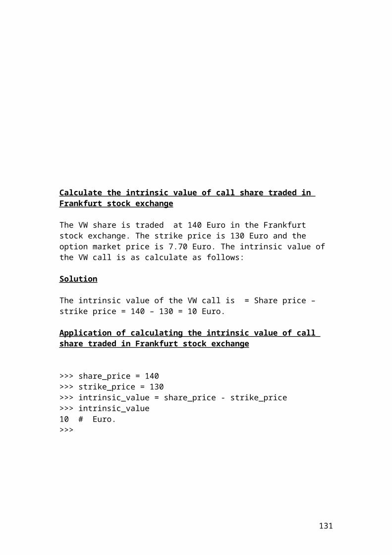
Source: author’s calculation.Let’s display the input signal x by filtering white noise by using the autoregressive filter. Estimate the power spectral density, (PSD) of x based on a third-order autoregressive prediction model of order three to show that the time span or life of the option decay or fall as we approach to maturity.
x = filter(1,a,randn(200,1)); % Signal generated from AR filter pcov(x,3) % Third-order estimate>>
131
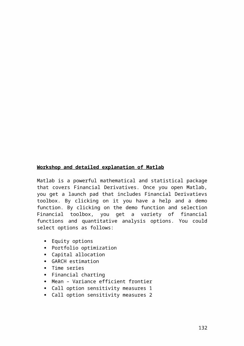
Source: author’s calculation.
Wavelet analysis is another tool that is used to analyze signals based on financial data.Wavelet analysis is characterized by two aspects, which are scale and time. Consequently every application has scale and time aspects. Financial data characterized by a time aspect are included in a list of domains to identify random signals when buying or selling an equity option, a swap contract or a future contract. This type of analysis helps the practitioner to use long time intervals in combination with precise low frequency data. On the other hand, it allows the practitioner to use shorter regions in combination with high frequency information.
For example, we want to plot complex Gaussian wavelets of order 3 for an equity option traded in the Eurex derivative market. The syntax is as follows:
[PSI,X] = cgauwavf(LB,UB,N,P)
% Set effective support and grid parameters.lb = -3; ub = 3; n = 2500;% Compute complex Gaussian wavelet of order 3.[psi,x] = cgauwavf(lb,ub,n,4);% Plot complex Gaussian wavelet of order 3.subplot(211)plot(x,real(psi)),title('Complex Gaussian wavelet of order 3')xlabel('Real part'), grid
132
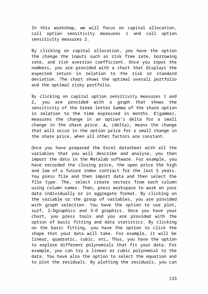
subplot(212)plot(x,imag(psi)) xlabel('Imaginary part'), grid
Source: author’s calculation.
Another toot of signal analysis is Fourier analysis. It decomposes a signal into parts of sinusoids of different frequencies. It is used to transform the signal from time to frequency mode. The problem with this transformation is that time information is omitted. Thus, you can not spot exactly the time that a particular macroeconomic event took place and show a buying or selling signal in the derivatives market. Different time series are non-stationary, random and erratic. Thus, by excluding the time factor through transformation, the prediction with Fourier analysis becomes less accurate and predictable.
Let’s assume an equity option that expires in 3 months. We want to plot the signal random noise in relation to the time by using Fourier analysis.
Please transform the signal from time to frequency mode by using the help menu of Matlab and comment about the accuracy of your results.
t = 1:2:3;x = sin(2*pi*30*t)+sin(2*pi*70*t);y = x + 2*randn(size(t));plot(y(1:30))title('Signal Random Noise')xlabel('period (months)')
133
Source: author’s calculation.
134
Simulink
Simulink is software that is used extensively in academia and in the industry to construct and build financial models. For example, it is used from the Federal Reserve Bank to model the effect of the fiscal and monetary policy. I have included a detailed example of Figure 1 with flow charts how Simulink could integrate the circular flow and effort of each individual with the fiscal and monetary policy of the Federal Reserve Bank and the derivatives market.
Monetary and fiscal policy of the circular flow of income J = I + G + X Firms
Households
W = S + T + M
Where:J is injections.W is withdrawals.S is net saving.T is taxes.M is import expenditure.I is investment.G is government expenditure.X is export expenditure.
The velocity of circulation determines the relationship between money and income. This velocity is integrated with the circular flow of spiritual effort in relation to the monetary and fiscal policy and the Financial Derivatives market. We have two types of monetary and fiscal policy. Tight and loose monetary policy, expansionary and contractionary fiscal policy. The optimum situation or equilibrium is to realign the different models with an ultimate objective to serve the household towards his/her spiritual integrity and salvation of the soul. Sinful actions are the result of hidden demons that restrict or delay the repentance and confession.
135
Tight monetary policy Loose monetary policy
Expansionary fiscal policy Contractionary fiscal policy
The Federal Reserve Bank buys treasury securities. This will affect short-term interest rates to go down. The central bank has more money to lend to the commercial banks, businesses and households. As an effect, there is an increase in employment and economic growth.
The Federal Reserve Bank sells treasury securities. This will affect short-term interest rates to go up. The central bank has less money to lend to the commercial banks, businesses and households. As an effect, there is a decrease in employment and economic growth.
Raising government expenditures.
Reducing taxes.
Increase aggregate demand.
Rise in national income.
Cutting government expenditures.
Raising taxes.
Decrease aggregate demand.
Decrease in national income.
136
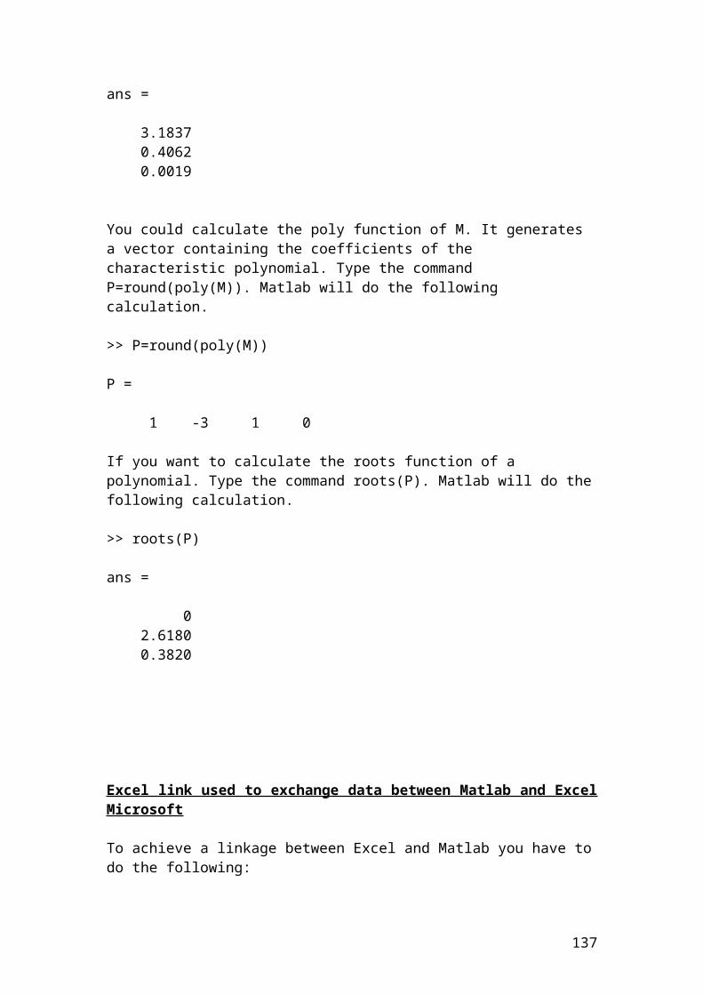
Financial Derivatives market
Buy very very low Never buy or sell in middle prices Sell very very high
The aim is to avoid psychological disorders, sustainable sinful condition and different illnesses.Source: Author’s illustration
To start the simulation, pull down the simulation menu and choose the start command. As the simulation runs, it will show that the accumulation of core values and additive variables reduce mortal, pardonable and sins of omission. In addition, it will show the interaction of the circular flow of income with the monetary, fiscal policy and the derivatives market.
137
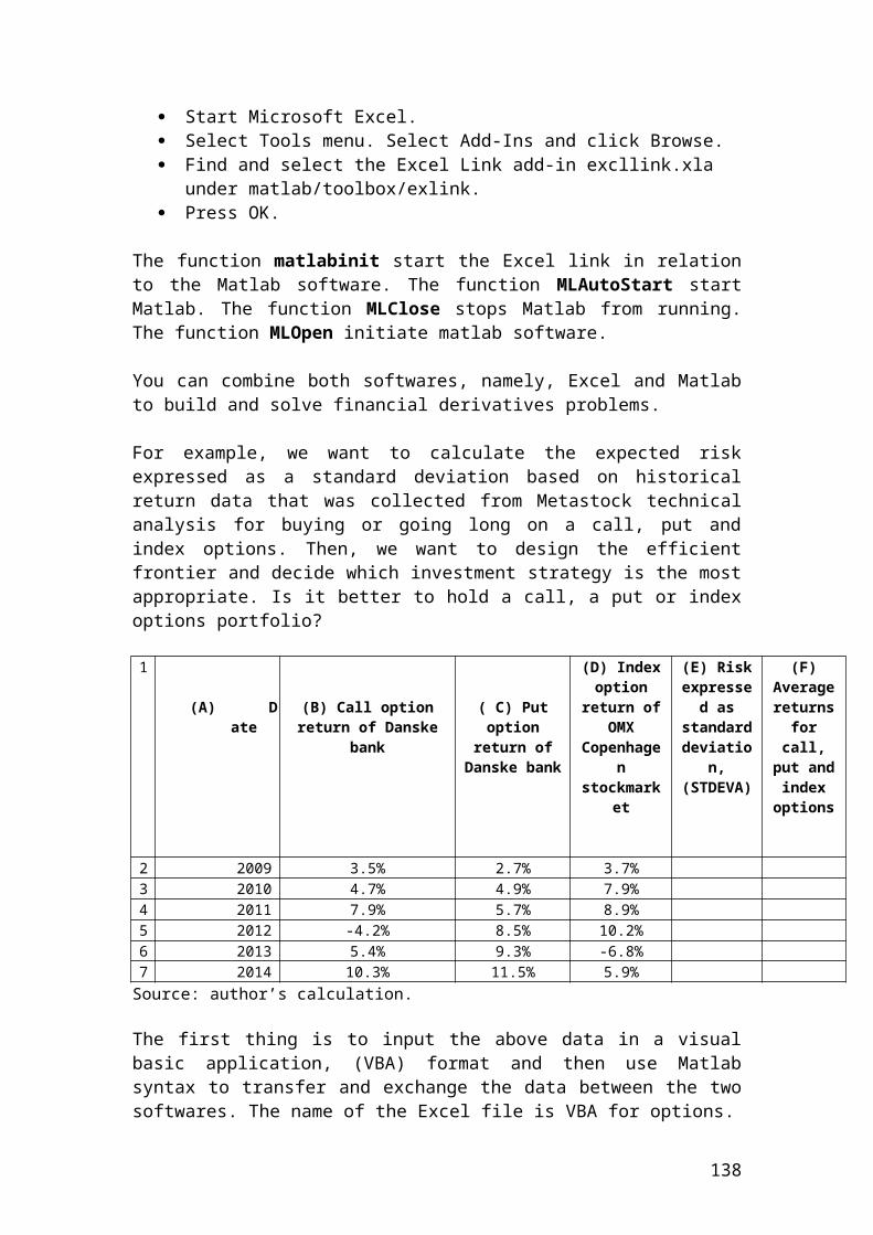
Workshop of analysis of financial data, scientific programming and simulation using R language programming
R is very useful language programming in modeling financial and statistical models. First of all, you should download the software for windows version R 3.2.2. A possible public domain is as follows:
Cran.r-project.org/bin/windows/base
Or
http://cran.ms.unimelb.edu.au
Please download R 3.3.3 for windows. Please read the instructions before to download the software. Once downloaded, then, open the R console and start to insert your variables, data and mathematical formulas.
Variable names are written with underscore followed by the equal sign. For example,
> interest_rate = 0.03Variable names could also be written with small letters adjacent to each other. For example, interestrate = 0.03
It is better to use underscore to separate them and be able to read them clearly.
> interest_rate =0.3> volatility = 0.5> interest_rate + volatility[1] 0.8>
In terms of arithmetic, R uses the symbols + for addition, - for subtraction, * for multiplication, / for division and ^ or ** for exponential functions. For example, powers are performed by using twice the symbol** or the exponential function ^.
For example, >3**5 243
Or >3 ^ 5243
If you would like to add comments, then, use the symbol # in front of the variable name.The operator # is used to write comments. For example,
>sigma = 0.5 # volatility.
138
I have included another example that shows the multiplication of two interest rates. > interest_rate1 = 0.02> interest_rate2 = 0.03> interest_rate1*interest_rate2[1] 6e-04
Division is performed using the sign / to get a float result. Use the as.integer function to get an integer result without fractional part. For example,> 7.0 / 3.0 2.33333> as.integer(7/3)[1] 2Or> as.integer(2.33333)[1] 2
Ceiling or floor is used for round up purposes. They are used to round up or down respectively. Let’s try the above example.> floor(7/3)[1] 2> ceiling(7/3)[1] 3
Rounding of two or three decimals figures is used as follows:
> 7.5/2.45[1] 3.061224> round(3.061224,digits=2)[1] 3.06> round(3.061224,digits=3)[1] 3.061
For inputting your variables, you can use the sign = or <-. For example, please consider the following input.
share_price_1 <- 0.24share_price_2<- 0.56
Or
share_price_1 = 0.24share_price_2 = 0.56In the calculation part, insert the formula by using the sign <- or =For example, please consider the above example.
share_price_1 <- 0.24share_price_2 <- 0.56
total_share_price <- share_price_1 + share_price_2
139
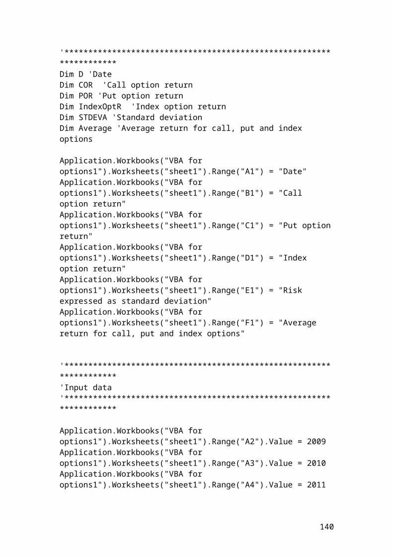
Calculation of the average of stock price returns expressed in percentages
> stock_price1 <- 10.0> stock_price2 <-12.0> stock_price3 <- 13.0> stock_price4 <- 14.0> stock_price5 <- 15.0> stock_price6 <- 16.0average<-(stock_price1+stock_price2+stock_price3+stock_price4+stock_price5+stock_price6)/6> average[1] 13.33333
Another way to find the average is as follows:
> x<-c(10,12,13,14,15,16)> sum(x)[1] 80> n = 6> average = sum(x)/n> average[1] 13.33333
140
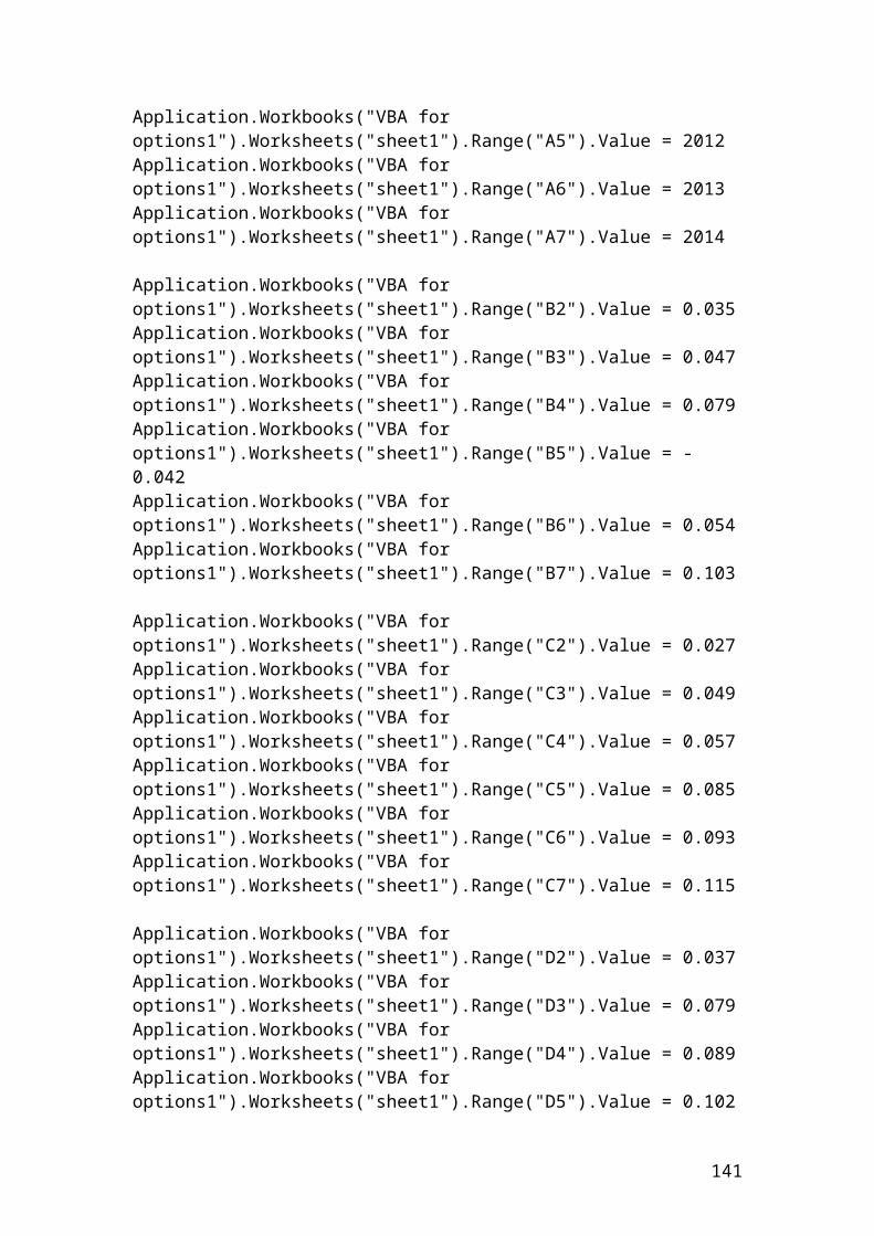
Repetition of the previous example to calculate the mean by getting an integer number without decimals. Returns are expressed as percentages
> stock_prices<-c(10,12,13,14,15,16)> n=6> sum(stock_prices)[1] 80> average = sum(stock_prices)/n> average[1] 13.33333> as.integer(average)[1] 13
Calculation of the mean, the variance and the standard deviation using the formulas that we have covered in the handout of measures of dispersion
> stock_prices<-c(10,12,13,14,15,16)> stock_prices[1] 10 12 13 14 15 16> n=6> sum(stock_prices)[1] 80> stock_prices.mean<-sum(x)/n # mean.> stock_prices.mean[1] 13.33333> sd<-sqrt(sum((stock_prices-mean(stock_prices))^2)/(n-1)) # standard deviation.> sd[1] 2.160247> stock_prices.var<-sum((stock_prices-stock_prices.mean)^2)/(n-1) # variance.> stock_prices.var[1] 4.666667
141
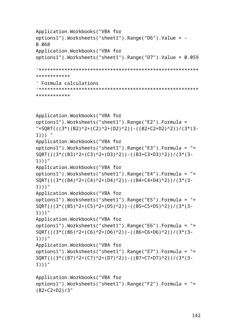
Calculations of European call and put prices and their related Greeks by applying Black and Scholes model, (BSM)
> S<- 70 # share price> K<- 70 # strike price> r <- 0.08 # interest rate> q <- 0.03 # dividend yield> sig <- 0.20 # volatility> T <- 0.5 # life to maturity> d1 <- (log(S/K)+((r-q)+sig*sig/2)*T)/(sig*sqrt(T))> d1[1] 0.2474874> d2 <-d1-sig*sqrt(T)> d2[1] 0.106066> call <-S*exp(-q*T)*pnorm(d1)-K*exp(-r*T)*pnorm(d2)> call[1] 4.750318> put <-K*exp(-r*T)*pnorm(-d2) - S*exp(-q*T)*pnorm(-d1)> put[1] 3.047743> round(3.047743,digits=2)[1] 3.05> calldelta <- exp(-q*T)*pnorm(d1)> calldelta[1] 0.5888354> round(0.5888354,digits=2)[1] 0.59> calltheta <- -(S*dnorm(d1)*sig*exp(-q*T))/(2*sqrt(T)) +(q*S*pnorm(d1)*exp(-q*T)) - (r*K*exp(-r*T)*pnorm(d2))> calltheta[1] -5.454086> callrho<- K*T*exp(-r*T)*pnorm(d2)> callrho[1] 18.23408> callandputgamma <- (dnorm(d1)*exp(-q*T))/(S*sig*sqrt(T))> callandputgamma[1] 0.03850192> callandputvega <- S*sqrt(T)*dnorm(d1)*exp(-q*T)> callandputvega[1] 18.86594> putdelta <- exp(-q*T)*(pnorm(d1)-1)> putdelta[1] -0.3962766> putrho<- -K*T*exp(-r*T)*pnorm(-d2)> putrho[1] -15.39355
142
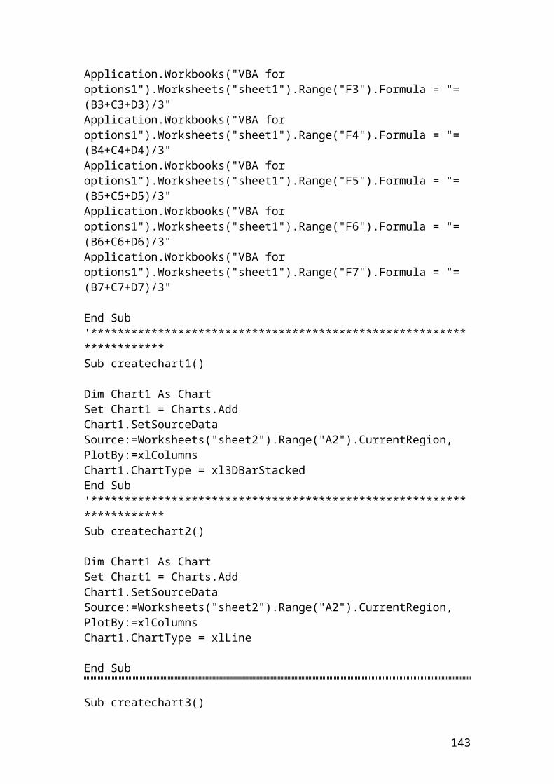
>puttheta <- -(S*pnorm(d1)*sig*exp(-q*T))/(2*sqrt(T)) – (q*S*dnorm(-d1)*exp(-q*T)) + (r*K*exp(-r*T)*dnorm(-d2))>puttheta[1] -2.1424002984583579
143
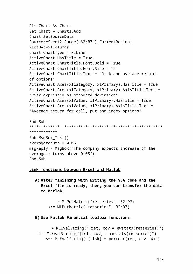
Calculations of the mean and the harmonic mean of share price returns, call option returns, put option returns and index option returns
> shareprice_return1<-0.08> shareprice_return2 <- 0.05> shareprice_return3 <- 0.04> shareprice_return4 <- 0.07> shareprice_return5 <- 0.02> shareprice_return6 <- 0.03>averageshareprice_returns<-(shareprice_return1+shareprice_return2+shareprice_return3+shareprice_return4+shareprice_return5 + shareprice_return6)/6> averageshareprice_returns[1] 0.04833333
You can use the mean function of share price returns from the statistical library bu using the appropriate heading
> stock_prices<-c(0.08,0.05,0.04,0.07,0.02,0.03)> sum(stock_prices)[1] 0.29> n=6> average = sum(stock_prices)/n> average[1] 0.04833333> round(average,digits=3)[1] 0.048
OR> stock_prices.mean<-sum(stock_prices)/n> stock_prices.mean[1] 0.04833333
Calculation of the harmonic mean of share price returns
First of all, you need to find the reciprocals of share price returns, then, find their average and finally take the reciprocal of the answer.
> shareprice_return1<-0.08> shareprice_return2 <- 0.05> shareprice_return3 <- 0.04> shareprice_return4 <- 0.07> shareprice_return5 <-0.02> shareprice_return6 <- 0.03>harmonicaverageshareprice_returns<-(1/((1/shareprice_return1+1/shareprice_return2 +1/shareprice_return3+1/shareprice_return4+1/shareprice_return5+1/shareprice_return6)/6))> harmonicaverageshareprice_returns[1] 0.03867997
144
> round(harmonicaverageshareprice_returns,digits=3)[1] 0.039
Use the mean function to calculate call option returns from the statistical library by including the appropriate heading
> call_option_price_returns<-c(0.01,0.02,0.04,0.05,0.06,0.06)> n=6> sum(call_option_price_returns)[1] 0.24> call_option_price_returns.mean<-sum(call_option_price_returns)/n> call_option_price_returns.mean[1] 0.04
Calculation of the harmonic mean of call option price returns
> calloptionprice_return1 <- 0.01> calloptionprice_return2 <- 0.02> calloptionprice_return3 <- 0.04> calloptionprice_return4 <- 0.05> calloptionprice_return5 <- 0.06> calloptionprice_return6 <- 0.06> harmoniccalloptionprice_returns <- (1/((1/calloptionprice_return1 + 1/calloptionprice_return2 + 1/calloptionprice_return3 + 1/calloptionprice_return4 + 1/calloptionprice_return5 + 1/calloptionprice_return6)/6))> harmoniccalloptionprice_returns[1] 0.026277372262773727
Use the mean function to calculate the put option returns from the statistical library by including the appropriate heading
> put_option_price_returns<-c(0.03,0.07,0.08,0.09,0.1,0.02)> put_option_price_returns.mean<-sum(put_option_price_returns)/n> n=6> put_option_price_returns.mean[1] 0.065
Calculation of the harmonic mean of put option price returns
> put_option_price_return_1 <- 0.03> put_option_price_return_2 <- 0.07> put_option_price_return_3 <- 0.08> put_option_price_return_4 <- 0.09> put_option_price_return_5 <- 0.1> put_option_price_return_6 <- 0.02> harmonicputoptionprice_returns <- (1/((1/put_option_price_return_1 + 1/put_option_price_return_2 + 1/put_option_price_return_3 + 1/put_option_price_return_4 + 1/put_option_price_return_5 + 1/put_option_price_return_6)/6))> harmonicputoptionprice_returns
145
[1]0.04572119745993347
Use the mean function to calculate the index option returns from the statistical library by including the appropriate heading
> index_option_price_returns<-c(0.12,0.23,0.34,0.15,0.2,0.11)> index_option_price_returns.mean<-sum(index_option_price_returns)/n> n=6> index_option_price_returns.mean[1] 0.1916667
Calculation of the harmonic mean of index option price returns
> index_option_price_return_1 <- 0.12> index_option_price_return_2 <-0.23> index_option_price_return_3 <- 0.34> index_option_price_return_4 <- 0.15> index_option_price_return_5 <- 0.2> index_option_price_return_6 <-0.11> harmonicindexoptionprice_returns <- (1/((1/index_option_price_return_1 + 1/index_option_price_return_2 + 1/index_option_price_return_3 + 1/index_option_price_return_4 + 1/index_option_price_return_5 + 1/index_option_price_return_6)/6))> harmonicindexoptionprice_returns[1]0.1649261839330223
146
Exercise of how to calculate the payoff of buying a call, a put and the net result or position of your investment position expressed in pounds
Payoff of buying a call
> share_price_1<-105> share_price_2<-110> share_price_3<-120> share_price_4<-130> share_price_5<-140> share_price_6<-150> exercise_price_1<-90> exercise_price_2<-90> exercise_price_3<-90> exercise_price_4<-90> exercise_price_5<-90> exercise_price_6<-90> premium_call<-14> total_number_contracts<-10> total_number_shares<-100>payoffbuy_call1<-(share_price_1-(exercise_price_1+premium_call))*total_number_contracts*total_number_shares> payoffbuy_call1[1] 1000> payoffbuy_call2 <-(share_price_2-(exercise_price_2+premium_call))*total_number_contracts*total_number_shares> payoffbuy_call2[1]6000> payoffbuy_call3 <- (share_price_3-(exercise_price_3+premium_call))*total_number_contracts*total_number_shares> payoffbuy_call3[1]16000> payoffbuy_call4 <- (share_price_4-(exercise_price_4+premium_call))*total_number_contracts*total_number_shares> payoffbuy_call4[1]26000> payoffbuy_call5 <- (share_price_5-(exercise_price_5+premium_call))*total_number_contracts*total_number_shares> payoffbuy_call5[1]36000> payoffbuy_call6 <-(share_price_6-(exercise_price_6+premium_call))*total_number_contracts*total_number_shares> payoffbuy_call6[1]46000
147
Payoff of buying a put
If you wish you can input underscore after each word to have a clear picture of your variables. For example, share_price_1 and exercise_price_put_1, etc…
> share_price1<-105> share_price2<-110> share_price3<-120> share_price4<-130> share_price5<-140> share_price6<-150
> exerciseprice_put1<-190> exerciseprice_put2<-190> exerciseprice_put3<-190> exerciseprice_put4<-190> exerciseprice_put5<-190> exerciseprice_put6<-190
> premiumof_put <- 9> totalnumber_contracts<-10> totalnumber_shares<-100
> payoffbuya_put1 <- (exerciseprice_put1-share_price1-premiumof_put)*totalnumber_contracts*totalnumber_shares> payoffbuya_put1[1]76000> payoffbuya_put2 <-(exerciseprice_put2-share_price2-premiumof_put)*totalnumber_contracts*totalnumber_shares> payoffbuya_put2[1]71000> payoffbuya_put3 <- (exerciseprice_put3-share_price3-premiumof_put)*totalnumber_contracts*totalnumber_shares> payoffbuya_put3[1]61000> payoffbuya_put4 <- (exerciseprice_put4-share_price4-premiumof_put)*totalnumber_contracts*totalnumber_shares> payoffbuya_put4[1]51000> payoffbuya_put5 <- (exerciseprice_put5-share_price5-premiumof_put)*totalnumber_contracts*totalnumber_shares> payoffbuya_put5[1]41000> payoffbuya_put6 <- (exerciseprice_put6-share_price6-premiumof_put)*totalnumber_contracts*totalnumber_shares> payoffbuya_put6[1]31000
148
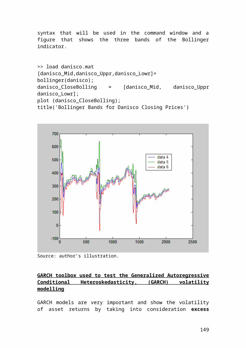
Net result
> netresult1 <- payoffbuy_call1 - payoffbuya_put1> netresult1[1]-75000> netresult2 <-payoffbuy_call2 - payoffbuya_put2> netresult2[1]-65000> netresult3 <- payoffbuy_call3 - payoffbuya_put3> netresult3[1]-45000> netresult4 <-payoffbuy_call4 - payoffbuya_put4> netresult4[1]-25000> netresult5 <-payoffbuy_call5 - payoffbuya_put5> netresult5[1]-5000> netresult6 <- payoffbuy_call6 - payoffbuya_put6> netresult6[1]15000
149
Exercise
Please calculate the range based on different share prices.
> share_price_1<- 20> share_price_2 <- 30> share_price_3 <- 40> share_price_4 <-50> share_price_5 <- 60> share_price_6 <-70> range <- share_price_6 - share_price_1> range[1] 50
150
Calculate the log returns and the average using actual share price returns expressed in pounds
> share_price_1 <- 14.23> share_price_2 <- 15.67> share_price_3 <- 12.13> share_price_4 <- 11.45> share_price_5 <- 10.11> dailyret2 <- log(share_price_2/share_price_1)> dailyret2[1]0.09639564426616845> dailyret3 <- log(share_price_3/share_price_2)> dailyret3[1]-0.25606633341197066> dailyret4 <- log(share_price_4/share_price_3)> dailyret4[1]-0.057691992955710175> dailyret5 <- log(share_price_5/share_price_4)> dailyret5[1]-0.12446469696786859> average <- (dailyret2 + dailyret3 + dailyret4 + dailyret5)/4> average[1]-0.08545684476734525
151
Calculation of the geometric average based on percentages of stock prices
> stock_price_1 <- 10> stock_price_2 <- 12> stock_price_3 <- 13> stock_price_4 <- 14> stock_price_5 <- 15> stock_price_6 <-16> Geometricaverage <- (stock_price_1*stock_price_2*stock_price_3*stock_price_4*stock_price_5*stock_price_6)**0.16666> Geometricaverage[1]13.17849601334643> round(Geometricaverage,digits =2)[1] 13.18
Calculation of the geometric average based on percentages of call option price returns
> Call_option_price_returns_1 <-5> Call_option_price_returns_2 <- 3> Call_option_price_returns_3 <- 2> Call_option_price_returns_4 <- 4> Call_option_price_returns_5 <- 7> Call_option_price_returns_6 <-8> Geometricaverage <- (Call_option_price_returns_1*Call_option_price_returns_2*Call_option_price_returns_3*Call_option_price_returns_4*Call_option_price_returns_5*Call_option_price_returns_6)**0.16666> Geometricaverage[1] 4.3437954197862885
152
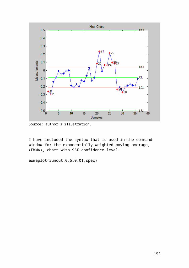
Calculation of the geometric average based on percentages of put option price returns
> Put_option_price_returns_1 <- 2> Put_option_price_returns_2 <- 3.3> Put_option_price_returns_3 <- 2.45> Put_option_price_returns_4 <- 4.21> Put_option_price_returns_5 <- 7.4> Put_option_price_returns_6 <- 4.34> Geometricaverage <- (Put_option_price_returns_1*Put_option_price_returns_2*Put_option_price_returns_3*Put_option_price_returns_4*Put_option_price_returns_5*Put_option_price_returns_6)**0.16666> Geometricaverage[1]3.6024392246983483
Calculation of the geometric average based on percentages of index option price returns
> Index_option_price_returns_1 <- 2> Index_option_price_returns_2 <- 2.31> Index_option_price_returns_3 <- 2.35> Index_option_price_returns_4 <- 4.51> Index_option_price_returns_5 <- 7.56> Index_option_price_returns_6 <- 4.39> Geometricaverage <- (Index_option_price_returns_1*Index_option_price_returns_2*Index_option_price_returns_3*Index_option_price_returns_4*Index_option_price_returns_5*Index_option_price_returns_6)**0.16666> Geometricaverage[1]3.4286570204871354
153
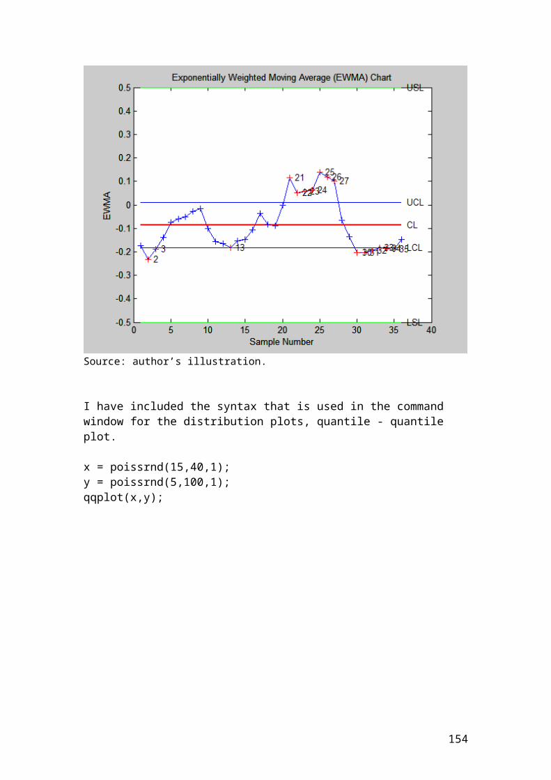
Calculate the portfolio return, the variance and the standard deviation in R for options with different returns and standard deviations
> CalloptionAexpectedreturn = 0.6> CalloptionAstandarddeviation = 0.2> CalloptionAweight = 0.35> CorrelationcoefficientbetweenAandB = 0.5> CalloptionBexpectedreturn = 0.1> CalloptionBstandarddeviation = 0.7> CalloptionBweight = 0.45> CorrelationcoefficientbetweenBandC = -0.1> CalloptionCexpectedreturn = 0.3> CalloptionCstandarddeviation = 0.4> CalloptionCweight = 0.2> CorrelationcoefficientbetweenAandC = -0.4
> Portfolioreturn = (CalloptionAexpectedreturn*CalloptionAweight)+(CalloptionBweight*CalloptionBexpectedreturn)+(CalloptionCexpectedreturn*CalloptionCweight)>>> Portfolioreturn[1] 0.315
You can omit the brackets from the Portfoliovariance. I have included them to show the different parts.
> Portfoliovariance = (CalloptionAweight**2*CalloptionAstandarddeviation**2)+ (CalloptionBweight**2*CalloptionBstandarddeviation**2)+(CalloptionCweight**2*CalloptionCstandarddeviation**2)+(2*CalloptionAweight*CalloptionBweight*CalloptionAstandarddeviation*CalloptionBstandarddeviation*CorrelationcoefficientbetweenAandB)+(2*CalloptionAweight*CalloptionCweight*CorrelationcoefficientbetweenAandC*CalloptionAstandarddeviation*CalloptionCstandarddeviation)+(2*CalloptionBweight*CalloptionCweight*CorrelationcoefficientbetweenBandC*CalloptionBstandarddeviation*CalloptionCstandarddeviation)> Portfoliovariance[1] 0.12305499999999998
> Portfolio_std = sqrt(Portfoliovariance)> Portfolio_std0.35079196113936245> round(Portfolio_std,digits=2)[1] 0.35
154
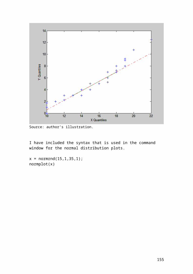
Calculate the portfolio return, the variance and the standard deviation or risk of the portfolio
>shareAexpRet <- 0.25>shareAstddev <- 0.10>shareAamount <- 50000>correlationAB <- 0.40>shareBexpRet <- 0.35>shareBstddev <- 0.18>shareBamount <- 50000>totalportfoliovalue <- 100000
># Calculate the weights for each share.
>weightA <- shareAamount / totalportfoliovalue> weightA[1]0.5
>weightB <-shareBamount / totalportfoliovalue> weightB[1]0.5
># Write the formula for portfolio return.
>Portfolioreturn <- (shareAexpRet*weightA)+(shareBexpRet*weightB)> Portfolioreturn[1]0.3
> # Write the formula for portfolio variance.
> Portfoliovariance <- (weightA**2*shareAstddev**2)+(weightB**2*shareBstddev**2)+(2*weightA*weightB*shareAstddev*shareBstddev*correlationAB)> Portfoliovariance[1]0.0142
># Write the formula for portfolio standard deviation.
>Portfolio_std <- sqrt(Portfoliovariance)> Portfolio_std[1]0.11916375287812986> round(Portfolio_std,digits=2)[1] 0.12
155
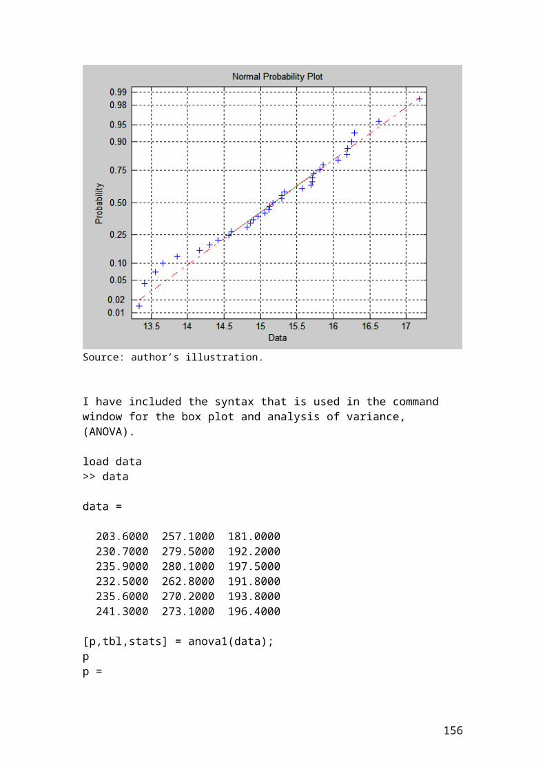
Exercise and solution
> # It is required to calculate the sum, and the average return.># The expected risk expressed as standard deviation of call, put and index options.># The figures represent percentages.
> call_option_returns <-c (3.5,4.7,7.9,-4.2,5.4,10.3)> put_option_returns <-c (2.7,4.9,5.7,8.5,9.3,11.5)> index_option_returns <-c (3.7,7.9,8.9,10.2,-6.8,5.9)> n<-6> sum(call_option_returns)[1] 27.600000000000005> average<- sum(call_option_returns)/n> average[1] 4.6000000000000005> sum(put_option_returns)[1] 42.6> average <-sum(put_option_returns)/n> average[1] 7.1000000000000005> sum(index_option_returns)[1] 29.799999999999997> average <- sum(index_option_returns)/n> average[1] 4.966666666666666> sd<-sqrt(sum((call_option_returns-mean(call_option_returns))^2)/(n-1))> sd[1] 4.953383> sd<-sqrt(sum((put_option_returns-mean(put_option_returns))^2)/(n-1))> sd[1] 3.234811> sd<-sqrt(sum((index_option_returns-mean(index_option_returns))^2)/(n-1))> sd[1] 6.203117> round(sd,digits=2)[1] 6.2
156
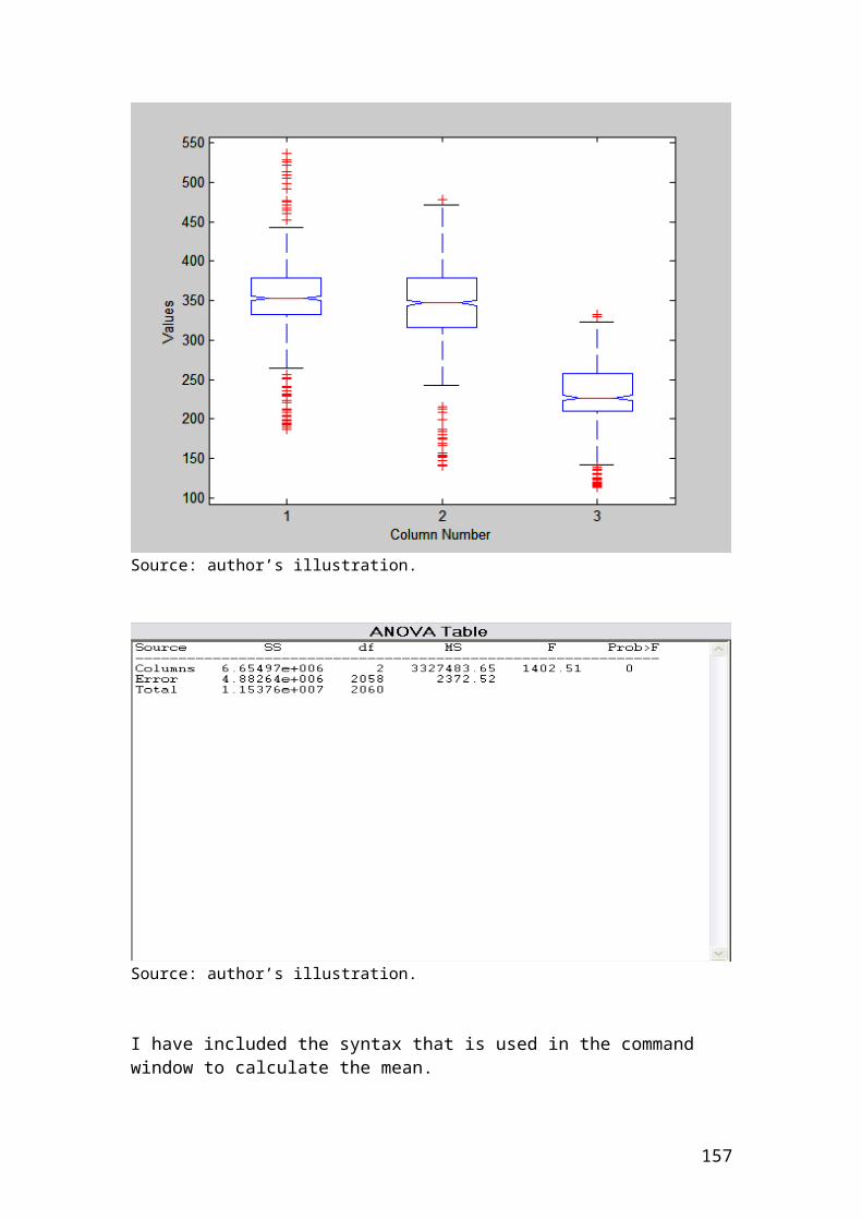
Example of pricing a forward contract and solution
A forward contract of 6 month has a market price of 52 Pounds when the spot price of the underlying commodity is 49 Pounds. There are no costs of carry and the discount rate is 7 percent. Calculate the value of the forward contract.
Solution
The current price of the forward contract (F0) should be equal to the value of the underlying commodity, (S0) at the discount rate r. Thus, the equation is as follows:
pounds 715.50207.0149)1(
)1(
00
00
rSF
rSF
Application of pricing a forward contract in R
> spot_price <- 49> discount_rate <- 0.07> # Insert the mathematical formula.> value_forward_contract <- spot_price *(1+discount_rate/2)> value_forward_contract50.714999999999996> round(50.715,digits=2)[1] 50.72 # Pounds
157
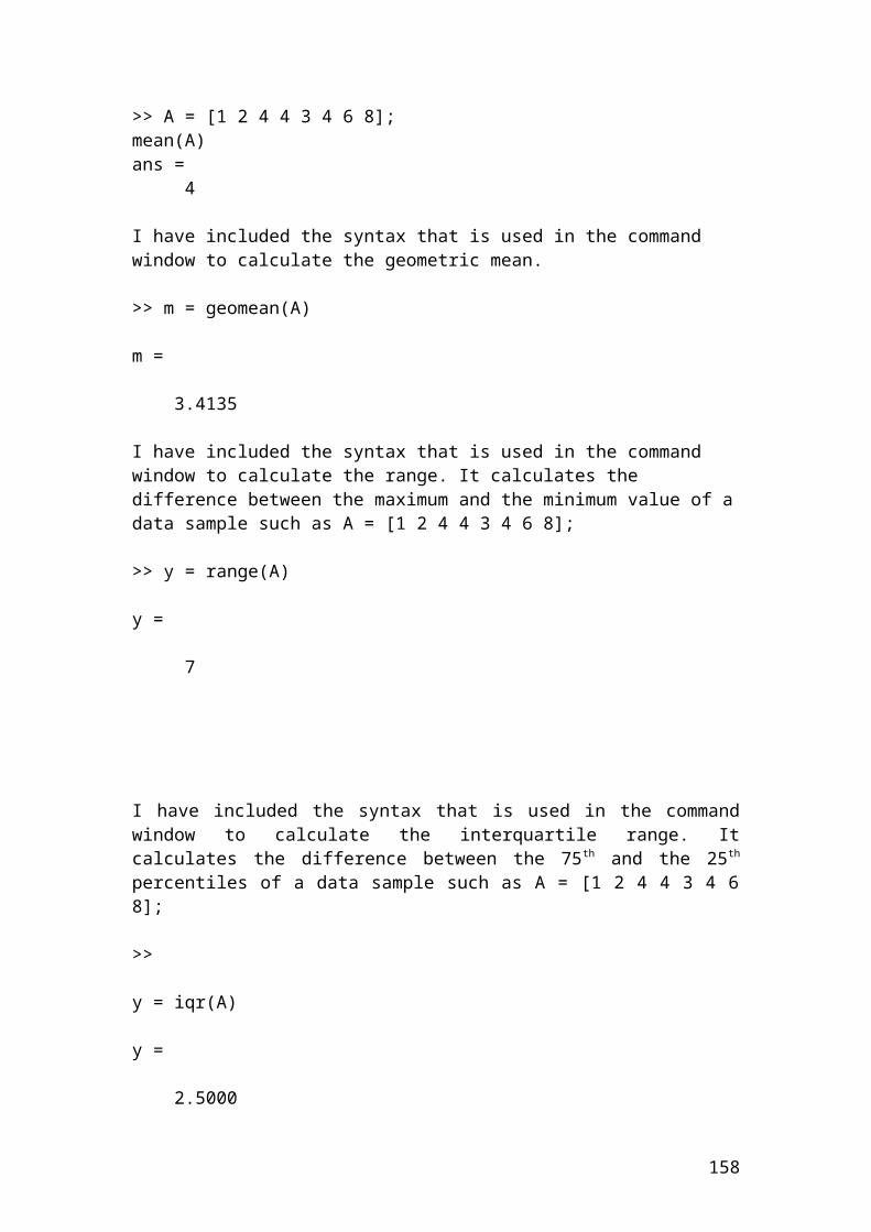
Example of interest rate payment and solution
A trader wants to calculate the interest amount that he / she will receive in three months from a forward contract of a Euribor deposit paying a Euro deposit rate of 3.55%. The principal amount is 300,000
The mathematical formula is as follows:
Interest payment = principal x [interest rate x (tdays / 360)]
Interest payment = 300,000 x [0.0355 x (90/360)]Interest payment = 2662.5 Euro.
Application of interest payment in R
> principal <- 300000> interest_rate <- 0.0355> days <- 90> # Insert the mathematical formula.> interest_payment <- principal*(interest_rate *days/360)> interest_payment[1] 2662.4999999999995> round(interest_payment,digits=2)[1] 2662.5 # Euro
158
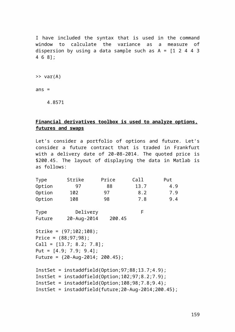
Example and solution of calculating profits and losses on futures contracts
An investor buys 8 S&P 500 futures contracts at $2189. He has closed the futures contract position with a price of $2236. The multiplier for S&P 500 futures contracts is 250 dollars. Did he record a profit or a loss?
Solution
The mathematical formula is as follows:
Where: fT is the final contract price. f0 is the initial contract price.
9400021892236 x250 x 8 Gain USD
When the prices move up, the investor will gain in long positions. When prices move down, the investor will gain in short positions.
Application of calculating profits and losses on futures contracts in R
> number_of_contracts <- 8> buying_price <- 2189> selling_price <- 2236> multiplier <-250> # Insert the mathematical formula.> profit_or_loss <- number_of_contracts*multiplier*(selling_price - buying_price)> profit_or_loss[1] 94000 # USD
159
Example and solution of semiannually currency swap between an investment bank and an insurance company
The investment bank borrows 20,000,000 Pounds from the insurance company at a fixed rate of 5% for 1 year. The insurance company borrows from the investment bank 10,000,000 Euros at a fixed rate of 5% for 1 year. Calculate the interest payments for the three years, if we assume semiannual payments?
At the beginning of the contract
€10,000,000Investment bank Insurance company
£ 20,000,000
The insurance company pays the investment bank the following interest payment.
£20,000,000 x 0.05/2 = 500,000 Pounds.
The investment bank pays the insurance the following interest payment.
€10,000,000 x 0.05/2 =250,000 Euros.
The following arrows illustrate the interest payments.
€ 250,000Investment bank Insurance company
£ 500,000
At the end of the third year, the two parties exchange the principal amounts in addition to the final interest payments.
€10,250,000Investment bank Insurance company
£20,500,000
160
Application of semiannually currency swap between an investment bank and an insurance company in R
> bank_borrows_from_insurance <- 20000000> insurance_borrows_from_bank <-10000000> interest_rate <- 0.05> semiannual_payment <- 2> # Insert the mathematical formula.> bank_pays_insurance <- insurance_borrows_from_bank *(interest_rate/semiannual_payment)> bank_pays_insurance[1] 250000.0 # Euros> # Insert the mathematical formula.> insurance_pays_bank <- bank_borrows_from_insurance *(interest_rate/semiannual_payment)> insurance_pays_bank[1] 500000.0 # Pounds or[1] 5e+05 # Pounds
161
Example and solution of interest rate swap
Interest rate swaps are very popular agreements between two parties in the debt or fixed-income department of the investment banks. The fixed income department of Bank A pays a fixed rate of 5.5% upon the principal of 50,000,000 Pounds. In contrast, Bank B pays a floating or reference rate of LIBOR accounted to 7.2%. The payment frequency is every 6 months for 2 years.
Fixed payment : £50,000,000 x 0.055/2 = 1,375,000 Bank A Bank B Floating payment: £50,000,000 x 0.072/2 = 1,800,000
Suppose in the second year that the LIBOR has increased by 12 basis points or 0.12%. Then, the floating payment will change and the calculation will be as follows:
Second year floating payment for Bank B = 50,000,000 x 0.0732 / 2 = 1,830,000 Pounds.
Bank A will continue to pay the same fixed amount, namely, £50,000,000 x 0.055/2 = £1,375,000.
Application of interest rate swap in R
> principal <- 50000000> interest_rate1 <- 0.055> interest_rate2 <- 0.072> interest_rate3 <- 0.0732> semiannual_payment <- 2> # Insert the mathematical formula.> fixed_payment <- principal*(interest_rate1/semiannual_payment)> fixed_payment[1]1375000.0 # pounds> # Insert the mathematical formula.> floating_payment_1 <- principal*(interest_rate2/semiannual_payment)> floating_payment_1[1] 1800000.0 # pounds> # Insert the mathematical formula.> floating_payment_2 <- principal*(interest_rate3/semiannual_payment)> floating_payment_2[1]1830000.0 # Pounds
162
Delta – neutral hedge
Delta – neutral hedge is common used in risk management to keep the value of the portfolio neutral due to changes in the share price. It is achieved from a long position in a share and a short position in a call option. The mathematical formula to determine the number of options is as follows:
option call of deltahedged shares ofNumber hedge neutral - Delta
Thus, if the investment bank has bought 30,000 shares of Vodafone and the delta of the call option of the same company is 0.50, then the numbers of call options that are needed to purchase to form a delta-neutral hedge are as follows:
Delta hedge = 30,000 / 0.50 = 60,000 options or 600 option contracts.
Application of delta- neutral hedge in R
> number_of_shares <- 30000> delta_of_call_option <- 0.50> # Insert the mathematical formula.> delta_neutral_hedge <- number_of_shares/delta_of_call_option> delta_neutral_hedge[1] 60000.0
163
Weighted mean price of a portfolio
Let’s assume that we have a portfolio of four options with their market prices and the number of shares bought. It is required to calculate the weighted mean price of the portfolio.
Options Price expressed in $
Number of shares
Weight Weight x Price
A 14.00 300 0.4 5.6B 12.00 200 0.3 3.6C 8.00 100 0.1 0.8D 5.00 150 0.2 1
Total 750 1Source: author’s calculation
The mathematical formula is as followed:
prices. theare P weights. theare w
portfolio. theof pricemean weighted theis X :
i
i
wWhere
PwX iiw
By substituting the numbers from the Table into the equation we have the following:
3.6 5.6 wX 0.8 + 1 = 11.
Application of weighted mean price of a portfolio in R
> price_1 <-14> price_2 <- 12> price_3 <- 8> price_4 <- 5> weight_1 <- 0.4> weight_2 <- 0.3> weight_3 <- 0.1> weight_4 <- 0.2>portfoliomean<-(price_1*weight_1+price_2*weight_2+price_3*weight_3+price_4*weight_4)> portfoliomean[1] 11.0 # Pounds
164
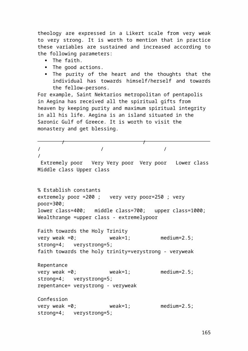
Example of Eurodollar futures
An investor wants to calculate the futures price of a 1-month Eurodollar time deposits based on a LIBOR rate of 3.40%. The initial principal is 1 million Pounds.
Solution
The price of the Eurodollar futures contract will be as follows:
Application of Eurodollar futures in R
> principal <- 1000000> interest_rate <- 0.034> days <- 30> Eurodollar_future <- principal*(1- interest_rate*(days/360))> Eurodollar_future[1] 997166.7 # Pounds
165
Example of forward rate agreement
An investment bank buys a 4 x 6 FRA from a building society in the UK for 4.0% by paying 2 million Pounds. 80 days latter, LIBOR is 5%. Who will receive the FRA payment and for how much?
Solution
The mathematical formula for Forward Rate Agreement, (FRA) is as follows:
360/trate var1360/rate fixed -rate variable
amount x NotionalPayment days
iablet
FRA days
The timeline schedule is as follows:
t = 0 4months 6 months
360/800.051
360/1200.04 -0.05 x000,000,2Payment FRA = ………. Please complete the
calculation.
Helpful hint: If the FRA payment is positive, then, the building society is the payer and the investment bank receives the FRA payment.
If the FRA payment is negative, then the investment bank is the payer and the building society receives the FRA payment.
Application of forward rate agreement in R
> principal <- 2000000> variable_rate <- 0.05> fixed_rate <- 0.04> FRA_payment <- principal*(variable_rate - fixed_rate)*0.333333333/1.011111111> FRA_payment[1] 6593.407> round(FRA_payment,digits=2)[1] 6593.41 # Pounds
166

Example of futures on Treasury bills
An investor wants to calculate the futures price of a 3-month Treasury bills. Treasury bills are short-term notes of limited period of 1- month, and 3 - month respectively. The initial principal is 5 million Pounds and the discount rate is 3.50%.
Solution
The price of the Treasury bill futures will be as follows:
360t
xratediscount -1 x Principal BillTreasury price daysFutures
Please complete the calculation …….
Application of futures on Treasury bills in R
> principal <- 5000000> discount_rate <- 0.035> days <- 90< # Insert the mathematical formula.> futures_treasury_bills <- principal*(1- discount_rate *(days/360))> futures_treasury_bills [1] 4956250 # Pounds
167
Example of stock index futures
For example, if you bought 10 contracts of the Dow Jones Industrial index at 10,000 and you expected an aggressive bull market that reaches the value of 16,000, then, the 6000 points increase are multiplied by the standardized value of 250. If the initial principal of investment is $100,000, the mathematical formula for the gains will be as follows:
10 x 100,000 x 6000 x 250 = 1.5 x 10¹² Dollars
Application of stock index futures in R
> principal <- 100000> points_increase <- 6000> multiplier <- 250> number_of_contracts <- 10> gains <- principal*points_increase*multiplier*number_of_contracts> gains[1] 1.5e+12 # USD
168
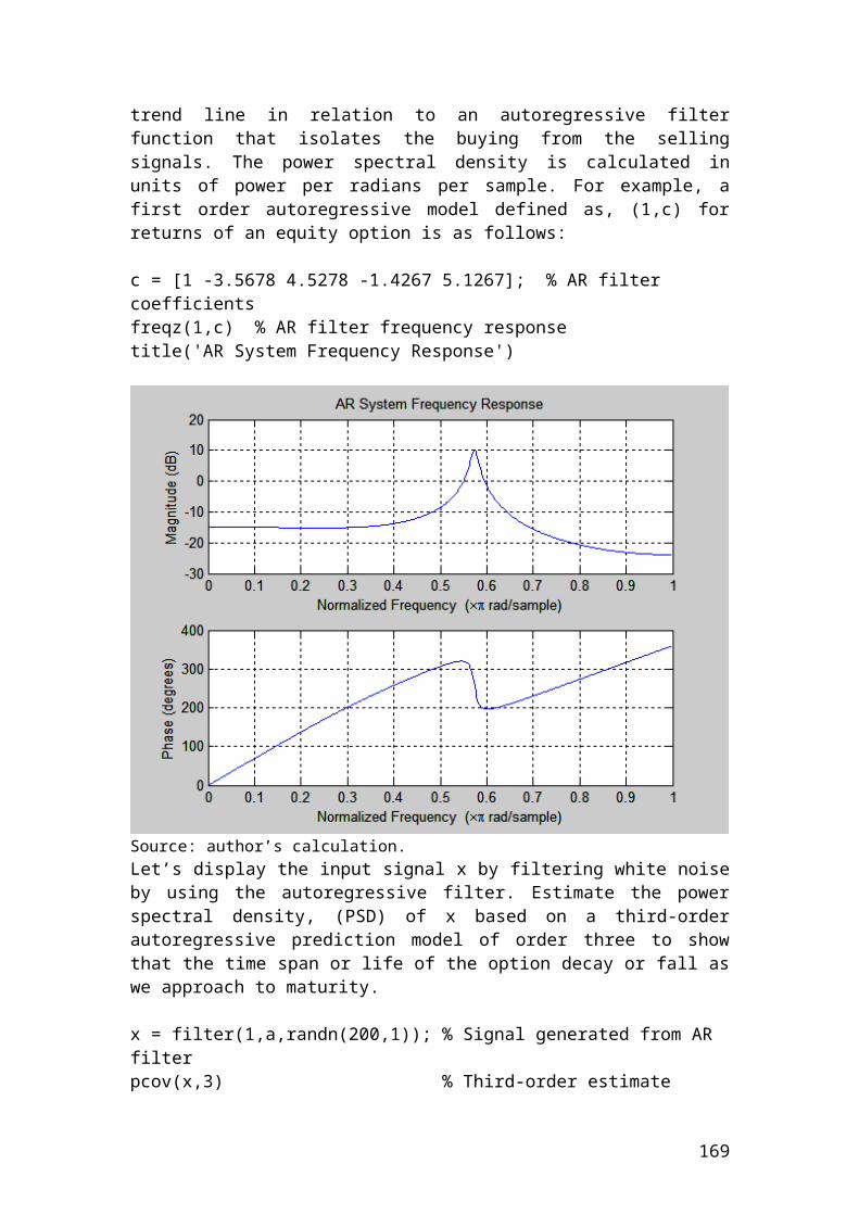
Example of currency futures
A manufacturer wants to calculate the currency futures price of EURO/USD traded in Frankfurt derivative market. For example, in August the contract is quoted as 1.35 EURO /USD and the contract size is 20,000. The principal is 300,000 Euro.
Solution
The contract price of 1 contract is as follows:
n....calculatio thecomplete Please
Euro .. ... price quotedAugust x sizecontract *principal EURO/USD futurecurrency of price
Futures
Application of currency futures in R
> principal =<-300000> quote <- 1.35> contract_size <- 20000> # Insert the mathematical formula.> futures_price_of_currency <- principal*quote*contract_size> futures_price_of_currency[1] 8.1e+09 # Euro
169
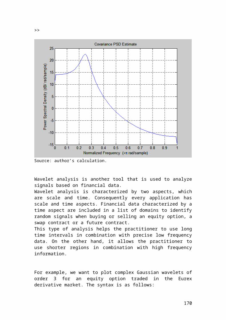
Please try based on the previous examples to illustrate the following example in R. If you have difficulties e-mail me.
Active return, active risk and information ratio
Active return is the difference in returns between a portfolio and the index or benchmark that is measured.
Active return = rp - rb
Where: rp is the portfolio return. rb is the benchmark or index return.
If the portfolio return is 0.80 and the benchmark return of the index is 0.70 then, the active return is………
Please complete the calculation.
Active risk or tracking error is the standard deviation of the difference of returns between a portfolio and the benchmark or index.
assets. ofnumber theisn index.an examplefor be couldIt return.benchmark portfolio is r
return. portfolio is r :
1
)(r risk
b
p
2p
Wheren
rActive b
If the portfolio return is 0.80, the number of assets is 10 and the benchmark return of the index is 0.40 then, the active risk is………
Please complete the calculation.
Information ratio shows the consistency of the fund manager towards the active return. The mathematical formula is as follows:
170
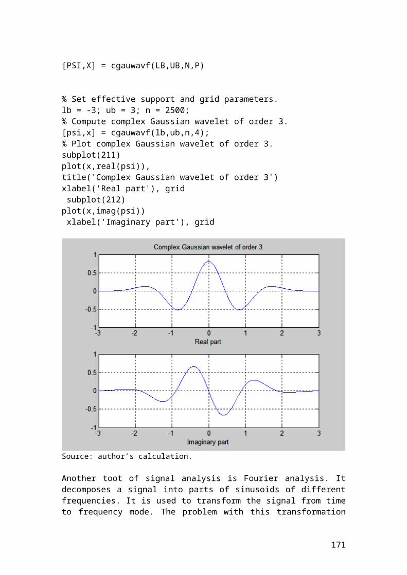
risk active theis
1
return.index or benchmark average theis r
return. portfolio of average theis :
1)(r
2
b
2p
nrr
rWhere
nr
rrIR
bp
p
b
bp
It could be calculated very easily in Excel software. I will illustrate a simple table with the relevant calculations.
Day rp rb rp - rb
1 0.03 0.02 0.012 0.02 0.014 0.0063 -0.04 0.034 -0.0744 0.05 0.067 -0.0175 0.08 0.012 0.0686 -0.01 -0.056 0.0467 0.07 0.031 0.0398 0.034 0.023 0.0119 -0.021 0.015 -0.03610 0.045 0.001 0.044
Average 0.0258 0.0161Standard deviation
0.043
Source: author’s calculation
By substituting the values that we have found in terms of rp =0.0258, rb = 0.0161 and standard deviation = 0.043 in the following equation we have:
1)(r 2
p
n
r
rrR
b
bp
2d.p.) (to 23.0043.0
0097.0043.0
0161.00258.0
R
But what is the interpretation of the information ratio of 0.23. It means that the fund manager gained around 23 basis points of active return per unit of active risk. The higher is this number, the better the manager is performing in relation to active risk.
171
Please convert the following exercise in R language programming.
Calculate the balance at the end of the 5th day from changes in the futures prices from 90 to 89, 91, 95, 97, 99. The trader has bought 50 futures contract for settlement in May. The initial margin is $8.
Day Beginning balance
Futures price Gain or loss Ending balance
0 400 90 0 4001 400 89 (50)2 350 91 1003 450 95 2004 650 97 1005 750 99 100
Source: author’s illustration.
Beginning balance = initial margin x number of contracts.Beginning balance = 8 x 50 = $400
Please complete the values of the column ending balance.
172
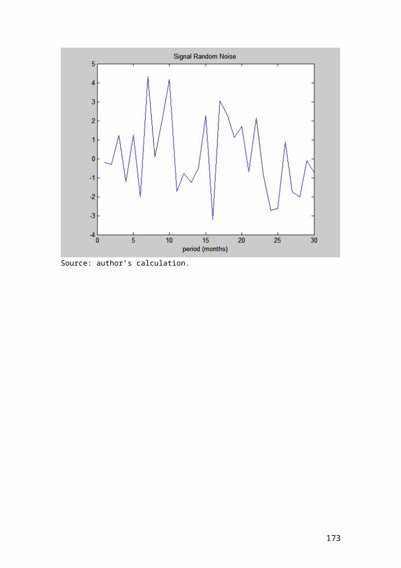
Application of the random function. It is very useful method that is used in simulations such as Monte Carlo simulation to price derivatives products
The uniform random function is given by the runif. Inside the brackets, there are three numbers. The first number symbolizes the total number of random numbers. The second number symbolizes the lower value and the third number symbolizes the upper value.
> rand.number<-runif(2,0,10000)> rand.number[1] 1848.823 7023.740> rand.number<-runif(5,0,10000)> rand.number[1] 5733.263 1680.519 9438.393 9434.750 1291.590
Other random functions available in R are related with different types of distributions. For example, the random number that is associated with a normal distribution is given by rnorm.The random number that is associated with an exponential distribution is given by rexp.
173
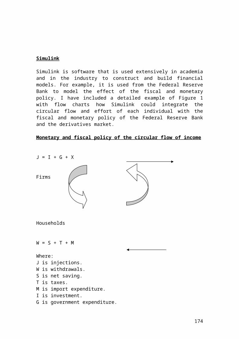
Example of profit or loss of a call option portfolio. The figures are expressed in Euros.
> shareprice_1 <-10.25> shareprice_2 <- 20.13> shareprice_3 <- 30.22> shareprice_4 <- 40.56> shareprice_5 <- 50.89> shareprice_6 <- 51.23> shareprice_7 <- 53.33> shareprice_8 <-54.63> shareprice_9 <- 66.23> shareprice_10 <- 68.23> strikeprice_1 <- 3.34> strikeprice_2 <- 8.34> strikeprice_3 <-18.78> strikeprice_4 <- 28.34> strikeprice_5 <- 31.12> strikeprice_6 <- 22.02> strikeprice_7 <- 34.23> strikeprice_8 <- 47.12> strikeprice_9 <- 48.45> strikeprice_10 <- 50.12> optionpremium_1 <- 1.50> optionpremium_2 <- 2.30> optionpremium_3 <- 2.56> optionpremium_4 <- 3.10> optionpremium_5 <- 3.25> optionpremium_6 <- 3.45> optionpremium_7 <- 3.56> optionpremium_8 <- 4.32> optionpremium_9 <- 5.12> optionpremium_10 <- 5.78> contractsize <- 100
> portfoliovalue1 <- (shareprice_1-(strikeprice_1+ optionpremium_1))* contractsize> portfoliovalue1[1] 541.0> portfoliovalue2 <- (shareprice_2-(strikeprice_2+ optionpremium_2))* contractsize> portfoliovalue2[1] 948.9999999999999> portfoliovalue3 <- (shareprice_3-(strikeprice_3+ optionpremium_3))* contractsize> portfoliovalue3[1] 887.9999999999999> portfoliovalue4 <- (shareprice_4-(strikeprice_4+ optionpremium_4))* contractsize> portfoliovalue4[1] 912.0000000000001> portfoliovalue5 <- (shareprice_5-(strikeprice_5+ optionpremium_5))* contractsize> portfoliovalue5
174
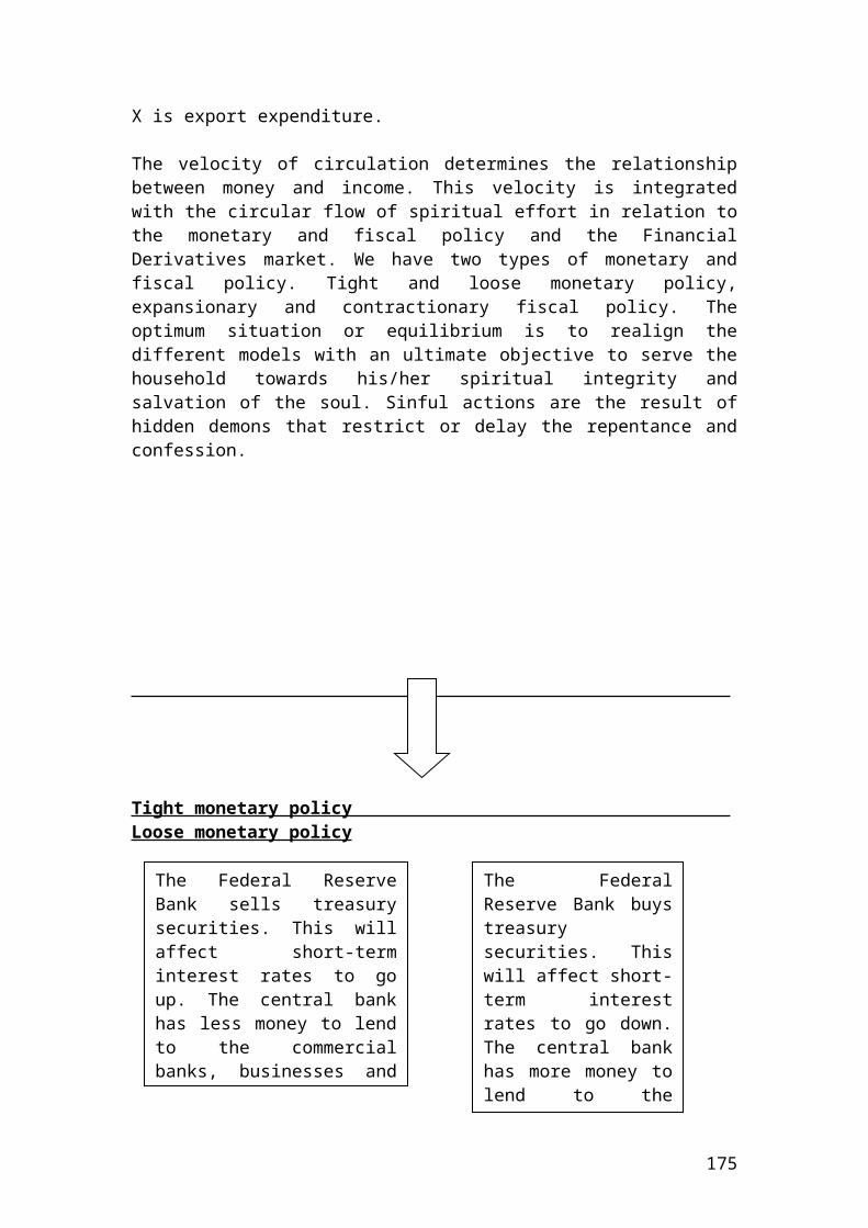
[1] 1651.9999999999995> portfoliovalue6 <- (shareprice_6-(strikeprice_6+ optionpremium_6))* contractsize> portfoliovalue6[1] 2576.0> portfoliovalue7 <- (shareprice_7-(strikeprice_7+ optionpremium_7))* contractsize> portfoliovalue7[1] 1554.0> portfoliovalue8 <- (shareprice_8-(strikeprice_8+ optionpremium_8))* contractsize> portfoliovalue8[1] 319.00000000000045> portfoliovalue9 <- (shareprice_9-(strikeprice_9+ optionpremium_9))* contractsize> portfoliovalue9[1] 1266.0000000000005> portfoliovalue10 <- (shareprice_10-(strikeprice_10+ optionpremium_10))* contractsize> portfoliovalue10[1] 1233.0000000000005
175
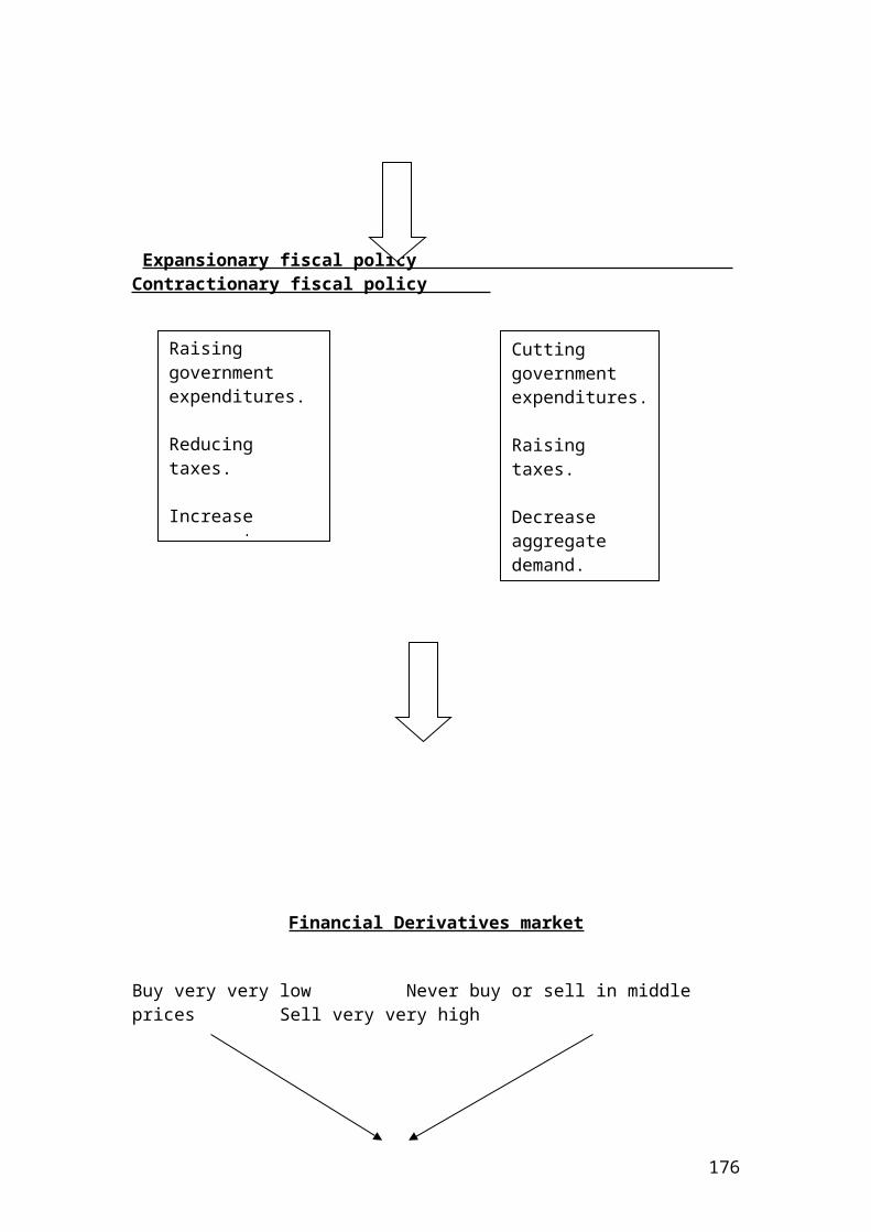
Example of profit or loss of a put option portfolio. The figures are expressed in Euro.
> shareprice_1 <- 10.25> shareprice_2 <- 20.13> shareprice_3 <- 30.22> shareprice_4 <- 40.56> shareprice_5 <- 50.89> shareprice_6 <- 51.23> shareprice_7 <- 53.33> shareprice_8 <- 54.63> shareprice_9 <- 66.23> shareprice_10 <- 68.23> strikeprice_1 <- 3.34> strikeprice_2 <- 8.34> strikeprice_3 <- 18.78> strikeprice_4 <- 28.34> strikeprice_5 <- 31.12> strikeprice_6 <- 22.02> strikeprice_7 <- 34.23> strikeprice_8 <- 47.12> strikeprice_9 <- 48.45> strikeprice_10 <- 50.12> optionpremium_1 <- 1.50> optionpremium_2 <- 2.30> optionpremium_3 <- 2.56> optionpremium_4 <- 3.10> optionpremium_5 <- 3.25> optionpremium_6 <- 3.45> optionpremium_7 <- 3.45> optionpremium_8 <- 4.32> optionpremium_9 <- 5.12> optionpremium_10 <- 5.78> contractsize <-100> portfoliovalue1 <- (strikeprice_1- optionpremium_1-shareprice_1)* contractsize> portfoliovalue1[1] -841.0> portfoliovalue2 <- (strikeprice_2- optionpremium_2- shareprice_2)* contractsize> portfoliovalue2[1] -1409.0> portfoliovalue3 <- (strikeprice_3- optionpremium_3- shareprice_3)* contractsize> portfoliovalue3[1] -1399.9999999999995> portfoliovalue4 <- (strikeprice_4 - optionpremium_4 - shareprice_4)* contractsize> portfoliovalue4[1] -1532.0000000000005> portfoliovalue5 <- (strikeprice_5- optionpremium_5- shareprice_5)* contractsize> portfoliovalue5[1] -2302.0
176
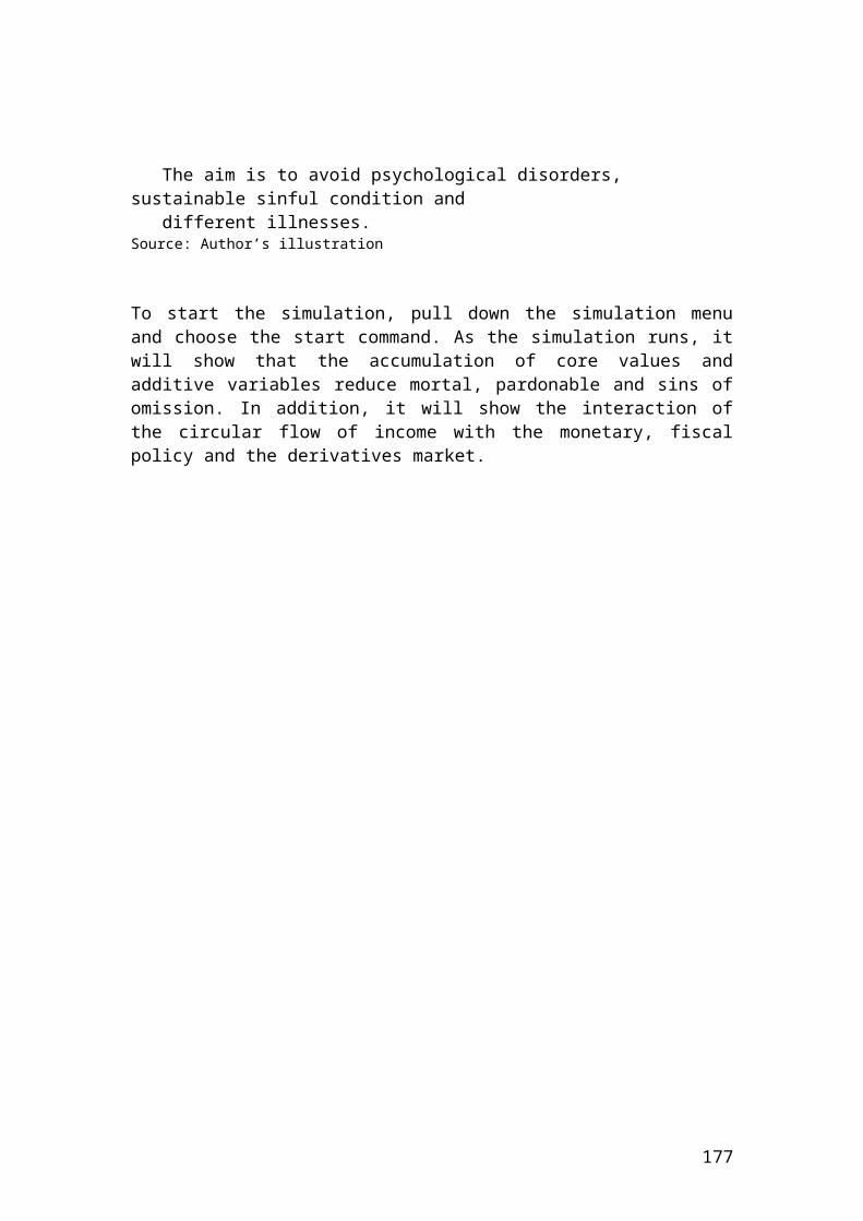
> portfoliovalue6 <- (strikeprice_6- optionpremium_6- shareprice_6)* contractsize> portfoliovalue6[1] -3265.9999999999995> portfoliovalue7 <- (strikeprice_7- optionpremium_7- shareprice_7)* contractsize> portfoliovalue7[1] -2255.0> portfoliovalue8 <- (strikeprice_8- optionpremium_8- shareprice_8)* contractsize> portfoliovalue8[1] -1183.0000000000005> portfoliovalue9 <- (strikeprice_9- optionpremium_9- shareprice_9)* contractsize> portfoliovalue9[1] -2290.0> portfoliovalue10 <- (strikeprice_10- optionpremium_10- shareprice_10)* contractsize> portfoliovalue10[1] -2389.000000000001
177
One – period binomial method
A share is traded in the Danish stock exchange at 50 DKK. First of all, we would like to calculate the possible price changes based on probabilities. The risk - free rate is 5% and the value of the call option has an exercise price of 50 DKK. It is required to calculate the expected value of the option at t =1. In addition, it is required to calculate the value of the option today discounted at the given risk-free rate.
We assume two scenarios. The first one is that the share will increase by 20% or by a factor of 1 + 0.20 = 1.20. The second one is that the share will decrease by 0.833. The number 0.833 is calculated as 1 / 1.20 = 0.833.
The mathematical formulas are as follows:
Down move = D = 1 / up move = 1 / 1.20 = 0.833
59128.0367.0217.0
0.833-1.200.833- 0.051
move. up theis U move.down theis D
rate. free-risk theis rf :
D-U
D-rf1 movement upan ofy probabilit neutral -risk
U
Where
U
0.40872 0.59128 - 1 movement down a ofy probabilit neutral - riskD
Thus, the payoff or the one-period binomial tree for share and option prices for the two possible scenarios will be as follows:
t = 0 t = 1
Probability Up = 0.59128 Share price = 50 x 1.20 = 60 DKK Call option = 60 – 50 = 10 DKK. 50 In this case, an increase of the share price will lead to the call option to pay back 10 DKK Probability Down =0.40872 Share price = 50 x 0.833 = 41.65 DKK Call option = 41.65 – 50 = -8.35 DKK = 0 DKK In this case the call option does not worth anything.
The expected value of the call option at t = 1 is as follows:
Expected call option = (10 x 0.59128) + ( 0 x 0.40872) = 5.9128 + 0 = 5.9128 DKK.
The value of the call option discounted at 5% risk – free rate is as follows:
178
Ctoday = 5.9128 / 1.05 = 5.63 DKK (to 2 d.p.).Application of one – period binomial method in R. The figures are expressed in DKK.
> share_price <- 50> exercise_price <- 50> upmove <- 1.20> downmove <- 0.833> risk_free_rate <- 0.05> # Insert the mathematical formulas of risk probability of up and down move.> riskprobofupmove <- (1+risk_free_rate-downmove) / (upmove - downmove)> riskprobofupmove[1] 0.5912806539509539> round(riskprobofupmove,digits=2)[1] 0.59> riskprobofdownmove <- 1 - riskprobofupmove> riskprobofdownmove[1] 0.40871934604904614> round(riskprobofdownmove,digits=2)[1] 0.41> # The payoffs are determined by the following equations.> shareprice1 <- share_price * upmove> shareprice1[1] 60.0> calloptionprice1 <- shareprice1 - exercise_price> calloptionprice1[1] 10.0> shareprice2 <- share_price *downmove> shareprice2[1] 41.65> calloptionprice2 <- shareprice2 - exercise_price> calloptionprice2[1] -8.350000000000001> calloptionprice2 =0> calloptionprice2[1] 0> #The expected value of the call option at t=1 is as follows:> expectedcalloption <- (calloptionprice1* riskprobofupmove) + (calloptionprice2 * riskprobofdownmove)> expectedcalloption[1] 5.912806539509539> round(expectedcalloption,digits=2)[1] 5.91># The value of the call option discounted at 5% risk - free rate is as follows:> valueofcalldiscounted <- expectedcalloption / 1.05> valueofcalldiscounted[1] 5.631244323342418> round(valueofcalldiscounted, digits= 2)[1] 5.63
179
Two – period binomial method
This method is based on the one – period binomial method, but it is extended to include a second period, t = 2. Thus, we have three periods. t = 0, t =1 and t =2. We use the same example of the previous section but extended to an additional period.
A share is traded in the Danish stock exchange at 50 DKK. First of all, we would like to calculate the possible price changes based on probabilities. The risk - free rate is 5% and the value of the call option has an exercise price of 50 DKK. It is required to calculate the expected value of the option. In addition, it is required to calculate the value of the option today discounted at the given risk-free rate.
We assume two scenarios. The first one is that the share will increase by 20% or by a factor of 1 + 0.20 = 1.20. The second one is that the share will decrease by 0.833. The number 0.833 is calculated as 1 / 1.20 = 0.833.
The mathematical formulas are as follows:
Down move = D = 1 / up move.
59128.0367.0217.0
0.833-1.200.833- 0.051
move. up theis U move.down theis D
rate. free-risk theis rf :
D-U
D-rf1 movement upan ofy probabilit neutral -risk
U
Where
U
0.40872 0.59128 - 1 movement down a ofy probabilit neutral - riskD
Thus, the payoff or the two-period binomial tree for share prices for the two possible scenarios will be as follows:
t = 0 t = 1 t =2 50*(1.20)2=72 DKKProbability Up = 0.59 S1 = 50 x 1.20 = 60 DKK S2 50*1.20*0.833 =49.98 50 DKK Probability Down =0.41 S1 = 50 x 0.833 = 41.65 DKK S2
50 * (0.833)2 = 34.69
The value of the call options for the period t =2 for both ups and downs are as follows:
180
Upside movementC1 = 72 – 50 = 22C2 = 49.98 – 50 = -0.02 =0 Negative values mean that the option does not worth.
Downside movementC1 = 49.98 -50 = -0.02 =0C2 = 34.69 -50 = -15.31 =0
The expected value of the call options for both movements for period t =1 are calculated based on the following equations:
Upside movement
DKK 12.3887
05.1008.13
05.1)040872.0(2259128.0
rf 1down xC PrC x upy Probabilit 21
up
up
Call
xxobabilityCall
Downside movement
005.1
0) 40872.0(0 59128.0rf 1
Cdown x PrC x up Pr 21
xxobabilityobabilityCalldown
The value of the call option today discounted is calculated based on the following formula:
3.d.p.) (to 976.605.1
32519.7
05.10 12.3887 x 59128.0
1Calldown x PrCall x up Pr downup
today
today
Call
rfobabilityobability
Call
The final format of the two-period binomial tree for call options is as follows:
t = 0 t = 1 t = 2
22.00 DKK 12.3887DKK 06.976 DKK 0 0
181
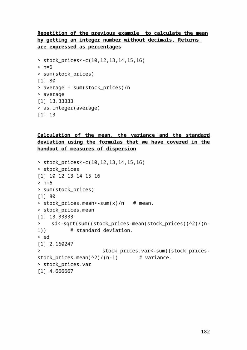
Application of two – period binomial method in R. The figures are expressed in DKK.
> share_price <- 50> exercise_price <- 50> upmove <- 1.20> downmove <- 0.833> risk_free_rate <- 0.05> # Insert the mathematical formulas of risk probability of up and down move.> riskprobofupmove <- (1+risk_free_rate-downmove) / (upmove - downmove)> riskprobofupmove[1] 0.5912806539509539> round(riskprobofupmove,digits=2)[1] 0.59> riskprobofdownmove <- 1 - riskprobofupmove> riskprobofdownmove[1] 0.40871934604904614> # The payoffs are determined by the following equations.> shareprice1 <- share_price * upmove> shareprice1[1] 60.0> shareprice2 <- share_price *downmove> shareprice2[1] 41.65> shareprice3 <-share_price * upmove**2> shareprice3[1] 72.0> calloptionprice3 <- shareprice3 - exercise_price> calloptionprice3[1] 22.0> shareprice4 <- share_price * downmove**2> shareprice4[1] 34.694449999999996> calloptionprice4 <- shareprice4 - exercise_price> calloptionprice4[1] -15.305550000000004> calloptionprice4 <-0> calloptionprice4[1] 0> shareprice5 <- share_price * upmove * downmove> shareprice5[1] 49.98> calloptionprice5 <- shareprice5 - exercise_price> calloptionprice5[1] -0.020000000000003126> calloptionprice5 <-0> calloptionprice5[1] 0
182
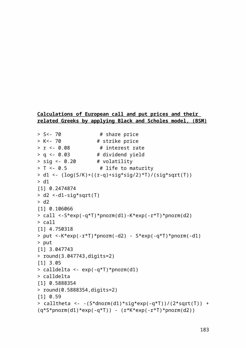
> #The expected value of the call option at t=2 is as follows:> expectedcalloptionupside <- (riskprobofupmove * calloptionprice3+ riskprobofdownmove* calloptionprice5) / 1.05> expectedcalloptionupside[1] 12.388737511353318> expectedcalloptiondownside <- (riskprobofupmove *calloptionprice4+ riskprobofdownmove * calloptionprice5) / 1.05> expectedcalloptiondownside[1] 0.0># The value of the call option discounted at 5% risk - free rate is as follows:> valueofcalldiscounted <- (riskprobofupmove * expectedcalloptionupside+riskprobofdownmove* expectedcalloptiondownside)/ 1.05> valueofcalldiscounted[1] 6.976400778418764> round(valueofcalldiscounted, digits=2)[1] 6.98
183
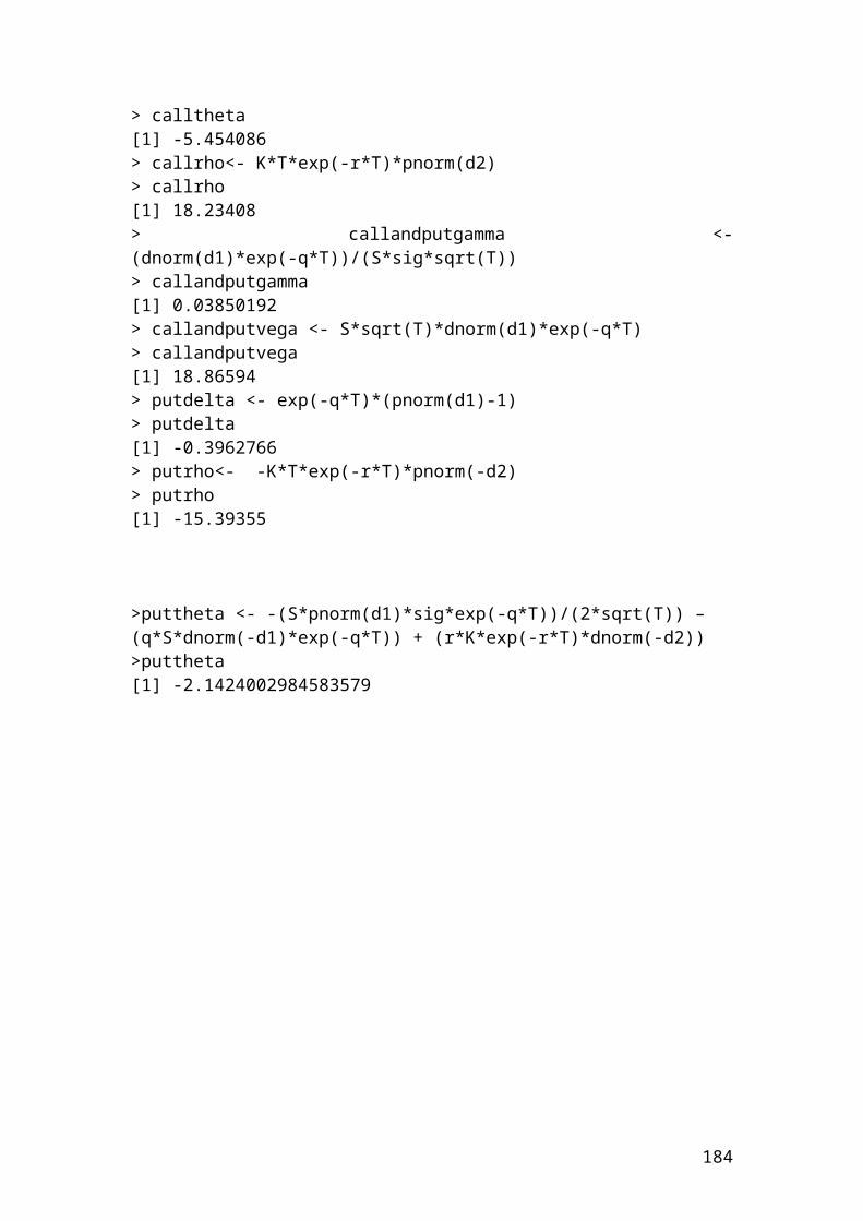
Stock index option
Let’s assume that a practitioner wants to buy a stock index call option that is related to the general movement of the S&P 500 index. The dollar multiplier for S&P 500 option contract is 250 dollars. The strike price of the index is 1240. The August premium is 20 index points.
Question
Calculate the cost of the August call and the net profit involved if the S&P 500 index reaches the price of 1540.
Solution
Cost of the August call = premium expressed in index points x dollar multiplier Cost of the August call = 20 x 250 = 5000 USD
The net profit incurred is calculated as follows:
(Ending index value – beginning index value x dollar multiplier ) – cost of the August call.
(1540 – 1240) x 250 – 5000 = 70,000 USD.
Application of stock index option in R
> beginning_index_value <- 1240> ending_index_value <- 1540> multiplier <- 250> premium <- 20> costofcall <- premium * multiplier> costofcall[1] 5000 # USD> netprofit <- (ending_index_value - beginning_index_value) * multiplier - costofcall> netprofit[1] 70000 # USD
184
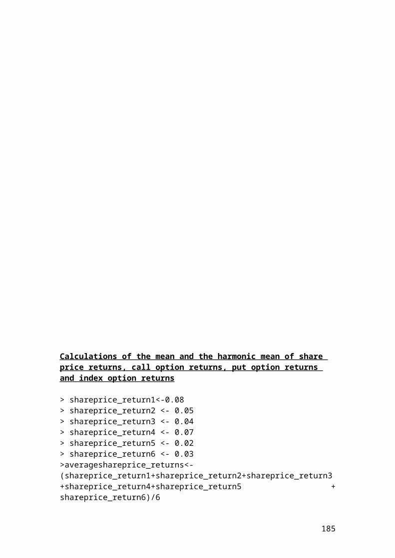
Exercise of an European interest rate option
Calculate the profit or loss of the interest rate difference between the actual and the strike rate of a call option. Let’s assume that an interest call option on a 6 –month Eurodollar has a strike rate of 4%. At expiration, the 6-month Eurodollar rate is 5%. The invested principal is 50,000,000 Euros. The duration of the contract is expressed in days divided by 360 days. Thus, 6 –months equal 180 days.
The mathematical formula for profit or loss is as follows:
Application of an European interest rate option in R
> principal <- 50000000> actual_rate <- 0.05> strike_rate <- 0.04> duration <- 180> days <- 360> # Insert the mathematical formula.> profitorloss <-principal*(actual_rate - strike_rate)*duration/days> profitorloss[1] 250000.0 # Euros
185
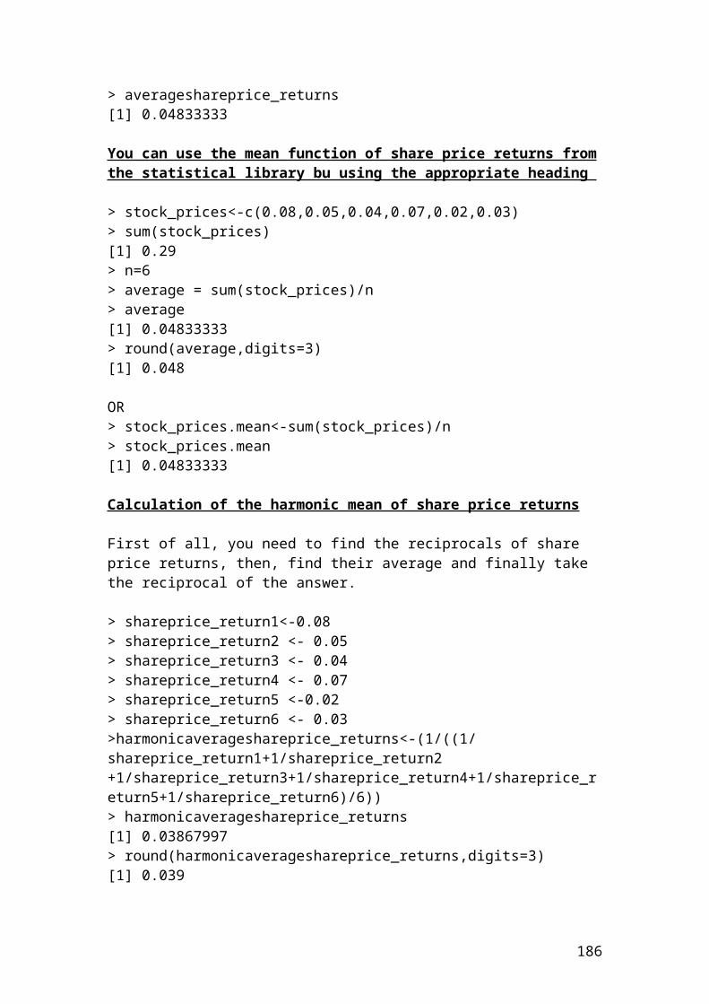
Currency option
Let’s assume that a wealthy investor buys a call currency option because it expects a rise in the exchange rate parity of the EURO against the USD, EURO/USD. The spot exchange rate is 1/1.3568. The strike price is 1.3568. The premium expressed as cents per Euro is 1.56. The initial principal is 100,000 USD.
Question
Calculate the net profit involved if the strike price increases to 1.3987.
Solution
The wealthy investor to record a profit, he or she should add to the strike price 1.3568 the premium expressed as cents per Euro. In our case, the breakeven point is1.3568 + 0.0156 = 1.3724. Above the price of 1.3724, he or she starts to record a profit. If the strike price reaches 1.3987, then the profit will be as follows:
Initial principal x (Ending strike price – beginning strike price – premium paid) =100,000 x (1.3987 – 1.3568 – 0.0156) = 2630 USD net profit
Application of currency option in R
> principal <- 100000> ending_strike_price <- 1.3987> beginning_strike_price <- 1.3568> premiumpaid <- 0.0156> netprofit <- principal *(ending_strike_price-beginning_strike_price-premiumpaid)> netprofit[1] 2630 # USD
186
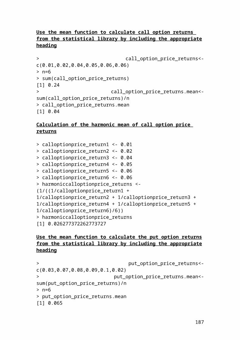
Example of calculating the payments of an interest rate cap based on different LIBOR rates
Interest rate cap is an agreement between two parties where one party pay the other at a specified period of time in which the interest rate or London interbank offered rate ,LIBOR, exceeds the strike price. It is used this contract to hedge against interest rate fluctuations. Let’s assume that an interest cap has a value of 5.5% and the LIBOR prices for the next three years are 7.5%, 8.3% and 4.65%. The principal is $50,000,000 and the payments take place semiannually.
The mathematical formula that is used to calculate the payments of each year is as follows:
Interest rate payment =[ principal x (LIBOR rate – cap rate)/0.5]
Therefore, the first year interest rate payment is as follows:
Year 1
Interest rate payment = [50,000,000 x (0.075 – 0.055)/2] = $ ………
Application of payments of an interest rate cap based on different LIBOR rates in R
> principal <- 50000000> liborrate_1 <- 0.075> liborrate_2 <- 0.083> caprate <- 0.055> duration <- 2> interestpay1 <- principal *(liborrate_1 - caprate) /duration> interestpay1[1] 5e+05 or 500000 # USD> interestpay2 <- principal *(liborrate_2 - caprate) / duration> interestpay2[1] 7e+05 or 700000 # USD
187
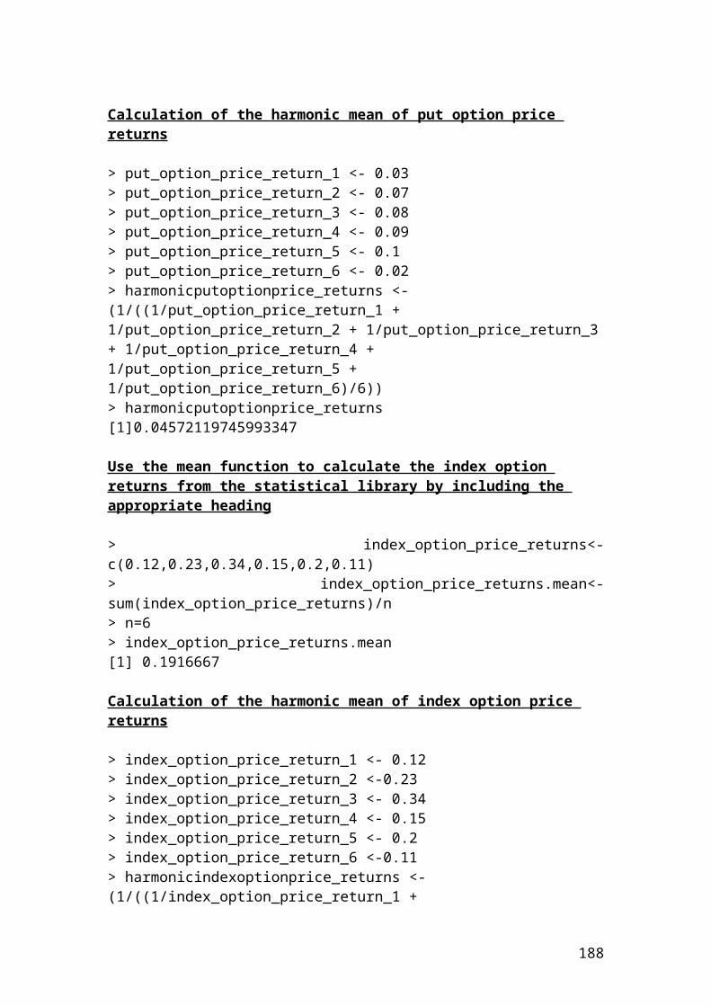
A six month interest rate cap has a rate of 0.08 and the principal is 20,000,000 USD. The settlements is done quarterly. The first quarter the 3 –month libor rate is 0.096 and the second quarter the rate is 0.087. Calculate the payoff for the cap the first and the second quarter?
Solution
Payoff the first quarter = 20,000,000 * = 80000 USD
Payoff the second quarter = 20,000,000 * 35000 USD
Application of payoff of interest rate cap in python
> principal <- 20000000> caprate <- 0.08> liborrate_1 <- 0.096> liborrate_2 <- 0.087> period <- 4> # Insert the mathematical formulas.> payoff1 <- (principal*(liborrate_1-caprate)/period)> payoff1[1] 80000 # USD> payoff2 <- (principal*(liborrate_2-caprate)/period)> payoff2[1] 35000 # USD
188
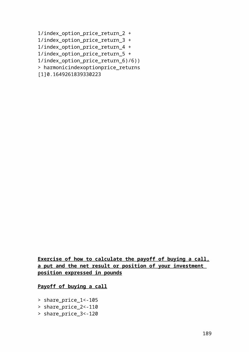
Swaption
An investor purchased a 1 year European swaption with exercise price 7.50%. The principal is 30,000,000USD. The floating rate payments are based on LIBOR. The 90, 180, 270, and 360 day annualized LIBOR rates and present value factors are as follows:
LIBOR Rate Present value factors90 day LIBOR 4% 0.990099180 day LIBOR 5.5% 0.973236270 day LIBOR 6% 0.956938360 day LIBOR 7% 0.934579
Calculate the semi-annual and annualized swap rate?Calculate the net cash flow at each payment and the value of swaption at maturity.
Solution
The present value factors are calculated as follows:
PV 90 days =
36090*04.01
1
0.990099
PV 180 days =
360180*055.01
1
0.973236
PV 270 days =
360270*06.01
1
0.956938
PV 360 days =
360360*07.01
1
0.934579
Semi - annual swap rate =
01697.0854852.3065421.0
934579.0956938.0973236.0990099.0934579.01
189
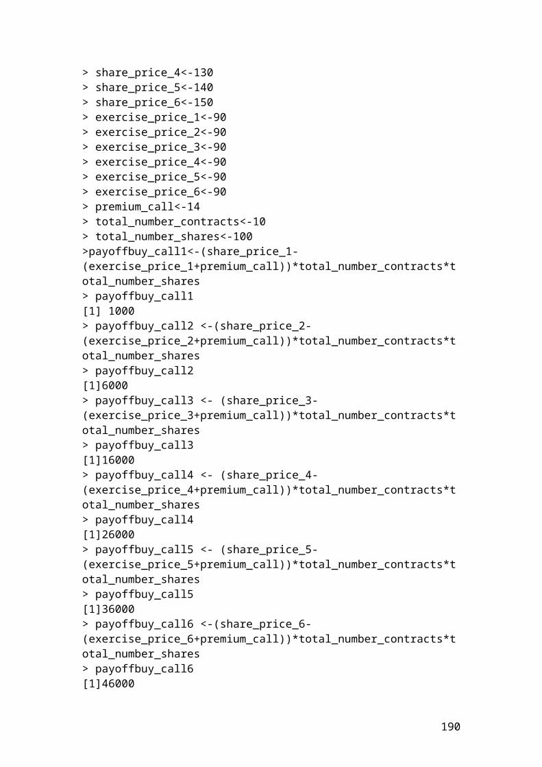
Annulaized swap rate = 6.788%or 06788.090/360*01697.0
The swaption is in the money because the exercise price 7.50% is greater than the market annualized swap rate 6.788%.
The net cash flow is as follows:
netCashFlow = (0.075 – 0.06788)*90/360 * 30000000 = 53400 USD
The value of swaption at maturity is as follows:
valueSwaption = 53400 *( 934579.0956938.0973236.0990099.0 ) = 205,849.1 USD
Application of swaption in R
> principal = 30000000> exercise_rate = 0.075> rate90 = 0.04> rate180 = 0.055> rate270 = 0.06> rate360 = 0.07> # Insert the mathematical formulas.> PV90 = 1 /(1+(rate90 * 90/360))> PV90[1] 0.9900990099009901> PV180 = 1/(1+(rate180 * 180/360))> PV180[1] 0.97323600973236> PV270 = 1/(1+(rate270 * 270/360))> PV270[1] 0.9569377990430623> PV360 = 1/(1+(rate360* 360/360))> PV360[1] 0.9345794392523364> semiAnnualRate = (1-PV360)/(PV90 +PV180 +PV270 +PV360)> semiAnnualRate[1] 0.01697096448070222> round(semiAnnualRate ,digits=5)0.01697> annualizedSwapRate = semiAnnualRate * (360/90)> annualizedSwapRate[1] 0.06788385792280888> round(annualizedSwapRate, digits=5)0.06788
Please repeat the above swaption problem in python and calculate the net cash flow and the value of swaption at maturity.
190
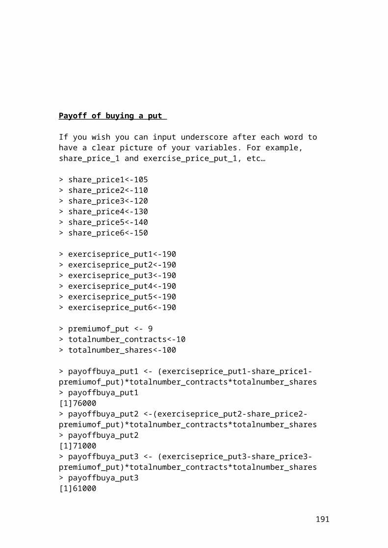
Put –call parity
The put – call parity shows the relationship between a call and a put option with the same expiration, strike and share prices. The mathematical formula is as follows:
option.put theand call both thefor price share theis S .expirationor maturity to time theis T
rate. free-rsik theis r call. theandput both the of price strike theis X
put. theof price theis P call. theof price theis C :
)1(
f
Where
SPrfXC T
Example
Calculate the price of a call if the price of a put is 5.34 Pounds, the share price is 94, the strike price is 97, the risk-free rate is 4% and the time to maturity, T=0.5. By rearranging formula (20) and solving for the price of a call, we have the following results:
Application of put - call parity in R
> put <- 5.34> share_price <- 94> strike_price <- 97> dis_risk_free_rate <-1.04> maturity <- 0.5> # Insert the mathematical formula.> call <- put + share_price - strike_price /(dis_risk_free_rate**maturity)> call4.223674457980749> round(call,digits=2)[1] 4.22 # Pounds
191
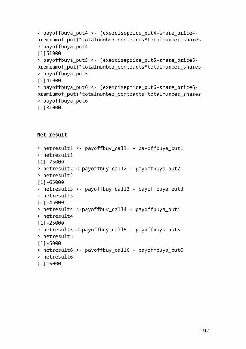
Example of margin payments in the clearinghouse
An investor open a margin account with a minimum initial margin of 5,200 dollars per contract. The maintenance margin is 1,500 dollars per contract. He/she buys 7 July wheat futures contracts with a standard contract size of 200 bushels priced at 230 dollars per bushel. The July contract size in the next 2 days recorded the prices of 220 and 210 dollars per bushel. Show the cash flows, gains and losses for the buyer and the seller?
Solution
Initial margin = 7 x 5,200 = 36,400 dollars
Maintenance margin = 7 x 1,500 = 10,500 dollars
The cash flows, gains and losses for the next two days will be as follows:
Day 1
Cash flows for the buyer’s: 36,400 + 14,000 = 50,400 dollars. The investor’s recorded a gain.
Cash flows for the seller’s: 36,400 – 14,000 = 22,400 dollars. The investor’s recorded a loss.
Helpful hint: the amount of 14,000 is calculated from the difference of the bushel prices, (fT-f0) x number of contracts x standard contract size. Thus, we have: (220-230) x 7 x 200 = (14,000 dollars). The same principle applies for the second day but with different bushel prices. Thus, we have: (210 – 230) x 7 x 200 = (28000 dollars). Gains or losses depends if you are the buyer or seller.
Day 2
Please do the calculations for the second day.
This is why I am stressing the importance that the investors should buy or sell ONLY when the market is aggressively increasing or falling. If he/she gets trapped in a market that is not strong bull or bear, then, he/she will have to compensate regularly for the losses or he/she will experience a very small profit. If the amounts as the days passes is below the maintenance margin, then, the investor’s will receive a margin call and he/she should add the capital required to proceed with the contract. If the investor’s is short of money, then, the position is closed with the incurred losses.
192
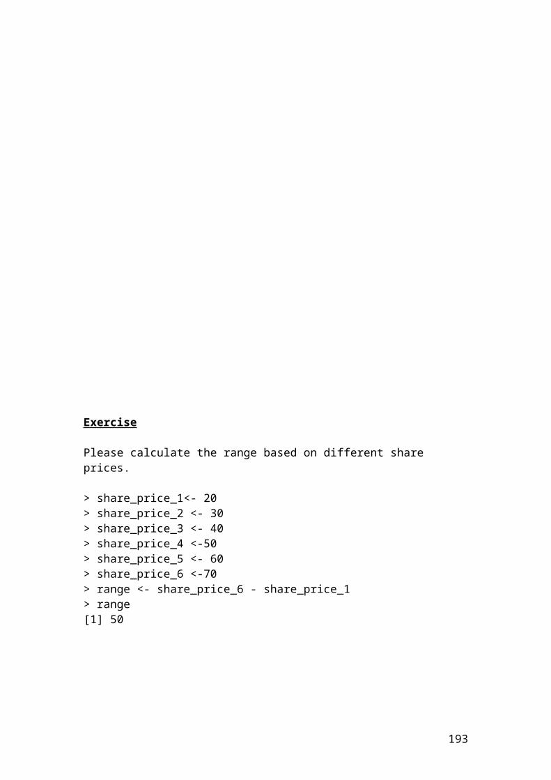
Application of margin payments in the clearinghouse in R
> initial_margin <- 5200> maintenance_margin <- 1500> contract_number <- 7> bushel_contract_size <- 200> bushel_price_1 <- 230> bushel_price_2 <- 220> # Insert the mathematical formulas.> initial_margin_with_contract <- initial_margin * contract_number> initial_margin_with_contract[1] 36400 # USD> maintenance_margin_with_contract <- maintenance_margin * contract_number> maintenance_margin_with_contract[1] 10500 # USD> bushel_contract <- (bushel_price_1-bushel_price_2) * bushel_contract_size * contract_number> bushel_contract[1] 14000 # USD> cash_flow_buyer <- initial_margin_with_contract + bushel_contract> cash_flow_buyer[1] 50400 # USD> cash_flow_seller <- initial_margin_with_contract – bushel_contract> cash_flow_seller[1] 22400 # USD
Please continue the calculations for the second day….
193
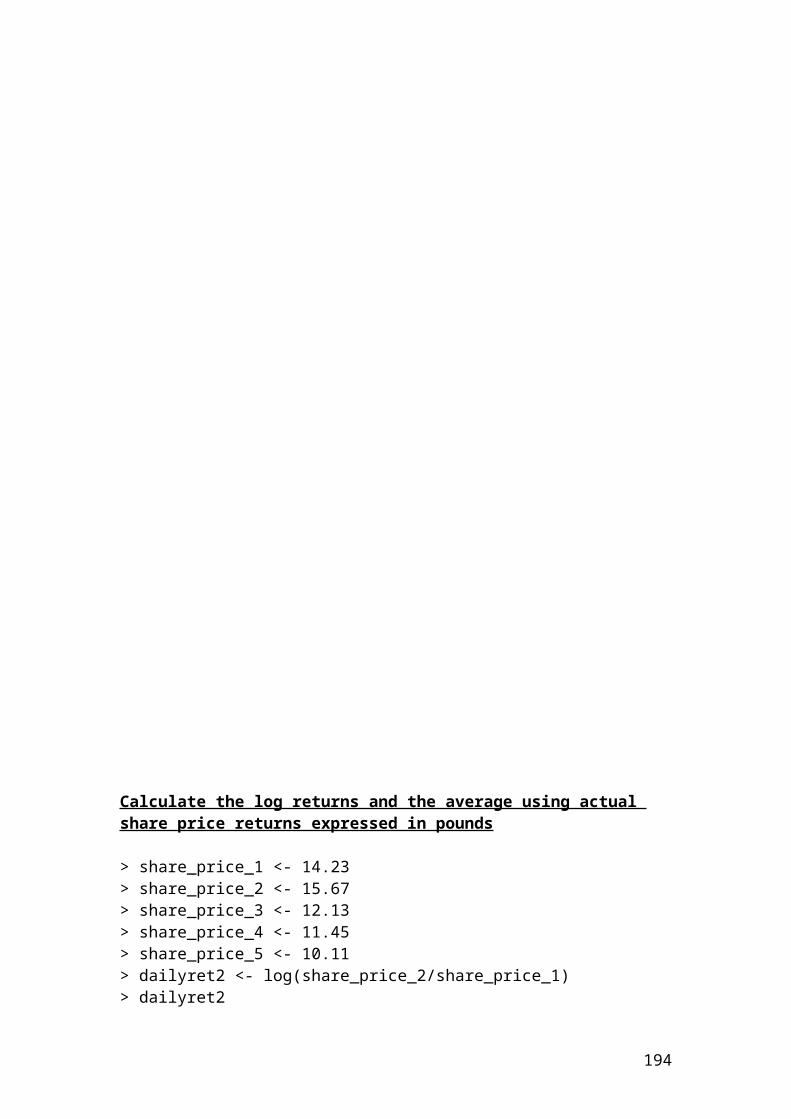
Example of calculating a margin call due to changes of price futures
An investor has opened a short position of 20 Soybean futures contract. The initial margin was 500 Pounds and the maintenance margin was 430 Pounds per contract. The price change that will create a margin call is as follows:
Solution
20
430- 500 sizecontract
margin emaintenanc -margin initial price aat created callMargin 3.5
Pounds
Application of margin call in R
> initial_margin <- 500> maintenance_margin <- 430> futures_contract <- 20> # Insert the mathematical formula.> margin_call <-(initial_margin-maintenance_margin) / futures_contract> margin_call[1] 3.5 # Pounds
194
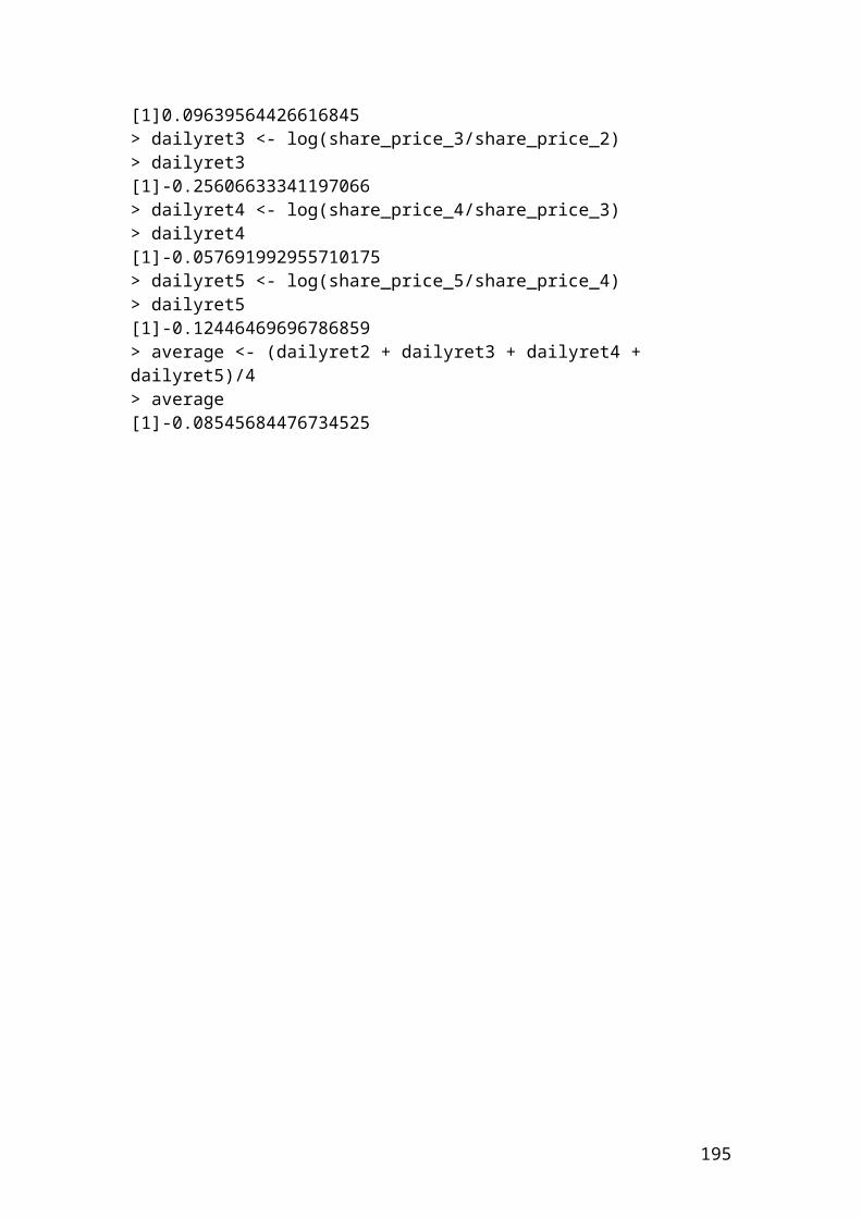
Solution of the above examples
Active return, active risk and information ratio
Active return is the difference in returns between a portfolio and the index or benchmark that is measured.
Active return = rp - rb
Where: rp is the portfolio return. rb is the benchmark or index return.
If the portfolio return is 0.80 and the benchmark return of the index is 0.70 then, the active return is………
Please complete the calculation.
Application of active return in R
> portfolio_return <- 0.8> benchmark_return <- 0.7> active_return <- portfolio_return - benchmark_return> active_return[1] 0.10000000000000009> round(active_return,digits=2)[1] 0.1
195
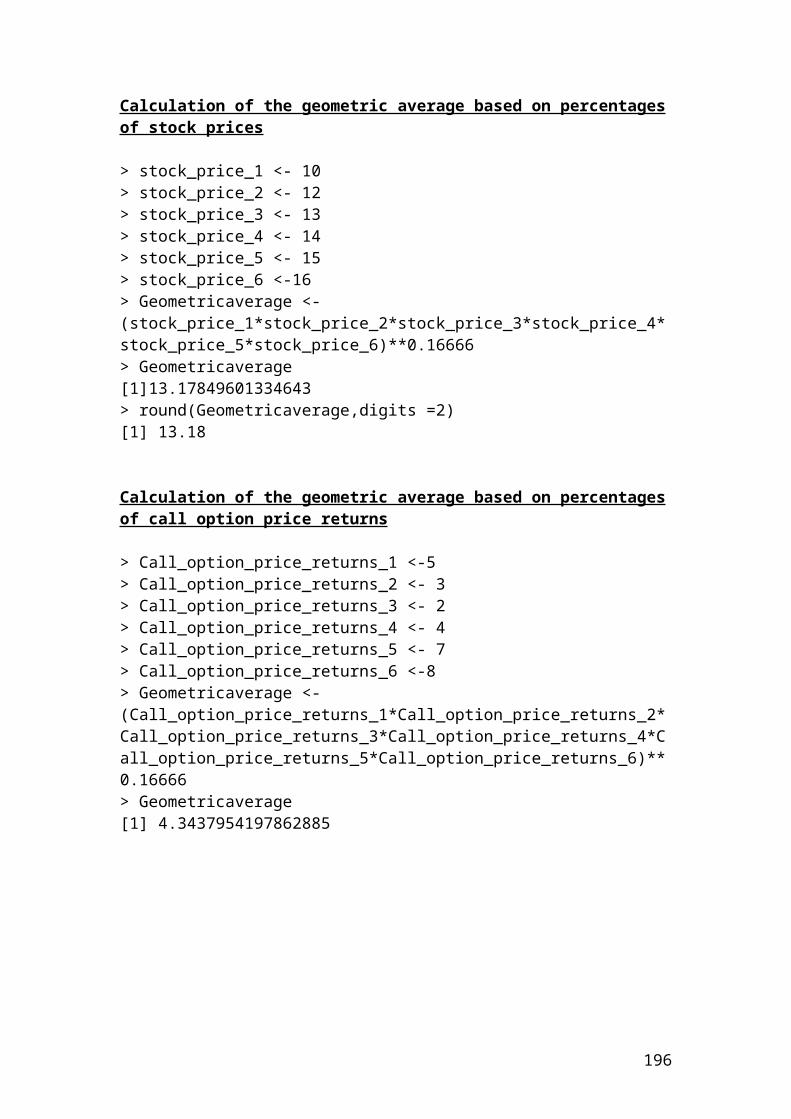
Active risk or tracking error is the standard deviation of the difference of returns between a portfolio and the benchmark or index.
ns.observatioor assets ofnumber theisn index.an examplefor be couldIt return.benchmark portfolio is r
return. portfolio is r :
1
)(r risk
b
p
2p
Wheren
rActive b
If the portfolio return is 0.80, the number of observations is 10 and the benchmark return of the index is 0.40 then, the active risk is………
Please complete the calculation.
Application of active risk in R
> portfolio_return <- 0.80> benchmark_return <- 0.40> n <-10> # Insert the mathematical formula.> active_risk <- sqrt((portfolio_return - benchmark_return)**2/9)> active_risk[1] 0.13333333333333336> round(active_risk,digits=2)[1] 0.13
196
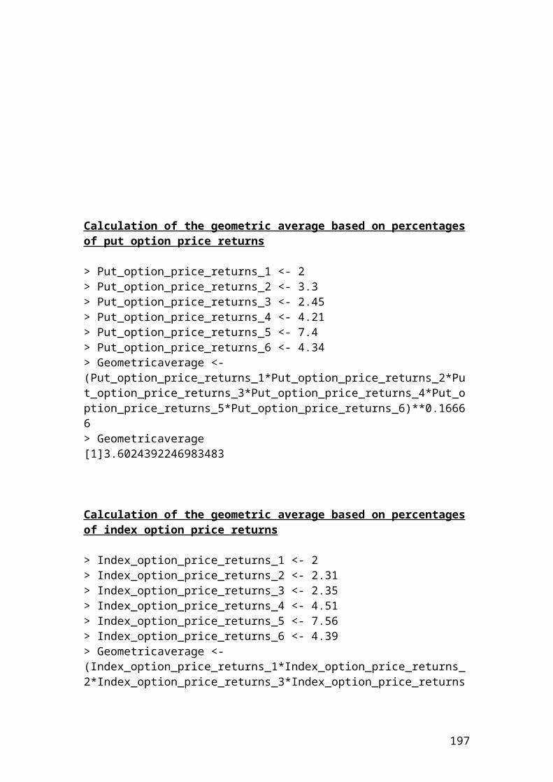
Information ratio shows the consistency of the fund manager towards the active return. The mathematical formula is as follows:
risk active theis
1
return.index or benchmark average theis r
return. portfolio of average theis :
1)(r
2
b
2p
nrr
rWhere
nr
rrIR
bp
p
b
bp
It could be calculated very easily in Excel software. I will illustrate a simple table with the relevant calculations.
Day rp rb rp - rb
1 0.03 0.02 0.012 0.02 0.014 0.0063 -0.04 0.034 -0.0744 0.05 0.067 -0.0175 0.08 0.012 0.0686 -0.01 -0.056 0.0467 0.07 0.031 0.0398 0.034 0.023 0.0119 -0.021 0.015 -0.03610 0.045 0.001 0.044
Average 0.0258 0.0161Standard deviation
0.043
Source: author’s calculation
By substituting the values that we have found in terms of rp =0.0258, rb = 0.0161 and standard deviation = 0.043 in the following equation we have:
1)(r 2
p
n
r
rrR
b
bp
2d.p.) (to 23.0043.0
0097.0043.0
0161.00258.0
R
197
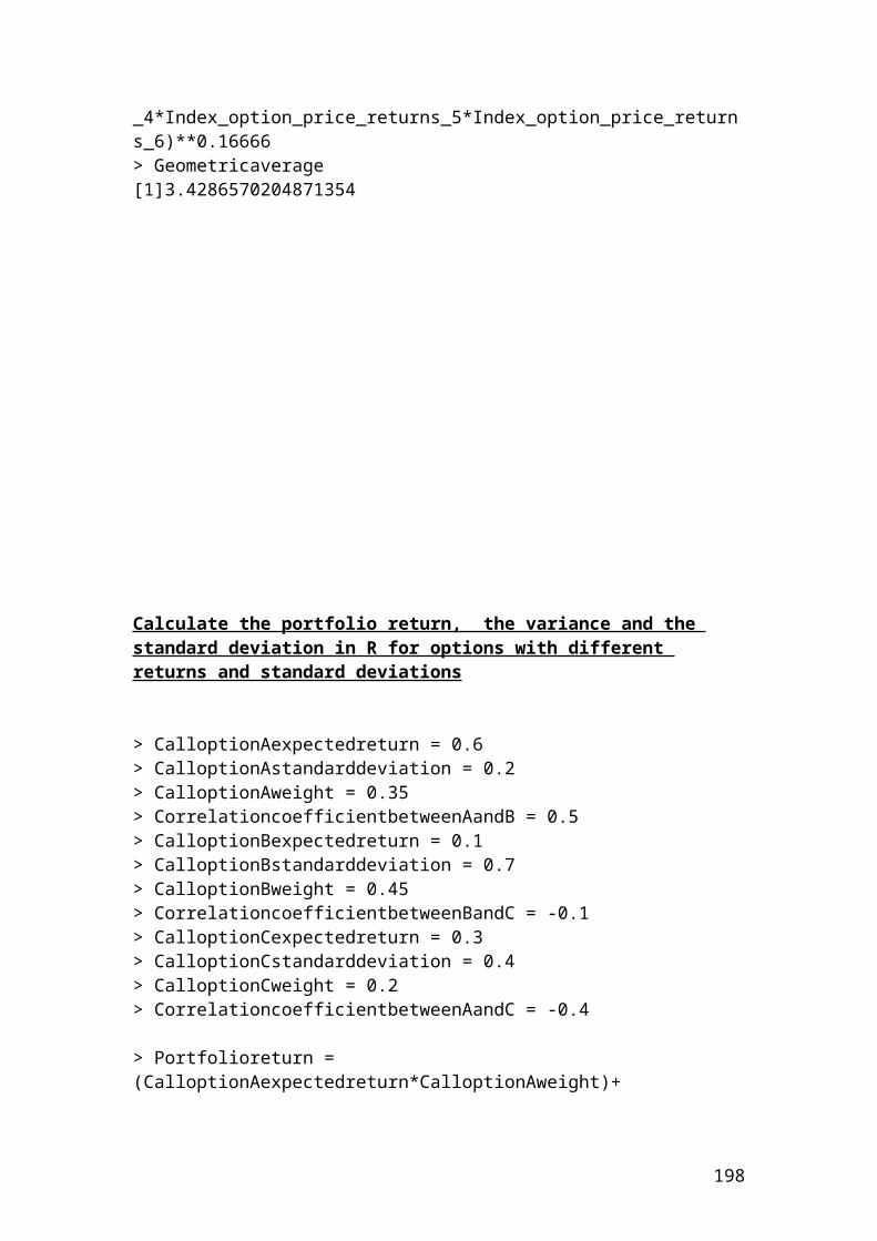
But what is the interpretation of the information ratio of 0.23. It means that the fund manager gained around 23 basis points of active return per unit of active risk. The higher is this number, the better the manager is performing in relation to active risk.
Application of information ratio in R
> portfolio_return1 = 0.03> portfolio_return2 = 0.02> portfolio_return3 = -0.04> portfolio_return4 = 0.05> portfolio_return5 = 0.08> portfolio_return6 = -0.01> portfolio_return7 = 0.07> portfolio_return8 = 0.034> portfolio_return9 = -0.021> portfolio_return10 = 0.045> # Insert the mathematical formula.> average_1 = (portfolio_return1 + portfolio_return2 + portfolio_return3 + portfolio_return4 + portfolio_return5 + portfolio_return6+ portfolio_return7 + portfolio_return8 + portfolio_return9+ portfolio_return10)/10> average_1[1] 0.0258> benchmark_return1 = 0.02> benchmark_return2 = 0.014> benchmark_return3 = 0.034> benchmark_return4 = 0.067> benchmark_return5 = 0.012> benchmark_return6 = -0.056> benchmark_return7 = 0.031> benchmark_return8 = 0.023> benchmark_return9 = 0.015> benchmark_return10 = 0.001> average_2 = (benchmark_return1 + benchmark_return2 + benchmark_return3 + benchmark_return4 + benchmark_return5 + benchmark_return6 + benchmark_return7 + benchmark_return8 + benchmark_return9+ benchmark_return10)/10> average_2[1] 0.016100000000000003># Insert the mathematical formulas to calculate the differences between the portfolioand benchmark return and then square it.> diff1 = portfolio_return1 - benchmark_return1> diff1[1] 0.009999999999999998> diff2 = portfolio_return2 - benchmark_return2> diff2[1] 0.006> diff3 = portfolio_return3 - benchmark_return3> diff3[1] -0.07400000000000001> diff4 = portfolio_return4 - benchmark_return4> diff4
198
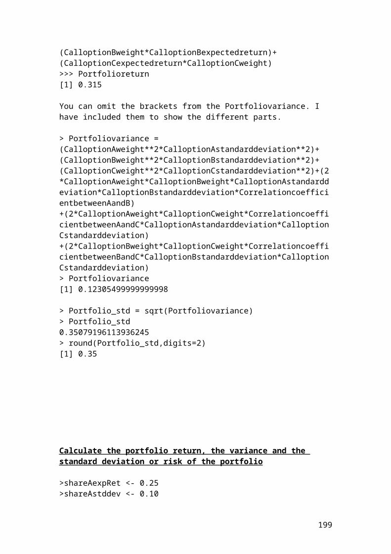
[1] -0.017> diff5 = portfolio_return5 - benchmark_return5> diff5[1] 0.068> diff6 = portfolio_return6 - benchmark_return6> diff6[1] 0.046> diff7 = portfolio_return7 - benchmark_return7> diff7[1] 0.03900000000000001> diff8 = portfolio_return8 - benchmark_return8> diff8[1] 0.011000000000000003> diff9 = portfolio_return9 - benchmark_return9> diff9[1] -0.036000000000000004> diff10 = portfolio_return10 - benchmark_return10> diff10[1] 0.044> #Find the sum from the differences.> sumDiff = diff1 + diff2 + diff3 + diff4 + diff5 + diff6 + diff7 + diff8 +diff9 +diff10> sumDiff[1] 0.09699999999999999># Find the average from the differences.> average3 = sumDiff /10> average3[1] 0.009699999999999999
Please complete the exercise……. If you have questions, then, please let me know.
199
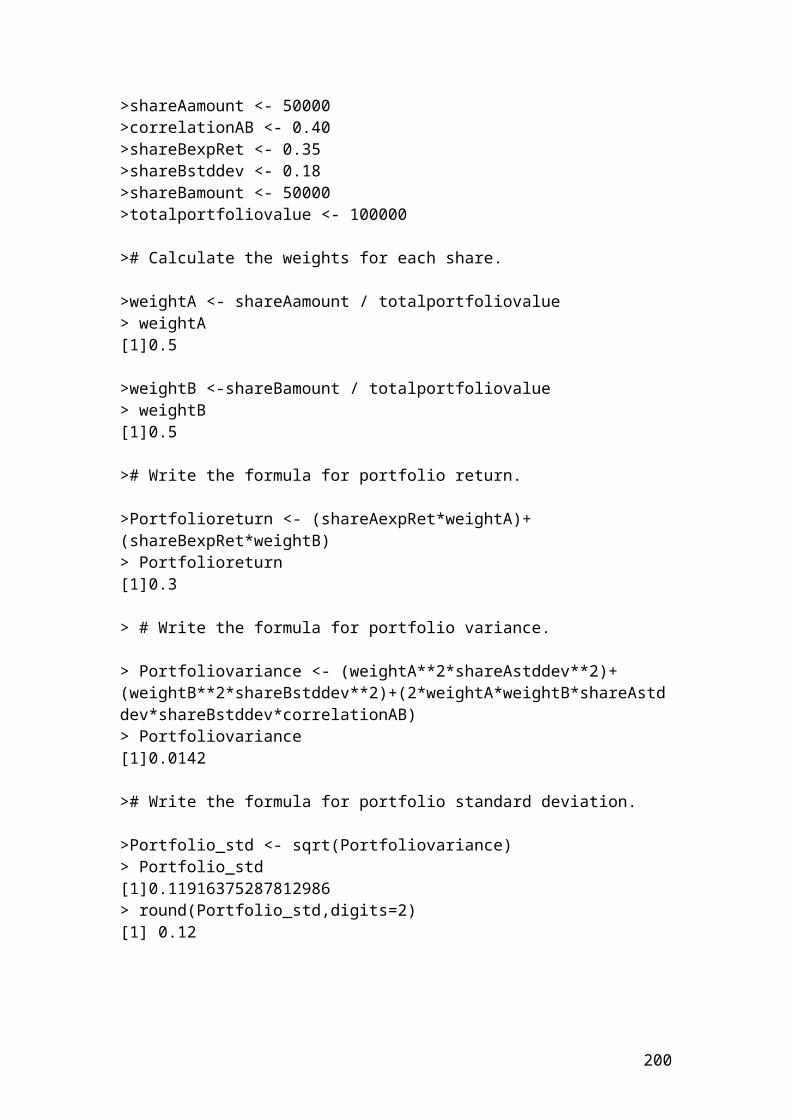
Please convert the following exercise in R language programming
Calculate the balance at the end of the 5th day from changes in the futures prices from 90 to 89, 91, 95, 97, 99. The trader has bought 50 futures contract for settlement in May. The initial margin is $8.
Day Beginning balance
Futures price Gain or loss Ending balance
0 400 90 0 4001 400 89 (50)2 350 91 1003 450 95 2004 650 97 1005 750 99 100
Source: author’s illustration.
Beginning balance = initial margin x number of contracts.Beginning balance = 8 x 50 = $400
Please complete the values of the column ending balance.
Solution
Day Beginning balance
Futures price Gain or loss Ending balance
0 400 90 0 4001 400 89 (50) 3502 350 91 100 4503 450 95 200 6504 650 97 100 7505 750 99 100 850
The ending balance at the 5th day in the margin account will be 850 USD.
200
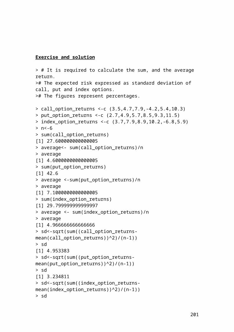
Calculate the caplet option payments based on different interest rates using a binomial 2 steps tree. The figures are expressed in pounds
> # Calculate the caplet values based on an interest rate cap using a binomial 2 steps tree. It is a similar example of a call option on interest rates. The payment is based on the difference between the current interest rate and the cap rate multiplied by the principal and divided by the discounted current interest rate. The buyer receives a payment when the current interest rate exceeds the cap strike price.
> strike <-0.02> principal <- 30000000> maturity <- 0.5> sigma <- 0.3> interest_rate <- 0.04> n <-2> p<-0.5> # Insert the mathematical formulas.> dt <- maturity/n # steps expressed in years.> dt[1] 0.25> u <- exp(sigma*sqrt(dt)) # multiplier of upmove.> u[1] 1.161834242728283> d <- 1/u # multiplier of downmove.> d[1] 0.8607079764250578># Identify the interest rates in each node.> interest_0 <- 0.04> interest_1i <- 0.0465> interest_1ii <- 0.0344> interest_2i <- 0.054> interest_2ii <- 0.04> interest_2iii <- 0.0296> #Identify the discounted interest rates.> disinterest_0 <- 1.04> disinterest_1i <- 1.0465> disinterest_1ii <- 1.0344> disinterest_2i <- 1.054> disinterest_2ii <- 1.04> disinterest_2iii <- 1.0296># Insert the mathematical formulas. It is a backward induction methodology.> capletPrice2i <- (principal*(interest_2i-strike)/disinterest_2i)> capletPrice2i[1] 967741.935483871> capletPrice2ii <- (principal*(interest_2ii-strike)/disinterest_2ii)> capletPrice2ii
201
[1] 576923.0769230769> capletPrice2iii <- (principal*(interest_2iii-strike)/disinterest_2iii)> capletPrice2iii[1] 279720.2797202797> capletPrice1i <- (((capletPrice2i*p)+(capletPrice2ii*p))/disinterest_1i)> capletPrice1i[1] 738014.8172035108> capletPrice1ii <- (((capletPrice2ii*p)+(capletPrice2iii*p))/disinterest_1ii)> capletPrice1ii[1] 414077.415237508> capletPrice0 <- (((capletPrice1i*p)+(capletPrice1ii*p))/disinterest_0)> capletPrice0[1] 553890.4963658744> round(capletPrice0,digits=1)[1] 553890.5
202
Calculate the floorlet option payments based on different interest rates using a binomial 2 steps tree. The figures are expressed in pounds
> # Calculate the floorlet values based on an interest rate floor using a binomial 2 steps tree. It is a similar example of a put option on interest rates. It protects the holder from declining interest rates. The payment is based on the difference between the floor rate and the current interest rate multiplied by the principal and divided by the discounted current interest rate.
> strike <- 0.02> principal <- 30000000> maturity <- 0.5> sigma <- 0.3> interest_rate <- 0.04> n <-2> p<-0.5> # Insert the mathematical formulas.> dt <- maturity/n # steps expressed in years.> dt[1] 0.25> from math import*> u <- exp(sigma*sqrt(dt)) # multiplier of upmove.> u[1] 1.161834242728283> d <-1/u # multiplier of downmove.> d[1] 0.8607079764250578># Identify the interest rates in each node.> interest_0 <- 0.04> interest_1i <- 0.0465> interest_1ii <- 0.0344> interest_2i <- 0.054> interest_2ii <- 0.04> interest_2iii <- 0.0296># Identify the discounted interest rates.> disinterest_0 <- 1.04> disinterest_1i <- 1.0465> disinterest_1ii <- 1.0344> disinterest_2i <- 1.054> disinterest_2ii <- 1.04> disinterest_2iii <- 1.0296># Insert the mathematical formulas. It is a backward induction methodology.> floorletPrice2i <- (principal*(strike - interest_2i)/disinterest_2i)> floorletPrice2i[1] 56925.99620493363> floorletPrice2ii <- (principal*(strike - interest_2ii)/disinterest_2ii)
203
> floorletPrice2ii[1] 461538.4615384615> floorletPrice2iii <- (principal*(strike - interest_2iii)/disinterest_2iii)> floorletPrice2iii[1] 769230.7692307691> floorletPrice1i <- (((floorletPrice2i*p)+(floorletPrice2ii*p))/disinterest_1i)> floorletPrice1i[1] 247713.5488501649> floorletPrice1ii <- (((floorletPrice2ii*p)+(floorletPrice2iii*p))/disinterest_1ii)> floorletPrice1ii[1] 594919.3884228686> floorletPrice0 <- (((floorletPrice1i*p)+(floorletPrice1ii*p))/disinterest_0)> floorletPrice0[1] 405111.9890735737> round(floorletPrice0,digits=2)[1] 405111.99
204
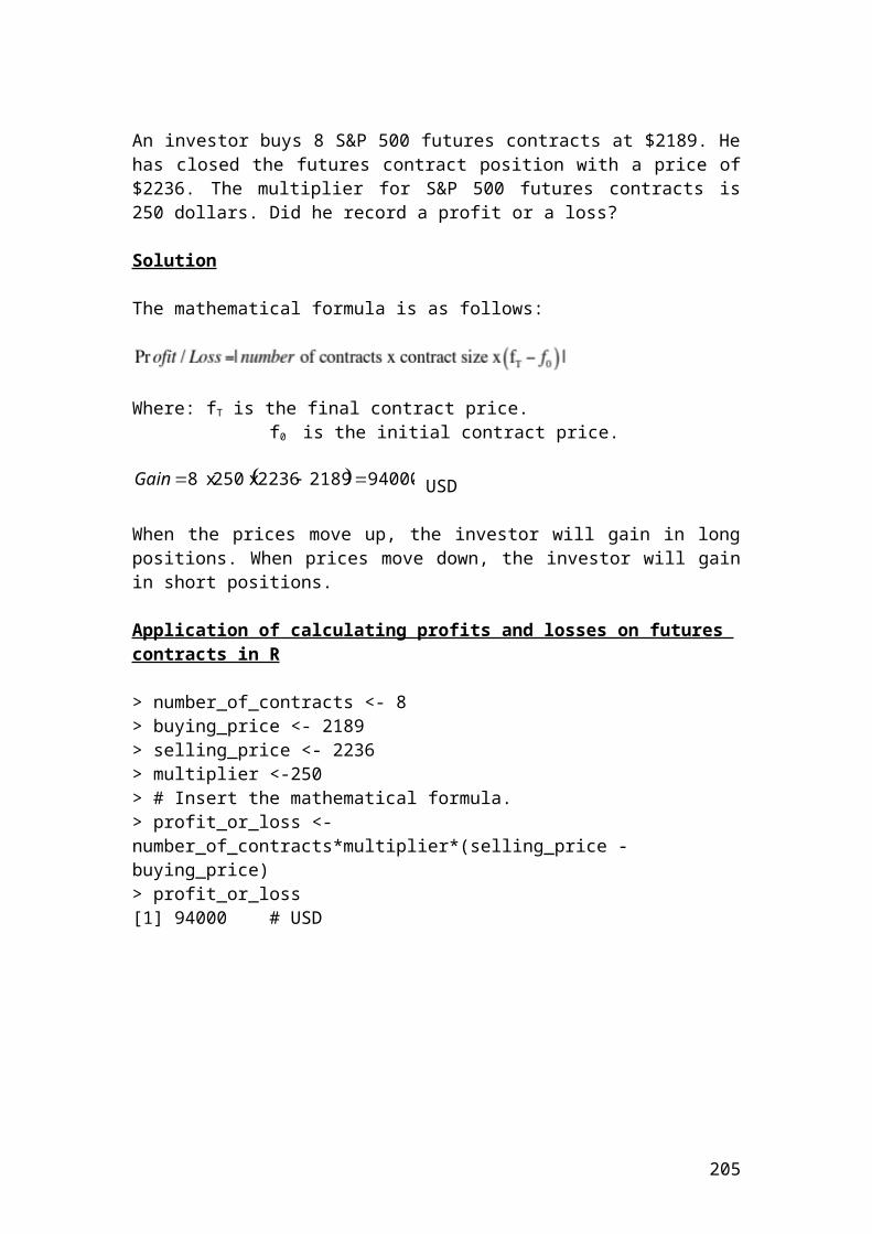
Calculate the bond put option prices based on different interest rates using a binomial 2 steps tree
> bond_price <- 100> strike <- 102> annual_coupon <- 7> maturity <- 0.5> sigma <- 0.3> interest_rate <- 4> n <-2> p <- 0.5> dt <- maturity/n # steps expressed in years.> dt[1] 0.25> u <- exp(sigma*sqrt(dt)) # multiplier of upmove.> u[1] 1.161834242728283> d <- 1/u # multiplier of downmove.> d[1] 0.8607079764250578># Insert the mathematical formulas. It is a backward induction methodology.> bondPrice2i <- (bond_price+annual_coupon)*(1/disinterest_2i)> bondPrice2i[1] 101.5180265654649> bondPrice2ii<-(bond_price+annual_coupon)*(1/disinterest_2ii)> bondPrice2ii[1] 102.88461538461537> bondPrice2iii <- (bond_price+annual_coupon)*(1/disinterest_2iii)> bondPrice2iii[1] 103.92385392385391> bondPrice1i <- ((((bondPrice2i+annual_coupon)*p)+(bondPrice2ii+annual_coupon)*p)/disinterest_1i)> bondPrice1i[1] 104.3490883660202> bondPrice1ii <- ((((bondPrice2ii+annual_coupon)*p)+(bondPrice2iii+annual_coupon)*p)/disinterest_1ii)> bondPrice1ii[1] 106.73263210966226> bondPrice0 <- ((((bondPrice1i+ annual_coupon)*p)+(bondPrice1ii+ annual_coupon)*p)/disinterest_0)> bondPrice0[1] 108.21236561330888
205
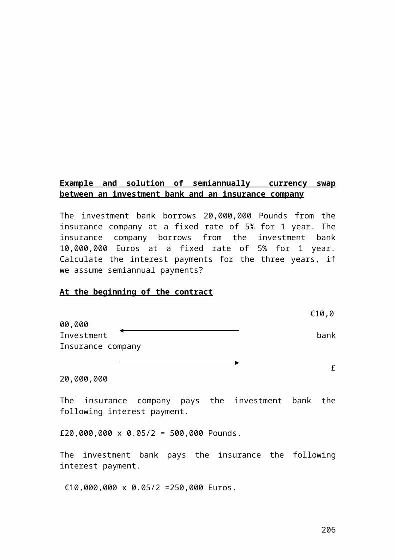
> putPriceUpmovestep2i <- strike - bondPrice2i> putPriceUpmovestep2i[1] 0.48197343453510655> putPriceUpdownmovestep2ii <- strike - bondPrice2ii> putPriceUpdownmovestep2ii[1] -0.8846153846153726> putPriceUpdownmovestep2ii <- 0> putPriceUpdownmovestep2ii[1] 0> putPriceDownmovestep2iii <- strike - bondPrice2iii> putPriceDownmovestep2iii[1]-1.9238539238539119> putPriceDownmovestep2iii <-0> putPriceDownmovestep2iii[1]0> putPriceUpmovestep1i<- (((putPriceUpmovestep2i*p)+(putPriceUpdownmovestep2ii*p))/disinterest_1i)> putPriceUpmovestep1i[1]0.2302787551529415> putPriceDownmovestep1ii<- (((putPriceUpdownmovestep2ii*p)+(putPriceDownmovestep2iii*p))/disinterest_1ii)> putPriceDownmovestep1ii[1]0.0> putPricestep0<- (((putPriceUpmovestep1i*p)+(putPriceDownmovestep1ii*p))/disinterest_0)> putPricestep0[1]0.11071093997737572
206
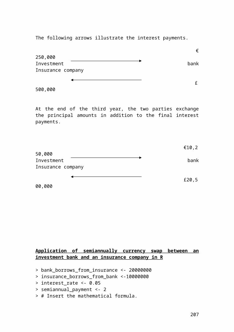
Calculate the bond call option prices based on different interest rates using a binomial 2 steps tree. The figures are expressed in pounds
> bond_price <- 100> strike <- 100> annual_coupon <- 7> maturity <- 0.5> sigma <- 0.3> interest_rate <- 4> n <-2> p <-0.5> dt <- maturity/n # steps expressed in years.> dt[1] 0.25> u <- exp(sigma*sqrt(dt)) # multiplier of upmove.> u[1] 1.161834242728283> d <- 1/u # multiplier of downmove.> d[1] 0.8607079764250578> #Identify the discounted interest rates.> disinterest_0 <- 1.04> disinterest_1i <- 1.0465> disinterest_1ii <- 1.0344> disinterest_2i <- 1.054> disinterest_2ii <- 1.04> disinterest_2iii <- 1.0296># Insert the mathematical formulas. It is a backward induction methodology.> bondPrice2i <- (bond_price+annual_coupon)*(1/disinterest_2i)> bondPrice2i[1] 101.5180265654649> bondPrice2ii<-(bond_price+annual_coupon)*(1/disinterest_2ii)> bondPrice2ii[1] 102.88461538461537> bondPrice2iii <- (bond_price+annual_coupon)*(1/disinterest_2iii)> bondPrice2iii[1] 103.92385392385391> bondPrice1i <- ((((bondPrice2i+annual_coupon)*p)+(bondPrice2ii+annual_coupon)*p)/disinterest_1i)> bondPrice1i[1] 104.3490883660202> bondPrice1ii <- ((((bondPrice2ii+annual_coupon)*p)+(bondPrice2iii+annual_coupon)*p)/disinterest_1ii)> bondPrice1ii[1] 106.73263210966226> bondPrice0 <- ((((bondPrice1i+ annual_coupon)*p)+(bondPrice1ii+ annual_coupon)*p)/disinterest_0)> bondPrice0
207
[1] 108.21236561330888> callPriceUpmovestep2i <- bondPrice2i - strike> callPriceUpmovestep2i[1] 1.5180265654648935> callPriceUpdownmovestep2ii <- bondPrice2ii - strike> callPriceUpdownmovestep2ii[1] 2.8846153846153726> callPriceDownmovestep2iii <- bondPrice2iii - strike> callPriceDownmovestep2iii[1] 3.923853923853912> callPriceUpmovestep1i<- (((callPriceUpmovestep2i*p)+(callPriceUpdownmovestep2ii*p))/disinterest_1i)> callPriceUpmovestep1i[1] 2.103507859570122> callPriceDownmovestep1ii<- (((callPriceUpdownmovestep2ii*p)+(callPriceDownmovestep2iii*p))/disinterest_1ii)> callPriceDownmovestep1ii[1] 3.291023447635965> callPricestep0<- (((callPriceUpmovestep1i*p)+(callPriceDownmovestep1ii*p))/disinterest_0)> callPricestep0[1] 2.5935246669260033> round(callPricestep0,digits=2)[1] 2.59
208
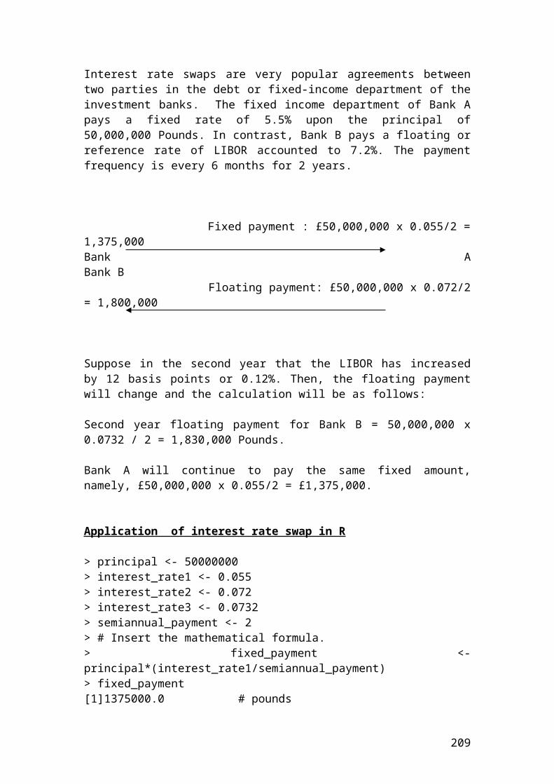
Calculate the bond prices of an option based on different interest rates using a binomial 2 steps tree. The figures are expressed in pounds
> bond_price <- 100> strike <- 100> annual_coupon <- 7> maturity <- 0.5> sigma <- 0.3> interest_rate <- 4> n <-2> p <- 0.5> dt <- maturity/n # steps expressed in years.> dt[1] 0.25> u <- exp(sigma*sqrt(dt)) # multiplier of upmove.> u[1] 1.161834242728283> d <- 1/u # multiplier of downmove.> d[1] 0.8607079764250578> #Identify the discounted interest rates.> disinterest_0 <- 1.04> disinterest_1i <- 1.0465> disinterest_1ii <- 1.0344> disinterest_2i <- 1.054> disinterest_2ii <- 1.04> disinterest_2iii <- 1.0296># Insert the mathematical formulas. It is a backward induction methodology.> bondPrice2i <- (bond_price+annual_coupon)*(1/disinterest_2i)> bondPrice2i[1] 101.5180265654649> bondPrice2ii <-(bond_price+annual_coupon)*(1/disinterest_2ii)> bondPrice2ii[1] 102.88461538461537> bondPrice2iii <- (bond_price+annual_coupon)*(1/disinterest_2iii)> bondPrice2iii[1] 103.92385392385391> bondPrice1i <- ((((bondPrice2i+annual_coupon)*p)+(bondPrice2ii+annual_coupon)*p)/disinterest_1i)> bondPrice1i[1] 104.3490883660202> bondPrice1ii <- ((((bondPrice2ii+annual_coupon)*p)+(bondPrice2iii+annual_coupon)*p)/disinterest_1ii)> bondPrice1ii[1] 106.73263210966226> bondPrice0 <- ((((bondPrice1i+ annual_coupon)*p)+(bondPrice1ii+ annual_coupon)*p)/disinterest_0)> bondPrice0[1] 108.21236561330888
209
210
Calculate the interest rates of an option bond based on a two – period binomial tree. The risk – neutral probability of an up and down move in the interest rate tree is always 50% or 0.5. The figures are expressed in percentages
> bond_price <-100> strike <- 100> annual_coupon <- 7> maturity <- 0.5> volatility <- 0.3> interest_rate <- 4> p<-0.5> n<-2>interestrate0 <- 4> interestrate1i <- interest_rate * u> interestrate1i[1] 4.647336970913132> interestrate1ii <- interest_rate * d> interestrate1ii[1] 3.4428319057002312> interestrate2i <- interest_rate * u**2> interestrate2i[1] 5.399435230304012> interestrate2ii<- interest_rate*u*d> interestrate2ii[1] 4.0> interestrate2iii<- interest_rate* d**2> interestrate2iii[1] 2.9632728827268715> round(interestrate2iii,digits=2)2.96
211
Calculate the share prices of a call option using a Cox, Ross, Rubinstein,(CRR) binomial 3 steps tree using a vector. The multipliers of up and down move depend on volatility and length of steps. The figures are expressed in pounds
S <- 60 # share price K <- 50 # strike price r <- 0.05 # interest rateq <- 0.02 # dividend yieldT <- 0.5 # maturitysig <- 0.3 # volatilityn <- 3> dt <- T/n> dt[1] 0.16666666666666666> u <- exp(sig*sqrt(dt))> u[1] 1.1302902827674572> d <- 1/u> d[1] 0.8847284766100544> share_price0 <- S> share_price0[1] 60> share_price_1upmove <- S*u> share_price1[1] 67.81741696604743> round(share_price1,digits=2)[1]67.82> share_price_1downmove <- S *d> share_price_1downmove[1] 53.083708596603266> share_price2upmove <- S *u**2> share_price2upmove[1] 76.6533673991123> share_price2downmove <- S*d**2> share_price2downmove[1] 46.96466863948485> share_price2upanddownmove <- S*u*d> share_price2upanddownmove[1] 60.0> share_price3downmove <- S*d**3> share_price3downmove41.55097973990743> share_price3upmove <- S*u**3> share_price3upmove[1] 86.64055631262043> share_price3updowndown <-S*u*d*d> share_price3updowndown[1] 53.083708596603266> share_price3upandupdown <- S*u*u*d
212
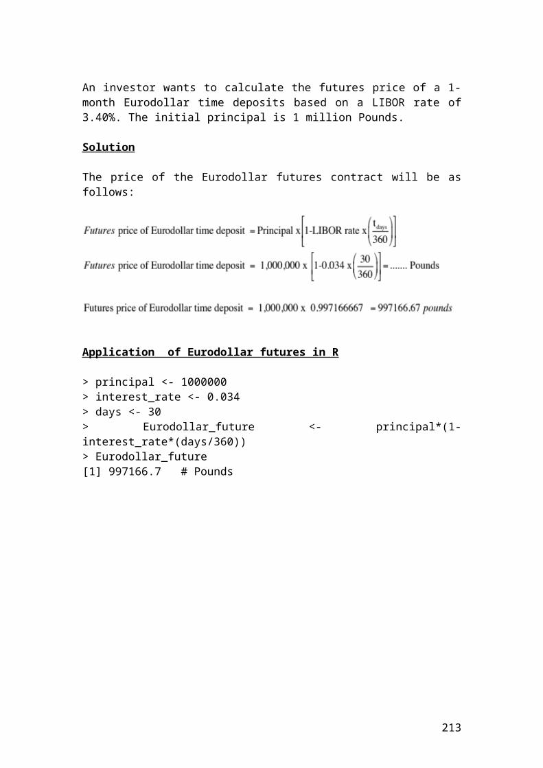
> share_price3upandupdown[1] 67.81741696604743
213
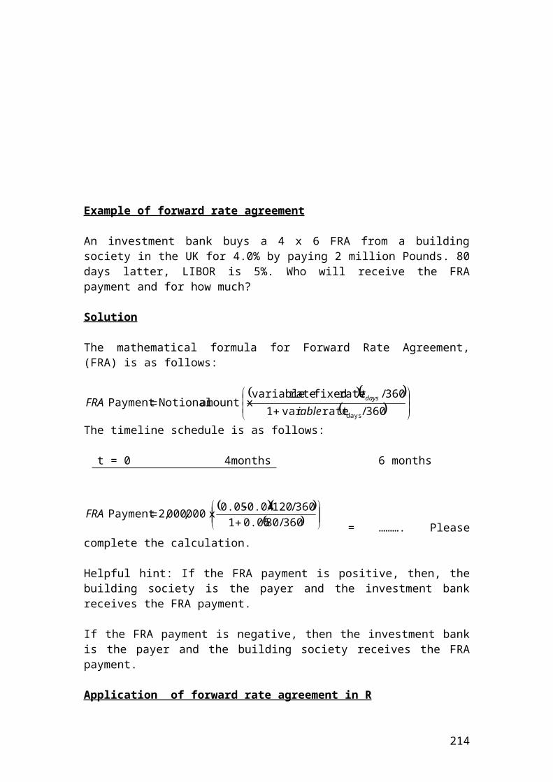
Calculate the call option prices using a Cox, Ross, Rubinstein,(CRR) binomial 3 steps tree. The figures are expressed in pounds
S <- 60 # share priceK <- 50 # strike pricer <- 0.05 # interest rateq <- 0.02 # dividend yieldT <- 0.5 # maturitysig <- 0.3 # volatilityn <- 3> dt <- T/n> dt[1] 0.16666666666666666> u <- exp(sig*sqrt(dt))> u[1] 1.1302902827674572> d <- 1/u> d[1] 0.8847284766100544> disfact <- exp(-r*dt)> disfact[1] 0.991701292638876> riskprobofupmove <- (exp((r-q)*dt)-d)/(u-d)> riskprobofupmove[1] 0.48983205544695174> #The option prices are calculated backwards.> callpayoffupmovestep3 <- S*u**3-K> callpayoffupmovestep3[1] 36.64055631262043> callpayoff3i <- S * u**2 * d -K> callpayoff3i[1] 17.817416966047432> callpayoff3ii <-S * d**2*u-K> callpayoff3ii[1] 3.083708596603259> callpayoffdownmovestep3 <- S*d**3-K> callpayoffdownmovestep3[1] -8.449020260092567> callpayoffdownmovestep3 <-0> callpayoffdownmovestep3[1] 0> callpriceupmovestep2 <- (disfact*(riskprobofupmove*callpayoffupmovestep3)+(1-riskprobofupmove)*callpayoff3i)> callpriceupmovestep2[1] 26.88865113426896> callpriceupdownmovestep2 <-(disfact*(riskprobofupmove*callpayoff3i)+(1-riskprobofupmove)*callpayoff3ii)> callpriceupdownmovestep2[1] 10.228323934729657
214
> callpricedownmovestep2 <-(disfact*(riskprobofupmove*callpayoff3ii)+(1-riskprobofupmove)*callpayoffdownmovestep3)> callpricedownmovestep2[1] 1.4979641284454819> callpriceupmovestep1 <- (disfact*(riskprobofupmove*callpriceupmovestep2)+(1-riskprobofupmove)*callpriceupdownmovestep2)> callpriceupmovestep1[1] 18.279784613543832>callpricedownmovestep1<-(disfact*(riskprobofupmove*callpriceupdownmovestep2)+(1-riskprobofupmove)*callpricedownmovestep2)> callpricedownmovestep1[1] 5.732796357703088> callpricestep0<- (disfact*(riskprobofupmove*callpriceupmovestep1)+(1-riskprobofupmove)*callpricedownmovestep1)> callpricestep0[1] 11.804406575946299>>> round(callpricestep0,digits=2)11.8
215
Calculate the put option prices using a Cox, Ross, Rubinstein,(CRR) binomial 3 steps tree. The figures are expressed in USD
> S <- 60 # share price> K <- 70 # strike price> r <- 0.02 # interest rate> q <- 0.03 # dividend yield> T <- 0.5 # maturity> sig <- 0.2 # volatility> n <- 3> dt <- T/n> dt[1] 0.16666666666666666> u <- exp(sig*sqrt(dt))> u[1] 1.0850755957772693> d <- 1/u> d[1] 0.9215947754162443> disfact <- exp(-r*dt)> disfact[1] 0.9966722160545233> riskprobofupmove <- (exp((r-q)*dt)-d)/(u-d)> riskprobofupmove[1] 0.46941253331873867> #The option prices are calculated backwards.> putpayoffupmovestep3 <- K-S*u**3> putpayoffupmovestep3[1] -6.653367399112284> putpayoffupmovestep3<-0> putpayoffupmovestep3[1] 0> putpayoff3i <- K- S * u**2 * d> putpayoff3i[1] 4.895464253363841> putpayoff3ii <-K- S * d**2*u> putpayoff3ii[1] 14.704313475025337> putpayoffdownmovestep3 <- K - S*d**3> putpayoffdownmovestep3[1] 23.035331360515137> putpriceupmovestep2 <- (disfact*(riskprobofupmove*putpayoffupmovestep3)+(1-riskprobofupmove)*putpayoff3i)> putpriceupmovestep2[1] 2.5974719764209926> putpriceupdownmovestep2 <-(disfact*(riskprobofupmove*putpayoff3i)+(1-riskprobofupmove)*putpayoff3ii)> putpriceupdownmovestep2[1] 10.092269491137635
216
> putpricedownmovestep2 <-(disfact*(riskprobofupmove*putpayoff3ii)+(1-riskprobofupmove)*putpayoffdownmovestep3)> putpricedownmovestep2[1] 19.101677490334147> putpriceupmovestep1 <- (disfact*(riskprobofupmove*putpriceupmovestep2)+(1-riskprobofupmove)*putpriceupdownmovestep2)> putpriceupmovestep1[1] 6.5700600829982925>putpricedownmovestep1<-(disfact*(riskprobofupmove*putpriceupdownmovestep2)+(1-riskprobofupmove)*putpricedownmovestep2)> putpricedownmovestep1[1] 14.85678328831304> putpricestep0<- (disfact*(riskprobofupmove*putpriceupmovestep1)+(1-riskprobofupmove)*putpricedownmovestep1)> putpricestep0[1] 10.956628441795559
217
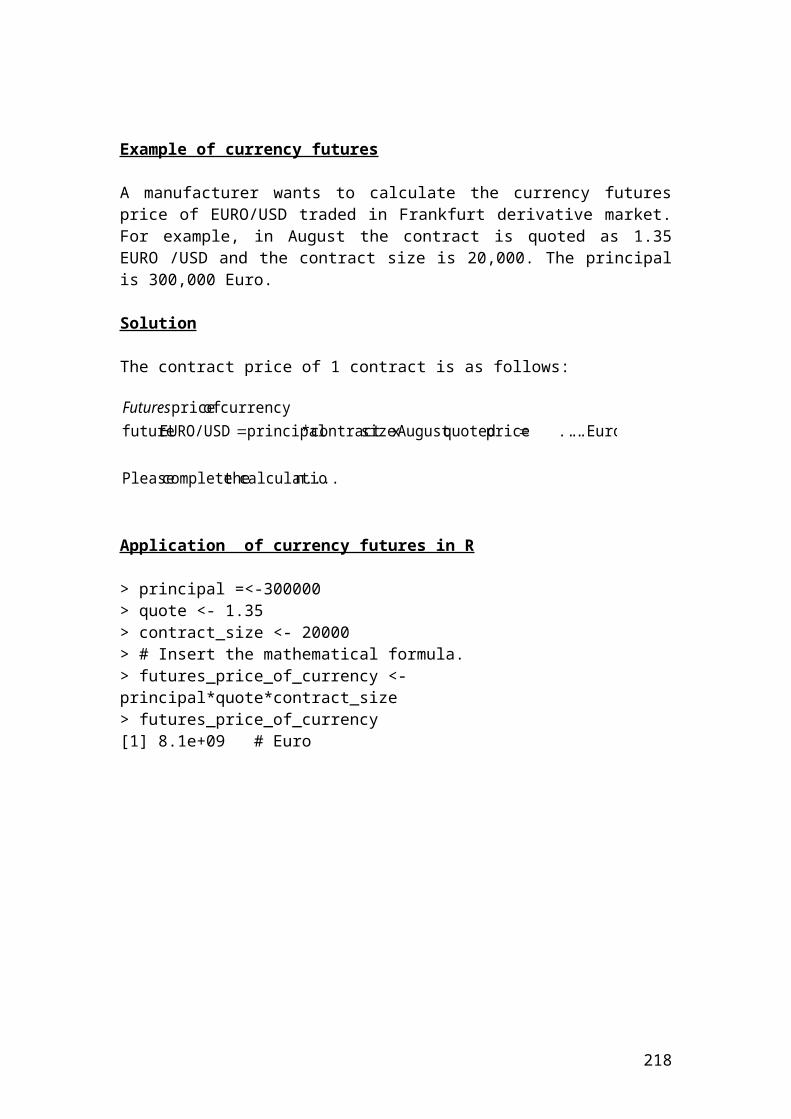
Calculation of a Monte Carlo put option using antithetic variables. The purpose of using antithetic variables is to improve the estimation results by reducing the standard error of the simulation results. The figures are expressed in USD
> number_of_simulation <- 199999> max_size <- 200000> initial_share_price <- 80> strike_price <- 110> interest_rate <- 0.07> dividend_yield <- 0.02> volatility <- 0.10> maturity <- 0.5> random.number <- (30000+3000)/300> random.number[1 110.0> sharePrice <- initial_share_price *exp((interest_rate-dividend_yield-0.5*volatility*volatility)*maturity*random.number*volatility *sqrt(maturity))> sharePrice[1] 95.30055> round(sharePrice,digits=2)[1] 95.30> value <- strike_price – initial_share_price> payoff <- (value*strike*sharePrice*sharePrice)^2> payoff[1] 29695052> optPrice <- (payoff * exp(-interest_rate*maturity))/ number_of_simulation/2> optPrice[1] 71.68462> round(optPrice,digits=2)[1] 71.68
218
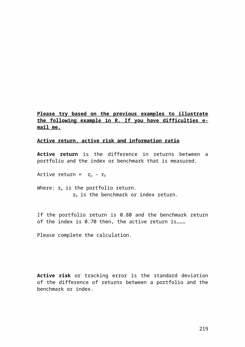
Calculate the call option prices using a Jarrow – Rudd, (JR), binomial 3 steps tree. The key difference between the Cox, Ross, Rubinstein,(CRR) binomial tree and the Jarrow – Rudd, (JR), binomila tree is in defining the parmeters of the multiplier of up and down move. The figures are expressed in pounds
> S <- 90 # share price> K <- 85 # strike price> r <- 0.04 # interest rate> q <- 0.03 # dividend yield> T <- 0.5 # maturity> sig <- 0.2 # volatility> n <- 3> dt <- T/n> dt <- T/n # steps expressed in years.> dt[1] 0.16666666666666666> u <- (exp((r-q -0.5*sig*sig)*dt + sig*sqrt(dt))) # multiplier of upmove.> u[1] 1.0832686426635116 > d <- (exp((r-q -0.5*sig*sig)*dt - sig*sqrt(dt))) # multiplier of downmove.> d[1] 0.9200600634058166> disfact <- exp(-r*dt) # discount factor.> disfact[1] 0.9933555062550344> riskprobofupmove <- (exp((r-q)*dt)-d)/(u-d) # risk neutral probability of upmove.> riskprobofupmove[1] 0.5000226905523886> callpayoffupmovestep3 <- S*u**3-K> callpayoffupmovestep3[1] 29.406585701387428> callpayoff3i <- S * u**2 * d -K> callpayoff3i[1] 12.169738279923607> callpayoff3ii <-S*d**2*u-K> callpayoff3ii[1] -2.470152793185349> callpayoff3ii <-0> callpayoff3ii[1] 0> callpayoffdownmovestep3 <- S*d**3-K> callpayoffdownmovestep3[1] -14.904352933845047> callpayoffdownmovestep3 <-0> callpayoffdownmovestep3[1] 0> callpriceupmovestep2 <- (disfact*(riskprobofupmove*callpayoffupmovestep3)+(1-riskprobofupmove)*callpayoff3i)> callpriceupmovestep2
219
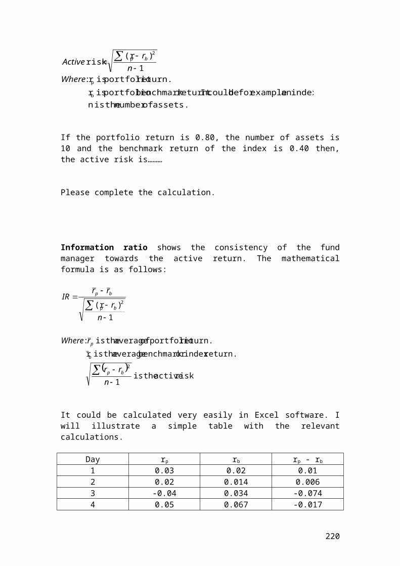
[1] 20.690852733318547> callpriceupdownmovestep2 <-(disfact*(riskprobofupmove*callpayoff3i)+(1-riskprobofupmove)*callpayoff3ii)> callpriceupdownmovestep2[1] 6.044712568308618> callpricedownmovestep2 <-(disfact*(riskprobofupmove*callpayoff3ii)+(1-riskprobofupmove)*callpayoffdownmovestep3)> callpricedownmovestep2[1] 0.0> callpriceupmovestep1 <- (disfact*(riskprobofupmove*callpriceupmovestep2)+(1-riskprobofupmove)*callpriceupdownmovestep2)> callpriceupmovestep1[1] 13.299371739539392> callpricedownmovestep1<-(disfact*(riskprobofupmove*callpriceupdownmovestep2)+(1-riskprobofupmove)*callpricedownmovestep2)> callpricedownmovestep1[1] 3.0024105032518027> callpricestep0<- (disfact*(riskprobofupmove*callpriceupmovestep1)+(1-riskprobofupmove)*callpricedownmovestep1)> callpricestep0[1] 8.10693896385682>>> round(callpricestep0,digits=2)8.11
220
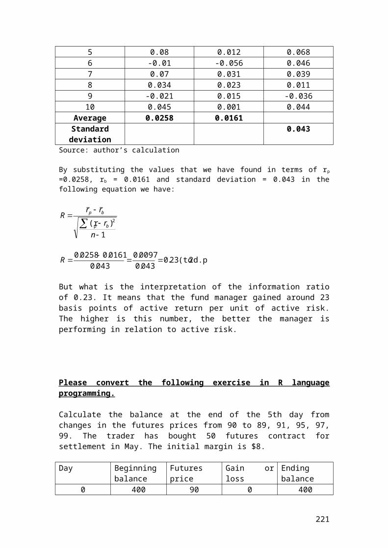
Calculate the share prices of a call option using a Jarrow – Rudd, (JR), binomial 3 steps tree. The prices are expressed in Euros.
> S <- 90> K <- 85> r <- 0.04> q <-0.03> T <- 0.5> sig <- 0.2> n <-3> dt <- T/n> dt[1] 0.16666666666666666> u <- (exp((r-q -0.5*sig*sig)*dt + sig*sqrt(dt)))> u[1] 1.0832686426635116> d <- (exp((r-q -0.5*sig*sig)*dt - sig*sqrt(dt)))> d[1] 0.9200600634058166> share_price0 <- S> share_price0[1] 90> share_priceupmove1 <- S*u> share_priceupmove[1] 97.49417783971604> share_pricedownmove1 <- S*d> share_pricedownmove1[1] 82.80540570652349> share_priceupmove2 <- S*u**2> share_priceupmove2[1] 105.61238569602422> share_priceupmovedownmove <- S*u*d> share_priceupmovedownmove[1] 89.70049944490711> share_pricedownmove2 <- S*d**2> share_pricedownmove2[1] 76.18594682468837> share_priceupmove3 <-S*u**3> share_priceupmove3[1] 114.40658570138743
Please complete the remaining calculations……
221
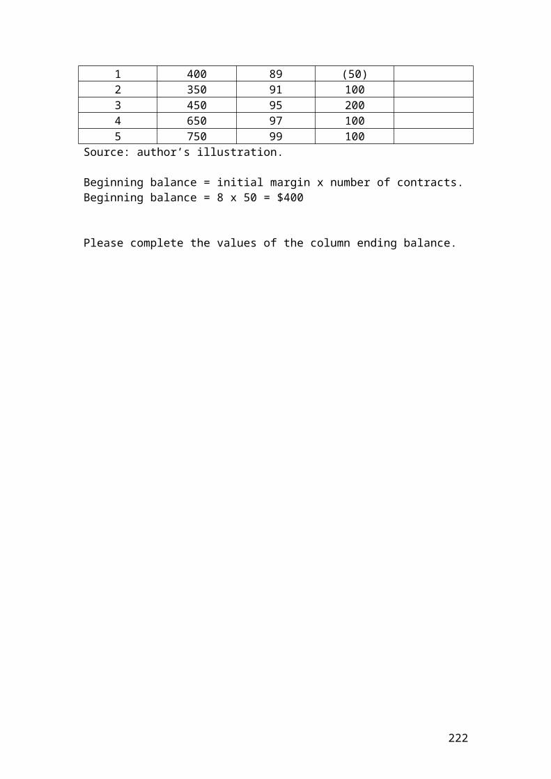
Example of simulating share prices by showing different price scenarios. The figure is expressed in pounds.
> number_of_simulation <- 6> S0 <- 60> r <- 0.03> q <- 0.02> sig <- 0.20> dt <- 1/250> dt[1] 0.004> random.number <- (30000+3000)/300> random.number110.0> sharePrice<-S0*exp((r-q-0.5*sig*sig)*dt*random.number*sig*sqrt(dt))> sharePrice59.99760004799936
Please complete the calculations to get different share prices….
222
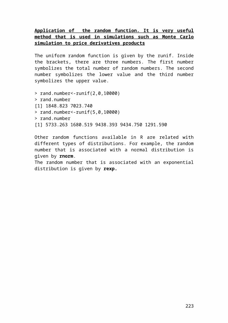
A manufacturing company sold a FRA contract expiring in 50 days with a principal of 30,000,000 USD. The underlying is 180 days LIBOR. The agreed rate on this FRA is 7%. At expiration, 90 days later, the actual rate on 180 days LIBOR is 8%. How much is the payoff of the manufacturing company at expiration?
Solution
The mathematical formula for Forward Rate Agreement, (FRA) is as follows:
FRA Payment = 30,000,000* ((0.08 – 0.07)*(180/360) / 1 + 0.08*(180/360)
FRA Payment = 30,000,000 * 0.005 / 1.04
FRA Payment = 144230.77 USD
Application of FRA payment in R
> principal <- 30000000> actual_rate <- 0.08> agreed_rate <- 0.07> days_1_underlying <- 180> days_2_expiration <- 180
Please complete the calculations using R……..
223
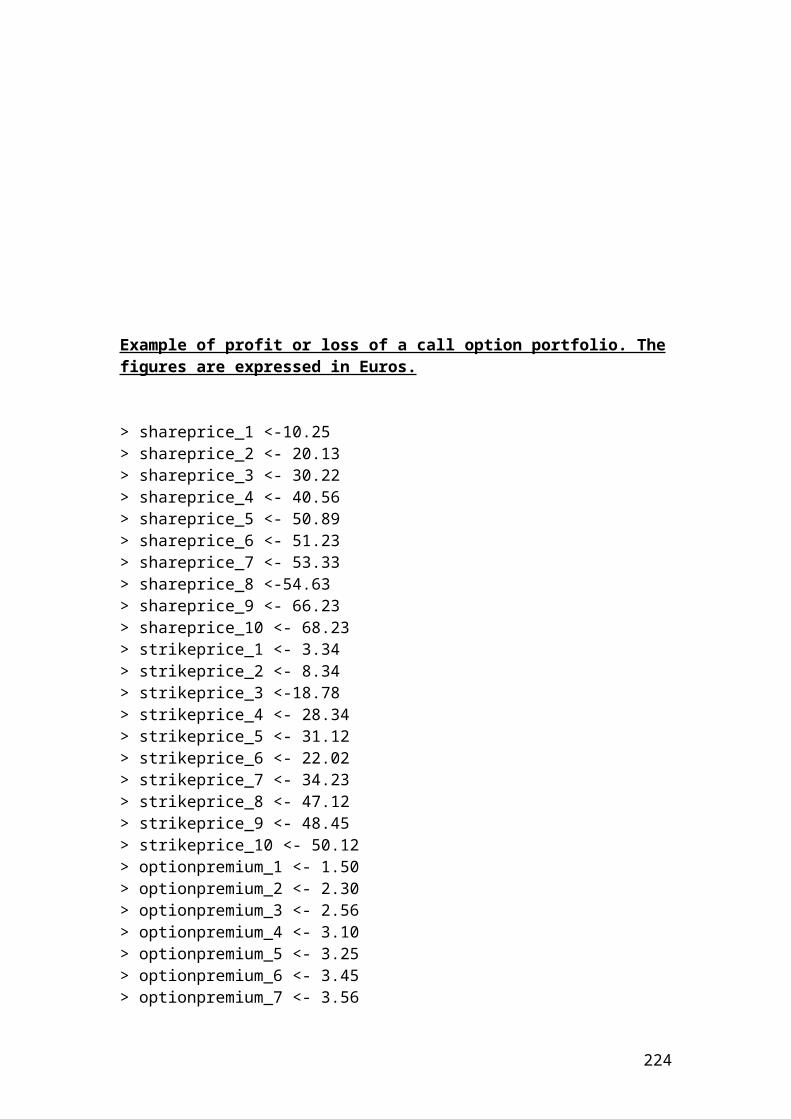
Currency futures
Futures Price = contract size * exchange rate
If the contract size is 20,000 USD and the quoted price is 1.573 USD, then, the futures price is as follows:
Futures Price = 20,000 * 1.573 = 31460 USD
Application of currency futures in R
> contract_size <- 20000> quoted_price <- 1.573> FuturesPrice <- contract_size * quoted_price> FuturesPrice[1] 31460.0 # USD
224
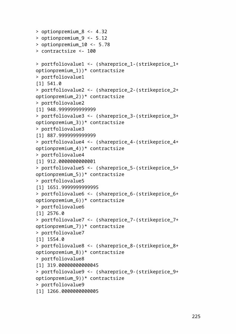
Minimum price required for a margin call
It is very important to check the maintenance margin level. The initial margin per contract for a gold futures contract is 1,500 USD. The maintenance margin per contract is 800 USD. The contract size is 5,000 ounces.
Solution
Minimum price required for a margin call = initial margin – maintenance margin / contract size
Minimum price required for a margin call = 1500 – 800 / 5000 = 0.14 USD.
Application of minimum price required for a margin call in R
> initial_margin_of_gold_futures <- 1500> maintenance_margin_percontract <- 800> contract_size <- 5000> minimum_price_required_for_a_margin_call <- (initial_margin_of_gold_futures - maintenance_margin_percontract) / contract_size> minimum_price_required_for_a_margin_call0.14 # USD
225
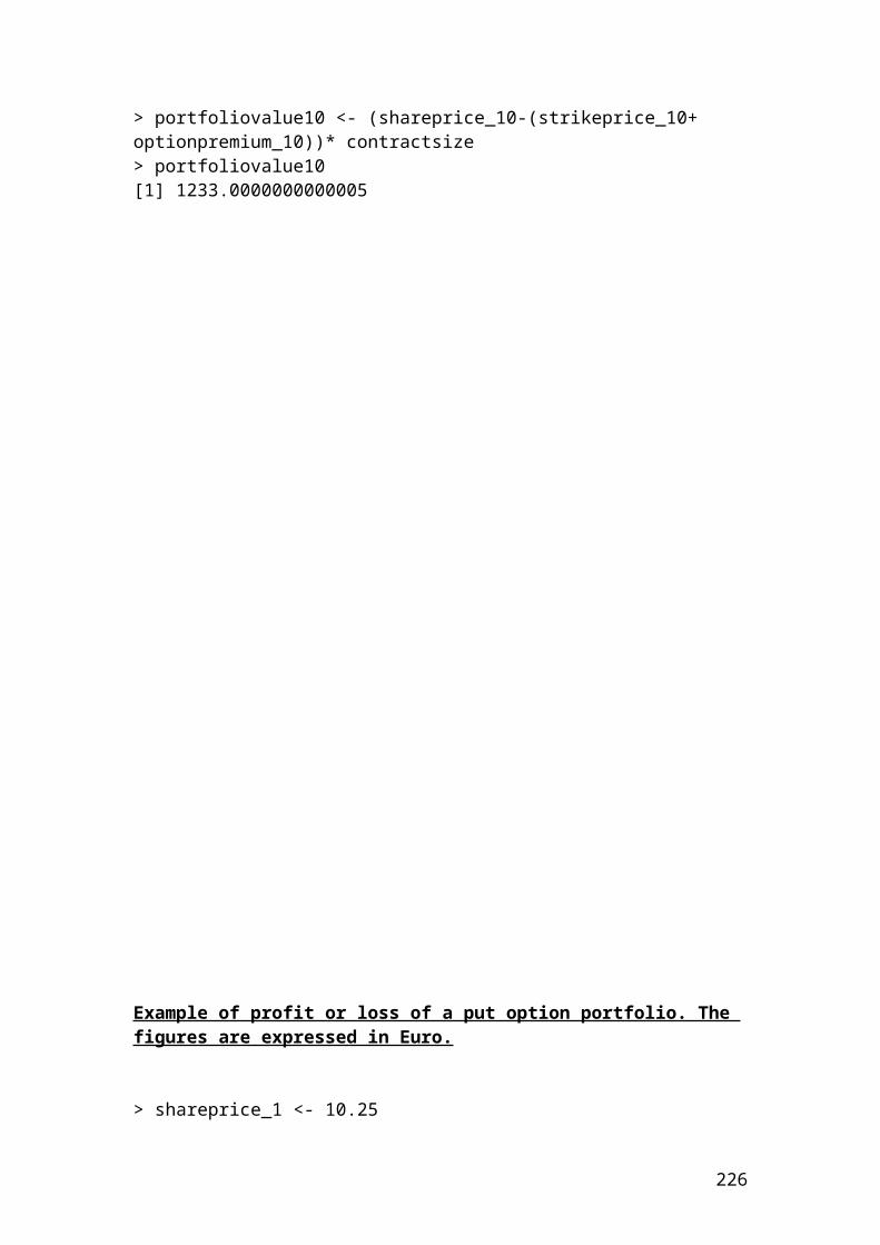
Loss on the futures position
Please consider a bond related to Eurodollar futures. The settlement price of the bond is 95.70 in December 2015. The principal is 2,000,000 Euros. The investor has adopted a long position of 100 contracts. The bond price has fallen to 90.15. Calculate the loss on the futures position.
Solution
Insert the mathematical formula.
Loss on the futures position = (settlement price – current price) / 100 * 100 contracts * 2,000,000
Loss on the futures position = (95.70 – 90.15) / 100 * 100 * 2,000,000 =
Loss on the futures position = 5.55 / 100 * 100 * 2000000 = 11,100,000 Euros.
Application of loss on the futures position in R
> settlement_price <- 95.70> current_price <- 90.15> principal <- 2000000> contract_size <- 100> Loss_on_the_futures_position <-(settlement_price - current_price)/100*contract_size*principal> Loss_on_the_futures_position11099999.999999994> round(Loss_on_the_futures_position, digits=2)11100000.0 # Euros
226
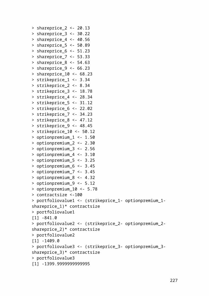
Variation margin call
The amount of variation margin call is used in futures when the price of the asset price falls below a certain amount. For example, consider the bond price of Eurodollar futures.
Consider a trader that has bought a Eurodollar bond futures with a principal of 10,000,000 Euros. The settlement price is 97.14. The long position includes 100 contracts. The price of the bond has fallen to 95.78. The maintenance price is 96.45. The price of the bond has fallen below the maintenance price.
Variation margin = (settlement price – current price) / 100 * 100 contracts * 10,000,000
Variation margin = (97.14 – 95.78) / 100 * 100 *10,000,000 =
Variation margin = 1.36 / 100 * 100 * 10,000,000 = 13,600,000 Euros.
Application of variation margin call in R
> settlement_price <- 97.14> current_price <- 95.78> principal <- 10000000> contract_size <- 100> variation_margin <-(settlement_price-current_price)/100*contract_size*10000000> variation_margin13599999.999999994> round(variation_margin,digits = 2)13600000.0 # Euros
227
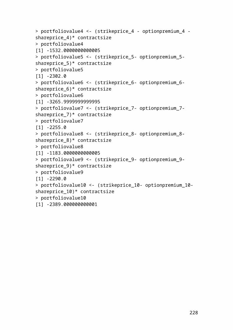
Calculate the volume and the open interest position in the July FTSE 100 index
Please consider 5 investors with the following short/long contract position.
First investor buys 3 contracts to open a long position.Second investor buys 5 contracts to open a long position.Third investor buys 2 contracts to open a long position.Fourth investor sells 7 contracts to close a long position.Fifth investor sells 4 contracts to close a long position.
If we assume that the initial open interest before the trades was 30 contracts. Calculate the volume and ending open interest.
Solution
Total volume = 3 + 5 + 2 + 7 + 4 = 21 contracts.
Ending open interest = initial open interest + opened positions - closed positions
Ending open interest = 30 + 3 + 5 + 2 - 7 – 4 = 29
Application of calculation the volume and the open interest position in the July FTSE 100 index in R
> first_investor_buys_3contracts <- 3> second_investor_buys_5contracts <- 5> third_investor_buys_2contracts <- 2> fourth_investor_sells_7contracts <- 7> fifth_investor_sells_4contracts <- 4> initial_open_interest <- 30> Total_volume <- 3+5+2+7+4> Total_volume21 # contracts> ending_open_interest <- 30 + 3 + 5 + 2 - 7 -4> ending_open_interest29 # ending open interest
228
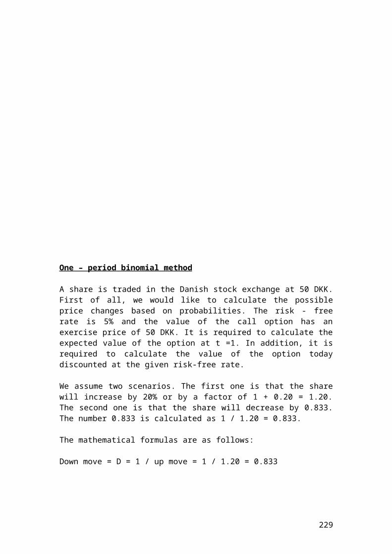
Calculation of the minimum price per ounce before a margin call
Please consider the following terms of the silver contract:
Initial margin = $ 3,500 per contract.Maintenance margin = $ 2,500 per contract.20 silver contracts sold at a price equals $700 per ounce.Contract size = 100 ounces.
Solution
The initial margin = 3,500 * 20 = 70,000 USD. The maintenance margin = 2,500 * 20 = 50,000 USD.The difference between the initial and maintenance margin is the amount recorded before a margin call take place. Thus, 70,000 – 50,000 = 20,000 USD.
The price is 20,000 / 20*100 = 10 USD per ounce. This is the price before a margin call take place.
Application of calculating the minimum up or down ounce price before a margin call in R
> initial_margin <- 3500> maintenance_margin <- 2500> silver_contracts <- 20> contract_size <- 100> minimum_price_required_for_a_margincall <- (3500 - 2500) / 100> minimum_price_required_for_a_margincall10.0 # USD per ounce.
229
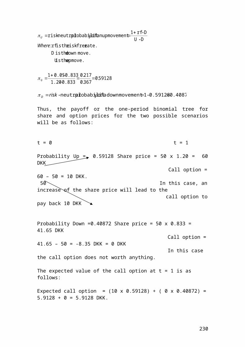
Calculate the intrinsic value of call share traded in Frankfurt stock exchange
The VW share is traded at 140 Euro in the Frankfurt stock exchange. The strike price is 130 Euro and the option market price is 7.70 Euro. The intrinsic value of the VW call is as calculate as follows:
Solution
The intrinsic value of the VW call is = Share price – strike price = 140 – 130 = 10 Euro.
Application of calculating the intrinsic value of call share traded in Frankfurt stock exchange
> share_price <- 140> strike_price <- 130> intrinsic_value <- share_price - strike_price> intrinsic_value10 # Euro.
230
Workshop of analysis of financial data, scientific programming and simulation using Java language programming
Java is very useful language programming in financial modeling. Please make yourself very familiar with C++. You will find a lot of similarities with Java. The main differences are in defining the headings and the output functions.
First of all, you should download the software as part of an integrated development environment, (IDE). A possible public domain is as follows:
www.drjava.org
You can start Java programming by creating a source code in the text editor. Then, press tools and select the compile current document to compile the code. Once compilation is completed, then, press run document from the tools section. At the bottom, you could see the output of the source code.
Press new to create a new text editor, then, in the header insert the title of the document to be saved. For example,
class Currency_futures
Press save and then insert the appropriate source code for financial calculation.
If you do not have the right headers, then, you will not be able to do compiling and run the document to see the output.
The comments, variables, functions, and mathematical formulas have to be inserted to be able to get the output. We use the symbol // to show a single line comment. The lines that include statements should end with semicolon ; in Java . We use numerical variables with fractional parts. In this case, the term double is inserted in front of each variable. Once you define a variable with capital or small letters, you can not change it with different layout as you move to the calculation part. Pay particular attention to the lower and upper case letters. For example, integer for interest rate is written as variable intRate or int_rate. Another example that can be used is the integer value for the amount. It is written as intAmount or int_amount. Use the symbols /* and */ for multiline comments. The symbol // is used for single comment.
231
Then, the source code should be enclosed between braces.
The main layout to start Java is as follows:
class name of the variable { public static void main (String[] args) {
/* Identify your given variables using double for numbers with fractions or int for integers numbers. Identify the variables that will be calculated. The symbols /* and */ are used for multiline comments.*/
// Insert the mathematical formula or formulas.
// Output functions.System.out.print ("type the sentence that will appear in the output before the calculated number")System.out.println(variable that is defined by a mathematical formula)You can add as many output functions as your mathematical formulas.
} }
232
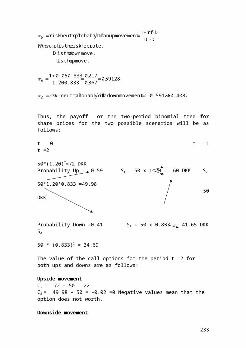
A simple example to illustrate the above is as follows:
// Calculate the average
class Average
{public static void main (String[] args) {
// Identify the variables.
double stock_price1=3;double stock_price2=5;double stock_price3=9;double average;
// Insert the mathematical formula.
average = (stock_price1 + stock_price2 + stock_price3)/3;
// Output functions.System.out.print("The average in $");System.out.println(average);}}
After compiling the current document, press run document from Tools, you should get $ 5.66.
233
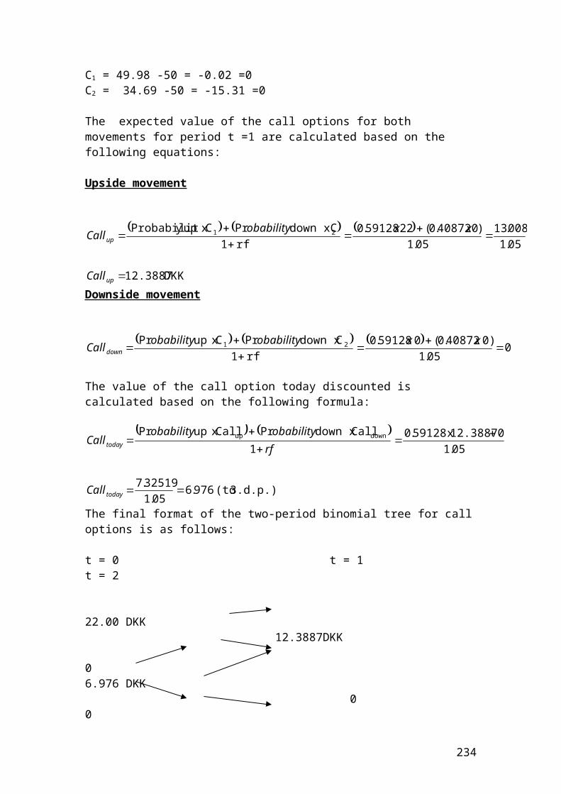
Calculations of the mean and the harmonic mean of share price returns, call option returns, put option returns and index option returns
class average_and_harmonic_average
{public static void main(String[] args) {
/* Calculations of the mean and the harmonic mean of share price returns, call option returns, put option returns and index option returns.*/ double SharePriceReturns1 = 0.08;double SharePriceReturns2= 0.05;double SharePriceReturns3 = 0.04;double SharePriceReturns4 = 0.07;double SharePriceReturns5 = 0.02;double SharePriceReturns6 = 0.03;
double CallOptionPriceReturns1 = 0.01;double CallOptionPriceReturns2 = 0.02;double CallOptionPriceReturns3 = 0.04;double CallOptionPriceReturns4 = 0.05;double CallOptionPriceReturns5 = 0.06;double CallOptionPriceReturns6 = 0.06;
double PutOptionPriceReturns1 = 0.03;double PutOptionPriceReturns2 = 0.07;double PutOptionPriceReturns3 = 0.08;double PutOptionPriceReturns4 = 0.09;double PutOptionPriceReturns5 = 0.1;double PutOptionPriceReturns6 = 0.02;
double IndexOptionPriceReturns1 = 0.12;double IndexOptionPriceReturns2 = 0.23;double IndexOptionPriceReturns3 = 0.34;double IndexOptionPriceReturns4 = 0.15;double IndexOptionPriceReturns5 = 0.2;double IndexOptionPriceReturns6 = 0.11;
double averageSharePriceReturns;double averageCallOptionPriceReturns;double averagePutOptionPriceReturns;double averageIndexOptionPriceReturns;double harmonicaverageSharePriceReturns;double harmonicaverageCallOptionPriceReturns;double harmonicaveragePutOptionPriceReturns;double harmonicaverageIndexOptionPriceReturns;
234
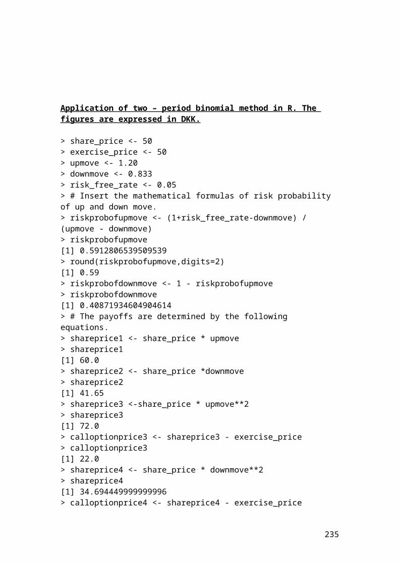
averageSharePriceReturns = (SharePriceReturns1 + SharePriceReturns2 + SharePriceReturns3 + SharePriceReturns4 + SharePriceReturns5 + SharePriceReturns6)/6;
averageCallOptionPriceReturns = (CallOptionPriceReturns1 + CallOptionPriceReturns2 + CallOptionPriceReturns3 + CallOptionPriceReturns4 + CallOptionPriceReturns5 + CallOptionPriceReturns6)/6;
averagePutOptionPriceReturns = (PutOptionPriceReturns1 + PutOptionPriceReturns2 + PutOptionPriceReturns3 + PutOptionPriceReturns4 + PutOptionPriceReturns5 + PutOptionPriceReturns6)/6;
averageIndexOptionPriceReturns = (IndexOptionPriceReturns1 + IndexOptionPriceReturns2 + IndexOptionPriceReturns3 + IndexOptionPriceReturns4 + IndexOptionPriceReturns5 + IndexOptionPriceReturns6)/6;
harmonicaverageSharePriceReturns = (1/((1/SharePriceReturns1 + 1/SharePriceReturns2 + 1/SharePriceReturns3 + 1/SharePriceReturns4 + 1/SharePriceReturns5 + 1/SharePriceReturns6)/6));
harmonicaverageCallOptionPriceReturns = (1/((1/CallOptionPriceReturns1 + 1/CallOptionPriceReturns2 + 1/CallOptionPriceReturns3 + 1/CallOptionPriceReturns4 + 1/CallOptionPriceReturns5 + 1/CallOptionPriceReturns6)/6));
harmonicaveragePutOptionPriceReturns = (1/((1/PutOptionPriceReturns1 + 1/PutOptionPriceReturns2 + 1/PutOptionPriceReturns3 + 1/PutOptionPriceReturns4 + 1/PutOptionPriceReturns5 + 1/PutOptionPriceReturns6)/6));
harmonicaverageIndexOptionPriceReturns = (1/((1/IndexOptionPriceReturns1 + 1/IndexOptionPriceReturns2 + 1/IndexOptionPriceReturns3 + 1/IndexOptionPriceReturns4 + 1/IndexOptionPriceReturns5 + 1/IndexOptionPriceReturns6)/6));
System.out.print("The average is");System.out.println(averageSharePriceReturns);System.out.print("The average of call option price returns is");System.out.println(averageCallOptionPriceReturns);System.out.print("The average of put option price returns is");System.out.println(averagePutOptionPriceReturns);System.out.print("The average of index option price returns is");System.out.println(averageIndexOptionPriceReturns);System.out.print("The harmonic average of share price returns is");System.out.println(harmonicaverageSharePriceReturns);System.out.print("The harmonic average of call option price returns is");System.out.println(harmonicaverageCallOptionPriceReturns);System.out.print("The harmonic average of put option price returns is");System.out.println(harmonicaveragePutOptionPriceReturns);System.out.print("The harmonic average of index option price returns is");
235

System.out.println(harmonicaverageIndexOptionPriceReturns);}}
Output results
After compiling the current document from tools and pressing the run document you should get the following results:
Welcome to DrJava. Working directory is C:\Documents and Settings\Owner\Desktop\Java Compiler> run average_and_harmonic_averageThe average is 0.04833333333333334The average of call option price returns is 0.04The average of put option price returns is 0.065The average of index option price returns is 0.19166666666666668The harmonic average of share price returns is 0.03867996930161166The harmonic average of call option price returns is 0.026277372262773727The harmonic average of put option price returns is 0.04572119745993347The harmonic average of index option price returns is 0.1649261839330223
236
Repetition of calculating the mean and the harmonic mean of share price returns, call option returns, put option returns and index option returns. I will show how to use the rounding function in Java
class average_and_harmonic_average {public static void main(String[] args) {
/* Calculations of the mean and the harmonic mean of share price returns, call option returns, put option returns and index option returns. */ double SharePriceReturns1 = 0.08;double SharePriceReturns2= 0.05;double SharePriceReturns3 = 0.04;double SharePriceReturns4 = 0.07;double SharePriceReturns5 = 0.02;double SharePriceReturns6 = 0.03;
double CallOptionPriceReturns1 = 0.01;double CallOptionPriceReturns2 = 0.02;double CallOptionPriceReturns3 = 0.04;double CallOptionPriceReturns4 = 0.05;double CallOptionPriceReturns5 = 0.06;double CallOptionPriceReturns6 = 0.06;
double PutOptionPriceReturns1 = 0.03;double PutOptionPriceReturns2 = 0.07;double PutOptionPriceReturns3 = 0.08;double PutOptionPriceReturns4 = 0.09;double PutOptionPriceReturns5 = 0.1;double PutOptionPriceReturns6 = 0.02;
double IndexOptionPriceReturns1 = 0.12;double IndexOptionPriceReturns2 = 0.23;double IndexOptionPriceReturns3 = 0.34;double IndexOptionPriceReturns4 = 0.15;double IndexOptionPriceReturns5 = 0.2;double IndexOptionPriceReturns6 = 0.11;
double averageSharePriceReturns;double averageCallOptionPriceReturns;double averagePutOptionPriceReturns;double averageIndexOptionPriceReturns;double harmonicaverageSharePriceReturns;double harmonicaverageCallOptionPriceReturns;double harmonicaveragePutOptionPriceReturns;double harmonicaverageIndexOptionPriceReturns;
237
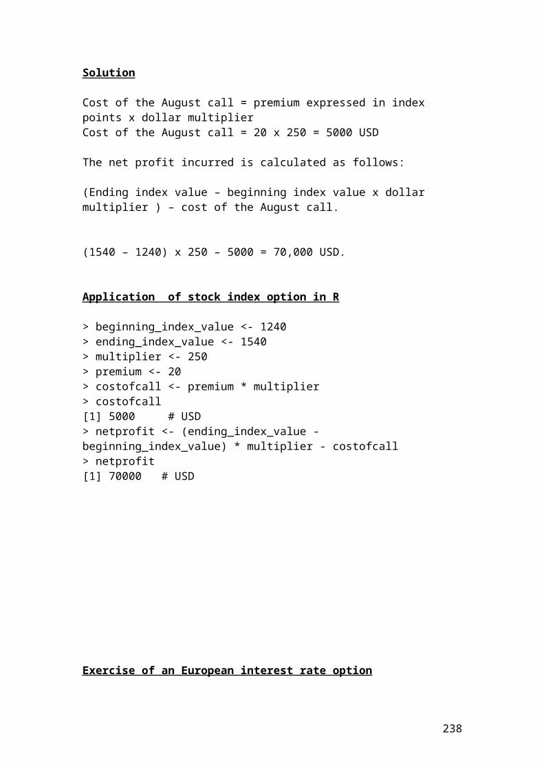
averageSharePriceReturns = (SharePriceReturns1 + SharePriceReturns2 + SharePriceReturns3 + SharePriceReturns4 + SharePriceReturns5 + SharePriceReturns6)/6;
averageCallOptionPriceReturns = (CallOptionPriceReturns1 + CallOptionPriceReturns2 + CallOptionPriceReturns3 + CallOptionPriceReturns4 + CallOptionPriceReturns5 + CallOptionPriceReturns6)/6;
averagePutOptionPriceReturns = (PutOptionPriceReturns1 + PutOptionPriceReturns2 + PutOptionPriceReturns3 + PutOptionPriceReturns4 + PutOptionPriceReturns5 + PutOptionPriceReturns6)/6;
averageIndexOptionPriceReturns = (IndexOptionPriceReturns1 + IndexOptionPriceReturns2 + IndexOptionPriceReturns3 + IndexOptionPriceReturns4 + IndexOptionPriceReturns5 + IndexOptionPriceReturns6)/6;
harmonicaverageSharePriceReturns = (1/((1/SharePriceReturns1 + 1/SharePriceReturns2 + 1/SharePriceReturns3 + 1/SharePriceReturns4 + 1/SharePriceReturns5 + 1/SharePriceReturns6)/6));
harmonicaverageCallOptionPriceReturns = (1/((1/CallOptionPriceReturns1 + 1/CallOptionPriceReturns2 + 1/CallOptionPriceReturns3 + 1/CallOptionPriceReturns4 + 1/CallOptionPriceReturns5 + 1/CallOptionPriceReturns6)/6));
harmonicaveragePutOptionPriceReturns = (1/((1/PutOptionPriceReturns1 + 1/PutOptionPriceReturns2 + 1/PutOptionPriceReturns3 + 1/PutOptionPriceReturns4 + 1/PutOptionPriceReturns5 + 1/PutOptionPriceReturns6)/6));
harmonicaverageIndexOptionPriceReturns = (1/((1/IndexOptionPriceReturns1 + 1/IndexOptionPriceReturns2 + 1/IndexOptionPriceReturns3 + 1/IndexOptionPriceReturns4 + 1/IndexOptionPriceReturns5 + 1/IndexOptionPriceReturns6)/6));
System.out.print("The average is");System.out.println(averageSharePriceReturns);System.out.println(Math.round(averageSharePriceReturns*100.0)/100.0);System.out.print("The average of call option price returns is");System.out.println(averageCallOptionPriceReturns);System.out.println(Math.round(averageCallOptionPriceReturns*100.0)/100.0);System.out.print("The average of put option price returns is");System.out.println(averagePutOptionPriceReturns);System.out.println(Math.round(averagePutOptionPriceReturns*100.0)/100.0);System.out.print("The average of index option price returns is");System.out.println(averageIndexOptionPriceReturns);System.out.println(Math.round(averageIndexOptionPriceReturns*100.0)/100.0);System.out.print("The harmonic average of share price returns is");System.out.println(harmonicaverageSharePriceReturns);System.out.println(Math.round(harmonicaverageSharePriceReturns*100.0)/100.0);
238
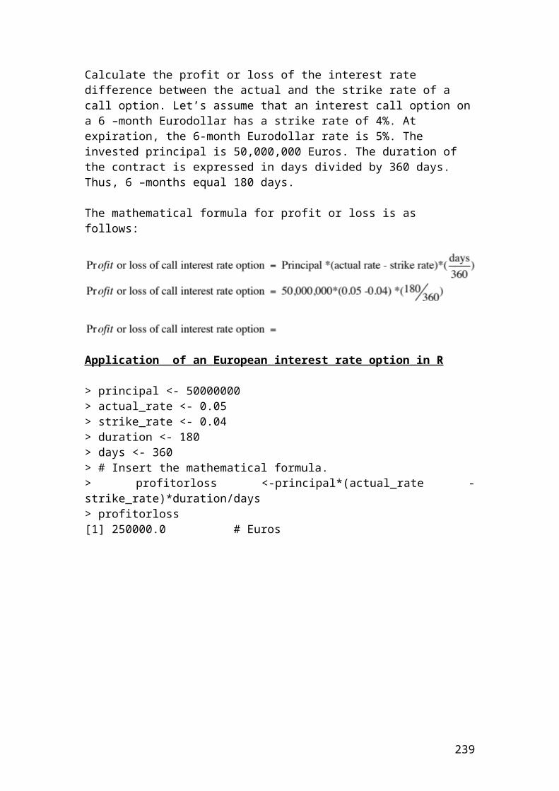
System.out.print("The harmonic average of call option price returns is");System.out.println(harmonicaverageCallOptionPriceReturns);System.out.println(Math.round(harmonicaverageCallOptionPriceReturns*100.0)/100.0);System.out.print("The harmonic average of put option price returns is");System.out.println(harmonicaveragePutOptionPriceReturns);System.out.println(Math.round(harmonicaveragePutOptionPriceReturns*100.0)/100.0);System.out.print("The harmonic average of index option price returns is");System.out.println(harmonicaverageIndexOptionPriceReturns);System.out.println(Math.round(harmonicaverageIndexOptionPriceReturns*100.0)/100.0);}}
Output results
After compiling the current document from tools and pressing the run document you should get the following results:
Welcome to DrJava. Working directory is C:\Documents and Settings\Owner\Desktop\Java Compiler> run average_and_harmonic_averageThe average is 0.048333333333333340.05The average of call option price returns is 0.040.04The average of put option price returns is 0.0650.07The average of index option price returns is 0.191666666666666680.19The harmonic average of share price returns is 0.038679969301611660.04The harmonic average of call option price returns is 0.0262773722627737270.03The harmonic average of put option price returns is 0.045721197459933470.05The harmonic average of index option price returns is 0.16492618393302230.16>
239
Exercise of how to calculate the payoff of buying a call, a put and the net result or position of your investment position expressed in pounds
class payoff {public static void main(String[] args) {
/*payoff of buying a call, a put and the net result or position of your investment position expressed in pounds. */
double SharePrice1 = 105;double SharePrice2 = 110;double SharePrice3 = 120;double SharePrice4 = 130;double SharePrice5 = 140;double SharePrice6 = 150;
double ExercisePriceCall1 = 90;double ExercisePriceCall2 = 90;double ExercisePriceCall3 = 90;double ExercisePriceCall4 = 90;double ExercisePriceCall5 = 90;double ExercisePriceCall6 = 90;
double ExercisePricePut1 = 190;double ExercisePricePut2 = 190;double ExercisePricePut3 = 190;double ExercisePricePut4 = 190;double ExercisePricePut5 = 190;double ExercisePricePut6 = 190;
double PremiumofCall= 14;
double PremiumofPut =9;
double TotalNumberofContracts = 10;
double totalNumberOfShares =100;
double payoffBuyaCall1;double payoffBuyaCall2;double payoffBuyaCall3;double payoffBuyaCall4;double payoffBuyaCall5;double payoffBuyaCall6;
double payoffBuyaPut1;double payoffBuyaPut2;double payoffBuyaPut3;double payoffBuyaPut4;
240
double payoffBuyaPut5;double payoffBuyaPut6;
double NetResult1;double NetResult2;double NetResult3;double NetResult4;double NetResult5;double NetResult6;
payoffBuyaCall1 = (SharePrice1-(ExercisePriceCall1+PremiumofCall))*TotalNumberofContracts*totalNumberOfShares;payoffBuyaCall2 = ( SharePrice2-(ExercisePriceCall2+PremiumofCall))*TotalNumberofContracts*totalNumberOfShares;payoffBuyaCall3 = ( SharePrice3-(ExercisePriceCall3+PremiumofCall))*TotalNumberofContracts*totalNumberOfShares;payoffBuyaCall4 = ( SharePrice4-(ExercisePriceCall4+PremiumofCall))*TotalNumberofContracts*totalNumberOfShares;payoffBuyaCall5 = ( SharePrice5-(ExercisePriceCall5+PremiumofCall))*TotalNumberofContracts*totalNumberOfShares;payoffBuyaCall6 = ( SharePrice6-(ExercisePriceCall6+PremiumofCall))*TotalNumberofContracts*totalNumberOfShares;
payoffBuyaPut1 = ( ExercisePricePut1-SharePrice1-PremiumofPut)*TotalNumberofContracts*totalNumberOfShares;payoffBuyaPut2 = ( ExercisePricePut2-SharePrice2-PremiumofPut)*TotalNumberofContracts*totalNumberOfShares;payoffBuyaPut3 = ( ExercisePricePut3-SharePrice3-PremiumofPut)*TotalNumberofContracts*totalNumberOfShares;payoffBuyaPut4 = ( ExercisePricePut4-SharePrice4-PremiumofPut)*TotalNumberofContracts*totalNumberOfShares;payoffBuyaPut5 = ( ExercisePricePut5-SharePrice5-PremiumofPut)*TotalNumberofContracts*totalNumberOfShares;payoffBuyaPut6 = ( ExercisePricePut6-SharePrice6-PremiumofPut)*TotalNumberofContracts*totalNumberOfShares;
NetResult1 = payoffBuyaCall1 - payoffBuyaPut1;NetResult2 = payoffBuyaCall2 - payoffBuyaPut2;NetResult3 = payoffBuyaCall3 - payoffBuyaPut3;NetResult4 = payoffBuyaCall4 - payoffBuyaPut4;NetResult5 = payoffBuyaCall5 - payoffBuyaPut5;NetResult6 = payoffBuyaCall6 - payoffBuyaPut6;
241
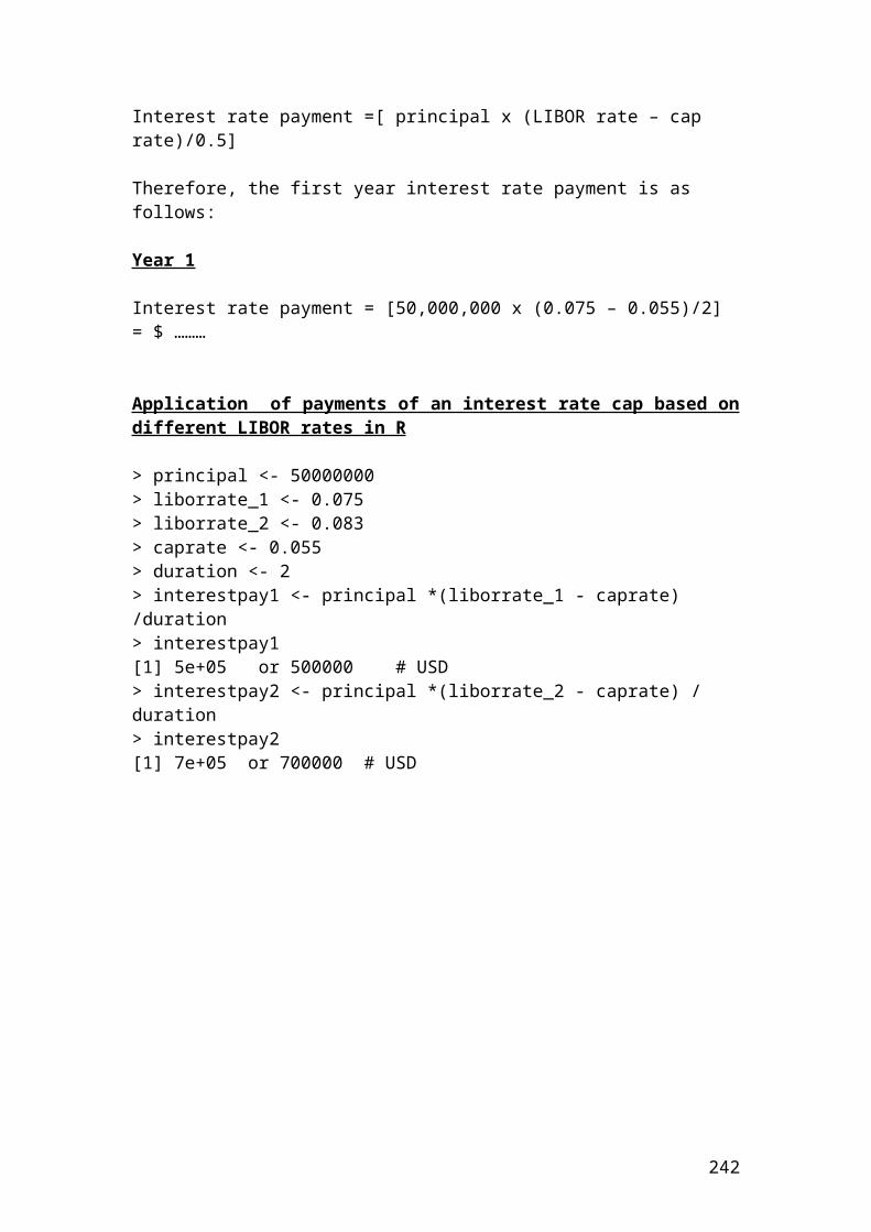
System.out.print("The payoff buy a call 1 in pounds is");System.out.println(payoffBuyaCall1);System.out.print("The payoff buy a call 2 in pounds is");System.out.println(payoffBuyaCall2);System.out.print("The payoff buy a call 3 in pounds is");System.out.println(payoffBuyaCall3);System.out.print("The payoff buy a call 4 in pounds is");System.out.println(payoffBuyaCall4);System.out.print("The payoff buy a call 5 in pounds is");System.out.println(payoffBuyaCall5);System.out.print("The payoff buy a call 6 in pounds is");System.out.println(payoffBuyaCall6);System.out.print("The payoff buy a put 1 in pounds is");System.out.println(payoffBuyaPut1);System.out.print("The payoff buy a put 2 in pounds is");System.out.println(payoffBuyaPut2);System.out.print("The payoff buy a put 3 in pounds is");System.out.println(payoffBuyaPut3);System.out.print("The payoff buy a put 4 in pounds is");System.out.println(payoffBuyaPut4);System.out.print("The payoff buy a put 5 in pounds is");System.out.println(payoffBuyaPut5);System.out.print("The payoff buy a put 6 in pounds is");System.out.println(payoffBuyaPut6);System.out.print("The net result 1 in pounds is");System.out.println(NetResult1);System.out.print("The net result 2 in pounds is");System.out.println(NetResult2);System.out.print("The net result 3 in pounds is");System.out.println(NetResult3);System.out.print("The net result 4 in pounds is");System.out.println(NetResult4);System.out.print("The net result 5 in pounds is");System.out.println(NetResult5);System.out.print("The net result 6 in pounds is");System.out.println(NetResult6);}}
242
Output results
After compiling the current document from tools and pressing the run document you should get the following results:
Welcome to DrJava. Working directory is C:\Documents and Settings\Owner\Desktop\Java Compiler> run payoff
The payoff buy a call 1 in pounds is1000.0The payoff buy a call 2 in pounds is6000.0The payoff buy a call 3 in pounds is16000.0The payoff buy a call 4 in pounds is26000.0The payoff buy a call 5 in pounds is36000.0The payoff buy a call 6 in pounds is46000.0The payoff buy a put 1 in pounds is76000.0The payoff buy a put 2 in pounds is71000.0The payoff buy a put 3 in pounds is61000.0The payoff buy a put 4 in pounds is51000.0The payoff buy a put 5 in pounds is41000.0The payoff buy a put 6 in pounds is31000.0The net result 1 in pounds is-75000.0The net result 2 in pounds is-65000.0The net result 3 in pounds is-45000.0The net result 4 in pounds is-25000.0The net result 5 in pounds is-5000.0The net result 6 in pounds is15000.0
243
Exercise
Please calculate the range in Java based on different share prices. The figures are nominated in USD.
class range{public static void main(String[] args) {
// Calculate the range.
double share_price_1 = 20;double share_price_2 = 30;double share_price_3 = 40;double share_price_4 = 50;double share_price_5 = 60;double share_price_6 = 70;
double range_share_price;
// Insert the mathematical formula.
range_share_price = (share_price_6-share_price_1);
// Output function.System.out.print("The range of share price in $ is ");System.out.println(range_share_price);}}
Output result
After compiling the current document from tools and pressing the run document you should get the following result:
Welcome to DrJava. Working directory is C:\Documents and Settings\Owner\Desktop\Java Compiler> run rangeThe range of share price in $ is 50.0>
244
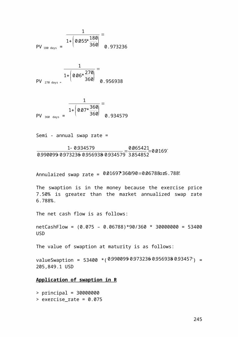
Calculate the log returns and the average using actual share price returns expressed in USD
class log_returns{public static void main(String[] args) {
//Identify the variables.
double dailyret2;double dailyret3;double dailyret4;double dailyret5;double average;
// Actual share prices.
double share_price1 = 14.23;double share_price2 = 15.67;double share_price3 = 12.13;double share_price4 = 11.45;double share_price5 = 10.11;
// Insert the mathematical formulas. dailyret2 = (share_price2/share_price1);dailyret3 =(share_price3/ share_price2);dailyret4 =(share_price4/ share_price3);dailyret5 =(share_price5/ share_price4); // Output functions.System.out.print("The dailyret2 is ");System.out.println("Math.log("+ dailyret2 +")="+Math.log(dailyret2));System.out.println(Math.round(Math.log(dailyret2)*100.0)/100.0);System.out.print("The dailyret3 is ");System.out.println("Math.log("+ dailyret3 +")="+Math.log(dailyret3));System.out.println(Math.round(Math.log(dailyret3)*100.0)/100.0);System.out.print("The dailyret4 is ");System.out.println("Math.log("+ dailyret4 +")="+Math.log(dailyret4));System.out.println(Math.round(Math.log(dailyret4)*100.0)/100.0);System.out.print("The dailyret5 is ");System.out.println("Math.log("+ dailyret5 +")="+Math.log(dailyret5));System.out.println(Math.round(Math.log(dailyret5)*100.0)/100.0);}}
245
Output results
After compiling the current document from tools and pressing the run document you should get the following results:
Welcome to DrJava. Working directory is C:\Documents and Settings\Owner\Desktop\Java Compiler> run log_returns
The dailyret2 is Math.log(1.101194659170766)=0.096395644266168450.1The dailyret3 is Math.log(0.7740906190172304)=-0.25606633341197066-0.26The dailyret4 is Math.log(0.9439406430338004)=-0.057691992955710175-0.06The dailyret5 is Math.log(0.8829694323144105)=-0.12446469696786859-0.12>
246
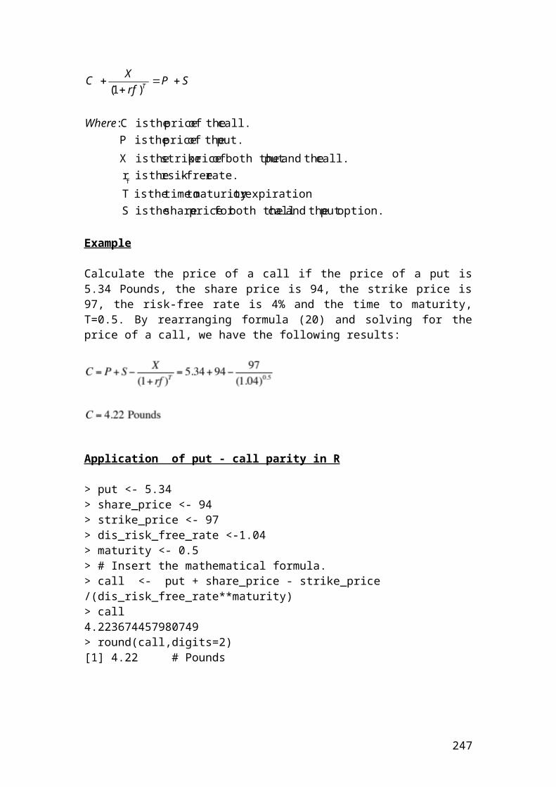
Calculation of the average, the daily and the annual volatility of percentage returns measured by the sample standard deviation
class average_and_standard_deviations{public static void main(String[] args) {
// Identify the variables.
double sum=0 ;double average; double sumDiffSqr;double DailystdDev;double AnnualstdDev;
double[]sharePrices = new double[]{0.1423,0.1567,0.1213,0.1145,0.1011};
/* The following expression inserts a variable x that tells the computerthat the first observation 0 is 0.1423 and x is less than 5 to include all observations.*/
for (int x = 0; x < 5; x++)
//We insert the formula for summation.
sum += sharePrices[x];
// We insert the formula for average.average = sum/5;
/* We calculate the sumDiffSqr by inserting the expression for that tells the computer the numbers that will be included in the calculation. We calculate the difference between each number and the average. Then, we square it and we sum it.*/
sumDiffSqr = 0;for (int x = 0; x < 5; x++) { sumDiffSqr = sumDiffSqr + Math.pow((sharePrices[x]-average),2); }/* Insert the formula of the sample standard deviation by taking into account the formual n-1.*/
DailystdDev = Math.sqrt(sumDiffSqr/4);
//We use 250 trading days per year instead of 365 days.
AnnualstdDev = DailystdDev * Math.sqrt(250);
247
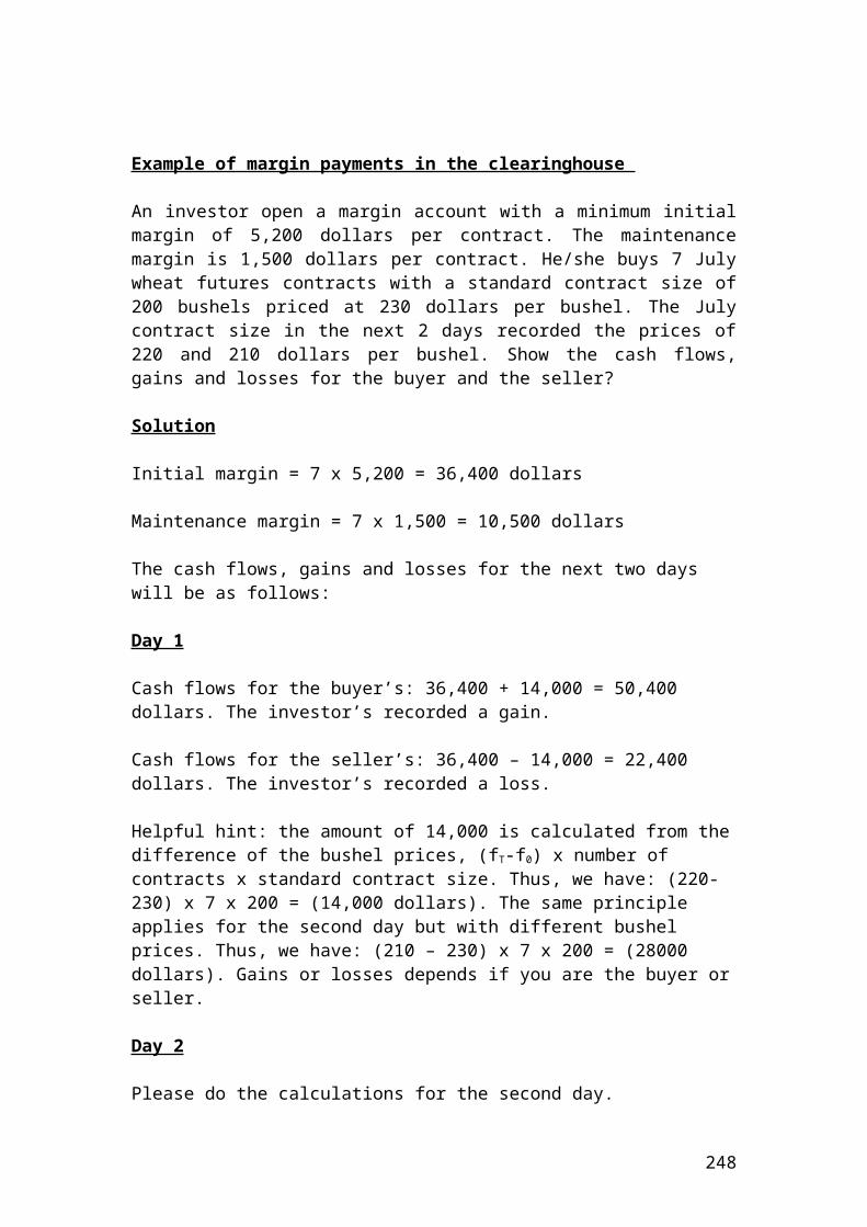
// Output functions.
System.out.print("The average is ");System.out.println(average);System.out.println(Math.round(average*100.0)/100.0); System.out.print("The daily standard deviation is ");System.out.println(DailystdDev);System.out.println(Math.round(DailystdDev*100.0)/100.0);System.out.print("The annual standard deviation is ");System.out.println(AnnualstdDev);System.out.println(Math.round(AnnualstdDev*100.0)/100.0);}}
Output results
After compiling the current document from tools and pressing the run document you should get the following results:
Welcome to DrJava. Working directory is C:\Documents and Settings\Owner\Desktop\Java Compiler> run average_and_standard_deviationsThe average is 0.127180000000000020.13The daily standard deviation is 0.022223681063226230.02The annual standard deviation is 0.351387250764736760.35>
248
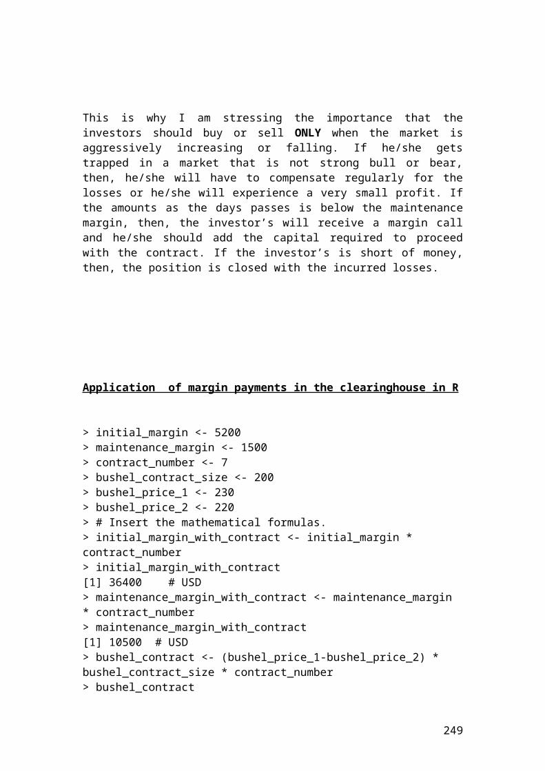
Calculation of the geometric average based on percentages of call option price returns
class geometric_average_call_option_price_returns{public static void main(String[] args) {
/* The call option price returns are expressed in percentages and we are trying to calculate the geometric mean or average. We insert the percentage values of each call option in an array format.*/
double call_option_price_return_1 = 5;double call_option_price_return_2 = 3;double call_option_price_return_3 = 2;double call_option_price_return_4 = 4;double call_option_price_return_5 = 7;double call_option_price_return_6 = 8;
// We define the variable that we want to calculate.double geometric_average;
// We write the mathematical equation of the geometric mean.
geometric_average = Math.pow(call_option_price_return_1*call_option_price_return_2*call_option_price_return_3*call_option_price_return_4*call_option_price_return_5*call_option_price_return_6,0.16666);
// Output functions.
System.out.println("Pow(" + call_option_price_return_1 + ", " + 0.16666 + ") = " + geometric_average);System.out.println(Math.round(geometric_average*100.0)/100.0); }}
Output result
After compiling the current document from tools and pressing the run document you should get the following result:
Welcome to DrJava. Working directory is C:\Documents and Settings\Owner\Desktop\Java Compiler> geometric_average_call_option_price_returnsPow(5.0, 0.16666) = 4.34379541978628854.34
249
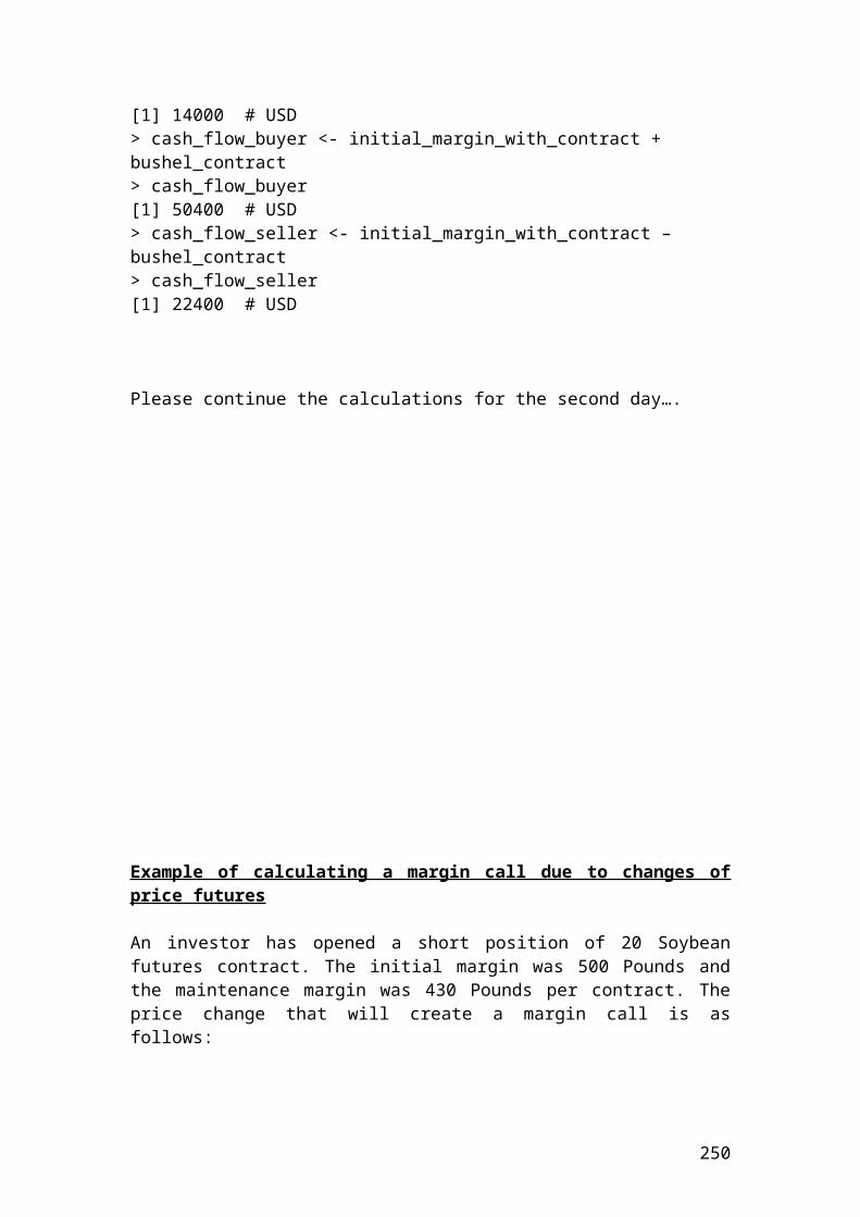
Calculation of the geometric average based on percentages of stock prices returns
class geometric_average_share_prices_returns{public static void main(String[] args) {
/* The stock prices express percentages and we are trying to calculate the geometric mean or average. We insert the percentage values of each stock in an array format.*/
double stock_price_1 = 10;double stock_price_2 = 12;double stock_price_3 = 13;double stock_price_4 = 14;double stock_price_5 = 15;double stock_price_6 = 16;
// We define the variable that we want to calculate.double geometric_average;
// We write the mathematical equation of the geometric mean.geometric_average = Math.pow(stock_price_1*stock_price_2*stock_price_3*stock_price_4*stock_price_5*stock_price_6,0.166666);
// Output functions.
System.out.println("Pow(" + stock_price_1 + ", " + 0.16666 + ") = " + geometric_average);System.out.println(Math.round(geometric_average*100.0)/100.0); }}
Output result
After compiling the current document from tools and pressing the run document you should get the following result:
Welcome to DrJava. Working directory is C:\Documents and Settings\Owner\Desktop\Java Compiler> geometric_average_share_prices_returnsPow(10.0, 0.16666) = 13.1797194671364513.18>
250
Calculation of the geometric average based on percentages of put option price returns
class geometric_average_put_option_price_returns{public static void main(String[] args) {
/* The put option price returns are expressed in percentages and we are trying to calculate the geometric mean or average.*/ // We insert the percentage values of each put option in an array format.
double put_option_price_return_1 = 2;double put_option_price_return_2 = 3.3;double put_option_price_return_3 = 2.45;double put_option_price_return_4 = 4.21;double put_option_price_return_5 = 7.4;double put_option_price_return_6 = 4.34;
// We define the variable that we want to calculate.double geometric_average;
// We write the mathematical equation of the geometric mean.
geometric_average = Math.pow(put_option_price_return_1*put_option_price_return_2*put_option_price_return_3*put_option_price_return_4*put_option_price_return_5*put_option_price_return_6,0.16666);
// Output functions.System.out.println("Pow(" + put_option_price_return_1 + ", " + 0.16666 + ") = " + geometric_average);System.out.println(Math.round(geometric_average*100.0)/100.0); }}
Output result
After compiling the current document from tools and pressing the run document you should get the following result:
Welcome to DrJava. Working directory is C:\Documents and Settings\Owner\Desktop\Java Compiler> geometric_average_put_option_price_returnsPow(2.0, 0.16666) = 3.60243922469834833.6>
251
Calculation of the geometric average based on percentages of index option price returns
class geometric_average_index_option_price_returns{public static void main(String[] args) {
/* The Index option price returns are expressed in percentages and we are trying to //calculate the geometric mean or average. We insert the percentage values of each index option in an array format.*/
double index_option_price_return_1 = 2;double index_option_price_return_2 = 2.31;double index_option_price_return_3 = 2.35;double index_option_price_return_4 = 4.51;double index_option_price_return_5 = 7.56;double index_option_price_return_6 = 4.39;
// We define the variable that we want to calculate.double geometric_average;
// We write the mathematical equation of the geometric mean.
geometric_average = Math.pow(index_option_price_return_1*index_option_price_return_2*index_option_price_return_3*index_option_price_return_4*index_option_price_return_5*index_option_price_return_6,0.16666);
// Output functions.System.out.println("Pow(" + index_option_price_return_1 + ", " + 0.16666 + ") = " + geometric_average);System.out.println(Math.round(geometric_average*100.0)/100.0); }}
Output result
After compiling the current document from tools and pressing the run document you should get the following result:
Welcome to DrJava. Working directory is C:\Documents and Settings\Owner\Desktop\Java Compiler> run geometric_average_index_option_price_returnsPow(2.0, 0.16666) = 3.42865702048713543.43>
252
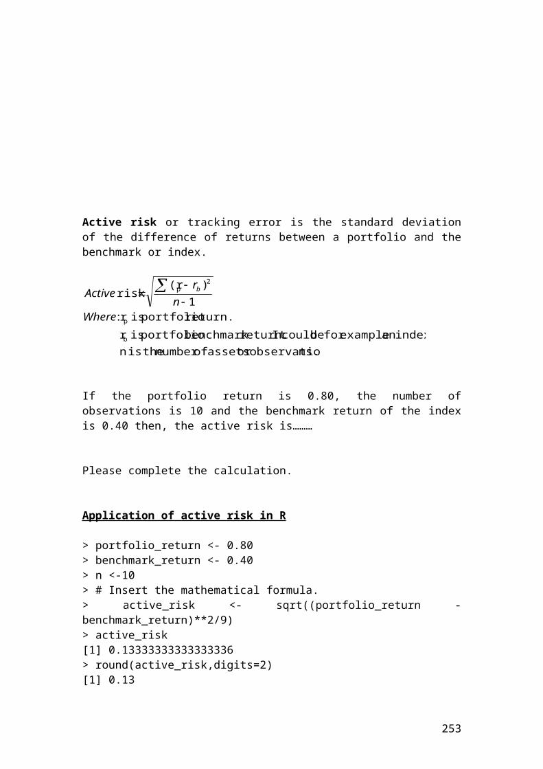
Calculate the portfolio return, the variance and the standard deviation in C++ for options with different returns and standard deviations
class portfolio_return_variance_and_standard_deviation{public static void main(String[] args) {
/* Calculate the portfolio return, the variance and the standard deviation or risk of theportfolio for options with different returns and standard deviations.*/
// Call option A expected return 0.6// Call option A standard deviation 0.2// Call option A weight 0.35// Correlation coefficient between A and B 0.5// Call option B expected return 0.1// Call option B standard deviation 0.7 // Call option B weight 0.45//Correlation coefficient between B and C -0.1// Call option C expected return 0.3// Call option C standard deviation 0.4// Call option C weight 0.2//Correlation coefficient between A and C -0.4
//Insert the given information by using the double function as we have fractions.
double CalloptionAexpectedreturn = 0.6;double CalloptionAstandarddeviation = 0.2;double CalloptionAweight = 0.35;double CorrelationcoefficientbetweenAandB = 0.5;double CalloptionBexpectedreturn = 0.1;double CalloptionBstandarddeviation = 0.7;double CalloptionBweight = 0.45;double CorrelationcoefficientbetweenBandC = -0.1;double CalloptionCexpectedreturn = 0.3;double CalloptionCstandarddeviation = 0.4;double CalloptionCweight = 0.2;double CorrelationcoefficientbetweenAandC = -0.4; /*Define the variables that we want to calculate. In other words, the portfolio return,variance and standard deviation.*/
double Portfolioreturn;double Portfoliovariance; double PortfoliostdDev;
// Write the formula of portfolio return.
253
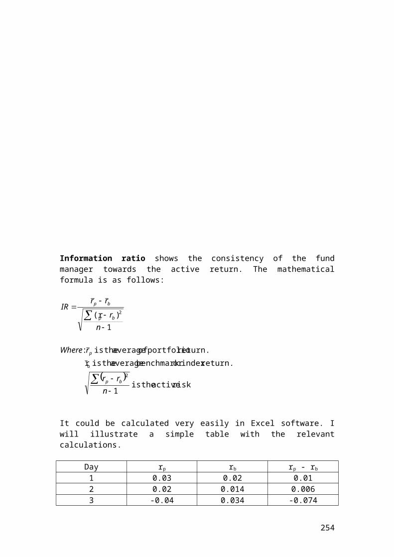
Portfolioreturn = (CalloptionAexpectedreturn*CalloptionAweight)+(CalloptionBweight*CalloptionBexpectedreturn)+(CalloptionCexpectedreturn*CalloptionCweight);// Write the formula for portfolio variance.
Portfoliovariance = Math.pow(CalloptionAweight*CalloptionAstandarddeviation,2)+ Math.pow(CalloptionBweight*CalloptionBstandarddeviation,2)+ Math.pow(CalloptionCweight*CalloptionCstandarddeviation,2)+(2*CalloptionAweight*CalloptionBweight*CalloptionAstandarddeviation*CalloptionBstandarddeviation*CorrelationcoefficientbetweenAandB)+(2*CalloptionAweight*CalloptionCweight*CorrelationcoefficientbetweenAandC*CalloptionAstandarddeviation*CalloptionCstandarddeviation)+(2*CalloptionBweight*CalloptionCweight*CorrelationcoefficientbetweenBandC*CalloptionBstandarddeviation*CalloptionCstandarddeviation);
// Write the formula for portfolio standard deviation.
PortfoliostdDev = Math.sqrt(Portfoliovariance);
//Output functions. System.out.print("The portfolio return is");System.out.println(Portfolioreturn);System.out.println(Math.round(Portfolioreturn*100.0)/100.0);System.out.print("The portfolio variance is");System.out.println(Portfoliovariance);System.out.println(Math.round(Portfoliovariance*100.0)/100.0);System.out.print("The portfolio standard deviation is");System.out.println(PortfoliostdDev);System.out.println(Math.round(PortfoliostdDev*100.0)/100.0);}}
Output results
After compiling the current document from tools and pressing the run document you should get the following results:
Welcome to DrJava. Working directory is C:\Documents and Settings\Owner\Desktop\Java Compiler> run portfolio_return_variance_and_standard_deviation
The portfolio return is0.3150.32The portfolio variance is0.123054999999999980.12The portfolio standard deviation is0.350791961139362450.35>
254
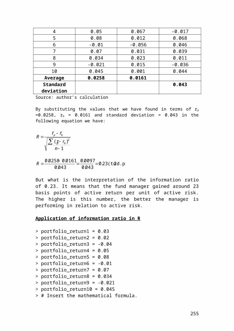
Calculate the portfolio return, the variance and the standard deviation or risk of the portfolio
class portfolio_return_variance_and_standard_deviation_of_portfolio{public static void main(String[] args) {
/* Calculate the portfolio return, the variance and the standard deviation or risk of theportfolio.*/
// Share A expected return 0.11// Share A standard deviation 0.15// Share A amount 50000// Correlation coefficient between A and B 0.30// Share B expected return 0.25// Share standard deviation 0.20 // Share B amount 50000// The total amount of the portfolio is 100000
double shareAexpRet = 0.25;double shareAstddev = 0.10;double shareAamount = 50000;double correlationAB = 0.40;double shareBexpRet = 0.35;double shareBstddev = 0.18;double shareBamount = 50000;double totalportfoliovalue = 100000;
/* Define the variables that we want to calculate.In other words, the portfolio return, variance and the standard deviation.*/
double weightA;double weightB;double Portfolioreturn;double Portfoliovariance; double PortfoliostdDev;
// Calculate the weights for each share.
weightA = shareAamount / totalportfoliovalue;weightB = shareBamount / totalportfoliovalue;
// Write the formula of portfolio return.
Portfolioreturn = (shareAexpRet*weightA)+(shareBexpRet*weightB);
// Write the formula for portfolio variance.
Portfoliovariance = Math.pow(weightA*shareAstddev,2)+ Math.pow(weightB*shareBstddev,2)
255
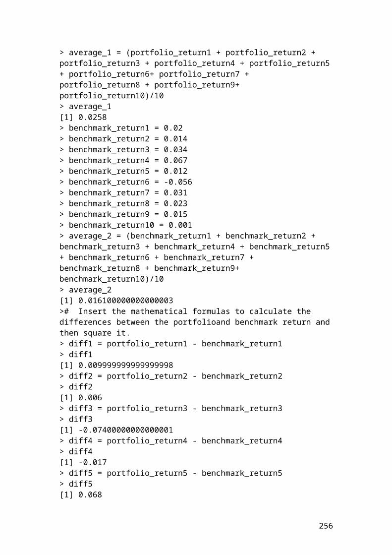
+(2*weightA*weightB*shareAstddev*shareBstddev*correlationAB);
// Write the formula for portfolio standard deviation.
PortfoliostdDev = Math.sqrt(Portfoliovariance);
//Output functions. System.out.print("The portfolio return is");System.out.println(Portfolioreturn);System.out.println(Math.round(Portfolioreturn*100.0)/100.0);System.out.print("The portfolio variance is");System.out.println(Portfoliovariance);System.out.println(Math.round(Portfoliovariance*100.0)/100.0);System.out.print("The portfolio standard deviation is");System.out.println(PortfoliostdDev);System.out.println(Math.round(PortfoliostdDev*100.0)/100.0);}}
Output results
After compiling the current document from tools and pressing the run document you should get the following results:
Welcome to DrJava. Working directory is C:\Documents and Settings\Owner\Desktop\Java Compiler> run portfolio_return_variance_and_standard_deviation_of_portfolioThe portfolio return is0.30.3The portfolio variance is0.01420.01The portfolio standard deviation is0.119163752878129860.12>
256
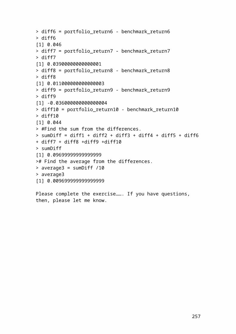
Example of pricing a forward contract and solution
A forward contract of 6 month has a market price of 52 Pounds when the spot price of the underlying commodity is 49 Pounds. There are no costs of carry and the discount rate is 7 percent. Calculate the value of the forward contract.
Solution
The current price of the forward contract (F0) should be equal to the value of the underlying commodity, (S0) at the discount rate r. Thus, the equation is as follows:
F0=S0(1+r )
F0=S0(1+r )=49(1+0 . 072 )=50 . 715 pounds
Application of pricing a forward contract in Java
class pricing_forward_contract{public static void main(String[] args) {
//Pricing a forward contract.
double Value_forward_contract;double spot_price = 49;double discount_rate = 0.07; // Insert the mathematical formula.
Value_forward_contract = spot_price*(1+discount_rate/2);
//Output function. System.out.print("The value of a forward contract in pounds is");System.out.println(Value_forward_contract);System.out.println(Math.round(Value_forward_contract*100.0)/100.0);
}}
257
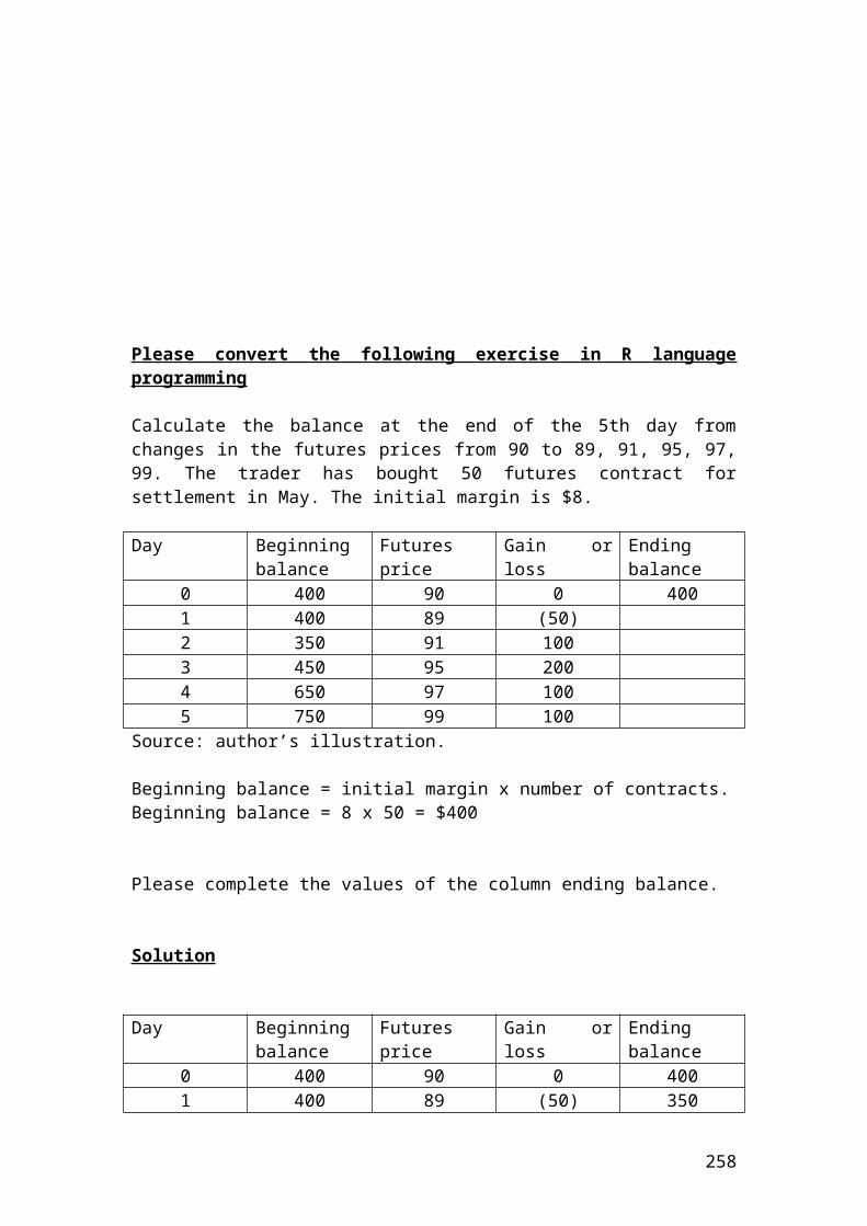
Output result
After compiling the current document from tools and pressing the run document you should get the following result:
Welcome to DrJava. Working directory is C:\Documents and Settings\Owner\Desktop\Java Compiler> run pricing_forward_contractThe value of a forward contract in pounds is50.71499999999999650.72>
258
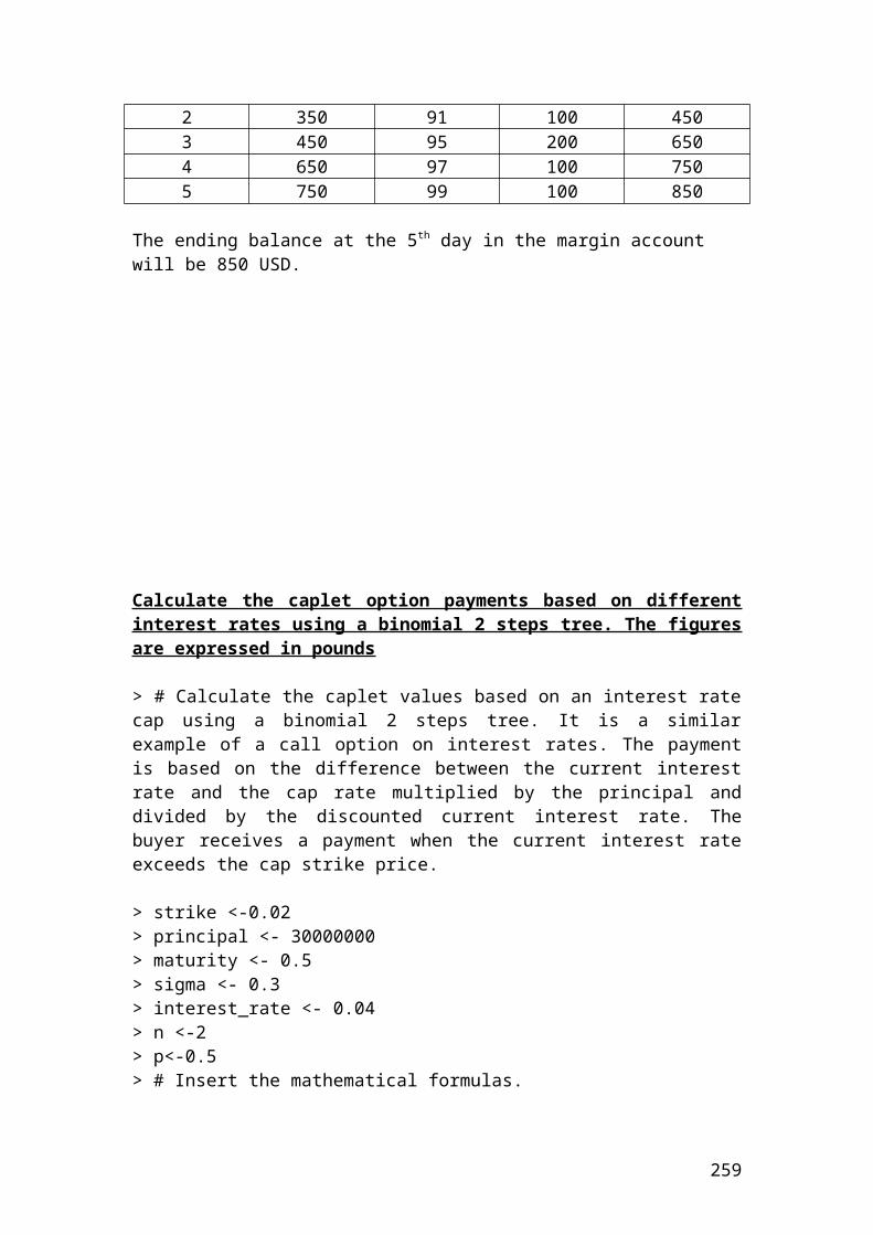
Example of interest rate payment and solution
A trader wants to calculate the interest amount that he / she will receive in three months from a forward contract of a Euribor deposit paying a Euro deposit rate of 3.55%. The principal amount is 300,000
The mathematical formula is as follows:
Interest payment = principal x [interest rate x (tdays / 360)]
Interest payment = 300,000 x [0.0355 x (90/360)]Interest payment = 2662.5 Euro.
First example: application of interest payment in Java
class interest_rate_payment{public static void main(String[] args) {
//Interest rate payment.
double interest_payment;double principal = 300000;double interest_rate = 0.0355;double days = 90;
// Insert the mathematical formula.
interest_payment = principal*(interest_rate *days/360);
//Output function. System.out.print("interest rate payment in euro is");System.out.println(interest_payment);System.out.println(Math.round(interest_payment*100.0)/100.0);}}
259
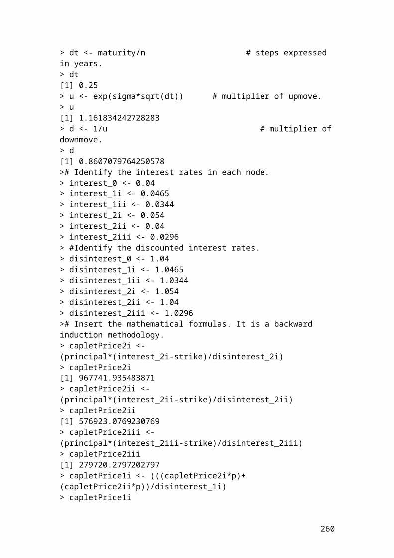
Output result
After compiling the current document from tools and pressing the run document you should get the following result:
Welcome to DrJava. Working directory is C:\Documents and Settings\Owner\Desktop\Java Compiler> run interest_rate_paymentinterest rate payment in euro is 2662.49999999999952662.5>
260
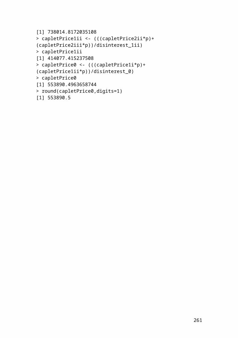
Example and solution of calculating profits and losses on futures contracts
An investor buys 8 S&P 500 futures contracts at $2189. He has closed the futures contract position with a price of $2236. The multiplier for S&P 500 futures contracts is 250 dollars. Did he record a profit or a loss?
Solution
The mathematical formula is as follows:
Pr ofit /Loss=number of contracts x contract size x ( f T−f 0 )
Where: fT is the final contract price. f0 is the initial contract price.
Gain=8 x 250 x (2236−2189 )=94000 USD
Application of calculating profits and losses on futures contracts in Java
class profits_losses_futures_contracts{public static void main(String[] args) {
// calculating profits and losses on futures contracts.
double profit_or_loss ; int number_of_contracts =8;double buying_price = 2189;double selling_price = 2236;int multiplier = 250;
// Insert the mathematical formula. profit_or_loss = number_of_contracts*multiplier*(selling_price - buying_price);
//Output function. System.out.print("Profit or loss on futures contract in USD is");System.out.println(profit_or_loss);System.out.println(Math.round(profit_or_loss*100.0)/100.0);
}}
261
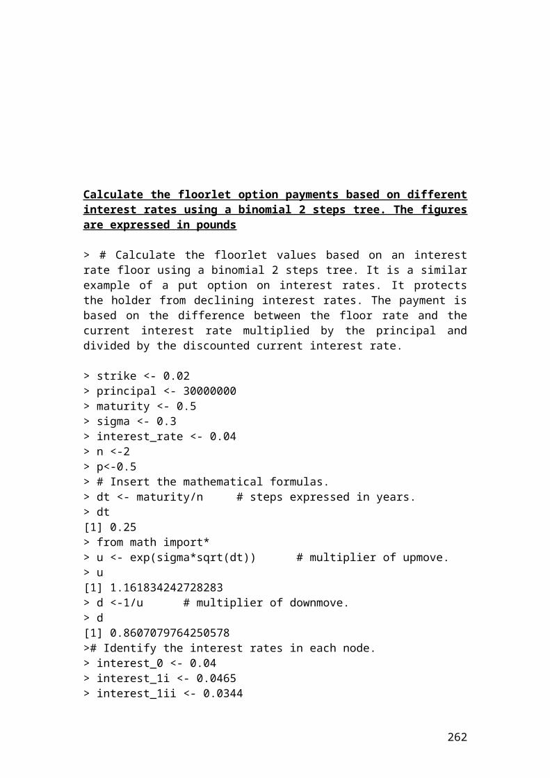
Output result
After compiling the current document from tools and pressing the run document you should get the following result:
Welcome to DrJava. Working directory is C:\Documents and Settings\Owner\Desktop\Java Compiler> run profits_losses_futures_contractsProfit or loss on futures contract in USD is94000.094000.0>
262
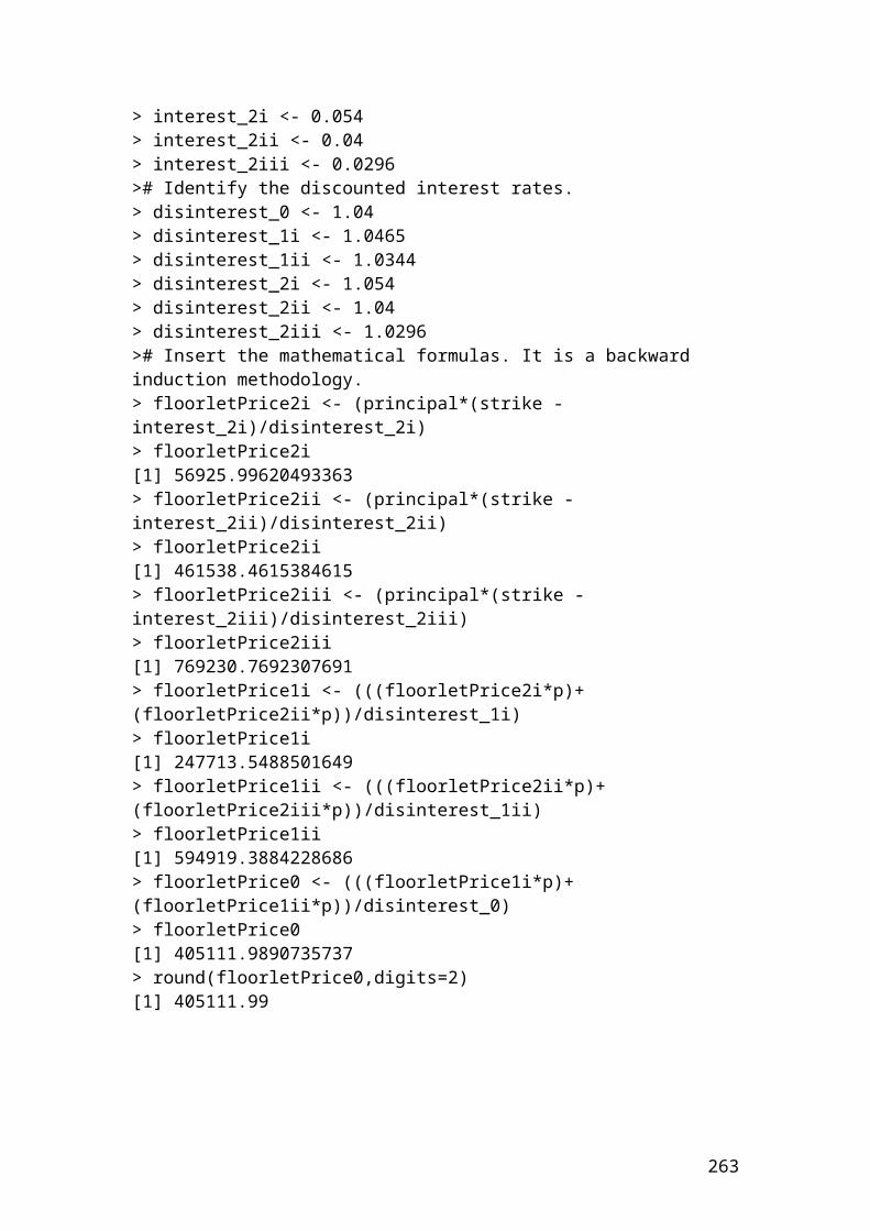
Example and solution of semiannually currency swap between an investment bank and an insurance company
The investment bank borrows 20,000,000 Pounds from the insurance company at a fixed rate of 5% for 1 year. The insurance company borrows from the investment bank 10,000,000 Euros at a fixed rate of 5% for 1 year. Calculate the interest payments for the three years, if we assume semiannual payments?
At the beginning of the contract
€10,000,000Investment bank Insurance company
£ 20,000,000
The insurance company pays the investment bank the following interest payment.
£20,000,000 x 0.05/2 = 500,000 Pounds.
The investment bank pays the insurance the following interest payment.
€10,000,000 x 0.05/2 =250,000 Euros.
The following arrows illustrate the interest payments.
€ 250,000Investment bank Insurance company
£ 500,000
At the end of the third year, the two parties exchange the principal amounts in addition to the final interest payments.
€10,250,000Investment bank Insurance company
£20,500,000
263
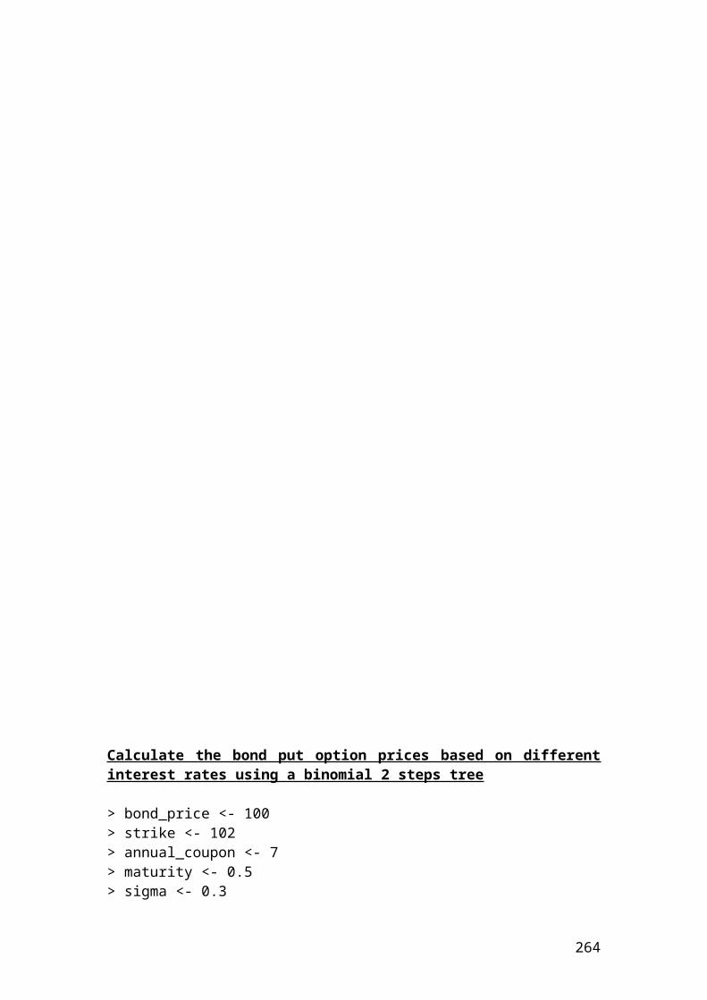
Application of semiannually currency swap between an investment bank and an insurance company in Java
class semiannual_currency_swap{public static void main(String[] args) {
//Semiannual swaps interest payments between an investment bank and an insurance company.
double bank_pays_insurance ;double insurance_pays_bank ;double bank_borrows_from_insurance =20000000;double insurance_borrows_from_bank = 10000000;double interest_rate = 0.05;int semi_annual_payment = 2;
//Insert the mathematical formulas. bank_pays_insurance = insurance_borrows_from_bank *(interest_rate/semi_annual_payment);insurance_pays_bank = bank_borrows_from_insurance *(interest_rate/semi_annual_payment);
//Output function. System.out.print("bank pays insurance in euros is");System.out.println(bank_pays_insurance);System.out.print("insurance pays bank in pounds is");System.out.println(insurance_pays_bank);}}
Output results
After compiling the current document from tools and pressing the run document you should get the following result:
Welcome to DrJava. Working directory is C:\Documents and Settings\Owner\Desktop\Java Compiler> run semiannual_currency_swapbank pays insurance in euros is 250000.0insurance pays bank in pounds is 500000.0>
264
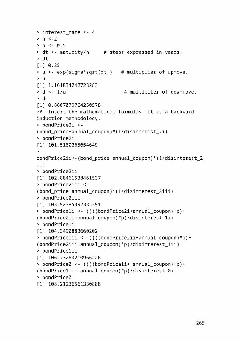
Example and solution of interest rate swap
Interest rate swaps are very popular agreements between two parties in the debt or fixed-income department of the investment banks. The fixed income department of Bank A pays a fixed rate of 5.5% upon the principal of 50,000,000 Pounds. In contrast, Bank B pays a floating or reference rate of LIBOR accounted to 7.2%. The payment frequency is every 6 months for 2 years.
Fixed payment : £50,000,000 x 0.055/2 = 1,375,000 Bank A Bank B Floating payment: £50,000,000 x 0.072/2 = 1,800,000
Suppose in the second year that the LIBOR has increased by 12 basis points or 0.12%. Then, the floating payment will change and the calculation will be as follows:
Second year floating payment for Bank B = 50,000,000 x 0.0732 / 2 = 1,830,000 Pounds.
Bank A will continue to pay the same fixed amount, namely, £50,000,000 x 0.055/2 = £1,375,000.
265
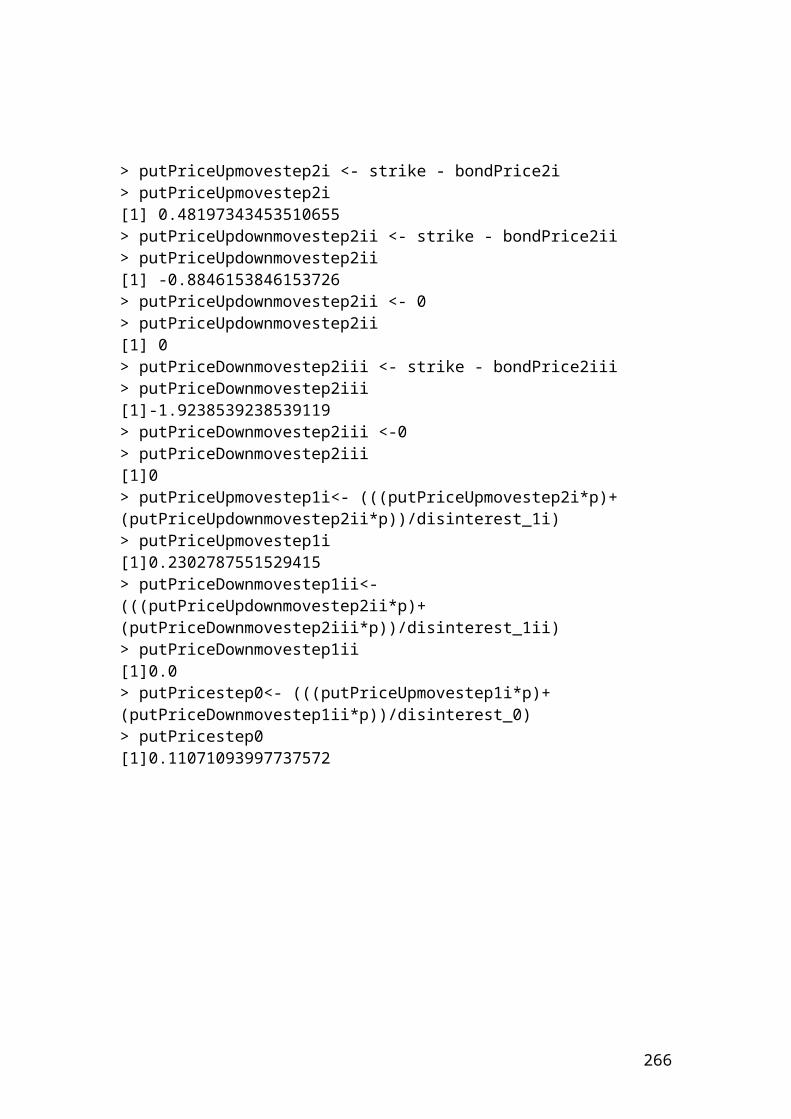
Application of interest rate swap in Java
class interest_rate_swap{public static void main(String[] args) {//Semiannual swaps interest payments between two parties.
double fixed_payment ;double floating_payment_1 ;double floating_payment_2 ;double principal = 50000000;double interest_rate_1 = 0.055;double interest_rate_2 = 0.072;double interest_rate_3 = 0.0732;int semiannual_payment = 2;
// Insert the mathematical formulas. fixed_payment = principal*(interest_rate_1/semiannual_payment);floating_payment_1 = principal*(interest_rate_2/semiannual_payment);floating_payment_2 = principal*(interest_rate_3/semiannual_payment);
//Output functions.System.out.print("The value of a fixed payment in pounds is");System.out.println(fixed_payment);System.out.println(Math.round(fixed_payment*100.0)/100.0);System.out.print("The value of a floating payment 1 in pounds is");System.out.println(floating_payment_1);System.out.println(Math.round(floating_payment_1*100.0)/100.0);System.out.print("The value of a floating payment 2 in pounds is");System.out.println(floating_payment_2);System.out.println(Math.round(floating_payment_2*100.0)/100.0);}}
Output results
After compiling the current document from tools and pressing the run document you should get the following results:
Welcome to DrJava. Working directory is C:\Documents and Settings\Owner\Desktop\Java Compiler> run interest_rate_swapThe value of a fixed payment in pounds is1375000.01375000.0The value of a floating payment 1 in pounds is1799999.99999999981800000.0The value of a floating payment 2 in pounds is1830000.01830000.0
266
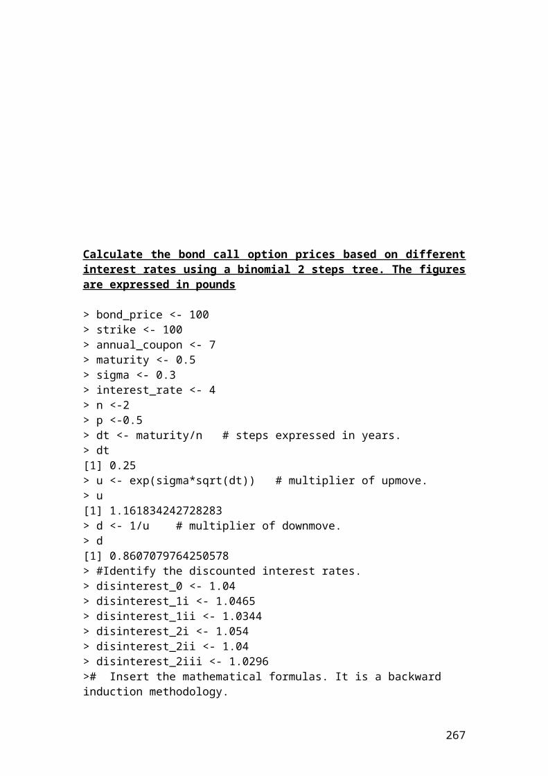
>Delta – neutral hedge
Delta – neutral hedge is common used in risk management to keep the value of the portfolio neutral due to changes in the share price. It is achieved from a long position in a share and a short position in a call option. The mathematical formula to determine the number of options is as follows:
Delta - neutral hedge =Number of shares hedgeddelta of call option
Thus, if the investment bank has bought 30,000 shares of Vodafone and the delta of the call option of the same company is 0.50, then the numbers of call options that are needed to purchase to form a delta-neutral hedge are as follows:
Delta hedge = 30,000 / 0.50 = 60,000 options or 600 option contracts.
Application of delta- neutral hedge in Java
class delta_neutral_hedge{public static void main(String[] args) { // Delta neutral hedge.
double delta_neutral_hedge ;double number_of_shares = 30000 ;double delta_call_option = 0.50 ; // Insert the mathematical equation.
delta_neutral_hedge = number_of_shares/delta_call_option;
// Output function.
System.out.print("The delta neutral hedge is");System.out.println(delta_neutral_hedge);System.out.println(Math.round(delta_neutral_hedge*100.0)/100.0);
}}
267
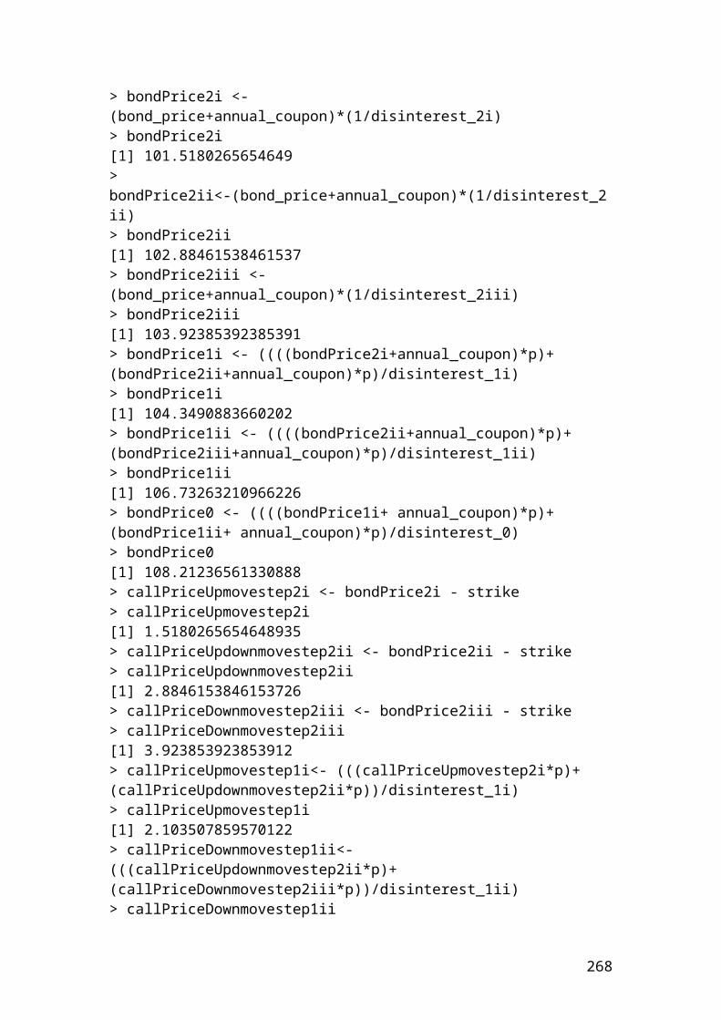
Output result
After compiling the current document from tools and pressing the run document you should get the following result:
Welcome to DrJava. Working directory is C:\Documents and Settings\Owner\Desktop\Java Compiler> run delta_neutral_hedgeThe delta neutral hedge is60000.060000.0>
268
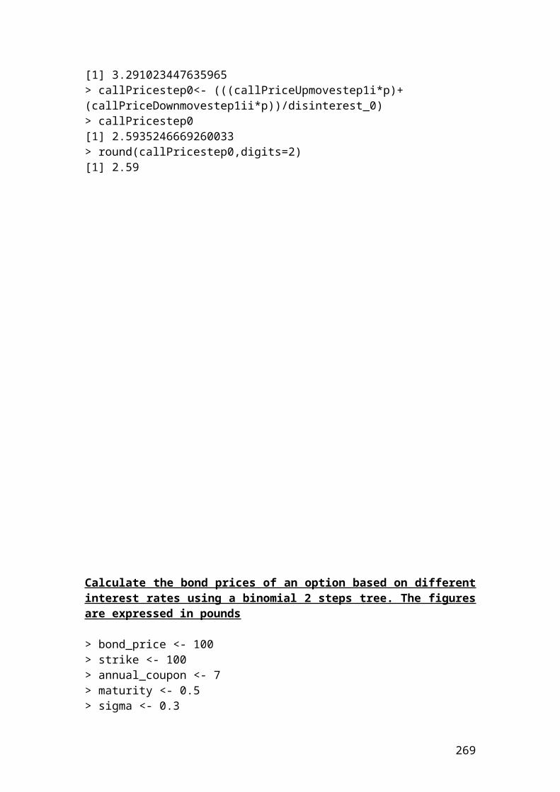
Weighted mean price of a portfolio
Let’s assume that we have a portfolio of four options with their market prices and the number of shares bought. It is required to calculate the weighted mean price of the portfolio.
Options Price expressed in $
Number of shares
Weight Weight x Price
A 14.00 300 0.4 5.6B 12.00 200 0.3 3.6C 8.00 100 0.1 0.8D 5.00 150 0.2 1
Total 750 1Source: author’s calculation
The mathematical formula is as followed:
X̄ w=∑ w i Pi
Where : X̄ w is the weighted mean price of the portfolio . w i are the weights . Pi are the prices .
By substituting the numbers from the Table into the equation we have the following:
X̄ w= 5 . 6 + 3. 6 + 0.8 + 1 = 11.
Application of weighted mean price of a portfolio in Java
class weighted_mean_price_portfolio{public static void main(String[] args) {
// Weighted mean price of a portfolio. double portfolio_mean ;
double price_1 = 14;double price_2 = 12;double price_3 = 8;double price_4 = 5;
double weight_1 = 0.4;double weight_2 = 0.3;double weight_3 = 0.1;double weight_4 = 0.2;
269
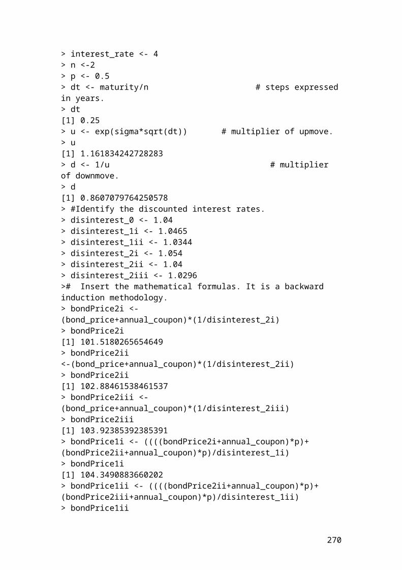
// Insert the mathematical equation.
portfolio_mean = (price_1*weight_1 + price_2*weight_2 + price_3*weight_3 + price_4*weight_4) ;
//Output function. System.out.print("The weighted mean price of a portfolio in USD is");System.out.println(portfolio_mean);}}
Output result
After compiling the current document from tools and pressing the run document you should get the following result:
Welcome to DrJava. Working directory is C:\Documents and Settings\Owner\Desktop\Java Compiler> run weighted_mean_price_portfolioThe weighted mean price of a portfolio in USD is11.0>
270

Example of Eurodollar futures
An investor wants to calculate the futures price of a 1-month Eurodollar time deposits based on a LIBOR rate of 3.40%. The initial principal is 1 million Pounds.
Solution
The price of the Eurodollar futures contract will be as follows:
Futures price of Eurodollar time deposit =Principal x [1-LIBOR rate x (tdays
360 )]
Futures price of Eurodollar time deposit = 1,000,000 x [1-0 .034 x (30360 )]=. . .. .. . Pounds
Futures price of Eurodollar time deposit = 1,000,000 x 0 .997166667 = 997166 .67 pounds
Application of Eurodollar futures in Java
class Eurodollar_futures{public static void main(String[] args) {
double Eurodollar_futures;double principal = 1000000;double interest_rate = 0.034;int days = 30;
// Insert the mathematical formula.
Eurodollar_futures = principal*(1- interest_rate *days/360);
//Output function. System.out.print("Eurodollar futures in pounds is");System.out.println(Eurodollar_futures);System.out.println(Math.round(Eurodollar_futures*100.0)/100.0);}}
271

Output result
After compiling the current document from tools and pressing the run document you should get the following result:
Welcome to DrJava. Working directory is C:\Documents and Settings\Owner\Desktop\Java Compiler> run Eurodollar_futuresEurodollar futures in pounds is997166.6666666666997166.67
Example of forward rate agreement
An investment bank buys a 4 x 6 FRA from a building society in the UK for 4.0% by paying 2 million Pounds. 80 days latter, LIBOR is 5%. Who will receive the FRA payment and for how much?
Solution
The mathematical formula for Forward Rate Agreement, (FRA) is as follows:
FRA Payment =Notional amount x( ( variable rate- fixed rate ) (t days /360 )1+var iable rate ( tdays/360 ) )
The timeline schedule is as follows:
t = 0 4months 6 months
FRA Payment =2, 000 , 000 x( (0 . 05- 0 . 04 ) (120/360 )1+0 . 05 (80/360 ) )
= ………. Please complete the calculation.
Helpful hint: If the FRA payment is positive, then, the building society is the payer and the investment bank receives the FRA payment.
If the FRA payment is negative, then the investment bank is the payer and the building society receives the FRA payment.
272
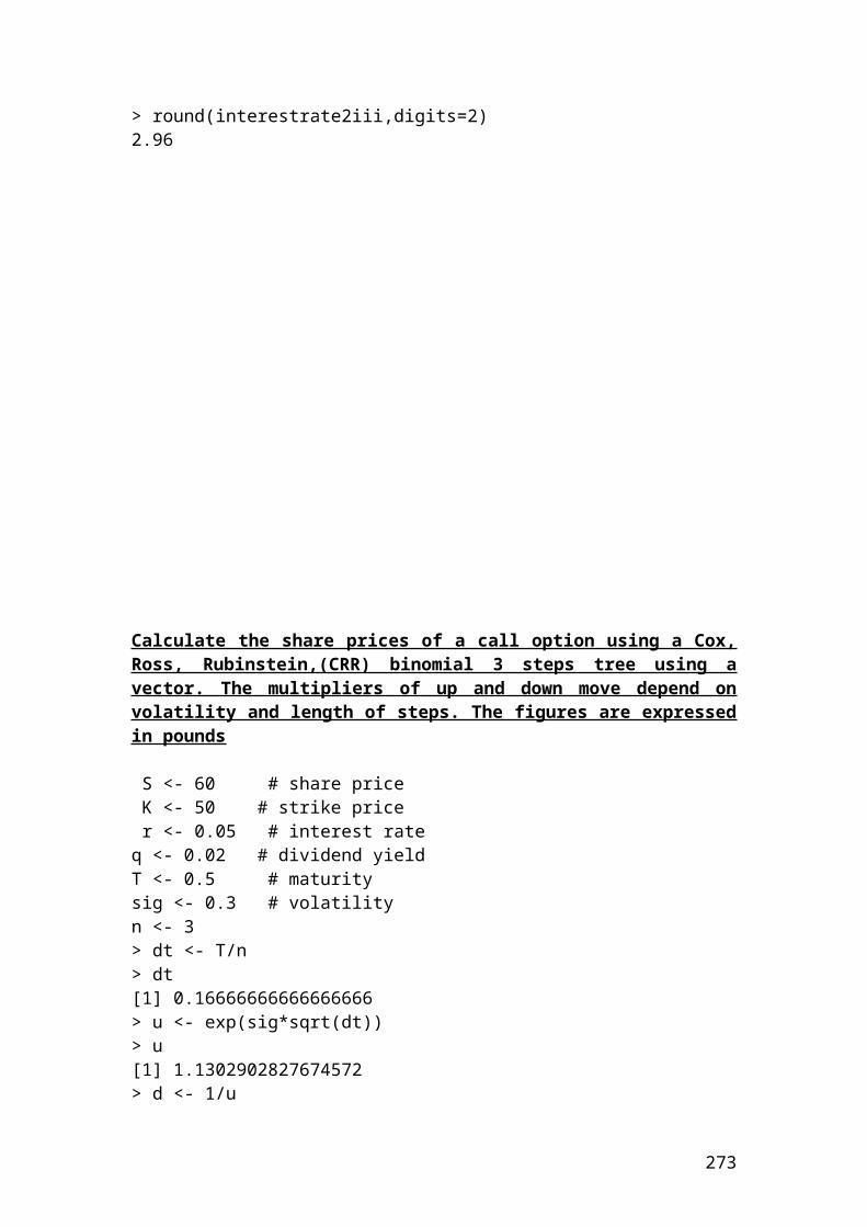
Application of forward rate agreement in Java
class Forward_rate_agreement{public static void main(String[] args) {
double FRApayment;double principal = 2000000;double variable_rate = 0.05;double fixed_rate = 0.04;
// Insert the mathematical formula.FRApayment= principal*(variable_rate - fixed_rate)*0.333333333/1.011111111;
// Output function.
System.out.print("Forward rate agreement in pounds is");System.out.println(FRApayment);System.out.println(Math.round(FRApayment*100.0)/100.0);}}
Output result
After compiling the current document from tools and pressing the run document you should get the following result:
Welcome to DrJava. Working directory is C:\Documents and Settings\Owner\Desktop\Java Compiler> run Forward_rate_agreementForward rate agreement in pounds is6593.4065875377396593.41>
273
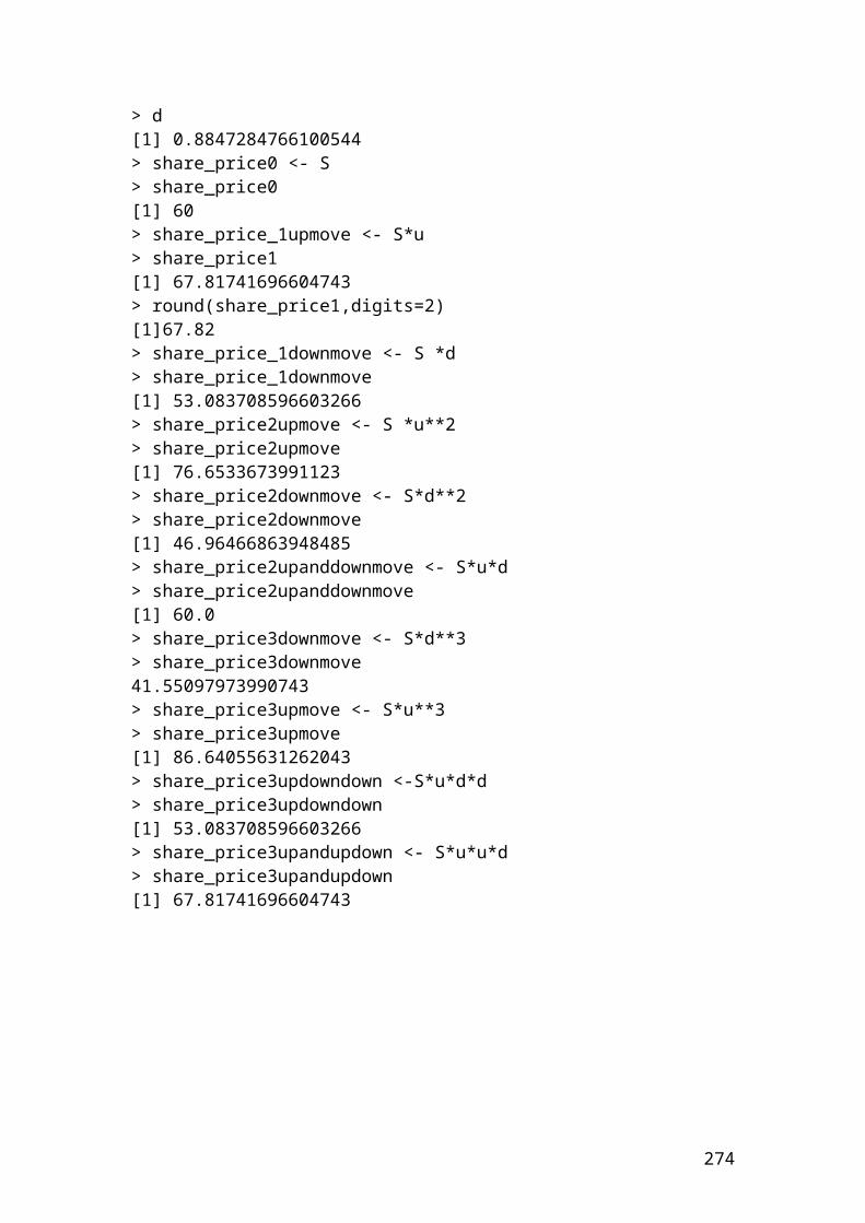
Example of futures on Treasury bills
An investor wants to calculate the futures price of a 3-month Treasury bills. Treasury bills are short-term notes of limited period of 1- month, and 3 - month respectively. The initial principal is 5 million Pounds and the discount rate is 3.50%.
Solution
The price of the Treasury bill futures will be as follows:
Futures price Treasury Bill = Principal x [1-discount rate x (t days
360 )]
Please complete the calculation …….
Application of futures on Treasury bills in Java
class Futures_Treasury_bills{public static void main(String[] args) {
double Futures_treasury_bills;double principal = 5000000;double discount_rate = 0.035;int days = 90;
//Insert the mathematical formula.
Futures_treasury_bills = principal*(1- discount_rate *days/360);
//Output function.
System.out.print("Futures on treasury bills in pounds is");System.out.println(Futures_treasury_bills);System.out.println(Math.round(Futures_treasury_bills*100.0)/100.0);}}
Output result
After compiling the current document from tools and pressing the run document you should get the following result:
Welcome to DrJava. Working directory is C:\Documents and Settings\Owner\Desktop\Java Compiler> run Futures_Treasury_billsFutures on treasury bills in pounds is4956250.0
274

4956250.0>
Example of stock index futures
For example, if you bought 10 contracts of the Dow Jones Industrial index at 10,000 and you expected an aggressive bull market that reaches the value of 16,000, then, the 6000 points increase are multiplied by the standardized value of 250. If the initial principal of investment is $100,000, the mathematical formula for the gains will be as follows:
10 x 100,000 x 6000 x 250 = 1.5 x 10¹² Dollars
Application of stock index futures in Java
class Stock_index_futures{public static void main(String[] args) { //The gains from stock index futures. double gains;double principal = 100000;double pointsincrease = 6000; int number_of_contracts = 10;int multiplier = 250;
// Insert the mathematical formula.
gains = principal*pointsincrease*multiplier*number_of_contracts;
// Output function.
System.out.print("The gains from stock index futures in USD are");System.out.println(gains);System.out.println(Math.round(gains*100.0)/100.0);
}}
Output result
After compiling the current document from tools and pressing the run document you should get the following result:
Welcome to DrJava. Working directory is C:\Documents and Settings\Owner\Desktop\Java Compiler> run Stock_index_futuresThe gains from stock index futures in USD are1.5E12
275
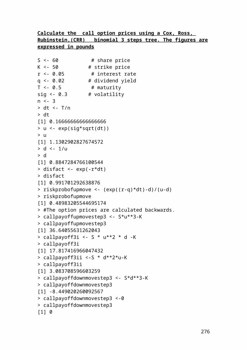
1.5E12>
Example of currency futures
A manufacturer wants to calculate the currency futures price of EURO/USD traded in Frankfurt derivative market. For example, in August the contract is quoted as 1.35 EURO /USD and the contract size is 20,000. The principal is 300,000 Euro.
Solution
The contract price of 1 contract is as follows:
Futures price of currency future EURO/USD = principal* contract size x August quoted price = . .. . . Euro
Please complete the calculation . .. .
Application of currency futures in Java
class Currency_futures{public static void main(String[] args) {
double Futures_price_of_currency;double principal = 300000;double quote = 1.35;int contract_size = 20000;
// Insert the mathematical formula.Futures_price_of_currency = principal*quote*contract_size ;
// Output function.
System.out.print("Futures price of currency in euro is");System.out.println(Futures_price_of_currency);System.out.println(Math.round(Futures_price_of_currency*100.0)/100.0);}}
Output result
After compiling the current document from tools and pressing the run document you should get the following result:
Welcome to DrJava. Working directory is C:\Documents and Settings\Owner\Desktop\Java Compiler
276
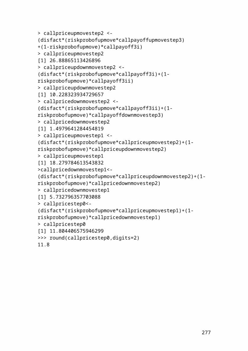
> run Currency_futuresFutures price of currency in euro is8.1E98.1E9
277
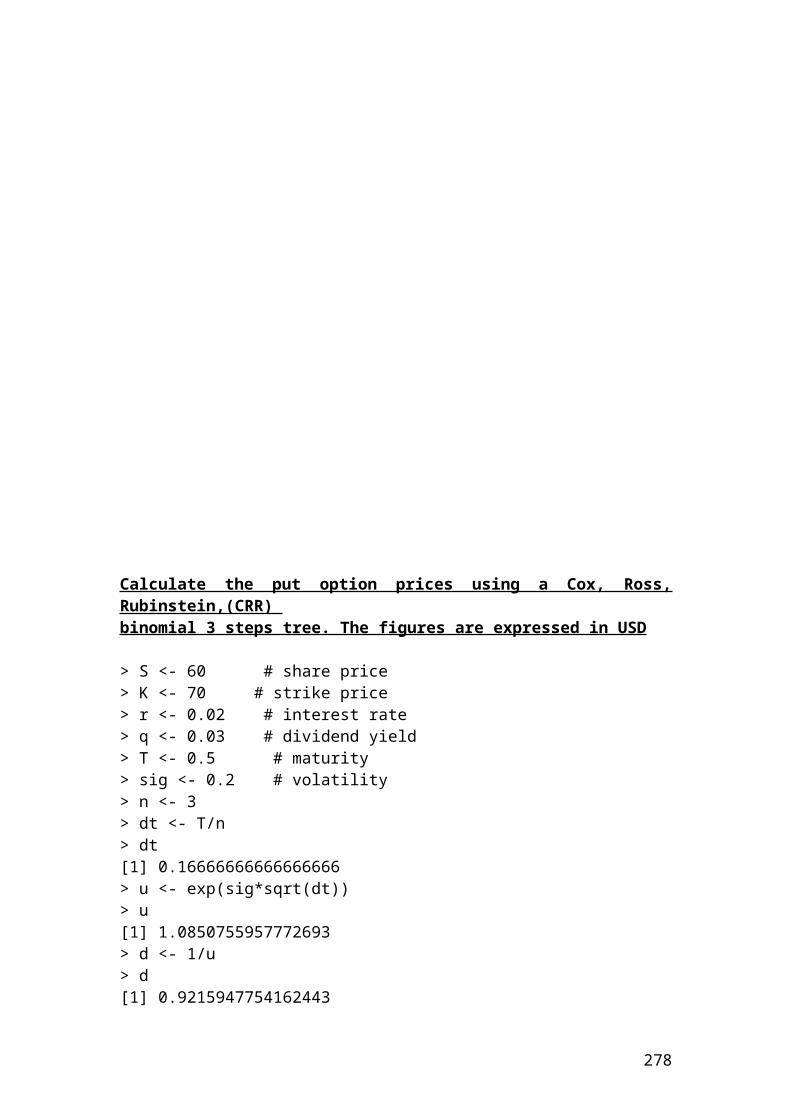
Example of calculating implied volatility of a call option price due to volatility
class Implied_volatility{public static void main(String[] args) { double S = 80.0; double K = 80.0; double r = 0.04; double q = 0.01; double T = 0.50; double sig, optPrice,tolerance ; int i;
optPrice = 8.34; // Option price. sig = 0; tolerance = 0.01; // Specification for the sigma or volatility with tolerance level //in relation with the theoretical and market option price. for(i = 1; i < 80 ; i++) { sig += tolerance; } // Output functions. System.out.print("Implied volatility is");System.out.println(sig);System.out.println(Math.round(sig*100.0)/100.0);System.out.print("Current option pricein USD is ");System.out.println(optPrice);}} Output results
After compiling the current document from tools and pressing the run document you should get the following results:
Welcome to DrJava. Working directory is C:\Documents and Settings\Owner\Desktop\Java Compiler> run Implied_volatilityImplied volatility is0.79000000000000050.79Current option price in USD is 8.34
278
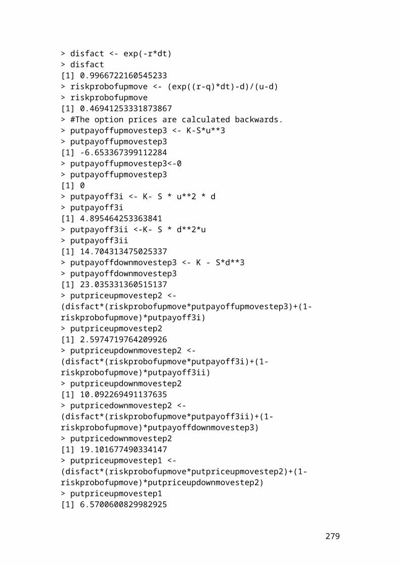
>
Example of calculating implied volatility of a put option price due to volatility
class Implied_volatility{public static void main(String[] args) { double S = 50.0; double K = 50.0; double r = 0.04; double q = 0.01; double T = 0.50; double sig, optPrice,tolerance ; int i;
optPrice = 5.34; // Put option price. sig = 0; tolerance = 0.01; /* Specification for the sigma or volatility with tolerance level in relation with the theoretical and market option price.*/ for(i = 1; i < 50 ; i++) { sig += tolerance; } // Output functions. System.out.print("Implied volatility is");System.out.println(sig);System.out.println(Math.round(sig*100.0)/100.0);System.out.print("Current option price in USD is ");System.out.println(optPrice);}}
Output results
After compiling the current document from tools and pressing the run document you should get the following results:
> run Implied_volatilityImplied volatility is0.490000000000000270.49Current option price in USD is 5.34>
279

Please try based on the previous examples to illustrate the following example in Java. If you have difficulties e-mail me
Active return, active risk and information ratio
Active return is the difference in returns between a portfolio and the index or benchmark that is measured.
Active return = rp - rb
Where: rp is the portfolio return. rb is the benchmark or index return.
If the portfolio return is 0.80 and the benchmark return of the index is 0.70 then, the active return is………
Please complete the calculation.
Active risk or tracking error is the standard deviation of the difference of returns between a portfolio and the benchmark or index.
Active risk =√∑ (r p−r b )2
n−1
Where : rp is portfolio return . rb is portfolio benchmark return . It could be for example an index . n is the number of assets .
If the portfolio return is 0.80, the number of assets is 10 and the benchmark return of the index is 0.40 then, the active risk is………
Please complete the calculation.
Information ratio shows the consistency of the fund manager towards the active return. The mathematical formula is as follows:
280
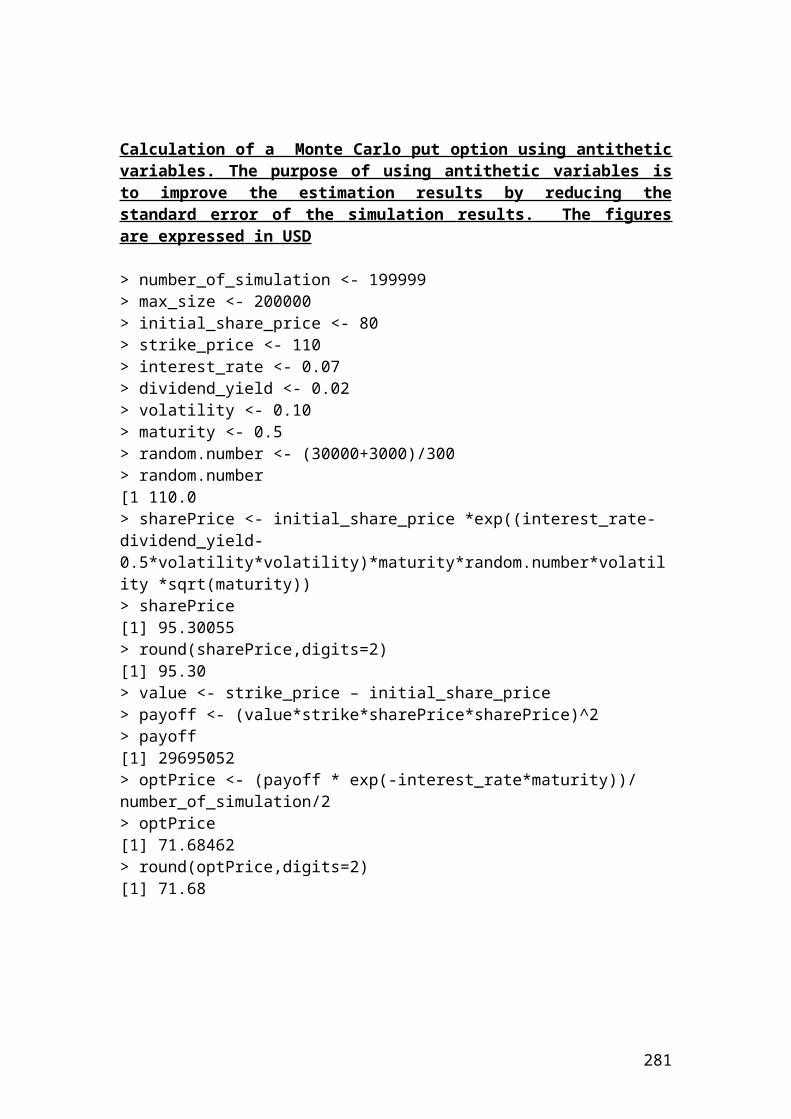
IR=r̄ p− r̄b
√∑ (r p−rb)2
n−1
Where : r̄ p is the average of portfolio return . { r̄ b
is the average benchmark or index return . ¿ √∑ (r p−r b)2
n−1 is the active risk ¿¿
It could be calculated very easily in Excel software. I will illustrate a simple table with the relevant calculations.
Day rp rb rp - rb
1 0.03 0.02 0.012 0.02 0.014 0.0063 -0.04 0.034 -0.0744 0.05 0.067 -0.0175 0.08 0.012 0.0686 -0.01 -0.056 0.0467 0.07 0.031 0.0398 0.034 0.023 0.0119 -0.021 0.015 -0.03610 0.045 0.001 0.044
Average 0.0258 0.0161Standard deviation
0.043
Source: author’s calculation
By substituting the values that we have found in terms of rp =0.0258, rb = 0.0161 and standard deviation = 0.043 in the following equation we have:
R=r̄ p−r̄ b
√∑ (r p−r b )2
n−1
R=0 .0258−0. 01610 .043
= 0 .00970 .043
=0 .23 ( to 2d . p .)
But what is the interpretation of the information ratio of 0.23. It means that the fund manager gained around 23 basis points of active return per unit of active risk. The higher is this number, the better the manager is performing in relation to active risk.
281
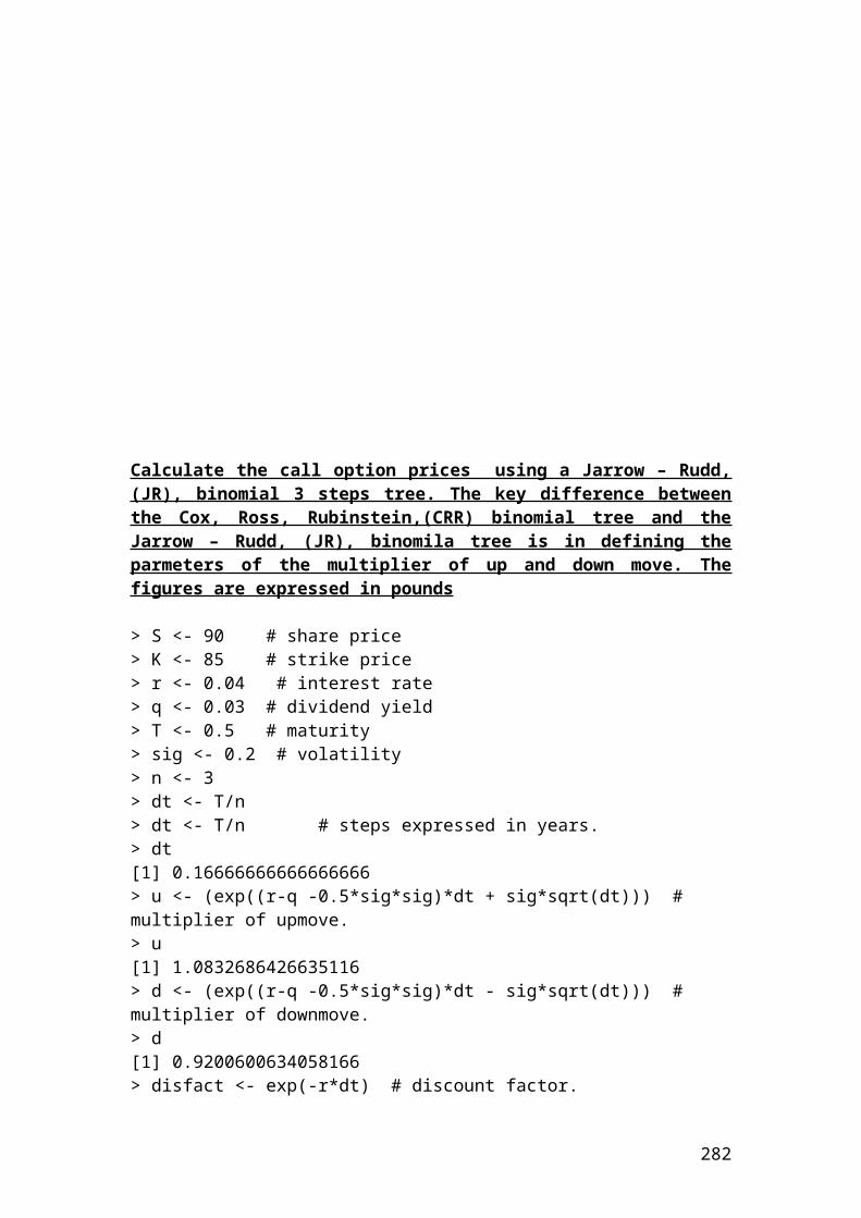
Please convert the following exercise in Java language programming
Calculate the balance at the end of the 5th day from changes in the futures prices from 90 to 89, 91, 95, 97, 99. The trader has bought 50 futures contract for settlement in May. The initial margin is $8.
Day Beginning balance
Futures price Gain or loss Ending balance
0 400 90 0 4001 400 89 (50)2 350 91 1003 450 95 2004 650 97 1005 750 99 100
Source: author’s illustration.
Beginning balance = initial margin x number of contracts.Beginning balance = 8 x 50 = $400
Please complete the values of the column ending balance.
282
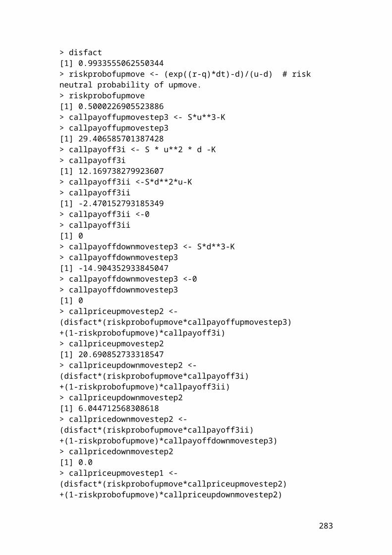
Example of profit or loss of a call option portfolio
class profit_or_loss_call_option_portfolio {public static void main(String[] args) {
double portfoliovalue1, portfoliovalue2, portfoliovalue3, portfoliovalue4, portfoliovalue5,portfoliovalue6,portfoliovalue7, portfoliovalue8,portfoliovalue9,portfoliovalue10 ; // portfolio value. double shareprice=10 ; // number of positions of share prices. double strikeprice=10; // number of positions of strike prices. double optionpremium=10; // Call option premiums. double contractsize = 100; // contract size.
/* Identifying the number of positions in relation to the share prices, strike prices and option premium.*/
double shareprice1 = 10.25; double shareprice2 = 20.13; double shareprice3 = 30.22; double shareprice4 = 40.56; double shareprice5 = 50.89; double shareprice6 = 51.23; double shareprice7 = 53.33; double shareprice8 = 54.63; double shareprice9 = 66.23; double shareprice10 = 68.23;
double strikeprice1 = 3.34; double strikeprice2 = 8.34; double strikeprice3 = 18.78; double strikeprice4 = 28.34; double strikeprice5 = 31.12; double strikeprice6 = 22.02; double strikeprice7 = 34.23; double strikeprice8 = 47.12; double strikeprice9 = 48.45; double strikeprice10 = 50.12; double optionpremium1 = 1.50; double optionpremium2 = 2.30; double optionpremium3 = 2.56; double optionpremium4 = 3.10; double optionpremium5 = 3.25; double optionpremium6 = 3.45; double optionpremium7 = 3.56; double optionpremium8 = 4.32; double optionpremium9 = 5.12;
283
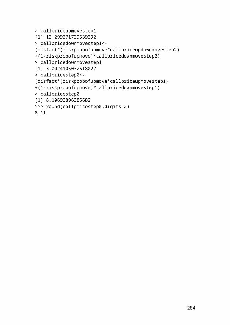
double optionpremium10 = 5.78; // Calculate the call option portfolio values. portfoliovalue1 = (shareprice1-(strikeprice1+ optionpremium1))* contractsize; portfoliovalue2 = (shareprice2-(strikeprice2+ optionpremium2))* contractsize; portfoliovalue3 = (shareprice3-(strikeprice3+ optionpremium3))* contractsize; portfoliovalue4 = (shareprice4-(strikeprice4+ optionpremium4))* contractsize; portfoliovalue5 = (shareprice5-(strikeprice5+ optionpremium5))* contractsize; portfoliovalue6 = (shareprice6-(strikeprice6+ optionpremium6))* contractsize; portfoliovalue7 = (shareprice7-(strikeprice7+ optionpremium7))* contractsize; portfoliovalue8 = (shareprice8-(strikeprice8+ optionpremium8))* contractsize; portfoliovalue9 = (shareprice9-(strikeprice9+ optionpremium9))* contractsize; portfoliovalue10 = (shareprice10-(strikeprice10+ optionpremium10))* contractsize;
System.out.print("The portfoliovalue1 in pounds is");System.out.println(portfoliovalue1);System.out.println(Math.round(portfoliovalue1*100.0)/100.0);System.out.print("The portfoliovalue2 in pounds is");System.out.println(portfoliovalue2);System.out.println(Math.round(portfoliovalue2*100.0)/100.0);System.out.print("The portfoliovalue3 in pounds is");System.out.println(portfoliovalue3);System.out.println(Math.round(portfoliovalue3*100.0)/100.0);System.out.print("The portfoliovalue4 in pounds is");System.out.println(portfoliovalue4);System.out.println(Math.round(portfoliovalue4*100.0)/100.0);System.out.print("The portfoliovalue5 in pounds is");System.out.println(portfoliovalue5);System.out.println(Math.round(portfoliovalue5*100.0)/100.0);System.out.print("The portfoliovalue6 in pounds is");System.out.println(portfoliovalue6);System.out.println(Math.round(portfoliovalue6*100.0)/100.0);System.out.print("The portfoliovalue7 in pounds is");System.out.println(portfoliovalue7);System.out.println(Math.round(portfoliovalue7*100.0)/100.0);System.out.print("The portfoliovalue8 in pounds is");System.out.println(portfoliovalue8);System.out.println(Math.round(portfoliovalue8*100.0)/100.0);System.out.print("The portfoliovalue9 in pounds is");System.out.println(portfoliovalue9);System.out.println(Math.round(portfoliovalue9*100.0)/100.0);System.out.print("The portfoliovalue10 in pounds is");System.out.println(portfoliovalue10);System.out.println(Math.round(portfoliovalue10*100.0)/100.0);}}
284
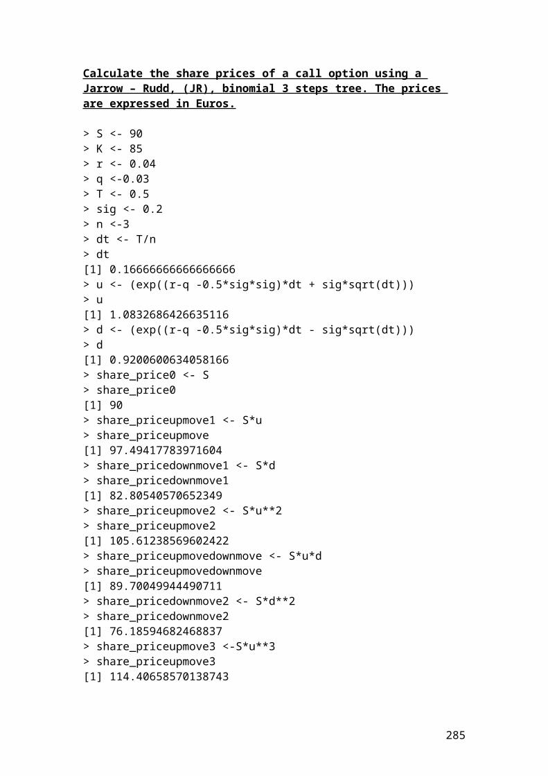
Output results
After compiling the current document from tools and pressing the run document you should get the following results:
Welcome to DrJava. Working directory is C:\Documents and Settings\Owner\Desktop\Java Compiler> run profit_or_loss_call_option_portfolioThe portfoliovalue1 in pounds is541.0541.0The portfoliovalue2 in pounds is948.9999999999999949.0The portfoliovalue3 in pounds is887.9999999999999888.0The portfoliovalue4 in pounds is912.0000000000001912.0The portfoliovalue5 in pounds is1651.99999999999951652.0The portfoliovalue6 in pounds is2576.02576.0The portfoliovalue7 in pounds is1554.01554.0The portfoliovalue8 in pounds is319.00000000000045319.0The portfoliovalue9 in pounds is1266.00000000000051266.0The portfoliovalue10 in pounds is1233.00000000000051233.0>
285
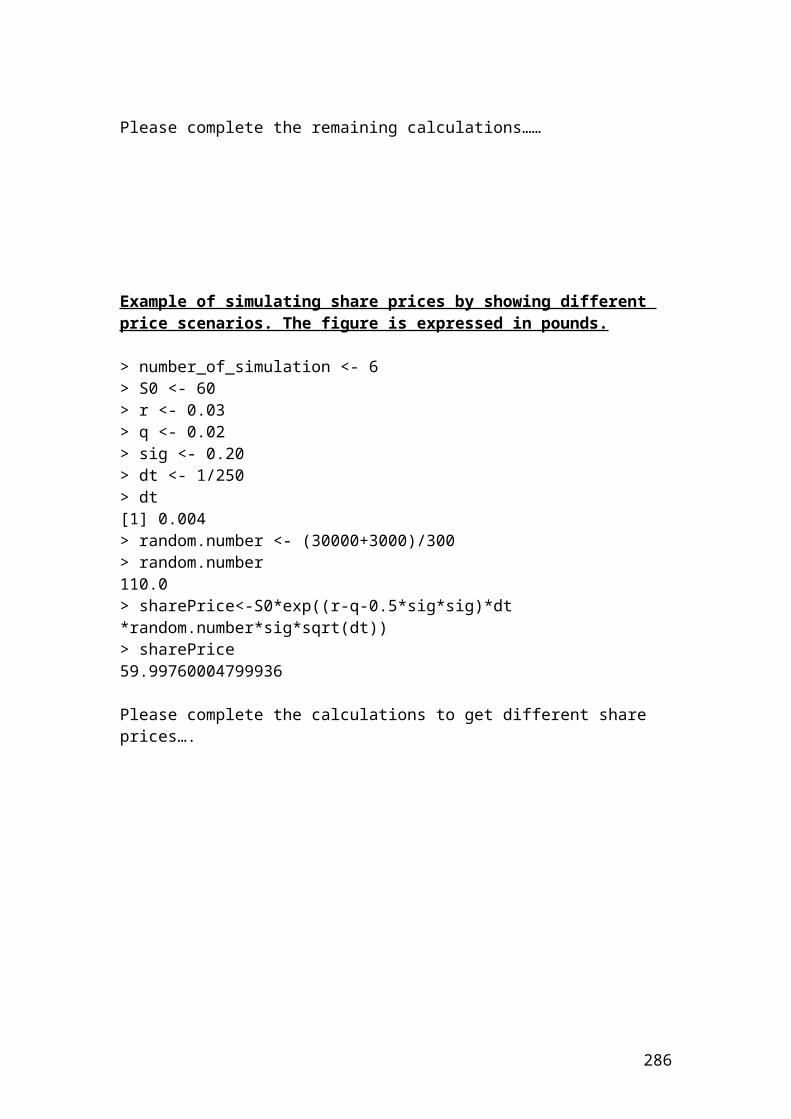
Example of profit or loss of a put option portfolio
class profit_or_loss_put_option_portfolio {public static void main(String[] args) {
double portfoliovalue1, portfoliovalue2, portfoliovalue3, portfoliovalue4, portfoliovalue5,portfoliovalue6,portfoliovalue7, portfoliovalue8,portfoliovalue9,portfoliovalue10 ; // portfolio value. double shareprice=10 ; // number of positions of share prices. double strikeprice=10; // number of positions of strike prices. double optionpremium=10; // Call option premiums. double contractsize = 100; // contract size.
/* Identifying the number of positions in relation to the share prices, strike prices and option premium.*/
double shareprice1 = 10.25; double shareprice2 = 20.13; double shareprice3 = 30.22; double shareprice4 = 40.56; double shareprice5 = 50.89; double shareprice6 = 51.23; double shareprice7 = 53.33; double shareprice8 = 54.63; double shareprice9 = 66.23; double shareprice10 = 68.23;
double strikeprice1 = 3.34; double strikeprice2 = 8.34; double strikeprice3 = 18.78; double strikeprice4 = 28.34; double strikeprice5 = 31.12; double strikeprice6 = 22.02; double strikeprice7 = 34.23; double strikeprice8 = 47.12; double strikeprice9 = 48.45; double strikeprice10 = 50.12; double optionpremium1 = 1.50; double optionpremium2 = 2.30; double optionpremium3 = 2.56; double optionpremium4 = 3.10; double optionpremium5 = 3.25; double optionpremium6 = 3.45; double optionpremium7 = 3.56; double optionpremium8 = 4.32; double optionpremium9 = 5.12;
286
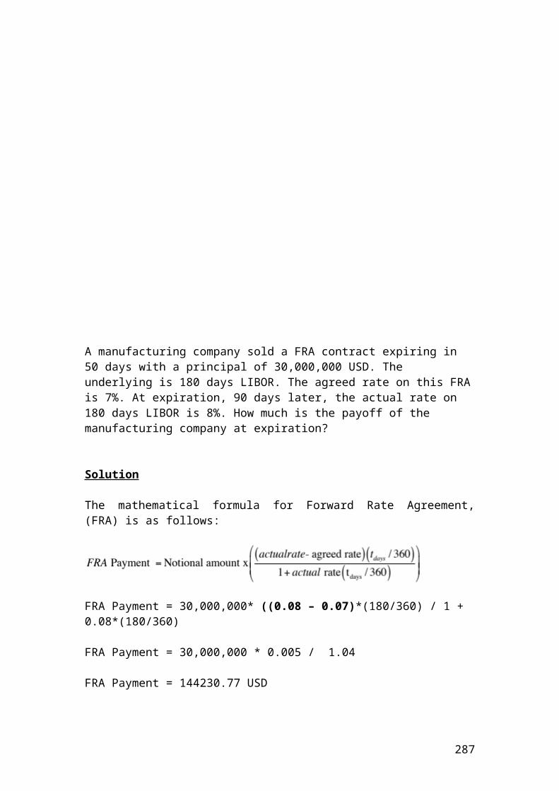
double optionpremium10 = 5.78; // Calculate the call option portfolio values. portfoliovalue1 = (strikeprice1-optionpremium1-shareprice1)* contractsize; portfoliovalue2 = (strikeprice2-optionpremium2-shareprice2)* contractsize; portfoliovalue3 = (strikeprice3-optionpremium3-shareprice3)* contractsize; portfoliovalue4 = (strikeprice4-optionpremium4-shareprice4)* contractsize; portfoliovalue5 = (strikeprice5-optionpremium5-shareprice5)* contractsize; portfoliovalue6 = (strikeprice6-optionpremium6-shareprice6)* contractsize; portfoliovalue7 = (strikeprice7-optionpremium7-shareprice7)* contractsize; portfoliovalue8 = (strikeprice8-optionpremium8-shareprice8)* contractsize; portfoliovalue9 = (strikeprice9-optionpremium9-shareprice9)* contractsize; portfoliovalue10 = (strikeprice10-optionpremium10-shareprice10)* contractsize;
System.out.print("The portfoliovalue1 in pounds is");System.out.println(portfoliovalue1);System.out.println(Math.round(portfoliovalue1*100.0)/100.0);System.out.print("The portfoliovalue2 in pounds is");System.out.println(portfoliovalue2);System.out.println(Math.round(portfoliovalue2*100.0)/100.0);System.out.print("The portfoliovalue3 in pounds is");System.out.println(portfoliovalue3);System.out.println(Math.round(portfoliovalue3*100.0)/100.0);System.out.print("The portfoliovalue4 in pounds is");System.out.println(portfoliovalue4);System.out.println(Math.round(portfoliovalue4*100.0)/100.0);System.out.print("The portfoliovalue5 in pounds is");System.out.println(portfoliovalue5);System.out.println(Math.round(portfoliovalue5*100.0)/100.0);System.out.print("The portfoliovalue6 in pounds is");System.out.println(portfoliovalue6);System.out.println(Math.round(portfoliovalue6*100.0)/100.0);System.out.print("The portfoliovalue7 in pounds is");System.out.println(portfoliovalue7);System.out.println(Math.round(portfoliovalue7*100.0)/100.0);System.out.print("The portfoliovalue8 in pounds is");System.out.println(portfoliovalue8);System.out.println(Math.round(portfoliovalue8*100.0)/100.0);System.out.print("The portfoliovalue9 in pounds is");System.out.println(portfoliovalue9);System.out.println(Math.round(portfoliovalue9*100.0)/100.0);System.out.print("The portfoliovalue10 in pounds is");System.out.println(portfoliovalue10);System.out.println(Math.round(portfoliovalue10*100.0)/100.0);}}
287
Output results
After compiling the current document from tools and pressing the run document you should get the following results:
Welcome to DrJava. Working directory is C:\Documents and Settings\Owner\Desktop\Java Compiler> run profit_or_loss_put_option_portfolioThe portfoliovalue1 in pounds is-841.0-841.0The portfoliovalue2 in pounds is-1409.0-1409.0The portfoliovalue3 in pounds is-1399.9999999999995-1400.0The portfoliovalue4 in pounds is-1532.0000000000005-1532.0The portfoliovalue5 in pounds is-2302.0-2302.0The portfoliovalue6 in pounds is-3265.9999999999995-3266.0The portfoliovalue7 in pounds is-2266.0-2266.0The portfoliovalue8 in pounds is-1183.0000000000005-1183.0The portfoliovalue9 in pounds is-2290.0-2290.0The portfoliovalue10 in pounds is-2389.000000000001-2389.0>
288
One – period binomial method
A share is traded in the Danish stock exchange at 50 DKK. First of all, we would like to calculate the possible price changes based on probabilities. The risk - free rate is 5% and the value of the call option has an exercise price of 50 DKK. It is required to calculate the expected value of the option at t =1. In addition, it is required to calculate the value of the option today discounted at the given risk-free rate.
We assume two scenarios. The first one is that the share will increase by 20% or by a factor of 1 + 0.20 = 1.20. The second one is that the share will decrease by 0.833. The number 0.833 is calculated as 1 / 1.20 = 0.833.
The mathematical formulas are as follows:
Down move = D = 1 / up move = 1 / 1.20 = 0.833
59128.0367.0217.0
0.833-1.200.833- 0.051
move. up theis U move.down theis D
rate. free-risk theis rf :
D-U
D-rf1 movement upan ofy probabilit neutral -risk
U
Where
U
0.40872 0.59128 - 1 movement down a ofy probabilit neutral - riskD
Thus, the payoff or the one-period binomial tree for share and option prices for the two possible scenarios will be as follows:
t = 0 t = 1
Probability Up = 0.59128 Share price = 50 x 1.20 = 60 DKK Call option = 60 – 50 = 10 DKK. 50 In this case, an increase of the share price will lead to the call option to pay back 10 DKK Probability Down =0.40872 Share price = 50 x 0.833 = 41.65 DKK Call option = 41.65 – 50 = -8.35 DKK = 0 DKK In this case the call option does not worth anything.
The expected value of the call option at t = 1 is as follows:
Expected call option = (10 x 0.59128) + ( 0 x 0.40872) = 5.9128 + 0 = 5.9128 DKK.
The value of the call option discounted at 5% risk – free rate is as follows:
289
Ctoday = 5.9128 / 1.05 = 5.63 DKK (to 2 d.p.).
Application of one – period binomial method in Java
class One_period_binomial_method{public static void main(String[] args) { //One - period binomial method. double shareprice = 50; double exerciseprice = 50; double upmove = 1.20; double downmove = 0.833; double riskfreerate = 0.05; double riskprobofupmove; double riskprobofdownmove; double shareprice1; double shareprice2; double calloptionprice1; double calloptionprice2; double expectedcalloption; double valueofcalldiscounted;
// Insert the mathematical formulas of risk probability of up and down move.
riskprobofupmove = (1+riskfreerate-downmove) / (upmove - downmove);riskprobofdownmove = 1 - riskprobofupmove;
// The payoff or one period binomial tree for share and option prices is as follows:
shareprice1 = shareprice * upmove;calloptionprice1 = shareprice1 - exerciseprice;
shareprice2 = shareprice *downmove;calloptionprice2 = shareprice2 - exerciseprice;calloptionprice2 =0;
// The expected value of the call option at t=1 is as follows:
expectedcalloption = (calloptionprice1* riskprobofupmove) + (calloptionprice2 * riskprobofdownmove);
// The value of the call option discounted at 5% risk - free rate is as follows:
valueofcalldiscounted = expectedcalloption / 1.05;
290
System.out.print("The risk probability of up move is");System.out.println(riskprobofupmove);System.out.println(Math.round(riskprobofupmove*100.0)/100.0);System.out.print("The risk probability of down move is");System.out.println(riskprobofdownmove);System.out.println(Math.round(riskprobofdownmove*100.0)/100.0);System.out.print("The share price 1 is");System.out.println(shareprice1);System.out.print("The share price 2 is");System.out.println(shareprice2);System.out.print("The call option price 1 is");System.out.println(calloptionprice1);System.out.print("The call option price 2 is");System.out.println(calloptionprice2);System.out.print("The expected call option is");System.out.println(expectedcalloption);System.out.println(Math.round(expectedcalloption*100.0)/100.0);System.out.print("The value of call option discounted is");System.out.println(valueofcalldiscounted);System.out.println(Math.round(valueofcalldiscounted*100.0)/100.0);}}
Output results
After compiling the current document from tools and pressing the run document you should get the following results:
Welcome to DrJava. Working directory is C:\Documents and Settings\Owner\Desktop\Java Compiler> run One_period_binomial_methodThe risk probability of up move is0.59128065395095390.59The risk probability of down move is0.408719346049046140.41The share price 1 in DKK is60.0The share price 2 in DKK is41.65The call option price 1 in DKK is10.0The call option price 2 in DKK is0.0The expected call option in DKK is5.9128065395095395.91The value of call option discounted in DKK is5.6312443233424185.63>
291
Two – period binomial method
This method is based on the one – period binomial method, but it is extended to include a second period, t = 2. Thus, we have three periods. t = 0, t =1 and t =2. We use the same example of the previous section but extended to an additional period.
A share is traded in the Danish stock exchange at 50 DKK. First of all, we would like to calculate the possible price changes based on probabilities. The risk - free rate is 5% and the value of the call option has an exercise price of 50 DKK. It is required to calculate the expected value of the option. In addition, it is required to calculate the value of the option today discounted at the given risk-free rate.
We assume two scenarios. The first one is that the share will increase by 20% or by a factor of 1 + 0.20 = 1.20. The second one is that the share will decrease by 0.833. The number 0.833 is calculated as 1 / 1.20 = 0.833.
The mathematical formulas are as follows:
Down move = D = 1 / up move.
59128.0367.0217.0
0.833-1.200.833- 0.051
move. up theis U move.down theis D
rate. free-risk theis rf :
D-U
D-rf1 movement upan ofy probabilit neutral -risk
U
Where
U
0.40872 0.59128 - 1 movement down a ofy probabilit neutral - riskD
Thus, the payoff or the two-period binomial tree for share prices for the two possible scenarios will be as follows:
t = 0 t = 1 t =2 50*(1.20)2=72 DKKProbability Up = 0.59 S1 = 50 x 1.20 = 60 DKK S2 50*1.20*0.833 =49.98 50 DKK Probability Down =0.41 S1 = 50 x 0.833 = 41.65 DKK S2
50 * (0.833)2 = 34.69
The value of the call options for the period t =2 for both ups and downs are as follows:
292
Upside movementC1 = 72 – 50 = 22C2 = 49.98 – 50 = -0.02 =0 Negative values mean that the option does not worth.
Downside movementC1 = 49.98 -50 = -0.02 =0C2 = 34.69 -50 = -15.31 =0
The expected value of the call options for both movements for period t =1 are calculated based on the following equations:
Upside movement
DKK 12.3887
05.1008.13
05.1)040872.0(2259128.0
rf 1down xC PrC x upy Probabilit 21
up
up
Call
xxobabilityCall
Downside movement
005.1
0) 40872.0(0 59128.0rf 1
Cdown x PrC x up Pr 21
xxobabilityobabilityCalldown
The value of the call option today discounted is calculated based on the following formula:
3.d.p.) (to 976.605.1
32519.7
05.10 12.3887 x 59128.0
1Calldown x PrCall x up Pr downup
today
today
Call
rfobabilityobability
Call
The final format of the two-period binomial tree for call options is as follows:
t = 0 t = 1 t = 2
22.00 DKK 12.3887DKK 06.976 DKK 0 0
Application of two – period binomial method in Java
class Two_period_binomial_method
293
{public static void main(String[] args) { //Two - period binomial method. double shareprice = 50; double exerciseprice = 50; double upmove = 1.20; double downmove = 0.833; double riskfreerate = 0.05; double riskprobofupmove; double riskprobofdownmove; double shareprice1; double shareprice2; double shareprice3; double shareprice4; double shareprice5; double calloptionprice1; double calloptionprice2; double calloptionprice3; double calloptionprice4; double calloptionprice5; double expectedcalloptionupside; double expectedcalloptiondownside; double valueofcalldiscounted; // Insert the mathematical formulas of risk probability of up and down move.
riskprobofupmove = (1+riskfreerate-downmove) / (upmove - downmove);riskprobofdownmove = 1 - riskprobofupmove;
// The payoff or two period binomial tree for share and option prices is as follows:
shareprice1 = shareprice * upmove;
shareprice2 = shareprice *downmove;
shareprice3 = shareprice * Math.pow(upmove,2);calloptionprice3 = shareprice3 - exerciseprice;
shareprice4 = shareprice * Math.pow(downmove,2);calloptionprice4 = shareprice4 - exerciseprice;calloptionprice4 =0;
shareprice5 = shareprice * upmove * downmove;calloptionprice5 = shareprice5 - exerciseprice;calloptionprice5 =0;
// The expected value of the call option at t=2 is as follows:expectedcalloptionupside = (riskprobofupmove * calloptionprice3
294
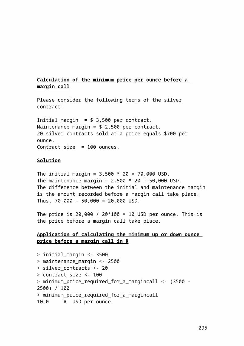
+ riskprobofdownmove* calloptionprice5) / 1.05;
expectedcalloptiondownside = (riskprobofupmove *calloptionprice4+ riskprobofdownmove * calloptionprice5) / 1.05;
// The value of the call option discounted at 5% risk - free rate is as follows:
valueofcalldiscounted = (riskprobofupmove * expectedcalloptionupside+riskprobofdownmove* expectedcalloptiondownside)/ 1.05;
// Output functions.System.out.print("The risk probability of up move is");System.out.println(riskprobofupmove);System.out.println(Math.round(riskprobofupmove*100.0)/100.0);System.out.print("The risk probability of down move is");System.out.println(riskprobofdownmove);System.out.println(Math.round(riskprobofdownmove*100.0)/100.0);System.out.print("The share price 1 in DKK is");System.out.println(shareprice1);System.out.print("The share price 2 in DKK is");System.out.println(shareprice2);System.out.print("The share price 3 in DKK is");System.out.println(shareprice3);System.out.print("The share price 4 in DKK is");System.out.println(shareprice4);System.out.print("The share price 5 in DKK is");System.out.println(shareprice5);System.out.print("The call option price 3 in DKK is");System.out.println(calloptionprice3);System.out.print("The call option price 4 in DKK is");System.out.println(calloptionprice4);System.out.print("The call option price 5 in DKK is");System.out.println(calloptionprice5);System.out.print("The expected call option upside in DKK is");System.out.println(expectedcalloptionupside);System.out.println(Math.round(expectedcalloptionupside*100.0)/100.0);System.out.print("The expected call option downside in DKK is");System.out.println(expectedcalloptiondownside);System.out.println(Math.round(expectedcalloptiondownside*100.0)/100.0);System.out.print("The value of call option discounted in DKK is");System.out.println(valueofcalldiscounted);System.out.println(Math.round(valueofcalldiscounted*100.0)/100.0);}}
Output results
295
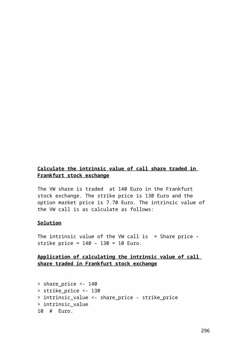
After compiling the current document from tools and pressing the run document you should get the following results:
Welcome to DrJava. Working directory is C:\Documents and Settings\Owner\Desktop\Java Compiler> run Two_period_binomial_methodThe risk probability of up move is0.59128065395095390.59The risk probability of down move is0.408719346049046140.41The share price 1 in DKK is60.0The share price 2 in DKK is41.65The share price 3 in DKK is72.0The share price 4 in DKK is34.694449999999996The share price 5 in DKK is49.98The call option price 3 in DKK is22.0The call option price 4 in DKK is0.0The call option price 5 in DKK is0.0The expected call option upside in DKK is12.38873751135331812.39The expected call option downside in DKK is0.00.0The value of call option discounted in DKK is6.9764007784187646.98>
Stock index option
296
Let’s assume that a practitioner wants to buy a stock index call option that is related to the general movement of the S&P 500 index. The dollar multiplier for S&P 500 option contract is 250 dollars. The strike price of the index is 1240. The August premium is 20 index points.
Question
Calculate the cost of the August call and the net profit involved if the S&P 500 index reaches the price of 1540.
Solution
Cost of the August call = premium expressed in index points x dollar multiplier Cost of the August call = 20 x 250 = 5000 USD
The net profit incurred is calculated as follows:
(Ending index value – beginning index value x dollar multiplier ) – cost of the August call.
(1540 – 1240) x 250 – 5000 = 70,000 USD.
Application of stock index option in Java
class Stock_index_option{public static void main(String[] args) {
double cost_of_call;double net_profit ;int premium = 20;int multiplier = 250;double ending_index_value = 1540;double beginning_index_value = 1240; // Insert the mathematical formula.
cost_of_call = premium * multiplier ;net_profit = (ending_index_value - beginning_index_value) * multiplier - cost_of_call;
// Output functions.
System.out.print("The cost of call in USD is");System.out.println(cost_of_call);System.out.println(Math.round(cost_of_call*100.0)/100.0);System.out.print("The net profit in USD is");System.out.println(net_profit);
297
System.out.println(Math.round(net_profit*100.0)/100.0);}}
Output result
After compiling the current document from tools and pressing the run document you should get the following result:
Welcome to DrJava. Working directory is C:\Documents and Settings\Owner\Desktop\Java Compiler> run Stock_index_optionThe cost of call in USD is 5000.05000.0The net profit in USD is 70000.070000.0>
Exercise of an European interest rate option
298
Calculate the profit or loss of the interest rate difference between the actual and the strike rate of a call option. Let’s assume that an interest call option on a 6 –month Eurodollar has a strike rate of 4%. At expiration, the 6-month Eurodollar rate is 5%. The invested principal is 50,000,000 Euros. The duration of the contract is expressed in days divided by 360 days. Thus, 6 –months equal 180 days.
The mathematical formula for profit or loss is as follows:
Application of an European interest rate option in Java
class European_interest_option{public static void main(String[] args) {
//Profit or loss of call interest rate option. double Profit_or_loss_call_interest_rate_option; // call interest rate option.double principal = 50000000;double actual_rate = 0.05;double strike_rate = 0.04;double duration = 180;double days = 360; // Insert the mathematical formula.
Profit_or_loss_call_interest_rate_option = principal *(actual_rate-strike_rate)*duration/days;
// Output function.
System.out.print("Profit_or_loss_call_interest_rate_option in euros is");System.out.println(Profit_or_loss_call_interest_rate_option);System.out.println(Math.round(Profit_or_loss_call_interest_rate_option*100.0)/100.0);}}
Output result
299
After compiling the current document from tools and pressing the run document you should get the following result:
Welcome to DrJava. Working directory is C:\Documents and Settings\Owner\Desktop\Java Compiler> run European_interest_optionProfit_or_loss_call_interest_rate_option in euros is250000.00000000003250000.0>
Currency option
300
Let’s assume that a wealthy investor buys a call currency option because it expects a rise in the exchange rate parity of the EURO against the USD, EURO/USD. The spot exchange rate is 1/1.3568. The strike price is 1.3568. The premium expressed as cents per Euro is 1.56. The initial principal is 100,000 USD.
Question
Calculate the net profit involved if the strike price increases to 1.3987.
Solution
The wealthy investor to record a profit, he or she should add to the strike price 1.3568 the premium expressed as cents per Euro. In our case, the breakeven point is1.3568 + 0.0156 = 1.3724. Above the price of 1.3724, he or she starts to record a profit. If the strike price reaches 1.3987, then the profit will be as follows:
Initial principal x (Ending strike price – beginning strike price – premium paid) =100,000 x (1.3987 – 1.3568 – 0.0156) = 2630 USD net profit
Application of currency option in Java
class Currency_option{public static void main(String[] args) { //Profit or loss of currency option. double net_profit;double principal = 100000;double ending_strike_price = 1.3987;double beginning_strike_price = 1.3568;double premium_paid = 0.0156; // Insert the mathematical formula.
net_profit = principal *(ending_strike_price-beginning_strike_price - premium_paid);
// Output function.
System.out.print("net profit in USD is");System.out.println(net_profit);System.out.println(Math.round(net_profit*100.0)/100.0);}}
Output result
301
After compiling the current document from tools and pressing the run document you should get the following result:
Welcome to DrJava. Working directory is C:\Documents and Settings\Owner\Desktop\Java Compiler> run Currency_optionnet profit in USD is2630.0000000000052630.0>
Example of calculating the payments of an interest rate cap based on different LIBOR rates
302
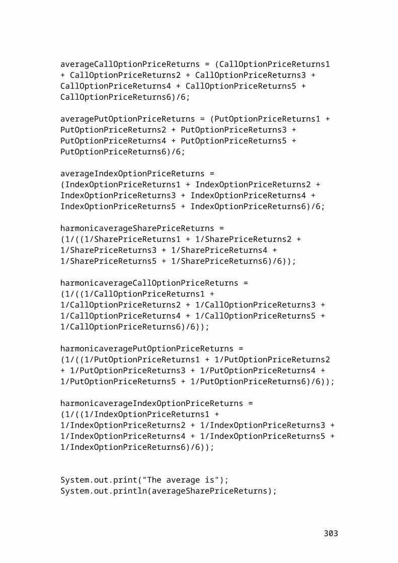
Interest rate cap is an agreement between two parties where one party pay the other at a specified period of time in which the interest rate or London interbank offered rate ,LIBOR, exceeds the strike price. It is used this contract to hedge against interest rate fluctuations. Let’s assume that an interest cap has a value of 5.5% and the LIBOR prices for the next three years are 7.5%, 8.3% and 4.65%. The principal is $50,000,000 and the payments take place semiannually.
The mathematical formula that is used to calculate the payments of each year is as follows:
Interest rate payment =[ principal x (LIBOR rate – cap rate)/0.5]
Therefore, the first year interest rate payment is as follows:
Year 1
Interest rate payment = [50,000,000 x (0.075 – 0.055)/2] = $ ………
Application of payments of an interest rate cap based on different LIBOR rates in Java
class Payments_interest_rate_cap{public static void main(String[] args) {
// Payments of an interest rate cap based on different LIBOR rates. double interest_pay_1;double interest_pay_2;double interest_pay_3;double principal = 50000000;double libor_rate_1 = 0.075;double libor_rate_2 = 0.083;double cap_rate = 0.055;double duration = 2; // Insert the mathematical formula.
interest_pay_1 = principal *(libor_rate_1 - cap_rate) /duration ;interest_pay_2 = principal *(libor_rate_2 - cap_rate) / duration ;
//Output functions.
System.out.print("interest_pay_1 in USD is");System.out.println(interest_pay_1);System.out.println(Math.round(interest_pay_1*100.0)/100.0);System.out.print("interest_pay_2 in USD is");System.out.println(interest_pay_2);
303
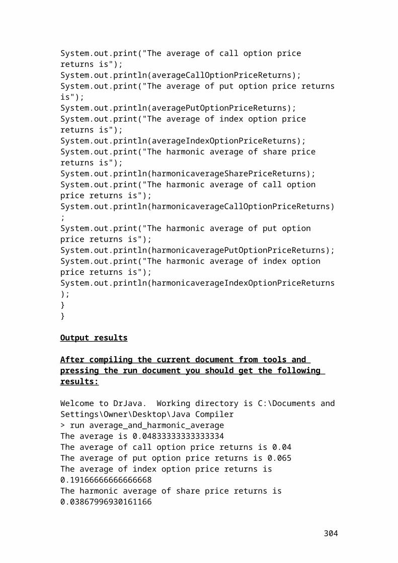
System.out.println(Math.round(interest_pay_2*100.0)/100.0);}}
Output result
After compiling the current document from tools and pressing the run document you should get the following result:
Welcome to DrJava. Working directory is C:\Documents and Settings\Owner\Desktop\Java Compiler> run Payments_interest_rate_capinterest_pay_1 in USD is499999.99999999994500000.0interest_pay_2 in USD is700000.0000000001700000.0>
A six month interest rate cap has a rate of 0.08 and the principal is 20,000,000 USD. The settlements is done quarterly. The first quarter the 3 –month libor rate is 0.096
304
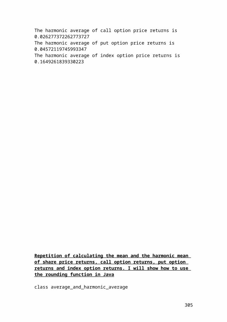
and the second quarter the rate is 0.087. Calculate the payoff for the cap the first and the second quarter?
Solution
Payoff the first quarter = 20,000,000 * = 80000 USD
Payoff the second quarter = 20,000,000 * =35000 USD
Application of payoff of interest rate cap in Java
class Payoff_interest_rate_cap{public static void main(String[] args) { //Payoff of interest rate cap. double payoff_1;double payoff_2;double principal = 20000000;double cap_rate = 0.08;double libor_rate_1 = 0.096;double libor_rate_2 = 0.087;double period = 4; // Insert the mathematical formulas. payoff_1 = (principal*(libor_rate_1-cap_rate)/period);payoff_2 = (principal*(libor_rate_2-cap_rate)/period);
// Output functions.
System.out.print("payoff_1 in USD is");System.out.println(payoff_1);System.out.println(Math.round(payoff_1*100.0)/100.0);System.out.print("payoff_2 in USD is");System.out.println(payoff_2);System.out.println(Math.round(payoff_2*100.0)/100.0);}}
Output results
305
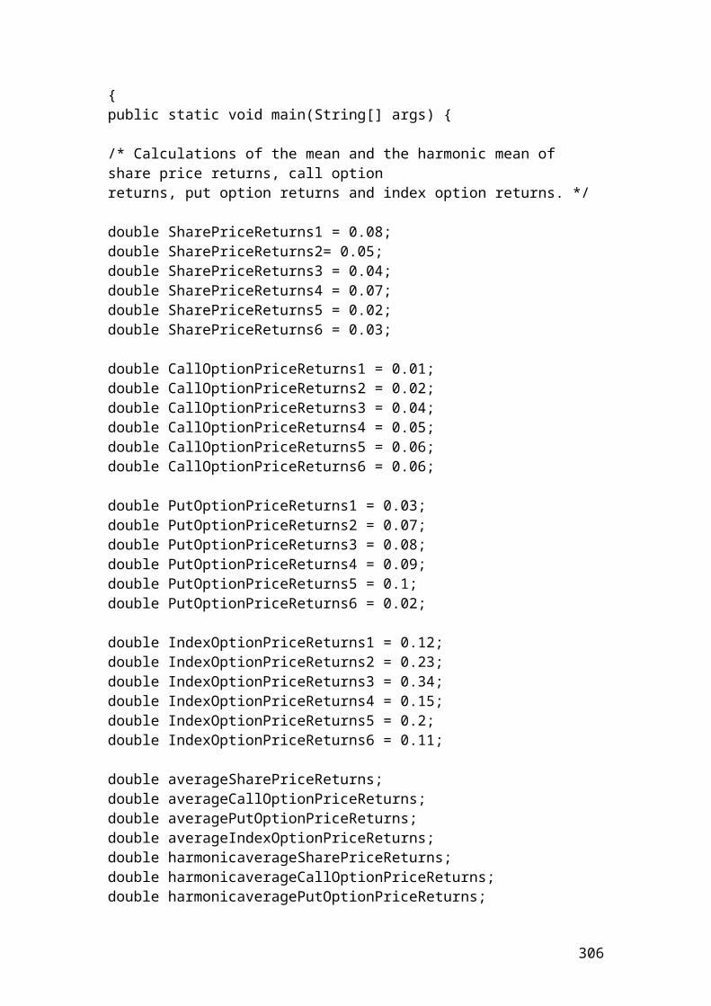
After compiling the current document from tools and pressing the run document you should get the following results:
Welcome to DrJava. Working directory is C:\Documents and Settings\Owner\Desktop\Java Compiler> run Payoff_interest_rate_cappayoff_1 in USD is80000.080000.0payoff_2 in USD is34999.9999999999635000.0>
Swaption
306
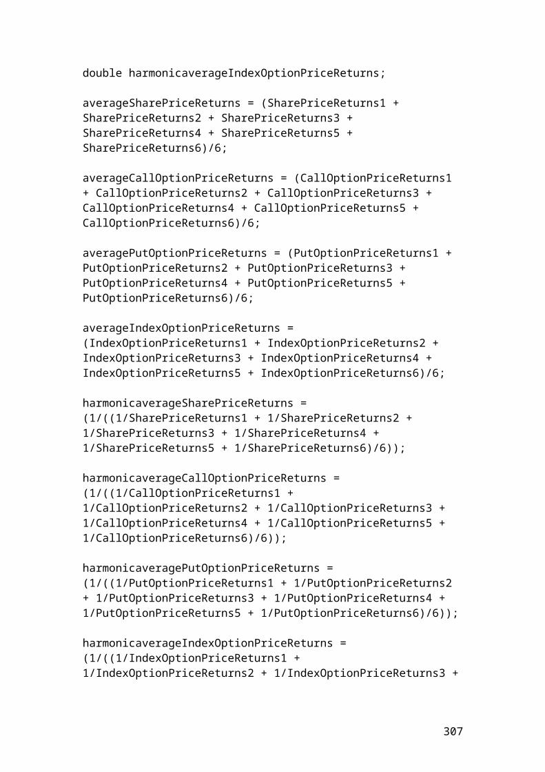
An investor purchased a 1 year European swaption with exercise price 7.50%. The principal is 30,000,000USD. The floating rate payments are based on LIBOR. The 90, 180, 270, and 360 day annualized LIBOR rates and present value factors are as follows:
LIBOR Rate Present value factors90 day LIBOR 4% 0.990099180 day LIBOR 5.5% 0.973236270 day LIBOR 6% 0.956938360 day LIBOR 7% 0.934579
Calculate the semi-annual and annualized swap rate?Calculate the net cash flow at each payment and the value of swaption at maturity.
Solution
The present value factors are calculated as follows:
PV 90 days =
36090*04.01
1
0.990099
PV 180 days =
360180*055.01
1
0.973236
PV 270 days =
360270*06.01
1
0.956938
PV 360 days =
360360*07.01
1
0.934579
Semi - annual swap rate =
01697.0854852.3065421.0
934579.0956938.0973236.0990099.0934579.01
Annulaized swap rate = 6.788%or 06788.090/360*01697.0
307
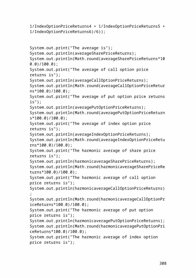
The swaption is in the money because the exercise price 7.50% is greater than the market annualized swap rate 6.788%.
The net cash flow is as follows:
netCashFlow = (0.075 – 0.06788)*90/360 * 30000000 = 53400 USD
The value of swaption at maturity is as follows:
valueSwaption = 53400 *( 934579.0956938.0973236.0990099.0 ) = 205,849.1 USD
Application of swaption in Java
class Swaption{public static void main(String[] args) { double Semi_annual_rate;double Annualized_swap_rate;double Net_cash_flow;double Value_swaption;double Exercise_rate = 0.075;double principal = 30000000;double PV90;double PV180;double PV270;double PV360;double rate_90 = 0.04;double rate_180 = 0.055;double rate_270 = 0.06 ;double rate_360 = 0.07; // Insert the mathematical formulas. PV90 = 1 /(1+(rate_90 * 90/360));PV180 = 1/(1+(rate_180 * 180/360));PV270 = 1/(1+(rate_270 * 270/360));PV360 = 1/(1+(rate_360* 360/360));
Semi_annual_rate = (1-PV360)/(PV90 +PV180 +PV270 +PV360);Annualized_swap_rate = Semi_annual_rate * (360/90);
// Output functions.
System.out.print("Semi_annual_rate is");System.out.println(Semi_annual_rate);System.out.println(Math.round(Semi_annual_rate*100.0)/100.0);
308
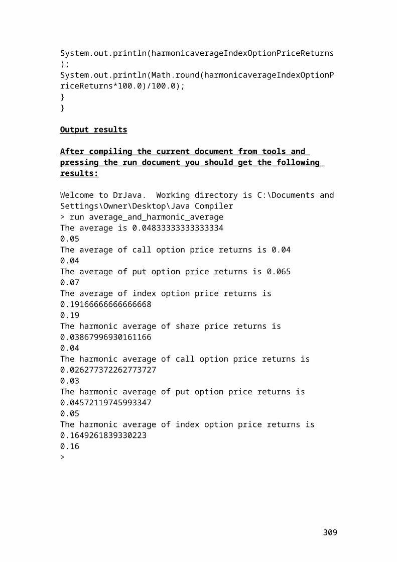
System.out.print("Annualized_swap_rate is");System.out.println(Annualized_swap_rate);System.out.println(Math.round(Annualized_swap_rate*100.0)/100.0);}}
Output results
After compiling the current document from tools and pressing the run document you should get the following results:
Welcome to DrJava. Working directory is C:\Documents and Settings\Owner\Desktop\Java Compiler> run SwaptionSemi_annual_rate is0.016970964480702220.02Annualized_swap_rate is0.067883857922808880.07>
Please repeat the above swaption problem and calculate the net cash flow and the value of swaption at maturity expressed in USD.
309
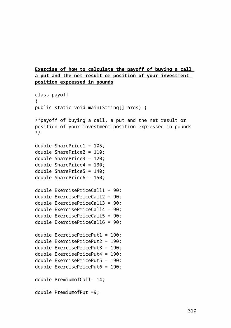
Put –call parity
The put – call parity shows the relationship between a call and a put option with the same expiration, strike and share prices. The mathematical formula is as follows:
option.put theand call both thefor price share theis S .expirationor maturity to time theis T
rate. free-rsik theis r call. theandput both the of price strike theis X
put. theof price theis P call. theof price theis C :
)1(
f
Where
SPrfXC T
Example
Calculate the price of a call if the price of a put is 5.34 Pounds, the share price is 94, the strike price is 97, the risk-free rate is 4% and the time to maturity, T=0.5. By rearranging formula (20) and solving for the price of a call, we have the following results:
pounds 22.4
)04.1(979434.5
)1( 5.0
C
rfXSPC T
Application of put - call parity in Java
class Put_call_parity{public static void main(String[] args) { // Put - call parity. Calculating the price of a call. double Call;double put = 5.34;double share_price = 94;double strike_price = 97;double dis_risk_free_rate = 1.04;double maturity = 0.5;
// Insert the mathematical formula.
Call= put + share_price - strike_price / Math.pow(dis_risk_free_rate,maturity);
310
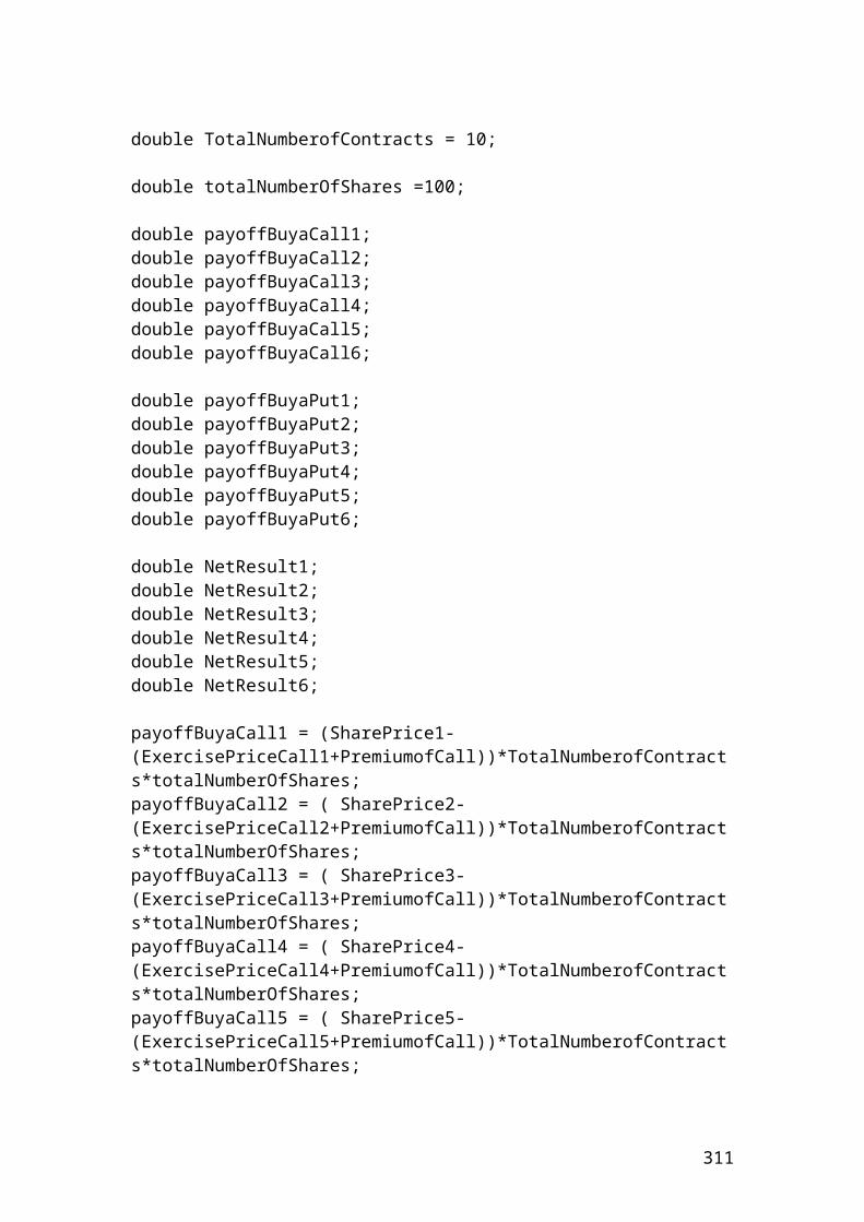
// Output function.
System.out.print("Call in pounds is");System.out.println(Call);System.out.println(Math.round(Call*100.0)/100.0);
}}
Output result
After compiling the current document from tools and pressing the run document you should get the following result:
Welcome to DrJava. Working directory is C:\Documents and Settings\Owner\Desktop\Java Compiler> run Put_call_parityCall in pounds is4.2236744579807494.22>
311
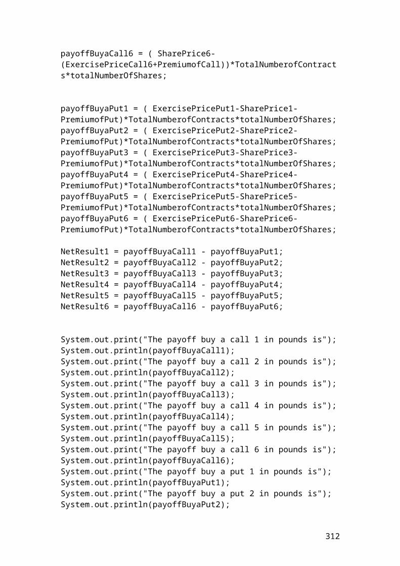
Example of margin payments in the clearinghouse
An investor open a margin account with a minimum initial margin of 5,200 dollars per contract. The maintenance margin is 1,500 dollars per contract. He/she buys 7 July wheat futures contracts with a standard contract size of 200 bushels priced at 230 dollars per bushel. The July contract size in the next 2 days recorded the prices of 220 and 210 dollars per bushel. Show the cash flows, gains and losses for the buyer and the seller?
Solution
Initial margin = 7 x 5,200 = 36,400 dollars
Maintenance margin = 7 x 1,500 = 10,500 dollars
The cash flows, gains and losses for the next two days will be as follows:
Day 1
Cash flows for the buyer’s: 36,400 + 14,000 = 50,400 dollars. The investor’s recorded a gain.
Cash flows for the seller’s: 36,400 – 14,000 = 22,400 dollars. The investor’s recorded a loss.
Helpful hint: the amount of 14,000 is calculated from the difference of the bushel prices, (f0-f) x number of contracts x standard contract size. Thus, we have: (230-220) x 7 x 200 = 14,000 dollars. The same principle applies for the second day but with different bushel price.
Day 2
Please do the calculations for the second day.
This is why I am stressing the importance that the investors should buy or sell ONLY when the market is aggressively increasing or falling. If he/she gets trapped in a market that is not strong bull or bear, then, he/she will have to compensate regularly for the losses or he/she will experience a very small profit. If the amounts as the days passes is below the maintenance margin, then, the investor’s will receive a margin call and he/she should add the capital required to proceed with the contract. If the investor’s is short of money, then, the position is closed with the incurred losses.
312
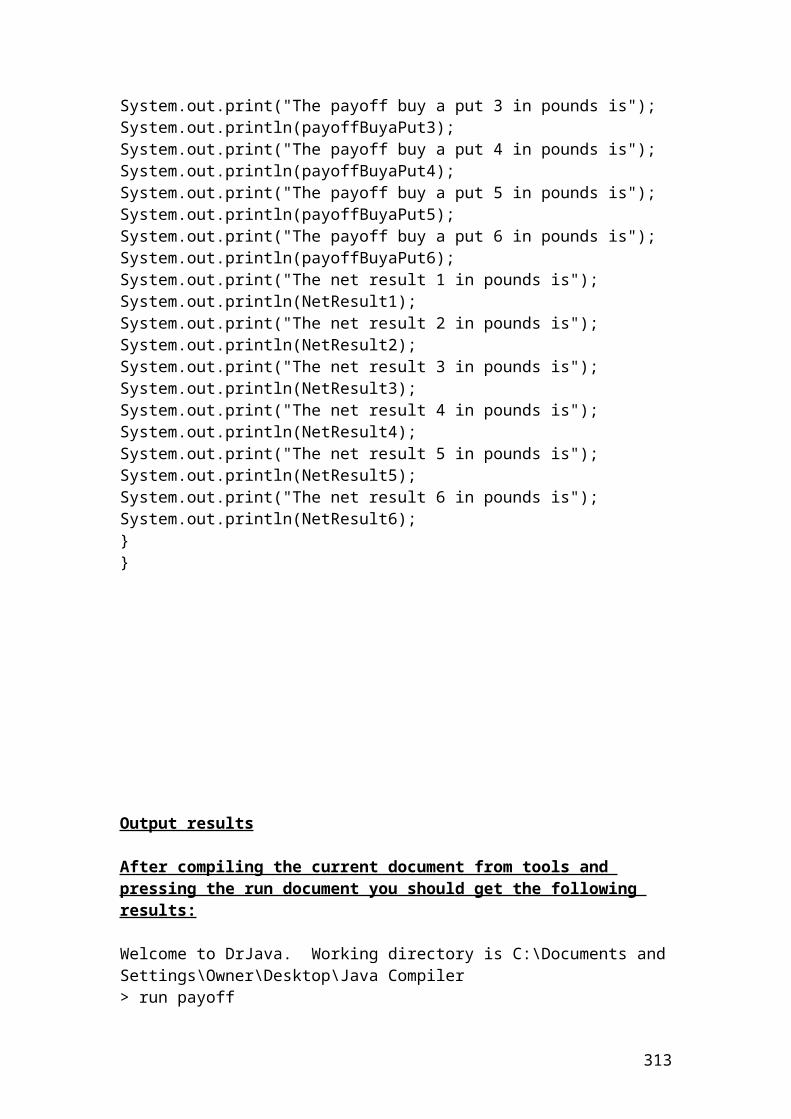
Application of margin payments in the clearinghouse in Java
class Margin_payments{public static void main(String[] args) {
// Margin payments. double Cash_flow_buyer ;double Cash_flow_seller ;double initial_margin = 5200;double maintenance_margin = 1500;int contract_number = 7;int bushel_contract_size = 200;double bushel_price_1 = 230;double bushel_price_2 = 220;double Initial_margin_with_contract ;double Maintenance_margin_with_contract;double Bushel_contract ;
// Insert the mathematical formulas.
Initial_margin_with_contract = initial_margin * contract_number;Maintenance_margin_with_contract = maintenance_margin * contract_number;
Bushel_contract =(bushel_price_1-bushel_price_2)*bushel_contract_size*contract_number;
Cash_flow_buyer = Initial_margin_with_contract + Bushel_contract; Cash_flow_seller = Initial_margin_with_contract-Bushel_contract;
// Output functions.
System.out.print(" Initial_margin_with_contract in USD is");System.out.println(Initial_margin_with_contract);System.out.print(" Maintenance_margin_with_contract in USD is");System.out.println(Maintenance_margin_with_contract);System.out.print(" Bushel_contract in USD is");System.out.println(Bushel_contract);System.out.print(" Cash_flow_buyer in USD is");System.out.println(Cash_flow_buyer);System.out.print(" Cash_flow_seller in USD is");System.out.println(Cash_flow_seller);}}
313
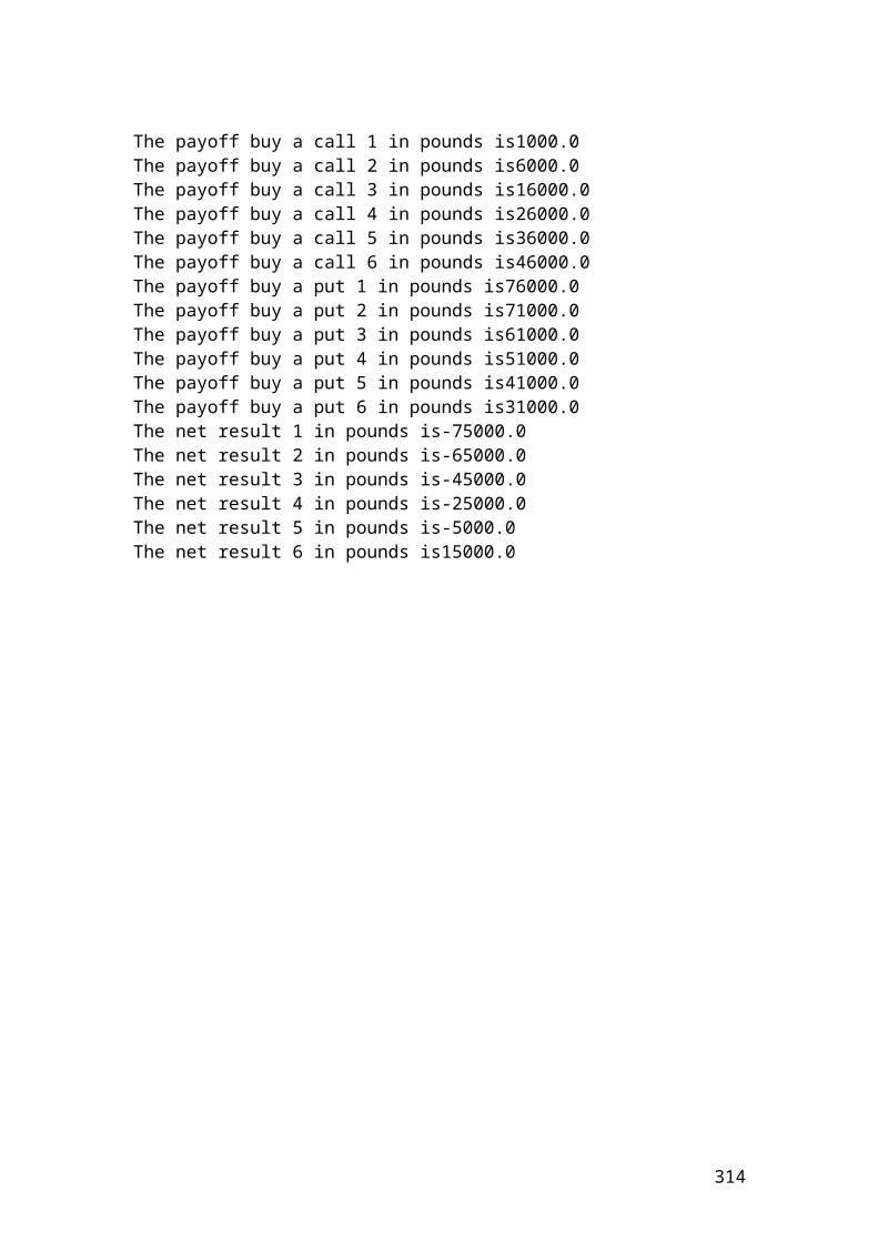
Output results
After compiling the current document from tools and pressing the run document you should get the following results:
Welcome to DrJava. Working directory is C:\Documents and Settings\Owner\Desktop\Java Compiler> run Margin_payments Initial_margin_with_contract in USD is36400.0 Maintenance_margin_with_contract in USD is10500.0 Bushel_contract in USD is14000.0 Cash_flow_buyer in USD is50400.0 Cash_flow_seller in USD is22400.0>
314
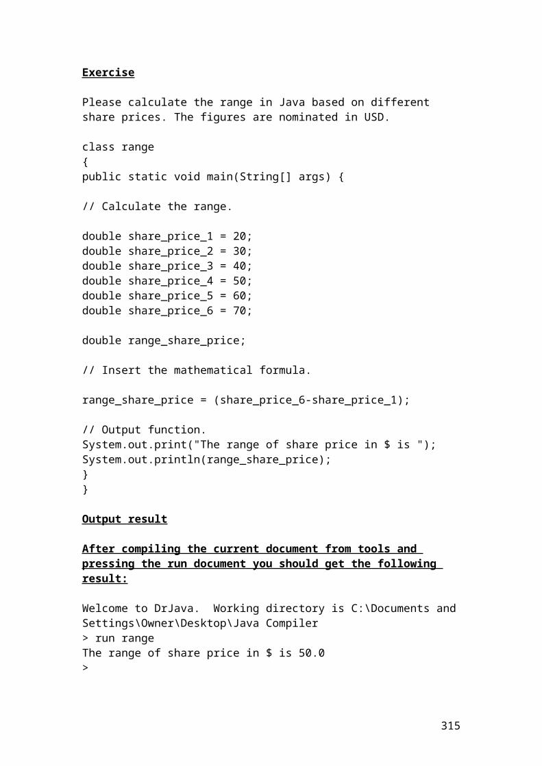
Example of calculating a margin call due to changes of price futures
An investor has opened a short position of 20 Soybean futures contract. The initial margin was 500 Pounds and the maintenance margin was 430 Pounds per contract. The price change that will create a margin call is as follows:
Solution
20
430- 500 sizecontract
margin emaintenanc -margin initial price aat created callMargin 3.5
Application of margin call in Java
class Margin_call {public static void main(String[] args) {
// Margin call. double initial_margin = 500;double maintenance_margin = 430;int futures_contract = 20;double margin_call;
// Insert the mathematical formula.
margin_call =( initial_margin-maintenance_margin) / futures_contract;
// Output function.
System.out.print(" margin_call in pounds is");System.out.println(margin_call);}}
Output result
After compiling the current document from tools and pressing the run document you should get the following result:
Welcome to DrJava. Working directory is C:\Documents and Settings\Owner\Desktop\Java Compiler> run Margin_call margin_call in pounds is3.5>
315
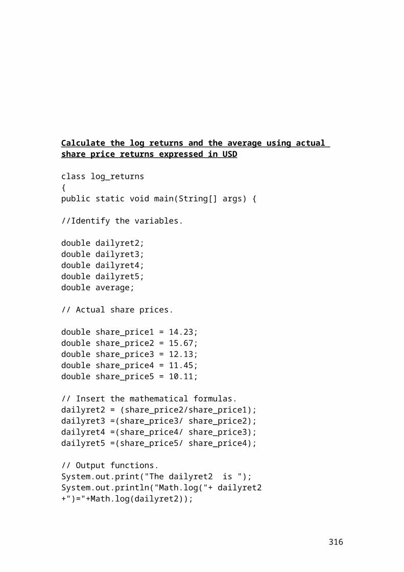
Calculate the call option prices using a Cox, Ross, Rubinstein,(CRR) binomial 3 steps tree. Please e-mail me to send you the binomial tree in Excel if this is complicated. I will also convert this example in VBA. Please check the VBA section in the document Financial Derivatives
class Cox_Ross_Rubinstein_call_option_calculations {public static void main(String[] args) { /* Calculate the call option prices using a Cox, Ross, Rubinstein,(CRR) binomial 3 steps tree. */ double S = 60; //share price double K = 50; // strike price double r = 0.05; // risk-free interest rate double q = 0.02; // dividend yield. If the dividend is zero, then, it is // not included in the equation of risk neutral // probability of upmove. double T = 0.5; // life to maturity double sig = 0.3; // volatility // Identify the variables. // u = multiplier of upmove. //d = multiplier of downmove. dt = steps expressed in years. //riskprobofupmove = risk neutral probability of upmove. //disfact = discount factor. double u; double d; double dt; double riskprobofupmove; double disfact; int n = 3; // Identify tree steps binomial tree. // Insert the mathematical formulas. dt = T/n; u = Math.exp(sig*Math.sqrt(dt)); d = 1/u; disfact = Math.exp(-r*dt); riskprobofupmove = (Math.exp((r-q)*dt)-d)/(u-d); double callpayoffupmovestep3; // (Shareprice * upmove^3)-Kdouble callpayoff3i; // (Shareprice * upmove^2 * downmove)-Kdouble callpayoff3ii; // (Shareprice * downmove^2*upmove)-K double callpayoffdownmovestep3; // (Shareprice * downmove^3) -K
// The option prices are calculated backwards.
316
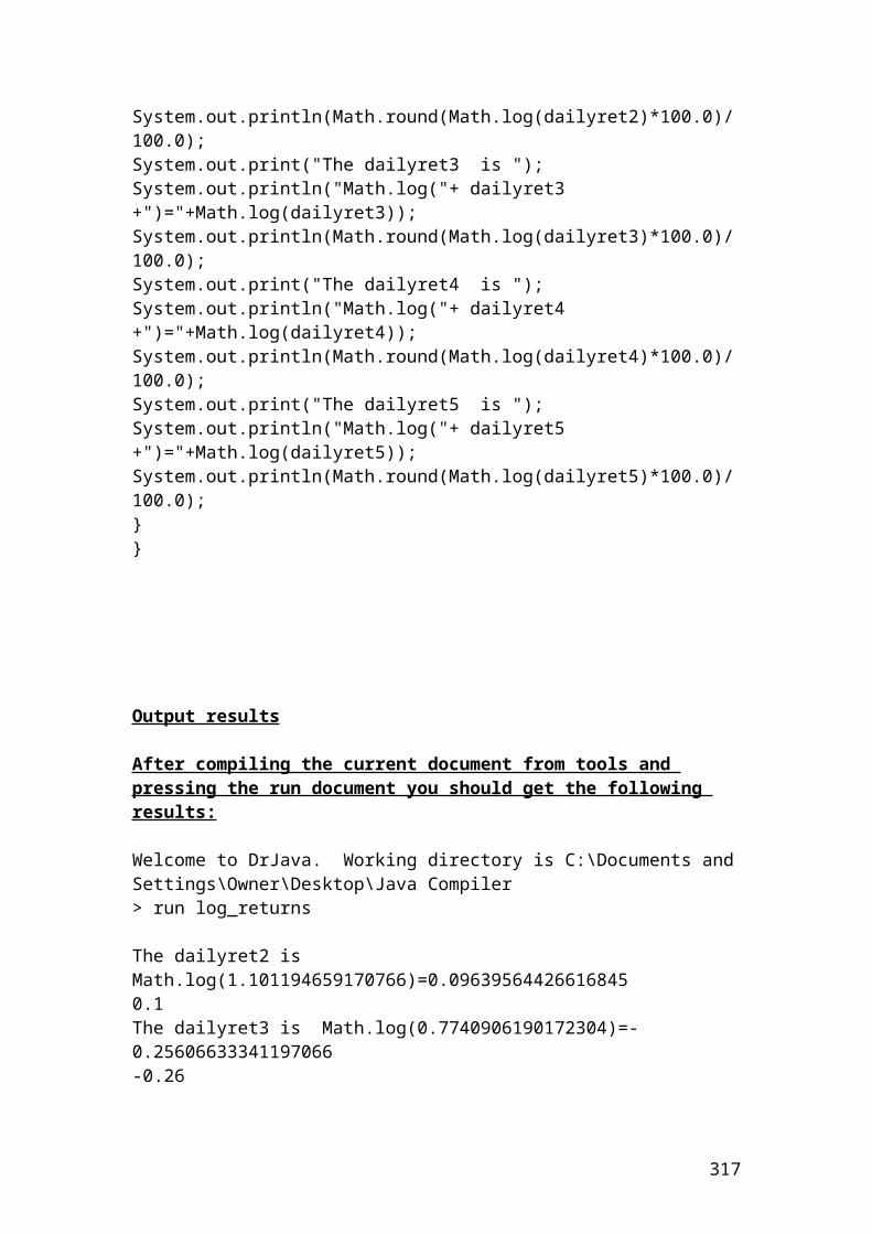
callpayoffupmovestep3 = S*Math.pow(u,3)-K;callpayoff3i = S * Math.pow(u,2) * d -K;callpayoff3ii =S * Math.pow(d,2)*u-K; callpayoffdownmovestep3 = S*Math.pow(d,3)-K;callpayoffdownmovestep3 =0;
double callpriceupmovestep2;double callpriceupdownmovestep2;double callpricedownmovestep2;
callpriceupmovestep2 = (disfact*(riskprobofupmove*callpayoffupmovestep3)+(1-riskprobofupmove)*callpayoff3i);
callpriceupdownmovestep2 =(disfact*(riskprobofupmove*callpayoff3i)+(1-riskprobofupmove)*callpayoff3ii);
callpricedownmovestep2 =(disfact*(riskprobofupmove*callpayoff3ii)+(1-riskprobofupmove)*callpayoffdownmovestep3);
double callpriceupmovestep1;double callpricedownmovestep1;
callpriceupmovestep1 = (disfact*(riskprobofupmove*callpriceupmovestep2)+(1-riskprobofupmove)*callpriceupdownmovestep2);
callpricedownmovestep1=(disfact*(riskprobofupmove*callpriceupdownmovestep2)+(1-riskprobofupmove)*callpricedownmovestep2);
double callpricestep0;
callpricestep0= (disfact*(riskprobofupmove*callpriceupmovestep1)+(1-riskprobofupmove)*callpricedownmovestep1);
//Output functions.
System.out.print("Steps expressed in years is ");System.out.println(dt);System.out.println(Math.round(dt*100.0)/100.0);System.out.print("Multiplier of upmove is ");System.out.println(u);System.out.println(Math.round(u*100.0)/100.0);System.out.print("Multiplier of downmove is ");System.out.println(d);System.out.println(Math.round(d*100.0)/100.0);System.out.print("Discount factor is ");System.out.println(disfact);System.out.println(Math.round(disfact*100.0)/100.0);System.out.print("Risk neutral probability of upmove is ");
317
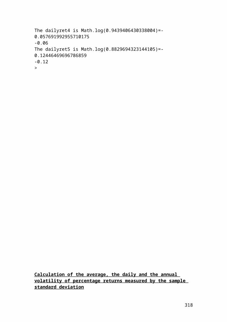
System.out.println(riskprobofupmove);System.out.println(Math.round(riskprobofupmove*100.0)/100.0);System.out.print("Call payoff upmove step [3] in pounds is ");System.out.println(callpayoffupmovestep3);System.out.println(Math.round(callpayoffupmovestep3*100.0)/100.0);System.out.print("Call payoff [3i] in pounds is ");System.out.println(callpayoff3i);System.out.println(Math.round(callpayoff3i*100.0)/100.0);System.out.print("Call payoff [3ii] in pounds is ");System.out.println(callpayoff3ii);System.out.println(Math.round(callpayoff3ii*100.0)/100.0);System.out.print("Call payoff downmove step [3] in pounds is ");System.out.println(callpayoffdownmovestep3);System.out.println(Math.round(callpayoffdownmovestep3*100.0)/100.0);System.out.print("Call price upmove step[2] in pounds is ");System.out.println(callpriceupmovestep2);System.out.println(Math.round(callpriceupmovestep2*100.0)/100.0);System.out.print("Call price updownmove step [2] in pounds is ");System.out.println(callpriceupdownmovestep2);System.out.println(Math.round(callpriceupdownmovestep2*100.0)/100.0);System.out.print("Call price downmove step [2] in pounds is ");System.out.println(callpricedownmovestep2);System.out.println(Math.round(callpricedownmovestep2*100.0)/100.0);System.out.print("Call price upmove step [1] in pounds is ");System.out.println(callpriceupmovestep1);System.out.println(Math.round(callpriceupmovestep1*100.0)/100.0);System.out.print("Call price downmove step [1] in pounds is ");System.out.println(callpricedownmovestep1);System.out.println(Math.round(callpricedownmovestep1*100.0)/100.0);System.out.print("Call price step[0] in pounds is ");System.out.println(callpricestep0);System.out.println(Math.round(callpricestep0*100.0)/100.0);}}
Output results
After compiling the current document from tools and pressing the run document you should get the following results:
Welcome to DrJava. Working directory is C:\Documents and Settings\Owner\Desktop\Java Compiler> run Cox_Ross_Rubinstein_call_option_calculationsSteps expressed in years is 0.166666666666666660.17Multiplier of upmove is 1.13029028276745721.13Multiplier of downmove is 0.88472847661005440.88Discount factor is 0.991701292638876
318
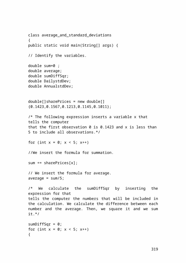
0.99Risk neutral probability of upmove is 0.489832055446951740.49Call payoff upmove step [3] in pounds is 36.6405563126204336.64Call payoff [3i] in pounds is 17.81741696604743217.82Call payoff [3ii] in pounds is 3.0837085966032593.08Call payoff downmove step [3] in pounds is 0.00.0Call price upmove step[2] in pounds is 26.8886511342689626.89Call price updownmove step [2] in pounds is 10.22832393472965710.23Call price downmove step [2] in pounds is 1.49796412844548191.5Call price upmove step [1] in pounds is 18.27978461354383218.28Call price downmove step [1] in pounds is 5.7327963577030885.73Call price step[0] in pounds is 11.80440657594629911.8>
319
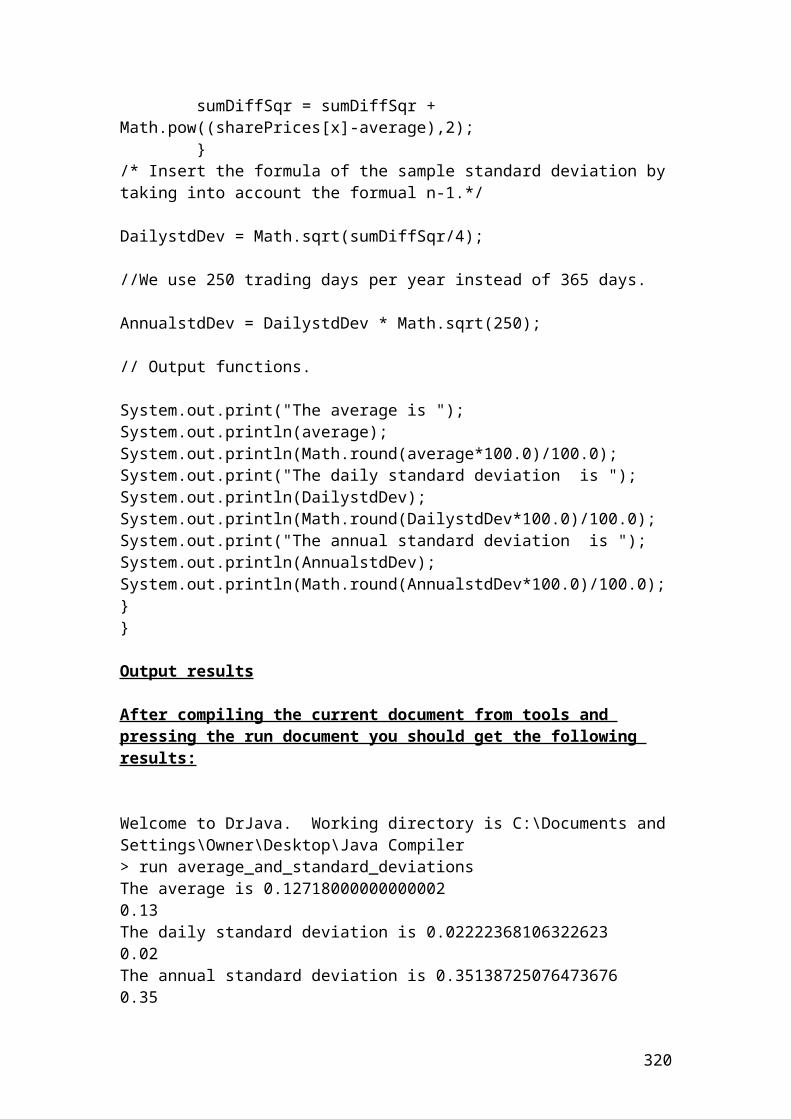
Calculate the put option prices using a Cox, Ross, Rubinstein,(CRR) binomial 3 steps tree. The multipliers of up and down move depend on volatility and the length of steps
class Cox_Ross_Rubinstein_put_option_calculations {public static void main(String[] args) {
/* Calculate the put option prices using a Cox, Ross, Rubinstein,(CRR) binomial 3 steps tree. */
double S = 60; // share price double K = 70; // strike price double r = 0.02; // risk-free interest rate double q = 0.03; // dividend yield double T = 0.5; // life to maturity double sig = 0.2; // volatility // Identify the variables. u = multiplier of upmove. //d = multiplier of downmove. dt = steps expressed in years. //riskprobofupmove = risk neutral probability of upmove. //disfact = discount factor. double u; double d; double dt; double riskprobofupmove; double disfact; int n = 3; // Identify tree steps binomial tree. // Insert the mathematical formulas. dt = T/n; u = Math.exp(sig*Math.sqrt(dt)); d = 1/u; disfact = Math.exp(-r*dt); riskprobofupmove = (Math.exp((r-q)*dt)-d)/(u-d); double putpayoffupmovestep3; // K - (Shareprice * upmove^3)double putpayoff3i; // K- (Shareprice * upmove^2 * downmove)double putpayoff3ii; // K-(Shareprice * downmove^2*upmove) double putpayoffdownmovestep3; // K-(Shareprice * downmove^3)
// The option prices are calculated backwards.
putpayoffupmovestep3 = K-S*Math.pow(u,3);putpayoffupmovestep3=0;putpayoff3i = K- S * Math.pow(u,2) * d;
320
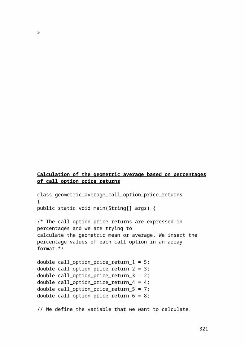
putpayoff3ii =K- S * Math.pow(d,2)*u; putpayoffdownmovestep3 = K - S*Math.pow(d,3);
double putpriceupmovestep2;double putpriceupdownmovestep2;double putpricedownmovestep2;
putpriceupmovestep2 = (disfact*(riskprobofupmove*putpayoffupmovestep3)+(1-riskprobofupmove)*putpayoff3i);
putpriceupdownmovestep2 =(disfact*(riskprobofupmove*putpayoff3i)+(1-riskprobofupmove)*putpayoff3ii);
putpricedownmovestep2 =(disfact*(riskprobofupmove*putpayoff3ii)+(1-riskprobofupmove)*putpayoffdownmovestep3);
double putpriceupmovestep1;double putpricedownmovestep1;
putpriceupmovestep1 = (disfact*(riskprobofupmove*putpriceupmovestep2)+(1-riskprobofupmove)*putpriceupdownmovestep2);
putpricedownmovestep1=(disfact*(riskprobofupmove*putpriceupdownmovestep2)+(1-riskprobofupmove)*putpricedownmovestep2);
double putpricestep0;
putpricestep0= (disfact*(riskprobofupmove*putpriceupmovestep1)+(1-riskprobofupmove)*putpricedownmovestep1);
//Output functions.System.out.print("Steps expressed in years is ");System.out.println(dt);System.out.println(Math.round(dt*100.0)/100.0);System.out.print("Multiplier of upmove is ");System.out.println(u);System.out.println(Math.round(u*100.0)/100.0);System.out.print("Multiplier of downmove is ");System.out.println(d);System.out.println(Math.round(d*100.0)/100.0);System.out.print("Discount factor is ");System.out.println(disfact);System.out.println(Math.round(disfact*100.0)/100.0);System.out.print("Risk neutral probability of upmove is ");System.out.println(riskprobofupmove);System.out.println(Math.round(riskprobofupmove*100.0)/100.0);System.out.print("Put payoff upmove step [3] in pounds is ");System.out.println(putpayoffupmovestep3);
321
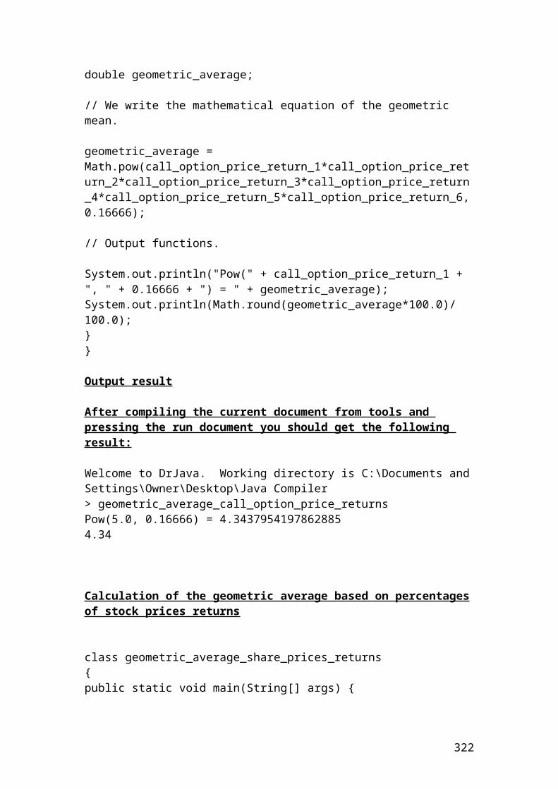
System.out.println(Math.round(putpayoffupmovestep3*100.0)/100.0);System.out.print("Put payoff [3i] in pounds is ");System.out.println(putpayoff3i);System.out.println(Math.round(putpayoff3i*100.0)/100.0);System.out.print("Put payoff [3ii] in pounds is ");System.out.println(putpayoff3ii);System.out.println(Math.round(putpayoff3ii*100.0)/100.0);System.out.print("Put payoff downmove step [3] in pounds is ");System.out.println(putpayoffdownmovestep3);System.out.println(Math.round(putpayoffdownmovestep3*100.0)/100.0);System.out.print("Put price upmove step[2] in pounds is ");System.out.println(putpriceupmovestep2);System.out.println(Math.round(putpriceupmovestep2*100.0)/100.0);System.out.print("Put price updownmove step [2] in pounds is ");System.out.println(putpriceupdownmovestep2);System.out.println(Math.round(putpriceupdownmovestep2*100.0)/100.0);System.out.print("Put price downmove step [2] in pounds is ");System.out.println(putpricedownmovestep2);System.out.println(Math.round(putpricedownmovestep2*100.0)/100.0);System.out.print("Put price upmove step [1] in pounds is ");System.out.println(putpriceupmovestep1);System.out.println(Math.round(putpriceupmovestep1*100.0)/100.0);System.out.print("Put price downmove step [1] in pounds is ");System.out.println(putpricedownmovestep1);System.out.println(Math.round(putpricedownmovestep1*100.0)/100.0);System.out.print("Put price step[0] in pounds is ");System.out.println(putpricestep0);System.out.println(Math.round(putpricestep0*100.0)/100.0);}}
322
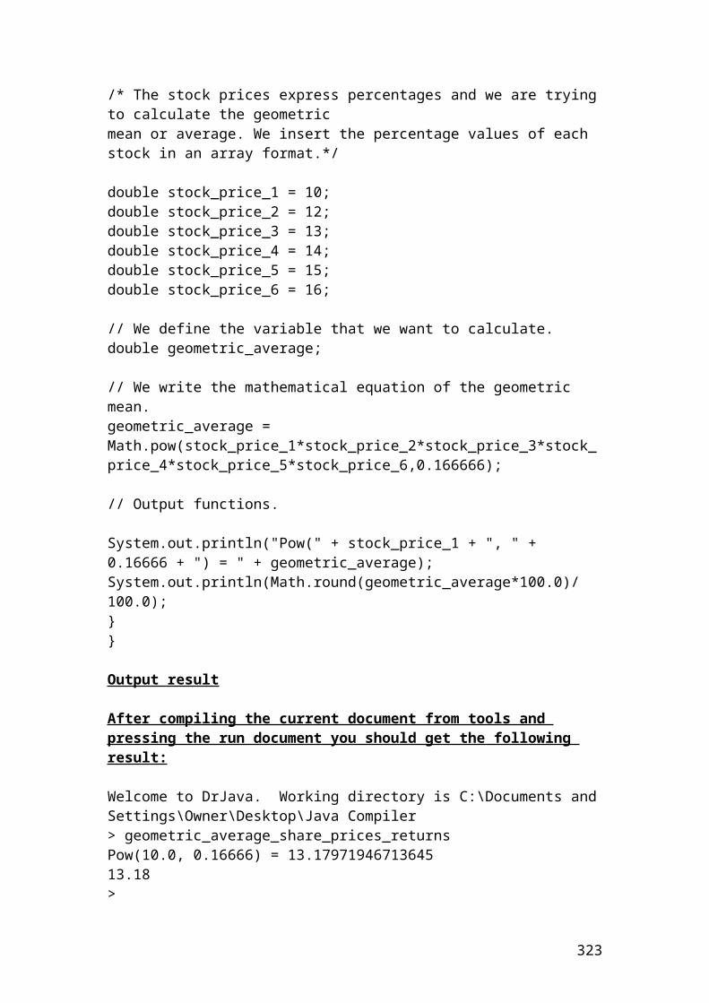
Output results
After compiling the current document from tools and pressing the run document you should get the following results:
Welcome to DrJava. Working directory is C:\Documents and Settings\Owner\Desktop\Java Compiler> run Cox_Ross_Rubinstein_put_option_calculationsSteps expressed in years is 0.166666666666666660.17Multiplier of upmove is 1.08507559577726931.09Multiplier of downmove is 0.92159477541624430.92Discount factor is 0.99667221605452331.0Risk neutral probability of upmove is 0.469412533318738670.47Put payoff upmove step [3] in pounds is 0.00.0Put payoff [3i] in pounds is 4.8954642533638414.9Put payoff [3ii] in pounds is 14.70431347502533714.7Put payoff downmove step [3] in pounds is 23.03533136051513723.04Put price upmove step[2] in pounds is 2.59747197642099262.6Put price updownmove step [2] in pounds is 10.09226949113763510.09Put price downmove step [2] in pounds is 19.10167749033414719.1Put price upmove step [1] in pounds is 6.57006008299829256.57Put price downmove step [1] in pounds is 14.8567832883130414.86Put price step[0] in pounds is 10.95662844179555910.96>
323
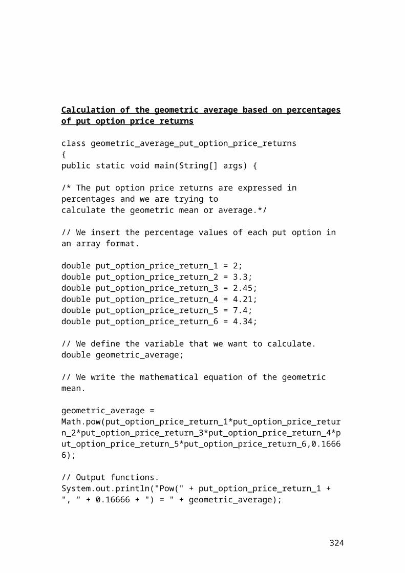
References
Alexander, C., (2003), Market Models. A Guide to Financial Data Analysis. John Wiley and Sons Ltd. ISMA Centre. The Business School For Financial Markets.
Amisano, G., and Giannini, C., (1997), “ Topics in Structural VAR Econometrics, 2nd
ed, Berlin: Springer – Verlag.
Ang,A., Piazzesi,M., and Wei,M.,(2006),” What Does the Yield Curve Tell Us About GDP Growth?. Journal of Econometrics, 131, pp.359 - 403.
Box, G.,E.,P. and Jenkins.,G.M, (1976), “ Time Series Analysis: Forecasting and Control, Revised Edition, Oakland, CA: Holden – Day.
Boswijk, P,H., (1995), “identifiability of Cointegrated Systems,”. Technical report. Tinbergen Institute.
Brooks,C.,(2002), Introductory econometrics for Finance. Cambridge University Press.
Campbell, J., and Shiller,R.J.,(1991),” Yield Spreads and Interest Rate Movements: A Bird’s Eye View. Review of Economic Studies, 58, pp. 495 -514.
Christiano, L.J.,M Eichenbaum, C.L.E, (1999), “Monetary Policy Shocks: What have we learned and to what end?” Chapter 2 in J.B.Taylor and M. Woodford, (eds.), Handbook of Macroeconomics, Volume 1A, Amsterdam: Elsevier Science Publishers B.V.
Davidson, R. and MacKinnon, J.G, (1993), “ Estimation and Inference in Econometrics”. Oxford: Oxford University Press.
Dickey,D.A and Fuller,W.A.,(1979),” Distribution of the Estimators for Autoregressive Time Series with a Unit Root. Journal of the American Statistical Association, 74, pp 427 – 431.
Doomik, J.A., and Hendry, D.F., (2009a), “ Empirical Econometric Modelling. Timberlake Consultants, Ltd.
Doornik, J.A and Hansen,H., (1994), “An Omnibus Test for Univariate and Multivariate Normality”. Manuscript.
Estrella,A., Hardouvelis, G.,(1990),”Possible Roles of the Yield Curve in Monetary Analysis”. In Intermediate Targets and Indicators for Monetary Policy. Federal Reserve Bank of New York.
Estrella,A., Hardouvelis, G.,(1991),” The Term Structure as a Predictor of Real Economic Activity”. Journal of Finance 46, no.2 (June).
324
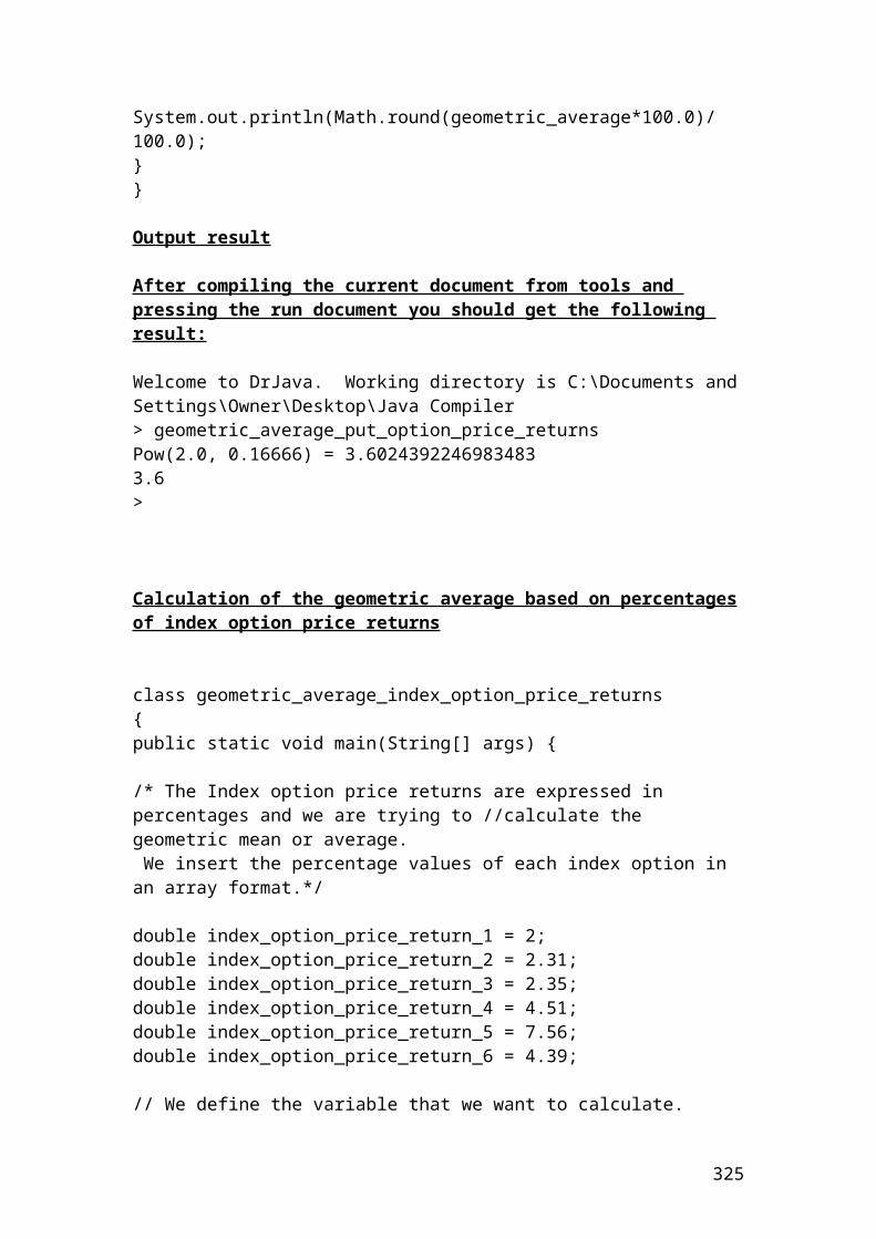
Estrella,A., Mishkin, F.,(1996), “The Yield Curve as a Predictor of US Recessions”. Federal Reserve Bank of New York. Current Issues in Economics and Finance,2.
Estrella, A., and Mishkin,F.,(1998),” Predicting US Recessions: Financial Variables as Leading Indicators”. Review of Economics and Statistics, 80, pp.45 -61.
Estrella, A., Rodrigues, A.P., and Schich,S.,(2003),” How Stable is the Predictive Power of the yield Curve: Evidence from Germany and the United States”. Review of Economics and Statistics, 85,pp.629 – 644.
EViews User’s Guide II,(2007), “Quantitative Micro Software”. pp.383,387.
Fisher, R.A., (1932), “Statistical Methods for Research Workers, 4 th Edition, Edinburgh: Oliver & Boyd.
Giacomini, Raffaella, and Rossi,B.,(2005),” How Stable is the Forecasting Performance of the Yield Curve for Output Growth”.mimeo, Duke University and University of California, Los Angeles.
Greene, William H.,(1997), “Econometric Analysis”. 3rd Edition. Upper Saddle River, NJ: Prentice Hall.
Hamilton,J.D.,(1994a), “ Time Series Analysis”, Princeton University Press.
Hamilton,J.D.,(1994b), “ State Space Models”, Chapter 50 in Robert F.Engle and Daniel L. McFaden (eds), Handbook of Econometrics, Volume 4, Amsterdam: Elsevier Science B.V.
Harvey, A.,C, (1989), “ Forecasting, Structural Time Series Models and the Kalman Filter, Cambridge: Cambridge University Press.
Johnston, J., and John Enrico DiNardo, (1997), “Econometric Methods, 4th Edition, New York: McGraw – Hill.
Koopman, Jan.,S, Shephard,N., and Doornik, J.A.,(1999), “ Statistical Algorithms for Models in State Space using SsfPack 2.2. Econometrics Journal, 2(1), pp.107 -160.
Mishkin,F.,(1990a),” What Does the Term Structure Tell Us About Future Inflation?”. Journal of Monetary Economics 25, pp.77-95.
Mishkin,F.,(1990b),” The Information in the Longer – Maturity Term Structure About Future inflation”. Quarterly Journal of Economics 55, pp 815 -28.
Piazzesi, M.,(2001),” An Econometric Model of the Yield Curve With Macroeconomic Jump Effects. National Bureau of Economic Research, Working paper no.8246.
Pindyck, R., and Rubinfeld, D,L.,(1998), “ Econometric Models and Economic Forecasts, 4th edition, New York: McGraw – Hill.
325
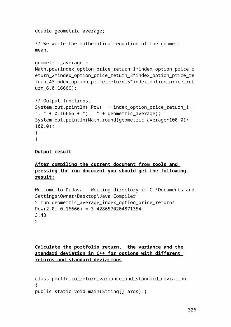
Sims, C.A.(1980), “ Macroeconomics and Reality”. Economterica, 48, 1 – 48.
Wooldridge, Jeffrey,M., (2000), “ Introductory Econometrics: A Modern Approach, South – Western College Publishing.
326
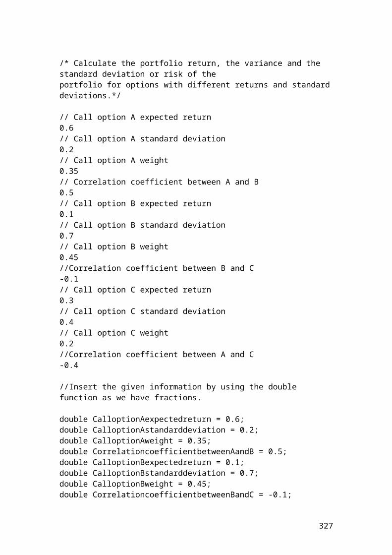
References & Bibliography
327