Old Dominion UniversityODU Digital Commons

Accounting Faculty Publications School of Accountancy

2017

Fixed Costs, Audit Production, and Audit Markets:Theory and EvidenceTracy Gu

Dan A. Simunic

Michael T. SteinOld Dominion University

Follow this and additional works at: https://digitalcommons.odu.edu/accounting_pubs

Part of the Accounting Commons

This Working Paper is brought to you for free and open access by the School of Accountancy at ODU Digital Commons. It has been accepted forinclusion in Accounting Faculty Publications by an authorized administrator of ODU Digital Commons. For more information, please contactdigitalcommons@odu.edu.

Repository CitationGu, Tracy; Simunic, Dan A.; and Stein, Michael T., "Fixed Costs, Audit Production, and Audit Markets: Theory and Evidence" (2017).Accounting Faculty Publications. 6.https://digitalcommons.odu.edu/accounting_pubs/6

Original Publication CitationGu, Tracy and Simunic, Dan A. and Stein, Michael T., Fixed Costs, Audit Production, and Audit Markets: Theory and Evidence( January 16, 2017). Available at SSRN: https://ssrn.com/abstract=2900389.

1

Fixed Costs, Audit Production, and Audit Markets: Theory and Evidence

by

Tracy Gu1, University of Hong Kong

Dan A. Simunic2, University of British Columbia

Michael T. Stein3, Old Dominion University

April, 2017 version

1Assistant Professor, E-mail: tracygu@hku.hk 2Professor, E-mail: dan.simunic@sauder.ubc.ca 3Professor, E-mail: mstein@odu.edu

Acknowledgements:

We thank Derek Chan, Minlei Ye, and workshop participants at the University of Technology-

Sydney, Rutgers University, Hong Kong Polytechnic University, the University of Hong Kong,

Old Dominion University, and the 2017 Journal of Contemporary Accounting and Economics

Conference at Tamkang University, Taipei for their comments on earlier versions of this paper.

2

Fixed Costs, Audit Production, and Audit Markets: Theory and Evidence

Abstract

We analyze the role of discretionary joint fixed costs in audit production. Given such costs, the

investment decision and production of audit services must be analyzed over a client portfolio. We

model this problem, and use monotone comparative statics (Milgrom and Shannon [1994]) to show

the implications of variations in client-specific losses and the number of clients for the optimum

level of fixed investment and audit assurance. We develop four hypotheses concerning the

relations between audit quality and (1) the magnitude of potential client-specific losses; (2) average

client losses in a portfolio; (3) the number of clients in a portfolio; and (4) the variability of losses

in a portfolio. Using discretionary accruals as the audit quality proxy, we find evidence consistent

with these hypotheses. Using PCAOB inspection results, and financial statement restatements as

proxies for audit quality, we find weaker evidence consistent with hypotheses 2, 3 and 4.

Keywords: Audit services, client portfolios, production, investments, discretionary common

fixed costs

3

1. Introduction and prior literature

In this paper we analyze the role of discretionary fixed costs in audit production. Such costs

can be changed period-to-period by an audit firm’s management, but are fixed at a moment in time

and are common or joint across a set of the firm’s audit clients. Our motivation is to better

understand the interaction of the production and supply of audit services and audit market

outcomes. Outcomes of interest include audit quality (i.e. audit assurance), the number of hours

utilized to service a client, and audit costs. Discretionary fixed costs can be associated with a

variety of investments that are made by a public accounting firm to facilitate its audit production,

including location specific investments (e.g. the construction of local offices), firm-wide training

programs for staff, and investments in audit technology. We conjecture that such investments

affect the transformation of audit effort (hours) into assurance, and that these investments (i.e.

fixed costs) influence production primarily through their effect on the efficiency of audit effort

(i.e. process improvements). Efficiency increasing investments (often referred to as labor

enhancing or productivity enhancing) can result in either lower cost audits or higher assurance

levels, or a combination of the two outcomes.

The investments and associated costs that we analyze are those that affect the audit of more

than a single client. Considered over multiple time periods, such costs are constant for a given

period of time, and are joint across the audits (of at least a subset) of clients serviced in that period.

We do not consider client-specific set-up costs that may be incurred when performing an audit. A

key implication of our focus on these discretionary, fixed, joint or common costs is that the

investment decision and the production of audit services cannot be fully analyzed on a client-by-

client basis but must consider the auditor’s portfolio of clients.

4

Existing research (e.g. O’Keefe, Simunic, and Stein [1994], Bell, Doogar, and Solomon

[2008], Akono and Stein [2014]) models audit production as a simple transformation of variable

labor inputs into audit assurance, without explicitly considering how (if at all) the efficiency

enhancing investments and the associated fixed costs enter into that transformation. While the

paper by Ye and Simunic [2017] also considers efficiency enhancing investments, the investments

and associated costs are assumed to be client-specific. In the absence of significant efficiency

enhancing common fixed costs, the production of audit services for a specific client is largely

separable from the audit production for other clients in the audit firm’s client portfolio. This greatly

simplifies the audit production problem. When the efficiency enhancing investments and the

resulting common fixed costs are an important feature of audit production, individual audits are

no longer separable because these investments will improve the efficiency of the production of all

audits, or at least a subset of the firm’s audits (e.g. clients in certain industries). Audit firms need

to aggregate these effects when making investment decisions.

Process improvements can be general for an audit firm’s whole pool of clients or limited

to a subset of specific clienteles. The modeling strategy we employ in this paper is flexible as it

can be extended to cover a multitude of auditing scenarios (e.g. audit firms as a whole, industry

specialization, etc.), at least to a first approximation. Our modelling strategy is novel, and we test

four hypotheses on the relationship between an audit firm’s client portfolio characteristics and

audit quality. The analysis does not encompass investments by the auditor that target the demand

side of the auditing market such as investments in advertising or customer relations.

We focus on the supply side of the auditing market. Supply conditions are critical to

understanding the market for audit services because a large portion of the audit market operates

under conditions where audits are mandatory and audit quality is ex-ante unobservable. This

5

implies that the demand for varying levels of audit quality is essentially a matter of auditor choice

(e.g. Big 4 vs. non-Big 4, or specialist vs. non-specialist), with the chosen supplier determining

the details of assurance production. The fact that a well specified and calibrated audit fee model

(e.g., Simunic [1980], Hay, Knechel and Wong [2006]) is able to explain 80% or more of the cross-

sectional variation in the logarithm of U.S. audit fees (which reflect audit costs) using variables

that capture supply-side work scope (e.g., client size and complexity) and the risk imposed by

association with a client on the auditor, suggests that supply-side factors are key to understanding

observable market outcomes.

Most existing research has treated audit production as simply involving variable labor

inputs which are (in some way) transformed into audit assurance, i.e., the probability, as assessed

by the auditor and financial statement users, that a client’s financial statements are not materially

misstated. A significant exception is the paper by Sirois, Marmousez, and Simunic [2016] which

applies the endogenous fixed cost (EFC) model developed by Sutton [1991] to the auditing

industry. In Sutton’s model as applied to auditing, technology plays a central role in determining

the level of audit quality and audit fees. Sirois et al further argue that Big 4 auditors make

differentially greater technology investments than non-Big 4 auditors and strategically compete on

both quality and price through these investments in technology, the level of which is increasing in

market size. Ferguson, Pinnuck and Skinner [2016] also apply Sutton’s EFC model to explain audit

market structure and the emergence of the two-tier audit market (Big 4 vs. non-Big 4) in Australia.

While Sutton’s EFC model incorporates technology investments and fixed costs, the

application of the EFC model to the analysis of the auditing industry has been largely verbal and

ad hoc. By contrast, in this paper we formally analyze the audit production problem when fixed

investments and the resulting discretionary fixed common costs are important. We first set up the

6

auditor’s problem as a simple expected cost minimization problem with client-specific labor hours

and the level of fixed investments (that benefit the audits of all clients) as the auditor’s choice

variables, and audit assurance as an outcome variable. This formulation is equivalent to a profit

maximization problem with fixed audit fees. We provide an analytical solution to this cost

minimization problem for a case in which specific functional forms of the assurance production

function and fixed investments cost function are assumed. We also provide numerical solutions

for both the special case and a broader class of reasonable functional forms. Next, the problem is

restated as a cost minimization problem, but with the level of fixed investments and the level of

assurance as the choice variables and the client-specific audit hours defined implicitly as a function

of the choice variables. This formulation facilitates the application of monotone comparative

statics (Milgrom and Shannon [1994]) to describe the more general relationship between the

characteristics of an auditor’s client portfolio and the level of investment and client-specific audit

assurance.

These analyses lead to several testable hypotheses regarding audit quality and the

characteristics of individual clients and the auditor’s portfolios of clients. We test these hypotheses

first by using the absolute value of discretionary accruals as the proxy for audit quality and using

four definitions of audit markets ranging from the broad U.S. national market (all publicly listed

companies) to companies operating in specific U.S. Metropolitan Statistical Areas (MSAs) in

specific 2-digit Standard Industrial Classification (SIC) industries. To address the concern that the

financial reporting outcomes (e.g., absolute discretionary accruals) may be caused by clients’

fundamentals rather than auditor-provided assurance, we employ two other measures that more

directly capture the auditors’ inputs as the proxies for audit quality. First, we examine the number

of audits with deficiencies and the number of specific audit failures in these audits as identified by

7

the Public Company Accounting Oversight Board’s (PCAOB) regular inspection of registered

audit firms. Then, we use financial statement restatements as another proxy for audit quality in our

supplemental analysis. The results of these various empirical tests suggest that the audit

investments associated with the discretionary fixed common costs that affect the production of

some (or all) of an audit firm’s portfolio of clients are an important, hitherto unexamined feature

of audit production which can help explain auditor-specific and client-specific systematic

variations in audit quality.

The remainder of the paper is organized as follows. In section 2, we set up a basic

formulation of the audit production problem where production requires variable labor input(s) but

fixed costs are not explicitly considered as a choice variable, either because they do not exist or

because technology and other investments associated with fixed costs are given. This formulation

is consistent with the way audit production has been conceived and modeled in the existing

literature. In section 3, which is the conceptual / theoretical core of our paper, we introduce

investments as a choice variable and the associated fixed costs into the analysis. We set up models

that describe audit firms and their clients by several exogenous parameters, and study the

characteristics of optimal production including the levels of investment, variable labor hours used,

and assurance levels provided. We also develop the comparative statics of the auditor’s expected

cost minimization problem. We conclude this section by developing testable hypotheses that

follow from our analyses. In section 4, we develop the empirical design for testing the four

hypotheses and report the empirical results. The last section summarizes and concludes the paper.

2. A Basic Model of the Audit Production Problem

2.1 BASIC SET-UP - SINGLE CLIENT OPTIMIZATION

8

A common assumption for analyzing audit production is that the competition in the market

for audits and/or the production of audits given a fixed audit fee motivate auditors to minimize the

costs of audit production (e.g., Simunic [1980], Dye [1993]). Formalizing this insight, a rational

auditor planning the audit of a single client using audit hours of various types (i.e. a choice among

junior, senior, manager, and partner hours) might solve (in concept) the following program:

1) Minimize c(h) = w ∙ h + L • [1 - q(h, a) ]

s.t. q(h, a) = 𝑞𝑝,

where, c(•), is the total cost function,

h, is a vector of audit hours of various types (e.g. junior, senior etc.),

w, is a vector of factor costs of various types of audit hours,

L, is the potential loss an auditor may incur through her association with a

client’s financial statements

q(•), is the audit transformation function in which audit hours

are transformed into assurance, where assurance is the auditor assessed

probability that the post-audit financial statements are free of material

misstatement.1

𝑞𝑝, is the planned level of assurance,

a, is a fixed audit investment (e.g. technology) parameter affecting audit

efficiency, and

(1 - q), is the probability of a post-audit loss.

Imposing appropriate structure to assure a solution and emphasizing that a is fixed and not a choice

variable, then the auditor’s problem is to pick the cost minimizing h, i.e.

𝒉∗ = argmin𝒉

𝑐(𝑎, 𝒘, 𝐿, 𝑞𝑝, 𝒉)

1 The assurance production function, q(•), implicitly includes all phases of an audit, i.e. planning, risk assessment,

substantive testing, and completion (see Blokdijk, Drieenhuizen, Simunic, and Stein [2006]).

9

If there is an interior solution to this problem, then it would be characterized by the usual

equalities between the ratios of the marginal rates of transformation and the ratios of the factor

costs (input prices). This model carries the essence of the auditor’s cost structure implicit in most

empirical cross-sectional audit fee or audit hour studies involving multiple labor inputs and was

used to motivate the empirical analysis of the audit hours utilized by a major public accounting

firm in O’Keefe, Simunic, and Stein [1994] and Bell, Doogar, and Solomon [2008].

If we specify an appropriate audit hour transformation function and substitute in parameter

values then, in theory, we could write down an audit cost function relative to the parameters as:

2) c(ℎ∗| a, w, L, 𝑞𝑝).

We can view 2) as a foundational model used to motivate archival audit fee studies where

w, the vector of wage rates, is assumed to be exogenous, and a represents the fixed investment in

technology and other factors utilized by the auditor. L, the potential loss, varies across clients and

is likely a function of the size, complexity, and other characteristics of the client (e.g. a closely

held vs. a listed company) as well as the legal and institutional environment associated with the

audit. We expect the potential loss to increase with client size, complexity, etc. and as the legal

and institutional regime becomes more onerous to auditors. Because liability is ultimately

constrained by the financial resources of the audit firm and / or its professional liability insurance,

L is finite and bounded from above. To focus on the essential features of audit service production

and to simplify our analyses, we assume that auditors are strictly liable for failing to detect material

misstatements in financial statements (i.e. there is no “negligence defense” based on adherence to

auditing standards) or the combination of auditing standards toughness and vagueness is such that

the auditor is motivated to ignore the standards (Ye and Simunic [2013]).

10

In program 1), 𝑞𝑝 is assumed to be fixed either by Generally Accepted Auditing Standards

(GAAS) or by audit firm policy. While this is a common assumption in the existing literature.2

the treatment of the planned level of assurance as a fixed parameter potentially conflicts with cost

minimization. If 𝑞𝑝 is fixed in advance or predetermined then there is no guarantee that c(ℎ∗| a, w,

L, 𝑞𝑝) will satisfy the requirement that c(ℎ∗ | a, w, L, 𝑞𝑝) < c(ℎ, 𝑞 |a, w, L) for all allowable

combinations of {h, q}. If, on the other hand, q is assumed to vary audit by audit then program 1)

would need to be changed to reflect optimization over both h and q.

Program 1) is a short-run cost minimization problem where fixed costs are treated as both

predetermined and sunk. This is consistent with existing literature in assuming that fixed costs (a)

are a predetermined characteristic of the audit firm which are unobservable by the researcher.

Empirically, the lack of controls for fixed investment is not necessarily problematic. If fixed costs

vary across auditors, then an auditor fixed effect potentially captures the cross-sectional

differences. Or if there is no across auditor variation in investment (due, perhaps to competition),

then the rental costs of fixed investments are included in the mark-up on cost. This mechanism is

consistent with the normal practice in service firms to add mark-up on direct labor costs to bill

overhead and earn profits.

However, fixed costs can play an important role in audit production. Some investments

associated with fixed costs (e.g., the adoption of a more intensive staff training program, or the

construction of a more powerful information system) can change the efficiency (marginal product)

of the various classes of labor to be transformed to audit assurance. Consequently, the changes in

the marginal product of labor will impact the vector of labor hours required to achieve the planned

level of assurance, 𝑞𝑝. Given that fixed investments can change the efficiency of audit labor and

2 For example, audit quality is usually assumed to vary systematically between Big 4 vs. non-Big 4 firms, but audit

quality is normally assumed to be the same, or perhaps vary randomly, within these audit firm categories.

11

that the fixed costs are shared by the auditor’s portfolio of clients, fixed costs, audit cost, and audit

quality are endogenously determined by the auditors’ cost minimization (given fixed audit fees)

or profit maximization over its portfolio of clients.

2.2 ANALYSIS WITH MULTIPLE CLIENTS

Before analyzing the role of fixed costs in the auditor’s cost minimization problem, we first

extend program 1) to incorporate a portfolio of clients, which better captures the reality of audit

production. In rewriting program 1), we represent any fixed investments by the parameter a in the

assurance transformation function. Higher levels of a imply larger fixed investments. In order to

simplify notation and because the mix of labor types is not important to subsequent analyses, we

assume a single type of labor going forward. Consequently, w and h are treated as scalars. Program

1) can be extended to incorporate a portfolio of clients:

3) Minimize w.r.t. ℎ𝑖: ∑ 𝑐𝑖(ℎ𝑖) 𝑛𝑡𝑖=1 = w ∑ ℎ𝑖

𝑛𝑡𝑖=1 + ∑ 𝐿𝑖(1 − 𝑞𝑝)

𝑛𝑡𝑖=1

s.t. q(ℎ𝑖, a) = 𝑞𝑝, for all i ∊ 𝑛𝑡,

where 𝑛𝑡 is the number of clients in auditor t’s set of clients. If audit production is separable in the

sense that ℎ𝒊 is independent of any other ℎj, then program 3) is a simple adding up of model 1).

However, interdependencies might enter the cost functions either through the loss function (see

Simunic and Stein [1990]) or through the assurance transformation function, as would occur if

learning increased the efficiency of labor. Given the interdependencies of the cost of individual

audits in affecting the auditor’s total cost, the optimal vectors of ℎ𝑖’s should be jointly determined

across the auditor’s client portfolio, rather than determined on an audit by audit basis. Further, if

an audit firm were to audit to a fixed level of assurance, 𝑞𝑝, across clients, it would make sense

12

for the firm to solve for the optimal 𝑞𝑝 at the portfolio level. That is, if there is a fixed level of

planned assurance as in 3) then dependencies are also built into the problem.

3. Re- formulating the Audit Production Problem

3.1 AUDIT PRODUCTION WITH INVESTMENTS ASSOCIATED WITH

DISCRETIONARY FIXED COSTS

In modeling the role of discretionary fixed costs in audit production, we treat the

technology and other investments associated with discretionary fixed costs, i.e., the parameter a,

as an input to the auditor’s assurance transformation function. We assume that such fixed

investments do not directly provide assurance, but rather affect the labor hours needed to produce

a given level of assurance. That is, in our model, discretionary fixed costs operate indirectly

through the relationship between the usage of hours and the production of assurance. As a

consequence of this assumption, fixed investments and costs are inherently efficiency oriented.

Investments in technology and other fixed costs reduce the marginal use of labor hours for any

target level of assurance.

To formulate the audit production problem in which efficiency enhancing discretionary

fixed costs are an auditor’s choice variable, we rewrite program 3) which emphasizes that the

problem is solved by each auditor at the audit firm level. Importantly, we conjecture and

subsequently drop the constraint which characterizes the prior literature that the assurance level

produced must equal some planned, target level. If there are t auditors in the market and each

auditor has nt clients, we denote auditor t’s choice of investment as 𝑎t. Thus auditors:

4) minimize𝑎𝑡,ℎ𝑖

∑ 𝑐𝑖(𝑎𝑡, ℎ𝑖) 𝑛𝑡𝑖=1 = min w ∑ ℎ𝑖

𝑛𝑡𝑖=1 + ∑ 𝐿𝑖(1 − 𝑞𝑖) + f(𝑎𝑡)

𝑛𝑡𝑖=1

13

s.t. q(ℎ𝑖, 𝑎𝑡) = 𝑞𝑖, for all i ∊ 𝑛𝑡,

where f(𝑎𝑡) is the fixed rental cost of 𝑎𝑡. We assume df/da > 0 and d2f/da2 ≥ 0; that is, the fixed

costs of investing in technology and other factors increase at a non-decreasing rate. The auditor

chooses a parameter value 𝑎𝑡 and a vector of client-specific labor hours, hi , that minimize the total

(expected) cost of auditing her portfolio. In program 4), because q(ℎ𝑖, 𝑎𝑡) = 𝑞𝑖 is a function of 𝑎𝑡

and ℎ𝑖, 𝑞𝑖 varies across audits (see section 3.2 below) and an audit-firm specific level of assurance

is achieved in terms of a portfolio average.

3.2 SOLUTION TO THE COST MINIMIZATION PROBLEM WITH 𝑛𝑡 IDENTICAL

CLIENTS AND KNOWN FUNCTIONS FOR f(𝑎𝑡) AND q(ℎ𝑖, 𝑎𝑡)

To obtain some intuition into the solution of program 4), suppose that an auditor has 𝑛𝑡

identical clients and is considering a new fixed investment, say in technology, that improves the

efficiency of production for each client. We rewrite program 4) to incorporate the identical client

assumption and specify the audit hour transformation function:

5) {ℎ𝑡∗, 𝑎𝑡

∗} = argmin𝑎𝑡, ℎ𝑡

𝑐𝑖(ℎ𝑡 , 𝑎𝑡

) = argmin𝑎𝑡, ℎ𝑡

𝑛𝑡 w ℎ𝑡+ 𝑛𝑡 𝐿 (1 - 𝑞𝑡 ) + f(𝑎𝑡)

s.t. 𝑞𝑡 = 𝛽 𝑎𝑡 ℎ𝑡

1/2 ∀ 𝑖 ∊ 𝑛𝑡 and 0 ≤ 𝑞𝑡 ≤ 1

where is a positive normalizing constant. To derive an algebraic solution to this problem we also

need to specify a functional form for f(•), the cost of the fixed factor 𝑎𝑡. We let

6) f(𝑎𝑡) = 𝑘𝑡 • 𝑎𝑡3.

Importantly, the cost of 𝑎𝑡 increases quickly enough to offset the concavity of the assurance

transformation function q(•).

14

Assuming an interior solution and working through the math (not shown), we solve for

the optimal values of the choice variables in terms of the parameters:

𝑞𝑡∗= ( 𝐿5 𝑛𝑡

2 𝛽5) / (72 𝑘𝑡2 𝑤3), 𝑎𝑡

∗ = ( 𝐿2 𝑛𝑡 𝛽2) / (6 𝑘𝑡 w), and ℎ𝑡

∗ = ( 𝐿6 𝑛𝑡2 𝛽6) / (144 𝑘𝑡

6 𝑤4)

These results satisfy the second order conditions for cost minimization and have the qualitative

attributes: 𝑞𝑡∗, 𝑎𝑡

∗, and ℎ𝑡∗, individually increase in L and 𝑛𝑡 and decrease in w and 𝑘𝑡.

To get a better sense for these results, we solve the problem numerically for a variety of

parameter values. In the table below we set =.0018, w =50 and 𝑘𝑡 = 2,000 and then vary both the

number of clients and the size of the potential loss of the clients. Optimal outcomes in terms of

total portfolio audit cost, fixed investment, audit effort per client, and assurance levels provided

are reported in the table below.

𝑛𝑡 L Cost a* h* q*

40 65,000 2.59924*106 0.9126 1.14007 0.974421

40 60,000 2.39953*106 0.7776 0.705277 0.653035

35 60,000 2.09969*106 0.6804 0.539978 0.49998

As a check on these results, we re-specify the model using an asymptotic assurance

transformation function. The quadratic assurance function specified in equation (5) can easily hit

the 100% assurance upper bound as a and h increase, so as an alternative we use the following

function: q = a h / ( + a h). This function converges to 100% assurance as a and h increase to

infinity. Using this functional form of q plus modifying equation 6) to f(𝑎𝑡) = 𝑘𝑡 • 𝑎𝑡 allow the

program to be solved analytically to derive optimal parameterizations of the choice variables (the

solutions are ungainly and not included). We then solve the modified model numerically by fixing

15

the following parameter values: = 10, w =50 and 𝑘𝑡 = 2,000 and once again varying both the

number of clients and the size of the potential loss of the clients. The results are given in the

following table.

𝑛𝑡 L Cost a* h* q*

40 65,000 140,224. 23.2272 23.2272 0.981802

40 60,000 136,486. 22.6003 22.6003 0.980798

35 60,000 124,825. 20.6629 23.6148 0.979918

In both examples, audit firms are assumed to be endowed with different numbers (𝑛𝑡) and

different types (Lt ) of clients, and are solving for the optimum production plan for their specific

client portfolio. Summarizing the numerical results presented in the above two tables, we observe

that i) the high risk portfolios (large L), ceteris paribus, use more labor, make larger fixed cost

investments, and provide higher assurance and ii) that auditors with the greater number of clients,

ceteris paribus, make larger fixed costs investments and provide a higher level of assurance. In

the quadratic assurance case the auditor with the greater number of clients uses more labor hours

per client, while in the asymptotic assurance case the auditor with the greater number of clients

uses fewer labor hours.

In both of the examples if we hold the size of the potential loss constant, then the average

cost per client is lower for the portfolio with the larger number of clients. This result, if true in

general, suggests that larger auditors could provide higher levels of assurance and undercut the

prices of smaller auditors – see footnote 3, below. Specific implications of this observation to audit

markets requires equilibrium modeling of audit demand and so lies beyond the scope of our current

16

research, but does raise the question: Is the provision of auditing services a potential natural

monopoly? We leave more extensive consideration of this question for future research.

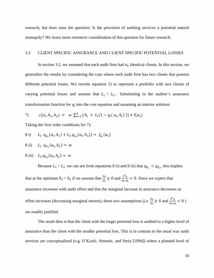
3.3 CLIENT SPECIFIC ASSURANCE AND CLIENT SPECIFIC POTENTIAL LOSSES

In section 3.2, we assumed that each audit firm had 𝑛𝑡 identical clients. In this section, we

generalize the results by considering the case where each audit firm has two clients that possess

different potential losses. We rewrite equation 5) to represent a portfolio with two clients of

varying potential losses and assume that 𝐿1 > 𝐿2

. Substituting in the auditor’s assurance

transformation function for 𝑞𝑖 into the cost equation and assuming an interior solution:

7) 𝑐(𝑎𝑡 , ℎ1

, ℎ2 ) = 𝑤 ∑ { ℎ𝑖 + 𝐿𝑖(1 − 𝑞𝑖( 𝑎𝑡, ℎ𝑖) )} + f(𝑎𝑡)2

𝑖=1

Taking the first order conditions for 7):

8 i) 𝐿1 𝑞𝑎𝑡

(𝑎𝑡, ℎ1) + 𝐿2 𝑞𝑎𝑡

(𝑎𝑡, ℎ2)} = 𝑓𝑎𝑡(𝑎𝑡)

8 ii) 𝐿1 𝑞ℎ1

(𝑎𝑡, ℎ1) = 𝑤

8 iii) 𝐿2 𝑞ℎ2

(𝑎𝑡, ℎ2) = 𝑤

Because 𝐿1 > 𝐿2

we can see from equations 8 ii) and 8 iii) that 𝑞ℎ1< 𝑞ℎ2

, this implies

that at the optimum ℎ1 > ℎ2

if we assume that 𝜕𝑞

𝜕ℎ≥ 0 and

𝜕2𝑞

𝜕ℎ 𝜕ℎ< 0. Since we expect that

assurance increases with audit effort and that the marginal increase in assurance decreases as

effort increases (decreasing marginal returns), these two assumptions (i.e. 𝜕𝑞

𝜕ℎ≥ 0 and

𝜕2𝑞

𝜕ℎ 𝜕ℎ< 0 )

are readily justified.

The result then is that the client with the larger potential loss is audited to a higher level of

assurance than the client with the smaller potential loss. This is in contrast to the usual way audit

services are conceptualized (e.g. O’Keefe, Simunic, and Stein [1994]) where a planned level of

17

assurance is delivered for each client (perhaps with random noise). The idea that assurance varies

systematically (not randomly) client-by-client around a firm mean is consistent with an economic

approach to the auditor’s problem in which auditors maximize their profits. In contrast, if the

assurance level is set as a constraint to be equaled or bettered, then it is hard to see that strategy as

being consistent with profit maximizing. It might be more consistent with the traditional

professionalism approach to audit planning, where audit firms are not simply profit maximizing

(cost minimizing) but try to maximize some type of social welfare function. But if the

professionalism approach violates profit maximization, is it realistic - particularly when audit

markets are competitive?

3.4 COMPARATIVE STATICS OF THE AUDITOR’S COST MINIMIZATION PROBLEM

In this section, we drop the known functional forms imposed on the assurance production

function, q(ℎ𝑖, 𝑎𝑡), and the cost of fixed investments, f(𝑎𝑡), and develop a general approach to

the comparative statics of the auditor’s cost minimization problem.

Consider an auditor with a portfolio of 𝑛𝑡 clients facing the following ex-ante single

period decision problem:

9) 𝜋(𝑎𝑡 , 𝒒𝒊

| 𝜽) = maximize𝑎𝑡

,𝒒𝒊

∑ [ R(𝑞𝑖) − 𝑤 𝐻(𝑎𝑡 , 𝑞𝑖

) − 𝐿𝑖(1 − 𝑞𝑖)] – f( 𝑎𝑡)

𝑛𝑡𝑖=1

where,

𝜽 = {𝑳𝒕, 𝑤 , 𝑘}, is a set of parameters. Noting{𝑳𝒕} is a vector and {w, k} are

scalars;

H(𝑎𝑡 , 𝑞𝑖) = ℎ𝑖 , ∀ 𝑖 ∈ 𝑛𝑡 . H(•) is the auditor’s labor function defined implicitly with

arguments investment, a, and assurance, q;

R(𝑞𝑖), is the auditor’s fee for audit i; and

18

f(𝑎𝑡), is the one period rental cost of fixed investment.

In this model, the auditor chooses parameter values {𝑎𝑡, 𝒒𝒊) – as distinct from (𝒉𝑖, 𝑎𝑡) in

our earlier formulation – to maximize the total (expected) profit of auditing her portfolio. We

specialize the profit maximization model by assuming revenues are fixed. Doing so equates profit

maximization with cost minimization. This is consistent with our primary interest in audit

production. Restricting our attention to the cost minimization component of the model allows us

to highlight the supply side of the market without engaging the multiple complications introduced

by market demand conditions. We acknowledge this restriction reduces the generality of our

results insofar as we are unable to fully characterize the optimal levels of assurance and investment

in equilibrium. However, the solution to the auditor’s cost minimization problem yields crucial

insights from the supply side about the relationships among the auditor’s portfolio of client

potential losses, the optimal provision of assurance, and the utilization of audit input factors even

without a fully specified demand side model.

Next, we again simplify the representation of the auditor’s portfolio to the number of clients

and the average size of the clients’ potential losses. With these assumptions in place the profit

maximization problem 9) is restated as a cost minimization problem:

10) 𝑐(𝑎𝑡∗, 𝑞𝑡

∗| 𝜽) = minimize𝑎𝑡,∈𝑅+

1 𝑞𝑡 ∈[0,1]𝑛𝑡 𝑤 𝐻(𝑎𝑡

, 𝑞𝑡

) + 𝑛𝑡 𝐿𝑡(1 − 𝑞𝑡) + f( 𝑎𝑡)

Further, we can define the set of optimizers that solves equation 10) (assuming an interior solution

exists) as:

11) {𝑎𝑡∗(𝜃), 𝑞𝑡

∗(𝜃)} = arg 𝑚𝑖𝑛 𝑞𝑡 ∈ [0,1], 𝑎𝑡 ∈ ℝ+

1

𝑐(𝑎𝑡 , 𝑞𝑡

| 𝜽)

Defining audit hours implicitly allows us to rewrite the cost function with investment and

assurance as the choice variables. Since we expect audit assurance, q, to be an increasing function

of both ℎ𝑖 and 𝑎𝑡 , it follows that the implicit hours function, H, would have the following

19

characteristics: 𝜕𝐻

𝜕𝑎≤ 0,

𝜕𝐻

𝜕𝑞≥ 0, and

𝜕2𝐻

𝜕𝑎 𝜕𝑞≤ 0. In words, we expect: i) audit effort to decrease in

the level of investment, holding assurance constant, ii) audit effort to increase in assurance, holding

investment constant, and iii) the rate of increase in audit effort due to an increase in assurance

decreases as investment increases. For completeness we also expect that 𝜕2𝐻

𝜕𝑞 𝜕𝑞≥ 0 and

𝜕2𝐻

𝜕𝑎 𝜕𝑎≥ 0.

Two assurance transformation functions that fit this characterization are the ones we used earlier

in our numerical examples: the quadratic assurance function, 𝑞𝑖 = 𝛽 𝑎𝑡ℎ𝑖1/2

, and the asymptotic

assurance function, 𝑞𝑖 =𝑎𝑡ℎ𝑖

𝛽+𝑎𝑡ℎ𝑖.

A benefit of defining audit effort implicitly is that we can eliminate the requirement that

{𝑎𝑡 , ℎ𝑖

}satisfy the bounds implied by the assurance variable and replace these constraints with the

requirement that the domain of 𝑞𝑖 is the closed interval [0,1]. This is helpful in our later analysis

since the domain of the subsequent minimization is a lattice defined on the product space [0,1] ×

ℝ+1 . Below we outline the connections between the cost minimization model and our empirical

tests.

The Application of Monotone Comparative Statics to the Auditor’s Cost Minimization Model.

We use the above representation of the cost minimization model to generalize our analysis

of changes in the parameters, 𝑛𝑡 and 𝐿𝑡, on audit production. One way to do this is to apply the

techniques of monotone comparative statics (MCS) Milgrom and Shannon [1994]. To see how this

approach works, first transform the minimization problem, equation 10), into a maximization

problem by multiplying through by -1. Then take the set of optimal solutions to the cost

minimization problem given in equation 11),{𝑎𝑡∗(𝜃), 𝑞𝑡

∗(𝜃)}, and ask the question: what conditions

does the objective function in 10) have to satisfy such that the pair of optimal solutions are jointly

20

(weakly) increasing or decreasing in the scalar parameter 𝜃? The short answer is that if the feasible

set is a lattice and the objective function has increasing (decreasing) differences in each of the pairs

{a, q}, {a, 𝜃}, and {q, 𝜃}, then the required conditions are met for the comparative static result,

i.e., the optimal values are jointly increasing (decreasing) in the chosen parameter. The increasing

(or decreasing) differences condition does not, in general, require that the objective function to be

either differentiable or concave and the MCS results can be obtained by verifying that the

increasing differences criterion holds. If one is willing to assume the differentiability of the

objective function, an assumption we apply for convenience and to make the verification procedure

more transparent to readers not familiar with MCS and Topkis’ theorem Topkis [2011], then

increasing differences can be checked by demonstrating that the appropriate pairwise cross-partial

derivatives are weakly positive on the feasible set, the fore-mentioned lattice.

Demonstration that Assurance and Investment are Non-decreasing (weakly increasing) in Client

Potential Loss

We begin by defining a function d(•):

12) 𝑑(𝑎𝑡 , 𝑞𝑡

, 𝜽) = −(𝑛𝑡 𝑤 𝐻(𝑎𝑡 , 𝑞𝑡

) + 𝑛𝑡 𝐿𝑡(1 − 𝑞𝑡) + f(𝑎𝑡) )

To show that {𝑎𝑡∗(𝐿), 𝑞𝑡

∗(𝐿)} are increasing in L we take the following cross-partial

derivatives of equation 12) substituting in 𝐿𝑡for 𝜽 and (assuming the objective function is twice

continuously differentiable):

13 i) 𝑑𝑎,𝑞(𝑎𝑡 , 𝑞𝑡

, 𝐿) = -𝑛𝑡 𝑤 𝐻𝑎,𝑞(𝑎𝑡 , 𝑞𝑡

) ≥ 0, the condition holds if

𝜕2𝐻

𝜕𝑎 𝜕𝑞≤ 0,

13 ii) 𝑑𝑎,𝐿(𝑎𝑡 , 𝑞𝑡

, 𝐿) = 0,

13 iii) 𝑑𝑞,𝐿(𝑎𝑡 , 𝑞𝑡

, 𝐿) = 𝑛𝑡 ≥ 0

21

All three of the required conditions (the pair-wise cross-partial derivatives are weakly

positive) are easily seen to hold. This verifies that the objective function is characterized by

increasing differences in each of the three relevant pairs.

Demonstration that Assurance and Investment are Non-decreasing (weakly increasing) in the

Number of Clients in an Audit Firm’s Portfolio.

Now to show that {𝑎𝑡∗(𝑛𝑡), 𝑞𝑡

∗(𝑛𝑡)} are increasing in 𝑛𝑡 we take the following cross-partial

derivatives of equation 12) substituting in 𝑛𝑡for 𝜽:

14 i) 𝑑𝑎,𝑞(𝑎𝑡 , 𝑞𝑡

, 𝑛𝑡) = -𝑛𝑡 𝑤 𝐻𝑎,𝑞(𝑎𝑡 , 𝑞𝑡

) ≥ 0, if

𝜕2𝐻

𝜕𝑎 𝜕𝑞≤ 0

14 ii) 𝑑𝑎,𝑛𝑡(𝑎𝑡

, 𝑞𝑡 , 𝑛𝑡) = -𝑤 𝐻𝑎(𝑎𝑡

, 𝑞𝑡

) ≥ 0, if

𝜕 𝐻

𝜕𝑎≤ 0

14 iii) 𝑑𝑞,𝑛𝑡(𝑎𝑡

, 𝑞𝑡 , 𝑛𝑡) = - 𝑤 𝐻𝑞(𝑎𝑡

, 𝑞𝑡

) + 𝐿𝑡 ≥ 0 = 0

Conditions 14 i) and 14 ii) are met given our assumptions on the hours function H(•).

Condition 14 iii) holds since 𝑤 𝐻𝑞(𝑎𝑡 , 𝑞𝑡

) + 𝐿𝑡 = 0 is a first order necessary condition for

optimality of the cost function (we assume the usual regularity conditions for an interior optimum

of the cost function are met).

Increasing Client Loss Variance Decreases Average Assurance and Investment: A Three Client

Numerical Model

In order to relax the assumption that 𝐿𝑡 is constant within an auditor’s portfolio, we take

equation 10) and form an auditor portfolio consisting of three clients. Next, we define the auditor’s

cost function as:

15) 𝑐(𝑎𝑡 , 𝑞1

, 𝑞2 , 𝑞3

| 𝜽) = ∑ { 𝑤 𝐻(𝑎𝑡 , 𝑞𝑖

) + 𝐿𝑖(1 − 𝑞𝑖)} + f( 𝑎𝑡)3

𝑖=1

where,

22

H(𝑎, 𝑞𝑖) =𝑞𝑖

𝑎(1−𝑞𝑖) , the audit hours function with 𝐻𝑎(𝑎, 𝑞𝑖) < 0, 𝐻𝑞(𝑎, 𝑞𝑖) > 0,

𝐻𝑎𝑎(𝑎, 𝑞𝑖) > 0, 𝐻𝑞𝑞(𝑎, 𝑞𝑖) > 0 and 𝐻𝑎𝑞(𝑎, 𝑞𝑖) < 0.

The potential losses for these three clients are defined as: 𝐿1 = 𝐿 + 𝜔, 𝐿2 = 𝐿 and 𝐿3 =

𝐿 − 𝜔, for 𝜔 > 0 which implies that 𝐿1 > 𝐿2 > 𝐿3, and we set f(𝑘, 𝑎𝑡) = 𝑘𝑎𝑡2. The assumption

that f(•) is convex in 𝑎𝑡 is required for the result. Linear investment costs reverse the numerical

results.

We constructed the above potential loss portfolio to be a mean preserving spread. The mean

of the client portfolio is increased by increasing L and the variance of the portfolio is increased by

increasing 𝜔 . We minimize equation 15) numerically to determine optimal values for

{𝑎𝑡 , 𝑞1

, 𝑞2 , 𝑞3

}. The numerical results are suggestive of how the model would extend to auditor

portfolios with varying client potential losses. In our numerical calculations we normalized the

wage rate to 1 (numeraire good) and set k = 200. The potential loss parameter values are listed

along with the q’s in each line of the results.

Cost a* 𝑞1∗ 𝑞2

∗ 𝑞3∗ Ave (𝑞𝑖

∗)

410.857 0.637299 0.967657

L =1,500

0.97199

L =2,000

0.974947

L =2,500

0.971531

409.07 0.635887 0.965219

L =1,300

0.971959

L =2,000

0.975866

L =2,700

0.971015

406.562 0.6339 0.96213

L =1,100

0.971915

L =2,000

0.976677

L =2,900

0.970241

As can be seen in the table above, increasing the variance of client specific losses in an

audit firm’s portfolio decreases optimal investment, average assurance, and portfolio cost.

Interestingly, the assurance level for client 2 also falls as portfolio variance increases even though

the potential loss for that client is held constant at 𝐿2 = 2,000.

23

3.5 TESTABLE EMPIRICAL IMPLICATIONS

Based on the foregoing analyses, we consider four empirical tests. Specifically:

1. For a given audit firm, audit quality is client specific and increases with the size of the

potential client specific losses (𝐿𝑖 ). This test follows from our assertion in section 3.3 that

varying assurance on a client-by-client basis is more consistent with cost minimization than

auditing to a static level of assurance when an auditor services heterogeneous clients.

2. In an audit market, the average audit quality produced by an audit firm increases as the

average client Li in the firm’s portfolio of clients in that market increases3 (as average 𝐿i

increases, 𝑎𝑡∗ increases, and 𝑞𝑖

∗ increases).

3. In an audit market, average audit quality produced by an audit firm increases as the number

of clients (nt) in the firm’s portfolio increases (as nt increases, 𝑎𝑡∗ increases, and

𝑞𝑖∗ increases).

4. In an audit market, average audit quality decreases as the variability of client losses (Li ) in

the firm’s portfolio increases.

We note that these predictions derive solely from production (i.e. supply-side)

considerations and do not make any assumptions about the demand for audit quality except that

audits are normal goods (i.e. given audit cost, more assurance is preferred to less).

4. Empirical Tests

3 In addition to increasing assurance levels, the labor enhancing characteristic of audit investment also implies that

auditors with larger investments become more efficient in the sense they will require fewer audit hours for a given

client and potentially incur lower costs to audit marginal clients than audit firms with lower levels of investment. We

conjecture that the resulting market structure will depend upon the interplay of optimal investment scale and market

size. For example, a sufficiently large audit market could sustain multiple auditors operating at optimal scale and

remain competitive since no audit firm gains a cost advantage due to the equalization of investment. In contrast, audit

markets too small to support multiple auditors at scale would tend to become dominated by a single provider.

24

4.1 KEY INDEPENDENT VARIABLES

The four empirical implications in section 3.5 predict that, in an audit market, the audit

quality of a specific client increases with the potential client-specific losses, the audit firm’s

portfolio average of potential client-specific losses, the number of clients in the audit firm’s client

portfolio, and audit quality decreases with the variability of the potential client-specific losses. To

test H1, we use the natural logarithm of clients’ total assets (Ln(Asset)) as the proxy for client-

specific losses (𝐿𝑖 ). Accordingly, for H2, the potential average client losses are proxied by the

average value of the natural logarithm of clients’ total assets, i.e. the average client size

(AvgClientsize). The number of clients in the audit firms’ client portfolio (Clientnum) corresponds

to H3. To test H4, the variability of the potential client-specific losses is proxied by the standard

deviation of client size (StdClientsize).

To construct an audit firm’s client portfolio, we define four audit markets: (1) the broad

U.S. national market, which includes all publicly listed companies; (2) U.S. public companies

operating in specific 2-digit Standard Industrial Classification (SIC) industries; (3) companies

operating in specific U.S. Metropolitan Statistical Areas (MSAs); and (4) companies operating in

specific U.S. MSAs in specific 2-digit SIC industries. The four audit markets are denoted as M1,

M2, M3, and M4, respectively. Note that the market level at which our empirical predictions as

developed from the theoretical model should be observable depends on the market level where

investments are made by audit firms. For example, the effects of investments in staff training at

the national level should be observable in market M1. Or, if audit firms make more local

investments that benefit audits of clients in certain industries, the effects should only be observable

in the M4 markets.

25

4.2 PROXIES FOR AUDIT QUALITY

Audit quality is defined as the auditor assessed level of assurance (probability) that the

financial statements are free of material misstatements after an audit is completed that results in

the issuance of an unqualified (normal) opinion on the financial statements.4 An ideal proxy for

audit quality should (somehow) measure this probability, which, of course, is not directly

observable. Note that auditor assurance is developed throughout the audit process that

encompasses planning, risk assessment, substantive testing, and completion procedures (such as

second partner review). Thus auditor assurance incorporates the auditor's assessment of client

managements’ contribution to the preparation of accurate financial statements through their

personal integrity, quality of accounting systems and controls, etc. We use several variables as the

proxies for audit quality: the absolute value of discretionary accruals, the number of audits with

deficiencies as well as the number of the audit firms’ specific failures as reported in the Public

Company Accounting Oversight Board’s (PCAOB) inspection reports, and (in a supplementary

analysis) financial statement restatements.

Absolute discretionary accruals have been used in a considerable amount of the prior

literature as a proxy for audit quality or as the outcome of a high quality audit (e.g. Becker et al.

[1998]). This proxy allows us to obtain a client-specific measure of audit quality. This measure is

the outcome of the financial reporting process and can be affected by client characteristics.

Accordingly, we control for client-specific characteristics in our empirical tests of the four

predictions.

4 Audit quality is normally defined as the joint probability that an auditor discovers any material misstatements that

exist, and truthfully reports the results of an audit. Since our focus is on audit production, we implicitly assume

truthful reporting.

26

In addition to the absolute value of discretionary accruals, we use the number of audits

with deficiencies, and the number of the audit firms’ specific failures as identified by PCAOB’s

inspection as two other proxies of audit quality. To enhance the audit quality of public companies,

Section 104 of the Sarbanes Oxley Act of 2002 and PCAOB Rule 4003 require the PCAOB to

regularly inspect PCAOB-registered accounting firms that provide audit reports for U.S.-listed

public companies. The inspections identify matters that the inspection team considered to be audit

deficiencies, which include failures by the audit firm to perform, or to perform at a sufficiently

high level, certain necessary audit procedures.5 After an inspection, the PCAOB sends inspection

results on engagement-specific audit deficiencies and the identified defects in the audit firms’

quality control system to the audit firm inspected. The results on engagement specific audit

deficiencies are listed in the inspection reports published on the PCAOB web site. The disclosed

information regarding engagement specific audit deficiencies are (1) the number of the inspected

audits that contain deficiencies of “such significance that it appeared to the inspection team that

the Firm, at the time it issued its audit report, had not obtained sufficient competent evidential

matter to support its opinion on the issuer’s financial statements”6, and (2) the specific failures to

perform sufficient procedures in supporting its audit opinions. As compared to the absolute

5 Section 104 of the Sarbanes Oxley Act of 2002 requires the PCAOB to “(1) inspect and review selected audit and

review engagements of the firm (which may include audit engagements that are the subject of ongoing litigation or

other controversy between the firm and 1 or more third parties), performed at various offices and by various associated

persons of the firm, as selected by the Board;(2) evaluate the sufficiency of the quality control system of the firm, and

the manner of the documentation and communication of that system by the firm; and (3) perform such other testing

of the audit, supervisory, and quality control procedures of the firm as are necessary or appropriate in light of the

purpose of the inspection and the responsibilities of the Board.” As documented in Auditing Standard No. 3, paragraph

9 and Appendix A to AS No. 3, paragraph A28, an observation that the audit firm did not perform a procedure, obtain

evidence, or reach an appropriate conclusion may be based on the absence of such documentation and the absence of

persuasive other evidence. 6 A typical PCAOB inspection report contains this description before describing specific audit failures. An example

is available at https://pcaobus.org/Inspections/Reports/Documents/2012_Accell_Audit_Compliance_PA.pdf.

27

discretionary accruals, these two PCAOB inspection-based proxies better capture auditors’ input

in providing audit assurance and are less likely to be affected by client characteristics.

Finally, we also use restatements as another proxy for audit quality in our supplemental

analysis. Different from discretionary accruals which is the output of the financial reporting

process and the audit deficiencies identified by the PCAOB’s regular inspection of registered

accounting firms, financial statement restatements occur because a material misstatement exists in

the audited financial statements. Thus a restatement is more probable as the quality of an audit

(assurance) decreases. Misstatements may be discovered either by client management or the

auditor after the audit report is issued. More specifically, factors affecting the revelation of an

existing material misstatement include the investigation of the company (i.e. the auditor’s client)

by private parties (e.g. analysts, employees, and lawyers can be the whistleblowers), a Securities

and Exchange Commission investigation, and the external legal environment that affects the firm’s

decision to restate earnings. For instance, as evidenced by Srinivasan, Wahid, and Yu [2014], firms

operating in an environment with stronger rule of law are more likely to admit their mistakes in

financial reporting, when material misstatements exist. Given the multiple-factors driving a

restatement, the absence of a restatement is not necessarily an indicator of high audit quality,

although a restatement provides direct evidence of audit failure in the restated year. In contrast,

because the PCAOB inspection is on a regular basis and is directly related to the quality of audit

production, the inspection results may provide a better audit-quality measure.7

4.3 REGRESSION MODELS

7 The PCAOB Rule 4003 mandates that public accounting firms auditing more than 100 U.S. public companies should

be inspected annually and those auditing fewer than 100 U.S. public companies should be inspected at least every

three years.

28

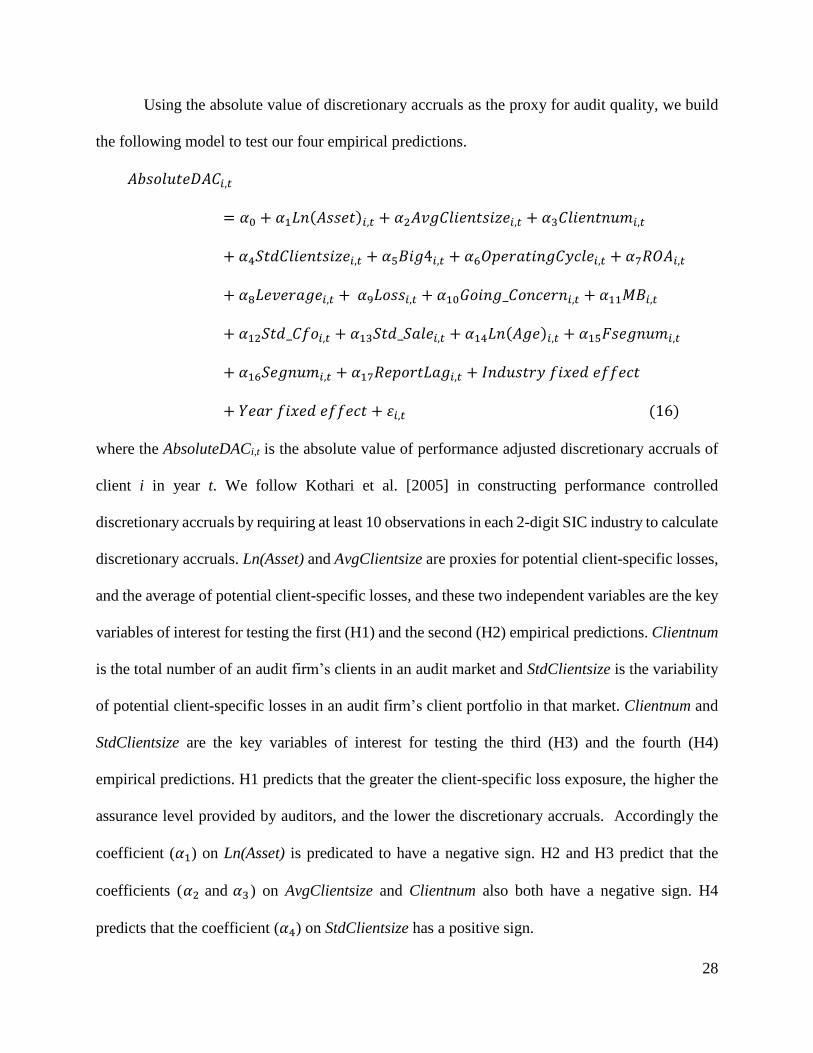
Using the absolute value of discretionary accruals as the proxy for audit quality, we build

the following model to test our four empirical predictions.

𝐴𝑏𝑠𝑜𝑙𝑢𝑡𝑒𝐷𝐴𝐶𝑖,𝑡

= 𝛼0 + 𝛼1𝐿𝑛(𝐴𝑠𝑠𝑒𝑡)𝑖,𝑡 + 𝛼2𝐴𝑣𝑔𝐶𝑙𝑖𝑒𝑛𝑡𝑠𝑖𝑧𝑒𝑖,𝑡 + 𝛼3𝐶𝑙𝑖𝑒𝑛𝑡𝑛𝑢𝑚𝑖,𝑡

+ 𝛼4𝑆𝑡𝑑𝐶𝑙𝑖𝑒𝑛𝑡𝑠𝑖𝑧𝑒𝑖,𝑡 + 𝛼5𝐵𝑖𝑔4𝑖,𝑡 + 𝛼6𝑂𝑝𝑒𝑟𝑎𝑡𝑖𝑛𝑔𝐶𝑦𝑐𝑙𝑒𝑖,𝑡 + 𝛼7𝑅𝑂𝐴𝑖,𝑡

+ 𝛼8𝐿𝑒𝑣𝑒𝑟𝑎𝑔𝑒𝑖,𝑡 + 𝛼9𝐿𝑜𝑠𝑠𝑖,𝑡 + 𝛼10𝐺𝑜𝑖𝑛𝑔_𝐶𝑜𝑛𝑐𝑒𝑟𝑛𝑖,𝑡 + 𝛼11𝑀𝐵𝑖,𝑡

+ 𝛼12𝑆𝑡𝑑_𝐶𝑓𝑜𝑖,𝑡 + 𝛼13𝑆𝑡𝑑_𝑆𝑎𝑙𝑒𝑖,𝑡 + 𝛼14𝐿𝑛(𝐴𝑔𝑒)𝑖,𝑡 + 𝛼15𝐹𝑠𝑒𝑔𝑛𝑢𝑚𝑖,𝑡

+ 𝛼16𝑆𝑒𝑔𝑛𝑢𝑚𝑖,𝑡 + 𝛼17𝑅𝑒𝑝𝑜𝑟𝑡𝐿𝑎𝑔𝑖,𝑡 + 𝐼𝑛𝑑𝑢𝑠𝑡𝑟𝑦 𝑓𝑖𝑥𝑒𝑑 𝑒𝑓𝑓𝑒𝑐𝑡

+ 𝑌𝑒𝑎𝑟 𝑓𝑖𝑥𝑒𝑑 𝑒𝑓𝑓𝑒𝑐𝑡 + 𝜀𝑖,𝑡 (16)

where the AbsoluteDACi,t is the absolute value of performance adjusted discretionary accruals of

client i in year t. We follow Kothari et al. [2005] in constructing performance controlled

discretionary accruals by requiring at least 10 observations in each 2-digit SIC industry to calculate

discretionary accruals. Ln(Asset) and AvgClientsize are proxies for potential client-specific losses,

and the average of potential client-specific losses, and these two independent variables are the key

variables of interest for testing the first (H1) and the second (H2) empirical predictions. Clientnum

is the total number of an audit firm’s clients in an audit market and StdClientsize is the variability

of potential client-specific losses in an audit firm’s client portfolio in that market. Clientnum and

StdClientsize are the key variables of interest for testing the third (H3) and the fourth (H4)

empirical predictions. H1 predicts that the greater the client-specific loss exposure, the higher the

assurance level provided by auditors, and the lower the discretionary accruals. Accordingly the

coefficient (𝛼1) on Ln(Asset) is predicated to have a negative sign. H2 and H3 predict that the

coefficients (𝛼2 and 𝛼3) on AvgClientsize and Clientnum also both have a negative sign. H4

predicts that the coefficient (𝛼4) on StdClientsize has a positive sign.

29

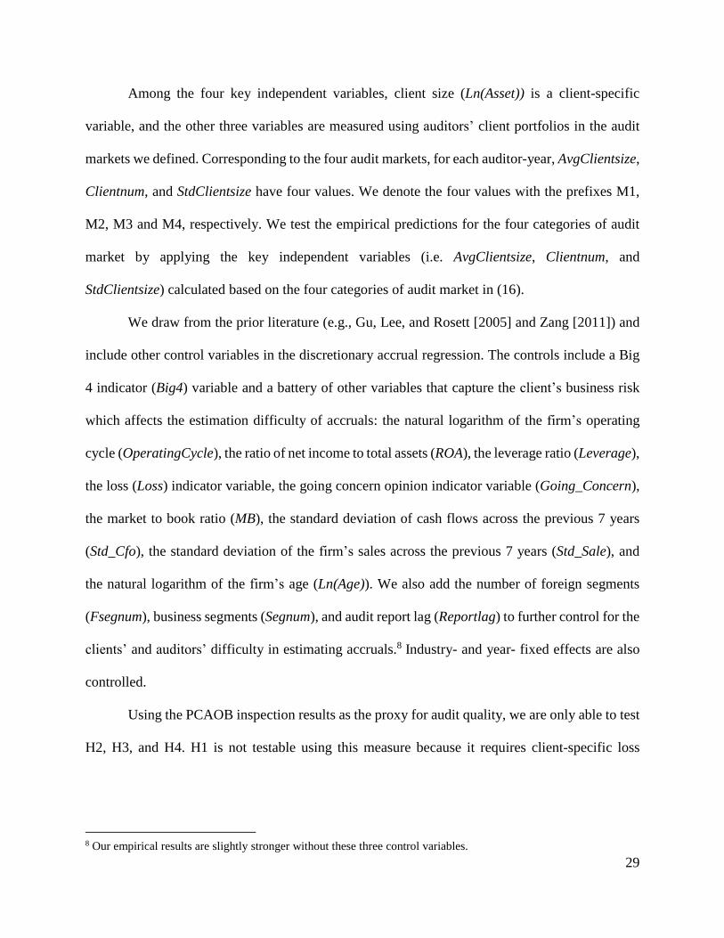
Among the four key independent variables, client size (Ln(Asset)) is a client-specific

variable, and the other three variables are measured using auditors’ client portfolios in the audit

markets we defined. Corresponding to the four audit markets, for each auditor-year, AvgClientsize,

Clientnum, and StdClientsize have four values. We denote the four values with the prefixes M1,

M2, M3 and M4, respectively. We test the empirical predictions for the four categories of audit

market by applying the key independent variables (i.e. AvgClientsize, Clientnum, and

StdClientsize) calculated based on the four categories of audit market in (16).

We draw from the prior literature (e.g., Gu, Lee, and Rosett [2005] and Zang [2011]) and

include other control variables in the discretionary accrual regression. The controls include a Big

4 indicator (Big4) variable and a battery of other variables that capture the client’s business risk

which affects the estimation difficulty of accruals: the natural logarithm of the firm’s operating

cycle (OperatingCycle), the ratio of net income to total assets (ROA), the leverage ratio (Leverage),

the loss (Loss) indicator variable, the going concern opinion indicator variable (Going_Concern),

the market to book ratio (MB), the standard deviation of cash flows across the previous 7 years

(Std_Cfo), the standard deviation of the firm’s sales across the previous 7 years (Std_Sale), and

the natural logarithm of the firm’s age (Ln(Age)). We also add the number of foreign segments

(Fsegnum), business segments (Segnum), and audit report lag (Reportlag) to further control for the

clients’ and auditors’ difficulty in estimating accruals.8 Industry- and year- fixed effects are also

controlled.

Using the PCAOB inspection results as the proxy for audit quality, we are only able to test

H2, H3, and H4. H1 is not testable using this measure because it requires client-specific loss

8 Our empirical results are slightly stronger without these three control variables.

30

exposure. Nevertheless, H1 is more of an assumption rather than an implication of our analysis

and is not crucial for the validity of H2- H4. We use the two models below to test H2, H3, and H4.

𝑁𝑢𝑚_𝐴𝑢𝑑𝑖𝑡𝑠𝑤𝑖𝑡ℎ_𝐷𝑒𝑓𝑖,𝑡

= 𝛽0 + 𝛽1𝐴𝑣𝑔𝐶𝑙𝑖𝑒𝑛𝑠𝑖𝑧𝑒𝑖,𝑡 + 𝛽2𝐶𝑙𝑖𝑒𝑛𝑡𝑛𝑢𝑚𝑖,𝑡 + 𝛽3𝑆𝑡𝑑𝐶𝑙𝑖𝑒𝑛𝑡𝑠𝑖𝑧𝑒𝑖,𝑡

+ 𝛽4𝐼𝑛𝑠𝑝𝑒𝑐𝑡𝑖𝑜𝑛_𝐷𝑢𝑟𝑎𝑡𝑖𝑜𝑛𝑖,𝑡 + 𝛽5𝑁𝑢𝑚_𝐼𝑛𝑠𝑝𝑒𝑐𝑡𝑒𝑑𝑖,𝑡 + 𝛽6𝐹𝑖𝑟𝑠𝑡_𝐼𝑛𝑠𝑝𝑒𝑐𝑡𝑖𝑜𝑛𝑖,𝑡

+ 𝛽7𝑁𝑢𝑚_𝑃𝑎𝑟𝑡𝑛𝑒𝑟𝑠𝑖,𝑡 + 𝛽8𝑁𝑢𝑚_𝑆𝑡𝑎𝑓𝑓𝑖,𝑡 + 𝛽9𝑇𝑟𝑖𝑒𝑛𝑛𝑖𝑎𝑙𝑙𝑦𝑖,𝑡

+ 𝑌𝑒𝑎𝑟 𝑓𝑖𝑥𝑒𝑑 𝑒𝑓𝑓𝑒𝑐𝑡 + 𝜀𝑖,𝑡 (17)

𝑁𝑢𝑚_𝐴𝑢𝑑𝑖𝑡𝑓𝑎𝑖𝑙𝑢𝑟𝑒𝑠𝑗,𝑡

= 𝛾0 + 𝛾1𝐴𝑣𝑔𝐶𝑙𝑖𝑒𝑛𝑡𝑠𝑖𝑧𝑒𝑗,𝑡 + 𝛾2𝐶𝑙𝑖𝑒𝑛𝑡𝑛𝑢𝑚𝑗,𝑡 + 𝛾3𝑆𝑡𝑑𝐶𝑙𝑖𝑒𝑛𝑡𝑠𝑖𝑧𝑒𝑗,𝑡

+ 𝛾4𝐼𝑛𝑠𝑝𝑒𝑐𝑡𝑖𝑜𝑛_𝐷𝑢𝑟𝑎𝑡𝑖𝑜𝑛𝑗,𝑡 + 𝛾5𝑁𝑢𝑚_𝐼𝑛𝑠𝑝𝑒𝑐𝑡𝑒𝑑𝑗,𝑡 + 𝛾6𝐹𝑖𝑟𝑠𝑡_𝐼𝑛𝑠𝑝𝑒𝑐𝑡𝑖𝑜𝑛𝑗,𝑡

+ 𝛾7𝑁𝑢𝑚_𝑃𝑎𝑟𝑡𝑛𝑒𝑟𝑠𝑗,𝑡 + 𝛾8𝑁𝑢𝑚_𝑆𝑡𝑎𝑓𝑓𝑗,𝑡 + 𝛾9𝑇𝑟𝑖𝑒𝑛𝑛𝑖𝑎𝑙𝑙𝑦𝑗,𝑡

+ 𝑌𝑒𝑎𝑟 𝑓𝑖𝑥𝑒𝑑 𝑒𝑓𝑓𝑒𝑐𝑡 + 𝜀𝑗,𝑡 (18)

where Num_Auditwith_Defj,t is the numeric count of audits with deficiencies as identified by the

PCAOB inspection of audit firm j in the inspection year of t+1. Inspection year is the year when

the PCAOB starts the inspection of the audit firm. Audit deficiencies identified by an inspection

conducted in year t+1 should have existed in the year when the audit is finished thus should be

earlier than year t+1. To choose a year close enough to the inspection year, we denote t as the year

in which the audit deficiencies exist. We use the audit firm’s average client size (AvgClientsize),

number of clients (Clientnum), and the standard deviation of client size (StdClientsize) in year t as

the audit firm characteristics corresponding to Num_Auditwith_Defj,t and Num_Auditfailuresj,t.

Average client size (AvgClientsize) and client number (Clientnum) are measured at the national

audit market. Num_Auditfailuresj,t is the numeric count the audit firm’s failures as identified by

the PCAOB inspection of audit firm j in the inspection year of t+1. Because our dependent

31

variables are count values that are always nonnegative, we use an ordered probit regression to

estimate models (17) and (18).9

The other control variables capture the PCAOB’s resource input into the inspection and

the audit firms’ labor resources. Inspection_Duration is the number of days between the inspection

start date and the inspection end date. A longer inspection duration indicates greater resource input

by the PCAOB, and can be driven by either the greater riskiness of the audits selected for

inspection or by the PCAOB-conjectured importance of the inspection. Num_Inspected is the

number of audits inspected in a specific inspection. First_Inspection is an indicator variable set to

1 if the inspection is the first time that the PCAOB inspects the audit firm and 0 otherwise.

Num_Partners is the number of the audit firm’s self-reported partners at the time of the inspection.

Num_Staff is the number of the audit firm’s self-reported personnel, except partners or

shareholders and administrative support personnel.10 Triennially is an indicator variable set to 1 if

the audit firm is auditing fewer than 100 U.S. public companies and 0 otherwise.11

The empirical results for models (16) to (18) are provided in sections 4.3 and 4.4. We apply

a probit model for our restatement analysis, following the absolute discretionary accrual model as

specified in model (16) in constructing the control variables. Section 4.5 provides empirical results

of the probit model that uses restatement as the audit quality proxy.

4.4 DATA AND SAMPLE

9 Linear regression is not an appropriate estimation technique for count data, as it fails to take into account the limited

number of possible values of the response variable. We follow Hausman, Lo, and MacKinlay [1992] in using the

ordered probit regression model. 10 As noted in a typical inspection report, the number of partners and professional staff is an indication of the size of

the audit firm, and does not necessarily represent the number of the audit firm’s professionals who participate in audits

of the public companies. 11 See footnote 7, above.

32

Because the data sources of the three audit quality measures (i.e. absolute discretionary

accruals, PCAOB identified audit deficiencies, and restatement) differ, the corresponding samples

also differ. To construct the sample for the discretionary accrual analysis, we start with the year

2000, the first year for which Audit Analytics provides an expanded set of audit related

information, such as the locations of auditors’ offices, audit fees, and going concern opinions, none

of which are available in Compustat. Our sample ends in 2014. We constrain our sample to U.S.-

listed companies headquartered and incorporated in the U.S. to ensure that all audit clients in the

sample are subject to the U.S. legal environment. We also require that the audit firms are located

in the U.S. so that the auditors are from the same national labor market and are subject to the U.S.

legal environment. We remove clients in the financial industry (SIC codes from 6000 to 6999)

because financial firms are regulated and auditors’ loss exposure associated with these clients can

be substantially different from their loss exposure associated with clients in other industries.

We require firms to have auditor choice, auditors’ location information, and accounting

data necessary to calculate discretionary accruals. Also, we must be able to classify firms into

U.S. Metropolitan Statistical Areas, and have other variables in the regression models. As a result

of these requirements, our final sample for the absolute discretionary accrual analysis contains

39,518 firm-years. The sample covers 6,291 firms. Accounting data are obtained from Compustat

and are winsorized at the 1th percentile and 99th percentile. The absolute values of the discretionary

accruals are winsorized at the 99th percentile. Table 1 panel A reports the summary statistics for

the variables used in this paper and panel B reports the Pearson correlation matrix for these

variables.

33

The PCAOB inspection data is purchased from Digi Data Mart Ltd. 12 The company

extracts data contained in the PCAOB’s public inspection reports. As collected by Digi Data Mart

Ltd., there are 2,124 unique inspections of U.S. audit firms conducted before 2015 (inclusive)

whose inspection reports have been disclosed at the PCAOB website.13 The first year of inspection

is 2003. We use the number of audits with deficiencies (if any) and the number of specific audit

failures contained in these inspection reports as two measures of audit-firm level audit quality.

Because the PCAOB does not disclose the inspected audits and a typical inspection usually

inspects more than one audit, there is no way to precisely identify the year for which the identified

audit deficiencies (i.e. the audit quality proxy) pertain. However, because an inspection (by

construction) targets audits that have been finished, the identified audit deficiencies should capture

audit quality for years before the inspection year. We obtain the audit firm’s client portfolio

characteristics for one year before the inspection year and use this information as the audit firm

characteristics corresponding to the identified audit deficiencies. This treatment is consistent with

the PCAOB inspection rule (Rule 4003) – noted above. To the extent that the audit quality of audit

firms can be expected to maintain a certain level of stability within two years, this treatment

matches audit quality with the associated client-portfolio characteristics while avoiding arbitrary

selection of the year of client-portfolio characteristics.

By requiring the inspected audit firm to have client information in Audit Analytics in the

year before inspection, we are able to manually match 708 audit firm-years between the inspection

reports and Audit Analytics.14 Among these 708 audit firm-years, 666 audit firm-years have non-

12 See https://auditor-inspection.myshopify.com/. 13 The audit deficiencies identified by an inspection starting in 2015 corresponds to audit deficiencies existing in 2014. 14 Because the names of some audit firms change, PCAOB inspection reports and Audit Analytics reports are often

not exactly that same, we start with a computerized matching and then manually check and match the audit firms’

names in inspection reports with the audit firms’ names in Audit Analytics. To ensure the accuracy of the matching,

when audit firm’s names are not exactly the same in the two sources, we check using a Google search for the phone

number, location, and other details of the audit firms.

34

missing information for the number of audits with deficiencies (or number of audit failures),

number of audits inspected, and inspection duration. Table 2 panel A provides details of the sample

construction and panel B provides the correlation table for the variables used in equestions (17)

and (18).

Restatement information is obtained from Audit Analytics. We include all types of

restatements (i.e. restatements caused by accounting errors and those caused by accounting

irregularities) in our analysis based on the rationale that a misstatement will not be restated if it is

not material and that auditors are responsible for assuring that financial statements are free of any

material misstatement, whether caused by fraud or simple error. Our restatement sample starts in

2000, the first year for which Audit Analytics provides comprehensive restatement information,

and ends in 2012. Ending in 2012 is consistent with the prior literature (e.g., Czerney, Schmidt,

and Thompson [2014], Files, Sharp, and Thompson [2014]) in allowing the company or its auditor

at least two years following the audit report year to identify issues that would require a restatement.

4.5 REGRESSION RESULTS

Tables 2 – 5 report the results of the regressions estimated using the four categories of audit

market with absolute discretionary accruals as the proxy for audit quality. In all the regressions,

the dependent variable AbsoluteDAC is client-year specific. In each table, columns (1) – (5) report

estimation results for five regressions. Before running the regression as specified in equation (16),

we start with a simple regression in column (2) that regresses the first audit quality measure

(AbsoluteDAC) on our first key variable of interest (Ln(Asset)) and the control variables drawn

from model (16), while excluding AvgClientsize, Clientnum, and StdClientsize from the regression

model. In columns (2) – (4), Ln(Asset)is retained as a control variable, and we regress

35

AbsoluteDAC on AvgClientsize, Clientnum, and StdClientsize, respectively, in each column, while

controlling for the battery of control variables drawn from equation (16). Column (5) of each table

reports regression results for equation (16), which is specified to test the four empirical

implications in one model. The coefficients on all variables in the four tables are standardized for

easier comparison.

In Table 2, the audit market is the broad U.S. national market, which includes all publicly

listed companies. An audit firm’s client portfolio in this market consists of all of the firm’s clients

that are operated and incorporated in the U.S. M1(AvgClientsize), M1(Clientnum), and

M1(StdClientsize) are the audit firm’s average client size, number of clients, and standard

deviation of client size in the U.S. national market. The prefix M1 refers to the first category of

audit market, i.e. national level market. As reported in column (5), the coefficient on Ln(Asset) is

significantly negative (coefficient estimate=-0.086, t = -8.14), suggesting that as client size

increases audit quality increases. This evidence is consistent with our first empirical prediction

(H1). Consistent with H2, the coefficient on M1(AvgClientsize) is -0.112 (t =-5.45), suggesting

that audit quality increases with the audit firm’s average client size in the national market.

Furthermore, the coefficients on M1(Clientnum) and M1(StdClientsize) are 0.041 (t = -4.08) and

0.018 (t = -1.74). These results suggest that audit quality increases as the number of clients in the

audit firm’s client portfolio increases and decreases as the variability of client size increases.

Additionally, the results in columns (1) – (4) are all consistent with results in column (5).

Collectively, the evidence is supportive of the four empirical implications applied to the national

audit market.

In Table 3, an audit market covers U.S. public companies operating in specific 2-digit

Standard Industrial Classification (SIC) industries. For each client-year in the five regressions,

36

M2(AvgClientsize) is calculated as the audit firm’s average size of clients operating in the specific

client’s 2-digit SIC industry. In a similar vein, M2(Clientnum) is the number of clients in the

specific client’s 2-digit SIC industry and M2(StdClientsize) is the standard deviation of the size of

clients in the specific industry portfolio. Columns (1) to (5) report regression results for the five

regressions. The results reported in columns (1) to (5) are consistent with the results in Table 2

and are supportive of our four empirical implications when we apply our analysis to the national

client-industry audit market.

In Table 4, the audit market is defined as clients operating in specific U.S. Metropolitan

Statistical Areas (MSAs). For each client-year, M3(AvgClientsize) is calculated as the audit firm’s

average size of clients operating in the U.S. Metropolitan Statistical Area where the audit office of

the specific client is located. Accordingly, M2(Clientnum) is the number of clients operating in the

U.S. Metropolitan Statistical Area where the audit office is located. M3(StdClientsize) is the

standard deviation of the size of clients within the specific MSA. In column (5), where the results

of the main regression (i.e. model (1)) are reported, the coefficients on Ln (Asset),

M3(AvgClientsize), and M2(Clientnum) are all significantly negative, and the coefficient on

M3(StdClientsize) is significantly positive. These results further support our four empirical

predictions.

In Table 5, the audit market consists of companies operating in specific U.S. MSAs in

specific 2-digit SIC industries. For each client-year, M4(AvgClientsize)is calculated as the average

size of clients in the client’s specific 2-digit SIC industry in the specific MSA area. M4(Clientnum)

and M4(StdClientsize) are also calculated using the auditor’s client portfolio within the specific

industry in the MSA where the client’s audit office is located. As reported in column (5), the

coefficients on all the key variables of interest are consistent with the predicted sign. The

37

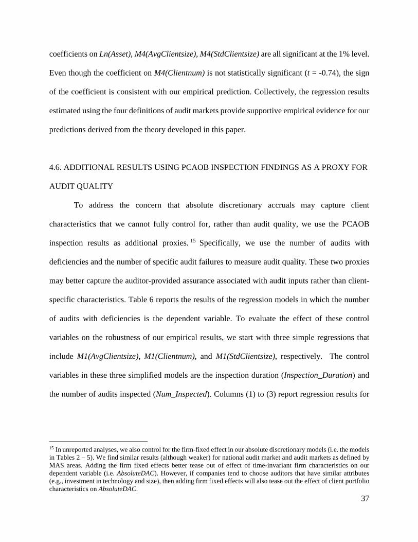
coefficients on Ln(Asset), M4(AvgClientsize), M4(StdClientsize) are all significant at the 1% level.

Even though the coefficient on M4(Clientnum) is not statistically significant (t = -0.74), the sign

of the coefficient is consistent with our empirical prediction. Collectively, the regression results

estimated using the four definitions of audit markets provide supportive empirical evidence for our

predictions derived from the theory developed in this paper.

4.6. ADDITIONAL RESULTS USING PCAOB INSPECTION FINDINGS AS A PROXY FOR

AUDIT QUALITY

To address the concern that absolute discretionary accruals may capture client

characteristics that we cannot fully control for, rather than audit quality, we use the PCAOB

inspection results as additional proxies. 15 Specifically, we use the number of audits with

deficiencies and the number of specific audit failures to measure audit quality. These two proxies

may better capture the auditor-provided assurance associated with audit inputs rather than client-

specific characteristics. Table 6 reports the results of the regression models in which the number

of audits with deficiencies is the dependent variable. To evaluate the effect of these control

variables on the robustness of our empirical results, we start with three simple regressions that

include M1(AvgClientsize), M1(Clientnum), and M1(StdClientsize), respectively. The control

variables in these three simplified models are the inspection duration (Inspection_Duration) and

the number of audits inspected (Num_Inspected). Columns (1) to (3) report regression results for

15 In unreported analyses, we also control for the firm-fixed effect in our absolute discretionary models (i.e. the models

in Tables 2 – 5). We find similar results (although weaker) for national audit market and audit markets as defined by

MAS areas. Adding the firm fixed effects better tease out of effect of time-invariant firm characteristics on our

dependent variable (i.e. AbsoluteDAC). However, if companies tend to choose auditors that have similar attributes

(e.g., investment in technology and size), then adding firm fixed effects will also tease out the effect of client portfolio

characteristics on AbsoluteDAC.

38

the three simplified models. The model in column (4) includes all of the three key independent

variables. In columns (5) to (8), we add other control variables progressively.

The statistical inferences for the three key independent variables as reported in columns

(1) to (8) are consistent. Specifically, column (8) reports the regression results for equation (2) as

specified in section 4.3. The coefficient on M1(AvgClientsize) is -0.1299 (t = -2.96), consistent

with H2 that the assurance level increases as the average loss exposure increases. The coefficient

on M1(Clientnum) is -0.0674 (t = -1.12), the sign of which is consistent with H3 that the assurance

level increases as the number of clients in an audit market increases even though it is not

statistically significant. The coefficient on M1(StdClientsize) is 0.0612 and is marginally

significant (t = 1.84), supporting H4 that the assurance level decreases as the variability of the

client-specific loss exposure increases in an audit market.

In Table 7, the dependent variable is the number of the audit firm’s specific failures as

identified by a specific inspection. The three key independent variables and all the control variables

are the same as the variables used in Table 6. Similar to the analyses in Table 6, we start with three

simplified models that control for Inspection_Duration and Num_Inspected and then add other

controls step by step. The statistical inferences as reported in Table 7 are similar to the ones in

Table 6, and are supportive of H2 and H4 without contradicting H3.

4.7. ADDITIONAL RESULTS USING RESTATEMENT AS AN AUDIT QUALITY PROXY

Section 4.6 uses the two count variables of PCAOB-identified audit deficiencies as proxy

measures of audit quality. To provide additional evidence, we use the likelihood of restatement as

an alternative proxy in this section. In columns (1) to (5) of Table 8, we estimate five probit models

that regress the likelihood of restatement by a specific client on its audit firm’s client portfolio

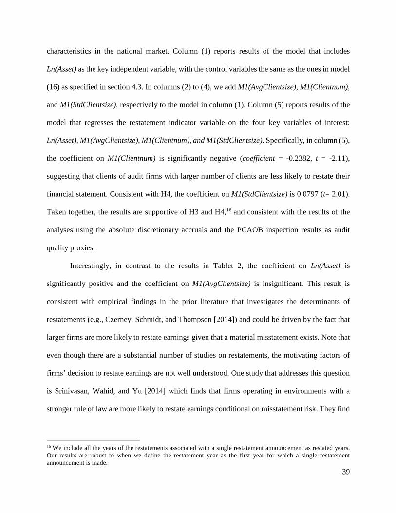
39

characteristics in the national market. Column (1) reports results of the model that includes

Ln(Asset) as the key independent variable, with the control variables the same as the ones in model

(16) as specified in section 4.3. In columns (2) to (4), we add M1(AvgClientsize), M1(Clientnum),

and M1(StdClientsize), respectively to the model in column (1). Column (5) reports results of the

model that regresses the restatement indicator variable on the four key variables of interest:

Ln(Asset), M1(AvgClientsize), M1(Clientnum), and M1(StdClientsize). Specifically, in column (5),

the coefficient on M1(Clientnum) is significantly negative (coefficient = -0.2382, t = -2.11),

suggesting that clients of audit firms with larger number of clients are less likely to restate their

financial statement. Consistent with H4, the coefficient on M1(StdClientsize) is 0.0797 (t= 2.01).

Taken together, the results are supportive of H3 and H4,16 and consistent with the results of the

analyses using the absolute discretionary accruals and the PCAOB inspection results as audit

quality proxies.

Interestingly, in contrast to the results in Tablet 2, the coefficient on Ln(Asset) is

significantly positive and the coefficient on M1(AvgClientsize) is insignificant. This result is

consistent with empirical findings in the prior literature that investigates the determinants of

restatements (e.g., Czerney, Schmidt, and Thompson [2014]) and could be driven by the fact that

larger firms are more likely to restate earnings given that a material misstatement exists. Note that

even though there are a substantial number of studies on restatements, the motivating factors of

firms’ decision to restate earnings are not well understood. One study that addresses this question

is Srinivasan, Wahid, and Yu [2014] which finds that firms operating in environments with a

stronger rule of law are more likely to restate earnings conditional on misstatement risk. They find

16 We include all the years of the restatements associated with a single restatement announcement as restated years.

Our results are robust to when we define the restatement year as the first year for which a single restatement

announcement is made.

40

a positive effect of client specific loss exposure on external auditors’ and managers’ decisions to

restate earnings. This effect could bias our tests against finding a negative association between the

likelihood of restatement and client’ loss exposure (i.e. Ln (Asset) and M1(AvgClientsize)).

5. Concluding Comments

In this paper, we analyze audit production when fixed investments associated with fixed

costs (e.g., audit technology) are important. A key feature of such investments and associated fixed

costs is that they affect the production of audit services for multiple clients. As a result, choosing

an optimal level of investment requires the analysis of production over a client portfolio, rather

than on a client-by-client basis as has been done in essentially all extant literature in the economics

of auditing since Simunic [1980], Dye [1993], and O’Keefe, Simunic and Stein [1994]. Another

feature of our analysis is that we assume that these investments influence the production of audit

assurance (which exists in the minds of auditors and financial statement users) through their impact

on the efficiency of labor (labor enhancing). For instance, technology investments do not produce

assurance directly, but make the auditor and her staff more efficient in producing assurance.

Our paper is in the spirit of Sutton’s [1991] endogenous / exogenous fixed cost model.

However, we build up our analysis from basic elements that reflect our understanding of key

features of audit production - a client specific service that is specifically tailored to suit the

characteristics (e.g. size, complexity, and riskiness) of each client.

While our focus is almost exclusively on supply-side (not demand side) considerations, we

believe that this emphasis is appropriate to understand both audit production and the market for

audit services. The fact that supply-side variables measuring the size, complexity, and riskiness of

client companies are able to account for 80% of the cross-sectional variation of U.S. listed

companies’ audit fees implies that the supply-side is critically important, particularly for listed

41

companies where audits are mandatory. As seen in the empirical implications of our analysis

discussed in section 3.4, the inclusion of fixed costs as an important feature of audit service

production yields a rich set of interesting and novel insights into the audit service market not

explored in the extant literature. For instance, Blokdijk, Drieenhuizen, Simunic, and Stein [2006]

tried to test whether audit quality was higher for the (then) Big 5 firms compared to non-Big 5

firms by studying total audit hours, and how those hours were utilized (e.g. risk analysis,

substantive testing, etc.) for a sample of about 100 Dutch audits. They concluded that any audit

quality differences were subtle and associated with the details of how audits were conducted rather

than with differences in total audit hours, since the total audit hours of applied by Big 5 firms and

non-Big 5 firms were virtually the same, ceteris paribus, in their sample. However, if Big 5 firms

have higher fixed investments in the Netherlands than non-Big 5 firms, then they would be

expected to utilize fewer audit hours, ceteris paribus. Thus the fact that the total audit hours of the

Big 5 and non-Big 5 were the same is consistent with the provision of higher audit quality by the

Big 5.

Another example of the importance of recognizing the potential role of fixed investments

in the interpretation of evidence on audit hours is the paper by Bell, Doogar, and Solomion [2008]

who replicate and extend the empirical tests in O’Keefe, Simunic and Stein [1994]. Bell et al. find

that mean audit hours decreased by about 10% for the same Big 4 firm between the sample periods

in the two studies (1989 vs. 2002) and attribute the difference to increasing use of the client

business risk audit methodology. However, this difference in hours has alternative interpretations

if (as is likely) the firm’s fixed investments (and related costs) changed between the two sample

periods.

42

As a final example of a deepened perspective derived from our analysis relates to the large

literature on auditor-industry specialization that originates with Craswell, Francis and Taylor

[1995]. That literature argues that audit firms holding a high market share in a client industry (e.g.

banking, manufacturing, etc.) are necessarily associated with the production and sale of

differentially higher quality audit services than auditors with lower market shares. Our analysis

applies to this setting since, presumably, the development of industry expertise requires fixed

investment in either physical or human capital. We (indirectly) show that high market share itself

is not sufficient to claim that audit quality is higher than average. A high market share that is based

on servicing (perhaps) a relatively small number of large clients is likely to have this effect, since

large clients motivate higher fixed investments which are associated with higher assurance levels.

However, a market share derived from servicing a large number of small clients, is much less likely

to have this effect. Moreover, even the audit firm that services large clients and has large fixed

investments will provide an assurance level that is positively correlated with client size. That is,

the assurance provided to small clients of a high market share auditor is not expected to be high;

the effect is client-specific.

In conclusion, modeling audit production to incorporate both fixed and variable resources

and costs yields a different perspective on the market for audit services than exists in the current

auditing literature. We believe that further research developing and extending this perspective is

likely to be both interesting and highly productive of new insights.

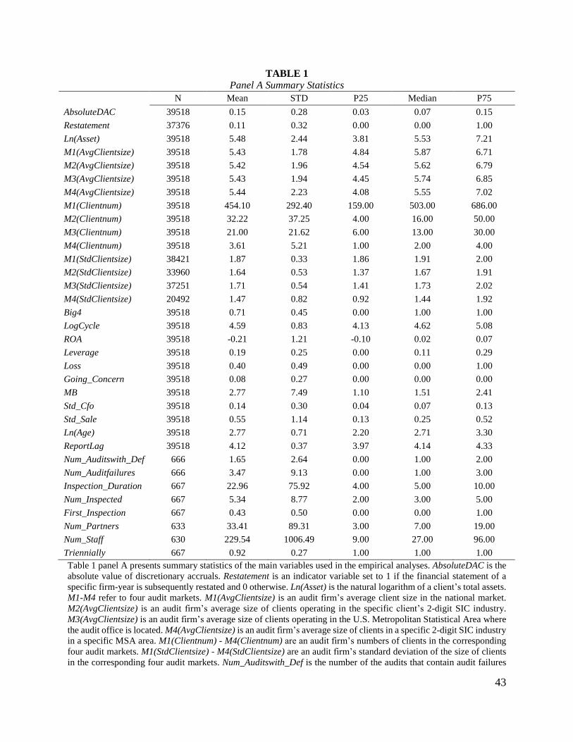
43

TABLE 1

Panel A Summary Statistics

N Mean STD P25 Median P75

AbsoluteDAC 39518 0.15 0.28 0.03 0.07 0.15

Restatement 37376 0.11 0.32 0.00 0.00 1.00

Ln(Asset) 39518 5.48 2.44 3.81 5.53 7.21

M1(AvgClientsize) 39518 5.43 1.78 4.84 5.87 6.71

M2(AvgClientsize) 39518 5.42 1.96 4.54 5.62 6.79

M3(AvgClientsize) 39518 5.43 1.94 4.45 5.74 6.85

M4(AvgClientsize) 39518 5.44 2.23 4.08 5.55 7.02

M1(Clientnum) 39518 454.10 292.40 159.00 503.00 686.00

M2(Clientnum) 39518 32.22 37.25 4.00 16.00 50.00

M3(Clientnum) 39518 21.00 21.62 6.00 13.00 30.00

M4(Clientnum) 39518 3.61 5.21 1.00 2.00 4.00

M1(StdClientsize) 38421 1.87 0.33 1.86 1.91 2.00

M2(StdClientsize) 33960 1.64 0.53 1.37 1.67 1.91

M3(StdClientsize) 37251 1.71 0.54 1.41 1.73 2.02

M4(StdClientsize) 20492 1.47 0.82 0.92 1.44 1.92

Big4 39518 0.71 0.45 0.00 1.00 1.00

LogCycle 39518 4.59 0.83 4.13 4.62 5.08

ROA 39518 -0.21 1.21 -0.10 0.02 0.07

Leverage 39518 0.19 0.25 0.00 0.11 0.29

Loss 39518 0.40 0.49 0.00 0.00 1.00

Going_Concern 39518 0.08 0.27 0.00 0.00 0.00

MB 39518 2.77 7.49 1.10 1.51 2.41

Std_Cfo 39518 0.14 0.30 0.04 0.07 0.13

Std_Sale 39518 0.55 1.14 0.13 0.25 0.52

Ln(Age) 39518 2.77 0.71 2.20 2.71 3.30

ReportLag 39518 4.12 0.37 3.97 4.14 4.33

Num_Auditswith_Def 666 1.65 2.64 0.00 1.00 2.00

Num_Auditfailures 666 3.47 9.13 0.00 1.00 3.00

Inspection_Duration 667 22.96 75.92 4.00 5.00 10.00

Num_Inspected 667 5.34 8.77 2.00 3.00 5.00

First_Inspection 667 0.43 0.50 0.00 0.00 1.00

Num_Partners 633 33.41 89.31 3.00 7.00 19.00

Num_Staff 630 229.54 1006.49 9.00 27.00 96.00

Triennially 667 0.92 0.27 1.00 1.00 1.00

Table 1 panel A presents summary statistics of the main variables used in the empirical analyses. AbsoluteDAC is the

absolute value of discretionary accruals. Restatement is an indicator variable set to 1 if the financial statement of a

specific firm-year is subsequently restated and 0 otherwise. Ln(Asset) is the natural logarithm of a client’s total assets.

M1-M4 refer to four audit markets. M1(AvgClientsize) is an audit firm’s average client size in the national market.

M2(AvgClientsize) is an audit firm’s average size of clients operating in the specific client’s 2-digit SIC industry.

M3(AvgClientsize) is an audit firm’s average size of clients operating in the U.S. Metropolitan Statistical Area where

the audit office is located. M4(AvgClientsize) is an audit firm’s average size of clients in a specific 2-digit SIC industry

in a specific MSA area. M1(Clientnum) - M4(Clientnum) are an audit firm’s numbers of clients in the corresponding

four audit markets. M1(StdClientsize) - M4(StdClientsize) are an audit firm’s standard deviation of the size of clients

in the corresponding four audit markets. Num_Auditswith_Def is the number of the audits that contain audit failures

44

among the audits inspected by the PCAOB in a specific inspection. Num_Auditfailures is the number of specific audit

failures of the audits with deficiencies as identified by a specific PCAOB inspection. See Appendix A for more detailed

definitions of these variables and for other variable definitions.

45

TABLE 1(Cont’d)

Panel B Correlation Table of Key Variables in the Absolute Discretionary Accruals and Restatement Regressions (1) (2) (3) (4) (5) (6) (7) (8) (9) (10) (11) (12) (13) (14) (15) (16)

(1)AbsoluteDAC 1.00

(2)Ln(Asset) -0.37 1.00

(0.00)

(3)M1(AvgClientsize) -0.34 0.69 1.00

(0.00) (0.00)

(4)M2(AvgClientsize) -0.37 0.79 0.86 1.00

(0.00) (0.00) (0.00)

(5)M3(AvgClientsize) -0.34 0.76 0.91 0.85 1.00

(0.00) (0.00) (0.00) (0.00)

(6)M4(AvgClientsize) -0.37 0.91 0.76 0.87 0.83 1.00

(0.00) (0.00) (0.00) (0.00) (0.00)

(7)M1(Clientnum) -0.22 0.47 0.67 0.59 0.61 0.51 1.00

(0.00) (0.00) (0.00) (0.00) (0.00) (0.00)

(8)M2(Clientnum) -0.07 0.15 0.34 0.17 0.25 0.15 0.54 1.00

(0.00) (0.00) (0.00) (0.00) (0.00) (0.00) (0.00)

(9)M3(Clientnum) -0.07 0.16 0.28 0.19 0.19 0.16 0.50 0.42 1.00

(0.00) (0.00) (0.00) (0.00) (0.00) (0.00) (0.00) (0.00)

(10)M4(Clientnum) -0.01 0.06 0.16 0.05 0.07 0.05 0.30 0.55 0.69 1.00

(0.01) (0.00) (0.00) (0.00) (0.00) (0.00) (0.00) (0.00) (0.00)

(11)M1(StdClientsize) -0.00 0.16 0.18 0.19 0.17 0.17 0.39 0.21 0.20 0.11 1.00

(0.42) (0.00) (0.00) (0.00) (0.00) (0.00) (0.00) (0.00) (0.00) (0.00)

(12)M2(StdClientsize) 0.05 0.07 0.13 0.05 0.09 0.05 0.22 0.23 0.13 0.12 0.33 1.00

(0.00) (0.00) (0.00) (0.00) (0.00) (0.00) (0.00) (0.00) (0.00) (0.00) (0.00)

(13)M3(StdClientsize) 0.04 0.06 0.03 0.06 0.04 0.05 0.19 0.11 0.17 0.04 0.55 0.22 1.00

(0.00) (0.00) (0.00) (0.00) (0.00) (0.00) (0.00) (0.00) (0.00) (0.00) (0.00) (0.00)

(14)M4(StdClientsize) 0.04 0.06 0.03 -0.04 0.02 0.04 0.10 0.11 0.14 0.12 0.21 0.49 0.37 1.00

(0.00) (0.00) (0.00) (0.00) (0.01) (0.00) (0.00) (0.00) (0.00) (0.00) (0.00) (0.00) (0.00)

(15)Big4 -0.24 0.58 0.82 0.72 0.75 0.63 0.87 0.46 0.39 0.23 0.42 0.25 0.19 0.10 1.00

(0.00) (0.00) (0.00) (0.00) (0.00) (0.00) (0.00) (0.00) (0.00) (0.00) (0.00) (0.00) (0.00) (0.00)

(16) Restatement 0.01 0.04 0.02 0.02 0.01 0.03 0.07 0.02 0.05 0.02 0.05 -0.00 0.02 0.01 0.05 1.00

(0.07) (0.00) (0.00) (0.00) (0.01) (0.00) (0.00) (0.00) (0.00) (0.00) (0.00) (0.95) (0.00) (0.04) (0.00)

Table 1 panel B presents the Pearson correlation matrix for the main variables used in the absolute discretionary accruals and restatement regressions. See Appendix

A for detailed variable definitions.

46

TABLE 1(Cont’d)

Panel C Correlation Table of the PCAOB Inspection Results Regression

(17) (18) (19) (20) (21) (22) (23) (24) (25) (26) (27)

(17)Num_Auditswith_Def 1.00

(18)Num_Auditfailures 0.86 1.00

(0.00)

(19)M1(AvgClientsize) 0.35 0.26 1.00

(0.00) (0.00)

(20)M1(Clientnum) 0.55 0.52 0.51 1.00

(0.00) (0.00) (0.00)

(21)M1(StdClientsize) 0.07 0.11 -0.11 0.08 1.00

(0.16) (0.02) (0.03) (0.10)

(22)Inspection_Duration 0.81 0.71 0.47 0.70 0.06 1.00

(0.00) (0.00) (0.00) (0.00) (0.19)

(23)Num_Inspected 0.83 0.76 0.39 0.62 0.08 0.80 1.00

(0.00) (0.00) (0.00) (0.00) (0.11) (0.00)

(24)First_Inspection -0.15 -0.10 -0.29 -0.21 -0.10 -0.19 -0.16 1.00

(0.00) (0.01) (0.00) (0.00) (0.05) (0.00) (0.00)

(25)Num_Partners 0.10 0.11 0.42 0.67 0.05 0.37 0.35 -0.19 1.00

(0.01) (0.01) (0.00) (0.00) (0.32) (0.00) (0.00) (0.00)

(26)Num_Staff 0.07 0.06 0.36 0.73 0.05 0.48 0.21 -0.15 0.90 1.00

(0.07) (0.12) (0.00) (0.00) (0.34) (0.00) (0.00) (0.00) (0.00)

(27)Triennially -0.70 -0.64 -0.41 -0.62 -0.11 -0.75 -0.72 0.23 -0.40 -0.30 1.00

(0.00) (0.00) (0.00) (0.00) (0.02) (0.00) (0.00) (0.00) (0.00) (0.00)

Table 1 panel C presents the Pearson correlation matrix for the main variables used in the PCAOB inspection results regression. See Appendix A for detailed

variable definitions.

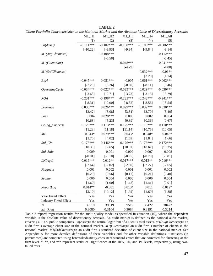
47

TABLE 2

Client Portfolio Characteristics in the National Market and the Absolute Value of Discretionary Accruals

M1_H1 M1_H2 M1_H3 M1_H4 M1_All

(1) (2) (3) (4) (5)

Ln(Asset) -0.111*** -0.102*** -0.108*** -0.105*** -0.086***

[-10.22] [-9.93] [-9.94] [-9.84] [-8.14]

M1(AvgClientsize) -0.108*** -0.112***

[-5.58] [-5.45]

M1(Clientnum) -0.048*** -0.041***

[-4.79] [-4.08]

M1(StdClientsize) 0.032*** 0.018*

[3.20] [1.74]

Big4 -0.045*** 0.051*** -0.005 -0.061*** 0.062***

[-7.20] [3.26] [-0.60] [-8.11] [3.46]

OperatingCycle -0.034*** -0.022*** -0.035*** -0.029*** -0.030***

[-3.68] [-2.71] [-3.73] [-3.15] [-3.29]

ROA -0.231*** -0.198*** -0.231*** -0.243*** -0.241***

[-8.31] [-9.00] [-8.32] [-8.56] [-8.54]

Leverage 0.030*** 0.026*** 0.029*** 0.032*** 0.030***

[3.42] [3.08] [3.31] [3.70] [3.40]

Loss 0.004 0.028*** 0.005 0.002 0.004

[0.68] [5.23] [0.89] [0.36] [0.67]

Going_Concern 0.126*** 0.113*** 0.125*** 0.119*** 0.110***

[11.23] [11.18] [11.14] [10.75] [10.05]

MB 0.043* 0.079*** 0.043* 0.048* 0.043*

[1.70] [4.02] [1.69] [1.84] [1.66]

Std_Cfo 0.176*** 0.146*** 0.176*** 0.178*** 0.172***

[10.33] [9.65] [10.32] [10.67] [10.35]

Std_Sale -0.009 -0.001 -0.009 -0.007 -0.008

[-0.91] [-0.10] [-0.95] [-0.70] [-0.81]

LN(Age) -0.016*** -0.012** -0.017*** -0.013** -0.016***

[-2.64] [-2.02] [-2.80] [-2.27] [-2.65]

Fsegnum 0.001 0.002 0.001 0.001 0.002

[0.29] [0.56] [0.17] [0.21] [0.40]

Segnum 0.006 0.004 0.006 0.006 0.004

[1.60] [1.00] [1.45] [1.41] [0.91]

ReportLag 0.014** -0.001 0.013* 0.011 0.012*

[2.10] [-0.12] [1.92] [1.60] [1.88]

Year Fixed Effect Yes Yes Yes Yes Yes

Industry Fixed Effect Yes Yes Yes Yes Yes

N 39519 39519 39519 38422 38422

adj. R-sq 0.3080 0.3104 0.3084 0.3191 0.3214

Table 2 reports regression results for the audit quality model as specified in equation (16), where the dependent

variable is the absolute value of discretionary accruals. An audit market is defined as the national audit market,

covering all U.S. public companies. Ln(Asset)is the natural logarithm of a client’s total assets. M1(AvgClientsize)is an

audit firm’s average client size in the national market. M1(Clientnum)is an audit firm’s number of clients in the

national market. M1(StdClientsize)is an audit firm’s standard deviation of client size in the national market. See

Appendix A for more detailed definitions of these variables and for other variable definitions. t-statistics (in

parentheses) are computed using heteroskedasticity-consistent standard errors that are corrected for clustering at the

firm level. *, **, and *** represent statistical significance at the 10%, 5%, and 1% levels, respectively, using two-

tailed tests.

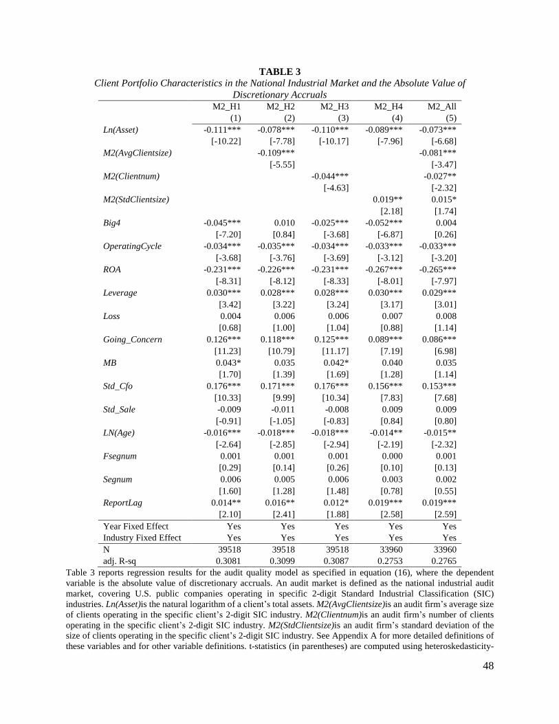
48

TABLE 3

Client Portfolio Characteristics in the National Industrial Market and the Absolute Value of

Discretionary Accruals

M2_H1 M2_H2 M2_H3 M2_H4 M2_All

(1) (2) (3) (4) (5)

Ln(Asset) -0.111*** -0.078*** -0.110*** -0.089*** -0.073***

[-10.22] [-7.78] [-10.17] [-7.96] [-6.68]

M2(AvgClientsize) -0.109*** -0.081***

[-5.55] [-3.47]

M2(Clientnum) -0.044*** -0.027**

[-4.63] [-2.32]

M2(StdClientsize) 0.019** 0.015*

[2.18] [1.74]

Big4 -0.045*** 0.010 -0.025*** -0.052*** 0.004

[-7.20] [0.84] [-3.68] [-6.87] [0.26]

OperatingCycle -0.034*** -0.035*** -0.034*** -0.033*** -0.033***

[-3.68] [-3.76] [-3.69] [-3.12] [-3.20]

ROA -0.231*** -0.226*** -0.231*** -0.267*** -0.265***

[-8.31] [-8.12] [-8.33] [-8.01] [-7.97]

Leverage 0.030*** 0.028*** 0.028*** 0.030*** 0.029***

[3.42] [3.22] [3.24] [3.17] [3.01]

Loss 0.004 0.006 0.006 0.007 0.008

[0.68] [1.00] [1.04] [0.88] [1.14]

Going_Concern 0.126*** 0.118*** 0.125*** 0.089*** 0.086***

[11.23] [10.79] [11.17] [7.19] [6.98]

MB 0.043* 0.035 0.042* 0.040 0.035

[1.70] [1.39] [1.69] [1.28] [1.14]

Std_Cfo 0.176*** 0.171*** 0.176*** 0.156*** 0.153***

[10.33] [9.99] [10.34] [7.83] [7.68]

Std_Sale -0.009 -0.011 -0.008 0.009 0.009

[-0.91] [-1.05] [-0.83] [0.84] [0.80]

LN(Age) -0.016*** -0.018*** -0.018*** -0.014** -0.015**

[-2.64] [-2.85] [-2.94] [-2.19] [-2.32]

Fsegnum 0.001 0.001 0.001 0.000 0.001

[0.29] [0.14] [0.26] [0.10] [0.13]

Segnum 0.006 0.005 0.006 0.003 0.002

[1.60] [1.28] [1.48] [0.78] [0.55]

ReportLag 0.014** 0.016** 0.012* 0.019*** 0.019***

[2.10] [2.41] [1.88] [2.58] [2.59]

Year Fixed Effect Yes Yes Yes Yes Yes

Industry Fixed Effect Yes Yes Yes Yes Yes

N 39518 39518 39518 33960 33960

adj. R-sq 0.3081 0.3099 0.3087 0.2753 0.2765

Table 3 reports regression results for the audit quality model as specified in equation (16), where the dependent

variable is the absolute value of discretionary accruals. An audit market is defined as the national industrial audit

market, covering U.S. public companies operating in specific 2-digit Standard Industrial Classification (SIC)

industries. Ln(Asset)is the natural logarithm of a client’s total assets. M2(AvgClientsize)is an audit firm’s average size

of clients operating in the specific client’s 2-digit SIC industry. M2(Clientnum)is an audit firm’s number of clients

operating in the specific client’s 2-digit SIC industry. M2(StdClientsize)is an audit firm’s standard deviation of the

size of clients operating in the specific client’s 2-digit SIC industry. See Appendix A for more detailed definitions of

these variables and for other variable definitions. t-statistics (in parentheses) are computed using heteroskedasticity-

49

consistent standard errors that are corrected for clustering at the firm level. *, **, and *** represent statistical

significance at the 10%, 5%, and 1% levels, respectively, using two-tailed tests.

50

TABLE 4

Client Portfolio Characteristics in the MSA Market and the Absolute Value of Discretionary Accruals

M3_H1 M3_H2 M3_H3 M3_H4 M3_All

(1) (2) (3) (4) (5)

Ln(Asset) -0.111*** -0.091*** -0.111*** -0.105*** -0.087***

[-10.22] [-8.41] [-10.17] [-9.58] [-7.86]

M3(AvgClientsize) -0.061*** -0.059***

[-4.58] [-4.58]

M3(Clientnum) -0.007 -0.013***

[-1.54] [-2.80]

M3(StdClientsize) 0.018*** 0.017***

[3.07] [2.79]

Big4 -0.045*** -0.011 -0.042*** -0.052*** -0.014

[-7.20] [-1.16] [-6.68] [-8.30] [-1.45]

OperatingCycle -0.034*** -0.034*** -0.034*** -0.030*** -0.031***

[-3.68] [-3.69] [-3.69] [-3.28] [-3.29]

ROA -0.231*** -0.230*** -0.231*** -0.245*** -0.244***

[-8.31] [-8.30] [-8.31] [-8.53] [-8.53]

Leverage 0.030*** 0.030*** 0.030*** 0.033*** 0.033***

[3.42] [3.49] [3.38] [3.69] [3.72]

Loss 0.004 0.003 0.005 0.002 0.003

[0.68] [0.59] [0.78] [0.38] [0.47]

Going_Concern 0.126*** 0.123*** 0.126*** 0.119*** 0.116***

[11.23] [10.99] [11.21] [10.57] [10.31]

MB 0.043* 0.040 0.043* 0.050* 0.048*

[1.70] [1.58] [1.70] [1.92] [1.82]

Std_Cfo 0.176*** 0.173*** 0.176*** 0.173*** 0.171***

[10.33] [10.16] [10.33] [10.24] [10.10]

Std_Sale -0.009 -0.009 -0.009 -0.006 -0.006

[-0.91] [-0.94] [-0.91] [-0.60] [-0.63]

LN(Age) -0.016*** -0.016** -0.017*** -0.016*** -0.016***

[-2.64] [-2.54] [-2.73] [-2.62] [-2.62]

Fsegnum 0.001 0.001 0.001 0.002 0.002

[0.29] [0.20] [0.36] [0.39] [0.44]

Segnum 0.006 0.007* 0.006 0.006 0.006

[1.60] [1.75] [1.54] [1.44] [1.48]

ReportLag 0.014** 0.015** 0.014** 0.011 0.012*

[2.10] [2.28] [2.08] [1.62] [1.78]

Year Fixed Effect Yes Yes Yes Yes Yes

Industry Fixed Effect Yes Yes Yes Yes Yes

N 39518 39518 39518 37251 37251

adj. R-sq 0.3081 0.3089 0.3081 0.3185 0.3194

Table 4 reports regression results for the audit quality model as specified in equation (16), where the dependent

variable is the absolute value of discretionary accruals. An audit market is defined as companies operating in the U.S.

Metropolitan Statistical Area (MSA) where the audit office is located. Ln(Asset)is the natural logarithm of a client’s

total assets. M3(AvgClientsize)is an audit firm’s average size of clients operating in the U.S. MSA where the audit

office of a specific client is located. M3(Clientnum)is an audit firm’s number of clients operating in the U.S. MSA

where the audit office is located. M3(StdClientsize)is an audit firm’s standard deviation of the size of clients operating

in the U.S. MSA where the audit office is located. See Appendix A for more detailed definitions of these variables

and for other variable definitions. t-statistics (in parentheses) are computed using heteroskedasticity-consistent

51

standard errors that are corrected for clustering at the firm level. *, **, and *** represent statistical significance at the

10%, 5%, and 1% levels, respectively, using two-tailed tests.

52

TABLE 5

Client Portfolio Characteristics in the MSA Industrial Market and the Absolute Value of Discretionary

Accruals

M4_H1 M4_H2 M4_H3 M4_H4 M4_All

(1) (2) (3) (4) (5)

Ln(Asset) -0.111*** -0.074*** -0.111*** -0.086*** -0.059***

[-10.22] [-5.38] [-10.22] [-6.05] [-3.88]

M4(AvgClientsize) -0.052*** -0.056***

[-3.76] [-3.36]

M4(Clientnum) -0.005 -0.006

[-0.91] [-0.74]

M4(StdClientsize) 0.018** 0.019**

[2.33] [2.50]

Big4 -0.045*** -0.034*** -0.044*** -0.059*** -0.038***

[-7.20] [-5.09] [-6.98] [-6.29] [-3.74]

OperatingCycle -0.034*** -0.035*** -0.034*** -0.030** -0.031**

[-3.68] [-3.78] [-3.69] [-2.38] [-2.46]

ROA -0.231*** -0.230*** -0.231*** -0.286*** -0.286***

[-8.31] [-8.30] [-8.31] [-7.62] [-7.63]

Leverage 0.030*** 0.030*** 0.030*** 0.033** 0.034***

[3.42] [3.45] [3.40] [2.53] [2.59]

Loss 0.004 0.004 0.004 0.003 0.003

[0.68] [0.73] [0.75] [0.32] [0.34]

Going_Concern 0.126*** 0.125*** 0.126*** 0.097*** 0.096***

[11.23] [11.17] [11.23] [6.29] [6.25]

MB 0.043* 0.041 0.043* 0.041 0.038

[1.70] [1.63] [1.70] [1.05] [0.99]

Std_Cfo 0.176*** 0.175*** 0.176*** 0.134*** 0.132***

[10.33] [10.26] [10.33] [5.77] [5.70]

Std_Sale -0.009 -0.009 -0.009 0.007 0.007

[-0.91] [-0.94] [-0.91] [0.55] [0.55]

LN(Age) -0.016*** -0.016*** -0.017*** -0.023*** -0.023***

[-2.64] [-2.64] [-2.72] [-2.76] [-2.81]

Fsegnum 0.001 0.001 0.002 -0.003 -0.001

[0.29] [0.30] [0.38] [-0.44] [-0.22]

Segnum 0.006 0.006 0.006 0.005 0.005

[1.60] [1.60] [1.52] [0.98] [1.03]

ReportLag 0.014** 0.014** 0.013** 0.018** 0.018**

[2.10] [2.13] [2.05] [2.03] [2.03]

Year Fixed Effect Yes Yes Yes Yes Yes

Industry Fixed Effect Yes Yes Yes Yes Yes

N 39518 39518 39518 20492 20492

adj. R-sq 0.3081 0.3084 0.3081 0.2799 0.2806

Table 5 reports regression results for the audit quality model as specified in equation (16), where the dependent

variable is the absolute value of discretionary accruals. An audit market is defined as companies operating in a specific

2-digit SIC industry in a specific MSA area. Ln(Asset)is the natural logarithm of a client’s total assets.

M4(AvgClientsize)is an audit firm’s average size of clients in a specific 2-digit SIC industry in a specific MSA area.

M4(Clientnum)is an audit firm’s number of clients in a specific 2-digit SIC industry in a specific MSA area.

M4(StdClientsize)is an audit firm’s standard deviation of the size of clients in a specific 2-digit SIC industry in a

specific MSA area. See Appendix A for more detailed definitions of these variables and for other variable definitions.

t-statistics (in parentheses) are computed using heteroskedasticity-consistent standard errors that are corrected for

53

clustering at the firm level. *, **, and *** represent statistical significance at the 10%, 5%, and 1% levels, respectively,

using two-tailed tests.

54

TABLE 6

Client Portfolio Characteristics in the National Market and the Number of Audits with Deficiencies

The Dependent Variable is the Number of Audits with Deficiencies (Num_Auditswith_Def)

(1) (2) (3) (4) (5) (6) (7) (8)

M1(AvgClientsize) -0.0836*** -0.0550** -0.0551** -0.1286*** -0.1278*** -0.1299***

[-4.54] [-2.15] [-2.15] [-3.10] [-2.91] [-2.96]

M1(Clientnum) -0.0120 -0.0025 -0.0025 0.0308 -0.0733 -0.0674

[-0.48] [-0.09] [-0.09] [0.63] [-1.21] [-1.12]

M1(StdClientsize) 0.0470*** 0.0387** 0.0386** 0.0574* 0.0612* 0.0612*

[3.09] [2.45] [2.44] [1.88] [1.84] [1.84]

Inspection_Duration 0.1255*** 0.0955** 0.1210*** 0.1538*** 0.1537*** 0.3155*** 0.2495*** 0.2738***

[2.87] [2.04] [3.39] [3.56] [3.56] [7.27] [4.09] [4.18]

Num_Inspected 0.2628*** 0.2596*** 0.1946*** 0.1987*** 0.1987*** 0.3010*** 0.3056*** 0.3090***

[5.48] [5.55] [4.61] [4.54] [4.54] [6.68] [6.41] [6.35]

First_Inspection -0.0011 0.0546 0.0466 0.0445

[-0.03] [0.84] [0.65] [0.62]

Num_Partners -0.1302*** -0.3346*** -0.3307***

[-2.61] [-2.85] [-2.79]

Num_Staff 0.2538** 0.2452**

[2.47] [2.35]

Triennially 0.0374

[0.75]

Year Fixed Effect Yes Yes Yes Yes Yes Yes Yes Yes

N 666 666 421 421 421 388 385 385

pseudo R-sq 0.1473 0.1389 0.1534 0.1572 0.1572 0.1307 0.1127 0.1131

Table 6 reports the ordered probit model regression results for the audit quality model, where the dependent variable

is the number of audits with deficiencies (Num_Auditswith_Def). The independent variables are defined in Appendix

A. t-statistics (in parentheses) are computed using heteroskedasticity-consistent standard errors. *, **, and ***

represent statistical significance at the 10%, 5%, and 1% levels, respectively, using two-tailed tests.

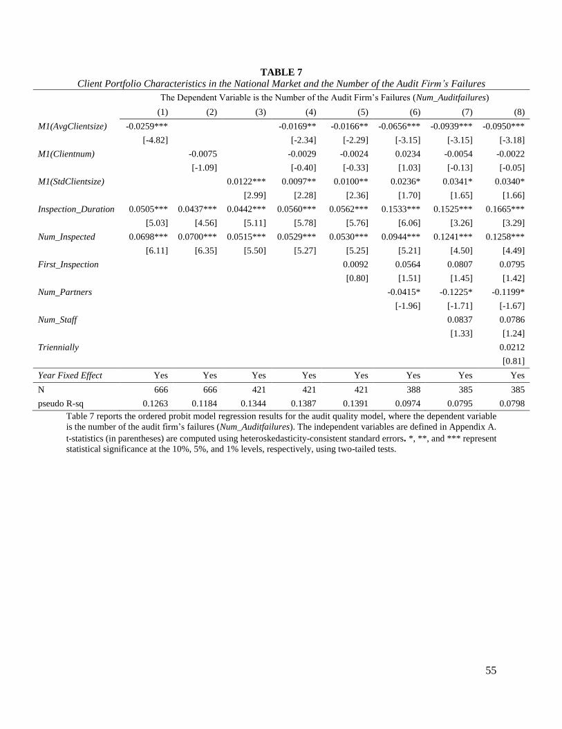
55

TABLE 7

Client Portfolio Characteristics in the National Market and the Number of the Audit Firm’s Failures

The Dependent Variable is the Number of the Audit Firm’s Failures (Num_Auditfailures)

(1) (2) (3) (4) (5) (6) (7) (8)

M1(AvgClientsize) -0.0259*** -0.0169** -0.0166** -0.0656*** -0.0939*** -0.0950***

[-4.82] [-2.34] [-2.29] [-3.15] [-3.15] [-3.18]

M1(Clientnum) -0.0075 -0.0029 -0.0024 0.0234 -0.0054 -0.0022

[-1.09] [-0.40] [-0.33] [1.03] [-0.13] [-0.05]

M1(StdClientsize) 0.0122*** 0.0097** 0.0100** 0.0236* 0.0341* 0.0340*

[2.99] [2.28] [2.36] [1.70] [1.65] [1.66]

Inspection_Duration 0.0505*** 0.0437*** 0.0442*** 0.0560*** 0.0562*** 0.1533*** 0.1525*** 0.1665***

[5.03] [4.56] [5.11] [5.78] [5.76] [6.06] [3.26] [3.29]

Num_Inspected 0.0698*** 0.0700*** 0.0515*** 0.0529*** 0.0530*** 0.0944*** 0.1241*** 0.1258***

[6.11] [6.35] [5.50] [5.27] [5.25] [5.21] [4.50] [4.49]

First_Inspection 0.0092 0.0564 0.0807 0.0795

[0.80] [1.51] [1.45] [1.42]

Num_Partners -0.0415* -0.1225* -0.1199*

[-1.96] [-1.71] [-1.67]

Num_Staff 0.0837 0.0786

[1.33] [1.24]

Triennially 0.0212

[0.81]

Year Fixed Effect Yes Yes Yes Yes Yes Yes Yes Yes

N 666 666 421 421 421 388 385 385

pseudo R-sq 0.1263 0.1184 0.1344 0.1387 0.1391 0.0974 0.0795 0.0798

Table 7 reports the ordered probit model regression results for the audit quality model, where the dependent variable

is the number of the audit firm’s failures (Num_Auditfailures). The independent variables are defined in Appendix A.

t-statistics (in parentheses) are computed using heteroskedasticity-consistent standard errors. *, **, and *** represent

statistical significance at the 10%, 5%, and 1% levels, respectively, using two-tailed tests.

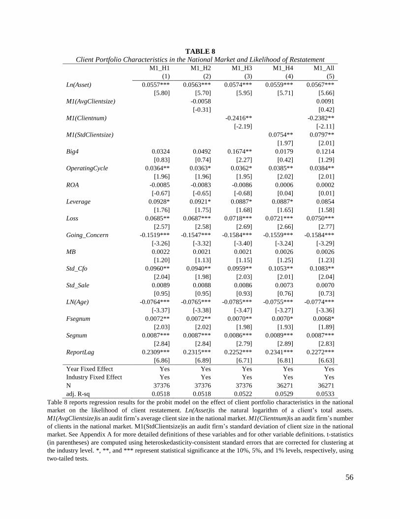
56

TABLE 8

Client Portfolio Characteristics in the National Market and Likelihood of Restatement

M1_H1 M1_H2 M1_H3 M1_H4 M1_All

(1) (2) (3) (4) (5)

Ln(Asset) 0.0557*** 0.0563*** 0.0574*** 0.0559*** 0.0567***

[5.80] [5.70] [5.95] [5.71] [5.66]

M1(AvgClientsize) -0.0058 0.0091

[-0.31] [0.42]

M1(Clientnum) -0.2416** -0.2382**

[-2.19] [-2.11]

M1(StdClientsize) 0.0754** 0.0797**

[1.97] [2.01]

Big4 0.0324 0.0492 0.1674** 0.0179 0.1214

[0.83] [0.74] [2.27] [0.42] [1.29]

OperatingCycle 0.0364** 0.0363* 0.0362* 0.0385** 0.0384**

[1.96] [1.96] [1.95] [2.02] [2.01]

ROA -0.0085 -0.0083 -0.0086 0.0006 0.0002

[-0.67] [-0.65] [-0.68] [0.04] [0.01]

Leverage 0.0928* 0.0921* 0.0887* 0.0887* 0.0854

[1.76] [1.75] [1.68] [1.65] [1.58]

Loss 0.0685** 0.0687*** 0.0718*** 0.0721*** 0.0750***

[2.57] [2.58] [2.69] [2.66] [2.77]

Going_Concern -0.1519*** -0.1547*** -0.1584*** -0.1559*** -0.1584***

[-3.26] [-3.32] [-3.40] [-3.24] [-3.29]

MB 0.0022 0.0021 0.0021 0.0026 0.0026

[1.20] [1.13] [1.15] [1.25] [1.23]

Std_Cfo 0.0960** 0.0940** 0.0959** 0.1053** 0.1083**

[2.04] [1.98] [2.03] [2.01] [2.04]

Std_Sale 0.0089 0.0088 0.0086 0.0073 0.0070

[0.95] [0.95] [0.93] [0.76] [0.73]

LN(Age) -0.0764*** -0.0765*** -0.0785*** -0.0755*** -0.0774***

[-3.37] [-3.38] [-3.47] [-3.27] [-3.36]

Fsegnum 0.0072** 0.0072** 0.0070** 0.0070* 0.0068*

[2.03] [2.02] [1.98] [1.93] [1.89]

Segnum 0.0087*** 0.0087*** 0.0086*** 0.0089*** 0.0087***

[2.84] [2.84] [2.79] [2.89] [2.83]

ReportLag 0.2309*** 0.2315*** 0.2252*** 0.2341*** 0.2272***

[6.86] [6.89] [6.71] [6.81] [6.63]

Year Fixed Effect Yes Yes Yes Yes Yes

Industry Fixed Effect Yes Yes Yes Yes Yes

N 37376 37376 37376 36271 36271

adj. R-sq 0.0518 0.0518 0.0522 0.0529 0.0533

Table 8 reports regression results for the probit model on the effect of client portfolio characteristics in the national

market on the likelihood of client restatement. Ln(Asset)is the natural logarithm of a client’s total assets.

M1(AvgClientsize)is an audit firm’s average client size in the national market. M1(Clientnum)is an audit firm’s number

of clients in the national market. M1(StdClientsize)is an audit firm’s standard deviation of client size in the national

market. See Appendix A for more detailed definitions of these variables and for other variable definitions. t-statistics

(in parentheses) are computed using heteroskedasticity-consistent standard errors that are corrected for clustering at

the industry level. *, **, and *** represent statistical significance at the 10%, 5%, and 1% levels, respectively, using

two-tailed tests.

57

APPENDIX A

VARIABLES DEFINITIONS

Dependent variables

AbsoluteDCA The absolute value of discretionary accruals. The discretionary accrual model follows the

modified Jones (1991) model, as implemented by Dechow, Sloan, and Sweeney (1995) and

modified by Kothari, Leone, and Wasley (2005). The abnormal discretionary accruals for firm

i (which is in industry j) in year t are the difference between the total accruals (TAC) and

predicted accruals estimated using the model specified as 𝑇𝐴𝐶𝑖,𝑗,𝑡

𝐴𝑇𝑖,𝑗,𝑡−1= 𝛼0,𝑗,𝑡 + 𝛼1,𝑗,𝑡

1

𝐴𝑇𝑖,𝑗,𝑡−1+

𝛼2,𝑗,𝑡 (∆𝑆𝐴𝐿𝐸𝑖,𝑗,𝑡−∆𝑅𝐸𝐶𝑇𝑖,𝑗,𝑡

𝐴𝑇𝑖,𝑗,𝑡−1) + 𝛼2,𝑗,𝑡 (

𝑃𝑃𝐸𝐺𝑇𝑖,𝑗,𝑡

𝐴𝑇𝑖,𝑗,𝑡−1) + 𝛼3,𝑗,𝑡 (

𝑁𝐼𝑖,𝑗,𝑡−1

𝐴𝑇𝑖,𝑗,𝑡−1) + 𝜀𝑖,𝑗,𝑡 . TAC=IBC-OANCF.

All the variables in the discretionary accrual model are winsorized at the 1st and 99th percentiles

before estimation. The estimated absolute value of abnormal discretionary accrual is winsorized

at 99th percentile. Source: Compustat.

Num_Auditswith_Def The number of the audits that contain audit failures among the audits inspected by the PCAOB,

as disclosed by the inspection reports. Source: The PCAOB’s inspection reports as summarized

by the data vendor Digi Data Mart Ltd.

Num_Auditfailures The number of the specific audit failures contained in the audits with deficiencies as identified

by a specific PCAOB inspection. A typical inspection report of the PCAOB will list the specific

audit failures. The count of the specific audit failures is obtained as this variable. Source: The

PCAOB’s inspection reports as summarized by the data vendor Digi Data Mart Ltd.

Restatement An indicator variable set to 1 if the financial statement of a specific firm-year is subsequently

restated and 0 otherwise.

Independent variables

Ln(Asset) The natural logarithm of a client’s total assets (AT). Source: Compustat.

M1(AvgClientsize) An audit firm’s average client size in the national market. Client size is measured by the natural

logarithm of a client’s total assets (AT).

M1(Clientnum) An audit firm’s number of clients in the national market. Source: Audit Analytics

M1(StdClientsize) An audit firm’s standard deviation of client size in the national market. Source: Audit Analytics

and Compustat

M2(AvgClientsize) An audit firm’s average size of clients operating in the specific client’s 2-digit SIC industry.

Source: Audit Analytics and Compustat

M2(Clientnum) An audit firm’s number of clients operating in the specific client’s 2-digit SIC industry. Source:

Audit Analytics

M2(StdClientsize) An audit firm’s standard deviation of the size of clients operating in the specific client’s 2-digit

SIC industry. Source: Audit Analytics and Compustat

M3(AvgClientsize) An audit firm’s average size of clients operating in the U.S. Metropolitan Statistical Area where

the audit office of a specific client is located. Source: Audit Analytics and Compustat

M3(Clientnum) An audit firm’s number of clients operating in the U.S. Metropolitan Statistical Area where the

audit office of a specific client is located. Source: Audit Analytics

M3(StdClientsize) An audit firm’s standard deviation of the size of clients operating in the U.S. Metropolitan

Statistical Area where the audit office of a specific client is located. Source: Audit Analytics

and Compustat

M4(AvgClientsize) An audit firm’s average size of clients in a specific 2-digit SIC industry in a specific MSA area

of a specific client. Source: Audit Analytics and Compustat

M4(Clientnum) An audit firm’s number of clients in a specific 2-digit SIC industry in a specific MSA area of a

specific client. Source: Audit Analytics

M4(StdClientsize) An audit firm’s standard deviation of the size of clients in a specific 2-digit SIC industry in a

specific MSA area of a specific client.

Big4 An indicator variable set to 1 when a firm uses one of the Big 4 auditors (Arthur Andersen,

PricewaterhouseCoopers, Ernst & Young, Deloitte & Touche, or KPMG) and 0 otherwise.

Source: Audit Analytics

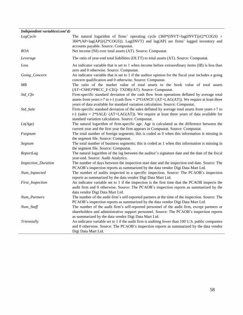
58

Independent variables(cont’d)

LogCycle The natural logarithm of firms’ operating cycle (360*(INVT+lag(INVT))/(2*COGS) +

360*(AP+lag(AP))/(2*COGS)). Lag(INVT) and lag(AP) are firms’ lagged inventory and

accounts payable. Source: Compustat.

ROA Net income (NI) over total assets (AT). Source: Compustat.

Leverage The ratio of year-end total liabilities (DLTT) to total assets (AT). Source: Compustat.

Loss An indicator variable that is set to 1 when income before extraordinary items (IB) is less than

zero and 0 otherwise. Source: Compustat.

Going_Concern An indicator variable that is set to 1 if the auditor opinion for the fiscal year includes a going

concern qualification and 0 otherwise. Source: Compustat.

MB The ratio of the market value of total assets to the book value of total assets

(AT+CSHO*PRCC_F-CEQ- TXDB)/AT). Source: Compustat.

Std_Cfo Firm-specific standard deviation of the cash flow from operations deflated by average total

assets from years t-7 to t-1 (cash flow = 2*OANCF/ (AT+LAG(AT)). We require at least three

years of data available for standard variation calculation. Source: Compustat.

Std_Sale Firm-specific standard deviation of the sales deflated by average total assets from years t-7 to

t-1 (sales = 2*SALE/ (AT+LAG(AT)). We require at least three years of data available for

standard variation calculation. Source: Compustat.

Ln(Age) The natural logarithm of firm-specific age. Age is calculated as the difference between the

current year and the first year the firm appears in Compustat. Source: Compustat.

Fsegnum The total number of foreign segments; this is coded as 0 when this information is missing in

the segment file. Source: Compustat.

Segnum The total number of business segments; this is coded as 1 when this information is missing in

the segment file. Source: Compustat.

ReportLag The natural logarithm of the lag between the auditor’s signature date and the date of the fiscal

year-end. Source: Audit Analytics.

Inspection_Duration The number of days between the inspection start date and the inspection end date. Source: The

PCAOB’s inspection reports as summarized by the data vendor Digi Data Mart Ltd.

Num_Inpsected The number of audits inspected in a specific inspection. Source: The PCAOB’s inspection

reports as summarized by the data vendor Digi Data Mart Ltd.

First_Inspection An indicator variable set to 1 if the inspection is the first time that the PCAOB inspects the

audit firm and 0 otherwise. Source: The PCAOB’s inspection reports as summarized by the

data vendor Digi Data Mart Ltd.

Num_Partners The number of the audit firm’s self-reported partners at the time of the inspection. Source: The

PCAOB’s inspection reports as summarized by the data vendor Digi Data Mart Ltd.

Num_Staff The number of the audit firm’s self-reported personnel of the audit firm, except partners or

shareholders and administrative support personnel. Source: The PCAOB’s inspection reports

as summarized by the data vendor Digi Data Mart Ltd.

Triennially An indicator variable set to 1 if the audit firm is auditing fewer than 100 U.S. public companies

and 0 otherwise. Source: The PCAOB’s inspection reports as summarized by the data vendor

Digi Data Mart Ltd.

59

References:

Akono, H., and M.T. Stein. (2014). Estimating audit fees and production models. Chapter 4 of

The Routledge Companion to Auditing, edited by Hay, Knechel and Willekens,

Routledge: 276-286.

Becker, C.L., M. L. DeFond, J. Jiambalvo, and K. R. Subramanyam. (1998) The Effect of Audit

Quality on Earnings Management. Contemporary Accounting Research (Vol 15, No. 1):

1–24.

Bell, T., R. Doogar, and I. Solomon. (2008). Audit labor usage and fees under business risk

auditing. Journal of Accounting Research. (Vol 46, No. 4): 729-760.

Blockdijk, H., F. Drieenhuizen, D.A. Simunic, and M.T. Stein. (2006). An analysis of cross-

sectional differences in big and non-big public accounting firms’ audit programs.

Auditing: A Journal of Practice and Theory (Vol 25, No. 1): 27-48.

Craswell, A., J. Frances, and S. Taylor. (1995) Auditor Brand Name Reputation and Industry

Specialization. Journal of Accounting and Economics (Vol 20, No. 3): 297-322.

Czerney, K., Schmidt, J. J., & Thompson, A. M. (2014). Does auditor explanatory language in

unqualified audit reports indicate increased financial misstatement risk?. The Accounting

Review. (Vol 89, No. 6), 2115-2149.

Dye, R. (1993). Auditing standards, legal liability, and auditor wealth. Journal of Political

Economy. (Vol 101, No. 5):887-914.

Dechow, P. M., R. G. Sloan, and A.P. Sweeney (1995). Detecting earnings management. The

Accounting Review (Vol 70, No. 2): 193-225.

Ferguson,C., M. Pinnuck, and D.J. Skinner. (2016). The evolution of audit market structure and

the emergence of the Big N: Evidence from Australia. Chicago Booth Research Paper

No. 14-13.

Gu, Z., C. W. J. Lee, and J. G. & Rosett (2005). What determines the variability of accounting

accruals?. Review of Quantitative Finance and Accounting (Vol. 24, No. 3): 313-334.

Hay, D., W.R. Knechel, and J. Wong. (2006). Audit fees: A meta-analysis of the effects of

supply and demand attributes. Contemporary Accounting Research (Vol. 23, No. 1): 141-

191.

Jones, J. (1991). Earnings management during import relief investigations. Journal of

Accounting Research (Vol. 29, No. 2): 193-228.

Kothari, S. P., A. J. Leone, & C. E. Wasley. (2005). Performance Matched Discretionary Accrual

Measures. Journal of Accounting and Economics (Vol 39, No. 1), 163 – 197.

O’Keefe, T.B., D.A. Simunic, and M.T. Stein (1994). The production of audit services: Evidence

from a major public accounting firm. Journal of Accounting Research (Vol. 32, No. 2):

241-261.

60

Milgrom, P., & Shannon, C. (1994). Monotone comparative statics. Econometrica: Journal of

the Econometric Society, 157-180.

Simunic, D.A. (1980). The pricing of audit services: Theory and evidence. Journal of Accounting

Research (Spring 1980): 161-190

Simunic, D.A., and M.T. Stein. (1990). Audit risk in a client portfolio context.

ContemporaryAccounting Research (Vol 6, No.2): 327-343.

Sirois, L.P., S. Marmousez, and D.A. Simunic. (2016). Auditor size and audit quality revisited:

The importance of audit technology. Comptabilite’- Controle – Audit, Tome 22,

Volume 3 (December 2016): 111-144.

Srinivasan, S., Wahid, A. S., & Yu, G. (2014). Admitting mistakes: Home country effect on the

reliability of restatement reporting. The Accounting Review (Vol. 90, No. 3): 1201-1240.

Sutton, J. (1991). Sunk costs and market structure: Price competition, advertising, and the

evolution of concentration. The MIT Press.

Topkis, D. (2011). Supermodularity and complementarity. Princeton University Press.

Ye, M and D.A. Simunic (2013). The economics of setting auditing standards. Contemporary

Accounting Research (Vol. 30, No. 3): 1191-1215.

Ye, M and D.A. Simunic (2017). The impact of PCAOB-type regulations on auditors under

different legal systems. Working paper, University of Toronto and UBC.

Zang, A. Y. (2011). Evidence on the trade-off between real activities manipulation and accrual-

based earnings management. The Accounting Review (Vol. 87, No. 2): 675-703.