
Five Balltree Construction Algorithms
23
Five Balltree Construction Algorithms Stephen M. Omohundro l TR-89-063 December 13,1989 INTERNATIONAL COMPUTER SCIENCE INSTITUTE 1947 Center Street, Suite 600 Berkeley, California 94704-1105
Transcript of Five Balltree Construction Algorithms

Five Balltree Construction Algorithms
Stephen M Omohundrol
TR-89-063
December 131989
INTERNATIONAL COMPUTER SCIENCE INSTITUTE 1947 Center Street Suite 600
Berkeley California 94704-1105
Five Balltree Construction Algorithms
Stephen M Omohundro1
TR-89-063
December 131989
Abstract
Balltrees are simple geometric data structures with a wide range of practical applicashytions to geometric middotlearning tasks In this report we compare 5 different algorithms for
constructing ball trees from data We study the trade-off between construction time and the quality of the constructed tree Two of the algorithms are on-line two construct the structures from the data set in a top down fashion and one uses a bottom up approach We empirically study the algorithms on random data drawn from eight different probability distributions representing smooth clustered and curve distributed data in different ambient space dimenshysions We find that the bottom up approach usually produces the best trees but has the longest construction time The other approaches have uses in specific circumstances
1 IntemauonaIComputer Science Institute Berkeley CA
Introduction
Introduction
Many tasks in robotics vision speech and graphics require the construction and manipushylation ofgeomebicrepresentatioris Systems which build th~e representations by learning from exampleS can be both flexible and robust We have developed a data structure which we caUtheballtree which is well suitedmiddotto geometric learningmiddottasks BaUtrees tune themshyselves to the structure of the represented datasupport dynamic insertions and deletions have goodaverage-caseeffidency deal well withhigh-dimensional entities and are easy to implement In this report we compare five different a1gorithms for building these strucshytures from data We discuss the trade-off between theeffidency ofthe conStruction algoshyrithmand the efficiency ofthe resulting structure Two ofthe algorithms are on-linetwo analyze the data in a tolHiown fashion and one analyzes it in a bottomup manner
The balltree strultture is related wothermiddot hierarchical representations such as k-d trees [Friedman et al 1977] andoct-trees [Samet 1984] buthas specific advantages in the doshymains ()f interest Weare applying these structures to representing learning and manipushylating point Sets smooth subrnanifolds nonlinear mappings and probability disbibutions Borne of these applications are described in (Omohundro 1987 1988 1989] in the context of k-dtreesTheoperCitionsthat are efficiently supported include nearestneighborretrievshyaI intersectioh and constraint queries and probability maximization The basic construcshytion techniques described here should be applicable to amiddotwide variety of other hierarchical geomebic data structureS ill which balls are replaced by boxes cubes ellipsoids or sim~ plices
Balltrees
We refer to the region bounded by a hyper-sphere in the n-dimensional Euclidean space 9tas a ball We represent balls by the n+l floatingpoint values which specify the coordishynates ofitscenterandtile length of its radius A balltreeis a complete binary tree in which a baH is associated with each node insuch a way thataninterior nodes ball is the smallest which contains the balls of its children The leaves of the tree hold the information relevant to the application the interior nodes are used -only to guide efficient search through the leaf structures Unlike the node regions in k-d trees Or oct-trees Sibling regions inba1ltrees are allowed to intersect and need not partition the entire space These two features are critical
3 Implementation
for the applications and give balltrces their representational power Figure 1 shows an exshyample of a two-dimensional balltrce
abc d 8 f A) B) C)
Figure 1 A) A set of balls in the plane B) A binary tree over Ihese balls C) The balls in the resulting balltlee
In this report we study the problem of building a balltree from given leaf balls Once the tree structure is specified the internal balls are determined bottom up from the leaf balls We would like to choose the tree structure to most effidently support the queries needed in practical usage Efficiency will depend both on the distribution of samples and queries and on the type of retrieval required We first discuss several important queries and then describe a cost function which appears to adequately approximate the costs for practical applications We then compare five different construction algorithms in terms of both the cost of the resulting tree and the construction time The algorithms are compared on samshyples drawn from several probability distributions which are meant to be representative of those that arise in practice
Implementation
Our implementation is in the Object oriented language Eiffel [Meyer 1989] There are classshyes for balls balltrees and balltree nodes BALL objects consist of a vector ctr which holds the center of the ball and a real value f containing the radius BLT_ND objects consist of a BALL bl and pointers par Itrt to the nodes parents and children BALLshyTREE objects have a pointer tree to the underlying tree and a variety other slots to enshyhance retrievals (such as local priority queues and caches) All reported times are in seconds on a Sun Sparcstation 1 with 16 Megabytes of memory running Eiffel Version 22 from Interactive Software Engineering Compilation was done with assertion checking off and garbage collection global class optimization and C optimization on As with any obshyject oriented language there is some extra overhead associated with dynamiC dispatching but this overhead should affect the different algOrithms similarly
Queries Which use Simple Pruning
Queries which use Simple Pruning
There are two broad classes ofquery which are efficiently supported by the balltree strucshyture The first class employs a search with simple pruning of irrelevant branches The secshyond class requir~s the use of branch and bound during search This section presents some simple pruning queries and the next gives examples of the more complex variety
Given a query ball we might require a list of all leaf balls which contain the query ball We implement this as a recursive search down the ball tree in which we prune away recursive caUsat internal nodes whose balldoesnot contain the query ball If an intemal nOdes ball doesntcontain the query ball it is not possible for any of the leaf balls beneath it to contain it either In the balltreenode class BLT NO we may define
pusheavescontainingball(bBALllLUSTISlTNDraquo is - Add the leaves under Current which contain b to I
do il ealthen
if blcontainsball(b)thenlpush(Current) end else
if blcontains_ball(b)then Itpush_leavesconfaining_ball(bl) rtpush_leaves_containing_ball(bl)
end if end-il
end
Similarly wemightaskfor all leaf balls which intersect a query ball We prune away reshycursive calls from internal nodes whose ball doesnt intersect the query ball
push_leavesjntersectinlLball(bBALLILLIST[BlT_NDJ) is - Add the leaves under Current which intersect b to Idomiddot
illeal thEIn il blintersects ball(b) then Ipush(Current) end
else il blintersectsball(b) henmiddot
ItpusfUeavesintersectingball(bI) rtpushJeavesjntersectingball(bI)
end il end-i
end
Finally we might ask for all leaf balls which are cOntained in the query ball Here we must continue to search beneath any intemal node whose ball intersects the query ball because some descendant ball might be contained in it
pushJeaves_containecUnball(bBALLILLlSTIBLT_NO)) is - Add the leaves under Current which are con talnedin b to 1
do if leal then
if bcontalnsball(bl) then LpushCurrent) end else
if bUntersects_ball(b) then Ilpush_leavescontained_in_ball(bI)
5 Queries which use Branch and Bound
rlpushJeaves_containedjn_ball(bI) end-if
end- if end
A point is just a degenerate ball Two important spedal cases of these queries in which some of the balls are points are the tasks of returning all leaf balls which contain a given point and returning all point leaves which are contained in a given ball
Queries which use Branch and Bound
More complex queries require a branch and bound search An important example for ballshytrees whose leaves hold points is to retrieve the m nearest neighbor points of a query point Using balltrees we may use a similar approach to that discussed in [Friedman d al 1977] for k-d trees Again we recursively search the tree Throughout the search we maintain the smallest-ball bball centered at the query point which contains the m nearest leaf points seen in the search so far In this algorithm we prune away recursive searches which start at internal nodes whose ball doesnt intersect the bball This pruning is likely to happen most effectively if at each internal node we first search the child which is nearer the query point and then the other child Because balltree nodes can intersect we cannot stop the search when the bballlies inside node ball as is possible in k-d trees Because node regions are tighter around the sample points however ball trees may be able to prune nodes in situa- tions where a k-d tree could not
To retrieve the m nearest neighbors we maintain a priority queue of the best leaves seen ordered by distance from the query point We will only show the function for finding the nearest neighbor but the extension to the m nearest neighbors should be clear
In this case we assume that nn_search is defined in a class which has lbball as an attribute and that its center bballctr has been set to the query point and its radius bballr to a large enough value that it contains the root ball Inn is another attribute which will hold the result when the routine returns IInear_dist_to_vectorll is a routine in the BALL class which returns the distance from the closest point in the ball to a given vector
nn_search(nT) is - Replace nn by closest leaf under n to bballctr if closer than bballr
local dktrdREAL do
if nleaf Ihen dbballctrdisUo_vector(nblctr) if d lt bballr Ihen bbanseU(d) nn=n end - reset best
else - at internal node 1d=nItblnear_discto_vector(bballctr) rd=nrtblneacdiscto_vector(bballctr) if Id gt bballr and rd gt bballr Ihen - no sense looking here else
6 Statistical Nature of the Data
if Idltrd then- search nearer node first nn_search(nIt) if rd lt bballtlhen nn_search(nrt) end - check if still worth searching
else M_search(nrt) if Idlt bballr then nn_search(nt) end - check if still worth searching
eOO- if ei1d- if
eOO- if end
There are several natural generalizations of this query to ones involving balls Distance ~ tween points may be replaced by distance between ball centers minimum distance ~ tween ballsor maximum distance between balls In each case the minimum distance to an ancestor node is a lower bound on the distance to a leaf and so may be exactly as above to prune the search
A query which arises in one of the construction algorithms we will describe below must retumtheIeafball which minimizes the volume ofthe smallest ball containing it and a queshyrybaltThe search prOceeds as above but with the pruning value equal to the volume of the smallest ball which contains the query ball and a single point of the interior node ball
Statistical Nature of the Data
The Criterion for a good ball tree structure depends on both the type of query it must supshyport and on the nature of the data it must store and access For most of the applications we have in mind iUs appropriate to take a statistical view of the stored data and queries We assume thatthe leaf balls are drawn randomly from an underlying probability distribution and that the queries aredrawn from the same distribution We would like systems to pershyfonn Well on average with respect to this underlying distribution Unfortunately we exshypectdistributions of very different types in different situations A very powerful nonparammicappr08ch to perfonnance analysis has begun to appear (eg [Friedmanet ai 1977] and [Noga and Allison 1985J) which gives provably good results for a wide variety ofdistributions in the asymptotic limit of large sample size In both of these references the underlying distribution is required to be non-singular and in the large sample limi teach small region becomes densely sampled and locally looks like a uniform distribution If an algorithm behaves well on the uniform distribution and adjusts itself to the local sample density thenit will have good asymptotic performance on non-singular distributions Unshyfortunately some of the most important applications have data of a very different characshyter Instead of being smooth the data itself may be hierarchically dusteredor has its
bullbullbull
7 Statistical Nature of the Data
-te middot III II ampI ~lt tIbullbull ~
fa
= I~ t - bull A B C 0
Flgur2 101 leaves from the four distribution types A) Uniform B) Cantor C) Curve 0) Uniform balls
SUpport on lower dimensional surfaces Part ot the motivation for the development ot the ball tree structure was that it should deal well with these cases
For any particular statistical model poSSibly singular one may hope to perform an asympshytotic analysis similar to that in [Friedman d al 1977] Because we are interested in the pershyformance on small data sets for a variety of distributions we have taken an empirical approach to comparing the different construction algorithms We studied each algorithm in 8 situations corresponding to 4 different probability distributions in 2-dimensions and similar distributions in S-dimensions Samples from the 2-dimensional versions of these distributions are shown in figure 2 Because the case in which the leaves are actually points is very important we have emphasized it in the tests
The first distribution is the uniform distribution in the unit cube For the reasons discussed above behavior on this should be characteristic of general smooth distributions For the second distribution we wanted to study a case with intrinsic hierarchical clustering We chose a distribution which is uniform on a fractal the Cantor set The one-dimensional Cantor set may be formed by starting with the unit interval removing the middle third and then recursively repeating the construction on the two portions of the interval which are left If points on the interval are expressed in ternary notation then the Cantor set points are those that have no ls in their representation In higher dimensions we just take the product of Cantor sets along each axis The third distribution is meant to study the situation in which sample points are restricted to a lower dimensional nonlinear submanshyifold We draw points from a polynomial curve which is embedded in such a way that it doesnt lie in any affine subspaces In the final distribution the leaves are balls instead of just points The centers are drawn uniformly from the unit cube and the radii uniformly from the interval [01]
8 The Volume Criterion
The Volume Criterion
It might appear that these different distributions would require the use of different balltree construction criteria in order to lead to good perfonnance We have found however that a simp(eefficiency measure is sufficient for most applications The most basic query is to return all leaf regions which contain a given point A natural quantity to consider for this query is the average number of nodes that must be examined during the processing of a uniformly distributed query point As described above to process a point we descend the tree pruning away subtrees when thcir root region does not contain the query point This process therefore examines the intcrnal nodes whose regions contain the point and their children We may miniriUzethe number of nodes examined by minimizing the number of internal balls which contain the point Under the uniform distribution the probability that a ball will contain a point is proportionaIto its volume We minimize the average query time by minirrllzing the total volume of the regions associated with the internal nodes While this argument does not directly apply to the other distributions small volume trees generaIJy adapt themselves to any hierarchical structure in the leafballs and so maximize the amount of pruning that may occur during any of the searches We therefore use the toshytal volume of all balls in a balltree as a measure of its quality All reported ball volumes were actUally computed by takingthe ball radius to a power equal to the dimension of the space and so are only proportional to the true volume
Unfortunately itappeats to be a difficult optimization problem to find the binary tree over a given set of leaf regions which minimizes the total tree node volume Instead we will compare several heuristic approaches to the construction The next few sections describe the five studied construction algorithms In each case we give the idea of the algorithm and a key Eiffel functionmiddot for its implementation So as not to obscure the structure we have eliminated all housekeeping and bullctproofing code used in the actual implementation Operations whose hnplemen~tioIi is straightforward are not defined the meaning should be clear from context
K-d Construction Algorithm
We will call the simplest algorithm the k-d construction algorithm because it is similar to the rnethoodescribedin Friedman et al 1977] for the construction of k-d trees It is an off-line top down algorithm By this we mean that all of the leaf balls mustbeavailablebefore conshystruction and that the tree is constructed from the root down to the leaves At each stage the algorithmsplits the leaf balls into 2 sets from which ball trees are recursively built These trees become the left and right children of the root node The balls are split by choosshyinga dimension and a value and splitting the balls into those whose center has a coordinate in the given dimension which is less than the given value and those in which it is greater
9 K-d Construction Algorithm
The dimension to split on is chosen to be the one in which the balls are most extended and the spli tting value is chosen to be the median Because median finding is linearin the numshyber of samples and there arelogN stages the whole construction is 0 (NlogN)
Introdudng a class whose instances are arrays of balls yields a clean implementation The key function is select_on_coord which moves the balls around so that the balls associated with a node are contiguous in the ball array The entire construction algorithm then looks very much like quicksort except that differen t dimensions are manipulated on different reshycursive calls
In the class BALL_ARRAY we define a fairly conventional selection algorithm whose runtshyime is linear in the length of the range
SelecLon_coord (ckliuiINTEGER) is - Move ells around between Ii and ui so that the kth element ctr - is gt= those below lt- those above in the coordinate c
locallurmiINTEGER tsT do
from I-li uui until not (Iltu) loop r mdinteger_lTl9-rnd(lu) - random integer in [Iu) t get(r) set(rgef(Iraquo set(It) - swap mI from bl+ 1 until igtu loop _
if gel(i)ctrgetc) lt tctrget(c) then mm+1 sgetm) set(mget(iraquo set(is) swap
end-if iai+1
end -loop s==getI) set(lget(mraquo setms) bullbull swap if mlt=k then I==m+1 end if mgt==k then u-mmiddot1 end
end-loop endshy
To actually construct the tree we initialize a BALL_ARRAY hIs with the desired leaf balls The construction can then proceed in a natural recursive manner
build_blUor_rangeIuINTEGER)BLT_NO is - Builds a bit for the balls in the range [Iu) of bls
local cmINTEGER bIBALL do
if u=1 then - make a leaf ResultCreate ResultseLbIblsget(uraquo
else c = blsmost_spread_coord(lu) m = int_div(l+u)2) blsselecLon_coordcmlu) - split left and right ResultCreate ResultseUt(buikCbIUor_range(lm)) ResultltsetPar(Resull) - do left side ResultseLrt(build_blUor_range(m+ 1uraquo ResultrtsetJlllrResult) - do right side bICreate(blsget(O)dim) blto_bound_balls(Resultitbl Resultrtbl) ResultseLbl(bl) - fill in ball
end-if end
The tree that is produced is perfectly balanced but may not adapt itself well to any hierarshychical structure in the leaf balls
10 Top Down Construction Algorithm
Top Down Construction Algorithm
The k-dconstructionalgorithm doesnt explicitly try to minimize the volume of the resultshyingtree For uniformly distributed data it is not hard to see that it should asymptotically do a good job Iris naturillhowever to think that using anexplidt volume minimization heuristic to choose the dimension to cut and the value at which to cut it might improve the petfonIlince ofthe algorithm We refer to this approach as the topdown construction al gorithmAsin thek-d approach we work recursively from the top down At each stage we choose the split dimension and the splitting value along that dimension so as to minishymize the total volume of the two bounding balls of the two sets of balls To iindthis optimal dimension and split value we sort the balls along each dilnension and construct a cost arshyray which gives the cost at each split location This is filled in by first making a sequential pass from left to right expanding atesf ball to contain each successive entry and inserting its volume in the cost array While the exact volumeof the bounding ball of a set of balls depends on the order in which they are inserted this approach gives a goOd approximation to the actual parent ball volume Next a sequential pass is made from right to left and the bounding balls volume is added in to the array In this manner the best dimension and split location are found in o(NlogN) time and the whole algorithm should take O(N (logN)2)
We implement this approach in a similar manner to the k-dapproach The array cst is used to hold the costs ofthe differcntcutting locations
IiIUn_cst(luINTEGER) is - Fill in the ~t array between I and u Split js above pI
local iINTEGER do
blto(blsget(I)) from i(until igt=u loop- do left side
blexpand_to_ball(blsget(i)) ~~set(iblpvol) 1=1+1
end loop blto(blsget(u)) from i=uuntiFiltlloop -do right side
bIexpand_to_ball(blsget(i))info relevant to ~1middot ~~set(i-l cstget(i-l )+blpvot) 11-1
end-Ioop end
Thetrcc construction proceeds by filling in the cost array for each of the dimensions and picking the best one to recurSively proceed with
build__bIUor_range(luINTEGER)BLT_NO is - Builds a bit lor Iheballsin Iherange [Iu) olbls
localijcm bdimblocINTEGERbcstREAL nblBALL do
if iJ=1 then - make a leal ResultCreate ResultseLbl(blsget(u))
On-line Insertion Algorithm u
else bdimoblocJ from 1=0 until jblsdim loop
blssort_on_COOtd(ilu) fin_in_cst(lu) if io then bcstaestget(1) end - initial value from jJ until jgtau loop
if cstget(j)ltbcst Iten bcstaestgetO) bdim=i bloc=j end j-j+1
end-Ioop i-i+1
end -loop bIssort_on_coord(bdimlu) - sort on best dim ResuitCreate Resuitsetjt(build_blCfor_range(Iblocraquo Resultltsecpar(Result) ResultseCrt(buftd_blUor_range(bloe+ 1uraquo ResultrtsetP8l(Result) nblCreate(blsdim) nblto_bound_balls(Resultltbl ResultrtbI) ResultseCbl(nbl)
end- if end
On-line Insertion Algorithm
The next algorithm builds up the tree incrementally We will allow a new node N to beshycome the Sibling of any node in an existing bal1tree The diagram shows the new node N
N
becoming the Sibling of the old node A under the new parent P The algorithm tries to find the insertion location which causes the total tree volume to increase by the smallest amount In addition to the volume of the new leaf there are two contributions to the volshyume increase the volume of the new parent node and the amount of volume expansion in the ancestor balls above it in the trcc As we descend the tree the total ancestor expansion almost always increases while the parent volume decreases As the search for the best inshysertion location proceeds we maintain the nodes at the fringe of the search in a priority
12 On-line Insertion Algorithm
queue ordered by their ancestor expansion We also keep track of the best insertion point
found so far and the volume expansion it would entail When the smallest ancestor expanshysion of any node in the queue is greater than the entire expansion of the best node the search is terminated Nodes may be deleted by simply removing them and their parent and adjusting the volumes of all higher ancestors Notice that because of the properties of bounding balls in rare circumstances the expansion of an ancestor node due to a smaller
node may be larger than for a smaller node (this doesnt happen if boxes are used instead of balls)
The new volume in internalballs that is created by this operation consists of the entire volshyume of P plus the amount of expansion created in aU the ancestors of P Choosing the inshysertionpoint according to the criterion of trying to minimize this new volume leads to several nice properties New balls which are large compared to the rest of the tree tend to get put near the top while small boxes which lie inside of existingballs end up near the bottom New balls which are far from existing balls also end up near the top In this way the tree structure tends to reflect the clustering structur~ of leaf balls
This routine in the BALLTREE class returns a poiriterto the best sibling in the tree tb is a test baH which is a global attribute of the class frng IS the priority queue which holds thefringe nodes
besUib (nlBL T _NO)BLT_NO is - Thebestsibling node when inserting new leaf nl
local bcostREALbestcost node vol ancestor expansion tf1f2BLT_FRNG[BLT_NO) - tast fringe elements doneBOOLEAN veREAL
do if Iree Void then-ResultVoid means tree is void else
frngclr~ Result=tree tbJoboun(Cballs(treebl nlbl) bcost=tbpvol if not Resultleaf then
tfCreate tfseuaexp(O) --no ancestors tfseLndvol(bcost) IfseLnd(Resull)
13 On-line Insertion Algorithm
fmgins(lf) - start out the queue end - if from until fmgempty or done loop
tf fmgpop- best cancidale if tfaexp gt- beast then - no way to get better than bnd
done true - this is the bound in branch and bound else
e = tfaexp + tfnclvol bull tfndpvol -new ancestor expans - do left node tblO_bound_baIls(tfndltbInlbl) v = tbpvol if V+8 lt beast then beest V+8 Result = tfndt end if not tfndltleaf then
tf2Creale tf2set_aexp(e) tf2set_nclvol(v) tf2secnd(tfndlt) fmgins(tf2)
end -if - now do right node tblO_bound_balls(tfndrtblnlbl) v tbpvol if V+8 lt beest then beast v+e Result tfndrt end If not tfndrtleaf then
tf2Create tf2secaexp(e) tf2set_nclvol(v) tf2secnd(tfndrt) fmgins(tf2)
end - if end-if
end -loop fmgclr
eOO- if end - besCsib
Once the sibling of the node is dctcnnincd the following routine will create a parent and insert it and the new leaf into the tree repair_parents recursively adjusts the bounding balls in the parents of a node with a changed ball
ins_acnode (nlnBL T_NO) is - Make nl be ns sibling nVoid if first node
local nblBALL nparndBLT_NO do
nlsetJ)8l(npar) - just in case something is there nlseUt(npar)nlseCrt(npar) if tree Void- if nothing there just insert nl then tree nl else
nparCreate nparset-par(npar) if npar Void then tree npar- insert at top elsif nparll=n then nparseUt(npar) else nparsecrt(npar) end - if nparseUt(n) nparsecrt(nl) nlset~r(npar) nset-par(npar) nblCreate(dim) nbltobound_balls(nlblnbl) nparsecbl(nbl) repair-parents(npar)
end- if end - ins_acnode
To remove a node we remove its parent and fix up the bounding balls of the ancestors
rem(nT) is - Remove leaf n from the tree Forget its parent
local npnsvdIBL T _NO
14 Cheaper On-line Algorithm
do if rio Void then-- do nothing if empty elsif nparVoid then treeforget - last node in tree else
np=npar if nnplt then ns=np else nsnplt end -- sibling nsset-Par(nppar) if npparVoid then tree=ns elsif npparlt=np then npparseUt(ns) else npparseL(ns) end npForget nset-Par(np)middotmiddot just in case someone asks for it from np=nspar until npVoid loop
npblto_bound_balls(npltblnprtbl) - adjust bailS np nppar
end -loop nsetpar(vdt)
end- if end -rem
Cheaper On-line Algorithm
We also investigated a cheaper version of the insertion algorithm in which no priority queue is maintained and only the cheaper of the two child nodes at any point is further exshyplored Again the search is terminated when the ancestor expansion exceeds the best total expansion
cheap_bast_sib (ntBlT_NO)Bl T _ND is - A cheap guess at the best sibling node for inserting new leaf nl
local bcostREAl-- best cost node vol + ancestor expansion aeREAl- accumulated ancestor expansion ndBlT_NO doneBOOlEAN IvrvwvREAl
do if tree Void then- Result Void means tree is void else
Result=tree tbto_bound_balls(treeblnlbl) wvtbpvol bcost=wv ae=O- ancestor expansion starts at zero from nd=tree until ndleaf or done loop
ae=ae+wv-ndpvol - correct for both children if aegt=bcost then done=true - cant do any better else
tbto_bound_balls(ndltblnlbl) Ivtbpvol tbto_bound_balls(ndblnlbl) rvtbpvol if ae+Ivlt=bcost then Result=ndlt bcost ae+lv end if ae+rvlt=bcost then Result=ndrt bcost=ae+rv end if Iv-ndltpvok=rv-ndpvol -- left expands less then wv=Iv nd=ndlt else wv=rv nd=nd end
endmiddotmiddot if end -loop
end - if end - cheap_besLsib
15 Bottom Up Construction Algorithm
Bottom Up Construction Algorithm
The bottom up heuristic repeatedly finds the two balls whose bounding ball has the smallshyest volume makes them siblings and inserts the parent ball back into the pool In some
ways this is similar to the Huffman algorithm for finding efficient codes Here though the cost depends on the combination of the two nodes being combined and so the choice beshycomes more expensive The simplest brute-force implementation maintains the current candidates in an array and on each iteration checks the volume of the bounding ball of each pair to find the best A straightforward implementation of this approachrequires N passes most of which are of size a (fIi2) for a total construction time of o(lI)
Improved Bottom Up Algorithm
Two observations allow us to substantially reduce the cost of this algorithm If each node kept track of the other node such that the volume of their joint bounding ball was minishymized and the volume of that ball then the node with the minimal stored cost and its stored mate would be the best pair to join Secondly most of the balls keep the same mate when a pair is formed and when ones mate is paired elsewhere the best costcan only inshycrease As described in the last section the ball tree is an ideal structure for determining each balls best mate We therefore maintain a dynamic balltree using one of the insertion algOrithms for holding the unfinished pieces of the bottom-up ball tree An initial pass deshytermines the best mate for each node The nodes are kept in a priority queue ordered by the volume of the bounding ball with their best mate As the algorithm proceeds some of these mates will become obsolete but the best bounding volume can only increase We therefore iterate removing the bestnode from the priority queueand if it has not already been paired we recompute its best mate using the insertion balltree If the recomputed cost is less than the top of the queue then we remove it and its mate from the insertion ball tree form a parshyent node above them compute the parents best mate and reinsert the parent into the inshysertion ball tree and the priority queue When there is only one node left in the insertion ball tree the construction is complete We present the routines for finding the best pair and for merging them pq is the priority queue of pending nodes and the variables bl and b2 will hold the best pair tp merge has_Ieaf tests whether a ball tree has a given node as a leaf
find_bestJ)8iris - Put best two fo merge in b 1b2 and remove from pq and bit
local doneBOOLEAN btmBLT_FPND do
b1Forget b2Fotget from untit done loop
if pqempty then done=true -- returns Void when done else
btm = pqpop if blthas_leaffbtm) then - if not there then keep on
16 Improved Bottom Up Algorithm
bltrem(btm)- take it out of the tree btmseLbvol(bltbesLvoUo_ball(btmblraquo --recomp it pqempty or else
btmbvol lt= pqtopbvol then done=true else
pqins(btm) bllcheapJns(btm) - Iry again end - it
end - it end - if
end-Ioop if nol btmVoid then
b1 =btm b2=bltbesl_node_to_ball(b1bl) bltrem(b2) end - if
end
merge_beSIJlSir is - Combine the best two replace combo in pq and bit
local bnBLT NO bIBALLvbtBL T FPNO ~ - shy
if (not b1Void) and (not b2Void) then bnCreate
bnseUt(b1tree) bnltsetJ)ar(bn) bnseLn(b2tree) bnnsetJlSr(bn) blCreste(bltdim) blto_bound_balls(bnltblbnnbl) bnset_bl(bl)b1Create b1seuree(bn) b1seLbl(bl) -- never resize socsn share b1seLbvol(bltbest_voLto_ball(bl)) pq-ins(b1) bltcheapins(b1) b1 =vbf b2=vbf
end - if end
The figures compare the construction time of the brute force approach against the algorithshymic one for uniform data in 2 5 and 10 dimensions and show that the speedup is substanshytial
11 Construction Data
Construction Tlme Construction lime 50000 900
40000 720
30000 540
20000 360
10000 180
OOO-+--q===p-~r--I~ O -I---==rIr--- o 40 80 160 200 o 40 80 120 160 200
Number of Leaves Number of Leaves Figure 3 COn$tructicm time vs size for bottumup Figure 4COn$truction lime VI size for bonum up con$truction method Brutaforce approachmiddotis construction method Brute force approach is compared with clever one for 2-dimen$ional compared with clever one for 5-dimensional
uniformly distributed point leaves uniformly distributed point leaves
Construction Time
122784
98227
73670
49114
24557
o 40 80 120 160 200 Number of Leaves
Figure 5 Construction time VI size for bottum up construction method Brute force approach is compared with clever one for 10-dimensional uniformly distributed point leaves
Construction Data
OOO+--______-r--r--r--
In this section we preSent the experimental results giving the volume of the constructed balltree and the construction time asa function of the number of leaves for each of the alshygorithms and eachof the distributions discussed above In each graph a different dashing pattern is used to denote each of the algOrithms The first figures label the curves and the usage is the same in the others
18 Construction Data
Balltree Volume
40 top_dn
32 ~ I 24 chpJns I 1 ~
~ I 16 -- I I kd 8 I r I 1 ns
- I J- O --f--------r-y--r-r-i
o 100 200 300 400 500 Number of Leaves
Figure 7 Baillree volume vs size for 2shydimensional uniformly distributed point leaves
Balltree Volume
1381
1105
829
552
276
OOO+----------r-r-y-- o 1 00 200 300 400 500
Number of Leaves Figure 9 Balltree volume vs size for 2shydimensional Cantor set distributed point leaves
BalHree Volume
423
338
254
169
085
OOO-l-~~~----~---r--I o 1 00 200 300 400 500
Number of Leaves
Flgure11 BalitreevolumriNS sizefor2middotdimensionalpoint leaves distributed on a curve
-
Construction Time
25488
20390
bull 15293
10195
5098
000 o 100 200 300 400 500
Number of Leaves
Figure 8 Balltree consllJction time vs size for 2shydimensional uniformly distributed point leaves
Construction Time
200
160
120
80
40
100 200 300 400 500 Number of Leaves
Figure 10 Balltree consllJction time vs size for 2shydimensional Cantor set distributed point leaves
Construction Time
12107
9686
100 200 300 400 500 Number of Leaves
Figure 12 Balltree construction time vs size for 2middot dimensional point leaves distributed on a curve
19 ConstructionmiddotData
Salltree Volume
9000
7200
5400 IV
3600 r ~ ~ shy1800 J- -_v ooo~f~
a 100200 300400 500 Number of Leaves
Frgure13 eaullee volumevs sizefor 2-dimensional uniforrilly diStributed leaf balls with radii uniformly diatributed below 1
Salltree Volume
1000
800 J (I I I
600 I
400 ) V IJ
t
~~- 200 -- h-- 0t4middot-=-~-$middot
a 100 200 300 400 500 Number of Leaves
F1gur15BaJltreevolume vs size for 5shydimensional uniformly diatributed point leaves
Balltree Volume
202898 AI
162318 i J I
121739 I I bull
81159 t _t A I - I
40580 I )_I~
ooo~~e-~~-==middot-=~ o 1 00 middot200 300 400 500
Number of leaves Flgura 11 Balltteevolumevs size lor 5shydimensional Cantorsetdistributed point leaves
Balltree Volume
ConstruCtion TIme
43359
i 1 ~JI8672 _~L)j-middot__
OOo+-~~~jIio7amp o 100 200 300 400 500
Number of Leaves Flgur 14middot BaIItree construction time vSsiZe lor 2shydimensional uniformly distributed leaf balls with radii uniformly distributed less than 1
Construction TIme
144922
115938
86953 I
57969 I 1
28984 J I-----V-
000-I-IOiiofIaij--=-Fmiddot=shy
o 100 200 300 400 500 Number of Leaves
Flgur16BaJltree construction timevs size lor 5 dimensional uniformly distributed point leaves
Construction Time
169545
135636
101727
33909
100 200 300 400 500 Number of Leaves
Figura 18 Balilree construcnontime VS size for5shydiniensional Cantonel distributed point leaves
Construction Time
20 Conclusions
Balltree Volume Construction Time
107448 230180 I I18414485958 I II 13810864469 I
9207242979 pound -shy 4603621490
sect-- -
000~~ OOO+--=T---F~~-
o 100 200 300 400 500 o 100 200 300 400 500 Number of Leaves Number of Leaves
FIgure 21 Balltree volume vs size for 5- Figure 22 Balltree constnJotion time vs size for 5shydimensional uniformly distributed leaf balls with dimensional uniformly distributed leaf balls with radii uniformly distributed below 1 radii uniformly distributed less than 1
Let US now discuss this data The rankings of the different algorithms for cost of construcshytion were almost identical in a)) the tests The bottom up algorithm was virtually always the most expensive (beingeclipsed only occasiona))y by the top down algorithm) This is perhaps to be expected since it must use one of the others during its construction The k-d algorithm in each case had the smallest construction time followed closely by the cheap inshysertion algOrithm It is heartening that in each case the cost appears to be growing only slightly faster than linear (with the possible exception of the top down algorithm)
The bottom up algorithm consistently produced the best trees followed closely by the inshysertion algorithm The k-d algorithm did very we)) on the uniform data (as expected) but rather poorly on the curve and Cantor data In the next section we will see that this is beshycause it doesnt adapt we)) to any sma))-scale structure in the data On the uniform data the top-down algorithm was the worst followed by the cheap insertion algorithm It is pershyhaps surprising that the top-down approach did worse than the k-d approach on the unishyform data The top-down approach appears very sensitive to the exact structure of the data as evidenced by the wild fluctuations in tree quality It appears that it must make choices which affect the whole structure and quality of the tree before their true impact is clear All of the algorithms did quite well on the curve data particularly in 5 dimensions
Conclusions
To give further insight into the nature of the trees constructed figure 23 shows the interior balls and tree structure produced by the five algorithms on 30 Cantor distributed points in the plane The k-d algorithm blindly slices the points in half taking no account ofthe hiershy
21 Bibliography
archical structure This allows it to produce a perfectly balanced tree but at the expense of missing the structure inthe data The two insertion algorithms produced exactly the same tree in this case It appears to have early on made a decision which forced the final tree to have a very large ballnear the root This is typieal of the cost of using an online algOrithm The top-ctown and bottom up algorithms found very similar trees of essentially eqllivalent quality
In cOnclusion if the data is smooth and there is lots of it the k-d approach is fast and simple and has much to recommend it If the data is clustered or sparse or has extra structure the k-d approach tends not to reflect that structure in its hierarchy The bottom IIp approach in all cases does~anexcel1ent job at finding any structure and aside ftom its construction cost is the preferred approaCh In situations where on-line insertion is necessary the full insershytion algorithm approaches the bottom up algorithm in quality The cheaper insertion apshyproachdoes significantly worse but leads to construction times nearing those ofthek-d approach A balltree constructed by any means maybe further modified using the insershytion or cheaper insertion algorithms
Bibliography
Jerome H Friedman Ion Louis Bentley and Raphael Ari Finkel An Algorithm for FindshyIngBestmiddotMatches in Logarithmic ExpeCted Time ACM Transactions on Mathematical Software 33(1977) 209-226
Bertrand Meyer Eiffel The LAnguage Interactive Software Engineering Goleta CA 1989
StephenMOmohundro Efficient Algorithms with Neural Network BehaviorComplex Systems 1 (1987)273-~7
StephenM Omohundro Foundations of Geometric Learning University of Illinois Deshypartment ofComputerSdcncc Technical Report NoUIUCDcsR-88-1408 (1988)
Stephen M OmohundroGeometricLeaming Algorifhms Proceedingsof the LosAlamshyos Conference on Emergent Comput1ltion (1989) (lCSl Technical Report NoTR-89(41)
M T Noga and D C S Allison Sorting in Linear Expected Time Bil2S (1985) 451-465
Hanan Samet The quadtree and related hierarchical data structuresACM Comshyputing Surveys 1621une (1984)187-2606
22 Bibliography
Kd
Top down
Insertion and Cheap insertion
Bottom up
Figure 23 The barr and tree structure created by the five algorithms on Cantor random data
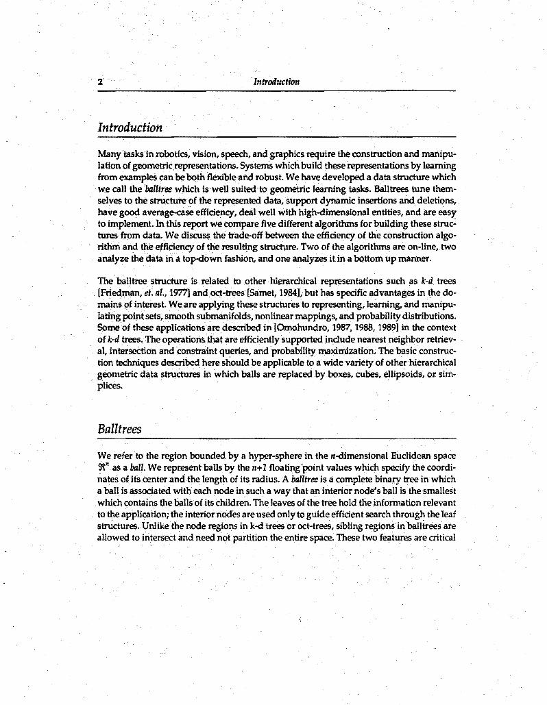
Introduction
Introduction
Many tasks in robotics vision speech and graphics require the construction and manipushylation ofgeomebicrepresentatioris Systems which build th~e representations by learning from exampleS can be both flexible and robust We have developed a data structure which we caUtheballtree which is well suitedmiddotto geometric learningmiddottasks BaUtrees tune themshyselves to the structure of the represented datasupport dynamic insertions and deletions have goodaverage-caseeffidency deal well withhigh-dimensional entities and are easy to implement In this report we compare five different a1gorithms for building these strucshytures from data We discuss the trade-off between theeffidency ofthe conStruction algoshyrithmand the efficiency ofthe resulting structure Two ofthe algorithms are on-linetwo analyze the data in a tolHiown fashion and one analyzes it in a bottomup manner
The balltree strultture is related wothermiddot hierarchical representations such as k-d trees [Friedman et al 1977] andoct-trees [Samet 1984] buthas specific advantages in the doshymains ()f interest Weare applying these structures to representing learning and manipushylating point Sets smooth subrnanifolds nonlinear mappings and probability disbibutions Borne of these applications are described in (Omohundro 1987 1988 1989] in the context of k-dtreesTheoperCitionsthat are efficiently supported include nearestneighborretrievshyaI intersectioh and constraint queries and probability maximization The basic construcshytion techniques described here should be applicable to amiddotwide variety of other hierarchical geomebic data structureS ill which balls are replaced by boxes cubes ellipsoids or sim~ plices
Balltrees
We refer to the region bounded by a hyper-sphere in the n-dimensional Euclidean space 9tas a ball We represent balls by the n+l floatingpoint values which specify the coordishynates ofitscenterandtile length of its radius A balltreeis a complete binary tree in which a baH is associated with each node insuch a way thataninterior nodes ball is the smallest which contains the balls of its children The leaves of the tree hold the information relevant to the application the interior nodes are used -only to guide efficient search through the leaf structures Unlike the node regions in k-d trees Or oct-trees Sibling regions inba1ltrees are allowed to intersect and need not partition the entire space These two features are critical
3 Implementation
for the applications and give balltrces their representational power Figure 1 shows an exshyample of a two-dimensional balltrce
abc d 8 f A) B) C)
Figure 1 A) A set of balls in the plane B) A binary tree over Ihese balls C) The balls in the resulting balltlee
In this report we study the problem of building a balltree from given leaf balls Once the tree structure is specified the internal balls are determined bottom up from the leaf balls We would like to choose the tree structure to most effidently support the queries needed in practical usage Efficiency will depend both on the distribution of samples and queries and on the type of retrieval required We first discuss several important queries and then describe a cost function which appears to adequately approximate the costs for practical applications We then compare five different construction algorithms in terms of both the cost of the resulting tree and the construction time The algorithms are compared on samshyples drawn from several probability distributions which are meant to be representative of those that arise in practice
Implementation
Our implementation is in the Object oriented language Eiffel [Meyer 1989] There are classshyes for balls balltrees and balltree nodes BALL objects consist of a vector ctr which holds the center of the ball and a real value f containing the radius BLT_ND objects consist of a BALL bl and pointers par Itrt to the nodes parents and children BALLshyTREE objects have a pointer tree to the underlying tree and a variety other slots to enshyhance retrievals (such as local priority queues and caches) All reported times are in seconds on a Sun Sparcstation 1 with 16 Megabytes of memory running Eiffel Version 22 from Interactive Software Engineering Compilation was done with assertion checking off and garbage collection global class optimization and C optimization on As with any obshyject oriented language there is some extra overhead associated with dynamiC dispatching but this overhead should affect the different algOrithms similarly
Queries Which use Simple Pruning
Queries which use Simple Pruning
There are two broad classes ofquery which are efficiently supported by the balltree strucshyture The first class employs a search with simple pruning of irrelevant branches The secshyond class requir~s the use of branch and bound during search This section presents some simple pruning queries and the next gives examples of the more complex variety
Given a query ball we might require a list of all leaf balls which contain the query ball We implement this as a recursive search down the ball tree in which we prune away recursive caUsat internal nodes whose balldoesnot contain the query ball If an intemal nOdes ball doesntcontain the query ball it is not possible for any of the leaf balls beneath it to contain it either In the balltreenode class BLT NO we may define
pusheavescontainingball(bBALllLUSTISlTNDraquo is - Add the leaves under Current which contain b to I
do il ealthen
if blcontainsball(b)thenlpush(Current) end else
if blcontains_ball(b)then Itpush_leavesconfaining_ball(bl) rtpush_leaves_containing_ball(bl)
end if end-il
end
Similarly wemightaskfor all leaf balls which intersect a query ball We prune away reshycursive calls from internal nodes whose ball doesnt intersect the query ball
push_leavesjntersectinlLball(bBALLILLIST[BlT_NDJ) is - Add the leaves under Current which intersect b to Idomiddot
illeal thEIn il blintersects ball(b) then Ipush(Current) end
else il blintersectsball(b) henmiddot
ItpusfUeavesintersectingball(bI) rtpushJeavesjntersectingball(bI)
end il end-i
end
Finally we might ask for all leaf balls which are cOntained in the query ball Here we must continue to search beneath any intemal node whose ball intersects the query ball because some descendant ball might be contained in it
pushJeaves_containecUnball(bBALLILLlSTIBLT_NO)) is - Add the leaves under Current which are con talnedin b to 1
do if leal then
if bcontalnsball(bl) then LpushCurrent) end else
if bUntersects_ball(b) then Ilpush_leavescontained_in_ball(bI)
5 Queries which use Branch and Bound
rlpushJeaves_containedjn_ball(bI) end-if
end- if end
A point is just a degenerate ball Two important spedal cases of these queries in which some of the balls are points are the tasks of returning all leaf balls which contain a given point and returning all point leaves which are contained in a given ball
Queries which use Branch and Bound
More complex queries require a branch and bound search An important example for ballshytrees whose leaves hold points is to retrieve the m nearest neighbor points of a query point Using balltrees we may use a similar approach to that discussed in [Friedman d al 1977] for k-d trees Again we recursively search the tree Throughout the search we maintain the smallest-ball bball centered at the query point which contains the m nearest leaf points seen in the search so far In this algorithm we prune away recursive searches which start at internal nodes whose ball doesnt intersect the bball This pruning is likely to happen most effectively if at each internal node we first search the child which is nearer the query point and then the other child Because balltree nodes can intersect we cannot stop the search when the bballlies inside node ball as is possible in k-d trees Because node regions are tighter around the sample points however ball trees may be able to prune nodes in situa- tions where a k-d tree could not
To retrieve the m nearest neighbors we maintain a priority queue of the best leaves seen ordered by distance from the query point We will only show the function for finding the nearest neighbor but the extension to the m nearest neighbors should be clear
In this case we assume that nn_search is defined in a class which has lbball as an attribute and that its center bballctr has been set to the query point and its radius bballr to a large enough value that it contains the root ball Inn is another attribute which will hold the result when the routine returns IInear_dist_to_vectorll is a routine in the BALL class which returns the distance from the closest point in the ball to a given vector
nn_search(nT) is - Replace nn by closest leaf under n to bballctr if closer than bballr
local dktrdREAL do
if nleaf Ihen dbballctrdisUo_vector(nblctr) if d lt bballr Ihen bbanseU(d) nn=n end - reset best
else - at internal node 1d=nItblnear_discto_vector(bballctr) rd=nrtblneacdiscto_vector(bballctr) if Id gt bballr and rd gt bballr Ihen - no sense looking here else
6 Statistical Nature of the Data
if Idltrd then- search nearer node first nn_search(nIt) if rd lt bballtlhen nn_search(nrt) end - check if still worth searching
else M_search(nrt) if Idlt bballr then nn_search(nt) end - check if still worth searching
eOO- if ei1d- if
eOO- if end
There are several natural generalizations of this query to ones involving balls Distance ~ tween points may be replaced by distance between ball centers minimum distance ~ tween ballsor maximum distance between balls In each case the minimum distance to an ancestor node is a lower bound on the distance to a leaf and so may be exactly as above to prune the search
A query which arises in one of the construction algorithms we will describe below must retumtheIeafball which minimizes the volume ofthe smallest ball containing it and a queshyrybaltThe search prOceeds as above but with the pruning value equal to the volume of the smallest ball which contains the query ball and a single point of the interior node ball
Statistical Nature of the Data
The Criterion for a good ball tree structure depends on both the type of query it must supshyport and on the nature of the data it must store and access For most of the applications we have in mind iUs appropriate to take a statistical view of the stored data and queries We assume thatthe leaf balls are drawn randomly from an underlying probability distribution and that the queries aredrawn from the same distribution We would like systems to pershyfonn Well on average with respect to this underlying distribution Unfortunately we exshypectdistributions of very different types in different situations A very powerful nonparammicappr08ch to perfonnance analysis has begun to appear (eg [Friedmanet ai 1977] and [Noga and Allison 1985J) which gives provably good results for a wide variety ofdistributions in the asymptotic limit of large sample size In both of these references the underlying distribution is required to be non-singular and in the large sample limi teach small region becomes densely sampled and locally looks like a uniform distribution If an algorithm behaves well on the uniform distribution and adjusts itself to the local sample density thenit will have good asymptotic performance on non-singular distributions Unshyfortunately some of the most important applications have data of a very different characshyter Instead of being smooth the data itself may be hierarchically dusteredor has its
bullbullbull
7 Statistical Nature of the Data
-te middot III II ampI ~lt tIbullbull ~
fa
= I~ t - bull A B C 0
Flgur2 101 leaves from the four distribution types A) Uniform B) Cantor C) Curve 0) Uniform balls
SUpport on lower dimensional surfaces Part ot the motivation for the development ot the ball tree structure was that it should deal well with these cases
For any particular statistical model poSSibly singular one may hope to perform an asympshytotic analysis similar to that in [Friedman d al 1977] Because we are interested in the pershyformance on small data sets for a variety of distributions we have taken an empirical approach to comparing the different construction algorithms We studied each algorithm in 8 situations corresponding to 4 different probability distributions in 2-dimensions and similar distributions in S-dimensions Samples from the 2-dimensional versions of these distributions are shown in figure 2 Because the case in which the leaves are actually points is very important we have emphasized it in the tests
The first distribution is the uniform distribution in the unit cube For the reasons discussed above behavior on this should be characteristic of general smooth distributions For the second distribution we wanted to study a case with intrinsic hierarchical clustering We chose a distribution which is uniform on a fractal the Cantor set The one-dimensional Cantor set may be formed by starting with the unit interval removing the middle third and then recursively repeating the construction on the two portions of the interval which are left If points on the interval are expressed in ternary notation then the Cantor set points are those that have no ls in their representation In higher dimensions we just take the product of Cantor sets along each axis The third distribution is meant to study the situation in which sample points are restricted to a lower dimensional nonlinear submanshyifold We draw points from a polynomial curve which is embedded in such a way that it doesnt lie in any affine subspaces In the final distribution the leaves are balls instead of just points The centers are drawn uniformly from the unit cube and the radii uniformly from the interval [01]
8 The Volume Criterion
The Volume Criterion
It might appear that these different distributions would require the use of different balltree construction criteria in order to lead to good perfonnance We have found however that a simp(eefficiency measure is sufficient for most applications The most basic query is to return all leaf regions which contain a given point A natural quantity to consider for this query is the average number of nodes that must be examined during the processing of a uniformly distributed query point As described above to process a point we descend the tree pruning away subtrees when thcir root region does not contain the query point This process therefore examines the intcrnal nodes whose regions contain the point and their children We may miniriUzethe number of nodes examined by minimizing the number of internal balls which contain the point Under the uniform distribution the probability that a ball will contain a point is proportionaIto its volume We minimize the average query time by minirrllzing the total volume of the regions associated with the internal nodes While this argument does not directly apply to the other distributions small volume trees generaIJy adapt themselves to any hierarchical structure in the leafballs and so maximize the amount of pruning that may occur during any of the searches We therefore use the toshytal volume of all balls in a balltree as a measure of its quality All reported ball volumes were actUally computed by takingthe ball radius to a power equal to the dimension of the space and so are only proportional to the true volume
Unfortunately itappeats to be a difficult optimization problem to find the binary tree over a given set of leaf regions which minimizes the total tree node volume Instead we will compare several heuristic approaches to the construction The next few sections describe the five studied construction algorithms In each case we give the idea of the algorithm and a key Eiffel functionmiddot for its implementation So as not to obscure the structure we have eliminated all housekeeping and bullctproofing code used in the actual implementation Operations whose hnplemen~tioIi is straightforward are not defined the meaning should be clear from context
K-d Construction Algorithm
We will call the simplest algorithm the k-d construction algorithm because it is similar to the rnethoodescribedin Friedman et al 1977] for the construction of k-d trees It is an off-line top down algorithm By this we mean that all of the leaf balls mustbeavailablebefore conshystruction and that the tree is constructed from the root down to the leaves At each stage the algorithmsplits the leaf balls into 2 sets from which ball trees are recursively built These trees become the left and right children of the root node The balls are split by choosshyinga dimension and a value and splitting the balls into those whose center has a coordinate in the given dimension which is less than the given value and those in which it is greater
9 K-d Construction Algorithm
The dimension to split on is chosen to be the one in which the balls are most extended and the spli tting value is chosen to be the median Because median finding is linearin the numshyber of samples and there arelogN stages the whole construction is 0 (NlogN)
Introdudng a class whose instances are arrays of balls yields a clean implementation The key function is select_on_coord which moves the balls around so that the balls associated with a node are contiguous in the ball array The entire construction algorithm then looks very much like quicksort except that differen t dimensions are manipulated on different reshycursive calls
In the class BALL_ARRAY we define a fairly conventional selection algorithm whose runtshyime is linear in the length of the range
SelecLon_coord (ckliuiINTEGER) is - Move ells around between Ii and ui so that the kth element ctr - is gt= those below lt- those above in the coordinate c
locallurmiINTEGER tsT do
from I-li uui until not (Iltu) loop r mdinteger_lTl9-rnd(lu) - random integer in [Iu) t get(r) set(rgef(Iraquo set(It) - swap mI from bl+ 1 until igtu loop _
if gel(i)ctrgetc) lt tctrget(c) then mm+1 sgetm) set(mget(iraquo set(is) swap
end-if iai+1
end -loop s==getI) set(lget(mraquo setms) bullbull swap if mlt=k then I==m+1 end if mgt==k then u-mmiddot1 end
end-loop endshy
To actually construct the tree we initialize a BALL_ARRAY hIs with the desired leaf balls The construction can then proceed in a natural recursive manner
build_blUor_rangeIuINTEGER)BLT_NO is - Builds a bit for the balls in the range [Iu) of bls
local cmINTEGER bIBALL do
if u=1 then - make a leaf ResultCreate ResultseLbIblsget(uraquo
else c = blsmost_spread_coord(lu) m = int_div(l+u)2) blsselecLon_coordcmlu) - split left and right ResultCreate ResultseUt(buikCbIUor_range(lm)) ResultltsetPar(Resull) - do left side ResultseLrt(build_blUor_range(m+ 1uraquo ResultrtsetJlllrResult) - do right side bICreate(blsget(O)dim) blto_bound_balls(Resultitbl Resultrtbl) ResultseLbl(bl) - fill in ball
end-if end
The tree that is produced is perfectly balanced but may not adapt itself well to any hierarshychical structure in the leaf balls
10 Top Down Construction Algorithm
Top Down Construction Algorithm
The k-dconstructionalgorithm doesnt explicitly try to minimize the volume of the resultshyingtree For uniformly distributed data it is not hard to see that it should asymptotically do a good job Iris naturillhowever to think that using anexplidt volume minimization heuristic to choose the dimension to cut and the value at which to cut it might improve the petfonIlince ofthe algorithm We refer to this approach as the topdown construction al gorithmAsin thek-d approach we work recursively from the top down At each stage we choose the split dimension and the splitting value along that dimension so as to minishymize the total volume of the two bounding balls of the two sets of balls To iindthis optimal dimension and split value we sort the balls along each dilnension and construct a cost arshyray which gives the cost at each split location This is filled in by first making a sequential pass from left to right expanding atesf ball to contain each successive entry and inserting its volume in the cost array While the exact volumeof the bounding ball of a set of balls depends on the order in which they are inserted this approach gives a goOd approximation to the actual parent ball volume Next a sequential pass is made from right to left and the bounding balls volume is added in to the array In this manner the best dimension and split location are found in o(NlogN) time and the whole algorithm should take O(N (logN)2)
We implement this approach in a similar manner to the k-dapproach The array cst is used to hold the costs ofthe differcntcutting locations
IiIUn_cst(luINTEGER) is - Fill in the ~t array between I and u Split js above pI
local iINTEGER do
blto(blsget(I)) from i(until igt=u loop- do left side
blexpand_to_ball(blsget(i)) ~~set(iblpvol) 1=1+1
end loop blto(blsget(u)) from i=uuntiFiltlloop -do right side
bIexpand_to_ball(blsget(i))info relevant to ~1middot ~~set(i-l cstget(i-l )+blpvot) 11-1
end-Ioop end
Thetrcc construction proceeds by filling in the cost array for each of the dimensions and picking the best one to recurSively proceed with
build__bIUor_range(luINTEGER)BLT_NO is - Builds a bit lor Iheballsin Iherange [Iu) olbls
localijcm bdimblocINTEGERbcstREAL nblBALL do
if iJ=1 then - make a leal ResultCreate ResultseLbl(blsget(u))
On-line Insertion Algorithm u
else bdimoblocJ from 1=0 until jblsdim loop
blssort_on_COOtd(ilu) fin_in_cst(lu) if io then bcstaestget(1) end - initial value from jJ until jgtau loop
if cstget(j)ltbcst Iten bcstaestgetO) bdim=i bloc=j end j-j+1
end-Ioop i-i+1
end -loop bIssort_on_coord(bdimlu) - sort on best dim ResuitCreate Resuitsetjt(build_blCfor_range(Iblocraquo Resultltsecpar(Result) ResultseCrt(buftd_blUor_range(bloe+ 1uraquo ResultrtsetP8l(Result) nblCreate(blsdim) nblto_bound_balls(Resultltbl ResultrtbI) ResultseCbl(nbl)
end- if end
On-line Insertion Algorithm
The next algorithm builds up the tree incrementally We will allow a new node N to beshycome the Sibling of any node in an existing bal1tree The diagram shows the new node N
N
becoming the Sibling of the old node A under the new parent P The algorithm tries to find the insertion location which causes the total tree volume to increase by the smallest amount In addition to the volume of the new leaf there are two contributions to the volshyume increase the volume of the new parent node and the amount of volume expansion in the ancestor balls above it in the trcc As we descend the tree the total ancestor expansion almost always increases while the parent volume decreases As the search for the best inshysertion location proceeds we maintain the nodes at the fringe of the search in a priority
12 On-line Insertion Algorithm
queue ordered by their ancestor expansion We also keep track of the best insertion point
found so far and the volume expansion it would entail When the smallest ancestor expanshysion of any node in the queue is greater than the entire expansion of the best node the search is terminated Nodes may be deleted by simply removing them and their parent and adjusting the volumes of all higher ancestors Notice that because of the properties of bounding balls in rare circumstances the expansion of an ancestor node due to a smaller
node may be larger than for a smaller node (this doesnt happen if boxes are used instead of balls)
The new volume in internalballs that is created by this operation consists of the entire volshyume of P plus the amount of expansion created in aU the ancestors of P Choosing the inshysertionpoint according to the criterion of trying to minimize this new volume leads to several nice properties New balls which are large compared to the rest of the tree tend to get put near the top while small boxes which lie inside of existingballs end up near the bottom New balls which are far from existing balls also end up near the top In this way the tree structure tends to reflect the clustering structur~ of leaf balls
This routine in the BALLTREE class returns a poiriterto the best sibling in the tree tb is a test baH which is a global attribute of the class frng IS the priority queue which holds thefringe nodes
besUib (nlBL T _NO)BLT_NO is - Thebestsibling node when inserting new leaf nl
local bcostREALbestcost node vol ancestor expansion tf1f2BLT_FRNG[BLT_NO) - tast fringe elements doneBOOLEAN veREAL
do if Iree Void then-ResultVoid means tree is void else
frngclr~ Result=tree tbJoboun(Cballs(treebl nlbl) bcost=tbpvol if not Resultleaf then
tfCreate tfseuaexp(O) --no ancestors tfseLndvol(bcost) IfseLnd(Resull)
13 On-line Insertion Algorithm
fmgins(lf) - start out the queue end - if from until fmgempty or done loop
tf fmgpop- best cancidale if tfaexp gt- beast then - no way to get better than bnd
done true - this is the bound in branch and bound else
e = tfaexp + tfnclvol bull tfndpvol -new ancestor expans - do left node tblO_bound_baIls(tfndltbInlbl) v = tbpvol if V+8 lt beast then beest V+8 Result = tfndt end if not tfndltleaf then
tf2Creale tf2set_aexp(e) tf2set_nclvol(v) tf2secnd(tfndlt) fmgins(tf2)
end -if - now do right node tblO_bound_balls(tfndrtblnlbl) v tbpvol if V+8 lt beest then beast v+e Result tfndrt end If not tfndrtleaf then
tf2Create tf2secaexp(e) tf2set_nclvol(v) tf2secnd(tfndrt) fmgins(tf2)
end - if end-if
end -loop fmgclr
eOO- if end - besCsib
Once the sibling of the node is dctcnnincd the following routine will create a parent and insert it and the new leaf into the tree repair_parents recursively adjusts the bounding balls in the parents of a node with a changed ball
ins_acnode (nlnBL T_NO) is - Make nl be ns sibling nVoid if first node
local nblBALL nparndBLT_NO do
nlsetJ)8l(npar) - just in case something is there nlseUt(npar)nlseCrt(npar) if tree Void- if nothing there just insert nl then tree nl else
nparCreate nparset-par(npar) if npar Void then tree npar- insert at top elsif nparll=n then nparseUt(npar) else nparsecrt(npar) end - if nparseUt(n) nparsecrt(nl) nlset~r(npar) nset-par(npar) nblCreate(dim) nbltobound_balls(nlblnbl) nparsecbl(nbl) repair-parents(npar)
end- if end - ins_acnode
To remove a node we remove its parent and fix up the bounding balls of the ancestors
rem(nT) is - Remove leaf n from the tree Forget its parent
local npnsvdIBL T _NO
14 Cheaper On-line Algorithm
do if rio Void then-- do nothing if empty elsif nparVoid then treeforget - last node in tree else
np=npar if nnplt then ns=np else nsnplt end -- sibling nsset-Par(nppar) if npparVoid then tree=ns elsif npparlt=np then npparseUt(ns) else npparseL(ns) end npForget nset-Par(np)middotmiddot just in case someone asks for it from np=nspar until npVoid loop
npblto_bound_balls(npltblnprtbl) - adjust bailS np nppar
end -loop nsetpar(vdt)
end- if end -rem
Cheaper On-line Algorithm
We also investigated a cheaper version of the insertion algorithm in which no priority queue is maintained and only the cheaper of the two child nodes at any point is further exshyplored Again the search is terminated when the ancestor expansion exceeds the best total expansion
cheap_bast_sib (ntBlT_NO)Bl T _ND is - A cheap guess at the best sibling node for inserting new leaf nl
local bcostREAl-- best cost node vol + ancestor expansion aeREAl- accumulated ancestor expansion ndBlT_NO doneBOOlEAN IvrvwvREAl
do if tree Void then- Result Void means tree is void else
Result=tree tbto_bound_balls(treeblnlbl) wvtbpvol bcost=wv ae=O- ancestor expansion starts at zero from nd=tree until ndleaf or done loop
ae=ae+wv-ndpvol - correct for both children if aegt=bcost then done=true - cant do any better else
tbto_bound_balls(ndltblnlbl) Ivtbpvol tbto_bound_balls(ndblnlbl) rvtbpvol if ae+Ivlt=bcost then Result=ndlt bcost ae+lv end if ae+rvlt=bcost then Result=ndrt bcost=ae+rv end if Iv-ndltpvok=rv-ndpvol -- left expands less then wv=Iv nd=ndlt else wv=rv nd=nd end
endmiddotmiddot if end -loop
end - if end - cheap_besLsib
15 Bottom Up Construction Algorithm
Bottom Up Construction Algorithm
The bottom up heuristic repeatedly finds the two balls whose bounding ball has the smallshyest volume makes them siblings and inserts the parent ball back into the pool In some
ways this is similar to the Huffman algorithm for finding efficient codes Here though the cost depends on the combination of the two nodes being combined and so the choice beshycomes more expensive The simplest brute-force implementation maintains the current candidates in an array and on each iteration checks the volume of the bounding ball of each pair to find the best A straightforward implementation of this approachrequires N passes most of which are of size a (fIi2) for a total construction time of o(lI)
Improved Bottom Up Algorithm
Two observations allow us to substantially reduce the cost of this algorithm If each node kept track of the other node such that the volume of their joint bounding ball was minishymized and the volume of that ball then the node with the minimal stored cost and its stored mate would be the best pair to join Secondly most of the balls keep the same mate when a pair is formed and when ones mate is paired elsewhere the best costcan only inshycrease As described in the last section the ball tree is an ideal structure for determining each balls best mate We therefore maintain a dynamic balltree using one of the insertion algOrithms for holding the unfinished pieces of the bottom-up ball tree An initial pass deshytermines the best mate for each node The nodes are kept in a priority queue ordered by the volume of the bounding ball with their best mate As the algorithm proceeds some of these mates will become obsolete but the best bounding volume can only increase We therefore iterate removing the bestnode from the priority queueand if it has not already been paired we recompute its best mate using the insertion balltree If the recomputed cost is less than the top of the queue then we remove it and its mate from the insertion ball tree form a parshyent node above them compute the parents best mate and reinsert the parent into the inshysertion ball tree and the priority queue When there is only one node left in the insertion ball tree the construction is complete We present the routines for finding the best pair and for merging them pq is the priority queue of pending nodes and the variables bl and b2 will hold the best pair tp merge has_Ieaf tests whether a ball tree has a given node as a leaf
find_bestJ)8iris - Put best two fo merge in b 1b2 and remove from pq and bit
local doneBOOLEAN btmBLT_FPND do
b1Forget b2Fotget from untit done loop
if pqempty then done=true -- returns Void when done else
btm = pqpop if blthas_leaffbtm) then - if not there then keep on
16 Improved Bottom Up Algorithm
bltrem(btm)- take it out of the tree btmseLbvol(bltbesLvoUo_ball(btmblraquo --recomp it pqempty or else
btmbvol lt= pqtopbvol then done=true else
pqins(btm) bllcheapJns(btm) - Iry again end - it
end - it end - if
end-Ioop if nol btmVoid then
b1 =btm b2=bltbesl_node_to_ball(b1bl) bltrem(b2) end - if
end
merge_beSIJlSir is - Combine the best two replace combo in pq and bit
local bnBLT NO bIBALLvbtBL T FPNO ~ - shy
if (not b1Void) and (not b2Void) then bnCreate
bnseUt(b1tree) bnltsetJ)ar(bn) bnseLn(b2tree) bnnsetJlSr(bn) blCreste(bltdim) blto_bound_balls(bnltblbnnbl) bnset_bl(bl)b1Create b1seuree(bn) b1seLbl(bl) -- never resize socsn share b1seLbvol(bltbest_voLto_ball(bl)) pq-ins(b1) bltcheapins(b1) b1 =vbf b2=vbf
end - if end
The figures compare the construction time of the brute force approach against the algorithshymic one for uniform data in 2 5 and 10 dimensions and show that the speedup is substanshytial
11 Construction Data
Construction Tlme Construction lime 50000 900
40000 720
30000 540
20000 360
10000 180
OOO-+--q===p-~r--I~ O -I---==rIr--- o 40 80 160 200 o 40 80 120 160 200
Number of Leaves Number of Leaves Figure 3 COn$tructicm time vs size for bottumup Figure 4COn$truction lime VI size for bonum up con$truction method Brutaforce approachmiddotis construction method Brute force approach is compared with clever one for 2-dimen$ional compared with clever one for 5-dimensional
uniformly distributed point leaves uniformly distributed point leaves
Construction Time
122784
98227
73670
49114
24557
o 40 80 120 160 200 Number of Leaves
Figure 5 Construction time VI size for bottum up construction method Brute force approach is compared with clever one for 10-dimensional uniformly distributed point leaves
Construction Data
OOO+--______-r--r--r--
In this section we preSent the experimental results giving the volume of the constructed balltree and the construction time asa function of the number of leaves for each of the alshygorithms and eachof the distributions discussed above In each graph a different dashing pattern is used to denote each of the algOrithms The first figures label the curves and the usage is the same in the others
18 Construction Data
Balltree Volume
40 top_dn
32 ~ I 24 chpJns I 1 ~
~ I 16 -- I I kd 8 I r I 1 ns
- I J- O --f--------r-y--r-r-i
o 100 200 300 400 500 Number of Leaves
Figure 7 Baillree volume vs size for 2shydimensional uniformly distributed point leaves
Balltree Volume
1381
1105
829
552
276
OOO+----------r-r-y-- o 1 00 200 300 400 500
Number of Leaves Figure 9 Balltree volume vs size for 2shydimensional Cantor set distributed point leaves
BalHree Volume
423
338
254
169
085
OOO-l-~~~----~---r--I o 1 00 200 300 400 500
Number of Leaves
Flgure11 BalitreevolumriNS sizefor2middotdimensionalpoint leaves distributed on a curve
-
Construction Time
25488
20390
bull 15293
10195
5098
000 o 100 200 300 400 500
Number of Leaves
Figure 8 Balltree consllJction time vs size for 2shydimensional uniformly distributed point leaves
Construction Time
200
160
120
80
40
100 200 300 400 500 Number of Leaves
Figure 10 Balltree consllJction time vs size for 2shydimensional Cantor set distributed point leaves
Construction Time
12107
9686
100 200 300 400 500 Number of Leaves
Figure 12 Balltree construction time vs size for 2middot dimensional point leaves distributed on a curve
19 ConstructionmiddotData
Salltree Volume
9000
7200
5400 IV
3600 r ~ ~ shy1800 J- -_v ooo~f~
a 100200 300400 500 Number of Leaves
Frgure13 eaullee volumevs sizefor 2-dimensional uniforrilly diStributed leaf balls with radii uniformly diatributed below 1
Salltree Volume
1000
800 J (I I I
600 I
400 ) V IJ
t
~~- 200 -- h-- 0t4middot-=-~-$middot
a 100 200 300 400 500 Number of Leaves
F1gur15BaJltreevolume vs size for 5shydimensional uniformly diatributed point leaves
Balltree Volume
202898 AI
162318 i J I
121739 I I bull
81159 t _t A I - I
40580 I )_I~
ooo~~e-~~-==middot-=~ o 1 00 middot200 300 400 500
Number of leaves Flgura 11 Balltteevolumevs size lor 5shydimensional Cantorsetdistributed point leaves
Balltree Volume
ConstruCtion TIme
43359
i 1 ~JI8672 _~L)j-middot__
OOo+-~~~jIio7amp o 100 200 300 400 500
Number of Leaves Flgur 14middot BaIItree construction time vSsiZe lor 2shydimensional uniformly distributed leaf balls with radii uniformly distributed less than 1
Construction TIme
144922
115938
86953 I
57969 I 1
28984 J I-----V-
000-I-IOiiofIaij--=-Fmiddot=shy
o 100 200 300 400 500 Number of Leaves
Flgur16BaJltree construction timevs size lor 5 dimensional uniformly distributed point leaves
Construction Time
169545
135636
101727
33909
100 200 300 400 500 Number of Leaves
Figura 18 Balilree construcnontime VS size for5shydiniensional Cantonel distributed point leaves
Construction Time
20 Conclusions
Balltree Volume Construction Time
107448 230180 I I18414485958 I II 13810864469 I
9207242979 pound -shy 4603621490
sect-- -
000~~ OOO+--=T---F~~-
o 100 200 300 400 500 o 100 200 300 400 500 Number of Leaves Number of Leaves
FIgure 21 Balltree volume vs size for 5- Figure 22 Balltree constnJotion time vs size for 5shydimensional uniformly distributed leaf balls with dimensional uniformly distributed leaf balls with radii uniformly distributed below 1 radii uniformly distributed less than 1
Let US now discuss this data The rankings of the different algorithms for cost of construcshytion were almost identical in a)) the tests The bottom up algorithm was virtually always the most expensive (beingeclipsed only occasiona))y by the top down algorithm) This is perhaps to be expected since it must use one of the others during its construction The k-d algorithm in each case had the smallest construction time followed closely by the cheap inshysertion algOrithm It is heartening that in each case the cost appears to be growing only slightly faster than linear (with the possible exception of the top down algorithm)
The bottom up algorithm consistently produced the best trees followed closely by the inshysertion algorithm The k-d algorithm did very we)) on the uniform data (as expected) but rather poorly on the curve and Cantor data In the next section we will see that this is beshycause it doesnt adapt we)) to any sma))-scale structure in the data On the uniform data the top-down algorithm was the worst followed by the cheap insertion algorithm It is pershyhaps surprising that the top-down approach did worse than the k-d approach on the unishyform data The top-down approach appears very sensitive to the exact structure of the data as evidenced by the wild fluctuations in tree quality It appears that it must make choices which affect the whole structure and quality of the tree before their true impact is clear All of the algorithms did quite well on the curve data particularly in 5 dimensions
Conclusions
To give further insight into the nature of the trees constructed figure 23 shows the interior balls and tree structure produced by the five algorithms on 30 Cantor distributed points in the plane The k-d algorithm blindly slices the points in half taking no account ofthe hiershy
21 Bibliography
archical structure This allows it to produce a perfectly balanced tree but at the expense of missing the structure inthe data The two insertion algorithms produced exactly the same tree in this case It appears to have early on made a decision which forced the final tree to have a very large ballnear the root This is typieal of the cost of using an online algOrithm The top-ctown and bottom up algorithms found very similar trees of essentially eqllivalent quality
In cOnclusion if the data is smooth and there is lots of it the k-d approach is fast and simple and has much to recommend it If the data is clustered or sparse or has extra structure the k-d approach tends not to reflect that structure in its hierarchy The bottom IIp approach in all cases does~anexcel1ent job at finding any structure and aside ftom its construction cost is the preferred approaCh In situations where on-line insertion is necessary the full insershytion algorithm approaches the bottom up algorithm in quality The cheaper insertion apshyproachdoes significantly worse but leads to construction times nearing those ofthek-d approach A balltree constructed by any means maybe further modified using the insershytion or cheaper insertion algorithms
Bibliography
Jerome H Friedman Ion Louis Bentley and Raphael Ari Finkel An Algorithm for FindshyIngBestmiddotMatches in Logarithmic ExpeCted Time ACM Transactions on Mathematical Software 33(1977) 209-226
Bertrand Meyer Eiffel The LAnguage Interactive Software Engineering Goleta CA 1989
StephenMOmohundro Efficient Algorithms with Neural Network BehaviorComplex Systems 1 (1987)273-~7
StephenM Omohundro Foundations of Geometric Learning University of Illinois Deshypartment ofComputerSdcncc Technical Report NoUIUCDcsR-88-1408 (1988)
Stephen M OmohundroGeometricLeaming Algorifhms Proceedingsof the LosAlamshyos Conference on Emergent Comput1ltion (1989) (lCSl Technical Report NoTR-89(41)
M T Noga and D C S Allison Sorting in Linear Expected Time Bil2S (1985) 451-465
Hanan Samet The quadtree and related hierarchical data structuresACM Comshyputing Surveys 1621une (1984)187-2606
22 Bibliography
Kd
Top down
Insertion and Cheap insertion
Bottom up
Figure 23 The barr and tree structure created by the five algorithms on Cantor random data

22 Bibliography
Kd
Top down
Insertion and Cheap insertion
Bottom up
Figure 23 The barr and tree structure created by the five algorithms on Cantor random data


