Fitting Generalized Additive Models:

A Comparison of Methods

Harald Binder & Gerhard Tutz

Universitat Freiburg i. Br.

Nr. 93 November 2006

Zentrum fur Datenanalyse und Modellbildung

Universitat Freiburg

Eckerstraße 1

D–79104 Freiburg im Breisgau

und

Institut fur Statistik

Ludwig-Maximilians-Universitat Munchen

Akademiestraße 1

D–80799 Munchen

binderh@fdm.uni-freiburg.de

tutz@stat.uni-muenchen.de

Abstract

There are several procedures for fitting generalized additive models, i.e. mul-

tivariate regression models for an exponential family response where the influence

of each single covariates is assumed to have unknown, potentially non-linear shape.

Simulated data is used to compare a smoothing parameter optimization approach for

selection of smoothness and covariate, a stepwise approach, a mixed model approach,

and a procedure based on boosting techniques. In particular it is investigated how

the performance of procedures is linked to amount of information, type of response,

total number of covariates, number of influential covariates, correlation between

covariates, and extent of non-linearity. Measures for comparison are prediction per-

formance, identification of influential covariates, and smoothness of fitted functions.

One result is that the mixed model approach returns sparse fits with frequently over-

smoothed functions, while the functions are less smooth for the boosting approach

and variable selection follows a less strict (implicit) criterion. The other approaches

are in between with respect to these measures. The boosting procedure is seen to

perform very well when little information is available and/or when a large number of

covariates is to be investigated. It is somewhat surprising that in scenarios with low

information the fitting of a linear model, even with stepwise variable selection, has

not much advantage over the fitting of an additive model when the true underlying

structure is linear. In cases with more information the prediction performance of all

procedures is very similar. So, in difficult data situations the boosting approach can

be recommended, in others the procedures can be chosen conditional on the aim of

the analysis.

Keywords: Generalized additive models, selection of smoothness, variable selection,

boosting, mixed model approach

2

1 Introduction

Generalized additive models, as introduced by Hastie and Tibshirani (1986), present a

flexible extension of generalized linear models (e.g. McCullagh and Nelder, 1989), allow-

ing for arbitrary functions for modelling the influence of each covariate on an exponential

family response in a multivariate regression setting. Various techniques can be employed

for actually fitting such models, some of them documented in two recent monographs

(Ruppert et al., 2003; Wood, 2006), and there is ongoing research on new ones. While

most of the available approaches have been developed with a specific application in mind,

there is quite some overlap of application settings where several procedures may be fea-

sible. There are relatively few studies that compare different methods available. Usually

comparisons are done when a new procedure is introduced and results are limited to

only few procedures (e.g. Wood, 2004). Also, often the focus is on univariate fitting of

splines (e.g. Lindstrom, 1999; Wand, 2000; Ruppert, 2002; Lee, 2003), i.e. the model

selection problem arising in multivariate settings is not dealt with. A precursor to the

present study is contained in Tutz and Binder (2006), where only a limited amount of

simulation scenarios for comparison with other methods is considered.

The focus of the present paper is on comparison of procedures for fitting generalized

additive models. We therefore use an extended set of examples with simulated data and

additional procedures for comparison. It cannot be expected that there is a “best pro-

cedure”. The advantage of one approach over the other will depend on the underlying

structure and the sampling scheme. We will explore several structures and sampling

schemes and compare the performance of the various procedures. In the following we

shortly sketch the, naturally subjective and limited, characteristics of the underlying

structure that can be expected to have an effect on the performance of fitting proce-

dures.

3

Amount of information. One feature that will have an effect on the performance is the

amount of structure underlying the data. This can be quantified by the signal-to-noise

ratio (definition given in Section 3). Generalized additive models are frequently used for

the exploratory analysis of data. In contrast, in an experimental setting one often has

some knowledge about the functional form of the response. Since in exploratory analyses

it is often not even clear whether the predictors contain any information at all, we will

focus on rather small signal-to-noise ratios.

Type of response. When a binary (or Poisson) response is used instead of a continuous

response with Gaussian error this can be seen as a coarsening of the response, i.e. the

signal-to-noise ratio decreases. Especially for binary response settings the question is

whether the relative performance of the various approaches for fitting generalized ad-

ditive models changes just in the way as if the signal-to-noise ratio would have been

decreased. If this is not the case the type of response has to be considered as a distinct

factor.

Number of non-influential covariates. If subject matter knowledge about the potential

influence of covariates is available, it is advisable to include only those covariates that

are truly influential. Nevertheless, sometimes there is a large number of covariates and

not enough subject matter knowledge to decide on a small set of covariates to be used.

Even for classical linear models procedures run into problems in the high dimensional

case, and therefore regularization techniques have to be used (e.g. Hoerl and Kennard,

1970; Tibshirani, 1996). For generalized additive models high dimensional settings are

even more difficult to handle, because for each covariate a function has to be estimated

instead of just one slope parameter. As each approach for fitting generalized additive

models has specific technique(s) for regularization of complexity, it will be instructive

to compare the decrease of performance when adding more and more not-influential

covariates (i.e. not changing the underlying structure and signal-to-noise ratio).

4

Number of influential predictors/distribution of information. Given the same signal-to-

noise ratio, information can be contained in few variables (constituting a sparse problem)

or distributed over a large number of covariates (dense problem). It has been recognized

that in the latter case usually no procedure can do really well and therefore one should

“bet on sparsity” (see e.g. Friedman et al., 2004). Nevertheless we will evaluate how the

performance of the various approaches changes when information is distributed over a

larger number of covariates.

Correlation between covariates. When covariates are correlated this is expected to render

fitting of the model more difficult (the signal-to-noise ratio kept at a fixed level). Beyond

evaluating to what extent prediction performance of the various approaches is affected,

we will investigate whether identification of influential covariates is affected differentially

by correlation between covariates.

Amount of non-linearity in the data. It is also worthwhile to explore the performance

of procedures when the structure underlying the data is simple. As noted for example

recently by Hand (2006), seemingly simple methods still offer surprisingly good perfor-

mance in applications with real data when compared to newer methods. Therefore a

procedure offering more complexity should offer means for automatic regulation of com-

plexity, thus being able to fit a complex model only when necessary and a simple one

when that is sufficient. It will be evaluated whether these mechanisms work even in the

extreme case, where the underlying structure is linear. This is important, because it

touches the question whether one can rely on fitting additive models, i.e., still expect

results to be reliable, even if the underlying model is linear.

One issues that will not be dealt with in the present study is that of covariates with

varying degrees of influence, because in preliminary studies we did not find a large effects

when using such non-uniform covariate influence profiles, when adjusting the signal-to-

noise ratio.

5

The results in this paper will be structured such that for each data property/issue listed

above recommendations can be derived. Section 2 reviews the generalized additive model

framework and the theoretical foundations of the procedures for fitting such models that

will be used for comparison. Section 3 presents the design of the simulation study, i.e. the

types of example data used, the specific details and implementations of the procedures,

and the measures used for comparison. The results are discussed in Section 4, with a

focus on the issues highlighted above. Finally, in Section 5 we summarize the results

and give general recommendations as to which procedure can or should be used for what

kind of objective.

2 Procedures for fitting generalized additive models

In this section we shortly sketch the procedures to be used for comparison in this paper.

It should be noted that one has to distinguish, between how a model is fitted, and

how the tuning parameters of a model are selected. Different approaches have different

typical procedures for the latter. The simulation study presented in the following is

performed in the statistical environment R (R Development Core Team, 2006), version

2.3.1, where implementations for the approaches for fitting generalized additive models

are available as packages.

Generalized additive models (GAMs) assume that data (yi, xi), i = 1, . . . , n, with covari-

ate vectors xTi = (xi1, . . . , xip) follow the model

µi = h(ηi), ηi = f(1)(xi1) + · · · + f(p)(xip),

where µi = E(yi|xi), h is a specified response function, and f(j), j = 1, . . . , p, are un-

specified functions of covariates. As in generalized linear models (GLMs) (McCullagh

and Nelder, 1989) it is assumed that y|x follows a simple exponential family, including

6

among others normally distributed, binary, or Poisson distributed responses.

2.1 Backfitting and stepwise selection of degrees of freedom

The most traditional algorithm for fitting additive models is the backfitting algorithm

(Friedman and Stuetzle, 1981) which has been propagated for additive models in Hastie

and Tibshirani (1990). The algorithm is based on univariate scatterplot smoothers which

are applied iteratively. The backfitting algorithm cycles through the individual terms in

the additive model and update each using an unidimensional smoother.

Thus if f(0)j (.), j = 1, . . . , p, are estimates, updates for additive models are computed

by

f(1)j =

∫Sj(y −

∑s<j

f (1)s −

∑s>j

f (0)s )

where Sj is a smoother matrix, yT = (y1, . . . , yn) and f(j)s = (f(s)(x1s), . . . , f(s)(xns))T

denotes the vector of evaluations. The second term on the right hand side represents par-

tial residuals that are smoothed in order to obtain an update for the left out component

fj . The algorithm is also known as Gauss-Seidel algorithm.

For generalized additive models the local scoring algorithm is used. In the algorithm

for each Fisher scoring step there is an inner loop that fits the additive structure of the

linear predictor in the form of an weighted backfitting algorithm. For details, see Hastie

and Tibshirani (1990).

The procedure that is used in the simulation study is called bfGAM, for traditional

backfitting combined with a stepwise procedure for selecting the degrees of freedom for

each component (package gam, version 0.97). The program uses cubic smoothing splines

as smoother and selects the smoothing parameters by stepwise selection of the degrees

of freedom for each component (procedure step.gam). The possible levels of degrees

of freedom we use are 0, 1, 4, 6, or 12, where 0 means exclusion of the covariate and

7

1 inclusion with linear influence. The procedure starts with a model where all terms

enter linearly and in a stepwise manner seeks improvement of AIC by upgrading or

downgrading the degrees of freedom for one component by one level (see Chambers and

Hastie, 1992).

2.2 Simultaneous estimation and optimization in smoothing parameter

space

Regression splines offer a way to approximate the underlying functions f(j)(.) by using

an expansion in basis functions. One uses the approximation

f(j)(xi) =m∑

s=1

β(j)s φs(xis)

where φs(.) are known basic functions. A frequently used set of basis functions are cubic

regression splines which assume that for a given sequences of knots τ1 < · · · < τm (from

the domain of the covariate under investigation) the function may be represented by a

cubic polynomial within each interval [τs, τs+1] and has first and second derivation at

the knots. Marx and Eilers (1998) proposed to use a large number of evenly spaced

knots and the B-spline basis in order to obtain a flexible fit and to use a penalized

log-likelihood criterion in order to obtain stable estimates. Then one maximizes the

penalized likelihood

lp = l + λ∑

i

(βi+1 − βi)2 (1)

where l denotes the used likelihood and λ is a tuning parameter which steers the differ-

ence penalty.

Wood (2004) extensively discusses the implementation of such an approach for penalized

estimation of the functions together with a technique for selection of the smoothing

parameters (see also Wood, 2000, 2006). The procedure is referred to as wGAM (for

8

woodGAM ). It performs simultaneous estimation of all components with optimization

in smoothing parameter space (gam in package mgcv, version 1.3-17). The packages

offers several choices for the basis functions and we use a cubic regression spline basis

(with default number and spacing of the knots). As wGAM can no longer be used

when the number of covariates gets too large, in parallel we also use wGAMstep, a

stepwise procedure, which, similar to bfGAM, evaluates the levels “exclusion”, “linear”,

and “smooth” for each component.

2.3 Mixed model approach

It has been pointed out already by Speed (1991) that fitting of a smoothing spline can

be formulated as the estimation of a random effects model, but only recently this has

been popularized (see e.g. Wang, 1998; Ruppert et al., 2003) and implementations have

been made readily available (Wood, 2004). Let the additive model be represented in the

matrix form

η = Φi1β1 + . . . + Φimβp (2)

where ηT = (η1, . . . , ηn) and Φis denotes matrices composed from the basis functions. By

assuming that the parameters β1, . . . , βp are random effects with a block-diagonal covari-

ance matrix, one may estimate the parameters by using best linear unbiased prediction

(BLUP) as used in mixed models. Smoothing parameters are obtained by maximum

likelihood or restricted maximum likelihood within the mixed models framework. For

details see (Ruppert et al., 2003; Wood, 2004).

The mixed model approach is denoted as GAMM (gamm in package mgcv).

9

2.4 Boosting approach

Boosting originates in the machine learning community where it has been proposed as a

technique to improve classification procedures by combining estimates with reweighted

observations. Since it has been shown that reweighting corresponds to minimizing iter-

atively a loss function (Breiman, 1999; Friedman, 2001) boosting has been extended to

regression problems in a L2-estimation framework by Buhlmann and Yu (2003). The ex-

tension to generalized additive models where estimates are obtained by likelihood based

boosting is outlined in Tutz and Binder (2006). Likelihood based boosting is an iterative

procedure in which estimates are obtained by applying a “weak learner” successively on

residuals of components of the additive structure. By iterative fitting of the residual

and selection of components the procedure adapts automatically to the possibly vary-

ing smoothness of components. Estimation in one boosting step is based on (1) with

λ being chosen very large, in order to obtain a weak learner. The number of boost-

ing steps is determined by a stopping criterion, e.g. cross-validation or an information

criterion.

We denote the procedure by GAMBoost (Tutz and Binder, 2006), which is a boosting

procedure with the number of boosting steps selected by AICC (Hurvich et al., 1998) in

the Gaussian response examples and by AIC otherwise (package GAMBoost, version 0.9-

3). To verify that the latter criterion works reasonably, we also run cvGAMBoost, which

is based on 10-fold cross-validation. There is also a variant of GAMBoost, spGAMBoost,

that fits more sparse models by choosing each boosting step based on AICC/AIC instead

of deviance.

Since the smoothness penalty λ is not as important as the number of boosting steps (Tutz

and Binder, 2006), it is determined by a coarse line search such that the corresponding

number of boosting steps (selected by AICC/AIC or cross-validation) is in the range

[50, 200] (procedure optimGAMBoostPenalty).

10

3 Design of the simulation study

3.1 Simulated data

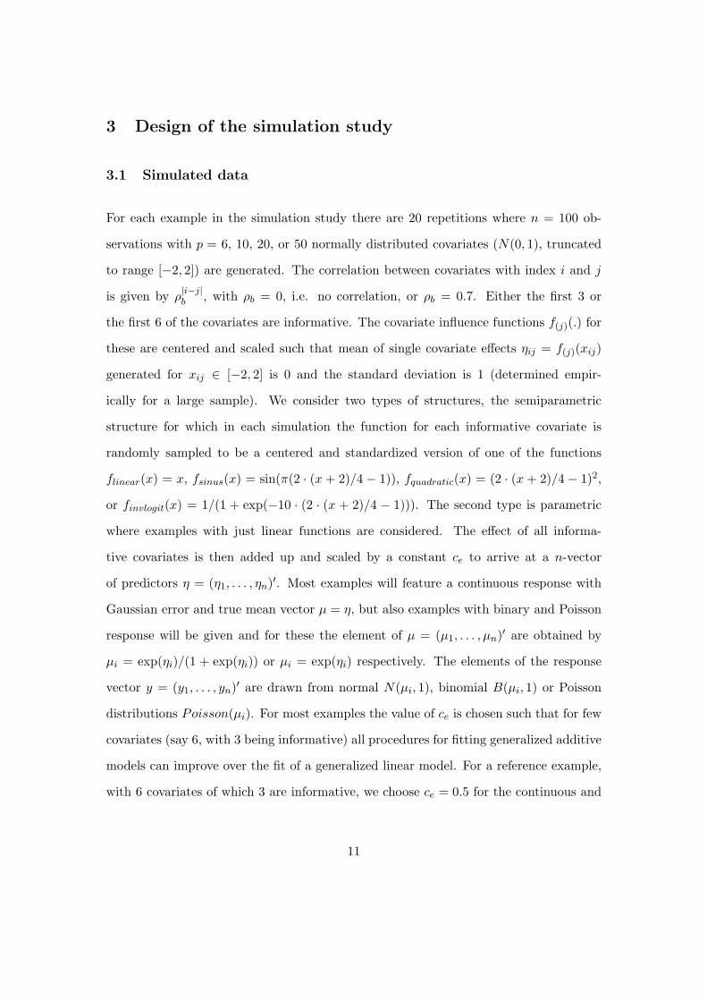
For each example in the simulation study there are 20 repetitions where n = 100 ob-

servations with p = 6, 10, 20, or 50 normally distributed covariates (N(0, 1), truncated

to range [−2, 2]) are generated. The correlation between covariates with index i and j

is given by ρ|i−j|b , with ρb = 0, i.e. no correlation, or ρb = 0.7. Either the first 3 or

the first 6 of the covariates are informative. The covariate influence functions f(j)(.) for

these are centered and scaled such that mean of single covariate effects ηij = f(j)(xij)

generated for xij ∈ [−2, 2] is 0 and the standard deviation is 1 (determined empir-

ically for a large sample). We consider two types of structures, the semiparametric

structure for which in each simulation the function for each informative covariate is

randomly sampled to be a centered and standardized version of one of the functions

flinear(x) = x, fsinus(x) = sin(π(2 · (x + 2)/4 − 1)), fquadratic(x) = (2 · (x + 2)/4 − 1)2,

or finvlogit(x) = 1/(1 + exp(−10 · (2 · (x + 2)/4 − 1))). The second type is parametric

where examples with just linear functions are considered. The effect of all informa-

tive covariates is then added up and scaled by a constant ce to arrive at a n-vector

of predictors η = (η1, . . . , ηn)′. Most examples will feature a continuous response with

Gaussian error and true mean vector µ = η, but also examples with binary and Poisson

response will be given and for these the element of µ = (µ1, . . . , µn)′ are obtained by

µi = exp(ηi)/(1 + exp(ηi)) or µi = exp(ηi) respectively. The elements of the response

vector y = (y1, . . . , yn)′ are drawn from normal N(µi, 1), binomial B(µi, 1) or Poisson

distributions Poisson(µi). For most examples the value of ce is chosen such that for few

covariates (say 6, with 3 being informative) all procedures for fitting generalized additive

models can improve over the fit of a generalized linear model. For a reference example,

with 6 covariates of which 3 are informative, we choose ce = 0.5 for the continuous and

11

the Poisson response case and ce = 1.5 for the binary response case. When examples

with more informative covariates or correlated covariates are used, the value of ce has

been decreased to maintain a similar level of information. The latter is quantified by

the (generalized) signal-to-noise ratio, which is estimated for each example on new test

data of size nnew = 1000 by

singal-to-noise ratio =∑

i(µi − µ)2∑i(µi − yi)2

(3)

with µ = 1/nnew∑

i µi.

3.2 Procedures

As already outlined in Section 2 we use the procedures

1. bfGAM : traditional backfitting combined with a stepwise procedure for selecting

the degrees of freedom for each component (package gam, version 0.97).

2. wGAM : simultaneous estimation of all components with optimization in smoothing

parameter space (gam in package mgcv, version 1.3-17) and wGAMstep, a stepwise

procedure, based on wGAM.,

3. GAMM : mixed model approach (gamm in package mgcv).

4. GAMBoost : GAMBoost with the number of boosting steps selected by AICC (Hur-

vich et al., 1998) in the Gaussian response examples and by AIC otherwise (package

GAMBoost, version 0.9-3), cvGAMBoost, which is based on 10-fold cross-validation

and spGAMBoost, which fits more sparse models by choosing each boosting step

based on AICC/AIC instead of using the deviance.

The following procedures are used as a performance reference:

• base: generalized linear model using only an intercept term, to check whether

12

the performance of procedures can get worse than a model that uses no covariate

information.

• GLM : full generalized linear model including all covariates, to check whether more

flexible procedures might perform worse than this conservative procedure, when

the true structure is linear. Because all other procedures perform some sort of vari-

able selection, we also use GLMse, that is GLM combined with stepwise variable

selection based on AIC (stepAIC from package MASS, version 7.2-27.1). This also

provides a performance reference for the identification of informative covariates.

For GLMse, bfGAM, wGAM, and wGAMstep the degrees of freedom, used for the model

selection criteria, are given more weight by multiplying them by 1.4 (wGAMr is a variant

of wGAM without this modification). In an earlier simulation study this consistently

increased performance (but not for GAMBoost procedures). Some reasoning for this

is given by Kim and Gu (2004). For the procedures used in the present study one ex-

planation might be, that they have to search for optimal smoothness parameters in a

high-dimensional space (the dimension being the number of smoothing parameters to

be chosen, typically equal to the number of covariates, p), guided by a model selection

criterion. When close-to-minimum values of the criterion stretch over a large area in

this space and the criterion is subject to random variation, there is a danger of moving

accidentally towards an amount of smoothing that is too small. Increasing the weight of

the degrees of freedom in the criterion reduces this potential danger1. In contrast, for

GAMBoost procedures there is only a single parameter, the number of boosting steps (ig-

noring the penalty parameter). Therefore finding the minimum is not so problematic and

increasing the weight of the degrees of freedom does not result in an improvement.

While for bfGAM (by default) smoothing splines are used, the other procedures employ

regression splines with penalized estimation and therefore there is some flexibility in1This reasoning is based on personal communication with Simon Wood

13

specifying the penalty structure. For all GAMBoost procedures and their B-spline basis

we use a first order difference penalty of the form (1). For wGAM and wGAMr we use

the “shrinkage basis” provided by the package, that leads to a constant function (instead

of a linear function) when the penalty goes towards infinity. Therefore these procedures

allow for complete exclusion of covariates from the final model instead of having to

feature at least a linear term for each covariate. For wGAMstep no shrinkage basis is

used, because covariates can be excluded in the stepwise course of the procedure.

3.3 Measures for comparison

We will use several measures to evaluate the performance. Prediction performance is

evaluated by the mean predictive deviance (minus two times the log-likelihood) on new

data of size nnew = 1000. This is a natural generalization of mean squared error to

binary and Poisson responses. For a side by side comparison of prediction performance

for various response types (e.g. to be able to judge whether a change in response type is

similar to a change in signal-to-noise ratio) we consider the relative (predictive) squared

error

RSE =∑

i(yi − µi)2∑i(yi − µi)2

, (4)

calculated on the new data. It will be equal to one when the true model is recovered

and larger otherwise.

While good prediction performance on new data is an important property, one usually

hopes that the fitted functions allow some insight into the effect of covariates. Thus

correct identification of informative covariates is therefore important. As a measure

for this we use the hit rate (i.e. the proportion of influential covariates identified) and

the false alarm rate (i.e. the proportion of non-influential covariate wrongly deemed

influential). In addition to the identification of influential covariates also the shape of the

14

fitted functions should be useful. While good approximation of the true functions may

already be indicated by good prediction performance, the “wiggliness” of fitted functions

strongly affects visual appearance and interpretation. One wants neither a function that

is too smooth, not revealing local structure, nor an estimate that is too wiggly, with local

features that reflect just noise. The former might be more severe because information

gets lost, while the overinterpretation of noise features in the latter case can be avoided

by additionally considering confidence bands. A measure that was initially employed to

control the fitting of smooth functions is integrated squared curvature

∫(f ′′

j (x))2dx (5)

(see e.g. Green and Silverman, 1994). We will use the integrated squared curvature of

the single fitted functions evaluated over the interval [−2, 2] as a measure to judge their

visual quality over a large number of fits.

4 Results

4.1 General results

The mean predictive deviances for most of the procedures and for most of the examples

with Gaussian, binary and Poisson response variable that will be presented in the fol-

lowing are given in Tables 1 - 3. Note that the best procedures for each scenario are

printed in boldface. This highlighting is not based on the numbers given in the tables,

but for each procedure and each data set it is evaluated whether it is one of the two

best procedures on that data set, given the fit was successful. That way procedures that

work only for specific data sets and then deliver good performance can be distinguished

from procedures that work also in difficult data constellations.

15

The mean hit rates/false alarm rates are given in Tables 4 - 6. The mean relative fitted

integrated squared curvatures, i.e. fitted integrated squared curvatures divided by true

integrated squared curvatures, are given in Tables 7 - 9.

Rather than discussing the tables in general we first discuss a reference example and then

evaluate the dependence on the underlying structure as outlined in the introduction. As

a reference example we use a rather simple estimation problem with only few covariates

and a signal-to-noise ratio of medium size (ce = 0.5). The response is continuous with

Gaussian error, the shape of covariate influence is potentially non-linear for 3 covariates

and there is no influence for the remaining 3 covariates. So there are 6 covariates in total,

which are uncorrelated and observed together with the response for n = 100 observations.

The mean estimated signal-to-noise ratio is 0.645, which corresponds to a mean R2

of 0.391 for the true model. This is what might be expected for non-experimental,

observational studies. For this example we did not expect problems when fitting a

generalized additive model with any of the procedures. Nevertheless for 2 out of the 20

repetitions no fit could be obtained for GAMM due to numerical problems.

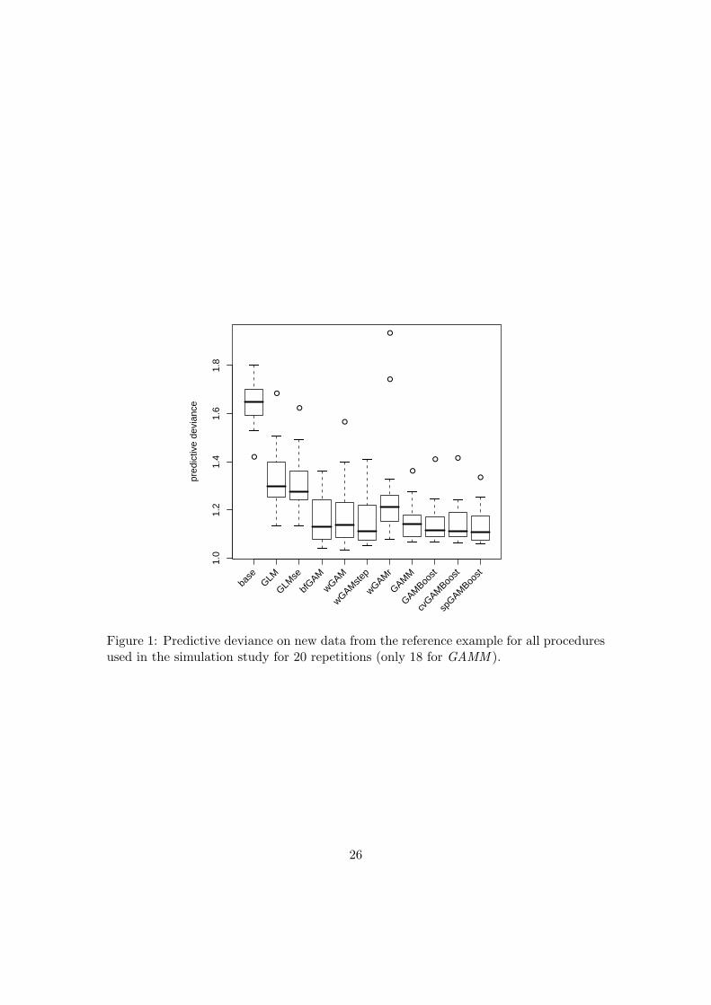
Figure 1 shows boxplots for the predictive deviance for all procedures. The procedures

that fit a generalized linear model, GLM and GLMse, despite being not adequate for

the underlying structure, are seen to improve over the baseline model (base) which

does not use covariate information. Nevertheless all procedures that fit a generalized

additive model can improve over the linear models. This indicates that there is enough

information in the data for the procedures to benefit from fitting non-linear functions. In

this rather simple example they all have similar prediction performance, with GAMBoost

procedures showing a slight advantage in terms of mean performance and variability, and

GAMM being close to the latter. The performance of the variant of wGAM that does

not employ an increased weight for the degrees of freedom, wGAMr, is distinctly worse

than that of wGAM. For the GAMBoost procedures there does not seem to be a large

16

Table 1: Mean predictive deviances for examples with Gaussian response and varyingamount of covariate effect (ce), number of covariates (p), number of informative covari-ates (inf) and (base) correlation (ρb). In addition each example is characterized by itssignal-to-noise ratio (stn). The fitted procedures are base (1), GLMse (2), bfGAM (3),wGAM (4), wGAMstep (5), GAMM (6), GAMBoost (7), and spGAMBoost (8). Foreach example the number of repetitions where no fit could be obtained for a procedure isgiven in parentheses. The best two procedures (evaluated on the remaining repetitions)are printed in boldface.ce p inf ρb stn procedures

(1) (2) (3) (4) (5) (6) (7) (8)linear covariate influence0.33 6 3 0 0.2 1.23 1.09 1.12 1.11 1.11 1.08 (2) 1.08 1.10

6 0 0.4 1.47 1.15 1.16 1.16 1.16 1.13 1.14 1.1710 3 0 0.2 1.23 1.10 1.14 1.17 1.14 1.09 (5) 1.10 1.15

6 0 0.4 1.45 1.16 1.20 1.23 1.20 1.14 (1) 1.16 1.210.5 6 3 0 0.5 1.53 1.08 1.11 1.13 1.11 1.09 (2) 1.11 1.13

0.7 1.1 2.15 1.10 1.16 1.13 1.15 1.10 (2) 1.11 1.136 0 1.0 2.06 1.09 1.13 1.16 1.13 1.13 1.17 1.19

10 3 0 0.5 1.51 1.08 1.13 1.17 1.12 1.10 (2) 1.12 1.160.7 1.1 2.17 1.11 1.16 1.16 1.17 1.10 (6) 1.11 1.15

6 0 1.0 2.02 1.10 1.16 1.20 1.14 1.13 (1) 1.20 1.2320 3 0 0.5 1.51 1.14 - - 1.26 - 1.13 1.1950 3 0 0.5 1.54 1.52 - - 1.61 - 1.18 1.28

0.75 6 3 0 1.1 2.18 1.07 1.11 1.12 1.10 1.09 (1) 1.12 1.1410 3 0 1.1 2.15 1.08 1.12 1.17 1.12 1.10 (2) 1.14 1.17

non-linear covariate influence0.33 6 3 0 0.3 1.29 1.19 1.19 1.18 1.18 1.13 (4) 1.11 1.12

6 0 0.6 1.59 1.37 1.31 1.26 1.28 1.25 (1) 1.20 1.2310 3 0 0.3 1.30 1.25 1.31 1.24 1.25 1.18 (4) 1.18 1.21

6 0 0.6 1.59 1.42 1.42 1.36 1.34 1.27 (3) 1.25 1.310.5 6 3 0 0.6 1.65 1.31 1.16 1.18 1.15 1.15 (2) 1.14 1.14

0.7 1.0 2.00 1.38 1.13 1.12 1.11 1.12 (2) 1.13 1.136 0 1.3 2.33 1.67 1.33 1.31 1.33 1.32 1.25 1.28

10 3 0 0.6 1.67 1.44 1.30 1.26 1.26 1.25 (5) 1.23 1.250.7 1.0 1.97 1.48 1.32 1.22 1.29 1.21 (2) 1.19 1.19

6 0 1.3 2.32 1.76 1.42 1.39 1.35 1.36 (3) 1.33 1.3520 3 0 0.6 1.64 1.48 - - 1.37 - 1.23 1.2750 3 0 0.6 1.61 1.87 - - 1.87 - 1.26 1.37

0.75 6 3 0 1.4 2.46 1.67 1.16 1.16 1.16 1.16 (1) 1.20 1.1710 3 0 1.4 2.48 1.85 1.28 1.30 1.26 1.20 (4) 1.28 1.24

17

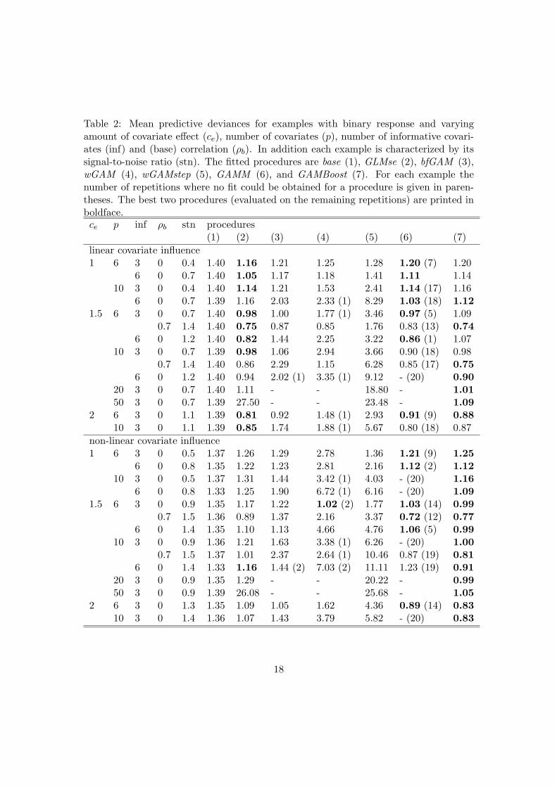
Table 2: Mean predictive deviances for examples with binary response and varyingamount of covariate effect (ce), number of covariates (p), number of informative covari-ates (inf) and (base) correlation (ρb). In addition each example is characterized by itssignal-to-noise ratio (stn). The fitted procedures are base (1), GLMse (2), bfGAM (3),wGAM (4), wGAMstep (5), GAMM (6), and GAMBoost (7). For each example thenumber of repetitions where no fit could be obtained for a procedure is given in paren-theses. The best two procedures (evaluated on the remaining repetitions) are printed inboldface.ce p inf ρb stn procedures

(1) (2) (3) (4) (5) (6) (7)linear covariate influence1 6 3 0 0.4 1.40 1.16 1.21 1.25 1.28 1.20 (7) 1.20

6 0 0.7 1.40 1.05 1.17 1.18 1.41 1.11 1.1410 3 0 0.4 1.40 1.14 1.21 1.53 2.41 1.14 (17) 1.16

6 0 0.7 1.39 1.16 2.03 2.33 (1) 8.29 1.03 (18) 1.121.5 6 3 0 0.7 1.40 0.98 1.00 1.77 (1) 3.46 0.97 (5) 1.09

0.7 1.4 1.40 0.75 0.87 0.85 1.76 0.83 (13) 0.746 0 1.2 1.40 0.82 1.44 2.25 3.22 0.86 (1) 1.07

10 3 0 0.7 1.39 0.98 1.06 2.94 3.66 0.90 (18) 0.980.7 1.4 1.40 0.86 2.29 1.15 6.28 0.85 (17) 0.75

6 0 1.2 1.40 0.94 2.02 (1) 3.35 (1) 9.12 - (20) 0.9020 3 0 0.7 1.40 1.11 - - 18.80 - 1.0150 3 0 0.7 1.39 27.50 - - 23.48 - 1.09

2 6 3 0 1.1 1.39 0.81 0.92 1.48 (1) 2.93 0.91 (9) 0.8810 3 0 1.1 1.39 0.85 1.74 1.88 (1) 5.67 0.80 (18) 0.87

non-linear covariate influence1 6 3 0 0.5 1.37 1.26 1.29 2.78 1.36 1.21 (9) 1.25

6 0 0.8 1.35 1.22 1.23 2.81 2.16 1.12 (2) 1.1210 3 0 0.5 1.37 1.31 1.44 3.42 (1) 4.03 - (20) 1.16

6 0 0.8 1.33 1.25 1.90 6.72 (1) 6.16 - (20) 1.091.5 6 3 0 0.9 1.35 1.17 1.22 1.02 (2) 1.77 1.03 (14) 0.99

0.7 1.5 1.36 0.89 1.37 2.16 3.37 0.72 (12) 0.776 0 1.4 1.35 1.10 1.13 4.66 4.76 1.06 (5) 0.99

10 3 0 0.9 1.36 1.21 1.63 3.38 (1) 6.26 - (20) 1.000.7 1.5 1.37 1.01 2.37 2.64 (1) 10.46 0.87 (19) 0.81

6 0 1.4 1.33 1.16 1.44 (2) 7.03 (2) 11.11 1.23 (19) 0.9120 3 0 0.9 1.35 1.29 - - 20.22 - 0.9950 3 0 0.9 1.39 26.08 - - 25.68 - 1.05

2 6 3 0 1.3 1.35 1.09 1.05 1.62 4.36 0.89 (14) 0.8310 3 0 1.4 1.36 1.07 1.43 3.79 5.82 - (20) 0.83

18

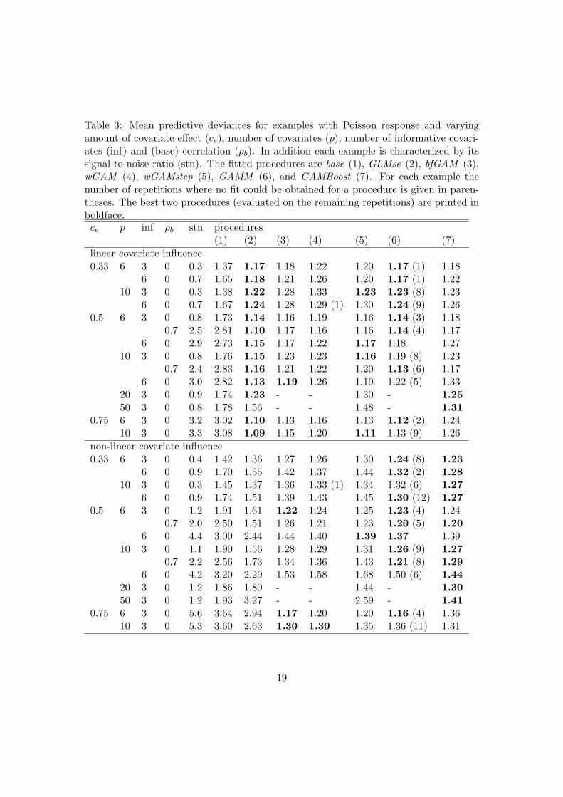
Table 3: Mean predictive deviances for examples with Poisson response and varyingamount of covariate effect (ce), number of covariates (p), number of informative covari-ates (inf) and (base) correlation (ρb). In addition each example is characterized by itssignal-to-noise ratio (stn). The fitted procedures are base (1), GLMse (2), bfGAM (3),wGAM (4), wGAMstep (5), GAMM (6), and GAMBoost (7). For each example thenumber of repetitions where no fit could be obtained for a procedure is given in paren-theses. The best two procedures (evaluated on the remaining repetitions) are printed inboldface.ce p inf ρb stn procedures

(1) (2) (3) (4) (5) (6) (7)linear covariate influence0.33 6 3 0 0.3 1.37 1.17 1.18 1.22 1.20 1.17 (1) 1.18

6 0 0.7 1.65 1.18 1.21 1.26 1.20 1.17 (1) 1.2210 3 0 0.3 1.38 1.22 1.28 1.33 1.23 1.23 (8) 1.23

6 0 0.7 1.67 1.24 1.28 1.29 (1) 1.30 1.24 (9) 1.260.5 6 3 0 0.8 1.73 1.14 1.16 1.19 1.16 1.14 (3) 1.18

0.7 2.5 2.81 1.10 1.17 1.16 1.16 1.14 (4) 1.176 0 2.9 2.73 1.15 1.17 1.22 1.17 1.18 1.27

10 3 0 0.8 1.76 1.15 1.23 1.23 1.16 1.19 (8) 1.230.7 2.4 2.83 1.16 1.21 1.22 1.20 1.13 (6) 1.17

6 0 3.0 2.82 1.13 1.19 1.26 1.19 1.22 (5) 1.3320 3 0 0.9 1.74 1.23 - - 1.30 - 1.2550 3 0 0.8 1.78 1.56 - - 1.48 - 1.31

0.75 6 3 0 3.2 3.02 1.10 1.13 1.16 1.13 1.12 (2) 1.2410 3 0 3.3 3.08 1.09 1.15 1.20 1.11 1.13 (9) 1.26

non-linear covariate influence0.33 6 3 0 0.4 1.42 1.36 1.27 1.26 1.30 1.24 (8) 1.23

6 0 0.9 1.70 1.55 1.42 1.37 1.44 1.32 (2) 1.2810 3 0 0.3 1.45 1.37 1.36 1.33 (1) 1.34 1.32 (6) 1.27

6 0 0.9 1.74 1.51 1.39 1.43 1.45 1.30 (12) 1.270.5 6 3 0 1.2 1.91 1.61 1.22 1.24 1.25 1.23 (4) 1.24

0.7 2.0 2.50 1.51 1.26 1.21 1.23 1.20 (5) 1.206 0 4.4 3.00 2.44 1.44 1.40 1.39 1.37 1.39

10 3 0 1.1 1.90 1.56 1.28 1.29 1.31 1.26 (9) 1.270.7 2.2 2.56 1.73 1.34 1.36 1.43 1.21 (8) 1.29

6 0 4.2 3.20 2.29 1.53 1.58 1.68 1.50 (6) 1.4420 3 0 1.2 1.86 1.80 - - 1.44 - 1.3050 3 0 1.2 1.93 3.27 - - 2.59 - 1.41

0.75 6 3 0 5.6 3.64 2.94 1.17 1.20 1.20 1.16 (4) 1.3610 3 0 5.3 3.60 2.63 1.30 1.30 1.35 1.36 (11) 1.31

19

Table 4: Mean hit rates/false alarm rates for examples with Gaussian response andvarying amount of covariate effect (ce), number of covariates (p), number of informativecovariates (inf) and (base) correlation (ρb). In addition each example is characterizedby its signal-to-noise ratio (stn). The fitted procedures are GLMse (2), bfGAM (3),wGAM (4), wGAMstep (5), GAMM (6), GAMBoost (7), and spGAMBoost (8). Foreach example the number of repetitions where no fit could be obtained for a procedureis given in parentheses.ce p inf ρb stn procedures

(2) (3) (4) (5) (6) (7) (8)linear covariate influence0.33 6 3 0 0.2 87/10 88/15 72/3 85/8 63/2 (2) 88/22 88/15

6 0 0.4 82/- 86/- 72/- 82/- 61/- 88/- 84/-10 3 0 0.2 90/14 92/16 67/14 80/14 67/4 (5) 95/24 93/24

6 0 0.4 86/15 89/19 70/16 82/14 65/7 (1) 88/25 86/250.5 6 3 0 0.5 98/12 98/17 95/5 95/10 91/4 (2) 97/28 97/22

0.7 1.1 82/5 83/13 90/12 72/12 70/0 (2) 98/23 95/226 0 1.0 99/- 99/- 95/- 98/- 92/- 99/- 99/-

10 3 0 0.5 100/14 100/16 98/14 98/13 96/6 (2) 100/24 100/240.7 1.1 85/14 83/16 90/11 80/12 83/4 (6) 98/27 98/23

6 0 1.0 100/16 100/19 99/15 98/14 94/5 (1) 99/26 98/2520 3 0 0.5 100/15 - - 98/19 - 98/19 100/1950 3 0 0.5 98/21 - - 98/19 - 100/13 100/13

0.75 6 3 0 1.1 100/13 100/20 100/7 100/15 100/5 (1) 100/25 100/2210 3 0 1.1 100/13 100/15 100/11 100/11 100/5 (2) 100/23 100/24

non-linear covariate influence0.33 6 3 0 0.3 65/15 78/20 67/17 73/18 58/10 (4) 85/23 87/23

6 0 0.6 57/- 77/- 66/- 72/- 67/- (1) 88/- 83/-10 3 0 0.3 53/14 75/18 67/15 68/13 58/4 (4) 77/21 70/14

6 0 0.6 57/9 85/22 73/16 77/14 64/9 (3) 92/24 86/210.5 6 3 0 0.6 77/12 98/15 97/12 97/13 96/7 (2) 100/23 100/23

0.7 1.0 58/3 97/8 90/3 87/5 83/2 (2) 98/20 98/106 0 1.3 70/- 97/- 92/- 97/- 90/- 100/- 100/-

10 3 0 0.6 67/14 97/18 95/16 93/14 82/6 (5) 98/24 98/230.7 1.0 60/10 85/22 90/10 82/14 81/4 (2) 98/21 98/19

6 0 1.3 65/8 96/20 95/14 97/14 93/9 (3) 99/25 98/2020 3 0 0.6 77/16 - - 95/14 - 97/19 93/1850 3 0 0.6 85/21 - - 92/18 - 97/17 98/17

0.75 6 3 0 1.4 77/13 100/13 100/7 100/12 100/7 (1) 100/27 100/2310 3 0 1.4 73/12 100/19 100/14 100/12 100/4 (4) 100/26 100/20

20

Table 5: Mean hit rates/false alarm rates for examples with binary response and varyingamount of covariate effect (ce), number of covariates (p), number of informative covari-ates (inf) and (base) correlation (ρb). In addition each example is characterized by itssignal-to-noise ratio (stn). The fitted procedures are GLMse (2), bfGAM (3), wGAM(4), wGAMstep (5), GAMM (6), and GAMBoost (7). For each example the number ofrepetitions where no fit could be obtained for a procedure is given in parentheses.

ce p inf ρb stn procedures(2) (3) (4) (5) (6) (7)

linear covariate influence1 6 3 0 0.4 95/20 95/25 78/13 63/18 74/15 (7) 93/33

6 0 0.7 93/- 93/- 68/- 77/- 74/- 90/-10 3 0 0.4 97/7 97/12 87/9 60/8 56/0 (17) 98/15

6 0 0.7 92/19 93/38 67/9 (1) 81/35 75/0 (18) 93/291.5 6 3 0 0.7 100/20 100/17 93/4 (1) 85/18 100/18 (5) 100/33

0.7 1.4 83/8 83/20 68/3 78/15 76/29 (13) 93/226 0 1.2 100/- 100/- 74/- 91/- 95/- (1) 100/-

10 3 0 0.7 100/10 100/14 90/4 92/20 100/7 (18) 100/170.7 1.4 90/16 92/28 78/4 70/36 78/29 (17) 100/16

6 0 1.2 98/20 98/32 (1) 73/5 (1) 81/30 -/- (20) 98/2520 3 0 0.7 100/14 - - 88/55 - 100/1350 3 0 0.7 75/51 - - 75/28 - 98/14

2 6 3 0 1.1 100/12 100/17 95/4 (1) 97/15 100/27 (9) 100/2810 3 0 1.1 100/8 100/21 88/3 (1) 88/27 100/0 (18) 100/19

non-linear covariate influence1 6 3 0 0.5 68/13 95/15 77/8 38/13 91/3 (9) 97/27

6 0 0.8 59/- 84/- 56/- 38/- 52/- (2) 94/-10 3 0 0.5 63/12 97/20 79/7 (1) 25/13 -/- (20) 95/25

6 0 0.8 54/8 78/19 32/4 (1) 42/18 -/- (20) 92/251.5 6 3 0 0.9 70/12 98/15 96/2 (2) 75/12 100/11 (14) 100/23

0.7 1.5 72/7 87/13 57/0 62/12 71/8 (12) 95/256 0 1.4 69/- 97/- 43/- 52/- 42/- (5) 98/-

10 3 0 0.9 68/12 98/24 68/9 (1) 63/27 -/- (20) 98/230.7 1.5 68/17 90/37 58/5 (1) 43/52 100/0 (19) 100/21

6 0 1.4 66/11 91/18 (2) 25/1 (2) 59/32 0/0 (19) 97/2620 3 0 0.9 67/13 - - 55/69 - 100/1550 3 0 0.9 83/49 - - 77/34 - 98/12

2 6 3 0 1.3 75/13 100/18 85/3 73/28 83/11 (14) 100/2310 3 0 1.4 78/9 100/18 67/2 68/25 -/- (20) 100/15

21

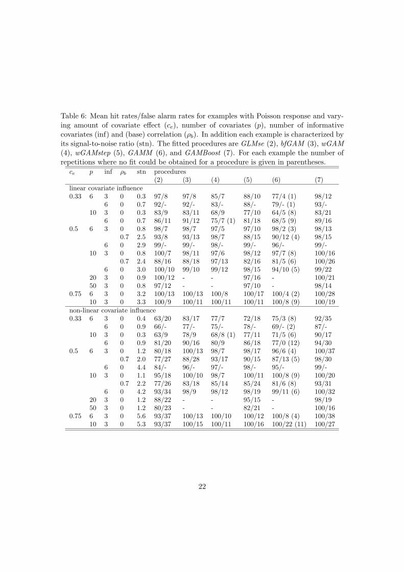
Table 6: Mean hit rates/false alarm rates for examples with Poisson response and vary-ing amount of covariate effect (ce), number of covariates (p), number of informativecovariates (inf) and (base) correlation (ρb). In addition each example is characterized byits signal-to-noise ratio (stn). The fitted procedures are GLMse (2), bfGAM (3), wGAM(4), wGAMstep (5), GAMM (6), and GAMBoost (7). For each example the number ofrepetitions where no fit could be obtained for a procedure is given in parentheses.

ce p inf ρb stn procedures(2) (3) (4) (5) (6) (7)

linear covariate influence0.33 6 3 0 0.3 97/8 97/8 85/7 88/10 77/4 (1) 98/12

6 0 0.7 92/- 92/- 83/- 88/- 79/- (1) 93/-10 3 0 0.3 83/9 83/11 68/9 77/10 64/5 (8) 83/21

6 0 0.7 86/11 91/12 75/7 (1) 81/18 68/5 (9) 89/160.5 6 3 0 0.8 98/7 98/7 97/5 97/10 98/2 (3) 98/13

0.7 2.5 93/8 93/13 98/7 88/15 90/12 (4) 98/156 0 2.9 99/- 99/- 98/- 99/- 96/- 99/-

10 3 0 0.8 100/7 98/11 97/6 98/12 97/7 (8) 100/160.7 2.4 88/16 88/18 97/13 82/16 81/5 (6) 100/26

6 0 3.0 100/10 99/10 99/12 98/15 94/10 (5) 99/2220 3 0 0.9 100/12 - - 97/16 - 100/2150 3 0 0.8 97/12 - - 97/10 - 98/14

0.75 6 3 0 3.2 100/13 100/13 100/8 100/17 100/4 (2) 100/2810 3 0 3.3 100/9 100/11 100/11 100/11 100/8 (9) 100/19

non-linear covariate influence0.33 6 3 0 0.4 63/20 83/17 77/7 72/18 75/3 (8) 92/35

6 0 0.9 66/- 77/- 75/- 78/- 69/- (2) 87/-10 3 0 0.3 63/9 78/9 68/8 (1) 77/11 71/5 (6) 90/17

6 0 0.9 81/20 90/16 80/9 86/18 77/0 (12) 94/300.5 6 3 0 1.2 80/18 100/13 98/7 98/17 96/6 (4) 100/37

0.7 2.0 77/27 88/28 93/17 90/15 87/13 (5) 98/306 0 4.4 84/- 96/- 97/- 98/- 95/- 99/-

10 3 0 1.1 95/18 100/10 98/7 100/11 100/8 (9) 100/200.7 2.2 77/26 83/18 85/14 85/24 81/6 (8) 93/31

6 0 4.2 93/34 98/9 98/12 98/19 99/11 (6) 100/3220 3 0 1.2 88/22 - - 95/15 - 98/1950 3 0 1.2 80/23 - - 82/21 - 100/16

0.75 6 3 0 5.6 93/37 100/13 100/10 100/12 100/8 (4) 100/3810 3 0 5.3 93/37 100/15 100/11 100/16 100/22 (11) 100/27

22

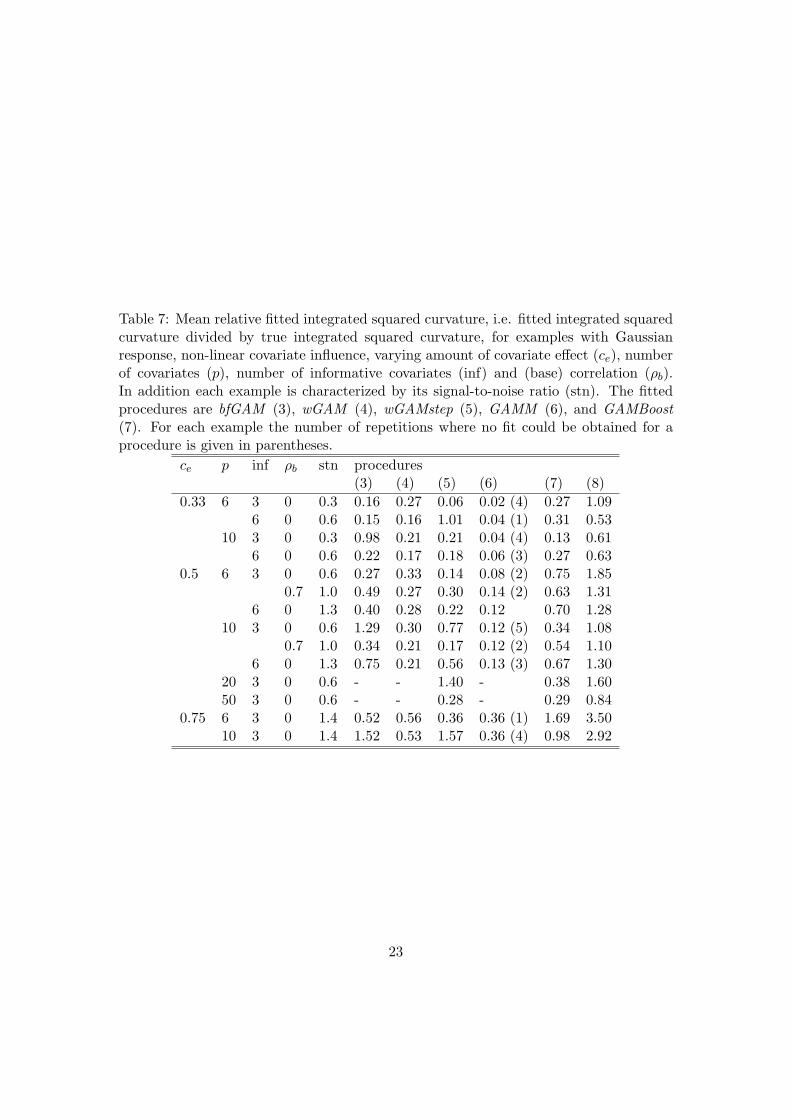
Table 7: Mean relative fitted integrated squared curvature, i.e. fitted integrated squaredcurvature divided by true integrated squared curvature, for examples with Gaussianresponse, non-linear covariate influence, varying amount of covariate effect (ce), numberof covariates (p), number of informative covariates (inf) and (base) correlation (ρb).In addition each example is characterized by its signal-to-noise ratio (stn). The fittedprocedures are bfGAM (3), wGAM (4), wGAMstep (5), GAMM (6), and GAMBoost(7). For each example the number of repetitions where no fit could be obtained for aprocedure is given in parentheses.

ce p inf ρb stn procedures(3) (4) (5) (6) (7) (8)

0.33 6 3 0 0.3 0.16 0.27 0.06 0.02 (4) 0.27 1.096 0 0.6 0.15 0.16 1.01 0.04 (1) 0.31 0.53

10 3 0 0.3 0.98 0.21 0.21 0.04 (4) 0.13 0.616 0 0.6 0.22 0.17 0.18 0.06 (3) 0.27 0.63

0.5 6 3 0 0.6 0.27 0.33 0.14 0.08 (2) 0.75 1.850.7 1.0 0.49 0.27 0.30 0.14 (2) 0.63 1.31

6 0 1.3 0.40 0.28 0.22 0.12 0.70 1.2810 3 0 0.6 1.29 0.30 0.77 0.12 (5) 0.34 1.08

0.7 1.0 0.34 0.21 0.17 0.12 (2) 0.54 1.106 0 1.3 0.75 0.21 0.56 0.13 (3) 0.67 1.30

20 3 0 0.6 - - 1.40 - 0.38 1.6050 3 0 0.6 - - 0.28 - 0.29 0.84

0.75 6 3 0 1.4 0.52 0.56 0.36 0.36 (1) 1.69 3.5010 3 0 1.4 1.52 0.53 1.57 0.36 (4) 0.98 2.92

23

Table 8: Mean relative fitted integrated squared curvature, i.e. fitted integrated squaredcurvature divided by true integrated squared curvature, for examples with binary re-sponse, non-linear covariate influence, varying amount of covariate effect (ce), numberof covariates (p), number of informative covariates (inf) and (base) correlation (ρb). Inaddition each example is characterized by its signal-to-noise ratio (stn). The fitted pro-cedures are bfGAM (3), wGAM (4), wGAMstep (5), GAMM (6), GAMBoost (7), andspGAMBoost (8). For each example the number of repetitions where no fit could beobtained for a procedure is given in parentheses. Values greater than 10 (mostly due toerroneously fitted asymptotes) are indicated by “>10”.

ce p inf ρb stn procedures(3) (4) (5) (6) (7)

1 6 3 0 0.5 3.60 >10 0.74 0.85 (9) >106 0 0.8 2.70 >10 >10 0.10 (2) >10

10 3 0 0.5 >10 >10 (1) >10 - (20) 2.386 0 0.8 >10 >10 (1) >10 - (20) 4.56

1.5 6 3 0 0.9 >10 5.77 (2) >10 1.20 (14) >100.7 1.5 >10 >10 >10 0.59 (12) 8.11

6 0 1.4 >10 >10 >10 0.28 (5) >1010 3 0 0.9 >10 >10 (1) >10 - (20) 5.22

0.7 1.5 >10 >10 (1) >10 0.78 (19) 3.216 0 1.4 >10 (2) >10 (2) >10 0.02 (19) 8.21

20 3 0 0.9 - - >10 - 3.6250 3 0 0.9 - - 0 - 3.17

2 6 3 0 1.3 >10 >10 >10 0.99 (14) >1010 3 0 1.4 >10 >10 >10 - (20) 7.24

24

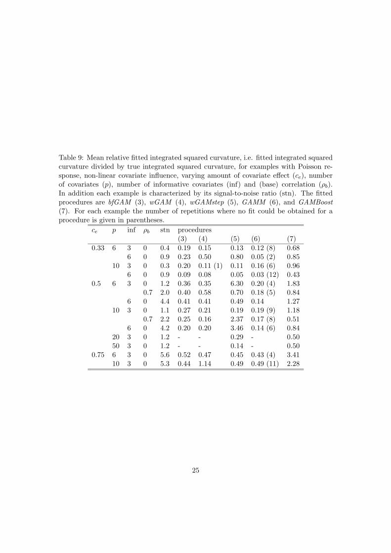
Table 9: Mean relative fitted integrated squared curvature, i.e. fitted integrated squaredcurvature divided by true integrated squared curvature, for examples with Poisson re-sponse, non-linear covariate influence, varying amount of covariate effect (ce), numberof covariates (p), number of informative covariates (inf) and (base) correlation (ρb).In addition each example is characterized by its signal-to-noise ratio (stn). The fittedprocedures are bfGAM (3), wGAM (4), wGAMstep (5), GAMM (6), and GAMBoost(7). For each example the number of repetitions where no fit could be obtained for aprocedure is given in parentheses.

ce p inf ρb stn procedures(3) (4) (5) (6) (7)

0.33 6 3 0 0.4 0.19 0.15 0.13 0.12 (8) 0.686 0 0.9 0.23 0.50 0.80 0.05 (2) 0.85

10 3 0 0.3 0.20 0.11 (1) 0.11 0.16 (6) 0.966 0 0.9 0.09 0.08 0.05 0.03 (12) 0.43

0.5 6 3 0 1.2 0.36 0.35 6.30 0.20 (4) 1.830.7 2.0 0.40 0.58 0.70 0.18 (5) 0.84

6 0 4.4 0.41 0.41 0.49 0.14 1.2710 3 0 1.1 0.27 0.21 0.19 0.19 (9) 1.18

0.7 2.2 0.25 0.16 2.37 0.17 (8) 0.516 0 4.2 0.20 0.20 3.46 0.14 (6) 0.84

20 3 0 1.2 - - 0.29 - 0.5050 3 0 1.2 - - 0.14 - 0.50

0.75 6 3 0 5.6 0.52 0.47 0.45 0.43 (4) 3.4110 3 0 5.3 0.44 1.14 0.49 0.49 (11) 2.28

25

●

●

●

●

●

●

●

● ●

●

1.0

1.2

1.4

1.6

1.8

pred

ictiv

e de

vian

ce

base

GLM

GLMse

bfGAM

wGAM

wGAMste

p

wGAMr

GAMM

GAMBoo

st

cvGAM

Boost

spGAM

Boost

Figure 1: Predictive deviance on new data from the reference example for all proceduresused in the simulation study for 20 repetitions (only 18 for GAMM ).

26

0.00 0.05 0.10 0.15 0.20 0.25 0.30

0.70

0.75

0.80

0.85

0.90

0.95

1.00

false alarm rate

hit r

ate

2

3/4*4 56

7/8

Figure 2: Mean hit rates/false alarm rates from the reference example for GLMse (2),bfGAM (3), wGAM (4), wGAMr (4*) ,wGAMstep (5), GAMM (6), GAMBoost (7), andspGAMBoost (8).

difference between the variant that uses AICC for selection of the number of boosting

steps, GAMBoost, and the variant that uses cross-validation, cvGAMBoost. There might

be a slightly better prediction performance for the sparse variant, spGAMBoost.

Besides prediction performance, identification of informative covariates is also an im-

portant performance measure. The mean hit rates/false alarm rates for the procedures

in this example are shown in Figure 2. The stepwise procedure for fitting a generalized

linear model (GLMse) is distinctly worse in terms of identification of influential covari-

ates, probably because it discards covariates with e.g. influence of quadratic shape. For

comparison, wGAM has the same false alarm rate but a much better hit rate at the

same time. The un-modified version of the latter, wGAMr, employs a more lenient (im-

27

● ●

●

●

●

●

●

●

02

46

810

fitte

d in

tegr

ated

squ

ared

cur

vatu

re

bfGAM

wGAM

GAMM

GAMBoo

st

bfGAM

wGAM

GAMM

GAMBoo

st

bfGAM

wGAM

GAMM

GAMBoo

st

bfGAM

wGAM

GAMM

GAMBoo

st

linear; 0 quadratic; 11.2 invlogit; 20.8 sinus; 24.4

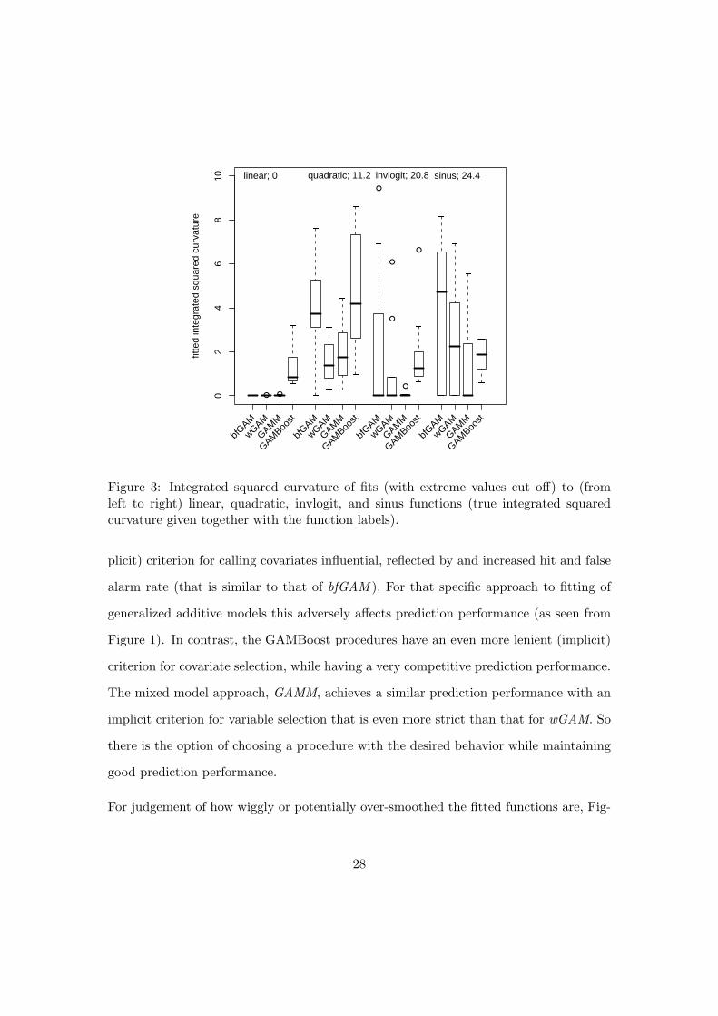
Figure 3: Integrated squared curvature of fits (with extreme values cut off) to (fromleft to right) linear, quadratic, invlogit, and sinus functions (true integrated squaredcurvature given together with the function labels).

plicit) criterion for calling covariates influential, reflected by and increased hit and false

alarm rate (that is similar to that of bfGAM ). For that specific approach to fitting of

generalized additive models this adversely affects prediction performance (as seen from

Figure 1). In contrast, the GAMBoost procedures have an even more lenient (implicit)

criterion for covariate selection, while having a very competitive prediction performance.

The mixed model approach, GAMM, achieves a similar prediction performance with an

implicit criterion for variable selection that is even more strict than that for wGAM. So

there is the option of choosing a procedure with the desired behavior while maintaining

good prediction performance.

For judgement of how wiggly or potentially over-smoothed the fitted functions are, Fig-

28

ure 3 shows the integrated squared curvature (5) (from left to right) for fits to linear

functions, fquadratic, finvlogit, and fsinus for some of the procedures. The order is ac-

cording to integrated squared curvature of the true functions (given together with the

function labels in Figure 3), so one could expect that the fitted squared curvature would

increase for each procedure from left to right. This is not the case. Especially for finvlogit

often no curvature, i.e. a linear function, is fitted. For the linear functions (leftmost

four boxes) all procedures except GAMBoost fit linear functions in almost all instances.

Except for the linear functions, the integrated squared curvature of the fits is always

smaller than that of the true functions. This might indicate that there is not enough

information in the data and therefore the bias-variance tradeoff implicitly performed by

the procedures leads to a large bias. Overall, GAMM fits the least amount of curvature

of all procedures, i.e. exhibits the largest bias. The curvature found for GAMBoost is

rather large and therefore closer to the true curvature. In addition, it is very similar for

all kinds of functions, which might be due to the specific penalization scheme used. An-

other explanation might be, that fitted curvature increases with the number of boosting

steps where a covariate receives an update. As more important covariates are targeted

in a larger number boosting steps the integrated squared curvature increases for these.

While this impedes adequate fits for linear functions, it provides the basis for less bias

in fits to non-linear functions.

Having investigated the behavior of the procedures in this reference example, we now

turn to the characteristics of the data highlighted in Section 1 and their effect on per-

formance.

29

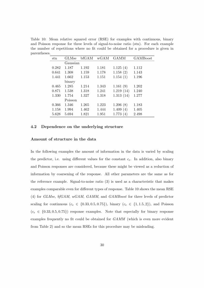
Table 10: Mean relative squared error (RSE) for examples with continuous, binaryand Poisson response for three levels of signal-to-noise ratio (stn). For each examplethe number of repetitions where no fit could be obtained for a procedure is given inparentheses.

stn GLMse bfGAM wGAM GAMM GAMBoostGaussian

0.282 1.187 1.192 1.181 1.125 (4) 1.1120.641 1.308 1.159 1.178 1.158 (2) 1.1431.441 1.662 1.153 1.151 1.154 (1) 1.196

binary0.465 1.285 1.214 1.343 1.161 (9) 1.2020.871 1.538 1.318 1.241 1.219 (14) 1.2401.330 1.754 1.327 1.318 1.313 (14) 1.277

Poisson0.366 1.346 1.265 1.223 1.206 (8) 1.1831.158 1.994 1.462 1.444 1.409 (4) 1.4055.628 5.694 1.821 1.951 1.773 (4) 2.498

4.2 Dependence on the underlying structure

Amount of structure in the data

In the following examples the amount of information in the data is varied by scaling

the predictor, i.e. using different values for the constant ce. In addition, also binary

and Poisson responses are considered, because these might be viewed as a reduction of

information by coarsening of the response. All other parameters are the same as for

the reference example. Signal-to-noise ratio (3) is used as a characteristic that makes

examples comparable even for different types of response. Table 10 shows the mean RSE

(4) for GLMse, bfGAM, wGAM, GAMM, and GAMBoost for three levels of predictor

scaling for continuous (ce ∈ {0.33, 0.5, 0.75}), binary (ce ∈ {1, 1.5, 2}), and Poisson

(ce ∈ {0.33, 0.5, 0.75}) response examples. Note that especially for binary response

examples frequently no fit could be obtained for GAMM (which is even more evident

from Table 2) and so the mean RSEs for this procedure may be misleading.

30

If binary and Poisson responses were essentialy a coarsening, i.e., discarding of informa-

tion, the RSEs should be similar for different response types when the signal-to-noise

ratio is similar. This is seen not to be the case. The mean RSEs for binary and Poisson

response examples are larger than that for examples with continuous response. Also, for

the change of prediction performance following a change in signal-to-noise ratio there is a

different pattern for different response types. For continuous response examples there is

only little change in mean RSE as the signal-to-noise ratio increases. In tendency it de-

creases for bfGAM and wGAM, indicating better performance for larger signal-to-noise

ratios, while for GAMBoost the mean RSE increases. The mean predictive deviances for

continuous response examples in Table 1 indicate that the latter method performs best

for small signal-to-noise ratios. For a large signal-to-noise ratio GAMM, when it works,

delivers the best prediction performance. For binary and Poisson response examples the

mean RSEs increase for all methods as the signal-to-noise ratio increases. This differ-

ent pattern might be explained by the fact that most of the procedures use different

algorithms for the generalized response case compared to continuous response examples.

For binary and Poisson response examples (see also Table 2) GAMBoost outperforms

the other procedures, except for the Poisson example with a very large signal-to-noise

ratio.

Number of non-influential covariates

Figure 4 shows the effect of the number of covariates on predictive deviance. All param-

eters of the data are the same as in the reference example, only the number of covariates

is increased, i.e., more and more non-informative covariates are added. So the leftmost

block of boxes is a subset of Figure 1. For up to 10 covariates all procedures for fit-

ting generalized additive models show similar performance that is well ahead of GLMse.

Table 2 indicates that this is not the case for the seemingly more difficult to fit binary

31

●●

●●

●

●

● ●

●

●

●

1.0

1.5

2.0

2.5

3.0

pred

ictiv

e de

vian

ce

GLMse

bfGAM

wGAM

wGAMste

p

GAMM

GAMBoo

st

spGAM

Boost

GLMse

bfGAM

wGAM

wGAMste

p

GAMM

GAMBoo

st

spGAM

Boost

GLMse

wGAMste

p

GAMBoo

st

spGAM

Boost

GLMse

wGAMste

p

GAMBoo

st

spGAM

Boost

p=6 p=10 p=20 p=50

Figure 4: Effect of the total number of covariates p on predictive deviance.

response examples: With non-linear covariate influence and 10 covariates only the per-

formance of GAMBoost is still better than that of the baseline model (and also that of

GLMse). For the Gaussian examples the largest variability in performance is found for

bfGAM, the least for GAMM and GAMBoost, but note that for GAMM for 2 repeti-

tions with 6 covariates and for 5 repetitions with 10 covariates no fit could be obtained.

spGAMBoost seems to have a slight advantage over GAMBoost for p = 6 and p = 10, but

performs worse for p = 20 and p = 50. This is not what one would expect, because the

optimization for sparseness in spGAMBoost should result in a performance advantage

in such sparse settings. For p = 20 and p = 50 wGAMstep is the only other procedure

with which still fits can be obtained. While for p = 20 it has reasonable performance,

for p = 50 it performs distinctly worse compared to the GAMBoost procedures.

For p = 10 covariates the mean hit rates/false alarm rates are as follows: bfGAM :

32

0.97/0.18; wGAM : 0.95/0.16; wGAMstep: 0.93/0.14; GAMM : 0.82/0.06; GAMBoost :

0.98/0.24. So the most severe drop in performance with respect to identification of

influential covariates compared to the reference example is seen for GAMM (for which

in addition for 5 repetitions no fit could be obtained). For all other procedure the

performance basically stays the same. For p = 20 the mean hit rates/false alarm rates

are 0.95/0.14 for wGAMstep and 0.97/0.19 for GAMBoost, and for p = 50 they are

0.92/0.18 and 0.97/0.17 respectively. It is surprising that while prediction performance

drastically decreases for wGAMstep as the number of covariates increases, there is only

a slight worsening of the hit rates and the false alarm rates. For GAMBoost even for

p = 50 there is hardly any change compared to p = 10. So it is seen to perform very

well in terms of identification of influential covariates as well as in terms of prediction

performance for a large number of covariates.

Number of influential covariates/distribution of information

The effect of changing the number of covariates over which the information in the data

is distributed is illustrated in Figure 5. The leftmost block of boxes shows the mean

predictive deviances from the reference example. In the block next to it there are 6

instead of three informative covariates, but the predictor is scaled (ce = 0.33), such that

the signal-to-noise ratio is approximately equal to that in the reference example. Note

that now all covariates are informative. In the right two blocks there are 10 covariates in

total and a larger signal-to-noise ratio is used. Again the left of the two blocks has 3 and

right one 6 informative covariates and the signal-to-noise ratio is fixed at a similar level

for both (with ce = 0.5 and ce = 0.75). An indication that the leftmost block and the 3rd

block from the left represent sparse examples and the other two non-sparse ones, is that

spGAMBoost, which is optimized for sparse scenarios, outperforms GAMBoost for the

former, but not for the latter. The GAMBoost procedures, compared the others, seem

33

●

●

●

●

●

●

●

●

●

1.0

1.2

1.4

1.6

1.8

2.0

pred

ictiv

e de

vian

ce

bfGAM

wGAM

GAMM

GAMBoo

st

spGAM

Boost

bfGAM

wGAM

GAMM

GAMBoo

st

spGAM

Boost

bfGAM

wGAM

GAMM

GAMBoo

st

spGAM

Boost

bfGAM

wGAM

GAMM

GAMBoo

st

spGAM

Boost

p=6; info=3 p=6; info=6 p=10; info=3 p=10; info=6

Figure 5: Effect of the number of covariates over which the information in the data isdistributed (“info”), given a similar signal-to-noise ratio, on mean predictive deviance.

34

●

●

●

●

●

●

●

●

●

●

1.0

1.2

1.4

1.6

1.8

2.0

pred

ictiv

e de

vian

ce

GLMse

bfGAM

wGAM

GAMM

GAMBoo

st

GLMse

bfGAM

wGAM

GAMM

GAMBoo

st

GLMse

bfGAM

wGAM

GAMM

GAMBoo

st

GLMse

bfGAM

wGAM

GAMM

GAMBoo

st

p=6; corr=0 p=6; corr=0.7 p=10; corr=0 p=10; corr=0.7

Figure 6: Effect of correlation between covariates on prediction performance with ex-amples with no correlation (1st and 3rd block of boxes from the left) and with ρb = 0.7(2nd and 4th block).

to be the least affected from switching from sparse scenarios to non-sparse scenarios.

This may be explained by the algorithm, which distributes small updates over a number

of covariates, where it does not matter much wether always the same or a larger number

of covariates receives the updates. While the other procedures perform similar to GAM-

Boost procedures or even better when the information in the data is distributed over a

small number of covariates, i.e. there is enough information per covariate to accurately

estimate the single functions, there performance gets worse when functions for a larger

number of covariates have to be estimated.

35

Correlation between covariates

The effect of correlation between covariates on prediction performance is shown in Figure

6. The second block of boxes from the left is from example data that is similar to the

reference example, except that there is correlation between the covariates (ρb = 0.7).

Because correlation between informative covariates increases the signal-to-noise ratio,

for the example data without correlation used for comparison, shown in the leftmost

block, the effect of the predictor has to be scaled up (ce = 0.65) to achieve a similar

signal-to-noise ratio. The predictive deviance of bfGAM, wGAM, and GAMBoost seems

to be hardly affected by correlation in this example. To check whether this is still the case

in more difficult scenarios, the two right blocks of boxes show the prediction performance

for examples where the number of covariates is increased to 10. Here slight decrease in

prediction performance is seen for bfGAM and GAMM when correlation is introduced

while for bfGAM and GAMBoost the performance even increases.

For the performance with respect to identification of influential covariates, the pattern is

reverse: While for the examples with 10 covariates the mean hit rates/false alarm rates

are hardly affected by introducing correlation, there is a difference for the examples

with p = 6. For the example without correlation the hit rates/false alarm rates are

as follows: bfGAM : 1/0.15; wGAM : 1/0.10; GAMM : 1/0.07; GAMBoost : 100/0.27.

With correlation they are as follows: bfGAM : 0.97/0.08; wGAM : 0.90/0.03; GAMM :

0.83/0.02; GAMBoost : 0.98/0.20. For all procedures the hit rates and the false alarm

rates decrease simultaneously, indicating a more cautious (implicit) criterion for variable

selection, i.e. models with fewer covariates are chosen. This effect is very strong for

GAMM, but only very weak for GAMBoost.

36

●

●● ● ● ● ●●

●

●●

●

●

1.0

1.5

2.0

2.5

rela

tive

squa

red

erro

r (R

SE

)

GLMse

bfGAM

wGAM

GAMM

GAMBoo

st

GLMse

bfGAM

wGAM

GAMM

GAMBoo

st

GLMse

bfGAM

wGAM

GAMBoo

st

GLMse

bfGAM

wGAM

GAMBoo

st

Gauss; non.lin. Gauss; linear binary; non.lin. binary; linear

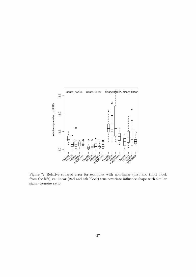
Figure 7: Relative squared error for examples with non-linear (first and third blockfrom the left) vs. linear (2nd and 4th block) true covariate influence shape with similarsignal-to-noise ratio.

37

Amount of non-linearity in the data

Figure 7 compares prediction performance (by RSE) for examples with non-linear under-

lying structure (first and third block of boxes) to that with linear underlying structure

(second and forth block of boxes) with similar signal-to-noise ratio. The data in the

leftmost block is from the reference example. In the corresponding example with linear

structure (second block from the left) all procedures have improved performance, indi-

cating that fitting linear functions is easier even for procedures that can fit generalized

additive models. There is only a slight performance advantage from using the adequate

procedure, GLMse, given that it is known, that the true structure is linear (which will

rarely be the case in applications). Inspection of the upper part of Table 2 indicates,

that in some of the difficult to fit binary response examples (low signal-to-noise ratio

and/or large number of covariates) there might be even a slight performance advantage

over GLMse. The results in the right two blocks of Figure 7 are from binary response ex-

amples with 10 covariates, of which 6 are informative, and a rather small signal-to-noise

ratio (ce = 1). When the true structure is non-linear (third block from the left) only

GAMBoost can improve over GLMse (GAMM is not shown because for most repetitions

no fit could be obtained). The good performance of GAMBoost seems to transfer to the

example with linear underlying structure (rightmost block of boxes). In this example it is

well competitive with GLMse. It might be argued that for such difficult situations there

are optimized procedures for fitting linear models, e.g. the Lasso (Tibshirani, 1996), but

consideration of these would lead too far here. So, at least when compared to standard

procedures for fitting a (generalized) linear model, using GAMBoost does not seem to

result in a loss of prediction performance in difficult data situations.

38

5 Concluding remarks

There are several properties by which a data situation, in which a generalized additive

model may be fitted, can be characterized. The present paper focused on the signal-to-

noise ratio, the type of response, the number of (uninformative) covariates, the number of

covariates over which information with respect to the response is distributed, correlation

between covariates, and on whether there is actually non-linear structure in the data.

We reviewed several techniques for fitting generalized additive models and evaluated how

their performance changes when the characteristics of the data situation change. Criteria

were prediction performance, hit rate/false alarm rate, and integrated squared curvature

of the fitted functions. It has been found that none of the procedures performs best in

all situations and with respect to all criteria. For prediction performance there seems

to be an advantage for GAMBoost procedures in “difficult” data situations. There was

no clear difference between deviance-based GAMBoost and sparse GAMBoost. While

the latter had some advantages in very sparse situations, the former outperformed the

latter in more situations than expected. With respect to integrated squared curvature

of the fits and hit rate/false alarm rate, the procedures have different properties, while

at the same time they often have very similar prediction performance. So it seems

they can be chosen guided by the specific objectives of data analysis. If very smooth

(often linear) fits are wanted, with a strong tendency to oversmoothing, and a very strict

criterion for calling covariates influential is also wanted, then the mixed model approach

is preferable, but this procedure may not always be feasible due to numerical problems

(especially for binary response data). Backfitting approaches or simultaneous estimation

present an intermediate solution with respect to the complexity of the fitted models,

where the latter might result in a slightly better prediction performance. When a very

lenient criterion for identification of influential covariates is wanted and oversmoothing

should be avoided, then GAMBoost is the method of choice. Finally, even when the

39

true underlying structure is hardly non-linear, at a maximum only a small performance

penalty is to be expected when using more modern methods such as GAMBoost. So one

can safely use such methods for fitting generalized additive models when the nature of

the underlying structure is unclear.

Acknowledgements

We gratefully acknowledge support from Deutsche Forschungsgemeinschaft (Project C4,

SFB 386 Statistical Analysis of Discrete Structures).

References

Breiman, L. (1999). Prediction games and arcing algorithms. Neural Computation,

11:1493–1517.

Buhlmann, P. and Yu, B. (2003). Boosting with the L2 loss: Regression and classification.

Journal of the American Statistical Association, 98:324–339.

Chambers, J. M. and Hastie, T. J. (1992). Statistical Models in S. Wadsworth, Pacific

Grove, California.

Friedman, J., Hastie, T., Rosset, S., Tibshirani, R., and Zhu, J. (2004). Statistical

behavior and consistency of classification methods based on convex risk minimization:

Discussion of the paper by T. Zhang. The Annals of Statistics, 32(1):102–107.

Friedman, J. H. (2001). Greedy function approximation: A gradient boosting machine.

The Annals of Statistics, 29:1189–1232.

Friedman, J. H. and Stuetzle, W. (1981). Projection pursuit regression. Journal of the

American Statistical Association, 76:817–823.

Green, P. J. and Silverman, B. W. (1994). Nonparametric Regression and Generalized

Linear Models. Chapman & Hall, London.

40

Hand, D. J. (2006). Classifier technology and the illusion of progress. Statistical Science,

21(1):1–14.

Hastie, T. and Tibshirani, R. (1986). Generalized additive models. Statistical Science,

1:295–318.

Hastie, T. J. and Tibshirani, R. J. (1990). Generalized Additive Models. Chapman &

Hall, London.

Hoerl, A. E. and Kennard, R. W. (1970). Ridge regression: Biased estimation for

nonorthogonal problems. Technometrics, 12(1):55–67.

Hurvich, C. M., Simonoff, J. S., and Tsai, C. (1998). Smoothing parameter selection in

nonparametric regression using an improved Akaike information criterion. Journal of

the Royal Statistical Society B, 60(2):271–293.

Kim, Y.-J. and Gu, C. (2004). Smoothing spline Gaussian regression: More scalable

computation via efficient approximation. Journal of the Royal Statistical Society B,

66(2):337–356.

Lee, T. C. M. (2003). Smoothing parameter selection for smoothing splines: A simulation

study. Computational Statistics & Data Analysis, 42:139–148.

Lindstrom, M. J. (1999). Penlized estimation of free-knot splines. Journal of Computa-

tional and Graphical Statistics, 8(2):333–352.

Marx, B. D. and Eilers, P. H. C. (1998). Direct generalized additive modelling with

penalized likelihood. Computational Statistics and Data Analysis, 28:193–209.

McCullagh, P. and Nelder, J. A. (1989). Generalized Linear Models. Chapman & Hall,

London, U.K., 2nd edition.

41

R Development Core Team (2006). R: A Language and Environment for Statistical

Computing. R Foundation for Statistical Computing, Vienna, Austria. ISBN 3-900051-

07-0.

Ruppert, D. (2002). Selecting the number of knots for penalized splines. Journal of

Computational and Graphical Statistics, 11:735–757.

Ruppert, D., Wand, M. P., and Carroll, R. J. (2003). Semiparametric Regression. Cam-

bridge University Press.

Speed, T. (1991). Comment on “That BLUP is a good thing: The estimation of random

effects” by G. K. Robinson. Statistical Science, 6(1):42–44.

Tibshirani, R. (1996). Regression shrinkage and selection via the lasso. Journal of the

Royal Statistical Society B, 58(1):267–288.

Tutz, G. and Binder, H. (2006). Generalized additive modelling with implicit variable

selection by likelihood based boosting. Biometrics, in press.

Wand, M. P. (2000). A comparison of regression spline smoothing procedures. Compu-

tational Statistics, 15:443–462.

Wang, Y. (1998). Mixed effects smoothing spline analysis of variance. Jounal of the

Royal Statistical Society B, 60(1):159–174.

Wood, S. N. (2000). Modelling and smoothing parameter estimation with multiple

quadratic penalties. Jounal of the Royal Statistical Society B, 62(2):413–428.

Wood, S. N. (2004). Stable and efficient multiple smoothing parameter estimation

for generalized additive models. Journal of the American Statistical Association,

99(467):673–686.

Wood, S. N. (2006). Generalized Additive Models. An Introduction with R. Chapman &

Hall/CRC, Boca Raton.

42