Fish stock assessment training Manual

Training Manual

Phase I: 27 November - 8 December 2006

Suva, Fiji Islands

Phase II: 14 - 25 January 2008

Apia, Samoa

based on the lectures by

Jeppe Kolding (University of Bergen, Norway)

Einar Hjörleifsson (Marine Research Institute of Iceland)

Prepared by

Warsha Singh

May 2009

C O M M O N W E A LT H

S E C R E A R I AT

Assessing the status of fish stock for management: the

collection and use of basic fisheries data and statistics

1

ABSTRACT

Under the Cooperation Arrangement between the Commonwealth Secretariat and the Government of

Iceland, training in the use of basic fisheries data in assessing the status of fish stocks was conducted for

the South Pacific region. The training was a joint effort of United Nations University – Fisheries Training

Programme (UNU-FTP, Iceland), Commonwealth Secretariat, Secretariat of the Pacific Community (SPC)

and University of the South Pacific (USP) which was conducted in two phases held in Fiji and Samoa

respectively. Participants from various Pacific Island Countries were trained.

The formal objectives of the training were:

i. To enhance the knowledge and skills in the use of basic fisheries data in the assessment of fish

stocks in the Pacific Island Countries.

ii. To review the theory and principal methods in quantitative biology and fisheries science with

particular emphasis on improving skills through practical training exercises.

iii. To review recent developments in multi-species ecosystem approach and their potential use in

fisheries science and management.

iv. To enable fisheries personnel to establish and develop a database of their inshore resources

v. To develop teaching of graduate fisheries courses at the USP.

This document serves as the training guidebook and is largely based on the lecture materials covered in

the training with additional references. Practical exercises in Excel are attached herewith with requisite

instructions for the users to get some practical training with data analysis. This teaching material is to be

eventually incorporated into the teaching curriculum of the University of the South Pacific as an

undergraduate course.

The manual begins with outlining the basics of fisheries population dynamics and the objectives of

fisheries stock assessment. Particular emphasis is then given to biostatistics and the use of mathematical

models in describing biological processes and the fundamental science of parameter estimation. The issue

of sampling and survey designs is discussed next. Some fundamental fishery concepts are introduced

before the elementary population parameters age, growth and mortality are discussed. The predictive

yield-per-recruit model is also briefly introduced followed by a discussion on the holistic surplus

production models. The last chapter puts emphasis on the regional situation and briefly describes

fisheries in the South Pacific countries and some complications associated with stock assessment of small-

scale fisheries. Consequently, the appropriate assessment techniques are considered.

Learning Objectives

By the end of the course, the trainees should be able to

i. know the type of data to collect in carrying out stock assessment

ii. know how to sample and how to adapt the sampling strategy to suit local conditions

iii. know how to collect and use catch and effort data in stock assessment

iv. explain how sampling methods can introduce bias in estimates

v. know how to store and retrieve data

vi. know how to analyze, interpret and present results in a meaningful manner

vii. estimate basic population parameters such as growth and mortality

viii. explain the impact of fishing on community structure

ix. know how to conduct cohort analysis

x. conduct stock assessment in a cost effective manner.

2

TABLE OF CONTENTS

1. INTRODUCTION............................................................................................................................... 5

1.1. FISH POPULATION DYNAMICS ...................................................................................................... 6 1.2. OBJECTIVES OF STOCK ASSESSMENT ............................................................................................ 8

2. BIOSTATISTICS.............................................................................................................................. 10

2.1. DESCRIPTIVE STATISTICS ........................................................................................................... 10 2.2. EXPLORATORY DATA ANALYSIS................................................................................................ 19 2.3. MODEL PARAMETER ESTIMATION.............................................................................................. 20 2.4. LINEAR MODELS ........................................................................................................................ 20 2.5. LINEAR REGRESSION.................................................................................................................. 22 2.6. MULTIPLE LINEAR REGRESSION.................................................................................................. 25 2.7. ANALYSIS OF VARIANCE (ANOVA) .......................................................................................... 26 2.8. AN INTRODUCTION TO BOOTSTRAP ............................................................................................ 27

3. SAMPLING AND SURVEYS.......................................................................................................... 29

3.1. SAMPLING DESIGN ..................................................................................................................... 30 3.2. SURVEYS .................................................................................................................................... 34 3.3. BASIC DATA COLLECTION ......................................................................................................... 34

4. FUNDAMENTAL FISHERY CONCEPTS.................................................................................... 36

5. GROWTH.......................................................................................................................................... 39

5.1. POPULATION GROWTH ............................................................................................................... 39 5.2. INDIVIDUAL GROWTH ................................................................................................................ 44

5.2.1. Data requirements ................................................................................................................ 46 5.2.2. Methods for Estimation of growth parameters from length-at-age data .............................. 47 5.2.3. Estimating age composition from length-frequencies........................................................... 48 5.2.4. Computer Packages.............................................................................................................. 55 5.2.5. Limitations of length frequency analysis .............................................................................. 56

6. MORTALITY ................................................................................................................................... 58

6.1. THE FATE OF A COHORT.............................................................................................................. 62 6.2. ESTIMATION OF MORTALITY ...................................................................................................... 64 6.3. NATURAL MORTALITY ............................................................................................................... 69

7. YIELD-PER-RECRUIT MODELS................................................................................................. 72

7.1. AGE BASED MODELS................................................................................................................... 74 7.2. LENGTH BASED MODELS............................................................................................................. 75

8. SURPLUS PRODUCTION MODELS............................................................................................ 77

9. MULTISPECIES MODELS ............................................................................................................ 82

10. PATTERNS OF EXPLOITATION............................................................................................ 83

11. FISHERIES IN THE PACIFIC .................................................................................................. 85

11.1. INDUSTRIAL FISHERIES............................................................................................................... 85 11.2. SMALL-SCALE FISHERIES............................................................................................................ 85

12. BIBLIOGRAPHY ........................................................................................................................ 93

3

List of Figures

Figure 1: Stock biomass dynamics of an exploited fish stock. The biomass is increased by growth and

recruitment and reduced by natural and fishing mortality............................................................. 7 Figure 2: Shows a box and whisker plot and its essential components .................................................. 13 Figure 3: Shows the shape of a normal distribution (Gaussian distribution) with different means and

variance.............................................................................................................................................. 16 Figure 4: Shows the concept of the Z-score.............................................................................................. 17 Figure 5: Shows a normal distribution with a 95% confidence interval ............................................... 17 Figure 6: Shows the relationship between CV, sample size and maximum relative error. Higher CV

results in higher relative error. Increasing sample size reduces the relative error but to a

certain optimum point ...................................................................................................................... 19 Figure 7: Shows three probability distributions (histogram with superimposed probability density

function) for a normal distribution (symmetrical), left skewed and right skewed with

appropriate locations of their central value and corresponding boxplots ................................... 20 Figure 8: Shows the calculation of sum of squares in a linear model .................................................... 22 Figure 9: Shows the partitioning of sums of squares for a simple linear regression ............................ 24 Figure 10: Shows the concept of accuracy and precision........................................................................ 29 Figure 11: Shows Simple random sampling for a homogeneous and heterogeneous population ........ 30 Figure 12: Shows stratification of a survey area into four homogeneous strata ................................... 31 Figure 13: Shows the population trajectory when growing according to the logistic curve (classic

sigmoid shape, obtained by integrating equation 1.4). K represents the asymptotic carrying

capacity. Maximum growth rate is at K/2 ....................................................................................... 40 Figure 14: Shows the plot of equilibrium rate of change of population size versus population size

(production vs. stock size curve) obtained by taking the slope of the curve in Figure 13 at each

time step and plotting against population size. Maximum productivity occurs at half K,

equilibrium occurs at zero and K..................................................................................................... 41 Figure 15: Shows the logistic Gordon-Schaefer model applied to fisheries........................................... 42 Figure 16: Shows the production curve for the discrete logistic growth. The diagonal line of

equilibrium is Nt+1 = Nt with the equilibrium carrying capacity at K. The curved line is the

surplus production (sum of new recruits and the growth of the existing individuals in the

population after subtracting natural mortality in the stock) with point of maximum production

at K/2 .................................................................................................................................................. 43 Figure 17: Shows the conventional fisheries management theory.......................................................... 44 Figure 18: Shows a growth trajectory of length of a fish as per the von Bertalanffy growth function

(von Bertalanffy growth curve)........................................................................................................ 45 Figure 19: Shows an example of a Gulland and Holt plot of growth rate against length..................... 48 Figure 20: Shows part of a Bhattacharya analysis, converting a normal distribution into a straight

line ...................................................................................................................................................... 50 Figure 21: Shows a Bhattacharya plot corresponding to columns D and E of Table 1, and regression

line estimated for the first cohort N1 with the intercept a = 5.33 and the slope b = -0.306. The

calculated values of column F are obtained by inserting the independent value (x) = upper limit

of the smallest of two adjacent length groups in the equation: y = a + bx ................................... 52 Figure 22: Shows the modal progression analysis method. A is a plot of the mean lengths from the

Bhattacharya analysis; B shows the connected mean lengths to represent growth curves of

assumed cohorts. ............................................................................................................................... 54 Figure 23: Shows the basic dynamics of the decay of a cohort with corresponding symbols used in

fishery models. The figure illustrates the impact of fishing to the survival rates, compared to

natural decay without fishing. The line N+ catch illustrates the fate of cohort when its exposed

to some fishing mortality as opposed to decay without exploitation............................................. 58 Figure 24: Shows the exponential decay of a cohort at different levels of total mortality Z. The higher

the Z the faster the population numbers decline. ........................................................................... 60 Figure 25: Shows the factors affecting mortality at various life stages of the life of a cohort.............. 61

4

Figure 26: Shows the development of a cohort through time based on catch in numbers of the

Icelandic Haddock in Table 6. The orange, yellow and red lines represent the 1985, 1988 and

1990 cohort respectively. The 1985 and 1990 are strong year classes with more fish numbers. In

contrast the 1988 is a weak year class ............................................................................................. 63 Figure 27: Shows the development of a cohort through time illustrating its entire life span based on

the data in Table 6. The blue, red and yellow line show the development of the 1985, 1988 and

1990 cohort respectively. The 1985 year class is 2 years old in 1987 and so forth and maximum

catch is seen around 4-5 years old ................................................................................................... 63 Figure 28: Shows the development of a cohort with log-transformed catch in numbers for Icelandic

Haddock. The blue, red and yellow line show the development of the 1985, 1988 and 1990

cohort respectively. The exponential decline or the slope of the straight line gives an estimate of

total mortality Z ................................................................................................................................ 64 Figure 29: Shows the age based linearised catch curve. The log-transformed catch is numbers at age

is regressed against age to get an estimate of the total mortality Z which is the slope of the

regression line.................................................................................................................................... 65 Figure 30: Shows how a cohort develops through time in numbers (red), weight (yellow) and biomass

(blue). After birth the numbers in a cohort decline exponentially and the individuals in a cohort

increase in size and weight. The biomass which is a product of the two increases to a certain

maximum and then decreases thereafter ........................................................................................ 74 Figure 31: Shows an example of a yield-per-recruit and a spawning stock biomass curve with the

target management point maxF and Y/R at maxF ............................................................................ 75

Figure 32: Shows the classic Gordon-Schaefer model with the concept of maximum sustainable yield

(MSY) which occurs at half the carrying capacity (K/2) and the biomass leading to MSY is

BMSY .................................................................................................................................................... 79

List of Tables

Table 1: Shows frequency tabulation of a random sample of lengths of 30 fish ................................... 12 Table 2: Shows the calculation of mean and median of a sample........................................................... 13 Table 3: Illustrates the calculation of sample variance ........................................................................... 14 Table 4: Shows the partitioning of sums of squares for a simple linear regression.............................. 24 Table 5: Shows the process of a Bootstrap ............................................................................................... 28 Table 6: Estimation of the first cohort, N1 from a composite length frequency distribution by means

of the Bhattacharya method, and the total minus N1 = N2+. The arrow indicates where to start

the calculation of N1 ......................................................................................................................... 51 Table 7: The total catch in numbers of Icelandic Haddock split up by age groups. The blue, red and

yellow line show the development of the 1985, 1988 and 1990 cohort respectively. The fate of a

specific cohort can be followed diagonally across the table. The 1985 and 1990 are strong year

classes with more fish numbers. In contrast the 1988 is a weak year class. A pseudocohort is

represented by the shaded area (Age 8) .......................................................................................... 62 Table 8: Shows the catch in numbers at age. The diagonal blue line represents the development of a

cohort and the straight line represents a pseudocohort. Part A of the table shows a constant

parameter system assuming that recruitment and mortality (F and M) remain constant every

year so that the number of survivors and the numbers caught would be the same for all cohorts.

Part B represents a variable parameter system with variable recruitment and mortality over

time which is a more realistic scenario............................................................................................ 66 Table 9: Shows Russell´s experiment of the effect of two fishing mortalities on a hypothetical fish

stock. This is based on weight at age data. The lower fishing mortality resulted in higher catch

weights ............................................................................................................................................... 72

5

1. Introduction

The objective of modern fisheries management deals with biological, economic,

recreational and social aspects (Hart and Reynolds 2002). Some management regimes try

to focus on all four dimensions with an underlying objective to ensure sustainable

development. “In fisheries terms, we should not destroy or diminish fish stocks to such a

degree that future generation would not have the opportunity to gain a living from them

in the way we do now or to benefit from the maintenance of biodiversity” (Hart and

Reynolds 2002). The economic point of view would be to consume resources in a way

that maximises utility over time. This directly leads to the formulation of the principles of

fisheries stock assessment or fish population dynamics.

Fishing has sustained a major part of the world’s population through providing food and

livelihood and its significance is widely acknowledged. The universal foundation for

fisheries management is outlined in the Food and Agricultural Organisation (FAO) Code

of Conduct for Responsible Fisheries. The Code recognises the nutritional, economic,

social, environmental and cultural importance of fisheries and “sets out principles and

international standards of behaviour for responsible practices with a view to ensuring the

effective conservation, management and development of living aquatic resources, with

due respect for the ecosystem and biodiversity” (FAO 1995).

Article 7 on general fisheries management says:

“States and all those engaged in fisheries management should, through an appropriate

policy, legal and institutional framework, adopt measures for the long-term conservation

and sustainable use of fisheries resources. Conservation and management measures,

whether at local, national, subregional or regional levels, should be based on the best

scientific evidence available and be designed to ensure the long-term sustainability of

fishery resources at levels which promote the objective of their optimum utilization and

maintain their availability for present and future generations; short term considerations

should not compromise these objectives”

“When considering the adoption of conservation and management measures, the best

scientific evidence available should be taken into account in order to evaluate the current

state of the fishery resources and the possible impact of the proposed measures on the

resources”

However lack of scientific information should not be used as an excuse of absence of

fisheries management, as such the precautionary principle says:

“States should apply the precautionary approach widely to conservation, management

and exploitation of living aquatic resources in order to protect them and preserve the

aquatic environment. The absence of adequate scientific information should not be used

as a reason for postponing or failing to take conservation and management measures”

6

“States should promote the use of research results as a basis for the setting of

management objectives, reference points and performance criteria, as well as for

ensuring adequate linkage between applied research and fisheries management “

In implementing the precautionary approach, states shall:

“a) Improve decision-making for fishery resource conservation and management by

obtaining and sharing the best scientific information available and implementing

improved techniques for dealing with risk and uncertainty;”

“d) Develop data collection programmes to assess the impact of fishing on non-target

and associated or dependent species and their environment, and adopt plans, which are

necessary to ensure the conservation of such species and to protect habitats of special

concern.”

1.1. Fish Population Dynamics

Fishing affects the dynamics of the fish populations. They can undergo many changes

such as changes in total numbers, total biomass, size frequency distributions, age-

structure, and spatial distributions. One of the major objectives of stock assessment is to

understand these variations which are revealed in the catches of different fisheries. The

underlying assumption is that if we can understand how populations respond to different

perturbations (fishing and natural fluctuations) then we should be able to manage those

fisheries according to our chosen objectives (Haddon 2001).

To put fish population dynamics into perspective a fish stock has to be seen as a simple

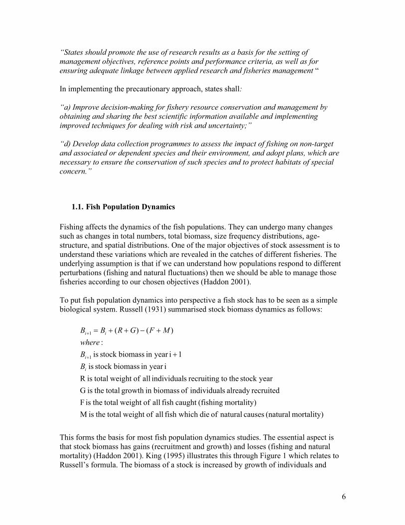
biological system. Russell (1931) summarised stock biomass dynamics as follows:

This forms the basis for most fish population dynamics studies. The essential aspect is

that stock biomass has gains (recruitment and growth) and losses (fishing and natural

mortality) (Haddon 2001). King (1995) illustrates this through Figure 1 which relates to

Russell’s formula. The biomass of a stock is increased by growth of individuals and

mortality) (natural causes natural of die fish which all of weight total theis M

mortality) (fishingcaught fish all of weight total theis F

recruitedalready sindividual of biomassin growth total theisG

yearstock the torecruiting sindividual all of weight totalis R

iyear in biomassstock is

1iyear in biomassstock is

:

)()(

1

1

i

i

ii

B

B

where

MFGRBB

+

+−++=

+

+

7

subsequent reproduction by the adult fish which leads to small fish being recruited into

the stock. In the figure three consecutive age classes are shown. At the same time, the

stock numbers get reduced due to fishing mortality (fish caught by fishermen) and natural

mortality (other causes such as predation). If the fish are removed at a high rate, the

number of adult fish may be reduced to a point where reproduction will be unable to

compensate for the numbers lost hence the stock size will decline.

Figure 1: Stock biomass dynamics of an exploited fish stock. The biomass is increased by growth and

recruitment and reduced by natural and fishing mortality

[Source: King (1995)].

A stock of fish or a unit stock can be defined as a discrete group of individuals having the

same gene pool which are self sustaining and having little connection with adjacent

groups (King 1995). A stock of fish usually occupies a particular geographical area with

little integration with adjacent groups. The growth and mortality parameters in a unit

stock are uniform over the distribution area of the stock. Assessments are made for each

stock separately. Identifying unit stocks can be fairly complicated. In order to determine

whether a species forms one or more distinct stocks, we should examine its spawning

areas, growth and mortality parameters, morphological and genetic characteristics,

compare fishing patterns.

There are at least three main reasons for failing to work properly with the stock unit.

• The full distribution area of the stock is not covered by the data collected, so that

only part of the stock is considered. This is a typical example where several

independent fisheries are exploiting the same stock.

• Several independent stocks are lumped together, for example, because their areas

of distribution overlap.

• Continuous immigration and emigration of the components of one or more stocks

from the fishing ground, migratory species e.g. tuna. Taking into account that

most of the exploited marine resources undertake migration, an essential element

to perform stock assessment is an understanding and knowledge of migration

routes (Kolding and Giordano 2001)

8

1.2. Objectives of stock assessment

The objective of fish stock assessment is to provide estimates of the state of the stock

(size, composition, regeneration rate, exploitation level, and fishing pattern) to assure, in

the long run, the self-sustainability of the stock under exploitation (Hilborn and Walters

1992). The ultimate aim is to provide biological and economic reference points to be used

as guidelines for the rational management of the fishery. For instance, some of the

conventional biological reference points for fisheries management have been estimation

of sustainable harvest levels, such as maximum sustainable yield (MSY) and/or

sustainable exploitation rates such as the optimum fishing mortality, fishing effort, and

the size of fish to be caught. The techniques used to obtain such biological reference

points, forms the scope of this manual.

Fisheries are renewable resources i.e. replenish by natural processes at a faster rate than

its rate of loss and fishing should not offset this natural balance. Even though maximizing

economic benefits from our natural resources through harvesting is also essential. Hence

the aim is to ensure maximum utilization of the stock in such a way that it is able to

sustain itself in the long run. If there is no fishing then there will be no catch and at low

levels of fishing effort the potential yield, or surplus production, of the resource is

normally under-utilised (Stefánsson). At very high levels of exploitation the removal will

surpass a stock’s regenerative capacity eventually leading to a collapse of the fishery.

Thus the point somewhere between no effort and very high effort needs to be found that

will give the maximum average yield with a maximum regenerative capacity of the stock

(King 1995).

Variations in yield are a combined effect of variations in effort, recruitment, natural

mortality and growth. One of the key goals is to understand both the natural variation

found in exploited populations and how harvesting affects their dynamics. This requires

an understanding of the productive stock (stock structure) as well as the individual

components of productivity (recruitment processes, individual growth, and mortality

processes). Each of these components needs to be considered. Fisheries science has

naturally developed into using mathematical and statistical descriptions of these

processes in attempts to understand the dynamics of exploited populations that is to

explain biological processes using mathematical models. It is a quantitative science based

to a large extent on statistical inference and analyses.

To a fisheries scientist understanding fundamental fisheries means; to understand the

growth aspects of an individual fish and a population of fish as a whole, to understand

how a population responds to increased mortality, and how a selective mortality

influences genetic changes, to know how these processes are modelled and the limitations

and underlying assumptions of these models, to recognize how useful information can be

extracted from the available data and simultaneously be conscious of the limitations and

uncertainties involved and at the same time to understand the natural fluctuations in the

environment apart from the human exploitation on a population (man is not the only

predator in the system). Most stocks are part of a food chain, or food web, either feeding

on or giving food to other stocks. Managing fisheries entails being able to translate and

9

explain all the understanding from the science to the community and the authorities and

to understand the implications of management regulations, not only for the fish

community but also the fishing community (Kolding 2006).

Stock assessment implies understanding the dynamic system (Figure 1) and estimating

these fundamental population parameters namely stock abundance, growth, recruitment

and mortality. These parameters can be estimated from different types of data set such as

length of fish/ length-frequencies, age, catch rates (catch per unit effort).

Essentially three basic elements are necessary:

• The input (e.g. the fishing effort in terms of fishing gears and amount of time

spent fishing)

• The output (landed catch) as a part of the biological production

• The processes that describe and link the input and output (the biological processes

and fishing operations represented by mathematical models) (Sparre and Venema

1998).

Sparre and Venema (1998) condense the fish stock assessment models into two main

groups:

• Analytical or dynamic pool models that are structured around individual fish as

the basic unit and where dynamic processes such as age, growth, mortality, and

maturity are each represented by a sub-model. These models are either length-

structured or age-structured and deal with a partial or the entire demographic

structure of the population. They have their origin from Thompson and Bell

(1934) and Beverton and Holt (1957).

• Holistic or biomass dynamic models that are structured around the overall stock

(population) as the basic unit where individually based processes such as growth

and reproduction are inherently encapsulated in the stock model. The starting

point of these models is population abundance indices generated from catch and

effort data or fishery independent biomass surveys (swept area method or acoustic

surveys). These models have their origin from Graham (1935), and Schaefer

(1954).

10

2. Biostatistics

In order to understand the dynamics of the exploited species, fisheries science has

developed into using mathematical and statistical descriptions to illustrate the biological

processes. Statistics applied to life sciences is often called biostatistics or biometry and is

used as a means of informing the decision-making processes. Before more technical

concepts are introduced, it is important to look into some essentials of biostatistics which

forms the basis of these mathematical models. One needs to be familiar with some

fundamental concepts of statistical sampling and common parameters and statistics.

2.1. Descriptive Statistics

A population is a finite number of separate objects defined in space and time. It is

generally not feasible to take measurements from the entire population therefore a sample

(subset of the population) is taken. Biologists usually make inferences about a population

from the sample taken from the population. Hence the sample needs to be random and

representative of the population. Information contained in the sample, i.e. sample

statistics are used to estimate population parameters. For example, not all fish can be

measured in a population, therefore a sample of fish are measured and some conclusions

can be drawn about the length distribution in the population based on the information

obtained from the sample. Inferences about the population are normally limited to the

space and time the sample is taken from. For example if we sample from a population of

animals at a certain location in October 2007 then our inference is restricted to that area

in October 2007.

Fisheries data normally consist of a collection of observations e.g. length of fish, number

of individuals. The actual property measured by the individual observations are called

variables e.g. length. In a given population, each variable can be characterised by certain

parameters e.g. mean length. Estimates of the parameters are obtained from a sample.

Every measured variable and its parameter estimate will have some degree of uncertainty

which is viewed in terms of probabilities. Thus every variable has an associated

probability distribution (Quinn and Keough 2002).

First the raw data (e.g. a range of length measurements) needs to be condensed into some

more useful form that allows some visual interpretation of the data. This is obtained by a

frequency tabulation to get a frequency distribution. A length group can be identified by

using index j, with an upper limit denoted by j+1;

dLLL jj +=+ )()1(

where the interval size is expressed as dL, a concept that appears frequently. The

midpoint of length interval j is defined as

11

2)(

dLL j +

A fish of length x (j) then belongs to the length group j when

dLLxL jjj +<<= )()()(

F(j) is the frequency of length group j, or the number of fish observed in the length group

j. When L(j) in a frequency table is just represented by one number, it represents the

lower interval limit of length group j.

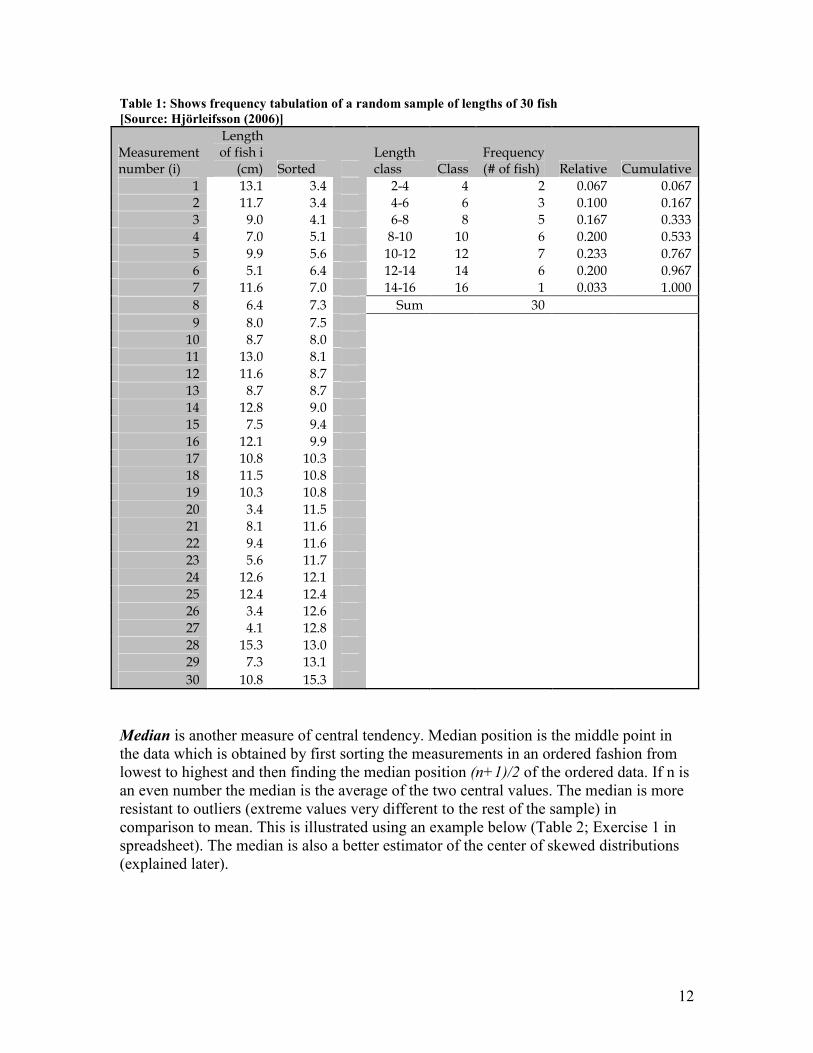
An example data set is used below to illustrate the frequency distribution process.

Consider a random sample of lengths of 30 fish from the population i.e. n (number of

observations) = 30. Firstly, one needs to decide on the number of classes to include in the

frequency distribution. Generally the number is kept in-between 5 to 15, although it

depends on the number of observations (more length classes would be allocated with

greater number of observations). The nature of the data also plays a role. Some general

guidelines include taking a square root of n or Sturge´s rule = (Xmax-Xmin) / (1+1.44

ln(n)). In this case 7 length classes are used. The class width is determined by finding the

range of the data (highest value-lowest value) and dividing by the number of classes and

rounded up to the next convenient number. Range: 15.3 cm – 3.4 cm = 11.9/ 7 = 1.7 cm

� 2 cm. For defining the class limits, start with the lowest value as the lower limit of the

first class (2cm), add the class width to this to obtain the lower limit for the second class,

2 + 2 = 4 cm etc. Count the number of fish in each length class, either by using a pencil

or a paper or a computer program. Relative frequency is the proportion of the observation

within a class. Cumulative frequency is the sum of the relative frequency of all classes

below and including the class indicated (Table 1; Exercise 1 in spreadsheet can be

referred to for frequency distribution plots).

Two aspects of the data are normally important, some measure of location or central

tendency (i.e. where is the middle of the population) and some measure of the spread or

variability (i.e. how different are the observations in a population).

One common measure of the center of the distribution is the arithmetic mean which is the

sum of all observations divided by the total number of observations

[ ]ni

i

n

i

i xxxxn

xn

xn

x ++++=== ∑∑==

...111

321

11

where n is the total number of measurements

i is the ith measurement

ix is the value of the ith measurement

The sample mean is an unbiased estimator of the population mean.

12

Table 1: Shows frequency tabulation of a random sample of lengths of 30 fish

[Source: Hjörleifsson (2006)]

Measurement number (i)

Length of fish i

(cm) Sorted Length class Class

Frequency (# of fish) Relative Cumulative

1 13.1 3.4 2-4 4 2 0.067 0.067

2 11.7 3.4 4-6 6 3 0.100 0.167

3 9.0 4.1 6-8 8 5 0.167 0.333

4 7.0 5.1 8-10 10 6 0.200 0.533

5 9.9 5.6 10-12 12 7 0.233 0.767

6 5.1 6.4 12-14 14 6 0.200 0.967

7 11.6 7.0 14-16 16 1 0.033 1.000

8 6.4 7.3 Sum 30

9 8.0 7.5

10 8.7 8.0

11 13.0 8.1

12 11.6 8.7

13 8.7 8.7

14 12.8 9.0

15 7.5 9.4

16 12.1 9.9

17 10.8 10.3

18 11.5 10.8

19 10.3 10.8

20 3.4 11.5

21 8.1 11.6

22 9.4 11.6

23 5.6 11.7

24 12.6 12.1

25 12.4 12.4

26 3.4 12.6

27 4.1 12.8

28 15.3 13.0

29 7.3 13.1

30 10.8 15.3

Median is another measure of central tendency. Median position is the middle point in

the data which is obtained by first sorting the measurements in an ordered fashion from

lowest to highest and then finding the median position (n+1)/2 of the ordered data. If n is

an even number the median is the average of the two central values. The median is more

resistant to outliers (extreme values very different to the rest of the sample) in

comparison to mean. This is illustrated using an example below (Table 2; Exercise 1 in

spreadsheet). The median is also a better estimator of the center of skewed distributions

(explained later).

13

Table 2: Shows the calculation of mean and median of a sample


Data set 1 Data set 2

Measurement number (i)

Measurement value (xi)

Measurement value (xi)

1 40 40

2 20 20

3 10 10

4 30 30

5 50 100

n 5 5

Sum 150 200

Mean (sum/n) 30 40

Median pos.: (n+1) / 2 3 3

Median value 10 10

The third measure is the mode, which is the value that occurs most often. This is not

affected by outliers but the problem is that there could be none or many modes.

The simplest measure of spread or variability is the range of the data (difference between

the largest and the smallest value). There is however no clear link between the sample

range and the population range and generally the range will rise as the sample increases

(Quinn and Keough 2002). A measure that is more robust to unusual observation is the

interquartile range, which is obtained by creating quartiles, Q1 Q2 Q3, which divide the

data set into four equal parts. A percentile divides the data set into 100 equal parts. The

first quartile Q1=P25 is the observation which has 25% of the observations below it. The

third quartile Q3 = P75 is the observation which has 75% of the observations below it or

25% above it. This information is used in the making box and whisker plots (boxplots;

Figure 2) that give an indication of the central value of the data and its distribution and is

an excellent exploratory data analysis tool.

MaximumMinimumQ1 = 25

th percentile

Q2 = 50th percentile

MedianQ3 = 75

th percentile

Interquartile range = 400 – 100 = 300

Range = 600 – 4 = 596

Measurements value

4 100 600400200

MaximumMinimumQ1 = 25

th percentile

Q2 = 50th percentile

MedianQ3 = 75

th percentile

Interquartile range = 400 – 100 = 300

Range = 600 – 4 = 596

Measurements value

4 100 600400200

Figure 2: Shows a box and whisker plot and its essential components

[Source: Hjörleifsson (2006)].

An imperative measure of variability is the sample variance which can be used to

estimate the population variance. Variance is based on the deviations of the individual

observations from the mean value. A sample variance 2S is

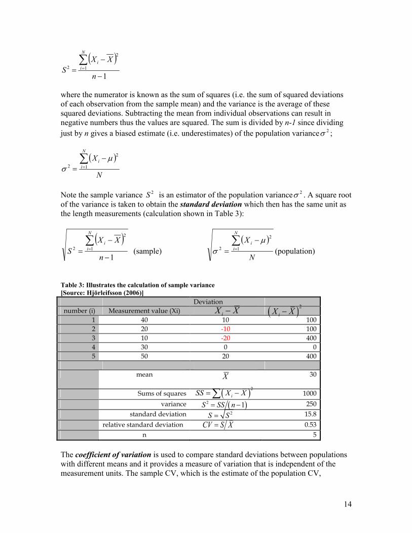
14

( )1

1

2

2

−

−=∑=

n

XX

S

N

i

i

where the numerator is known as the sum of squares (i.e. the sum of squared deviations

of each observation from the sample mean) and the variance is the average of these

squared deviations. Subtracting the mean from individual observations can result in

negative numbers thus the values are squared. The sum is divided by n-1 since dividing

just by n gives a biased estimate (i.e. underestimates) of the population variance 2σ ;

( )

N

XN

i

i∑=

−= 1

2

2

µσ

Note the sample variance 2S is an estimator of the population variance 2σ . A square root

of the variance is taken to obtain the standard deviation which then has the same unit as

the length measurements (calculation shown in Table 3):

( )1

1

2

2

−

−=∑=

n

XX

S

N

i

i

(sample)

( )

N

XN

i

i∑=

−= 1

2

2

µσ (population)

Table 3: Illustrates the calculation of sample variance


Deviation

number (i) Measurement value (Xi)

1 40 10 100

2 20 -10 100

3 10 -20 400

4 30 0 0

5 50 20 400

mean X

30

Sums of squares 1000

variance 250

standard deviation 15.8

relative standard deviation 0.53

n 5

The coefficient of variation is used to compare standard deviations between populations

with different means and it provides a measure of variation that is independent of the

measurement units. The sample CV, which is the estimate of the population CV,

iX X− ( )2iX X−

( )2iSS X X= −∑

CV S X=

2S S=( )2 1S SS n= −

15

describes the standard deviation as a percentage of the mean. It gives an indication of the

data dispersion; how the individuals in a population are distributed relative to one

another.

X

SCV =

or X

SCV 100% =

Fisheries scientists use standard error (explained later) as opposed to standard deviation

for calculating CV. The statistical theory states that CV is inversely related to the square

root of the number of samples;

x

n

s

CV 100=

A rule of thumb is that a survey becomes of uncertain value if the CV is greater than

30%. A high CV implies that the statistical precision of the population mean is not very

good i.e. the mean density given by the sample provides a relatively uncertain estimate of

the mean density of the population (Haddon). From the above formula a decrease in the

CV would imply an increase in the sample size n. If information is available about the

variability in the population (standard deviation) then optimum number of samples can be

calculated for any desired CV. The higher the desired statistical precision of the mean

density or abundance estimate, the more samples are required i.e. CV of 15% requires

more samples than a CV of 30%.

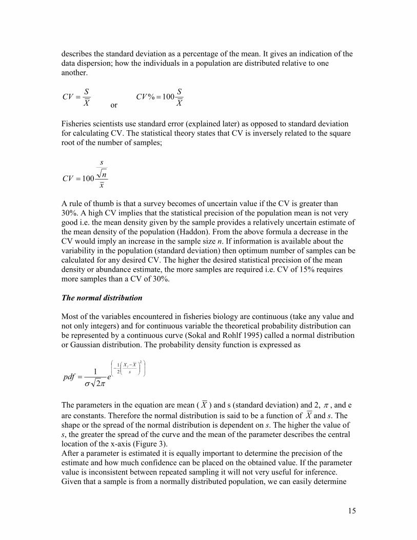
The normal distribution

Most of the variables encountered in fisheries biology are continuous (take any value and

not only integers) and for continuous variable the theoretical probability distribution can

be represented by a continuous curve (Sokal and Rohlf 1995) called a normal distribution

or Gaussian distribution. The probability density function is expressed as

−−

=

2

2

1

2

1 s

XX i

epdfπσ

The parameters in the equation are mean ( X ) and s (standard deviation) and 2, π , and e

are constants. Therefore the normal distribution is said to be a function of X and s. The

shape or the spread of the normal distribution is dependent on s. The higher the value of

s, the greater the spread of the curve and the mean of the parameter describes the central

location of the x-axis (Figure 3).

After a parameter is estimated it is equally important to determine the precision of the

estimate and how much confidence can be placed on the obtained value. If the parameter

value is inconsistent between repeated sampling it will not very useful for inference.

Given that a sample is from a normally distributed population, we can easily determine

16

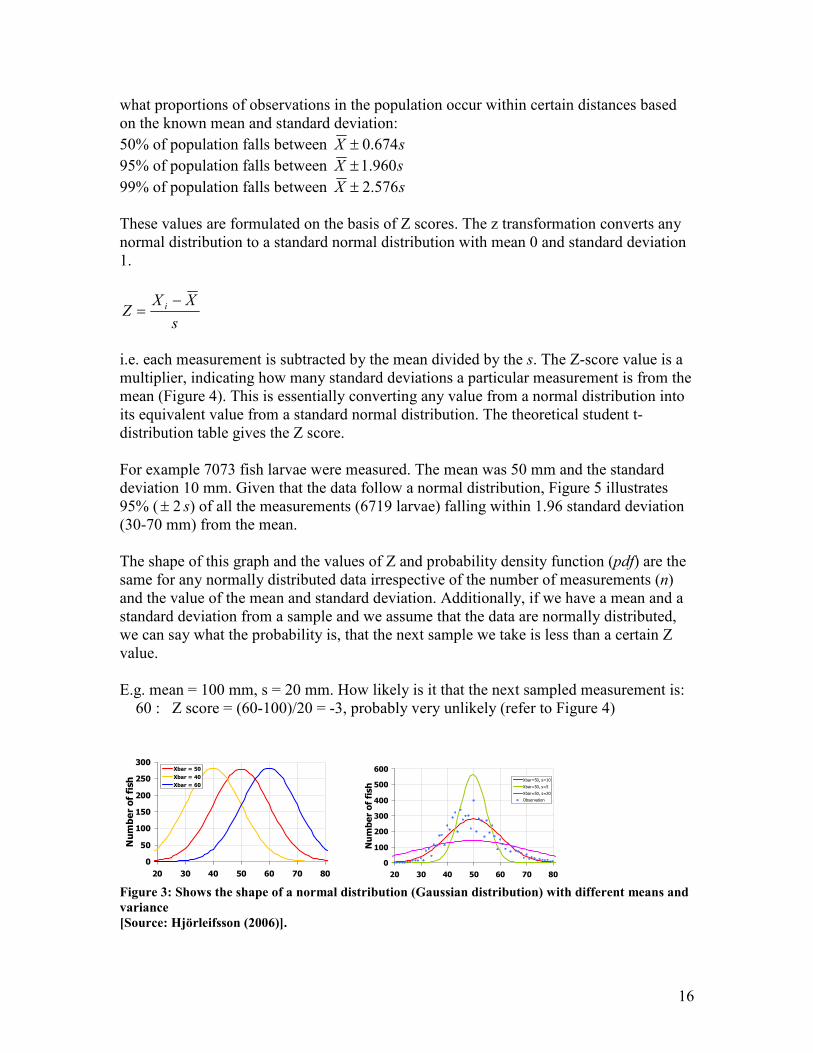
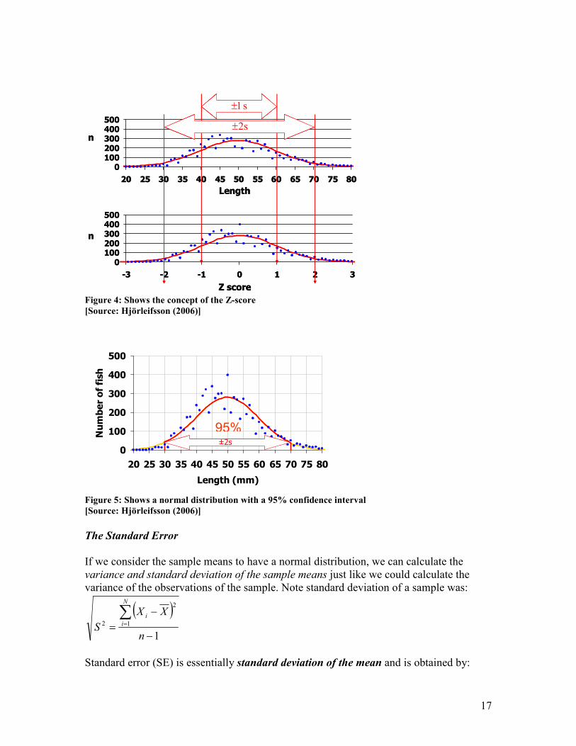
what proportions of observations in the population occur within certain distances based

on the known mean and standard deviation:

50% of population falls between sX 674.0±



These values are formulated on the basis of Z scores. The z transformation converts any

normal distribution to a standard normal distribution with mean 0 and standard deviation

1.

s

XXZ i −=

i.e. each measurement is subtracted by the mean divided by the s. The Z-score value is a

multiplier, indicating how many standard deviations a particular measurement is from the

mean (Figure 4). This is essentially converting any value from a normal distribution into

its equivalent value from a standard normal distribution. The theoretical student t-

distribution table gives the Z score.

For example 7073 fish larvae were measured. The mean was 50 mm and the standard

deviation 10 mm. Given that the data follow a normal distribution, Figure 5 illustrates

95% ( 2± s) of all the measurements (6719 larvae) falling within 1.96 standard deviation

(30-70 mm) from the mean.

The shape of this graph and the values of Z and probability density function (pdf) are the

same for any normally distributed data irrespective of the number of measurements (n)

and the value of the mean and standard deviation. Additionally, if we have a mean and a

standard deviation from a sample and we assume that the data are normally distributed,

we can say what the probability is, that the next sample we take is less than a certain Z

value.

E.g. mean = 100 mm, s = 20 mm. How likely is it that the next sampled measurement is:

60 : Z score = (60-100)/20 = -3, probably very unlikely (refer to Figure 4)

0

50

100

150

200

250

300

20 30 40 50 60 70 80

Number of fish

Xbar = 50

Xbar = 40

Xbar = 60

0

100

200

300

400

500

600

20 30 40 50 60 70 80

Number of fish

Xbar=50, s=10

Xbar=50, s=5

Xbar=50, s=20

Observation

Figure 3: Shows the shape of a normal distribution (Gaussian distribution) with different means and

variance


17

0100200300400500

20 25 30 35 40 45 50 55 60 65 70 75 80

0100200300400500

-3 -2 -1 0 1 2 3

Length

n

n

±1s

Z score

±2s

0100200300400500

20 25 30 35 40 45 50 55 60 65 70 75 80

0100200300400500

-3 -2 -1 0 1 2 3

Length

n

n

±1s±1s±1s

Z score

±2s±2s±2s

Figure 4: Shows the concept of the Z-score


0

100

200

300

400

500

20 25 30 35 40 45 50 55 60 65 70 75 80

Length (mm)

Number of fish

±2s±2s

Figure 5: Shows a normal distribution with a 95% confidence interval


The Standard Error

If we consider the sample means to have a normal distribution, we can calculate the

variance and standard deviation of the sample means just like we could calculate the

variance of the observations of the sample. Note standard deviation of a sample was:

( )1

1

2

2

−

−=∑=

n

XX

S

N

i

i

Standard error (SE) is essentially standard deviation of the mean and is obtained by:

95%

18

n

SSE =

where S is the standard deviation of the sample and n is the sample size. This indicates

the variation in the sample mean. If SE is large then repeated samples are likely to

produce very different means and the mean of any single sample might not be a reliable

measure of the population mean and vice versa. Thus this estimate gives a measure of

confidence in the mean estimate.

Confidence Intervals for population means

As was shown earlier 95% of population falls between sX 960.1± , therefore 95% of the

sample means would fall between sX 960.1± multiplied by the standard deviation of the

sample means i.e. standard error. Thus the 95% confidence limits (CL) of a population

mean given the sample mean and standard error can be calculated is given as follows:

30nfor ) tas dillustrate be also(can 96.1 Zwhere 1,0.05-n95% ≥=

±=±n

SZXCLX

Suppose that we require that the estimated mean landings from samples should not

deviate more than 7% (maximum relative error) from the true landings and that we want

to be 95% certain of this. The maximum relative error of the mean can be calculated

from:

X

SCVCV

n

tn100 where

05.0,1

max == −ε

Increasing sample size (n) lowers the maximum relative error. Higher CV results in

higher relative error for a given sample size (Figure 6).

We could further ask, how many samples are needed in order to be 95% sure that the

estimated mean from the samples does not deviate more than 7% from the true mean?

The answer is it depends on your CV. If CV is 10%, need 10 samples are needed to

achieve the required precision and if CV is 20%, then 35 samples are needed to achieve

the required precision (Figure 6). However it must be noted that increasing the number of

samples (for any given CV) does not proportionally increase the precision of the value

and the cost of obtaining the sample could get disproportionately higher the closer one

gets to the “true value” or minimum relative error..

19

0%

5%

10%

15%

20%

0 10 20 30 40 50 60

Sample size (n)

Maxim

um relative error

CV = 10%

CV = 20%

Figure 6: Shows the relationship between CV, sample size and maximum relative error. Higher CV

results in higher relative error. Increasing sample size reduces the relative error but to a certain

optimum point


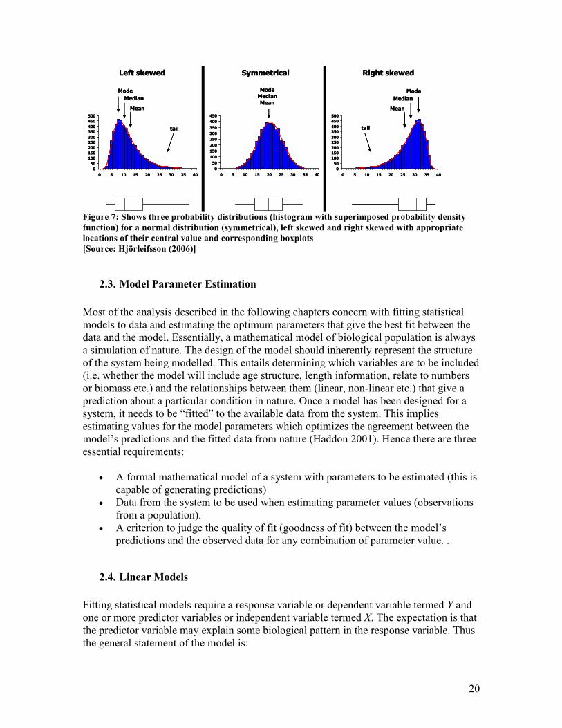
2.2. Exploratory Data Analysis

The first step in any data analysis is to explore or do a preliminary check on your data.

This is done to; (1) familiarize yourself with the data; (2) ensure in a way that the data is

meaningful, (3) detect errors, (4) see patterns in the data which may not be revealed by

statistical analysis, (5) determine outliers (unusual values) (Quinn and Keough 2002).

The prime thing we want to know about our data (and hence the population it is taken

from) is the shape of its distribution. Most of the statistical techniques operate on the

underlying assumption that the data is normally distributed. Some of the plots are very

useful for studying the distribution of your data such as scatterplot, histogram (a useful

addition is to superimpose a probability density function), boxplot (Figure 7).

If the data are non-normally distributed (skewed), transformation of the data to normality

is a solution. The most common use of transformations in biology is to help the data meet

the distributional and variance assumptions required for linear models. Sokal and Rohlf

1995 provide a good explanation on transformations. Some of the common

transformations of biological data include logarithms, square root or fourth root, power

transformations. It is important to check the data after transformation to ensure that the

transformation improved the distribution of the data.

Outliers (unusually high/low values out of the data range) can have serious effects on

data analysis. The outlying data points should be identified and dealt with. Formal test are

available for detecting outliers.

20

0

50

100

150

200

250

300

350

400

450

500

0 5 10 15 20 25 30 35 40

Left skewed

Mode

Median

Mean

tail

0

50

100

150

200

250

300

350

400

450

500

0 5 10 15 20 25 30 35 40

Left skewed

Mode

Median

Mean

tail

0

50

100

150

200

250

300

350

400

450

0 5 10 15 20 25 30 35 40

Symmetrical

ModeMedianMean

0

50

100

150

200

250

300

350

400

450

0 5 10 15 20 25 30 35 40

Symmetrical

ModeMedianMean

0

50

100

150

200

250

300

350

400

450

500

0 5 10 15 20 25 30 35 40

Right skewed

Mode

Median

Mean

tail

0

50

100

150

200

250

300

350

400

450

500

0 5 10 15 20 25 30 35 40

Right skewed

Mode

Median

Mean

tail

Figure 7: Shows three probability distributions (histogram with superimposed probability density

function) for a normal distribution (symmetrical), left skewed and right skewed with appropriate

locations of their central value and corresponding boxplots


2.3. Model Parameter Estimation

Most of the analysis described in the following chapters concern with fitting statistical

models to data and estimating the optimum parameters that give the best fit between the

data and the model. Essentially, a mathematical model of biological population is always

a simulation of nature. The design of the model should inherently represent the structure

of the system being modelled. This entails determining which variables are to be included

(i.e. whether the model will include age structure, length information, relate to numbers

or biomass etc.) and the relationships between them (linear, non-linear etc.) that give a

prediction about a particular condition in nature. Once a model has been designed for a

system, it needs to be “fitted” to the available data from the system. This implies

estimating values for the model parameters which optimizes the agreement between the

model’s predictions and the fitted data from nature (Haddon 2001). Hence there are three

essential requirements:

• A formal mathematical model of a system with parameters to be estimated (this is

capable of generating predictions)

• Data from the system to be used when estimating parameter values (observations

from a population).

• A criterion to judge the quality of fit (goodness of fit) between the model’s

predictions and the observed data for any combination of parameter value. .

2.4. Linear Models

Fitting statistical models require a response variable or dependent variable termed Y and

one or more predictor variables or independent variable termed X. The expectation is that

the predictor variable may explain some biological pattern in the response variable. Thus

the general statement of the model is:

21

response variable = model + error

where the model component incorporates the predictor variables and the parameters

relating the predictor and response variables and becomes the prediction ( Y ). In a linear

model the predictor variables and the parameters are included as a linear combination and

vice-versa for a non-linear model. The error term indicates the uncertainty of the model

fit i.e. the variation part of the response variable that was unexplained by the predictor

variables and the model parameters.

The criterion for goodness of fit is often called an objective function:

iii YY ε+= ˆ

where

iY is the observed values (response variable)

iY is the predicted values of observation i from the mathematical model (predictor

variable and the model parameters)

iε is the residual of observation i, this value is used as to calculate some criterion to judge

the goodness of fit

i stands for a certain observation, i = 1,2,3, …n

Parameter estimation is the fundamental science of modeling populations and is carried

out by optimizing the fit between the expectations from the model (predicted values) and

the observed data from nature. Since iε is the difference (deviation) between the

predicted and the observed values:

iii YY ˆ−=ε

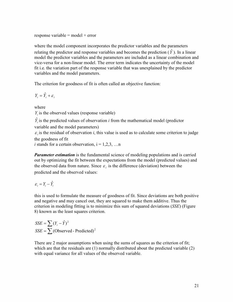
this is used to formulate the measure of goodness of fit. Since deviations are both positive

and negative and may cancel out, they are squared to make them additive. Thus the

criterion in modeling fitting is to minimize this sum of squared deviations (SSE) (Figure

8) known as the least squares criterion.

∑ −= 2)ˆ( YYSSE i

∑= 2Predicted) - (ObservedSSE

There are 2 major assumptions when using the sums of squares as the criterion of fit;

which are that the residuals are (1) normally distributed about the predicted variable (2)

with equal variance for all values of the observed variable.

22

0.0

5.0

0 100

Expected

Xi

Observed|

εi

|

iii YY ˆ−=ε

iY

iY

0.0

5.0

0 100

Expected

Xi

Observed|

εi

|

iii YY ˆ−=ε

0.0

5.0

0 100

Expected

Xi

Observed|

εi

|

iii YY ˆ−=ε

iY

iY

0.0

5.0

0 100

( ) =−=∑∑22 ˆ

iii YYε

0.0

5.0

0 100

( ) =−=∑∑22 ˆ

iii YYε ( ) =−=∑∑22 ˆ

iii YYε

Figure 8: Shows the calculation of sum of squares in a linear model


Whether the model is simple or complex the principal of the criterion for the goodness of

fit for the least squares is always the same, i.e. minimize the sums of squares SSE. Note

that only one combination of the parameters will give the minimum SSE, the aim is to

find this combination. The complexity arises in the algorithm used to obtain the best

parameter estimates that describe the predicted value. Computationally it easy to search

for values of the parameters to find the ones that fulfil the condition of minimum sums of

squares. It can be done through:

• Grid search: try different values for the model parameter and calculate SSE for

each case

• Inbuilt minimization routines: most statistical programs have these routines. They

are for all practical purposes “black boxes”, how it is done is not important, the

principal understanding is the issue. In Excel the black box is called Solver.

It is important to take note of some of the synonyms used in the literature generally:

observed value = measurement = response variable = dependent variable

predicted value = fitted value = expected value

residual error = deviation = random error = residual = error = noise

2.5. Linear Regression

Linear regression is based on statistical models that assume a linear relationship between

one response variable (Y) and one predictor variable (X). The simple linear regression

analysis has three main purposes:

• To describe the linear relationship between Y and X

• To determine how much of the variation in Y can be explained by the linear

relationship with X and how much remains unexplained

• To predict new values of Y (predicted value) from the new values of X.

The formal statement of the model is;

23

iii XY εβα ++=

where:

iY is the dependent/ response variable

α and β are parameters

iX is the dependent/ predictor variable

iε ~ n (0, 2σ ) is the error term of the model with mean 0 and variance 2σ (assumed to be

independent and identically distributed)

The Y and X variables are regressed to estimate α (intercept) and β (slope) by ordinary

least squares method which involves minimising the sums of squares i.e. minimising the

difference between the expected values ii XY βα +=ˆ and iY ;

( )2

1

)(∑=

+−=n

i

ii XYSSE βα

It can be shown that the estimates of α and β, called a and b respectively here, that

minimises the SSE can be given by;

XbYa −=

( )( )( )∑

∑−

−−=

2XX

YYXXb

This is an analytical solution (derivations have been omitted). Although an analytical

solution for finding the value of parameters of interest, fulfilling the criterion of best fit,

are available for simple linear models such is not always the case for more complex

models for which numerical search methods (computational methods) become essential.

The null hypothesis ( oH ) being tested in a simple linear regression analysis is β = 0. The

reason for choosing β for a normal regression model is because the condition β = 0

implies that there is no linear association between X and Y. The t statistic is used to test

the general hypothesis concerning β . Since the estimate of β , b is known to come from a

t-distribution with 2−n degrees of freedom, tests concerning β can be set using the t-

distribution where the t value is computed by )(b

bt

σ= (i.e. estimate divided by its

standard deviation). oH is rejected if the computed t-value is greater than the theoretical

t-value (read from the students t-distribution table) at 2−n degrees of freedom and a

certain significance level (e.g. 05.0=α ).

24

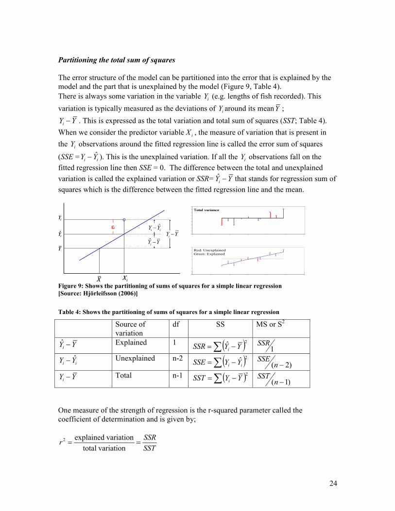
Partitioning the total sum of squares

The error structure of the model can be partitioned into the error that is explained by the

model and the part that is unexplained by the model (Figure 9, Table 4).

There is always some variation in the variable iY (e.g. lengths of fish recorded). This

variation is typically measured as the deviations of iY around its meanY ;

YYi − . This is expressed as the total variation and total sum of squares (SST; Table 4).

When we consider the predictor variable iX , the measure of variation that is present in

the iY observations around the fitted regression line is called the error sum of squares

(SSE = ii YY ˆ− ). This is the unexplained variation. If all the iY observations fall on the

fitted regression line then SSE = 0. The difference between the total and unexplained

variation is called the explained variation or SSR= YYi −ˆ that stands for regression sum of

squares which is the difference between the fitted regression line and the mean.

îY Y−

î iY Y−

iY

X iX

îY

Y

|

εi

|iY Y−

îY Y−

î iY Y−

iY

X iX

îY

Y

|

εi

|iY Y−

Total variance

Red: Unexplained

Green: Explained

Total variance

Red: Unexplained

Green: Explained

Figure 9: Shows the partitioning of sums of squares for a simple linear regression


Table 4: Shows the partitioning of sums of squares for a simple linear regression

Source of

variation

df SS MS or S2

YYi −ˆ Explained 1 ( )2ˆ∑ −= YYSSR i 1SSR

ii YY ˆ− Unexplained n-2 ( )2ˆ∑ −= ii YYSSE )2( −nSSE

YYi − Total n-1 ( )2∑ −= YYSST i )1( −n

SST

One measure of the strength of regression is the r-squared parameter called the

coefficient of determination and is given by;

SST

SSRr ==

variationtotal

variationexplained2

25

The coefficient of determination shows the level of variation explained by the regression

model. The value of 2r is between 0 and 1. The 2r will be close to 1 if the explained error

is high in comparison with the total variation and vice versa.

Linear models have four main assumptions:

• linearity

• normality

• constant variance (homoscedasticity)

• independence

Formal tests are available to check the conformity of these assumptions i.e. to test the

reliability of the regression analysis. However these are not dealt with in this manual. In

principle the residuals from the regression analysis should be randomly distributed and

not show a systematic pattern.

If model assumptions appear to be violated there are some remedies:

• Try alternative model if there is a systematic pattern in the residuals (often add

more parameters)

• Transformation of data if constant variance assumption is violated

• Alternative formulation of the objective function, i.e. use some other criterion

than the minimum sums of squares

2.6. Multiple linear regression

Instead of having only one variable X, explaining the observations Y, we may have two

variables, X and Z. A possible model would be:

iii ZXY εγβα +++=

Thus three parameters γβα ,, need to be estimated. More parameters can be added

similarly. The objective remains the same to minimize SSE;

( )2)(∑ ++−= iii cZbXaYSSE

The aim is to find a combination of the three parameters a, b and c (estimates of

γβα ,, respectively) which give the lowest SSE;

In order to determine if the new variable Z helps in explaining any further variation than

variable X an F-test is used. In order words it is important to determine if parameter c is

significant. The F-test involves comparing the full model with all parameters to a reduced

model with one lesser number of parameters. In this case the full model is;

26

iii ZXY εγβα +++= ( )2)(∑ ++−= iiiF cZbXaYSSE

and the reduced model is;

iii XY εβα ++= ( )2)(∑ +−= iiR bXaYSSE

The SSE for the full model should be lower than the SSE for the reduced model if the

additional variable is explaining some variation in the observations. If RF SSESSE ≈ then

the new parameter is not significant i.e. it does not explain any more variation about the

regression line. The analyses of the sums of squares are converted to variances by

dividing by the degrees of freedom (df) in order to apply the F-test to compare them. The

formal test is:

F

F

FR

FR

dfSSE

dfdf

SSESSE

F−−

=

If F is higher than some theoretical value then the reduced model is rejected and the

parameter is significant.

Exercise 2 set up in Excel demonstrates the simple and multiple linear regression

2.7. Analysis of Variance (ANOVA)

Analysis of variance, often abbreviated with the acronym ANOVA is a technique for

identifying and measuring the various sources of variation within a collection of data

(Kachigan, 1991). It is a flexible technique that allows making comparisons between any

numbers of sample means, all in a single test. The potential sources being tested are

sometimes referred to as “treatments” or “factors”. For instance the amount of catch

landed at three different sites (markets) need to be formally compared. Then the mean

weights of landed catch is compared between markets, which is the factor is this case.

The Model assumptions are:

1. The observations in each cell constitute an independent random sample of size n

and come from a population with mean µij.

2. Each population represented by the cell samples is normal and has the same

variance σ2.

The Model hypotheses are:

1 Null hypothesis H0: µ1 = µ 2 = … = µk, all means are equal

2. Alternative hypothesis Ha: at least one pair of µ´s are not equal.

Difference in the mean of the samples gives rise to two sources of variability (1)

variability due to differences among factors (SSfactor ) (2) variability within factors (SSError

) which sum up to form Total Sum of Squares (SSTotal) (Glover and Mitchell 2002). The

27

analyses of the sums of squares are converted to variances by dividing by the degrees of

freedom (df) in order to apply the F-test to compare them.

error

factor

SSerror

SSfactor

dfSS

dfSSF ==

variancesamplewithin

variancesamplebetween

If F ratio is 1 then H0 is true whereas the hypothesis is rejected with F ratio > 1.

2.8. An introduction to Bootstrap

Bootstrap essentially involves generating a number of samples from a given number of

original samples. This technique is based on re-sampling. Bootstrap re-sampling is a

general form of re-sampling in that it is re-sampling with replacement to produce samples

of size n (Haddon 2001). This technique was developed by Efron (1982) and they named

it Bootstrap in the honour of the unbelievable tales of Baron Munchausen who had, in

one of his many adventurous travels fallen to the bottom of a deep lake and just as he was

to succumb to his fate he thought of pulling himself up by his own bootstrap

(Hjörleifsson 2006).

Suppose “we have a set of real-valued observations nxx ...1 independently sampled from

an unknown probability distribution F. We are interested in estimating some parameter Q

by using the information in the sample data with an estimatorQ)

. Some measure of the

estimate’s accuracy is as important as the estimate itself; we want a standard error of

Q)

and, even better a confidence interval on the true value Q” (Efron and LePage 1992).

Bootstrap becomes most useful where the sampled population cannot fit into classical

sampling theory and cannot be represented by a normal distribution and especially where

the underlying distribution is unknown (Haddon 2001).

Bootstrap involves randomly re-sampling with replacement from the same original

sample, using a random number generator. Suppose a sample data set is available for

which a mean and standard deviation can be calculated. By doing this we assume the

distribution of the data to be normal. It can be risky to make this assumption if the true

distribution of the population is not known and enough samples from the population are

not available. We can generate a number of “bootstrap” data sets from the original data

using a random draw with replacement from the observations in the original data set. For

example, 1000 samples can be generated from one sample using a bootstrap. The

generated samples will have the same size as the original sample. This is illustrated in

Table 5 below. Because the numbers are picked randomly with replacement, some

measurements can be repeated within a sample. The model is refitted to each bootstrap

data set and the statistics of interest (mean and standard deviation) is calculated. This

generates a frequency distribution and the estimate of the parameter is the mean of the

distribution and the standard error of the mean is the standard deviation of the frequency

28

distribution. Bootstrap can be used to measure the bias in an estimate i.e. the difference

between the actual population parameter and the expected value.

Table 5: Shows the process of a Bootstrap

Sample Data Bootstrap sample number

i 1 2 3 4 … n

1 3 7 11 7 8 11

2 5 7 7 3 8 8

3 7 11 8 7 8 8

4 8 7 3 11 3 3

5 9 7 5 7 7 5

6 11 9 9 5 3 3

mean 7.17 8.00 7.17 6.67 6.17 6.33

sd 2.86 1.67 2.86 2.66 2.48 3.20

Further suggested readings on biostatistics are Glover and Mitchell (2002), Quinn and

Keough (2002), Neter et al. (2005) and Haddon (2001).

29

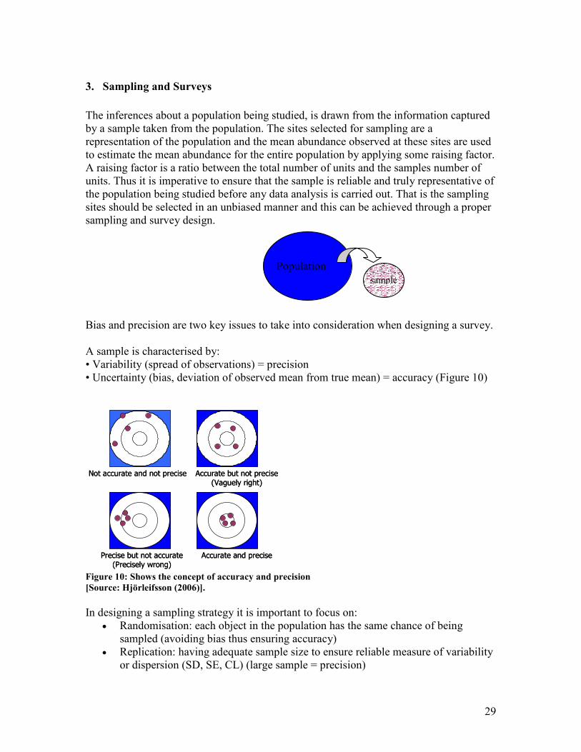
3. Sampling and Surveys

The inferences about a population being studied, is drawn from the information captured

by a sample taken from the population. The sites selected for sampling are a

representation of the population and the mean abundance observed at these sites are used

to estimate the mean abundance for the entire population by applying some raising factor.

A raising factor is a ratio between the total number of units and the samples number of

units. Thus it is imperative to ensure that the sample is reliable and truly representative of

the population being studied before any data analysis is carried out. That is the sampling

sites should be selected in an unbiased manner and this can be achieved through a proper

sampling and survey design.

Bias and precision are two key issues to take into consideration when designing a survey.

A sample is characterised by:

• Variability (spread of observations) = precision

• Uncertainty (bias, deviation of observed mean from true mean) = accuracy (Figure 10)

Not accurate and not precise Accurate but not precise(Vaguely right)

Accurate and precisePrecise but not accurate(Precisely wrong)

Not accurate and not precise Accurate but not precise(Vaguely right)

Accurate and precisePrecise but not accurate(Precisely wrong)

Figure 10: Shows the concept of accuracy and precision


In designing a sampling strategy it is important to focus on:

• Randomisation: each object in the population has the same chance of being

sampled (avoiding bias thus ensuring accuracy)

• Replication: having adequate sample size to ensure reliable measure of variability

or dispersion (SD, SE, CL) (large sample = precision)

Population

sample

30

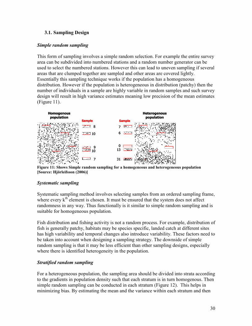
3.1. Sampling Design

Simple random sampling

This form of sampling involves a simple random selection. For example the entire survey

area can be subdivided into numbered stations and a random number generator can be

used to select the numbered stations. However this can lead to uneven sampling if several

areas that are clumped together are sampled and other areas are covered lightly.

Essentially this sampling technique works if the population has a homogeneous

distribution. However if the population is heterogeneous in distribution (patchy) then the

number of individuals in a sample are highly variable in random samples and such survey

design will result in high variance estimates meaning low precision of the mean estimates

(Figure 11).

Homogenouspopulation

Sample

Heterogenouspopulation

Sample

8

10

910

7

7

6

013

31

Homogenouspopulation

Sample

Heterogenouspopulation

Sample

8

10

910

7

7

6

013

31

Figure 11: Shows Simple random sampling for a homogeneous and heterogeneous population


Systematic sampling

Systematic sampling method involves selecting samples from an ordered sampling frame,

where every kth element is chosen. It must be ensured that the system does not affect

randomness in any way. Thus functionally is it similar to simple random sampling and is

suitable for homogeneous population.

Fish distribution and fishing activity is not a random process. For example, distribution of

fish is generally patchy, habitats may be species specific, landed catch at different sites

has high variability and temporal changes also introduce variability. These factors need to

be taken into account when designing a sampling strategy. The downside of simple

random sampling is that it may be less efficient than other sampling designs, especially

where there is identified heterogeneity in the population.

Stratified random sampling

For a heterogeneous population, the sampling area should be divided into strata according

to the gradients in population density such that each stratum is in turn homogenous. Then

simple random sampling can be conducted in each stratum (Figure 12). This helps in

minimizing bias. By estimating the mean and the variance within each stratum and then

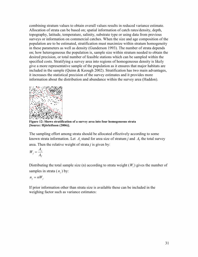
31

combining stratum values to obtain overall values results in reduced variance estimate.

Allocation of strata can be based on; spatial information of catch rates/density, depth,

topography, latitude, temperature, salinity, substrate type or using data from previous

surveys or information on commercial catches. When the size and age composition of the

population are to be estimated, stratification must maximize within stratum homogeneity

in these parameters as well as density (Gunderson 1993). The number of strata depends

on; how heterogeneous the population is, sample size within stratum needed to obtain the

desired precision, or total number of feasible stations which can be sampled within the

specified costs. Stratifying a survey area into regions of homogeneous density is likely

give a more representative sample of the population as it ensures that major habitats are

included in the sample (Quinn & Keough 2002). Stratification has two main advantages,

it increases the statistical precision of the survey estimates and it provides more

information about the distribution and abundance within the survey area (Haddon).

4

2

3

1

4

2

3

1

Figure 12: Shows stratification of a survey area into four homogeneous strata


The sampling effort among strata should be allocated effectively according to some

known strata information. Let jA stand for area size of stratum j and TA the total survey

area. Then the relative weight of strata j is given by:

T

j

jA

AW =

Distributing the total sample size (n) according to strata weight ( iW ) gives the number of

samples in strata ( jn ) by:

jj nWn =

If prior information other than strata size is available these can be included in the

weighing factor such as variance estimates:

32

jjej AA σ=

∑=

ej

ej

jA

AW

jj nWn =

where jσ is the variance of the strata and ejA is the weighting factor based on strata area

and strata variance that are summed over all strata ∑ ejA .

As a general rule, the sampling intensity is higher in areas where the variance is greater

and often greater variance is observed where the density is higher. Thus sampling

intensity is often proportional to density.

Similarly cost information can be incorporated. Higher cost of sampling in strata would

lead to a lower sample size per those strata. The sample size in stratum as a function of

sample size, sample variance and sample cost would be:

j

jj

ejC

AA

σ=

∑=

ej

ej

jA

AW

jj nWn =

where jC is cost per sample in stratum j.

The mean within each stratum or stratified mean is calculated by:

j

n

i

ji

jn

y

y∑== 1

,

∑=

=L

j

jjst yWy1

where

jiy , is catch of the ith tow in stratum j

jn is number of tows in the ith stratum

jy is mean catch rate in the jth stratum

jW is weight of stratum j

sty is estimated stratified mean density in the entire area

(note: tow is used as a reference and can be replaced by other sampling method such as

transects)

33

The standard deviation of the samples can be calculated by:

( )1

1

2

,2

−

−=∑=

j

n

i

jji

jn

yy

s

j

jL

j

jstn

sWyV

2

1

2)( ∑

=

=

)( sty yVSEst=

where

2

js is variance in stratum j

)( styV is estimated variance of the stratified mean

stySE is standard error estimate of the stratified mean

If the sample is large enough, then there is a 95% chance that the true mean lies in the

interval:

stynst SEty 05.0,1−±

where t is from the theoretical student’s t distribution with n-1 degrees of freedom and

05.0=α (this alpha level corresponds to getting 95% confidence interval).

One of the crucial factors is the choice of sample size (i.e. the number of replicates)

which will optimize the statistical analysis and the estimates obtained. Replicates are

essential because most biological and ecological systems are inherently variable and to be

able to achieve a precise estimate, the survey needs to take this variability into account

(Quinn and Keough 2002). However this always becomes a matter of capacity and cost.

At the same time, precision is not just a function of how many samples are taken but how

the samples are taken (Helle and Pennington 2004). Effort should be expended to ensure

that sample sizes are equal between the treatment levels. For instance, if the treatment

levels are different geographical locations, then equal number of samples should be taken

from each location. Secondly, if treatments are to be compared with any confidence, it is

vital that surveying procedures be as identical as possible so that the number of

uncontrolled variables is reduced (Quinn & Keough 2002). In case of coral reefs, to cater

for the large-scale environmental gradient, the sampling area can be divided into

homogenous sub-areas such as lagoon, reef flat and reef slope, and sampled. This will

also require that an equal number of replicates are taken from each of these sub-areas.

Linear model analyses usually rely on comparing the variation between treatment groups

(e.g. sub-areas of the coral reefs) to the inherent variability within the treatment groups

(replicates) (Quinn & Keough 2002).

34

Randomisation in fisheries is in practise very difficult due to gear selectivity, unknown

spatial and temporal distribution of population and bias introduced when catches are

sorted or discarded at sea.

In summary, stratum sampling size:

• Should be large if the stratum (area, numbers) is large

• Should be large if the variance is large

• Should be large if the sampling is inexpensive

For further reading on sampling and data collection FAO 1998 is recommended

The sampling design is always a compromise between different objectives. Sampling

theory can however always help. It is generally difficult to determine either the accuracy

or the precision of estimates based on commercial catch data, and it is not clear how to

improve, at a reasonable cost, the collection of catch data. Therefore it is recommended

to always get an independent estimate of your statistics once in while.

3.2. Surveys

Independent surveys of fisheries resources often appear to provide a more accurate

prognosis of the status of a fish stock than commercial catch sampling (Pennington and

Strømme 1998, Korsbrekke et al., 2001). These surveys are normally carried out by

fishery independent research vessels. Surveys were actively promoted during the

exploration phase of fisheries resources in the 1970s and early 1980s, when the concept

of Exclusive Economic Zone (EEZ) was adopted by the UNCLOS (United Nations

Convention on the Law of the Sea). Since then, standardised scientific abundance survey

data has become an important tool to estimate “indices of abundance” in the current

situation and for long-term monitoring of most of the commercially important stocks

(Kolding and Giordano 2001). An advantage that survey-based assessments have over

those based on commercial catch statistics is that the uncertainties associated with survey

estimates can be studied and quantified, and based on such research, survey methods, and

ultimately stock assessments, can be improved (Godø, 1994).

3.3. Basic Data Collection

Preferably data should be collected at the highest resolution possible. Some of the basic

data needed for fisheries resource assessments include:

• Catch or landed catch (numbers or weight of fish) recorded by sampling area

• Location of catch; latitude, longitude, provincial boundaries, statistical rectangles

35

• Species of fish (catch and stock composition); especially tropical coral reef

systems are multispecies and the landed catch comprises of a significant number

of species

• Effort which is a measure of fishing activity such as number of boats, numbers of

days fished, number of hours fished

• Measurements of individual fish in a sample

♦ Length frequency measurements: fish are normally measured on a

measuring board and counts are tallied e.g.

cm

10

11 |

12 ||

13 |

14 |||

15 ||

16

17 |||

18 ||

♦ Individual measurements can be recorded and tabulated in which case

together with length (le), weight (wt), sex (0/1 to represent M/F), maturity

stage etc. is also recorded for each fish. If the fish can be aged through

readings of hard structures such as otoliths/scales then this information can

also be added e.g.

no le wt sex mat age

1 14.5 12.5 0 4 2

2 15.0 13.0 0 5 3

3 14.5 12.0 1 4 3

♦ Other detailed biological measurements include, liver weight, fat content,

RNA/DNA ratios, size and number of eggs (Stefánsson)

• A measure of discarded catch

• For economic analysis: cost of fishing, number of jobs

Data collection can be a costly affair. Therefore it becomes necessary to prioritise and

compromise under funding constraints. More so it is necessary to optimise through

information sharing. Such as government agencies, NGO’s, private sectors and fishermen

can team up in information gathering.

36

4. Fundamental Fishery Concepts

The basic assumption in fisheries theory is that catch (C) and stock abundance, or

standing biomass (B) are related by:

BEqC ..=

where q is the catchability coefficient

E is a measurement of fishing effort

Catch and effort are two fundamental data required for managing any fishery. The most

common index of abundance is catch per unit effort (CPUE) which is catch divided by

effort E

C . CPUE is recorded in many ways depending on the nature of the fishery and

the fishing gear used. For example, number of fish caught per hook per hour, or number

of fish caught per hour of trawling. For gillnet fishery, CPUE maybe recorded as kg per

fisher and if information is available by day then kg per fisher per day. In principle one

unit of fishing effort will catch a constant proportion (called a catchability coefficient q)

of a total homogeneous stock (King 1995). Thus the above equation can be rewritten in

terms of CPUE:

BqCPUE .=

Normally absolute abundance (total number of fish in an area i.e. total biomass) cannot

be estimated from CPUE alone as the factor q is unknown. However CPUE can be used

as a measure of relative abundance over spatial or temporal changes. This linear

relationship assumes that a decline in CPUE would mean a decline in the stock and vice

versa. However this direct relationship may not always be the case. There are many cases

in which CPUE has turned out to be a poor indicator of stock abundance. The key

problem is in the difference between how fishing effort is measured and the way the

actual fishing effort is changing. For instance an increase in fishing efficiency (such as

use of modern gear) could lead to an increase in catch even though the actual abundance

of the fish stock might be decreasing. For scientific research surveys, or experimental

fishing, effort is standardised and fishing gears kept constant in order to keep a simple

relationship between catch rates and population abundance i.e. to minimise the inherent

measurement errors and/or variations in E and q (Kolding and Giordano 2001).

In most cases absolute abundance are measured by taking small samples from the

population and raising the information obtained from the sample to the whole population

as discussed earlier.

Fishing Mortality

Most management principles entail deciding on an optimum level of fishing effort that

maximises the catch (yield) and is sustainable at the same time. Fishing effort is

37

expressed as number of fishermen, number of boats etc. Unfortunately, due to changes in

the catchability coefficient q (which is related to the fishing gear selectivity and

efficiency) there is no fundamental relation between the magnitude of the effort and the

magnitude of the catch. For stock assessment purposes, there is a need for a measure of

fishing effort that has a constant effect upon the fish population. Therefore the measure,

commonly used in population dynamics is the so-called fishing mortality (F) (Kolding

and Giordano 2001). This is simply defined as the fraction of average population taken

by fishing. F is also called instantaneous rate of fishing mortality. Note this is a rate i.e.

the rate at which fish are dying due to fishing, and therefore expressed per time unit,

usually per year and not the proportion of fish caught each year. Thus two types of

fishing mortality are the instantaneous rate of fishing mortality F and proportional

annual mortality denoted H, known as the harvest rate (Haddon 2001). H is related to F

by:

FeH −−= 1

F can now be defined as:

B

CEqF == .

Substituting this in the equation ( BEqC ..= ) above gives

BFC .=

that is some measure of fishing applied to the stock biomass gives a catch.

F is a rate therefore technically it should have a value between 0 and 1 on an annual basis

however in practise this is not the case. Some stocks, especially the smaller sized tropical

fish species have a high biological turnover or production to biomass (P/B) ratio i.e.

annual productivity of such stocks can be much higher than the average standing

abundance which leads to F being greater than 1 in such situations.

Gear Selectivity

All fishing gear is selective to some degree (Jennings et. al. 2001). For instance, the size

of the hook used for fishing will determine the lower and upper sizes of the fish being

hooked and the mesh size of the net will determine the size of the fish trapped in the net.

Suppose, the smallest fish (smaller size classes) caught in a trawl were aged to get an

estimate of size at age in the stock. This could easily lead to overestimation of the size at

age as fish which are smaller for the age may have escaped the trawl and not appeared in

the samples at all. Knowing about fishing gear selectivity is important in order to

understand the biases created by it in the sampling programmes and to correct for their

effects. Additionally understanding of selectivity can be used for management purposes

such as regulating the mesh size to control the size of catches and in turn mortality rates

38

for different classes and for correcting length-frequency distributions of samples, by

adjusting for differential catchability at size (Jennings et. al. 2001). Selectivity is not

entirely based on mesh size but also the shape of the mesh, the orientation of the netting

and the direction of the towed gear (for trawls surveys for example). For trawling gear,

mesh selectivity can be studied by placing fine mesh covers over codend to catch

escapees and the size distribution of the codend and cover are used to study selectivity.

Selectivity is defined as the probability of fish being retained in a fishing gear as a

function of the length of the fish (Kolding and Giordano 2001). The probability can be

modelled using a logistic curve. A selection curve (i.e. the probability of capture plotted

against the size of the fish) for trawl gears is mostly sigmoid or S-shaped, whereas bell-

shaped curves are normally the case for gill-nets and hook and line. Important selectivity

measures are L50, defined as the fish length, where the fish have a 50% probability of

being retained by the gear on encounter, and the selection factor, defined as L50 divided

by mesh size in cm. In addition to the selection range which is defined as L75 – L25 (L75

is fish length where 75 % of the fish is retained, and L25 is fish length where 25 % of the

fish is retained), these parameters describe the size selection characteristics of fishing

gears (Sparre and Venema 1998 and Kolding and Giordano 2001).

Gear selectivity forms the basis of the parameter catchability coefficient (q), the

relationship between the catch rate (CPUE) and the true population size (B). Catchability

is the proportion of the stock caught for a given effort so the unit of catchability is fish

caught per fish available per effort unit and per time unit (Kolding and Giordano 2001). It

is also called gear efficiency (Hilborn and Walters 1992) or sometimes fishing power and

in principle can be divided into efficiency and availability. Efficiency would refer to the

number of fish actually caught and retained by the net to the number of fish in the trawl

path for example. And availability refers to the proportion of the stock in the area being

fished (Jennings et. al. 2001). Thus the probability of a fish being caught depends on

several factors and can be summarised as follows:

Biological factors:

• fish availability on the fishing ground

• behaviour of fish towards the fishing gear

• the size, shape, and external features of the fish

• these factors are dependent on season, age, environment and fish species

Technological factors:

• Gear type, design, size, colour, and material

• Gear position, duration, and handling

• Experience of the fisherman

• these factors are dependent of biological changes

Hence CPUE cannot be considered as an index of absolute abundance and the

understanding and information of gear selectivity and catchability is essential for stock

assessment purposes.

39

5. Growth

The study of age and growth is fundamental in stock assessment as the production from a

fish stock is a function of the recruitment of new individuals and the growth of the

existing individuals in the population. Consequently, growth is a combination of

population growth (change in biomass due to change in numbers from recruitment and

mortality) and individual growth (increase in length and weight). The growth of a

population or an individual is often represented by mathematical models describing the

average change per unit of time.

5.1. Population Growth

In describing how a population grows, the most abstract form can be seen as a population

growing in an unlimited environment. For example a colonizing species settles in an area

with unlimited resources and accelerates in growth. This type of accelerating growth is

described as exponential growth. It implies that with each time step, the population

increases by a constant proportion given the birth and death rates are constant at all

population sizes. This can be described using the differential equation

rNNdbdt

dN≡−= )( (1.1)

where, dN/dt is the rate of change of the population size N relative to time t, b is the birth

rate, d is the death rate and r = (b-d) and is called the intrinsic rate of increase or the

instantaneous rate of population growth. In exponential growth r is a constant and is

assumed to be independent of population size N i.e. the births and deaths are unaffected

by the population size. Because of this independence this type of growth is termed

“density-independent”.

However, it is known that populations cannot grow indefinitely as all populations live in

a limited environment with limited resources. Thus positive exponential growth can only

be a short-term phenomenon. The total biomass of a non exploited stock cannot grow

beyond a certain limit. The value of that limit depends, for each resource, on the available

space, on the feeding facilities, on the competition with other species, etc. In conclusion,

it depends on the capacities of the ecosystem to maintain the stock and is density

dependent. That size limit of the biomass will be designated by carrying capacity, K.

The simplest model derived from the exponential growth model to include the density

dependent effects is the logistic model of growth. This means that the birth and death

rates are related to population size in a linear manner. To achieve this some modifying

parameter needs to be included in a linear equation:

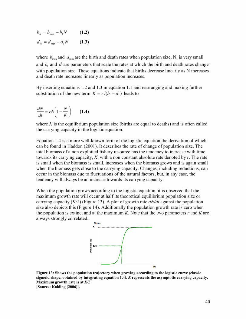
40

NbbbN 1max −= (1.2)

Nddd N 1min −= (1.3)

where maxb and mind are the birth and death rates when population size, N, is very small

and 1b and 1d are parameters that scale the rates at which the birth and death rates change

with population size. These equations indicate that births decrease linearly as N increases

and death rate increases linearly as population increases.

By inserting equations 1.2 and 1.3 in equation 1.1 and rearranging and making further

substitution of the new term )/( 11 dbrK −= leads to

−=K

NrN

dt

dN1 (1.4)

where K is the equilibrium population size (births are equal to deaths) and is often called

the carrying capacity in the logistic equation.

Equation 1.4 is a more well-known form of the logistic equation the derivation of which

can be found in Haddon (2001). It describes the rate of change of population size. The

total biomass of a non exploited fishery resource has the tendency to increase with time

towards its carrying capacity, K, with a non constant absolute rate denoted by r. The rate

is small when the biomass is small, increases when the biomass grows and is again small

when the biomass gets close to the carrying capacity. Changes, including reductions, can

occur in the biomass due to fluctuations of the natural factors, but, in any case, the

tendency will always be an increase towards its carrying capacity.

When the population grows according to the logistic equation, it is observed that the

maximum growth rate will occur at half its theoretical equilibrium population size or

carrying capacity (K/2) (Figure 13). A plot of growth rate dN/dt against the population

size also depicts this (Figure 14). Additionally the population growth rate is zero when

the population is extinct and at the maximum K. Note that the two parameters r and K are

always strongly correlated.

K

K/2

Popula

tion s

ize

K

K/2

Popula

tion s

ize

K

K/2

Popula

tion s

ize

Figure 13: Shows the population trajectory when growing according to the logistic curve (classic

sigmoid shape, obtained by integrating equation 1.4). K represents the asymptotic carrying capacity.

Maximum growth rate is at K/2

[Source: Kolding (2006)].

41

KK/2

Population size

Rat

e of

chan

ge

(dN

/dt)

200

1200

1000

800

600

400

KK/2

Population size

Rat

e of

chan

ge

(dN

/dt)

200

1200

1000

800

600

400

Figure 14: Shows the plot of equilibrium rate of change of population size versus population size

(production vs. stock size curve) obtained by taking the slope of the curve in Figure 13 at each time

step and plotting against population size. Maximum productivity occurs at half K, equilibrium occurs

at zero and K


Any population takes time to respond to any changes in population size (births, deaths,

fishing). Therefore it appears realistic to introduce time intervals in the differential

equation 1.4. Thus the logistic model set up as a difference equation (known as discrete

logistic model incorporating time intervals) could be

−+=+K

NrNNN t

tt 11 (1.5)

An extra source of mortality, such as fishing mortality, could be represented by adding an

extra term tC

tt

tt CK

NrNNN −

−+=+ 11 (1.6)

where tC depicts the catch levels, either constant or a time series of catches.

The logistic model applied to fisheries science becomes

tt

tt CK

BrBBB −

−+=+ 11 (1.7)

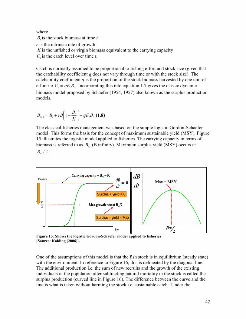
42

where

tB is the stock biomass at time t

r is the intrinsic rate of growth

K is the unfished or virgin biomass equivalent to the carrying capacity

tC is the catch level over time t.

Catch is normally assumed to be proportional to fishing effort and stock size (given that

the catchability coefficient q does not vary through time or with the stock size). The

catchability coefficient q is the proportion of the stock biomass harvested by one unit of

effort i.e =tC ttBqE . Incorporating this into equation 1.7 gives the classic dynamic

biomass model proposed by Schaefer (1954, 1957) also known as the surplus production

models.

ttt

tt BqEK

BrBBB −

−+=+ 11 (1.8)

The classical fisheries management was based on the simple logistic Gordon-Schaefer

model. This forms the basis for the concept of maximum sustainable yield (MSY). Figure

15 illustrates the logistic model applied to fisheries. The carrying capacity in terms of

biomass is referred to as ∞B (B infinity). Maximum surplus yield (MSY) occurs at

2/∞B .

Max growth rate at B∞/2K

2

Carrying capacity = B∞ = K

dB

dt= 0

Surplus = yield = 0

Surplus = yield = Max

Density

Max growth rate at B∞/2K

2Max growth rate at B∞/2Max growth rate at B∞/2

K

2


dB

dt= 0


dB

dt= 0

Surplus = yield = 0


Surplus = yield = 0


Density

dB

dt

B∞2

Max = MSYdB

dt

B∞2

Max = MSY

B∞2

Max = MSY

Figure 15: Shows the logistic Gordon-Schaefer model applied to fisheries


One of the assumptions of this model is that the fish stock is in equilibrium (steady state)

with the environment. In reference to Figure 16, this is delineated by the diagonal line.

The additional production i.e. the sum of new recruits and the growth of the existing

individuals in the population after subtracting natural mortality in the stock is called the

surplus production (curved line in Figure 16). The difference between the curve and the

line is what is taken without harming the stock i.e. sustainable catch. Under the

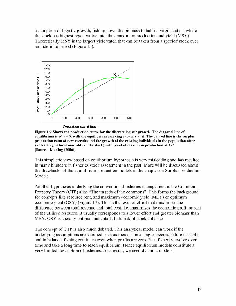
43

assumption of logistic growth, fishing down the biomass to half its virgin state is where

the stock has highest regenerative rate, thus maximum production and yield (MSY).

Theoretically MSY is the largest yield/catch that can be taken from a species' stock over

an indefinite period (Figure 15).

Popula

tion s

ize

at tim

e t+

1

0

100

200

300

400

500

600

700

800

900

1000

1100

1200

1300

0 200 400 600 800 1000 1200

Population size at time t

K

Popula

tion s

ize

at tim

e t+

1

0

100

200

300

400

500

600

700

800

900

1000

1100

1200

1300

0 200 400 600 800 1000 1200


K

0

100

200

300

400

500

600

700

800

900

1000

1100

1200

1300

0 200 400 600 800 1000 1200


K

Figure 16: Shows the production curve for the discrete logistic growth. The diagonal line of

equilibrium is Nt+1 = Nt with the equilibrium carrying capacity at K. The curved line is the surplus

production (sum of new recruits and the growth of the existing individuals in the population after

subtracting natural mortality in the stock) with point of maximum production at K/2


This simplistic view based on equilibrium hypothesis is very misleading and has resulted

in many blunders in fisheries stock assessment in the past. More will be discussed about

the drawbacks of the equilibrium production models in the chapter on Surplus production

Models.

Another hypothesis underlying the conventional fisheries management is the Common

Property Theory (CTP) alias “The tragedy of the commons”. This forms the background

for concepts like resource rent, and maximum economic yield (MEY) or optimum

economic yield (OSY) (Figure 17). This is the level of effort that maximises the

difference between total revenue and total cost, i.e. maximises the economic profit or rent

of the utilised resource. It usually corresponds to a lower effort and greater biomass than

MSY. OSY is socially optimal and entails little risk of stock collapse.

The concept of CTP is also much debated. This analytical model can work if the

underlying assumptions are satisfied such as focus is on a single species, nature is stable

and in balance, fishing continues even when profits are zero. Real fisheries evolve over

time and take a long time to reach equilibrium. Hence equilibrium models constitute a

very limited description of fisheries. As a result, we need dynamic models.

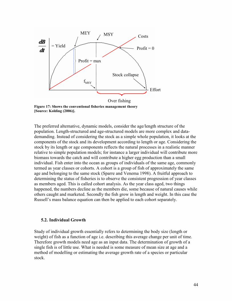
44

Figure 17: Shows the conventional fisheries management theory


The preferred alternative, dynamic models, consider the age/length structure of the

population. Length-structured and age-structured models are more complex and data-

demanding. Instead of considering the stock as a simple whole population, it looks at the

components of the stock and its development according to length or age. Considering the

stock by its length or age components reflects the natural processes in a realistic manner

relative to simple population models; for instance a larger individual will contribute more

biomass towards the catch and will contribute a higher egg production than a small

individual. Fish enter into the ocean as groups of individuals of the same age, commonly

termed as year classes or cohorts. A cohort is a group of fish of approximately the same

age and belonging to the same stock (Sparre and Venema 1998). A fruitful approach to

determining the status of fisheries is to observe the consistent progression of year classes

as members aged. This is called cohort analysis. As the year class aged, two things

happened, the numbers decline as the members die, some because of natural causes while

others caught and marketed. Secondly the fish grow in length and weight. In this case the

Russell’s mass balance equation can then be applied to each cohort separately.

5.2. Individual Growth

Study of individual growth essentially refers to determining the body size (length or

weight) of fish as a function of age i.e. describing this average change per unit of time.

Therefore growth models need age as an input data. The determination of growth of a

single fish is of little use. What is needed is some measure of mean size at age and a

method of modelling or estimating the average growth rate of a species or particular

stock.

= Yield

CostsMSY

Profit = 0

MEY

Effort

Over fishing

Stock collapse

fMSY

Profit = max

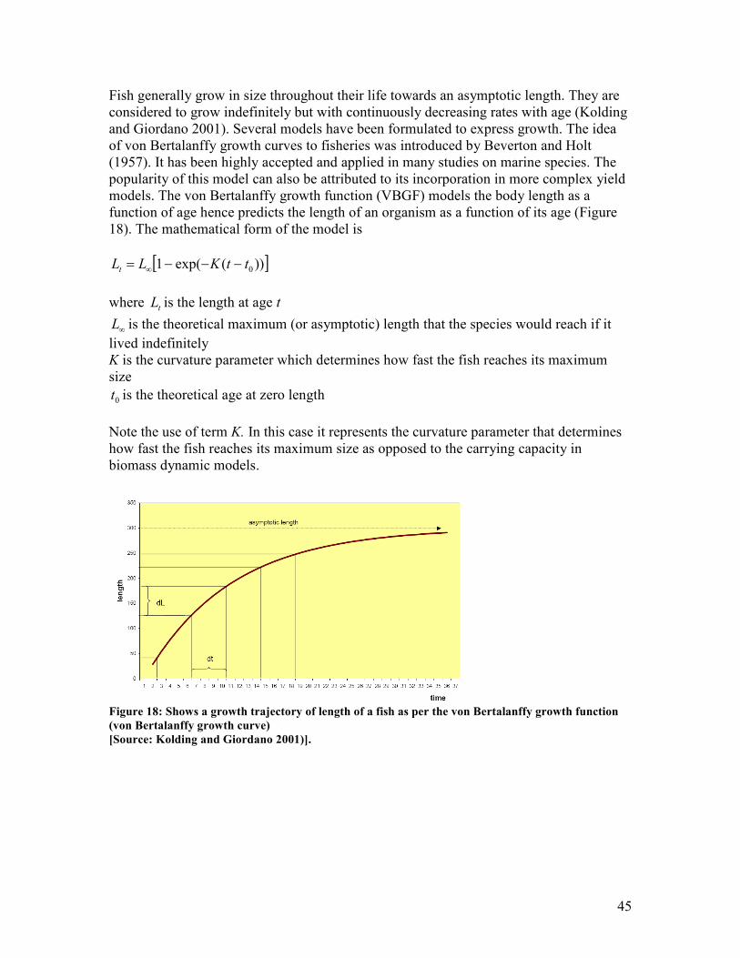
45

Fish generally grow in size throughout their life towards an asymptotic length. They are

considered to grow indefinitely but with continuously decreasing rates with age (Kolding

and Giordano 2001). Several models have been formulated to express growth. The idea

of von Bertalanffy growth curves to fisheries was introduced by Beverton and Holt

(1957). It has been highly accepted and applied in many studies on marine species. The

popularity of this model can also be attributed to its incorporation in more complex yield

models. The von Bertalanffy growth function (VBGF) models the body length as a

function of age hence predicts the length of an organism as a function of its age (Figure

18). The mathematical form of the model is

[ ]))(exp(1 0ttKLLt −−−= ∞

where tL is the length at age t

∞L is the theoretical maximum (or asymptotic) length that the species would reach if it

lived indefinitely

K is the curvature parameter which determines how fast the fish reaches its maximum

size

0t is the theoretical age at zero length

Note the use of term K. In this case it represents the curvature parameter that determines

how fast the fish reaches its maximum size as opposed to the carrying capacity in

biomass dynamic models.

Figure 18: Shows a growth trajectory of length of a fish as per the von Bertalanffy growth function

(von Bertalanffy growth curve)

[Source: Kolding and Giordano 2001)].

46

An animal is not likely to grow according to the above equation throughout its life span,

particularly in pre-adult stages hence the curve often cuts the X-axis at a value less than

zero, hence 0t often has a small negative value. Essentially the model is used to derive the

growth parameters ∞L , K & 0t and predict length as a function of age.

Combining the von Bertalanffy growth equation with the length/weight relationship 3

tt qLw = gives the weight based von Bertalanffy growth equation as a function of age

[ ]30))(exp(1 ttKWWt −−−= ∞

where the asymptotic weight ∞w corresponding to the asymptotic length is 3

∞∞ = qLW .

5.2.1. Data requirements

Generally the data consists of measurements of age, size (often length or width) and

weight. When a fish is caught, it is first measured for length and/or weight and then

commonly its otoliths are removed (how they are removed varies from species to species,

this can be a highly skilled art when done properly) which are then used to age the fish by

counting the yearly rings. Obtaining age data is more problematic. In temperate waters,

ageing fish is less complicated as year rings can be counted on hard parts of the fish, such

as otoliths and scales. These rings are formed due to strong environmental fluctuations

(summer to winter and vice versa). Such strong environmental conditions are missing in

the tropics therefore it becomes much very difficult to use seasonal rings for age

determination. The methods available for ageing tropical fish are normally too expensive.

As such, length measurements of fish are used to estimate age compositions through

length-frequency analysis to estimate growth and mortality parameters for most tropical

species. When applied with caution, these methods can give similar estimates as obtained

by other techniques although the sources and impacts of uncertainty are higher. Lengths

are easily measured accurately than weight; hence most of the methods are length-based.

Thus for the range of models available, the input data could either be age and/or length

measurements (age obtained from actual otolith readings) or simply length measurements

which are used to obtain age estimates. These could be obtained from resources surveys

of sampling commercial catches. Another category of data collection includes the Mark

and Recapture tagging experiments where two or more length measurements are taken.

Methods of data analysis pertaining to the former two will be discussed here.

Firstly the models used for estimating growth parameters are briefly described. Following

this is a description of some length-frequency analysis techniques which can be used to

estimate age from length data. These are then applied to the models to show how the

growth parameters can be estimated.

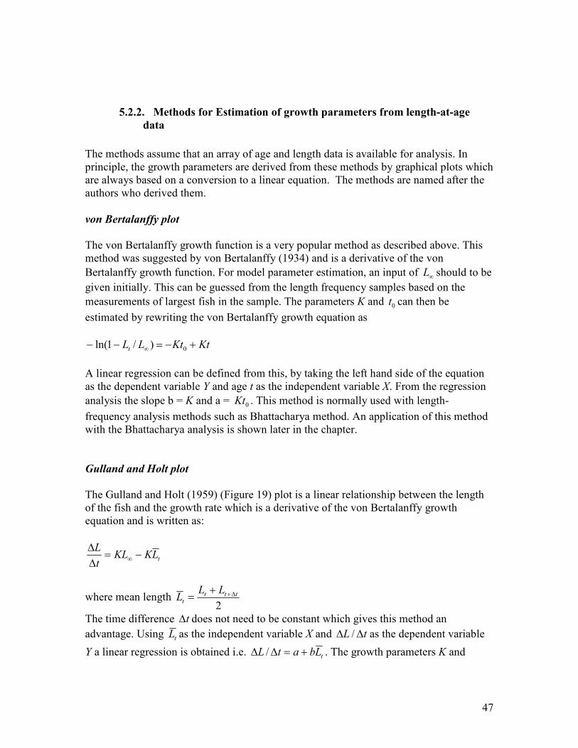
47

5.2.2. Methods for Estimation of growth parameters from length-at-age

data

The methods assume that an array of age and length data is available for analysis. In

principle, the growth parameters are derived from these methods by graphical plots which

are always based on a conversion to a linear equation. The methods are named after the

authors who derived them.

von Bertalanffy plot

The von Bertalanffy growth function is a very popular method as described above. This

method was suggested by von Bertalanffy (1934) and is a derivative of the von

Bertalanffy growth function. For model parameter estimation, an input of ∞L should to be

given initially. This can be guessed from the length frequency samples based on the

measurements of largest fish in the sample. The parameters K and 0t can then be

estimated by rewriting the von Bertalanffy growth equation as

KtKtLLt +−=−− ∞ 0)/1ln(

A linear regression can be defined from this, by taking the left hand side of the equation

as the dependent variable Y and age t as the independent variable X. From the regression

analysis the slope b = K and a = 0Kt . This method is normally used with length-

frequency analysis methods such as Bhattacharya method. An application of this method

with the Bhattacharya analysis is shown later in the chapter.

Gulland and Holt plot

The Gulland and Holt (1959) (Figure 19) plot is a linear relationship between the length

of the fish and the growth rate which is a derivative of the von Bertalanffy growth

equation and is written as:

tLKKLt

L−=

∆∆

∞

where mean length 2

tttt

LLL ∆++=

The time difference t∆ does not need to be constant which gives this method an

advantage. Using tL as the independent variable X and tL ∆∆ / as the dependent variable

Y a linear regression is obtained i.e. tLbatL +=∆∆ / . The growth parameters K and

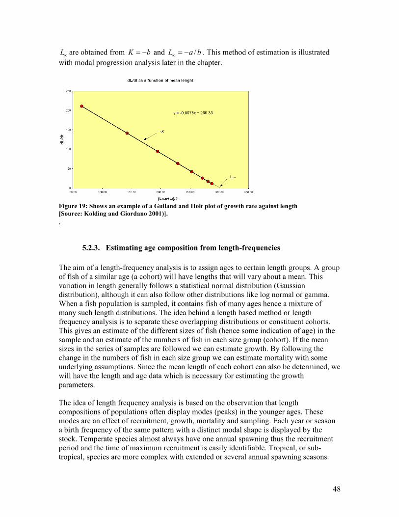
48

∞L are obtained from bK −= and baL /−=∞ . This method of estimation is illustrated

with modal progression analysis later in the chapter.

Figure 19: Shows an example of a Gulland and Holt plot of growth rate against length


.

5.2.3. Estimating age composition from length-frequencies

The aim of a length-frequency analysis is to assign ages to certain length groups. A group

of fish of a similar age (a cohort) will have lengths that will vary about a mean. This

variation in length generally follows a statistical normal distribution (Gaussian

distribution), although it can also follow other distributions like log normal or gamma.

When a fish population is sampled, it contains fish of many ages hence a mixture of

many such length distributions. The idea behind a length based method or length

frequency analysis is to separate these overlapping distributions or constituent cohorts.

This gives an estimate of the different sizes of fish (hence some indication of age) in the

sample and an estimate of the numbers of fish in each size group (cohort). If the mean

sizes in the series of samples are followed we can estimate growth. By following the

change in the numbers of fish in each size group we can estimate mortality with some

underlying assumptions. Since the mean length of each cohort can also be determined, we

will have the length and age data which is necessary for estimating the growth

parameters.

The idea of length frequency analysis is based on the observation that length

compositions of populations often display modes (peaks) in the younger ages. These

modes are an effect of recruitment, growth, mortality and sampling. Each year or season

a birth frequency of the same pattern with a distinct modal shape is displayed by the

stock. Temperate species almost always have one annual spawning thus the recruitment

period and the time of maximum recruitment is easily identifiable. Tropical, or sub-

tropical, species are more complex with extended or several annual spawning seasons.

49

Still, in most cases it is possible to identify some pattern as a result of concentrated

spawning periods, and the number and extent of recruitment periods can be defined.

The spawning period of fish falls within a range and the “birthday” of a single fish is

considered as a random process within this timeframe therefore it is considered as a

continuous random variable and can be represented by a normal distribution. It is

furthermore assumed that the growth in length is a random variable (i.e. each individual

has its own set of growth parameters; ∞L , K , and 0t if the von Bertalanffy growth

function is adopted), but with the same probability function, i.e. a Gaussian distribution.

Therefore, because of different birthdays, the individuals within a cohort do not have

exactly the same age at the same time, and because of different growth, the individuals

also do not have the same length at the same age. As a result, a certain spread in lengths

is expected which leads to the growth of individuals in a cohort to be considered as a

random variable also with a normal probability distribution.

The normal distribution has three important characteristics, the mean of the distribution,

the standard deviation and the number in the distribution. It is first important to determine

the number of distribution which forms the composite distribution and then determine the

mean, standard deviation and number in each distribution. From the length frequency

analysis standpoint the information that needs to be extracted is; the number of cohorts

that make up the sample, the mean length of each cohort and its relative contribution in

numbers to the sample.

Bhattacharya´s method

This is a graphical method. Bhattacharya is a useful method for splitting the combined

distribution into separate normal distributions each representing a cohort of fish. The

fundamental concept in this method is to transform the normal distribution into a straight

line and through regression analysis, calculate mean, standard deviation and number of

fish in each cohort.

In order to transform a normal distribution into a straight line, first the logarithms of the

numbers (frequency in each length group) needs to taken, denoted by )(ln xf here. This

when plotted against an independent value x gives a parabola. The consecutive

logarithmic values are then subtracted ))(ln()(ln( xfdlxf −+ which is then plotted

against a new independent value 2/dlxz += where dl refers to the length interval. This

gives a straight line (Figure 20) which makes carrying out a linear regression possible.

The slope b and intercept a from the regression analysis is used to obtain the mean length

x and standard deviation s as follows:

bax /−=

bdls /−=

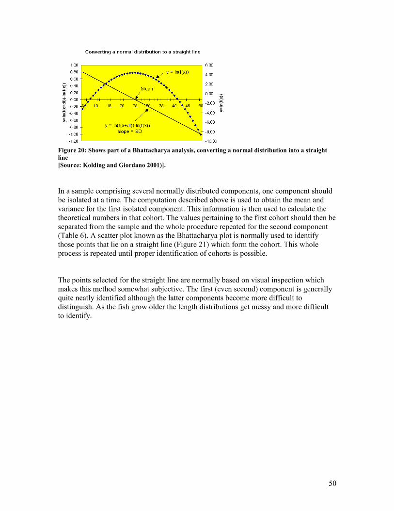
50

Figure 20: Shows part of a Bhattacharya analysis, converting a normal distribution into a straight

line


In a sample comprising several normally distributed components, one component should

be isolated at a time. The computation described above is used to obtain the mean and

variance for the first isolated component. This information is then used to calculate the

theoretical numbers in that cohort. The values pertaining to the first cohort should then be

separated from the sample and the whole procedure repeated for the second component

(Table 6). A scatter plot known as the Bhattacharya plot is normally used to identify

those points that lie on a straight line (Figure 21) which form the cohort. This whole

process is repeated until proper identification of cohorts is possible.

The points selected for the straight line are normally based on visual inspection which

makes this method somewhat subjective. The first (even second) component is generally

quite neatly identified although the latter components become more difficult to

distinguish. As the fish grow older the length distributions get messy and more difficult

to identify.

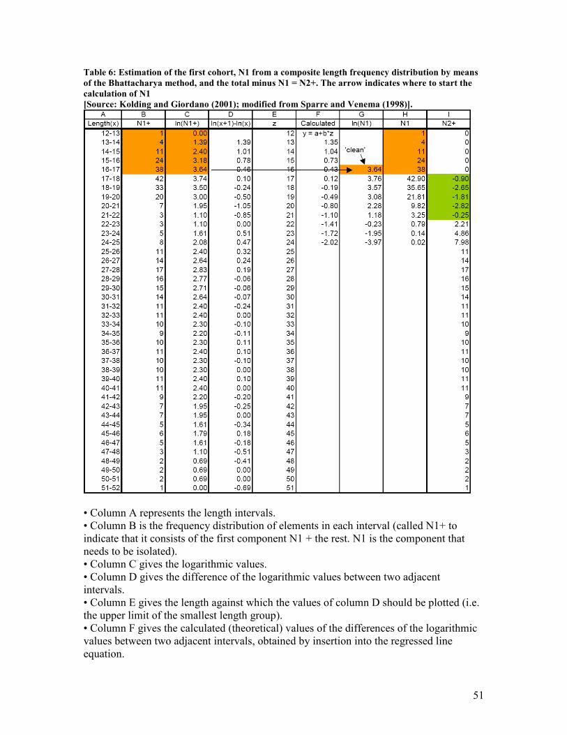
51

Table 6: Estimation of the first cohort, N1 from a composite length frequency distribution by means

of the Bhattacharya method, and the total minus N1 = N2+. The arrow indicates where to start the

calculation of N1

[Source: Kolding and Giordano (2001); modified from Sparre and Venema (1998)].

• Column A represents the length intervals.

• Column B is the frequency distribution of elements in each interval (called N1+ to

indicate that it consists of the first component N1 + the rest. N1 is the component that

needs to be isolated).

• Column C gives the logarithmic values.

• Column D gives the difference of the logarithmic values between two adjacent

intervals.

• Column E gives the length against which the values of column D should be plotted (i.e.

the upper limit of the smallest length group).

• Column F gives the calculated (theoretical) values of the differences of the logarithmic

values between two adjacent intervals, obtained by insertion into the regressed line

equation.

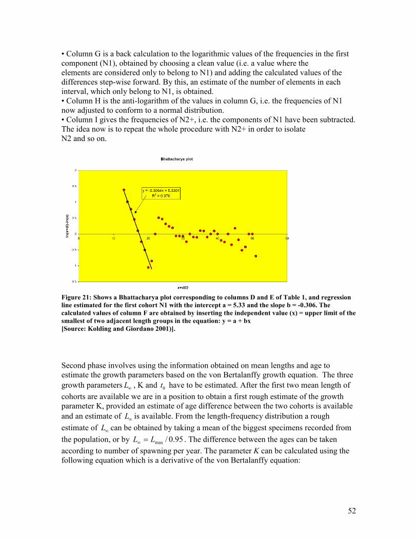
52

• Column G is a back calculation to the logarithmic values of the frequencies in the first

component (N1), obtained by choosing a clean value (i.e. a value where the

elements are considered only to belong to N1) and adding the calculated values of the

differences step-wise forward. By this, an estimate of the number of elements in each

interval, which only belong to N1, is obtained.

• Column H is the anti-logarithm of the values in column G, i.e. the frequencies of N1

now adjusted to conform to a normal distribution.

• Column I gives the frequencies of N2+, i.e. the components of N1 have been subtracted.

The idea now is to repeat the whole procedure with N2+ in order to isolate

N2 and so on.

Figure 21: Shows a Bhattacharya plot corresponding to columns D and E of Table 1, and regression

line estimated for the first cohort N1 with the intercept a = 5.33 and the slope b = -0.306. The

calculated values of column F are obtained by inserting the independent value (x) = upper limit of the

smallest of two adjacent length groups in the equation: y = a + bx


Second phase involves using the information obtained on mean lengths and age to

estimate the growth parameters based on the von Bertalanffy growth equation. The three

growth parameters ∞L , K and 0t have to be estimated. After the first two mean length of

cohorts are available we are in a position to obtain a first rough estimate of the growth

parameter K, provided an estimate of age difference between the two cohorts is available

and an estimate of ∞L is available. From the length-frequency distribution a rough

estimate of ∞L can be obtained by taking a mean of the biggest specimens recorded from

the population, or by 95.0/maxLL =∞ . The difference between the ages can be taken

according to number of spawning per year. The parameter K can be calculated using the

following equation which is a derivative of the von Bertalanffy equation:

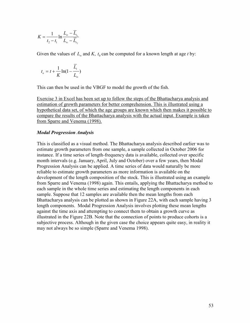
53

2

1ln1

12 t

t

LL

LL

ttK

−

−

−=

∞

∞

Given the values of ∞L and K, 0t can be computed for a known length at age t by:

)1ln(1

∞

−+=L

L

Ktt

t

o

This can then be used in the VBGF to model the growth of the fish.

Exercise 3 in Excel has been set up to follow the steps of the Bhattacharya analysis and

estimation of growth parameters for better comprehension. This is illustrated using a

hypothetical data set, of which the age groups are known which then makes it possible to

compare the results of the Bhattacharya analysis with the actual input. Example is taken

from Sparre and Venema (1998).

Modal Progression Analysis

This is classified as a visual method. The Bhattacharya analysis described earlier was to

estimate growth parameters from one sample, a sample collected in October 2006 for

instance. If a time series of length-frequency data is available, collected over specific

month intervals (e.g. January, April, July and October) over a few years, then Modal

Progression Analysis can be applied. A time series of data would naturally be more

reliable to estimate growth parameters as more information is available on the

development of the length composition of the stock. This is illustrated using an example

from Sparre and Venema (1998) again. This entails, applying the Bhattacharya method to

each sample in the whole time series and estimating the length components in each

sample. Suppose that 12 samples are available then the mean lengths from each

Bhattacharya analysis can be plotted as shown in Figure 22A, with each sample having 3

length components. Modal Progression Analysis involves plotting these mean lengths

against the time axis and attempting to connect them to obtain a growth curve as

illustrated in the Figure 22B. Note that the connection of points to produce cohorts is a

subjective process. Although in the given case the choice appears quite easy, in reality it

may not always be so simple (Sparre and Venema 1998).

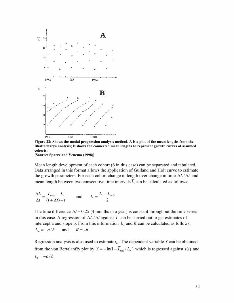
54

Figure 22: Shows the modal progression analysis method. A is a plot of the mean lengths from the

Bhattacharya analysis; B shows the connected mean lengths to represent growth curves of assumed

cohorts.

[Source: Sparre and Venema (1998)]

Mean length development of each cohort (6 in this case) can be separated and tabulated.

Data arranged in this format allows the application of Gulland and Holt curve to estimate

the growth parameters. For each cohort change in length over change in time tL ∆∆ / and

mean length between two consecutive time intervals tL can be calculated as follows;

ttt

LL

t

L ttt

−∆+−

=∆∆ ∆+

)( and

2

tttt

LLL ∆++=

The time difference t∆ = 0.25 (4 months in a year) is constant throughout the time series

in this case. A regression of tL ∆∆ / against L can be carried out to get estimates of

intercept a and slope b. From this information ∞L and K can be calculated as follows:

baL /−=∞ and K = -b.

Regression analysis is also used to estimate 0t . The dependent variable Y can be obtained

from the von Bertalanffy plot by )/1ln( )( ∞−−= LLY it which is regressed against )(it and

bat /0 −= .

55

The least squares method

This method is more advanced than the methods described above and hence requires

more computational work. A series of pairs of observations of lengths and age are

required. These can be obtained through age reading or through length-frequency analysis

such as modal progression analysis or cohort slicing (i.e. visual inspection of the

distribution and cutting the normal distribution at mid point to get mean lengths (this

method however needs some prior information on growth from independent survey).

The method relies on minimizing the sum of the squared deviations between the model

and the observations with respect to the growth parameters ∞L , K and 0t to estimate their

optimum values. In principle, this measure of goodness of fit is the same as the one used

in linear regression. The von Bertalanffy growth curve is normally used.

5.2.4. Computer Packages

Several computer packages are available to enable analysis of length frequency data

primarily intended for tropical fish stock assessment. Descriptions of the main packages

are given by Sparre and Venema (1998) and Hart and Reynolds (2002) and are briefly

discussed below.

One package developed by FAO (Sparre 1987) is the Length-based Fish Stock

Assessment (LFSA). The program “MODALPR” can execute the modal progression

analysis. The package also allows continuing from the Bhattacharya analysis (program

“BHATTAC”) with a least squares estimation of the growth parameters using program

“VONBER” instead of the Gulland and Holt plot. The package has various other sub-

packages or programs for analysis. This can be considered as a computer-assisted version

of the Bhattacharya method, with the underlying assumption that the length frequency

distribution of each cohort is normally distributed.

The ELEFAN (Electronic Length Frequency ANalysis) was introduced by Pauly and

David (1981). A description of the entire package and a clear review can be found in

Pauly (1987). The modern version of this length-frequency method is the ELEFAN I

module incorporated in the widely used FiSAT package. The FiSAT Package was

developed to have both LFSA and ELEFAN complement each other. This was a joint

initiative by FAO and ICLARM (International Center for Living Aquatic Resources

Management (Gayanialo et. al. 1995). This method is basically a modal progression

analysis. However if a times series of samples are not present the package can simulate

the data based on the information available in the given sample assuming that the same

recruitment and growth pattern are followed by all cohorts.

ELEFAN works by attempting to find a maximum for a goodness of fit function based on

peaks and troughs seen in the data. This is based on how often a von Bertalanffy growth

curve hits modes in the data. The length frequency data are restructured and moving

56

average is applied to allocate points. A moving average above 5-points is identified as a

peak. The number of peaks gives the maximum “available sum of peaks” (ASP). Growth

curves (von Bertalanffy) with different parameters ( ∞L and K) are run and mapped. For

each trial an “explained sum of peaks” (ESP) is calculated. The goodness-of-fit function

is the ratio ESP/ASP. The set of growth parameters which yield the highest ratio are

taken to be the best growth parameters which explain the peaks and troughs in the data.

The parameter 0t can be calculated from the ∞L and K values. If peaks are well defined in

the data then this method gives reliable results however it tends to underestimate K in

general. The drawbacks are that it is sensitive to the appearance of the modes in the data

and it is an ad hoc method and lacks clear statistical error structure and thus does not

provide standard errors of estimates and a measure of performance (Hart and Reynolds

2002).

The maximum-likelihood-method is more computational and works by calculating a

goodness-of-fit between the sample data and a distribution mixture specified by its

component parameters. This method is reviewed by MacDonald and Pitcher (1979).

Automatic search of the maximum goodness-of-fit gives the best estimate of the growth

parameters. This is similar to ELEFAN except the goodness-of-fit criteria used here is

chi-square. However the user needs to give the number of cohorts that constitute the

sample. This method provides variance estimates of the parameters. This forms the basis

of statistical mixture analysis represented by the MIX technique (MacDonald and Pitcher

1979). The main problem with the MIX technique is obtaining the number of components

in the mixture however the growth parameter estimates are shown to be quite robust by

Rosenberg and Beddington (1988). MULTIFAN (Fournier et. al. 1990) is a more

complex method which gets around the problem of estimating the number of cohorts by

using a von Bertalanffy curve to provide the number of cohorts in a similar manner as the

graphical and visual methods explained earlier (Hart and Reynolds 2002).

In the tropics there is often more than one cohort recruiting each year which is a

consequence of monsoon like seasonality in productivity. Thus care needs to be taken

during analysis and appropriate assumptions should be made when analyzing length-

frequencies and identifying modes.

5.2.5. Limitations of length frequency analysis

The major downside of length-frequency analysis is to be able to reliably separate the

composite length distribution into components. The younger components are easier to

separate as a significant difference in length is present and the distributions have small

overlap. As the fish grow older there is a smaller difference in length between older ages

and separating the distribution becomes considerably tricky with mean values lying very

close to each other in relation to the size of the standard deviations (Sparre and Venema

1998). As outlined in Kolding and Giordano (2001), one solution to this problem was

proposed by Hasselbald (1966), McNew and Summerfelt (1978) and Clark (1981) and is

known as the separation index I which is given by:

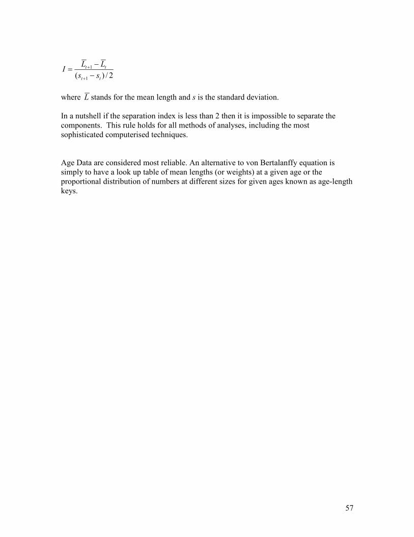
57

2/)( 1

1

tt

tt

ss

LLI

−−

=+

+

where L stands for the mean length and s is the standard deviation.

In a nutshell if the separation index is less than 2 then it is impossible to separate the

components. This rule holds for all methods of analyses, including the most

sophisticated computerised techniques.

Age Data are considered most reliable. An alternative to von Bertalanffy equation is

simply to have a look up table of mean lengths (or weights) at a given age or the

proportional distribution of numbers at different sizes for given ages known as age-length

keys.

58

6. Mortality

After a certain number of individuals are hatched, the numbers in that group can only

decline through time. The concept of mortality essentially aims to describe this death

process of a population and is not individually focused. The focus is on the number of

fish in each cohort and how it declines through time. To define this process of how fish

numbers decline in a stock after spawning (birth), it is essential to follow the fate of a

“cohort”. As defined earlier a cohort is a batch of fish all of approximately the same age

and belonging to the same stock (Sparre and Venema 1998). All fish of a cohort are

assumed to have the same age at a given time so that they all attain the recruitment age at

the same time. In the context of mortality we are interested in the number of survivors

from a cohort as a function of age. Mortality can be divided into fishing and natural

mortality. Estimating mortality entails determining the total mortality first and then

splitting this into natural and fishing mortalities as appropriate.

How a cohort develops through time is illustrated in Figure 23. In a cohort model; it is

assumed that R individuals are recruited into the fishery at the age rt (denoting age at

recruitment). From this age fish are exposed to some degree of natural mortality M

(such as predation, competition). After certain time these fish are exposed to fishing at

age ct (age at first capture) denoted by F for fishing mortality. At some point maxt the

older fish are not vulnerable to fishing. Note that the model assumes a knife-edge

selection, which means at ct either none or all fish in an age-class are either recruited or

not or are vulnerable or not, and once vulnerable all age-classes are equally vulnerable

(Sparre and Venema 1998).

Figure 23: Shows the basic dynamics of the decay of a cohort with corresponding symbols used in

fishery models. The figure illustrates the impact of fishing to the survival rates, compared to natural

decay without fishing. The line N+ catch illustrates the fate of cohort when its exposed to some

fishing mortality as opposed to decay without exploitation

[Source: Kolding and Giordano (2001)].

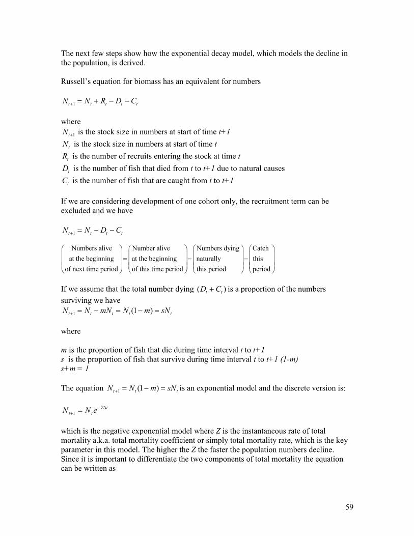
59

The next few steps show how the exponential decay model, which models the decline in

the population, is derived.

Russell’s equation for biomass has an equivalent for numbers

ttttt CDRNN −−+=+1

where

1+tN is the stock size in numbers at start of time t+1

tN is the stock size in numbers at start of time t

tR is the number of recruits entering the stock at time t

tD is the number of fish that died from t to t+1 due to natural causes

tC is the number of fish that are caught from t to t+1

If we are considering development of one cohort only, the recruitment term can be

excluded and we have

tttt CDNN −−=+1

If we assume that the total number dying )( tt CD + is a proportion of the numbers

surviving we have

ttttt sNmNmNNN =−=−=+ )1(1

where

m is the proportion of fish that die during time interval t to t+1

s is the proportion of fish that survive during time interval t to t+1 (1-m)

s+m = 1

The equation ttt sNmNN =−=+ )1(1 is an exponential model and the discrete version is:

tZ

tt eNN ∆−+ =1

which is the negative exponential model where Z is the instantaneous rate of total

mortality a.k.a. total mortality coefficient or simply total mortality rate, which is the key

parameter in this model. The higher the Z the faster the population numbers decline.

Since it is important to differentiate the two components of total mortality the equation

can be written as

Numbers alive Number alive Numbers dying Catch

at the beginning at the beginning naturally this

of next time period of this time period this period period

= − −

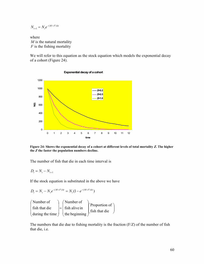
60

tFM

tt eNN ∆+−+ = )(

1

where

M is the natural mortality

F is the fishing mortality

We will refer to this equation as the stock equation which models the exponential decay

of a cohort (Figure 24).

Exponential decay of a cohort

0

200

400

600

800

1000

1200

0 1 2 3 4 5 6 7 8 9 10 11 12

time

N(t)

Z=0.2

Z=0.5

Z=1.0

Figure 24: Shows the exponential decay of a cohort at different levels of total mortality Z. The higher

the Z the faster the population numbers decline.

The number of fish that die in each time interval is

1+−= ttt NND

If the stock equation is substituted in the above we have

)1( )()( tFM

t

tFM

ttt eNeNND ∆+−∆+− −=−=

=

diefish that

of Proportion

beginning the

in alivefish

ofNumber

time theduring

diefish that

ofNumber

The numbers that die due to fishing mortality is the fraction (F/Z) of the number of fish

that die, i.e.

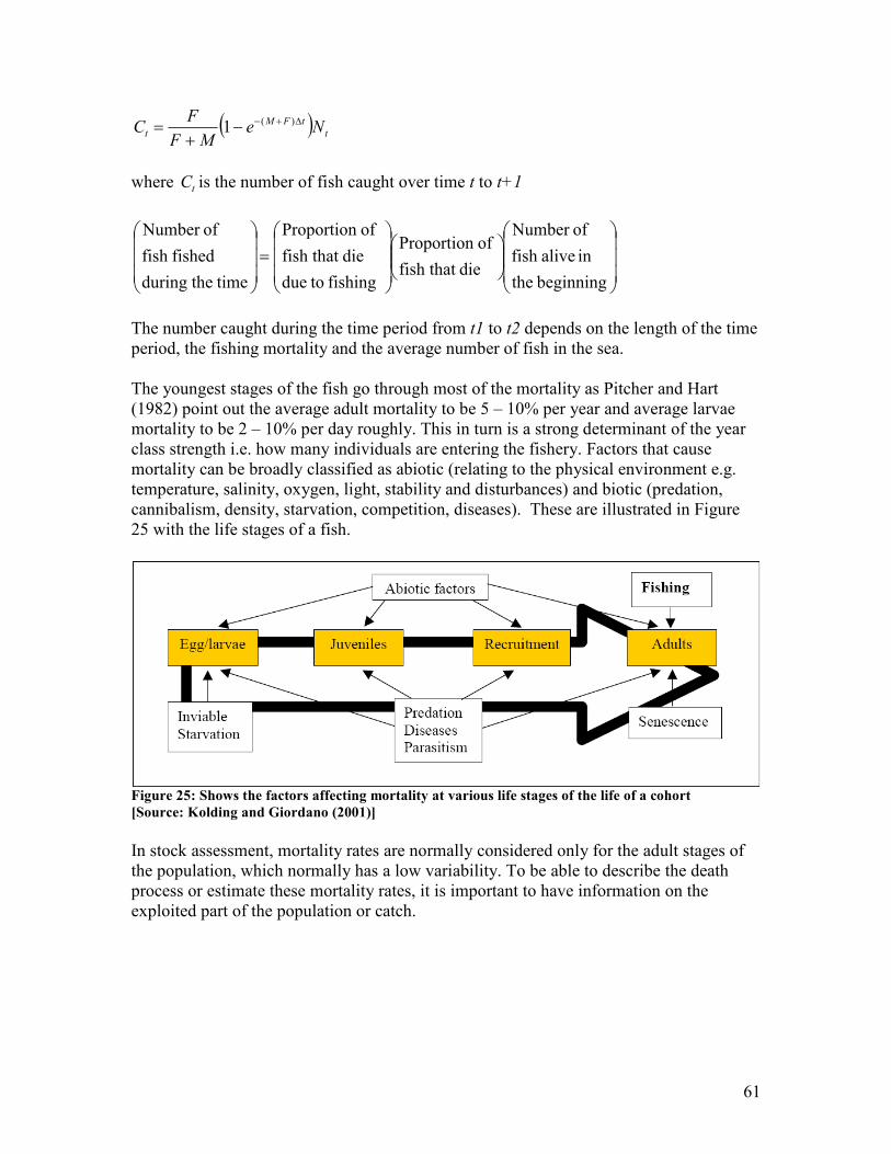
61

( ) t

tFM

t NeMF

FC ∆+−−

+= )(1

where tC is the number of fish caught over time t to t+1

=

beginning the

in alivefish

ofNumber

diefish that

of Proportion

fishing todue

diefish that

of Proportion

time theduring

fishedfish

ofNumber

The number caught during the time period from t1 to t2 depends on the length of the time

period, the fishing mortality and the average number of fish in the sea.

The youngest stages of the fish go through most of the mortality as Pitcher and Hart

(1982) point out the average adult mortality to be 5 – 10% per year and average larvae

mortality to be 2 – 10% per day roughly. This in turn is a strong determinant of the year

class strength i.e. how many individuals are entering the fishery. Factors that cause

mortality can be broadly classified as abiotic (relating to the physical environment e.g.

temperature, salinity, oxygen, light, stability and disturbances) and biotic (predation,

cannibalism, density, starvation, competition, diseases). These are illustrated in Figure

25 with the life stages of a fish.

Figure 25: Shows the factors affecting mortality at various life stages of the life of a cohort

[Source: Kolding and Giordano (2001)]

In stock assessment, mortality rates are normally considered only for the adult stages of

the population, which normally has a low variability. To be able to describe the death

process or estimate these mortality rates, it is important to have information on the

exploited part of the population or catch.

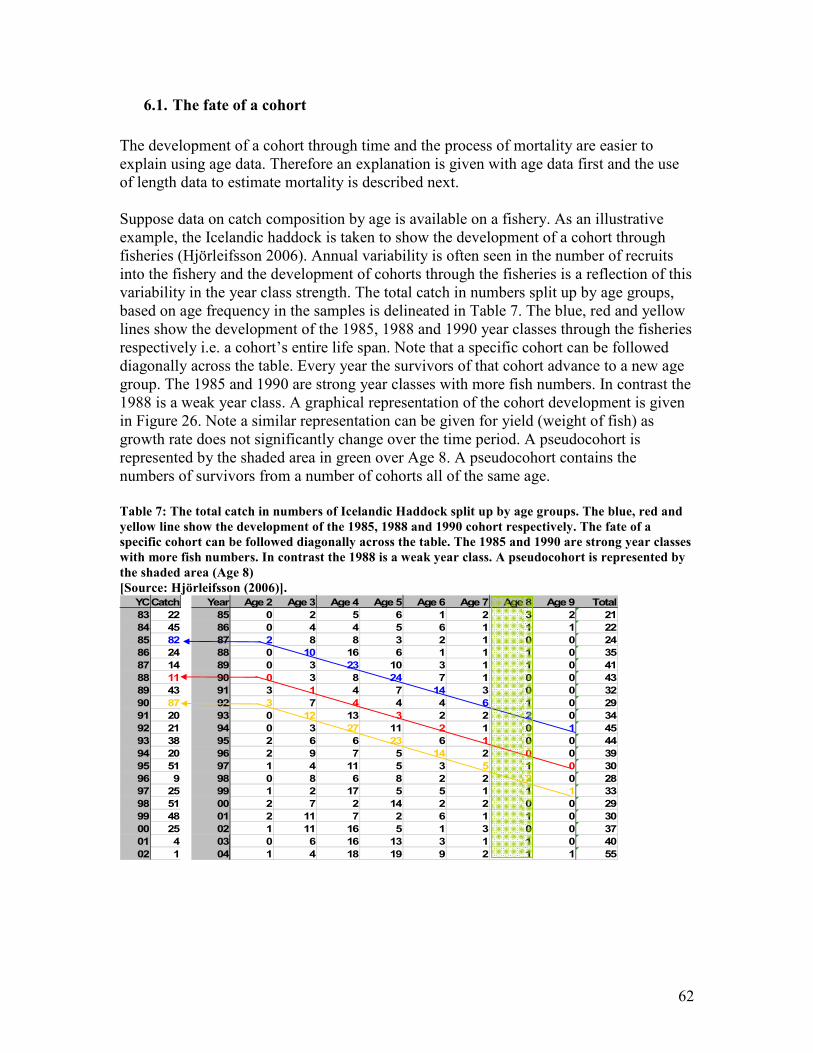
62

6.1. The fate of a cohort

The development of a cohort through time and the process of mortality are easier to

explain using age data. Therefore an explanation is given with age data first and the use

of length data to estimate mortality is described next.

Suppose data on catch composition by age is available on a fishery. As an illustrative

example, the Icelandic haddock is taken to show the development of a cohort through

fisheries (Hjörleifsson 2006). Annual variability is often seen in the number of recruits

into the fishery and the development of cohorts through the fisheries is a reflection of this

variability in the year class strength. The total catch in numbers split up by age groups,

based on age frequency in the samples is delineated in Table 7. The blue, red and yellow

lines show the development of the 1985, 1988 and 1990 year classes through the fisheries

respectively i.e. a cohort’s entire life span. Note that a specific cohort can be followed

diagonally across the table. Every year the survivors of that cohort advance to a new age

group. The 1985 and 1990 are strong year classes with more fish numbers. In contrast the

1988 is a weak year class. A graphical representation of the cohort development is given

in Figure 26. Note a similar representation can be given for yield (weight of fish) as

growth rate does not significantly change over the time period. A pseudocohort is

represented by the shaded area in green over Age 8. A pseudocohort contains the

numbers of survivors from a number of cohorts all of the same age.

Table 7: The total catch in numbers of Icelandic Haddock split up by age groups. The blue, red and

yellow line show the development of the 1985, 1988 and 1990 cohort respectively. The fate of a

specific cohort can be followed diagonally across the table. The 1985 and 1990 are strong year classes

with more fish numbers. In contrast the 1988 is a weak year class. A pseudocohort is represented by

the shaded area (Age 8)

[Source: Hjörleifsson (2006)]. YCCatch Year Age 2 Age 3 Age 4 Age 5 Age 6 Age 7 Age 8 Age 9 Total

83 22 85 0 2 5 6 1 2 3 2 21

84 45 86 0 4 4 5 6 1 1 1 22

85 82 87 2 8 8 3 2 1 0 0 24

86 24 88 0 10 16 6 1 1 1 0 35

87 14 89 0 3 23 10 3 1 1 0 41

88 11 90 0 3 8 24 7 1 0 0 43

89 43 91 3 1 4 7 14 3 0 0 32

90 87 92 3 7 4 4 4 6 1 0 29

91 20 93 0 12 13 3 2 2 2 0 34

92 21 94 0 3 27 11 2 1 0 1 45

93 38 95 2 6 6 23 6 1 0 0 44

94 20 96 2 9 7 5 14 2 0 0 39

95 51 97 1 4 11 5 3 5 1 0 30

96 9 98 0 8 6 8 2 2 2 0 28

97 25 99 1 2 17 5 5 1 1 1 33

98 51 00 2 7 2 14 2 2 0 0 29

99 48 01 2 11 7 2 6 1 1 0 30

00 25 02 1 11 16 5 1 3 0 0 37

01 4 03 0 6 16 13 3 1 1 0 40

02 1 04 1 4 18 19 9 2 1 1 55

63

Year 1985 2005

0

50

100

150

8 5 8 6 8 7 8 8 8 9 9 0 9 1 9 2 9 3 9 4 9 5 9 6 9 7 9 8 9 9 2 000 2 001 2 002 2 003 2 004 2 005

1

7

Age

Numbers

85 88 90

0

200

400

8 5 8 6 8 7 8 8 8 9 9 0 9 1 9 2 9 3 9 4 9 5 9 6 9 7 9 8 9 9 2 000 2 001 2 002 2 003 2 004 2 005

0

200

400

8 5 8 6 8 7 8 8 8 9 9 0 9 1 9 2 9 3 9 4 9 5 9 6 9 7 9 8 9 9 2 000 2 001 2 002 2 003 2 004 2 005

0

100

200

300

8 5 8 6 8 7 8 8 8 9 9 0 9 1 9 2 9 3 9 4 9 5 9 6 9 7 9 8 9 9 2 000 2 001 2 002 2 003 2 004 2 005

0

100

200

8 5 8 6 8 7 8 8 8 9 9 0 9 1 9 2 9 3 9 4 9 5 9 6 9 7 9 8 9 9 2 000 2 001 2 002 2 003 2 004 2 005

0

50

100

8 5 8 6 8 7 8 8 8 9 9 0 9 1 9 2 9 3 9 4 9 5 9 6 9 7 9 8 9 9 2 000 2 001 2 002 2 003 2 004 2 005

0

10

20

8 5 8 6 8 7 8 8 8 9 9 0 9 1 9 2 9 3 9 4 9 5 9 6 9 7 9 8 9 9 2 000 2 001 2 002 2 003 2 004 2 005

Year 1985 2005

0

50

100

150

8 5 8 6 8 7 8 8 8 9 9 0 9 1 9 2 9 3 9 4 9 5 9 6 9 7 9 8 9 9 2 000 2 001 2 002 2 003 2 004 2 005

1

7

Age

Numbers

85 88 90

0

200

400

8 5 8 6 8 7 8 8 8 9 9 0 9 1 9 2 9 3 9 4 9 5 9 6 9 7 9 8 9 9 2 000 2 001 2 002 2 003 2 004 2 005

0

200

400

8 5 8 6 8 7 8 8 8 9 9 0 9 1 9 2 9 3 9 4 9 5 9 6 9 7 9 8 9 9 2 000 2 001 2 002 2 003 2 004 2 005

0

100

200

300

8 5 8 6 8 7 8 8 8 9 9 0 9 1 9 2 9 3 9 4 9 5 9 6 9 7 9 8 9 9 2 000 2 001 2 002 2 003 2 004 2 005

0

100

200

8 5 8 6 8 7 8 8 8 9 9 0 9 1 9 2 9 3 9 4 9 5 9 6 9 7 9 8 9 9 2 000 2 001 2 002 2 003 2 004 2 005

0

50

100

8 5 8 6 8 7 8 8 8 9 9 0 9 1 9 2 9 3 9 4 9 5 9 6 9 7 9 8 9 9 2 000 2 001 2 002 2 003 2 004 2 005

0

10

20

8 5 8 6 8 7 8 8 8 9 9 0 9 1 9 2 9 3 9 4 9 5 9 6 9 7 9 8 9 9 2 000 2 001 2 002 2 003 2 004 2 005

0

50

100

150

8 5 8 6 8 7 8 8 8 9 9 0 9 1 9 2 9 3 9 4 9 5 9 6 9 7 9 8 9 9 2 000 2 001 2 002 2 003 2 004 2 005

1

7

Age

Numbers

85 88 90

0

200

400

8 5 8 6 8 7 8 8 8 9 9 0 9 1 9 2 9 3 9 4 9 5 9 6 9 7 9 8 9 9 2 000 2 001 2 002 2 003 2 004 2 005

0

200

400

8 5 8 6 8 7 8 8 8 9 9 0 9 1 9 2 9 3 9 4 9 5 9 6 9 7 9 8 9 9 2 000 2 001 2 002 2 003 2 004 2 005

0

100

200

300

8 5 8 6 8 7 8 8 8 9 9 0 9 1 9 2 9 3 9 4 9 5 9 6 9 7 9 8 9 9 2 000 2 001 2 002 2 003 2 004 2 005

0

100

200

8 5 8 6 8 7 8 8 8 9 9 0 9 1 9 2 9 3 9 4 9 5 9 6 9 7 9 8 9 9 2 000 2 001 2 002 2 003 2 004 2 005

0

50

100

8 5 8 6 8 7 8 8 8 9 9 0 9 1 9 2 9 3 9 4 9 5 9 6 9 7 9 8 9 9 2 000 2 001 2 002 2 003 2 004 2 005

0

10

20

8 5 8 6 8 7 8 8 8 9 9 0 9 1 9 2 9 3 9 4 9 5 9 6 9 7 9 8 9 9 2 000 2 001 2 002 2 003 2 004 2 005

Figure 26: Shows the development of a cohort through time based on catch in numbers of the

Icelandic Haddock in Table 6. The orange, yellow and red lines represent the 1985, 1988 and 1990

cohort respectively. The 1985 and 1990 are strong year classes with more fish numbers. In contrast

the 1988 is a weak year class


9

8

7

6

5

3

2

4

9876

54

32 9

8

7

6

5

3

2

4

0

5

10

15

20

25

30

1985 1986 1987 1988 1989 1990 1991 1992 1993 1994 1995 1996 1997 1998 1999 2000 2001 2002 2003 2004 2005

Catch (millions)

Year class

1985

1988

1990

9

8

7

6

5

3

2

4

9876

54

32 9

8

7

6

5

3

2

4

0

5

10

15

20

25

30

1985 1986 1987 1988 1989 1990 1991 1992 1993 1994 1995 1996 1997 1998 1999 2000 2001 2002 2003 2004 2005

Catch (millions)

Year class

1985

1988

1990

Figure 27: Shows the development of a cohort through time illustrating its entire life span based on

the data in Table 6. The blue, red and yellow line show the development of the 1985, 1988 and 1990

cohort respectively. The 1985 year class is 2 years old in 1987 and so forth and maximum catch is

seen around 4-5 years old


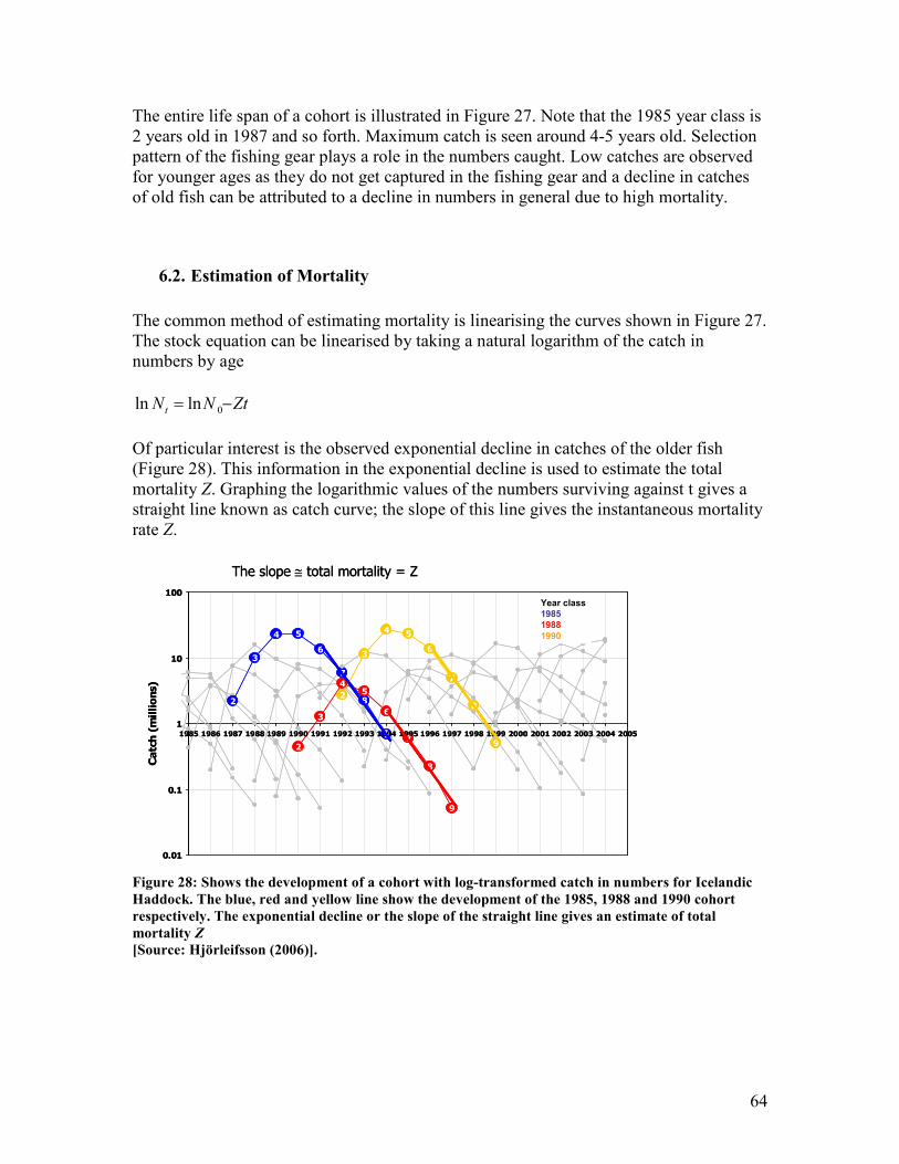
64

The entire life span of a cohort is illustrated in Figure 27. Note that the 1985 year class is

2 years old in 1987 and so forth. Maximum catch is seen around 4-5 years old. Selection

pattern of the fishing gear plays a role in the numbers caught. Low catches are observed

for younger ages as they do not get captured in the fishing gear and a decline in catches

of old fish can be attributed to a decline in numbers in general due to high mortality.

6.2. Estimation of Mortality

The common method of estimating mortality is linearising the curves shown in Figure 27.

The stock equation can be linearised by taking a natural logarithm of the catch in

numbers by age

Of particular interest is the observed exponential decline in catches of the older fish

(Figure 28). This information in the exponential decline is used to estimate the total

mortality Z. Graphing the logarithmic values of the numbers surviving against t gives a

straight line known as catch curve; the slope of this line gives the instantaneous mortality

rate Z.

9

8

7

6

5

3

2

4

9

8

7

6

54

3

2 9

8

7

6

5

3

2

4

0.01

0.1

1

10

100

1985 1986 1987 1988 1989 1990 1991 1992 1993 1994 1995 1996 1997 1998 1999 2000 2001 2002 2003 2004 2005

Catch (millions)

Year class

1985

1988

1990

The slope ≅ total mortality = Z

9

8

7

6

5

3

2

4

9

8

7

6

54

3

2 9

8

7

6

5

3

2

4

0.01

0.1

1

10

100

1985 1986 1987 1988 1989 1990 1991 1992 1993 1994 1995 1996 1997 1998 1999 2000 2001 2002 2003 2004 2005

Catch (millions)

Year class

1985

1988

1990

The slope ≅ total mortality = Z

Figure 28: Shows the development of a cohort with log-transformed catch in numbers for Icelandic

Haddock. The blue, red and yellow line show the development of the 1985, 1988 and 1990 cohort

respectively. The exponential decline or the slope of the straight line gives an estimate of total

mortality Z


ZtNN t −= 0lnln

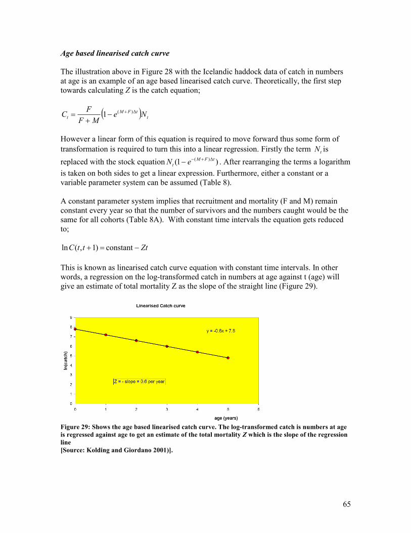
65

Age based linearised catch curve

The illustration above in Figure 28 with the Icelandic haddock data of catch in numbers

at age is an example of an age based linearised catch curve. Theoretically, the first step

towards calculating Z is the catch equation;

( ) t

tFM

t NeMF

FC ∆+−

+= )(1

However a linear form of this equation is required to move forward thus some form of

transformation is required to turn this into a linear regression. Firstly the term tN is

replaced with the stock equation )1( )( tFM

t eN ∆+−− . After rearranging the terms a logarithm

is taken on both sides to get a linear expression. Furthermore, either a constant or a

variable parameter system can be assumed (Table 8).

A constant parameter system implies that recruitment and mortality (F and M) remain

constant every year so that the number of survivors and the numbers caught would be the

same for all cohorts (Table 8A). With constant time intervals the equation gets reduced

to;

ZtttC −=+ constant )1,(ln

This is known as linearised catch curve equation with constant time intervals. In other

words, a regression on the log-transformed catch in numbers at age against t (age) will

give an estimate of total mortality Z as the slope of the straight line (Figure 29).

Figure 29: Shows the age based linearised catch curve. The log-transformed catch is numbers at age

is regressed against age to get an estimate of the total mortality Z which is the slope of the regression

line


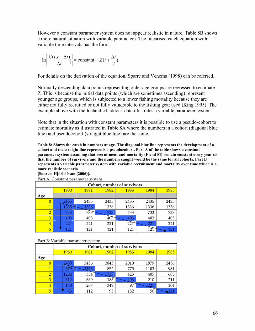
66

However a constant parameter system does not appear realistic in nature. Table 8B shows

a more natural situation with variable parameters. The linearised catch equation with

variable time intervals has the form:

)2

(constant),(

lnt

tZt

tttC ∆+−=

∆

∆+

For details on the derivation of the equation, Sparre and Venema (1998) can be referred.

Normally descending data points representing older age groups are regressed to estimate

Z. This is because the initial data points (which are sometimes ascending) represent

younger age groups, which is subjected to a lower fishing mortality because they are

either not fully recruited or not fully vulnerable to the fishing gear used (King 1995). The

example above with the Icelandic haddock data illustrates a variable parameter system.

Note that in the situation with constant parameters it is possible to use a pseudo-cohort to

estimate mortality as illustrated in Table 8A where the numbers in a cohort (diagonal blue

line) and pseudocohort (straight blue line) are the same.

Table 8: Shows the catch in numbers at age. The diagonal blue line represents the development of a

cohort and the straight line represents a pseudocohort. Part A of the table shows a constant

parameter system assuming that recruitment and mortality (F and M) remain constant every year so

that the number of survivors and the numbers caught would be the same for all cohorts. Part B

represents a variable parameter system with variable recruitment and mortality over time which is a

more realistic scenario


Part A: Constant parameter system

Cohort, number of survivors

1980 1981 1982 1983 1984 1985

Age

0 2435 2435 2435 2435 2435 2435

1 1336 1336 1336 1336 1336 1336

2 733 733 733 733 733 733

3 403 403 403 403 403 403

4 221 221 221 221 221 221

5 121 121 121 121 121 121

Part B: Variable parameter system

Cohort, number of survivors

1980 1981 1982 1983 1984 1985

Age

0 2435 3456 2845 2010 1879 2456

1 679 1336 852 775 1103 981

2 1282 354 733 423 405 605

3 512 669 185 403 210 211

4 140 267 349 97 221 104

5 73 112 95 182 50 121

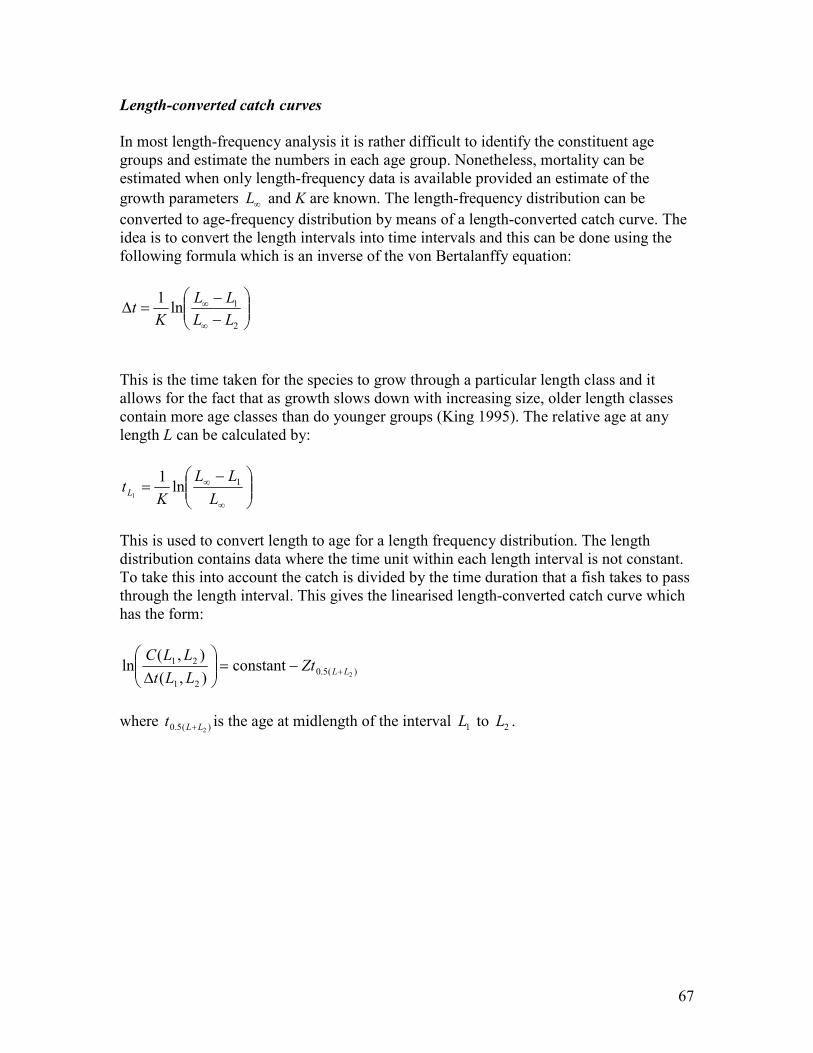
67

Length-converted catch curves

In most length-frequency analysis it is rather difficult to identify the constituent age

groups and estimate the numbers in each age group. Nonetheless, mortality can be

estimated when only length-frequency data is available provided an estimate of the

growth parameters ∞L and K are known. The length-frequency distribution can be

converted to age-frequency distribution by means of a length-converted catch curve. The

idea is to convert the length intervals into time intervals and this can be done using the

following formula which is an inverse of the von Bertalanffy equation:

−−

=∆∞

∞

2

1ln1

LL

LL

Kt

This is the time taken for the species to grow through a particular length class and it

allows for the fact that as growth slows down with increasing size, older length classes

contain more age classes than do younger groups (King 1995). The relative age at any

length L can be calculated by:

−=

∞

∞

L

LL

KtL

1ln1

1

This is used to convert length to age for a length frequency distribution. The length

distribution contains data where the time unit within each length interval is not constant.

To take this into account the catch is divided by the time duration that a fish takes to pass

through the length interval. This gives the linearised length-converted catch curve which

has the form:

)(5.0

21

21

2constant

),(

),(ln LLZt

LLt

LLC+−=

∆

where )(5.0 2LLt + is the age at midlength of the interval 1L to 2L .

68

This essentially means that the catch in numbers are replaced with the frequency between

1L and 2L and t is the age class interval mid-point. The age at midlength of the interval

1L to 2L is also calculated using an inverse of the von Bertalanffy equation;

+−=

∞

∞+

L

LLL

Kt LL

21)(5.0

(5.0ln

121

The length-converted catch curve forms a linear equation where

∆=

),(

),(ln

21

21

LLt

LLCY and

)(5.0 2LLtX += and the slope is an estimate of Z.

The initial ascending data points representing the younger ages are not fitted in the

regression line. This is because these individuals are either not fully recruited or are too

small to be totally vulnerable to the fishing gear. Data points close to ∞L are also

excluded since the relationship between length and age becomes uncertain in old fish

(King 1995). The conversion of lengths into ages is fairly complex. Further details on the

derivation of the equations can be found in Sparre and Venema (1998) for interested

readers. Length based Z calculations are very sensitive to the value of K and ∞L used

therefore some careful consideration needs to be given to that. It is best is to estimate K

and ∞L on the stock of interest and if values from literature are used, then they have to be

appropriate for the stock in question

Exercise 4 in Excel gives an application of the age-based linearised catch curve and the

length-converted catch curves.

Catch-per-unit effort data to estimate Z

Given that the effort applied to the fishery remains constant over time with an assumption

of constant catchability, the log ratio of the number of fish caught at each time interval

can be used to estimate total mortality. The methods described above rely somewhat on

the abundance of individuals in different age classes. CPUE is considered an index of

abundance. CPUE data can used to estimate mortality if recruitment periods are

pronounced. Then the decrease in CPUE over the period between one recruitment and the

following will give some indication of average mortality of all ages combined.

Assumptions are that all age groups are equally exposed to fishing with a constant

mortality.

69

=

=

==

=

+++++

++

)/(

)/(lnlnZ

equation;stock from Following

and Assume

/

111,11

t

11

,

ayya

ayay

t

t

aayy

ayayya

qEC

qEC

N

N

qqEE

ECCPUE

It is not necessary to know the absolute values of tN and 1+tN , only their ratio is required.

Beverton and Holt’s Z-equation

The data requirements for the Beverton and Holt Z-equation are less than the length

converted catch curve. It estimates Z from the mean lengths of fish in the catch and the

von Bertalanffy growth parameters K and ∞L . Thus it assumes that growth follows the

VBGF, mortality can be represented by a negative exponential decay and that L is

estimated from a sample representing a steady-state population and Z is calculated by:

′−

−= ∞

LL

LLKZ

where L is the mean length of all fish of length L′ and longer and L′ is defined as “some

length for which all fish for that length and longer are under full exploitation”.

6.3. Natural Mortality

The techniques described so far are used to approximate total mortality. Natural mortality

is an important parameter because to deduce fishing mortality this has to be subtracted

from total mortality.

Death that occurs from any factors aside from fishing is lumped as natural mortality. This

includes predation, competition, starvation, parasitism, diseases, and death due to old age

(Figure 25). The natural mortality phenomenon is still poorly defined as it is difficult to

characterize and measure what happens in the natural environment. Instantaneous rate of

natural mortality is normally expressed as M and is assumed to be a constant in most

situations and is usually “guesstimated”. The models although do not explicitly require M

to be a constant. Vetter (1998) and Caddy (1991) review the problems involved with

estimating natural mortality of fish stocks.

The natural mortality rate and pattern is one of the driving forces of evolution and

consequently, the natural mortality rate has clear correlations with other life history

parameters. Hence the parameter M is a function of the following factors:

• Growth and therefore indirectly to the VBGF parameters K and ∞L .

70

• Size or weight, which is partly a function of longevity

• Age at maturation, which is also a function of longevity

• Reproductive effort (the relative distribution of energy into gonad or somatic

tissue)

• Temperature which determines the metabolic rate and therefore growth

• Environmental stability which may also affect longevity

• Intrinsic population growth rate r (Malthusian factor) (Kolding and Giordano

2001).

Several methods of estimating M are available. Some methods are described below

briefly. The approaches are either based on (1) using catch data from commercial

fisheries, or sampling programmes or mark and recapture methods (2) correlation with

other life history parameters (3) using stomach content analysis and consumption

experiments to estimate predation.

Estimation of M from catch data (Paloheimo 1961)

Based on the following equation:

EqZFZM ttttt −=−=

a linear regression can be defined. Given that a range of total mortality Z and effort (E)

(covering a wide range of effort level ) are available over time, a regression between Z as

the dependent variable and effort as the independent variable gives M as the intercept and

q (catchability coefficient) as the slope. The underlying assumption is that q is constant.

Pauly’s Empirical formula

Pauly (1980) proposed a formula based on the von Bertalanffy growth parameters and

annual average habitat temperature (T):

))ln(463.0)ln(6543.0)ln(279.0015.0(

8.0TKL

eM++−− ∞=

where 0.8 is an adjustment factor used for ‘schooling species’.

Rikhter and Efanov’s method

This method of Rikhter and Efanov (1976) is based on the relationship between M and

the age at which 50% of the fish population mature %)50(Tm :

155.0%)50(

521.172.0−=

TmM

71

Gunderson and Dygert Method

Gunderson and Dygert (1988) show an association between M and a life history

parameter, Gonad Somatic Index (GSI) by

GSIM .68.133.0 +=

where

weightsomaticmean

weightgonadmean =GSI

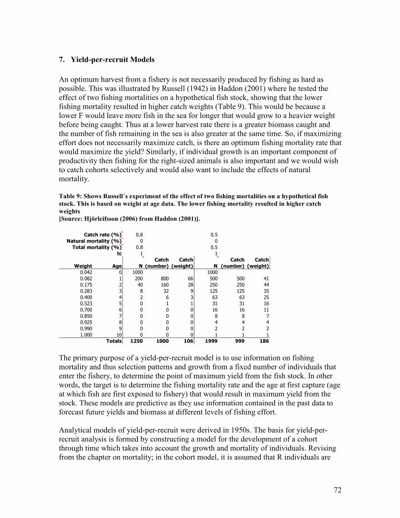
72

7. Yield-per-recruit Models

An optimum harvest from a fishery is not necessarily produced by fishing as hard as

possible. This was illustrated by Russell (1942) in Haddon (2001) where he tested the

effect of two fishing mortalities on a hypothetical fish stock, showing that the lower

fishing mortality resulted in higher catch weights (Table 9). This would be because a

lower F would leave more fish in the sea for longer that would grow to a heavier weight

before being caught. Thus at a lower harvest rate there is a greater biomass caught and

the number of fish remaining in the sea is also greater at the same time. So, if maximizing

effort does not necessarily maximize catch, is there an optimum fishing mortality rate that

would maximize the yield? Similarly, if individual growth is an important component of

productivity then fishing for the right-sized animals is also important and we would wish

to catch cohorts selectively and would also want to include the effects of natural

mortality.

Table 9: Shows Russell´s experiment of the effect of two fishing mortalities on a hypothetical fish

stock. This is based on weight at age data. The lower fishing mortality resulted in higher catch

weights

[Source: Hjörleifsson (2006) from Haddon (2001)].

Catch rate (%) 0.8 0.5

Natural mortality (%) 0 0

Total mortality (%) 0.8 0.5

tc 1 1

Weight Age N

Catch

(number)

Catch

(weight) N

Catch

(number)

Catch

(weight)

0.042 0 1000 1000

0.082 1 200 800 66 500 500 41

0.175 2 40 160 28 250 250 44

0.283 3 8 32 9 125 125 35

0.400 4 2 6 3 63 63 25

0.523 5 0 1 1 31 31 16

0.700 6 0 0 0 16 16 11

0.850 7 0 0 0 8 8 7

0.925 8 0 0 0 4 4 4

0.990 9 0 0 0 2 2 2

1.000 10 0 0 0 1 1 1

Totals 1250 1000 106 1999 999 186

The primary purpose of a yield-per-recruit model is to use information on fishing

mortality and thus selection patterns and growth from a fixed number of individuals that

enter the fishery, to determine the point of maximum yield from the fish stock. In other

words, the target is to determine the fishing mortality rate and the age at first capture (age

at which fish are first exposed to fishery) that would result in maximum yield from the

stock. These models are predictive as they use information contained in the past data to

forecast future yields and biomass at different levels of fishing effort.

Analytical models of yield-per-recruit were derived in 1950s. The basis for yield-per-

recruit analysis is formed by constructing a model for the development of a cohort

through time which takes into account the growth and mortality of individuals. Revising

from the chapter on mortality; in the cohort model, it is assumed that R individuals are

73

recruited into the fishery at the age rt (denoting age at recruitment). From this age fish are

exposed to some degree of natural mortality M (predation, competition). After certain

time these fish are exposed to fishing at age ct (age at first capture) denoted by F for

fishing mortality. At some point maxt the older fish are not vulnerable to fishing. Note that

the model assumes a knife-edge selection, which means at ct either none or all fish in an

age-class are either recruited or not or are vulnerable or not, and once vulnerable all age-

classes are equally vulnerable (Figure 23). The simple yield-per-recruit model proposed

by Beverton and Holt (1957) assumes the cohort is exposed to the same rate of fishing

mortality for life.

An initial number of recruits tN entering the fishery should be known. The equation of

exponential decline illustrates the development of a cohort through time, i.e. how the age

class progresses into the next one with the changes in stock size due to mortalities

(fishing and natural):

tFM

tt eNN ∆+−+ = )(

1

The number of deaths is the difference in the stock size between successive years:

)1( )()( tFM

t

tFM

ttt eNeNND ∆+−∆+− −=−=

The fraction that dies due to fishing mortality (catch) is the fraction )/( ttt FMF + of the

numbers that die:

( ) t

tFM

t NeMF

FC ∆+−−

+= )(1

To convert this into yield we need to multiply the catch by the average weight at age tw :

t

t

t

tCwYc

∑=max

The biomass of a cohort is the numbers at time t multiplies by the weight at age:

∑=maxt

t

tt

c

NwB

The latter two Y and B can be summed up for the whole life time of a cohort.

Therefore, after birth the numbers in a cohort decline exponentially and the individuals in

a cohort increase in size and weight. The biomass which is a product of the two increases

to a certain maximum and then decreases thereafter (Figure 30). This could be attributed

to the fact that at young age, despite being high in abundance (numbers) the fish are low

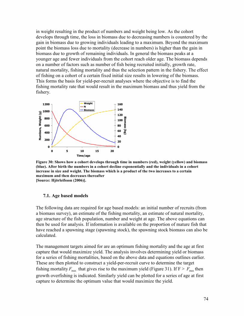
74

in weight resulting in the product of numbers and weight being low. As the cohort

develops through time, the loss in biomass due to decreasing numbers is countered by the

gain in biomass due to growing individuals leading to a maximum. Beyond the maximum

point the biomass loss due to mortality (decrease in numbers) is higher than the gain in

biomass due to growth of remaining individuals. In general the biomass peaks at a

younger age and fewer individuals from the cohort reach older age. The biomass depends

on a number of factors such as number of fish being recruited initially, growth rate,

natural mortality, fishing mortality and thus the selection pattern in the fishery. The effect

of fishing on a cohort of a certain fixed initial size results in lowering of the biomass.

This forms the basis for yield-per-recruit analyses where the objective is to find the

fishing mortality rate that would result in the maximum biomass and thus yield from the

fishery.

0

200

400

600

800

1000

1200

0 5 10 15 20

Time/age

Numbers, Weight (g)

0

20

40

60

80

100

120

140

160

Biomass (k

g)

Weight

N

Biomass

Figure 30: Shows how a cohort develops through time in numbers (red), weight (yellow) and biomass

(blue). After birth the numbers in a cohort decline exponentially and the individuals in a cohort

increase in size and weight. The biomass which is a product of the two increases to a certain

maximum and then decreases thereafter


7.1. Age based models

The following data are required for age based models: an initial number of recruits (from

a biomass survey), an estimate of the fishing mortality, an estimate of natural mortality,

age structure of the fish population, number and weight at age. The above equations can

then be used for analysis. If information is available on the proportion of mature fish that

have reached a spawning stage (spawning stock), the spawning stock biomass can also be

calculated.

The management targets aimed for are an optimum fishing mortality and the age at first

capture that would maximize yield. The analysis involves determining yield or biomass

for a series of fishing mortalities, based on the above data and equations outlines earlier.

These are then plotted to construct a yield-per-recruit curve to determine the target

fishing mortality maxF that gives rise to the maximum yield (Figure 31). If F > maxF then

growth overfishing is indicated. Similarly yield can be plotted for a series of age at first

capture to determine the optimum value that would maximize the yield.

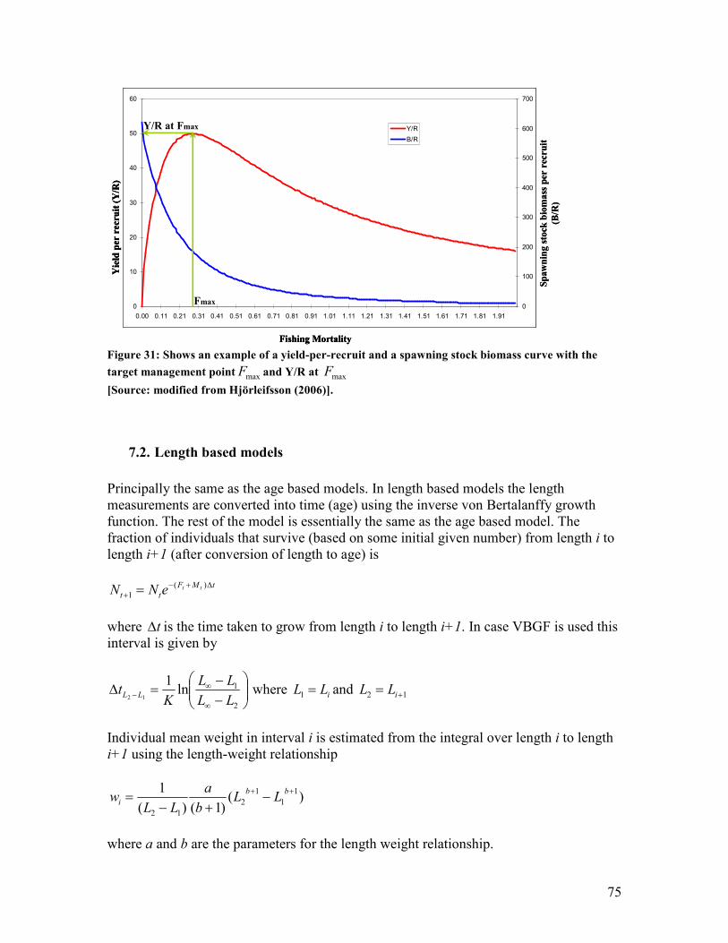
75

Spawning stock biomass per recruit

(B/R)

0

10

20

30

40

50

60

0.00 0.11 0.21 0.31 0.41 0.51 0.61 0.71 0.81 0.91 1.01 1.11 1.21 1.31 1.41 1.51 1.61 1.71 1.81 1.91

0

100

200

300

400

500

600

700

Y/R

B/R

Yield per recruit (Y/R)

Fishing Mortality

Fmax

Y/R at Fmax

Spawning stock biomass per recruit

(B/R)

0

10

20

30

40

50

60

0.00 0.11 0.21 0.31 0.41 0.51 0.61 0.71 0.81 0.91 1.01 1.11 1.21 1.31 1.41 1.51 1.61 1.71 1.81 1.91

0

100

200

300

400

500

600

700

Y/R

B/R


Fishing Mortality

Fmax

Y/R at Fmax

0

10

20

30

40

50

60

0.00 0.11 0.21 0.31 0.41 0.51 0.61 0.71 0.81 0.91 1.01 1.11 1.21 1.31 1.41 1.51 1.61 1.71 1.81 1.91

0

100

200

300

400

500

600

700

Y/R

B/R


Fishing Mortality

Fmax

Y/R at Fmax

Figure 31: Shows an example of a yield-per-recruit and a spawning stock biomass curve with the

target management point maxF and Y/R at maxF

[Source: modified from Hjörleifsson (2006)].

7.2. Length based models

Principally the same as the age based models. In length based models the length

measurements are converted into time (age) using the inverse von Bertalanffy growth

function. The rest of the model is essentially the same as the age based model. The

fraction of individuals that survive (based on some initial given number) from length i to

length i+1 (after conversion of length to age) is

tMF

tttteNN∆+−

+ = )(

1

where t∆ is the time taken to grow from length i to length i+1. In case VBGF is used this

interval is given by

−−

=∆∞

∞−

2

1ln1

12 LL

LL

Kt LL where iLL =1 and 12 += iLL

Individual mean weight in interval i is estimated from the integral over length i to length

i+1 using the length-weight relationship

)()1()(

1 1

1

1

2

12

++ −+−

= bb

i LLb

a

LLw

where a and b are the parameters for the length weight relationship.

76

Therefore the data required are an estimate of K and ∞L , a relationship between length

and weight, selection pattern in the fishery to deduce fishing mortality patterns, some

likely values of natural mortality and an estimate of some initial number of recruits.

Maturity at length data would be needed to estimate the spawning stock biomass.

Empirical evidence suggests that due to the equilibrium assumptions of YPR, maxF tends

to be too high which leads to stock declines. To counteract this, fishing mortality estimate

1.0F was developed which is lower than maxF . Many fisheries around the world are being

managed using 1.0F . Numerically the value of 1.0F is determined by finding the fishing

mortality rate at which the slope of the YPR curve is 10% of the slope at the origin. It

should be noted that the 1.0F strategy is ad hoc and has no theoretical justification.

Experimentally it appears to be more conservative and risk averse and appears as a

theoretical breakthrough as they provide a replacement for maxF and MSY and appear to

be more robust. Important note maxF is not the same as MSYF that gives rise to maximum

sustainable yield, they are two different target reference points. Standard yield-per-recruit

is based on growth and mortality only, recruitment variation is not taken into account.

Hence, whether the maximum yield is also sustainable cannot be told.

The simple Beverton and Holt (1957) “Yield-per-recruit” assumes a constant fishing

mortality model and is essentially a “steady state model” i.e. what happens to one cohort

is representative of what happens to all cohorts. There are several uncertainties inherent

in the yield-per-recruit. It is unrealistic to assume that the fishery has reached equilibrium

with the given fishing mortality as we know most fisheries are unstable with high

recruitment variability, age structure and changing exploitation patterns. The Thompson

and Bell model gives an option for a non-steady state. This is then based on an array of

fishing mortalities by age or length, which is then used for modeling the yield for a series

of fishing mortalities. However both models assume a constant natural mortality.

Additionally getting an estimate of F is a very difficult process which requires a good

estimate of the population size and good records of total commercial catch.

Yield-per-recruit analysis is species specific. Some forecasts or management measures

based on such analysis could include increases or reductions of fishing fleets, use

selective fishing gear that only catches the larger individuals in which gains through

individual growth would be maximizes, changes in minimum mesh sizes, closed seasons,

closed areas, etc. In principle these models form a direct link between fish stock

assessment and fishery resource management. They can also incorporate aspects of

prices and value of the catch which make then suitable as a basis for bio-economic

analyses, where biological and economic inputs are used to predict future yields, biomass

levels and value of the catch under all kinds of assumptions (Haddon 2001). The

materials in this chapter are mostly taken from Hjöleifsson (2006) and Haddon (2001).

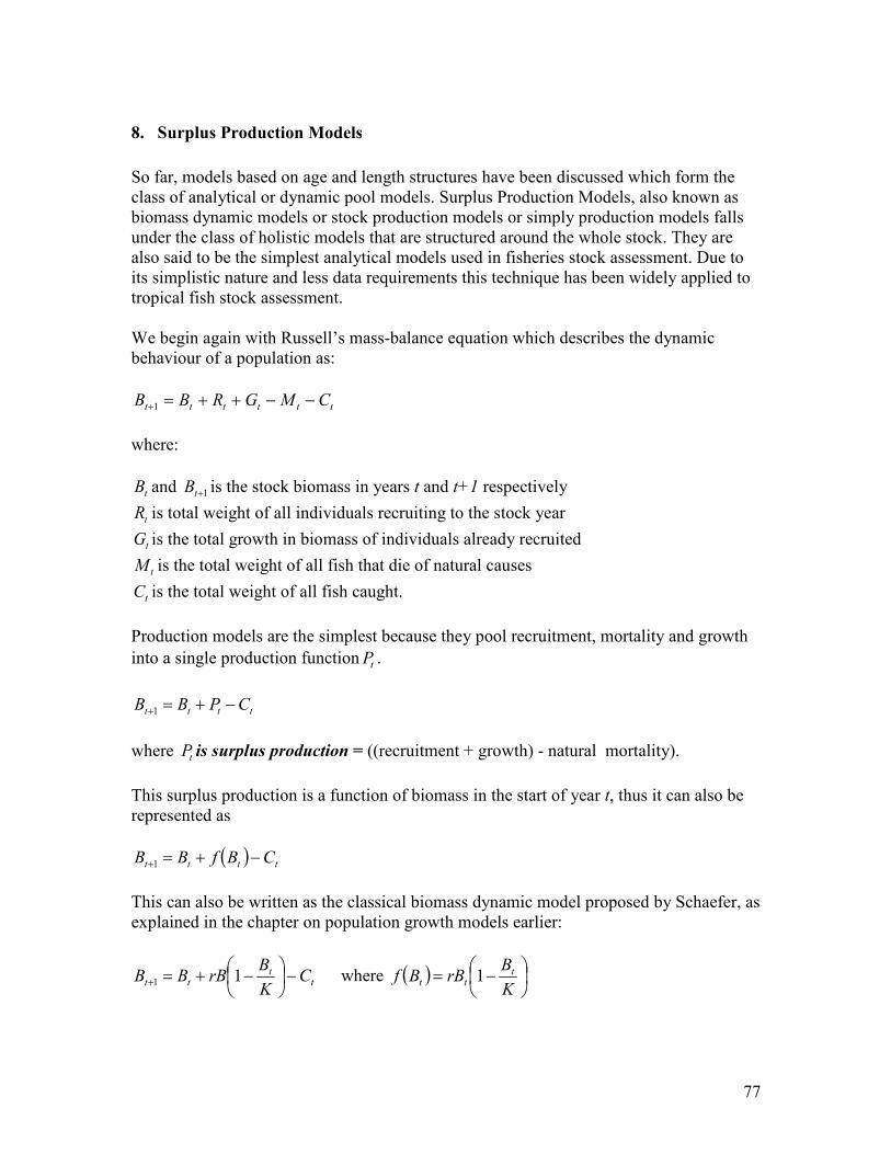
77

8. Surplus Production Models

So far, models based on age and length structures have been discussed which form the

class of analytical or dynamic pool models. Surplus Production Models, also known as

biomass dynamic models or stock production models or simply production models falls

under the class of holistic models that are structured around the whole stock. They are

also said to be the simplest analytical models used in fisheries stock assessment. Due to

its simplistic nature and less data requirements this technique has been widely applied to

tropical fish stock assessment.

We begin again with Russell’s mass-balance equation which describes the dynamic

behaviour of a population as:

tttttt CMGRBB −−++=+1

where:

tB and 1+tB is the stock biomass in years t and t+1 respectively

tR is total weight of all individuals recruiting to the stock year

tG is the total growth in biomass of individuals already recruited

tM is the total weight of all fish that die of natural causes

tC is the total weight of all fish caught.

Production models are the simplest because they pool recruitment, mortality and growth

into a single production function tP .

tttt CPBB −+=+1

where tP is surplus production = ((recruitment + growth) - natural mortality).

This surplus production is a function of biomass in the start of year t, thus it can also be

represented as

( ) tttt CBfBB −+=+1

This can also be written as the classical biomass dynamic model proposed by Schaefer, as

explained in the chapter on population growth models earlier:

tt

tt CK

BrBBB −

−+=+ 11 where ( )

−=K

BrBBf t

tt 1

78

This gives a symmetrical curve which implies application to equilibrium conditions.

Another variation of the Schaefer model is the Pella and Tomlinson model which

introduces a parameter p that gives a provision for introducing an asymmetry in the

production curve:

( )

−=p

ttt

K

BB

p

rBf 1

If p is set to 1, this simplifies to the original Schaefer model.

Catch is normally assumed to be related to the fishing mortality rate and the available

biomass (stock size). Fishing mortality is then related to the effort applied to the fishery

and the catchability coefficient, i.e. the proportion of the stock biomass harvested by one

unit of effort (E), thus =tC ttBqE . This incorporated gives the classic equilibrium

Schaefer model in fisheries

ttt

tt BqEK

BrBBB −

−+=+ 11

The two parameters in the model are r and K. The intrinsic rate of natural increase r, is a

species specific constant related to its life history. The density limit of the stock (standing

biomass), or its carrying capacity is K. Based on the principles of the logistic model

maximum production occurs at K/2 (as explained earlier with reference to population

growth models). Thus the management strategy is to bring the stock down to a size where

maximum surplus production would occur, giving maximum sustainable yield (MSY)

(Figure 32). Other management targets include the corresponding biomass that gives

MSY (BMSY), the effort and the fishing mortality rate that gives rise to MSY (EMSY) and

(FMSY) respectively. The classical logistic model is based on equilibrium assumptions of

the fish stock. The stock is assumed to be in a steady state i.e. tt BB =+1 meaning the

stock biomass does not change from year to year. Any production that occurs beyond the

steady stock size can be harvested, leaving the stock in the condition it was before

production and harvesting. Therefore catch becomes equivalent to surplus production i.e.

−=K

BrBC t

t 1 . Meaning each year’s catch and effort data represent an equilibrium

situation where the catch is equal to the surplus production at that level of effort. If the

fishing regime is changed (altering effort or harvest rate) the stock is assumed to move

instantaneously to a different stable equilibrium biomass with associated surplus

production.

The model thus demands a time series of an index of relative abundance, such as catch

per unit effort i.e a time series of catch and effort data are required. Given the

assumption,

−=K

BrBC t

t 1 and substituting t

tt

qE

CB = ; the equation can be solved for

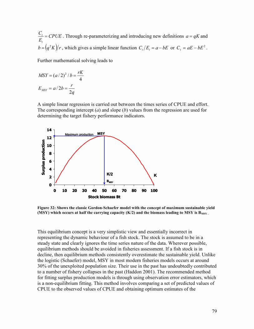
79

CPUEE

C

t

t = . Through re-parameterizing and introducing new definitions qKa = and

( ) rKqb 2= , which gives a simple linear function bEaEC tt −= or 2bEaECt −= .

Further mathematical solving leads to

4/)2/( 2 rKbaMSY ==

q

rbaEMSY

22/ ==

A simple linear regression is carried out between the times series of CPUE and effort.

The corresponding intercept (a) and slope (b) values from the regression are used for

determining the target fishery performance indicators.

0

2

4

6

8

10

12

14

0 10 20 30 40 50 60 70 80 90 100

Stock biomass Bt

Surplus production

K

Maximum production

K/2

BMSY

MSY

0

2

4

6

8

10

12

14

0 10 20 30 40 50 60 70 80 90 100

Stock biomass Bt

Surplus production

K

Maximum production

K/2

BMSY

MSY

Figure 32: Shows the classic Gordon-Schaefer model with the concept of maximum sustainable yield

(MSY) which occurs at half the carrying capacity (K/2) and the biomass leading to MSY is BMSY .

This equilibrium concept is a very simplistic view and essentially incorrect in

representing the dynamic behaviour of a fish stock. The stock is assumed to be in a

steady state and clearly ignores the time series nature of the data. Wherever possible,

equilibrium methods should be avoided in fisheries assessment. If a fish stock is in

decline, then equilibrium methods consistently overestimate the sustainable yield. Unlike

the logistic (Schaefer) model, MSY in most modern fisheries models occurs at around

30% of the unexploited population size. Their use in the past has undoubtedly contributed

to a number of fishery collapses in the past (Haddon 2001). The recommended method

for fitting surplus production models is through using observation error estimators, which

is a non-equilibrium fitting. This method involves comparing a set of predicted values of

CPUE to the observed values of CPUE and obtaining optimum estimates of the

80

parameters r, K, B0 . The assumption is that the population model

−+=+K

BrBBB t

tt 11

exactly describes the population dynamics without any error i.e. 11ˆ++ = tt BB (where the ^

symbol indicates predicted/estimated values). The observations (catch and effort) on the

other hand are made with an error hence the observation model is expressed with an error

term ε+= ttt qBEC / . Some initial estimates of the parameters r, K and B0 are substituted

in the population model to obtain a set of predicted biomass values 1ˆ+tB . Using this

predicted biomass values and an estimate of catchability coefficient q, the predicted

values of CPUE (denoted as Ut) are obtained ε+= tt qBU . These predicted series of

CPUE are then compared with the observed CPUE through least squares method

( )2

0

minˆ∑

=

−=t

t

tt UUSS to obtain the best set of parameters r, K, B0 that minimise the sum of

squares. The error is assumed to be normal with constant variance. The model fitting

relies on minimising the sums of squares or the alternative is to maximise the appropriate

likelihood function ∏−−

=t

ILnLnI tt

eqKrBdataL2

2

ˆ2

)ˆ(

0ˆ2

1),,,( σ

σπThis can be greatly

simplified to a log-likelihood so that

)1)ˆ(2)2((2

++−= σπ LnLnn

LL

where n in the number of observations and

∑ −=

n

ILnLnI tt

22 )ˆ(

σ

An estimate of q that maximises the log likelihood function is given by the geometric

average of the time series of individual q estimates

∑=

)ˆ

(1

ˆ t

t

B

ILn

neq

In summary one makes predictions about the deterministic trajectory of the system from a

hypothesized set of parameters and initial starting conditions and then compares the

observed values with the predictions. The parameters can then be used to calculate the

fishery performance indicators, MSY and EMSY from the formulas given above.

Initial estimates of the parameters r, K, B0 can be deduced from available data on the

particular fishery. The intrinsic rate of growth can be obtained from some available

biological information on the species; the catchability coefficient can be estimated from

absolute biomass estimates from direct counts, acoustics or trawl surveys for one or two

years; K could be based on the area or habitat information.

In principle “you cannot understand how a stock will respond to exploitation unless the

stock has been exploited” (Hilborn and Walters 1992). Ideally we need three types of

81

situations to make predictions reliably. The stock has to be low (growing) and with low

effort (no fishing) to get information about the growth parameter r. The get information

on carrying capacity K, stock has to be high with low effort. To understand the

catchability coefficient we need high effort to understand the efficiency of the fishing

patterns on a high or low stock. However due to time series nature of stock and fishery

development it is virtually impossible to get three such divergent and informative

situations. Furthermore, it is assumed that CPUE is proportional to biomass. However we

know that the fishing efficiency (q) is likely to increase with time and improved fishing

gear technology. Thus true nature of the relationship between CPUE and biomass may

not be linear. The data should be carefully studied before any model is fitted to it. What

the data portrays should be interpreted with caution.

Surplus production models are the most abused stock-assessment technique. Any

published information based on equilibrium assumptions should be ignored. Non-

equilibrium fitting are more reliable for management purposes however caution should be

exercised as the data may not be informative enough.

The materials in this chapter are mostly taken from Hjöleifsson (2006) and Haddon

(2001).

Exercise 5 in Excel gives an example of an equilibrium model and a non-equilibrium

model.

82

9. Multispecies models

The stock assessment techniques described so far have been for single species

applications. However we know that different species of fish co-exist in the environment.

Production is a result of biological interactions which define predator prey relationships

and consequently a whole food web. These biological interactions in the ecosystem will

in turn have an effect on the fisheries production levels. It is almost impossible to harvest

only a single species at one time as we know that fishing gear are not species selective.

Every fishing (industrial or small-scale) has some degree of bycatch i.e. species that are

not targeted by the fishery.

Multispecies models have been developed to take these ecosystem interactions into

account. A brief mention of some of the available models is made but is not discussed in

any detail.

Multispecies yield-per-recruit takes into account the technical interactions such as the

effects of direct mortality on target species and incidental mortality on bycatch. It does

not take the biological interactions.

Multispecies surplus production models take some technical and biological interaction

between species into account. They are based on the assumption of constant catchability

and consistent fishing techniques. However when considering a combination of species,

MSY for each species will be different and maximum yield for one species may easily

under/over exploit another species.

Multispecies virtual population analysis is another method which is more elaborate then

the former two. It is also more data demanding and takes the predator-prey relationships

of the different species into account. This in turn requires analysis of stomach contents of

potential predators and preys and consumption rates together with other elementary data

such as catch at age, weight at age, fishing mortalities.

ECOPATH is a description of the ecosystem represented by biomasses aggregated into

ecologically functional groups. The Ecopath approach uses mass balance principles to

estimate flows between user defined ecological groups. Each group is represented by one

balanced linear equation and requires six input parameters: (1) biomass (B) (2)

production (P) (3) consumption (Q) (4) ecotrophic efficiency (EE) (5) diet composition

(DC) and (6) catch of each group (EX). It differs from the above multispecies models in

that it does not require representation of individual species and age structure of species.

Predators and prey are linked through consumption defined by a diet composition matrix

and consumption rate parameters (Q/B) (Kolding 2006). (More can be read at

http://www.ecopath.org/).

83

10. Patterns of Exploitation

In general the world of commercial fishing can be divided into industrial and artisanal

fishing. Industrialised fleets exploit oceanic fisheries resources. These are modern

techniques which are much more intensive and efficient fishing methods than those

employed in the artisanal fishing which include traditional fishing methods exploiting the

coastal and inland waters mostly in reference to the developing countries. Essentially the

methods used in industrial and artisanal fishing are similar but the size of the gear, of the

tools for gear handling, of the vessels, equipment for navigation and fish finding, of the

catches taken and the costs involved are considerably different (Hart & Reynolds).

Fisheries habitats and resources can be generally classified into three categories; coastal

zone, continental shelf and high seas. Different zones can be characterised by the

different fishing gears used. Mainly in the coastal zone beach seines, diving, traps, nets,

lines, lift nets, boat seines, pots are predominant. In the continental shelf the prevalent

methods of fishing are trawls, purse seines, traps, gillnets, long lines and the in high seas

pelagic trawls, driftnets, long-lines, purse seines, jiggers are common.

Overall the world fisheries are mostly dominated by industrial fleets which exploit

fisheries in the high seas. They can be characterised as capital intensive having relatively

large vessels with a high degree of mechanization, specialized gear and advanced

navigational equipment. This is mostly international market oriented with a high

production capacity and high catch per unit effort. The type of fisheries targeted is mostly

high value offshore demersal and pelagic stocks and highly migratory species. These

fisheries are mainly foreign exchange earners and important for national GDP. The

Northern hemisphere, what is known is the developed world, dominates in industrial

fisheries with the highest landings recorded in the Atlantic. Fisheries monitoring and

management is also fairly well established for industrial fleets particularly in the

Northern Hemisphere with reasonably good time-series of data and regular stock

assessment mostly on a single species basis (Hart and Reynolds 2002 and Kolding 2006).

Small-scale or artisanal fisheries are generally considered less intensive and less stressful

on fish populations than modern industrialised fishing techniques. Artisanal fisheries is

characterised by a diverse number of species, diverse number of fishing gears with a

large number of fishermen operating. It exploits the coastal zone mainly and is normally

restricted geographically within the reach of the communities. This type of fishery can

further be divided into subsistence fishery, which refers to catch for home consumption

utilising primitive fishing methods such as canoes, rafts, wading, barriers, traps, spears,

hook and line, nets, pots and commercial fishing which refers to the catch which is

retailed in the market and uses more modern fishing techniques such as decked vessels,

dredges, automated haulers, jiggers. Small-scale fisheries are an important source of

employment, food security and income, particularly in the developing world. Due to its

diverse nature (multi-species, multi-gear and multi-fleet), the artisanal fisheries turns out

to be quite complex to study and stock assessment becomes difficult. Generally

quantitative research is quite limited and not much is known about the actual status of the

84

stocks (Hart and Reynolds 2002 and Kolding 2006). Single species stock assessment

becomes quite difficult and somewhat inappropriate to apply as many species coexist in

one environment (such as coral reefs) and a single fishing gear targets many species.

Coastal fisheries in most parts of the world are being heavily exploited with unselective

and destructive fishing methods such as dynamite fishing. For the most part, due to lack

of data, management of small-scale fisheries was based on assumptions from industrial

fisheries. Nonetheless, since conventional stock assessment based on single species

cannot be realistically applied to artisanal fisheries (such as estimating total allowable

catch or setting catch quotas), the new management solution for this type of fishery

seems to be co-management and Marine Protected Areas (MPAs). These form the basis

for ecosystem based management or ecosystem approach to fisheries which is the new

paradigm in fisheries management.

The current statistics on fisheries landings and their economic values can be found at

www.fao.org

85

11. Fisheries in the Pacific

Pacific Island States comprise roughly 0.005% of the world’s total catch (FAO 2007).

11.1. Industrial Fisheries

The industrial component is dominated by Tuna fishery. The three main species targeted

by the tuna industry include South Pacific albacore (Thunnus alalunga), bigeye (Thunnus

obesus), yellowfin (Thunnus albacares) and skipjack (Katsuwonus pelamis). Due to its

economic importance the monitoring and management of tuna fisheries is well

established in the Pacific in effect of UNCLOS in 1994 and the Implementing Agreement

of 1995 which focused attention on management of tuna in the Pacific (Hunt 1997). The

management of tuna and other commercial species in the region is the responsibility of

Forum Fisheries Agency (FFA) which handles the economic and political issues and

scientific assessment and monitoring (stock assessment) of these major species in the

Western and Central Pacific Ocean is carried out by the Oceanic Fisheries Programme of

the Secretariat of the Pacific Community (SPC) based on the data collected in the

respective Pacific Island countries which is collated by SPC. The standard stock

assessment tool used is MULTIFAN-CL developed by Fournier et. al. (1998).

11.2. Small-scale fisheries

Most pacific islanders are maritime people with ongoing fishing traditions (Veitayaki

2005). Fisheries has been part of their lives throughout their history. The archipelagic and

inshore waters are rich in marine biodiversity. Large parts of the population who are

confined to the coastal areas rely heavily on the reefs, lagoons and shorelines for

subsistence, livelihood and source of income making the inshore marine environment

crucial for its subsistence and economic development. This puts a lot of pressure on the

fisheries resources.

The dilemma of fisheries stock assessment in the Pacific is associated with the

monitoring and management of small-scale fisheries.

Global perspective

Overall, the world’s fisheries are perceived to be in crisis. “Historical data from marine

ecosystems clearly suggest that overfishing has had, for thousands of years, a major

impact on target species and have fundamentally altered marine ecosystems including

coral reefs” (Morato et. al 2006). According to FAO statistics over 70% of the world’s

commercially important marine fish stocks are overexploited, depleted or recovering

from over-exploitation (FAO 1997). The ever-growing demand of an expanding human

population together with an increasing trend in the per capita resource consumption and

failure to comply with the management regulations are sought to be the main drivers of

86

the serious erosion of the marine environment. The coral reef ecosystems have also been

a part of this resource downfall. Over the past three decades, many documents have

reported evident signs of deterioration in coral reef communities at local, regional and

global scales (Wilkinson, 2004) hence the dramatic decline of coastal fisheries is the

signal we see. As Bell et. al (2006) states that coral reefs are in decline worldwide and

the rapid changes occurring to reefs indicates that the reefs are being stressed beyond

their adaptive capability. The issue of coral reef crisis is complex, but there is a general

consensus of two broad categories of impact; global warming and climate change and

local-scale impacts. Coral reefs normally need an optimum temperature to survive and

the rising sea temperatures lead to coral bleaching. Local impacts comprise of the natural

disasters and more significantly the human populations in the coastal areas, which are

large and growing. The human impacts include increased nutrient and sediment loads,

habitat modification, destructive fishing and chronic overfishing. The coral reefs in the

South Western Pacific Islands are no exception and are under increased pressure from

these similar factors (Zann 1994). As the physical complexities of the reefs are

deteriorated, they are not able to support long-term fish productivity. The global fisheries

crisis is threatening the livelihood and nutritional security of fishery-dependent areas of

mostly the developing nations. These trends have severe negative implications for

hundreds of thousands of jobs in industrialized countries and entire fisheries dependent

communities in the developing world (Constance 2000).

Coral reefs are among the most biologically diverse habitats and the most productive

ecosystems in the world. The conventional single-species fisheries management does not

seem to apply to management of coral reefs because of their complex reef fisheries and

habitats. Marine Protected Areas (MPAs) or Marine reserves have long been recognised

as a suitable and effective management tool for tropical inshore fisheries as they are seen

as a central tool for multi-species management and ecosystem-based management (Rudd

et. al. 2003) and there is an increasing shift in MPAs’ being used to protect biologically

rich habitats. The International Union for the Conservation of Nature and Natural

Resources defines MPAs as “any area of the intertidal or sub-tidal terrain, together with

its overlying water and associated flora, fauna, historical and cultural features, which has

been reserved by law or other effective means to protect part or all of the enclosed

environment (IUCN, 1994). Various forms of MPAs exist such as marine parks, nature

reserves and locally managed marine areas but they all serve the purpose of protecting the

ecosystem, whether it be coral reefs or sea-grass beds or sea bed in deep water

(Kenchington et. al. 2003). The theoretical basis for establishing marine reserves for

fisheries management is straightforward. A marine reserve, by eliminating fishing

pressure in a particular area, allows biomass in the closed area to rebuild, through both

growth and reproduction and lead to an eventual spill out of the fish stock into the

surrounding open areas (Smith et. al. 2006). The number of marine reserves has increased

dramatically over the years and they appear as a useful tool for conservation and a need

for more marine reserves is felt in order to deal with the global fisheries crisis (Salm et

al., 2000). MPAs range from small, fully protected no-take areas, restricting all activities,

to large areas divided into specific zones with different levels of regulated activity.

Globally approximately 0.6% of the oceans are MPAs and 0.01% of the oceans are

actually entirely closed to fishing (Jacquet 2007).

87

The accrued benefits of MPAs are numerous. These include conservation of stocks

including species of commercial value, protection of endangered or threatened species,

maintenance of genetic diversity, protection of spawning stock biomass, reduction of

growth overfishing, provision of a baseline for monitoring of stock status and the health

of the ecosystem (Agardy 2000). Additionally, they protect critical and unique habitats;

act as an insurance against unforeseen ecosystem impacts and changes, provide socio-

economic benefits for coastal communities; and increase recreation and tourism

opportunities (Salm et al., 2000). From a fisheries management perspective MPAs

improve the stability of catches; protect stocks from overfishing; increase fish abundance

and size and possibly act as insurance against management failures (Roberts and

Hawkins, 2000).

Ecosystem based management (EBM) is increasingly viewed as the only real alternative

for managing reef fisheries and MPAs are seen as a primary tool to implement EBM.

Recent scientific evidence has indicated that marine reserves can increase fish yields

while conserving biological diversity. Agardy (2000) quotes a few recent examples of

success of MPAs in Philippines, Kenya, New Zealand and the Mediterranean.

In the past ten or so years, the development of community-based marine protected areas

has become an important tool for marine resource conservation (Calamia 2005). The

IUCN defines the Community Conserved Areas (CCA) as “natural and modified

ecosystems with significant biodiversity, ecological and related cultural values,

voluntarily conserved by indigenous people and local communities through customary

laws or other effective means”. CCAs have three essential features; communities are

related to the ecosystem through cultural, livelihood or economic ties, the community

decision leads to conservation of marine area and biodiversity and cultural values;

communities are major players in the decision making (IUCN 2006).

South Pacific situation

The global fisheries management approach has had little impact in the South Pacific

region as a whole in relation to management of coastal fisheries. This is mainly due to its

traditional systems and important recognition of the resource rights. The current

management practise in the South Pacific is stepping away from the modern approach

and western thinking and reverting to the old-age Pacific Island practise of community-

based resource management. Whilst MPAs are conventionally more formal and policy

oriented setting up CCAs is a more informal process. Since there is limited amount of

documented scientific information on the status of the coral reefs and limited capacity to

measure it, the agencies normally rely on anecdotal information and indigenous

knowledge to determine suitable management strategies. Thus community based MPAs

seem to be a favourable solution to a large extent. The past decade has seen significant

progress of community-based marine resource management in the South Pacific with

numerous MPAs set up throughout the region. Some successful community initiatives

can be found in Fiji, Samoa and Vanuatu. These community initiatives rely on traditional

mechanisms but not entirely. The Government and Non-Government Organisations

88

(NGOs) responsible for implementing the planning process normally integrate knowledge

with some scientific studies for monitoring purposes.

Some of the networks and agencies actively working in the region consist of the Locally

Managed Marine Areas network (LMMA); ProcFish which is an initiative of the SPC;

NGOs such as Worldwide Fund for Nature (WWF), World Conservation Society (WCS)

and Fisheries departments of the respective countries. In common their approach of

setting up community based MPAs is through initiatives from concerned communities,

who have been experiencing declining catches. The procedure involves interviewing the

key informants in the village, especially the village head (chief), fishermen and village

elders. They try to gather all anecdotes about the marine environment and the status of

the stock from the experience and traditional knowledge of the people. At the same time

the local people are also educated. Together the main problem that the community is

facing is ruled out such as, identifying which species are threatened, which areas are

over-exploited or exposed to pollution. Possible solutions are then identified which

normally include either complete protection of some identified areas (full reserve) or

species specific harvest or size specific harvest. At the same time, alternative sources of

livelihood are also weighed for the people. Normally agriculture is a substitute. After all

these dialogue the communities then identify the area that they want to close to fishing

and thus an MPA is demarcated. The network then carries out a biological survey of the

area. This is normally done through underwater visual surveys (underwater visual

census). An important component is training villagers to monitor the resources within the

protected areas. The general notion behind this step is to make the communities

independent so they can monitor the progress of their reserves. Socio-economic surveys

are also carried out. This involves interviewing households in the communities through

official questionnaires

Nonetheless, the downsides of this practice have to be taken into consideration if the

future of fisheries management is not to be jeopardised. Data analysis and scientific

reporting are lagging behind in a way and generally more emphasis is needed on

scientific data collection. It is not argued that MPAs are not successful however; it would

be valuable if some scientific evidence is available to quantify the success of these

community based MPAs. Measuring basic and essential variables such as abundance,

size, biomass and species diversity are imperative. As more no-take marine reserves are

established, the importance of evaluating effectiveness retrospectively is growing (Smith

et. al. 2006). It would also be important to determine at the same time if these reserves

are adequate in protecting some highly mobile species. In the same line, scientific

monitoring of the protected areas is of equal importance to show empirical success of the

MPAs. The solution still lies in monitoring, data collection and stock assessment. Some

relevant data collection and analysis issues are discussed below.

Underwater visual surveys

Underwater Visual Census (UVC) is one widely applied technique for studying coral reef

systems and has been extensively applied for studying reef-fish population

89

dynamics (Samoilys and Carlos 2000, Saimolys and Carlos 2001; Kulbicki and

Sarramégna 1999; Watson and Quinn II 1997). This methodology of a diver swimming

along transects and taking a direct count of animals was initially proposed by Brock

(1954) (Sale and Sharp 1983). Sampling transects can either be placed randomly or

systematically and the count of the animals are used to estimate the density (number or

weight) by extrapolating the sample results to the entire study area to estimate population

size or biomass. The initial idea has been modified over the years and various techniques

of UVC exist today. The observers either snorkel or scuba dive and the basic information

collected are on abundance and length-frequency distributions by species. The sampling

devices used are transects for organisms distributed at larger spatial scale and quadrants

for sessile organisms. The different types of transects used are; (1) Line transect where a

diver swims along the transect and estimates the distance and direction of target animals

from that line at regular intervals; (2) Strip transect where a diver is either swimming or

is being towed along a strip of known length and width, or two divers are swimming on

either side of the transect: (3) Time transect where sampling is carried out for a fixed time

interval; (4) Point count where the diver is scanning 360 degrees while descending to a

fixed point (5) Rapid visual techniques where a diver lists fish species sighted in rank

order of initial encounter for each species (Edgar et. al. 2004). The size (length and

width) of transects are survey specific. The most commonly used are line and strip

transects and point counts (Edgar et. al. 2004; Kulbicki and Sarramégna 1999).

There are certain advantages of visual surveys which have led to adoption of this method

in many coastal studies. They give rapid assessments of the reef areas and are relatively

cheap to perform (Watson and Quinn II 1997). The survey is able to give information on

a variety of variables such as density, relative abundance, size structure, species

composition and habitat characteristics and the method does not require extensive

subsequent lab-work. Additionally, the non-destructive nature of the survey makes it

particularly useful for surveying marine protected areas (Stobart et. al. 2007). In the

fisheries management context, visual estimates are useful because they provide an

independent estimate of the fish abundance (Saimolys and Carlos 2001).

Basically data analysis can be done in the following manner. The fish lengths recorded in

the surveys are converted into weight using a length-weight relationship. The parameters

from for the length-weight relationships are normally taken from literature. This

multiplied by the number of fish observed gives a total weight per transect which gives

an estimate of the fish abundance by species. If the total area of the survey site is known

and the area sampled by the survey is known a raising factor can be applied to get an

estimate of the total abundance (biomass) in the area. Other forms of analysis can also be

carried out such as comparing mean lengths of species in different areas using analysis of

variance.

Bias in UVC

There are a number of potential sources of error in any density estimate. The UVC

methodologies have many such problems of bias and precision inherent in them. The

following sources of bias are known be to associated with UVC; divers level of

90

experience, given the technique relies highly on diver’s skill and his efficiency in

counting and estimating distance, divers behaviour underwater such as swimming speed,

field view available to the diver, subjectivity in the decision making by the diver, average

sampling time and time required to go to the next sampling point and moreover the

response of fish (attraction or escape) towards the presence of divers (Sale 1983; Stobart

et. al. 2007; Watson and Quinn II 1997). Other constraints associated with this

methodology are the associated constraints of scuba diving, environmental constraints,

physical limitations (Stobart et. al. 2007) and the complex behaviour of coral reef fishes

that have patchy distributions and occur in heterogeneous, diverse habitats and different

geographical locations. These factors make it difficult to determine optimal survey

methods of UVC. These drawbacks have led to a high criticism of the methodology. Even

though the method has its downsides, visual census are the most practical method and the

widely applied technique in monitoring coral reefs (Harvey et. al. 2002; Saimolys and

Carlos 2001; Colvocoresses and Acosta 2007). However, there is continuing concern

over the accuracy and precision of the UVC estimates. As a result the reliability of the

surveys has been widely assessed and various studies have looked into these issues.

The accuracy and precision of UVC estimates can be investigated by crossvalidation i.e.

comparing them with estimates obtained from other independent surveys or comparing

two or more different techniques of UVC to determine the optimal survey method. In

marine ecology, standard error (of the mean) to mean ratios, which gives the coefficient

of variation (CV), are often calculated to examine precision of data (Saimolys and Carlos

2000).

For example, fish counts from all transects of the UVC survey (i.e. numbers and lengths

of fish on species level) in a particular area can be combined to estimate the mean and

standard deviation by species. These can be used for computing CV for each species.

Species can be identified according to their abundance or commercial importance for

instance. The CV then gives an indication of how statistically precise and reliable the

survey is in estimating the mean density of each species. Based on the relationship

between sample size and CV and the variance information available for the different

species from the survey, optimal samples sizes can then be calculated according to

desired CV which should normally be less then 30%.

Essentially the survey design issues discussed earlier need to be taken into consideration

when designing these surveys.

Socio-economic surveys

The socio-economic survey involves questionnaire interviews of randomly selected

households in a community. A senior member of the household is normally

interviewed and the information gathered includes fisher and community attributes, such

as age, education, household size, assets, occupation, dependence on fishery resources,

frequency of fishing trips, trip duration, fishing methods, fishing area, catch per trip with

species composition, and fish consumption rates. Catch per

91

trip per household and the number of fishing trips per household can be utilized to

evaluate the total yield per household per year. These can be obtained on a species level.

Assuming that the survey is a true sample representative of the population (includes

fishing and non-fishing households) a deterministic total catch per community can be

calculated by applying some raising factor (total number of households in a community /

the number of households sampled).

These surveys are normally snapshots recording catch per household which can be raised

to obtain the catch per community. Resources are normally constrained to enable

surveying at regular intervals. With just one sample at hand it is not possible to get a

confidence limit on the point estimate of landed catch weight. Additionally annual catch

per household in villages normally do not follow a Gaussian distribution. Bootstrap

technique can be applied to the annual catch per household to generate a number of such

samples which will represent the population. These samples can be raised to obtain the

standard error of the total catch estimates and bootstrap confidence limits. A coefficient

of variation for the sampling can also be obtained.

Bias in socio-economic surveys

The information gathered by household surveys can be very subjective. Such information

is also subject to various kinds of “memory error” and a tendency to misreport on the part

of the respondent (FAO 2000). As such these estimates need to be verified. Normally

surveys of this nature also have a parallel independent survey, which is used for the

verification of the information obtained from households. Rawlinson et. al. (1993) carried

out a socio-economic survey of artisanal and subsistence fishery for Viti Levu, Fiji. In

this survey, a creel survey was also carried out in three villages that were interviewed for

verification of the information obtained by the respondents. Kuster et.

al. (2005) carried out a questionnaire survey on the island of Ono-i-Lau. In this study the

verification process involved taking a sub-sample of the population and monitoring their

fish consumption daily for two weeks

It should be ensured that the sample obtained should be truly representative of the

community being studied and not be biased in its selection. A true sample will be an

indication of the number of fishing and non-fishing households and commercial

operators. A post-stratification approach can be of help where the households within a

community can be divided into frequently fishing, non-frequent fishing, and licensed

households, for instance, and random samples taken from each strata. Sampling should

also give an indication of the licensed fishermen as they also exploit part of the fishing

grounds. Catch information on other licensed fishermen who are not residents of the

village but have the permit to fish in the area would also be necessary if the objective is

to estimate total removal from the fishing area.

Samples that have missing information are a loss therefore consistency in the data

recording system needs to be ensured. It is natural some households will have problems

92

in remembering their catch amounts and species composition. Therefore if it is realised

during the survey that one sample is not fully representative, it should be discarded and a

replacement sample taken. However, care must be taken that this strategy does not create

a bias in the sampling. For example, discarding households that cannot remember their

catch because they are infrequent fishers might result in only frequently fishing

households being sampled.

Effectiveness of the field operations will directly affect the quality of the collected data.

The quality of the data will affect its utility and statistical reliability. “The backbone of a

fishery survey is the field team of data recorders and their supervisors who form the

primary interface between fishers and fisheries management” (FAO 2000). It is important

that the data recorders should have a good understanding of the purpose and the utility of

the survey. To ensure this thorough training and re-training of data collectors would be

required. Workshops and training courses concerning aspects of data recording would

ensure positive contribution to survey planning and the revision of the survey design

(FAO 2000).

The UVC survey and the socio-economic survey highly complement each other as they

normally target the same fishing area. Given the biomass estimate from the UVC data

and the catch estimate from the socio-economic data, would give some indication of

fishing mortalities of the different species;

B

CF =

An example has been set up in Excel which exemplifies how a typical UVC data set can

be explored and analysed [Source: Kolding (2006) and Hjörleifsson (2006)]

93

12. Bibliography

Agardy, T. 2000. Information needs for marine protected areas: scientific and societal.

Bulletin of Marine Pollution (66): 875-888

Bell J.D. Ratner, B.D. Stobutzki, I., Oliver, J. 2006. Addressing the coral reef crisis in the

developing countries. Ocean & Coastal Management (49): 976–985

Bertalanffy, L. von. (1938). A quantitative theory of organic growth (Inquiries in growth

laws II). Hum. Biol., (10):181-213.

Beverton, R. J. H., Holt, S. J. 1957. On the Dynamics of Exploited Fish Populations.

Fishery Investigations, Minist. Agric. Fish. Food, Ser. II, 533

Brock, V. E. 1954. A Preliminary report on a method of estimating reef fish populations.

Journal of Wildlife Management, 18(3):297-308

Caddy, J.F. 1991. Death rates and time intervals: is there an alternative to the constant

natural mortality axoim?. Reviews in Fish Biology and Fisheries, 1:109-138.

Calamia, M.A. 2005. Environmental entitlements and establishment of community-based

marine conservation areas. Pacem in Maribus XXXI, Conference, Australia.

Colcocoresses, J. Acosta, A. 2007. A large-scale field comparison of strip transect and

stationary point count methods for conducting length-based underwater visual surveys of

reef fish populations. Fisheries Research (85): 130–141

Constance, D.H., Bonnano, A. 2000. Regulating the global fisheries: The World Wildlife

Fund, Unilever, and the Marine Stewardship Council. Agriculture and Human Values

(17):125–139

Edgar, G.J. Barrett, N.S. Mortonb, A.J. 2004. Biases associated with the use of

underwater visual census techniques to quantify the density and size-structure of fish.

Journal of Experimental Marine Biology and Ecology (308): 269– 290

Efron, B. 1982. The Jacknife, the Bootstrap and other resampling plans. CBMS-NF 38,

S.I.A.M., Philadelphia

Efron, B., LePage, R. 1992. Introduction to the Bootstrap: pp 3-10 In: Lepage, R. and

Billard, L. (eds). Exploring the limits of bootstrap. John Wiley & Sons, New York

FAO (United Nations Food and Agriculture Organization) (1997). The State of World

Fisheries and Aquaculture: 1996. UNFAO

FAO 1995. Code of Conduct for Responsible Fisheries. Rome, FAO. 41

94

FAO. 1998. Guidelines for routine collection of capture fishery data. FAO Fisheries

Technical Paper. No. 382. Rome, FAO. 113

FAO. 2000. Manual on sample-based data collection for fisheries assessment. FAO

Fisheries Technical Paper 398, Rome: FAO

FAO. 2006. The State of World Fisheries and Aquaculture: 2006. UNFAO

Fournier, D. A., Hampton, J., Sibert, J. R. 1998. MULTIFAN-CL: a length based, age-

structured model for fisheries stock assessment with application to South Pacific

albacore, Thunnus alalunga. Canadian Journal of Aquatic Science 55(9): 2105-2116.

Gayanilo, F. C. Jr., Pauly, D. (eds.). 1997. FAO-ICLARM Stock Assessment tools.

(FiSAT). Reference manual. FAO Comp. Inf. Ser. (Fish.). No. 8. FAO, Rome, 262

Glover, T., Mitchell, K. 2002. An Introduction to Biostatistics. McGraw-Hill. 416

Godø, O.R. 1994. Factors affecting reliability of abundance estimates of ground fish

from bottom trawl surveys. p. 166-199 In: A. Fernø, and S. Olsen (Eds.) Marine Fish

Behaviour in Capture and Abundance Estimation. Fishing News Books, Oxford.

Graham, M. 1935. Modern theory of exploiting a fishery, and application to North Sea

trawling. J.Cons. Perm. Int. Expl. Mer (10): 264-274

Gulland, J. A., Holt, S. J. 1959. Estimation of growth parameters for data at unequal time

intervals. J. Cons. CIEM, (26): 215-222

Gunderson, D.R, P.H. Dygert. 1988. Reproductive effort as a predictor of natural

mortality rate. J. Cons. int. Explor. Mer, (44): 200-209

Gunderson, D.R. 1993. Surveys of fisheries resources. John Wiley & Sons, Inc. New

York. 248

Haddon, M. 2001. Modelling and Quantitative methods in Fisheries. USA: Chapman &

Hall/CRC, 406

Haddon, M. Stratified random survey design. University of Sydney. (Unpublished)

Hart, P. J., Reynolds, J. D. 2002. Handbook of fish and fisheries biology. Volume 2:

Fisheries. Blackwell Publishing

Harvey, E. Fletcher, D.A. Shortis, M.R. Kendrick, G.A. 2002. Estimation of reef fish

length by divers and by stereo-video: A first comparison of the accuracy and precision in

the field on living fish under operational conditions. Fisheries Research (57): 255–265

95

Helle, K. and Pennington, M. 2004. Survey design considerations for estimating the

length composition of the commercial catch of some deep-water species in the northeast

Atlantic. Fisheries Research: 70(1), 55-60

Hilborn, R. and Walters, C. J. 1992. Quantitative Fisheries Stock Assessment Choice,

dynamics & Uncertainty. Chapman & Hall. 570

Hjörleifsson, E. 2006. Fisheries Statistics and Stock Assessment Training, Fiji. Lecture

Notes and exercises

Hunt, C. 1997. Management of the South Pacific Tuna Fishery. Marine Policy, 21(2):

155-171

IUCN (International Union for the Conservation of Nature and Natural Resources). 1994.

Guidelines for Protected Area Management Categories. Internatonal Union for the

Conservation of Nature and Natural Resources. 2006. Community conserved areas.

PARKS (16) No. 1

Jacquet, J. 2007. Silent water: a brief examination of the marine fisheries crisis. Environ

Dev Sustain. Springer

Jennings, S., Kaiser, M. J., Reynolds, J. D. 2001. Marine Fisheries Ecology. Blackwell

Publishing. 417

Kenchington, R., Ward, T. and Hegerl, E. 2003. The Benefits of Marine Protected Areas.

http://www.deh.gov.au/coasts/mpa/wpc/pubs/benefits-mpas-technical.pdf

King, M. 1995. Fisheries Biology, Assessment and Management. Blackwell Science. 341

Kolding, J. 2006. Fisheries Statistics and Stock Assessment Training, Fiji. Lecture Notes

and exercises

Kolding, J., Giordano, W.U. 2001. AdriaMed Training Course on Fish Population

Dynamics and Stock Assessment. FAO-AdriaMed technical document No. 8.

Korsbrekke, K., Mehl, S., Nakken, O., Pennington, M. 2001. A survey based assessment

of Northeast Artic cod. ICES Jounal of Marine Science, 58(4):763-769

Kulbicki, M. Sarramégna, S. 1999. Comparison of density estimates derived from strip

transect and distance sampling for underwater visual censuses: a case study of

Chaetodontidae and Pomacanthidae. Aquat. Living Resour. 12 (5): 315−325

Kuster, C., Vuki, V. C., Zann and L. P. 2005. Long-term trends in subsistence fishing

patterns and coral reef fisheries yield from a remote Fijian Island. Journal of Fisheries

Research (76): 221-228

96

MacDonald, P. D. M.,Pitcher, T. J. 1979. Age group from size frequency data, a versatile

and efficient method of analyzing distribution mixtures. J. Fish. Res. Board Can. (36):

987-1001.

Morato, T. Watson, R. Pitcher, T.J. Pauly, D. 2006. Fishing down the deep. Fish and

Fisheries (7): 24 – 34

Neter, J., Kutner, M. H., Nachtsheim, C. J., Li, W. 2005. Applied Linear Statistical

Models (Fifth Edition). McGraw-Hill. 1396

Pauly, D. 1980. On the interrelationships between natural mortality, growth parameters,

and mean environmental temperature in 175 fish stocks. J. Cons. CIEM. 39(2): 175-192.

Pauly, D. 1987. A Review of the ELEFAN system for analysis of length-frequency data in

fish and aquatic invertebrates. ICLARM Conf. Proc., (13):7-34

Pauly, D., David, N. 1981. ELEFAN 1, a BASIC program for the objective extraction of

growth parameters from length-frequency data. Meeresforsch, (28) : 205-211.

Pennington, M., Strømme, T. 1998. Surveys as a research tool for managing dynamic

stocks. Fisheries Research, 37(1-3): 97-106

Pitcher, T.J., Hart, P.J.B. (1982). Fisheries ecology, (American edition) The Avi

Publ.Com. Inc. Westport, Connecticut. 414

Quinn, G.P Keough, M.J. 2002. Experimental design and data analysis for biologists.

Cambridge University Press, 537

Rawlinson, N. J. F., Milton, D. A., Blaber, S. J. M., Sesewa, A., Sharma, S.P. 1993. A

Survey of the Subsistence and Artisanal Fisheries in the rural areas of Viti Levu, Fiji.

CSIRO. 103

Rikther, V. A., Efanov, V. N. 1976. On one of the approaches to estimation of natural

mortality of fish populations. ICNAF Res. Doc. 76/VI/8, 12

Roberts, C. M., Hawkins, J. P. 2000. Fully Protected Marine Reserves: A Guide. World

Wildlife Fund (WWF) Endangered Seas Campaign.

Rosenberg, A. A., Beddington, J. R. 1988. Length-based methods of fish stock

assessment. 83-103 In: Gulland, J. A. (ed.). Fish population dynamics: the implications

for management. Chichester, John Wiley and Sons Ltd. 422

Rudd, M. A. Tupper, M. H. Folmer, H. Cooper, G.C. 2003. Policy analysis for tropical

marine reserves: challenges and directions. Fish and Fisheries (4): 65-85

97

Russell, E. S. 1931. Some theoretical considerations on the “overfishing” problem. J.

Cons.CIEM, (6):1-20

Saimolys, M.E. Carlos, G. 2001. Determining methods of underwater visual census for

determining the abundance of coral reef fishes. Environmental Biology of Fishes (57):

289–304

Sale, P.F. Sharp, B. J. 1983. Correction for bias in visual transect censuses of coral reef

fishes. Coral Reefs (2):37-42

Salm, R. V., Clark, J., Siirila, E. (Editors). 2000. Marine and Coastal Protected Areas: A

Guide for Planners and Managers. International Union for the Conservation of Nature

and Natural Resources (IUCN).

Schaefer, M. 1957. A study of the dynamics of the fishery for yellowfin tuna in tropical

Pacific Ocean. Bull. I-ATTC/Bol. CIAT, (2):247-268

Schaefer, M.B. 1954. Some aspects of the dynamics of populations important to the

management of commercial marine fisheries.Bull. Inter-Amer. Trop. Tuna Commission 1:

27-56.

Smith, M.D. Zhang, J. Coleman, F. 2006. Effectiveness of marine reserves for large scale

fisheries management. Can. J. Fish. Aquat. Sci. (63) 153–164

Sokal, R. R., Rohlf, F. J. 1995. Biometry (Third edition). W.H. Freeman and Company.

887

Sparre, P. and Venema, S. C. 1998. Introduction to Tropical Fish Stock Assessment. Part

I: Manual. FAO Fish. Tech. Pap. 306/1, Rev. 2. FAO, Rome, 407

Sparre, P.1987. Computer programs for fish stock assessment. Length-based assessment

for Apple II computers. FAO Fish.Tech.Pap. 101:2-218

Stefansson, G. 2000-2009. Tutor-Web. Fishery Science Department: Introduction to fish

population dynamics. http://www.tutor-web.net/

Stobart, B. Garcia-Charton, J. A. Espejo, C. Rochel, E. Goñi, R. Reñones, O. Herrero, A.

Crec'hriou, R. Polti, S. Marcos, C. Planes, S. Pérez-Ruzafa, A. 2007. A baited underwater

video technique to assess shallow-water Mediterranean fish assemblages: Methodological

evaluation. Journal of Experimental Marine Biology and Ecology (345):158–174

Thompson, W. F., Bell, F. H. 1934. Biological statistics of the Pacific halibut fishery. 2.

Effects of changes in intensity upon total yield and yield per unit of gear. Rep. Int.Fish.

(Pacific halibut) Comm. 8. 49

98

Veitayaki, J. 2005. “Fisheries resource-use culture in Fiji and its implications” In:

Culture and sustainable development in the Pacific: The Australian National University,

Asia Pacific Press, 116 – 130

Vetter, E. F. 1988. Estimation of natural mortality in fish stocks: A review. Fishery

Bulletin (86): 25-43

Watson, R.A. Quinn II, T. J. 1997. Performance of transect and point count underwater

visual census methods. Ecological Modelling (104):103–112

Wilkinson, C. . 2004. Status of Coral Reefs of the World: 2004. Australian Institute of

Marine Science, Australia.

http://www.aims.gov.au/pages/research/coral-bleaching/scr2004/pdf/scr2004v1-00.pdf

Zann, L. 1994. The status of coral reefs in the south western pacific islands. Marine

pollution bulletin 29(13): 52-61

Fish stock assessment training Manual

Documents

Transcript of Fish stock assessment training Manual