
Fiscal Multipliers and Institutions in Peru: Getting the ... · C. Sub-national Framework .....14....
24
WP/16/144 Fiscal Multipliers and Institutions in Peru: Getting the Largest Bang for the Sol by Svetlana Vtyurina and Zulima Leal IMF Working Papers describe research in progress by the author(s) and are published to elicit comments and to encourage debate. The views expressed in IMF Working Papers are those of the author(s) and do not necessarily represent the views of the IMF, its Executive Board, or IMF management.
Transcript of Fiscal Multipliers and Institutions in Peru: Getting the ... · C. Sub-national Framework .....14....
WP/16/144
Fiscal Multipliers and Institutions in Peru: Getting the Largest Bang for the Sol
by Svetlana Vtyurina and Zulima Leal
IMF Working Papers describe research in progress by the author(s) and are published
to elicit comments and to encourage debate. The views expressed in IMF Working
Papers are those of the author(s) and do not necessarily represent the views of the IMF, its
Executive Board, or IMF management.
© 2016 International Monetary Fund WP/16/144
IMF Working Paper
Western Hemisphere Department
Fiscal Multipliers and Institutions in Peru: Getting the Largest Bang for the Sol
Prepared by Svetlana Vtyurina and Zulima Leal1
Authorized for distribution by Alfredo Cuevas
July 2016
Abstract
With the end of the commodity super cycle, Peru’s potential growth has declined, raising
questions of what government policies could do to help boost growth, including over the
medium-term. Our econometric analysis shows that public investment multipliers have a
larger effect on growth than current spending or tax-related stimulus in the short and medium
terms. Peru’s low debt and financial savings grants fiscal space for increasing investment
spending, which could also entice and complement private investment, provided the former is
efficient, fiscally sustainable and complemented by further reforms in public investment
management and changes to the decentralization framework.
JEL Classification Numbers: E02, E62, G23, N26
Keywords: Peru, fiscal policy, fiscal sustainability, nonlinear models, multipliers, public
investment management, decentralization.
Author’s E-Mail Address: [email protected]; [email protected]
1 We thank Anja Baum and Gabriel Bruneau for sharing the initial codes, and Amyra Asamoah and Kaitlyn
Douglass for related assistance on the investment efficiency dataset. Comments from Marcello Estevão, Anja
Baum, Xavier Debrun and colleagues at the Central Reserve Bank of Peru are gratefully acknowledged.
IMF Working Papers describe research in progress by the author(s) and are published to
elicit comments and to encourage debate. The views expressed in IMF Working Papers are
those of the author(s) and do not necessarily represent the views of the IMF, its Executive Board,
or IMF management.
2
Contents Page
Abstract .....................................................................................................................................1
I. Context ..................................................................................................................................3
II. Public Investment Trends and Fiscal Levers ...................................................................4
III. Background on Multipliers ..............................................................................................7
IV. Methodology and Results ..................................................................................................9
V. Quality, Efficiency and Management of Public Infrastructure ....................................10 A. Infrastructure Quality and Efficiency .....................................................................11 B. Public Investment Management System .................................................................13 C. Sub-national Framework .........................................................................................14
VI. Conclusions and Recommendations ..............................................................................16
Figures:
1. Selected Indicators .....................................................................................................3
2. Contributions to Real GDP Growth ...........................................................................4
3. Public Fixed Investment Spending ............................................................................5
4. Overall PPP Environment ..........................................................................................5
5. Investment Dynamics.................................................................................................6
6. Cumulative Fiscal Multipliers in Fiscal Expansion .................................................10
7. Public Investment Spending ....................................................................................11
8. Selected Competitiveness and Quality Indicators....................................................12
9. Strength of Public Investment Management by Institution .....................................13
10. Infrastructure Spending by Government Level......................................................15
Tables:
1. Infrastructure Gap by Sector ......................................................................................5
2. Selected Fiscal Stimulus Measures ............................................................................7
3. Anti-Crisis Fiscal Measures (2008-09) ......................................................................7
4. Selected Empirical Estimates of Fiscal Multipliers ..................................................8
5. Summary of Recommendations ...............................................................................17
Appendix: Background on Data and Methodology ............................................................18
References ...............................................................................................................................22
3
I. CONTEXT
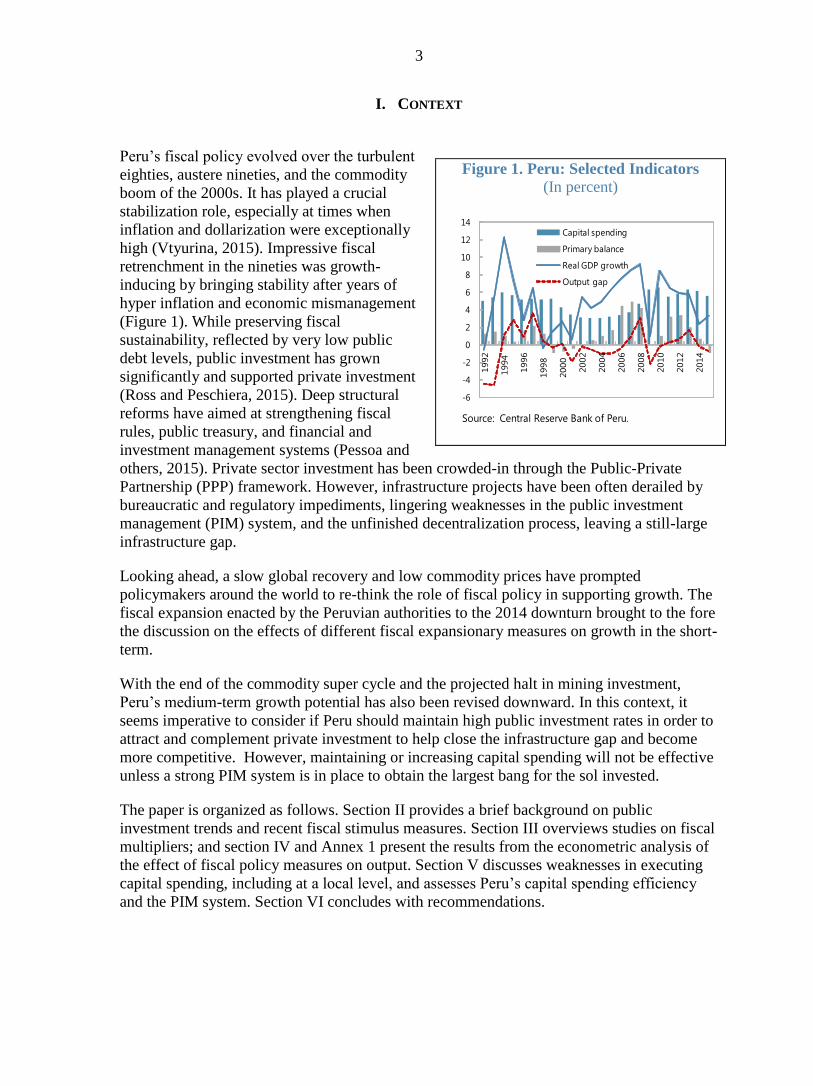
Peru’s fiscal policy evolved over the turbulent
eighties, austere nineties, and the commodity
boom of the 2000s. It has played a crucial
stabilization role, especially at times when
inflation and dollarization were exceptionally
high (Vtyurina, 2015). Impressive fiscal
retrenchment in the nineties was growth-
inducing by bringing stability after years of
hyper inflation and economic mismanagement
(Figure 1). While preserving fiscal
sustainability, reflected by very low public
debt levels, public investment has grown
significantly and supported private investment
(Ross and Peschiera, 2015). Deep structural
reforms have aimed at strengthening fiscal
rules, public treasury, and financial and
investment management systems (Pessoa and
others, 2015). Private sector investment has been crowded-in through the Public-Private
Partnership (PPP) framework. However, infrastructure projects have been often derailed by
bureaucratic and regulatory impediments, lingering weaknesses in the public investment
management (PIM) system, and the unfinished decentralization process, leaving a still-large
infrastructure gap.
Looking ahead, a slow global recovery and low commodity prices have prompted
policymakers around the world to re-think the role of fiscal policy in supporting growth. The
fiscal expansion enacted by the Peruvian authorities to the 2014 downturn brought to the fore
the discussion on the effects of different fiscal expansionary measures on growth in the short-
term.
With the end of the commodity super cycle and the projected halt in mining investment,
Peru’s medium-term growth potential has also been revised downward. In this context, it
seems imperative to consider if Peru should maintain high public investment rates in order to
attract and complement private investment to help close the infrastructure gap and become
more competitive. However, maintaining or increasing capital spending will not be effective
unless a strong PIM system is in place to obtain the largest bang for the sol invested.
The paper is organized as follows. Section II provides a brief background on public
investment trends and recent fiscal stimulus measures. Section III overviews studies on fiscal
multipliers; and section IV and Annex 1 present the results from the econometric analysis of
the effect of fiscal policy measures on output. Section V discusses weaknesses in executing
capital spending, including at a local level, and assesses Peru’s capital spending efficiency
and the PIM system. Section VI concludes with recommendations.
Figure 1. Peru: Selected Indicators
(In percent)
Source: Central Reserve Bank of Peru.
-6
-4
-2
0
2
4
6
8
10
12
14
1992
1994
1996
1998
2000
2002
2004
2006
2008
2010
2012
2014
Capital spending
Primary balance
Real GDP growth
Output gap
4
II. PUBLIC INVESTMENT TRENDS AND FISCAL LEVERS
Stylized facts on investment
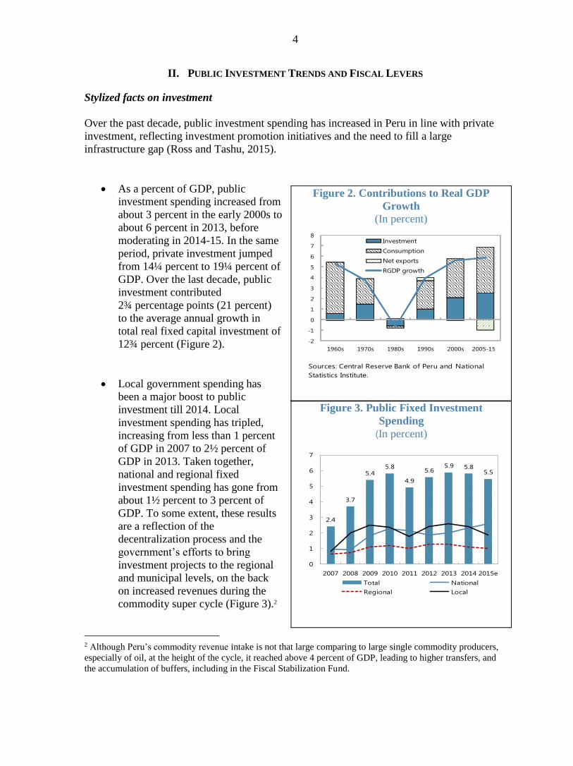
Over the past decade, public investment spending has increased in Peru in line with private
investment, reflecting investment promotion initiatives and the need to fill a large
infrastructure gap (Ross and Tashu, 2015).
As a percent of GDP, public
investment spending increased from
about 3 percent in the early 2000s to
about 6 percent in 2013, before
moderating in 2014-15. In the same
period, private investment jumped
from 14¼ percent to 19¼ percent of
GDP. Over the last decade, public
investment contributed
2¾ percentage points (21 percent)
to the average annual growth in
total real fixed capital investment of
12¾ percent (Figure 2).
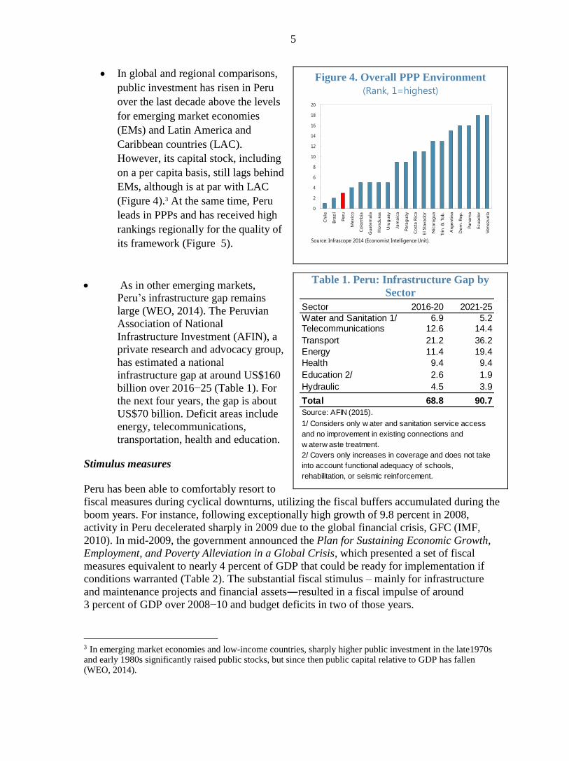
Local government spending has
been a major boost to public
investment till 2014. Local
investment spending has tripled,
increasing from less than 1 percent
of GDP in 2007 to 2½ percent of
GDP in 2013. Taken together,
national and regional fixed
investment spending has gone from
about 1½ percent to 3 percent of
GDP. To some extent, these results
are a reflection of the
decentralization process and the
government’s efforts to bring
investment projects to the regional
and municipal levels, on the back
on increased revenues during the
commodity super cycle (Figure 3).2
2 Although Peru’s commodity revenue intake is not that large comparing to large single commodity producers,
especially of oil, at the height of the cycle, it reached above 4 percent of GDP, leading to higher transfers, and
the accumulation of buffers, including in the Fiscal Stabilization Fund.
Figure 2. Contributions to Real GDP
Growth
(In percent)
Figure 3. Public Fixed Investment
Spending
(In percent)
-2
-1
0
1
2
3
4
5
6
7
8
1960s 1970s 1980s 1990s 2000s 2005-15e
Investment
Consumption
Net exports
RGDP growth
Sources: Central Reserve Bank of Peru and National
Statistics Institute.
2.4
3.7
5.45.8
4.9
5.65.9 5.8
5.5
0
1
2
3
4
5
6
7
2007 2008 2009 2010 2011 2012 2013 2014 2015e
Total National
Regional Local
5
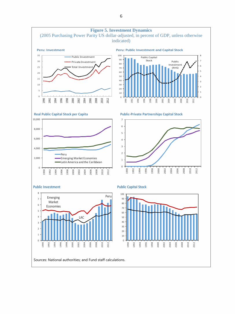
In global and regional comparisons,
public investment has risen in Peru
over the last decade above the levels
for emerging market economies
(EMs) and Latin America and
Caribbean countries (LAC).
However, its capital stock, including
on a per capita basis, still lags behind
EMs, although is at par with LAC
(Figure 4).3 At the same time, Peru
leads in PPPs and has received high
rankings regionally for the quality of
its framework (Figure 5).
As in other emerging markets,
Peru’s infrastructure gap remains
large (WEO, 2014). The Peruvian
Association of National
Infrastructure Investment (AFIN), a
private research and advocacy group,
has estimated a national
infrastructure gap at around US$160
billion over 2016−25 (Table 1). For
the next four years, the gap is about
US$70 billion. Deficit areas include
energy, telecommunications,
transportation, health and education.
Stimulus measures
Peru has been able to comfortably resort to
fiscal measures during cyclical downturns, utilizing the fiscal buffers accumulated during the
boom years. For instance, following exceptionally high growth of 9.8 percent in 2008,
activity in Peru decelerated sharply in 2009 due to the global financial crisis, GFC (IMF,
2010). In mid-2009, the government announced the Plan for Sustaining Economic Growth,
Employment, and Poverty Alleviation in a Global Crisis, which presented a set of fiscal
measures equivalent to nearly 4 percent of GDP that could be ready for implementation if
conditions warranted (Table 2). The substantial fiscal stimulus – mainly for infrastructure
and maintenance projects and financial assets―resulted in a fiscal impulse of around
3 percent of GDP over 2008−10 and budget deficits in two of those years.
3 In emerging market economies and low-income countries, sharply higher public investment in the late1970s and early 1980s significantly raised public stocks, but since then public capital relative to GDP has fallen (WEO, 2014).
Figure 4. Overall PPP Environment
(Rank, 1=highest)
Table 1. Peru: Infrastructure Gap by
Sector
Sector 2016-20 2021-25
Water and Sanitation 1/ 6.9 5.2Telecommunications 12.6 14.4
Transport 21.2 36.2
Energy 11.4 19.4
Health 9.4 9.4
Education 2/ 2.6 1.9
Hydraulic 4.5 3.9
Total 68.8 90.7
Source: AFIN (2015).
1/ Considers only w ater and sanitation service access
and no improvement in existing connections and
w aterw aste treatment.
2/ Covers only increases in coverage and does not take
into account functional adequacy of schools,
rehabilitation, or seismic reinforcement.
0
2
4
6
8
10
12
14
16
18
20
Ch
ile
Bra
zil
Peru
Mexic
o
Co
lom
bia
Gu
ate
mala
Ho
nd
ura
s
Uru
gu
ay
Jam
aic
a
Para
gu
ay
Co
sta R
ica
El Sla
vad
or
Nic
ara
gu
a
Trin
. &
To
b.
Arg
en
tin
a
Do
m. R
ep
.
Pan
am
a
Ecu
ad
or
Ven
ezu
ela
Source: Infrascope 2014 (Economist Intelligence Unit).
6
Figure 5. Investment Dynamics
(2005 Purchasing Power Parity US dollar-adjusted, in percent of GDP, unless otherwise
indicated)
Sources: National authorities; and Fund staff calculations.
Real Public Capital Stock per Capita Public-Private Partnerships Capital Stock
0
1
2
3
4
5
6
7
19
90
19
92
19
94
19
96
19
98
20
00
20
02
20
04
20
06
20
08
20
10
20
120
2,000
4,000
6,000
8,000
10,000
19
90
19
92
19
94
19
96
19
98
20
00
20
02
20
04
20
06
20
08
20
10
20
12
PeruEmerging Market EconomiesLatin America and the Caribbean
Public Investment Public Capital Stock
PeruEmerging Market
Economies
LAC
0
1
2
3
4
5
6
7
8
19
90
19
92
19
94
19
96
19
98
20
00
20
02
20
04
20
06
20
08
20
10
20
12
0
10
20
30
40
50
60
70
80
90
100
19
90
19
92
19
94
19
96
19
98
20
00
20
02
20
04
20
06
20
08
20
10
20
12
Peru: Investment Peru: Public Investment and Capital Stock
0
5
10
15
20
25
30
35
1990
1992
1994
1996
1998
2000
2002
2004
2006
2008
2010
2012
Public Investment
Private Investment
Total Investment
Public Capital Stock Public
Investment (RHS)
0
1
2
3
4
5
6
7
8
0
10
20
30
40
50
60
70
80
90
100
1990
1992
1994
1996
1998
2000
2002
2004
2006
2008
2010
2012
7
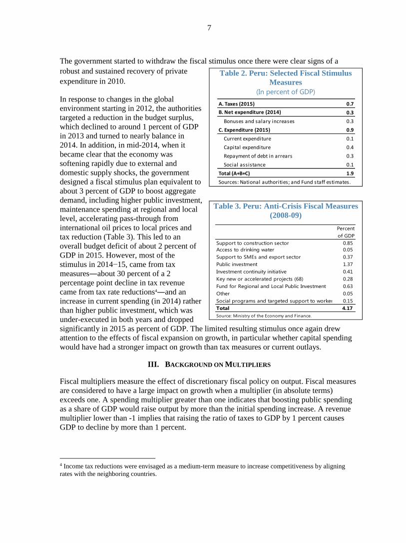
The government started to withdraw the fiscal stimulus once there were clear signs of a
robust and sustained recovery of private
expenditure in 2010.
In response to changes in the global
environment starting in 2012, the authorities
targeted a reduction in the budget surplus,
which declined to around 1 percent of GDP
in 2013 and turned to nearly balance in
2014. In addition, in mid-2014, when it
became clear that the economy was
softening rapidly due to external and
domestic supply shocks, the government
designed a fiscal stimulus plan equivalent to
about 3 percent of GDP to boost aggregate
demand, including higher public investment,
maintenance spending at regional and local
level, accelerating pass-through from
international oil prices to local prices and
tax reduction (Table 3). This led to an
overall budget deficit of about 2 percent of
GDP in 2015. However, most of the
stimulus in 2014−15, came from tax
measures―about 30 percent of a 2
percentage point decline in tax revenue
came from tax rate reductions4―and an
increase in current spending (in 2014) rather
than higher public investment, which was
under-executed in both years and dropped
significantly in 2015 as percent of GDP. The limited resulting stimulus once again drew
attention to the effects of fiscal expansion on growth, in particular whether capital spending
would have had a stronger impact on growth than tax measures or current outlays.
III. BACKGROUND ON MULTIPLIERS
Fiscal multipliers measure the effect of discretionary fiscal policy on output. Fiscal measures
are considered to have a large impact on growth when a multiplier (in absolute terms)
exceeds one. A spending multiplier greater than one indicates that boosting public spending
as a share of GDP would raise output by more than the initial spending increase. A revenue
multiplier lower than -1 implies that raising the ratio of taxes to GDP by 1 percent causes
GDP to decline by more than 1 percent.
4 Income tax reductions were envisaged as a medium-term measure to increase competitiveness by aligning
rates with the neighboring countries.
Table 2. Peru: Selected Fiscal Stimulus
Measures
(In percent of GDP)
Table 3. Peru: Anti-Crisis Fiscal Measures
(2008-09)
A. Taxes (2015) 0.7
B. Net expenditure (2014) 0.3
Bonuses and salary increases 0.3
C. Expenditure (2015) 0.9
Current expenditure 0.1
Capital expenditure 0.4
Repayment of debt in arrears 0.3
Social assistance 0.1
Total (A+B+C) 1.9
Sources: National authorities; and Fund staff estimates.
Percent
of GDP
Support to construction sector 0.85
Access to drinking water 0.05
Support to SMEs and export sector 0.37
Public investment 1.37
Investment continuity initiative 0.41
Key new or accelerated projects (68) 0.28
Fund for Regional and Local Public Investment 0.63
Other 0.05
Social programs and targeted support to workers 0.15
Total 4.17
Source: Ministry of the Economy and Finance.
8
The implementation of contra-cyclical responses around the world has not been without
controversy with respect to their magnitude or composition. The fiscal multiplier depends on
certain macroeconomic characteristics, being substantially high, for instance, if individuals’
marginal propensity to consume is high, if automatic stabilizers are small, if the fiscal
expansion does not trigger interest rate increases, if the exchange rate is fixed and if the fiscal
accounts are sustainable (Spilimbergo et al., 2009). The composition of the fiscal expansion
(taxes, current, or capital spending) matters as well; and capital spending on average has been
found to provide an effective impulse both in the short and in the long term (WEO, 2014).
This said, findings have varied with the degree of a country’s economic development,
especially if PIM systems are poorly designed. This implies an important caveat, as it takes
time to design and implement capital expenditures, possibly rendering them ineffective when
trying to time a fiscal stimulus to stabilize the economic cycle or even producing an
involuntary pro-cyclical fiscal stance (Rossini and others, 2012; MEF, 2015). Estimates of
multipliers vary, sometimes significantly. Due to data limitations, it is harder to measure
multipliers in emerging markets (EMs), and some studies propose a range of multipliers
derived for countries with similar structural characteristics (Batini et al. (2014)). Peru fits
into the country category with medium-size overall multipliers (0.4-0.6) in the first year of
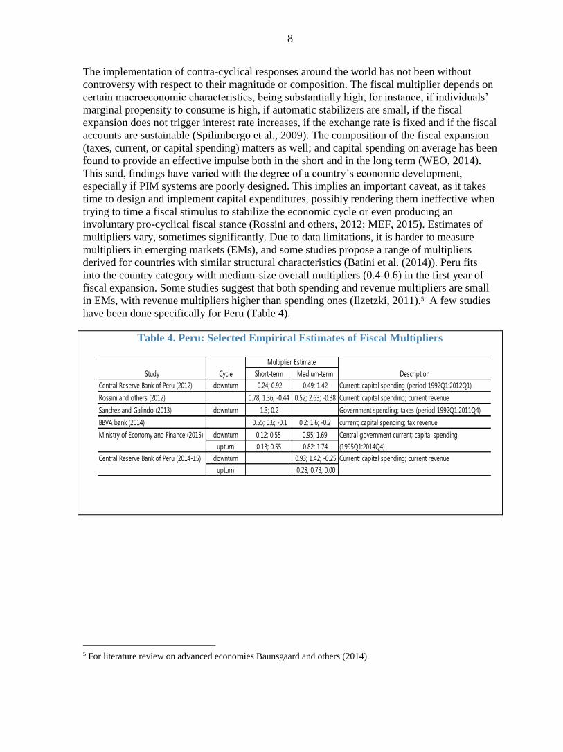
fiscal expansion. Some studies suggest that both spending and revenue multipliers are small
in EMs, with revenue multipliers higher than spending ones (Ilzetzki, 2011).5 A few studies
have been done specifically for Peru (Table 4).
Table 4. Peru: Selected Empirical Estimates of Fiscal Multipliers
5 For literature review on advanced economies Baunsgaard and others (2014).
Study Cycle Short-term Medium-term Description
Central Reserve Bank of Peru (2012) downturn 0.24; 0.92 0.49; 1.42 Current; capital spending (period 1992Q1:2012Q1)
Rossini and others (2012) 0.78; 1.36; -0.44 0.52; 2.63; -0.38 Current; capital spending; current revenue
Sanchez and Galindo (2013) downturn 1.3; 0.2 Government spending; taxes (period 1992Q1:2011Q4)
BBVA bank (2014) 0.55; 0.6; -0.1 0.2; 1.6; -0.2 current; capital spending; tax revenue
Ministry of Economy and Finance (2015) downturn 0.12; 0.55 0.95; 1.69 Central government current; capital spending
upturn 0.13; 0.55 0.82; 1.74 (1995Q1:2014Q4)
Central Reserve Bank of Peru (2014-15) downturn 0.93; 1.42; -0.25 Current; capital spending; current revenue
upturn 0.28; 0.73; 0.00
Multiplier Estimate
9
IV. METHODOLOGY AND RESULTS
We used a non-linear model to estimate the asymmetric response of growth to discretionary
changes in fiscal revenues and expenditures at two different stages of the economic cycle.
That is, fiscal multipliers are estimated using a threshold vector autoregressive model
(TVAR) in which a threshold variable is used to indicate the change from a regime of lower
growth to a regime of higher growth, and vice versa. The general idea is to evaluate whether
the response of fiscal policy is different depending on the economic cycle, which cannot be
tested using conventional linear vector autoregressive models (VAR or SVAR). In this
model, we use gross domestic product (GDP) growth as the threshold variable and its value is
determined endogenously from the model, as it chooses the value that best fits the data in
both regimes.
While several regimes (cycles) can be estimated from the TVAR model, for our purpose we
only use two. The regimes are defined based on the boundary value of a threshold variable or
indicator variable that marks the change from one regime to another. This threshold value
can be chosen either endogenously or exogenously and the variables from the model will
have different coefficients depending on the regime in which they are.
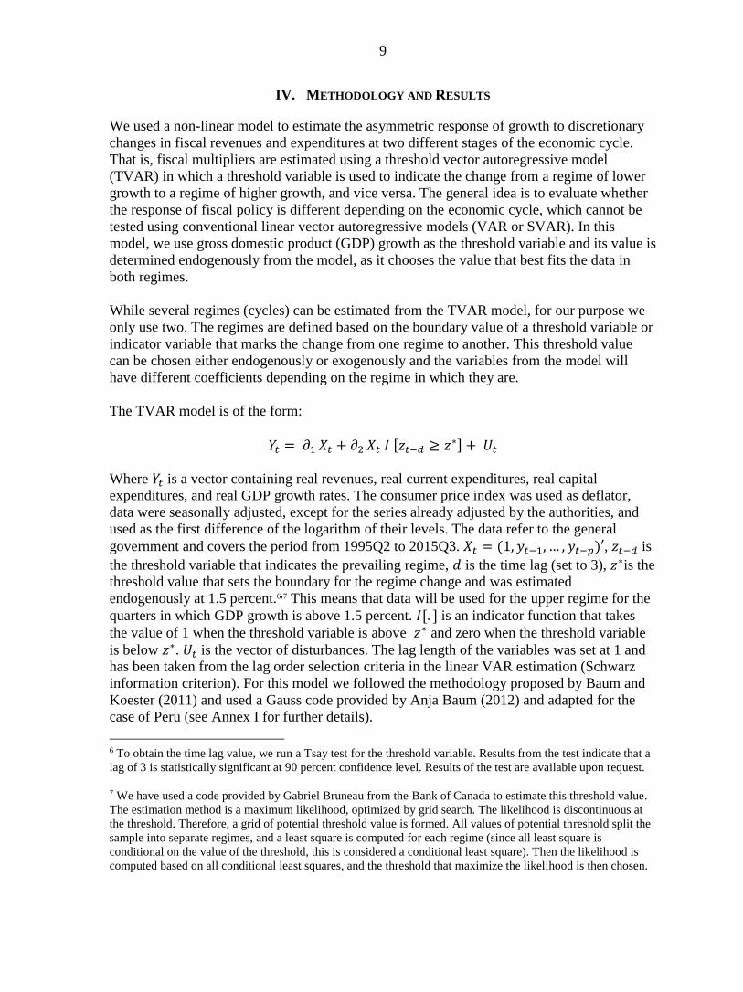
The TVAR model is of the form:
𝑌𝑡 = 𝜕1 𝑋𝑡 + 𝜕2 𝑋𝑡 𝐼 [𝑧𝑡−𝑑 ≥ 𝑧∗] + 𝑈𝑡
Where 𝑌𝑡 is a vector containing real revenues, real current expenditures, real capital
expenditures, and real GDP growth rates. The consumer price index was used as deflator,
data were seasonally adjusted, except for the series already adjusted by the authorities, and
used as the first difference of the logarithm of their levels. The data refer to the general
government and covers the period from 1995Q2 to 2015Q3. 𝑋𝑡 = (1, 𝑦𝑡−1, … , 𝑦𝑡−𝑝)′, 𝑧𝑡−𝑑 is
the threshold variable that indicates the prevailing regime, 𝑑 is the time lag (set to 3), 𝑧∗is the
threshold value that sets the boundary for the regime change and was estimated
endogenously at 1.5 percent.6,7 This means that data will be used for the upper regime for the
quarters in which GDP growth is above 1.5 percent. 𝐼[. ] is an indicator function that takes
the value of 1 when the threshold variable is above 𝑧∗ and zero when the threshold variable
is below 𝑧∗. 𝑈𝑡 is the vector of disturbances. The lag length of the variables was set at 1 and
has been taken from the lag order selection criteria in the linear VAR estimation (Schwarz
information criterion). For this model we followed the methodology proposed by Baum and
Koester (2011) and used a Gauss code provided by Anja Baum (2012) and adapted for the
case of Peru (see Annex I for further details).
6 To obtain the time lag value, we run a Tsay test for the threshold variable. Results from the test indicate that a
lag of 3 is statistically significant at 90 percent confidence level. Results of the test are available upon request.
7 We have used a code provided by Gabriel Bruneau from the Bank of Canada to estimate this threshold value.
The estimation method is a maximum likelihood, optimized by grid search. The likelihood is discontinuous at
the threshold. Therefore, a grid of potential threshold value is formed. All values of potential threshold split the
sample into separate regimes, and a least square is computed for each regime (since all least square is
conditional on the value of the threshold, this is considered a conditional least square). Then the likelihood is
computed based on all conditional least squares, and the threshold that maximize the likelihood is then chosen.
10
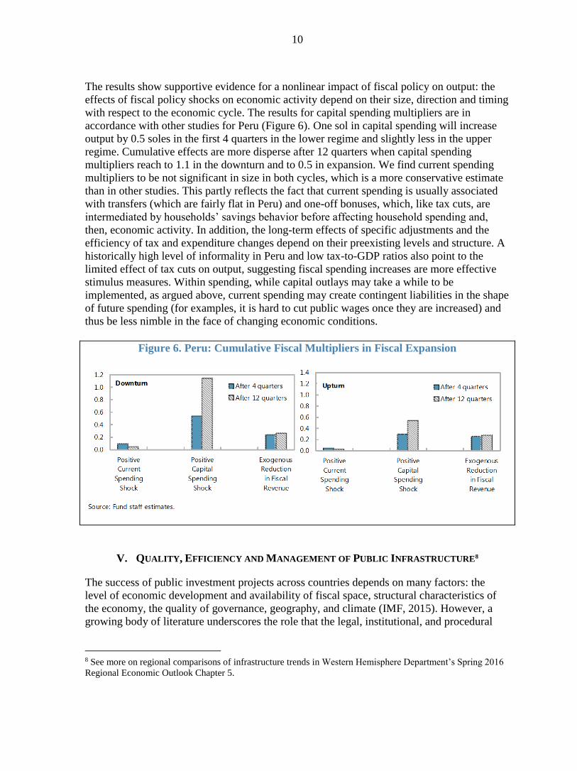
The results show supportive evidence for a nonlinear impact of fiscal policy on output: the
effects of fiscal policy shocks on economic activity depend on their size, direction and timing
with respect to the economic cycle. The results for capital spending multipliers are in
accordance with other studies for Peru (Figure 6). One sol in capital spending will increase
output by 0.5 soles in the first 4 quarters in the lower regime and slightly less in the upper
regime. Cumulative effects are more disperse after 12 quarters when capital spending
multipliers reach to 1.1 in the downturn and to 0.5 in expansion. We find current spending
multipliers to be not significant in size in both cycles, which is a more conservative estimate
than in other studies. This partly reflects the fact that current spending is usually associated
with transfers (which are fairly flat in Peru) and one-off bonuses, which, like tax cuts, are
intermediated by households’ savings behavior before affecting household spending and,
then, economic activity. In addition, the long-term effects of specific adjustments and the
efficiency of tax and expenditure changes depend on their preexisting levels and structure. A
historically high level of informality in Peru and low tax-to-GDP ratios also point to the
limited effect of tax cuts on output, suggesting fiscal spending increases are more effective
stimulus measures. Within spending, while capital outlays may take a while to be
implemented, as argued above, current spending may create contingent liabilities in the shape
of future spending (for examples, it is hard to cut public wages once they are increased) and
thus be less nimble in the face of changing economic conditions.
Figure 6. Peru: Cumulative Fiscal Multipliers in Fiscal Expansion
V. QUALITY, EFFICIENCY AND MANAGEMENT OF PUBLIC INFRASTRUCTURE8
The success of public investment projects across countries depends on many factors: the
level of economic development and availability of fiscal space, structural characteristics of
the economy, the quality of governance, geography, and climate (IMF, 2015). However, a
growing body of literature underscores the role that the legal, institutional, and procedural
8 See more on regional comparisons of infrastructure trends in Western Hemisphere Department’s Spring 2016
Regional Economic Outlook Chapter 5.
11
arrangements, including risk management, for public investment management play in
determining the level, composition, and impact of public investment on the economy.
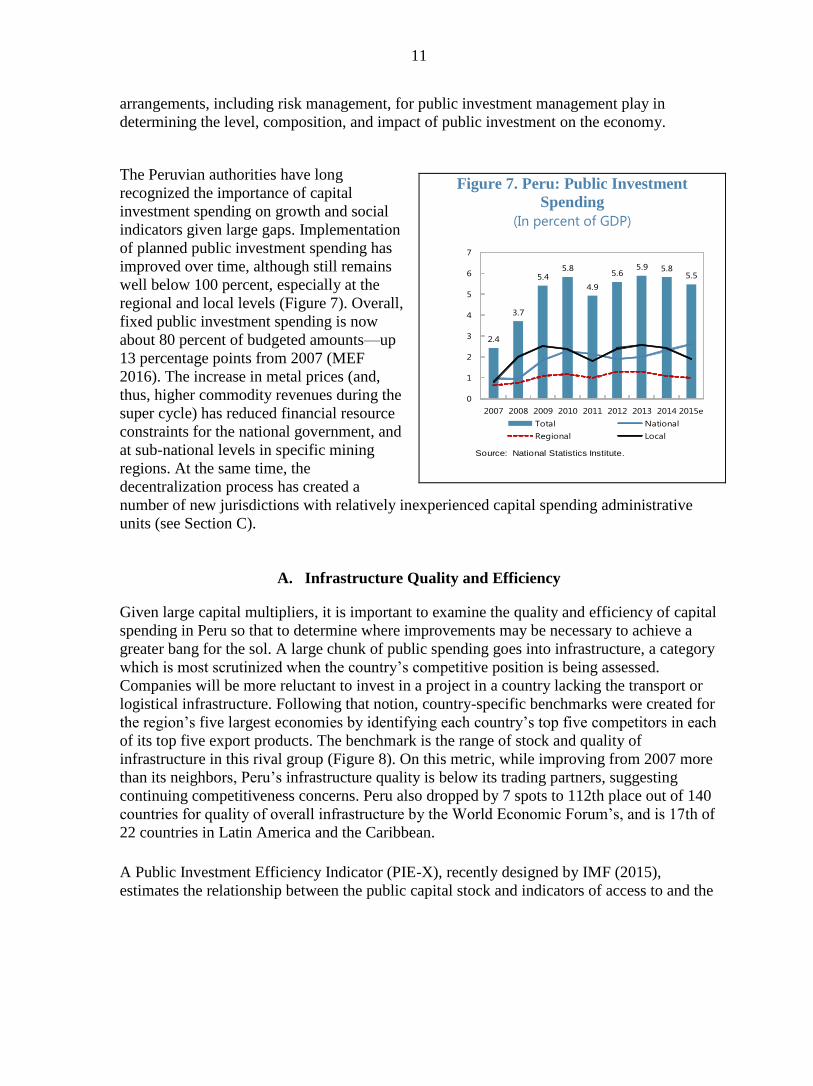
The Peruvian authorities have long
recognized the importance of capital
investment spending on growth and social
indicators given large gaps. Implementation
of planned public investment spending has
improved over time, although still remains
well below 100 percent, especially at the
regional and local levels (Figure 7). Overall,
fixed public investment spending is now
about 80 percent of budgeted amounts—up
13 percentage points from 2007 (MEF
2016). The increase in metal prices (and,
thus, higher commodity revenues during the
super cycle) has reduced financial resource
constraints for the national government, and
at sub-national levels in specific mining
regions. At the same time, the
decentralization process has created a
number of new jurisdictions with relatively inexperienced capital spending administrative
units (see Section C).
A. Infrastructure Quality and Efficiency
Given large capital multipliers, it is important to examine the quality and efficiency of capital
spending in Peru so that to determine where improvements may be necessary to achieve a
greater bang for the sol. A large chunk of public spending goes into infrastructure, a category
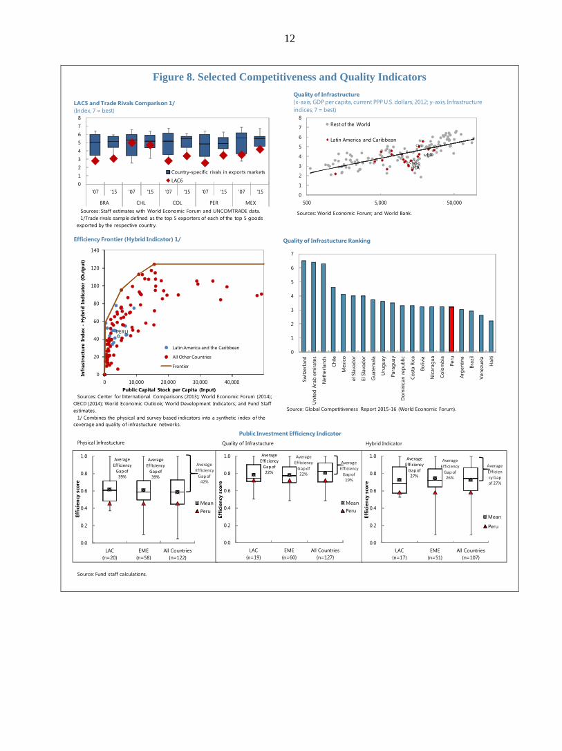
which is most scrutinized when the country’s competitive position is being assessed.
Companies will be more reluctant to invest in a project in a country lacking the transport or
logistical infrastructure. Following that notion, country-specific benchmarks were created for
the region’s five largest economies by identifying each country’s top five competitors in each
of its top five export products. The benchmark is the range of stock and quality of
infrastructure in this rival group (Figure 8). On this metric, while improving from 2007 more
than its neighbors, Peru’s infrastructure quality is below its trading partners, suggesting
continuing competitiveness concerns. Peru also dropped by 7 spots to 112th place out of 140
countries for quality of overall infrastructure by the World Economic Forum’s, and is 17th of
22 countries in Latin America and the Caribbean.
A Public Investment Efficiency Indicator (PIE-X), recently designed by IMF (2015),
estimates the relationship between the public capital stock and indicators of access to and the
Figure 7. Peru: Public Investment
Spending
(In percent of GDP)
Chile
Mexico
Uruguay
Paraguay
Bolivia
Nicaragua
Colombia
Peru
2.4
3.7
5.45.8
4.9
5.65.9 5.8
5.5
0
1
2
3
4
5
6
7
2007 2008 2009 2010 2011 2012 2013 2014 2015e
Total National
Regional Local
Source: National Statistics Institute.
12
Figure 8. Selected Competitiveness and Quality Indicators
0.0
0.2
0.4
0.6
0.8
1.0
LAC
n=20
EME
n=58
All Countries
n=122
Eff
icie
ncy
sco
re
Mean
Peru
Average
Efficiency
Gap of 42%
Average
Efficiency
Gap of 39%
Average Efficiency
Gap of 39%
0.0
0.2
0.4
0.6
0.8
1.0
LAC
n=19
EME
n=60
All Countries
n=127
Eff
icie
ncy
sco
re
Mean
Peru
Average Efficiency
Gap of 19%
Average
Efficiency
Gap of 22%
Average Efficiency
Gap of 22%
0.0
0.2
0.4
0.6
0.8
1.0
LAC
n=17
EME
n=51
All Countries
n=107
Eff
icie
ncy
sco
re
Mean
Peru
Average
Efficiency Gap of 27%
Average
Efficiency Gap of 26%
Average
Efficiency
Gap of 27%
PERU
0
20
40
60
80
100
120
140
0 10,000 20,000 30,000 40,000
Infr
ast
ruct
ure
In
dex -
Hyb
rid
In
dic
ato
r (O
utp
ut)
Public Capital Stock per Capita (Input)
Latin America and the Caribbean
All Other Countries
Frontier
Efficiency Frontier (Hybrid Indicator) 1/
Sources: Center for International Comparisons (2013); World Economic Forum (2014);
OECD (2014); World Economic Outlook; World Development Indicators; and Fund Staff
estimates.
1/ Combines the physical and survey based indicators into a synthetic index of the
coverage and quality of infrastucture networks.
0
1
2
3
4
5
6
7
Sw
itze
rland
United
Ara
b e
mir
ate
s
Neth
erl
and
s
Chile
Mexi
co
el S
lava
do
r
El S
lava
do
r
Guate
mala
Uru
guay
Para
guay
Do
min
ican r
ep
ub
lic
Co
sta R
ica
Bo
livia
Nic
ara
gua
Co
lom
bia
Peru
Arg
entina
Bra
zil
Venezu
ela
Haiti
Quality of Infrastucture Ranking
Source: Global Competitiveness Report 2015-16 (World Economic Forum).
0
1
2
3
4
5
6
7
8
'07 '15 '07 '15 '07 '15 '07 '15 '07 '15
BRA CHL COL PER MEX
Country-specific rivals in exports markets
LAC6
Sources: Staff estimates with World Economic Forum and UNCOMTRADE data.
1/Trade rivals sample defined as the top 5 exporters of each of the top 5 goods
exported by the respective country.
LAC5 and Trade Rivals Comparison 1/
(Index, 7 = best)
Public Investment Efficiency Indicator
Physical Infrastucture Quality of Infrastucture Hybrid Indicator
BRACOL
CHL
MEX
PER
0
1
2
3
4
5
6
7
8
500 5,000 50,000
Rest of the World
Latin America and Caribbean
Quality of Infrastructure
(x-axis, GDP per capita, current PPP U.S. dollars, 2012; y-axis, Infrastructure
indices, 7 = best)
Sources: World Economic Forum; and World Bank.
Source: Fund staff calculations.
13
quality of infrastructure assets (Figure 8).9 The PIE-X estimate for Peru confirms that there is
substantial scope for improving public investment efficiency. While Peru compares fairly
well with other LAC countries and EMs when looking at survey-based indicators (efficiency
gap of 28 comparing to the average of 19 for LAC and EMs), it lags significantly behind on
the physical indicator measure (54 versus 39, respectively).
B. Public Investment Management System
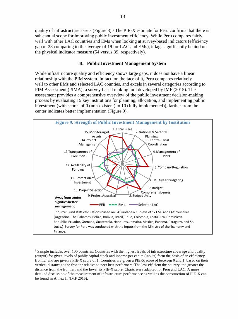
While infrastructure quality and efficiency shows large gaps, it does not have a linear
relationship with the PIM system. In fact, on the face of it, Peru compares relatively
well to other EMs and selected LAC counties, and excels in several categories according to
PIM Assessment (PIMA), a survey-based ranking tool developed by IMF (2015). The
assessment provides a comprehensive overview of the public investment decision-making
process by evaluating 15 key institutions for planning, allocation, and implementing public
investment (with scores of 0 (non-existent) to 10 (fully implemented)), farther from the
center indicates better implementation (Figure 9).
Figure 9. Strength of Public Investment Management by Institution
9 Sample includes over 100 countries. Countries with the highest levels of infrastructure coverage and quality
(output) for given levels of public capital stock and income per capita (inputs) form the basis of an efficiency
frontier and are given a PIE-X score of 1. Countries are given a PIE-X score of between 0 and 1, based on their
vertical distance to the frontier relative to peer best performers. The less efficient the country, the greater the
distance from the frontier, and the lower its PIE-X score. Charts were adapted for Peru and LAC. A more
detailed discussion of the measurement of infrastructure performance as well as the construction of PIE-X can
be found in Annex II (IMF 2015).
Source: Fund staff calculations based on FAD and desk surveys of 12 EMS and LAC countires
(Argentina, The Bahamas, Belize, Bolivia, Brazil, Chile, Colombia, Costa Rica, Dominican
Republic, Ecuador, Grenada, Guatemala, Honduras, Jamaica, Mexico, Panama, Paraguay, and St.
Lucia.) Survey for Peru was conducted with the inputs from the Ministry of the Economy and
Finance.
1. Fiscal Rules2. National & Sectoral
Planning3. Central-Local Coordination
4. Management of PPPs
5. Company Regulation
6. Multiyear Budgeting
7. Budget Comprehensiveness
8. Budget Unity9. Project Appraisal
10. Project Selection
11. Protection of Investment
12. Availability of Funding
13.Transparency of Execution
14.Project Management
15. Monitoring of Assets
PER EMs Selected LAC
Away from centersignifies better management
14
Peru scores exceptionally well in the area of planning (categories 1-5). Ensuring sustainable
levels of public investment manifests itself through the existence of fiscal rules that allow for
planning for resources, including for public investment, making sure that public investment
decisions are based on clear and realistic priorities and cost estimates, that there is certainty
about funding from the central government and a sustainable level of sub-national borrowing,
that management of PPPs leads to effective selection of projects and that regulation of
infrastructure companies promoted open and competitive markets.
Peru scores more modestly in the area of resource allocation (categories 6-10). A rather
obvious weakness lies in the area of multi-year budgeting. This category implies the practice
in budgeting that provides transparency and predictability regarding levels of investment by
ministry, program and project over the medium term. Project selection and appraisal use
standard methodology and systematic vetting. Peru does not publish projections of capital
spending beyond the budget year as the budget is approved on a yearly basis.10 Thus, there
are no multiyear targets/ceilings on capital expenditure by ministry or program. And while
projections of the total cost of major capital projects are published, they are not presented
together with annual projections over a three-to-five year horizon. A particular weakness
relates to multi-year investment spending, as there is no official record regarding
commitments in future years from signed public investment contracts. This fact, coupled with
the lack of absorption capacity, generates work abandonment and unplanned project
modifications, particularly at the sub-national level. Peru does well in budget
comprehensiveness, which ensures that all public investment is authorized by the legislature
and disclosed in the budget recommendation.
Project implementation could also be improved substantially (categories 11-15). Peru scores
well in project management by having a designated staff to prepare implementation plans,
and in monitoring of public assets through comprehensive asset surveys that are conducted
regularly by the government. This said, project appropriations are not sufficient to ensure the
coverage of total project costs as they are approved by congress on a one-year basis and
unspent appropriations of capital lapse at the end of the year (with a few exceptions). Cash
flow forecasts are not prepared or updated regularly and ministries/agencies are not provided
with commitment ceilings in a timely manner and cash for project outlays is sometimes
released with delays, leading to some setbacks in project implementation. Finally, many
major projects are tendered in a competitive process, but the public has only limited access to
procurement information and only some large projects are subject to external audit.
C. Sub-national Framework
As discussed briefly above, the decentralization process that started in 2002, and is not yet
complete, also poses a challenge for Peru’s PIM (Cheasty and Pichihua, 2015). To fund
subnational government responsibilities, regional and local governments are supposed to
share transfers from the national government, license fees (canons), and royalties from
commodity-related operations. That has allowed decentralization of public spending, but
actual implementation has greatly varied across regions and municipalities, both in terms of
quantity and quality. To a large extent this is explained by the diversity of Peru’s subnational
10 Peru publishes projections of fiscal accounts on a three-year basis in the MEF’s Macroeconomic Framework
report but these are not binding beyond the budget year.
15
governments, many of which are small and have limited capacity to deliver local services.
The local level in Peru is now one of the most fragmented in Latin America, which makes it
quite challenging to assess their capacity to invest.
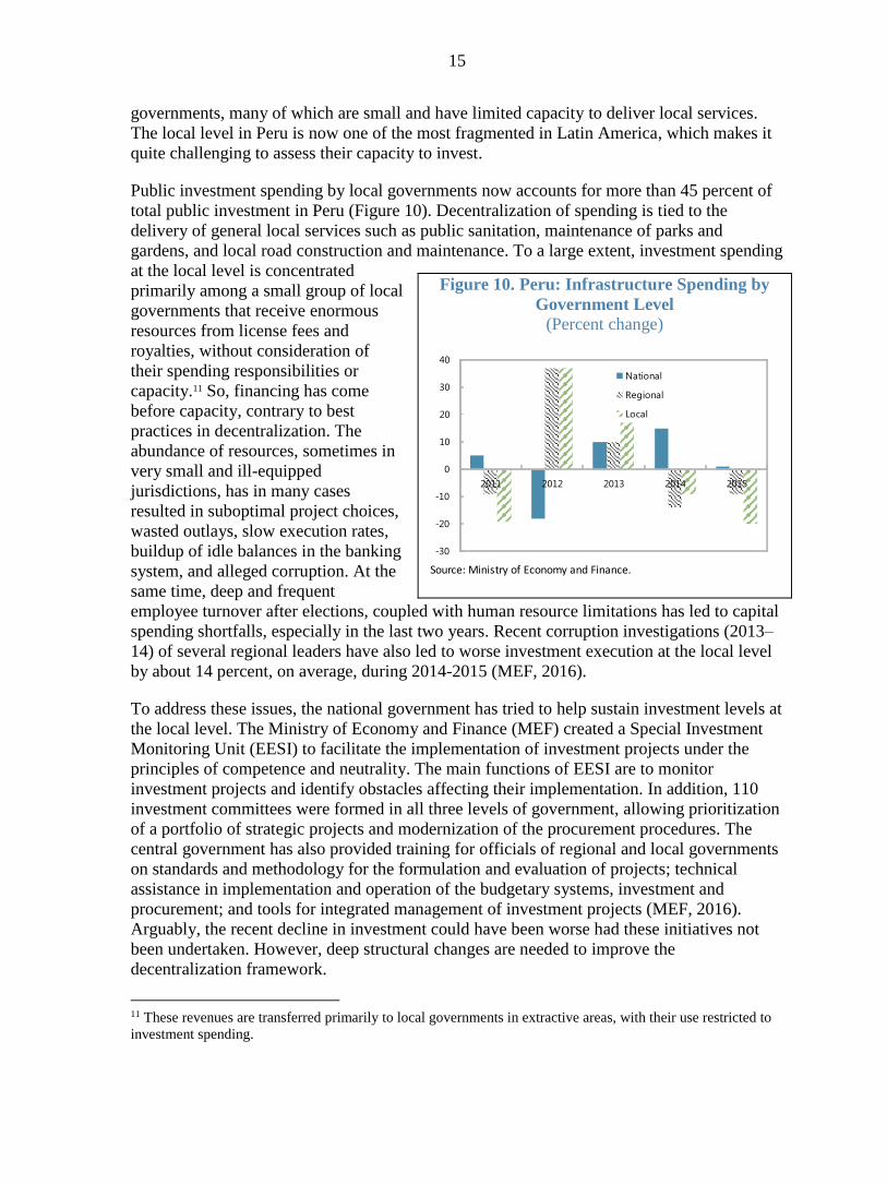
Public investment spending by local governments now accounts for more than 45 percent of
total public investment in Peru (Figure 10). Decentralization of spending is tied to the
delivery of general local services such as public sanitation, maintenance of parks and
gardens, and local road construction and maintenance. To a large extent, investment spending
at the local level is concentrated
primarily among a small group of local
governments that receive enormous
resources from license fees and
royalties, without consideration of
their spending responsibilities or
capacity.11 So, financing has come
before capacity, contrary to best
practices in decentralization. The
abundance of resources, sometimes in
very small and ill-equipped
jurisdictions, has in many cases
resulted in suboptimal project choices,
wasted outlays, slow execution rates,
buildup of idle balances in the banking
system, and alleged corruption. At the
same time, deep and frequent
employee turnover after elections, coupled with human resource limitations has led to capital
spending shortfalls, especially in the last two years. Recent corruption investigations (2013–
14) of several regional leaders have also led to worse investment execution at the local level
by about 14 percent, on average, during 2014-2015 (MEF, 2016).
To address these issues, the national government has tried to help sustain investment levels at
the local level. The Ministry of Economy and Finance (MEF) created a Special Investment
Monitoring Unit (EESI) to facilitate the implementation of investment projects under the
principles of competence and neutrality. The main functions of EESI are to monitor
investment projects and identify obstacles affecting their implementation. In addition, 110
investment committees were formed in all three levels of government, allowing prioritization
of a portfolio of strategic projects and modernization of the procurement procedures. The
central government has also provided training for officials of regional and local governments
on standards and methodology for the formulation and evaluation of projects; technical
assistance in implementation and operation of the budgetary systems, investment and
procurement; and tools for integrated management of investment projects (MEF, 2016).
Arguably, the recent decline in investment could have been worse had these initiatives not
been undertaken. However, deep structural changes are needed to improve the
decentralization framework.
11 These revenues are transferred primarily to local governments in extractive areas, with their use restricted to
investment spending.
Figure 10. Peru: Infrastructure Spending by
Government Level
(Percent change)
Source: Ministry of Economy and Finance.
-30
-20
-10
0
10
20
30
40
2011 2012 2013 2014 2015
National
Regional
Local
16
VI. CONCLUSIONS AND RECOMMENDATIONS
With the end of the commodity super cycle, Peru needs a new engine for growth, which
could be non-mining investment and exports. Its low tax burden provides fiscal space for
increasing public capital spending to improve infrastructure and competitiveness through
better fiscal revenue collection. Higher public investment would continue to complement and
encourage private sector investment, as long as it is efficient (further reforms in PIM and
changes to the decentralization framework would contribute to greater efficiency) and
fiscally sustainable. Despite increased investment in infrastructure and improved
frameworks, Peru faces challenges in developing, executing, and managing investments, as
infrastructure stocks have stagnated and are not considered of high quality. Based on our
analysis, we offer the following considerations:
Investment push: Our econometric exercise shows that public investment multipliers
have a larger effect on aggregate output than current spending or tax-related stimulus
in both the short and the medium terms, and especially during downturns.12 In fact,
weighting revenue and spending impulses by their respective multipliers, the impact
of the fiscal impulse on the economy in 2015 was a negative 0.3 percent, despite the
attempted measures. Had capital spending been executed as budgeted in 2015, real
output growth would have been higher by 0.1 percentage point of GDP. While the
effect is smaller in the short term, on the demand side, an extra boost could have
come from crowding in private investment as there was some economic slack; and an
improvement in confidence. Over the longer term, if Peru increases investment to 6-
6.5 percent of GDP, this could result in about 2-percentage-points increase in output
growth. Supply-side effects should kick in and raise potential output further, mainly
through higher capital stock and TFP, as has happened in Peru previously. This would
also improve potential for private sector investment, which would benefit from
improved infrastructure, both indirectly and directly (through participation in PPPs).
In this way, infrastructure can lift near-term demand and potential growth, which
would also help counter risks of a significant drop in potential output owing to the
end of the commodity super cycle.
Fiscal sustainability: Peru’s debt levels are very low, with net debt at 7 percent of
GDP. However, given the exposure to commodity cycles, natural disasters, and
contingent liabilities, it would be advisable for Peru to follow a medium-term fiscal
path that allows for higher capital spending yet keeps current spending in check and
ensures increasing tax collection as a percent of GDP. Independently of the
combination of higher public investment and higher fiscal revenues, for debt to
stabilize below 30 percent (starting from 2021), the budget would have to run primary
balances of about 0.5 percent of GDP because the interest rate paid on the public debt
12 Increased public investment raises output, both in the short term because of demand effects and in the long
term as a result of supply effects. But these effects vary with a number of mediating factors, including (1) the
degree of economic slack and monetary accommodation, (2) the efficiency of public investment, and (3) how
public investment is financed (WEO, 2014).
17
is expected to be somewhat above nominal trend economic growth, unless potential
GDP growth rises significantly in coming years as a result of this investment push.13
Enhancements in PIM: Increasing public investment may lead to limited output
gains, if efficiency in the investment process is not improved (WEO, 2014). While
Peru scores well in several areas of PIM best practices, there is room for
improvement (Table 5).14 The new administration has a unique opportunity to
embrace past successes and answer to challenges by steadfast implementation of
reforms where possible and by building political consensus for reforms in more
sensitive areas.
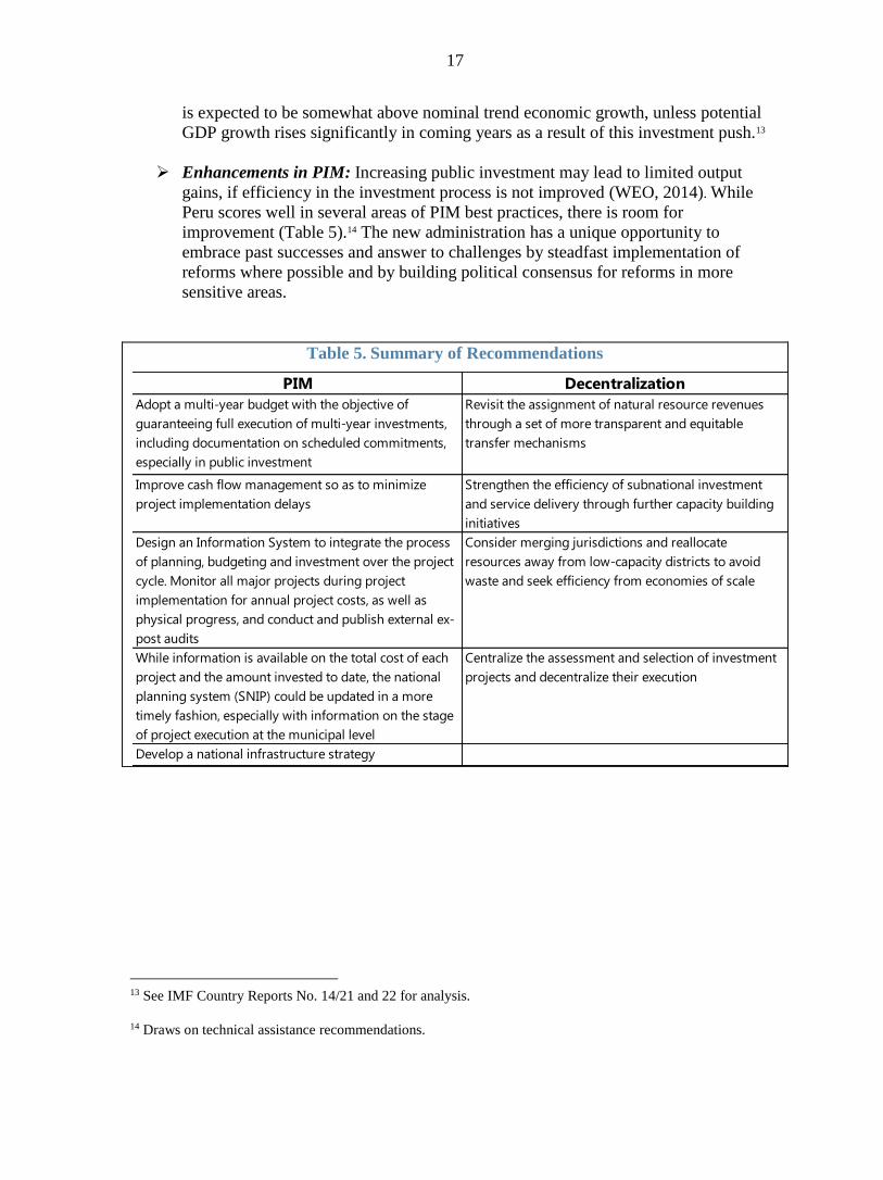
Table 5. Summary of Recommendations
13 See IMF Country Reports No. 14/21 and 22 for analysis.
14 Draws on technical assistance recommendations.
PIM Decentralization
Adopt a multi-year budget with the objective of
guaranteeing full execution of multi-year investments,
including documentation on scheduled commitments,
especially in public investment
Revisit the assignment of natural resource revenues
through a set of more transparent and equitable
transfer mechanisms
Improve cash flow management so as to minimize
project implementation delays
Strengthen the efficiency of subnational investment
and service delivery through further capacity building
initiatives
Design an Information System to integrate the process
of planning, budgeting and investment over the project
cycle. Monitor all major projects during project
implementation for annual project costs, as well as
physical progress, and conduct and publish external ex-
post audits
Consider merging jurisdictions and reallocate
resources away from low-capacity districts to avoid
waste and seek efficiency from economies of scale
While information is available on the total cost of each
project and the amount invested to date, the national
planning system (SNIP) could be updated in a more
timely fashion, especially with information on the stage
of project execution at the municipal level
Centralize the assessment and selection of investment
projects and decentralize their execution
Develop a national infrastructure strategy
18
APPENDIX: BACKGROUND ON DATA AND METHODOLOGY1
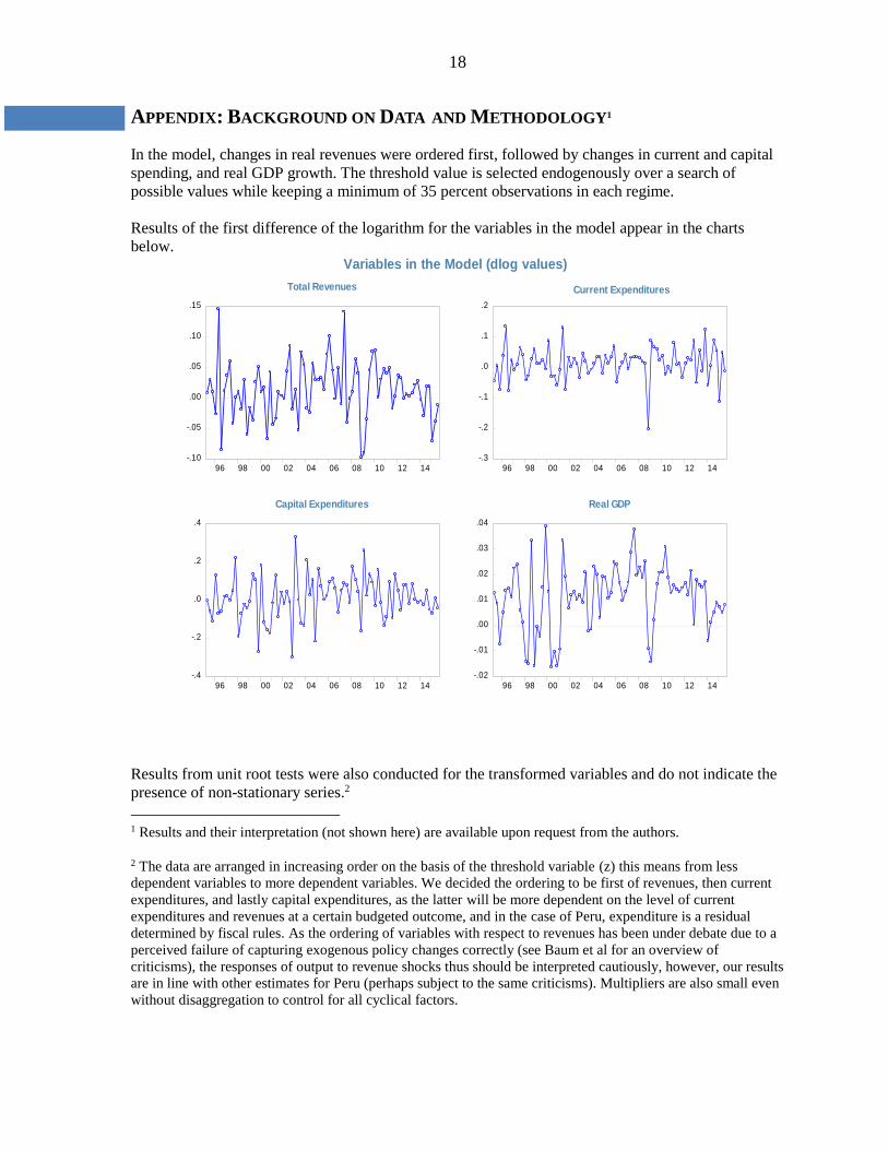
In the model, changes in real revenues were ordered first, followed by changes in current and capital
spending, and real GDP growth. The threshold value is selected endogenously over a search of
possible values while keeping a minimum of 35 percent observations in each regime.
Results of the first difference of the logarithm for the variables in the model appear in the charts
below.
-.10
-.05
.00
.05
.10
.15
96 98 00 02 04 06 08 10 12 14
Total Revenues
-.3
-.2
-.1
.0
.1
.2
96 98 00 02 04 06 08 10 12 14
Current Expenditures
-.4
-.2
.0
.2
.4
96 98 00 02 04 06 08 10 12 14
Capital Expenditures
-.02
-.01
.00
.01
.02
.03
.04
96 98 00 02 04 06 08 10 12 14
Real GDP
Variables in the Model (dlog values)
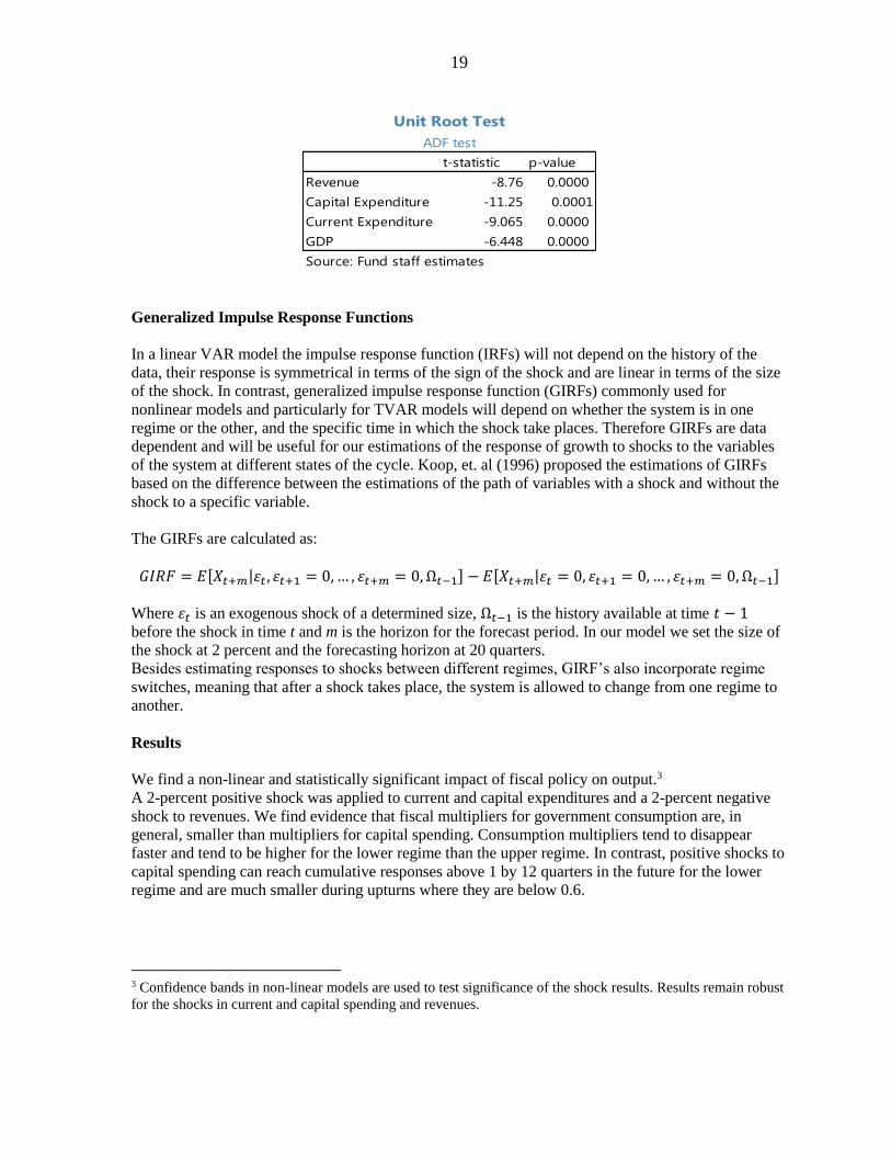
Results from unit root tests were also conducted for the transformed variables and do not indicate the
presence of non-stationary series.2
1 Results and their interpretation (not shown here) are available upon request from the authors.
2 The data are arranged in increasing order on the basis of the threshold variable (z) this means from less
dependent variables to more dependent variables. We decided the ordering to be first of revenues, then current
expenditures, and lastly capital expenditures, as the latter will be more dependent on the level of current
expenditures and revenues at a certain budgeted outcome, and in the case of Peru, expenditure is a residual
determined by fiscal rules. As the ordering of variables with respect to revenues has been under debate due to a
perceived failure of capturing exogenous policy changes correctly (see Baum et al for an overview of
criticisms), the responses of output to revenue shocks thus should be interpreted cautiously, however, our results
are in line with other estimates for Peru (perhaps subject to the same criticisms). Multipliers are also small even
without disaggregation to control for all cyclical factors.
19
Generalized Impulse Response Functions
In a linear VAR model the impulse response function (IRFs) will not depend on the history of the
data, their response is symmetrical in terms of the sign of the shock and are linear in terms of the size
of the shock. In contrast, generalized impulse response function (GIRFs) commonly used for
nonlinear models and particularly for TVAR models will depend on whether the system is in one
regime or the other, and the specific time in which the shock take places. Therefore GIRFs are data
dependent and will be useful for our estimations of the response of growth to shocks to the variables
of the system at different states of the cycle. Koop, et. al (1996) proposed the estimations of GIRFs
based on the difference between the estimations of the path of variables with a shock and without the
shock to a specific variable.
The GIRFs are calculated as:
𝐺𝐼𝑅𝐹 = 𝐸[𝑋𝑡+𝑚|𝜀𝑡 , 𝜀𝑡+1 = 0, … , 𝜀𝑡+𝑚 = 0, Ω𝑡−1] − 𝐸[𝑋𝑡+𝑚|𝜀𝑡 = 0, 𝜀𝑡+1 = 0, … , 𝜀𝑡+𝑚 = 0, Ω𝑡−1]
Where 𝜀𝑡 is an exogenous shock of a determined size, Ω𝑡−1 is the history available at time 𝑡 − 1
before the shock in time t and m is the horizon for the forecast period. In our model we set the size of
the shock at 2 percent and the forecasting horizon at 20 quarters.
Besides estimating responses to shocks between different regimes, GIRF’s also incorporate regime
switches, meaning that after a shock takes place, the system is allowed to change from one regime to
another.
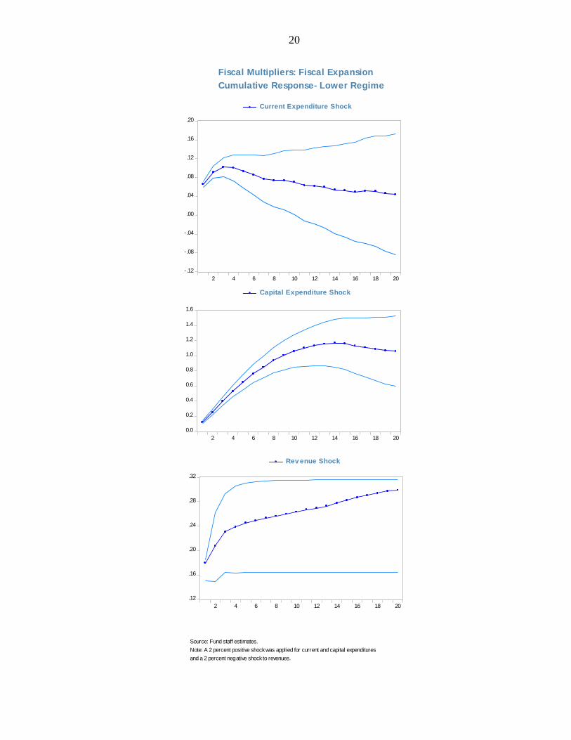
Results
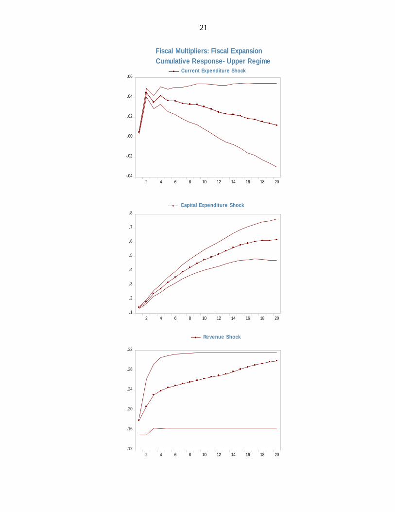
We find a non-linear and statistically significant impact of fiscal policy on output.3
A 2-percent positive shock was applied to current and capital expenditures and a 2-percent negative
shock to revenues. We find evidence that fiscal multipliers for government consumption are, in
general, smaller than multipliers for capital spending. Consumption multipliers tend to disappear
faster and tend to be higher for the lower regime than the upper regime. In contrast, positive shocks to
capital spending can reach cumulative responses above 1 by 12 quarters in the future for the lower
regime and are much smaller during upturns where they are below 0.6.
3 Confidence bands in non-linear models are used to test significance of the shock results. Results remain robust
for the shocks in current and capital spending and revenues.
t-statistic p-value
Revenue -8.76 0.0000
Capital Expenditure -11.25 0.0001
Current Expenditure -9.065 0.0000
GDP -6.448 0.0000
Source: Fund staff estimates
ADF test
Unit Root Test
20
-.12
-.08
-.04
.00
.04
.08
.12
.16
.20
2 4 6 8 10 12 14 16 18 20
Current Expenditure Shock
0.0
0.2
0.4
0.6
0.8
1.0
1.2
1.4
1.6
2 4 6 8 10 12 14 16 18 20
Capital Expenditure Shock
.12
.16
.20
.24
.28
.32
2 4 6 8 10 12 14 16 18 20
Rev enue Shock
Fiscal Multipliers: Fiscal Expansion
Cumulative Response- Lower Regime
Source: Fund staff estimates.
Note: A 2 percent positive shock was applied for current and capital expenditures
and a 2 percent negative shock to revenues.
21
-.04
-.02
.00
.02
.04
.06
2 4 6 8 10 12 14 16 18 20
Current Expenditure Shock
.1
.2
.3
.4
.5
.6
.7
.8
2 4 6 8 10 12 14 16 18 20
Capital Expenditure Shock
.12
.16
.20
.24
.28
.32
2 4 6 8 10 12 14 16 18 20
Revenue Shock
Fiscal Multipliers: Fiscal Expansion
Cumulative Response- Upper Regime
22
REFERENCES
Afonso, António, Jaromír Baxa, and Michal Slavík, 2011, “Fiscal Developments and Financial
Stress: A Threshold VAR Analysis,” European Central Bank (April).
Anderson, Heather, and Timo Teräsvirta, 1992, “Characterizing Nonlinearities in Business
Cycles Using Smooth Transition Autoregressive Models,” Journal of Applied Econometrics
Supplement: Special Issue on Nonlinear Dynamics and Econometrics, Vol.7, (December),
pp.119–136.
Batini, Nicoletta, and others, 2014, “Fiscal Multipliers: Size, Determinants, and Use in
Macroeconomic Projections”, IMF Technical Guidance Note.
Baum, Anja, Marcos Poplawski-Ribeiro, and Anke Weber, “Fiscal Multipliers and the State of
the Economy,” IMF Working Paper No.12/286 (Washington: International Monetary Fund).
Baum, Anja, and Gerrit Koester, 2011, “The Impact of Fiscal Policy on Economic Activity over
the Business Cycle-Evidence from a Threshold VAR analysis”, Bundesbank Discussion Paper,
03/2011 (Frankfurt: Deutsche Bundesbank).
BBVA Reseach, 2014, Situtación Peru: Quatro Trimestere de 2014 (Lima, Peru).
Central Reserve Bank of Peru, 2012, “Inflation Report: Recent Trends and Macroeconomic
Forecasts 2012–14” (June).
Cheasty, Adrienne and Juan Pichihua, 2015, “Peru: Fiscal Decentralization: Progress and
Challenges for the Future,” Chapter 10 in Peru: Staying the Course of Economic Success
(Washington: International Monetary Fund).
Fazzari, Steven, James Morley, and Irina Panovskay, 2012, “Fiscal Policy Asymmetries: A
Threshold Vector Autoregression Approach,” January 2012, available at
https://www.researchgate.net/publication.
Galindo, Hamilton, and William Sanchez, 2011, “Estimación del Multiplicar Fiscal en el Perú: en
Enfoque Bayesiano,” Banco Central De Reserva Del Peru, October.
Galindo, Hamilton, and William Sánchez Tapia, 2013, “Efectos Simétricos y Asimétricos de la
Política Fiscal en el Perú”, Universidad Nacional De Ingeniería, Consorcio de Investigación
Económica y Social (Lima; Perú).
Hansen, Bruce, 2011, “Threshold Autoregression in Economics”. Statistics and Its Interface,
Volume 4 (2011) 123–127 (February).
Ilzetzki, Ethan, Enrique Mendoza and Carlos Végh, “How Big (Small?) are Fiscal Multipliers?”,
IMF Working Paper No. 11/52 (Washington: International Monetary Fund).
International Monetary Fund, IMF Country Reports 10/98 and 14/22.
23
International Monetary Fund, “Is it time for an Infrastructure Push? The Macroeconomic Effects
of Public Investment”, Chapter 3 in World Economic Outlook (October 2014).
International Monetary Fund, 2015, Making Public Investment More Efficient, IMF Staff Report
(Washington: International Monetary Fund).
Koop, Gary, Hashem Pesaran, and Simon Potter, 1996, “Impulse Response Analysis in Nonlinear
Multivariate Models,” Journal of Econometrics, Vol. 74(1), pp. 119-147.
Loyola, Jorge, Renzo Rossini, and Zenón Quispe, 2012, “Fiscal Policy Considerations in the
Design of Monetary Policy in Peru,” Central Reserve Bank of Peru, (November).
Multiannual Macroeconomic Framework (Marco Macronomico Annual), 2016-18. Ministry of
Finance of Peru (April 2015).
Mitra, Pritha, and Tigram Pogosyan, “Fiscal Multipliers in Ukraine,” IMF Working Paper
No.15/71 (Washington: International Monetary Fund).
Pessoa, Mario, Israel Fainboim, and Almudena Fernandez, 2015, “Modernization of Public
Investment Management Systems,” Chapter 9 in Peru: Staying the Course of Economic Success
(Washington: International Monetary Fund).
Pre-Election Report (Informe Preelectoral, Administracion 2011-2016), Ministry of Economy
and Finance, January 2016.
Ross, Kevin, and Melesse Tashu, 2015, “Investment Dynamics in Peru”, Chapter 4 in Peru:
Staying the Course of Economic Success (Washington: International Monetary Fund).
Ross, Kevin, and Alonso Peschiera, 2015, “Explaining the Peruvian Growth Miracle”, Chapter 3
in Peru: Staying the Course of Economic Success (Washington: International Monetary Fund).
Schmidt, Julia, 2013, “Country Risk Premia, Endogenous Collateral Constraints
and Non-linearities: A Threshold VAR Approach,” May 2013, available at http://julia-
schmidt.org/Nonlinearities_Schmidt.pdf
Teräsvirta, Timo, and Yukai Yang, 2014, “Specification, Estimation and Evaluation of Vector
Smooth Transition Autoregressive Models with Applications”, March 2014, available at
ftp://ftp.econ.au.dk/creates/rp/14/rp14_08.pdf
Tsay, Ruey, 1998, “Testing and Modeling Multivariate Threshold Models”, Journal of the
American Statistical Association, Vol. 93, pp. 1188-1202.
Vtyurina, Svetlana, 2015, “The Role of Fiscal Policies in Peru’s Transformation”, Chapter 5 in
Peru: Staying the Course of Economic Success (Washington: International Monetary Fund).