Fiscal multiplier in the Russo–Japanese War:

A business cycle accounting perspective∗

Hiroshi Gunji† Kenji Miyazaki‡

February 28, 2016

Abstract

In this paper, we use business cycle accounting, introduced by Chari et al. (2007, Econo-metrica 75 (3), 781–836), to estimate the fiscal multiplier in Japan during the Russo–Japanese War, 1904–1905. This event is considered to be a natural experiment for thefollowing reasons. 1) The ratio of government spending to GNP was relatively greater thanthat of the other wars involving Japan. 2) As the battlefields were in Korea and China, thewar caused little damage to Japan’s physical capital or labor supply. 3) The Russo–JapaneseWar did not involve any monetary transfer to the Japanese economy. 4) Before the war,people were not convinced that Japan and Russia would go to war. Using business cycleaccounting, we estimate the value of the fiscal multiplier to be about 0.2 in the short runand about one in the long run. These results are consistent with the previous literature,which estimates the multiplier in different sample periods using econometric models such asstructural vector autoregression (VAR) models.

∗This research was financially supported by the 2014 Grant-in-Aid No. 1429 from the Zengin Foundationfor Studies on Economics and Finance and JSPS KAKENHI Grant Number 24530320. We would like to thankKohei Aono, Masataka Eguchi, Kazuki Hiraga, Hirokazu Ishise, Kengo Nutahara, Takeki Sunakawa, Shiba Suzuki,Tomoaki Yamada, Koiti Yano, and the participants of the 79th International Atlantic Economic Conference, the2015 spring meeting of the Japanese Economic Association, and seminars at Daito Bunka University, HoseiUniversity, Kagoshima University, Kyoto Sangyo University, and Meiji University.

†Daito Bunka University‡Hosei University

0

1 Introduction

A large number of researchers have estimated the fiscal multipliers of government expenditures,

but the estimates differ because of differences in the data and estimation methods used. Most

government expenditures, however, are planned in the previous fiscal year, and thus they are

not unexpected shocks. Economic agents make decisions using published, imprecise data about

government expenditure, which leads to a miscalculation of the fiscal multiplier.

To avoid such miscalculation, some researchers use military expenditure as unexpected and

temporary expenditure. Barro and Redlick (2011) use US data from World War II (WWII),

and their reduced-form models of regression analysis estimate that the multiplier of military

expenditure lies between 0.4 and 0.7. Using vector autoregression (VAR) models with war

dummy variables, Ramey (2011) estimates the fiscal multiplier to be 0.6–1.2. Furthermore,

Owyang et al. (2013) uses 1890–2010 US historical data and reports that the fiscal multiplier

of military expenditure is 0.7–0.9. These studies use all wars in their sample period as shocks

to government spending. However, some of the wars may have been expected many months

before the outbreak of war. As an example of an unexpected war shock, we focus on the Russo–

Japanese War. To our knowledge, there is no empirical research for Japan that estimates fiscal

multipliers using military expenditure.

Using the Russo–Japanese War as a natural experiment has some advantages. First, the ratio

of government spending to GNP was relatively greater than that for other wars involving Japan.

Japan had experienced three great wars that required enormous government expenditure: the

Sino–Japanese War, 1894–95; the Russo–Japanese War, 1904–05; and WWII, 1941–45. The

Sino–Japanese War was the first war in which the Japanese military was modernized. Military

expenditure accounted for 50 percent of total government expenditure in the Sino–Japanese War

and 58 percent in WWII. On the other hand, it accounted for 74 percent in the Russo–Japanese

War.1

Second, in the Russo–Japanese War, as for the US in WWII, Japan was at war with Russia

on foreign soil, and therefore not as many people were killed. The Japanese labor force totaled

about 25 million workers at that time. While the number of dead was 85,000 (0.4% of the labor

force), the number of injured was 150,000 (0.6% of the labor force). These figures are small

1See Ohkawa et al. (1974, p. 22).

1

relative to not only other wars involving Japan, but also other wars in general. Moreover, unlike

the Sino–Japanese War, data on hours worked during the Russo–Japanese War are available.

Third, Japan gained only the southern half of Sakhalin and control of Korea, but did not

get any monetary compensation in the Treaty of Portsmouth in 1905. This implies that the

Russo–Japanese War did not involve any monetary transfer to the Japanese economy, while

requiring a vast amount of government spending.

Fourth, the outbreak of this war was largely unexpected. According to Itaya (2012),

Japanese bonds had been stable and priced at around 76 yen prior to the start of the war;

however, the price dropped to 67 yen two days after the outbreak. Sussman and Yafeh (2000)

points out that because it was generally believed that Japan would lose the war, a large risk

premium was attached to Japanese bonds.2 Therefore, using government expenditure in this

period is suitable for estimating the fiscal multiplier.

To investigate the effects of the government spending during the Russo–Japanese War, this

paper uses business cycle accounting (BCA), introduced by Chari et al. (2007). BCA separates

factors that affect economic variables (real GNP, consumption, investment, and labor supply)

into four wedges: efficiency, labor, investment, and government consumption. These wedges

exactly replicate the allocation in the economy. Allowing for spillover effects to other variables

and wedges, this method allows us to evaluate the effect of government spending.

When estimating fiscal multipliers, BCA has more advantages than regression analysis and

dynamic stochastic general equilibrium (DSGE) models. In regression analysis, several out-

breaks of war would be required to estimate fiscal multipliers statistically. It is difficult to

obtain such data for Japan. Furthermore, regression analysis requires appropriate regressors

to avoid estimator bias, and VAR analysis requires appropriate structures to obtain efficient

estimators, both of which pose problems in this context.

Although Braun and McGrattan (1993) and McGrattan and Ohanian (2010) analyze the

effects of war using DSGE models, we use BCA to analyze the effects of war. DSGE analysis

specifies the structure and shocks of the model, and then compares the simulated and observed

data. This approach cannot replicate the original time series, and therefore cannot estimate

the effects of fiscal shocks accurately. On the other hand, in BCA, wedges estimated from

2There are some studies that investigate financial markets’ awareness of the beginning of wars. For instance,Suzuki (2012) shows that the stock markets of the countries damaged during WWII did not predict the beginningof the war.

2

data can replicate the original data series. Therefore, we can estimate the effect of government

expenditure controlling for other business cycle factors. Furthermore, BCA wedges represent

several distortions of business cycles. As proved by Chari et al. (2007), for instance, financial

frictions associated with the allocation of intermediate inputs corresponds to the efficiency wedge

and sticky wages corresponds to the labor wedge. As many types of frictions correspond to one

or more wedges, we do not have to be concerned about the specification of the model.

This paper makes three contributions. First, as far as we know, this paper is the first to

use data for the Russo–Japanese War to estimate the fiscal multiplier. Second, we utilize BCA

to estimate the fiscal multiplier. Finally, we propose a new method for calculating the effect of

wedges. Although most papers calculate the effect of wedges following Chari et al. (2007), their

methodology does not allow for correlations between wedges. Our paper takes such correlations

into consideration.

The main conclusion of our paper is that BCA estimates the value of the short-run fiscal

multiplier to be 0.20–0.22. We also estimate the long-run multiplier to be 0.98–1.06. These

results are consistent with the previous literature.

The structure of the paper is as follows. In the next section, we provide a description of

BCA. Section 3 explains how to calculate fiscal multipliers using our framework. Section 4

describes our data. Section 5 presents our estimation results. Section 6 concludes. In two

appendices, we provide details about estimating the spillover effects of the government wedge

and constructing labor force data.

2 The Model

In this section, we provide a description of BCA. BCA requires a neoclassical growth model,

called a prototype economy, with four wedges: efficiency, labor, investment, and government

consumption. Using the framework of a real business cycle model, these four wedges corre-

spond to total factor productivity, taxes on labor income, taxes on investment, and the residual

calculated by subtracting consumption and investment from output.

Chari et al. (2007) shows that the allocations of many DSGE models are the same as those

provided by a prototype economy under certain conditions on the wedges. In other words,

the wedges in BCA can represent any type of frictions in DSGE models. Furthermore, the

3

wedges are estimated to reproduce the actual data, so BCA allows us to simulate counterfactual

situations, for instance, an economy that has only an efficiency wedge. If the wedges that are

most important for replicating the actual data were known, the frictions equivalent to these

wedges would be the major candidates for causes of business cycles.

The representative household in the prototype economy maximizes its lifetime utility as

follows:

E0

∞∑t=0

U(ct, lt)Nt, (1)

subject to the budget constraint,

ct + (1 + τxt)xt = (1− τlt)wtlt + rtkt + Tt, (2)

and the law of motion for capital,

(1 + γn)kt+1 = (1− δ)kt + xt, (3)

where ct is consumption expenditure per capita, lt is labor supply per capita, Nt is population,

xt is investment expenditure per capita, kt is capital stock per capita, Tt is government transfers

per capita, wt is the wage rate, rt is the rental rate, τlt is the labor wedge, τxt is the investment

wedge, β is the subjective discount rate, γn is the rate of population growth, δ is the rate of

depreciation, and U(·, ·) is instantaneous utility.

Firms maximize

AtF (kt, (1 + γA)tlt)− rtkt − wtlt,

where At is the efficiency wedge, F (·, ·) is technology in terms of labor and capital, and γA is

the labor-augmenting technological progress rate.

The equilibrium of this prototype economy is summarized by the resource constraint

ct + xt + gt = yt,

and the following conditions:

yt = AtF (kt, (1 + γA)tlt),

4

−Ult

Uct= (1− τlt)At(1 + γA)

tFlt,

Uct(1 + τxt) = βEt(Uc,t+1[At+1Fk,t+1 + (1− δ)(1 + τx,t+1)]),

and (3), where gt is the government consumption wedge.

We assume the instantaneous utility function u(ct, 1 − lt) = ln ct + ϕ ln(1 − lt) and the

production technology F (kt, (1+γA)tlt) = kαt ((1+γA)

tlt)1−α. We detrend from data. Denoting

zt ≡ Zt/((1 + γA)tNt), we obtain

yt = Atkαt l

1−αt , (4)

yt = ct + xt + gt, (5)

ϕct1− lt

= (1− τlt)(1− α)ytlt, (6)

(1 + γA)(1 + τxt)

ct= βEt

[αyt+1/kt+1 + (1 + τx,t+1)(1− δ)

ct+1

], (7)

(1 + γA)(1 + γn)kt+1 = (1− δ)kt + xt. (8)

We also assume that the state at time t is st = (gt, At, τlt, τxt)′ and the log-linearized st follows

a first-order VAR(1) process

st = P st−1 + εt, (9)

where εt is a normally distributed error term with mean zero and covariance matrix V . Unlike

the earlier papers on BCA, we set the government consumption wedge gt to be the first variable

in the state vector st, because we use a Cholesky decomposition to conduct a counterfactual

experiment in Section 5. The artificial shock on gt is provided only for 1904, so the decomposition

does not affect the other periods.

As we cannot solve the prototype model explicitly like other DSGE models, we log-linearize

the model and apply the Uhlig (1995) method to derive the policy functions.3

3 Fiscal Multipliers

In this section, we explain how to calculate the fiscal multipliers using BCA. We divide the

government consumption wedge into military expenditure, get, and others, i.e., government

3The code is available from the authors upon request.

5

consumption plus net export minus military expenditure, nxt. Log-linearizing the equation, we

have

gt =ge

gget +

nx

gnxt, (10)

where the variables without time subscripts, t, denote steady state values. We set military

expenditure to be in a steady state—i.e., ge1904 = 0—and compare the simulated and actual

GNP to identify the effect of government expenditure. Denoting the simulated GNP in 1904 as

yt(ge1904 = 0), we have the fiscal multiplier

FMS =y1904 − y1904(ge1904 = 0)

g1904 − g1904(ge1904 = 0)

=y[exp(y1904)− exp(y1904(ge1904 = 0))]

g[exp(g1904)− exp(g1904(ge1904 = 0))].

This is a short-run fiscal multiplier. Moreover, the cumulative effect from 1904 is defined as

FML =y∑T

s=0[exp(y1904+s)− exp(y1904+s(ge1904 = 0))]

g∑T

s=0[exp(ge1904+s)− exp(g1904(ge1904 = 0))],

which is called a long-run fiscal multiplier.

We conduct simulations that set the deviation of a component of government expenditure,

i.e., only military expenditure, from the steady state equal to zero. We employ two types

of counterfactuals. The first method uses the counterfactual government consumption wedge

and three other actual wedges for 1904, so there is no spillover effect of the counterfactual to

the three other wedges. Put differently, we use {(nx/g)nx1904, A1904, τl,1904, τx,1904} instead of

{g1904, A1904, τl,1904, τx,1904}. This method is different from that of Chari et al. (2007), which

sets one of the wedges to be zero over the simulation period. This method investigates the direct

effect of the government consumption wedge and ignores the indirect effect of the government

consumption wedge on the other wedges.

The second method substitutes the counterfactual government consumption wedge into the

data-generating process of the wedges (9) to obtain the wedges over subsequent periods. In

this case, the shock on the innovation of the government consumption wedge for 1904 first

affects those of the other wedges, and thereafter affects them through the coefficient vector of

the VAR. Therefore, we estimate two channels of the spillover effect. At t = 1904, we use

sc1904 = {(nx/g)nx1904, A1904, τl,1904, τx,1904} and the structural error εC1904. For the estimation

6

method of εC1904, see Appendix 1. At t > 1904, we use the wedges simulated from the VAR

sct = Psct−1 + εt,

where εt is the residual from the actual data. After that, we estimate the wedges recursively. In

this case, there is an indirect effect of the government consumption wedge; that is, all wedges

vary from the actual wedge at t > 1904.

The sample period is short, so we constrain the parameter matrix, P , and covariance matrix,

V , to estimate (9) efficiently. As for P , we assume that the government consumption wedge

affects the other three wedges in the next period, but the converse is not true; that is,

P =

p11 0 0 0

p21 p22 p23 p24

p31 p32 p33 p34

p41 p42 p43 p44

.

Chari et al. (2007) and Saijo (2008) also assume p21 = p31 = p41 = 0. However, we do

not use this restriction because we allow for a spillover effect from the government consumption

wedge because military expenditure was the major component of government expenditure in this

period; however, the economic condition does not necessarily affect the change in government

expenditure. As for V , following Chari et al. (2007) and Saijo (2008), we assume

V =

σ11 σ21 σ31 σ41

σ21 σ22 0 0

σ31 0 σ33 0

σ41 0 0 σ44

.

That is, errors of the government consumption wedge might have a correlation with those of

the other three wedges, but errors of the other three wedges are uncorrelated each other.

7

4 Data

Here we discuss the data used in the paper and the parameters of the model. Following Chari

et al. (2007), we assume the instantaneous utility function u(c, l) = ln c + ϕ ln(1 − l) and

the production function F (k, l) = kαl1−α. Yt, Ct, and Xt are gross national expenditure,

consumption expenditure, and gross domestic fixed capital formation, respectively, measured

using fixed prices from Ohkawa et al. (1974) (hereafter, LTES 1). Kt is gross capital stock

measured using fixed prices from Ohkawa and Shinohara (1979).

For details regarding labor supply, lt, see Appendix 2. The time period is 1889 to 1937

because of data availability limitations. We divide the variables by the number of those in the

population who are over 10 years of age, Nt, to obtain per capita variables, yt, ct, xt, and k.

We also detrend the variables by dividing them by (1 + γA)t. To obtain the deviation from the

steady state, we use a Hodrick–Prescott filter with annual parameter λ = 100.

The parameters are calibrated as follows. To estimate the labor-augmenting technological

progress rate, γA, we use

lnyt

kαt l1−αt

= lnAt + [ln(1 + γA)](1− α)t

from the production function. The coefficient of t from the OLS (ordinary least squares) esti-

mation, b, yields γA = exp(b/(1−α))− 1 = 0.0234. Following Hayashi and Prescott (2008), the

capital share, α, is 1/3, the subjective discount rate, β, is 0.96, and the depreciation rate, δ, is

0.038146, which is the average from 1899 to 1937. The population growth rate, γn, is 0.0117,

which is the average growth rate of Nt.

The time-allocation parameter, ϕ, is calibrated from the intratemporal optimal condition.

Prior to this, however, it is necessary to obtain the labor wedge. We set the target of the

minimum value of the labor wedge to be 3%, which is the ceiling of the labor income tax rates.

In this period, the labor income tax rates were quite low relative to the present rates: they

ranged from 1% for 300–1,000 yen of annual income up to 3% for 30,000 yen. Additionally,

the number of hours worked was high: the average weekly hours worked in the nonagricultural

sectors in our sample period is 68 hours. These facts suggest that the labor wedges are not very

high. Therefore, we set the target of the labor wedge to be 3% and obtain ϕ = 0.9351.

8

The government consumption wedge gt consists of government spending get and net export

nxt. If nxt is negative and gt is negative, we cannot log-linearize the prototype model. To

obtain positive value of the variables, we divide the government consumption wedge into

gt = get + ext − imt,

where ext is exports and imt is imports. Log-linearizing this equation, we have

gt =ge

gget +

ex

gext −

im

g˜imt.

As get, ext, and imt are positive, we can use the HP (Hodrick–Prescott) filtered data for the

variables signified with a tilde and the sample averages for the steady states to obtain gt.

The counterfactual is that the deviation of government expenditure from the steady state

in 1904, ge1904, is zero. We employ the following four assumptions related to government

expenditure.

The first counterfactual is that military expenditure equals zero in 1904. The military and

war-related expenditures are available from Emi and Shionoya (1966) (LTES 7). However,

LTES 1 excludes government fixed capital formation from general government consumption

expenditure and adds it to domestic fixed capital formation, so it is interpreted as military

capital formation. Therefore, subtracting items related to fixed capital formation from military

and war-related expenditures, we use expenditure related to conscription, war expenses (ex-

traordinary military special account and ministries other than army and navy), and war-related

expenses (military allowances in the form of aid, annuities and pensions). We also remove

duplications in the extraordinary military special account and other accounts. Furthermore,

we should remove fixed capital formation from the extraordinary military special account, but

these data are not available. Instead, we multiply the extraordinary military special account by

the share of the sum of personnel expenses, consumption good expenses, provision and fodder,

clothing, and transportation and communication to obtain military consumption expenditure.

We call this broad military expenditure:

Broad military expenditure = ME × ζ1,

9

where

ME =expenditure related to conscription + war expenses + war-related expenses

− duplications,

ζ1 =(personnel expenses + consumption goods + provision and fodder + clothing

+ transportation and communication)/extraordinary military special account.

The second counterfactual is that military expenditure is defined in a narrower sense: broad

military expenditure minus expenditure abroad for requisition; i.e., expenditure related to pro-

vision and fodder and to transportation and communications. Ikeyama (2001) suggests that

the Japanese army requisitioned provisions—e.g., rice, wheat, and soy sauce—from many do-

mestic areas at low prices. However, because the Japanese government had a military currency

on issue since the Sino–Japanese war in 1894–95, it is unlikely that all provisions and fodders

were requisitioned within Japan. Therefore, we also estimate the fiscal multiplier using narrow

military expenditure:

Narrow military expenditure = ME × ζ2,

where

ζ2 =(personnel expenses + consumption goods + clothing)

/extraordinary military special account.

For comparison, we employ two more counterfactuals. The third counterfactual is that the

government consumption wedge equals zero in 1904. This means that the change in the govern-

ment consumption wedge in 1904 is entirely the result of the war. This is the same assumption

that was used in the simulations in earlier studies on BCA. The fourth counterfactual is that

government expenditure equals zero in 1904. The government consumption wedge consists of

government expenditure and net exports, so the latter is assumed to be influenced only by the

war.

As discussed in the introduction, military expenditure can be considered as unexpected or

temporary shocks, so the third or fourth assumption is preferable in the sense of calculating the

fiscal multiplier.

10

5 The Results

In this section, we present our estimation results. However, we first estimate the parameters

of VAR(1). Table 1 presents the parameters of the VAR(1) estimated using the maximum

likelihood method. We use these parameters to estimate the wedges.

The estimated wedges are shown in Figure 1. All the wedges rise dramatically for 1904, but

they are not strongly correlated in the other period. The outbreak of war is a political issue,

so most of the movement in the government consumption wedge in 1904 is exogenous. On the

other hand, the other three wedges increase in the same way, so the movements are caused by

the government consumption wedge.

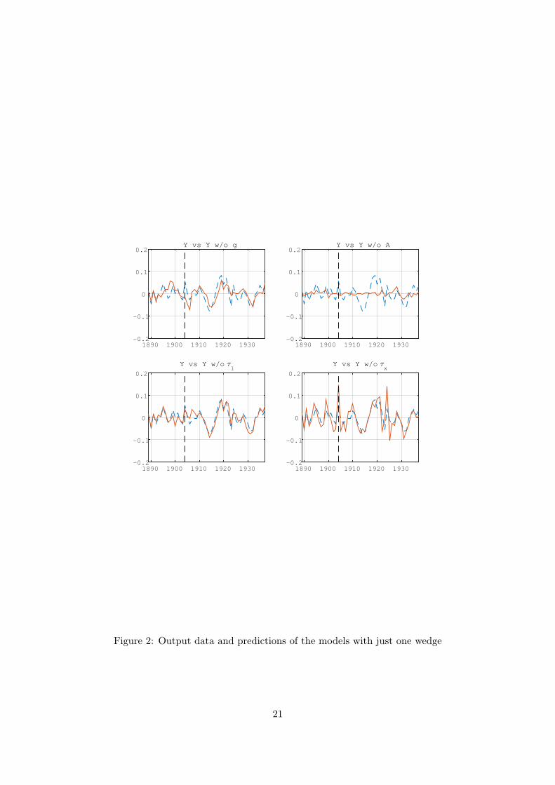
Following the earlier studies, e.g., Chari et al. (2007), however, we first simulate the model

with only one wedge, that is, without three wedges over time. Figure 2 depicts the simulation

results of the effect of each wedge on real GNP. The broken line is log-linearized output around

the steady state, and the solid line is output without each wedge. As output without the

efficiency wedge is virtually unchanged, the efficiency wedge would be the most important

factor for output. This is consistent with earlier studies. The labor and investment wedges

affect output during the war to some extent. However, the latter is slightly volatile. By

contrast, output without the government consumption wedge is different from actual output

over time. While earlier studies rarely considered the effect of the government consumption

wedge, our analysis implies that it plays an important role in this period.

Next, Table 2 presents the estimates of the fiscal multipliers. The first row shows the

short-run fiscal multipliers without the spillover effects among wedges. The multipliers of the

government consumption wedge and total government expenditure are 0.28 and 0.23, respec-

tively. In the second row, the multipliers with the spillover effects are 0.30 and 0.25. The

multipliers of broad and narrow military expenditures are 0.22 and 0.20, respectively, which are

relatively small. They are all less than one, as are the fiscal multipliers calculated from normal

DSGEs. As shown in Woodford (2011), this is because government expenditure increases not

only output but also the disutility of labor supply, causing a fall in output. Therefore, each of

the military expenditures does not have a large effect on output in the short run.

However, the long-run multipliers produce different results. This is because a temporary

change in government expenditure can affect the capital stock after the shock and thereby

11

change output. For the multiplier without spillovers, which does not consider the dynamic

effects among the wedges, the fiscal multipliers of the government consumption wedge and

government expenditure are 0.07 and 0.44, and those of broad and narrow military expenditures

are 0.38 and 0.34, respectively. Although the multipliers without spillover effects are small in

the short run, they are around double their short-run values in the long run. For the multiplier

with spillovers, which allows the spillover effect after the shock of the government consumption

wedge in 1904, the fiscal multipliers are larger than those from the multiplier without spillovers,

but they are around one. As military expenditure is more preferable, we conclude that the fiscal

multiplier in the long run is 0.98–1.06.

To see this intuitively, we plot the change in output for each simulation. Figure 3 shows

the change in output for the multiplier without spillovers. The shock to each variable increases

output in 1904, but the effect disappears quickly. On the other hand, Figure 4 depicts the same

simulation for the multiplier with spillovers. In this case, the shock in 1904 affects all wedges

and the capital stock through the law of motion for capital, (3), and the VAR, (9). These

effects increase output from 1904 to 1915, but they seem to disappear from 1916 onwards. The

reason why the fiscal multipliers with spillovers are larger than those without spillovers is that

the government consumption wedge in the multiplier with spillovers does not shrink after 1904

because of the dynamic effect of the VAR. As the difference between the actual government

consumption wedge and the simulated wedge in the multiplier without spillovers arises only in

1904, the effect of the government spending is limited.

We next show the impulse-response functions for a shock in narrow military expenditure

in 1904, which is the most reliable data for the government spending shock of the Russo–

Japanese War. Figure 5 shows the results. The change in the government consumption wedge

in 1904 increases the other three wedges: the impacts are about 0.1 percent. The increases in

the labor and investment wedges decrease output in 1904, while the increase in the efficiency

wedge increases output and the fiscal multiplier. Interestingly, consumption expenditure de-

creases temporarily in 1904, but increases afterwards. This is partly because the labor wedge

also increases after 1905. In standard macroeconomics, government expenditure crowds out

consumption. However, our counterfactual experiment increases consumption.

In summary, we found that the fiscal multiplier for the shock in 1904 is 0.20–0.22 in the short

12

run and 0.98–1.06 in the long run. These findings are consistent with earlier studies, discussed

in the introduction.

6 Concluding Remarks

In this paper, we utilized BCA to estimate the fiscal multiplier during the Russo–Japanese War.

BCA decomposes the frictions of many DSGEs into four wedges, which replicate exactly the

actual endogenous variables. These features allow us to avoid the model misspecification that

can occur in DSGE and VAR models.

For estimating fiscal multipliers, data for the Russo–Japanese War period have the advantage

that the war was unexpected and involved little damage to the capital stock or the labor force.

We employed a government consumption wedge, total government expenditure, broad military

expenditure, and narrow military expenditure as measures of government expenditure for the

calculation of the multipliers.

Using the BCA approach, we can conclude that the short-run multiplier is 0.20–0.22, and

the long-run multiplier is 0.98–1.06. This is consistent with the results estimated using other

methods in earlier studies.

Our conclusion is drawn using a BCA approach, in which the prototype model is essentially a

one-sector growth model with four stochastic wedges. On the other hand, Hayashi and Prescott

(2008) and Golosov et al. (2014) propose a two-sector model for macroeconomic analysis before

World War II. Developing a two-sector model for BCA is left for future research.

13

Appendix 1: The estimation of simultaneous spillover effects

The estimation method of the spillover effect of the government consumption wedge in 1904,

εC1904, is as follows. As we would like to set military expenditure get equal to zero only at t = 1904

from (10), we seek to find a structural shock v1,1904 so that the government consumption wedge

is (nx/g)nx1904. First, we use the estimated coefficient matrix P to obtain the residual,

εt = st − Pst−1.

Next, we implement a Cholesky decomposition on the variance–covariance matrix V = QQ′ and

obtain the structural shock,

vt = Q−1εt.

This allows us to transform the error term εt into the idiosyncratic shock vt, in which each factor

is not correlated with each other. Moreover, the first equation in (9) is an AR(1) process by

assumption, so we would like to obtain the government consumption wedge g1904 = p11g1903 +

ε1,1904 = (nx/g)nxt. Using ε1,t = q11v1,t, we solve this equation to obtain the idiosyncratic

shock of government military expenditure,

vC1,1904 =g1904 − p11g1903

q11.

Finally, we replace the actual residual of the government consumption wedge with vC1,1904,

εC1904 = Q

[vC1,1904 v2,1904 v3,1904 v4,1904

]′.

This is the simultaneous spillover effect. After this period, we calculate the wedges using (10).

Appendix 2: The construction of labor force data

In this appendix, we provide details about the construction of labor force data. We could not find

suitable aggregate labor force data for the prewar period for Japan. There are no aggregate data

of hours worked in prewar Japan. In this appendix, we describe how we estimated the number

of hours worked. For the agricultural sector only, we can utilize the number of employees, Eat ,

14

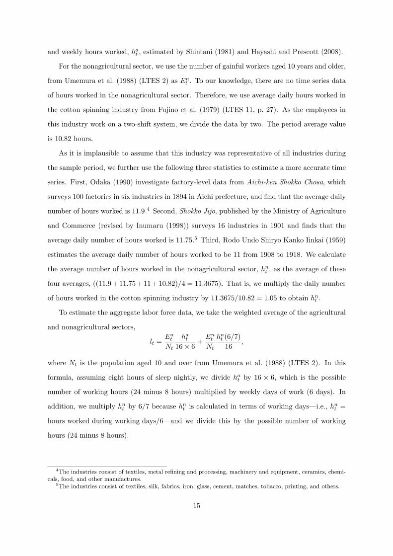
and weekly hours worked, hat , estimated by Shintani (1981) and Hayashi and Prescott (2008).

For the nonagricultural sector, we use the number of gainful workers aged 10 years and older,

from Umemura et al. (1988) (LTES 2) as Ent . To our knowledge, there are no time series data

of hours worked in the nonagricultural sector. Therefore, we use average daily hours worked in

the cotton spinning industry from Fujino et al. (1979) (LTES 11, p. 27). As the employees in

this industry work on a two-shift system, we divide the data by two. The period average value

is 10.82 hours.

As it is implausible to assume that this industry was representative of all industries during

the sample period, we further use the following three statistics to estimate a more accurate time

series. First, Odaka (1990) investigate factory-level data from Aichi-ken Shokko Chosa, which

surveys 100 factories in six industries in 1894 in Aichi prefecture, and find that the average daily

number of hours worked is 11.9.4 Second, Shokko Jijo, published by the Ministry of Agriculture

and Commerce (revised by Inumaru (1998)) surveys 16 industries in 1901 and finds that the

average daily number of hours worked is 11.75.5 Third, Rodo Undo Shiryo Kanko Iinkai (1959)

estimates the average daily number of hours worked to be 11 from 1908 to 1918. We calculate

the average number of hours worked in the nonagricultural sector, hnt , as the average of these

four averages, ((11.9+11.75+11+10.82)/4 = 11.3675). That is, we multiply the daily number

of hours worked in the cotton spinning industry by 11.3675/10.82 = 1.05 to obtain hnt .

To estimate the aggregate labor force data, we take the weighted average of the agricultural

and nonagricultural sectors,

lt =Ea

t

Nt

hat16× 6

+En

t

Nt

hnt (6/7)

16,

where Nt is the population aged 10 and over from Umemura et al. (1988) (LTES 2). In this

formula, assuming eight hours of sleep nightly, we divide hat by 16 × 6, which is the possible

number of working hours (24 minus 8 hours) multiplied by weekly days of work (6 days). In

addition, we multiply hnt by 6/7 because hnt is calculated in terms of working days—i.e., hnt =

hours worked during working days/6—and we divide this by the possible number of working

hours (24 minus 8 hours).

4The industries consist of textiles, metal refining and processing, machinery and equipment, ceramics, chemi-cals, food, and other manufactures.

5The industries consist of textiles, silk, fabrics, iron, glass, cement, matches, tobacco, printing, and others.

15

References

Barro, R. J. and C. J. Redlick (2011) “Macroeconomic Effects From Government Purchases and

Taxes,” The Quarterly Journal of Economics, Vol. 126, No. 1, pp. 51–102, January.

Braun, R. A. and E. R. McGrattan (1993) “The Macroeconomics of War and Peace,” in NBER

Macroeconomics Annual, Vol. 8: National Bureau of Economic Research, Inc, Chap. 4, pp.

197-258.

Chari, V. V., P. J. Kehoe, and E. R. McGrattan (2007) “Business Cycle Accounting,” Econo-

metrica, Vol. 75, No. 3, pp. 781–836.

Emi, K. and Y. Shionoya (1966) Estimates of Long-Term Economic Statistics of Japan Since

1868, 7: Government Expenditure: Toyo Keizai, [in Japanese].

Fujino, S., S. Fujino, and A. Ono (1979) Estimates of Long-Term Economic Statistics of Japan

Since 1868, 11: Textiles: Toyo Keizai, [in Japanese].

Golosov, M., S. Guriev, A. Cheremukhin, and A. Tsyvinski (2014) “The Industrialization

and Economic Development of Russia through the Lens of a Neoclassical Growth Model,”

manuscript.

Hayashi, F. and E. C. Prescott (2008) “The Depressing Effect of Agricultural Institutions on

the Prewar Japanese Economy,” Journal of Political Economy, Vol. 116, No. 4, pp. 573-632.

Ikeyama, H. (2001) “Nisshin-Nichiro Sensoki Niokeru Gunji Busshi Chohatsu to Minshu no

Keizaiteki Futan,” Yokkaichi University Ronshu, Vol. 13, No. 2, pp. 87-113.

Inumaru, G. (1998) Shokko Jijo: Iwanami Shoten, [in Japanese].

Itaya, T. (2012) Nichiro Senso, Shikin Chotatsu no Tatakai: Takahashi Korekiyo to Obei Banka

Tachi: Shinchosha, [in Japanese].

McGrattan, E. R. and L. E. Ohanian (2010) “Does Neoclassical theory account for the effect

of big fiscal shocks? Evidence from World War II,” International Economic Review, Vol. 51,

No. 2, pp. 509–532, May.

16

Odaka, K. (1990) “Sangyo no Ninaite,” in Nishikawa, S. and T. Abe eds. Sangyoka no Jidai,

Jo (Nihon Keizaishi 4): Iwanami Shoten, pp. 303–350, [in Japanese].

Ohkawa, K., N. Takamatsu, and Y. Yamamoto (1974) Estimates of Long-Term Economic Statis-

tics of Japan Since 1868, 1: National Income: Toyo Keizai, [in Japanese].

Ohkawa, K. and M. Shinohara eds. (1979) Patterns of Japanese Economic Development: A

Quantitative Appraisal, New Haven: Yale University Press.

Owyang, M. T., V. A. Ramey, and S. Zubairy (2013) “Are Government Spending Multipli-

ers Greater during Periods of Slack? Evidence from Twentieth-Century Historical Data,”

American Economic Review, Vol. 103, No. 3, pp. 129–34.

Ramey, V. A. (2011) “Can Government Purchases Stimulate the Economy?” Journal of Eco-

nomic Literature, Vol. 49, No. 3, pp. 673–85.

Rodo Undo Shiryo Kanko Iinkai (1959) Nihon Rodo Undo Shiryo, Vol. 10: Rodo Undo Shiryo

Kanko Iinkai, [in Japanese].

Saijo, H. (2008) “The Japanese Depression in the Interwar Period: A General Equilibrium

Analysis,” The B.E. Journal of Macroeconomics, Vol. 8, No. 1, pp. 1-26.

Shintani, M. (1981) “Nogyo Bumon Niokeru Toka Rodo Nissu no Shinsuikei, 1874–1977,” Seinan

Gakuin University Keizaigaku Ronshu, Vol. 15, No. 3, pp. 73–95.

Sussman, N. and Y. Yafeh (2000) “Institutions, Reforms, and Country Risk: Lessons from

Japanese Government Debt in the Meiji Era,” The Journal of Economic History, Vol. 60, No.

2, pp. 442-467.

Suzuki, S. (2012) “Stock market booms in economies damaged duringWorldWar {II},” Research

in Economics, Vol. 66, No. 2, pp. 175 - 183.

Uhlig, H. (1995) “A Toolkit for Analyzing Nonlinear Dynamic Stochastic Models Easily,” in

Computational Methods for the Study of Dynamic Economies, pp. 30–61: Oxford University

Press.

17

Umemura, M., K. Akasaka, R. Minami, N. Takamatsu, K. Arai, and S. Itoh (1988) Estimates

of Long-Term Economic Statistics of Japan Since 1868, 2: Manpower: Toyo Keizai, [in

Japanese].

Woodford, M. (2011) “Simple Analytics of the Government Expenditure Multiplier,” American

Economic Journal: Macroeconomics, Vol. 3, No. 1, pp. 1–35.

18

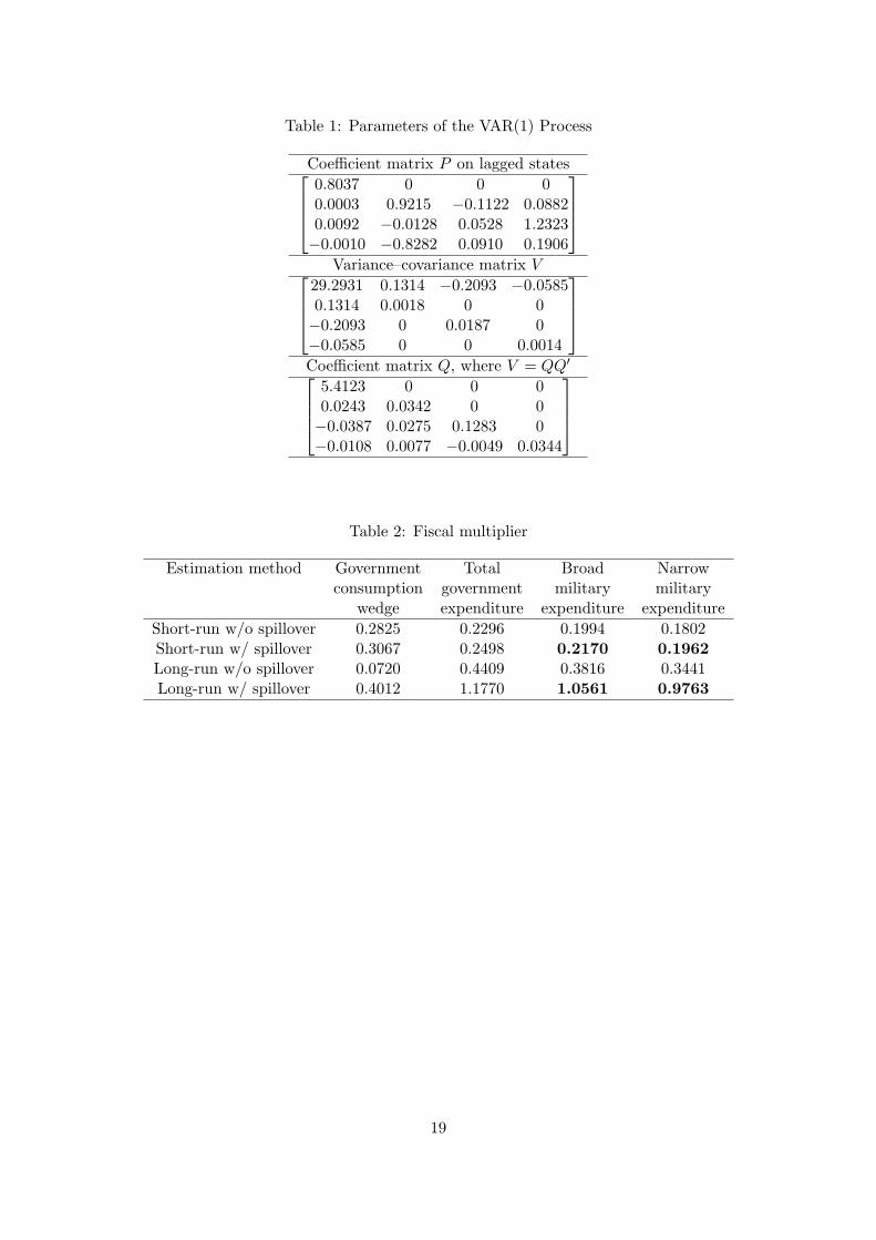
Table 1: Parameters of the VAR(1) Process

Coefficient matrix P on lagged states0.8037 0 0 00.0003 0.9215 −0.1122 0.08820.0092 −0.0128 0.0528 1.2323−0.0010 −0.8282 0.0910 0.1906

Variance–covariance matrix V

29.2931 0.1314 −0.2093 −0.05850.1314 0.0018 0 0−0.2093 0 0.0187 0−0.0585 0 0 0.0014

Coefficient matrix Q, where V = QQ′5.4123 0 0 00.0243 0.0342 0 0−0.0387 0.0275 0.1283 0−0.0108 0.0077 −0.0049 0.0344

Table 2: Fiscal multiplier

Estimation method Government Total Broad Narrowconsumption government military military

wedge expenditure expenditure expenditure

Short-run w/o spillover 0.2825 0.2296 0.1994 0.1802Short-run w/ spillover 0.3067 0.2498 0.2170 0.1962Long-run w/o spillover 0.0720 0.4409 0.3816 0.3441Long-run w/ spillover 0.4012 1.1770 1.0561 0.9763

19

1890 1900 1910 1920 1930-2

-1

0

1

2g

1890 1900 1910 1920 1930-0.1

-0.05

0

0.05

0.1A

1890 1900 1910 1920 1930-0.4

-0.2

0

0.2

0.4

=l

1890 1900 1910 1920 1930-1

-0.5

0

0.5

1

=x

Figure 1: Estimated wedges

20

1890 1900 1910 1920 1930-0.2

-0.1

0

0.1

0.2Y vs Y w/o g

1890 1900 1910 1920 1930-0.2

-0.1

0

0.1

0.2Y vs Y w/o A

1890 1900 1910 1920 1930-0.2

-0.1

0

0.1

0.2

Y vs Y w/o =l

1890 1900 1910 1920 1930-0.2

-0.1

0

0.1

0.2

Y vs Y w/o =x

Figure 2: Output data and predictions of the models with just one wedge

21

1900 1905 1910 1915 1920 1925 1930 1935-0.1

-0.08

-0.06

-0.04

-0.02

0

0.02

0.04

0.06

0.08

0.1

yy w/o broad govt exp.y w/o narrow govt exp.

Figure 3: Output data and predictions of the models without government expenditure in 1904,w/o spillover

22

1900 1905 1910 1915 1920 1925 1930 1935-0.1

-0.08

-0.06

-0.04

-0.02

0

0.02

0.04

0.06

0.08

0.1

yy w/o broad govt exp.y w/o narrow govt exp.

Figure 4: Output data and predictions of the models without government expenditure in 1904,w/ spillover

23

1910 1920 1930-0.1

0

0.1

0.2g

1910 1920 1930

#10 -4

-5

0

5

10A

1910 1920 1930

#10 -3

-1

0

1

=l

1910 1920 1930

#10 -4

-15

-10

-5

0

5

=x

1910 1920 1930

#10 -3

0

5

10y

1910 1920 1930

#10 -3

-15

-10

-5

0

5c

1910 1920 1930-0.02

0

0.02

0.04

0.06

x

1910 1920 1930

#10 -3

-5

0

5

10

15l

1910 1920 1930

#10 -3

-5

0

5

10

15k

Figure 5: Impulse-response functions to narrow military expenditure in 1904

24