Fiscal and Monetary Policy During Downturns: Evidence from the G7

Daniel Leigh and Sven Jari Stehn

WP/09/50

© 2009 International Monetary Fund WP/09/50 IMF Working Paper Fiscal Affairs Department

Fiscal and Monetary Policy During Downturns: Evidence from the G7 1

Prepared by Daniel Leigh and Sven Jari Stehn

Authorized for distribution by Manmohan S. Kumar

March 2009

Abstract

This Working Paper should not be reported as representing the views of the IMF. The views expressed in this Working Paper are those of the author(s) and do not necessarily represent those of the IMF or IMF policy. Working Papers describe research in progress by the author(s) and are published to elicit comments and to further debate.

This paper analyzes how fiscal and monetary policy typically respond during downturns in G7 countries. It evaluates whether discretionary fiscal responses to downturns are timely and temporary, and compares the response of fiscal policy to that of monetary policy. The results suggest that while responding more weakly and less quickly than monetary policy, discretionary fiscal policy is more timely than conventional wisdom would suggest, particularly in “Anglo-Saxon” countries, but the response differs substantially across fiscal instruments. Both fiscal and monetary policy are found to be subject to an easing bias, with more easing during downturns than tightening during upturns; and liable to easing in response to erroneously perceived downturns, many of which are subsequently revised to expansions. JEL Classification Numbers: E62, E63, H50 Keywords: Fiscal stabilization, government revenue, government expenditure

Author’s E-Mail Address: Dleigh@imf.org, sstehn@imf.org

1 We would like to thank Mark De Broeck, Alasdair Scott, and Steven Symansky for helpful comments.

2

Contents Page

I. Inroduction and Summary ......................................................................................................3

II. Event-Study Analysis............................................................................................................3 A. Data and Methodology..............................................................................................3 B. Results .......................................................................................................................4

III. Vector-Autoregression (VAR) Analysis..............................................................................6 A. Methodology .............................................................................................................6 B. Baseline Results ........................................................................................................7 C. Asymmetry..............................................................................................................12 D. Policy in Real Time.................................................................................................14

IV. Case Study: Have U.S. Tax Cuts Been Timely and Temporary? ......................................18

V. Conclusion ..........................................................................................................................19 Tables 1. How Often and Quickly did Fiscal Stimulus Arriva During Downturns?.............................5 2. How Often and Quickly did Fiscal Stimulus Arrive During Upturns?..................................6 3. How Reliable are Preliminary Growth Estimates? ..............................................................15 4. Legislated Tax Changes During Downturns........................................................................19 5. Summary of Countercyclical Tax Changes .........................................................................20 Figures 1. How Strongly do Fiscal and Monetary Policy Respond? ......................................................9 2. How does the Response Vary Across Fiscal Instruments and G7 Members? .....................10 3. How Robust is the Response to the Cyclical Indicator? ......................................................11 4. Is There a Bias Towards Easing in Downturn? ...................................................................13 5. Errors in Identifying Negative Growth in the G7 ................................................................14 6. Has Policy Erroneously Responded to Perceived Growth Shocks? ....................................17 References................................................................................................................................21

3

I. INTRODUCTION AND SUMMARY

The present economic slowdown and the aggressive easing of fiscal and monetary policy in the United States has revived interest in the role of fiscal policy in stabilizing the cycle. The accepted wisdom, however, is that while monetary policy is a timely and powerful countercyclical instrument, fiscal policy provides too little stimulus too late. Similarly, there is a view that while central bankers adjust policy symmetrically over the cycle, fiscal policy responds asymmetrically, loosening in downturns, and failing to tighten sufficiently in expansions. As policy decisions are made in real time, uncertainty regarding the state of the economy poses an important additional challenge to monetary and fiscal policymakers. Despite the prevalence of this conventional wisdom, there is a surprising lack of research that quantifies the behavior of fiscal and monetary policy during downturns in the group-of-seven countries (G7). While the countercyclical behavior of monetary policy has been well documented (Taylor 1993, Clarida et al 1999), the literature generally finds that fiscal policy in the G7 has been weakly countercyclical or a-cyclical (Gali and Perotti 2003, Lane 2003, Auerbach 2003). Romer and Romer (1994) conduct an event study of monetary and fiscal policies around recessions and recoveries for the US, and find that while monetary policy and the cyclical (automatic) primary balance consistently eased during recessions, discretionary fiscal easing, proxied by the cyclically-adjusted primary balance, generally arrived after the end of recessions, and provided a weak degree of stimulus. Using quarterly data, this paper focuses on the cyclical behavior of fiscal and monetary policy in the G7 since 1980. Using an event study, Section II analyzes how often and how quickly fiscal policy respond to a downturn. The analysis shows how the response speed varies across fiscal instruments and how it compares with that of monetary policy. Section III uses a vector auto-regression to analyze the strength of fiscal and monetary policy responses to a growth shock. This section moreover documents how much of the fiscal stimulus is withdrawn during subsequent recoveries, and how the symmetry of fiscal policy compares to that of monetary policy. Finally, the section analyzes how important uncertainties regarding the state of the economy are. Section IV focuses on the experience of the United States, for which detailed quarterly data on legislated tax changes since the 1960s are available. In particular the timeliness and temporariness of countercyclical tax legislation are assessed based on the new database of Romer and Romer (2007).

II. EVENT-STUDY ANALYSIS

A. Data and Methodology

Defining economic downturns and fiscal and monetary stimulus is inevitably somewhat subjective. In this paper, downturns are defined as periods during which either the growth rate is negative or the output gap is “unusually” negative (defined as one standard deviation below zero). This definition is more general than defining a downturn simply in terms of negative growth (as in Romer and Romer (1994)), because that would miss periods where output is significantly less than potential but still rising.

4

This paper uses the change in the short-term nominal interest rate as the indicator of monetary policy. The measure of fiscal stimulus starts with the primary fiscal balance, the difference between total general government revenues and expenditure net of interest payments on consolidated general government liabilities. Changes in the primary balance can arise passively, as revenues and expenditures rise and fall with economic activity, or actively, as governments make choices about tax, transfer and spending policies. What is needed, therefore, is a measure of the cyclically-adjusted primary balance, the intuition being that changes in the cyclically-adjusted primary balance should reflect changes in policy. When looking at the responses of fiscal policy to changes in economic activity, we identify automatic stabilizers with changes in the cyclical component of the primary balance and discretionary fiscal policy with changes in the cyclically-adjusted primary balance. Following the literature (e.g., Alesina and Perotti 1995), the event-study analysis identifies discretionary changes as “large” changes in the policy instruments, because even policy indicators can fluctuate for reasons other than discretionary policy choices. The focus is therefore on large changes in discretionary fiscal variables, defined as those that exceed 0.25 percent of GDP per quarter. Similarly, discretionary changes in nominal short-term interest rates are defined as those that exceed 25 basis points in one quarter. Quarterly data from 1980Q1-2007Q4 is taken from the OECD Economic Outlook and the IMF’s IFS database. The OECD publishes cyclical adjustment of the budget items, which uses an estimate of the output gap together with constructed elasticities to extract the cyclical component from the budget items. Quarterly data on the output gap and real GDP growth are taken from the OECD Economic Outlook, and are seasonally adjusted. Changes in monetary policy are proxied by the quarterly change in the nominal short-term interest rate taken from the Fund’s IFS database. All changes are quarter-over-quarter and unannualized.

B. Results

Table 1 and present summary statistics regarding the cyclical behavior of monetary and fiscal policy during downturns and recoveries, respectively. Applying the abovementioned definition of a downturn, Table 1 indicates that downturns occurred in about 26 percent of the sample. For the G7 as a whole, discretionary fiscal stimulus arrived in 21 percent of all downturn quarters, less than half as frequently as interest-rate easing. However, the discretionary fiscal stimulus arrived, on average, 2.4 quarters after the onset of a downturn, 1.6 quarters after interest-rate easing. Capital spending had the lowest response frequency, with easing in only 13 percent of all downturn quarters, and an arrival lag of almost 4 quarters. In contrast, and as expected, automatic fiscal easing, proxied by a fall in the cyclical primary balance occurred in almost all downturns in the quarter of the downturn itself.2

2 The automatic stabilizers do not necessarily ease in all downturns since the definition of a downturn does not rule out an increase in growth or narrowing of a negative output gap (as long as the output gap is unusually negative).

5

However, some of these findings for the G7 average hide important cross-country differences. In particular, discretionary fiscal easing was more frequent in “Anglo-Saxon” countries (Canada, the United Kingdom, and the United States) than in other G7 members. In particular, discretionary fiscal easing occurred in 34, 39, and 26 percent of downturn quarters in these countries, respectively, compared with an average of 12 percent in the other countries. This difference is attributable to a more frequent easing in both revenues and current spending.

Table 1. How Often and Quickly Did Fiscal Stimulus Arriva during Downturns?

G7 Canda Germany France Italy Japan UK US

Number of downturns 104 9 24 14 17 22 7 11Length of downturns 2.3 3.8 1.5 1.5 2.1 1.6 3.3 2.0

Quarter of first easing after start of downturnCyclically-adjusted primary balance 2.4 2.4 2.6 4.2 2.5 1.8 1.2 2.1Cyclical primary balance 0.0 0.0 0.0 0.0 0.0 0.0 0.0 0.2Cyclically-adjuste revenue 2.3 1.1 1.7 5.5 3.0 3.3 0.6 0.9Cyclically-adjusted current spending 1.8 1.8 1.5 2.2 1.5 1.7 1.0 3.0Capital spending 3.8 5.9 1.3 8.5 0.9 1.9 2.6 5.4Nominal policy interest rate 0.8 0.7 0.5 1.0 0.8 0.5 0.6 1.6

Share of downturn quarters with easingCyclically-adjusted primary balance 21 34 3 10 19 17 39 26Cyclical primary balance 96 100 100 90 97 97 96 91Cyclically-adjuste revenue 17 34 6 0 14 6 30 26Cyclically-adjusted current spending 28 48 11 24 25 8 52 30Capital spending 13 7 17 0 28 8 22 13Nominal policy interest rate 51 72 44 48 53 22 70 48

Memorandum items

Number of downturn quarters 204 29 36 21 36 36 23 23Total number of quarters in sample 784 112 112 112 112 112 112 112Proportion of time spent in downturn (percent) 26 26 32 19 32 32 21 21

G7: Policy Response Times, 1980-2007Quarter of first easing with respect to start of downturn

Sources: IMF staff estimates, OECD.

6

Table 2. How Often and Quickly did Fiscal Stimulus Arrive during Upturns?

G7 Canada Germany France Italy Japan UK US

Number of upturns 110 10 25 15 18 23 7 12Length of upturns 8.1 7.0 3.3 6.0 4.1 3.3 21.7 11.0

Quarter of first tightening after start of upturnCyclically-adjusted primary balance 2.1 0.8 1.8 3.4 2.8 3.9 1.3 0.7Cyclical primary balance 0.5 0.2 0.4 1.5 0.1 0.2 0.0 0.9Cyclically-adjusted revenue 1.9 2.3 1.6 3.0 1.6 2.1 1.8 0.7Cyclically-adjusted current spending 1.9 0.5 1.3 1.5 2.2 4.5 0.9 2.8Capital spending 2.9 4.1 1.0 5.8 1.2 2.3 1.5 4.6Nominal policy interest rate 2.2 3.3 0.6 4.6 1.0 1.2 0.4 4.7

Share of upturn quarters with tighteningCyclically-adjusted primary balance 24 37 16 13 24 11 35 33Cyclical primary balance 68 73 67 58 67 75 67 65Cyclically-adjusted revenue 23 30 14 13 30 14 36 24Cyclically-adjusted current spending 14 33 13 3 14 3 27 6Capital spending 18 14 29 3 28 21 22 7Nominal policy interest rate 27 36 24 24 28 17 27 33

Memorandum items

Number of upturn quarters 580 83 76 91 76 76 89 89Total number of quarters in sample 784 112 112 112 112 112 112 112Proportion of time spent in upturn (percent) 74 74 68 81 68 68 79 79

G7: Policy Response Times, 1980-2007Quarter of first tightening with respect to start of upturn

Sources: IMF staff estimates, OECD. Table 2 provides the same summary statistics for upturns. The table indicates that upturns occurred in 74 percent of the sample. While fiscal policy displays similar cyclical behavior as during downturns, monetary policy responds noticeably less frequently (only in 27 percent of upturns) and with a longer delay (of 2.2 quarters) than during downturns. While monetary policy provided much quicker and more frequent easing during downturns than fiscal policy, its performance is therefore similar to that of fiscal policy during upturns.

III. VECTOR-AUTOREGRESSION (VAR) ANALYSIS

A. Methodology

To quantify the speed and strength of the cyclical response of fiscal policy, and compare this response with that of monetary policy, a VAR is estimated using quarterly data for each G7 country.3 The variables included in the VAR, and their ordering are as follows: actual real GDP growth minus potential real GDP growth; inflation (based on the GDP deflator); changes in the nominal interest rate; changes in the primary cyclically-adjusted fiscal balance; and changes in the automatic (cyclical) fiscal balance. For simplicity, two lags of each variable are included in the VAR for each country.

3 Unlike much of the VAR literature, the analysis presented here does not evaluate the response of growth to fiscal policy shocks. Rather, the focus is on the response of fiscal policy variables to a growth shock.

7

B. Baseline Results

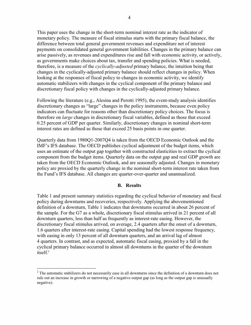
Figure 1 displays the changes in monetary policy and discretionary fiscal policy (including its components) in response to a one percentage fall of growth below potential.4 The figure reports responses for three samples, the entire sample covering 1980Q1–2007Q4 (solid line), an “early” sample covering 1980Q1–1991Q4 (dashed line), and a “late” sample covering 1992Q1–2007Q4 (dotted line). The late sample corresponds to important changes in policy frameworks, including European Monetary Union, Japan’s prolonged recession, and the adoption of inflation targeting in Canada and the United Kingdom. The results suggest that discretionary fiscal policy in G7 countries has on average responded weakly to downturns.5 In all three samples, the discretionary fiscal easing is much weaker and slower to arrive than that of automatic stabilizers, and interest rates. A comparison of the early and late samples suggests that the countercyclical response of fiscal policy has improved modestly since the early 1990s.6 In the early sample, discretionary fiscal policy is pro-cyclical on impact and provides a cumulative pro-cyclical contraction of 0.05 percentage points of trend GDP over four quarters. In the later sample, while discretionary policy still provides no stimulus on impact, it provides a cumulative stimulus of 0.2 percentage points over four quarters. Figure 2 summarizes policy responses during the three samples by reporting the cumulative response of the policy instruments during the first four quarters for the G7, as well as different country groups. A look at the responses of spending and revenue components reveals that the procyclicality in the early sample is due to a combination of mildly pro-cyclical revenue increases, small counter-cyclical current spending increases and large pro-cyclical capital spending cuts. The greater degree of fiscal policy countercyclicality observed since the early 1990s is due to cuts in revenues, larger increases in current spending, and much smaller cuts in capital spending. The countercyclical response of monetary policy to a downturn and the automatic stabilizers remained broadly unchanged in the second sample. In addition, Figure 2 reveals interesting cross-country differences. Confirming the event-study results, the figure indicates that discretionary fiscal policy has been more timely and more countercyclical in “Anglo-Saxon” countries, than in continental Europe or Japan. Taking the late sample as an example, in Anglo-Saxon countries, discretionary fiscal policy has eased on impact in response to slowing growth, and provided a total stimulus of 0.8 percentage points of trend GDP over the first four quarters. In continental European

4 Changing the ordering of the fiscal and monetary policy variables in the VAR has no effect on the results, as long as they are ordered after growth and inflation. Including the change in the public debt-to-GDP ratio in the system does not change the qualitative results.

5 The VAR treats downturns and upturns symmetrically, and therefore impulse responses associated with a positive growth are of the opposite sign and the same magnitude as those reported in the figure. A later section estimates responses separately for downturns and upturns.

6 This finding is consistent with, for example, Gali and Perotti (2003) and WEO (2003).

8

countries, in contrast, discretionary fiscal policy has been pro-cyclical, with a cumulative tightening of 0.4 percentage points of GDP during the first four quarters. Japan also provided a pro-cyclical impulse on impact, but discretionary policy easing in the subsequent three quarters provided cumulative easing of 0.3 percentage points of trend GDP. Moreover, in Anglo-Saxon and continental European countries, monetary policy provided timely and strongly countercyclical stimulus in response to slowing growth, with interest rates falling on impact, and a cumulative easing of around 100 basis points after 4 quarters. There has been almost no nominal interest rate response in Japan, due to the zero lower bound. Figure 3 explores the robustness of these results to the cyclical indicator. In addition to the response to a fall in growth below potential (which has been used above), policy responses to a fall in growth and to a fall in the output gap are considered. Despite some differences, especially in response to a fall in the output gap, Figure 3 shows that the qualitative conclusions regarding the cyclical behavior of monetary and fiscal policy are robust to the choice of the cyclical indicator.

9

Figure 1. How Strongly do Fiscal and Monetary Policy Respond?

(Average of G7 Impulse responses to a one percentage-point fall in growth below potential)

Change in Interest Rate(percent)

-0.40

-0.30

-0.20

-0.10

0.00

0.10

0.20

1 2 3 4 5 6 7 8 9 10

1980-2007

1980-1991

1992-2007

Change in C-A Revenue (CAR) (percent of trend GDP)

-0.10

-0.08

-0.06

-0.04

-0.02

0.00

0.02

0.04

0.06

0.08

0.10

1 2 3 4 5 6 7 8 9 10

Change in C-A Primary Current Spending (CAX), (percent of trend GDP)

-0.04

-0.02

0.00

0.02

0.04

0.06

0.08

0.10

1 2 3 4 5 6 7 8 9 10

Change in Cyclical Primary Balance (CPB)(percent of GDP)

-0.40

-0.30

-0.20

-0.10

0.00

0.10

0.20

1 2 3 4 5 6 7 8 9 10

Change in C-A Primary Capital Spending (CAK), (percent of trend GDP)

-0.08

-0.06

-0.04

-0.02

0.01

0.03

0.05

1 2 3 4 5 6 7 8 9 10

Change in C-A Primary Balance (CAPB)(percent of GDP) /1

-0.15

-0.10

-0.05

0.00

0.05

0.10

0.15

1 2 3 4 5 6 7 8 9 10 1/ The cyclically adjusted primary balance is calculated from its components.

10

Figure 2. How does the Response Vary Across Fiscal Instruments and G7 Members?

(Cumulative four-quarter responses to a one percentage point fall in growth: alternative samples)

Nominal Interest Rate(percent)

-2.00

-1.50

-1.00

-0.50

0.00

0.50

G7 ANGLO3 EU3 JPN

1980-2007 1980-91 1992-2007

C-A Revenue(percent of trend GDP)

-0.60

-0.40

-0.20

0.00

0.20

0.40

0.60

G7 ANGLO3 EU3 JPN

C-A Current Spending(percent of trend GDP)

-0.20

-0.10

0.00

0.10

0.20

0.30

0.40

G7 ANGLO3 EU3 JPN

Cyclical Primary Balance(percent of GDP)

-0.70

-0.60

-0.50

-0.40

-0.30

-0.20

-0.10

0.00

0.10

0.20

G7 ANGLO3 EU3 JPN

C-A Capital Spending(percent of trend GDP)

-0.30-0.25-0.20-0.15-0.10-0.050.000.050.100.150.20

G7 ANGLO3 EU3 JPN

C-A Primary Balance(percent of trend GDP) /1

-1.00

-0.80

-0.60

-0.40

-0.20

0.00

0.20

0.40

0.60

0.80

1.00

G7 ANGLO3 EU3 JPN

1/ The cyclically adjusted primary balance is calculated from its components.

11

Figure 3. How Robust is the Response to the Cyclical Indicator?

(Cumulative four-quarter responses to alternative cyclical indicators for the G7: 1992Q1-2007Q4)

Nominal Interest Rate(percent)

-1.80

-1.30

-0.80

-0.30

0.20

G7 ANGLO3 EU3 JPN

GrowthChange in Output GapOutput Gap

C-A Revenue(percent of trend GDP)

-0.70

-0.50

-0.30

-0.10

0.10

0.30

0.50

0.70

G7 ANGLO3 EU3 JPN

C-A Current Spending(percent of trend GDP)

-0.10

0.00

0.10

0.20

0.30

0.40

0.50

G7 ANGLO3 EU3 JPN

Cyclical Primary Balance(percent of GDP)

-0.70-0.60-0.50-0.40-0.30-0.20-0.100.000.100.200.30

G7 ANGLO3 EU3 JPN

C-A Capital Spending(percent of trend GDP)

-0.25

-0.20

-0.15

-0.10

-0.05

0.00

0.05

0.10

0.15

0.20

G7 ANGLO3 EU3 JPN

C-A Primary Balance(percent of trend GDP) /1

-0.90

-0.70

-0.50

-0.30

-0.10

0.10

0.30

0.50

0.70

0.90

G7 ANGLO3 EU3 JPN

1/ The cyclically adjusted primary balance is calculated from the behavior of its components.

12

C. Asymmetry

A concern that often arises regarding countercyclical discretionary activism is that policymakers may respond in an asymmetric manner, easing in downturns and not tightening sufficiently in upturns. In the U.S., it is often argued that monetary policy tightened insufficiently during the 1998–2000 dotcom boom, while interest rates were cut sharply in response to the following downturn. The result of an easing bias in fiscal policy could be a permanent increase in the public-debt-to-GDP ratio with potentially adverse consequences for long-run growth. To investigate whether monetary and fiscal policy in G7 countries have displayed such an asymmetric tendency, the VAR framework is adapted to allow for an asymmetric response to upturns and downturns. In particular, for each country, the VAR now includes the following variables: growth minus potential growth when the economy is in a downturn and zero otherwise; growth minus potential growth when the economy is in an upturn and zero otherwise, and the previously included variables, i.e., inflation, changes in nominal interest rates, and changes in fiscal instruments. As before, downturns are defined as quarters in which growth is either negative or below trend with the output gap more than one standard deviation below zero. The results are robust to changing the ordering of the two halves of growth (downturns and upturns) in the VAR, to alternative orderings for the fiscal and monetary policy variables, and to including a time trend in each equation. The cumulative responses during the first four quarters reported in Figure 3 are consistent with the existence of an expansionary bias in both discretionary fiscal policy and monetary policy. In particular, monetary policy easing during downturns has been more pronounced than tightening during upturns. Discretionary fiscal policy displays a tendency to provide a substantial stimulus in downturns that is not offset by a tightening in upturns. While European countries are symmetrically pro-cyclical, the Anglo-Saxon countries display strongly asymmetric behavior with large easing in both spending and revenues during downturns. In contrast to these asymmetric responses, and as expected, automatic stabilizers respond in a symmetric way, with the easing observed in downturns almost exactly offset by tightening during upturns.7

7 The results are robust to changing the ordering of the two halves of growth (downturns and upturns) in the VAR, and to alternative orderings for the fiscal and monetary policy variables.

13

Figure 4. Is There a Bias Towards Easing in Downturn?

(Cumulative four-quarter responses in upturns and downturns: 1992Q1–2007Q4)

Nominal Interest Rate(percent)

-2.00

-1.50

-1.00

-0.50

0.00

0.50

1.00

1.50

2.00

G7 ANGLO3 EU3 JPN

UpturnDownturn

C-A Revenue(percent of trend GDP)

-1.60

-1.10

-0.60

-0.10

0.40

0.90

1.40

G7 ANGLO3 EU3 JPN

C-A Current Spending(percent of trend GDP)

-1.20

-0.70

-0.20

0.30

0.80

G7 ANGLO3 EU3 JPN

Cyclical Primary Balance(percent of GDP)

-1.20

-0.70

-0.20

0.30

0.80

G7 ANGLO3 EU3 JPN

C-A Capital Spending(percent of trend GDP)

-0.30

-0.20

-0.10

0.00

0.10

0.20

0.30

G7 ANGLO3 EU3 JPN

C-A Primary Balance(percent of trend GDP) /1

-2.50

-2.00

-1.50

-1.00

-0.50

0.00

0.50

1.00

1.50

2.00

G7 ANGLO3 EU3 JPN

1/ The cyclically adjusted primary balance is calculated from the behavior of its components.

14

D. Policy in Real Time

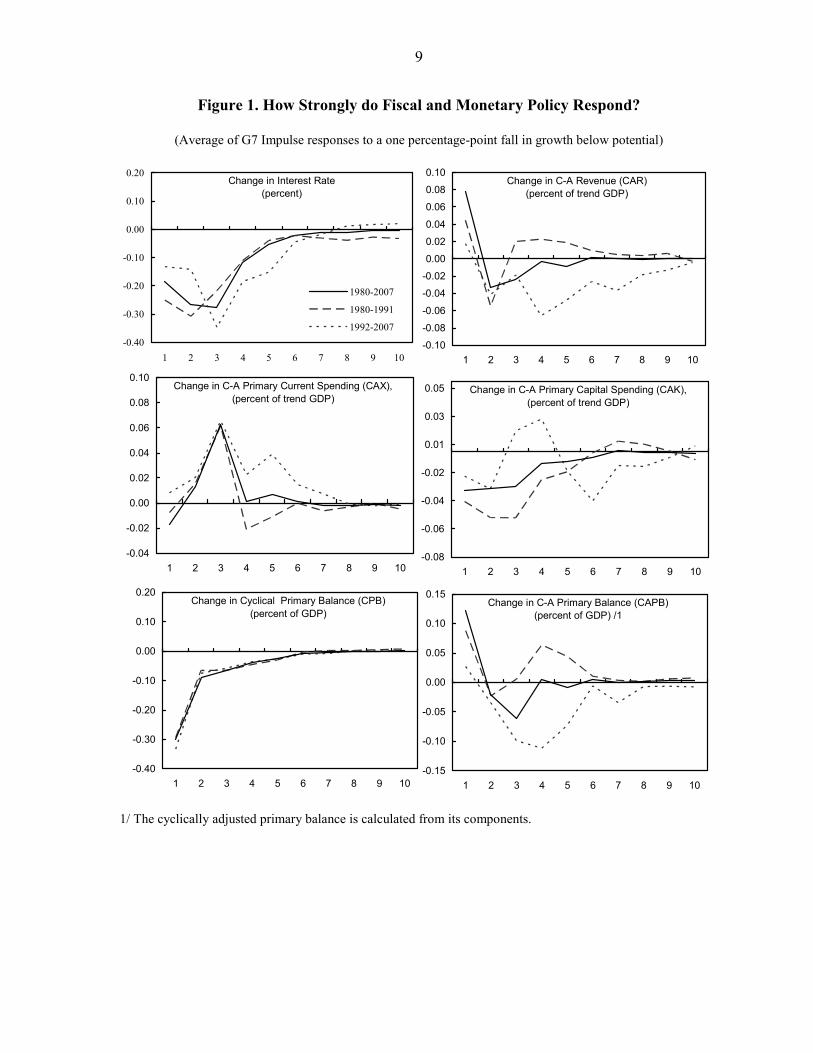
An additional concern in the analysis of countercyclical monetary and fiscal activism is that policymakers face substantial uncertainties regarding the cyclical position, and run the risk of destabilizing the economy by responding to erroneously perceived downturns. To quantify the severity of this potential problem, the reliability of preliminary GDP estimates produced by national authorities is assessed.8 Figure 4 displays the relationship between preliminary growth estimates and subsequent revisions. While an unbiased preliminary estimate of growth should have no systematic relationship with the subsequent revision, Figure 4 indicates a strong negative relationship, suggesting that initial estimates are biased. In particular, the data suggest that of all preliminary estimates indicating negative quarter-over-quarter growth 39 percent were subsequently revised to positive growth (Table 2). At the same time, 30 percent of quarters that according to the final data in fact had negative growth showed positive growth in the preliminary estimates. More generally, standard forecast efficiency tests find strong evidence of a bias towards pessimism in preliminary growth estimates, with the average bias for G7 countries estimated at 0.34 percentage points (unannualized) and highly statistically significant. The subsequent upward revision is particularly large for negative growth estimates. For example, an initial quarterly growth estimate of -0.6 percent is, on average, revised upwards by 0.6 percentage points to zero.

Figure 5. Errors in Identifying Negative Growth in the G7 (Preliminary Growth Estimates and Subsequent Revisions, 1965–2004)

-20

24

revi

sion

to g

row

th ra

te

-5 0 5preliminary growth rate

Type-One Error Type-Two Error

Source: OECD monthly economic indicators (various vintages). A type-one error indicates negative growth that was subsequently revised to positive. A type-two error indicates positive growth that was subsequently revised to negative.

8 The analysis updates the estimates of Faust, Rogers, and Wright (2003) that used data ending in 1997, using the OECD Monthly Economic Indicators (MEI). The sample ends in 2004 to ensure that no further data revisions for the most recent data were likely. Revisions are defined as the difference between the data as they stood in the most recent MEI database (June 2008) and the data when they were first published in the MEI.

15

The data are consistent with the view that the preliminary data available to policymakers in real time are biased towards suggesting that the economy is in a downturn, and that an intended countercyclical response to such data may turn out to be procyclical. The bias varies across countries, with less evidence in the case of the United States and France. In addition, while remaining statistically significant, the bias appears to have declined in recent years, possibly reflecting the more stable and predictable growth environment.

Table 3. How Reliable are Preliminary Growth Estimates?

G7 Canada France Germany Italy Japan U.K. U.S.

Errors in Identifying Negative Growth

p (Type-One Error) 38.9 40.7 25.0 40.0 42.9 46.4 46.9 30.0p (Type-Two Error) 29.6 27.3 40.0 30.0 23.8 31.8 21.2 33.3

Preliminary Growth Estimates and Subsequent RevisionsModel: Revision = α + βPrelim + u

Revisions, Full Sampleα 0.341*** 0.428*** 0.122* 0.238*** 0.299*** 0.278*** 0.442*** 0.148**

[12.72] [5.215] [1.864] [3.045] [5.089] [4.135] [7.674] [2.209]β -0.427*** -0.373*** -0.16 -0.462*** -0.610*** -0.411*** -0.520*** -0.11

[-14.38] [-4.537] [-1.454] [-4.161] [-6.712] [-7.879] [-9.153] [-1.421]F ( H0: α = β = 0) 113.50 13.66 1.74 8.74 26.31 33.26 51.51 2.82p -val 0.00 0.00 0.15 0.00 0.00 0.00 0.00 0.16Observations 891 160 69 101 101 140 160 160

Revisions, 1995Q1-2004Q4α 0.262*** 0.145** 0.147** 0.240** 0.169* 0.13 0.377*** 0.10

[3.922] [2.350] [2.076] [2.446] [1.693] [1.252] [5.881] [1.104]β -0.421*** -0.02 -0.20 -0.791*** -0.36 -0.327** -0.408*** -0.186*

[-3.571] [-0.156] [-1.411] [-4.688] [-1.313] [-2.339] [-3.756] [-1.856]F ( H0: α = β = 0) 7.70 5.76 2.18 11.00 1.44 2.88 19.00 2.07p -val 0.00 0.88 0.17 0.00 0.20 0.02 0.00 0.07Observations 280 40 40 40 40 40 40 40

Sources: IMF staff estimates, OECD. Note: Robust t statistics in brackets, *** significant at 1 percent, ** significant at 5 percent, * significant at 10 percent level. Results for individual G7 country regressions have heteroskedastiticy and autocorrelation robust standard errors obtained using the Newey-West (1987) procedure with a lag truncation parameter of four. Results for the G7 panel obtained using fixed effects with robust standard errors. To investigate how fiscal policy in G7 countries has been affected by errors in growth estimates, the VAR framework is augmented with the growth estimation errors. The VAR now includes the preliminary estimation errors in addition to the previously included variables. The estimation errors are ordered in the VARs after growth and inflation but before the policy variables. As before the results are robust to alternative orderings amongst the errors and policy variables.

16

Focusing on the late sample, confirms that both discretionary fiscal and monetary policy have been affected by errors in preliminary growth estimates. In the G7 on average, interest rates were cut by around 50 basis points in response to a one percentage point fall in perceived growth relative to final revised growth. Figure 6 shows that this easing is entirely driven by expansionary policy in the Anglo-Saxon countries. While the cyclical balance (by construction) does not respond to erroneously perceived downturns, the discretionary fiscal balance-to-potential GDP ratio falls by around 0.3 percentage points, driven both by cuts in revenues and increases in current spending. The Anglo-Saxon countries again provide the largest stimulus, but discretionary fiscal policy is also eased in continental Europe and Japan. These findings suggest that concern over policy errors is well founded. While Anglo-Saxon countries have provided timely and sizable stimulus during downturns, these discretionary actions have often been in response to erroneously perceived downturns, highlighting the dangers of discretionary activism in real time. The findings are of particular concern, as fiscal policy decisions are likely less easily reversed than monetary policy decisions, and fiscal policy errors bear potentially long-lived consequences for debt.

17

Figure 6. Has Policy Erroneously Responded to Perceived Growth Shocks?

(Cumulative four-quarter responses in response to erroneously perceived growth shocks: 1992Q1–2007Q4)

Nominal Interest Rate(percent)

-1.40-1.20-1.00-0.80-0.60-0.40-0.200.000.200.400.60

G7 ANGLO3 EU3 JPN

C-A Revenue(percent of trend GDP)

-0.20

-0.15

-0.10

-0.05

0.00

0.05

0.10

G7 ANGLO3 EU3 JPN

C-A Current Spending(percent of trend GDP)

0.000.020.040.060.080.100.120.140.160.180.20

G7 ANGLO3 EU3 JPN

Cyclical Primary Balance(percent of GDP)

-1.20

-0.70

-0.20

0.30

0.80

G7 ANGLO3 EU3 JPN

C-A Capital Spending(percent of trend GDP)

-0.08

-0.06

-0.04

-0.02

0.00

0.02

0.04

0.06

G7 ANGLO3 EU3 JPN

C-A Primary Balance(percent of trend GDP) /1

-0.40

-0.30

-0.20

-0.10

0.00

0.10

0.20

G7 ANGLO3 EU3 JPN 1/ The cyclically adjusted primary balance is calculated from the behavior of its components.

18

IV. CASE STUDY: HAVE U.S. TAX CUTS BEEN TIMELY AND TEMPORARY?

A caveat to the analysis based on conventional policy indicators is that the policy variables that were identified as “discretionary” could move for reasons unrelated to intentional policy actions. In particular, the cyclically-adjusted primary balance is a noisy indicator of discretionary policy for a number of reasons, including measurement error in the estimation of the output gap, and the influence of variables, such as asset prices, that have an effect on the budget balance beyond their effect on the cyclical position. Moreover, the preceding analysis focuses on the behavior of the average change in fiscal policy irrespective of its rationale, which may differ from a change in policy specifically motivated by countercyclical considerations. This section provides a case study of fiscal policy in the Unites States, for which an alternative fiscal policy indicator that eliminates some of these shortcomings is available. This indicator is based on a recently constructed database of all post-war legislated tax changes (Romer and Romer, 2007a).9 Romer and Romer (2007a) construct a database of all legislated tax changes between 1945 and 2007 and classify these tax changes according to their motivation using governmental documents. Their classification contains four motivations: (i) exogenous long-run (ii) exogenous spending-driven; (iii) endogenous “deficit-driven;” and (iv) endogenous countercyclical. This dataset is unique in that allows for a detailed case study of the discretionary behavior of tax policy. In a careful analysis Romer and Romer single out 5 tax changes that were motivated explicitly by countercyclical objectives. In the Annex summarizes these and adds the 2008 Stimulus Package. Table 4 assesses how quickly after the onset of a downturn the tax changes were legislated and implemented, how temporary they were, and how well targeted they were. In assessing how close to a downturn the tax cuts arrived, the analysis defines a downturn as in the main text. Four out of the five cyclically-motivated tax cuts occurred within one quarter of a downturn. In the case of 2002, the stimulus arrived three quarters after the downturn. The database also permits a further breakdown of the total response lag into the “decision lag” (delay between observing the recession and signing the tax acts) and the “implementation lag” (delay between signing and enacting the tax acts) of countercyclical tax cuts. Table 4 shows that the average implementation lag was equal to about one quarter.

9 We are grateful to Romer and Romer for sharing their newly constructed data with us.

19

Table 4. Legislated Tax Changes During Downturns

Date of Nearest ImplementationDownturn Lag (Quarters) Planned Actual Planned Actual

1970Q1 Tax Reform 1.2 1970Q1 1 0 0 permanent permanent1975Q2 Tax Reduction 3.6 1975Q1 1 97 78 2.3 1.01977Q3 Tax Reduction and Simplification 1.0 1977Q4 1 77 67 1.3 1.02001Q3 Economic Growth 1.7 2001Q3 1 100 100 1.3 1.3

and Tax Relief Reconcililation2002Q2 Job Creation and Worker Assistance 1.1 2001Q3 1 100 67 3.7 4.02008Q2 Economic Stimulus 1.1 … 1 100 … 1.6 …

Mean 1.6 1 79 62 2.0 1.8

Timeliness TemporarinessLegislated Tax CutDate

Stimulus Arrived

Name of Act Proportion Temporary Duration of Temporary Part Size of Stimulus (% of GDP)

Source: Romer-and-Romer (2007). Note: Temporary stimulus defined as one that expires. Actual duration can exceed planned duration because of legislated extensions. Downturn defined as quarter with negative or below-trend growth and output gap more than one standard deviation below zero. The dataset also provides direct insights into the temporariness of countercyclical tax changes. Using the Romer-and-Romer database, and additional governmental documents, Table 4 also summarizes how temporary tax changes were intended to be and how temporary they actually turned out to be. The table shows that 84 percent of the average stimulus provided by tax changes was scheduled to be temporary, mostly due to rebates (which accounted for 52 percentage points of the total). However, only 73 percent of tax changes turned out to be temporary because some non-rebate tax changes were subsequently prolonged. The average duration of tax changes was scheduled to be 2.5 quarters (consisting of rebates with an average duration of 1 quarter and nonrebates with an average duration of 4.6 quarters).

V. CONCLUSION

This paper has explored the conventional wisdom that monetary policy in the G7 is a reliable countercyclical tool while discretionary fiscal policy fails to provide fiscal stimulus during downturns. The analysis confirms that monetary policy has been consistently timely and strongly countercyclical in downturns across a range of measures. The assessment of fiscal policy, however, is more nuanced than its common perception. Discretionary fiscal actions have mostly been delayed and pro-cyclical in continental European countries and Japan, but have generally been countercyclical and more timely in Anglo-Saxon countries. While these findings show that timely fiscal activism is possible, the paper has also highlighted two likely problems in its implementation. Policy actions are shown to be asymmetric over the cycle and responsive to measurement errors of the cycle.

20

Table 5. Summary of Countercyclical Tax Changes

Year Act Signed Effective

Lag: Signed to Effective (Quarters) Description

$ bn % GDP

1966 Suspension of Investment Tax Credit 11/8/1966 1966Q4 0 1.5 0.2 Suspension of the existing 7% investment tax credit (ITC)

1968 Revenue and Expenditure Control Act 6/28/1968 1968Q3 1 25.5 2.8 Retroactive 10% surcharge on personal and corporate income tax1968Q4 -17.0 -1.8 End of retroactive tax increase1969Q1 1.7 0.2 Various

1969 Tax Reform Act 12/30/1969 1970Q1 1 -3.1 -0.3 Repeal of 1966 ITC, reduction of 1968 surcharge (from 10% to 2.5%) and others1970Q2 -3.6 -0.3 End of retroactive repeal of ITC1971Q1 -4.7 -0.4 Reduction of 1968 surcharge (2.5% to 0%) and various reform and relief provisions1972Q1 -1.1 -0.1 Various reform and relief provisions

1975 Tax Reduction Act 3/29/1975 1975Q2 1 -58.1 -3.6 Rebate, tax credits, reductions in standard deduction and increase of ITC (from 7 to 10%)1975Q3 45.3 2.7 End of retroactive tax cut

1977 Tax Reduction and Simplification Act 5/23/1977 1977Q3 1 -21.0 -1.0 Permanent increase in standard deduction and temporary business tax incentives 1977Q4 14.0 0.7 End of retroactive tax cuts

2001 Economic Growth and Tax Relief Reconciliation Act 6/7/2001 2001Q3 1 -171.0 -1.7 Reduction of tax rates and increase in child credit benefit2001Q4 114.0 1.1 End of retroactive tax cuts and child benefit increase2002Q1 57.0 0.6 End of retroactive child benefit increase

2002 Job Creation and Worker Assistance Act 3/9/2002 2002Q2 1 -110.7 -1.1 Incentives for businesses to expense investments2002Q3 73.8 0.7 Retroactive investment incentives disappear

2008 Stimulus Act 2/13/2008 2008Q2 1 -152.0 -1.1 Refundable tax credit and expensing for new business investments

Average 0.9

Source: Romer and Romer (2007), the Economic Report of the President (various)

Value

21

REFERENCES

Alesina, A. and R. Perotti (1995): “Fiscal Expansions and Adjustments in OECD Economies,” Economic Policy 21, 207-48

Auerbach, A. (2003): “Fiscal policy: Past and Present,” Brookings Papers on Economic Activity, 2003, v2003(1), 75-138.

Clarida, R., J. Gali and M. Gertler (1999): “The Science of Monetary Policy: A New Keynesian Perspective,” Journal of Economic Literature 37, 1661-1707

Faust, Jon, John H. Rogers, and Jonathan Wright, “News and Noise in G-7 GDP Announcements,” Journal of Money, Credit and Banking, vol. 37 (2005), pp. 403-419.

Gali, J. and R. Perotti (2003): “Fiscal Policy and Monetary Integration in Europe,” Economic Policy, vol. 37, 2003, pp. 533-572

Lane, P. (2003): “The cyclical behavior of fiscal policy: evidence from the OECD,” Journal of Public Economics 87, 2661-2675.

Newey, Whitney K & West, Kenneth D, 1987, “A Simple, Positive Semi-definite, Heteroskedasticity and Autocorrelation Consistent Covariance Matrix,” Econometrica, Econometric Society, Vol. 55(3), pp. 703-08, May.

OECD, 2006, “Cyclically-adjusted Budget Balances: A Methodological Note”

OECD Monthly Economic Indicators, various issues.

Romer, C. and D. Romer (1994): “What ends recessions?,” NBER Macroeconomics Annual 1994, Stanley Fischer and Julio Rotemberg, eds. 13-57, (Cambridge: MIT Press: 1994).

Romer, C. and D. Romer (2004): “A New Measure of Monetary Shocks: Derivation and Implications,” American Economic Review 94, 1055-1084

Romer, C. and D. Romer (2007a): “A narrative analysis of postwar tax changes,” mimeo, University of Berkeley.

Taylor, John (1993): “Discretion versus policy rules in practice,” Carnegie-Rochester Conference series on public policy, 39, 195-214.