FIRST DIRECT DOUBLE-BETA DECAY Q-VALUE …publications.nscl.msu.edu/thesis/Lincoln_2013_353.pdfticle...
138
FIRST DIRECT DOUBLE-BETA DECAY Q-VALUE MEASUREMENT OF THE NEUTRINOLESS DOUBLE-BETA DECAY CANDIDATE 82 Se AND DEVELOPMENT OF A HIGH-PRECISION MAGNETOMETER By David Louis Lincoln A DISSERTATION Submitted to Michigan State University in partial fulfillment of the requirements for the degree of Physics – Doctor of Philosophy 2013
-
Upload
nguyenminh -
Category
Documents
-
view
215 -
download
2
Transcript of FIRST DIRECT DOUBLE-BETA DECAY Q-VALUE …publications.nscl.msu.edu/thesis/Lincoln_2013_353.pdfticle...

FIRST DIRECT DOUBLE-BETA DECAY Q-VALUE MEASUREMENT OF THENEUTRINOLESS DOUBLE-BETA DECAY CANDIDATE 82Se AND DEVELOPMENT
OF A HIGH-PRECISION MAGNETOMETER
By
David Louis Lincoln
A DISSERTATION
Submitted toMichigan State University
in partial fulfillment of the requirementsfor the degree of
Physics – Doctor of Philosophy
2013

ABSTRACT
FIRST DIRECT DOUBLE-BETA DECAY Q-VALUE MEASUREMENT OFTHE NEUTRINOLESS DOUBLE-BETA DECAY CANDIDATE 82Se AND
DEVELOPMENT OF A HIGH-PRECISION MAGNETOMETER
By
David Louis Lincoln
The results of recent neutrino oscillation experiments indicate that the mass of the neu-
trino is nonzero. The mass hierarchy and the absolute mass scale of the neutrino, however,
are unknown. Furthermore, the nature of the neutrino is also unknown; is it a Dirac or Ma-
jorana particle, i.e. is the neutrino its own antiparticle? If experiments succeed in observing
neutrinoless double-beta decay, there would be evidence that the neutrino is a Majorana par-
ticle and that conservation of total lepton number is violated − a situation forbidden by the
Standard Model of particle physics. In support of understanding the nature of the neutrino,
the first direct double-beta decay Q-value measurement of the neutrinoless double-beta decay
candidate 82Se was performed [D. L. Lincoln et al., Physical Review Letters 110, 012501
(2013)]. The measurement was carried out using Penning trap mass spectrometry, which
has proven to be the most precise and accurate method for determining atomic masses and
therefore, Q-values. The high-precision measurement resulted in a Q-value with nearly an
order of magnitude improvement in precision over the literature value. This result is impor-
tant for the theoretical interpretations of the observations of current and future double-beta
decay studies. It is also important for the design of future and next-generation double-beta
decay experiments, such as SuperNEMO, which is planned to observe 100 - 200 kg of 82Se for
five years.
The high-precision measurement was performed at the Low-Energy Beam and Ion Trap

(LEBIT) facility located at the National Superconducting Cyclotron Laboratory (NSCL).
The LEBIT facility was the first Penning trap mass spectrometry facility to utilize rare
isotope beams produced via fast fragmentation and has measured nearly 40 rare isotopes
since its commissioning in 2005. To further improve the LEBIT facility’s performance,
technical improvements to the system are being implemented. As part of this work, to
increase the precision of measurements and to maximize the use of beam time, a high-
precision magnetometer was developed. The magnetometer will monitor drifts in the LEBIT
facility’s 9.4 T superconducting magnet to a relative precision on the order of 1 part in 108.
This will eliminate the need to perform reference measurements during an experiment, thus
expanding the LEBIT facility’s measurement capabilities and scientific output.

ACKNOWLEDGMENTS
I would first like to thank my advisor, Georg Bollen, for whose guidance I am deeply
indebted. I am grateful for the amount of time Georg spent with me brainstorming innovative
solutions throughout the design phase and troubleshooting issues during the testing phase of
the magnetometer. Georg’s persistence, determination, and ingenuity helped me recognize
solutions to problems encountered throughout my tutelage as a graduate research assistant. I
am also greatly indebted to Matthew Redshaw, the postdoctoral fellow I worked very closely
with throughout both the Q-value measurement and the development of the magnetometer.
Matt’s expertise, hard work, and motivation helped pave the way for my success as a graduate
student. I would also like to express my gratitude to my committee members Prof. Dave
Morrissey, Prof. Bhanu Mahanti, Prof. Hendrik Schatz, and Prof. Edward Brown as their
willingness to provide guidance has been deeply appreciated.
I would also like to thank Stefan Schwarz, a staff scientist of the LEBIT group who taught
me how to troubleshoot and repair electronic devices and scientific instrumentation, as well
as how to design electronic circuits of my own. I must also thank Ryan Ringle, another
staff scientist of the LEBIT group, for all his help and support in not only understanding
and maintaining the LEBIT facility’s control system and associated electronics, but also for
his leadership in relocating and recommissioning the LEBIT facility. I also worked with the
previous post-doctoral fellows, Rafael Ferrer and Maxime Brodeur, and would like to express
my thanks to them for their help and support. I’d also like to thank the previous graduate
students of the LEBIT group that I worked closely with, Josh Savory and Ania Kwiatkowski,
as well as the current LEBIT graduate students Scott Bustabad, Sam Novario, and Adrian
Valverde for their help and support. A big thanks goes out to the three REU students,
iv

Anne Benjamin, Robert Baker, and Almira Sonea, who were instrumental in developing,
fabricating, and testing components utilized by the magnetometer.
I greatly appreciate the time and effort put into designing and manufacturing the magne-
tometer by the NSCL’s Mechanical Engineering department and machine shop. John Puro,
Don Lawton, Jack Otterson, and especially Scott Stephens were instrumental during the
design phase. Jay Pline helped coordinate the fabrication of the magnetometer and also
helped machine ancillary parts as needed. Finally, a big thanks goes to Keith Leslie who
fabricated all of the magnetometer electrodes to the tolerances required by the MiniTrap to
achieve the required precision.
Last but not least, I am greatly indebted to my family and friends. I am grateful for
the unconditional love and support from my parents, Louis and Diane Lincoln, who always
allowed me to follow my own path and for painstakingly listening to me expound my ideas
concerning science, technology, philosophy, and the meaning of life. I’d like to give my
heartfelt thanks to my wife, Ngoc Nguyen and her parents, Chin and Duc Nguyen, and her
sister Nga Nguyen for their acceptance, love, and support over the years. A big thanks to
my brother, Matt Lincoln, and sister-in-law, Shireen Lincoln, for being great role models
and providing me with an example to live up to. Finally, I’d like to thank some of my closest
friends, the McIntire’s, Colin Bamford, Mike Brayman, Craig Karlson, Alex Gauthier, Shaun
Wooden, Matt Cenci, and Jeff Herzog for encouraging me along my journey. A special thanks
goes to Patrick Millard, Eric Lawrence, and Pat Brown who constantly remind me to live
life to the fullest and appreciate everything life has to offer. I assure all of you that I greatly
appreciate your companionship over the years and I am looking forward to many more great
times together. I hope this work makes all of you proud.
v

TABLE OF CONTENTS
LIST OF TABLES . . . . . . . . . . . . . . . . . . . . . . . . . . . . . . . . . . . . viii
LIST OF FIGURES . . . . . . . . . . . . . . . . . . . . . . . . . . . . . . . . . . . ix
Chapter 1 Introduction . . . . . . . . . . . . . . . . . . . . . . . . . . . . . . . 11.1 Neutrinoless Double-Beta Decay . . . . . . . . . . . . . . . . . . . . . . . . . 21.2 PTMS at the NSCL and Enhancements . . . . . . . . . . . . . . . . . . . . . 4
Chapter 2 LEBIT Facility . . . . . . . . . . . . . . . . . . . . . . . . . . . . . . 52.1 LEBIT I - First Experiments with Rare Isotopes . . . . . . . . . . . . . . . . 62.2 LEBIT II - Features of Relocated Facility . . . . . . . . . . . . . . . . . . . . 72.3 Basic Components of the LEBIT Facility . . . . . . . . . . . . . . . . . . . . 9
2.3.1 Ion Sources . . . . . . . . . . . . . . . . . . . . . . . . . . . . . . . . 102.3.2 Cooler and Buncher . . . . . . . . . . . . . . . . . . . . . . . . . . . . 132.3.3 9.4 T Penning Trap Mass Spectrometer . . . . . . . . . . . . . . . . . 14
2.4 LEBIT II - Techniques Used at the LEBIT Facility . . . . . . . . . . . . . . 152.4.1 Ion Preparation and Non-Isobaric Beam Purification . . . . . . . . . 152.4.2 Penning Trap Mass Spectrometry . . . . . . . . . . . . . . . . . . . . 172.4.3 Reference Measurements . . . . . . . . . . . . . . . . . . . . . . . . . 21
Chapter 3 First Direct Double-Beta Decay Q-value Measurement of 82Se 253.1 Motivation for Determining the 82Se Double-Beta Decay Q-value . . . . . . . 253.2 Experimental Setup . . . . . . . . . . . . . . . . . . . . . . . . . . . . . . . . 283.3 Measurements . . . . . . . . . . . . . . . . . . . . . . . . . . . . . . . . . . . 303.4 Data Analysis . . . . . . . . . . . . . . . . . . . . . . . . . . . . . . . . . . . 323.5 Discussion of Results and Conclusion . . . . . . . . . . . . . . . . . . . . . . 34
Chapter 4 Development of a High-Precision Magnetometer for the LEBITFacility . . . . . . . . . . . . . . . . . . . . . . . . . . . . . . . . . . . 35
4.1 Motivation for a High-Precision Magnetometer . . . . . . . . . . . . . . . . . 364.2 Magnetometer Concept and Design Requirements . . . . . . . . . . . . . . . 384.3 Technical Development of the Magnetometer . . . . . . . . . . . . . . . . . . 39
4.3.1 Fourier Transform – Ion Cyclotron Resonance (FT-ICR) . . . . . . . 404.3.2 Ion Production . . . . . . . . . . . . . . . . . . . . . . . . . . . . . . 454.3.3 Testing Ion Production and FT-ICR Techniques in the LEBIT Penning
Trap . . . . . . . . . . . . . . . . . . . . . . . . . . . . . . . . . . . . 474.4 MiniTrap Magnetometer Design and Fabrication . . . . . . . . . . . . . . . . 54
4.4.1 Trap Geometry and Factors Affecting Trap Dimensions . . . . . . . . 54
vi

4.4.2 Determination of Trap Dimensions . . . . . . . . . . . . . . . . . . . 604.4.3 Design and Fabrication of the MiniTrap . . . . . . . . . . . . . . . . 65
4.5 Testing the MiniTrap Magnetometer . . . . . . . . . . . . . . . . . . . . . . 714.5.1 Detection of Ion Motion via FT-ICR . . . . . . . . . . . . . . . . . . 73
4.5.1.1 Magnetron Motion . . . . . . . . . . . . . . . . . . . . . . . 734.5.1.2 Reduced Cyclotron Motion . . . . . . . . . . . . . . . . . . 76
4.5.2 True Cyclotron Frequency Determination . . . . . . . . . . . . . . . . 834.5.2.1 Quadrupole Pickup Detection Method . . . . . . . . . . . . 844.5.2.2 Precision of the MiniTrap Magnetometer . . . . . . . . . . . 884.5.2.3 Tracking the B Field Using the True Cyclotron Frequency . 924.5.2.4 Improving the Precision of the MiniTrap . . . . . . . . . . . 95
4.5.3 Summary of Results . . . . . . . . . . . . . . . . . . . . . . . . . . . 97
Chapter 5 Summary and Outlook . . . . . . . . . . . . . . . . . . . . . . . . . 99
APPENDICES. . . . . . . . . . . . . . . . . . . . . . . . . . . . . . . . . . . . . . . . 102Appendix A: MiniTrap Electronics . . . . . . . . . . . . . . . . . . . . . . . . . . 103Appendix B: MiniTrap Control System . . . . . . . . . . . . . . . . . . . . . . . . 110
BIBLIOGRAPHY . . . . . . . . . . . . . . . . . . . . . . . . . . . . . . 115
vii

LIST OF TABLES
Table 3.1 Average cyclotron frequency ratios Rrun= νintc (82Kr+)/νc(82Se+)with their statistical errors as obtained in four separate runs withN frequency ratio measurements performed in each run. Also given isthe final weighted average RLEBIT with its statistical and final uncer-tainty and the ratio calculated using the mass values from AME2003[75]. . . . . . . . . . . . . . . . . . . . . . . . . . . . . . . . . . . . . 33
Table 4.1 Dimensionless trap parameter ratios and the corresponding physicaltrap parameters (with ρo = 2.5 mm) for the optimized (minimizedC4 and C6) open-ended, electrically compensated, cylindrical trap asdetermined through Mathematica analysis of SIMION potentials. . . 64
Table 4.2 Electrode voltages and the resulting Cn coefficients for the optimizedtrap using the dimensions given in Table 4.1. Note that the endcapand ring voltages are scalable (see text). . . . . . . . . . . . . . . . . 64
Table 4.3 Optimal excitation parameters identified by a 3-dimensional scanof ρ− for a range of endcap-to-ring voltage ratios for different cy-clotron excitation amplitudes. The magnetron and cyclotron exci-tation times and frequencies where held constant at 10.25 kHz for∼ 1.5 ms and 5.6428 MHz for ∼ 100µs, respectively, within a poten-tial well of 7.735 V. *A 10 dB attenuator was used to attenuate thecyclotron excitation. . . . . . . . . . . . . . . . . . . . . . . . . . . . 86
Table B.1 An example of a script string used in the Script tab of the MTCSto control a continuous monitoring process of ten thousand cyclotronfrequency measurements of fc(H3O+). . . . . . . . . . . . . . . . . . 113
viii

LIST OF FIGURES
Figure 2.1 Basic layout of the rare isotope production technique via projectilefragmentation at the National Superconducting Cyclotron Labora-tory’s Coupled Cyclotron Facility. “For interpretation of the refer-ences to color in this and all other figures, the reader is referred tothe electronic version of this dissertation.” . . . . . . . . . . . . . . 6
Figure 2.2 Schematic layout of the upgraded beam stopping facility, low-energyarea, and reaccelerator. . . . . . . . . . . . . . . . . . . . . . . . . 8
Figure 2.3 Layout of the upgraded LEBIT facility. . . . . . . . . . . . . . . . . 9
Figure 2.4 Components of the upgraded beam stopping facility showing (a) aphoto of the next-generation linear gas cell, (b) a schematic of theupgraded ion guides, and (c) a photo of the cycstopper being as-sembled. . . . . . . . . . . . . . . . . . . . . . . . . . . . . . . . . . 11
Figure 2.5 The plasma test ion source assembly shown removed from the vacuumchamber. . . . . . . . . . . . . . . . . . . . . . . . . . . . . . . . . . 12
Figure 2.6 Photos of (a) the cooler and (b) the buncher before insertion into thebeam line. . . . . . . . . . . . . . . . . . . . . . . . . . . . . . . . . 13
Figure 2.7 Photos of (a) LEBIT’s hyperbolic Penning trap and (b) the 9.4 Tsuperconducting magnet. . . . . . . . . . . . . . . . . . . . . . . . . 14
Figure 2.8 Schematic diagram of ion preparation, non-isobaric purification, andion detection equipment at the LEBIT facility. . . . . . . . . . . . . 15
Figure 2.9 Schematic of a Penning trap. The hyperbolic electrode structure ofthe Penning trap is used to create a quadrupole potential by apply-ing a voltage, Vo, across the endcap and ring electrodes in a strongmagnetic field, B. The size of the trap is characterized by the traplength, zo, and the trap radius, ρo. . . . . . . . . . . . . . . . . . . . 17
ix

Figure 2.10 Illustration of the eigenmotions executed in a Penning trap in a strongmagnetic field: axial oscillations in the direction parallel to the mag-netic field, the slower radial magnetron motion due to the E×B drift,and the faster radial reduced cyclotron motion. . . . . . . . . . . . . 19
Figure 2.11 A typical time-of-flight cyclotron resonance curve. A fit of the theo-retical line shape to the data is represented by the solid line (red). . 21
Figure 2.12 (a) Magnetic field drift of LEBIT’s 9.4 T superconducting magnetduring rare isotope measurements of 37Ca and 38Ca. The solid line(red) represents the atmospheric pressure data from a local weatherstation as reported by Weather Underground (Wunder) and the dashedline represents the pressure data recorded from a high-precision barom-eter (Setra) located at the NSCL. Note that (∆B/B)/dp = 4.5× 10⁻⁸
mbar−1. (b) Residual non-linear drift after stabilizing the pressure ofthe liquid helium bath of the superconducting magnet and subtract-ing out the linear magnetic field decay. (Note the change in scalesbetween the two graphs.) . . . . . . . . . . . . . . . . . . . . . . . . 23
Figure 2.13 Cartoon showing how reference cyclotron frequency measurements(blue dots) are used to interpolate the strength of the magnetic fieldduring a rare isotope cyclotron frequency measurement (red dots). . 23
Figure 3.1 Example of a time-of-flight cyclotron resonance curve for 82Se+. Anexcitation time of TRF = 750 ms was used to obtain a resolving powerof 2× 10⁶. The results of fitting the theoretical line shape to the datais represented by the solid line (red). . . . . . . . . . . . . . . . . . . 30
Figure 3.2 Difference between the cyclotron frequency ratio of 82Kr+ to 82Se+
and the ratio obtained from literature mass data [75]. The solidlines indicate the weighted average and the 1σ statistical uncertaintyband. . . . . . . . . . . . . . . . . . . . . . . . . . . . . . . . . . . . 31
Figure 4.1 Cartoon showing how two reference cyclotron frequency measure-ments (blue dots) are used to calibrate a magnetometer that cantrack short-term fluctuations in the magnetic field allowing for ei-ther a longer rare isotope frequency measurement time, or as shown,increase the number of rare isotope frequency measurements (reddots). . . . . . . . . . . . . . . . . . . . . . . . . . . . . . . . . . . . 37
Figure 4.2 Location of the magnetometer depicted in an image of the Penningtrap along with injection and ejection optics shown removed from thebore of LEBIT’s solenoidal 9.4 T superconducting magnet. . . . . . . 39
x

Figure 4.3 Schematic representation of the basic FT-ICR technique where ionsare driven by excitation electrodes (white) and induce an image cur-rent in the detection electrodes (green), which is then amplified anddetected through FFT Fourier analysis. (Note that the endcap elec-trodes of the Penning trap that provide axial confinement in the di-rection of the magnetic field are not shown.) . . . . . . . . . . . . . 41
Figure 4.4 Schematic representation of the narrow-band FT-ICR technique whichincludes a variable capacitor (blue) and inductor coil (dark green) tocreate a resonant circuit. The pickup coil (light green) is used todecouple the resonant circuit to reduce parasitic capacitance. Again,the endcap electrodes of the Penning trap are not shown. (In practice,the primary inductor coil is center-tapped and grounded to alleviatecharge build-up on the detection electrodes.) . . . . . . . . . . . . . 42
Figure 4.5 Images of a field emission point fabricated at the National Supercon-ducting Cyclotron Laboratory as imaged by (a) an optical microscope,(b) a Scanning Electron Microscope (SEM) at 1800× magnification,and (c) an SEM at 37,000× magnification. . . . . . . . . . . . . . . 46
Figure 4.6 Schematic of the ion production test setup using the LEBIT 9.4 Tsuperconducting magnet. The electron beam created by the FEPpasses through a beam steerer that can block the electron beam frompassing through the Penning trap and being collected on a Faradayplate. (The turbo and roughing pumps located on the ejection sideof the magnet are not shown in the figure.) . . . . . . . . . . . . . . 47
Figure 4.7 An FFT resonance of self-excited magnetron motion with trappedions in a 40 V potential well. . . . . . . . . . . . . . . . . . . . . . . 50
Figure 4.8 FFT resonances of two different ion species in the trap using thebroadband axial detection method. Both ions were excited simulta-neously using a sweep excitation applied to one endcap, while theimage current was picked up on the other endcap. The peak on theleft was identified as H3O+ and the peak on the right was identifiedas HO+
2 . . . . . . . . . . . . . . . . . . . . . . . . . . . . . . . . . . 51
Figure 4.9 An FFT resonance of reduced cyclotron motion of an H3O+ ionbunch composed of ∼ 2000 ions. The resonance has a full-width half-maximum of 5 Hz and a signal to noise ratio greater than 20. . . . . 52
xi

Figure 4.10 Results of the FT-ICR reduced cyclotron frequency monitoring pro-cess in the LEBIT magnet showing the average f+(H3O+) measure-ments and fit residuals as a function of time recorded during thecourse of ∼ 9 hours. Each data point is the average of 10 frequencymeasurements where the error bars correspond to the 1σ uncertaintyassociated with the distribution of those 10 measurements. The solidlines (red) are the best linear fits to the data. The standard deviationof the fit residuals was determined to be 0.35 Hz corresponding to arelative precision of ∼ 5× 10⁻⁸ for the entire data set. . . . . . . . . 52
Figure 4.11 Results of the precision obtained during the reduced cyclotron fre-quency monitoring process in the LEBIT hyperbolic trap where in(a) the standard deviation of the entire data set is given when eachfrequency measurement is the average of a given number of measure-ments and (b) is a plot of the same data but indicates the measure-ment time necessary to achieve a given relative precision (assuming10 seconds per measurement). The solid line (red) in each graph isthe best fit to a square root power law which illustrates the statisticalbehavior of increasing the precision by the square root of the numberof individual measurements averaged for a frequency measurement. . 53
Figure 4.12 Cylindrical open-ended Penning trap electrode structure and dimen-sional nomenclature (see text). The compensation electrodes eachhave four-fold segmentation where the detection electrodes are shownin green and the excitation electrodes are shown in white. . . . . . . 60
Figure 4.13 (a) The normalized radius vs normalized height necessary to orthog-onalize a cylindrical trap with negligible gaps and infinite endcaps.(b) Variation of the coefficients, C6 (in blue) and C8 (in red), areshown with respect to normalized height for an orthogonalized traptuned for C4 = 0. . . . . . . . . . . . . . . . . . . . . . . . . . . . . 61
Figure 4.14 (a) A cross-sectional side view of the orthogonalized cylindrical, elec-trically compensated, open-ended configuration with grounding elec-trodes on either side created in SIMION, where the solid black linesrepresent equipotential lines. (b) A plot of the trapping potentialalong the z-axis in the trapping region where the dotted line is theon-axis potential extracted from SIMION when the electrode voltagesare set to make C4 = 0. The solid line (red) is the best quadratic fitto that potential in a trapping region of length zo. . . . . . . . . . . 63
Figure 4.15 Screenshot of the Google SketchUp rendering of the MiniTrap assem-bly concept pointing out the various components. (Note that theoutside of the enclosure is not shown.) . . . . . . . . . . . . . . . . . 65
xii
Figure 4.16 Isometric view of the copper electrodes utilized to extract the electronbeam. . . . . . . . . . . . . . . . . . . . . . . . . . . . . . . . . . . . 66
Figure 4.17 Isometric view of one (a) four-fold segmented correction electrode and(b) a kapton spacer. . . . . . . . . . . . . . . . . . . . . . . . . . . . 67
Figure 4.18 Isometric view of the MiniTrap assembly designed in SolidWorks.(Note that the top of the enclosure has been removed.) . . . . . . . 69
Figure 4.19 (a) Image of the extraction and trapping electrodes (before gold plat-ing and without the correction rings) before assembly. (b) Image ofthe fully assembled MiniTrap with the top half of the annular en-closure removed before wiring the electrodes. (Note the difference inscale between the two images.) . . . . . . . . . . . . . . . . . . . . . 70
Figure 4.20 Image of the SIPT magnet before the beam line components for test-ing the MiniTrap had been installed. . . . . . . . . . . . . . . . . . . 71
Figure 4.21 Image of the MiniTrap assembly fully wired (with the top of theenclosure removed and shown near the traps), ready to be mountedand inserted into the SIPT magnet. The two separate wires are of alarger gauge for supplying current to the thermionic emitter. . . . . 72
Figure 4.22 A LabVIEW screenshot of an FFT resonance of self-excited mag-netron motion of trapped ions of unknown species in a 6.8 V potentialwell in the MiniTrap. . . . . . . . . . . . . . . . . . . . . . . . . . . 74
Figure 4.23 Results of trap tuning scans with the MiniTrap showing f− versusthe drive amplitude (proportional to ρ−) for seven different endcap-to-ring voltage ratios for a 6 V potential well depth (the ring, byconvention, is always negative). Note that the solid lines show poly-nomial fits (using only the first five even terms) to the data, wherethe error bars are shown, but are too small to be resolved in thisimage. . . . . . . . . . . . . . . . . . . . . . . . . . . . . . . . . . . 76
Figure 4.24 Example from the dipole cleaning technique utilized to determinethe ion species in the MiniTrap. Each data point is the average of25 magnetron excitation and detection measurements when the trapwas first cleaned by applying a RF dipole electric field at 5 Vpp for100µs at the cleaning frequency, fRF . The Lorentzian fit to the datais represented by the solid line (red) where the fit results indicatef+ = 5.645(1) MHz. . . . . . . . . . . . . . . . . . . . . . . . . . . . 77
xiii

Figure 4.25 A LabVIEW screenshot of an FFT resonance of reduced cyclotronmotion of H3O+ ions in a 6 V potential well in the MiniTrap usingbroadband FT-ICR detection. The faint solid yellow line representsthe best Lorentzian fit produced by the LabVIEW program. . . . . . 78
Figure 4.26 Results of trap tuning scans with the MiniTrap showing f+ as afunction of the drive amplitude (proportional to ρ+) for five differentendcap-to-ring voltage ratios for an 8 V potential well depth (the ring,by convention, is always negative). Note that the solid lines show theresults of polynomial fits (using only the first five even terms) to thedata, where the error bars are shown, but are too small to be resolvedin this image. . . . . . . . . . . . . . . . . . . . . . . . . . . . . . . 79
Figure 4.27 Results of the MiniTrap reduced cyclotron frequency monitoring pro-cess showing the average f+(H3O+) measurements and the averageFFT amplitudes as a function of time recorded over a period of ∼ 17hours. Each data point is the average of 120 frequency measurements(requiring 10 minutes) where the error bars correspond to the 1σ un-certainty associated with the distribution of those 120 measurements.The average slope of the entire data set corresponds to a magneticfield decay rate of -5.82(4)× 10−8 hr−1. . . . . . . . . . . . . . . . . 80
Figure 4.28 Results of the precision obtainable from the f+(H3O+) monitoringprocess with 10780 measurements. (a) The standard deviation of thedata set is given when each frequency measurement is an averageof a given number of measurements and (b) the measurement timenecessary to achieve a given relative precision from the same data.The solid line (red) in each graph is the best fit to a square root powerlaw. (Note that the time required for an individual measurement was∼ 6 seconds.) . . . . . . . . . . . . . . . . . . . . . . . . . . . . . . . 81
Figure 4.29 Average reduced cyclotron frequency as a function of average FFTamplitude from the f+ monitoring process of H3O+. Each data pointrepresents one average measurement of 120 individual f+ measure-ments. The solid line (red) is the best linear fit to the data and hasa slope of -1371(80) Hz/a.u. . . . . . . . . . . . . . . . . . . . . . . . 82
Figure 4.30 Results of the pressure scan showing (a) the average reduced cyclotronfrequency of H3O+ and (b) the average FFT amplitude as a functionof pressure, and (c) the average reduced cyclotron frequency as afunction of the average FFT amplitude. Each data point representsthe average of 20 individual f+ measurements. The solid lines (red)are the best linear fits to the data. The fit results of (c) give a slopeof -1336(108) Hz/a.u. . . . . . . . . . . . . . . . . . . . . . . . . . . 82
xiv

Figure 4.31 A LabVIEW screenshot of FFT resonances of both reduced cyclotronmotion (left) and true cyclotron motion (right) of H3O+ ions in a7.73 V potential well in the MiniTrap using the broadband FT-ICRquadrupole detection configuration. . . . . . . . . . . . . . . . . . . 85
Figure 4.32 Results from the electron beam current scan of fc and f+ for H3O+
using the optimized parameters. Each data point is the average of 100measurements where the error bars represent the standard deviationof the individual measurements (some of which cannot be resolved).(Note the difference between the frequency shift of fc and f+ as afunction of electron beam current, especially at lower electron beamcurrents – the scales are equivalent). . . . . . . . . . . . . . . . . . . 87
Figure 4.33 Results of the trap depth scan of fc and f+ of H3O+. Each datapoint is an average of 30 measurements where the error bars repre-sent the standard deviation of those measurements (the error bars inthe plot of f+ are too small to be resolved). The linear best fit of<f+(H3O+)> as a function of trapping potential (solid red line) re-sulted in a slope of -1350(3) Hz/V. (Note the change in vertical scalesbetween the plot of fc and f+.) . . . . . . . . . . . . . . . . . . . . 88
Figure 4.34 Results from the true cyclotron frequency monitoring process whileramping the current in the coil (wrapped around the MiniTrap enclo-sure) to produce changes in the total magnetic field. Each data pointis an average of 100 measurements with the error bars representingthe standard deviation of those measurements. The solid line (red)represents the variation of the current supplied by the power supply(values given on the right axis). . . . . . . . . . . . . . . . . . . . . 89
Figure 4.35 Results of the true cyclotron frequency monitor while alternating ev-ery five measurements between a B field scan current and a B fieldreference current of 10 mA to produce relative changes in the mag-netic field. Each data point represents 4000 fc measurements wherethe error bars represent the standard deviation of those measurements(see text). The solid red line is the linear best fit to the data and thesolid black line is the zero-shift reference. The linear best fit resultedin a slope of 0.080(3) Hz/mA. . . . . . . . . . . . . . . . . . . . . . . 90
Figure 4.36 Illustration of the precision obtained from the alternating B field scanwhere (a) the standard deviation of the data is given when each fre-quency measurement was an average of a given number of measure-ments and (b) the measurement time necessary to achieve a givenrelative precision from the same data. The solid line (red) in eachgraph is the best fit to a square root power law fit. . . . . . . . . . . 91
xv

Figure 4.37 An FFT spectrum showing the resonances from the reduced cyclotronmotion (left), the reference signal (middle), and the true cyclotronmotion (right) from an individual measurement of H3O+ in the Mini-Trap. (The height of the fRef resonance peak has been truncated toclearly show the f+ and fc resonance peaks.) . . . . . . . . . . . . . 93
Figure 4.38 Results of the long-term MiniTrap monitoring process showing the<fc(H3O+)> and associated <f+(H3O+)> measurements over thecourse of ∼ 11 days and 9 hours. Each data point is the average of 100frequency measurements (10 minutes each) where the error bars corre-spond to the 1σ uncertainty associated with the distribution of those100 measurements. The linear best fit of the fc data (shown in red)corresponds to a magnetic field decay rate of -3.3(2)× 10−10 hr−1.(Note that the difference in scales between the two graphs is ∼ afactor of four.) . . . . . . . . . . . . . . . . . . . . . . . . . . . . . . 93
Figure 4.39 Frequency correlation with FFT amplitude from the long-term moni-toring process for (a)<fc(H3O+)> and (b)<f+(H3O+)>. Each datapoint represents an average of 100 individual measurements. The lin-ear best fits to the data (solid red lines) for (a) and (b) resulted inslopes of 20(3) Hz/a.u. and -156(2) Hz/a.u., respectively. . . . . . . . 95
Figure A.1 Schematic of the RF switch used to eliminate leakage output fromthe function generator. . . . . . . . . . . . . . . . . . . . . . . . . . 108
Figure B.1 Screenshot of the MiniTrap control system (MTCS) front panel (withtext removed to conform to thesis submission guidelines). . . . . . . 111
xvi

Chapter 1
Introduction
One of the driving forces behind the work presented in this dissertation is to support the evo-
lution of the scientific understanding of neutrino physics by directly measuring the double-
beta decay Q-value of the neutrinoless double-beta decay candidate 82Se. In addition, I
have developed a device, a high-precision magnetometer, to enhance the mass measurement
program at the Low-Energy Beam and Ion Trap (LEBIT) facility at the National Supercon-
ducting Cyclotron Laboratory (NSCL).
In nuclear physics, the Q-value corresponds to the energy change in a nuclear reaction
or decay and is defined as the difference between the total mass-energy of the reactants or
mother nucleus and the total mass-energy of the products or daughter nucleus. Therefore,
to determine a Q-value to high-precision, these masses need to be known to high-precision.
Many Penning Trap Mass Spectrometry (PTMS) facilities throughout the world have been
used to perform mass measurements on stable and short-lived isotopes in recent years to
investigate nuclear shell structure [1, 2, 3], halo nuclei [4, 5], nuclear astrophysics [6, 7, 8],
tests of the Isobaric Multiplet Mass Equation (IMME) [9, 10] and fundamental interactions
[11, 12], in addition to determining beta decay Q-values [13]. PTMS facilities have achieved
1

mass measurement fractional precisions as small as 7 parts in 10−12 for stable isotopes [12]
and less than 10−8 for unstable isotopes [14, 15]. Short-lived isotopes with half-lives on the
order of 10 ms have been measured [4], but generally at a sacrificed precision. Because of the
success of PTMS over the years, it is now considered to be the most precise and accurate
method for determining atomic masses and, therefore, beta decay Q-values [16].
1.1 Neutrinoless Double-Beta Decay
Of the four fundamental forces, the weak force is responsible for beta decay (β decay).
β decay occurs either when, in the nucleus of an atom, a neutron decays into a proton and
emits an electron and an electron antineutrino or when a proton decays into a neutron and
emits a positron and an electron neutrino, in processes referred to as β− decay and β+ decay,
respectively. Nuclei also undergo double-beta decay (ββ decay) where the atomic number is
changed by two units in a one-step process. Both single β decay and ββ decay can only occur
when energetically allowed, i.e. the decaying nucleus must have a smaller binding energy
than the final nucleus. It is theoretically possible that during ββ decay the neutrino could
be exchanged as a virtual particle between the decaying nucleons resulting in no neutrinos
being emitted, in a process called neutrinoless double-beta decay (0νββ decay). 0νββ decay
can only occur if the neutrino has mass and is its own antiparticle (a Majorana particle),
but 0νββ decay has yet to be experimentally observed. Many nuclei are allowed to undergo
ββ decay; ββ decay is highly suppressed, however, compared to single β decay. In order to
experimentally observe 0νββ decay it is therefore necessary to search for ββ decay in nuclei
that are energetically forbidden to undergo single β decay.
The neutrino was first proposed by Wolfgang Pauli in 1930 in an effort to resolve the
2

missing energy observed in β− decay as required by the laws of conservation of energy,
momentum, and angular momentum [17]. In 1956, Cylde Cowan and Frederick Reines pub-
lished an article in Science [18] confirming the existence of the neutrino through β decay
experiments performed near nuclear reactors. Since their monumental work, three different
neutrino flavors, corresponding to the three types of leptons, have been experimentally ver-
ified. More recently, the results of neutrino oscillation experiments indicate that the mass
of the neutrino is non-zero [19, 20, 21]. The mass hierarchy (mass ordering of the three
mass eigenstates) and the absolute mass scale of the neutrino, however, are unknown. Fur-
thermore, the nature of the neutrino is also unknown; is it a Dirac or Majorana particle,
i.e. is the neutrino its own antiparticle or not? This is a pressing question in physics since
verification of the Majorana nature of the neutrino would indicate new physics beyond the
Standard Model. At present the only known practical method for determining the nature
of the neutrino is through 0νββ decay measurements [22]. These experiments rely on pre-
cise and accurate ββ decay Q-values not only for their design, but also for the theoretical
interpretations of the observations.
In some cases ββ decay Q-values determined prior to direct Penning trap measurements
were found to vary by more than 10 keV [23]. The Q-values for a number of 0νββ decay
candidates have been determined via PTMS [23, 24, 25, 26, 27, 28, 29, 30, 31, 32, 33].
Of all the 0νββ decay candidates currently employed in 0νββ decay experiments, 82Se is
the only one whose Q-value has not been measured directly through high-precision PTMS.
In anticipation of 0νββ decay experiments with 82Se, the first direct 0νββ decay Q-value
measurement of 82Se that was performed at the LEBIT PTMS facility is presented.
3

1.2 PTMS at the NSCL and Enhancements
The LEBIT facility began performing high-precision mass measurements at the NSCL with
a pilot experiment in 2005 [14]. Since the LEBIT facility’s first mass measurement, the
masses of nearly forty other isotopes of various elements have been measured with fractional
precisions ranging from a few parts in 107 [34, 35] to better than 5 parts in 109 [36]. Even
though the techniques utilized in performing mass measurements at the LEBIT facility have
been refined, enhancements can be made to further improve sensitivity, increase precision,
and boost efficiency to maximize the use of beam time and expand scientific output.
Two enhancements that have recently been installed and commissioned are the Stored
Wave Inverse Fourier Transform (SWIFT) cleaning technique [37] and a Laser Ablation ion
Source (LAS). The SWIFT cleaning technique increases the LEBIT facility’s operational
efficiency by eliminating the need to identify contaminant ions in the trap while increasing
beam purity to reduce systematic effects. The LAS will increase the precision of the LEBIT
mass spectrometer by facilitating tests for mass-dependent systematic effects with mass
measurements of carbon clusters that provide exact mass intervals. The LAS will also expand
science opportunities by producing stable and long-lived isotopes for mass measurements.
Another enhancement is the development of single ion sensitivity with a Single Ion Penning
Trap (SIPT) to measure the masses of exotic rare isotopes available only at very low yields
[38]. Finally, the development project presented in this work will increase the precision
and sensitivity of mass measurements performed at the LEBIT facility while expanding
scientific output by increasing measurement efficiency. To accomplish this goal, a high-
precision magnetic field monitoring device was developed to continuously monitor short-term
magnetic field strength fluctuations of the LEBIT facility’s 9.4 T superconducting magnet.
4

Chapter 2
LEBIT Facility
Located at the NSCL on the campus of Michigan State University, the LEBIT PTMS facility
was the first PTMS facility to perform high-precision mass measurements on isotopes pro-
duced via projectile fragmentation [14]. To produce rare isotopes at the NSCL, a high-energy
(∼ 140 MeV/u) heavy ion beam, from the Coupled Cyclotron Facility (CCF), impinges on
a thin target of a light element, e.g. beryllium, as shown in Fig. 2.1. A plethora of frag-
ments exit the target and are separated in-flight by their mass-to-charge ratio in the A1900
fragment separator [39]. What separates this rare isotope production technique from the
others is that it is chemically independent, it is fast so the rare isotope beam experiences
minimal decay losses, and it produces a wide variety of rare isotopes far from stability. A
beam stopping facility then manipulates the high-energy beam to provide a pure, low-energy
beam with low emittance as required by low-energy experiments, such as high-precision mass
measurements [40, 41]. The beam is then accelerated and delivered to the LEBIT facility
where it is cooled and bunched before it is injected into the high-precision 9.4 T Penning
trap mass spectrometer [42].
5

Figure 2.1: Basic layout of the rare isotope production technique via projectile fragmentationat the National Superconducting Cyclotron Laboratory’s Coupled Cyclotron Facility. “Forinterpretation of the references to color in this and all other figures, the reader is referred tothe electronic version of this dissertation.”
2.1 LEBIT I - First Experiments with Rare Isotopes
Since 2005, the LEBIT facility has made numerous contributions to many fields of physics.
In 2006, the first article reporting a mass measurement using the LEBIT facility was with a
high-precision mass measurement of 38Ca, a superallowed β emitter [14]. This measurement
together with a high-precision mass measurement of 37Ca provided data to test the vector
current conservation hypothesis and confirm the IMME [15]. The shortest lived isotope
LEBIT has measured so far is 66As [43], with a half-life 96 ms. This measurement was
part of a series of high-precision mass measurements near N = Z = 33 investigating the rp
process for nuclear astrophysics and neutron-proton pairing energies for nuclear structure
studies. In 2008, the LEBIT group discovered a nuclear isomer in 65Fe [34]. The LEBIT
group again made contributions to understanding the rp process in nuclear astrophysics
with mass measurements of the N ≈ Z ≈ 34 nuclides [44]. In 2009, a result was published
on the validity of the IMME for the A = 32, T = 2 quintet, but this time indicated a
breakdown of the model [36]. Another noteworthy publication reported mass measurements
6

of the neutron-rich Fe and Co isotopes around N = 40 with implications in nuclear shell
structure, and included the confirmation of an isomeric state of 67Co [35].
In 2009, owing to the success of the LEBIT PTMS facility in conjunction with the
beam stopping techniques developed at the NSCL, the original beam stopping and LEBIT
facilities were decommissioned to make way for the next-generation of low-energy precision
experiments at the NSCL. The next-generation beam stopping program includes upgrades
to expand its reach to the most exotic rare isotopes and to not only deliver low-energy rare
isotope beams to the upgraded LEBIT facility, but also for reacceleration with a new linear
accelerator (ReA3) and to a recently commissioned laser spectroscopy facility (BECOLA).
In addition, the enhancements being made to the LEBIT facility will allow a greater reach
to isotopes further from the valley of stability, enhance sensitivity, increase precision, and
improve efficiency to maximize the use of beam time and increase scientific output.
2.2 LEBIT II - Features of Relocated Facility
To make room for the upgrades to the beam stopping facility, the expansion of the low-
energy experimental area, and the installation of ReA3, the entire LEBIT beam line had to
be relocated to a new low-energy experimental area. A schematic layout of the upgraded
facilities is shown in Fig. 2.2. The relocation required all of the vacuum components, beam
line components, electronics, and wiring to be completely dismantled and reassembled. Much
of the time required to upgrade the beam stopping facility was devoted to rebuilding the
LEBIT beam line and bringing the LEBIT facility back on-line. To provide efficient transport
of the beam while leaving the transport beam line on ground potential, the beam stopping
components, the low-energy high-precision experiments, as well as the reaccelerator have to
7

Figure 2.2: Schematic layout of the upgraded beam stopping facility, low-energy area, andreaccelerator.
operate at 60 kV. To achieve this, the LEBIT beam line was retrofitted with 60 kV insulators
and a high voltage isolation transformer was installed to power the LEBIT facility’s beam
line electronics.
The LEBIT facility was recommissioned during the spring of 2012 with a high-precision
mass measurement of 48Ca that utilized an off-line ion source. Together with a recent 48Ti
mass measurement [45], a more precise ββ decay Q-value of 48Ca was obtained [46]. More
recently, a direct double-electron capture Q-value measurement of 78Kr [47] and the direct
ββ decay Q-value measurements of 48Ca [48] and 96Zr [49] have been performed. In the
spring of 2013, the upgraded LEBIT facility received its first rare isotope beam from the
NSCL’s CCF together with the upgraded beam stopping facility and successfully performed
a high-precision mass measurement of 63Co, with a half-life of 26.9 seconds.
8

Figure 2.3: Layout of the upgraded LEBIT facility.
2.3 Basic Components of the LEBIT Facility
The main components that comprise the LEBIT facility are shown in Fig. 2.3. First, the
vacuum system allows all of the components of the LEBIT facility to be maintained at
Ultra-High Vacuum (UHV). Gate valves are located throughout the facility to separate
various sections of the UHV system for maintenance purposes. To transport the beam, the
UHV beam line sections of the facility are fitted with electrostatic lenses and deflectors
[50]. Two off-line ion sources are connected to the beam line: an off-line plasma Test
Ion Source (TIS) and the recently commissioned LAS. Another main component of the
LEBIT facility is the beam cooler and buncher which prepares the ions for a high-precision
mass measurement. The LEBIT facility houses a high-precision measurement Penning trap
in a 9.4 T superconducting magnet to provide the strong and very uniform magnetic field
necessary for PTMS. Finally, Beam Observation Boxes (BOBs) fitted with Multi-Channel
Plate (MCP) detectors, silicon detectors, and Faraday cups are used to characterize the
beam and detect ionized isotopes.
The LEBIT facility is controlled remotely via LabVIEW software on a server machine
9

that is interfaced to a programmable logic controller. This allows convenient remote control
of all turbo pumps, gate valves, electrode voltages, detectors, and associated electronics
needed to perform a mass measurement. Not only is remote control over the entire system
convenient, but it is also necessary since the beam line must be held at 60 kV above ground
potential to accept beam from the recently upgraded beam stopping facility. Even when
operating the beam line at ground potential, remote control of the beam line components is
required as two sections of the beam line operate at -5 kV and -2 kV with respect to the rest
of the beam line for efficient beam transport.
2.3.1 Ion Sources
Before a measurement can be performed, an ionized isotope of interest needs to be produced.
The LEBIT facility now has three ion sources capable of providing ionized isotopes: one on-
line source and two off-line sources. The on-line ion source consists of the CCF and beam
stopping facility that delivers exotic rare isotopes. The two off-line ion sources are the TIS
and the recently commissioned LAS.
The rare isotopes provided by projectile fragmentation from NSCL’s CCF are transported
by the high-energy beam lines to a gas cell in the beam stopping facility. The high-energy
beam passes through the gas cell where the ions are stopped and thermalized through col-
lisions in ultra-high purity helium at a pressure of up to 100 mbar. The thermalized ions,
with a significant fraction in the 1+ charge state, are extracted and delivered into high vac-
uum through a Radio-Frequency Quadrupole (RFQ) ion guide (shown in Fig. 2.4(b)), then
accelerated to 60 keV into a beam line system which transports them efficiently to a dipole
magnet where the rare isotopes are separated by their mass-to-charge ratio, or m/q, with
a resolving power of ∼ 300 (the location of the dipole magnet can be seen in the stopped
10
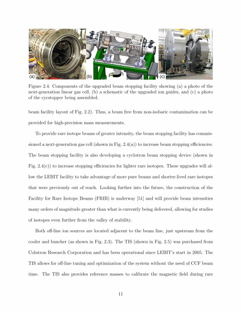
Figure 2.4: Components of the upgraded beam stopping facility showing (a) a photo of thenext-generation linear gas cell, (b) a schematic of the upgraded ion guides, and (c) a photoof the cycstopper being assembled.
beam facility layout of Fig. 2.2). Thus, a beam free from non-isobaric contamination can be
provided for high-precision mass measurements.
To provide rare isotope beams of greater intensity, the beam stopping facility has commis-
sioned a next-generation gas cell (shown in Fig. 2.4(a)) to increase beam stopping efficiencies.
The beam stopping facility is also developing a cyclotron beam stopping device (shown in
Fig. 2.4(c)) to increase stopping efficiencies for lighter rare isotopes. These upgrades will al-
low the LEBIT facility to take advantage of more pure beams and shorter-lived rare isotopes
that were previously out of reach. Looking further into the future, the construction of the
Facility for Rare Isotope Beams (FRIB) is underway [51] and will provide beam intensities
many orders of magnitude greater than what is currently being delivered, allowing for studies
of isotopes even further from the valley of stability.
Both off-line ion sources are located adjacent to the beam line, just upstream from the
cooler and buncher (as shown in Fig. 2.3). The TIS (shown in Fig. 2.5) was purchased from
Colutron Research Corporation and has been operational since LEBIT’s start in 2005. The
TIS allows for off-line tuning and optimization of the system without the need of CCF beam
time. The TIS also provides reference masses to calibrate the magnetic field during rare
11

Figure 2.5: The plasma test ion source assembly shown removed from the vacuum chamber.
isotope measurements.
The TIS is able to produce stable alkali ions (Na, K, Rb, and Cs) as well as ionized noble
gases (Ne, Ar, and Kr) depending on which mode the TIS is utilized. In surface ionization
mode, a tungsten filament is heated by passing a current through the filament, positively
biased to ∼ 100 V, inside a boron nitride oven operated at temperatures up to 2000 degrees
Celsius. When the filament is heated, alkali ions (as impurities in the filament) are created
through surface ionization and are extracted through a pin hole in the anode at the end of
the chamber. Alternatively, ionized noble gases can be produced by feeding a neutral gas
into the ion source chamber through a support gas inlet in the back of the ion source. The
filament is then reversed biased until a discharge is created. The shower of electrons created
from the discharge bombards the gas molecules and ionizes the gas through electron-impact
ionization. The TIS is located perpendicular to the beam line, therefore, an electrostatic
quadrupole steering element is utilized to deflect the beam either upstream to the beam
stopping facility or downstream through the beam cooler and buncher to the 9.4 T Penning
trap mass spectrometer.
12

Figure 2.6: Photos of (a) the cooler and (b) the buncher before insertion into the beam line.
One of the upgrades recently made to the LEBIT facility was the construction of the
LAS by Scott Bustabad. The LAS is located opposite from the TIS on the other side
of the beam line. The LAS produces ions by focusing a laser beam, produced by a high
power ∼ 2 W Nd:YAG laser, onto a metallic target. When a pulse from the laser strikes the
target ionized material is ejected, extracted, and transported to the electrostatic quadrupole
steering element that deflects the beam either upstream or downstream.
2.3.2 Cooler and Buncher
The cooler and buncher [52] are located just downstream of the off-line ion sources and the
components are shown, removed from the beam line, in Fig. 2.6. The cooler and buncher
transform the continuous beam into the low-emittance pulses with low-energy spread required
for high-precision Penning trap mass measurements. The cooler and buncher are composed
of a gas-filled RFQ in conjunction with a linear Paul trap, a standard tool used to produce
low-emittance pulsed ion beams [42].
13

Figure 2.7: Photos of (a) LEBIT’s hyperbolic Penning trap and (b) the 9.4 T superconductingmagnet.
2.3.3 9.4 T Penning Trap Mass Spectrometer
After the continuous beam has been cooled and bunched, it is transported to the 9.4 T su-
perconducting Penning trap mass spectrometer. The LEBIT mass spectrometer employs
a persistent superconducting magnet with a horizontal bore (shown in Fig. 2.7(b)) to pro-
duce a highly uniform magnetic field with a strength of 9.4 T. The Penning trap, shown in
Fig. 2.7(a), consists of two hyperbolic endcaps and an eightfold segmented ring used to create
an electric quadrupole trapping potential with a cylindrical symmetry. The Penning trap
electrode structure resides in the center of the bore of the magnet and can be held at room
temperature or cooled with Liquid Nitrogen (LN2). To reduce the influence of external fields
affecting the homogeneity of the magnetic field, the magnet is actively shielded through the
implementation of Gabrielse coils [53].
14

Figure 2.8: Schematic diagram of ion preparation, non-isobaric purification, and ion detec-tion equipment at the LEBIT facility.
2.4 LEBIT II - Techniques Used at the LEBIT Facility
2.4.1 Ion Preparation and Non-Isobaric Beam Purification
A basic schematic diagram of the equipment used to prepare, purify, and detect ions at the
LEBIT facility is shown in Fig. 2.8. Before the rare isotope beam enters into the cooler, it
is slowed down to ∼ 10 eV using a set of electrostatic deceleration electrodes. (Alternatively,
ions can be sent to the cooler from either the TIS or the LAS.) The ions then enter the
cooler section of the cooler and buncher where slowing and transverse cooling of the ions is
performed through buffer-gas cooling. The RFQ ion guide structure in the cooler provides
radial confinement of the ions [54] through a set of four rodlike electrodes. A Radio-Frequency
(RF) signal at a given phase, amplitude, and frequency is applied to two electrodes opposite
one another. The same signal is applied to the other two rods, but 180 degrees out of phase.
The application of these signals to the rods creates a pseudopotential that radially confines
the ions [55, 56].
The RFQ structure in the cooler implements a novel design where the four ion guide
15
electrodes are located inside a cylindrical electrode which is split lengthwise into four wedge-
shaped electrodes to provide a field gradient that drags the ions through the buffer-gas [50].
The cooler is usually filled with ultra-pure helium gas at a pressure of a few 10−2 mbar
and is regulated by an electromagnetic solenoid valve controlled by a Proportional-Integral-
Derivative (PID) loop [57].
A micro-RFQ (µRFQ) separates the cooler and buncher sections to allow for differential
pumping and for efficient transport from the cooler to the buncher. In the µRFQ, a helium
background is maintained at a pressure of 10−4 mbar. The buncher electrode configuration
consists of a conventional RFQ ion guide located inside seven ring electrodes. The ion guide
provides the radial confinement of the ions and the seven ring electrodes are used to produce
an axial electrostatic field. In continuous mode, the beam’s emittance and energy spread is
lowered in the cooler, then the beam is transported through the µRFQ and passes through
the buncher. Alternatively, the seven ring segments can be biased to create an axial potential
well where the ions can be accumulated and further cooled, usually for about 30 ms. The
cooled ion bunch is ejected from the buncher by lowering the potential on the final ring
electrode to deliver a low-emittance bunch with a sub-µs pulse width [57].
The low-emittance pulse of ions ejected from the buncher is accelerated to 2 keV, focused,
and transported to the high-precision Penning trap located inside the horizontal bore of the
9.4 T superconducting solenoid magnet. During transport to the magnet, the ions pass
through a pulsed drift tube that adjusts the kinetic energy of the ion bunches for optimal
injection into the Penning trap [58]. Before injection into the magnet, any non-isobaric
contaminants present in the pulse of ions from the buncher can be separated by their A/Q
value using a Time-Of-Flight (TOF) mass filter with a resolving power of ∼ 200 [57]. The
ions are then slowed inside the injection optics, located in the first half of the magnet, leading
16

Figure 2.9: Schematic of a Penning trap. The hyperbolic electrode structure of the Penningtrap is used to create a quadrupole potential by applying a voltage, Vo, across the endcapand ring electrodes in a strong magnetic field, B. The size of the trap is characterized bythe trap length, zo, and the trap radius, ρo.
to the Penning trap. Before the ions enter the Penning trap, a Lorentz steerer is used to
quickly prepare the ions for a mass measurement [59].
2.4.2 Penning Trap Mass Spectrometry
PTMS relies on the fundamental motion of charged particles trapped in a strong magnetic
field. To achieve 3-D confinement of charged particles, an axial quadrupole electric field is
superimposed on top of a strong, homogeneous axial magnetic field as shown in Fig. 2.9. The
strong magnetic field confines the ions radially, while the quadrupole electric field confines
the ions in the axial direction. The quadruple electric field at the LEBIT facility is created by
two hyperbolic endcap electrodes and one hyperbolic ring electrode that has been segmented
eight-fold for the application of various RF electromagnetic fields. To allow the injection
and ejection of ions into and out of the trap there is a small hole in the center of each of the
endcaps. The size of the Penning trap can be described by the characteristic trap parameter,
d, given by:
d =
√ρ2o
4+z2o
2, (2.1)
17

where ρo corresponds to the trap radius, and zo corresponds to the trap length. The LEBIT
Penning trap, for example, has a d of 10.23 mm.
The hyperbolic electrode structure is the most desirable Penning trap geometry, because
higher order components of the quadrupole electric field are minimized. Imperfections in
the trapping potential due to the segmented ring electrodes and the holes in the endcaps,
however, distort the perfect quadrupole potential and introduce anharmonic terms to the
pure quadrupole potential. Machining imperfections also contribute to anharmonicities in
the trapping potential. Therefore, additional correction electrodes between the endcaps and
ring electrodes and at the entrance and exit holes of the endcaps (not shown in Fig. 2.9),
surround the trap and are tuned to minimize the effects of these trap imperfections on the
ion motion [58].
Charged particles in the presence of a magnetic field undergo cyclotron motion, a radial
motion about the magnetic field as described by the Lorentz force, at a frequency that
depends only on the charge, q , and mass, m, of the particles together with the strength of
the magnetic field, B , at the position of the particles, and is given by the expression:
ωc =q
mB. (2.2)
When charged particles are also axially confined inside a Penning trap, by superimposing
the quadrupole electric field on top of the magnetic field, they undergo the three basic
eigenmotions, or normal-mode oscillations, shown in Fig. 2.10: one in the axial direction at
a frequency, ωz , and two in the radial direction at frequencies ω− and ω+. The eigenmotion
associated with frequency ω−, known as magnetron motion, is resultant of the E×B drift
motion and is typically much slower than the reduced cyclotron motion at the modified
18

Figure 2.10: Illustration of the eigenmotions executed in a Penning trap in a strong magneticfield: axial oscillations in the direction parallel to the magnetic field, the slower radialmagnetron motion due to the E×B drift, and the faster radial reduced cyclotron motion.
frequency of ω+.
For particles in a Penning trap with a pure electric quadrupole potential, the radial
frequencies of the eigenmotions are related to the true cyclotron frequency and the axial
oscillation frequency by the expression:
ω± =ωc2±√ω2c
4− ω2
z
2. (2.3)
The axial oscillation frequency, ωz , can be found through the relation:
ωz =
√qVomd2
, (2.4)
where Vo is the potential difference between the endcaps and the ring electrode and d is the
characteristic trap parameter. Two other important equations that relate the frequencies of
the radial motions of ions confined in a Penning trap are:
ω+ + ω− = ωc (2.5)
19

and
ω+ω− =ω2z
2. (2.6)
At the LEBIT facility, the true cyclotron frequency, νc = ωc/2π, of an ion is measured
using the TOF – Ion Cyclotron Resonance (TOF-ICR) detection technique [60, 61]. First, the
ions are given an initial kick off-center with the Lorentz steerer [62] prior to entering the trap
to prepare them with some initial magnetron motion. The ions are then dynamically captured
in the Penning trap such that the ions’ axially energy in the trap is minimized by setting
the pulsed drift tube potential. Potential isobaric contaminants are then removed from the
Penning trap by driving them to large radial orbits with a resonant RF azimuthal dipole
field. Then, to measure νc , the trapped ions are exposed to an azimuthal quadrupole RF
field at a frequency νRF near their cyclotron frequency with the appropriate RF amplitude
and excitation time which fully converts the ions’ initial magnetron motion into cyclotron
motion [60, 61].
After ejection from the trap, the ions travel through the inhomogeneous section of the
magnetic field, where the ions’ radial energy is transferred into axial energy [63]. An ion’s
TOF is then determined by detecting the ion with the MCP located just downstream of the
superconducting magnet. In resonance, i.e., νRF = νc, the energy pickup of an ion’s radial
motion is maximized and results in a shorter TOF to the MCP [61]. For a cyclotron frequency
determination, this cycle of trapping, excitation, ejection, and TOF measurement is repeated
for different frequencies near the cyclotron frequency of the ion of interest. Through this
process cyclotron resonance curves, as shown in Fig. 2.11, with a centroid at νc are obtained.
The mass resolving power, defined as m/∆m of a cyclotron frequency measurement, is
linearly proportional to the RF excitation time, TRF , and the cyclotron frequency, ωc, and
20

Figure 2.11: A typical time-of-flight cyclotron resonance curve. A fit of the theoretical lineshape to the data is represented by the solid line (red).
can be written as:
R ≡ m
∆m= TRF · νc. (2.7)
It is therefore desirable to use excitation times as long as possible, the limits of which
are set by damping due to collisions with background gas and the lifetime of the isotope
being measured. Increased precision of the cyclotron frequency measurement isn’t enough
to extract an ion’s mass since the mass also depends on the strength of the magnetic field,
which needs to be known to a precision comparable to the precision of the cyclotron frequency
measurement. To determine the strength of the magnetic field, interleaving calibration (or
reference) measurements on an ion species with a well-known mass (and known charge state)
must be performed.
2.4.3 Reference Measurements
In a perfect world, the magnetic field would only need to be calibrated once; the magnetic
field strength of LEBIT’s persistent 9.4 T superconducting magnet, however, slowly decays
21
over time. The magnetic field is persistent, meaning it is only energized once, and as the
electrons encounter a small resistance while flowing through splices in the superconducting
wire of the magnet the current slowly decreases [64]. Thankfully, the resistance is so small
that the relative change in the magnetic field is on the order of (dB/B)/dt ≈ -8× 10⁻⁸ hr−1
[65], but it can still have an effect on a high-precision measurement that might extend over
the course of an hour or so and result in a broadening of the cyclotron resonance curve. To
mitigate broadening of cyclotron frequency resonances due to the magnetic field decay, a
small current is passed through room-temperature compensation coils, composed of a pair
of insulated copper wires wound around the bore tube of the magnet, that is ramped at a
steady rate to stabilize the drift of the resulting total magnetic field. Thus, if the magnetic
field drift of the superconducting magnet is linear with a constant rate of decay, there would
be minimal need for reference measurements (except for initial calibration measurements
when the power supply of the magnetic field compensation coils is reset). Unfortunately,
non-negligible changes in the magnetic field are known to be caused by pressure fluctuations
in a pressure unregulated cryostat of a superconducting magnet containing Liquid Helium
(LHe) [66] and can be just as important as those caused by magnetic field decay.
During the LEBIT facility’s pilot experiment, significant changes in the magnetic field
were found to be correlated to variations in the atmospheric pressure as shown in Fig. 2.12(a)
[65]. To eliminate the effects of atmospheric pressure affecting the internal pressure of
the LHe bath in the cryostat, an electromagnetic flow regulating valve together with a
high-precision barometer (Setra), used to measure the cryostat’s pressure, and a LabVIEW
controlled PID loop were implemented to regulate the cryostat’s pressure to within 10 ppm
[65]. Fig. 2.12(b) shows that even with a pressure stabilized cryostat, noticeable non-linear
changes in the magnetic field were still present on the scale of a few hours. It was therefore
22

Figure 2.12: (a) Magnetic field drift of LEBIT’s 9.4 T superconducting magnet during rareisotope measurements of 37Ca and 38Ca. The solid line (red) represents the atmosphericpressure data from a local weather station as reported by Weather Underground (Wunder)and the dashed line represents the pressure data recorded from a high-precision barometer(Setra) located at the NSCL. Note that (∆B/B)/dp = 4.5× 10⁻⁸ mbar−1. (b) Residual non-linear drift after stabilizing the pressure of the liquid helium bath of the superconductingmagnet and subtracting out the linear magnetic field decay. (Note the change in scalesbetween the two graphs.)
Figure 2.13: Cartoon showing how reference cyclotron frequency measurements (blue dots)are used to interpolate the strength of the magnetic field during a rare isotope cyclotronfrequency measurement (red dots).
23

decided that high-precision mass measurements require a cyclotron frequency measurement
with a reference ion (a well-known mass) be performed prior to and following a cyclotron
frequency measurement of the ion of interest, no more than an hour apart from one another.
In this scenario, the magnetic field can be interpolated from the reference measurements to
the time when the cyclotron frequency of the ion of interest was measured as depicted in
Fig. 2.13.
24

Chapter 3
First Direct Double-Beta Decay
Q-value Measurement of 82Se
3.1 Motivation for Determining the 82Se Double-Beta
Decay Q-value
Interest in ββ decay has been increasing since the laboratory verification of the weak, but
allowed, two-neutrino double-beta decay (2νββ decay) of 82Se [67]. Including laboratory,
geochemical, and radiochemical experiments, twelve isotopes have been observed to undergo
2νββ decay: 48Ca, 76Ge, 82Se, 96Zr, 100Mo, 116Cd, 128Te, 130Te, 136Xe, 150Nd, 238U, and
double-electron capture in 130Ba [68, 69]. With the exception of the unconfirmed claim in
Ref. [70] for 76Ge, 0νββ decay has yet to be observed. If 0νββ decay is confirmed, there
would be evidence that the neutrino is a Majorana particle and that conservation of total
lepton number is violated – a situation forbidden by the Standard Model of particle physics.
Is is therefore not surprising that there are a number of groups currently building large scale
detectors all vying to be the first to unambiguously observe 0νββ decay.
25

The defining observable of 0νββ decay is a single peak in the electron sum-energy spec-
trum at the ββ decay Q-value, Qββ . Hence, it is crucial to have an accurate and precise
determination of Qββ . The Q-value is also required to calculate the Phase Space Factor
(PSF) of the decay. The effective Majorana neutrino mass, together with the corresponding
PSF and Nuclear Matrix Element (NME) for a 0νββ decay candidate provide the necessary
information to determine the 0νββ decay half-life, which is given by:
(T 0ν1/2)−1 = G0ν(Qββ
5, Z)|M0ν |2(〈mββ〉/me)2, (3.1)
where M0ν is the relevant NME, 〈mββ〉 is the effective Majorana neutrino mass, me is
the mass of the electron, and G0ν is the PSF for the 0νββ decay, which is a function of
Qββ5 and the nuclear charge, Z . Thus, to obtain an accurate estimation of the half-life
sensitivity required to detect a given 〈mββ〉, or conversely, to determine 〈mββ〉 if the half-life
is measured, the NME and especially the Q-value need to be known with sufficient precision.
An extensive campaign is currently underway to develop next-generation experiments to
detect 0νββ decay in a number of candidate isotopes (see Ref. [71] for a recent review of
planned experiments). The seven most developed and promising projects aimed to detect
0νββ decay include the GERmanium Detector Array (GERDA) and Majorana experiments
which will probe for 0νββ decay with 76Ge, the Super Neutrino Ettore Majorana Obser-
vatory (SuperNEMO) with 82Se, the Cryogenic Underground Observatory for Rare Events
(CUORE) with 130Te, the Enriched Xenon Observatory (EXO) and the Kamioka Liquid
scintillator AntiNeutrino Detector (KamLAND-Xe) with 136Xe, and the Sudbury Neutrino
Observatory (SNO+) with 150Nd [71]. The SuperNEMO experiment is expected to provide
an increase in sensitivity of three orders of magnitude over its predecessor, NEMO-III, and
26

is projected to reach a half-life sensitivity at the 90% confidence level of 1 - 2× 1026 years by
observing 100 - 200 kg of 82Se for five years [71, 72]. These experiments are currently, or are
planning to reach sensitivities of an effective neutrino mass of tens of meV. At this sensitivity,
not only does the probability increase for detecting 0νββ decay, but these experiments may
also allow identification of the mass hierarchy of the three neutrino mass eigenstates [22].
To experimentally resolve the single 0νββ decay peak in the electron sum-energy spec-
trum above the tail of the 2νββ decay electron sum-energy distribution, a Qββ greater than
2 MeV is desired. In 2012, the LEBIT facility began a measurement campaign to determine
the Q-values of the four (of the eleven) 0νββ decay candidates with Q-values greater than
2 MeV [22] that have not been measured via PTMS. The seven 0νββ decay candidates (with
Q-values greater than 2 MeV) previously determined through measurements at PTMS facil-
ities include: 76Ge [24, 25, 26], 100Mo [25], 110Pd [23, 27], 116Cd [28], 130Te [28, 29, 30],
136Xe [31, 32], and 150Nd [33]. The LEBIT facility’s 0νββ decay Q-value measurement cam-
paign began with a new determination of the ββ decay Q-value of 48Ca [46] and the first
direct ββ decay Q-value measurement of 82Se [73] (as part of this work) and ended with
the ββ decay Q-value determination of 96Zr [49]. During this time, the ββ decay Q-value of
124Sn was determined directly via PTMS at SHIPTRAP [74].
The previous literature value for the ββ decay Q-value of 82Se was published by the
2003 Atomic Mass Evaluation (AME2003) [75]. In the AME2003, the mass of each iostope
was determined by evaluating the results of various experiments and a weighted average
was calculated to obtain the respective mass values (the reader is referred to Ref. [75] for
details). The mass of 82Se was evaluated using the results of two high resolution mass
spectrometer measurements [76, 77] and a 82Se(p,t)80Se reaction Q-value measurement [78].
The mass of 82Kr was evaluated using the results of a PTMS measurement [79], the high
27

resolution mass spectrometer measurement from [76], and an experiment which reported the
β decay scheme of 82Br as determined through coincidence and direct measurements from an
intermediate-image spectrometer and a conventional gamma-gamma coincidence scintillation
spectrometer [80]. Using these mass data, AME2003 determined the ββ decay Q-value to
be Qββ = 2 996(2) keV. This level of precision is sufficiently precise for SuperNEMO which
will rely on plastic scintillators to determine the energy of the emitted electrons with a
resolution of ∆E/E ∼ 8 - 10 % (FWHM) at E = 1 MeV [71]. Future experiments searching
for 0νββ decay with 82Se could improve energy resolution by utilizing large mass ZnSe
bolometers which can currently achieve an energy resolution on the keV level [81]. If these
detectors are utilized to search for 0νββ decay of 82Se, a sub-keV uncertainty in the Q-value
would be required to ensure that the detected peak is resultant from 0νββ decay and not
background events. In addition, an improvement in the precision of the Q-value by an order
of magnitude would further constrain the mass of the neutrino if 0νββ decay of 82Se is
observed.
3.2 Experimental Setup
The direct Qββ measurement of 82Se was carried out at the NSCL using the LEBIT facility
where the TIS was used as a source of the measured isotopes. One of the benefits of the TIS
is that not only can stable noble and alkali ions be produced, but elements with high enough
vapor pressures can be heated inside the oven, vaporized, and ionized with a discharge
in noble gas mode. In this technique, a ceramic charge holder is filled with the desired
element of interest and secured on both ends with a bit of glass wool before being inserted
into the ion source chamber. Glass wool is convenient since it is rigid enough to contain
28

the desired element, but also porous enough to allow the vaporized element to escape into
the ion source chamber. The vapor is then ionized in noble gas mode, and a buffer gas
is utilized to facilitate multiplication of electrons from the filament. Using this technique,
mass measurements can be performed on long-lived rare isotopes off-line, depending on
the natural abundances of the isotopes of the element placed in the charge holder. This
method was previously utilized to perform a mass measurement on 48Ca [46], with a natural
abundance of 0.187 %, but it becomes more difficult to produce rare isotopes with smaller
natural abundances using this method without obtaining isotopically enriched samples. This
method was well suited for producing 82Se and 82Kr isotopes with natural abundances of
8.73 % and 11.58 %, respectively.
The plasma TIS was used to simultaneously produce ions of 82Se and of the ββ decay
daughter, 82Kr. To produce the ions, the ceramic charge holder was filled with ∼ 200 mg
of granulated selenium and inserted into the oven of the TIS. The granulated selenium was
then vaporized and some fraction was ionized. A helium support gas for the source was
mixed with the proper amount of krypton to maintain a balance in the ratio of the number
of 82Kr and 82Se ions produced within a factor of three. The extracted ion beam was guided
through a RFQ mass filter to suppress the strong accompanying helium current before being
deflected downstream by the quadrupole steerer to the beam cooler and buncher. The short
low-emittance ion bunches produced by the beam cooler and buncher were then sent to the
Penning trap [42]. On their path the ions were purified further by using the TOF mass filter
[82], allowing only ion species with an A/Q = 82 to be dynamically captured in the trap.
29

Figure 3.1: Example of a time-of-flight cyclotron resonance curve for 82Se+. An excitationtime of TRF = 750 ms was used to obtain a resolving power of 2× 10⁶. The results of fittingthe theoretical line shape to the data is represented by the solid line (red).
3.3 Measurements
The measurement process for the determination of Qββ(82Se) consisted of alternating cy-
clotron frequency measurements of 82Kr+ and 82Se+. These measurements were performed
in a series of four runs. The first run consisted of measurements using TRF = 500 ms, but for
increased precision, a TRF = 750 ms was used for the final three runs. Each TOF resonance
was the average of 25 to 40 scans over the respective frequency range with 41 trapping cycles
per scan. A TOF resonance of 82Se+ with TRF = 750 ms is shown in Fig. 3.1. During
the measurement process the number of ions in each pulse ejected from the buncher was
limited using the appropriate accumulation time such that only an average of 2 ions per
trapping cycle were recorded by the MCP, corresponding to < 7 ions in the trap at one
time (assuming 30 % detector efficiency). This was done to limit the number of contaminant
ions produced via charge-exchange reactions with residual gas in the trap. Each resonance
30

Figure 3.2: Difference between the cyclotron frequency ratio of 82Kr+ to 82Se+ and the ratioobtained from literature mass data [75]. The solid lines indicate the weighted average andthe 1σ statistical uncertainty band.
consisted of ∼ 500 - 3000 detected ions, depending on the number of scans per resonance and
the beam current from the ion source. To determine νc , each resonance was fitted using the
theoretical line shape described in Ref. [61]. The standard deviation of νc for each resonance
was ∼ 30 ppb (parts per billion).
Drifts in the magnetic field during the frequency ratio determination of 82Kr+ to 82Se+
were accounted for by linearly interpolating between the two cyclotron frequency measure-
ments of 82Kr+ bracketing each 82Se+ measurement to obtain νintc (82Kr+). This interpo-
lated cyclotron frequency was used to obtain the frequency ratio R = νintc (82Kr+)/νc(82Se+).
The values obtained from a total of 110 ratio determinations and their weighted average are
shown in Fig. 3.2. The difference to the reference ratio, RAME2003, was calculated using
RAME2003 = [m(82Kr)−me ]/[m(82Se)−me ] with the mass values from AME2003 [75].
31

3.4 Data Analysis
In preparation for, and during the measurement process, great care was taken to minimize
possible systematic effects. By measuring mass doublets, contributions to the measurement
uncertainty arising from mass dependent systematic effects due to frequency shifts, for ex-
ample caused by field imperfections, are essentially removed. Nevertheless, prior to the
measurements, imperfections of the trapping potential were carefully minimized by tuning
the correction electrodes of the hyperbolic Penning trap according to the tuning procedure
described in Ref. [83].
Any effect from non-linear magnetic field drifts are not accounted for in this data eval-
uation and are not mitigated by using a mass doublet. Therefore, the cyclotron frequency
measurements of 82Kr+ and 82Se+ were alternated with a period of no greater than 1 hour.
Based on an earlier study [15], this should lead to residual systematic effects of the cyclotron
frequency ratio no greater than 1 ppb. This uncertainty was further minimized as the pres-
sure in the cryostat was stabilized to 10 ppm (parts per million) during the measurements
[65], resulting in an uncertainty well below 1 ppb. In addition, simultaneously trapped ions
with a different m/q value can cause frequency shifts [84]. This effect was minimized by
verifying that contaminant ions were never present at a level exceeding a few percent, low
enough to not lead to a significant shift at the desired precision.
The weighted average of the ratios for the individual runs and the corresponding sta-
tistical uncertainty are listed in Table 3.1 together with the weighted average RLEBIT of
all results and the value RAME2003 calculated using the mass values of 82Kr and 82Se from
AME2003 [75]. Through evaluation of the entire data set, with statistical errors as obtained
from fitting the theoretical lineshapes to the measured cyclotron resonance curves, a Birge
32

Table 3.1: Average cyclotron frequency ratios Rrun= νintc (82Kr+)/νc(82Se+) with theirstatistical errors as obtained in four separate runs with N frequency ratio measurementsperformed in each run. Also given is the final weighted average RLEBIT with its statisticaland final uncertainty and the ratio calculated using the mass values from AME2003 [75].
Run N Rrun1 53 1.000 039 285(5)2 2 1.000 039 30(2)3 7 1.000 039 29(1)4 48 1.000 039 290(4)RLEBIT 1.000 039 290(4)(5)RAME2003 1.000 039 26(3)
ratio [85] of 1.27(5) was determined. While close to unity, the significant deviation from
unity indicates the presence of residual systematic effects at the 0.8 ppb level not discovered
in the individual measurements or in the tests for systematic effects performed. Therefore, to
account for these non-statistical contributions, the statistical uncertainty of the weighted av-
erage RLEBIT for all data was multiplied by the value of the Birge ratio. Both the statistical
and total uncertainty for RLEBIT are given in Table 3.1.
The ββ decay Q-value was determined from the mass difference between the mother
nuclide of mass mm and daughter nuclide of mass md through:
Qββ
c2= mm −md = (R− 1) (md −me), (3.2)
where R is the cyclotron frequency ratio between the singly charged ions of the daughter
and mother nuclides, c is the speed of light, and me accounts for the missing electron mass
of singly charged ions used in the measurement. Using the final frequency ratio RLEBIT and
the AME2003 mass for 82Kr, the Q-value was calculated to be Qββ = 2 997.9(3) keV. The
new LEBIT Q-value is nearly an order of magnitude more precise than the previous value
published in AME2003 [75] and is a dramatic improvement to one of the ingredients needed
33

for a better determination of the half-life limit for 0νββ decay in 82Se.
3.5 Discussion of Results and Conclusion
By using Penning trap mass spectrometry, the first direct Q-value measurement of 82Se
ββ decay was performed by measuring the cyclotron frequency ratio between singly charged
ions of 82Se and the ββ decay daughter, 82Kr. The result, Qββ = 2 997.9(3) keV, is nearly
an order of magnitude more precise than the previous value published in AME2003 [75].
Following the procedure in Ref. [86] and using the new Q-value, the PSF for the 0νββ decay
mode of 82Se was calculated to be G0ν = 2.848(1)× 10−14 yr−1, where the uncertainty has
also been improved by nearly an order of magnitude. With a corrected shell model NME
calculation [73] and the current upper limits of 〈mββ〉= 140 - 380 meV from the EXO-200
experiment [87] a lower limit range for the 82Se 0νββ decay half-life of 5.0× 1024 - 3.7× 1025
years was obtained. Assuming SuperNEMO achieves its projected sensitivity at the 90%
confidence level of 1 - 2× 1026 years, an effective neutrino mass as low as 60 - 85 meV could
be detected.
34

Chapter 4
Development of a High-Precision
Magnetometer for the LEBIT Facility
To increase the precision of high-precision mass measurements at the LEBIT facility (and
other PTMS facilities) changes in the magnetic field need to be measured to a precision better
than the mass measurements, which can be better than 1 part in 108. A commercial Nuclear
Magnetic Resonance (NMR) magnetometer could be installed, but they are currently limited
to resolutions of about 1 part in 107. It is also advantageous to develop a magnetometer
that is radiation hard for high-precision magnetic field monitoring in the presence of high
levels of ionizing radiation where NMR probes cannot be used.
The development of the magnetometer required a multi-disciplinary approach including
ion trap physics, mechanical and electrical engineering, software development, chemistry, and
advanced microscopy. The main component of the magnetometer, a Penning trap, needed
to be optimized not only to achieve high-precision, but also engineered for ease of assembly
and installation. In addition, the magnetometer had to be installed in a superconducting
35

magnet to demonstrate that it could indeed detect changes in the magnetic field strength to
a relative precision of 1 part in 108.
4.1 Motivation for a High-Precision Magnetometer
The LEBIT facility, and similar PTMS facilities, rely on mass measurements of a well-
known ion species to calibrate the magnetic field before and after each rare isotope cyclotron
frequency TOF resonance. This technique has worked well, but there are a couple drawbacks
to the reference measurement interpolation method. First, valuable beam time is wasted
on performing reference measurements. Second, this method does not account for non-
linear fluctuations in the magnetic field strength of the superconducting magnet that may
occur on time scales shorter than the time required to perform a TOF cyclotron frequency
measurement, which is typically on the order of 10 minutes for a reference measurement. For
a cyclotron frequency measurement of rare isotopes, however, the time required to obtain a
TOF resonance is determined by the rate at which the rare isotope is delivered to the Penning
trap. If non-linear magnetic field fluctuations are present, a broadening and shifting of the
TOF resonance curve could occur for the cyclotron frequency measurements of the more
exotic rare isotopes with longer measurement times. The non-linearity of the magnetic field
thus presents a limitation on the precision and feasibility of a measurement when pushing
the limits of mass measurements to extremely rare isotopes. If the strength of the magnetic
field could be determined by some other method simultaneous to a rare isotope frequency
measurement, more precise mass measurements of the most exotic rare isotopes measurable
by PTMS could be obtained.
Measuring short-term fluctuations of the magnetic field without performing reference
36

Figure 4.1: Cartoon showing how two reference cyclotron frequency measurements (bluedots) are used to calibrate a magnetometer that can track short-term fluctuations in themagnetic field allowing for either a longer rare isotope frequency measurement time, or asshown, increase the number of rare isotope frequency measurements (red dots).
measurements between (or during) rare isotope measurements (as depicted in Fig. 4.1) would
allow the LEBIT facility, and similar PTMS facilities, to increase efficiency. For less exotic
rare isotopes, more measurements could be performed resulting in a reduced uncertainty
in the measurement with increased statistics. With a greater efficiency, less time would be
necessary to reach a given precision and measurements of more rare isotope species could
be performed during a given beam time, increasing the LEBIT facility’s scientific output.
Finally, by continuously monitoring the magnetic field, the precision of measurements of
extremely rare isotopes could be improved. Therefore, a novel high-precision magnetometer
was designed, built, and tested that will be installed in the LEBIT facility’s 9.4 T supercon-
ducting magnet.
37

4.2 Magnetometer Concept and Design Requirements
The idea behind the high-precision magnetometer is to continuously monitor magnetic field
fluctuations by monitoring the cyclotron frequency of a reference ion in a miniature Penning
trap (MiniTrap) installed adjacent to the LEBIT facility’s high-precision measurement trap
in the bore of the 9.4 T superconducting magnet. Ideally, the magnetic field would be
measured by the magnetometer at both the same time and location as the rare isotope
measurement, however, this was not thought to be possible. The time requirement can be
satisfied to within a second or two, however it would be impossible to physically locate
the magnetometer at the center of the Penning trap for obvious reasons. Therefore, the
magnetometer needs to be located as close as possible to the measurement trap since changes
in the magnetic field should be consistent throughout the homogeneous region of the magnetic
field. In this scenario, a simultaneous measurement of a reference ion in the measurement
trap can be used to calibrate the magnetometer, then the magnetometer will track global
changes in the magnetic field (as shown in Fig. 4.1).
The main requirement that, in part, makes the design of the MiniTrap difficult is the
location requirement – the magnetometer needs to be installed directly adjacent to the
measurement trap where it must fit within the existing electrode structure in the bore of the
magnet. A small annular region located adjacent to and just downstream of the hyperbolic
measurement trap, as shown in Fig. 4.2, is available for installation of the magnetometer.
The annular region measures 8.9 cm in length and has inner and outer diameters of 2.4 cm
and 7.3 cm, respectively. The MiniTrap electrode structures must fit within an enclosure no
larger than that annular region.
38

Figure 4.2: Location of the magnetometer depicted in an image of the Penning trap alongwith injection and ejection optics shown removed from the bore of LEBIT’s solenoidal 9.4 Tsuperconducting magnet.
4.3 Technical Development of the Magnetometer
Two methods are used in PTMS to determine cyclotron frequencies, and thus masses, of
ions in a Penning trap. The first is the TOF-ICR method, a destructive technique, and is
utilized at the LEBIT facility to perform high-precision mass measurements as previously
discussed. The second method is called the Fourier Transform – Ion Cyclotron Resonance
(FT-ICR) technique, a non-destructive technique. Instead of detecting ions ejected from
the trap with an MCP detector and recording their TOF, the FT-ICR technique can be
implemented to determine the cyclotron frequency directly in the Penning trap by picking
up a signal induced by the ions’ motion on detection electrodes. The latter method was
chosen for the MiniTrap since it allows the magnetometer to be self-contained. Because
the FT-ICR technique had never been utilized at the LEBIT facility, initial tests required
development work to demonstrate this technique with the LEBIT hyperbolic trap.
Another aspect of the MiniTrap that required technical development was the production
method of the reference ions for which the cyclotron frequency would be measured. It was
39

determined that electron-impact ionization of background gas would be the most convenient
technique. In this method an electron beam is used to remove an electron from an atom
or molecule, thus ionizing it, so that the ion can be trapped and manipulated with the
electromagnetic fields in the MiniTrap.
4.3.1 Fourier Transform – Ion Cyclotron Resonance (FT-ICR)
The FT-ICR technique has been utilized for many years and is very well understood (see ref.
[88] for a review of FT-ICR principles), therefore, I will only cover the basics necessary for the
development of the MiniTrap. FT-ICR operates on the principle of electrostatic induction
where a charge located near the surface of a conductor creates an image charge on the
conductor. When an ion oscillates near the surface of the conductor, the image charge also
oscillates creating an oscillating image current. A schematic representation of the technique
is shown in Fig. 4.3. To detect the image current, ions first need to be confined by a Penning
trap in the presence of a strong magnetic field. Once confined, the radial motions of the
ions need to be excited, thus coalescing the trapped ions into a bunch [60], by applying an
azimuthal RF dipole electromagnetic field. This is accomplished by applying two RF signals
at the same frequency near the frequency of the ions’ radial motion, but 180 degrees out of
phase, to two excitation electrodes opposite one another (shown in Fig. 4.3). The ion bunch,
as it undergoes its radial motion in the plane perpendicular to the magnetic field, induces an
image current on pickup electrodes, usually located on the ring segments of the Penning trap.
The induced image current from two detection electrodes, located opposite one another, is
then amplified by a low noise differential amplifier and subsequently analyzed with a Fast
Fourier Transform (FFT) algorithm to transform the amplified time domain signal into a
frequency domain signal, resulting in a single peak at the frequency of the radial motion.
40

Figure 4.3: Schematic representation of the basic FT-ICR technique where ions are drivenby excitation electrodes (white) and induce an image current in the detection electrodes(green), which is then amplified and detected through FFT Fourier analysis. (Note that theendcap electrodes of the Penning trap that provide axial confinement in the direction of themagnetic field are not shown.)
This technique, known as broadband FT-ICR, is widely used in analytical chemistry and
allows a wide range of masses to be detected [88]. One limitation to this technique, however,
is that it requires many moving ions in order to produce a signal large enough to detect
above the background noise created by surrounding electronic equipment and the thermal
noise of the electronics necessary to transfer and amplify the signal [60].
To achieve the greatest precision, the number of trapped ions should actually be min-
imized. This is necessary to keep the ion bunch coherent and to minimize shifts of the
cyclotron frequency due to image charges [89] and shot-to-shot variations in the number of
trapped ions [84]. With fewer numbers of trapped ions, the image current induced on the
detection electrodes is reduced to the point where the ion’s signal cannot be detected above
background noise. In addition, a large peak in the frequency spectrum of the FFT results
41

Figure 4.4: Schematic representation of the narrow-band FT-ICR technique which includesa variable capacitor (blue) and inductor coil (dark green) to create a resonant circuit. Thepickup coil (light green) is used to decouple the resonant circuit to reduce parasitic capac-itance. Again, the endcap electrodes of the Penning trap are not shown. (In practice, theprimary inductor coil is center-tapped and grounded to alleviate charge build-up on thedetection electrodes.)
in a better fit and thus a lower uncertainty in the center frequency of the resonance peak.
It is thus beneficial to maximize the voltage signal delivered to the pre-amplifier by utilizing
a narrow-band FT-ICR detection method depicted in Fig. 4.4. The narrow-band FT-ICR
detection method requires the installation of an inductor, with inductance Lcoil, and a vari-
able capacitor in parallel to the detection electrodes to create an LCR resonant circuit, with
a resonant frequency, ωo, equal to the radial frequency of the ion’s motion. This allows the
voltage signal produced by the image current to be amplified by the magnitude of the total
impedance of the LCR circuit in resonance, Ro, which is given by:
Ro =Q
ωoC= QωoL, (4.1)
42

where Q is the quality factor, or Q factor, of the resonant circuit and is defined by:
Q ≡ ωo∆ω
, (4.2)
and of course,
ωo =1√LC
. (4.3)
Note that ∆ω corresponds to the frequency width of the resonance where the amplitude is
equal to 1/√
2 of the maximum, L denotes the value of Lcoil plus the parasitic inductance
of the circuit, and C denotes the total capacitance of the circuit (including parasitic capaci-
tance). It is important to maximize the Q factor of the circuit to maximize the amplification
of the signal, which leads to an increase of the signal-to-noise ratio by√Q [90].
To maximize the Q factor of the resonant circuit, several things need to be optimized.
First, a larger circuit capacitance generally leads to a reduction of the Q factor. It is
thus important to build the trap electrodes such that capacitance between the electrodes
is minimized. Second, wiring of the trap electrodes to the resonant circuit must be done
to not only minimize capacitance, but also to minimize the background noise picked up by
the wires. Also, the inductor should be fabricated with an inductance only slightly smaller
than that needed such a that minimal capacitance is required by the variable capacitor used
to tune the resonant frequency of the circuit to match the cyclotron frequency of the ions’
radial motion. Finally, to further minimize parasitic capacitance, a pickup coil wrapped
around the primary inductor should be used to decouple the resonant circuit from the pre-
amplifier. (When using the pickup coil, the primary coil should have a center-tap at ground
to eliminate charge buildup on the detection electrodes.) The resonant circuit and the pre-
amplifier should be placed as close as possible to the detection electrodes (ideally adjacent
43

to the trap in the bore of the superconducting magnet) to reduce the pick-up of background
noise and minimize parasitic capacitance.
It is also important to carefully choose the mass of the reference ion to increase the
precision of the magnetometer. Consider that the MiniTrap measures an ion’s cyclotron
frequency, which is proportional to the magnetic field strength, therefore:
∆ωcωc
∣∣∣∣∆B
=∆B
B. (4.4)
This expression indicates that for a given frequency resolution, to decrease the uncertainty in
a magnetic field measurement, one should measure an ion with as large a cyclotron frequency
as possible, i.e. lighter masses. However, there is a practical limit to how high in frequency,
and thus how light an ion, one can measure. The main limitation comes from the LCR circuit
required for narrow-band detection, where the resonant frequency of the circuit is limited
by the total capacitance and parasitic inductance of the detection circuit. In addition, to
obtain a reasonable Q factor, Lcoil should be non-negligible.
For the implementation of the MiniTrap, the variable capacitor, primary and secondary
inductor, along with the pre-amplifier were located outside of the superconducting magnet
for simplicity and ease of testing. Unfortunately, this configuration increases the total ca-
pacitance and parasitic inductance of the detection circuit. Even with this limitation, an ion
species with a mass as small as 2 u, such as H+2 (corresponding to a frequency of ∼ 72 MHz
in a 9.4 T magnetic field), should be within reach.
44

4.3.2 Ion Production
A convenient way to ionize atoms and molecules in a small volume, as required by the space
constraints of the MiniTrap, is to use either a Field Emission Point (FEP), or a thermionic
emitter. FEPs are composed of a rod of conducting material that has been electrochemically
etched to produce a sharp tip with a radius as small as a few tens of nanometers. The
application of a large potential to the tip of an FEP results in a large local electric field that
enables electrons in the conduction band to overcome the potential barrier at the surface of
the tip and be emitted into vacuum (for a full theoretical description of field emission, see
Ref. [91]). One of the advantages of using an FEP is that it is a cold emitter, i.e. heat is
not needed to produce the electron beam. A thermionic emitter is composed of a metallic
filament that is heated by passing a current through it, thus imparting thermal energy to
the conduction electrons enabling them to overcome the potential barrier. Initially it was
determined that the low operating temperatures of FEPs was an advantage over thermionic
emitters, therefore, considerable effort was required to develop a fabrication technique for
producing FEPs at the NSCL for the MiniTrap.
A variety of techniques have been used over the years to produce FEPs (see ref. [92]
for a basic review of the various techniques). Ultimately, a variation of the lamella drop-off
technique [93, 94] and the floating layer technique [95, 96] was developed by the LEBIT team
and implemented as described in detail in ref. [97]. In Fig. 4.5 an optical image and two
Scanning Electron Microscope (SEM) images at different magnifications of an FEP produced
by the LEBIT team are shown. The imaging was found to be necessary to determine the
likelihood of a tip being “good” before testing, since the testing procedure ranged in time
from several hours to several days for each FEP.
45

Figure 4.5: Images of a field emission point fabricated at the National SuperconductingCyclotron Laboratory as imaged by (a) an optical microscope, (b) a Scanning ElectronMicroscope (SEM) at 1800× magnification, and (c) an SEM at 37,000× magnification.
After testing nearly one hundred FEPs, only a handful were found to emit an electron
beam current stable enough (within 10% of the nominal current) to be used in the MiniTrap.
Tungsten filament thermionic emitters from Kimball Physics Inc. (model number ES-020)
were tested to compare electron beam stability to the FEPs and to determine if thermionic
emitters would heat the vacuum chamber enough to cause problems when producing several
nanoamps of electron beam current. The thermionic emitters outperformed the FEPs with
regards to electron beam current stability with fluctuations of only 5% of the nominal current.
Also, tests of the thermionic emitters indicated that the ambient temperature increased
by no more than 10 degrees Celsius (at several nanoamps of electron beam current) and
could be tolerated by the MiniTrap. For testing FT-ICR with the LEBIT trap, FEPs were
experimented with to ionize background gas, but ultimately, it was decided that the stability
of the thermionic emitters was more beneficial to the precision and reliability of the MiniTrap.
46

Figure 4.6: Schematic of the ion production test setup using the LEBIT 9.4 T superconduct-ing magnet. The electron beam created by the FEP passes through a beam steerer that canblock the electron beam from passing through the Penning trap and being collected on aFaraday plate. (The turbo and roughing pumps located on the ejection side of the magnetare not shown in the figure.)
4.3.3 Testing Ion Production and FT-ICR Techniques in the LEBIT
Penning Trap
Once a good FEP tip was fabricated and found to provide a reproducible electron beam
current, the ion production method was tested in the LEBIT 9.4 T superconducting magnet.
This was convenient at the time, since the LEBIT beam line had yet to be assembled after
the move to the new stopped beam area leaving the LEBIT magnet available. The setup
consisted of the superconducting magnet which was pumped down to a pressure below a few
10−7 mbar using a turbo pump coupled to a roughing pump. On the ejection side of the
magnet, a Faraday plate was mounted to measure the current of the electron beam emitted
from the FEP that was produced on the far side of the magnet after passing through the
Penning trap. To support and locate the FEP on the injection side of the magnet I designed,
optimized (with simulations in SIMION), and fabricated an FEP steering mount which also
allowed the electron beam to be blocked during a cyclotron frequency measurement. A
schematic of the setup for testing ion production in the LEBIT magnet is shown in Fig. 4.6.
47

When installing the FEP, care had to taken, as it needed to be aligned with a 1 mm
hole in the extraction electrode through which electrons could pass to the steering section.
The steering section was used to direct the beam away from or through a small slit at the
end of the steering section to allow the beam to be either blocked or sent through to the
Penning trap while keeping the FEP in a constant emitting mode. To produce the electron
beam the FEP was first biased to -100 V and an extraction electrode, located just a few mm
downstream of the FEP, was adjusted to a potential large enough to produce electron field
emission. The voltage of the extraction electrode was adjusted with a LabVIEW controlled
PID loop to stabilize the electron beam current. When the beam was blocked, the electron
beam current was picked up by the electrodes forming the slit at the end of the steering
section and measured by a Keithley picoammeter. The Faraday plate on the ejection side of
the Penning trap measured the electron beam current that had successfully passed through
the FEP steerer mount and the Penning trap. This provided both verification that the
electron beam was properly aligned and measurement of the actual electron beam current
required to ionize the background gas.
The sequence of events for performing an FT-ICR measurement in the LEBIT trap
consisted of first allowing the electron beam, at a stabilized current and at an energy of
100 eV, to pass through the closed Penning trap (with between a few to 40 V on the endcaps
and the ring segments held at ground potential) for a given period of time (generally 1 second
for an electron beam current of several nanoamps). As the electron beam passed through the
beam line some of the background gas became ionized through electron-impact ionization
and ions created within the potential well of the Penning trap were confined. Once confined,
excitation and detection of the trapped ions was performed.
Before trying to excite radial ion motion, self-excited magnetron motion was detected in
48

the LEBIT hyperbolic Penning trap using the broadband FT-ICR detection scheme. (Here,
the self-excited magnetron motion is referred to as the phenomenon of a random cloud of ions
in a Penning trap coalescing themselves into a bunch through electromagnetic interactions
between the ions and the induced image charges on the ring segments of the Penning trap.) In
order to produce a self-excited magnetron signal, the LEBIT magnet bore was first pumped
down to below 5× 10⁻⁷ mbar. The FEP steerer was then used to allow an electron beam
current of a few nanoamps to pass through the Penning trap for 1 second. After waiting
several seconds, the signal from the pre-amplifier was then acquired and analyzed using the
LabVIEW-based MiniTrap Control System (MTCS) which allowed for the automation of an
FT-ICR measurement and is described in Appendix B. Because the magnetron motion of
ions in a Penning trap is unbound [98], the ions migrate outward from the center of the trap
closer to the detection electrodes where an increased image current will be induced. Waiting
several seconds after ionizing the background gas was, therefore, necessary to obtain a strong
FFT signal. An FFT resonance of self-excited magnetron motion is shown in Fig. 4.7.
Detection of the reduced cyclotron motion at ω+, the largest frequency of the three eigen-
motions, is necessary since it is the only eigenfrequency largely proportional to the magnetic
field. Before detecting reduced cyclotron motion, the methods of exciting magnetron motion
with both sweep and pulsed excitations (see [88] for technical details) were investigated.
Testing both excitation methods was necessary because reduced cyclotron motion does not
self-cohere similar to magnetron motion, not to mention ω+ is highly mass dependent and
it was unclear what residual gas species were being ionized and detected in the Penning
trap through their magnetron motion. Experimenting with not only excitations of a fixed
frequency and amplitude to drive the magnetron motion, but also with a frequency sweep
signal at a fixed amplitude, enabled a broad frequency range to be probed to search for and
49

Figure 4.7: An FFT resonance of self-excited magnetron motion with trapped ions in a 40 Vpotential well.
identify ion species confined in the trap.
The frequency sweep excitation was used to identify ion species in the Penning trap
using the axial detection method of FT-ICR. Since the axial frequency is related to an ion’s
mass through Eqn. 2.4, this method allowed identification of the mass of the ion species by
determining ωz. (Note that this method was convenient, since the frequency range to probe
the axial motion of the ions is generally an order of magnitude smaller than that for cyclotron
motion.) To probe for axial motion, the ions axial motion was excited with a sweep signal
applied to the one of the endcaps of the hyperbolic trap while the pre-amplifier was connected
directly to the other endcap (the broadband FT-ICR axial detection configuration). The ring
and correction electrodes were then negatively biased to create the proper trapping potential
(with the endcap electrodes at ground potential). Using a trapping potential of 40 V, two
resonances were observed and are shown in Fig. 4.8. Analysis of the peaks indicated that
the peak on the left resulted from the axial motion of H3O+, while the peak on the right
50

Figure 4.8: FFT resonances of two different ion species in the trap using the broadband axialdetection method. Both ions were excited simultaneously using a sweep excitation appliedto one endcap, while the image current was picked up on the other endcap. The peak on theleft was identified as H3O+ and the peak on the right was identified as HO+
2 .
resulted from the axial motion of HO+2 , at masses of 19 u and 33 u, respectively. Once the
ion species were identified, it was fairly easy to obtain the resonance shown in Fig. 4.9 for
the reduced cyclotron motion of H3O+.
After successfully exciting and detecting ω+ using the LEBIT hyperbolic trap, the MTCS
was set up to monitor the magnetic field by performing ω+ measurements repeatedly with a
cycle time of ∼ 10 seconds. The reduced cyclotron frequency was monitored for ∼ 9 hours to
determine the drift of the magnetic field and an approximate relative precision that could be
obtained. The results of this monitoring process using the LEBIT trap are shown in Fig. 4.10
where each data point is the average of 10 reduced cyclotron frequency measurements, and
the error bars represent the 1σ uncertainty in the distribution of those 10 data points.
The monitoring process revealed a drift in the magnetic field with a decay rate of
(∆B/B)/dt = -2.5(1)× 10−8 hr−1 which is close to the value of the drift obtained previ-
51

Figure 4.9: An FFT resonance of reduced cyclotron motion of an H3O+ ion bunch composedof ∼ 2000 ions. The resonance has a full-width half-maximum of 5 Hz and a signal to noiseratio greater than 20.
Figure 4.10: Results of the FT-ICR reduced cyclotron frequency monitoring process in theLEBIT magnet showing the average f+(H3O+) measurements and fit residuals as a functionof time recorded during the course of ∼ 9 hours. Each data point is the average of 10frequency measurements where the error bars correspond to the 1σ uncertainty associatedwith the distribution of those 10 measurements. The solid lines (red) are the best linearfits to the data. The standard deviation of the fit residuals was determined to be 0.35 Hzcorresponding to a relative precision of ∼ 5× 10⁻⁸ for the entire data set.
52

Figure 4.11: Results of the precision obtained during the reduced cyclotron frequency mon-itoring process in the LEBIT hyperbolic trap where in (a) the standard deviation of theentire data set is given when each frequency measurement is the average of a given numberof measurements and (b) is a plot of the same data but indicates the measurement timenecessary to achieve a given relative precision (assuming 10 seconds per measurement). Thesolid line (red) in each graph is the best fit to a square root power law which illustrates thestatistical behavior of increasing the precision by the square root of the number of individualmeasurements averaged for a frequency measurement.
ously of (∆B/B)/dt ≈ -8× 10⁻⁸ hr−1 through TOF-ICR measurements [65]. The standard
deviation of the fit residuals suggests that the relative precision of the monitor is ∼ 5× 10⁻⁸
when averaging 10 individual measurements per each frequency measurement. To improve
the precision of a frequency measurement, a greater number of individual measurements
could be averaged, where the standard deviation should decrease by the square root of the
number of measurements. This increase in precision is illustrated in Fig. 4.11 where both
the standard deviation as a function of the number of measurements averaged to make up
a frequency measurement and the relative precision that was attained for varying lengths
of measurement times (assuming 10 seconds per measurement) are shown. Note that these
figures were produced by summing the data for the reduced cyclotron frequency monitoring
process in the LEBIT magnet shown in Fig. 4.10.
As can be seen from Fig. 4.11, averaging 60 individual measurements, which required
53

∼ 10 minutes (about the same amount of time required to perform a reference measurement
using the TOF-ICR method), resulted in a relative precision of almost 2× 10⁻⁸. Similarly,
a relative precision using the FT-ICR method could reach nearly 1.5× 10⁻⁸ by doubling the
measurement time to 20 min. In addition, the measurement cycle could be optimized and, in
principle, could be shorter than 2 seconds. The resolution could also be increased if a lighter
ion was identified and monitored. Therefore, given these results, a precision of 1× 10⁻⁸
should be attainable by the MiniTrap utilizing the FT-ICR technique within a reasonable
measurement time.
4.4 MiniTrap Magnetometer Design and Fabrication
The design and fabrication process of the MiniTrap required a year to complete, and re-
sulted in a novel design that would not only be able to fit inside an enclosure of the required
dimensions, but would also be relatively easy to manufacture and assemble. Different con-
cepts to produce the proper trapping potentials with electrodes of various materials and
methods were studied. One example includes producing the trapping potential by applying
voltages to electrodes that could be coated on the inside of machined ceramic blocks. An-
other was injecting electrodes into glass blocks that had been etched out by micromachining.
Other concepts and variations of these were explored, however, the following presentation
concentrates on the details of the final design.
4.4.1 Trap Geometry and Factors Affecting Trap Dimensions
A variety of trap geometries and electrode configurations have been researched for use in FT-
ICR mass spectrometry (see [99] for a review of trap geometries and electrode configurations).
54

Of these geometries the two most commonly used in high-precision PTMS are the hyperbolic
and cylindrical ring geometries. To maximize the ease of manufacturing, a Penning trap
with a cylindrical geometry was chosen. The two cylindrical geometries considered were the
mechanically compensated and the electrically compensated cylindrical traps in either the
open-ended or closed-ended configurations that are described in detail in Refs. [100] and
[101]. The electrically compensated cylindrical trap in the open-ended configuration was
chosen for ease of tuning and to allow injection of the electron beam in addition to providing
increased gas conductance to achieve a lower background pressure.
Many factors were taken into consideration when designing the overall size of the Penning
trap. Due do the annular geometry of the space available to locate the magnetometer,
the electrode structure assembly should ideally fit within a hollow cylinder with an outer
diameter of 2.5 cm, leading to a trap size with a radius no larger than 1 cm. There are
more important factors, however, that must be analyzed to determine the proper trap radius
and include effects due to special relativity, magnetic field inhomogeneity, electrostatic field
imperfections, trap voltage stability, and image charge shifts.
The first major constraint on the trap radius arose from effects due to special relativity
and magnetic field inhomogeneity. As detailed in [102], the effects due to special relativity
can be seen by substituting γm for m in Eqn. 2.2 and expanding γ to lowest order in v/c.
In the regime of |ωc| ≈ |ω+| � |ωz| � |ω−|, the relativistic shift to the reduced cyclotron
motion becomes:
∆ω+
ω+≈ −1
2
(qBmc
)2ρ2
+, (4.5)
55

and by propagation of errors:
δ(∆ω+
ω+
)≈ −
(qBmc
)2ρ+σρ+ , (4.6)
where c is the speed of light and ρ+ (σρ+) is the radius (and its standard deviation) to which
the ion cloud is excited with respect to the center of the trap. As we can see from Eqn. 4.6,
the shot-to-shot variation in ω+ is proportional to both the extent and the reproducibility of
the radii to which the ions are excited, however, the mass of the ion plays a bigger role. For
example, ionized water molecules, with a mass of 18 u, can be excited to ρ+ > 3 mm with σρ+
of a few percent with negligible shifts due to special relativity. However, for ionized diatomic
hydrogen, with a mass of 2 u, the effects of special relativity become non-negligible at ρ+
> 1.5 mm for σρ+ of a few percent. A shift in ω+ can also be caused by inhomogeneities
in the magnetic field and can become non-negligible when exciting the ions to larger z and
ρ+. Fortunately, the frequency shift due to magnetic field inhomogeneities caused by axial
amplitudes averages out, and the variation of the magnetic field over such a small region of
space causes a frequency shift that is negligible in comparison to the frequency shift caused by
special relativity. Nevertheless, to limit contributions to the inhomogeneity of the magnetic
field, care was taken to build the MiniTrap using the proper materials with low magnetic
susceptibilities.
Ideally, the trap radius should be only slightly larger than ρ+ to maximize the image
current induced on the detection electrodes, but the effects of electrostatic field imperfections,
trap voltage stability, and image charge shifts increase for traps with small radii. The trap
radius must, therefore, be made as small as possible to maximize the image current for
ions excited to a smaller ρ+ (as necessitated by the effects of special relativity), but kept
56

large enough such that the effects of electrostatic field imperfections, trap voltage stability,
and image charge shifts remain negligible. A careful analysis of the trapping potential
was performed to determine the minimum trap size for an allowable range of electric field
imperfections.
In a cylindrical Penning trap, the electrostatic potential produced is only approximately
quadratic near the center of the trap. To quantify the anharmonicities present near the
center of the trap it is useful to expand the electrostatic potential, V, as a series of Legendre
polynomials:
V =Vo2
∞∑n=0
Cn
(rd
)nPn(cosθ), (4.7)
where Vo is the potential difference between the ring and endcap electrodes and d is the
characteristic trap parameter described in Eqn. 2.1. In Eqn. 4.7, the dimensionless coeffi-
cients, Cn, for n = even combine with even powers, and n = odd combine with odd powers
of the normal-mode amplitudes, but due to the axial and cylindrical symmetry of the trap
the n = odd coefficients are expected to be zero. For a perfect quadrupole potential, the n
= 0 term is just an overall constant, the n = 2 term is equal to 1, and all other coefficients
are zero. Thus, the even Cn coefficients greater than 2 in the actual potential indicate the
degree of anharmonicities present in the trapping potential. It is important to calculate and
minimize these anharmonic terms for a given trap geometry since they produce shifts in the
normal-mode frequencies of the trapped ions. Note that the equation for the axial eigenfre-
quency given in Eqn. 2.4 is actually a first order approximation and is only valid when C2
= 1, and due to the geometry of an open-ended cylindrical trap C2 6= 1 in the MiniTrap. To
57

first order, the axial frequency can be represented by the equation:
ωz =
√qVomd2
C2. (4.8)
The higher order coefficients of Eqn. 4.7 become less significant when ρ+ is small com-
pared to d. In this case, the lowest order coefficients contribute most to shifts in the normal-
mode frequencies, and have been derived in [103]. The leading order terms (assuming negli-
gible magnetron and axial normal-mode oscillation amplitudes) are:
∆ω+
ω+≈ 3
2
ω−ω+
C4
(ρ+
d
)2for n = 4 (4.9)
and
∆ω+
ω+≈ −15
8
ω−ω+
C6
(ρ+
d
)4for n = 6, (4.10)
where the approximations ωc ≈ ω+ and ρc ≈ ρ+ have been made. First of all, notice that
the absolute shift in ω+ is proportional to the Cn terms. In addition, Eqn. 4.9 and Eqn. 4.10
indicate that the overall shift in ω+ can be reduced by implementing a trap with a larger
characteristic trap parameter. These absolute frequency shifts, however, are unimportant
so long as they are reproducible from one measurement to the next. From Eqns. 4.9 and
4.10, it can be shown that the reproducibility of ρ+ minimizes the shot-to-shot variation in
ω+ for smaller characteristic trap parameters. Particularly, as long as the reproducibility
of ρ+ is kept to within a few percent, the shot-to-shot variation in ω+ becomes negligible
(at a relative precision of 1 part in 10−8) with values of C4 and C6 smaller than 0.02 for
characteristic trap parameters as small as 2.1 mm.
Not only do larger traps benefit from a reduced shift to ω+ caused by trapping potential
58

anharmonicities, but the effects of trap voltage stability and image charge shifts are also
reduced for larger values of d (at the cost of a reduced image current signal). Using Eqns. 2.2,
2.5, 2.6, and 4.8 together with the approximation that ω+ ≈ ωc, it can be shown that the
shift in ω+ due to trap voltage fluctuations can be described as:
∆ω+
ω+≈ −1
2
(m/q)C2
B2d2∆V. (4.11)
As long as voltage fluctuations are kept below 500µV, the shift due to voltage fluctuations
(at the desired level of precision) is negligible for characteristic trap parameters greater than
2.1 mm. In addition, image charge shifts also become negligible for an ion bunch with fewer
than a thousand ions in a cylindrical trap of d > 2.1 mm (for ions excited to half the trap
radius) [89]. To further minimize shifts due to image charges, it is necessary not only to
provide a stable electron current (within a few percent) to minimize the variation in the
number of ions produced from one measurement to the next, but to also trap and detect as
few ions as possible.
In the end, a trap with a characteristic trap parameter of ∼ 2.2 mm was chosen. A trap
of this size should be small enough to allow the detection of ion clouds with small ρ+ to
reduce the shift caused by special relativity for lighter masses, such as H+2 . A d of 2.2 mm
should also be large enough to limit the effects due to electrostatic field imperfections, trap
voltage stability, and image charge shifts that would result in non-negligible shifts to ω+
(provided that a trapping potential could be produced with C4 and C6 smaller than 0.02,
σρ+ could be limited to a few percent, the trapping potential stabilized to within 500µV,
and the electron beam current stabilized to within a few percent).
59

Figure 4.12: Cylindrical open-ended Penning trap electrode structure and dimensionalnomenclature (see text). The compensation electrodes each have four-fold segmentationwhere the detection electrodes are shown in green and the excitation electrodes are shownin white.
4.4.2 Determination of Trap Dimensions
Analytical and numerical simulations were performed to determine the trap electrode dimen-
sions and the allowable machining tolerances that would produce an electric quadrupole field
with minimum contribution to higher order terms. In Fig. 4.12, the open-ended cylindrical
trap dimensions are shown, where ρo and zo are the characteristic trap radius and length,
respectively, zc and ze are the lengths of the correction electrodes and the endcaps, respec-
tively, and zg is the gap size between the electrodes. (Using this nomenclature convention,
zc includes both gaps on either side of the correction electrodes.) The correction electrodes
(instead of the ring) have a four-fold segmentation to maximize the surface area of the de-
60

Figure 4.13: (a) The normalized radius vs normalized height necessary to orthogonalize acylindrical trap with negligible gaps and infinite endcaps. (b) Variation of the coefficients, C6(in blue) and C8 (in red), are shown with respect to normalized height for an orthogonalizedtrap tuned for C4 = 0.
tection electrodes, resulting in an increased induced image current. The procedure utilized
to optimize the trap dimensions closely followed that described in [101] and the reader is
referred to that work for greater detail.
An orthogonalized trap geometry was implemented for the MiniTrap. This was accom-
plished by choosing the value of ρo/zo that allows C2 (and thus the axial frequency of the
trapped ions) to become independent of the voltages applied to the correction electrodes
[100]. This was not a requirement for the MiniTrap since the axial frequency would not be
used to monitor or tune the trap, however, the radial eigenfrequencies also depend on C2.
By using the orthogonalized geometry, shifts to the radial eigenfrequencies caused by tun-
ing would thus be minimized. The normalized radii and compensation electrode heights to
orthogonalize the open-ended trap of cylindrical geometry (without gaps) were found (using
Mathematica) using the method of [101]. The results are shown in Fig. 4.13(a).
In an orthogonalized Penning trap, it is possible to tune the trapping potential such that
the leading order anharmonic term of Eqn. 4.7, C4, can be set to zero for the proper relative
61

potential of the correction electrodes. However, C6 and C8 should also be minimized for
high-precision measurements. Fig. 4.13(b) shows the values of C6 and C8 as a function of
the normalized height for a trap geometry that has been both orthogonalized and tuned for
C4 = 0. As Gabrielse et. al. [101] pointed out, the normalized height of zc/zo ≈ 0.835 is
enticing, since here, both C4 and C6 are equal to zero. These results, however, are only valid
for a trap with infinite endcap electrodes with negligible gap sizes. For a cylindrical trap
with ze ≥ 3ρo, the coefficients, Cn, are within 1 % of the infinite endcap electrode limit [101].
In larger traps, the effects due to the gaps are negligible, but for smaller trap sizes, they have
to be taken into account. In addition, ground potential electrodes, located on either side
of the trap (for electron beam extraction and electron beam measurements), needed to be
taken into account. Therefore, many numerical simulations were carried out with SIMION
to verify the analytical results and to determine the proper dimensions that would allow for
realistic trapping potentials and achievable machining tolerances.
The simulations using the SIMION code provided trapping potentials created from elec-
trode configurations that could realistically be manufactured. First, to extract the coeffi-
cients of the trapping potential, the electrostatic potential for a given electrode geometry
was refined, as shown in Fig 4.14(a), and the value of the potential associated with each
electrode along the z-axis of the trap in the trapping region the size of zo was extracted. A
Mathematica routine (based on the fit procedure described in [58]) was then used to adjust
the ring and endcap electrode potentials as needed to provide an overall potential with C4 =
0. The routine also performed a best fit to the overall potential created by SIMION, shown
in Fig. 4.14(b), and calculated the relevant Cn terms. Following the procedure in [104], an
F-test [105] on the fit of the overall on-axis potential indicated that including more than
the first five even terms overconstrained the fit, therefore, only the first five even terms were
62

Figure 4.14: (a) A cross-sectional side view of the orthogonalized cylindrical, electricallycompensated, open-ended configuration with grounding electrodes on either side created inSIMION, where the solid black lines represent equipotential lines. (b) A plot of the trappingpotential along the z-axis in the trapping region where the dotted line is the on-axis potentialextracted from SIMION when the electrode voltages are set to make C4 = 0. The solid line(red) is the best quadratic fit to that potential in a trapping region of length zo.
used to describe the on-axis potential.
Many geometries were investigated to first orthogonalize the trap, tune for C4 = 0, and
minimize C6 for different gap sizes, endcap electrode lengths, and distances between the
grounded electrodes and the endcaps. The results of the optimal trap parameters from the
analysis are given in Table 4.1, where the tolerances were determined by constraining C6 to
be no greater than +/- 0.01. The corresponding electrode voltages and the five resulting
even Cn coefficients are given in Table 4.2. To achieve a C6 within +/- 0.01, the electrodes
needed to be machined with tolerances as low as 0.5 mil, or 0.0127 mm, which was achievable
at the NSCL’s machine shop.
63

Table 4.1: Dimensionless trap parameter ratios and the corresponding physical trap param-eters (with ρo = 2.5 mm) for the optimized (minimized C4 and C6) open-ended, electricallycompensated, cylindrical trap as determined through Mathematica analysis of SIMION po-tentials.
Parameter Valueρo/zo 0.990(13)zc/zo 0.867(13)ze/zo 2.970(14)zg/zo 0.0495(40)
ρo 2.500(29) mmzo 2.525(29) mmzc 2.190(29) mmze 7.500(26) mmzg 0.125(10) mm
Table 4.2: Electrode voltages and the resulting Cn coefficients for the optimized trap usingthe dimensions given in Table 4.1. Note that the endcap and ring voltages are scalable (seetext).
Parameter ValueEndcaps 1.0 V
Correction Rings 0 VRing (-) 0.14391 VC0 0.203750C2 0.559036C4 0.000005C6 -0.000046C8 -0.027249
64

Figure 4.15: Screenshot of the Google SketchUp rendering of the MiniTrap assembly conceptpointing out the various components. (Note that the outside of the enclosure is not shown.)
4.4.3 Design and Fabrication of the MiniTrap
The initial design of the MiniTrap was performed using Google SketchUp. For ease of assem-
bly, maintenance, and mounting in the LEBIT magnet, one annular enclosure was utilized
that could be mounted onto the ejection drift tube located just downstream of the hyperbolic
trap. The Google SketchUp model shown in Fig. 4.15 shows the final design concept that
was later detailed by the NSCL’s Mechanical Engineering department in SolidWorks before
being sent to the NSCL’s machine shop for fabrication.
The MiniTrap assembly concept had an annular enclosure with an inner diameter of
∼ 2.86 cm (only a couple millimeters greater than the diameter of the drift tube), an outer
diameter of∼ 7.3 cm, and a length of∼ 7.5 cm. The assembly was designed such that all of the
components could easily fit inside the enclosure and could be assembled without difficulty.
65

Figure 4.16: Isometric view of the copper electrodes utilized to extract the electron beam.
The design of the MiniTrap assembly was broken up into seven different components: 1.
the electron beam emitter shelf, 2. the electron beam extraction electrodes, 3. the trap
electrodes, 4. the Faraday plate, 5. the alignment and mounting for those four components,
6. the alignment and mounting for the entire structure, and 7. the wiring feedthroughs.
The MiniTrap required the mounting of an FEP or a thermionic emitter to provide a
beam of electrons to ionize the background gas. For flexibility, an electron beam emitter
shelf was designed to allow easy replacement of FEPs and thermionic emitters. The shelf
was slotted to allow for installation of a thermionic emitter or an FEP (secured in an FEP
holder) of the same dimensions as the thermionic emitter. During operation of an FEP, the
entire shelf was negatively biased to provide the initial energy for the electron beam while
the extraction electrode was positively biased to create the field necessary for field emission.
On the other hand, only the filament of the thermionic emitter needed to be biased to give
the electron beam an initial energy and was accomplished by biasing the power supply used
to heat the filament.
The extraction electrodes shown in Fig. 4.16 were implemented to provide potentials
that not only extract the beam from the FEP, but also to block or to pass the electron
beam through to ionize the background gas without changing the beam’s energy. This was
accomplished with four Oxygen-Free Electronic (OFE) copper electrodes 3 mm in thickness
with 1 mm diameter holes machined through center. (The ratio of thickness to diameter
66

Figure 4.17: Isometric view of one (a) four-fold segmented correction electrode and (b) akapton spacer.
was strategically chosen to prevent stray electric fields from passing through the electrodes.)
The first electrode, the extraction electrode, had to be positively biased to a potential large
enough to induce field emission from an FEP and produce a stable current (in the case of the
thermionic emitter, this electrode would be grounded). The second electrode, permanently
at ground potential, was necessary to bring the beam created by the FEP back to its initial
energy. The third electrode could be set higher than the beam’s initial energy to block the
electron beam or could be lowered to allow the beam, or a portion of the beam, to pass. The
fourth electrode was also permanently held at ground potential to bring the beam back to
its initial energy after passing through the blocking electrode. This electrode also provided
a ground reference for the trap. In the corner of each electrode, four holes were located to
allow ceramic mounting rods to be inserted. For insulation, four #2 ceramic washers were
placed between each electrode and aligned by the mounting rods.
The trap electrode structure was designed to provide proper electrode spacing and elec-
trical isolation, while maintaining the alignment necessary to keep within the tolerance limits
given in Table 4.1. To obtain the proper axial spacing and isolation, 125µm thick kapton
sheets, shown in Fig. 4.17(b)), were located between each electrode, perpendicular to the
trap axis. To properly align each electrode (including the four-fold segmented correction ring
67

electrodes shown in Fig. 4.17(a)), a lengthwise groove along the outside of each of the trap
electrodes was added for which a ceramic square rod with a small tolerance could be inserted
during assembly. The groove was also beneficial for lowering the capacitance between the
electrodes to promote a higher Q factor of the resonant circuit. The trap electrode structure
was designed to be compressed into a single unit for ease of assembly and to fix the position
of the trap electrodes. To mount the trap assembly, a hole was located in each corner of
each electrode for the ceramic mounting rods to be inserted.
A Faraday plate, located just downstream of the trap electrodes, was used to measure
the electron beam current that passed through the trap. Like the other electrodes it was
composed of OFE copper and had holes in the corners to allow the ceramic mounting rods
to be inserted through the otherwise solid Faraday plate. The Faraday plate was 1 mm thick
and thinner than the extraction electrodes to conserve space.
The method by which wires could be attached to the extraction, trapping, and Faraday
plate electrodes was also carefully considered. A crimping method was chosen in which 26
gauge wire was inserted into a groove in a tab projecting from each electrode and the tab
crimped to secure the wire. The benefit of this technique was that the connection would be
permanent and individual components would not come free due to vibration or expansion
and contraction of the materials. The only electrodes not equipped with the crimping tabs
were the endcaps for which wire could be secured by the clamping screws.
The electron beam emitter shelf, the extraction electrodes, the assembled trapping elec-
trodes, and the Faraday plate were located with respect to one another with ceramic tubes
placed on the four ceramic mounting rods that passed through each of the electrodes and
terminated inside recessed holes in the lower and upper mounting plates. Axial alignment
of the trap with respect to the whole enclosure was accomplished by mounting the structure
68

Figure 4.18: Isometric view of the MiniTrap assembly designed in SolidWorks. (Note thatthe top of the enclosure has been removed.)
onto two titanium 4-40 threaded rods that extended through the mounting plates and the
annular enclosure which also provided the compression necessary, through the use of nuts
and copper-beryllium springs, to hold the MiniTrap assembly together. A photograph of
two completed trap assemblies is shown in Fig. 4.19(b).
Routing the wires through the enclosure for the detection signals and the application of
voltages to the electrodes relied on UHV sub-D connectors by Accuglass. The wires crimped
to the electrodes were fitted with pins and inserted into a 15-pin female connector inside the
enclosure. Wire harnesses (secured to the 15-pin sub-D female connector) on the outside of
the enclosure could be attached to two hermetic 9-pin sub-D connector conflat assemblies to
route the wires out of the beam line.
Once the requirements of the MiniTrap had been worked out, the detailed design was
taken to the Mechanical Engineering department at the NSCL. The final assembly drawing is
69
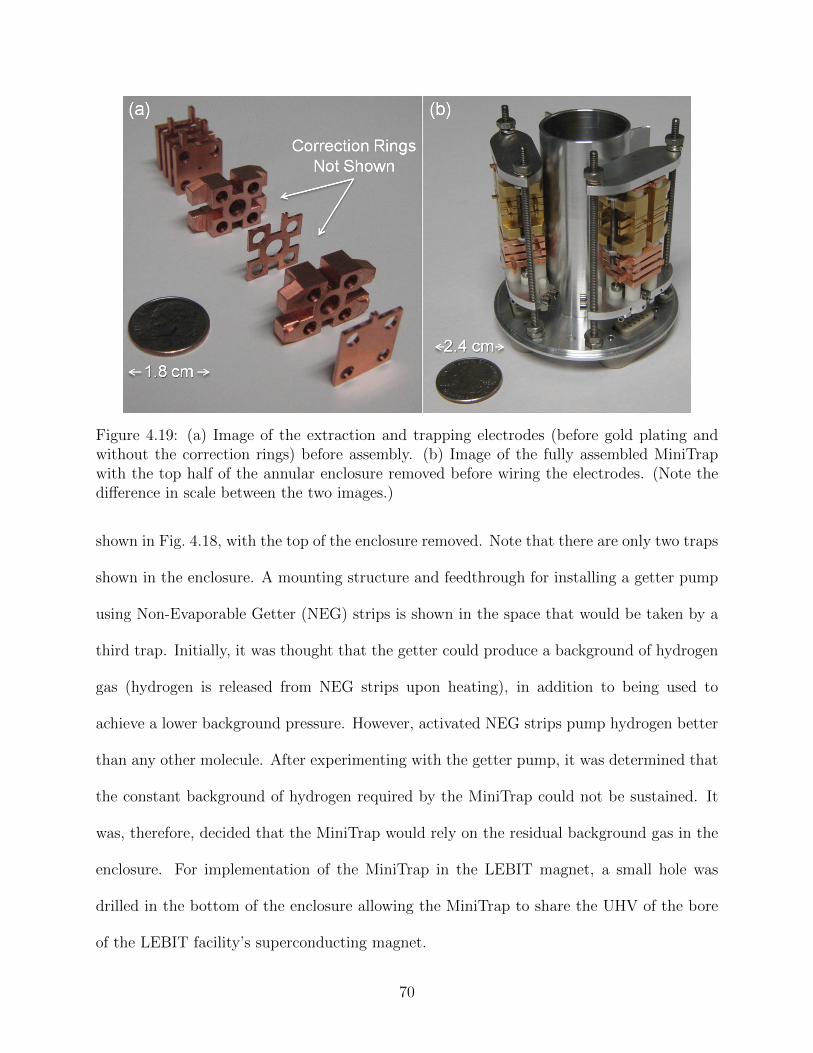
Figure 4.19: (a) Image of the extraction and trapping electrodes (before gold plating andwithout the correction rings) before assembly. (b) Image of the fully assembled MiniTrapwith the top half of the annular enclosure removed before wiring the electrodes. (Note thedifference in scale between the two images.)
shown in Fig. 4.18, with the top of the enclosure removed. Note that there are only two traps
shown in the enclosure. A mounting structure and feedthrough for installing a getter pump
using Non-Evaporable Getter (NEG) strips is shown in the space that would be taken by a
third trap. Initially, it was thought that the getter could produce a background of hydrogen
gas (hydrogen is released from NEG strips upon heating), in addition to being used to
achieve a lower background pressure. However, activated NEG strips pump hydrogen better
than any other molecule. After experimenting with the getter pump, it was determined that
the constant background of hydrogen required by the MiniTrap could not be sustained. It
was, therefore, decided that the MiniTrap would rely on the residual background gas in the
enclosure. For implementation of the MiniTrap in the LEBIT magnet, a small hole was
drilled in the bottom of the enclosure allowing the MiniTrap to share the UHV of the bore
of the LEBIT facility’s superconducting magnet.
70

Figure 4.20: Image of the SIPT magnet before the beam line components for testing theMiniTrap had been installed.
After the extraction and trapping electrodes had been fabricated from OFE copper, as
shown in Fig. 4.19(a), the trapping electrodes were gold plated to reduce possible patch
effects that could produce an inhomogeneous surface charge distribution. The completely
assembled MiniTrap is shown in Fig. 4.19(b) before installing the electrode wiring to con-
nect the electrodes to the 15-pin sub-D female connector. All of the metallic components
used in the assembly were either copper, aluminum, brass, or titanium with low magnetic
susceptibilities to limit the production of magnetic field inhomogeneities.
4.5 Testing the MiniTrap Magnetometer
The test of the MiniTrap was performed in the 7 T superconducting magnet obtained for the
SIPT facility [97] (shown in Fig. 4.20). On one end of the magnet a Leybold turbo pump
capable of pumping 200 L/s, backed by a Varian TriScroll roughing pump, was connected
71

Figure 4.21: Image of the MiniTrap assembly fully wired (with the top of the enclosureremoved and shown near the traps), ready to be mounted and inserted into the SIPT magnet.The two separate wires are of a larger gauge for supplying current to the thermionic emitter.
to the bore tube, in addition to an MKS Pirani gauge and a cold cathode Penning gauge
capable of measuring pressures as low as 10−10 mbar. On the opposite side of the magnet a
6 inch conflat 6-way cross was attached. The MiniTrap assembly was supported by a 24 mm
diameter aluminum rod attached to the center of a 6 inch conflat flange (secured to the 6-way
cross) that held the MiniTrap assembly axis along the central axis of the magnet’s bore.
A thermionic emitter was installed due to its proven reliability and stability. In addition,
tests indicated that for electron beam currents of ∼ 1 nA, the trap temperature was expected
to only increase by a few degrees Celsius. The final MiniTrap assembly, shown in Fig. 4.21,
was secured to the mounting rod which located the MiniTrap in the center of the magnet.
Before being inserted into the magnet, the MiniTrap enclosure was wrapped with a solenoid
by winding of 28 coils of 16 gauge wire around the MiniTrap enclosure. A direct current
could be sent through the coil and thus change the magnetic field by a known amount.
72

(Using the infinite solenoid approximation, a current of 1 mA should change the magnetic
field by ∼ 10−6 T, corresponding to a shift in the cyclotron frequency of ∼ 0.6 Hz.) The two
sub-d connectors (shown in Fig. 4.21), were connected to two sub-d conflat connector flanges
attached to the 6-way cross. The two thermionic emitter wires and the two solenoid wires
were attached to a four-connector current feedthrough that was also attached to the 6-way
cross. (The reader is referred to Appendix A for a discussion of the setup and operation of
the electronics.)
4.5.1 Detection of Ion Motion via FT-ICR
The first test was to detect the self-excited magnetron motion that was observed during
the tests using the LEBIT magnet. Then, the excitation and detection parameters were
determined for automated measurements of ω− with the MTCS. The trap was first tuned
by measuring ω− as part of the process to determine the optimal trapping potential which
minimized the shift to ω− as a function of excitation radius, ρ−. With the proper excitation
parameters and tuned trapping potential, it was then possible to search for reduced cyclotron
motion by utilizing the detection of the magnetron motion as a probe. After cyclotron motion
was detected, the trapping potential was tuned to minimize shifts to ω+ by measuring ω+
as a function of ρ+. Finally, repeating excitation and detection of the reduced cyclotron
motion was used to monitor relative changes in the magnetic field.
4.5.1.1 Magnetron Motion
In a background pressure of ∼ 10−7 mbar (as recorded by the Penning gauge attached to
the beam line outside of the magnet), the thermionic emitter was biased to ∼ -90 V and
heated by supplying a current of ∼ 2 A. With all of the extraction electrodes and trapping
73

Figure 4.22: A LabVIEW screenshot of an FFT resonance of self-excited magnetron motionof trapped ions of unknown species in a 6.8 V potential well in the MiniTrap.
electrodes grounded, an electron beam current of several nA’s was measured by a Keithley
picoammeter attached to the Faraday plate. The trapping potential was then raised by
setting the endcaps to 6 V and the ring electrode to -0.8 V to give an endcap-to-ring voltage
ratio of 1 to 0.13 (approximately the same as that calculated in simulations using the values
in Table 4.2). After ionizing the residual background gas for several seconds, the scope-card
was triggered using the MTCS to acquire a signal for 80 ms at 25 megasamples per second
(MS/s) from the differential pre-amplifier directly connected to two azimuthally opposing
sets of correction electrodes (broadband dipole detection). The signal was analyzed using
LabVIEW FFT analysis software, and resulted in the FFT resonance shown in Fig. 4.22.
For the MiniTrap geometry and applied voltages a magnetron frequency, f−, of ∼ 9110 Hz
would be expected, whereas in Fig. 4.22 f− ≈ 9400 Hz. The several hundred Hz shift was
most likely due to image-charge shifts from the large number of ions being confined and
self-excited in the trap.
74

Trap tuning scans of ω− were performed with a fewer number of ions (at a lower electron
beam current). A script was implemented in the MTCS that would first dump the trap
for one second (then raise the trap), ionize the residual gas for 1 second with an electron
beam current of 1 nA, then apply a sweep signal from 6 to 11 kHz on two sets of azimuthally
opposing correction electrodes, 180 degrees out of phase, with a sweep cycle time of 5 ms.
The MTCS would subsequently record the signal from the pre-amplifier (using broadband
dipole detection) for 80 ms at 25 MS/s and analyze the resulting FFT resonance, and thus
perform one magnetron frequency measurement. For trap tuning, 5 magnetron frequency
measurements were performed each at a given sweep excitation amplitude beginning at 0.07
volts peak-to-peak (Vpp) and incrementing up to 0.28 Vpp in 0.015 Vpp steps. One of these
more involved scans shows the shift in f− as a function of ρ− at a given endcap-to-ring
voltage ratio.; for a perfectly tuned trap, the frequency would remain constant.
The f− versus ρ− scan was performed at various endcap-to-ring voltage ratios (while
keeping the total trapping potential at 6 V) to determine the optimum trapping potential.
The results of one of these f− trap tuning scans is shown in Fig. 4.23 where the optimal
endcap and ring voltages were 5.4 V and 0.6 V, respectively. Note that this ratio of endcap-to-
ring voltage of 1 to 0.11 is only slightly larger than that determined from values obtained from
the simulations given in Table 4.2, and is possibly due to imperfections in the trap geometry
or alignment. Of greater importance is the ability to minimize shifts to f−, indicating that
anharmonicities in the trapping potential can indeed be tuned out as required for optimal
performance of the MiniTrap. The tuning of the MiniTrap’s trapping electrodes to minimize
shifts in f− thus provided optimal parameters for the detection of reduced cyclotron motion.
75

Figure 4.23: Results of trap tuning scans with the MiniTrap showing f− versus the driveamplitude (proportional to ρ−) for seven different endcap-to-ring voltage ratios for a 6 Vpotential well depth (the ring, by convention, is always negative). Note that the solid linesshow polynomial fits (using only the first five even terms) to the data, where the error barsare shown, but are too small to be resolved in this image.
4.5.1.2 Reduced Cyclotron Motion
To identify the ion species in the trap, a magnetron frequency measurement was performed,
however, prior to exciting the magnetron motion, the reduced cyclotron motion of the ions
was excited (using dipole excitation) with a burst at a given frequency, fRF , for ∼ 100µs at
5 Vpp. Application of this signal was more than enough to drive any ions, whose reduced
cyclotron frequency ≈ fRF , out of the trap. Subsequently, fRF was scanned over a broad
range, and when fRF ≈ f+ (of an abundant ion species in the trap) the excited ions would
no longer be in the trap resulting in a decreased magnetron FFT resonance amplitude.
A frequency range of 1 MHz was scanned, where 25 data points were obtained for each
fRF , in steps of 5 kHz, and required ∼ 14 hours to complete. A portion of the results from a
5 MHz to 6 MHz scan using these parameters is shown in Fig. 4.24, where a minimum in the
76

Figure 4.24: Example from the dipole cleaning technique utilized to determine the ion speciesin the MiniTrap. Each data point is the average of 25 magnetron excitation and detectionmeasurements when the trap was first cleaned by applying a RF dipole electric field at 5 Vppfor 100µs at the cleaning frequency, fRF . The Lorentzian fit to the data is represented bythe solid line (red) where the fit results indicate f+ = 5.645(1) MHz.
magnetron FFT amplitude at ∼ 5.645 MHz is clearly evident (corresponding to the reduced
cyclotron frequency of the ions driven out of the trap). Using Eqns. 2.3 and 4.8 with the
C2 value listed in Table 4.2 and a magnetic field of 7 T, this frequency corresponds to a
mass of ∼ 19 u, the mass of H3O+. It is also worth mentioning that the resonance did not
completely disappear and that an additional magnetron “dipole” resonance was also seen at
∼ 3.246 MHz, corresponding to a mass of 33 u, or HO+2 , the same ion species identified in
the background gas during the tests in the LEBIT magnet using broadband axial detection.
The HO+2 “dipole” resonance, however, was not nearly as pronounced, indicating that H3O+
was the most abundant ion species in the trap.
With H3O+ verified as the most abundant ion species in the trap, and the reduced
cyclotron frequency determined for the operating parameters, reduced cyclotron motion was
excited and detected. Excitation times of TRF ≈ 100µs were used to excite reduced cyclotron
motion. The excitation amplitude was varied until a resonance appeared; an example is
77

Figure 4.25: A LabVIEW screenshot of an FFT resonance of reduced cyclotron motion ofH3O+ ions in a 6 V potential well in the MiniTrap using broadband FT-ICR detection. Thefaint solid yellow line represents the best Lorentzian fit produced by the LabVIEW program.
shown in Fig 4.25. Narrow-band FT-ICR detection was then implemented by installing an
inductor with a Q value of ∼ 280 in parallel to the detection electrodes in addition to a 5 -
25 pF air-core variable capacitor, from which the signal was transferred to the pre-amplifier
via a secondary pickup coil as shown in Fig. 4.4. The detection circuit was carefully tuned
to have a resonant frequency of 5.645 MHz and resulted in a Q-factor of ∼ 250.
To verify the parameters obtained from the trap tuning performed with magnetron mo-
tion, a trap tuning scan was performed by determining the shifts in the reduced cyclotron
frequency utilizing the same procedure used to generate the graph shown in Fig. 4.23, excit-
ing the ions at f+ instead of f−. The results of this second trap tuning procedure are shown
in Fig. 4.26. An analysis of the even Cn coefficients indicates that the optimal endcap and
ring voltages are 7.1 V and -0.9 V, respectively, resulting in an endcap-to-ring voltage ratio
of 1 to 0.13. This value for the endcap-to-ring voltage ratio is in better agreement with the
calculated endcap-to-ring voltage ratio found with simulations of 1 to 0.14, as compared to
78

Figure 4.26: Results of trap tuning scans with the MiniTrap showing f+ as a function of thedrive amplitude (proportional to ρ+) for five different endcap-to-ring voltage ratios for an8 V potential well depth (the ring, by convention, is always negative). Note that the solidlines show the results of polynomial fits (using only the first five even terms) to the data,where the error bars are shown, but are too small to be resolved in this image.
that found with f− versus ρ−. Once the proper trap potential was found, an f+ monitoring
process was used to continuously cycle through measurements of f+ to track changes in the
magnetic field.
Before testing the f+ monitoring process, an appropriate sample time to acquire the f+
signal was determined. Longer sample times improved the resolution of the FFT, however,
longer sample times resulted in the broadening of the FFT resonance linewidth together with
a decrease in the FFT resonance amplitude, possibly due to loss of coherence of the ion cloud.
At a pressure of ∼ 10−7 mbar (as measured near the turbo pump), linewidth broadening was
noticeable with 50 ms long sample times. At a background pressure of ∼ 3× 10⁻⁸ mbar, a
sample time of 100 ms resulted in reduced cyclotron FFT resonances with no indication of
linewidth broadening. Therefore, to probe for longer periods of time, and thus increase the
FFT frequency resolution, a lower background pressure would be necessary.
79

Figure 4.27: Results of the MiniTrap reduced cyclotron frequency monitoring process show-ing the average f+(H3O+) measurements and the average FFT amplitudes as a function oftime recorded over a period of ∼ 17 hours. Each data point is the average of 120 frequencymeasurements (requiring 10 minutes) where the error bars correspond to the 1σ uncertaintyassociated with the distribution of those 120 measurements. The average slope of the entiredata set corresponds to a magnetic field decay rate of -5.82(4)× 10−8 hr−1.
To monitor the drift in the magnetic field and to determine the precision of the magne-
tometer, an f+ monitoring process recorded the reduced cyclotron frequency of H3O+ over
the course of ∼ 17 hours in the SIPT magnet. Each measurement consisted of ionizing the
background gas with a steady (within a few percent) electron beam current of 0.2 nA for 1
second. The trapped ions were excited with a burst excitation at 5.642 MHz for 100µs at
0.28 Vpp using dipole excitation. The signal was picked up using the narrow-band technique
similar to that in the f+ trap tuning. A 10 MHz custom bandpass filter, installed between
the pre-amplifier and the scope-card used to record the signal, reduced the high-frequency
background noise that was mixed down to lower frequencies. A small leak valve, mounted to
the magnet bore, allowed a steady stream of air to be injected into the magnet bore to main-
tain a background pressure of ∼ 3.5× 10⁻⁸ mbar as measured by the Penning gauge near the
turbo pump. Some of the results of the f+ monitoring process are shown in Fig. 4.27.
80
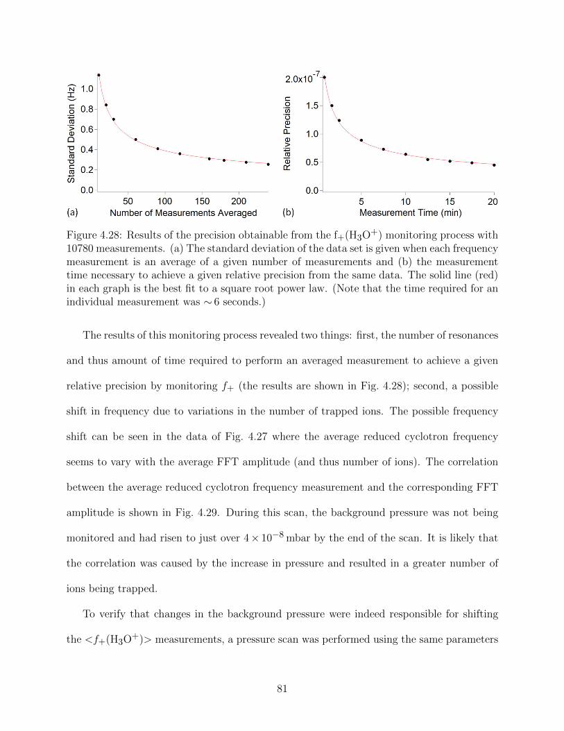
Figure 4.28: Results of the precision obtainable from the f+(H3O+) monitoring process with10780 measurements. (a) The standard deviation of the data set is given when each frequencymeasurement is an average of a given number of measurements and (b) the measurementtime necessary to achieve a given relative precision from the same data. The solid line (red)in each graph is the best fit to a square root power law. (Note that the time required for anindividual measurement was ∼ 6 seconds.)
The results of this monitoring process revealed two things: first, the number of resonances
and thus amount of time required to perform an averaged measurement to achieve a given
relative precision by monitoring f+ (the results are shown in Fig. 4.28); second, a possible
shift in frequency due to variations in the number of trapped ions. The possible frequency
shift can be seen in the data of Fig. 4.27 where the average reduced cyclotron frequency
seems to vary with the average FFT amplitude (and thus number of ions). The correlation
between the average reduced cyclotron frequency measurement and the corresponding FFT
amplitude is shown in Fig. 4.29. During this scan, the background pressure was not being
monitored and had risen to just over 4× 10⁻⁸ mbar by the end of the scan. It is likely that
the correlation was caused by the increase in pressure and resulted in a greater number of
ions being trapped.
To verify that changes in the background pressure were indeed responsible for shifting
the <f+(H3O+)> measurements, a pressure scan was performed using the same parameters
81

Figure 4.29: Average reduced cyclotron frequency as a function of average FFT amplitudefrom the f+ monitoring process of H3O+. Each data point represents one average measure-ment of 120 individual f+ measurements. The solid line (red) is the best linear fit to thedata and has a slope of -1371(80) Hz/a.u.
Figure 4.30: Results of the pressure scan showing (a) the average reduced cyclotron frequencyof H3O+ and (b) the average FFT amplitude as a function of pressure, and (c) the averagereduced cyclotron frequency as a function of the average FFT amplitude. Each data pointrepresents the average of 20 individual f+ measurements. The solid lines (red) are the bestlinear fits to the data. The fit results of (c) give a slope of -1336(108) Hz/a.u.
82

as those used in the monitoring process, but the background pressure was increased from
3.0× 10⁻⁸ mbar to 5.5× 10⁻⁸ mbar in 0.5× 10⁻⁸ mbar steps after every 20 measurements.
The results of the pressure scan are shown in Fig. 4.30. A linear relationship between both
shifts in <f+(H3O+)> and the respective average FFT amplitudes was observed. More
importantly, perfect agreement is seen between the slope of the fit in Fig. 4.29 and that
in Fig. 4.30(c), indicating that the change in frequency observed during the f+ monitoring
process of H3O+ was caused by pressure fluctuations (and thus fluctuations in the number
of trapped ions). With this information it is possible to correct for these shifts, however, the
ideal scenario for monitoring the magnetic field should be insensitive to varying numbers of
trapped ions.
4.5.2 True Cyclotron Frequency Determination
It is possible to detect not only the resonances of f−, fz, and f+, but also the (f+ +f−) res-
onance which, for an ideal trap, is equal to fc, the “true” cyclotron frequency (see Eqn. 2.5).
Observation of the (f+ + f−), or fc, resonance, however, necessitates the implementation
of the quadrupole detection scheme [60]. In this scheme, the image current is detected on
two adjacent electrodes (rather than opposite electrodes in the dipole detection scheme).
Exciting and detecting true cyclotron motion is advantageous since shifts in f− and f+ due
to changes in number of ions and image charge shifts from space charge can cancel each other
out [106]; also, fc is independent of the trapping voltage. Detection of fc has been carried
out previously using FT-ICR techniques [107], and the reader is referred to this work for a
more detailed description.
83

4.5.2.1 Quadrupole Pickup Detection Method
To pick up the image current induced by the motion of the ions at fc, the (f+ + f−) signal,
the detection electrodes were connected in a quadrupole configuration which was easily
accomplished by swapping one excitation electrode with one detection electrode. When
changing to the quadrupole detection scheme, the resonant circuit was retuned, since the
capacitance of the detection circuit changed. This time the detection circuit was tuned to
5.653 MHz ≈ fc to maximize the amplification of the induced fc signal.
To detect fc, the trapped ion cloud must have some initial magnetron motion. This
motion was induced by exciting the ions with a burst of RF power applied to one set of
correction electrodes for ∼ 1.5 ms at a frequency ≈ f−. (Various magnetron excitation am-
plitudes were investigated and optimized for different trapping potentials.) Then cyclotron
motion was imparted to the ions already undergoing magnetron motion, by applying a burst
of RF power to a different set of correction electrodes for ∼ 100µs at a frequency ≈ f+.
The cyclotron excitation amplitude was adjusted depending on the magnetron excitation
amplitude and the trapping potential. Initially, both the excitation voltages and the trap-
ping potential were adjusted manually to obtain the first fc resonance, shown in Fig. 4.31,
with the accompanying f+ resonance. (In quadrupole detection utilizing only two adjacent
electrodes, with the other two opposing electrodes grounded, both fc and f+ can be detected
simultaneously. If all four electrodes were utilized in the quadrupole detection configuration,
only the fc resonance would have been observed [107].)
The parameter space was explored by adjusting the magnetron and cyclotron excitation
amplitudes at various endcap-to-ring voltage ratios to maximize the FFT amplitude of the fc
resonance. However, optimizing for the largest fc FFT amplitude did not seem to consistently
84

Figure 4.31: A LabVIEW screenshot of FFT resonances of both reduced cyclotron motion(left) and true cyclotron motion (right) of H3O+ ions in a 7.73 V potential well in theMiniTrap using the broadband FT-ICR quadrupole detection configuration.
decrease the shot-to-shot variations in fc, i.e. didn’t improve precision. In an attempt to
increase precision, an automated 3-dimensional search probing for shifts in both fc and f+
was carried out by scanning ρ− over a range of endcap-to-ring voltage ratios for different
cyclotron excitation amplitudes. To minimize the frequency shift due to number of ions, this
optimization scan was performed at a background pressure of a few 10−8 mbar and ionizing
the background gas for 1 s with an electron beam current of ∼ 0.065 nA, resulting in the
fewest number of ions that could be detected with FFT resonance signal-to-noise ratios no
smaller than 5.
The data from this optimization scan were analyzed to determine the best parameters that
minimized shot-to-shot fluctuations while also minimizing shifts to f+ and fc as a function
of magnetron drive amplitude. The optimum parameters are listed in Table 4.3, where it
is important to recognize that the range of the optimized values lie within the precision of
the function generator and the power supplies that generate the values of the respective
85

Table 4.3: Optimal excitation parameters identified by a 3-dimensional scan of ρ− for arange of endcap-to-ring voltage ratios for different cyclotron excitation amplitudes. Themagnetron and cyclotron excitation times and frequencies where held constant at 10.25 kHzfor ∼ 1.5 ms and 5.6428 MHz for ∼ 100µs, respectively, within a potential well of 7.735 V.*A 10 dB attenuator was used to attenuate the cyclotron excitation.
Parameter ValueEndcap 6.985 - 6.990 V
Ring (-) 0.745 - 0.750 VMagnetron Excitation 0.615 - 0.635 VppCyclotron Excitation 0.17 - 0.18 Vpp*
parameters. The optimized endcap-to-ring voltage ratio was ∼ 1 to 0.11, in agreement with
the magnetron tuning result, but larger than that from the reduced cyclotron tuning method.
This discrepancy was most likely due to the increased radial extent that the ion cloud
traversed as it executed the two radial normal-mode oscillations.
An electron beam current scan was performed to determine the frequency dependence
on the number of ions by adjusting the current supplied to the thermionic emitter at a
background pressure of a few 10−8 mbar (as read by the Penning gauge by the turbo pump).
This scan was utilized to determine the electron beam current where frequency shifts due to a
larger ion cloud begin to become non-negligible. The results are shown in Fig. 4.32, where the
frequency shift due to the number of ions is shown for both fc and f+. Only minimal shifts in
fc are present when using an electron beam current of ∼ 0.04 nA to almost 0.085 nA, however,
f+ shifts down by ∼ 10 Hz. These results clearly indicate both the acceptable operating
currents (at the associated background pressure) for limiting shifts in fc due to the number
of ions and the benefits of measuring fc instead of f+. Specifically, an electron beam current
of ∼ 0.06 nA is ideal for creating enough ions to consistently resolve frequency peaks with
a signal-to-noise ratio greater than 5, while limiting the shift in fc due to variations in the
number of ions in the trap to a negligible level.
86

Figure 4.32: Results from the electron beam current scan of fc and f+ for H3O+ using theoptimized parameters. Each data point is the average of 100 measurements where the errorbars represent the standard deviation of the individual measurements (some of which cannotbe resolved). (Note the difference between the frequency shift of fc and f+ as a function ofelectron beam current, especially at lower electron beam currents – the scales are equivalent).
Not only is the shift in fc smaller than f+ due do the number of ions, but a frequency shift
to fc due to variations in trap depth are almost eliminated. (A shift in fc due to variations
in trap depth vanish completely in a perfect trap.) A trap depth scan that monitored both
fc and f+ was performed as the trap depth was varied from 7.631 V to 7.839 V in steps of
0.052 V, while maintaining a constant endcap-to-ring voltage ratio of ∼ 1 to 0.11. The ions
were excited using the optimal parameters listed in Table 4.3. The results of this scan are
shown in Fig. 4.33, where fc and f+ were recorded simultaneously. A series expansion of
Eqn. 2.3 to first order reveals a linear dependence of f− and f+ on the trap potential, Vo,
where ω− ≈ Vo/(2d2B) and ω+ ≈ ωc−Vo/(2d2B) as is clearly displayed in the variation
of <f+(H3O+)> as a function of trapping potential shown in Fig. 4.33. The true cyclotron
frequency, however, remains fairly constant for a change in trap depth of ∼ 20 mV, whereas
the reduced cyclotron frequency shifts by almost 300 Hz.
87

Figure 4.33: Results of the trap depth scan of fc and f+ of H3O+. Each data point is anaverage of 30 measurements where the error bars represent the standard deviation of thosemeasurements (the error bars in the plot of f+ are too small to be resolved). The linear bestfit of <f+(H3O+)> as a function of trapping potential (solid red line) resulted in a slope of-1350(3) Hz/V. (Note the change in vertical scales between the plot of fc and f+.)
4.5.2.2 Precision of the MiniTrap Magnetometer
To probe the precision of the MiniTrap, known changes to the magnetic field were introduced.
This was achieved by changing the magnetic field by a controlled amount to see if the change
in the magnetic field could be resolved. The magnetic field was changed by passing a small
current, of 1 to 10 mA, through the coil wrapped around the MiniTrap enclosure. A scan
was set up to continuously monitor f+(H3O+) as a function of applied current to the coil to
test the effectiveness of this method. The test consisted of ramping the current in the coil
up from 2 mA to 11 mA and then back down from 11 mA to 2 mA in 1 mA steps, where 100
fc measurements were performed at each current setting. This scan was repeated 5 times
and the results are shown in Fig. 4.34.
This initial test of the precision of the magnetometer revealed that changes in the mag-
88

Figure 4.34: Results from the true cyclotron frequency monitoring process while rampingthe current in the coil (wrapped around the MiniTrap enclosure) to produce changes in thetotal magnetic field. Each data point is an average of 100 measurements with the error barsrepresenting the standard deviation of those measurements. The solid line (red) representsthe variation of the current supplied by the power supply (values given on the right axis).
netic field corresponding to a relative precision of at least 10−7 could be achieved by averaging
100 individual fc measurements over a period of 10 min. The resolution of this particular
scan, however, was not extremely high and also neglected changes in the magnetic field dur-
ing the ∼ 3 hour long ramping period. To more accurately determine the precision that the
MiniTrap could achieve, smaller changes in the magnetic field would have to be made. It
would also be necessary to perform fc measurements at a reference B field current after every
few fc measurements at a given B field scan current to eliminate the effects of the magnetic
field changing on the few-minute time scale. (The power supply used to pass current through
the coil had a precision of 0.5 mA, so a current divider circuit was installed to reduce the
current by about a factor of 10 to allow for finer changes to the magnetic field.)
An alternating B field precision scan was performed to provide a more accurate test of the
precision of the magnetometer. The scan consisted of operating the fc monitoring process
during which five fc measurements were performed at a given B field reference current (for
this scan 10 mA was the reference current), then five fc measurements at a B field scan
current. These 10 measurements were repeated 400 times to give 2000 fc measurements at
89

Figure 4.35: Results of the true cyclotron frequency monitor while alternating every fivemeasurements between a B field scan current and a B field reference current of 10 mA toproduce relative changes in the magnetic field. Each data point represents 4000 fc mea-surements where the error bars represent the standard deviation of those measurements (seetext). The solid red line is the linear best fit to the data and the solid black line is thezero-shift reference. The linear best fit resulted in a slope of 0.080(3) Hz/mA.
each B field current, resulting in a total of 4000 fc measurements for one B field scan current
setting. Data was taken for 15 different B field scan current settings in 1 mA steps, including
a control setting where 4000 fc measurements were taken at the B field reference current
of 10 mA. Each set of 2000 fc measurements were averaged and assigned an uncertainty
equal to the standard deviation of those measurements divided by the square root of the
number of measurements. The observed shift in <fc(H3O+)> was then calculated as the
difference between the average of the 2000 fc measurements at the 10 mA reference current
and the B field scan current. The uncertainty in <fc(H3O+)> was calculated by adding
the uncertainties of the average fc measurements at the 10 mA reference current and the B
field scan current in quadrature. The results of this analysis are presented in Figure 4.35.
Note that the fit indicates that a change in the magnetic field from applying a 1 mA current
(which was subsequently divided down by a factor of ∼ 10) shifted fc by 0.08 Hz.
90

Figure 4.36: Illustration of the precision obtained from the alternating B field scan where(a) the standard deviation of the data is given when each frequency measurement was anaverage of a given number of measurements and (b) the measurement time necessary toachieve a given relative precision from the same data. The solid line (red) in each graph isthe best fit to a square root power law fit.
The data from the alternating B field measurement was analyzed to obtain the average
experimental precision for a given number of measurements averaged and for averaging mea-
surements over a given period of time. The standard deviation was calculated for the data
set when broken up into average measurements composed of various numbers of individual
measurements to obtain the relative precision as a function of the number of measurements,
or measurement time (the period of each individual measurement was 6 seconds). The re-
sults, shown in Fig. 4.36, indicate that a relative precision of < 4× 10⁻⁸ can be achieved
by averaging fifty individual measurements, or a relative precision of < 3× 10⁻⁸ for one
hundred measurements, or a relative precision of < 2× 10⁻⁸ for two hundred measurements
(all at the 1σ level). Note that this is the relative precision of an individual averaged mea-
surement, and to obtain the uncertainty associated with the difference between two averaged
values (and to obtain the corresponding uncertainties for the data shown in Fig. 4.35), the
uncertainties associated with these relative precisions would need to be multiplied by√
2.
The MiniTrap has thus demonstrated that it can achieve the required relative precision
91

but at the cost of temporal resolution. However, the six second individual measurement
time was not fully optimized, and it is conceivable that individual measurement times of two
seconds could be possible, which would result in both better relative precision and temporal
resolution. For two second measurement times, a relative precision of < 2× 10⁻⁸ could be
achieved by averaging individual measurements over a period of seven minutes. However,
there is another trick that one can play to further increase the relative precision of the
MiniTrap that will be discussed in a following section.
4.5.2.3 Tracking the B Field Using the True Cyclotron Frequency
A long-term <fc(H3O+)> monitoring process was performed to track the drift of the 7 T
SIPT superconducting magnet and to verify the performance of the MiniTrap. To verify
the accuracy and precision of the function generator used to apply RF power to the ions, a
reference frequency from an additional function generator, at 5.648 MHz, was added on top
of the signal recorded by the scope-card. The reference signal was attenuated to result in
an FFT amplitude about a factor of ten larger than that of the cyclotron frequency peaks.
Fig. 4.37 depicts an FFT spectrum of one individual measurement with the monitor showing
the f+, fRef, and fc resonances on the left, middle, and right of the spectrum, respectively.
The monitoring process ran continuously for eleven days and nine hours. The results of the
long-term monitoring process are shown in Fig. 4.38 where each data point represents the
average of 100 individual measurements. (Analysis of the monitor data for the reference
frequency signal indicated that the observed changes in the cyclotron frequency were real.)
There are two features of the results of the long-term monitoring process that require
explanation. The first feature to note is the momentary increase in both fc and f+ that
occurred just after the start of the monitor and once again near the end. These shifts in
92

Figure 4.37: An FFT spectrum showing the resonances from the reduced cyclotron motion(left), the reference signal (middle), and the true cyclotron motion (right) from an individualmeasurement of H3O+ in the MiniTrap. (The height of the fRef resonance peak has beentruncated to clearly show the f+ and fc resonance peaks.)
Figure 4.38: Results of the long-term MiniTrap monitoring process showing the<fc(H3O+)>and associated <f+(H3O+)> measurements over the course of ∼ 11 days and 9 hours. Eachdata point is the average of 100 frequency measurements (10 minutes each) where the errorbars correspond to the 1σ uncertainty associated with the distribution of those 100 measure-ments. The linear best fit of the fc data (shown in red) corresponds to a magnetic field decayrate of -3.3(2)× 10−10 hr−1. (Note that the difference in scales between the two graphs is ∼a factor of four.)
93

frequency occurred during the LN2 fill of the SIPT magnet and were exactly correlated
with the duration of the fill. This was a good indication that the MiniTrap was functioning
properly and able to track short-term changes in the magnetic field.
The second feature of the data from the long-term monitoring process is the occasional
momentary negative shift in both fc and f+ that occurred throughout the data set, and re-
quires further investigation. The duration of the temporary shift ranged from 5 to 15 minutes,
and the extent of the shift ranged from 0.5 to 2 Hz for <fc(H3O+)> and from 1 to 7 Hz for
<f+(H3O+)>. The data was further analyzed for correlations in amplitude. No correlation
could be found with respect to the FFT amplitude of <fc(H3O+)>, however, the decreases
were associated with minor increases in the FFT amplitude of <f+(H3O+)>. Drifts in the
FFT amplitude by the same amount throughout the monitoring process, however, did not
result in changing the frequency by the amount observed during these short-term shifts.
One possible explanation for these infrequent events are momentary changes in the ex-
citation amplitudes produced by the function generators. Another possible explanation is
a momentary change in the trapping potential or number of ions produced in the trap.
Verification of these scenarios would require further investigation. It is unlikely that the
magnetic field was changing and that these shifts were actually caused by shifts in the mag-
netic field, however, verifying this scenario would require the simultaneous operation of a
secondary monitoring device. It would thus be beneficial to operate both traps simultane-
ously with independent power supplies, function generators, and ancillary electronics. This
would not only help determine the cause of the short-term systematic shifts to the true cy-
clotron frequency, but would also identify any systematic long-term drifts while increasing
the confidence in the reliability, as well as precision, of the magnetometer.
Note the generally positive drift of <f+(H3O+)> seen in Fig. 4.38. To look for correla-
94

Figure 4.39: Frequency correlation with FFT amplitude from the long-term monitoringprocess for (a) <fc(H3O+)> and (b) <f+(H3O+)>. Each data point represents an averageof 100 individual measurements. The linear best fits to the data (solid red lines) for (a) and(b) resulted in slopes of 20(3) Hz/a.u. and -156(2) Hz/a.u., respectively.
tions, both <fc(H3O+)> and <f+(H3O+)> were plotted as a function of their respective
amplitudes. The results are shown in Fig. 4.39, where a correlation of <f+(H3O+)> with
amplitude was present, indicating that the upward trend of <f+(H3O+)> throughout the
long-term monitoring process was the result of the number of trapped ions slowly decreas-
ing. As expected, the dependence of <fc(H3O+)> on FFT amplitude is much smaller (by
an order of magnitude) than that of <f+(H3O+)>, and gives rise to a slope (in this range of
amplitudes) corresponding to a frequency shift on the order of the precision of the MiniTrap.
The extent of the scatter in the <fc(H3O+)> data seen in Fig. 4.39(a) suggests that the
frequency shift in fc is either not associated with the FFT amplitude or that the shift was
within the uncertainty of the measurements.
4.5.2.4 Improving the Precision of the MiniTrap
Some improvements can be made to the MiniTrap system to further increase the relative
precision of the magnetometer while also improving the temporal resolution. One fairly
straightforward technique was already mentioned briefly, and relies on decreasing the time
95
required to perform a single fc measurement. For example, ten second cycle times were
used for the tests with the LEBIT magnet which was decreased to six seconds for the tests
with the SIPT magnet. For the tests in the SIPT magnet, one second ionization times were
used. It may be possible to decrease the ionization time by increasing the electron beam
current and produce the same number of ions. In addition, one second trap dumping times
were used. This could be drastically shortened (to sub-ms) especially if carried out with a
fast switch to reverse the polarity of the trapping potential. Finally, a script in the MTCS
was used to control the measurement process in a step-wise procedure. The measurement
routine could be completely streamlined and controlled with a single instance of a LabVIEW
Field-Programmable Gate Array (FPGA) module. (For the measurement process used in
the measurements in this work, the LabVIEW FPGA module was used for timing the ion-
ization cycle and controlling the trapping electrodes, but not simultaneously.) Streamlining
the measurement process would allow parallel operations of recording data and controlling
voltages and currents, thus eliminating dead time during the measurement process. The mea-
surement cycle time would then be mainly limited by electron beam ionization times plus
excitation and detection times. Two second measurement times are conceivable, however,
this optimization procedure was outside the scope of this project.
Another increase in precision could come from measuring a lighter mass, such as He+
or H+2 , instead of H3O+. This would, in principle, increase the precision of the MiniTrap
by up to a factor of 10 as the frequency and its resolution are inversely proportional to
mass as indicated by Eqns. 2.2 and 4.4. An improvement in precision by this amount would
allow a relative precision of 10−8 to be reached within 10 cyclotron frequency measurements
and, with optimized cycle times, in 20 seconds. However, using H+2 as a reference ion
species to monitor changes in the magnetic field is not so trivial. This is because one
96

would prefer the majority of the ionized background gas to be H+2 , since frequency shifts
due to any contaminant ions are known to occur [84]. It would be possible, though, to
remove known contaminants from the trap, e.g. H3O+, by exciting them to large radii
with a strong dipole pulse, thus driving them out of the trap before performing a cyclotron
frequency measurement of H+2 . Another option would be to increase the ratio of H2 in the
background gas by installing a leak valve and tube connecting the MiniTrap to a source
of hydrogen outside the magnet, however, this is not a an ideal situation for a variety of
reasons. Alternatively, leaking in He is also possible and would provide about a factor of 5
increase in precision. Monitoring lighter ions together with shorter measurement cycle times
suggests that the demonstrated relative precision by monitoring H3O+ is not the lower limit,
and should be viewed as a upper limit to the precision obtainable by the MiniTrap.
4.5.3 Summary of Results
The test of electron beam production in the LEBIT magnet demonstrated the ability to ionize
the residual gas using electron-impact ionization. This test also indicated the feasibility of
performing FT-ICR cyclotron frequency measurements of a reference ion to obtain a relative
precision of the change in the magnetic field at the level of 1 part in 108. The analytical
and numerical simulations performed identified the optimal trap geometry parameters to
maximize the precision of the MiniTrap. The MiniTrap was successfully fabricated and
assembled with minimal difficulties. Finally, tests in the 7 T superconducting SIPT magnet
demonstrated that the MiniTrap could detect changes in strong magnetic fields with a relative
precision of nearly 1 part in 108, with a temporal resolution of ∼ 30 minutes, by monitoring
the cyclotron frequency of H3O+. A threefold increase in temporal resolution should be
relatively easy to achieve by streamlining the measurement process. In addition, the overall
97

precision of the MiniTrap could be increased by a factor of 5 to 10 by monitoring the cyclotron
frequency of lighter masses such as H+2 or He+.
98

Chapter 5
Summary and Outlook
The current efforts to perform next-generation experiments to discover 0νββ decay highlights
the importance of neutrino physics and the implications that such a discovery would have,
such as leading to new physics beyond the Standard Model. Even if 0νββ decay is not
observed at the limits of sensitivity strived for by these experiments, the nature of the
neutrino will have been further constrained and would further contribute to the success of
the Standard Model.
In light of the current efforts to build a next-generation experiment, SuperNEMO, and
future experiments to discover 0νββ decay by observing 82Se, the first direct ββ decay Q-
value measurement of 82Se was performed. This measurement was necessary to not only
precisely determine the energy of the single peak in the electron sum-energy spectrum with
an uncertainty below the keV level, but also to improve the accuracy in the estimation of
the half-life sensitivity required to detect a given effective neutrino mass, or conversely, to
improve the precision of the effective neutrino mass if the half-life is measured.
The direct Qββ measurement of 82Se was performed at the LEBIT facility using the TOF-
ICR technique to determine the cyclotron frequency ratio between 82Se+ and 82Kr+ ions.
99

The measured ratio resulted in a ββ decay Q-value of Qββ = 2 997.9(3) keV, which is nearly
an order of magnitude more precise than the previous literature value [75] and is sufficient
for locating the 0νββ decay peak in future experiments utilizing large mass bolometers. In
addition, the uncertainty in the half-life or the effective neutrino mass due to a Q-value
of this precision is negligible compared to the uncertainty in the NME. By calculating an
improved PSF, using a NME from a corrected shell model calculation [73], and the current
upper limits for the effective neutrino mass from the EXO-200 experiment [87], a lower limit
range for the 82Se 0νββ decay half-life of 5.0× 1024 - 3.7× 1025 years was obtained. This
indicates that if SuperNEMO is able to achieve its projected sensitivity, an effective neutrino
mass as low as 60 - 85 meV could be detected and may allow identification of the neutrino
mass hierarchy.
To enhance the high-precision mass measurement program at the LEBIT facility, a minia-
ture Penning trap magnetometer has been developed to increase precision and maximize
scientific output with increased efficiency by continuously monitoring the drift of the LEBIT
facility’s 9.4 T superconducting magnet. The development of the MiniTrap magnetometer
resulted in the successful development of FEP production methods and the demonstration of
the FT-ICR technique in the LEBIT magnet. After carefully optimizing the dimensions of a
miniature Penning trap for detecting light ions using the FT-ICR technique, the MiniTrap
was successfully designed, fabricated, and assembled. Finally, the stand-alone high-precision
MiniTrap magnetometer was tested in the 7 T superconducting SIPT magnet. The results of
monitoring the true cyclotron frequency of H3O+ indicated that the desired relative precision
in the change of the magnetic field on the order of 1 part in 108 was achieved.
The next step is to install the MiniTrap in the LEBIT facility’s 9.4 T superconducting
magnet to monitor short-term fluctuations in the magnetic field during rare isotope mea-
100

surements. In addition, improvements can be made to improve temporal resolution and
increase the MiniTrap’s absolute precision. Finally, the MiniTrap could be redesigned and
repackaged to monitor drifts in other magnets with strong magnetic fields to high precision
or for applications where high-level ionizing radiation prevents the use of conventional NMR
probes.
101

APPENDICES
102

Appendix A
MiniTrap Electronics
A National Instruments (NI) Peripheral component interconnect eXtensions for Instrumenta-
tion (PXI), model PXI-1042, was the main hub for communicating between the components
of the MTCS composed of LabVIEW programming software and all of the electronic devices
needed to control the MiniTrap. The PXI-1042 was equipped with a NI PXI-4110 power
supply, NI PXI-5114 scope card, NI-6229 Data AcQuisition (DAQ) card, NI PXI-7811R
FPGA timing module, a NI PXI General Purpose Interface Bus (GPIB) controller, and a NI
PXI-8336 interface to directly communicate with a server Personal Computer (PC) through
a fiber optic link. Other electronics utilized for the MiniTrap include: NF Corporation (NF)
SA-420F5 low noise Field-Effect Transistor (FET) differential amplifier with a 15 V Directi
Current (DC) power supply, Symmetricom 8040 rubidium frequency standard, Tektronix
Arbitrary Function Generator (AFG) 3252 dual channel arbitrary function generator, Agi-
lent 33500B waveform generator, Keithley 6485 picoammeter, B&K Precision 9123A single
output programmable DC power supply, GwInstek PSM-2010 programmable power supply,
Stanford Research Systems (SRS) PS350 high-voltage (HV) power supply, Keithley 2000-
20 multimeter, custom-made bipolar switching power supply, custom-made phase splitter,
103

custom-made RF switch, custom-made filters, and attenuators.
The National Instruments (NI) PXI-1042 was equipped with a NI PXI-4110 power supply,
a NI PXI-5114 scope card, a NI-6229 DAQ card, a NI PXI-7811R FPGA timing module,
and a NI PXI-GPIB controller. The NI PXI-4110 power supply was controlled by the MTCS
and was used to set the ring and endcap voltages. Due to high-frequency noise from the
electronics, the voltages were filtered through a DC low-pass filter before being routed to
the MiniTrap.
The NI PXI-5114 scope card recorded the output from the NF SA-420F5 low noise
FET differential amplifier after high-frequency noise was attenuated using a low-pass filter.
The scope card required a frequency reference (supplied by a Symmetricom 8040 rubidium
frequency standard), because the internal onboard clock was observed to shift by several Hz
with single degree temperature fluctuations.
The -10 V to +10 V analog outputs of the NI-6229 DAQ card were used to provide scaled
voltages for setting the FEP/thermionic emitter bias voltage, the electron beam energy set
voltage, the electron beam blocking voltage, and the FEP extraction voltage. The analog
inputs of the NI-6229 DAQ card were used to monitor the FEP/thermionic emitter bias
voltage, the electron beam energy set voltage, and the electron beam current output from
the Keithley 6485 picoammeter.
A NI PXI-7811R FPGA timing module was used to provide Transistor-Transistor Logic
(TTL) signals that were used to time events during a cyclotron frequency measurement
such as triggering the function generator, switching the electron beam blocking voltage,
and triggering an RF switch to block leakage signals from the AFG when applying a sweep
excitation. Reconfiguring the FPGA timing generator would be the key to streamlining the
entire measurement process by triggering each measurement operation with a single FPGA
104

routine in the MTCS. (The outputs from the timing card were first buffered through line
drivers composed of op-amps before supplying the TLL voltages to the respective devices.)
Finally, the NI PXI-GPIB controller allowed communication with all devices equipped
with a GPIB interface and included the function generators, Keithley 6485 picoammeter,
B&K Precision and GwInstek power supplies, and the SRS HV power supply. This commu-
nication was critical to allow the MTCS to control each device remotely.
The NF SA-420F5 low noise FET differential amplifier was used to amplify the signal
from the secondary pickup coil of the FT-ICR detection circuit. To avoid high-frequency
background noise from being mixed down into the frequency range of interest, the signal
passed through a low-pass filter before being delivered to the NI PXI-5114 scope card. (In the
case of H3O+, a 10 MHz low-pass filter was used). A bandpass filter could be installed which
would also attenuate low-frequency noise to eliminate higher order harmonics, however, this
was not an issue when detecting fc(H3O+). The NF SA-420F5 low-noise FET differential
amplifier was powered by a 15 V DC power supply built by the NSCL electronics shop.
A Tektronix AFG 3252 dual channel arbitrary function generator was used to provide
the excitation signals that were directly routed to the excitation electrodes of the MiniTrap.
During a cyclotron frequency measurement the Tektronix AFG 3252 was triggered by the
FPGA timing module and the trigger delay times were set accordingly for each channel to
provide excitations from both channels at arbitrary times. Conveniently, all of the functions
can be controlled via the MTCS through GPIB communication. In addition to providing a
reference clock to the PXI-5114 scope card, the Tektronix AFG 3252, as well as the Agilent
33500B were also locked to the 10 MHz signal from the Symmetricom 8040 rubidium fre-
quency standard. The Agilent 33500B waveform generator was used to provide the reference
signal to verify that the devices were all locked during cyclotron frequency measurements.
105

The electron beam current was measured by directly connecting the MiniTrap Faraday
plate to the Keithley 6485 picoammeter. The picoammeter was controlled via GPIB and
can also record the current through GPIB as well. However, when implementing the PID
loop (needed to stabilize the electron beam current from FEPs) the GPIB current readback
was too slow. When using the PID loop, the 0 to 2 V analog output was used to provide a
scaled electron beam current to an analog input of the NI-6229 DAQ card which allowed the
electron beam current to be recorded at a much faster rate.
The B&K Precision 9123A single output programmable DC power supply provided the
current necessary to power the thermionic emitter. The power supply was completely con-
trolled by the MTCS via GPIB and was usually operated in constant current mode. To bias
the emitter, a bias voltage was applied to the positive output of the B&K Precision 9123A
power supply while the ground output of both power supplies were connected together. This
allowed for the energy of the electron beam to be defined with respect to the common ground
of the system. A shielded (and grounded) cable was used to route the wires to the power
feedthrough located on the 6-way conflat cross.
For testing the precision of the MiniTrap in the SIPT magnet, the magnetic field needed
to be varied and was accomplished by supplying a current by the GwInstek PSM-2010
programmable power supply to a coil wrapped around the MiniTrap enclosure. Again, this
power supply was completely controlled by the MTCS via GPIB. This power supply could
also be used to provide the current necessary to heat the NEG pump that could potentially
be installed in the MiniTrap.
To operate FEPs, high voltages needed to be applied to the electron beam extraction
electrode. This potential was created by a Stanford Research Systems (SRS) PS350 high-
voltage (HV) power supply. The SRS HV power supply provided voltages up to 5 kV and
106

was controlled remotely via GPIB. This power supply was only used when creating an elec-
tron beam from an FEP and during the FT-ICR test in the LEBIT magnet. When using
thermionic emitters this power supply was not utilized and instead the first electron beam
extraction electrode was grounded.
The Keithley 2000-20 multimeter was used to measure the ambient room temperature
by measuring the resistance of a thermistor attached to the bore of the SIPT magnet. A
cold cathode penning gauge together with an MKS pressure controller was used to monitor
the pressure in the bore of the SIPT magnet and was recorded by the LEBIT control sys-
tem. Monitoring the background pressure together with the ambient room temperature is
important to determine if there were any correlations to changes in the cyclotron frequency.
Many custom-made electronics were utilized in the MiniTrap setup. First, the LEBIT
bipolar switching power supply was implemented to provide two independent outputs capable
of supplying between -120 V and +120 V. Each channel had three separate set voltages that
were internally set to accept between -10 V to +10 V, and would correspond to an output
voltage scaled by a factor of 12. Two TTL inputs were used to select one of the three set
voltages referenced to determine the output voltage. One channel of this power supply was
used to provide the bias voltage for thermionic emitter and was never switched. The second
channel supplied the voltage to the electron beam blocking electrode and switched between
two different voltages to either block the electron beam or allow it to pass. The switching
of the second channel was performed by supplying a TTL signal from the timing generator.
A custom-made RF phase splitter was implemented to produce two signals, 180 degrees
out of phase, from a single output from a function generator. This was accomplished quite
simply through a set of RF inverting op-amp circuits with a gain equal to 1. The phase
splitter was used to provide dipole excitation when the dipole detection configuration of FT-
107

Figure A.1: Schematic of the RF switch used to eliminate leakage output from the functiongenerator.
ICR was used (in the FT-ICR quadrupole detection configuration, the phase splitter was not
utilized).
When using the sweep excitation to excite magnetron and axial motion, the AFG output
a small leakage signal at the stop frequency defined by the sweep range. To eliminate the
leakage signal an RF switch was built to that was triggered by a TTL signal (provided by
the FPGA timing module) to block the signal during a cyclotron frequency measurement.
The schematic of the switch is shown in Fig. A.1. The switch operated on the basis of an
NPN transistor switch that controlled an RF relay. The RF switch was powered by a DC
power supply of 9 to 24 V. The RF switch had three modes which were selected via switch,
S1: on mode, off mode, or automatic mode. When in either on mode or auto mode and the
TTL is high, the RF switch allowed the RF input to be transmitted to the output and the
108

Light-Emitting Diode (LED) indicator light was on. When the switch, S1, was off or when
the TTL was low in auto mode, the relay grounds the RF output and the LED indicator
light was off. The RF switch could be easily modified and reproduced to allow switching
between two different voltages of a power supply and could be controlled remotely from the
FPGA timing generator to help streamline the measurement process, for example to eject
ions from the trap.
MiniCircuits attenuators were used for various reasons throughout the MiniTrap experi-
ment, but in the end only one 10 dB attenuator was used to attenuate the reduced cyclotron
excitation signal from the AFG. However, various other passive filters were custom built, such
as low-pass filters and band-pass filters, which were all designed using Almost All Digital
Electronics (AADE) Filter Design and Analysis software.
109

Appendix B
MiniTrap Control System
The MTCS was developed in LabVIEW as a means to completely control all of the MiniTrap
electronics remotely and to automate the cyclotron frequency measurement process. The
front panel of the MTCS is shown in Fig. B.1. The first set of tabs on in the upper left
portion of the MTCS front panel provided the basic set-up and addressing of each device.
The graphing tabs allowed the depiction of the acquired signal to be viewed in either the
time domain or frequency domain. A fitting procedure programmed in LabView located
and produced the best Lorentzian fit to a peak and recorded the fit data. The excitation
and acquisition control tabs were located just below the graphing tabs. Here the type of
excitation could be chosen and the relevant parameters could be adjusted. Finally, there
were a set of tabs on the right portion of the MTCS front panel and include the Frequencies
and Voltages tab, the FEP (Manual Mode) tab, FEP PID tab, W thermal emitter tab, Data
Save Settings tab, Script tab, Script Array tab, and the FFT Data tab.
The Frequencies and Voltages tab also includes the three sub-tabs (the Voltages, e-beam
Bias/Blocker, and Getter Pump tabs). In this tab the excitation modes, frequencies, and
amplitudes, the trap voltages, the electron beam bias and extraction voltages, electron beam
110

Figure B.1: Screenshot of the MiniTrap control system (MTCS) front panel (with textremoved to conform to thesis submission guidelines).
ionization times, and finally the getter pump power supply can all be controlled. (The
getter pump power supply was actually used to control the current passing through the coil
wound around the MiniTrap enclosure to cause small changes in the strength of the magnetic
field.) The three tabs directly under the Frequencies and Voltages tab were responsible for
controlling the electron beam current. The two basic modes for operating the electron beam
were the constant applied current mode and the conditioning mode. The constant applied
current mode was used when the emitted electron beam current was stable and the current
that passed through the emitter was held constant (or extraction voltage is held constant
in the case of an FEP). In conditioning mode the MTCS adjusted the applied current (or
voltage) to maintain the electron beam current within a specified range. The FEP PID
tab also included a PID loop that could be activated to maintain a constant electron beam
current when ionizing the residual gas. (The PID loop was not implemented for the thermal
111

emitter because the stability of the current did not necessitate the use of the PID loop.)
The Data Save Settings tab, directly under the three electron beam control tabs, was
where the location of a respective data set could be saved. This tab was necessary because
the MTCS allowed all of the relevant data to be recorded and saved in an appropriate file
in a specified folder. The MTCS was able to save all FEP electron beam current data,
all relevant cyclotron measurement parameters, each FFT resonance, and all power supply
monitor data. The MTCS was set up to save the data in a dated folder created by the
program, and the user had the capability to change the individual file names to which the
data was saved.
One of the most important tabs was the Script tab, directly under the Data Save Settings
tab, and was where the automation of the measurement process was handled. The script
language was programmed from scratch in LabVIEW and required that the script start with
the ”Begin” command and finish with the ”End” command. There was also a ”Repeat”
command that allowed a certain portion of the script to be repeated a given number of
times. The command array was filled with many different commands that executed various
functions and set various values. The commands could be programmed by the user, however,
most of the possible commands that would ever be needed had already been created. The user
could also step through various values by adding ”(Array1)” or ”(Step1)” to any command
which sets a numerical value, such as a voltage or frequency, to automate scans of various
parameters. The values listed in the Script Array tab would then be called upon as indexed
by the scan number in the script. (Note that if nested repeats are utilized with the array or
step command, the ”ZeroScanNum” command must be called upon first to reset the scan
number back to 0.) An example of a script string used to control a continuous monitoring
process of ten thousand cyclotron frequency measurements of fc(H3O+) is given in Table B.1.
112

Table B.1: An example of a script string used in the Script tab of the MTCS to control a con-tinuous monitoring process of ten thousand cyclotron frequency measurements of fc(H3O+).
*BeginUpdateFileName()AutoFitPeak(Off)AutoSave(On)SaveFFT(On)SaveEBeamData(Off)ThermalEmitter(Off)FireTime(1000)//SetOutput1(On)SetFreq1(5642800)SetAmp1(0.625)ModeChan1(Burst)UpdateChan1()SetOutput2(On)SetAmp2(0.175)SetFreq2(10250)UpdateChan2()Conditioning(Off)Blocker(On)//Ring(0.745)ECap(6.990)@Top1Trap(Open)ReadTemp()Wait(0.7)Trap(Set)Wait(0.1)FireEBeamWait(1.3)Acquire()Repeat(Top1,10000;10000)//Trap(Open)Blocker(On)Conditioning(Off)AutoFitPeak(Off)AutoSave(Off)SaveFFT(Off)SaveEBeamData(Off)End
113

Finally, the FFT Data tab recorded and graphed in real time the fit results of each
cyclotron frequency measurement. This tab was very useful to observe short-term trends in
the cyclotron frequency when scanning parameters by hand. For long-term measurements,
this function tended to increase the cycle time of the MTCS, therefore, a switch in the Script
tab could turn the graphing function on or off, and was generally left in the off position except
for short-term scans and monitoring processes.
The MTCS went through many revisions and was the end result of much development
work, however, there is much room for improvement. First of all, if FEPs will no longer
be used, the FEP tabs should be eliminated. Also the scripting array should be modified
and incorporated into a single FPGA timing routine to streamline the measurement process.
This would require some development work, but by decreasing the cycle time of a cyclotron
frequency measurement the precision of the MiniTrap could be increased and its temporal
resolution could be improved.
114

BIBLIOGRAPHY
115

BIBLIOGRAPHY
[1] T. Otto et al., Nucl. Phys. A 567, 281 (1994).
[2] F. Herfurth et al., J. Phys. B - At. Mol. Opt. 36, 391 (2003).
[3] C. Guenaut et al., Phys. Rev. C 75, 044303 (2007).
[4] M. Smith et al., Phys. Rev. Lett. 101, 202501 (2008).
[5] M. Brodeur et al., Phys. Rev. Lett. 108, 052504 (2012).
[6] H. Schatz, Int. J. Mass Spectrom., 251, 293 (2006).
[7] C. Weber et al., Phys. Rev. C 78, 054310 (2008).
[8] E. Haettner et al., Phys. Rev. Lett. 106, 122501 (2011).
[9] K. Blaum, G. Audi, D. Beck, B. Bollen, F. Herfurth, A. Kellerbauer, H.-J. Kluge, E.Sauvan, and S. Schwarz, Phys. Rev. Lett. 91, 260801 (2003).
[10] S. Ettenauer et al., Phys. Rev. C 81, 024313 (2010).
[11] G. Savard et al., Nucl. Phys. A 654, 961c (1999).
[12] S. Rainville et al., Nature 438, 1096 (2005).
[13] R. Schuch, I. Bergstrom, K. Blaum, T. Fritioff, Sz. Nagy, A. Solders, M. Suhonen,Hyperfine Interact. 173, 73 (2006).
[14] G. Bollen et al., Phys. Rev. Lett. 96, 152501 (2006).
[15] R. Ringle et al., Phys. Rev. C 75, 055503 (2007).
[16] D. Lunney, J. M. Pearson, and C. Thibault, Rev. Mod. Phys. 75, 1021 (2003).
116

[17] L. M. Brown, Physics Today, September, 23 (1978).
[18] C. L. Cowan, Jr., R. Reines, F. B. Harrison, H. W. Kruse, and A. D. McGuire, Science124, 3212 (1956).
[19] S. Abe et al. (KamLAND Collaboration), Phys. Rev. Lett. 100, 221803 (2008).
[20] P. Adamson et al. (MINOS Collaboration), Phys. Rev. Lett. 101, 131802 (2008).
[21] B. Aharmim et al. (SNO Collaboration), Phys. Rev. C 81, 055504 (2010).
[22] F. T. Avignone, III, S. R. Elliott, and J. Engel, Rev. Mod. Phys. 80, 481 (2008).
[23] D. Fink et al., Phys. Rev. Lett. 108, 062502 (2012).
[24] G. Douysset, T. Fritioff, and C. Carlberg, Phys. Rev. Lett. 86, 19 (2001).
[25] S. Rahaman et al., Phys. Lett. B 662, 111 (2008).
[26] B. J. Mount, M. Redshaw, and E. G. Myers, Phys. Rev. C 81, 032501(R) (2010).
[27] C. Smorra et al., Phys. Rev. C 85, 027601 (2012).
[28] S. Rahaman et al., Phys. Lett. B 703, 412 (2011).
[29] N. D. Scielzo et al., Phys. Rev. C 80, 025501 (2009).
[30] M. Redshaw, B. J. Mount, E. G. Myers, and F. T. Avignone III, Phys. Rev. Lett. 102,212502 (2009).
[31] M. Redshaw, E. Wingfield, J. McDaniel, and E. G. Myers, Phys. Rev. Lett. 98, 053003(2007).
[32] V. S. Kolhinen et al., Phys. Lett. B 697, 116 (2011).
[33] V. S. Kolhinen et al., Phys. Rev. C 82, 022501(R) (2010).
[34] M. Block et al., Phys. Rev. Lett. 100,132501 (2008).
117

[35] R. Ferrer et al., Phys. Rev. C 81, 044318 (2010).
[36] A. A. Kwiatkowski et al., Phys. Rev. C 80, 051302(R) (2009).
[37] A. A. Kwiatkowski, submitted to Int. J. Mass Spectrom.
[38] M. Redshaw, G. Bollen, S. Bustabad, A. A. Kwiatkowski, D. L. Lincoln, S. J. Novario,R. Ringle, S. Schwarz, and A. A. Valverde, Nucl. Instrum. Meth. B, in press.
[39] D. J. Morrissey, B. M. Sherrill, M. Steiner, et al., Nucl. Instr. and Meth. B, 204:90(2003).
[40] H. Weick, H. Geissel, C. Scheidenberger, et al.. Nucl. Instr. and Meth. B, 164-165:168(2000).
[41] L. Weissman, D. A. Davies, P. A. Lofy, and D. J. Morrissey, Nucl. Instr. and Meth. A,531:416 (2004).
[42] S. Schwarz, G. Bollen, D. Lawton, A. Neudert, R. Ringle, P. Schury, and T. Sun, Nucl.Instrum. Meth. B 204, 474 (2003).
[43] P. Schury et al., Phys. Rev. C 75, 055801, (2007).
[44] J. Savory et al., Phys. Rev. Lett. 102, 132501 (2009).
[45] S. Naimi et al., Phys. Rev. C 86, 014325 (2012).
[46] M. Redshaw, G. Bollen, M. Brodeur, S. Bustabad, D. L. Lincoln, S. J. Novario, R.Ringle, and S. Schwarz, Phys. Rev. C 86, 041306(R) (2012).
[47] S. Bustabad, G. Bollen, M. Brodeur, D. L. Lincoln, S. J. Novario, M. Redshaw, R.Ringle, and S. Schwarz, Phys. Rev. C 88, 035502 (2013).
[48] S. Bustabad, G. Bollen, M. Brodeur, D. L. Lincoln, S. J. Novario, M. Redshaw, R.Ringle, S. Schwarz, and A. A. Valverde, Phys. Rev. C 88, 022501(R) (2013).
[49] S. Novario et al., in preparation.
[50] T. Sun, Ph.D. thesis, Michigan State University (2006).
118

[51] M. Thoennessen, Nucl. Phys. A 834, 688c (2010).
[52] T. Sun, S. Schwarz, G. Bollen, D. Lawton, R. Ringle, and P. Schury, Eur. Phys. J. A25, s01, 61-62 (2005).
[53] G. Gabrielse and J. Tan. J. Appl. Phys., 63, 5143 (1988).
[54] G. Bollen, S. Schwarz, D. Davies, P. Lofy, D. Morrissey, R. Ringle, P. Schury, T. Sun,and L. Weissman, Nucl. Instr. and Meth. A, 532:203 (2004).
[55] H. G. Dehmelt. Advan. At. Mol. Phys., 3:53 (1967).
[56] P. Schury, Ph.D. thesis, Michigan State University (2007).
[57] J. Savory, Ph.D. thesis, Michigan State University (2009).
[58] R. Ringle, Ph.D. thesis, Michigans State University (2006).
[59] R. Ringle et al., Int. J. Mass Spectrom., 251, 300 (2006).
[60] G. Bollen, R. B. Moore, G. Savard, and H. Stolzenberg, J. Appl. Phys. 68, 4355 (1990).
[61] M. Konig, G. Bollen, H.-J. Kluge, T. Otto, and J. Szerypo, Int. J. Mass Spectrom. IonProcesses 142, 95 (1995).
[62] R. Ringle, G. Bollen, A. Prinke, J. Savory, P. Schury, S. Schwarz, and T. Sun, Int. J.Mass Spectrom. 263, 38 (2007).
[63] G. Graff, H. Kalinowsky, and J. Traut, Z. Phys. A 297, 35 (1980).
[64] P. McIntyre, Y. Wu, G. Liang, C. Meitzler, IEEE Trans. Appl. Supercond., 5, 238(1995).
[65] R. Ringle, G. Bollen, A. Prinke, J. Savory, P. Schury, S. Schwarz, and T. Sun, Nucl.Instrum. Meth. A 604, 536 (2009).
[66] R.S. VanDyck Jr., D. L. Farnham, S. L. Zafonte, P. B. Schwinberg, Rev. Sci. Instr.,70, 1665 (1999).
[67] S. R. Elliott, A. A. Hahn, and M. K. Moe, Phys. Rev. Lett. 59, 2020 (1987).
119

[68] A. S. Barabash, Phys. At. Nucl. 73, 162 (2010).
[69] N. Ackerman et al. (EXO Collaboration), Phys. Rev. Lett. 107, 212501 (2011).
[70] H. V. Klapdor-Kleingrothaus, A. Dietz, H. L. Harney, and I. V. Krivosheina, Mod.Phys. Lett. A 16, 2409 (2001).
[71] A. S. Barabash, Phys. Part. Nuclei 42, 613 (2011).
[72] R. Saakyan (NEMO3 and SuperNEMO Collaborations), J. Phys. Conf. Ser. 179,012006 (2009).
[73] D. L. Lincoln, J. D. Holt, G. Bollen, M. Brodeur, S. Bustabad, J. Engel, S. J. Novario,M. Redshaw, R. Ringle, and S. Schwarz, Phys. Rev. Lett 110, 012501 (2013).
[74] D. A. Nesterenko et al., Phys. Rev. C 86, 044313 (2012).
[75] G. Audi, A. H. Wapstra, and C. Thibault, Nucl. Phys. A 729, 337 (2003).
[76] J. N. Nxumalo, J. G. Hykawy, P. P. Unger, C. A. Lander, R. C. Barber, K. S. Sharma,and H. E. Duckworth, Phys. Lett. B 302, 13 (1993).
[77] R. J. Ellis, R. C. Barber, G. R. Dyck, B. J. Hall, K. S. Sharma, C. A. Lander, and H.E. Duckworth, Nucl. Phys. A 435, 34 (1985).
[78] J. D. Zumbro, A. A. Rollefson, R. W. Tarara, and C. P. Browne, Phys. Rev. C 26,2668 (1982).
[79] F. Herfurth et al., Eur. Phys. J. A 15, 17 (2002).
[80] R. C. Waddell and E. N. Jensen, Phys. Rev. 102, 816 (1956).
[81] J. W. Beeman et al., J. Instrum. 8, P05021 (2013).
[82] P. Schury, G. Bollen, M. Block, D. J. Morrissey, R. Ringle, A. Prinke, J. Savory, S.Schwarz, and T. Sun, Hyperfine Interact. 173, 165 (2006).
[83] M. Brodeur et al., Int. J. Mass Spectrom. 310, 20 (2012).
120

[84] G. Bollen, H.-J. Kluge, M. Konig, T. Otto, G. Savard, H. Stolzenberg, R. B. Moore,G. Rouleau, G. Audi, (ISOLDE Collaboration), Phys. Rev. C 46, R2140 (1992).
[85] R.T. Birge, Phys. Rev. 40, 207 (1932).
[86] J. Suhonen and O. Civitarese, Phys. Rep. 300, 123 (1998).
[87] M. Auger et al. (EXO Collaboration), Phys. Rev. Lett. 109, 032505 (2012).
[88] A. G. Marshall, C. L. Hendrickson, and G. S. Jackson, Mass Spectrom. Rev. 17, 1(1998).
[89] X. Xiang, P. B. Grosshans, and A. G. Marshall, Int. J. Mass Spectrom. Ion Processes125, 33 (1993).
[90] J. Repp, Diploma thesis, Johannes Gutenberg-Universitat Mainz (2008).
[91] R. O. Jenkins, Rep. Prog. Phys. 9, 177 (1942).
[92] A. J. Melmed, J. Vac. Sci. Technol. B 9, 601 (1991).
[93] M. Klein and G. Schwitzgebel, Rev. Sci. Instrum. 68, 3099 (1997).
[94] S. Kerfriden, A. H. Nahle, S. A. Campbell, F. C. Walsh, and J. R. Smith, Electrochim-ica Acta, 43, 1939 (1998).
[95] H. Lemke, T. Goddenhenrich, H. P. Bochem, U. Hartmann, and C. Heiden, Rev. Sci.Instrum. 61, 2538 (1990).
[96] J. P. Song, N. H. Pryds, K. Glejbøl, K. A. Mørch, A. R. Tholen, and L. N. Christensen,Rev. Sci. Instrum. 64, 900 (1993).
[97] M. Redshaw, D. L. Lincoln, A. Benjamin, G. Bollen, R. Ferrer, R. Ringle, S. Schwarz,and A. Valdez, in preparation.
[98] G. Bollen, S. Becker, H.-J. Kluge, M. Konig, R. B. Moore, T. Otto, H. Raimbault-Hartmann, G. Savard, L. Schweikhard, H. Stolzenberg, (ISOLDE Collaboration), Nucl.Instr. and Meth. A, 368, 675 (1996).
121

[99] S. Guan and A. G. Marshall, Int. J. Mass Spectrom. Ion Processes 146/147, 261(1995).
[100] G. Gabrielse F. C. Mackintosh, Int. J. Mass Spectrom. Ion Processes 57, 1 (1984).
[101] G. Gabrielse, L. Haarsma, and S. L. Rolston, Int. J. Mass Spectrom. Ion Processes 88,319 (1989).
[102] J. Ketter, T. Eronen, M. Hocker, M. Schuh, S. Streubel, K. Blaum, arXiv:1310.4463.
[103] S. Rainville, Ph.D. thesis, Massachusetts Institute of Technology, (2003).
[104] M. Redshaw, Ph.D. thesis, Florida State University, (2008).
[105] P. R. Bevington and D. K. Robinson, Data Reduction and Error Analysis for thePhysical Sciences (McGraw-Hill, New York, 2003), 3rd Edition.
[106] J. B. Jeffries, S. E. Barlow, and G. H. Dunn, Int. J. Mass Spectrom. Ion Processes 54,169 (1983).
[107] L. Schweikhard, M. Lindinger, and H.-J. Kluge, Int. J. Mass Spectrom. Ion Processes98, 25 (1990).
122


![Leptogenesis from Neutralino Decay with … Introduction The creation ofa lepton asymmetry, i.e. leptogenesis [1, 2, 3], which gets converted into the present observed baryon asymmetry](https://static.fdocuments.us/doc/165x107/5b08b1267f8b9abe5d8b896b/leptogenesis-from-neutralino-decay-with-introduction-the-creation-ofa-lepton-asymmetry.jpg)