Andrews University Andrews University

Digital Commons @ Andrews University Digital Commons @ Andrews University

Faculty Publications

7-9-2007

First Cross-correlation Analysis of Interferometric and Resonant-First Cross-correlation Analysis of Interferometric and Resonant-

bar Gravitational-wave Data for Stochastic Backgrounds bar Gravitational-wave Data for Stochastic Backgrounds

B. Abbott California Institute of Technology

R. Abbott California Institute of Technology

R. Adhikari California Institute of Technology

J. Agresti California Institute of Technology

P. Ajith Max Planck Institute for Gravitational Physics (Albert Einstein Institute)

See next page for additional authors Follow this and additional works at: https://digitalcommons.andrews.edu/pubs

Part of the Astrophysics and Astronomy Commons

Recommended Citation Recommended Citation Abbott, B.; Abbott, R.; Adhikari, R.; Agresti, J.; Ajith, P.; Allen, B.; Amin, R.; Anderson, S. B.; Anderson, W. G.; Arain, M.; Araya, M.; Armandula, H.; Ashley, M.; Aston, S.; Aufmuth, P.; Aulbert, C.; Babak, S.; Ballmer, S.; Bantilan, H.; Barish, B. C.; Barker, C.; Barker, D.; Barr, B.; Barriga, P.; Barton, M. A.; Bayer, K.; Belczynski, K.; Betzwieser, J.; Beyersdorf, P. T.; Bhawal, B.; Bilenko, I. A.; and Summerscales, Tiffany Z., "First Cross-correlation Analysis of Interferometric and Resonant-bar Gravitational-wave Data for Stochastic Backgrounds" (2007). Faculty Publications. 1987. https://digitalcommons.andrews.edu/pubs/1987

This Article is brought to you for free and open access by Digital Commons @ Andrews University. It has been accepted for inclusion in Faculty Publications by an authorized administrator of Digital Commons @ Andrews University. For more information, please contact repository@andrews.edu.

Authors Authors B. Abbott, R. Abbott, R. Adhikari, J. Agresti, P. Ajith, B. Allen, R. Amin, S. B. Anderson, W. G. Anderson, M. Arain, M. Araya, H. Armandula, M. Ashley, S. Aston, P. Aufmuth, C. Aulbert, S. Babak, S. Ballmer, H. Bantilan, B. C. Barish, C. Barker, D. Barker, B. Barr, P. Barriga, M. A. Barton, K. Bayer, K. Belczynski, J. Betzwieser, P. T. Beyersdorf, B. Bhawal, I. A. Bilenko, and Tiffany Z. Summerscales

This article is available at Digital Commons @ Andrews University: https://digitalcommons.andrews.edu/pubs/1987

arX

iv:g

r-qc

/070

3068

v1 1

2 M

ar 2

007

LIGO-P050020-08-Z

First Cross-Correlation Analysis of Interferometric and Resonant-Bar

Gravitational-Wave Data for Stochastic Backgrounds

B. Abbott,14 R. Abbott,14 R. Adhikari,14 J. Agresti,14 P. Ajith,2 B. Allen,2, 51 R. Amin,18 S. B. Anderson,14

W. G. Anderson,51 M. Arain,39 M. Araya,14 H. Armandula,14 M. Ashley,4 S. Aston,38 P. Aufmuth,35 C. Aulbert,1

S. Babak,1 S. Ballmer,14 H. Bantilan,8 B. C. Barish,14 C. Barker,16 D. Barker,16 B. Barr,40 P. Barriga,50

M. A. Barton,40 K. Bayer,15 K. Belczynski,24 J. Betzwieser,15 P. T. Beyersdorf,27 B. Bhawal,14 I. A. Bilenko,21

G. Billingsley,14 R. Biswas,51 E. Black,14 K. Blackburn,14 L. Blackburn,15 D. Blair,50 B. Bland,16 J. Bogenstahl,40

L. Bogue,17 R. Bork,14 V. Boschi,14 S. Bose,52 P. R. Brady,51 V. B. Braginsky,21 J. E. Brau,43 M. Brinkmann,2

A. Brooks,37 D. A. Brown,14, 6 A. Bullington,30 A. Bunkowski,2 A. Buonanno,41 M. Burgamy,18, a O. Burmeister,2

D. Busby,14, b R. L. Byer,30 L. Cadonati,15 G. Cagnoli,40 J. B. Camp,22 J. Cannizzo,22 K. Cannon,51

C. A. Cantley,40 J. Cao,15 L. Cardenas,14 M. M. Casey,40 G. Castaldi,46 C. Cepeda,14 E. Chalkey,40 P. Charlton,9

S. Chatterji,14 S. Chelkowski,2 Y. Chen,1 F. Chiadini,45 D. Chin,42 E. Chin,50 J. Chow,4 N. Christensen,8

J. Clark,40 P. Cochrane,2 T. Cokelaer,7 C. N. Colacino,38 R. Coldwell,39 R. Conte,45 D. Cook,16 T. Corbitt,15

D. Coward,50 D. Coyne,14 J. D. E. Creighton,51 T. D. Creighton,14 R. P. Croce,46 D. R. M. Crooks,40

A. M. Cruise,38 A. Cumming,40 J. Dalrymple,31 E. D’Ambrosio,14 K. Danzmann,35, 2 G. Davies,7 D. DeBra,30

J. Degallaix,50 M. Degree,30 T. Demma,46 V. Dergachev,42 S. Desai,32 R. DeSalvo,14 S. Dhurandhar,13 M. Dıaz,33

J. Dickson,4 A. Di Credico,31 G. Diederichs,35 A. Dietz,7 E. E. Doomes,29 R. W. P. Drever,5 J.-C. Dumas,50

R. J. Dupuis,14 J. G. Dwyer,10 P. Ehrens,14 E. Espinoza,14 T. Etzel,14 M. Evans,14 T. Evans,17 S. Fairhurst,7, 14

Y. Fan,50 D. Fazi,14 M. M. Fejer,30 L. S. Finn,32 V. Fiumara,45 N. Fotopoulos,51 A. Franzen,35 K. Y. Franzen,39

A. Freise,38 R. Frey,43 T. Fricke,44 P. Fritschel,15 V. V. Frolov,17 M. Fyffe,17 V. Galdi,46 J. Garofoli,16 I. Gholami,1

J. A. Giaime,17, 18 S. Giampanis,44 K. D. Giardina,17 K. Goda,15 E. Goetz,42 L. Goggin,14 G. Gonzalez,18

S. Gossler,4 A. Grant,40 S. Gras,50 C. Gray,16 M. Gray,4 J. Greenhalgh,26 A. M. Gretarsson,11 R. Grosso,33

H. Grote,2 S. Grunewald,1 M. Guenther,16 R. Gustafson,42 B. Hage,35 W. O. Hamilton,18, a D. Hammer,51

C. Hanna,18 J. Hanson,17, b J. Harms,2 G. Harry,15, b E. Harstad,43 T. Hayler,26 J. Heefner,14 I. S. Heng,40, b

A. Heptonstall,40 M. Heurs,2 M. Hewitson,2 S. Hild,35 E. Hirose,31 D. Hoak,17 D. Hosken,37 J. Hough,40 E. Howell,50

D. Hoyland,38 S. H. Huttner,40 D. Ingram,16 E. Innerhofer,15 M. Ito,43 Y. Itoh,51 A. Ivanov,14 D. Jackrel,30

B. Johnson,16 W. W. Johnson,18, b D. I. Jones,47 G. Jones,7 R. Jones,40 L. Ju,50 P. Kalmus,10 V. Kalogera,24

D. Kasprzyk,38 E. Katsavounidis,15 K. Kawabe,16 S. Kawamura,23 F. Kawazoe,23 W. Kells,14 D. G. Keppel,14

F. Ya. Khalili,21 C. Kim,24 P. King,14 J. S. Kissel,18 S. Klimenko,39 K. Kokeyama,23 V. Kondrashov,14

R. K. Kopparapu,18 D. Kozak,14 B. Krishnan,1 P. Kwee,35 P. K. Lam,4 M. Landry,16 B. Lantz,30 A. Lazzarini,14

B. Lee,50 M. Lei,14 J. Leiner,52 V. Leonhardt,23 I. Leonor,43 K. Libbrecht,14 P. Lindquist,14 N. A. Lockerbie,48

M. Longo,45 M. Lormand,17 M. Lubinski,16 H. Luck,35, 2 B. Machenschalk,1 M. MacInnis,15 M. Mageswaran,14

K. Mailand,14 M. Malec,35 V. Mandic,14 S. Marano,45 S. Marka,10 J. Markowitz,15 E. Maros,14 I. Martin,40

J. N. Marx,14 K. Mason,15 L. Matone,10 V. Matta,45 N. Mavalvala,15 R. McCarthy,16 D. E. McClelland,4

S. C. McGuire,29 M. McHugh,20 K. McKenzie,4 J. W. C. McNabb,32 S. McWilliams,22 T. Meier,35 A. Melissinos,44

G. Mendell,16 R. A. Mercer,39 S. Meshkov,14 E. Messaritaki,14 C. J. Messenger,40 D. Meyers,14 E. Mikhailov,15

P. Miller,18, a S. Mitra,13 V. P. Mitrofanov,21 G. Mitselmakher,39 R. Mittleman,15 O. Miyakawa,14 S. Mohanty,33

V. Moody,41, a G. Moreno,16 K. Mossavi,2 C. MowLowry,4 A. Moylan,4 D. Mudge,37 G. Mueller,39 S. Mukherjee,33

H. Muller-Ebhardt,2 J. Munch,37 P. Murray,40 E. Myers,16 J. Myers,16 D. Nettles,18, a G. Newton,40 A. Nishizawa,23

K. Numata,22 B. O’Reilly,17 R. O’Shaughnessy,24 D. J. Ottaway,15 H. Overmier,17 B. J. Owen,32 H.-J. Paik,41, a

Y. Pan,41 M. A. Papa,1, 51 V. Parameshwaraiah,16 P. Patel,14 M. Pedraza,14 S. Penn,12 V. Pierro,46 I. M. Pinto,46

M. Pitkin,40 H. Pletsch,51 M. V. Plissi,40 F. Postiglione,45 R. Prix,1 V. Quetschke,39 F. Raab,16 D. Rabeling,4

H. Radkins,16 R. Rahkola,43 N. Rainer,2 M. Rakhmanov,32 S. Ray-Majumder,51 V. Re,38 H. Rehbein,2 S. Reid,40

D. H. Reitze,39 L. Ribichini,2 R. Riesen,17 K. Riles,42 B. Rivera,16 N. A. Robertson,14, 40 C. Robinson,7

E. L. Robinson,38 S. Roddy,17 A. Rodriguez,18 A. M. Rogan,52 J. Rollins,10 J. D. Romano,7 J. Romie,17 R. Route,30

S. Rowan,40 A. Rudiger,2 L. Ruet,15 P. Russell,14 K. Ryan,16 S. Sakata,23 M. Samidi,14 L. Sancho de la Jordana,36

V. Sandberg,16 V. Sannibale,14 S. Saraf,25 P. Sarin,15 B. S. Sathyaprakash,7 S. Sato,23 P. R. Saulson,31 R. Savage,16

P. Savov,6 S. Schediwy,50 R. Schilling,2 R. Schnabel,2 R. Schofield,43 B. F. Schutz,1, 7 P. Schwinberg,16 S. M. Scott,4

A. C. Searle,4 B. Sears,14 F. Seifert,2 D. Sellers,17 A. S. Sengupta,7 P. Shawhan,41 D. H. Shoemaker,15 A. Sibley,17

J. A. Sidles,49 X. Siemens,14, 6 D. Sigg,16 S. Sinha,30 A. M. Sintes,36, 1 B. J. J. Slagmolen,4 J. Slutsky,18 J. R. Smith,2

M. R. Smith,14 K. Somiya,2, 1 K. A. Strain,40 D. M. Strom,43 A. Stuver,32 T. Z. Summerscales,3 K.-X. Sun,30

M. Sung,18 P. J. Sutton,14 H. Takahashi,1 D. B. Tanner,39 M. Tarallo,14 R. Taylor,14 R. Taylor,40 J. Thacker,17

2

K. A. Thorne,32 K. S. Thorne,6 A. Thuring,35 K. V. Tokmakov,40 C. Torres,33 C. Torrie,40 G. Traylor,17 M. Trias,36

W. Tyler,14 D. Ugolini,34 C. Ungarelli,38 K. Urbanek,30 H. Vahlbruch,35 M. Vallisneri,6 C. Van Den Broeck,7

M. Varvella,14 S. Vass,14 A. Vecchio,38 J. Veitch,40 P. Veitch,37 A. Villar,14 C. Vorvick,16 S. P. Vyachanin,21

S. J. Waldman,14 L. Wallace,14 H. Ward,40 R. Ward,14 K. Watts,17 J. Weaver,18, a D. Webber,14 A. Weber,18, a

A. Weidner,2 M. Weinert,2 A. Weinstein,14 R. Weiss,15 S. Wen,18 K. Wette,4 J. T. Whelan,1 D. M. Whitbeck,32

S. E. Whitcomb,14 B. F. Whiting,39 C. Wilkinson,16 P. A. Willems,14 L. Williams,39 B. Willke,35, 2 I. Wilmut,26

W. Winkler,2 C. C. Wipf,15 S. Wise,39 A. G. Wiseman,51 G. Woan,40 D. Woods,51 R. Wooley,17 J. Worden,16

W. Wu,39 I. Yakushin,17 H. Yamamoto,14 Z. Yan,50 S. Yoshida,28 N. Yunes,32 M. Zanolin,15 J. Zhang,42

L. Zhang,14 P. Zhang,18, a C. Zhao,50 N. Zotov,19 M. Zucker,15 H. zur Muhlen,35 and J. Zweizig14

(The LIGO Scientific Collaboration [http://www.ligo.org/] and ALLEGRO Collaboration)1Albert-Einstein-Institut, Max-Planck-Institut fur Gravitationsphysik, D-14476 Golm, Germany

2Albert-Einstein-Institut, Max-Planck-Institut fur Gravitationsphysik, D-30167 Hannover, Germany3Andrews University, Berrien Springs, MI 49104 USA

4Australian National University, Canberra, 0200, Australia5California Institute of Technology, Pasadena, CA 91125, USA

6Caltech-CaRT, Pasadena, CA 91125, USA7Cardiff University, Cardiff, CF2 3YB, United Kingdom

8Carleton College, Northfield, MN 55057, USA9Charles Sturt University, Wagga Wagga, NSW 2678, Australia

10Columbia University, New York, NY 10027, USA11Embry-Riddle Aeronautical University, Prescott, AZ 86301 USA12Hobart and William Smith Colleges, Geneva, NY 14456, USA

13Inter-University Centre for Astronomy and Astrophysics, Pune - 411007, India14LIGO - California Institute of Technology, Pasadena, CA 91125, USA

15LIGO - Massachusetts Institute of Technology, Cambridge, MA 02139, USA16LIGO Hanford Observatory, Richland, WA 99352, USA

17LIGO Livingston Observatory, Livingston, LA 70754, USA18Louisiana State University, Baton Rouge, LA 70803, USA

19Louisiana Tech University, Ruston, LA 71272, USA20Loyola University, New Orleans, LA 70118, USA21Moscow State University, Moscow, 119992, Russia

22NASA/Goddard Space Flight Center, Greenbelt, MD 20771, USA23National Astronomical Observatory of Japan, Tokyo 181-8588, Japan

24Northwestern University, Evanston, IL 60208, USA25Rochester Institute of Technology, Rochester, NY 14623, USA

26Rutherford Appleton Laboratory, Chilton, Didcot, Oxon OX11 0QX United Kingdom27San Jose State University, San Jose, CA 95192, USA

28Southeastern Louisiana University, Hammond, LA 70402, USA29Southern University and A&M College, Baton Rouge, LA 70813, USA

30Stanford University, Stanford, CA 94305, USA31Syracuse University, Syracuse, NY 13244, USA

32The Pennsylvania State University, University Park, PA 16802, USA33The University of Texas at Brownsville and Texas Southmost College, Brownsville, TX 78520, USA

34Trinity University, San Antonio, TX 78212, USA35Universitat Hannover, D-30167 Hannover, Germany

36Universitat de les Illes Balears, E-07122 Palma de Mallorca, Spain37University of Adelaide, Adelaide, SA 5005, Australia

38University of Birmingham, Birmingham, B15 2TT, United Kingdom39University of Florida, Gainesville, FL 32611, USA

40University of Glasgow, Glasgow, G12 8QQ, United Kingdom41University of Maryland, College Park, MD 20742 USA42University of Michigan, Ann Arbor, MI 48109, USA

43University of Oregon, Eugene, OR 97403, USA44University of Rochester, Rochester, NY 14627, USA

45University of Salerno, 84084 Fisciano (Salerno), Italy46University of Sannio at Benevento, I-82100 Benevento, Italy

47University of Southampton, Southampton, SO17 1BJ, United Kingdom48University of Strathclyde, Glasgow, G1 1XQ, United Kingdom

49University of Washington, Seattle, WA, 9819550University of Western Australia, Crawley, WA 6009, Australia51University of Wisconsin-Milwaukee, Milwaukee, WI 53201, USA

3

52Washington State University, Pullman, WA 99164, USA(Dated: 2007 March 9)

Data from the LIGO Livingston interferometer and the ALLEGRO resonant bar detector, takenduring LIGO’s fourth science run, were examined for cross-correlations indicative of a stochasticgravitational-wave background in the frequency range 850-950 Hz, with most of the sensitivity arisingbetween 905Hz and 925Hz. ALLEGRO was operated in three different orientations during theexperiment to modulate the relative sign of gravitational-wave and environmental correlations. Nostatistically significant correlations were seen in any of the orientations, and the results were usedto set a Bayesian 90% confidence level upper limit of Ωgw(f) ≤ 1.02, which corresponds to a

gravitational wave strain at 915Hz of 1.5×10−23 Hz−1/2. In the traditional units of h2100Ωgw(f), this

is a limit of 0.53, two orders of magnitude better than the previous direct limit at these frequencies.The method was also validated with successful extraction of simulated signals injected in hardwareand software.

PACS numbers:

I. INTRODUCTION

One of the signals targeted by the current genera-tion of ground-based gravitational wave (GW) detectorsis a stochastic gravitational-wave background (SGWB)[1, 2, 3]. Such a background is analogous to the cosmicmicrowave background, although the dominant contribu-tion is unlikely to have a blackbody spectrum. A SGWBcan be characterized as cosmological or astrophysical inorigin. Cosmological backgrounds can arise from, forexample, pre-big-bang models [4, 5, 6], amplification ofquantum vacuum fluctuations during inflation [7, 8, 9],phase transitions [10, 11], and cosmic strings [12, 13, 14].Astrophysical backgrounds consist of a superposition ofunresolved sources, which can include rotating neutronstars [15, 16], supernovae [17] and low-mass X-ray bina-ries [18].The standard cross-correlation search [19] for a SGWB

necessarily requires two or more GW detectors. Suchsearches have been performed using two resonant bar de-tectors [20] and also using two or more kilometer-scaleGW interferometers (IFOs) [22, 23, 24]. The presentwork describes the results of the first cross-correlationanalysis carried out between an IFO (the 4 km IFO atthe LIGO Livingston Observatory (LLO), known as L1)and a bar (the cryogenic ALLEGRO detector, referred toas A1). This pair of detectors is separated by only 40 km,the closest pair among modern ground-based GW detec-tor sites, which allows it to probe the stochastic GWspectrum around 900Hz. In addition, the ALLEGRObar can be rotated, changing the response of the corre-lated data streams to stochastic GWs and thus providinga means to distinguish correlations due to a SGWB fromthose due to correlated environmental noise [25]. This pa-per describes cross-correlation analysis of L1 and A1 datataken between February 22 and March 23, 2005, duringLIGO’s fourth science run (S4). Average sensitivities of

aMember of ALLEGRO CollaborationbMember of LIGO Scientific Collaboration and ALLEGRO Collab-

oration

L1 and A1 during S4 are shown in Fig. 1. ALLEGROwas operated in three orientations, which modulated theGW response of the LLO-ALLEGRO pair through 180

of phase.

850 860 870 880 890 900 910 920 930 940 95010

−23

10−22

10−21

10−20

10−19

10−18

Avg Calibrated ASD from S4 non−NULL non−PG

Frequency (Hz)

Am

plitu

de S

pect

rum

(S

trai

n / √

Hz)

L1 ASDA1 ASDSpectrum for Ω

gw(f)=1.02

FIG. 1: Sensitivity of the LLO IFO (L1) and the AL-LEGRO bar (A1) during S4, along with strain associatedwith Ωgw(f) = 1.02 (assuming a Hubble constant of H0 =72 km/s/Mpc). (There are two Ωgw(f) = 1.02 curves, cor-responding to the different strain levels such a backgroundwould generate in an IFO and a bar, as explained in Sec.IIand [27].) The quantity plotted is amplitude spectral den-sity (ASD), the square root of the one-sided power spectraldensity defined in (4.2), at a resolution of 0.25Hz.

The LLO-ALLEGRO correlation experiment is com-plementary to experiments using data from the two LIGOsites, in that it is sensitive to a SGWB at frequenciesof around 900Hz rather than 100Hz. Targeted sourcesare thus those with a relatively narrow-band spectrumpeaked near 900Hz. Spectra with such shapes can arisefrom exotic cosmological models, as described in Sec. II,or from astrophysical populations [16].

The organization of this paper is as follows. Sec. IIreviews the properties and characterization of a SGWB.

4

Sec. III describes the LLO and ALLEGRO experimen-tal arrangements, including the data acquisition andstrain calibration for each instrument. Sec. IV describesthe cross-correlation method and its application to thepresent situation. Sec. V describes the details of the post-processing methods and statistical interpretation of thecross-correlation results. Sec. VI describes the results ofthe cross-correlation measurement and the correspond-ing upper limit on the SGWB strength in the range 850–950Hz. Sec. VII describes the results of our analysispipeline when applied to simulated signals injected bothwithin the analysis software and in the hardware of theinstruments themselves. Sec. VIII compares our resultsto those of previous experiments and to the sensitivitiesof other operating detector pairs. Sec. IX considers theprospects for future work.

II. STOCHASTIC GRAVITATIONAL-WAVE

BACKGROUNDS

A gravitational wave (GW) is described by the metrictensor perturbation hab(~r, t). A given GW detector, lo-cated at position ~rdet on the Earth, will measure a GWstrain which, in the long-wavelength limit, is some pro-jection of this tensor:

h(t) = hab(~rdet, t)dab (2.1)

where dab is the detector response tensor, which is

dab(ifo) =1

2(xaxb − yayb) (2.2)

for an interferometer with arms parallel to the unit vec-tors x and y and

dab(bar) = uaub (2.3)

for a resonant bar with long axis parallel to the unitvector u.A stochastic GW background (SGWB) can arise from a

superposition of uncorrelated cosmological or astrophys-ical sources. Such a background, which we assume to beisotropic, unpolarized, stationary and Gaussian, will gen-erate a cross-correlation between the strains measured bytwo detectors. In terms of the continuous Fourier trans-form defined by a(f) =

∫∞

−∞dt a(t) exp(−i2πft), the ex-

pected cross-correlation is

〈h∗

1(f)h2(f′)〉 = 1

2δ(f − f ′)Sgw(f) γ12(f) (2.4)

where

γ12(f) = d1ab dcd2

5

4π

∫∫d2Ωn P

TTnabcd e

i2πfn·(~r2−~r1)/c

(2.5)is the overlap reduction function (ORF) [26] between thetwo detectors, defined in terms of the projector PTTnab

cdonto traceless symmetric tensors transverse to the unit

0 100 200 300 400 500 600 700 800 900 1000

−1

−0.8

−0.6

−0.4

−0.2

0

0.2

0.4

0.6

0.8

1

Frequency (Hz)

Overlap Reduction Function

LLO−LHO

LLO−ALLEGRO (N108°W) "XARM"

LLO−ALLEGRO (N18°W) "YARM"

LLO−ALLEGRO (N63°W) "NULL"

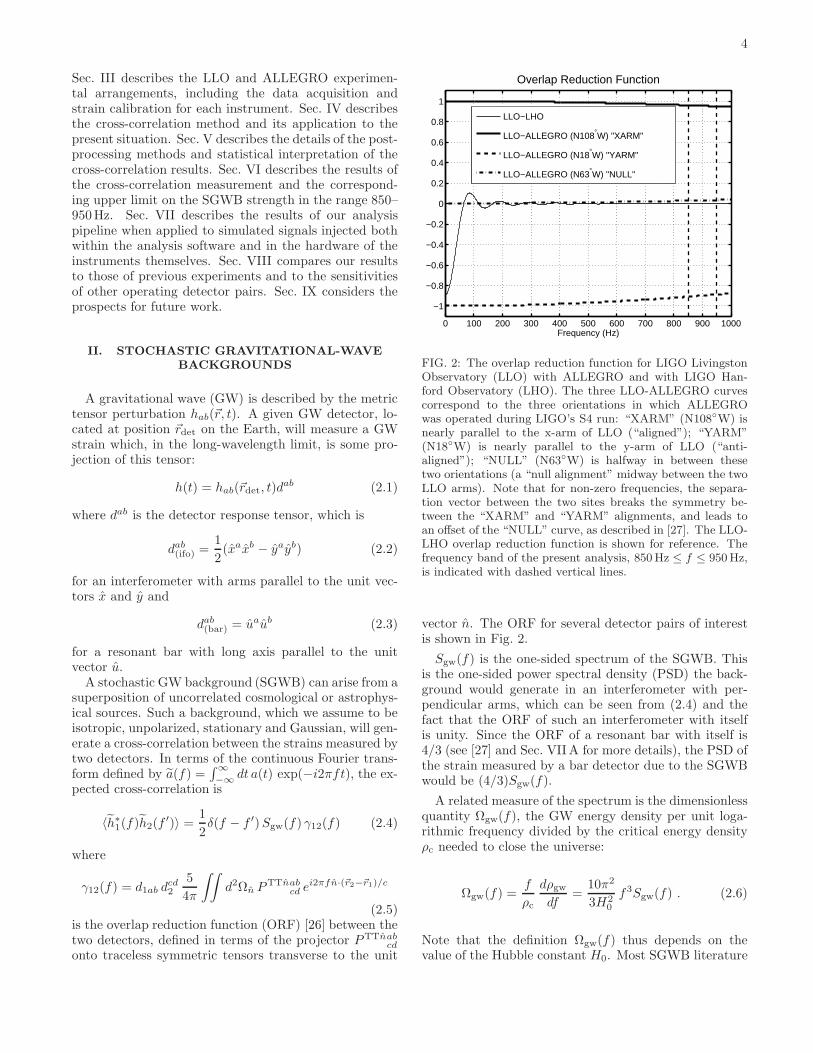
FIG. 2: The overlap reduction function for LIGO LivingstonObservatory (LLO) with ALLEGRO and with LIGO Han-ford Observatory (LHO). The three LLO-ALLEGRO curvescorrespond to the three orientations in which ALLEGROwas operated during LIGO’s S4 run: “XARM” (N108W) isnearly parallel to the x-arm of LLO (“aligned”); “YARM”(N18W) is nearly parallel to the y-arm of LLO (“anti-aligned”); “NULL” (N63W) is halfway in between thesetwo orientations (a “null alignment” midway between the twoLLO arms). Note that for non-zero frequencies, the separa-tion vector between the two sites breaks the symmetry be-tween the “XARM” and “YARM” alignments, and leads toan offset of the “NULL” curve, as described in [27]. The LLO-LHO overlap reduction function is shown for reference. Thefrequency band of the present analysis, 850Hz ≤ f ≤ 950Hz,is indicated with dashed vertical lines.

vector n. The ORF for several detector pairs of interestis shown in Fig. 2.

Sgw(f) is the one-sided spectrum of the SGWB. Thisis the one-sided power spectral density (PSD) the back-ground would generate in an interferometer with per-pendicular arms, which can be seen from (2.4) and thefact that the ORF of such an interferometer with itselfis unity. Since the ORF of a resonant bar with itself is4/3 (see [27] and Sec. VIIA for more details), the PSD ofthe strain measured by a bar detector due to the SGWBwould be (4/3)Sgw(f).

A related measure of the spectrum is the dimensionlessquantity Ωgw(f), the GW energy density per unit loga-rithmic frequency divided by the critical energy densityρc needed to close the universe:

Ωgw(f) =f

ρc

dρgwdf

=10π2

3H20

f3Sgw(f) . (2.6)

Note that the definition Ωgw(f) thus depends on thevalue of the Hubble constant H0. Most SGWB literature

5

avoids this artificial uncertainty by working in terms of

h2100Ωgw(f) =

(H0

100 km/s/Mpc

)2

Ωgw(f) (2.7)

rather than Ωgw(f) itself. We will instead follow theprecedent set by [23] and quote numerical values forΩgw(f) assuming a Hubble constant of 72 km/s/Mpc.A variety of spectral shapes have been proposed for

Ωgw, for both astrophysical and cosmological stochasticbackgrounds [3, 30, 31]. For example, whereas the slow-roll inflationary model predicts a constant Ωgw(f) in thebands of LIGO or ALLEGRO, certain alternative cosmo-logical models predict broken-power law spectra, wherethe rising and falling slopes, and the peak-frequency aredetermined by model parameters [3]. String-inspired pre-big-bang cosmological models belong to this category[5, 28]. For certain ranges of these three parametersthe LLO-ALLEGRO correlation measurement offers thebest constraints on theory that can be inferred from anycontemporary observation. This can happen, e.g., if thepower-law exponent on the rising spectral slope is greaterthan 3 and the peak-frequency is sufficiently close to 900Hz [29].

III. EXPERIMENTAL SETUP

A. The LIGO Livingston Interferometer

The experimental setup of the LIGO observatories hasbeen described at length elsewhere [38]. Here we pro-vide a brief review, with particular attention paid to de-tails significant for the LLO-ALLEGRO cross-correlationmeasurement.The LIGO Livingston Observatory (LLO) is an inter-

ferometric GW detector with perpendicular 4-km arms.The laser interferometer senses directly any changes inthe differential arm length. It does this by splitting alight beam at the vertex, sending the separate beamsinto 4-km long optical cavities of their respective arms,and then recombining the beams to detect any change inthe optical phase difference between the arms, which isequivalent to a difference in light travel time. This pro-vides a measurement of h(t) as defined in (2.1) and (2.2).However, the measured quantity is not exactly h(t) fortwo reasons:First, there are local forces which perturb the test

masses, and so produce changes in arm length. Thereare also optical and electronic fluctuations that mimicreal strains. The combination of these effects causes astrain noise n(t) to always be present in the output, pro-ducing a measurement of

s(t) = h(t) + n(t) (3.1)

Second, the test masses are not really free. There isa servo system, which uses changes in the differentialarm length as its error signal q(t), and then applies extra

(“control”) forces to the test masses to keep the differ-ential arm length nearly zero. It is this error signal q(t)which is recorded, and its relationship to the strain esti-mate s(t) is most easily described in the Fourier domain:

s(f) = R(f)q(f) (3.2)

The response function R(f) is estimated by a combina-tion of modelling and measurement [39] and varies slowlyover the course of the experiment.Because the error signal q(t) has a smaller dynamic

range than the reconstructed strain s(t), our analysisstarts from the digitized time series q[k] = q(tk) (sam-pled 214 = 16384 times per second, and digitally down-sampled to 4096Hz in the analysis) and reconstructs theLLO strain only in the frequency domain.

B. The ALLEGRO Resonant Bar Detector

The ALLEGRO resonant detector, operated by agroup from Louisiana State University [41], is a two-tonaluminum cylinder coupled to a niobium secondary res-onator. The secondary resonator is part of an inductivetransducer [42] which is coupled to a DC SQUID. Strainalong the cylindrical axis excites the first longitudinalvibrational mode of the bar. The transducer is tunedfor sensitivity to this mechanical mode. Raw data ac-quired from the detector thus reflect the high Q resonantmechanical response of the system. A major technicalchallenge of this analysis is due to the extent to whichthe bar data differ from those of the interferometer.

1. Data Acquisition, Heterodyning and Sampling

The ALLEGRO detector has a relatively narrow sen-sitive band of ∼ 100Hz centered around ∼ 900Hz nearthe two normal modes of the mechanical bar-resonatorsystem. For this reason, the output of the detector canfirst be heterodyned with a commercial lock-in ampli-fier to greatly reduce the sampling rate, which is set at250 samples/s. Both the in-phase and quadrature out-puts of the lock-in are recorded and the detector outputcan thus be represented as a complex time series whichcovers a 250Hz band centered on the lock-in referenceoscillator frequency. This reference frequency is chosento be near the center of the sensitive band, and duringthe S4 run it was set to 904Hz. The overall timing ofdata heterodyned in this fashion is provided by both thesampling clock and the reference oscillator. Both timebases were locked to GPS.The nature of the resonant detector and its data acqui-

sition system gives rise to a number of timing issues: het-erodyning, filter delays of the electronics and the timingof the data acquisition system itself [21]. It is of criticalimportance that the timing be fully understood so that

6

the phase of any potential signal may be recovered. Con-vincing evidence that all of the issues are accounted forin is demonstrated by the recovery and cross-correlationof test signals simultaneously injected into both detec-tors. The signals were recovered at the expected phaseas presented in Sec. VII.

2. Strain Calibration

The raw detector output is proportional to the dis-placement of the secondary resonator, and thus has aspectrum with sharp line features due to the high-Q res-onances of the bar-resonator system as can be seen inFig. 3. The desired GW signal is the effective strain on

840 860 880 900 920 940 96010

0

101

102

103

104

Raw spectrum, S4 run − averaged over orientation

frequency (Hz)

Am

plitu

de S

pect

rum

(co

unts

/ √H

z)

XARMYARMNULL

FIG. 3: The graph displays the amplitude spectral densityof raw ALLEGRO detector output during S4, at a frequencyresolution of 0.1 Hz. For this graph these data have not beentransformed to strain via the calibrated response function Thevertical scale represents digital counts/

√Hz The normal me-

chanical modes where the detector is most sensitive are at880.78 Hz and 917.81 Hz. There is an injected calibration lineat 837Hz. Also prominent are an extra mechanical resonanceat 885.8 Hz and a peak at 904Hz (DC in the heterodyned datastream)

the bar, and recovering this means undoing the resonantresponse of the detector. This response has a long co-herence time – thus long stretches of data are neededto resolve the narrow lines in the raw data. The straindata have a much flatter spectrum, as shown in Fig. 1.Therefore it is practical to generate the calibrated straintime series, s(t), and use that as the input to the crosscorrelation analysis.The calibration procedure, described in detail in [21],

is carried out in the frequency domain and consists ofthe following: A 30 minute stretch of clean ALLEGROdata is windowed and Fourier-transformed. The mechan-ical mode frequencies drift slightly due to small temper-

ature variations, so these frequencies are determined foreach stretch and those are incorporated into the model ofthe mechanical response of the system to a strain. Themodel consists of two double poles at these normal modefrequencies. In addition to this response we must thenaccount for the phase shifts due to the time delays in thelock-in and anti-aliasing filters.After applying the full response function, the data are

then inverse Fourier-transformed back to the time do-main. The next 50% overlapping 30 minute segment isthen taken. The windowed segments are stitched to-gether until the entire continuous stretch of good datais completed. The first and last 15 minutes are dropped.The result represents a heterodyned complex time seriesof strain, whose amplitude spectral density is shown inFig. 1.The overall scale of the detector output in terms of

strain is determined by applying a known signal to thebar. A force applied to one end of the bar has a sim-ple theoretical relationship to an equivalent gravitationalstrain [21, 32, 33]. A calibrated force can be applied viaa capacitive “force generator” which also provides themechanism used for hardware signal injections. A recip-rocal measurement – excitation followed by measurementwith the same transducer – along with known propertiesof the mechanical system, allows the determination ofthe force generator constant . With that constant deter-mined (with units of newtons per volt) a calibrated forceis applied to the bar and the overall scale of the responsedetermined.

3. Orientation

A unique feature of this experiment is the ability to ro-tate the ALLEGRO detector and modulate the responseof the ALLEGRO-LLO pair to a GW background [25].Data were taken in three different orientations of ALLE-GRO, known as XARM, YARM, and NULL, detailed inTable I. As shown in Fig. 2 and (2.4), these orientationscorrespond to different pair responses due to differentoverlap reduction functions. In the XARM orientation–the bar axis parallel to the x-arm of the interferometer–a GW signal produces positive correlation between thedata in the two detectors detectors. In the YARM orien-tation a GW signal produces an anti-correlation. In theNULL orientation–the bar aligned halfway between thetwo arms of the interferometer–the pair has very nearlyzero sensitivity as a GW signal produces almost zero cor-relation between the detectors’ data. A real signal is thusmodulated whereas many types of instrumental correla-tion would not have the same dependence on orientation.

IV. CROSS-CORRELATION METHOD

This section describes the method to used to searchfor a SGWB by cross-correlating detector outputs. In the

7

Dates orientation azimuth γ(850Hz) γ(915Hz) γ(950Hz)

2005 Feb 22–2005 Mar 4 YARM N108W -0.9087 -0.8947 -0.8867

2005 Mar 4–2005 Mar 18 XARM N18W 0.9596 0.9533 0.9498

2005 Mar 18–2005 Mar 23 NULL N63W 0.0280 0.0318 0.0340

TABLE I: Orientations of ALLEGRO during the LIGO S4 Run, including overlap reduction function evaluated at the extremesof the analyzed frequency range, and at the frequency of peak sensitivity. Note that while the NULL orientation representsperfect misalignment (γ = 0) at 0Hz, it is not quite perfect at the frequencies of interest. This is primarily because of anazimuth-independent offset term in γ(f) which contributes at non-zero frequencies [25, 27]. Due to this term, it is impossibleto orient ALLEGRO so that γ(f) = 0 at all frequencies, and to set it to zero around 915Hz one would have to use an azimuthof N62W rather than N63W.

case of L1-A1 correlation measurements, it is complicatedby the different sampling rates for the two instrumentsand the fact that the A1 data are heterodyned at 904Hzprior to digitization.

A. Continuous-Time Idealization

Both ground-based interferometric and resonant-massdetectors produce a time-series output which can be re-lated to a discrete sampling of the signal

si(t) = hi(t) + ni(t) (4.1)

where i labels the detector (1 or 2 in this case), hi(t) isthe gravitational-wave strain defined in (2.1), and ni(t)is the instrumental noise associated with each detector,converted into an equivalent strain. The detector outputis characterized by its power spectral density Pi(f)

〈s∗i (f)si(f ′)〉 = 1

2δ(f − f ′)Pi(f) (4.2)

which should be dominated by the auto-correlation of thenoise (〈s∗i (f)si(f ′)〉 ≈ 〈n∗

i (f)ni(f′)〉). If the instrument

noise is approximately uncorrelated, the expected cross-correlation of the detector outputs is [cf. (2.4)]

〈s∗1(f)s2(f ′)〉 ≈ 〈h∗

1(f)h2(f′)〉

=1

2δ(f − f ′)Sgw(f) γ12(f)

(4.3)

which can be used along with the auto-correlation (4.2)to determine the statistical properties of the cross-correlation statistic defined below.We use the optimally-filtered cross-correlation method

described in [19, 22] to calculate a cross-correlation statis-tic which is an approximation to the continuous-timecross-correlation statistic

Y c =

∫dt1 dt2 s1(t1)Q(t1 − t2)s2(t2)

=

∫df s∗1(f) Q(f) s2(f)

(4.4)

In the continuous-time idealization, such a cross-correlation statistic, calculated over a time T , has an

expected mean

µY c = 〈Y c〉 ≈ T

2

∫∞

−∞

df γ(|f |)Sgw(f)Q(f) (4.5)

and variance

σ2Y c = 〈(Y c − µY c)2〉 ≈ T

4

∫∞

−∞

df P1(f)P2(f)∣∣∣Q(f)

∣∣∣2

(4.6)Using (4.5) and (4.6), the optimal choice for the filter

Q(f), given a predicted shape for the spectrum Sgw(f)can be shown [19] to be

Q(f) ∝ γ(|f |)Sgw(f)

P1(f)P2(f)(4.7)

If the spectrum of gravitational waves is assumed to bea power law over the frequency band of interest, a con-venient parameterization of the spectrum, in terms ofΩgw(f) defined in (2.6), is

Ωgw(f) = ΩR

(f

fR

)α

(4.8)

where fR us a conveniently-chosen reference frequencyand ΩR = Ωgw(fR). The cross-correlation measurementis then a measurement of ΩR, and if the optimal filter isnormalized according to

Q(f) = N γ(f) (f/fR)α

|f |3 P1(f)P2(f)(4.9a)

where

N =20π2

3H02

(∫∞

−∞

df

f6

[γ(f) (f/fR)α]2

P1(f)P2(f)

)−1

(4.9b)

then the expected statistics of Y c in the presence of abackground of actual strength ΩR are

µY c = ΩR T (4.10)

and

σ2Y c = T

(10π2

3H02

)2 (∫ ∞

−∞

df

f6

[γ(f) (f/fR)α]2

P1(f)P2(f)

)−1

(4.11)and a measurement of Y c/T provides a point estimate ofthe background strength ΩR with associated estimatederrorbar σY c/T .

8

B. Discrete-Time Method

1. Handling of Different Sampling Rates and Heterodyning

Stochastic-background measurements using pairs ofLIGO interferometers [22] have implemented (4.4) fromdiscrete samplings si[k] = s(t0+k δt) as follows: First thecontinuous Fourier transforms s(f) were approximatedusing the discrete Fourier transforms of windowed andzero-padded versions of the discrete time series; thenan optimal filter was constructed using an approxima-tion to (4.7), and finally the product of the three wassummed bin-by-bin to approximate the integral over fre-

quencies. The discrete version of Q(f) was simplified intwo ways: first, because of the averaging used in calculat-ing the power spectrum, the frequency resolution on theoptimal filter was generally coarser than that associatedwith the discrete Fourier transforms of the data streams,and second, the value of the optimal filter was arbitrar-ily set to zero outside some desired range of frequenciesfmin ≤ f ≤ fmax. This was justified because the optimalfilter tended to have little support for frequencies outsidethat range.

The present experiment has two additional compli-cations associated with the discretization of the time-series data. First, the A1 data are not a simple time-sampling of the gravitational-wave strain, but are base-banded with a heterodyning frequency fh

2 = 904Hz asdescribed in Sec. III B 1–IIIB 2. Second, the A1 dataare sampled at (δt2)

−1 = 250Hz, while the L1 data aresampled at 16384Hz, and subsequently downsampled to(δt1)

−1 = 4096Hz. This would make a time-domaincross-correlation extremely problematic, as it would ne-cessitate a large variety of time offsets t1 − t2. In thefrequency domain, it means that the downsampled L1data, once calibrated, represent frequencies ranging from−2048Hz to 2048Hz, while the calibrated A1 data rep-resent frequencies ranging from (904− 125)Hz = 779Hzto (904 + 125)Hz = 1029Hz. These different frequencyranges do not pose a problem, as long as the range of fre-quencies chosen for the integral satisfies fmin > 779Hzand fmax < 1029Hz. Another requirement is that for thechosen frequency resolution, the A1 data heterodyne ref-erence frequency must align with a frequency bin in theL1 data. This is satisfied for integer-second data spansand integer-hertz reference frequencies. With these con-ditions, the Fourier transforms of the A1 and L1 dataare both defined over a common set of frequencies, asdetailed in [36]. Looking at the A1 spectrum in Fig. 1, areasonable range of frequencies should be a subset of therange 850Hz . f . 950Hz.

2. Discrete-Time Cross-Correlation

Explicitly, the time-series inputs to the analysispipeline, from each T = 60 sec of analyzed data, are:

• For L1, a real time series q1[j]|j = 0, . . . N1 − 1,sampled at (δt1)

−1 = 4096Hz, consisting of N1 =T/δt1 = 245760 points. This is obtained by down-sampling the raw data stream by a factor of 4.The data are downsampled to 4096Hz rather than2048Hz to ensure that the rolloff of the associ-ated anti-aliasing filter is outside the frequencyrange being analyzed. The raw L1 data are relatedto gravitational-wave strain by the calibration re-

sponse function R1(f) constructed as described inSec. III A.

• For A1, a complex time series sh2 [k]|k = 0, . . .N2−1, sampled at (δt2)

−1 = 250Hz, consisting ofN2 = T/δt2 = 15000 points. This is calibratedto represent strain data as described in Sec. III B 2,but still heterodyned.

To produce an approximation of the Fourier transformof the data from detector i, the data are multiplied byan appropriate windowing function, zero-padded to twicetheir original length, discrete-Fourier-transformed, andmultiplied by δti. In addition, the L1 data are multipliedby a calibration response function, while the A1 dataare interpreted as representing frequencies appropriatein light of the heterodyne. For L1,

s1(fℓ) ∼ s1[ℓ]

:= R1(fℓ)

N1−1∑

j=0

w1[j]q1[j] exp

(−i 2π ℓj

2N1

)δt1 ,

ℓ = −N1, . . . , N1 − 1 (4.12)

where fℓ = ℓ2T is the frequency associated with the ℓth

frequency bin. In the case of A1, the identification isoffset by ℓh2 = fh · (2T ) = 107880:

s2(fℓ) ∼ s2[ℓ]

:=

N2−1∑

k=0

w2[k]q2[k] exp

(−i 2π (ℓ− ℓh2 )k

2N2

)δt2 ,

ℓ = ℓh2 −N2, . . . , ℓh2 +N2 − 1 (4.13)

As is shown in [36], if we construct a cross-correlationstatistic

Y :=

ℓmax∑

ℓ=ℓmin

1

2T[s1(fℓ)]

∗ Q(fℓ) s2(fℓ) (4.14)

the expected mean value in the presence of a stochasticbackground with spectrum Sgw(f) is

µ := 〈Y 〉 ≈ w1w2T

2

ℓmax∑

ℓ=ℓmin

1

2T[Q(fℓ)] γ(fℓ)Sgw(fℓ)

(4.15)where w1w2 is an average of the product of the two win-dows, calculated using the points which exist at both

9

sampling rates; specifically, if r1 and r2 are the smallestintegers such that δt1/δt2 = r1/r2 = 125/2048,

w1w2 =r1r2N

N/(r1r2)−1∑

n=0

w1[nr2]w2[nr1] (4.16)

Note that while the average value given by (4.15) is mani-festly real, any particular measurement of Y will be com-plex, because of the band-pass associated with the het-erodyning of the A1 data. As shown in [36], the realand imaginary parts of the cross-correlation statistic eachhave expected variance

σ2 :=1

2〈Y ∗Y 〉

≈ T

8w2

1w22

ℓmax∑

ℓ=ℓmin

1

2T

∣∣∣Q(fℓ)∣∣∣2

P1(|fℓ|)P2(|fℓ|)

(4.17)

where once again w21w

22 is an average over the time sam-

ples the two windows have “in common”:

w21w

22 =

r1r2N

N/(r1r2)−1∑

n=0

(w1[nr2])2(w2[nr1])

2 (4.18)

3. Construction of the Optimal Filter

To perform the cross-correlation in (4.14), we need toconstruct an optimal filter by a discrete approximationto (4.9). We approximate the power spectra P1(f) usingWelch’s method [37]; as a consequence of the averaging ofperiodograms constructed from shorter stretches of data,the power spectra are estimated with a frequency reso-lution δf which is coarser than the 1/2T associated withthe construction in (4.14). As detailed in [22], we han-dle this by first multiplying together [s1(fℓ)]

∗ and s2(fℓ)at the finer frequency resolution, then summing togethersets of 2T δf bins and multiplying them by the coarser-grained optimal filter. For our search, δf = 0.25Hz andT = 60 sec, so 2T δf = 30.

4. Power Spectrum Estimation

Because the noise power spectrum of the LLO can varywith time, we continuously update the optimal filter usedin the cross-correlation measurement. However, using anoptimal filter constructed from power spectra calculatedfrom the same data to be analyzed leads to a bias in thecross-correlation statistic Y , as detailed in [34]. To avoidthis, we analyze each T = 60 sec segment of data using anoptimal filter constructed from the average of the powerspectra from the segments before and after the segmentto be analyzed. This method is known as “sliding powerspectrum estimation” because, as we analyze successive

segments of data, the segments used to calculated thePSDs for the optimal filter slide through the data to re-main adjacent. The δf = 0.25Hz resolution is obtainedby calculating the power spectra using Welch’s methodwith 29 overlapped 4-second sub-segments in each 60-second segment of data, for a total of 58 sub-segments.

V. POST-PROCESSING TECHNIQUES

A. Stationarity Cut

The sliding power spectrum estimation method de-scribed in Sec. IVB4 can lead to inaccurate results if thenoise level of one or both instruments varies widely oversuccessive intervals. Most problematically, if the dataare noisy only within a single analysis segment, consid-eration of the power spectrum constructed from the seg-ments before and after, which are not noisy, will causethe segment to be over-weighted when combining cross-correlation data from different segments. To avoid this,we calculate for each segment both the usual estimatedstandard deviation σI using the “sliding” PSD estimatorand the “naıve” estimated standard deviation σ′

I usingthe data from the segment itself. If the ratio of these twois too far from unity, the segment is omitted from thecross-correlation analysis. The threshold used for thisanalysis was 20%. The amount of data excluded basedon this cut was between 1% and 2% in each of the threeorientations, and subsequent investigations show the finalresults would not change significantly for any reasonablechoice of threshold.

B. Bias-Correction of Estimated Errorbars

Although use of the sliding power spectrum estima-tor removes any bias from the optimally-filtered cross-correlation measurement, the methods of [34] show thatthere is still a slight underestimation of the estimatedstandard deviation associated with the finite number ofperiodograms averaged together in calculating the powerspectrum. To correct for this, we have to scale up the er-rorbars by a factor of 1+ 1/(Navg × 9/11), where Navg isthe number sub-segments whose periodograms are aver-aged together in estimating the power spectrum for theoptimal filter. For the data analyzed with the slidingpower spectrum estimator, 29 overlapping four-secondsub-segments are averaged from each of two 60-secondsegments, for a total Navg = 58. This gives a correctionfactor of 1+1/(58×9/11) = 1.021. The “naıve” estimatedsigmas, derived from power spectra calculated using 29averages in a single 60-second segment, are scaled up bya factor of 1 + 1/(29× 9/11) = 1.042.

10

C. Combination of Analysis Segment Results

As shown in [19], the optimal way to combine a seriesof independent cross-correlationmeasurements YI withassociated one-sigma errorbars is

Y opt =

∑I σ

−2I YI∑

I σ−2I

(5.1a)

σY opt =

(∑

I

σ−2I

)−1/2

(5.1b)

To minimize spectral leakage, we use Hann windows inour analysis segments, which would reduce the effectiveobserving time by approximately one-half, so we over-lap the segments by 50% to make full use of as muchdata as possible. This introduces correlations betweenoverlapping data segments, which modifies the optimalcombination slightly, as detailed in [35].

D. Statistical Interpretation

The end result of the analysis and post-processing ofa set of data is a an optimally combined complex cross-correlation statistic Y opt with a theoretical mean of ΩRTand an associated standard deviation of σY opt on both thereal and imaginary parts. We can construct from this ouroverall point estimate on the unknown actual value of ΩR

and the corresponding one-sigma errorbar:

ΩR = Y opt/T (5.2a)

σΩ = σY opt/T (5.2b)

For a given value of ΩR, and assuming σΩ to be given,the likelihood function for the complex point estimate to

have a particular value ΩR = x+ iy is

P (x, y|ΩR, σΩ) =d2P

dxdy=

1

2πσ2Ω

exp

(−|x+ iy − ΩR|2

2σ2Ω

)

=1

2πσ2Ω

e−(x−ΩR)2/2σ2Ωe−y2/2σ2

Ω

(5.3)

Given a prior probability density function on ΩR, Bayes’stheorem allows us to construct a posterior

P (ΩR|x, y, σΩ) =P (x, y|ΩR, σΩ)P (ΩR)

P (x, y|σΩ)

∝ e−(x−ΩR)2/2σ2ΩP (ΩR)

(5.4)

where x = Re ΩR. In this work we choose a uniformprior over the interval [0,Ωmax], where Ωmax is chosento be 116 (the previous best upper limit at frequenciesaround 900Hz [20]), except in the case of the hardwareinjections in Sec. VII C, where the a priori upper limit istaken to be well above the level of the injection.

Given a posterior probability density function (PDF),the 90% confidence level Bayesian upper limit ΩUL isdefined by

∫ ΩUL

0

dΩR P (ΩR|x, y, σΩ) = 0.90 (5.5)

Alternatively, any range containing 90% of the area underthe posterior PDF can be thought of as a Bayesian 90%confidence level range. To allow consistent handling ofresults with and without simulated signals, we choosethe narrowest range which represents 90% of the areaunder the posterior PDF. (This is the range whose PDFvalues are larger than all those outside the range.) For a

low enough signal-to-noise ratio Re ΩR/σΩ, this range isfrom 0 to ΩUL.

E. Treatment of Calibration Uncertainty

In reality, the conversion of raw data from the LIGOand ALLEGRO GW detectors into GW strain is not per-fect. We model this uncertainty in the calibration processas a time- and frequency-independent phase and magni-

tude correction, so that ΩR = x+ iy and σΩ are actuallyrelated to ΩRe

Λ+iφ, where Λ and φ are unknown ampli-tude and phase corrections; the likelihood function thenbecomes

P (x, y|ΩR, σΩ,Λ, φ) =1

2πσ2Ω

exp

(−∣∣x+ iy − ΩRe

Λ+iφ∣∣2

2σ2Ω

)

(5.6)Given a prior PDF P (Λ, φ) for the calibration correc-tions, we can marginalize over these nuisance parametersand obtain a marginalized likelihood function

P (x, y|ΩR, σΩ)

=

∫∞

−∞

dΛ

∫ π

−π

dφP (x, y|ΩR, σΩ,Λ, φ)P (Λ, φ) (5.7)

We take this prior PDF to be Gaussian in Λ and φ, with astandard deviation added in quadrature from the quotedamplitude and phase uncertainty for the two instruments.For L1, this is 5% in amplitude and 2 in phase [39] andfor A1 it is 10% in amplitude and 3 in phase [21].

VI. ANALYSIS OF COINCIDENT DATA

A. Determination of Analysis Parameters

To avoid biasing our results, we set aside approxi-mately 9% of the data, spread throughout the run, asa playground on which to tune our analysis parameters.Based on playground investigations, we settled on thefollowing parameters for our analysis:

• Overlapping 60-second Hann-windowed analysissegments

11

• Frequency range 850Hz ≤ f ≤ 950Hz, 0.25Hz res-olution for optimal filter

• L1 data downsampled to 4096Hz before analysis

• Removal of the following frequencies from the op-timal filter: 900Hz (2.25Hz wide), 904Hz (0.25Hzwide).

The frequencies to remove were chosen on the basis ofstudies of the coherence of stretches of L1 and A1 data(see Fig. 4); 900Hz is the only harmonic of the 60Hzpower line within our analysis band, and detectable co-herence is seen for frequencies within 1Hz of the line.904Hz is notched out because, as the heterodyne fre-quency, it corresponds to DC in the heterodyned A1 data.After completing the cross-correlation analysis, we com-puted the coherence from the full run of data, as shownin Fig. 5. The results are similar to those from the play-ground, except for a lower background level, and a featureat the heterodyning frequency.The relevant range of frequencies can be determined by

looking at the support of the integrand of (4.11), knownas the sensitivity integrand. The overall sensitivity in-tegrand, constructed as a weighted average over all thenon-playground data used in the analysis, is plotted inFig. 6. The area under this curve for a range of frequen-cies is proportional to that frequency range’s contributionto σ−2. We see that the integrand does indeed becomenegligible by a frequency of 850Hz on the lower end and950Hz on the upper end. We further see that most ofthe sensitivity comes from a 20-Hz wide band centeredaround 915Hz.

B. Cross-Correlation and Upper Limit Results

After data quality cuts, exclusion of the “playground”,and application of the stationarity cut described inSec. VA, 44806 one-minute segments of data were ana-lyzed, for an effective observing time of 384.1 hours (con-sidering the effects of Hann windowing), of which 181.2hours was in the XARM orientation, 114.7 in the YARMorientation, and 88.2 in the NULL orientation. The re-sults are shown in Table II. No statistically significantcorrelation is seen in any orientation, and optimal combi-nation of all data leads to a point estimate of 0.31+0.30ifor ΩR, with a one-sigma errorbar of 0.48 each on thereal and imaginary parts.The results in Table II include the ORF describ-

ing the geometry in the optimal filter. This meansan orientation-independent non-GW cross-correlationpresent in the data would change sign between XARMand YARM, and would look much larger in the NULLresult. One way to remove the effects of the observinggeometry and compare orientation-independent cross-correlations is to remove the γ(f) from (4.9). Since theORF for each orientation is nearly constant across theobserving band, and notably across the region of peak

850 860 870 880 890 900 910 920 930 940 95010

−7

10−6

10−5

10−4

10−3

10−2

10−1

100A1L1 S4 playground Coherence −− combined orientations

frequency (Hz)

896 897 898 899 900 901 902 903 904

10−4

10−3

10−2

10−1

A1L1 S4 playground Coherence −− combined orientations ZOOM

frequency (Hz)

FIG. 4: LLO-ALLEGRO (L1-A1) coherence, calculated from48.66 hours of playground data spanning nearly 30 days. Theonly significant feature is the power line harmonic at 900Hz.The closeup view in the second plot shows that the coherenceis insignificant beyond 1Hz away from the line. Based on this,we mask out the nine 0.25-Hz frequency bins around 900Hzfrom our analysis.

sensitivity, it is sufficient to multiply the overall resultsin each case by γ(915Hz). This is shown in Table III,where we again see no significant cross-correlation, andsensitivities whose relative sizes are well explained by thediffering observing times.

We use the methods of Sec. VD and VE to constructa posterior PDF from the overall cross-correlation mea-surement of 0.31 + 0.30i and estimated errorbar of 0.48,taking into consideration the nominal calibration uncer-tainty of 11% in magnitude and 3.6 in phase to obtainthe posterior PDF shown in Fig. 7. The narrowest likely90% confidence interval on ΩR is [0, 1.02]. We thus set anupper limit of 1.02 on ΩR = Ωgw(fR), which translates to

an upper limit on Sgw(915Hz) of (1.5× 10−23Hz−1/2)2.

12

850 860 870 880 890 900 910 920 930 940 95010

−7

10−6

10−5

10−4

10−3

10−2

10−1

100

A1L1 S4 full−run Coherence −− combined orientations

frequency (Hz)

896 897 898 899 900 901 902 903 904

10−4

10−3

10−2

10−1

A1L1 S4 full−run Coherence −− combined orientations ZOOM

frequency (Hz)

FIG. 5: LLO-ALLEGRO (L1-A1) coherence, calculated fromall S4 data without regard to playground status. Again, the900Hz line is seen to be comfined to a 2Hz wide range. Ad-ditionally, a feature at the heterodyning frequency of 904Hz(which was masked a priori in our main cross-correlation anal-ysis) becomes visible.

VII. VALIDATION VIA SIGNAL INJECTION

To check the effectiveness of our algorithm at detectingstochastic GW signals, we performed our search on datawith simulated waveforms “injected” into them. This wasdone both by introducing the simulated signals into theanalysis pipeline (software injections), and by physicallydriving both instruments in coincidence (hardware injec-tions). Hardware injections provide an end-to-end test ofour detection pipeline and also a test on the calibrationaccuracies of our instruments, but are necessarily short induration because they corrupt the GW data taken duringthe injection. Software injections can be carried out forlonger times and therefore at lower signal strengths, and

850 860 870 880 890 900 910 920 930 940 9500

0.01

0.02

0.03

0.04

0.05

0.06

0.07

0.08

0.09Sensitivity Integrand from S4 non−playground data

Frequency (Hz)

Fra

ctio

nal S

ensi

tivity

Inte

gran

d (H

z−1 )

FIG. 6: The sensitivity integrand for the data used in thecross-correlation analysis, normalized so its integral equalsunity. The area under this curve, between two frequencies, isthe fractional contribution to σ−2 from that range of frequen-cies. Notice that the nine frequency bins masked out around900Hz and the one at 904Hz give no contribution, and thatthe sensitivity integrand is also suppressed at other frequen-cies corresponding to lines in the A1 noise power spectrum.

Teff ΩR

Type (hrs) Point Estimate Error Bar

XARM 181.2 0.61 + 0.25i 0.56

YARM 114.7 −0.47 + 0.47i 0.90

non-NULL 295.8 0.31 + 0.31i 0.48

NULL 88.2 10.96 − 43.89i 28.62

all 384.1 0.31 + 0.30i 0.48

TABLE II: Results of optimally-filtered cross-correlation ofnon-playground data. Results are shown for data in each ofthree orientations (XARM, YARM, and NULL). Addition-ally, the XARM and YARM results are combined with theoptimal weighting (proportional to one over the square of theerrorbar) to give a “non-NULL” result, and results from allthree orientations are optimally combined to give an overallresult. In each case, Teff is the effective observing time includ-ing the effects of overlapping Hann windows. Note that sincethe non-NULL data are much more sensitive than the NULLdata, they dominate the final result. Note also that becausethe optimal filter includes the the ORF, the relative orien-tation of LLO and ALLEGRO is already included in theseresults. This is reflected, for example, in the large errorbarson the NULL result.

can be repeated to perform statistical studies. Softwareinjections, however, cannot check for calibration errors.

13

Teff γΩR

Type (hrs) Point Estimate Error Bar

XARM 181.2 0.58 + 0.24i 0.53

YARM 114.7 0.42− 0.42i 0.80

NULL 88.2 0.35− 1.40i 0.91

TABLE III: The cross-correlation results of Table II, scaledby γ(915Hz) from Table I, the value of the ORF at the fre-quency of peak sensitivity. This gives a sense of the “raw”cross-correlation, independent of the orientation-dependentgeometrical factor. The different observing times explain theremaining variation in the one-sigma errorbar for the measure-ment, which should be inversely proportional to the squareroot of the observing time.

0 0.2 0.4 0.6 0.8 1 1.2 1.4 1.6 1.8 20

0.5

1

1.5

2

2.5

Ωgw

Pos

terio

r P

DF

Posterior PDF & 90% conf band from all non−PG data

FIG. 7: Posterior probability density function associated withthe overall combined point estimate of 0.31 + 0.30i and esti-mated errorbar of 0.48, considering the uncertainty in thephase and amplitude of the calibration. The shaded regionrepresents 90% of the area under the curve, leading to an up-per limit on ΩR of 1.02, which corresponds to a gravitationalwave strain of 1.5 × 10−23 Hz−1/2 at the peak frequency of915Hz.

A. Signal Simulation Algorithm

To simulate a correlated SGWB signal in an interfer-ometer and a bar, the formulas in, e.g., [19] need to begeneralized slightly. This is because the ORF of a detec-tor with itself is in general [27]

γ = 2

[dabdab −

1

3(daa)

2

], (7.1)

which is unity for an IFO with perpendicular arms (2.2)but 4/3 for a bar (2.3). Writing this quantity for detector1 or 2 as γ11 or γ22, respectively, makes the required

cross-correlations in a simulated SGWB signal

〈h∗

1(f)h1(f′)〉 = 1

2δ(f − f ′)Sgw(f) γ11 (7.2a)

〈h∗

1(f)h2(f′)〉 = 1

2δ(f − f ′)Sgw(f) γ12(f) (7.2b)

〈h∗

2(f)h2(f′)〉 = 1

2δ(f − f ′)Sgw(f) γ22 . (7.2c)

The above expressions do not determine a unique algo-rithm for converting a set of random data streams intoindividual detector strains. One possible prescription is

h1(f) =1

2

√Sgw(f)

√γ11 (x1(f) + iy1(f)) (7.3a)

h2(f) = h1(f)γ12(f)

γ11

+1

2

√Sgw(f)

(γ22 −

γ212(f)

γ11

)(x2(f) + iy2(f)) ,

(7.3b)

where x1(f), y1(f), x2(f), and y2(f) are statistically in-dependent real Gaussian random variables, each of zeromean and unit variance. In the above pair, γ12(f) is

used only in the construction of h2(f) and not of h1(f).A different pair, where γ12 is explicitly included in thecalculation of both strains more symmetrically, can bedefined as follows: Let zk(f) := (xk(f) + iyk(f))/

√2 be

a pair (k = 1, 2) of complex random functions and let

s :=√1− γ2

12/(γ11γ22). Then, the second pair can beexpressed as:

h1(f) =

√Sgw(f)

2

√γ11 (a(f)z1(f) + b(f)z2(f)) (7.4a)

h2(f) =

√Sgw(f)

2

√γ22 (b(f)z1(f) + a(f)z2(f)) ,

(7.4b)

where a =√(1 + s)/2 and b = γ12/

√2(1 + s)γ11γ22 are

determined completely by the three ORFs. Either pairof simulated strains obeys (7.2). The signals for softwareinjections were generated using (7.4); those for hardwareinjections were generated by an older code which used(7.3). Further details of simulated signal generation arein [40].

B. Results of Software Simulation

We performed software injections into the full S4 co-incident playground, 4316 overlapping one-minute anal-ysis segments with an effective observing time of 37.0hours considering the effects of Hann windows (16.7 hoursof this is in the XARM orientation, 11.2 hours in theYARM orientation, and 9.0 hours in the NULL orienta-tion). We injected constant-Ωgw(f) spectra of strengthscorresponding to ΩR =1.9, 3.9, 9.6, and 19, as well as a

14

ΩR injected Point Estimate Error Bar 90% conf int

0 0.32 − 1.00i 1.54 [0.00,2.74]

1.9 2.22 − 0.86i 1.55 [0.09,4.35]

3.9 4.14 − 0.79i 1.55 [1.61,6.66]

9.6 9.89 − 0.65i 1.56 [7.32,12.45]

19 19.56 − 0.49i 1.58 [16.96,22.15]

TABLE IV: Results of software injections. All figures are forconstant-Ωgw(f) and listed by ΩR level. The 90% confidencelevel ranges are calculated without marginalizing over anycalibration uncertainty.

test with the SGWB amplitude set to 0 to reproducethe analysis of the playground itself. Note that eventhe strongest of these injections does not produce cor-relations detectable in an individual one-minute analysissegment. The results are summarized in table IV. Ineach case, the actual injected value of ΩR is consistentwith the real part of the point estimate to within theone-sigma estimated error bar; the imaginary part of thepoint estimate remains zero to within the errorbar. Theresults for injections at ΩR = 1.9 and stronger would cor-respond to statistical “detections” at the 90% or betterconfidence level.

C. Results of Hardware Injection

During S4, a set of simulated signals was injected inthe hardware of ALLEGRO and LLO. These injectionsserved to test the full detection pipeline as well as thecalibrations of both instruments. As described in detailin [40], the preparation of simulated waveforms for hard-ware injections requires application of the transfer func-tion of the hardware component that is actuated, such asone of the two end test masses in LLO, to the theoreti-cal strain for that instrument. Subsequent refinements toinstrumental calibration mean that the precise injectedsignal strength is determined after the fact. Six hardwareinjections performed during S4, each 1020 seconds long,had an effective constant Ωgw(f) of 8100. The series ofinjections we call “A” and “B” were performed duringthe XARM and NULL observation periods, respectively.Independent of the physical orientation of ALLEGRO,the injection and analysis was performed for three differ-ent assumed orientations, producing “plus” (aligned, asin the XARM orientation), “minus” (anti-aligned, as inYARM), and “null” (misaligned, as in NULL) injectionsin each series. The results (after correcting for knownphase offsets in the injection systems) for each of the sixinjections are shown in Table V.The results show some variation of magnitude and

phase of the point estimates, especially for the “null” in-jections. However, all the injection results are consistentwith the injected signal strength to within statistical andsystematic uncertainties. This is illustrated informally

in Fig. 8, which shows the point estimates on the com-plex plane, each surrounded by an error circle of radius2.15 times the corresponding estimated errorbar. (Thisradius was chosen because 90% of the volume under atwo-dimensional Gaussian falls within a circle of radius2.15σ.) Those circles all overlap with a region centered atthe actual injection strength illustrating the magnitudeand phase uncertainty in the calibration. The system-atic error can be more quantitatively evaluated using themethod of Sec. VE to produce a posterior PDF associ-ated with each injection measurement. This is illustratedfor the optimally-combined point estimate of 7448 + 65iand associated estimated errorbar 47 in Fig. 9, and rangescorresponding to the most likely 90% confidence rangeunder the posterior PDFs (with and without marginal-ization) are included in Table V. For each of the sixinjections, as well as for the combined result, the actualinjected value of 8100 falls into the range after marginal-ization over the calibration uncertainty.

VIII. COMPARISON TO OTHER

EXPERIMENTS

The previous most sensitive direct upper limit at thefrequencies probed by this experiment was set by cross-correlating the outputs of the EXPLORER and NAU-TILUS resonant bar detectors [20]. They found an up-per limit on h2

100Ωgw(907.20Hz) of 60. Using the value of72 km/s/Mpc for the Hubble constant, that translates toa limit of 116 on Ωgw(907.20Hz), upon which our limitof 1.02 is a hundredfold improvement.Data from LLO, taken during S4, were also corre-

lated with data from the LIGO Hanford Observatory(LHO) to set an upper limit on Ωgw(f) at frequencies be-tween 50Hz and 150Hz [24]. Correlations between LLOand LHO are not suited to measurements at high fre-quencies because of the effects of the ORF, illustratedin Fig. 2. For comparison, rough measurements usingS4 LLO-LHO data and a band from 850Hz to 950Hzyield upper limits of around 20, while those confined to905Hz ≤ f ≤ 925Hz (the band contributing most of theL1-A1 sensitivity give upper limits of around 80.Correlations between the 4km and 2km IFOs at LHO,

known as H1 and H2, respectively, are not suppressedby the ORF, which is identically unity for colocated,coaligned IFOs. Since H1 and L1 have comparable sensi-tivities, the most significant factor in comparing H1-H2to L1-A1 sensitivity is the relative sensitivities of A1 andH2. Since H2 was about a factor of 50 (in power) moresensitive than A1 during S4, averaged across the bandfrom 905Hz to 925Hz, we would expect an H1-H2 cor-relation measurement during S4 to be a factor of 7 orbetter more sensitive than L1-A1 as a measure of Ωgw(f)at these frequencies. However, the fact that H1 and H2share the same physical environment at LHO necessitatesa careful consideration of correlated noise which is ongo-ing [43].

15

γΩR γΩR ΩR ΩR Point Estimate unmarg. range marg. range

Injection Error Bar Point Estimate Error Bar Value Mag Phase min max min max

A-minus 83 −6623 − 126i 93 7403 + 141i 7404 1.1 7250 7555 6212 8820

A-null 99 205 + 19i 3106 6429 + 607i 6457 5.4 1565 11294 1435 11562

A-plus 83 6983 + 64i 87 7325 + 67i 7325 0.5 7182 7468 6146 8726

B-minus 95 −6845 + 49i 106 7650 − 55i 7651 −0.4 7478 7825 6417 9115

B-null 111 366− 50i 3486 11492 − 1576i 11600 −7.8 5950 17035 5857 17365

B-plus 92 7128 + 77i 96 7477 + 80i 7477 0.6 7317 7634 6272 8907

all N/A 47 7448 + 65i 7448 0.5 7371 7526 6256 8867

TABLE V: Results of hardware injections. Simulated waveforms with an effective signal strength of Ωgw(f) = 8100 wereinjected coincidentally in the ALLEGRO and the LIGO-Livingston (LLO) detectors. The “A” and “B” sets of injections tookplace during the XARM and NULL observing times, respectively. Independent of the actual orientation, the simulated signalswere generated and analyzed assuming different orientations: YARM, NULL, and XARM orientations were assumed for theinjections labelled “minus”, “null”, and “plus”, respectively. The first pair of columns shows the errorbars and point estimatesscaled by γ(915Hz) to give a “raw” cross-correlation as in Table III. (Note that since the “null” alignment represents not-quite-perfect misalignment, as noted in Table I [γ(915Hz) = 0.03 rather than zero], the injection still leads to a statistically significantcross-correlation even in the “null” orientation.) Note that the errorbars, thus scaled, are comparable for all six injections,while the level of correlation or anti-correlation depends on the orientation associated with the injection being analyzed. Thesubsequent columns relate to the standard cross-correlation statistic, with the ORF included in the optimal filter, so therelative insensitivity in the “null” alignment is reflected in large errorbars, while the point estimates are all positive and in thevicinity of the injected value of 8100. All point estimates given include corrections for known phase offsets associated with theinjection system. The row labelled “all” gives the optimally-weighted combination of all six results. The point estimates andone-sigma estimated errorbars were combined to give 90% confidence ranges with and without marginalization over calibrationuncertainty, mimicking the statistical analysis described in Sec. VD and VE.

Work is also currently underway to search for a SGWBat frequencies around 900Hz by correlating data fromthe Virgo IFO with the resonant bar detectors AURIGA,EXPLORER, and NAUTILUS [44].Finally, an indirect limit can be set on SGWB strength

due to the energy density in the associated gravitationalwaves themselves, which is given by

ρgw = ρcrit

∫∞

0

Ωgw(f)

fdf (8.1)

The most stringent limit is on a cosmological SGWB, setby the success of big-bang nucleosynthesis, is ρgw/ρcrit ≤1.1 × 10−5 [3]. In comparison, a background of thestrength constrained by our measurement, ΩR = 1.02,would contribute about 2 × 10−2 to ρgw/ρcrit, if it wereconfined to the most sensitive region between 905Hzand 925Hz. (Spread over the full range of integration850Hz ≤ f ≤ 950Hz, it would contribute 1 × 10−1.)Note, however, that this nucleosynthesis bound is notrelevant for a SGWB of astrophysical origin.

IX. FUTURE PROSPECTS

LIGO’s S5 science run began in November 5 with theaim of collecting one year of coincident data at LIGOdesign sensitivity. ALLEGRO has also been in opera-tion over that time period, so the measurement docu-mented in this paper could be repeated with S5 data.Such a measurement would be more sensitive due to L1’s

roughly fivefold reduction in strain noise power at 900Hzbetween S4 and S5, and because of the larger volume ofdata (roughly 20 times as much). Those two improve-ments could combine to lead to an improvement of aboutan order of magnitude in ΩR sensitivity. However, noimmediate plans exist to carry out an analysis with S5data, because this incremental quantitative improvementin sensitivity would still leave us far from the level neededto detect a cosmological background consistent with thenucleosynthesis bound, or an astrophysical backgroundarising from a realistic model.Additionally, the greater sensitivity of the H1-H2 pair

means that a background detectable with L1-A1 wouldfirst be seen in H1-H2. In the event that a “surprise” cor-relation is seen in H1-H2 which cannot be attributed tonoise, correlation measurements such as LLO-ALLEGROand Virgo-AURIGA could be useful for confirming or rul-ing out a gravitational origin.

X. CONCLUSIONS

We have reported the results of the first truly het-erogeneous cross-correlation measurement to search fora stochastic gravitational-wave background. While the

upper limit of 1.5 × 10−23 Hz−1/2 on the strain of theSGWB corresponds to a hundredfold improvement overthe previous direct upper limit on Ωgw(f) in this fre-quency band [20], the amplitude of conceivable spectralshapes is already constrained more strongly by results atother frequencies [23, 24]. The lasting legacy of this work

16

−4000 0 4000 8000 12000 16000 20000 24000−1.2

−0.8

−0.4

0

0.4

0.8

1.2x 10

4

Re(Point Estimate)

Im(P

oint

Est

imat

e)

Extraction of Hardware Injections

A−minusA−plusA−nullB−minusB−plusB−nullinjected

6800 7200 7600 8000 8400 8800−800

−400

0

400

800

Re(Point Estimate)

Im(P

oint

Est

imat

e)

Extraction of Hardware Injections

A−minusA−plusB−minusB−plusinjected

FIG. 8: Visualization of hardware injection results. Each of the six point estimates of ΩR is plotted on the complex plane,with an associated error circle of 2.15 times the estimated one-sigma errorbar. (This contains 90% of the volume under thecorresponding likelihood surface.) The five-pointed star indicates the actual injected level of ΩR = 8100. The dashed teardrop-shaped region indicates the calibration uncertainty, corresponding to a 2.15-sigma ellipse in log-amplitude/phase space. Onthe left we see that the two “null” injections are consistent in amplitude and phase with the actual injection, considering thestatistical uncertainty associated with the real and imaginary parts of their point estimates. The plot on the right (in whichthe edge of the dashed calibration uncertainty teardrop can just be seen) shows that the “plus” and “minus” injections areall statistically consistent with each other, and consistent with the injection when systematic uncertainties associated withcalibration are taken into account.

is thus more likely the overcoming of technical challengesof cross-correlating data streams from instruments withsignificantly different characteristics. Most obviously, weperformed a coherent analysis of data from resonant-massand interferometric data, but additionally the data weresampled at different rates, ALLEGRO data were hetero-dyned and therefore complex in the time domain, andentirely different methods were used for the calibrationsof both instruments. Lessons learned from this analysiswill be valuable not only for possible collaborations be-tween future generations of detectors of different types,but also between interferometers operated by differentcollaborations.

Acknowledgments

The authors gratefully acknowledge the support of theUnited States National Science Foundation for the con-struction and operation of the LIGO Laboratory and the

Particle Physics and Astronomy Research Council of theUnited Kingdom, the Max-Planck-Society and the Stateof Niedersachsen/Germany for support of the construc-tion and operation of the GEO600 detector. The authorsalso gratefully acknowledge the support of the research bythese agencies and by the Australian Research Council,the Natural Sciences and Engineering Research Coun-cil of Canada, the Council of Scientific and IndustrialResearch of India, the Department of Science and Tech-nology of India, the Spanish Ministerio de Educacion yCiencia, The National Aeronautics and Space Adminis-tration, the John Simon Guggenheim Foundation, theAlexander von Humboldt Foundation, the LeverhulmeTrust, the David and Lucile Packard Foundation, the Re-search Corporation, and the Alfred P. Sloan Foundation.The ALLEGRO observatory is supported by the NationalScience Foundation, grant PHY0215479.

This paper has been assigned LIGO Document Num-ber LIGO-P050020-08-Z.

[1] N. Christensen, Phys. Rev. D 46, 5250 (1992)[2] B. Allen, in Proceedings of the Les Houches School on As-

trophysical Sources of Gravitational Waves, Les Houches,1995, edited by J. A. Marck and J. P. Lasota (Cambridge,1996), p. 373.

[3] M. Maggiore, Phys. Rep. 331, 283 (2000).[4] M. Gasperini and G. Veneziano Astropart. Phys. 1, 317

(1993).[5] M. Gasperini and G. Veneziano Phys. Rep. 373, 1 (2003).[6] A. Buonanno, M. Maggiore, and C. Ungarelli, Phys. Rev.

D 55, 3330 (1997)[7] L. P. Grishchuk, Sov. Phys. JETP 40, 409 (1975).[8] L. P. Grishchuk, Class. Quant. Grav. 14, 1445 (1997)[9] A. A. Starobinsky, Pis’ma Zh. Eksp. Teor. Fiz. 30, 719

17

0 2000 4000 6000 8000 10000 12000 14000 16000 18000 200000

0.1

0.2

0.3

0.4

0.5

0.6

0.7

0.8

0.9

1x 10

−3

Ωgw

Pos

terio

r P

DF

Posterior PDF & 90% conf band from all HW injections

FIG. 9: Posterior probability density function associatedwith combined hardware injection measurement, includingmarginalization over calibration uncertainties. Note thatwhile the combined one-sigma statistical errorbar is only 47,the shaded 90% area under the curve has a width of over 2000.This is because systematic errors dominate in the presence ofthe large point estimate. The solid vertical line indicates theactual injection level of ΩR = 8100.

(1979).[10] A. Kosowsky, M. S. Turner, and R. Watkins, Phys. Rev.

Lett. 69, 2026 (1992)[11] R. Apreda, M. Maggiore, A. Nicolis, and A. Riotto, Nucl.

Phys. B 631, 342 (2002).[12] R. R. Caldwell and B. Allen. Phys. Rev. D 45, 3447

(1992)[13] T. Damour and A. Vilenkin, Phys. Rev. Lett. 85, 3761

(2000)[14] T. Damour and A. Vilenkin, Phys. Rev. D 71, 063510

(2005)[15] T. Regimbau and J. A. de Freitas Pacheco, Astron. and

Astrophys. 376, 381 (2001).[16] T. Regimbau and J. A. de Freitas Pacheco, Astron. and

Astrophys. 447, 1 (2006).[17] D. M. Coward, R. R. Burman, and D. G. Blair, Mon.

Not. R. Astron. Soc. 329, 411 (2002).[18] A. Cooray, Mon. Not. R. Astron. Soc. 354, 25 (2004).[19] B. Allen and J. D. Romano, Phys. Rev. D 59, 102001

(1999)[20] P. Astone et al., Astronomy and Astrophysics 351, 811

(1999).[21] M. P. McHugh and W.W. Johnson (2006), LIGO Report,

http://www.ligo.caltech.edu/docs/T/T060096-00.pdf

[22] B. Abbott et al. (LIGO Scientific Collaboration), Phys.Rev. D 69, 122004 (2004)

[23] B. Abbott et al. (LIGO Scientific Collaboration), Phys.Rev. Lett. 95, 221101 (2005)

[24] B. Abbott et al. (LIGO Scientific Collaboration),astro-ph/0608606

[25] L. S. Finn and A. Lazzarini, Phys. Rev. D 64, 082002(2001)

[26] E.E. Flanagan, Phys. Rev. D 48, 2389 (1993).[27] J. T. Whelan, Class. Quant. Grav. 23, 1181 (2006)[28] R. Brustein, M. Gasperini, M. Giovannini and

G. Veneziano, Phys. Lett. B 361, 45 (1995)[arXiv:hep-th/9507017].

[29] S. Bose, Phys. Rev. D 71, 082001 (2005)[arXiv:astro-ph/0504048].

[30] D. M. Coward, R. R. Burman, and D. G. Blair,Mon. Not. R. Astron. Soc. 324, 1015 (2001).

[31] V. Ferrari, S. Matarrese, and R. Schneider,Mon. Not. R. Astron. Soc. 303, 247 (1999).

[32] M. P. McHugh et al., Class. Quant. Grav. 22, S965 (2005)[33] A. Morse et al., Phys. Rev. D 59, 062002 (1997).[34] A. Lazzarini (2004), LIGO Report,

http://www.ligo.caltech.edu/docs/T/T040128-02.pdf

[35] A. Lazzarini and J. Romano (2004), LIGO Report,http://www.ligo.caltech.edu/docs/T/T040089-00.pdf

[36] J. T. Whelan et al, Class. Quant. Grav. 22, S1087 (2005)[37] P. D. Welch, IEEE Transactions on Audio and Electroa-

coustics AU-15, 70 (1967)[38] B. Abbott et al., Nucl. Instrum. Methods A 517, 154

(2004).[39] A. Dietz et al (2005), LIGO Report,

http://www.ligo.caltech.edu/docs/T/T050262-00.pdf

[40] S. Bose et al., Class. Quant. Grav. 20, S677 (2003)[41] http://gravity.phys.lsu.edu/[42] Gregory M. Harry, thesis, University of Maryland 1999[43] Nickolas V. Fotopoulos for the LIGO Scientific Collabo-

ration Class. Quant. Grav. 23, S693 (2006)[44] Elena Cuoco for the Virgo Collaboration, “Virgo Data

Analysis for C6 and C7 engineering runs”, presentationfrom the XIth Marcel Grossmann Meeting, July 2006.http://wwwcascina.virgo.infn.it/vsb/slides/Cuoco MG11.ppt

To appear in the proceedings of the XIth Marcel Gross-mann Meeting, July 2006.