Firms and the Decline in Earnings Inequality in Brazil

Firms and the Decline in Earnings Inequality in Brazil

Jorge Alvarez, Felipe Benguria, Niklas Engbom, and Christian Moser∗

April 7, 2017

Abstract

We document a large decrease in earnings inequality in Brazil between 1996 and 2012. Us-

ing administrative linked employer-employee data, we fit high-dimensional worker and firm

fixed effects models to understand the sources of this decrease. Firm effects account for 40 per-

cent of the total decrease and worker effects for 29 percent. Changes in observable worker and

firm characteristics contributed little to these trends. Instead, the decrease is primarily due to

a compression of returns to these characteristics, particularly a declining firm productivity pay

premium. Our results shed light on potential drivers of earnings inequality dynamics.

JEL Codes: D22, E24, J31

Keywords: Earnings Inequality, Linked Employer-Employee Data, Firm and Worker Hetero-

geneity, Productivity

∗Alvarez: International Monetary Fund, 700 19th Street NW, Washington, DC 20431 (e-mail: [email protected]);Benguria: Department of Economics, Gatton College of Business and Economics, University of Kentucky, 550 SouthLimestone Street, Lexington, KY 40506-0034 (e-mail: [email protected]); Engbom: Department of Economics, PrincetonUniversity, 001 Fisher Hall, Princeton, NJ 08544 (e-mail: [email protected]); Moser: Graduate School of Busi-ness, Columbia University, 3022 Broadway, New York, NY 10027 (e-mail: [email protected]). We thank the editorand three anonymous referees for their input, which helped to greatly improve the paper. We are grateful for the gen-erous advice of Richard Rogerson since the inception of this project. We thank Elhanan Helpman and Marc Muendlerfor help in launching our investigation. We also benefitted from input by Mark Aguiar, Adrien Auclert, Angus Deaton,Henry Farber, Mike Golosov, Fatih Guvenen, Oleg Itskhoki, Gregor Jarosch, Greg Kaplan, Nobu Kiyotaki, Alan Krueger,Ilyana Kuziemko, Alex Mas, Ben Moll, Chris Neilson, Ezra Oberfield, Stephen O’Connell, Stephen Redding, HarveyRosen, Hannes Schwandt, Yongseok Shin, Tom Vogl, Chris Woodruff, and seminar participants at Princeton Univer-sity, Peterson Institute for International Economics, IMF, PEDL conference in Warwick, Barcelona GSE Summer Forum,Cambridge-INET conference, and LACEA-LAMES conference in Medellín. Special thanks go to Carlos Corseuil, Glau-cia Ferreira, Leandro Justino, Carlos Lessa, and Luis Carlos Pinto at IBGE and IPEA for facilitating our data work. Theauthors gratefully acknowledge financial support from the Private Enterprise Development in Low Income Countries(PEDL) research initiative by DFID-CEPR, the Gregory C. and Paula K. Chow Macroeconomic Research Program, theIndustrial Relations Section, the Fellowship of Woodrow Wilson Scholars, the Institute for International and RegionalStudies at Princeton University, and the Ewing Marion Kauffman Foundation. The views expressed in this study arethe sole responsibility of the authors and should not be attributed to the International Monetary Fund, its ExecutiveBoard, or its management. All errors are our own.

1

mailto:[email protected]




1 Introduction

Since the mid-1990s, Brazil has experienced a large reduction in earnings inequality resembling

the experience of other Latin American economies during this period. This decrease in earnings

inequality stands in stark contrast to that of the US and many developed countries, which saw

inequality steadily increasing over the past two decades.1 This paper studies the sources of this

decrease.

To this end, we exploit a large administrative linked employer-employee dataset containing

information on hundreds of millions of job spells between 1988 and 2012. By repeatedly esti-

mating an additive worker and firm fixed effects model due to Abowd, Kramarz and Margolis

(1999a)—henceforth AKM—we quantify the contributions of firm and worker-specific factors to-

wards changes in Brazilian inequality. In a second stage, we link this earnings decomposition

to a rich set of worker demographics and firm financials data for Brazilian manufacturing and

mining firms. The merged data allow us to study the transmission from worker and firm char-

acteristics into pay in a large developing economy. In doing so, we distinguish between changes

in the distribution of worker and firm characteristics on one hand and changing returns to these

characteristics on the other hand.

We uncover three main results. First, firms played an important role in the decrease in earnings

inequality in Brazil over this period, explaining 40 percent of the fall in the variance of log earnings

between 1996 and 2012. Compression in worker fixed effects explains an additional 29 percent of

the decrease, with the remaining part attributable to a decrease in the covariance between worker

and firm fixed effects and the residual. Given that worker heterogeneity is the most important

component in explaining pay levels throughout this period, the compression in firm-specific pay

contributed more than proportionately towards Brazil’s inequality decrease.

Second, changes in the link between firm performance and pay account for a significant frac-

tion of the compression in the firm component of workers’ earnings.2 We first show that a substan-

tial share of the cross-sectional variation in the firm component of pay is explained by differences

in observable firm characteristics, with more productive and larger firms paying more. Moreover,

1See Lopez and Perry (2008) and Tsounta and Osueke (2014) for inequality trends in Brazil and the rest of LatinAmerica. Kopczuk et al. (2010) and Heathcote et al. (2010) document the evolution of earnings inequality in the US,while Atkinson and Bourguignon, eds (2015) discuss inequality trends across other high- and middle-income countries.

2This part of the analysis is based on the subpopulation of larger mining and manufacturing firms for which wehave data. As we discuss in greater detail later, this subpopulation has experienced both a similar amount of overallcompression in earnings inequality and a similar contribution of workers and firms towards it.

2

more than half of the decrease in the firm component is accounted for by observable firm char-

acteristics. All of this decrease is driven by a weakening pass-through from firm characteristics

to pay, while none is due to firms becoming more similar in observable characteristics over time.

Altogether, a weaker link between observable firm characteristics and worker pay explains 30

percent of the overall fall in the variance of log earnings over this period.

Third, a decrease in the return to measures of ability such as experience and education explains

a sizable share of the fall in the variance of the worker component of pay. In levels, age and

education explain close to 40 percent of the variance of the worker component of pay. However,

we do not observe a large compression in the underlying distributions of such characteristics over

time. Instead, the decrease in worker pay heterogeneity is driven by a rapid fall in the returns

to observable measures of worker ability, particularly the education premia. Lower returns to

worker age and education explain 14 percent of the overall fall in the variance of log earnings

over the 1996–2012 period.

This decomposition of the sources of Brazil’s earnings inequality decrease informs our un-

derstanding of various commonly proposed explanations of the decrease. On the worker side,

our results do not support an often articulated view that changes in educational attainment ac-

counted for the largest share of Brazil’s inequality evolution over the period (Barros et al., 2010).

While educational attainment increased rapidly over this period, those gains were largely offset

by concurrent decreases in the high school and college education premia. We reach similar con-

clusions regarding the implications of changes in the age structure of the workforce. On the firm

side, a reading of the existing literature would suggest that trade and other factors affecting the

productivity distribution during this period could have been an important driver behind changes

to the earnings distribution.3 Yet, in line with US trends, we find that the Brazilian productivity

distribution actually grew more dispersed over this period.

These findings pose a challenge to candidate explanations behind Brazil’s decrease in earnings

inequality over this period. Our results suggest that a theory of the inequality decrease needs to be

consistent with the following three facts: (i) firm-level pay differences explain a significant share

of initial inequality levels and a disproportionately large share of its decrease; (ii) lower pass-

through from firm productivity to pay is a key driver behind compression in the firm component

3See for example Dunne et al. (2004) and Faggio et al. (2010) who conclude that parts of the increase in earningsinequality in the US can be explained by widening dispersion in the firm productivity distribution.

3

of pay; and (iii) lower returns to worker ability explain a significant share of the compression

in the worker component of pay. We conclude that changes in pay policies rather than shifts in

the distribution of worker and firm fundamentals played an important role in Brazil’s inequality

decrease during this period.

Related literature. We contribute to three broad strands of the literature. First, we provide a

decomposition of earnings into worker and firm heterogeneity in a developing economy. With the

increasing availability of large, administrative matched employer-employee datasets, a growing

literature examines the role of firms in wage determination. A seminal methodological contribu-

tion that separately identifies worker and firm heterogeneity in pay is the work by AKM. They find

an important role for firms in explaining observed wage dispersion in French linked employer-

employee data. Similar conclusions have been reached among others for Germany (Andrews et

al., 2008; Card et al., 2013), Italy (Iranzo et al., 2008), Portugal (Card et al., 2016), Brazil (Lopes de

Melo, 2015), Sweden (Bonhomme et al., 2016), Denmark (Bagger and Lentz, 2016), and the United

States (Abowd et al., 1999b, 2002; Woodcock, 2015; Sorkin, 2015; Engbom and Moser, 2017b). Some

recent papers are closely related to the first stage of our empirical methodology, which applies

the AKM framework in overlapping subperiods to study changes in earnings components over

time. Card et al. (2013) find that increasing dispersion in the firm-specific component of pay con-

tributed significantly to rising earnings inequality in West Germany. Barth et al. (2016) and Song

et al. (2016) show that firms were an important driver behind the increase in US labor earnings

inequality since 1980, with the latter set of authors highlighting an increased assortativeness in the

allocation of workers across firms through the lens of the AKM framework.

Second, we contribute to a literature studying worker pay in relation to firm outcomes by

linking our decomposition results to worker and firm characteristics. In previous work, Blanch-

flower et al. (1996) suggest and implement a test for rent-sharing in the US manufacturing sector.

Van Reenen (1996) examines pass-through from firm-level innovation to worker wages in the UK.

Guiso et al. (2005) assess to what extent firm-level productivity shocks are passed on to workers

in Italy. AKM study the link between measures of firm performance and estimated firm effects

in France, but do not focus on changes over time to this relationship. Similarly, Menezes-Filho

et al. (2008) focus on the cross-sectional relationship between firm characteristics and wages in

Brazil’s manufacturing and mining sectors. Card et al. (2014) focus on the relationship between

4

rent-sharing and firm investments in Italy. Bagger et al. (2014) investigate the role of labor misal-

location in driving the positive correlation between labor productivity and firm-level wages using

Danish data. Card et al. (2016) analyze the degree of rent-sharing in Portugal with a particular

emphasis on gender differences in profit participation and the allocation of workers across firms.

By differentiating between changes in the underlying distribution versus changes in the returns

to worker and firm characteristics over time, we contribute toward this literature and shed light

on the sources behind Brazil’s large decrease in earnings inequality.

Third, we add to the literature on the drivers of inequality dynamics in Brazil by providing

a comprehensive decomposition of its inequality evolution that cuts across specific explanations.

Many previous papers have studied the role of isolated mechanisms in Brazil’s inequality decrease

over the last two decades. For example, Ulyssea (2014) and Meghir et al. (2015) study the effects of

policies on Brazil’s formal and informal sector employment. Alvarez (2017) interprets empirical

worker switches between sectors through the lens of a Roy model to investigate determinants

of the agricultural wage gap in Brazil. Dix-Carneiro and Kovak (2017) analyze the long-lasting

impact of industry-specific tariff cuts in the presence of imperfect interregional labor dynamics

related to slow capital adjustment and agglomeration economies. In related work, Dix-Carneiro

et al. (2016) relate Brazil’s trade liberalization to income inequality and crime at the regional level,

while Dix-Carneiro and Kovak (2015) examine its impact on the evolution of the skill premium.

Helpman et al. (2016) show that a significant share of the rise in Brazilian wage inequality from

1986–1995 is due to between-firm differences and that these trends are consistent with the effects

of trade liberalization in a heterogenous-firm model of trade and inequality. Adão (2016) finds that

movements in world commodity prices explain part of the decrease in Brazilian wage inequality

from 1991–2010. Medeiros et al. (2014) use administrative tax return data to study the evolution

of top income inequality in Brazil from 2006–2012, but they cannot distinguish between the role

played by worker versus firm characteristics during that period. Using a empirical methodology

similar to ours, Lopes de Melo (2015) conducts a static decomposition of earnings inequality levels

in Brazil’s formal sector into components due to firms and workers. de Araujo (2014) studies the

role of labor adjustment costs in propagating wage inequality in the Brazilian context. Finally,

using administrative linked employer-employee data and an equilibrium search model, Engbom

and Moser (2017a) argue that the rise in the minimum wage was an important driver behind

Brazil’s inequality decrease from 1996–2012.

5

Outline. The rest of the paper is structured as follows: Section 2 provides an overview of the

main institutional changes and macroeconomic trends affecting Brazilian labor markets from 1988

to 2012. Section 3 summarizes the administrative datasets used in our empirical analysis and dis-

cusses sample selection as well as variable definitions. Section 4 provides descriptive statistics on

trends in earnings inequality in Brazil during this period. Section 5 introduces our two-stage em-

pirical framework, which first decomposes earnings into worker and firm components and then

links this decomposition to worker and firm characteristics. Section 6 describes our main empiri-

cal results, presents checks on the validity of our empirical framework, and discusses implications

for potential explanations behind Brazil’s inequality decrease. Finally, Section 7 summarizes our

key findings and concludes.

2 Institutions and macroeconomic trends in Brazil

During our period of study, Brazil resumed democratic elections in 1989, ended a decade of hyper-

inflation in 1994, and recovered from a financial crisis in 1999. The latter came with a floating of

the exchange rate and fiscal adjustment, which resulted in the government turning a deficit into a

primary surplus. After a "lost decade" of economic growth leading up to 1994, real GDP per capita

grew by a half percentage point a year up until 2002, by a rapid three percent per year 2002–2008,

contracted by two percent in 2009, and rebounded quickly with six percent growth in 2010. In this

section, we discuss some of the institutional changes that could have affected inequality during

this period, including labor regulation, trade liberalization and social policy.

Brazil had a highly regulated labor market before reforms started in the late 1980s. Since 1965

a national Wage Adjustment Law mandated yearly wage increases for all workers in the economy

and dismissal costs were high. After the transition to civil rule and the signing of a new constitu-

tion in 1988, flexibility in labor markets was further affected by firing penalties and the increasing

power of labor unions, which gather about a quarter of employed formal workers in Brazil. The

Wage Adjustment Law was finally abandoned in 1995, introducing a period of greater flexibility

and less regulated wage-setting practices. Further legislation in 1997–1998 eased restrictions on

temporary contracts and lowered dismissal barriers. Subsequently, formal employment increased

by around five percent and unemployment fell from 10 percent in 2000 to around six percent in

2011. The overall labor force participation rate has remained roughly stable at 65–70 percent over

6

this period (World Bank, 2016).

Hyperinflation resulted in widespread indexation of wages to the minimum wage. From 1980

to 1989, yearly inflation averaged 355 percent, which was followed by a yearly average of 1,667

percent between 1990 and 1994 (World Bank, 2016). To keep up, the minimum wage was adjusted

first annually and then on a monthly basis proportionately to the previous period’s realized in-

flation rate. In 1994, hyperinflation finally subsided with the introduction of the Plano Real. This

ambitious stabilization program introduced a gradual float of the local currency, tightened mone-

tary and fiscal policy, and lowered inflation below two-digits.

In parallel to monetary stabilization, Brazil liberalized trade during this period. Starting with

initially high import tariffs that had substituted import bans from the previous decade, a series

of trade liberalization bills in the late 1980s eliminated selected tariffs and eradicated quantitative

import controls. Upon becoming president in 1995, social democrat Fernando Henrique Cardoso

further strengthened this agenda with a reduction of tariff and non-tariff trade barriers to one tenth

of their levels in 1987 (Pavcnik et al., 2004). The opening up to trade over the last 25 years has been

frequently cited as a major contributor to the country’s growth in total factor productivity (Ferreira

and Rossi, 2003; Ferreira et al., 2007; Moreira, 2004; Muendler, 2004; Córdova and Moreira, 2003).

In addition, Helpman et al. (2016) argue that trade reforms contributed to the rise in earnings

inequality in the late 1980s and early 1990s.

Health, education and other social programs began expanding during the late 1990s. This

trend further strengthened with the election of the left-wing Workers’ Party in 2003, who doubled

social expenditure as a fraction of GDP. Although social spending remains less than one percent

of GDP, it is often portrayed as an important contributor to the reduction in household income

inequality.4 The reach of the public cash transfer program, Bolsa Famìlia, increased to cover 11

million families in 2006, which comprised nearly 25 percent of the total population (Barros et al.,

2010). Education spending increased to 5.5 percent of GDP in 2009 (compared to 3.5 percent in

2000 and 5.7 percent among G20). As we discuss in Appendix A, this is reflected in a rapidly

rising share of the labor force with a high school degree. Moreover, the quality of education

relative to other countries, as measured by the international PISA scores, has also improved, with

Brazil having the greatest increase in mathematics among 65 countries since 2003 (Organisation

4Using household data, Barros et al. (2010) estimate that social programs accounted for about 20 percent of thedecrease in household income inequality.

7

for Economic Co-operation and Development, 2012).

The Worker’s Party complemented social policies with accelerated minimum wage increases.

Within their first year in office, they implemented a 20 percent increase of the minimum wage in

2003 and continued to implement yearly increases averaging over 10 percent during the next 10

years. As a result, the minimum to median earnings of adult male workers in Brazil increased

from around 34 percent in 1996—similar to US levels—to over 60 percent, which is close to the

level in France. Engbom and Moser (2017a) argue that this large increase in the minimum wage

can explain a significant fraction of the reduction in earnings inequality in Brazil over the 1996–

2012 period, while being consistent with the key facts in this paper.

3 Data

Our analysis uses two confidential administrative datasets from Brazil: the Relação Anual de In-

formações Sociais (RAIS) contains earnings and demographic characteristics of workers as reported

by employers, and the Pesquisa Industrial Anual - Empresa (PIA-Empresa, or PIA in short) contains

detailed information on revenues and costs of firms in Brazil’s mining and manufacturing sectors.

In the following section, we briefly discuss their collection, coverage, variable definitions, and

sample selection.

3.1 Linked employer-employee data (RAIS)

Collection and coverage. The RAIS data contains linked employer-employee records that are

constructed from a mandatory survey filled annually by all registered firms in Brazil and admin-

istered by the Brazilian Ministry of Labor and Employment (Ministerio do Trabalho e Emprego, or

MTE). Data collection was initiated in 1986 within a broad set of regions, reaching complete cover-

age of all employees at formal establishments of the Brazilian economy in 1994.5 Fines are levied

on late, incomplete, or inaccurate reports, and as a result many businesses hire a specialized ac-

countant to help with the completion of the survey. In addition, MTE conducts frequent checks on

5Because registration with the central tax authorities is necessary for a firm to be surveyed, the RAIS covers onlyworkers in Brazil’s formal sector. Complementing our analysis with data from the Brazilian household survey PesquisaNacional por Amostra de Domicílios (PNAD), we find that the formal sector employment share among male workers of age18–49 grew from 64 to 74 percent between 1996 and 2012. Differential inequality trends between formal and informalsector workers are discussed at more length in Engbom and Moser (2017a).

8

establishments across the country to verify the accuracy of information reported in RAIS, particu-

larly with regards to earnings, which are checked to adhere to the minimum wage legislation.6

The RAIS contains an anonymized, time-invariant person identifier for each worker, which al-

lows us to follow individuals over time. It also contains anonymized time-invariant establishment

and firm identifiers that we use to link multiple workers to their employers and follow those over

time. Although it would be possible to conduct part of our analysis at the establishment instead

of firm level, this paper focuses on firms for three reasons. First, to the extent that there is substan-

tial variation in pay across establishments within firms, our firm-level analysis provides a lower

bound on the importance of workers’ place of employment.7 Second, we think that many of the

factors that could give rise to employer-specific components of pay, including corporate culture,

company leadership, etc., act at the firm level. Additionally, many regulations targeting pay poli-

cies differ as a function of firm-level employment, not establishment-level employment. Third,

we will later use data on firm characteristics such as financial performance that are not available

at the establishment-level.

Variable definitions. For each firm at which a worker was employed during the year, the RAIS

contains information on the start and end date of the employment relationship, the amount the

worker was paid and worker background characteristics. Reported earnings are gross and include

regular salary payments, holiday bonuses, performance-based and commission bonuses, tips, and

profit-sharing agreements. While this is a broad measure of earnings, it does not contain other

sources of income such as capital income or in-kind transfers. To control for variation in labor

supply, we divide total earnings from an employment relationship in a given year by the duration

of the job spell.8 As weekly hours only exist from 1994, our main analysis does not use per hour

pay. Instead, to limit the impact of unmeasured labor supply differences, we focus on adult males.

In the years for which we have hours, more than 75 percent of adult males report working 44

6In addition to being fined, non-compliant firms are added to a “Black List of Slave Work Employers,” made avail-able publicly under law Decree No. 540/2004. Current versions of the list are disseminated by the Brazilian televisionnews channel Repórter Brasil.

7As we will show later, however, the explanatory power of our model incorporating firm and person effects is high,leaving little variation to be explained by separate establishment level effects. This is in line with evidence from the USin Barth et al. (2016) and Song et al. (2016) who show that most across firm dispersion drives the vast majority of crossplant variation.

8That is, if an employment relationship is reported as active for seven months during the year, we divide totalearnings reported for that employment relationship for that year by seven.

9

hours a week.9

We define a consistent age variable by calculating the year of birth for any observation, and

then setting an individual’s year of birth as the modal implied value and finally reconstructing

age in each year using this imputed year of birth.10 Because age is only reported in bins prior to

1994, we code all subsequent years into the same age bins: less than 18, 18–24, 25–29, 30–39, 40–49,

and more than 49 years old.

We define a consistent measure of years of schooling by first setting it to its modal value within

a year in case of multiple job spells in a year and then ensuring that the years of schooling are non-

decreasing across years. Subsequently, we define four education groups based on degree comple-

tion implied by the reported number of years of schooling and the education system in Brazil:

primary school (four years), middle school (seven years), high school (12 years), and college (12

or more years).

The data also contain information on detailed occupation classification of the job and detailed

sector classification of the employer establishment. Both the industry and occupation classifica-

tion systems underwent a significant change during the period we study. For occupations, we use

the pre-2003 classification (Classificação Brasileira de Ocupações, or CBO) at the one-digit level. We

also use two-digit sectoral classifications (Classificação Nacional de Atividades Económicas, or CNAE)

according to the pre-2003 period. We make occupations and sectors reported for 2003–2012 consis-

tent with the older CBO and CNAE classifications by using conversion tables provided by IBGE.

In order to increase consistency between the old and the new classification schemes we opt for

one digit occupation classification and two digit sector classification, which for the purpose of this

paper we think provides sufficient detail.

Our firm size measure is the number of full-time equivalent workers during the reference

year. We calculate it as the total number of worker-months employed by the firm during the year

divided by 12.11

Sample selection. We exclude observations with either firm or worker identifiers reported as

invalid as well as data points with missing earnings, dates of employment, educational attainment9We show in Appendix D that similar inequality trends hold in hourly wage rates for full-time employed adult

males for the years for which we have data on hours.10We use age instead of experience throughout our analysis; results are similar using age plus six minus years of

education as a measure of experience.11This is computed prior to making any sample restrictions so that it reflects accurately, to the extent possible, the

total amount of labor used by the firm during the year.

10

or age. Together, these cleaning procedures drop less than one percent of the original population,

indicative of the high quality of the data. Subsequently, to limit the computational complexity

associated with estimating our model, we restrict attention to one observation per worker-year.

We impose this restriction by choosing the highest-paying among all longest employment spells

in any given year. As the average number of jobs held during the year is 1.2 and there is no trend

in this, we believe that loosening this restriction would not meaningfully affect our results.

Finally, we restrict attention to male workers age 18–49. We make this restriction as a trade-off

between on the one hand our results being comparable to a large part of the literature focusing

on prime age males, and on the other to obtain as complete as possible coverage of changes in the

Brazilian earnings structure over the period. The restriction to male workers has the advantage

of avoiding issues with changing patterns of female labor supply over time. The restriction to

age 49 and below is made to avoid issues related to early retirement, which is more common in

Brazil than in the US and other developed countries. In previous versions of the paper, we have

considered a wider age range as well as both genders, leading to broadly similar findings as what

we present here.

Descriptive statistics. Table 1 provides key summary statistics for the RAIS data for the six sub-

periods that we will later use in our AKM analysis, namely 1988–1992, 1992–1996, 1996–2000,

2000–2004, 2004–2008, and 2008–2012. Since our analysis focuses separately on adult males as well

as adult males working for larger manufacturing and mining firms, we provide a brief compari-

son of these subpopulations to the overall population of formal sector employees. As we will be

primarily concerned with the later four subperiods during which inequality decreased markedly

and for which we have firm level data, we focus our discussion on these periods.

Panel A shows statistics for the overall formal sector work force in Brazil, while Panel B shows

statistics for the subpopulation of prime age adult males. The latter group has 0.67 years of school-

ing less than the overall sample in the 1996–2000 subperiod; this gradually drops to 0.57 years in

the last subperiod. Adult males earn 4–13 log points more than the overall population, and the

variance of log earnings is slightly higher than that of the overall population.

Panel C presents statistics on the subpopulation of adult males working at larger mining and

manufacturing firms. Adult males in the PIA subpopulation are about 0.03 years younger than

all adult males in the 1996–2000 subperiod, which gradually increases to 0.5 years younger in the

11

last subperiod. They are similar to all adult males in terms of education. The PIA sample of adult

males earned on average 28 log points more than all adult males in the 1996–2000 subperiod; this

decreased to 20 log points in the last subperiod. Finally, they display a three and five log point

higher standard deviation of log earnings in the 1996–2000 and 2008–2012 period, respectively.

Table 1. RAIS summary statistics

# Worker- Earnings Age Schoolingyears # Workers Mean St.d. Mean St.d. Mean St.d.

PANEL A. ALL FORMAL SECTOR WORKERS (RAIS)1988–1992 165.5 41.3 1.10 0.86 31.90 11.44 7.65 4.431992–1996 162.1 43.0 1.18 0.86 33.17 11.29 8.09 4.401996–2000 174.6 46.7 1.19 0.84 33.67 11.26 8.61 4.262000–2004 202.7 52.6 1.00 0.80 34.01 11.32 9.50 4.052004–2008 254.2 62.4 0.81 0.74 34.21 11.45 10.27 3.782008–2012 326.5 75.7 0.71 0.71 34.46 11.62 10.81 3.51

PANEL B. ADULT MALE WORKERS

1988–1992 78.4 23.5 1.23 0.86 30.80 8.05 7.17 4.251992–1996 78.9 24.3 1.28 0.86 31.42 8.10 7.50 4.201996–2000 83.9 26.5 1.26 0.83 31.54 8.17 7.94 4.072000–2004 94.7 29.8 1.04 0.78 31.58 8.22 8.81 3.892004–2008 112.9 34.0 0.85 0.72 31.65 8.24 9.60 3.672008–2012 135.0 39.6 0.76 0.68 31.76 8.21 10.24 3.46

PANEL C. ADULT MALE WORKERS AT LARGE MANUFACTURING AND MINING FIRMS (PIA)1996–2000 15.5 5.8 1.54 0.86 31.51 8.05 7.95 4.012000–2004 16.7 6.3 1.28 0.83 31.30 8.13 8.87 3.842004–2008 21.0 7.8 1.07 0.77 31.12 8.14 9.52 3.692008–2012 23.9 9.0 0.96 0.73 31.26 8.08 10.16 3.51

Note: The number of worker-years and number of unique workers are reported in millions. Statistics on earnings are in log multiples

of the current monthly minimum wage, schooling is in years, a person’s age is the average age of his age bin. Panel A includes all

workers in the RAIS dataset. Panel B includes male workers that are between 18 and 49 years old. Panel C includes male workers

age 18–49 working at larger manufacturing and mining firms included in the PIA firm characteristics data. Means are computed by

period. The standard deviation is calculated by first demeaning variables by year and then pooling the years within a subperiod.

Source: RAIS.

3.2 Firm characteristics data (PIA)

Collection and coverage. The PIA data contain information on firm financial characteristics

from 1996–2012. The dataset is constructed by the Brazilian National Statistical Institute (Instituto

Brasileiro de Geografia e Estatística, or IBGE) based on annual firm surveys in the manufacturing

and mining sector. This survey is mandatory for all firms with either more than 30 employees or

12

above a revenue threshold as well as for an annual random sample of smaller firms.12 As with

RAIS, completion of the survey is mandatory and non-compliance is subject to a fine by national

authorities. Each firm has a unique, anonymized identifier, which we use to link firm characteris-

tics data from PIA to worker-level outcomes in the RAIS data.

Variable definitions. The PIA dataset includes a breakdown of operational and non-operational

revenues, costs, investment and capital sales, number of employees and payroll. All nominal val-

ues are converted to real values using the CPI index provided by the IBGE. Instead of the measure

of firm size in the PIA, we prefer our measure of full-time-equivalent employees constructed from

the RAIS as it accounts for workers only employed during part of the year. We define operational

costs as the cost of raw materials, intermediate inputs, electricity and other utilities, and net rev-

enues as the gross sales value due to operational and non-operational firm activities net of any

returns, cancellations, and corrected for changes in inventory.13 We construct value added as the

difference between net revenues and intermediate inputs, and value added per worker as value

added divided by full-time equivalent workers. This is our main measure of firm productivity. We

have also constructed several alternative measures of firm productivity by cleaning value added

per worker off industry-year effects and some measures of worker skill, with similar results.

Our productivity measure differs from commonly used total factor productivity (Bartelsman

et al., 2009, 2013) since it does not control for capital intensity. We opt for this measure because

we do not directly observe capital stocks in the PIA data, only investment. To construct a measure

of the capital stock, one would need to assume a depreciation rate to be able to impute capital

using reported investment. In the absence of firm investment data prior to 1996, one would also

need to impute initial capital stocks at the firm-level in 1996, as well as for any firm that (re-)enters

the PIA population. We have constructed such a measure of the capital stock, but the multiple

imputations required to obtain capital and fact that the investment data is incomplete for many

firms lead us to prefer value added per worker as our measure of firm productivity. Instead we

have constructed several variants of this labor productivity measure, making various adjustments

for worker input quality that lead to very similar results to what we present below.14

12The revenue threshold for inclusion in the deterministic survey has grown over the years, standing at USD300,000in 2012.

13We have explored alternative revenue definitions such as only restricting attention to operational revenues or ex-cluding certain types of non-operational revenues. Such robustness checks yield very similar results to what we reportbelow.

14Specifically, in the construction of labor productivity, we alternatively divide value added by the raw number of

13

Sample selection. The PIA firm survey spans the universe of larger firms (as defined above)

in Brazil’s manufacturing and mining sectors in addition to a random sample of smaller firms.

Because parts of our analysis make use of the panel dimension on the firm side and to avoid issues

with excessive sample attrition related to our later estimation procedure, we focus our analysis on

the deterministic set of relatively larger firms.

Table 2. PIA summary statistics

Firm size Value added p.w.# Firm-years # Unique firms Mean St.d. Mean St.d.

1996–2000 110.5 34.8 6.41 1.74 11.15 1.132000–2004 130.6 40.9 6.35 1.79 11.19 1.322004–2008 156.5 48.8 6.57 1.90 11.22 1.342008–2012 176.8 55.8 6.69 1.98 11.30 1.31

Note: The number of firm-years and number of unique firms are reported in thousands. Firm size is the log number of full-time

equivalent employees. Value added per worker is the log of real value added per worker. Means and standard deviations are weighted

by the number of full-time employees. The standard deviation is calculated by first demeaning variables by year and then pooling the

years within a subperiod. Source: PIA.

Descriptive statistics. Table 2 shows key summary statistics on firms during the four subperi-

ods for which we have firm financial data: 1996–2000, 2000–2004, 2004–2008, and 2008–2012. All

results are weighted by the number of full-time equivalent workers employed by the firm. The

number of firms in the PIA increased by 60 percent between the first and the last period. The aver-

age log firm size increased by 28 log points and average log real value added per worker grew by

15 log points. There is significant dispersion in both log firm size and log value added per worker

across firms, with the standard deviation of the former being close to two and that of the latter

exceeding one. Furthermore, there is no evidence of convergence in either measure: the standard

deviation of firm size monotonically increases whereas the standard deviation of value added per

worker first increases rapidly, then falls again in the last subperiod.

workers, the full-time equivalent workers, measurable human capital-augmented (i.e. accounting for education andage) workers, and also adjusting for unobserved worker characteristics captured by the worker fixed effect in pay.

14

4 Inequality trends in Brazil from 1988–2012

In this section, we provide a first overview of Brazil’s rapid decrease in earnings inequality us-

ing our sample of prime age males.15 We demonstrate that the decrease in inequality in Brazil

occurred throughout a large part of the earnings distribution. Subsequently, we provide some

suggestive evidence of firms being an important source of inequality as well as a factor behind the

decrease in inequality in Brazil.

4.1 The evolution of earnings inequality

Starting from high initial levels, Brazil experienced a rapid and steady fall in earnings inequality

from the mid 1990s onwards. The decrease followed years of stable or slightly increasing inequal-

ity between the late 1980s and the mid-1990s. To illustrate this, Figure 1 plots the variance of

log earnings over the 1988–2012 period in the RAIS. Between 1996 and 2012, the variance of log

earnings in Brazil decreased by 28 log points or 39 percent, from 0.73 to 0.44. To put this decrease

into context, the US saw an increase in the variance of log annual earnings of 30 log points from

1967–2005 (Heathcote et al., 2010).

Figure 1. Variance of log earnings in Brazil, 1988–2012

0.4

50

.50

0.5

50

.60

0.6

50

.70

0.7

50

.80

Va

ria

nce

of

log

ea

rnin

gs

1988 1990 1992 1994 1996 1998 2000 2002 2004 2006 2008 2010 2012

Note: Statistics computed for males of age 18–49. See text for details. Source: RAIS.

To depict the comprehensive nature of the decrease in inequality, Figure 2 plots the log per-

15For clarity and consistency with our main estimation results, we present these trends using the sample of malesaged 18–49 only. The trends described in this section are also present in the overall population.

15

centile ratios of earnings, normalized to zero in 1996.16 Two striking facts emerge: First, the com-

pression was wide-spread throughout the earning distribution, reaching as high as the 75th per-

centile. Second, the amount of compression gradually decreases as one moves further up in the

distribution. For instance, whereas the log 90–50 percentile ratio falls by 26 log points from 1996

to 2012, the log 50–10 ratio decreases by 38 log points, and the log 50–5 ratio by a remarkable 53

log points. We see less compression above the 75th percentile, and some divergence among the

top 10 percent of the earnings distribution, with the log 95–50 percentile ratio falling slightly less

than the log 90–50 ratio.

Figure 2. Log percentile ratios of the earnings distribution in Brazil, normalized to 0 in 1996

−0.6

−0.5

−0.4

−0.3

−0.2

−0.1

0.0

0.1

norm

aliz

ed log incom

e p

erc

entile

ratio

1988 1990 1992 1994 1996 1998 2000 2002 2004 2006 2008 2010 2012

P50−P5 P50−P10 P50−P25

Lower−tail inequality

−0.6

−0.5

−0.4

−0.3

−0.2

−0.1

0.0

0.1

norm

aliz

ed log incom

e p

erc

entile

ratio

1988 1990 1992 1994 1996 1998 2000 2002 2004 2006 2008 2010 2012

P75−P50 P90−P50 P95−P50

Upper−tail inequality


Importantly, the inequality decrease was not driven by the rapid educational attainment ex-

pansion and demographic changes during this period. Appendix A shows within a Mincer frame-

work that most of the decrease is in fact orthogonal to worker observables. The weak explanatory

power from this worker-side analysis, along with recent evidence of firm-driven inequality trends

in developed economies, motivate us to study the role of firms in the Brazilian labor market.

4.2 Earnings dispersion between and within firms

For a long time, economists have recognized that worker observables fail to explain a large frac-

tion of the variance of earnings (Mincer, 1974; Heckman et al., 2003). A recent literature instead

highlights the role played by firms in giving rise to differences in pay. As a first step towards

16Appendix B shows that there was wide-spread real earnings growth over this period.

16

understanding the role of firms in the inequality decrease, we investigate the variance of earnings

within and between firms. To this end, let yijt denote log earnings of worker i employed by firm j

in year t, and yjt denote average log earnings in firm j in year t. Following Fortin et al. (2011) and

Song et al. (2016) we can write17

Var(yijt)︸︷︷︸

overall

= Var(

y jt

)︸︷︷︸

between firms

+Var(

yijt

∣∣∣ i ∈ j)

︸︷︷︸within firms

That is, variance in overall earnings can be decomposed into the variance of average log earnings

at the firm across firms (weighted by worker-years) and the variance of the difference between

workers’ log earnings and the average log earnings at their firm.

Based on these definitions, one could imagine two hypothetical polar extremes. First, aver-

age earnings could be identical across firms so that overall earnings inequality is completely due

to variance in earnings within firms. In this case, a firm is just a microcosm of the overall econ-

omy. Second, all workers could receive the same earnings within the firm so that inequality arises

entirely due to differences in earnings across firms. In reality, the question is which channel is

quantitatively most important.

Figure 3 plots the decomposition of these channels over time in Brazil. We note two insights:

Firstly, there is significant variability in earnings within firms, but an even greater amount of

earnings inequality between firms.18 Secondly, although both measures of inequality fell during

this time, the decrease was particularly pronounced between firms. Inequality between firms

decreased by 18 log points or 42 percent from 1988–2012, whereas within-firm inequality dropped

by 11 log points or 36 percent.19

The decrease in between-firm inequality is not due to a compression of differences between

17To derive this expression, first use the identity

yijt = yt︸︷︷︸economy average

+(

y jt − yt

)︸︷︷︸

employer deviation

+(

yijt − y jt

)︸︷︷︸

worker deviation

Taking variances on both sides, we get

Var(

yijt − yt

)= Var

(y j

t − yt

)+ Var

(yijt − y j

t

)+ 2Cov

(y j

t − yt, yijt − y jt

)︸︷︷︸

=0

where the last term is zero by construction. Simplifying, we arrive at the decomposition in the text.18In contrast, Song et al. (2016) document larger within relative to across firm dispersion. As will become clear later,

this difference is driven by three factors. First, dispersion in the firm component of pay play a relatively larger role inBrazil (at least in the first periods). Second, we estimate a higher degree of assortative matching between workers and

17

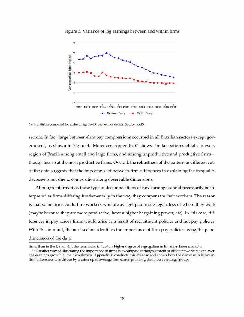
Figure 3. Variance of log earnings between and within firms

0.1

.2.3

.4.5

.6

Va

ria

nce

of

log

la

bo

r in

co

me

1988 1990 1992 1994 1996 1998 2000 2002 2004 2006 2008 2010 2012

Between firms Within firms


sectors. In fact, large between-firm pay compressions occurred in all Brazilian sectors except gov-

ernment, as shown in Figure 4. Moreover, Appendix C shows similar patterns obtain in every

region of Brazil, among small and large firms, and among unproductive and productive firms—

though less so at the most productive firms. Overall, the robustness of the pattern to different cuts

of the data suggests that the importance of between-firm differences in explaining the inequality

decrease is not due to composition along observable dimensions.

Although informative, these type of decompositions of raw earnings cannot necessarily be in-

terpreted as firms differing fundamentally in the way they compensate their workers. The reason

is that some firms could hire workers who always get paid more regardless of where they work

(maybe because they are more productive, have a higher bargaining power, etc). In this case, dif-

ferences in pay across firms would arise as a result of recruitment policies and not pay policies.

With this in mind, the next section identifies the importance of firm pay policies using the panel

dimension of the data.

firms than in the US Finally, the remainder is due to a higher degree of segregation in Brazilian labor markets.19 Another way of illustrating the importance of firms is to compare earnings growth of different workers with aver-

age earnings growth at their employers. Appendix B conducts this exercise and shows how the decrease in between-firm differences was driven by a catch-up of average firm earnings among the lowest earnings groups.

18

Figure 4. Variance between and within firms, by sector0

.1.2

.3.4

.5.6

Va

ria

nce

of

log

la

bo

r in

co

me

1988 1990 1992 1994 1996 1998 2000 2002 2004 2006 2008 2010 2012


Oil and Resources

0.1

.2.3

.4.5

.6

Va

ria

nce

of

log

la

bo

r in

co

me

1988 1990 1992 1994 1996 1998 2000 2002 2004 2006 2008 2010 2012


Manufacturing

0.1

.2.3

.4.5

.6

Va

ria

nce

of

log

la

bo

r in

co

me

1988 1990 1992 1994 1996 1998 2000 2002 2004 2006 2008 2010 2012


Construction

0.1

.2.3

.4.5

.6

Va

ria

nce

of

log

la

bo

r in

co

me

1988 1990 1992 1994 1996 1998 2000 2002 2004 2006 2008 2010 2012


Services

0.1

.2.3

.4.5

.6

Va

ria

nce

of

log

la

bo

r in

co

me

1988 1990 1992 1994 1996 1998 2000 2002 2004 2006 2008 2010 2012


Public Sector

0.1

.2.3

.4.5

.6

Va

ria

nce

of

log

la

bo

r in

co

me

1988 1990 1992 1994 1996 1998 2000 2002 2004 2006 2008 2010 2012


Agriculture


5 Empirical framework

The evidence in the previous section suggests that firms might be an important determinant of

earnings in Brazil. Motivated by these insights, we estimate high-dimensional fixed effects econo-

19

metric models controlling for both unobserved worker and firm heterogeneity. To be able to speak

to changes over time in the components of inequality, we estimate our model separately in six

subperiods covering 1988–1992, 1992–1996, 1996–2000, 2000–2004, 2004–2008, and 2008–2012, re-

spectively.20 Subsequently, we correlate the estimated firm and worker effects with observed char-

acteristics of firms and workers in order to investigate what may have caused changes in the firm

and worker component of pay over time.

5.1 Worker and firm fixed effects model

In order to separately identify the contribution of individual and firm components in pay, one

needs to observe a panel of workers linked to their employers. The RAIS, our linked employer-

employee data from Brazil, satisfy these requirements. Within subperiods that we set to be five

years in length, we observe a number I of workers working at J firms for a total of N worker-

years. Let J (i, t) denote the employer of worker i in year t (as we uniquely defined in Section 3).

We assume that log earnings of individual i in year t, denoed yit, consist of the sum of a worker

component, αi, a firm component, αJ(i,t), a year effect, Υt, and an error component, ε it, so we can

write,21

log yit = αi + αJ(i,t) + Υt + ε it

where we assume that the error satisfies the strict exogeneity condition

E[ε it|αi, αJ(i,t), Υt

]= 0

Our specification does not control in this first stage for observable worker and firm character-

istics. Instead, we correlate estimated fixed effects with worker and firm observables in a second

stage of our analysis. We prefer this specification to avoid identifying the time-varying effects

off changes within workers and firms during the limited time frame of each subperiod.22 Fur-

thermore, we find this two-stage approach helpful in terms of understanding what the firm and

worker effects may ultimately be standing for.23

20In Appendix D we show that similar results obtain in longer, nine-year subperiods.21Although our current paper does not model the underlying, fundamental sources of this reduced form specification,

in subsequent work we show how it can be rationalized in a frictional labor market with firm productive heterogeneityand worker ability differences (Engbom and Moser, 2017a).

22Including age effects in the above framework with individual and year effects would require a normalization, asfor instance the restriction advocated by Deaton (1997).

23In this sense, our approach is reminiscent of that of Bertrand and Schoar (2003) in their study of the determinants

20

Table 3. Frequency of switches, by period

# Unique workers Average # of jobs % switchers

1988–1992 23.1 1.56 0.371992–1996 23.7 1.48 0.331996–2000 25.6 1.45 0.322000–2004 28.8 1.46 0.322004–2008 33.0 1.54 0.362008–2012 38.6 1.66 0.42

Note: Number of unique workers in millions. A switcher is defined as a worker who is associated with two or more employers during

the period. Source: RAIS.

As shown by AKM, worker and firm effects can only be separately identified within a set of

firms and workers connected through the mobility of workers. Table 13 in Appendix F presents

summary statistics on the largest set of connected workers in each subperiod—this covers 97–98

percent of all workers in each subperiod. Given the high coverage, it is not surprising that the

restricted subpopulation looks very similar to the overall population. Thus the restriction to the

largest connected set seems relatively innocuous.

As identification of the model derives from workers switching between firms, Table 3 presents

statistics on the fraction of switchers in each subperiod. The degree of labor mobility is high in

Brazil, with more than 30 percent of the population switching firms at some point during each five-

year subperiod. The average number of firms worked at during the five years in each subperiod

is about 1.5. There is no strong trend in either statistic.

The assumption on the error term is referred to in the literature as that of requiring exogenous

mobility. As explained by AKM, this rules out mobility based on the unobserved error component.

Following Card et al. (2013), we investigate the validity of this assumption in several ways. We

divide estimated firm effects into quartiles and study whether the gain in the firm component of

those switching between for instance the first and fourth quartile is similar to the loss of those

making the reverse switch. To the extent that match effects are an important determinant of earn-

ings and mobility, we would expect all workers to make gains from switching. Furthermore, we

examine the distribution of the average residual across worker and firm effects to check for any

systematic deviation from zero (which could indicate that the log linear model is misspecified).

Let ai denote the estimated worker effect, aJ(i,t) the estimated firm effect, Yt the estimated year

effect, and eit the residual. Based on our estimated equation, we decompose the variance of log

of CEO pay.

21

earnings within any subperiod into the variance of the worker component, the firm component,

and the year trend, as well as the covariance between the worker and the firm component, the

worker and year component, the firm and year component, and the variance of the residual:

Var (log yit) = Var (ai) + Var(

aJ(i,t)

)+ Var (Yt) + 2Cov

(ai, aJ(i,t)

)+2Cov (ai, Yt) + 2Cov

(aJ(i,t), Yt

)+ Var (eit) (1)

Note that sampling error in the estimated effects will cause us to overestimate the variance of

worker and firm effects, and in general induce a negative bias in the covariance between worker

and firm effects (see for instance Andrews et al., 2008). Following Card et al. (2013), we do not

attempt to correct for this, but instead assume that this error is constant over time, so that even if

the level of our estimated variances is slightly overstated, the changes we document over time are

still valid.24

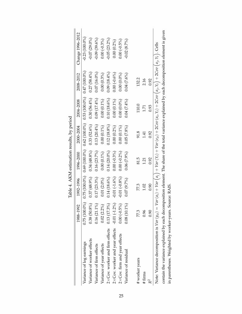
5.2 Determinants of the estimated firm effects

In the second stage of our empirical investigation, we study how the estimated firm effects relate

to observable measures of firm performance available in the PIA survey. In particular, we are

interested in understanding what firm characteristics are related to pay, and whether changes in

the distribution of firm effects over time can be explained by underlying changes in firm charac-

teristics or the way the labor market translates those into pay. Since the PIA only covers larger

manufacturing and mining firms,25 we are forced to restrict attention to only these firms and

workers when linking firm effects to firm characteristics. We implement this by first estimating

the AKM model for the universe of firms and workers, and subsequently restricting attention to

only larger manufacturing firms.

Let Xj denote a vector of firm characteristics—for each subperiod we regress by OLS

aj = Xjβ + ηj

24To better estimate firm effects, Bonhomme et al. (2016) suggest restricting attention to firms whose fixed effect is“well-identified” due to a high number of switchers. In practice, this procedure boils down to restricting attention toworkers at firms with at least 10 switchers during the estimation period. Implementing this restriction, we get similarresults as those reported below.

25As described in Section 3, we restrict attention to the deterministic stratum of PIA containing only larger firms. Wedrop small firms contained in the random stratum to ensure that firms stay in the sample for multiple years for ourestimation procedure below.

22

All regressions are weighted by worker-years. We consider versions including average log value

added per worker during the subperiod, average log firm size during the subperiod, state fixed

effects, and two-digit subsector fixed effects. Additionally, we have considered versions including

a range of other firm characteristics as well as higher order terms, but these add only marginally

to the explanatory power of the regressions so in the interest of space we do not show them.

Based on the above regression, we compute the variance in firm effects explained by firm

observables as

Var (a) = b′Var(X)b

where b is the estimated coefficient vector and X is the design matrix. In order to isolate the impor-

tance of a compression in firm fundamentals versus a compression in the pass-through from such

fundamentals to pay, we consider two counterfactuals. First, we assume that the pass-through

from firm characteristics to pay, β, remains at its initial level, while the distribution of firm char-

acteristics, Var(X), changes over time. Second, we assume that Var(X) stays the same while β

changes as in the data. A comparison of the two counterfactuals allows us to address whether a

change in the variance of firm pay is explained by changes in underlying firm characteristics or

due to a change in the degree of pass-through from such characteristics to worker pay.

5.3 Determinants of the estimated worker effects

We also investigate what factors influence the worker component of pay. To this end, we proceed

in a similar fashion as for firms and regress the predicted worker effects on a vector of worker

observables, Wi:

ai = Wiζ + ηi

All regressions are weighted by worker-years. We include in Wi a constant, a worker’s age bin,

four education dummies, and state fixed effects (the former two computed as the modal value

during the subperiod). We have also considered versions of this regression with age and education

interacted as well as including occupation or sector controls, but as neither of these alternatives

changes the estimated results meaningfully we do not report the results.

Based on this regression, we predict the variance explained by worker observables as

Var (a) = z′Var(W)z

23

where z is the estimated coefficient vector and W is the design matrix. Subsequently, we de-

compose the evolution of the variance of the explained part of the worker effect into that due to a

change in the underlying distribution of such characteristics versus a change in the return to them.

That is, we first keep the estimated return to the characteristic of interest constant and change only

the underlying distribution to match its evolution in the data. This shows how important changes

in the distribution of worker characteristics were for the overall inequality decrease. Secondly,

we instead change the return to the characteristic of interest as in the data, while holding the un-

derlying distribution constant. This evaluates how important changes in the returns to age and

education were for the overall inequality decrease.

6 Results

In this section, we first present results from our first-stage two-way fixed effects model, decom-

posing earnings inequality into a firm and a worker component. Subsequently, we investigate the

sources of the firm and worker component of pay. Finally, we provide additional results evaluat-

ing the assumptions imposed by our econometric model.

6.1 AKM decomposition

Table 4 presents the variance decomposition based on the estimation results of the AKM model

in equation (1) for each of the six five-year subperiods between 1988 and 2012.26 To illustrate the

relative importance of the various components of this decomposition over time, Figure 5 plots

the variance of raw earnings (solid blue line with circles), the variance of estimated worker ef-

fects (dashed red line with squares), and the variance of firm effects (dash-dotted green line with

diamonds). The variance of year effects and covariance terms are small in magnitude and play

an insignificant role in the overall inequality decrease. These terms are excluded for brevity. All

results are weighted by worker-years.

Two important results emerge from our analysis. First, worker heterogeneity is the single

most important determinant of earnings inequality. In the 1996–2000 subperiod, the variance of

worker fixed effects makes up 49 percent of the total variance of log earnings. This increases

monotonically to 58 percent by the last subperiod. The variance of firm effects makes up 24 percent

26Appendix D shows that similar results are obtained using three longer, nine-year subperiods.

24

Tabl

e4.

AK

Mes

tim

atio

nre

sult

s,by

peri

od

1988

–199

219

92–1

996

1996

–200

020

00–2

004

2004

–200

820

08–2

012

Cha

nge

1996

–201

2

Var

ianc

eof

log

earn

ings

0.75

(100

.0%

)0.

75(1

00.0

%)

0.69

(100

.0%

)0.

62(1

00.0

%)

0.53

(100

.0%

)0.

47(1

00.0

%)

-0.2

3(1

00.0

%)

Var

ianc

eof

wor

ker

effe

cts

0.38

(50.

8%)

0.37

(48.

9%)

0.34

(48.

8%)

0.33

(52.

6%)

0.30

(56.

4%)

0.27

(58.

4%)

-0.0

7(2

9.0%

)V

aria

nce

offir

mef

fect

s0.

16(2

1.1%

)0.

17(2

3.3%

)0.

16(2

3.7%

)0.

13(2

0.4%

)0.

09(1

7.4%

)0.

07(1

6.0%

)-0

.09

(39.

6%)

Var

ianc

eof

year

effe

cts

0.02

(2.2

%)

0.01

(2.0

%)

0.00

(0.1

%)

0.00

(0.1

%)

0.00

(0.1

%)

0.00

(0.3

%)

0.00

(-0.

3%)

2×C

ov.w

orke

ran

dfir

mef

fect

s0.

13(1

7.3%

)0.

14(1

8.6%

)0.

14(2

0.0%

)0.

12(1

8.8%

)0.

10(1

8.6%

)0.

09(1

8.4%

)-0

.05

(23.

2%)

2×C

ov.w

orke

ran

dye

aref

fect

s-0

.01

(-1.

2%)

-0.0

1(-

1.6%

)0.

00(-

0.3%

)0.

00(0

.2%

)0.

00(0

.1%

)0.

00(-

0.6%

)0.

00(0

.2%

)2×

Cov

.firm

and

year

effe

cts

0.00

(-0.

5%)

-0.0

1(-

0.8%

)0.

00(-

0.2%

)0.

00(0

.1%

)0.

00(0

.0%

)0.

00(0

.0%

)0.

00(-

0.5%

)V

aria

nce

ofre

sidu

al0.

08(1

0.1%

)0.

07(9

.7%

)0.

06(7

.9%

)0.

05(7

.8%

)0.

04(7

.4%

)0.

04(7

.6%

)-0

.02

(8.7

%)

#w

orke

rye

ars

77.3

77.3

81.5

91.8

110.

013

2.2

#fir

ms

0.96

1.02

1.21

1.41

1.71

2.16

R2

0.90

0.90

0.92

0.92

0.93

0.92

Not

e:V

aria

nce

deco

mpo

siti

onis

Var

(yit)=

Var

(ai)+

Var( a j) +

Var

(Yt)+

Var

(eit)+

2Cov

(ai,

Y t)+

2Cov( a j

,Yt) +

2Cov( a j

,Yt) .C

ells

cont

ain

the

vari

ance

expl

aine

dby

each

deco

mpo

siti

onel

emen

t.Th

esh

are

ofth

eto

talv

aria

nce

expl

aine

dby

each

deco

mpo

siti

onel

emen

tis

give

nin

pare

nthe

ses.

Wei

ghte

dby

wor

ker-

year

s.So

urce

:RA

IS.

25

of the variance of log earnings in the 1996–2000 subperiod, decreasing to 16 percent by the last

subperiod. Finally, the covariance between the worker and firm effects consistently explains just

under 20 percent of the overall variance.

Figure 5. Variance decomposition from AKM model

0.0

0.2

0.4

0.6

0.8

Va

ria

nce

1988−1992 1992−1996 1996−2000 2000−2004 2004−2008 2008−2012

Total earnings Worker effects Firm effects


Second, in terms of explaining time trends, we observe a more than proportionate fall in the

variance of firm effects. Between 1996–2000 and 2008–2012, the variance of firm effects falls from

16 to seven log points whereas the variance of person effects falls from 34 to 27 log points. The

correlation between worker and firm effects stays fairly constant at around 0.3 throughout the

period, and hence the covariance term falls in line with the standard deviations of the worker and

firm effects. Given the large role played by firms in the inequality decrease, understanding the

drivers of more equal pay across employers over time is an important question which we address

in the following section.

6.2 The link between firm effects and firm characteristics

When studying the link between firm effects and firm characteristics, we limit attention to the

manufacturing and mining sector, for which we have data on firm performance and characteris-

tics. Table 5 compares AKM estimates for this subpopulation with the estimates for the overall

population. As noted earlier, we impose the restriction to the PIA subpopulation after estimating

26

Tabl

e5.

Com

pari

son

ofA

KM

esti

mat

ion

resu

lts

betw

een

wor

kers

atla

rger

man

ufac

turi

ng&

min

ing

firm

san

dla

rges

tcon

nect

edse

t,by

peri

od

1996

–200

020

00–2

004

2004

–200

820

08–2

012

Cha

nge

1996

–201

2

Var

ianc

eof

log

earn

ings

(%of

pop.

esti

mat

e)0.

74(1

06.9

%)

0.70

(113

.0%

)0.

60(1

14.2

%)

0.53

(112

.6%

)-0

.22

(95.

1%)

Var

ianc

eof

wor

ker

effe

cts

(%of

pop.

esti

mat

e)0.

37(1

09.8

%)

0.37

(112

.3%

)0.

35(1

16.4

%)

0.32

(116

.6%

)-0

.05

(81.

3%)

Var

ianc

eof

firm

effe

cts

(%of

pop.

esti

mat

e)0.

14(8

6.8%

)0.

12(9

2.1%

)0.

08(8

4.3%

)0.

06(8

1.4%

)-0

.08

(91.

2%)

Var

ianc

eof

year

effe

cts

(%of

pop.

esti

mat

e)0.

00(1

05.4

%)

0.00

(99.

4%)

0.00

(100

.0%

)0.

00(9

9.9%

)0.

00(9

3.5%

)2×

Cov

.wor

ker

and

firm

effe

cts

(%of

pop.

esti

mat

e)0.

17(1

25.9

%)

0.17

(141

.4%

)0.

14(1

37.8

%)

0.11

(127

.3%

)-0

.07

(123

.6%

)2×

Cov

.wor

ker

and

year

effe

cts

(%of

pop.

esti

mat

e)0.

00(1

11.8

%)

0.00

(122

.4%

)0.

00(1

18.8

%)

0.00

(107

.4%

)0.

00(9

0.1%

)2×

Cov

.firm

and

year

effe

cts

(%of

pop.

esti

mat

e)0.

00(8

5.3%

)0.

00(1

01.4

%)

0.00

(84.

6%)

0.00

(-11

.8%

)0.

00(9

6.8%

)V

aria

nce

ofre

sidu

al(%

ofpo

p.es

tim

ate)

0.05

(95.

2%)

0.05

(96.

1%)

0.04

(98.

1%)

0.03

(98.

7%)

-0.0

2(8

9.0%

)

#w

orke

rye

ars

(%of

pop.

esti

mat

e)15

.5(1

9.0%

)16

.7(1

8.2%

)21

.0(1

9.1%

)23

.9(1

8.1%

)#

firm

s(%

ofpo

p.es

tim

ate)

0.03

(2.9

%)

0.04

(2.9

%)

0.05

(2.8

%)

0.06

(2.6

%)

R2

(%of

pop.

esti

mat

e)0.

93(1

00.9

%)

0.93

(101

.3%

)0.

94(1

01.1

%)

0.93

(101

.0%

)

Not

e:V

aria

nce

deco

mpo

siti

onof

AK

Mm

odel

for

larg

erm

anuf

actu

ring

firm

sco

vere

dby

PIA

.The

rati

obe

twee

nes

tim

ates

usin

gm

anuf

actu

ring

firm

sre

lati

veto

AK

Mes

tim

ates

usin

gal

lsec

tors

isgi

ven

inpa

rent

hese

s.W

orke

r-an

dfir

m-y

ears

inm

illio

ns.W

eigh

ted

byw

orke

r-ye

ars.

Sour

ce:R

AIS

and

PIA

.

27

Tabl

e6.

Res

ults

from

regr

essi

onof

esti

mat

edfir

mef

fect

son

firm

char

acte

rist

ics

1996

–200

020

00–2

004

2004

–200

820

08–2

012

PAN

EL

A.N

OC

ON

TR

OL

S

Val

uead

ded

p.w

.0.

256

0.13

60.

198

0.09

90.

158

0.09

00.

140

0.07

8Fi

rmsi

ze0.

109

-0.0

140.

077

-0.1

790.

050

-0.1

200.

045

-0.0

97V

alue

adde

dp.

w.x

Firm

size

0.01

50.

016

0.01

10.

009

Wor

ker-

year

s15

.515

.515

.516

.716

.716

.721

.021

.021

.023

.923

.923

.9R

20.

582

0.24

70.

601

0.55

80.

160

0.57

10.

527

0.11

70.

537

0.46

40.

130

0.47

4

PAN

EL

B.S

UB

SEC

TO

RC

ON

TR

OL

S

Val

uead

ded

p.w

.0.

234

0.12

20.

179

0.08

20.

140

0.07

30.

120

0.05

3Fi

rmsi

ze.1

06-0

.107

0.08

0-0

.139

0.05

6-0

.086

0.04

7-0

.079

Val

uead

ded

p.w

.xFi

rmsi

ze0.

013

0.13

80.

009

0.00

8

Wor

ker-

year

s15

.515

.515

.516

.716

.716

.721

.021

.021

.023

.923

.923

.9R

20.

653

0.45

90.

676

0.64

60.

430

0.66

00.

627

0.42

40.

638

0.61

30.

457

0.62

9

PAN

EL

C.S

TAT

EC

ON

TR

OL

S

Val

uead

ded

p.w

.0.

228

0.13

30.

177

0.09

90.

143

0.08

20.

128

0.06

5Fi

rmsi

ze0.

111

-0.0

590.

083

-0.1

060.

057

-0.0

830.

051

-0.0

71V

alue

adde

dp.

w.x

Firm

size

0.00

90.

011

0.00

80.

007

Wor

ker-

year

s15

.515

.515

.516

.716

.716

.721

.021

.021

.023

.923

.923

.9R

20.

667

0.50

20.

698

0.64

10.

410

0.65

10.

600

0.35

30.

609

0.55

20.

360

0.56

7

Not

e:D

epen

dent

vari

able

isth

ees

tim

ated

firm

effe

cta j

.Num

ber

ofw

orke

r-ye

ars

inm

illio

ns.W

eigh

ted

byw

orke

r-ye

ars.

Sour

ce:R

AIS

and

PIA

.

28

the AKM model on the entire population of adult males. This group includes a small percentage of

firms in the overall economy (2.6–2.9 percent), but covers 18–19 percent of employment given the

larger size of firms in the manufacturing and mining sectors. The overall variance of log earnings

is five log points higher in the PIA subpopulation during the 1996–2000 subperiod and falls by 22

log points until the 2008–2012 subperiod, compared to 23 log points in the overall population. The

variance of worker effects is three log points higher in the 1996–2000 subperiod and falls by two

log point less. The variance of firm effects is two log points less in 1996–2000 and falls by one log

point less. We conclude that inequality trends are similar in the PIA subpopulation compared to

the overall population.

Why do some firms pay more than others, and what makes firms offer more equal pay over

time? Table 6 reports results from regressing estimated firm effects on average log value added per

worker and average log firm size by subperiod, either with or without subsector or state controls.

All regressions are weighted by worker-years. Several features are worth highlighting. First, more

productive and larger firms pay significantly more after controlling for sorting of workers. Our

estimates suggest that a one log point more productive firm pays a given worker 0.26 log points

more, or alternatively that a one standard deviation more productive firm pays over 30 percent

more to a given worker. Furthermore, we find that essentially the entire return to working at a

larger firm is due to a strong positive correlation between firm size and productivity—controlling

for value added per worker a larger firm pays only marginally better.

Second, the amount of dispersion in firm effects explained by firm productivity is notable.

Only a linear term in average log value added per worker explains around half of the variation in

the firm component of pay, despite the fact that sampling error in the estimated firm effects will

lead us to understate the importance of productivity for pay. Adding also controls for subsector,

the R2 is over 0.6.

Third, the pass-through from firm performance to the firm component of pay falls substantially

between 1996–2000 and 2008–2012. As noted above, in the first subperiod a one log point more

productive firm paid 0.26 log points more—by the last subperiod this pass-through has almost

halved to 0.14. Given that the standard deviation of value added per worker remained roughly

constant at just above one over this period, the variation in pay attributable to variation in firm

productivity fell substantially. On the contrary, although both subsectors and states explain a

non-trivial amount of the level of inequality in firm pay, compression across states or subsectors

29

explains little of the declining dispersion in firm pay.

Figure 6 illustrates the relationship by plotting by period the average estimated AKM firm ef-

fects against 90 quantile bins of value added per worker. Over most of its support, the relationship

is approximately linear, and it displays a clear flattening over time.

Figure 6. Estimated AKM firm effects versus value added per worker, by period−

.6−

.4−

.20

.2.4

.6A

KM

firm

eff

ect

7 8 9 10 11 12 13 14value added p.w.

1996−2000 2000−2004 2004−2008 2008−2012

Note: Statistics computed for males of age 18–49. See text for details. Source: RAIS and PIA.

To illustrate the importance of the fall in the pass-through for the overall inequality decrease,

Figure 7 plots the variance of firm effects (solid blue line with circles), the predicted variance due to

value added per worker and subsector controls (dashed red line with squares), and the predicted

variance due to only changing the passthrough from productivity to pay (dash-dotted green line

with diamonds). Between 1996–2000 and 2008–2012, the variance explained by observable firm

characteristics decreases by six log points, or roughly 30 percent of the overall decrease in the

variance of log earnings over this period. All of this is driven by changes in the pass-through.

One possibility is that the pass-through from value added per worker to pay differs system-

atically by size of firm, and that changes in the firm size distribution over time has led to a fall

in the measured pass-through. Table 7 investigates this by pooling all subperiods and including

a time invariant interaction between value added per worker and firm size, in addition to period

effects and period specific pass-throughs from value added per worker and firm size to pay. The

estimated fall in pass-through from value added per worker to pay is comparable to our previous

30

estimation results, confirming that the decrease has taken place conditional on firm size.27 Figure

8 illustrates this by plotting the relationship between estimated AKM firm effects and value added

per worker separately by firm size quartiles over time.

Figure 7. Variance of firm effects, variance explained by value added per worker, andcounterfactual variance with constant returns

0.0

00

.04

0.0

80

.12

0.1

6V

aria

nce

of

firm

eff

ects

1996−2000 2000−2004 2004−2008 2008−2012

Firm effects Explained by value added + subsectors

Due to change in returns Due to change in distribution


6.3 The link between worker effects and worker characteristics

We finally turn to our results regarding the link between observable worker characteristics and

the worker component of pay. Table 8 shows estimates from regressing the estimated worker ef-

fects on age and education, with or without state controls. We note the following: First, more

able workers, as measured by labor market experience or education level, are paid more. For in-

stance, the oldest age group earns 44–54 log points more than the youngest age group conditional

on place of work, and a college graduate earns more than twice the amount of the lowest educa-

tion group. Observable worker characteristics jointly explain 37–42 percent of the variance in the

worker component of pay, with most of the dispersion being observed within states.

Second, both the age gradient and the return to education decrease over time. Workers aged

40–49 experienced a decrease in pay relative to those aged 18–24 of eight log points (or 15 percent)

27Appendix E investigates whether opening up to trade may have mechanically reduced the pass-through by sep-arately considering exporters and non-exporters, and finds that both groups have experienced a similar fall in thepass-through as the overall economy.

31

Table 7. Results from regression of estimated firm effects on firm characteristics controllingfor differential pass-through by firm size

Baseline State Sector

Value added p.w.

1996–2000 0.158 0.139 0.1422000–2004 0.124 0.116 0.1062004–2008 0.082 0.075 0.0622008–2012 0.058 0.053 0.040

Firm size

1996–2000 -0.105 -0.063 -0.0782000–2004 -0.133 -0.092 -0.1002004–2008 -0.134 -0.092 -0.0992008–2012 -0.130 -0.089 -0.096

Value added p.w. x Firm size 0.012 0.009 0.010

Subsector controls No No YesState controls No Yes NoWorker-years 77.1 77.1 77.1R2 0.553 0.627 0.648

Note: Dependent variable is the estimated firm effect aj. All specifications include period effects. Number of worker-years in millions.

Weighted by worker-years. Source: RAIS and PIA.

between 1996–2000 and 2008–2012. Over the same time period, middle school, high-school and

college graduates saw decreases of five, 19 and nine log points, respectively, relative to those with

only primary school. Figure 9 illustrates these results by plotting the overall variance of worker

effects (solid blue line with circles), the predicted variance due to age and education (dashed red

line with squares), the counterfactual variance explained by changes only in the returns (dash-

dotted green line with diamonds), and the counterfactual variance explained by changes only in

the distribution. We find that education and age account for roughly 50 percent of the decline in

dispersion in the worker component, and this is all due to a change in returns.28

6.4 Support for the AKM model

A large part of our analysis has been based on estimation results from repeated applications of

the AKM framework. Although the consistently high R2 of our model suggests that it provides

a good fit to the data, our estimates can be biased if the match effect is correlated with either the

firm or worker component of earnings. To investigate this possibility further, we replicate two

robustness exercises proposed by Card et al. (2013) using the Brazilian RAIS data.

28Of course, falling returns could result from changes in the distribution. The counterfactual of holding the distribu-tion constant while changing returns should be interpret with this qualification in mind.

32

Tabl

e8.

Res

ults

from

regr

essi

onof

esti

mat

edw

orke

ref

fect

son

wor

ker

char

acte

rist

ics

1988

–199

219

92–1

996

1996

–200

020

00–2

004

2004

–200

820

08–2

012

Age

grou

ps25

–29

0.19

40.

200

0.18

00.

187

0.18

30.

188

0.17

70.

182

0.15

80.

165

0.15

80.

165

30–3

90.

399

0.40

40.

355

0.36

40.

347

0.35

40.

347

0.35

20.

318

0.32

30.

299

0.30

440

–49

0.53

30.

538

0.51

50.

523

0.51

30.

520

0.50

50.

509

0.47

20.

475

0.43

60.

437

Educ

atio

ngr

oups

Mid

dle

scho

ol0.

204

0.20

00.

189

0.18

10.

154

0.14

20.

135

0.11

70.

122

0.10

10.

103

0.08

4H

igh

scho

ol0.

617

0.62

30.

572

0.57

60.

463

0.45

90.

380

0.36

30.

320

0.29

60.

269

0.24

6C

olle

geor

mor

e1.

235

1.22

81.

192

1.17

81.

152

1.12

81.

176

1.14

61.

125

1.08

81.

066

1.03

0

Stat

eco

ntro

lsN

oYe

sN

oYe

sN

oYe

sN

oYe

sN

oYe

sN

oYe

sW

orke

r-ye

ars

77.3

77.3

77.3

77.3

81.5

81.5

91.8

91.8

110.

011

0.0

132.

213

2.2

R2

0.39

80.

423

0.37

90.

409

0.36

50.

401

0.36

80.

404

0.36

60.

399

0.36

50.

392

Not

e:D

epen

dent

vari

able

isth

ees

tim

ated

wor

ker

effe

cta i

.Num

ber

ofw

orke

r-ye

ars

inm

illio

ns.W

eigh

ted

byw

orke

r-ye

ars.

Educ

atio

nes

tim

ates

are

rela

tive

tole

ssth

anm

iddl

esc

hool

(<7

year

s),a

gees

tim

ates

are

rela

tive

toag

e18

–24.

Sour

ce:R

AIS

.

33

Figure 8. Estimated AKM firm effects versus value added per worker, by firm size quartileand period

−.6

−.4

−.2

0.2

.4.6

AK

M f

irm

eff

ect

7 8 9 10 11 12 13 14value added p.w.

1996−2000 2000−2004 2004−2008 2008−2012

Firm size quartile 1 (smallest)

−.6

−.4

−.2

0.2

.4.6

AK

M f

irm

eff

ect

7 8 9 10 11 12 13 14value added p.w.

1996−2000 2000−2004 2004−2008 2008−2012

Firm size quartile 2

−.6

−.4

−.2

0.2

.4.6

AK

M f

irm

eff

ect

7 8 9 10 11 12 13 14value added p.w.

1996−2000 2000−2004 2004−2008 2008−2012

Firm size quartile 3

−.6

−.4

−.2

0.2

.4.6

AK

M f

irm

eff

ect

7 8 9 10 11 12 13 14value added p.w.

1996−2000 2000−2004 2004−2008 2008−2012

Firm size quartile 4 (largest)


First, Figure 10 shows the average earnings of workers who switch firms up to two years prior

to the switch and two years after the switch for the latest subperiod.29 Switchers are classified

by the firm effect quartile of their pre- and post-transition employers. Consistent with the AKM

specification, the gains of those switching up are similar to the losses of those making the reverse

switch.30

Second, Figure 11 shows the average estimated residual by decile of worker and firm effects

for the subperiods 1996–2000 and 2008–2012.31 There is some evidence of misspecification for the

lowest decile of worker effects in the sense that they display a systematically positive residual

while working at the lowest-paying firms, and vice versa for highest-paying firms. Similarly, the

29Similar results hold in other subperiods and across other quartiles.30Bonhomme et al. (2016) caution that models that do not feature log additivity in earnings may also satisfy this test.

The results of this event study should be interpreted with this qualification in mind.31Similar results hold in other subperiods.

34

Figure 9. Variance of worker effects, variance explained by age and education, and varianceholding the return to age and education constant

0.0

00

.10

0.2

00

.30

0.4

0

Va

ria

nce

of

wo

rke

r e

ffe

cts

1988−1992 1992−1996 1996−2000 2000−2004 2004−2008 2008−2012

Worker effects Explained by age + education

Due to change in returns Due to change in distribution


Figure 10. Average changes in earnings of workers switching employers

−1

.0−

0.6

−0

.20

.20

.61

.0

Lo

g e

arn

ing

s

−2 −1 0 1 2Years relative to switch

Q1 to Q1 Q1 to Q2 Q1 to Q3 Q1 to Q4


1996−2000

−1

.0−

0.6

−0

.20

.20

.61

.0

Lo

g e

arn

ing

s

−2 −1 0 1 2Years relative to switch



2008−2012


35

Figure 11. AKM residual by firm and worker fixed effect deciles

Worker effect decile-0.04

-0.02

0

109

0.02

8

1996 - 2000

10

0.04

7 9

Firm effect decile

6 875 64 53 42 31 21 Worker effect decile

Worker effect decile

-0.04

-0.02

0

109

0.02

8

2008 - 2012

10

0.04

7 96 8

7564

53 4

2 31 2

1Firm effect decile Worker effect decile


lowest firm effects decile shows systematic positive mean residuals for the lowest-paid workers,

and vice versa for the highest-paid workers. However, the magnitude of these errors is modest

and beyond the lowest deciles of worker and firm effects errors do not exhibit a strong systematic

relationship.32

6.5 Potential explanations behind decreasing inequality in Brazil

A key takeaway from our analysis is that changes in the pass-through from worker and firm char-

acteristics to pay was a major driver behind Brazil’s inequality decrease from 1996 to 2012. While

measures of worker ability and firm productivity are positively correlated with pay throughout

this period, it is not the case that Brazil became more equal in terms of such fundamentals. Instead

the pass-through from these characteristics to pay collapsed, resulting in a lower worker skill pay

premium and a lower firm productivity pay premium. An important question is what might have

caused this decrease in pass-through.

Although our current paper stops short of providing a complete story behind the fall in pass-

through, we highlight a few explanations that we view as more or less promising based on our

empirical analysis. We first note that an overwhelming majority of the inequality decrease took

place within states and detailed industry classifications. Second, the pass-through from produc-

32Engbom and Moser (2017a) argue that this pattern is consistent with a binding minimum wage.

36

tivity to pay fell within firm size groups, for exporters and non-exporters, and for a balanced

panel of surviving firms. Based on these observations, we believe that a convincing explanation

goes beyond the direct effect of compositional changes.

Consistent with our empirical findings, we briefly discuss three promising explanations be-

hind Brazil’s inequality decrease. First, there was a rapid expansion in educational attainment

over this period. By increasing the labor supply of higher education groups, this may have con-

tributed towards falling education premiums. It would be interesting to quantify this channel

through an equilibrium model estimated to the microdata. However, it is worth stressing that

most of Brazil’s inequality decrease was due to forces on the firm side. It is less clear to us why

changes in the market for education would affect firm-specific pay components.

Second, changes in bargaining between employers and employees over firm-specific surplus

may directly speak to the declining dispersion in firm-level pay. Higher baseline pay and lower de-

pendence on firm-specific (worker-specific) performance could plausibly explain our documented

facts on rising real earnings and a lower pass-through from firm productivity (worker ability) to

pay. Specifically, although unions have held a strong role in Brazil throughout this period, to the

extent that the bargaining process became more centralized over this period, this may have made

earnings less dependent on firm-specific performance and more on regional, industry or aggregate

negotiation outcomes. Using detailed data on union bargaining agreements to study this further

would be an interesting avenue for future research.

Third, Brazil’s federal minimum wage rose by 119 percent in real terms from 1996 to 2012.

Given that this legislation cuts across sectors and states, we view it as a promising candidate for

explaining the decrease of inequality in Brazil over this period. Consistent with our finding that

the inequality decrease is primarily due to changes in the returns to worker and firm character-

istics, the minimum wage may plausibly affect the way that firm-specific surplus is split without

directly affecting the distribution of worker and firm characteristics. A challenge for this story,

however, is to explain why inequality fell throughout large parts of the earnings distribution. In

Engbom and Moser (2017a), we pursue this idea further by developing an equilibrium search

model and estimating spillover effects of the minimum wage.

37

7 Conclusion

In this paper, we used detailed linked employer-employee dissect the evolution of inequality in

Brazil between 1988 and 2012. After increasing moderately between 1988–1996, the variance of log

labor earnings decreased by 28 log points between 1996–2012. To understand the sources of this

decrease, we estimate high-dimensional fixed effects models of earnings controlling for worker

and firm heterogeneity. Our results suggest that firms contributed more than proportionately to

the decrease.

While more productive firms pay more, compression in firm productivity was not a factor

behind declining inequality. Instead, we find that a declining pass-through from firm productivity

to pay played an important role behind the decrease. On the worker side, higher ability workers

as measured by educational attainment or experience are paid more, yet such measures of worker

ability show no compression over time. Rather, a significant share of the explained decrease in

worker heterogeneity is due to rapidly falling returns to such measures of worker ability. We

conclude that changes in pay policies, rather than changes in firm and worker fundamentals,

played a significant role in Brazil’s inequality decrease.

Our findings propose a set of facts that any potential theory of the inequality decrease in Brazil

should be consistent with. Such a theory must generate pay differences between firms for identical

workers that are strongly positively correlated with firm productivity. Moreover, any promising

explanation needs to generate a compression in firm pay differences over time not through com-

pression in the distribution of firm productivity, but through a weaker link between productivity

and pay. On the worker side, it should generate compression primarily through declining returns

to ability and not through compression in the underlying ability distribution.

We think that promising candidates behind the decrease in inequality in Brazil are changes in

the nature of wage setting. In follow-up work (Engbom and Moser, 2017a), we argue that the rapid

rise in the minimum wage in Brazil during this period has had large effects on earnings inequality,

while being consistent with the stylized facts presented in this paper. Our work suggests that

investigating other labor market institutions represents a promising avenue for future research in

the context of earnings inequality dynamics in Brazil and potentially elsewhere.

38

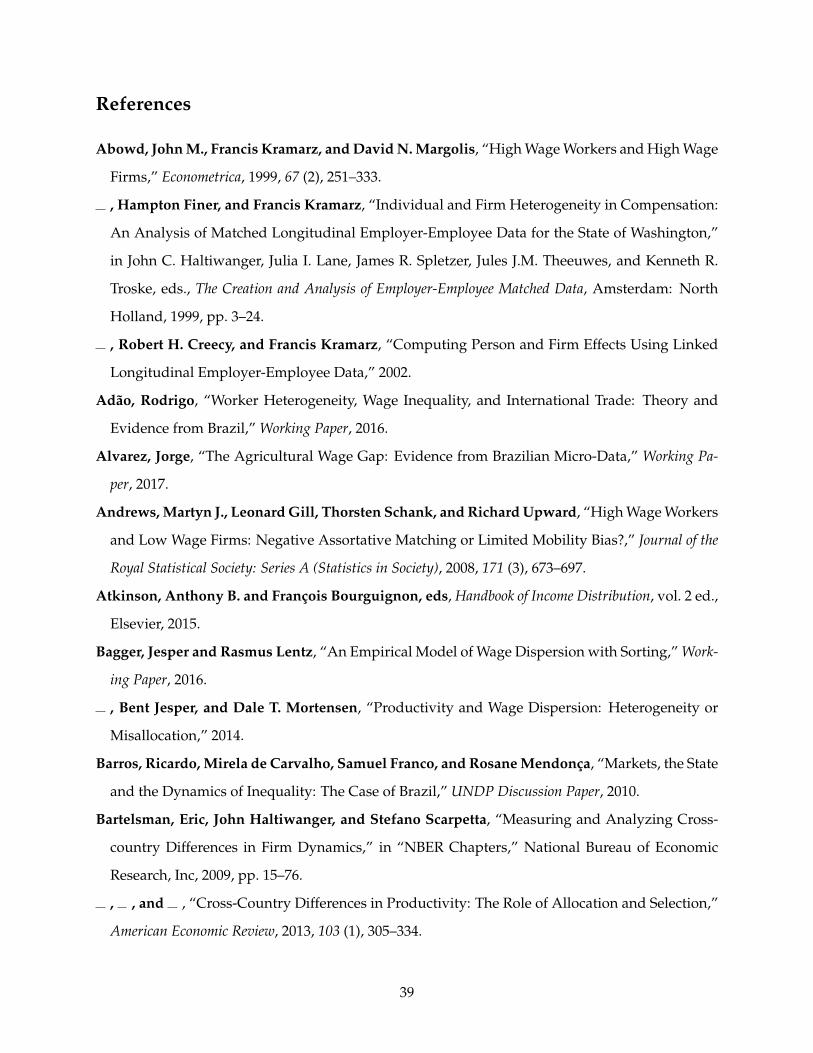
References

Abowd, John M., Francis Kramarz, and David N. Margolis, “High Wage Workers and High Wage

Firms,” Econometrica, 1999, 67 (2), 251–333.

, Hampton Finer, and Francis Kramarz, “Individual and Firm Heterogeneity in Compensation:

An Analysis of Matched Longitudinal Employer-Employee Data for the State of Washington,”

in John C. Haltiwanger, Julia I. Lane, James R. Spletzer, Jules J.M. Theeuwes, and Kenneth R.

Troske, eds., The Creation and Analysis of Employer-Employee Matched Data, Amsterdam: North

Holland, 1999, pp. 3–24.

, Robert H. Creecy, and Francis Kramarz, “Computing Person and Firm Effects Using Linked

Longitudinal Employer-Employee Data,” 2002.

Adão, Rodrigo, “Worker Heterogeneity, Wage Inequality, and International Trade: Theory and

Evidence from Brazil,” Working Paper, 2016.

Alvarez, Jorge, “The Agricultural Wage Gap: Evidence from Brazilian Micro-Data,” Working Pa-

per, 2017.

Andrews, Martyn J., Leonard Gill, Thorsten Schank, and Richard Upward, “High Wage Workers

and Low Wage Firms: Negative Assortative Matching or Limited Mobility Bias?,” Journal of the

Royal Statistical Society: Series A (Statistics in Society), 2008, 171 (3), 673–697.

Atkinson, Anthony B. and François Bourguignon, eds, Handbook of Income Distribution, vol. 2 ed.,

Elsevier, 2015.

Bagger, Jesper and Rasmus Lentz, “An Empirical Model of Wage Dispersion with Sorting,” Work-

ing Paper, 2016.

, Bent Jesper, and Dale T. Mortensen, “Productivity and Wage Dispersion: Heterogeneity or

Misallocation,” 2014.

Barros, Ricardo, Mirela de Carvalho, Samuel Franco, and Rosane Mendonça, “Markets, the State

and the Dynamics of Inequality: The Case of Brazil,” UNDP Discussion Paper, 2010.

Bartelsman, Eric, John Haltiwanger, and Stefano Scarpetta, “Measuring and Analyzing Cross-

country Differences in Firm Dynamics,” in “NBER Chapters,” National Bureau of Economic

Research, Inc, 2009, pp. 15–76.

, , and , “Cross-Country Differences in Productivity: The Role of Allocation and Selection,”

American Economic Review, 2013, 103 (1), 305–334.

39

Barth, Erling, Alex Bryson, James C. Davis, and Richard Freeman, “It’s Where You Work: In-

creases in the Dispersion of Earnings across Establishments and Individuals in the United

States,” Journal of Labor Economics, 2016, 34 (S2), S67–S97.

Bertrand, Marianne and Antoinette Schoar, “Managing with Style: The Effect of Managers on

Firm Policies,” The Quarterly Journal of Economics, 2003, 118 (4), 1169–1208.

Blanchflower, D. G., A. J. Oswald, and P. Sanfey, “Wages, Profits, and Rent-Sharing,” The Quar-

terly Journal of Economics, feb 1996, 111 (1), 227–251.

Bonhomme, Stéphane, Thibaut Lamadon, and Elena Manresa, “A Distributional Framework for

Matched Employer Employee Data,” 2016.

Card, D., F. Devicienti, and A. Maida, “Rent-sharing, Holdup, and Wages: Evidence from

Matched Panel Data,” The Review of Economic Studies, oct 2014, 81 (1), 84–111.

Card, David, Ana Rute Cardoso, and Patrick Kline, “Bargaining, Sorting, and the Gender Wage

Gap: Quantifying the Impact of Firms on the Relative Pay of Women,” The Quarterly Journal of

Economics, 2016, 131 (2), 633–686.

, Joerg Heining, and Patrick Kline, “Workplace Heterogeneity and the Rise of West German

Wage Inequality,” Quarterly Journal of Economics, 2013, 128 (3), 967–1015.

Córdova, José Ernesto López and Mauricio Mesquita Moreira, “Regional Integration and Pro-

ductivity: The Experiences of Brazil and Mexico,” IDB Publications (Working Papers), 2003.

de Araujo, Ana Luisa Pessoa, “Wage Inequality and Job Stability,” 2014.

Deaton, Angus, The Analysis of Household Surveys: A Microeconometric Approach to Development

Policy 1997.

Dix-Carneiro, Rafael and Brian K. Kovak, “Trade Liberalization and the Skill Premium: A Local

Labor Markets Approach,” American Economic Review, may 2015, 105 (5), 551–557.

and , “Trade Liberalization and Regional Dynamics,” 2017.

, Rodrigo R. Soares, and Gabriel Ulyssea, “Economic Shocks and Crime: Evidence from the

Brazilian Trade Liberalization,” Working Paper, 2016.

Dunne, Timothy, Lucia Foster, John Haltiwanger, and Kenneth R. Troske, “Wage and Produc-

tivity Dispersion in United States Manufacturing: The Role of Computer Investment,” Journal

of Labor Economics, 2004, 22 (2), 397–430.

Engbom, Niklas and Christian Moser, “Earnings Inequality and the Minimum Wage: Evidence

from Brazil,” 2017.

40

and , “Returns to Education Through Access to Higher-Paying Firms: Evidence from US

Matched Employer-Employee Data,” American Economic Review, 2017, 107 (5).

Faggio, G., K. G. Salvanes, and J. Van Reenen, “The Evolution of Inequality in Productivity and

Wages: Panel Data Evidence,” Industrial and Corporate Change, 2010, 19 (6), 1919–1951.

Ferreira, Francisco H. G., Phillippe G. Leite, and Matthew Wai-Poi, Trade Liberalization, Employ-

ment Flows, And Wage Inequality In Brazil Policy Research Working Papers, The World Bank,

2007.

Ferreira, Pedro Cavalcanti and Jose Luiz Rossi, “New Evidence from Brazil on Trade Liberaliza-

tion and Productivity Growth,” International Economic Review, 2003, 44 (4), 1383–1405.

Fortin, Nicole, Thomas Lemieux, and Sergio Firpo, “Decomposition Methods in Economics,” in

“Handbook of Labor Economics,” Vol. 4 2011, pp. 1–102.

Guiso, Luigi, Luigi Pistaferri, and Fabiano Schivardi, “Insurance within the Firm,” Journal of

Political Economy, oct 2005, 113 (5), 1054–1087.

Heathcote, Jonathan, Fabrizio Perri, and Giovanni L. Violante, “Unequal We Stand: An Em-

pirical Analysis of Economic Inequality in the United States, 1967-2006,” Review of Economic

Dynamics, 2010, 13 (1), 15–51.

Heckman, James J., Lance J. Lochner, and Petra E. Todd, “Fifty Years of Mincer Earnings Regres-

sions,” 2003.

Helpman, Elhanan, Oleg Itskhoki, Marc-Andreas Muendler, and Stephen Redding, “Trade and

Inequality: From Theory to Estimation,” Review of Economic Studies, 2016, (Forthcoming).

Iranzo, Susana, Fabiano Schivardi, and Elisa Tosetti, “Skill Dispersion and Firm Productivity:

An Analysis with Employer Employee Matched Data,” Journal of Labor Economics, 2008, 26 (2),

247–285.

Kopczuk, Wojciech, Emmanuel Saez, and Jae Song, “Earnings Inequality and Mobility in the

United States: Evidence from Social Security Data since 1937,” Quarterly Journal of Economics,

2010, 125 (1), 91–128.

Lopes de Melo, Rafael, “Firm Wage Differentials and Labor Market Sorting: Reconciling Theory

and Evidence,” 2015.

Lopez, J. Humberto and Guillermo Perry, “Inequality in Latin America: Determinants and Con-

sequences,” 2008.

41

Medeiros, Marcelo, Pedro H. G. Ferreira de Souza, and Fábio Avila de Castro, “O topo da dis-

tribuição de renda no Brasil: primeiras estimativas com dados tributários e comparação com

pesquisas domiciliares, 2006–2012,” 2014.

Meghir, Costas, Renata Narita, and Jean-Marc Robin, “Wages and Informality in Developing

Countries,” American Economic Review, 2015, 105 (4), 1509–1546.

Menezes-Filho, Naércio Aquino, Marc-Andreas Muendler, and Garey Ramey, “The Structure of

Worker Compensation in Brazil, with a Comparison to France and the United States,” Review of

Economics and Statistics, may 2008, 90 (2), 324–346.

Mincer, Jacob, Schooling, Experience, and Earnings, New York: NBER Press, 1974.

Moreira, Mauricio Mesquita, “Brazil’s Trade Liberalization and Growth: Has it Failed?,” Interna-

tional Trade, 2004.

Muendler, Marc-Andreas, “Trade, Technology, and Productivity: A Study of Brazilian Manufac-

turers, 1986-1998,” CESifo Working Paper Series, 2004.

Organisation for Economic Co-operation and Development, “Country Note: Programme for In-

ternational Student Assessment (PISA) Results from PISA 2012,” Technical Report, Organisation

for Economic Co-operation and Development, Paris 2012.

Pavcnik, Nina, Andreas Blom, Pinelopi Goldberg, and Norbert Schady, “Trade Liberalization

and Industry Wage Structure: Evidence from Brazil,” World Bank Economic Review, 2004, 18 (3),

319–344.

Song, Jae, David J. Price, Fatih Guvenen, Nicholas Bloom, and Till von Wachter, “Firming Up

Inequality,” 2016.

Sorkin, Isaac, “Ranking Firms Using Revealed Preference,” 2015.

Tsounta, Evridiki and Anayochukwu I. Osueke, “What is Behind Latin America’s Declining In-

come Inequality?,” 2014.

Ulyssea, Gabriel, “Firms, Informality and Development: Theory and Evidence from Brazil,” 2014.

Van Reenen, J., “The Creation and Capture of Rents: Wages and Innovation in a Panel of U. K.

Companies,” The Quarterly Journal of Economics, feb 1996, 111 (1), 195–226.

Woodcock, Simon D., “Match Effects,” Research in Economics, 2015, 69 (1), 100–121.

World Bank, “World Development Indicators,” 2016.

42

Appendix

A Mincer regressions

This section studies changes in worker observables and their returns within a Mincer framework.

In contrast to a popularly held belief, Brazil’s inequality decline was not driven by worker observ-

ables and the rapid increase in educational attainment that took place during this period.

Building on the classical framework by Mincer (1974), we regress log monthly real earnings

on worker observables. Specifically, we include five age group dummies interacted with nine

education group dummies, one digit occupation dummies and two digit sector dummies,

log (yit) = ageit × eduit + occit + secit + ε it

Note that all explanatory variables are allowed to vary freely by year. Based on this regression, we

calculate the predicted value due to each component and report the variance of these predicted

values.

Figure 12 plots the results. We draw two conclusions: First, worker observables jointly explain

about 45 percent of the overall variance in log earnings. In contrast, our AKM methodology in

Section 5 suggests that worker observables explain 37–40 percent of the variance of the worker com-

ponent of earnings (which constitutes 50–60 percent of the overall variance). Partly, the difference

can be explained by the fact that we let observables as well as their returns vary by year in the

Mincer framework while the AKM framework uses averages over the subperiod. Conceptually

more important, the discrepancy suggests that part of the return to education and experience is

due to a selection into better paying firms.

Second, the fraction of earnings dispersion explained by worker observables does not change

much over time. Hence, worker observables and sector controls explain close to 23 percent of

the fall in inequality. Decomposing this, age and education account for roughly 20 percent of the

variance of log earnings and six percent of the decline. Inequality between occupations remains

relatively constant around six to eight percent of total variance. The fraction of total inequality

explained by differences in means across sectors falls from seven to three percent—this accounts

for 15 percent of the overall decline in variance. Finally, covariances between the explanatory

variables remain stable around 12–14 of total variance. We conclude that even when controlling

43

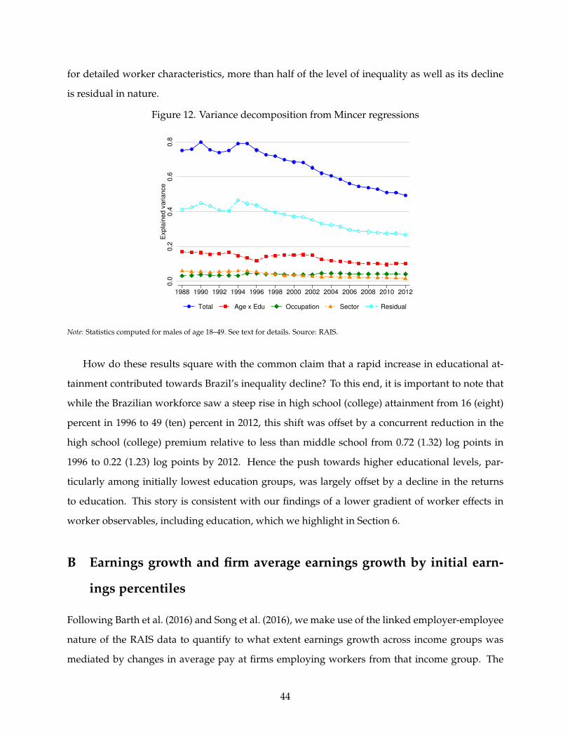
for detailed worker characteristics, more than half of the level of inequality as well as its decline

is residual in nature.

Figure 12. Variance decomposition from Mincer regressions

0.0

0.2

0.4

0.6

0.8

Exp

lain

ed

va

ria

nce

1988 1990 1992 1994 1996 1998 2000 2002 2004 2006 2008 2010 2012

Total Age x Edu Occupation Sector Residual


How do these results square with the common claim that a rapid increase in educational at-

tainment contributed towards Brazil’s inequality decline? To this end, it is important to note that

while the Brazilian workforce saw a steep rise in high school (college) attainment from 16 (eight)

percent in 1996 to 49 (ten) percent in 2012, this shift was offset by a concurrent reduction in the

high school (college) premium relative to less than middle school from 0.72 (1.32) log points in

1996 to 0.22 (1.23) log points by 2012. Hence the push towards higher educational levels, par-

ticularly among initially lowest education groups, was largely offset by a decline in the returns

to education. This story is consistent with our findings of a lower gradient of worker effects in

worker observables, including education, which we highlight in Section 6.

B Earnings growth and firm average earnings growth by initial earn-

ings percentiles

Following Barth et al. (2016) and Song et al. (2016), we make use of the linked employer-employee

nature of the RAIS data to quantify to what extent earnings growth across income groups was

mediated by changes in average pay at firms employing workers from that income group. The

44

results of this exercise are shown in Figure 13 for the period 1988–1996, when inequality increased

mildly, and for the period 1996–2012, when earnings inequality declined rapidly.

Figure 13. Individual real labor earnings growth between and within firms

−0.3

0.0

0.3

0.6

0.9

Log g

row

th in p

erc

entile

earn

ings

0 10 20 30 40 50 60 70 80 90 100Earnings percentile

Individuals Firms Individuals/Firms

1988−1996

−0.3

0.0

0.3

0.6

0.9

Log g

row

th in p

erc

entile

earn

ings

0 10 20 30 40 50 60 70 80 90 100Earnings percentile

Individuals Firms Individuals/Firms

1996−2012


There are three features worth noting. First, real labor earnings growth occurred at almost

every percentile of the distribution throughout both periods. Second, individual earnings growth

(solid blue line with circles) slopes mildly upward in initial earnings percentiles from 1988–1996

and pronouncedly slopes downward from 1996–2012, indicating that earnings inequality increased

45

a little during the first period and decreased significantly during the second period. Third, indi-

vidual earnings growth throughout the distribution is almost entirely explained by the growth of

firm average earnings (dashed red line with squares) among those groups. Remarkably, there were

no significant changes in within-firm earnings inequality (dash-dotted green line with diamonds).

We interpret these results as suggestive evidence in favor of firms playing an important role

in explaining earnings inequality dynamics during the period of increasing inequality from 1988–

1996 and also during the large decrease in inequality from 1996–2012.

C Variance between and within firms by region, firm size and produc-

tivity

We now show that the compression in pay across firms was not solely driven by a particular subset

of regions or firms, nor was it driven by a compression in average differences between regions or

productivity groups.

Figure 14 plots inequality across and within firms within Brazilian regions. Although there are

differences in levels, all regions display substantial compression of pay over time. Moreover, the

dominance of between-firm compression is present in every region.

Similarly, Figures 15 and 16 plot the same decomposition of inequality between and within

firms by size of the firm and by productivity of the firm, respectively. We observe a similar pattern

of substantial compression across firms within small, medium and large firms, as well as within

low-productivity and medium-productivity firms. The decline is less pronounced among high

productivity firms.

46

Figure 14. Variance between and within firms within Brazilian regions.0

.1.2

.3.4

.5.6

Va

ria

nce

of

log

la

bo

r in

co

me

1988 1990 1992 1994 1996 1998 2000 2002 2004 2006 2008 2010 2012


North

0.1

.2.3

.4.5

.6

Va

ria

nce

of

log

la

bo

r in

co

me

1988 1990 1992 1994 1996 1998 2000 2002 2004 2006 2008 2010 2012


Northeast

0.1

.2.3

.4.5

.6

Va

ria

nce

of

log

la

bo

r in

co

me

1988 1990 1992 1994 1996 1998 2000 2002 2004 2006 2008 2010 2012


Southeast

0.1

.2.3

.4.5

.6

Va

ria

nce

of

log

la

bo

r in

co

me

1988 1990 1992 1994 1996 1998 2000 2002 2004 2006 2008 2010 2012


South

0.1

.2.3

.4.5

.6

Va

ria

nce

of

log

la

bo

r in

co

me

1988 1990 1992 1994 1996 1998 2000 2002 2004 2006 2008 2010 2012


Central−East


47

Figure 15. Variance between and within firms, by firm size terciles0

.1.2

.3.4

.5.6

Va

ria

nce

of

log

la

bo

r in

co

me

1988 1990 1992 1994 1996 1998 2000 2002 2004 2006 2008 2010 2012


Firm size tercile 1 (smallest)

0.1

.2.3

.4.5

.6

Va

ria

nce

of

log

la

bo

r in

co

me

1988 1990 1992 1994 1996 1998 2000 2002 2004 2006 2008 2010 2012


Firm size tercile 2 (middle)

0.1

.2.3

.4.5

.6

Va

ria

nce

of

log

la

bo

r in

co

me

1988 1990 1992 1994 1996 1998 2000 2002 2004 2006 2008 2010 2012


Firm size tercile 3 (largest)


48

Figure 16. Variance between and within firms, by productivity terciles0

.1.2

.3.4

.5.6

Va

ria

nce

of

log

la

bo

r in

co

me

1996 1998 2000 2002 2004 2006 2008 2010 2012


Productivity tercile 1 (lowest)

0.1

.2.3

.4.5

.6

Va

ria

nce

of

log

la

bo

r in

co

me

1996 1998 2000 2002 2004 2006 2008 2010 2012


Productivity tercile 2 (middle)

0.1

.2.3

.4.5

.6

Va

ria

nce

of

log

la

bo

r in

co

me

1996 1998 2000 2002 2004 2006 2008 2010 2012


Productivity tercile 3 (highest)


D Robustness of AKM results

The following section presents additional robustness results to our first-stage AKM regressions.

First, we show that similar results are obtained in longer, nine-year subperiods instead of our

baseline five-year subperiods. Second, we present results for the last four subperiods using hourly

wages.

D.1 Longer subperiods

Table 9 shows results for nine-year subperiods 1988–1996, 1996–2004, and 2004–2012. As expected,

worker effects explain a few percentage points less of the overall variation in earnings, which is

offset by a larger variance of the residual. The share contributed by firm effects remains roughly

49

the same. Our main conclusion that worker effects explain most of the level of inequality while

firm effects explain a disproportionate share of the decline continues to hold.

Table 9. AKM robustness results, longer subperiods

1988–1996 1996–2004 2004–2012 Change 1996–2012

Variance of log earnings 0.77 (100.0%) 0.70 (100.0%) 0.54 (100.0%) -0.23 (100.0%)Variance of worker effects 0.35 (45.9%) 0.32 (46.0%) 0.29 (53.6%) -0.06 (27.6%)Variance of firm effects 0.170 (21.9%) 0.15 (21.7%) 0.09 (16.3%) -0.08 (35.3%)Variance of year effects 0.03 (3.3%) 0.00 (0.2%) 0.00 (0.2%) -0.03 (10.9%)2×Cov. worker and firm 0.15 (19.7%) 0.15 (21.2%) 0.11 (20.5%) -0.04 (17.7%)2×Cov. worker and year -0.02 (-2.3%) 0.00 (0.5%) 0.00 (-0.2%) 0.02 (-7.3%)2×Cov. firm and year -0.01 (-1.4%) 0.00 (0.3%) 0.00 (0.0%) 0.01 (-4.6%)Variance of residual 0.10 (12.8%) 0.07 (10.3%) 0.05 (9.6%) -0.05 (20.6%)

# worker-years 155.6 175.9 249.4# firms 1.45 1.93 2.80R2 0.87 0.90 0.90

Note: Variance decomposition is Var (yit) = Var (ai) + Var(aj)+ Var (Yt) + Var (eit) + 2Cov (ai , Yt) + 2Cov

(aj, Yt

)+ 2Cov

(aj, Yt

).

Cells contain variance explained by each decomposition element. The share of the total variance explained by each decomposition

element given in parentheses. Weighted by worker-years. Source: RAIS.

D.2 Hourly wages

Our data do not contain information on hours prior to 1994, but we do have data on contracted

weekly hours after that year. We find relatively small variation in contracted hours for prime age

males, with the top 75 percent of the distribution reporting working 44 hours a week (conditional

on working). To further verify the robustness of our results to variation in labor supply, Table 10

shows results from our first stage regression for the last four subperiods using hourly wages.

Inequality in hourly wages falls by four log points more than inequality in monthly income.

This is primarily accounted for by a larger fall in the variance of the worker component of pay,

while the fall in the firm component is in line with our earlier findings. Yet, our main conclusion

that a compression in the firm component of pay contributed the most to the overall fall remains.

E Robustness of the relationship between productivity and pay

The following section presents additional robustness results related to our second-stage regres-

sions of firm effects on productivity. First, we show results estimated using a balanced panel of

50

Tabl

e10

.AK

Mro

bust

ness

resu

lts,

hour

lyw

age

rate

1996

–200

020

00–2

004

2004

–200

820

08–2

012

Cha

nge

1996

–201

2

Var

ianc

eof

log

wag

es0.

73(1

01.4

%)

0.65

(99.

2%)

0.55

(96.

1%)

0.49

(93.

8%)

-0.2

4(1

20.9

%)

Var

ianc

eof

wor

ker

effe

cts

0.34

(94.

8%)

0.33

(91.

8%)

0.29

(88.

4%)

0.27

(86.

9%)

-0.0

7(1

45.5

%)

Var

ianc

eof

firm

effe

cts

0.18

(108

.3%

)0.

14(1

10.4

%)

0.11

(111

.7%

)0.

09(1

11.0

%)

-0.0

9(1

05.9

%)

Var

ianc

eof

Y t0.

00(1

12.4

%)

0.00

(86.

5%)

0.00

(88.

7%)

0.00

(128

.2%

)0.

00(1

51.8

%)

2×C

ov.w

orke

ran

dfir

mef

fect

s0.

16(1

10.9

%)

0.13

(109

.0%

)0.

11(1

05.7

%)

0.10

(101

.3%

)-0

.06

(132

.2%

)2×

Cov

.wor

ker

effe

cts

and

Y t0.

00(1

20.6

%)

0.00

(96.

6%)

0.00

(83.

3%)

0.00

(128

.5%

)0.

00(1

78.9

%)

2×C

ov.fi

rmef

fect

san

dY t

0.00

(112

.9%

)0.

00(9

3.9%

)0.

00(1

03.1

%)

0.00

(173

.6%

)0.

00(1

06.9

%)

Var

ianc

eof

resi

dual

0.05

(99.

0%)

0.05

(98.

1%)

0.04

(97.

0%)

0.03

(96.

9%)

-0.0

2(1

02.8

%)

#w

orke

r-ye

ars

80.1

90.2

108.

213

0.0

#fir

ms

1.20

1.40

1.70

2.15

R2

0.93

0.93

0.93

0.93

Not

e:V

aria

nce

deco

mpo

siti

onis

Var

(yit)=

Var

(ai)+

Var( a j) +

Var

(Yt)+

Var

(eit)+

2Cov

(ai,

Y t)+

2Cov( a j

,Yt) +

+2C

ov( a j

,Yt) .C

ells

cont

ain

vari

ance

expl

aine

dby

each

deco

mpo

siti

onel

emen

t.Th

era

tio

ofth

eva

rian

cein

hour

ly

earn

ings

rela

tive

tom

onth

lyin

com

eis

give

nin

pare

nthe

ses.

Wei

ghte

dby

wor

ker-

year

s.So

urce

:RA

IS.

51

firms. Second, we explore the relationship between exporting status and the firm component of

pay.

E.1 Regressions of firm effects on firm observables in a balanced panel

We repeat our second-stage estimation for a balanced panel of firms who are present in the PIA

data in all four periods from 1996 to 2012. Estimating the second stage on only surviving firms

sheds light on the role of exit and entry versus changes in pay within surviving firms. We find that

the results using a balanced panel are in line with those previously presented in Table 6. There is

a slightly steeper relationship between value added per worker and firm effects in the balanced

panel, with a similar decline in the magnitude of the coefficient over time across all specifications.

E.2 Relationship between firm effects, productivity, and exporter status

Table 12 shows the results of second-stage regressions of firm effects on value added per worker

using an export indicator and export intensity as additional controls.33 All regressions include a

vector of subsector dummies. The positive relationship between value added per worker and firm

effects remains after controlling for exporting variables, and the coefficient declines over time. The

patterns and magnitudes of the productivity-pay relationship are similar to the ones discussed in

section 6.

Moreover, exporting firms pay a higher premium than non-exporting firms, although the pre-

mium among exporting firms decreases with export intensity. The difference between exporting

and non-exporting firms decreases from 13–25 log points to 2–7 log points once we control for dif-

ferences in productivity. Also, the positive relationship between value added per worker and firm

effects is present among exporting and non-exporting firms, and this has flattened among both

groups. Figure 17 depicts these patterns in graphical form. The consistently positive gradient

between value added per worker and firm effects among exporting and non-exporting firms, the

large decline in exporting premiums after controlling for differences in value added per worker,

and the finding that the firm effects gradient in value added per worker declined for both ex-

porters and non-exporters motivate our focus on the firm productivity dimension.

33We define export intensity as revenues from exports divided by total revenues.

52

Tabl

e11

.R

egre

ssio

nsof

esti

mat

edfir

mef

fect

son

firm

char

acte

rist

ics

usin

ga

bala

nced

pane

l

1996

–200

020

00–2

004

2004

–200

820

08–2

012

PAN

EL

A.N

OC

ON

TR

OL

S

Val

uead

ded

p.w

.0.

278

0.17

60.

219

0.14

80.

179

0.13

30.

157

0.08

97Fi

rmsi

ze0.

109

-0.1

160.

0697

-0.1

290.

0411

-0.0

872

0.03

99-0

.107

Val

uead

ded

p.w

.xFi

rmsi

ze0.

012

0.01

10.

007

0.00

9

Wor

ker-

year

s9.

89.

89.

811

.711

.711

.714

.414

.414

.415

.115

.115

.1R

20.

621

0.24

30.

634

0.58

90.

124

0.59

50.

571

0.06

80.

576

0.50

20.

082

0.51

0

PAN

EL

B.S

UB

SEC

TO

RC

ON

TR

OL

S

Val

uead

ded

p.w

.0.

258

0.15

20.

200

0.12

50.

158

0.11

30.

136

0.07

37Fi

rmsi

ze0.

109

-0.0

950.

076

-0.0

990.

052

-0.0

540.

046

-0.0

75V

alue

adde

dp.

w.x

Firm

size

0.01

10.

010

0.00

60.

007

Wor

ker-

year

s9.

89.

89.

811

.711

.711

.714

.414

.414

.415

.115

.115

.1R

20.

695

0.47

10.

714

0.68

60.

435

0.69

20.

682

0.43

60.

686

0.66

00.

452

0.66

7

PAN

EL

C.S

TAT

EC

ON

TR

OL

S

Val

uead

ded

p.w

.0.

248

0.17

30.

195

0.15

00.

161

0.12

00.

142

0.07

48Fi

rmsi

ze0.

110

-0.0

210.

079

-0.0

460.

053

-0.0

550.

052

-0.0

76V

alue

adde

dp.

w.x

Firm

size

0.00

50.

005

0.00

50.

008

Wor

ker-

year

s9.

89.

89.

811

.711

.711

.714

.414

.414

.415

.115

.115

.1R

20.

705

0.53

30.

728

0.67

30.

417

0.67

70.

640

0.34

50.

643

0.59

60.

367

0.60

7

Not

e:D

epen

dent

vari

able

isth

ees

tim

ated

firm

effe

cta j

.Num

ber

ofw

orke

r-ye

ars

inm

illio

ns.W

eigh

ted

byw

orke

r-ye

ars.

Sour

ce:R

AIS

and

PIA

.

53

Tabl

e12

.R

egre

ssio

nsof

esti

mat

edfir

mef

fect

son

expo

rtin

gst

atus

1996

–200

020

00–2

004

2004

–200

820

08–2

012

Expo

rter

0.25

10.

066

-0.4

490.

215

0.02

0-0

.471

0.16

80.

020

-0.6

000.

133

0.02

4-0

.602

Expo

rtin

tens

ity

-0.1

44-0

.107

0.35

2-0

.114

-0.1

44-0

.193

-0.0

27-0

.018

0.21

2-0

.003

0.01

40.

450

Val

uead

ded

p.w

.0.

226

0.20

40.

182

0.15

40.

137

0.10

50.

116

0.08

8Ex

port

erx

Val

uead

ded

p.w

.0.

047

0.04

50.

057

0.05

6Ex

port

inte

nsit

yx

Val

uead

ded

p.w

.-0

.040

0.00

4-0

.020

-0.0

38

Wor

ker-

year

s15

.515

.515

.516

.716

.716

.721

.021

.021

.023

.923

.923

.9R

20.

353

0.65

70.

660

0.36

00.

653

0.65

80.

382

0.62

80.

637

0.41

00.

615

0.62

6

Not

e:D

epen

dent

vari

able

isth

ees

tim

ated

firm

effe

cta j

.All

regr

essi

ons

incl

ude

subs

ecto

rco

ntro

ls.N

umbe

rof

wor

ker-

year

sin

mill

ions

.Wei

ghte

dby

wor

ker-

year

s.So

urce

:RA

ISan

dPI

A.

54

Figure 17. Estimated AKM firm effects versus value added per worker, by exporter statusand period

−.6

−.4

−.2

0.2

.4.6

AK

M f

irm

eff

ect

7 8 9 10 11 12 13 14value added p.w.

1996−2000 2000−2004 2004−2008 2008−2012

Non−exporters

−.6

−.4

−.2

0.2

.4.6

AK

M f

irm

eff

ect

7 8 9 10 11 12 13 14value added p.w.

1996−2000 2000−2004 2004−2008 2008−2012

Exporters


F Largest connected set

Table 13 compares workers in the largest connected set to the overall population of adult males.

Given that the largest connected set covers 97–98 percent of the overall population, it is not sur-

prising that the two are very similar.

55

Tabl

e13

.Sum

mar

yst

atis

tics

onw

orke

rsin

larg

estc

onne

cted

set,

rela

tive

toad

ultm

ales

Earn

ings

Age

Scho

olin

g#

Wor

ker-

year

s#

Wor

kers

Mea

nSt

.d.

Mea

nSt

.d.

Mea

nSt

.d.

1988

–199

277

.3(9

8.6%

)23

.1(9

8.2%

)1.

24(1

00.9

%)

0.86

(99.

8%)

30.8

2(1

00.1

%)

8.04

(100

.0%

)7.

16(9

9.9%

)4.

26(1

00.2

%)

1992

–199

677

.3(9

8.0%

)23

.7(9

7.5%

)1.

30(1

01.2

%)

0.86

(99.

8%)

31.4

6(1

00.1

%)

8.10

(99.

9%)

7.49

(99.

9%)

4.21

(100

.2%

)19

96–2

000

81.5

(97.

2%)

25.6

(96.

7%)

1.27

(101

.3%

)0.

83(1

00.1

%)

31.6

0(1

00.2

%)

8.16

(99.

9%)

7.93

(99.

9%)

4.09

(100

.4%

)20

00–2

004

91.8

(96.

9%)

28.8

(96.

5%)

1.05

(101

.3%

)0.

78(1

00.4

%)

31.6

1(1

00.1

%)

8.22

(100

.0%

)8.

81(1

00.0

%)

3.91

(100

.4%

)20

04–2

008

110.

0(9

7.4%

)33

.0(9

7.0%

)0.

86(1

01.2

%)

0.72

(100

.4%

)31

.64

(100

.0%

)8.

23(1

00.0

%)

9.61

(100

.0%

)3.

68(1

00.3

%)

2008

–201

213

2.2

(97.

9%)

38.6

(97.

5%)

0.77

(101

.0%

)0.

68(1

00.3

%)

31.7

4(9

9.9%

)8.

20(9

9.9%

)10

.24

(100

.0%

)3.

47(1

00.2

%)

Not

es:W

ere

port

inpa

rent

hese

sth

epr

opor

tion

ofth

ere

port

edst

atis

tics

rela

tive

toth

egr

oup

ofad

ultm

ales

desc

ribe

din

Tabl

e1.

Earn

ings

are

inlo

gm

ulti

ples

ofth

em

onth

lym

inim

umw

age,

scho

olin

gis

year

sof

educ

atio

n,ag

eis

assi

gned

asth

eav

erag

eof

aw

orke

r’s

age

bin.

Sour

ce:R

AIS

.

56

Firms and the Decline in Earnings Inequality in Brazil

Documents

Transcript of Firms and the Decline in Earnings Inequality in Brazil