HAL Id: tel-03119251https://tel.archives-ouvertes.fr/tel-03119251

Submitted on 23 Jan 2021

HAL is a multi-disciplinary open accessarchive for the deposit and dissemination of sci-entific research documents, whether they are pub-lished or not. The documents may come fromteaching and research institutions in France orabroad, or from public or private research centers.

L’archive ouverte pluridisciplinaire HAL, estdestinée au dépôt et à la diffusion de documentsscientifiques de niveau recherche, publiés ou non,émanant des établissements d’enseignement et derecherche français ou étrangers, des laboratoirespublics ou privés.

Firm heterogeneity, country-level asymmetry and thestructure of the gains from trade

Badis Tabarki

To cite this version:Badis Tabarki. Firm heterogeneity, country-level asymmetry and the structure of the gains fromtrade. Economics and Finance. Université Panthéon-Sorbonne - Paris I, 2020. English. NNT :2020PA01E022. tel-03119251

,,,,,,

UNIVERSITÉ PARIS 1 PANTHÉON-SORBONNE

PARIS SCHOOL OF ECONOMICS (PSE)

Doctoral Thesis

Firm Heterogeneity, Country-levelAsymmetry and the Structure of the Gains

from Trade

Author:

BADIS TABARKI

Advisor:

LIONEL FONTAGNÉ

Thèse pour l’obtention du grade de Docteur en Sciences Économiques,déposée à Paris, le 31 Juillet 2020.

Jury:

Maria Bas, Professeur, Université Paris 1 Panthéon-SorbonneMonika Mrazova (Rapporteur), Professeur, Université de Genève

Thomas Chaney (Rapporteur), Professeur, Sciences PoMathieu Parenti, Professeur, Université Libre de Bruxelles

Ariell Reshef, Directeur de Recherche, CNRS

1

Acknowledgements

First and foremost, I am very grateful to my Advisor, Lionel Fontagné, to whom I am greatlyindebted for offering me the chance to be one of his Ph.D. students and the opportunity to workon the Heterogeneous Firms Theory which I have been passionate about since I was his under-graduate student. Thank you for your support, your kindness, your constant encouragementand for everything you have taught me. It has been a great pleasure to work under your super-vision since the Master thesis.

A special thank you goes to Ariell Reshef, who is in my thesis committee and who took the timeto discuss my chapters and propose insightful suggestions which considerably improved mychapters. I would also like to thank Mathieu Parenti, who is also member of my thesis commit-tee, for his helpful comments and for guiding me towards more general theoretical approachesusing subtle nesting techniques. This was inspiring for me, and helped improve the quality ofdissertation.

I would also like to thank Monika Mrazova, and Thomas Chaney, who gracefully accepted to bepart of my jury. I very much appreciate the attention and consideration they gave to my work.Their insightful comments and helpful suggestions greatly contributed to improve my thesis.

I seize this occasion to thank Antoine Vatan and Farid Toubal for their early encouragements topursue a Ph.D, and for sharing inspiring references when I was their undergraduate student.I would also like to thank the first lady who taught me Economics at high school, Saadia Mouhbi,for her inspiring lectures which made passionate about economic intuition and theoretical rea-soning in economics.

I am also very happy to acknowledge the help and support of my amazing office 314 friends: ElsaLeromain, Evgenii Monastyrenko,Zenathan Hassanudin, Stephan Worack, Nevine El-Mallakh,Katharina Längle, Zaneta Kubik, Enxhi Tresa, Camille Reverdy, and Irene Iodice. A big Thankto all of you for sharing great times but also for giving me great advice.

Words will never be enough to express my gratitude towards my family. To my parents Kaderand Nadia, my sister Molka, and my brother Anis, who have given me everything, it is to youthat I owe this achievement. Thank you for all your unconditional love and support. You aresimply the first and best gift life gave me!

2

Contents

Introduction 5

1 A Simple Model of Standards Liberalization 101.1 Introduction . . . . . . . . . . . . . . . . . . . . . . . . . . . . . . . . . . . . . . . . . 101.2 The Model . . . . . . . . . . . . . . . . . . . . . . . . . . . . . . . . . . . . . . . . . . 121.3 Characterization of the equilibrium . . . . . . . . . . . . . . . . . . . . . . . . . . . . 131.4 Welfare implications of Standards Harmonization . . . . . . . . . . . . . . . . . . . 171.5 Welfare Analysis: Towards a Parsimonious Extension . . . . . . . . . . . . . . . . . 19

1.5.1 More Realistic Assumptions on the Demand and the Supply side . . . . . . 191.5.2 Solving for the General Equilibrium Domestic Cutoff . . . . . . . . . . . . . 201.5.3 Welfare Implications of "Standards Alignment" vs "Standards Harmoniza-

tion" . . . . . . . . . . . . . . . . . . . . . . . . . . . . . . . . . . . . . . . . . 21

Appendix A 23

2 Structural Gravity under Size Asymmetry and Non-Homotheticity 262.1 Introduction . . . . . . . . . . . . . . . . . . . . . . . . . . . . . . . . . . . . . . . . . 262.2 Theoretical Framework . . . . . . . . . . . . . . . . . . . . . . . . . . . . . . . . . . . 29

2.2.1 Set up of the model . . . . . . . . . . . . . . . . . . . . . . . . . . . . . . . . . 292.2.2 Income vs Size effects on trade margins in general equilibrium . . . . . . . 372.2.3 Generalized Structural Gravity and Trade Elasticity . . . . . . . . . . . . . . 402.2.4 Solving for nominal wages in general equilibrium . . . . . . . . . . . . . . . 432.2.5 Welfare Analysis . . . . . . . . . . . . . . . . . . . . . . . . . . . . . . . . . . 44

2.3 Empirical Analysis . . . . . . . . . . . . . . . . . . . . . . . . . . . . . . . . . . . . . 502.3.1 Data Sources . . . . . . . . . . . . . . . . . . . . . . . . . . . . . . . . . . . . . 512.3.2 Econometric Challenges and Solutions . . . . . . . . . . . . . . . . . . . . . 512.3.3 Econometric Specifications . . . . . . . . . . . . . . . . . . . . . . . . . . . . 522.3.4 Interpretation of the Gravity Estimation Results . . . . . . . . . . . . . . . . 54

2.4 Conclusion . . . . . . . . . . . . . . . . . . . . . . . . . . . . . . . . . . . . . . . . . . 56

Appendix B 57

3

Appendix C 69

3 International Trade under Monopolistic Competition beyond the CES 763.1 Introduction . . . . . . . . . . . . . . . . . . . . . . . . . . . . . . . . . . . . . . . . . 763.2 A Flexible Demand System . . . . . . . . . . . . . . . . . . . . . . . . . . . . . . . . 78

3.2.1 Generalized Gorman-Pollak Demand . . . . . . . . . . . . . . . . . . . . . . 783.2.2 Conditions for integrability . . . . . . . . . . . . . . . . . . . . . . . . . . . . 783.2.3 A Useful Parameterization . . . . . . . . . . . . . . . . . . . . . . . . . . . . 79

3.3 Characterization of Demand Curvature . . . . . . . . . . . . . . . . . . . . . . . . . 793.3.1 A simple Measure of Demand Curvature . . . . . . . . . . . . . . . . . . . . 79

3.4 Illustrating Comparative Statics Results . . . . . . . . . . . . . . . . . . . . . . . . . 823.4.1 Variable markups and Relative pass-through . . . . . . . . . . . . . . . . . . 823.4.2 Demand Curvature, Firm Selection, and Partitioning of Firms . . . . . . . . 83

3.5 Monopolistic Competition with Heterogeneous Firms under Generalized Demands 883.5.1 Supply . . . . . . . . . . . . . . . . . . . . . . . . . . . . . . . . . . . . . . . . 893.5.2 Trade Equilibrium . . . . . . . . . . . . . . . . . . . . . . . . . . . . . . . . . 903.5.3 Welfare Analysis . . . . . . . . . . . . . . . . . . . . . . . . . . . . . . . . . . 963.5.4 Demand Curvature and Gains from Higher Exposure to Trade . . . . . . . 1033.5.5 A More Granular Analysis of the Gains From Trade . . . . . . . . . . . . . . 107

3.6 Conclusion . . . . . . . . . . . . . . . . . . . . . . . . . . . . . . . . . . . . . . . . . . 119

Appendix D 120

Bibliography 128

4

Introduction

The seminal contribution by Melitz (2003) has paved the way for a large body of the literatureto study international trade from a firm-level perspective. A crude summary of the findings ofthis strand of the literature: (i) only more productive firms can export, (ii) aggregate trade flowsare attributable to a handful of firms which export many products to many destinations, (iii)these happy few exporters are more skill and capital intensive, pay higher wages, and expandafter trade liberalization while non-exporters shrink (Melitz, 2003; Mayer and Ottaviano, 2007;Bernard et al., 2007). As stressed by Melitz (2003), the heterogeneous impact of trade on firms isa direct consequence of their initial heterogeneity in productivity.

Now if we extrapolate this conjecture to a World economy comprised of asymmetric countries,shall we expect trade liberalization to affect countries differently? which mechanism would ex-plain such a heterogeneous impact of trade on asymmetric countries? There are four potentialcross-country differences in: (i) the state of technology, (ii) market size, (iii) stringency of localstandards, and (iv) demand structure. In an early extension of the Melitz (2003) model to theasymmetric case, Demidova (2008) focuses on technological asymmetry and shows that traderaises welfare in the technologically advanced country at the expense of a welfare loss for thelaggard one. Demidova and Rodriguez-Clare (2013) propose a two-country version of the Melitz(2003) model which allows for a possible asymmetry in market size. In contrast to Demidova(2008), they find that unilateral trade liberalization is welfare improving for both partners.

This contradiction mainly stems from the absence of the Home market effect in Demidova andRodriguez-Clare (2013), and mirrors thus a dependence of the nature of the impact of trade (onasymmetric countries) on the modeling strategy. This possible theoretical debate was absent insubsequent literature, which remains silent on the welfare implications of country-level asym-metry in market size under firm heterogeneity. Another aspect of asymmetry that received littleattention in theoretical literature is the difference in the degree of stringency of local standardsacross countries. In deed, given the absence of a conventional modeling approach of non-tariffbarriers, trade models have seldom examined the welfare implications of such asymmetry inlocal standards.

5

On the demand side, since earliest work by Linder (1961), cross-country difference in demandstructure has received little attention in the literature. The Linder (1961) hypothesis predictsmore trade between similar countries, with rich countries trading high-quality goods, and poorcountries trading low-quality ones. The pervasiveness of horizontal differentiation in earliervariants of the Melitz (2003) model could be one of the reasons why asymmetry in demand hasnot been studied in great detail. Nevertheless, even when we abstract from quality, asymme-try on the demand side may arise when preferences are non-CES. Using quadratic preferences,Melitz and Ottaviano (2008) show that larger countries are characterized by a higher degree ofprice sensitivity, which implies a tougher competitive environment. This, in turn, induces atougher selection into exporting and forces foreign exporters to charge lower markups to largerdestinations.

By contrast, using a different class of preferences, Bertoletti, Etro, and Simonovska (2018) ob-tain an opposite result, whereby selection into exporting and export prices do not vary with adestination’s population size. Instead, they solely depend on its per-capita income level. In par-ticular, the authors show that as the elasticity of demand decreases with individual income un-der indirectly-separable preferences, rich markets are easier to penetrate and foreign exporterscharge them higher markups, and thus higher prices. Simonovska (2015) provides empiricalsupport for this theoretical prediction. She finds that an identical good is sold at a higher priceon richer destinations.

Seen this way, the country-specific aspect of the demand elasticity has been implemented inthese non-CES models for two main reasons. The first is to predict the impact of per-capita in-come and population size on the extensive margin of trade. The second is to provide a theoreticalrationale for the empirically observed price discrimination. However, little has been said on thepotential implications of these more realistic patterns of price sensitivity for income and sizeeffects on the intensive margin of trade, and on whether it may give rise to a variable elasticityof trade margins to trade costs across countries. For instance, despite strong empirical evidenceshowing that per-capita income affects significantly price elasticities, (Simonovska, 2015; Faberand Fally, 2017; Handbury, 2019), whether this implies a stronger income effect on the intensivemargin of trade, and potentially induces a country-specific elasticity of trade margins to tradecosts, has not been explored yet in theoretical trade models.

6

Besides allowing for a possible cross-country difference in the degree of price sensitivity, non-CES preferences offer additional features of flexibility, under firm heterogeneity, which receivedmore attention in the literature. For instance, the variability of markups across firms and theincompleteness of the pass-through it entails have been studied in more details. Under differ-ent alternatives to the CES, (Melitz and Ottaviano, 2008; Bertoletti, Etro, and Simonovska, 2018;Arkolakis et al., 2018; Mrázová and Neary, 2017) highlighted that more productive firms faceless elastic demand, an so charge higher markups and do not fully pass on a cost reduction toconsumers. Bertoletti, Etro, and Simonovska (2018) show both theoretically and empirically thatthe incompleteness of the pass-through significantly reduces the magnitude of welfare gainsfrom trade.

The flexibility in markups under firm heterogeneity and non-CES preferences has also revivedthe debate on the existence of the "pro-competitive effect of trade". By considering two pos-sible behaviours of the relative love for variety (RLV)1 under directly-separable preferences,Zhelobodko et al. (2012) find that the pro-competitive effect of market size enlargement holdsonly under increasing RLV.2 However, it turns into an "anti-competitive effect" in the oppositecase. A recent work by Arkolakis et al. (2018), shows that pro-competitive reduction in domesticmarkups is either dominated by an increase in foreign markups when preferences are directly-separable, or both effects exactly cancel out when preferences are homothetic. This reveals thatthe existence of variable markups at the firm-level may dampen rather than magnify the gainsfrom trade.

In this sense, in recent trade models incorporating firm heterogeneity and variable markups, thefocus is squarely on restoring a theoretical role for the pro-competitive effect of trade, whichappears to be elusive (Arkolakis et al., 2018; Fally, 2019). However, another theoretically appeal-ing feature of such settings has received little attention: the demand elasticity is firm-specific.Besides giving rise to variable markups, this key property opens the door for a more realisticmodeling of consumer behavior than allowed by homothetic CES preferences. In particular,in the absence of restrictions on demand curvature, consumers may be more, or less reactiveto price variations of varieties supplied by more, or less productive firms. This induces moreflexible patterns of allocation of additional export market shares upon trade liberalization, withimportant implications for the gains from trade. In spite of being theoretically appealing, thewelfare implications of the firm-specific aspect of the demand elasticity has received little atten-tion in recent theoretical work.

1This corresponds to the elasticity of the inverse demand.2This corresponds to the case where the price elasticity of demand is decreasing in individual consumption, as

initially assumed by Krugman (1979).

7

The main objective of this dissertation is to address the aforementioned questions, which de-spite their theoretical appeal, received little attention in existing theoretical work in internationaltrade, and are thus still open. The goal of this dissertation is thus threefold. The first consistsin studying the welfare implications of standards liberalization under country-level asymmetryboth in market size and stringency of local standards. The second is to examine both theoreti-cally and empirically the income effect on trade margins, and on the degree of their sensitivityto trade costs. The third objective is to concentrate on the firm-specific aspect of the demandelasticity beyond the CES, and to examine the role it plays in determining the magnitude andthe structure of the gains from trade.

Towards this goal, I embed alternative assumptions both on the demand and supply side in thecanonical Melitz-Chaney model of international trade with heterogeneous firms (Melitz, 2003;Chaney, 2008). With the aid of these simple amendments, I propose different variants of thiscanonical model which are well-suited to address the question that is at stake in each chapter.In so doing, the current dissertation contributes to trade theory with heterogeneous firms alongthree lines.

In Chapter 1, I propose a version of the Melitz (2003) model for the case of three possibly asym-metric countries separated by non-tariff barriers. In the absence of a pre-established cost hierar-chy to standards, this chapter covers two possible hierarchies. The first is "purely vertical" wherecompliance with foreign standards is costly only when they are more stringent than local ones.The second is "verti-zontal" in the sense that compliance is always costly regardless of whetherforeign standards are less, or more stringent than local ones. The contribution of this chapteris twofold. First, I show that standards liberalization is welfare improving only when the costhierarchy is "verti-zontal" and the trading partner is larger than the excluded country. Second,upon implementing more realistic assumptions on consumer behavior, I show that this resultholds only when consumers’ preference for better standards is relatively weak.

In Chapter 2, I propose a structural gravity model with heterogeneous firms, asymmetric coun-tries and indirectly additive preferences nesting non-homotheticity as a general case and theCES as a homothetic exception. The contribution of this chapter is threefold. First, I show, boththeoretically and empirically, that the intensive margin of trade increases only with per-capitaincome in general equilibrium, and that per-capita income dampens the sensitivity of trade mar-gins to trade costs. Second, I highlight two new welfare channels: an additional selection effectoccurring on the export market, and an increase in nominal wage in the liberalizing country.Third, the contribution of the current chapter to the gravity literature is a fully structural gravityequation that exhibits both inward and outward multilateral resistances, and additionally ex-hibits a variable elasticity of aggregate trade flows to fixed trade barriers under non-homothetic

8

preferences. Finally, aiming at obtaining general results without losing in tractability, the currentchapter proposes a new method that I call "the Exponent Elasticity Method" (EEM). This simplemethod delivers tractable solutions in general equilibrium despite added flexibility in prefer-ences.

Chapter 3 considers a general yet tractable demand system encompassing directly- and indirectly-separable preferences, with homothetic CES as a common ground. An added flexibility of thisdemand system is that it allows for two alternative curvatures of demand. Beyond the CES,demand may be either "sub-convex": less convex than the CES, or "super-convex": more convexthan the CES. Embedded in a general equilibrium trade model featuring standard assumptionson the supply side, this flexible demand system yields new comparative statics results and awide range of predictions for the gains from trade, while illustrating existing ones in a simpleand compact way.

The main finding of this chapter is that demand curvature plays a crucial role in driving com-parative statics results, shaping the structure of the gains from trade as well as determining themagnitude of these gains, whereas the type of preferences affects only marginally the results. Inparticular, taking the CES as a boundary case, I show that when demand is sub-convex, selec-tion into markets is more relaxed, the partitioning of firms by export status is more pronounced,net variety gains and gains from selection coexist, and gains from trade are smaller than thoseobtained under CES demand. I also emphasize that the type of preferences plays only a second-order role. For instance, under sub-convex demands, directly-separable preferences provide anupper bound for the gains from trade, while indirectly-separable preferences provide a lowerbound. All these patterns are reversed when demand is super-convex.

9

Chapter 1

A Simple Model of Standards Liberalization

1.1 Introduction

Empirical research in international trade has overwhelmingly substantiated cross-country dif-ferences in stringency of local standards and its detrimental effect on bilateral trade flows (Chenand Mattoo, 2008; Otsuki, Wilson, and Sewadeh, 2001). Such asymmetry gave rise to a continu-ous process of standards harmonization mainly between developed and developing countries,with important implications for North-South and South-South trade. This has been empiricallyinvestigated by Disdier, Fontagné, and Cadot (2015) who show that standards harmonizationfosters North-South trade, yet at the expense of reducing South-South trade. The authors em-phasized that such scenario of standards liberalization is welfare improving for Northern andSouthern participants, while it might induce a welfare loss for excluded Southern countries.

While this conjecture is empirically well established, it received little attention in theoretical liter-ature. For instance, international trade models have seldom examined the welfare implicationsof standards liberalization mainly due to the absence of a pre-established cost hierarchy to stan-dards, and of a conventional way to model compliance costs. The objective of the current chapteris threefold. First, I build on the baseline Melitz (2003) model to provide a theoretical frameworkthat is well-suited for examining the welfare implications of standards liberalization. Second, Iexamine the welfare implications of standards liberalization under standard assumptions bothon the demand and supply side. Third, upon incorporating more realistic assumptions on con-sumer behavior and cost compliance, I separately examine two different scenarios of standardsliberalization; (i) an alignment of a country on the local standards of its partner; and (ii) stan-dards harmonization, whereby initially different standards converge to an intermediate degreeof stringency.

10

Towards this goal, I proceed in three steps. First, I consider the case of three countries that areasymmetric both in market size and stringency of local standards. Second, I propose two pos-sible cost hierarchies to standards. The first is “purely vertical" where compliance with foreignstandards is costly only when they are more stringent than local ones. The second is "verti-zontal" in the sense that compliance is always costly even when foreign standards are less strin-gent than local ones.1 Third, I embed these simple amendments in the Melitz (2003) model, andincrementally introduce more realistic assumptions on the demand and supply side.

The current chapter highlights two novel results on the welfare implications of standards liberal-ization. First, I show that standards liberalization is welfare improving only when the cost hier-archy is "verti-zontal" and the trading partner is larger than the excluded country. Second, undermore realistic assumptions, I show that standards liberalization occurring through harmoniza-tion or alignment, is welfare improving only when consumers’ preference for better standards isrelatively weak.

The remainder of this chapter is organized as follows. The next section spells out the model.Section 3 offers a characterization of the general equilibrium. In section 4, I study the welfareeffect of standards liberalization. Section 5 offers a parsimonious extension which allows tostudy two different scenarios of standards harmonization under more plausible assumptions.The last section concludes. The main proofs are provided in Appendix A.

1The term "verti-zontal" has been first introduced by Di Comite, Thisse, and Vandenbussche (2014) to describea hybrid product differentiation regime. I find it useful to resort to their terminology in this asymmetric standardscontext where the term "verti-zontal" has the following meaning. Despite their vertical nature (one standards ismore stringent than another), standards are horizontal in terms of the cost of compliance they entail. That is, theyimply an identical cost of compliance.

11

1.2 The Model

Consider three countries indexed by ι=i,j,k and populated by Lι identical agents, each of whichsupplies Eι units of efficient labor. Using labor as a unique factor of production, each economyproduces two goods. The first is horizontally differentiated and supplied as a continuum ofvarieties (indexed by ω ∈ Ω) which are produced by monopolistically competitive firms. Thesecond is homogeneous and produced under perfect competition at a unit cost. Free labor mobil-ity across sectors along with the latter assumption on the homogeneous good fix nominal wageto 1. Individual labor endowment Eι is thus both income and expenditure. These countries maybe asymmetric only in market size (Y=EL) and in stringency of local standards.

In each country, preferences of the representative consumer are represented with an indirectutility function that has an inter-sectoral Cobb-Douglas form:

V = (Eph

)α ( [∫

ω∈Ω(

pω

E)1−σdω ]

11−σ )1−α

where α ∈]0.1[, ph is the price of the homogeneous good, and σ > 1 is the constant elastic-ity of substitution (CES) between varieties of the differentiated good. On the supply side, eachcountry has an endogenous mass of entrants Me

ι , each of which aims to engage in monopolisticcompetition and to sell its own variety of the differentiated good conditionally on successfulentry. For instance, upon paying the sunk fixed cost of entry Fe (in efficiency labor units), firmsdraw their random productivity ϕ from a cumulative distribution function G(ϕ). As in Melitz(2003), CES demand along with the presence of fixed trade cost ( fij > fii) guarantee the exis-tence and uniqueness of the domestic and export productivity cutoffs, respectively given by ϕ∗iiand ϕ∗ij.

2 At this stage, the partitioning of firms by export status (ϕ∗ij > ϕ∗ii) is ensured by the factthat international trade involves higher fixed cost than does domestic trade ( fij > fii).

Non-Tariff barriers- Let us assume that the stringency of local standards significantly varies acrossthese countries. Such asymmetry implies that exporting a variety from an origin i to a destina-tion j involves also a variable cost of compliance with country j’s local standards cij ≥ 1.3 Forinstance, any firm intending to export to a given country has to follow these steps: it first pro-duces its variety according to local standards (to be eligible to sell on the domestic market),

2Recall that under the CES, the operating profit of a ϕ-productivity firm is given by πo(ϕ) = r(ϕ)σ . Given the

exogeneity of σ and the completeness of the pass-through it implies, the operating profit increases monotonicallywith firm productivity at a constant slope (σ− 1). As a result, the upward sloping profit line crosses the horizontalfixed cost line only once. This intersection yields the cutoff productivity level ϕ∗ at which the firm makes zero profit(π(ϕ∗) = πo(ϕ∗)− f = 0)

3For expositional simplicity, the nature of the variable cost of compliance cij ≥ 1 is assumed to be multiplicative.

12

adapts the fraction of its output that is destined to be exported to a foreign country to its specificrequirements (which include conformity assessment, packaging, and labeling), and then exportswith no risk of rejection at the border.

Hierarchy of standards- For the sake of generality, I consider two possible cases. The first wherestandards are "purely vertical": compliance with foreign standards is compulsory only if theyare more stringent than local standards. Put differently, exporting a variety produced accordingto stringent standards to a destination where local standards are relatively less stringent doesnot require any additional cost of compliance as there is no risk of rejection at the border. In thesecond case, standards are assumed to be "verti-zontal": exporting always involves a variablecost of compliance with foreign standards regardless of whether they are more or less stringentthat local standards. In other words, a variety that is initially produced according to very strin-gent standards should be adapted to foreign standards despite their relatively lower stringency,otherwise it can be rejected at the border.

Let si > 0 be a measure of stringency of standards in country i, the two possible hierarchies ofstandards can be summarized as follows:

Case(1) : Vertical : cij

> 1 if sj > si

1 otherwise; Case(2) : Vertizontal : cij > 1 ∀sj, si

1.3 Characterization of the equilibrium

To start with, individual demand captured by a ϕ-productivity firm on its domestic market j canbe obtained using the Roy identity as follows:

xjj(ϕ) = βEjpjj(ϕ)−σ

P1−σj

; β =σ− 1

σ− 1 + (α/1− α)< 1; (1.1)

where pjj(ϕ) = ϕ−1 σσ−1 is the profit maximizing price that firm (ϕ) charges to domestic con-

sumers, and Pj is the price index in country j given by

P1−σj = Me

j

∫ +∞

ϕ∗jj

pjj(ϕ)1−σdG(ϕ) + Mei

∫ +∞

ϕ∗ij

pij(ϕ)1−σdG(ϕ) + Mek

∫ +∞

ϕ∗kj

pkj(ϕ)1−σdG(ϕ), (1.2)

13

where Me is the endogenous mass of entrants in each country, and pij(ϕ) = cij pii(ϕ) = cij ϕ−1 σσ−1

is the optimal price set by a ϕ-productivity exporter serving destination j from origin i.4 Firm-level domestic revenues are given by rjj(ϕ) = pjj(ϕ) xjj(ϕ) Lj, and using the Lerner index5,domestic operating profits can be written as:

πojj(ϕ) =

rjj(ϕ)

σ; rjj(ϕ) = β (EjLj) (

pjj(ϕ)

Pj)1−σ (1.3)

Following Melitz (2003), I use the zero cutoff profit condition which states that the least produc-tive successful entrant on a given market (say, j) makes zero profits: πjj(ϕ∗jj) = πo

jj(ϕ∗jj)− f jj = 0and I obtain the following partial equilibrium expression of the domestic cutoff in country j:

(ϕ∗jj)σ−1 = κ1 β−1 σ f jj Y−1

j P1−σj , (1.4)

where κ1 = (σ/σ− 1)σ−1 is a constant and Yj = EjLj is country j’s market size.

Recall that the mass of entrants Me in the price index in equation (1.2) is endogenous. Using thefree entry and the labor market clearing conditions, I solve for it as follows:

The free entry condition for firms in any country (say, j) equalizes average expected profits ofentering the market to the sunk cost of entry, and is given by :

P(ϕ ≥ ϕ∗jj)[∫ +∞

ϕ∗jj

πjj(ϕ)g(ϕ)

P(ϕ ≥ ϕ∗jj)dϕ + Pji

∫ +∞

ϕ∗ji

πji(ϕ)g(ϕ)

P(ϕ ≥ ϕ∗ji)dϕ + Pjk

∫ +∞

ϕ∗jk

πjk(ϕ)g(ϕ)

P(ϕ ≥ ϕ∗jk)dϕ ] = Fe,

(1.5)

As in Melitz (2003), Pji =P(ϕ≥ϕ∗ji)

P(ϕ≥ϕ∗jj)and Pjk =

P(ϕ≥ϕ∗jk)

P(ϕ≥ϕ∗jk)stand respectively for the probability of

exporting to destinations i and k from country j. Using the Lerner index and rearranging, theabove free entry condition can be rewritten as:

∫ +∞

ϕ∗jj

rjj(ϕ)g(ϕ)dϕ +∫ +∞

ϕ∗ji

rji(ϕ)g(ϕ)dϕ +∫ +∞

ϕ∗jk

rjk(ϕ)g(ϕ)dϕ = σΛ(.), (1.6)

where Λ(.) = [Fe + P(ϕ ≥ ϕ∗jj) f jj + P(ϕ ≥ ϕ∗ji) f ji + P(ϕ ≥ ϕ∗jk) f jk].

4Similarly, pkj(ϕ) = ckj pkk(ϕ) = ckj ϕ−1 σσ−1

5(pjj(ϕ)−ϕ−1

pjj(ϕ)= σ−1)

14

Next, let us look at the labor market clearing condition that equalizes total labor demand to totallabor supply in country j. While all entrants (both successful and unsuccessful) incur the sunkentry cost Fe, only the successful amongst them use labor to start producing. Specifically, labordemand by a ϕ-productivity successful entrant ld(ϕ) depends on its export status:

ld(ϕ) =

[(qjj(ϕ) ∗ ϕ−1) + f jj], if ϕ ≥ ϕ∗jj

[(qji(ϕ) ∗ cji ϕ−1) + f ji] if ϕ ≥ ϕ∗ji

[(qjk(ϕ) ∗ cjk ϕ−1) + f jk] if ϕ ≥ ϕ∗jk

(1.7)

where qjj(ϕ) = xjj(ϕ)Lj is the market demand captured by ϕ-productivity firm on the domesticmarket.6 Using the optimal pricing rule, the labor demand per firm can be rewritten as follows:

ld(ϕ) =

[(σ−1

σ )rjj(ϕ) + f jj] if ϕ ≥ ϕ∗jj

[(σ−1σ )rji(ϕ) + f ji] if ϕ ≥ ϕ∗ji

[(σ−1σ )rjk(ϕ) + f jk] if ϕ ≥ ϕ∗jk

(1.8)

Using firm labor demand from the above equation, the labor market clearing condition can bewritten as :

(1− α)EjLj = Mej [ Λ(.)+ (

σ− 1σ

)(∫ +∞

ϕ∗jj

rjj(ϕ)g(ϕ)dϕ+∫ +∞

ϕ∗ji

rji(ϕ)g(ϕ)dϕ+∫ +∞

ϕ∗jk

rjk(ϕ)g(ϕ)dϕ) ],

(1.9)By plugging the expected average revenues of successful entrants in j from equation (1.6) intothe above equation and rearranging, I obtain the mass of entrants in country j :

Mej =

(1− α)EjLj

σΛ(.)(1.10)

Notice that the mass of entrants obtained above is still endogenous since Λ(.)7 depends on threeendogenous variables which are the cutoff productivity levels to serve the domestic market jand the two export markets i,k : ϕ∗jj, ϕ∗ji, and ϕ∗jk. Following Feenstra (2010), in order to derive anequivalent expression of the mass of entrants that is purely exogenous, I start with specifying two

6Likewise, qji(ϕ) = xji(ϕ)Li and qjk(ϕ) = xjk(ϕ)Lk stand respectively for the market demand a ϕ-productivityexporter reaps on destinations i, and k.

7Recall that Λ = [Fe + P(ϕ ≥ ϕ∗jj) f jj + P(ϕ ≥ ϕ∗ji) f ji + P(ϕ ≥ ϕ∗jk) f jk]

15

useful assumptions.

First, let us assume that in all countries, firm productivity ϕ is Pareto distributed over (1, +∞)with shape parameter θ: G(ϕ0 < ϕ) = 1− ϕ−θ. The second is a direct implication of the freeentry condition: since there are zero net profits at equilibrium, the total revenues reaped bymonopolistically competitive firms must equate total payments to the labor force involved inthe production of the differentiated good. With the aid of these two amendments, I obtain apurely exogenous equivalent of the mass of entrants previously derived in equation (1.10):8

Mej = ΨYj (1.11)

where Ψ = (1−α)(σ−1)σθFe

. In line with Feenstra (2010) and as assumed by Chaney (2008), the generalequilibrium9 mass of entrants Me

j is proportional to country j’s market size Yj.10.Now I can start solving for the general equilibrium price index in country j and I proceed in threesteps. First, as demand is isoelastic and firm productivity is drawn from a Pareto distributionthat is unbounded above, I can easily solve for the integrals embodying the expected averageprices set by domestic firms and exporters serving market j in equation (1.2). Second, based onthe partial equilibrium expression of the domestic cutoff ϕ∗jj, I show that the presence of non-tariff barriers marginally tightens selection into exporting11 by expressing the relative exportcutoffs12 as follows:

ϕ∗ijϕ∗jj

= cij (fijf jj)

1σ−1 > 1

ϕ∗kjϕ∗jj

= ckj (fkjf jj)

1σ−1 > 1

(1.12)

Finally, upon solving for the integrals and using the above expressions of the relative exportcutoffs along with the equilibrium mass of entrants from equation (1.11), I solve for the generalequilibrium price index in country j:

P1−σj = κ2 ϕ∗jj

σ−1−θ [Mej + Me

i c−θij (

fij

f jj)1− θ

σ−1 + Mek c−θ

kj (fkj

f jj)1− θ

σ−1 ] (1.13)

8See Appendix A.1 for a detailed proof.9Hereafter, bold symbols refer to the general equilibrium expression of the endogenous variable at question.

10Recall that Yj = EjLj11As mentioned in the first section, selection into exporting is initially dictated by relatively higher fixed costs of

exporting: fij > fii12As compared with the domestic cutoff in country j.

16

where κ2 is a constant13 and Mei = ΨYi, Me

k = ΨYk stand respectively for the equilibrium massof entrants in countries i, k. Now by plugging the general equilibrium price index P1−σ

j in thepartial equilibrium expression of the domestic cutoff in equation (1.4) and rearranging, I solvefor the domestic cutoff in country j in general equilibrium:

ϕ∗jj = κ3 f

1θjj Y−

1θ

j [Mej + Me

i c−θij (

fij

f jj)1− θ

σ−1 + Mek c−θ

kj (fkj

f jj)1− θ

σ−1 ]1θ (1.14)

where κ3 is a constant.14

It is worth mentioning that, as in Melitz (2003), the welfare effect of standards harmonizationcan be fully captured by the behavior of the productivity cutoff for domestic sellers ϕ∗

jj.

For instance, since firms make zero net profits at equilibrium, the real wage, Wj = P−1j , can be

considered as a sufficient measure of welfare per capita in country j.15 Then, by simply rearrang-ing equation (1.4), it is readily verified that consumer welfare Wj increases proportionally withthe domestic cutoff ϕ∗

jj:16

Wj = P−1j = κ4 (

Yj

σ f jj)

1σ−1 ϕ∗

jj (1.15)

Finally, it is noteworthy to stress that given the purely exogenous nature of the equilibrium massof entrants17 Me, standards liberalization would never imply a shift in the pattern of entry in thelong run. As a result, the home market effect is ruled out despite the presence of an outsidesector. The welfare analysis can be then simply carried on using equations (1.14) and (1.15).

1.4 Welfare implications of Standards Harmonization

As well documented in the literature, countries adopt different standards. Specifically, whilerich countries adopt stringent national or regional standards, developing countries align on in-ternational standards which are relatively less stringent (Chen and Mattoo, 2008). As mentionedin the first section, this chapter covers two possible hierarchies of standards: (i) a purely verticalhierarchy where the additional cost of compliance with foreign standards is required only if they

13κ2 = ( σσ−1 )

1−σ θ[θ−(σ−1)]

14κ3 = ( σθβ[θ−(σ−1)] )

1θ

15Recall that the nominal wage is exogenously pinned down by the outside sector and fixed to unity.16κ4 = ( β

κ1)1/(σ−1)

17See equations (1.11) and (1.13).

17

are more stringent than local ones; (ii) a verti-zontal hierarchy where the additional cost of compli-ance is always compulsory to avoid rejection regardless of whether foreign standards are more,or less stringent than those adopted locally.

In this section, I separately examine welfare implications of standards liberalization under eachtype of cost hierarchy. Then, I specify the conditions under which standards liberalization iswelfare improving. Let us now consider a country pair (j, k) and assume that local standards ink are more stringent than in j: sk > sj. Then, I study the welfare implication of an alignment ofcountry j on the local standards adopted in country k.

Case 1: Purely Vertical standards

Proposition 1. If the hierarchy of standards is purely vertical, the country that aligns on its partner’slocal standards experiences a welfare loss.

Proof. See Appendix A.2

Intuition: Under this scenario of standards liberalization, local standards in country j becomemore stringent.18 This immediately implies an increase in the cost of compliance for exporters incountry i (cij), which in turn makes exporting from i to j more selective. The decrease in the massof exporters 19 it entails makes competition in country j more relaxed, which leads to a decreasein the domestic cutoff ϕ∗

jj, and hence to a welfare loss.

Case 2: Verti-zontal standards

Proposition 2. Under verti-zontal standards, the country that aligns on its partner’s local standardsenjoys a welfare gain if and only if its partner is larger than the excluded country.

Proof. See Appendix A.3

Intuition: The alignment of country j on local standards in country k implies a simultaneousdecrease / increase in the cost of compliance for exporters serving market j from country k /country i. This translates into an increase in the number of varieties imported from country kand a decrease in the number of those imported from country i. As the equilibrium mass ofentrants is proportional to market size, a relatively larger market size of the partner k20 ensures

18Since it has aligned on the standards of country k which are initially more stringent19Notice that the mass of firms serving market j from country k remains unchanged. For instance, they never

incur a cost of compliance (ckj = 1) since country k’s standards are more stringent.20As compared with excluded country i

18

then that the former effect dominates the latter. This net increase in the mass of firms competingon market j reflects tougher competitive conditions and leads to an increase in the domestic cut-off ϕ∗

jj, and hence to a welfare gain.

1.5 Welfare Analysis: Towards a Parsimonious Extension

In this section, I build on the simple welfare analysis provided in Section.4 and I propose a par-simonious extension that is more realistic and more granular as compared to the previous one.The key idea I explore here is how a more realistic modeling of consumer behavior and of thecost of compliance with standards opens the door for a wide range of predictions for welfaregains from standards liberalization. Another major benefit of this new approach is that it pavesthe way for a more granular welfare analysis. Indeed, it allows to study two different scenariosof standards liberalization. The first consists in an alignment of a country on initially more strin-gent standards imposed by its partner, and can be called ‘"Standards Alignment". The secondcorresponds to "Standards Harmonization", whereby two countries whose standards, initiallydifferent in terms of stringency, converge to an intermediate level.

I proceed in three steps. First, I start with imposing three additional and plausible assumptions.Second, I show how these simple amendments induce only slight changes in the general equi-librium expression of the domestic cutoff, which guarantees then high tractability despite addedcomplexity. Finally, I derive novel welfare predictions under each of the above mentioned sce-narios.

1.5.1 More Realistic Assumptions on the Demand and the Supply side

Assumption A1. In all countries, consumers perceive the stringency of standards as a signal of higherquality and have a preference for goods produced under more stringent standards. Specifically, Let usassume that such a preference for higher standards is captured by the exogenous parameter γ ≥ 0 in theutility function described below:

V = (Eph

)α ( [∫

ω∈ΩEσ−1 (

pω

sγω)1−σdω ]

11−σ )1−α

Assumption A2. For all domestic firms established in any given country, having the right to sell theirvarieties on the domestic market is conditional on compliance with local standards. This latter involvesonly a variable cost of compliance, denoted by "vc", that is strictly increasing in the stringency of localstandards and given by: vcd = sδ

ω, with δ ≥ 0.

19

Assumption A3. For all firms established in any country (say, i), exporting to a foreign market (say,j) involves, not only a fixed cost ( fij), but also, a variable cost of compliance with foreign standards. Thislatter is denoted by vci,j, and given by: vci,j= (

sjsi)εi,j ,

where as before, si > 0 and sj > 0 are positive measures of stringency of standards, respectively, incountry i and country j, and εi,j captures the nature of the cost hierarchy of standards, as follows:

εi,j

> 0 if sj > si for any cost hierarchy of standards

= 0 if sj < si and the hierarchy is “purely vertical"

< 0 if sj < si and the hierarchy is “verti-zontal"

1.5.2 Solving for the General Equilibrium Domestic Cutoff

As was the case for the preceding analysis, the domestic cutoff is a sufficient statistics for welfareanalysis. In order to solve for the general equilibrium expression of this key variable, I proceedin two steps. To start with, I show how these additional assumptions induce changes in thepricing rules on the domestic and the export market as follows:

∀ϕ ≥ ϕ∗ii, pii(ϕ) = σσ−1 ϕ−1 sδ

i

∀ϕ ≥ ϕ∗ij, pij(ϕ) = σσ−1 ϕ−1 sδ

i (sjsi)εi,j

By taking into account consumers’ preference for higher standards, as indicated in AssumptionA1, and the above changes in the pricing rule, the initial partial equilibrium expression of thedomestic cutoff, in country j, in equation (1.4) can be rewritten as:

ϕ∗jj = κ0 s(δ−γ)j f

1σ−1jj Y

− 1σ−1

j P−1j (1.16)

where κ0= (σκ1β )

1σ−1 is a constant, and f jj is the fixed cost of accessing market j for local firms.

Yj and Pj respectively denote aggregate expenditure and the partial equilibrium price index incountry j. Here, the degree of stringency of standards in country j, sj, arise as a new determinantof firm selection on this market in partial equilibrium. Now by taking Assumptions A1, A2,and A3 in due account, solving for the general equilibrium price index, and plugging its expres-sion in equation (1.16) and rearranging yields the following solution for the domestic cutoff ingeneral equilibrium:

20

ϕ∗jj = κ6 s(δ−γ)

j f1θjj Y−

1θ

j [sθ(γ−δ)j Yj + sθ(γ−δ)

i Yi (sj

si)−θεi,j (

fij

f jj)1− θ

σ−1 + sθ(γ−δ)k Yk (

sj

sk)−θεk,j (

fkj

f jj)1− θ

σ−1 ]1θ

(1.17)

where κ6 is a constant.21

1.5.3 Welfare Implications of "Standards Alignment" vs "StandardsHarmonization"

As in the preceding analysis, let us assume first that the degree of stringency of standards variesacross countries. While local standards are the most stringent in country k, they are the leaststringent in country i. Within these bounds, local standards in country j have an intermediatedegree of stringency: sk > sj > si. Let us also recall that these three countries are assumed to beasymmetric in size, with country k is the largest and country i the smallest: Yk > Yj > Yi.

Now based on the above order of stringency of standards across countries and by invoking As-sumption A3, the theoretically possibles signs of εi,j and εk,j can be summarized as follows:

Cost Hierarchy of Standards Purely-vertical Verti-zontalεi,j > 0 > 0εk,j 0 < 0

Let us also briefly recall that δ is a new supply-side parameter, that is identical across countriesand firms, and corresponds to the elasticity of marginal cost with respect to the degree of strin-gency of local standards in any country. Similarly, as stated in Assumption A1, γ is a newlyintroduced demand shifter, that is identical across countries and firms, and captures consumers’preference for higher standards.Now by using the above definitions of these additional parameters and inspecting the new gen-eral equilibrium expression of the domestic cutoff in equation (17), I obtain two novel welfarepredictions clearly stated in the following propositions:

Proposition 3. Under purely vertical standards, an alignment of country j on the standards of country kis welfare improving if and only if the elasticity of marginal costs with respect to local standards exceedsthe degree of preference of consumers for higher standards: δ > γ.

21κ6 = ( (1−α)(σ−1)β[θ−(σ−1)]Fe

)1θ

21

Proposition 4. Under verti-zontal standards, standards liberalization occurring through an alignmentof country j on the standards of country k, or a harmonization of standards is welfare improving if andonly if the elasticity of marginal costs with respect to local standards exceeds the degree of preference ofconsumers for higher standards: δ > γ.

Conclusion

In this chapter, I combine cross-country differences in stringency of local standards with country-level asymmetry in market size in a Melitz-like framework. In the absence of cost hierarchy tostandards, I consider two possibles cases where compliance can be costly or not depending onthe difference between local and foreign standards. Under standard assumptions on the sup-ply and the demand side, I show that standards liberalization is welfare improving only whenthe cost hierarchy is "verti-zontal" and the trading partner is larger than the excluded coun-try. Then, upon implementing more realistic assumptions on consumer behavior and the cost ofcompliance with standards, I show that standards liberalization, occurring through alignment orharmonization, is welfare improving only when consumers exhibit a weak preference for betterstandards.

22

Appendix A

A.1 Deriving an exogenous equivalent of the equilibrium massof entrants:

In order to isolate the endogenous component of the equilibrium expression of Mej obtained in

equation (1.10), this latter can be rewritten as follows:

Mej =

(1− α)EjLj

σ[Fe + P(ϕ ≥ ϕ∗jj) f jj + P(ϕ ≥ ϕ∗ji) f ji + P(ϕ ≥ ϕ∗jk) f jk](1.18)

⇐⇒ (1− α)EjLj = σ[Mej Fe + Υj]; Υj = Mj f jj + Mji f ji + Mjk f jk (1.19)

where Mj = Mej P(ϕ ≥ ϕ∗jj) is the equilibrium mass of domestic firms in country j, and Mji =

Mej P(ϕ ≥ ϕ∗ji), Mjk = Me

j P(ϕ ≥ ϕ∗jk) stand for the equilibrium mass of firms exporting to desti-nations i, and k respectively.

Moreover, a straightforward implication of the free entry condition is that in any country (say,j), total equilibrium revenues of successful entrants equalize total payments to the labor forceinvolved in the production of the differentiated good:

(1− α)EjLj = Mj

∫ +∞

ϕ∗jj

rjj(ϕ)g(ϕ)

P(ϕ ≥ ϕ∗jj)dϕ + Mji

∫ +∞

ϕ∗ji

rji(ϕ)g(ϕ)

P(ϕ ≥ ϕ∗ji)dϕ + Mjk

∫ +∞

ϕ∗jk

rjk(ϕ)g(ϕ)

P(ϕ ≥ ϕ∗jk)dϕ

(1.20)

Recall that the zero cutoff profit condition on the domestic and exports markets implies that:rjj(ϕ∗jj) = σ f jj, rji(ϕ∗ji) = σ f ji, and rjk(ϕ∗jk) = σ f jk, by multiplying and dividing each term of theequation above with the respective cutoff revenue, it can be rewritten as follows:

Rj = Mjσ f jj

∫ +∞

ϕ∗jj

rjj(ϕ)

rjj(ϕ∗jj)µjj(ϕ)dϕ + Mjiσ f ji

∫ +∞

ϕ∗ji

rji(ϕ)

rji(ϕ∗ji)µji(ϕ)dϕ + Mjkσ f jk

∫ +∞

ϕ∗jk

rjk(ϕ)

rjk(ϕ∗jk)µjk(ϕ)dϕ

(1.21)

23

where Rj = (1 − α)EjLj and µ(ϕ) is equilibrium distribution.22 As demand is CES and firmproductivity is drawn from an unbounded Pareto distribution (with θ as a shape parameter), itreadily verified that:

∫ +∞

ϕ∗jj

rjj(ϕ)

rjj(ϕ∗jj)µjj(ϕ)dϕ =

∫ +∞

ϕ∗ji

rji(ϕ)

rji(ϕ∗ji)µji(ϕ)dϕ =

∫ +∞

ϕ∗jk

rjk(ϕ)

rjk(ϕ∗jk)µjk(ϕ)dϕ =

θ

[θ − (σ− 1)](1.22)

Now by plugging the above solution of the integrals in equation (1.21) and rearranging, I obtainthe following exogenous equivalent of the endogenous component Υ:

Υj = Mj f jj + Mji f ji + Mjk f jk = (1− α)EjLj[θ − (σ− 1)]

σθ(1.23)

Finally, by plugging the above expression of Υj in equation (1.19) and rearranging, I obtain apurely exogenous equilibrium expression of the mass of entrants in country j:

Mej =

(1− α)(σ− 1)σθFe︸ ︷︷ ︸

Ψ

EjLj = ΨYj (1.24)

A.2 Welfare effect of standards harmonization under a purelyvertical hierarchy of standards:

An alignment of country j on its partner k’s more stringent standards implies higher variable costof compliance for firms serving market j from the excluded country i. As a result, the mass offirms exporting from i to j decreases, and country j experiences thus a welfare loss visible thougha decline in its domestic cutoff. Using the general equilibrium expression of the domestic cutofffrom equation (1.14), this can be shown as follows:

ϕ∗jj = κ3 f

1θjj Y−

1θ

j [Mej + Me

i c−θij (

fij

f jj)1− θ

σ−1 + Mek c−θ

kj (fkj

f jj)1− θ

σ−1 ]1θ

εϕ∗

jjcij =

d ln(ϕ∗jj)

d ln(cij)= −

∆ij

∆j< 0 ;

∆ij = Mei c−θ

ij (fijf jj)1− θ

σ−1

∆j = [Mej + Me

i c−θij (

fijf jj)1− θ

σ−1 + Mek c−θ

kj (fkjf jj)1− θ

σ−1 ](1.25)

22µjj(ϕ) = g(ϕ)P(ϕ≥ϕ∗jj)

, µji(ϕ) = g(ϕ)P(ϕ≥ϕ∗ji)

, and µjk(ϕ) = g(ϕ)P(ϕ≥ϕ∗jk)

.

24

A.3 Welfare effect of standards harmonization under a purelyverti-zontal hierarchy of standards:

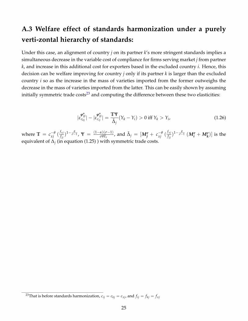
Under this case, an alignment of country j on its partner k’s more stringent standards implies asimultaneous decrease in the variable cost of compliance for firms serving market j from partnerk, and increase in this additional cost for exporters based in the excluded country i. Hence, thisdecision can be welfare improving for country j only if its partner k is larger than the excludedcountry i so as the increase in the mass of varieties imported from the former outweighs thedecrease in the mass of varieties imported from the latter. This can be easily shown by assuminginitially symmetric trade costs23 and computing the difference between these two elasticities:

|εϕ∗

jjckj | − |ε

ϕ∗jj

cij | =TΨ∆j

(Yk −Yi) > 0 iff Yk > Yi, (1.26)

where T = c−θxj (

fxjf jj)1− θ

σ−1 , Ψ = (1−α)(σ−1)σθFe

, and ∆j = [Mej + c−θ

xj (fxjf jj)1− θ

σ−1 (Mei + Me

k)] is theequivalent of ∆j (in equation (1.25) ) with symmetric trade costs.

23That is before standards harmonization, cij = ckj = cxj, and fij = fkj = fxj

25

Chapter 2

Structural Gravity under Size Asymmetryand Non-Homotheticity

2.1 Introduction

The Constant Elasticity of Substitution (CES) model of monopolistic competition has long been asolid foundation for seminal contributions in international trade theory (Krugman, 1980; Melitz,2003; Anderson and Van Wincoop, 2003; Chaney, 2008). Yet it is fair to say that this model suf-fers from two major drawbacks. First, it imposes a constant demand elasticity, which mainlyprecludes pro-competitive reduction in domestic markups to occur upon trade liberalization.Second, such rigidity in preferences, not only, constrains per-capita income and population sizeto have an identical effect on trade margins, but also, restricts the sensitivity of trade margins totrade costs to be constant in a gravity context (Chaney, 2008).

In recent trade models incorporating asymmetry both in income and size at the country-level,firm heterogeneity in productivity levels and non-CES preferences (Arkolakis et al., 2018; Fally,2019), the standard homothetic CES assumption has been mainly relaxed to allow for variablemarkups at the firm-level, so as to restore a theoretical role for the “pro-competitive effect oftrade". In spite of deriving a gravity equation under flexible preferences and country-level asym-metry, these recent papers remain silent on the potential implications of these more realistic as-sumptions for income and size effects on trade margins, and on whether it may give rise to avariable elasticity of trade margins to trade costs across countries.

In contrast, this is what the current chapter mainly focuses on. Does the fact that per-capitaincome affects significantly price elasticities, as documented in recent micro-level studies, seee.g. (Simonovska, 2015; Faber and Fally, 2017; Handbury, 2019), imply stronger income effect ontrade margins, and on their sensitivity to trade costs? Does the structure of welfare gains fromunilateral trade liberalization depend on whether the trading partner is relatively large or small?

26

These are the two main questions that I address in the current chapter. I do so in the con-text of a new class of gravity models featuring monopolistic competition, firm-level heterogene-ity, country-level asymmetry, unbounded Pareto distribution, indirectly-separable preferences,while taking the presence of variable and fixed trade barriers in due account.

Importantly, the family of preferences considered in this chapter offers a subtle nesting of theCES case as a homothetic benchmark, and a prominent non-homthetic alternative exhibiting anincome-decreasing price elasticity. This latter allows then for a more realistic modeling of con-sumer behavior, whereby richer consumers are less price sensitive. Thus, by combining cross-country differences in income levels with such added flexibility in preferences, I can properlyexamine the following questions: does the dampening effect of per-capita income on the priceelasticity induce a stronger income effect on trade margins in general equilibrium? does it implythat higher income level dampens the sensitivity of trade margins to trade costs?

The benefit of focusing on unbounded Pareto is twofold. First, it makes it possible to derivea gravity equation and gives rise to constant trade elasticity. This restricts then the theoreticalfocus on trade margins and allows for a solid empirical examination of the above questions. Sec-ond, this supply side restriction also gives rise to a constant uni-variate distribution of markups.Hence, in the welfare analysis, the focus is squarely on gains from selection as in Melitz (2003),and variety gains as in Krugman (1980).

The contribution of this chapter is threefold. First, I show, both theoretically and empirically,that the intensive margin of trade increases only with per-capita income in general equilibrium,and that per-capita income dampens the sensitivity of trade margins to trade costs. Second, Ihighlight two new welfare channels: an additional selection effect occurring on the export mar-ket, and an increase in nominal wage in the liberalizing country. Third, the contribution of thecurrent chapter to the gravity literature is a fully structural gravity equation that exhibits bothinward and outward multilateral resistances, and additionally exhibits a variable elasticity ofaggregate trade flows to fixed trade barriers under non-homothetic preferences. Finally, aim-ing at obtaining general results without losing in tractability, the current chapter proposes anew method that I call "the Exponent Elasticity Method" (EEM). This simple method deliverstractable solutions in general equilibrium despite added flexibility in preferences.

The findings of the current chapter are related to a large number of theoretical and empiricalpapers in the international trade literature. Many authors examined income and size effects onbilateral trade flows under non-homothetic preferences. By introducing non-homotheticity ina Ricardian framework, Fieler (2011) finds that bilateral trade increases significantly with per-

27

capita income, whereas it remains unaffected by population size. Markusen (2013) derives anidentical prediction in a Heckscher Ohlin framework. A more recent work by Bertoletti, Etro,and Simonovska (2018) have addressed this question under monopolistic competition with het-erogeneous firms. They find that the extensive margin of trade (number of exporters) increasesonly with destination’s per-capita income. Despite apparent similarity to these previous conclu-sions, here the key novelty is in the increased granularity of the analysis. In deed, I emphasizethat the significant impact of per-capita on aggregate trade flows is mainly driven by its strongimpact on the intensive margin of trade. I also show that per-capita income affects not only trademargins, but also determines the degree of their sensitivity to trade barriers, which is a novel re-sult in this strand of the literature.

A large body of work has examined the welfare gains from trade under various classes of pref-erences; see e.g (Melitz, 2003; Melitz and Ottaviano, 2008; Melitz and Redding, 2015; Arkolakiset al., 2018; Feenstra, 2018; Fally, 2019). Modeling approaches and conclusions vary, but a com-mon feature of the aforementioned papers is their overwhelming focus on gains from tougherselection on the domestic market, due to Melitz (2003). In contrast, the current chapter showsthat this selection effect is not always operative. It occurs only if the trading partner is largeenough compared to the World economy. Additionally, under this case, I highlight two newsources of gains from trade: a selection effect occurring on the export market, and increase innominal wage in the liberalizing country.

Another related paper in the literature is by Melitz and Ottaviano (2008) who derive a structuralgravity equation where the toughness of competition in the destination is jointly determinedby its market size and a measure of market access and comparative advantage. Instead, in thischapter, the effects of per-capita income, population size and market access on trade margins arestudied separately. In particular, the toughness of competition in the importing country and theexporter’s ease of market access are solely captured by their respective multilateral resistanceterms as in Anderson and Van Wincoop (2003). In this sense, the gravity equation I derive canbe considered as an augmented version of this of Chaney (2008) in two respects. First, its struc-tural aspect is reinforced as it exhibits both inward and outward multilateral resistances as inAnderson and Van Wincoop (2003). Second, it yields an income-decreasing elasticity of bilateraltrade flows with respect to fixed trade barriers, when preferences are non-homothetic.

The rest of this chapter is organized as follows. In Section 2, I spell out the model and derivenovel theoretical predictions both under non-homotheticity and market size asymmetry.Section 3 presents the empirical analysis and tests the validity of the novel results obtainedunder non-homotheticity. Section 4 concludes. Empirical results are provided in Appendix B.Appendix C provides the proofs for the main theoretical results, and explains the "EEM" method.

28

2.2 Theoretical Framework

2.2.1 Set up of the model

Consumer preferences.– I assume that consumer preferences are indirectly additive:

V =∫

ω∈Ωv(

pω

w) dω, with v′(

pω

w) < 0 and v′′(

pω

w) > 0 (2.1)

As stressed by Bertoletti and Etro (2016), a key property of this family of preferences is that theprice elasticity of demand corresponds to the elasticity of the marginal sub-utility and is thus

given by σ( pw ) = −

v′′( pw )

pw

v′( pw )

> 1. This implies that preferences are always non-homothetic, except

under the CES case where the price elasticity of demand ceases to vary with the price-incomeratio.

In order to shed light on the sensitivity of the theoretical predictions of the model to the natureof preferences (non-homothetic vs CES) and to test their empirical validity, I cover two possiblecases. A general and realistic non-homothetic case where σ( p

w ) is increasing in the price-incomeratio ( p

w ),1 opposed to the rigid CES case where σ is exogenous. Following Mrázová and Neary

(2017), I use the elasticity of the second derivative of the sub-utility function ς( pw ) = − v′′′( p

w )pw

v′′( pw )

as a unit-free measure of demand convexity and I a specify a subtle condition for both cases tobe nested:2

σ′(pw) =

> 0, if ς( pw ) < 1 + σ( p

w ) (non− homothetic)

= 0, if ς( pw ) = 1 + σ( p

w ) (homothetic : CES)(2.2)

Asymmetric countries.– Consider a World economy composed of N asymmetric countries thatdiffer both in size and income levels. Let country i be populated by Li identical agents, eachsupplying a unit of efficient labor. As each economy involves only one sector producing a differ-entiated good k, nominal wage wi is endogenous and corresponds to both per-capita income and

1Notice that only this alternative case is considered since the other theoretically possible alternative: (σ increas-ing in income) does not seem to be plausible and requires additional conditions to guarantee weak convexity andavoid thus issues related to the existence of the equilibrium.

2Mrázová and Neary (2017) propose the elasticity of the slope of direct demand as a sufficient measure of de-mand convexity. Here, I simply apply this general definition to the case of indirectly-additive preferences.

29

individual expenditure on horizontally differentiated varieties of good k. I solve for the nominalwage in general equilibrium upon closing the model using the trade balance condition.3

Identical Technology and Costly Trade.– In all countries, firm productivity ϕ is Pareto distributedover [1,+∞[ with shape parameter θ: G(ϕ0 < ϕ) = 1 - ϕ−θ.4 Any ϕ-productivity firm based incountry i and aiming to serve country j must pay a fixed cost wi fij (where fij is measured inefficiency labor units) and a variable trade cost that takes the form of an iceberg transport costτij > 1. Domestic trade involves only an overhead production cost fii, τii = 1.

Individual demand and optimal pricing rule.– Using the Roy identity (x = − ∂V∂p / ∂V

∂w ), the individualdemand a ϕ-productivity exporter from country i captures on destination j can be derived asfollows:

xij(ϕ) =|v′( pij(ϕ)

wj)|

|ηj|(2.3)

where |ηj| is the price aggregator in country j reflecting the toughness of competition on thismarket through the number of domestic and foreign firms competing on its market, as well astheir average degree of price competitiveness, as shown below:

|ηj| = |N

∑i=1

Mei

∫ +∞

ϕ∗ij

pij(ϕ)

wjv′(

pij(ϕ)

wj)dG(ϕ)| (2.4)

where Mei is the endogenous mass of entrants in origin i and pij(ϕ) is the profit-maximizing

export price charged by a ϕ-productivity exporter from origin i to consumers in destination j:

pij(ϕ) =

wiτij

ϕ mij(ϕ) preferences: non-homotheticwiτij

ϕ mij(ϕ) preferences: homothetic CES3I purposely abstract from including an outside sector pinning down wages so that general equilibrium effect

on wages is not ruled out. Moreover, this ensures the absence of the Home market effect (HME) and thus simplifiesthe welfare analysis.

4Notice that under the general non-homothetic case, σ( pw ) is increasing in price and thus firm-specific since firms

are heterogeneous. As the cutoff exporter (serving destination j from origin i) is the least productive and charges the

highest price, he faces relatively more elastic demand (than an average productivity exporter): σ∗ij(p∗ijwj) > σij(

pijwj). It

is then sufficient to assume that θ - (σ∗ij − 1) ∈]0, 1[ ∀i, j to ensure that productivity distribution of firms has a finitemean. However, under the CES, only this standard assumption: θ > (σ− 1) is needed as σ is identical across firms.

30

where mij(ϕ) is the markup set by a ϕ-productivity exporter from origin i while serving marketj, and is given by:

mij(ϕ) =

σ(

pijwj

)

σ(pijwj

)−1preferences: non-homothetic

σσ−1 preferences: homothetic CES

Incomplete pass-through and destination-specific pricing .– The above expression of the pricing ruleon the export market clearly indicates that the export price has four determinants: (i) nominalwage in the origin country wi; (ii) the variable trade cost τij; (iii) nominal wage in the destinationwj; and (iv) the exporter’s productivity level ϕ. Following the same order, let ρ1, ρ2, ρ3, and ρ4

respectively denote the elasticity of the export price with respect to each of its determinants:

ρ1 =dlog pij(ϕ)

dlog wi, ρ2 =

dlog pij(ϕ)

dlog τij, ρ3 =

dlog pij(ϕ)

dlog wj, and ρ4 =

dlog pij(ϕ)

dlog ϕ

Inspection of the export pricing rule clearly shows that nominal wage in the origin country wi,the variable trade cost τij, and the productivity level of the exporting firm ϕ enter the expressionof the marginal cost in a multiplicative way. It follows then that ρ1 = ρ2 = |ρ4|. Clearly, thesethree parameters capture the degree of completeness of the relative cost-price pass-through, andtheir value hinges on the nature of preferences:

ρ1 = ρ2 = |ρ4| =

1 + [

dlog mij(ϕ)

dlog σij(ϕ)︸ ︷︷ ︸<0

dlog σij(ϕ)

dlog pij(ϕ)︸ ︷︷ ︸>0

] < 1 preferences: non-homothetic

1 since σ ⊥ pij preferences: homothetic CES

31

Under the homothetic CES case, the demand elasticity is exogenous, this implies a constantmarkup, and thus a complete pass-through: ρ1 = ρ2 = |ρ4| = 1. However, beyond the CES case,the demand elasticity increases with the price level, and thus decreases with firm productivity.This implies that more productive firms face lower demand and so, set higher markups and onlypartially pass-on their cost advantage to consumers. Hence, beyond the CES case, the relativepass-through is incomplete: ρ1 = ρ2 = |ρ4| < 1.

Similarly, as the non-homothetic alternative allows the demand elasticity to decrease with per-capita income, it is then readily verified that the export price increases with the income level ofthe destination only under this case:

ρ3 =

[dlog mij(ϕ)

dlog σij(ϕ)︸ ︷︷ ︸<0

dlog σij(ϕ)

dlog wj︸ ︷︷ ︸<0

] > 0 preferences: non-homothetic

0 since σ ⊥ wj preferences: homothetic CES

Three key properties of indirectly-additive preferences are worth emphasizing. First, it allowsfor a subtle nesting of the homothetic CES case and a non-homothetic alternative using a uniquecondition that is pinned down by the relationship between the elasticity and convexity of directdemand, the so-called “demand manifold" by Mrázová and Neary (2017). Second, under thenon-homothetic case, the price elasticity of demand is allowed to increase with prices and de-crease with per-capita income. Combined with heterogeneity at the firm-level and asymmetryat the country level, this added flexibility allows then for a more realistic modeling of consumerand firm behavior. That is, on any market, more productive firms set higher markups, as doc-umented by De Loecker and Warzynski (2012), and at the world level, consumers in richestcountries are the least price sensitive. Third, this class of preferences allows for added flexibilityin both price and income effects while retaining the property that prices are summarized by aunique price aggregator, which is very convenient under monopolistic competition.

It is also worth noting that indirectly-separable preferences can be seen as an exception in thisregard. For instance, all alternative classes of preferences have properties that are too restrictivein terms of income and price effects. Under directly-separable preferences, as in Arkolakis et al.(2018), the price elasticity varies across goods, yet the income effect remains very implicit.Melitz and Ottaviano (2008) work with quasi-linear preferences, which generates a price-increasingdemand elasticity, but suppresses income effects. Comin, Lashkari, and Mestieri (2015) obtainflexible income effects using Non-homothetic CES preferences. Yet, this latter restricts price elas-ticities to be identical across goods.

32

Theoretically, it may yield more flexible price effects but at the price of more complexity, sincethis requires two price aggregators to fully characterize the demand system Fally (2018). TheQMOR preferences used by Feenstra (2018), and the case of implicitly-additive preferences con-sidered by Arkolakis et al. (2018) in a heterogeneous firms setting offer two examples of thiscomplex case.

Equilibrium conditions .– Now let us recall that the mass of entrants Mei in any origin i is endoge-

nous. Using the Free Entry (FE) and the Labor Market Clearing (LMC) conditions, I solve for itas follows :

The Free Entry condition states that in any country (say, i), average expected profits by entrant,conditional on successful entry, must equate the sunk cost of entry, and is given by :

P(ϕ ≥ ϕ∗ii) [∫ +∞

ϕ∗ii

πii(ϕ)g(ϕ)

P(ϕ ≥ ϕ∗ii)dϕ +

(N−1)

∑j=1

Pij

∫ +∞

ϕ∗ij

πij(ϕ)g(ϕ)

P(ϕ ≥ ϕ∗ij)dϕ ] = wiFe

(2.5)

where Pij =P(ϕ≥ϕ∗ij)

P(ϕ≥ϕ∗ii)is the probability of exporting from country i to country j as in Melitz,

2003. Domestic profits and revenues are, respectively, given by πii(ϕ) = rii(ϕ)σii(wi) − wi fii, with

rii(ϕ) = pii(ϕ)xii(ϕ)Li, ∀ϕ ≥ ϕ∗ii. Likewise, export profits and revenues can be written as

πij(ϕ) =rij(ϕ)

σij(wj) − wi fij, rij(ϕ) = pij(ϕ)xij(ϕ)Lj ∀ϕ ≥ ϕ∗ij, using the pricing rule pij(ϕ) and

the individual demand xij(ϕ) described in equation (2.3).5

Using the Lerner index and rearranging, the free entry condition boils down to :

Ri = σvi (w) [ wiFe + P(ϕ ≥ ϕ∗ii) wi fii +

(N−1)

∑j=1

P(ϕ ≥ ϕ∗ij) wi fij ] (2.6)

where Ri=∫ +∞

ϕ∗iirii(ϕ)g(ϕ)dϕ + ∑

(N−1)j=1

∫ +∞ϕ∗ij

rij(ϕ)g(ϕ)dϕ stands for the expected average rev-

enues of successful entrants in country i, and σvi (w) = ∑N

j=1(wjLjYv

)σij(wj) is the weighted average

5The expression of the operating profit πoii(ϕ) = rii(ϕ)

σii(wi) is obtained using the Lerner index: pii(ϕ)−(wi/ϕ)pii(ϕ)

= 1σii(wi) .

Importantly, notice that I always assume non-homotheticity and consider the CES as a homothetic exception. Asa result, the price elasticity of demand faced by ϕ-productivity exporter from origin i on market j is expressed asa function of nominal wage in the destination wj, not only for expositional simplicity, but also to put an emphasison its destination specific aspect. The firm (ϕ)/origin(wi) and dyad(τij)- specific aspects of σ are recalled and putin use only when needed. The same choice of terminology applies to domestic firms facing σii(wi) on the domesticmarket.

33

price elasticity of demand that a firm from origin i expects to face while serving the world mar-ket.

Notice that σij(wj) =∫ +∞

ϕ∗ijσij(

pij(ϕ)wj

)g(ϕ)dϕ is the expected price elasticity of demand to be faced

by an average productivity exporter serving destination j from origin i. It is also worth mention-ing that Yv = ∑N

j=1 wjLj = wLv is the World GDP, with w is the average per-capita income at theWorld level and Lv = ∑N

j=1 Lj is the World population.

The Labor Market Clearing condition (LMC) requires that total labor demand by entrants equatesa country’s labor endowment. While all entering firms (both successful and unsuccessful) incurthe sunk entry cost Fe, only successful entrants use labor to start producing. In particular, la-bor demand by a ϕ-productivity successful entrant in any country (say, i), ld(ϕ) depends on itsexport status:

∀ϕ ≥ ϕ∗ii, ld(ϕ) = [(qii(ϕ) ∗ ϕ−1) + fii] +(N−1)

∑j=1

[(qij(ϕ) ∗ τij ϕ−1) + fij]Xij (2.7)

where Xij is a dummy, equal to 1 if ϕ ≥ ϕ∗ij, and 0 otherwise. qii(ϕ) = xii(ϕ)Li is the marketdemand captured by ϕ-productivity firm on the domestic market. Likewise, qij(ϕ) = xij(ϕ)Lj isthe market demand a ϕ-productivity exporter reaps on destination j. Using the optimal pricingrule, the labor demand per successful entrant can be rewritten as follows:

ld(ϕ) = [w−1i (

σii(wi)− 1σii(wi)

)rii(ϕ) + fii] +(N−1)

∑j=1

[w−1i (

σij(wj)− 1σij(wj)

)rij(ϕ) + fij]Xij

(2.8)

Using firm labor demand from the above equation, the labor market clearing condition can besimplified and written as :

Li = Mei [ (Fe + P(ϕ ≥ ϕ∗ii) fii +

(N−1)

∑j=1

P(ϕ ≥ ϕ∗ij) fij) + w−1i µ(σv

i )Ri ] (2.9)

where µ(σvi ) = σv

i (w)−1σv

i (w)is the inverse of the markup that a successful entrant in country i would

charge while serving the World market.6

6Notice that µ boils down to (σ− 1/σ) under the CES since σ is exogenous.

34

By plugging the expected average revenues of successful entrants in i from the free entry condi-tion in equation (2.6) into the labor market condition in equation (2.9) and rearranging, I solvefor the equilibrium mass of entrants in origin i as follows:

Mei =

wiLi

σvi (w)Ψi

(2.10)

As assumed by Chaney (2008), the equilibrium mass of entrants is proportional to market size.Clearly, Me

i also decreases proportionally with the average level of price sensitivity at the World

level σvi (w), and importantly with Ψi = [ wiFe + P(ϕ ≥ ϕ∗ii) wi fii + ∑

(N−1)j=1 P(ϕ ≥ ϕ∗ij) wi fij]

which reflects the degree of remoteness of origin i from all potential destination markets in theWorld economy.

Solving for the general equilibrium.– In order to gain in generality without losing in tractability, Ipropose a new method that I call "the Exponent Elasticity Method" (EEM, hereafter). The objec-tive of this simple method is to deliver tractable solutions in general equilibrium despite addedflexibility in preferences. The starting point is the partial equilibrium expression of the priceaggregator initially provided in equation (2.4). Using the above expression of the equilibriummass of entrants, the partial equilibrium price aggregator can be rewritten as:

|ηj| = (wjLj)(wjLj

Yv)−1

N

∑i=1

cEi (

wiLi

Yv) f−1

ij

∫ +∞

ϕ∗ij

pij(ϕ)

wj|v′(

pij(ϕ)

wj)|dG(ϕ)︸ ︷︷ ︸

I

(2.11)

where cEi = [ σv

i (w) wi (αe + αii P(ϕ ≥ ϕ∗ii) + P(ϕ ≥ ϕ∗ij) + ∑(N−2)j=1 αik P(ϕ ≥ ϕ∗ij) ) ]

−1 is a proxy

for entry conditions in country i, αe =Fefij

, αii =fiifij

, and αik =fikfij

.

Clearly, the mathematical challenge here is how to solve for the above integral (I) without speci-fying a functional form of the sub-utility function. As is well known, this latter should exhibit aconstant demand elasticity, which can be used then as a constant for integrating. Such simplicityis only possible under CES demand, which is the unique case where it is possible to solve forthis integral. As the flexible family of preferences considered in this chapter encompasses theCES and a non-homothetic alternative allowing the demand elasticity to vary with prices andincome levels, it is then impossible to solve for the above integral under such added flexibilityin preferences.

35

Given the impossibility to solve for the integral in the current setting, the key idea that theEEM method proposes is to locally approximate the integral (I) around the equilibrium with amultiplicative equivalent which has a finite number of determinants, such as the exponent of

each determinant embodies the elasticity of [pij(ϕ)

wj|v′( pij(ϕ)

wj)| ] with respect to it. This requires a

multi-step procedure that I expose in detail in a supplementary Appendix. With the aid of thissimple method, I obtain a tractable solution for the price aggregator in general equilibrium:

|ηj| ≡ w(

1+εF3

1−εF7)

j L(

1+εF3

1−εF7)

j (wjLj

Yw)

1(εF

7−1) Ψ1

(εF7−1)

j (2.12)

where Ψj = [∑Ni=1(

wi LiYw

) f (εF5−1)

ij τεF

2ij wεF

1i ]−1 is a reminiscent of the inward multilateral resistance

term in Anderson and Van Wincoop (2003), and the explicit expressions of the above exponentsare given by:

εF1 = ρ1(1− σij(wj)) + [ [|ρ4|(σij(wj)− 1)− θ]

[1−ρ∗1(1−σ∗ij(wj))]

|ρ∗4 |(σ∗ij(wj)−1) ] < 0

εF2 = ρ2( 1− σij(wj) ) + [ |ρ4|(σij(wj)− 1)− θ ] = −θ < 0

εF3 = (1− ρ3)( σij(wj)− 1 ) + [ [ θ − |ρ4|(σij(wj)− 1) ]

[(1−ρ∗3)(σ∗ij(wj)−1)+1+δ∗]

|ρ∗4 |(σ∗ij(wj)−1) ] > 1

εF5 = − [ θ−|ρ4|(σij(wj)−1) ]

|ρ∗4 |(σ∗ij(wj)−1) < 0

εF7 = − [ θ−|ρ4|(σij(wj)−1) ]

|ρ∗4 |(σ∗ij(wj)−1) < 0

(2.13)

The multilateral resistance term Ψj can be interpreted as a remoteness index since it reflects howfar is destination j from the rest of the world. Importantly, given the negative sign of εF

7 , |ηj| isstrictly decreasing in Ψj. This implies that the more remote is a destination, the fewer are thefirms serving it and thus the more relaxed is competition on its market.7

Last, but not least, it worth noting that the "EEM" method delivers a unique solution for thegeneral equilibrium price aggregator since it rests on a local approximation around a uniquetrade equilibrium. Nevertheless, such local approximation allows only to study the impact ofsmall deviations from the equilibrium. Accordingly, I only examine the general equilibriumeffects of small changes in per-capita income and in the variable trade cost in the next sections.

7Regardless of the nature of preferences, a straightforward implication of Pareto distribution is that a change inthe variable trade cost affects only the extensive margin, while the intensive margin remains silent. As a result, thetoughness of competition is characterized solely with the number of competing firms, while the average price levelis not taken into account.

36

2.2.2 Income vs Size effects on trade margins in general equilibrium

The intensive margin of trade

Using the general expression of firm-level export revenues, and this of the general equilibriumprice aggregator from equation (2.12) and rearranging, I can solve for the intensive margin ingeneral equilibrium as follows:

rij(ϕ) ≡ wε1i τε2

ij ϕε4 wζ−1j (

wjLj

Yw)

1(1−εF

7 ) Ψ1

(1−εF7 )

j︸ ︷︷ ︸Chaney(2008)

(2.14)

The exponents (ε1, ε2, ε4) respectively capture the elasticity of firm-level export revenues withrespect to nominal wage in the origin country wi, the variable trade cost τij, and firm productiv-ity ϕ. Their expressions are respectively given by:ε1 = ρ1 ( 1− σij(wj) ) ; ε2 = ρ2 ( 1− σij(wj) ) ; ε4 = |ρ4| ( σij(wj)− 1 ).

While the expressions of these elasticities are quite standard, here the novel element is ζ whichcaptures the gross positive income effect on firm-level export revenues in general equilibrium,

and given by ζ = 1 + [ (1 + ε3) − (1+εF

31−εF

7) ], with ε3 = (1 − ρ3)( σij(wj) − 1 ).8 Inspection of its

expression immediately reveals that it boils down to 1 when preferences are CES. Hence, un-der the CES case, per-capita income wj and population size Lj affect the intensive margin onlythrough the RMS channel, exactly as in Chaney (2008). By contrast, under the non-homotheticalternative, ζ exceeds unity, allowing then per-capita income to have a stronger impact on theintensive margin in general equilibrium, as explained below.

It is also easy to notice that the remoteness of the destination Ψj and its relative market size,

(RMS, hereafter), (wjLjYw

) both affect positively the intensive margin and with the same magni-tude. These two channels have already been highlighted in Chaney (2008). The focus here ison the different channels through which income and size affect separately the intensive margin.This is a theoretically clean way to highlight the novel implications of non-homotheticity, andthus compare the results with the Chaney (2008) benchmark.

Size effect.– The general equilibrium expression of the intensive margin in (2.14) clearly indicatesthat the RMS is the unique channel through which population size (Lj) can affect firm-level ex-port revenues. For instance, it is readily verified that a population size enlargement implies

8To avoid confusion, "income" refers to per-capita income (wj), "size" to population size (Lj) and "market size"to their scalar (wjLj).

37

larger market demand- a proportional increase in the number of consumers-, but also, toughercompetition - a proportional increase in the mass of domestic competitors.9 Given their identicalmagnitude, these two opposite effects always cancel out under indirectly-separable preferences.

Income effect.– Contrary to population size, the magnitude of the income effect and the channelsthrough which it affects the intensive margin crucially depend on the nature of preferences:10

ζ =

> 1 if preferences are non-homothetic

1 otherwise(2.15)

When preferences are CES, σ is exogenous and demand is iso-elastic, the gross positive incomeeffect boils down to a proportional increase in individual demand (ζ equates unity, as indicatedabove). This positive impact on individual demand is then ruled out by a proportional increasein the mass of domestic competitors. Put differently, as the homothetic aspect of the CES impliesthat consumer preferences are unaffected by per-capita income, this latter acts only as a sizeparameter. Hence, under the CES case, the Chaney (2008) result is replicated, the RMS standsthen as the unique channel through which income and size would have a positive and identicalimpact on the intensive margin.

By contrast, when preferences are non-homothetic, the price elasticity of demand is decreasingin income (σ′j (wj) < 0), any ϕ-productivity exporter charges then a higher markup to richerdestinations where consumers are less price sensitive. In spite of charging higher prices, the ex-porting firm reaps larger individual demand for two reasons. First, as the export price increasesless than proportionally with the destination’s income level (ρ3 < 1, ∀ϕ), the exported varietyprovides the consumer with a higher level of marginal sub-utility. This, in turn, increases indi-vidual demand for this variety. Second, and importantly, these two partial equilibrium effects(higher price and larger individual demand) prevail in general equilibrium as they dominatethe total income effect on export revenues of all other active exporters (intensive) as well asinfra-marginal ones (extensive).11 Therefore, the gross positive income effect is more than pro-portional (ζ > 1) and dominates thus the negative competition effect (-1), yielding thus a netpositive income effect:

ζn = ζ − 1

> 0 if preferences are non-homothetic

= 0 otherwise(2.16)

9Recall that the mass of domestic entrants is proportional to market size as indicated in equation (2.10).10See Appendix C.1 for a detailed proof.11See Appendix C.1 for a detailed decomposition of the income effect in general equilibrium.

38

The extensive margin of trade

Similarly, by recalling that the cutoff productivity exporter makes zero profits, and using theexpression of firm-level profits and the general equilibrium price aggregator from equation (12),I can solve for the extensive margin in general equilibrium as follows:12

ϕ∗ij ≡ w(

1−ε∗1ε∗4

)

i τij f1

ε∗4ij w∆5

j L∆6j (

wjLj

Yw)

1ε∗4 (ε

F7−1) Ψ

1ε∗4 (ε

F7−1)

j︸ ︷︷ ︸Chaney(2008)

(2.17)

where ∆5 = 1ε∗4

[ (1+εF

31−εF

7)− (ε∗3 + 1 + δ∗) ] and ∆6 = 1

ε∗4[ (

1+εF6

1−εF7)− 1 ], εF

6 =[ θ−|ρ4|(σij(wj)−1) ]|ρ∗4 |(σ∗ij(wj)−1) > 0

and δ∗= -dlog σ∗ij(wj)

dlog wj; ε∗1 = ρ∗1 ( 1 - σ∗ij(wj) ) ; ε∗3 = (1 - ρ∗3) ( σ∗ij(wj) - 1 ); ε∗4 = |ρ∗4 | ( σ∗ij(wj) - 1 ).

Equation (2.17) clearly indicates that while (1−ε∗1

ε∗4) and ( 1

ε∗4), respectively, correspond to the elas-

ticity of the extensive margin with respect the nominal wage in the origin country wi, and thefixed cost of exporting fij, here the two novel elements are ∆5, and ∆6. These latter respectivelycapture the direct income and size effects on the extensive margin in general equilibrium (ex-cluding their common indirect effect channeled through the RMS).

Inspection of their respective expressions immediately reveals that while ∆6 is always equal tozero regardless of whether preferences are CES or non-homothetic, the sign of ∆5 hinges on thenature of preferences. This has an important implication for the income and size effects on theextensive margin in general equilibrium, as explained below.

12See Appendix C.5 for a detailed explanation.

39

Size effect.– Regardless of the nature of preferences, it is readily verified that the unique channelthrough which population size Lj could affect the toughness of firm selection into exporting isthe RMS as highlighted in Chaney (2008). For instance, since εF

6 = |εF7 |, ∆6 collapses always to

zero whether preferences are CES or non-homothetic.

Income effect.– Contrary to population size, per-capita income can affect the extensive marginthrough an additional channel conditionally on non-homotheticity. Specifically, when prefer-ences are non-homothetic, the price elasticity of demand is increasing in price and decreasingin income, which implies that ∆5 < 0.13 A new "preference" channel arises then: an increase inper-capita income makes selection into exporting less tough as infra-marginal exporters face henceforth aless elastic demand (as consumers become less price sensitive once they get richer).

Nevertheless, under the CES case, σ is identical across firms, ∆5 collapses to zero and the new“preference" channel is ruled out. As a result, per-capita income and population size act againinterchangeably as size parameters. Their impact on the extensive margin is solely channeledthrough the RMS (∆5 = ∆6 = 0). The Chaney (2008) result is thus replicated.

∆5

< 0 if preferences are non-homothetic

= 0 otherwise(2.18)

2.2.3 Generalized Structural Gravity and Trade Elasticity

In this section, I derive a generalized structural gravity equation and I shed light on the extentto which the nature of preferences affects the sensitivity of trade flows to variations in tradebarriers. Bilateral exports from origin i to destination j are given by:

Xij = Mei

∫ +∞

ϕ∗ij

rij(ϕ)g(ϕ)dϕ (2.19)

Using individual demand from equation (2.3), the equilibrium mass of entrants in (2.10) andrearranging, bilateral exports can be rewritten as:

Xij = [σvi (w)]−1 wiLi

Ψi

wjLj

|ηj|

∫ +∞

ϕ∗ij

pij(ϕ)

wj|v′(

pij(ϕ)

wj)| g(ϕ)dϕ,︸ ︷︷ ︸

I

(2.20)

13See Appendix C.2 for a detailed proof.

40

where σvi (w) is the average price elasticity of demand at the World level and Ψi measures the

degree of remoteness of origin i from all potential destination markets in the World economy.14

Notably, a straightforward implication of the free entry condition is that it allows the averagedegree of price sensitivity at the world level σv

i (w) and remoteness from destination markets Ψi

to have a deterrent impact on entry in any origin i.

As mentioned in the previous section, the integral (I) is approximated with the aid of the "EEM"method. This latter delivers a tractable solution for the price aggregator in general equilibrium inequation (2.12). By plugging this general equilibrium expression in the bilateral trade equationabove, I derive the following Structural Gravity Equation:

Xij = κ6 [σvi (w)]−1 YiYj

Yv

Ψj

ΨiwεF

1i τ

εF2

ij f εF5

ij , (2.21)

where εF1 = ρ1( 1− σij(wj) ) + [ [ |ρ4|(σij(wj)− 1)− θ ]

[1−ρ∗1(1−σ∗ij(wj))]

|ρ∗4 |(σ∗ij(wj)−1) ] < 0,

εF2 = ρ2( 1− σij(wj) ) + [ |ρ4|(σij(wj)− 1)− θ ] = −θ < 0 and εF

5 = − [ θ−|ρ4|(σij(wj)−1) ]|ρ∗4 |(σ∗ij(wj)−1) < 0.

This structural gravity equation can be considered as an augmented version of Chaney (2008)’sgravity equation in three respects. First, its structural aspect is reinforced since it exhibits, notonly the inward multilateral resistance term (Ψj measures the easiness of penetrating destina-tion j), but also the outward multilateral resistance term (Ψi captures the toughness of exportingfrom origin i) as in Anderson and Van Wincoop (2003). These multilateral resistance terms haveopposite effects on bilateral trade and affect it through different margins. While the positiveimpact of the former Ψj occurs at both margins (extensive and intensive)15 as in Chaney (2008),the negative impact of the latter Ψi occurs only at the extensive margin.

This effect is absent in the Chaney (2008) model since the free entry condition is not imposed andcan be explained as follows: the more remote is an origin i from destination markets (mainly due to itsgeographical location which entails higher fixed costs of exporting: high fij ∀ j),16 the lower are expectedexport profits, the fewer are entrants and thus exporters.17

14Ψi = [wiFe + P(ϕ ≥ ϕ∗ii)wi fii + ∑(N−1)j=1 P(ϕ ≥ ϕ∗ij)wi fij], as indicated in equation (2.10)

15As competition is more relaxed in remote destinations, this, not only, offers easier entry conditions for prospec-tive exporters, but also, allows successful ones to reap large market shares. Hence, the remoteness of the destinationrespectively magnifies the extensive and intensive margins of trade.

16I focus only on geography and abstract from the cost of labor in the origin wi because it also corresponds toindividual expenditure on the differentiated good and thus has a positive impact on entry as well.

17For any given level of trade barriers and destination characteristics.

41

As in (Chaney, 2008; Melitz and Ottaviano, 2008; Arkolakis et al., 2018), regardless of the natureof preferences, unbounded Pareto distribution of firm productivity always gives rise to a con-stant trade elasticity (εF

2 = −θ). However, the second novelty here is that in spite of generating aconstant elasticity of aggregate trade flows to the variable trade cost, it allows per-capita incometo determine the degree of sensitivity of trade margins to variable trade cost variation whenpreferences are non-homothetic, as in (Mrázová and Neary, 2014; Carrère, Mrázová, and Neary,2020). In particular, using the definition of the elasticity of bilateral trade to the variable tradecost (εF

2 ), its absolute value can be decomposed into an (intensive: firm-level export revenues)and (extensive: Number of exporting firms) component capturing the elasticity of each marginto the variable trade cost:

|εXijτij | = |ε

F2 | = ρ2( σij(wj)− 1 )︸ ︷︷ ︸

ι:intensive

+ [ θ − |ρ4|(σij(wj)− 1) ]︸ ︷︷ ︸χ:extensive

= θ (2.22)

As highlighted by Chaney (2008), σ magnifies the sensitivity of the intensive margin, whereasit dampens the sensitivity of the extensive margin to a small change in the variable trade cost.As non-homotheticity implies that the price elasticity of demand is decreasing in income, a newtheoretical prediction arises: When preferences are indirectly additive and non-homothetic, higher per-capita income affects the sensitivity of trade margins to a small variation in the variable trade cost in twoopposite ways: it dampens the sensitivity of the intensive margin, whereas it magnifies the sensitivity ofthe extensive margin.

Third, another novelty of this structural gravity equation is that it allows for the fixed trade costelasticity of bilateral trade flows to be either constant or variable depending on the nature ofpreferences. In contrast to the CES case where this elasticity is constant as in Chaney (2008), non-homotheticity breaks this constant link, yielding an income-decreasing fixed trade cost elasticityof bilateral trade. Using the expression of (εF

5 ), the absolute value of the elasticity of aggregatetrade flows with respect to the fixed trade cost can be decomposed as follows:

|εXijfij| = |εF

5 | = 0︸︷︷︸ι:intensive

+[ θ − |ρ4|(σij(wj)− 1) ]|ρ∗4|(σ∗ij(wj)− 1)︸ ︷︷ ︸

χ:extensive

=

θ

σ−1 − 1 (CES)θ

|ρ∗4 |(σ∗ij(wj)−1) − υ (non-homothetic)

(2.23)

where υ =|ρ4|(σij(wj)−1)|ρ∗4 |(σ∗ij(wj)−1) < 1 is orthogonal to destination’s per-capita income wj as the effects of

income on both elasticities cancel out.

42

Under non-homotheticity, the fixed trade cost elasticity of bilateral trade is decreasing in des-

tination’s per-capita income: d|εF5 |

dwj< 0. The underlying economics are simple: an increase in

destination’s per-capita income (w′j > wj) lowers the export cutoff (ϕ∗′ij < ϕ∗ij), which in turn

generates a more than proportional increase in the cutoff export price (p∗′ij > p∗ij)).

18 As the priceelasticity of demand is increasing in the price-income ratio, the “new" cutoff exporter faces thena more elastic demand (σ∗

′ij > σ∗ij), which in turn lowers the fixed trade cost elasticity of bilateral

trade ( |εF5 |′< |εF

5 | ). In deed, as rich destinations are the easiest to penetrate, the productivitylevel of infra-marginal exporters is the lowest, these latter capture then very small market sharesupon a reduction in the fixed trade cost. Therefore, rich destinations are the least elastic to avariation in fixed trade barriers as long as they are the least selective.

Last, but not least, it is worth mentioning that it is necessary to assume that the liberalizingcountry j is a small open economy. This additional assumption ensures that any variation in thevariable or fixed cost of importing in destination j (τij, fij ∀i) has no impact on entry conditionsin any source country i (σv

i (w), Ψi).19

2.2.4 Solving for nominal wages in general equilibrium

In this short section, I close the model by solving for the nominal wage in destination j, wj, usingthe trade balance condition (TB):

(TB)j :(N−1)

∑i=1

Xji︸ ︷︷ ︸j′s exports

=(N−1)

∑i=1

Xij︸ ︷︷ ︸j′s imports

(2.24)

By plugging bilateral trade flows from the structural gravity from equation (2.21) in the tradebalance condition above and rearranging, I solve for the relative wage in destination j as follows:

wj = (Ψj

ΨRow)

1(εF

1−1) Λ1

(εF1−1) , (2.25)

where ΨRow ≡ ∑(N−1)i=1,i 6=j(

LiLv)Ψi is the weighted average degree of remoteness of all destinations

in the World, excluding j and Λ is a general equilibrium object that is orthogonal to bilateraltariffs.20

18Due to a joint increase in the cutoff marginal cost and in markups when the destination gets richer.19 dσv

i (w)dτij

=dσv

i (dw)d fij

= dΨidτij

= dΨid fij

= 0.20See Appendix C.3 for a detailed derivation.

43

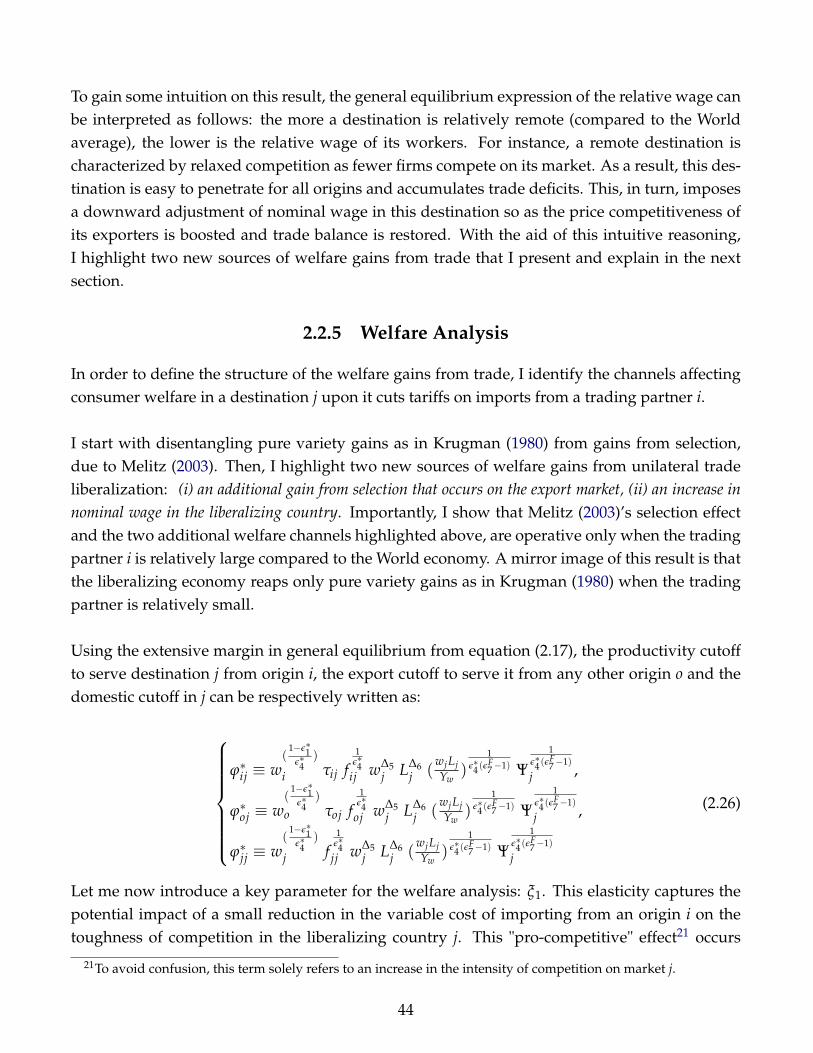
To gain some intuition on this result, the general equilibrium expression of the relative wage canbe interpreted as follows: the more a destination is relatively remote (compared to the Worldaverage), the lower is the relative wage of its workers. For instance, a remote destination ischaracterized by relaxed competition as fewer firms compete on its market. As a result, this des-tination is easy to penetrate for all origins and accumulates trade deficits. This, in turn, imposesa downward adjustment of nominal wage in this destination so as the price competitiveness ofits exporters is boosted and trade balance is restored. With the aid of this intuitive reasoning,I highlight two new sources of welfare gains from trade that I present and explain in the nextsection.

2.2.5 Welfare Analysis

In order to define the structure of the welfare gains from trade, I identify the channels affectingconsumer welfare in a destination j upon it cuts tariffs on imports from a trading partner i.

I start with disentangling pure variety gains as in Krugman (1980) from gains from selection,due to Melitz (2003). Then, I highlight two new sources of welfare gains from unilateral tradeliberalization: (i) an additional gain from selection that occurs on the export market, (ii) an increase innominal wage in the liberalizing country. Importantly, I show that Melitz (2003)’s selection effectand the two additional welfare channels highlighted above, are operative only when the tradingpartner i is relatively large compared to the World economy. A mirror image of this result is thatthe liberalizing economy reaps only pure variety gains as in Krugman (1980) when the tradingpartner is relatively small.

Using the extensive margin in general equilibrium from equation (2.17), the productivity cutoffto serve destination j from origin i, the export cutoff to serve it from any other origin o and thedomestic cutoff in j can be respectively written as:

ϕ∗ij ≡ w(

1−ε∗1ε∗4

)

i τij f1

ε∗4ij w∆5

j L∆6j (

wjLjYw

)1

ε∗4 (εF7−1) Ψ

1ε∗4 (ε

F7−1)

j ,

ϕ∗oj ≡ w(

1−ε∗1ε∗4

)

o τoj f1

ε∗4oj w∆5

j L∆6j (

wjLjYw

)1

ε∗4 (εF7−1) Ψ

1ε∗4 (ε

F7−1)

j ,

ϕ∗jj ≡ w(

1−ε∗1ε∗4

)

j f1

ε∗4jj w∆5

j L∆6j (

wjLjYw

)1

ε∗4 (εF7−1) Ψ

1ε∗4 (ε

F7−1)

j

(2.26)

Let me now introduce a key parameter for the welfare analysis: ξ1. This elasticity captures thepotential impact of a small reduction in the variable cost of importing from an origin i on thetoughness of competition in the liberalizing country j. This "pro-competitive" effect21 occurs

21To avoid confusion, this term solely refers to an increase in the intensity of competition on market j.

44

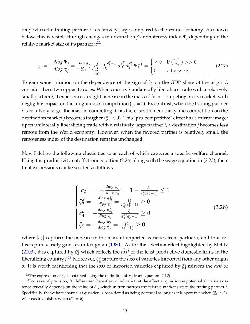
only when the trading partner i is relatively large compared to the World economy. As shownbelow, this is visible through changes in destination j’s remoteness index Ψj depending on therelative market size of its partner i:22

ξ1 = −dlog Ψj

dlog τij= (

wiLi

Yv) εF

2︸︷︷︸<0

f (εF5−1)

ij τεF

2ij wεF

1i Ψ−1

j =

< 0 if (wi LiYv

) >> 0+

0 otherwise(2.27)

To gain some intuition on the dependence of the sign of ξ1 on the GDP share of the origin i,consider these two opposite cases. When country j unilaterally liberalizes trade with a relativelysmall partner i, it experiences a slight increase in the mass of firms competing on its market, withnegligible impact on the toughness of competition (ξ1 = 0). By contrast, when the trading partneri is relatively large, the mass of competing firms increases tremendously and competition on thedestination market j becomes tougher (ξ1 < 0). This "pro-competitive" effect has a mirror image:upon unilaterally liberalizing trade with a relatively large partner i, a destination j becomes lessremote from the World economy. However, when the favored partner is relatively small, theremoteness index of the destination remains unchanged.

Now I define the following elasticities so as each of which captures a specific welfare channel.Using the productivity cutoffs from equation (2.26) along with the wage equation in (2.25), theirfinal expressions can be written as follows:

|ξ2| = | −dlog ϕ∗ijdlog τij

| = 1− ξ1ε∗4(ε

F7−1)≤ 1

ξd3 = −

dlog ϕ∗jjdlog τij

= ξ1ε∗4(ε

F7−1)≥ 0

ξo4 = −

dlog ϕ∗ojdlog τij

= ξ1ε∗4(ε

F7−1)≥ 0

ξ5 = −dlog wjdlog τij

= ξ1(εF

1−1)≥ 0

(2.28)

where |ξ2| captures the increase in the mass of imported varieties from partner i, and thus re-flects pure variety gains as in Krugman (1980). As for the selection effect highlighted by Melitz(2003), it is captured by ξd

3 which reflects the exit of the least productive domestic firms in theliberalizing country j.23 Moreover, ξo

4 capture the loss of varieties imported from any other origino. It is worth mentioning that the loss of imported varieties captured by ξo

4 mirrors the exit of

22The expression of ξ1 is obtained using the definition of Ψj from equation (2.12).23For sake of precision, "tilde" is used hereafter to indicate that the effect at question is potential since its exis-

tence crucially depends on the value of ξ1, which in turn mirrors the relative market size of the trading partner i.Specifically, the welfare channel at question is considered as being potential as long as it is operative when (ξ1 < 0),whereas it vanishes when (ξ1 = 0).

45

the least productive firms serving destination j from any origin o due to tougher selection on theexport market j, which leads to an ˜increase in average export productivity. This additional gainfrom selection (on the export market) represents a new welfare channel and is complementaryto the selection effect, due to Melitz (2003) which occurs on the domestic market.

Finally, ξ5 captures the impact of unilateral trade liberalization on the nominal wage in the lib-eralizing country wj. In particular, this effect is positive when the partner is relatively large (ξ1

< 0), and thus can be considered as another new source of welfare gains from trade. However,this new welfare channel vanishes when the trading partner is relatively small (ξ1 = 0), as it isthe case for the selection effects (both on the domestic and the export markets) mentioned above.

Now using the elasticities in (2.28), the different sources of welfare gains from trade can be cap-tured by the following summary statistic:

Γ = [ |ξ2| − ( ξd3 +

(N−2)

∑o=1,o 6=i,j

ξo4) ]︸ ︷︷ ︸

Θv :Net Variety E f f ect

+ [ ξd3 +

(N−2)

∑o=1,o 6=i,j

ξo4 ]︸ ︷︷ ︸

Θs :Melitz(domestic)+Additional selection(export)

+ ξ5︸︷︷︸impact on nominal wage

(2.29)

Importantly, in such a global equilibrium with asymmetric countries, it is insightful to stress thatthe relative size of the trading partner shapes the structure of welfare gains for the liberalizingcountry. For instance, it is readily verified from equation (2.27) that when its partner i is relativelysmall (ξ1 = 0), the liberalizing economy j reaps only pure variety gains as in Krugman (1980).By contrast, when partner i is relatively large (ξ1 < 0), the magnitude of the gross variety gain24

is reduced, the selection effect as in Melitz (2003) is operative, and two new sources of welfaregains arise: an additional selection effect on the export market and an increase in nominal wagein the liberalizing country. In order to shed more light on the mechanisms underlying these twodifferent structures of welfare gains, I proceed to a two-cases analysis as follows:

Case 1: the trading partner i is relatively small

Under this case, the liberalizing economy reaps only small gains from variety as in Krugman(1980) despite firm heterogeneity and the presence of fixed costs. The absence of the gains fromselection as in Melitz (2003) -along with the two new welfare channels mentioned above- is dueto the fact that the arrival of few newly imported varieties from partner i has a negligible impacton the intensity of competition on the destination market j (ξ1 = 0). As a result, neither the least

24It refers to the increase in the mass of imported varieties from country i.

46

productive domestic firms in country j, nor the least productive exporters serving this destina-tion from all other origins (∀o 6= i) are forced to exit the market.

It is worth mentioning that despite the rigidity of labor supply in this one sector model, firmexit can only be caused by tougher competition on the final good market since unilateral tradeliberalization by country j does not entail any positive demand shock on its domestic labor mar-ket. Melitz and Ottaviano (2008) studied the welfare implications of unilateral trade liberaliza-tion using a linear demand system exhibiting a choke price that is decreasing in the number ofcompeting firms. They find that, in the short run, the liberalizing economy gains always fromselection25 as in Melitz (2003) regardless of the size of the partner as an increase in the number ofcompeting firms translates mechanically into tougher competitive conditions for domestic firms.

Moreover, the authors show that the liberalizing economy experiences a welfare loss in the longrue due to changes in the patterns of entry (Home Market Effect). By contrast, as I depart froma different theoretical setting involving only one sector, many asymmetric countries, indirectlyadditive preferences and fixed costs, I obtain different results. In particular, in the current chap-ter, the toughness of competition on a given destination j is mainly captured by its remotenessindex26 Ψj which varies significantly only when the the trading partner is relatively large. As aresult, the selection effect 27 is not operative when the trading partner is relatively small and theliberalizing country reaps only pure variety gains in the short run.

As for the long run effects, in contrast to Melitz and Ottaviano (2008), the liberalizing economydoes not experience a welfare loss since the Home Market Effect is not operative in the absenceof a freely traded outside sector, as in Demidova and Rodriguez-Clare (2013). Finally, there isno significant28 variation in nominal wages in the liberalizing country j, this can be explainedas follows. Given the small relative size of partner i, the arrival of few newly imported varietiesfrom this country has a negligible impact on destination j’s remoteness index (ξ1 = 0). This im-plies that the degree of easiness of penetrating market j from any other origin (∀o 6= i) remainsunchanged. Hence, there is no variation in country j’s imports from all other sources. This, inturn, implies that there is no necessary adjustment of nominal wage in country j to restore tradebalance.

Therefore, the liberalizing country enjoys only pure variety gains as in Krugman (1980) de-spite firm heterogeneity. Using indirectly additive preferences, Bertoletti, Etro, and Simonovska

25It also enjoys net variety gains and a pro-competitive reduction in domestic markups.26Along with the mass of domestic competitors.27Both on the domestic market as in Melitz (2003) and on the export market (additional selection effect).28Notice that when the partner is relatively small, the impact of unilateral trade liberalization on the remoteness

index of the liberalizing country is negligible, which implies a negligible effect on nominal wages in this country.

47

(2018) find a similar result, yet the mechanism is different. Specifically, they abstract from fixedcosts and highlight only pure variety gains since the choke price is orthogonal to the mass ofcompeting firms under indirectly-additive preferences. Instead, I incorporate fixed costs in themodel and I show that despite their presence, the liberalizing economy gains only from varietysince the intensity of competition on its market remains unchanged when its partner is relativelysmall, and thus all other welfare channels are ruled out.

Case 2: the trading partner i is relatively large

Under this case, the arrival of a large number of newly imported varieties from partner i makescompetition tougher on the destination market j. This pro-competitive effect is mirrored by asignificant decrease in destination j’s remoteness index upon reducing the variable cost of im-porting from partner i (ξ1 < 0). Importantly, this increase in the intensity of competition in theliberalizing economy has three major consequences that shape the structure of its welfare gains.First, it forces the least productive domestic firms in country j to exit the market, gains fromselection as in Melitz (2003) are thus recovered.

Second, due to tougher competitive conditions on market j, the least productive exporters serv-ing this destination from all other origins (∀o 6= i) are also forced to exit this export market. Thisadditional selection effect occurring on the export market leads to an increase in average exportproductivity and can be then considered as a new source of welfare gain. Nevertheless, due tothese two waves of firm exit, the liberalizing economy j experiences a net variety loss for countryj. For instance, the less than proportional increase in the mass of varieties imported from partneri does not compensate the total variety loss implied by the exit of domestic firms and the leastproductive exporters from all other origins.29

Third, this variety loss reflects the fact that the liberalizing country j is importing less from allother sources (∀o 6= i) and accumulating trade surpluses. Hence, an upward adjustment of thenominal wage in country j is needed so that its exporters become less price competitive, exportless to all other countries, and thus trade balance is restored. This increase in the nominal wagein the liberalizing economy is the second new welfare channel highlighted in this chapter. Incontrast to Demidova and Rodriguez-Clare (2013), the impact of unilateral trade liberalizationon nominal wage in the liberalizing country is overturned. For instance, in their two-countrymodel, unilateral trade liberalization implies a downward adjustment of nominal wage in theliberalizing economy to boost the price competitiveness of its exporters so that they export moreand trade balance is restored.

29In spite of being relatively large, partner i’s GDP share can not exceed 12 .

48

Moreover, the authors emphasized that despite the decrease in nominal wage it entails, uni-lateral trade liberalization is welfare improving since the selection effect and the decrease inaverage price it implies dominate the negative impact on nominal wage. By contrast, I find thatnominal wage and the domestic cutoff vary in the same direction: they both increase upon uni-laterally liberalizing trade with a relatively large partner. Seen this way, the increase in nominalwage arises as an additional source of welfare gains. Importantly, it is complementary to Melitz(2003)’s selection effect on the domestic market along with the new selection effect on the exportmarket, and the sum of these gains outweighs the previously mentioned net variety loss. Finally,the structure of welfare gains can be summarized as follows:

Γ =

|ξ2| = 1 if i is relatively small

Θv︸︷︷︸<0

+ Θs︸︷︷︸>0

+ ξ5︸︷︷︸>0

if i is relatively large (2.30)

49

2.3 Empirical Analysis

The objective of the current empirical exercise is twofold. First, I separately estimate the impactof a destination j’s income level wj and population size Lj on the number of firms based in anyforeign country i and able to sell varieties of any HS2-defined good k on its market (Nij,k: ex-tensive margin of trade), and on the revenues each foreign exporter earns on its market (rij,k:intensive margin of trade).30 Second, after classifying destinations into three income categories(low, middle and high-income), I investigate the role that a destination’s per-capita income levelplays in determining the degree of sensitivity of both trade margins to variable and fixed tradebarriers.

Before proceeding, let us recall that the preceding theoretical exercise highlighted three novelpredictions under non-homotheticity:

1. Only per-capita income has a significant positive impact on the intensive margin of tradein general equilibrium.

2. Per-capita income dampens the elasticity of the intensive margin with respect to the vari-able trade cost

3. Per-capita income dampens the elasticity of the extensive margin with respect to the fixedtrade cost

Hence, what is at stake here is to check whether these three novel theoretical predictions, derivedunder non-homothetic preferences, are empirically relevant or not. As throughout the theoret-ical model, non-homotheticity has been proposed as a prominent alternative to the homotheticCES benchmark, the current empirical exercise can show then whether this theoretically appeal-ing alternative outperforms the CES empirically, or not.

I proceed in four steps. First, I describe data sources. Second, I discuss the econometric chal-lenges to be encountered during the current exercise and propose conventional solutions to meetthem. Third, I propose two different types of estimation: the first using panel data, and the sec-ond is cross-sectional, and I spell out the corresponding econometric specification. Fourth, Iprovide a detailed interpretation of the empirical results, and draw a conclusion on the empiri-cal relevance of non-homotheticity.

30By multiplying both margins, I obtain the value of destination j’s total imports of good k from origin i Xij,k andestimate the impact of country j’s characteristics on its bilateral imports at the industry level.

50

2.3.1 Data Sources

Data on both margins of trade are retrieved from the World Bank’s Exporter Dynamics Database.This dataset provides precise information on the number of exporters from origin i serving des-tination j in HS2-defined industry k in year t Nij,k,t (extensive margin) and the average rev-enue per exporter rij,k,t (intensive margin) for 218 countries and 97 HS2-defined industries dur-ing the 1997-2014 period. Data on weighted average ad valorem equivalents of tariff protec-tion at the HS2-industry level are collected from MacMap-HS6 and WITS, respectively, pro-vided by CEPII, and ITC (UNCTAD-WTO). As for data on time-invariant gravity variablessuch as physical distance, contiguity, common language and colonial ties, it is collected fromCEPII’s GeoDist database. Moreover, the World Bank’s World Development Indicators reports data oncountry-specific variables such as per-capita income w and population size L. Finally, the UnitedNations’s Historical Classification database provides a time-varying classification of all countries byincome categories.

2.3.2 Econometric Challenges and Solutions

As stressed by Yotov et al. (2016), estimating the structural gravity model is challenging as it issubject to numerous econometric issues that should be addressed properly. Specifically, to obtaineconometrically sound estimates of the parameters of interest, I have to address the followingissues: presence of zero trade flows; heteroskedasticity in trade data; endogeneity of the tradepolicy variable; gradual adjustment to trade policy changes; and unobservable multilateral re-sistance terms.

I start with focusing on the endogeneity of trade policy variables, and I show that it is readilytaken in due account by invoking a common key property of the data sets on ad valorem equiv-alents of tariff protection used in the current exercise. For instance, the authors of MacMap-HS6clearly state that ad valorem equivalents (AVEs, hereafter) and weighting schemes are not com-puted country by country, but instead using reference groups of countries. These latter are builtas a result of a clustering procedure based on trade openness and GDP per capita, and are de-signed as large groups of countries sharing similar trade-relevant characteristics. As a result, theuse of this methodology limits the direct influence of country-specific protection, since protec-tion patterns differ significantly across countries in each group. This, in turn, minimizes endo-geneity while computing and aggregating protection (Guimbard et al., 2012). The authors alsoemphasize that ITC (UNCTAD-WTO) methodology is also based on reference groups, while itdiffers only in terms of weighting schemes.

Then, following Yotov et al. (2016), I meet the remaining challenges as follows. In order to takeinto account the information contained in zero trade flows and to control for heteroscedasticity of

51

trade data, I use the Poisson Pseudo Maximum Likelihood (PPML) estimator recommended bySilva and Tenreyro (2006).31 In line with Trefler (2004) who severely criticized trade estimationsperformed with panel data pooled over consecutive years, Olivero and Yotov (2012) provedthat it produces suspicious estimates of trade elasticity. To avoid such a critique, I use onlythe years: 1999, 2002, 2005, 2008, 2011 and 2014, which is comparable to the 3-year intervals inTrefler (2004). Finally, time-varying, directional (source and destination), country-sector-specificdummies control for the multilateral resistance terms (Ψi,k; Ψj,k) and expenditures (Yi,k; Yj,k) atthe industry k level.

2.3.3 Econometric Specifications

A. Panel Data Estimation

1. Income vs Size Effects on Trade Margins

Tij,k,t = exp[β0 + β1lnLAG_TARIFFij,k,t + β2lnINCOMEj,t + β3lnSIZEj,t +

β4lnMRTj,k,t + νi,k,t + γij] + εij,k,t

Here Tij,k,t is a trade covariate which refers to each trade margin (intensive: rij,k,t; extensive:Nij,k,t), as well as their scalar (Xij,k,t) which corresponds to the value of bilateral trade in com-modity k between partners i and j in year t. Moreover, lnLAG_TARIFFij,k,t is the first lag of thelogarithm of the variable trade cost. lnINCOMEj,t, lnSIZEj,t and lnMRTj,k,t correspond to thelogarithm of destination j’s per-capita income, population size and multilateral resistance term,respectively. νi,k,t encompasses the time varying and sector-specific source country dummy vari-ables that account for the (log of) outward multilateral resistances and total shipments. γij cap-tures the country-pair fixed effects which absorb time-invariant components of trade cost (suchas, distance, contiguity, common language and colonial links).

Notably, as multilateral resistances are not directly observable, I construct the inward multilat-eral resistance term based on the theoretically-derived remoteness index of destination j (Ψj) asfollows:32

31I also estimate and report OLS estimates to allow for an immediate comparison with PPML estimates.32See equation (2.12).

52

MRTj,k,t =N

∑i=1

(Xi,k,t

Xv,k,t) distanceij (2.31)

where Xv,k,t = ∑Ni=1 Xi,k,t is the value of total World exports of good k in year t. MRTj,k,t reflects

then destination j’s geographical remoteness form World’s best exporters of good k. Finally, εij,k,t

is an error term.

2. Income effect on the elasticity of the intensive margin with respect to the variable tradecost

rij,k,t = exp[β0 + β1 IC1cj,t ∗ lnLAG_TARIFFij,k,t + β2 IC2c

j,t ∗ lnLAG_TARIFFij,k,t +

β3 IC3cj,t ∗ lnLAG_TARIFFij,k,t + β4lnDISTij + β5BRDRij + β6LANGij + β7CLNYij + νi,k,t +

µj,k,t] + εij,k,t

Here rij,k,t corresponds to the intensive margin of trade. To capture the gradual reactivity ofthis trade margin to the variable trade cost depending on the income level of the destination, Iinteract the lagged tariff with the following dummies. IC1c

j,t, IC2cj,t and IC3c

j,t indicate whetherthe destination j is classified as a low-income, middle-income or high-income country in year t,respectively.

Specifically, I classify destinations by income categories using two methods. The first consists inresorting to the distribution of GDP per capita. Low-income destinations are destinations with aGDP per capita below the 25th percentile of the distribution, while middle-income destinationsare those with GDP per capita between the 25th and 75th percentile of the distribution. High-income destinations are those whose GDP per capita exceeds the 75th percentile. The secondsimply adopts the United Nations’s historical classification. Notice that the superscript (c) ofincome category dummies indicates the classification method in use, such as (a) refers to thefirst method and (b) to the second. lnDISTij is the logarithm of bilateral distance. BRDRij,LANGij and CLNYij are indicator variables that capture the presence of contiguous borders,common language and colonial ties, respectively. νi,k,t and µj,k,t denote the directional, time-varying country-sector specific fixed effects, which account for the multilateral resistances andmarket size, respectively, on the exporter and on the importer side. Importantly, due to the highdimension of these fixed effects, pairwise fixed effects are absent from this specification, so as toobtain a reasonable magnitude of the coefficients of interest (β1;β2;β3). The above specificationincludes then a standard set of time-invariant gravity variables such as: distance, contiguity,common language and colonial links. Finally, εij,k,t is an error term.

53

3. Income effect on the elasticity of the extensive margin with respect to the fixed trade cost

Similarly, in order to test empirically the income effect on the sensitivity of the extensive marginto fixed trade barriers, I adopt the following specification:

Nij,k,t = exp[β0 + β1lnLAG_TARIFFij,k,t + β2 IC1cj,t ∗ lnDISTij + β3 IC2c

j,t ∗ lnDISTij

+ β4 IC3cj,t ∗ lnDISTij + β5BRDRij + β6LANGij + β7CLNYij + νi,k,t + µj,k,t] + εij,k,t

B. Cross-Sectional Estimation

This estimation draws heavily on the three specifications used in the preceding analysis, withonly two amendments. First, in the first specification, the pair fixed effect is now substitutedwith a standard set of time-invariant gravity variables, including distance, contiguity, commonlanguage and colonial links. Sencond, in the three preceding specifications, the time subscript tis now dropped. The three regressions are run for each of the following years: 2002, 2005, and2008.

2.3.4 Interpretation of the Gravity Estimation Results

Inspection of the results obtained with Panel data estimation reveals that the non-homotheticalternative always outperforms the CES empirically. First, CES preferences imposes a similaritybetween per-capita income and population size both in terms of the channels through whichthey affect trade margins in general equilibrium, and the magnitude of their effects. It fails thento explain why while destination’s per-capita income wj has a positive and significant impact onthe intensive margin and thus on bilateral trade, its population size has no significant impact onit, as shown in table A, Appendix B.

By contrast, non-homotheticity allows individual income to determine the degree of price sensi-tivity of the consumer and explains this empirical result as follows: as per-capita income dampensthe price elasticity of demand, exporters from any origin country charge higher markups and thus setshigher export prices for richer destinations. This positive price effect is accompanied by a positive effecton the volume of firm-level exports. In deed, since the export price increases less than proportionallywith destination’s per-capita income, exported varieties provide foreign consumer with a higher marginalsub-utility, which induces an increase in individual demand for foreign varieties despite their high price.These two positive partial-equilibrium income effects persists in general equilibrium and dominate thenegative impact of tougher domestic competition. This generates then a net positive income effect undernon-homotheticity in general equilibrium.

54

Second, results in table (B) validate the second novel theoretical prediction under non-homotheticity:the elasticity of the intensive margin with respect to the variable trade cost is decreasing in destination’sper-capita income since richer consumers are less price sensitive. However, the CES-based predictionis in stark contrast with this empirical result as long as the degree of price sensitivity is assumedto exogenous in a CES world. Moreover, results in table (C) validate the third novel theoreticalprediction: the elasticity of the extensive margin with respect to the fixed trade cost is decreasing in des-tination’s per-capita income since richer destinations are easier to penetrate, which implies relatively lowproductivity level of infra-marginal exporters. As a result, they capture small export market shares upona reduction in fixed trade barriers. This is reflected by the mild reaction of the extensive margin in richdestinations.

These three novel theoretical predictions are also empirically validated by the cross-sectionalestimation (Tables D1, D2, D3, E1, E2, E3, F1, F2, and F3), with only one slight change comparedto the preceding results: the positive significant impact of destination’s population size on theintensive margin is restored.

55

2.4 Conclusion

The current chapter embedded indirectly-additive preferences in a gravity model featuring stan-dard assumptions on the supply side, while taking country-level asymmetry and the presenceof both variable and fixed trade barriers in due account. By combining cross-country differ-ence in per-capita income levels with flexibility in preferences, the model generates three noveltheoretical predictions. First, the intensive margin of trade increases only with a destionation’sper-capita income in general equilibrium. Sencond, higher income dampens the sensitivity ofthe intensive margin to the variable trade cost. Third, higher income also dampens the sensitiv-ity of the extensive margin to the fixed trade cost. With the aid of a structural gravity estimation,this chapter proves the empirical validity of these novel theoretical predictions obtained undernon-homotheticity. In this sense, the current chapter provides an alternative to the homotheticCES which is both theoretically more appealing and empirically more relevant.

On the other hand, the current chapter examines the role that country-level asymmetry in mar-ket size plays in shaping the structure of welfare gains from unilateral trade liberalization. Inparticular, I show that when the trading partner is relatively small, unilateral trade liberalizationdelivers only pure variety gains as in Krugman (1980) despite firm heterogeneity and the pres-ence of fixed costs. In contrast, when this latter is relatively large, Melitz (2003)’s selection effecton domestic firms is restored, and two new welfare channels arise: an additional selection effectoccurring on the export market, and an increase in nominal wage in the liberalizing country.Finally, the contribution of this chapter to the gravity literature is a structural gravity equationthat can be considered as an augmented version of this of Chaney (2008) in two respects. First,its structural aspect is reinforced as it exhibits both inward and outward multilateral resistancesas in Anderson and Van Wincoop (2003). Second, it yields an income-decreasing elasticity ofbilateral trade flows with respect to fixed trade barriers, when preferences are non-homothetic.

56

Appendix B

Table A. Destination’s income vs size effects on trade margins

(1) (2) (3) (4) (5) (6)VARIABLES X N r ln_X ln_N ln_r

ln_ LAG_TARIFF -2.012*** -0.915*** -0.948*** -1.421*** -0.468*** -0.953***(0.296) (0.106) (0.288) (0.106) (0.0406) (0.0824)

ln_INCOME 0.682*** 0.138 0.360*** 0.511*** 0.169*** 0.342***(0.0952) (0.0866) (0.0910) (0.0467) (0.0273) (0.0410)

ln_SIZE 0.353 0.534*** -0.200 0.519*** 0.286*** 0.233**(0.266) (0.134) (0.303) (0.128) (0.0576) (0.114)

ln_MRT 0.556*** 0.131*** 0.293*** 0.263*** 0.103*** 0.160***(0.0531) (0.0108) (0.0354) (0.0138) (0.00658) (0.00964)

Observations 219,444 219,444 219,444 176,338 176,338 176,338R-squared 0.635 0.787 0.564pair FE Yes Yes Yes Yes Yes Yesorigin-sector-year FE Yes Yes Yes Yes Yes Yes

Zeros included Yes Yes Yes No No NoEstimator PPML PPML PPML OLS OLS OLSpairwise clustering Yes Yes Yes Yes Yes Yes

Robust standard errors in parentheses*** p<0.01, ** p<0.05, * p<0.1

57

Table B. Income-decreasing elasticity of the intensive margin to the variable trade cost

(1) (2) (3) (4)VARIABLES r ln_r r ln_r

IC1a ∗ ln_LAG_TARIFF -2.610*** -1.948***(0.420) (0.326)

IC2a ∗ ln_LAG_TARIFF -1.820*** -1.666***(0.384) (0.234)

IC3a ∗ ln_LAG_TARIFF -1.654*** -0.920***(0.299) (0.239)

ln_DIST -0.481*** -0.624*** -0.477*** -0.623***(0.0285) (0.0239) (0.0284) (0.0239)

BRDR 0.177*** 0.311*** 0.176*** 0.309***(0.0632) (0.0666) (0.0633) (0.0666)

LANG 0.0255 0.151*** 0.0141 0.147***(0.0625) (0.0445) (0.0625) (0.0444)

CLNY 0.158** 0.0787 0.165** 0.0810(0.0741) (0.0740) (0.0745) (0.0738)

IC1b ∗ ln_LAG_TARIFF -2.543*** -1.951***(0.627) (0.435)

IC2b ∗ ln_LAG_TARIFF -2.863*** -2.040***(0.269) (0.256)

IC3b ∗ ln_LAG_TARIFF -0.915*** -0.774***(0.250) (0.211)

Observations 217,938 177,312 217,938 177,312R-squared 0.898 0.687 0.898 0.687destination-sector-year FE Yes Yes Yes Yesorigin-sector-year FE Yes Yes Yes YesIncome classification method a a b bZeros included Yes No Yes NoEstimator PPML OLS PPML OLSpairwise clustering Yes Yes Yes Yes

Standard errors in parentheses*** p<0.01, ** p<0.05, * p<0.1

58

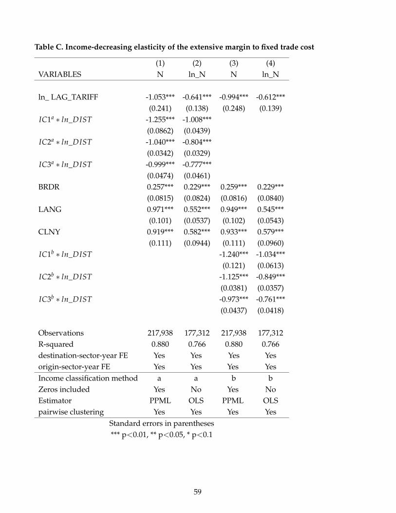
Table C. Income-decreasing elasticity of the extensive margin to fixed trade cost

(1) (2) (3) (4)VARIABLES N ln_N N ln_N

ln_ LAG_TARIFF -1.053*** -0.641*** -0.994*** -0.612***(0.241) (0.138) (0.248) (0.139)

IC1a ∗ ln_DIST -1.255*** -1.008***(0.0862) (0.0439)

IC2a ∗ ln_DIST -1.040*** -0.804***(0.0342) (0.0329)

IC3a ∗ ln_DIST -0.999*** -0.777***(0.0474) (0.0461)

BRDR 0.257*** 0.229*** 0.259*** 0.229***(0.0815) (0.0824) (0.0816) (0.0840)

LANG 0.971*** 0.552*** 0.949*** 0.545***(0.101) (0.0537) (0.102) (0.0543)

CLNY 0.919*** 0.582*** 0.933*** 0.579***(0.111) (0.0944) (0.111) (0.0960)

IC1b ∗ ln_DIST -1.240*** -1.034***(0.121) (0.0613)

IC2b ∗ ln_DIST -1.125*** -0.849***(0.0381) (0.0357)

IC3b ∗ ln_DIST -0.973*** -0.761***(0.0437) (0.0418)

Observations 217,938 177,312 217,938 177,312R-squared 0.880 0.766 0.880 0.766destination-sector-year FE Yes Yes Yes Yesorigin-sector-year FE Yes Yes Yes YesIncome classification method a a b bZeros included Yes No Yes NoEstimator PPML OLS PPML OLSpairwise clustering Yes Yes Yes Yes

Standard errors in parentheses*** p<0.01, ** p<0.05, * p<0.1

59

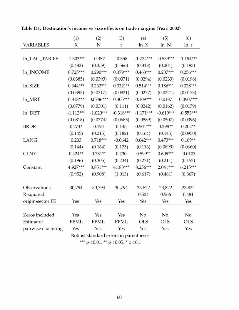
Table D1. Destination’s income vs size effects on trade margins (Year: 2002)

(1) (2) (3) (4) (5) (6)VARIABLES X N r ln_X ln_N ln_r

ln_LAG_TARIFF -1.303*** -0.357 -0.558 -1.734*** -0.539*** -1.194***(0.482) (0.359) (0.566) (0.318) (0.201) (0.193)

ln_INCOME 0.725*** 0.290*** 0.379*** 0.463*** 0.207*** 0.256***(0.0385) (0.0393) (0.0371) (0.0294) (0.0233) (0.0198)

ln_SIZE 0.644*** 0.262*** 0.332*** 0.514*** 0.186*** 0.328***(0.0393) (0.0317) (0.0821) (0.0277) (0.0221) (0.0173)

ln_MRT 0.318*** 0.0786*** 0.305*** 0.109*** 0.0187 0.0907***(0.0779) (0.0301) (0.111) (0.0242) (0.0162) (0.0179)

ln_DIST -1.112*** -1.020*** -0.318*** -1.171*** -0.619*** -0.553***(0.0818) (0.0774) (0.0685) (0.0589) (0.0507) (0.0396)

BRDR 0.274* 0.194 0.145 0.501*** 0.298** 0.202**(0.145) (0.215) (0.182) (0.164) (0.145) (0.0950)

LANG 0.203 0.718*** -0.0642 0.642*** 0.473*** 0.169**(0.144) (0.164) (0.125) (0.116) (0.0899) (0.0660)

CLNY 0.424** 0.731** 0.230 0.599** 0.609*** -0.0103(0.196) (0.305) (0.234) (0.271) (0.211) (0.152)

Constant 4.927*** 3.851*** 4.183*** 8.256*** 2.041*** 6.215***(0.952) (0.908) (1.013) (0.617) (0.481) (0.367)

Observations 30,794 30,794 30,794 23,822 23,822 23,822R-squared 0.524 0.566 0.481origin-sector FE Yes Yes Yes Yes Yes Yes

Zeros included Yes Yes Yes No No NoEstimator PPML PPML PPML OLS OLS OLSpairwise clustering Yes Yes Yes Yes Yes Yes

Robust standard errors in parentheses*** p<0.01, ** p<0.05, * p<0.1

60

Table D2. Destination’s income vs size effects on trade margins (Year: 2005)

(1) (2) (3) (4) (5) (6)VARIABLES X N r ln_X ln_N ln_r

ln_LAG_TARIFF -2.703*** -1.019*** -1.379*** -1.532*** -0.598*** -0.934***(0.616) (0.367) (0.400) (0.247) (0.148) (0.154)

ln_INCOME 0.654*** 0.230*** 0.363*** 0.408*** 0.207*** 0.201***(0.0464) (0.0655) (0.0408) (0.0250) (0.0186) (0.0159)

ln_SIZE 0.647*** 0.241*** 0.373*** 0.496*** 0.185*** 0.310***(0.0347) (0.0369) (0.0362) (0.0251) (0.0182) (0.0134)

ln_MRT 0.839*** 0.257*** 0.267** 0.264*** 0.0780*** 0.186***(0.116) (0.0603) (0.107) (0.0315) (0.0194) (0.0198)

ln_DIST -1.121*** -1.069*** -0.174* -1.238*** -0.650*** -0.588***(0.0777) (0.0732) (0.0891) (0.0531) (0.0415) (0.0300)

BRDR 0.122 0.0551 0.201 0.388*** 0.238** 0.150*(0.191) (0.194) (0.247) (0.139) (0.110) (0.0882)

LANG -0.0237 0.640*** -0.172 0.533*** 0.404*** 0.130**(0.125) (0.129) (0.128) (0.0873) (0.0614) (0.0534)

CLNY 0.951*** 1.297*** 0.559** 0.783*** 0.727*** 0.0561(0.213) (0.375) (0.247) (0.200) (0.174) (0.135)

Constant 1.613 3.508*** 3.890*** 8.042*** 1.654*** 6.388***(1.133) (0.833) (0.868) (0.535) (0.377) (0.327)

Observations 53,395 53,395 53,395 40,304 40,304 40,304R-squared 0.517 0.545 0.485origin-sector FE Yes Yes Yes Yes Yes Yes

Zeros included Yes Yes Yes No No NoEstimator PPML PPML PPML OLS OLS OLSpairwise clustering Yes Yes Yes Yes Yes Yes

Robust standard errors in parentheses*** p<0.01, ** p<0.05, * p<0.1

61

Table D3. Destination’s income vs size effects on trade margins (Year: 2008)

VARIABLES X N r ln_X ln_N ln_r

ln_LAG_TARIFF -3.154*** -1.356*** -1.124** -1.902*** -0.759*** -1.143***(0.600) (0.389) (0.482) (0.203) (0.122) (0.129)

ln_INCOME 0.611*** 0.226*** 0.355*** 0.362*** 0.206*** 0.155***(0.0381) (0.0317) (0.0288) (0.0199) (0.0136) (0.0124)

ln_SIZE 0.647*** 0.288*** 0.327*** 0.472*** 0.209*** 0.263***(0.0283) (0.0253) (0.0315) (0.0194) (0.0128) (0.0107)

ln_MRT 0.653*** 0.210*** 0.364*** 0.304*** 0.0867*** 0.217***(0.0933) (0.0495) (0.0668) (0.0330) (0.0185) (0.0196)

ln_DIST -1.062*** -0.972*** -0.369*** -1.199*** -0.657*** -0.542***(0.0553) (0.0587) (0.0458) (0.0419) (0.0292) (0.0228)

BRDR 0.557*** 0.419*** 0.0464 0.712*** 0.451*** 0.261***(0.136) (0.149) (0.141) (0.121) (0.0937) (0.0696)

LANG 0.0858 0.843*** -0.179** 0.552*** 0.455*** 0.0972**(0.136) (0.118) (0.0848) (0.0712) (0.0508) (0.0442)

CLNY 0.563*** 0.879*** 0.0412 0.565*** 0.516*** 0.0489(0.159) (0.227) (0.136) (0.137) (0.104) (0.0789)

Constant 3.546*** 2.590*** 5.556*** 8.545*** 1.246*** 7.299***(0.908) (0.768) (0.648) (0.447) (0.307) (0.252)

Observations 82,241 82,241 82,241 62,208 62,208 62,208R-squared 0.531 0.588 0.491origin-sector FE Yes Yes Yes Yes Yes Yes

Zeros included Yes Yes Yes No No NoEstimator PPML PPML PPML OLS OLS OLSpairwise clustering Yes Yes Yes Yes Yes Yes

Robust standard errors in parentheses*** p<0.01, ** p<0.05, * p<0.1

62

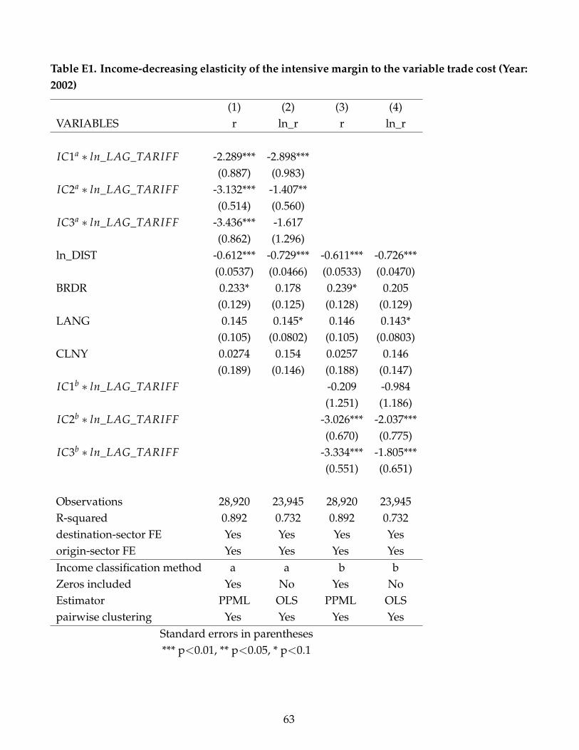
Table E1. Income-decreasing elasticity of the intensive margin to the variable trade cost (Year:2002)

(1) (2) (3) (4)VARIABLES r ln_r r ln_r

IC1a ∗ ln_LAG_TARIFF -2.289*** -2.898***(0.887) (0.983)

IC2a ∗ ln_LAG_TARIFF -3.132*** -1.407**(0.514) (0.560)

IC3a ∗ ln_LAG_TARIFF -3.436*** -1.617(0.862) (1.296)

ln_DIST -0.612*** -0.729*** -0.611*** -0.726***(0.0537) (0.0466) (0.0533) (0.0470)

BRDR 0.233* 0.178 0.239* 0.205(0.129) (0.125) (0.128) (0.129)

LANG 0.145 0.145* 0.146 0.143*(0.105) (0.0802) (0.105) (0.0803)

CLNY 0.0274 0.154 0.0257 0.146(0.189) (0.146) (0.188) (0.147)

IC1b ∗ ln_LAG_TARIFF -0.209 -0.984(1.251) (1.186)

IC2b ∗ ln_LAG_TARIFF -3.026*** -2.037***(0.670) (0.775)

IC3b ∗ ln_LAG_TARIFF -3.334*** -1.805***(0.551) (0.651)

Observations 28,920 23,945 28,920 23,945R-squared 0.892 0.732 0.892 0.732destination-sector FE Yes Yes Yes Yesorigin-sector FE Yes Yes Yes YesIncome classification method a a b bZeros included Yes No Yes NoEstimator PPML OLS PPML OLSpairwise clustering Yes Yes Yes Yes

Standard errors in parentheses*** p<0.01, ** p<0.05, * p<0.1

63

Table E2. Income-decreasing elasticity of the intensive margin to the variable trade cost (Year:2005)

(1) (2) (3) (4)VARIABLES r ln_r r ln_r

IC1a ∗ ln_LAG_TARIFF -3.169*** -1.648***(0.829) (0.556)

IC2a ∗ ln_LAG_TARIFF -1.449*** -1.291***(0.492) (0.380)

IC3a ∗ ln_LAG_TARIFF -1.516*** -0.679*(0.386) (0.390)

Distance -0.494*** -0.688*** -0.495*** -0.688***(0.0447) (0.0336) (0.0447) (0.0337)

contiguity 0.399*** 0.217** 0.387*** 0.210**(0.101) (0.0932) (0.102) (0.0934)

common language 0.150* 0.184*** 0.143* 0.178***(0.0817) (0.0647) (0.0820) (0.0647)

colonial links 0.160 -0.00573 0.160 -0.000731(0.120) (0.133) (0.120) (0.132)

IC1b ∗ ln_LAG_TARIFF -3.138** -2.321***(1.234) (0.628)

IC2b ∗ ln_LAG_TARIFF -2.154*** -1.665***(0.537) (0.493)

IC3b ∗ ln_LAG_TARIFF -1.196*** -0.620**(0.405) (0.300)

Observations 51,466 40,629 51,466 40,629R-squared 0.946 0.673 0.946 0.674destination-sector FE Yes Yes Yes Yesorigin-sector FE Yes Yes Yes YesIncome classification method a a b bZeros included Yes No Yes NoEstimator PPML OLS PPML OLSpairwise clustering Yes Yes Yes Yes

Standard errors in parentheses*** p<0.01, ** p<0.05, * p<0.1

64

Table E3. Income-decreasing elasticity of the intensive margin to the variable trade cost (Year:2008)

(1) (2) (3) (4)VARIABLES r ln_r r ln_r

IC1a ∗ ln_LAG_TARIFF -3.508*** -1.257***(0.716) (0.423)

IC2a ∗ ln_LAG_TARIFF -2.736*** -2.588***(0.433) (0.343)

IC3a ∗ ln_LAG_TARIFF -1.855*** -1.097***(0.448) (0.305)

Distance -0.472*** -0.597*** -0.472*** -0.596***(0.0342) (0.0247) (0.0342) (0.0248)

contiguity 0.142* 0.324*** 0.141* 0.324***(0.0776) (0.0661) (0.0775) (0.0658)

common language 0.0780 0.109** 0.0773 0.107**(0.0702) (0.0504) (0.0702) (0.0503)

colonial links 0.115 0.0548 0.116 0.0566(0.0924) (0.0799) (0.0923) (0.0797)

IC1b ∗ ln_LAG_TARIFF -3.782*** -1.304**(0.966) (0.544)

IC2b ∗ ln_LAG_TARIFF -2.820*** -2.706***(0.439) (0.353)

IC3b ∗ ln_LAG_TARIFF -1.892*** -0.899***(0.403) (0.276)

Observations 80,837 63,010 80,837 63,010R-squared 0.829 0.644 0.829 0.644destination-sector FE Yes Yes Yes Yesorigin-sector FE Yes Yes Yes YesIncome classification method a a b bZeros included Yes No Yes NoEstimator PPML OLS PPML OLSpairwise clustering Yes Yes Yes Yes

Standard errors in parentheses*** p<0.01, ** p<0.05, * p<0.1

65

Table F1. Income-decreasing elasticity of the extensive margin to fixed trade cost (Year: 2002)

(1) (2) (3) (4)VARIABLES N ln_N N ln_N

ln_ LAG_TARIFF -0.728** -0.177 -0.506 -0.164(0.359) (0.346) (0.385) (0.369)

IC1a ∗ ln_DIST -1.251*** -1.058***(0.148) (0.0626)

IC2a ∗ ln_DIST -0.934*** -0.789***(0.0489) (0.0554)

IC3a ∗ ln_DIST -1.232*** -0.855***(0.113) (0.159)

BRDR 0.233* 0.0647 0.204 0.0622(0.137) (0.144) (0.140) (0.154)

LANG 0.627*** 0.456*** 0.579*** 0.450***(0.117) (0.0819) (0.101) (0.0818)

CLNY 1.058*** 0.632*** 1.074*** 0.606***(0.148) (0.164) (0.154) (0.171)

IC1b ∗ ln_DIST -1.167*** -1.033***(0.198) (0.0927)

IC2b ∗ ln_DIST -1.180*** -0.904***(0.0666) (0.0673)

IC3b ∗ ln_DIST -0.958*** -0.780***(0.0538) (0.0670)

Observations 28,920 23,945 28,920 23,945R-squared 0.910 0.813 0.906 0.811destination-sector FE Yes Yes Yes Yesorigin-sector FE Yes Yes Yes YesIncome classification method a a b bZeros included Yes No Yes NoEstimator PPML OLS PPML OLSpairwise clustering Yes Yes Yes Yes

Standard errors in parentheses*** p<0.01, ** p<0.05, * p<0.1

66

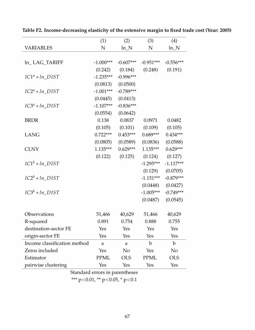
Table F2. Income-decreasing elasticity of the extensive margin to fixed trade cost (Year: 2005)

(1) (2) (3) (4)VARIABLES N ln_N N ln_N

ln_ LAG_TARIFF -1.000*** -0.607*** -0.951*** -0.556***(0.242) (0.184) (0.248) (0.191)

IC1a ∗ ln_DIST -1.235*** -0.996***(0.0813) (0.0500)

IC2a ∗ ln_DIST -1.001*** -0.789***(0.0445) (0.0413)

IC3a ∗ ln_DIST -1.107*** -0.836***(0.0554) (0.0642)

BRDR 0.138 0.0837 0.0971 0.0482(0.105) (0.101) (0.109) (0.105)

LANG 0.722*** 0.453*** 0.689*** 0.434***(0.0805) (0.0589) (0.0836) (0.0588)

CLNY 1.135*** 0.629*** 1.135*** 0.629***(0.122) (0.125) (0.124) (0.127)

IC1b ∗ ln_DIST -1.295*** -1.117***(0.129) (0.0705)

IC2b ∗ ln_DIST -1.151*** -0.879***(0.0448) (0.0427)

IC3b ∗ ln_DIST -1.005*** -0.749***(0.0487) (0.0545)

Observations 51,466 40,629 51,466 40,629R-squared 0.891 0.754 0.888 0.755destination-sector FE Yes Yes Yes Yesorigin-sector FE Yes Yes Yes YesIncome classification method a a b bZeros included Yes No Yes NoEstimator PPML OLS PPML OLSpairwise clustering Yes Yes Yes Yes

Standard errors in parentheses*** p<0.01, ** p<0.05, * p<0.1

67

Table F3. Income-decreasing elasticity of the extensive margin to fixed trade cost (Year: 2008)

(1) (2) (3) (4)VARIABLES N ln_N N ln_N

ln_ LAG_TARIFF -1.325*** -0.782*** -1.248*** -0.777***(0.379) (0.199) (0.381) (0.197)

IC1a ∗ ln_DIST -1.322*** -0.993***(0.0948) (0.0534)

IC2a ∗ ln_DIST -1.109*** -0.810***(0.0413) (0.0371)

IC3a ∗ ln_DIST -0.978*** -0.759***(0.0533) (0.0401)

BRDR 0.310*** 0.337*** 0.334*** 0.352***(0.0890) (0.0893) (0.0882) (0.0910)

LANG 1.039*** 0.584*** 1.025*** 0.574***(0.123) (0.0594) (0.122) (0.0595)

CLNY 0.892*** 0.513*** 0.919*** 0.517***(0.122) (0.0938) (0.121) (0.0946)

IC1b ∗ ln_DIST -1.239*** -0.956***(0.111) (0.0639)

IC2b ∗ ln_DIST -1.158*** -0.840***(0.0458) (0.0368)

IC3b ∗ ln_DIST -0.997*** -0.764***(0.0493) (0.0410)

Observations 80,837 63,010 80,837 63,010R-squared 0.865 0.742 0.864 0.741destination-sector FE Yes Yes Yes Yesorigin-sector FE Yes Yes Yes YesIncome classification method a a b bZeros included Yes No Yes NoEstimator PPML OLS PPML OLSpairwise clustering Yes Yes Yes Yes

Standard errors in parentheses*** p<0.01, ** p<0.05, * p<0.1

68

Appendix C

C.1 Gross positive income effect on the intensive margin:

This effect is captured by ζ, which is given by: ζ = 1 + [(1 + ε3)− (1+εF

31−εF

7)].

I show that this gross effect exceeds unity only under non-homotheticity as follows. First, when

preferences are homothetic (CES case), it is readily verified that (1 + ε3) = (1+εF

31−εF

7) = σ.

Hence, ζ collapses to 1.

Second, when preferences are non-homothetic, I need to rewrite (1+εF

31−εF

7) as follows, so as to de-

compose the general equilibrium effect of income into an "intensive" (impact on export revenuesof active exporters) and an "extensive" (impact on infra-marginal exporters) components as fol-lows:

Denote by ∆1 = (1 + ε3) = [ρ3 + (1− ρ3)σij(wj)], which capture the impact of income variation

on the export revenues of the firm (ϕ) at question33 Likewise, ∆2 = (1+εF

31−εF

7) = ∆3 + ∆4 such as:

• ∆3 = ∆31 ∆32 = ∆31 [ρ3 + (1− ρ3)σij(wj)] embodies the income effect on the "intensive" margin,

with ∆31 =|ρ∗4 |∗(σ∗ij(wj)−1)

θ+|ρ∗4 |(σ∗ij(wj)−1)−|ρ4|(σij(wj)−1) < 1 since θ > |ρ∗4 |(σ∗ij(wj)− 1),

and |ρ∗4 |(σ∗ij(wj)− 1) > |ρ4|(σij(wj)− 1) as σ is increasing in price.

• ∆4 = ∆41 ∆42 = ∆41 [(1− ρ∗3)(σ∗ij(wj)− 1) + 1 + δ∗] embodies the income effect on the “exten-

sive" margin, with ∆41 =θ−|ρ4|(σij(wj)−1)

θ+|ρ∗4 |(σ∗ij(wj)−1)−|ρ4|(σij(wj)−1) ≈ 0.

Therefore, ζ = 1 +[ ∆1︸︷︷︸>1

- [ ∆31︸︷︷︸<1

∆32 + ∆41︸︷︷︸≈0

∆42 ] > 1.

33The absence of superscript indicates that a random exporter is at question.

69

C.2 direct34 income effect on the extensive margin

This effect is captured by ∆5, which can be written, using the ∆s defined above, as :

∆5 = 1ε∗4[∆2 − ∆42] and its sign crucially depends on the nature of preferences:

• Under the CES, it easy to verify that ∆2 = ∆42 = σ. Hence, ∆5 collapses to 0.

• Under non-homotheticity, ∆2 − ∆42 = ∆31︸︷︷︸<1

∆32 - (1− ∆41)︸ ︷︷ ︸≈1

∆42 < 0

since ∆32 = [ρ3 + (1− ρ3)σij(wj)] < ∆42 = [(1− ρ∗3)(σ∗ij(wj)− 1) + 1 + δ∗], as σ∗ij(wj) > σij(wj).

C.3 Solving for nominal wage in the liberalizing country j

I solve for the nominal wage in destination j wj using the trade balance condition (TB):

(TB)j :(N−1)

∑i=1

Xji︸ ︷︷ ︸j′s exports

=(N−1)

∑i=1

Xij︸ ︷︷ ︸j′s imports

(2.32)

Using equation (2.21), bilateral trade flows can be written as:

Xji = κ6 [σvj (w)]−1 YjYi

Yv

ΨiΨj

wεF1

j τεF

2ji f εF

5ji

Xij = κ6 [σvi (w)]−1 YiYj

Yv

ΨjΨi

wεF1

i τεF

2ij f εF

5ij

(2.33)

By plugging bilateral trade flows in the trade balance condition above, normalizing nominalwage in all other countries to unity wi = 1 ∀i 6= j, along with simplifying by [σv

j (w)]−1 andLj, and rearranging, I obtain the following general equilibrium expression of nominal wage incountry j:

wj = (Ψj

ΨRow)

1(εF

1−1) Λ1

(εF1−1) , (2.34)

34Putting aside the common (RMS) channel.

70

where ΨRow ≡ ∑(N−1)i=1,i 6=j(

LiLv)Ψi is the weighted average degree of remoteness of all destinations

in the World, excluding j, and Λ is a general equilibrium object that is orthogonal to bilateraltariffs, as shown below:

Λ =Ψj

ΦOUTj

(ΦINj )−1

ΨRow,

(ΦINj )−1 = ∑

(N−1)i=1,i 6=j(

LiLv)τ

εF2

ij f εF5

ij

ΦOUTj = ∑

(N−1)i=1,i 6=j(

LiLv)τ

εF2

ji f εF5

ji

(2.35)

Notice that Ψj =Ψjwj

refers to the remoteness index of country j (as an origin) from all otherdestinations, derived in equation (2.10), adjusted by its domestic cost of labor (and thus orthog-onal to wj). Moreover, ΦOUT

j is an equivalent measure of the country j’s outward multilateral

resistance term. As they are both decreasing in bilateral tariffs, the ratioΨj

ΦOUTj

is thus orthogonal

to τji. Similarly, ΨRow= ∑(N−1)i=1,i 6=j(

LiLv)Ψi is the weighted average outward multilateral resistance

term of all other countries. Moreover, (ΦINj )−1 is an inverse measure of country j’s inward mul-

tilateral resistance term. Hence, as they are both decreasing in bilateral tariffs, their ratio is thusorthogonal to τij.

C.4 The "EEM" method: a detailed explanation

C.4.1 Objective of the "EEM" method

As stressed in the main text, added flexibility in preferences raises tractability issues. Thus, inorder to gain in flexibility without losing in tractability, I resort to a new and simple method that Icall the "Exponent Elasticity Method" (EEM, hereafter). The objective of this simple method is todeliver a tractable solution for the general equilibrium price aggregator despite added flexibilityin preferences. The starting point is the partial equilibrium expression of the price aggregatorinitially provided in equation (2.11):

|ηj| = (wjLj)(wjLj

Yv)−1

N

∑i=1

cEi (

wiLi

Yv) f−1

ij

∫ +∞

ϕ∗ij

pij(ϕ)

wj|v′(

pij(ϕ)

wj)| dG(ϕ)︸ ︷︷ ︸

I

where cEi = [ σv

i (w) wi (αe + αii P(ϕ ≥ ϕ∗ii) + P(ϕ ≥ ϕ∗ij) + ∑(N−2)j=1 αik P(ϕ ≥ ϕ∗ij) ) ]

−1 is a proxy

for entry conditions in country i, αe =Fefij

, αii =fiifij

, and αik =fikfij

.

71

Clearly, the mathematical challenge here consists in solving for the above integral (I) withoutspecifying a functional form of the sub-utility function. Assuming that the productivity distri-bution is unbounded Pareto is necessary, but not sufficient for the above integral to be solved. Indeed, this further requires that the sub-utility function should exhibit a constant demand elas-ticity which, in turn, can be used as a constant for integrating. Such simplicity is only possibleunder homothetic CES preferences, which is the unique case where it is possible to solve forthis integral. Since the flexible family of preferences considered in this chapter encompasses thehomothetic CES and a non-homothetic alternative allowing the demand elasticity to vary withprices and income levels, it is then impossible to solve for integral (I) under such added flexibil-ity in preferences.

Given the impossibility to solve for the integral in the current setting, the key idea that the“EEM" method proposes is to locally approximate the integral (I) around the equilibrium witha multiplicative equivalent which has a finite number of determinants, such as the exponent of

each determinant embodies the elasticity of [pij(ϕ)

wj|v′( pij(ϕ)

wj)| ] with respect to it. This requires a

five-step procedure that I explain in detail as follows.

C.4.2 A Five-step procedure:

Step 1. Rewrite the integral (I) using unbounded Pareto:

By invoking this assumption, it is readily verified that that P(ϕ ≥ ϕ∗ij) = ϕ∗ij−θ. Using this,

integral (I) can be rewritten as:

I = ϕ∗ij−θ

∫ +∞

ϕ∗ij

pij(ϕ)

wj|v′(

pij(ϕ)

wj)| γij(ϕ) dϕ︸ ︷︷ ︸

I0

(2.36)

where γij(ϕ)= g(ϕ)P(ϕ≥ϕ∗ij)

is the productivity distribution conditional on successful penetration of

country j’s market for firms based in country i. Clearly, the unique difference between the initialintegral (I) and new integral (I0) is that this latter is expressed using the conditional productivitydistribution γij(ϕ).

Step 2. Approximate integral (I0) with a multiplicative equivalent:

Now by recalling that under indirectly-separable preferences, the price elasticity of demand is

equal to the elasticity of the marginal sub-utility: σ( pw ) = − v′′( p

w )pw

v′( pw )

> 1, and that the elasticity

72

of the export price with respect to each of its determinants is given by: ρ1 =dlog pij(ϕ)

dlog wi, ρ2 =

dlog pij(ϕ)

dlog τij, ρ3 =

dlog pij(ϕ)

dlog wj, and ρ4 =

dlog pij(ϕ)

dlog ϕ , the integral (I0) can be locally approximated asfollows:

I0 ≡ wρ1(1−σij(wj))

i τρ2(1−σij(wj))

ij w(1−ρ3)(σij(wj)−1)j ϕij(ϕ∗ij)

|ρ4|(σij(wj)−1) (2.37)

Since operating profits are monotonically increasing in productivity, and exporting from countryi to country j involves not only, a variable trade cost τij, but also a fixed cost fij, the equilibriumexport cutoff ϕ∗ij exists and is unique. This, in turn, ensures that this local approximation (aroundthe trade equilibrium) delivers a unique multiplicative equivalent to integral I0.

Step 3. Obtain a final expression of integral (I) using this of (I0) and un-bounded Pareto:

Let us now recall that unbounded Pareto distribution gives rise to constant mean-to-min ratio:ϕij = θ

θ−1 ϕ∗ij. By plugging the multiplicative equivalent of integral (I0) from equation (2.37) intothe initial expression of integral (I) in equation (2.36) and invoking this practical property ofunbounded Pareto, I obtain the following multiplicative equivalent for integral (I):

I ≡ κ wρ1(1−σij(wj))

i τρ2(1−σij(wj))

ij w(1−ρ3)(σij(wj)−1)j ϕ∗ij

[ |ρ4|(σij(wj)−1)−θ ] (2.38)

where κ = ( θθ−1)

|ρ4|(σij(wj)−1) is a constant.

Step 4. Approximate the partial equilibrium export cutoff ϕ∗ij with an explicitmultiplicative equivalent:

Let us first recall that the export cutoff ϕ∗ij is endogenous and is defined as the implicit solutionof the zero profit condition on the export market: πij(ϕ∗ij)=0

ϕ∗ij : [p∗ij(ϕ∗ij)− wiτij(ϕ∗ij)−1]|v′(

p∗ij(ϕ∗ij)

wj)|

|ηj|Lj − wi fij = 0 (2.39)

Now by isolating the firm-specific component of the operating profit on the left hand-side, ap-proximating it in a multiplicative way, as in equation (2.38), and rearranging, I obtain the fol-lowing explicit equivalent of the partial equilibrium export cutoff:

73

ϕ∗ij ≡ τij w

[1−ρ∗1(1−σ∗ij(wj))]

|ρ∗4 |(σ∗ij(wj)−1)

i w−

[(1−ρ∗3)(σ∗ij(wj)−1)+1+δ∗ ]

|ρ∗4 |(σ∗ij(wj)−1)

j f1

|ρ∗4 |(σ∗ij(wj)−1)

ij L− 1|ρ∗4 |(σ

∗ij(wj)−1)

j |ηj|1

|ρ∗4 |(σ∗ij(wj)−1)

(2.40)

where the superscript (*) refers to the firm at the export cutoff, and δ∗ = -dlog σ∗ij(wj)

dlog wjis the absolute

value of the elasticity of the price elasticity of demand, faced by the cutoff exporter in country i,with respect to per-capita income in destination j.

Step 5. Solving for the general equilibrium price aggregator |ηj| :

Now by plugging the explicit equivalent of the export cutoff from equation (2.40) in the expres-sion of integral (I) in equation (2.38), this latter can be expressed solely as a function of (wi, τij,wj, fij, Lj, |ηj| ). Then, by plugging this latter in the partial equilibrium expression of the priceaggregator given by equation (2.11), and rearranging, I obtain the following general equilibriumexpression of the price aggregator:

|ηj| ≡ w(

1+εF3

1−εF7)

j L(

1+εF3

1−εF7)

j (wjLj

Yw)

1(εF

7−1) Ψ1

(εF7−1)

j (2.41)

where Ψj = [∑Ni=1(

wi LiYw

) f (εF5−1)

ij τεF

2ij wεF

1i ]−1, and the explicit expressions of the above exponents are

given by:

εF1 = ρ1(1− σij(wj)) + [ [|ρ4|(σij(wj)− 1)− θ]

[1−ρ∗1(1−σ∗ij(wj))]

|ρ∗4 |(σ∗ij(wj)−1) ] < 0

εF2 = ρ2( 1− σij(wj) ) + [ |ρ4|(σij(wj)− 1)− θ ] = −θ < 0

εF3 = (1− ρ3)( σij(wj)− 1 ) + [ [ θ − |ρ4|(σij(wj)− 1) ]

[(1−ρ∗3)(σ∗ij(wj)−1)+1+δ∗]

|ρ∗4 |(σ∗ij(wj)−1) ] > 1

εF5 = − [ θ−|ρ4|(σij(wj)−1) ]

|ρ∗4 |(σ∗ij(wj)−1) < 0

εF7 = − [ θ−|ρ4|(σij(wj)−1) ]

|ρ∗4 |(σ∗ij(wj)−1) < 0

(2.42)

74

C.5 Solving for trade margins in general equilibrium

Let us start with writing an approximate equivalent of firm-level export revenues (intensivemargin) in partial equilibrium:

rij(ϕ) ≡ wε1i τε2

ij w(ε3+1)j ϕε4 Lj |ηj|−1 (2.43)

where the exponents (ε1, ε2, ε3, ε4) are respectively given by:ε1 = ρ1 ( 1 - σij(wj) ) ; ε2 = ρ2 ( 1 - σij(wj) ) ; ε3 = (1 - ρ3) ( σij(wj) - 1 ); ε4 = |ρ4| ( σij(wj) - 1 ).

Now by plugging the general equilibrium price aggregator from equation (2.41) in the aboveexpression and rearranging, I solve for the intensive margin of trade in general equilibrium:

rij(ϕ) ≡ wε1i τε2

ij ϕε4 wζ−1j (

wjLj

Yw)

1(1−εF

7 ) Ψ1

(1−εF7 )

j︸ ︷︷ ︸Chaney(2008)

(2.44)

where ζ = 1+ [ (1+ ε3)− (1+εF

31−εF

7) ] captures the gross positive income effect on firm-level export

revenues.

Similarly, by plugging the general equilibrium price aggregator from equation (2.41) in the ex-plicit partial equilibrium expression of the export cutoff, I can solve for the extensive margin oftrade in general equilibrium as follows:

ϕ∗ij ≡ w(

1−ε∗1ε∗4

)

i τij f1

ε∗4ij w∆5

j L∆6j (

wjLj

Yw)

1ε∗4 (ε

F7−1) Ψ

1ε∗4 (ε

F7−1)

j︸ ︷︷ ︸Chaney(2008)

(2.45)

where ∆5 = 1ε∗4

[ (1+εF

31−εF

7)− (ε∗3 + 1 + δ∗) ] and ∆6 = 1

ε∗4[ (

1+εF6

1−εF7)− 1 ], εF

6 =[ θ−|ρ4|(σij(wj)−1) ]|ρ∗4 |(σ∗ij(wj)−1) > 0

and δ∗= -dlog σ∗ij(wj)

dlog wj; ε∗1 = ρ∗1( 1− σ∗ij(wj) ); ε∗3 = (1 - ρ∗3)( σ∗ij(wj)− 1 ); ε∗4 = |ρ∗4 | ( σ∗ij(wj)− 1 ).

75

Chapter 3

International Trade under MonopolisticCompetition beyond the CES

3.1 Introduction

Recent empirical research in international trade has revealed that the price elasticity of demandvaries significantly across firms. This central observation stands in stark contradiction with CESdemand which imposes a constant demand elasticity under monopolistic competition. This sug-gests that it is crucial to depart from the homothetic CES to examine gains from trade under morerealistic patterns of price sensitivity. In theoretical trade literature, transition to non-CES prefer-ences took place gradually. While in earlier departures from the CES, a large body of work hasfocused on specific types of preferences, only few recent papers have proposed more generaldemand systems encompassing prominent alternatives to the CES case.

However, increased generality raises tractability issues, which in turn requires some conces-sions. Accordingly, a large body of work always impose a restriction on the curvature of de-mand: they generally assume that demand is "sub-convex". They also abstract from fixed costsof accessing markets. Instead, they resort to assuming the existence of a choke price to ensureself-selection of firms into markets, see e.g. (Melitz and Ottaviano, 2008; Bertoletti, Etro, andSimonovska, 2018; Arkolakis et al., 2018; Feenstra, 2018; Fally, 2019). Alternatively, other paperssquarely focus on a specific type of preferences, while keeping demand curvature unrestrictedand taking fixed costs in due account (Zhelobodko et al., 2012; Mrázová and Neary, 2017). Bothexisting modeling approaches exhibit the same limitations for welfare analysis. First, they implythat at least one channel of welfare gains from trade is ruled out. Second, they preclude the wel-fare implications of the curvature of demand and those of the type pf preferences to be studiedin a common framework.

76

In contrast, this is what the current chapter aims for. Towards this goal, I propose a theoreticalframework combining standards assumptions on the supply side with a flexible and restriction-free demand system. In particular, the supply side is identical to (Melitz, 2003; Chaney, 2008;Arkolakis, Costinot, and Rodriguez-Clare, 2012; Arkolakis et al., 2018; Fally, 2019), and incor-porates monopolistic competition, firm heterogeneity and Pareto distribution of firm productiv-ity. However, here the novel aspect is that I consider a flexible demand system which encom-passes two commonly used families of preferences (directly- and indirectly-separable), and neststwo alternative curvatures of demand (beyond the CES, demand can be either "sub-convex" or"super-convex"). By imposing standard restrictions on the supply side, the modeling approachproposed in this chapter offers then a theoretically clean way to examine the welfare implica-tions of these alternative assumptions on the curvature of demand and the nature of preferences.

The goal of this chapter is to examine three major questions in trade theory with heterogeneousfirms under more realistic consumer behavior than allowed by CES preferences. First, does de-mand curvature play a role in determining the toughness of firm selection and the degree oftheir partitioning by export status? Second, under which demand conditions, net variety gainsand gains from selection coexist in general equilibrium? Third, to which extent the curvature ofdemand and the type of preferences determine the magnitude of the gains from trade?

The main finding of this chapter is that demand curvature plays a crucial role in driving com-parative statics results, shaping the structure of the gains from trade as well as determining themagnitude of these gains, whereas the type of preferences affects only marginally the results. Inparticular, taking the CES as a boundary case, I show that when demand is sub-convex, selec-tion into markets is more relaxed, the partitioning of firms by export status is more pronounced,net variety gains and gains from selection coexist, and gains from trade are smaller than thoseobtained under CES demand. I also emphasize that the type of preferences plays only a second-order role. For instance, under sub-convex demands, directly-separable preferences provide anupper bound for the gains from trade, while indirectly-separable preferences provide a lowerbound. All these patterns are reversed when demand is super-convex.

The rest of this chapter is organized as follows. Section 2 describes in detail the general demandsystem considered in the current chapter. Section 3 offers a simple characterization of demandcurvature. Section 4 illustrates novel comparative statics results. Section 5 examines the gainsfrom trade and highlights novel welfare implications of demand curvature. The last sectionconcludes. Appendix D provides the proofs for the main results as well as a detailed explanationof the "EEM" method.

77

3.2 A Flexible Demand System

This section describes the generalized Gorman-Pollak demand system considered by Fally (2019)and recalls sufficient conditions under which such demand system is integrable, following Fally(2018). It also proposes a simple and useful parameterization that allows for a subtle nesting ofdirectly- and indirectly-separable preferences.

3.2.1 Generalized Gorman-Pollak Demand

Consider a representative consumer whose income w is entirely spent on a set of varieties, de-noted by Ω. For each variety ω ∈ Ω, suppose that demand is determined by its price pω, con-sumer income w and an aggregator Λ :

xω = Q(Λ) Dω(V(Λ)pω

w), (3.1)

where Λ=Λ(p, w) is itself a scalar function off all prices and income, homogeneous of degreezero in (p, w). Λ is implicitly determined by the budget constraint, i.e. it is the implicit solutionof :

∫ω∈Ω

pω Q(Λ) Dω(V(Λ)pω

w) dω = w (3.2)

3.2.2 Conditions for integrability

Integrability conditions can be defined as regularity restrictions that are sufficient to ensure that ademand system can be derived from a rational utility maximizing consumption behavior (Fally,2018).1 Following Fally (2018), the generalized Gorman-Pollak demand system is integrableunder the following conditions:

1. Dω is differentiable and sufficiently downward slopping and elastic, i.e. σω=− dlog Dω

dlog pω> 1.

2. Q and V are differentiable and [εV σω - εQ] has the same sign for all Λ and pω

w .

3. For any set of normalized prices pω

w , equation (1) admits a solution in Λ,

where εQ and εV denote the elasticity of Q and V with respect to Λ.

1See Fally (2018) for further details on integrability conditions.

78

3.2.3 A Useful Parameterization

In order to nest indirectly- and directly-separable preferences in a simple way, I propose the fol-lowing parameterization: Q(Λ)=Λ−β and V(Λ)=Λα. It is without loss of generality to assumethat α and β are both dummies (whose values can be either 0 or 1), such as the case (α=0 andβ=1) corresponds to indirectly-separable preferences, while directly-separable preferences cor-respond to (α=1 and β=0). This implies that the difference [εV σω - εQ] is positive under bothcases, which is sufficient to ensure integrability.

3.3 Characterization of Demand Curvature

At this stage, the flexibility of the demand system described above is reflected in how departingfrom homothetic CES preferences allows the demand elasticity to vary either with normalizedprices when preferences are indirectly-separable, or with consumption levels when preferencesare directly-separable. However, such flexibility raises the following question: under which con-ditions the demand elasticity increases, decreases, or ceases to vary with normalized prices orindividual consumption?

This section aims at addressing this question, and by doing so it completes the characterizationof the demand side of the model. Towards this goal, the current section draws heavily on Mrá-zová and Neary (2017). For instance, it adopts their approach that they call "a firm’s eye view ofdemand".

3.3.1 A simple Measure of Demand Curvature

Following Mrázová and Neary (2017), the starting point is the fact that a monopolistically com-petitive firm takes the demand function it perceives as given. As this approach is partial-equilibrium by definition, it is more convenient to express the Gorman-Pollak demand in equa-tion (1) solely as a function of the price: x(Λ, p

w ) ≡ x(D(p)) ≡ x(p).2

Let us recall that the price elasticity of demand is given by:

σ = −dlog x(p)dlog p

= −dlog D(p)dlog p

> 0

As in Mrázová and Neary (2017), I measure the convexity of demand using the elasticity of theslope of direct demand :

2I drop the variety subscript for expositional simplicity. Since consumer income and the aggregator are taken asgiven, they are dropped from this simplified demand function, so as to concentrate on the relationship between xand p.

79

ζ = −dlog D′(p)dlog p

Now in order to measure demand curvature in a simple and unit-free way, I work with the"superelasticity" of Kimball (1995), defined as the elasticity with respect to price of the elasticityof demand:

S =dlog σ

dlog p= (1 + σ)− ζ

Clearly, the sign of the "superelasticity" S is pinned down by the relationship between the elas-ticity σ and the convexity ζ of the direct demand function, the so-called "demand manifold" byMrázová and Neary (2017). Interestingly, the "superelasticity", due to Kimball (1995), can be con-sidered as a sufficient statistic for demand curvature. That is, its sign clearly indicates whetherdemand is CES, sub-convex, or super-convex :

demand is

sub-convex if S > 0

CES if S = 0

super-convex if S < 0

A peculiar property of CES demand is that it exhibits an exogenous demand elasticity, which isreflected by zero "superelasticity". It is then convenient to take the CES case as a benchmark tocharacterize both alternative curvatures in a simple way. Following Mrázová and Neary (2017),a demand function is locally sub-convex if for the same level of demand elasticity σ, it exhibitsa lower degree of convexity ζ as compared to the CES case. Similarly, a demand function issuper-convex if it is more convex than the CES at a given level of demand elasticity.

80

Figure 1. Localising Demand Curvature in the space of Elasticity and Convexity.

It is now possible to graphically illustrate these three possible cases of demand curvature in asimple and compact way in the (ζ , σ) space. Before proceeding, I resort to the first- and second-order conditions of profit maximization to impose restrictions on the values of σ and ζ, as inMrázová and Neary (2017).

As indicated in the beginning of this section, I consider a monopolistically competitive firmthat takes the direct demand function it perceives as given and maximizes its profit accordingly.From the first-order condition, a positive price-cost margin implies that the price elasticity ofdemand must be greater than one:

(p− ϕ−1)x′ + x = 0⇒ σ > 1 (3.3)

where ϕ−1 is the marginal cost of a ϕ-productivity firm.

From the second-order condition, decreasing marginal revenue requires that the degree of de-mand convexity ζ must be smaller than twice the demand elasticity:

2x′ + (p− ϕ−1)x′′ < 0⇒ ζ < 2 σ (3.4)

As in Mrázová and Neary (2017), the above restrictions imply an admissible region in (ζ , σ)space, as shown by the shaded region in Figure 1, panel A.3

3Ideally, one would borrow an upper bound estimate of the demand elasticity from the empirical literature, andthus concentrate on a more realistic part of the admissible region.

81

As illustrated in Figure 1, panel B, the CES line (whose equation is given by ζ = 1+σ) dividesthe admissible region in two. While points located above the CES line correspond to super-convex demands, points below the CES boundary correspond to the case of sub-convex de-mands. Within the sub-convex region, the "superelasticity" is positive (S > 0), which impliesthat the demand elasticity increases in price (or, equivalently, decreases with consumption) ifand only if demand is sub-convex.

In contrast, the super-convex region is characterized with a negative "superelasticity" (S < 0).This implies that the demand elasticity decreases in price (or, equivalently increases with con-sumption) when demand is super-convex. Clearly, CES demand is a boundary case under whichthe demand elasticity does not vary with price or consumption levels, as reflected by the zero"superelasticity" (S=0). Hence, moving along the CES line only changes the value of the elasticityof demand while preserving its exogenous nature.

3.4 Illustrating Comparative Statics Results

3.4.1 Variable markups and Relative pass-through

Again, following Mrázová and Neary (2017), the starting point of the analysis is the fact that amonopolistically competitive firm producing a variety ω at a ϕ−1 marginal cost takes the priceaggregator Λ as given. Whether it perceives the partial equilibrium demand function in its director inverse form, the first-order condition of profit maximization in equation (3.3) yields a uniqueoptimal pricing rule:

p(ϕ) = ϕ−1 m(ϕ), (3.5)

where m(ϕ) = σ(ϕ)σ(ϕ)−1 is the markup set by the ϕ-productivity firm.

Let us now denote by η(ϕ) = - dlog p(ϕ)dlog ϕ the absolute value of the elasticity of price with respect

to firm productivity :

η(ϕ) ≡ 1 +dlog m(ϕ)

dlog σ(ϕ)S

82

The above expression clearly shows how demand curvature governs the degree of completenessof the relative pass-through.4 Under the CES case, demand elasticity is exogenous (∀ϕ, σ(ϕ) =

σ), the "superelasticity" of demand S collapses to zero, and so η is fixed to unity : η = 1. Depart-ing from the CES benchmark allows then for a positive or negative deviation of η(ϕ) from unitythat is pinned down by the sign of the "superelasticity" S :

η(ϕ)

< 1 if S > 0

= 1 if S = 0

> 1 if S < 0

Therefore, when demand is sub-convex, a higher productivity, which other things equal im-plies lower price (or equivalently, higher individual consumption), is associated with a lowerdemand elasticity and so, a higher markup, implying less than 100 percent pass-through. Bycontrast, when demand is super-convex, a higher productivity is associated with a higher de-mand elasticity and so, a lower markup, implying more than 100 percent pass-through.

3.4.2 Demand Curvature, Firm Selection, and Partitioning of Firms

In order to examine the role that demand curvature plays in determining the toughness of firmselection and the partitioning of firms by export status,5 I proceed in two steps.

First, I show how demand curvature determines the nature of the elasticity of a firm’s operatingprofit with respect to its productivity; whether it is constant, increasing or decreasing with firmproductivity. Then, I graphically illustrate the results in a compact way and infer new implica-tions of demand curvature for firm selection and the partitioning of firms by export status.

4Notice that the final expression of η(ϕ) has been simplified using the fact that an increase in productivity,other things equal, must lower a firm’s price (and equivalently, increases individual consumption of the variety itsupplies).

5This concept initially introduced by Melitz (2003) refers to the fact that exporting is more selective than servingthe domestic market, and so only more productive firms export. This implies then that exporters are on averagemore productive than non-exporters.

83

Figure 2. Demand Curvature, Firm Selection, and Partitioning of Firms by Export Status.

1. Constant vs Variable productivity elasticity of operating profits

Again, as in Mrázová and Neary (2017), the starting point is the fact that a ϕ productivity firm,which engages in monopolistic competition, takes the demand function as given and maximizesits profit accordingly. Its operating profit can be written in an approximate way:6

πo(ϕ) =p(ϕ) x(ϕ) L

σ(ϕ)≡ p(ϕ)1−σ(ϕ)

σ(ϕ)L ≡ ϕe(ϕ) L, (3.6)

where e(ϕ)= dlog πo(ϕ)dlog ϕ = η(ϕ)[σ(ϕ)− 1 + S] > 0.

It is readily verified that the operating profit is always monotonically increasing in firm pro-ductivity regardless of the curvature of demand. However, this latter plays a critical role indetermining whether the pace at which the logarithm of operating profits increases with this offirm productivity is constant, or variable.

Clearly, the CES case is very special: as the demand elasticity is exogenous (∀ϕ, σ(ϕ) = σ), the"superelasticity" collapses to zero (S=0), and the relative pass-through is complete (∀ϕ, η(ϕ) =

1). This yields a constant elasticity of operating profits with respect to firm productivity (bothin logarithms): log πo(ϕ) always increases with log ϕ at a constant pace regardless of the firm’sproductivity level (∀ϕ, e(ϕ) = σ − 1). This is illustrated by the upward sloping "CES" line inFigure 2, panel A.

6Notice that the price aggregator Λ and individual income w are absent in this simplified version of the Gorman-Pollak demand function described in equation (3.1). In deed, as these latter are assumed to be taken as given, andthe focus is squarely on the relationship between operating profits and firm productivity, I abstract from both ofthem in the above expression for expositional simplicity.

84

Therefore, departing from CES demand allows for a variable elasticity of operating profits: e(ϕ)may then increase or decrease with firm productivity ϕ. This implies that the pace at whichlog πo(ϕ) increases with log ϕ may be faster or slower, as compared to the CES benchmark,depending on demand curvature.To show this in a simple way, let us define E as the productivity elasticity of the elasticity ofoperating profits:

E =dlog e(ϕ)

dlog ϕ=

dlog η(ϕ)

dlog ϕ+

dlog [σ(ϕ)− 1 + S]dlog σ(ϕ)

dlog σ(ϕ)

dlog p(ϕ)

dlog p(ϕ)

dlog ϕ(3.7)

After simplification, the final expression of E boils down to:

E ≡ −ηS

< 0 if demand is sub-convex

= 0 if demand is CES

> 0 if demand is super-convex

(3.8)

This reveals that log πo(ϕ) is convex/concave in log ϕ when demand is super-convex/sub-convex, as shown in Figure 2, panel A. Here, the CES case arises again as a boundary for thiscomparative statics result. Visibly, under super-convex demands, a movement from left to rightalong the horizontal axis implies a relatively faster movement (as compared with the CES case)along the log πo(ϕ) curve. By contrast, the same movement along the horizontal axis generatesa relatively slower movement along the log πo(ϕ) curve when demand is sub-convex.

The underlying economics are simple: when demand is super-convex, the demand elasticityincreases in firm productivity, and this has three implications for firm profits. First, more pro-ductive firms set lower markups, and so a higher productivity induces a more than proportionalreduction in price (∀ϕ, η(ϕ) > 1). This reveals that under super-convex demands, a firm’s initiallevel of price competitiveness (given by its productivity level) is magnified by lower markups.Second, consumers are more reactive to price variations of varieties supplied by more produc-tive firms. Third, the markup rate ( 1

σ(ϕ)) is lower for more productive firms. Combination of

the first two effects clearly shows that the super-convex aspect of demand magnifies the sensi-tivity of firm revenues to firm productivity. As illustrated in Figure 2, panel A, this generates arelatively faster response of operating profits to firm productivity,7 despite the fact that higherproductivity implies lower markup rate.

7Both in logarithmic terms.

85

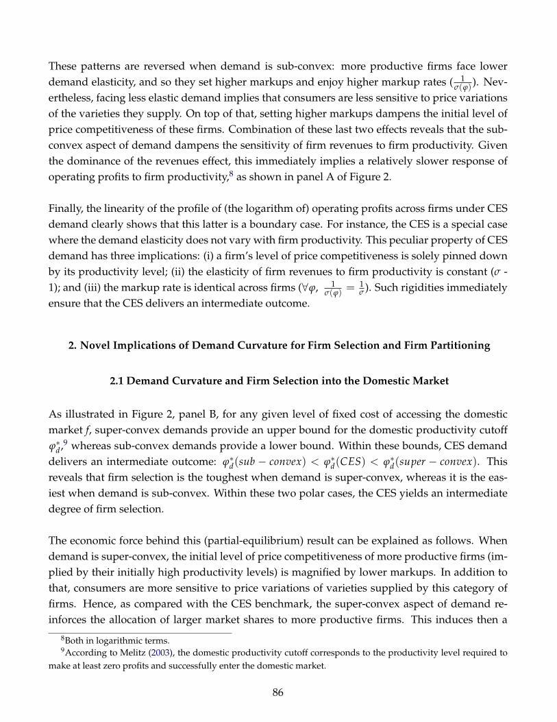
These patterns are reversed when demand is sub-convex: more productive firms face lowerdemand elasticity, and so they set higher markups and enjoy higher markup rates ( 1

σ(ϕ)). Nev-

ertheless, facing less elastic demand implies that consumers are less sensitive to price variationsof the varieties they supply. On top of that, setting higher markups dampens the initial level ofprice competitiveness of these firms. Combination of these last two effects reveals that the sub-convex aspect of demand dampens the sensitivity of firm revenues to firm productivity. Giventhe dominance of the revenues effect, this immediately implies a relatively slower response ofoperating profits to firm productivity,8 as shown in panel A of Figure 2.

Finally, the linearity of the profile of (the logarithm of) operating profits across firms under CESdemand clearly shows that this latter is a boundary case. For instance, the CES is a special casewhere the demand elasticity does not vary with firm productivity. This peculiar property of CESdemand has three implications: (i) a firm’s level of price competitiveness is solely pinned downby its productivity level; (ii) the elasticity of firm revenues to firm productivity is constant (σ -1); and (iii) the markup rate is identical across firms (∀ϕ, 1

σ(ϕ)= 1

σ ). Such rigidities immediatelyensure that the CES delivers an intermediate outcome.

2. Novel Implications of Demand Curvature for Firm Selection and Firm Partitioning

2.1 Demand Curvature and Firm Selection into the Domestic Market

As illustrated in Figure 2, panel B, for any given level of fixed cost of accessing the domesticmarket f, super-convex demands provide an upper bound for the domestic productivity cutoffϕ∗d,9 whereas sub-convex demands provide a lower bound. Within these bounds, CES demanddelivers an intermediate outcome: ϕ∗d(sub − convex) < ϕ∗d(CES) < ϕ∗d(super − convex). Thisreveals that firm selection is the toughest when demand is super-convex, whereas it is the eas-iest when demand is sub-convex. Within these two polar cases, the CES yields an intermediatedegree of firm selection.

The economic force behind this (partial-equilibrium) result can be explained as follows. Whendemand is super-convex, the initial level of price competitiveness of more productive firms (im-plied by their initially high productivity levels) is magnified by lower markups. In addition tothat, consumers are more sensitive to price variations of varieties supplied by this category offirms. Hence, as compared with the CES benchmark, the super-convex aspect of demand re-inforces the allocation of larger market shares to more productive firms. This induces then a

8Both in logarithmic terms.9According to Melitz (2003), the domestic productivity cutoff corresponds to the productivity level required to

make at least zero profits and successfully enter the domestic market.

86

relatively tougher competitive environment for low productivity firms. As compared to the CEScase, setting higher markups makes these less productive firms even less price competitive. Thisimplies then additional difficulty in capturing enough market shares to successfully enter themarket, which is reflected by higher domestic cutoff under super-convex demands. All thesepatterns are reversed when demand is sub-convex.

2.2 Demand Curvature and Partitioning of Firms by Export Status

Now let us consider a simple case where the World is comprised of many symmetric countries,and accessing a foreign market via exporting involves only a fixed cost fx. In the absence ofvariable trade costs,10 I must assume that fx > f , to ensure that firms are partitioned by exportstatus as in Melitz (2003). That is, among successful entrants (firms with productivity ϕ ≥ ϕ∗d),only more productive firms export (a subset of firms with productivity ϕ ≥ ϕ∗x > ϕ∗d).

Such partitioning of firms is quite standard in heterogeneous firms models. However, the novelidea I explore here is how demand curvature determines the degree of this partitioning of firmsby export status. As illustrated in Figure 2, panel B, while the distance between the export andthe domestic cutoffs [ϕ∗x - ϕ∗d] is the smallest when demand is super-convex; it is the largest whendemand is sub-convex. CES demand, again delivers an intermediate result:

[ϕ∗x - ϕ∗d] (super-convex) < [ϕ∗x - ϕ∗d] (CES) < [ϕ∗x - ϕ∗d] (sub-convex)

The underlying economics are simple: when demand is super-convex, selection is relativelytougher (as compared to the CES benchmark) and only (relatively)11 more productive firms suc-cessfully enter the domestic market. Hence, a relatively large subset of these very productivefirms can export. Put differently, these firms are enough productive to successfully enter thedomestic market despite tougher competitive conditions implied by super-convex demands. Itfollows then that a large fringe of these firms is enough price competitive to penetrate the exportmarket. This reveals then that, as compared with the CES benchmark, the partitioning of firmsby export status is less pronounced when demand is super-convex. This result is reversed whendemand is sub-convex.

Finally, it is worth noting that these two novel comparative statics results are partial-equilibriumby definition.12 Yet, the intuitive explanation for both results provides the basis for understand-

10Here, I abstract from variable trade costs for expositional simplicity. However, they will be taken in due accountin the general equilibrium trade model that I spell out in the next section.

11This refers to an immediate comparison with the CES benchmark.12Thus far, I have worked with Mrázová and Neary (2017)’s "firm’s eye view of demand" which is a partial

equilibrium approach, as stated by the authors.

87

ing the general equilibrium behavior. For instance, in Section 5.4, I will show that both resultshold in general equilibrium, and that they have crucial implications for the gains from trade.

3.5 Monopolistic Competition with Heterogeneous Firmsunder Generalized Demands

To illustrate the usefulness of the theoretical approach I have developed in previous sections, Iturn next to apply it to a canonical model of international trade, a one-sector, one-factor, multi-country, general equilibrium model of monopolistic competition, where firms are heterogeneousin productivity levels, and countries are symmetric and separated by symmetric trade barriers,as in Melitz (2003).

More specifically, I assume throughout the model that the World economy is comprised of Nsymmetric countries which share the same level of labor endowment L and the same wage w.This latter is normalized to one (w=1) by choice of labor as numéraire. Each economy involvesone sector supplying a continuum of horizontally differentiated varieties using labor as a uniqueproduction factor. Labor is immobile across countries, and serving foreign markets is only possi-ble via exporting, and this involves both variable and fixed trade costs. Following Melitz (2003),I consider three possible scenarios of higher exposure to trade: (i) a (small) decrease in the vari-able trade cost; (ii) a (small) decrease in the fixed trade cost; and (iii) a (small) increase in thenumber of trading countries in the World economy.

I begin with a brief exposition of the supply-side of the model in Section 5.1. This latter drawsheavily on Melitz (2003), with only one additional assumption: firm productivity is Pareto dis-tributed. In Section 5.2, I first embed the general demand system (described in Section I) in themodel. Then, I derive firm-level variables and spell out the equilibrium conditions. Then, inSection 5.3, I propose a new and simple method and show how it delivers tractable solutions ingeneral equilibrium despite increased generality on the demand-side.

In Section 5.4, I show that the new comparative statics results (discussed in Section 4.2) hold ingeneral equilibrium. In particular, I emphasize that demand curvature, by governing these com-parative statics at the industry level, plays a critical role in determining the magnitude and thestructure of the gains from higher exposure to trade. However, the type of preferences has only asecond-order importance from a welfare standpoint. Finally, Section 5.5 proposes a more gran-ular analysis of the gains from trade. It examines three different scenarios of trade liberalization,and provides a firm-level explanation for the main result of this chapter.

88

3.5.1 Supply

Each country has an endogenous mass Me of monopolistically competitive firms that incur asunk fixed cost fe to enter the market. Firms then endogenously enter up to the point at whichaggregate profits net of the fixed entry cost, fe, are zero. As in Melitz (2003), upon entry, firmsdraw their initial productivity level ϕ from a common distribution g(ϕ). This latter has positivesupport over [1, +∞] and has a continuous cumulative distribution G(ϕ). I assume that G(ϕ) isPareto with the same shape parameter θ > 0 around the World:

Assumption A1 [Unbounded Pareto] ∀ϕ ∈ [1,+∞], G(ϕ) = 1 - ϕ−θ, with θ > 0.

Thus far, the above assumption is the unique restriction that I have imposed in the currentmodel.13 Specifically, I concentrate on the case where the Pareto distribution is unboundedabove. Far from being a minor technical detail, this specific feature of the productivity distri-bution has three main benefits which are worth emphasizing.

First, this unique restriction on the supply side is sufficient to greatly simplify the analysis, whilekeeping the demand system very flexible and unrestricted. In particular, unbounded Pareto isthe central assumption on which rests the simple method that I propose to obtain tractable so-lutions in general equilibrium under general demands. Second, as is well known, unboundedPareto is a common distributional assumption in models of monopolistic competition featuringfirm-level heterogeneity and CES preferences. Hence, imposing Assumption A1 ensures that thenovel results highlighted in the current chapter are solely attributable to alternative assumptionsabout the curvature of demand and the type of preferences.

Third, in more recent trade models with heterogeneous firms incorporating non-CES prefer-ences, some authors work with bounded Pareto distribution, which has important implicationsfor the gains from trade. As demonstrated by Feenstra (2018), bounded Pareto is a sufficientcondition for gains from (i) selection, (ii) variety, and (iii) reduction in domestic markups to co-exist in general equilibrium. Hence, assuming instead that the Pareto distribution is unboundedabove opens the door for a purely demand-driven condition for the coexistence of these gains ingeneral equilibrium.

Accordingly, I will be able to properly address the following questions: under such standardassumptions on the supply side, what are the novel implications of the flexible demand system

13Pareto distribution of firm productivity is obviously the most common assumption in models of monopolisticcompetition incorporating firm-level heterogeneity in productivity levels (Chaney, 2008; Melitz and Ottaviano,2008; Feenstra, 2010; Feenstra, 2018; Arkolakis, Costinot, and Rodriguez-Clare, 2012; Arkolakis et al., 2018; Fally,2019).

89

considered in this chapter for the gains from trade? What matters more from a welfare stand-point: the curvature of demand or the type of preferences? Clearly, this is a theoretically cleanway to highlight the novel welfare predictions that can be derived by solely departing from thehomothetic CES benchmark.

3.5.2 Trade Equilibrium

In this section, I characterize the trade equilibrium for arbitrary values of trade costs. I proceedin three steps. I first show how the general demand system, introduced in Section 2, shapesfirm-level variables. Using these latter, I write then the equilibrium conditions more explicitly.Finally, I introduce a new and simple method that I call the "Exponent Elasticity Method" (EEM,hereafter), and I show how it delivers tractable solutions in general equilibrium under generaldemands.

1. Firm-level Variables

Following Melitz (2003), I assume that each firm must incur an overhead production cost f (inlabor units) to start producing for the domestic market. Serving foreign markets is only possiblevia exporting, and is more costly than operating on the domestic market. For instance, exportinginvolves two types of costs: a fixed cost of accessing foreign markets fx, and a variable trade costτ modeled in the standard iceberg formulation, whereby τ > 1 units of a good must be shippedfor 1 unit to arrive at destination.

Accordingly, for a firm with productivity ϕ, the constant marginal cost of serving the domestic,and export markets are respectively given by ϕ−1 and τϕ−1. The first-order condition of profitmaximization from equation (3.3) implies that a firm’s pricing rule on these respective marketsis given by:

pd(ϕ) = ϕ−1 σ(ϕ)σ(ϕ)−1

px(ϕ) = τϕ−1 σ(ϕ)σ(ϕ)−1

(3.9)

The above expressions of firm-level markups σ(ϕ)σ(ϕ)−1 stem from a combination of firm-level het-

erogeneity in productivity levels on the supply side and flexibility in preferences on the demandside.

90

As stressed in Section 3, in the current setting, the demand elasticity always varies with firmproductivity σ(ϕ) except under the CES case which imposes a constant demand elasticity.14

As to whether the demand elasticity increases or decreases with firm productivity, this hingeson the curvature of demand. As shown in Section 3, when demand is sub-convex, the priceelasticity of demand is decreasing in firm productivity, and thus more productive firms chargehigher markups as they face less elastic demand. In contrast, when demand is super-convex,the price elasticity of demand is increasing in firm productivity, and thus more productive firmscharge lower markups since they face more elastic demand.

Now by rewriting the generalized Gorman-Pollak demand function in equation (3.1) more ex-plicitly using the parameterization (described in Section 2.3), along with invoking the symmetryassumption at the country level and rearranging, the revenues earned from domestic sales andexport sales to a given country can be, respectively, written as:15

rd(ϕ) = pd(ϕ)1−σ(ϕ) Pa(ϕ) L

rx(ϕ) = px(ϕ)1−σ(ϕ) Pa(ϕ) L(3.10)

where L and P denote the aggregate expenditure and the partial equilibrium price index in everycountry, and a(ϕ) = β + α σ(ϕ)

β + α σ . Then, with the aid of the Lerner index,16 I can simply expressoperating profits as revenues divided by the price elasticity of demand, as is standard in theliterature:

πod(ϕ) = rd(ϕ)

σ(ϕ)

πox(ϕ) = rx(ϕ)

σ(ϕ)

(3.11)

Finally, taking into account the presence of fixed costs, domestic and export profits can be, re-spectively, written as:

πd(ϕ) = πod(ϕ)− f

πx(ϕ) = πox(ϕ)− fx

(3.12)

14As previously mentioned in Section 3, beyond the CES case, the demand elasticity may vary with individualconsumption (under directly-separable preferences) or with price levels (under indirectly-separable preferences).Since both variables are pinned down by firm productivity ϕ at equilibrium, it is then both useful and meaningfulto write the demand elasticity as a function of firm productivity.

15See Appendix D.1 for more details.16As is well known, the Lerner index stems from the first-order condition of profit maximization, and implies

that the markup rate is inversely related to the demand elasticity: p(ϕ)−ϕ−1

p(ϕ)= σ(ϕ)−1.

91

Two key implications of the symmetry assumption are worth emphasizing. First, by ensuringthat all markets are identical both in terms of size L and intensity of competition (captured bythe price index P), it implies that the difference between domestic and export profits is solelydriven by the presence of trade frictions. Second, the symmetry assumption also ensures that allcountries share the same average demand elasticity σ. I can thus concentrate on the firm-specificaspect of the demand elasticity and examine its implications in general equilibrium.

2. Equilibrium Conditions

As in Melitz (2003), since operating profits are monotonically increasing in productivity, thepresence of fixed costs of accessing domestic and foreign markets, f and fx, implies the existenceof two productivity cutoffs. The first is the domestic productivity cutoff, denoted by ϕ∗d, and de-fined as the minimum productivity level required to make non-negative profits on the domesticmarket. The second is the export productivity cutoff ϕ∗x such that among successful entrants inany country, only those with a productivity level of at least ϕ∗x find it profitable to export.

By their definition, the domestic cutoff must then satisfy the zero profit condition on the domes-tic market (ZPCD): πd(ϕ∗d) = 0. Similarly, the export cutoff must satisfy the zero profit conditionon the export market (ZPCX): πx(ϕ∗x) = 0. Using these two equilibrium conditions, the cutofflevels can be identified implicitly by:

(ZPCD) ϕ∗d : σ∗d (ϕ∗d)−1 p∗d(ϕ)1−σ∗d (ϕ∗d) Pa∗d(ϕ∗d) L = f

(ZPCX) ϕ∗x : σ∗x (ϕ∗x)−1 p∗x(ϕ)1−σ∗x (ϕ∗x) Pa∗x(ϕ∗x) L = fx

(3.13)

where P is the price index in any country and is given by:

P = M−1e [

∫ +∞

ϕ∗d

pd(ϕ)1−σ(ϕ)g(ϕ)dϕ + (N − 1)∫ +∞

ϕ∗xpx(ϕ)1−σ(ϕ)g(ϕ)dϕ ]−1

(3.14)

As previously mentioned in Section 4.2, for any arbitrary values of the per-unit trade cost τ,assuming that the fixed cost of exporting is larger than the fixed cost of accessing the domesticmarket, fx > f , ensures that exporting is always a more selective activity: ∀τ ≥ 1, ϕ∗x > ϕ∗d. Thispartitioning implies then that exporters are on average more productive than firms serving onlythe domestic market.

92

Upon sinking the fixed entry cost fe, all entering firms expect positive profits. Yet, as mentionedabove, only successful entrants on a given market (either domestic, or export) earn positiveprofits. This, in turn, implies that the average profit at the industry level is positive. FollowingMelitz (2003), the average profit, net of the sunk entry cost, must be set to zero to ensure abounded mass of entrants at equilibrium. This requires imposing the Free Entry condition (FE).This equilibrium condition equalizes the average expected profit conditional on successful entryto the sunk entry cost fe:

[1− G(ϕ∗d)]∫ +∞

ϕ∗d

πd(ϕ)µd(ϕ)dϕ + (N − 1)[1− G(ϕ∗x)]∫ +∞

ϕ∗xπx(ϕ)µx(ϕ)dϕ = fe

(3.15)

where µd(ϕ) and µx(ϕ) correspond to the productivity distribution conditionally on successfulentry, respectively, on the domestic, and the export market: µd(ϕ) = g(ϕ)

[1−G(ϕ∗d)]∀ ϕ ≥ ϕ∗d

µx(ϕ) = g(ϕ)[1−G(ϕ∗x)]

∀ ϕ ≥ ϕ∗x

Finally, the last equilibrium condition is the Labor Market Clearing condition (LMC). This latterensures that in any country, total labor demand equates total labor supply:

Me [ fe + [1− G(ϕ∗d)]∫ +∞

ϕ∗d

ld(ϕ)µd(ϕ)dϕ + (N − 1)[1− G(ϕ∗x)]∫ +∞

ϕ∗xlx(ϕ)µx(ϕ)dϕ ] = L

(3.16)

where ld(ϕ) and lx(ϕ) correspond, respectively, to the amount of labor used by a ϕ-productivityfirm to serve the domestic, and the export market:ld(ϕ) = σ(ϕ)−1

σ(ϕ)rd(ϕ) + f ∀ ϕ ≥ ϕ∗d

lx(ϕ) = σ(ϕ)−1σ(ϕ)

rx(ϕ) + f x ∀ ϕ ≥ ϕ∗x

To summarize, there are 4 equilibrium conditions: the Labor Market Clearing condition (LMC),the Free Entry condition (FE), and two Zero Cutoff Profit conditions: (ZPCD) and (ZPCX). Byimposing the symmetry assumption at the country level, along with normalizing wage to unity(by choice of labor as numéraire), the set of unknown equilibrium variables is reduced to 4: themass of entrants Me, the price index P, and the two productivity cutoffs ϕ∗d and ϕ∗x.

93

3. Solving for the General Equilibrium

I start with solving for the equilibrium mass of entrants Me using the Free Entry (FE) and theLabor Market Clearing (LMC) conditions:

Me =L

σ [ fe + [1− G(ϕ∗d)] f + (N − 1)[1− G(ϕ∗x)] fx ](3.17)

where σ = 1N

∫ +∞ϕ∗d

σ(ϕ) g(ϕ)dϕ + N−1N

∫ +∞ϕ∗x

σ(ϕ) g(ϕ)dϕ is the weighted average demand elas-ticity to be faced by a successful entrant while serving the World market.

Since increased generality raises tractability issues, I resort to a new and simple method thatI call "the Exponent Elasticity Method" (EEM, hereafter). The objective of this method is todeliver a tractable solution for the general equilibrium price index despite added flexibility onthe demand side. The starting point is the partial equilibrium price index in equation (3.14):

P = M−1e [

∫ +∞

ϕ∗d

pd(ϕ)1−σ(ϕ)g(ϕ)dϕ︸ ︷︷ ︸Id

+ (N − 1)∫ +∞

ϕ∗xpx(ϕ)1−σ(ϕ)g(ϕ)dϕ︸ ︷︷ ︸

Ix

]−1

Clearly, the mathematical challenge consists in solving for both integrals (Id, Ix) without assum-ing that the demand elasticity is identical across firms (∀ϕ, σ(ϕ) = σ) and then using this latteras a constant for integrating. Such simplicity is only possible under CES demand, which is theunique case where it is possible to solve for these integrals. As the general demand system con-sidered in this chapter encompasses the CES and more flexible alternatives allowing the demandelasticity to vary across firms, it is then impossible to solve for these integrals under general de-mands.

Given the impossibility to solve for these integrals in the current setting, the key idea that theEEM method proposes is to locally approximate both integrals (Id, Ix) around the equilibriumwith a multiplicative equivalent which has a finite number of determinants, such as the exponentof each determinant embodies the elasticity of the average price with respect to it.17 This requiresa multi-step procedure that I expose in detail in Appendix D.2. By implementing this simplemethod, I obtain a tractable solution for the general equilibrium price index:

17To be precise, this corresponds to the average price to the power of (1− σ): p1−σdd and p1−σx

x .

94

P ≡ c[1 + ε Ix (P)]−1

E L−[

1 + ε Ix (L)1 + ε Ix (P) ] T(τ, fx, N)−[1 + ε Ix (P)]−1

(3.18)

where cE = σ [ fe +[1−G(ϕ∗d)] f +(N− 1)[1−G(ϕ∗x)] fx ], and T(τ, fx, N) =N τ−θ f− [θ−ηx(σx(ϕx)−1)]

η∗x [σ∗x (ϕ∗x)−1+S]x

is an index of exposure to trade. That is, an increase in an economy’s exposure to trade occur-ring through a decrease in variable or fixed trade costs, or an increase in the number of tradingcountries in the World economy, implies a higher level of T(τ, fx, N). As shown in AppendixD.2, both elasticities ε Ix(L) and ε Ix(P) take a simple form, and are respectively given by:

ε Ix(L) = [θ−ηx(σx(ϕx)−1)]η∗x [σ∗x (ϕ∗x)−1+S] > 0

ε Ix(P) = a∗x(ϕ∗x)[θ−ηx(σx(ϕx)−1)]η∗x [σ∗x (ϕ∗x)−1+S] > 0

(3.19)

Given the positive sign of ε Ix(P), it is then readily verified that higher exposure to trade inducestougher competition on the domestic market of any economy by lowering its price index. Nowby plugging the above general equilibrium expression of the price index in the zero profit condi-tions in equation (3.13) and rearranging, I obtain the following expressions of the domestic andthe export productivity cutoffs, in general equilibrium :

ϕ∗d ≡ fεϕ∗d

( f )cγ∗d

E Lεϕ∗d

(L)T(τ, fx, N)

εϕ∗d(T)

(3.20)

where the above exponents are respectively given by:

εϕ∗d( f ) = 1

η∗d [σ∗d (ϕ∗d)−1+S]

γ∗d = − a∗d(ϕ∗d)η∗d [σ

∗d (ϕ∗d)−1+S] [1 + ε Ix(P)]−1

εϕ∗d(L) = 1

η∗d [σ∗d (ϕ∗d)−1+S] [ a∗d(ϕ∗d)

1 + ε Ix (L)1 + ε Ix (P) − 1 ]

εϕ∗d(T) = a∗d(ϕ∗d)

η∗d [σ∗d (ϕ∗d)−1+S] [1 + ε Ix(P)]−1

Similarly, the general equilibrium export cutoff can be written as:

ϕ∗x ≡ τ fεϕ∗x ( fx)x cγ∗x

E Lεϕ∗x (L) T(τ, fx, N)εϕ∗x (T) (3.21)

where the above exponents are respectively given by:

95

εϕ∗x( fx) =1

η∗x [σ∗x (ϕ∗x)−1+S]

γ∗x = − a∗x(ϕ∗x)η∗x [σ∗x (ϕ∗x)−1+S] [1 + ε Ix(P)]−1

εϕ∗x(L) = 1η∗x [σ∗x (ϕ∗x)−1+S] [ a∗x(ϕ∗x)

1 + ε Ix (L)1 + ε Ix (P) − 1 ]

εϕ∗x(T) =a∗x(ϕ∗x)

η∗d [σ∗x (ϕ∗x)−1+S] [1 + ε Ix(P)]−1

Finally, I can solve for the general equilibrium operating profits on the domestic and the exportmarkets by plugging the general equilibrium expression of the price index in their respectivepartial equilibrium expression provided in equation (3.11):

∀ϕ ≥ ϕ∗d, πod(ϕ) = cγ(ϕ)

E ϕη(ϕ)[σ(ϕ)−1+S] Lεπo(ϕ)(L) T(τ, fx, N)επo(ϕ)(T)

∀ϕ ≥ ϕ∗x, πox(ϕ) = cγ(ϕ)

E ϕη(ϕ)[σ(ϕ)−1+S] τη(ϕ)[1−σ(ϕ)−S] Lεπo(ϕ)(L) T(τ, fx, N)επo(ϕ)(T)

(3.22)

where γ(ϕ)= a(ϕ) [1 + ε Ix(P)]−1, επo(ϕ)(L) = 1− a(ϕ) [1 + ε Ix (L)1 + ε Ix (P) ], and finally, επo(ϕ)(T) is given

by επo(ϕ)(T) = - a(ϕ) [1 + ε Ix(P)]−1.

3.5.3 Welfare Analysis

In the previous section, I have solved for the main equilibrium variables (Me, P, ϕ∗d, ϕ∗x). Now Iuse their general equilibrium expressions to solve for two key variables for welfare analysis: thetotal mass of firms competing in a single country, M, and the weighted average productivity ofthese firms, ϕ. I proceed as follows.

Let Md denote the equilibrium mass of domestic firms. Using the equilibrium mass of entrantsMe, and the general equilibrium expression of the domestic cutoff ϕ∗d, Md can be then written as:Md = Me [1− G(ϕ∗d)]. Similarly, the equilibrium mass of exporting firms in any country is givenby Mx = Me [1− G(ϕ∗x)]. The total mass of firms competing in any country (or, alternatively thetotal mass of available varieties in any country) is then given by M = Md + (N − 1) Mx.

As in Melitz (2003), the weighted average productivity of all firms (both domestic and foreignexporters) competing in a single country can be written as:

ϕ =Md

MW

∫ +∞

ϕ∗d

ϕ µd(ϕ)dϕ +(N − 1)Mx

MW

∫ +∞

ϕ∗xϕ µx(ϕ)dϕ (3.23)

where MW = NMe is the total mass of entrants at the World level, and can be thought of as aproxy for the size of the World market. By solving for the above integrals, and using the generalequilibrium expressions of the domestic and the export cutoffs and rearranging, ϕ can be thenwritten as a function of the domestic cutoff:

96

ϕ = ϕ∗d Ψ(.)︸︷︷︸>1

(3.24)

where Ψ(.) is larger than one and can be considered as constant since Assumption A1 implies aconstant mean-to-min ratio ϕ

ϕ∗d.18

Since Free Entry implies that there are zero net profits at equilibrium, the real wage, P−1, is thena sufficient measure for welfare per worker W in this setting:

W = P−1 = M p(ϕ)1−σ(ϕ) ≡ M ϕ η[σ(ϕ)−1] (3.25)

Now by plugging the final expression of ϕ from equation (3.24) in the above expression and sim-plifying,19 I can write welfare per capita W as a function of solely the total number of availablevarieties M, and the domestic cutoff ϕ∗d:

W ≡ M ϕ∗dη[σ(ϕ)−1] (3.26)

It is now worth noting that all the variables that I have solved for in general equilibrium mainlydepend on the trade exposure index T(τ, fx, N). Hence, trade liberalization can be genericallymodeled as an increase in T(τ, fx, N), which simply reflects that an economy is more exposed totrade. Following Melitz (2003), I can then go more granular and separately examine three differ-ent mechanisms that lead to an increase in the exposure of an economy to trade. As previouslymentioned, these scenarios include: (i) a small reduction in the variable trade cost τ; (ii) a smalldecrease in the fixed cost of exporting fx ; and (iii) a small increase in the number of tradingcountries N.

1. Measuring the Gains From Trade

The final expression of welfare per capita W in equation (3.26) clearly shows that consumer wel-fare is more sensitive to changes in the domestic cutoff ϕ∗d than to variations of the total mass ofavailable varieties M. Moreover, inspection of the general equilibrium expression of the domestic

18As is well known, this a straightforward implication of unbounded Pareto. For expositional clarity, the explicitexpression of Ψ(.) is relegated to Appendix D.4

19Visibly, the simplification consists simply in dropping the constant Ψ(.) from the final expression of welfare perworker in equation (3.26).

97

cutoff immediately reveals that an increase in the exposure to trade, higher T(τ, fx, N), inducesan increase in the the productivity cutoff for domestic firms ϕ∗d. This ensures then that higherexposure to trade, occurring through any of the aforementioned mechanisms, always generatesa welfare gain. In other words, by inducing tougher selection on the domestic market, trade isalways welfare improving even if this selection effect may lead to a net decrease in the total massof available varieties.

Based on this standard result, due to Melitz (2003), I can use the elasticity of the domestic cutoffwith respect to the trade exposure index as a sufficient measure of the magnitude of the gainsfrom trade (GFT, hereafter):20

GFT = εϕ∗d(T(τ, fx, N)) =

dlog ϕ∗ddlog T(τ, fx, N)

> 0 (3.27)

Then, when the welfare analysis gets more granular, the magnitude of the gains from higherexposure to trade occurring under each specific scenario is simply given by: 21

GFT(τ−) = −εϕ∗d

(τ) =dlog ϕ∗d

dlog T(τ, fx,N)(− dlog T(τ, fx,N)

dlog τ )

GFT( f−x ) = −εϕ∗d( fx) =

dlog ϕ∗ddlog T(τ, fx,N)

(− dlog T(τ, fx,N)dlog fx

)

GFT(N+) = εϕ∗d(N) =

dlog ϕ∗ddlog T(τ, fx,N)

( dlog T(τ, fx,N)dlog N )

(3.28)

While the above measures are quite standard, here the novel idea I explore is how alternativeassumptions about the curvature of demand and the nature of preferences affect the magnitudeof the gains from trade. Does this latter mainly hinge on the curvature of demand or the type ofpreferences? Departing from the CES benchmark, under which alternative assumptions aboutpreferences and demand, gains from trade are smaller or larger than those obtained under theCES? The first objective of the current chapter is to address these two questions. This is what Ido in Sections 5.4 and 5.5 .

Before that, I provide first a detailed exposition of the sources of gains from trade that are theo-retically possible both in closely related literature and in the current chapter. Then, I recall thesecond objective of this chapter, which consists in separately examining the novel implicationsof the curvature of demand and the nature of preferences for the coexistence of these sources ofwelfare gains from trade in general equilibrium.

20Notice that I use the same notation as in Section 2, whereby εY(x)= dlog Ydlog x is the elasticity of Y with respect to x.

21Notice that GFT(τ−), GFT( f−x ), and GFT(N+) reflect three different scenarios where higher exposure to tradeoccurs, respectively, through (i) a small reduction in the variable trade cost (τ−); (ii) a small reduction in the fixedtrade cost ( f−x ); and (ii) a small increase in the number of trading countries (N+)

98

2. Sources of Welfare Gains From Trade

2.1 Potential Sources under Monopolistic Competition with Heterogeneous Firms

Under monopolistic competition, the potential sources of welfare gains from trade are threefold.First, consumers have access to a wider range of products, as newly imported varieties becomeavailable on the domestic market. This first source is emphasized by Krugman (1980), and canbe referred to as a "gross variety gain". The second gain arises in a setting with heterogeneousfirms as in Melitz (2003) and can be explained as follows. As trade reallocates market shares fromdomestic firms to relatively more productive exporters, the least productive domestic firms areforced to exit the market, which leads to an increase in (weighted) average productivity at theindustry level. This welfare channel highlighted by Melitz (2003) can be thought of as a "gainfrom selection", or equivalently called Melitz (2003) ’s "selection effect". The third source consistsin a reduction in the markups charged by domestic firms due to import competition. This is so-called "pro-competitive effect of trade" is due to Krugman (1979).

2.2 Active Sources in Previous Trade Models with Heterogeneous Firmsand CES preferences

Trade models incorporating firm heterogeneity and CES utility have overwhelmingly substan-tiated that gains from trade solely stem from the "selection effect", due to Melitz (2003). Theabsence of the two other welfare channels is caused by the rigidity of CES preferences. First,under monopolistic competition, CES utility imposes constant markups, which precludes thenthe "pro-competitive effect of trade" to occur. Second, as demonstrated by Feenstra (2010), theconsumer’s gross gain from newly imported varieties exactly cancels out with the loss of domes-tic varieties (due to firm exit) when preferences are CES. Thus, trade yields zero net gains fromvariety.22

2.3 Active Sources in More Recent Trade Models with Heterogeneous Firms and Non-CESpreferences

In more recent trade models incorporating firm heterogeneity and non-CES preferences, identi-fying the welfare channel(s) that is (are) operative in general equilibrium is more complex and

22Feenstra (2010) derives this result using also unbounded Pareto distribution of firm productivity on the supplyside. More recent work by Melitz and Redding (2015) emphasizes that trade yields only gains from selection underCES demand regardless of whether the Pareto distribution is bounded or unbounded above. This ensures then thatFeenstra (2010)’s result is solely driven by the rigidity of CES preferences.

99

requires more subtle distinctions between two different modeling approaches.

On the one hand, a large body of work (Melitz and Ottaviano, 2008; Bertoletti, Etro, and Si-monovska, 2018; Feenstra, 2018; Arkolakis et al., 2018; Fally, 2019) abstracted from fixed costs,restricted demand to be sub-convex, and assumed that it exhibits a choke price to ensure selec-tion into both domestic and export markets.23 A key implication of this modeling approach isthat the type of preferences determines whether a welfare channel is operative or not, and thusshapes the structure of the gains from trade. Arkolakis et al. (2018) focus on directly-separable aswell as homothetic preferences (excluding the CES case). They abstract from variety gains giventhe absence of fixed costs in their setting and emphasize that trade generates only gains fromselection, as in Melitz (2003). In particular, they show that the "pro-competitive effect of trade"does not represent an additional source of gains from trade. In fact, upon trade liberalization,the reduction in domestic markups is either dominated by the increase in foreign markups whenpreferences are directly-separable, or exactly offset by higher foreign markups when preferencesare homothetic. Using indirectly-separable preferences, Bertoletti, Etro, and Simonovska (2018)find a different result. They show that trade liberalization yields only pure variety gains as inKrugman (1980) despite firm heterogeneity in productivity levels.

On the other hand, only few papers went beyond the CES using a different modeling approach(Mrázová and Neary, 2017; Zhelobodko et al., 2012). Specifically, while allowing demand to beeither sub-convex or super-convex, both papers concentrate on directly-separable preferences.24

Moreover, both papers assume that trade is frictionless and model globalization as an increasein the size of the World market.25 The last important detail is that in the absence of a choke priceon the demand side, both papers incorporate fixed costs to ensure selection into the domesticmarket. Given the absence of trade frictions, there is no selection into exporting in both papers,and so all active firms serve the World market.

23Imposing a choke price is a necessary restriction to ensure firm selection in the absence of fixed costs. It alsorules out the CES case in papers considering general demand systems, such as Arkolakis et al. (2018) and Fally(2019).

24Notice that Mrázová and Neary (2017) and Zhelobodko et al. (2012) characterize the behavior of the demandelasticity in the same way, yet using a different terminology. In deed, Zhelobodko et al. (2012) use the concept ofRLV (the Relative Love for Variety) to measure the elasticity of the inverse demand. This latter corresponds to theelasticity of the marginal sub-utility with respect to consumption levels. An increasing RLV implies then that theprice elasticity of demand decreases in consumption, which corresponds to the case of "sub-convex demand" in theterminology of Mrázová and Neary (2017). Similarly, a decreasing RLV in Zhelobodko et al. (2012) is equivalent tothe case that Mrázová and Neary (2017) call "super-convex demand".

25To be precise, while Zhelobodko et al. (2012) study the impact of an enlargement in market size of a giventrading country (L), Mrázová and Neary (2017) examine the impact of an increase in the number of trading countriesat the World level (N). Under cross-country symmetry in both papers, this is then equivalent to focusing on theintensive margin of the World market size in the former paper, and to concentrating on the extensive margin in thelatter.

100

This modeling approach has three implications for the gains from trade that are worth noting.First, the variety effect occurs only on "cutoff" domestic varieties. In particular, globalizationmay induce a decrease or an increase in the number of domestic varieties in any market. Sec-ond, Melitz (2003)’s selection effect is operative only when demand is sub-convex (Mrázová andNeary, 2017; Zhelobodko et al., 2012).26 Third, when the selection effect of trade occurs, it isfully driven by the pro-competitive reduction in markups of less efficient firms (Zhelobodkoet al., 2012). This implies that the magnitude of gains from selection is governed by this of thepro-competitive effect of trade. Nevertheless, this decrease in markups of less productive firms(occurring under sub-convex demands) can not be considered as an additional gain from tradebecause it exactly cancels out with the increase in markups set by more productive firms (Mrá-zová and Neary, 2017).

In short, all the aforementioned papers convey the same message: regardless of the type ofpreferences and whether demand is CES or sub-convex, trade liberalization delivers only gainsfrom selection as in Melitz (2003).27 In this regard, the recent work by Feenstra (2018) where herestores a theoretical role for the pro-competitive effect of trade and gains from variety can beseen as an exception in the literature. In particular, Feenstra (2018) shows that the three welfarechannels (that are theoretically possible under monopolistic competition and firm heterogeneity)can be simultaneously operative if and only if firm productivity is drawn from a bounded Paretodistribution.

2.4 Active Sources of Welfare Gains in the Current Chapter

In this chapter, I propose a different modeling approach which combines standard assumptionson the supply side with a flexible demand system, while taking variable and fixed trade barriersin due account. The main objective of this approach is to identify a demand-based conditionwhich is sufficient to restore a theoretical role for these three sources of welfare gains from trade.Despite apparent similarity to Feenstra (2018), the main difference is in the nature of the condi-tion under which these three welfare channels are simultaneously operative in general equilib-rium. This theoretically possible result can be hereafter referred to as a state of "coexistence ofgains from trade". As hinted to in the previous paragraph, in Feenstra (2018), the coexistence ofgains from selection, variety, and domestic markup reduction in general equilibrium hinges ona feature of the supply side: productivity distribution must be Pareto and bounded above.

26As shown by Mrázová and Neary (2017), globalization encourages entry of less efficient firms when demand issuper-convex. Similarly, Zhelobodko et al. (2012) find that market size enlargement triggers entry of less productivefirms under decreasing RLV.

27While retaining Bertoletti, Etro, and Simonovska (2018) as an exception in this regard.

101

In contrast, in the current model, the distribution is Pareto, but unbounded above, which imme-diately rules out the supply side effect in Feenstra (2018). Hence, here the novel aspect is thatthe coexistence of these three sources of gains from trade solely hinges on demand conditions.

3. A Sufficient Statistic for Coexistence of Gains From Trade

As stressed in the two previous subsections, Melitz (2003)’s selection effect is always operativein the current model. In fact, the general equilibrium expression of the domestic cutoff clearlyshows that for any curvature of demand and type of preferences, higher exposure to trade al-ways constrains less efficient domestic firms to exit the market. While ensuring that trade alwaysdelivers welfare gains as in Melitz (2003), this result indicates that trade liberalization has coun-tervailing effects on the total mass of available varieties. On the one hand, higher exposure totrade leads to an increase in the mass of imported varieties. On the other hand, it forces theleast productive firms to exit the market, and leads then to a reduction in the mass of domesticvarieties. The sign of the net variety effect (NVE, hereafter) will thus depend on a horse racebetween the initial gross variety gain from newly imported varieties as in Krugman (1980), andthe loss from disappearing domestic varieties due to firm exit as in Melitz (2003). Therefore, theNVE can be simply measured as follows:

NVE = εMm(T(τ, fx, N)) − εMd(T(τ, fx, N)) (3.29)

where Mm = (N − 1)Mx is the total mass of imported varieties in any trading country, andεMm(T(τ, fx, N)), εMd(T(τ, fx, N)) are, respectively, the elasticities of the equilibrium mass ofimported varieties, and the equilibrium mass of domestic firms with respect to the trade expo-sure index.28 Inspection of the above expression clearly indicates that net variety gains and gainsfrom selection coexist if and only if the net variety effect of trade is strictly positive: NVE > 0.

Departing from the CES benchmark, the flexible demand system considered in this chapterallows for the demand elasticity to be firm-specific, which implies the existence of variablemarkups in the current setting. This raises then the following question: Is it theoretically possi-ble that the three sources of gains from trade coexist in the current model? Put differently, underwhich condition(s) the coexistence of net variety gains and gains from selection can be accom-panied by a pro-competitive reduction in domestic markups?

28Notice that the general equilibrium export cutoff (embodied in Mm) is written as a function of τ, fx andT(τ, fx, N), it is then more convenient to separately examine the net variety effect of trade under each of the threescenarios of trade liberalization considered in this chapter.

102

As I will show in the next two sections (5.4 and 5.5), the current chapter provides a clear andgradual response to this question. Departing from the homothetic CES as a boundary case wheretrade yields a zero net variety effect (NVE=0),29 I show that the sign of the NVE is solely pinneddown by the curvature of demand. That is, whether gains from selection and net variety coexistin general equilibrium (NVE > 0) or not (NVE < 0) crucially depends on whether demand issub-convex or super-convex. Then, once the coexistence of these two gains is ensured, I showthat whether they are accompanied by the pro-competitive effect on domestic markups or not,depends on whether preferences are directly- or indirectly-separable.

As mentioned earlier in this section, the objective of this chapter is twofold. First, I separatelyexamine the role that the curvature of demand and the type of preferences play in determiningthe magnitude of the gains from trade. Second, I characterize sufficient conditions for the threesources of welfare gains to coexist in general equilibrium. This is what I focus on next.

3.5.4 Demand Curvature and Gains from Higher Exposure to Trade

This section shows how demand curvature plays a crucial role in determining the magnitude ofthe gains from higher exposure to trade. It also provides an industry-level explanation for thisnovel result. To do so, I proceed in three steps.

First, I derive a general formula for the gains from increased exposure to trade occurring throughany of the three aforementioned scenarios of trade liberalization. This simple formula is pre-sented and interpreted in Theorem 1. Second, I derive two novel results showing how demandcurvature determines, not only, the degree of toughness of firm selection on any market, butalso, the degree of their partitioning by export status. These two general equilibrium results arerespectively presented in Theorem 2, and Theorem 3. Finally, I connect these three theoremsand I provide an industry-level explanation for the new welfare result, whereby demand curva-ture, by governing the toughness of firm selection and the degree of their partitioning, plays acritical role in determining the gains from trade.

29As I will show next, under CES demand, I replicate Feenstra (2010)’s result, whereby trade yields zero net gainsfrom variety (NVE=0) and generates thus only gains from selection.

103

1. A Simple Welfare Formula

Theorem 1 Under Generalized Gorman-Pollak demand, unbounded Pareto distribution of firm produc-tivity and country-level symmetry, welfare gains from increased exposure to trade, occurring through anymechanism of trade liberalization, are given by

GFT(T) =η∗x [σ

∗x (ϕ∗x)− 1 + S]

η∗d [σ∗d (ϕ∗d)− 1 + S]

a∗d(ϕ∗d)

a∗x(ϕ∗x) θ + ∆x> 0

where θ is the shape parameter of the Pareto distribution, S is the "superelasticity" of Kimball(1995), and ∆x = [ η∗x(σ

∗x (ϕ∗x)− 1)− a∗x(ϕ∗x) ηx(σx(ϕx)− 1) + S ] reflects the curvature of demand.

a∗d(ϕ∗d) and a∗x(ϕ∗x), are respectively given by a∗d(ϕ∗d) = β + α σ∗d (ϕ∗d)β + α σ , a∗x(ϕ∗x) = β + α σ∗x (ϕ∗x)

β + α σ . Finally, α

and β are dummies capturing the type of preferences as described in Section 2.

Clearly, the above formula offers a parsimonious generalization of previous welfare formulasderived by (Arkolakis, Costinot, and Rodriguez-Clare, 2012; Arkolakis et al., 2018; Fally, 2019)in two respects. First, it encompasses three theoretically possible scenarios of trade liberaliza-tion. For instance, it clearly shows that regardless of whether higher exposure to trade occursthrough a small reduction in variable or fixed trade costs, or a small increase in the number oftrading countries, the welfare gains it delivers always take the same simple form. Second, ascompared with Arkolakis et al. (2018), and Fally (2019), here the novel aspect of this formula isthat it allows, not only, the type of preferences, but also, the curvature of demand to play a rolein determining the magnitude of the gains from trade.

By recalling that under the CES case, the demand elasticity is identical across firms (∀ϕ, σ(ϕ) =

σ), the pass-through is complete (η=1) and the "superelasticity" is equal to zero (S=0), and so∆x boils down to zero (∆x=0), it follows by inspection that Arkolakis, Costinot, and Rodriguez-Clare (2012)’s result is replicated under the CES case: (GFT = 1

θ ). Beyond the CES, it is clear thatincreased generality of the current demand system allows, not only, the curvature of demand,but also, the type of preferences to play a role in determining the magnitude of the gains fromtrade. Yet, as in the current section the focus is squarely on the role of demand curvature, let usnow examine its novel implications for the gains from trade.

When demand is sub-convex (S > 0), the demand elasticity decreases in firm productivity. Thisimplies that the firm at the domestic cutoff faces a higher elasticity than the firm at the exportcutoff: σ∗d (ϕ∗d) > σ∗x (ϕ∗x). This latter faces then a higher demand elasticity than the averageproductivity exporter: σ∗x (ϕ∗x) > σx(ϕx), and so ∆x is strictly positive (∆x > 0).

104

Inspection of the new welfare formula immediately reveals that sub-convex demands yieldsmaller gains from trade as compared with the CES benchmark (where ∆x=0). This result isreversed when demand is super-convex (S < 0): now the firm at the domestic cutoff faces thelowest demand elasticity, and the cutoff exporter faces a lower demand elasticity than the av-erage productivity exporter: σ∗d (ϕ∗d) < σ∗x (ϕ∗x) < σx(ϕx). This yields a strictly negative value of∆x (∆x < 0). This, in turn, immediately implies that super-convex demands deliver larger gainsfrom trade as compared with the CES benchmark.

2. General Equilibrium Implications of Demand Curvature for Firm Selection andPartitioning of Firms by Export Status

In Section 4, I highlighted two novel comparative statics results showing how demand curvaturegoverns the toughness of firm selection as well as the degree of the partitioning of firms by exportstatus. I also provided a partial equilibrium explanation for both results and emphasized thatthis latter sets the scene for understanding the general equilibrium behavior. Now I show thatboth results hold in general equilibrium, as clearly stated in the two following theorems:30

Theorem 2 Under Generalized Gorman-Pollak demand, unbounded Pareto distribution of firm produc-tivity, country-level symmetry and the presence of fixed costs of accessing markets, super-convex demandsprovide an upper bound for the degree of toughness of firm selection on any market in general equilibrium,while sub-convex demands provide a lower bound. Within these bounds, CES demand delivers an inter-mediate outcome.

∀ f > 0, ϕ∗d (sub− convex) < ϕ∗d (CES) < ϕ∗d (super− convex)

∀ f > fx, ϕ∗x (sub− convex) < ϕ∗x (CES) < ϕ∗x (super− convex)

Theorem 3 Under Generalized Gorman-Pollak demand, unbounded Pareto distribution of firm produc-tivity, country-level symmetry and the presence of fixed costs of accessing markets, super-convex demandsprovide a lower bound for the degree of partitioning of firms by export status in general equilibrium, whilesub-convex demands provide an upper bound. Within these bounds, CES demand delivers an intermediateoutcome.

∀ f > fx,ϕ∗xϕ∗d

(super− convex) <ϕ∗xϕ∗d

(CES) <ϕ∗xϕ∗d

(super− convex)

30Proofs of Theorem 2, and Theorem 3 are respectively provided in sections D.5 and D.6 of Appendix D.

105

3. An Industry-level Explanation for the Welfare Implications of Demand Curvature

Based on the partial equilibrium explanation provided in Section 4.2, here I emphasize that thereis a common economic force driving Theorem 2 and Theorem 3. Then, I show that it is by gov-erning these comparative statics results, that demand curvature determines the magnitude ofthe gains from higher exposure to trade.

As mentioned in Section 4.2, departing from the CES benchmark, when demand is super-convex, selection is relatively tougher and only very productive firms successfully enter thedomestic market. Hence, a relatively large subset of these very productive firms can export. Inother words, these firms are enough productive to successfully enter the domestic market de-spite tougher competitive conditions implied by super-convex demands. It follows then thata large fringe of these firms is enough price competitive to penetrate the export market. Thisreveals then that under super-convex demands, the partitioning of firms by export status is lesspronounced as compared with the CES case. This result is reversed when demand is sub-convex.

Importantly, these novel comparative statics results have crucial implications for the gains fromtrade, which can be explained as follows. Departing from the CES case, when demand is super-convex, successful entrants are relatively fewer and more productive since selection is relativelytougher under this curvature of demand. In addition to that, the fact that the partitioning offirms is relatively less pronounced under this case clearly indicates that a relatively large fringeof active firms export. Therefore, when demand is super-convex, the import competition effectis magnified since domestic firms in any trading country face a relatively fiercer competitionfrom a relatively large number of exporters that are on average relatively more productive (ascompared to the CES benchmark). This, in turn, induces a relatively stronger selection effectof trade, forcing then a relatively larger fringe of domestic firms to exit the market. Therefore,by magnifying Melitz (2003)’s selection effect, super-convex demands deliver larger gains fromtrade than those obtained under CES demand. These patterns are reversed when demand issub-convex.

106

3.5.5 A More Granular Analysis of the Gains From Trade

As compared with the preceding analysis, this section goes more granular in two respects. First,I separately examine three different scenarios of trade liberalization, including a (small) decreasein either the variable or fixed trade cost, and a (small) increase in the number of trading coun-tries. Second, under each scenario, I provide a more granular explanation where added flexibil-ity in both firm and consumer behaviors plays a critical role.

I will show that increases in the exposure to trade occurring through any of these scenarios willgenerate very similar results. In all cases, while demand curvature plays a crucial role in deter-mining the magnitude and the structure of welfare gains from trade, the type of preferences hasonly a second-order importance from a welfare standpoint.

In particular, I show that sub-convex demands provide a lower bound for the gains from tradeand super-convex demands provide a higher bound. Within these bounds, CES demand deliversan intermediate outcome. Under sub-convex demands, directly-separable preferences deliverslarger gains than those obtained with indirectly-separable preferences. When demand demandis super-convex, this order is reversed. As for the structure of welfare gains from trade, I willshow that net variety gains and gains from selection coexist if and only if demand is sub-convex.Under this case, only when preferences are directly-separable, the pro-competitive effect of tradeis restored, and thus the three sources of gains from trade coexist.

1. A Small Decrease in the Variable Trade Cost

In this subsection, I examine the gains from higher exposure to trade occurring through a smallreduction in the variable trade cost τ. I proceed in three steps. First, I show how demand curva-ture plays a first-order role in determining the magnitude of the gains from trade, while the typeof preferences only marginally affects the result. Second, I characterize a sufficient condition forcoexistence of gains from selection, net variety gains, and pro-competitive reduction in domesticmarkups. Third, I provide a finer explanation at the firm-level for these novel results.

1.1 Magnitude of the Gains From Trade

For a general demand system which encompasses the CES and two alternative types of pref-erences (directly- and indirectly-separable) and curvatures of demand (sub-convex and super-convex), I show that gains from a small reduction in the variable trade cost take a simple form:

107

GFT(τ−) = −εϕ∗d(τ) =

η∗x [σ∗x (ϕ∗x)− 1 + S]

η∗d [σ∗d (ϕ∗d)− 1 + S]

a∗d(ϕ∗d) θ

a∗x(ϕ∗x) θ + ∆x(3.30)

where θ is the shape parameter of the Pareto distribution, S is the "superelasticity" of Kimball(1995), and ∆x = [ η∗x(σ

∗x (ϕ∗x)− 1)− a∗x(ϕ∗x) ηx(σx(ϕx)− 1) + S ] reflects the curvature of demand.

a∗d(ϕ∗d) and a∗x(ϕ∗x), are respectively given by a∗d(ϕ∗d) = β + α σ∗d (ϕ∗d)β + α σ , a∗x(ϕ∗x) = β + α σ∗x (ϕ∗x)

β + α σ , where α

and β are exogenous parameters capturing the type of preferences as described in Section 2.

Clearly, the above expression offers a parsimonious generalization of Feenstra (2010)’s resultwhere he shows that under CES demand, a small reduction in the variable trade cost leads to aproportional increase in the domestic cutoff. By recalling that under the CES case, the demandelasticity is identical across firms (∀ϕ, σ(ϕ) = σ), the pass-through is complete (η=1) and the"superelasticity" is equal to zero (S=0), and so ∆x boils down to zero (∆x=0), it follows by inspec-tion that Feenstra (2010)’s result is replicated under the CES case. Beyond the CES, it is clearthat added flexibility of the current demand system allows, not only, the curvature of demand,but also, the type of preferences to play a role in determining the magnitude of the gains fromtrade. The welfare implications of these prominent alternatives to the CES case can be studiedseparately as follows.

The Role of Demand Curvature

When demand is sub-convex (S > 0), the demand elasticity decreases in firm productivity. Thisimplies that the firm at the domestic cutoff faces a higher elasticity than the firm at the exportcutoff: σ∗d (ϕ∗d) > σ∗x (ϕ∗x). This latter faces then a higher demand elasticity than the average pro-ductivity exporter: σ∗x (ϕ∗x) > σx(ϕx). Thus, ∆x is strictly positive (∆x > 0), which immediatelyimplies smaller gains from trade as compared with the CES benchmark (where ∆x=0).

This result is reversed when demand is super-convex (S < 0): now the firm at the domesticcutoff faces the lowest demand elasticity, and the cutoff exporter faces a lower demand elasticitythan the average productivity exporter: σ∗d (ϕ∗d)< σ∗x (ϕ∗x)< σx(ϕx). This yields a strictly negativevalue of ∆x (∆x < 0), and immediately implies larger gains from trade as compared with the CESbenchmark.

108

The Role of the Type of Preferences

When preferences are indirectly-separable (including the CES case), a∗d=a∗x=1.31 However, whenpreferences are directly-separable and non-CES, a∗d and a∗x may be higher or lower than 1 depend-ing on demand curvature. In fact, a∗d and a∗x respectively capture the relative demand elasticityfaced by firms at the domestic, and the export cutoffs. Such firms are the least productive amongall active firms in their respective markets and so, when demand is sub-convex, they face a rela-tively higher demand elasticity: a∗d > 1 and a∗x > 1. In contrast, when demand is super-convex,the demand elasticity increases in firm productivity and so, both cutoff firms face a relativelylower elasticity: a∗d < 1 and a∗x < 1.

Inspection of the simple expression of the gains from trade in in equation (3.30) reveals that in-creases less than proportionally with a∗d.32 As mentioned above, this latter positively deviatesfrom unity only when preferences are directly-separable and demand is sub-convex. Hence,under sub-convex demands, directly-separable preferences yield higher gains from trade thanindirectly-separable preferences. This order is reversed when demand is super-convex: a∗d neg-atively deviates from from unity under directly-separable preferences. This latter delivers thenlower gains from trade than indirectly-separable preferences under super-convex demands.

The above results clearly show that while demand curvature plays a critical role in determiningthe magnitude of the gains from trade, the type of preferences plays only a second-order role.This latter has only a marginal impact on the magnitude of the gains that is initially pinneddown by the curvature of demand. This novel finding of the current chapter can be graphicallyillustrated in Figure 3.

31As indicated in Section 2, indirectly-separable preferences correspond to the case where β = 1 and α = 0. Thisimmediately implies that parameter (a) is identical across all firms and fixed to unity under this class of preferences:∀ϕ, a(ϕ) = 1.

32Since both of a∗d and a∗x simultaneously deviate from unity and in the same direction, when preferences aredirectly-separable and non-CES.

109

Figure 3. Demand Curvature, Type of Preferences, and Magnitude of the Gains from Trade.

1.2 Structure of the Gains From Trade

Using the standard measure proposed in equation (3.29) and the general equilibrium expressionsof the domestic and export cutoffs, the net variety effect of a small reduction in the variable tradecost can be simply written as:

NVE(τ−) ≡ 1− |εϕ∗d(τ)| = 1 − η∗x [σ

∗x (ϕ∗x)− 1 + S]

η∗d [σ∗d (ϕ∗d)− 1 + S]

a∗d(ϕ∗d) θ

a∗x(ϕ∗x) θ + ∆x(3.31)

where θ is the shape parameter of the Pareto distribution, S is the "superelasticity" of Kimball(1995), and ∆x = [ η∗x(σ

∗x (ϕ∗x)− 1)− a∗x(ϕ∗x) ηx(σx(ϕx)− 1) + S ] reflects the curvature of demand.

a∗d(ϕ∗d) and a∗x(ϕ∗x), are respectively given by a∗d(ϕ∗d) = β + α σ∗d (ϕ∗d)β + α σ , a∗x(ϕ∗x) = β + α σ∗x (ϕ∗x)

β + α σ , where α

and β are exogenous parameters capturing the type of preferences as described in Section 2.

Under the CES case, I can immediately replicate Feenstra (2010)’s result. In the current setting,the CES is a unique exception where the demand elasticity is identical across firms (∀ϕ, σ(ϕ) =

σ), the pass-through is complete (η=1) and the "superelasticity" is equal to zero (S=0). Thus,∆x boils down to zero (∆x=0), and so |εϕ∗d

(τ)| equates unity: |εϕ∗d(τ)| = 1. Hence, under CES

demand, a small reduction in the variable trade cost yields zero net gains from variety, as inFeenstra (2010). In this sense, the CES can be considered as a boundary case where gross gainsfrom newly imported varieties exactly cancel out with disappearing domestic varieties due tofirm exit.

Inspection of the above expression reveals that beyond the CES case, the NVE may be strictlypositive or negative depending on demand curvature. When demand is sub-convex, the de-mand elasticity is decreasing in firm productivity and so, the firm at the domestic cutoff facesthe highest demand elasticity: σ∗d (ϕ∗d) > σ∗x (ϕ∗x) > σx(ϕx). This implies a strictly positive valueof ∆x (∆x > 0) and so, a less than proportional increase in the domestic cutoff upon a small

110

reduction in the variable trade cost: |εϕ∗d(τ)| < 1. This, in turn, immediately yields a positive net

variety effect (NVE>0). This result is reversed when demand is super-convex: the firm at thedomestic cutoff faces the lowest demand elasticity: σ∗d (ϕ∗d) < σ∗x (ϕ∗x) < σx(ϕx). This implies astrictly negative value of ∆x (∆x < 0) and so, a more than proportional increase in the domesticcutoff upon a small reduction in the variable trade cost: |εϕ∗d

(τ)| > 1. This, in turn, immediatelyyields a negative net variety effect (NVE<0).

Therefore, regardless of whether preferences are directly- or indirectly-separable, gains from se-lection and net variety gains coexist in general equilibrium if and only if demand is sub-convex.As was the case for the magnitude of the gains from trade, the type of preferences has only amarginal effect on the structure of the gains from trade. This what I discuss next.

Now by simply invoking peculiar properties of both families of preferences, I can easily specifythe additional condition for the pro-competitive effect of trade to be operative. When prefer-ences are indirectly-separable, the demand elasticity is invariant to changes in the intensity ofcompetition (Bertoletti and Etro, 2017; Bertoletti, Etro, and Simonovska, 2018). This peculiarproperty precludes any adjustment in domestic markups upon trade liberalization. In contrast,when preferences are directly-separable, the demand elasticity varies with consumption level,and may thus increase or decrease with changes in the intensity of competition depending onthe curvature of demand.

As is well known, when preferences are directly-separable and demand is sub-convex, the de-mand elasticity decreases with the consumption level. As higher exposure to trade lowers de-mand for domestic varieties, domestic firms face then a higher demand elasticity and are thusforced to reduce their markups. By contrast, under this class of preferences, when demand issuper-convex, trade induces an increase in domestic markups (Mrázová and Neary, 2017; Zh-elobodko et al., 2012).Therefore, an increase in the exposure of an economy to trade, occurringthrough a decrease in the variable trade cost, delivers gains from: (i) selection; (ii) a net increasein product variety; and (iii) a pro-competitive reduction in domestic markups, if and only de-mand is sub-convex and preferences are directly-separable.

111

1.3 A Finer Explanation at the Firm-level

In order to provide a finer explanation for the results highlighted above, I proceed in three steps.I first study the effect of a small reduction in the variable trade cost on the profile of profitsacross exporting firms. Then, I show how this initial effect on export profits is transmitted topurely domestic firms through the competition channel. Finally, I connect the last two effects toshow how the added flexibility in consumer and firm behaviors gives rise to these novel welfarepredictions.

The Impact of Trade on the Profile of Operating Profits across Active Exporters

The impact of a small reduction in the variable trade cost τ on operating profits of any activeexporter (∀ϕ ≥ ϕ∗x) can be derived using the absolute value of the elasticity of its general equilib-rium expression with respect to τ. Using the general equilibrium expression of operating profitson the export market in equation (3.22), this elasticity can be simply written as:

∀ϕ ≥ ϕ∗x, επox(ϕ)(τ

−) = η(ϕ)[σ(ϕ)− 1 + S]︸ ︷︷ ︸I+

− a(ϕ) θ

[1 + ε Ix(P)]︸ ︷︷ ︸C−

(3.32)

The above expression shows that the net outcome depends on a horse race between two oppo-site effects. The first is positive, given by (I+), and can be called "the initial positive effect". Thatis, a reduction in the variable trade cost makes any active exporter more price competitive, andthus raises its revenues and operating profits at the initial level of competition. The second isnegative, given by (C−), and can be thought of as a "competition effect". In deed, this reductionin the variable trade cost makes every active exporter more price competitive and may inducean increase in the number of exporters.33 This, in turn, leads to an increase in the intensity ofcompetition on the export market.

As shown below in Table 1, the net effect is always heterogeneous across active exporters, exceptunder the CES case where it boils down to zero for all exporters. As to whether this net effectis strictly positive or negative for the least or the most productive exporters, I show that thiscrucially depends on demand curvature.

33Inspection of the general equilibrium expression of the export cutoff clearly indicates that a reduction in thevariable trade cost always leads to a proportional increase in the mass of exporters. Yet, this standard result holdsonly when the instantaneous general equilibrium effect (channeled through the trade exposure index) is ignored.

112

Figure 4. Impact of Trade on Active Exporters and Domestic Firms under Sub-convex Demands.

Table 1. Heterogeneous vs Identical Impact of Trade on Active Exporters

Demand Sub-convex CES Super-convexLeast productive

exporters: ϕ→ ϕ∗x

επox(ϕ)(τ

−) > 0 επox(ϕ)(τ

−) = 0 επox(ϕ)(τ

−) < 0

Most productiveexporters: ϕ→ +∞

επox(ϕ)(τ

−) < 0 επox(ϕ)(τ

−) = 0 επox(ϕ)(τ

−) > 0

Regardless of the type of preferences, upon a small reduction in the variable trade cost τ, operat-ing profits rise for the least productive exporters, whereas they fall for the most productive oneswhen demand is sub-convex. This is illustrated in Figure 4, panel A, where the solid locus πx de-notes the initial profile of export profits across firms, while the dashed locus π′x denotes the post-variable trade cost reduction profile when demand is sub-convex. By contrast, when demand issuper-convex, this result is reversed. As illustrated in Figure 5, panel A, the outcome exhibits astrong "Matthew Effect": while the most productive exporters (who are initially the most prof-itable) experience a net increase in their operating profits, the least productive exporters (whoare initially the least profitable) experience a net decrease in their operating profits.34

34In the words of Mrázová and Neary (2017), the "Matthew Effect" refers to the case where "to those who have,more shall be given". It is also worth noting that this effect occurs under sub-convex demands in Mrázová andNeary (2017). By contrast, in the current chapter, the "Matthew Effect" occurs when demand is super-convex.I will explain why we obtain the same result under opposite demand curvatures in the next subsection.

113

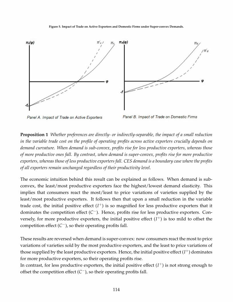
Figure 5. Impact of Trade on Active Exporters and Domestic Firms under Super-convex Demands.

Proposition 1 Whether preferences are directly- or indirectly-separable, the impact of a small reductionin the variable trade cost on the profile of operating profits across active exporters crucially depends ondemand curvature. When demand is sub-convex, profits rise for less productive exporters, whereas thoseof more productive ones fall. By contrast, when demand is super-convex, profits rise for more productiveexporters, whereas those of less productive exporters fall. CES demand is a boundary case where the profitsof all exporters remain unchanged regardless of their productivity level.

The economic intuition behind this result can be explained as follows. When demand is sub-convex, the least/most productive exporters face the highest/lowest demand elasticity. Thisimplies that consumers react the most/least to price variations of varieties supplied by theleast/most productive exporters. It follows then that upon a small reduction in the variabletrade cost, the initial positive effect (I+) is so magnified for less productive exporters that itdominates the competition effect (C−). Hence, profits rise for less productive exporters. Con-versely, for more productive exporters, the initial positive effect (I+) is too mild to offset thecompetition effect (C−), so their operating profits fall.

These results are reversed when demand is super-convex: now consumers react the most to pricevariations of varieties sold by the most productive exporters, and the least to price variations ofthose supplied by the least productive exporters. Hence, the initial positive effect (I+) dominatesfor more productive exporters, so their operating profits rise.In contrast, for less productive exporters, the initial positive effect (I+) is not strong enough tooffset the competition effect (C−), so their operating profits fall.

114

Curvature of Demand vs Type of Preferences: A Detailed Discussion

Clearly, the result highlighted above is solely attributable to added flexibility on the demandside in the current model. In deed, incorporating both cases of sub-convex and super-convexdemands opens the door for a more realistic modeling of consumer behavior than allowed bythe homothetic CES. The added flexibility here is that consumers may exhibit either a weak orstrong price sensitivity to the cheapest or the most expensive varieties. This, in turn, allows thegeneral equilibrium effect of trade to be heterogeneous across exporters beyond the CES case.

Here, again the type of preferences has minor implications for this result. Specifically, the natureof preferences solely determines whether the competition effect (C−) is identical across exportersor firm-specific. As previously mentioned, when preferences are indirectly-separable, (a) is al-ways equal to one (∀ϕ, a(ϕ) = 1), which clearly indicates that the competition effect is identicalacross exporters under this class of preferences.

By contrast, when preferences are directly-separable and non-CES, a(ϕ) may be either strictlyhigher or lower than one depending on demand curvature and the productivity level of the firmat question. That is, under sub-convex demands, a(ϕ) is strictly higher than one for the lessproductive exporters, and strictly lower than one for more productive exporters (∀ϕ → ϕ∗x,a(ϕ) > 1; ∀ϕ → +∞, a(ϕ) < 1).35 This order is reversed under super-convex demands(∀ϕ → ϕ∗x, a(ϕ) < 1; ∀ϕ → +∞, a(ϕ) > 1). Now I can easily verify that even when thecompetition effect is firm-specific, the novel result highlighted in Proposition 1 always holdswith the aid of the following example:

Under sub-convex demands, and directly-separable preferences, even though the competitioneffect is magnified for the least productive exporters, these latter experience a net increase intheir operating profits, as highlighted in Proposition 1. This immediately reveals that the initialpositive effect (I+) always dominates the competition effect (C−). Hence, it is the magnitude ofthe initial positive effect (I+) that pins down the sign of the net effect of trade on export profits,as reflected by Proposition 1. Finally, as demand curvature governs the magnitude of the initialpositive effect (I+), I can then conclude that demand curvature plays a first-order role in drivingthis result, while the type of preferences has only a second-order importance in this regard.

Impact of Trade on Purely Domestic Firms

As illustrated in panel B of Figures 4 and 5, trade liberalization always induces an increase inthe domestic cutoff, which reflects that increased exposure to trade forces the least productivedomestic firms to exit the market. While this is a standard result due to Melitz (2003), the noveltyhere is twofold.

35Given the definition of demand curvature and the expression of a(ϕ), this follows by inspection.

115

First, demand curvature determines the nature of the competitive effect of trade. Inspection ofProposition 1 reveals that whether demand is CES or not plays a critical role. When they are,operating profits of all active exporters remain unchanged, and thus additional export marketshares are entirely reapt by infra-marginal exporters. Increased labor demand by these newexporters bids up the real wage and forces the the least productive firms to exit, exactly as inMelitz (2003). Hence, as stressed by Melitz (2003), the rigidity of the CES constrains the compet-itive effect of trade to occur only on the labor market. It precludes then another important andmore intuitive channel for the competitive effect of trade, which operates through increases inthe intensity of competition on the final good market.36

However, beyond CES demand, higher exposure to trade always increases profits of one cat-egory of active exporters. Whether this latter corresponds to the most or the least productiveexporters, this crucially depends on whether demand is sub-convex or super-convex. This im-mediately ensures that under both alternatives, the competitive effect of trade operates throughan increase in the intensity of competition on the final good market.

Second, demand curvature governs the magnitude of the competitive effect of trade. As hintedto in the previous paragraph, demand curvature determines which category of active exportersreaps additional market shares upon trade liberalization. By doing so, it immediately pins downthe magnitude of firm exit. For instance, as highlighted in Proposition 1, when demand is super-convex, additional export market shares are reapt by the most productive exporters. Since thiscategory of exporters has initially large market shares, their increase (upon variable trade costreduction) leads then to a sharp increase in the intensity of competition. This, in turn, forces alarge fringe of domestic firms to exit the market.

In contrast, when demand is sub-convex, additional export market shares are reapt by the leastproductive exporters. Their market shares are initially small, and so their increase induces aslight increase in the intensity of competition. Hence, only a small fringe of domestic firms isforced to exit the market. The CES is then a special case where additional export market sharesare reapt by new exporters. Only under CES demand, these latter face the average demand elas-ticity (∀ϕ, σ(ϕ)=σ=σ). Hence, the magnitude of firm exit under CES demand can be consideredas an intermediate outcome.

36Melitz and Ottaviano (2008) restored a theoretical role for this channel using quadratic preferences, which arenon-additive.

116

2. A small Decrease in the Fixed Trade Cost

Now I study the case where higher exposure to trade occurs through a small reduction in thefixed cost of exporting fx. As in the previous case, I separately examine the welfare implicationsof the curvature of demand and the type of preferences. Using the standards measures proposedin Section 5.3, the magnitude of the gains from trade (GFT) and the net variety effect (NVE)which captures their structure are respectively given by:

GFT( f−x ) = −εϕ∗d( fx) =

[θ−ηx(σx(ϕx)−1)]η∗d [σ

∗d (ϕ∗d)−1+S]

a∗d(ϕ∗d)a∗x(ϕ∗x) θ+∆x

NVE( f−x ) ≡ 1η∗x [σ∗x (ϕ∗x)−1+S] − |εϕ∗d

( fx)| = 1η∗x [σ∗x (ϕ∗x)−1+S] −

[θ−ηx(σx(ϕx)−1)]η∗d [σ

∗d (ϕ∗d)−1+S]

a∗d(ϕ∗d)a∗x(ϕ∗x) θ+∆x

(3.33)

Inspection of the above expressions clearly shows that a small decrease in the fixed trade costinduces identical results to those described for the small reduction in the variable trade cost.

The only difference here is in the theoretical mechanism driving the result. In deed, under thisscenario of trade liberalization, such small reduction in the fixed cost of exporting encouragesentry of infra-marginal firms to the export market. As to whether they capture small or largemarket shares, this crucially depends on demand curvature. When demand is super-convex,these new exporters face the lowest demand elasticity, their relatively low productivity level isthus a mild disadvantage under this case and so, they capture large market shares. This, in turn,magnifies the import competition effect. This induces then a strong selection effect of trade, forc-ing a large fringe of domestic firms to exit the market. These patterns are reversed when demandis sub-convex. As it imposes the demand elasticity to be identical across firms, CES demand isclearly a boundary case.

Therefore, by magnifying Melitz (2003)’s selection effect, super-convex demands provides anupper bound for the gains from trade. As before, sub-convex demands provide a lower bound,while the CES delivers an intermediate outcome. As for the structure of the gains from trade, it isreadily verified that, as before, gains from selection and net variety gains coexist only under sub-convex demands. Additionally, under this curvature of demand, when preferences are directly-separable, the pro-competitive effect of trade on domestic markups is operative, and thus thethree sources of welfare gains from trade coexist.

117

3. A small Increase in the Number of Trading Countries N

Similarly, I can now investigate the case where higher exposure to trade occurs through a smallincrease in the number of trading countries at the World level. As in the previous two cases,the objective is to separately examine the welfare implications of the curvature of demand andthe type of preferences. As before, using the standards measures proposed in Section 5.3, themagnitude of the gains from trade (GFT) and the net variety effect (NVE) which captures theirstructure are respectively given by:

GFT(N+) = εϕ∗d(N) = η∗x [σ

∗x (ϕ∗x)−1+S]

η∗d [σ∗d (ϕ∗d)−1+S]

a∗d(ϕ∗d)a∗x(ϕ∗x) θ+∆x

NVE(N+) ≡ 1− εϕ∗d(N) = 1 − η∗x [σ

∗x (ϕ∗x)−1+S]

η∗d [σ∗d (ϕ∗d)−1+S]

a∗d(ϕ∗d)a∗x(ϕ∗x) θ+∆x

(3.34)

Inspection of the above expressions clearly shows that a small increase in the number of tradingcountries yields identical results to those described for the two previous scenarios.

The only difference here is in the theoretical mechanism underlying the result. In deed, underthis scenario of trade liberalization, such small increase in the number of countries implies thatdomestic firms in any existing country face an additional competition from exporters in thesenewly trading countries. As to whether this competition effect is strong or mild , this is fully gov-erned by demand curvature. When demand is super-convex, additional export market sharesare reapt by the most productive exporters in these newly trading countries. This, in turn, mag-nifies the import competition effect, which induces then a strong selection effect of trade, forcinga large fringe of domestic firms to exit the market. These patterns are reversed when demand issub-convex. As it imposes the demand elasticity to be identical across exporters, CES demand isclearly a boundary case.

Hence, as before, by magnifying Melitz (2003)’s selection effect, super-convex demands pro-vides an upper bound for the gains from trade. Sub-convex demands provide a lower bound,while the CES delivers an intermediate outcome. As for the structure of the gains from trade,it is readily verified that, as before, gains from selection and net variety gains coexist only un-der sub-convex demands. Additionally, under this curvature of demand, when preferences aredirectly-separable, the pro-competitive effect of trade on domestic markups is restored. There-fore, these three sources of welfare gains from trade coexist if and only if demand is sub-convexand preferences are directly-separable.

118

3.6 Conclusion

This chapter develops a general yet tractable theoretical framework which combines standardassumptions on the supply side with a flexible demand system, while taking variable and fixedtrade barriers in due account. The current model is then well-suited to examine the welfare im-plications of different scenarios of trade liberalization under general demand conditions. Thenovelty here is that it is possible to separately examine the implications of the curvature of de-mand and the type of preferences for the gains from trade. The key finding of this chapter isthat while demand curvature plays a crucial role in driving comparative statics results and de-termining the structure and the magnitude of the gains from trade, the type of preferences hasonly a second-order importance from a welfare standpoint. A key message of this chapter is thatrather than assuming a specific type of preferences, more precise estimates of the curvature ofdemand are necessary to answer comparative statics questions, and to quantify the gains fromtrade.

119

Appendix D

D.1 Deriving firm-level revenues in partial equilibrium

Let us start with recalling that the price aggregator is the implicit solution of the following equa-tion:

∫ω∈Ω

pω Q(Λ) Dω(V(Λ)pω

w) dω = w (3.35)

Now using the parameterization of functions Q(Λ) and V(Λ): Q(Λ)=Λ−β, V(Λ)=Λα, and re-calling that the elasticity of each function with respect to its determinant is given by: εQ = −β,εV= α, and εDω = −σω > 1, along with normalizing wage to unity (w=1) by choice of labor asnuméraire, and rearranging yields:

Λ = [∫

ω∈Ωp1−σω

ω dω]1

(β+ασ) (3.36)

where σ is the average demand elasticity at the industry level, α and β are both dummies captur-ing the type of preferences, such as the case (α=0 and β=1) corresponds to indirectly-separablepreferences, while directly-separable preferences correspond to (α=1 and β=0).

Now let us denote by P(Λ) = Λ−(β+α σ) = [∫

ω∈Ω p1−σωω dω]−1 the conventional price index. Then,

with the aid of the parameterization along with the above definition of the conventional priceindex P, the Gorman-Pollak demand function described in equation (3.1) (in the main text) boilsdown to xω = p−σω

ω Paω , where aω = β+α σω

β+α σ . By assuming that any ω variety is supplied by aϕ productivity firm, I can work throughout with ϕ as a firm subscript: σω = σ(ϕ); aω = a(ϕ).Finally, by recalling that consumers are identical and a firm’s market demand is given byq(ϕ) = x(ϕ) L, firm revenues boil down to: r(ϕ) = p(ϕ) q(ϕ) = p(ϕ)1−σ(ϕ) Pa(ϕ) L.

120

D.2 The "Exponent Elasticity Method" (EEM)

As stressed in the main text, increased generality raises tractability issues. Thus, in order togain in generality without losing in tractability, I resort to a new and simple method that I callthe "Exponent Elasticity Method" (EEM, hereafter) which delivers a tractable solution for thegeneral equilibrium price index despite added flexibility in preferences. The starting point is thepartial equilibrium expression of the price index provided in equation (3.14) in the main text:

P = M−1e [

∫ +∞

ϕ∗d

pd(ϕ)1−σ(ϕ)g(ϕ)dϕ︸ ︷︷ ︸Id

+ (N − 1)∫ +∞

ϕ∗xpx(ϕ)1−σ(ϕ)g(ϕ)dϕ︸ ︷︷ ︸

Ix

]−1

Clearly, the mathematical challenge consists in solving for both integrals (Id, Ix) without assum-ing that the demand elasticity is identical across firms (∀ϕ, σ(ϕ) = σ) and then using this latteras a constant for integrating. Such simplicity is only possible under CES demand, which is theunique case where it is possible to solve for these integrals. As the general demand system con-sidered in this chapter encompasses the CES and more flexible alternatives allowing the demandelasticity to vary across firms, it is then impossible to solve for these integrals under general de-mands.

Given the impossibility to solve for these integrals in the current setting, the key idea that theEEM method proposes is to locally approximate both integrals (Id, Ix) around the equilibriumwith a multiplicative equivalent which has a finite number of determinants, such as the exponentof each determinant embodies the elasticity of the average price with respect to it.37 This requiresa five-step procedure that I explain in detail as follows.

The "EEM" method: A Five-step Procedure

Step 1. Rewrite the integral (Ix) using unbounded Pareto:

By invoking this assumption, it is readily verified that [1− G(ϕ∗x)] = ϕ∗x−θ. Using this, integral

Ix can be rewritten as:

Ix = ϕ∗x−θ

∫ +∞

ϕ∗xpx(ϕ)1−σ(ϕ) µx(ϕ)dϕ︸ ︷︷ ︸

Ix0

(3.37)

37To be precise, this corresponds to the average price to the power of (1− σ): p1−σdd and p1−σx

x .

121

where µx(ϕ) = g(ϕ)[1−G(ϕ∗x)]

is the productivity distribution conditional on successful penetrationof the export market. Clearly, the unique difference between the initial integral Ix and the newintegral Ix0 is that this latter is expressed using the conditional productivity distribution µx(ϕ).

Step 2. Approximate integral Ix0 with a multiplicative equivalent:

Now by recalling that η(ϕ) = - dlog p(ϕ)dlog ϕ is our measure of the relative cost-price pass-through

and that the variable trade cost τ is multiplicative by definition, the integral Ix0 can be locallyapproximated as follows:

Ix0 ≡ τηx(1−σx(ϕx)) ϕx(ϕ∗x)ηx(σx(ϕx)−1) (3.38)

Since operating profits are monotonically increasing in productivity, and exporting involves notonly, a variable trade cost τij, but also a fixed cost fx, the equilibrium export cutoff ϕ∗x exists andis unique. This, in turn, ensures that this local approximation (around the trade equilibrium)delivers a unique multiplicative equivalent to integral Ix0 .

Step 3. Obtain a final expression of integral Ix using this of Ix0 and unboundedPareto:

Let us now recall that unbounded Pareto distribution gives rise to constant mean-to-min ratio:ϕx = θ

θ−1 ϕ∗x. By plugging the multiplicative equivalent of integral Ix0 from equation (3.38) intothe initial expression of integral Ix in equation (3.37) and invoking this practical property ofunbounded Pareto, I obtain the following multiplicative equivalent for integral Ix:

Ix ≡ κ τηx(1−σx(ϕx)) ϕ∗x[ηx(σx(ϕx)−1)−θ] (3.39)

where κ = ( θθ−1)

ηx(σx(ϕx)−1) is a constant.

Step 4. Approximate the partial equilibrium export cutoff ϕ∗x with an explicitmultiplicative equivalent:

Let us first recall that the export cutoff ϕ∗x is endogenous and defined as the implicit solution ofthe zero profit condition on the export market (ZPCX): πx(ϕ∗x)=0, described in equation (3.13) inthe main text:

122

(ZPCX) ϕ∗x : σ∗x (ϕ∗x)−1 p∗x(ϕ)1−σ∗x (ϕ∗x) Pa∗x(ϕ∗x) L = fx (3.40)

Now by isolating the firm-specific component of the operating profit on the left hand-side, ap-proximating it in a multiplicative way, as in equation (3.38), and rearranging, I obtain the fol-lowing explicit equivalent of the partial equilibrium export cutoff:

ϕ∗x ≡ τ f1

η∗x [σ∗x (ϕ∗x)−1+S]x L

− 1η∗x [σ∗x (ϕ∗x)−1+S]

j P− a∗x(ϕ∗x)

η∗x [σ∗x (ϕ∗x)−1+S] (3.41)

Step 5. Solving for the general equilibrium price aggregator P :

Now by plugging the explicit equivalent of the export cutoff from equation (3.41) in the ex-pression of integral Ix in equation (3.39), this latter can be expressed solely as a function of(τ, fx, L, P).Then, by applying the same procedure for integral Id, and plugging the final expressions of bothintegrals in the partial equilibrium price index given by equation (3.14) in the main text, andrearranging, I obtain a tractable solution for the general equilibrium price index:

P ≡ c[1 + ε Ix (P)]−1

E L−[

1 + ε Ix (L)1 + ε Ix (P) ] T(τ, fx, N)−[1 + ε Ix (P)]−1

(3.42)

where cE = σ [ fe + [1− G(ϕ∗d)] f + (N − 1)[1− G(ϕ∗x)] fx ] captures entry conditions in everycountry,

T(τ, fx, N) =N τ−θ f− [θ−ηx(σx(ϕx)−1)]

η∗x [σ∗x (ϕ∗x)−1+S]x is an index of exposure to trade, and both elasticities ε Ix(L)

and ε Ix(P) take a simple form, and are respectively given by:

ε Ix(L) = [θ−ηx(σx(ϕx)−1)]η∗x [σ∗x (ϕ∗x)−1+S] > 0

ε Ix(P) = a∗x(ϕ∗x)[θ−ηx(σx(ϕx)−1)]η∗x [σ∗x (ϕ∗x)−1+S] > 0

(3.43)

123

D.3 Solving for the domestic and export cutoffs in general equi-librium

By plugging the general equilibrium price index from equation (3.42) in the explicit partial equi-librium expression of the export cutoff in equation (3.41), and applying the same procedure forthe domestic cutoff, I can solve for their general equilibrium expressions, respectively, as follows:

ϕ∗x ≡ τ fεϕ∗x ( fx)x cγ∗x

E Lεϕ∗x (L) T(τ, fx, N)εϕ∗x (T) (3.44)

where the above exponents are respectively given by:

εϕ∗x( fx) =1

η∗x [σ∗x (ϕ∗x)−1+S]

γ∗x = − a∗x(ϕ∗x)η∗x [σ∗x (ϕ∗x)−1+S] [1 + ε Ix(P)]−1

εϕ∗x(L) = 1η∗x [σ∗x (ϕ∗x)−1+S] [ a∗x(ϕ∗x)

1 + ε Ix (L)1 + ε Ix (P) − 1 ]

εϕ∗x(T) =a∗x(ϕ∗x)

η∗d [σ∗x (ϕ∗x)−1+S] [1 + ε Ix(P)]−1

Similarly, the general equilibrium domestic cutoff can be written as:

ϕ∗d ≡ fεϕ∗d

( f )cγ∗d

E Lεϕ∗d

(L)T(τ, fx, N)

εϕ∗d(T)

(3.45)

where the above exponents are respectively given by:

εϕ∗d( f ) = 1

η∗d [σ∗d (ϕ∗d)−1+S]

γ∗d = − a∗d(ϕ∗d)η∗d [σ

∗d (ϕ∗d)−1+S] [1 + ε Ix(P)]−1

εϕ∗d(L) = 1

η∗d [σ∗d (ϕ∗d)−1+S] [ a∗d(ϕ∗d)

1 + ε Ix (L)1 + ε Ix (P) − 1 ]

εϕ∗d(T) = a∗d(ϕ∗d)

η∗d [σ∗d (ϕ∗d)−1+S] [1 + ε Ix(P)]−1

D.4 Solving for the weighted average productivity at the indus-try level in general equilibrium

As mentioned in the main text, the weighted average productivity of all firms (both domesticand foreign exporters) competing in a single country can be written as:

124

ϕ =Md

MW

∫ +∞

ϕ∗d

ϕ µd(ϕ)dϕ +(N − 1)Mx

MW

∫ +∞

ϕ∗xϕ µx(ϕ)dϕ (3.46)

where MW = NMe is the total mass of entrants at the World level, and can be thought of as aproxy for the size of the World market. By solving for the above integrals, ϕ can be then writtenas a function of the domestic and the export cutoffs:

ϕ =Md

MW(

θ

θ − 1) ϕ∗d +

(N − 1)Mx

MW(

θ

θ − 1) ϕ∗x (3.47)

Now using the general equilibrium expressions of the export and domestic cutoffs, respectively,from equations (3.44) and (3.45), the ratio ϕ∗x

ϕ∗dcan be written as:

ϕ∗xϕ∗d

= τ (f

εϕ∗x ( fx)x

fεϕ∗d

( f )) c∆x,d(cE)

E L∆x,d(L) T∆x,d(T) (3.48)

where ∆x,d(cE) = γ∗x - γ∗d , ∆x,d(L) = εϕ∗x(L) - εϕ∗d(L), and ∆x,d(T) = εϕ∗x(T) - εϕ∗d

(T).Using the above relationship between the export and the domestic cutoff, the weighted averageproductivity in equation (3.47) can be rewritten as follows:

ϕ = ϕ∗d Ψ(.) (3.49)

where Ψ(.) = [ MdMW

( θθ−1) +

(N−1)MxMW

( θθ−1) τ ( f

εϕ∗x( fx)

x

fεϕ∗d

( f ) ) c∆x,d(cE)E L∆x,d(L) T∆x,d(T) ] > 1.

D.5 Proof of Theorem 2

Theorem 2 states that on any market (domestic, or export), super-convex demands provide anupper bound for the productivity cutoff in general equilibrium, while sub-convex demands pro-vide a lower bound. Within these bounds, the CES delivers an intermediate result. This canbe shown using the general equilibrium expression of the domestic cutoff in equation (3.45) (or,equivalently this of the general equilibrium export cutoff) as follows:Let ϕ∗d(super), and ϕ∗d(sub) denote the domestic cutoffs, respectively, under super-convex de-

mands, and sub-convex demands. Using equation (11), the ratio ϕ∗d [super]ϕ∗d [sub] can be written as:

125

ϕ∗d[super]ϕ∗d[sub]

= f ∆1 c∆2E L∆3 T∆4 (3.50)

Using the expressions of the elasticity of the general equilibrium domestic cutoff with respect toeach of its determinants provided in equation (3.45), ∆1, ∆2, ∆3, and ∆4 are respectively givenby:

∆1 = εϕ∗d( f )[super] − εϕ∗d

( f )[sub]

∆2 = γ∗d [super] − γ∗d [sub]

∆3 = εϕ∗d(L)[super] − εϕ∗d

(L)[sub]

∆4 = εϕ∗d(T)[super] − εϕ∗d

(T)[sub]

Finally, inspecting the expressions of the above elasticities, and recalling that the firm at thecutoff faces the lowest demand elasticity under super-convex demands, whereas it faces the

highest demand elasticity under sub-convex demands, immediately reveals that ϕ∗d [super]ϕ∗d [sub] > 1.

Since under CES demand, the cutoff productivity firm faces the average demand elasticity, thisensures then that the CES delivers an intermediate result:ϕ∗d[sub− convex] < ϕ∗d[CES] < ϕ∗d[super− convex].

D.6 Proof of Theorem 3

Theorem 3 states that super-convex demands provide a lower bound for the degree of parti-tioning of firms by export status in general equilibrium, while sub-convex demands provide anupper bound. Within these bounds, the CES delivers an intermediate result. This can be shownusing the general equilibrium expression of the ratio ϕ∗x

ϕ∗din equation (3.48), as follows:

ϕ∗xϕ∗d

= (f

εϕ∗x ( fx)x

fεϕ∗d

( f ))︸ ︷︷ ︸

(1)

τ c∆x,d(cE)E L∆x,d(L) T∆x,d(T) (3.51)

Since entry conditions cE, market size L, and the degree of exposure to trade T are identicalacross countries, the partitioning of firms by export status is mainly driven by the presence ofvariable and fixed trade barriers. Hence, inspecting the above ratio while restricting our focus onits first component (1), and recalling that under super-convex demands, the firm at the domesticcutoff faces a lower demand elasticity than the firm at the export cutoff and that this order

126

is reversed under sub-convex demands, immediately reveals that ϕ∗xϕ∗d

[super-convex] < ϕ∗xϕ∗d

[sub-convex]. Finally, recalling that under CES demands both cutoff firms face the same demandelasticity σ∗d = σ∗x = σ ensures that the CES delivers an intermediate outcome, and thus completesthe proof.

127

Bibliography

Anderson, James E and Eric Van Wincoop (2003). “Gravity with gravitas: a solution to the borderpuzzle”. In: American economic review 93.1, pp. 170–192.

Arkolakis, Costas, Arnaud Costinot, and Andres Rodriguez-Clare (2012). “New trade models,same old gains?” In: American Economic Review 102.1, pp. 94–130.

Arkolakis, Costas et al. (2018). “The elusive pro-competitive effects of trade”. In: The Review ofEconomic Studies 86.1, pp. 46–80.

Bernard, Andrew B et al. (2007). “Firms in international trade”. In: Journal of Economic perspectives21.3, pp. 105–130.

Bertoletti, Paolo and Federico Etro (2016). “Monopolistic competition when income matters”. In:The Economic Journal 127.603, pp. 1217–1243.

— (2017). “Monopolistic competition when income matters”. In: The Economic Journal 127.603,pp. 1217–1243.

Bertoletti, Paolo, Federico Etro, and Ina Simonovska (2018). “International trade with indirectadditivity”. In: American Economic Journal: Microeconomics 10.2, pp. 1–57.

Carrère, Céline, Monika Mrázová, and J Peter Neary (2020). “Gravity Without Apology: the Sci-ence of Elasticities, Distance and Trade”. In: The Economic Journal 130.628, pp. 880–910.

Chaney, Thomas (2008). “Distorted gravity: the intensive and extensive margins of internationaltrade”. In: American Economic Review 98.4, pp. 1707–21.

Chen, Maggie Xiaoyang and Aaditya Mattoo (2008). “Regionalism in Standards: Good or Badfor Trade?” In: Canadian Journal of Economics/Revue canadienne d’économique, pp. 838–863.

Comin, Diego A, Danial Lashkari, and Martí Mestieri (2015). Structural change with long-run in-come and price effects. Tech. rep. National Bureau of Economic Research.

De Loecker, Jan and Frederic Warzynski (2012). “Markups and firm-level export status”. In:American economic review 102.6, pp. 2437–71.

128

Demidova, Svetlana (2008). “Productivity improvements and falling trade costs: boon or bane?”In: International Economic Review 49.4, pp. 1437–1462.

Demidova, Svetlana and Andres Rodriguez-Clare (2013). “The simple analytics of the Melitzmodel in a small economy”. In: Journal of International Economics 90.2, pp. 266–272.

Di Comite, Francesco, Jacques-François Thisse, and Hylke Vandenbussche (2014). “Verti-zontaldifferentiation in export markets”. In: Journal of International Economics 93.1, pp. 50–66.

Disdier, Anne-Célia, Lionel Fontagné, and Olivier Cadot (2015). “North-South standards harmo-nization and international trade”. In: The World Bank Economic Review 29.2, pp. 327–352.

Faber, Benjamin and Thibault Fally (2017). Firm heterogeneity in consumption baskets: Evidence fromhome and store scanner data. Tech. rep. National Bureau of Economic Research.

Fally, Thibault (2018). Integrability and generalized separability. Tech. rep. National Bureau of Eco-nomic Research.

— (2019). “Generalized separability and the gains from trade”. In: Economics Letters 178, pp. 8–12.

Feenstra, Robert C (2010). “Measuring the gains from trade under monopolistic competition”.In: Canadian Journal of Economics/Revue canadienne d’économique 43.1, pp. 1–28.

— (2018). “Restoring the product variety and pro-competitive gains from trade with heteroge-neous firms and bounded productivity”. In: Journal of International Economics 110, pp. 16–27.

Fieler, Ana Cecilia (2011). “Nonhomotheticity and bilateral trade: Evidence and a quantitativeexplanation”. In: Econometrica 79.4, pp. 1069–1101.

Guimbard, Houssein et al. (2012). “MAcMap-HS6 2007, an exhaustive and consistent measureof applied protection in 2007”. In: International Economics 130, pp. 99–121.

Handbury, Jessie (2019). Are poor cities cheap for everyone? non-homotheticity and the cost of livingacross us cities. Tech. rep. National Bureau of Economic Research.

Kimball, Miles S (1995). “The quantitative analytics of the basic neomonetarist model”. In: Journalof Money, Credit, and Banking 27.4, p. 1241.

Krugman, Paul (1980). “Scale economies, product differentiation, and the pattern of trade”. In:The American Economic Review 70.5, pp. 950–959.

Krugman, Paul R (1979). “Increasing returns, monopolistic competition, and international trade”.In: Journal of international Economics 9.4, pp. 469–479.

129

Linder, Staffan Burenstam (1961). An essay on trade and transformation. Almqvist & Wiksell Stock-holm.

Markusen, James R (2013). “Putting per-capita income back into trade theory”. In: Journal ofInternational Economics 90.2, pp. 255–265.

Mayer, Thierry and Gianmarco Ottaviano (2007). “The happy few: new facts on the internation-alisation of European firms”. In: Bruegel-CEPR EFIM2007 Report, Bruegel Blueprint Series 3.

Melitz, Marc J (2003). “The impact of trade on intra-industry reallocations and aggregate indus-try productivity”. In: econometrica 71.6, pp. 1695–1725.

Melitz, Marc J and Gianmarco IP Ottaviano (2008). “Market size, trade, and productivity”. In:The review of economic studies 75.1, pp. 295–316.

Melitz, Marc J and Stephen J Redding (2015). “New trade models, new welfare implications”. In:American Economic Review 105.3, pp. 1105–46.

Mrázová, Monika and J Peter Neary (2014). “Together at last: trade costs, demand structure, andwelfare”. In: American Economic Review 104.5, pp. 298–303.

— (2017). “Not so demanding: Demand structure and firm behavior”. In: American EconomicReview 107.12, pp. 3835–74.

Olivero, María Pía and Yoto V Yotov (2012). “Dynamic gravity: endogenous country size andasset accumulation”. In: Canadian Journal of Economics/Revue canadienne d’économique 45.1,pp. 64–92.

Otsuki, Tsunehiro, John S Wilson, and Mirvat Sewadeh (2001). “Saving two in a billion:: quanti-fying the trade effect of European food safety standards on African exports”. In: Food policy26.5, pp. 495–514.

Silva, JMC Santos and Silvana Tenreyro (2006). “The log of gravity”. In: The Review of Economicsand statistics 88.4, pp. 641–658.

Simonovska, Ina (2015). “Income differences and prices of tradables: Insights from an onlineretailer”. In: The Review of Economic Studies 82.4, pp. 1612–1656.

Trefler, Daniel (2004). “The long and short of the Canada-US free trade agreement”. In: AmericanEconomic Review 94.4, pp. 870–895.

Yotov, Yoto V et al. (2016). An advanced guide to trade policy analysis: The structural gravity model.World Trade Organization Geneva.

Zhelobodko, Evgeny et al. (2012). “Monopolistic competition: Beyond the constant elasticity ofsubstitution”. In: Econometrica 80.6, pp. 2765–2784.

130