Federal Reserve Bank of Minneapolis Research Department Staff Report 544

February 2018

Firm Entry and Exit and Aggregate Growth*

Jose Asturias

Georgetown University Qatar

Sewon Hur University of Pittsburgh

Timothy J. Kehoe University of Minnesota, Federal Reserve Bank of Minneapolis, and National Bureau of Economic Research

Kim J. Ruhl Pennsylvania State University

ABSTRACT___________________________________________________________________ Applying the Foster, Haltiwanger, and Krizan (FHK) (2001) decomposition to plant-level manufacturing data from Chile and Korea, we find that a larger fraction of aggregate productivity growth is due to entry and exit during periods of fast GDP growth. Studies of other countries confirm this empirical relationship. To analyze this relationship, we develop a simple model of firm entry and exit based on Hopenhayn (1992) in which there are analytical expressions for the FHK decomposition. When we introduce reforms that reduce entry costs or reduce barriers to technology adoption into a calibrated model, we find that the entry and exit terms in the FHK decomposition become more important as GDP grows rapidly, just as they do in the data from Chile and Korea. ______________________________________________________________________________ Keywords: Entry, Exit, Productivity, Entry costs, Barriers to technology adoption JEL Codes: E22, O10, O38, O47 *This paper has benefited from helpful discussions at numerous conference and seminar presentations. We thank Paco Buera, V.V. Chari, Hal Cole, John Haltiwanger, Boyan Jovanovic, Joseph Kaboski, Pete Klenow, Erzo G.J. Luttmer, Ezra Oberfield, B. Ravikumar, Felipe Saffie, and Juan Sanchez for helpful discussions. We also thank James Tybout, the Instituto National de Estadística of Chile, and the Korean National Statistical Office for their assistance in acquiring data. All of the publically available data used in this paper can be found at http://users.econ.umn.edu/~tkehoe/. The views expressed herein are those of the authors and not necessarily those of the Federal Reserve Bank of Minneapolis or the Federal Reserve System.

1

1. Introduction

Findings in empirical studies vary widely on the importance of the entry and exit of plants in

accounting for aggregate productivity growth. Consider, for example, two widely cited studies:

Foster, Haltiwanger, and Krizan (FHK) (2001) find that the entry and exit of plants account for 25

percent of U.S. manufacturing productivity growth, while Brandt, et al. (2012), using the same

decomposition, find that entry and exit account for 72 percent of Chinese manufacturing

productivity growth.1 In this paper, we account for the stark differences in the U.S. and Chinese

data both by examining data from other countries and by developing a simple model in which we

can understand the driving forces behind those differences.

The first contribution of this paper is empirical. We apply the FHK decomposition to

manufacturing plant-level data from Chile and Korea. We find that plant entry and exit account for

a larger fraction of aggregate manufacturing productivity growth during periods of fast growth in

GDP per working-age person. A meta-analysis of the productivity literature, spanning a number of

countries and time periods, supports this empirical regularity. We summarize our findings in Figure

3, in which we plot growth in GDP per working-age person against the contribution of the entry

and exit of plants to growth in aggregate manufacturing productivity. This empirical relationship

is novel to the literature and suggests that the entry and exit of plants play an important role in

explaining periods of fast growth.

Our second contribution is theoretical. We develop a dynamic general equilibrium model with

endogenous entry and exit, based on Hopenhayn (1992), that can quantitatively account for the

patterns we document in the data. Our model is simple enough that there are analytical expressions

that correspond to terms in the FHK decomposition. When we introduce reforms that reduce entry

costs or reduce barriers to technology adoption into a calibrated model, we find that the entry and

exit terms in the FHK decomposition become more important as GDP grows rapidly, just as they

do in the data. Our simple model, meant to highlight the forces driving productivity growth,

performs surprisingly well in quantitatively matching the behavior we observe in the data.

Our general equilibrium model is of the entire economy, but the productivity decompositions

in both the existing literature and our own work cover only the manufacturing sector. If we could

1 To calculate that entry and exit account for 25 percent of U.S. manufacturing productivity growth, see Table 8.7 in FHK and find the average net entry share for the 1977–1982, 1982–1987, and 1987–1992 windows. To find the contribution of entry and exit in China, see Figure 7 in Brandt, et al. (2012).

2

compute the FHK decompositions using economy-wide data for Chile and Korea and we could

find comparable results for other countries in the literature, then we would not need to restrict

ourselves to the manufacturing sector. Due to the availability of data, we assume that the FHK

decomposition for aggregate manufacturing productivity growth assigns the same proportions to

entry and exit of plants as would a decomposition of aggregate productivity growth for the whole

economy. This assumption allows us to make comparisons between the model and the data.

In our empirical work, Chile and South Korea are good candidates for our analysis because

both countries have experienced periods of fast and slow growth. Real GDP per working-age

person in Chile grew 4.0 percent per year during 1995–1998, slowing to 2.7 percent per year during

2001–2006. In South Korea, real GDP per working-age person grew by 6.1 percent per year in

1992–1997 and by 4.3 percent per year in 2001–2006 and slowed to 3.0 percent per year in 2009–

2014. Studying periods of slow and fast growth in the same country allows us to avoid cross-

country differences and use consistent datasets through time, which reduces issues of

measurement.

We use the FHK decomposition to measure the contribution of net entry. In this

decomposition, the net entry term is higher if entering plants are relatively productive compared

to the overall industry, and exiting plants are relatively unproductive. The continuing plant

contribution consists of both within-plant productivity dynamics and the reallocation of market

shares across continuing plants. We find that, in both countries, net entry plays a more important

role during periods of fast GDP growth. During periods of slow growth, when GDP per working-

age person grows at less than 4 percent per year, entry and exit account for less than 25 percent of

aggregate manufacturing productivity growth on average, similar to the average contribution of

entry and exit in the United States. During periods of fast GDP growth, however, entry and exit

account for a larger fraction of aggregate manufacturing productivity growth, ranging from 37 to

58 percent. We also find that the increasing importance of entry and exit is mainly driven by the

change in the relative productivity of entering and exiting plants, rather than by differences in their

market shares. Our findings are robust to using alternative decompositions.

Our own analysis is limited by the availability of establishment-level data. Fortunately, the

FHK decomposition is widely used in the productivity literature. To get a broader understanding

of the empirical relationship between growth and the role of net entry, we survey papers in the

literature that use the FHK decomposition. We find that continuing establishments — plants in

3

four of the papers, firms in the other papers — consistently account for the bulk of aggregate

manufacturing productivity growth when GDP per working-age person grows slowly. During

episodes of fast GDP growth, the entry and exit of plants play a more important role.

Motivated by our empirical work with the FHK decomposition, we build a simple model that

has three sources of productivity growth. First, in each period, potential entrants draw efficiencies

from a distribution with a mean that grows at rate 1eg − . Second, continuing firm efficiencies

improve with age. This efficiency growth depends on an exogenous growth factor and spillovers

from average efficiency growth. Finally, firms optimally choose when to exit production, which

induces a selection effect in which inefficient firms exit.

The economy is subject to three types of policy distortions. First, a potential entrant must pay

an entry cost to draw an efficiency. Second, a successful entrant must pay a fixed cost to continue

production in each period. These two costs are partly technological and partly the result of policy.

We think of these policy-related costs as distortions that can be reduced through economic reform.

Third, new firms face barriers to technology adoption in the spirit of Parente and Prescott (1994).

Better technologies exist but are not used because of policies that restrict their adoption.

We show that the model has a balanced growth path on which income grows at the same rate

regardless of the severity of the policy distortions. Income levels on the balanced growth path,

however, are determined by the distortions: More severe distortions yield lower balanced growth

paths. These results are consistent with the data from the United States and other industrialized

economies. These economies have grown at about 2 percent per year for several decades, despite

persistent differences in income levels. Kehoe and Prescott (2002) provide an in-depth discussion

of these empirical regularities. Similarly, Jones (1995) discusses the stable growth rates shown by

the United States over extended periods of time.

The simplicity of our model allows us to analytically characterize the FHK decompositions of

the model on the balanced growth path. The decompositions highlight the ways that firm turnover,

selection, and the efficiency advantage of entrants affect the contribution of net entry to aggregate

productivity growth. These forces are present in many of the growth models in the literature, and

our model allows us to understand how they map into empirical decompositions.

We further show that, in the balanced growth path, the contribution of entry and exit to

productivity growth, just like GDP growth rates, is the same for all economies on the balanced

growth path regardless of the level of distortions in the model. We also show that, under certain

4

parameters, the importance of entry and exit is decreasing in the efficiency growth of continuing

firms, a fact that we use in our calibration strategy.

After enacting a reform, the economy grows quickly and eventually converges to a higher

balanced growth path. This overall pattern is also consistent with empirical evidence of episodes

of fast growth. For example, Eichengreen et al. (2012) study episodes of fast growth followed by

economic slowdowns. Using data that starts in 1957, they consider a slowdown to have occurred

if the seven-year average GDP per capita growth rate is at least 3.5 percent for seven years prior

to the slowdown, and the growth rate exhibited a decline of at least 2 percentage points in the

subsequent seven years after the slowdown. The authors restrict the sample to countries with GDP

per capita of at least $10,000 in 2005 constant dollars at the time of the slowdown. They find that,

in the average country that experienced a slowdown, the growth rate slowed from 5.6 to 2.1 percent

per year.

We calibrate the model to establishment-level data for the entire U.S. economy. The major

exception to using economy-wide data in the calibration of our model is that we target the fact that

entry and exit account for 25 percent of U.S. aggregate manufacturing productivity growth

according to FHK, which we assume to be the fraction of growth due to entry and exit in the entire

economy. Our model also includes spillovers from growth of entering firms to continuing firms.

In estimating these spillovers, we rely on manufacturing data from Chile and Mexico, which also

is an exception to calibrating to establishment-level data of the entire U.S. economy.

After calibrating the model, we document the reforms that took place in Chile and Korea

during the periods of fast GDP growth. We find that the majority of reforms during these periods

can be interpreted as the lowering of entry costs and the barriers to technology adoption in the

context of our model.

We create three separate distorted economies to evaluate reforms to entry costs, barriers to

technology adoption, and fixed continuation costs. The spirit of the exercise is that these distorted

economies are exactly the same as the U.S. economy except for the policy distortion that we are

studying. We raise one of the distortions in each economy so that the balanced growth path income

level is 15 percent below that of the United States. It is important to note that, in the balanced

growth path, these distorted economies grow at 2 percent per year and net entry accounts for 25

percent of aggregate productivity growth.

5

We then remove the distortion in each economy and study the transition to the higher balanced

growth path. When we lower entry costs, the GDP growth rate rises to 4.6 percent per year for five

years, and entry and exit account for 60 percent of productivity growth. In that sense, the model

matches the increasing importance of firm entry and exit during periods of fast GDP growth, even

though the model is calibrated so that entry and exit are relatively unimportant in the balanced

growth path. We also find that the model has patterns that are similar to the neoclassical growth

model. For example, immediately after a reform, interest rates increase due to a boom in

investment from more potential entrants paying the entry cost. The increase in interest rates

discourages consumption, and consumption growth temporarily declines immediately after the

reform. Decreasing barriers to technology adoption in the model is quantitatively similar.

Not all reforms, however, generate the dynamics consistent with the data. When we lower

fixed continuation costs in this economy, the economy experiences GDP growth, but this fast

growth is accompanied by a decline in aggregate productivity. Lowering the fixed continuation

cost allows less productive firms to enter and prevents less productive firms from exiting, which

results in a decline in aggregate productivity during periods of fast growth in GDP. The reform

also results in capital deepening: GDP increases, labor input remains fixed, and aggregate

productivity falls, which implies that there are increases in the capital stock. The increase in the

capital stock is due to the increased number of firms in the economy.

What do we learn from comparing the different simulations? Consider the results from the

experiment in which we lower entry costs and the results of the experiment in which we lower

barriers to technology adoption. Except for an increase in potential entry, the transitions in the two

experiments are the same. The reason is that the increasing number of firms that try to enter and

fail when entry costs are lowered push up the efficiency cutoff for successful firms to operate. This

mechanism is very much in the spirit of Schumpeter (1942). Thus, we find that lowering entry

costs is almost equivalent to improving the potential technology from which firms draw. Results

from the experiment in which we lower the fixed continuation cost show that reforms that increase

GDP do not always increase aggregate productivity. Our result that the drop in aggregate

productivity is mostly due to an increase in the net entry term of the FHK decomposition still holds

even in this experiment. The experiment in which we lower fixed continuation costs is not as

interesting as the other two, however, because it results in aggregate productivity falling at the

6

same time that GDP is rising. This is not the case in any of the episodes we study in Chile and

Korea. Nor is it the case in any of the episodes we study in the literature.

Our empirical analysis is broadly related to the productivity decomposition literature,

including Baily et al. (1992), Griliches and Regev (1995), Olley and Pakes (1996), Petrin and

Levinsohn (2012), and Melitz and Polanec (2015), which develops methodologies for

decomposing aggregate productivity. These types of decompositions are often used to study the

effect of policy reform (Olley and Pakes 1996; Pavcnik 2002; Eslava et al. 2004; Bollard et

al. 2013). Our work is the first to document the relationship between the importance of plant entry

and exit and aggregate growth in GDP per working-age person. These empirical results suggest

that the entry and exit of firms make up an important ingredient if we want to explain fast economic

growth. It also provides empirical facts that can be used to discipline models that study productivity

growth in fast-growing countries. In a related paper, Garcia-Macia et al. (2016) use a calibrated

model to determine that the bulk of aggregate productivity growth in the United States is due to

incumbents rather than entering firms.

Our model is related to other works that attempt to understand how the FHK decomposition

is related to structural models of firm entry and exit. For example, we are the first to analytically

characterize the FHK productivity decomposition along the balanced growth path of a general

equilibrium model with firm entry and exit. The characterizations show how the parameters of the

model are related to the FHK decompositions. In other papers, such as Acemoglu et al. (2013),

Arkolakis (2015), and Lentz and Mortensen (2008), the authors numerically compute the FHK

decomposition using a calibrated model and compare it to the data.

Our modeling approach builds on the endogenous growth literature in which productivities

are drawn from a distribution that improves over time (see Alvarez et al. 2017; Buera and Oberfield

2016; Lucas and Moll 2014; Perla and Tonetti 2014; Sampson 2016). Relative to these papers, we

take a simplified approach where the productivity distribution that entrants draw from improves at

an exogenous rate, which is similar to Luttmer (2007). The idea that potential entrants in any

economy can draw their productivity from the frontier productivity distribution is related to the

literature on technology diffusion and adoption (see Parente and Prescott 1999; Eaton and Kortum

1999; Alvarez et al. 2017).

Finally, our paper is also related to a series of papers that use quantitative models to study the

extent to which entry costs can account for cross-country income differences, such as Herrendorf

7

and Teixeira (2011), Poschke (2010), Barseghyan and DiCecio (2011), Bergoeing et al. (2011),

D’Erasmo and Moscoso Boedo (2012), Moscoso Boedo and Mukoyama (2012), D’Erasmo et al.

(2014), Bah and Fang (2016), and Asturias et al. (2016). Distortions in our model also drive

differences in balanced growth path income levels, but our focus is on the behavior of productivity

and entry and exit dynamics during the transition between balanced growth paths.

In Section 2, we use productivity decompositions to document the positive relationship

between the importance of entry and exit in aggregate manufacturing productivity growth and the

growth in GDP per working-age person in the economy. Section 3 lays out our dynamic general

equilibrium model, and Section 4 discusses the existence and characteristics of the model’s

balanced growth path. In Section 5, we discuss the measurement of productivity in the model. In

Section 6, we present analytical characterizations of the FHK decomposition of the model on the

balanced growth path. In Section 7, we conduct quantitative exercises to show that the calibrated

model replicates the empirical relationship that we find in Section 2. Section 8 concludes and

provides directions for future research.

2. Productivity Decompositions

In this section, we use Chilean and Korean manufacturing data to decompose changes in aggregate

manufacturing productivity into the contribution of entering and exiting plants and the contribution

of continuing plants. We find that, compared to periods of slow growth in GDP per working-age

person, the entry and exit of plants account for a larger share of aggregate manufacturing

productivity growth during years of fast growth in GDP per working-age person. We then analyze

previous work on plant entry and exit and aggregate manufacturing productivity. This literature

was not explicitly focused on the role of entry and exit during different kinds of growth

experiences. We find, however, that previous studies support our finding that countries with fast-

growing GDP per working-age person also tend to have a larger share of aggregate manufacturing

productivity growth accounted for by the entry and exit of plants.

We use manufacturing data because this information is more widely available than data for

services. For example, we are not aware of any plant-level panel data on the service sector for

Chile and Korea. Furthermore, the wider availability of manufacturing data allows us to conduct

a survey of the literature to expand the analysis to a greater set of countries.

8

We consider a country to be experiencing fast growth if the GDP per working-age person

growth rate is at least 4 percent per year. To be clear, we use the terms fast growth and slow growth

only in a descriptive sense to ease exposition. We find it illustrative to categorize countries as

relatively fast- or slow-growing and make comparisons across the groups. In our final analysis, we

regard both the GDP per working-age person growth rates and the contribution of entry and exit

as continuous (see Figure 3). In our model, we consider a country to be slow-growing if it is on a

balanced growth path and to be fast-growing if it is in transition to a higher growth balanced growth

path.

2.1. Decomposing Changes in Aggregate Productivity Growth

Our aggregate productivity decomposition follows FHK. We define the industry-level productivity

of industry i at time t , itZ , to be

log logt

it e t ti

i ee

Z s z∈

= ∑ , (1)

where eits is the share of plant e’s gross output in industry i and etz is the plant’s productivity.

The industry’s productivity change during the window of 1t − to t is

, 1log log logit i tit Z ZZ −∆ = − . (2)

The industry-level productivity change can be written as the sum of two components,

log log l ,ogNE Cit it itZ Z Z∆ = ∆ + ∆ (3)

where log NEitZ∆ is the change in industry-level productivity attributed to the entry and exit of

plants and log CitZ∆ is the change attributed to continuing plants.

The first component in (3), log NEitZ∆ , is

( ) ( ), 1 , 1 , 1 , 1

entering exiting

log log log log logit it

NEit eit et i t ei t e t i t

e N e XZ s z Z s z Z− − − −

∈ ∈

∆ = − − −∑ ∑

, (4)

where itN is the set of entering plants and itX is the set of exiting plants. We define a plant as

entering if it is only active at t and exiting if it is only active at 1t − . The first term, the entering

plant component, positively contributes to aggregate productivity growth if entering plants’

productivity levels are greater than the initial industry average. The second term, the exiting plant

9

component, positively contributes to aggregate productivity growth if the exiting plants’

productivity levels are less than the initial industry average.

The second component in (3), log CitZ∆ , is

( ), 1 , 1

within reallocation

log log log logit it

Cit ei t et et i t et

e C e CZ s z z Z s− −

∈ ∈

∆ = ∆ + − ∆∑ ∑

, (5)

where itC is the set of continuing plants. We define a plant as continuing if it is active in both 1t −

and t . The first term in (5), the within-plant component, measures productivity growth that is due

to changes in the productivity of existing plants. The second term in (5), the reallocation

component, measures productivity growth that is due to the reallocation of output shares among

existing plants.

2.2. The Role of Net Entry in Chile and Korea

We decompose aggregate manufacturing productivity in two countries that experienced fast

growth in the 1990s followed by a slowdown in the 2000s: Chile and Korea. We plot real GDP per

working-age person in Chile and Korea in Figure 1. GDP per working-age person in Chile grew at

an annualized rate of 4.0 percent during 1995–1998 and, in Korea, GDP per working-age person

grew at 6.1 percent during 1992–1997 and 4.3 percent during 2001–2006. GDP growth in Chile

slowed to 2.7 percent during 2001–2006 and, in Korea, GDP growth declined to 3.0 percent during

2009–2014. Using plant-level data from these periods, we examine how the importance of net

entry in aggregate manufacturing productivity growth evolves in an economy that has fast growth

in GDP per working-age person and then experiences a slowdown. The benefit of looking across

multiple periods in the same country is that we can avoid cross-country differences and use

consistent datasets.

10

Figure 1: Real GDP per working-age person in Chile and Korea.

The Chilean data is drawn from the Encuesta Nacional Industrial Anual dataset provided by

the Chilean statistical agency, the Instituto Nacional de Estadística. The panel dataset covers all

manufacturing establishments in Chile with more than 10 employees for the years 1995–2006. For

Korea, we use the Mining and Manufacturing Surveys provided by the Korean National Statistical

Office. This panel dataset covers all manufacturing establishments in Korea with at least 10

workers. We have three panels: 1992–1997, 2001–2006, and 2009–2014. The full details of the

data preparation can be found in Appendix A.

The first step in the decomposition is to compute plant-level productivity. For plant e in

industry i , we assume the production function is

log log log loog gl i i ieit k eit eitei m eitt z k my β β β= + + +

, (6)

where eity is gross output, eitz is the plant’s productivity, eitk is capital, eit is labor, eitm is

intermediate inputs, and ijβ is the industry-specific coefficient of input j in industry i .

To define an industry, we use the most disaggregated classification possible. For the Chilean

data, this is the 4-digit International Standard Industrial Classification (ISIC) Revision 3. For the

Korean data, depending upon the sample window, this is a Korean national system that is based on

Chile

fast growth (4.0%)1995-1998

slow growth (2.7%)2001-2006

Korea

fast growth (6.1%)1992-1997

fast growth (4.3%)2001-2006

slow growth (3.0%)2009-2014

100

200

400

Inde

x (1

985=

100)

1985 1990 1995 2000 2005 2010 2015

11

the 4-digit ISIC Revision 3 or Revision 4. To get a sense of the level of disaggregation, note that

ISIC Revisions 3 and 4 have, respectively, 127 and 137 industries.

We construct measures of real factor inputs for each plant. Gross output, intermediate inputs,

and capital are measured in local currencies, and we use price deflators to build the real series. For

labor, we use man-years in the Chilean data and number of employees in the Korean data.

Following FHK, the coefficients ijβ are the industry-level factor cost shares, averaged over the

beginning and end of each time window.

We calculate the industry-level productivity, log itZ , for industry i in each year using (1) and

decompose these changes into net entry and continuing terms using (4) and (5). To compute the

aggregate manufacturing-wide productivity change, log tZ∆ , we weight the productivity change

of each industry by the fraction of nominal gross output accounted for by that industry, averaged

over the beginning and end of each time window. We follow the same process to compute the

aggregate entering, exiting, and continuing terms.

Before we compare the results, we must make an adjustment for the varying lengths of the

time windows considered. We face the constraint that our data for Chile that covers the fast growth

period is three years: The data begin in 1995, and the period of fast growth ends in 1998.

Furthermore, in Section 2.3 we describe how we supplement our own work with studies from the

literature, which also use windows of varying lengths. The length of the sample window is

important because longer sample windows increase the importance of net entry in productivity

growth.

We use our calibrated model (discussed in Sections 3–7) to convert each measurement into 5-

year equivalent windows. To do so, we compute the contribution of net entry generated by the

model (on the balanced growth path) using window lengths of 5, 10, and 15 years. The contribution

of net entry to aggregate productivity growth in the model is 25.0 percent when measured over a

5-year window, 41.1 percent when measured over a 10-year window, and 53.9 percent when

measured over a 15-year window. Using these points, we fit a quadratic equation that relates the

importance of net entry to the window length, which we plot in Figure 2. We use the fitted curve

to adjust the measurements that do not use 5-year windows.

12

Figure 2: Contribution of net entry under various windows in the model.

The contribution of net entry to aggregate manufacturing productivity growth in Chile during

the period 1995–1998, for example, is 35.5 percent. To adjust this 3-year measurement to its 5-

year equivalent, we divide the model’s net entry contribution to aggregate productivity at 5 years

(25.0 percent) by the net entry contribution at 3 years (17.6 percent, the square on the curve at 3

years in Figure 2) to arrive at an adjustment factor of 1.42 (=25.0/17.6). The 5-year equivalent

Chilean measurement is 50.4 (=1.42×35.5) percent.

We summarize the Chilean and Korean manufacturing productivity decompositions in Table

1. We find that periods with faster GDP growth are accompanied by faster manufacturing

productivity growth, and larger contributions of net entry to aggregate manufacturing productivity

growth. From 1995 to 1998, Chilean manufacturing productivity experienced annual growth of 3.3

percent compared to 1.9 percent growth during the 2001–2006 period. During the period of fast

growth for Chile, net entry accounts for 50.4 percent of aggregate manufacturing productivity

growth, whereas it accounts for only 22.8 percent during the period with slower growth. In Korea,

the manufacturing sector experienced annual productivity growth of 3.6 percent during 1992–1997

and 3.3 percent during 2001–2006, compared to 1.5 percent during 2009–2014. During the periods

of fast growth, net entry accounts for 48.0 percent of aggregate manufacturing productivity growth

in 1992–1997 and 37.3 percent in 2001–2006, compared to only 25.1 percent in 2009–2014.

0

10

20

30

40

50

60

Cont

ribut

ion

of n

et e

ntry

to a

ggre

gate

pro

duct

ivity

1 2 3 4 5 6 7 8 9 10 11 12 13 14 15Window length (years)

13

Table 1: Contribution of net entry in manufacturing productivity decompositions.

Period Country

Real GDP per working-age person

annual growth (percent)

Aggregate manufacturing productivity

annual growth (percent)

Contribution of net entry (percent)

1995–1998 Chile 4.0 3.3 50.4* 2001–2006 Chile 2.7 1.9 22.8 1992–1997 Korea 6.1 3.6 48.0 2001–2006 Korea 4.3 3.3 37.3 2009–2014 Korea 3.0 1.5 25.1

*Measurements adjusted to be comparable with the results from the 5-year windows.

In Appendix B, we consider alternative productivity decompositions described in Griliches

and Regev (1995) and Melitz and Polanec (2015). Our finding that net entry is a more important

contributor to aggregate manufacturing productivity during periods of fast growth in GDP per

working-age person is robust to these alternative methods. We also show that this fact is robust to

using the Wooldridge (2009) extension of the Levinsohn and Petrin (2003) methodology

(Wooldridge-Levinsohn-Petrin) to estimate the production function. It is also robust to using value

added as weights, as opposed to gross output weights.

As a next step, we further decompose both the entering and exiting terms in (4) to investigate

whether the increased importance of entry and exit is associated with changes in the relative

productivities of entering and exiting plants or their market shares. Appendix C contains additional

details regarding this decomposition. Table 2 reports the results. We find that during periods of fast

growth in GDP per working-age person, we tend to see both the entering and exiting terms

contributing more to aggregate manufacturing productivity growth. It is useful to note that, as

shown in (4), if the exiting term is negative then it has a positive effect on productivity growth.

We find that the relative productivity of entering and exiting plants, rather than their market shares,

tends to be the most consistent driver of changes in both of these terms.

14

Table 2: Entering and exiting terms decomposed multiplicatively.

Entering term Exiting term

Period Entering term

Relative productivity of entrants

Entrant market share

Exiting term

Relative productivity

of exiters

Exiter market share

Chile 1995–1998* 6.6 28.1 0.24 −1.1 −5.7 0.20 2001–2006 2.5 6.8 0.36 0.2 0.9 0.23 Korea 1992–1997 5.6 15.0 0.38 −3.7 −10.5 0.35 2001–2006 2.0 7.3 0.27 −4.6 −18.9 0.24 2009–2014 −0.6 −2.4 0.27 −2.6 −10.5 0.24

*Measurements adjusted to be comparable with the results from the 5-year windows.

2.3. The Role of Net Entry in the Cross Section

In Section 2.2 we studied the contribution of net entry to aggregate manufacturing productivity

growth in Chile and Korea, countries that experienced both fast growth in GDP per working-age

person and a subsequent slowdown. This approach is ideal because we eliminate problems that

might arise from cross-country differences. We would like to study the determinants of aggregate

manufacturing productivity growth in as many countries as possible, but access to plant-level data

constrains the set of countries that we are able to consider. Fortunately, several researchers have

used the same methodology that we describe in Section 2.1 to study countries that are growing

relatively slowly (Japan, Portugal, the United Kingdom, and the United States) and countries that

are growing relatively fast (Chile, China, and Korea). As mentioned before, we consider a country

to be growing relatively fast if the GDP per working-age person growth rate is at least 4 percent

per year. These studies are not focused on the questions that we ask here, but their use of TFP as

the measure of productivity, gross output production functions, gross output as weights,

manufacturing data, and the FHK decomposition make their calculations comparable to ours for

Chile and Korea.

Table 3 summarizes our findings as well as those in the literature. The sixth column in the

table contains the contributions of net entry to aggregate manufacturing productivity growth as

reported in the studies, and the seventh column contains the adjusted 5-year equivalents. In the

first panel of Table 3, we gather results from countries with relatively slow GDP per working-age

person growth rates. In this set of countries, the contribution of net entry ranges from 12 percent

15

to 35 percent, with an average of 22 percent. In the second panel of Table 3, we gather the results

from countries with relatively high GDP per working-age person growth rates. In this set of

countries, the contribution of net entry to aggregate manufacturing productivity growth ranges

between 37 and 58 percent, with an average of 47 percent.

Figure 3: The contribution of net entry and GDP growth.

In Figure 3, we summarize our findings. On the vertical axis, we plot the contribution of net

entry to aggregate manufacturing productivity growth, and on the horizontal axis we plot the

economy’s GDP per working-age person growth rate. The figure shows a clear, positive

correlation: The net entry of plants is more important for aggregate manufacturing productivity

growth during periods of fast GDP per working-age person growth. Combining our results with

studies from the literature yields a more complete picture of the relationship between GDP per

working-age person growth and the contribution of net entry to aggregate manufacturing

productivity growth. Note that there is also a positive relationship between aggregate productivity

growth in manufacturing and net entry. This is not a surprise as the correlation between GDP per

working-age person growth rates and aggregate manufacturing productivity growth rates is 0.73,

and if we remove one outlier observation (Portugal 1991–1994), this correlation rises to 0.88.

JPN 1994-01*

PRT 1991-94*

PRT 1994-97*

GBR 1982-87

USA 1977-82

USA 1982-87

USA 1987-92

CHL 2001-06KOR 2009-14

CHN 1998-01*CHN 2001-07*

CHL 1990-97*

KOR 1990-98*

CHL 1995-98*KOR 1992-97

KOR 2001-06

0

10

20

30

40

50

60

Cont

ribut

ion

of n

et e

ntry

(per

cent

)

-1 0 1 2 3 4 5 6 7 8 9 10GDP (per 15-64) growth rate (percent)

* denotes 5-year equivalents

16

Table 3: Productivity decompositions.

Country Period GDP/WAP growth rate

Aggregate manufacturing productivity growth rate

Window Net entry contribution

Net entry contribution, 5-year equiv.

Source

Japan 1994–2001 1.1 0.3 7 years 29 23 Fukao and Kwon (2006) Portugal 1991–1994 -0.5 3.0 3 years 19 26 Carreira and Teixeira (2008) Portugal 1994–1997 3.4 2.5 3 years 11 16 Carreira and Teixeira (2008) U.K. 1982–1987 3.3 2.9 5 years 12 12 Disney et al. (2003) United States 1977–1982 0.4 0.5 5 years 25 25 Foster et al. (2001) United States 1982–1987 3.7 1.4 5 years 14 14 Foster et al. (2001) United States 1987–1992 1.6 0.7 5 years 35 35 Foster et al. (2001) Chile 2001–2006 2.7 1.9 5 years 23 23 Authors’ calculations Korea 2009–2014 3.0 1.5 5 years 25 25 Authors’ calculations Average 2.1 1.6 22 China 1998–2001 6.4 3.2 3 years 41 58 Brandt et al. (2012) China 2001–2007 9.4 4.5 6 years 62 54 Brandt et al. (2012) Chile 1990–1997 6.4 3.4 7 years 49 39 Bergoeing and Repetto (2006) Korea 1990–1998 4.3 3.5 8 years 57 41 Ahn et al. (2004) Chile 1995–1998 4.0 3.3 3 years 36 50 Authors’ calculations Korea 1992–1997 6.1 3.6 5 years 48 48 Authors’ calculations Korea 2001–2006 4.3 3.3 5 years 37 37 Authors’ calculations Average 5.8 3.5 47

Notes: The third column reports annual growth rates of real GDP per working-age person (in percent) over the period of study. The fourth column reports the aggregate manufacturing productivity growth (in percent) in the manufacturing sector as described in (2). The fifth column reports the sample window’s length. The sixth column reports the contribution of net entry (in percent) during the sample window using the decomposition described in (3). The seventh column reports the net entry contribution (in percent) normalized to 5-year sample windows. The eighth column reports the source of the information. All studies use TFP as the measure of productivity, use the gross output production function, use gross output shares as weights, and use manufacturing data. All studies use plants except for Brandt et al. (2012), Fukao and Kwon (2006), and Carreira and Teixeira (2008), which use firms.

17

3. Model

In this section, we develop a simple dynamic general equilibrium model of firm entry and exit

based on Hopenhayn (1992). We model a continuum of firms in a closed economy. In the

conclusion, we discuss how our model can be extended to an open economy model. Openness was

undoubtedly important in the growth experiences of Chile and Korea. In this paper, however, we

want to focus on the simplest possible model so that we can understand the economics of the FHK

decomposition. Furthermore, when we look at the reforms implemented in both Chile and Korea

during the episodes that we study, we do not find major trade reforms. In our model, the firms are

heterogeneous in their marginal efficiencies and produce a single good in a perfectly competitive

market. Time is discrete and there is no aggregate uncertainty.

In our model, as in Parente and Prescott (1994) and Kehoe and Prescott (2002), all countries

grow at the same rate when they are on the balanced growth path, but the level of the balanced

growth path depends on the distortions in the economy. We incorporate three distortions, a portion

of which we interpret as being the result of government policy. First, potential firms face entry

costs. Second, new firms face barriers that prevent them from adopting the most efficient

technology. Third, there is a fixed continuation cost that firms must pay to operate each period.

When these policy-induced barriers are reduced, the economy transits to a higher balanced growth

path.

The model has three key features. First, the distribution from which potential entrants draw

their efficiencies exogenously improves each period. Second, the efficiency of existing firms

improves both through an exogenous process and through spillovers from the rest of the economy.

Finally, firm entry and exit are endogenous, although we also allow for exogenous exit.

In terms of linking the empirical work and the model, we make two points. First, firms in the

model are heterogeneous in their efficiencies. These efficiencies are not the same as the

productivity that we measure in the data. When we decompose aggregate productivity growth in

the model, we must compute a firm’s productivity using the same process described in Section 2.2.

Second, our plant-level data do not distinguish between single and multi-plant firms. Given this

lack of data, we treat a plant in the data as being equivalent to a firm in our model.

18

3.1. Households

The representative household inelastically supplies one unit of labor to firms and chooses

consumption and bond holdings to solve

0

1 1

0

max log

s.t.0, no Ponzi schemes, given,

tt

t

t t t t t t t

t

C

PC q B w BBC

D

β∞

=

+ ++≥

+= +

∑ (7)

where β is the discount factor, tC is household consumption, tP is the price of the good, 1tq + is

the price of the one-period bond, 1tB + are the holdings of one-period bonds purchased by the

household, tw is the wage, and tD are aggregate dividends paid by firms. We normalize 1tP =

for all t .

3.2. Producers

In each period t , potential entrants pay a fixed entry cost, tκ , to draw a marginal efficiency, x ,

from the distribution, ( )tF x , whose mean grows exogenously by 1eg > . This entry cost is paid

by the household, entitling it to the future dividends of firms that operate. After observing their

efficiencies, potential entrants choose whether to operate. We refer to potential entrants that draw

a high enough efficiency to justify operating as successful entrants. Potential entrants that do not

draw a high enough efficiency are failed entrants. Firms that operate may exit for exogenous

reasons (with probability δ ), or they may endogenously exit when the firm’s value is negative.

We first characterize the profit maximization problem of a firm that has chosen to operate. A

firm with efficiency x uses a decreasing returns to scale production technology,

y x α= , (8)

where is the amount of labor used by the firm and 0 1α< < . Conditional on operating, firms

hire labor to maximize dividends, ( )td x ,

( ) max ( ) ( )t t t t td x x x w x fα= − −

, (9)

where tf is the fixed continuation cost, which is denominated in units of the consumption good.

The solution to (9) is given by

19

11

( )tt

xxw

αα − =

. (10)

Notice that labor demand is increasing in the efficiency of the firm. An important mechanism in

our model is the increase in the wage that results from an inflow of relatively productive new firms.

At the beginning of each period, an operating firm chooses whether to produce in the current

period or to exit. If the firm chooses to exit, its dividends are zero and the firm cannot reenter in

subsequent periods. The value of a firm with efficiency x is

1 1 , 1( ) max{ ( ) (1 ) ( ), 0}t t t t c tV x d x q V xgδ+ + += + − , (11)

where , 1c tg + is the continuing firm’s efficiency growth factor from t to 1t + . This efficiency

growth factor is characterized by

ct tg ggε= , (12)

where g is a constant, tg is the growth factor from 1t + to t of the unweighted mean efficiency

of all firms that operate in each period, and ε measures the degree of spillovers from the aggregate

economy to the firm. These spillovers are not important for our theory, but they are important for

our quantitative results. We assume that 1eg g ε−< , which ensures endogenous exit in the balanced

growth path.

Since ( )td x is increasing in x , ( )tV x is also increasing in x , and firms operate if and only

if they have an efficiency above the cutoff threshold, ˆtx , which is characterized by

ˆ( ) 0t tV x = . (13)

It is also useful to define the minimum efficiency of firms in a cohort of age j , ˆ jtx . For all firms

age 1j = , we have that 1ˆ ˆt tx x= since firms only enter if the firm’s value is positive. For all firms

age 2j ≥ , ˆ jtx is characterized by

{ }1, 1ˆ ˆ ˆmax ,jt t j t ctx x x g− −= . (14)

If there are firms in a cohort that choose to exit, then ˆ ˆjt tx x= . If no firms in the cohort choose to

exit, then the minimum efficiency evolves with the efficiency of the least-efficient operating firm

adjusted for efficiency growth, 1, 1ˆ ˆjt j t ctgx x − −= .

20

3.3. Entry

Upon paying the fixed entry cost, tκ , a potential entrant draws its efficiency, x , from a Pareto

distribution,

( ) 1t te

xF xg

γϕ

−

= −

, (15)

for /tex g ϕ≥ . The parameter γ governs the shape of the efficiency distribution. We assume that

( )1 2γ α− > , which ensures that the firm size (employment) distribution has a finite variance. In

the spirit of Parente and Prescott (1994), the parameter ϕ characterizes the barriers to technology

adoption faced by potential entrants. When 1ϕ > , potential entrants draw their efficiencies from a

distribution that is stochastically dominated by the frontier efficiency distribution. The mean of

(15) is proportional to /teg ϕ , so increasing barriers to technology adoption lowers the mean

efficiency of potential entrants.

We assume that both the entry cost, tt egκ κ= , and the fixed continuation cost, t

t ef fg= , grow

at the same rate as the potential entrant’s average efficiency. In the next section, we show that these

assumptions imply that the fixed costs incurred are a constant share of output per capita and thus

ensure the existence of a balanced growth path. Our formulation is similar to that of Acemoglu et

al. (2003), who assume that fixed costs are proportional to the frontier technology. In Appendix F,

we consider an alternative model in which fixed costs are denominated in units of labor, which has

the same property. We assume that the cost of entry, ( )1T κκ κ τ= + , is composed of two parts. The

first, Tκ , is technological and is common across all countries. The second, 0kτ ≥ , is the result of

policy. The fixed continuation cost is defined analogously as (1 )T ff f τ= + .

The mass of potential entrants, tµ , is determined by the free entry condition,

[ ]( )x t tE V x κ= . (16)

At time t , the mass of firms of age j in operation, jtη , is

( ) ( )( )11 1 ˆ1 1 /j

jt t j t j t tj jF gxη µ δ −+ − + −= − − , (17)

21

where ,1

1 1c t sj

jt sg g −= +

−=∏ is a factor that converts the time- t efficiency of an operating firm to its

initial efficiency, which is needed to index the efficiency distribution. The total mass of operating

firms is

1

t iti

η η∞

=

= ∑ . (18)

3.4. Equilibrium

The economy’s initial conditions are the measures of firms operating in period zero for ages

1,...,j = ∞ , given by 1 10 , 1ˆ{ , , } jt j j c t jgxµ − + − + =∞ and the households’ bond holdings 0B .

Definition: Given the initial conditions, an equilibrium is sequences of minimum efficiencies

0{ }ˆ jt tx ∞= for 1,...,j = ∞ , masses of potential entrants 0{ }t tµ =

∞ , masses of operating firms 0{ }t tη =∞ ,

firm allocations, 0{ ( ), ( )} , 0tt ty x x x∞= > , prices 01{ , }t t tw q ∞

+ = , aggregate dividends and output

0{ , }t t tD Y =∞ , and household consumption and bond holdings 1 0{C , }t t tB ∞

+ = , such that, for all 0t ≥ :

1. Given 1 0{ , , }t t t tw D q + =∞ , the household chooses 01{ , }tt tC B ∞

+ = to solve (7).

2. Given 0{ }t tw =∞ , the firm with efficiency 0x > chooses 0( ){ }t tx =

∞ to solve (9).

3. The mass of potential entrants is characterized by the free entry condition in (16).

4. The mass of operating firms is characterized by (17) and (18).

5. The labor market clears,

( ) ( )11 1ˆ

11 (1 /)

jt

jt j t t j jt

jx

d x gx Fµ δ∞ ∞−

+ − +=

− =

− ∫∑ . (19)

6. Entry-exit thresholds 0{ }ˆ jt tx =∞ satisfy conditions (13) and (14) for all 1,...,j = ∞ .

7. The bond market clears, 1 0tB + = .

8. The goods market clears,

( ) ( ) ( )1ˆ1

11 1 /

jt

jt t t t t t t j t t j jt

jx

C Y x xf dF x gαη µκ µ δ∞ ∞

+ − −=

−+

+ + = = −∑ ∫

. (20)

9. Aggregate dividends are the sum of firm dividends less entry costs,

22

( ) ( )11 1ˆ

11 ( ) /

jt

jt t j t t j jt tx

jtd x dF xD gµ δ µκ

=

∞ ∞−+ − − +

= − − ∑ ∫ . (21)

4. Balanced Growth Path

In this section, we define a balanced growth path for the model described in Section 3 and prove

its existence. We also conduct comparative statics exercises to show how the output level on the

balanced growth path depends on entry costs, fixed continuation costs, and barriers to technology

adoption.

4.1. Definition and Proof of Existence

Definition: A balanced growth path is an equilibrium, for the appropriate initial conditions, such

that the sequences of wages, output, consumption, dividends, and entry-exit thresholds grow at

rate 1eg − , and bond prices, measures of potential entrants, and measures of operating firms are

constant. In the balanced growth path, for all 0t ≥ and 1j ≥ ,

1 1 1 , 11ˆˆ

t t te

t t t

j tt

t jt

w Y C D gw D

xxY C

+++ + += == = = , (22)

and 1 / et gq β+ = , tµ µ= , tη η= .

Proposition 1. A balanced growth path exists.

Proof: On the balanced growth path, the profitability of a firm declines over time because of the

continual entry of firms with higher efficiencies. Thus, once a firm becomes unprofitable, it exits,

which implies that the cutoff efficiency is characterized by the static zero-profit condition,

( ) 0ˆt td x = . Furthermore, firms of every age endogenously exit each period, so ˆ ˆjt tx x= for all

1j ≥ . The mass of operating firms is

( ) ( )(1 ) 1, ,

, ,f

f fγ αη κ ϕλ κ ϕ γ

=− − , (23)

where ( ) ( )/, , , ,te tf g fYλ κ ϕ κ ϕ= , which is constant in the balanced growth path. Thus, the entry

cost is a constant share of output per capita,

23

( ) ( ), ,

, ,t

t

ffY

κλ κ ϕ κκ ϕ

= . (24)

An analogous argument proves that the fixed continuation cost is also a constant share of output

per capita. The mass of potential entrants is

( ) ( ), ,

, ,f

fξκ ϕ

λ κµ

ϕ κγω= , (25)

where ξ and ω are positive constants. The cutoff efficiency to operate is given by

( ) ( )( )

1

, ,ˆ , ,, ,

t

te f

x ff

g γµ κ ϕκ

η κϕϕ ω

ϕ

=

, (26)

which, because ( , , )fµ κ ϕ and ( , , )fλ κ ϕ are constants, grows at rate 1.eg −

Since the cutoffs grow at rate 1eg − , the other aggregate variables related to income also grow

at rate 1eg − ,

( ) ( )( ) ( ) ( )

1

ˆ, , , , , ,1

11t tY f f x f

αγ

κ ϕ η κ ϕα

ακ ϕ

γ

− −

= − − , (27)

( ) ( ), , , ,t tf fw Yκ ϕ α κ ϕ= , (28)

( ) ( ), , , ,t tD f Y fω ξκ ϕ κ ϕγω−

= . (29)

From the household’s first order conditions, the bond price is given by 1 /t eq gβ+ = . Finally,

( )( ) 11 1 1

, ,f fγ α

αγ αγαλ κ ϕ ϕ κ ν− −

= , (30)

where ν is a positive constant. Appendix D contains further details. □

How does the improving efficiency distribution of new firms generate growth? Each entering

cohort of firms has a higher average efficiency than the previous cohort. These more efficient firms

increase the demand for labor, as seen in (10), increasing the wage and the efficiency needed to

operate. Thus, inefficient firms from previous generations are replaced by more efficient firms.

The balanced growth path has the interesting feature that, although there is efficiency growth

among continuing firms, long-run output growth in the economy is solely determined by the

24

improving efficiency of potential entrants, eg . This is due to endogenous selection: Because

inefficient firms exit, the remaining incumbents are more efficient than the previous cohort of

incumbents by a factor of eg . Furthermore, if two economies have the same eg , they grow at the

same rate, regardless of their entry costs, barriers to technology adoption, or fixed continuation

costs. The cross-country differences in these parameters map into differences in the level of output

on the balanced growth path.

4.2. Comparative Statics

We conduct comparative statics to understand the mechanisms through which lowering distortions

raises output. Three points are worth mentioning. First, as seen in (27), income can rise because of

an increase in the mass of operating firms or an increase in the efficiency cutoffs. Second, each

policy change has both direct and indirect effects. The indirect effect is summarized by changes in

( ), , ,fλ κ ϕ which relates the size of fixed costs to output, as shown in (24). Finally, it is useful to

know that ξ , ω , and ν are positive constants that do not depend on κ , ϕ , or f , whereas

( , , )fλ κ ϕ is increasing in each of its arguments.

We now show that each reform operates through different channels. We focus on the direct

effect and thus hold ( ), ,fλ κ ϕ fixed. First, consider an economy that decreases its entry cost,κ .

Lower entry costs lead to an increase in the mass of potential entrants in (25), which increases the

cutoff efficiency in (26). The increase in the cutoff efficiency results in an increase in output in

(27). Second, when a country lowers the barriers to technology adoption, ϕ , there is an increase

in the efficiency threshold in (26), which increases output. In contrast to the decline in entry costs,

the mass of potential entrants remains unchanged. Rather, efficiency thresholds increase due to

firms having access to a better efficiency distribution. Finally, consider a reduction in the fixed

continuation cost, f . Equation (23) shows that this leads to an increase in the mass of operating

firms. There are two resulting contradictory effects. On the one hand, the increase in the mass of

operating firms lowers the efficiency cutoffs in (26), which lowers output in (27). On the other

hand, the increase in the mass of operating firms also raises output in (27). We can show that the

latter effect dominates. Thus, lowering fixed continuation costs raises output and, in contrast to

reforms to entry costs and barriers to technology adoption, lowers efficiency cutoffs.

25

All of the reforms we discuss above have the same indirect effect through changes in

( , , )fλ κ ϕ . A reduction in entry costs, barriers to technology adoption, or fixed continuation costs

has the indirect effect of decreasing the fixed costs relative to output. This increases both the mass

of operating firms in (23) and the mass of potential entrants in (25). The increase in the mass of

operating firms results in an increase in output in (27). Note that these indirect effects have no

impact on efficiency thresholds. To see how this is the case, substitute (23) and (25) into (26).

5. Measurement

We need to define the capital stock of firms in the model so that we can measure productivity in

the model in the same way we measure it in the data. When a new firm is created, the firm invests

t tfκ + units of consumption to create t tfκ + units of capital. We assume that, in each period, the

capital stock depreciates by 1( )t t tf κ κ+ −− and, if the firm continues to operate, it invests 1tf + .

This implies that the firm’s capital stock in 1t + is

[ ]1 1 1 1 1( )t t t t t t t t tk f f f fκ κ κ κ+ + + + += + − − − + = + . (31)

This formulation implies that all firms have the same capital stock, which keeps the model

tractable. The complete details are available in Appendix E. In Appendix G, we also report the

quantitative results from an alternative model in which labor is a composite of variable labor and

variable capital. We find that the results are qualitatively similar but the contribution of entry and

exit to aggregate productivity growth during periods of fast GDP growth is larger.

The productivity z of a firm with efficiency x is measured as

[ ] [ ] [ ] ( )log ( ) log ( ) log ( ) log ,t t t t kt tz x y x x kα α= − −

(32)

where /t t tw Yα =

is the labor share, /kt t t tR K Yα = is the capital share, 1 / 1tt ktR q δ= − + is the

rental rate of capital, tK is the aggregate capital stock, and ktδ is the aggregate depreciation rate.

Note that tP has been normalized to 1 in our model, which implies that ( ) ( )t t ty x P y x= . This is

identical to the way productivities and factor shares are computed in Section 2, with the exception

that we do not have intermediate goods in our model. In Appendix E, we provide the derivation of

the aggregate depreciation rate, which is constant in the balanced growth path but not in the

transition. Once we measure firm productivity, we calculate aggregate productivity and the FHK

decompositions using the model-generated data as described in (4) and (5).

26

It is useful to discuss how measured productivity is related to efficiency in the model. We

substitute the production function in (8) into (32) and use the fact that tα α=

to obtain

[ ] ( )log ( ) log log tt t tkz x x fα κ= − + . (33)

Thus, measured productivity and efficiency are tightly linked, the only difference being the last

term, which is common across all firms. It follows that, in the balanced growth path, the aggregate

productivity growth rate is smaller than the GDP growth rate, eg , due to the growth of capital. In

particular, we have that

( )log 1 log .it k egZ α∆ −= (34)

6. Analytical Characterizations of the FHK Decomposition

A strength of our modeling approach is that we can recover analytic expressions for the FHK

productivity decomposition on the balanced growth path. This allows us to understand how the

parameters of our model are connected to the terms in the decomposition. In the balanced growth

path, the decomposition is

log 1 (1 )

log,

Entryc

e

gg

ZZ

γ

δ

− −

∆

=∆

(35)

( )

11log log( ) log( )(1 ) ,

log 1 log( )c e c

e

Ex

k

it

e

g g gg g

ZZ

γα

δα

−− −

− − − =

∆∆ (36)

( )

1 11 1log log( ) log( )(1 ) ,

log 1 log( )c c c

e k

Ce

e e

ZZ

g g g gg g g

γα α

δα

−− −

− − ∆ − −

=

∆ (37)

where log EntryZ∆ is the entering component in (4), log ExitZ∆ is the exiting component in (4), and

log CZ∆ is defined in (5). The contribution of net entry to aggregate productivity growth is

( log log ) / logEntry ExitZ Z Z∆ −∆ ∆ . To generate endogenous exit in the balanced growth path, we

assume that 1eg g ε−< , which implies that c eg g< . Thus, the contribution of entry is bounded

between δ and 1.

Before we discuss the relationship between model parameters and the importance of net entry,

note that, in the balanced growth path, the FHK decomposition of aggregate productivity growth,

27

like the GDP growth rate, does not depend on the policy distortions φ , κτ , and fτ . Any country

on a balanced growth path, regardless of its levels of distortions, has the same FHK decomposition.

The analytic decompositions in (35)–(37) highlight the three fundamental forces that drive

aggregate productivity growth in the model: firm turnover, related to δ ; firm heterogeneity and

selection, governed by γ ; and productivity growth in incumbent firms relative to entrants,

determined by eg and cg . We turn to comparative statics to demonstrate these relationships.

To understand the ways that firm turnover shapes the decompositions, first consider the case

in which δ , the exogenous death probability, is one: All firms die at the end of each period. In this

case, all aggregate productivity growth is attributed to entering firms. The contribution of the

exiting term is zero because it depends on the difference between the productivity of exiting firms

and the overall productivity in the prior period when these firms were active, which, in this case,

is zero since the two sets of firms are identical.

As δ falls, more firms remain in operation from one period to the next and the fraction of

productivity growth that is attributed to continuing firms increases. The contribution of firm exit

also increases. The larger mass of incumbent firms implies a larger mass of firms that

endogenously exit. Finally, since a smaller δ implies less exit and thus less entry, the contribution

from entry to aggregate productivity growth falls.

Firm heterogeneity in the balanced growth path is a function of the heterogeneity in the

underlying distribution of entrant productivity, which is governed by γ . To see how firm

heterogeneity affects the FHK productivity decomposition, consider the limiting case in which γ

approaches infinity. Since c eg g< , the entry term accounts for all of aggregate productivity

growth. When γ approaches infinity, there is no heterogeneity within each cohort. The lack of

heterogeneity in each cohort, along with the fact that entrants have higher productivities, implies

that entrants will displace all of the continuing firms. In this case, even though the incumbent firms

exit endogenously, they do not contribute to aggregate productivity growth because their

productivity is the same as the average productivity in the previous period. If there is no selection,

exit does not contribute to aggregate productivity growth.

As γ decreases, heterogeneity within each cohort increases. As a result, the entry term

becomes less important. Greater heterogeneity implies that there are high-productivity incumbent

firms that do not exit. This also implies that the continuing component becomes more important,

28

as more firms from previous cohorts remain. The importance of the exiting component also

increases, as the larger mass of continuing firms induces selection, forcing out firms that are

relatively inefficient compared to continuing firms.

How does the difference in entrant and incumbent efficiency growth rates shape the

productivity decomposition? Suppose c eg g= . This implies that the efficiency distributions of

entering and continuing firms are the same. To see why, consider a cohort of firms that enters in

period t . In period 1t + , the efficiency distribution of the cohort has increased by a factor of cg .

Since c eg g= , the distribution of efficiencies of the cohort of entering firms is the same as the

cohort that entered the previous period. In this case once a firm enters, it will only exit through

exogenous death. The reason is that the firm cutoffs grow at eg , which is the same growth factor

as the efficiencies of continuing firms. Since the efficiency distributions are identical, the

contribution of entering firms is equal to their market share, which is given by the exogenous death

probability of existing firms, δ , and the contribution of continuing firms is characterized by their

market share, 1 δ− . Exiting firms do not contribute to productivity growth since their productivity

is the same as the average productivity in the previous period.

In the general case in which c eg g< , the entering term always decreases with cg . We can

similarly show that the exiting term is decreasing in cg whenever

( )

log1 11e

ec

g gg

αγ α

−< − −

. (38)

In Section 7, we find that this condition is satisfied with the calibrated parameters. Thus, in the

range of parameters we consider, the importance of entry and exit declines with cg .

The balanced growth path analytics make it easy to see how firm turnover, selection, and the

entrant productivity advantage shape the contribution of net entry to aggregate productivity

growth. We cannot analytically characterize the decompositions off the balanced growth path, but

the intuition we have developed here will carry over.

7. Quantitative Exercises

We now take our model to the data. We begin by calibrating the model so that it replicates key

features of the entire U.S. economy. We think of the U.S. economy as being distortion-free,

29

0f κτ τ= = and 1ϕ = , so the calibration identifies the model’s technological parameters. A

period in the model is five years, the same length as the time window for the productivity

decompositions.

After calibrating the model, we create three separate distorted economies that have income

levels that are 15 percent below that of the United States. The first distorted economy is the same

as the United States except that entry costs are higher. Similarly, the second and third distorted

economies are the same as the United States except for higher barriers to technology adoption and

higher fixed continuation costs, respectively. We then introduce a reform into each of these

distorted economies to determine whether the reforms can quantitatively match the relationships

that we observe in the data regarding GDP growth and the importance of entry and exit.

We find that the reforms to entry costs and barriers to technology adoption result in growth in

GDP and aggregate productivity. Furthermore, we find that both of these reforms induce similar

transition dynamics, including the importance of entry and exit in productivity growth, during the

reform. One important difference between the two reforms is that the mass of potential entrants

increases more in the reform to entry costs. Even though the efficiency distribution of the potential

entrants remains the same when entry costs are lowered, the increase in the mass of potential

entrants increases the efficiency threshold. Thus, we find that lowering entry costs is almost

equivalent to improving the efficiency distribution of potential entrants through the lowering of

barriers to technology adoption. Finally, we find that the reform to the fixed continuation cost

causes an increase in GDP but results in a decline in aggregate productivity, which is not consistent

with the data on Chile and Korea nor the evidence of other episodes from the literature.

It is worth noting that tY in the model is real GDP. Equation (20) shows that tY is the sum of

all consumption and investment in the economy. Furthermore, because the labor endowment is

constant in the model, growth in tY is the same as growth in real GDP per working-age person.

7.1. Calibration A summary of the calibrated parameters is given in Table 4. We set the fixed continuation cost,

Tf , so that the model generates an average establishment size of 14.0 employees, which is the

mean during the period 1976 to 2000 as found in U.S. Census Bureau (2011). We set Tκ so that

the ratio of the entry cost to the annual fixed continuation cost, / ( / 5),TT fκ is 0.82, which is

30

consistent with the findings of Barseghyan and DiCecio (2011), who survey the empirical literature

on entry and continuation costs. We calibrate the tail parameter, γ , to match the standard deviation

of establishment employment, which has an average value of 89.0 between 1976 and 2000

according to U.S. Census Bureau (2011). The exogenous death rate, δ , is set so that exiting plants

destroy 19.3 percent of employment every five years, which is the average between 1976 and 2000

according to U.S. Census Bureau (2011).

We assume that the FHK decomposition for aggregate manufacturing productivity growth

assigns the same proportions to entry and exit as would a productivity decomposition for the entire

economy. We set g , which determines the efficiency growth rate of continuing firms, to match

the contribution of entry and exit to U.S. aggregate manufacturing productivity growth, which

FHK find to be 25 percent.

Table 4: Calibrated parameters.

Parameter Value Target

Operating cost (technological) Tf 0.46×5 Average U.S. establishment size: 14.0

Entry cost (technological) Tκ 0.38 Entry cost / continuation cost: 0.82

Tail parameter γ 6.10 S.D. of U.S. establishment size: 89.0

Entrant efficiency growth eg 1.025 BGP growth rate of U.S.: 2 percent

Returns to scale α 0.67 BGP labor share of U.S.: 0.67

Death rate δ 1 – 0.965 Exiting plant employment share of U.S.: 19.3 percent

Discount factor β 0.985 Real interest rate of U.S.: 4 percent

Firm growth g 1.0065 Effect of entry and exit on U.S. manufacturing productivity growth: 25 percent

We next pin down ε , which characterizes the relationship between continuing-plant and

aggregate efficiency growth. In the data, we observe an increase in the productivity growth of

continuing plants when there is an increase in industry-level productivity growth. Ideally, for this

exercise we would like to use data for all U.S. plants, but without access to these data, we use data

for Chilean and Korean manufacturing plants. To quantify this relationship, we take the logarithm

of (12)

log log logct tg g gε= + , (39)

31

to arrive at an equation that we can estimate using plant-level data. Using ordinary least squares,

we estimate,

, 0log logct i it itg gεβ υ+= + , (40)

where ,ct ig is the productivity growth of continuing plants of industry i (weighted by the gross

output of plants), itg is the aggregate productivity growth in industry i , and itυ is an error term.

In the data, a continuing plant is one that is present at both the beginning and the end of the sample

window. Although ε governs the growth rate of continuing-firm efficiency, we use productivity

data to estimate (40). The estimated ε is correct, however, since log productivity is a linear

transformation of log efficiency. The constant term in the regression is not an estimate of g .

Table 5: Productivity spillover estimates.

Chile Korea 1995–1998 2001–2006 1992–1997 2002–2007 2009–2014 Industry productivity growth 0.720*** 0.834*** 0.551*** 0.700*** 0.378***

(0.051) (0.054) (0.079) (0.036) (0.043) Observations 92 89 138 170 179 Adj. R-squared 0.69 0.73 0.26 0.69 0.30

Notes: Estimates of (40) using plant-level data from Chile and Korea. Standard errors are reported in parentheses. ***Denotes p < 0.01.

Table 5 reports the results of the regression across the five windows that we study. We find

that the regression coefficient ranges from 0.38 to 0.70 for Korea and from 0.72 to 0.83 for Chile.

We use the average over the five estimates to find that 0.64ε = . One concern is that, whereas we

are calibrating the model to an economy that is on the balanced growth path, we estimate ε using

plant-level data for countries that are not on a balanced growth path. However, we do not see any

systematic relationship between the regression coefficient and whether the economy is in a period

of fast growth. Nonetheless, in Appendix H, we also explore the robustness of our quantitative

results to changing ε . The quantitative results show that the model matches the positive

correlation between fast growth and the contribution of net entry for ε ranging from 0.38 to 0.83.

We now compare the efficiency growth rates of continuing and entering firms in the calibrated

economy. As mentioned before, the efficiency distribution of entering plants has a growth factor

32

of 51.02eg = . We use (12) to compute the efficiency growth factor of continuing firms and arrive

at 51.019cg = , using the fact that average efficiency grows by eg in the balanced growth path.

Note that condition (38), which is the condition under which increases in cg lead to a decline in

the importance of entry and exit, is satisfied under the calibrated parameters.

7.2. Policy Reforms in Chile and Korea

In Appendix I, we summarize the key reforms conducted in Chile and Korea during the periods of

fast growth. For Chile, we consider reforms in the 1993−1997 period, affecting the 1995−1998

window. For Korea, we consider reforms in the 1990−1995 period and the 1998−2004 period,

affecting the 1992−1997 window and the 2002−2007 window, respectively.

We attempt to map these reforms to changes in the policy variables in our model, which are

entry and fixed continuation costs and barriers to technology adoption. We find that the types of

reforms that Chile and Korea undertook are mostly consistent with the lowering of entry costs and

barriers to technology adoption. For example, we find that both Chile and Korea relaxed foreign

direct investment (FDI) restrictions, which reduces the barriers to technology adoption as it

improves access to foreign technologies. Similarly, both of these countries made reforms to the

financial system, making it easier for firms to finance large up-front costs and, in that sense, lower

barriers to technology adoption and entry costs. It is worth noting that Midrigan and Xu (2014)

use a model of establishment dynamics with financial frictions calibrated to Korean manufacturing

plants and find that financial frictions primarily distort entry and technology adoption decisions.

Finally, the Korean government instituted pro-competitive reforms to allow for greater

competition, which lowers entry costs.

We do not find that either Chile or Korea implemented major trade reforms during the periods

of fast growth. It is worth noting, however, that the literature on trade and productivity emphasizes

improvements in the efficiency distribution of firms resulting from a trade reform. In that sense,

reforms to barriers to technology adoption in the model have features that resemble the efficiency

gains emphasized by this literature. For instance, Sampson (2016) builds a model in which

potential entrants draw efficiencies from a distribution that is related to the efficiency of incumbent

firms. In this model, trade reforms lead to the exit of unproductive firms, which results in the

improvement of the efficiency distribution that entrants draw from. Perla et al. (2015) and Buera

33

and Oberfield (2016) also build models in which trade reforms lead to an improvement in the

efficiency distribution that firms draw from.

7.3. Policy Reforms in the Model

In this section, we consider policy reforms that move the economy to a higher balanced growth

path by lowering either entry costs, barriers to technology adoption, or the fixed continuation costs.

The goal of these experiments is to determine whether these types of reforms can quantitatively

account for the contribution of entry and exit to productivity growth during periods of fast GDP

growth. Although the reforms that Chile and Korea conducted over this period are most similar to

reducing entry costs and barriers to technology adoption, we also examine the quantitative results

of reductions in the fixed continuation costs.

We first create three separate distorted economies. Each economy is parameterized as the U.S.

economy, with one exception. In the first distorted economy, we increase the policy-related portion

of the entry costs, κτ , so that GDP on the balanced growth path is 15 percent lower than in the

nondistorted economy. In the second and third distorted economies, we raise the barriers to

technology adoption, ϕ , and the policy-related portion of the fixed continuation cost, fτ , so that

GDP on the balanced growth path also declines 15 percent respectively in each of these economies.

This requires setting 0.74κ = and 1.12ϕ = and 4.48f = .

34

Figure 4: Real GDP (entry cost reform).

We institute a reform by eliminating the distortion in each economy and then studying the

transition to the new balanced growth path. We begin by reporting the results of the reform that

reduces entry costs. In Figure 4, we plot the GDP of the economy. The transition of the economy

is quick, and within two model periods, the economy is very close to converging to the new

balanced growth path. GDP grows 4.6 percent annually in the initial 5-year period after the reform

and quickly declines to 2 percent.

To understand the mechanisms at work in the model, we plot key economic variables during

the transition. The smaller entry costs lead to a permanent increase in the mass of potential entrants,

as seen in Figure 5(a). The increase in the mass of potential entrants leads to an increase in the

efficiency threshold needed for an entrant to successfully operate. There is also an increase in the

mass of failed entrants. In Figure 5(b), we plot the efficiency threshold, normalizing the first period

value to 100. The series has been detrended by dividing the threshold by teg so that the detrended

efficiency threshold is constant when the economy is on the balanced growth path. Note that we

have exit in each cohort, so the threshold efficiency level is the same for all incumbents and

successful entrants.

100

200

400 R

eal G

DP

(mod

el p

erio

d 0

= 10

0)

0 2 4 6 8 10 Model periods

35

Figure 5: Potential entrants and efficiency thresholds (entry cost reform).

(a) Mass of potential entrants (b) Detrended efficiency thresholds

In Figure 6, we plot firm entry and exit. The reform leads to a spike in firm turnover during

the transition, and firm turnover is permanently higher on the new balanced growth path. We also

see that during the transition, relatively inefficient firms exit and relatively efficient firms enter,

which drives the increased importance of entry and exit for productivity growth during periods of

fast growth in GDP.

Figure 6: Firm entry and exit (entry cost reform).

(a) Mass of successful entrants (b) Mass of exiting firms

Other model variables exhibit patterns similar to the neoclassical growth model. We plot

consumption and interest rates in Figure 7. To understand their behavior, recall that creating new

firms is investment: The household forgoes consumption to create long-lived firms that generate

increases in future income. Decreasing entry costs leads to an increase in the demand for potential

0.1

0.2

0.3

0.4

0.5

0.6

Mas

s of

pot

entia

l ent

rant

s

0 2 4 6 8 10 Model periods

100

105

110

115

Det

rend

ed e

ffici

ency

thre

shol

ds,

(mod

el p

erio

d 0

= 10

0)

0 2 4 6 8 10 Model periods

0.01

0.02

0.03

Mas

s of

suc

cess

ful e

ntra

nts

0 2 4 6 8 10 Model periods

0.01

0.02

0.03

Mas

s of

exi

ting

firm

s

0 2 4 6 8 10 Model periods

36

entrants. As a result, there is an increase in the interest rate during the reform and a decline in

consumption growth. As the investment boom subsides, consumption rises to its new balanced

growth path value.

Figure 7: Consumption and interest rates (entry cost reform).

(a) Detrended consumption (b) Interest rate

Table 6 reports the GDP and productivity growth rates and the contribution of net entry to

productivity growth when we decrease entry costs in the model. Before the reform, the calibrated

economy is on a balanced growth path in which GDP grows at 2 percent per year and net entry

contributes 25 percent of aggregate productivity growth. During the reform period, GDP grows at

an annualized rate of 4.6 percent and there is a surge in the contribution of net entry to 59.6 percent.

Note that increases in the aggregate capital stock imply that productivity growth is smaller than in

GDP growth.

Table 6: Productivity decompositions (entry cost reform).

Model periods (five years)

Entry cost

Real GDP growth (percent, annualized)

Aggregate productivity growth (percent, annualized)

Contribution of net entry to aggregate productivity (percent)

0–3 0.74 2.0 1.3 25.0 4 (reform) 0.38 4.6 2.9 59.6 5 0.38 2.5 1.5 36.5 6 0.38 2.1 1.3 28.1 7+ 0.38 2.0 1.3 25.0

Our second reform, lowering the barriers to technology adoption ( )ϕ , generates similar

outcomes as lowering entry costs. For example, when a reform to ϕ takes place (period 4), GDP

100

105

110

115

120

Det

rend

ed c

onsu

mpt

ion,

(mod

el p

erio

d 0

= 10

0)

0 2 4 6 8 10 Model periods

4

5

6

7

Inte

rest

rate

0 2 4 6 8 10 Model periods

37

growth and net entry are the same up to the first decimal place as those reported in Table 6, while

aggregate productivity growth is a little lower (2.7 percent). The figures that characterize the key

economic variables for the reform to barriers to technology adoption are similar to those in Figures

4–7. The only substantial difference is that the mass of potential entrants in Figure 5(a) increases

less after the reform to ϕ . In Figure 8 we show the mass of potential entrants under both reforms.

Note that after the reform, both economies converge to the same nondistorted economy. As seen

in (25), lowering κ directly affects the mass of potential entrants. This is in addition to the indirect

effects that operate through λ . Lowering ϕ , however, does not have a direct effect on the mass

of potential entrants.

Figure 8: Mass of potential entrants (entry cost versus barriers to technology adoption

reform).

The increased competition after entry costs are lowered generates a better efficiency

distribution of successful entrants through the increase in the mass of potential entrants.

Furthermore, this reform has an effect very similar to the reform to lowering barriers to technology

adoption, which directly improves the efficiency distribution from which potential entrants draw.

technology adoptionreform

entry cost reform0.1

0.2

0.3

0.4

0.5

0.6

Mas

s of

pot

entia

l ent

rant

s

0 2 4 6 8 10 Model periods

38

We now quantitatively evaluate the effect of reforms to the fixed continuation cost. We report

the results of this reform in Table 7. A surge in GDP growth occurs immediately after the reform.

However, this reform leads to a decline in aggregate productivity. Note the contrast between

lowering entry costs and lowering fixed continuation costs. The former generates more potential

entrants, thereby raising the efficiency threshold needed to operate. The latter discourages

unproductive firms from exiting once they are operating. In the data, we observe that periods of

higher GDP growth are associated with higher productivity growth, which is not consistent with

reforms to the fixed continuation cost in the model. Given this counterfactual implication, we do

not further study reforms to the fixed continuation cost. It is also worth noting that reforms to the

continuation cost result in capital deepening in the model: GDP rises, the total labor input of the

economy is fixed, aggregate productivity falls, and the capital stock of the economy increases.

This increase in capital is due to the increasing number of firms.

Table 7: Productivity decompositions (fixed continuation cost reform).

Model periods (five years)

Operation cost

Real GDP growth (percent, annualized)

Aggregate productivity growth (percent, annualized)

Contribution of net entry (percent)

0–3 4.48 2.0 1.3 25.0 4 (reform) 2.32 4.1 −1.1 88.8 5 2.32 2.8 1.1 36.9 6 2.32 2.2 1.2 28.5 7+ 2.32 2.0 1.3 25.1

In Appendix F, we consider an alternative model in which the fixed costs are denominated in

labor. We calibrate this model and redo the quantitative exercise. We find similar quantitative

results as in the baseline case. In Appendix G, we use the same model as in Appendix F but

reinterpret labor to be a composite input of labor and capital. We calibrate and redo the quantitative

exercise under this alternative interpretation. We find that the new quantitative results yield a

similar pattern but have a larger increase in the contribution of entry and exit relative to the

baseline.

7.4. Net Entry in the Model and the Data

In this section, we examine the extent to which reforms to entry costs and barriers to technology

adoption quantitatively match the contribution of net entry to aggregate productivity growth that

39

we observe in the data during periods of fast growth. In Table 8, we report growth in GDP per

working-age person and the contribution of net entry to aggregate manufacturing productivity

growth in the data. Since Table 3 has multiple observations for countries that are experiencing fast

and slow growth, we report the average GDP per working-age person growth and the contribution

of net entry to productivity growth over all the fast-growing economies and all the slow-growing

economies. We also report the equivalent statistics from the model. Recall that the labor

endowment is fixed in the model, which implies that growth in GDP is equivalent to growth in

GDP per working-age person.

During periods of slow growth in GDP, which correspond to the balanced growth path in our

model, the model is calibrated to generate the GDP growth rate and the net entry contribution that

we observe in the U.S. data. We have not used any of the model’s transition path behavior in the

calibration, so the net entry contribution following reform is informative about the model’s

performance. The model successfully matches the patterns we find in the data. GDP in the model

grows at 4.6 percent during the reform, compared to 5.8 percent in the data. The contribution of

net entry during this period is 60 percent in the model, compared to 47 percent in the data.

Table 8: Contribution of net entry, model and data.

Real GDP per working-age

person growth (percent, annualized)

Contribution of net entry to productivity growth

(percent) Data fast growth 5.8 47 Model reform (κ ) 4.6 60 Model reform (ϕ ) 4.6 60 Data slow growth 2.1 22 Model BGP 2.0 25

We further analyze the model’s outcomes by decomposing the entering and exiting terms

in (4) into components that correspond to the relative productivity of entrants or exiters and their

gross output shares. In Table 9, we report the decomposition from our model as well as a summary

of the data found in Table 2. Overall, the model matches these nontargeted moments well. In the

data, changes in the entering and exiting terms were driven mainly by changes in the relative

productivities of entrants and exiters. During periods of fast growth, entrants in the model are 14

percent more productive than the average firm in the previous period, compared to 17 percent in

40

the data. During periods of slower GDP growth, the relative productivity of entrants falls to 6

percent in the model, compared to 2 percent in the data. Similarly, during periods of fast growth,

exiting firms are 10 percent less productive than the average firm in the model, compared to 12

percent less productive in the data. During periods of slow growth, the model also generates exiters

that are 2 percent less productive than the average firm, compared to 5 percent in the data.

Table 9: FHK entering and exiting terms decomposed, model and data.

Entering term Exiting term

Entering term

Relative productivity

entrants

Entrant market share

Exiting term

Relative productivity

exiters

Exiter market share

Fast growth Data 4.7 16.8 0.30 −3.1 −11.7 0.26 Model reform (κ ) 5.9 14.1 0.42 −2.5 −9.5 0.27 Model reform (ϕ ) 5.9 14.0 0.42 −2.5 −9.5 0.27 Slow growth Data 1.0 2.2 0.32 −1.2 −4.8 0.24 Model BGP 1.3 6.4 0.20 −0.3 −1.6 0.19

Notes: The entering and exiting terms are the components of the net entry term in (4). The relative productivity term is the average entering (or exiting) firm productivity at t (or 1t − ) relative to the average productivity of all firms in

1t − . Since each component is averaged over several observations, the multiplicative decomposition may not hold in the data exactly.

Two caveats should be made to the results in Table 9. First, in the two data rows, we report

results from Chilean and Korean manufacturing data, whereas the model results apply to the entire

economy. Second, notice that the decomposition of the entering term in the data does not

completely match that in the model. In particular, changes in shares play an important role in the

model but not in the data. In the model, the entrants’ market share increases from 20 percent in

periods of slow growth to 42 percent in periods of fast growth, whereas there is no such

corresponding increase in the data. Similarly, the exiter market share in the model increases from

19 percent in periods of slow growth to 27 percent in periods of fast growth, qualitatively matching

the increase in exiter market share in the data. Our simple model of firm dynamics captures the

relative productivity of entering and exiting firms reasonably well. This is important because Table

2 indicates that changes in the contribution of entry and exit are mainly driven by changes in the

relative productivity of entering and exiting plants. A more nuanced model of firm growth may be

41

able to better capture the behavior of market shares, but our model performs well along many

dimensions and is simple enough to retain analytic tractability.

8. Conclusion and Direction for Future Research

Our work shows three areas for potential future research. First, this paper, as well as most of the

literature that studies aggregate productivity growth, has focused on the manufacturing sector.

Because of this limitation, we have assumed that the fraction of productivity growth accounted for

by entry and exit is the same in manufacturing as it is in the entire economy. Thus, conducting the

FHK decompositions for an entire economy, especially an economy that has experienced both fast

and slow growth, would be useful to better understand the importance of entry and exit during

periods of fast and slow growth. We are not aware of any study that has calculated the FHK

decomposition for the entire economy using firm- or plant-level TFP as the measure of

productivity.

A second area of future research is to extend our model to an open economy setting, which

would allow us to study the importance of entry and exit after a reform under this alternative

setting. As mentioned before, we abstract from international trade and capital flows in order to

build a simple model that allows us to understand the economics of the FHK decomposition. In a

model with international trade, a trade reform can give firms more incentive to attempt entry and

will affect the importance of entry and exit. Furthermore, if the economy is open to international

capital flows, then it would not see an increase in the interest rate after a reform. In our economy,

the rising interest rate slows down the transition. Thus, an economy that is open to capital flows

will see a faster transition.

A final area of research is to understand how being a potential entrant (an entrepreneur who

has taken an efficiency draw), a failed entrant (a potential entrant who does not have an efficiency

high enough to operate), and a successful entrant (a potential entrant who has an efficiency high

enough to operate) maps to the data. For example, a longitudinal study of business creation, the

Panel Study of Entrepreneurial Dynamics, documents the different stages of creating a new

business (Reynolds and Curtin, 2011). After 72 months, 30 percent have begun production, 48

percent have quit, and 22 percent are still in the start-up process. Do we consider a potential entrant

to be a start-up, a failed entrant to be a start-up that quit, and a successful entrant to be a start-up

that began production? An alternative interpretation is given by Bartelsman et al. (2013), who in

42

their calibration interpret failed entrants as businesses that do not survive the first five years. Future

research should investigate how the phases of starting a new business map to the process of firm

creation in our model, which is in the same manner as Hopenhayn (1992).

43

References

D. Acemoglu, P. Aghion, and F. Zilibotti (2003), “Vertical Integration and Distance to Frontier,” Journal of the European Economic Association, 1, 630–638.

D. Acemoglu, U. Akcigit, N. Bloom, and W. Kerr (2013), “Innovation, Reallocation and Growth,” NBER Working Paper 18993.

S. Ahn, K. Fukao, and H. U. Kwon (2004), “The Internationalization and Performance of Korean and Japanese Firms: An Empirical Analysis Based on Micro-Data,” Seoul Journal of Economics, 17, 439–482.

F. Alvarez, F. J. Buera, and R. E. Lucas, Jr. (2017), “Idea Flows, Economic Growth, and Trade,” NBER Working Paper 19667.

C. Arkolakis (2015), “A Unified Theory of Firm Selection and Growth,” Quarterly Journal of Economics, 131, 89–155.

J. Asturias, S. Hur, T. J. Kehoe, and K. J. Ruhl (2016), “The Interaction and Sequencing of Policy Reforms,” Journal of Economic Dynamics and Control, 72, 45–66.

A. Atkeson and P. J. Kehoe (2005). “Modeling and Measuring Organization Capital,” Journal of Political Economy, 113, 1026–1053.

E.-H. Bah and L. Fang (2016), “Entry Costs, Financial Frictions, and Cross-Country Differences in Income and TFP,” Macroeconomic Dynamics, 20, 884–908.

M. N. Baily, C. Hulten, and D. Campbell (1992), “Productivity Dynamics in Manufacturing Plants,” in M. Baily and C. Winston, eds., Brookings Papers on Economic Activity: Microeconomics, Brookings Institute.

L. Barseghyan and R. DiCecio (2011), “Entry Costs, Industry Structure, and Cross-Country Income and TFP Differences,” Journal of Economic Theory, 146, 1828–1851.

E. Bartelsman, J. Haltiwanger, and S. Scarpetta (2013), “Cross-Country Differences in Productivity: The Role of Allocation and Selection,” American Economic Review, 103, 305–334.

R. Bergoeing, N. Loayza, and P. Facundo (2011), “The Complementary Impact of Micro Distortions,” World Bank.

R. Bergoeing and A. Repetto (2006), “Micro Efficiency and Aggregate Growth in Chile,” Cuadernos de Economía, 43, 169–191.

A. Bollard, P. J. Klenow, and G. Sharma (2013), “India’s Mysterious Manufacturing Miracle,” Review of Economic Dynamics, 16, 59–85.

44

L. Brandt, J. Van Biesebroeck, and Y. Zhang (2012), “Creative Accounting or Creative Destruction? Firm-Level Productivity Growth in Chinese Manufacturing,” Journal of Development Economics, 97, 339–351.

F. J. Buera and E. Oberfield (2016), “The Global Diffusion of Ideas,” NBER Working Paper 21844.

C. Carreira and P. Teixeira (2008), “Internal and External Restructuring over the Cycle: A Firm-Based Analysis of Gross Flows and Productivity Growth in Portugal,” Journal of Productivity Analysis, 29, 211–220.

Y.-I. Chung (2007), South Korea in the Fast Lane: Economic Development and Capital Formation, Oxford University Press.

P. N. D’Erasmo and H. J. Moscoso Boedo (2012), “Financial Structure, Informality, and Development,” Journal of Monetary Economics, 59, 286–302.

P. N. D’Erasmo, H. J. Moscoso Boedo, and A. Senkal (2014), “Misallocation, Informality, and Human Capital: Understanding the Role of Institutions,” Journal of Economic Dynamics and Control, 42, 122–142.

R. Disney, J. Haskel, and Y. Heden (2003), “Restructuring and Productivity Growth in UK Manufacturing,” Economic Journal, 113, 666–694.

J. Eaton and S. Kortum (1999), “International Technology Diffusion: Theory and Measurement,” International Economic Review, 40, 537–570.

B. Eichengreen, W. Lim, Y. C. Park, and D. H. Perkins (2015), The Korean Economy: From a Miraculous Past to a Sustainable Future, Harvard University Press.

B. Eichengreen, D. Park, and K. Shin (2012), “When Fast-Growing Economies Slow Down: International Evidence and Implications for China,” Asian Economic Papers, 11, 42–87.

M. Eslava, J. Haltiwanger, A. Kugler, and M. Kugler (2004), “The Effects of Structural Reforms on Productivity and Profitability Enhancing Reallocation: Evidence from Colombia,” Journal of Development Economics, 75, 333–371.

L. Foster, J. C. Haltiwanger, and C. J. Krizan (2001), “Aggregate Productivity Growth: Lessons from Microeconomic Evidence,” in C. R. Hulten, E. R. Dean, and M. J. Harper, eds., New Developments in Productivity Analysis, University of Chicago Press, 303–372.

K. Fukao and H. U. Kwon (2006), “Why Did Japan’s TFP Growth Slow Down in the Lost Decade? An Empirical Analysis Based on Firm-Level Data of Manufacturing Firms,” Japanese Economic Review, 57, 195–228.

D. Garcia-Macia, C.-T. Hsieh, and P. J. Klenow (2016), “How Destructive is Innovation?” NBER Working Paper 22953.

45

P. Gomes and Z. Kuehn (2014), “Human Capital and the Size Distribution of Firms,” IZA Discussion Paper 8268.

Z. Griliches and H. Regev (1995), “Firm Productivity in Israeli Industry 1979–1988,” Journal of Econometrics, 65, 175–203.

S. Haggard and J. Mo (2000), “The Political Economy of the Korean Financial Crisis,” Review of International Political Economy, 7, 197–218.

B. Herrendorf and A. Teixeira (2011), “Barriers to Entry and Development,” International Economic Review, 52, 573–602.

H. A. Hopenhayn (1992), “Entry, Exit, and Firm Dynamics in Long Run Equilibrium,” Econometrica, 60, 1127–1150.

C. I. Jones (1995), “Time Series Tests of Endogenous Growth Models,” Quarterly Journal of Economics, 110, 495–525.

T. J. Kehoe and E. C. Prescott (2002), “Great Depressions of the 20th Century,” Review of Economic Dynamics, 5, 1–18.

S. Lee, W. Lim, J. Suh, and M. J. Tcha (2007), “Designing a New Economic Framework,” in J. Suh and D. H. C. Chen, eds., Korea as a Knowledge Economy: Evolutionary Process and Lessons Learned, International Bank for Reconstruction and Development / World Bank, 53–77.

R. Lentz and D. T. Mortensen (2008), “An Empirical Model of Growth through Product Innovation,” Econometrica, 76, 1317–1373.

J. Levinsohn and A. Petrin (2003), “Estimating Production Functions Using Inputs to Control for Unobservables,” Review of Economic Studies, 70, 317–341.

L. Liu and J. Tybout (1996), “Productivity Growth in Chile and Colombia: The Role of Entry, Exit, and Learning,” in M. J. Roberts and J. R. Tybout, eds., Industrial Evolution in Developing Countries: Micro Patterns of Turnover, Productivity, and Market Structure, Oxford University Press, 73–103.

R. E. Lucas, Jr. (1978), “On the Size Distribution of Business Firms,” Bell Journal of Economics, 9, 508–523.

R. E. Lucas, Jr. and B. Moll (2014), “Knowledge Growth and the Allocation of Time,” Journal of Political Economy, 122, 1–51.

E. G. J. Luttmer (2007), “Selection, Growth, and the Size Distribution of Firms,” Quarterly Journal of Economics, 122, 1103–1144.

M. J. Melitz and S. Polanec (2015), “Dynamic Olley-Pakes Productivity Decomposition with Entry and Exit,” RAND Journal of Economics, 46, 362–375.

46

V. Midrigan and D. Y. Xu (2014), “Finance and Misallocation: Evidence from Plant-Level Data,” American Economic Review, 104, 422–458.

H. J. Moscoso Boedo and T. Mukoyama (2012), “Evaluating the Effects of Entry Regulations and Firing Costs on International Income Differences,” Journal of Economic Growth, 17, 143–170.

OECD (2003), Economic Survey of Chile, Paris.

G. S. Olley and A. Pakes (1996), “The Dynamics of Productivity in the Telecommunications Equipment Industry,” Econometrica, 64, 1263–1297.

S. L. Parente and E. C. Prescott (1994), “Barriers to Technology Adoption and Development,” Journal of Political Economy, 102, 298–321.

S. L. Parente and E. C. Prescott (1999), “Monopoly Rights: A Barrier to Riches,” American Economic Review, 89, 1216–1233.

N. Pavcnik (2002), “Trade Liberalization, Exit, and Productivity Improvements: Evidence from Chilean Plants,” Review of Economic Studies, 69, 245–276.

J. Perla and C. Tonetti (2014), “Equilibrium Imitation and Growth,” Journal of Political Economy, 122, 52–76.

J. Perla, C. Tonetti, and M. E. Waugh (2015), “Equilibrium Technology Diffusion, Trade, and Growth,” NBER Working Paper 20881.

G. Perry and D. M. Leipziger, eds. (1999), Chile: Recent Policy Lessons and Emerging Challenges, World Bank International Bank for Reconstruction and Development.

A. Petrin and J. Levinsohn (2012), “Measuring Aggregate Productivity Growth Using Plant-level Data,” RAND Journal of Economics, 43, 705–725.

M. Poschke (2010), “The Regulation of Entry and Aggregate Productivity,” Economic Journal, 120, 1175–1200.

P. D. Reynolds and R. T. Curtin (2011), “PSED I, II Harmonized Transitions, Outcomes Data Set, Documentation, Appendix I-II.”

T. Sampson (2016), “Dynamic Selection: An Idea Flows Theory of Entry, Trade, and Growth,” Quarterly Journal of Economics, 131, 315–380.

J. A. Schumpeter (1942), Capitalism, Socialism, and Democracy, Harper & Bros.

J. Suh (2007), “Overview of Korea’s Development Process until 1997,” in J. Suh and D. H. C. Chen, eds., Korea as a Knowledge Economy: Evolutionary Process and Lessons Learned, International Bank for Reconstruction and Development / World Bank, 17–46.

47

J. R. Tybout (1996), “Chile, 1976–86: Trade Liberalization and its Aftermath,” in M. J. Roberts and J. R. Tybout, eds., Industrial Evolution in Developing Countries: Micro Patterns of Turnover, Productivity, and Market Structure, Oxford University Press, 200–226.

U.S. Census Bureau (2011), “Synthetic LBD Beta Version 2.0,” U.S. Census Bureau and Cornell University, Synthetic Data Server, Washington, DC and Ithaca, NY, USA, Computer file, 2011.

J. M. Wooldridge (2009), “On Estimating Firm-Level Production Functions Using Proxy Variables to Control for Unobservables,” Economics Letters, 104, 112–114.

48

Appendix A: Data Appendix

Data Description for Chilean Manufacturing Productivity Decompositions

We use the ENIA (Encuesta Nacional Industrial Anual) dataset provided by the Chilean statistical

institute INE (Instituto Nacional de Estadística). The dataset is a panel of all manufacturing

establishments in Chile with more than 10 employees covering 1995–2006. The data use the 4-

digit ISIC Rev. 3 industry classification system. To give a sense of the level of disaggregation, we

note that ISIC Rev. 3 has 127 industries.

The first step is to compute plant-level productivity. We assume that plant e in industry t

operates the following production function:

log log log loog gl i i ieit k eit eitei m eitt z k my β β β= + + +

, (A1)

where eitz is the plant’s productivity, eity is gross output, eitk is capital, eit is total labor measured

in man-years, eitm is intermediate inputs, and ijβ is the coefficient of input j in industry i .

We construct gross output and factor inputs in the same manner as Liu and Tybout (1996)

and Tybout (1996). Gross output is the sum of total income (sales of goods produced; goods

shipped to other establishments; resales of products; and work, repairs, and installations for third

parties), electricity sold, buildings produced for own use, machinery produced for own use,

vehicles produced for own use, goods produced that go to inventory (final inventory of goods in

process plus final inventory of goods produced minus initial inventory of goods in process minus

initial inventory of goods produced). For intermediate inputs, we include the purchases of

intermediates (materials, fuels, goods purchased for resale, cost of work done by third parties,

water, greases, and oil), electricity, and the materials used from inventories (initial inventories

minus final inventories). We use gross output and intermediate input deflators at the 4-digit level

(ISIC Rev. 3) to convert these variables into 1995 pesos. These deflators were created by the INE

to be used with the ENIA plant-level data.2 For the labor input, we use man-years, adjusted for

labor quality (between blue-collar and white-collar workers) using relative wages.

2 For more details, see http://www.ine.cl/canales/chile_estadistico/estadisticas_economicas/industria/series_estadisticas/series_estadisticas_enia.php.

49

In constructing the real capital stock, we consider three types of capital: buildings, machinery,

and vehicles. We use the book value of capital reported by firms and use an investment deflator to

arrive at the real stock of capital in 1995 pesos.

To find the parameters ikβ , iβ

, and imβ of the production function, we use nominal industry

cost shares for each input. The cost shares that we calculate are at the 4-digit industry level for

each input, averaged over the beginning and end of the period. For cost of labor, we use total

employee remuneration. For intermediate input usage, we use the nominal value constructed to

create the real intermediate input usage.

We do not have a direct measure of the user cost of capital to use in computing the cost share

of capital. We use the no-arbitrage relationship to find the user cost of capital, j ,

,

1

11 (1m x ,a )K

t jK

tj

j

tjt t j

t

PPR rP P

δ δ+

+

= + − −

, (A2)

where jtR is the user cost of capital, tP is the price level of the aggregate economy, KtjP is the

price of a unit of capital type j in period t , and tr is the real interest rate. For tr we use the

economy-wide real interest rate, for 1 /t tP P+ we use the GDP deflator, and for 1, /K Kt j tjP P+ we use

the aggregate investment deflator.

Given real input factors and cost shares, we determine the productivity of plant e in industry

i as

( )log log log lg oglo i i ieit k eit eit m e tit ieyz k mβ β β= − + +

. (A3)

We can thus calculate the industry-level productivity itZ for industry i for all years using (1).

Furthermore, we decompose these changes in industry-level productivity using (2), (3), (4), and

(5). To compute the changes in aggregate productivity, we weight the productivity growth of each

industry by the fraction of nominal gross output accounted for by that industry, averaged over

beginning and end. We follow the exact same process to compute the aggregate contribution of

continuing firms and net entry.

50

Data Description for Korean Manufacturing Productivity Decompositions

We use the Mining and Manufacturing Survey purchased from the Korean National Statistical

Office. This dataset is a panel that covers all manufacturing establishments in Korea with at least

10 workers. We have three panels: 1992–1997, 2001–2006, and 2009–2014. Each plant’s industry

is given at the 5-digit level using the Korean Standard Industrial Classification (KSIC Rev. 6 for

1992–1997, Rev. 8 for 2001–2006, and Rev. 9 for 2009–2014).3 As in the Chilean data, we use 4-

digit KSIC industries as the main unit of industry analysis.

The first step is to compute plant-level productivity. We assume that plant e in industry i

operates the following production function:

log log log loog gl i i ieit k eit eitei m eitt z k my β β β= + + +

, (A4)

where eity is gross output, eitz is total factor productivity, eitk is capital, eit is labor, eitm is

intermediate inputs, and ijβ is the coefficient of input j in industry i .

For gross output, we use production value reported in Korean won. We use producer price

indices (obtained from the Bank of Korea, henceforth BOK), broken down at the 4-digit level, to

put this series into real 2010 Korean won. For labor, we use the number of production workers

plus a quality-adjusted estimate of nonproduction workers. As in Bailey et al. (1992), the

adjustment is made using the relative earnings of nonproduction workers, calculated separately for

each plant.4 For the capital stock, we consider three types of capital: buildings and structures,

machinery and equipment, and vehicles and ships. We use the average reported book value of each

type of capital at the beginning and end of each year, deflated by the GDP deflator for gross fixed

capital formation (BOK). Once we have computed the real capital stock series, we sum the value

of buildings and structures, machinery and equipment, and vehicles and ships to obtain the total

capital stock of the plant,

et ej

itjk k= ∑ . (A5)

For intermediate inputs, we use the total value of materials, electricity, fuel, and water usage, and

outsourced processing costs reported by the plant in Korean won. We use intermediate input

3 KSIC Revs. 6 and 8 are comparable to the International Standard Industrial Classification (ISIC Rev. 3), and KSIC Rev. 9 is comparable to ISIC Rev. 4. 4 For the 2009–2014 window, in which employees are reported as full-time and temporary workers, the analogous adjustment is made for temporary workers.

51

deflators constructed using the input-output matrix (BOK) to convert this series into real 2010

Korean won. We build three sets of deflators: one based on KSIC Rev. 6 using the input-output

matrix for 1995, one based on KSIC Rev. 8 using the input-output matrix for 2003, and one based

on KSIC Rev. 9 using the input-output matrix for 2011. We obtain the matrix of intermediate

deflators, D , by

industry codes product codes product codes yearsindustry codes yearslogexpD I P

× ××

= ⋅

, (A6)

where I is the input-output matrix and P is the matrix of the producer price indices by year.

The factor elasticities kβ , β

, and mβ of the production function are obtained using the 4-

digit industry average nominal cost shares, averaged over the beginning and ending year of the

sample period. For the labor input, we use the total annual salary reported by the plant in Korean

won. For capital, we impute the user cost of capital j , jtR as

,

1

11 (1m x ,a )K

t jK

tj

j

tjt t j

t

PPR rP P

δ δ+

+

= + − −

, (A7)

where tr is the real interest rate, jδ is the depreciation rate for capital of type j , tP is the price

level of the aggregate economy, and KtjP is the price of a unit of capital type j in period t . For tr

we use the economy-wide real interest rate, for 1 /t tP P+ we use the GDP deflator, and for 1, /K Kt j tjP P+

we use the aggregate investment deflator. Following Levinsohn and Petrin (2003), we use

depreciation rates of 5 percent for buildings and structures, 10 percent for machinery and

equipment, and 20 percent for vehicles and ships.

Given these estimates, the productivity of plant e in industry i at time t is

( )log log log lg oglo i i ieit k eit eit m e tit ieyz k mβ β β= − + +

. (A8)

52

Appendix B: Sensitivity of Empirical Results

Alternative Decompositions for Chile and Korea

To check the robustness of our findings for Chile and Korea, we consider alternative

decompositions proposed by Griliches and Regev (1995) and Melitz and Polanec (2015),

henceforth GR and MP, respectively. In particular, we decompose aggregate manufacturing

productivity growth over the same windows using the GR and MP decompositions and see if the

contribution of net entry is higher during the period of fast growth. Furthermore, we decompose

productivity growth using model output to examine the contribution of net entry in the balanced

growth path and during the transition.

It is informative to see that the net entry term, log NEitZ∆ , and the continuing term, log ,C

itZ∆

can be rewritten using aggregate statistics of entering, exiting, and continuing plants as described

by Melitz and Polanec (2015). To do so, we first rewrite the end-of-window productivity of

industry i at time t as

log log logN N C Cit it iit it ts sZ Z Z= + , (A9)

where Nits is the share of gross output accounted for by entering plants in industry i at time t , and

NitZ is the aggregate productivity of entering plants at time t , and likewise for continuing plant

( )C . In the same manner, we rewrite the beginning-of-window industry productivity at time 1t −

as

, 1 , 1 1, , ,1 1log log logC C X Xi t i t i t it tiZ Z s Zs − − −− −+= , (A10)

where , 1Xi ts − is the share of gross output accounted for by exiting plants at time 1t − . Notice that

an entrant is only active at time t , and an exiting plant is only active at time 1t − .

Second, we rewrite (4) and (5) of the FHK decomposition as

( ) ( )entering exiting

, 1 , 1 , 1 , 1log log log log logN X Xit i t i t i

NE Nit i t i tt Z Z Z ZZ s s− − − −−∆ −−=

(A11)

and

( ) ( ), 1 , 1, 1 , 1log log log lo o .g l gi t iC C C C Cit it it i t i t tZ Z Z ZZ s s− − − −∆ = −− − (A12)

53

Equations (A11) and (A12) show that the only statistics needed to calculate the net entry and

continuing plant components of the FHK decompositions are the share of output and the weighted

productivity of continuing, entering, and exiting plants.

The MP decomposition rewrites the continuing and net entry terms as

( ) ( )

, 1

, 1 , 1 , 1

log log log

log log log log l .og

C C Cit it i t

NE N N C X X Cit it it it i t i t i t

Z Z

Z Z

Z

Z s s Z Z−

− − −

∆ −

= − −

=

∆ − (A13)

Notice that the reference group for new plants is the productivity of continuing plants at time t ,

and the reference group for exiting plants is the productivity of continuing plants at time 1t − . The

change in reference group would affect the net entry term.

Lastly, we can write the GR decomposition as

( ) ( )( ) ( )

, 1 , 1

, 1 , 1

log log log log log

log log log log ,log

C C C C Cit it it i t i t

NE N N X Xit it it

it it

it iti t i t

Z s s

Z s s

Z Z Z Z

Z Z Z Z

− −

− −

∆ = −

∆

− −

−= −− (A14)

where

, 1log loglog

2it i t

it

Z ZZ −+

= . (A15)

In the GR decomposition, the reference group for all plants is the industry-level productivity,

averaged over the beginning and end of the window. GR decomposition may be less prone to

measurement error in output and inputs because of the averaging over time.

The results from the three decompositions can be found in Table A1 and Table A2. We see

that the pattern of high contributions of net entry during the fast growth years, followed by lower

contributions of net entry, still holds under all of the decompositions. For Chile, the contribution

of net entry goes from 23.8 percent to 10.8 percent using GR and 22.4 percent to −50.9 percent

using MP. The GR net entry contribution has been adjusted using the model so that the 1995–1998

window is comparable to other 5-year windows. The MP net entry contribution does not depend

on the window length used. In the case of Korea, the contribution of net entry goes from 43.1

percent to 31.5 percent and then to 25.6 percent using GR. The contribution of net entry goes from

3.9 percent to −2.7 percent and then to −16.5 percent using MP.

54

Table A1: Chilean contribution of net entry.

Periods FHK GR MP

1995–1998* 50.4 23.5 22.4

2001–2006 22.8 10.8 −50.9

*Measurements adjusted to be comparable with the results from the 5-year windows.

Table A2: Korean contribution of net entry.

Periods FHK GR MP

1992–1997 48.0 43.1 3.9

2001–2006 37.3 31.5 −2.7

2009–2014 25.1 25.6 −16.5

We calculate these decompositions using output from the model. The results can be found in

Table A3. The decompositions for the “reform” use model output from the 5-year window

immediately after the reform. We find that the results for GR are very similar to those of FHK.

This finding is consistent with FHK, which finds that the contribution of net entry to productivity

growth is similar under both FHK and GR in U.S. manufacturing data. We find that both the MP

and GR decompositions show an increase in the net entry component after the reforms.

Table A3: Model output contribution of net entry.

Periods FHK GR MP

Reform (lower entry costs) 59.6 42.8 24.4

Reform (lower ϕ ) 59.6 42.9 24.4

BGP 25.0 15.3 5.9

Alternative Method to Determine Production Function: Woolridge-Levinsohn-Petrin

In our baseline specification, we use industry-level cost shares to remain consistent with FHK. As

a robustness check, we use the Wooldridge (2009) extension of the Levinsohn and Petrin (2003)

method (WLP) for estimation of the production function. With the new elasticities of the

production function, we find the plant-level productivities and compute the FHK productivity

decompositions. The contribution of net entry and aggregate manufacturing productivity growth

55

is reported in Table A4. As before, we find a similar pattern in which the contribution of net entry

is higher during periods of fast growth.

Table A4: Net entry in manufacturing productivity decompositions (WLP).

Annual growth rate (percent) Period Country Real GDP per

working-age person Aggregate

productivity Contribution of

net entry (percent)

1995–1998 Chile 4.0 4.4 73.6* 2001–2006 Chile 2.7 3.4 45.4 1992–1997 Korea 6.1 4.3 39.1 2001–2006 Korea 4.3 3.5 39.2 2009–2014 Korea 3.0 1.4 23.4

*Results have been adjusted to be comparable with the results from the 5-year windows using the calibrated model.

Alternative Weighting across Plants

In our baseline specification, we use gross output as weights to calculate industry productivity and

then to aggregate changes in industry productivity. This methodology is consistent with that of

FHK. As a robustness check, we redo the exercise using value added as weights. The results,

reported in Table A5, show that the pattern still holds: the contribution of net entry is higher during

periods of fast growth.

Table A5: Net entry in manufacturing productivity decompositions (VA weights).

Annual growth rate (percent) Period Country Real GDP per

working-age person Aggregate

productivity Contribution of

net entry (percent)

1995–1998 Chile 4.0 4.2 59.1* 2001–2006 Chile 2.7 1.7 −9.4 1992–1997 Korea 6.1 3.9 45.9 2001–2006 Korea 4.3 4.0 35.8 2009–2014 Korea 3.0 1.9 20.7

*Results have been adjusted to be comparable with the results from the 5-year windows using the calibrated model.

56

Appendix C: Net Entry Term Further Decomposed

We now describe the decomposition of the entering and exiting terms. To do so, we aggregate the

net entry term in (A11) in the following manner:

( )

( )

, 1

, 1 , 1

1 1

1, 1

log lol g

log log ,

ogI I

i

NE N Nit it it it it i t

X Xit i t i t

it i

iI

w Z w s Z Z

sw Z Z

−

−

=

=− −

=

= −

−

∆

−

∑ ∑

∑ (A16)

where I is the number of industries and itw is the weight given to industry i when aggregating.

Thus, we have the following decomposition:

( ), 1

average entrant market share

average relative productivity of entrants

,

1

1

11

,

1

1 1

l log log

lo

ogI I

II j

i i

NNE N Nit it

it it it i t jt jtNjt jt

Xit

j

Ii t

Xjt j tj

s Z Z sww Z ww

w

s

ss

w

== =

=

=

−

−

−

= −

∆

−

∑ ∑ ∑

∑

∑

( ), 1 , 1 , 1

average exiter market share

average relative productivity of exiters

11

,g logI

X Xi t i t jt j t

I

ji

Z wZ s− − −==

−

∑ ∑

(A17)

which allows us to determine whether changes in the entering and exiting term are driven by

changes in the shares or the relative productivities.

57

Appendix D: Proof of Proposition 1

The proof of Proposition 1 involves guessing and verifying the existence of an equilibrium with a

balanced growth path.

From the first order condition of the consumer and applying the balanced growth path

conditions ( 1 /t t eC C g+ = ), we obtain 1t eq gβ+ = . Next, using the zero profit condition, we can

derive

1

1 ˆt txf

wα

ααλ

−

=

− , (A18)

where

/ tteg Yλ = , (A19)

which is constant in the balanced growth path. The labor market clearing condition gives

1

11

1 (1 ) ˆ(1 ) 1

1 tt txw α

αγ α ηα γ α

−−

−− −

= . (A20)

Substituting (A18) into (A20), we obtain the expression for the mass of operating firms:

(1 ) 1f

γ αηγλ− −

= . (A21)

Using equation (18) and applying the balanced growth path conditions

( 1, / ,t t e et ctY gY g ggεµ µ += = = ), we obtain the expression for the entry-exit threshold,

1

ˆ et

tgxγωµ

ϕ η

=

, (A22)

where

( )( )1

1

11

ii e

i c

gg

γ

ω δ−

−

=

∞ −

= ∑ . (A23)

The free entry condition in (16) can be rewritten as

( ) 11

1 ,1

1 11

1 ,ˆ1 1 1

1 ( )i

t i c t ss

i ii

t s t i c t s txt gi s s

q d g x dF xκ δ −−

+ − +=

∞ − −∞−+ + − +

= = =

= − ∏ ∑ ∏ ∏∫ . (A24)

58

Evaluating the integral in (A24) and substituting (A20), we obtain

( )1 1

1 11 ,

1 1 1

ˆ 11i i

i t t it s e t i c t s tt

i s s

wq g x g fγ γγ γ ακ δ ϕα η

− −− −

∞+ −

+ + − += = =

− = − −

−∑ ∏ ∏ . (A25)

Substituting 1 1 /t i t iY w α+ − + −= and (A21) into (A25), we obtain

( )1

1, 1 1

1 1

ˆ1t i

iet t s c t s t i t i

i sw g q g w x

γγ γλκ δ

γη

−− −

+ + + − +

∞

−= =

= −

∑ ∏ . (A26)

Substituting (A22) into (A26) and applying the balanced growth path conditions

( 1 1/ ,t e tt ew w g q gβ+ += = , ct cg g= ), we obtain

µ ξγλκω

= , (A27)

where

( )( )1

11

11

iii e

i c

gg

γ

ξ β δ∞

−−−

=

= −

∑ . (A28)

Finally, substituting /t tY w α= into (A19) and applying the balanced growth path conditions, we

obtain

( )

( )111 1

1 11 1

fγ α

αγαγα

γ ακλ ϕα ξ α

− −

− − = − −, (A29)

which is increasing in κ , ϕ , and f .

Thus, our guess has been verified and all optimality conditions are satisfied. □

59

Appendix E: Measuring Capital in the Model

We construct a measure of capital at the firm level in order to estimate productivity using the model

output in the same manner as we did with the data, which is described in Section 2.2.

When a firm enters at time t , its investment is t tf κ+ . Subsequently, its investment each

period is the fixed continuation cost. Capital, tk , evolves as follows:

1 (1 ,)t kt t tk k Iδ+ = − + (A30)

where ktδ is the depreciation rate and tI is investment at time t . When a firm enters at time t , its

capital stock is t t tk fκ= + . If the depreciation rate is

( )1 ,t t tkt

t t

ff

κ κδ

κ+ −+

−= (A31)

then the subsequent capital stock is

,t t tk k f+= (A32)

for all t after entry. Note that the total depreciation in a given period is

( ) ( )1 .kt t t t t tffδ κ κ κ++ −= − (A33)

This expression implies that the total depreciation of capital at the firm level is the fixed

continuation cost minus any increase in the fixed capital stock. The fact that all firms have the

same capital stock is counterfactual but allows us to keep the model analytically tractable.

We now define the aggregate depreciation rate and the aggregate capital stock. Aggregate

investment is ,t t t tfµκ η+ and the aggregate capital stock is ( )1( )t t t t t tfη κ µ η κ+ + − . The

depreciation of capital is the sum of the capital of firms that die, entry costs of failed entrants, and

1( )t t tf κ κ+− − for continuing firms as discussed above. We find that the aggregate depreciation

rate is

( )( ) ( )

1 1 1 11

1 1

1 1( )1

( ) ( )t t t t t t t

ktt

t t t

t t t t t tt t t t t

f ff f

µ η κµ η κ

η κ µκ ηδη κ η µκ η κ

+ + + ++ ++ + += − +

+ −+ +−+−

. (A34)

Notice that this depreciation rate is constant on the balanced growth path but not in the transition.

60

Appendix F: Fixed Costs Denominated in Terms of Labor

In this section, we change our baseline model so that the fixed costs are denominated in terms of

labor. We then calibrate the new model and redo the quantitative exercise in Section 7.

All of the equations that characterize the model in Section 3 remain the same except for the

equations that we now characterize. Potential entrants pay an entry cost, κ , which is denominated

in units of labor to draw a marginal efficiency, x . The condition in (9) becomes

( ) max ( ) ( ) ,t t t t td x x x w x w fα= − −

(A35)

where f is the fixed continuation cost paid in units of labor. The mass of potential entrants, tµ ,

characterized by (16) becomes

[ ]( ) .x t tE V x wκ= (A36)

The labor market condition, characterized by (19), becomes

( ) ( )1ˆ1

111 (1 /) .

jt

jt j t t j j tx

jt tdF xx g fµ δ η µκ

∞ ∞−+ − + −

=

= + + −∑ ∫

(A37)

The goods market clearing condition, characterized by (20), becomes

( ) ( ) ( )11 1ˆ

11 / .

jt

jt t t j t t j

jjtx

C F x gY x x dαµ δ∞ ∞−

+ − − +=

== − ∫∑

(A38)

Aggregate dividends, characterized by (21), become

( ) ( )11

11ˆ

1 ( ) / .jt

tj

jt t j t t j jt tx

D d x dF x g wµ δ µ κ∞ ∞−

+ +=

− − = − − ∑ ∫ (A39)

Under the new formulation, we can show a proposition similar to Proposition 1 in which (22)

is satisfied along with 1 / et gq β+ = , tµ µ= , tη η= . The equations that characterize the balanced

growth path become

1

,ˆte

tgx

γωµϕ η

=

(A40)

1

1 ˆ ,tt xf

wα

ααα

− −

= (A41)

61

1

1 ,ˆt txf

Yα

αψαα

− −

= (A42)

,ξµ ψγκω

= (A43)

( )1 1,

fγ α

η ψγ− −

= (A44)

( )

.1γωψ

γ ω ξ=

− + (A45)

As before, the efficiency cutoffs, real wages, and output grow at rate 1eg − . The mass of potential

entrants, µ , and the mass of operating firms, η , are also constant on the balanced growth path.

As in our baseline, we treat fixed costs as investment. When a firm enters at time t , its nominal

investment is ( )tw f κ+ . The firm’s real investment is ( )0ttegI w f κ= + , where 0w is the base

year wages, and teg reflects improvements in the quality of capital. After a firm enters, nominal

investment each period is the fixed continuation cost tw f and its real investment is 0tteI w fg= .

Real capital, tk , evolves as follows:

1 11 ) ,(t kt t tk k Iδ+ += − + (A46)

where ktδ is the depreciation rate and 1tI + is real investment at time 1t + . When a firm enters at

time t , its real capital stock is ( )0t

t egk w f κ= + . If the depreciation rate is

1 ,ekt

gfκδκ

= −+

(A47)

then the subsequent capital stock is

( )0 ,tt egk w f κ= + (A48)

for all t after entry. As in the baseline model, the fact that all firms have the same fixed capital

stock generates a clean relationship between efficiency and productivity.

To calibrate the model, we follow a similar strategy as before. The calibrated parameters are

reported in Table A6. One thing to note is that firm size is measured in units of variable labor, as

in the baseline calibration.

62

Table A6: Calibrated parameters.

Parameter Value Target

Operating cost (technological) Tf 0.69 5× Average U.S. establishment size: 14.0

Entry cost (technological) Tκ 0.57 Entry cost / continuation cost: 0.82

Tail parameter γ 6.10 S.D. of U.S. establishment size: 89.0

Entrant efficiency growth eg 51.02 BGP growth rate of U.S.: 2 percent

Returns to scale α 0.67 BGP labor share of U.S.: 0.67

Death rate δ 51 0.960− Exiting plant employment share of U.S.: 19.3 percent

Discount factor β 50.98 Real interest rate of U.S.: 4 percent

Firm growth g 51.006 Effect of entry and exit on U.S. manufacturing productivity growth: 25 percent

As before, we create distorted economies in order to study the transition dynamics when we

remove distortions. We only report the results for the quantitative exercise that involve lowering

entry costs since reducing barriers to technology adoption yields similar results. In the distorted

economy, we raise the entry cost to 1.53 so that income is 15 percent lower on the balanced growth

path. We report the results of the reforms to entry costs in Table A7. We find that, as before, GDP

and productivity growth rates increase immediately after the reform. We also see an increase in

the contribution of net entry. The results are quantitatively similar to our baseline.

63

Table A7: Productivity decompositions (entry cost reform).

Model periods (five years)

Entry cost

Real GDP growth (percent, annualized)

Aggregate productivity growth (percent, annualized)

Contribution of net entry to aggregate productivity (percent)

0–3 1.53 2.0 1.3 25.0 4 (reform) 0.57 4.7 4.3 56.5 5 0. 57 2.4 1.3 34.0 6 0. 57 2.2 1.3 28.0 7+ 0. 57 2.0 1.3 24.9

64

Appendix G: Model with a Composite of Variable Labor and Capital

In this section, we recalibrate the model that was presented in Appendix F in which fixed costs are

denominated in terms of labor. We reinterpret labor in the model to be equipped labor. Equipped

labor is created by a bundler that uses a Cobb-Douglas technology to combine variable labor and

variable capital, both of which are owned by the household. The bundler operates under perfect

competition.

The new interpretation of α is the span-of-control parameter in Lucas’s (1978) model. We use

a value of 0.85α = , which is consistent with Gomes and Kuehn (2014) and Atkeson and Kehoe

(2005). Given the new value of α , we recalibrate all other parameters as described in Table A8.

Most targets are similar to the baseline calibration. One point to make is that after normalizing the

labor and capital endowments, we can calculate the targets that use employment statistics in the

model, such as the average establishment size. We also set the coefficient of variable labor in the

bundler’s Cobb-Douglas technology so that the model matches a labor share of 0.67.

Table A8: Calibration of model with a composite of variable labor and capital.

Parameter Value Target

Operating cost (technological) Tf 0.25 5× Average U.S. establishment size: 14.0

Entry cost (technological) Tκ 0.20 Entry cost / continuation cost: 0.82

Tail parameter γ 13.42 S.D. of U.S. establishment size: 89.0

Entrant efficiency growth eg 51.02 BGP growth rate of U.S.: 2 percent

Span-of-control α 0.85 Atkeson and Kehoe (2005)

Death rate δ 51 0.963− Exiting plant employment share of U.S.: 19.3 percent

Discount factor β 50.98 Real interest rate of U.S.: 4 percent

Firm growth g 51.006 Effect of entry and exit on U.S. manufacturing productivity growth: 25 percent

We create a distorted economy by raising the entry cost so that income on the balanced growth

path is 15 percent lower. We then conduct a reform by reducing entry costs and study the

subsequent transition to the new balanced growth path. Table A9 summarizes the new results. We

find that the results are qualitatively the same as before. The main difference is that the contribution

of net entry in the period of reform is higher than in the baseline case (74.0 vs. 59.6). Notice,

65

however, that the model can still account for the positive correlation between GDP growth and the

contribution of net entry.

Table A9: Productivity decompositions (entry cost reform).

Model periods (five years)

Entry cost

Real GDP growth (percent, annualized)

Aggregate productivity growth (percent, annualized)

Contribution of net entry to aggregate productivity (percent)

0–3 1.80 2.0 1.7 25.0 4 (reform) 0.20 5.0 4.8 74.0 5 0.20 2.3 1.6 33.5 6 0.20 2.1 1.7 26.6 7+ 0.20 2.0 1.7 25.0

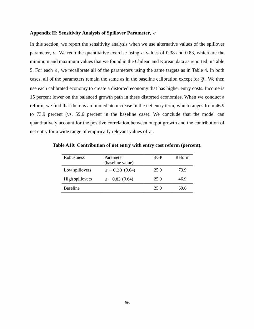
66

Appendix H: Sensitivity Analysis of Spillover Parameter, ε

In this section, we report the sensitivity analysis when we use alternative values of the spillover

parameter, ε . We redo the quantitative exercise using ε values of 0.38 and 0.83, which are the

minimum and maximum values that we found in the Chilean and Korean data as reported in Table

5. For each ε , we recalibrate all of the parameters using the same targets as in Table 4. In both

cases, all of the parameters remain the same as in the baseline calibration except for g . We then

use each calibrated economy to create a distorted economy that has higher entry costs. Income is

15 percent lower on the balanced growth path in these distorted economies. When we conduct a

reform, we find that there is an immediate increase in the net entry term, which ranges from 46.9

to 73.9 percent (vs. 59.6 percent in the baseline case). We conclude that the model can

quantitatively account for the positive correlation between output growth and the contribution of

net entry for a wide range of empirically relevant values of ε .

Table A10: Contribution of net entry with entry cost reform (percent).

Robustness Parameter (baseline value)

BGP Reform

Low spillovers 0.38ε = (0.64) 25.0 73.9

High spillovers 0.83ε = (0.64) 25.0 46.9

Baseline 25.0 59.6

67

Appendix I: Reforms in Chile and Korea

Table A11 describes the reforms conducted in Chile (enacted 1993−1997) and Korea (enacted 1990−1995 and 1998−2004).

Table A11: Summary of reforms in Chile and Korea.

Country (Year)

Reform Details Source

Chile (1993)

FDI reforms “The last revision of that rule [minimum permanence requirement for the equity portion of the investment] was made in 1993, when the limit was reduced from three years to one year.”

OECD (2003), p. 77

Chile (1993)

Financial reforms “This law [banking regulatory reform in 1986] ... was complemented by a securities law in 1993 that increased transparency in the capital markets and regulated conflicts of interest.”

Perry and Leipziger (1999), p. 113

Chile (1993)

Deregulation and privatization of services

“The law [1982 regulatory law of Chilean telecoms sector] was amended ... in 1993 to allow for competition in long-distance telephone services.”

Perry and Leipziger (1999), p. 358

Chile (1997)

Financial reforms “At the end of 1997 a new law widened banks' activities and set rules for the internationalization of the banking system.”

Perry and Leipziger (1999), p. 113

Chile (1997)

Deregulation and privatization of services

“Legislation was passed in 1997 to allow private involvement in the water and sewage sector and private management of the state-owned ports.”

Perry and Leipziger (1999), p. 287

Korea (1990)

Monopoly Regulation and Fair Trade Act

“the government strengthened the institutional basis to regulate unfair and anticompetitive trade practices”

Suh (2007), p. 23

Korea (1991)

FDI reforms “allowed foreign investment in manufacturing with a foreign-investment ratio not exceeding 50 percent”

Chung (2007), pp. 278-279

Korea (1992)

Subsidy for high-tech firms

“The government specified 58 areas for which tax exemption [for foreign-invested firms] would apply. Among these were high-tech manufacturers.”

Chung (2007), p. 279

Korea (1993)

Entry and financial reforms

“a combination of deregulation of corporate entry and of the financial system”

Haggard and Mo (2000)

Korea (1994)

Entry reforms “relax entry and investment restrictions in steel and semiconductor industries.”

Haggard and Mo (2000)

Korea (1994)

Financial reforms “the authorities lifted ceilings on short-term foreign currency borrowing by commercial banks”

Eichengreen et al. (2015), p.166

68

Korea (1995)

FDI reforms “raise the ceiling on foreign equity ownership of listed corporations”

Chung (2007), p. 280

Korea 1998)

FDI reforms “Ceilings on foreign investment in equities, with the exception of investment in public corporations, were then lifted.”

Eichengreen et al. (2015), p.100

Korea (1998)

Financial reforms “Firms were permitted to borrow abroad on long as well as short terms, and other foreign exchange transactions were relaxed.”

Eichengreen et al. (2015), p.169

Korea (1998)

Financial reforms “removed most of the restrictions on foreign exchange transactions and domestic transactions in foreign currencies”

Chung (2007), p. 281

Korea (1998)

FDI reforms “Abolished ceiling on equity investment by foreigners”

Lee et al. (2007), p. 60

Korea (1998)

Labor Standards Act

“labor market reforms focused on labor market flexibility”

Lee et al. (2007), p. 75

Korea (1998−2001)

Corporate governance

“Adopted international accounting and auditing standards”

Lee et al. (2007), p. 60

Korea (1999)

Monopoly Regulation and Fair Trade Act

“merger-specific efficiencies now had to clearly outweigh the harmful effects of reduced competition”

Eichengreen et al. (2015), p.169

Korea (1999)

Omnibus Cartel Repeal Act

“removed legal exemptions for 20 cartels and 18 statutes”

Eichengreen et al. (2015)

Korea (2004)

Financial reforms “waves of financial liberalization set off in 1993, 1998, and 2004”

Eichengreen et al. (2015)

Korea (2004)

Second Cartel Reformation Act

“legislated to abolish anticompetitive laws and systems”

Lee et al. (2007), p. 61