(FIRM) - Boat Design

FREE INTERNET ROWING MODEL(FIRM)

EXAMPLES: Single Sculls

March 25, 2015

FIRM IS RESEARCH CODE!

Please check all estimates generated by the programagainst experimental results before committing anytime or funds to your project as no liability can be

accepted by Cyberiad.

c©2015 Cyberiad

Contents

1 INTRODUCTION 1

2 W1x: Women’s Single Sculls 22.1 W1x exercises . . . . . . . . . . . . . . . . . . . . . . . . . . . . . . . . . . . . . . . . . . . . . . . . . . . . . 4

3 LW1x: Lightweight Women’s Single Sculls 8

4 M1x: Men’s Single Sculls 13

5 LM1x: Lightweight Men’s Single Scull 18

1 INTRODUCTION

Four single scull examples are included in this version of FIRM. More will be added in future versions.

1

2 W1x: Women’s Single Sculls

Many of the results for this sculler (who we have named Aage) have been used throughout the FIRM manual. Measuredvalues of rigging details, oar angles, gate normal forces, and her anthropometry were used as input to FIRM. Body angleregimes for three complete strokes were extracted from videos taken during the trial and these were used to constrain theangles predicted by the inverse kinematic procedures.

Table 1: Summary of experimental results for this simulation: number of strokes, stroke rate, non-dimensional pull phase duration(tp/ts), minimum hull velocity (Umin), maximum hull velocity (Umax), and mean hull velocity (U).

Item Value

Nstrokes 28Rate (spm) 35.111 ±0.214tp/ts 0.540 ±0.005Umin (ms−1) 3.288 ±0.063Umax (ms−1) 5.430 ±0.060

U (ms−1) 4.529 ±0.061

Table 1 summarises the main quantities relating to the simulation for this sculler. Values are given ± one standarddeviation.

Table 2: Experimental oar-related values for this simulation: minimum and maximum oar angles, and maximum gate normal force.

Port Oar Starboard OarName Min. Angle Max. Angle Max. FGn Min. Angle Max. Angle Max. FGn

(degrees) (degrees) (N) (degrees) (degrees) (N)

Aage -59.8±0.43 43.2±0.33 404.4±14.1 -56.4±0.38 44.5±0.42 387.0±16.0

A blade loss factor of kloss = 0.015 has been used to bring FIRM predictions in line with the experimental mean speedof U = 4.529ms−1. Given the many uncertainties, this small 1.5% reduction seems quite acceptable. (Instead of using theblade loss factor, we could have adjusted, for example, the oarhandle centre of effort, the viscous form factor, or the air dragcoefficients). A further justification for the small adjustments is that they are well within the standard deviations aroundthe means of the maximum gate normal forces given in Table 1.

-1.5

-1

-0.5

0

0.5

1

0 0.1 0.2 0.3 0.4 0.5 0.6 0.7 0.8 0.9 1

a (g

)

t/ts

W1x: Aage Exp. Exp. Mean ± SD Pred. Crew

3

3.5

4

4.5

5

5.5

6

0 0.1 0.2 0.3 0.4 0.5 0.6 0.7 0.8 0.9 1

U (

ms-1

)

t/ts

W1x: Aage Exp. Exp. Mean ± SD Pred. Crew

Figure 1: Hull propulsive acceleration and crew cg acceleration (left); hull velocity and crew cg velocity (right).

The hull propulsive acceleration is shown in the left panel of Fig. 1. Experimental data is shown as pink dots; the thickblack curve is the mean of the measured values and the thin lines are one standard deviation (SD) either side of the meancurve. The green curve is FIRM’s prediction.

The agreement is quite good, however, it should be kept in mind that it was achieved by using body angle regimesspecifically chosen to get that good agreement.

2

There is a small dip at about t/ts = 0.15 where the acceleration drops below zero. That, of course, must reduce theboat speed, and this can be seen as a corresponding dip in the right panel of the figure. The cause of the dip is mostprobably a question of rowing technique. FIRM has been able to reproduce the curve, but it cannot be used on its own tosuggest reasonable ways to correct the deficiency. That requires good coaching, and a more thorough biomechanical analysis.Kleshnev [?] has examined similar “double peaks” in boat acceleration.

-200

-100

0

100

200

300

0 0.1 0.2 0.3 0.4 0.5 0.6 0.7 0.8 0.9 1

Forc

e (N

)

t/ts

W1x: Aage Fprop Fboat Fcrew -Fdrag Fsys

0

25

50

75

100

0 0.1 0.2 0.3 0.4 0.5 0.6 0.7 0.8 0.9 1

Dra

g (N

)t/ts

W1x: Aage Air Viscous Wave Total

Figure 2: Equation of motion forces (left) and drag components (right).

The forces in the equations of motion are shown in the left panel of Fig. 2. Drag components during the stroke are inthe panel at the right.

-80

-60

-40

-20

0

20

40

60

0 0.1 0.2 0.3 0.4 0.5 0.6 0.7 0.8 0.9 1

ψxy

(de

gree

s)

t/ts

W1x: Aage Exp. Port Exp. Star FIRM: Port FIRM: Star

-60

-30

0

30

60

90

120

150

180

0 0.1 0.2 0.3 0.4 0.5 0.6 0.7 0.8 0.9 1

Join

t Ang

le (

degr

ees)

t/ts

W1x: Aage Knee Hip Neck Shoulder

Figure 3: Oar azimuth angles Ψxy (left); joint angles (right)).

Experimental oar azimuth angles in the plot at the left of Fig. 3 have been shifted so they are referenced to the centre ofthe pin. The continuous curves are the values used as input to FIRM.

Joint angle regimes are shown in the plot at the right of Fig. 3. Solid curves are the values used as input to FIRM.Gate normal forces are shown at the left of Fig. 4. The curves are the values used as input to FIRM.Oarblade propulsive forces are shown in the right panel of Fig. 4. These include the variation in the OBCP during the

stroke.The x-wise velocities of the OHCE are shown at the left of Fig. 5. The velocity is negative during the drive because the

handle travels in the negative x-direction.The seat velocity is shown in the right panel of Fig. 5. It too is negative during the pull phase. At the release the seat

velocity slows down and remains at zero for a short time before the stern is pulled towards the rower during the recovery.

3

0

50

100

150

200

250

300

350

400

450

0 0.1 0.2 0.3 0.4 0.5 0.6 0.7 0.8 0.9 1

F Gn

(N)

t/ts

W1x: Aage Exp. Port Exp. Star FIRM: Port FIRM: Star

0

25

50

75

100

125

0 0.1 0.2 0.3 0.4 0.5 0.6 0.7 0.8 0.9 1

F Bx

(N)

t/ts

W1x: Aage Port Star

Figure 4: Gate normal forces FGn (left); blade propulsive forces FBx (right).

-3

-2

-1

0

1

2

3

0 0.1 0.2 0.3 0.4 0.5 0.6 0.7 0.8 0.9 1

OH

CE

x-v

eloc

ity (

m/s

)

t/ts

W1x: Aage Port Star

-1.5

-1

-0.5

0

0.5

1

1.5

0 0.1 0.2 0.3 0.4 0.5 0.6 0.7 0.8 0.9 1

Seat

vel

ocity

(m

/s)

t/ts

W1x: Aage Hip (Seat)

Figure 5: OHCE horizontal velocity (left); seat velocity (right).

Yawing moment lever arms are shown in the left plot of Fig. 6. These, and the yawing moments shown at the right ofthe figure both contain the effects of the OBCP varying during the stroke.

Vertical oar angles are shown in the plot at the left of Fig. 7. The corresponding locations of the OBCP for both oarsare shown at the right. The vertical angles and vertical locations for both oars are identical, however, the azimuth angles aredifferent.

The OBCP is below the water from about t/ts = 0.01 to t/ts = 0.55. For the purposes of this plot, the OBCP is assumedto be at the geometric centre of the blade when it is out of the water.

The trajectories of the joints are shown in the plot at the left of Fig. 8; trajectories of the segment and oar centres ofgravity are shown at the right.

The trajectory of the hip is a flat line because it is the same as that of the seat which does not move up or down duringthe stroke. The trajectory of the sum of the CG is the black trace in the right-hand plot. It can be seen that the verticaldisplacement is much less than the horizontal which justifies ignoring the vertical component in many models.

The OBCP trajectories in Fig. 9 have been plotted on the same side of the hull for clarity and comparison. Puddles aremost likely to be formed during the period immediately before the release.

2.1 W1x exercises

Once we have good agreement between FIRM predictions of hull propulsive acceleration and hull velocity, there are manysimple “what if” type questions we can ask. Most of the short exercises can be done by making very simple modifications to

4

-3

-2

-1

0

1

2

3

0 0.1 0.2 0.3 0.4 0.5 0.6 0.7 0.8 0.9 1

Yaw

ing

mom

ent l

ever

arm

(m

)

t/ts

W1x: Aage Port Star

-400

-300

-200

-100

0

100

200

300

400

0 0.1 0.2 0.3 0.4 0.5 0.6 0.7 0.8 0.9 1

Yaw

ing

Mom

ent (

Nm

)

t/ts

W1x: Aage Port Star Sum

Figure 6: Yawing moment lever arms (left); yawing moments (right).

0

2

4

6

8

10

12

0 0.1 0.2 0.3 0.4 0.5 0.6 0.7 0.8 0.9 1

ψyz

(de

gree

s)

t/ts

W1x: Aage Port Star

-0.2

-0.1

0

0.1

0.2

0 0.1 0.2 0.3 0.4 0.5 0.6 0.7 0.8 0.9 1

z obc

p (m

. abo

ve w

ater

)

t/ts

W1x: Aage Waterplane Port OBCP Star OBCP

Figure 7: Vertical oar angles Ψyz (left); OBCP trajectories in the yz-plane (right).

one of the input files.Remember to restore the original value in the file before you try another example. The best method is to make a copy of

the line you want to modify, then use the # character to comment out the original line. After you finish the exercise, deletethe modified line, and remove the # character from the original line. (If you forget what modifications you made, delete theentire FIRM directory and re-install it: that should only take a few seconds.)

Before making any modifications to the files, run FIRM for the original file and record the mean hull velocity that appearson the Model Screen, or in the summary.csv file.

Exercise W1x 1.0: What is the predicted mean hull velocity at 20◦C water and 20◦C air temperature?Hint: change the values near the start of the main input file, aage.inExercise W1x 1.1: What difference in time over 2000m does the change in mean velocity represent?Exercise W1x 1.2: How many metres does the change in mean velocity represent?

Exercise W1x 2.0: When rowers resume training after a lay-off, they are usually not as strong as when they are at their peak.What is the effect of reducing the maximum gate forces by 10%? Hint: Change the blade loss factor.

Exercise W1x 3.0: Although the boat used in this example is very similar to the actual boat used in the on-water trials, itseems a little large for this rower. (Some people refer to this as “over-boating”). What is the effect of using a different hull,for example the slightly shorter S075L101g1 hull?Hint: change the line in the Hull Filename block of the file aage.in fromhulls/S080L106a1.csv

5

0

0.2

0.4

0.6

0.8

1

-1.6 -1.2 -0.8 -0.4 0 0.4 0.8

z-or

dina

te o

f jo

int r

elat

ive

to a

nkle

(m

)

x-ordinate of joint relative to ankle (m)

W1x: Aage Knee Hip Neck Port Hand Star Hand

0

0.2

0.4

0.6

0.8

1

-1.6 -1.2 -0.8 -0.4 0 0.4 0.8

z-or

dina

te o

f C

G r

elat

ive

to a

nkle

(m

)

x-ordinate of CG relative to ankle (m)

W1x: Aage Shank Thigh Torso Head Upper Arm Forearm Port Oar Star Oar Sum

Figure 8: Joint trajectories (left); trajectories of centres of gravity (right).

1.6

1.8

2

2.2

2.4

2.6

2.8

-2.8 -2.6 -2.4 -2.2 -2 -1.8 -1.6 -1.4 -1.2

Lat

eral

dis

tanc

e fr

om h

ull c

entr

elin

e (m

)

x (m)

Direction of

Boat Travel

Release

Catch

W1x: Aage Port Star

Figure 9: OBCP trajectories in the xy-plane.

tohulls/S075L101g1.csv

Exercise W1x 3.1: Examine the effect of changing the dimensions of the S080L106a1.csv hull. For example, change the lengthof the hull from 7.90 to 7.80. What is the effect on mean hull speed? How does it affect transverse stability (i.e. on GMT0)?

Exercise W1x 3.2: Make the S080L106a1.csv hull narrower by reducing the overall beam from 0.275m to 0.270m. What isthe effect on mean hull speed and transverse stability?

Exercise W1x 4.0: What is the effect on hull velocity of increasing the hull weight by 1, 2, or 3 kgs?Hint: change the values in the hull input file.

Exercise W1x 5.0: What is the effect of increasing the rower’s weight by 1, 2 and 3 kgs?Hint: change the values of the rower’s weight in the anthro.csv input file.Exercise W1x 5.1: Is the effect exactly the same as increasing the hull weight by the same amount, for example, by carryinglarge bottles of water?

Exercise W1x 6.0: Look up the world’s best time for this event in the Appendix to the FIRM manual. Now change the gateforces for this sculler, run FIRM and note the new mean hull velocity. What percentage increase in force is required for Aageto equal the world record time?

6

W1x: AageRate 35.1 spmSpeed 4.53 m/s

Dead Mass 14.0 kgMoving Mass 76.2 kgTotal Mass 90.2 kgA.

MUSCULAREFFORT

398 W

100 %

NetKinetic Energy

Work onOarhandles

B.HANDLES

B/A

316 W

79 %

E.SYSTEMMOMENTUME/A

82 W

21 %

NOTE: B+F=D+H and C+E=D+G

C.PROPULSION

C/A

254 W

64 %

Blade EfficiencyC/B = 80.5 %

Propelling EfficiencyD/(D+H) = 83.6 %

F.FOOT BOARDS(External)F/A

59 W

15 %

Mom. EfficiencyF/E = 71.9 %

Work doneon shellD.

DRAG

D/A

313 W

79 %

AirVisc.Wave

11 % 82 % 7 %

Transferred to air and water

H.BLADELOSSESH/A

62 W

15 %Lost to water

G.BODY FLEX(Internal)G/A

23 W

6 %Lost as heat, breath etc.

Velocity Efficiency1-G/A = 94.2 %I=D+G+H.

TOTALLOSSI/A

398 W

100.0 %Net Efficiency

D/(D+H)-G/A = 77.8 %

Figure 10: Power flow chart.

7

3 LW1x: Lightweight Women’s Single Sculls

The on-water trial for this lightweight sculler, “Lara”, was conducted over 500m. Air and water temperatures were notrecorded: they were estimated as 10◦C and 10◦C respectively. Measured values of rigging details, oar angles, gate normalforces, and her anthropometry were used as input to FIRM. Body angle regimes were not recorded but were estimated bythe author using a complicated fitting process.


Item Value


U (ms−1) 4.061 ±0.022


Table 4: Experimental oar-related values for this simulation: Minimum and maximum oar angles, and maximum gate normal forceFgn.



Lara -62.9±1.19 43.2±0.48 354.3±10.4 -60.3±0.56 44.0±0.47 362.7±12.9

-1

-0.8

-0.6

-0.4

-0.2

0

0.2

0.4

0.6

0 0.1 0.2 0.3 0.4 0.5 0.6 0.7 0.8 0.9 1

a (g

)

t/ts

LW1x: Lara Exp. Exp. Mean ± SD Pred. Crew

2.75

3

3.25

3.5

3.75

4

4.25

4.5

4.75

0 0.1 0.2 0.3 0.4 0.5 0.6 0.7 0.8 0.9 1

U (

ms-1

)

t/ts

LW1x: Lara Exp. Exp. Mean ± SD Pred. Crew

Figure 11: Hull propulsive acceleration and crew CG acceleration (left); hull velocity and crew CG velocity (right).


The most notable feature of the hull speed curve in the plot at the right of Fig. 11 is the long, relatively constant regionduring the recovery. This behaviour is not evident in other classes of rowing; it might be peculiar to this particular lightweightsculler, or to lightweight women sculling at relatively low rates and with short drive phase durations.


Experimental oar azimuth angles and values used as input to FIRM are shown in the plot at the left of Fig. 13.Estimated joint angle regimes used as input to FIRM are shown in the plot at the right of Fig. 13.

8

-200

-100

0

100

200

300

0 0.1 0.2 0.3 0.4 0.5 0.6 0.7 0.8 0.9 1

Forc

e (N

)

t/ts

LW1x: Lara Fprop Fboat Fcrew -Fdrag Fsys

0

10

20

30

40

50

60

0 0.1 0.2 0.3 0.4 0.5 0.6 0.7 0.8 0.9 1

Dra

g (N

)

t/ts

LW1x: Lara Air Viscous Wave Total


-80

-60

-40

-20

0

20

40

60

0 0.1 0.2 0.3 0.4 0.5 0.6 0.7 0.8 0.9 1

ψxy

(de

gree

s)

t/ts

LW1x: Lara Exp. Port Exp. Star FIRM: Port FIRM: Star

-60

-30

0

30

60

90

120

150

180

0 0.1 0.2 0.3 0.4 0.5 0.6 0.7 0.8 0.9 1

Join

t Ang

le (

degr

ees)

t/ts

LW1x: Lara Knee Hip Neck Shoulder


Gate normal forces are shown at the left of Fig. 14. The curves are the values used as input to FIRM.Oarblade propulsive forces are shown in the right panel of Fig. 14. These include the variation in the OBCP during the


handle travels in the negative x-direction.The seat velocity is shown in the right panel of Fig. 15. It too is negative during the pull phase. At the release the seat

velocity slows down and remains at zero for a very short time before the stern moves towards the rower during the recovery.Yawing moment lever arms are shown in the left plot of Fig. 16. These, and the yawing moments shown at the right of

the figure both contain the effects of the OBCP varying during the stroke. The nett yawing moment is quite small for thissculler.


The OBCP is below the water from about t/ts = 0.01 to t/ts = 0.45; the latter value was specified in the main input file.For the purposes of this plot, the OBCP is assumed to be at the geometric centre of the blade when it is out of the water.The OBCP trajectories in Fig. 18 have been plotted on the same side of the hull for clarity and comparison. Puddles are

most likely to be formed during the period immediately before the release.

9

-50

0

50

100

150

200

250

300

350

400

0 0.1 0.2 0.3 0.4 0.5 0.6 0.7 0.8 0.9 1

F Gn

(N)

t/ts

LW1x: Lara Exp. Port Exp. Star FIRM: Port FIRM: Star

0

25

50

75

100

125

0 0.1 0.2 0.3 0.4 0.5 0.6 0.7 0.8 0.9 1

F Bx

(N)

t/ts

LW1x: Lara Port Star

Figure 14: Gate normal forces (left); blade propulsive forces (right).

-3

-2

-1

0

1

2

3

0 0.1 0.2 0.3 0.4 0.5 0.6 0.7 0.8 0.9 1

OH

CE

x-v

eloc

ity (

m/s

)

t/ts


-1.5

-1

-0.5

0

0.5

1

1.5

0 0.1 0.2 0.3 0.4 0.5 0.6 0.7 0.8 0.9 1

Seat

vel

ocity

(m

/s)

t/ts

LW1x: Lara Hip (Seat)


-3

-2

-1

0

1

2

3

0 0.1 0.2 0.3 0.4 0.5 0.6 0.7 0.8 0.9 1

Yaw

ing

mom

ent l

ever

arm

(m

)

t/ts


-300

-200

-100

0

100

200

300

0 0.1 0.2 0.3 0.4 0.5 0.6 0.7 0.8 0.9 1

Yaw

ing

Mom

ent (

Nm

)

t/ts

LW1x: Lara Port Star Sum


10

0

2

4

6

8

0 0.1 0.2 0.3 0.4 0.5 0.6 0.7 0.8 0.9 1

ψyz

(de

gree

s)

t/ts


-0.2

-0.1

0

0.1

0 0.1 0.2 0.3 0.4 0.5 0.6 0.7 0.8 0.9 1

z obc

p (m

. abo

ve w

ater

)t/ts

LW1x: Lara Waterplane Port OBCP Star OBCP


1.6

1.8

2

2.2

2.4

2.6

-2.8 -2.6 -2.4 -2.2 -2 -1.8 -1.6 -1.4 -1.2

Lat

eral

dis

tanc

e fr

om h

ull c

entr

elin

e (m

)

x (m)

Direction of

Boat Travel

Release

Catch



11

LW1x: LaraRate 27.9 spmSpeed 4.07 m/s


MUSCULAREFFORT

268 W

100 %

NetKinetic Energy

Work onOarhandles

B.HANDLES

B/A

223 W

83 %

E.SYSTEMMOMENTUME/A

45 W

17 %


C.PROPULSION

C/A

171 W

64 %




35 W

13 %


Work doneon shellD.

DRAG

D/A

205 W

77 %

AirVisc.Wave

11 % 81 % 9 %


H.BLADELOSSESH/A

53 W

20 %Lost to water


10 W



TOTALLOSSI/A

268 W


D/(D+H)-G/A = 75.8 %


12

4 M1x: Men’s Single Sculls

The on-water trial for this sculler, “Stevo”, was conducted over 500m. Air and water temperatures were not recorded:they were estimated as 22◦C and 22◦C respectively. Measured values of rigging details, oar angles, gate normal forces, andhis anthropometry were used as input to FIRM. Body angle regimes for 2 complete strokes were extracted from videos takenduring the trial.


Item Value


U (ms−1) 4.942 ±0.071


Table 6: Experimental oar-related values for this simulation: Minimum and maximum oar angles, and maximum gate normal force.



Stevo -64.7±0.50 41.7±0.92 538.8±24.5 -61.3±0.55 43.3±0.49 602.9±26.9

-1.6

-1.2

-0.8

-0.4

0

0.4

0.8

1.2

0 0.1 0.2 0.3 0.4 0.5 0.6 0.7 0.8 0.9 1

a (g

)

t/ts

M1x: Stevo Exp. Exp. Mean ± SD Pred. Crew

3

3.5

4

4.5

5

5.5

6

6.5

0 0.1 0.2 0.3 0.4 0.5 0.6 0.7 0.8 0.9 1

U (

ms-1

)

t/ts

M1x: Stevo Exp. Exp. Mean ± SD Pred. Crew

Figure 20: Hull propulsive acceleration and crew cg acceleration (left); hull velocity and crew cg velocity (right).

The hull propulsive acceleration is shown in the left panel of Fig. 20. Experimental data is shown as pink dots; the thickblack curve is the mean of the measured values and the thin lines are one standard deviation (SD) either side of the meancurve. The green curve is FIRM’s prediction. Hull and crew CG velocities are shown at the right. Maximum gate normalforces were increased by 1% to make measured and predicted predicted mean velocity coincide more closely.


Experimental oar azimuth angles in the plot at the left of Fig. 22 have been shifted so they are referenced to the centreof the pin. The continuous curves are the values used as input to FIRM.


stroke.

13

-300

-200

-100

0

100

200

300

400

0 0.1 0.2 0.3 0.4 0.5 0.6 0.7 0.8 0.9 1

Forc

e (N

)

t/ts

M1x: Stevo Fprop Fboat Fcrew -Fdrag Fsys

0

20

40

60

80

100

120

0 0.1 0.2 0.3 0.4 0.5 0.6 0.7 0.8 0.9 1

Dra

g (N

)

t/ts

M1x: Stevo Air Viscous Wave Total


-80

-60

-40

-20

0

20

40

60

0 0.1 0.2 0.3 0.4 0.5 0.6 0.7 0.8 0.9 1

ψxy

(de

gree

s)

t/ts

M1x: Stevo Exp. Port Exp. Star FIRM: Port FIRM: Star

-60

-30

0

30

60

90

120

150

180

0 0.1 0.2 0.3 0.4 0.5 0.6 0.7 0.8 0.9 1

Join

t Ang

le (

degr

ees)

t/ts

M1x: Stevo Knee Hip Neck Shoulder


The x-wise velocities of the OHCE are shown at the left of Fig. 24. The velocity is negative during the drive because thehandle travels in the negative x-direction.

The seat velocity is shown in the right panel of Fig. 24.Yawing moment lever arms are shown in the left plot of Fig. 25. These, and the yawing moments shown at the right of

the figure both contain the effects of the OBCP varying during the stroke.Vertical oar angles are shown in the plot at the left of Fig. 26. The corresponding locations of the OBCP for both oars

are shown at the right. The vertical angles and vertical locations for both oars are identical, however, the azimuth angles aredifferent.

The OBCP is below the water from about t/ts = 0.01 to t/ts = 0.497. For the purposes of this plot, the OBCP is assumedto be at the geometric centre of the blade when it is out of the water.

The OBCP trajectories in Fig. 27 have been plotted on the same side of the hull for clarity and comparison.

14

0

100

200

300

400

500

600

700

0 0.1 0.2 0.3 0.4 0.5 0.6 0.7 0.8 0.9 1

F Gn

(N)

t/ts

M1x: Stevo Exp. Port Exp. Star FIRM: Port FIRM: Star

0

50

100

150

200

0 0.1 0.2 0.3 0.4 0.5 0.6 0.7 0.8 0.9 1

F Bx

(N)

t/ts

M1x: Stevo Port Star

Figure 23: Gate normal forces FGn (left); blade propulsive forces FBx (right).

-3

-2

-1

0

1

2

3

0 0.1 0.2 0.3 0.4 0.5 0.6 0.7 0.8 0.9 1

OH

CE

x-v

eloc

ity (

m/s

)

t/ts


-2

-1.5

-1

-0.5

0

0.5

1

1.5

0 0.1 0.2 0.3 0.4 0.5 0.6 0.7 0.8 0.9 1

Seat

vel

ocity

(m

/s)

t/ts

M1x: Stevo Hip (Seat)


-3

-2

-1

0

1

2

3

0 0.1 0.2 0.3 0.4 0.5 0.6 0.7 0.8 0.9 1

Yaw

ing

mom

ent l

ever

arm

(m

)

t/ts


-500

-400

-300

-200

-100

0

100

200

300

400

500

0 0.1 0.2 0.3 0.4 0.5 0.6 0.7 0.8 0.9 1

Yaw

ing

Mom

ent (

Nm

)

t/ts

M1x: Stevo Port Star Sum


15

0

2

4

6

8

10

0 0.1 0.2 0.3 0.4 0.5 0.6 0.7 0.8 0.9 1

ψyz

(de

gree

s)

t/ts


-0.2

-0.1

0

0.1

0.2

0 0.1 0.2 0.3 0.4 0.5 0.6 0.7 0.8 0.9 1

z obc

p (m

. abo

ve w

ater

)t/ts

M1x: Stevo Waterplane Port OBCP Star OBCP


1.6

1.8

2

2.2

2.4

2.6

2.8

-2.8 -2.6 -2.4 -2.2 -2 -1.8 -1.6 -1.4 -1.2

Lat

eral

dis

tanc

e fr

om h

ull c

entr

elin

e (m

)

x (m)

Direction of

Boat Travel

Release

Catch



16

M1x: StevoRate 35.0 spmSpeed 4.94 m/s


MUSCULAREFFORT

578 W

100 %

NetKinetic Energy

Work onOarhandles

B.HANDLES

B/A

462 W

80 %

E.SYSTEMMOMENTUME/A

116 W

20 %


C.PROPULSION

C/A

360 W

62 %




88 W

15 %


Work doneon shellD.

DRAG

D/A

448 W

77 %

AirVisc.Wave

10 % 82 % 8 %


H.BLADELOSSESH/A

102 W

18 %Lost to water


28 W



TOTALLOSSI/A

578 W


D/(D+H)-G/A = 76.6 %


17

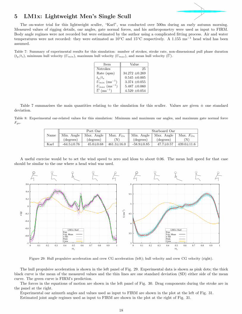
5 LM1x: Lightweight Men’s Single Scull

The on-water trial for this lightweight sculler, “Karl”, was conducted over 500m during an early autumn morning.Measured values of rigging details, oar angles, gate normal forces, and his anthropometry were used as input to FIRM.Body angle regimes were not recorded but were estimated by the author using a complicated fitting process. Air and watertemperatures were not recorded: they were estimated as 10◦C and 15◦C respectively. A 1.155 ms−1 head wind has beenassumed.


Item Value


U (ms−1) 4.529 ±0.054


Table 8: Experimental oar-related values for this simulation: Minimum and maximum oar angles, and maximum gate normal forceFgn.



Karl -64.5±0.76 45.0±0.68 461.3±16.0 -58.9±0.85 47.7±0.57 439.0±11.6

A useful exercise would be to set the wind speed to zero and kloss to about 0.06. The mean hull speed for that caseshould be similar to the one where a head wind was used.

-1

-0.8

-0.6

-0.4

-0.2

0

0.2

0.4

0.6

0 0.1 0.2 0.3 0.4 0.5 0.6 0.7 0.8 0.9 1

a (g

)

t/ts

LM1x: Karl Exp. Exp. Mean ± SD Pred. Crew

3

3.5

4

4.5

5

5.5

6

0 0.1 0.2 0.3 0.4 0.5 0.6 0.7 0.8 0.9 1

U (

ms-1

)

t/ts

LM1x: Karl Exp. Exp. Mean ± SD Pred. Crew

Figure 29: Hull propulsive acceleration and crew CG acceleration (left); hull velocity and crew CG velocity (right).



Experimental oar azimuth angles and values used as input to FIRM are shown in the plot at the left of Fig. 31.Estimated joint angle regimes used as input to FIRM are shown in the plot at the right of Fig. 31.

18

-300

-200

-100

0

100

200

300

0 0.1 0.2 0.3 0.4 0.5 0.6 0.7 0.8 0.9 1

Forc

e (N

)

t/ts

LM1x: Karl Fprop Fboat Fcrew -Fdrag Fsys

0

20

40

60

80

100

0 0.1 0.2 0.3 0.4 0.5 0.6 0.7 0.8 0.9 1

Dra

g (N

)

t/ts

LM1x: Karl Air Viscous Wave Total


-80

-60

-40

-20

0

20

40

60

0 0.1 0.2 0.3 0.4 0.5 0.6 0.7 0.8 0.9 1

ψxy

(de

gree

s)

t/ts

LM1x: Karl Exp. Port Exp. Star FIRM: Port FIRM: Star

-60

-30

0

30

60

90

120

150

180

0 0.1 0.2 0.3 0.4 0.5 0.6 0.7 0.8 0.9 1

Join

t Ang

le (

degr

ees)

t/ts

LM1x: Karl Knee Hip Neck Shoulder




handle travels in the negative x-direction. The seat velocity is shown in the right panel.Yawing moment lever arms are shown in the left plot of Fig. 34. These, and the yawing moments shown at the right of

the figure both contain the effects of the OBCP varying during the stroke. The nett yawing moment is quite small for thissculler.


The OBCP is below the water from about t/ts = 0.01 to t/ts = 0.54; the latter value was specified in the main input file.For the purposes of this plot, the OBCP is assumed to be at the geometric centre of the blade when it is out of the water.The OBCP trajectories in Fig. 36 have been plotted on the same side of the hull for clarity and comparison.

19

-100

0

100

200

300

400

500

0 0.1 0.2 0.3 0.4 0.5 0.6 0.7 0.8 0.9 1

F Gn

(N)

t/ts

LM1x: Karl Exp. Port Exp. Star FIRM: Port FIRM: Star

-25

0

25

50

75

100

125

150

0 0.1 0.2 0.3 0.4 0.5 0.6 0.7 0.8 0.9 1

F Bx

(N)

t/ts

LM1x: Karl Port Star

Figure 32: Gate normal forces (left); blade propulsive forces (right).

-3

-2

-1

0

1

2

3

0 0.1 0.2 0.3 0.4 0.5 0.6 0.7 0.8 0.9 1

OH

CE

x-v

eloc

ity (

m/s

)

t/ts


-1.5

-1

-0.5

0

0.5

1

1.5

0 0.1 0.2 0.3 0.4 0.5 0.6 0.7 0.8 0.9 1

Seat

vel

ocity

(m

/s)

t/ts

LM1x: Karl Hip (Seat)


-3

-2

-1

0

1

2

3

0 0.1 0.2 0.3 0.4 0.5 0.6 0.7 0.8 0.9 1

Yaw

ing

mom

ent l

ever

arm

(m

)

t/ts


-400

-300

-200

-100

0

100

200

300

400

0 0.1 0.2 0.3 0.4 0.5 0.6 0.7 0.8 0.9 1

Yaw

ing

Mom

ent (

Nm

)

t/ts

LM1x: Karl Port Star Sum


20

0

2

4

6

8

10

0 0.1 0.2 0.3 0.4 0.5 0.6 0.7 0.8 0.9 1

ψyz

(de

gree

s)

t/ts


-0.1

-0.05

0

0.05

0.1

0 0.1 0.2 0.3 0.4 0.5 0.6 0.7 0.8 0.9 1

z obc

p (m

. abo

ve w

ater

)t/ts

LM1x: Karl Waterplane Port OBCP Star OBCP


1.6

1.8

2

2.2

2.4

2.6

-2.8 -2.6 -2.4 -2.2 -2 -1.8 -1.6 -1.4 -1.2

Lat

eral

dis

tanc

e fr

om h

ull c

entr

elin

e (m

)

x (m)

Direction of

Boat Travel

Release

Catch



21

LM1x: KarlRate 34.3 spmSpeed 4.53 m/s


MUSCULAREFFORT

436 W

100 %

NetKinetic Energy

Work onOarhandles

B.HANDLES

B/A

347 W

80 %

E.SYSTEMMOMENTUME/A

89 W

20 %


C.PROPULSION

C/A

269 W

62 %




65 W

15 %


Work doneon shellD.

DRAG

D/A

334 W

77 %

AirVisc.Wave

17 % 77 % 6 %


H.BLADELOSSESH/A

77 W

18 %Lost to water


24 W



TOTALLOSSI/A

436 W


D/(D+H)-G/A = 75.6 %


22

(FIRM) - Boat Design

Documents

Transcript of (FIRM) - Boat Design