Finslerian indicatrices as algebraic curves and surfaces

Finslerian indicatrices as

algebraic curves and surfaces

P. Chansri, P. Chansangiam and S. V. Sabau

Abstract. We show how to construct new Finsler metrics, in two andthree dimensions, whose indicatrices are pedal curves or pedal surfacesof some other curves or surfaces, respectively. These Finsler metrics aregeneralizations of the famous slope metric, also called Matsumoto metric.

M.S.C. 2010: 53C60, 14H50.Key words: algebraic curves; pedal curves and surfaces; Finsler manifolds; curvature.

1 Introduction

Finsler manifolds are natural generalizations of Riemannian manifolds in the same re-spect as normed spaces and Minkowski spaces are generalizations of Euclidean spaces.

In the case of the Euclidean space, or more general, of Riemannian manifolds,the space looks uniform and isotropic, that is, the same in all directions. However,our daily experiences, as well as the metrics and distances naturally appearing inapplications to real life problems in Physics, Computer Science, Biology, etc. showthat the space is not isotropic, there exists same preferred directions (see [1], [5], [7],[11]).

To be more precise, we recall that a Finsler metric (M,F ) is given by specifying aFinsler norm F : TM → R defined on the tangent space (TM,M) of an n-dimensionalmanifold M . A Finsler norm has the following properties

1. F is C∞ on TM := TM \ {O}, where O is the zero section;

2. F is 1- positive homogeneous, i.e. F (x, λy) = λ ·F (x, y), ∀λ > 0, (x, y) ∈ TM ;

3. F is strongly convex, i.e. the Hessian gij := 12∂2F 2

∂yi∂yj (x, y) is positive defined for

any (x, y) ∈ TM .

Observe that the fundamental function F determines and it is determined by itsindicatrix (the unit tangent bundle) ΣF := {(x, y) ∈ TM : F (x, y) = 1}, which isa smooth hypersurface of TM . For each point x ∈ M, we can define the indicatrix

∗Balkan Journal of Geometry and Its Applications, Vol.25, No.1, 2020, pp. 19-33.c© Balkan Society of Geometers, Geometry Balkan Press 2020.

20 P. Chansri, P. Chansangiam and S. V. Sabau

at x as Σx := {y ∈ TM : F (x, y) = 1} = ΣF ∩ TxM , which is a smooth, closed,strictly convex hypersurface in TxM. It is therefore important to remark that to givea Finsler structure F on a manifold M is equivalent to giving a smooth hypersurfaceΣ ↪→ TM for which, the canonical projection π : Σ → M is a surjective submersionwith the property that, for each x ∈ M , the π-fiber Σ = π−1(x) is a strictly convexhypersurface in TxM enclosing the origin. If (M,F ) is a Finsler manifold, then therestriction of F to each tangent space TxM induces a Minkowski norm in TxM . Togive such a Minkowski norm is equivalent to giving the indicatrix Σx at x. A Finslerstructure on M is a family of Minkowski norms (Fx, TxM) moving smoothly on themanifold.

From now on, we are going to regard Finsler and Minkowski norms as hypersur-faces in TM and TxM , respectively. With this image in mind, constructing examplesof Finsler manifolds or Minkowski norms reduce to the effective construction of thehypersurfaces Σ and Σx, respectively. Observe that the central symmetric spheresor ellipsoids give Riemannian metrics since they are all quadratic forms in the fibercoordinate y of TxM , hence we need to construct simple hypersurface which are notquadratic forms in y′s.

Even though there exists already a lot of literature about Finsler manifolds andindicatrices ([10]), as well as about the pedal curves ([9]) and algebraic curves ingeneral ([4]), our approach, we reconsider this topic in modern terminology, aimingto provide new insights into the theory of Finsler spaces.

For instance, recall that the Randers and Kropina metrics are obtained by a rigidtranslation of the unit sphere such that the origin is enclosed by it or it is includedin its boundary, respectively. We point out that Kropina metrics are actually conicFinsler metrics (see [11], [3] for details).

Another similar example of Finsler metric is the slope metric (see [3], [6]), where,in the two-dimensional case, the indicatrix curve is a limacon. The associated Finsler

norm is written in the general form F = α2

α−β and called the slope metric (or a

Matsumoto metric), where α =√aijyiyj is a Riemannian metric and β = biy

j is alinear 1-form. In [3] we have studied the geometry of the slope metric globally inducedon a surface of revolution.

On the other hand, let us observe that a limacon is an algebraic curve obtainedas the pedal curve of a circle with respect to the origin. This insight opens a newperspective on indicatrices i.e. Finsler metrics, as algebraic curves. In the three (orhigher) dimensional case it is also possible to regard indicatrices as hyper-surfaces.

In the present paper we study the following problems:

1. How to construct two dimensional Finsler metrics whose indicatrices are pedalcurves of some algebraic curves as generalization of the slope metric and pointout the convexity conditions of the pedal curves. In special we will consider thecase of pedal of conics.

2. How to extend this study to the three dimensional case (and arbitrary dimen-sional case). This study is new in the sense that indicatrices of three dimensionalslope metrics are studied for the first time. From algebraic point of view thegeometry of pedal surfaces is also an interesting topic.

Arbitrary dimension Finsler metrics whose indicatrices are pedal hypersurfaces canbe studied in a similar manner, but the concrete computations can be quite messy.

Finslerian indicatrices as algebraic curves and surfaces 21

Finally, we point out that our approach is important because it illustrates andclarifies the geometrical meaning of three (and higher) dimensional slope metrics,called Matsumoto metrics in the arbitrary dimensional case. Indeed, initially, thetwo-dimensional slope metric was defined by Matsumoto as the Finsler metric whoseindicatrix is a limacon (see [6]). After seeing that these Finsler metrics are of the type

F = α2

α−β , where α is a Riemannian metric and β a linear one form, they were simplygeneralized to the arbitrary dimensional case without any further considerations onthe geometrical meaning. By using our pedal curves and surfaces approach one cansee that the higher dimensional Matsumoto metrics are those Finsler metrics whoseindicatrices are pedal hypersurfaces of spheres.

2 The pedal curve of a plane algebraic curve

Let us consider a plane algebraic curve (C) given in parametric form

(2.1) (C) : x = x(t), y = y(t),

then, at regular values of the parameter t, the tangent line to (C) is

(2.2) (`) : y(t) · x− x(t) · y + {x(t) · y(t)− x(t) · y(t)} = 0,

and the orthogonal line to (`) through a point P (x0, y0) is given by

(`)⊥ : y − y0 = − x(t)

y(t)(x− x0),

where dots represent the derivative of a function of one variable with respect to t.For a regular plane algebraic curve (C), and a fixed point P (x0, y0), called the

pedal point, the pedal curve of the curve (C) with respect to P is the parameterizedcurve obtained by associating to the parameter t the orthogonal projection p(t) ofP onto the tangent line at t (see [4], [9] for details on algebraic curves). The pedalcurves are considered important in geometrical optics and kinematics.

We recall that the moving equation of the Frenet frame (T (t), N(t)) along (C) aregiven by

dT

dt= |c′(t)| · kc ·N(t)

dN

dt= −|c′(t)| · kc · T (t),

where (T (t), N(t)) are the unit tangent and normal vectors along c, respectively,|c′(t)| =

√x(t)2 + y(t)2 is the speed of (C) and

kc :=〈c′′(t), N(t)〉|c′(t)|2

is the curvature of the curve (C). Here 〈·, ·〉 is the usual inner product of the Euclideanplane.


A straighforward computation shows that the pedal curve of (C) with respect tothe point P is given by

(2.3) p(t) = 〈c− r0, N〉 ·N + r0,

where we denote by r0 the position vectors of the point P (x0, y0).

Proposition 2.1. If (C) is a continuously differentiable closed curve in plane, thenits pedal curve (P) : p = p(t) with respect to a point P (x0, y0) is also a continuouslydifferentiable closed curve in plane.

Proof. From hypothesis, after some rescaling of the parameter t, we have c(0) =c(2π), c(0) = c(2π), and hence T (0) = T (π), N(0) = N(π). Using now (2.3) itfollows p(0) = p(2π), i.e. p is also periodic with the some period as (C). Moreover,p(0) = 2π, where by derivation of (2.3) we get

(2.4) p(t) = kc · |c′| · [〈r0 − c, T 〉 ·N + 〈r0 − c,N〉 · T ] .

�

We will ask now the question if the pedal curve p(t) goes though the origin O(0, 0)of R2. This is equivalent to asking if the vectorial equation

p(t) = 〈c,N〉 ·N + 〈r0, T 〉 · T = (0, 0)t, where t denote the transposed matrix,

has solution. Since N and T are linearly independent, this equation is equivalent tothe system of equations,

(2.5) 〈c,N〉 = 0, 〈r0, N〉 = 0.

We consider

Case 1. Assume the pedal point is origin, i.e. r0 = (0, 0). In this case we get only theequation

〈c,N〉 = −∣∣∣∣ c1 c2c1 c2

∣∣∣∣ = 0,

and observe that for a continuous differentiable curve this is possible if and onlyif (C) passes through origin.

Hence, in this case (P) passes through origin if and only if (C) passes throughorigin.

Case 2. Assume the pedal point P is not the origin, i.e. x0 6= 0 or y0 6= 0. Then weconsider further the cases:

2.1 The curve (C) passes through origin, i.e. there exists t0 to such that c(t0) =(0, 0), c(t0) 6= (0, 0). In this case we obtain 〈r0, T (t0)〉 = 0, i.e. r0 and T (t0)are orthogonal.

2.2 The curve (C) do not pass through the origin, i.e. both conditions in (2.5)must be simultaneously verified, but this is impossible. Indeed, since (C)is continuously differentiable curve, c(t) cannot be collinear to T (t), nor r0can be always orthogonal to T since (C) is a closed curve.


We conclude:

Theorem 2.2. Let C) be a plane algebraic curve with parametric equation (2.1) andP (x0, y0) a point in R2, P /∈ (C).

• If P is the origin, then (P) passes through origin if and only if (C) also passesthrough origin.

• If P is not the origin, and (C) passes through the origin then (P) passes throughorigin if and only if r0 and T (t0) are orthogonal, where t0 is the value of theparameter t such that c(t0) = (0, 0).

• If P is not the origin, and (C) does not pass through origin, then (P) does notpass origin either.

Next, we will study the convexity condition of the pedal curve (P) in (2.3). Werecall that a curve p = p(t) is strongly convex if and only if

(2.6)p(t)× p(t)p(t)× p(t)

> 0,

where the cross product of two vector u = (a, b), v = (c, d) is given by u×v = ad−bc,(see for instance [2], page 88). Observe that this condition is independent on theparameterization of p(t). A straightforward computation gives

p× pp× p

=

∣∣∣∣ v1 v2u1 u2

∣∣∣∣∣∣∣∣ v0 v1u0 u1

∣∣∣∣ =

kc|c|2∣∣∣∣ 〈r0 − c, T 〉 −1 + 2kc〈r0 − c,N〉〈r0 − c,N〉 −2kc〈r0 − c, T 〉

∣∣∣∣∣∣∣∣ 〈c,N〉〈r0 − c,N〉〈r0, T 〉〈r0 − c, T 〉

∣∣∣∣=kc|c|2

[−2kc〈r0 − c, T 〉2 + 〈r0 − c,N〉 − 2kc〈r0 − c,N〉2

]〈c,N〉〈r0 − c,N〉 − 〈r0, T 〉〈r0 − c, T 〉

,

where we have used p(t) = −kc · |c|2{〈c, T 〉 ·N + 〈c,N〉 · T}. Hence, we obtain

Theorem 2.3. The pedal curve (P) is strongly convex if and only if

kp(t) :=kc{−2kc〈r0 − c, T 〉2 + 〈r0 − c,N〉 − 2kc〈r0 − c,N〉2}〈c,N〉〈r0, N〉+ 〈c, T 〉〈r0, T 〉 − 〈c,N〉2 − 〈r0, T 〉2

> 0,(2.7)

for all t ∈ [0, 2π).

Remark 2.1. In the case when the pedal point P is the origin, formula (2.7) simplifiesto

(2.8) kc[2kc〈c, T 〉2 + 〈c,N〉+ 2kc〈c,N〉2

]> 0.

Moreover, observe that the position vector c(t) can be decomposed in the orthonor-mal basis {T,N} as c(t) = 〈c(t), T (t)〉T (t) + 〈c(t), N(t)〉N(t), hence 〈c(t), c(t)〉 =〈c(t), T (t)〉2 + 〈c(t), N(t)〉2. It is now easy to see now that the formula (2.8) is equiv-alent to kc

[2kc|c|2 + 〈c,N〉

]> 0.


3 Some remarkable pedal curves and theircorresponding Finsler metrics

3.1 The slope metric whose indicatrix is a limacon

3.1.1 The pedal curve

It is easy to see that the pedal curve of the circle with center (0, k) and radius a withrespect to the origin of R2 is a limacon.

Indeed, the curve (C) is the circle (x−k)2 +y2 = a2, then the equation (2.3) givesthe pedal curve {

p1(t) = (a+ k cos t) · cot t

p2(t) = (a+ k cos t) · sin t.

This is equivalent with the polar equation r = a+ k · cos θ, where (r, θ) are the polarcoordinates in R2, or the implicit equation

(3.1) (x2 + y2 − kx)2 = a2(x2 + y2).

Observe that the pedal pedal curve (P) is not passing through origin (Theorem 2.2).Moreover, the curvature of the limacon reads now

kp(t) =a2 + 3ak cos t+ 2k2

a2 + 2ak cos t+ k2,

and since a2 + 2ak cos t + k2 ≥ a2 − 2ak + k2 = (a − k)2 > 0, for a 6= k, thecondition kp(t) > 0 is therefore equivalent to a2 + 3ak cos t + 2k2 > 0. Observe thatthe minimum of this expression is obtained for cos t = −1, hence a2+3ak cos t+2k2 >a2 − 3ak + 2k2 = (a− k)(a− 2k) > 0, for a > 2k.

This is the convexity condition for the pedal p(t) in this case (see Figure 1).

Figure 1: A convex limacon curve for a = 3, k = 1 (left) and a non-convex limaconcurve for a = 1, k = 1 (right).


3.1.2 The Finsler metric

The Finsler metric whose indicatrix is given as a curve in each tangent space can easilydetermined. Indeed, observe that the limacon implicit equation (3.1) is equivalent to

x2 + y2

a√x2 + y2 + kx

= 1,

hence the corresponding Minkowski norm in R2 is

F (x, y) =x2 + y2

a√x2 + y2 + kx

,

that is a Minkowski slope metric (see [6], this approach is sometimes called theOkubo’s method). By smoothly moving this Minkowski norm on a 2- dimensional

smooth manifold M we get the usual slope metric on M F = α2

α−β , where α is a

Riemanninan metric M and β a linear 1-form (see our recent paper [3] for a study ofthe slope metric on a surface of revolution).

In conclusion ([2], [3], [6]):

Proposition 3.1. The Finsler metric on a two dimensional manifold M whose in-dicatrix is given by the pedal curve of a circle (x− k)2 + y2 = a2 with origin as pedal

point is a slope type metric F = α2

α−β . This Finsler metric is strongly convex fora > 2k.

Remark 3.1. We observe that a similar result can be obtained when (C) is the unitcircle and P (a, 0) a point on the x-axis. By a similar computation as in the caseabove, we obtain the pedal curve parametric equations

(3.2)

{p1(t) = (1− a cos t) · cos t+ a

p2(t) = (1− a cos t) · sin t.

Observe that this curve can be regarded as a limacon with parameters (−a, 1) withcenter translated from origin to (a, 1). The convexity condition reads − 1

2 < a < 12 .

We obtain that the Finsler metric on a two dimensional manifold M whose indi-catrix is given by the pedal curve of a unit circle x2 + y2 = 1 with pedal point (a, 0)is of type

F =α2

β1 −√

(α− β)2 + β22

,

where α is a Riemannian metric and β1, β2 are the linear forms in TM . This Finslermetric is strongly convex for a ∈

(− 1

2 ,12

).

3.2 The pedal curve of an ellipse

3.2.1 The pedal curve

Remark 3.2 (Motivation). Let us recall that two polynomials P,Q in x, y with realcoefficients are equivalent if there exists a non zero λ ∈ R such that P = λ · Q.This is an equivalence relation on the set of polynomials and an equivalence class


is called an affine plane curve. Moreover, two affine curves (c1) : f(x, y) = 0,(c2) : g(x, y) = 0 are called affinely equivalent if there exists an affine map φ on R2

and a scalar λ 6= 0 such that g(x, y) = λ ·f(φ(x, y)). Since the set of affine maps on R2

is a group (Aff(2), 0), with the operation of composition, affine equivalence definesan equivalence relation for plane curves in R2. Observe that the degree d of a curvesis an affine invariant. Clearly d = 1 gives straight lines, so they are not interestingfor us.

The next simple case is d = 2, i.e. conic, the circle being affinely equivalent toreal ellipse, which is the only closed and convex conic.

It is therefore naturally to consider the general case when the curve (C) is anellipse, i.e.

(C) : x = k + a cos t, y = b sin t, k > 0, b > 0, a > 0, a 6= b,

and P (x0, y0) an arbitrary point.The pedal curve of (C) with respect to the pedal point P (x0, y0) is

p(t) =1

|c′|2

{b(k cos t+ a)

(b cos ta sin t

)+ (−x0 · a sin t+ y0b · cos t)

(−a sin tb cos t

)}.

For the sake of simplicity, we consider the case when P ≡ O is the origin. In thiscase, the pedal curve has the parametric equations

(3.3)

{p1(t) = 1

|c′|2 b2(k cos t+ a) cos t

p2(t) = 1|c′|2 ab(k cos t+ a) sin t,

and from here it follows the implicit equation a2x2 + b2y2 = (x2 + y2 − kx)2.Recall that a curve p = p(t) is convex if and only if kc[2kc|c|2 + 〈c,N〉] > 0, so we

compute this equation and get the condition

−a3 + 2ak2 + 2ab2 + (a2 − b2) cos2 t(k cos t+ 3a) + 3ka2 cos t > 0.

Again for simplicity we can consider a > b, then we have to check that

3a2k cos t− a3 + 2ak2 + 2ab2 > −3a2k − a3 + 2ak2 + 2ab2 > 0,

then strongly convexity reads (see Figure 2)

(3.4) a > b >1√2

√3ak + a2 − 2k2.


If we apply Okubo’s method we obtain the Minkowski norm

(3.5) F =x2 + y2√

a2x2 + b2y2 + kx,


with the strongly convexity condition a > b > 1√2

√3ak + a2 − 2k2. Observe that this

gives the Finsler metric on M

(3.6) F =α21

α2 − β,

where α1, α2 are two different Riemannian metrics. In the case α1 = α2 we obtainthe usual slope metric.

Figure 2: The convex curve in (3.3) for a = 10, b = 9, k = 2 (left), and the non-convexcase for a = 10, b = 6, k = 2 (right).

We summarize

Theorem 3.2. The Finsler metric on a two dimensional manifold M whose indicatrix

is given by the pedal curve of the ellipse(x−ka

)2+(yb

)2= 1 with origin as pedal point is

of type F =α2

1

α2−β , where α1, α2 are two different Riemannian metrics and β is a linear

form in TM . This Finsler metric is strongly convex for a > b > 1√2

√3ak + a2 − 2k2.

Remark 3.3. Observe that if put a = b in theorem (3.2) we obtained the Finsler

metric F = x2+y2

a√x2+y2+kx

, with strongly convexity condition a >1√2

√3ak + a2 − 2k2,

or, equivalently

(3.7) 2a2 > 3ak + a2 − 2k2, (a− k)(a− 2k) > 0.

Therefore we obtain a > 2k, that is same result as in Proposition 3.1.

4 The pedal surface

We are going to extend our considerations from curves of surfaces. Instead of thecurve (C), we are going to consider a smooth surface S ↪→ R3 embedded in R3 withparametric equations

(4.1) (S) : x = x(u, v), y = y(u, v), z = z(u, v),


and observe that, at any regular vector (u, v) of the parameters, the tangent plane to(S) at (x(u, v), y(u, v), z(u, v)) ∈ S is given by

(π) :∂(y, z)

∂(u, v)(x− x(u, v)) +

∂(z, x)

∂(u, v)(y − y(u, v)) +

∂(x, y)

∂(u, v)(z − z(u, v)) = 0,

where

∂(y, z)

∂(u, v)=

∣∣∣∣ ∂y∂u

∂y∂v

∂z∂u

∂z∂v

∣∣∣∣ =

∣∣∣∣ yu yvzu zv

∣∣∣∣and so on. The normal to (π) at a point (u, v) is given by

(π⊥) :x

∂(y,z)∂(u,v)

=y

∂(z,x)∂(u,v)

=z

∂(x,y)∂(u,v)

.

Let (S) be a regular surface parameterized on in (4.1) and let P (x0, y0, z0) be a fixedpoint, the pedal point. Then the pedal surface of the surface (S) with respect to thepoint P is the parameterized surface obtained by associating to the parameter (u, v)the orthogonal projection p(u, v) of P onto the tangent plane (π) at S(u, v).

The tangent plane (π) is generated by the vectors Su = (xu, yu, zu)t, and Sv =

(xv, yv, zv)t, while the unit normal vector to (S) is

N =Su × Sv||Su × Sv||

=1

||Su × Sv||

(∂(y, z)

∂(u, v),∂(z, x)

∂(u, v),∂(x, y)

∂(u, v)

)t.

Similarly with the plane curve’s case, a straightforward computation shows that thepedal surface of the surface (S) with respect to the point P is given by

(4.2) p(u, v) = 〈S − r0, N〉 ·N + r0.

The convexity condition of the pedal surface is given by the condition K > 0,there K is the Gauss curvature, that is,

(4.3)

∣∣∣∣ 〈puu, pu × pv〉〈puv, pu × pv〉〈puv, pu × pv〉〈pvv, pu × pv〉

∣∣∣∣ > 0.

The formula can be quite complicate in the general case, but we will consider someexamples.

Remark 4.1. In the same way we can define the pedal hypersurface of an n-dimensionalsurface S ↪→ Rn+1. The formula (4.2) is clearly true for any dimensions, but thesectional curvature computations and the determination of the strongly convexitycondition becomes more difficult. Nevertheless, in the case of the n-sphere the com-putations are quite straightforward as we shall see.


5 Some remarkable pedal surfaces and thecorresponding Finsler metrics

5.1 The pedal surface of a 2-sphere

5.1.1 The pedal surface

The easiest case is in the case where (S) in the 2-sphere S2 ↪→ R3 with center (k, 0, 0)and radius r, i.e.

(S) : x = k + r sin v cosu, y = r sin v sinu, z = r cos v, k > 0, r > 0.

Then the exterior oriented unit normal vector is

N =Sv × Su||Sv × Su||

= (cosu sin v, sinu sin v, cos v)t,

and hence the pedal surface of the 2-sphere (S) center at (k, 0, 0) with respect to thepedal point P ≡ O (origin of R3) is

p(u, v) :

x(u, v) = sin v(r + k cosu sin v) cosu

y(u, v) = sin v(r + k cosu sin v) sinu

z(u, v) = cos v(r + k cosu sin v).

The implicit equation of p(u, v) can be written in the form f(x, y, z) = 0 where

f(x, y, z) = x2 + y2 + z2 − r√x2 + y2 + z2 − kx.

This surface can be called the limacon surface, or the two dimensional limacon.We recall that a surface is called strongly convex when LN − M2 > 0, where

L = 〈puu, V 〉, N = 〈pvv, V 〉 and M = 〈puv, V 〉. Then, the unit normal vector is givenby V := ∇f/||∇f ||, hence the strongly convexity condition reads 〈puu,∇f〉〈pvv,∇f〉−〈puv,∇f〉2 > 0, and a straightforward computation gives

∇f :

(∂f

∂x,∂f

∂y,∂f

∂z

)t=

(2Ak + r)A− k(2Ak + r) sinu sin v(2Ak + r) cos v

,

where A := cosu sin v.Moreover, we have

〈puu,∇f〉 =[(−4kA2 − rA+ 2k sin2 v)(2A2k + rA− k)

−(4kA+ r)(2kA+ r) sin2 v sin2 u

−kA(2Ak + r) cos2 v],

〈pvv,∇f〉 =[(−4kA2 − rA+ 2k cos2 u)(2A2k + rA− k) + 2kA(2Ak + r) sin2 u

−(4kA+ r)(2kA+ r)(1−A2)],

〈puv,∇f〉 =2Ak2 cos v sinu.


The strongly convexity condition reads now

〈puu,∇f〉〈pvv,∇f〉 − 〈puv,∇f〉2 = sin2 v(3Akr + 2k2 + r2)(Ak + r)(2Ak + r) > 0.

Taking into account that −1 ≤ A ≤ 1, and r, k > 0 it results that the pedalsurface is strongly convex for r > 2k. This condition is consistent with the conditionobtained in the case of the pedal curve of the circle (see Figure 3).


The Minkowski metric associated can be easily obtained by Okubo’s method

F =x2 + y2 + z2

r√x2 + y2 + z2 + kx

,

that is a slope metric F = α2

α−β on the surface M .

Figure 3: The convex pedal surface of the sphere, with pedal point in origin, fork = 1

3 , r = 1 (left), and the non-convex case for k = 1, r = 1 (right).

By smoothly moving this Minkowski norm on a 3- dimensional smooth manifold

M we get the usual slope metric on M F = α2

α−β , where α is a Riemanninan metricM and β a linear 1-form.

In conclusion we get:

Theorem 5.1. The Finsler metric on a three dimensional manifold M whose indi-catrix is given by the pedal surface of a sphere (x− k)2 + y2 + z2 = r2 with origin as

pedal point is a slope type metric F = α2

α−β , where α is a Riemannian metric on Mand β a linear one form on TM . This Finsler metric is strongly convex for r > 2k.

Remark 5.1. Without giving here the concrete computations, a quick look at theformulas above show that the same is true for the arbitrary dimensional case as well.We only formulate here without proof the following

Theorem 5.2. The Finsler metric on an n ≥ 2-dimensional manifold M whoseindicatrix is given by the pedal hypersurface of an n−1-sphere (x1−k)2+x22+· · ·+x2n =

r2 with origin as pedal point is a slope type metric F = α2

α−β , where α is a Riemannianmetric on M and β a linear one form on TM . This Finsler metric is strongly convexfor r > 2k.


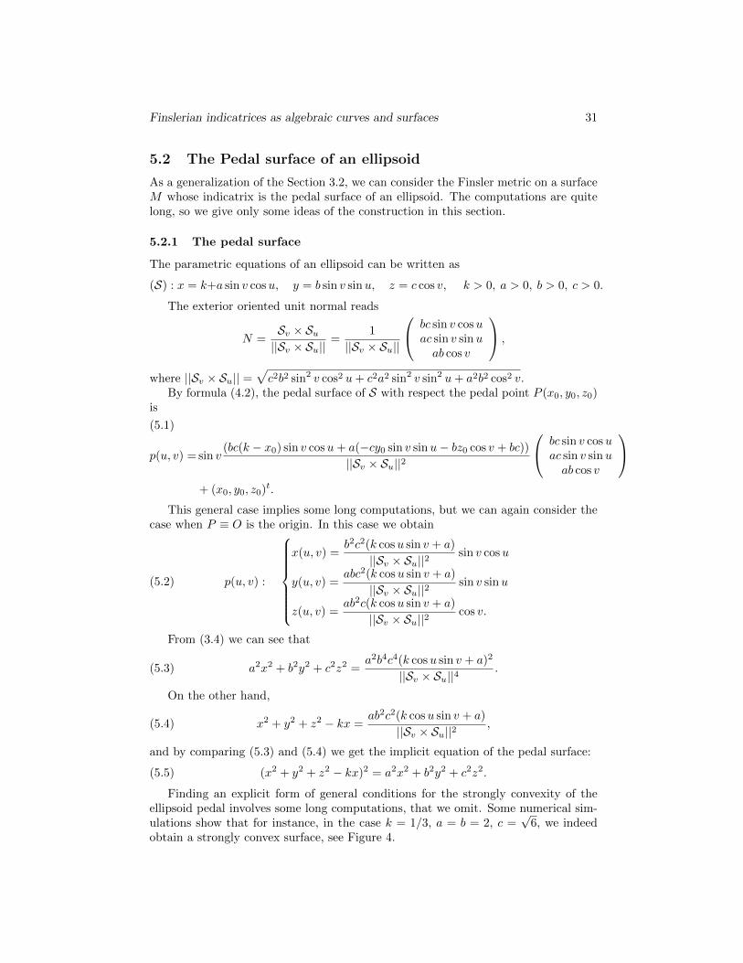
5.2 The Pedal surface of an ellipsoid

As a generalization of the Section 3.2, we can consider the Finsler metric on a surfaceM whose indicatrix is the pedal surface of an ellipsoid. The computations are quitelong, so we give only some ideas of the construction in this section.

5.2.1 The pedal surface

The parametric equations of an ellipsoid can be written as

(S) : x = k+a sin v cosu, y = b sin v sinu, z = c cos v, k > 0, a > 0, b > 0, c > 0.

The exterior oriented unit normal reads

N =Sv × Su||Sv × Su||

=1

||Sv × Su||

bc sin v cosuac sin v sinuab cos v

,

where ||Sv × Su|| =√c2b2 sin2 v cos2 u+ c2a2 sin2 v sin2 u+ a2b2 cos2 v.

By formula (4.2), the pedal surface of S with respect the pedal point P (x0, y0, z0)is

p(u, v) = sin v(bc(k − x0) sin v cosu+ a(−cy0 sin v sinu− bz0 cos v + bc))

||Sv × Su||2

bc sin v cosuac sin v sinuab cos v

+ (x0, y0, z0)t.

(5.1)

This general case implies some long computations, but we can again consider thecase when P ≡ O is the origin. In this case we obtain

(5.2) p(u, v) :

x(u, v) =b2c2(k cosu sin v + a)

||Sv × Su||2sin v cosu

y(u, v) =abc2(k cosu sin v + a)

||Sv × Su||2sin v sinu

z(u, v) =ab2c(k cosu sin v + a)

||Sv × Su||2cos v.

From (3.4) we can see that

(5.3) a2x2 + b2y2 + c2z2 =a2b4c4(k cosu sin v + a)2

||Sv × Su||4.

On the other hand,

(5.4) x2 + y2 + z2 − kx =ab2c2(k cosu sin v + a)

||Sv × Su||2,

and by comparing (5.3) and (5.4) we get the implicit equation of the pedal surface:

(5.5) (x2 + y2 + z2 − kx)2 = a2x2 + b2y2 + c2z2.

Finding an explicit form of general conditions for the strongly convexity of theellipsoid pedal involves some long computations, that we omit. Some numerical sim-ulations show that for instance, in the case k = 1/3, a = b = 2, c =

√6, we indeed

obtain a strongly convex surface, see Figure 4.


Figure 4: The convex pedal surface of an ellipsoid, with pedal point at origin, fork = 1/3, a = b = 2, c =

√6 and the non-convex case for k = 1/3, a = b = 2, c = 4.


Applying Okubo’s method to (5.5) we obtain the Minkowski norm F = x2+y2+z2√a2x2+b2y2+c2z2+kx

that is clearly the generalization of (3.5).The Finsler metric corresponding to this indicatrix surface is of the type (3.6),

where α1, α2 are two different Riemannian metrics. This the generalization of thediscussion in Section 3.2.

We can summarize

Theorem 5.3. The Finsler metric on a three dimensional manifold M whose indi-

catrix is given by the pedal surface of the ellipsoid(x−ka

)2+(yb

)2+(zc

)2= 1 with

origin as pedal point is of type F =α2

1

α2−β , where α1, α2 are two different Riemannianmetrics and β is a linear form in TM . This Finsler metric is strongly convex subjectto some conditions for a, b, c and k.

Remark 5.2. Similarly with the sphere case, without giving here the concrete com-putations, one can easily see that the same formulas are true for the arbitrary dimen-sional case as well.

The Finsler metric on an n-dimensional manifold M whose indicatrix is given bythe pedal hypersurface of an ellipsoid with origin as pedal point is a slope type metric

F =α2

1

α2−β , where α1, α2 are two different Riemannian metrics on M and β a linearone form on TM . This Finsler metric is strongly convex for some further conditionson the constants giving the axes of the ellipsoid and the coordinates of its center.

Acknowledgements. We are extremely grateful to Prof. H. Shimada for manyuseful discussions during the preparation of this manuscript.

This research was supported by King Mongkut’s Institute of Technology Ladkra-bang Research Fund, grant no. KREF046201.

References

[1] P. L. Antonelli, R. S. Ingarden, M. Matsumoto, The Theory of Sprays and FinslerSpaces with Applications in Physics and Biology, Kluwer Acad. Publ., FTP Vol.58, 1993.


[2] D. Bao, S. S. Chern, Z. Shen, An Introduction to Riemann-Finsler Geometry,Springer, Graduate Texts in Mathematics, 2000.

[3] P. Chansri, P. Chansangiam, S. V. Sabau, The geometry on the slope of a moun-tain, arXiv:1811.02123 [math.DG], 2018.

[4] C. G. Gibson, Elementary Geometry of Algebraic Curves, Cambridge UniversityPress, 1998.

[5] S. Markvorsen,A Finsler geodesic spray paradigm for wildfire spread modeling,Nonlinear Analysis: Real World Applications, 28 (2015), 208–228.

[6] M. Matsumoto, A slope of mountain is a Finsler surface with respect to a timemeasure, J. Math. Kyoto Univ., 29 (1989), 17–25.

[7] S. V. Sabau, K. Shibuya, H. Shimada, Metric structures associated to Finslermetrics, Publ. Math. Debrecen, 84, 1-2 (2014), 89–103.

[8] S. V. Sabau, K. Shibuya, R. Yoshikawa, Geodesics on strong Kropina manifolds,European J. Math. 3 (2017), 1172–1224.

[9] I. D. Teodorescu, S. D. Teodorescu, Collection of problems of elementary geom-etry, Didactical and Pedagogical Editorial House, Bucharest, 1975, 61–65.

[10] C. Udriste, Finsler-Lagrange-Hamilton structures associated to control systems,Eds: M. Anastasiei, P.L. Antonelli, Proceedings of a Conference held on August26-31, 2001, Iasi, Romania, Kluwer Academic Publishers, 2003, 233–243.

[11] R. Yoshikawa, S. V. Sabau, Kropina metrics and Zermelo navigation on Rieman-nian manifolds, Geometriae Dedicata, 171 (1) (2014), 199–148.

Authors’ addresses:

Pipatpong ChansriDepartment of Mathematics,Faculty of Science, KMITL, Bangkok, 10520, Thailand.E-mail: [email protected]

Pattrawut ChansangiamDepartment of Mathematics, Faculty of Science,King Mongkut’s Institute of Technology Ladkrabang,Bangkok, 10520, Thailand.E-mail: [email protected]

Sorin Vasile SabauDepartment of Biology,Tokai University, Sapporo 005 – 8600, Japan.E-mail: [email protected]

Finslerian indicatrices as algebraic curves and surfaces

Documents

Transcript of Finslerian indicatrices as algebraic curves and surfaces