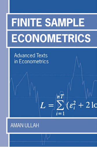
Finite Sample Eco No Metrics

ADVANCED TEXTS IN ECONOMETRICS

General Editors

Manuel Arellano Guido Imbens Grayham E.Mizon

Adrain Pagan Mark Watson

Advisory Editor

C. W. J. Granger

Other Advanced Texts in Econometrics

ARCH: Selected ReadingsEdited by Robert F. EngleAsymptotic Theory for Integrated ProcessesBy H. Peter BoswijkBayesian Inference in Dynamic Econometric ModelsBy Luc Bauwens, Michel Lubrano, and Jean-François RichardCo-integration, Error Correction, and the Econometric Analysis of Non-Stationary DataBy Anindya Banerjee, Juan J. Dolado, John W. Galbraith, and David HendryDynamic EconometricsBy David F. HendryLikelihood-Based Inference in Cointegrated Vector Autoregressive ModelsBy Søren JohansenLong-Run Economic Relationships: Readings in CointegrationEdited by R. F. Engle and C. W. J. GrangerModelling Economic Series: Readings in Econometric MethodologyEdited by C. W. J. GrangerModelling Non-Linear Economic RelationshipsBy Clive W. J. Granger and Timo TeräsvirtaModelling SeasonalityEdited by S. HyllebergNon-Stationary Time Series Analysis and CointegrationEdited by Colin P. HargreavesOutlier Robust Analysis of Economic Time SeriesBy André Lucas, Philip H. Franses, and Dick van DijkPanel Data EconometricsBy Manuel ArellanoPeriodicity and Stochastic Trends in Economic Time SeriesBy Philip Hans FransesProgressive Modelling: Non-nested Testing and EncompassingEdited by Massimiliano Marcellino and Grayham E. MizonStochastic Limit Theory: An Introduction for EconometriciansBy James DavidsonStochastic VolatilityEdited by Neil ShephardTesting ExogeneityEdited by Neil R. Ericsson and John S. IronsTime Series with Long MemoryEdited by Peter M. RobinsonTime-Series-Based Econometrics: Unit Roots and Co-integrationsBy Michio HatanakaWorkbook on CointegrationBy Peter Reinhard Hansen and Søren Johansen

Finite Sample Econometrics

AMAN ULLAH

Great Clarendon Street, Oxford OX2 6DPOxford University Press is a department of the University of Oxford.

It furthers the University's objective of excellence in research, scholarship,and education by publishing worldwide in

Oxford New YorkAuckland Bangkok Buenos Aires Cape Town Chennai

Dar es Salaam Delhi Hong Kong Istanbul Karachi KolkataKuala Lumpur Madrid Melbourne Mexico City Mumbai Nairobi

São Paulo Shanghai Taipei Tokyo TorontoOxford is a registered trade mark of Oxford University Press

in the UK and in certain other countriesPublished in the United States

by Oxford University Press Inc., New York© Aman Ullah 2004

The moral rights of the authors have been assertedDatabase right Oxford University Press (maker)

First published 2004All rights reserved. No part of this publication may be reproduced,

stored in a retrieval system, or transmitted, in any form or by any means,without the prior permission in writing of Oxford University Press,

or as expressly permitted by law, or under terms agreed with the appropriatereprographics rights organization. Enquiries concerning reproduction

outside the scope of the above should be sent to the Rights Department,Oxford University Press, at the address above

You must not circulate this book in any other binding or coverand you must impose this same condition on any acquirer

British Library Cataloguing in Publication DataData available

Library of Congress Cataloging in Publication DataData available

ISBN 0-19-877447-8 (hbk.)ISBN 0-19-877448-6 (pbk.)

1 3 5 7 9 10 8 6 4 2

Contents

Preface ix1 Introduction 12 Finite Sample Moments 92.1 Introduction 92.2 Exact Moments: Normal Case 92.3 Exact Moments: Nonnormal Case 18

2.3.1 Binomial Distribution 182.3.2 Poisson Distribution 192.3.3 Gamma Distribution 192.3.4 Exponential Family 202.3.5K-Parameter Exponential Density 212.3.6 Mixtures of Distributions 222.3.7 Edgeworth Density or Gram–Charlier Density 23

2.4 Exact Moments: General Case 242.5 Approximations of Moments 26

2.5.1 Large Sample Approximations: Normal and Nonnormal 272.5.2 Small-σ Approximations: Normal and Nonnormal 362.5.3 Results for Non-i.i.d Cases 442.5.4 The Laplace Approximation: Normal and Nonnormal 45

2.6 Summary and Survey 483 Finite Sample Distributions 513.1 Introduction 513.2 Exact Distribution 51

3.2.1 Distribution of Ratio of Quadratic Forms 523.3 Approximations of the Distribution of Quadratic Forms 553.4 Limiting Distributions 563.5 Nonnormal Case 573.6 Large-n Edgeworth Expansion 57

3.7 Small-σ Edgeworth Expansion of h(y) (Normal and Nonnormal) 673.8 Remarks on the Edgeworth Expansion 69

4 Regression Model 754.1 Introduction 754.2 Model Specification and Least Squares Estimation 754.3 Properties of Estimators 77

4.3.1 Coefficients Estimators 774.3.2 Residuals and Residual Sum of Squares 804.3.3R2 and Adjusted R2 834.3.4 The F-Ratio 864.3.5 Prediction 874.3.6 Exact Moments Under Nonnormal 894.3.7 Approximate Moments 904.3.8 Hypothesis Testing 944.3.9 Nonlinear Regression Models 96

5 Models with Nonscalar Covariance Matrix of Errors 975.1 Introduction 975.2 General Model with Nonscalar Covariance Matrix 97

5.2.1 Exact Moments 975.2.2 Approximate Distribution and Moments 1005.2.3 Hypothesis Testing 104

5.3 Specialized Models 1075.3.1 Heteroskedasticity 1075.3.2 Heteroskedasticity Testing 1125.3.3 Model with Autocorrelation 1135.3.4 Seemingly Unrelated Regressions 1165.3.5 Limited Dependent Variable Models 1205.3.6 Panel Data Models 123

6 Dynamic Time Series Model 1296.1 Introduction 1296.2 Model and Least-Squares Estimator 1296.3 Finite Sample Results for Dynamic Model 133

6.3.1 Review 1336.3.2 Exact Results for AR(1) model 1376.3.3 Approximate Methods 1396.3.4 Probability Distributions 1456.3.5 ARMAX model 1476.3.6 Nonnormal Case 1486.3.7 Cointegration Model 149

6.4 Conclusion 151

vi CONTENTS

7 Simultaneous Equations Model 1537.1 Introduction 1537.2 Simultaneous Equations Model 154

7.2.1 Model Specification 1547.2.2 Moments of the Single Equation Estimators 1557.2.3 Moments of the IV Estimators of β 1627.2.4 General Case of m Endogenous Variables 1627.2.5 Approximate Moments 1647.2.6 Nonlinear Simultaneous Equations Model 1647.2.7 Density Function of IV Estimator 1667.2.8 Further Finite Sample Results 1687.2.9 Summary of Results 170

7.3 Analysis of Weak Instruments 1717.3.1 Effects on the Moments and Distribution 1717.3.2 Issue of Optimal Instruments 175

Appendix AStatistical Methods 179A.1 Moments and Cumulants 179A.2 Gram–Charlier and Edgeworth Series 180A.3 Asymptotic Expansion and Asymptotic Approximation 182

A.3.1 Asymptotic Expansion (Stochastic) 184A.4 Moments of the Quadratic Forms Under Normality 185A.5 Moments of Quadratic Forms Under Nonnormality 187A.6 Moment of Quadratic Form of a Vector of Squared Nonnormal Random Variables 188A.7 Moments of Quadratic Forms in Random Matrices 189A.8 Distribution of Quadratic Forms 192

A.8.1 Density and Moments of a Noncentral Chi-square Variable 193A.8.2 Moment Generating Function and Characteristic Function 194A.8.3 Density Function Based on Characteristic Function 195

A.9 Hypergeometric Functions 196A.9.1 Asymptotic Expansion 197

A.10 Order of Magnitudes (Small o and Large O) 197References 199Index 227

CONTENTS vii

To my daughter, Sushana Ullah

Preface

Over the last five decades, significant advances in the estimation and inference of various econometric models havetaken place. This includes the classical linear model where the explanatory variables are nonstochastic (fixed) and theerror is normally distributed, and the non-classical models, where these classical assumptions are violated. Thesemodels are frequently used in applied work, such as the simultaneous equation models, models with heteroskedasticityand/or serial correlation, limited dependent variable models, panel data models, and a large class of time series models.Many of these models may also be nonlinear, explanatory variables can be stochastic and errors follow nonnormaldistributions. While the classical linear model is often estimated by the ordinary least squares (LS) or generalized leastsquares (GLS) estimators, the non-classical models have largely used the maximum likelihood (ML), the method ofmoments, the instrumental variable, and the extremum estimation techniques. Within this setup, establishing theproperties of estimators in the classical linear model are straightforward for samples of any size and they are wellpresented in econometrics textbooks. For the non-classical models, however, textbooks have mostly presented largesample theory results despite the existing finite sample analytical results. One explanation of this may be the technicaldifficulties in developing the existing finite sample results and the complexities of their expressions.

It is well known that the large sample theory properties may not imply the finite sample behavior of econometricsestimators and test statistics. In fact, the use of asymptotic theory results for small or even moderately large samplesmay give misleading results. The field of finite sample theory has been developing rapidly since the seminalcontributions of Sir R. A. Fisher. Its applications in improving the inference for finite samples, the issues of bias-adjusted estimation, analyzing weak instruments, determining optimal instruments and bootstrapping have furtherenhanced the importance of the large existing literature on the finite sample.

This book is intended to provide a somewhat first comprehensive and unified treatment of finite sample theory and toapply the basic tools of this to various estimators and test statistics used in various econometric models. Both timeseries and cross section data models as well as panel data models are considered.

The results are explored for linear and nonlinear models as well as models with normal and nonnormal errors.

An aspect of the book is to use fairly unified approaches to develop the results in finite sample theory. Within thisframework we also indicate, at appropriate places, the alternative methods developed by others and provide the resultsin a simpler way. In some cases we are able to establish more general results and sometimes we provide new results.Since we include some new results in addition to previously known ones we hope that this book may be helpful forfurther developments of the finite sample results in many other econometric situations.

The book contains seven chapters and an appendix. Chapter 1 gives the introduction to finite sample econometrics.Chapter 2 gives the methods of obtaining the moments of econometric statistics. The methods of analyzingdistributions are given in Chapter 3. The finite sample results for various econometric models are then discussed inChapters 4–7. Chapter 4 deals with the results in the classical regression model. Chapter 5 considers the analysis ofmodels such as the heteroskedasticity model, the serial correlation model, the seemingly unrelated regressions model,the limited dependent variable model, and the panel data model. The time series models are analyzed in Chapter 6.Finally, Chapter 7 gives results for the simultaneous equations models. It is assumed that the reader is familiar with thebasic concepts of calculus and statistics and has a good background in introductory econometrics.

This book is designed for graduate courses in econometrics and statistics. It can be used both as a textbook and as areference for the graduate courses in econometrics and statistics. Since the focus of the book is on the finite sampleresults and not on details about econometric models, this book can also be supplemented by standard econometricstexts. Finally, the book may also be useful for students and researchers in other applied sciences, such as medicine,psychology, engineering, and sociology.

I want to express my deep appreciation to those who have helped and influenced the gradual development of this overthe years work. In particular, I would like to thank R. A. L. Carter, D. E. A. Giles, D. Hendry, G. Hillier, G. Judge, J.Knight, E. Maasoumi, R. Mittelhammer, A. L. Nagar, G. D. A. Phillips, P. C. B. Phillips, B. Raj, H. D. Vinod, A.Zellner, and V. Zinde-Walsh. Clive Granger was especially encouraging regarding this project and provided usefulcomments. Yong Bao and Xiao Huang read the complete manuscript and provided helpful comments. I am deeplygrateful to Carolina Stickley, who typed this challenging manuscript with remarkable skill and accuracy. Finally, thelargest debt, of course, belongs to my wife Shobha and daughter Sushana for their patience and help in making thiswork a reality. I would especially like to acknowledge my great debt to my guru A. L. Nagar, and to my friend and co-author, the late Viren Srivastava.

x PREFACE

1 Introduction

An important tool of econometric inference for analyzing an economic phenomenon is the use of the asymptoticdistribution theory of estimators and test statistics. One important reason for the popularity of the asymptotic theoryresults in econometric analysis is their ultimate simplicity. For example, using the central limit theorems, most of theestimators can be shown to follow normality, which can then be utilized to form confidence intervals. It is oftenobserved, however, that asymptotic properties are commonly shared by several estimators of any specific parameter ofinterest. For example, the ordinary least squares (LS) estimator and the Stein-rule estimators (under certain conditions)for coefficient vectors in a linear regression model have the same asymptotic distribution. Similarly, for coefficients inan over-identified structural equation of a simultaneous equation model, the two-stage LS, and the limited informationmaximum likelihood (ML) are known to have identical asymptotic properties under some mild conditions. A similarresult holds for the three-stage LS and for the full information maximum likelihood estimators too. In the context ofseemingly unrelated regression equations, all feasible generalized LS estimators stemming from the consistentestimation of the variance–covariance matrix of disturbances have identical asymptotic distributions. Consequently, insuch circumstances it is not possible to deduce any clear preference of one estimator over the other. Besides this,asymptotic properties hinge upon a crucial condition that the number of observations be infinitely large. Thiscondition is generally not met in practice, although there are an increasing number of data sets in finance, developmenteconomics, and labor economics, which contain a large number of observations. Even if a large number ofobservations is available, it may not be desirable to use them because they may not satisfy some of the other conditionsof the asymptotic theory results, which are often not verified by the practitioners. For instance, longer time seriesobservations may tend to violate the assumption of constancy of parameters on which the asymptotic theory is based.Also the time series observations may follow random walks or

some other kind of nonstationarity, which can violate the standard asymptotic normality results, a point first brought toattention by Granger and Newbold (1974) and developed by Phillips (1986). Moreover, the question relating to how“large” the number of observations should be to achieve the asymptotic properties results remains largely unanswered.Thus the basic requirement of the number of observations to be infinitely large for the asymptotic results to hold truemay not be achieved in many practical applications and therefore the use of inference procedures based on theasymptotic distribution theory may cast doubts about their continued validity in finite samples since the asymptoticresults need not carry over to finite samples, a point first brought to attention in the seminal work of Fisher (1921). Forexample, if the asymptotic distribution of an estimator has the smallest variability, its finite sample exact distributionmay not continue to possess the property of smallest variability. To illustrate this point, let us consider a bivariate linearregression model:

where yi and xi denote the ith observation on the variable and the explanatory variable, β is the unknown regressioncoefficient and ui is the error term with the following properties:

σ2 being an unknown but finite quantity. Further, it is assumed that tends to a finite nonzero quantity mxx as napproaches ∞. This assumption does not hold, for instance, in the presence of trend. For example, if xi = i, we have

whose limiting value as n → ∞ is obviously not finite.

The ordinary LS estimator of β is given by

which is the best linear unbiased estimator with variance as

The asymptotic distribution of n1/2(b − β) is a normal distribution with mean 0 and variance (σ2/mxx).

2 INTRODUCTION

Similarly, an unbiased estimator of σ2 based on ordinary LS residuals is given by

If the errors follow a normal probability law, it is well known that the exact distribution of b is normal with mean β andvariance while the exact distribution of (n − 1)s2/σ2 is the χ2 distribution with (n − 1) degrees of freedom (d.f.).Further, b and s2 are stochastically independent.

Now let us consider the following two estimators of θ = β2:

If we define

it follows from the normality of disturbances that

Using these results, we observe that

so that the bias of is

INTRODUCTION 3

Similarly, the mean squared error (MSE) of is

For the estimator , we find that the bias and MSE are

4 INTRODUCTION

Examining the expressions (1.8) and (1.10), we find that the estimator is biased and the bias is positive while theestimator is unbiased. Similarly, we observe from (1.9) and (1.11) that the MSE of is larger than the variance ofwhen n exceeds 3. These results are exact in nature. If we look at the asymptotic properties, it is easy to see that boththe estimators and are consistent. Further, the asymptotic variances of and are identical andtheir expression is (4β2σ2/mxx). It thus follows that both the estimators are asymptotically equivalent in the sense thatthey have the same asymptotic properties and therefore one cannot be preferred over the other. However, thecorresponding results in finite samples clearly reveal that and have markedly different properties.

Next, let us consider the estimation of θ = (1/β), the inverse of the regression coefficient β(≠ 0). It is customary toestimate it by . Now consider the rth (r > 0) moment of it:

which is infinite. It thus follows that has no finite moments. In other words, the exact distribution of possesses nofinite moments. However, it can easily be seen that the asymptotic distribution of is normal with mean 0 andvariance . Thus the moments are finite for an infinitely large number of observations while they are infinitefor a finite number of observations.

The results in (1.2) to (1.12) can also be verified for a special case where xi = 1 for i = 1, …, n. In this case, (1.1)becomes the population mean model yi = β + ui and the estimator b in (1.2) reduces to the sample mean y = ∑yi/n. Toemphasize the above points further, consider b1 = nb/(n+1) to be an alternative estimator of the mean β. Then, onecan easily show that both b1 and b are asymptotically unbiased and their asymptotic MSEs are equivalent, that is nMSE(b1) = n MSE (b) = σ2 as n→ ∞. However, their finite sample behaviors are different. While b is unbiased, b1 is biased;E(b1) − β = −β/(n + 1). Further MSE(b) =V(b) = σ2/n, but MSE(b1) = (n2/(n + 1)2)V(b) + β2/(n + 1)2. Thus MSE(b) <MSE(b1) so long as σ2/β2 < n/(2n + 1).

The above illustrations clearly demonstrate that the asymptotic distribution theory may lead to some results, whichmay significantly depart from those based on exact finite sample distribution theory. This is not to suggest that theasymptotic distributions should be outrightly discarded; they are valuable in their own right. They are not completelyirrelevant from a practical point of view because generally when we estimate an unknown parameter, we want theestimator to be quite precise and in order to achieve this objective we have to have a large sample. The limitations ofthe asymptotic distribution theory with special reference to its failure to shed light on the performance of inferenceprocedures in certain finite sample situations clearly sensitize as well as emphasize the need of an investigation of finitesample distribution theory to base our conclusions on it. Indeed the availability of both the finite sample and theasymptotic results is also useful for answering the questions as to how large the observations should be so that theasymptotic results hold.

INTRODUCTION 5

Having discussed above the importance of finite sample econometrics we now turn to a brief description of thedevelopments in this area and then indicate the methodologies to be used in this book. Fisher (1921, 1922, 1928,1935), more than seven decades ago, laid the foundation of modern finite sample theory. Also, see the fundamentalwork of Cramér (1946) on the distribution theory. It was brought into econometrics by the seminal work of Haavelmo(1947), and Anderson and Rubin (1949) on the exact confidence regions of structural coefficients, and that of Hurwicz(1950) on the exact LS bias in an autoregressive model. This was followed by the important contributions of Basmann(1961), Bergstrom (1962), Kabe (1963, 1964), Richardson (1968), Sawa (1969), Anderson and Sawa (1973), Ullah andNagar (1974), Hillier, Kinal, and Srivastava (1984), and Phillips (1983) on the exact density and moments of theestimators in the simultaneous equations model. All these important contributions were related to obtaining exactresults, which hold for any size of the sample; small, moderately large, or very large. However, these results were oftenvery complicated to draw meaningful inferences from them. A major development took place through the pioneeringwork of Nagar (1959) on obtaining the approximate moments of the k-class estimators in simultaneous equations.Sargan (1975, 1976, 1980), and Phillips (1977b, 1978, 1980) rigorously developed the theory and applications ofEdgeworth expansions to derive the approximate distribution functions of econometric estimators. The idea of theEdgeworth expansions stems from the fundamental work of Edgeworth (1896, 1905)—see also Chebyshev (1890),Gram (1879), Charlier (1905), and Cramér (1928). More details on the Edgeworth expansion can be found in Wallace(1958), Chibishov (1972), Phillips (1980), and Rothenberg (1984a). The moments of the Edgeworth approximatedistributions can be the same as Nagar's approximations of the moments (Rothenberg 1984a). These approximatedistributions are also known as the asymptotic expansions or large sample approximations, and these provide theresults which will tend to be between the exact and asymptotic results. Thus it can tell us how much we lose by usingthe asymptotic result and how far we are from the known exact results. The latter also measures the accuracy of theapproximate results. A significant growth in the literature took place through the dedicated work of J. D. Sargan and hisstudents at the London School of Economics, A. L. Nagar and his students at the Delhi School of Economics, R. L.Basmann and his students at Texas A&M, T. W. Anderson and his students at Stanford, and P. C. B. Phillips, amongothers. Most of the contributions of these schools were confined to the analytical derivations of the moments anddistributions in the simultaneous equations model, the details of which can be found in the surveys by Basmann(1974), Anderson (1982), Mariano (1982), Phillips (1980, 1983), Taylor (1983), and Maasoumi (1988). Thesedevelopments include the finite sample results by using the Monte Carlo methodology (see Hendry 1984). Recently,bootstrapping (resampling) techniques have become popular (see Hall 1992; Jeong and Maddala 1993; Li and Maddala1996; Vinod 1993; Horowitz 2001). Both Monte

6 INTRODUCTION

Carlo and bootstrapping will not be discussed in this book. The analytical results we develop here, however, are usefulfor both these simulation methods.

Despite the above research contributions, the discussion of analytical finite sample results in elementary as well asadvanced text books is almost negligible. Usually a typical text book starts with analytical finite sample results (exactmean and variance, say, of the LS estimator) in the regression chapter and then continues using, instead, asymptotictheory in the remaining chapters.

There are perhaps several reasons for this. First, the derivations of finite sample results, especially exact results, areoften demanding and require a knowledge of statistical distribution theory. Terms like Wishart distribution, zonalpolynomials, manifolds, noncentral distributions, have undoubtedly kept economists away from this area of research.In addition, the results are often complicated and lengthy. Second, results are mainly available for estimators in staticsimultaneous equations but not as much for other models such as the heteroskedastic, dynamic regression, limiteddependent variables, or rational expectations. Third, several different techniques have been developed to study thefinite sample behavior of a given estimator or test statistic. For example, several papers (e.g. Sawa 1972; Nagar andUllah 1973) exist on the exact moments of the two-stage least squares and, similarly, several papers on its exact density(see Richardson 1968; Anderson and Sawa 1979). Learning and mastering each and every technique is beyond thescope of most graduate students and researchers. No attempt is made in this book to present these various techniquesand interested readers are referred for detailed references to Phillips (1983, 1987d), Mariano (1982), Taylor (1983), andRothenberg (1984a).

In this book we attempt to provide unified approaches to study finite sample econometrics. Essentially we discuss aunified technique for obtaining the exact moments, and a technique for obtaining the exact distributions. This is basedon the observations in Ullah (1990), Lye (1987, 1988), and Cribbett, Lye, and Ullah (1989) that a large class ofeconometric estimators and test statistics can be written as a ratio of quadratic forms, or in general a real valuedfunction h(y) of the vector y of observations on the dependent variable of an econometric model. Basically, using Ullah(1990), the technique of obtaining the exact moments amounts to replacing the expectation of h(y), y ∼ N(μ, 1), by h(d),where the operator d = μ + ∂/∂μ. This is an extremely simplified generalization of the techniques used in Baranchik(1964), Ullah and Nagar (1974), and A. Ullah and S. Ullah (1978). To obtain the exact density functions, the use ofGurland (1948), Imhof (1961), Davies (1980), and Forchini (2002) evaluation of the distribution function of the ratioof quadratic forms is proposed. The alternative techniques of obtaining the exact moments and distributions arecompared, discussed, or referred to at appropriate places.

The exact results are often complicated to analyze. In view of this, the approximate distributions based on the resultsfor the Edgeworth expansion of distributions of a function h(y) are presented. For obtaining the approximateEdgeworth type moments, Nagar (1959) large sample approximation and

INTRODUCTION 7

its generalization in Rilstone, Srivastava, and Ullah (1996), Bao and Ullah (2002), and Kadane (1971) small-σapproximation and its generalization in Ullah, Srivastava, and Roy (1995) are considered in this book. In some specialcases, these approximations are compared with the Laplace approximation in Lieberman (1994a).

The techniques of obtaining the exact and approximate moments described above are presented in Chapter 2 alongwith some examples. The techniques for the exact and approximate distributions are presented in Chapter 3. Theapplications of these techniques and other finite sample results for various econometric models are then presented inthe remaining chapters. Essentially, Chapter 4 analyzes the finite sample analysis of the estimators and test statistics inthe case of regression models with the scalar covariance matrix of the errors. Chapter 5 then considers the regressionmodels with the nonscalar covariance matrix of the errors. This includes the estimators and test statistics in the contextof linear regression with heteroskedasticity and serial correlation, seemingly unrelated regressions, limited dependentvariables, and panel data models. In Chapter 6 we deal with the dynamic time series models. Finally, Chapter 7considers the analysis of the simultaneous equations model. The important features of all these chapters can besummarized below: (a) focus of each chapter is on analyzing finite sample behavior of the econometric estimators andtest statistics; (b) simpler and unified techniques are used for deriving exact and approximate results; (c) results areexplored for both normal and nonnormal error; (d) finite sample results are presented and analyzed for different kindsof econometric models in cross section and time series cases.

8 INTRODUCTION

2 Finite Sample Moments

2.1 IntroductionIt was discussed in Chapter 1 that there is a need for unified techniques to obtain the exact and approximate momentsof econometric estimators and test statistics. The objective of this chapter is essentially to provide such techniques.These techniques will be supported by illustrative examples to help clear the basic ideas behind the main results.

2.2 Exact Moments: Normal CaseLet y be a scalar random variable, which is distributed according to normal law with μ = Ey and σ2 = V(y). The densityfunction of y can be written as

This is well known to be symmetric around μ, its mean, median, and mode coincide, its kurtosis coefficient is 3, and itsinflexion points occur at μ ± σ where ∂2f(y)/∂y2 = 0. A feature of the normal density, which is not well known but playsan important role in developing our main results is that

which can be rewritten as

where d is the derivative operator involving μ and σ2

This feature of the first derivative of normal density in (2.3) can be generalized as

where h(y) is any real valued analytic function of y. The equality in (2.5) is obtained by first writing the Taylor seriesexpansion of h(y) around d as

and then noting that

because (y − d)sf(y) = 0 for s = 1, 2, …, from (2.3); h(s) (d) = ∂(s)h(y)/∂ys evaluated at y = d.

Exercise 1 Let h(y) be a real valued scalar analytic function of an n × 1 normal random vector y with the n × 1 meanvector μ and the n × n positive definite covariance matrix Σ, that is, y ∼ N (μ, Σ). Show that

where

Solution The multivariate normal density of y can be written as

Then ∂f(y)/∂μ = Σ−1(y − μ)f(y), or yf(y) = (μ + Σ(∂/∂μ))f(y) = df(y), which gives h(y)f(y) = h(d)f(y) by using the Taylorexpansion of the function of a vector y, h(y).

The feature of normal density in (2.5) and Exercise 1 shows that a normal density multiplied by a function h(y) isidentical to multiplying it by h(d) where d is nonstochastic. This fundamental feature of the normal density helps us toobtain the exact moments of the function of y, h(y), in a straightforward way.

Lemma 1If h(y) = (h1(y),…, hm(y))′ is an m × 1 vector of real valued analytic functions of an n × 1 normal random vector y with themean vector μ and variance covariance matrix Σ, that is, y ∼ N (μ, Σ), and Eh(y) exists, then

10 EXACT MOMENTS: NORMAL CASE

where d = μ + Σ (∂/∂μ). Further, if h(y) and g(y) are two column vectors of real valued functions of y, and have finite expectations, then

Proof From Exercise 1, hj(y)f(y) = hj(d)f(y) for j = 1,…, m. Thus for the m × 1 vector h(y), h(y)f(y) = h(d)f(y). The result in(2.11) then follows by noting that

Similarly

In (2.13) we note that f(y) is an exponential function and the fact that differentiation under the integral sign ispermitted. Further in (2.11) h(d) · 1 reminds us that the derivative operator d is to be used on the constant 1.

The result in Lemma 1 provides a unified and simple technique for obtaining exact moments of various special casesof the function h(y). Essentially, this technique transforms the problem of obtaining the expectation of complicatedfunctions with the evaluation of their derivatives, which can be easily obtained and/or numerically calculated. Sincemost of the estimators and test statistics can be written in terms of the function of a data vector y, Lemma 1 provides asingle method for obtaining their moments. We note, however, that for some econometric statistics (2.11) of Lemma 1is useful, and for others (2.12) of Lemma 1 along with Lemma 2 below is useful. The results in both the lemmas aresimple and do not require any extensive knowledge of statistical distribution theory.

Another important point is that Lemma 1 provides a recurrence relationship among the higher order moments of h(y).For example, if we consider h(y) to be a scalar function

where r ≥ 1. When r = 2, Eh2(y) = h2(d) · 1 = h(d)Eh(y). For the vector function h(y), Eh(y) h′(y) = h(d)Eh′(y) = h(d)h′(d) ·1.

FINITE SAMPLE MOMENTS 11

Exercise 2 Let y ∼ N (μ, Σ). Then show that Ey = μ and V(y) = Σ.

Solution Let h(y) = y. Then from Lemma 1 Ey = d · 1 = (μ + Σ(∂/∂μ)) · 1 = μ. NowV(y) = Eyy′ − μμ′. But from (2.12)in Lemma 1, Eyy′ = dd′ · 1 = dμ′ = (μ + Σ (∂/∂μ))μ′ = μμ′ + Σ so that V(y) = Σ.

Two points are important to remember. First, higher order derivatives should be obtained recursively, for example d2 ·1 = d(d · 1) rather than doing the square of (μ + σ2(∂/∂μ)) and then operating it on 1. Second, when Ey = μ = 0 thenEh(y) follows by first considering μ ≠ 0 in deriving h(d) · 1 and then substituting μ = 0 in the final result. For example,E(y − μ)2 = (d − μ)2 · 1 = 0 is not correct, but E(y − μ)2 = σ2 from Exercise 2 or alternativelyfor μ0 = 0, where d0 = μ0 + σ2 (∂/∂μ0) and we first consider E(y − μ) = μ0 ≠ 0.

Exercise 3 Let y ∼ N(μ, Σ). Then

where N is a symmetric matrix and r ≥ 1.

Solution Taking h(y) = y′ Ny, the result in (2.15) follows from (2.14). Alternatively, substitute h(y) = (y′ Ny)r in (2.11).

From (2.15) we note that

where dd′ · 1 = μμ′ + Σ from Exercise 1. Further

When μ = 0 and Σ = I, E(y′ Ny) = tr N and E(y′ Ny)2 = (tr N)2 + 2tr N2. Further when N is an idempotent matrix ofrank m ≤ n then E(y′ Ny) = m and E(y′ Ny)2 = m(m + 2), which is the well-known result for the moments of a χ2 = y′ Nyvariable with m degrees of freedom (d.f.).

The results in (2.16) and (2.17) also hold for y′ Ny whenN is not a symmetric matrix. In this case we need to replaceNby the symmetric matrix (N + N′)/2 since y′ Ny = y′(N + N′)y/2.


Exercise 4 Let y ∼ N(μ, I) and N1 and N2 be two symmetric matrices. Then

Solution From (2.11) or (2.12)

Using E(y′ N2y) from (2.16) we then get the result in (2.18).

When N1 = N2, (2.18) reduces to (2.17) with Σ = I.

Let y ∼ N(μ, Σ). Then

where H(y) is an m × m matrix of elements hij(y), i = 1, …, m, j = 1, …, m.

This follows by noting that Ehij(y) = hij(d) from Lemma 1.

In deriving the moments of econometric estimators we often encounter a scalar function g(y), which is an inversefunction of y. More specifically we often find g(y) = w−r, where w = y′ Ny and N is any symmetric (often nonnegativedefinite) matrix, and r is a nonnegative real number. For such a g(y) we can present E g(y) in the following Lemma.

Lemma 2If w = y′ Ny is a real valued quadratic form in the vector y ∼ N (μ, Σ), and the rank of N > 2r then

where N0 = I + 2tΣN = Σ(Σ−1 + 2tN) and .

Proof First we note from the gamma integral that


Thus

But E exp{−tw} = ∫exp{−ty′Ny}f(y) dy = |N0|−1/2 exp{−½μ′N0*μ}, where we use y′ Ay − 2b′y = (y − A−1b)′A (y −A−1b) − b′A−1b for some matrix A and vector b. The result in (2.20) then follows. (Q.E.D.)

The matrix N0 is such that |N0| = |Σ| |Σ−1 + 2tN| = |I + 2tΣ1/2NΣ1/2| and

where Σ = Σ1/2Σ1/2 and we use P to be an orthogonal matrix such that P′Σ1/2NΣ1/2P = ∧ and ∧ is a diagonal matrix ofeigenvalues λ1, …, λn of Σ1/2NΣ1/2. In econometric applications the structures of μ, Σ, and N are usually known.Further,N*0 = Σ−1 − Σ−1(Σ−1 + 2tN)−1Σ−1 = Σ−1/2 (I − (I + 2tΣ1/2NΣ1/2)−1)Σ−1/2. A series representation of Ew−r is given inSrivastava and Khatri (1979, ch. 2), Phillips (1986), and Smith (1988).

In a special case where Σ1/2NΣ1/2 or NΣ is an idempotent matrix (NΣ N = N) of rank p = rank of NΣ = tr(NΣ), theny′Ny is a noncentral χ2 with p degreees of freedom. In the case, λ1 = λ2 = ·s = λp = 1 and λp + 1 = ·s = λn = 0 so theresult in (2.20) along with (2.23) can be written as an infinite series. This gives the rth inverse moment of thenoncentral χ2 distribution as

where θ = (μ′Σ−1/2NΣ−1/2μ)/2 is a noncentrality parameter and

is a confluent hypergeometric function, see Appendix A.8.1 and A.9. Further if μ = 0, (2.24) reduces to

which is the rth inverse moment of the central χ2 distribution. If r is negative, (2.26) gives the moments of a central χ2distribution.

If N is a stochastic matrix but independent of y, then

which can be evaluated by taking the expectation of Ew−r with respect to the elements of N.


An important application of Lemma 2 is in obtaining the rth moment of the ratio of quadratic forms, q = y′N1y/y′Ny.This is given in the following Lemma.

Lemma 3Let y ∼ N(μ, Σ), and N1 and N be two symmetric matrices. Then, for r ≥ 1,

where d is the operator in (2.9). For r = 1,2 we get

where μ* = Σ−1μ, N2 = N0−1Σ = Σ(I − N*0Σ).

Proof From Lemma 1 (substituting h(y) = (y′N1y)r and g(y) = (y′ Ny)−r) we can write

where Ew−r is as given in Lemma 2. For r = 1, Eq = (d′N1d) Ew−1 = tr (N1dd′Ew−1), which gives Eq in (2.29). Further forr = 2, Eq2 = (d′N1d)2Ew−2 = (d′N1d) tr (N1dd′Ew−2), which gives Eq2 in (2.29).

Sawa (1972) used a result for the joint moment generating functions (mgf) of w1 = y′ N1y and w2 = y′Ny, M(θ1, θ2), andobtained the rth moment of q as

provided the expectation exists. The mgf is

where η = L−1μ, C = L′(θ1N1 + θ2N) and L is the matrix such that Σ = LL′. A choice of L is Σ1/2 as described above.For r = 1, 2 one can verify that (2.30) gives the results in (2.29). Magnus (1986) provides an explicit expression for E qr.His result is given below.

Lemma (Magnus)Let y ∼ N (μ, Σ = LL′). Let N1 be a symmetric matrix and N be a positive semi definite matrix, N ≠ 0. Let Pbe an orthogonal


matrix and D be a diagonal matrix such that P′ L′NLP = D and define N1* = P′L′N1LP, μ* = P′L−1μ. Then, if the expectationexists, for r = 1, 2,…

where the summation is over all 1 × r vectors v = (n 1, n2, …, nr) where elements nj are non-negative integers satisfying ,

and Δ is a diagonal positive definite matrix, R is a symmetric matrix and ξ is a vector given by

For the proof see Magnus who also gives the condition of existence of the moments in (2.30). This is given below.

Lemma (Magnus)Let N1 be the symmetric n × n matrix and N be a n × n positive semi definite of rank m ≥ 1. If m ≤ n − 1, letQ be an n × (n − m) matrix of full column rank n − m such that L N L Q = 0

1. If m ≤ n − 1 and L′N1LQ = 0, or if m = n then Eqr exists for all r ≥ 02. If m ≤ n − 1,Q′L′N1LQ = 0 and L′N1LQ ≠ 0 then Eqr exists for 0 ≤ r < m and does not exist for r ≥ m, and3. If m ≤ n − 1 and Q′L′N1LQ ≠ 0 then Eqr exists for 0 ≤ r < m/2 and does not exist for r ≥ m/2.

A large number of econometric estimators are in terms of the ratio of bilinear to quadratic forms, that is,

where y1 and y2 are n × 1 vectors and M1 and M are n × n symmetric matrices. Our problem is to obtain Eqr. Here weshow that this result can be obtained from the moments of the ratio of quadratic forms given above. For this we firstnote that

where


The important point is that the bilinear form y2′ M1y1 can be written as a quadratic form. Thus

is as given above with y ∼ N (μ, Σ) being a 2n × 1 vector and

μi = Eyi and Σij = Eyiyj′ for i, j = 1, 2.

The number of econometric estimators and test statistics that can be written as the ratio of quadratic forms or the ratioof bilinear to quadratic forms are quite large. We present some of them below. The details on them and others arediscussed in the relevant chapters.

Exercise 5 Consider the regression model y = Xβ + u where y is an n × 1 vector, X is an n × k nonstochastic matrixand u is an n × 1 disturbance vector. Show that the goodness of fit statistic R2 and Durbin–Watson statistic (D–W) are

whereN = I − ιι′/n, N1 = N − M, M = I − X(X′X)−1X′, M1 =M AM; ι is an n × 1 vector of unit elements and A is ann × n matrix of known constants.

Solution If the regression contains an intercept, that is, the first column of X contains unit elements, it is well knownthat (e.g. see Greene 2000)

where and M2 = M. Using these in R2 and D–W the results in Exercise 5 follow.

Exercise 6 Consider a single equation of the system of simultaneous equations as

where y1 and y2 are n × 1 vectors of observations on the endogenous variables, γ is a scalar and u is n × 1. Show that the2SLS estimator of γ is

where y, N1, and N are as in (2.37) with ; X is an n × k matrix of exogenous variables appearingin the remaining equations of the system.


Solution The well known form of the 2SLS is

see, for example, Theil (1971), Greene (2000). In its current setup is the ratio of a bilinear to quadratic forms.However, using (2.37) and the result follows immediately.

2.3 Exact Moments: Nonnormal CaseHere we first consider the case of discrete distributions and then take up the case of the continuous distributions. Ineach case we explore an operator corresponding to the operator d in the normal case, which can help to provide themoments of a function of y.

2.3.1 Binomial DistributionLet y be a scalar random variable, which is distributed as binomial with Ey = mπ = μ and σ2 = V(y) = mπ (1 − π); π isthe probability of success in a given trial. The density function of y can be written as

Then it can be verified that

or

where

Thus the operator (2.4) and hence Lemma 1 for the normal case goes through for the binomial distribution. This is,for the scalar y,

Exercise 7 Suppose y is distributed as a binomial with parameter π and density in (2.40). Show that

SolutionEy = d · 1 = (mπ + π(1 − π)∂/∂π) · 1 = mπ. Further Ey2 = (mπ + π(1 − π)∂/∂π)2 · 1 = (mπ + π(1 − π)∂/∂π) mπ= (mπ)2 + mπ(1 − π). Thus V(y) = Ey2 − (Ey)2 = mπ (1 − π).


2.3.2 Poisson DistributionLet y be a scalar random variable, which is distributed as a Poisson with Ey = λ = μ and V(y) = λ = σ2. The densityfunction of y is

Then it can be verified that

or

where

Thus the operator (2.4) and Lemma 1 for the normal case hold for the case of Poisson distribution also. That is Eh(y)= h(d) · 1.

Exercise 8 If y is distributed as a Poisson with the density in (2.45), show that Ey = λ and V(y) = λ.

SolutionEy = d · 1 = (λ + λ (∂/∂λ)) · 1 = λ and Ey2 = d2 · 1 = (λ + λ(∂/∂λ))λ = λ2 + λ. Thus V(y) = λ2 + λ −λ2 = λ.

Exercise 9 If yi, i = 1, …, n, is independent identically distributed (i.i.d) random variables with the Poisson density in(2.45), and y is an n × 1 random vector. Then show that, for a symmetric matrix N of constants,

SolutionE(y′ Ny) = trN(Eyy′). Now and E(yiyj) = (Eyi)(Eyj) = λ2 from the exercise above. Using these the resultfollows.

We now turn to the continuous distributions.

2.3.3 Gamma DistributionLet y be a scalar random variable with two parameters gamma density

For this density μ = Ey = r/λ and σ2 = V(y) = r/λ2. Further


or

where

Thus the operator d and Lemma 1 hold for gamma density as well. That is Eh(y) = h(d) · 1.

Exercise 10 Suppose yi, i = 1, …, n, is the i.i.d. random variables with the gamma density in (2.49). Show that

Solution First Eyi = d · 1 = ((r/λ) − (∂/∂λ)) · 1 = r/λ and Eyi2 = d.d · 1 = (r/λ)2 + r/λ2. Using this in E(y′ Ny) = trN(Eyy′) we get the result.

We note that gamma distribution includes exponential density (r = 1).

and χ2 (λ = 1/2), f(y) = yr−1e−(1/2)y/2r Γ r, as the special cases. For these cases also Eh(y) = h(d) · 1.

2.3.4 Exponential FamilyConsider a scalar random variable with an exponential family of densities as

where θ is a scalar parameter. For this density

which gives

or

where the operator d is


If g(y) is linear in y, for example, g(y) = y then (y − d) f(y) = 0 from (2.57) and we get Eh(y) = h(d) · 1. However, if g(y) isnot linear in y then

and E[h(g(y))] = h(d) · 1. Thus we can obtain the moments of the form h(g(y)) for every analytical function of h.

In the special case of a standard exponential family

g(y) = y is linear, c(θ) = θ and b(y) = 1. For this case the operator d in (2.58) reduces to

Further, for the exponential density in (2.53) d = ((1/λ) − (∂/∂λ)).

2.3.5K-Parameter Exponential DensityLet us consider a K-parameter exponential family as

Then, for i, j = 1, …, K,

where cji = ∂cj/∂θi. This gives

where and ; a = a(θ1, …, θK) and .

We note that the normal density with μ = θ1 and σ2 = θ2 is a special case of the K = 2 parameter exponential family.Other densities described above can also be seen as special cases.


2.3.6 Mixtures of DistributionsA family of mixtures of distributions can be written by considering the conditional distribution of y containing aparameter θ, say, f(y|θ), weighting it by a distribution of θ, say, f(θ), and then integrating with respect to θ. This gives

where Eθ represents the expectation with respect to random variable θ with density f(θ). For example, if f(y|θ) is anormal density with mean β and variance θ, and f(θ) is an inverted gamma density then f(y) is a t density. In general f(y)is a mixture of normal density if f(y|θ) is normal.

Using (2.65)

This implies that the moments of h(y), under (2.65), can be obtained in two steps: (a) obtain the expectations under aconditional density f(y|θ) (b) take expectation of these results with respect to θ.

Exercise 11 Suppose f(y|σ) is a normal density with the mean zero and variance σ2, and f(σ) is an inverted gammadensity

Show that f(y) is a t-density with m d.f. as

Solution From (2.65),

Now using the variable transformation (y2 + m)/2σ2 = z and the gamma integral we can easily verify the required resultin the exercise.


Exercise 12 Suppose y is a t-density with zero mean and m d.f. Show that, for m > 2,

Solution Using (2.66) and the above exercise

where f(σ) is the inverted gamma density. The integral in the last equality is a second moment of the inverted gammadensity, which is (Γ(m − 2)/2)/(Γ(m/2))(m/2) = m/(m − 2), m > 2, see Zellner (1971: 372). Hence the result in theexercise follows.

2.3.7 Edgeworth Density or Gram–Charlier DensitySuppose yi is distributed with mean μi and variance σi2. Then the Edgeworth density of or Gram–Charlier seriesexpansion of f(yi) is

where represents the normal density, that is, , and cj is as given in (A.10) (see Appendix A.2 andA.8.2). Davis (1976) gave an alternative convenient representation of (2.67), which is

where is and wi is a pseudo variate with mean and variance 0, and higher order cumulants thesame as those of .

As in the case of mixtures density, the moments of h(y) under the Edgeworth density can be obtained in two steps: (a)obtain the results under y | μ + w ∼ N(μ + w, I) (b) take expectation of these results with respect to w. That is

where E(h(y) | w) is the expectation of h(y) when y | μ + w ∼ N(μ + w, I).

Exercise 13 Suppose an n × 1 random vector y, with i.i.d. elements, follows an Edgeworth density with mean 0 andvariance I. Let be the sample average. Show that

Solution Using (2.68) . Further .


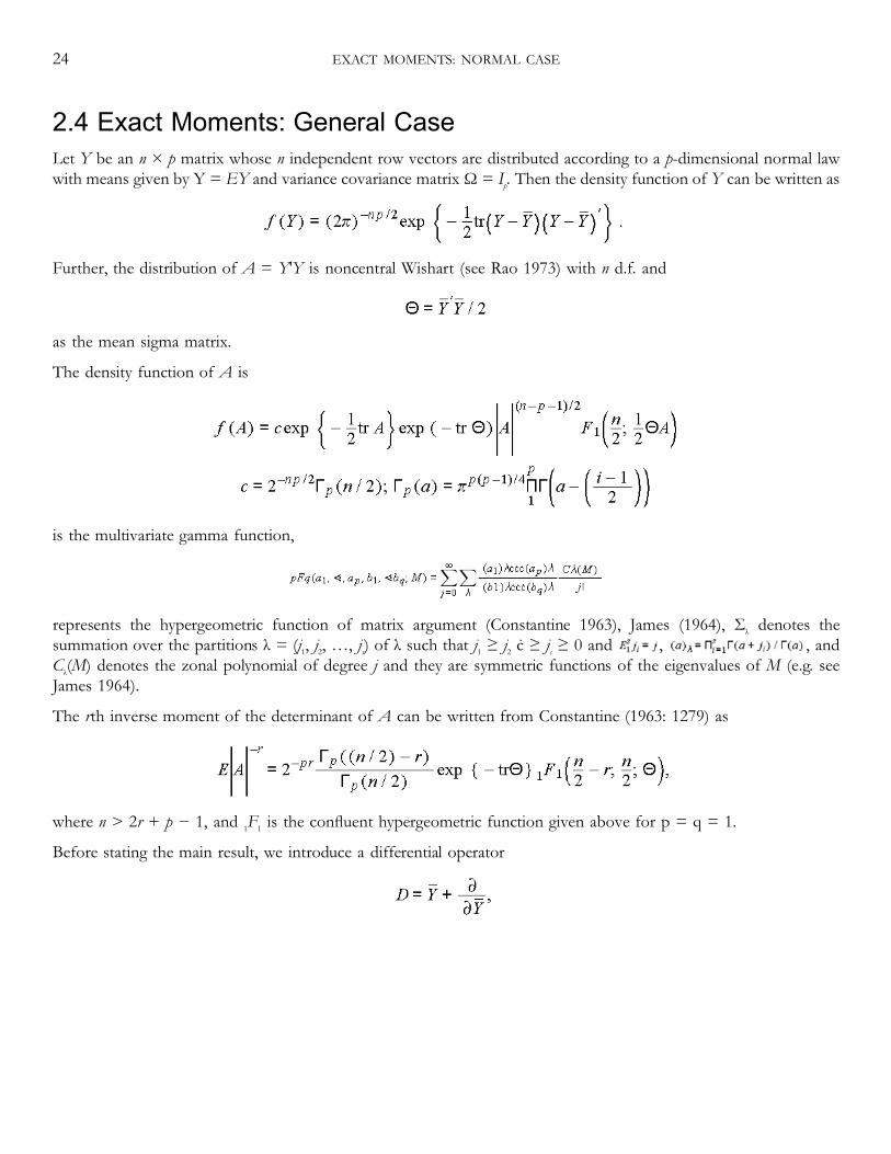
2.4 Exact Moments: General CaseLet Y be an n × p matrix whose n independent row vectors are distributed according to a p-dimensional normal lawwith means given by Y = EY and variance covariance matrix Ω = Ip. Then the density function of Y can be written as

Further, the distribution of A = Y′Y is noncentral Wishart (see Rao 1973) with n d.f. and

as the mean sigma matrix.

The density function of A is

is the multivariate gamma function,

represents the hypergeometric function of matrix argument (Constantine 1963), James (1964), Σλ denotes thesummation over the partitions λ = (j1, j2, …, js) of λ such that j1 ≥ j2 ċ ≥ js ≥ 0 and , , andCλ(M) denotes the zonal polynomial of degree j and they are symmetric functions of the eigenvalues of M (e.g. seeJames 1964).

The rth inverse moment of the determinant of A can be written from Constantine (1963: 1279) as

where n > 2r + p − 1, and 1F1 is the confluent hypergeometric function given above for p = q = 1.

Before stating the main result, we introduce a differential operator


which is such that Df(y) = Yf(y) or (D − Y)f(Y) = 0. This follows immediately by using the procedure (2.2) on f(y).Furthermore, if h(y) is any integer matrix valued analytic function of Y, then by using its Taylor series expansion aroundD and noting that (D − Y) f(y) = 0 we get

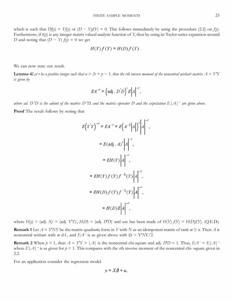
We can now state our result.

Lemma 4Let r be a positive integer such that n > 2r + p − 1, then the rth inverse moment of the noncentral wishart matrix A = Y′Yis given by

where adj. D′D is the adjoint of the matrix D′D, and the matrix operator D and the expectation E|A|−r are given above.

Proof The result follows by noting that

where H(y) = (adj. A)r = (adj. Y′Y)r, H(D) = (adj. D′D)r and use has been made of H(Y) f(Y) = H(D)f(Y). (Q.E.D.)

Remark 1 LetA = Y′NY be the matrix quadratic form in Y withN as an idempotent matrix of rank m ≤ n. ThenA isnoncentral wishart with m d.f., and EA−r is as given above with ⊖ = Y′NY/2.

Remark 2 When p = 1, then A = Y′Y = |A| is the noncentral chi-square and adj. D′D = 1. Thus, EA−r = E|A|−r

where E|A|−r is as given for p = 1. This compares with the rth inverse moment of the noncentral chi- square given in2.2.

For an application consider the regression model


where y is an n × 1 vector, X is an n × p matrix of p stochastic regressors such that X′X = A is noncentral wishartmatrix with n d.f. and the mean-sigma matrix ⊖, and u is an n × 1 disturbance vector with the mean 0 and thecovariance matrix σ2In. For the sake of simplicity we assume that X and u are independent.

The least-squares (LS) estimator of β is

Since X and u are independent, E(b − β) = 0. Further

where EA−1 = (adj. D′D)E|A|−1 provided n > p + 1. When p = 1, we get

where , and .

Further for large n or small σx we get the approximate variance, up to O (1/θ2)

by using the expansion of 1F1 in Appendix A.9.1. This can also be obtained by the small-σ expansion method ofapproximation to E(x′x)−1 in 2.5.2 where X = x = μ + σxV and V ∼ N (0, I). This gives, up to ,

which gives V(b), up to O(1/θ2), as given above with .

2.5 Approximations of MomentsIn the above sections we looked into the techniques of obtaining the exact moments of econometric estimators andtest statistics. These techniques require the specification of the density of the data vector y, for example, normal, and


they provide the results, which hold for any size of the data. The exact results are, however, difficult to derive under ageneral nonnormal framework. Even under a specified density the exact expressions for the moments in manysituations are sufficiently intricate and do not lend themselves to further algebraic manipulations for deducing any clearinference. This is despite the fact that Lemma 3 provides a much simpler way of obtaining exact moments comparedwith previous studies described there. In some situations, especially in the commonly used empirical econometricmodels such as dynamic models, sample selection models, probit models, the numerical evaluations of exactexpressions may be extremely difficult or cannot be derived by the presently known mathematical and statistical tools.In view of the above problems with the exact results, obtaining the approximate moments have been popular ineconometrics since they are simpler to derive, provide simpler expressions, easier to calculate, and often provide usefulinferences. Further, the approximations presented here are useful for the moderately large samples and they liebetween the often unknown exact sample results, and infinite sample limiting results, which are routinely discussed intext books and used in applied work even though they give poor results for small and moderately large samples. Herewe look into the following approaches of deriving approximate moments (a) large sample approximations, (b) small-σapproximation, (c) Laplace approximations.

2.5.1 Large Sample Approximations: Normal and NonnormalThe large sample method, also known as Nagar's (1959) approximation, of obtaining the approximate momentsessentially involves the asymptotic expansion of the sampling error (the difference between the statistic and theparameter) such that the successive terms are in descending order of sample size n in probability. Suppose θ is a k × 1parameter vector and is its estimator so that the sampling error is . Then the asymptotic expansion,obtained by using the Taylor Series expansion, is of the form

where ξ0 is a fixed quantity in the sense that it does not vary stochastically with n. In other words, ξ0 contains forms oforder Op(n0) = Op (1) (see Appendix for definitions of small o and capital O). Similarly ξ−1/2 denotes the expression inwhich terms are of order Op(n−1/2). Lastly, ξ* is the remainder term containing terms of higher order of smallness thanOp(n−1/2) to mean that the terms in ξ* are of order Op(n−(1/2)−s) with s > 0.

When ξ0 = 0, will be a consistent estimator so that ξ0 provides a measure for inconsistency of the estimator .Thus assuming to be a consistent


estimator, we have the asymptotic expansion

whence it follows that we can approximate the estimation error by ξ−1/2. Now the properties of ξ−1/2 shed light on theproperties of subject to the usual qualification that n is large enough for the approximation to be satisfactory andreasonably good. We point out here that the Taylor series in (2.70) and (2.71) are the large-n asymptotic expansions inthe sense that they are absolutely convergent for large n, though they may be divergent for a fixed n. Thus thetruncations may provide good approximations or make sense for moderately large samples. For details on the validityof asymptotic expansions of nonstochastic series see Whittaker and Watson (1965), and Appendix A.3, and forstochastic series see Sargan (1975, 1976), Phillips (1977b), and Appendix A.3.1.

Once the asymptotic expansion is written the large sample asymptotic approximation of the bias to O(n−1/2) is givenby E(ξ−1/2) while the large sample asymptotic approximation to O(n−1) for the mean squared error (MSE) is . Itmay be pointed out that the distribution of n1/2ξ−1/2 is nothing but the conventional limiting (asymptotic) distribution of

.

As an extension of the above approach, if we retain higher order terms in the expansion of we get large sampleasymptotic approximations of higher orders. Suppose that we use an infinite Taylor series expansion for the estimationerror and group the terms according to the order of magnitude in probability. This yields

where ξ* = Op(n−(q/2)−s), s > 0, and the expression for ξ−j/2 is of Op(n−j/2) consisting of sums and products of sampleaverages. Now if we approximate the estimation error by the truncated sum ξ = ξ−1/2+ ċ + ξ−q/2 of first q terms inthe expansion and neglect the remaining terms, the difference between the estimation error and the truncated sum is ofOp(n−q/2). The properties of the truncated sum ξ provide useful information about the properties of provided n issufficiently large for the accuracy of the approximation. Of course, while the accuracy of these approximations willchiefly depend upon the magnitude of n it may also be affected by the other parameters of the econometric model andthe nature of data under consideration.

Regarding the properties of we note that the first-order bias and MSE (asymptotic bias to O(n−1/2) and MSEto O(n−1)) are obtained by taking expectation of first term on the right-hand side in (2.72) and its product, respectively.The second-order bias to O(n−1) is defined as the expectation of


the first two terms on the right-hand side in (2.72). Further the second-order MSE, up to O(n−2), is

where

and

In Chapter 3 it is indicated that these approximate moments are the moments of the Edgeworth expansion of thedistribution of . We note that A−1 is the asymptotic variance (MSE) and A−2 can be interpreted as a correction termfor the moderately large samples. Similarly one can consider third-order approximations of bias and MSE byconsidering first four terms, see Akahira and Takeuchi (1981) for details.

To see the nature of the elements ξ−j/2 for an econometric estimator or test statistic, consider for theeconometric models y = μ + u where μ = Ey is an n × 1 vector. We can write the Taylor series expansion of h(y) aroundμ as

where θ = h(μ),

The ξ−j/2 is the collection of terms of Op(n−j/2), which depend on the orders of u′Δ, u′Δ2u, and (u′Δ2u)2 for the estimatorunder consideration. An alternative equivalent expression of the Taylor expansion can also be written as

where ⊗ is the kronecker product and

are 1 × n and 1 × n2 vectors. Similarly ∇3 = (∂/∂y′)∇2|y=μ and ∇4 = (∂/∂y′)∇3|y=μ are 1 × n3 and 1 × n4 vectors of recursivederivatives. This


form of Taylor series expansion will be useful for the nonlinear estimators given below. Also it provides results fornonnormal u more easily.

To see the examples of the expressions of ξ−j/2 we consider the asymptotic expansion of the LS estimator in the linearmodel y = Xβ + u = μ + u, where μ = Ey = Xβ and X is nonstochastic with X′X = O(n). Thengives

where ξ−1/2 = (X′X)−1X′u is Op(n−1/2) because X′u = Op(n1/2). Note that this result also follows using the Taylor expansionabove since β = h(μ),∇ = (X′X)−1X′ and ∇2 = 0 = ∇3 = ∇4.

WhenX is stochastic we can writeX′X/n = X′X/n + D − D whereD = 1/nEX′X is O(1). Then, assuming C = (X′X/n) − D = Op (n−1/2),

Again ξ−1/2 = D−1(X′u/n), ξ−1 = −D−1CD−1(X′u/n) and ξ−3/2 = D−1(CD−1)2(X′u/n). The bias and MSE of then followfrom (2.73).

Nonlinear EstimatorsThe asymptotic expansion given above can be used for the econometric statistic where the explicit form of h(y)is known. However, for many statistics, for example, nonlinear maximum likelihood (ML) and method of moments,the form of h(y) is not known. For these cases we develop the asymptotic expansion below. As a special case this alsoprovides the results for , with explicit forms of h(y). Let us consider the class of estimators , which may be written asthe solution of a set of moment equations of the form , that is

where gi (θ) = g(zi, θ) is a known k × 1 vector valued function of the m-dimensional i.i.d. data zi and a k dimensionalparameter vector θ such that E[gi(θ)] = 0 only for true value of θ and for all i. The special cases of this are MLestimators, LS and other extremum estimators, many generalized method of


moments estimators, and certain two step estimators, which involve a nuisance parameter. The obvious difficulty withnonlinear estimators is that they cannot be expressed as explicit functions of the data. Because of this, obtaining theirexact moments are extremely difficult. Obtaining the asymptotic expansion of the form (2.72) is also notstraightforward for the nonlinear estimators. Rilstone, Srivastava, and Ullah (RSU) (1996), assuming that is arbitrarilyclosed to θ, used iterative techniques to derive approximate solutions to the first-order conditions , also see DeBruijn (1961) and Barndorft-Nielsen and Cox (1979). For this solution RSU (1996) made the following assumptions:

Assumptions 1 The sth order derivatives of gi(θ) exist in a neighborhood of θ and E‖∇sgi(θ)‖2 < ∞, where ‖A‖, for amatrix A, denotes the usual norm, trace [AA′]1/2, and ∇sA(θ) is the matrix of sth order partial derivations of a matrixA(θ) with respect to θ and obtained recursively.

Assumptions 2 For some neighborhood of θ, (∇ψn(θ))−1 = Op(1).

Assumptions 3 ‖∇sgi(θ) − ∇sgi(θ0)‖≤‖ θ − θ0‖Mi for some neighborhood of θ0, where E| Mi | ≤ C < ∞, i = 1, 2, …

Note that the above assumptions, with s ≥ 1, are sufficient for as n→ ∞, Π1 = (E∇g1)−1Eg1g1′(E∇g1)′−1.This provides an important result that , which is useful in developing the following Lemma.

Lemma (RSU1996)Let Assumptions 1–3 hold for some s ≥ 3. Then

where

a bar over a function indicates its expectation so that Ā(θ) = EA(θ), Hj = ∇jψn, j = 1, 2, 3, , ,and ; .

The proof of the above lemma follows by first writing the first-order Taylor series expansion of as


where is between and θ. This gives

where . We note here that ε−1/2 = Op(n−1/2) and this is the term upon which theusual asymptotic distribution of is based.

Now write the second-order Taylor series expansion of as

We then get

Finally the result in Lemma follows by taking the third-order Taylor series expansion as

and substituting (2.77) and (2.79) in this equation, see RSU (1996).

Combining the result in the above lemma with (2.72) and (2.73) and evaluating the expectations using the techniques inthe Appendix we get the following Proposition.

Proposition (RSU1996) Let Assumptions 1–3 hold for some s ≥ 2. Then the bias of to order O(n−1) is

where , , and di = Q gi. Further if Assumptions 1–3 hold for some s ≥ 3, then the MSE of toorder O(n−2) is


where

We note that the MSE is a corrected version of RSU (1996) where 1/4, −1/2, −1/2 in Π3 are 1,1,1 respectively andbefore the curly bracket in the last but one term in Π4 is missing, see Bao and Ullah (2002). A number of remarks

are worth making with respect to the above expression. First, the second-order bias depends explicitly on the curvatureof the model, and ∇g. This expression allows one to evaluate the influence of second-order terms on the location ofthe estimator. For highly nonlinear models, this term may be


relatively large and one may be interested in estimating it either directly or by some resampling technique or at leasttaking it into account informally when making inferences.

For models that are linear in the parameters, the second term is zero. For linear regression models estimated with LSor generalized least squares, the first term is also zero from the orthogonality property of the disturbances and theregressors.

A third point is that the simple structure of the second-order bias suggests a natural estimate from the sample analogueevaluated at the estimated value of θ, for example, . However, this should be interpreted with somecare; see, for example, Phillips and Park (1987).

A final point to be emphasized is that, apart from the existence of moments, this result does not require anydistributional assumptions regarding the random variables in the model. In particular, there is no need to assume, say,normality of the zi's. This remark also holds with respect to the derivation of the second-order MSE of .

As with the second-order bias, the second-order MSE is shown to be the expectation of sums and products of sums ofzero mean random matrices. The second-order MSE is thus a combination of the usual O(n−1) first-order asymptoticcovariance matrix, Π1, and a number of second-order terms. As will be seen in the examples, many of the higher-orderterms are equal to zero under various symmetry, linearity, and exogeneity assumptions.

A few additional remarks are worth making with respect to the form of the second-order MSE. In this form the MSEis not necessarily positive definite, although one might expect it to be for most samples. This should not be surprisingsince, for example, high-order Edgeworth expansions are generally not valid distribution functions. The fact that theMSE may not be positive definite could actually be reassuring in some practical contexts. Most applied researchershave probably been in a situation where the usual standard errors seem to overestimate the sample variability of theirestimator. For example, they may have observed that a given coefficient seems quite robust for various data sets orslightly different model specifications. One possible explanation could be that the asymptotic variance overstates thetrue dispersion of their estimate. The result in Proposition could thus provide a motivation for constructing alternativevariance estimates.

Also important to note is under what conditions the high-order terms may have a substantial impact on the finite-sample precision of an estimator. Referring back to the definitions of the random variables it can be seen that thehigher-order terms are comprised of expressions that depend on the second- and third-order derivatives of the model.Thus, a general rule of thumb would seem that variance estimates based on Π1 will tend to lack precision for mostnonlinear models. The terms to O(1/n2) can also be used to evaluate the effect of nonnormality on the MSE of . Thiscan be done by comparing the expression of the MSE under nonnormality with that under normality.


Some additional points should be made with respect to application of the above results. First is that one can consider abias-corrected estimator: where . It is straightforward that this estimator isunbiased to order O(n−1).

Notice that is an estimator in the true sense only when δ is known. Generally, δ will involve several unknownquantities (parameter values and population moments) and consequently as such may not be feasible. A simplesolution is then to replace these unknown quantities by their estimators or sample analogues. This will provide anestimator of δ. Using such an estimator, (say), one can propose the estimator , which will be unbiased toorder O(n−1) provided that is a consistent estimator of δ; see more on bias correction by MacKinnon and Smith(1998).

With respect to efficiency issues it is well established that the bias-corrected MLE is second-order efficient with respectto the mean squared error criterion, see Rothenberg (1984a). Further discussion of the efficiency properties of feasibleversions of will demand inclusion of higher-order terms. This would be a difficult exercise, although for someparticular examples it may not be that difficult. In RSU (1996) they report on how estimates of and perform ina Monte Carlo setting for the exponential regression model. Results there indicate that bias corrections can lead tosubstantial improvements in inferences.

Exercise 14 Consider a population with mean μ and variance σ2. Let and be the sampleestimates based on the i.i.d. sample yi, i = 1, …, n. Obtain the exact and large-n approximate bias and MSE of

Solution First we write

where gi(μ) = yi − μ is such that E gi(μ) = 0. Then E(y − μ) = 0, that is the exact bias is zero. Further the exact MSE(y)= V(y) = σ2/n.

Now to obtain the approximate bias and MSE we first note from the Lemma that

Thus in this case the exact approximate and asymptotic results are the same.

Regarding 1/y we note that the exact mean


cannot be obtained without specifying the form of a density f( ). For example, if yi's are normal y is N(μ, σ2/n) and E(1/y) is infinite. Further the MSE of 1/y is also infinite. However, for some nonnormal distribution E(1/y) may exist, butit may be difficult to obtain explicit expressions.

To obtain the approximate moments we write

so that gives and E gi(θ) = 0 for θ = 1/μ. Then, the bias of 1/y follows from the Proposition, where

so that

This gives

where the last equality is for θ = 1/μ. The MSE can be similarly obtained for θ = 1/μ as

where γ1 is the skewness coefficient.

From the above exercise we note that the bias goes to zero as n→ ∞, and it is monotonically decreasing function of μ.Further the bias-corrected estimator can be written as . Also, the MSE for the positively skeweddistributions with μ > 0 is smaller compared with the symmetric distributions.

2.5.2 Small-σ Approximations: Normal and NonnormalThe small-σ (disturbance) method of obtaining the approximate moments, first proposed by Kadane (1971) for thenormal case and later explored by Ullah, Srivastava, and Roy (1995) for the nonnormal case, involves the asymptoticexpansion of the sampling error such that the successive terms are in descending order of σ, the standard deviation, inprobability. That is the sampling error , using the Taylor series expansion, is of the form

where ζj is the jth term of the series, and ζ* = O(σq+s), s > 0.


The technique for obtaining the small-σ asymptotic approximations can be explained by first noting that a class ofeconometric models can be written as

where y is an n × 1 vector, μ = Ey is an n × 1 vector, and u is an n × 1 vector of disturbances with finite first fourmoments. For example, a univariate population with the scalar mean μ and a multivariate regression model with μ = Xβ are special cases of the above model. For these models , by expanding around μ, gives

where

where ∇h(y) = (∂/∂y′) h(y) is a 1 × n vector, ∇2h(y) = ∂/∂y′∇ h(y) is a 1 × n2 vector and so on as defined in 2.5.1. Ifis a k × 1 vector then ∇h(y) is a k × n matrix.

The Taylor series expansion may be convergent or divergent. However, if we consider σ to be small and close to zero itcan be regarded as an asymptotic expansion where the terms are in decreasing order of magnitude in σ. In that caseone can retain the first few terms and study the properties of this truncated sum. These properties are referred to assmall-σ (disturbance) asymptotic properties of .

For example, the bias to order O(σ2) and MSE to O(σ4), respectively, are given by

and


Obviously, how successful and satisfactory these approximations are in any given practical application depends uponthe smallness of σ among other things. Since σ measures the variability in the disturbance term of an econometricmodel, the assumption that σ is small, or tends to zero, implies that the postulated econometric model is assumed toexplain y well. Thus the smallness of σ is an appealing assumption and it is consistent with the philosophy of large-n(small 1/n) asymptotics in 2.5.1.

We thus observe that the methodology for deriving the small-σ asymptotic approximations is similar to that of largesample asymptotic approximations. However, the latter requires the number of observations to be large while theformer needs no such condition. Even the assumptions like the finiteness of the limiting value of sample momentssuch as X′X/n, required in regression contexts, are not needed. This also makes small-σ expansions easier to derivesince one does not have to determine the order of magnitude of the terms ζj in (2.87) in contrast to the large-nexpansions, which need to evaluate the order of magnitudes of ξj in (2.72) or (2.75) as n goes to infinity.

We can now present a more explicit expression for the bias to O(σ2) and MSE to O(σ4) of a general class of linear andnonlinear estimators of the parameter vector θ in the model y = μ + σu. We make the following assumptions aboutthe elements ui, i = 1, …, n, of the vector u.

Assumptions 4 The elements of the vector u are independently and identically distributed such that

where γ1 and γ2 are measures of skewness and kurtosis of the distribution.

Assumptions 5 The h(y) and the sth order derivatives of h(y) exist in the neighborhood of Ey = μ.

Now we can state the result due to Ullah, Srivastava, and Roy (USR) (1995).

Theorem (USR)Under the assumptions 4 and 5 the expectation of is

where for i, j = 1, …, n and s = 2, 3, 4.

Proof The proof follows by taking expectations in (2.86) from the Appendix, and simplifying the resulting terms. (Q.E.D.)


The following observations may be deduced from our results given above.

First, the result in Theorem provides the mean of a general function h(y) of the nonnormal vector y. The results forvarious econometric estimators and test statistics follow from this general result. The higher order moments alsofollow from the direct use of the Theorem. For example, for the rth moment of h(y) we need to evaluate Eg(y) whereg(y) = hr(y) and this expectation can be obtained by replacing g(y) with h(y) in the Theorem.

Second, the result in the Theorem shows that the moments of econometric estimators and test statistics can be easilyobtained by simply evaluating their first four derivatives at the mean value, Ey = μ. Since a large class of econometricestimators and test statistics are the ratios of quadratic forms in y or products of quadratic forms in y and polynomialsin y their derivatives can be obtained by simple and well-known calculus methods.

Alternatively, the derivatives of any given function h(y) can be obtained either numerically or analytically by usingrecently developed computer software, for example, Mathematica.

Third, from the Theorem we observe that, up to O(σ2), the moments for both normal and nonnormal cases are thesame. However, up to O(σ4), the behavior of the moments in the nonnormal case can be quite different from those inthe normal case where γ1 = 0 = γ2. In fact, if the true distribution of y is not normal and we falsely assume it to benormal then the moments can be under or overestimated by the magnitude

where Δ3 and Δ4 are as given in (2.91). It is clear from this result that the third- and fourth-order derivatives of h(y) at y= μ and the magnitudes of skewness and kurtosis of the distributions are the main determinants of the magnitude ofmisspecification error on the moments of h(y).

Fourth, we observe from the Theorem that the bias of h(y), up to O(σ2), depends crucially on the curvature properties(second derivatives) of h(y). For example, for the econometric estimators and test statistics, which are the concave/convex functions of y, the directions of bias are negative/positive. Of course for estimators, which are linear functionsof y, for example, the LS estimator in the linear regression case with fixed regressors, the Δ22 as well as Δs are equal tozero for s = 2, 3, 4 and therefore they become unbiased.

Finally, we observe from the Theorem that the estimator , where

has the zero mean up to O(σ2). This result is useful in providing bias-adjusted econometric estimators. The analysis ofefficiency properties of these bias-adjusted estimators will be a useful subject of future research.

Further, we note that the above results are useful for the estimators, which have explicit solutions so that h(y) is known.This may not be the case for


some nonlinear estimators which are the solution of , see (2.74). For these estimators the bias to O(σ2) andMSE to O(σ4) may be the same as the bias to O(1/n) and MSE to O(1/n2) given in (2.81) and (2.82), respectively.

In general the results from the two approaches are not the same and the question arises, which of these twoapproaches give more accurate results. This issue is explored in the book. Often it is the case that for small samplesand small-σ the accuracy of results based on small-σ asymptotics is better compared with large-n asymptotics. In somecases the results of large-n asymptotics can be derived from the small-σ results, and in some special cases these twoapproaches give the same results. A trivial example is the properties of the sample mean as an estimator of thepopulation mean μ in the model yi = μ + σui, i = 1, …, n where E ui = 0 and V(ui) = 1. In this case as indicated inExercise 14, the exact sampling error is

so that the infinite series expansion contains only the first term which is of O(σ), or due to limiting behaviorof ū. Thus the large-n expansion is the same as small-σ and it is also reflected in the MSE (y) = V(y) = σ2/n.Similarly in the regression model y = μ + σ u, μ = Xβ, the sampling error of the LS estimator is

, which is the same as the Op(n−1/2) expansion in 2.5.1. Thus the large-n and small-σexpansions are the same and so is the . In Exercise 15 we consider a case where the two approximationsare different. We also show in Chapters 4 and 6 that the moment approximations by these two approximations aredifferent for the goodness of fit measure R2 and dynamic models, but they are the same for the instrumental variablesestimators in Chapter 7. Ullah (2002) proposes using Kullback–Leibler divergence measure for evaluating the qualityof two and more approximations methods.

Exercise 15 Obtain the small-σ asymptotic expansion of where y is the sample mean estimator of μ in themodel yi = μ +ui, i = 1, …, n.

Solution Since , we get h(μ) = 1/μ = θ.

Further

This gives


which is, upto O(σ2), the same as the bias to O(1/n) in Exercise 14. To obtain MSE we need to obtain

Now consider 1/y2 = g(y). Then g(μ) = 1/μ2,

Using this

Thus

The above exercise provides an example where the bias to O(n−1) and O(σ2) are the same but the MSE expressions toO(σ4) differs with the MSE to O(n−2) by the term (3σ4/n3)γ2μ−6. However, knowing MSE to O(σ4) one can derive theexpression of the MSE up to O(n−2) by dropping (3σ4/n3)γ2 μ−6.

Exercise 16 Show that the rth order moment of the ratio of quadratic forms y′ N1y/y′ N2y, up to O(σ4), where N1 andN2 are symmetric matrices and the n × 1 vector y follows y = μ + σu, is given by

where


Further,

and cj is the same as cj with r replaced by −r and θ1 by θ2. Further Aj is Aj with cj interchanged with cj and N1 with N2.

Solution The result follows by substituting the first four derivatives of h(y) = (y′ N1y/y′ N2y)r in (2.90) and simplifying theresults. An alternative proof follows by directly substituting y = μ + σu in (y′ N1y)/(y′ N2y), then expanding

and taking expectations using Appendix A.5. This is the approach taken in Ullah and Srivastava (1994).

An alternative expression, which will be easier in special cases, can be written as

where

These expectations can be evaluated from the results in Appendix A.5.

The result for the normal case follows by substituting γ2 = γ1 = 0. Thus the moments can be under- or overestimatedby falsely assuming normality by the magnitude


These results can also be extended for obtaining expectations of . In this case the result is the same asin Exercise 16 except that and cj is cj with r1 replaced by −r2 and θ1 by θ2.

The results for the special cases of the ratio of quadratic forms will be considered in detail in the following chapters.

Finally the results can be generalized for the case where

and

where Y is n × k, M = E Y is n × k and U = ((uit)) = (u1,…, uk) is an n × k matrix of random errors. Again taking theexpectations of the expansion of h(y) after substituting Y = M + σ U we can write

w h e r e Θ j = M ′ N j M w i t h | Θ j | ≠ 0 , f o r j = 2 , 3 , 4 a n d; aj = 0 for j = 2, 3, bj = 0 for j = 2 and 1 for j =

3, 4; V1 = c1A1 and

cj and cj are the same as in Exercise 16 without θ1 and θ2. Finally the expression for Vj is the same as that of Vj exceptthat r, N1, Θ1 are replaced by −r, N2, Θ2 respectively.

An explicit expression of Δj can be written by substituting the expectations from Appendix A.7. This will be quitelengthy. But an easier expression may appear when applied to some econometric estimators in the special cases.

It is to be pointed out here that the sampling error of the econometric estimators are generally the functions of samplesize and the parameter σ. Thus fixing σ one can obtain the asymptotic expansion for large n or fixing n one can obtainthe asymptotic expansion for small-σ. For many other econometric estimators the sampling error may be a function ofn, σ, and other parameters. For example, in a regression model with first-order serial correlation the sampling error willbe a function of n, σ, and the correlation coefficient parameter ρ. In this case, while not studied in this book, one couldconsider the asymptotic expansion with respect to small or large ρ fixing n and σ.


2.5.3 Results for Non-i.i.d CasesAll the above results are given for the case where the error in the models is i.i.d. satisfying assumption 4. These resultscan be generalized for the case where ui is non i.i.d and nonnormal such that, for i, j, k, l = 1, …, n,

For large classes of econometric models the errors will be non-i.i.d, for example, the models with heteroskedasticityand/or dependent time series models. In such cases the expectation of is

where

are all evaluated at y = μ. Under the i.i.d. assumption this result reduces to the result in Theorem (URS). The proof ofthe above result follows by taking the expectations of the asymptotic expansion in (2.87), also see Ullah (2002).

Lastly the expectation of , when y = μ + u distributed with Ey = μ and u is a non i.i.d vector, can beobtained as a special case of the above result. When u ∼ N(0, Σ) or y ∼ N(μ, Σ) then we can also obtain

where y* = Σ−1/2y ∼ N(μ* = Σ−1/2μ, σ2I), N1* = Σ1/2NΣ1/2, and N2* = Σ1/2N2Σ1/2. The matrix Σ1/2 = Q∧1/2Q′, ∧ is thematrix of eigenvalues of Σ and Q is the orthogonal matrix of corresponding eigenvectors. The result now follows fromExercise 16.

The result for the large-n expansion of can also be written from the large-n asymptotic expansions of in 2.5.1. Forexample, for the large class of econometric estimators given by (2.74) the bias, up to O(n−1), and MSE, up to O(n−2) canbe obtained when the observations are non i.i.d. and nonnormal by using (2.73) and (2.75). This is given by

where d = Qψn and Q, V, and are given in 2.5.1. Further the MSE, up to O(n−2), is


where

whereW and are given in 2.5.1. In many applications it may be easier to obtain the bias and MSE of an estimatordirectly by using (2.75) and (2.76) with (2.73), see Bao and Ullah (2002). For the i.i.d case the above results reduce tothe results in (2.81) and (2.82).

2.5.4 The Laplace Approximation: Normal and NonnormalThe Laplace method is a method of approximating a definite integral by evaluating it in a small neighborhood aroundthe point where it attains it's maximum value. For this to work well the neighborhood of this point must dominatecompared with all other regions in the range of integration. Specifically, consider the integral of the formwhere t is a “large” positive constant, the first two derivatives of g(x) and p(x) exist, a < b and both may be either finiteor infinite, p(x) has only one maximum at x = x0 where a ≤ x0 ≤ b, and x0 are finite. If g(x) attains its maximum at x =x0 then the integral around x = x0 will dominate compared to all other regions. Therefore replace g(x) by the first twonon-zero terms and p(x) by the first non-zero term of their respective Taylor series expansions around x = x0. TheTaylor expansions are:

so that for p(x0) ≠ 0, and the case where x0 = b, b ≥ 0, and g(1)(x) > 0 in the range of integration we get:


Since the region around b dominates anyway we may extend the range of integration to (−∞, b) to get:

so that for large t:

For a rigorous treatment of this method see Olver (1974) Chapter 7 or De Bruijn (1958) Chapter 4. An example of ause of this method is in Lieberman (1994a) where he uses it to approximate the moments of a ratio of quadratic forms.His basic technique is to use the moment generating function to get the estimator (represented as a ratio of quadraticforms) into the same structure as the left-hand side of (2.104) and then apply the Laplace method. This technique willbe used below to approximate the moments of estimators that can be written as a ratio of quadratic forms. Asindicated above, many econometric estimators can be written in terms of a ratio of quadratic forms.

Let us consider the ratio of quadratic forms (y′ N1y)/(y′ N2y), where N1 is symmetric and N2 is positive definite. LetM(w1, w2) be the m. g. f. of y′ N1y and y′ N2y given by

where f(y) is the density of y. Then it can easily be verified that the exact rth moment

where . An alternative representation for E(y′ N1y/y′ N2y)r is given in (2.30). When y follows an Edgeworthdensity the M(w1, w2) and exact moments are analyzed by Peters (1989), also see Knight (1985). In general, undernonnormality, any tractable exact formula for these moments do not exist. That is the solution of multiple integrals in(2.107), under a general class of nonnormality, is not available. In view of this Lieberman (1994a) provided anapproximation of this multiple integral or the rth moment by using the Laplace approximation method. This is analternative to the small-σ and large-n approximation methods discussed above. Assuming that E(y′ N2y) and E(y′ N1y)rexist, r ≥ 1, the following theorem holds.

Theorem (Lieberman1994a)The Laplace approximation for the rth moment of (y′ N1y)/(y′ N2y) about the origin is


Proof First we write the integrand in the multiple integral (2.107) in a form suitable for the application of the Laplacemethod as

where and

Now since y′ N2y is assumed to be positive definite

On the range −∞ to 0, the monotonicity of g(0, w2) implies that its maximum is attained at the boundary points w21 = ċw2r = 0 or w2 = 0. Therefore, applying the method of Laplace around the point of maximum 0, we have

But Mr(0, 0) = E(y′ N1y)r and g(1)(0, 0) = E(y′ N2y). Therefore the result in the Theorem follows. (Q.E.D)

Lieberman (1994a) provides sufficient conditions under which the Laplace approximation will have an error of O(n−1).These conditions are (i) pth cumulant of y′ N2y, κp, is O(n), (ii) E(y′ N1y)r = O(nr), (iii) The γ = 1 + m order and δ = r + mdegree generalized cumulant of the product of (y′ N1y)κ and (y′ N2y)m, κrm, is O(nℓ) with ℓ ≤ r. These conditions aresatisfied for the ratio of independent chi-squares each with O(n) d.f. In general, these conditions provide the Laplaceexpansion of the rth moment as


where

where the generalized cumulants

can be evaluated by using the expectations in Appendix.We note that unlike the large-n and small-σ expansions, whichhold for a general class of estimators expressed as h(y), the Laplace approximation is for the class of econometricestimators, which can be written as the ratio of quadratic forms. It will be useful to extend the above results for theLaplace approximations of the moments of h(y). It is also conjectured here that the Laplace approximation would gothrough for the estimators, which are the ratio of quadratic forms in the n × k random matrix Y. That is

2.6 Summary and SurveyIn this chapter we have provided the techniques of obtaining exact and approximate moments of a function of randomvector/matrix. The exact technique is based on the work of Ullah (1990), large-n approximation is based on Nagar(1959) and Rilstone, Srivastava, and Ullah (1996) results; small-σ approximation is based on the results due to Kadane(1971), Ullah, Srivastava, and Roy (1995), and Ullah (2002); and Laplace approximation is due to Lieberman (1994a). Aspecial case of the function considered is the ratio of quadratic forms, which contains a large class of econometricestimators and test statistics. The exact and approximate moments of this are also presented using the abovetechniques. There is a vast statistics literature on deriving the moments of the ratio of quadratic forms, see forexample, Mathai and Provost (1992). This dates back to the work of Von Neumann (1941) on obtaining the momentsof the ratio of mean successive differences to the sample variance. Gurland (1956) derived the expectation of the ratioof quadratic forms in normal variables. White (1957), and Shenton and Johnson (1965) analyzed the moments of theLS estimator of the correlation coefficient ρ in yi = ρ yi−1 + ui, which can be expressed as the ratio of quadratic forms in


normal variables, see Chapter 6. Sawa (1972) obtained the moments of the ratio of quadratic forms using the jointmoment generating function of two quadratic forms, also see Hoque (1985). Dwivedi and Chaubey (1981), Chaubeyand Talukdev (1983), and Morin-Wahhab (1985) studied the moments of the ratio where , and

are mutually independent chi-square variables. Note that this ratio can be expressed as (y′ N1y)/(y′ N2y). Magnus(1986) provided the conditions of existence of moments and gave the expression in terms of an integral. Smith (1989)provided the expressions in terms of zonal polynomials. For a more general ratio where the numerator is y′ N1y + δ1′y +δ2 and the denominator is y′ N2y + δ3′ y + δ4 the results, based on the extended version of Sawa's (1972) result, can befound in Mathai and Provost (1992).

All the above results are for the normal case. For the nonnormal case, an extension of Sawa's (1972) result is given inPeters (1989) for the Edgeworth density, also see Knight (1985) and Provost (1989a,b,c).

The approximation techniques given in this chapter provide the moments for the general class of functions that alsoincludes the ratio of quadratic forms. Both the normal and nonnormal cases are considered. Also the results areanalyzed for both the i.i.d and non-i.i.d observations and for linear and nonlinear models. These techniques forapproximations along with the techniques for exact moments are applied for various econometric models in Chapters4–7.


3 Finite Sample Distributions

3.1 IntroductionIn the earlier chapter, we discussed the techniques of evaluating the exact and approximate moments of theeconometric estimators and test statistics. This was done by providing the moments of a general function h(y) of therandom vector y and then specializing to the ratio of quadratic forms. It was indicated that the expressions of exactmoments may often be very complicated and so the approximate moments are useful tools to study the behavior ofvarious statistics. However, in many practical situations in econometrics just studying moments of econometricestimators or test statistics is not enough. For example, one needs to study the whole sampling distribution of variousstatistics in order to construct confidence intervals (regions) and test the hypotheses. Also, sometimes one or moreestimators do not possess moments so that the comparison of estimators on the basis of moments become infeasible.In such cases one can consider coverage probability as the performance criterion, which prefers the estimator withhigh probabilities of being close to the true value of the parameter. This requires the knowledge of the samplingdistribution of the estimators.

As in the case of the exact expressions for the moments of estimators, the exact probability distributions are generallydifficult to derive. Also the expressions, if derived, are often difficult to be fruitfully used and they require extensivenumerical calculations. This has stimulated the development of several approximation techniques, which provide easierasymptotic expansions for the density and distributions functions.

3.2 Exact DistributionAs in Chapter 2, consider h(y) to be the real valued function of an n × 1 random vector y. Then we can write thedistribution function of

q = h(y) as

where f(q) is the density function of h(y) and I(·) is an indicator function, which takes the value 1 if q = h(y) ≤ q0 and 0otherwise. Note that I(q) is not a continuous function of y so we cannot use the results of Chapter 2 to obtain E[I(q)].

An alternative expression for the distribution function is to obtain the characteristic function (c.f.) and then use theinversion formula. The c.f. of h(y) is

and the density function of q = h(y) is

provided ψ(t) is absolutely integrable, see Appendix Section A.8.3.

It is clear that, unlike the exact expectation of h(y) in Chapter 2, a simple expression for the distribution of a general h(y)may not be possible. However, as noted in Chapter 2, a large class of econometric estimators and test statistics h(y) arein the form of the ratio of quadratic forms. Thus we turn to the distribution of such h(y) in the following section.

3.2.1 Distribution of Ratio of Quadratic FormsLet us write the ratio of quadratic forms as

where y is an n × 1 random vector with the mean vector μ and covariance matrix Σ, and both N1 and N2 are n × nnonstochastic matrices. Then

where N = N1−q0N2. Since the covariance matrix of y is ∑ we can also write (3.5) as

52 EXACT DISTRIBUTION

where z = P′Σ−1/2y and P is an orthogonal matrix of eigenvectors of Σ1/2NΣ1/2 such that P′Σ1/2NΣ1/2P = Λ, a diagonalmatrix of eigenvalues λ1,…, λn of Σ1/2NΣ1/2; Σ1/2 = QD1/2Q′ where D is the diagonal matrix of eigenvalues of ∑ and Q isthe matrix of corresponding eigenvectors.

The equations (3.5) and (3.6) show that the distribution of the ratio of quadratic forms reduce to the distribution of anindefinite quadratic form y′Ny, where N is an indefinite matrix. There is a vast statistics literature studying thedistribution of indefinite quadratic forms in the normal case, that is, y ∼ N(μ, Σ). In this case z ∼ N(μz = P′Σ−1/2μ,I) and

where is a noncentral χ2 with one (degrees of freedom) d.f.

The infinite series representation of F(q) in the normal case was given by Gurland (1955, 1956); also see Shah (1963),Press (1966), and Taneja (1976). However, the numerical evaluation of this is difficult. Imhof (1961) provided anumerical integral representation of (3.7), which is based on the Gil-Pelaez (1951) inversion formula for the indefinitequadratic form, also see Davies (1973). This formula is

where Img {∈} represents the imaginary part of ∈ and

is the c.f. of z′Λz. Imhof (1961) has shown that (3.8) can be written as

where

and rj's are the multiplicities of the nonzero distinct λjs. For q0* = 0 we get P(z′Λz ≤ 0) = F(q0) by substituting q0* = 0 in(3.10) and (3.11).

Since v ρ (v) is monotically increasing towards +∞, in numerical work the integration in (3.10) is carried out for 0 ≤ v ≤v* only. Imhof's technique

FINITE SAMPLE DISTRIBUTIONS 53

provides excellent accuracy and it is almost exact. Computer programs for evaluating the numerical integration of(3.10) are described in Koerts and Abrahamse (1969), and Davies (1980). An advantage of the Davies program is thatboth the truncation and numerical integration errors are controlled with guaranteed accuracy. For the numericalimplementation of these programs the eigenvalues and corresponding eigenvectors of the matrix Σ1/2(N1−q0N2)Σ1/2 areneeded. These can always be found numerically, and in some cases analytically. Palm and Sneek (1984) have suggestedmodifications, which eliminate the need to compute eigenvalues. Evans and Savin (1984) have developed an algorithm,which is efficient with regard to time taken in calculating the eigenvalues and eigenvectors.

The distribution of q can also be obtained directly by the numerical inversion formula in Gurland (1948). This is

where ψ(., .) is the joint c.f. of y′N1y and y′N2y.

Another numerical inversion formula, proposed by Martynov (1977), is

where q0* ≥ 0, α ≥ 0 and

, εj = 1/λj, j = 1, …, n. For large q0* > 0, (3.13) may be more efficient computationally comparedwith (3.10). The density function of q can be obtained by the numerical differentiation of the distribution function. Formore on numerical evaluations, see Beran (1975), Rice (1980), Helstrom (1983), Luigannini and Rice (1984), andFarebrother (1984, 2002).

We note that for the central case, μz = 0, the integrand in (3.10) simplifies considerably. For alternative expressions inthe central case, see Provost (1989b, c), Provost and Rudink (1991), and Forchini (2002); also see Hillier (2001) for theexact density function of q. For the simplified finite expressions in the central case where z′Λz is positive definite, seeMathai and Provost (1992, ch. 4).


3.3 Approximations of the Distribution of Quadratic FormsThere is an extensive statistics literature on the approximation of the distribution of . This includes the workof Patnaik (1949), who approximates the distribution of central q by where λ and ℓ are chosen so that q and havethe same first two moments. This gives and . Pearson (1959) considered a noncentral

, where zjs are standard normal and bj are constants, and suggested a three moment approximation ofthe distribution of q as where c = θ3/θ2, , and ; for s = 1, 2, 3.Thus where . In both Patnaik's and Pearson's approximations, ℓ can be fractionalso that one needs to calculate by using interpolations. Alternatively one can use Wilson and Hilferty (1931)approximation. Imhof (1961) result indicates that Pearson approximation is much better than Patnaik's approximation,particularly in the upper tail.

Siddiqui (1965) looks into the approximation by quadratic bounds. Okatomo (1960) has provided an upper bound forthe distribution of a central where zjs are independent with nj d.f. and λj > 0 for all j. His result is

where , . Siotani (1964) shows that this approximation works well if the variation in λjs is not toolarge.

Jensen and Solomon (1972) considered a normal approximation of q* = (q/θ1)r, where as above, q =∑λj(zj + bj)2 with λj > 0, bj as bounded constants and zjs are mutually independent standard normal, and r is determinedby the first three moments so that the leading term in the expansion in powers of of the third central moment of q*vanishes. The distribution of q* is approximated by a normal distribution with mean and variance given by

Jensen and Solomon indicate better performance of this compared with Patnaik's and Pearson's. Solomon andStephens (1978) have proposed another approximation to the density of q by fitting a Pearson curve with the same firstfour moments as q. In another work Solomon and Stephens (1977) provide the approximation of the distribution of qby where the constants A, p, and d are found by matching the first three moments of q and . The computerroutines are also provided by the authors for doing all the calculations. This approximation, except in the lower tail,performs better than the Jensen and


Solomon approximation. For other approximation procedures, see Oman and Zacks (1981), Robbins and Pitman(1949), and Moschopoulos (1983).

We note that most of the above approximations developed were useful during the period when the computertechnology did not exist or was not advanced. With the current and future advancements in computers it will be moreuseful to calculate almost exact results by Imhof and other methods described above. However, the large-n and small-σapproximations considered in the later sections will be quite useful in practice.

3.4 Limiting DistributionsOften the approximate distributions will not be as accurate as the exact distributions. However, they may improve theaccuracy over the limiting (asymptotic) distribution. This may especially be the case when the sample is small ormoderately large and we use large-n and small-σ approximations given in the following sections. In view of this it isuseful to look into the asymptotic distribution of q. This is given in the following theorem.

TheoremLet where yis are independently distributed with zero mean. Further, suppose the following conditions aresatisfied:

1. E|yi|4+2δ < ∞ and E(|yi|4+2δ)/(V(yi))2+δis uniformly bounded for all yi and some δ in (0, 1).2. for some d > 0 and all i3. The integers j = 1, …, n can be groupoed into a finite number of sets g1, g2, …, gr such that

and

where and . Then, as n → ∞, q is distributed as normal.

Proof See Whittle (1964). (Q.E.D.)

The above theorem is as given in Mathai and Provost (1992: 180). If we consider the case where yis are identicallydistributed and aij = ai−j then the above Theorem holds under the conditions (a) E|yi|4+δ < ∞ and (b) is finite.Grenader and Szegö (1958) showed the asymptotic normality of q for the case where yi is a normally distributedstationary process with discrete time


parameter with a spectral density bounded by zero and ∞ and for j, k = 1, …, n; w(λ) =w(−λ) and aj−k being the elements of the Toeplitz matrix A, also see Avram (1988). Whittle (1964) indicates that theapproximation of q by a chi-square variable is better than the approximation of q by a normal variable. Further, thenormal limiting distributions are poor approximations when n is not too large, see Burman (1987), and Konishi, Niki,and Gupta (1988) among others. In view of this we look into higher order approximation theory in Section 3.6.

3.5 Nonnormal CaseWe note form (3.1) that

where g(y) = I(h(y)). Thus using the results in Chapter 2 we can obtain the distribution of h(y), under the Edgeworthdensity and the mixtures of normal, by following two steps, (a) obtain the density under the conditional normality; (b)take expectation of these results with respect to the conditioning variable. Since the results for the special case ofquadratic form h(y) = y′Ny under normality are given above they can be extended for the above nonnormal cases, seefor example, Knight (1985, 1986). However, the results for the nonnormal cases like binomial, Poisson, exponential donot follow from the expectation results in Chapter 2 since g(y) here is a discrete indicator function. This is anotherreason why approximations results in Section 3.6 are useful since they hold for general nonnormal cases. For morereferences on the distribution of quadratic forms under nonnormality see Menzefricke (1981), Khatri (1987),Anderson and Fang (1987), and Kwapien and Woyczynski (1987).

3.6 Large-n Edgeworth ExpansionLet us consider the econometric estimators, which are asymptotically normal and which are expressed as with θ= h(μ) where μ = Ey and V(y) = I. Further denote a class of statistics as

where ∇(s) is the sth order derivative of h(y) at y = μ; ∇(1) = ∇. Then Zn is said to admit an Edgeworth expansion to O(n−1)if we can write


Fn(z) = P(Zn ≤ z) as

where Φ(z) is the standard normal distribution function and A and B are integrable functions, typically polynomialstimes the standard normal density φ(z). Φ, the limiting distribution, is called as a first-order approximation to Fn andthe right side of (3.18), F(z), a second-order approximation. The first and second moments of F will be considered assecond-order approximations to the first two moments of Zn and they will be the same as the large-n Nagar'sexpansion discussed in Chapter 2.

The Edgeworth approximation, as described above, is essentially a finite number of terms of an asymptotic seriesexpansion of the distribution function of an estimator or test statistic under consideration. The idea behind theapproximation is to improve upon the gap between the exact distribution and the limiting distribution (n ⇛ ∞) bymeans of correction terms, which capture the higher order nature of h(y). Essentially this is achieved by looking at thedistribution of the approximation of Zn by a polynomial of higher order than the linear representation. The Edgeworthapproximation thus obtained provides an improvement over the limiting distribution of the statistics based on thelinear representation. This Edgeworth asymptotic expansion is closely related to the series (expansion) known as theGram (1879)–Charlier (1905) series, which represents the density of an appropriately standardized statistic as a linearcombination of the standardized normal density and its successive derivatives, see Appendix Section A.2.

To see an Edgeworth expansion and its relationship with the Gram–Charlier expansion let us consider thestandardized statistic

where Zi = (yi-μ)/σ and yi are independent and identically distributed random variables with mean μ, variance σ2 andpossess moments (and, hence, cumulants) up to order 4. Thus each of Zi and Zn have mean zero and variance 1 and Znis the n−1/2 time the sum of i.i.d random variables Zi.

Let ψ(t) be the c.f. and K(t) = log ψ(t) be the cumulant generating function (c.g.f, see Appendix Section A.1) of Zi. Then,using Taylor series, c.g.f. can be expanded around the origin as

and κr = (i)−rKr(0) is the rth cumulant of the density f of Zi, and Kr(0) is the rth derivative of K(t) at t = 0. We notethat κ1 = 0 and


κ2 = 1. From the c.g.f. we can obtain the c.f. as

where c0 = 1, c1 = c2 = 0, c3 = −κ3/3!, c4 = κ4/4!, c5 = κ5/5!, , see Appendix Section A.2 for cj when j >6.

Now define ψn(t), Kn(t), fn(t), and Fn to be the c.f., c.g.f., density and cumulative distribution of Zn, respectively. Furthernote that the rth cumulant of Zn is κrn(2−r)/2, for r > 2, see Cramér (1946: 225). Then the c.f. of Zn can be written as

where c0* = c0 = 1, c1* = c2* = 0, c3* = n−1/2c3, c4* = n−1c4, c5* = n−3/2c5, , and so on. An alternativederivation of ψn can be obtained by obtaining the c.g.f. , where is obtained bywriting t with in log ψ(t) given above. Then ψn(t) = exp[log ψn(t)] will give the expansion as above.

Using the expansion of ψn and the inversion theorem (Appendix Section A.8.3) the Gram–Charlier expansion (seeAppendix Section A.2) can be written as

where φ(z) is a standard normal density and it is the limiting distribution of Zn, φj(z) represent the jth derivative of φ(z)and Hj(z) is the Hermite polynomial of degree j defined as


Thus H3(z) = z2 − 3z, H4(z) = z4 − 6z2 + 3, H5(z) = z5 − 10z3 + 15z, H6(z) = z6 − 15z4 + 45z2 − 15.

We observe that the coefficient cj* depends on n and it is of order O(n[j/3]−j/2), where [j/3] stands for the highest integernot exceeding (j/3). For instance, c3* is of order O(n−1/2), c4* and c6* are of order O(n−1), c5*, c7*, and c9* are of orderO(n−2/3), c8*, c10*, and c12* are of order O(n−2) and so on. Thus it is noticed that the order of the terms in the seriesexpansion of ψn(t) and fn(z) do not steadily decrease. To examine the implication of it, let us consider the Gram–Charlier(see Appendix) expansion (3.23) for fn(z) and suppose that we retain terms up to order O(n−1) in order to improve uponthe approximate φ(z) of f(z). This means that the correction, to order O(n−1), to be applied to φ(z) requires the inclusionof all the following terms,

the evaluation of which needs sixth order moments or equivalently sixth order cumulants. However, if we look at theexplicit expressions for c3*, c4*, c5*, and c6*, we observe that merely two cumulants κ3 and κ4 are essential to evaluate thecontributions to order O(n−1) in c3*, c4*, c5*, and c6*. Thus actually we need not go for the knowledge of cumulantsbeyond fourth order. This kind of inadequacy continues to be present if we proceed further to retain terms of higherorder in an attempt to obtain still better approximates for f(z). Besides it, when we approximate fn(z) by the sum of afew terms in the expansion, this approximation can sometimes take, for instance, negative values violating the basicrequirement of a probability density function. These limitations reduce the utility of Gram–Charlier series expansionfor developing approximates of the functions fn(z) and Fn(z).

An additional approximation developed from the Gram–Charlier series expansion, which contains the terms indeclining powers of n and the computation of terms to a certain specific order of magnitude in n does not call for theknowledge of those moments or cumulants that are not really necessary, is given by the Edgeworth series expansion.This is obtained by reassembling the terms from the Gram–Charlier series expansion in the powers of n−1/2. Such aseries has the property that when we retain a finite number of terms for serving as an approximation, the remainderpart has the same order of magnitude as the first neglected term. In this sense, the Edgeworth series is a properasymptotic expansion obtained in terms of the parameter n−1/2 by regrouping terms of the Gram–Charlier series.

Alternatively, to obtain the Edgeworth expansion of the distribution of Zn, up to O(n−1), we can first arrange ψn(t) as apower series in n−1/2 and write

The Edgeworth approximation to the density function for Zn in (3.26), up to O(n−1), can then be obtained by applyingthe inversion theorem and dropping


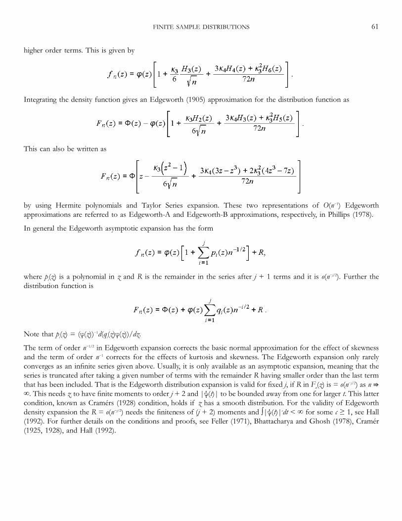
higher order terms. This is given by

Integrating the density function gives an Edgeworth (1905) approximation for the distribution function as

This can also be written as

by using Hermite polynomials and Taylor Series expansion. These two representations of O(n−1) Edgeworthapproximations are referred to as Edgeworth-A and Edgeworth-B approximations, respectively, in Phillips (1978).

In general the Edgeworth asymptotic expansion has the form

where pi(z) is a polynomial in z and R is the remainder in the series after j + 1 terms and it is o(n−j/2). Further thedistribution function is

Note that pi(z) = (φ(z))−1d(qi(z)φ(z))/dz.

The term of order n−1/2 in Edgeworth expansion corrects the basic normal approximation for the effect of skewnessand the term of order n−1 corrects for the effects of kurtosis and skewness. The Edgeworth expansion only rarelyconverges as an infinite series given above. Usually, it is only available as an asymptotic expansion, meaning that theseries is truncated after taking a given number of terms with the remainder R having smaller order than the last termthat has been included. That is the Edgeworth distribution expansion is valid for fixed j, if R in Fn(z) is = o(n−j/2) as n ⇛∞. This needs zi to have finite moments to order j + 2 and |ψ(t)| to be bounded away from one for larger t. This lattercondition, known as Cramér's (1928) condition, holds if z has a smooth distribution. For the validity of Edgeworthdensity expansion the R = o(n−j/2) needs the finiteness of (j + 2) moments and ∫|ψ(t)|cdt < ∞ for some c ≥ 1, see Hall(1992). For further details on the conditions and proofs, see Feller (1971), Bhattacharya and Ghosh (1978), Cramér(1925, 1928), and Hall (1992).


A General ExpansionMost econometric estimators and test statistics, written as Zn, are not a simple sum of i.i.d random variables, hence theclassical asymptotic Edgeworth expansions are not directly useful. To develop their Edgeworth expansions we firstwrite their asymptotic stochastic expansion (see Appendix Section A.3.1) as a power series in n−1/2 as

where ξ−i = Op(n−i), Tn, An, and Bn are well behaved random variables with limiting distributions as n ⇛ ∞. Suppose thelimiting distribution of Tn is N(0,1). Further Rn is stochastically bounded. Based on this stochastic expansion one canobtain the Nagar-type large-n approximations of first four moments of Zn, see Chapter 2. Let these be andV(Zn) = 1 + (a2/n) where a1 and a2 are nonstochastic terms of O(1). Using these results define

which has zero mean, unit variance, and approximate third and fourth moments as and E(Zn*)4 = 3 + (a4/n) where a3 and a4 are of O(1). Then using (3.28) and replacing a3 and a4 by κ3 and κ4, respectively, we get the Edgeworthexpansion, up to O(n−1), as

where

see Rothenberg (1984a).

The above method needs to develop large-n first four moments in order to develop the classical expansion. Analternative is to obtain the c.f. of the stochastic expansion of Zn and then obtain the distribution function using theinversion theorem. We provide this result for a general class of econometric estimators and test statistic in a latersection.


Another method of developing the Edgeworth expansion of econometric statistics is due to Sargan (1975). Hisapproach is based on the observation that the estimators and associated statistics commonly employed in econometricwork are not straightforwardly defined. They are expressed as functions of multivariate variables and involve functionsof first- and second-order moments of observations, for example, the mean and standard deviation. These momentsare generally consistent, and quite often unbiased too, estimators of their population counterparts. Their standarderrors are generally of order O(n−1/2). The estimation error (the difference between the estimator and parameter β) isof order Op(n−1/2) and consequently Zn is Op(1). Motivated by it, suppose the estimation error e is expressible as afunction of two random vectors p and w where p is a vector of stochastic variables following a multivariate normaldistribution and w is a vector of stochastic variables. The vectors p and w are assumed to be independently distributed.The functional form of e is supposed to be such that it is equal to 0 when p and w are set as null vectors. In addition tothe normality requirement of p, are assumed to have bounded moments of all orders. Further the function e isassumed to satisfy a smoothness and invariability condition.

Under this setup, Sargan (1975, theorem 1) proved that the distribution function F of n1/2e or the distribution Fn of Zncan be approximated by few leading terms in the Edgeworth series expansion as n → ∞. Up to order O(n−1), this isgiven by Sargan (1975) as

and alternatively

where g's and g*s are the functions of the derivatives of e and moments of p and w. For the applications of Sargan'sresult see Phillips (1979, 1980) and Ullah (1982), among others.

To show that Zn has a valid Edgeworth expansion up to O(n−1) we need conditions on the behavior of Tn, An, and Bnsuch that the approximation error is O(n−1), this follows from the results of Chibishov (1980). When the Edgeworthexpansion is obtained for the stochastic expansion of the estimation error function e(p,w) = e then its validity has beenstudied by Bhattacharya and Ghosh (1978), Sargan (1975, 1976) and Phillips (1977b).

Exercise 1 For the application of Edgeworth expansion consider a simple example. Suppose yi is i.i.d as N(μ, σ2).Consider the problem of obtaining the Edgeworth approximation to the distribution of


where s2 is an unbiased sample variance. Note that both and s2 − σ2 are of Op(n−1/2). Thus noting that

the asymptotic expansion of Zn, up to O(n−1), is

where , An = −½SnTn and with .

Since Sn and Tn are independent, Tn ∼ N(0,1) and (n − 1) s2/σ2 is a χ2 distribution with n−1 degrees function so that ESn= 0 and V(Sn) = 2n/(n−1) we can obtain the following approximate moments of Zn.

Further the approximate moments of Zn* are EZn* = 0, V(Zn*) = 1, E(Zn*)3 = 0, E(Zn*)4 = 3 + 6/n. Thus, using a1 = a3= 0, a2 = 2, and a4 = 6 the Edgeworth expansion is

This is an approximation of the exact distribution of Zn, which is a student-t distribution.

In the above example Zn is a function of p = Tn and w = Sn. These p and w are independent and all of their moments arefinite. Thus one can also use Sargan's (1975) result to obtain Edgeworth expansion. This is left as an exercise for thereader. For more applications on Sargan's approach see Phillips (1977a, 1980, 1979), Anderson and Sawa (1973), Ullah(1982), Ullah, Carter and Srivastava (1984), Carter, M.S. Srivastava, V. K. Srivastava and Ullah (1990), among others.

Exercise 2 Consider a consumption function

where y1t is aggregate consumption at time t, y2t aggregate income at time t, α the marginal propensity to consume andα0 is the coefficient of a


predetermined variable, which assumes the value 1 for all observations; further, it contains the identity

xt = net investment at time t. In this case, y1, y2 are interpreted as endogenous variables and x is exogenous orpredetermined.

We assume that n observations are available on all variables, and the reduced form exists:

that is, α ≠ 1. In fact, we assume 0 ≤ α ≤ 1.

The two-stage least squares estimator of α is given by

where , .

A little algebraic manipulation will show that

where

Then the stochastic asymptotic expansion of Zn can be written as

where , , , and . We note that z = Op(n−1/2) because is of Op(n−1/2) ifis assumed to be bounded in probability as n → ∞.

First we obtain the exact distribution of Zn. For this we note that if we assume Xt to be nonstochastic and ut are i.i.dnormal random errors with mean 0 and variance σ2, then z ∼ N(0, δ2) where


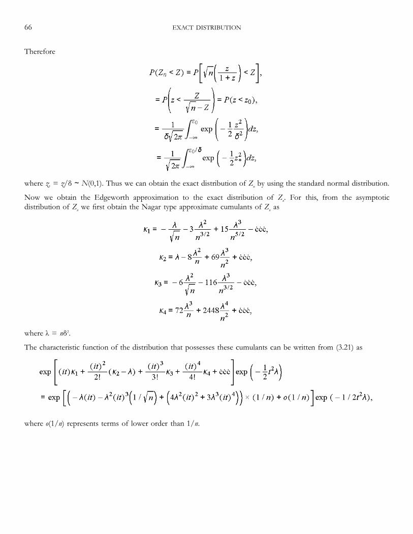
Therefore

where z* = z/δ ∼ N(0,1). Thus we can obtain the exact distribution of Zn by using the standard normal distribution.

Now we obtain the Edgeworth approximation to the exact distribution of Zn. For this, from the asymptoticdistribution of Zn we first obtain the Nagar type approximate cumulants of Zn as

where λ = nδ2.

The characteristic function of the distribution that possesses these cumulants can be written from (3.21) as

where o(1/n) represents terms of lower order than 1/n.


If we expand the exponential in the usual manner, we can write the characteristic function as

If we retain the leading term of the expansion, the characteristic function is exp((−1/2)t2λ). This is the characteristicfunction of a normal distribution with mean zero and variance λ. Therefore, the limiting distribution of Zn is normalwith mean zero and variance λ.

If we retain terms to order , we get an approximation to the characteristic function as

Applying the Inversion Theorem we get the Edgeworth approximation, to order , of the probability densityfunction of Zn as

Since Zn is the ratio of normal variables the exact moments or cumulants (moments of the exact distribution) areinfinite. The approximate cumulants can be obtained from the Edgeworth expansion of the density of Zn. These resultswill be identical to the Nagar type approximate cumulants given above.

3.7 Small-σ Edgeworth Expansion of h(y) (Normal and Nonnormal)In order to obtain the asymptotic distribution of ξ = h(y)−h(μ) we consider , and using the expansion ofh(y) around μ with y − μ = σu we write

where , ; are evaluated at y = μ.

Consider the characteristic function Zn as


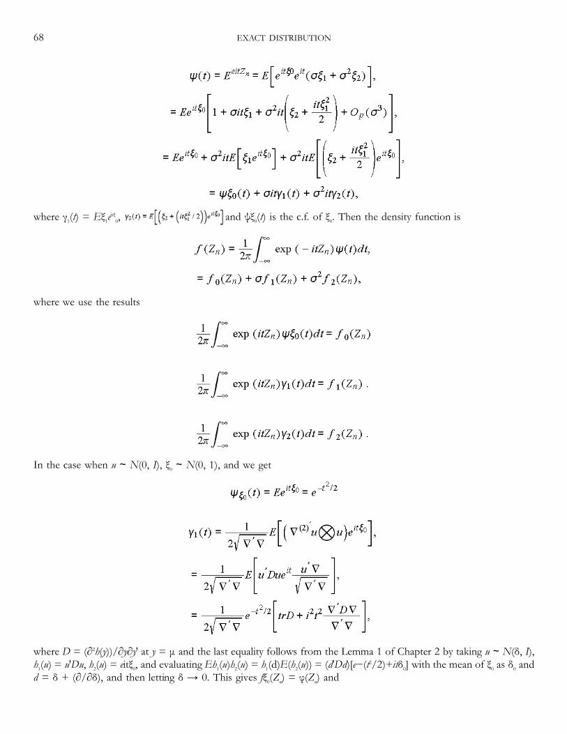
where γ1(t) = Eξ1eitξ0, and ψξ0(t) is the c.f. of ξ0. Then the density function is

where we use the results

In the case when u ∼ N(0, I), ξ0 ∼ N(0, 1), and we get

where D = (∂2h(y))/∂y∂y′ at y = μ and the last equality follows from the Lemma 1 of Chapter 2 by taking u ∼ N(δ, I),h1(u) = u′Du, h2(u) = eitξ0, and evaluating Eh1(u)h2(u) = h1(d)E(h2(u)) = (d′Dd)[e−(t2/2)+itδ0] with the mean of ξ0 as δ0 andd = δ + (∂/∂δ), and then letting δ → 0. This gives fξ0(Zn) = φ(Zn) and


. Hence, up to O(σ),

When h(y) is a vector, the joint probability density function of a normalized form of h(y) − h(μ) can be evaluated in asimilar manner, see Carter, M. S. Srivastava, V. K. Srivastava and Ullah (1990), Chaturvedi, Hoa, and Lal (1992) andChaturvedi and Shukla (1990). The large-n Edgeworth expansion of Zn, up to O(n−1), can be written similarly.

3.8 Remarks on the Edgeworth Expansion1. The Edgeworth expansions are useful in comparing two asymptotically equivalent econometric statistics. But for thepurposes of inference the quality of Edgeworth approximations in the tails is often not good in the sense that it canproduce small or negative density in the tails, see Phillips (1977b, 1978). Under this scenario it is sensible toapproximate ratios of tail probabilities Fn(−z)/Φ(−z) and (1 − Fn(z))/(1 − Φ(z)) for instead of Fn, see Phillips(1980). An additional point is to see the question of where to approximate the distribution. For this we look into thesaddle point approximates, which provide improved performance in certain environments of the parameters,particularly in the tail parts of the distributions. Essentially the techniques involve using a cleverer inversion of thecharacteristic or moment generating function to obtain the approximations, see Daniels (1954, 1956). The resultingapproximation has the features that the density function fn(z) is in powers of n−1, not n−1/2 and it is always positive. Forapplications of saddle point approximations, see Phillips (1978), Durbin (1979), Holly and Phillips (1979) andLieberman (1994c) among others. It may be pointed out that the saddle point approximation is applied only in somespecific situations, for instance, when the characteristic function is available or when a set of sufficient statistics for theestimation of parameters is available; see Daniels (1956) and Durbin (1979).

2. Let us write the statistic , where and is the asymptotic Cramér-Rao bound for θ andis asymptotically efficient with the Edgeworth expansion Fn(z) up to O(n−1), where first term is the limiting normaldistribution and then there are terms of O(n−1/2) and O(n−1) terms. This is called in this book to be second-orderapproximation and the approximation up to first term is called the first-order approximation. This terminology is,however, different with those in Akahira and Takeuchi (1981), Pfangal and Wefelmeyer (1978), and others where theapproximations up to O(n−1/2) are considered second order and the approximations up to O(n−1) as third-order.


3. For the estimation case, the maximum likelihood (ML) estimator is known to be first-order efficient under generalregularity conditions. If we correct the bias of the ML estimator to second order, then the variance of the bias-corrected ML, is the bias term, is less than or equal to any other second-order bias corrected first-order efficient estimators, see Efron (1979, 1982). For example, it is well known that the bias-adjusted limitedinformation ML estimator in a structural model is second-order efficient compared with the instrumental variablesestimator. Rothenberg (1984a) provides a procedure of obtaining the second-order efficient estimator as

where k = 1,2 and L(1) and L(2) represent the first and second derivatives of the log likelihood of a scalar θ. Using aninitial consistent estimator will give , which is first-order equivalent to the ML estimator. Similarly obtained issecond-order efficient. In the case of testing θ = θ0 against θ < θ0, suppose has a valid Edgeworthexpansion Fn(z) up to O(n−1). Then the α-percentage critical value z* is the value, which solves Fn(z*) = 1 − α. Testbased on this z* is called a second-order size corrected test of size α. Pfanzagl and Wefelmyer (1978) have shown thatin the class of second-order size corrected tests the test based on the ML estimator is locally uniformly morepowerful compared with other first-order efficient .

4. Given the Edgeworth expansion of probability distribution of an econometric statistic, one can use it to obtain theapproximate moments of the statistic. These moments will be the same as those obtained by using large-n Nagar typemoment expansions. Sargan (1974) showed that a large class of Nagar type large-n moment expansions are valid asasymptotic approximations, provided only that the corresponding moments of the exact distribution exist and are ofO(1) as n→ ∞, also see Srinivasan (1970), and Basmann (1974) on this issue. This result of Sargan (1974) is importantin view of the fact that for some econometric statistics, for example, the instrumental estimator for a just identifiedstructural equation with normal errors, the exact moments do not exist but the Nagar type large-n moments or themoments based on the Edgeworth distribution approximation or the bootstrap based moments are available. It shouldbe pointed out that knowing the nonexistence moments may not be relevant in determining the underlying exactdistribution function. For example, the instrumental variable estimator in the just identified structural equation casedoes not have any moment existing but it has a well defined distribution of the ratio of two normal random variablesand also a well defined limiting distribution.

5. The analytical theory of Edgeworth expansions has made an important impact on the resampling techniques, suchas the bootstrap and the jackknife,


of developing the sampling distributions and moments of econometric statistics. Hall (1992) discusses the link betweenEdgeworth expansion and the bootstrap and shows that the bootstrap may be used as a method for the estimatingsecond-order Edgeworth expansion, also see Jeong and Maddala (1993), Vinod (1993), and Horowitz (2001) for theeconometrics literature on the bootstrap. The role of analytical results on the Edgeworth expansion of the econometricestimators is now more important. For example, without knowing the analytical validity of the Edgeworth expansionor the forms of moments and distribution of the econometric statistics under consideration the bootstrap exercise hassomewhat of a black box flavor. Also a problem with the resampling techniques is that they usually change with theparticular resampling and they may be very time-intensive in the contexts of nonlinear and dependent time seriesmodels. The analytical results can also be useful to have qualitative or analytical knowledge about the finite sampledistribution to place bounds on inferences about the parameters of interest. It can also provide a measure of theaccuracy of resampling techniques.

6. The Edgeworth expansion is only a valid asymptotic expression in the sense that it works well for large ormoderately large n. For a small fixed n the second-order approximation error may not be smaller than that of the firstorder limiting normal approximation. This is because the second-order approximations for econometric statisticsdepend on the data structure of the economic variables and the cumulants. The approximate distributions usuallydepend on the unknown parameters, but they can be substituted with their consistent estimators and order ofapproximation adjusted accordingly. Finally the form of the Edgeworth expansion of the econometric statistics willdepend upon the assumption of the distribution of observations.

7. We note here that while Edgeworth expansion provides the order of magnitude of the error from the limitingnormal approximation as n→ ∞, it does not provide the absolute magnitude of the error when n does not go to ∞. Animportant result, however, was given by Berry (1941) and Eseen (1945) as

where and c ≥ 2.031 is an absolute, universal constant, also see Petrov (1975) for nonidentically distributedvariables and Bhattacharya (1975) for the multivariate distributions.

8. There is some work on the Edgeworth expansion of the ratio of polynomials in y. Let us consider q = h(y) = h1(y)/h2(y) where h1(y) = a0 + ∑ aiyi + ∑i ∑jaijyiyj + … and h2(y) = b0 + ∑biyi + ∑i∑jbijyiyj + … are arbitrary polynomialtransformation of y, a's and b's are constants, and y is a random vector with the elements, which could be dependentand nonidentically distributed. Note that the ratio of quadratic forms is a special case of q above. The Edgeworthasymptotic expansion of q can be obtained by the procedure described in this chapter, also see Phillips (1983). TheEdgeworth


asymptotic expansion involves two types of errors, one due to the truncation of h(y) by Taylor series and then due tothe truncation of the Edgeworth expansion. Lieberman's (1997) result avoids the expansion of q at the first stage, andhence the only error is due to the truncation of the Edgeworth expansion at some point, although it is possible to writeit in infinite expansion. Using this one can obtain the Edgeworth asymptotic expansion by collecting terms ofdecreasing order of magnitude of n−1/2.

9. Let Zn represent a statistic which has the Edgeworth asymptotic expansion given above. Denoting Qα = Qα(n) for theα–level quantile of Zn, given by

and let qα be the α–level quantile of the standardized normal distribution, given byΦ(qα) = α. Then the expansion of Qα

in terms of qα and qα in terms of Qα can be written from the Edgeworth expansion as

where functions Pi1 and Pi2 are polynomials. The asymptotic expansions are called Cornish–Fisher expansions and theyare available uniformly in ɛ < α < 1− ɛ for any 0 < ɛ < 0.5. The polynomials Pi1 and Pi2 are completely expressed interm of the polynomials qi in (3.30). See Hall (1992).

10. Several econometrics statistics are nonpivotal/asymptotically nonpivotal in the sense that their exact/asymptoticdistributions depend on the parameters of the models. The difference of the exact distribution from the estimatedEdgeworth expansions or the bootstrap distribution of such asymptotically nonpivotal statistics is known to be ofO(n−1/2), which is the same as the difference of the exact distribution from the first order limiting approximation. Incontrast for the asymptotically pivotal statistics having distributions free from the parameters, the exact distributiondiffers with the limiting Edgeworth approximation (bootstrap distribution) by O(n−1). As an illustration, see Exercise 1of Section 3.6 where the statistics Zn is pivotal with the Edgeworth expansion of O(n−1) whereas the Edgeworthexpansion of the distribution of the nonpivotal statistic in Exercise 2 is of O(n−1/2). Thus the second-order Edgeworthexpansions or bootstrap distributions for the pivitol statistics may have better approximation of their exactdistributions, see Hall (1992) and Horowitz (2001).

11. We have discussed the techniques of obtaining the Edgeworth expansion of econometric statistics. One way todevelop this is to obtain the first four moments (cumulants) of the statistics under consideration. This was done in


developing large-n Edgeworth expansions of Exercises 1 and 2 in Section 3.6. Alternatively one can first obtain thecharacteristic function based on the asymptotic expansion of the statistic. This was followed for the econometricstatistics h(y) in Section 3.7 in developing its small-σ Edgeworth expansion. It can similarly be followed for developingthe large-n Edgeworth expansions of a general class of econometric statistics with a large-n asymptotic expansion asgiven in (2.75).


4 Regression Model

4.1 IntroductionIn this chapter, the regression model is considered and the application of results of Chapters 2 and 3 are demonstratedin the evaluation of moments and distribution of various statistics encountered in drawing inferences from the model.Most of the results for the normal distribution, it may be pointed out, have been obtained in the econometrics textbooks in a different way but here our objective is to illustrate the technique, which merely rests on the knowledge ofmultivariate normal distribution and its simple properties. The technique will appear to be more fruitful in subsequentchapters. The results for the nonnormal cases are also presented, which have rarely been discussed in the literature.

4.2 Model Specication and Least Squares EstimationLet us postulate the following linear regression model:

where y is an n × 1 vector of n observations on the study variable, X is an n × p matrix of n observations on pexplanatory variables, β is a p × 1 vector of unknown regression coefficients and u is an n × 1 vector of disturbances.

For the estimation of coefficient vector β, the following assumptions are made:

1. The matrix X has full column rank meaning thereby that there are no exact linear relationships among theexplanatory variables and the number of observations do not fall short of the number of explanatory variables.

2. The matrix X is nonstochastic.3. The disturbance vector u has mean vector null and variance covariance matrix σ2In with σ2 as the unknown

disturbance variance and In as the identity matrix of order n × n.

The least squares (LS) estimator of β is given by

which is the best linear unbiased estimator according to Gauss–Markov theorem. Writing A = (X′X)−1X′ if ai denotesthe ith row vector of A, the LS estimator of the ith element βi of β can be expressed as

Next, denoting M = In − XA, the residual vector is

whence the residual sum of squares (RSS) is given by

This provides an unbiased estimator of σ2, the disturbance variance, as follows:

If the model contains an intercept term or equivalently if one of the explanatory variables in the model is constant, thecoefficient of multiple determination is defined by

which is the square of multiple correlation coefficient between the study variable and the explanatory variables. Herey¯ denotes the mean of observations on the study variable and ι in the specification of matrix N is an n × 1 vector withall elements unity.

If a correction for the degrees of freedom (d.f.) is applied to R2, we obtain the adjusted R2 given by

76 PROPERTIES OF ESTIMATORS

Next, consider the conventional F-ratio for testing H0:β = 0, which is given by

Note that this F is related to R2 given in (4.7), that is

Finally, let us consider the predictor

which can be utilized either for predicting the actual values of study variable or for the mean values.

In case we wish to predict some future value (say, yf) associated with pre-specified values of explanatory variables, theprediction or forecast is given by

where xf denotes a 1 × p vector consisting of the pre-specified values of p explanatory variables.

4.3 Properties of Estimators

4.3.1 Coefcients EstimatorsLet us assume that the disturbances are normally distributed. Now if we write

then z has a normal distribution N(μ,Ip). Further, we observe from (2.4) and (2.9) that

whence it follows that d′ · 1 = μ′. Using it, we see that

REGRESSION MODEL 77

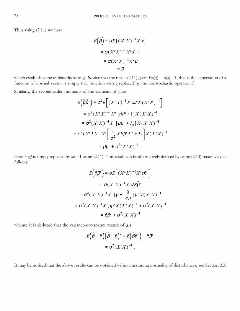
Thus using (2.11) we have

which establishes the unbiasedness of . Notice that the result (2.11) gives Eh(z) = h(d) · 1, that is the expectation of afunction of normal vector is simply that function with z replaced by the nonstochastic operator d.

Similarly, the second-order moments of the elements of are

Here Ezz′ is simply replaced by dd′ · 1 using (2.11). This result can be alternatively derived by using (2.14) recursively asfollows:

whence it is deduced that the variance–covariance matrix of is

It may be noticed that the above results can be obtained without assuming normality of disturbances, see Section 2.3.


Now let us evaluate the moments of given by (4.3). First, from (4.13) we have

where ιi denotes a 1 × p vector with all elements 0 except the ith element, which is 1. In other words, ιi is the ith rowvector of an identity matrix Ip.

Next, consider the second-order moments. Following the manipulation indicated in (4.17), we have

where cji denotes the (j,i) the element of the matrix C = (X′X)−1 = AA′.

From (4.19) and (4.20) we can write

which leads to the expression (4.18).

Next, let us find the third-order moments:

REGRESSION MODEL 79

from which, using (4.19) and (4.20), we find

Similarly, we can obtain the fourth-order moments:

From above, we obtain

Further higher-order moments can be straightforwardly found in a similar manner. It may be pointed out that theabove results can also be derived from the moment generating function or characteristic function of in theconventional manner but the process may be algebraically difficult for higher-order moments than the recursive kindof aforesaid procedure. When X is a stochastic matrix the results have been discussed in Chapter 2.

4.3.2 Residuals and Residual Sum of SquaresConsider the ith element of the residual vector û in (4.4):

where mi is the ith row vector of M = [In − X(X′X)−1X′]. The moments of ûi can be evaluated precisely in the samemanner as indicated for . The resulting expressions can be further simplified by noting the following results

arising from the identity MX = 0 and the idempotency of M. Here mij denotes the (i,j)th element of M. Thus we find


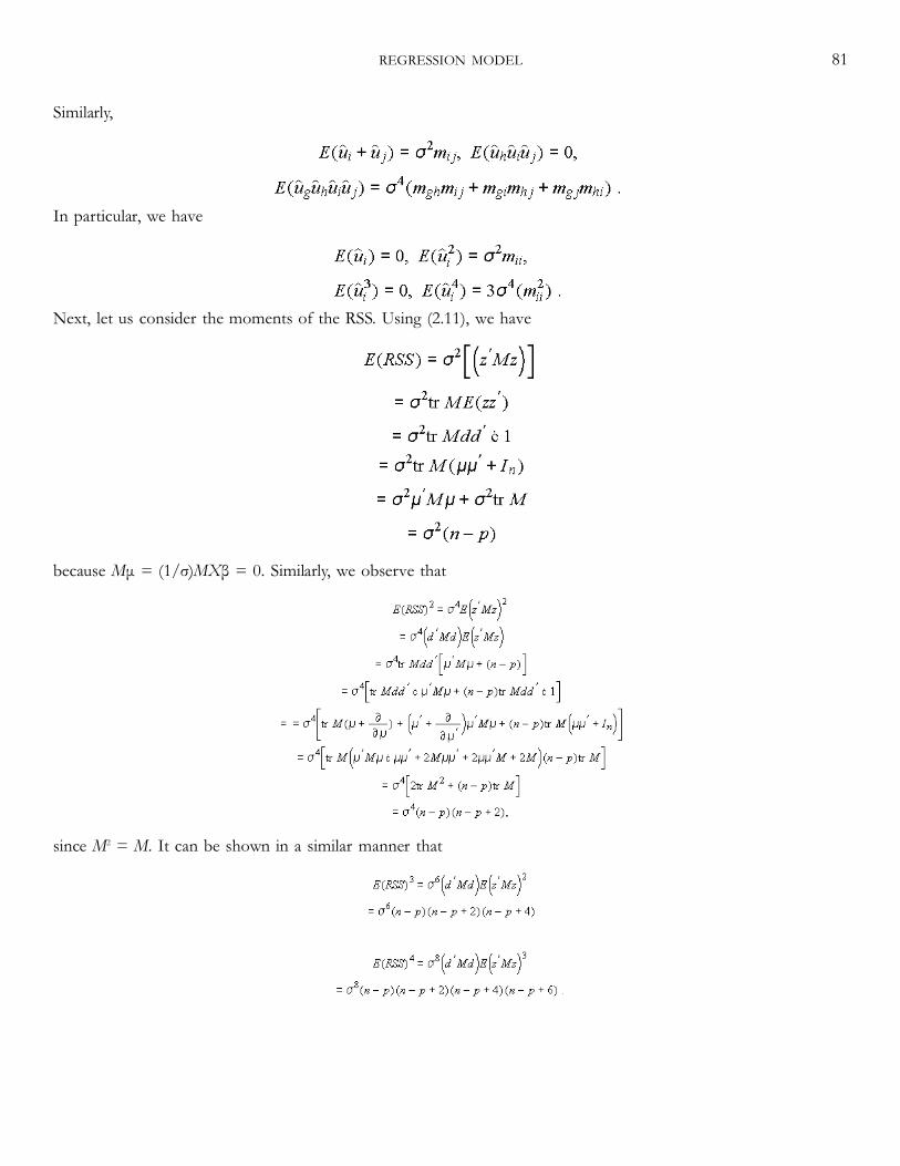
Similarly,

In particular, we have

Next, let us consider the moments of the RSS. Using (2.11), we have

because Mμ = (1/σ)MXβ = 0. Similarly, we observe that

since M2 = M. It can be shown in a similar manner that

REGRESSION MODEL 81

Higher-order moments can be derived in the same way. From these results, one can find the expressions for momentsof residual variance estimator . For instance, the first four central moments of are

whence the Pearson's measures for the excess of skewness and kurtosis of the distribution of can bestraightforwardly obtained:

implying that the distribution of is positively skewed and leptokurtic.

Sometimes we may be interested in finding out the inverse moments. These can be obtained from result (2.20). Forinstance, the rth inverse moment of the RSS is

provided that r is less than (1/2)(n − p).

Since M is an idempotent matrix of rank (n − p), it has only (n − p) nonzero characteristic roots and these roots are allequal to one. Thus it is easy to see that |In + 2tM| = (1 + 2t)(n − p) and μ′M(In + 2tM)−1μ = 0.

Now applying the transformation t* = (1 + 2t)−1 we obtain the following expression


whence the rth inverse moment of is

provided that r < (1/2)(n − p).

If we are interested in the distribution of , for example, in Bayesian inference, the mean and variance are

while the Pearson's measures of excess of skewness and kurtosis are

It is thus seen that the distribution of inverted is positively skewed. Further, it is leptokurtic as (n − p) > 8.4.3.3R2 and Adjusted R2

Let us first consider the moment of R2 defined by (4.7). The rth moment of R2 is given by

where N and M are idempotent matrices. Here we restrict our attention to the first two moments only. The higher-order moments can be evaluated using the result (2.28) in a recursive manner. In particular the mean is

with Δ = (In + 2tN)−1 provided that n exceeds 3.

Since the regression model is assumed to contain an intercept term, the vector ι appears in X as one of the columnvectors so that Mι = 0. This

REGRESSION MODEL 83

implies that MN = M. Further, using the results

for any nonsingular matrix D, vector d and scalar g, it is easy to see that

whence it follows that |Δ| = (1/(1 + 2t))n [1 + 2(t/n)ι′ι] = (1/(1 + 2t))n−1} and NΔ = (1 + 2t)−1N. Further, we find (N−M)Δ = (1/(1 + 2t))(N −M), μ′Δ(N −M)Δμ = (1/(1 + 2t))2μ′μ, μ′NΔμ = (1/(1 + 2t))μ′μ, which when substituted in(4.44) yields

Applying the transformation t* = (1 + 2t)−1 we get

where θ = (1/2)μ′μ = (1/2σ2)β′X′Xβ is the noncentrality parameter.

An alternative expression for the mean is

which is the form obtained by Cramer (1987).


Similarly, using the result (2.29) it is easy to see that the second moment of R2 is

provided that n exceeds 5.

If we define the population counterpart of R2 as

it is easy to see that R2 serves as a consistent estimator of φ; see Cramer (1987: 256–7). Further, it is obvious from(4.48) that R2 is a biased estimator. For assessing the magnitude of bias, Cramer (1987) carried out a numericalevaluation of bias and standard deviation of R2 for few selected values of p, n, and φ, viz., p = 2,3, n = 5, 10, 50, 200,and φ = 0.9, 0.667, 0.5, 0.333. The numerical results revealed that R2 as an estimator of φ has an upward bias, whichcan be substantial when the number of observations is small. However, the bias declines rapidly as n grows large.When the bias is noticeable, R2 has very large standard errors. The standard error appears to have a strongerdependence upon φ in comparison to p and n, and it is this dependence, Cramer stated, that often leads to erroneousinferences from the value of R2 taken as a measure of goodness of fit.

Next, let us consider the moments of adjusted R2. These moments can be straightforwardly found from the momentsof R2. For instance, the mean is

REGRESSION MODEL 85

Similarly, the second moment of can be found:

whence an explicit expression for the variance of can be obtained.

It is interesting to note from the above expression that does not explicitly depend upon p, the number ofexplanatory variables in the model, while does. As a consequence, Cramer (1987) observed from his numericalresults that bias of virtually vanishes and in fact it may be downward. Next, we observe that

from which it follows that has larger variance than R2. Thus, for a smaller number of observations, may havesmaller bias than R2 but owing to larger variability it can be more unreliable than R2.

4.3.4 The F-RatioThe F-ratio given by (4.9) can be written as

so that its rth moment is given by

where use has been made of (2.28). Thus the mean is


Similarly, setting r = 2 in (4.56), the second moment of F is

where we have used the result

Similarly, the higher-order moments of F can be found from (4.56) in a recursive way.

It may be mentioned that the expression for the rth moment of F is essentially the rth moment of a singly noncentralF-distribution with p and (n − p) d.f. and (μ′μ/2) the noncentrality parameter.

4.3.5 PredictionLet us consider the predictor defined by (4.11):

If it is employed for predicting the actual values of the study variable, the prediction error is

from which the predictive bias and the predictive mean squared error (MSE) or variance are

Higher-order moments of the prediction error can be determined from the moments of residuals (see Section 4.3.2). Ifthe predictor is used for the mean values of study variable, the prediction error is given by

REGRESSION MODEL 87

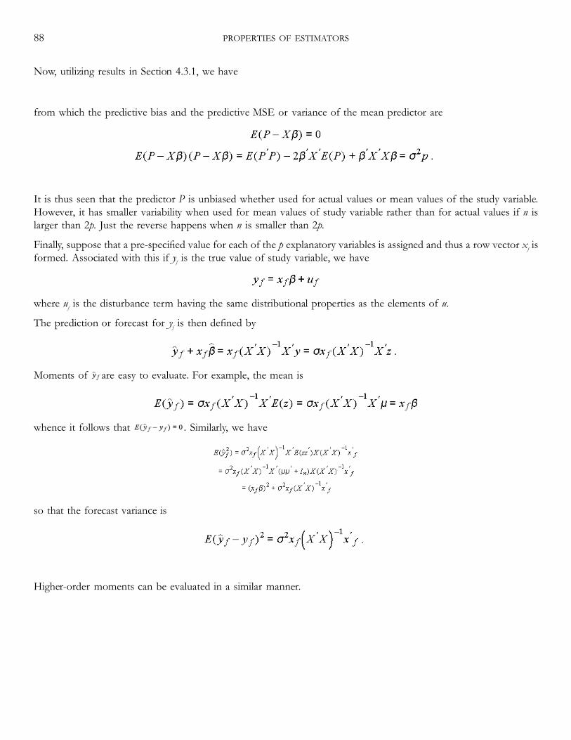
Now, utilizing results in Section 4.3.1, we have

from which the predictive bias and the predictive MSE or variance of the mean predictor are

It is thus seen that the predictor P is unbiased whether used for actual values or mean values of the study variable.However, it has smaller variability when used for mean values of study variable rather than for actual values if n islarger than 2p. Just the reverse happens when n is smaller than 2p.

Finally, suppose that a pre-specified value for each of the p explanatory variables is assigned and thus a row vector xf isformed. Associated with this if yf is the true value of study variable, we have

where uf is the disturbance term having the same distributional properties as the elements of u.

The prediction or forecast for yf is then defined by

Moments of are easy to evaluate. For example, the mean is

whence it follows that . Similarly, we have

so that the forecast variance is

Higher-order moments can be evaluated in a similar manner.


4.3.6 Exact Moments Under NonnormalSince R2 and F are essentially ratio of quadratic forms, their exact moments under normality follow from the results inChapter 2 and they have been discussed above. For a specific family of exponential density the results can bedeveloped by the procedures described in Section 2.3. Further, since R2 and F are scale invariant, the exact resultsunder normality will continue to hold for any spherically symmetric error density, a special case of which is multivariatet-density, see Ullah and Zinde-Walsh (1984), Ullah and Phillips (1986), Ohtani and Hasegawa (1993), Zellner (1976),King (1980), and Breusch, Robertson, and Welsh (1993). Furthermore the exact moments of R2 and F can also bewritten under the Edgeworth type density of disturbances from Peters (1989).

If, however, the interest is to compare the exact bias and MSE properties of R2 and , without making distributionalassumption and without deriving the explicit expressions of bias and MSE, it can be done by simply looking at therelationship between R2 and . This is

Cramér (1987) has pointed out that has the same probability limit as R2 provided all the explanatory variables in themodel are asymptotically cooperative in the sense that the limiting term of matrix n−1(X′MX) as n → ∞ is finite andnonsingular. Consequently, both R2 and can be regarded as consistent estimators of their population counterpart φ (0≤ φ ≤ 1).

The efficiency properties of R2 and can now be studied by noting

Thus, , which implies that , that is, where . Similarly

so that

that is, the exact variance of will always be larger than that of R2.

Turning to the MSE of R2 and we note from (4.68) that

Therefore, squaring and taking expectations

REGRESSION MODEL 89

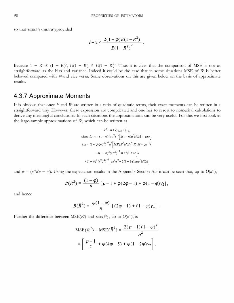
so that provided

Because 1 − R2 ≥ (1 − R2)2, E(1 − R2) ≥ E(1 − R2)2. Thus it is clear that the comparison of MSE is not asstraightforward as the bias and variance. Indeed it could be the case that in some situations MSE of R2 is betterbehaved compared with and vice versa. Some observations on this are given below on the basis of approximateresults.

4.3.7 Approximate MomentsIt is obvious that once F and R2 are written in a ratio of quadratic terms, their exact moments can be written in astraightforward way. However, these expression are complicated and one has to resort to numerical calculations toderive any meaningful conclusions. In such situations the approximations can be very useful. For this we first look atthe large-sample approximations of R2, which can be written as

and w = (n−1u′u − σ2). Using the expectation results in the Appendix Section A.5 it can be seen that, up to O(n−1),

and hence

Further the difference between MSE(R2) and , up to O(n−1), is


When γ2 = 0 the above results are for the case of normal disturbances, see V. K. Srivastava, A. K. Srivastava, and Ullah(1995).

Several observations about bias and MSE can be made on the basis of above results. First while the bias of R2 ismonotonically increased with the number of regressors p it is not the case with the bias of . This is consistent withthe well known fact that R2 is a monotonically increasing function of p. Second the bias of R2 and are not affected bythe asymmetry of disturbances, though kurtosis does have its impact on the magnitude of bias. However,

Thus the magnitude of approximate bias of R2 will be larger than that of for the i.i.d. disturbances. This is consistentwith the exact result above, which holds for all distributions, including non i.i.d.

As regards the variances of these estimators, we observe from (4.75) to (4.77) that the difference in variances of R2 andup to the order O(n−2) is given by

Now this D is always negative because of positivity of (γ2+2) for all types of distributions. This result is also consistentwith the exact result above which holds for all distributions, including those which are not i.i.d. Further,D increases asp grows large. This supports the result that the larger is the number of explanatory variables in the model, the moreinefficient is in comparison to R2 according to the criterion of variance to order O(n−2) irrespective of the nature ofdistribution of the disturbances.

However, variance is not an appropriate criterion for judging efficiency of biased estimators; the right choice is theMSE and, therefore, we should consider this for comparing the performance of R2 and . Accordingly, from (4.77),has a smaller MSE, to the order of our approximation, than R2 when

Now if the disturbances are mesokurtic, that is, if they are normally distributed (γ2 = 0), then the condition reduces to

which holds true for all values of θ so long as p-1 exceeds 3; see Table 4.1.

Table 4.1 Evaluation of (4.81)

θ 0.0 0.1 0.2 0.3 0.4 0.5 0.6 0.7 0.8 0.9 1.02θ(5−4θ)

0.00 0.92 1.68 2.28 2.72 3.00 3.12 3.05 2.88 2.52 2.00

2θ(1−2θ)

0.00 0.16 0.24 0.24 0.16 0.00 −0.24 −0.56 −0.96 −1.44 −2.00

REGRESSION MODEL 91

Thus, when the distribution of disturbances is mesokurtic (normal), is definitely superior to R2 as long as thenumber of explanatory variables is four or more, in the sense that has not only smaller bias but also smaller MSEtoo. This result may hold for three or less explanatory variables also provided θ is small enough, with θ ≤ 0.2 twoexplanatory variables are enough.

When the distribution of disturbances departs from normality, it follows from inequality (4.80) and the table givenabove that is more efficient than R2 for all platykurtic distributions (−2 ≤ γ2 < 0), at least as long as (p − 1) exceedsthree. This result continues to remain true for all leptokurtic distributions (γ2 > 0) also provided θ does not fall below0.5, that is, the model does not fit the data very poorly. When θ is less than 0.5 so that the model fits poorly, thecondition (4.80) for superiority of over R2 may require (p − 1) to be somewhat larger depending upon the value of γ2for leptokurtic distributions.

It is thus found that the adjusted is not that unreliable as it emerges out to be from variance viewpoint alone.

Now we turn to the question of the limitations of the approximate result. For this we make the following observations.It is interesting to note that both the results and , based on large-n approximations, are thesame as the exact results. Also, under the normality assumption, a comparison of the exact bias of R2 given in the table1 of Cramer (1987) with the corresponding calculations of approximate bias above suggests that the two results arequite close. For example, when p = 2 (k = 2 in Cramer) and θ = 0.9, we get the exact bias with approximate bias inparenthesis as 0.036 (0.034), 0.018 (0.017), 0.006 (0.006), 0.002 (0.002) for n = 5, 10, 30, 100, respectively. For p = 3, θ= 0.9 and the same n values, in order, we get 0.057 (0.054), 0.028 (0.027), 0.009 (0.009), 0.003 (0.003). Though notreported here, similar results were obtained for other values of θ considered in Cramer (1987). The same phenomenonoccurred in the case of MSE comparisons of the exact versus the approximate results. Again, when p = 2 and θ = 0.9,the exact and approximate values of were −0.001 (−0.0006), −0.00018 (−0.00015), 0.0000 (0.0000)for n = 5, 10, and 30, respectively. Note that while the approximate difference in MSE is calculated by using (4.77), theexact value of difference is calculated by noting that we can rewrite this from (4.72) as l[2(1 − φ)(l + 1)B(R2) − (2 +l)MSE(R2) − l(1 − φ)2] and using the results in table 1 of Cramer. It is thus clear that the approximate numerical resultsin the normal case are very close to the corresponding exact results and they are identical when n is thirty and above.Also, as indicated above, the analytical comparisons of the approximate bias and variance, in the general nonnormalcase, provide the same results as those based on the exact results. Nevertheless, it remains the subject of a future studyto see if the dominance condition in (4.80) and (4.81), based on the approximate MSE, will go through for the exactMSE case.


Now we consider the small-σ approximation of the bias and MSE. These follow from the results in (2.91) or (2.95).For example, the bias up to O(σ2) is

and hence

where we also use 1 − φ = nσ2/(nσ2 + β′X′NXβ) ⋍ nσ2/β′X′NXβ.

From the above results we note that the bias of R2 depends on the number of regressors p and it is a decreasingfunction of φ and n, since β ′X′NXβ/σ2 can be written as nφ/(1 − φ). The bias of is also a decreasing function of nand φ, and it is considerably smaller than the bias of R2 especially when p is large.

Turning to Laplace approximations, we note from (2.108) that

Further, using the expectations in the Appendix we get

and

Comparing the large-n, small-σ, and Laplace approximations we first observe that while both the small-σ and Laplaceresults remain the same under the normal and nonnormal errors this is not the case with the large-n approximation,which depends on γ2. The MSEs, based on all the approximations, can be shown to be affected by γ2 indicating that thedistribution of R2 is affected by the nonnormality. For the comparison of ER2 based on these three approximations, seeSmith (1996) where he indicates better accuracy of large-n approximation. But as σ decreases, with n fixed, hiscalculations suggest that the accuracy of each approximation method improves.

The exact distributions of R2 and F can be evaluated by the Imhof procedure given in Chapter 3.

REGRESSION MODEL 93

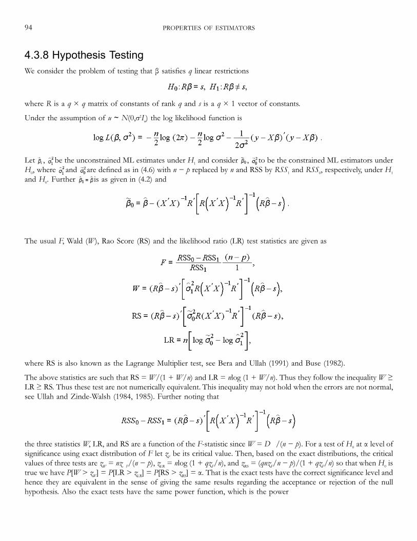
4.3.8 Hypothesis TestingWe consider the problem of testing that β satisfies q linear restrictions

where R is a q × q matrix of constants of rank q and s is a q × 1 vector of constants.

Under the assumption of u ∼ N(0,σ2In) the log likelihood function is

Let , be the unconstrained ML estimates under H1 and consider , to be the constrained ML estimators underH0, where and are defined as in (4.6) with n − p replaced by n and RSS by RSS1 and RSS0, respectively, under H1

and H0. Further is as given in (4.2) and

The usual F, Wald (W), Rao Score (RS) and the likelihood ratio (LR) test statistics are given as

where RS is also known as the Lagrange Multiplier test, see Bera and Ullah (1991) and Buse (1982).

The above statistics are such that RS =W/(1 +W/n) and LR = nlog (1 +W/n). Thus they follow the inequalityW ≥LR ≥ RS. Thus these test are not numerically equivalent. This inequality may not hold when the errors are not normal,see Ullah and Zinde-Walsh (1984, 1985). Further noting that

the three statistics W, LR, and RS are a function of the F-statistic sinceW = nqF/(n − p). For a test of H0 at α level ofsignificance using exact distribution of F let zF be its critical value. Then, based on the exact distributions, the criticalvalues of three tests are zW = nqzF/(n − p), zLR = nlog (1 + qzF/n), and zRS = (qnzF/n − p)/(1 + qzF/n) so that when H0 istrue we have P[W > zW] = P[LR > zLR] = P[RS > zRS] = α. That is the exact tests have the correct significance level andhence they are equivalent in the sense of giving the same results regarding the acceptance or rejection of the nullhypothesis. Also the exact tests have the same power function, which is the power


function of the F-test. Thus though three tests are not numerically equivalent they do not provide conflicting resultsbased on the respective critical values using exact distributions.

Under suitable regularity conditions it is well known that the three test statistics have the same asymptotic chi-squaredistribution with q d.f., under the null hypothesis. Let z be the critical value corresponding to the upper α percentagepoint of this chi-square distribution. Then the asymptotic tests, based on z, reject the null hypothesis ifW > z, RS > z,and LR > z provided n goes to infinity. But the exact critical values of each of the tests may be substantially differentfrom the asymptotic critical value z. Thus given the inequality among these three tests, for small or moderately largesamples, the critical regions of them may not be the same α-percentage. Thus these tests may give conflicting results byusing the same asymptotic critical value, also the true powers of the asymptotic tests cannot be equal; see Berndt andSavin (1977), and also Evans and Savin (1982) for the calculations of probabilities of conflict and the true power ofasymptotic tests.

The conflict between the asymptotic tests is essentially due to the fact that the significance levels are not correct for theactual sample of observations. For this we can develop Edgeworth expansions of each of the tests and determine thecorrection factors for the chi-square critical value z, which make the significance level of each test correct to order n−1.For the Edgeworth expansion, up to O(n−1), of the distribution of LR under H0 and H1, see Rothenberg (1984a). ThisEdgeworth expansion can be obtained by deriving the first four approximate cumulants of LR and then determiningthe characteristic function, see Chapter 3. This provides the Edgeworth corrected LR, as

where

This correction ensures that the LR has the correct significance level to order n−1.W* is simply modifiedW in which nis replaced by n − p in order to have an unbiased estimatior of the error variance. A similar modification in RS is

To obtain the critical values ofW* and RS* we note the following stochastic expansions ofW* and RS*, up to O(n−1),

REGRESSION MODEL 95

These give the critical values as

The W* and RS* tests, based on these critical values, are referred size-corrected tests as in the LRe test. These size-corrected tests generally provide the right significance levels and hence negligible probability of conflict in practice.Further they have the same power to order n−1, see Evans and Savin (1982) and Rothenberg (1984a).

The above results are valid under the normality of errors. It will be an interesting study to extend the above results forthe nonnormal errors. The results in Ali and Sharma (1996), Ullah and Phillips (1986), Knight (1985), and Lieberman(1997) among others, will be useful in this context.

4.3.9 Nonlinear Regression ModelsConsider a nonlinear model of the form

whereXi is an i.i.d variable, β is a scalar parameter and ui is i.i.d with E(ui|Xi) = 0 andV(ui|Xi) = σ2. The estimator ofβ solves the moment condition

where qi = uiXi. The jth order derivative of qi with respect to β is ∇jqi = −Xif(j)(Xi,β) = −Xifi(j). Using the results (2.81) and(2.82) of Chapter 2 we get

and

where , , and , which is also the asymptotic variance of .

When the model is linear the and the last two terms in are zero because . Also .

When X is nonstochastic and we replace and by and , respectively. Further the results forthe case where Xi and ui are non i.i.d, as in time series, follow from the results in (2.101) and (2.102).


5 Models with Nonscalar Covariance Matrix ofErrors

5.1 IntroductionIn Chapter 4, we considered the regression model where the errors have a scalar covariance matrix. The regressioncoefficients were estimated by the method of least squares (LS). But a large class of econometric models are suchwhere the covariance matrix of errors is nonscalar. Usually the error covariance matrix is unknown so an estimatedmatrix is obtained and the resulting estimators of β are obtained by the feasible generalized least squares (FGLS) or bythe maximum likelihood (ML) method. These contain the linear regression model where the errors are heteroskedasticor serially correlated, the seemingly unrelated regressions, random effect panel data model, and the limited dependentvariables. The objective of this chapter is to analyze the exact and approximate distributions and moments of thefeasible GLS and ML estimators of the parameters of these models. The results for several test statistics will also beexplored.

5.2 General Model with Nonscalar Covariance Matrix

5.2.1 Exact MomentsLet us consider the linear model:

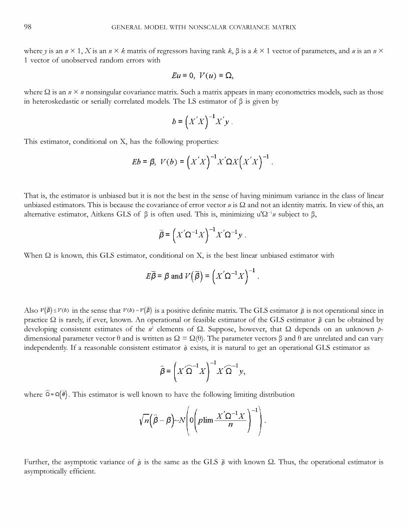
where y is an n × 1, X is an n × k matrix of regressors having rank k, β is a k × 1 vector of parameters, and u is an n ×1 vector of unobserved random errors with

whereΩ is an n × n nonsingular covariance matrix. Such a matrix appears in many econometrics models, such as thosein heteroskedastic or serially correlated models. The LS estimator of β is given by

This estimator, conditional on X, has the following properties:

That is, the estimator is unbiased but it is not the best in the sense of having minimum variance in the class of linearunbiased estimators. This is because the covariance of error vector u isΩ and not an identity matrix. In view of this, analternative estimator, Aitken's GLS of β is often used. This is, minimizing u′Ω−1u subject to β,

When Ω is known, this GLS estimator, conditional on X, is the best linear unbiased estimator with

Also in the sense that is a positive definite matrix. The GLS estimator is not operational since inpractice Ω is rarely, if ever, known. An operational or feasible estimator of the GLS estimator can be obtained bydeveloping consistent estimates of the n2 elements of Ω. Suppose, however, that Ω depends on an unknown p-dimensional parameter vector θ and is written as Ω = Ω(θ). The parameter vectors β and θ are unrelated and can varyindependently. If a reasonable consistent estimator exists, it is natural to get an operational GLS estimator as

where . This estimator is well known to have the following limiting distribution

Further, the asymptotic variance of is the same as the GLS with known Ω. Thus, the operational estimator isasymptotically efficient.

98 GENERAL MODEL WITH NONSCALAR COVARIANCE MATRIX

It will then be interesting to investigate how the asymptotic inference based on differs from inference based on b andwhen n is small or moderately large, but large relative to p and k. For example, in the case where we have AR or

moving average (MA) process, the number of parameters p can be much smaller than n. We will take up these caseslater after getting a general case of .

First we note that the operational GLS estimator is an unbiased estimator of β when is an even function of u and ufollows a symmetric distribution. This is because, in this case

where if û is a function of u and hence y. If is an even function of û, H(û) =H(u) is an even function of a symmetric error u, then

because H(u) u is an odd function of a symmetric error. Thus, is exactly an unbiased estimator of β.

Now considering u ∼ N(0, Ω), where Ω = Ω (θ), the ML estimator of β and θ can be obtained by Maxlog L(θ, β) withrespect to β and θ. This is

which gives

Thus, obtained from above clearly satisfies to be an even function of u, , where

. Thus, the ML estimator is also unbiased whenever exists.

There is no explicit expression available for the variance of for a general , even when is an even function of u.However, it is interesting to note the following result.

If is an even function of u and does not depend on β, then is distributed symmetrically about the origin andindependently of . Further,

MODELS WITH NONSCALAR COVARIANCE MATRIX OF ERRORS 99

This result follows by writing

whereM* = I − X[X′Ω−1(θ)X]−1X′Ω−1(θ) is an idempotent matrix, and the definition ofH1 and H2 is obvious. For givenθ, is a complete sufficient statistic for β. Hence, both and are distributed independently of by Basu'sTheorem (see Lehmann 1983: 46), which says that any statistic whose distribution does not depend on β must bedistributed independently of . Thus,

or = a positive definite matrix. Thus, the variance of will be larger than its asymptotic variance.

Now we look at a sufficient condition for the existence of the second moment of a class of estimators:

whereH(û) is such thatH(û)X = I and H(û) is an even function. For , we have . If H(û)is continuous and scale invariant (H(û) = H(aû), a > 0), then H(û) = H(û/û′û) and H(û) is bounded by, say, B0. Thisimplies

As noted above, while the operational GLS estimator is unbiased, its exact covariance matrix is not known except thatit will be bigger than the covariance matrix of . The exact distribution of is also not available. In view of this wenow look at the approximate distribution of .

5.2.2 Approximate Distribution and MomentsFirst let us consider the approximate distributions of the vector and the scalar , where c is a k × 1 vector ofconstants. Under the assumption of u ∼ N(0, Ω), the standardized statistic:


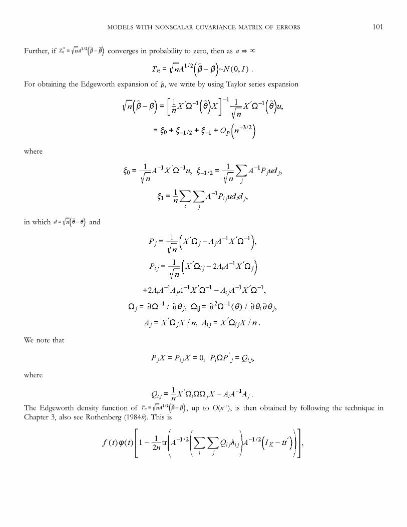
Further, if converges in probability to zero, then as n ⇛ ∞

For obtaining the Edgeworth expansion of , we write by using Taylor series expansion

where

in which and

We note that

where

The Edgeworth density function of , up to O(n−1), is then obtained by following the technique inChapter 3, also see Rothenberg (1984b). This is


where φ(t) is the standard normal density and λij is the i, jth element of ∧ which is the asymptotic covariance of aconsistent estimator such that . Further, the distribution, up to O(n−1), is a normal distribution:

where Φ(t) is the cumulative distribution of a standard normal variable and

is the covariance matrix of .

The bias vector, up to O(n−1), and mean square error (MSE) matrix of , to O(n−2), is

The approximate distributions of the scalar c′ follow from the above results. In this case, up to O(n−1),

where , up to O(n−2), where B is a p × p matrix of

Also, the bias to O(n−1) and variance to O(n−2) are

The above distribution can be extended up to O(n−3/2). This is given by


where

and an is the fourth cumulant of An given by

the element An appears in the following expansion:

where

and Rn is stochastically bounded with P[|Rn| > (log n)ℓ] = o(n−2) for some ℓ, see Rothenberg (1984b).

To use the above distribution of we need to have the O(n−2) term in σn2. But this is usually difficult to obtainexcept for the cases where we know the specific forms of . In practice, therefore, it is easier to use the simple normalapproximation up to O(n−1) in (5.29).

We summarize the results discussed above. First the error introduced by using the estimated covariance matrix has noeffect on the limiting distribution of regression estimators and test statistics, but only modifies second- and higher-order terms in the asymptotic expansions of their distribution functions. In fact, the effect is small even to secondorder in the sense that there is no effect on the approximate distribution of , which is still normal, except thatestimating covariance matrix increases the variance. These results hold under the fact that based on the LS regressionresiduals û are distributed independently of . However, when the errors are nonnormal, this independence does notnecessarily hold. Cavanagh and Rothenberg (1983) show that the results under normality go through for nonnormalcases under the weaker condition that are asymptotically uncorrelated with . This is usually not satisfied in themodels with heteroskedasticity, but hold in time series models. Thus, even under nonnormality, the shape of thedistribution of will be similar to that of , but they may not be normal.


5.2.3 Hypothesis TestingNow we consider the problem of testing that β satisfies the q linear restrictions

where R is a q × k matrix of constants of rank q and r is a q × 1 vector of constants. Under the assumption ofnormality of the errors, the log likelihood function is

Let be the unconstrained ML estimates under H1 and let be the constrained ML estimators under H0. Then,, where is as before and

where .

The Wald (W), Rao Score (RS), and the likelihood ratio (LR) test statistics are given as

where .

Under suitable regularity conditions, it is well known that each of these statistics is asymptotically χ2 with q degrees offreedom (d.f.) under the null hypothesis. Let zα be the initial point corresponding to the upper α-percentage point of adistribution. Then the asymptotic tests W, RS, and LR reject the null hypothesis if W > zα, RS > zα, and LR > zα,

provided n goes to infinity. But for small or moderately large samples, the probabilities of rejections (critical regions)may not be α-percentage for any of these tests. Therefore, as in Chapter 4, we need to look at the Edgeworth-typeexpansions for the probability distributions of each of these tests which can provide their accurate critical regions. Wecan then also compare the approximate local power functions of three size-corrected tests.


The Edgeworth expansion of the distributions of W, RS, and LR can be obtained by first obtaining the approximatecharacteristic function (moment generating function) and then using the inversion theorem (Chapter 3 and Rothenberg(1984c)). This gives, up to O(1/n),

where , is a noncentral χ2 with the noncentrality parameter δ′δ, δ = [R(X′Ω−1X)−1R′]−1/2(Rβ −r),a = tr(2D − C), b = 2trB1, c = trC, fr(z) is the noncentral χ2 with q + r d.f., and


Further, ∧ = ((λij)), Ωi and Ωij are given above, and as before as n ⇛ ∞, where

Under H0 we have δ = 0, which gives the Edgeworth-corrected critical values, up to O(n−1), for the three tests as

where , , and we use zf(z) = qf2(z) + δ′δf4(z). This gives, under H0, the critical region LR > zLR,W > zW, and RS > zRS of size α upto a second order of approximation.

Under the local alternatives, the approximate power function of the size-adjusted LR, W and RS statistics can bewritten as

where

When q = 1, w1 to w3 are zero and so these three tests have the same approximate power function. When q > 1, evenafter correcting for the size, the tests do not have the same power function. There exists a possibility of conflictingresults, partly due to the fact that three tests are not functions


of each other. For example, LR = (W + RS)/2 + Op(n−1) (see Rothenberg 1984c). Thus, while the conflicting resultsbased on the asymptotic test can be avoided by doing size adjusted tests for small samples in the regression with scalarcovariance matrix (Chapter 4), this is not the case in the nonscalar covariance matrix case. This is because in the scalarcovariance matrix case, the tests are monotonic functions of F statistic.

The Edgeworth expansions of the test statistics above are based on some regularity conditions (Rothenberg 1984c).These are

A1′: The matrices X′ ΩiX/n, X′ΩijX/n, and X′ΩiΩΩjX/n tend to a finite limit, and X′Ω−1X/n tends to a positivedefinite matrix as n ⇛ ∞.

A2′: The matrices

, , , converge to zero in probability. The same applies if is replacedby .

A3′: The matrix ∂2log L/∂θi∂θj, evaluated at the true parameter value and at the constrained and unconstrainedparameter estimators, converges to -∧−1.

A4′: The third partial derivatives of log L, evaluated at the true values and estimated values, converge to constants inprobability.

In addition, the derivatives up to the third order of Ω−1 with θ are assumed to hold. Further, the derivatives of theaverage log L should behave well as n ⇛ ∞.

5.3 Specialized Models

5.3.1 HeteroskedasticityWhen the regression disturbances have variances which are not constant across observations, the disturbances are saidto have the problem of conditional heteroskedasticity. It arises both in the time series and cross-sections data. In thiscase, for i = 1, …, n,

which gives the conditional covariance matrix as

If we do not have any a priori assumption about , then it is the heteroskedasticity of unknown form. On the otherhand, in many applications, is assumed to be a parametric function of xi or some other variable not in the regressionmodel (5.1) with regressors x. For example, in many


studies on household consumptions, the variance across household consumption expenditure is assumed to increase asincome increases. This is formulated as

where xi is the income variable. If this parametric form is not consistent with the data, then this misspecification mayaffect the statistical quality of econometric analysis. A solution to this problem is to use the nonparametric method todetermine the data-based specification, see Pagan and Ullah (1999, chapter 5). Another example of parametricallyspecified heteroskedasticity is the autoregressive conditional heteroskedastic (ARCH) model or generalized ARCH(GARCH) often observed in the time series data on exchange rate, inflation, and stock return; see Engle (1982) andBollerslev (1986). In this case,

where εi has a distribution with zero mean and unit variance. We assume that Cov(xi, uj) = 0, for all i and j = 1,…, n sothe model (5.1) is still a classical regression model with E(ui | ui−1) = Eui = 0. But,

Therefore, conditional on ui−1, ui is heteroskedastic. The unconditional variance, however, is

by assuming that the unconditional variance does not change over time. For examples of heteroskedasticity due tovarying regression parameters, see Raj and Ullah (1981).

Let us consider the estimation of β. The LS estimator is b = (X′X)−1X′y and the variance of b is V(b) =(X′X)−1X′ΩX(X′X)−1. The usual formula σ2(X′X)−1 is not the correct variance if Ω ≠ σ2I. We note that, for Ω* = Ω/σ2,

is a positive semidefinite matrix if I −Ω* is a positive definite matrix. This will depend upon the eigenvalues of I −Ω*.Thus, the standard error based


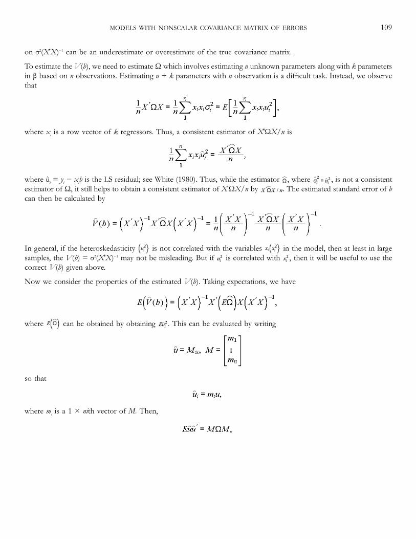
on σ2(X′X)−1 can be an underestimate or overestimate of the true covariance matrix.

To estimate theV(b), we need to estimateΩ which involves estimating n unknown parameters along with k parametersin β based on n observations. Estimating n + k parameters with n observation is a difficult task. Instead, we observethat

where xi is a row vector of k regressors. Thus, a consistent estimator of X′ΩX/n is

where ûi = yi − xib is the LS residual; see White (1980). Thus, while the estimator , where , is not a consistentestimator of Ω, it still helps to obtain a consistent estimator of X′ΩX/n by . The estimated standard error of bcan then be calculated by

In general, if the heteroskedasticity is not correlated with the variables in the model, then at least in largesamples, the V(b) = σ2(X′X)−1 may not be misleading. But if is correlated with , then it will be useful to use thecorrect V(b) given above.

Now we consider the properties of the estimated V(b). Taking expectations, we have

where can be obtained by obtaining . This can be evaluated by writing

so that

where mi is a 1 × nith vector of M. Then,


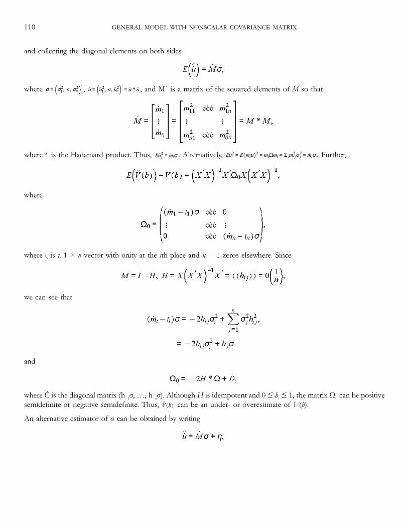
and collecting the diagonal elements on both sides

where , , and M˙ is a matrix of the squared elements of M so that

where * is the Hadamard product. Thus, . Alternatively, . Further,

where

where ιi is a 1 × n vector with unity at the ith place and n − 1 zeros elsewhere. Since

we can see that

and

where Ċ is the diagonal matrix (h˙1σ,…, h˙nσ). Although H is idempotent and 0 ≤ hij ≤ 1, the matrix Ω0 can be positivesemidefinite or negative semidefinite. Thus, can be an under- or overestimate of V(b).

An alternative estimator of σ can be obtained by writing


where . Thus, the LS estimator of σ is

which is Rao's (1970) minimum norm quadratic unbiased estimator (MINQUE) of σ, . This estimator is definedwhen M˙ is nonsingular (see Mallela 1972) for these conditions. Alternatively, if M˙ is singular we can writewhere M˙+ is a generalized inverse of M˙. Again is not a consistent estimator of σ but X′ΩX/n can be consistentlyestimated by .

Notice that M = I − H = I + O(1/n). Thus, for large n, M ≃ I and hence M˙ ≃ I. In this case, reduces to andreduces to .

An advantage of using is that it provides

which is unbiased, that is

Now we look into the efficient estimation of β. For known heteroskedasticity Ω, the GLS estimator is BLUE. ForunknownΩ, the operational GLS can be used for the parametrically specified heteroskedasticity given above; see otherspecifications in Johnston and DiNardo (1997). One can also determine by nonparametric kernel estimators,where the vector zi can also include xi. This is given by

where K is the weight (kernel) and h is the window width around the point zi. Essentially is an estimator ofby data points which are in the interval h around zi. The kernel K is chosen so that it gives low weight to the data on zwhich are far away from zi and high weight to the data which are close to zi. Using this nonparametric estimator of

, we can get the operational or feasible GLS estimator , which is known as the semiparametric GLS estimator,see Pagan and Ullah (1999, chapter 5). This estimator is useful in practice since obtaining the operational GLSestimator is not available when is unknown. This is because while is a consistent estimator of , theestimator is not a consistent estimator of X′Ω−1X/n.

Since is an even function of û or u, the semiparametric GLS estimator, conditional on x and z, is unbiased, seeSection 5.2.1. Also see Linton (1992, 1996) for Edgeworth expansions.


Now we turn to the time series regression model with the ARCH errors. In this case, the estimation of the parametersβ, α0, α1 are done by the ML estimation. The log likelihood function is

where ui = yi − xiβ. The score function is

where θ = (β′, α0, α1) ′. The iterative ML estimation is obtained by using

where H() is the Hessian matrix of log L, also see Engle (1982) for a simpler four-step procedure. The finite samplebias, up to O(n−1), and MSE, up to O(n−2), of this follows from the results in Chapter 2. This follows by noting that theestimator of θ is a solution from ES(θ) = 0; also see Bao and Ullah (2002), and Iglesias and Phillips (2001).

5.3.2 Heteroskedasticity TestingLet us now consider a test statistic for testing heteroskedasticity, , where the first element of 1 × qvector zi is unity and α = (α1, α2, …, αq)′. Thus, testing for heteroskedasticity implies testing for

The test statistic is half of the regression sum of squares in the regression of on zi, which is

and it follows as n ⇛ ∞; ι is an n × 1 vector of unit elements. Our aim is to see the effect on the null distribution ofQ under nonnormality of u in the regression y = Xβ + u.

Under H0, u ∼ (0, σ2), where σ2 = h(α1). Also,


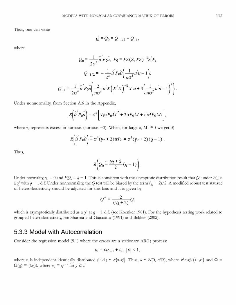
Thus, one can write

where

Under nonnormality, from Section A.6 in the Appendix,

where γ2 represents excess in kurtosis (kurtosis −3). When, for large n, M˙ ≃ I we get 3)

Thus,

Under normality, γ2 = 0 and EQ0 = q − 1. This is consistent with the asymptotic distribution result that Q, under H0, isa χ2 with q − 1 d.f. Under nonnormality, the Q test will be biased by the term (γ2 + 2)/2. A modified robust test statisticof heteroskedasticity should be adjusted for this bias and it is given by

which is asymptotically distributed as a χ2 at q − 1 d.f. (see Koenker 1981). For the hypothesis testing work related togrouped heteroskedasticity, see Sharma and Giaccotto (1991) and Bekker (2002).

5.3.3 Model with AutocorrelationConsider the regression model (5.1) where the errors are a stationary AR(1) process:

where εi is independent identically distributed (i.i.d.) ∼ . Thus, u ∼ N(0, σ2Ω), where and Ω =Ω(ρ) = ((wij)), where wij = ρj − i for j ≥ i.


The estimator of ρ is

where ûi are the LS residuals. There are other estimators of ρ such as by Theil (1971) as andDurbin–Watson (DW) as 1 − ½d, where . But these do not change the approximate results givenbelow.

The GLS estimator with given above is known as the Prais–Winsten (PW) two-stage estimator. Iterating thisestimator with respect to based on the new estimator of β gives the iterative Prais–Winsten estimator. The iterativeML estimator of β is given by

where, denoting ,

and summation is from 2 to n, see Beach and Mackinnon (1978).

Since is an even function of û, the above estimators of β are unbiased. Magee et al. (1983) show that the MSEestimator of , up to O(n−2), remains the same for different choices of . Further, Magee (1985) shows that the MSEsof , iterative Prais–Winsten and ML estimator, up to O(n−2), are shown to be the same. This is given by

where F = Ω − X(X′Ω−1X)−1X′. The readers can attempt to develop this result alternatively by using the result inSection 2.5.3. It is simple to verify that

because F is a positive semidefinite matrix. Thus, the variance of is more compared to due to estimation of .


An estimator which is used extensively in applied work is the Cochrane–Orcutt (CO, 1949) estimator which is basedon n − 1 observations. This is given by

where X* is the matrix of , y* is the vector of , is a matrix such that , and C = [0: In−1] is an n− 1 × n constant matrix. Then,

where D is a diagonal matrix with a first element of 1 and the other diagonal elements equal to zero; hence D is apositive semidefinite matrix. Thus,

which implies that the CO estimator is inefficient compared to PW or ML estimator for small samples.

The variance (MSE) approximation given above also follows (5.28), and it also gives the , which can be writtenfrom (5.31), up to O(n−2), as

where λ = 1 − ρ2 and b is as in (5.30) with Ωi and Ωj replaced by Ω(ρ). It can also be shown that the variance of isbounded by c′(X′Ω1X)−1c[1 + (4/n)((1 + |ρ|)/(1 − |ρ|))]. This shows that the approximate variance is not negligiblewhen |ρ| is close to 1. In fact the approximate given above is invalid for |ρ| = 1, and they are least accurate forlarge |ρ|. This is also consistent with the simulation studies of Beach and Mackinnon (1978) that the MSE of theiterative PW and ML are very similar but differ most when |ρ| = 1.

The numerical calculations of the determinant and trace ofV(b), , and in Magee, Ullah, and Srivastava (1987)and Magee (1985) suggest that the efficiency of these estimators is affected by the values of ρ and the nature of x. Theresults are consistent with the theoretical results discussed above. In addition, they show that the LS estimator is betterthan for small ρ in 0 < ρ ≤ 0.3. However, is better than the LS estimator for large ρ. Also LS is particularly bad forlarge ρ values when there is an intercept and/or trend in the model. Further, CO estimator also performs worse withintercept and trend model. We note that the O(1/n2) terms of the MSE of PW and ML estimators of are the sameand the simulation studies also indicate this similarity. To


see the differences in the MSE of iterative PW and ML and different choices of , one may need to analyze higher-order approximation than O(1/n2).

The Edgeworth expansion of the distribution of with is normal from (5.26) with the variance given by(5.27).

Ullah and Zinde-Walsh (1984, 1985, 1987), Vinod and Ullah (1981), and Dufour (1984) have explored the numericaland inferential robustness of the exact F, LR, RS, and W tests, for testing H0: Rβ = r against H1: Rβ ≠ r, by comparingthe numerical values and distributions, respectively, under the assumptions of spherical normality with mean zero andvariance σ2I and elliptical normal against the general class of elliptical error distributions (zero mean and covariancematrix Ω). They show that for autoregressive moving average models (ARMA) and/or heteroskedastic structuresnumerical robustness is rare in the sense that the usual test statistics for σ2I cases are not identical with those under Ω≠ I cases. For inferential robustness they explore bounds for critical values of these tests which will ensure that theconclusions based on the usual tests are not affected against a particular class of elliptical distributions.

Finally, we note that the exact distributions of and DW, which are the ratio of quadratic forms in y or u, have beenextensively studied in Koerts and Abrahamse (1969) and Farebrother (1984, 2002), King (1980), and others. Ali andSharma (1993) derived first four moments of the null distribution of DW, up to O(1/n3), when the errors arenonnormal and find that nonnormality has an insignificant effect on the mean and the fourth central moment of thedistribution. The test tends to be deflated (inflated) if the distribution is long tailed (short tailed). Further, the test isrelatively robust for moderate nonnormality and large n.

5.3.4 Seemingly Unrelated RegressionsWe consider here the multi-regression (seemingly unrelated regression equations, SURE) model developed by Zellner(1962). Such a model is needed when we wish to analyze a set of demand equations of different commodities or a setof investment functions for various industries. The temporal cross-section models (including panel data) which containa number of cross-sectional units observed over time and the random coefficient model of Swamy (1970, 1971) canalso belong to a multi-regression model.

Let us postulate the following SURE model of M equations:

where yi is n × 1, Xi is n × ki of full column rank, βi is ki × 1, and ui is n × 1. We can write this as


where

The error vectors ui and uj, i, j = 1, …, M are assumed to be correlated only at the same time point, and within eachequation the disturbance vector is assumed to be homoskedastic. Thus, E(ui) = 0 and E(uiuj′) = σijIn so that

where σij is the (i, j)th element of the M × M matrix Σ.

The operational or feasible GLS estimator , known as the SURE estimator, is obtained by using the consistentestimator of σij as

where ûi = yi − Xibi is the LS residual vector of the ith regression and , where Zi is a n × k matrix on all kdistinct regressors in the model. We note that SURE estimators based on and are referred to as SURR (RR isrestricted residual) and SUUR (UR is unrestricted) estimators.

Since is an even function of û, the SURR and SUUR estimators are again exactly unbiased. The exact covariancematrix of SURR is obtained in Hillier and Satchell (1986); see also Srivastava and Giles (1987, chapter 4). Ullah andRafiquzaman (1977), however, developed first four exact moments of for the case ofM = 2, X2 is a subset of X1 andu ∼ N(0, Ω). Based on the four moments the following results for skewness and kurtosis of , the kth element of ,are

where

where , n0 = n − k1 > 4 for the fourth moments to exist, aki is the (k, i)th element of (X1′X1)−1X1′(I −X2(X2′X2)−1X2′) and

where cki is the element of (X1′X1)−1X1′.


As expected, skewness = 0 and kurtosis = 3 as n ⇛ ∞, that is, the sampling distribution of SURE estimator issymmetric, but kurtosis >3 implies that the distribution is leptokurtic and falls under Pearsonian Type VII family ofdistribution. Further, when the correlation in the contemporaneous disturbances across equations is close to one (ρ2 ⇛1), the exact distribution of becomes normal.

Under the normality of u, Srivastava (1970), and Srivastava and Upadhyaya (1978) obtained a large-n approximation ofthe covariance matrix of SURR and SUUR and showed that they are identical upto O(n−2). Srivastava and Maekawa(1995) considered the bias and MSE of both SURR and SUUR under nonnormal errors of uit whose first fourmoments exist such that

The bias, up to O(n−1), of SURR is then given as

where Ω0 = (X′Ω−1X)−1 and δ′ = (δ1′, δ2′, …, δM′) with

Further, the MSE of , up to O(n−2), is

where N is an M × M matrix of

σgh denotes the (g, h)th element of Σ−1, and D = F + F′ with F as an M × M matrix given as


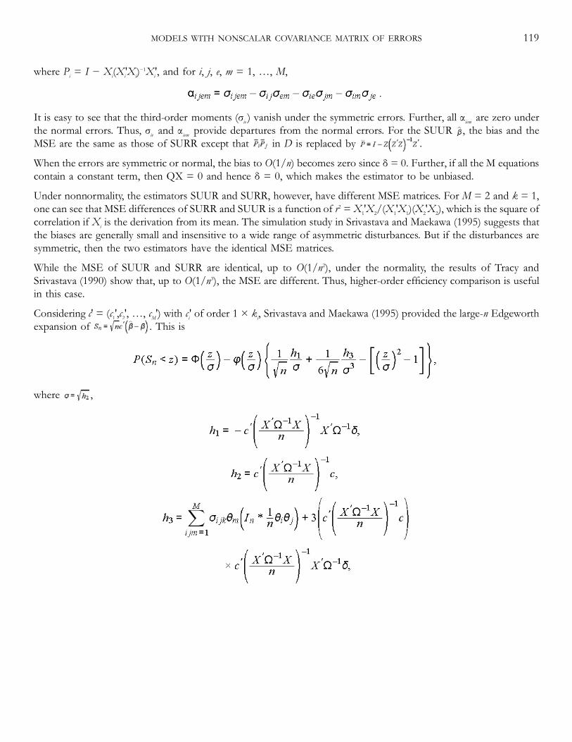
where Pi = I − Xi(Xi′Xi)−1Xi′, and for i, j, e, m = 1, …, M,

It is easy to see that the third-order moments (σije) vanish under the symmetric errors. Further, all αijem are zero underthe normal errors. Thus, σije and αijem provide departures from the normal errors. For the SUUR , the bias and theMSE are the same as those of SURR except that in D is replaced by .

When the errors are symmetric or normal, the bias to O(1/n) becomes zero since δ = 0. Further, if all the M equationscontain a constant term, then QX = 0 and hence δ = 0, which makes the estimator to be unbiased.

Under nonnormality, the estimators SUUR and SURR, however, have different MSE matrices. For M = 2 and k = 1,one can see that MSE differences of SURR and SUUR is a function of r2 = X1′X2/(X1′X1)(X2′X2), which is the square ofcorrelation if Xi is the derivation from its mean. The simulation study in Srivastava and Maekawa (1995) suggests thatthe biases are generally small and insensitive to a wide range of asymmetric disturbances. But if the disturbances aresymmetric, then the two estimators have the identical MSE matrices.

While the MSE of SUUR and SURR are identical, up to O(1/n2), under the normality, the results of Tracy andSrivastava (1990) show that, up to O(1/n3), the MSE are different. Thus, higher-order efficiency comparison is usefulin this case.

Considering c′ = (c1′,c2′,…, cM′) with ci′ of order 1 × ki, Srivastava and Maekawa (1995) provided the large-n Edgeworthexpansion of . This is

where ,


where , wrs are the elements of (X′Ω−1X/n)−1. The asymptotic distributional results for both the SUURand SURR estimators are the same, up to O(n−1/2), but the results up to O(n−1) can be different. Under normality, h1 = h3= 0, so the distributions of both the SUUR and SURR estimators become Φ(z/σ). Maekawa (1985) (also see Phillips1977c) also shows that this is the case up to O(n−1) since the approximate distribution did not contain any term up toO(n−1). Thus, while the distributions of both the estimators converge to the same normal distribution irrespective of thedistributional structures of the errors, the nonnormality of errors slows down the convergence rate to O(n−1/2) undernonnormality and of O(n−1) under normality. The simulation results in some special cases of two equations inSrivastava and Maekawa suggest that the approximate results are quite accurate for small samples and robust todepartures from normality of errors. In general, relying on the normality of errors may give misleading results whenthe distributions are in fact nonnormal.

5.3.5 Limited Dependent Variable ModelsHere we consider models which are commonly used in applied work, especially in the labor economics. A popularmodel is the latent variable decision model in which

where zi* is the unobserved latent variable which is the net utility, cost or profit, Wi is a kw × 1 vector of explanatoryvariables, and ui is the error term with the variance normalized to one. This model is useful for analyzing migration,labor force participation, decision of participating in a program or organization (union), among others. For theestimation of γ, we observe an indicator variable

For example, in the labor force participation model, zi = 1 implies the individual taking job if the net benefit zi* ispositive. Then,

where Φ() is the cumulative distribution function. Therefore,

where ei is the error term. The estimation of γ is then done by specifying the form ofΦ as a logit or probit specificationand using ML procedure. The log


likelihood function is

and

where n1 is the number of observations for which zi = 1. The score function is

where

and

The λi is known as the inverse Mill's ratio. Under the logit assumption, and under the probitassumption, φ and Φ become the density and cumulative distribution of a standardized normal variable, respectively.The ML estimator of γ is then obtained which is known to be consistent and asymptotically normal.

An extension of the above limited dependent variable is the sample selection model. In this case, the equation ofinterest is

where yi is observed only if zi* ≥ 0, that is, zi = 1. Due to this, E(vi | zi = 1) ≠ 0 and hence . So the LSregression of yi on xi will be asymptotically biased and inconsistent. To correct for this bias we need to know E(yi | zi =1). For this let us consider ui and vi to be a joint normal distribution with correlation coefficient ρ and vi with variance. Then, conditional on zi = 1, vi has a truncated normal distribution and E(vi | zi = 1) = ρσvλi and so

or

where η = ρσv and λi = λ(Wiγ). Further, E(εi | zi = 1) = 0 and , where is thefirst derivative of λi with respect to γ. This is a model which adjusts for the sample selection bias.


Heckman's (1979) two-step estimator of estimating k × 1 vector β = (α′, η, γ′)′, k = kx + kw + 1, first estimates γ by MLfrom the decision model. This provides observation on λi after which the LS estimation of α and η are obtained in theabove regression model. To obtain the finite sample properties of this two-step estimator, we first write it in terms ofthe method of moments estimator, which leads to solving the following moments:

where

Before analyzing finite sample results, let us consider the known results on the asymptotic results which are helpful ininterpreting the finite sample results. Heckman (1979) showed that

where

where di = (E(∇qi))−1qi and ∇qi(β) is the k × k matrix of the first derivative of qi(β) with respect to β.

The asymptotic standard errors, by looking at the diagonal elements of Σ, can be inspected to be large (E∇qiapproaches to singularity) when xi are closely collinear, especially when λi can be written as a linear combination of thexs. This can be a problem when the wis are a subset of xi or are highly correlated with them and λi is approximated by alinear function wiγ. By inspection, another situation in which the standard errors can be large is when the degree ofsimultaneity ρ is large. In many applied studies, it has been found that these two situations of large standard errors arefrequently found.

The second-order bias, up to O(n−1), can be written from (2.81) as

where is the k × k2 matrix of second-order derivative and Vi = ∇ qi − E(∇qi). We note that if eth row of ∇qi(β)contains the gradient vector of the eth element of qi(β), the eth row of ∇2qi contains the vectorized Hessian matrix of theeth element of qi(β).


It is clear that the bias depends on the curvature of the model implied by ∇qi and ∇2qi. Further, EVidi is the correlationof Vi and qi, usually small, and E(di ⊗ di) is the vectorization of the term Edidi′ in the asymptotic variance. Thus, thefactors influencing these are similar to those affecting (E(∇qi))−1 and hence asymptotic variance described above, whichare near nonidentification (collinearity) and simultaneity. Finally, an estimate of bias can be obtained by calculatingsample averages at , for example, replacing E(∇qi) by .

The simulations results in Rilstone and Ullah (2002) indicate that in the case of small sizes 50, 100 and for the case ofsingle variables in each of x and w, increases as ρ increases or ρxw(correlation between x and w) increases. Furtherthe MSE of also increases with ρ and ρxw. These results are consistent with the analytical results on the bias above.The analytical MSE results can also be written and analyzed from the results in Chapter 2.

5.3.6 Panel Data ModelsHere we consider the estimation of linear models with the data on n cross-sectional units over T time points. Such amodel is known as a panel data model, and such models are used to study the behavior of the cross-sections of groups,regions, countries, and households over time. There is an extensive literature on the theory and applications of thesemodels; see Hsiao (1986) and Baltagi (2001). The possibility of observing variations across both cross-section and timepoints creates several interesting opportunities in applied econometrics; see Baltagi (2001) and Deaton (1997) for theadvantages of panel data models.

A basic difference between the panel data models and the traditional models is the presence of changing (varying)intercepts across cross-sections and across time. These are called as heterogeneity parameters which take care ofunobservable variables which change with cross-sectional units but are fixed over time (cross-sectional heterogeneity)and unobservable variables which are fixed over cross-sections but change over time (time series heterogeneity). Forexample, in a production function management, efficiency variable will qualify for the cross-sectional heterogeneity andtechnology variable will represent the time heterogeneity. There are two kinds of panel data models. First is the fixedeffect panel data model where the heterogeneity parameters are treated as fixed parameters. In this case, the model isestimated by the LS procedure which provides the best linear unbiased estimator under the Gauss–Markovassumptions. Second is the random effect (error components) model in which the heterogeneity parameters are treatedas random error along with the equational random error. Such a model is estimated by the GLS method, the smallsample properties of which will be discussed below.

Let us consider a random effect panel data model as


where yit is the dependent variable, xit is a 1 × k vector of regressors, uit is the error term, and the heterogeneityparameter αi is the cross-sectional random effect, and uit and αi are independently distributed random variables.

In the matrix notation, we can express the model as

where y is nT × 1 vector, X is nT × k matrix, w is nT × 1 vector, α is n × 1 vector of random effects, and D = In ⊗ ι; ι =(1, …, 1) ′. It is assumed that for all i and t,

Note that γ1 and γ2 represent the skewness and kurtosis measures, respectively. If γ1 = γ2 = 0, the αi and uit have anormal distribution.

The LS estimator of β is

which is unbiased. The variance–covariance matrix of b is given by

where , , , , , . Obviously,Q and are independent idempotent matrices, thus Q2 = Q, , . The GLS estimator is given by

which is unbiased and its variance–covariance matrix is

where .

The FGLS of β is given by

where , in which ,


, and MZ = InT − Z(Z′Z)−1Z′ and Z = [X D].

In addition to the above estimators, one can also obtain the following two independent unbiased estimators of β. Oneis the within fixed effect estimator or simply the within estimator of β. For this we write:

so that the LS estimator of β is

where w represents within estimator and MD = I − D(D′D)−1D′ transforms the data into deviation from cross-sectional(time averaged) means. Its .

Second, an unbiased estimator is the between estimator represented by . This is given by doing LS in the followingregression :

which gives

where transforms the data grouped by cross-sectional units into time averages for each unit. Its.

Assuming the unobservable to be uncorrelated with the exogenous variables, both and are unbiased for β andare independent. Further, it can be verified that the GLS estimator is a matrix weighted average of the within andbetween estimators

where


Of course the FGLS estimator is also , where is ▵ with and replaced by and given above.

The GLS estimator is the BLUE estimator. Also, from Lehmann (1983, theorem 1.1, p. 77), is also the uniformlyminimum variance unbiased (UMVU) estimator of β. That is, in the class of unbiased estimators, , theUMVU estimator is for ▵0 = ▵. But this result does not hold for the FGLS estimator .

The FGLS estimator is an unbiased estimator of β since is an even function of the random errors α and u. Theexact variance, under normality is developed in Taylor (1980) in terms of hypergeometric infinite series. The numericalcalculations there suggest that, for any sample size, the variance of the limiting distribution of , (X′Ω−1X)−1,understates the true variance by no more than 17 percent, but for small n − k, this understatement remains around12–14 percent for samples of 25 or 50. Thus, the total sample size does not help in the accuracy of the asymptoticmoment approximation and that convergence is probably slower. Second, using more efficient estimators of anddo not improve the efficiency of much. Next, for the larger cross-sectional units, the estimator is more efficientcompared to within estimator, but for smaller samples (n − k ≤ 10), there is an ambiguity in the selection of estimator.Also, if the relative efficiencies of the between and within estimators are close to one, there are larger sets of samplesizes for which is more efficient compared to within estimator.

We now look at the nature of approximate bias, up to O(n−1), for a general class of nonnormal errors, assuming T to befixed. This is given by

where

The following remarks follow from this result.

We observe that the approximate bias in the estimator is affected by the skewness coefficients γ1 but it does notdepend on the measure of kurtosis. Further, for the symmetric distributions of errors (γ1α = γ1u = 0), the estimatorbecomes unbiased. The bias is also zero if λ is 0 or 1. This case implies or , that is, the random effect errorsbecome the usual errors. Moreover, the bias is zero if X′ι = 0, which is the case if the matrix X contains variablesdeviated from their means.

Next, the direction of bias depends upon the signs of σuγ1u − Tσαγ1α and the average values of the regressors X, since 0< λ < 1 and , which is positive semidefinite. Assuming that the average


value of each regressor is positive,

Thus, if γ1α < 0 and γ1u > 0, then will be positively biased.

The approximate bias expression in (5.124) can be verified using the stochastic expansion in (5.20) and then evaluatingit under the nonnormal errors. The result for approximate MSE can be similarly obtained. For the bias analysis in thenonlinear panel models, see Hahn and Newey (2002).


This page intentionally left blank

6 Dynamic Time Series Model

6.1 IntroductionIn this chapter we consider the finite sample analysis of the time series models used in economics and finance. Weconsider the autoregressive model (AR), AR with regressors, and autoregressive moving average models withregressors (ARMAX). The exact and approximate (Laplace, Large-n, and Small-σ) moments as well as the distributionsof the estimators of the lag coefficients and the regression coefficients have been derived and analyzed. Based on theseresults the bias and mean squared error (MSE) of the one period and s-periods ahead forecast errors have beenanalyzed. Since unit root and cointegration play an important role in the modern time series, these cases are alsocovered in this chapter.

6.2 Model and Least-Squares EstimatorLet us write the general first-order dynamic model as

where yi−1 is a lagged value of the dependent variable with fixed or random startup condition, xi is the ith observationon the 1 × p vector of exogenous variables, α and β are parameters, and ui is the disturbance term. Using recursivesubstitutions we can write (6.1) as

where

In the matrix notation

where y = (y1, …, yn)′, y−1 = (y0, …, yn−1)′, X is a n × p matrix, and u is an n × 1 vector. We note that

where ι1 = (1 0 0 - - - 0)′ is an n × 1 vector and L is an n × n matrix as

Substituting (6.5) in (6.4) we get

or

which gives

where

and

Further


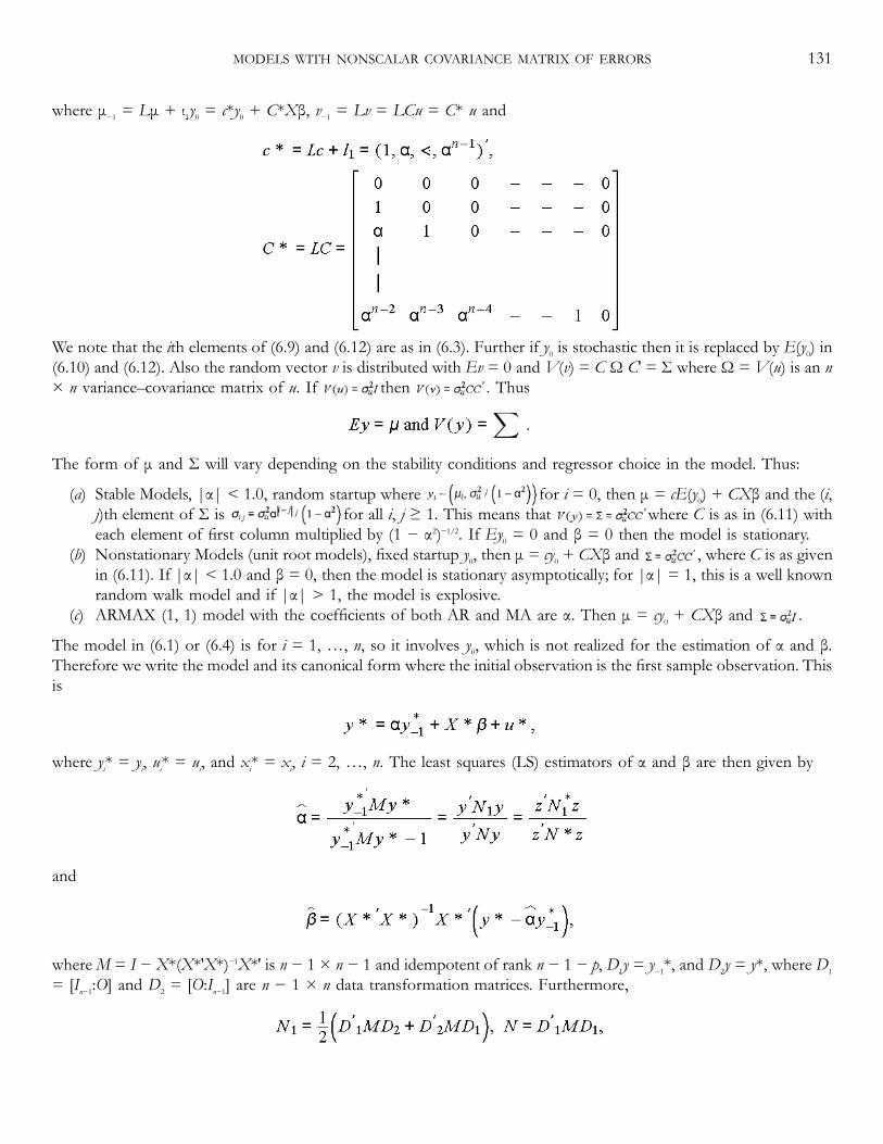
where μ−1 = Lμ + ι1y0 = c*y0 + C*Xβ, v−1 = Lv = LCu = C* u and

We note that the ith elements of (6.9) and (6.12) are as in (6.3). Further if y0 is stochastic then it is replaced by E(y0) in(6.10) and (6.12). Also the random vector v is distributed with Ev = 0 and V(v) = C Ω C′ = Σ where Ω = V(u) is an n× n variance–covariance matrix of u. If then . Thus

The form of μ and Σ will vary depending on the stability conditions and regressor choice in the model. Thus:

(a) Stable Models, |α| < 1.0, random startup where for i = 0, then μ = cE(y0) + CXβ and the (i,j)th element of Σ is for all i, j ≥ 1. This means that where C is as in (6.11) witheach element of first column multiplied by (1 − α2)−1/2. If Ey0 = 0 and β = 0 then the model is stationary.

(b) Nonstationary Models (unit root models), fixed startup y0, then μ = cy0 + CXβ and , where C is as givenin (6.11). If |α| < 1.0 and β = 0, then the model is stationary asymptotically; for |α| = 1, this is a well knownrandom walk model and if |α| > 1, the model is explosive.

(c) ARMAX (1, 1) model with the coefficients of both AR and MA are α. Then μ = cy0 + CXβ and .

The model in (6.1) or (6.4) is for i = 1, …, n, so it involves y0, which is not realized for the estimation of α and β.Therefore we write the model and its canonical form where the initial observation is the first sample observation. Thisis

where yi* = yi, ui* = ui, and xi* = xi, i = 2, …, n. The least squares (LS) estimators of α and β are then given by

and

whereM = I − X*(X*′X*)−1X*′ is n − 1 × n − 1 and idempotent of rank n − 1 − p, D1y = y−1*, and D2y = y*, where D1

= [In−1:O] and D2 = [O:In−1] are n − 1 × n data transformation matrices. Furthermore,


where N is an idempotent matrix of rank n − 1 − p. The canonical reduced form variables are defined as z = Σ−1/2y,where Σ−1/2 = P ∧−1/2P′, ∧ = diagonal (λi), i = 1,…, n, where λi are eigenvalues of Σ and P is the orthogonal matrix of theeigenvectors of Σ. Thus, N1* = Σ1/2N1Σ1/2, N* = Σ1/2NΣ1/2, and

where μz = Σ−1/2μ and η = Σ−1/2v such that V(η) = V(z) = I and z ∼ (μz, I).

In a special case where β = 0 so that

and M = In−1, the estimator becomes

where

and

We now give the forecasts based on (6.1) or (6.4). For example one period ahead forecast is

and its forecast error is

where ιn = [0 … 0, 1]. If β = 0, then . Similarly .


When we develop forecasts s-time periods ahead we use

and

Further the forecast error is

When β = 0,

Further if we define y¯n+s = E(yn+s|yn) = αsyn, then .

6.3 Finite Sample Results for Dynamic Model

6.3.1 ReviewWe consider the AR(1) model in (6.20) and consider the properties of the LS estimator in (6.21). Since this modelhas been extensively studied in the literature we first provide a brief summary of the results for this model and thenpresent analytical expressions.

Hurwicz (1950) was the first to investigate the small sample bias in this model. He finds that for small samples the biasof LS is as much as 25 percent of the value of α. For the case of normally distributed u's he provided a closed formequation for the bias of the LS estimator when n = 3 or 4 for the stationary case and for n = 3 for the fixed startupcase where y0 = 0. For other “n” he suggests a Maclaurin series expansion but only demonstrates how the first term ofsuch an expansion would be calculated.

Copas (1966) used Monte Carlo methods to compare the MSE of the LS, and the maximum-likelihood (ML) when theu's are distributed N(0, 1) for the stationary case and for the fixed startup case when y0 = 1. Copas found that the MLand LS estimators are on average the best in terms of the MSE and that for the stationary case the ML has a slightlylower MSE in the region |α| < 0.6 and LS has a slightly lower MSE in the region 0.6 < |α| < 0.9. The regionconsidered was |α| < 0.9. Copas did not tell us which region each estimator does best for the fixed startup case, butfor both the stationary and the fixed startup cases he showed that the ML does slightly better on average over theregion considered. For another Monte Carlo study related to AR(1) model, see Thornber (1967).

Sawa (1978) developed the exact moments by using the moment generating function and calculated the exact smallsample bias and variance of for |α| < 1


in the stationary case with normal error terms. Sawa (1978) also added to Hurwicz (1950) results by recording the biasof for α = 0.2, 0.4, 0.6, and 0.8, and 6 < n < 30 in the stationary case with normal error terms.

Hoque (1985) extended Sawa (1978) by deriving the exact first and second moments of for the case where the u'sfollow an MA(1) process. Hoque and Peters (1986), and Mercurio (2000) developed the exact moments of the LSestimators of the parameters in the AR models with exogenous variables. For these models, Kiviet and Phillips (1993),Srivastava and Ullah (1995), and Bao and Ullah (2002) analyzed the large-n and small-σ approximate moments. Theextension to the case of AR (p) models is also considered in Bao and Ullah (2002). Peters (1989) provided the exactmoments for the nonnormal error case.

Now we turn to the distribution of , which has been studied extensively. Asymptotically, it has a normal distribution(Mann and Wald 1943) if |α| < 1. White (1958) found that for |α| > 1, has a Cauchy distribution inthe limit when the u's are normally distributed which Anderson (1959) note implied that

has mean zero normal distribution in the limit for |α| ≠ 1. White (1958, 1959) also showed that the distribution offor |α| = 1 was not normal. Anderson (1959) showed that for |α| > 1, has a mean zero normal distributionin the limit when the u's are i.i.d. Anderson (1959) also builds on the results of White (1958) by showing that thelimiting distribution of for |α| > 1 depends on the distribution of the u's. White (1961) builds on Hurwicz(1950) by calculating the first three terms on the MacLaurin expansion approximation for the first two moments of .

The exact distribution of can be written by using the Imhof (1961) result on the distribution of the quadratic forms,see Chapter 3. It was numerically computed by Phillips (1977a, 1978), Evans and Savin (1981), and Tsui and Ali (1994)for various values of α and n. An extensive numerical study of unit root distributions was done by Evans and Savin(1981, 1984), which warned that the conventional tests are not good detectors of unit root behavior since they havelow powers in typical sample sizes. In addition several authors (Dickey 1976; Fuller 1976) have done Monte CarloStudies to tabulate the distribution of for the case of α = 1 and y0 = 0, also see bootstrap unit root test by Park(2003). These distributions can be used to test for unit root hypothesis. Nankervis and Savin (1985, 1988) examinedhow well hypothesis testing on α does with the t-statistic when yi is stationary and for a fixed nonzero y0, also seeDickey and Fuller (1981). They use Monte Carlo methods to estimate the exact distribution of the t-statistic and findthat the student-t is not a good approximation for small sample sizes.

Phillips (1987a,b,c) extended White's distributional results using ratios of functions of Wiener processes, also seeAbadir (1994) for the exact distribution. Phillips (1987c), and Stock (1987) also showed that the LS estimatorconverges to α faster in the unit root case compared to the stable root (|α| < 1) case. Banerjee, Donaldo, Hendry, andSmith (1986) explored this result through a Monte Carlo study and found out that the LS bias did not


decline at the expected rate when the sample size was increased. In an important paper Abadir (1993a) reconciled thefindings of Phillips and Stock with Banerjee, Dolando, Hendry, and Smith by providing a higher order analyticalapproximate bias of for the case of α = 1. This result proves analytically that the bias declines at a rate, which isslower than the consistency rate, thus explaining Banerjee and coworkers simulation findings. He also shows cases of nand nonzero values of y0/σ, where the bias increases with the sample size.

In addition to the work on the exact distribution, several authors have attempted to obtain approximations to thedistribution of . Phillips (1977a, 1978), Satchell (1984), Tsui and Ali (1992), Wang (1992), and Lieberman (1994)developed the Edgeworth expansion, Cornish–Fisher type expansion, and saddle point approximations of thedistribution for the case of stationary AR(1) model. They indicate that the Edgeworth expansion is unsatisfactoryexcept for smaller values of α. In most of these studies the accuracy has been tested for only a few values of n and α.Furthermore the approximations have been found to be computationally demanding, especially for large n for themodel where y0 is fixed at zero. Phillips (1987a), Lieberman (1994b), and Nabeya and Taneka (1990) have looked at thelimiting distribution of under a near-integrated random process, also see Park (2003). Further Perron (1991)has analyzed the approximate distribution of for the case where y0 is fixed at a nonzero constant. Again these studiesconsider the accuracy at a few selected points of n and α. Ali (2002) considered both the cases of stationary and fixedmodels and provided a uniform asymptotic expansion for the distribution, which is applicable for all the values of α.This uniform expansion, however, provides a mixed result on its accuracy.

Now we turn to the works on the properties of forecasts. Box and Jenkins (1970) obtained the asymptotic MSE of thes>0 period ahead forecast for the stationary AR(1) model when LS is applied as:

so that for a one period ahead forecast:

where the one period ahead forecast for n observations is . Bloomfield (1972) extended this result to a oneperiod ahead stationary AR(p) model and Yamamoto (1976) extended it further to an “s” period ahead stationaryAR(p) model.

Malinvaud (1970) showed that if y0 is a mean zero symmetric random variable then the forecast bias of LS is zero.Phillips (1979) pointed out that this is an unconditional forecast error and that what is far more interesting is the forecastbias conditioned on known values of the dependent variable, such as yn. That is to say that since we have observed ynwe should use this information


when deciding what the forecast error is. Phillips (1979) develops an approximation to the distribution of the forecastbias conditional on yn and finds that forecasts are biased toward the origin for almost all values of yn. If and yn areassumed independent and yi is stationary then he finds that:

If, as is usually the case, and yn are dependent then

Hoque, Magnus, and Pesaran (1988) give an exact expression for the MSE of the forecast for both the fixed startupand the stationary cases. They find that the MSE decreases as the number of periods into the future of the forecast isincreased and that the behavior of the fixed startup and stationary cases are very similar except for |α| near one.

Now we look into the results for the AR(1) with an intercept. Orcutt and Winokur (1969) used Monte Carlotechniques to study the LS estimation of the model yi = γ + αyi−1 + ui in the stationary case, where the u's are normaland i.i.d. He finds that LS produced no bias in estimating γ and that a Student-t distribution may be used as anapproximate sampling distribution for γ. However, there is a significant bias in the estimation of α. He examined thebias correction technique of Marriott and Pope (1954) and found it has lower MSE than LS for higher values of α.However, in terms of the estimated Monte Carlo MSE of the forecast the Marriott and Pope (1954) technique did notimprove on LS. Sawa (1978) applied a numerical method to the stationary case of the model yi = γ + αyi−1 + ui and findsthat in this model is severely biased for n < 100 confirming Orcutt and Winokur's (1969) Monte Carlo results. Sawa(1978) also used numerical integration method to calculate the exact small sample bias and variance of for the modelyi = γ + αyi−1 + ui, where |α| < 1 in the stationary case with normal error terms. Hoque (1985) extended this to thecase where the u's follow an MA(1) process. Dickey and Fuller (1979) were also able to find the limiting distribution forwhen y0 = 0 and |α| = 1.

As stated above, Orcutt and Winokur (1969) showed that in terms of the estimated Monte Carlo MSE of predictionthe Marriott and Pope (1954) technique does not improve on LS. Fuller and Hasza (1980) building on the work ofMalinvaud (1970) showed that if yi is a mean zero symmetric random variable then the forecast bias of LS is zero forthe model yi = γ + αyi−1 + ui for the cases: (a) |α| < 1 and stationary, that is, mean of the process equals γ/(1 − α), (b) γ= 0 = mean of process, and (c) γ = 0 and α = 1. Dufour (1984) showed the same results of unbiasedness undersomewhat weaker conditions. As stated above, it is important to remember that these are unconditional results and thatthe bias or MSE conditioned on the known y's are more


interesting statistics from the point of view of the applied researcher. Also these results assume E(y0) = 0, which maynot always be a good assumption. Fuller and Hasza (1981b) find that conditional on yn the MSE is:

Hoque (1985) looks at the unconditional forecast bias of the model (6.1) and finds it to be nonzero as opposed to the(6.20) model, which has a zero unconditional forecast bias.

6.3.2 Exact Results for AR(1) modelThe finite sample behavior of the LS estimator in (6.21) and the forecasts are analyzed for the model (6.20), yi = αyi−1+ ui, i = 2,…, n with y1 = αy0 + u1 = μ1 + u1. Both the stable models with random startup and the nonstationary modelwith fixed startup will be considered. In the fixed startup we consider the cases where μ1 = αy0 = 0 and μ1 ≠ 0. Theexact results on the moments are compared with the Monte Carlo results as well as the approximate moments by theLaplace, the large-n and small-σ methods.

From (6.21)

where N1 and N are as given in (6.22) and (6.23). Further, assuming we get y ∼ N(μ, Σ) where μ = cy0 andwhere c and C are given in (6.11). Therefore the exact mean, and are as in (2.28). Thus the exact

.

Now we look into the exact moments of the one period ahead forecast

where ιn = [0,…, 0, 1]′ is an n × 1 vector. We note that and ι′n = g(y). Thus from Lemma 1 in Chapter 2 we notethat


where is the derivative of (2.29) with respect to μ. Further

where and ∂2/∂μ∂μ′ is the second derivative of in (2.29).

Suppose Ey0 = 0 for the random startup or y0 = 0 for the fixed startup so that μ1 = 0 and hence μ = 0. Furtheris zero for μ = 0. Thus Eŷn+1 = 0 = E(yn+1), and

Similarly for sth period ahead forecast, for μ = 0 because forμ = 0 follows by writing from (2.28) or (2.32). Thus for μ1 = 0, the forecast bias E(ŷn+s − yn+s) is zero. This compareswith the results of Malinvaud (1970), Fuller and Hasza (1980), and Dufour (1984). Hoque, Magnus, and Pesaran(1988) also provided the result that E(ŷn + s − yn+s) exists when 1 ≤ s ≤ n − 2. When μ1 ≠ 0 we note that the bias will notbe zero and it is given by (6.33).

Regarding the MSE of the forecast error we note that

and for one period forecast error

It is easy to verify that, at μ = 0,


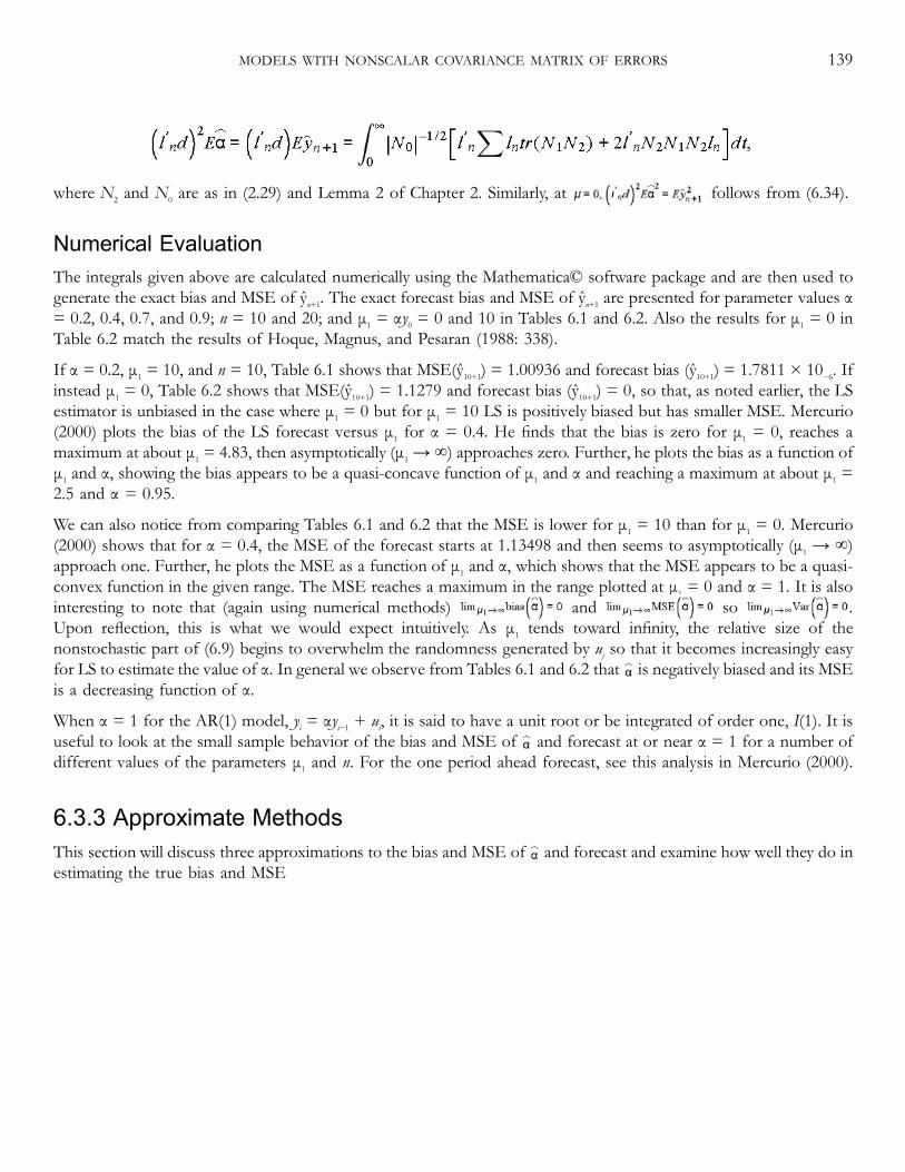
where N2 and N0 are as in (2.29) and Lemma 2 of Chapter 2. Similarly, at follows from (6.34).

Numerical EvaluationThe integrals given above are calculated numerically using the Mathematica© software package and are then used togenerate the exact bias and MSE of ŷn+1. The exact forecast bias and MSE of ŷn+1 are presented for parameter values α= 0.2, 0.4, 0.7, and 0.9; n = 10 and 20; and μ1 = αy0 = 0 and 10 in Tables 6.1 and 6.2. Also the results for μ1 = 0 inTable 6.2 match the results of Hoque, Magnus, and Pesaran (1988: 338).

If α = 0.2, μ1 = 10, and n = 10, Table 6.1 shows that MSE(ŷ10+1) = 1.00936 and forecast bias (ŷ10+1) = 1.7811 × 10−6. Ifinstead μ1 = 0, Table 6.2 shows that MSE(ŷ10+1) = 1.1279 and forecast bias (ŷ10+1) = 0, so that, as noted earlier, the LSestimator is unbiased in the case where μ1 = 0 but for μ1 = 10 LS is positively biased but has smaller MSE. Mercurio(2000) plots the bias of the LS forecast versus μ1 for α = 0.4. He finds that the bias is zero for μ1 = 0, reaches amaximum at about μ1 = 4.83, then asymptotically (μ1 → ∞) approaches zero. Further, he plots the bias as a function ofμ1 and α, showing the bias appears to be a quasi-concave function of μ1 and α and reaching a maximum at about μ1 =2.5 and α = 0.95.

We can also notice from comparing Tables 6.1 and 6.2 that the MSE is lower for μ1 = 10 than for μ1 = 0. Mercurio(2000) shows that for α = 0.4, the MSE of the forecast starts at 1.13498 and then seems to asymptotically (μ1 → ∞)approach one. Further, he plots the MSE as a function of μ1 and α, which shows that the MSE appears to be a quasi-convex function in the given range. The MSE reaches a maximum in the range plotted at μ1 = 0 and α = 1. It is alsointeresting to note that (again using numerical methods) and so .Upon reflection, this is what we would expect intuitively. As μ1 tends toward infinity, the relative size of thenonstochastic part of (6.9) begins to overwhelm the randomness generated by uj so that it becomes increasingly easyfor LS to estimate the value of α. In general we observe from Tables 6.1 and 6.2 that is negatively biased and its MSEis a decreasing function of α.

When α = 1 for the AR(1) model, yi = αyi−1 + ui, it is said to have a unit root or be integrated of order one, I(1). It isuseful to look at the small sample behavior of the bias and MSE of and forecast at or near α = 1 for a number ofdifferent values of the parameters μ1 and n. For the one period ahead forecast, see this analysis in Mercurio (2000).

6.3.3 Approximate MethodsThis section will discuss three approximations to the bias and MSE of and forecast and examine how well they do inestimating the true bias and MSE


Table 6.1 Model: yj = αyj−1 + uj, , μ1=10,

n α E(ŷn+1) E(yn+1) Bias(ŷn+1)

MSE(ŷn+1)

10 0.2 0.1963-71

0.04738 −0.003-62

0.0088-3993

0.0510-67

0.2084-46

2.8051× 10−6

1.024 ×10−6

1.7811× 10−6

1.00936

10 0.4 0.3927-42

0.16206 −0.007-2576

0.0078-6964

0.2001-07

0.4764-88

0.0014-3832

0.0010-4858

3.8974× 10−4

1.00939

10 0.7 0.6874-11

0.47759 −0.012-5891

0.0052-2083

1.0733 1.50135 0.3008-12

0.2824-75

0.0183-37

1.01121

10 0.9 0.8868-58

0.78917 −0.013-1416

0.0028-3256

16.6956 18.0876 3.52422 3.48678 0.0374-565

1.0404

10 0.99 0.9800-09

0.96219 −0.009-9905

0.0016-7824

92.8213 92.6691 9.06282 9.04382 0.0190-018

1.09561

20 0.2 0.1966-77

0.04675 −0.003-3230

0.0080-8355

0.0502-464

0.2084-28

4.1522× 10−13

1.049 ×10−13

3.104 ×10−13

1.00854

20 0.4 0.3933-54

0.16186 −0.006-6456

0.0071-8581

0.1992-46

0.4764-35

1.8055× 10−7

1.100 ×10−7

7.0595× 10−8

1.00857

20 0.7 0.6883-76

0.47844 −0.011-6243

0.0047-1764

0.9711-76

1.37377 0.0089-512

0.0079-7923

0.0009-7198

1.00874

20 0.9 0.8855-28

0.7863-11

−0.014-472

0.0023-6074

5.84414 6.39379 1.24371 1.21577 0.0279-445

1.01356


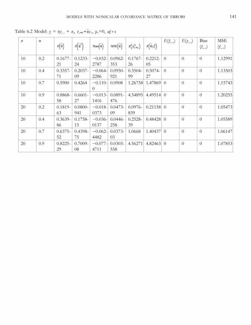
Table 6.2 Model: yj = αyj−1 + uj, , μ1=0,

n α E(ŷn+1) E(yn+1) Bias(ŷn+1)

MSE(ŷn+1)

10 0.2 0.1677-21

0.1233-24

−0.032-2787

0.0962-353

0.1767-26

0.2212-05

0 0 0 1.12991

10 0.4 0.3357-71

0.2037-09

−0.064-2286

0.0950-921

0.3504-99

0.5074-27

0 0 0 1.13503

10 0.7 0.5900 0.4264 −0.110-0

0.0908 1.26758 1.47869 0 0 0 1.15743

10 0.9 0.8868-58

0.6601-27

−0.013-1416

0.0891-476

4.54895 4.49514 0 0 0 1.20255

20 0.2 0.1819-63

0.0800-941

−0.018-0373

0.0473-09

0.0976-839

0.21158 0 0 0 1.05473

20 0.4 0.3639-86

0.1758-15

−0.036-0137

0.0446-258

0.2528-39

0.48428 0 0 0 1.05589

20 0.7 0.6375-52

0.4398-75

−0.062-4482

0.0373-03

1.0668 1.40437 0 0 0 1.06147

20 0.9 0.8225-29

0.7009-08

−0.077-4711

0.0303-558

4.56271 4.82463 0 0 0 1.07853


when LS is used. Since we know from above that the exact bias and MSE are

and

where d = μ + Σ∂/∂μ. Thus we first find approximations to and and from these calculate the approximationsof the bias and MSE of the forecast error.

The Laplace ApproximationDenote the Laplace approximation to . Through the use of the Laplace method discussed in Chapter 2 weobtain

Similarly

where

from (2.17). Thus,

where

Further,


where

Similarly and (ι′nd)2α2 are the same with replaced by and α2. The derivatives of and

with respect to μ are straightforward to obtain.

Small-σ ExpansionThe results for the bias and MSE of , based on small-σ expansion, follow from the results in Chapter 2. First wemake the assumption that

Note that if β = 0 and y0 = 0 then y = v = Cu or σuCu if V(u) = I and becomes invariant to σu and so the small-σexpansion does not exist. Same is true if y0 in the random startup has Ey0 = 0.

The bias of , to O(σ2), is

Similarly, the MSE is as in 6.3.5 withM = I. The result on the bias is also in Kiviet and Phillips (1993), and Srivastavaand Ullah (1995), and the MSE is in Srivastava and Ullah (1995).

Using the bias and MSE of we get

where ι′nd = (ι′nμ + ι′nΣ∂/∂μ). The derivatives are straightforward and they are left as an exercise.


Large-n approximationThe large-n approximations can be obtained from the results (2.101) and (2.102) in Chapter 2 and the results of Kivietand Phillips (1993). First we note that

where μ−1 and C* are given above. Then, using α < 1,

When , also see White (1961: 89–90). As before the bias of the one period ahead forecast is

Similarly the MSE of can be obtained from (2.102), which will give the MSE of ŷn+1.

We can make some comparisons between the small-σ bias with the large-n . The O(n−1) approximationis a nonlinear function of whereas the small-σ bias is a linear function of . Second the does not exist if β = 0and y0 or Ey0 = 0 but this is not the case for . In fact O(n−1) bias approximations are essentially the same whetheror not we condition on y0, since .

It is easy to note that and . Thus the large-n bias contains all the terms ofsmall-σ expansion, whereas small-σ expansion does not contain all the terms of large-n. Thus, for the AR(1) model,large-n approximation may be more accurate than the small-σ approximation, except when σ is small.

The approximate one period ahead LS forecast bias using the Laplace, large-n, and small-σ methods, is compared withthe exact one period ahead LS forecast bias for various parameter values in Mercurio (2000). From these results, itappears no one approximation method dominates over all parameter values. When sigma is very small, the small-σmethod dominates for all values of α and μ1. For larger sigma and intermediate values of α, the Laplace method seemsto give the best approximation. For larger values of sigma and larger values of alpha, the large-n approximation doesthe best.

The above approximations do not work for α = 1. Abadir (1993a) provides a useful result on the approximate bias offor |α| = 1 when y0 = 0 and β = 0. Let us write


where ; . Then from (2.30) in Chapter 2

Abadir (1993a) then uses an innovative expansion of the moment generating function M(U, −V) to obtain the biasresult as an asymptotic expansion in 1/n. The first term in this asymptotic expansion for can be shown to be

, derived earlier by Shenton and Johnson (1965), and LeBreton and Pham (1989).

Abadir has looked into the accuracy of the asymptotic expansion with the exact results, also see Evans and Savin(1981). His results suggest that the approximate bias of is an overestimate of less than 0.8 percent of true valuefor n = 50. He also indicates that his approximate bias result is more accurate compared with Tsui and Ali (1989),which have provided series expansion of for α ≤ 1.

Numerical results in Abadir suggest that for small n, is a nonlinear function of n. Based on the behavior of ,Abadir shows that the relative bias is of order lower than 1/n. This is consistent with the super-consistency rate of 1/n,and the simulation results of Banerjee, Donaldo, Hendry, and Smith (1986). Abadir also considers the case where y0 isnot zero and shows that a higher y0/σu reduces the bias for any given n, but the bias may even increase with n in finitesamples. Thus the large samples do not necessarily reduce biases under α = 1.

Finally we note that a corrected LS estimator can be obtained as

where is the value of bias above with α and replaced by and , . Kiviet and Phillips (1993)have shown that , for α < 1, is unbiased up to O(n−1) and its Monte Carlo MSE are generally smaller than those of .

6.3.4 Probability DistributionsWe now look at the probability distributions of and the forecasts. First, the exact distribution of , which is the ratioof quadratic forms, can be analyzed by the Imhof result in Chapter 3, see the contributions by Phillips (1977a, 1978),Tsui and Ali (1994), and Evans and Savin (1981). Further, from Phillips (1979), the approximate distribution,conditional on yn, is


where z* = z/(1 − α2)1/2 and . Deleting the term 1 − (yn/σy)2 gives the unconditional distribution, see Phillips (1977a, 1978), and Lieberman (1994b). Thus for the conditional distribution, the skewness

of the unconditional distribution is accentuated when |yn| ≤ σy. However, if yn is an outlier the skewness of theconditional distribution is less marked.

The approximation to the t-ratio statistic , where and is based on the LS residuals, is given by

see Phillips (1977a). Also see Phillips (1978) for the saddle point approximation. These and the approximatedistributions given above are usually not very satisfactory in the tails for small n and large |α| values. Given theapproximate distributions one can also obtain the bias and MSE of .

From the above result one can also deduce the approximation to the conditional distribution of ŷn+1 − y¯n+1 given yn,where y¯n+1 = E(yn+1| yn). This is

when yn > 0, and when yn < 0

Deleting (yn/σy)2 we get the distributions when and yn are independent. Thus the dependence of and yn canaccentuate the skewness toward the origin.

Phillips (1979) also provides the distribution of forecast error ŷn+1 − yn+1. This is up to O(n−2)


When and yn are independent the term 3 − (yn/σy)2 is dropped. The conditional distribution of ŷn+1 − yn+1 is negatively/positively skewed when yn > 0/yn < 0. Further the conditional distribution is accentuated when |yn| < σy and and ynare dependent.

The distribution of the sth period ahead forecast error and that of are also discussed in Phillips (1979).

6.3.5 ARMAX modelLet us consider the AR(1) model with p regressors (ARMAX) given in (6.15). Then the exact moments of are asgiven in (2.29) with N1 and N matrices given by (6.18). To obtain the results for we write

and

where , , H = (X*′X*)−1X* and μ is as in (6.10). Further

where

with

The evaluations of and are as given in 6.3.2.

The approximate results by Laplace, large-n and small-σ follow by noting the following results for . The Laplaceapproximations of and are as given in 6.3.3 by appropriate substitutions ofN1, N, and μ. The small-σ bias andMSE are given from Srivastava and Ullah (1995) as

and


Taking the derivatives of the above approximations we obtain the approximations for the moments of . The exactand approximate moments of the one period ahead forecast error can then be obtained in the same way as in 6.3.2 and6.3.3. For this we write

which gives

and

where

Finally we note that Carter and Ullah (1979) and Ullah and Maasoumi (1986) considered the ARMX (1, 1) where ui in(6.1) follows an MA(1) process with the coefficient α. In this case and so the integral representation of theexact moments reduces to confluent hypergeometric series, see Chapter 2. Also see Hoque (1985), and Hoque andPeters (1986) for ARMAX models. In another work Dufour and Kiviet (1994) have the ARMAX (p, 0) model andprovided the exact tests for the restrictions on the parameters.

6.3.6 Nonnormal CaseThe exact moments of for the nonnormal case is analyzed in Peters (1989). This is done by developing the jointmoment generating of y′N1y and y′Ny under an Edgeworth–Gram–Charlier type nonnormal family of the errordistribution. The exact moments are then obtained by using the results of Sawa (1972) given in Chapter 2. These wereevaluated numerically over the space of values of parameters involved in the moments. It appeared that the bias andMSE of in a stationary intercept model are not affected by the direction of skewness and that both are sensitive toleptokurtosis when α gets to the unit circle. At α = 1, both the bias and MSE are affected by the skewness direction. Inthis case the bias is still negative and robust to changes in third (κ3) and fourth (κ4) cumulants. But the MSE is verysensitive to changes in κ3 and κ4.


The results for the nontrended model suggest that for low α values MSE is relatively insensitive to κ3 and κ4 comparedto α close to unit root. The bias is generally robust.

Overall, while the bias is relatively insensitive to skewness and kurtosis the MSE is relatively sensitive to both skewnessand kurtosis and this sensitivity increases as the signal to noise ratio increases. Therefore the inference based on theassumption of normality of error can be misleading if the true error is nonnormal.

The approximate moments of by the large-n, Laplace, and small-σ can be written from the results in Chapter 2.These results also suggest that the MSE are sensitive to the changes in skewness and kurtosis. Lieberman (1994b) alsoprovides the approximate Laplace distribution of .

6.3.7 Cointegration ModelLet us consider a simple cointegration model

where ui = ui−1 + vi2 and (vi1, vi2) is i.i.d normal errors with zero means, , , and cov(vi1, vi2) = 0. If β1 = 0then there is no linear trend. Assuming α β ≠ 1, the reduced form of the model is

which imply that yi and xi are random walks with drifts, β1/(1 − αβ), αβ1/(1 − α β), respectively. Therefore xi and yi arecointegrated with cointegrating coefficient α.

Let be the LS estimator of α, then

Using in the reduced form and doing simplifications can be written as a ratio of quadratic forms(Ellison and Satchell 1988, and Fan 1990). Thus

where δ = (1/β) − α, z = [ε′v′]′ is a 2n × 1 vector with the element zj = [εjvj]′ with εj = (β1 + vj2)/σ2 and vj = vj1/σ1, j = 1,…, n and N1 and N are


2n × 2n nonsymmetric matrices

in which λ = βσ1/2σ2, J = PP′ and

The variable z ∼ N(μ, I2n) where

and ι is an n × 1 vector of unit elements.

Given that the LS estimator is a ratio of quadratic forms its moments and distributions immediately follow from theresults (2.28) and (2.29) in Chapter 2 and 3.2.1 in Chapter 3. First from the result in 2.2 it can be verified that the LSestimator has finite sample moments up to order n − 1 and does not have any other higher order moments. Secondthe first two moments of are given by the results in (2.29). Consider the first moment, which is

Since λ appears in N and N1 and λ0 appears in μ the first moment is a function of λ and λ0. But for any fixed λ andsample size n it can be verified that the function under the integral is a strictly decreasing function of λ0. Therefore

is a strictly decreasing function of λ0. This also implies that the bias of is always smaller when λ0 ≠ 0 thanwhen λ0 = 0 or β1 = 0 (no drift).

The approximate moments of can also be written from the small-σ and large-n results in 6.3.3 or from 2.5.1 and2.5.2.

Next the exact distribution and density of follows from the result on the Imhof distribution of the ratio ofquadratic forms in Chapter 3. This has been studied in Fan (1990), also see Ellison and Satchell (1988) where λ0 = 0.

The density functions of the standardized , for fixed n and λ0, is skewed to the right for small values of λ, thenbecomes less and less skewed as λ increases, finally becoming skewed to the left. However, the change of the densityfunction from being positively skewed to negatively skewed appears at much larger λ value for λ0 ≠ 0 compared to themodel with no drift (λ0 = 0). This implies


that the finite sample bias of goes up as λ0 decreases. Thus the model with no drift has larger bias compared to themodel with a drift.

Next the asymptotic distribution of the standardized in the model with a drift is well known to be normal, that is, and it depends on λ and λ0. For a model with no drift, however, the asymptotic distribution

is nonnormal with nonzero mean. Comparisons of the asymptotic distribution with the exact distribution reveals thatfor small λ and large λ0 the asymptotic distribution provides a good approximation for n as small as 25. But, as λ0decreases or λ increases, the asymptotic distribution approximation becomes less and less satisfactory and may lead tomisleading inferences in small samples.

Finally as pointed above the bias of declines very quickly for increases in λ0. Also the bias of when λ0 ≠ 0 declinesmuch more quickly than the bias when λ0 = 0 for changing n, which is consistent with the faster asymptoticconvergence of n3/2 when λ0 ≠ 0. Thus for the models with a drift the use of for testing may not be too hazardous,see Banerjee, Donaldo, Hendry, and Smith (1986), Ellison and Satchell (1988), and Fan (1990).

Most of these results have been developed for a simple model and under the assumptions of normality. It will beinteresting to use the results of Chapters 2 and 3 to develop the results for nonnormal errors. In this case theapproximate moments can be developed and using them an Edgeworth expansion of the distribution can also bedeveloped.

6.4 ConclusionIn this chapter we have presented the results on the exact and approximate moments and distribution of theparameters of AR(1) model for both the stable and nonstationary cases. The AR(1) model with exogenous variables isalso analyzed. These results show the applications of the procedures in Chapters 2 and 3. A systematic application ofthe approximate moments results (2.101) and (2.102) is developed in Bao and Ullah (2002) for various time seriesmodels. This includes the AR(p) models, MA(1) models, ARMAX models, structural model with AR(1) errors, VARmodel, partial adjustment model, and ARCH models. For bias corrections in ARMA models, see Cordeiro and Klein(1994). Phillips (1986, 1987c) explores the asymptotic expansion of the regression coefficients in nonstationary VARs,also see Vahid and Issler (2002) for common cycles features in VAR and Abadir, Hadri and Tzavalis (1999). Kiviet andDufour (1997) have considered an AR(p) model with regressors and developed the procedures which yield exactinference. For given (up to an unknown scalar factor) distribution of the innovative errors, these include exact tests onthe maximum lag length, structural change, and on the presence of unit roots. On the works related to testing indynamic regression models, also see Dufour


and Kiviet (1996), Dufour and King (1991), Dufour (1990), Kiviet and Phillips (1990, 1992), Müller and Elliott (2001),Pesaran and Timmermann (2003), and Rothenberg (2002). The finite sample moments of the ML estimators in ARCHmodels are analyzed in Iglesias and Phillips (2001). Linton (1997) provides asymptotic expansion of the distribution ofthe parameters in the GARCH (1, 1). For the dynamic panel data model, see Kiviet (1995). Xiao and Phillips (2002)develop asymptotic expansions for Wald test statistics in time series regressions with integrated processes, also seeXiao and Phillips (1998) for second-order expansions and MSE approximations for efficient frequency domainregression estimators.


7 Simultaneous Equations Model

7.1 IntroductionMost of our earlier chapters were related to the finite sample analysis of single equation models. However, it is wellknown that most of the developments in economics theory are based on the system of several economic relationships,for example, system of demand equations and models of macro economy. The interactions or endogeneity of theeconomic variables have special implications for the interpretation and statistical inference of part or complete systemof the economic models. The implications of simultaneity or enodogeneity for econometric estimation are buried in theworks of Working (1926) and Haavelmo (1943) among others. Cowles Commission monographs published in 1950and 1953 were perhaps the first to deal extensively and exclusively with the problem of identification and estimation ofsimultaneous equation models. This subject matter of econometrics has grown rapidly over the last five decades, seethe text books by Davidson and Mackinnon (1996), Amemiya (1985), and Greene (2000) for details.

Major work on the finite sample analysis in econometrics was initiated and developed for the estimators of theparameters of the simultaneous equations model. This literature can be classified in the areas of exact samplingdistributions, exact moments, and approximate moments and distributions of the two-stage least squares (2SLS) andordinary least-squares (OLS) estimators in a structural equation. Based on the early works by Haavelmo (1947), andAnderson and Rubin (1949) on the confidence regions for structural coefficients, the pioneering works toward theexact sampling distribution were done by Basmann (1961), Bergstrom (1962), and Kabe (1963, 1964), and later on byRichardson (1968), Basmann (1974), Anderson (1984), Anderson and Sawa (1979), Mariano (1982), Phillips (1983),and Cribbett, Lye and Ullah (1989).

The developments in analyzing the exact moments were the outcomes of the works by Richardson (1968), Sawa(1972), Takeuchi (1970), Nagar and Ullah (1973), Ullah and Nagar (1974), and Hillier, Kinal, and Srivastava (1984). Aparallel development took place by the pioneering work of Nagar (1959) on the asymptotic expansion giving the large-n approximate moments of the k-class estimators. This was followed by the work of Sargan (1974) who explored thevalidity of Nagar's large-n expansions (Edgeworth expansions) in the light of the questions raised by Srinivasan (1970).Kadane (1971) provided small-σ expansion of the k-class estimators. Phillips (1977b, 1980), and Sargan (1975, 1976,1980) provided a major breakthrough by their important contributions to analyze the validity and applications ofEdgeworth expansions for econometric estimators and test statistics, also see Arellano and Sargan (1990). For detailson the various techniques and details of results in these works see the reviews by Phillips (1983), Mariano (1982),Rothenberg (1984a, 1988), and Taylor (1983).

In this chapter we analyze the moments and distribution of the estimators in the simultaneous equations models, byusing the techniques in Chapters 2 and 3.

7.2 Simultaneous Equations Model

7.2.1 Model SpecicationLet us write the structural form of a system of M contemporaneous simultaneous equations models as

where Ys = [y1, …, yM] is a n × M matrix of n observations of M endogeneous variables, X = [x1, …, xK] is a n × Kmatrix of n observations of K nonrandom exogenous variables and U = [u1,…, uM] is a n × M matrix of the structuraldisturbances of the system. Further the vectors yi,ui, and xl for i = 1, …, M and l = 1, …, K are n × 1 vectors. Thecoefficient matrices Γ(M × M) (assumed to be nonsingular) and B(K × M) consist of parameters that are to beestimated from the data.

The reduced form of the structural form in (7.1) is

where Πs = −BΓ−1 and Vs = UΓ−1 are the matrices of reduced form coefficients and disturbances, respectively.

We will be working with a single structural equation of (7.1). By incorporating the exclusion type restrictions, this canbe written in the following form:

154 SIMULTANEOUS EQUATIONS MODEL

or

where y1(n × 1) and Y1(n × m1) contain n observations of m1 + 1 included endogenous variables, X1 is a n × K1 matrix ofincluded exogenous variables and u is the vector of random disturbances on this equation. Also, γ and β are m1 × 1 andK1 × 1 coefficient vectors, respectively, and δ is a (m1 + K1) × 1 vector. Thus, (7.3) represents one equation of the fullmodel (7.1). Further, the reduced form of (7.3) is written as

or

where Y = [y1Y1], X = [X1X1*], and X1* is a n × K1*, K1* = K − K1, matrix of excluded exogenous variables from (7.3).We also assume that K1* ≥ m1 and the submatrix Π22(K1* × m1) has full rank m1 so that the structural equation isidentified. We note that (7.3) can be obtained by postmultiplication of (7.5) by (1 − γ′)′, which provides

The parameters K1* − m1 ≥ 0 will be used here as the measure of the degree by which the structural equation (7.3) isover identified. When K1* − m1 = 0 we have a just identified equation.

7.2.2 Moments of the Single Equation EstimatorsWe consider the estimation of the complete system in (7.1) by estimating each equation incorporating the identifiabilityrestrictions. These are known as the limited information estimators.

We will begin by considering the instrumental variable (IV) estimator, , of the coefficient vector δ in (7.4) basedon the instrument matrix W. minimizes the function

and writing

we obtain the following expression for the IV estimator δ:

SIMULTANEOUS EQUATIONS MODEL 155

Further the expressions for the IV estimators of γ and β can be written as

In the usual case where W includes X1 as a subset of its instruments and PWX1 = X1 we get

where

The ordinary least squares (OLS) and the two-stage least squares (2SLS) estimators can be written as the special casesof the IV estimators, and they differ with respect to N matrices. These are

If N = PX − PX1 − (K1* − 2)/n then we get a bias-corrected 2SLS (B2SLS) estimator in Donald and Newey (2001).Also see Nagar (1959), and Sawa (1973a) for other types of bias-corrected estimators.

We also note that the k-class estimators of γ and β can also be written as and with

The values of k = 0, 1 provide the OLS and 2SLS estimators, respectively. The limited information maximumlikelihood (LIML) estimator is given for the value of k which is the smallest root of the determinantal equation

This is the same as the LIML of γ* = (1 − γ′)′, which is the value of γ* for which the ratio isminimum or the concentrated likelihood L (γ*) attains its maximum. We also note here that the OLS/2SLS estimatorsgiven above can also be seen as the value of γ which minimizes and γ*′Y′ (PX − PX1)Yγ* with respect to γ*.

We note that the single equation estimators given above differ with respect to the matrix N in (7.12). Here we will firstanalyze the moments of the OLS, 2SLS, LIML, and k-class estimators and then consider their distributions in thefollowing Section. We will go into details for the case of 2 endogenous variables and then discuss the results for thegeneral case.


For analyzing the exact moments we consider the structural equation with two endogenous variables. In this case, Y1 issimply a column vector (say, y2) and γ is a scalar quantity. So we can write the equation as

and the IV estimator of γ from (7.12) is

where

BothN1, and N2 are the symmetric matrices. We assume that the elements of X are nonstochastic and fixed in repeatedsamples, rank of X = K < n, and the vector u is distributed with Eu = 0 and . Further the vector y is assumedto be a 2n × 1 vector distributed as

where π1 = (π11 π12)′ and π2 = (π21 π22)′.

The exact moments of the IV estimator c and that of (7.10), for m1 = 1, can then be written from (2.28) and (2.29).These include the results for the OLS, 2SLS, and k-class estimators, but not for the LIML for which k is a stochasticvariable. However, the matrix N and hence N2 are idempotent matrices of rank n − K1 and K1*, respectively, for theOLS and 2SLS cases. Therefore the integral representation of the exact moments can be written in terms of theconfluent hypergeometric series expressions given in Chapter 2. The results for the 2SLS estimator can be writtenas

where

and


is a noncentrality parameter of O(n). For the confluent hypergeometric function1F1(), see Appendix A.9.

We can also develop the third and fourth moments as

and

See Ullah and Ullah (1976).

Using the asymptotic expansion of the confluent hypergeometric functions from the Appendix A.9.1, the followingresults can be easily obtained for large θ. Since large θ could be due to large-n or small - w22 the results given below areequivalent to Nagar's (1959) large-n expansions and Kadane's (1971) small-w22 expansions. Thus the bias, up to O(n−2),and the MSE, up to O(n−2), are

Further the variance and the central third moments, up to O(n−2), are

and the central fourth moment, up to O(n−3), is


Thus the Pearsonian Skewness and Kurtosis coefficients of the distributions of c, up to O(1/θ) or O(1/n), are

and

It is clear that the 2SLS estimator is unbiased if ρ = γ. This holds for both the exact and approximate biases. Also theapproximate bias shows that it vanishes for K1* = 2. Further the direction of bias is opposite to the sign of (γ − ρ). Wealso note Skewness→ 0 and Kurtosis→ 3 as θ→ ∞. In fact it is well known that the limiting distribution of the 2SLSestimator is normal. However, it is interesting to note that the departure from symmetry and mesokurticity depends onthe value of γ. If γ = ρ, then we have Skewness = 0 and Kurtosis = 3 + 6/θ, that is, the distribution of c is symmetrical.However, if γ < ρ, c is negatively skewed and positively skewed if γ > ρ, even for small samples. Further, for smallsamples, the distribution of c is platykurtic.

For n → ∞, we observe that the estimator c is asymptotically unbiased. Further the asymptotic variance is

where as n → ∞. The use of this variance for the moderately large sample may provide an underestimation oroverestimation of the variance by the magnitude of O(1/θ2) term which is

This term is positive for which implies the underestimation in using the asymptotic variance. On the other handif K1*4 then the O(1/θ2) term becomes negative, which implies overestimation in using the asymptotic variance. Asdiscussed below K1* ≥ 2 is needed for the existence of the bias, and K1* ≥ 3 for the MSE.

As mentioned above the moments of IV estimator, which includes k-class estimators, is given by the equations (2.28)and (2.29). For the OLS and 2SLS the integral representations can be written in terms of an infinite series representedby confluent hypergeometric function, and this is analyzed for the 2SLS estimator above. Similarly the exact momentsof k-class estimator, , can be expressed as an infinite series. These are given for 0 ≤ k ≤ 1 from Sawa (1972) as


and the second moment for 0 ≤ k ≤ 1 when n − K1 ≥ 3 and for k = 1 when K1* ≥ 3 as

where

and for 0 ≤ k < 1 and p > 1

and for k = 1 and p − q > 1

Note that G is an 1F1 function for k = 0 also.

It can be seen from the Magnus’ Lemma in Chapter 2 that the first two moments of ck exist for 0 ≤ k < 1, provided n− K1 ≥ 2 for bias and n − K1 ≥ 3 for the MSE, and when k = 1 provided K1* ≥ 2 for the bias and K1* ≥ 3 for the MSE.It is also true that the moments do not exist for k > 1 (Sawa 1972).

It is clear that the k-class estimator is unbiased if γ = ρ. If γ ≠ ρ, then ck is biased in the same direction for all 0 ≤ k ≤ 1,which is opposite to the sign of (γ − ρ). Further, the absolute value of the bias is a strictly decreasing and concavefunction of k. This follows by noting that ∂sG/∂ks > 0, for 0 ≤ k ≤ 1 and s = 1, 2, …. For k = 0, 1 the results inRichardson and Wu (1971) show that the absolute bias of 2SLS is always the smaller of the OLS estimator. But the2SLS estimator may have a larger MSE for some values of the parameters β and θ, especially for small samples.

To look into the approximate moments of the k-class estimators we first write the asymptotic expansion of G functionby using the expansion of the


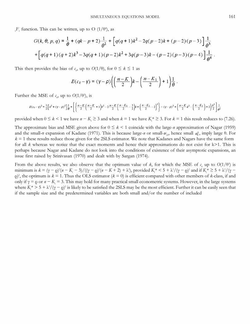
1F1 function. This can be written, up to O (1/θ4), as

This then provides the bias of ck, up to O(1/θ), for 0 ≤ k ≤ 1 as

Further the MSE of ck, up to O(1/θ2), is

provided when 0 ≤ k < 1 we have n − K1 ≥ 3 and when k = 1 we have K1* ≥ 3. For k = 1 this result reduces to (7.26).

The approximate bias and MSE given above for 0 ≤ k < 1 coincide with the large-n approximation of Nagar (1959)and the small-σ expansion of Kadane (1971). This is because large-n or small-w22, hence small , imply large θ. Fork = 1 these results reduce those given for the 2SLS estimator. We note that Kadane's and Nagar's have the same formfor all k whereas we notice that the exact moments and hence their approximations do not exist for k>1. This isperhaps because Nagar and Kadane do not look into the conditions of existence of their asymptotic expansions, anissue first raised by Srinivasan (1970) and dealt with by Sargan (1974).

From the above results, we also observe that the optimum value of k, for which the MSE of ck up to O(1/θ2) isminimum is k = (γ − ρ)2(n − K1 − 3)/((γ − ρ)2(n − K + 2) + λ2), provided K1* < 5 + λ2/(γ − ρ)2 and if K1* ≥ 5 + λ2/(γ −ρ)2, the optimum is k = 1. Thus the OLS estimator (k = 0) is efficient compared with other members of k-class, if andonly if γ = ρ or n − K1 = 3. This may hold for many practical small econometric systems. However, in the large systemswhere K1* > 5 + λ2/(γ − ρ)2 is likely to be satisfied the 2SLS may be the most efficient. Further it can be easily seen thatif the sample size and the predetermined variables are both small and/or the number of included


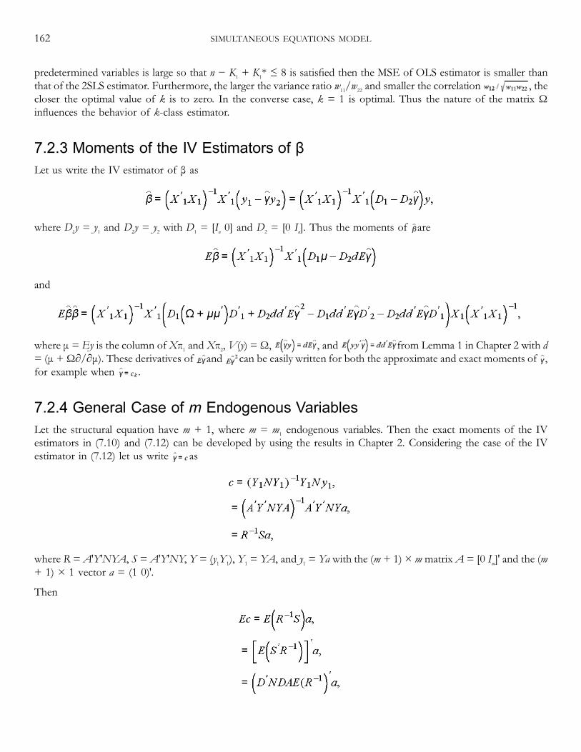
predetermined variables is large so that n − K1 + K1* ≤ 8 is satisfied then the MSE of OLS estimator is smaller thanthat of the 2SLS estimator. Furthermore, the larger the variance ratio w11/w22 and smaller the correlation , thecloser the optimal value of k is to zero. In the converse case, k = 1 is optimal. Thus the nature of the matrix Ωinfluences the behavior of k-class estimator.

7.2.3 Moments of the IV Estimators of βLet us write the IV estimator of β as

where D1y = y1 and D2y = y2 with D1 = [In 0] and D2 = [0 In]. Thus the moments of are

and

where μ = Ey is the column ofXπ1 and Xπ2,V(y) =Ω, , and from Lemma 1 in Chapter 2 with d= (μ + Ω∂/∂μ). These derivatives of and can be easily written for both the approximate and exact moments of ,for example when .

7.2.4 General Case of m Endogenous VariablesLet the structural equation have m + 1, where m = m1 endogenous variables. Then the exact moments of the IVestimators in (7.10) and (7.12) can be developed by using the results in Chapter 2. Considering the case of the IVestimator in (7.12) let us write as

where R =A′Y′NYA, S = A′Y′NY, Y = (y1Y1), Y1 = YA, and y1 = Ya with the (m + 1) × m matrix A = [0 Im]′ and the (m+ 1) × 1 vector a = (1 0)′.

Then


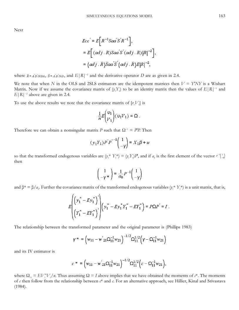
Next

where , , and E|R|−2 and the derivative operator D are as given in 2.4.

We note that when N in the OLS and 2SLS estimators are the idempotent matrices then V = Y′NY is a WishartMatrix. Now if we assume the covariance matrix of (y1Y1) to be an identity matrix then the values of E|R|−1 andE|R|−2 above are given in 2.4.

To use the above results we note that the covariance matrix of [v1V1] is

Therefore we can obtain a nonsingular matrix P such that Ω−1 = P′P. Then

so that the transformed endogenous variables are (y1* Y1*) = (y1Y1)P′, and if a0 is the first element of the vectorthen

and β* = β/a0. Further the covariance matrix of the transformed endogenous variables (y1* Y1*) is a unit matrix, that is,

The relationship between the transformed parameter and the original parameter is (Phillips 1983)

and its IV estimator is

where Ω11 = EV1′V1/n. Thus assuming Ω = I above implies that we have obtained the moments of c*. The momentsof c then follow from the relationship between c* and c. For an alternative approach, see Hillier, Kinal and Srivastava(1984).


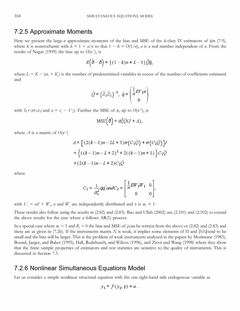
7.2.5 Approximate MomentsHere we present the large-n approximate moments of the bias and MSE of the k-class IV estimators of in (7.9),where k is nonstochastic with k = 1 + a/n so that 1 − k = O(1/n), a is a real number independent of n. From theresults of Nagar (1959) the bias up to O(n−1), is

where L = K − (m1 + K1) is the number of predetermined variables in excess of the number of coefficients estimatedand

with and u = v1 − V1γ. Further the MSE of , up to O(n−2), is

where A is a matrix of O(n−1)

where

with V1 = uπ′ + W1, u and W1 are independently distributed and π is m1 × 1.

These results also follow using the results in (2.82) and (2.83). Bao and Ullah (2002) use (2.101) and (2.102) to extendthe above results for the case where u follows AR(1) process.

In a special case where m1 = 1 and K1 = 0 the bias and MSE of can be written from the above or (2.82) and (2.83) andthese are as given in (7.26). If the instruments matrix X is weak, it implies some elements of Π and tend to besmall and the bias will be larger. This is the problem of weak instruments analyzed in the papers by Morimune (1983),Bound, Jaeger, and Baker (1995), Hall, Rudebusch, and Wilcox (1996), and Zivot and Wang (1998) where they showthat the finite sample properties of estimators and test statistics are sensitive to the quality of instruments. This isdiscussed in Section 7.3.

7.2.6 Nonlinear Simultaneous Equations ModelLet us consider a simple nonlinear structural equation with the one right-hand side endogenous variable as


Suppose there is one instrument xi. Then an IV estimator is a solution of

where . Let us denote fi(j) as the jth derivative of f(yi2,γ) with respect to γ, and

where and put ρj = E(uvj). In a special case when f(yi2,γ) is linear fi(1) = yi2, and v1i = vi.

In the above case the bias to O(1/n) can be written from the general result in (2.81) as

where

When xi is nonstochastic we replace Ex2 with and E(f(2)x) with . For the linear case, f(yi2,γ) = yi2γ, this biasresult reduces to that given above. The MSE is left as an exercise.

The result given above suggests that the bias is affected by the derivatives (curvature) of the function. If f(1) is very smallthen the bias will tend to be high. In the linear case f(1) became the correlation parameter and hence the measure of thequality of instrument. In the nonlinear case this may not necessarily be the case. For example, assuming Ex = 0 andusing the approximation f(1)(y2) ≃ f(1)(y¯2) + (y − y¯2)f(2)(y¯2),

Then

This shows that the bias depends on the f(2)(y¯2), f(3)(y¯2) of the regression f(y2,γ) at y2 = y¯2 = Ey2. These derivatives willdepend on the nature of the structural parameters. For example, if f(yi2,γ) = ey2γ} then and


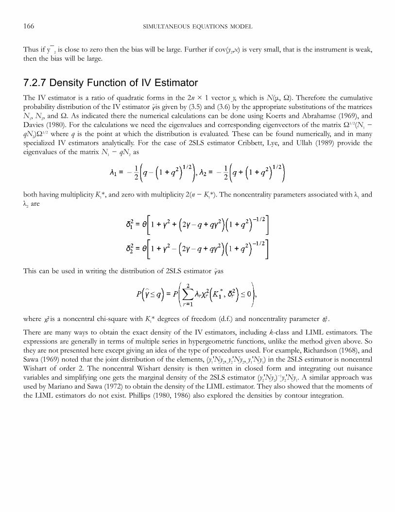
Thus if y¯2 is close to zero then the bias will be large. Further if cov(y2,x) is very small, that is the instrument is weak,then the bias will be large.

7.2.7 Density Function of IV EstimatorThe IV estimator is a ratio of quadratic forms in the 2n × 1 vector y, which is N(μ, Ω). Therefore the cumulativeprobability distribution of the IV estimator is given by (3.5) and (3.6) by the appropriate substitutions of the matricesN1, N2, and Ω. As indicated there the numerical calculations can be done using Koerts and Abrahamse (1969), andDavies (1980). For the calculations we need the eigenvalues and corresponding eigenvectors of the matrix Ω1/2(N1 −qN2)Ω1/2 where q is the point at which the distribution is evaluated. These can be found numerically, and in manyspecialized IV estimators analytically. For the case of 2SLS estimator Cribbett, Lye, and Ullah (1989) provide theeigenvalues of the matrix N1 − qN2 as

both having multiplicity K1*, and zero with multiplicity 2(n − K1*). The noncentrality parameters associated with λ1 andλ2 are

This can be used in writing the distribution of 2SLS estimator as

where is a noncentral chi-square with K1* degrees of freedom (d.f.) and noncentrality parameter .

There are many ways to obtain the exact density of the IV estimators, including k-class and LIML estimators. Theexpressions are generally in terms of multiple series in hypergeometric functions, unlike the method given above. Sothey are not presented here except giving an idea of the type of procedures used. For example, Richardson (1968), andSawa (1969) noted that the joint distribution of the elements, (y1′Ny2, y2′Ny2, y1′Ny1) in the 2SLS estimator is noncentralWishart of order 2. The noncentral Wishart density is then written in closed form and integrating out nuisancevariables and simplifying one gets the marginal density of the 2SLS estimator (y2′Ny2)−1y2′Ny1. A similar approach wasused by Mariano and Sawa (1972) to obtain the density of the LIML estimator. They also showed that the moments ofthe LIML estimators do not exist. Phillips (1980, 1986) also explored the densities by contour integration.


For the k-class, 0 ≤ k ≤ 1, Anderson and Sawa (1973) explored an alternative method to provide the exact density as afourth-order infinite series. The expressions for the densities of 2SLS and OLS estimators are given in terms of doublynoncentral F-distribution. Cribbett, Lye, and Ullah (1989) compared the calculations based on the straightforwardImhof distribution of the 2SLS in (7.65) with the Anderson and Sawa (1973, 1979) expressions. They found that theabsolute difference between the results are negligible. The largest absolute difference arose in all cases where Andersonand Sawa (1979) had computational difficulties with their exact density and used the approximate density. We thereforerecommend the using of Imhof procedure, which is also useful for a class of other econometric estimators discussed inearlier chapters.

From the extensive calculations in Anderson and Sawa one can observe the following findings. The distribution of2SLS estimator is asymmetric except when γ = ρ. This was also earlier reported on the basis of the skewness andkurtosis coefficients in (7.29) and (7.30). Further the LIML estimator tends to have larger dispersion and thicker tailsthan the 2SLS, perhaps because of the nonexistence of the LIML estimator moments. But the distribution of LIMLtends to normality much faster than that of 2SLS, and that in many cases the asymptotic normal theory may be a betterapproximation to the exact density of LIML but not so in the case of 2SLS.

While we have discussed above the exact density of the IV estimator, Anderson and Sawa (1973) have also provided anasymptotic expansion of the k-class estimator. This is done by first obtaining the exact characteristic function of the k-class estimator and its normalized form and then expand the logarithm of this characteristic function as a TaylorSeries. Then using the inversion theorem an Edgeworth Series expansion of the distribution function is obtained in theform

where ϕi(q) is a polynomial of finite degree in q and is O(1) and Φ(·) and φ(·) denote the cumulative distribution andprobability density functions, respectively, of the standard unit normal, see Chapter 3 for details.

To see the application of the Edgeworth expansion for the 2SLS estimator c we consider the distribution of

Then from the moments of c − γ given above we can verify that and V(Zn) = 1 + (c2/θ) where c1 and c2 arenonstochastic terms of O(1). Using these results define


which has zero mean, unit variance, and approximate third and fourth moments as and ,where c3 and c4 are of O(1). Then the Edgeworth expansion of Zn or Zn* is as given in (3.33) where c1 to c4 are given fromthe moments of (c − γ) and (c − Ec) above. This expression is an Edgeworth-B (3.30) type expansion. The Edgeworth-A expansion can also be developed from (3.29) by using the moments of c − γ. This is, up to ,

The density of Zn is then

see also Anderson and Sawa (1973).

Usually, the asymptotic expansions may not perform well in the tails of the distribution. For more details on the qualityof asymptotic approximations, see Phillips (1980, 1986), and Holly and Phillips (1979).

7.2.8 Further Finite Sample ResultsPhillips (1986) has provided a representation of the exact joint density function of IV estimators for m1 + 1endogenous variable case. It shows that as the number of endogenous variables increases the marginal distributions ofIV estimator tend to concentrate more slowly as n → ∞ and it may lead to reduction in the precision of estimation.Further the marginal distribution has more bias if more numbers of instruments are used for the m1 endogenousvariables.

There are various attempts in getting improved estimators for structural coefficients. Nagar (1959) provided a class ofalmost unbiased k-class estimators. Sawa (1973a,b) provided a linear combination of the OLS and 2SLS estimators,which is unbiased up to O(σ2) in the small-σ sense. Morimiune (1978) provided a combined estimator based on theLIML and 2SLS which has smaller MSE, up to O(σ4), compared to LIML. But both Morimiune's as well as Sawa'sestimators are dominated by the 2SLS for the low degrees of over identification. Fuller (1977) considers a modificationof LIML by using k − α/(n − k) with k as defined for the LIML above and α is some arbitrary nonstochastic realnumber determined under an optimizing criterion. This modified LIML estimator possesses moments, it isapproximately unbiased for α = 1 and has the minimum approximate MSE for α = 4, also see Rothenberg (1978) andTakeuchi and Morimiune (1979) for higher-order efficiency. Ullah and Srivastava (1988) provide a Stein-type shrinkage2SLS estimator which has smaller MSE compared to 2SLS estimator under certain conditions. Further Zellner (1998)analyzes the finite sample properties of Bayesian method of moments estimators and Kiviet and Phillips (1987)provide bias reduction in


a dynamic simultaneous equation model. Gao and Lahiri (2002), and Dwivedi and Srivastava (1984) have analyzed themoments of Nagar's (1962) double k-class estimators. The results of Gao and Lahiri (2002) also suggest the superiorperformance of Zellner's (1998) Bayesian estimators. Tsurumi's (1990) work analyzed the results for MELOestimators, also see Koenker and Machaso (1999) for the GMM estimators.

The finite sample properties of the reduced form coefficients estimators, unrestricted and partially restricted, havebeen analyzed by many authors, see Goldberger, Nagar, and Odeh (1961), McCarthy (1972), Nagar and Sahay (1978),Knight (1977), and Sargan (1973, 1974). Maasoumi (1978) considered the Stein-type improved estimation of thereduced form coefficients.

The literature on the hypothesis testing is much more limited compared with estimation of structural models.Richardson and Rohr (1971), when m1 = 1, provided the exact distribution of a t–test statistic based on the 2SLSestimator:

where is the estimator of the asymptotic covariance from in (7.53) with

which is not the usual large sample estimate of the σ2. But this definition of helps Richardson and Rohr to show thatthe derived exact distribution, which is in terms of a doubly infinite series of hypergeometric functions, converges tostudent-t distribution with K1* − 1 d.f. Maddala (1974), however, shows that the Monte Carlo power calculations ofthis statistic is smaller compared to the t with having , or in place of PX − PX1} and K1*-1 replaced by n-K orn-K-1. Further the test t above is skewed over the parameter space, even for large noncentrality parameter θ. Also, thedifference between the exact distribution of t and Student-t with one d.f. may be large, especially for small θ.

Several authors have analyzed the distributions of the identifiability test statistic

based on k-class estimators including the LIML estimator. For details see, for example, Basmann (1965, 1966),Richardson (1968), McDonald (1972), Kadane (1974), Rhodes (1981), and Anderson and Rubin (1950). For details onthe use of Edgeworth series expansions for econometric test statistics based on k-class estimators, see Sargan (1975,1976, 1980) and Sargan and Mikhail (1971). Further, for the results on the moments and distribution of the residualvariance, see Basmann (1974), Basmann and Richardson (1973), Ebbeler and McDonald (1973), and Smith (1994)among others.


7.2.9 Summary of ResultsHere we look into the main results emerging from the works on the moments and distribution of the k-classestimators. These are as follows.

The direction of the bias of estimator, for nonstochastic 0 ≤ k ≤ 1, depends on the sign of the ρ. If ρ < 0 there is adownward bias, and if ρ > 0 then we have an upward bias. For k > 1 the moments of k-class estimators do not exist.This is also the case for the LIML estimator, and the 2SLS estimator for the just identified case. Nonexistence of themoments do not imply that those estimators are bad, instead they simply mean that the quadratic loss function (MSE)is not the suitable way of comparing the efficiency of these estimators. For example, as indicated above and below,LIML estimator is considered to be a well behaved estimator.

The exact MSE of the k-class estimators (0 ≤ k ≤ 1) can be shown to be a decreasing function of θ, increasing functionof |ρ| and an indefinite function of the degrees of overidentification of OLS, K1* − 1, or the degree ofoveridentification of 2SLS, n − K1 − 1. Further an additional observation will decrease the MSE of 2SLS but it has anindefinite effect for other estimators. Also the optimal value of k minimizing MSE is sensitive to changes in the samplesize and parameter values.

Regarding the behavior of the members of k-class, we note that the absolute bias of the OLS is higher to 2SLS. Alsofor higher ρ the OLS bias becomes higher relative to 2SLS.

Regarding the MSE for large θ and large n the 2SLS does much better than OLS because of the inconsistency of OLS.However, in cases such as small value of ρ and n the OLS would dominate 2SLS. Regarding the comparison of LIMLwith 2SLS we compare the asymptotic MSE, up to O(n−1), since the finite sample MSE of LIML estimator does notexist. From Anderson (1974),

where , b2 = a2/r2, and r is the correlation between u and v2. Thus if K1* (degree ofoveridentification is K1* − 1) is less than 7 then 2SLS is more efficient. On the other hand for K1* > 7 and a2 is not toosmall LIML will be more efficient. Similar results were obtained by Anderson (1974), and Fujikoshi and Veitch (1979)on the basis of the approximate distributions of LIML and 2SLS, up to O(n−1). They show by comparing theconcentration probabilities, P(|c − γ|), that while LIML is favorable for high K1*, 2SLS is better for small K1* and forsmall r2.

Regarding the distribution of OLS and 2SLS the calculations in Sawa (1969), and Anderson and Sawa (1973, 1979)suggest that while the OLS distribution is almost symmetric the distribution of 2SLS is quite asymmetric. When the K1*is large, however, the distribution of OLS and 2SLS tend to be the same. Also the convergence of the distribution of2SLS to normality is very slow, especially when either K1* or r or both are large. In contrast the distribution


of LIML converges to normality faster, and is more symmetric but has more spread. Further the approximate LIMLdistribution, up to O(n−1) is median unbiased.

The impact of misspecification, with wrongly omitted variables, on the distributions and moments of the OLS, 2SLS,and LIML estimators have been done by Hale, Mariano, and Ramage (1980), Mariano and Ramage (1978), Marianoand McDonald (1979), Rhodes and Westbrook (1981), and Maasonmi and Phillips (1982), among others. These workssuggest that under the misspecification the nonstochastic k-class estimators are dominated by both OLS and 2SLSestimators. Further OLS is generally relatively insensitive to specification error and when the error of misspecificationis more severe compared with degree of simultaneity OLS is preferable to 2SLS. The effect of multi-collinearity on theproperties of estimators is also analyzed. The results here suggest that unlike in the regression models, highermulticollinearity can increase or decrease the MSE of estimators depending upon the values of the parameters in θ andthe values of exogenous variables.

Based on the above discussions we summarize that OLS and 2SLS estimators show similar statistical patterns for amedium to large econometric model where K1* is usually large and d.f. is low. If, in addition, ρ is high the LIML may bemore preferable. Next, for K1* < 7 2SLS is better than LIML and preferred over OLS in the presence of moderate tostrong ρ (simultaneity). Further, in the case of a very small sample, very week ρ, or strong presence ofmisspecifications OLS would be a fine estimator, for more details see Mariano (1982).

7.3 Analysis of Weak Instruments

7.3.1 Effects on the Moments and DistributionHere we consider the effect of the quality of instruments and the degree of endogeneity on the bias and MSE and thedistribution of the IV estimators. The quality of instruments is judged by the correlation of the instrument with theendogenous variables and the lack of association with the structural error or with the outcome of study. In general theF statistic or goodness of fit R2 of the first stage reduced form regression of the right hand endogenous variables onthe instruments will indicate the quality of instruments. A small F or small goodness of fit R2 is referred to as the weakinstruments. Similarly the degree of endogenity is measured by the correlations of the right hand endogenous variableswith the structural error.

When regressors are endogenous, OLS is a biased and inconsistent estimator. But, under the assumptions that theinstruments are correlated with the endogenous regressor but uncorrelated with the outcome variable, the IV estimatoris a consistent estimator, see Bowden and Turkington (1984). Note that the MSE of the IV estimator given above goesto zero as n tends to infinity.


However, it is often the case that the IV's are weak instruments in which case several problems may arise. First, evenwith a weak endogeneity, the IV can have a large inconsistency, see Bound, Jaeger, and Baker (1995), and Staiger andStock (1997). Second, in finite samples, IV estimates are biased in the same direction as the OLS estimator, with themagnitude of the bias approaching that of OLS as the first stage R2 approaching to 0. Third, the IV estimators mayhave large standard errors. These problems can produce misleading results in empirical work. For example, in Angristand Krueger (AK 1991) a large sample of U.S. census data is used to estimate wage equations with quarter of birthused as an instrument for educational attainment. This instrument was chosen because of the evidence of itsassociation with the educational attainment, for example the individuals born during the first quarter start school later,have lower educational attainment, and earn less than those born in the other quarters. Furthermore the quarter ofbirth is unlikely to have a strong correlation with wages. AK argued that the compulsory school attendance laws lead tothe correlation between quarter of birth and education. However, Bound, Jarger, and Baker (1995) find the quarter ofbirth to be a weak instrument, since R2 in the first stage of regression of quarter of birth on educational attainment tobe 0.0001 and 0.0002 in their samples. Given this they find significantly different numerical values of the estimatescompared to AK estimates, and report significant finite sample bias in some of AK estimates. Based on these resultsthey conclude that quarter of birth does not give much usable information regarding the effect of education onearnings. They further conclude that even those working with the large cross sectional samples should be careful withhaving weak instruments. To see these findings we look at the following analytical results.

Consider a special case of (7.17) where

Thus there is no exogenous variable in the structural equation and total number of instruments are K variables in X.Then it is easy to show that

and

where , c0 is the OLS estimator and c1 is the 2SLS (IV) estimator. It is clear that the OLS will beconsistent if V(y2) = σ2 ≠ 0 and y2 must be uncorrelated with u. Similarly the IV estimator will be consistent if V(ŷ2) isnonzero, that is X must be correlated with y2, and cor(ŷ2, u) = 0, which means that X is uncorrelated with u and hencey1 (outcome variable).


From above the relative asymptotic bias is

where is the population goodness of fit in the regression of y2 on X*1. If both the structural and reducedforms have the matrix X1 then will be replaced by the partial in the regression of on X*1. Further, when K= 1, can be written as ρx,u/(ρy2,u × ρy2,x), where ρ is the correlation coefficient.

It is clear from above that in the case of having a weak instrument ( or ρy2,x small), even a weak endogeneity (smallcorrelation ρy2,u) can produce a larger inconsistency in the IV estimator than in the OLS estimator.

We note that Staiger and Stock (1997) consider the case that , where π0 is a matrix of constants. They refer tothis as the case of weak instruments. In this case the ρ0

2 is of O(n−1), and condition of a good instrument that W′Z1/nconverges in probability to a nonrandom matrix fails. They show that, under the weak instruments, cIV − γ convergesto a nonrandom variable and the nonzero mean of the cIV − γ (asymptotic bias) is in the same direction as the bias ofOLS as indicated above. Han and Schmidt (2001) consider the case of irrelevant instruments where π0 = 0 so that π =0 in the reduced form for all n. They show that the mean of the asymptotic distribution of cIV − γ is the same as (plim c0− γ), the asymptotic bias of the OLS estimator.

As indicated above Staiger and Stock (1997) considered the case of weak instruments in the local to zero sense at therate of . They showed that both the LIML and 2SLS estimators become inconsistent and their asymptoticdistributions are nonstandard. An explanation for this is that as n tending to infinity the concentration (noncentrality)parameter does not increase and is of O(1) as long as the number of instruments K remains fixed. Chao and Swanson(2002) have considered a more general case where the weak instruments are in a general sense of local to zero at anunspecified rate of 1/bn, consider the k-class estimators along with the Jacknife IV estimator of Angrist, Imbens, andKreuger (1999) and assume the number of instruments K and hence the noncentrality parameters increasing with thesample size. Under this scenario they show that the above estimators are consistent and the use of many weakinstruments in empirical applications may be beneficial. They also explore the connection between their approach andthe asymptotic analysis based on the taking of infinite instruments by Morimiune (1983), Bekker (1994), Hahn (1997),Hahn and Inoue (2000), and Hahn, Hausman, and Kuersteiner (2001).

To see the effect of weak instruments on the finite sample bias let us write the bias, up to O(n−1), from (7.26) as


where is approximately the A bias(c0) when X explains very little variation in y2 and . Thisresult suggests the finite sample approximate bias of the IV relative to the asymptotic OLS bias is inversely related toθ/K, which is population analog of the F statistics in the reduced form regression (F value on the excluded instrumentsX*1 when X1 is present in both equations). Generally sample F tends to overestimate θ/K in the same way as thesample R2 tends to have an upward bias of ρ0

2, see Chapter 4. Thus the examination of the F or R2 statistic on theexcluded instruments in the reduced form regression is useful in judging the quality of instruments and their impact onthe finite sample behavior of the IV estimator.

While the above result on the finite sample bias is based on the approximate bias, a similar result holds on the basis ofthe exact expressions, which is from (7.21)

where k = 0 for the OLS and k = 1 for the 2SLS(IV), and nk = n − 1, for k = 0 and it is K for k = 1. Note that θ/n − 1is the population in the regression y2 onX. Numerical results in Bound, Jaeger and Baker (1995) suggest that the biasof the IV relative to the bias of LS depends on θ/K as was in the case of approximate bias.

Woglom (2001) considers the model with m1 = 1, K1 = 0, and K1* = K = 1, and analyzed the distribution of the IVestimator with moderately weak instruments (R2 ≃ 1/n), very weak instruments, and various degrees of endogeneity.He finds that in the case of moderately weak instruments the distribution will be much more peaked than theasymptotic distribution with a mode somewhere between the true value and the p of OLS estimators. In the case ofvery weak instruments (R2 ≃ 0), the distribution approaches a student t with a mode at the p lim of OLS in the totallyunidentified case. Further, as the degree of endogeneity increases, the distribution becomes more peaked and the modemoves away from the true value. When the degree of endogeneity is very high with moderate first stage R2 thedistribution can have an important second mode. Finally when the instruments are very weak (R2 ≃ 0) the t statisticbased on cIV − γ will concentrate around the number greater than 1, with moderate or high endogeneity.

The above discussion emphasizes that under the weak instruments the inference based on IV estimators andasymptotic standard errors is generally misleading in finite samples. This is because the IV estimator is strongly biasedand the estimated standard error is too small, with the result that the true null hypothesis is rejected much too often.Traditional confidence intervals based on IV estimation and asymptotic standard errors provide a valid approach in thesense of producing confidence regions that cover the true value with the stated probability when the system is wellidentified and have large sample. But when the instruments are weak and the endogeneity is strong, this traditionalapproach produces confidence regions that are highly misleading. Zivot, Startz,


and Nelson (1997) provide the examples where the size of Wald(W) Test is 100 percent. Staiger and Stock (1997) showthat under the weak instruments the asymptotic distribution of W-test for linear restrictions on δ is not χ2 under thenull hypothesis. Zivot, Startz, and Nelson (1997) provide alternative confidence regions based on inverting Rao scoretest, likelihood ratio, and Anderson-Rubin statistics, which are easy to compute and provide better size and powerproperties. Zivot, Startz, and Nelson show that W-based confidence intervals provide better probability of rejecting thenull than their nominal size, also see Hall, Rudebusch, and Wilcox (1996). This is partly because of the bias of IVestimator, leading to an underestimate of the variance of the estimator. This set of results is important since weakinstruments are often the case, see AK (1991, 1992). Furthermore, see Moore, Fuhrer, and Sehuh (1995), Hall (1988),McClellan et al. (1994), and Koenker and Machaso (1999) among others.

7.3.2 Issue of Optimal InstrumentsDonald and Newey (2001) considered the model in (7.3) and (7.5) and have looked into the issue of determining theoptimal choice of the number of instruments K for 2SLS, LIML, and bias-corrected 2SLS (B2SLS) estimators given in7.2.1. The procedure of selecting the instruments is based on minimizing the approximate MSE of a linearcombination of the IV estimator . For the MSE of they considered Nagar (1959) type expansion for K and n suchthat K2/n→ 0 for the case of 2SLS and K/n→ 0 for LIML and B2SLS. As n and K increase they indicate that the MSEof LIML and B2SLS are smaller compared with 2SLS, and LIML is best among them for large K, also see Morimune(1983). In general the MSE for LIML is smaller than that of B2SLS for all K. The comparison between LIML and2SLS depends on the size of the simultaneity (endogeneity) σuv1. For σuv1 = 0, 2SLS has smaller MSE than LIML for allK and optimal choice of K would be large leading to OLS for K = n, the optimal estimator under no endogeneity. Forthe case of endogeneity, σuv1 ≠ 0, the LIML may perform better than 2SLS for various values of n, K.

Let us consider again the empirical equation of AK(1991), which deals with log weekly wage equation with theexplanatory variables as education (number of years of schooling), intercept, nine year of birth dummies and 50 statedummies (AK, table VII). The quarter of birth was used as instruments. The sample was from 1980 U.S. census andconsisted of 329,500 men born in 1930–39. The OLS estimate on schooling was 0.0673 and its standard error was0.0003.

For the model under consideration, y1 = log wage, y2 = education, X1 is a set of 60 (1 + 9 + 50) explanatory variables.In the reduced form for y2 the IV matrices WK = [X1X2] considered are


where Q*Y is interaction of quarter of birth dummies with the 9 year of birth dummies, S is state dummies, R4 is threeregion dummies, R9 is nine region dummies. Note that X2 is like X*1 in 7.2.1.

Using the above sets of instruments the first stage reduced form regressions gave largest set of instruments; K = 240,as the best cross validated Mallows' (1973) goodness of fit. Also Wald test was significant and partial R2 = 0.0014.Based on K = 240 the IV estimates can be obtained. This is the usual practice in applied work, also see AK (1991).Instead of this Donald and Newey (2001) determined optimal K for 2SLS, LIML, and B2SLS by evaluating theirestimated MSE for different sets of instruments given above. For 2SLS and B2SLS the MSE criteria suggest that oneshould use the minimal number of instruments 63, that is using the set of quarter of birth dummy variables. But forthe LIML its MSE is smallest for the largest instrument set, 240, which is optimal for first-stage regression.

Estimates of the returns to education for different instruments sets can be obtained for three estimators. Theseestimates and their standard errors are similar for LIML and B2SLS, but those of 2SLS are smaller than LIML andB2SLS even though the point estimates for the optimal K = 63 for 2SLS and B2SLS and K = 240 for the LIML aresimilar, although the standard error for LIML is smaller. AK (1991) used 2SLS based on K = 240 instruments and gotthe point estimate of 0.0928 and a standard error of 0.0093. Compared to this the estimates using the MSE basedoptimal number of instruments are larger with a standard error that is 50 percent larger when using LIML and 100percent larger when using 2SLS or B2SLS.

The above example indicates that for 2SLS, choosing instruments to minimize MSE avoids cases where asymptoticinterness are bad due to the bias (discussed above due to weak instruments) being large relative to the standarddeviation. For AK data this produces a 2SLS estimate that uses smallest number of instruments and is similar toLIML, which is known to have less bias. For LIML and B2SLS the optimum number of instruments helps avoid underestimated variances.

We note that the above is the choice of optimum number of instruments from a large set of valid instruments. This isdifferent than searching for the largest set of valid instruments in Andrews (1999). The results discussed here


may be sensitive when the errors (u,v1) are not assumed to be homoskedastic and/or they are nonnormally distributed.

There are also some studies which look into the effect of weak instruments and endogeneity on the distribution of IVestimators and the tests based on them.

Under the weak instruments (R2 < 1/n), Nelson and Startz (1990a,b) exposed to the substantial differences betweenthe exact distribution of the IV estimator with its asymptotic distribution in following ways: (a) The IV estimates willconcentrate around a value more than the p of the OLS estimate and the ratio of the IV to OLS biases will fall as thedegree of endogeneity rises, also see above. (b) The t-statistic based on the asymptotic standard errors will tend to bearound a value greater than 1, and this increases with the degree of endogeneity. (c) The true distribution is bimodaland the density is zero at a point between the modes, and hence the true distribution is quite different compared withasymptotic distribution. Maddala and Jeong (1992), however, point out that the distribution of the IV estimator is notbimodal except when the correlation between u and v, ρuv, is very high, thus the bimodality of Nelson and Startz are notdue to instrument quality but due to the assumption of ρuv = 1.

Phillips (1989) pioneered the study of the distribution of IV in the totally unidentified case, where the populationcorrelation between the instrument and the instrument is zero. For the case of one right hand endogenous variable heshowed that the exact distribution of the IV estimator is equal to the p lim of OLS estimate plus a unimodal t-distribution. In this case of totally unidentified equation Zivot, Startz, and Nelson (1997), and Zivot and Wang (1998)showed that, with no endogeneity, (ρuv = 0), the exact unimodal distribution is concentrated with a median error ofzero. But when the degree of endogeneity approaches to 1, the distribution collapses at a spike at the p lim of OLS. Inthis case the asymptotic result is a biased approximation for the exact distribution


Appendix A Statistical Methods

The finite sample theories of econometrics heavily depend on several statistical concepts. These include moments,distributions, and asymptotic expansions. Accordingly, the objective here is to present results that are useful for thefinite sample results covered in this book. In doing so it is assumed that the reader has a basic knowledge of probabilityand statistics.

A.1 Moments and CumulantsThe characteristic function of a random variable y is

where μr′ = Eyr and the last equality is the expansion of ψ(t) around zero. Then the rth moment around zero of y is

where ψ(r)(0) is the rth derivative of ψ(t) with respect to t and evaluated at t = 0.

The cumulant function is defined by

Using the expansion of K(t) around 0

where

is the rth cumulant of y.

It is easy to verify that κ1 = μ1′, κ2 = μ2, κ3 = μ3, , κ5 = μ5 − 10μ3μ2, , where μr = E(y −Ey)r is the rth central moment around mean.

A.2 Gram–Charlier and Edgeworth SeriesGram (1879), and Charlier (1905) series represent the density of a standardized variable y as a linear combination of thestandardized normal density φ (y) and its derivatives. That is

where the cj are constants and

Hj(y) is a polynomial in y of degree j, which is the coefficient of tj/j! in exp (ty − ½t2), for example H0(y) = 1, H1(y) = y,H2(y) = y2 − 1, H3(y) = y3 − 3y, and H4(y) = y4 − 6y2 + 3. These Hj(y) form an orthogonal set of polynomials (HermitePolynomials) with respect to normal density φ (y), that is

Because of this, multiplying f(y) by Hj(y) and integrating term by term we get

These cj can be obtained in terms of the moments of y, and these are


Then the Gram–Charlier series of Type A can be written as

Using this

If y is not a standardized variable then

where (j)r = j(j − 1) ċċċ (j − r +1). Then

In this case

The Edgeworth Type A (1905) series is closely related to Gram–Charlier series. For this we obtain the characteristicfunction around the normal distribution and then use inversion theorem to obtain the series expansion of the density.Let us write


where cj is given by (A.10). Alternatively, (A.14) can be obtained by using (A.4) as

Now using the inversion theorem

and the fact that if f has the characteristic function ψ(t) the f(j) has the characteristic function (−it)jψ (t), which gives

we obtain the Gram–Charlier type series expansion in (A.11). If we collect the terms containing elements not higherthan H6 we can write

This is often called the Edgeworth form of the Type A series, see Kendall and Stuart (1977). Further, if cumulantsabove the fourth are neglected the Edgeworth series reduces to

We note that the above series can also be written as

where D = d/dy. This is the form originally suggested by Edgeworth (1905), also see Kendall and Stuart (1977). Theidea behind these series goes back to Chebyshev (1890), also see Cramér (1925, 1928) for the historical details.

A.3 Asymptotic Expansion and Asymptotic ApproximationFor large values of nonstochastic x, consider


is the asymptotic expansion of a function f(x) if the coefficients are determined as follows:

The series on the right, viz.,

may be convergent for large values of x or divergent for all values of x.

However, it should be noted that the difference between f(x) and the sum of the n terms of its asymptotic expansion:

is of the same order as the (n + 1)th term when |x| is large. Then the asymptotic expansion may be considered moresuitable for approximate numerical computation than a convergent series.

Let us illustrate this point with the help of the following example, from Whittaker and Watson (1965: 150–151).

Consider the function

where x is real and positive. By repeated integration by parts, we get

We observe that the absolute value of the ratio of the (m + 1)th term to the mth term is equal to


which tends to ∞ as m ⇛ ∞ for all values of x. It follows that the series expansion of f(x) is, in fact, divergent for allvalues of x. In spite of this, however, the series can be used for the calculation of f(x). This may be seen asfollows:Write

and

such that

Then, because e|x−t| < 1

This is very small (for any value of n) for sufficiently large values of x. It follows, therefore, that the value of thefunction f(x) can be calculated with great accuracy for large values ofx. Even for small values of x and n

and

It has also been shown by Whittaker and Watson (1965: 153, section 8.31), that it is permissible to integrate anasymptotic expansion term by term, the resulting series being the asymptotic expansion of the integral of the functionrepresented by original series. It has also been stated that a given series can be an asymptotic expansion of severaldistinct functions; however, a given function cannot be represented by more than one asymptotic expansion, seeCopson (1967), Kendall and Stuart (1977), and Srinivasan (1970).

A.3.1 Asymptotic Expansion (Stochastic)Now we consider the case of stochastic asymptotic expansion. Most econometric estimators and test statistics can beexpanded in a power series in n−1/2 with coefficients that are well behaved random variables. Suppose, for example,


Zn is an estimator or test statistic whose stochastic expansion is

where ξ−j = Op(n−j) and Tn, An, and Bn are sequences of random variables with limiting distribution as n tends to infinity.If Rn is stochastically bounded, that is, P[|Rn| > c] < ε as n ⇛ ∞ for every ε > 0 and a constant c, then the limitingdistribution of is the same as the limiting distribution of An. Then expansion in (A.19) is the asymptoticexpansion of Zn, see Chapter 3 for examples.

A.4 Moments of the Quadratic Forms Under NormalityLetNi, for i = 1, 2, 3, 4, be the symmetric matrices. Further consider a n × 1 vector y, which is distributed as a normaldistribution with the mean vector Ey = μ and variance matrix as V(y) = Σ. Then the following results can be verifiedfrom the result of Lemma 1 and Exercises 2 and 4 in Chapter 2.

To write these results we first introduce the notations as given below:

where tr represents the trace of a matrix. Then


The above results can also be developed from Mathai and Provost (1992) where the moment generating functionsapproach is used.

In the special case where μ = 0, y ∼ N(0, Σ), the above results reduce to the following results.

When y ∼ N(0, I) then these results in (A.22) remain the same except that Σ = I in all the terms. For the alternativederivations of these results see Magnus (1978, 1979), Srivastava and Tiwari (1976), and Mathai and Provost (1992).

In another special case where y ∼ N(0, I) and N1 is an idempotent matrix of rank m then y′N1y is distributed as a centralχ2 at m d.f. In this case , and

which generalizes to

This is the rth moment of a central χ2 distribution.

When the matrix N1 is not a symmetric matrix then we can write y′N1y = y′((N1 + N1′)/2)y where ((N1 + N1′)/2) isalways a symmetric matrix. Thus the above results also go through when the matrices N1 to N4 are not symmetric.


A.5 Moments of Quadratic Forms Under NonnormalityLet y = (y1, …,yn)′ to be an n × 1 vector of i.i.d. elements with

for i = 1,…, n, where γ1 and γ2 are the Pearson's measures of skewness and kurtosis of the distribution and these andγ3 and γ4 can be regarded as measures for deviation from normality. For normal distributions, the parameters γ1, γ2, γ3,and γ4 are zero while for symmetrical distributions, only γ1 and γ3 are zero. These γ′s can also be expressed ascumulants, for example, γ1 and γ2 represent the third and fourth cumulants, see Section A.1.

Under the above assumptions the following results follow, whereN1 andN2 matrices are not assumed to be symmetric,ι is an n × 1 vector of unit elements and * represents the Hadamard product:


Setting γ1, γ2, γ3, and γ4 equal to zero, we obtain the results for normally distributed disturbances given above. Forderivations and applications, see Chandra (1983) and Ullah, Srivastava, and Chandra (1983).

We also note that E(y′N1y.yy′) above gives the result for E((y′N1y) (y′N2y)) = tr[N2E(y′N1y.yy′)]. Similarly E[(y′N1y)(y′N2y)yy′] gives the result for E((y′N1y)(y′N2y)(y′N3y)) = tr[N3E(y′N1y.y′N2y.yy′)]. Further the results for the case where themean of y is a vector Ey = μ the above results can be extended by writing, say, y′N1y = (y − μ + μ)′N1(y − μ + μ) = (y −μ)′ × N1(y − μ) + μ′N1μ + 2(y − μ)′N1μ. Then E(y′N1y) = E((y − μ)′N1(y − μ)) + μ′N1μ = σ2 tr(N1) + μ′N1μ.

Now consider the case where the elements yi are non i.i.d. such that

for i, j, k, l = 1,…, n. Define a n × n matrixΘk = ((σijk)) and another n × n matrix Δkl = ((σijkl)) for i, j = 1,…, n. Furtherdenote

Then

A.6 Moment of Quadratic Form of a Vector of Squared NonnormalRandom VariablesConsider an n × 1 random vector

where y is an n × 1 random vector with Ey = 0, V(y) = σ2In, and M is an n × n idempotent matrix of rank r.

Let us write e = (e1, …, en)′, where ei = miy and mi is a 1 × nith vector element of the matrix


i, j = 1, …, n. Further denote as an n × 1 vector of squares of ei and as an n × n matrix of thesquares of the elements of M. Then, for a matrix N = ((nij))

and when M˙ ≃ In.

For the proof of this write

Then using the results in (A.25) we get the result in (A.29).

When y ∼ N(0,σ2I) then

An application of this result can occur in the linear regression model y = Xβ + u where X is an n × k matrix. In thiscase e =My =Mu whereM = I − X(X′X)−1X′ is an idempotent matrix of rank n − k. Several tests of heteroskedasticityare expressible as a quadratic form of ė, see Chapter 5.

A.7 Moments of Quadratic Forms in Random MatricesLet us consider a stochastic n × M matrix Y = ((yit)) = (y1, …, yM), where t = 1, …, n, i = 1, …, M and yi is a n × 1vector. We assume that, for all i and t,

where j, k, e = 1, …, M.


Define

so that σijk and γijke are 0 for normally distributed disturbances.

If N1 is any nonstochastic matrix, we have

Further denoting (1/n)E(Y′Y) = Σ = ((σij)) and considering N1 of appropriate dimensions we have

Now introducing the following notations:

and considering N1 and N2 are of appropriate dimensions we have


For the following results we introduce additional matrix representations:

where n1i, n2i, and n3i are now vectors for i = 1, …, M. We also use N1 = ((n1ij)), N2 = ((n2ij)) and N3 = ((n3ij)). Then


where M = ((mij)) and mij for M1 to M8 are, respectively,

The above results simplify for the normal distribution by using σijk = 0 and γijke = 0. For the applications, see Ullah andSrivastava (1994), Ullah (2002), Srivastava and Maekawa (1995), among others. These results are useful in developingthe moments of various econometric statistics under nonnormal errors, also see Lieberman (1997).

A.8 Distribution of Quadratic FormsLet y ∼ N(μ, Σ) be an n × 1 normal vector with Ey = μ and V(y) = Σ. Further consider N to be an n × n nonstochasticmatrix and b and c to be constants. Then

if and only if r = Rank(NΣ), ΣNΣNΣ = ΣNΣ, Σ(b + Nμ) = ΣNΣ(b + Nμ) and θ = c + 2b′μ + μ′Nμ. Therepresents the noncentral chi-square distribution with the d.f. r and the noncentrality parameter θ. For θ = 0,


becomes a central chi-square with the d.f. r, see Srivastava and Khatri (1979: 64), Rao (1973), and Mathai andProvost (1992).

A necessary and sufficient condition for

is that ΣNΣNΣ = ΣNΣ with d.f. = r = Rank of NΣ, and θ = μ′Nμ. For μ = θ = 0, , which is a central chi-square.

If |Σ| ≠ 0 then the above necessary and sufficient condition becomes NΣN = N with the d.f. r = Rank of NΣ. Thisimplies the condition that NΣ or Σ1/2NΣ1/2 is an idempotent matrix of rank r, where Σ = Σ1/2Σ1/2, see Rao (1973: 188)and Srivastava and Khatri (1979: 64).

A necessary and sufficient condition that the vector N1y and the quadratic form (y − μ)′N(y − μ) are statisticallyindependent is ΣNΣN1 = 0, or NΣN1 = 0 if |Σ| ≠ 0, whereN1 is an n × n nonstochastic matrix. Similarly (y − μ)′N1(y− μ) and (y − μ)′N(y − μ) are independent if ΣN1ΣNΣ = 0, or N1ΣN = 0 if |Σ| ≠ 0.

A.8.1 Density and Moments of a Noncentral Chi-square VariableLet y ∼ N(μ, Σ). Then

whereN is assumed to be an idempotent matrix of rank r, θ = (1/2)μ′Σ−1/2NΣ−1/2μ and Σ−1/2y ∼ N(Σ−1/2μ, I). The densityfunction of the noncentral χ2 variable y* is

Further the sth inverse moment of y* is

which gives, for s = 1,2, …,

see Ullah (1974).


Using the derivatives of the confluent hypergeometric function in Slater (1960: 15, eq. 2.1.8) we have

for m = 1,2,….

When μ = 0 so that θ = 0, the density of y* given above reduces to the density of a central . Further

We note that the distribution of y′Ny = y′Σ−1/2(Σ1/2NΣ1/2)Σ−1/2y is not a noncentral χ2 distribution unless Σ1/2NΣ1/2 isidempotent. If Σ1/2NΣ1/2 is not idempotent the sth inverse moment of y′Ny is as given in Chapter 2.

A.8.2 Moment Generating Function and Characteristic FunctionLet y ∼ N(μ, Σ), where Σ = PP′. Let Let N1, N2, …, Nm be m symmetric n × n matrices. Then the joint momentgenerating function of y′N1y, …, y′Nmy is

where C = P′(t1N1 + ··· + tmNm)P and μ0 = P−1μ, see Magnus (1986), and Mathai and Provost (1992). For m = 2 thisresult is given in Chapter 2 and it has been used in Sawa (1972), Magnus (1986), and Mathai and Provost (1992) toobtain the moments of the product and ratio of quadratic forms. For example, if y1* = y′N1y and y2* = y′N2y, then

For the moments of the ratio of y1*/y2*, see Chapter 2.

Now we consider the vector y distributed nonnormally with Ey = μ and V(y) = Σ, which is a diagonal matrix of , i =1, …, n. If we let be a normal density with mean μi and variance then the Edgeworth or Gram–Charlierseries expansion of the density for f(yi) in Section A.2 can be


written as (Davis 1976)

where and cr is as in (A.10).

Since y|z ∼ N(μ + z, Σ), therefore using the Davis (1976) technique the characteristic (c.f.) or moment generatingfunction (m.g.f.) under the {Edgeworth} density can be obtained in two steps. First find the c.f. for the normal case.Second consider the expectation of this c.f. with respect to z. With this approach Knight (1985) provided the c.f. of alinear form a′y and the quadratic form y′Ny with corrections for skewness and kurtosis, that is the first four terms ofthe Edgeworth expansion.

These results on the c.f. and m.g.f. provide the moments of the products and ratio of quadratic forms under theEdgeworth density of y. For applications, see Knight (1985, 1986) for the moments and distribution of the 2SLSestimator and Peters (1989) for the moments of the LS estimator in a dynamic regression model.

A.8.3 Density Function Based on Characteristic FunctionWhen the absolute value of the c.f. ψ(t) = ψ(t1,…, tn) is integrable then the density function f(y) exists and is continuousfor all y, and it is given by

This is known as the uniqueness theorem or inversion theorem for the c.f., see Cramér (1946).

Next consider the variable q, which is the ratio of two random variables Y and X, q = Y/X. Let ψ(t1, t2) be the c.f. of(Y,X). Then the density of q is given by

see Cramér (1946). Phillips (1985) generalizes this result to matrix quotients Q = X−1Y where X is a k × k positivedefinite matrix whose expectation of the determinant exists and Y is a k × l matrix. As an application of this resultPhillips (1985) shows that the LS regression coefficient matrix for multivariate normal sample is a matrix t-distribution.


A.9 Hypergeometric FunctionsHere we present well known power series, which are used in the text.

A power series

is known as the confluent hypergeometric function or Kummer's series, see Slater (1960: 2). It has been usedextensively in finite sample econometrics, see Ullah (1974), Sawa (1972), and Phillips (1983), among others. Also, seeAbadir (1999) for an introduction to hypergeometric function for economists.

Another power series, hypergeometric functions, is written as

for |c| > 0 and |x| < 1, see Slater (1960), and Ullah and Nagar (1974).

Now we consider the integral of a function, which has a power series expansion in terms of hypergeometric functions,see Sawa (1972). This is, for 0 ≤ k < 1 and p > 1

where

For k = 1 and p − q > 1

To derive the above result we can first use the following change of variable transformation t = 1/(1 − 2x). Then

Then using the binomial expansion of [1 − k(1 − t)]−q and doing term by term integration gives the above result, Sawa(1972).


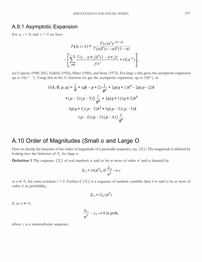
A.9.1 Asymptotic ExpansionFor a, c > 0, and x > 0 we have

see Copson (1948: 265), Erdelyi (1956), Slater (1960), and Sawa (1972). For large x this gives the asymptotic expansionup to O(x−(r − 1)). Using this in the G function we get the asymptotic expansion, up to O(θ−4), as

A.10 Order of Magnitudes (Small o and Large O)Here we decide the measure of the order of magnitude of a particular sequence, say, {Xn}. The magnitude is defined bylooking into the behavior of Xn for large n.

Definition 1 The sequence {Xn} of real numbers is said to be at most of order nk and is denoted by

as n ⇛ ∞, for some constant c > 0. Further if {Xn} is a sequence of random variables then it is said to be at most oforder nk in probability,

if, as n ⇛ ∞,

where cn is a nonstochastic sequence.


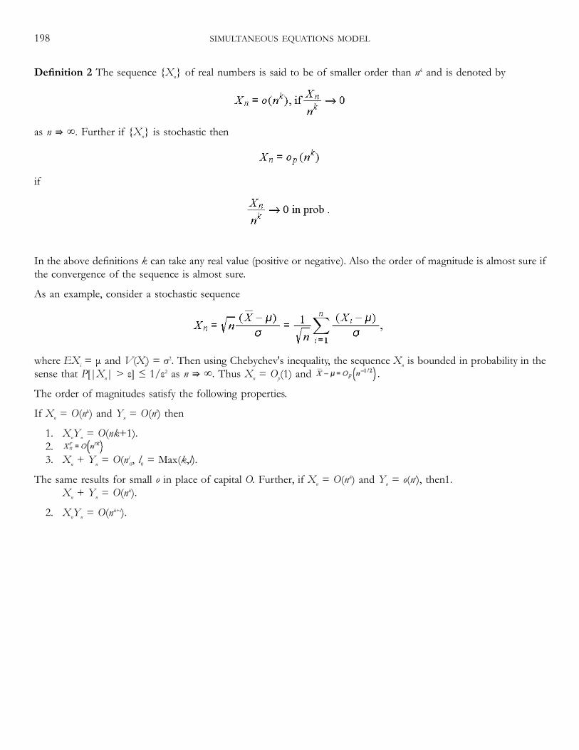
Definition 2 The sequence {Xn} of real numbers is said to be of smaller order than nk and is denoted by

as n ⇛ ∞. Further if {Xn} is stochastic then

if

In the above definitions k can take any real value (positive or negative). Also the order of magnitude is almost sure ifthe convergence of the sequence is almost sure.

As an example, consider a stochastic sequence

where EXi = μ and V(Xi) = σ2. Then using Chebychev's inequality, the sequence Xn is bounded in probability in thesense that P[|Xn| > ε] ≤ 1/ε2 as n ⇛ ∞. Thus Xn = Op(1) and .

The order of magnitudes satisfy the following properties.

If Xn = O(nk) and Yn = O(nl) then

1. XnYn = O(nk+1).2.3. Xn + Yn = O(nl0, l0 = Max(k,l).

The same results for small o in place of capital O. Further, if Xn = O(nk) and Yn = o(nl), then1.Xn + Yn = O(nk).

2. XnYn = O(nk+l).


REFERENCES

Abadir, K. M. (1993a). ‘OLS Bias in a Nonstationary Autoregression’, Econometric Theory, 9:81–93.—— (1993b). ‘The Limiting Distribution of the Autocorrelation Coefficient Under a Unit Root’, The Annals of Statistics,

212:1058–70.—— (1994). ‘The Joint Density of Two Functionals of Brownian Motion’, Discussion Paper 94-03, University of

Exeter.—— (1999). ‘An Introduction to Hypergeometric Functions for Economists’, Econometric Reviews, 18:287–330.—— Hadri, K., and Tzavalis, E. (1999). ‘The Influence of VAR Dimensions on Estimator Biases’, Econometrica,

67:163–82.Akahira, M. and Takeuchi, K. (1981). Asymptotic Efficiency of Statistical Estimators: Concepts and Higher Order Asymptotic

Efficiency (New York: Springer-Verlag).Ali, M. M. (2002). ‘Distribution of the Least Squares Estimator in a First-Order Autoregressive Model’, Econometric

Reviews, 21(1):89–119.—— and Sharma, S. C. (1993). ‘Robustness to Nonnormality of Durbin–Watson Test for Autocorrelation’, Journal of

Econometrics, 57:117–36.—— —— (1996). ‘Robustness to Non-Normality of Regression F-tests’, Journal of Econometrics, 71:175–205.Amemiya, T. (1985). Advanced Econometrics, 1st edition (Cambridge: Harvard University Press).Anderson, T. W. (1959). ‘On Asymptotic Distribution of Estimates of Parameters of Stochastic Difference Equations’,

The Annals of Mathematical Statistics, 30:676–87.—— (1974). ‘An Asymptotic Expansion of the Distribution of the Limited Information Maximum Likelihood

Estimate of a Coefficient in a Simultaneous Equation System’, Journal of the American Statistical Association,69:565–73.

Anderson, T. W. (1982). ‘Some Recent Developments on the Distributions of Single-Equation Estimators’, in R. L.Basmann and G. F. Rhodes, Jr. (eds.), Advances in Econometrics (Cambridge University Press).

—— (1984). An Introduction to Multivariate Statistical Analysis (New York: Wiley).—— and Fang, K. T. (1987). ‘Cochran's Theorem for Elliptically Contoured Distributions’, Sankhya, 49:305–15.—— and Rubin, H. (1949). ‘Estimation of the Parameters of a Single Equation in a Complete System of Stochastic

Equation’, The Annals of Mathematical Statistics, 20:46–63.—— —— (1950). ‘The Asymptotic Properties of Estimates of the Parameters of a Single Equation in a Complete

System of Stochastic Equations’, The Annals of Mathematical Statistics, 21:570–82.—— and Sawa, T. (1973). ‘Distributions of Estimator of Coefficients of a Single Equation in a Simultaneous System

and their Asymptotic Expansions’, Econometrica, 41:683–714.—— —— (1979). ‘Evaluation of the Distribution Function of the Two-Stage Least Squares Estimate’, Econometrica,

47:163–82.Andrews, D. W. K. (1999). ‘Consistent Moment Selection Procedures for Generalized Method of Moments

Estimation’, Econometrica, 67:543–64.Angrist, J. D. and Kreuger, A. B. (1991). ‘Does Compulsory School Attendance Affect Schooling and Earnings?‘,

Quarterly Journal of Econometrics, 106:979–1014.—— —— (1992). ‘The Effect of Age at School Entry on Educational Attainment: An Application of Instrumental

Variables with Moments from Two Samples’, Journal of the American Statistical Association, 87:328–336.—— Imbens, G. W., and Kreuger, A. B. (1999). ‘Jackknife Instrumental Variable Estimation’, Journal of Applied

Econometrics, 14:57–67.Arellano, M. and Sargan, J. D. (1990). ‘Imhof Approximations to Econometric Estimators’, Review of Economic Studies,

57:627–46.Avram, F. (1988). ‘On Bilinear Forms in Gaussian Random Variables and Toeplitz Matrices’, Probability Theory and

Related Fields, 79:37–45.Baltagi, B. H. (2001). Econometric Analysis of Panel Data (New York: John Wiley).Banerjee, A., Dolando, J. J., Hendry, D. F., and Smith, G. W. (1986). ‘Exploring Equilibrium Relationships in

Economics Through Static Models: Some

200 REFERENCES

Monte Carlo Evidence’, Oxford Bulletin of Economics and Statistics, 48:253–77.Bao, Y. and Ullah, A. (2002). ‘The Second-Order Bias and Mean Squared Error of Nonlinear Estimators in Time

Series’, Manuscript, University of California, Riverside.Baranchik, A. J. (1964). ‘Multiple Regression and Estimation of the Mean of a Multivariate Normal Distribution’,

Technical Report 51, Department of Statistics, Stanford University, Stanford.Barndorff-Nielsen, O. E. and Cox, D. R. (1979). ‘Edgeworth and Saddle-Point Approximations with Statistical

Applications’, Journal of the Royal Statistical Society, 41:279–312.—— —— (1989). Asymptotic Techniques for Use in Statistics (New York, NY: Chapman and Hall).Basmann, R. L. (1961). ‘Note on the Exact Finite Sample Frequence Functions of Generalized Classical Linear

Estimators in Two Leading Overidentified Cases’, Journal of the American Statistical Association, 56:619–36.—— (1965). ‘On the Application of the Identifiability Test Statistic in Predictive Testing of Explanatory Economic

Models’, Econometric Annual of the Indian Economic Journal, 13:387–423.—— (1966). ‘On the Application of the Indentifiability Test Statistics Predictive Testing of Explanatory Economic

Models’, The Econometric Annual of the Indian Economic Journal, 13:387–423; Part II, idem 14, 233–52.—— (1974). ‘Exact Finite Sample Distribution for Some Econometric Estimators and Test Statistics: A Survey and

Appraisal’, in M. D. Intriligator and D. A. Kendrick (eds.), Frontiers of Quantitative Economics, vol. 2 (Amsterdam:North Holland).

—— and Richardson, D. H. (1973). ‘The Exact Finite Sample Distribution of a Non-Consistent Structural VarianceEstimator’, Econometrica, 41: 41–58.

Beach, C. M. and Mackinon, J. G. (1978). ‘A Maximum Likelihood Procedure for Regression and AutocorrelatedErrors’, Econometrica, 46:51–8.

Bekker, P. A. (1994). ‘Alternative Approximations to the Distributions of Instrumental Variable Estimators’,Econometrica, 62:657–81.

—— (2002). ‘Exact Inference for the Linear Model With Groupwise Heteroscedastic Spherical Disturbances’, Journalof Econometrics, 111: 285–302.

Bera, A. K. and Ullah, A. (1991). ‘Rao's Score Test in Econometrics’, Journal of Quantitative Economics, 7:189–220.

REFERENCES 201

Beran, R. (1975). ‘Tail Probabilities of Non-Central Quadratic Forms’, The Annals of Statistics, 3:969–74.Bergstrom, A. R. (1962). ‘The Exact Sampling Distributions at Least Squares and Maximum Likelihood Estimators of

the Marginal Propensity to Consume’, Econometrica, 30:480–90.Berndt, E. and Savin, N. E. (1977). ‘Conflict Among Criteria for Testing Hypotheses in the Multivariate Linear

Regression Model’, Econometrica, 45:1263–77.Berry, A. C. (1941). ‘The Accuracy of the Gaussian Approximation to the Sum of Independent Variates’, Transactions of

the American Mathematical Society, 48:122–36.Bhattacharya, R. N. (1975). ‘On Errors of Normal Approximation’, The Annals of Probability, 3:815–28.—— and Ghosh, J. K. (1978). ‘On the Validity of the Formal Edgeworth Expansion’, The Annals of Statistics, 6:434–51.Bloomfield, P. (1972). ‘On the Error of Prediction of Time-Series’, Biometrika, 59:501–08.Bollerslev, T. (1986). ‘Generalized Autoregressive Conditional Heteroskedasticity’, Journal of Econometrics, 31:307–327.Bound, J., Jaeger, D. A., and Baker, R. (1995). ‘Problems with Instrumental Variables Estimation when the Correlation

Between the Instruments and the Endogenous Exlanatory Variables is Weak’, Journal of the American StatisticalAssociation, 90:443–50.

Bowden, R. J. and Turkington, D. A. (1984). Instrumental Variables (Cambridge: Cambridge University Press).Box, G. E. P. and Jenkins, G. M. (1970). Time-Series Analysis: Forecasting and Control (San Francisco: Holden Day).Breusch, T. S., Robertson, J. C., and Welsh, A. H. (1993). ‘The Multivariate Student t Model in Robust Inference and

Data Analysis’, Working Paper No. 259, the Australian National University, Australia.Burman, P. (1987). ‘Central Limit Theorem for Quadratic Forms for Sparse Tables’, Journal of Multivariate Statistics,

22:258–77.Buse, A. (1982). ‘The Likelihood Ratio, Wald and Lagrange Multiplier Tests: An Expository Note’, American Statistician,

36:153–57.Carter, R. A. L. and Ullah, A. (1979). ‘The Finite Sample Properties of OLS and IV Estimators in Special Rational

Distributed Lag Models’, Sankhya, 41:1–18.

202 REFERENCES

—— Srivastava, M. S., Srivastava, V. K., and Ullah, A. (1990). ‘Unbiased Estimation of the MSE Matrix of Stein-RuleEstimators, Confidence Ellipsoids and Hypothesis Testing’, Econometric Theory, 6:63–74.

Cavanagh, C. L. and Rothenberg, T. J. (1983). ‘The Second-Order Inefficiency of the Efficient Score Test’, WorkingPaper, Institute of Business and Economic Research, University of California, Berkeley.

Chandra, R. (1983). ‘Estimation of Econometric Models when Disturbances are not Necessarily Normal’, Ph.D.Thesis, Department of Statistics, Lucknow University.

Chao, J. C. and Swanson, N. R. (2002). ‘Consistent Estimation with a Large Number of Weak Instruments’, WorkingPaper, Deparment of Economics, University of Maryland.

Charlier, C. V. L. (1905). ‘Uber Das Fehlergesetz’, Ark. Mat. Astr. Fiz., 2, No. 8.Chaturvedi, A. and Shukla, G. (1990). ‘Stein Rule Estimation in Linear Model with Nonscalar Error Covariance

Matrix’, Sankhya B, 52:293–303.—— Hoa, T. V., and Lal, R. (1992). ‘Improved Estimation of the Linear Regression Model with Autocorrelated

Errors’, Journal of Quantitative Economics, 8:347–52.Chaubey, Y. P. and Nur Enayet Talukdev, A. B. M. (1983). ‘Exact Moments of a Ratio of Two Positive Quadratic

Forms in Normal Variables’, Communications in Statistics-Theory and Methods, 12:675–79.Chebyshev, P. L. (1890). ‘Sur Deux Theorems Relatifs Aux Probabilités’, Acta Mathematica, 14:305–15.Chibishov, D. M. (1980). ‘An Asymptotic Expansion for the Distribution of a Statistic Admitting an Asymptotic

Expansion’, Theory of Probability and Its Applications, 25:732–44.Cochrane, D. and Orcutt, G. H. (1949). ‘Application of Least Squares Regressions to Relationships Containing

Autocorrelated Error Terms’, Journal of the American Statistical Association, 44:32–61.Constantine, A. G. (1963). ‘Some Noncentral Distribution Problems in Multivariate Analysis’, The Annals of

Mathematical Statistics, 34: 1270–85.Copas, J. B. (1966). ‘Monte Carlo Results for Estimation in a Stable Markov Time Series’, Journal of the Royal Statistical

Society, 129:110–16.Copson, E. T. (1967). Asymptotic Expansions (Cambridge: Cambridge University Press).

REFERENCES 203

Copson, E. T. (1948). Theory of Functions of a Complex Variable (London: Oxford University Press).Cordeiro, G. M. and Klien, R. (1994). ‘Bias Correction in ARMA Models’, Statistics and Probabilities Letters, 19:169–796.Cramér, H. (1925). ‘On Some Classes of Series Used in Mathematical Statistics’, Proceedings of the Sixth Scandinavian

Congress of Mathematicians, Copenhagen, 399–425.—— (1928). ‘On the Composition of Elementary Errors’, Skand. Aktnarietidskrift, 11:13–74, 141–80.—— (1946). Mathematical Methods of Statistics (Princeton: Princeton University Press).Cramér, J. S. (1987). ‘Mean and Variance of R2 in Small and Moderate Samples’, Journal of Econometrics, 35:253–66.Cribbett, P., Lye, J. N., and Ullah, A. (1989). ‘Evaluation of the 2SLS Distribution Function by Imhof's Procedure’,

Journal of Quantitative Economics, 5(1):91–96.Daniels, H. E. (1954). ‘Saddlepoint Approximations in Statistics’, Biometrika, 59:204–7.—— (1956). ‘The Approximate Distribution of Serial Correlation Coefficients’, Biometrika, 43:169–85.Davidson, R. and MacKinnon, J. G. (1988). ‘Monte Carlo Experiments’, Manuscript, Queen's University, Ontario.—— —— (1996). The Size Distortion of Bootstrap Tests, (Kingston, Ontario, Canada: Queen's University).Davis, A. W. (1976). ‘Statistical Distributions in Univariate and Multivariate Edgeworth Populations’, Biometrika,

63:661–70.Davies, R. B. (1973). ‘Numerical Inversion of a Characteristic Function’, Biometrika, 60:415–17.—— (1980). ‘The Distribution of a Linear Contribution of χ2 Random Variables’, Applied Statistics, 29:323–33.Deaton, A. (1997). ‘The Analysis of Household Surveys: Microeconomic Analysis for Development Policy‘, (Maryland: John

Hopkins University Press).De Bruijn, N. G. (1958). Asymptotic Methods in Analysis (Amsterdam: North Holland).—— (1961). Asymptotic Methods in Analysis (Amsterdam: North Holland).

204 REFERENCES

Dickey, D. A. (1976). ‘Estimation and Hypothesis Testing for Nonstationary Time Series’, Ph.D. Dissertation, IowaState, Ames.

—— and Fuller, W. A. (1979). ‘Distribution of the Autoregressive Time Series with a Unit Root’, Journal of the AmericanStatistical Association, 74:427–31.

—— —— (1981). ‘Likelihood Ratio Statistics for Autoregressive Time Series with a Unit Root’, Econometrica,49:1057–72.

Donald, S. G. and Newey, W. K. (2001). ‘Choosing the Number of Instruments’, Econometrica, 69:1161–91.Dufour, J.-M. (1984). ‘Unbiasedness of Predictions from Estimated Autoregressions when the True Order is

Unknown’, Econometrica, 52:209–16.—— (1990). ‘Exact Tests and Confidence Sets in Linear Regressions with Autocorrelated Errors’, Econometrica,

58:479–94.—— and King, M. L. (1991). ‘Optimal Invariant Test for Both Autocorrelation Coefficient in Linear Regressions with

Stationary or Nonstationary AR(1) Errors’, Journal of Econometrics, 47:115–43.—— and Kiviet, J. F. (1994). ‘Exact Inference Methods for First-Order Autoregressive Distributed Lag Models’,

Technical Report, C. R. D. E., Université de Montréal and Tinbergen Institute, University of Amsterdam.—— —— (1996). ‘Exact Tests for Structural Change in First Order Dynamic Models’, Journal of Econometrics,

70:39–68.Durbin, J. (1979). ‘Discussion of the Paper by Barndorff-Nielsen and Cox’, Journal of the Royal Statistical Society,

41:301–2.Dwivedi, T. D. and Chaubey, Y. P. (1981). ‘Moments of a Ratio of Two Positive Quadratic Forms in Normal Variables’,

Communication in Statistics, 10:503–16.—— and Srivastava, V. K. (1984). ‘Exact Finite Sample Properties of Double k-class Estimators in Simultaneous

Equations’, Journal of Econometrics, 25:263–83.Ebbeler, D. H. and McDonald, J. B. (1973). ‘An Analysis of the Properties of the Exact Finite Sample Distribution of a

Nonconsistent GCL Structural Variance Estimator’, Econometrica, 41:59–65.Edgeworth, F. Y. (1896). ‘The Asymmetrical Probability Curve’, Philosophical Magazine, 41:90–9.—— (1905). ‘The Law of Error’, Transactions of the Cambridge Philosophical Society, 20:36–65, 113–41.

REFERENCES 205

Efron, B. (1979). ‘Bootstrap Methods: Another Look at the Jacknife’, Annals of Statistics, 7:1–26.—— (1982). The Jackknife, the Bootstrap and Other Resampling Plans (Philadelphia: SIAM).Ellison, G. and Satchell, S. E. (1988). Finite Sample Properties of a Co-integration Model. (Cambridge: Cambridge University).Engle, R. F. (1982). ‘Autoregressive Conditional Heteroskedasticity with Estimates of the Variance United Kingdom

Inflation’, Econometrica, 50:987–1007.Erdelyi, A. (1956). Asymptotic Expansions (Dover, New York).Esseen, C.-G. (1945). ‘Fourier Analysis of Distribution Functions. A Mathematical Study of the Laplace–Gaussian

Law’, Acta Mathematica, 77:1–125.Evans, G. B. A. and Savin, N. E. (1981). ‘Testing Unit Roots: 1’, Econometrica, 49:753–79.—— —— (1982). ‘Conflict Among the Criteria Revisited: The W, LR and LM Tests’, Econometrica, 50:737–48.—— —— (1984). ‘Testing for Unit Roots: 2’, Econometrica, 50:1241–89.Fan, Y. (1990). ‘Properties of OLS Estimator in Models with Integrated and Polynomial Trend Regressors’,

Manuscript, University of Windsor, Ontario.Farebrother, R. W. (1984). ‘The Distribution of a Linear Combination of χ2 Random Variables’, Applied Statistics,

33:366–9.—— (2002). ‘Computing the Distribution as a Quadratic Form in Normal Variables’, in A. Ullah, A. Wan, and A.

Chaturvedi (eds.), Handbook of Applied Economics and Statistical Inference, (Marcel Dekker), pp. 231–50.Feller, W. (1971). An Introduction to Probability Theory and its Applications, vol. 2 (New York: Wiley).Fisher, R. A. (1921). ‘On the Probable Error of a Coefficient of Correlation Deduced from a Small Sample’, Metron,

1:1–32.—— (1922). ‘The Goodness of Fit of Regression Formulae and the Distribution of Regression Coefficients’, Journal of

the Royal Statistical Society, 85:597–612.—— (1928). ‘The General Sampling Distribution of the Multiple Correlation Coefficient’, Proceedings of the Royal

Statistical Society, 121:654–73.

206 REFERENCES

—— (1935). ‘The Mathematical Distributions Used in the Common Tests of Significance’, Econometrica, 3:353–65.Forchini, G. (2002). ‘The Exact Cumulative Distribution Function of a Ratio of Quadratic Forms in Normal Variables,

with Applications to the AR(1) Model’, Econometric Theory, 18:823–52.Fujikoshi, Y. and Veitch, L. G. (1979). ‘Estimation of Dimensionality in Canonical Correlation Analysis’, Biometrika,

66:345–51.Fuller, W. (1977). ‘Some Properties of a Modification of the Limited Information Estimator’, Econometrica, 45:939–53.Fuller, W. A. (1976). Introduction to Statistical Time Series (New York: Wiley).—— and Hasza, D. P. (1980). ‘Predictors for the First-Order Autoregressive Process’, Journal of Econometrics,

13:139–57.—— —— (1981a). ‘Corrigenda: Properties of Predictors for Autoregressive Time Series’, Journal of the American

Statistical Association, 76:1023.—— —— (1981b). ‘Properties of Predictors for Autoregressive Time Series’, Journal of the American Statistical

Association, 76:155–61.Gao, C. and Lahiri, K. (2002). ‘A Note on the Double k-class Estimator in Simultaneous Equations’, Journal of

Econometrics, 108:101–11.Gil-Pelaez, J. (1951). ‘Note On the Inversion Theorem’, Biometrika, 38:481–2.Goldberger, A. S., Nagar, A. L., and Odeh, H. S. (1961). ‘The Covariance Matrices of Reduced Form Coefficients and

Forecasts for a Structural Econometric Model’, Econometrica, 29:556–73.Gram, J. P. (1879). Om Raekkeudviklinger bestempte ved Hjaelp av de mindste Kvadraters Methode (Kobenhavn).Granger, C. W. J. and Newbold, P. (1974). ‘Spurious Regressions in Econometrics’, Journal of Econometrics, 2:111–20.Greene, W. H. (2000). Econometric Analysis (Upper Saddle River, NJ: Prentice Hall).Grenader, U. and Szego, G. (1958). Toeplitz Forms and Their Applications (Berkeley: University of California).Gurland, J. (1948). ‘Inversion Formulae for the Distribution of Ratios’, The Annals of Mathematical Statistics, 19:228–37.—— (1955). ‘Distribution of Definite and Indefinite Quadratic Forms’, The Annals of Mathematical Statistics, 26:122–7.

REFERENCES 207

Gurland, J. (1956). ‘Quadratic Forms in Normally Distributed Random Variables’, Sankhya, 17:37–50.Haavelmo, T. (1943). ‘The Statistical Implications of a System of Simultaneous Equations’, Econometrica, 11:1–12.—— (1947). ‘Methods of Measuring the Marginal Propensity to Consume’, Journal of the American Statistical Association,

42:105–22.Hahn, J. (1997). ‘Optimal Inference with Many Instruments’, Working Paper, Department of Economics, University of

Pennsylvania.—— and Inoue, A. (2000). ‘A Monte Carlo Comparison of Various Asymptotic Approximations to the Distribution of

Instrumental Variable Estimators’, Working Paper, Department of Economics, Brown University.—— and Newey, W. (2002). ‘Jacknife and Analytical Bias Reduction for Nonlinear Panel Models’, manuscript, MIT,

Massachusetts.—— Hausman, J., and Kuersteiner, G. (2001). ‘Higher Order MSE of Jackknife 2SLS’, Working Paper, Department of

Economics, MIT.Hale, C., Mariano, R. S., and Ramage, J. G. (1980). ‘Finite Sample Analysis of Misspecification in Simultaneous

Equation Models’, Journal of the American Statistical Association, 75:418–27.Hall, P. (1988). ‘Theoretical Comparison of Bootstrap Confidence Intervals’, The Annals of Statistics, 16:927–53.—— (1992). The Bootstrap and Edgeworth Expansion (New York: Springer-Verlag).Hall, A. R., Rudebusch, G. D., and Wilcox, D. W. (1996). ‘Judging Instrument Relevance in Instrumental Variables

Estimation’, International Economic Review, 37:283–98.Han, C. and Schmidt, P. (2001). ‘The Asymptotic Distribution of the Instrumental Variable Estimators when the

Instruments are not Correlated with the Regressors’, Economics Letters, 74:61–6.Heckman, J. J. (1979). ‘Sample Selection Bias as a Specification Error’, Econometrica, 47:153–61.Helstom, C. W. (1983). ‘Comment. Distribution of Quadratic Forms in Normal Random Variables—Evaluation by

Numerical Integration’, SIAM Journal on Scientific and Statistical Computing, 4:353–56.Hendry, D. F. (1984). ‘The Monte Carlo Experimentation in Econometrics’, in M. D. Intriligator and Z. Griliches

(eds.), Handbook of Econometrics, vol. 2 (Amsterdam: North Holland).

208 REFERENCES

Hillier, G. (2001). ‘The Density of a Quadratic Form in a Vector Uniformly Distributed on the n-Sphere’, EconometricTheory, 17:1–28.

—— Kinal, T., and Srivastava, V. K. (1984). ‘On the Moments of Ordinary Least Squares and Instrumental VariableEstimators in a General Structural Equation’, Econometrica, 52:185–202.

Hillier, G. H. and Satchell, S. E. (1986). ‘Finite Sample Properties of a Two-Stage Single Equation Estimator in theSUR Model’, Econometric Theory, 2:66–74.

Holly, A. and Phillips, P. C. B. (1979). ‘A Saddlepoint Approximation to the Distribution of the k-Class Estimator of aCoefficient in a Simultaneous System’, Econometrica, 47:1527–47.

Hoque, A. (1985). ‘The Exact Moments of Forecast Error in the General Dynamic Models’, Sankhya, 47:128–43.—— and Peters, T. (1986). ‘Finite Sample Analysis of the ARMAX Models’, Sankhya: The Indian Journal of Statistics,

48:266–83.—— Magnus, J. R., and Pesaran, B. (1988). ‘The Exact Multi-Period Mean-Square Forecast Error for the First-Order

Autoregressive Model’, Journal of Econometrics, 39:327–46.Horowitz, J. L. (2001). ‘The Bootstrap in Econometrics’, in J. J. Heckman and E. Leamer (eds.), Handbook of

Econometrics, vol. 5 (Amsterdam: North Holland).Hsiao, C. (1986). Analysis of Panel Data (Cambridge: Cambridge University Press).Hurwicz, L. (1950). ‘Least Squares Bias in Time Series’, in T. C. Koopmans (ed.), Statistical Inference in Dynamic Economic

Models, (New York: Wiley).Iglesias, E. and Phillips, G. D. A. (2001). ‘Small Sample Properties of ML Estimators in AR-ARCH Models’, Mimeo,

Cardiff Business School, Cardiff University, Cardiff, Wales, UK.Imhof, P. J. (1961). ‘Computing the Distribution of Quadratic Form in Normal Variables’, Biometrika, 48:419–26.James, A. T. (1964). ‘Distributions of Matrix Variates and Latent Roots Derived from Normal Samples’, The Annals of

Mathematical Statistics, 35:450–75.Jensen, D. R. and Solomon, H. (1972). ‘A Gaussian Approximation to the Distribution of a Definite Quadratic Form’,

Journal of the American Statistical Association, 67:898–902.

REFERENCES 209

Jeong, J. and Maddala, G. S. (1993). ‘A Perspective on Application of Bootstrap Methods in Econometrics’, in G. S.Maddala, C. R. Rao, and H. D. Vinod (eds.), Handbook of Statistics, vol. 11, pp. 573–610, (New York: NorthHolland).

Johnston, J. and DiNardo, J. (1997). Econometric Methods, 4th edition (New York: McGraw Hill).Kabe, D. G. (1963). ‘A Note on the Exact Distributions of the GCL Estimators in Two-LeadingOveridentified Cases’,

Journal of the American Statistical Association, 58:535–7.—— (1964). ‘On the Exact Distributions of the GCL Estimators in a Leading Three-Equation’, Journal of the American

Statistical Association, 58:881–94.Kadane, J. (1971). ‘Comparison of k-Class Estimators when the Disturbances are Small’, Econometrica, 39:723–37.—— (1974). ‘Testing a Subset of the Overidentifying Restrictions’, Econometrica, 42:853–67.Kadane, J. B. (1970). ‘Testing Overidentifying Restrictions when the Disturbances are Small’, Journal of the American

Statistical Association, 65:182–5.Kendall, M. and Stuart, A. (1977). The Advanced Theory of Statistics, (New York: Macmillan Publishing).Khatri, C. G. (1987). ‘Quadratic Forms and Null Robustness for Elliptical Distributions’, Proceedings of the Second

International Tampere Conference in Statistics, Tempere, Finland, 177–203.King, M. L. (1980). ‘Robust Tests for Spherical Symmetry and Their Application to Least Squares Regression’, The

Annals of Statistics, 8: 1265–71.Kiviet, J. F. (1995). ‘On Bias, Inconsistency and Efficiency of Various Estimators in Dynamic Panel Data Models’,

Journal of Econometrics, 68:53–78.—— and Durfour, J. M. (1997). ‘Exact Tests in Single Equation Autoregressive Distributed Lag Models’, Journal of

Econometrics, 80:325–53.—— and Phillips, G. D. A. (1987). ‘Bias Reduction in Dynamic Simultaneous Equation Models’, Discussion Paper

#ES193, Deparment of Econometric and Social Statistics, University of Manchester.—— —— (1990). ‘Exact Similar Tests for the Root of a First Order Autoregressive Regression Model’, University of

Amsterdam, AE Report, 12/90, Paper presented at ESWM'90, Barcelona.

210 REFERENCES

—— and Phillips, G. D. A. (1992). ‘Exact Similar Tests for Unit Roots and Cointegration’, Oxford Bulletin of Economicsand Statistics, 54: 349–67.

—— —— (1993). ‘Alternative Bias Approximations in Regressions with a Lagged Dependent Variable’, EconometricTheory, 9:62–80.

Knight, J. L. (1977). ‘On the Existence of Moments of the Partially Restricted Reduced-Form Estimators from aSimultaneous-Equation Model’, Journal of Econometrics, 5:315–21.

—— (1985). ‘The Moments of OLS and 2SLS when the Disturbances are Non-Normal’, Journal of Econometrics,27:39–60.

—— (1986). ‘Non-Normal Errors and the Distribution of OLS and 2SLS Structural Estimators’, Econometric Theory,2:75–102.

Koenker, R. (1981). ‘A Note On Studentizing a Test for Heteroscedasticity’, Journal of Econometrics, 17:107–12.—— and Machaso, J. A. F. (1999). ‘GMM Inference when the Number of Moment Conditions is Large’, Journal of

Econometrics, 93: 327–44.Koerts, J. and Abrahamse, A. P. J. (1969). On the Theory and Application of the General Linear Model (Rotterdam: Rotterdam

University Press).Konishi, S., Niki, N., and Gupta, A. K. (1988). ‘Asymptotic Expansions for the Distribution of Quadratic Forms in

Normal Variables’, The Annals of the Institute of Statistical Mathematics, 40:279–96.Kwapien, S. and Woyczynski, W. A. (1987). ‘Double Stochastic Integrals, Random Quadratic Forms and Random

Series in Orlicz Spaces’, The Annals of Probability, 15:1072–96.LeBreton, A. and Pham, D. T. (1989). ‘On the Bias of the Least Squares Estimator for the First-Order Autoregression

Process’, The Annals of the Institute of Statistical Mathematics, 41:555–63.Lehmann, E. L. (1983). Testing Statistical Hypotheses, 1st edition (New York: John Wiley & Sons).Li, H. and Maddala, G. S. (1996). ‘Bootstrapping Time Series Models’, Econometric Reviews, 15:115–58.Lieberman, O. (1994a). ‘A Laplace Approximation to the Moments of a Ratio of Quadratic Forms’, Biometrika,

81(4):681–90.—— (1994b). ‘Saddlepoint Approximations for the Least Squares Estimator in First-Order Autoregression’,

Biometrika, 81(4):807–11.

REFERENCES 211

Lieberman, O. (1994c). ‘Saddlepoint Approximation for the Distribution of a Ratio of Quadratic Form in NormalVariables’, Journal of American Statistical Association, 89:924–8.

—— (1997). ‘The Effect of Nonnormality’, Econometric Theory, 13:52–78.Linton, O. (1992). ‘Small Sample Properties of Adaptive GLS Estimators’, Discussion Papers in Economics No. 75:

Nuffield College, Oxford.—— (1996). ‘Second Order Approximation in a Linear Regression with Heteroscedasticity of Unknown Form’,

Econometric Theory, 15:1–32.—— (1997). ‘An Asymptotic Expansion In the GARCH(1,1) Model’, Econometric Theory, 13, 558–81.Luigannini, R. and Rice, S. (1980). ‘Saddle Point Approximation for the Distribution of the Sum of Independent

Random Variables’, Advanced Applied Probability, 12:475–90.—— —— (1984). ‘Distribution of the Ratio of Quadratic Forms in Normal Variables—Numerical Methods’, SIAM

Journal on Scientific and Statistical Computing, 5:476–88.Lye, J. N. (1987). ‘Some Further Results on the Distribution of Double k-Class Estimators’, Manuscript, University of

Canterbury.—— (1988). ‘On the Exact Distribution of a Ratio of Bilinear to Quadratic Form in Normal Variables with

Econometric Applications’, Manuscript, University of Canterbury.Maasoumi, E. (1978). ‘A Modified Stein-Like Estimator for the Reduced Form Coefficients of Simultaneous

Equations’, Econometrica, 46:695–703.—— (1988). Contributions to Econometrics, vol. 2 (Cambridge: Cambridge University Press).—— and Phillips, P. C. B. (1982). ‘On the Behavior of Inconsistent Instrumental Variable Estimators’, Journal of

Econometrics, 19:183–201.MacKinnon, J. G. and Smith, A. A. Jr. (1998). ‘Approximate Bias Correction in Econometrics’, Journal of Econometrics,

85:205–30.Maddala, G. S. (1974). ‘Some Small Sample Evidence on Tests of Significance in Simultaneous Equations Models’,

Econometrica, 42:841–51.—— and Jeong, J. (1992). ‘On the Exact Small Sample Distribution of the Instrumental Variable Estimator’,

Econometrica, 60:181–3.Maekawa, K. (1985). ‘Asymptotic Theory in Regression Analysis’, Hiroshima University Monograph series, Hiroshima

University, Hiroshima (in Japanese).

212 REFERENCES

Magee, L. (1985). ‘Efficiency of Iterative Estimators in the Regression Model with AR(1) Disturbances’, Journal ofEconometrics, 29:275–87.

—— Ullah, A., and Srivastava, V. K. (1987). ‘Efficiency of Estimators in the Regression Model with First OrderAutoregressive Errors’, in M. L. King and D. E. A. Giles (eds.), Specification Analysis in the Linear Model, pp.81–98, (Routledge and Kegan Paul, New York).

Magnus, J. R. (1978). ‘The Moments of Products of Quadratic Forms in Normal Variables’, Statistica Neerlandica,32:201–10.

—— (1979). ‘The Expectation of Products of Quadratic Forms in Normal Variables: The Practice’, StatisticaNeerlandica, 331:131–6.

—— (1986). ‘The Exact Moments of a Ratio of Quadratic Forms in Normal Variable’, Annals d'Economie et deStatistique, 4:95–109.

Malinvaud, E. (1970). Statistical Methods of Econometrics, 2nd edition (Amsterdam: North Holland).Mallela, P. (1972). ‘Necessary and Sufficient Conditions for MINQU-Estimation of Heteroskedastic Variances in

Linear Models’, Journal of the American Statistical Association, 67:486–7.Mallows, C. L. (1973). ‘Some Comments On CP’, Technometrics, 15: 661–75.Mann, H. B. and Wald, A. (1943). ‘On the Statistical Treatment of Linear Stochastic Difference Equations’,

Econometrica, 11:173–220.Mariano, R. S. (1982). ‘Analytical Small-Sample Distribution Theory in Econometrics: The Simultaneous-Equations

Case’, International Economic Review, 23:503–33.—— and McDonald, J. (1979). ‘A Note on the Distribution Functions of LIML and 2SLS Coefficient Estimators in

the Exactly Defined Case’, Journal of the American Statistical Association, 74:847–8.—— and Ramage, J. G. (1978). ‘Ordinary Least Squares Versus Other Single Equation Estimators: A Return Bout

Under Misspecification in Simultaneous Systems’, Discussion Paper No. 400, University of Pennsylvania.—— and Sawa, T. (1972). ‘The Exact Finite Sample Distribution of the Limited Information Maximum Likelihood

Estimator in the Case of Two Included Endogenous Variables’, Journal of the American Statistical Association,67:159–63.

Marriot, F. and Pope, J. (1954). ‘Bias in the Estimation of Autocorrelation’, Biometrika, 41:390–402.

REFERENCES 213

Martynov, G. V. (1977). ‘A Generalization of Smirnov's formula for the Distribution Functions of Quadratic Forms’,Theory of Probability and its Applications, 22:602–7.

Mathai, A. M. and Provost, S. B. (1992). Quadratic Forms in Random Variables (New York: Marcel Dekker, Inc.).McCarthy, M. D. (1972). ‘A Note on the Forecasting Properties of 2SLS Restricted Reduced Forms’, International

Economic Review, 13: 757–61.McClellan, M., McNeil, B. J., and Newhouse, J. P. (1994). ‘Does More Intensive Treatment of Acute Myocardial

Infarction in the Elderly Reduce Mortality? Analysis Using Instrumental Variables’, Journal of the American MedicalAssociation, 272:859–66.

McDonald, J. B. (1972). ‘The Exact Finite Sample Distribution Function of the Limited Information MaximumLikelihood Identifiability Test Statistic’, Econometrica, 40:1109–19.

Menzefricke, U. (1981). ‘On Positive Definite Quadratic Forms in Correlated t Variables’, The Annals of the Institute ofStatistical Mathematics, 33:385–90.

Mercurio, M. (2000). ‘Econometric Analysis of Forecasts in Dynamic and Panel Data Models’, Ph.D. Dissertation,University of California, Riverside.

Moore, G. R., Fuhrer, J. C., and Schuh, S. D. (1995). ‘Estimating the Linear-Quadratic Inventory Model: MaximumLikelihood Versus Generalized Method of Moments’, Journal of Monetary Economics, 35: 115–57.

Morimune, K. (1978). ‘Improving the Limited Information Maximum Likelihood Estimator when the Disturbancesare Small’, Journal of the American Statistical Association, 73:867–71.

—— (1983). ‘Approximate Distributions of k-Class Estimators when the Degree of Overidentifiability is LargeCompared with Sample Size’, Econometrica, 57:1341–60.

Morin-Wahhab, D. (1985). ‘Moments of Ratios of Quadratic Forms’, Communications in Statistics-Theory and Methods,14:499–508.

Moschopoulos, P. (1983). ‘On a New Transformation to Normality’, Communications in Statistics, 12:1873–5.Müller, U. K. and Elliott, G. (2001). ‘Tests for Unit Roots and the Initial Observation’, Manuscript, University of

California, San Diego.

214 REFERENCES

Nabeya, S. and Tanaka, K. (1990). ‘A General Approach to the Limiting Distribution for Estimators in Time SeriesRegression with Nonstable Autoregressive Errors’, Econometrica, 58:145–63.

Nagar, A. L. (1959). ‘The Bias and Moments Matrix of the General k-Class Estimators of the Parameters in StructuralEquations’, Econometrica, 27:575–95.

—— (1962). ‘Double k-class Estimators of Parameters in Simultaneous Equations and Their Small SampleProperties’, Internal Economic Review, 3:168–88.

—— and Sahay, S. N. (1978). ‘The Bias and Mean Squared Error of Forecasts from Partially Restricted ReducedForm’, Journal of Econometrics, 7:227–43.

—— and Ullah, A. (1973). ‘Note on Approximate Skewness and Kurtosis of the Two Stage Least Squares Estimator’,Indian Economic Review, 7:70–80.

Nankervis, J. S. and Savin, N. E. (1985). ‘Testing the Autoregressive Parameter with the t-Statistics’, Journal ofEconometrics, 27:143–62.

—— —— (1988). ‘The Student's-t Approximation in a Stationary First-Order Autoregressive Model’, Econometrica,56:119–45.

Nelson, C. R. and Startz, R. (1990a). ‘The Distribution of the Instrumental Variable Estimator and its t-Ratio when theInstrument is a Poor One’, Journal of Business, 63:125–40.

—— —— (1990b). ‘Some Further Results on the Exact Small Properties of the Instrumental Variable Estimator’,Econometrica, 58:967–76.

Neumann, von J. (1941). ‘Distribution of the Ratio of the Mean Square Successive Difference to the Variance’, TheAnnals of Mathematical Statistics, 12:367–95.

Ohtani, K. and Hasegawa, H. (1993). ‘On the Small Sample Properties of R2 in a Linear Regression Model withMultivariate t Errors and Proxy Variables’, Econometric Theory, 9:504–15.

Okamoto, M. (1960). ‘An Inequality for the Weighted Sum of c2 Variates’, Bulletin of Mathematical Statistics, 9:69–70.Olver, F. W. J. (1974). Asymptotics and Special Functions (New York: Academic Press).Oman, S. D. and Zacks, S. (1981). ‘A Mixture Approximation to the Distribution of a Weighted Sum of Chi-Squared

Variables’, Journal of Statistical Computation and Simulation, 13:215–24.

REFERENCES 215

Orcutt, G. H. and Winokur, H. S. (1969). ‘First Order Autoregression: Inference Estimation and Prediction’,Econometrica, 37:1–14.

Pagan, A., and Ullah, A. (1999). Nonparametric Econometrics, (New York: Cambridge University Press).Palm, F. C. and Sneek, J. M. (1984). ‘Significance Tests and Spurious Correlation in Regression Models with

Autocorrelated Errors’, Statistische Hefte, L5:87–105.Park, J. Y. (2003). ‘Bootstrap Unit Root Tests’, Econometrica, 71:1845–95.Patnaik, P. B. (1949). ‘The Non-Central c2 and F-Distributions and their Applications’, Biometrika, 36:202–32.Pearson, E. S. (1959). ‘Note on the Approximation to the Distribution of Non-Central χ2’, Biometrika, 46:364.Perron, P. A. (1991). ‘A Continuous Time Approximation to the Unstable First-Order Autoregressive Process: The

Case Without an Intercept’, Econometrica, 59(1), 211–36.Pesaran, M. and Timmermann, A. (2003). ‘Small Sample Properties of Forecasts from Autoregressive Models Under

Structural Breaks’, Manuscript, University of Cambridge, Cambridge.Peters, T. A. (1989). ‘The Exact Moments of OLS in Dynamic Regression Models with Non-Normal Errors’, Journal of

Econometrics, 40:279–305.Petrov, V. V. (1975). Sums of Independent Random Variables (Berlin: Springer-Verlag).Pfanzagl, J. and Wefelmeyer, W. (1978). ‘An Asymptotically Complete Class of Tests’, Zeitschrift fur Wahrscheinlichkeits-

theorie, 45:49–72.Phillips, P. C. B. (1977a). ‘Approximations to Some Finite Sample Distributions Associated with a First-Order

Stochastic Difference Equation’, Econometrica, 45:463–85.—— (1977b). ‘A General Theorem in the Theory of Asymptotic Expansions as Approximations to the Finite Sample

Distributions of Econometric Estimators’, Econometrica, 45b: 1517–34.—— (1977c). ‘An Approximation to the Finite Sample Distribution of Zellner's Seemingly Unrelated Regression

Estimator’, Journal of Econometrics, 6:147–64.—— (1978). ‘Edgeworth and Saddlepoint Approximations in the First-Order Non Circular Autoregression’,

Biometrika, 65:91–8.

216 REFERENCES

—— (1979). ‘The Sampling Distribution of Forecasts from a First-Order Autoregression’, Journal of Econometrics,9:241–61.

—— (1980). ‘Finite Sample Theory and the Distributions of Alternative Estimators of the Marginal Propensity toConsume’, Review of Economic Studies, 47:183–224.

—— (1983). ‘Exact Small Sample Theory in Simultaneous Equations Models’, in M. D. Intriligator and Z. Griliches(eds.), Handbook of Econometrics, vol. 1 (Amsterdam: North Holland).

—— (1985). ‘The Distribution of Matrix Quotients’, Journal of Multivariate Analysis, 16:157–61.—— (1986). ‘The Exact Distribution of the Wald Statistic’, Econometrica, 54:881–95.—— (1987a). ‘Time Series Regression with a Unit Root’, Econometrica, 55:277–301.—— (1987b). ‘Towards a Unified Asymptotic Theory for Autoregression’, Biometrika, 74:535–47.—— (1987c). ‘Asymptotic Expansions in Nonstationary Vector Autoregression’, Econometric Theory, 3:45–68.—— (1987d). ‘Fractional Matrix Calculus and the Distribution of Multivariate Tests’, in I. MacNeill and G. Umphrey

(eds.), Time Series and Econometric Modelling (Reidell Press, Holland).—— (1989). ‘Partially Identified Econometric Models’, Econometric Theory, 5:181–240.—— and Park, J. Y. (1987). ‘On the Formulation of Wald Tests of Nonlinear Restrictions’, Econometrica, 55:1065–84.Press, S. J. (1966). ‘Linear Combinations of Non-Central Chi-Squared Variates’, The Annals of Mathematical Statistics, 37:

480–7.Provost, S. B. (1989a). ‘On Sums of Independent Gamma Variables’, Statistics, 20:1–8.Provost, S. B. (1989b). ‘The Distribution Function of Some Ratios of Quadratic Forms’, in Recent Developments in

Statistical and Actuarial Science, 143–54 (SCI-TEX publications, London, Canada).—— (1989c). ‘On the Distribution of the Ratio of Powers of Sums of Gamma Random Variables’, The Pakistan Journal

of Statistics, 5:157–73.

REFERENCES 217

Provost, S. B. and Rudnik, E. (1991). ‘Some Distributional Aspects of Ratios of Quadratic Forms’, Technical Report91-01, Department of Statistical and Actuarial Sciences, U. W. O., London, Canada.

Raj, B. and Ullah, A. (1981). Econometrics: A Random Coefficient Approach (England: Croom Helm).Rao, C. R. (1970). ‘Estimation of Heteroskedastic Variances in Linear Models’, Journal of the American Statistical

Association, 65:161–72.—— (1973). Linear Statistical Inference and Its Applications (New York: John Wiley & Sons).Rhodes, G. F. (1981). ‘Exact Density Functions and Approximate Critical Regions for Likelihood Ratio Identifiability

Test Statistics’, Econometrica, 49:1035–56.—— and Westbrook, M. D. (1981). ‘A Study of Estimator Densities and Performance Under Misspecification’, Journal

of Econometrics, 16:311–37.Rice, S. O. (1980). ‘Distribution of Quadratic Forms in Normal Variables—Evaluation by Numerical Integration’,

SIAM Journal on Scientific and Statistical Computing, 1:438–48.Richardson, D. H. (1968). ‘The Exact Distributions of a Structural Coefficient Estimator’, Journal of the American

Statistical Association, 63: 1214–26.—— and Rohr, R. J. (1971). ‘The Distribution of a Structural t-Statistic for the Case of Two Included Endogenous

Variables’, Journal of the American Statistical Association, 66:375–82.—— and Wu, D. M. (1971). ‘A Note on the Comparison of Ordinary and Two Stage Least Squares Estimators’,

Econometrica, 39:973–81.Rilstone, P. and Ullah, A. (2002). ‘The Second-Order Bias of Heckman's Sample Bias Estimator’, Manuscript, in Y. P.

Chaubey (ed.), Recent Advances in Statistical Methods (New Jersey: World Scientific Publishing).—— Srivatsava, V. K., and Ullah, A. (1996). ‘The Second Order Bias and MSE of Nonlinear Estimators’, Journal of

Econometrics, 75:239–395.Robbins, H. E. and Pitman, E. J. G. (1949). ‘Application of the Method of Mixtures to Quadratic Forms in Normal

Variates’, The Annals of Mathematical Statistics, 20:552–60.Rothenberg, T. J. (1978). ‘Multivariate Asymptotic Expansions for Structural Coefficient Estimators’, Mimeo,

University of California, Berkeley.—— (1984a). ‘Approximating the Distribution of Econometric Estimators and Test Statistics’, in M. D. Intriligator

and Z. Griliches (eds.), Handbook of Econometrics, vol. 2 (Amsterdam: North Holland).

218 REFERENCES

—— (1984b). ‘Approximate Normality of Generalised Squares Estimates’, Econometrica, 52:811–25.—— (1984c). ‘Hypothesis Testing in the Linear Model when the Error Covariance Matrix is Nonscalar’, Econometrica,

52:827–42.—— (1988). ‘Approximate Power Functions for Some Robust Tests of Regression Coefficients’, Econometrica,

56:997–1019.—— (2002). ‘Some Elementary Distribution Theory for an Autoregression Fitted to a Random Walk’, Journal of

Econometrics, 111:355–61.Sargan, J. D. (1973). ‘The Bias of the FIML Estimates of the Reduced Form Coefficients’, unpublished.—— (1974). ‘The Validity of Nagar's expansion for the Moments of Econometric Estimators’, Econometrica,

42:169–76.—— (1975). ‘Gram–Charlier Approximations Applied to t-Ratios of k-Class Estimators’, Econometrica, 43:326–46.—— (1976). ‘Econometric Estimators and the Edgeworth Approximation’, Econometrica, 44:421–48.—— (1980). ‘Some Approximations to the Distribution of Econometric Criteria which are Asymptotically Distributed

as Chi-Squared’, Econometrica, 48:1107–38.—— and Mikhail, W. N. (1971). ‘A General Approximation to the Distribution of Instrumental Variable Estimates’,

Econometrica, 39:131–69.Satchell, S. E. (1984). ‘Approximations to the Finite Sample Distributions for Non-Stable First Order Difference

Equations’, Econometrica, 52:1271–88.Sawa, T. (1969). ‘The Exact Sampling Distributions of Ordinary Least Squares and Two Stage Least Squares

Estimates’, Journal of the American Statistical Association, 64:923–80.—— (1972). ‘Finite Sample Properties of k-Class Estimators’, Econometrica, 40:653–80.—— (1973a). ‘Almost Unbiased Estimator in Simultaneous Equations Systems’, International Economic Review,

14:97–106.—— (1973b). ‘The Mean Square Error of a Combined Estimator and Numerical Comparison with the TSLS

Estimator’, Journal of Econometrics, 1:115–32.—— (1978). ‘The Exact Moments of the Least Squares Estimator for the Autoregressive Model’, Journal of

Econometrics, 8:159–72.

REFERENCES 219

Shah, B. K. (1963). ‘Distribution of Definite and of Indefinite Quadratic Forms from a Non-Central NormalDistribution’, The Annals of Mathematical Statistics, 34:186–90.

Sharma, S. C. and Giaccotto, C. (1991). ‘Power and Robustness of Jacknife and Likelihood Ratio Tests for GroupedHeteroscedasticity’, Journal of Econometrics, 49:343–72.

Shenton, L. R. and Johnson, W. I. (1965). ‘Moments of a Serial Correlation Coefficient’, Journal of the Royal StatisticalSociety, 27:308–20.

Siddiqui, M. M. (1965). ‘Approximations to the Distribution of Quadratic Forms’, The Annals of Mathematical Statistics,36:677–82.

Siotani, M. (1964). ‘Tolerance Regions for a Multivariate Normal Population’, The Annals of the Institute of StatisticalMathematics, 16:135–53.

Slater, L. J. (1960). Confluent Hypergeometric Functions (Cambridge: University Press).Smith, M. D. (1988). ‘Convergent Series Expressions for Inverse Moments of Quadratic Forms in Normal Variables’,

The Australian Journal of Statistics, 30:245–6.—— (1989). ‘On the Expectation of a Ratio of Quadratic Forms in Normal Variables’, Journal of Multivariate Analysis,

31:244–57.—— (1994). ‘Exact Densities for Variance Estimators of the Structural Disturbances in Simultaneous Equation

Models’, Journal of Econometrics, 60:157–80.—— (1996). ‘Comparing Approximations to the Expectation of a Ratio of Quadratic Forms in Normal Variables’,

Econometric Reviews, 15:81–95.Solomon, H. and Stephens, M. A. (1977). ‘Distribution of a Sum of Weighted Chi-Square Variables’, Journal of the

American Statistical Association, 72:881–5.—— —— (1978). ‘Approximations to Density Functions Using Pearson Curves’, Journal of the American Statistical

Association, 73: 153–160.Srinivasan, T. N. (1970). ‘Approximation to Finite Sample Moments of Estimators Where Exact Sampling

Distributions are Unknown’, Econometrica, 38:533–41.Srivastava, M. S. and Khatri, C. G. (1979). An Introduction to Multivariate Statistics (New York: North Holland).Srivastava, V. K. (1970). ‘The Efficiency of Estimating Seemingly Unrelated Regression Equations’, The Annals of the

Institute of Statistical Mathematics, 22:483–93.

220 REFERENCES

—— and Giles, D. E. A. (1987). Seemingly Unrelated Regression Equations Model (New York: Marcel Dekker).—— and Maekawa, K. (1995). ‘Efficiency Properties of Feasible Generalized Least Squares Estimators in SURE

Models Under Non-Normal Disturbances’, Journal of Econometrics, 66:99–121.—— and Tiwari, R. (1976). ‘Evaluation of Expectations of Products of Stochastic Matrices’, Scandanivian Journal of

Statistics, 3:135–8.—— and Ullah, A. (1995). ‘Stein-rule estimation in models with a lagged-dependent variable’, Communications in

Statistics. Theory Methods, 24:1343–1353.—— and Upadhyaya, S. (1978). ‘Large-Sample Approximations in Seemingly Unrelated Regression Equations’, The

Annals of the Institute of Statistical Mathematics, 30:89–96.—— Srivastava, A. K., and Ullah, A. (1995). ‘The Coefficient of Determination and its Adjusted Version in Linear

Regression Models’, Econometric Reviews, 14:229–40.Staiger, D. and Stock, J. H. (1997). ‘Instrumental Variables Regression with Weak Instruments’, Econometrica,

65:557–86.Stock, J. H. (1987). ‘Asymptotic Properties of Least Squares Estimators of Cointegrating Vectors’, Econometrica,

55:1035–56.Swamy, P. A. V. B. (1970). ‘Efficient Inference in a Random Coefficient Regression Model’, Econometrica, 38:311–23.—— (1971). Statistical Inference in Random Coefficient Regression Models (New York: Springer-Verlag).Szego, G. (1939). Orthogonal Polynomials, American Mathematical Society Colliquium publication 23 (New York:

American Mathematical Society) p. 370.Takeuchi, K. (1970). ‘Exact Sampling Moments of Ordinary Least Squares, Instrumental Variable and Two-Stage

Least Squares Estimators’, International Economic Review, 11:1–12.—— and Morimune, K. (1979). ‘Asymptotic Completeness of the Extended Maximum Likelihood Estimators in

Simultaneous Equations System’, unpublished.Taneja, V. S. (1976). ‘Approximations to the Distribution of Indefinite Quadratic Forms in Non-Central Normal

Variables’, Metron, 34:255–68.Taylor, W. E. (1980). ‘Small Sample Considerations in Estimation from Panel Data’, Journal of Econometrics, 13:203–23.

REFERENCES 221

Taylor, W. E. (1983). ‘On the Relevance of Finite Sample Distribution Theory’, Econometric Reviews, 2:1–39.Theil, H. (1971). Principles of Econometrics (New York: Wiley).Thornber, H. (1967). ‘Finite Sample Monte Carlo Studies: An Autoregressive Illustration’, Journal of the American

Statistical Association, 62:801–18.Tracy, D. S. and Srivastava, A. K. (1990). ‘Third Order Comparison of Seemingly Unrelated Regression Estimators’,

Journal of Quantitative Economics, 6:351–65.Tsui, A. K. and Ali, M. M. (1989). ‘Exact Moments of the Least Squares Estimator in a First-Order Nonstationary

Autoregressive Model’, Proceedings of the American Statistical Association, 220–5.—— —— (1992). ‘Approximations to the Distribution of the Least Squares Estimator in a First Order Stationary

Autoregressive Model’, Communications in Statistics-Simulation, 21(2):463–84.—— —— (1994). ‘Exact Distributions, Density Functions and Moments of the Least Squares Estimator in a First-

Order Autoregressive Model’, Computational Statistics and Data Analysis, 17:433–54.Tsurumi, H. (1990). ‘Comparing Bayesian and Non-Bayesian Limited Information Estimators’, in S. Geisser, J. S.

Hodges, S. J. Press and A. Zellner (eds.), Bayesian and Likelihood Methods in Statistics and Econometrics (Amsterdam:North-Holland).

Ullah, A. (1974). ‘On the Sampling Distribution of Improved Estimators for Coefficients in Linear Regression,‘ Journalof Econometrics, 2: 143–50.

—— (1982). ‘The Approximate Distribution of the Stein-Rule Estimator’, Economics Letters, 10:305–8.—— (1990). ‘Finite Sample Econometrics: A Unified Approach’, in R. A. L. Carter, J. Dutta and A. Ullah (eds.),

Contributions to Econometric Theory and Application, Volume in Honor of A. L. Nagar pp. 242–92 (New York: Springer-Verlag).

—— (2002). ‘Uses of Entropy and Divergence Measures for Evaluating Econometric Approximations and Inference’,Journal of Econometrics, 107:313–26.

—— and Maasoumi, E. (1986). ‘Moments of OLS Estimators in an Autoregressive Moving Average Model withExplanatory Variables’, Economics Letters, 21:265–9.

—— and Nagar, A. L. (1974). ‘The Exact Mean of the Two Stage Least Squares Estimator of the StructuralParameters in the Equation Having Three Endogenous Variables’, Econometrica, 42:749–58.

222 REFERENCES

—— and Phillips, P. C. B. (1986). ‘Distribution of the F-Ratio’, Econometric Theory, 2:449–52.—— and Srivastava, V. K. (1994). ‘Moments of the Ratio of Quadratic Forms in Non-Normal Variables with

Econometric Examples’, Journal of Econometrics, 62:129–41.—— —— (1988). ‘On the Improved Estimation of Structural Coefficients’, Sankhya, Series B, 50:111–18.—— and Ullah, S. (1976). ‘On the Sampling Distribution of the Two-Stage Least Squares Estimator of the

Coefficients of Explanatory Variables’, Manuscript, Department of Economics, University of Western Ontario.—— —— (1978). ‘Double k-Class Estimators of Coefficients in Linear Regression’, Econometrica, 46:705–22.—— and Zinde-Walsh, V. (1984). ‘On the Robustness of LM, LR and W Tests in Regression Models’, Econometrica,

52:1055–66.—— —— (1985). ‘Estimation and Testing in a Regression Model with Spherically Symmetric Errors’, Economics

Letters, 17:127–32.—— —— (1987). ‘On Robustness of Tests in Linear Models with Elliptical Error Distribution’, in I. MacNeill and G.

Umphrey (eds.), Time Series and Econometric Modelling, (Reidell Press, Holland).—— Carter, R. A. L., and Srivastava, V. K. (1984). ‘The Sampling Distribution of Shrinkage Estimators and their F-

Ratios in the Regression Model’, Journal of Econometrics, 25:109–22.—— Srivastava, V. K., and Chandra, R. (1983). ‘Properties of Shrinkage Estimators when the Disturbances are not

Normal’, Journal of Econometrics, 21:389–402.—— —— and Roy, N. (1995). ‘Moments of the Function of Non-Normal Random Vector with Applications to

Econometric Estimators and Test Statistics’, Econometric Reviews, 4:459–71.Vahid, F. and Issler, J. V. (2002). ‘The Importance of Common Cyclical Features in VAR Analysis: A Monte-Carlo

Study’, Journal of Econometrics, 109(2), 341–63.Vinod, H. D. (1993). ‘Bootstrap Methods: Applications In Econometrics’, in G. S. Maddala, C. R. Rao, and H. D.

Vinod (eds.), Handbook of Statistics: Econometrics, vol. 11, pp. 629–61 (New York: North Holland).—— and Ullah, A. (1981). Recent Advances in Regression Methods (New York: Marcel Dekker).

REFERENCES 223

Wallace, D. L. (1958). ‘Asymptotic Approximations to Distributions’, The Annals of Mathematical Statistics, 29:635–54.Wang, S. (1992). ‘Tail Probability Approximations in the First-Order Noncircular Autoregression’, Biometrika,

79:431–4.White, H. (1980). ‘A Heteroskedasticity-Consistent Covariance Matrix and a Direct Test for Heteroskedasticity’,

Econometrica, 48:817–38.White, J. S. (1957). ‘Approximation Moments for the Serial Correlation Coefficients’, The Annals of Mathematical

Statistics, 28:798–803.—— (1958). ‘The Limiting Distribution of the Serial Correlation Coefficient in the Explosive Case’, The Annals of

Mathematical Statistics, 29:1188–97.—— (1959). ‘The Limiting Distribution of the Serial Correlation Coefficient in the Explosive Case II’, The Annals of

Mathematical Statistics, 30:831–34.—— (1961). ‘Asymptotic Expansions for the Mean and Variance of the Serial Correlation Coefficient’, Biometrika,

48:85–94.Whittaker, E. T. and Watson, G. N. (1965). A Course of Modern Analysis (Cambridge: Cambridge University Press).Whittle, P. (1964). ‘On the Convergence to Normality of Quadratic Forms in Independent Variables’, Teoriya

Veroyatnostei i ee Primeneniya, 9:113–18.Wilson, E. B. and Hilferty, M. M. (1931). ‘The Distribution of Chi-Square’, Proceedings of the National Academy of Sciences,

17:684–8.Working, H. (1926). ‘Bank Deposits as a Forecaster of the General Wholesale Price Level’, The Review of Economic

Statistics, 8:120–33.Woglom, G. (2001). ‘More Results on the Exact Small Sample Properties of the Instrumental Variable Estimator’,

Econometrica, 69: 1381–89.Xiao, Z. and Phillips, P. C. B. (1998). ‘Higher Order Approximations for Frequency Domain Time Series Regression’,

Journal of Econometrics, 86:297–336.—— —— (2002). ‘Higher Order Approximation for Wald Statistics in Time Series Regression with Integrated

Process’, Journal of Econometrics, 108(1):157–97.Yamamoto, T. (1976). ‘Asymptotic Mean Square Prediction Error for an Autoregressive Model with Estimated

Coefficients’, Applied Statistics, 25:123–7.Zellner, A. (1962). ‘An Efficiency Method of Estimating Seemingly Unrelated Regression Equations and Tests for

Aggregation Bias’, Journal of the American Statistical Association, 57:348–68.

224 REFERENCES

—— (1971). An Introduction to Bayesian Inference in Econometrics (New York: Wiley).—— (1976). ‘Bayesian and Non-Bayesian Analysis of the Regression Model with Multivariate Student t Error Terms’,

Journal of the American Statistical Association, 71:400–5.—— (1998). ‘The Finite Sample Properties of Simutaneous Equations’ Estimates and Estimators: Bayesian and Non-

Bayesian Approaches’, Journal of Econometrics, 83:185–212.Zivot, E. and Wang, J. (1998). ‘Inference on Structural Parameters in Instrumental Variables Regressions with Weak

Instruments’, Econometrica, 66:1389–404.—— Startz, R., and Nelson, C. R. (1997).Valid Confidence Intervals and Inference in the Presence of Weak Instruments, (Seattle:

University of Washington).

REFERENCES 225

Index

autoregressive conditional heteroskedasticity ; (ARCH) 108,112, 151–152; generalized (GARCH) 108, 152

approximation ; distribution of quadratic forms 55; Laplace8, 27, 45–48, 93, 129, 137, 142, 147; large-n 27–36, 46, 48,93, 118, 143–144; saddle point 69, 135, 146; second-order 58, 69, 71; small-σ 8, 26–27, 36–45, 48, 56, 93,134, 144; third-order 29, 69

autocorrelation 113–116; test 114autoregressive (AR) model ; approximate distribution

145–146; approximation of bias and MSE 142–145; biasand MSE of forecast 135–139; exact moments 133–134,137, 147–148; nonnormal 134, 148–149, 151; nonsta-tionary 131, 137, 151

asymptotic expansion ; nonstochastic 182–184; stochastic184–185

Bayesian inference 83bias ; asymptotic 28, 173; first order 28; second order 28,

33–34, 122binomial 57; distribution 18; expansion 196bootstrap 70–72characteristic function 52, 58, 66–69, 73, 80, 95, 105, 167, 179,

181–182, 194–195Cauchy distribution 134Chebychev's inequality 198chi-squared distribution 49, 57, 95, 193; moments 12, 14;

noncentral 25, 166, 192–193Cochrane-Orcutt estimator 115cointegration model 149–151concentration ; parameter 173; probability 170Cornish-Fisher expansions 72, 135Cramér's condition 61Cramér-Rao bound 69cumulants 23, 48, 58, 60, 66–67, 71–72, 95, 148, 179, 182, 187derivative operator ; binomial distribution 18; exponential

family 20–21; gamma distribution 19; k-parameterexponential density 21; normal distribution 9; Poissondistribution 19

distribution ; Edgeworth expansion 7, 29, 60, 72, 105, 116,151; quadratic forms 55, 57, 192–195; large-n approx-imation 57; ratio of quadratic forms 52; small-σapproximation 67

Durbin-Watson statistic 17, 114, 116dynamic time series models seeautoregressive models

228 INDEX

Edgeworth ; density 23, 46, 49, 57, 61, 101, 195; expansion 6,57, 58, 61–65, 67, 69–73, 95, 101, 105, 119, 135, 151,167–168, 195A type 168B type 168ratio of polynomials71second-order 71; large-n Nagar's expansion 58, 70;relationship with Gram-Charlier series 58–61; series 60,63, 167, 169, 180, 182; small-σ expansion 67–69; third-order approximation 69; Type A series 181–182

eigenvalues 14, 24, 44, 53–54, 108, 132, 166eigenvectors 44, 53–54, 132, 166endogeneity 172–175, 177exact distribution ; AR process 134–135, 145, 150–151;

numerical integration 53; IV estimator 174exact moments ; adjusted R2 85–86; AR process 133–134,

137, 147–148; forecast 137; LS estimator 134; underbinomial distribution 18; under exponential family20–21; under Gamma distribution 19; under nonnormal18–23, 89, 134, 148; under Poisson distribution 19; ratioof normal variables 67; R2 83–85

exponential density 20–21, 89extremum estimators 30F test 94–95forecast 77, 88, 129, 132–133, 135–139, 142, 144, 146–148;

approximations of the bias and MSE 142; approximatedistribution 146; exact moments 137–139

gamma distribution 19–20GARCH seeARCHgeneralized least squares (GLS) estimator 34, 97–98, 100–111,

114, 123–126; exact covariance matrix 100; randomeffects model 124; semiparametric 111

generalized method of moments (GMM) estimators 169Gram-Charlier series seeEdgeworthgoodness of fit statistic 17, 40, 74–75, 81, 87–91, 168, 171;

approximate bias and MSE 90–93; adjusted 76, 83, 85,92; bias 85–86; exact bias and MSE 89; Laplaceapproximation 93; large sample approximation 90–92;small-σ approximation 93

Hadamard product 110, 187Heckman's two-step estimator 122Hermite polynomials 61, 180heteroskedasticity 8, 44, 103, 107–109, 111–113, 189hypergeometric function ; asymptotic expansion 197; con-

fluent 14, 24, 158–159, 166, 196; derivatives 194; doublyinfinite series of 166

hypothesis testing 94, 104, 113, 134, 169; ARMA models 116;Edgeworth-corrected critical values 106; Edgeworthexpansion 105; heteroskedasticity 112–113; powerfunction 104; size-correted tests 70, 96, 104

identifiability ; restrictions 155; test statistic 169Imhof procedure 93, 167instrumental variable (IV) estimator 70, 155–157, 159, 162,

164–168, 171–177; density function of 166; optimal175–177; weak 164, 171–175

inverted gamma density 22inversion theorem 59–60, 62, 67, 105, 167, 181–182, 195jackknife 70

INDEX 229

k-class estimators 6, 154, 156–157, 159–160, 168–171, 173;moments 170

Kummer's series 196kurtosis 9, 38–39, 61, 82–83, 91, 113, 117–118, 124, 126, 149,

159, 167, 187, 195Laplace approximation 8, 27, 46–48, 93, 142, 147; moments

46, 48large sample approximation 6–7, 27, 46, 48, 62, 90, 92–93, 118,

143–144, 161; Edgeworth expansion 57–67; first orderbias and MSE 28; GMM estimators 30–31; least square30; maximum likelihood estimator 30; bias and MSE of k-class IV estimator 161; nonlinear estimators 30–31; R2

90; simultaneous equations model 164least squares estimators 1–2, 7, 26, 30, 39–40, 48, 65, 76, 97,

108, 111, 115, 129, 131, 137, 139, 145, 150leptokurtosis 148likelihood ratio test statistic 94, 104, 175limited dependent variable models 120limited information maximum likelihood (LIML) ; estimators

1, 70, 156–157, 166–171, 173, 175–176Maclaurin series expansion 133maximum likelihood (ML) estimator 30, 70, 94, 99, 104,

114–115, 121, 133, 152mean square error (MSE) ; first-order 28; least square

estimator 133, 162; non-i.i.d. 44; nonlinear estimators32; second-order 29, 34

MELO estimators 169mesokurtic 91–92Mill's ratio 121mixture of distributions 22moments ; adjusted R2 83; approximate 6, 8–9, 27, 29, 36, 48,

51, 64, 70, 90, 134, 137, 148–151, 153–154, 160, 164;existence 16, 34, 49, 100; LS estimator 48; noncentralchi-square distribution 193; product of quadratic forms194; quadratic forms in random matrices 189–192;quadratic forms of a vector of squared nonnormalrandom variables 188–189; quadratic forms under non-normality 187–188; quadratic forms under normality185–186; ratio of quadratic forms 15, 41, 49; residualvariance estimator 82; R2 83

moment generating function (m.g.f.) 15, 46, 49, 80, 105, 133,145, 194–195

moving average (MA) process 99, 131, 134, 136, 148multivariate normal distribution 63, 75Nagar's approximation ; seelarge sample approximationnonlinear estimators 30–31, 38, 40nonnormality 34, 46, 57, 93, 103, 112–113, 116, 119–120, 187normal density 9–10, 21–23, 58–59, 180, 194nonparametric 108, 111nuisance parameter 31order of magnitudes 197–198panel data model 97, 116, 123–127, 152; between estimator

125; within estimator 125Pearson curve 55platykurtic 92, 159pivatol 72Prais-Winsten two-stage estimator 114quadratic forms 15–17, 48–49; approximation of the distribu-

tion 55; distributions 192; indefinite 53; moments 185quantile 72

230 INDEX

random effects model ; approximate bias 126Rao Score (RS) test statistic 94, 104, 175Rao's MINQUE 111regression model ; F-ratio 77, 86; least square estimator 76;

first order serial correlation 43; hypothesis testing 94;nonlinear model 96; prediction 77, 87–88; R2 76, 83;unbiasedness 78

Residual Sum of Squares (RSS) 76, 81–82, 94; inversemoments 82; moments 81–82

saddle point approximation seeapproximationsample selection model 27, 121Seemingly Unrelated Regressions Equations (SURE) ; approx-

imate distribution 120; bias and MSE 118–119; SURRand SUUR 117–120

semiparametric 111simultaneous equations ; approximate moments 153–154,

160, 164; density function of IV estimator 166; exactmoments of IV estimators 157; IV estimators 156, 162,164, 166, 168, 171–172, 174, 177; nonlinear 164–165;weak instruments 164, 171–177

skewness 36, 38–39, 61, 82–83, 117–118, 124, 126, 146,148–149, 159, 167, 187, 195

small-σ approximation 8, 27, 36–38, 48, 56, 93, 134, 144; bias37, 39, 41; Edgeworth expansion 67; Kullback-Leiblerdivergence measure 40; MSE 37–38, 40–41; momentsfor nonnormal 36, 39; moments for normal 36, 39;nonnormal 36, 39,; R2 40, 93; ratio of quadratic forms41

Stein-rule estimators 1Stein-type estimators 168–169student-t tlistribution 64, 136, 169, 174t density 22–23, 89Taylor series 10, 25, 27–32, 36–37, 45, 58, 61, 72, 101, 167three-stage LS estimator 1two-stage least square (2SLS) estimator 1, 7, 17–18, 65, 153,

156–157, 159–163, 166–173, 175–176, 195uniqueness theorem for characteristic function ; seeinversion

theoremunit root 129, 131, 134, 139, 149VAR models 139, 151weak instruments estimator 161, 168–174; distribution

171–175, 177; finite sample bias 173; MSE 171, 175–176Wishart distribution ; inverse moment of 25; noncentral 24,

166Wald test statistic 94, 104, 134, 152, 175zonal polynomial 7, 24, 49

Finite Sample Eco No Metrics

Documents

Transcript of Finite Sample Eco No Metrics