Finite Projective Geometries and Linear Codes

Tom Edgar

Advisor: Dr. Anton Betten

Department of Mathematics

In partial fulfillment of the requirements

for the degree of Master Science

Fort Collins, Colorado

Spring 2004

Abstract

In this paper, we study the connections between linear codes andprojective geometries over finite fields. Often good codes come frominteresting structures in projective geometries. For example, MDScodes come from arcs (i.e. sets of points which are extremal in thesense that they admit no other than the obvious dependencies). Inaddition, we take a closer look at ovals and hyperovals in projectiveplanes and ovoids in projective 3-spaces. In particular, we examineGlynn’s condition for the existence of hyperovals.

Contents

1 Introduction 3

2 Projective Geometry 32.1 A Brief Introduction and Basic Definitions . . . . . . . . . . . 3

2.1.1 Quadratic Forms: Classification . . . . . . . . . . . . . 62.2 Arcs, Caps, and Normal Rational Curves . . . . . . . . . . . . 82.3 Ovals and Hyperovals in PG2(q) . . . . . . . . . . . . . . . . . 9

2.3.1 Glynn’s Condition for Existence of Hyperovals . . . . . 142.4 k-arcs, k-caps and minihypers in PGn(q) . . . . . . . . . . . . 25

2.4.1 k-arcs in general . . . . . . . . . . . . . . . . . . . . . 252.4.2 A Glimpse into the World of k-caps: Ovoids . . . . . . 292.4.3 Minihypers . . . . . . . . . . . . . . . . . . . . . . . . 34

3 Coding Theory 353.1 Basic Definitions . . . . . . . . . . . . . . . . . . . . . . . . . 353.2 MDS Codes . . . . . . . . . . . . . . . . . . . . . . . . . . . . 39

4 From Geometry to Linear Codes 424.1 Results: Arcs to MDS Codes . . . . . . . . . . . . . . . . . . . 42

4.1.1 Minihypers and the Griesmer Bound . . . . . . . . . . 444.2 Conjectures . . . . . . . . . . . . . . . . . . . . . . . . . . . . 45

5 Conclusion 46

2

1 Introduction

When coding theory was first introduced, the connections to projective ge-ometry were not known and hence not studied. Only recently have therebeen important advances in the connections between projective geometryand coding theory. In this paper, we introduce some of the basic ideas andconnections between finite projective spaces and coding theory. We begin bystudying projective geometries in general and extend this to studying certainincidence structures called arcs inside of projective geometries. From this, weintroduce some very interesting structures in projective planes which lead tomany other interesting areas of finite geometry. Our focus then shifts to cod-ing theory and in particular MDS codes. The main desire in coding theory isto get a great deal of information across a noisy communication channel withonly short codewords and a large distance between them. MDS codes turnout to be one possible type of optimal codes and hence are of interest. Weattempt to describe some of the results in this area. In addition, we examinethe connection between MDS codes and arcs in projective geometries. Weintend to introduce at least some of the main open problems and conjecturesin this area. We assume a basic graduate level of math is known, and hope toinclude most of the relevant information in this area. The paper is a compi-lation of existing results, and we attempt to bring these together. We intendfor the paper to read like a textbook so that it may be used as a resourcefor someone interested in researching and studying projective geometry andcoding theory.

2 Projective Geometry

2.1 A Brief Introduction and Basic Definitions

To begin we must first introduce some basic terminology with respect tofinite geometry. We consider only finite fields, Fq, where q = pd, p prime.We assume some knowledge of the structure of finite fields and vector spacesis known. Let F

×q be the set of non-zero elements of Fq.

Definition 2.1.1 A finite geometry is a pair G = (Ω, I) where Ω is afinite set and I is a relation on Ω that is symmetric and reflexive. I is calledan incidence relation on Ω.

3

Definition 2.1.2 A projective space of dimension n over a field Fq isthe set of non-zero subspaces of F

n+1q with respect to inclusion. We denote

this PGn(Fq), also called PGn(q).

Remark 2.1.1 PGn(q) is a finite geometry with Ω being the set of non-zerosubpaces of F

n+1q and I is symmetric inclusion. We call the one dimensional

subspaces of Fn+1q the points, the two dimensional subspaces of F

n+1q the

lines, and the n-dimensional subspaces of Fn+1q the hyperplanes of the ge-

ometry. There are always 1 + q + ... + qn points and each line contains q + 1points.

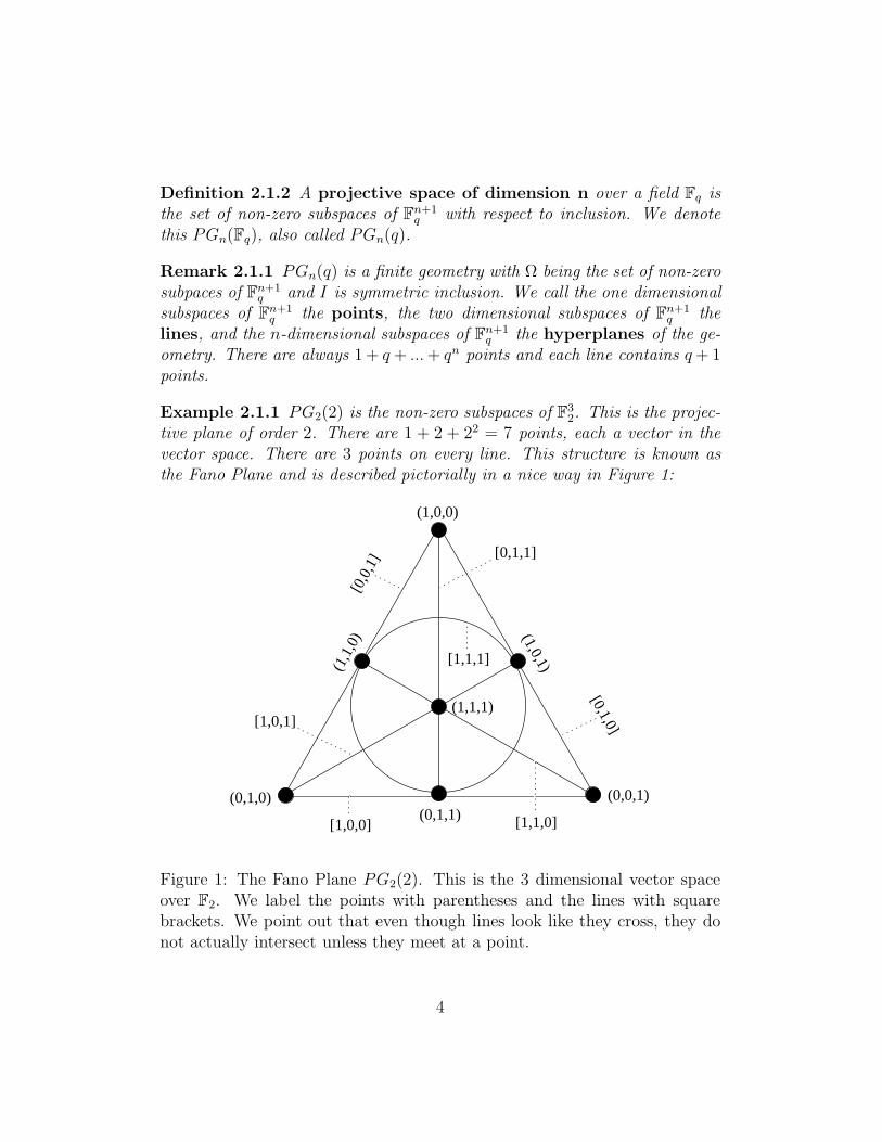
Example 2.1.1 PG2(2) is the non-zero subspaces of F32. This is the projec-

tive plane of order 2. There are 1 + 2 + 22 = 7 points, each a vector in thevector space. There are 3 points on every line. This structure is known asthe Fano Plane and is described pictorially in a nice way in Figure 1:

(1,0,0)

(0,1,0) (0,0,1)(0,1,1)

(1,1

,0) (1,0,1)

(1,1,1)

[1,0,0] [1,1,0]

[0,1,1]

[0,1,0]

[0,0

,1]

[1,0,1]

[1,1,1]

Figure 1: The Fano Plane PG2(2). This is the 3 dimensional vector spaceover F2. We label the points with parentheses and the lines with squarebrackets. We point out that even though lines look like they cross, they donot actually intersect unless they meet at a point.

4

Definition 2.1.3 The points a1, a2, ..., am in PGn(q) are collinear if thereexists a line that contains every point ai.

We say a point p = (x0, ..., xn) is on a line L = [y0, ..., yn] if and only ifx0y0 + x1y1 + ... + xnyn = 0.

There is a more general definition of a projective geometry. It turns out thatall projective spaces with n ≥ 3 are of the form PGn(q) for q a prime power.However, in the special case of n = 2, i.e. the projective planes, there arecertain examples that do not arise from the structure of F

n+1q . In this case,

we do include the general definition of a projective plane.

Definition 2.1.4 A projective plane of order n is a set (P, B, I), whereP is the set of points, B the set of lines, and I the incidence relation betweenthem. The number of points is n2+n+1 and the number of lines is n2+n+1.Any line has n + 1 points on it and there are n + 1 lines on any point. Inaddition, we require that any two points determine a unique line and that anytwo lines intersect in a unique point.

Projective planes in general form an interesting area of study. One of themain conjectures in the area is that projective planes of order n exist if andonly if n is a prime power. It has been shown that projective planes oforder 6 and order 10 do not exist. The case n = 12 is still open. Thoughthere are many fascinating aspects to these general projective planes, fromnow on, we will only be considering projective spaces of the form PGn(q) asdefined above. Like many disciplines in mathematics, we can learn a greatdeal about a structures in projective space by studying the automorphismsof a projective geometry.

Definition 2.1.5 A collineation of a projective geometry is a permutationof the points such that the lines are mapped onto lines, and thus subpaces aremapped to subspaces.

Definition 2.1.6 We consider the set of all invertible semilinear transfor-mations of PGn(q). This set forms a group under composition called ΓL(n+1, q). Now, if H is the pointwise stabiliser of PGn(q), then H is a subgroupof ΓL(n + 1, q) and we get that PΓL(n + 1, q) = ΓL(n + 1, q)/H is called theprojective semilinear group.

5

The set of collineations of a projective geometry forms a group called theautomorphism group, denoted by AutPGn(q).

Theorem 2.1.1 (cf. [1]) Let n ≥ 2. Then AutPGn(q) = PΓL(n + 1, q).

This theorem is known as the Fundamental Theorem of Projective Ge-ometry. Baer has a nice proof of this in [1]. A good source of information onthe collineations of a projective geometry is [15]. The idea of automorphismsof the projective geometry will allow us to decide if structures are unique upto isomorphism.

Definition 2.1.7 Two sets of points in PGn(q) are called projectivelyequivalent if there exists an element α ∈ PΓL(n + 1, q) such that α mapsone set to the other.

2.1.1 Quadratic Forms: Classification

Before we can introduce and discuss quadratic forms, we first introduce bi-linear forms.

Definition 2.1.8 A bilinear form B on Fnq is a map from F

nq × F

nq → Fq

defined by (x, y) → B(x, y) such that:

1. B(x + x′, y) = B(x, y) + B(x′, y)

2. B(x, y + y′) = B(x, y) + B(x, y′)

3. B(ax, y) = aB(x, y) = B(x, ay)

For our purposes, we will only consider symmetric bilinear forms. Theseare the forms which have the special property that B(x, y) = B(y, x) forall x, y. We restrict ourselves to this case since when looking at the seconddefinition of a quadratic form, we find that the bilinear form involved willbe a symmetric one. So, from this point on, we only consider that B issymmetric.

Definition 2.1.9 A quadratic form is a polynomial function arising froma homogeneous polynomial of degree 2 in n-variables. A homogeneous poly-nomial of degree 2 has the form

∑

1≤i≤j≤n

ci,jxixj ci,j ∈ F

6

It follows from this that if e1, ..., en is a basis for Fnq , then a quadratic form

is a map from Fqn → Fq defined by

x =n

∑

i=1

aiei →∑

i≤j

ci,jaiaj ci,j ∈ F

In addition to this, there is an alternate definition of a quadratic form usingbilinear forms (one can show that these two definitions are equivalent):

Definition 2.1.10 A quadratic form Q is a map from Fnq → Fq defined

by x → Q(x) such that:

1. Q(ax) = a2Q(x) for all a ∈ Fq and for all x ∈ Fnq .

2. B(x, y) = Q(x + y) − Q(x) − Q(y) is bilinear. We call B the polar-ization of Q.

Definition 2.1.11 The radical of a bilinear form B over a vector space Fnq

is denoted rad(B) and given by

rad(B) = v ∈ Fnq |B(u, v) = 0 ∀u ∈ F

nq

We are now ready to describe a special condition that can exist for quadraticforms called non-degeneracy. This will eventually lead to nice sets in projec-tive geometries.

Definition 2.1.12 A quadratic form Q on Fnq with polarization B is non-

degenerate if v ∈ rad(B) and Q(v) = 0 implies that v = 0.

With this basic knowledge of quadratic forms, we now classify the threedifferent types of quadratic forms.

Theorem 2.1.2 (cf. [12]) Any quadratic form over Fq is of the one of thefollowing forms:

1. Parabolic: Q0(x) = x1x2 +x3x4 + ...+xn−2xn−1+cx2n where c ∈ 1, a

where a ∈ F×q

2if q is odd and c = 1 if q is even.

2. Hyperbolic: Q1(x) = x1x2 + ... + xn−1xn.

7

3. Elliptic: Q2(x) = x1x2+...+xn−3xn−2+p(xn−1, xn), where p(xn−1, xn)is an irreducible quadratic form in 2 variables.

In general, since quadratic forms are homogeneous polynomials, it makessense to evaluate them on projective points (Q(λx) = λ2Q(x) for all x ∈F

n+1q ). Hence, the zero set of a quadratic form in PGn(q) is a well-defined

set of projective points (i.e. the one-dimensional subspaces of Fn+1q ). In

PGn(q), a set of points that make up the zero set of some quadratic form iscalled a quadric. With these basic definitions and ideas in place, we havethe tools to help us in studying some interesting structures in projectivegeometries that will eventually have nice connections to coding theory.

2.2 Arcs, Caps, and Normal Rational Curves

We introduce of points in finite projective spaces with certain properties.

Definition 2.2.1 A k-cap in PGn(q) is a set of k points such that no 3 arecollinear.

Definition 2.2.2 A k-arc in PGn(q) is a set K of k points with k ≥ n + 1such that no n + 1 points lie in a hyperplane.

Definition 2.2.3 An arc K is complete if it is not properly contained ina larger arc.

Definition 2.2.4 A normal rational curve of PGn(q) is any set of pointsin PGn(q) which is projectively equivalent to

(1, t, t2, ..., tn−1, tn)|t ∈ Fq ∪ (0, 0, ..., 0, 1)

Remark 2.2.1 A normal rational curve contains q + 1 points. We call thepoint (0, 0, ..., 0, 1) the point at infinity, P∞. For q ≥ n, a normal rationalcurve forms a (q + 1)-arc.

Before we look at general k-arcs and k-caps, we look at the special case ofPG2(q). In this space k-arcs and k-caps are the same since hyperplanes inPG2(q) are just the lines.

8

2.3 Ovals and Hyperovals in PG2(q)

In this section, we will only be considering PG2(q), i.e. projective planes.We introduce two special types of k-arcs that are widely studied for theirmany connections to other geometric structures.

Definition 2.3.1 A (q + 1)-arc in PG2(q) is called an oval.

Definition 2.3.2 A (q + 2)-arc in PG2(q) is called a hyperoval.

Definition 2.3.3 A line that intersects an oval, or hyperoval, in 0, 1, 2points is called a external, tangent, secant line respectively.

Proposition 2.3.1 For every q, ovals exist in PG2(q).

Proof:We let (x0, x1, x2) with xi ∈ Fq ∀ i be the general form of a point in PG2(q).Now, we consider the non-degenerate irreducible parabolic quadratic formx1

2 + x0x2. Then the set of zeros of this quadratic form is

(1, t, t2)|t ∈ Fq ∪ (0, 0, 1)

Clearly this is a set of q + 1 points and no 3 are collinear because the formis non-degenerate. Thus this set forms an oval in PG2(q).

Proposition 2.3.2 For q even, hyperovals exist in PG2(q).

Proof:We consider the set above which is attained as the zero set of the quadraticform x1

2 + x0x2. As we have seen this gives us an oval:

θ′ = (1, t, t2)|t ∈ Fq ∪ (0, 0, 1)

Now for a point x ∈ θ′, there are q lines through x that hit θ′ in at mostone more point. However, we know there are q + 1 lines total through x.First, we note that the point (0, 1, 0) 6∈ θ′. Next, we know every point ofθ′ is collinear with (0, 1, 0). We claim that the line that connects any pointx ∈ θ′ to (0, 1, 0) is the unique line through x that hits the oval at no otherpoint. Assume not, then there are two points collinear in θ′ such that the linethrough them contains (0, 1, 0). A general line through (0, 0, 1) and another

9

point of θ′ is [t, 1, 0]. Now, (0, 1, 0) is not on this line as this would implythat 1=0. Lastly, a general line through two points of θ′/(0, 0, 1), (1, t, t2)and (1, s, s2) with s 6= t, is [st, s+ t, 1]. If this line contains (0, 1, 0), then thisimplies s + t = 0 which contradicts that s 6= t. Thus, we can add the point(0, 1, 0) to our oval θ′ to get a hyperoval:

θ = (1, t, t2)|t ∈ Fq ∪ (0, 0, 1), (0, 1, 0)

Note that this does in fact require us to be in characteristic 2 (i.e. we needq to be even).

The construction above is a usual construction of hyperovals which takesan oval and adds a point, called the nucleus. In this case (0, 1, 0) wasthe nucleus. From the previous two propostions we introduce the followingtheorem:

Theorem 2.3.1 (Bose [3]) In PG2(q) we get the following result aboutarcs:

1. For q even, a hyperoval is the largest arc.

2. For q odd, an oval is the largest arc.

The proof of this comes from Bose in 1947.Proof:Let K be a k-arc, and suppose x ∈ K. Then, there is at most 1 other pointin K on a line through x. Now, there are q + 1 lines through x, so we getthat k − 1 ≤ q + 1, so k ≤ q + 2.

1. Now, first we note that a hyperoval allows no tangent lines. This istrue because if K is a hyperoval, then any point x is connected toevery other of the (q + 1) points of K. Since x only has (q + 1) linesthrough it, this requires that every line through x is a secant. Now,let y be a point such that y 6∈ K. If we consider the lines through y,we see that since no tangent lines exist on K, then the lines on y areeither external to K or secants of K. Thus, for each line on y that issecant to K, we get 2 points on K. This implies that q + 2 is even sowe see that q is even.

10

2. This is just a corollary to the above proof. When q is odd, then if Kwere a hyperoval (i.e. q +2 points, which is odd) then there must be atleast one tangent through K, which contradicts that it is a hyperoval.So from this we get that for q odd, we must have k ≤ q + 1. And weknow that ovals do exist in PGn(q).

Not only can we classify that there are no hyperovals in PGn(q), q odd, butwe also have a nice result which classifies the structure of all ovals in thesespaces.

Theorem 2.3.2 (Segre [19]) In PG2(q), q odd, every oval is a conic (thezero set of a non-degenerate quadratic form in 3-variables).

The proof due to Segre in 1955 is long and involved so it is omitted here.This is however a very important result. This classifies all ovals in oddcharacteristic, and thus we no longer study this area. So from this pointon in this section, we will only be considering PG2(q), q = 2h for someh. As we have seen, in this case, there will exist hyperovals. A main areaof current study is to classify all different families of infinite hyperovals. Tointroduce this area of research, we introduce the main form of hyperovals andsome known conditions on how to get them in general. There are not manyconditions, so the research is often left to an exhaustive computer search tofind hyperovals.

As we have seen, we can construct a hyperoval by finding a non-degenerateconic and adding the nucleus. We have a special name for these types ofhyperovals:

Definition 2.3.4 A hyperoval is called regular (or hyperconic) if it isthe union of a non-degenerate conic and its nucleus.

In general, since Segre classified the structure of all ovals in odd characteristic,a widely studied area of projective planes is to classify the structure of allhyperovals in even characteristic. We introduce a few methods that are usedto do this classification, which we point out is still an open problem.

Definition 2.3.5 If q = 2h, the map T : Fq → F2 defined by

T (x) = x + x2 + x4 + ... + x2h−1

=∑

α∈Aut(Fq )

α(x)

is called the trace map.

11

Basic knowledge in algebraic theory gives us the following theorem about thetrace map:

Theorem 2.3.3 For the trace map T :

1. T is well defined.

2. T maps Fq onto F2.

3. T is additive.

4. |ker(T )| = q

2.

5. T (α(x)) = T (x) ∀α ∈ Aut(Fq)

Proof:

1. Now, we note that y2 = y ⇔ y ∈ F2. Let y = T (x). Then T (x)2 +T (x) = T (x) + T (x) = 0 since we are in characteristic 2 and we knowthat T (x)2 = T (x) because we just rearrange all the automorphisms toget them all back again. (Binomial theorem in characteristic 2).

2. Assume that Im(T ) 6= F2. This implies that Im(T ) = 0. So we seethat from this that

x + x2 + x4 + ... + x2h−1

= 0

for all x ∈ Fq. However, this polynomial has degree 2h−1 = q

2and has q

roots, which is impossible. So we get a contradction, thus Im(T ) = F2.

3. It suffices to show that x → x2 is additive. In characteristic 2, (a+b)2 =a2 + b2. This then implies that T (a + b) = T (a) + T (b).

4. T is F2-linear and dim(Im(T )) = 1. This means that dim(ker(T )) =h − 1. Thus, |ker(T )| = 2h−1 = q

2.

5. Note that Aut(Fq) forms a group under composition. With this inmind:

T (α(x)) =∑

β∈Aut(Fq )

β(α(x)) =∑

γ∈Aut(Fq )

γ(x) = T (x)

since βα runs through all the automorphisms.

12

We can now define a certain type of polynomial that will give rise to hyper-ovals.

Definition 2.3.6 A polynomial f such that D(f) = (1, t, f(t)|t ∈ Fq ∪(0, 0, 1), (0, 1, 0) is a hyperoval is called an o-polynomial.

Lemma 2.3.1 (Slope Condition) Let f : Fq → Fq be a 1 − 1 and ontofunction, q = 2h. Then f is an o-polynomial if and only if the followingcondition holds:

f(x) + f(y)

x + y6=

f(x) + f(z)

x + z

for all distinct x, y, z ∈ Fq.

In addtion to this, Tim Penttila added another condition to require that afunction is an o-polynomial.

Theorem 2.3.4 (Penttila [16]) Let, f, F, g : Fq → Fq be functions, qeven. Suppose that f(0) = 0, f(1) = 1, F (0) = 0 and that the followingcondition holds:

T(

F(f(s) + f(t)

s + t

)

(g(s) + g(t)))

= 1

for all s, t ∈ Fq and s 6= t. Then we have that f is an o-polynomial.

Proof:First, we suppose that f is not injective. Then there would exist two elementss 6= t with f(s) = f(t). This then implies that

1 = T(

F(f(s) + f(t)

s + t

)

(g(s) + g(t)))

= T (F (0)(g(s) + g(t))) = T (0) = 0

This is a contradiction, and thus f is injective.

Now, we show that f satisfies the slope condition (Lemma 2.3.1). Assumethat the slope condition is not satisfied. Now we let r 6= s 6= t 6= r all beelements in Fq with the property that

f(s) + f(t)

s + t=

f(s) + f(r)

s + r= a

13

This gives us that f(s)+ f(t) = a(s + t) and f(s)+ f(r) = a(s + r). We addthese two equations together to get

f(t) + f(r) = a(t + r) ⇒ a =f(t) + f(r)

t + r(1)

Now because of the assumption in the theorem, T (F (a)(g(s)+ g(t))) = 1and also T (F (a)(g(s) + g(r))) = 1. Now we recall that the trace function isadditive and so we add these two equations to get

T (F (a)(g(t) + g(r))) = 1 + 1 = 0

since we are in characteristic 2. But because of Equation 1, we know thatthis implies that

T(

F(f(t) + f(r)

t + r

)

(g(t) + g(r))

= 0

which is a contradiction. Thus we see that f satisfies the slope condition.Together, since f is injective and satisfies the slope condition, Lemma 2.3.1implies that f is indeed an o-polynomial.

This condition helps to test if a function is an o-polynomial. From here weget another nice method that will eliminate possible functions from beingo-polynomials.

2.3.1 Glynn’s Condition for Existence of Hyperovals

David Glynn has an interesting condition for a function f(x) to give a hy-peroval. We introduce some basic theorems, definitions and lemmas that willlead us to Glynn’s final result. This area is most interesting as it includes awide area of combinatorial mathematics, not just projective geometry. As wehave seen, when considering a hyperoval, we can assume it has the generalform

θ = (1, t, f(t))|t ∈ Fq ∪ (0, 1, 0), (0, 0, 1)

where f(t) is an o-polynomial with degree less than or equal to q − 2. Givenθ as is, we want to distinguish a condition that will require f to be an o-polynomial. We note that most of the material in the following section isbased on [9].

14

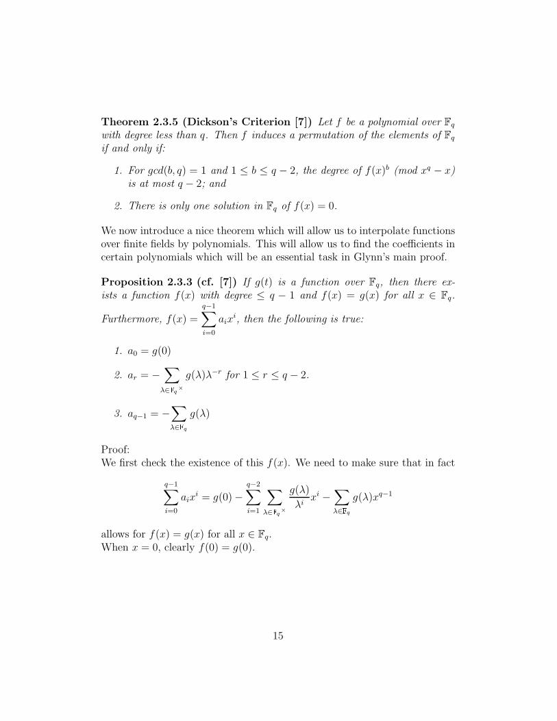
Theorem 2.3.5 (Dickson’s Criterion [7]) Let f be a polynomial over Fq

with degree less than q. Then f induces a permutation of the elements of Fq

if and only if:

1. For gcd(b, q) = 1 and 1 ≤ b ≤ q − 2, the degree of f(x)b (mod xq − x)is at most q − 2; and

2. There is only one solution in Fq of f(x) = 0.

We now introduce a nice theorem which will allow us to interpolate functionsover finite fields by polynomials. This will allow us to find the coefficients incertain polynomials which will be an essential task in Glynn’s main proof.

Proposition 2.3.3 (cf. [7]) If g(t) is a function over Fq, then there ex-ists a function f(x) with degree ≤ q − 1 and f(x) = g(x) for all x ∈ Fq.

Furthermore, f(x) =

q−1∑

i=0

aixi, then the following is true:

1. a0 = g(0)

2. ar = −∑

λ∈Fq×

g(λ)λ−r for 1 ≤ r ≤ q − 2.

3. aq−1 = −∑

λ∈Fq

g(λ)

Proof:We first check the existence of this f(x). We need to make sure that in fact

q−1∑

i=0

aixi = g(0) −

q−2∑

i=1

∑

λ∈Fq×

g(λ)

λixi −

∑

λ∈Fq

g(λ)xq−1

allows for f(x) = g(x) for all x ∈ Fq.When x = 0, clearly f(0) = g(0).

15

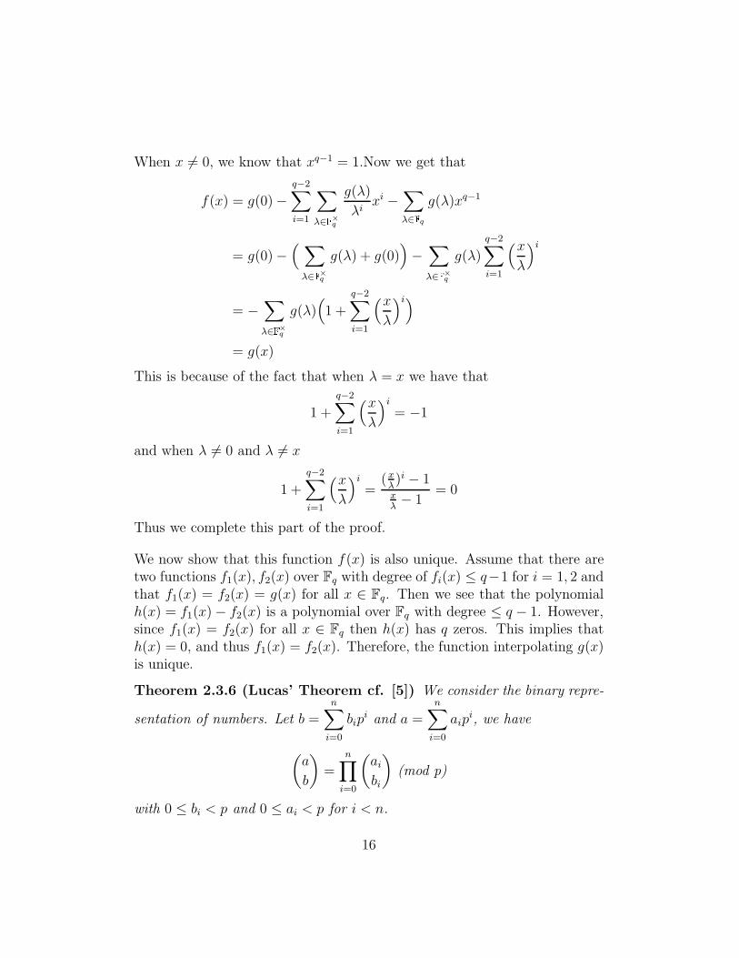
When x 6= 0, we know that xq−1 = 1.Now we get that

f(x) = g(0) −

q−2∑

i=1

∑

λ∈F×q g(λ)

λixi −

∑

λ∈Fq

g(λ)xq−1

= g(0) −(

∑

λ∈F×q g(λ) + g(0))

−∑

λ∈F×q g(λ)

q−2∑

i=1

(x

λ

)i

= −∑

λ∈F×q g(λ)(

1 +

q−2∑

i=1

(x

λ

)i)

= g(x)

This is because of the fact that when λ = x we have that

1 +

q−2∑

i=1

(x

λ

)i

= −1

and when λ 6= 0 and λ 6= x

1 +

q−2∑

i=1

(x

λ

)i

=(x

λ)i − 1

xλ− 1

= 0

Thus we complete this part of the proof.

We now show that this function f(x) is also unique. Assume that there aretwo functions f1(x), f2(x) over Fq with degree of fi(x) ≤ q−1 for i = 1, 2 andthat f1(x) = f2(x) = g(x) for all x ∈ Fq. Then we see that the polynomialh(x) = f1(x) − f2(x) is a polynomial over Fq with degree ≤ q − 1. However,since f1(x) = f2(x) for all x ∈ Fq then h(x) has q zeros. This implies thath(x) = 0, and thus f1(x) = f2(x). Therefore, the function interpolating g(x)is unique.

Theorem 2.3.6 (Lucas’ Theorem cf. [5]) We consider the binary repre-

sentation of numbers. Let b =n

∑

i=0

bipi and a =

n∑

i=0

aipi, we have

(

a

b

)

=n

∏

i=0

(

ai

bi

)

(mod p)

with 0 ≤ bi < p and 0 ≤ ai < p for i < n.

16

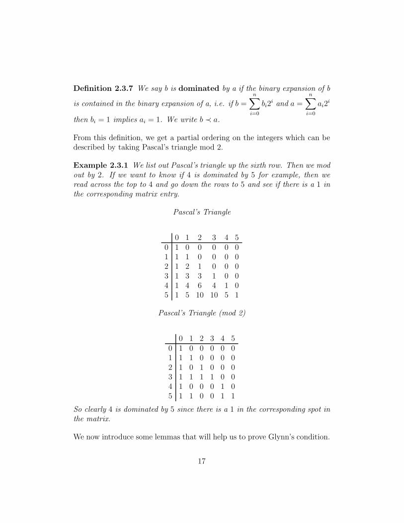
Definition 2.3.7 We say b is dominated by a if the binary expansion of b

is contained in the binary expansion of a, i.e. if b =

n∑

i=0

bi2i and a =

n∑

i=0

ai2i

then bi = 1 implies ai = 1. We write b ≺ a.

From this definition, we get a partial ordering on the integers which can bedescribed by taking Pascal’s triangle mod 2.

Example 2.3.1 We list out Pascal’s triangle up the sixth row. Then we modout by 2. If we want to know if 4 is dominated by 5 for example, then weread across the top to 4 and go down the rows to 5 and see if there is a 1 inthe corresponding matrix entry.

Pascal’s Triangle

0 1 2 3 4 50 1 0 0 0 0 01 1 1 0 0 0 02 1 2 1 0 0 03 1 3 3 1 0 04 1 4 6 4 1 05 1 5 10 10 5 1

Pascal’s Triangle (mod 2)

0 1 2 3 4 50 1 0 0 0 0 01 1 1 0 0 0 02 1 0 1 0 0 03 1 1 1 1 0 04 1 0 0 0 1 05 1 1 0 0 1 1

So clearly 4 is dominated by 5 since there is a 1 in the corresponding spot inthe matrix.

We now introduce some lemmas that will help us to prove Glynn’s condition.

17

Lemma 2.3.2 θ is a hyperoval if and only if the q2−q lines of PG2(2, q) notpassing through (0, 1, 0) and (0, 0, 1) always intersect θ in an even number ofpoints.

Proof:First, we verify there are q2 − q lines in PG2(q) not through (0,0,1) and(0,1,0). Clearly there are q +1 lines through (0,0,1) and through (0,1,0), butone of those is the line between (0,0,1) and (0,1,0) so there are a total of2q +1 lines in PG2(q) which go through either (0,0,1) or (0,1,0). Since thereare a total of q2 + q + 1 lines, there are q2 + q + 1 − 2q − 1 = q2 − q lines ofPG2(q) not going through (0,0,1) and (0,1,0).Now, assume that θ is a hyperoval. Then we know that every line in PG2(q)either does not contain points of θ or is a secant of θ. Therefore, they intersectin 0 or 2 points.Now, assume that the q2 − q lines in PG2(q) not through (0,0,1) and (0,1,0)always intersect θ in an even number of points. We have to show that θ isa hyperoval, i.e. that no line of the plane contains more than 2 points of θ.Consider another point of θ, P. There are q − 1 lines through P that mustintersect in at least one other point, not (0,0,1) or (0,1,0). This is because Pmust have q+1 lines on it, with one through (0,0,1) and one through (0,1,0),and the line must intersect θ again by our assumption. Now, there are onlyq − 1 points left on θ \ (0, 1, 0), (0, 0, 1), P since θ has q + 2 points. Sothere are q − 1 lines through P and q − 1 points left on θ \ (0, 1, 0), (0, 0, 1)so each line through P must intersect θ \ (0, 1, 0), (0, 0, 1) at at most oneother point. These two statements together say that the lines through P hitθ \ (0, 1, 0), (0, 0, 1) at exactly one more point. So these q − 1 lines eachcontain exactly two points of θ. So now we connect each point to (0,0,1) witha line and we have a total of q+1 points, no three collinear, since (0,0,1) is noton any of the lines we had before. Note, these lines cannot also go through(010) because there is a unique line between (0,0,1) and (0,1,0) which byassumption cannot hit any points of θ \ (0, 1, 0), (0, 0, 1). So θ \ (0, 1, 0)is an oval. Lastly, we show that (0,1,0) is the nucleus of the oval which wehave created. This is evident by the fact that each point of θ \ (0, 1, 0)has one more line on it which goes through (0,1,0) and these lines were notalready in θ \ (0, 1, 0) by assumption. Thus, we add (0,0,1) and see thatno 3 points are collinear and we have q + 2 points. So θ is a hyperoval.

This gives a nice combinatorial condition for a hyperoval.

18

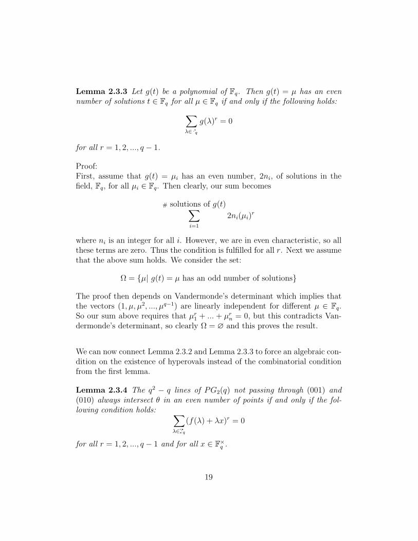
Lemma 2.3.3 Let g(t) be a polynomial of Fq. Then g(t) = µ has an evennumber of solutions t ∈ Fq for all µ ∈ Fq if and only if the following holds:

∑

λ∈Fq

g(λ)r = 0

for all r = 1, 2, ..., q − 1.

Proof:First, assume that g(t) = µi has an even number, 2ni, of solutions in thefield, Fq, for all µi ∈ Fq. Then clearly, our sum becomes

# solutions of g(t)∑

i=1

2ni(µi)r

where ni is an integer for all i. However, we are in even characteristic, so allthese terms are zero. Thus the condition is fulfilled for all r. Next we assumethat the above sum holds. We consider the set:

Ω = µ| g(t) = µ has an odd number of solutions

The proof then depends on Vandermonde’s determinant which implies thatthe vectors (1, µ, µ2, ..., µq−1) are linearly independent for different µ ∈ Fq.So our sum above requires that µr

1 + ... + µrn = 0, but this contradicts Van-

dermonde’s determinant, so clearly Ω = ∅ and this proves the result.

We can now connect Lemma 2.3.2 and Lemma 2.3.3 to force an algebraic con-dition on the existence of hyperovals instead of the combinatorial conditionfrom the first lemma.

Lemma 2.3.4 The q2 − q lines of PG2(q) not passing through (001) and(010) always intersect θ in an even number of points if and only if the fol-lowing condition holds:

∑

λ∈Fq

(f(λ) + λx)r = 0

for all r = 1, 2, ..., q − 1 and for all x ∈ F×q .

19

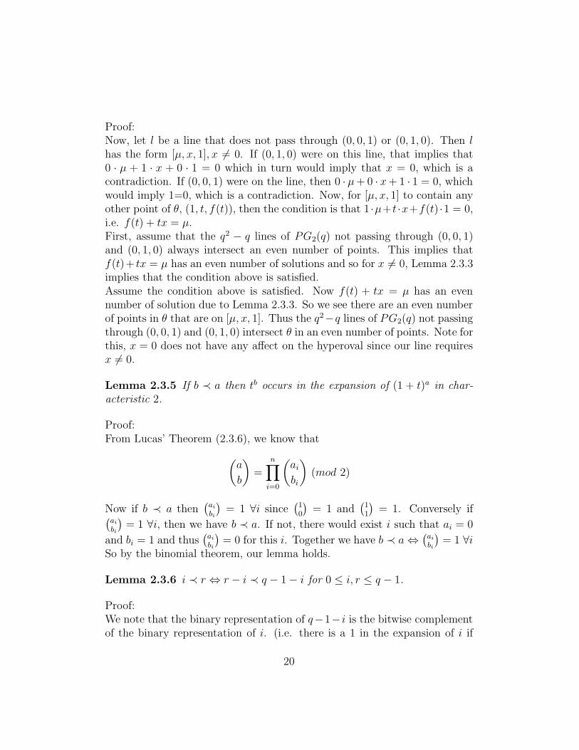
Proof:Now, let l be a line that does not pass through (0, 0, 1) or (0, 1, 0). Then lhas the form [µ, x, 1], x 6= 0. If (0, 1, 0) were on this line, that implies that0 · µ + 1 · x + 0 · 1 = 0 which in turn would imply that x = 0, which is acontradiction. If (0, 0, 1) were on the line, then 0 · µ + 0 · x + 1 · 1 = 0, whichwould imply 1=0, which is a contradiction. Now, for [µ, x, 1] to contain anyother point of θ, (1, t, f(t)), then the condition is that 1 ·µ+t ·x+f(t) ·1 = 0,i.e. f(t) + tx = µ.First, assume that the q2 − q lines of PG2(q) not passing through (0, 0, 1)and (0, 1, 0) always intersect an even number of points. This implies thatf(t)+ tx = µ has an even number of solutions and so for x 6= 0, Lemma 2.3.3implies that the condition above is satisfied.Assume the condition above is satisfied. Now f(t) + tx = µ has an evennumber of solution due to Lemma 2.3.3. So we see there are an even numberof points in θ that are on [µ, x, 1]. Thus the q2−q lines of PG2(q) not passingthrough (0, 0, 1) and (0, 1, 0) intersect θ in an even number of points. Note forthis, x = 0 does not have any affect on the hyperoval since our line requiresx 6= 0.

Lemma 2.3.5 If b ≺ a then tb occurs in the expansion of (1 + t)a in char-acteristic 2.

Proof:From Lucas’ Theorem (2.3.6), we know that

(

a

b

)

=

n∏

i=0

(

ai

bi

)

(mod 2)

Now if b ≺ a then(

ai

bi

)

= 1 ∀i since(

10

)

= 1 and(

11

)

= 1. Conversely if(

ai

bi

)

= 1 ∀i, then we have b ≺ a. If not, there would exist i such that ai = 0

and bi = 1 and thus(

ai

bi

)

= 0 for this i. Together we have b ≺ a ⇔(

ai

bi

)

= 1 ∀iSo by the binomial theorem, our lemma holds.

Lemma 2.3.6 i ≺ r ⇔ r − i ≺ q − 1 − i for 0 ≤ i, r ≤ q − 1.

Proof:We note that the binary representation of q−1− i is the bitwise complementof the binary representation of i. (i.e. there is a 1 in the expansion of i if

20

and only if there is a zero in the expansion of q − 1 − i.)“⇐” Assume i 6≺ r. Consider the first coefficient with i containing a 1 and rcontaining a 0. ⇒ r − i has corresponding coefficent 1.But i has coefficient 1 ⇔ q − 1 − i has coefficient 0.⇒ r − i 6≺ q − 1 − i. This proves the result by contraposition.

“⇒” Let there be a 1 as coefficient of r − i.Since i ≺ r, ⇒ r has corresponding coefficient 1 and i has correspondingcoefficient 0.i having 0 ⇒ q − 1 − i has corresponding coefficient 1.⇒ r − i ≺ q − 1 − i.So clearly r − i ≺ q − 1 − i.Now, we can put all of the previous results together to get a nice condi-tion formulated by Glynn which will determine whether or not f(t) is ano-polynomial.

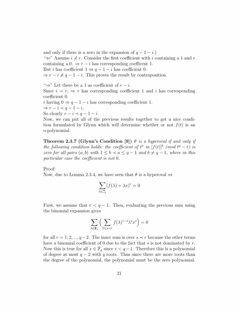
Theorem 2.3.7 (Glynn’s Condition [9]) θ is a hyperoval if and only ifthe following condition holds: the coefficient of ta in [f(t)]b (mod tq − t) iszero for all pairs (a, b) with 1 ≤ b ≺ a ≤ q − 1 and b 6= q − 1, where in thisparticular case the coefficient is not 0.

Proof:Now, due to Lemma 2.3.4, we have seen that θ is a hyperoval ⇔

∑

λ∈Fq

(f(λ) + λx)r = 0

First, we assume that r < q − 1. Then, evaluating the previous sum usingthe binomial expansion gives

∑

λ∈Fq

(

∑

0≤s≺r

f(λ)r−sλsxs)

= 0

for all r = 1, 2, ..., q−2. The inner sum is over s ≺ r because the other termshave a binomial coefficient of 0 due to the fact that s is not dominated by r.Now this is true for all x ∈ Fq since r < q−1. Therefore this is a polynomialof degree at most q − 2 with q roots. Thus since there are more roots thanthe degree of the polynomial, the polynomial must be the zero polynomial.

21

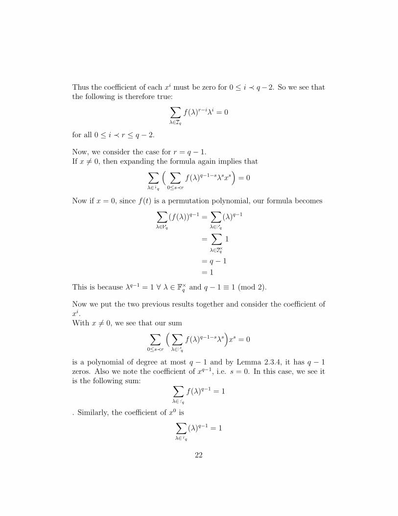
Thus the coefficient of each xi must be zero for 0 ≤ i ≺ q−2. So we see thatthe following is therefore true:

∑

λ∈Fq

f(λ)r−iλi = 0

for all 0 ≤ i ≺ r ≤ q − 2.

Now, we consider the case for r = q − 1.If x 6= 0, then expanding the formula again implies that

∑

λ∈Fq

(

∑

0≤s≺r

f(λ)q−1−sλsxs)

= 0

Now if x = 0, since f(t) is a permutation polynomial, our formula becomes∑

λ∈Fq

(f(λ))q−1 =∑

λ∈Fq

(λ)q−1

=∑

λ∈F×q 1

= q − 1

= 1

This is because λq−1 = 1 ∀ λ ∈ F×q and q − 1 ≡ 1 (mod 2).

Now we put the two previous results together and consider the coefficient ofxi.With x 6= 0, we see that our sum

∑

0≤s≺r

(

∑

λ∈Fq

f(λ)q−1−sλs)

xs = 0

is a polynomial of degree at most q − 1 and by Lemma 2.3.4, it has q − 1zeros. Also we note the coefficient of xq−1, i.e. s = 0. In this case, we see itis the following sum:

∑

λ∈Fq

f(λ)q−1 = 1

. Similarly, the coefficient of x0 is∑

λ∈Fq

(λ)q−1 = 1

22

This therefore implies that our formula is xq−1 + ... − 1 = 0. But xq−1 − 1 isthe unique formula with q − 1 zeros, so we see that our above double sum inthis case is xq−1 − 1. But this is also true for our case with x = 0 since wehave seen that for x = 0 we get our sum equal to 1. Thus, together we seethat when r = q − 1

∑

λ∈Fq

(f(λ) + λx)q−1 = xq−1 − 1

∀ x ∈ Fq.We use this to see that the coefficient of xq−1 is clearly 1, and to see that thecoefficient of all xi with 1 ≤ i ≤ q − 2 is 0 so that:

∑

λ∈Fq

f(λ)q−1−iλi = 0

Now, with both cases r = q − 1 and r ≤ q − 2 together, we see that forr ≤ q − 1, we see that

∑

λ∈Fq

f(λ)r−iλi = 0

for all 0 ≤ i ≺ r ≤ q − 1 as long as (i, r) 6= (0, q − 1) or (q − 1, q − 1). Wehave seen that in the (0, q − 1) case we get the sum is 1. In the (q − 1, q − 1)case the sum is also 1.

We now use the formula for evaluation of polynomials over a finite field(2.3.3). We first note that −i = q − 1 − i in this case due to reduction bytq − t. This gives us that the coefficient of t−i in f(t)r−i is given by:

a−i =∑

λ∈Fq

f(λ)r−iλ−(−i)

So this evaluation result along with our conclusion from above implies thatthe coefficient of t−i in f(t)r−i is 0, i.e. a−i = 0. Now, we can mod out bytq − t. By assumption, i ≺ r and thus by Lemma 2.3.6 r− i ≺ q−1− i. Thisimplies that r− i ≺ −i. So, set r− i = b,−i = a and we see that for all pairsof (a, b) with 1 ≤ b ≺ a ≤ q − 1 with b 6= q − 1, we get that the coefficient ofta in f(t)b (mod tq − t) is 0. This then proves the result in one direction. Sowe turn to the other direction.

23

Now, we assume that all the coefficients are zero. So now, we use this in theexpansion of

∑

λ∈Fq

(f(λ) + λx)r = 0

and we see that this is true for all 1 ≤ r ≤ q − 2. For the case r = q − 1, andthus x 6= 0, we get that

∑

λ∈Fq

(f(λ) + λx)r

reduces to

∑

λ∈Fq

f(λ)q−1 +∑

λ∈Fq

λq−1xq−1 =∑

λ∈Fq

f(λ)q−1 + xq−1

Now since x 6= 0, we see that xq−1 = 1 and so for the entire expression to bezero, we need

∑

λ∈Fq

f(λ)q−1 = 1

But this is true since we assume that the coefficient [tq−1] in f(t)q−1 is notzero, thus it must be 1. From our interpolation formula, this coefficient isgiven by

aq−1 = −∑

λ∈Fq

f(λ)q−1

Therefore, we actually get that

∑

λ∈Fq

(f(λ) + λx)r = 0

for all 1 ≤ r ≤ q − 1 except (0, q − 1). Therefore θ is a hyperoval. Thiscompletes the result.

Remark 2.3.1 Glynn’s paper does not include the additional assumptionthat the coefficient of [tq−1] in f(t)q−1 is not 0. We have found that the proofrequires this assumption and thus we have added it. We make a note thatthis slight change has been added upon suggestion by Stan Payne.

24

Remark 2.3.2 While this theorem may seem hard to use, we never reallyraise a polynomial to a power. Instead, just consider the coefficients as de-fined by Proposition 2.3.3 of a power of a polynomial function.

Additionally, we get the following result due to Segre and Bartocci as acorollary:

Corollary 2.3.1 ([18]) An o-polynomial has only even degree terms.

Proof:We apply Glynn’s condition with b = 1. Since if c is odd, then 1 ≺ c and thecoefficient of xc must be zero.

2.4 k-arcs, k-caps and minihypers in PGn(q)

We now extend the general idea of ovals and hyperoval to any dimension ninstead of just the projective planes. Hyperovals and ovals are nice becausethey are simultaneously k-arcs and k-caps. As we have previously seen, thenormal rational curves form (q + 1)-arcs if q ≥ n. This of course leads to thequestion of whether other large size arcs exist in these spaces. We not onlywant to find other k-arcs, but we especially would like to find k-arcs whichare complete and not normal rational curves. To help us study this area, weintroduce a few theorems that help us to classify if other k-arcs exist.

2.4.1 k-arcs in general

Theorem 2.4.1 (cf. [13]) If every (q + 1)-arc of PGn(q), n ≥ 3 and q ≥n + 3, is a normal rational curve, then q + 1 is the maximum value of k forwhich k-arcs exist in PGn+1(q).

This theorem helps us to search for large size arcs if we can classify thatsome projective space has only normal rational curves as (q + 1)-arcs. Thisnaturally leads us to wonder if we can extend a normal rational curve to a(q + 2)-arc. Due to Storme and Thas, we have the following result:

Theorem 2.4.2 (cf. [13]) A point P = (a0, a1, ..., aq−2) extends the normalrational curve K = (1, t, t2, ..., tq−2)|t ∈ Fq∪(0, 0, ..., 0, 1) to a (q+2)-arc

25

if and only if F (X) =

q−2∑

i=0

aq−2−iXi+1 defines a hyperoval

θ = 1, t, F (t))| t ∈ Fq ∪ (0, 0, 1), (0, 1, 0)

in PG2(q). Moreover, we get a 1− 1 correspondence if we require F (1) = 1.

We also question whether there are maximal complete arcs which are notnormal rational curves. David Glynn was able to come up with an examplewhich we will present momentarily. We first provide a lemma about normalrational curves which will help us to prove Glynn’s unique result.

Lemma 2.4.1 (cf. [22]) A normal rational curve in PG4(9) is an inter-section of zero sets of non-degenerate irreducible quadratic forms (i.e. anintersection of non-degenerate quadrics).

Proof:As we have seen we may assume that our normal rational curve T has theform:

T = (1, t, t2, t3, t4)|t ∈ F9 ∪ (0, 0, 0, 0, 1)

due to projective equivalence. Clearly, we see that x21 = x0x2, x2

2 = x0x4,x2

3 = x2x4, and x0x3 = x1x2 are all irreducible quadratic forms (quadrics)containing T . Furthermore, we show that the intersection of these quadricsis T . Now let (x0, x1, x2, x3, x4) be in the intersection of the quadrics. Next,fix x0 = 1. Then call x1 = s. So necessarily from the first quadratic form,x2 = s2. This leads us to see that x4 = (s2)2 = s4 by the second quadraticform. The third quadratic form gives us x3 = s3. Lastly, if we instead letx0 = 0, then the forms imply that this is necessarily the point (0, 0, 0, 0, 1).This proves the result.

We are now ready to introduce an maximal complete arc that is not projec-tively equivalent to a normal rational curve.

Theorem 2.4.3 (Glynn’s 10-arc [8]) In PG4(9), a normal rational curveis a 10-arc. However, there is also another 10-arc which is not projectivelyequivalent to a normal rational curve, but instead it is projectively equivalentto the following set of points:

L = (1, x, x2 + ηx6, x3, x4)| x ∈ F9 ∪ (0, 0, 0, 0, 1)

with η ∈ F9 and η4 = −1.

26

We give the following nice proof of this statement described in [22].Proof:We first show that L is a 10-arc. To do this, we verify that any five pointsfrom L span a 5-dimensional vector space over F9. First consider only pointsnot of the form (0, 0, 0, 0, 1). Now we let det(1, xi, x

2i +ηx6

i , x3i , x

4i ) denote the

determinant of the following matrix:

1 x1 x21 + ηx6

1 x31 x4

1...

......

......

1 x5 x25 + ηx6

5 x35 x4

5

So, we assume that these five points do not span a 5-dimensional vector space.This implies that det(1, xi, x

2i + ηx6

i , x3i , x

4i ) = 0. Since the determinant is a

bilinear form, this also gives us

det(1, xi, x2i + ηx6

i , x3i , x

4i ) = det(1, xi, x

2i , x

3i , x

4i ) + ηdet(1, xi, x

6i , x

3i , x

4i ).

This in turn implies that

det(1, xi, x2i , x

3i , x

4i ) = −ηdet(1, xi, x

6i , x

3i , x

4i ). (2)

Now, since F9 has characteristic 3, the map x → x3 is a field automorphism(Frobenius automorphism). This gives us that

[det(1, xi, x2i , x

3i , x

4i )]

3 = −η3[det(1, xi, x6i , x

3i , x

4i )]

3.

This gives us the following relation (due to the fact that in F9 we have thatx9 = x ∀x):

det(1, x3i , x

6i , xi, x

4i ) = −η3det(1, x3

i , x2i , xi, x

4i ).

And from linear algebra we know we can rearrange the rows of a matrix with-out changing the determinant, so suitable rearranging gives us the followingrelation:

det(1, xi, x3i , x

4i , x

6i ) = −η3det(1, xi, x

2i , x

3i , x

4i ).

Additionally by equation 2 along with the previous result we get that

det(1, xi, x3i , x

4i , x

6i ) = η4det(1, xi, x

6i , x

3i , x

4i ) = η4det(1, xi, x

3i , x

4i , x

6i )

by rearranging. Now due to Vandermonde’s determinant, we know thatdet(1, xi, x

3i , x

4i , x

6i ) 6= 0, and so this implies that η4 = 1. However, we assume

27

in the theorem that η4 = −1, and thus we get a contradiction. We can alsomake a symmetric argument if we consider one of the five points to be thepoint (0, 0, 0, 0, 1), and we will get a similar contradiction. Thus we see thatany 5 (=4+1) points of L are linearly independent and so L is a 10-arc.

We now must show that L is not a normal rational curve. From Lemma2.4.1 we know that a normal rational curve in PG4(9) is an intersection ofnon-degenerate quadrics. We will prove that L is not the intersection of non-degenerate quadrics. We assume that L is an intersection of quadrics, Qi,i.e. L = ∩i∈IQi. We let

Qi = (x0, ..., x4)|xi ∈ F9, Qi(x0, ..., x4) = 0

where Qi is a quadratic form, i.e. 0 6= Qi =

4∑

r,s=0

c(i)r,sxrxs and c

(i)r,s ∈ F9. Now,

in each quadratic form the coefficient c(i)4,4 = 0 because (0, 0, 0, 0, 1) ∈ L. Since

(0, 0, 1, 0, 0) 6∈ L then there exists a Q = Qi such that c2,2 = c(i)2,2 6= 0. With

this Q, we consider the following polynomial:

∑

j

ajxj = f(x) = Q(1, x, x2 + ηx6, x3, x4) ∈ F9[x]

Now we know that (1, x, x2 + ηx6, x3, x4) ∈ L for every x ∈ F9, and so F9

vanishes on f(x), i.e. f(x) = 0 for all x ∈ F9. Because of this, basic fieldtheory tells us that f(x) must be a multiple of x9 −x. Therefore we see thatf(x) = (x9 − x)h(x) where h(x) ∈ F9. Since c2,2 6= 0 then we know that(x2 + ηx6)(x2 + ηx6) is part of f(x). This implies that f(x) has degree 12,and thus h(x) has degree 3. Now, from this we see that f(x) has no termwith degree 8, and thus a8 = 0. However, since c2,2(x

2 + ηx6)(x2 + ηx6) is

part of f(x) and c(i)4,4 = 0, we see that a8 = 2c2,2η. This is a contradiction as

2c2,2η 6= 0. Therefore, L cannot be an intersection of quadrics. By Lemma2.4.1 we see that since a normal rational curve is an intersection of quadrics,then L cannot be a normal rational curve.

To my knowledge, this is the only known complete arc which is not attainedfrom a normal rational curve in PGn(q) with n > 2. This is an amazingresult, and it is a big challenge to find further examples like this.

28

2.4.2 A Glimpse into the World of k-caps: Ovoids

We can also study k-caps in general projective spaces. For our purposes, weonly consider a special type of k-cap. The special k-cap we are interestedin is called an ovoid. There are two separate definitions for an ovoid thatturn out to be the same in some cases. In general, ovoids are not onlyinteresting in their connections to codes, but also they have a great deal ofrelationships with other structures created from projective spaces such asgeneralized quadrangles, spreads, and translation planes to name a few. Webegin with the definition of an ovaloid, which in the special case of n = 3 wecall an ovoid.

Definition 2.4.1 (due to Segre) In PG3(q), a (q2 + 1)-cap is called anovoid. This can also be stated that an ovoid is a set of (q2 + 1) points inPG3(q) such that no 3 are collinear.

Example 2.4.1 We consider the zero set of the following non-degenerateelliptic quadratic form (i.e. elliptic quadric) in PG3(q):

x20 + x0x1 + ax2

1 + x2x3

where a ∈ Fq such that x2 + x + a is irreducible over Fq. We see that the setof points of PGn(q) which are zero under this form is

(s, t, s2 + st + at2, 1)|s, t ∈ Fq ∪ (0, 0, 1, 0)

and this is a set of q2 + 1 projective points. Since the points come from anon-degenerate elliptic quadratic form, no three are collinear.

From here we can further study ovoids and their properties.

Proposition 2.4.1 (cf. [4]) In PG3(2) a maximum k-cap is not an ovoid,but has 8 points.

Proof:A hyperplane in PG3(2) has (23 − 1)/(2 − 1) = 7 points. Since there are 15points total, then the complement of a hyperplane has 8 points. Clearly, nothree of these are collinear since if they were then there would be a line whichis disjoint from a hyperplane, which is a contradiction to the dimension. Since

29

in this space on any point there are 7 lines, then the maximum possible sizefor a k-cap is 8.

We proved the previous proposition because it is a special case. For all otherq, that is q > 2, we get the nice following result:

Theorem 2.4.4 (cf. [2]) In PG3(q), q > 2, an ovoid is a maximum cap.

Proof:For q odd, let P and Q be points of an ovoid O and l the line they span.Now, there are q + 1 planes on l, and each of these planes can intersectO in at most q − 1 points more (because q is odd and we know that anoval is the largest cap in a plane). So along with P and Q, we get that|O| ≤ (q + 1)(q − 1) + 2 = q2 + 1. As mentioned above, the elliptic quadricattains that bound and hence we have equality.Now assume q is even. First we show that through each point there is at leastone tangent to O. To do this, we assume that there are no tangent lines toO. Then, consider two points P and Q in O and the line that connects them,l. There are q + 1 planes on l and each of these planes must intersect O ina hyperoval, q + 2 points. So we have q + 1 planes containing q points otherthan P and Q. So we see that this implies that |O| = q(q+1)+2 = q2+q+2.Now, we consider a line g which contains no points of O (on any point outsideof O we have this or else |O| = 2(q2 + q + 2) which is not true). Now, let kdenote the number of planes through g intersecting O in a hyperoval (q + 2)points. Then we get that

k(q + 2) = |O| = q2 + q + 2

Now rewriting we get that k(q + 2) = (q − 1)(q + 2) + 4. Then this impliesthat (q + 2) must divide 4 and so q = 2, but we have excluded this case.Thus we get a contradiction, so every point of O must contain at least onetangent line.

We now know that if q 6= 2, then there exists a tangent line, m, to O atsome point Z. If we consider the q +1 planes about m, we see that these canintersect O in at most q + 1 points or else would contradict the maximalityof a hyperoval. If each plane on m meets O in at most q points we have that|O| ≤ (q + 1)(q − 1) + 1 ≤ q2 which is a contradiction. So we can assumethat there is a plane π on m meeting O in an oval (q + 1 points). Then, we

30

know since q is even that there is a nucleus to this oval, which we can add toform a hyperoval. Because π cannot meet O in a hyperoval, then the nucleusmust lie on at least one secant line of O, call this line m′. Then, each planeon m′ meets the oval in a tangent. Therefore, any of these planes meets Oin at most q + 1 points. So we consider the q + 1 planes on m′ which canmeet O in at most q − 1 lines other than the two points making m′. Thisgives |O| ≤ (q + 1)(q − 1) + 2 = q2 + 1. Again, we have the elliptic quadricfor equality and so the result is proved.We now introduce a nice theorem about the structure of ovoids. To provethis theorem, we find the following lemma useful.

Lemma 2.4.2 (cf. [4]) Let Ω be an ovoid in PG3(q), q > 2. Then forP ∈ Ω, the union of all the tangent lines on P is a plane.

Proof:Case 1: Assume q is odd. Let P, Q be two points of Ω. Now, with q beingodd, each plane of PG3(q) can meet Ω in at most q + 1 points. Now theplanes that are spanned by P and Q intersect Ω in exactly q + 1 points (anoval), or we would get a contradiction to the maximality of Ω. Therefore, asecant line of Ω can only lie on the planes meeting Ω in an oval. Now welet l1, l2 be two tangents to Ω at P and π be the plane they span. Since πcontains two tangents to Ω, then it cannot meet Ω in an oval, thus it cannotcontain any secants. Therefore we see that π ∩Ω = P so therefore π mustcontain all the tangents to P so it is the union of all tangents on P .Case 2: Assume q is even. Now let P ∈ Ω and l be a tangent line to Ω onP . We have seen in Theorem 2.4.4 that there must be a plane π on l withπ ∩Ω being an oval with nucleus N on some secant line, m′. Since q is even,we have seen that this each point in this oval is on a tangent line connectedto N . So if we consider any plane on m′, this plane must contain a tangentline on N by intersection with π. Therefore we see that each plane on m′

intersects Ω in an oval. In any of these planes, the nucleus N lies on a uniquetangent line (q+1 tangent lines and q+1 planes on m′). This unique tangentline must be the intersection of the plane with π then. So we see that allof the tangents on the nucleus N must be in π. Now we consider any otherplane on our original line l that contains another point of Ω, call the pointQ. This plane then contains a secant < N, Q >, therefore must meet Ω inan oval. This shows that any plane on our line l intersects Ω in P or in anoval. Therefore, the tangent lines to P must form a plane since they do not

31

intersect Ω in any further points. This lemma leads to the following theoremwhich will be relatively easy to prove.

Theorem 2.4.5 (cf. [4]) Let Ω be an ovoid in PG3(q). Then exactly q2 +1planes of PG3(q) meet Ω in a unique point and the other q3 + q planes meetΩ in an oval.

Proof:There are q3 + q2 + q + 1 planes in PG3(q). Now, by Lemma 2.4.2 there areq2 + 1 tangent planes to Ω. Thus there must be q3 + q ovoids remaining. Ifthese do not intersect Ω in an oval, then we would contradict the maximalityof Ω.

We now turn to an alternate definition of an ovoid. The following definitiononly relies on axioms to define what is meant by an ovoid.

Definition 2.4.2 (due to Tits) An ovoid is a set of points O such thatfollowing hold:

• No three points of O are collinear.

• For each point P ∈ O, the tangents through P cover exactly a hyper-plane.

We see that both definitions of an ovoid coincide for the case of n = 3 dueto Theorem 2.4.5.

In addition to connecting these two definitions, we see the following theoremdefines when an ovoid as defined by Tits can exist:

Theorem 2.4.6 (Dembowski [6]) If PGn(q) has an ovoid Ω as defined byTits, then

1. |Ω| = qn−1 + 1

2. n ≤ 3

Proof:Let P be a point of Ω

32

1. Since the tangents on P cover a hyperplane and a hyperplane has qn−1−1q−1

lines, then there are exactly this many tangents on P . This impliesthere are qn−2 + qn−3 + ...+ q +1 tangent lines on P and since there area total of qn−1 + qn−2 + qn−3 + ... + q + 1 total lines on P , then thereare qn−1 secants on P . So the point P connects to qn−1 other pointsand this is all of the possible points in the ovoid. Thus we have a totalof qn−1 + 1 points of O.

2. For n = 2 we have seen that a non-degenerate parabolic quadratic form(or non-degenerate conic) forms an oval which is q +1 points satisfyingthe above axioms. For n = 3, we have seen before that the zero set ofa non-degenerate elliptic quadratic form is an ovoid.Now, assume that n > 3. We count the number of incident pairs ofpoints of Ω and non-tangent hyperplanes to Ω. We let k be the totalnumber of hyperplanes intersecting Ω in an ovoid in the hyperplane.Then the count gives us

(qn−1 + 1)(qn − q)

q − 1= k(qn−2 + 1)

This is true because we know there are qn−1 + ... + q + 1 hyperplaneson a point of Ω and one of them must be a tangent giving us a total ofqn−1 + ... + q = q(qn−2 + ... + q + 1) = qn−q

q−1. There are qn−1 + 1 points

in Ω. Also, on every hyperplane intersecting Ω in an ovoid, there areqn−2 + 1 points of Ω on each of these hyperplanes.Now, we know that for n > 4, there are always PG4(q) embeddedin PGn(q). Therefore we will get a contradiction for n = 4. In thecase with n = 4 we get that if k is again the number of hyperplanesintersecting Ω in an ovoid, then we have

(q3 + 1)(q)(q3 − 1)

q − 1= k(q2 + 1)

This yields(q3 + 1)(q)(q2 + q + 1) = k(q2 + 1)

Therefore we see that q2+1 must divide (q3+1)(q)(q2+q+1). Reducingthis modulo q2 + 1, we get (q + 1) which is not zero. Thus we see thatthis gives a contradiction as q2+1 does not divide (q3+1)(q)(q2+q+1),and so k would not be a natural number.This proves that any PGn(q)with n ≥ 4 cannot have an ovoid since it contains a PG4(q).

33

This result is intriguing and has led to many investigations of these ovoidsin PG3(q). As with our study of hyperovals, we can begin to describe thecurrent classifications of ovoids. It turns out that there are not many resultsabout existing ovoids, but we do have the following theorem about existenceof ovoids in certain spaces:

Theorem 2.4.7 (cf. [13]) In PG3(q) there are two known types of ovoids:

1. (Barlotti, Panella) For q odd or q = 4, an ovoid is an elliptic quadric(i.e. a zero set of a non-degenerate elliptic quadratic form).

2. (Tits) For q = 22e+1, with e ≥ 1, there exists an ovoid which is notan elliptic quadric. We call this the Tits ovoid, and it is projectivelyequivalent to the set

K = (0, 1, 0, 0) ∪ (1, z, y, x)| z = xy + xσ+2 + yσ

where x, y ∈ Fq and σ = 2e+1.

Though we omit the proof of the previous theorem, we note that proof usesthe fact that these ovoids are in fact different because they have differentstabilizer groups in PΓL(n+1, q). This is a nice way to show that two struc-tures are not projectively equivalent. It is also interesting to note that theonly known types of ovoids in any projective spaces are the elliptic quadricsand the Tits ovoids.

2.4.3 Minihypers

On a side note, we take this opportunity to introduce another related struc-ture in projective spaces that will have a nice link to coding theory (thoughnot through MDS codes). Even though it is not related to MDS codes, it isnicely connected to k-arcs that we have been studying.

If we have a k-arc, we can consider the complementing points in the projectivespace. These points then form a nice structure called a minihyper:

Definition 2.4.3 A r,k,n,q-minihyper is a set of r points called K inPGn(q) such that there are at least m points of K on every hyperplane, andone hyperplane contains exactly m points of K.

34

Now we know that a k-arc gives a set of k points in PGn(q) such that no

n+1 lie in a hyperplane. We define the number νi = qi+1−1q−1

to be the number

of points of PGi(q). Thus, we know that PGn(q) has 1 + q + ... + qn−1 = νn

points and a hyperplane has 1 + q + ... + qn−2 = νn−1 points. The resultingminihyper attained by a complement of a k-arc in PGn(q) has r = νn − kpoints with m = νn−1 − (n + 1).

3 Coding Theory

From projective geometry, we switch to coding theory which will initiallyappear to have no connection to the ideas above. Before we introduce themain idea of MDS codes, we first discuss some of the basic definitions andideas in coding theory so that the rest of the article may be fully understood.

3.1 Basic Definitions

Definition 3.1.1 A code of length n over an alphabet A of size q, q ≥ 2,is a set of words constructed from A, i.e. n-tuples with entries in A.

Definition 3.1.2 A linear [n, k, d]-code C over Fq is a k-dimensional sub-space of the n-dimensional vector space F

nq with minimum distance d. From

this we see that |C| = qk.

Definition 3.1.3 The Hamming distance between to codewords x, y ∈ Fnq ,

denoted d(x, y) is the number of postions in which xi 6= yi, for x = (x1, ..., xn)and y = (y1, ..., yn).

Proposition 3.1.1 By this definition, the Hamming distance forms a metricand thus turns F

nq into a metric vector space.

Proof:

1. Clearly d(x, y) ≥ 0 and d(x, y) = 0 ⇔ x = y.

2. Clearly, d(x, y) = d(y, x).

3. For the triangle inequality, we note that d(x, z) ≤ d(x, y)+d(y, z) sinceif xi 6= zi then necessarily either xi 6= yi or yi 6= zi.

35

Definition 3.1.4 The minimum distance d of a linear code C is thesmallest number of positions in which two different elements of C differ,i.e. d = mind(x, y)|x, y ∈ C, x 6= y.

Definition 3.1.5 The Hamming weight of a vector x in a linear code C isdefined as the number of non-zero coordinates of x. We denote this wt(x).From this it can be inferred that the minimum distance and the minimumweight of a linear code are the same.

It is important to see that the minimum weight is the same as the minimumdistance if C is a linear code. This comes from the fact that the zero vectoris always in a linear code. From here, we define a few more basic ideas thatwill be necessary for our discussion of MDS codes.

Definition 3.1.6 If we have a linear [n, k, d]-code, then we also have thedual code C⊥ which is a linear [n, n − k, d′]-code. We form C⊥ by lookingat the dual of the vector space which forms C.

Definition 3.1.7 For a code, we have two matrices that determine the code:

1. A generator matrix G of a linear [n, k, d]-code C is a k × n matrixover Fq whose rows form a basis of C.

2. A parity check matrix H of a linear [n, k, d]-code C is a (n− k)×nmatrix over Fq whose rows form a basis of C⊥.

From these two definitions we get some nice relationships between the ma-trices and codewords.

Proposition 3.1.2 Let C and C⊥ be dual linear codes. The following allhold:

1. For any codeword c ∈ C we have that cHT = 0.

2. For any codeword c′ ∈ C⊥, we have c′GT = 0.

3. GHT = 0

Proof:We know that since C and C⊥ are dual codes, then G is generator matrixfor C and a parity check matrix for C⊥, and H is a generator matrix for C⊥

and a parity check matrix for C.

36

1. Since H contains rows that are a basis for C⊥, then any codeword,c ∈ C will have dot product zero with every row.

2. This proof holds for the same reason above because G contains rowsthat are a basis for C = (C⊥)⊥.

3. This is just an extension of the above two proofs. We know that anycodeword in C has dot product zero with any codeword of C⊥ bydefinition of the dual space.

These rules allow us to use G and H to further understand the linear codesthey produce.

Definition 3.1.8 If C is an [n, k, d]-linear code with generator matrix G,then a set of k coordinates (from n) is called an information set if thecorresponding columns of G are linearly independent.

Theorem 3.1.1 (cf. [14], 1.4.14) The minimum distance of a [n, k]-linearcode, C, is d if and only if in any parity check matrix H, any non-empty setof at most d − 1 columns are linearly independent and there exist d columnswhich are linearly dependent.

Proof:Assume that there are d − 1 linearly dependent columns. Without loss ofgenerality, we assume they are the first d − 1 columns in the parity checkmatrix H . We call these columns v1, ..., vd−1. Then there exist some at’ssuch that a1v1 + ... + ad−1vd−1 = 0. However, then we can create a codewordc = (a1, a2, ..., ad−1, 0, ..., 0) ∈ C since cHT = 0 by construction. This is acontradiction though since c has weight d − 1 and hence distance d − 1. Bya similar argument, if there are not d columns of H linearly independent,then we could not construct a word of weight d hence distance d. This wouldimply that d(C) = d + 1 a contradiction.

In addition to these definitions we introduce and prove two important boundson the minimum distance that will eventually lead to certain types of codesin the situations where we have equalities in the bounds. These codes willconnect nicely to some of the projective structures described in section 2.

Theorem 3.1.2 (Singleton Bound [20]) For any code, C with minimumdistance d, we have |C| ≤ qn−d+1. For a linear [n, k, d]-code, this means thatqk ≤ qn−d+1. This in turn implies that k ≤ n − d + 1 or d ≤ n − k + 1.

37

Proof:If we consider a code with size |C| and distance d, we know that every worddiffers in at least d positions. If we were to truncate the codewords by ignoringthe last d− 1 positions, all the new codewords must be different. So we stillhave |C| codewords remaining. But now we are in dimension n − (d − 1).We know there are a total of qn−(d−1) codewords of this dimension, thereforewe see that |C| ≤ qn−d+1. We see that this proves the result along with theknowledge that when C is linear, |C| is just the size of the k-dimensionalsubspace over Fq, which is qk.

We also introduce another bound which is slightly stronger than the Singletonbound, however first we introduce a few more ideas that will help in the proof.

Definition 3.1.9 If G is a generator matrix with respect to a linear code C,then we define the residual code, Res(C, c), of C with respect to c ∈ C asthe code generated by the restriction of G to the columns where c has a zero.

Lemma 3.1.1 (cf. [11]) Suppose that C is a linear [n, k, d]-code over Fq.Also, let c ∈ C and wt(c) = w with w < dq

q−1. Then Res(C, c) is a linear

[n − w, k − 1, d0]-code with

d0 ≥ d − w +⌈w

q

⌉

Proof:Clearly, Res(C, c) has length n − w. Then, without loss of generality weassume that c has the form c = 00...011...1. Now, for any other codewordx ∈ C we write x = (x0|x1), where x0 ∈ Res(C, c). Now, if Res(C, c) is nota (k − 1)-dimensional code, then we would have a non-zero codeword x in

C with x0 = 0. But then we would have in C that wt(x − λc) ≤ w(q−1)q

for

some λ ∈ Fq. This contradicts that w < dq

q−1.

Now, we let x ∈ C be such that wt(x0) = d0. Now for some λ ∈ Fq. at least⌈w

q⌉ entries of x1 are equal to λ. Thus this gives

d ≤ w(x − λc) ≤ w −⌈w

q

⌉

+ d0

thus we get that the result holds as d0 ≥ d − w +⌈

wq

⌉

This lemma leads us easily to the next bound.

38

Theorem 3.1.3 (Griesmer Bound cf. [11]) Let C be a linear [n, k, d]-

code over Fq. Then we must have that n ≥

k−1∑

i=0

⌈ dqi ⌉.

Proof:Now from the previous lemma, the residual code of a linear [n, k, d]-code, C,with respect to a word of weight d is a linear [n − d, k − 1, ⌈d

q⌉]-code call it

C ′. This tells us thatn − d = |C| − d ≥ |C ′|

Thus, we get that

n ≥⌈ d

q0

⌉

+ |C ′|

From this, we do the same process to |C ′|. We pick a code word in C ′ ofminimum distance and create the residual code of |C ′| with respect to thisword and call it C ′′. So C ′′ is a linear [n − d − ⌈d

q⌉, k − 1 − 1, ⌈ d

q2 ⌉]-code. Sousing the previous lemma we get

|C ′| −⌈d

q

⌉

≥ |C ′′|

This together with the first result gives us that

n ≥⌈ d

q0

⌉

+⌈ d

q1

⌉

+ |C ′′|

Now if we use induction on the size of k (realizing that each time we do this, kdecreases by 1) we can continue this process to each successive residual codeto get the final desired result. Thus we have proven the Griesmer Bound.

The Singleton bound is a special case of the Griesmer bound. For our specifictopic of MDS codes, the Singleton bound will prove to be more useful thanthe Griesmer bound. However, we do have one nice connection of a structurein projective spaces to the Griesmer bound so we have included it for thatreason.

3.2 MDS Codes

We now can finally introduce MDS codes and prove a few things about them.As a reminder, we note that in this section we only discuss linear codes,

39

as results for non-linear codes are difficult to nicely connect to projectivegeometry.

Definition 3.2.1 If C is a [n, k, n − k + 1]-linear code, i.e. d = n − k + 1(Singleton Bound is met), then we call C a Maximum Distance Seperablecode (or an MDS code).

Example 3.2.1 (Trivial Cases) We demonstrate three trivial examples ofMDS codes:

1. The vector space Fnq itself forms a linear [n, n, 1]-MDS code. Note that

1 = n − n + 1.

2. Over F2, we get a linear [n, 1, n]-MDS code. Note that n = n − 1 +1. This is called the repetition code where the only word is the vector(1, ..., 1).

3. For n ≥ 2, we let the even weight code be given by

C = c ∈ Fn2 | wt(c) ≡ 0 (mod 2).

(Notice that the sum of two even weight words in Fn2 is again an even

weight word). This code forms a linear [n, n− 1, 2]-MDS code. We seethat 2 = n − (n − 1) + 1.

These three examples are all trivial MDS codes. We would like to have a niceway of getting new, non-trivial MDS codes. It turns out that some structuresin finite projective spaces actually give us a nice way to construct these non-trivial MDS codes. Before we see learn about this construction, we introducea nice theorem that helps us work with and gives us more information aboutMDS codes.

Theorem 3.2.1 (cf. [14]) If C is any [n, k, d]-linear code with correspond-ing generator matrix G and parity check matrix H, then the following areequivalent:

1. C is an MDS code.

2. Any (n−k) columns of the parity check matrix H are linearly indepen-dent.

40

3. The dual code C⊥ is an MDS code.

4. Any k columns of the generator matrix G are linearly independent.

5. Given any d coordinates, there is a codeword of minimum weight whosenon-zero entries are in precisely these coordinates.

Proof:1 ⇔ 2, we use Theorem 3.1.1 and note that d = n − k + 1 so d − 1 = n − k.

2 ⇔ 3, Any (n−k) columns of H are linearly independent. So we assume thatH = [In−k|A] where I is the (n − k) identity matrix and A is a (n − k) × kmatrix. From this, we assume that the codeword of minimum weight, c′,occurs in H . Now, this implies that wt(c′) ≤ k + 1 (k entries from A and1 entry from I). Now if wt(c′) ≤ k then there is a column in A that willbe linearly dependent with n − k − 1 columns of I (since it has a zero insome row spot). This contradicts that any (n − k) columns are linearlyindependent. So wt(c′) = k + 1. Thus C⊥, which is generated by H is alinear [n, n − k, k + 1]-code, thus d = k + 1 = n − (n − k) + 1 and so C⊥ isMDS.

3 ⇔ 4, we note that C⊥ being a linear MDS [n, n − k, k + 1]-code impliesthat in its parity check matrix, any n−(n−k) linearly independent columns.However, we know that the parity check matrix of C⊥ is just the generatormatrix G of C. Thus any k columns of G are linearly independent.

2 ⇔ 5, since H has any (n − k) columns linearly independent, and therow space is of size (n − k), it follows that any (n − k + 1) columns arelinearly dependent. So for given any d = n − k + 1 coordinates, we take thecorresponding columns of H , call them v1, ..., vn−k+1, and construct a word,c of C based on the linear dependence of v1, ..., vn−k+1. This word is in Csince cHT = 0. Thus we have a connection between the linear independenceof (n − k) columns and the codewords of C with minimum weight d.

With the theory of linear codes, especially MDS codes, in place, we finallyget to connect geometry to codes.

41

4 From Geometry to Linear Codes

We have introduced projective geometries over finite fields and we have seenlinear codes come from finite fields. As these two different ideas are linked bytheir underlying vector spaces, we expect to see some connections betweenthe two. We now explain the relationship between finite geometry and MDScodes. Additionally, we will add some conjectures about further connections.

4.1 Results: Arcs to MDS Codes

Theorem 4.1.1 (cf. [2]) For n and k positive integers. Then a linear MDS[n, k, 4]-code exists if and only if there exists an n-cap in PGn−k−1(2).

Theorem 4.1.2 An n-arc in PGn−k−1(q) defines a linear MDS [n, k, n−k+1]-code C.

This theorem comes from [13], however a proof is not included. We includethe following basic proof.Proof:Let K be an n-arc in PGn−k−1(q). Any point of the arc has the form(x0, x1, ..., xn−k−1). If we take each point in the arc and make it a columnin a matrix, H , then H clearly becomes a (n − k) × n matrix. This matrixbecomes a parity check matrix for a code. Since the columns of H come froman n-arc, then we know that any n − k − 1 + 1 = n − k of them are linearlyindependent. Due to our theorem about MDS codes, this implies that C, thecode defined by H , is an MDS code.

Corollary 4.1.1 An n-arc in PGk−1(q) corresponds to a linear MDS [n, n−k, k + 1]-code C⊥.

We see that in fact C and C⊥ are dual codes.

We introduce some examples of how to construct an MDS code using theprevious construction.

Example 4.1.1 We consider the projective plane of order 2, i.e. PG2(2)also known as the Fano plane. This is just the set of non-zero vectors ofF

32. It is easy to see that the regular hyperoval of this space consists of the 4

42

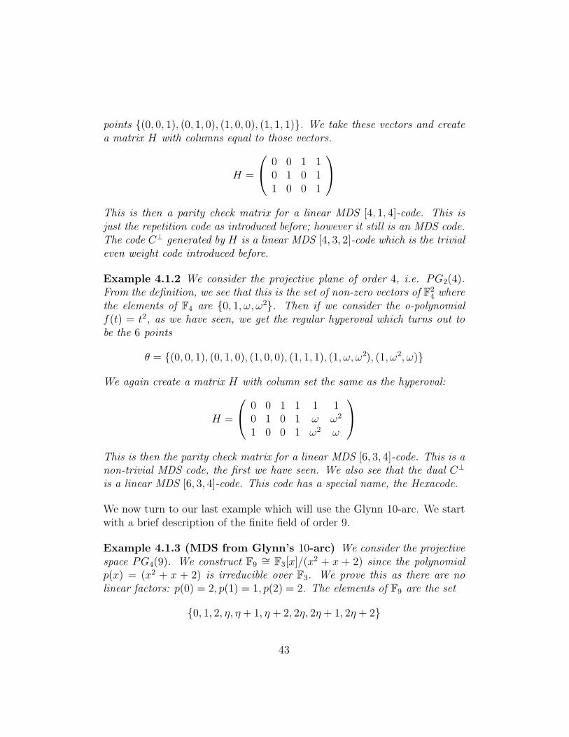
points (0, 0, 1), (0, 1, 0), (1, 0, 0), (1, 1, 1). We take these vectors and createa matrix H with columns equal to those vectors.

H =

0 0 1 10 1 0 11 0 0 1

This is then a parity check matrix for a linear MDS [4, 1, 4]-code. This isjust the repetition code as introduced before; however it still is an MDS code.The code C⊥ generated by H is a linear MDS [4, 3, 2]-code which is the trivialeven weight code introduced before.

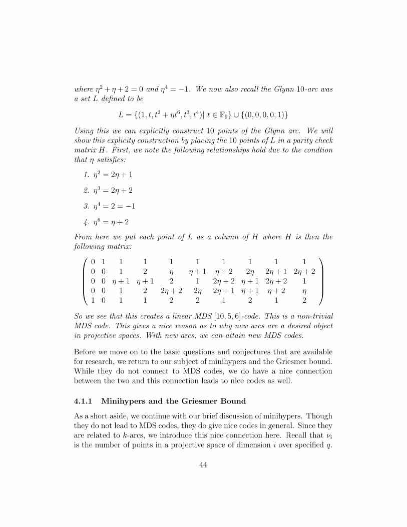
Example 4.1.2 We consider the projective plane of order 4, i.e. PG2(4).From the definition, we see that this is the set of non-zero vectors of F

24 where

the elements of F4 are 0, 1, ω, ω2. Then if we consider the o-polynomialf(t) = t2, as we have seen, we get the regular hyperoval which turns out tobe the 6 points

θ = (0, 0, 1), (0, 1, 0), (1, 0, 0), (1, 1, 1), (1, ω, ω2), (1, ω2, ω)

We again create a matrix H with column set the same as the hyperoval:

H =

0 0 1 1 1 10 1 0 1 ω ω2

1 0 0 1 ω2 ω

This is then the parity check matrix for a linear MDS [6, 3, 4]-code. This is anon-trivial MDS code, the first we have seen. We also see that the dual C⊥

is a linear MDS [6, 3, 4]-code. This code has a special name, the Hexacode.

We now turn to our last example which will use the Glynn 10-arc. We startwith a brief description of the finite field of order 9.

Example 4.1.3 (MDS from Glynn’s 10-arc) We consider the projectivespace PG4(9). We construct F9

∼= F3[x]/(x2 + x + 2) since the polynomialp(x) = (x2 + x + 2) is irreducible over F3. We prove this as there are nolinear factors: p(0) = 2, p(1) = 1, p(2) = 2. The elements of F9 are the set

0, 1, 2, η, η + 1, η + 2, 2η, 2η + 1, 2η + 2

43

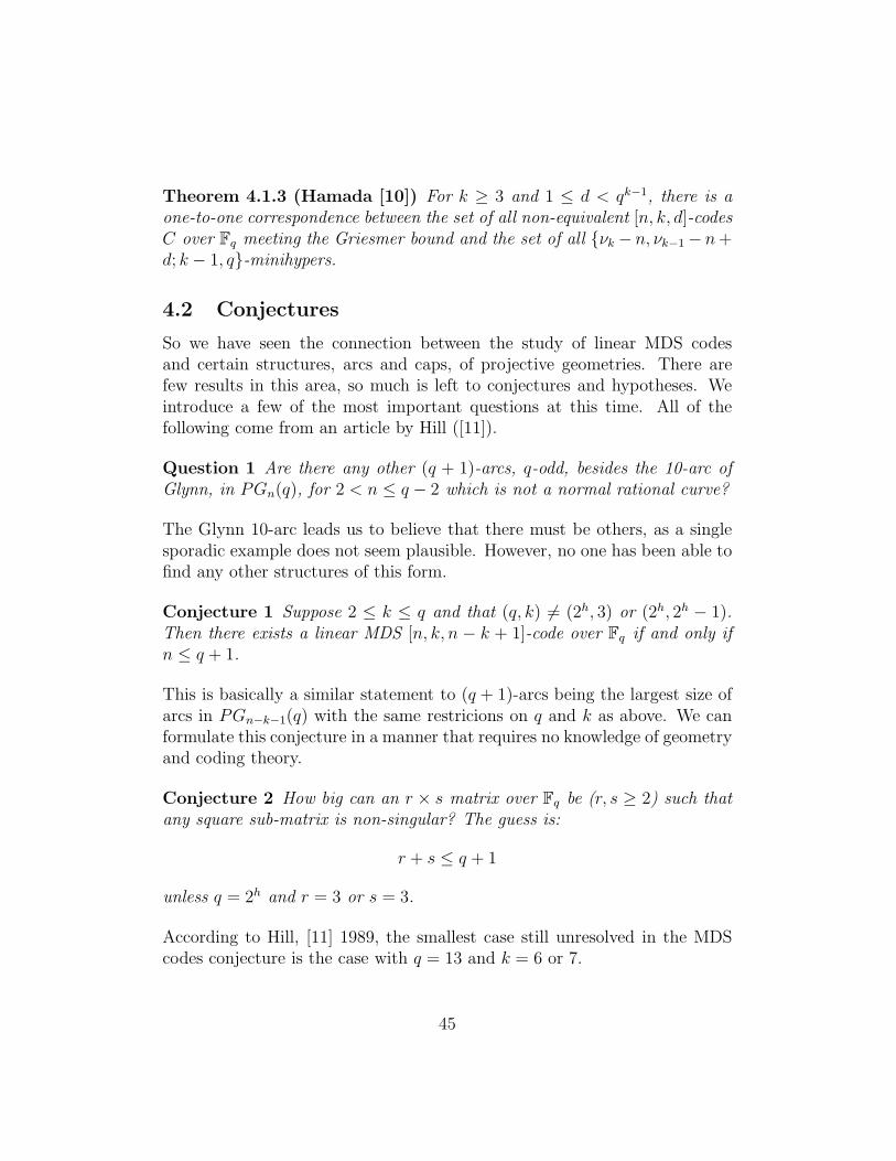
where η2 + η + 2 = 0 and η4 = −1. We now also recall the Glynn 10-arc wasa set L defined to be

L = (1, t, t2 + ηt6, t3, t4)| t ∈ F9 ∪ (0, 0, 0, 0, 1)

Using this we can explicitly construct 10 points of the Glynn arc. We willshow this explicity construction by placing the 10 points of L in a parity checkmatrix H. First, we note the following relationships hold due to the condtionthat η satisfies:

1. η2 = 2η + 1

2. η3 = 2η + 2

3. η4 = 2 = −1

4. η6 = η + 2

From here we put each point of L as a column of H where H is then thefollowing matrix:

0 1 1 1 1 1 1 1 1 10 0 1 2 η η + 1 η + 2 2η 2η + 1 2η + 20 0 η + 1 η + 1 2 1 2η + 2 η + 1 2η + 2 10 0 1 2 2η + 2 2η 2η + 1 η + 1 η + 2 η1 0 1 1 2 2 1 2 1 2

So we see that this creates a linear MDS [10, 5, 6]-code. This is a non-trivialMDS code. This gives a nice reason as to why new arcs are a desired objectin projective spaces. With new arcs, we can attain new MDS codes.

Before we move on to the basic questions and conjectures that are availablefor research, we return to our subject of minihypers and the Griesmer bound.While they do not connect to MDS codes, we do have a nice connectionbetween the two and this connection leads to nice codes as well.

4.1.1 Minihypers and the Griesmer Bound

As a short aside, we continue with our brief discussion of minihypers. Thoughthey do not lead to MDS codes, they do give nice codes in general. Since theyare related to k-arcs, we introduce this nice connection here. Recall that νi

is the number of points in a projective space of dimension i over specified q.

44

Theorem 4.1.3 (Hamada [10]) For k ≥ 3 and 1 ≤ d < qk−1, there is aone-to-one correspondence between the set of all non-equivalent [n, k, d]-codesC over Fq meeting the Griesmer bound and the set of all νk − n, νk−1 − n +d; k − 1, q-minihypers.

4.2 Conjectures

So we have seen the connection between the study of linear MDS codesand certain structures, arcs and caps, of projective geometries. There arefew results in this area, so much is left to conjectures and hypotheses. Weintroduce a few of the most important questions at this time. All of thefollowing come from an article by Hill ([11]).

Question 1 Are there any other (q + 1)-arcs, q-odd, besides the 10-arc ofGlynn, in PGn(q), for 2 < n ≤ q − 2 which is not a normal rational curve?

The Glynn 10-arc leads us to believe that there must be others, as a singlesporadic example does not seem plausible. However, no one has been able tofind any other structures of this form.

Conjecture 1 Suppose 2 ≤ k ≤ q and that (q, k) 6= (2h, 3) or (2h, 2h − 1).Then there exists a linear MDS [n, k, n − k + 1]-code over Fq if and only ifn ≤ q + 1.

This is basically a similar statement to (q + 1)-arcs being the largest size ofarcs in PGn−k−1(q) with the same restricions on q and k as above. We canformulate this conjecture in a manner that requires no knowledge of geometryand coding theory.

Conjecture 2 How big can an r × s matrix over Fq be (r, s ≥ 2) such thatany square sub-matrix is non-singular? The guess is:

r + s ≤ q + 1

unless q = 2h and r = 3 or s = 3.

According to Hill, [11] 1989, the smallest case still unresolved in the MDScodes conjecture is the case with q = 13 and k = 6 or 7.

45

5 Conclusion

We have been able to introduce and discuss a few of the many interestingstructures in projective geometries. With this knowledge, we can continue tostudy in this area in hopes of finding new structures, larger k-arcs, or evenmore arcs like the Glynn arc that are not rational curves. The study of finitegeometry is ever changing, and with more advances, we see more connectionsto other areas of combinatorics. Every time we learn more about geometry,we can in turn learn more about, and further advance the world of codingtheory.We have seen a nice connection between k-arcs and and MDS codes as wellas shortly introduced the connection between minihypers and codes meetingthe Griesmer bound. Many skeptics regard finite incidence geometry to beonly a tool of pure mathematics that has no application. However, this niceapplication provides us with codes that meet the Singleton bound, and inturn have a maximal minimum distance. The study of these codes will thenhelp us advance the world of coding theory and communication theory.By linking geometry and coding theory, we again just show that there areusually many different ways to attack certain problems. Our main interestlies in finding solutions to problems in hopes of applying them in other areas.We hope that the paper has taught a basic introduction to the theory of finitegeometries and coding theory. Additionally, we have added a few interestingopen problems at the end in the hope to inspire further thought and advancein the connections between MDS codes and finite projective spaces.

We also note that for further reading in coding theory and finite projectivegeometries we recommend [17], [14], [21].

46

References

[1] Reinhold Baer. Linear algebra and projective geometry. Academic PressInc., New York, N. Y., 1952.

[2] Albrecht Beutelspacher and Ute Rosenbaum. Projective geometry: fromfoundations to applications. Cambridge University Press, Cambridge,1998.

[3] R. C. Bose. Mathematical theory of the symmetrical factorial design.Sankhya, 8:107–166, 1947.

[4] Matthew Brown. (Hyper)ovals and ovoids in projective spaces, 2000.Socrates Intensive Course, Finite Geometry and its Applications.

[5] Peter J. Cameron. Combinatorics: topics, techniques, algorithms. Cam-bridge University Press, Cambridge, 1994.

[6] Peter Dembowski. Finite geometries. Classics in Mathematics. Springer-Verlag, Berlin, 1997. Reprint of the 1968 original.

[7] Leonard Eugene Dickson. Linear groups: With an exposition of the Ga-lois field theory. with an introduction by W. Magnus. Dover PublicationsInc., New York, 1958.

[8] David G. Glynn. The nonclassical 10-arc of PG(4, 9). Discrete Math.,59(1-2):43–51, 1986.

[9] David G. Glynn. A condition for the existence of ovals in PG(2, q), qeven. Geom. Dedicata, 32(2):247–252, 1989.

[10] Noboru Hamada. A characterization of some [n, k, d; q]-codes meetingthe Griesmer bound using a minihyper in a finite projective geometry.Discrete Math., 116(1-3):229–268, 1993.

[11] R. Hill. Optimal linear codes. In Cryptography and coding, II (Cirences-ter, 1989), volume 33 of Inst. Math. Appl. Conf. Ser. New Ser., pages75–104. Oxford Univ. Press, New York, 1992.

[12] J. W. P. Hirschfeld. Projective geometries over finite fields. OxfordMathematical Monographs. The Clarendon Press Oxford UniversityPress, New York, second edition, 1998.

47

[13] J. W. P. Hirschfeld and L. Storme. The packing problem in statistics,coding theory and finite projective spaces. J. Statist. Plann. Inference,72(1-2):355–380, 1998. R. C. Bose Memorial Conference (Fort Collins,CO, 1995).

[14] W. Cary Huffman and Vera Pless. Fundamentals of error-correctingcodes. Cambridge University Press, Cambridge, 2003.

[15] Maska Law. Flocks, Generalised Quadrangles, and Translation Planesfrom BLT-sets. PhD thesis, University of Western Australia, 2003.

[16] Christine M. O’Keefe and Tim Penttila. Polynomials for hyperovals ofDesarguesian planes. J. Austral. Math. Soc. Ser. A, 51(3):436–447, 1991.

[17] Tim Pentilla and Maska Law. Flocks, ovals and generalised quadrangles,2000. Four Lectures in Napoli, June 2000.

[18] B. Segre and U. Bartocci. Ovali ed altre curve nei piani di Galois dicaratteristica due. Acta Arith., 18:423–449, 1971.

[19] Beniamino Segre. Ovals in a finite projective plane. Canad. J. Math.,7:414–416, 1955.

[20] Richard C. Singleton. Maximum distance q-nary codes. IEEE Trans.Information Theory, IT-10:116–118, 1964.

[21] Joseph A. Thas. Projective geometry over a finite field. In Handbook ofincidence geometry, pages 295–347. North-Holland, Amsterdam, 1995.

[22] Wolfgang Willems. Codierungstheorie. Walter de Gruyter, Inc., 1999.

48