
Finite elements for modeling of localized failure in ...
242
HAL Id: tel-00997197 https://tel.archives-ouvertes.fr/tel-00997197 Submitted on 27 May 2014 HAL is a multi-disciplinary open access archive for the deposit and dissemination of sci- entific research documents, whether they are pub- lished or not. The documents may come from teaching and research institutions in France or abroad, or from public or private research centers. L’archive ouverte pluridisciplinaire HAL, est destinée au dépôt et à la diffusion de documents scientifiques de niveau recherche, publiés ou non, émanant des établissements d’enseignement et de recherche français ou étrangers, des laboratoires publics ou privés. Finite elements for modeling of localized failure in reinforced concrete Miha Jukic To cite this version: Miha Jukic. Finite elements for modeling of localized failure in reinforced concrete. Other. École normale supérieure de Cachan - ENS Cachan; Univerza v Ljubljani. Fakulteta za gradbeništvo in geodezijo, 2013. English. NNT : 2013DENS0064. tel-00997197
Transcript of Finite elements for modeling of localized failure in ...
HAL Id: tel-00997197https://tel.archives-ouvertes.fr/tel-00997197
Submitted on 27 May 2014
HAL is a multi-disciplinary open accessarchive for the deposit and dissemination of sci-entific research documents, whether they are pub-lished or not. The documents may come fromteaching and research institutions in France orabroad, or from public or private research centers.
L’archive ouverte pluridisciplinaire HAL, estdestinée au dépôt et à la diffusion de documentsscientifiques de niveau recherche, publiés ou non,émanant des établissements d’enseignement et derecherche français ou étrangers, des laboratoirespublics ou privés.
Finite elements for modeling of localized failure inreinforced concrete
Miha Jukic
To cite this version:Miha Jukic. Finite elements for modeling of localized failure in reinforced concrete. Other. Écolenormale supérieure de Cachan - ENS Cachan; Univerza v Ljubljani. Fakulteta za gradbeništvo ingeodezijo, 2013. English. NNT : 2013DENS0064. tel-00997197
ENSC-(n° d’ordre)
THESE DE DOCTORAT
DE L’ECOLE NORMALE SUPERIEURE DE CACHAN
Présentée par
Monsieur JUKIC Miha
pour obtenir le grade de
DOCTEUR DE L’ECOLE NORMALE SUPERIEURE DE CACHAN
Domaine :
MECANIQUE – GENIE MECANIQUE – GENIE CIVIL
Sujet de la thèse :
Finite elements for modeling
of localized failure in reinforced concrete
Thèse présentée et soutenue à Ljubljana le 13/12/2013 devant le jury composé de : M. PETROVIC Dusan Professeur des Universités Président M. BICANIC Nenad Professeur des Universités Rapporteur M. JELENIC Gordan Professeur des Universités Rapporteur M. PLANINC Igor Professeur des Universités Examinateur M. BRANK Bostjan Professeur des Universités Directeur de thèse M. IBRAHIMBEGOVIC Adnan Professeur des Universités Directeur de thèse
LMT-Cachan, ENS CACHAN
61, avenue du Président Wilson, 94235 CACHAN CEDEX (France)


Jukic, M. 2013. Koncni elementi za modeliranje lokaliziranih porusitev v armiranem betonu.
Doktorska disertacija. Ljubljana, UL, FGG.
I
IZJAVA O AVTORSTVU
Podpisani Miha Jukic izjavljam, da sem avtor doktorske disertacije z naslovom “Koncni elementi za
modeliranje lokaliziranih porusitev v armiranem betonu”.
Izjavljam, da je elektronska razlicica disertacije enaka tiskani razlicici, in dovoljujem njeno objavo v
digitalnem repozitoriju UL FGG.
Ljubljana, 19.12.2013

II Jukic, M. 2013. Finite elements for modeling of localized failure in reinforced concrete.
Doctoral thesis. Cachan, ENSC, LMT.
ERRATA
Page Line Error Correction

Jukic, M. 2013. Koncni elementi za modeliranje lokaliziranih porusitev v armiranem betonu.
Doktorska disertacija. Ljubljana, UL, FGG.
III
BIBLIOGRAPHIC-DOCUMENTALISTIC INFORMATION AND ABSTRACT
UDC 624.012.45:624.042.2:624.042.7(043.3)
Author: Miha Jukic
Supervisor: prof. Bostjan Brank, Ph.D.
Co-supervisor: prof. Adnan Ibrahimbegovic, Ph.D.
Title: Finite elements for modeling of localized failure in reinforced concrete
Document type: doctoral dissertation
Notes: 200 p., 120 fig., 424 eq.
Keywords: failure analysis, finite element method, reinforced concrete, localized failure,
embedded discontinuity, stress-resultant, multi-layer, Euler-Bernoulli beam,
Timoshenko beam
Abstract
In this work, several beam finite element formulations are proposed for failure analysis of planar rein-
forced concrete beams and frames under monotonic static loading. The localized failure of material is
modeled by the embedded strong discontinuity concept, which enhances standard interpolation of dis-
placement (or rotation) with a discontinuous function, associated with an additional kinematic parameter
representing jump in displacement (or rotation). The new parameters are local and are condensed on
the element level. One stress resultant and two multi-layer beam finite elements are derived. The stress
resultant Euler-Bernoulli beam element has embedded discontinuity in rotation. Bending response of
the bulk of the element is described by elasto-plastic stress resultant material model. The cohesive re-
lation between the moment and the rotational jump at the softening hinge is described by rigid-plastic
model. Axial response is elastic. In the multi-layer beam finite elements, each layer is treated as a
bar, made of either concrete or steel. Regular axial strain in a layer is computed according to Euler-
Bernoulli or Timoshenko beam theory. Additional axial strain is produced by embedded discontinuity
in axial displacement, introduced individually in each layer. Behavior of concrete bars is described by
elasto-damage model, while elasto-plasticity model is used for steel bars. The cohesive relation between
the stress at the discontinuity and the axial displacement jump is described by rigid-damage softening
model in concrete bars and by rigid-plastic softening model in steel bars. Shear response in the Tim-
oshenko element is elastic. The multi-layer Timoshenko beam finite element is upgraded by including
viscosity in the softening model. Computer code implementation is presented in detail for the derived
elements. An operator split computational procedure is presented for each formulation. The expressions,
required for the local computation of inelastic internal variables and for the global computation of the
degrees of freedom, are provided. Performance of the derived elements is illustrated on a set of numeri-
cal examples, which show that the multi-layer Euler-Bernoulli beam finite element is not reliable, while
the stress-resultant Euler-Bernoulli beam and the multi-layer Timoshenko beam finite elements deliver
satisfying results.

IV Jukic, M. 2013. Finite elements for modeling of localized failure in reinforced concrete.
Doctoral thesis. Cachan, ENSC, LMT.
BIBLIOGRAFSKO-DOKUMENTACIJSKA STRAN IN IZVLECEK
UDK 624.012.45:624.042.2:624.042.7(043.3)
Avtor: Miha Jukic
Mentor: prof. dr. Bostjan Brank
Somentor: prof. dr. Adnan Ibrahimbegovic
Naslov: Koncni elementi za modeliranje lokaliziranih porusitev v armiranem betonu
Tip dokumenta: doktorska disertacija
Obseg in oprema: 200 str., 120 sl., 424 en.
Kljucne besede: porusna analiza, metoda koncnih elementov, armirani beton, lokalizirana
porusitev, vgrajena nezveznost, rezultantni model, vecslojni model, Euler-
Bernoullijev nosilec, Timosenkov nosilec
Izvlecek
V disertaciji predlagamo nekaj formulacij koncnih elementov za porusno analizo armiranobetonskih
nosilcev in okvirjev pod monotono staticno obtezbo. Lokalizirano porusitev materiala modeliramo z
metodo vgrajene nezveznosti, pri kateri standardno interpolacijo pomikov (ali zasukov) nadgradimo
z nezvezno interpolacijsko funkcijo in z dodatnim kinematicnim parametrom, ki predstavlja velikost
nezveznosti v pomikih (ali zasukih). Dodatni parametri so lokalnega znacaja in jih kondenziramo
na nivoju elementa. Izpeljemo en rezultantni in dva vecslojna koncna elementa za nosilec. Rezul-
tantni element za Euler-Bernoullijev nosilec ima vgrajeno nezveznost v zasukih. Njegov upogibni odziv
opisemo z elasto-plasticnim rezultantnim materialnim modelom. Kohezivni zakon, ki povezuje moment
v plasticnem clenku s skokom v zasuku, opisemo s togo-plasticnim modelom mehcanja. Osni odziv je
elasticen. V vecslojnih koncnih elementih vsak sloj obravnavamo kot betonsko ali jekleno palico. Stan-
dardno osno deformacijo v palici izracunamo v skladu z Euler-Bernoullijevo ali s Timosenkovo teorijo
nosilcev. Vgrajena nezveznost v osnem pomiku povzroci dodatno osno deformacijo v posamezni palici.
Obnasanje betonskega sloja opisemo z modelom elasto-poskodovanosti, za sloj armature pa uporabimo
elasto-plasticni model. Kohezivni zakon, ki povezuje napetost v nezveznosti s skokom v osnem pomiku,
opisemo z modelom mehcanja v poskodovanosti za beton in s plasticnim modelom mehcanja za jeklo.
Strizni odziv Timosenkovega nosilca je elasticen. Vecslojni koncni element za Timosenkov nosilec nad-
gradimo z viskoznim modelom mehcanja. Za vsak koncni element predstavimo racunski algoritem ter
vse potrebne izraze za lokalni izracun neelasticnih notranjih spremenljivk in za globalni izracun pros-
tostnih stopenj. Delovanje koncnih elementov preizkusimo na vec numericnih primerih. Ugotovimo, da
vecslojni koncni element za Euler-Bernoullijev nosilec ni zanesljiv, medtem ko rezultantni koncni ele-
ment za Euler-Bernoullijev nosilec in vecslojni koncni element za Timosenkov nosilec dajeta zadovoljive
rezultate.
Jukic, M. 2013. Koncni elementi za modeliranje lokaliziranih porusitev v armiranem betonu.
Doktorska disertacija. Ljubljana, UL, FGG.
V
INFORMATION BIBLIOGRAPHIQUE-DOCUMENTAIRE ET RESUME
CDU 624.012.45:624.042.2:624.042.7(043.3)
Auteur: Miha Jukic
Directeur de these: prof. Bostjan Brank, Ph.D.
Co-directeur de these: prof. Adnan Ibrahimbegovic, Ph.D.
Titre: Elements finis pour la modelisation de la rupture localisee dans le beton
arme
Type de document: memoire de these de doctorat
Notes: 200 p., 120 fig., 424 eq.
Mots-cles: rupture, methode des elements finis, beton arme, rupture localisee,
discontinuite forte, modele en effort resultant, multicouche, poutre
d’Euler Bernoulli, poutre de Timoshenko
Resume
Dans ce travail, differentes formulations d’elements de poutres sont proposees pour l’analyse a rupture de struc-
tures de type poutres ou portiques en beton arme soumises a des chargements statiques monotones. La rupture
localisee des materiaux est modelisee par la methode a discontinuite forte, qui consiste a enrichir l’interpolation
standard des deplacements (ou rotations) avec des fonctions discontinues associees a un parametre cinematique
supplementaire interprete comme un saut de deplacement (ou rotation). Ces parametres additionnels sont lo-
caux et condenses au niveau elementaire. Un element fini ecrit en efforts resultants et deux elements finis multi-
couches sont developpes dans ce travail. L’element de poutre d’Euler Bernouilli ecrit en effort resultant presente
une discontinuite en rotation. La reponse en flexion du materiau hors discontinuite est decrite par un modele
elastoplastique en effort resultant et la relation cohesive liant moment et saut de rotation sur la rotule plastique
est, quant a elle, decrite par un modele rigide plastique. La reponse axiale est suppposee elastique. Pour ce
qui concerne l’approche multi-couche, chaque couche est consideree comme une barre constituee de beton ou
d’acier. La partie reguliere de la deformation de chaque couche est calculee en s’appuyant sur la cinematique
associee a la theorie d’Euler Bernoulli ou de Timoshenko. Une deformation axiale additionnelle est consideree par
l’introduction d’une discontinuite du deplacement axial, introduite independamment dans chaque couche. Le com-
portement du beton est pris en compte par un modele elasto-endommageable alors que celui de l’acier est decrit
par un modele elastoplastique. La relation cohesive entre la traction sur la discontinuite et le saut de deplacement
axial est decrit par un modele rigide endommageable adoucissant pour les barres (couches) en beton et rigide plas-
tique adoucissant pour les barres en acier. La reponse en cisaillement pour l’element de Timoshenko est supposee
elastique. Enfin, l’element multi-couche de Timoshenko est enrichi en introduisant une partie visqueuse dans la
reponse adoucissante. L’implantation numerique des differents elements developpes dans ce travail est presentee
en detail. La resolution par une procedure d’operator split est decrite pour chaque type d’element. Les differentes
quantites necessaires pour le calcul au niveau local des variables internes des modeles non lineaires ainsi que pour
la construction du systeme global fournissant les valeurs des degres de liberte sont precisees. Les performances
des elements developpes sont illustrees a travers des exemples numeriques montrant que la formulation basee sur
un element multicouche d’Euler Bernouilli n’est pas robuste alors les simulations s’appuyant sur des elements
d’Euler Bernouilli en efforts resultants ou sur des elements multicouche de Timoshenko fournissent des resultats
tres satisfaisants.
VI Jukic, M. 2013. Finite elements for modeling of localized failure in reinforced concrete.
Doctoral thesis. Cachan, ENSC, LMT.
TABLE OF CONTENTS
BIBLIOGRAPHIC-DOCUMENTALISTIC INFORMATION AND ABSTRACT III
BIBLIOGRAFSKO-DOKUMENTACIJSKA STRAN IN IZVLECEK IV
INFORMATION BIBLIOGRAPHIQUE-DOCUMENTAIRE ET RESUME V
1 INTRODUCTION 1
1.1 Motivation . . . . . . . . . . . . . . . . . . . . . . . . . . . . . . . . . . . . . . . . . . . . . . 1
1.2 Theoretical background . . . . . . . . . . . . . . . . . . . . . . . . . . . . . . . . . . . . . . . 2
1.3 Goals and outline of the thesis . . . . . . . . . . . . . . . . . . . . . . . . . . . . . . . . . . . . 4
2 STRESS RESULTANT EULER-BERNOULLI BEAM FINITE ELEMENT
WITH EMBEDDED DISCONTINUITY IN ROTATION 7
2.1 Introduction . . . . . . . . . . . . . . . . . . . . . . . . . . . . . . . . . . . . . . . . . . . . . 7
2.2 Finite element formulation . . . . . . . . . . . . . . . . . . . . . . . . . . . . . . . . . . . . . . 7
2.2.1 Kinematics . . . . . . . . . . . . . . . . . . . . . . . . . . . . . . . . . . . . . . . . . 7
2.2.2 Derivation of operator G . . . . . . . . . . . . . . . . . . . . . . . . . . . . . . . . . . 10
2.2.3 Relations between global and local quantities . . . . . . . . . . . . . . . . . . . . . . . 11
2.2.4 Virtual work equation . . . . . . . . . . . . . . . . . . . . . . . . . . . . . . . . . . . . 15
2.2.5 Constitutive models . . . . . . . . . . . . . . . . . . . . . . . . . . . . . . . . . . . . . 18
2.3 Computational procedure . . . . . . . . . . . . . . . . . . . . . . . . . . . . . . . . . . . . . . 22
2.3.1 Computation of internal variables . . . . . . . . . . . . . . . . . . . . . . . . . . . . . 23
2.3.2 Computation of nodal degrees of freedom . . . . . . . . . . . . . . . . . . . . . . . . . 28
2.4 Numerical examples . . . . . . . . . . . . . . . . . . . . . . . . . . . . . . . . . . . . . . . . . 32
2.4.1 Failure of a cantilever beam . . . . . . . . . . . . . . . . . . . . . . . . . . . . . . . . 33
2.4.2 Failure of simply supported and clamped beams . . . . . . . . . . . . . . . . . . . . . . 35
2.4.3 Four point bending test of a simply supported beam . . . . . . . . . . . . . . . . . . . . 37
2.4.4 Two story reinforced concrete frame . . . . . . . . . . . . . . . . . . . . . . . . . . . . 38
2.5 Concluding remarks . . . . . . . . . . . . . . . . . . . . . . . . . . . . . . . . . . . . . . . . . 40
Jukic, M. 2013. Koncni elementi za modeliranje lokaliziranih porusitev v armiranem betonu.
Doktorska disertacija. Ljubljana, UL, FGG.
VII
3 MULTI-LAYER EULER-BERNOULLI BEAM FINITE ELEMENT WITH
LAYER-WISE EMBEDDED DISCONTINUITIES IN AXIAL DISPLACEMENT 41
3.1 Introduction . . . . . . . . . . . . . . . . . . . . . . . . . . . . . . . . . . . . . . . . . . . . . 41
3.2 Finite element formulation . . . . . . . . . . . . . . . . . . . . . . . . . . . . . . . . . . . . . . 41
3.2.1 Kinematics . . . . . . . . . . . . . . . . . . . . . . . . . . . . . . . . . . . . . . . . . 41
3.2.2 Relations between global and local quantities . . . . . . . . . . . . . . . . . . . . . . . 44
3.2.3 Virtual work equation . . . . . . . . . . . . . . . . . . . . . . . . . . . . . . . . . . . . 48
3.2.4 Derivation of operators GR and GV . . . . . . . . . . . . . . . . . . . . . . . . . . . . 52
3.2.5 Constitutive models . . . . . . . . . . . . . . . . . . . . . . . . . . . . . . . . . . . . . 59
3.3 Computational procedure . . . . . . . . . . . . . . . . . . . . . . . . . . . . . . . . . . . . . . 68
3.3.1 Computation of internal variables . . . . . . . . . . . . . . . . . . . . . . . . . . . . . 69
3.3.2 Computation of nodal degrees of freedom . . . . . . . . . . . . . . . . . . . . . . . . . 79
3.4 Numerical examples . . . . . . . . . . . . . . . . . . . . . . . . . . . . . . . . . . . . . . . . . 82
3.4.1 One element tension and compression tests . . . . . . . . . . . . . . . . . . . . . . . . 82
3.4.2 Cantilever beam under end moment . . . . . . . . . . . . . . . . . . . . . . . . . . . . 88
3.4.3 Cantilever beam under end transversal force . . . . . . . . . . . . . . . . . . . . . . . . 91
3.4.4 Two story reinforced concrete frame . . . . . . . . . . . . . . . . . . . . . . . . . . . . 92
3.5 Concluding remarks . . . . . . . . . . . . . . . . . . . . . . . . . . . . . . . . . . . . . . . . . 94
4 MULTI-LAYER TIMOSHENKO BEAM FINITE ELEMENT WITH LAYER-WISE
EMBEDDED DISCONTINUITIES IN AXIAL DISPLACEMENT 96
4.1 Introduction . . . . . . . . . . . . . . . . . . . . . . . . . . . . . . . . . . . . . . . . . . . . . 96
4.2 Finite element formulation . . . . . . . . . . . . . . . . . . . . . . . . . . . . . . . . . . . . . . 96
4.2.1 Kinematics . . . . . . . . . . . . . . . . . . . . . . . . . . . . . . . . . . . . . . . . . 96
4.2.2 Derivation of operator G . . . . . . . . . . . . . . . . . . . . . . . . . . . . . . . . . . 98
4.2.3 Relations between global and local quantities . . . . . . . . . . . . . . . . . . . . . . . 101
4.2.4 Virtual work equation . . . . . . . . . . . . . . . . . . . . . . . . . . . . . . . . . . . . 105
4.2.5 Constitutive models . . . . . . . . . . . . . . . . . . . . . . . . . . . . . . . . . . . . . 108
4.3 Computational procedure . . . . . . . . . . . . . . . . . . . . . . . . . . . . . . . . . . . . . . 118
4.3.1 Computation of internal variables . . . . . . . . . . . . . . . . . . . . . . . . . . . . . 119
4.3.2 Computation of nodal degrees of freedom . . . . . . . . . . . . . . . . . . . . . . . . . 127
4.4 Numerical examples . . . . . . . . . . . . . . . . . . . . . . . . . . . . . . . . . . . . . . . . . 131
4.4.1 One element tension and compression tests . . . . . . . . . . . . . . . . . . . . . . . . 131
4.4.2 Cantilever beam under end moment . . . . . . . . . . . . . . . . . . . . . . . . . . . . 135

VIII Jukic, M. 2013. Finite elements for modeling of localized failure in reinforced concrete.
Doctoral thesis. Cachan, ENSC, LMT.
4.4.3 Cantilever beam under end transversal force . . . . . . . . . . . . . . . . . . . . . . . . 138
4.4.4 Simply supported beam . . . . . . . . . . . . . . . . . . . . . . . . . . . . . . . . . . . 140
4.4.5 Reinforced concrete portal frame . . . . . . . . . . . . . . . . . . . . . . . . . . . . . . 143
4.4.6 Two story reinforced concrete frame . . . . . . . . . . . . . . . . . . . . . . . . . . . . 147
4.5 Concluding remarks . . . . . . . . . . . . . . . . . . . . . . . . . . . . . . . . . . . . . . . . . 149
5 VISCOUS REGULARIZATION OF SOFTENING RESPONSE FOR MULTI-LAYER
TIMOSHENKO BEAM FINITE ELEMENT 153
5.1 Introduction . . . . . . . . . . . . . . . . . . . . . . . . . . . . . . . . . . . . . . . . . . . . . 153
5.2 Virtual work equation . . . . . . . . . . . . . . . . . . . . . . . . . . . . . . . . . . . . . . . . 153
5.3 Computation of internal variables . . . . . . . . . . . . . . . . . . . . . . . . . . . . . . . . . . 155
5.3.1 Discontinuity in concrete layer . . . . . . . . . . . . . . . . . . . . . . . . . . . . . . . 155
5.3.2 Discontinuity in reinforcement layer . . . . . . . . . . . . . . . . . . . . . . . . . . . . 156
5.4 Computation of nodal degrees of freedom . . . . . . . . . . . . . . . . . . . . . . . . . . . . . . 158
5.5 Numerical examples . . . . . . . . . . . . . . . . . . . . . . . . . . . . . . . . . . . . . . . . . 159
5.5.1 One element tension and compression tests . . . . . . . . . . . . . . . . . . . . . . . . 159
5.5.2 Tension and compression tests on a mesh of several elements . . . . . . . . . . . . . . . 161
5.5.3 Cantilever beam under end moment . . . . . . . . . . . . . . . . . . . . . . . . . . . . 163
5.6 Concluding remarks . . . . . . . . . . . . . . . . . . . . . . . . . . . . . . . . . . . . . . . . . 165
6 CONCLUSIONS 166
RAZSIRJENI POVZETEK 170
BIBLIOGRAPHY 195
APPENDICES 200
Jukic, M. 2013. Koncni elementi za modeliranje lokaliziranih porusitev v armiranem betonu.
Doktorska disertacija. Ljubljana, UL, FGG.
IX
LIST OF FIGURES
2.1 Finite element with six nodal degrees of freedom and embedded discontinuity in rotation. . . . . 8
2.2 Interpolation functions for axial displacement (left) and axial strain (right). . . . . . . . . . . . . 8
2.3 Interpolation functions for transversal displacement (left) and curvature (right). . . . . . . . . . 9
2.4 Interpolation function M and its first derivative M ′ (left). Heaviside and Dirac-delta functions
(right). . . . . . . . . . . . . . . . . . . . . . . . . . . . . . . . . . . . . . . . . . . . . . . . . 10
2.5 Curvature-free deformation of the beam when the moment in the hinge drops to zero. . . . . . . 11
2.6 Degrees of freedom at a node of the finite element mesh. . . . . . . . . . . . . . . . . . . . . . 12
2.7 Global (left) and local (right) degrees of freedom, associated with a finite element. . . . . . . . . 13
2.8 Internal forces, corresponding to degrees of freedom at a node of the finite element mesh. . . . . 14
2.9 Contribution of a finite element to internal forces of the structure in global (left) and local (right)
coordinate system. . . . . . . . . . . . . . . . . . . . . . . . . . . . . . . . . . . . . . . . . . . 15
2.10 Moment - curvature diagram (left). Bilinear hardening law (right). Only positive parts of the
diagrams are shown. They are valid for constant value of axial force. . . . . . . . . . . . . . . . 19
2.11 Moment at the hinge - rotational jump diagram. . . . . . . . . . . . . . . . . . . . . . . . . . . 21
2.12 Algorithm for phase (A) of k-th iteration for finite element (e). . . . . . . . . . . . . . . . . . . 24
2.13 Cantilever beam under different loads. . . . . . . . . . . . . . . . . . . . . . . . . . . . . . . . 33
2.14 Moment - rotation diagrams for cantilever beam under end moment: all finite elements are the
same (left), one element is slightly weaker (right). . . . . . . . . . . . . . . . . . . . . . . . . . 34
2.15 Moment - rotation diagram for cantilever beam under end moment: with and without axial force. 34
2.16 Moment at support - transversal displacement diagram for cantilever beam under end transversal
force: all finite elements are the same. . . . . . . . . . . . . . . . . . . . . . . . . . . . . . . . 35
2.17 Simply supported beam: use of symmetry in computational model. . . . . . . . . . . . . . . . . 35
2.18 Clamped beam: use of symmetry in computational model. . . . . . . . . . . . . . . . . . . . . 36
2.19 Force - displacement under the force diagrams for simply supported and clamped beams. Elasto-
plastic (left) and elastic (right) behavior in the hardening phase. . . . . . . . . . . . . . . . . . . 36
2.20 Four point bending test of simply supported beam: computational model. . . . . . . . . . . . . . 37
2.21 Force - displacement at the middle of the beam diagrams for different positions of the force:
La = 0.96m (left), La = 1.30m (middle), La = 1.60m (right). . . . . . . . . . . . . . . . . . . 37
2.22 Two story frame: geometry, loading pattern and cross-sections. . . . . . . . . . . . . . . . . . . 38
2.23 Moment - rotation divided by length of FE diagrams for beam and column. . . . . . . . . . . . . 39

X Jukic, M. 2013. Finite elements for modeling of localized failure in reinforced concrete.
Doctoral thesis. Cachan, ENSC, LMT.
2.24 Response of two story frame and material state at different stages of analysis (left). Comparison
with experiment and results of Pham et al. (right). . . . . . . . . . . . . . . . . . . . . . . . . . 39
2.25 Response of two story frame up to total collapse for different material data (left). Comparison
with results of analysis with multi-layer finite element (right). . . . . . . . . . . . . . . . . . . . 40
3.1 Finite element with seven nodal degrees of freedom. . . . . . . . . . . . . . . . . . . . . . . . . 41
3.2 Interpolation functions for axial (left) and transversal displacement (right). . . . . . . . . . . . . 42
3.3 Finite element divided into layers, before and after occurrence of discontinuity in i-th layer, with
corresponding axial displacement in the layer. . . . . . . . . . . . . . . . . . . . . . . . . . . . 43
3.4 Interpolation functions for axial strain due to axial (left) and transversal displacement (right). . . 44
3.5 Degrees of freedom at nodes of the finite element mesh. . . . . . . . . . . . . . . . . . . . . . . 45
3.6 Global (left) and local (right) degrees of freedom, associated with a finite element. . . . . . . . . 46
3.7 Internal forces, corresponding to degrees of freedom at nodes of the finite element mesh. . . . . 47
3.8 Contribution of a finite element to internal forces of the structure in global (left) and local (right)
coordinate system. . . . . . . . . . . . . . . . . . . . . . . . . . . . . . . . . . . . . . . . . . . 48
3.9 Interpolation of standard axial displacement in i-th layer between nodal displacements of the finite
element (left) and between nodal axial displacements of the layer (right). . . . . . . . . . . . . . 52
3.10 Domain and sub-domains of a cracked layer. Heaviside and Dirac-delta functions. . . . . . . . . 53
3.11 Construction of interpolation function Mi in case of discontinuity between nodes 1 and 3 (left)
and in case of discontinuity between nodes 3 and 2 (right). . . . . . . . . . . . . . . . . . . . . 54
3.12 Construction of interpolation function Mi in case of constant strain. . . . . . . . . . . . . . . . 56
3.13 Operator GR for interpolation of additional real strain. . . . . . . . . . . . . . . . . . . . . . . 57
3.14 Linear strain and bilinear stress in a structural element, modeled with five finite elements. . . . . 57
3.15 Operator GV for interpolation of additional virtual strain. . . . . . . . . . . . . . . . . . . . . . 58
3.16 Stress - strain diagram for bulk of concrete layer. . . . . . . . . . . . . . . . . . . . . . . . . . 60
3.17 Traction - displacement jump diagram for discontinuity in concrete layer. . . . . . . . . . . . . . 62
3.18 Stress - strain diagram for bulk of reinforcement layer. . . . . . . . . . . . . . . . . . . . . . . 65
3.19 Traction - displacement jump diagram for discontinuity in reinforcement layer. . . . . . . . . . . 67
3.20 Algorithm for phase (A) of k-th iteration for i-th layer of finite element (e). . . . . . . . . . . . 70
3.21 Seven possible linear stress states in a layer. . . . . . . . . . . . . . . . . . . . . . . . . . . . . 72
3.22 Beam in pure tension/compression: geometry. . . . . . . . . . . . . . . . . . . . . . . . . . . . 83
3.23 Axial force - displacement diagrams for concrete beam in pure tension (left) and pure compression
(right). . . . . . . . . . . . . . . . . . . . . . . . . . . . . . . . . . . . . . . . . . . . . . . . . 83
3.24 Axial force - displacement diagram for steel beam (layer) in pure tension. . . . . . . . . . . . . 84
3.25 Axial force - displacement diagrams for reinforced concrete beam in pure tension (left) and pure
compression (right). . . . . . . . . . . . . . . . . . . . . . . . . . . . . . . . . . . . . . . . . . 84
Jukic, M. 2013. Koncni elementi za modeliranje lokaliziranih porusitev v armiranem betonu.
Doktorska disertacija. Ljubljana, UL, FGG.
XI
3.26 Linear stress in i-th layer (left) and resulting unequal contributions of the layer to axial internal
forces of the finite element at the two nodes (right). . . . . . . . . . . . . . . . . . . . . . . . . 85
3.27 Individual layers out of balance (left) and finite element in balance (right). . . . . . . . . . . . . 85
3.28 Axial force - displacement diagrams for reinforced concrete beam in pure tension (left) and pure
compression (right) with imposed location of discontinuity at L/2. . . . . . . . . . . . . . . . . 86
3.29 Locations and sizes of discontinuities in layers of the beam in pure tension, when transversal
displacement of the free end of the beam v2 is non-zero. . . . . . . . . . . . . . . . . . . . . . . 86
3.30 Axial force - displacement diagrams for reinforced concrete beam in pure tension (left) and pure
compression (right): the case of non-zero transversal displacement. . . . . . . . . . . . . . . . . 87
3.31 Transversal displacement (left) and rotation (right) at the free end of RC beam in tension. . . . . 87
3.32 Shear force (left) and moment (right) at the support of RC beam in tension. . . . . . . . . . . . 87
3.33 Cantilever beam under end moment: geometry. . . . . . . . . . . . . . . . . . . . . . . . . . . 88
3.34 Moment - rotation diagrams for cantilever beam under end moment: original softening moduli
(left), softening moduli modified according to length of FE (right). . . . . . . . . . . . . . . . . 88
3.35 Moment - rotation diagram for cantilever beam under end moment: weaker reinforcement in one
of the finite elements. . . . . . . . . . . . . . . . . . . . . . . . . . . . . . . . . . . . . . . . . 89
3.36 Moment - rotation diagrams for cantilever beam under end moment: imposed location of discon-
tinuity at L/2. Original softening moduli (left), modified softening moduli (right). . . . . . . . . 90
3.37 Moment - rotation diagram for cantilever beam under end moment: imposed location of disconti-
nuity at L/2. Weaker reinforcement in one of the finite elements. . . . . . . . . . . . . . . . . . 90
3.38 Cantilever beam under end transversal force: geometry. . . . . . . . . . . . . . . . . . . . . . . 91
3.39 Moment at support - transversal displacement diagram for cantilever beam under end transversal
force: all finite elements are the same. . . . . . . . . . . . . . . . . . . . . . . . . . . . . . . . 91
3.40 Two story frame: geometry, loading pattern and cross-sections. . . . . . . . . . . . . . . . . . . 92
3.41 Constitutive diagrams for steel (left) and concrete in compression (right): comparison with exper-
imental curves. . . . . . . . . . . . . . . . . . . . . . . . . . . . . . . . . . . . . . . . . . . . 93
3.42 Response of two story frame: comparison with experiment. . . . . . . . . . . . . . . . . . . . . 93
4.1 Finite element with six nodal degrees of freedom. . . . . . . . . . . . . . . . . . . . . . . . . . 96
4.2 Interpolation functions for displacements (left) and strain (right). . . . . . . . . . . . . . . . . . 97
4.3 Finite element divided into layers, before and after occurrence of discontinuity in i-th layer, with
corresponding axial displacement in the layer. . . . . . . . . . . . . . . . . . . . . . . . . . . . 98
4.4 Interpolation of standard axial displacement in i-th layer between nodal displacements of the finite
element (left) and between nodal axial displacements of the layer (right). . . . . . . . . . . . . . 99
4.5 Domain and sub-domains of a cracked layer, Heaviside and Dirac-delta functions (left). Construc-
tion of interpolation function Mi (right). . . . . . . . . . . . . . . . . . . . . . . . . . . . . . . 100
4.6 Degrees of freedom at a node of the finite element mesh. . . . . . . . . . . . . . . . . . . . . . 101
4.7 Global (left) and local (right) degrees of freedom, associated with a finite element. . . . . . . . . 102

XII Jukic, M. 2013. Finite elements for modeling of localized failure in reinforced concrete.
Doctoral thesis. Cachan, ENSC, LMT.
4.8 Internal forces, corresponding to degrees of freedom at a node of the finite element mesh. . . . . 103
4.9 Contribution of a finite element to internal forces of the structure in global (left) and local (right)
coordinate system. . . . . . . . . . . . . . . . . . . . . . . . . . . . . . . . . . . . . . . . . . . 104
4.10 Stress - strain diagram for bulk of concrete layer. . . . . . . . . . . . . . . . . . . . . . . . . . 109
4.11 Traction - displacement jump diagram for discontinuity in concrete layer. . . . . . . . . . . . . . 112
4.12 Stress - strain diagram for bulk of reinforcement layer. . . . . . . . . . . . . . . . . . . . . . . 115
4.13 Traction - displacement jump diagram for discontinuity in reinforcement layer. . . . . . . . . . . 117
4.14 Algorithm for phase (A) of k-th iteration for i-th layer of finite element (e). . . . . . . . . . . . 119
4.15 Stress in the bulk (left) and traction at the discontinuity (right) of a concrete layer: value from the
previous step (n), and trial and final values from the current step (n+1). . . . . . . . . . . . . . 124
4.16 Beam in pure tension/compression: geometry. . . . . . . . . . . . . . . . . . . . . . . . . . . . 132
4.17 Axial force - displacement diagrams for concrete beam in pure tension (left) and pure compression
(right). . . . . . . . . . . . . . . . . . . . . . . . . . . . . . . . . . . . . . . . . . . . . . . . . 132
4.18 Axially loaded concrete beam: switching from softening in tension to compression (left) and back
to tension (right). . . . . . . . . . . . . . . . . . . . . . . . . . . . . . . . . . . . . . . . . . . 133
4.19 Axially loaded concrete beam: switching from hardening in compression to tension (left) and
back to compression (middle). Switching from softening in compression to tension (right). . . . 133
4.20 Axial force - displacement diagram for steel beam (layer) in pure tension. . . . . . . . . . . . . 134
4.21 Axially loaded steel beam: switching from hardening in tension to compression (left) and back to
tension (middle). Switching from softening in tension to compression (right). . . . . . . . . . . 134
4.22 Axial force - displacement diagrams for reinforced concrete beam in pure tension (left) and pure
compression (right). . . . . . . . . . . . . . . . . . . . . . . . . . . . . . . . . . . . . . . . . . 135
4.23 Cantilever beam under end moment: geometry. . . . . . . . . . . . . . . . . . . . . . . . . . . 136
4.24 Moment - rotation diagrams for cantilever beam under end moment: original softening moduli
(left), softening moduli modified according to length of FE (right). . . . . . . . . . . . . . . . . 136
4.25 Moment - rotation diagrams for cantilever beam under end moment: weaker reinforcement in one
of the finite elements (left), weaker concrete and reinforcement in one of the elements (right). . . 137
4.26 Cantilever beam under end transversal force: geometry. . . . . . . . . . . . . . . . . . . . . . . 138
4.27 Moment at support - transversal displacement diagrams for cantilever beam under end transversal
force: original softening moduli (left), moduli modified according to length of FE (right). . . . . 138
4.28 Simply supported beam: use of symmetry in computational model. . . . . . . . . . . . . . . . . 140
4.29 Force - displacement under the force diagrams for simply supported beam: results for different
meshes (left), comparison of results for 8 FE with results of Pham (right). . . . . . . . . . . . . 141
4.30 Force - displacement under the force diagrams for simply supported beam: different number of
concrete layers in 5 FE mesh (left), different hardening modulus of steel in 8 FE mesh (right). . . 141
4.31 Simply supported beam: material state at different stages of analysis (marked with dots). . . . . 142
4.32 Simply supported beam: discontinuities (cracks) at different stages of analysis. . . . . . . . . . 142
Jukic, M. 2013. Koncni elementi za modeliranje lokaliziranih porusitev v armiranem betonu.
Doktorska disertacija. Ljubljana, UL, FGG.
XIII
4.33 Pinned portal frame: geometry, loading pattern and reinforcement. . . . . . . . . . . . . . . . . 143
4.34 P −w diagram: results for different meshes of finite elements if all elements to the right of force
P are the same (left) and if reinforcement is weakened in one of them (right). . . . . . . . . . . 144
4.35 P −w diagram: comparison to experiment and results of Saje et al. . . . . . . . . . . . . . . . . 144
4.36 Moments at the joint of the beam and the column (left) and in the middle of the span (right):
comparison to experiment and results of Saje et al. . . . . . . . . . . . . . . . . . . . . . . . . . 144
4.37 Portal frame: material state at different stages of analysis (marked with dots). . . . . . . . . . . 145
4.38 Portal frame: discontinuities (cracks) at different stages of analysis (marked with dots). . . . . . 146
4.39 Two story frame: geometry, loading pattern and cross-sections. . . . . . . . . . . . . . . . . . . 147
4.40 Stress - strain diagrams for steel (left) and concrete in compression (right) used by Vecchio and
Emara, compared to diagrams used in present analysis. . . . . . . . . . . . . . . . . . . . . . . 148
4.41 Response of two story frame: results for different meshes (left), comparison of results for 16 FE
in a column and 14 FE in a beam with experiment and results of Pham (right). . . . . . . . . . . 148
4.42 Response of two story frame: loading and unloading for a mesh of 16 FE in a column and 14 FE
in a beam. Comparison to experiment. . . . . . . . . . . . . . . . . . . . . . . . . . . . . . . . 149
4.43 Two story frame: stages of analysis, corresponding to images in Figs. 4.44 and 4.45. . . . . . . . 149
4.44 Two story frame: material state at different stages of analysis, marked in Fig. 4.43. . . . . . . . . 150
4.45 Two story frame: discontinuities at different stages of analysis, marked in Fig. 4.43. . . . . . . . 151
5.1 Axial force - displacement diagrams for concrete beam in pure tension (left) and pure compression
(right) for different values of viscosity parameter. . . . . . . . . . . . . . . . . . . . . . . . . . 160
5.2 Axial force - displacement diagram for steel beam (layer) in pure tension for different values of
viscosity parameter. . . . . . . . . . . . . . . . . . . . . . . . . . . . . . . . . . . . . . . . . . 161
5.3 Axial force - displacement diagram for concrete beam in pure compression for different meshes
of finite elements - without viscosity. . . . . . . . . . . . . . . . . . . . . . . . . . . . . . . . . 161
5.4 Axial force - displacement diagram for concrete beam in pure compression for different values of
viscosity parameter (5 FE mesh). . . . . . . . . . . . . . . . . . . . . . . . . . . . . . . . . . . 162
5.5 Axial force - displacement diagram for steel beam (layer) in pure tension for different meshes of
finite elements - without viscosity. . . . . . . . . . . . . . . . . . . . . . . . . . . . . . . . . . 163
5.6 Axial force - displacement diagram for steel beam (layer) in pure tension for different values of
viscosity parameter (5 FE mesh). . . . . . . . . . . . . . . . . . . . . . . . . . . . . . . . . . . 163
5.7 Moment - rotation diagram for cantilever beam under end moment for different meshes of finite
elements - without viscosity. . . . . . . . . . . . . . . . . . . . . . . . . . . . . . . . . . . . . 164
5.8 Moment - rotation diagram for cantilever beam under end moment for different values of viscosity
parameter (5 FE mesh). . . . . . . . . . . . . . . . . . . . . . . . . . . . . . . . . . . . . . . . 164

XIV Jukic, M. 2013. Finite elements for modeling of localized failure in reinforced concrete.
Doctoral thesis. Cachan, ENSC, LMT.
KAZALO SLIK
2.1 Koncni element s sestimi prostostnimi stopnjami in vgrajeno nezveznostjo v zasuku. . . . . . . . 8
2.2 Interpolacijske funkcije za osni pomik (levo) in osno deformacijo (desno). . . . . . . . . . . . . 8
2.3 Interpolacijske funkcije za precni pomik (levo) in ukrivljenost (desno). . . . . . . . . . . . . . . 9
2.4 Interpolacijska funkcija M in njen prvi odvod M ′ (levo). Heaviside-ova in Dirac-delta funkcija
(desno). . . . . . . . . . . . . . . . . . . . . . . . . . . . . . . . . . . . . . . . . . . . . . . . . 10
2.5 Deformirana lega brez ukrivljenosti, ko moment v plasticnem clenku pade na nic. . . . . . . . . . 11
2.6 Prostostne stopnje v posameznem vozliscu mreze koncnih elementov. . . . . . . . . . . . . . . . 12
2.7 Globalne (levo) in lokalne (desno) prostostne stopnje, povezane s koncnim elementom. . . . . . . 13
2.8 Notranje sile, ki ustrezajo prostostnim stopnjam v vozliscu mreze koncnih elementov. . . . . . . 14
2.9 Prispevek koncnega elementa k notranjim silam konstrukcije v globalnem (levo) in lokalnem
(desno) koordinatnem sistemu. . . . . . . . . . . . . . . . . . . . . . . . . . . . . . . . . . . . 15
2.10 Diagram moment - ukrivljenost (levo). Bilinearno utrjevanje (desno). Prikazana sta samo pozi-
tivna dela diagramov. Veljata za konstantno osno silo. . . . . . . . . . . . . . . . . . . . . . . . 19
2.11 Diagram moment v clenku - skok v zasuku. . . . . . . . . . . . . . . . . . . . . . . . . . . . . . 21
2.12 Algoritem za fazo (A) k-te iteracije za koncni element (e). . . . . . . . . . . . . . . . . . . . . . 24
2.13 Konzola pod razlicnimi obtezbami. . . . . . . . . . . . . . . . . . . . . . . . . . . . . . . . . . 33
2.14 Diagram moment - zasuk za konzolo, obtezeno z momentom: vsi koncni elementi so enaki (levo),
en element je malce sibkejsi (desno). . . . . . . . . . . . . . . . . . . . . . . . . . . . . . . . . 34
2.15 Diagram moment - zasuk za konzolo, obremenjeno z momentom: ob prisotnosti in brez prisotnosti
osne sile. . . . . . . . . . . . . . . . . . . . . . . . . . . . . . . . . . . . . . . . . . . . . . . . 34
2.16 Diagram moment ob podpori - precni pomik za konzolo, obremenjeno s precno silo: vsi koncni
elementi so enaki. . . . . . . . . . . . . . . . . . . . . . . . . . . . . . . . . . . . . . . . . . . 35
2.17 Prostolezeci nosilec: uporaba simetrije v racunskem modelu. . . . . . . . . . . . . . . . . . . . 35
2.18 Togo podprti nosilec: uporaba simetrije v racunskem modelu. . . . . . . . . . . . . . . . . . . . 36
2.19 Diagram sila - pomik pod silo za prostolezeci in togo podprti nosilec. Elasto-plasticno (levo) in
elasticno (desno) obnasanje v utrjevanju. . . . . . . . . . . . . . . . . . . . . . . . . . . . . . . 36
2.20 Stiritockovni upogibni preizkus prostolezecega nosilca: racunski model. . . . . . . . . . . . . . 37
2.21 Diagrami sila - pomik na sredini nosilca za razlicne pozicije sile: La = 0.96m (levo), La = 1.30m
(sredina), La = 1.60m (desno). . . . . . . . . . . . . . . . . . . . . . . . . . . . . . . . . . . . 37
2.22 Dvoetazni okvir: geometrija, obtezba in precni prerezi. . . . . . . . . . . . . . . . . . . . . . . . 38
2.23 Diagram moment - zasuk, deljen z dolzino KE za precko in steber. . . . . . . . . . . . . . . . . . 39
Jukic, M. 2013. Koncni elementi za modeliranje lokaliziranih porusitev v armiranem betonu.
Doktorska disertacija. Ljubljana, UL, FGG.
XV
2.24 Odziv dvoetaznega okvirja in stanje materiala v posameznih fazah analize (levo). Primerjava z
eksperimentom in z rezultati Pham et al. (desno). . . . . . . . . . . . . . . . . . . . . . . . . . . 39
2.25 Odziv dvoetaznega okvirja do popolne porusitve za razlicne materialne podatke (levo). Primerjava
z rezultati analize z vecslojnim koncnim elementom (desno). . . . . . . . . . . . . . . . . . . . . 40
3.1 Koncni element s sedmimi prostostnimi stopnjami. . . . . . . . . . . . . . . . . . . . . . . . . . 41
3.2 Interpolacijske funkcije za osni (levo) in precni pomik (desno). . . . . . . . . . . . . . . . . . . 42
3.3 Na sloje razdeljen koncni element pred in po nastanku nezveznosti v i-tem sloju ter pripadajoci
osni pomik v sloju. . . . . . . . . . . . . . . . . . . . . . . . . . . . . . . . . . . . . . . . . . . 43
3.4 Interpolacijske funkcije za osno deformacijo zaradi osnega (levo) in precnega pomika (desno). . . 44
3.5 Prostostne stopnje v vozliscih mreze koncnih elementov. . . . . . . . . . . . . . . . . . . . . . . 45
3.6 Globalne (levo) in lokalne (desno) prostostne stopnje, povezane s koncnim elementom. . . . . . . 46
3.7 Notranje sile, ki ustrezajo prostostnim stopnjam v vozliscih mreze koncnih elementov. . . . . . . 47
3.8 Prispevek koncnega elementa k notranjim silam konstrukcije v globalnem (levo) in lokalnem
(desno) koordinatnem sistemu. . . . . . . . . . . . . . . . . . . . . . . . . . . . . . . . . . . . 48
3.9 Interpolacija standardnega osnega pomika v i-tem sloju med prostostne stopnje koncnega ele-
menta (levo) in med vozliscne osne pomike sloja (desno). . . . . . . . . . . . . . . . . . . . . . 52
3.10 Domena in poddomeni razpokanega sloja. Heaviside-ova in Dirac-delta funkcija. . . . . . . . . . 53
3.11 Konstruiranje interpolacijske funkcije Mi v primeru nezveznosti med vozliscema 1 in 3 (levo) in
v primeru nezveznosti med vozliscema 3 in 2 (desno). . . . . . . . . . . . . . . . . . . . . . . . 54
3.12 Konstruiranje interpolacijske funkcije Mi v primeru konstantnih deformacij. . . . . . . . . . . . 56
3.13 Operator GR za interpolacijo dodatnih pravih deformacij. . . . . . . . . . . . . . . . . . . . . . 57
3.14 Linearne deformacije in bilinearne napetosti v konstrukcijskem elementu, modeliranem s petimi
koncnimi elementi. . . . . . . . . . . . . . . . . . . . . . . . . . . . . . . . . . . . . . . . . . . 57
3.15 Operator GV za interpolacijo dodatnih virtualnih deformacij. . . . . . . . . . . . . . . . . . . . 58
3.16 Diagram napetost - deformacija za sloj betona. . . . . . . . . . . . . . . . . . . . . . . . . . . . 60
3.17 Diagram napetost - skok v pomiku za nezveznost v sloju betona. . . . . . . . . . . . . . . . . . . 62
3.18 Diagram napetost - deformacija za sloj armature. . . . . . . . . . . . . . . . . . . . . . . . . . . 65
3.19 Diagram napetost - skok v pomiku za nezveznost v sloju armature. . . . . . . . . . . . . . . . . . 67
3.20 Algoritem za fazo (A) k-te iteracije za i-ti sloj koncnega elementa (e). . . . . . . . . . . . . . . 70
3.21 Sedem moznih linearnih razporedov napetosti v sloju. . . . . . . . . . . . . . . . . . . . . . . . 72
3.22 Nosilec v cistem nategu/tlaku: geometrija. . . . . . . . . . . . . . . . . . . . . . . . . . . . . . 83
3.23 Diagram osna sila - pomik za betonski nosilec v cistem nategu (levo) in cistem tlaku (desno). . . 83
3.24 Diagram osna sila - pomik za jekleni nosilec (sloj) v cistem nategu. . . . . . . . . . . . . . . . . 84
3.25 Diagram osna sila - pomik za armiranobetonski nosilec v cistem nategu (levo) in cistem tlaku
(desno). . . . . . . . . . . . . . . . . . . . . . . . . . . . . . . . . . . . . . . . . . . . . . . . . 84
XVI Jukic, M. 2013. Finite elements for modeling of localized failure in reinforced concrete.
Doctoral thesis. Cachan, ENSC, LMT.
3.26 Linearen potek napetosti v i-tem sloju (levo) in rezultirajoca razlicna prispevka k osnim notranjim
silam koncnega elementa v obeh vozliscih (desno). . . . . . . . . . . . . . . . . . . . . . . . . . 85
3.27 Neuravnotezeni posamezni sloji (levo) in koncni element v ravnotezju (desno). . . . . . . . . . . 85
3.28 Diagram osna sila - pomik za armiranobetonski nosilec v cistem nategu (levo) in cistem tlaku
(desno) ob vsiljeni nezveznosti pri L/2. . . . . . . . . . . . . . . . . . . . . . . . . . . . . . . . 86
3.29 Lokacije in velikosti nezveznosti po slojih pri nosilcu v cistem nategu, ko je precni pomik prostega
konca nosilca v2 razlicen od nic. . . . . . . . . . . . . . . . . . . . . . . . . . . . . . . . . . . . 86
3.30 Diagram osna sila - pomik za armiranobetonski nosilec v cistem nategu (levo) in cistem tlaku
(desno): primer, ko je precni pomik razlicen od nic. . . . . . . . . . . . . . . . . . . . . . . . . 87
3.31 Precni pomik (levo) in zasuk (desno) na prostem koncu AB nosilca v nategu. . . . . . . . . . . . 87
3.32 Precna sila (levo) in moment (desno) ob podpori AB nosilca v nategu. . . . . . . . . . . . . . . . 87
3.33 Konzola, obremenjena z momentom: geometrija. . . . . . . . . . . . . . . . . . . . . . . . . . . 88
3.34 Diagram moment - zasuk za konzolo, obtezeno z momentom: originalni moduli mehcanja (levo),
moduli mehcanja prirejeni glede na dolzino KE (desno). . . . . . . . . . . . . . . . . . . . . . . 88
3.35 Diagram moment - zasuk za konzolo, obtezeno z momentom: malce sibkejsa armatura v enem od
koncnih elementov. . . . . . . . . . . . . . . . . . . . . . . . . . . . . . . . . . . . . . . . . . . 89
3.36 Diagram moment - zasuk za konzolo, obtezeno z momentom: vsiljena nezveznost pri L/2. Origi-
nalni moduli mehcanja (levo), moduli mehcanja prirejeni glede na dolzino KE (desno). . . . . . . 90
3.37 Diagram moment - zasuk za konzolo, obtezeno z momentom: vsiljena nezveznost pri L/2. Malce
sibkejsa armatura v enem od koncnih elementov. . . . . . . . . . . . . . . . . . . . . . . . . . . 90
3.38 Konzola, obremenjena s precno silo: geometrija. . . . . . . . . . . . . . . . . . . . . . . . . . . 91
3.39 Diagram moment ob podpori - precni pomik za konzolo, obremenjeno s precno silo: vsi koncni
elementi so enaki. . . . . . . . . . . . . . . . . . . . . . . . . . . . . . . . . . . . . . . . . . . 91
3.40 Dvoetazni okvir: geometrija, obtezba in precni prerezi. . . . . . . . . . . . . . . . . . . . . . . . 92
3.41 Konstitutivna zakona za jeklo (levo) in beton v tlaku (desno): primerjava z eksperimentalnimi
krivuljami. . . . . . . . . . . . . . . . . . . . . . . . . . . . . . . . . . . . . . . . . . . . . . . 93
3.42 Odziv dvoetaznega okvirja: primerjava z eksperimentom. . . . . . . . . . . . . . . . . . . . . . 93
4.1 Koncni element s sestimi prostostnimi stopnjami. . . . . . . . . . . . . . . . . . . . . . . . . . . 96
4.2 Interpolacijske funkcije za pomike (levo) in deformacije (desno). . . . . . . . . . . . . . . . . . 97
4.3 Na sloje razdeljen koncni element pred in po nastanku nezveznosti v i-tem sloju ter pripadajoci
osni pomik v sloju. . . . . . . . . . . . . . . . . . . . . . . . . . . . . . . . . . . . . . . . . . . 98
4.4 Interpolacija standardnega osnega pomika v i-tem sloju med prostostne stopnje koncnega ele-
menta (levo) in med vozliscne osne pomike sloja (desno). . . . . . . . . . . . . . . . . . . . . . 99
4.5 Domena in poddomeni razpokanega sloja, Heaviside-ova in Dirac-delta funkcija (levo). Konstru-
iranje interpolacijske funkcije Mi (desno). . . . . . . . . . . . . . . . . . . . . . . . . . . . . . 100
4.6 Prostostne stopnje v posameznem vozliscu mreze koncnih elementov. . . . . . . . . . . . . . . . 101
4.7 Globalne (levo) in lokalne (desno) prostostne stopnje, povezane s koncnim elementom. . . . . . . 102

Jukic, M. 2013. Koncni elementi za modeliranje lokaliziranih porusitev v armiranem betonu.
Doktorska disertacija. Ljubljana, UL, FGG.
XVII
4.8 Notranje sile, ki ustrezajo prostostnim stopnjam v vozliscu mreze koncnih elementov. . . . . . . 103
4.9 Prispevek koncnega elementa k notranjim silam konstrukcije v globalnem (levo) in lokalnem
(desno) koordinatnem sistemu. . . . . . . . . . . . . . . . . . . . . . . . . . . . . . . . . . . . 104
4.10 Diagram napetost - deformacija za sloj betona. . . . . . . . . . . . . . . . . . . . . . . . . . . . 109
4.11 Diagram napetost - skok v pomiku za nezveznost v sloju betona. . . . . . . . . . . . . . . . . . . 112
4.12 Diagram napetost - deformacija za sloj armature. . . . . . . . . . . . . . . . . . . . . . . . . . . 115
4.13 Diagram napetost - skok v pomiku za nezveznost v sloju armature. . . . . . . . . . . . . . . . . . 117
4.14 Algoritem za fazo (A) k-te iteracije za i-ti sloj koncnega elementa (e). . . . . . . . . . . . . . . 119
4.15 Napetost v sloju (levo) in v nezveznosti sloja betona (desno): vrednost iz prejsnjega koraka (n)
ter testna in koncna vrednost iz trenutnega koraka (n+1). . . . . . . . . . . . . . . . . . . . . . 124
4.16 Nosilec v cistem nategu/tlaku: geometrija. . . . . . . . . . . . . . . . . . . . . . . . . . . . . . 132
4.17 Diagram osna sila - pomik za betonski nosilec v cistem nategu (levo) in cistem tlaku (desno). . . 132
4.18 Osno obremenjen betonski nosilec: prehod iz mehcanja v nategu v tlak (levo) in nazaj v nateg
(desno). . . . . . . . . . . . . . . . . . . . . . . . . . . . . . . . . . . . . . . . . . . . . . . . . 133
4.19 Osno obremenjen betonski nosilec: prehod iz utrjevanja v tlaku v nateg (levo) in nazaj v tlak
(sredina). Prehod iz mehcanja v tlaku v nateg (desno). . . . . . . . . . . . . . . . . . . . . . . . 133
4.20 Diagram osna sila - pomik za jekleni nosilec (sloj) v cistem nategu. . . . . . . . . . . . . . . . . 134
4.21 Osno obremenjen jekleni nosilec: prehod iz utrjevanja v nategu v tlak (levo) in nazaj v nateg
(sredina). Prehod iz mehcanja v nategu v tlak (desno). . . . . . . . . . . . . . . . . . . . . . . . 134
4.22 Diagram osna sila - pomik za armiranobetonski nosilec v cistem nategu (levo) in cistem tlaku
(desno). . . . . . . . . . . . . . . . . . . . . . . . . . . . . . . . . . . . . . . . . . . . . . . . . 135
4.23 Konzola, obremenjena z momentom: geometrija. . . . . . . . . . . . . . . . . . . . . . . . . . . 136
4.24 Diagram moment - zasuk za konzolo, obtezeno z momentom: originalni moduli mehcanja (levo),
moduli mehcanja prirejeni glede na dolzino KE (desno). . . . . . . . . . . . . . . . . . . . . . . 136
4.25 Diagram moment - zasuk za konzolo, obtezeno z momentom: malce sibkejsa armatura v enem od
koncnih elementov (levo), sibkejsa armatura in beton v enem od elementov (desno). . . . . . . . 137
4.26 Konzola, obremenjena s precno silo: geometrija. . . . . . . . . . . . . . . . . . . . . . . . . . . 138
4.27 Diagram moment ob podpori - precni pomik za konzolo, obremenjeno s precno silo: originalni
moduli mehcanja (levo), moduli mehcanja prirejeni glede na dolzino KE (desno). . . . . . . . . . 138
4.28 Prostolezeci nosilec: uporaba simetrije v racunskem modelu. . . . . . . . . . . . . . . . . . . . 140
4.29 Diagram sila - pomik pod silo za prostolezeci nosilec: rezultati za razlicne mreze koncnih elemen-
tov (levo), primerjava rezultatov za 8 KE s Phamovimi rezultati (desno). . . . . . . . . . . . . . 141
4.30 Diagram sila - pomik pod silo za prostolezeci nosilec: razlicno stevilo slojev betona v mrezi s 5
KE (levo), razlicen modul utrjevanja jekla v mrezi z 8 KE (desno). . . . . . . . . . . . . . . . . 141
4.31 Prostolezeci nosilec: stanje materiala v posameznih fazah analize (oznacene s pikami). . . . . . . 142
4.32 Prostolezeci nosilec: nezveznosti (razpoke) v posameznih fazah analize. . . . . . . . . . . . . . 142
XVIII Jukic, M. 2013. Finite elements for modeling of localized failure in reinforced concrete.
Doctoral thesis. Cachan, ENSC, LMT.
4.33 Vrtljivo podprt portalni okvir: geometrija, obtezba in armatura. . . . . . . . . . . . . . . . . . . 143
4.34 Diagram P −w: rezultati za razlicne mreze koncnih elementov, ce so vsi elementi desno od sile
P enaki (levo) in ce je v enem od njih armatura oslabljena (desno). . . . . . . . . . . . . . . . . 144
4.35 Diagram P −w: primerjava z eksperimentom in z rezultati Saje et al. . . . . . . . . . . . . . . . 144
4.36 Moment na stiku stebra in precke (levo) ter na sredini razpona (desno): primerjava z eksperimen-
tom in z rezultati Saje et al. . . . . . . . . . . . . . . . . . . . . . . . . . . . . . . . . . . . . . 144
4.37 Portalni okvir: stanje materiala v posameznih fazah analize (oznacene s pikami). . . . . . . . . . 145
4.38 Portalni okvir: nezveznosti (razpoke) v posameznih fazah analize (oznacene s pikami). . . . . . . 146
4.39 Dvoetazni okvir: geometrija, obtezba in precni prerezi. . . . . . . . . . . . . . . . . . . . . . . . 147
4.40 Diagrama napetost - deformacija za jeklo (levo) in beton v tlaku (desno), ki sta ju uporabila
Vecchio in Emara, v primerjavi z diagramoma, uporabljenima v tej analizi. . . . . . . . . . . . . 148
4.41 Odziv dvoetaznega okvirja: rezultati za razlicne mreze koncnih elementov (levo), primerjava
rezultatov za 16 KE v stebru in 14 KE v precki s Phamovimi rezultati (desno). . . . . . . . . . . 148
4.42 Odziv dvoetaznega okvirja: obremenjevanje in razbremenjevanje za mrezo s 16 KE v stebru in s
14 KE v precki. Primerjava z eksperimentom. . . . . . . . . . . . . . . . . . . . . . . . . . . . 149
4.43 Dvoetazni okvir: faze analize, ki ustrezajo stanjem materiala na slikah 4.44 in 4.45. . . . . . . . 149
4.44 Dvoetazni okvir: stanje materiala v fazah analize, oznacenih na sliki 4.43. . . . . . . . . . . . . . 150
4.45 Dvoetazni okvir: nezveznosti v fazah analize, oznacenih na sliki 4.43. . . . . . . . . . . . . . . . 151
5.1 Diagram osna sila - pomik za betonski nosilec v cistem nategu (levo) in cistem tlaku (desno) za
razlicne vrednosti viskoznega parametra. . . . . . . . . . . . . . . . . . . . . . . . . . . . . . . 160
5.2 Diagram osna sila - pomik za jekleni nosilec (sloj) v cistem nategu za razlicne vrednosti viskoznega
parametra. . . . . . . . . . . . . . . . . . . . . . . . . . . . . . . . . . . . . . . . . . . . . . . 161
5.3 Diagram osna sila - pomik za betonski nosilec v cistem tlaku za razlicne mreze koncnih elementov
- brez viskoznosti. . . . . . . . . . . . . . . . . . . . . . . . . . . . . . . . . . . . . . . . . . . 161
5.4 Diagram osna sila - pomik za betonski nosilec v cistem tlaku za razlicne vrednosti viskoznega
parametra (mreza s 5 KE). . . . . . . . . . . . . . . . . . . . . . . . . . . . . . . . . . . . . . . 162
5.5 Diagram osna sila - pomik za jekleni nosilec (sloj) v cistem nategu za razlicne mreze koncnih
elementov - brez viskoznosti. . . . . . . . . . . . . . . . . . . . . . . . . . . . . . . . . . . . . 163
5.6 Diagram osna sila - pomik za jekleni nosilec v cistem nategu za razlicne vrednosti viskoznega
parametra (mreza s 5 KE). . . . . . . . . . . . . . . . . . . . . . . . . . . . . . . . . . . . . . . 163
5.7 Diagram moment - zasuk za konzolo, obtezeno z momentom, za razlicne mreze koncnih elementov
- brez viskoznosti. . . . . . . . . . . . . . . . . . . . . . . . . . . . . . . . . . . . . . . . . . . 164
5.8 Diagram moment - zasuk za konzolo, obtezeno z momentom, za razlicne vrednosti viskoznega
parametra (mreza s 5 KE). . . . . . . . . . . . . . . . . . . . . . . . . . . . . . . . . . . . . . . 164

Jukic, M. 2013. Koncni elementi za modeliranje lokaliziranih porusitev v armiranem betonu.
Doktorska disertacija. Ljubljana, UL, FGG.
1
1 INTRODUCTION
In the introductory chapter, the motivation for research on numerical modeling of localized failure of material, with
emphasis on reinforced concrete, is presented. Previous achievements in this field of research are briefly reviewed,
and the goals and the outline of the thesis are explained.
1.1 Motivation
Localized failure is a common phenomenon in variety of materials, used in civil engineering. At a certain load
level, materials often exhibit highly localized deformations before failing. Typical examples are cracks in brittle
materials, such as concrete, stone, brick or ceramic, and shear bands in metals or soils, see [1] and references
therein. Growth of localized deformations is accompanied by reduction of stress, a process called softening of
material. Adequate description of this phenomenon is essential for a comprehensive material model, which allows
for a more accurate numerical modeling of structures and structural elements, made of such material.
In this work, we focus on reinforced concrete beams and frames, which are one of the most widespread structural
forms. It has been observed in experimental tests, as well as on actual buildings, damaged in earthquakes, that
most of material damage is concentrated at several critical locations in the structure. Localized failure of reinforced
concrete comprises cracking and crushing of concrete, yielding of reinforcement and bond slip between the two
components. This leads to the concept of plastic hinge in the limit load and push-over analyses, see e.g. [2–4]. In
the classical limit load analysis, the limit capacity of each plastic hinge is kept constant, while additional hinges
develop with the increasing load. This approach restrains the accuracy, with which the limit load of the structure
is determined, and prevents the computation of structure’s ductility and post-peak response. In highly statically
undetermined structures, failure of a critical element does not jeopardize their integrity. It is therefore essential
for an accurate analysis to be able to describe the softening response of the critical element, associated with the
localized failure. This leads to the concept of softening plastic hinge, which allows for computation of ductility
and post-peak response of the analyzed structure.
There are many different approaches to modeling of softening hinges in numerical analysis, see e.g. [5, 6]. In
earthquake engineering, researchers often deal with large scale models of complex structures under rather compli-
cated loads. Effective analysis of such problems can only be performed by using relatively simple finite elements,
e.g. finite element with lumped plasticity, see [7, 8], where all plastic deformations are concentrated in the nodes,
while the rest of the finite element stays elastic. Plastic hardening and softening of the element are described by
the moment-rotation relationship of the nodes. Another way to model a softening hinge is to use a short crack-
band finite element, in which localization is smeared over the whole element, see [9–11]. Since the softening is
described on strain level, a fixed length of the crack-band element has to be computed, which is then considered
a material property. In contrast to these two typical approaches, we decide to use lately established strong discon-
tinuity concept, main characteristic of which is incorporation of discontinuous displacement fields into standard
displacement based finite elements. The aim is to develop precise, effective and robust finite elements, capable of
accurate description of localized failure in reinforced concrete beams and frames.
2 Jukic, M. 2013. Finite elements for modeling of localized failure in reinforced concrete.
Doctoral thesis. Cachan, ENSC, LMT.
1.2 Theoretical background
Past decades have seen significant improvement in modeling of localized failure in numerical analysis, however,
many issues still remain unsolved. A brief history and an overview of proposed solutions can be found in [12–14].
In earlier attempts, the structural softening response, associated with localized failure of material, was modeled
simply by using elastoplastic constitutive model with softening to describe the local relation between the strain
measure and the conjugate stress (or stress resultant), e.g. curvature and bending moment. The moment was com-
puted in the same way as in classical elastoplasticity, except that after the limit load was reached, moment decreased
with increasing curvature. This very simple model, called strain softening, is troubled by several problems, which
are usually described as mathematical, physical and numerical [12].
In a structural element, discretized with a mesh of finite elements, only the critical element fails. Due to volumetric
character of energy dissipation, determined by strain softening, the total energy dissipated in the softening range
approaches zero when the mesh is refined. From mathematical point of view, the tangent stiffness matrix in
softening ceases to be positive definite due to the negative value of tangent modulus. The boundary value problem
becomes ill-posed and the solution of the problem is no longer unique [12, 15, 16]. The limit solution, when finite
element size approaches zero, suggests failure of the structure without energy dissipation, which is physically
unrealistic. From the aspect of numerical modeling, strain softening model leads to severe mesh dependency
[17, 18].
Different approaches have been used to tackle the above mentioned problems. They are often referred to as local-
ization limiters because their purpose is to prevent the strain localization to a vanishing volume. The earlier ones
are briefly described in [19]. The simplest way to deal with the problem is to limit the minimum size of finite ele-
ments, as in crack band models [20–22], where the fracture is smeared over the whole finite element. The crack is
therefore represented by an element-wide crack band. The volume of material, where strain softening takes place,
is obviously still mesh dependent, so the strain softening modulus has to be adjusted according to the chosen mesh,
in order to preserve the fracture energy. A similar approach is to embed a strain softening band of fixed width into
a finite element, with the width of the band a material property [23,24]. As stated in [12], these approaches do not
solve the mathematical issue of an ill-posed boundary value problem and the solution is restricted to certain types
of failure.
Nonlocal continuum theories have been proposed as an alternative [19, 25–27]. Here, the stress at a certain point
of material domain is considered to be a function of average (nonlocal) strain in a representative volume of ma-
terial, centered at that point. More generally, nonlocal strain is a weighted value of the entire strain field, and
the weighting functions determine the domain of influence of strain on stress. This method enables the finite ele-
ment analysis to overcome some problems caused by singularities, such as crack-tip problems. According to [12],
nonlocal theories are fully regularized from the mathematical point of view.
Several variations of the nonlocal continuum model exist. By expanding the nonlocal variable into Taylor series
and neglecting the higher order derivatives, the gradient (also weakly nonlocal) theory is obtained [28, 29]. Here,
the stress at a certain point is computed from the values of strain and strain gradient at that point. Alternatively,
incorporation of higher order derivatives in the constitutive relation results in higher order gradient theory, e.g. [30]
for plasticity.
Apart from the above described localization limiters, several other regularization concepts have been proposed,
such as Cosserat (or micropolar) continuum models [31, 32], which include local rotation of points in addition to
their translation, or viscoplastic regularization, where the problem is treated as rate dependent [33]. The common
aim of all presented approaches is to capture as accurately as possible the material behavior on the micro scale
and incorporate it into finite elements for numerical analysis of structures subject to localized failure. The finite
elements are devised to automatically develop localization at the critical point of the structure or the structural
element (within their limitations). Appropriate behavior of structural elements on the macro scale is therefore
Jukic, M. 2013. Koncni elementi za modeliranje lokaliziranih porusitev v armiranem betonu.
Doktorska disertacija. Ljubljana, UL, FGG.
3
granted by sufficiently accurate material description on the micro scale.
Quite an opposite approach is often used in development of finite elements for numerical analysis in earthquake
engineering. Dealing with large and complex structures under rather complicated loading, the analysis can become
very time consuming and computationally demanding, so the finite elements are designed in the simplest possible
way that still provides appropriate macro scale behavior of the structural element. For instance, columns of multi-
story buildings subject to earthquake loading are known to exhibit highly localized inelastic deformations at their
ends. Such behavior can be approximated by the lumped plasticity model, see e.g. [34, 35], where all inelastic
response is concentrated at the zero-length hinges at the ends of the element, while the bulk of the element remains
elastic. Of course, this does not correspond exactly to the actual material state of the beam, but the model captures
all essential properties of the column’s response.
The discrete approach to modeling of localized failure, used in the lumped plasticity and similar models, is an
alternative to the smeared approach, used in previously described concepts. Both have advantages and drawbacks.
The main advantage of the smeared fracture concepts is that the finite elements are developed on the micro scale,
so they can generally represent any piece of material, regardless of its size and position in the structure, and the
localization is positioned automatically. On the downside, many models have been found to suffer from stress
locking due to inadequate kinematic description of discontinuous displacements around a macroscopic crack, see
[13,36] and references within. Besides that, most techniques require sufficiently fine meshing of the softening zone
to achieve mesh objectivity, which can prove computationally too demanding for large structures [12, 36]. In the
discrete approach, the issues regarding size and representation of the softening zone are avoided by contracting it
to a single point and introducing a localized dissipative mechanism. Another benefit of this method is that the finite
elements are capable of kinematically accurate description of strong discontinuities in displacement and rotation.
Consequently, a structure can be represented by a relatively coarse finite element mesh. The main drawback is that
the localized failures can only occur at the predetermined locations.
A new family of methods, characterized by incorporation of the discontinuity within the finite element, has become
very popular recently. Strain (weak) discontinuity models were developed first, by adding new discontinuous
modes into the strain field [37, 38]. The displacement field remained continuous, however, which limited their
applicability, see [36] and references within. This led to development of the strong discontinuity approach, utilized
also in this work.
Numerous variations of strong discontinuity models have been developed, see [39–48] among others. Their ap-
plication to beam finite elements, as in [49–56], is especially relevant for this work. All the models are based
on the same idea. The finite volume of highly localized strain, which represented the fracture energy dissipation
zone in smeared crack approaches, is replaced by a displacement (strong) discontinuity and an associated localized
dissipative mechanism. This is achieved by upgrading displacement interpolation of standard finite elements with
additional discontinuous shape functions. Each interpolation function is associated with an additional parameter,
representing the corresponding displacement jump. Introduction of the conjugate traction at the discontinuity,
related to the displacement jump by a softening cohesive law, establishes a localized dissipative mechanism. Addi-
tional equations for the new parameters are written in the form of local equilibrium between the stress in the bulk
of the element and the traction at the discontinuity [1, 14].
Strong discontinuity approach can be described as a hybrid of the smeared and discrete approaches and it combines
strong points of both concepts. Since the fracture energy dissipation is associated with the discontinuity, which
has zero volume, the issues with the vanishing volume of the localization zone are successfully avoided and the
physically unrealistic failure without energy dissipation is prevented. Mesh objectivity is granted as well, because
the width of the softening zone and the energy dissipation at the discontinuity do not depend on the finite element
size. From the mathematical point of view, the boundary value problem is well posed, which means that the
concept efficiently copes with the physical, numerical and mathematical inconsistencies, presented earlier.
The enhanced kinematics provide an accurate description of the discontinuous displacement field around the frac-
4 Jukic, M. 2013. Finite elements for modeling of localized failure in reinforced concrete.
Doctoral thesis. Cachan, ENSC, LMT.
ture, allowing for development of non-locking finite elements, namely the additional displacement modes are
designed in such manner that they enable the finite elements to capture the stress-free state in case of a fully
softened discontinuity [14]. Moreover, incorporation of local kinematics, describing the small-scale response of
material (fracture), into the large-scale material model, corresponds well to the multi-scale nature of the consid-
ered physical problem [1, 12, 14, 36, 40]. Hence, the discontinuity can be adequately modeled with a relatively
coarse mesh. Since each finite element is capable of forming a discontinuity, there is no need to predetermine its
location. It occurs automatically and propagates through the structure, without modification of the original finite
element mesh. These properties make the strong discontinuity concept convenient for numerical analysis of larger
problems.
Implementation of displacement jumps can be performed by different methods, but generally two major families
are distinguished – extended finite element methods (X-FEM) [39,40,42,57–59], and embedded discontinuity finite
element methods (ED-FEM) [41, 60–63]. They differ in treatment of the additional parameters, associated with
enhanced displacement modes. In X-FEM methods, the parameters are connected to the nodes of the finite element
mesh and treated as global unknowns. In ED-FEM methods on the other hand, the parameters are associated with
the finite elements and treated as local variables. Several studies have been performed, comparing advantages
and disadvantages of both approaches [14, 64]. The main advantage of ED-FEM methods is that the additional
unknowns can be eliminated from the global equations by static condensation, while in X-FEM each additional
discontinuity increases the global system of equations. In this work, we follow the ED-FEM concept, motivated
mainly by the previous work and experience in our research group. Illustration of the method on a basic 1D
example can be found in [65].
1.3 Goals and outline of the thesis
Failure analysis has received much attention in our research group. Recently, a great part of research has been
focused on modeling of localized failure of material with the strong discontinuity approach, more specifically the
embedded discontinuity concept (ED-FEM) [46–48, 54, 66, 67]. The original contribution of Ibrahimbegovic and
Brancherie [48] with respect to the strong discontinuity approach was to combine two inelastic mechanisms, both
hardening in fracture process zone and softening at the discontinuity. This concept has been generalized to different
structural models - continuum mechanics, plate and shell models, beam elements etc. The thesis relates particularly
to the recent works, dealing with beam models. Dujc et al. [54] have developed a stress-resultant Euler-Bernoulli
beam finite element with embedded discontinuities in rotation and axial displacement for failure analysis of steel
(metal) beams and frames. Pham et al. [52] have presented a stress-resultant Timoshenko beam finite element with
embedded discontinuity in rotation for failure analysis of reinforced concrete beams and frames. The first objective
of the thesis is to combine the two concepts, namely to develop a similar finite element that uses Euler-Bernoulli
kinematics and material laws for reinforced concrete. The next objective is to extend this concept to a multi-layer
finite element in a similar manner as presented in [51]. More specifically, the goals are to:
• develop a straight planar stress-resultant Euler-Bernoulli beam finite element with embedded discontinuity
in rotation for simple, robust and efficient failure analysis of reinforced concrete beams and frames,
• develop a straight planar multi-layer Euler-Bernoulli beam finite element with layer-wise embedded discon-
tinuities in axial displacement for precise failure analysis of reinforced concrete beams and frames, and for
computation of stress-resultant properties, required in analysis with the stress-resultant finite element,
• develop a straight planar multi-layer Timoshenko beam finite element with layer-wise embedded disconti-
nuities in axial displacement for precise failure analysis of reinforced concrete beams and frames, and for
computation of stress-resultant properties, required in analysis with the stress-resultant finite element,
• upgrade the multi-layer Timoshenko beam finite element by applying viscous regularization.

Jukic, M. 2013. Koncni elementi za modeliranje lokaliziranih porusitev v armiranem betonu.
Doktorska disertacija. Ljubljana, UL, FGG.
5
Besides the introduction, where the motivation, the theoretical background and the objectives are presented, the
dissertation comprises five other chapters. Their outline is as follows.
In chapter 2, a stress-resultant Euler-Bernoulli beam finite element is developed. Standard kinematics is enhanced
by incorporating a strong discontinuity in rotation. Enhanced curvature is defined by an additional parameter
(degree of freedom) and a corresponding discontinuous interpolation function. The shape function is determined in
such a manner, that the finite element is able to describe a stress-free state in case of a fully softened discontinuity.
Equilibrium equations are derived from the virtual work principle, taking into account the contribution of the
additional parameter. This produces an additional equation, describing the local equilibrium between the bulk of
the element and the discontinuity. Due to the local character, it is solved on the element level and the additional
parameter is condensed out of the global system of equations. Constitutive relation between the moment and the
curvature of the bulk is defined by an elastoplastic material law with bilinear hardening and the relation between the
moment and the rotational jump at the discontinuity is described by a plastic linear softening law. Axial response
is assumed linear elastic. An operator split iterative computational procedure is developed, in which the internal
variables and the additional degree of freedom are computed on the element level, and the standard displacements
(degrees of freedom) are computed globally - on the structure level. The derived finite element is tested on several
numerical examples. Finally, concluding remarks are presented.
A multi-layer Euler-Bernoulli beam finite element is considered in chapter 3. A reinforced concrete beam is
divided into a desired number of concrete and steel layers. Axial displacements (and deformations) of a layer
are computed in accordance with Euler-Bernoulli kinematics. Then, each layer is treated separately as a special
“bar” - special in the sense that strain is generally linear in a layer, which can be attributed to interaction between
layers. Layer kinematics is enhanced by introduction of a strong discontinuity in axial displacement. The enhanced
layer strain is determined by an additional parameter (limited to a single layer) and a corresponding discontinuous
shape function. The latter is derived on the layer level in such way, that it does not alter the layer displacements
at the nodes. A different discontinuous shape function is derived for interpolation of virtual enhanced strain,
so as not to collide with the definition of the traction at the discontinuity. Equilibrium equations are derived
from the virtual work principle, taking into account the contributions of the additional parameters. In addition to
standard equilibrium equations of the finite element, an extra equation is acquired for each layer. It represents local
equilibrium between the bulk of the layer and the discontinuity. On account of their local nature, they are solved
on the layer level and the enhanced parameters are condensed out of the global system of equations. Behavior of a
concrete layer is controlled by an elasto-damage hardening law in the bulk (stress vs. strain) and a damage softening
law at the discontinuity (traction vs. displacement jump). Behavior of a reinforcement layer is controlled by an
elastoplastic hardening law in the bulk (stress vs. strain) and a plastic softening law at the discontinuity (traction
vs. displacement jump). An operator split iterative computation procedure is presented. The internal variables
and the enhanced parameters are calculated locally in each finite element, and the standard degrees of freedom
are computed on the global level. Performance of the finite element is tested on several numerical examples. The
chapter ends with concluding remarks.
In chapter 4, a multi-layer Timoshenko beam finite element is derived, following the procedure from chapter 3. A
reinforced concrete is divided into concrete and steel layers. Axial displacements (and deformations) of a layer are
determined according to Timoshenko kinematics. Layers are then treated individually, as bars. Due to Timoshenko
beam theory, strain is constant over the length of each layer. Layer kinematics is enhanced by introducing a strong
discontinuity in axial displacements. Enhanced strain is defined by an additional parameter and an additional
discontinuous interpolation function. Contrary to the Euler-Bernoulli multi-layer beam, virtual enhanced strain is
interpolated with the same shape function as the real strain. Equilibrium equations are derived from the virtual
work principle, taking into account the contributions of enhanced parameters. This provides an additional equation
for each layer, on top of the standard equilibrium equations. The additional equations are strictly local and are
solved on the layer level, allowing for condensation of the additional parameters. They describe local equilibrium
between the bulk of the layer and the discontinuity. Axial response of layers is controlled by identical material
6 Jukic, M. 2013. Finite elements for modeling of localized failure in reinforced concrete.
Doctoral thesis. Cachan, ENSC, LMT.
laws as in chapter 3 - two laws (bulk, discontinuity) are given for a concrete layer, and two for a reinforcement
layer. Additionally, a shear constitutive relation has to be defined for a Timoshenko beam. The shear response is
assumed linear elastic. Equations of the problem are solved by an operator split iterative procedure. The internal
variables and additional degrees of freedom are computed locally in each element. The nodal degrees of freedom
are computed globally. The finite element is tested on several numerical examples. At the end of the chapter,
concluding remarks are given.
In chapter 5, the multi-layer Timoshenko beam element from chapter 4 is upgraded, so as to include viscous regu-
larization of the softening response. This is done by introducing at each discontinuity a viscous force, depending
on the rate of change of the displacement jump and on the additional viscosity parameter. The viscous forces
are added into the virtual work equation, derived in chapter 4, resulting in a modified local equilibrium equation,
describing the relation between the stress in the bulk of the layer and the traction at the discontinuity. The global
equilibrium equations, as well as kinematic and constitutive equations, remain unchanged. New expressions are
derived for the softening multiplier, the traction at the discontinuity and the displacement jump. The modified el-
ement stiffness matrix is defined. Performance of the altered finite element is tested on basic numerical examples.
The chapter is rounded with concluding remarks.
Finally, conclusions of the dissertation are presented in chapter 6.
Jukic, M. 2013. Koncni elementi za modeliranje lokaliziranih porusitev v armiranem betonu.
Doktorska disertacija. Ljubljana, UL, FGG.
7
2 STRESS RESULTANT EULER-BERNOULLI BEAM FINITE ELEMENT
WITH EMBEDDED DISCONTINUITY IN ROTATION
2.1 Introduction
In this chapter we derive a planar stress-resultant Euler-Bernoulli beam finite element with embedded strong dis-
continuity in rotation, intended for analysis of reinforced concrete beams and frames up to complete failure, with
automatic generation of softening plastic hinges at critical locations of the structure to describe localized failure
in bending. Similar finite elements have been developed by Dujc et al. in [54] and Pham et al. in [52]. Dujc et
al. derived a stress resultant Euler-Bernoulli beam element with embedded discontinuity in rotation for analysis of
metal beams and frames. Pham et al. derived a stress-resultant Timoshenko beam with embedded discontinuity
in rotation for reinforced concrete structures, which can describe only constant moment over the length of the
element. Our finite element combines features of both above mentioned elements - constitutive equations suit-
able for reinforced concrete, and linear description of moment over the element in accordance with the standard
Euler-Bernoulli beam element.
The derived element is based on small deformation kinematics. It features a strong discontinuity in rotation (rota-
tional jump) at a location where a softening plastic hinge forms when carrying capacity of the element is reached.
Behavior of the bulk is described by an elastoplastic material law with bilinear isotropic hardening. Behavior of
the discontinuity is described by a linear softening law.
The chapter is organized as follows: Kinematic, constitutive and equilibrium equations are considered in section
2.2. Finite element discretization and numerical procedure are presented in section 2.3. Performance of the finite
element is illustrated by several numerical examples in section 2.4. Concluding remarks of the chapter are given
in section 2.5.
2.2 Finite element formulation
2.2.1 Kinematics
Let us consider a planar Euler-Bernoulli beam finite element with two nodes, presented in Fig. 2.1. Each node has
three degrees of freedom, two in-plane displacements and rotation about the axis, perpendicular to the plane. If
carrying capacity of the beam is reached, a softening plastic hinge forms at a distance xd from the first node. The
hinge is kinematically described by embedded strong discontinuity in rotation α.
Axial displacement u(x) is interpolated between the axial nodal displacements u, using linear interpolation func-
tions Nu (x), shown in Fig. 2.2 (left).
u(x) = Nu (x)u, Nu (x) =
1−x
L,x
L
, u = u1,u2T
(2.1)
Axial strain ε(x) is computed as the first derivative of axial displacement over coordinate x. Interpolation functions
Bu are the derivatives of Nu and are constant. They are depicted in Fig. 2.2 (right).
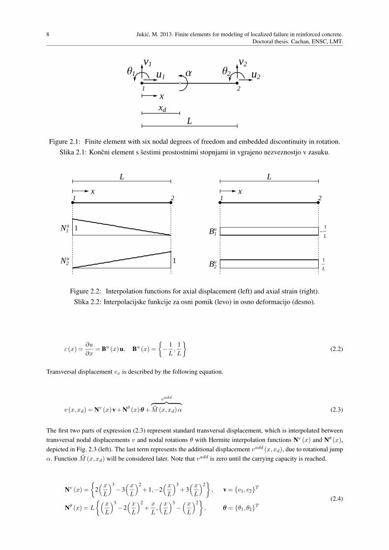
8 Jukic, M. 2013. Finite elements for modeling of localized failure in reinforced concrete.
Doctoral thesis. Cachan, ENSC, LMT.
xxd
L
u1
v1Θ1 u2
v2Θ2Α
1 2
Figure 2.1: Finite element with six nodal degrees of freedom and embedded discontinuity in rotation.
Slika 2.1: Koncni element s sestimi prostostnimi stopnjami in vgrajeno nezveznostjo v zasuku.
N1u
N2u
x
L
1 2
1
1
B1u
B2u
x
L
1 2
-1
L
1
L
Figure 2.2: Interpolation functions for axial displacement (left) and axial strain (right).
Slika 2.2: Interpolacijske funkcije za osni pomik (levo) in osno deformacijo (desno).
ε(x) =∂u
∂x= Bu (x)u, Bu (x) =
−1
L,
1
L
(2.2)
Transversal displacement vx is described by the following equation.
v (x,xd) = Nv (x)v+Nθ (x)θ+
vadd︷ ︸︸ ︷
M (x,xd)α (2.3)
The first two parts of expression (2.3) represent standard transversal displacement, which is interpolated between
transversal nodal displacements v and nodal rotations θ with Hermite interpolation functions Nv (x) and Nθ (x),
depicted in Fig. 2.3 (left). The last term represents the additional displacement vadd (x,xd), due to rotational jump
α. Function M (x,xd) will be considered later. Note that vadd is zero until the carrying capacity is reached.
Nv (x) =
2( x
L
)3
−3( x
L
)2
+1,−2( x
L
)3
+3( x
L
)2
, v = v1,v2T
Nθ (x) = L
( x
L
)3
−2( x
L
)2
+x
L,( x
L
)3
−( x
L
)2
, θ = θ1,θ2T
(2.4)
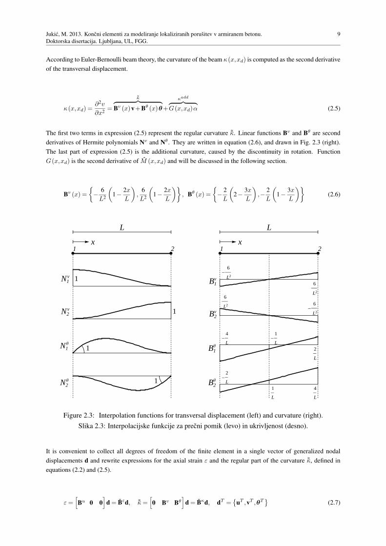
Jukic, M. 2013. Koncni elementi za modeliranje lokaliziranih porusitev v armiranem betonu.
Doktorska disertacija. Ljubljana, UL, FGG.
9
According to Euler-Bernoulli beam theory, the curvature of the beam κ(x,xd) is computed as the second derivative
of the transversal displacement.
κ(x,xd) =∂2v
∂x2=
˜κ︷ ︸︸ ︷
Bv (x)v+Bθ (x)θ+
κadd
︷ ︸︸ ︷
G(x,xd)α (2.5)
The first two terms in expression (2.5) represent the regular curvature ˜κ. Linear functions Bv and Bθ are second
derivatives of Hermite polynomials Nv and Nθ. They are written in equation (2.6), and drawn in Fig. 2.3 (right).
The last part of expression (2.5) is the additional curvature, caused by the discontinuity in rotation. Function
G(x,xd) is the second derivative of M (x,xd) and will be discussed in the following section.
Bv (x) =
−6
L2
(
1−2x
L
)
,6
L2
(
1−2x
L
)
, Bθ (x) =
−2
L
(
2−3x
L
)
,−2
L
(
1−3x
L
)
(2.6)
N1v
N2v
N1Θ
N2Θ
x
L
1 2
1
1
1
1
B1v
B2v
B1Θ
B2Θ
x
L
1 2
-6
L2
6
L2
6
L2-
6
L2
-4
L-
1
L2
L
-2
L1
L
4
L
Figure 2.3: Interpolation functions for transversal displacement (left) and curvature (right).
Slika 2.3: Interpolacijske funkcije za precni pomik (levo) in ukrivljenost (desno).
It is convenient to collect all degrees of freedom of the finite element in a single vector of generalized nodal
displacements d and rewrite expressions for the axial strain ε and the regular part of the curvature ˜κ, defined in
equations (2.2) and (2.5).
ε=[
Bu 0 0]
d = Bεd, ˜κ=[
0 Bv Bθ]
d = Bκd, dT =
uT ,vT ,θT
(2.7)
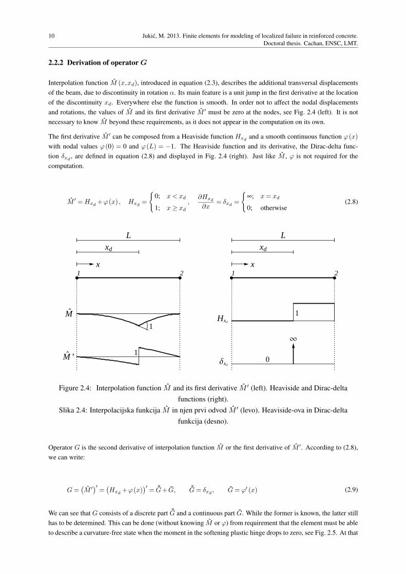
10 Jukic, M. 2013. Finite elements for modeling of localized failure in reinforced concrete.
Doctoral thesis. Cachan, ENSC, LMT.
2.2.2 Derivation of operator G
Interpolation function M (x,xd), introduced in equation (2.3), describes the additional transversal displacements
of the beam, due to discontinuity in rotation α. Its main feature is a unit jump in the first derivative at the location
of the discontinuity xd. Everywhere else the function is smooth. In order not to affect the nodal displacements
and rotations, the values of M and its first derivative M ′ must be zero at the nodes, see Fig. 2.4 (left). It is not
necessary to know M beyond these requirements, as it does not appear in the computation on its own.
The first derivative M ′ can be composed from a Heaviside function Hxd and a smooth continuous function ϕ(x)
with nodal values ϕ(0) = 0 and ϕ(L) = −1. The Heaviside function and its derivative, the Dirac-delta func-
tion δxd , are defined in equation (2.8) and displayed in Fig. 2.4 (right). Just like M , ϕ is not required for the
computation.
M ′ =Hxd +ϕ(x) , Hxd =
0; x < xd
1; x≥ xd
,∂Hxd
∂x= δxd =
∞; x= xd
0; otherwise(2.8)
M`
M`
’
x
xd
L
1 2
1
1
Hxd
∆xd
x
xd
L
1 2
1
¥
0
Figure 2.4: Interpolation function M and its first derivative M ′ (left). Heaviside and Dirac-delta
functions (right).
Slika 2.4: Interpolacijska funkcija M in njen prvi odvod M ′ (levo). Heaviside-ova in Dirac-delta
funkcija (desno).
Operator G is the second derivative of interpolation function M or the first derivative of M ′. According to (2.8),
we can write:
G=(M ′)′=(Hxd +ϕ(x)
)′= ¯G+ G, ¯G= δxd , G= ϕ′ (x) (2.9)
We can see that G consists of a discrete part ¯G and a continuous part G. While the former is known, the latter still
has to be determined. This can be done (without knowing M or ϕ) from requirement that the element must be able
to describe a curvature-free state when the moment in the softening plastic hinge drops to zero, see Fig. 2.5. At that

Jukic, M. 2013. Koncni elementi za modeliranje lokaliziranih porusitev v armiranem betonu.
Doktorska disertacija. Ljubljana, UL, FGG.
11
point, the element should behave as two rigid bodies, connected by a rotation hinge, which implies the following
relations between the nodal degrees of freedom:
v2 = v1 +Lθ1 +(L−xd)α, θ2 = θ1 +α (2.10)
X
Y
u1,v1
u2,v2
Θ 1
Θ 2
Αx
Figure 2.5: Curvature-free deformation of the beam when the moment in the hinge drops to zero.
Slika 2.5: Deformirana lega brez ukrivljenosti, ko moment v plasticnem clenku pade na nic.
Let us now rewrite the expression (2.5) for curvature, taking into account the form of G.
κ(x,xd) =
κ︷ ︸︸ ︷
Bv (x)v+Bθ (x)θ+ G(x,xd)α+
¯κ︷ ︸︸ ︷
¯G(x,xd)α (2.11)
Continuous part of expression (2.11) is designated with κ and represents the curvature of the bulk of the element.
The discrete part ¯κ represents the infinite curvature at location of the discontinuity xd. In a situation, depicted
in Fig. 2.5, the bulk curvature is zero. After applying relations (2.10) and equations (2.6) for Bv and Bθ, the
expression for κ is equaled to zero. Solution of obtained equation delivers the expression for G.
G(x,xd) =−1+3
(
1− 2xdL
)(1− 2x
L
)
L(2.12)
2.2.3 Relations between global and local quantities
2.2.3.1 Real degrees of freedom
A structure is modeled with a mesh of finite elements. A part of such mesh is depicted in Fig. 2.6. The total number
of the nodes in the mesh is designated with nN . Each node has three degrees of freedom - displacement U parallel
to the global X axis, displacement V parallel to the global Y axis, and rotation Θ about the axis, perpendicular to
the XY plane. The structure has in total nDOF = 3nN degrees of freedom, which are collected in the vector dstr.
dstr =U1,V1,Θ1,U2,V2,Θ2, ... ,UnN ,VnN ,ΘnN
T(2.13)
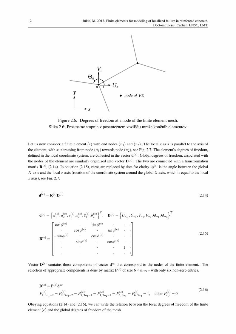
12 Jukic, M. 2013. Finite elements for modeling of localized failure in reinforced concrete.
Doctoral thesis. Cachan, ENSC, LMT.
X
Ynode of FE
n Un
Vn
Qn
Figure 2.6: Degrees of freedom at a node of the finite element mesh.
Slika 2.6: Prostostne stopnje v posameznem vozliscu mreze koncnih elementov.
Let us now consider a finite element (e) with end nodes (n1) and (n2). The local x axis is parallel to the axis of
the element, with x increasing from node (n1) towards node (n2), see Fig. 2.7. The element’s degrees of freedom,
defined in the local coordinate system, are collected in the vector d(e). Global degrees of freedom, associated with
the nodes of the element are similarly organized into vector D(e). The two are connected with a transformation
matrix R(e), (2.14). In equation (2.15), zeros are replaced by dots for clarity. φ(e) is the angle between the global
X axis and the local x axis (rotation of the coordinate system around the global Z axis, which is equal to the local
z axis), see Fig. 2.7.
d(e) = R(e)D(e) (2.14)
d(e) =
u(e)1 ,u
(e)2 ,v
(e)1 ,v
(e)2 ,θ
(e)1 ,θ
(e)2
T, D(e) =
Un1,Un2
,Vn1,Vn2
,Θn1,Θn2
T
R(e) =
cosφ(e) · sinφ(e) · · ·
· cosφ(e) · sinφ(e) · ·
−sinφ(e) · cosφ(e) · · ·
· −sinφ(e) · cosφ(e) · ·
· · · · 1 ·
· · · · · 1
(2.15)
Vector D(e) contains those components of vector dstr that correspond to the nodes of the finite element. The
selection of appropriate components is done by matrix P(e) of size 6×nDOF with only six non-zero entries.
D(e) = P(e)dstr
P(e)1, 3n1−2 = P
(e)2, 3n2−2 = P
(e)3, 3n1−1 = P
(e)4, 3n2−1 = P
(e)5, 3n1
= P(e)6, 3n2
= 1, other P(e)i,j = 0
(2.16)
Obeying equations (2.14) and (2.16), we can write the relation between the local degrees of freedom of the finite
element (e) and the global degrees of freedom of the mesh.

Jukic, M. 2013. Koncni elementi za modeliranje lokaliziranih porusitev v armiranem betonu.
Doktorska disertacija. Ljubljana, UL, FGG.
13
d(e) = R(e)P(e)dstr (2.17)
n1 Un1
Vn1
Qn1
n2 Un2
Vn2
Qn2
HeL
1
u1
v1
Θ1
2
u2
v2
Θ2
HeL
X
Y
xy
Φ
Figure 2.7: Global (left) and local (right) degrees of freedom, associated with a finite element.
Slika 2.7: Globalne (levo) in lokalne (desno) prostostne stopnje, povezane s koncnim elementom.
2.2.3.2 Virtual degrees of freedom
Virtual displacements are a kinematically admissible variation of real displacements. As with the real displace-
ments, they are interpolated between the nodal values with appropriate interpolation functions. The virtual defor-
mation of the mesh is therefore defined by the virtual displacements of its nodes.
The global virtual degrees of freedom (virtual nodal displacements of the structure) dstr, the virtual displacements
of the element d(e) and the selection D(e) of the global virtual displacements, associated with the element (e), are
defined analogously to the real quantities dstr, d(e) and D(e), defined in equations (2.13) and (2.15).
dstr =U1, V1, Θ1, U2, V2, Θ2, ... , UnN , VnN , ΘnN
T
d(e) =
u(e)1 , u
(e)2 , v
(e)1 , v
(e)2 , θ
(e)1 , θ
(e)2
T, D(e) =
Un1
, Un2, Vn1
, Vn2, Θn1
, Θn2
T(2.18)
Relations between them are equivalent to equations (2.14)-(2.17), matrices R(e) and P(e) remain the same.
d(e) = R(e)D(e), D(e) = P(e)dstr, d(e) = R(e)P(e)dstr (2.19)
2.2.3.3 Internal forces
Internal forces can be organized in the same way as the generalized displacements. Each degree of freedom from
the vector dstr is accompanied by a corresponding internal force. Analogously to equation (2.13) we can write:
f int,str =
f intU1,f int
V1,f int
Θ1,f int
U2,f int
V2,f int
Θ2, ... ,f int
UnN,f int
VnN,f int
ΘnN
T(2.20)
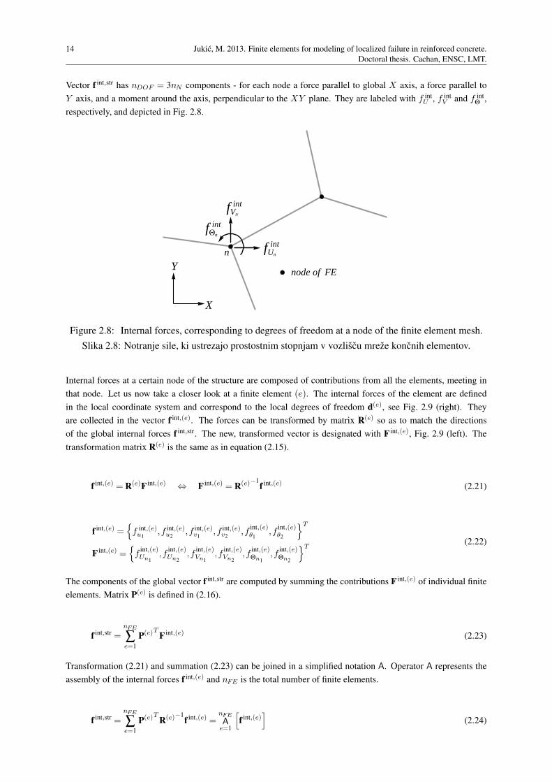
14 Jukic, M. 2013. Finite elements for modeling of localized failure in reinforced concrete.
Doctoral thesis. Cachan, ENSC, LMT.
Vector f int,str has nDOF = 3nN components - for each node a force parallel to global X axis, a force parallel to
Y axis, and a moment around the axis, perpendicular to the XY plane. They are labeled with f intU , f int
V and f intΘ ,
respectively, and depicted in Fig. 2.8.
X
Ynode of FE
n fUn
int
fVn
int
fQn
int
Figure 2.8: Internal forces, corresponding to degrees of freedom at a node of the finite element mesh.
Slika 2.8: Notranje sile, ki ustrezajo prostostnim stopnjam v vozliscu mreze koncnih elementov.
Internal forces at a certain node of the structure are composed of contributions from all the elements, meeting in
that node. Let us now take a closer look at a finite element (e). The internal forces of the element are defined
in the local coordinate system and correspond to the local degrees of freedom d(e), see Fig. 2.9 (right). They
are collected in the vector f int,(e). The forces can be transformed by matrix R(e) so as to match the directions
of the global internal forces f int,str. The new, transformed vector is designated with F int,(e), Fig. 2.9 (left). The
transformation matrix R(e) is the same as in equation (2.15).
f int,(e) = R(e)F int,(e) ⇔ F int,(e) = R(e)−1f int,(e) (2.21)
f int,(e) =
f int,(e)u1
,f int,(e)u2
,f int,(e)v1
,f int,(e)v2
,fint,(e)θ1
,fint,(e)θ2
T
F int,(e) =
fint,(e)Un1
,fint,(e)Un2
,fint,(e)Vn1
,fint,(e)Vn2
,fint,(e)Θn1
,fint,(e)Θn2
T(2.22)
The components of the global vector f int,str are computed by summing the contributions F int,(e) of individual finite
elements. Matrix P(e) is defined in (2.16).
f int,str =nFE
∑e=1
P(e)T F int,(e) (2.23)
Transformation (2.21) and summation (2.23) can be joined in a simplified notation A. Operator A represents the
assembly of the internal forces f int,(e) and nFE is the total number of finite elements.
f int,str =nFE
∑e=1
P(e)T R(e)−1f int,(e) =
nFE
Ae=1
[
f int,(e)]
(2.24)

Jukic, M. 2013. Koncni elementi za modeliranje lokaliziranih porusitev v armiranem betonu.
Doktorska disertacija. Ljubljana, UL, FGG.
15
n1 fUn1
int,HeL
fVn1
int,HeL
fQn1
int,HeL
n2 fUn2
int,HeL
fVn2
int,HeL
fQn2
int,HeL
HeL
1
fu1
int,HeL
fv1
int,HeL
fΘ1
int,HeL
2
fu2
int,HeL
fv2
int,HeL
fΘ2
int,HeL
HeL
X
Y
xy
Φ
Figure 2.9: Contribution of a finite element to internal forces of the structure in global (left) and local
(right) coordinate system.
Slika 2.9: Prispevek koncnega elementa k notranjim silam konstrukcije v globalnem (levo) in lokalnem
(desno) koordinatnem sistemu.
Another useful relation can be observed. For rotation matrix R(e) it holds RT = R−1 or RT R = I, where I is the
identity matrix. By using this property as well as equations (2.19) and (2.21), we can conclude that the scalar
product of virtual displacements and internal forces is equal in local and global coordinate system.
d(e)T f int,(e) = D(e)T R(e)T R(e) F int,(e) = D(e)T F int,(e) (2.25)
2.2.4 Virtual work equation
Equilibrium of a structure can be described in a weak from, by the virtual work principle, which states that the
virtual work of internal forces G int on any kinematically admissible perturbation of displacements - virtual dis-
placements - must be equal to the work of external forces Gext on the same displacements.
G int −Gext = 0 (2.26)
Since we are dealing with a discretized model, the external loads are defined at the nodes of the mesh. Distributed
loads have to be transferred to the nodes appropriately. The virtual work of external forces is therefore computed
simply as a scalar product of the vector of virtual nodal displacements of the mesh dstr and the corresponding
vector of generalized external forces f ext,str. Virtual displacements are defined in equation (2.18) and the external
forces are defined analogously to the internal forces in equation (2.20).
Gext = dstrT f ext,str =nDOF
∑j=1
dstrj f ext,str
j (2.27)
Here nDOF is the number of the structure’s degrees of freedom. Many components of the sum (2.27) may be zero.
The virtual work of internal forces is composed of contributions from individual finite elements. The total number
of finite elements in the mesh is nFE .
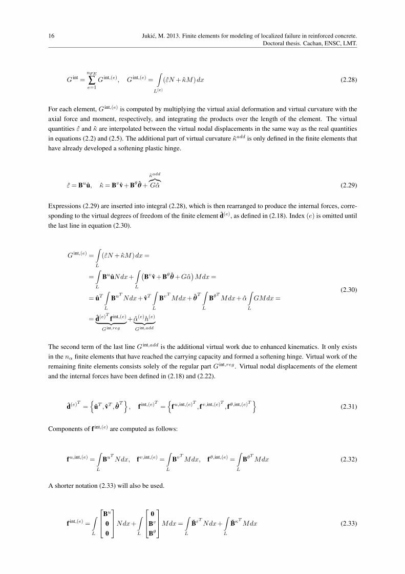
16 Jukic, M. 2013. Finite elements for modeling of localized failure in reinforced concrete.
Doctoral thesis. Cachan, ENSC, LMT.
G int =nFE
∑e=1
G int,(e), G int,(e) =∫
L(e)
(εN + κM)dx (2.28)
For each element, G int,(e) is computed by multiplying the virtual axial deformation and virtual curvature with the
axial force and moment, respectively, and integrating the products over the length of the element. The virtual
quantities ε and κ are interpolated between the virtual nodal displacements in the same way as the real quantities
in equations (2.2) and (2.5). The additional part of virtual curvature κadd is only defined in the finite elements that
have already developed a softening plastic hinge.
ε= Buu, κ= Bv v+Bθθ+
κadd
︷︸︸︷
Gα (2.29)
Expressions (2.29) are inserted into integral (2.28), which is then rearranged to produce the internal forces, corre-
sponding to the virtual degrees of freedom of the finite element d(e), as defined in (2.18). Index (e) is omitted until
the last line in equation (2.30).
G int,(e) =∫
L
(εN + κM)dx=
=∫
L
BuuNdx+∫
L
(Bv v+Bθθ+Gα
)Mdx=
= uT∫
L
BuT
Ndx+ vT∫
L
BvT
Mdx+ θT∫
L
BθTMdx+ α∫
L
GMdx=
= d(e)T f int,(e)︸ ︷︷ ︸
G int,reg
+ α(e)h(e)︸ ︷︷ ︸
G int,add
(2.30)
The second term of the last line G int,add is the additional virtual work due to enhanced kinematics. It only exists
in the nα finite elements that have reached the carrying capacity and formed a softening hinge. Virtual work of the
remaining finite elements consists solely of the regular part G int,reg . Virtual nodal displacements of the element
and the internal forces have been defined in (2.18) and (2.22).
d(e)T =
uT , vT , θT
, f int,(e)T =
fu,int,(e)T , fv,int,(e)T , fθ,int,(e)T
(2.31)
Components of f int,(e) are computed as follows:
fu,int,(e) =∫
L
BuT
Ndx, fv,int,(e) =∫
L
BvTMdx, fθ,int,(e) =∫
L
BθTMdx (2.32)
A shorter notation (2.33) will also be used.
f int,(e) =∫
L
Bu
0
0
Ndx+
∫
L
0
Bv
Bθ
Mdx=
∫
L
BεTNdx+∫
L
BκT
Mdx (2.33)
Jukic, M. 2013. Koncni elementi za modeliranje lokaliziranih porusitev v armiranem betonu.
Doktorska disertacija. Ljubljana, UL, FGG.
17
Quantity h(e) corresponds to the virtual rotational jump α(e).
h(e) =∫
L
GMdx=∫
L
(G+ δxd
)Mdx=
∫
L
GMdx+ M |xd =∫
L
GMdx+ t (2.34)
In (2.34), we have used equation (2.9) for G and rule (2.35) for integration of the Dirac-delta function. Quantity
M |xd is the value of function M (x) at coordinate xd. We assign to it a new symbol t and assume it as the moment
at the discontinuity (the moment in the softening hinge).
∫
L
g (x)δxddx= g (xd) (2.35)
The virtual work of external and internal forces in the equilibrium equation (2.26) is replaced by expressions (2.27)
and (2.28), applying also (2.30) and (2.25). Remember, that the additional virtual work G int,add is only included
for the nα finite elements, already in the softening phase. For the sake of simplicity, it is assumed that they are
labeled with consecutive numbers from 1 to nα. Finally, the second of equations (2.19) allows us to express the
weak equilibrium in the manner of global virtual displacement vector dstr and virtual rotational jumps α(e).
0 =nFE
∑e=1
G int,(e)−Gext =
=nFE
∑e=1
D(e)T F int,(e)+nα
∑e=1
α(e)h(e)− dstrT f ext,str =
= dstrTnFE
∑e=1
P(e)T F int,(e)+nα
∑e=1
α(e)h(e)− dstrT f ext,str =
= dstrT(
f int,str − f ext,str)
+nα
∑e=1
α(e)h(e)
(2.36)
Equilibrium (2.36) must hold for any kinematically admissible virtual displacements dstr and virtual rotational
jumps α(e). From this requirement we can conclude:
f int,str − f ext,str = 0
∀e ∈ 1,2, . . . ,nα : h(e) = 0(2.37)
The first of equations (2.37) represents equilibrium of every individual node of the mesh, or the global equilibrium.
Here f int,str and f ext,str are vectors of internal and external forces on the structural level. They correspond in position
and direction to the degrees of freedom of the structure. Their length is equal to the total number of degrees of
freedom nDOF . The second of equations (2.37) can be better interpreted after inserting expression (2.34) for
h(e). Equation (2.38) represents a weak form (integral form) of Cauchy equilibrium between the moment t at the
discontinuity and the moment M in the bulk of the element.
h(e) = 0 ⇔ t=−∫
L
GMdx (2.38)
18 Jukic, M. 2013. Finite elements for modeling of localized failure in reinforced concrete.
Doctoral thesis. Cachan, ENSC, LMT.
Another verification is required at this place. The principle of embedded discontinuity can be regarded as a method
of incompatible modes. In that view, the additional virtual work G int,add, performed on the virtual rotational jump
α, should be zero at least for the case of constant moment in the element.
α∫
L
GMdx= αM︸︷︷︸
6=0
∫
L
Gdx= 0 ⇒∫
L
Gdx= 0 (2.39)
Taking into account the rule (2.35) for integration of the Dirac-delta function, requirement (2.39) can be reformu-
lated.
∫
L
Gdx=∫
L
(G+ δxd
)dx=
∫
L
Gdx+
=1︷ ︸︸ ︷∫
L
δxddx= 0 ⇒∫
L
Gdx=−1 (2.40)
Operator G, as defined in equation (2.12) satisfies this condition, regardless of the location of the discontinuity xd.
2.2.5 Constitutive models
In this section we describe selected constitutive models. Bending is controlled by two separate laws, one for the
bulk of the element and the other for the softening hinge at the location of the discontinuity.
2.2.5.1 Axial response
The axial response is presumed linear elastic. In equation (2.41), N is the axial force, E is the elastic modulus, A
is the cross-section and ε is the axial strain, computed according to equation (2.2).
N = EAε,∂N
∂ε= EA (2.41)
2.2.5.2 Bending response for the bulk of the element
Behavior of the bulk of the element is described by elasto-plastic model with bilinear isotropic hardening. A
typical moment-curvature diagram is shown in Fig. 2.10 (left). Response is linear elastic up to moment Mc, at
which the first cracks in concrete appear, reducing the bending stiffness of the beam. Another drop in stiffness
occurs at moment My , when the reinforcement starts to yield. Unloading lines are parallel to the initial elastic
line. This also holds for the part of the diagram between Mc and My . Although a combined damage-plasticity
model would be more accurate, this simple plasticity model performs well enough for typical reinforced concrete
cross-sections, where the largest part of inelastic deformations comes from tensile reinforcement. The diagrams in
Fig. 2.10 depend on the axial force N . In this chapter, we limit ourselves to beams with symmetrical cross-section,
which implies a symmetrical response for positive and negative bending moment. The bulk material model is
mathematically described by the following equations, which can be derived from the principle of maximum plastic
dissipation, see e.g. [54].
Remark. For beams with a non-symmetrical cross-section, the material parameters, which determine the dia-
grams in Fig. 2.10, would be different for positive and negative moments.

Jukic, M. 2013. Koncni elementi za modeliranje lokaliziranih porusitev v armiranem betonu.
Doktorska disertacija. Ljubljana, UL, FGG.
19
EI
H 1
H 2
Κc Κy ΚuΚ
Mc
My
Mu
M
H1
H2
Ξ
My-Mc
Mu-Mc
-q
Figure 2.10: Moment - curvature diagram (left). Bilinear hardening law (right). Only positive parts of
the diagrams are shown. They are valid for constant value of axial force.
Slika 2.10: Diagram moment - ukrivljenost (levo). Bilinearno utrjevanje (desno). Prikazana sta samo
pozitivna dela diagramov. Veljata za konstantno osno silo.
Moment M is related to curvature κ by equation (2.42), which represents the elastic loading path and elastic
unloading/reloading path of the M − κ diagram.
M = EI (κ− κp) , κ= Bvv+Bθθ+ Gα (2.42)
Here E is the elastic modulus, I is the moment of inertia, κp plastic curvature, and κ the bulk curvature, as defined
in equation (2.11). Before the formation of the softening hinge, the rotational jump α is zero. The plastic loading
path of the M − κ diagram is determined indirectly by the remaining equations in this section.
φ(M,q) = |M |− (Mc− q) (2.43)
Yield function φ prescribes the admissible moments. Elasticity limit Mc is the absolute value of the moment, at
which the first plastic deformation occurs. Moment-like hardening variable q controls the yield threshold evolution.
q =
−H1ξ; ξ ≤ ξ∆H
− (My −Mc)−H2
(ξ− ξ∆H
); ξ > ξ∆H
ξ∆H =My −Mc
H1(2.44)
Equation (2.44) describes the bilinear isotropic hardening of the material, presented in Fig. 2.10 (right). Here
H1 > 0 and H2 > 0 are constant hardening moduli, ξ is a curvature-like hardening variable with the initial value
zero, and ξ∆H is the value of ξ, at which the slope in the q− ξ diagram changes from H1 to H2. Evolution in
pseudo-time of internal hardening variables for plasticity, κp and ξ, is prescribed by evolution equations (2.45).
˙κp = ˙γ sign(M) , ˙ξ = ˙γ (2.45)
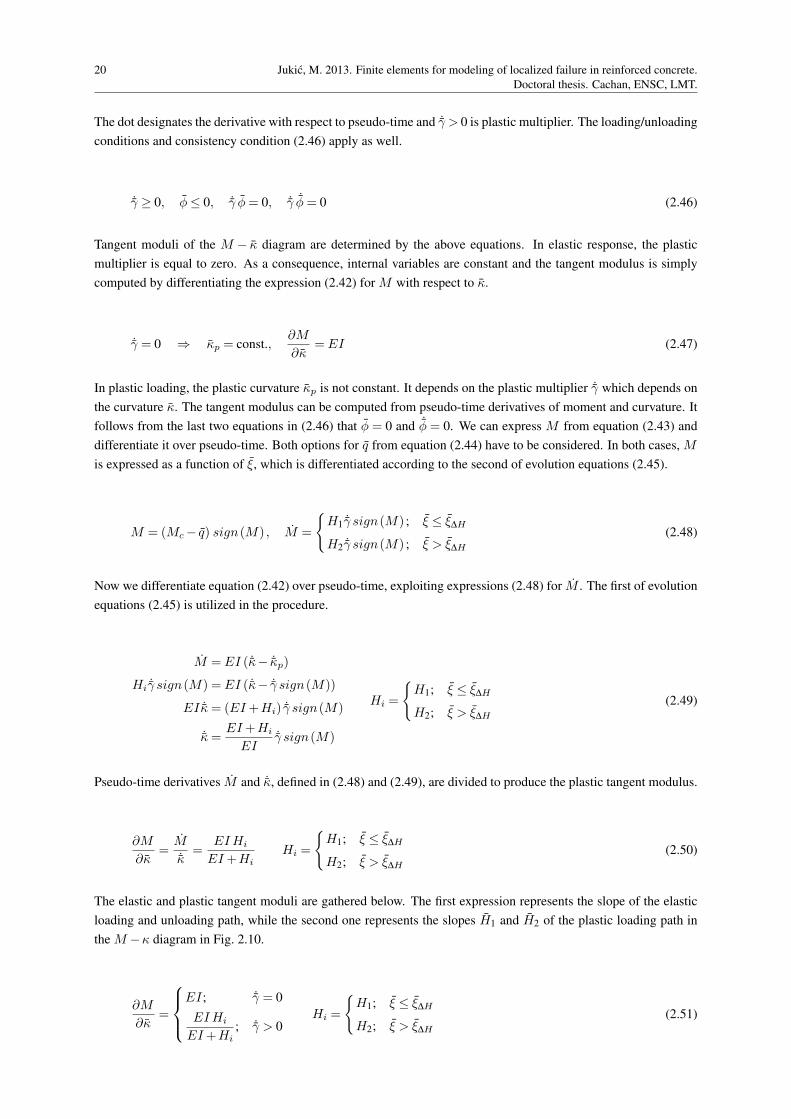
20 Jukic, M. 2013. Finite elements for modeling of localized failure in reinforced concrete.
Doctoral thesis. Cachan, ENSC, LMT.
The dot designates the derivative with respect to pseudo-time and ˙γ > 0 is plastic multiplier. The loading/unloading
conditions and consistency condition (2.46) apply as well.
˙γ ≥ 0, φ≤ 0, ˙γ φ= 0, ˙γ ˙φ= 0 (2.46)
Tangent moduli of the M − κ diagram are determined by the above equations. In elastic response, the plastic
multiplier is equal to zero. As a consequence, internal variables are constant and the tangent modulus is simply
computed by differentiating the expression (2.42) for M with respect to κ.
˙γ = 0 ⇒ κp = const.,∂M
∂κ= EI (2.47)
In plastic loading, the plastic curvature κp is not constant. It depends on the plastic multiplier ˙γ which depends on
the curvature κ. The tangent modulus can be computed from pseudo-time derivatives of moment and curvature. It
follows from the last two equations in (2.46) that φ = 0 and ˙φ = 0. We can express M from equation (2.43) and
differentiate it over pseudo-time. Both options for q from equation (2.44) have to be considered. In both cases, M
is expressed as a function of ξ, which is differentiated according to the second of evolution equations (2.45).
M = (Mc− q) sign(M) , M =
H1 ˙γ sign(M) ; ξ ≤ ξ∆H
H2 ˙γ sign(M) ; ξ > ξ∆H
(2.48)
Now we differentiate equation (2.42) over pseudo-time, exploiting expressions (2.48) for M . The first of evolution
equations (2.45) is utilized in the procedure.
M = EI ( ˙κ− ˙κp)
Hi ˙γ sign(M) = EI ( ˙κ− ˙γ sign(M))
EI ˙κ= (EI+Hi) ˙γ sign(M)
˙κ=EI+Hi
EI˙γ sign(M)
Hi =
H1; ξ ≤ ξ∆H
H2; ξ > ξ∆H
(2.49)
Pseudo-time derivatives M and ˙κ, defined in (2.48) and (2.49), are divided to produce the plastic tangent modulus.
∂M
∂κ=
M˙κ
=EIHi
EI+HiHi =
H1; ξ ≤ ξ∆H
H2; ξ > ξ∆H
(2.50)
The elastic and plastic tangent moduli are gathered below. The first expression represents the slope of the elastic
loading and unloading path, while the second one represents the slopes H1 and H2 of the plastic loading path in
the M −κ diagram in Fig. 2.10.
∂M
∂κ=
EI; ˙γ = 0
EIHi
EI+Hi; ˙γ > 0
Hi =
H1; ξ ≤ ξ∆H
H2; ξ > ξ∆H
(2.51)
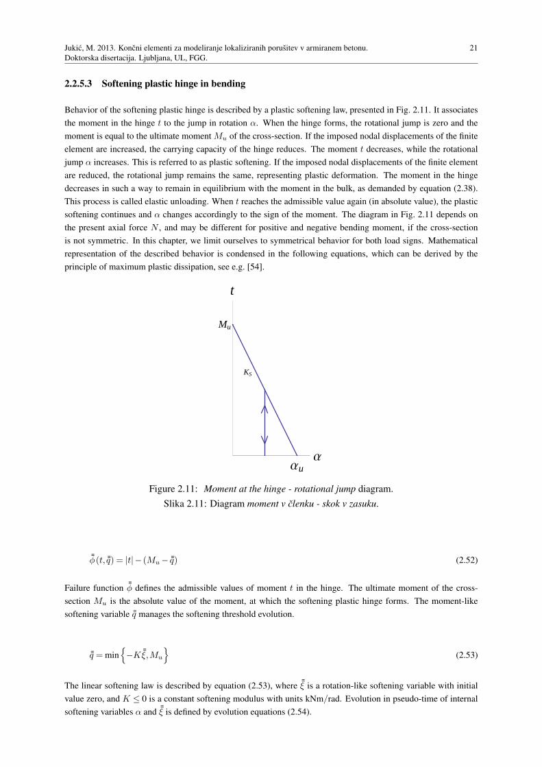
Jukic, M. 2013. Koncni elementi za modeliranje lokaliziranih porusitev v armiranem betonu.
Doktorska disertacija. Ljubljana, UL, FGG.
21
2.2.5.3 Softening plastic hinge in bending
Behavior of the softening plastic hinge is described by a plastic softening law, presented in Fig. 2.11. It associates
the moment in the hinge t to the jump in rotation α. When the hinge forms, the rotational jump is zero and the
moment is equal to the ultimate moment Mu of the cross-section. If the imposed nodal displacements of the finite
element are increased, the carrying capacity of the hinge reduces. The moment t decreases, while the rotational
jump α increases. This is referred to as plastic softening. If the imposed nodal displacements of the finite element
are reduced, the rotational jump remains the same, representing plastic deformation. The moment in the hinge
decreases in such a way to remain in equilibrium with the moment in the bulk, as demanded by equation (2.38).
This process is called elastic unloading. When t reaches the admissible value again (in absolute value), the plastic
softening continues and α changes accordingly to the sign of the moment. The diagram in Fig. 2.11 depends on
the present axial force N , and may be different for positive and negative bending moment, if the cross-section
is not symmetric. In this chapter, we limit ourselves to symmetrical behavior for both load signs. Mathematical
representation of the described behavior is condensed in the following equations, which can be derived by the
principle of maximum plastic dissipation, see e.g. [54].
KS
ΑuΑ
Mu
t
Figure 2.11: Moment at the hinge - rotational jump diagram.
Slika 2.11: Diagram moment v clenku - skok v zasuku.
¯φ(t, ¯q) = |t|− (Mu− ¯q) (2.52)
Failure function ¯φ defines the admissible values of moment t in the hinge. The ultimate moment of the cross-
section Mu is the absolute value of the moment, at which the softening plastic hinge forms. The moment-like
softening variable ¯q manages the softening threshold evolution.
¯q = min
−K ¯ξ,Mu
(2.53)
The linear softening law is described by equation (2.53), where ¯ξ is a rotation-like softening variable with initial
value zero, and K ≤ 0 is a constant softening modulus with units kNm/rad. Evolution in pseudo-time of internal
softening variables α and ¯ξ is defined by evolution equations (2.54).
22 Jukic, M. 2013. Finite elements for modeling of localized failure in reinforced concrete.
Doctoral thesis. Cachan, ENSC, LMT.
α= ˙γ sign(t) ,˙ξ = ˙γ (2.54)
The dot designates the derivative with respect to pseudo-time and ˙γ > 0 is plastic softening multiplier. The load-
ing/unloading conditions and consistency condition (2.55) also apply.
˙γ ≥ 0, ¯φ≤ 0, ˙γ ¯φ= 0, ˙γ˙φ= 0 (2.55)
The equation of the plastic softening loading path of t−α diagram is not unique. It depends on the loading history.
If the softening process alternates between both load signs, the loading path is translated sideways (left or right).
The slope, however, is not affected and can be determined from the pseudo-time derivatives of t and α. In softening
process, when ˙γ > 0, the failure function ¯φ = 0. Expression for t is then determined from (2.52) and (2.53). The
derivative is obtained in accordance with evolution equation (2.54) for ¯ξ.
t= (Mu− ¯q)sign(t) =
(
Mu+K ¯ξ)
sign(t) ; ¯q <Mu
0; ¯q =Mu
t=
K ˙γsign(t) ; ¯q <Mu
0; ¯q =Mu
(2.56)
The slope of the plastic softening path, defined as the derivative of t over α, is computed by dividing the pseudo-
time derivatives (2.56) and (2.54) of both quantities.
∂t
∂α=
t
α=
not defined; ˙γ = 0
K; ˙γ > 0, ¯q <Mu
0; ˙γ > 0, ¯q =Mu
(2.57)
A third option was added in equation (2.57). It corresponds to elastic unloading path with ˙γ = 0. It follows from
evolution equations (2.54) that α= 0 in that case. And since the failure function ¯φ is no longer required to be zero,
the traction t cannot be computed as in (2.56). It changes in accordance with equation (2.38) which represents the
equilibrium between the bulk and the discontinuity. The derivative ∂t/∂α cannot be defined in this case, because
α is constant.
2.3 Computational procedure
Response of a structure, discretized by a mesh of nFE above derived finite elements, is computed at discrete
pseudo-time points τ0, τ1, . . . , τn, τn+1, . . . , T by solving at each pseudo-time point nonlinear equations (2.58)
for current values of nodal displacements/rotations.
f int,str − f ext,str = 0
∀e ∈ 1, 2, ... , nα : h(e) = 0(2.58)
Here, nα is the number of elements that have reached the carrying capacity and formed a softening plastic hinge.
At a particular pseudo-time point τn+1, the solution is searched iteratively by the Newton-Raphson method. Each
iteration, denoted by k, consists of two subsequent phases: (A) computation of internal variables, corresponding

Jukic, M. 2013. Koncni elementi za modeliranje lokaliziranih porusitev v armiranem betonu.
Doktorska disertacija. Ljubljana, UL, FGG.
23
to the current iterative values of nodal displacements/rotations, in order to compute the moments in the bulk and
in the softening plastic hinge according to the chosen material laws; (B) solution of linearized equations (2.58)
in order to update the iterative values of nodal displacements/rotations. When one phase of the computation is
completed, the results are used immediately in the next one.
For a pseudo-time point τn+1, the computational problem related to a generic finite element (e) can be stated as:
given
d(e)n ; κ
(e)p,n, ξ
(e)n , α
(e)n , ¯ξ
(e)n
find
d(e)n+1; κ
(e)p,n+1, ξ
(e)n+1, α
(e)n+1,
¯ξ(e)n+1
Note that superscript (e) was omitted in section 2.2.5 for the above internal variables. The subscript n and n+ 1
denote the values at pseudo-times τn and τn+1, respectively.
2.3.1 Computation of internal variables
In this section we will present computations of phase (A). The internal variables for element (e) at pseudo-time
point τn+1 will be computed for the k-th iteration, while the nodal displacements/rotations are fixed at the values
from the previous iteration d(e),(k−1)n+1 . Since every internal variable is connected to a single finite element, the
computations are local, i.e. they are performed independently for each element. The condition of the discontinuity
is known by the following flag.
crack(e) =
false . . . no discontinuity in element (e)
true . . . discontinuity in element (e)(2.59)
The algorithm in Fig. 2.12 is applied. If there was no discontinuity in the previous pseudo-time step, we begin with
equations for the hardening phase of material, described in section 2.3.1.2. We must do so even if the previous
iteration of the current step indicated occurrence of the discontinuity, because that was not a converged result. We
check if the carrying capacity is reached. If not, we keep the obtained results, otherwise we discard them and use
equations for the softening phase of material, described in section 2.3.1.3. If the discontinuity already existed in
the previous pseudo-time step, it must also exist in the current step, therefore we follow the procedure from section
2.3.1.3.
The integrals that appear in expressions (2.32), (2.34) and (2.38) for f int,(e), h(e) and t, are evaluated with numerical
integration. A three-point Gauss-Lobatto integration scheme is used with integration points at both ends and at the
center of the finite element. Curvature, moment and hardening internal variables are therefore computed only at
those three locations. Softening internal variables are defined at the location of the discontinuity, which coincides
with one of the integration points (although the two are not connected).
For the sake of clarity we will omit in the rest of this section the superscript (e), denoting the finite element.
2.3.1.1 Axial response
Computation of the axial response is straightforward. Axial strain is computed according to equation (2.7) with
the current values of the nodal displacements. Axial force is calculated from (2.41).
ε(k)n+1 = Bεd
(k−1)n+1 , N
(k)n+1 = EAε
(k)n+1,
∂N
∂ε
∣∣∣∣
(k)
n+1
= EA (2.60)
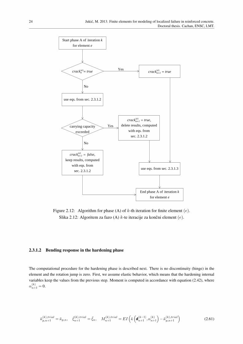
24 Jukic, M. 2013. Finite elements for modeling of localized failure in reinforced concrete.
Doctoral thesis. Cachan, ENSC, LMT.
Start phase A of iteration k
for element e
cracknHeL= true
use eqs. from sec. 2.3.1.2
carrying capacity
exceeded
crackn+1HeL= false,
keep results, computed
with eqs. from
sec. 2.3.1.2
crackn+1HeL= true
crackn+1HeL= true,
delete results, computed
with eqs. from
sec. 2.3.1.2
use eqs. from sec. 2.3.1.3
End phase A of iteration k
for element e
Yes
Yes
No
No
Figure 2.12: Algorithm for phase (A) of k-th iteration for finite element (e).
Slika 2.12: Algoritem za fazo (A) k-te iteracije za koncni element (e).
2.3.1.2 Bending response in the hardening phase
The computational procedure for the hardening phase is described next. There is no discontinuity (hinge) in the
element and the rotation jump is zero. First, we assume elastic behavior, which means that the hardening internal
variables keep the values from the previous step. Moment is computed in accordance with equation (2.42), where
α(k)n+1 = 0.
κ(k),trialp,n+1 = κp,n, ξ
(k),trialn+1 = ξn, M
(k),trialn+1 = EI
(
κ(
d(k−1)n+1 ,α
(k)n+1
)
− κ(k),trialp,n+1
)
(2.61)

Jukic, M. 2013. Koncni elementi za modeliranje lokaliziranih porusitev v armiranem betonu.
Doktorska disertacija. Ljubljana, UL, FGG.
25
Trial yield function φ(k),trialn+1 is computed, as defined in (2.43) and (2.44).
φ(k),trialn+1 =
∣∣∣M
(k),trialn+1
∣∣∣−(
Mc− q(k),trialn+1
)
q(k),trialn+1 =
−H1ξn; ξn ≤ ξ∆H
− (My −Mc)−H2
(ξn− ξ∆H
); ξn > ξ∆H
(2.62)
The trial solution is accepted if the trial yield function is negative or zero.
φ(k),trialn+1 ≤ 0 ⇒ κ
(k)p,n+1 = κ
(k),trialp,n+1 , ξ
(k)n+1 = ξ
(k),trialn+1 , M
(k)n+1 =M
(k),trialn+1 (2.63)
If the trial yield function is positive, the internal variables must be corrected, according to incremental form of
evolution equations (2.45), where γ(k)n+1 = ˙γ
(k)n+1 (τn+1 − τn) > 0. It is shown in appendix A that sign
(
M(k)n+1
)
=
sign(
M(k),trialn+1
)
.
φ(k),trialn+1 > 0 ⇒ κ
(k)p,n+1 = κp,n+ γ
(k)n+1sign
(
M(k),trialn+1
)
, ξ(k)n+1 = ξn+ γ
(k)n+1 (2.64)
By exploiting equations (2.64), the moment M(k)n+1 can be expressed with the trial moment and the plastic multiplier
γ(k)n+1.
M(k)n+1 =M
(k),trialn+1 −EI γ
(k)n+1sign
(
M(k),trialn+1
)
(2.65)
We do the same for the moment-like hardening variable q(k)n+1. Since the expression for q depends on the value of
ξ, we have to consider three options. The values form previous and current step, ξn and ξn+1, can be either both
smaller than ξ∆H , both greater, or one smaller and one greater. Note that ξn+1 is the greater of the two values,
because γ(k)n+1 is positive.
q(k)n+1 =
q(k),trialn+1 −H1γ
(k)n+1; ξn < ξn+1 ≤ ξ∆H
q(k),trialn+1 − (H1 −H2)
(ξ∆H − ξn
)−H2γ
(k)n+1; ξn ≤ ξ∆H , ξn+1 > ξ∆H
q(k),trialn+1 −H2γ
(k)n+1; ξn+1 > ξn > ξ∆H
(2.66)
Yield function φ(k)n+1 is expressed as a function of plastic multiplier γ
(k)n+1 by employing equations (2.65) and
(2.66). Value of the plastic multiplier is computed from requirement φ(k)n+1 = 0, coming from the loading/unloading
conditions.
φ(k)n+1 =
∣∣∣M
(k)n+1
∣∣∣−(
Mu− q(k)n+1
)
= φ(k)n+1
(
γ(k)n+1
)
= 0 (2.67)
26 Jukic, M. 2013. Finite elements for modeling of localized failure in reinforced concrete.
Doctoral thesis. Cachan, ENSC, LMT.
Considering the different values of q(k)n+1, we obtain three expressions for γ
(k)n+1.
γ(k)n+1 =
φ(k),trialn+1
EI+H1; ξn < ξn+1 ≤ ξ∆H
φ(k),trialn+1 − (H1 −H2)
(ξ∆H − ξn
)
EI+H2; ξn ≤ ξ∆H , ξn+1 > ξ∆H
φ(k),trialn+1
EI+H2; ξn+1 > ξn > ξ∆H
(2.68)
Consistent tangent modulus is computed as the derivative of moment over curvature. Moment takes the trial value
from equation (2.61) if plastic multiplier γ(k)n+1 is zero, and the value from (2.65) if γ
(k)n+1 is positive. In the second
case, equations (2.64), (2.68), (2.62) and (2.61) are used to express the moment as a function of curvature.
∂M
∂κ
∣∣∣∣
(k)
n+1
=
EI; γ(k)n+1 = 0
EIHi
EI+Hi; γ
(k)n+1 > 0
Hi =
H1; ξ ≤ ξ∆H
H2; ξ > ξ∆H
(2.69)
The hardening internal variables, the moment and the tangent modulus have been calculated under assumption that
the ultimate moment is not exceeded. This still requires verification. If the assumption is confirmed, the above
results are accepted. Otherwise, they are discarded and recomputed with the presence of the discontinuity.
The first step in the verification is to determine the location of the potential discontinuity xd. Since we have
restricted ourselves to symmetric cross-sections, the hinge is simply placed at the location of maximal moment in
absolute value. This can occur at either end of the element because of the linear form of moment. If the moment is
constant, the discontinuity is placed in the middle of the element.
M1 =M2 =M3 ⇒ xd = L/2
|M1|> |M2| ⇒ xd = 0
|M1|< |M2| ⇒ xd = L
where
M1 = M |x=0
M2 = M |x=L
M3 = M |x=L/2
(2.70)
Remark. For beams with a non-symmetrical cross-section, the positioning of the discontinuity would be less
simple because of the different values of ultimate moment Mu for positive and negative moments. Location of
the discontinuity would be determined in a similar way as in a concrete layer of a multi-layer element in section
3.3.1.1 of the next chapter.
With the location of the potential discontinuity determined, we can calculate the potential value of moment at the
discontinuity t(k),potn+1 by equation (2.38). The integral is evaluated numerically with the three-point Gauss-Lobatto
integration scheme.
t(k),potn+1 =−
∫
L
GM(k)n+1dx (2.71)
Failure function ¯φ(k),potn+1 is evaluated with the moment-like softening variable ¯q equal to zero, as there has been no
reduction of carrying capacity in previous steps.
¯φ(k),potn+1 =
∣∣∣t(k),potn+1
∣∣∣−(
Mu− ¯q(k),potn+1
)
, ¯q(k),potn+1 = 0 (2.72)
Jukic, M. 2013. Koncni elementi za modeliranje lokaliziranih porusitev v armiranem betonu.
Doktorska disertacija. Ljubljana, UL, FGG.
27
We set the value of the discontinuity flag to true if the failure function is positive, and to false otherwise. The
value is not final, however, until the converged state is reached. It can change in following iterations.
¯φ(k),potn+1 ≤ 0 ⇒ crack
(e)n+1 = false
¯φ(k),potn+1 > 0 ⇒ crack
(e)n+1 = true
(2.73)
If the carrying capacity is exceeded, the above computed values of internal hardening variables and moment in the
bulk of the element are discarded and computed again, as explained in the following section.
2.3.1.3 Bending response in the softening phase
This section describes the computational procedure for an element in the softening phase. It is applied if the current
value of the discontinuity flag crack(e)n+1 = true, which happens if the discontinuity already existed in the previous
step, or if the carrying capacity of the element was exceeded in this iteration, see equation (2.73). In any case, the
hardening internal variables take the values from the previous step, which are the last converged results.
κ(k)p,n+1 = κp,n, ξ
(k)n+1 = ξn (2.74)
We start by assuming a trial solution, keeping the softening internal variables at the values from the previous step.
The moment in the bulk and the moment at the discontinuity are computed according to equations (2.42) and
(2.38), respectively.
α(k),trialn+1 = αn,
¯ξ(k),trialn+1 = ¯ξn,
M(k),trialn+1 = EI
(
κ(
d(k−1)n+1 ,α
(k),trialn+1
)
− κp,n
)
, t(k),trialn+1 =−
∫
L
GM(k),trialn+1 dx
(2.75)
The integral is computed numerically with the three-point Gauss-Lobatto integration scheme and evaluates to
t(k),trialn+1 = M
(k),trialn+1
∣∣∣xd
for the linear distribution of moment over the bulk of the element.
The trial value of failure function ¯φ(k),trialn+1 is calculated, respecting equations (2.52) and (2.53).
¯φ(k),trialn+1 =
∣∣∣t(k),trialn+1
∣∣∣−(
Mu− ¯q(k),trialn+1
)
, ¯q(k),trialn+1 = min
−K ¯ξ(k),trialn+1 ,Mu
= ¯qn (2.76)
If ¯φ(k),trialn+1 ≤ 0, the trial solution is accepted.
α(k)n+1 = α
(k),trialn+1 , ¯ξ
(k)n+1 =
¯ξ(k),trialn+1 , M
(k)n+1 =M
(k),trialn+1 , t
(k)n+1 = t
(k),trialn+1 (2.77)
If ¯φ(k),trialn+1 > 0, the assumed solution is not admissible. The softening internal variables are updated according to
the incremental form of evolution equations (2.54), where ¯γ(k)n+1 =
˙γ(k)n+1 (τn+1 − τn) > 0. It is shown in appendix
A that sign(
t(k)n+1
)
= sign(
t(k),trialn+1
)
.
α(k)n+1 = αn+ ¯γ
(k)n+1sign
(
t(k),trialn+1
)
, ¯ξ(k)n+1 =
¯ξn+ ¯γ(k)n+1 (2.78)
28 Jukic, M. 2013. Finite elements for modeling of localized failure in reinforced concrete.
Doctoral thesis. Cachan, ENSC, LMT.
By using equations (2.78), the moment at the discontinuity t(k)n+1 and the moment-like softening variable ¯q
(k)n+1 are
expressed with their trial values and the softening multiplier ¯γ(k)n+1.
t(k)n+1 = M
(k)n+1
∣∣∣xd
=[
EI(
Bκd(k−1)n+1 + Gα
(k)n+1 − κp,n
)]
x=xd=
=[
EI(
Bκd(k−1)n+1 + Gαn− κp,n
)]
x=xd+[
EI G ¯γ(k)n+1sign
(
t(k),trialn+1
)]
x=xd=
= t(k),trialn+1 +EI G
∣∣xd
¯γ(k)n+1sign
(
t(k),trialn+1
)
(2.79)
¯q(k)n+1 =
¯qAn+1 = ¯q(k),trialn+1 −K ¯γ
(k)n+1; −K
(¯ξn+ ¯γA
n+1
)
<Mu
¯qBn+1 =Mu; −K(
¯ξn+ ¯γAn+1
)
>Mu
(2.80)
Linear operator G in expression for t(k)n+1 is evaluated at xd. Obtained expressions are inserted in equation ¯φ
(k)n+1 = 0,
coming from loading/unloading conditions (2.55).
¯φ(k)n+1 =
∣∣∣t(k)n+1
∣∣∣−(
Mu− ¯q(k)n+1
)
= 0 ⇔ t(k)n+1 =
(
Mu− ¯q(k)n+1
)
sign(
t(k),trialn+1
)
(2.81)
After a short derivation we get two expressions for ¯γ(k)n+1, depending on the expression, used for ¯q
(k)n+1.
¯γ(k)n+1 =
¯γAn+1 =
¯φ(k),trialn+1
− G∣∣xdEI+K
; −K(
¯ξn+ ¯γAn+1
)
<Mu
¯γBn+1 =
∣∣∣t(k),trialn+1
∣∣∣
− G∣∣xdEI
; −K(
¯ξn+ ¯γAn+1
)
>Mu
(2.82)
The tangent modulus is computed as the derivative of moment at the discontinuity t(k)n+1 over the rotation jump
α(k)n+1. If ¯γ
(k)n+1 > 0, the moment takes the value from (2.81). Equations (2.80) and (2.78) are used to express t
(k)n+1
as a function of α(k)n+1. If ¯γ
(k)n+1 = 0, the rotation jump remains constant, while the moment at the discontinuity
changes to satisfy the local equilibrium (2.38). The tangent modulus cannot be determined, but it is not required
for further computation.
∂t
∂α
∣∣∣∣
(k)
n+1
=
not defined; ¯γ(k)n+1 = 0
K; ¯γ(k)n+1 > 0, ¯q
(k)n+1 <Mu
0; ¯γ(k)n+1 > 0, ¯q
(k)n+1 =Mu
(2.83)
The discontinuity flag is set to crack(e)n+1 = true.
2.3.2 Computation of nodal degrees of freedom
In this section we will describe the computations of phase (B) of k-th iteration, mentioned in the introduction of
section 2.3. In this phase, a linearized form of equilibrium equations (2.58) is solved to provide the k-th update of
Jukic, M. 2013. Koncni elementi za modeliranje lokaliziranih porusitev v armiranem betonu.
Doktorska disertacija. Ljubljana, UL, FGG.
29
the nodal displacements/rotations at pseudo-time point τn+1. The computation is performed with known values of
internal variables κ(e),(k)p,n+1 , ξ
(e),(k)n+1 , α
(e),(k)n+1 and ¯ξ
(e),(k)n+1 for each finite element, freshly updated in preceding phase
(A) of the same iteration. Since the nodal degrees of freedom are generally common to several finite elements,
the equations of phase (B) must be handled on structural (global) level. Hence, they are also referred to as global
equations.
The first of equations (2.58) would be sufficient for calculating the new values of generalized displacements d(e),(k)n+1 ,
if all rotational jumps α(e),(k)n+1 were fixed at the values, computed in phase (A). To improve convergence, however,
it is useful to update the rotational jumps as well. For that purpose, the second of equations (2.58) are engaged.
Actually, they have once already been satisfied by using expression (2.38) for the moment at the discontinuity, but
that equality held for the displacements from the previous iteration d(e),(k−1)n+1 . Updating the displacements would
disrupt the equilibrium between the moment at the discontinuity and the moment in the bulk of the element, unless
the rotational jumps are updated as well. Solving the whole system of equations (2.58) therefore promises a more
accurate solution.
2.3.2.1 Linearization of equilibrium equations
The first of equations (2.58) ensures the equilibrium of the structure, i.e. of its each and every node. It is linearized
around the current values of nodal degrees of freedom of the structure dstr,(k−1)n+1 .
∂fint,str,(k)n+1
∂dstr,(k−1)n+1
︸ ︷︷ ︸
Kstr,(k)n+1
∆dstr,(k)n+1 = f
ext,strn+1 − f
int,str,(k)n+1 ,
∂fext,strn+1
∂dstr,(k−1)n+1
= 0 (2.84)
The derivative on the left side of the equation is designated with Kstr,(k)n+1 and named the tangent stiffness matrix of
the structure. ∆dstr,(k)n+1 is the sought update of the nodal displacements in this iteration. The vector of external forces
fext,strn+1 represents the loading, which is defined in advance for each pseudo-time point τn+1 and is independent of
the nodal displacements. The vector of internal forces fint,str,(k)n+1 is computed from contributions of individual finite
elements, according to equation (2.24). Matrices P(e) and R(e) are constant.
fint,str,(k)n+1 =
nFE
∑e=1
P(e)T R(e)−1
fint,(e),(k)n+1
Kstr,(k)n+1 =
∂fint,str,(k)n+1
∂dstr,(k−1)n+1
=nFE
∑e=1
P(e)T R(e)−1 ∂fint,(e),(k)n+1
∂dstr,(k−1)n+1
(2.85)
Let us recall the relation (2.17) between the vector of nodal displacements of a finite element d(e),(k−1)n+1 and the
vector of nodal displacements of the structure dstr,(k−1)n+1 . The derivative of one over the other will prove useful.
d(e),(k−1)n+1 = R(e)P(e)d
str,(k−1)n+1 ⇒
∂d(e),(k−1)n+1
∂dstr,(k−1)n+1
= R(e)P(e) (2.86)
Internal forces fint,(e),(k)n+1 of finite element (e) are defined in equation (2.33). In nα elements, that have developed
a hinge, internal forces are functions of nodal displacements d(e),(k−1)n+1 and rotational jumps α
(e),(k)n+1 , while in the

30 Jukic, M. 2013. Finite elements for modeling of localized failure in reinforced concrete.
Doctoral thesis. Cachan, ENSC, LMT.
remaining elements (without discontinuity) they depend solely on the nodal displacements. For the sake of clarity
it is assumed that the elements with a softening hinge are numbered with consecutive numbers from 1 to nα.
e ∈ 1,2, . . . ,nα : fint,(e),(k)n+1 = f
int,(e),(k)n+1
(
d(e),(k−1)n+1 ,α
(e),(k)n+1
)
e ∈ nα+1, . . . ,nFE : fint,(e),(k)n+1 = f
int,(e),(k)n+1
(
d(e),(k−1)n+1
) (2.87)
The derivative ∂fint,(e),(k)n+1 /∂d
str,(k−1)n+1 , which appears in expression (2.85), is examined next. For the finite elements
without discontinuity, the expression is simple.
e ∈ nα+1, . . . ,nFE :∂f
int,(e),(k)n+1
∂dstr,(k−1)n+1
=∂f
int,(e),(k)n+1
∂d(e),(k−1)n+1
︸ ︷︷ ︸
Kfd,(e),(k)n+1
∂d(e),(k−1)n+1
∂dstr,(k−1)n+1
︸ ︷︷ ︸
R(e)P(e)
(2.88)
The derivative Kfd,(e),(k)n+1 can be easily computed and the last term has been defined in (2.86). For the nα elements,
that have already entered the softening phase, the expression is more complicated.
e ∈ 1,2, . . . ,nα :∂f
int,(e),(k)n+1
∂dstr,(k−1)n+1
=
∂fint,(e),(k)n+1
∂d(e),(k−1)n+1
︸ ︷︷ ︸
Kfd,(e),(k)n+1
+∂f
int,(e),(k)n+1
∂α(e),(k)n+1
︸ ︷︷ ︸
Kfα,(e),(k)n+1
∂α(e),(k)n+1
∂d(e),(k−1)n+1
∂d(e),(k−1)n+1
∂dstr,(k−1)n+1
︸ ︷︷ ︸
R(e)P(e)
(2.89)
The derivatives, marked with Kfd,(e),(k)n+1 and K
fα,(e),(k)n+1 , can be easily computed and the last term has been defined
in (2.86). The term ∂α(e),(k)n+1 /∂d
(e),(k−1)n+1 depends on the type of the loading step. Let us denote the number of
finite elements in plastic softening step ( ¯γ(e),(k)n+1 > 0) with nPα. For the sake of simplicity we assume that they are
numbered with consecutive numbers from 1 to nPα. The number of finite elements in elastic step of the softening
phase ( ¯γ(e),(k)n+1 = 0) is marked with nEα = nα−nPα.
For the nEα elements in elastic step of the softening phase, α is constant and the term ∂α(e),(k)n+1 /∂d
(e),(k−1)n+1 is
zero. For the nPα elements in the plastic softening step, the term is not zero and it is determined from the second
of equilibrium equations (2.58), which is linearized and solved locally, i.e. independently for each finite element.
This can be done because h(e),(k)n+1 depends on the nodal displacements and rotational jump of a single element.
∂h(e),(k)n+1
∂d(e),(k−1)n+1
︸ ︷︷ ︸
Khd,(e),(k)n+1
∆d(e),(k)n+1 +
∂h(e),(k)n+1
∂α(e),(k)n+1
︸ ︷︷ ︸
Khα,(e),(k)n+1
∆α(e),(k)n+1 =−h
(e),(k)n+1 = 0 ⇒
⇒ ∆α(e),(k)n+1 =−
(
Khα,(e),(k)n+1
)−1
Khd,(e),(k)n+1
︸ ︷︷ ︸
∂α(e),(k)n+1 /∂d
(e),(k−1)n+1
∆d(e),(k)n+1
(2.90)
Note that each h(e),(k)n+1 , computed by (2.34), evaluates to zero because the moment at the discontinuity t
(e),(k)n+1
has been computed by expression (2.38). The derivatives, designated with Khd,(e),(k)n+1 and K
hα,(e),(k)n+1 can be
Jukic, M. 2013. Koncni elementi za modeliranje lokaliziranih porusitev v armiranem betonu.
Doktorska disertacija. Ljubljana, UL, FGG.
31
easily calculated. Equation (2.90) defines the relation between the increment of nodal displacements ∆d(e),(k)n+1
and the increment of rotational jump ∆α(e),(k)n+1 . Since we are dealing with linearized equations, the derivative
∂α(e),(k)n+1 /∂d
(e),(k−1)n+1 is equal to the ratio of the increments.
e ∈ 1,2, . . . ,nPα : ¯γ(e),(k)n+1 > 0,
∂α(e),(k)n+1
∂d(e),(k−1)n+1
=−(
Khα,(e),(k)n+1
)−1
Khd,(e),(k)n+1
e ∈ nPα+1, . . . ,nα : ¯γ(e),(k)n+1 = 0,
∂α(e),(k)n+1
∂d(e),(k−1)n+1
= 0
(2.91)
We gather expressions (2.88) and (2.89) for all nFE elements in the structure, applying relations (2.91) to the latter.
e ∈ 1, . . . ,nPα :∂f
int,(e),(k)n+1
∂dstr,(k−1)n+1
=
K(e),(k)n+1
︷ ︸︸ ︷(
Kfd,(e),(k)n+1 −K
fα,(e),(k)n+1
(
Khα,(e),(k)n+1
)−1
Khd,(e),(k)n+1
)
R(e)P(e)
e ∈ nPα+1, . . . ,nFE :∂f
int,(e),(k)n+1
∂dstr,(k−1)n+1
= Kfd,(e),(k)n+1 R(e)P(e)
(2.92)
Here Kfd,(e),(k)n+1 is the standard stiffness matrix of finite element (e). We observe that it is computed in the same
way for the nFE −nα elements in the hardening phase and for the nEα elements in elastic step of the softening
phase. Stiffness matrix of the nPα finite elements in plastic softening step is designated with K(e),(k)n+1 . Finally, we
can assemble the tangent stiffness matrix of the structure by inserting (2.92) into (2.85).
Kstr,(k)n+1 =
nPα
∑e=1
P(e)T R(e)−1
K(e),(k)n+1 R(e)P(e)+
nFE
∑e=nPα+1
P(e)T R(e)−1
Kfd,(e),(k)n+1 R(e)P(e) (2.93)
2.3.2.2 Components of internal forces and stiffness matrix
Internal forces fint,(e),(k)n+1 of element (e) are computed according to equations (2.33), where bending moment and
axial force take the values computed in phase (A) of this iteration. In order to determine the components of the
stiffness matrix, h(e),(k)n+1 must be written as well. It is computed in accordance with (2.34).
fint,(e),(k)n+1 =
∫
L
BεTN(e),(k)n+1 dx+
∫
L
BκT
M(e),(k)n+1 dx, h
(e),(k)n+1 =
∫
L
GM(e),(k)n+1 dx+ t
(e),(k)n+1 (2.94)
To obtain the components of the element stiffness matrix, expressions (2.94) are differentiated over nodal degrees
of freedom and over rotational jump.

32 Jukic, M. 2013. Finite elements for modeling of localized failure in reinforced concrete.
Doctoral thesis. Cachan, ENSC, LMT.
Kfd,(e),(k)n+1 =
∂fint,(e),(k)n+1
∂d(e),(k−1)n+1
=∫
L
BεT ∂N
∂ε
∣∣∣∣
(e),(k)
n+1
Bε︸︷︷︸
∂ε/∂d
dx+∫
L
BκT ∂M
∂κ
∣∣∣∣
(e),(k)
n+1
Bκ︸︷︷︸
∂κ/∂d
dx
Kfα,(e),(k)n+1 =
∂fint,(e),(k)n+1
∂α(e),(k)n+1
=∫
L
BκT ∂M
∂κ
∣∣∣∣
(e),(k)
n+1
G︸︷︷︸
∂κ/∂α
dx
Khd,(e),(k)n+1 =
∂h(e),(k)n+1
∂d(e),(k−1)n+1
=∫
L
G∂M
∂κ
∣∣∣∣
(e),(k)
n+1
Bκ︸︷︷︸
∂κ/∂d
dx
Khα,(e),(k)n+1 =
∂h(e),(k)n+1
∂α(e),(k)n+1
=∫
L
G∂M
∂κ
∣∣∣∣
(e),(k)
n+1
G︸︷︷︸
∂κ/∂α
dx+∂t
∂α
∣∣∣∣
(e),(k)
n+1
(2.95)
The tangent moduli (∂M/∂κ )(e),(k)n+1 and (∂t/∂α )
(e),(k)n+1 are defined by equations (2.69) and (2.83). The latter
is not defined for ¯γ(k)n+1 = 0, but we have shown above that K
hα,(e),(k)n+1 is not required in that case. The tangent
stiffness matrix is symmetrical.
2.3.2.3 Solution of global equations
The system of global equilibrium equations (2.84) is rewritten in a clearer form.
Kstr,(k)n+1 ∆d
str,(k)n+1 = ∆f
str,(k)n+1 , ∆f
str,(k)n+1 = f
ext,strn+1 − f
int,str,(k)n+1 (2.96)
The external forces are an input to the analysis, internal forces are defined by equations (2.85) and (2.94), and
the tangent stiffness matrix of the structure is defined by (2.93), (2.92) and (2.95). Finally, we can compute the
increments and update the nodal displacements of the structure.
∆dstr,(k)n+1 =
(
Kstr,(k)n+1
)−1
∆fstr,(k)n+1 , d
str,(k)n+1 = d
str,(k−1)n+1 +∆d
str,(k)n+1 (2.97)
The updates of the rotational jumps could be computed from (2.90), but there is no benefit from that because they
will be recomputed anyway in phase (A) of the next iteration.
The iterations at pseudo-time τn+1 are repeated until the tolerance requirements are met.
∥∥∥∆f
str,(k)n+1
∥∥∥< tol,
∥∥∥∆d
str,(k)n+1
∥∥∥< tol (2.98)
When the converged solution is found, we proceed to the next pseudo-time step.
2.4 Numerical examples
The computer code for the above described finite element was generated by the AceGen program [68] that com-
bines manipulation of symbolic expressions, automatic differentiation and code generation. The obtained code
was introduced into the finite element program AceFEM [69], in which the presented numerical examples were
performed. Both programs have been developed by prof. J. Korelc from University of Ljubljana.
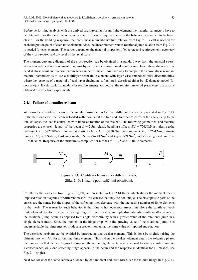
Jukic, M. 2013. Koncni elementi za modeliranje lokaliziranih porusitev v armiranem betonu.
Doktorska disertacija. Ljubljana, UL, FGG.
33
Before performing analysis with the derived stress-resultant beam finite element, the material parameters have to
be obtained. For the axial response, only axial stiffness is required because the behavior is assumed to be linear
elastic. For the bending response, the three-linear moment-curvature relation from Fig. 2.10 (left) is needed for
each integration point of each finite element. Also, the linear moment versus rotational jump relation from Fig. 2.11
is needed for each element. The curves depend on the material properties of concrete and reinforcement, geometry
of the cross-section and the level of the axial force.
The moment-curvature diagram of the cross-section can be obtained in a standard way from the uniaxial stress-
strain concrete and reinforcement diagrams by enforcing cross-sectional equilibrium. From those diagrams, the
needed stress resultant material parameters can be estimated. Another way to compute the above stress resultant
material parameters is to use a multilayer beam finite element with layer-wise embedded axial discontinuities,
where the response of a material of each layer (including softening) is described either by 1D damage model (for
concrete) or 1D elastoplastic model (for reinforcement). Of course, the required material parameters can also be
obtained directly from experiments.
2.4.1 Failure of a cantilever beam
We consider a cantilever beam of rectangular cross-section for three different load cases, presented in Fig. 2.13.
In the first load case, the beam is loaded with moment at the free end. In order to perform the analysis up to the
total collapse, the load is controlled with imposed rotation of the free end. The following geometrical and material
properties are chosen: length of the beam L = 2.5m, elastic bending stiffness EI = 77650kNm2, elastic axial
stiffness EA = 3727200kN, moment at elasticity limit Mc = 37.9kNm, yield moment My = 268kNm, ultimate
moment Mu = 274kNm, hardening moduli H1 = 29400kNm2 and H2 = 272kNm2, and softening modulus K =
−18000kNm. Response of the structure is computed for meshes of 1, 2, 5 and 10 finite elements.
L
M
L
M N
L
F
Figure 2.13: Cantilever beam under different loads.
Slika 2.13: Konzola pod razlicnimi obtezbami.
Results for the load case from Fig. 2.13 (left) are presented in Fig. 2.14 (left), which shows the moment versus
imposed rotation diagrams for different meshes. We can see that they are not unique. The elastoplastic parts of the
curves are the same, but the slopes of the softening lines decrease with the increasing number of finite elements
in the mesh. The reason for such behavior is that, due to homogeneous stress state along the cantilever, each
finite element develops its own softening hinge. In finer meshes, multiple discontinuities with smaller values of
the rotational jump occur, as opposed to a single discontinuity with a greater value of the rotational jump in a
single element mesh. Since the moment at the hinge drops with the growing value of the rotational jump, it is
understandable that finer meshes produce a greater moment at the same value of imposed end rotation.
The described problem can be avoided by introducing one weaker element. This is done by slightly raising the
ultimate moment Mu for all but one finite element. Thus, when the weakest element enters the softening phase,
the moment in that element begins to drop and the remaining elements have to unload to satisfy equilibrium. As
a consequence, only one softening hinge appears in the beam and the response is identical for all meshes, see
Fig. 2.14 (right).
Next we consider the same cantilever, loaded by end moment and axial force, see the middle image in Fig. 2.13.
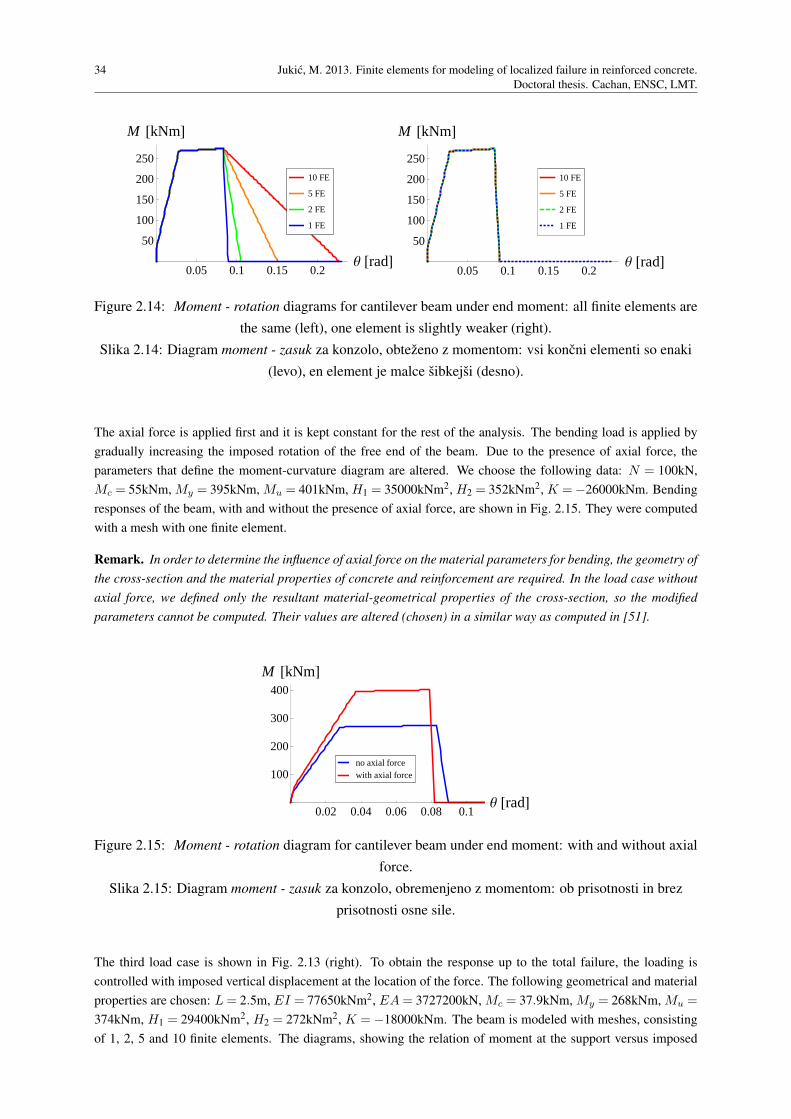
34 Jukic, M. 2013. Finite elements for modeling of localized failure in reinforced concrete.
Doctoral thesis. Cachan, ENSC, LMT.
0.05 0.1 0.15 0.2Θ @radD
50
100
150
200
250
M @kNmD
1 FE
2 FE
5 FE
10 FE
0.05 0.1 0.15 0.2Θ @radD
50
100
150
200
250
M @kNmD
1 FE
2 FE
5 FE
10 FE
Figure 2.14: Moment - rotation diagrams for cantilever beam under end moment: all finite elements are
the same (left), one element is slightly weaker (right).
Slika 2.14: Diagram moment - zasuk za konzolo, obtezeno z momentom: vsi koncni elementi so enaki
(levo), en element je malce sibkejsi (desno).
The axial force is applied first and it is kept constant for the rest of the analysis. The bending load is applied by
gradually increasing the imposed rotation of the free end of the beam. Due to the presence of axial force, the
parameters that define the moment-curvature diagram are altered. We choose the following data: N = 100kN,
Mc = 55kNm, My = 395kNm, Mu = 401kNm, H1 = 35000kNm2, H2 = 352kNm2, K =−26000kNm. Bending
responses of the beam, with and without the presence of axial force, are shown in Fig. 2.15. They were computed
with a mesh with one finite element.
Remark. In order to determine the influence of axial force on the material parameters for bending, the geometry of
the cross-section and the material properties of concrete and reinforcement are required. In the load case without
axial force, we defined only the resultant material-geometrical properties of the cross-section, so the modified
parameters cannot be computed. Their values are altered (chosen) in a similar way as computed in [51].
0.02 0.04 0.06 0.08 0.1Θ @radD
100
200
300
400
M @kNmD
with axial forceno axial force
Figure 2.15: Moment - rotation diagram for cantilever beam under end moment: with and without axial
force.
Slika 2.15: Diagram moment - zasuk za konzolo, obremenjeno z momentom: ob prisotnosti in brez
prisotnosti osne sile.
The third load case is shown in Fig. 2.13 (right). To obtain the response up to the total failure, the loading is
controlled with imposed vertical displacement at the location of the force. The following geometrical and material
properties are chosen: L= 2.5m, EI = 77650kNm2, EA= 3727200kN, Mc = 37.9kNm, My = 268kNm, Mu =
374kNm, H1 = 29400kNm2, H2 = 272kNm2, K = −18000kNm. The beam is modeled with meshes, consisting
of 1, 2, 5 and 10 finite elements. The diagrams, showing the relation of moment at the support versus imposed
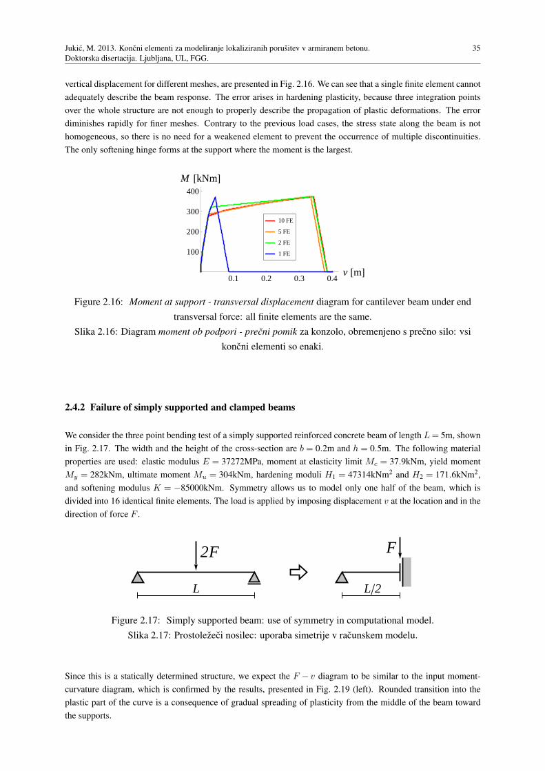
Jukic, M. 2013. Koncni elementi za modeliranje lokaliziranih porusitev v armiranem betonu.
Doktorska disertacija. Ljubljana, UL, FGG.
35
vertical displacement for different meshes, are presented in Fig. 2.16. We can see that a single finite element cannot
adequately describe the beam response. The error arises in hardening plasticity, because three integration points
over the whole structure are not enough to properly describe the propagation of plastic deformations. The error
diminishes rapidly for finer meshes. Contrary to the previous load cases, the stress state along the beam is not
homogeneous, so there is no need for a weakened element to prevent the occurrence of multiple discontinuities.
The only softening hinge forms at the support where the moment is the largest.
0.1 0.2 0.3 0.4v @mD
100
200
300
400
M @kNmD
1 FE
2 FE
5 FE
10 FE
Figure 2.16: Moment at support - transversal displacement diagram for cantilever beam under end
transversal force: all finite elements are the same.
Slika 2.16: Diagram moment ob podpori - precni pomik za konzolo, obremenjeno s precno silo: vsi
koncni elementi so enaki.
2.4.2 Failure of simply supported and clamped beams
We consider the three point bending test of a simply supported reinforced concrete beam of length L= 5m, shown
in Fig. 2.17. The width and the height of the cross-section are b = 0.2m and h = 0.5m. The following material
properties are used: elastic modulus E = 37272MPa, moment at elasticity limit Mc = 37.9kNm, yield moment
My = 282kNm, ultimate moment Mu = 304kNm, hardening moduli H1 = 47314kNm2 and H2 = 171.6kNm2,
and softening modulus K = −85000kNm. Symmetry allows us to model only one half of the beam, which is
divided into 16 identical finite elements. The load is applied by imposing displacement v at the location and in the
direction of force F .
L L2
2F F
Figure 2.17: Simply supported beam: use of symmetry in computational model.
Slika 2.17: Prostolezeci nosilec: uporaba simetrije v racunskem modelu.
Since this is a statically determined structure, we expect the F − v diagram to be similar to the input moment-
curvature diagram, which is confirmed by the results, presented in Fig. 2.19 (left). Rounded transition into the
plastic part of the curve is a consequence of gradual spreading of plasticity from the middle of the beam toward
the supports.
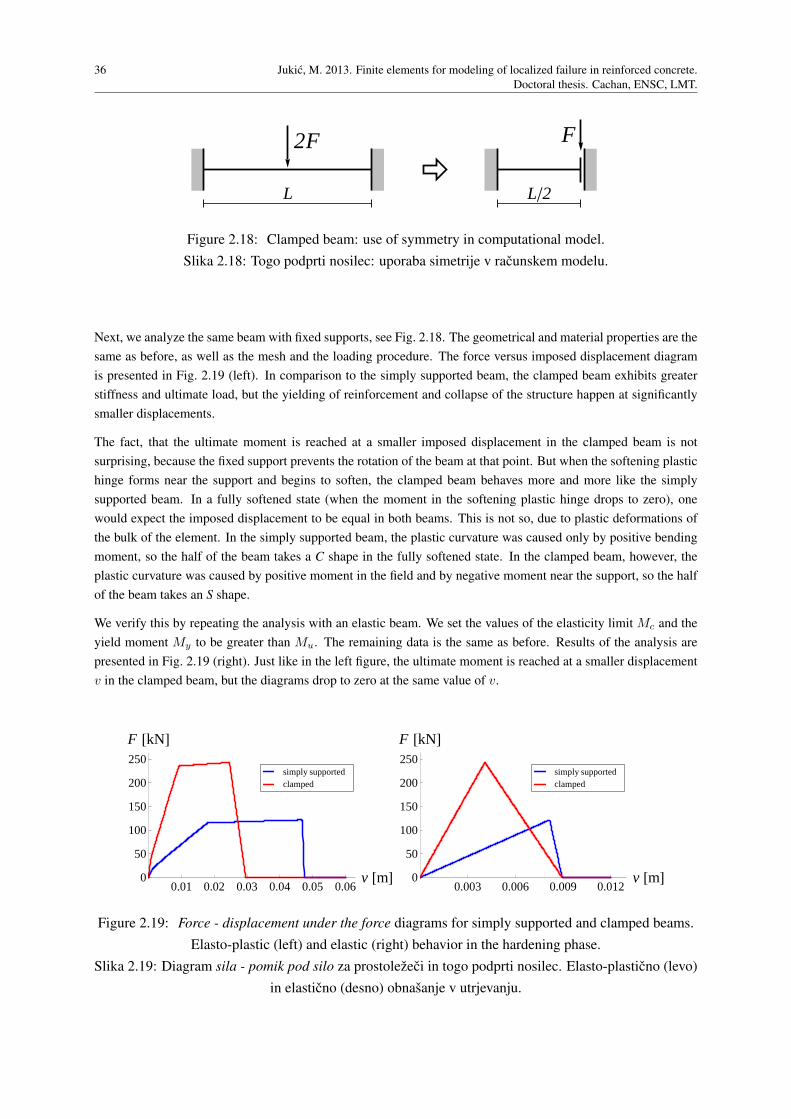
36 Jukic, M. 2013. Finite elements for modeling of localized failure in reinforced concrete.
Doctoral thesis. Cachan, ENSC, LMT.
L L2
2F F
Figure 2.18: Clamped beam: use of symmetry in computational model.
Slika 2.18: Togo podprti nosilec: uporaba simetrije v racunskem modelu.
Next, we analyze the same beam with fixed supports, see Fig. 2.18. The geometrical and material properties are the
same as before, as well as the mesh and the loading procedure. The force versus imposed displacement diagram
is presented in Fig. 2.19 (left). In comparison to the simply supported beam, the clamped beam exhibits greater
stiffness and ultimate load, but the yielding of reinforcement and collapse of the structure happen at significantly
smaller displacements.
The fact, that the ultimate moment is reached at a smaller imposed displacement in the clamped beam is not
surprising, because the fixed support prevents the rotation of the beam at that point. But when the softening plastic
hinge forms near the support and begins to soften, the clamped beam behaves more and more like the simply
supported beam. In a fully softened state (when the moment in the softening plastic hinge drops to zero), one
would expect the imposed displacement to be equal in both beams. This is not so, due to plastic deformations of
the bulk of the element. In the simply supported beam, the plastic curvature was caused only by positive bending
moment, so the half of the beam takes a C shape in the fully softened state. In the clamped beam, however, the
plastic curvature was caused by positive moment in the field and by negative moment near the support, so the half
of the beam takes an S shape.
We verify this by repeating the analysis with an elastic beam. We set the values of the elasticity limit Mc and the
yield moment My to be greater than Mu. The remaining data is the same as before. Results of the analysis are
presented in Fig. 2.19 (right). Just like in the left figure, the ultimate moment is reached at a smaller displacement
v in the clamped beam, but the diagrams drop to zero at the same value of v.
0.01 0.02 0.03 0.04 0.05 0.06v @mD0
50
100
150
200
250
F @kND
clampedsimply supported
0.003 0.006 0.009 0.012v @mD0
50
100
150
200
250
F @kND
clampedsimply supported
Figure 2.19: Force - displacement under the force diagrams for simply supported and clamped beams.
Elasto-plastic (left) and elastic (right) behavior in the hardening phase.
Slika 2.19: Diagram sila - pomik pod silo za prostolezeci in togo podprti nosilec. Elasto-plasticno (levo)
in elasticno (desno) obnasanje v utrjevanju.
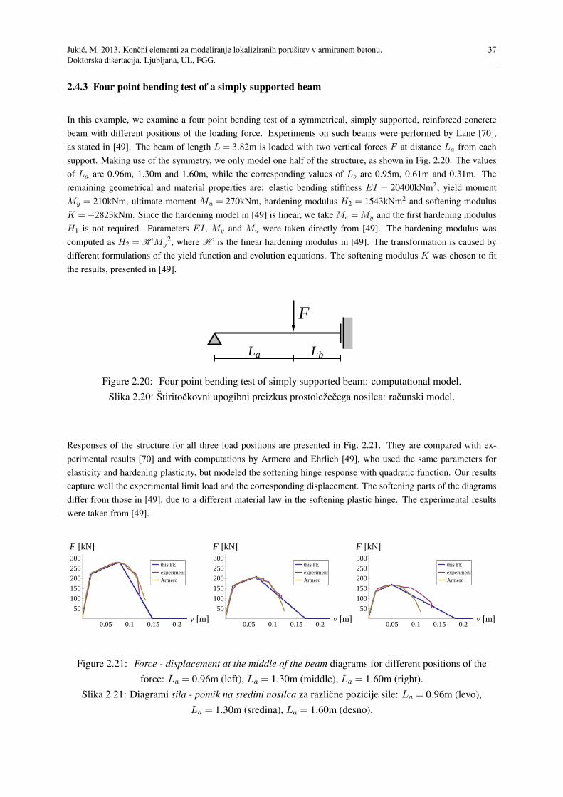
Jukic, M. 2013. Koncni elementi za modeliranje lokaliziranih porusitev v armiranem betonu.
Doktorska disertacija. Ljubljana, UL, FGG.
37
2.4.3 Four point bending test of a simply supported beam
In this example, we examine a four point bending test of a symmetrical, simply supported, reinforced concrete
beam with different positions of the loading force. Experiments on such beams were performed by Lane [70],
as stated in [49]. The beam of length L = 3.82m is loaded with two vertical forces F at distance La from each
support. Making use of the symmetry, we only model one half of the structure, as shown in Fig. 2.20. The values
of La are 0.96m, 1.30m and 1.60m, while the corresponding values of Lb are 0.95m, 0.61m and 0.31m. The
remaining geometrical and material properties are: elastic bending stiffness EI = 20400kNm2, yield moment
My = 210kNm, ultimate moment Mu = 270kNm, hardening modulus H2 = 1543kNm2 and softening modulus
K =−2823kNm. Since the hardening model in [49] is linear, we take Mc =My and the first hardening modulus
H1 is not required. Parameters EI , My and Mu were taken directly from [49]. The hardening modulus was
computed as H2 = H My2, where H is the linear hardening modulus in [49]. The transformation is caused by
different formulations of the yield function and evolution equations. The softening modulus K was chosen to fit
the results, presented in [49].
La Lb
F
Figure 2.20: Four point bending test of simply supported beam: computational model.
Slika 2.20: Stiritockovni upogibni preizkus prostolezecega nosilca: racunski model.
Responses of the structure for all three load positions are presented in Fig. 2.21. They are compared with ex-
perimental results [70] and with computations by Armero and Ehrlich [49], who used the same parameters for
elasticity and hardening plasticity, but modeled the softening hinge response with quadratic function. Our results
capture well the experimental limit load and the corresponding displacement. The softening parts of the diagrams
differ from those in [49], due to a different material law in the softening plastic hinge. The experimental results
were taken from [49].
0.05 0.1 0.15 0.2v @mD
50
100
150
200
250
300
F @kND
Armero
experiment
this FE
0.05 0.1 0.15 0.2v @mD
50
100
150
200
250
300
F @kND
Armero
experiment
this FE
0.05 0.1 0.15 0.2v @mD
50
100
150
200
250
300
F @kND
Armero
experiment
this FE
Figure 2.21: Force - displacement at the middle of the beam diagrams for different positions of the
force: La = 0.96m (left), La = 1.30m (middle), La = 1.60m (right).
Slika 2.21: Diagrami sila - pomik na sredini nosilca za razlicne pozicije sile: La = 0.96m (levo),
La = 1.30m (sredina), La = 1.60m (desno).
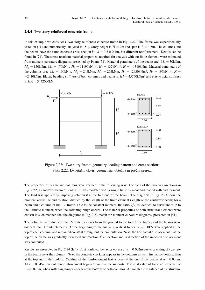
38 Jukic, M. 2013. Finite elements for modeling of localized failure in reinforced concrete.
Doctoral thesis. Cachan, ENSC, LMT.
2.4.4 Two story reinforced concrete frame
In this example we consider a two story reinforced concrete frame in Fig. 2.22. The frame was experimentally
tested in [71] and numerically analyzed in [51]. Story height is H = 2m and span is L= 3.5m. The columns and
the beams have the same concrete cross-section b×h = 0.3× 0.4m, but different reinforcement. Details can be
found in [71]. The stress-resultant material properties, required for analysis with our finite element, were estimated
from moment-curvature diagrams, presented by Pham [51]. Material parameters of the beams are: Mc = 30kNm,
My = 150kNm, Mu = 170kNm, H1 = 11190kNm2, H2 = 137kNm2, K = −1310kNm. Material parameters of
the columns are: Mc = 100kNm, My = 245kNm, Mu = 265kNm, H1 = 12450kNm2, H2 = 195kNm2, K =
−2410kNm. Elastic bending stiffness of both columns and beams is EI = 45760kNm2 and elastic axial stiffness
is EA= 3432000kN.
L
H
H
700 kN 700 kN
Fu
0.04
0.04
0.32
0.30
0.03
0.03
0.34
0.30
4´3cm2
4´3cm2
4´3cm2
4´3cm2
BEAM
COLUMN
Figure 2.22: Two story frame: geometry, loading pattern and cross-sections.
Slika 2.22: Dvoetazni okvir: geometrija, obtezba in precni prerezi.
The properties of beams and columns were verified in the following way. For each of the two cross-sections in
Fig. 2.22, a cantilever beam of length 1m was modeled with a single finite element and loaded with end moment.
The load was applied by imposing rotation θ at the free end of the beam. The diagrams in Fig. 2.23 show the
moment versus the end rotation, divided by the length of the finite element (length of the cantilever beam) for a
beam and a column of the RC frame. Due to the constant moment, the ratio θ/L is identical to curvature κ up to
the ultimate moment, when the softening hinge occurs. The material properties of both structural elements were
chosen in such manner, that the diagrams in Fig. 2.23 match the moment-curvature diagrams, presented in [51].
The columns were divided into 16 finite elements from the ground to the top of the frame, and the beams were
divided into 14 finite elements. At the beginning of the analysis, vertical forces N = 700kN were applied at the
top of each column, and remained constant throughout the computation. Next, the horizontal displacement u at the
top of the frame was gradually increased and reaction F at location and in direction of the imposed displacement
was computed.
Results are presented in Fig. 2.24 (left). First nonlinear behavior occurs at u= 0.002m due to cracking of concrete
in the beams near the columns. Next, the concrete cracking appears in the columns as well, first at the bottom, then
at the top and in the middle. Yielding of the reinforcement first appears at the end of the beams at u = 0.035m.
At u = 0.045m the column reinforcement begins to yield at the supports. Maximal value of force F is reached at
u= 0.073m, when softening hinges appear at the bottom of both columns. Although the resistance of the structure
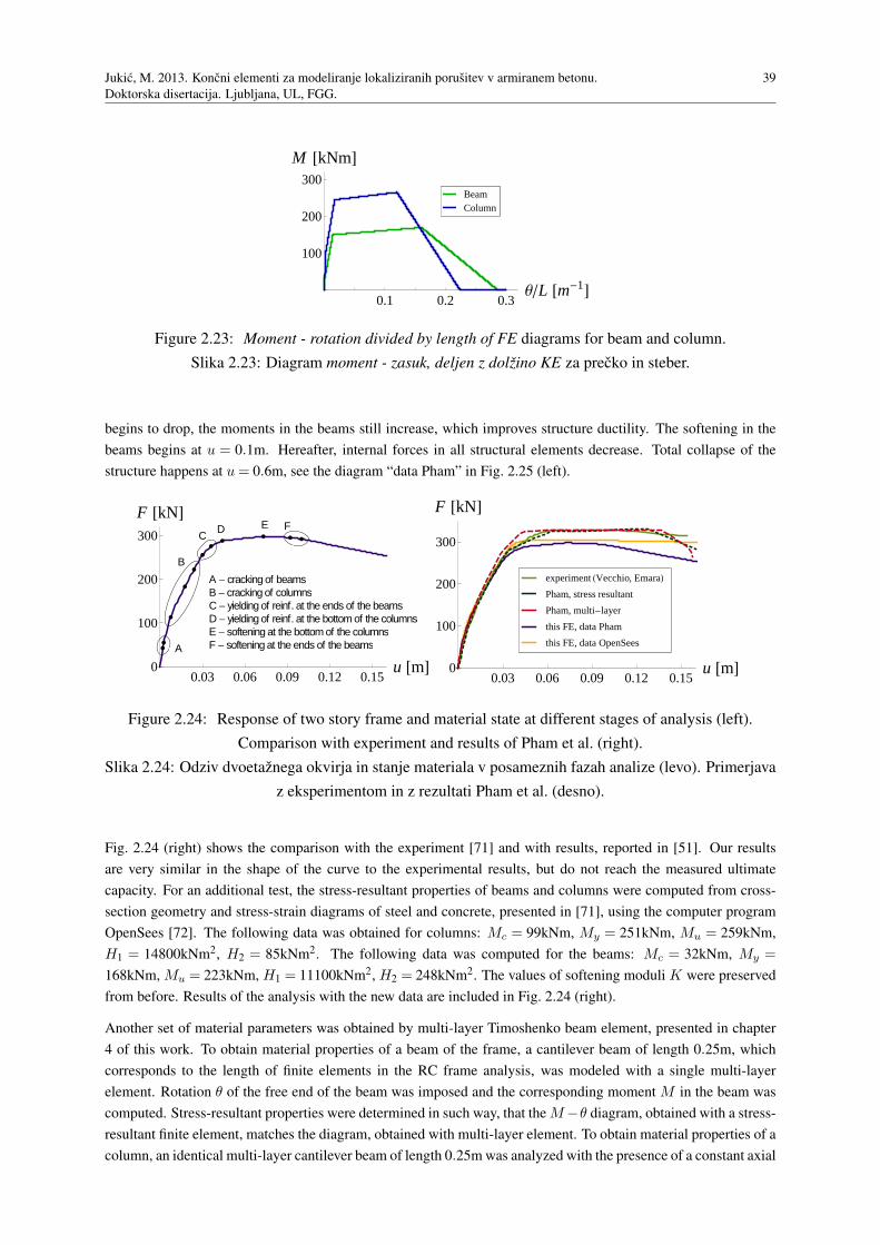
Jukic, M. 2013. Koncni elementi za modeliranje lokaliziranih porusitev v armiranem betonu.
Doktorska disertacija. Ljubljana, UL, FGG.
39
0.1 0.2 0.3ΘL @m-1D
100
200
300
M @kNmD
ColumnBeam
Figure 2.23: Moment - rotation divided by length of FE diagrams for beam and column.
Slika 2.23: Diagram moment - zasuk, deljen z dolzino KE za precko in steber.
begins to drop, the moments in the beams still increase, which improves structure ductility. The softening in the
beams begins at u = 0.1m. Hereafter, internal forces in all structural elements decrease. Total collapse of the
structure happens at u= 0.6m, see the diagram “data Pham” in Fig. 2.25 (left).
A
B
CD E F
A - cracking of beamsB- cracking of columnsC- yielding of reinf. at the ends of the beamsD- yielding of reinf. at the bottom of the columnsE- softening at the bottom of the columnsF- softening at the ends of the beams
0.03 0.06 0.09 0.12 0.15u @mD0
100
200
300
F @kND
0.03 0.06 0.09 0.12 0.15u @mD0
100
200
300
F @kND
this FE, data OpenSees
this FE, data Pham
Pham, multi-layer
Pham, stress resultant
experiment HVecchio, EmaraL
Figure 2.24: Response of two story frame and material state at different stages of analysis (left).
Comparison with experiment and results of Pham et al. (right).
Slika 2.24: Odziv dvoetaznega okvirja in stanje materiala v posameznih fazah analize (levo). Primerjava
z eksperimentom in z rezultati Pham et al. (desno).
Fig. 2.24 (right) shows the comparison with the experiment [71] and with results, reported in [51]. Our results
are very similar in the shape of the curve to the experimental results, but do not reach the measured ultimate
capacity. For an additional test, the stress-resultant properties of beams and columns were computed from cross-
section geometry and stress-strain diagrams of steel and concrete, presented in [71], using the computer program
OpenSees [72]. The following data was obtained for columns: Mc = 99kNm, My = 251kNm, Mu = 259kNm,
H1 = 14800kNm2, H2 = 85kNm2. The following data was computed for the beams: Mc = 32kNm, My =
168kNm, Mu = 223kNm, H1 = 11100kNm2, H2 = 248kNm2. The values of softening moduli K were preserved
from before. Results of the analysis with the new data are included in Fig. 2.24 (right).
Another set of material parameters was obtained by multi-layer Timoshenko beam element, presented in chapter
4 of this work. To obtain material properties of a beam of the frame, a cantilever beam of length 0.25m, which
corresponds to the length of finite elements in the RC frame analysis, was modeled with a single multi-layer
element. Rotation θ of the free end of the beam was imposed and the corresponding moment M in the beam was
computed. Stress-resultant properties were determined in such way, that the M−θ diagram, obtained with a stress-
resultant finite element, matches the diagram, obtained with multi-layer element. To obtain material properties of a
column, an identical multi-layer cantilever beam of length 0.25m was analyzed with the presence of a constant axial

40 Jukic, M. 2013. Finite elements for modeling of localized failure in reinforced concrete.
Doctoral thesis. Cachan, ENSC, LMT.
0.2 0.4 0.6 0.8 1u @mD0
100
200
300
F @kND
this FE, data our multi-layer
this FE, data OpenSees
this FE, data Pham
0.03 0.06 0.09 0.12 0.15 0.18u @mD0
100
200
300
F @kND
our multi-layer FE
this FE, data our multi-layer
experiment HVecchio, EmaraL
Figure 2.25: Response of two story frame up to total collapse for different material data (left).
Comparison with results of analysis with multi-layer finite element (right).
Slika 2.25: Odziv dvoetaznega okvirja do popolne porusitve za razlicne materialne podatke (levo).
Primerjava z rezultati analize z vecslojnim koncnim elementom (desno).
force N = 700kN. The following material properties were calculated for beams: Mc = 31kNm, My = 165kNm,
Mu = 236kNm, H1 = 25800kNm2, H2 = 349kNm2, K = −5250kNm. The computed properties of columns:
Mc = 100kNm, My = 281kNm, Mu = 333kNm, H1 = 33800kNm2, H2 = 216kNm2, K =−4750kNm. Response
of the two-story frame, analyzed with this data, is shown in Fig. 2.25 (left), along with responses, obtained for the
data from OpenSees and data estimated from [51]. We observe that the data, computed with our multi-layer
element, produces a significantly higher ultimate load and a steeper softening line.
Fig. 2.25 (right) shows the response of the frame, computed by the multi-layer finite element from chapter 4. It
is compared to the results of analysis with stress-resultant element, developed in this chapter, and material data,
provided by the former multi-layer element. Both curves reach the same ultimate value of force F , but not at the
same value of imposed displacement u. In comparison to other results, the curves match pretty well.
2.5 Concluding remarks
We have presented a planar stress-resultant Euler-Bernoulli beam finite element with embedded discontinuity in
rotation, which can be used for analysis of reinforced concrete beams and frames up to complete failure. The
formulation is based on small deformation kinematics. Stress resultant elastoplasticity with bilinear isotropic hard-
ening is used to model the bending of the bulk of the element, and rigid plasticity is used for the softening bending
hinge. The element is able to describe the major characteristics of the reinforced concrete beam behavior up to
complete failure. The finite element provides a mesh independent softening response of the modeled structure. The
obtained results compare reasonably well to other results available in the literature and to experimental results.
The geometrical and material properties have to be determined individually for each cross-section and for each
level of the axial force. The moment-curvature and moment-rotational jump diagrams, required as an input for
the analysis, can be determined experimentally or computed with a more complex finite element, such as the
multi-layer beam finite elements, presented in the following chapters.

Jukic, M. 2013. Koncni elementi za modeliranje lokaliziranih porusitev v armiranem betonu.
Doktorska disertacija. Ljubljana, UL, FGG.
41
3 MULTI-LAYER EULER-BERNOULLI BEAM FINITE ELEMENT WITH
LAYER-WISE EMBEDDED DISCONTINUITIES IN AXIAL DISPLACEMENT
3.1 Introduction
In this chapter we derive a multi-layer Euler-Bernoulli beam finite element with layer-wise embedded discon-
tinuities in axial displacement. The element is intended for precise analysis of reinforced concrete beams and
structures up to complete failure, as well as for computation of stress-resultant properties of cross-sections, which
are required as input data in analysis with stress-resultant finite element, presented in previous chapter.
The element is composed of several layers of concrete and reinforcement, each with embedded discontinuity in
axial displacement. Axial response of concrete layer is determined by elasto-damage hardening law in the bulk and
damage softening law at the discontinuity. Axial response of reinforcement layer is controlled by elastoplasticity
hardening law in the bulk and plastic softening at the discontinuity. Small deformation kinematics is employed.
The outline of the chapter is the following: Kinematic, constitutive and equilibrium equations are developed in sec-
tion 3.2. Finite element discretization and computational procedure are presented in section 3.3. Several numerical
examples are shown in section 3.4. Finally, concluding remarks are given in section 3.5.
3.2 Finite element formulation
3.2.1 Kinematics
We consider a planar Euler-Bernoulli beam finite element with three nodes, shown in Fig. 3.1. The two end nodes
have regular degrees of freedom, two in-plane displacements and rotation about the axis, perpendicular to the plane.
The third node is located in the middle of the element and has one degree of freedom, the axial displacement. Its
purpose is to raise the interpolation order of axial displacements, which ensures compatibility of the axial strain
contributions by bending and axial deformation.
x L
u1
v1Θ1 u2
v2Θ2u3
1 3 2
Figure 3.1: Finite element with seven nodal degrees of freedom.
Slika 3.1: Koncni element s sedmimi prostostnimi stopnjami.
u(x) = Nu (x)u, Nu (x) =
1−3x
L+
2x2
L2,−
x
L+
2x2
L2,
4x
L−
4x2
L2
, u = u1,u2,u3T
(3.1)
Axial displacement u(x) of the middle axis of the beam is interpolated between the three nodal displacements
u, using quadratic shape functions Nu (x) shown in Fig. 3.2 (left). Lateral displacement v (x) is interpolated as
follows.
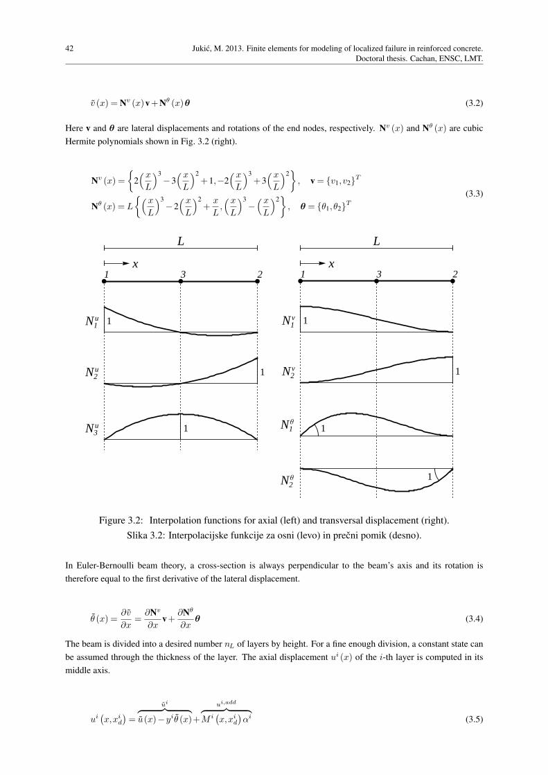
42 Jukic, M. 2013. Finite elements for modeling of localized failure in reinforced concrete.
Doctoral thesis. Cachan, ENSC, LMT.
v (x) = Nv (x)v+Nθ (x)θ (3.2)
Here v and θ are lateral displacements and rotations of the end nodes, respectively. Nv (x) and Nθ (x) are cubic
Hermite polynomials shown in Fig. 3.2 (right).
Nv (x) =
2( x
L
)3
−3( x
L
)2
+1,−2( x
L
)3
+3( x
L
)2
, v = v1,v2T
Nθ (x) = L
( x
L
)3
−2( x
L
)2
+x
L,( x
L
)3
−( x
L
)2
, θ = θ1,θ2T
(3.3)
N1u
N2u
N3u
x
L
1 23
1
1
1
N1v
N2v
N1Θ
N2Θ
x
L
1 23
1
1
1
1
Figure 3.2: Interpolation functions for axial (left) and transversal displacement (right).
Slika 3.2: Interpolacijske funkcije za osni (levo) in precni pomik (desno).
In Euler-Bernoulli beam theory, a cross-section is always perpendicular to the beam’s axis and its rotation is
therefore equal to the first derivative of the lateral displacement.
θ (x) =∂v
∂x=
∂Nv
∂xv+
∂Nθ
∂xθ (3.4)
The beam is divided into a desired number nL of layers by height. For a fine enough division, a constant state can
be assumed through the thickness of the layer. The axial displacement ui (x) of the i-th layer is computed in its
middle axis.
ui(x,xi
d
)=
ui
︷ ︸︸ ︷
u(x)−yiθ (x)+
ui,add
︷ ︸︸ ︷
M i(x,xi
d
)αi (3.5)
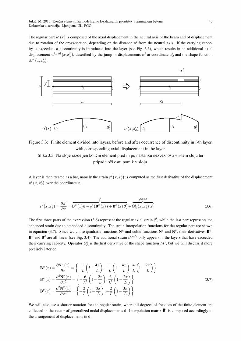
Jukic, M. 2013. Koncni elementi za modeliranje lokaliziranih porusitev v armiranem betonu.
Doktorska disertacija. Ljubljana, UL, FGG.
43
The regular part ui (x) is composed of the axial displacement in the neutral axis of the beam and of displacement
due to rotation of the cross-section, depending on the distance yi from the neutral axis. If the carrying capac-
ity is exceeded, a discontinuity is introduced into the layer (see Fig. 3.3), which results in an additional axial
displacement ui,add(x,xi
d
), described by the jump in displacements αi at coordinate xi
d and the shape function
M i(x,xi
d
).
u iHxL u1i u2
iu3i
L
hyi i
1 3 2
uiHx,xdi L u1
i u2iu3
i
Α i
xdi
Α i
i
1 3 2
Figure 3.3: Finite element divided into layers, before and after occurrence of discontinuity in i-th layer,
with corresponding axial displacement in the layer.
Slika 3.3: Na sloje razdeljen koncni element pred in po nastanku nezveznosti v i-tem sloju ter
pripadajoci osni pomik v sloju.
A layer is then treated as a bar, namely the strain εi(x,xi
d
)is computed as the first derivative of the displacement
ui(x,xi
d
)over the coordinate x.
εi(x,xi
d
)=
∂ui
∂x=
˜εi
︷ ︸︸ ︷
Bu (x)u−yi(Bv (x)v+Bθ (x)θ
)+
εi,add︷ ︸︸ ︷
GiR
(x,xi
d
)αi (3.6)
The first three parts of the expression (3.6) represent the regular axial strain ˜εi, while the last part represents the
enhanced strain due to embedded discontinuity. The strain interpolation functions for the regular part are shown
in equation (3.7). Since we chose quadratic functions Nu and cubic functions Nv and Nθ, their derivatives Bu,
Bv and Bθ are all linear (see Fig. 3.4). The additional strain εi,add only appears in the layers that have exceeded
their carrying capacity. Operator GiR is the first derivative of the shape function M i, but we will discuss it more
precisely later on.
Bu (x) =∂Nu (x)
∂x=
−1
L
(
3−4x
L
)
,−1
L
(
1−4x
L
)
,4
L
(
1−2x
L
)
Bv (x) =∂2Nv (x)
∂x2=
−6
L2
(
1−2x
L
)
,6
L2
(
1−2x
L
)
Bθ (x) =∂2Nθ (x)
∂x2=
−2
L
(
2−3x
L
)
,−2
L
(
1−3x
L
)
(3.7)
We will also use a shorter notation for the regular strain, where all degrees of freedom of the finite element are
collected in the vector of generalized nodal displacements d. Interpolation matrix Bi is composed accordingly to
the arrangement of displacements in d.
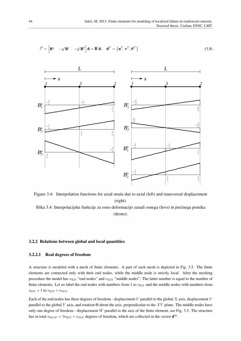
44 Jukic, M. 2013. Finite elements for modeling of localized failure in reinforced concrete.
Doctoral thesis. Cachan, ENSC, LMT.
˜εi =[
Bu −yiBv −yiBθ]
d = Bid, dT =
uT ,vT ,θT
(3.8)
B1u
B2u
B3u
x
L
1 23
-3
L-
1
L
1
L
-1
L
1
L
3
L
4
L
-4
L
B1v
B2v
B1Θ
B2Θ
x
L
1 23
-6
L2
6
L2
6
L2
-6
L2
-4
L-
1
L
2
L
-2
L
1
L
4
L
Figure 3.4: Interpolation functions for axial strain due to axial (left) and transversal displacement
(right).
Slika 3.4: Interpolacijske funkcije za osno deformacijo zaradi osnega (levo) in precnega pomika
(desno).
3.2.2 Relations between global and local quantities
3.2.2.1 Real degrees of freedom
A structure is modeled with a mesh of finite elements. A part of such mesh is depicted in Fig. 3.5. The finite
elements are connected only with their end nodes, while the middle node is strictly local. After the meshing
procedure the model has nEN “end nodes” and nMN “middle nodes”. The latter number is equal to the number of
finite elements. Let us label the end nodes with numbers from 1 to nEN and the middle nodes with numbers from
nEN +1 to nEN +nMN .
Each of the end nodes has three degrees of freedom - displacement U parallel to the global X axis, displacement V
parallel to the global Y axis, and rotation Θ about the axis, perpendicular to the XY plane. The middle nodes have
only one degree of freedom - displacement W parallel to the axis of the finite element, see Fig. 3.5. The structure
has in total nDOF = 3nEN +nMN degrees of freedom, which are collected in the vector dstr.

Jukic, M. 2013. Koncni elementi za modeliranje lokaliziranih porusitev v armiranem betonu.
Doktorska disertacija. Ljubljana, UL, FGG.
45
X
Ymiddle node of FE
end node of FE
n Un
Vn
Qnm
Wm
Figure 3.5: Degrees of freedom at nodes of the finite element mesh.
Slika 3.5: Prostostne stopnje v vozliscih mreze koncnih elementov.
dstr =
dTEN ,dT
MN
T, dEN =
U1,V1,Θ1,U2,V2,Θ2, ... ,UnEN
,VnEN,ΘnEN
T,
dMN =WnEN+1,WnEN+2, ... ,WnEN+nMN
T(3.9)
Let us now consider a finite element (e) with end nodes (n1), (n2) and a middle node (n3). The local x axis is
parallel to the axis of the element, with x increasing from node (n1) towards node (n2), see Fig. 3.6. The element’s
degrees of freedom, defined in the local coordinate system, are collected in the vector d(e), in accordance with
equation (3.8). Global degrees of freedom, associated with the nodes of the element can be similarly organized
into vector D(e). The two are connected with a transformation matrix R(e). Zeros are replaced by dots for clarity.
φ(e) is the angle between the global X axis and the local x axis (rotation of the local coordinate system).
d(e) = R(e)D(e) (3.10)
d(e) =
u(e)1 ,u
(e)2 ,u
(e)3 ,v
(e)1 ,v
(e)2 ,θ
(e)1 ,θ
(e)2
T, D(e) =
Un1
,Un2,Wn3
,Vn1,Vn2
,Θn1,Θn2
T
R(e) =
cosφ(e) · · sinφ(e) · · ·
· cosφ(e) · · sinφ(e) · ·
· · 1 · · · ·
−sinφ(e) · · cosφ(e) · · ·
· −sinφ(e) · · cosφ(e) · ·
· · · · · 1 ·
· · · · · · 1
(3.11)
Vector D(e) contains those components of vector dstr that correspond to the nodes of the finite element. The
selection of appropriate components is done by matrix P(e) of size 7×nDOF with only seven non-zero components.

46 Jukic, M. 2013. Finite elements for modeling of localized failure in reinforced concrete.
Doctoral thesis. Cachan, ENSC, LMT.
n1 Un1
Vn1
Qn1
n2 Un2
Vn2
Qn2
n3
Wn3
HeL
1
u1
v1
Θ1
2
u2
v2
Θ2
3
u3HeL
X
Y
xy
Φ
Figure 3.6: Global (left) and local (right) degrees of freedom, associated with a finite element.
Slika 3.6: Globalne (levo) in lokalne (desno) prostostne stopnje, povezane s koncnim elementom.
D(e) = P(e)dstr
P(e)1, 3n1−2 = P
(e)2, 3n2−2 = P
(e)3, 3nEN+(n3−nEN )
= P(e)4, 3n1−1 = P
(e)5, 3n2−1 = P
(e)6, 3n1
= P(e)7, 3n2
= 1(3.12)
Obeying equations (3.10) and (3.12), we can finally write the relation between the local degrees of freedom of the
finite element (e) and the global degrees of freedom of the structure.
d(e) = R(e)P(e)dstr (3.13)
3.2.2.2 Virtual degrees of freedom
Virtual displacements are a kinematically admissible variation of real displacements. As with the real displace-
ments, they are interpolated between the nodal values with appropriate interpolation functions. The virtual defor-
mation of the structure is therefore defined by the virtual displacements of its nodes.
The global virtual degrees of freedom (virtual displacements of the structure) dstr, the virtual displacements of the
element d(e) and the selection D(e) of global virtual displacements, associated with the element (e), are defined
analogously to the real quantities dstr, d(e) and D(e), defined in equations (3.9) and (3.11).
dstr =
dTEN , dT
MN
T,
dEN =U1, V1, Θ1, ... , UnEN
, VnEN, ΘnEN
T, dMN =
WnEN+1, ... ,WnEN+nMN
T
d(e) =
u(e)1 , u
(e)2 , u
(e)3 , v
(e)1 , v
(e)2 , θ
(e)1 , θ
(e)2
T, D(e) =
Un1
, Un2,Wn3
, Vn1, Vn2
, Θn1, Θn2
T
(3.14)
Relations between them are equivalent to equations (3.10)-(3.13), matrices R(e) and P(e) remain the same.
d(e) = R(e)D(e), D(e) = P(e)dstr, d(e) = R(e)P(e)dstr (3.15)

Jukic, M. 2013. Koncni elementi za modeliranje lokaliziranih porusitev v armiranem betonu.
Doktorska disertacija. Ljubljana, UL, FGG.
47
3.2.2.3 Internal forces
Internal forces can be organized in the same way as the generalized displacements. Each degree of freedom from
the vector dstr is accompanied by a corresponding internal force. Analogously to equation (3.9) we can write:
f int,str =
f intT
EN , f intT
MN
T, f int
EN =
f intU1,f int
V1,f int
Θ1,f int
U2,f int
V2,f int
Θ2, ... ,f int
UnEN,f int
VnEN,f int
ΘnEN
T
f intMN =
f intWnEN+1
,f intWnEN+2
, ... ,f intWnEN+nMN
T(3.16)
Vector f intEN contains the internal forces of the “end nodes” - for each node a pair of forces, parallel to global X and
Y axis, and a moment around the axis, perpendicular to the XY plane. They are labeled with f intU , f int
V and f intΘ ,
respectively. Vector f intMN contains the internal forces of the “middle nodes”, which are parallel to the local x axis,
and labeled with f intW , see Fig. 3.7.
X
Ymiddle node of FE
end node of FE
n fUn
int
fVn
int
fQn
int m
fWm
int
Figure 3.7: Internal forces, corresponding to degrees of freedom at nodes of the finite element mesh.
Slika 3.7: Notranje sile, ki ustrezajo prostostnim stopnjam v vozliscih mreze koncnih elementov.
Internal forces at a certain node of the structure are composed of contributions from all the elements, joined in that
node. Let us now take a closer look at a finite element (e). The internal forces of the element are defined in the local
coordinate system and correspond to the local degrees of freedom d(e), see Fig. 3.8 (right). They are collected in
the vector f int,(e). The forces can be transformed by matrix R(e) so as to match the directions of the global internal
forces f int,str. The new, transformed vector is designated with F int,(e), Fig. 3.8 (left). The transformation matrix
R(e) is the same as in equation (3.11).
f int,(e) = R(e)F int,(e) ⇔ F int,(e) = R(e)−1
f int,(e) (3.17)
f int,(e) =
f int,(e)u1
,f int,(e)u2
,f int,(e)u3
,f int,(e)v1
,f int,(e)v2
,fint,(e)θ1
,fint,(e)θ2
T
F int,(e) =
fint,(e)Un1
,fint,(e)Un2
,fint,(e)Wn3
,fint,(e)Vn1
,fint,(e)Vn2
,fint,(e)Θn1
,fint,(e)Θn2
T(3.18)
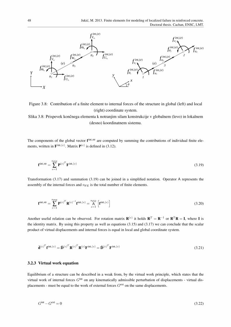
48 Jukic, M. 2013. Finite elements for modeling of localized failure in reinforced concrete.
Doctoral thesis. Cachan, ENSC, LMT.
n1 fUn1
int,HeL
fVn1
int,HeL
fQn1
int,HeL
n2 fUn2
int,HeL
fVn2
int,HeL
fQn2
int,HeL
n3
fWn3
int,HeL
HeL
1
fu1
int,HeL
fv1
int,HeL
fΘ1
int,HeL
2
fu2
int,HeL
fv2
int,HeL
fΘ2
int,HeL
3
fu3
int,HeL
HeL
X
Y
xy
Φ
Figure 3.8: Contribution of a finite element to internal forces of the structure in global (left) and local
(right) coordinate system.
Slika 3.8: Prispevek koncnega elementa k notranjim silam konstrukcije v globalnem (levo) in lokalnem
(desno) koordinatnem sistemu.
The components of the global vector f int,str are computed by summing the contributions of individual finite ele-
ments, written in F int,(e). Matrix P(e) is defined in (3.12).
f int,str =nFE
∑e=1
P(e)T F int,(e) (3.19)
Transformation (3.17) and summation (3.19) can be joined in a simplified notation. Operator A represents the
assembly of the internal forces and nFE is the total number of finite elements.
f int,str =nFE
∑e=1
P(e)T R(e)−1
f int,(e) =nFE
Ae=1
[
f int,(e)]
(3.20)
Another useful relation can be observed. For rotation matrix R(e) it holds RT = R−1 or RT R = I, where I is
the identity matrix. By using this property as well as equations (3.15) and (3.17) we can conclude that the scalar
product of virtual displacements and internal forces is equal in local and global coordinate system.
d(e)T f int,(e) = D(e)T R(e)T R(e)F int,(e) = D(e)T F int,(e) (3.21)
3.2.3 Virtual work equation
Equilibrium of a structure can be described in a weak from, by the virtual work principle, which states that the
virtual work of internal forces Gint on any kinematically admissible perturbation of displacements - virtual dis-
placements - must be equal to the work of external forces Gext on the same displacements.
Gint −Gext = 0 (3.22)
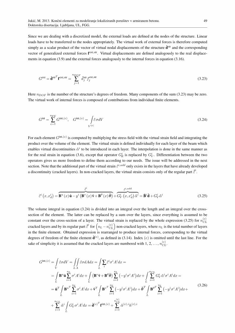
Jukic, M. 2013. Koncni elementi za modeliranje lokaliziranih porusitev v armiranem betonu.
Doktorska disertacija. Ljubljana, UL, FGG.
49
Since we are dealing with a discretized model, the external loads are defined at the nodes of the structure. Linear
loads have to be transferred to the nodes appropriately. The virtual work of external forces is therefore computed
simply as a scalar product of the vector of virtual nodal displacements of the structure dstr and the corresponding
vector of generalized external forces f ext,str. Virtual displacements are defined analogously to the real displace-
ments in equation (3.9) and the external forces analogously to the internal forces in equation (3.16).
Gext = dstrT f ext,str =nDOF
∑j=1
dstrj f ext,str
j (3.23)
Here nDOF is the number of the structure’s degrees of freedom. Many components of the sum (3.23) may be zero.
The virtual work of internal forces is composed of contributions from individual finite elements.
Gint =nFE
∑e=1
Gint,(e), Gint,(e) =∫
V (e)
εσdV (3.24)
For each element Gint,(e) is computed by multiplying the stress field with the virtual strain field and integrating the
product over the volume of the element. The virtual strain is defined individually for each layer of the beam which
enables virtual discontinuities αi to be introduced in each layer. The interpolation is done in the same manner as
for the real strain in equation (3.6), except that operator GiR is replaced by Gi
V . Differentiation between the two
operators gives us more freedom to define them according to our needs. The issue will be addressed in the next
section. Note that the additional part of the virtual strain εi,add only exists in the layers that have already developed
a discontinuity (cracked layers). In non-cracked layers, the virtual strain consists only of the regular part ˆεi.
εi(x,xi
d
)=
ˆεi
︷ ︸︸ ︷
Bu (x) u−yi(Bv (x) v+Bθ (x) θ
)+
εi,add︷ ︸︸ ︷
GiV
(x,xi
d
)αi = Bid+Gi
V αi (3.25)
The volume integral in equation (3.24) is divided into an integral over the length and an integral over the cross-
section of the element. The latter can be replaced by a sum over the layers, since everything is assumed to be
constant over the cross-section of a layer. The virtual strain is replaced by the whole expression (3.25) for n(e)CL
cracked layers and by its regular part ˆεi
for(
nL−n(e)CL
)
non-cracked layers, where nL is the total number of layers
in the finite element. Obtained expression is rearranged to produce internal forces, corresponding to the virtual
degrees of freedom of the finite element d(e), as defined in (3.14). Index (e) is omitted until the last line. For the
sake of simplicity it is assumed that the cracked layers are numbered with 1, 2, . . . , n(e)CL.
Gint,(e) =∫
V
εσdV =∫
L
∫
A
εσdAdx=∫
L
∑i
εiσiAidx=
=∫
L
BuunL
∑i=1
σiAidx+∫
L
(Bv v+Bθθ
) nL
∑i=1
(−yiσiAi
)dx+
∫
L
nCL
∑i=1
GiV α
iσiAidx=
= uT∫
L
BuTnL
∑i=1
σiAidx+ vT∫
L
BvTnL
∑i=1
(−yiσiAi
)dx+ θ
T∫
L
BθTnL
∑i=1
(−yiσiAi
)dx+
+nCL
∑i=1
αi∫
L
GiV σ
iAidx= d(e)T f int,(e)+
n(e)CL
∑i=1
α(e),ih(e),i
(3.26)

50 Jukic, M. 2013. Finite elements for modeling of localized failure in reinforced concrete.
Doctoral thesis. Cachan, ENSC, LMT.
A condensed form of expressions (3.14) and (3.18) for d(e) and f int,(e) can be used.
d(e)T =
uT , vT , θT
, f int,(e)T =
fu,int,(e)T , fv,int,(e)T , fθ,int,(e)T
(3.27)
Components of f int,(e) are defined in (3.28). The order of integration and summation can be reversed. Therefore
we can compute the internal forces as a sum of contributions of individual layers, which proves to be very helpful
in the computational procedure. Here nL is the total number of layers in the finite element.
fu,int,(e) =∫
L
BuTnL
∑i=1
σiAidx=nL
∑i=1
∫
L
BuT
σiAidx
fv,int,(e) =∫
L
BvTnL
∑i=1
(−yiσiAi
)dx=
nL
∑i=1
−∫
L
BvT yiσiAidx
fθ,int,(e) =∫
L
BθTnL
∑i=1
(−yiσiAi
)dx=
nL
∑i=1
−∫
L
BθT yiσiAidx
(3.28)
A shorter notation (3.29) will also be used, where f int,(e),i is contribution of the i-th layer to the vector of internal
forces of the finite element.
f int,(e) =nL
∑i=1
Ai∫
L
BuT
−yiBvT
−yiBθT
σ
idx=nL
∑i=1
Ai∫
L
BiT σidx
︸ ︷︷ ︸
f int,(e),i
(3.29)
The last term of the last line in (3.26) is the additional virtual work due to enhanced kinematics. The sum has
n(e)CL summands, one for each cracked layer. Quantity h(e),i is an equivalent of internal force, corresponding to the
virtual displacement jump α(e),i, and is defined as follows.
h(e),i =∫
L
GiV σ
iAidx, i= 1,2, . . . ,n(e)CL (3.30)
The virtual work of external and internal forces in the equilibrium equation (3.22) is replaced by expressions
(3.23) and (3.24), respecting (3.26) and (3.21). Finally, the second of equations (3.15) allows us to express the
weak equilibrium in the manner of global virtual displacement vector dstr and virtual displacement jumps α(e),i.
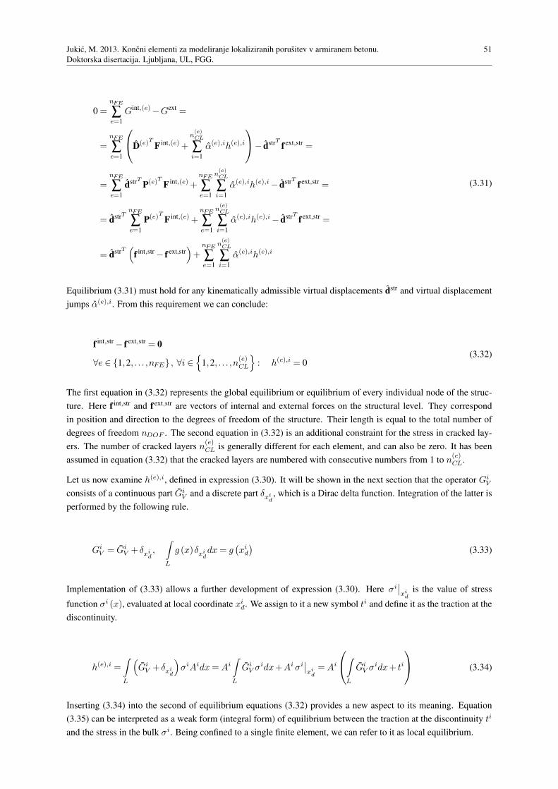
Jukic, M. 2013. Koncni elementi za modeliranje lokaliziranih porusitev v armiranem betonu.
Doktorska disertacija. Ljubljana, UL, FGG.
51
0 =nFE
∑e=1
Gint,(e)−Gext =
=nFE
∑e=1
D(e)T F int,(e)+
n(e)CL
∑i=1
α(e),ih(e),i
− dstrT f ext,str =
=nFE
∑e=1
dstrT P(e)T F int,(e)+nFE
∑e=1
n(e)CL
∑i=1
α(e),ih(e),i− dstrT f ext,str =
= dstrTnFE
∑e=1
P(e)T F int,(e)+nFE
∑e=1
n(e)CL
∑i=1
α(e),ih(e),i− dstrT f ext,str =
= dstrT(
f int,str − f ext,str)
+nFE
∑e=1
n(e)CL
∑i=1
α(e),ih(e),i
(3.31)
Equilibrium (3.31) must hold for any kinematically admissible virtual displacements dstr and virtual displacement
jumps α(e),i. From this requirement we can conclude:
f int,str − f ext,str = 0
∀e ∈ 1,2, . . . ,nFE , ∀i ∈
1,2, . . . ,n(e)CL
: h(e),i = 0(3.32)
The first equation in (3.32) represents the global equilibrium or equilibrium of every individual node of the struc-
ture. Here f int,str and f ext,str are vectors of internal and external forces on the structural level. They correspond
in position and direction to the degrees of freedom of the structure. Their length is equal to the total number of
degrees of freedom nDOF . The second equation in (3.32) is an additional constraint for the stress in cracked lay-
ers. The number of cracked layers n(e)CL is generally different for each element, and can also be zero. It has been
assumed in equation (3.32) that the cracked layers are numbered with consecutive numbers from 1 to n(e)CL.
Let us now examine h(e),i, defined in expression (3.30). It will be shown in the next section that the operator GiV
consists of a continuous part GiV and a discrete part δxi
d, which is a Dirac delta function. Integration of the latter is
performed by the following rule.
GiV = Gi
V + δxid,∫
L
g (x)δxiddx= g
(xid
)(3.33)
Implementation of (3.33) allows a further development of expression (3.30). Here σi∣∣xid
is the value of stress
function σi (x), evaluated at local coordinate xid. We assign to it a new symbol ti and define it as the traction at the
discontinuity.
h(e),i =∫
L
(
GiV + δxi
d
)
σiAidx=Ai∫
L
GiV σ
idx+Aiσi∣∣xid=Ai
∫
L
GiV σ
idx+ ti
(3.34)
Inserting (3.34) into the second of equilibrium equations (3.32) provides a new aspect to its meaning. Equation
(3.35) can be interpreted as a weak form (integral form) of equilibrium between the traction at the discontinuity ti
and the stress in the bulk σi. Being confined to a single finite element, we can refer to it as local equilibrium.
52 Jukic, M. 2013. Finite elements for modeling of localized failure in reinforced concrete.
Doctoral thesis. Cachan, ENSC, LMT.
h(e),i = 0 ⇔ ti =−∫
L
GiV σ
idx (3.35)
3.2.4 Derivation of operators GR and GV
3.2.4.1 Derivation of operator GR for real strain
Interpolation of the axial displacement field ui (x) in the i-th layer is defined in equation (3.5). The regular part
ui (x) is computed from the axial displacement of the middle axis u(x) and rotation θ (x) of the cross-section.
Since they are both quadratic functions of x, ui (x) is quadratic as well. By the definition it is interpolated between
the nodal displacements u, v and θ of the finite element. However, if we regard the layer as a special type of a
bar with quadratic axial displacement field, then ui (x) can be interpolated between the nodal displacements ui
of this bar, see Fig. 3.9. If they are positioned at the ends and in the middle of the layer, the interpolation can be
performed with the original interpolation functions Nu (x) for axial displacements, defined in (3.1).
ui (x) = u(x)−yiθ (x) = Nu (x)ui, ui =ui
1,ui2,u
i3
T(3.36)
u1
v1
Θ1
u2
v2
Θ2
u3
L
hyi
uHxL u1u2u3
-yi ΘHxL-yiΘ1
-yiΘ2
u iHxL u1i u2
iu3i
u1i u3
i
u2i
u1i N1
uHxL u1i
u2i N2
uHxLu2
i
u3i N3
uHxLu3
i
u iHxL u1i u2
iu3i
Figure 3.9: Interpolation of standard axial displacement in i-th layer between nodal displacements of
the finite element (left) and between nodal axial displacements of the layer (right).
Slika 3.9: Interpolacija standardnega osnega pomika v i-tem sloju med prostostne stopnje koncnega
elementa (levo) in med vozliscne osne pomike sloja (desno).
The “nodal” displacements ui of the i-th layer can be calculated from ui (x) by inserting for x the coordinates of
the layer’s “nodes”, which are 0, L and L/2.

Jukic, M. 2013. Koncni elementi za modeliranje lokaliziranih porusitev v armiranem betonu.
Doktorska disertacija. Ljubljana, UL, FGG.
53
ui =
ui∣∣x=0
, ui∣∣x=L
, ui∣∣x=L/2
T=
=
u1 −yiθ1,u2 −yiθ2,u3 −yi(
−3(v1 −v2)
2L−
θ1 +θ2
4
)T (3.37)
The regular axial displacement ui (x) is enriched with the additional part ui,add (x,xd), which represents the
additional axial displacement due to occurrence of a discontinuity in the layer. It is determined by the interpolation
function M i(x,xi
d
)and the displacement jump αi at the discontinuity of the layer.
ui(x,xi
d
)= ui (x)+M i
(x,xi
d
)αi (3.38)
The interpolation function M i must not influence the nodal displacements ui of the layer, which means that it must
have zero values at all nodes of the layer, and it must have a unit jump at the location of the discontinuity xid. The
easiest way to meet the requirements is to use a combination of the Heaviside function and the suitable choice of
shape functions Nu.
x
L
xdi
W
W- W+
i
Hxdi 0 1
∆xdi 0
¥
Figure 3.10: Domain and sub-domains of a cracked layer. Heaviside and Dirac-delta functions.
Slika 3.10: Domena in poddomeni razpokanega sloja. Heaviside-ova in Dirac-delta funkcija.
Domain Ω of the cracked layer is divided by the discontinuity into two parts. Ω− is the part before the discontinuity,
with x < xid, and Ω+ is the part after the discontinuity, with x ≥ xi
d, see Fig. 3.10. The value of the Heaviside
function is 0 on Ω− and 1 on Ω+. Its derivative is the Dirac delta function δxid, which has an infinite value at xi
d
and zero value elsewhere.
Hxid=
0; x < xid
1; x≥ xid
∂Hxid
∂x= δxi
d=
∞; x= xid
0; otherwise(3.39)
54 Jukic, M. 2013. Finite elements for modeling of localized failure in reinforced concrete.
Doctoral thesis. Cachan, ENSC, LMT.
Heaviside function Hxid
satisfies the requirement of a unit jump at the discontinuity. Its value, however, is only zero
on Ω−, and not at all nodes of the layer. This can be fixed by subtracting from it those shape functions Nuj ∈ Nu,
that correspond to the nodes j, included in Ω+. Since Nuj are continuous and have zero values at all nodes except
j, they will not affect previously fulfilled demands.
M i =Hxid− ∑
j∈Ω+
Nuj (3.40)
To avoid complications, let us decide that the discontinuity can occur infinitesimally close to a node, but not at the
node itself. Two options remain for the function M i. If the discontinuity appears in the left half of the layer, Ω+
contains nodes 2 and 3, and if it appears in the right half, Ω+ contains only node 2, see Fig. 3.11.
M i =
Hxid− (Nu
2 +Nu3 ) ; 0 < xi
d < L/2
Hxid−Nu
2 ; L/2 < xid < L
(3.41)
x
L
xdi
u1i u2
iu3i
W- W+i
Hxdi
N2u
N3u
M i
1
1
1
1
x
L
xdi
u1i u2
iu3i
W- W+i
Hxdi
N2u
M i
1
1
1
Figure 3.11: Construction of interpolation function Mi in case of discontinuity between nodes 1 and 3
(left) and in case of discontinuity between nodes 3 and 2 (right).
Slika 3.11: Konstruiranje interpolacijske funkcije Mi v primeru nezveznosti med vozliscema 1 in 3
(levo) in v primeru nezveznosti med vozliscema 3 in 2 (desno).
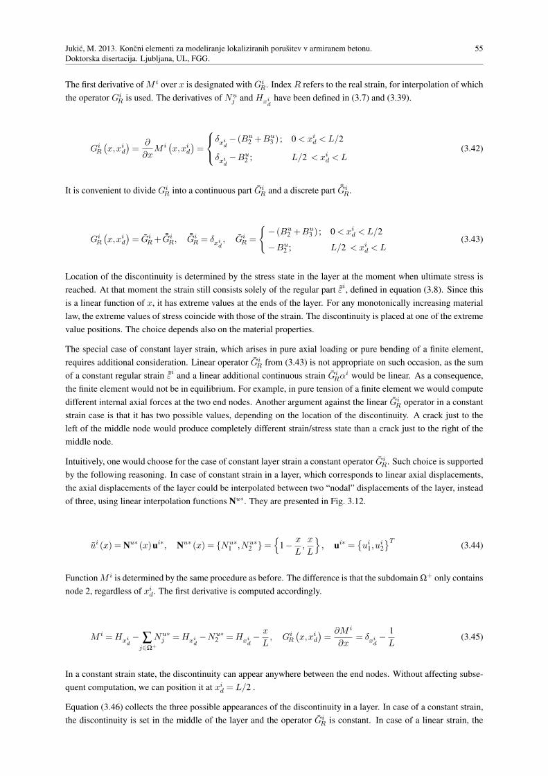
Jukic, M. 2013. Koncni elementi za modeliranje lokaliziranih porusitev v armiranem betonu.
Doktorska disertacija. Ljubljana, UL, FGG.
55
The first derivative of M i over x is designated with GiR. Index R refers to the real strain, for interpolation of which
the operator GiR is used. The derivatives of Nu
j and Hxid
have been defined in (3.7) and (3.39).
GiR
(x,xi
d
)=
∂
∂xM i(x,xi
d
)=
δxid− (Bu
2 +Bu3 ) ; 0 < xi
d < L/2
δxid−Bu
2 ; L/2 < xid < L
(3.42)
It is convenient to divide GiR into a continuous part Gi
R and a discrete part ¯GiR.
GiR
(x,xi
d
)= Gi
R+ ¯GiR,
¯GiR = δxi
d, Gi
R =
− (Bu2 +Bu
3 ) ; 0 < xid < L/2
−Bu2 ; L/2 < xi
d < L(3.43)
Location of the discontinuity is determined by the stress state in the layer at the moment when ultimate stress is
reached. At that moment the strain still consists solely of the regular part ˜εi, defined in equation (3.8). Since this
is a linear function of x, it has extreme values at the ends of the layer. For any monotonically increasing material
law, the extreme values of stress coincide with those of the strain. The discontinuity is placed at one of the extreme
value positions. The choice depends also on the material properties.
The special case of constant layer strain, which arises in pure axial loading or pure bending of a finite element,
requires additional consideration. Linear operator GiR from (3.43) is not appropriate on such occasion, as the sum
of a constant regular strain ˜εi and a linear additional continuous strain GiRα
i would be linear. As a consequence,
the finite element would not be in equilibrium. For example, in pure tension of a finite element we would compute
different internal axial forces at the two end nodes. Another argument against the linear GiR operator in a constant
strain case is that it has two possible values, depending on the location of the discontinuity. A crack just to the
left of the middle node would produce completely different strain/stress state than a crack just to the right of the
middle node.
Intuitively, one would choose for the case of constant layer strain a constant operator GiR. Such choice is supported
by the following reasoning. In case of constant strain in a layer, which corresponds to linear axial displacements,
the axial displacements of the layer could be interpolated between two “nodal” displacements of the layer, instead
of three, using linear interpolation functions Nu∗. They are presented in Fig. 3.12.
ui (x) = Nu∗ (x)ui∗, Nu∗ (x) = Nu∗1 ,Nu∗
2 =
1−x
L,x
L
, ui∗ =ui
1,ui2
T(3.44)
Function M i is determined by the same procedure as before. The difference is that the subdomain Ω+ only contains
node 2, regardless of xid. The first derivative is computed accordingly.
M i =Hxid− ∑
j∈Ω+
Nu∗j =Hxi
d−Nu∗
2 =Hxid−
x
L, Gi
R
(x,xi
d
)=
∂M i
∂x= δxi
d−
1
L(3.45)
In a constant strain state, the discontinuity can appear anywhere between the end nodes. Without affecting subse-
quent computation, we can position it at xid = L/2 .
Equation (3.46) collects the three possible appearances of the discontinuity in a layer. In case of a constant strain,
the discontinuity is set in the middle of the layer and the operator GiR is constant. In case of a linear strain, the
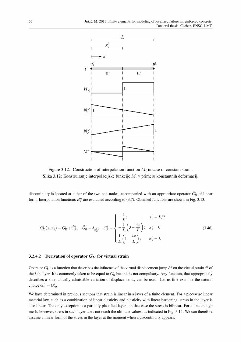
56 Jukic, M. 2013. Finite elements for modeling of localized failure in reinforced concrete.
Doctoral thesis. Cachan, ENSC, LMT.
x
L
xdi
u1i u2
i
W- W+i
Hxdi
N1u*
N2u*
M i
1
1
1
1
Figure 3.12: Construction of interpolation function Mi in case of constant strain.
Slika 3.12: Konstruiranje interpolacijske funkcije Mi v primeru konstantnih deformacij.
discontinuity is located at either of the two end nodes, accompanied with an appropriate operator GiR of linear
form. Interpolation functions Buj are evaluated according to (3.7). Obtained functions are shown in Fig. 3.13.
GiR
(x,xi
d
)= Gi
R+ ¯GiR,
¯GiR = δxi
d, Gi
R =
−1
L; xi
d = L/2
−1
L
(
3−4x
L
)
; xid = 0
1
L
(
1−4x
L
)
; xid = L
(3.46)
3.2.4.2 Derivation of operator GV for virtual strain
Operator GiV is a function that describes the influence of the virtual displacement jump αi on the virtual strain εi of
the i-th layer. It is commonly taken to be equal to GiR but this is not compulsory. Any function, that appropriately
describes a kinematically admissible variation of displacements, can be used. Let us first examine the natural
choice GiV =Gi
R.
We have determined in previous sections that strain is linear in a layer of a finite element. For a piecewise linear
material law, such as a combination of linear elasticity and plasticity with linear hardening, stress in the layer is
also linear. The only exception is a partially plastified layer - in that case the stress is bilinear. For a fine enough
mesh, however, stress in such layer does not reach the ultimate values, as indicated in Fig. 3.14. We can therefore
assume a linear form of the stress in the layer at the moment when a discontinuity appears.
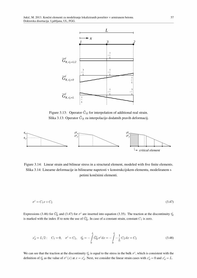
Jukic, M. 2013. Koncni elementi za modeliranje lokaliziranih porusitev v armiranem betonu.
Doktorska disertacija. Ljubljana, UL, FGG.
57
x
L
1 23
GR, xdi =L2
i
GR, xdi =0
i
GR, xdi =L
i
-1
L
-3
L-
1
L
1
L
1
L
-1
L-
3
L
Figure 3.13: Operator GR for interpolation of additional real strain.
Slika 3.13: Operator GR za interpolacijo dodatnih pravih deformacij.
Εu
Εy
ΣuΣy
ΣuΣy
critical element
Figure 3.14: Linear strain and bilinear stress in a structural element, modeled with five finite elements.
Slika 3.14: Linearne deformacije in bilinearne napetosti v konstrukcijskem elementu, modeliranem s
petimi koncnimi elementi.
σi = C1x+C2 (3.47)
Expressions (3.46) for GiR and (3.47) for σi are inserted into equation (3.35). The traction at the discontinuity tiR
is marked with the index R to note the use of GiR. In case of a constant strain, constant C1 is zero.
xid = L/2 : C1 = 0, σi = C2, tiR =−
L∫
0
GiRσidx=−
L∫
0
−1
LC2 dx= C2 (3.48)
We can see that the traction at the discontinuity tiR is equal to the stress in the bulk σi, which is consistent with the
definition of tiR as the value of σi (x) at x= xid. Next, we consider the linear strain cases with xi
d = 0 and xid = L.
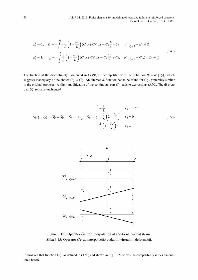
58 Jukic, M. 2013. Finite elements for modeling of localized failure in reinforced concrete.
Doctoral thesis. Cachan, ENSC, LMT.
xid = 0 : tiR =−
L∫
0
−1
L
(
3−4x
L
)
(C1x+C2)dx= C1L
6+C2, σi
∣∣xid=0
= C2 6= tiR
xid = L : tiR =−
L∫
0
1
L
(
1−4x
L
)
(C1x+C2)dx= C15L
6+C2, σi
∣∣xid=L
= C1L+C2 6= tiR
(3.49)
The traction at the discontinuity, computed in (3.49), is incompatible with the definition tiR = σi(xid
), which
suggests inadequacy of the choice GiV = Gi
R. An alternative function has to be found for GiV , preferably similar
to the original proposal. A slight modification of the continuous part GiV leads to expressions (3.50). The discrete
part ¯GiV remains unchanged.
GiV
(x,xi
d
)= Gi
V + ¯GiV ,
¯GiV = δxi
d, Gi
V =
−1
L; xi
d = L/2
−2
L
(
2−3x
L
)
; xid = 0
2
L
(
1−3x
L
)
; xid = L
(3.50)
x
L
1 23
GV, xdi =L2
i
GV, xdi =0
i
GV, xdi =L
i
-1
L
-4
L-
1
L
2
L
2
L
-1
L-
4
L
Figure 3.15: Operator GV for interpolation of additional virtual strain.
Slika 3.15: Operator GV za interpolacijo dodatnih virtualnih deformacij.
It turns out that function GiV , as defined in (3.50) and shown in Fig. 3.15, solves the compatibility issues encoun-
tered before.

Jukic, M. 2013. Koncni elementi za modeliranje lokaliziranih porusitev v armiranem betonu.
Doktorska disertacija. Ljubljana, UL, FGG.
59
xid = 0 : ti =−
L∫
0
−2
L
(
2−3x
L
)
(C1x+C2)dx= C2, σi∣∣xid=0
= C2 = ti
xid = L : ti =−
L∫
0
2
L
(
1−3x
L
)
(C1x+C2)dx= C1L+C2, σi∣∣xid=L
= C1L+C2 = ti
(3.51)
Operator GiV should also satisfy the patch test which requires the additional virtual work (performed on the virtual
displacement jumps αi) to be zero in case of constant stress σi. Thus, the introduction of αi does not affect the
energy dissipation at least for the constant stress state. Such state is approached by refining the finite element mesh.
αi∫
L
GiV σ
iAidxσi=const.
= αiσiAi︸ ︷︷ ︸
6=0
∫
L
GiV dx= 0 ⇒
∫
L
GiV dx= 0 (3.52)
Taking into account the rule (3.33) for integration of GiV , requirement (3.52) can be reformulated.
∫
L
GiV dx=
∫
L
(
GiV + δxi
d
)
dx=∫
L
GiV dx+
=1︷ ︸︸ ︷∫
L
δxiddx= 0 ⇒
∫
L
GiV dx=−1 (3.53)
It can be easily verified that each of expressions (3.50) for GiV satisfies (3.53).
3.2.5 Constitutive models
In this section we describe constitutive models which control the behavior of concrete and reinforcement layers.
For each material, there are two separate models, one for the bulk of the layer and one for the discontinuity.
3.2.5.1 Bulk of concrete layer
Behavior of the bulk of the concrete layer is described by 1D elasto-damage model. Response of the material
is linear elastic up to the elasticity limit. Further increase of stress produces micro damage (micro cracking in
tension and micro crushing in compression) continuously over the layer, which results in reduction of the elasticity
modulus. Unloading is linear elastic with the current value of the elasticity modulus, and leads to the origin of the
stress-strain diagram (see Fig. 3.16). These properties of concrete are collected in the following equations, which
can be derived through the principle of maximum damage dissipation, see [73].
Equation (3.54) shows the linear elastic relation between stress and strain. It represents the loading curve/path up
to elasticity limit and the unloading/reloading curve in the σi− εi diagram.
σi = Di−1
εi, Di ∈[E−1
c ,∞), εi = Bid+Gi
Rαi =
εi︷ ︸︸ ︷
Bid+ GiRα
i+ ¯GiRα
i (3.54)
Here Di is compliance of the bulk material, Ec elastic modulus of intact concrete, and εi the continuous part of
axial strain in the i-th layer, composed of the regular strain and the continuous part of the additional strain. The

60 Jukic, M. 2013. Finite elements for modeling of localized failure in reinforced concrete.
Doctoral thesis. Cachan, ENSC, LMT.
Ε
Σ
Σ fct
Σdt
Σ i
-Σdc
-Σ fcc
Ε i Ec
Di-1
elas
ticlo
adin
g
elasti
c unloa
ding
reloa
ding
damage loading
Figure 3.16: Stress - strain diagram for bulk of concrete layer.
Slika 3.16: Diagram napetost - deformacija za sloj betona.
latter is zero until the discontinuity is formed. The non-elastic part of the loading curve in the σi− εi diagram is
defined indirectly by the remaining equations in this section.
φi(σi, qi
)=∣∣σi∣∣−(σd− qi
), σd =
σdc for compression
σdt for tension(3.55)
Damage function φi prescribes the admissible values of axial stress σi in the i-th layer. Elasticity limit σd > 0
marks the beginning of micro damage and is defined separately for tension and compression. Stress-like hardening
variable qi handles the damage threshold evolution.
qi =−Hcξi, Hc =
Hcc for compression
Hct for tension(3.56)
Linear hardening of the material is described by equation (3.56), where ξi is a strain-like hardening variable with
initial value equal to zero, and Hc > 0 is a constant hardening modulus of concrete with separate values for tension
and compression. Evolution in pseudo-time of internal hardening variables Di and ξi is defined by evolution
equations (3.57).
˙Di=
˙γisign(σi)
σi, ˙ξ
i= ˙γi
(3.57)
Jukic, M. 2013. Koncni elementi za modeliranje lokaliziranih porusitev v armiranem betonu.
Doktorska disertacija. Ljubljana, UL, FGG.
61
The dot designates the derivative with respect to pseudo-time and ˙γiis damage multiplier. The loading/unloading
conditions and consistency condition (3.58) also apply.
˙γi ≥ 0, φi ≤ 0, ˙γiφi = 0, ˙γi ˙φi= 0 (3.58)
Tangent moduli of the σi− εi diagram can be determined from the above equations. The elastic loading/unloading
path corresponds to condition ˙γi = 0. It follows from evolution equations (3.57), that compliance Di is constant.
The tangent modulus is obtained if expression (3.54) for σi is differentiated with respect to εi.
˙γi = 0 ⇒ Di = const.,∂σi
∂εi= Di−1
(3.59)
In case of damage loading, when ˙γi > 0, the procedure is more complex. From the third and the fourth of conditions
(3.58) we can conclude that φi = 0 and ˙φi= 0. From (3.55) we can write the expression for σi and differentiate it
over pseudo-time. We use the appropriate evolution equation to differentiate ξi.
σi =(σd− qi
)sign
(σi)=(σd+Hcξ
i)sign
(σi), σi =Hc ˙γisign
(σi)
(3.60)
The stress can be replaced by expression (3.54). The obtained equation is again differentiated over pseudo-time.
Note that compliance Di is not constant any more.
Di−1
εi =(σd+Hcξ
i)sign
(σi)
−Di−2 ˙Diεi+ Di−1
˙εi =Hc˙ξisign
(σi) /
˙Di=
˙γisign(σi)
σi, ˙ξ
i= ˙γi
−Di−2 ˙γisign(σi)
σiεi+ Di−1
˙εi =Hc ˙γisign(σi) / εi
σi= Di
−Di−1˙γisign
(σi)+ Di−1
˙εi =Hc ˙γisign(σi)
˙εi =Di−1
+Hc
Di−1˙γisign
(σi)
(3.61)
The tangent modulus is computed by dividing the pseudo-time derivatives σi and ˙εi from (3.60) and (3.61).
∂σi
∂εi=
σi
˙εi=
Di−1Hc
Di−1+Hc
(3.62)
To sum up, the tangent modulus is described by two expressions. The first one covers the elastic behavior -
unloading and reloading, including the first elastic loading with the initial value of compliance Di = E−1c . The
second expression represents the slope of the damage loading curve.
∂σi
∂εi=
Di−1
; ˙γi = 0
Di−1Hc
Di−1+Hc
; ˙γi > 0(3.63)
62 Jukic, M. 2013. Finite elements for modeling of localized failure in reinforced concrete.
Doctoral thesis. Cachan, ENSC, LMT.
3.2.5.2 Discontinuity in concrete layer
Energy dissipation at the discontinuity of a concrete layer is described by a softening damage law, which connects
the traction at the discontinuity to the displacement jump. When the discontinuity is introduced, the displacement
jump is zero and the traction is equal to the failure stress of concrete. An increase of the displacement jump (in
absolute value) reduces the carrying capacity and thus produces a lower traction. A subsequent decrease of the
displacement jump (in absolute value) reduces the traction as well, but the carrying capacity remains the same.
Obviously, the problem needs to be controlled by imposed displacements to provide a unique solution. The term
“loading” therefore refers to the increase of displacement jump (in absolute value) and “unloading” refers to the
decrease of displacement jump. The unloading is always linear elastic, but there are two possibilities for loading.
Elastic (re)loading follows the unloading curve, increases the traction, and leaves the internal variables unchanged.
When carrying capacity is reached, damage loading continues. It decreases the traction and changes the internal
variables (see Fig. 3.17). This material law is mathematically described by the following equations, which can be
derived by using the principle of maximum damage dissipation, see [73].
Kct*
Kcc*
Α
t
Σ fct
ti
-Σ fcc
Α i Di-1
elas
ticun-r
eloa
ding
damage softening
Figure 3.17: Traction - displacement jump diagram for discontinuity in concrete layer.
Slika 3.17: Diagram napetost - skok v pomiku za nezveznost v sloju betona.
Equation (3.64) describes the linear elastic relation between the traction at the discontinuity ti and the displacement
jump αi. It represents the unloading/reloading path in the ti−αi diagram.
ti = ¯Di−1
αi, ¯Di∈ [0,∞) (3.64)
Here ¯Di
is compliance of the discontinuity which increases with progression of the localized failure. The loading
curve of the ti−αi diagram is defined indirectly by the remaining equations in this section.
Jukic, M. 2013. Koncni elementi za modeliranje lokaliziranih porusitev v armiranem betonu.
Doktorska disertacija. Ljubljana, UL, FGG.
63
¯φi(
ti, ¯qi)
=∣∣ti∣∣−(
σfc− ¯qi)
, σfc =
σfcc for compression
σfct for tension(3.65)
Failure function ¯φi
prescribes the admissible values of traction ti at the discontinuity of a concrete layer. Failure
stress of concrete σfc > 0 indicates the occurrence of the discontinuity and is defined separately for tension and
compression. Stress-like softening variable ¯qi handles the damage threshold evolution and is described by an
exponential function.
¯qi = σfc
(
1−eKc¯ξi)
, Kc =
Kcc =−σfcc
2Gfccfor compression
Kct =−σfct
2Gfctfor tension
(3.66)
Here ¯ξi
is a displacement-like softening variable with initial value set to zero, and Kc < 0 is a constant softening
modulus of concrete with units m−1 and separate values for compression and tension. These are determined by the
fracture energies per cross-section unit Gfcc and Gfct for concrete in compression and tension, respectively. The
fracture energy has units kJm−2 and is measured in a uniaxial compression/tension test. Fracture energies Gfcc and
Gfct represent the areas between the horizontal axis, and the compressive and tensile softening lines of the t−α
diagram in Fig. 3.17, respectively. Evolution in pseudo-time of internal softening variables ¯Di
and ¯ξi is defined by
evolution equations (3.67).
˙D
i
=˙γisign
(ti)
ti,
˙ξi
= ˙γi
(3.67)
The dot designates the derivative with respect to pseudo-time and ˙γi
is damage multiplier. The loading/unloading
conditions and consistency condition (3.68) also apply.
˙γi≥ 0, ¯φ
i≤ 0, ˙γ
i ¯φi= 0, ˙γ
i ˙φi
= 0 (3.68)
A closer inspection of equations (3.64)-(3.68) reveals that the damage loading path of ti−αi diagram, correspond-
ing to condition ¯φi= 0, is a straight line, see appendix B. The discovery suggests a possibility of simplification,
but more insight is required.
Each point of the damage loading path is determined by its ordinate ti and the slope ¯Di−1
of the unloading line,
which connects the point to the origin. Abscissa αi is computed from equation (3.64). Evolution equations (3.67)
dictate the change of ¯Di
and ¯ξi, the latter defining ti through equations (3.65), (3.66) and (3.68). Both ¯D
iand
ti change non-linearly with respect to ¯γi = ˙γi∆τ (∆τ being pseudo-time step), the first one because of non-linear
evolution equation (3.67), and the second due to exponential softening law (3.66). However, the two non-linearities
neutralize each other, yielding a linear relation between ti and αi.
The same damage loading path can be constructed by defining coordinates αi and ti. If they both change linearly
with respect to some new variable, the diagram will be a straight line. We introduce a new displacement-like
variable ¯ξi∗
and the softening law takes a linear form.
¯ξi∗=−
1
Kc
(
1−eKc¯ξi)
, ¯qi = σfc
(
1−eKc¯ξi)
=−Kcσfc¯ξi∗=−K∗
c¯ξi∗
(3.69)
64 Jukic, M. 2013. Finite elements for modeling of localized failure in reinforced concrete.
Doctoral thesis. Cachan, ENSC, LMT.
The expression for ¯qi in (3.69) holds for ¯ξi< ∞, or equivalently ¯ξ
i∗<−1/Kc . After that ¯qi would become greater
than the failure stress of concrete σfc, which is not acceptable. Physically, it means that the carrying capacity
cannot drop below zero.
¯qi = min
−K∗c
¯ξi∗,σfc
, K∗c =Kcσfc (3.70)
Then, the introduction of a new damage multiplier ¯γi∗allows us to write a new set of linear evolution equations
for αi and ¯ξi∗
. See appendix B for details.
¯γi∗ =−1
Kc
(
1−eKc ¯γi)
, αi = ˙γi∗sign
(ti),
˙ξi∗= ˙γ
i∗(3.71)
The new softening law (3.70) and evolution equations (3.71), due to their linear form, simplify the computa-
tional procedure significantly. But there is another advantage over the original equations. As the original dam-
age multiplier ¯γiapproaches infinity, the traction ti approaches zero and the displacement jump αi approaches
−sign(ti)/Kc . No matter how much we increase the multiplier, αi cannot pass that value. For an individual bar,
such limitation is logical, as the complete loss of carrying capacity implies singularity of the problem and a further
increase of the discontinuity is meaningless. However, if a layer of a beam loses all carrying capacity, the beam
as a whole still possesses stiffness. The broken layer just follows the rest of the beam without resistance. It is
therefore necessary to allow αi to grow past the point of failure. When the new damage multiplier ¯γi∗reaches the
value −1/Kc , the original multiplier is pushed to infinity and the old evolution equations (3.67) get out of scope.
The new evolution equations (3.71), however, withstand further increase of ¯γi∗. As the latter approaches infinity,
so does αi (in absolute value). Once past the failure point the traction ti remains zero. The constitutive law at the
discontinuity is summed up below.
ti =
¯Di−1
αi; ˙γi∗= 0
σfc sign(αi)+σfcKcα
i; ˙γi∗> 0, ¯qi < σfc
0; ˙γi∗> 0, ¯qi = σfc
(3.72)
The first expression represents the elastic unloading path, the second one the damage loading path until the traction
drops to zero, and the third one the damage loading path further on. The tangent moduli are obtained by a simple
differentiation of (3.72).
∂ti
∂αi=
¯Di−1
; ˙γi∗= 0
K∗c = σfcKc; ˙γ
i∗> 0, ¯qi < σfc
0; ˙γi∗> 0, ¯qi = σfc
(3.73)
3.2.5.3 Bulk of reinforcement layer
Behavior of the bulk of a layer of reinforcement is described by 1D elasto-plasticity model with isotropic hardening.
It is symmetrical in tension and compression. Response of the material is linear elastic until yield stress is reached.
If loading increases, plastic deformations occur and grow continuously over the layer. Elasticity limit is raised
as well. Unloading is elastic and follows a line, parallel to the first loading path. When the stress drops to zero,

Jukic, M. 2013. Koncni elementi za modeliranje lokaliziranih porusitev v armiranem betonu.
Doktorska disertacija. Ljubljana, UL, FGG.
65
plastic deformations remain in the layer (Fig. 3.18). Behavior of steel is mathematically described by the following
equations, which can be derived by using the principle of maximum plastic dissipation [73].
Ε
Σ
Σ fs
Σy
Σ i
Ε iΕ ip
Es Es
elas
ticlo
adin
g
elas
ticun
load
ing
relo
adin
g
plastic loading
Figure 3.18: Stress - strain diagram for bulk of reinforcement layer.
Slika 3.18: Diagram napetost - deformacija za sloj armature.
Stress σi is computed from equation (3.74), which represents the elastic loading path and elastic unloading or
reloading path of the σi− εi diagram.
σi = Es
(εi− εip
), εi = Bid+Gi
Rαi =
εi︷ ︸︸ ︷
Bid+ GiRα
i+ ¯GiRα
i (3.74)
Here Es is the elastic modulus of steel, εip plastic strain, and εi the continuous part of axial strain in the i-th
layer, composed of the regular strain and the continuous part of the additional strain. Before the appearance of the
discontinuity the additional strain is zero. The plastic loading path of the σi− εi diagram is determined indirectly
by the rest of the equations in this section.
φi(σi, qi
)=∣∣σi∣∣−(σy − qi
)(3.75)
Yield function φi prescribes the admissible axial stress in the layer. Yield stress σy > 0 is the absolute value of
the stress, at which the first plastic deformations occur. Stress-like hardening variable qi controls yield threshold
evolution.
qi =−Hsξi (3.76)
Equation (3.76) describes the linear isotropic hardening of the material. Here Hs > 0 is a constant hardening

66 Jukic, M. 2013. Finite elements for modeling of localized failure in reinforced concrete.
Doctoral thesis. Cachan, ENSC, LMT.
modulus of steel and ξi is a strain-like hardening variable with the initial value zero. Evolution in pseudo-time of
internal hardening variables for plasticity, εip and ξi, is prescribed by evolution equations (3.77).
˙εip = ˙γisign(σi)
, ˙ξi= ˙γi
(3.77)
The dot designates the derivative with respect to pseudo-time and ˙γiis plastic multiplier. The loading/unloading
conditions and consistency condition (3.78) apply as well.
˙γi ≥ 0, φi ≤ 0, ˙γiφi = 0, ˙γi ˙φi= 0 (3.78)
Tangent moduli of the σi− εi diagram are determined by the described equations. In elastic response, the plastic
multiplier is equal to zero. As a consequence, internal variables are constant and the tangent modulus is simply
computed by differentiating the expression (3.74) for σi with respect to εi.
˙γi = 0 ⇒ εip = const.,∂σi
∂εi= Es (3.79)
In plastic loading, the plastic strain εip is not constant. It depends on the plastic multiplier ˙γi > 0 and consequently
on the strain εi. The tangent modulus can be computed from pseudo-time derivatives of stress and strain. It
follows from the last two equations in (3.78) that φi = 0 and ˙φi= 0. We can express σi from equation (3.75) and
differentiate it over pseudo-time.
σi =(σy − qi
)sign
(σi)=(σy +Hsξ
i)sign
(σi), σi =Hs ˙γisign
(σi)
(3.80)
We can replace the stress σi with expression (3.74) and differentiate the modified equation over pseudo-time again.
Evolution equations (3.77) are utilized in the procedure.
Es
(εi− εip
)=(σy +Hsξ
i)sign
(σi)
Es
(
˙εi− ˙εip
)
=Hs˙ξisign
(σi) /
˙εip = ˙γisign(σi), ˙ξ
i= ˙γi
Es ˙εi−Es ˙γisign(σi)=Hs ˙γisign
(σi)
˙εi =Es+Hs
Es
˙γisign(σi)
(3.81)
Pseudo-time derivatives σi and ˙εi, defined in (3.80) and (3.81), are divided to produce the plastic tangent modulus.
∂σi
∂εi=
σi
˙εi=
EsHs
Es+Hs(3.82)
The elastic and plastic tangent moduli are gathered below. The first expression represents the slope of the elastic
loading and unloading path, while the second one represents the slope of the plastic loading path in the σi − εi
diagram.
∂σi
∂εi=
Es; ˙γi = 0
EsHs
Es+Hs; ˙γi > 0
(3.83)
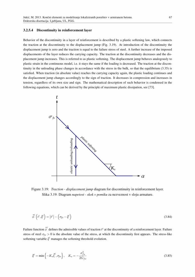
Jukic, M. 2013. Koncni elementi za modeliranje lokaliziranih porusitev v armiranem betonu.
Doktorska disertacija. Ljubljana, UL, FGG.
67
3.2.5.4 Discontinuity in reinforcement layer
Behavior of the discontinuity in a layer of reinforcement is described by a plastic softening law, which connects
the traction at the discontinuity to the displacement jump (Fig. 3.19). At introduction of the discontinuity the
displacement jump is zero and the traction is equal to the failure stress of steel. A further increase of the imposed
displacements of the layer reduces the carrying capacity. The traction at the discontinuity decreases and the dis-
placement jump increases. This is referred to as plastic softening. The displacement jump behaves analogously to
plastic strain in the continuous model, i.e. it stays the same if the loading is decreased. The traction at the discon-
tinuity in the unloading phase changes in accordance with the stress in the bulk, so that the equilibrium (3.35) is
satisfied. When traction (in absolute value) reaches the carrying capacity again, the plastic loading continues and
the displacement jump changes accordingly to the sign of traction. It decreases in compression and increases in
tension, regardless of its own size and sign. The mathematical description of such behavior is condensed in the
following equations, which can be derived by the principle of maximum plastic dissipation, see [73].
Ks
Α
t
Σ fs
elas
tic
unlo
adin
gre
load
ing
plastic softening
Figure 3.19: Traction - displacement jump diagram for discontinuity in reinforcement layer.
Slika 3.19: Diagram napetost - skok v pomiku za nezveznost v sloju armature.
¯φi(
ti, ¯qi)
=∣∣ti∣∣−(
σfs− ¯qi)
(3.84)
Failure function ¯φi
defines the admissible values of traction ti at the discontinuity of a reinforcement layer. Failure
stress of steel σfs > 0 is the absolute value of the stress, at which the discontinuity first appears. The stress-like
softening variable ¯qi manages the softening threshold evolution.
¯qi = min
−Ks¯ξi,σfs
, Ks =−σ2fs
2Gfs(3.85)
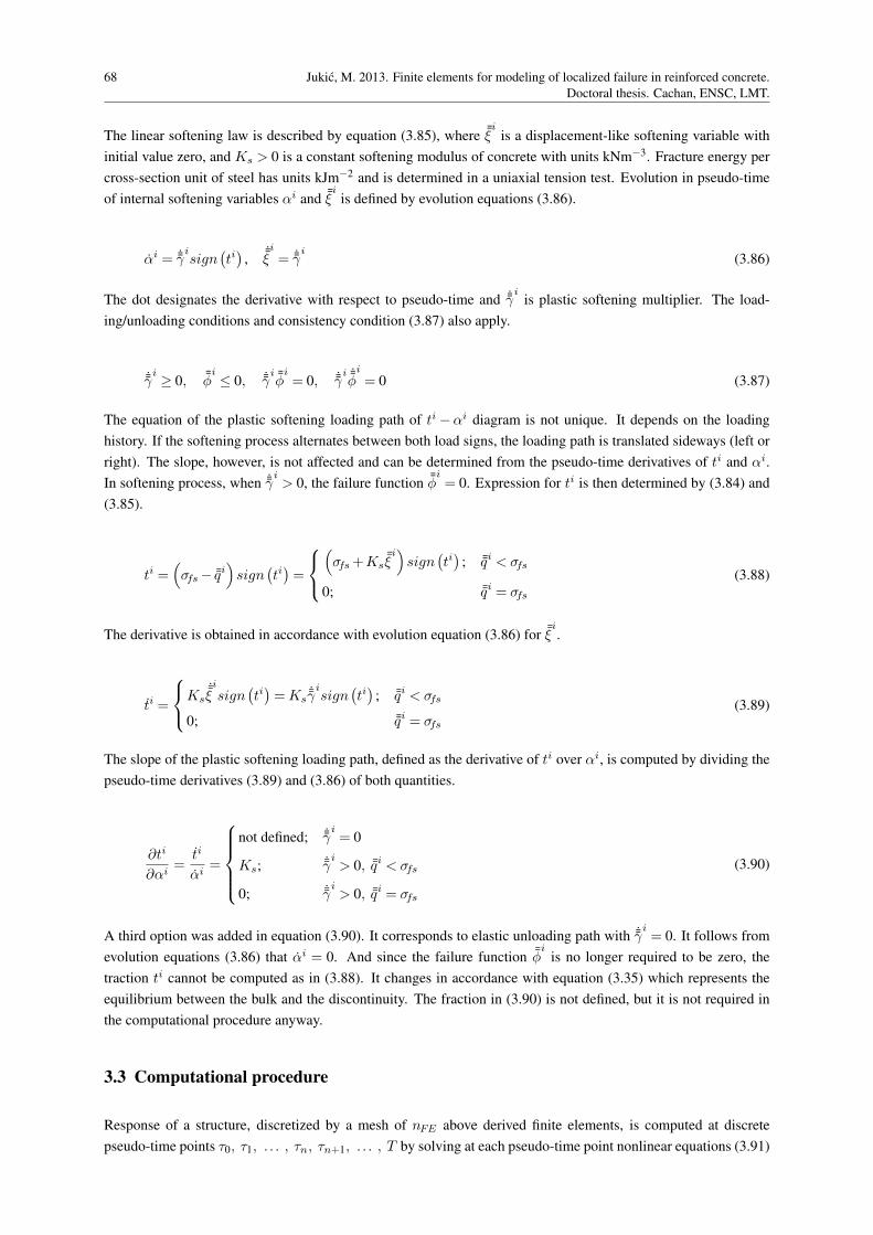
68 Jukic, M. 2013. Finite elements for modeling of localized failure in reinforced concrete.
Doctoral thesis. Cachan, ENSC, LMT.
The linear softening law is described by equation (3.85), where ¯ξi
is a displacement-like softening variable with
initial value zero, and Ks > 0 is a constant softening modulus of concrete with units kNm−3. Fracture energy per
cross-section unit of steel has units kJm−2 and is determined in a uniaxial tension test. Evolution in pseudo-time
of internal softening variables αi and ¯ξi
is defined by evolution equations (3.86).
αi = ˙γisign
(ti)
,˙ξi
= ˙γi
(3.86)
The dot designates the derivative with respect to pseudo-time and ˙γi
is plastic softening multiplier. The load-
ing/unloading conditions and consistency condition (3.87) also apply.
˙γi≥ 0, ¯φ
i≤ 0, ˙γ
i ¯φi= 0, ˙γ
i ˙φi
= 0 (3.87)
The equation of the plastic softening loading path of ti −αi diagram is not unique. It depends on the loading
history. If the softening process alternates between both load signs, the loading path is translated sideways (left or
right). The slope, however, is not affected and can be determined from the pseudo-time derivatives of ti and αi.
In softening process, when ˙γi> 0, the failure function ¯φ
i= 0. Expression for ti is then determined by (3.84) and
(3.85).
ti =(
σfs− ¯qi)
sign(ti)=
(
σfs+Ks¯ξi)
sign(ti)
; ¯qi < σfs
0; ¯qi = σfs
(3.88)
The derivative is obtained in accordance with evolution equation (3.86) for ¯ξi.
ti =
Ks˙ξi
sign(ti)=Ks
˙γisign
(ti)
; ¯qi < σfs
0; ¯qi = σfs(3.89)
The slope of the plastic softening loading path, defined as the derivative of ti over αi, is computed by dividing the
pseudo-time derivatives (3.89) and (3.86) of both quantities.
∂ti
∂αi=
ti
αi=
not defined; ˙γi= 0
Ks; ˙γi> 0, ¯qi < σfs
0; ˙γi> 0, ¯qi = σfs
(3.90)
A third option was added in equation (3.90). It corresponds to elastic unloading path with ˙γi= 0. It follows from
evolution equations (3.86) that αi = 0. And since the failure function ¯φi
is no longer required to be zero, the
traction ti cannot be computed as in (3.88). It changes in accordance with equation (3.35) which represents the
equilibrium between the bulk and the discontinuity. The fraction in (3.90) is not defined, but it is not required in
the computational procedure anyway.
3.3 Computational procedure
Response of a structure, discretized by a mesh of nFE above derived finite elements, is computed at discrete
pseudo-time points τ0, τ1, . . . , τn, τn+1, . . . , T by solving at each pseudo-time point nonlinear equations (3.91)
Jukic, M. 2013. Koncni elementi za modeliranje lokaliziranih porusitev v armiranem betonu.
Doktorska disertacija. Ljubljana, UL, FGG.
69
for current values of nodal displacements/rotations.
f int,str − f ext,str = 0
∀e ∈ 1,2, . . . ,nFE , ∀i ∈
1,2, . . . ,n(e)CL
: h(e),i = 0(3.91)
Here, n(e)CL is the number of cracked layers in element (e). At a particular pseudo-time point τn+1, the solution
is searched iteratively by the Newton-Raphson method. Each iteration, denoted by k, consists of two subsequent
phases: (A) computation of internal variables, corresponding to the current iterative values of nodal displace-
ments/rotations, in order to compute the stress in accordance with given material laws; (B) solution of linearized
equations (3.91) in order to update the iterative values of nodal displacements/rotations. When one phase of the
computation is completed, the results are used immediately in the next one.
For a pseudo-time point τn+1, the computational problem related to a generic element (e) and material layer i can
be stated as:
given d(e)n and
D(e),in , ξ(e),in , ¯D(e),i
n , ¯ξ(e),in
ε(e),ip,n , ξ(e),in ,α(e),in , ¯ξ(e),in
find d(e)n+1 and
D(e),in+1 , ξ
(e),in+1 ,
¯D(e),in+1 ,
¯ξ(e),in+1
ε(e),ip,n+1, ξ
(e),in+1 ,α
(e),in+1 ,
¯ξ(e),in+1
Note that superscript (e) was omitted in section 3.2.5 for the above internal variables. The subscript n and n+ 1
denote the values at pseudo-times τn and τn+1, respectively.
3.3.1 Computation of internal variables
In this section we will present computations of phase (A). The internal variables for i-th layer of element (e) at
pseudo-time point τn+1 will be computed for the k-th iteration, while the nodal displacements/rotations are fixed
at the values from the previous iteration d(e),(k−1)n+1 . Since every internal variable is connected to a single layer of a
single finite element, the computations are local, i.e. they are performed independently for each element and each
layer. The condition of the discontinuity is known by the following flag.
crack(e),i =
false . . . no discontinuity in layer i
true . . . discontinuity in layer i(3.92)
The algorithm in Fig. 3.20 is applied. If there was no discontinuity in the layer in the previous pseudo-time step,
we begin with equations for the hardening phase of material, described in sections 3.3.1.1 for concrete and 3.3.1.3
for steel. We must do so even if the previous iteration of the current step indicated occurrence of the discontinuity,
because that was not a converged result. We check if the carrying capacity of the layer is exceeded. If not, we keep
the obtained results, otherwise we discard them and use equations for the softening phase of material, described in
sections 3.3.1.2 for concrete and 3.3.1.4 for steel. If the discontinuity already existed in the previous pseudo-time
step, it must also exist in the current step, therefore we follow the procedure from sections 3.3.1.2 or 3.3.1.4.
The integrals, that appear in expressions (3.29), (3.30) and (3.35) for f int,(e), h(e),i and ti, are evaluated with
numerical integration. A three-point Gauss-Lobatto integration scheme is used with integration points at both ends
and at the center of the finite element. Strain, stress and hardening internal variables are therefore computed only at
those three locations. Softening internal variables are defined at the location of the discontinuity, which coincides
with one of the integration points (although the two are not connected).
For the sake of clarity we will omit in the rest of this section the superscript (e), denoting the finite element, and
the superscript i, denoting the layer.
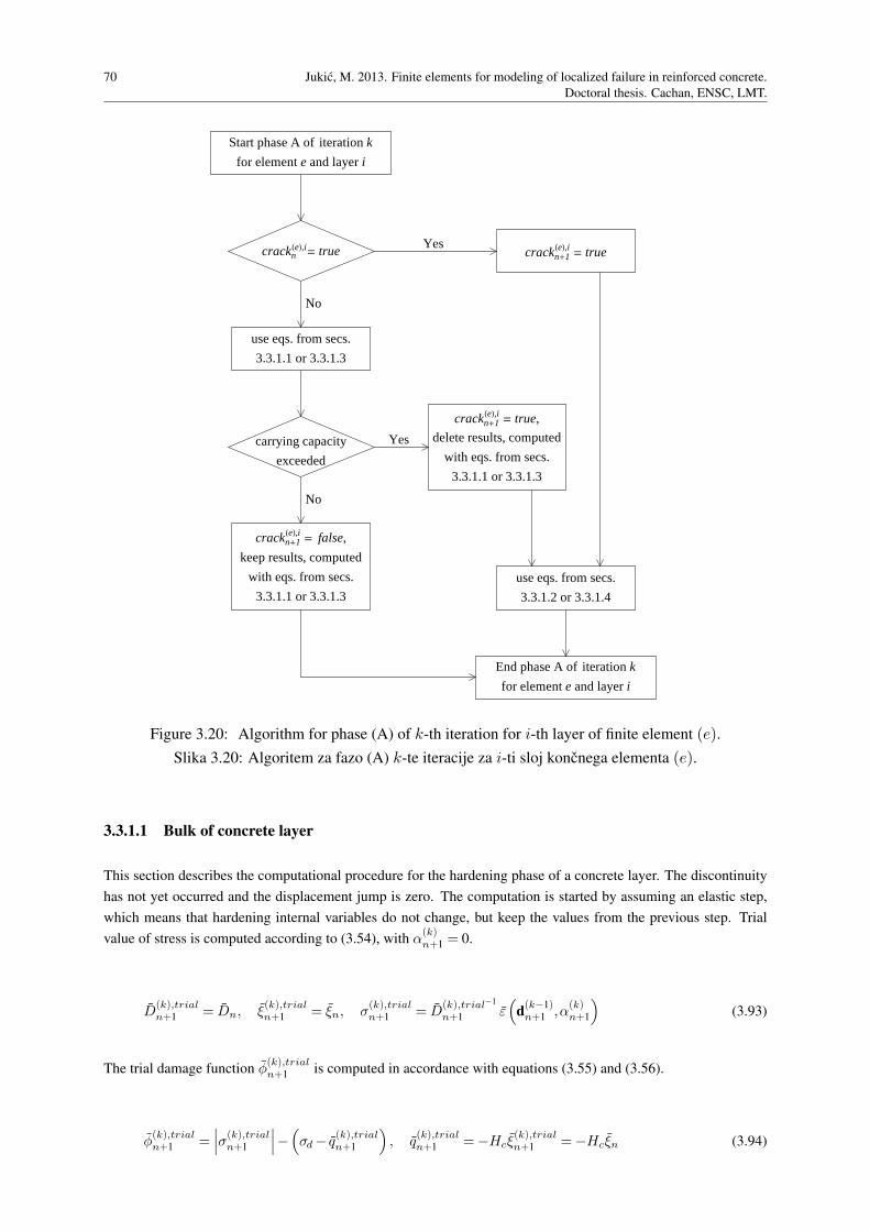
70 Jukic, M. 2013. Finite elements for modeling of localized failure in reinforced concrete.
Doctoral thesis. Cachan, ENSC, LMT.
Start phase A of iteration k
for element e and layer i
cracknHeL,i= true
use eqs. from secs.
3.3.1.1 or 3.3.1.3
carrying capacity
exceeded
crackn+1HeL,i= false,
keep results, computed
with eqs. from secs.
3.3.1.1 or 3.3.1.3
crackn+1HeL,i= true
crackn+1HeL,i= true,
delete results, computed
with eqs. from secs.
3.3.1.1 or 3.3.1.3
use eqs. from secs.
3.3.1.2 or 3.3.1.4
End phase A of iteration k
for element e and layer i
Yes
Yes
No
No
Figure 3.20: Algorithm for phase (A) of k-th iteration for i-th layer of finite element (e).
Slika 3.20: Algoritem za fazo (A) k-te iteracije za i-ti sloj koncnega elementa (e).
3.3.1.1 Bulk of concrete layer
This section describes the computational procedure for the hardening phase of a concrete layer. The discontinuity
has not yet occurred and the displacement jump is zero. The computation is started by assuming an elastic step,
which means that hardening internal variables do not change, but keep the values from the previous step. Trial
value of stress is computed according to (3.54), with α(k)n+1 = 0.
D(k),trialn+1 = Dn, ξ
(k),trialn+1 = ξn, σ
(k),trialn+1 = D
(k),trial−1
n+1 ε(
d(k−1)n+1 ,α
(k)n+1
)
(3.93)
The trial damage function φ(k),trialn+1 is computed in accordance with equations (3.55) and (3.56).
φ(k),trialn+1 =
∣∣∣σ
(k),trialn+1
∣∣∣−(
σd− q(k),trialn+1
)
, q(k),trialn+1 =−Hcξ
(k),trialn+1 =−Hcξn (3.94)
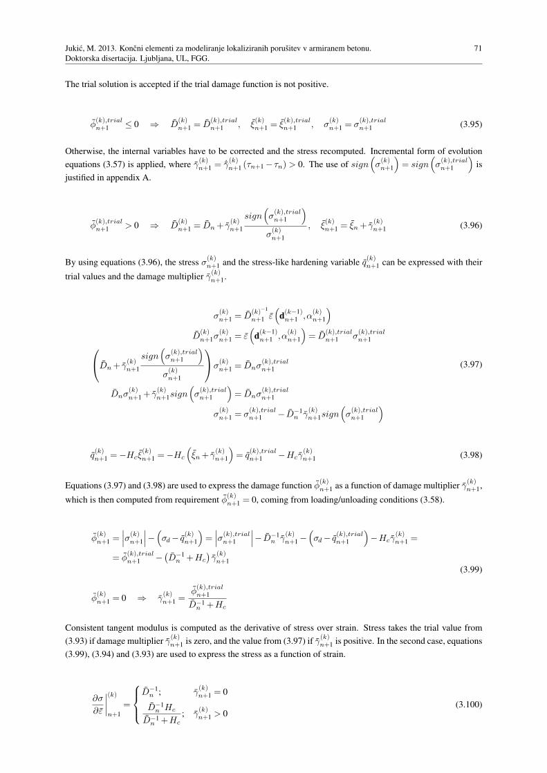
Jukic, M. 2013. Koncni elementi za modeliranje lokaliziranih porusitev v armiranem betonu.
Doktorska disertacija. Ljubljana, UL, FGG.
71
The trial solution is accepted if the trial damage function is not positive.
φ(k),trialn+1 ≤ 0 ⇒ D
(k)n+1 = D
(k),trialn+1 , ξ
(k)n+1 = ξ
(k),trialn+1 , σ
(k)n+1 = σ
(k),trialn+1 (3.95)
Otherwise, the internal variables have to be corrected and the stress recomputed. Incremental form of evolution
equations (3.57) is applied, where γ(k)n+1 = ˙γ
(k)n+1 (τn+1 − τn) > 0. The use of sign
(
σ(k)n+1
)
= sign(
σ(k),trialn+1
)
is
justified in appendix A.
φ(k),trialn+1 > 0 ⇒ D
(k)n+1 = Dn+ γ
(k)n+1
sign(
σ(k),trialn+1
)
σ(k)n+1
, ξ(k)n+1 = ξn+ γ
(k)n+1 (3.96)
By using equations (3.96), the stress σ(k)n+1 and the stress-like hardening variable q
(k)n+1 can be expressed with their
trial values and the damage multiplier γ(k)n+1.
σ(k)n+1 = D
(k)−1
n+1 ε(
d(k−1)n+1 ,α
(k)n+1
)
D(k)n+1σ
(k)n+1 = ε
(
d(k−1)n+1 ,α
(k)n+1
)
= D(k),trialn+1 σ
(k),trialn+1
Dn+ γ(k)n+1
sign(
σ(k),trialn+1
)
σ(k)n+1
σ(k)n+1 = Dnσ
(k),trialn+1
Dnσ(k)n+1 + γ
(k)n+1sign
(
σ(k),trialn+1
)
= Dnσ(k),trialn+1
σ(k)n+1 = σ
(k),trialn+1 − D−1
n γ(k)n+1sign
(
σ(k),trialn+1
)
(3.97)
q(k)n+1 =−Hcξ
(k)n+1 =−Hc
(
ξn+ γ(k)n+1
)
= q(k),trialn+1 −Hcγ
(k)n+1 (3.98)
Equations (3.97) and (3.98) are used to express the damage function φ(k)n+1 as a function of damage multiplier γ
(k)n+1,
which is then computed from requirement φ(k)n+1 = 0, coming from loading/unloading conditions (3.58).
φ(k)n+1 =
∣∣∣σ
(k)n+1
∣∣∣−(
σd− q(k)n+1
)
=∣∣∣σ
(k),trialn+1
∣∣∣− D−1
n γ(k)n+1 −
(
σd− q(k),trialn+1
)
−Hcγ(k)n+1 =
= φ(k),trialn+1 −
(D−1
n +Hc
)γ(k)n+1
φ(k)n+1 = 0 ⇒ γ
(k)n+1 =
φ(k),trialn+1
D−1n +Hc
(3.99)
Consistent tangent modulus is computed as the derivative of stress over strain. Stress takes the trial value from
(3.93) if damage multiplier γ(k)n+1 is zero, and the value from (3.97) if γ
(k)n+1 is positive. In the second case, equations
(3.99), (3.94) and (3.93) are used to express the stress as a function of strain.
∂σ
∂ε
∣∣∣∣
(k)
n+1
=
D−1n ; γ
(k)n+1 = 0
D−1n Hc
D−1n +Hc
; γ(k)n+1 > 0
(3.100)
72 Jukic, M. 2013. Finite elements for modeling of localized failure in reinforced concrete.
Doctoral thesis. Cachan, ENSC, LMT.
The hardening internal variables, stress and tangent modulus have been determined under assumption, that carrying
capacity is not exceeded. A control is required to verify that assumption. If indeed the carrying capacity is not
reached, the results are accepted. In the opposite case, the results are discarded and computed again, taking into
account the newly appeared discontinuity.
To perform the control, the location xd of the potential discontinuity must first be determined. It is positioned
according to the stress state in the layer. In case of constant stress, it is placed in the middle of the layer. In case
of a linear stress distribution, the positioning is not so trivial because of different failure stresses of concrete in
tension and compression. Let us consider the situation, when the highest value of stress is at node 1, σ1 > σ2. The
seven possible linear stress states are shown in Fig. 3.21. Criterion σ3 ≥ 0 covers the cases a, b, c and d, where
the greatest tensile stress is greater than or equal to the absolute value of the biggest compressive stress. Since
the ultimate stress is much higher in compression, the failure is only possible in tension and the discontinuity is
placed at the left node. In cases f and g, where σ1 ≤ 0, the whole layer is in compression and the failure can only
occur at node 2. In case e, the location of the discontinuity is determined from the ratio of maximum compressive
stress to maximum tensile stress in the layer, compared to the ratio of ultimate stresses in compression and tension.
Situation σ1 < σ2 would be treated in the same way. Here σ1 = σ|x=0, σ2 = σ|x=L and σ3 = σ|x=L/2 .
σ1 = σ2 = σ3 ⇒ xid = L/2
σ1 > σ2 ⇒
σ3 ≥ 0 ⇒ xid = 0
σ3 < 0 ⇒
σ1 ≤ 0 ⇒ xid = L
σ1 > 0 ⇒
|σ2/σ1 | ≤ (σfcc/σfct ) ⇒ xid = 0
|σ2/σ1 |> (σfcc/σfct ) ⇒ xid = L
σ1 < σ2 ⇒ analogously to σ1 > σ2
(3.101)
a 1 3 2
b 1 3 2
c 1 3
2
d 1 3
2
e 1
3 2
f1 3 2
g1 3 2
+
+
+
+-
-
-
-
Σ1
Σ3
Σ2 Σ1
Σ3
Σ2
Figure 3.21: Seven possible linear stress states in a layer.
Slika 3.21: Sedem moznih linearnih razporedov napetosti v sloju.
When location of the potential discontinuity is known, we can compute the potential value of traction at the
discontinuity t(k),potn+1 according to equation (3.35). Appropriate operator GV is chosen from (3.50), depending on

Jukic, M. 2013. Koncni elementi za modeliranje lokaliziranih porusitev v armiranem betonu.
Doktorska disertacija. Ljubljana, UL, FGG.
73
xd. The integral is evaluated numerically with the three-point Gauss-Lobatto integration scheme.
t(k),potn+1 =−
∫
L
GV σ(k)n+1dx (3.102)
As we have shown in section 3.2.4.2, the value of t(k),potn+1 is equal to σ
(k)n+1
∣∣∣xd
for a linear stress distribution. Failure
function ¯φ(k),potn+1 is then evaluated with the stress-like softening variable ¯q
(k),potn+1 equal to zero, because there has
been no reduction of carrying capacity in previous steps.
¯φ(k),potn+1 =
∣∣∣t(k),potn+1
∣∣∣−(
σfc− ¯q(k),potn+1
)
, ¯q(k),potn+1 = 0 (3.103)
The discontinuity flag is set to true if the failure function is positive, and to false otherwise. Note that the value
of the flag is not final, until the converged state is reached. It can change in following iterations.
¯φ(k),potn+1 ≤ 0 ⇒ crack
(e),in+1 = false
¯φ(k),potn+1 > 0 ⇒ crack
(e),in+1 = true
(3.104)
If the carrying capacity is exceeded ( ¯φ(k),potn+1 > 0), the above computed values of internal variables, stress and
tangent modulus are discarded for this iteration and computed anew as described in section 3.3.1.2.
3.3.1.2 Discontinuity in concrete layer
In this section we describe the computational procedure for the softening phase of the concrete layer. The procedure
is used if the current value of discontinuity flag crack(e),in+1 = true. This is a consequence of either an existing
discontinuity in the previous step (crack(e),in = true), or exceeded ultimate stress in this iteration, as written in
equation (3.104). In both cases, the hardening internal variables take the last converged values, i.e. the values from
the last step. The error of such choice is negligible for small enough pseudo-time step.
D(k)n+1 = Dn, ξ
(k)n+1 = ξn (3.105)
The computation is started by assuming an elastic step, which implies no change in the softening internal variables
in this iteration. We use the displacement-like softening variable ¯ξ∗, introduced in equation (3.69).
¯D(k),trialn+1 = ¯Dn,
¯ξ∗(k),trialn+1 = ¯ξ∗n (3.106)
The trial value of traction at the discontinuity is defined by equation (3.107), where operator GR is chosen from
expressions (3.46), accordingly to the position of the discontinuity xd, which is known either from the previous
step or from equation (3.101). Linear functions B and GR are evaluated at xd and the bulk compliance Dn at xd is
used. Derivation of the expression is shown in appendix C.
t(k),trialn+1 =
[
Bd(k−1)n+1
Dn− GR¯Dn
]
x=xd
(3.107)
74 Jukic, M. 2013. Finite elements for modeling of localized failure in reinforced concrete.
Doctoral thesis. Cachan, ENSC, LMT.
The trial stress in the layer is computed according to expression (3.54), where the trial value of displacement jump
α(k),trialn+1 is calculated from equation (3.64).
σ(k),trialn+1 = Dn ε
(
d(k−1)n+1 ,α
(k),trialn+1
)
, α(k),trialn+1 = ¯Dnt
(k),trialn+1 (3.108)
Next, the trial value of failure function ¯φ(k),trialn+1 is computed, using expression (3.70) for computation of the
stress-like softening variable ¯q(k),trialn+1 .
¯φ(k),trialn+1 =
∣∣∣t(k),trialn+1
∣∣∣−(
σfc− ¯q(k),trialn+1
)
, ¯q(k),trialn+1 = min
−K∗c
¯ξ∗(k),trialn+1 ,σfc
= ¯qn (3.109)
If ¯φ(k),trialn+1 ≤ 0, the trial solution is accepted.
¯D(k)n+1 =
¯D(k),trialn+1 , ¯ξ
∗(k)n+1 =
¯ξ∗(k),trialn+1 , α
(k)n+1 = α
(k),trialn+1
t(k)n+1 = t
(k),trialn+1 , σ
(k)n+1 = σ
(k),trialn+1
(3.110)
If ¯φ(k),trialn+1 > 0, the assumed trial values are not admissible. We have to compute the softening damage multi-
plier ¯γ∗(k)n+1 =
˙γ∗(k)n+1 (τn+1 − τn) > 0 from equation ¯φ
(k)n+1 = 0 in order to compute new values of internal softening
variables, see appendix C. Linear operator GR is evaluated at xd and the bulk compliance Dn at xd is used.
¯γ∗(k)n+1 =
¯φ(k),trialn+1
(
Dn− GR¯Dn
)
K∗c Dn− GR
x=xd
(3.111)
If ¯q(k)n+1 =−K∗
c
(¯ξ∗n+ ¯γ
∗(k)n+1
)
< σfc, the softening internal variables are updated, following the incremental form of
evolution equations (3.71).
α(k)n+1 =
(
αmaxn + ¯γ
∗(k)n+1
)
sign(
t(k),trialn+1
)
, ¯ξ∗(k)n+1 =
¯ξ∗n+ ¯γ∗(k)n+1,
¯D(k)n+1 =
α(k)n+1
t(k)n+1
=αmaxn + ¯γ
∗(k)n+1
σfc+K∗c
¯ξ∗(k)n+1
(3.112)
Here, αmaxn = ¯Dnt
maxn = ¯Dn
(
σfc+K∗c
¯ξ∗n
)
is the maximal elastic value of α for the given carrying capacity that
was reached in the last softening step. Traction at the discontinuity and stress in the layer are computed as follows.
t(k)n+1 =
(
σfc− ¯q(k)n+1
)
sign(
t(k),trialn+1
)
, σ(k)n+1 = Dn ε
(
d(k−1)n+1 ,α
(k)n+1
)
(3.113)
If −K∗c
(¯ξ∗n+ ¯γ
∗(k)n+1
)
>σfc = ¯q(k)n+1, material has lost all carrying capacity and traction at the discontinuity becomes
zero.
t(k)n+1 = σ
(k)n+1
∣∣∣xd
=[
Dn
(
Bd(k−1)n+1 + GRα
(k)n+1
)]
x=xd= 0 (3.114)
Jukic, M. 2013. Koncni elementi za modeliranje lokaliziranih porusitev v armiranem betonu.
Doktorska disertacija. Ljubljana, UL, FGG.
75
From above equation we can compute the displacement jump and the compliance at the discontinuity. Note that
the linear functions B and GR are evaluated at xd.
α(k)n+1 =
[
−Bd
(k−1)n+1
GR
]
x=xd
, ¯D(k)n+1 =
α(k)n+1
t(k)n+1
= ∞ (3.115)
The tangent modulus is computed as the derivative of traction at the discontinuity over the displacement jump.
If ¯γ∗(k)n+1 = 0, their relation is described by equation (3.108). If ¯γ
∗(k)n+1 > 0 and ¯q
(k)n+1 = −K∗
c
(¯ξ∗n+ ¯γ
∗(k)n+1
)
< σfc,
traction takes the value from (3.113). The first of equations (3.112) is used to express the traction as a function of
displacement jump. If ¯γ∗(k)n+1 > 0 and ¯q
(k)n+1 = σfc, traction is constantly zero.
∂t
∂α
∣∣∣∣
(k)
n+1
=
¯D−1n ; ¯γ
∗(k)n+1 = 0
K∗c = σfcKc; ¯γ
∗(k)n+1 > 0, ¯q
(k)n+1 < σfc
0; ¯γ∗(k)n+1 > 0, ¯q
(k)n+1 = σfc
(3.116)
The discontinuity flag is set to crack(e),in+1 = true.
3.3.1.3 Bulk of reinforcement layer
The computational procedure for the hardening phase of the reinforcement layer is described next. There is no
discontinuity in the layer and the displacement jump is zero. First, we assume elastic behavior, meaning that
hardening internal variables keep the values from the previous step. Stress is computed in accordance with equation
(3.74), where α(k)n+1 = 0.
ε(k),trialp,n+1 = εp,n, ξ
(k),trialn+1 = ξn, σ
(k),trialn+1 = Es
(
ε(
d(k−1)n+1 ,α
(k)n+1
)
− ε(k),trialp,n+1
)
(3.117)
Trial yield function φ(k),trialn+1 is computed, as defined in (3.75) and (3.76).
φ(k),trialn+1 =
∣∣∣σ
(k),trialn+1
∣∣∣−(
σy − q(k),trialn+1
)
, q(k),trialn+1 =−Hsξ
(k),trialn+1 =−Hsξn (3.118)
The trial solution is accepted if the trial yield function is negative or zero.
φ(k),trialn+1 ≤ 0 ⇒ ε
(k)p,n+1 = ε
(k),trialp,n+1 , ξ
(k)n+1 = ξ
(k),trialn+1 , σ
(k)n+1 = σ
(k),trialn+1 (3.119)
If the trial yield function is positive, the internal variables must be corrected, according to incremental form of
evolution equations (3.77), where γ(k)n+1 = ˙γ
(k)n+1 (τn+1 − τn) > 0. It is shown in appendix A that sign
(
σ(k)n+1
)
=
sign(
σ(k),trialn+1
)
.
φ(k),trialn+1 > 0 ⇒ ε
(k)p,n+1 = εp,n+ γ
(k)n+1sign
(
σ(k),trialn+1
)
, ξ(k)n+1 = ξn+ γ
(k)n+1 (3.120)

76 Jukic, M. 2013. Finite elements for modeling of localized failure in reinforced concrete.
Doctoral thesis. Cachan, ENSC, LMT.
By exploiting equations (3.120), the stress σ(k)n+1 and the stress-like hardening variable q
(k)n+1 can be expressed with
their trial values and the damage multiplier γ(k)n+1.
σ(k)n+1 = Es
(
ε(
d(k−1)n+1 ,α
(k)n+1
)
− ε(k)p,n+1
)
=
= Es
(
ε(
d(k−1)n+1 ,α
(k)n+1
)
− εp,n
)
−Esγ(k)n+1sign
(
σ(k),trialn+1
)
=
= σ(k),trialn+1 −Esγ
(k)n+1sign
(
σ(k),trialn+1
)
(3.121)
q(k)n+1 =−Hsξ
(k)n+1 =−Hs
(
ξn+ γ(k)n+1
)
= q(k),trialn+1 −Hsγ
(k)n+1 (3.122)
Yield function φ(k)n+1 is expressed as a function of plastic multiplier γ
(k)n+1 by employing equations (3.121) and
(3.122). Value of the plastic multiplier is computed from requirement φ(k)n+1 = 0.
φ(k)n+1 =
∣∣∣σ
(k)n+1
∣∣∣−(
σy − q(k)n+1
)
=∣∣∣σ
(k),trialn+1
∣∣∣−Esγ
(k)n+1 −
(
σy − q(k),trialn+1
)
−Hsγ(k)n+1 =
= φ(k),trialn+1 − (Es+Hs) γ
(k)n+1
φ(k)n+1 = 0 ⇒ γ
(k)n+1 =
φ(k),trialn+1
Es+Hs
(3.123)
Consistent tangent modulus is computed as the derivative of stress over strain. Stress takes the trial value from
equation (3.117) if plastic multiplier γ(k)n+1 is zero, and the value from (3.121) if γ
(k)n+1 is positive. In the second
case, equations (3.123), (3.118) and (3.117) are used to express the stress as a function of strain.
∂σ
∂ε
∣∣∣∣
(k)
n+1
=
Es; γ(k)n+1 = 0
EsHs
Es+Hs; γ
(k)n+1 > 0
(3.124)
The hardening internal variables, stress in the layer and the tangent modulus have been calculated under assumption
that the ultimate stress is not exceeded. This still requires verification. If the assumption is confirmed, the above
results are accepted. Otherwise, they are discarded and recomputed with the presence of the discontinuity.
The first step is to determine the location of the potential discontinuity xd. Since the behavior of steel is sym-
metric in tension and compression, the discontinuity is simply placed at the location of maximal stress in absolute
value. This can occur at either end of the layer because of the linear form of stress. If the stress is constant, the
discontinuity is placed in the middle of the layer.
σ1 = σ2 = σ3 ⇒ xid = L/2
|σ1|> |σ2| ⇒ xid = 0
|σ1|< |σ2| ⇒ xid = L
where
σ1 = σ|x=0
σ2 = σ|x=L
σ3 = σ|x=L/2
(3.125)
With the location of the potential discontinuity determined, we can calculate the potential value of traction at the
discontinuity t(k),potn+1 by equation (3.35). Correct operator GV is chosen from (3.50), depending on xd. The integral
is evaluated numerically with the three-point Gauss-Lobatto integration scheme.
t(k),potn+1 =−
∫
L
GV σ(k)n+1dx (3.126)
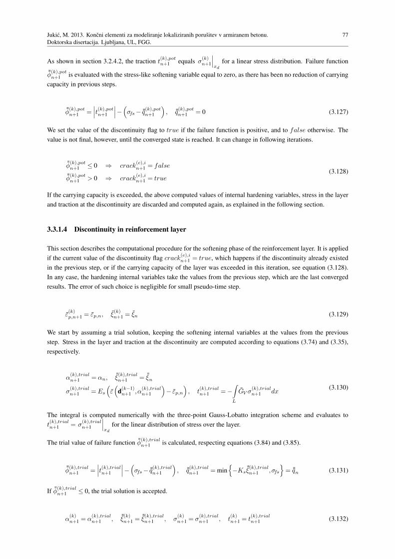
Jukic, M. 2013. Koncni elementi za modeliranje lokaliziranih porusitev v armiranem betonu.
Doktorska disertacija. Ljubljana, UL, FGG.
77
As shown in section 3.2.4.2, the traction t(k),potn+1 equals σ
(k)n+1
∣∣∣xd
for a linear stress distribution. Failure function
¯φ(k),potn+1 is evaluated with the stress-like softening variable equal to zero, as there has been no reduction of carrying
capacity in previous steps.
¯φ(k),potn+1 =
∣∣∣t(k),potn+1
∣∣∣−(
σfs− ¯q(k),potn+1
)
, ¯q(k),potn+1 = 0 (3.127)
We set the value of the discontinuity flag to true if the failure function is positive, and to false otherwise. The
value is not final, however, until the converged state is reached. It can change in following iterations.
¯φ(k),potn+1 ≤ 0 ⇒ crack
(e),in+1 = false
¯φ(k),potn+1 > 0 ⇒ crack
(e),in+1 = true
(3.128)
If the carrying capacity is exceeded, the above computed values of internal hardening variables, stress in the layer
and traction at the discontinuity are discarded and computed again, as explained in the following section.
3.3.1.4 Discontinuity in reinforcement layer
This section describes the computational procedure for the softening phase of the reinforcement layer. It is applied
if the current value of the discontinuity flag crack(e),in+1 = true, which happens if the discontinuity already existed
in the previous step, or if the carrying capacity of the layer was exceeded in this iteration, see equation (3.128).
In any case, the hardening internal variables take the values from the previous step, which are the last converged
results. The error of such choice is negligible for small pseudo-time step.
ε(k)p,n+1 = εp,n, ξ
(k)n+1 = ξn (3.129)
We start by assuming a trial solution, keeping the softening internal variables at the values from the previous
step. Stress in the layer and traction at the discontinuity are computed according to equations (3.74) and (3.35),
respectively.
α(k),trialn+1 = αn,
¯ξ(k),trialn+1 = ¯ξn
σ(k),trialn+1 = Es
(
ε(
d(k−1)n+1 ,α
(k),trialn+1
)
− εp,n
)
, t(k),trialn+1 =−
∫
L
GV σ(k),trialn+1 dx
(3.130)
The integral is computed numerically with the three-point Gauss-Lobatto integration scheme and evaluates to
t(k),trialn+1 = σ
(k),trialn+1
∣∣∣xd
for the linear distribution of stress over the layer.
The trial value of failure function ¯φ(k),trialn+1 is calculated, respecting equations (3.84) and (3.85).
¯φ(k),trialn+1 =
∣∣∣t(k),trialn+1
∣∣∣−(
σfs− ¯q(k),trialn+1
)
, ¯q(k),trialn+1 = min
−Ks¯ξ(k),trialn+1 ,σfs
= ¯qn (3.131)
If ¯φ(k),trialn+1 ≤ 0, the trial solution is accepted.
α(k)n+1 = α
(k),trialn+1 , ¯ξ
(k)n+1 =
¯ξ(k),trialn+1 , σ
(k)n+1 = σ
(k),trialn+1 , t
(k)n+1 = t
(k),trialn+1 (3.132)

78 Jukic, M. 2013. Finite elements for modeling of localized failure in reinforced concrete.
Doctoral thesis. Cachan, ENSC, LMT.
If ¯φ(k),trialn+1 > 0, the assumed solution is not admissible. The softening internal variables are updated according to
the incremental form of evolution equations (3.86), where ¯γ(k)n+1 =
˙γ(k)n+1 (τn+1 − τn) > 0. It is shown in appendix
A that sign(
t(k)n+1
)
= sign(
t(k),trialn+1
)
.
α(k)n+1 = αn+ ¯γ
(k)n+1sign
(
t(k),trialn+1
)
, ¯ξ(k)n+1 =
¯ξn+ ¯γ(k)n+1 (3.133)
By using equations (3.133), the traction at the discontinuity t(k)n+1 and the stress-like softening variable ¯q
(k)n+1 are
expressed with their trial values and the softening multiplier ¯γ(k)n+1.
t(k)n+1 = σ
(k)n+1
∣∣∣xd
=[
Es
(
Bd(k−1)n+1 + GRα
(k)n+1 − εp,n
)]
x=xd=
=[
Es
(
Bd(k−1)n+1 + GRαn− εp,n
)]
x=xd+[
EsGR ¯γ(k)n+1sign
(
t(k),trialn+1
)]
x=xd=
= t(k),trialn+1 +Es GR
∣∣xd
¯γ(k)n+1sign
(
t(k),trialn+1
)
(3.134)
¯q(k)n+1 =
¯qAn+1 = ¯q(k),trialn+1 −Ks ¯γ
(k)n+1; −Ks
(¯ξn+ ¯γA
n+1
)
< σfs
¯qBn+1 = σfs; −Ks
(¯ξn+ ¯γA
n+1
)
> σfs(3.135)
Linear operator GR in expression for t(k)n+1 is evaluated at xd. Obtained expressions are inserted in equation ¯φ
(k)n+1 =
0, coming from loading/unloading conditions (3.87).
¯φ(k)n+1 =
∣∣∣t(k)n+1
∣∣∣−(
σfs− ¯q(k)n+1
)
= 0 ⇔ t(k)n+1 =
(
σfs− ¯q(k)n+1
)
sign(
t(k),trialn+1
)
(3.136)
After a short derivation we get two expressions for ¯γ(k)n+1, depending on the expression, used for ¯q
(k)n+1.
¯γ(k)n+1 =
¯γAn+1 =
¯φ(k),trialn+1
− GR
∣∣xdEs+Ks
; −Ks
(¯ξn+ ¯γA
n+1
)
< σfs
¯γBn+1 =
∣∣∣t(k),trialn+1
∣∣∣
− GR
∣∣xdEs
; −Ks
(¯ξn+ ¯γA
n+1
)
> σfs
(3.137)
The tangent modulus is computed as the derivative of traction at the discontinuity over the displacement jump. If
¯γ(k)n+1 > 0, traction takes the value from (3.136). Equations (3.135) and (3.133) are used to express the traction as
a function of displacement jump. If ¯γ(k)n+1 = 0, the displacement jump remains constant, while the traction changes
to satisfy the local equilibrium with stress in the layer. The tangent modulus cannot be determined, but it is not
required for further computation.
∂t
∂α
∣∣∣∣
(k)
n+1
=
not defined; ¯γ(k)n+1 = 0
Ks; ¯γ(k)n+1 > 0, ¯q
(k)n+1 < σfs
0; ¯γ(k)n+1 > 0, ¯q
(k)n+1 = σfs
(3.138)
The discontinuity flag is set to crack(e),in+1 = true.
Jukic, M. 2013. Koncni elementi za modeliranje lokaliziranih porusitev v armiranem betonu.
Doktorska disertacija. Ljubljana, UL, FGG.
79
3.3.2 Computation of nodal degrees of freedom
In this section we will describe the computations of phase (B) of k-th iteration, mentioned in the introduction of
section 3.3. In this phase, a linearized form of equilibrium equations (3.91) is solved to provide the k-th update
of the nodal displacements/rotations at pseudo-time point τn+1. The computation is performed with known values
of internal variables for each layer of each finite element - D(e),i,(k)n+1 , ξ
(e),i,(k)n+1 , ¯D
(e),i,(k)n+1 , ¯ξ
(e),i,(k)n+1 for a concrete
layer, and ε(e),i,(k)p,n+1 , ξ
(e),i,(k)n+1 , α
(e),i,(k)n+1 , ¯ξ
(e),i,(k)n+1 for a layer of reinforcement - freshly updated in preceding phase
(A) of the same iteration. Since the nodal degrees of freedom are generally common to several finite elements,
the equations of phase (B) must be handled on structural (global) level. Hence, they are also referred to as global
equations.
The first of equations (3.91) would be sufficient for calculating the new values of generalized displacements d(e),(k)n+1 ,
if all displacement jumps α(e),i,(k)n+1 were fixed at the values, computed in phase (A). To improve convergence, how-
ever, it is useful to update the displacement jumps as well. For that purpose, the second of equations (3.91)
are engaged. Actually, they have once already been satisfied by using expression (3.35) for the traction at the
discontinuity, but that equality held for the displacements from the previous iteration d(e),(k−1)n+1 . Updating the dis-
placements would disrupt the equilibrium between the traction at the discontinuity and the stress in the layer, unless
the displacement jumps are updated as well. Solving the whole system of equations (3.91) therefore promises a
more accurate solution.
3.3.2.1 Linearization of equilibrium equations
The first of equations (3.91) ensures the equilibrium of the structure, i.e. of its each and every node. It is linearized
around the current values of nodal degrees of freedom of the structure dstr,(k−1)n+1 .
∂fint,str,(k)n+1
∂dstr,(k−1)n+1
︸ ︷︷ ︸
Kstr,(k)n+1
∆dstr,(k)n+1 = f
ext,strn+1 − f
int,str,(k)n+1 ,
∂fext,strn+1
∂dstr,(k−1)n+1
= 0 (3.139)
The derivative on the left side of the equation is designated with Kstr,(k)n+1 and named the tangent stiffness matrix of
the structure. ∆dstr,(k)n+1 is the sought update of the nodal displacements in this iteration. The vector of external forces
fext,strn+1 represents the loading, which is defined in advance for each pseudo-time point τn+1 and is independent of
the nodal displacements. The vector of internal forces fint,str,(k)n+1 is computed from contributions of individual finite
elements, according to equation (3.20). Matrices P(e) and R(e) are constant.
fint,str,(k)n+1 =
nFE
∑e=1
P(e)T R(e)−1
fint,(e),(k)n+1
Kstr,(k)n+1 =
∂fint,str,(k)n+1
∂dstr,(k−1)n+1
=nFE
∑e=1
P(e)T R(e)−1 ∂fint,(e),(k)n+1
∂dstr,(k−1)n+1
(3.140)
Let us recall the relation (3.13) between the vector of nodal displacements of a finite element d(e),(k−1)n+1 and the
vector of nodal displacements of the structure dstr,(k−1)n+1 . The derivative of one over the other will prove useful.
d(e),(k−1)n+1 = R(e)P(e)d
str,(k−1)n+1 ⇒
∂d(e),(k−1)n+1
∂dstr,(k−1)n+1
= R(e)P(e) (3.141)

80 Jukic, M. 2013. Finite elements for modeling of localized failure in reinforced concrete.
Doctoral thesis. Cachan, ENSC, LMT.
Internal forces fint,(e),(k)n+1 of finite element (e) are defined in equation (3.29) as a sum of contributions of nL
layers. Contributions fint,(e),i,(k)n+1 of the n
(e)CL cracked layers are functions of nodal displacements d
(e),(k−1)n+1 and
displacement jumps α(e),i,(k)n+1 , while the contributions of the remaining (non-cracked) layers depend solely on the
nodal displacements. For the sake of clarity it is assumed that the cracked layers are numbered with consecutive
numbers from 1 to n(e)CL.
fint,(e),(k)n+1 =
nL
∑i=1
fint,(e),i,(k)n+1 =
n(e)CL
∑i=1
fint,(e),i,(k)n+1
(
d(e),(k−1)n+1 ,α
(e),i,(k)n+1
)
+nL
∑i=n
(e)CL
+1
fint,(e),i,(k)n+1
(
d(e),(k−1)n+1
)
(3.142)
The derivative of fint,(e),(k)n+1 over d
str,(k−1)n+1 , which appears in expression (3.140), can be developed as follows.
∂fint,(e),(k)n+1
∂dstr,(k−1)n+1
=
n(e)CL
∑i=1
∂fint,(e),i,(k)n+1
∂d(e),(k−1)n+1
︸ ︷︷ ︸
Kfd,(e),i,(k)n+1
+∂f
int,(e),i,(k)n+1
∂α(e),i,(k)n+1
︸ ︷︷ ︸
Kfα,(e),i,(k)n+1
∂α(e),i,(k)n+1
∂d(e),(k−1)n+1
R(e)P(e)
︷ ︸︸ ︷
∂d(e),(k−1)n+1
∂dstr,(k−1)n+1
+nL
∑i=n
(e)CL
+1
Kfd,(e),i,(k)n+1
︷ ︸︸ ︷
∂fint,(e),i,(k)n+1
∂d(e),(k−1)n+1
R(e)P(e)
︷ ︸︸ ︷
∂d(e),(k−1)n+1
∂dstr,(k−1)n+1
(3.143)
The derivatives of fint,(e),i,(k)n+1 , marked with K
fd,(e),i,(k)n+1 and K
fα,(e),i,(k)n+1 , can be computed and the last term of both
sums has been defined in (3.141). The only unknown term ∂α(e),i,(k)n+1 /∂d
(e),(k−1)n+1 is determined by the second of
equilibrium equations (3.91), which is linearized and solved locally, i.e. independently for each finite element and
layer. This can be done because h(e),i,(k)n+1 depends on the nodal displacements of a single finite element and on the
displacement jump of a single layer.
∂h(e),i,(k)n+1
∂d(e),(k−1)n+1
︸ ︷︷ ︸
Khd,(e),i,(k)n+1
∆d(e),(k)n+1 +
∂h(e),i,(k)n+1
∂α(e),i,(k)n+1
︸ ︷︷ ︸
Khα,(e),i,(k)n+1
∆α(e),i,(k)n+1 =−h
(e),i,(k)n+1 = 0 ⇒
⇒ ∆α(e),i,(k)n+1 =−
(
Khα,(e),i,(k)n+1
)−1
Khd,(e),i,(k)n+1
︸ ︷︷ ︸
∂α(e),i,(k)n+1 /∂d
(e),(k−1)n+1
∆d(e),(k)n+1
(3.144)
Note that each h(e),i,(k)n+1 , computed by (3.34), evaluates to zero because the traction at the discontinuity t
(e),i,(k)n+1
has been computed by expression (3.35). The derivatives, designated with Khd,(e),i,(k)n+1 and K
hα,(e),i,(k)n+1 can be
easily calculated. Equation (3.144) defines the relation between the increment of nodal displacements ∆d(e),(k)n+1
and the increment of displacement jump ∆α(e),i,(k)n+1 in the i-th layer of the finite element. Since we are dealing with
linearized equations, the derivative ∂α(e),i,(k)n+1 /∂d
(e),(k−1)n+1 must be equal to the ratio of the increments.
∂α(e),i,(k)n+1
∂d(e),(k−1)n+1
=−(
Khα,(e),i,(k)n+1
)−1
Khd,(e),i,(k)n+1 (3.145)
Jukic, M. 2013. Koncni elementi za modeliranje lokaliziranih porusitev v armiranem betonu.
Doktorska disertacija. Ljubljana, UL, FGG.
81
We can rewrite expression (3.143), now being able to compute all its components.
∂fint,(e),(k)n+1
∂dstr,(k−1)n+1
=
n(e)CL
∑i=1
(
Kfd,(e),i,(k)n+1 −K
fα,(e),i,(k)n+1
(
Khα,(e),i,(k)n+1
)−1
Khd,(e),i,(k)n+1
)
︸ ︷︷ ︸
K(e),i,(k)n+1
R(e)P(e)+
+nL
∑i=n
(e)CL
+1
Kfd,(e),i,(k)n+1 R(e)P(e)
(3.146)
The expression in parenthesis, marked with K(e),i,(k)n+1 , is the contribution of a cracked layer to the tangent stiffness
matrix of finite element (e), and Kfd,(e),i,(k)n+1 is the contribution of an non-cracked layer. Finally, we can assemble
the tangent stiffness matrix of the structure by inserting (3.146) into (3.140).
Kstr,(k)n+1 =
nFE
∑e=1
P(e)T R(e)−1
n(e)CL
∑i=1
K(e),i,(k)n+1 +
nL
∑i=n
(e)CL
+1
Kfd,(e),i,(k)n+1
︸ ︷︷ ︸
K(e),(k)n+1
R(e)P(e) (3.147)
Here K(e),(k)n+1 is the tangent stiffness matrix of finite element (e).
3.3.2.2 Components of internal forces and stiffness matrix
Contribution fint,(e),i,(k)n+1 of i-th layer to internal forces of element (e) is computed according to equation (3.29),
where stress takes the values computed in phase (A) of this iteration. In order to determine the components of the
stiffness matrix, h(e),i,(k)n+1 must be written as well. It is computed in accordance with (3.34).
fint,(e),i,(k)n+1 =Ai
∫
L
BiT σ(e),i,(k)n+1 dx, h
(e),i,(k)n+1 =Ai
∫
L
GiV σ
(e),i,(k)n+1 dx+ t
(e),i,(k)n+1
(3.148)
To obtain layer components of the element stiffness matrix, expressions (3.148) are differentiated over nodal de-
grees of freedom and over displacement jumps.
Kfd,(e),i,(k)n+1 =
∂fint,(e),i,(k)n+1
∂d(e),(k−1)n+1
=Ai∫
L
BiT ∂σ
∂ε
∣∣∣∣
(e),i,(k)
n+1
Bi︸︷︷︸
∂ε/∂d
dx
Kfα,(e),i,(k)n+1 =
∂fint,(e),i,(k)n+1
∂α(e),i,(k)n+1
=Ai∫
L
BiT ∂σ
∂ε
∣∣∣∣
(e),i,(k)
n+1
GiR
︸︷︷︸
∂ε/∂α
dx
Khd,(e),i,(k)n+1 =
∂h(e),i,(k)n+1
∂d(e),(k−1)n+1
=Ai
∫
L
GiV
∂σ
∂ε
∣∣∣∣
(e),i,(k)
n+1
Bi︸︷︷︸
∂ε/∂d
dx
Khα,(e),i,(k)n+1 =
∂h(e),i,(k)n+1
∂α(e),i,(k)n+1
=Ai
∫
L
GiV
∂σ
∂ε
∣∣∣∣
(e),i,(k)
n+1
GiR
︸︷︷︸
∂ε/∂α
dx+∂t
∂α
∣∣∣∣
(e),i,(k)
n+1
(3.149)

82 Jukic, M. 2013. Finite elements for modeling of localized failure in reinforced concrete.
Doctoral thesis. Cachan, ENSC, LMT.
The tangent moduli (∂σ/∂ε )(e),i,(k)n+1 and (∂t/∂α )
(e),i,(k)n+1 are defined by equations (3.100) and (3.116) for concrete,
and by equations (3.124) and (3.138) for reinforcement. Note that in case of an elastic step in a cracked layer of
reinforcement, when ¯γ(k)n+1 = 0, the second expression is infinite.
∂t
∂α
∣∣∣∣
(e),i,(k)
n+1
= ∞ ⇒ Khα,(e),i,(k)n+1 = ∞,
(
Khα,(e),i,(k)n+1
)−1
= 0 (3.150)
Since the inverse value of component Khα,(e),i,(k)n+1 is consequently zero, the contribution of the i-th layer to the
element tangent stiffness matrix is computed in the same way as for the non-cracked layer.
K(e),i,(k)n+1 = K
fd,(e),i,(k)n+1 −K
fα,(e),i,(k)n+1
(
Khα,(e),i,(k)n+1
)−1
Khd,(e),i,(k)n+1 = K
fd,(e),i,(k)n+1 (3.151)
3.3.2.3 Solution of global equations
The system of global equilibrium equations (3.139) is rewritten in a clearer form.
Kstr,(k)n+1 ∆d
str,(k)n+1 = ∆f
str,(k)n+1 , ∆f
str,(k)n+1 = f
ext,strn+1 − f
int,str,(k)n+1 (3.152)
The external forces are an input to the analysis, internal forces are defined by equations (3.140), (3.142) and
(3.148), and the tangent stiffness matrix of the structure is defined by (3.147) and (3.149). Finally, we can compute
the increments and update the nodal displacements of the structure.
∆dstr,(k)n+1 =
(
Kstr,(k)n+1
)−1
∆fstr,(k)n+1 , d
str,(k)n+1 = d
str,(k−1)n+1 +∆d
str,(k)n+1 (3.153)
The updates of the displacement jumps could be computed from (3.144), but there is no benefit from that because
they will be recomputed anyway in phase (A) of the next iteration.
The iterations at pseudo-time τn+1 are repeated until the tolerance requirements are met.
∥∥∥∆f
str,(k)n+1
∥∥∥< tol,
∥∥∥∆d
str,(k)n+1
∥∥∥< tol (3.154)
When the converged solution is found, we proceed to the next pseudo-time step.
3.4 Numerical examples
In this section we show some numerical examples to examine the performance of the derived finite element. The
element is tested on several beam and frame examples, carried out in the finite element program AceFEM [69].
3.4.1 One element tension and compression tests
We analyze a beam in Fig. 3.22, clamped at one end. At the other end, axial displacement u is imposed and
corresponding reaction F is computed. The test is performed for concrete, steel and reinforced concrete beams, in
order to verify the correct implementation of material models for tension and compression.

Jukic, M. 2013. Koncni elementi za modeliranje lokaliziranih porusitev v armiranem betonu.
Doktorska disertacija. Ljubljana, UL, FGG.
83
xL
F
CONCRETE
b
h
STEEL
AS,2
AS,1
REINF. CONC.
aS,1
aS,2
Figure 3.22: Beam in pure tension/compression: geometry.
Slika 3.22: Nosilec v cistem nategu/tlaku: geometrija.
3.4.1.1 Concrete beam
Concrete beam of rectangular cross-section is modeled with one element with two layers. The imposed axial
displacement produces either tension or compression. In unloading we do not switch from tension to compression
or vice versa. The geometry and the material data are: beam length is L = 2.5m, cross-section width is b =
0.2m, cross-section height is h= 0.5m, elastic modulus is Ec = 4×10⁷kNm−2, elasticity limit in compression is
σdc = 40820kNm−2, limit strength in compression is σfcc = 44902kNm−2, hardening modulus in compression is
Hcc = 2× 10⁶kNm−2, softening modulus in compression is K∗cc = −5.2× 10⁶kNm−3, limit strength in tension
is σfct = 4000kNm−2, and softening modulus in tension is K∗ct = −8× 10⁶kNm−3. By setting σdt > σfct we
assume no damage of the bulk in tension before crack formation. The diagrams in Fig. 3.23 show computed elasto-
damage relations between the end force F and the end displacement u and suggest that the implementation of the
elasto-damage model of concrete was correct.
0.0002 0.0004 0.0006 0.0008u @mD0
100
200
300
400
F @kND
0.002 0.004 0.006 0.008 0.01u @mD0
1000
2000
3000
4000
F @kND
Figure 3.23: Axial force - displacement diagrams for concrete beam in pure tension (left) and pure
compression (right).
Slika 3.23: Diagram osna sila - pomik za betonski nosilec v cistem nategu (levo) in cistem tlaku (desno).
3.4.1.2 Steel beam
Steel beam is modeled with one element with two layers. The following data is used: beam length is L =
2.5m, cross-sections of both layers are As,1 = As,2 = 0.001m2, distances of layer axes from the beam axis are
h/2− as,1 = h/2− as,2 = 0.21m (as,1 = as,2 = 0.04m), elastic modulus is Es = 2×10⁸kNm−2, elasticity limit is
σy = 4×10⁵kNm−2, failure strength is σfs = 5×10⁵kNm−2, hardening modulus is Hs = 107kNm−2, and soften-
ing modulus is Ks =−5×10⁷kNm−3. Diagram in Fig. 3.24 shows elasto-plastic relation between the end force F
and the end displacement u in tension. Response of the beam in compression is identical. The diagram in Fig. 3.24
suggests that the implementation of the elasto-plastic model of steel was correct.

84 Jukic, M. 2013. Finite elements for modeling of localized failure in reinforced concrete.
Doctoral thesis. Cachan, ENSC, LMT.
0.01 0.02 0.03 0.04 0.05u @mD0
200
400
600
800
1000
F @kND
Figure 3.24: Axial force - displacement diagram for steel beam (layer) in pure tension.
Slika 3.24: Diagram osna sila - pomik za jekleni nosilec (sloj) v cistem nategu.
3.4.1.3 Reinforced concrete beam
Reinforced concrete beam is composed from the two previously presented beams, see Fig. 3.22. Geometry and
material properties are listed in sections 3.4.1.1 and 3.4.1.2. The beam is modeled with one finite element with
ten concrete layers and two layers of reinforcement. Diagrams in Fig. 3.25 display the responses of the beam
under tensile and compressive load. In tension (left image), the first peak represents the point where concrete starts
cracking and the force F begins to drop. When it starts rising again, the concrete is completely broken and the
whole load is taken by the two reinforcement layers. Hereafter, the response should be equal to the response of
the steel beam, modeled in section 3.4.1.2, because in our model there is no shear interaction between concrete
and steel layers. However, a comparison of Fig. 3.24 and Fig. 3.25 (left) shows a different situation. Although the
yielding and the softening of the material begin at the same values of force F , both processes start at significantly
smaller displacements u in the reinforced concrete beam. There is no yield plateau, typical for steel, and the
softening slope is not as steep.
The diagram in Fig. 3.25 (right) shows the response of the beam in compression. After the initial elastic part, the
stiffness of the beam drops twice, due to micro-cracking of concrete and yielding of reinforcement, respectively.
The peak of the diagram marks the moment when concrete begins to soften. Afterwards, the response is different
from the expectations. The stress in concrete layers should drop to zero at u≈ 0.0086m and then the curve should
match the diagram in Fig. 3.24. Up to u≈ 0.03m, the beam should offer significant resistance, but F becomes zero
at one third of that displacement. Obviously, the finite element is not working properly in this case.
0.002 0.004 0.006 0.008 0.01u @mD0
200
400
600
800
1000
F @kND
0.003 0.006 0.009 0.012 0.015u @mD0
1000
2000
3000
4000
5000
F @kND
Figure 3.25: Axial force - displacement diagrams for reinforced concrete beam in pure tension (left)
and pure compression (right).
Slika 3.25: Diagram osna sila - pomik za armiranobetonski nosilec v cistem nategu (levo) in cistem
tlaku (desno).
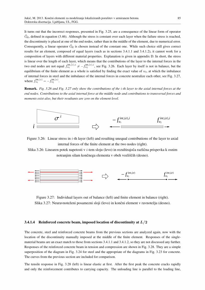
Jukic, M. 2013. Koncni elementi za modeliranje lokaliziranih porusitev v armiranem betonu.
Doktorska disertacija. Ljubljana, UL, FGG.
85
It turns out that the incorrect responses, presented in Fig. 3.25, are a consequence of the linear form of operator
GR, defined in equation (3.46). Although the stress is constant over each layer when the failure stress is reached,
the discontinuity is placed at one of the end nodes, rather than in the middle of the element, due to numerical error.
Consequently, a linear operator GR is chosen instead of the constant one. While such choice still gives correct
results for an element, composed of equal layers (such as in sections 3.4.1.1 and 3.4.1.2), it cannot work for a
composition of layers with different material properties. Explanation is given in appendix D. In short, the stress
is linear over the length of each layer, which means that the contributions of the layer to the internal forces in the
two end nodes are not equal fint,(e),iu1 6= −f
int,(e),iu2 , see Fig. 3.26. Each layer by itself is not in balance, but the
equilibrium of the finite element as a whole is satisfied by finding the exact value of u3, at which the imbalance
of internal forces in steel and the imbalance of the internal forces in concrete neutralize each other, see Fig. 3.27,
where fint,(e)u1 =−f
int,(e)u2 .
Remark. Fig. 3.26 and Fig. 3.27 only show the contributions of the i-th layer to the axial internal forces at the
end nodes. Contributions to the axial internal force at the middle node and contributions to transversal forces and
moments exist also, but their resultants are zero on the element level.
Σ i
i- fu1
int,HeL,i fu2
int,HeL,i
Figure 3.26: Linear stress in i-th layer (left) and resulting unequal contributions of the layer to axial
internal forces of the finite element at the two nodes (right).
Slika 3.26: Linearen potek napetosti v i-tem sloju (levo) in rezultirajoca razlicna prispevka k osnim
notranjim silam koncnega elementa v obeh vozliscih (desno).
- fu1
int,HeL fu2
int,HeL
Figure 3.27: Individual layers out of balance (left) and finite element in balance (right).
Slika 3.27: Neuravnotezeni posamezni sloji (levo) in koncni element v ravnotezju (desno).
3.4.1.4 Reinforced concrete beam, imposed location of discontinuity at L/2
The concrete, steel and reinforced concrete beams from the previous sections are analyzed again, now with the
location of the discontinuity manually imposed at the middle of the finite element. Responses of the single-
material beams are an exact match to those from sections 3.4.1.1 and 3.4.1.2, so they are not discussed any further.
Responses of the reinforced concrete beam in tension and compression are shown in Fig. 3.28. They are a simple
superposition of the diagram in Fig. 3.24 for steel and the appropriate of the diagrams in Fig. 3.23 for concrete.
The curves from the previous section are included for comparison.
The tensile response in Fig. 3.28 (left) is linear elastic at first. After the first peak the concrete cracks rapidly
and only the reinforcement contributes to carrying capacity. The unloading line is parallel to the loading line,
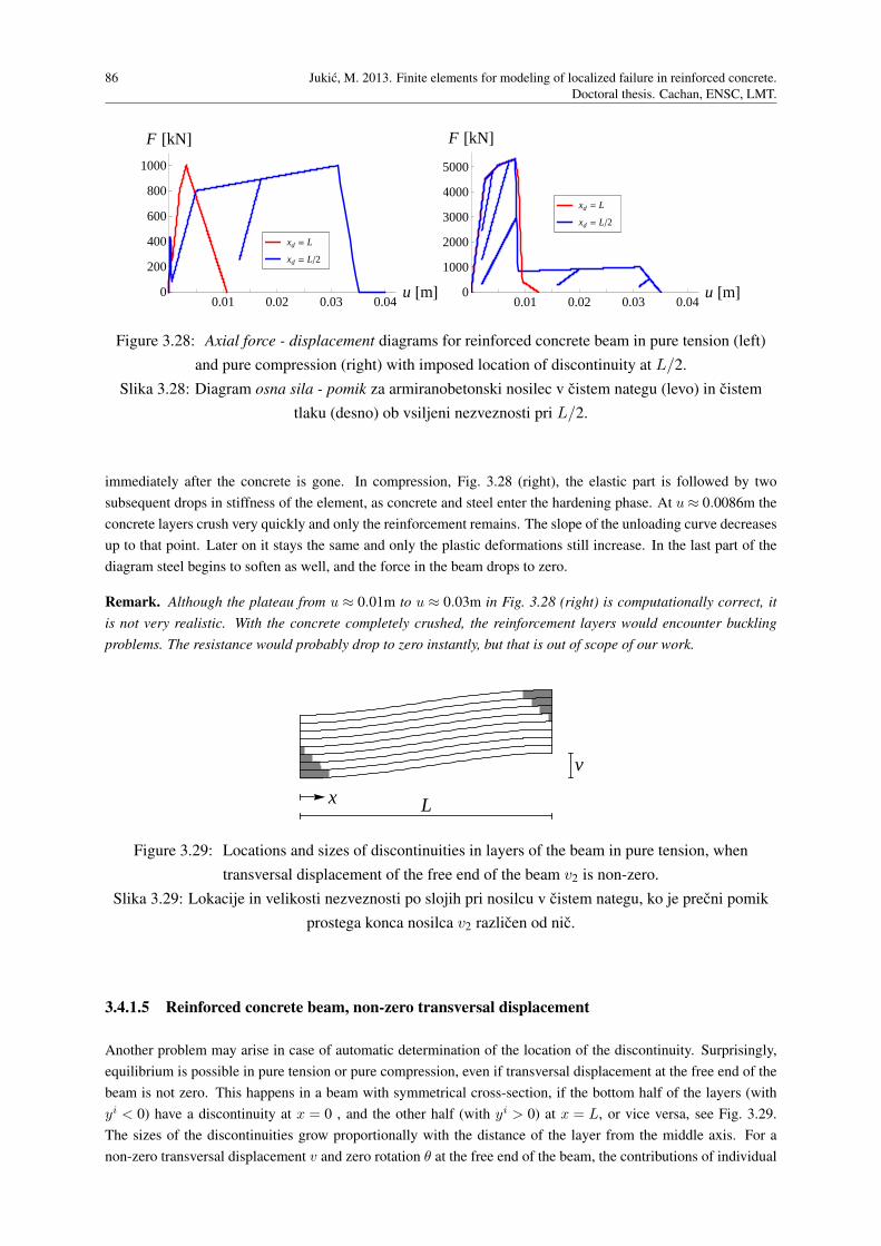
86 Jukic, M. 2013. Finite elements for modeling of localized failure in reinforced concrete.
Doctoral thesis. Cachan, ENSC, LMT.
0.01 0.02 0.03 0.04u @mD0
200
400
600
800
1000
F @kND
xd = L2
xd = L
0.01 0.02 0.03 0.04u @mD0
1000
2000
3000
4000
5000
F @kND
xd = L2
xd = L
Figure 3.28: Axial force - displacement diagrams for reinforced concrete beam in pure tension (left)
and pure compression (right) with imposed location of discontinuity at L/2.
Slika 3.28: Diagram osna sila - pomik za armiranobetonski nosilec v cistem nategu (levo) in cistem
tlaku (desno) ob vsiljeni nezveznosti pri L/2.
immediately after the concrete is gone. In compression, Fig. 3.28 (right), the elastic part is followed by two
subsequent drops in stiffness of the element, as concrete and steel enter the hardening phase. At u≈ 0.0086m the
concrete layers crush very quickly and only the reinforcement remains. The slope of the unloading curve decreases
up to that point. Later on it stays the same and only the plastic deformations still increase. In the last part of the
diagram steel begins to soften as well, and the force in the beam drops to zero.
Remark. Although the plateau from u ≈ 0.01m to u ≈ 0.03m in Fig. 3.28 (right) is computationally correct, it
is not very realistic. With the concrete completely crushed, the reinforcement layers would encounter buckling
problems. The resistance would probably drop to zero instantly, but that is out of scope of our work.
x L
v
Figure 3.29: Locations and sizes of discontinuities in layers of the beam in pure tension, when
transversal displacement of the free end of the beam v2 is non-zero.
Slika 3.29: Lokacije in velikosti nezveznosti po slojih pri nosilcu v cistem nategu, ko je precni pomik
prostega konca nosilca v2 razlicen od nic.
3.4.1.5 Reinforced concrete beam, non-zero transversal displacement
Another problem may arise in case of automatic determination of the location of the discontinuity. Surprisingly,
equilibrium is possible in pure tension or pure compression, even if transversal displacement at the free end of the
beam is not zero. This happens in a beam with symmetrical cross-section, if the bottom half of the layers (with
yi < 0) have a discontinuity at x = 0 , and the other half (with yi > 0) at x = L, or vice versa, see Fig. 3.29.
The sizes of the discontinuities grow proportionally with the distance of the layer from the middle axis. For a
non-zero transversal displacement v and zero rotation θ at the free end of the beam, the contributions of individual
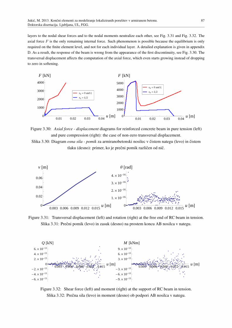
Jukic, M. 2013. Koncni elementi za modeliranje lokaliziranih porusitev v armiranem betonu.
Doktorska disertacija. Ljubljana, UL, FGG.
87
layers to the nodal shear forces and to the nodal moments neutralize each other, see Fig. 3.31 and Fig. 3.32. The
axial force F is the only remaining internal force. Such phenomenon is possible because the equilibrium is only
required on the finite element level, and not for each individual layer. A detailed explanation is given in appendix
D. As a result, the response of the beam is wrong from the appearance of the first discontinuity, see Fig. 3.30. The
transversal displacement affects the computation of the axial force, which even starts growing instead of dropping
to zero in softening.
0.01 0.02 0.03 0.04u @mD0
1000
2000
3000
4000
F @kND
xd = L2
xd = 0 and L
0.01 0.02 0.03 0.04u @mD0
1000
2000
3000
4000
5000
F @kND
xd = L2
xd = 0 and L
Figure 3.30: Axial force - displacement diagrams for reinforced concrete beam in pure tension (left)
and pure compression (right): the case of non-zero transversal displacement.
Slika 3.30: Diagram osna sila - pomik za armiranobetonski nosilec v cistem nategu (levo) in cistem
tlaku (desno): primer, ko je precni pomik razlicen od nic.
0.003 0.006 0.009 0.012 0.015u @mD0
0.02
0.04
0.06
v @mD
0.003 0.006 0.009 0.012 0.015u @mD0
1.´ 10-16
2.´ 10-16
3.´ 10-16
4.´ 10-16
Θ @radD
Figure 3.31: Transversal displacement (left) and rotation (right) at the free end of RC beam in tension.
Slika 3.31: Precni pomik (levo) in zasuk (desno) na prostem koncu AB nosilca v nategu.
0.003 0.006 0.009 0.012 0.015u @mD
-6.´ 10-13
-4.´ 10-13
-2.´ 10-13
0
2.´ 10-13
4.´ 10-13
6.´ 10-13
Q @kND
0.003 0.006 0.009 0.012 0.015u @mD
-9.´ 10-13
-6.´ 10-13
-3.´ 10-13
3.´ 10-13
6.´ 10-13
9.´ 10-13
M @kNmD
Figure 3.32: Shear force (left) and moment (right) at the support of RC beam in tension.
Slika 3.32: Precna sila (levo) in moment (desno) ob podpori AB nosilca v nategu.
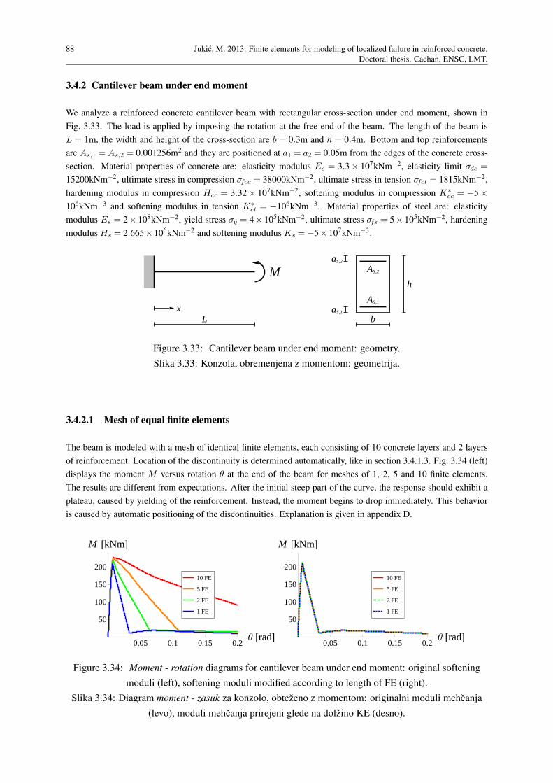
88 Jukic, M. 2013. Finite elements for modeling of localized failure in reinforced concrete.
Doctoral thesis. Cachan, ENSC, LMT.
3.4.2 Cantilever beam under end moment
We analyze a reinforced concrete cantilever beam with rectangular cross-section under end moment, shown in
Fig. 3.33. The load is applied by imposing the rotation at the free end of the beam. The length of the beam is
L = 1m, the width and height of the cross-section are b = 0.3m and h = 0.4m. Bottom and top reinforcements
are As,1 = As,2 = 0.001256m2 and they are positioned at a1 = a2 = 0.05m from the edges of the concrete cross-
section. Material properties of concrete are: elasticity modulus Ec = 3.3 × 10⁷kNm−2, elasticity limit σdc =
15200kNm−2, ultimate stress in compression σfcc = 38000kNm−2, ultimate stress in tension σfct = 1815kNm−2,
hardening modulus in compression Hcc = 3.32 × 10⁷kNm−2, softening modulus in compression K∗cc = −5 ×
106kNm−3 and softening modulus in tension K∗ct = −106kNm−3. Material properties of steel are: elasticity
modulus Es = 2× 10⁸kNm−2, yield stress σy = 4× 10⁵kNm−2, ultimate stress σfs = 5× 10⁵kNm−2, hardening
modulus Hs = 2.665×10⁶kNm−2 and softening modulus Ks =−5×10⁷kNm−3.
xL
M
b
h
AS,2
AS,1
aS,1
aS,2
Figure 3.33: Cantilever beam under end moment: geometry.
Slika 3.33: Konzola, obremenjena z momentom: geometrija.
3.4.2.1 Mesh of equal finite elements
The beam is modeled with a mesh of identical finite elements, each consisting of 10 concrete layers and 2 layers
of reinforcement. Location of the discontinuity is determined automatically, like in section 3.4.1.3. Fig. 3.34 (left)
displays the moment M versus rotation θ at the end of the beam for meshes of 1, 2, 5 and 10 finite elements.
The results are different from expectations. After the initial steep part of the curve, the response should exhibit a
plateau, caused by yielding of the reinforcement. Instead, the moment begins to drop immediately. This behavior
is caused by automatic positioning of the discontinuities. Explanation is given in appendix D.
0.05 0.1 0.15 0.2Θ @radD
50
100
150
200
M @kNmD
1 FE
2 FE
5 FE
10 FE
0.05 0.1 0.15 0.2Θ @radD
50
100
150
200
M @kNmD
1 FE
2 FE
5 FE
10 FE
Figure 3.34: Moment - rotation diagrams for cantilever beam under end moment: original softening
moduli (left), softening moduli modified according to length of FE (right).
Slika 3.34: Diagram moment - zasuk za konzolo, obtezeno z momentom: originalni moduli mehcanja
(levo), moduli mehcanja prirejeni glede na dolzino KE (desno).
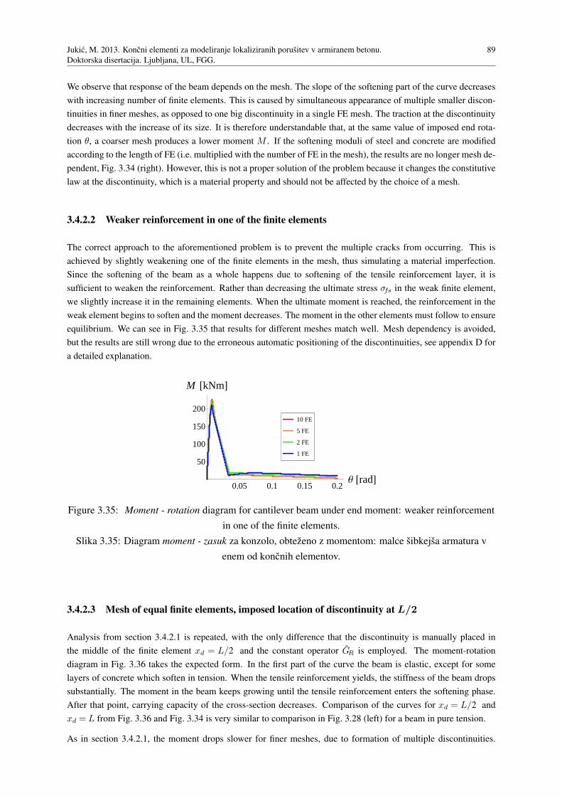
Jukic, M. 2013. Koncni elementi za modeliranje lokaliziranih porusitev v armiranem betonu.
Doktorska disertacija. Ljubljana, UL, FGG.
89
We observe that response of the beam depends on the mesh. The slope of the softening part of the curve decreases
with increasing number of finite elements. This is caused by simultaneous appearance of multiple smaller discon-
tinuities in finer meshes, as opposed to one big discontinuity in a single FE mesh. The traction at the discontinuity
decreases with the increase of its size. It is therefore understandable that, at the same value of imposed end rota-
tion θ, a coarser mesh produces a lower moment M . If the softening moduli of steel and concrete are modified
according to the length of FE (i.e. multiplied with the number of FE in the mesh), the results are no longer mesh de-
pendent, Fig. 3.34 (right). However, this is not a proper solution of the problem because it changes the constitutive
law at the discontinuity, which is a material property and should not be affected by the choice of a mesh.
3.4.2.2 Weaker reinforcement in one of the finite elements
The correct approach to the aforementioned problem is to prevent the multiple cracks from occurring. This is
achieved by slightly weakening one of the finite elements in the mesh, thus simulating a material imperfection.
Since the softening of the beam as a whole happens due to softening of the tensile reinforcement layer, it is
sufficient to weaken the reinforcement. Rather than decreasing the ultimate stress σfs in the weak finite element,
we slightly increase it in the remaining elements. When the ultimate moment is reached, the reinforcement in the
weak element begins to soften and the moment decreases. The moment in the other elements must follow to ensure
equilibrium. We can see in Fig. 3.35 that results for different meshes match well. Mesh dependency is avoided,
but the results are still wrong due to the erroneous automatic positioning of the discontinuities, see appendix D for
a detailed explanation.
0.05 0.1 0.15 0.2Θ @radD
50
100
150
200
M @kNmD
1 FE
2 FE
5 FE
10 FE
Figure 3.35: Moment - rotation diagram for cantilever beam under end moment: weaker reinforcement
in one of the finite elements.
Slika 3.35: Diagram moment - zasuk za konzolo, obtezeno z momentom: malce sibkejsa armatura v
enem od koncnih elementov.
3.4.2.3 Mesh of equal finite elements, imposed location of discontinuity at L/2
Analysis from section 3.4.2.1 is repeated, with the only difference that the discontinuity is manually placed in
the middle of the finite element xd = L/2 and the constant operator GR is employed. The moment-rotation
diagram in Fig. 3.36 takes the expected form. In the first part of the curve the beam is elastic, except for some
layers of concrete which soften in tension. When the tensile reinforcement yields, the stiffness of the beam drops
substantially. The moment in the beam keeps growing until the tensile reinforcement enters the softening phase.
After that point, carrying capacity of the cross-section decreases. Comparison of the curves for xd = L/2 and
xd = L from Fig. 3.36 and Fig. 3.34 is very similar to comparison in Fig. 3.28 (left) for a beam in pure tension.
As in section 3.4.2.1, the moment drops slower for finer meshes, due to formation of multiple discontinuities.
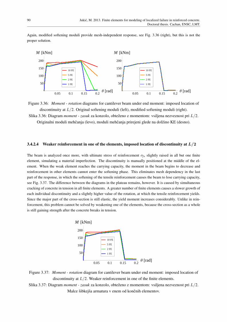
90 Jukic, M. 2013. Finite elements for modeling of localized failure in reinforced concrete.
Doctoral thesis. Cachan, ENSC, LMT.
Again, modified softening moduli provide mesh-independent response, see Fig. 3.36 (right), but this is not the
proper solution.
0.05 0.1 0.15 0.2Θ @radD
50
100
150
200
M @kNmD
1 FE
2 FE
5 FE
10 FE
0.05 0.1 0.15 0.2Θ @radD
50
100
150
200
M @kNmD
1 FE
2 FE
5 FE
10 FE
Figure 3.36: Moment - rotation diagrams for cantilever beam under end moment: imposed location of
discontinuity at L/2. Original softening moduli (left), modified softening moduli (right).
Slika 3.36: Diagram moment - zasuk za konzolo, obtezeno z momentom: vsiljena nezveznost pri L/2.
Originalni moduli mehcanja (levo), moduli mehcanja prirejeni glede na dolzino KE (desno).
3.4.2.4 Weaker reinforcement in one of the elements, imposed location of discontinuity at L/2
The beam is analyzed once more, with ultimate stress of reinforcement σfs slightly raised in all but one finite
element, simulating a material imperfection. The discontinuity is manually positioned at the middle of the el-
ement. When the weak element reaches the carrying capacity, the moment in the beam begins to decrease and
reinforcement in other elements cannot enter the softening phase. This eliminates mesh dependency in the last
part of the response, in which the softening of the tensile reinforcement causes the beam to lose carrying capacity,
see Fig. 3.37. The difference between the diagrams in the plateau remains, however. It is caused by simultaneous
cracking of concrete in tension in all finite elements. A greater number of finite elements causes a slower growth of
each individual discontinuity and a slightly higher value of the rotation, at which the tensile reinforcement yields.
Since the major part of the cross-section is still elastic, the yield moment increases considerably. Unlike in rein-
forcement, this problem cannot be solved by weakening one of the elements, because the cross-section as a whole
is still gaining strength after the concrete breaks in tension.
0.05 0.1 0.15 0.2Θ @radD
50
100
150
200
M @kNmD
1 FE
2 FE
5 FE
10 FE
Figure 3.37: Moment - rotation diagram for cantilever beam under end moment: imposed location of
discontinuity at L/2. Weaker reinforcement in one of the finite elements.
Slika 3.37: Diagram moment - zasuk za konzolo, obtezeno z momentom: vsiljena nezveznost pri L/2.
Malce sibkejsa armatura v enem od koncnih elementov.

Jukic, M. 2013. Koncni elementi za modeliranje lokaliziranih porusitev v armiranem betonu.
Doktorska disertacija. Ljubljana, UL, FGG.
91
3.4.3 Cantilever beam under end transversal force
A cantilever beam is subjected to prescribed lateral displacement at the free end, see Fig. 3.38. The length of the
beam is L= 2.5m, the width and the height of the cross-section b= 0.2m and h= 0.5m. The tensile and compres-
sive reinforcement are As,1 =As,2 = 0.001m2 and the distances from the center of the reinforcement layers to the
edges of the concrete cross-section are a1 = a2 = 0.04m. Material properties of concrete are: elasticity modulus
Ec = 4× 10⁷kNm−2, elasticity limit σdc = 40820kNm−2, ultimate stress in compression σfcc = 44902kNm−2,
ultimate stress in tension σfct = 4000kNm−2, hardening modulus in compression Hcc = 2×10⁶kNm−2, softening
modulus in compression K∗cc =−5.2×10⁵kNm−3 and softening modulus in tension K∗
ct =−8×10⁵kNm−3. Ma-
terial properties of steel are: elasticity modulus Es = 2× 10⁸kNm−2, yield stress σy = 4× 10⁵kNm−2, ultimate
stress σfs = 5×10⁵kNm−2, hardening modulus Hs = 107kNm−2 and softening modulus Ks =−3×10⁷kNm−3.
xL
F
b
h
AS,2
AS,1
aS,1
aS,2
Figure 3.38: Cantilever beam under end transversal force: geometry.
Slika 3.38: Konzola, obremenjena s precno silo: geometrija.
Moment at the support versus imposed lateral displacement diagrams are presented in Fig. 3.39. The curves match
pretty well. There are no great deviations in the softening part because the moment is linear over the length of the
beam and only the finite element at the support can reach the ultimate moment. There is no need for artificially
created material imperfection. The influence of the mesh on the softening of concrete in tension cannot be avoided
because the cross-section is still gaining strength when the concrete breaks, like in section 3.4.2.4.
0.05 0.1 0.15 0.2v @mD
100
200
300
M @kNmD
1 FE
2 FE
5 FE
10 FE
Figure 3.39: Moment at support - transversal displacement diagram for cantilever beam under end
transversal force: all finite elements are the same.
Slika 3.39: Diagram moment ob podpori - precni pomik za konzolo, obremenjeno s precno silo: vsi
koncni elementi so enaki.
It is difficult to assess the results solely from the diagrams in Fig. 3.39, but inspection of the stress state reveals an
error. Let us examine the beam, modeled with a single FE, just before the occurrence of the first discontinuity, when
all layers are still elastic. The values of stress are anti-symmetric in the cross-section (negative below and positive
above the middle axis), their absolute values grow from the middle axis toward the edges. In each layer, they reduce

92 Jukic, M. 2013. Finite elements for modeling of localized failure in reinforced concrete.
Doctoral thesis. Cachan, ENSC, LMT.
linearly from the support toward the free end, where they are zero. Such distribution of stress is also assumed in
the trial state of the first iteration of the next increment. However, the tensile strength is exceeded at the supported
end of the topmost layer. The trial value of stress σi,trial = Di−1Bid is replaced by σi = Di−1(
Bid+ GiRα
i). The
additional part Di−1GiR (x)αi has a negative value at the supported end, where the discontinuity is located, and a
positive value at the free end. Thus, after the first iteration, the stress in the top layer is no longer zero at the free
end of the beam. Of course, this is not the equilibrium state, but even in the following iterations the stress at the
free end does not vanish. Instead, it becomes non-zero also in the remaining layers. Only the resultant axial force
and moment at the free end are zero, as required by the equilibrium equations.
This issue arises from completely independent consideration of discontinuities in separate layers. In the stress
resultant finite element, the operator G is defined for the whole finite element and it contains information, how
the cracked element should deform, in order to preserve equilibrium. It imposes an imbalance that is annulled
by appropriate nodal displacements. In a multi-layer element, the operator GiR is defined for a single layer and
contains information, how the cracked layer should deform to preserve “equilibrium of the layer”. However,
the layer cannot deform freely. Modification of the nodal displacements also affects the remaining layers. The
imbalance, introduced by GiR into the cracked layer (and through summation into the finite element), is balanced
out by (additional) deformation of all layers in the element, so the final strain/stress in the cracked layer is not the
same, as if it would stand alone. The operator GiR, as defined here, cannot perform its original function, which is
to provide physically appropriate strain/stress in the cracked layer.
Since the occurrence of a discontinuity in one of the layers actually affects the whole finite element, the operator
GiR should be defined on the element level. This is not easily done, though. The influence of the discontinuity
would depend on the type of the load (e.g. pure tension or pure bending), which prevents unique definition of GiR.
L
H
H
700 kN 700 kN
Fu
0.04
0.04
0.32
0.30
0.03
0.03
0.34
0.30
4´3cm2
4´3cm2
4´3cm2
4´3cm2
BEAM
COLUMN
Figure 3.40: Two story frame: geometry, loading pattern and cross-sections.
Slika 3.40: Dvoetazni okvir: geometrija, obtezba in precni prerezi.
3.4.4 Two story reinforced concrete frame
Two-story reinforced concrete frame has been experimentally tested in [71] and numerically analyzed in [51, 74]
with stress-resultant Timoshenko and Euler-Bernoulli finite elements with embedded strong discontinuity in rota-
tion. Analysis with multi-layer Timoshenko element with layer-wise embedded discontinuities in axial displace-
ment and elasto-plastic models for concrete and reinforcement has been done in [51, 52]. Story height of the
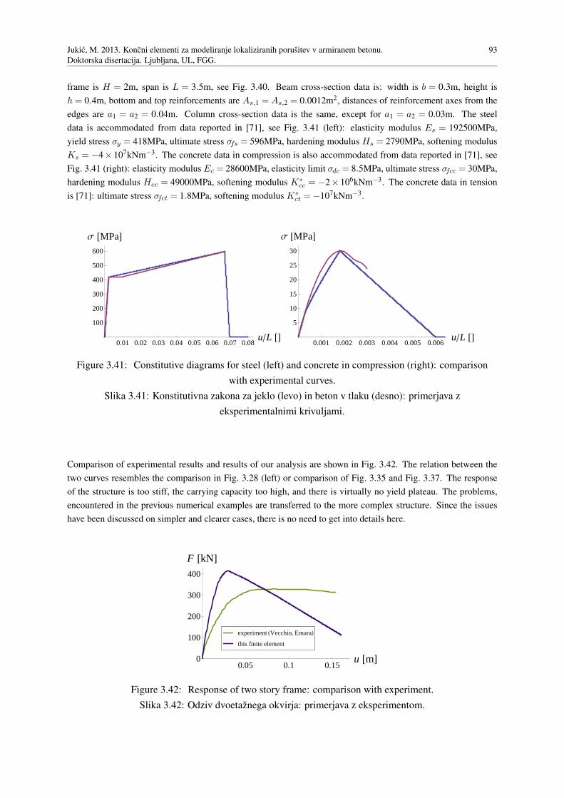
Jukic, M. 2013. Koncni elementi za modeliranje lokaliziranih porusitev v armiranem betonu.
Doktorska disertacija. Ljubljana, UL, FGG.
93
frame is H = 2m, span is L = 3.5m, see Fig. 3.40. Beam cross-section data is: width is b = 0.3m, height is
h = 0.4m, bottom and top reinforcements are As,1 = As,2 = 0.0012m2, distances of reinforcement axes from the
edges are a1 = a2 = 0.04m. Column cross-section data is the same, except for a1 = a2 = 0.03m. The steel
data is accommodated from data reported in [71], see Fig. 3.41 (left): elasticity modulus Es = 192500MPa,
yield stress σy = 418MPa, ultimate stress σfs = 596MPa, hardening modulus Hs = 2790MPa, softening modulus
Ks = −4× 10⁷kNm−3. The concrete data in compression is also accommodated from data reported in [71], see
Fig. 3.41 (right): elasticity modulus Ec = 28600MPa, elasticity limit σdc = 8.5MPa, ultimate stress σfcc = 30MPa,
hardening modulus Hcc = 49000MPa, softening modulus K∗cc = −2× 10⁶kNm−3. The concrete data in tension
is [71]: ultimate stress σfct = 1.8MPa, softening modulus K∗ct =−107kNm−3.
0.01 0.02 0.03 0.04 0.05 0.06 0.07 0.08uL @D
100
200
300
400
500
600
Σ @MPaD
0.001 0.002 0.003 0.004 0.005 0.006uL @D
5
10
15
20
25
30
Σ @MPaD
Figure 3.41: Constitutive diagrams for steel (left) and concrete in compression (right): comparison
with experimental curves.
Slika 3.41: Konstitutivna zakona za jeklo (levo) in beton v tlaku (desno): primerjava z
eksperimentalnimi krivuljami.
Comparison of experimental results and results of our analysis are shown in Fig. 3.42. The relation between the
two curves resembles the comparison in Fig. 3.28 (left) or comparison of Fig. 3.35 and Fig. 3.37. The response
of the structure is too stiff, the carrying capacity too high, and there is virtually no yield plateau. The problems,
encountered in the previous numerical examples are transferred to the more complex structure. Since the issues
have been discussed on simpler and clearer cases, there is no need to get into details here.
0.05 0.1 0.15u @mD0
100
200
300
400
F @kND
this finite element
experiment HVecchio, EmaraL
Figure 3.42: Response of two story frame: comparison with experiment.
Slika 3.42: Odziv dvoetaznega okvirja: primerjava z eksperimentom.
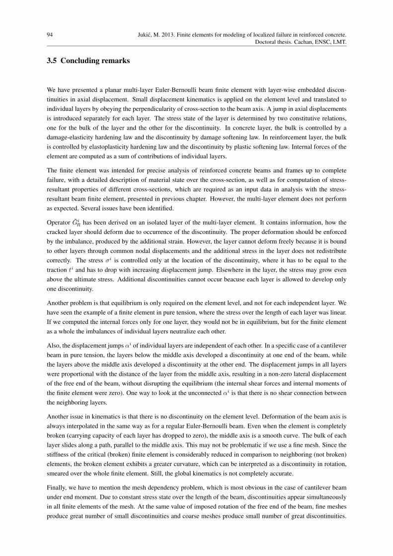
94 Jukic, M. 2013. Finite elements for modeling of localized failure in reinforced concrete.
Doctoral thesis. Cachan, ENSC, LMT.
3.5 Concluding remarks
We have presented a planar multi-layer Euler-Bernoulli beam finite element with layer-wise embedded discon-
tinuities in axial displacement. Small displacement kinematics is applied on the element level and translated to
individual layers by obeying the perpendicularity of cross-section to the beam axis. A jump in axial displacements
is introduced separately for each layer. The stress state of the layer is determined by two constitutive relations,
one for the bulk of the layer and the other for the discontinuity. In concrete layer, the bulk is controlled by a
damage-elasticity hardening law and the discontinuity by damage softening law. In reinforcement layer, the bulk
is controlled by elastoplasticity hardening law and the discontinuity by plastic softening law. Internal forces of the
element are computed as a sum of contributions of individual layers.
The finite element was intended for precise analysis of reinforced concrete beams and frames up to complete
failure, with a detailed description of material state over the cross-section, as well as for computation of stress-
resultant properties of different cross-sections, which are required as an input data in analysis with the stress-
resultant beam finite element, presented in previous chapter. However, the multi-layer element does not perform
as expected. Several issues have been identified.
Operator GiR has been derived on an isolated layer of the multi-layer element. It contains information, how the
cracked layer should deform due to occurrence of the discontinuity. The proper deformation should be enforced
by the imbalance, produced by the additional strain. However, the layer cannot deform freely because it is bound
to other layers through common nodal displacements and the additional stress in the layer does not redistribute
correctly. The stress σi is controlled only at the location of the discontinuity, where it has to be equal to the
traction ti and has to drop with increasing displacement jump. Elsewhere in the layer, the stress may grow even
above the ultimate stress. Additional discontinuities cannot occur beacuse each layer is allowed to develop only
one discontinuity.
Another problem is that equilibrium is only required on the element level, and not for each independent layer. We
have seen the example of a finite element in pure tension, where the stress over the length of each layer was linear.
If we computed the internal forces only for one layer, they would not be in equilibrium, but for the finite element
as a whole the imbalances of individual layers neutralize each other.
Also, the displacement jumps αi of individual layers are independent of each other. In a specific case of a cantilever
beam in pure tension, the layers below the middle axis developed a discontinuity at one end of the beam, while
the layers above the middle axis developed a discontinuity at the other end. The displacement jumps in all layers
were proportional with the distance of the layer from the middle axis, resulting in a non-zero lateral displacement
of the free end of the beam, without disrupting the equilibrium (the internal shear forces and internal moments of
the finite element were zero). One way to look at the unconnected αi is that there is no shear connection between
the neighboring layers.
Another issue in kinematics is that there is no discontinuity on the element level. Deformation of the beam axis is
always interpolated in the same way as for a regular Euler-Bernoulli beam. Even when the element is completely
broken (carrying capacity of each layer has dropped to zero), the middle axis is a smooth curve. The bulk of each
layer slides along a path, parallel to the middle axis. This may not be problematic if we use a fine mesh. Since the
stiffness of the critical (broken) finite element is considerably reduced in comparison to neighboring (not broken)
elements, the broken element exhibits a greater curvature, which can be interpreted as a discontinuity in rotation,
smeared over the whole finite element. Still, the global kinematics is not completely accurate.
Finally, we have to mention the mesh dependency problem, which is most obvious in the case of cantilever beam
under end moment. Due to constant stress state over the length of the beam, discontinuities appear simultaneously
in all finite elements of the mesh. At the same value of imposed rotation of the free end of the beam, fine meshes
produce great number of small discontinuities and coarse meshes produce small number of great discontinuities.
Jukic, M. 2013. Koncni elementi za modeliranje lokaliziranih porusitev v armiranem betonu.
Doktorska disertacija. Ljubljana, UL, FGG.
95
According to the softening material law, the traction at the discontinuity drops with its increasing size. Therefore,
different meshes lead to different values of moment in the beam. The greatest deviations appear in the last part
of the response when the beam as a whole enters the softening phase, which usually happens due to softening
of tensile reinforcement. This can be cured by slightly weakening reinforcement in one of the finite elements.
When the weak element begins to soften, the remaining elements unload and cannot develop a discontinuity in
reinforcement. If softening of the element happens due to crushing of concrete in compression, the problem
cannot be solved so effectively because there are multiple critical layers, as opposed to a single critical layer in
case of tensile reinforcement. Also, the mesh dependency due to cracking of concrete in tension, when moment
in the beam is increasing, cannot be avoided. Even if one of the elements is weaker, the concrete in the remaining
elements will crack sooner or later, because the moment is still rising.
Considering all the deficiencies, the above derived multi-layer Euler-Bernoulli beam finite element cannot be
recommended for general use. The only viable application is in case of constant strain/stress state over the length
of the beam, which can occur either in pure tension/compression or in pure bending. In case of bending, the mesh
dependency cannot be completely avoided.
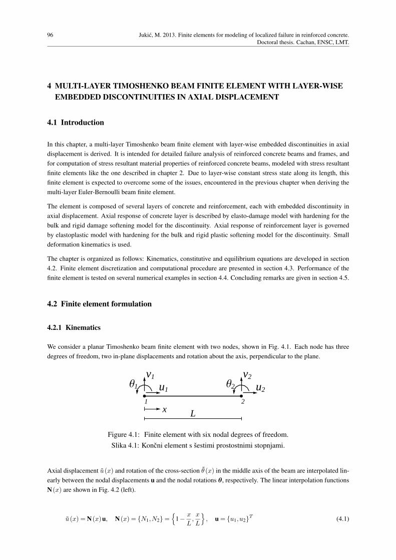
96 Jukic, M. 2013. Finite elements for modeling of localized failure in reinforced concrete.
Doctoral thesis. Cachan, ENSC, LMT.
4 MULTI-LAYER TIMOSHENKO BEAM FINITE ELEMENT WITH LAYER-WISE
EMBEDDED DISCONTINUITIES IN AXIAL DISPLACEMENT
4.1 Introduction
In this chapter, a multi-layer Timoshenko beam finite element with layer-wise embedded discontinuities in axial
displacement is derived. It is intended for detailed failure analysis of reinforced concrete beams and frames, and
for computation of stress resultant material properties of reinforced concrete beams, modeled with stress resultant
finite elements like the one described in chapter 2. Due to layer-wise constant stress state along its length, this
finite element is expected to overcome some of the issues, encountered in the previous chapter when deriving the
multi-layer Euler-Bernoulli beam finite element.
The element is composed of several layers of concrete and reinforcement, each with embedded discontinuity in
axial displacement. Axial response of concrete layer is described by elasto-damage model with hardening for the
bulk and rigid damage softening model for the discontinuity. Axial response of reinforcement layer is governed
by elastoplastic model with hardening for the bulk and rigid plastic softening model for the discontinuity. Small
deformation kinematics is used.
The chapter is organized as follows: Kinematics, constitutive and equilibrium equations are developed in section
4.2. Finite element discretization and computational procedure are presented in section 4.3. Performance of the
finite element is tested on several numerical examples in section 4.4. Concluding remarks are given in section 4.5.
4.2 Finite element formulation
4.2.1 Kinematics
We consider a planar Timoshenko beam finite element with two nodes, shown in Fig. 4.1. Each node has three
degrees of freedom, two in-plane displacements and rotation about the axis, perpendicular to the plane.
x L
u1
v1Θ1 u2
v2Θ2
1 2
Figure 4.1: Finite element with six nodal degrees of freedom.
Slika 4.1: Koncni element s sestimi prostostnimi stopnjami.
Axial displacement u(x) and rotation of the cross-section θ (x) in the middle axis of the beam are interpolated lin-
early between the nodal displacements u and the nodal rotations θ, respectively. The linear interpolation functions
N(x) are shown in Fig. 4.2 (left).
u(x) = N(x)u, N(x) = N1,N2=
1−x
L,x
L
, u = u1,u2T
(4.1)

Jukic, M. 2013. Koncni elementi za modeliranje lokaliziranih porusitev v armiranem betonu.
Doktorska disertacija. Ljubljana, UL, FGG.
97
θ (x) = N(x)θ, θ = θ1,θ2T
(4.2)
Linear interpolation of transversal displacement v (x) of the middle axis would result in shear locking of the finite
element. The problem is avoided by raising the order of interpolation of v (x) with a quadratic bubble function
N3 (x), see Fig. 4.2 (left). Parameter v3 is determined so as to allow the finite element to describe a shear-free
stress state in case of constant moment.
v (x) = N(x)v+N3 (x)v3, v = v1,v2T , N3 (x) =
4(L−x)x
L2, v3 =
L
8(θ1 −θ2) (4.3)
In Timoshenko beam theory, the cross-section is not necessarily perpendicular to the beam axis and the shear strain
γ (x) is computed as the difference between the derivative of the transversal displacement and the rotation of the
cross-section.
γ =∂v
∂x− θ = Bv+B∗θ, B = B1,B2=
−1
L,
1
L
, B∗ = B∗,B∗=
−1
2,−
1
2
(4.4)
For the interpolations of transversal displacement and rotation, chosen in equations (4.2) and (4.3), the shear strain
is constant. Components of the strain interpolation functions B and B∗ are shown in Fig. 4.2 (right). A simple
verification confirms that the shear strain is zero in case of constant moment/curvature (v1 = v2, θ1 =−θ2).
N1
N2
N3
x
L
1 2
1
1
1
B1
B2
B*
x
L
1 2
-1
L
1
L
-1
2
Figure 4.2: Interpolation functions for displacements (left) and strain (right).
Slika 4.2: Interpolacijske funkcije za pomike (levo) in deformacije (desno).
The beam is treated as a composition of nL layers of concrete and steel. Constant state is assumed over the
thickness of each layer and its displacements ui (x) are computed in its middle axis. Embedded discontinuity
concept is used to model the material failure of each layer.
ui(x,xi
d
)=
ui
︷ ︸︸ ︷
u(x)−yiθ (x)+
ui,add
︷ ︸︸ ︷
M i(x,xi
d
)αi (4.5)
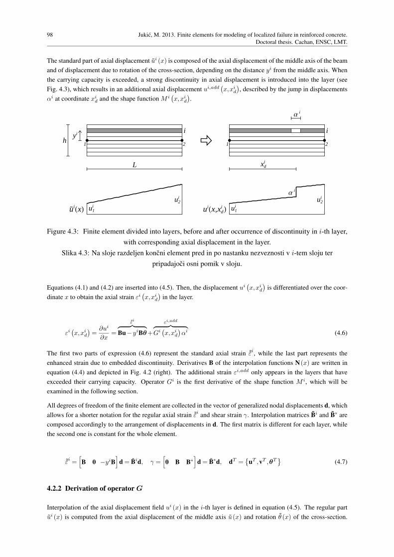
98 Jukic, M. 2013. Finite elements for modeling of localized failure in reinforced concrete.
Doctoral thesis. Cachan, ENSC, LMT.
The standard part of axial displacement ui (x) is composed of the axial displacement of the middle axis of the beam
and of displacement due to rotation of the cross-section, depending on the distance yi from the middle axis. When
the carrying capacity is exceeded, a strong discontinuity in axial displacement is introduced into the layer (see
Fig. 4.3), which results in an additional axial displacement ui,add(x,xi
d
), described by the jump in displacements
αi at coordinate xid and the shape function M i
(x,xi
d
).
u iHxL u1i
u2i
L
hyi i
1 2
uiHx,xdi L u1
iu2
iΑ i
xdi
Α i
i
1 2
Figure 4.3: Finite element divided into layers, before and after occurrence of discontinuity in i-th layer,
with corresponding axial displacement in the layer.
Slika 4.3: Na sloje razdeljen koncni element pred in po nastanku nezveznosti v i-tem sloju ter
pripadajoci osni pomik v sloju.
Equations (4.1) and (4.2) are inserted into (4.5). Then, the displacement ui(x,xi
d
)is differentiated over the coor-
dinate x to obtain the axial strain εi(x,xi
d
)in the layer.
εi(x,xi
d
)=
∂ui
∂x=
˜εi
︷ ︸︸ ︷
Bu−yiBθ+
εi,add︷ ︸︸ ︷
Gi(x,xi
d
)αi (4.6)
The first two parts of expression (4.6) represent the standard axial strain ˜εi, while the last part represents the
enhanced strain due to embedded discontinuity. Derivatives B of the interpolation functions N(x) are written in
equation (4.4) and depicted in Fig. 4.2 (right). The additional strain εi,add only appears in the layers that have
exceeded their carrying capacity. Operator Gi is the first derivative of the shape function M i, which will be
examined in the following section.
All degrees of freedom of the finite element are collected in the vector of generalized nodal displacements d, which
allows for a shorter notation for the regular axial strain ˜εi and shear strain γ. Interpolation matrices Bi and B∗ are
composed accordingly to the arrangement of displacements in d. The first matrix is different for each layer, while
the second one is constant for the whole element.
˜εi =[
B 0 −yiB]
d = Bid, γ =[
0 B B∗]
d = B∗d, dT =
uT ,vT ,θT
(4.7)
4.2.2 Derivation of operator G
Interpolation of the axial displacement field ui (x) in the i-th layer is defined in equation (4.5). The regular part
ui (x) is computed from the axial displacement of the middle axis u(x) and rotation θ (x) of the cross-section.
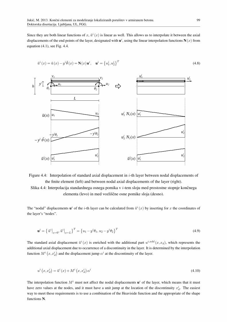
Jukic, M. 2013. Koncni elementi za modeliranje lokaliziranih porusitev v armiranem betonu.
Doktorska disertacija. Ljubljana, UL, FGG.
99
Since they are both linear functions of x, ui (x) is linear as well. This allows us to interpolate it between the axial
displacements of the end points of the layer, designated with ui, using the linear interpolation functions N(x) from
equation (4.1), see Fig. 4.4.
ui (x) = u(x)−yiθ (x) = N(x)ui, ui =ui
1,ui2
T(4.8)
u1
v1
Θ1
u2
v2
Θ2
L
hyi
uHxL u1u2
-yi ΘHxL-yiΘ1 -yiΘ2
u iHxL u1i
u2i
u1i
u2i
u1i N1HxL u1
i
u2i N2HxL
u2i
u iHxL u1i
u2i
Figure 4.4: Interpolation of standard axial displacement in i-th layer between nodal displacements of
the finite element (left) and between nodal axial displacements of the layer (right).
Slika 4.4: Interpolacija standardnega osnega pomika v i-tem sloju med prostostne stopnje koncnega
elementa (levo) in med vozliscne osne pomike sloja (desno).
The “nodal” displacements ui of the i-th layer can be calculated from ui (x) by inserting for x the coordinates of
the layer’s “nodes”.
ui =ui∣∣x=0
, ui∣∣x=L
T=u1 −yiθ1, u2 −yiθ2
T(4.9)
The standard axial displacement ui (x) is enriched with the additional part ui,add (x,xd), which represents the
additional axial displacement due to occurrence of a discontinuity in the layer. It is determined by the interpolation
function M i(x,xi
d
)and the displacement jump αi at the discontinuity of the layer.
ui(x,xi
d
)= ui (x)+M i
(x,xi
d
)αi (4.10)
The interpolation function M i must not affect the nodal displacements ui of the layer, which means that it must
have zero values at the nodes, and it must have a unit jump at the location of the discontinuity xid. The easiest
way to meet these requirements is to use a combination of the Heaviside function and the appropriate of the shape
functions N.

100 Jukic, M. 2013. Finite elements for modeling of localized failure in reinforced concrete.
Doctoral thesis. Cachan, ENSC, LMT.
x
L
xdi
W
W- W+
i
Hxdi 1
∆xdi
¥
x
L
xdi
u1i u2
i
W- W+
Hxdi
N2
M i
1
1
1
Figure 4.5: Domain and sub-domains of a cracked layer, Heaviside and Dirac-delta functions (left).
Construction of interpolation function Mi (right).
Slika 4.5: Domena in poddomeni razpokanega sloja, Heaviside-ova in Dirac-delta funkcija (levo).
Konstruiranje interpolacijske funkcije Mi (desno).
Domain Ω of the cracked layer is divided by the discontinuity into two parts. Ω− is the part before the discontinuity,
with x < xid, and Ω+ is the part after the discontinuity, with x≥ xi
d, see Fig. 4.5 (left). The value of the Heaviside
function is 0 on Ω− and 1 on Ω+. Its derivative is the Dirac delta function δxid, which has an infinite value at xi
d
and zero value elsewhere.
Hxid=
0; x < xid
1; x≥ xid
∂Hxid
∂x= δxi
d=
∞; x= xid
0; otherwise(4.11)
Heaviside function Hxid
satisfies the requirement of a unit jump at the discontinuity. Its value, however, is only
zero on Ω−, and not at all nodes of the layer. This can be fixed by subtracting from it those shape functions Nj ∈N,
that correspond to the nodes j, included in Ω+. Since Nj are continuous and have zero values at all nodes except
j, they will not affect previously fulfilled demands. As we are dealing with a simple two-node finite element, we
have to subtract the shape function N2, regardless of the location of the discontinuity, see Fig. 4.5 (right).
M i(x,xi
d
)αi =Hxi
d
(x,xi
d
)−N2 (x) (4.12)
The first derivative of M i over x is designated with Gi and is composed of a continuous part Gi and a discrete part¯Gi. The derivative of N2 is B2, defined in (4.4), and the derivative of Hxi
dis defined in (4.11).
Gi(x,xi
d
)=
∂
∂xM i(x,xi
d
)= Gi+ ¯Gi, ¯Gi = δxi
d, Gi =−B2 =−
1
L(4.13)

Jukic, M. 2013. Koncni elementi za modeliranje lokaliziranih porusitev v armiranem betonu.
Doktorska disertacija. Ljubljana, UL, FGG.
101
Considering the constant strain state in a layer, see equation (4.7), the discontinuity could appear anywhere between
the end nodes. Without loss of generality, we can place it at xid = L/2 .
4.2.3 Relations between global and local quantities
4.2.3.1 Real degrees of freedom
A structure is modeled with a mesh of finite elements. A part of such mesh is depicted in Fig. 4.6. The total number
of the nodes in the structure is designated with nN . Each node has three degrees of freedom - displacement
U parallel to the global X axis, displacement V parallel to the global Y axis, and rotation Θ about the axis,
perpendicular to the XY plane. The structure has in total nDOF = 3nN degrees of freedom, which are collected
in the vector dstr.
dstr =U1,V1,Θ1,U2,V2,Θ2, . . . ,UnN ,VnN ,ΘnN
T(4.14)
X
Ynode of FE
n Un
Vn
Qn
Figure 4.6: Degrees of freedom at a node of the finite element mesh.
Slika 4.6: Prostostne stopnje v posameznem vozliscu mreze koncnih elementov.
Let us now consider a finite element (e) with end nodes (n1) and (n2). The local x axis is parallel to the axis of
the element, with x increasing from (n1) towards (n2), see Fig. 4.7. The element’s degrees of freedom, defined
in the local coordinate system, are collected in the vector d(e), in accordance with equation (4.7). Global degrees
of freedom, associated with the nodes of the element can be similarly organized into vector D(e). The two are
connected with a transformation matrix R(e). Zeros are replaced by dots for clarity. φ(e) is the angle between the
global X axis and the local x axis (rotation of the local coordinate system).
d(e) = R(e)D(e) (4.15)

102 Jukic, M. 2013. Finite elements for modeling of localized failure in reinforced concrete.
Doctoral thesis. Cachan, ENSC, LMT.
d(e) =
u(e)1 ,u
(e)2 ,v
(e)1 ,v
(e)2 ,θ
(e)1 ,θ
(e)2
T, D(e) =
Un1,Un2
,Vn1,Vn2
,Θn1,Θn2
T
R(e) =
cosφ(e) · sinφ(e) · · ·
· cosφ(e) · sinφ(e) · ·
−sinφ(e) · cosφ(e) · · ·
· −sinφ(e) · cosφ(e) · ·
· · · · 1 ·
· · · · · 1
(4.16)
n1 Un1
Vn1
Qn1
n2 Un2
Vn2
Qn2
HeL
1
u1
v1
Θ1
2
u2
v2
Θ2
HeL
X
Y
xy
Φ
Figure 4.7: Global (left) and local (right) degrees of freedom, associated with a finite element.
Slika 4.7: Globalne (levo) in lokalne (desno) prostostne stopnje, povezane s koncnim elementom.
Vector D(e) contains those components of vector dstr that correspond to the nodes of the finite element. The
selection of appropriate components is done by matrix P(e) of size 6×nDOF with only six non-zero components.
D(e) = P(e)dstr
P(e)1, 3n1−2 = P
(e)2, 3n2−2 = P
(e)3, 3n1−1 = P
(e)4, 3n2−1 = P
(e)5, 3n1
= P(e)6, 3n2
= 1, other P(e)i,j = 0
(4.17)
Obeying equations (4.15) and (4.17), we can write the relation between the local degrees of freedom of the finite
element (e) and the global degrees of freedom of the structure.
d(e) = R(e)P(e)dstr (4.18)
4.2.3.2 Virtual degrees of freedom
Virtual displacements are a kinematically admissible variation of real generalized displacements. As with the real
displacements, they are interpolated between the nodal values with appropriate interpolation functions. The virtual
deformation of the mesh is therefore defined by the virtual displacements of its nodes.
The global virtual degrees of freedom (virtual nodal displacements of the mesh) dstr, the virtual nodal displace-
ments of the element d(e) and the selection D(e) of global virtual displacements, associated with the element (e),
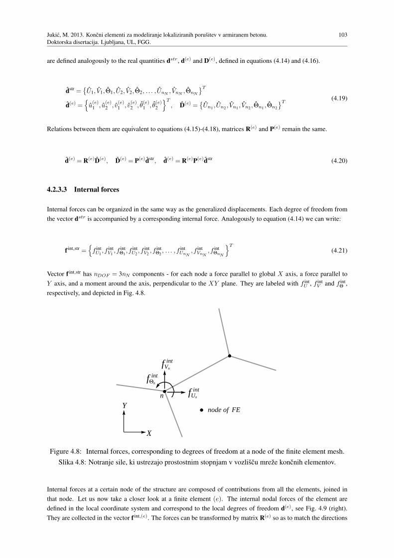
Jukic, M. 2013. Koncni elementi za modeliranje lokaliziranih porusitev v armiranem betonu.
Doktorska disertacija. Ljubljana, UL, FGG.
103
are defined analogously to the real quantities dstr, d(e) and D(e), defined in equations (4.14) and (4.16).
dstr =U1, V1, Θ1, U2, V2, Θ2, . . . , UnN , VnN , ΘnN
T
d(e) =
u(e)1 , u
(e)2 , v
(e)1 , v
(e)2 , θ
(e)1 , θ
(e)2
T, D(e) =
Un1
, Un2, Vn1
, Vn2, Θn1
, Θn2
T(4.19)
Relations between them are equivalent to equations (4.15)-(4.18), matrices R(e) and P(e) remain the same.
d(e) = R(e)D(e), D(e) = P(e)dstr, d(e) = R(e)P(e)dstr (4.20)
4.2.3.3 Internal forces
Internal forces can be organized in the same way as the generalized displacements. Each degree of freedom from
the vector dstr is accompanied by a corresponding internal force. Analogously to equation (4.14) we can write:
f int,str =
f intU1,f int
V1,f int
Θ1,f int
U2,f int
V2,f int
Θ2, . . . ,f int
UnN,f int
VnN,f int
ΘnN
T(4.21)
Vector f int,str has nDOF = 3nN components - for each node a force parallel to global X axis, a force parallel to
Y axis, and a moment around the axis, perpendicular to the XY plane. They are labeled with f intU , f int
V and f intΘ ,
respectively, and depicted in Fig. 4.8.
X
Ynode of FE
n fUn
int
fVn
int
fQn
int
Figure 4.8: Internal forces, corresponding to degrees of freedom at a node of the finite element mesh.
Slika 4.8: Notranje sile, ki ustrezajo prostostnim stopnjam v vozliscu mreze koncnih elementov.
Internal forces at a certain node of the structure are composed of contributions from all the elements, joined in
that node. Let us now take a closer look at a finite element (e). The internal nodal forces of the element are
defined in the local coordinate system and correspond to the local degrees of freedom d(e), see Fig. 4.9 (right).
They are collected in the vector f int,(e). The forces can be transformed by matrix R(e) so as to match the directions
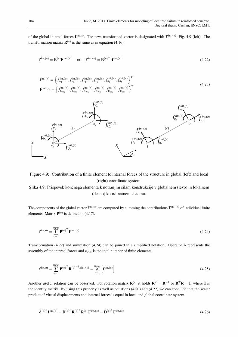
104 Jukic, M. 2013. Finite elements for modeling of localized failure in reinforced concrete.
Doctoral thesis. Cachan, ENSC, LMT.
of the global internal forces f int,str. The new, transformed vector is designated with F int,(e), Fig. 4.9 (left). The
transformation matrix R(e) is the same as in equation (4.16).
f int,(e) = R(e)F int,(e) ⇔ F int,(e) = R(e)−1f int,(e) (4.22)
f int,(e) =
f int,(e)u1
,f int,(e)u2
,f int,(e)v1
,f int,(e)v2
,fint,(e)θ1
,fint,(e)θ2
T
F int,(e) =
fint,(e)Un1
,fint,(e)Un2
,fint,(e)Vn1
,fint,(e)Vn2
,fint,(e)Θn1
,fint,(e)Θn2
T(4.23)
n1 fUn1
int,HeL
fVn1
int,HeL
fQn1
int,HeL
n2 fUn2
int,HeL
fVn2
int,HeL
fQn2
int,HeL
HeL
1
fu1
int,HeL
fv1
int,HeL
fΘ1
int,HeL
2
fu2
int,HeL
fv2
int,HeL
fΘ2
int,HeL
HeL
X
Y
xy
Φ
Figure 4.9: Contribution of a finite element to internal forces of the structure in global (left) and local
(right) coordinate system.
Slika 4.9: Prispevek koncnega elementa k notranjim silam konstrukcije v globalnem (levo) in lokalnem
(desno) koordinatnem sistemu.
The components of the global vector f int,str are computed by summing the contributions F int,(e) of individual finite
elements. Matrix P(e) is defined in (4.17).
f int,str =nFE
∑e=1
P(e)T F int,(e) (4.24)
Transformation (4.22) and summation (4.24) can be joined in a simplified notation. Operator A represents the
assembly of the internal forces and nFE is the total number of finite elements.
f int,str =nFE
∑e=1
P(e)T R(e)−1f int,(e) =
nFE
Ae=1
[
f int,(e)]
(4.25)
Another useful relation can be observed. For rotation matrix R(e) it holds RT = R−1 or RT R = I, where I is
the identity matrix. By using this property as well as equations (4.20) and (4.22) we can conclude that the scalar
product of virtual displacements and internal forces is equal in local and global coordinate system.
d(e)T f int,(e) = D(e)T R(e)T R(e) F int,(e) = D(e)T F int,(e) (4.26)
Jukic, M. 2013. Koncni elementi za modeliranje lokaliziranih porusitev v armiranem betonu.
Doktorska disertacija. Ljubljana, UL, FGG.
105
4.2.4 Virtual work equation
Equilibrium of a structure can be described in a weak from, by the virtual work principle, which states that the
virtual work of internal forces G int on any kinematically admissible perturbation of generalized displacements -
virtual displacements - must be equal to the work of external forces Gext on the same virtual displacements.
Gint −Gext = 0 (4.27)
Since we are dealing with a discretized model, the external loads are defined at the nodes of the structure. Linear
loads have to be transferred to the nodes appropriately. The virtual work of external forces is therefore computed
simply as a scalar product of the vector of virtual nodal displacements of the structure dstr and the corresponding
vector of generalized external forces f ext,str. Virtual displacements are defined in equation (4.19) and the external
forces analogously to the internal forces in equation (4.21).
Gext = dstrT f ext,str =nDOF
∑j=1
dstrj f ext,str
j (4.28)
Here nDOF is the number of the structure’s degrees of freedom. Many components of the sum (4.28) may be zero.
The virtual work of internal forces is composed of contributions from individual finite elements.
Gint =nFE
∑e=1
Gint,(e), Gint,(e) =∫
V (e)
(εσ+ γτ)dV (4.29)
For each element, Gint,(e) is computed by multiplying the corresponding components of the stress field and the
virtual strain field and integrating the product over the volume of the element. Virtual shear strain γ is interpolated
between the virtual nodal displacements in the same way as the real strain in equation (4.4) and is constant all over
the finite element. Virtual axial strain ε is defined individually for each layer and interpolated in the same manner
as the real strain in equation (4.6). Note that the additional part of the virtual strain εi,add only exists in the cracked
layers. In non-cracked layers, the virtual strain consists only of the regular part ˆεi.
γ = Bv+B∗θ = B∗d, εi =
ˆεi
︷ ︸︸ ︷
Bu−yiBθ+
εi,add︷ ︸︸ ︷
Giαi = Bid+Giαi (4.30)
The volume integral in equation (4.29) is divided into an integral over the length and an integral over the cross-
section of the element. The latter can be replaced by a sum over the layers, since everything is assumed to be
constant over the cross-section Ai of a layer. The virtual axial strain is replaced by the whole expression (4.30) for
n(e)CL cracked layers and by its regular part ˆε
ifor(
nL−n(e)CL
)
non-cracked layers, where nL is the total number of
layers in the finite element. Shear strain γ is constant over the whole element and is replaced by (4.30) for all nL
layers. Shear stress τ i depends on the material law and is different for concrete and steel. Obtained expression is
rearranged to produce internal forces, corresponding to the virtual degrees of freedom of the finite element d(e),
defined in (4.19). Index (e) is omitted until the last line. For the sake of simplicity it is assumed that the cracked
layers are numbered with 1, 2, . . . , n(e)CL.

106 Jukic, M. 2013. Finite elements for modeling of localized failure in reinforced concrete.
Doctoral thesis. Cachan, ENSC, LMT.
Gint,(e) =∫
V
(εσ+ γτ)dV =∫
L
∫
A
(εσ+ γτ)dAdx=∫
L
∑i
(εiσi+ γτ i
)Aidx=
=∫
L
nL
∑i=1
BuσiAidx+∫
L
nL
∑i=1
Bθ(−yiσiAi
)dx+
∫
L
nCL
∑i=1
GiαiσiAidx+
+∫
L
nL
∑i=1
Bvτ iAidx+∫
L
nL
∑i=1
B∗θ τ iAidx=
= uT∫
L
nL
∑i=1
BTσiAidx+ vT∫
L
nL
∑i=1
BTτ iAidx+ θT∫
L
nL
∑i=1
(
−yiBTσi+B∗Tτ i)
Aidx+
+nCL
∑i=1
αi∫
L
GiσiAidx= d(e)T f int,(e)+
n(e)CL
∑i=1
α(e),ih(e),i
(4.31)
A condensed form of expressions (4.19) and (4.23) for d(e) and f int,(e) is used.
d(e)T =
uT , vT , θT
, f int,(e)T =
fu,int,(e)T , fv,int,(e)T , fθ,int,(e)T
(4.32)
Components of f int,(e) are defined in (4.33). Since all present quantities are constant over the length of the finite
element, the integrals are easily evaluated. The internal forces are calculated as a sum of contributions of individual
layers, which proves to be helpful in the computational procedure.
fu,int,(e) =∫
L
nL
∑i=1
BTσiAidx=nL
∑i=1
BTσiAiL
fv,int,(e) =∫
L
nL
∑i=1
BTτ iAidx=nL
∑i=1
BTτ iAiL
fθ,int,(e) =∫
L
nL
∑i=1
(
−yi BTσi+B∗Tτ i)
Aidx=nL
∑i=1
(
−yi BTσi+B∗Tτ i)
AiL
(4.33)
A shorter notation (4.34) will also be used. Here, f int,(e),i is contribution of the i-th layer to the vector of nodal
internal forces of the finite element.
f int,(e) =nL
∑i=1
BT
0
−yiBT
σ
iAiL+
0
BT
B∗T
τ
iAiL
=
nL
∑i=1
(
BiTσi+ B∗Tτ i)
AiL︸ ︷︷ ︸
f int,(e),i
(4.34)
The second term of the last line in (4.31) is the additional virtual work due to enhanced kinematics. The sum has
n(e)CL summands, one for each cracked layer. Quantity h(e),i corresponds to the virtual displacement jump α(e),i,
and is defined as follows:
h(e),i =∫
L
GiσiAidx, i= 1,2, . . . ,n(e)CL (4.35)
Jukic, M. 2013. Koncni elementi za modeliranje lokaliziranih porusitev v armiranem betonu.
Doktorska disertacija. Ljubljana, UL, FGG.
107
The virtual work of external and internal forces in the equilibrium equation (4.27) is replaced by expressions
(4.28) and (4.29), respecting (4.31) and (4.26). Finally, the second of equations (4.20) allows us to express the
weak equilibrium in the manner of global virtual displacement vector dstr and virtual displacement jumps α(e),i.
0 =nFE
∑e=1
Gint,(e)−Gext =
=nFE
∑e=1
D(e)T F int,(e)+
n(e)CL
∑i=1
α(e),ih(e),i
− dstrT f ext,str =
=nFE
∑e=1
dstrT P(e)T F int,(e)+nFE
∑e=1
n(e)CL
∑i=1
α(e),ih(e),i− dstrT f ext,str =
= dstrTnFE
∑e=1
P(e)T F int,(e)+nFE
∑e=1
n(e)CL
∑i=1
α(e),ih(e),i− dstrT f ext,str =
= dstrT(
f int,str − f ext,str)
+nFE
∑e=1
n(e)CL
∑i=1
α(e),ih(e),i
(4.36)
Equilibrium (4.36) must hold for any kinematically admissible virtual displacements dstr and virtual displacement
jumps α(e),i. From this requirement we can conclude:
f int,str − f ext,str = 0
∀e ∈ 1,2, . . . ,nFE , ∀i ∈
1,2, . . . ,n(e)CL
: h(e),i = 0(4.37)
The first equation in (4.37) represents the global equilibrium of every individual node of the mesh. Here f int,str and
f ext,str are vectors of internal and external nodal forces on the structural mesh. They correspond in position and
direction to the degrees of freedom of the mesh. Their length is equal to the total number of degrees of freedom
nDOF . The second equation in (4.37) is an additional constraint for the stress in cracked layers. The number of
cracked layers n(e)CL is generally different for each element, and can also be zero. It has been assumed in equation
(4.37) that the cracked layers are numbered with consecutive numbers from 1 to n(e)CL.
Let us now examine h(e),i, defined in expression (4.35). Operator Gi, defined by equation (4.13), consists of a
continuous part Gi and the Dirac delta function δxid. Integration of the latter is performed by the following rule:
Gi = Gi+ δxid,∫
L
g (x)δxiddx= g
(xid
)(4.38)
Implementation of (4.38) allows a further development of expression (4.35). We introduce σi∣∣xid
as the value of
stress function σi (x), evaluated at local coordinate xid. We assign to it a new symbol ti and define it as the traction
at the discontinuity.
h(e),i =∫
L
(
Gi+ δxid
)
σiAidx=Ai∫
L
Giσidx+Aiσi∣∣xid=Ai
∫
L
Giσidx+ ti
(4.39)
Inserting (4.39) into the second of equilibrium equations (4.37) provides a new aspect to its meaning. Equation
(4.40) represents equilibrium between the traction at the discontinuity ti and the stress in the bulk σi. Being
108 Jukic, M. 2013. Finite elements for modeling of localized failure in reinforced concrete.
Doctoral thesis. Cachan, ENSC, LMT.
confined to a single finite element, we can refer to it as local equilibrium. Relation Gi = −1/L from equation
(4.13) is used as well.
h(e),i = 0 ⇔ ti =−∫
L
Giσidx= σi (4.40)
In the spirit of the method of incompatible modes, the operator Gi should also meet the requirement, that the
additional virtual work (performed on the virtual displacement jumps αi) be zero in case of constant stress σi.
Thus, the introduction of αi does not affect the internal virtual work. Since the stress is always constant in our
finite element, this test is trivial (fulfilled already by equilibrium equation (4.40)).
αi∫
L
GiσiAidx= αiσiAi︸ ︷︷ ︸
6=0
∫
L
Gi dx= 0 ⇒∫
L
Gi dx= 0 (4.41)
Taking into account the rule (4.38) for integration of Gi, requirement (4.41) can be reformulated.
∫
L
Gi dx=∫
L
(
Gi+ δxid
)
dx=∫
L
Gi dx+
=1︷ ︸︸ ︷∫
L
δxiddx= 0 ⇒
∫
L
Gi dx=−1 (4.42)
Equality Gi =−1/L satisfies the condition (4.42).
4.2.5 Constitutive models
In this section we describe constitutive models which control the axial and shear response of concrete and steel-
reinforcement layers. Axial response of each material is described by two models, one for the bulk of the layer
and one for the discontinuity. Shear model is only required for the bulk of the layer, as there are no discontinuities
involved.
4.2.5.1 Shear stress model
The transverse response is assumed to be elastic. While the shear strain is constant all over the finite element, the
shear stress is different in concrete and steel layers, due to different material parameters. In equation (4.43), µc
and µs are the shear moduli of concrete and steel, respectively, and c is the shear correction factor for rectangular
cross-section. Shear strain γ is computed according to equation (4.4).
τ i = cµiγ, c= 5/6, µi =
µc for concrete
µs for steel,
∂ τ i
∂ γ= cµi (4.43)
The shear moduli µc and µs are computed from the elastic moduli Ec and Es, and Poisson’s ratios νc and νs of
concrete and steel. The usual values are used for νc and νs.
µc =Ec
2(1+νc), µs =
Es
2(1+νs), νc = 0.2, νs = 0.3 (4.44)

Jukic, M. 2013. Koncni elementi za modeliranje lokaliziranih porusitev v armiranem betonu.
Doktorska disertacija. Ljubljana, UL, FGG.
109
4.2.5.2 Bulk of concrete layer
Behavior of the bulk of the concrete layer is described by 1D elasto-damage model. Response of the material
is linear elastic up to the elasticity limit. Further increase of stress produces micro damage (micro cracking in
tension and micro crushing in compression) continuously over the layer, which results in reduction of the elasticity
modulus. Unloading is linear elastic with the current value of the elasticity modulus, and leads to the origin of the
stress-strain diagram (see Fig. 4.10). These properties of concrete are collected in the following equations, which
can be derived through the principle of maximum damage dissipation [73].
Ε
Σ
Σ fct
Σdt
Σ i
-Σdc
-Σ fcc
Ε i Ec
Di-1
elas
ticlo
adin
g
elasti
c unloa
ding
reloa
ding
damage loading
Figure 4.10: Stress - strain diagram for bulk of concrete layer.
Slika 4.10: Diagram napetost - deformacija za sloj betona.
Equation (4.45) shows the linear elastic relation between the stress and the strain. It represents the loading
curve/path up to elasticity limit and the unloading/reloading curve in the σi− εi diagram.
σi = Di−1
εi, Di ∈[E−1
c ,∞), εi = Bid+Giαi =
εi︷ ︸︸ ︷
Bid+ Giαi+ ¯Giαi (4.45)
Here Di is the compliance of the bulk material, Ec the elastic modulus of intact concrete, and εi the continuous
part of axial strain in the i-th layer, composed of the regular strain and the continuous part of the additional strain.
The latter is zero until the discontinuity is formed. The non-elastic part of the loading curve in the σi− εi diagram
is defined indirectly by the remaining equations in this section.

110 Jukic, M. 2013. Finite elements for modeling of localized failure in reinforced concrete.
Doctoral thesis. Cachan, ENSC, LMT.
φi(σi, qi
)=∣∣σi∣∣−(σd− qi
), σd =
σdc for compression
σdt for tension(4.46)
Damage function φi prescribes the admissible values of axial stress σi in the i-th layer. Elasticity limit σd > 0
marks the beginning of micro damage and is defined separately for tension and compression. Stress-like hardening
variable qi handles the damage threshold evolution.
qi =−Hcξi, Hc =
Hcc for compression
Hct for tension(4.47)
Linear hardening of the material is described by equation (4.47), where ξi is a strain-like hardening variable with
initial value equal to zero, and Hc > 0 is a constant hardening modulus of concrete with separate values for tension
and compression. Evolution in pseudo-time of internal hardening variables Di and ξi is defined by evolution
equations (4.48).
˙Di=
˙γisign(σi)
σi, ˙ξ
i= ˙γi
(4.48)
The dot designates the derivative with respect to pseudo-time and ˙γiis damage multiplier. The loading/unloading
conditions and consistency condition (4.49) also apply.
˙γi ≥ 0, φi ≤ 0, ˙γiφi = 0, ˙γi ˙φi= 0 (4.49)
Tangent moduli of the σi− εi diagram can be determined from the above equations. The elastic loading/unloading
path corresponds to condition ˙γi = 0. It follows from evolution equations (4.48), that compliance Di is constant.
The tangent modulus is obtained if expression (4.45) for σi is differentiated with respect to εi.
˙γi = 0 ⇒ Di = const.,∂σi
∂εi= Di−1
(4.50)
In case of damage loading, when ˙γi > 0, the procedure is more complex. From the third and the fourth of conditions
(4.49) we can conclude that φi = 0 and ˙φi= 0. From (4.46) we can write the expression for σi and differentiate it
over pseudo-time. We use the appropriate evolution equation to differentiate ξi within.
σi =(σd− qi
)sign
(σi)=(σd+Hcξ
i)sign
(σi), σi =Hc ˙γisign
(σi)
(4.51)
The stress can be replaced by expression (4.45). The obtained equation is again differentiated over pseudo-time.
Note that compliance Di is not constant any more.
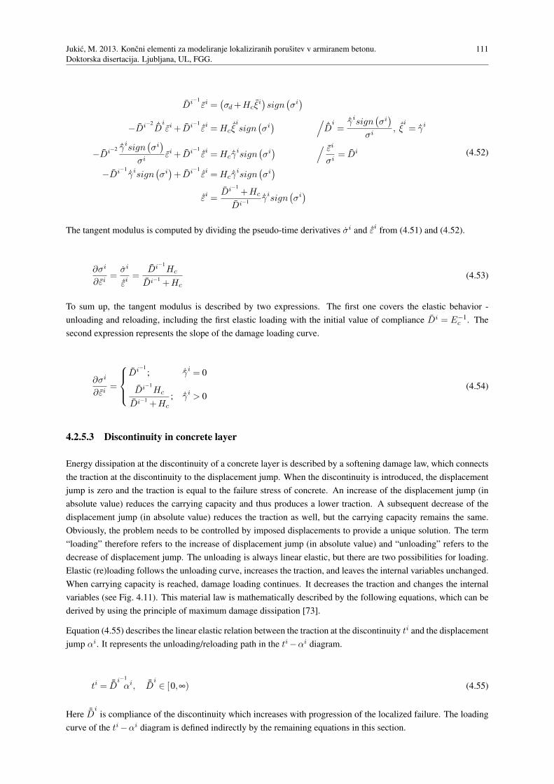
Jukic, M. 2013. Koncni elementi za modeliranje lokaliziranih porusitev v armiranem betonu.
Doktorska disertacija. Ljubljana, UL, FGG.
111
Di−1
εi =(σd+Hcξ
i)sign
(σi)
−Di−2 ˙Diεi+ Di−1
˙εi =Hc˙ξisign
(σi) /
˙Di=
˙γisign(σi)
σi, ˙ξ
i= ˙γi
−Di−2 ˙γisign(σi)
σiεi+ Di−1
˙εi =Hc ˙γisign(σi) / εi
σi= Di
−Di−1˙γisign
(σi)+ Di−1
˙εi =Hc ˙γisign(σi)
˙εi =Di−1
+Hc
Di−1˙γisign
(σi)
(4.52)
The tangent modulus is computed by dividing the pseudo-time derivatives σi and ˙εi from (4.51) and (4.52).
∂σi
∂εi=
σi
˙εi=
Di−1Hc
Di−1+Hc
(4.53)
To sum up, the tangent modulus is described by two expressions. The first one covers the elastic behavior -
unloading and reloading, including the first elastic loading with the initial value of compliance Di = E−1c . The
second expression represents the slope of the damage loading curve.
∂σi
∂εi=
Di−1
; ˙γi = 0
Di−1Hc
Di−1+Hc
; ˙γi > 0(4.54)
4.2.5.3 Discontinuity in concrete layer
Energy dissipation at the discontinuity of a concrete layer is described by a softening damage law, which connects
the traction at the discontinuity to the displacement jump. When the discontinuity is introduced, the displacement
jump is zero and the traction is equal to the failure stress of concrete. An increase of the displacement jump (in
absolute value) reduces the carrying capacity and thus produces a lower traction. A subsequent decrease of the
displacement jump (in absolute value) reduces the traction as well, but the carrying capacity remains the same.
Obviously, the problem needs to be controlled by imposed displacements to provide a unique solution. The term
“loading” therefore refers to the increase of displacement jump (in absolute value) and “unloading” refers to the
decrease of displacement jump. The unloading is always linear elastic, but there are two possibilities for loading.
Elastic (re)loading follows the unloading curve, increases the traction, and leaves the internal variables unchanged.
When carrying capacity is reached, damage loading continues. It decreases the traction and changes the internal
variables (see Fig. 4.11). This material law is mathematically described by the following equations, which can be
derived by using the principle of maximum damage dissipation [73].
Equation (4.55) describes the linear elastic relation between the traction at the discontinuity ti and the displacement
jump αi. It represents the unloading/reloading path in the ti−αi diagram.
ti = ¯Di−1
αi, ¯Di∈ [0,∞) (4.55)
Here ¯Di
is compliance of the discontinuity which increases with progression of the localized failure. The loading
curve of the ti−αi diagram is defined indirectly by the remaining equations in this section.
112 Jukic, M. 2013. Finite elements for modeling of localized failure in reinforced concrete.
Doctoral thesis. Cachan, ENSC, LMT.
Kct*
Kcc*
Α
t
Σ fct
ti
-Σ fcc
Α i Di-1
elas
ticun-r
eloa
ding
damage softening
Figure 4.11: Traction - displacement jump diagram for discontinuity in concrete layer.
Slika 4.11: Diagram napetost - skok v pomiku za nezveznost v sloju betona.
¯φi(
ti, ¯qi)
=∣∣ti∣∣−(
σfc− ¯qi)
, σfc =
σfcc for compression
σfct for tension(4.56)
Failure function ¯φi
prescribes the admissible values of traction ti at the discontinuity of a concrete layer. Failure
stress of concrete σfc > 0 indicates the occurrence of the discontinuity and is defined separately for tension and
compression. Stress-like softening variable ¯qi handles the damage threshold evolution and is described by an
exponential function.
¯qi = σfc
(
1−eKc¯ξi)
, Kc =
Kcc =−σfcc
2Gfccfor compression
Kct =−σfct
2Gfctfor tension
(4.57)
Here ¯ξi is a displacement-like softening variable with initial value set to zero, and Kc < 0 is a constant softening
modulus of concrete with units m−1 and separate values for compression and tension. These are determined by the
fracture energies per cross-section unit Gfcc and Gfct for concrete in compression and tension, respectively. The
fracture energy has units kJm−2 and can be determined by different tests. Evolution in pseudo-time of internal
softening variables ¯Di
and ¯ξi is defined by evolution equations (4.58).
Jukic, M. 2013. Koncni elementi za modeliranje lokaliziranih porusitev v armiranem betonu.
Doktorska disertacija. Ljubljana, UL, FGG.
113
˙D
i
=˙γisign
(ti)
ti,
˙ξi
= ˙γi
(4.58)
The dot designates the derivative with respect to pseudo-time and ˙γi
is damage multiplier. The loading/unloading
conditions and consistency condition (4.59) also apply.
˙γi≥ 0, ¯φ
i≤ 0, ˙γ
i ¯φi= 0, ˙γ
i ˙φi
= 0 (4.59)
A closer inspection of equations (4.55)-(4.59) reveals that the damage loading path of ti−αi diagram, correspond-
ing to condition ¯φi= 0, is a straight line, see appendix B. This suggests a possibility of simplifying the equations.
Each point of the damage loading path is determined by its ordinate ti and the slope ¯Di−1
of the unloading line,
which connects the point to the origin. Abscissa αi is computed from equation (4.55). Evolution equations (4.58)
dictate the change of ¯Di
and ¯ξi, the latter defining ti through equations (4.56), (4.57) and (4.59). Both ¯Di
and
ti change non-linearly with respect to ¯γi = ˙γi∆t (∆t being pseudo-time step), the first one because of non-linear
evolution equation (4.58), and the second due to exponential softening law (4.57). However, it is shown in appendix
B that the two non-linearities neutralize each other, yielding a linear relation between ti and αi.
The damage loading path can also be constructed by defining coordinates αi and ti. If they both change linearly
with respect to some new variable, the diagram will be a straight line. We introduce a new displacement-like
variable ¯ξi∗
and the softening law takes a linear form.
¯ξi∗=−
1
Kc
(
1−eKc¯ξi)
, ¯qi = σfc
(
1−eKc¯ξi)
=−Kcσfc¯ξi∗=−K∗
c¯ξi∗
(4.60)
The expression for ¯qi in (4.60) holds for ¯ξi < ∞, or equivalently ¯ξi∗<−1/Kc . After that ¯qi would become greater
than the failure stress of concrete σfc, which is not acceptable. Physically, it means that the carrying capacity
cannot drop below zero.
¯qi = min
−K∗c
¯ξi∗,σfc
, K∗c =Kcσfc (4.61)
Then, the introduction of a new damage multiplier ¯γi∗allows us to write a new set of linear evolution equations
for αi and ¯ξi∗
. See appendix B for details.
¯γi∗ =−1
Kc
(
1−eKc ¯γi)
, αi = ˙γi∗sign
(ti),
˙ξi∗= ˙γ
i∗(4.62)
The new softening law (4.61) and evolution equations (4.62), due to their linear form, simplify the computa-
tional procedure significantly. But there is another advantage over the original equations. As the original dam-
age multiplier ¯γiapproaches infinity, the traction ti approaches zero and the displacement jump αi approaches
−sign(ti)/Kc . No matter how much we increase the multiplier, αi cannot pass that value. For an individual bar,
such limitation is logical, as the complete loss of carrying capacity implies singularity of the problem and a further
increase of the discontinuity is meaningless. However, if a layer of a beam loses all carrying capacity, the beam
as a whole still possesses stiffness. The broken layer just follows the rest of the beam without resistance. It is

114 Jukic, M. 2013. Finite elements for modeling of localized failure in reinforced concrete.
Doctoral thesis. Cachan, ENSC, LMT.
therefore necessary to allow αi to grow past the point of failure. When the new damage multiplier ¯γi∗reaches the
value −1/Kc , the original multiplier is pushed to infinity and the old evolution equations (4.58) get out of scope.
The new evolution equations (4.62), however, withstand further increase of ¯γi∗. As the latter approaches infinity,
so does αi (in absolute value). Once past the failure point the traction ti remains zero. The relation t−α at the
discontinuity is described by equation (4.63).
ti =
¯Di−1
αi; ˙γi∗= 0
σfc sign(αi)+σfcKcα
i; ˙γi∗> 0, ¯qi < σfc
0; ˙γi∗> 0, ¯qi = σfc
(4.63)
The first expression represents the elastic unloading path, the second one the damage loading path until the traction
drops to zero, and the third one the damage loading path further on. The tangent moduli are obtained by a simple
differentiation of (4.63).
∂ti
∂αi=
¯Di−1
; ˙γi∗= 0
K∗c = σfcKc; ˙γ
i∗> 0, ¯qi < σfc
0; ˙γi∗> 0, ¯qi = σfc
(4.64)
4.2.5.4 Bulk of reinforcement layer
Behavior of the bulk of a layer of reinforcement is described by 1D elasto-plasticity model with isotropic hardening.
It is symmetrical in tension and compression. Response of the material is linear elastic until yield stress is reached.
If loading increases, plastic deformations occur and grow continuously over the layer. Elasticity limit is raised
as well. Unloading is elastic and follows a line, parallel to the first loading path. When the stress drops to zero,
plastic deformations remain in the layer (Fig. 4.12). Behavior of steel is mathematically described by the following
equations, which can be derived by using the principle of maximum plastic dissipation [73].
Stress σi is computed from equation (4.65), which represents the elastic loading path and elastic unloading or
reloading path of the σi− εi diagram.
σi = Es
(εi− εip
), εi = Bid+Giαi =
εi︷ ︸︸ ︷
Bid+ Giαi+ ¯Giαi (4.65)
Here Es is the elastic modulus of steel, εip plastic strain, and εi the continuous part of axial strain in the i-th
layer, composed of the regular strain and the continuous part of the additional strain. Before the appearance of the
discontinuity the additional strain is zero. The plastic loading path of the σi− εi diagram is determined indirectly
by the rest of the equations in this section.
φi(σi, qi
)=∣∣σi∣∣−(σy − qi
)(4.66)
Yield function φi prescribes the admissible axial stress in the layer. Yield stress σy > 0 is the absolute value of
the stress, at which the first plastic deformation occurs. Stress-like hardening variable qi controls yield threshold
evolution.
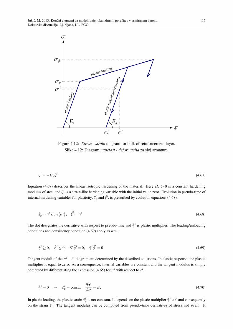
Jukic, M. 2013. Koncni elementi za modeliranje lokaliziranih porusitev v armiranem betonu.
Doktorska disertacija. Ljubljana, UL, FGG.
115
Ε
Σ
Σ fs
Σy
Σ i
Ε iΕ ip
Es Es
elas
ticlo
adin
g
elas
ticun
load
ing
relo
adin
g
plastic loading
Figure 4.12: Stress - strain diagram for bulk of reinforcement layer.
Slika 4.12: Diagram napetost - deformacija za sloj armature.
qi =−Hsξi (4.67)
Equation (4.67) describes the linear isotropic hardening of the material. Here Hs > 0 is a constant hardening
modulus of steel and ξi is a strain-like hardening variable with the initial value zero. Evolution in pseudo-time of
internal hardening variables for plasticity, εip and ξi, is prescribed by evolution equations (4.68).
˙εip = ˙γisign(σi)
, ˙ξi= ˙γi
(4.68)
The dot designates the derivative with respect to pseudo-time and ˙γiis plastic multiplier. The loading/unloading
conditions and consistency condition (4.69) apply as well.
˙γi ≥ 0, φi ≤ 0, ˙γiφi = 0, ˙γi ˙φi= 0 (4.69)
Tangent moduli of the σi− εi diagram are determined by the described equations. In elastic response, the plastic
multiplier is equal to zero. As a consequence, internal variables are constant and the tangent modulus is simply
computed by differentiating the expression (4.65) for σi with respect to εi.
˙γi = 0 ⇒ εip = const.,∂σi
∂εi= Es (4.70)
In plastic loading, the plastic strain εip is not constant. It depends on the plastic multiplier ˙γi > 0 and consequently
on the strain εi. The tangent modulus can be computed from pseudo-time derivatives of stress and strain. It
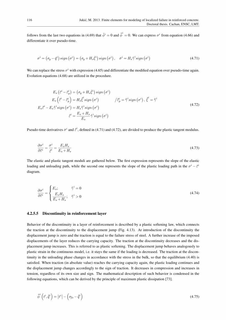
116 Jukic, M. 2013. Finite elements for modeling of localized failure in reinforced concrete.
Doctoral thesis. Cachan, ENSC, LMT.
follows from the last two equations in (4.69) that φi = 0 and ˙φi= 0. We can express σi from equation (4.66) and
differentiate it over pseudo-time.
σi =(σy − qi
)sign
(σi)=(σy +Hsξ
i)sign
(σi), σi =Hs ˙γisign
(σi)
(4.71)
We can replace the stress σi with expression (4.65) and differentiate the modified equation over pseudo-time again.
Evolution equations (4.68) are utilized in the procedure.
Es
(εi− εip
)=(σy +Hsξ
i)sign
(σi)
Es
(
˙εi− ˙εip
)
=Hs˙ξisign
(σi) /
˙εip = ˙γisign(σi), ˙ξ
i= ˙γi
Es ˙εi−Es ˙γisign(σi)=Hs ˙γisign
(σi)
˙εi =Es+Hs
Es
˙γisign(σi)
(4.72)
Pseudo-time derivatives σi and ˙εi, defined in (4.71) and (4.72), are divided to produce the plastic tangent modulus.
∂σi
∂εi=
σi
˙εi=
EsHs
Es+Hs(4.73)
The elastic and plastic tangent moduli are gathered below. The first expression represents the slope of the elastic
loading and unloading path, while the second one represents the slope of the plastic loading path in the σi − εi
diagram.
∂σi
∂εi=
Es; ˙γi = 0
EsHs
Es+Hs; ˙γi > 0
(4.74)
4.2.5.5 Discontinuity in reinforcement layer
Behavior of the discontinuity in a layer of reinforcement is described by a plastic softening law, which connects
the traction at the discontinuity to the displacement jump (Fig. 4.13). At introduction of the discontinuity the
displacement jump is zero and the traction is equal to the failure stress of steel. A further increase of the imposed
displacements of the layer reduces the carrying capacity. The traction at the discontinuity decreases and the dis-
placement jump increases. This is referred to as plastic softening. The displacement jump behaves analogously to
plastic strain in the continuous model, i.e. it stays the same if the loading is decreased. The traction at the discon-
tinuity in the unloading phase changes in accordance with the stress in the bulk, so that the equilibrium (4.40) is
satisfied. When traction (in absolute value) reaches the carrying capacity again, the plastic loading continues and
the displacement jump changes accordingly to the sign of traction. It decreases in compression and increases in
tension, regardless of its own size and sign. The mathematical description of such behavior is condensed in the
following equations, which can be derived by the principle of maximum plastic dissipation [73].
¯φi(
ti, ¯qi)
=∣∣ti∣∣−(
σfs− ¯qi)
(4.75)
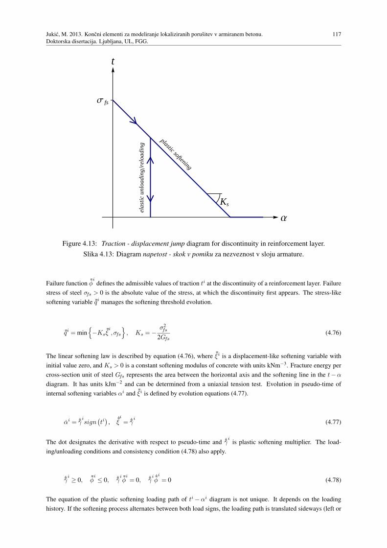
Jukic, M. 2013. Koncni elementi za modeliranje lokaliziranih porusitev v armiranem betonu.
Doktorska disertacija. Ljubljana, UL, FGG.
117
Ks
Α
t
Σ fs
elas
tic
unlo
adin
gre
load
ing
plastic softening
Figure 4.13: Traction - displacement jump diagram for discontinuity in reinforcement layer.
Slika 4.13: Diagram napetost - skok v pomiku za nezveznost v sloju armature.
Failure function ¯φi
defines the admissible values of traction ti at the discontinuity of a reinforcement layer. Failure
stress of steel σfs > 0 is the absolute value of the stress, at which the discontinuity first appears. The stress-like
softening variable ¯qi manages the softening threshold evolution.
¯qi = min
−Ks¯ξi,σfs
, Ks =−σ2fs
2Gfs(4.76)
The linear softening law is described by equation (4.76), where ¯ξi is a displacement-like softening variable with
initial value zero, and Ks > 0 is a constant softening modulus of concrete with units kNm−3. Fracture energy per
cross-section unit of steel Gfs represents the area between the horizontal axis and the softening line in the t−α
diagram. It has units kJm−2 and can be determined from a uniaxial tension test. Evolution in pseudo-time of
internal softening variables αi and ¯ξi is defined by evolution equations (4.77).
αi = ˙γisign
(ti)
,˙ξi
= ˙γi
(4.77)
The dot designates the derivative with respect to pseudo-time and ˙γi
is plastic softening multiplier. The load-
ing/unloading conditions and consistency condition (4.78) also apply.
˙γi≥ 0, ¯φ
i≤ 0, ˙γ
i ¯φi= 0, ˙γ
i ˙φi
= 0 (4.78)
The equation of the plastic softening loading path of ti −αi diagram is not unique. It depends on the loading
history. If the softening process alternates between both load signs, the loading path is translated sideways (left or

118 Jukic, M. 2013. Finite elements for modeling of localized failure in reinforced concrete.
Doctoral thesis. Cachan, ENSC, LMT.
right). The slope, however, is not affected and can be determined from the pseudo-time derivatives of ti and αi.
In softening process, when ˙γi> 0, the failure function ¯φ
i= 0. Expression for ti is then determined by (4.75) and
(4.76).
ti =(
σfs− ¯qi)
sign(ti)=
(
σfs+Ks¯ξi)
sign(ti)
; ¯qi < σfs
0; ¯qi = σfs
(4.79)
The derivative is obtained in accordance with evolution equation (4.77) for ¯ξi.
ti =
Ks˙ξi
sign(ti)=Ks
˙γisign
(ti)
; ¯qi < σfs
0; ¯qi = σfs(4.80)
The slope of the plastic softening loading path, defined as the derivative of ti over αi, is computed by dividing the
pseudo-time derivatives (4.80) and (4.77) of both quantities.
∂ti
∂αi=
ti
αi=
not defined; ˙γi= 0
Ks; ˙γi> 0, ¯qi < σfs
0; ˙γi> 0, ¯qi = σfs
(4.81)
A third option was added in equation (4.81). It corresponds to elastic unloading path with ˙γi= 0. It follows
from evolution equations (4.77) that αi = 0 in such case. And since the failure function ¯φi
is no longer required
to be zero, the traction ti cannot be computed as in (4.79). It changes in accordance with equation (4.40) which
represents the equilibrium between the bulk and the discontinuity. The fraction in (4.81) is not defined, but it is not
required in the computational procedure anyway.
4.3 Computational procedure
Response of a structure, discretized by a mesh of nFE above derived finite elements, is computed at discrete
pseudo-time points τ0, τ1, . . . , τn, τn+1, . . . , T by solving at each pseudo-time point nonlinear equations (4.82)
for current values of nodal displacements/rotations.
f int,str − f ext,str = 0
∀e ∈ 1,2, . . . ,nFE , ∀i ∈
1,2, . . . ,n(e)CL
: h(e),i = 0(4.82)
Here, n(e)CL is the number of cracked layers in element (e). At a particular pseudo-time point τn+1, the solution
is searched iteratively by the Newton-Raphson method. Each iteration, denoted by k, consists of two subsequent
phases: (A) computation of internal variables, corresponding to the current iterative values of nodal displace-
ments/rotations, in order to compute the stress in accordance with given material laws; (B) solution of linearized
equations (4.82) in order to update the iterative values of nodal displacements/rotations. When one phase of the
computation is completed, the results are used immediately in the next one.
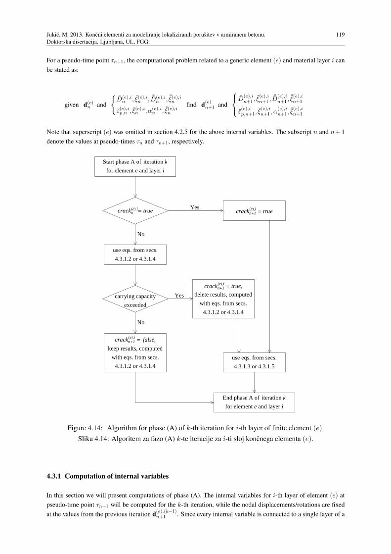
Jukic, M. 2013. Koncni elementi za modeliranje lokaliziranih porusitev v armiranem betonu.
Doktorska disertacija. Ljubljana, UL, FGG.
119
For a pseudo-time point τn+1, the computational problem related to a generic element (e) and material layer i can
be stated as:
given d(e)n and
D(e),in , ξ(e),in , ¯D(e),i
n , ¯ξ(e),in
ε(e),ip,n , ξ(e),in ,α(e),in , ¯ξ(e),in
find d(e)n+1 and
D(e),in+1 , ξ
(e),in+1 ,
¯D(e),in+1 ,
¯ξ(e),in+1
ε(e),ip,n+1, ξ
(e),in+1 ,α
(e),in+1 ,
¯ξ(e),in+1
Note that superscript (e) was omitted in section 4.2.5 for the above internal variables. The subscript n and n+ 1
denote the values at pseudo-times τn and τn+1, respectively.
Start phase A of iteration k
for element e and layer i
cracknHeL,i= true
use eqs. from secs.
4.3.1.2 or 4.3.1.4
carrying capacity
exceeded
crackn+1HeL,i= false,
keep results, computed
with eqs. from secs.
4.3.1.2 or 4.3.1.4
crackn+1HeL,i= true
crackn+1HeL,i= true,
delete results, computed
with eqs. from secs.
4.3.1.2 or 4.3.1.4
use eqs. from secs.
4.3.1.3 or 4.3.1.5
End phase A of iteration k
for element e and layer i
Yes
Yes
No
No
Figure 4.14: Algorithm for phase (A) of k-th iteration for i-th layer of finite element (e).
Slika 4.14: Algoritem za fazo (A) k-te iteracije za i-ti sloj koncnega elementa (e).
4.3.1 Computation of internal variables
In this section we will present computations of phase (A). The internal variables for i-th layer of element (e) at
pseudo-time point τn+1 will be computed for the k-th iteration, while the nodal displacements/rotations are fixed
at the values from the previous iteration d(e),(k−1)n+1 . Since every internal variable is connected to a single layer of a

120 Jukic, M. 2013. Finite elements for modeling of localized failure in reinforced concrete.
Doctoral thesis. Cachan, ENSC, LMT.
single finite element, the computations are local, i.e. they are performed independently for each element and each
layer. The condition of the discontinuity is known by the following flag.
crack(e),i =
false . . . no discontinuity in layer i
true . . . discontinuity in layer i(4.83)
The algorithm in Fig. 4.14 is applied. If there was no discontinuity in the layer in the previous pseudo-time step,
we begin with equations for the hardening phase of material, described in sections 4.3.1.2 for concrete and 4.3.1.4
for steel. We must do so even if the previous iteration of the current step indicated occurrence of the discontinuity,
because that was not a converged result. We check if the carrying capacity of the layer is exceeded. If not, we keep
the obtained results, otherwise we discard them and use equations for the softening phase of material, described in
sections 4.3.1.3 for concrete and 4.3.1.5 for steel. If the discontinuity already existed in the previous pseudo-time
step, it must also exist in the current step, therefore we follow the procedure from sections 4.3.1.3 or 4.3.1.5.
For the sake of clarity we will omit in the rest of this section the superscript (e), denoting the finite element, and
the superscript i, denoting the layer.
4.3.1.1 Shear response
Computation of the shear response is straightforward. Shear strain is computed according to equation (4.7) with
the current values of the nodal displacements. Shear stress is then calculated from (4.43).
γ(k)n+1 = B∗d
(k−1)n+1 , τ
i,(k)n+1 = cµiγ
(k)n+1,
∂ τ i
∂ γ
∣∣∣∣
(k)
n+1
= cµi (4.84)
4.3.1.2 Bulk of concrete layer
This section describes the computational procedure for the hardening phase of a concrete layer. The discontinuity
has not yet occurred and the displacement jump is zero. The computation is started by assuming an elastic step,
which means that hardening internal variables do not change, but keep the values from the previous step. Trial
value of stress is computed according to (4.45), with α(k)n+1 = 0.
D(k),trialn+1 = Dn, ξ
(k),trialn+1 = ξn, σ
(k),trialn+1 = D
(k),trial−1
n+1 ε(
d(k−1)n+1 ,α
(k)n+1
)
(4.85)
The trial damage function φ(k),trialn+1 is computed in accordance with equations (4.46) and (4.47).
φ(k),trialn+1 =
∣∣∣σ
(k),trialn+1
∣∣∣−(
σd− q(k),trialn+1
)
, q(k),trialn+1 =−Hcξ
(k),trialn+1 =−Hcξn (4.86)
The trial solution is accepted if the trial damage function is not positive.
φ(k),trialn+1 ≤ 0 ⇒ D
(k)n+1 = D
(k),trialn+1 , ξ
(k)n+1 = ξ
(k),trialn+1 , σ
(k)n+1 = σ
(k),trialn+1 (4.87)

Jukic, M. 2013. Koncni elementi za modeliranje lokaliziranih porusitev v armiranem betonu.
Doktorska disertacija. Ljubljana, UL, FGG.
121
Otherwise, the internal variables have to be corrected and the stress recomputed. Incremental form of evolution
equations (4.48) is applied, where γ(k)n+1 = ˙γ
(k)n+1 (τn+1 − τn) > 0. The use of sign
(
σ(k)n+1
)
= sign(
σ(k),trialn+1
)
is
justified in appendix A.
φ(k),trialn+1 > 0 ⇒ D
(k)n+1 = Dn+ γ
(k)n+1
sign(
σ(k),trialn+1
)
σ(k)n+1
, ξ(k)n+1 = ξn+ γ
(k)n+1 (4.88)
By using equations (4.88), the stress σ(k)n+1 and the stress-like hardening variable q
(k)n+1 can be expressed with their
trial values and the damage multiplier γ(k)n+1.
σ(k)n+1 = D
(k)−1
n+1 ε(
d(k−1)n+1 ,α
(k)n+1
)
D(k)n+1σ
(k)n+1 = ε
(
d(k−1)n+1 ,α
(k)n+1
)
= D(k),trialn+1 σ
(k),trialn+1
Dn+ γ(k)n+1
sign(
σ(k),trialn+1
)
σ(k)n+1
σ(k)n+1 = Dnσ
(k),trialn+1
Dnσ(k)n+1 + γ
(k)n+1sign
(
σ(k),trialn+1
)
= Dnσ(k),trialn+1
σ(k)n+1 = σ
(k),trialn+1 − D−1
n γ(k)n+1sign
(
σ(k),trialn+1
)
(4.89)
q(k)n+1 =−Hcξ
(k)n+1 =−Hc
(
ξn+ γ(k)n+1
)
= q(k),trialn+1 −Hcγ
(k)n+1 (4.90)
Equations (4.89) and (4.90) are used to express the damage function φ(k)n+1 as a function of damage multiplier γ
(k)n+1,
which is then computed from requirement φ(k)n+1 = 0, coming from loading/unloading conditions (4.49).
φ(k)n+1 =
∣∣∣σ
(k)n+1
∣∣∣−(
σd− q(k)n+1
)
=∣∣∣σ
(k),trialn+1
∣∣∣− D−1
n γ(k)n+1 −
(
σd− q(k),trialn+1
)
−Hcγ(k)n+1 =
= φ(k),trialn+1 −
(D−1
n +Hc
)γ(k)n+1
φ(k)n+1 = 0 ⇒ γ
(k)n+1 =
φ(k),trialn+1
D−1n +Hc
(4.91)
Consistent tangent modulus is computed as the derivative of stress over strain. Stress takes the trial value from
(4.85) if damage multiplier γ(k)n+1 is zero, and the value from (4.89) if γ
(k)n+1 is positive. In the second case, equations
(4.91), (4.86) and (4.85) are used to express the stress as a function of strain.
∂σ
∂ε
∣∣∣∣
(k)
n+1
=
D−1n ; γ
(k)n+1 = 0
D−1n Hc
D−1n +Hc
; γ(k)n+1 > 0
(4.92)
The hardening internal variables, stress and tangent modulus have been determined under assumption, that the
carrying capacity is not exceeded, which remains to be verified. If indeed the carrying capacity is not reached, the
results are accepted. In the opposite case, the results are discarded and computed again, taking into account the
newly appeared discontinuity.
122 Jukic, M. 2013. Finite elements for modeling of localized failure in reinforced concrete.
Doctoral thesis. Cachan, ENSC, LMT.
First, the potential value of traction at the discontinuity t(k),potn+1 is computed according to equation (4.40). Failure
function ¯φ(k),potn+1 is then evaluated with the stress-like softening variable ¯q
(k),potn+1 equal to zero, because there has
been no reduction of carrying capacity in previous steps.
t(k),potn+1 =−
∫
L
Gσ(k)n+1dx= σ
(k)n+1,
¯φ(k),potn+1 =
∣∣∣t(k),potn+1
∣∣∣−(
σfc− ¯q(k),potn+1
)
, ¯q(k),potn+1 = 0 (4.93)
The discontinuity flag is set to true if the failure function is positive, and to false otherwise. Note that the value
of the flag is not final, until the converged state is reached. It can change in following iterations.
¯φ(k),potn+1 ≤ 0 ⇒ crack
(e),in+1 = false
¯φ(k),potn+1 > 0 ⇒ crack
(e),in+1 = true
(4.94)
If the carrying capacity is exceeded ( ¯φ(k),potn+1 > 0), the above computed values of internal variables, stress and
tangent modulus are discarded for this iteration and computed anew as described in section 4.3.1.3.
4.3.1.3 Discontinuity in concrete layer
Here we describe the computational procedure for the softening phase of the concrete layer. The procedure is used
if the current value of discontinuity flag crack(e),in+1 = true. This is a consequence of either an existing discontinuity
in the previous step (crack(e),in = true), or exceeded ultimate stress in this iteration, as written in equation (4.94).
In both cases, the hardening internal variables take the last converged values, i.e. the values from the last step.
D(k)n+1 = Dn, ξ
(k)n+1 = ξn (4.95)
The computation is started by assuming an elastic step, which implies no change in the softening internal variables
in this iteration. We use the displacement-like softening variable ¯ξ∗, introduced in equation (4.60).
¯D(k),trialn+1 = ¯Dn,
¯ξ∗(k),trialn+1 = ¯ξ∗n (4.96)
The trial value of traction at the discontinuity is defined by equation (4.97). Derivation of the expression is shown
in appendix C. According to equation (4.40) it is equal to the trial stress. The trial value of displacement jump is
computed from equation (4.55).
t(k),trialn+1 = σ
(k),trialn+1 =
Bd(k−1)n+1
Dn− G ¯Dn
, α(k),trialn+1 = ¯Dnt
(k),trialn+1 (4.97)
Next, the trial value of failure function ¯φ(k),trialn+1 is computed, using expression (4.61) for the stress-like softening
variable ¯q(k),trialn+1 .
¯φ(k),trialn+1 =
∣∣∣t(k),trialn+1
∣∣∣−(
σfc− ¯q(k),trialn+1
)
, ¯q(k),trialn+1 = min
−K∗c
¯ξ∗(k),trialn+1 ,σfc
= ¯qn (4.98)
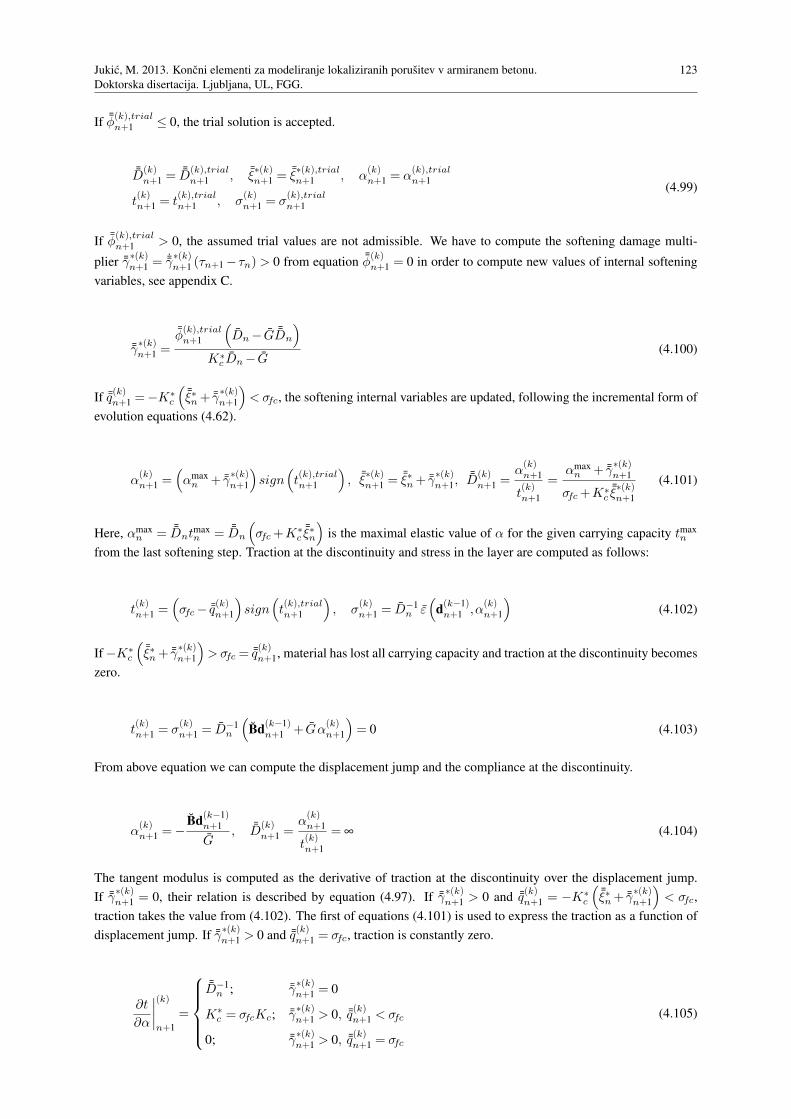
Jukic, M. 2013. Koncni elementi za modeliranje lokaliziranih porusitev v armiranem betonu.
Doktorska disertacija. Ljubljana, UL, FGG.
123
If ¯φ(k),trialn+1 ≤ 0, the trial solution is accepted.
¯D(k)n+1 =
¯D(k),trialn+1 , ¯ξ
∗(k)n+1 =
¯ξ∗(k),trialn+1 , α
(k)n+1 = α
(k),trialn+1
t(k)n+1 = t
(k),trialn+1 , σ
(k)n+1 = σ
(k),trialn+1
(4.99)
If ¯φ(k),trialn+1 > 0, the assumed trial values are not admissible. We have to compute the softening damage multi-
plier ¯γ∗(k)n+1 =
˙γ∗(k)n+1 (τn+1 − τn) > 0 from equation ¯φ
(k)n+1 = 0 in order to compute new values of internal softening
variables, see appendix C.
¯γ∗(k)n+1 =
¯φ(k),trialn+1
(
Dn− G ¯Dn
)
K∗c Dn− G
(4.100)
If ¯q(k)n+1 =−K∗
c
(¯ξ∗n+ ¯γ
∗(k)n+1
)
< σfc, the softening internal variables are updated, following the incremental form of
evolution equations (4.62).
α(k)n+1 =
(
αmaxn + ¯γ
∗(k)n+1
)
sign(
t(k),trialn+1
)
, ¯ξ∗(k)n+1 =
¯ξ∗n+ ¯γ∗(k)n+1,
¯D(k)n+1 =
α(k)n+1
t(k)n+1
=αmaxn + ¯γ
∗(k)n+1
σfc+K∗c
¯ξ∗(k)n+1
(4.101)
Here, αmaxn = ¯Dnt
maxn = ¯Dn
(
σfc+K∗c
¯ξ∗n
)
is the maximal elastic value of α for the given carrying capacity tmaxn
from the last softening step. Traction at the discontinuity and stress in the layer are computed as follows:
t(k)n+1 =
(
σfc− ¯q(k)n+1
)
sign(
t(k),trialn+1
)
, σ(k)n+1 = D−1
n ε(
d(k−1)n+1 ,α
(k)n+1
)
(4.102)
If −K∗c
(¯ξ∗n+ ¯γ
∗(k)n+1
)
>σfc = ¯q(k)n+1, material has lost all carrying capacity and traction at the discontinuity becomes
zero.
t(k)n+1 = σ
(k)n+1 = D−1
n
(
Bd(k−1)n+1 + Gα
(k)n+1
)
= 0 (4.103)
From above equation we can compute the displacement jump and the compliance at the discontinuity.
α(k)n+1 =−
Bd(k−1)n+1
G, ¯D
(k)n+1 =
α(k)n+1
t(k)n+1
= ∞ (4.104)
The tangent modulus is computed as the derivative of traction at the discontinuity over the displacement jump.
If ¯γ∗(k)n+1 = 0, their relation is described by equation (4.97). If ¯γ
∗(k)n+1 > 0 and ¯q
(k)n+1 = −K∗
c
(¯ξ∗n+ ¯γ
∗(k)n+1
)
< σfc,
traction takes the value from (4.102). The first of equations (4.101) is used to express the traction as a function of
displacement jump. If ¯γ∗(k)n+1 > 0 and ¯q
(k)n+1 = σfc, traction is constantly zero.
∂t
∂α
∣∣∣∣
(k)
n+1
=
¯D−1n ; ¯γ
∗(k)n+1 = 0
K∗c = σfcKc; ¯γ
∗(k)n+1 > 0, ¯q
(k)n+1 < σfc
0; ¯γ∗(k)n+1 > 0, ¯q
(k)n+1 = σfc
(4.105)
124 Jukic, M. 2013. Finite elements for modeling of localized failure in reinforced concrete.
Doctoral thesis. Cachan, ENSC, LMT.
Σ
Ε
Σfc
Σ trialn+1
Σn
Σn+1
Σd
Ε nΕ n+1 Ε n+1trial
Ec
Dn-1
n+1,trial
n+1n
t
Α
Σfc
tn+1trial
tntn+1
tnmax
Α n Α n+1trialΑ n+1
Α nmax
qn
Φn+1
trial
Dn-1
Dn+1-1
n+1,trial
n+1n
Figure 4.15: Stress in the bulk (left) and traction at the discontinuity (right) of a concrete layer: value
from the previous step (n), and trial and final values from the current step (n+1).
Slika 4.15: Napetost v sloju (levo) in v nezveznosti sloja betona (desno): vrednost iz prejsnjega koraka
(n) ter testna in koncna vrednost iz trenutnega koraka (n+1).
The discontinuity flag is set to crack(e),in+1 = true.
4.3.1.4 Bulk of reinforcement layer
The computational procedure for the hardening phase of the reinforcement layer is described next. There is no
discontinuity in the layer and the displacement jump is zero. First, we assume elastic behavior, meaning that
hardening internal variables keep the values from the previous step. Stress is computed in accordance with equation
(4.65), where α(k)n+1 = 0.
ε(k),trialp,n+1 = εp,n, ξ
(k),trialn+1 = ξn, σ
(k),trialn+1 = Es
(
ε(
d(k−1)n+1 ,α
(k)n+1
)
− ε(k),trialp,n+1
)
(4.106)
Trial yield function φ(k),trialn+1 is computed, as defined in (4.66) and (4.67).
φ(k),trialn+1 =
∣∣∣σ
(k),trialn+1
∣∣∣−(
σy − q(k),trialn+1
)
, q(k),trialn+1 =−Hsξ
(k),trialn+1 =−Hsξn (4.107)
The trial solution is accepted if the trial yield function is negative or zero.
φ(k),trialn+1 ≤ 0 ⇒ ε
(k)p,n+1 = ε
(k),trialp,n+1 , ξ
(k)n+1 = ξ
(k),trialn+1 , σ
(k)n+1 = σ
(k),trialn+1 (4.108)
If the trial yield function is positive, the internal variables must be corrected, according to incremental form of
evolution equations (4.68), where γ(k)n+1 = ˙γ
(k)n+1 (τn+1 − τn) > 0. It is shown in appendix A that sign
(
σ(k)n+1
)
=
Jukic, M. 2013. Koncni elementi za modeliranje lokaliziranih porusitev v armiranem betonu.
Doktorska disertacija. Ljubljana, UL, FGG.
125
sign(
σ(k),trialn+1
)
.
φ(k),trialn+1 > 0 ⇒ ε
(k)p,n+1 = εp,n+ γ
(k)n+1sign
(
σ(k),trialn+1
)
, ξ(k)n+1 = ξn+ γ
(k)n+1 (4.109)
By exploiting equations (4.109), the stress σ(k)n+1 and the stress-like hardening variable q
(k)n+1 can be expressed with
their trial values and the damage multiplier γ(k)n+1.
σ(k)n+1 = Es
(
ε(
d(k−1)n+1 ,α
(k)n+1
)
− ε(k)p,n+1
)
=
= Es
(
ε(
d(k−1)n+1 ,α
(k)n+1
)
− εp,n
)
−Esγ(k)n+1sign
(
σ(k),trialn+1
)
=
= σ(k),trialn+1 −Esγ
(k)n+1sign
(
σ(k),trialn+1
)
(4.110)
q(k)n+1 =−Hsξ
(k)n+1 =−Hs
(
ξn+ γ(k)n+1
)
= q(k),trialn+1 −Hsγ
(k)n+1 (4.111)
Yield function φ(k)n+1 is expressed as a function of plastic multiplier γ
(k)n+1 by employing equations (4.110) and
(4.111). Value of the plastic multiplier is computed from requirement φ(k)n+1 = 0.
φ(k)n+1 =
∣∣∣σ
(k)n+1
∣∣∣−(
σy − q(k)n+1
)
=∣∣∣σ
(k),trialn+1
∣∣∣−Esγ
(k)n+1 −
(
σy − q(k),trialn+1
)
−Hsγ(k)n+1 =
= φ(k),trialn+1 − (Es+Hs) γ
(k)n+1
φ(k)n+1 = 0 ⇒ γ
(k)n+1 =
φ(k),trialn+1
Es+Hs
(4.112)
Consistent tangent modulus is computed as the derivative of stress over strain. Stress takes the trial value from
equation (4.106) if plastic multiplier γ(k)n+1 is zero, and the value from (4.110) if γ
(k)n+1 is positive. In the second
case, equations (4.112), (4.107) and (4.106) are used to express the stress as a function of strain.
∂σ
∂ε
∣∣∣∣
(k)
n+1
=
Es; γ(k)n+1 = 0
EsHs
Es+Hs; γ
(k)n+1 > 0
(4.113)
The hardening internal variables, stress in the layer and the tangent modulus have been calculated under assumption
that the ultimate stress is not exceeded. This still requires verification. If the assumption is confirmed, the above
results are accepted. Otherwise, they are discarded and recomputed with the presence of the discontinuity, see
Fig. 4.14.
Potential value of traction at the discontinuity t(k),potn+1 is computed from equation (4.40). Then the failure function
¯φ(k),potn+1 is evaluated with the stress-like softening variable equal to zero, as there has been no reduction of carrying
capacity in previous steps.
t(k),potn+1 =−
∫
L
Gσ(k)n+1dx,
¯φ(k),potn+1 =
∣∣∣t(k),potn+1
∣∣∣−(
σfs− ¯q(k),potn+1
)
, ¯q(k),potn+1 = 0 (4.114)
126 Jukic, M. 2013. Finite elements for modeling of localized failure in reinforced concrete.
Doctoral thesis. Cachan, ENSC, LMT.
We set the value of the discontinuity flag to true if the failure function is positive, and to false otherwise. The
value is not final, however, until the converged state is reached. It can change in following iterations.
¯φ(k),potn+1 ≤ 0 ⇒ crack
(e),in+1 = false
¯φ(k),potn+1 > 0 ⇒ crack
(e),in+1 = true
(4.115)
If the carrying capacity is exceeded, the above computed values of internal hardening variables, stress in the layer
and traction at the discontinuity are discarded and computed again, as explained in the following section.
4.3.1.5 Discontinuity in reinforcement layer
This section describes the computational procedure for the softening phase of the reinforcement layer. It is applied
if the current value of the discontinuity flag crack(e),in+1 = true, which happens if the discontinuity already existed
in the previous step, or if the carrying capacity of the layer was exceeded in this iteration, see equation (4.115) and
Fig. 4.14. In any case, the hardening internal variables take the values from the previous step, which are the last
converged results. The error of such choice is negligible for small pseudo-time step.
ε(k)p,n+1 = εp,n, ξ
(k)n+1 = ξn (4.116)
We start by assuming a trial solution, keeping the softening internal variables at the values from the previous
step. Stress in the layer and traction at the discontinuity are computed according to equations (4.65) and (4.40),
respectively.
α(k),trialn+1 = αn,
¯ξ(k),trialn+1 = ¯ξn
σ(k),trialn+1 = Es
(
ε(
d(k−1)n+1 ,α
(k),trialn+1
)
− εp,n
)
, t(k),trialn+1 = σ
(k),trialn+1
(4.117)
The trial value of failure function ¯φ(k),trialn+1 is calculated, respecting equations (4.75) and (4.76).
¯φ(k),trialn+1 =
∣∣∣t(k),trialn+1
∣∣∣−(
σfs− ¯q(k),trialn+1
)
, ¯q(k),trialn+1 = min
−Ks¯ξ(k),trialn+1 ,σfs
= ¯qn (4.118)
If ¯φ(k),trialn+1 ≤ 0, the trial solution is accepted.
α(k)n+1 = α
(k),trialn+1 , ¯ξ
(k)n+1 =
¯ξ(k),trialn+1 , σ
(k)n+1 = σ
(k),trialn+1 , t
(k)n+1 = t
(k),trialn+1 (4.119)
If ¯φ(k),trialn+1 > 0, the assumed solution is not admissible. The softening internal variables are updated according to
the incremental form of evolution equations (4.77), where ¯γ(k)n+1 =
˙γ(k)n+1 (τn+1 − τn) > 0. It is shown in appendix
A that sign(
t(k)n+1
)
= sign(
t(k),trialn+1
)
.
α(k)n+1 = αn+ ¯γ
(k)n+1sign
(
t(k),trialn+1
)
, ¯ξ(k)n+1 =
¯ξn+ ¯γ(k)n+1 (4.120)

Jukic, M. 2013. Koncni elementi za modeliranje lokaliziranih porusitev v armiranem betonu.
Doktorska disertacija. Ljubljana, UL, FGG.
127
By using equations (4.120), the traction at the discontinuity t(k)n+1 and the stress-like softening variable ¯q
(k)n+1 are
expressed with their trial values and the softening multiplier ¯γ(k)n+1.
t(k)n+1 = σ
(k)n+1 = Es
(
Bd(k−1)n+1 + Gα
(k)n+1 − εp,n
)
=
= Es
(
Bd(k−1)n+1 + Gαn− εp,n
)
+EsG ¯γ(k)n+1sign
(
t(k),trialn+1
)
=
= t(k),trialn+1 +EsG ¯γ
(k)n+1sign
(
t(k),trialn+1
)
(4.121)
¯q(k)n+1 =
¯qAn+1 = ¯q(k),trialn+1 −Ks ¯γ
(k)n+1; −Ks
(¯ξn+ ¯γA
n+1
)
< σfs
¯qBn+1 = σfs; −Ks
(¯ξn+ ¯γA
n+1
)
> σfs(4.122)
Obtained expressions are inserted in equation ¯φ(k)n+1 = 0, coming from loading/unloading conditions (4.78).
¯φ(k)n+1 =
∣∣∣t(k)n+1
∣∣∣−(
σfs− ¯q(k)n+1
)
= 0 ⇔ t(k)n+1 =
(
σfs− ¯q(k)n+1
)
sign(
t(k),trialn+1
)
(4.123)
After a short derivation we get two expressions for ¯γ(k)n+1, depending on the expression, used for ¯q
(k)n+1.
¯γ(k)n+1 =
¯γAn+1 =
¯φ(k),trialn+1
−GEs+Ks; −Ks
(¯ξn+ ¯γA
n+1
)
< σfs
¯γBn+1 =
∣∣∣t(k),trialn+1
∣∣∣
−GEs; −Ks
(¯ξn+ ¯γA
n+1
)
≥ σfs
(4.124)
The tangent modulus is computed as the derivative of traction at the discontinuity over the displacement jump. If
¯γ(k)n+1 > 0, traction takes the value from (4.123). Equations (4.122) and (4.120) are used to express the traction as
a function of displacement jump. If ¯γ(k)n+1 = 0, the displacement jump remains constant, while the traction changes
to satisfy the local equilibrium with stress in the layer. The tangent modulus cannot be determined, but it is not
required in further computation.
∂t
∂α
∣∣∣∣
(k)
n+1
=
not defined; ¯γ(k)n+1 = 0
Ks; ¯γ(k)n+1 > 0, ¯q
(k)n+1 < σfs
0; ¯γ(k)n+1 > 0, ¯q
(k)n+1 = σfs
(4.125)
The discontinuity flag is set to crack(e),in+1 = true.
4.3.2 Computation of nodal degrees of freedom
In this section we will describe the computations of phase (B) of k-th iteration, mentioned in the introduction of
section 4.3. In this phase, a linearized form of equilibrium equations (4.82) is solved to provide the k-th update
of the nodal displacements/rotations at pseudo-time point τn+1. The computation is performed with known values
of internal variables for each layer of each finite element - D(e),i,(k)n+1 , ξ
(e),i,(k)n+1 , ¯D
(e),i,(k)n+1 , ¯ξ
(e),i,(k)n+1 for a concrete

128 Jukic, M. 2013. Finite elements for modeling of localized failure in reinforced concrete.
Doctoral thesis. Cachan, ENSC, LMT.
layer, and ε(e),i,(k)p,n+1 , ξ
(e),i,(k)n+1 , α
(e),i,(k)n+1 , ¯ξ
(e),i,(k)n+1 for a layer of reinforcement - freshly updated in preceding phase
(A) of the same iteration. Since the nodal degrees of freedom are generally common to several finite elements,
the equations of phase (B) must be handled on structural (global) level. Hence, they are also referred to as global
equations.
The first of equations (4.82) would be sufficient for calculating the new values of generalized displacements d(e),(k)n+1 ,
if all displacement jumps α(e),i,(k)n+1 were fixed at the values, computed in phase (A). To improve convergence, how-
ever, it is useful to update the displacement jumps as well. For that purpose, the second of equations (4.82)
are engaged. Actually, they have once already been satisfied by using expression (4.40) for the traction at the
discontinuity, but that equality held for the displacements from the previous iteration d(e),(k−1)n+1 . Updating the dis-
placements would disrupt the equilibrium between the traction at the discontinuity and the stress in the layer, unless
the displacement jumps are updated as well. Solving the whole system of equations (4.82) therefore promises a
more accurate solution.
4.3.2.1 Linearization of equilibrium equations
The first of equations (4.82) ensures the equilibrium of the structure, i.e. of its each and every node. It is linearized
around the current values of nodal degrees of freedom of the structure dstr,(k−1)n+1 .
∂fint,str,(k)n+1
∂dstr,(k−1)n+1
︸ ︷︷ ︸
Kstr,(k)n+1
∆dstr,(k)n+1 = f
ext,strn+1 − f
int,str,(k)n+1 ,
∂fext,strn+1
∂dstr,(k−1)n+1
= 0 (4.126)
The derivative on the left side of the equation is designated with Kstr,(k)n+1 and named the tangent stiffness matrix of
the structure. ∆dstr,(k)n+1 is the sought update of the nodal displacements in this iteration. The vector of external forces
fext,strn+1 represents the loading, which is defined in advance for each pseudo-time point τn+1 and is independent of
the nodal displacements. The vector of internal forces fint,str,(k)n+1 is computed from contributions of individual finite
elements, according to equation (4.25). Matrices P(e) and R(e) are constant.
fint,str,(k)n+1 =
nFE
∑e=1
P(e)T R(e)−1
fint,(e),(k)n+1
Kstr,(k)n+1 =
∂fint,str,(k)n+1
∂dstr,(k−1)n+1
=nFE
∑e=1
P(e)T R(e)−1 ∂fint,(e),(k)n+1
∂dstr,(k−1)n+1
(4.127)
Let us recall the relation (4.18) between the vector of nodal displacements of a finite element d(e),(k−1)n+1 and the
vector of nodal displacements of the structure dstr,(k−1)n+1 . The derivative of one over the other will prove useful.
d(e),(k−1)n+1 = R(e)P(e)d
str,(k−1)n+1 ⇒
∂d(e),(k−1)n+1
∂dstr,(k−1)n+1
= R(e)P(e) (4.128)
Internal forces fint,(e),(k)n+1 of finite element (e) are defined in equation (4.34) as a sum of contributions of nL
layers. Contributions fint,(e),i,(k)n+1 of the n
(e)CL cracked layers are functions of nodal displacements d
(e),(k−1)n+1 and
displacement jumps α(e),i,(k)n+1 , while the contributions of the remaining (non-cracked) layers depend solely on the

Jukic, M. 2013. Koncni elementi za modeliranje lokaliziranih porusitev v armiranem betonu.
Doktorska disertacija. Ljubljana, UL, FGG.
129
nodal displacements. For the sake of clarity it is assumed that the cracked layers are numbered with consecutive
numbers from 1 to n(e)CL.
fint,(e),(k)n+1 =
nL
∑i=1
fint,(e),i,(k)n+1 =
n(e)CL
∑i=1
fint,(e),i,(k)n+1
(
d(e),(k−1)n+1 ,α
(e),i,(k)n+1
)
+nL
∑i=n
(e)CL
+1
fint,(e),i,(k)n+1
(
d(e),(k−1)n+1
)
(4.129)
The derivative of fint,(e),(k)n+1 over d
str,(k−1)n+1 , which appears in expression (4.127), is developed as follows:
∂fint,(e),(k)n+1
∂dstr,(k−1)n+1
=
n(e)CL
∑i=1
∂fint,(e),i,(k)n+1
∂d(e),(k−1)n+1
︸ ︷︷ ︸
Kfd,(e),i,(k)n+1
+∂f
int,(e),i,(k)n+1
∂α(e),i,(k)n+1
︸ ︷︷ ︸
Kfα,(e),i,(k)n+1
∂α(e),i,(k)n+1
∂d(e),(k−1)n+1
R(e)P(e)
︷ ︸︸ ︷
∂d(e),(k−1)n+1
∂dstr,(k−1)n+1
+nL
∑i=n
(e)CL
+1
Kfd,(e),i,(k)n+1
︷ ︸︸ ︷
∂fint,(e),i,(k)n+1
∂d(e),(k−1)n+1
R(e)P(e)
︷ ︸︸ ︷
∂d(e),(k−1)n+1
∂dstr,(k−1)n+1
(4.130)
The derivatives of fint,(e),i,(k)n+1 , marked with K
fd,(e),i,(k)n+1 and K
fα,(e),i,(k)n+1 , can be computed and the last term of both
sums has been defined in (4.128). The only unknown term ∂α(e),i,(k)n+1 /∂d
(e),(k−1)n+1 is determined by the second of
equilibrium equations (4.82), which is linearized and solved locally, i.e. independently for each finite element and
layer. This can be done because h(e),i,(k)n+1 depends on the nodal displacements of a single finite element and on the
displacement jump of a single layer.
∂h(e),i,(k)n+1
∂d(e),(k−1)n+1
︸ ︷︷ ︸
Khd,(e),i,(k)n+1
∆d(e),(k)n+1 +
∂h(e),i,(k)n+1
∂α(e),i,(k)n+1
︸ ︷︷ ︸
Khα,(e),i,(k)n+1
∆α(e),i,(k)n+1 =−h
(e),i,(k)n+1 = 0 ⇒
⇒ ∆α(e),i,(k)n+1 =−
(
Khα,(e),i,(k)n+1
)−1
Khd,(e),i,(k)n+1
︸ ︷︷ ︸
∂α(e),i,(k)n+1 /∂d
(e),(k−1)n+1
∆d(e),(k)n+1
(4.131)
Note that each h(e),i,(k)n+1 , computed by (4.39), evaluates to zero because the traction at the discontinuity t
(e),i,(k)n+1
has been computed by expression (4.40). The derivatives, designated with Khd,(e),i,(k)n+1 and K
hα,(e),i,(k)n+1 can be
easily calculated. Equation (4.131) defines the relation between the increment of nodal displacements ∆d(e),(k)n+1
and the increment of displacement jump ∆α(e),i,(k)n+1 in the i-th layer of the finite element. Since we are dealing with
linearized equations, the derivative ∂α(e),i,(k)n+1 /∂d
(e),(k−1)n+1 is equal to the ratio of the increments.
∂α(e),i,(k)n+1
∂d(e),(k−1)n+1
=−(
Khα,(e),i,(k)n+1
)−1
Khd,(e),i,(k)n+1 (4.132)
130 Jukic, M. 2013. Finite elements for modeling of localized failure in reinforced concrete.
Doctoral thesis. Cachan, ENSC, LMT.
We can rewrite expression (4.130), now being able to compute all its components.
∂fint,(e),(k)n+1
∂dstr,(k−1)n+1
=
n(e)CL
∑i=1
(
Kfd,(e),i,(k)n+1 −K
fα,(e),i,(k)n+1
(
Khα,(e),i,(k)n+1
)−1
Khd,(e),i,(k)n+1
)
︸ ︷︷ ︸
K(e),i,(k)n+1
R(e)P(e)+
+nL
∑i=n
(e)CL
+1
Kfd,(e),i,(k)n+1 R(e)P(e)
(4.133)
The expression in parenthesis, marked with K(e),i,(k)n+1 , is the contribution of a cracked layer to the tangent stiffness
matrix of finite element Kfd,(e),i,(k)n+1 is the contribution of an non-cracked layer. Finally, we can assemble the
tangent stiffness matrix of the structure by inserting (4.133) into (4.127).
Kstr,(k)n+1 =
nFE
∑e=1
P(e)T R(e)−1
n(e)CL
∑i=1
K(e),i,(k)n+1 +
nL
∑i=n
(e)CL
+1
Kfd,(e),i,(k)n+1
︸ ︷︷ ︸
K(e),(k)n+1
R(e)P(e) (4.134)
Here K(e),(k)n+1 is the (symmetric) tangent stiffness matrix of finite element (e).
4.3.2.2 Components of internal forces and stiffness matrix
Contribution fint,(e),i,(k)n+1 of i-th layer to internal forces of element (e) is computed according to equation (4.34),
where stress takes the values computed in phase (A) of this iteration. In order to determine the components of the
stiffness matrix, h(e),i,(k)n+1 must be written as well. It is computed in accordance with (4.39) and (4.40).
fint,(e),i,(k)n+1 =
(
BiTσ(e),i,(k)n+1 + B∗Tτ
(e),i,(k)n+1
)
AiL, h(e),i,(k)n+1 =Ai
(
−σ(e),i,(k)n+1 + t
(e),i,(k)n+1
)
(4.135)
To obtain layer components of the element stiffness matrix, expressions (4.135) are differentiated over nodal de-
grees of freedom and over displacement jumps.
Kfd,(e),i,(k)n+1 =
∂fint,(e),i,(k)n+1
∂d(e),(k−1)n+1
=
BiT ∂σ
∂ε
∣∣∣∣
(e),i,(k)
n+1
Bi︸︷︷︸
∂ε/∂d
+ B∗T ∂τ
∂γ
∣∣∣∣
(e),i,(k)
n+1
B∗︸︷︷︸
∂γ/∂d
AiL
Kfα,(e),i,(k)n+1 =
∂fint,(e),i,(k)n+1
∂α(e),i,(k)n+1
=
BiT ∂σ
∂ε
∣∣∣∣
(e),i,(k)
n+1
Gi︸︷︷︸
∂ε/∂α
AiL
Khd,(e),i,(k)n+1 =
∂h(e),i,(k)n+1
∂d(e),(k−1)n+1
=
−∂σ
∂ε
∣∣∣∣
(e),i,(k)
n+1
Bi︸︷︷︸
∂ε/∂d
Ai
Khα,(e),i,(k)n+1 =
∂h(e),i,(k)n+1
∂α(e),i,(k)n+1
=
−∂σ
∂ε
∣∣∣∣
(e),i,(k)
n+1
Gi︸︷︷︸
∂ε/∂α
+∂t
∂α
∣∣∣∣
(e),i,(k)
n+1
Ai
(4.136)
Jukic, M. 2013. Koncni elementi za modeliranje lokaliziranih porusitev v armiranem betonu.
Doktorska disertacija. Ljubljana, UL, FGG.
131
The tangent modulus (∂τ/∂γ )(e),i,(k)n+1 for shear is defined by equation (4.84). The tangent moduli (∂σ/∂ε )
(e),i,(k)n+1
and (∂t/∂α )(e),i,(k)n+1 are defined by equations (4.92) and (4.105) for concrete, and by equations (4.113) and (4.125)
for reinforcement.
The only exception is the elastic step in a cracked layer of reinforcement (when ¯γ(k)n+1 = 0). The derivative
(∂t/∂α )(e),i,(k)n+1 is not defined in that case, neither is it required. Although α
(e),i,(k)n+1 appears in the expression
for internal forces, it appears as a constant, and fint,(e),i,(k)n+1 is function of nodal displacements d
str,(k−1)n+1 alone. The
component Kfα,(e),i,(k)n+1 from equation (4.130) is therefore zero for that layer, and the contribution of the layer to
the element tangent stiffness matrix consists solely of the part Kfd,(e),i,(k)n+1 , the same as for a non-cracked layer.
α(e),i,(k)n+1 = const. ⇒ f
int,(e),i,(k)n+1 = f
int,(e),i,(k)n+1
(
dstr,(k−1)n+1
)
⇒
Kfα,(e),i,(k)n+1 = 0
K(e),i,(k)n+1 = K
fd,(e),i,(k)n+1
(4.137)
4.3.2.3 Solution of global equations
The system of global equilibrium equations (4.126) is rewritten in a clearer form.
Kstr,(k)n+1 ∆d
str,(k)n+1 = ∆f
str,(k)n+1 , ∆f
str,(k)n+1 = f
ext,strn+1 − f
int,str,(k)n+1 (4.138)
The external forces are an input to the analysis, internal forces are defined by equations (4.127), (4.129) and
(4.135), and the tangent stiffness matrix of the structure is defined by (4.134) and (4.136). Finally, we can compute
the increments and update the nodal displacements of the structure.
∆dstr,(k)n+1 =
(
Kstr,(k)n+1
)−1
∆fstr,(k)n+1 , d
str,(k)n+1 = d
str,(k−1)n+1 +∆d
str,(k)n+1 (4.139)
The updates of the displacement jumps could be computed from (4.131), but there is no benefit from that because
they will be recomputed anyway in phase (A) of the next iteration.
The iterations at pseudo-time τn+1 are repeated until the tolerance requirements are met.
∥∥∥∆f
str,(k)n+1
∥∥∥< tol,
∥∥∥∆d
str,(k)n+1
∥∥∥< tol (4.140)
When the converged solution is found, we proceed to the next pseudo-time step.
4.4 Numerical examples
In this section we present a set of numerical examples to assess the ability of the derived element to simulate failure
of reinforced concrete beams and frames. The element has been programmed in AceGen [68] implemented into
the finite element program AceFEM [69].
4.4.1 One element tension and compression tests
We analyze a beam in Fig. 4.16, clamped at one end and subjected to prescribed axial displacement u at the other
end. Corresponding reaction F is computed. With this test, we check response of concrete, steel and reinforced
132 Jukic, M. 2013. Finite elements for modeling of localized failure in reinforced concrete.
Doctoral thesis. Cachan, ENSC, LMT.
beams in tension and compression. The chosen values of some material parameters may be unrealistic, but they
were chosen in order to clearly present the behavior of models used for concrete and steel.
xL
F
CONCRETE
b
h
STEEL
AS,2
AS,1
REINF. CONC.
aS,1
aS,2
Figure 4.16: Beam in pure tension/compression: geometry.
Slika 4.16: Nosilec v cistem nategu/tlaku: geometrija.
4.4.1.1 Concrete beam
Concrete beam of rectangular cross-section is modeled with one element with two layers. The imposed axial dis-
placement produces either tension or compression. The geometry and the material data are: beam length is L =
2.5m, cross-section width is b = 0.2m, cross-section height is h = 0.5m, elastic modulus is Ec = 4×10⁷kNm−2,
elasticity limit in compression is σdc = 40820kNm−2, limit strength in compression is σfcc = 44902kNm−2, hard-
ening modulus in compression is Hcc = 2 × 10⁶kNm−2, softening modulus in compression is K∗cc = −5.2 ×
106kNm−3, limit strength in tension is σfct = 4000kNm−2, and softening modulus in tension is K∗ct = −8 ×
106kNm−3. By setting σdt > σfct we assume no damage of the bulk in tension before crack formation.
The diagrams in Fig. 4.17 show computed elasto-damage relations between the end force F and the end displace-
ment u when the beam is either in tension or compression. The left image represents the tensile response, which is
linear elastic, followed by linear softening. Unloading lines return toward the origin, which is typical for a damage
model. The right image shows the response in compression. Initial elastic part is followed by damage hardening,
which is not linear (although not far from it for this particular data). The softening line is linear. Unloading, both
from hardening and softening, returns linearly toward the origin.
0.0001 0.0003 0.0005 0.0007u @mD
100
200
300
400F @kND
0.001 0.003 0.005 0.007 0.009u @mD
1000
2000
3000
4000
F @kND
Figure 4.17: Axial force - displacement diagrams for concrete beam in pure tension (left) and pure
compression (right).
Slika 4.17: Diagram osna sila - pomik za betonski nosilec v cistem nategu (levo) in cistem tlaku (desno).
Response is characterized by the following facts: (i) single strain-like internal variable ¯ξic controls softening both in
tension and compression, (ii) current values of compliance moduli (Di and ¯Di) are transferred from compression
Jukic, M. 2013. Koncni elementi za modeliranje lokaliziranih porusitev v armiranem betonu.
Doktorska disertacija. Ljubljana, UL, FGG.
133
to tension and vice versa, (iii) once softening is activated, the hardening variables Di and ξic remain unchanged. Of
course, the elasto-damage concrete material model can be carefully designed to comply with specific experimental
results, however, this is beyond the scope of this work. The results in Fig. 4.18 and Fig. 4.19 illustrate that the
present elasto-damage material model is able to describe well enough the common cases of alternating load sign,
although it has not been designed for cyclic loading.
u
F
u
F
Figure 4.18: Axially loaded concrete beam: switching from softening in tension to compression (left)
and back to tension (right).
Slika 4.18: Osno obremenjen betonski nosilec: prehod iz mehcanja v nategu v tlak (levo) in nazaj v
nateg (desno).
u
F
u
F
u
F
Figure 4.19: Axially loaded concrete beam: switching from hardening in compression to tension (left)
and back to compression (middle). Switching from softening in compression to tension (right).
Slika 4.19: Osno obremenjen betonski nosilec: prehod iz utrjevanja v tlaku v nateg (levo) in nazaj v tlak
(sredina). Prehod iz mehcanja v tlaku v nateg (desno).
Behavior of implemented model for a beam switching from tension to compression (or from compression to
tension) is shown in Fig. 4.18 and Fig. 4.19. On these figures, the light-gray line represents F − u curves for
monotonically increasing tensile and compressive forces. The used data is the same as the above, except for
σfct = 2×10⁴kNm−2. Fig. 4.18 (left) shows transition from softening in tension to softening in compression. This
situation is very uncommon in non-cyclic loading. It may happen that a layer that was in tension softening becomes
compressed (e.g. when the neutral axis of the element shifts), however, the compressive stress would normally be
far away from the compressive strength. The case, shown in Fig. 4.18 (right), is far more common. Fig. 4.19 shows
transition from compression to tension. For example, Fig. 4.19 (right) presents path from compression softening
to tension: since σfct is much lower than σfcc, the carrying capacity in tension is lost due to ¯ξic accumulated in
compression.

134 Jukic, M. 2013. Finite elements for modeling of localized failure in reinforced concrete.
Doctoral thesis. Cachan, ENSC, LMT.
4.4.1.2 Steel beam
Steel beam is modeled with one element with two layers. The following data is used: beam length is L =
2.5m, cross-sections of both layers are As,1 = As,2 = 0.001m2, distances of layer axes from the beam axis are
h/2− as,1 = h/2− as,2 = 0.21m (as,1 = as,2 = 0.04m), elastic modulus is Es = 2×10⁸kNm−2, elasticity limit is
σy = 4×10⁵kNm−2, failure strength is σfs = 5×10⁵kNm−2, hardening modulus is Hs = 107kNm−2, and softening
modulus is Ks =−5×10⁷kNm−3.
Diagram in Fig. 4.20 shows elasto-plastic relation between the end force F and the end displacement u in tension.
The initial linear elastic response is followed by linear plastic hardening and linear plastic softening with unloading
lines, parallel to the initial loading line. Response of the beam in compression is identical.
0.01 0.02 0.03 0.04u @mD
200
400
600
800
1000
F @kND
Figure 4.20: Axial force - displacement diagram for steel beam (layer) in pure tension.
Slika 4.20: Diagram osna sila - pomik za jekleni nosilec (sloj) v cistem nategu.
The diagrams in Fig. 4.21 show response of the beam when loading switches from tension to compression. The
light grey lines represent the response of a monotonically loaded beam. The left image is characteristic for isotropic
hardening - material yields in compression at the same (absolute) value of F , at which unloading started in tension.
If loading is still increased in compression, as shown in the middle image of Fig. 4.21, softening occurs at the same
force F as in monotonic loading, but at a smaller displacement u, due to accumulation of plastic deformations in
both tension and compression. Change of load sign in softening, Fig. 4.21 (right), produces an equivalent response
- unloading is parallel to the elastic loading, and softening in compression begins at the same (absolute) value of
F , at which unloading started in tension.
u
F
u
F
u
F
Figure 4.21: Axially loaded steel beam: switching from hardening in tension to compression (left) and
back to tension (middle). Switching from softening in tension to compression (right).
Slika 4.21: Osno obremenjen jekleni nosilec: prehod iz utrjevanja v nategu v tlak (levo) in nazaj v nateg
(sredina). Prehod iz mehcanja v nategu v tlak (desno).

Jukic, M. 2013. Koncni elementi za modeliranje lokaliziranih porusitev v armiranem betonu.
Doktorska disertacija. Ljubljana, UL, FGG.
135
4.4.1.3 Reinforced concrete beam
Reinforced concrete beam is composed from the two previously presented beams, see Fig. 4.16. Geometry and
material properties are listed in sections 4.4.1.1 and 4.4.1.2. The beam is modeled with one finite element with ten
concrete layers and two layers of reinforcement. Diagrams in Fig. 4.22 display the responses of the beam under
tensile and compressive load. In tension (left image), the first peak represents the point when concrete enters the
softening phase and the force F begins to drop. When the concrete breaks completely, the whole load is taken by
the two reinforcement layers, which are still elastic. Force F starts rising again. Hereafter, the diagram is equal to
the response of the steel beam in Fig. 4.20.
The diagram in Fig. 4.22 (right) shows the response of the beam in compression. After the initial elastic part, the
stiffness of the beam drops around F = 4500kN due to micro-cracking of concrete, and again at approximately
F = 5000kN due to yielding of reinforcement. The peak of the diagram marks the moment when concrete begins
to soften. Force F drops suddenly, until concrete loses all carrying capacity and only the reinforcement remains to
take the load. From now on, the diagram is the same as in Fig. 4.20. The unloading lines return toward the origin,
until reinforcement enters hardening phase and first plastic deformations occur. The slope of the unloading lines
(axial stiffness of the element) keeps decreasing until the stress in concrete drops to zero. Afterwards it remains
constant and only plastic deformations increase. Like in tension, the diagram is a superposition of diagrams of
concrete (Fig. 4.17) and steel (Fig. 4.20).
0.01 0.02 0.03 0.04u @mD
200
400
600
800
1000
F @kND
0.01 0.02 0.03 0.04u @mD
1000
2000
3000
4000
5000
F @kND
Figure 4.22: Axial force - displacement diagrams for reinforced concrete beam in pure tension (left)
and pure compression (right).
Slika 4.22: Diagram osna sila - pomik za armiranobetonski nosilec v cistem nategu (levo) in cistem
tlaku (desno).
4.4.2 Cantilever beam under end moment
We analyze a reinforced concrete cantilever beam with rectangular cross-section under end moment, shown in
Fig. 4.23. The load is applied by imposing the rotation at the free end of the beam. The length of the beam is
L= 1m, the width and the height of the cross-section are b= 0.3m and h= 0.4m. Bottom and top reinforcements
are As,1 = As,2 = 0.001256m2 and they are positioned at a1 = a2 = 0.05m from the edges of the concrete cross-
section. Material properties of concrete are: elasticity modulus Ec = 3.3 × 10⁷kNm−2, elasticity limit σdc =
15200kNm−2, ultimate stress in compression σfcc = 38000kNm−2, ultimate stress in tension σfct = 1815kNm−2,
hardening modulus in compression Hcc = 3.32 × 10⁷kNm−2, softening modulus in compression K∗cc = −5 ×
106kNm−3 and softening modulus in tension K∗ct = −106kNm−3. Material properties of steel are: elasticity
modulus Es = 2× 10⁸kNm−2, yield stress σy = 4× 10⁵kNm−2, ultimate stress σfs = 5× 10⁵kNm−2, hardening
modulus Hs = 2.665×10⁶kNm−2 and softening modulus Ks =−5×10⁷kNm−3.
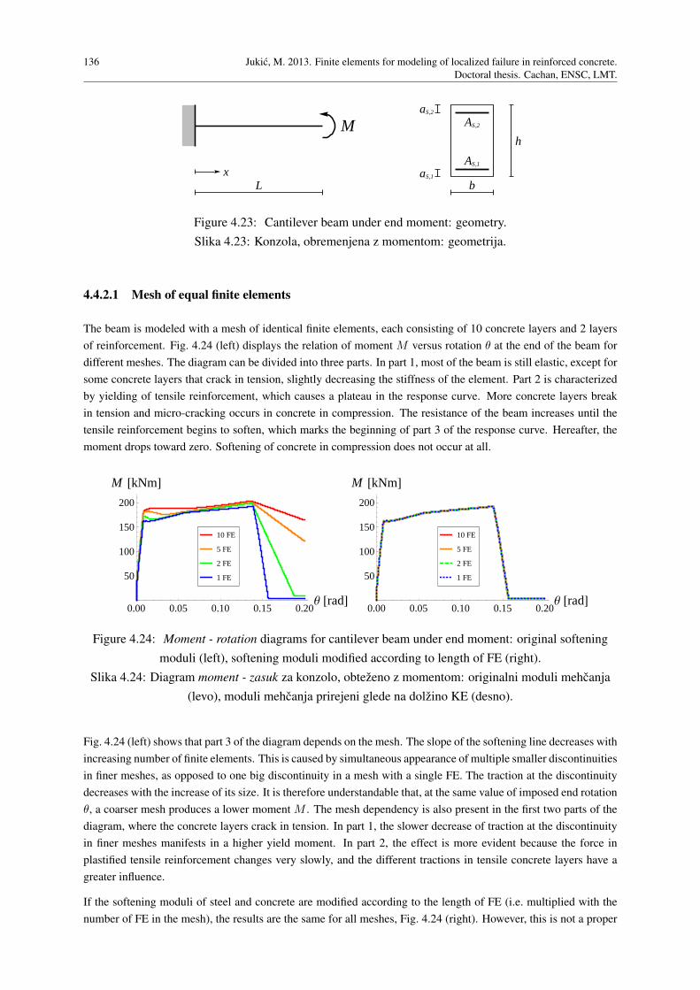
136 Jukic, M. 2013. Finite elements for modeling of localized failure in reinforced concrete.
Doctoral thesis. Cachan, ENSC, LMT.
xL
M
b
h
AS,2
AS,1
aS,1
aS,2
Figure 4.23: Cantilever beam under end moment: geometry.
Slika 4.23: Konzola, obremenjena z momentom: geometrija.
4.4.2.1 Mesh of equal finite elements
The beam is modeled with a mesh of identical finite elements, each consisting of 10 concrete layers and 2 layers
of reinforcement. Fig. 4.24 (left) displays the relation of moment M versus rotation θ at the end of the beam for
different meshes. The diagram can be divided into three parts. In part 1, most of the beam is still elastic, except for
some concrete layers that crack in tension, slightly decreasing the stiffness of the element. Part 2 is characterized
by yielding of tensile reinforcement, which causes a plateau in the response curve. More concrete layers break
in tension and micro-cracking occurs in concrete in compression. The resistance of the beam increases until the
tensile reinforcement begins to soften, which marks the beginning of part 3 of the response curve. Hereafter, the
moment drops toward zero. Softening of concrete in compression does not occur at all.
0.00 0.05 0.10 0.15 0.20Θ @radD
50
100
150
200
M @kNmD
1 FE
2 FE
5 FE
10 FE
0.00 0.05 0.10 0.15 0.20Θ @radD
50
100
150
200
M @kNmD
1 FE
2 FE
5 FE
10 FE
Figure 4.24: Moment - rotation diagrams for cantilever beam under end moment: original softening
moduli (left), softening moduli modified according to length of FE (right).
Slika 4.24: Diagram moment - zasuk za konzolo, obtezeno z momentom: originalni moduli mehcanja
(levo), moduli mehcanja prirejeni glede na dolzino KE (desno).
Fig. 4.24 (left) shows that part 3 of the diagram depends on the mesh. The slope of the softening line decreases with
increasing number of finite elements. This is caused by simultaneous appearance of multiple smaller discontinuities
in finer meshes, as opposed to one big discontinuity in a mesh with a single FE. The traction at the discontinuity
decreases with the increase of its size. It is therefore understandable that, at the same value of imposed end rotation
θ, a coarser mesh produces a lower moment M . The mesh dependency is also present in the first two parts of the
diagram, where the concrete layers crack in tension. In part 1, the slower decrease of traction at the discontinuity
in finer meshes manifests in a higher yield moment. In part 2, the effect is more evident because the force in
plastified tensile reinforcement changes very slowly, and the different tractions in tensile concrete layers have a
greater influence.
If the softening moduli of steel and concrete are modified according to the length of FE (i.e. multiplied with the
number of FE in the mesh), the results are the same for all meshes, Fig. 4.24 (right). However, this is not a proper
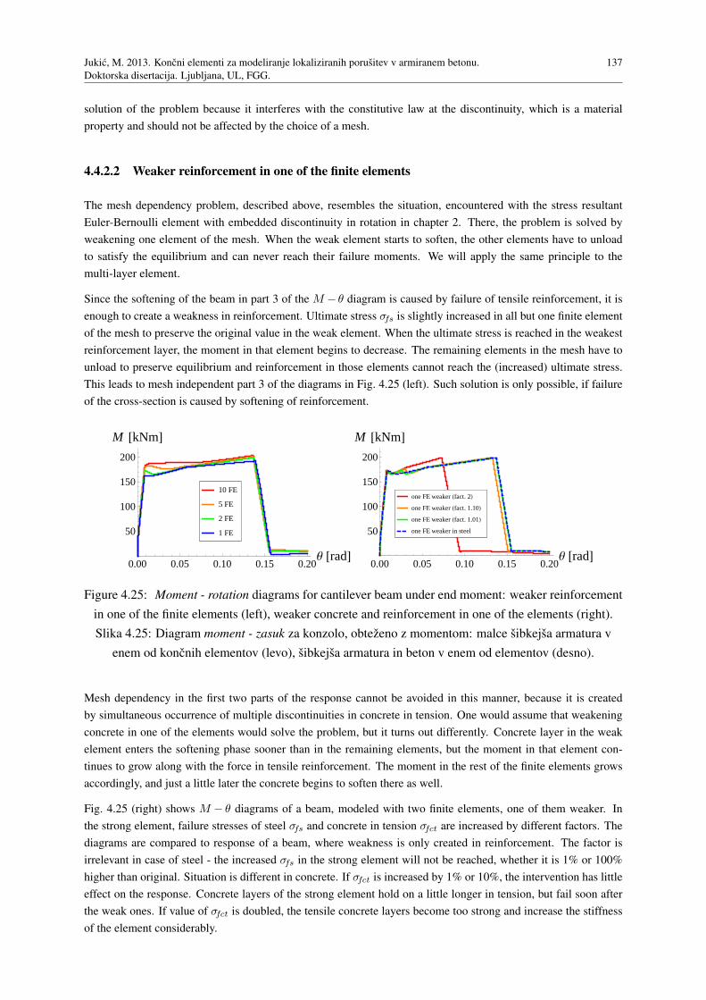
Jukic, M. 2013. Koncni elementi za modeliranje lokaliziranih porusitev v armiranem betonu.
Doktorska disertacija. Ljubljana, UL, FGG.
137
solution of the problem because it interferes with the constitutive law at the discontinuity, which is a material
property and should not be affected by the choice of a mesh.
4.4.2.2 Weaker reinforcement in one of the finite elements
The mesh dependency problem, described above, resembles the situation, encountered with the stress resultant
Euler-Bernoulli element with embedded discontinuity in rotation in chapter 2. There, the problem is solved by
weakening one element of the mesh. When the weak element starts to soften, the other elements have to unload
to satisfy the equilibrium and can never reach their failure moments. We will apply the same principle to the
multi-layer element.
Since the softening of the beam in part 3 of the M − θ diagram is caused by failure of tensile reinforcement, it is
enough to create a weakness in reinforcement. Ultimate stress σfs is slightly increased in all but one finite element
of the mesh to preserve the original value in the weak element. When the ultimate stress is reached in the weakest
reinforcement layer, the moment in that element begins to decrease. The remaining elements in the mesh have to
unload to preserve equilibrium and reinforcement in those elements cannot reach the (increased) ultimate stress.
This leads to mesh independent part 3 of the diagrams in Fig. 4.25 (left). Such solution is only possible, if failure
of the cross-section is caused by softening of reinforcement.
0.00 0.05 0.10 0.15 0.20Θ @radD
50
100
150
200
M @kNmD
1 FE
2 FE
5 FE
10 FE
0.00 0.05 0.10 0.15 0.20Θ @radD
50
100
150
200
M @kNmD
one FE weaker in steel
one FE weaker Hfact. 1.01L
one FE weaker Hfact. 1.10L
one FE weaker Hfact. 2L
Figure 4.25: Moment - rotation diagrams for cantilever beam under end moment: weaker reinforcement
in one of the finite elements (left), weaker concrete and reinforcement in one of the elements (right).
Slika 4.25: Diagram moment - zasuk za konzolo, obtezeno z momentom: malce sibkejsa armatura v
enem od koncnih elementov (levo), sibkejsa armatura in beton v enem od elementov (desno).
Mesh dependency in the first two parts of the response cannot be avoided in this manner, because it is created
by simultaneous occurrence of multiple discontinuities in concrete in tension. One would assume that weakening
concrete in one of the elements would solve the problem, but it turns out differently. Concrete layer in the weak
element enters the softening phase sooner than in the remaining elements, but the moment in that element con-
tinues to grow along with the force in tensile reinforcement. The moment in the rest of the finite elements grows
accordingly, and just a little later the concrete begins to soften there as well.
Fig. 4.25 (right) shows M − θ diagrams of a beam, modeled with two finite elements, one of them weaker. In
the strong element, failure stresses of steel σfs and concrete in tension σfct are increased by different factors. The
diagrams are compared to response of a beam, where weakness is only created in reinforcement. The factor is
irrelevant in case of steel - the increased σfs in the strong element will not be reached, whether it is 1% or 100%
higher than original. Situation is different in concrete. If σfct is increased by 1% or 10%, the intervention has little
effect on the response. Concrete layers of the strong element hold on a little longer in tension, but fail soon after
the weak ones. If value of σfct is doubled, the tensile concrete layers become too strong and increase the stiffness
of the element considerably.
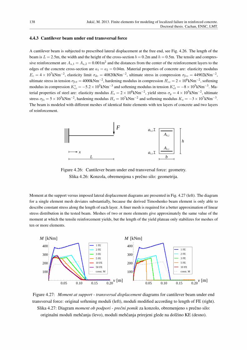
138 Jukic, M. 2013. Finite elements for modeling of localized failure in reinforced concrete.
Doctoral thesis. Cachan, ENSC, LMT.
4.4.3 Cantilever beam under end transversal force
A cantilever beam is subjected to prescribed lateral displacement at the free end, see Fig. 4.26. The length of the
beam is L= 2.5m, the width and the height of the cross-section b= 0.2m and h= 0.5m. The tensile and compres-
sive reinforcement are As,1 =As,2 = 0.001m2 and the distances from the center of the reinforcement layers to the
edges of the concrete cross-section are a1 = a2 = 0.04m. Material properties of concrete are: elasticity modulus
Ec = 4× 10⁷kNm−2, elasticity limit σdc = 40820kNm−2, ultimate stress in compression σfcc = 44902kNm−2,
ultimate stress in tension σfct = 4000kNm−2, hardening modulus in compression Hcc = 2×10⁶kNm−2, softening
modulus in compression K∗cc =−5.2×10⁵kNm−3 and softening modulus in tension K∗
ct =−8×10⁵kNm−3. Ma-
terial properties of steel are: elasticity modulus Es = 2× 10⁸kNm−2, yield stress σy = 4× 10⁵kNm−2, ultimate
stress σfs = 5×10⁵kNm−2, hardening modulus Hs = 107kNm−2 and softening modulus Ks =−3×10⁷kNm−3.
The beam is modeled with different meshes of identical finite elements with ten layers of concrete and two layers
of reinforcement.
xL
F
b
h
AS,2
AS,1
aS,1
aS,2
Figure 4.26: Cantilever beam under end transversal force: geometry.
Slika 4.26: Konzola, obremenjena s precno silo: geometrija.
Moment at the support versus imposed lateral displacement diagrams are presented in Fig. 4.27 (left). The diagram
for a single element mesh deviates substantially, because the derived Timoshenko beam element is only able to
describe constant stress along the length of each layer. A finer mesh is required for a better approximation of linear
stress distribution in the tested beam. Meshes of two or more elements give approximately the same value of the
moment at which the tensile reinforcement yields, but the length of the yield plateau only stabilizes for meshes of
ten or more elements.
0.05 0.10 0.15 0.20v @mD
100
200
300
400
M @kNmD
const. M
50 FE
10 FE
5 FE
3 FE
2 FE
1 FE
0.05 0.10 0.15 0.20v @mD
100
200
300
400
M @kNmD
const. M
10 FE
5 FE
3 FE
2 FE
1 FE
Figure 4.27: Moment at support - transversal displacement diagrams for cantilever beam under end
transversal force: original softening moduli (left), moduli modified according to length of FE (right).
Slika 4.27: Diagram moment ob podpori - precni pomik za konzolo, obremenjeno s precno silo:
originalni moduli mehcanja (levo), moduli mehcanja prirejeni glede na dolzino KE (desno).
Jukic, M. 2013. Koncni elementi za modeliranje lokaliziranih porusitev v armiranem betonu.
Doktorska disertacija. Ljubljana, UL, FGG.
139
The same beam is analyzed again under a different load. Instead of the force, a moment is applied at the free
end, producing a constant moment over the length. This allows us to model the beam with a single finite element
and avoid the influence of mesh refinement on the results. Results for the one element mesh are presented as
diagram of moment at the support versus lateral displacement at the free end - the black dashed line in Fig. 4.27.
Although we cannot expect the curves of different load cases to match, the reinforcement should yield at the same
moment. However, comparison in Fig. 4.27 (left) shows that the beam under end force withstands substantially
higher moment than the beam under end moment, before yielding.
Analysis of the beam under end force is repeated with a modified set of softening moduli - original values are
scaled according to the length of the finite elements (multiplied with the number of FE in the mesh). Results are
presented in Fig. 4.27 (right). In these diagrams, the “yield moment” decreases for finer meshes, and for a mesh
of ten elements gets very close to the value from the “constant moment” diagram. The ultimate moment is still a
little higher. Another change is evident in the right image - the softening parts of the diagrams are more parallel
than before and even grow steeper for finer meshes.
Let us take a closer look at what happens inside the finite element. The stress σi is constant over the length of each
layer. The resulting moment M , computed from equation (4.141), is constant as well.
M = ∑i
−yiσiAi (4.141)
The internal forces fθ,int, defined by equation (4.33), are different from M , however. After inserting expressions
(4.4) for B and B∗, and defining shear force Q= ∑iτ iAi, we obtain the following expressions for nodal moments:
f intθ1
= ∑i
(
yi1
L(e)σi−
1
2τ i)
AiL(e) =
−M︷ ︸︸ ︷
∑i
yiσiAi−L(e)
2
Q︷ ︸︸ ︷
∑i
τ iAi =−
(
M +L(e)
2Q
)
f intθ2
= ∑i
(
−yi1
L(e)σi−
1
2τ i)
AiL(e) =
M︷ ︸︸ ︷
∑i
−yiσiAi−L(e)
2
Q︷ ︸︸ ︷
∑i
τ iAi =M −L(e)
2Q
(4.142)
We can see that the two moments have a different absolute value. The difference L(e)Q, where L(e) is the length
of the finite element, derives from the shear stress, and it enables the finite element to deal with linear moment
in the analyzed structure. Based on equation (4.142), we can characterize M as the average moment in the finite
element.
We say that an element yields when the stress in tensile reinforcement reaches the yield value. The matching yield
moment My is computed from equation (4.141). But when M reaches the yield moment, the corresponding nodal
moments fθ,int take the values from (4.142), which can differ significantly from My , especially in a coarse mesh.
The most evident example is the mesh, composed of a single finite element. Since the moment is zero at the free
end, the moment at the support is twice as big as the average moment M . When the tensile reinforcement yields,
the moment at the support has twice the value of My . This is confirmed by comparing the “1FE” and “const. M”
diagrams in Fig. 4.27. The yield plateau in the first curve is twice as high as in the second. In the constant moment
case, the shear stress is zero and the nodal moments fθ,int are equal to the average moment M , which activates
plastification. The problems, arising from the described property of Timoshenko beam element, are avoided by
using a fine enough mesh, so the nodal moments f intθ1
and f intθ2
are almost equal.
Refining of the finite element mesh brings about another problem, however. As we have seen in section 4.4.2,
shortening the finite elements causes them to soften more slowly. Let us imagine a short section of the tested
cantilever beam next to the support, with the tensile reinforcement on the verge of yielding. Concrete in tension
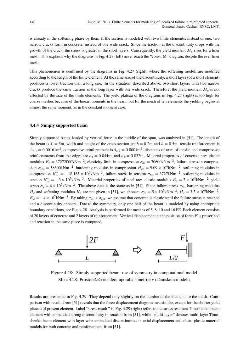
140 Jukic, M. 2013. Finite elements for modeling of localized failure in reinforced concrete.
Doctoral thesis. Cachan, ENSC, LMT.
is already in the softening phase by then. If the section is modeled with two finite elements, instead of one, two
narrow cracks form in concrete, instead of one wide crack. Since the traction at the discontinuity drops with the
growth of the crack, the stress is greater in the short layers. Consequently, the yield moment My rises for a finer
mesh. This explains why the diagrams in Fig. 4.27 (left) never reach the “const. M” diagram, despite the ever finer
mesh.
This phenomenon is confirmed by the diagrams in Fig. 4.27 (right), where the softening moduli are modified
according to the length of the finite element. At the same size of the discontinuity, a short layer (of a short element)
produces a lower traction than a long one. In the situation, described above, two short layers with two narrow
cracks produce the same traction as the long layer with one wide crack. Therefore, the yield moment My is not
affected by the size of the finite elements. The yield plateau of the diagrams in Fig. 4.27 (right) is too high for
coarse meshes because of the linear moments in the beam, but for the mesh of ten elements the yielding begins at
almost the same moment, as in the constant moment case.
4.4.4 Simply supported beam
Simply supported beam, loaded by vertical force in the middle of the span, was analyzed in [51]. The length of
the beam is L = 5m, width and height of the cross-section are b = 0.2m and h = 0.5m, tensile reinforcement is
As,1 = 0.00161m2, compressive reinforcement isAs,2 = 0.0001m2, distances of axes of tensile and compressive
reinforcements from the edges are a1 = 0.044m, and a2 = 0.032m. Material properties of concrete are: elastic
modulus Ec = 37272000kNm−2, elasticity limit in compression σdc = 30600kNm−2, failure stress in compres-
sion σfcc = 38300kNm−2, hardening modulus in compression Hcc = 9.09× 10⁶kNm−2, softening modulus in
compression K∗cc = −18.165 × 10⁶kNm−3, failure stress in tension σfct = 3727kNm−2, softening modulus in
tension K∗ct = −3× 10⁷kNm−3. Material properties of steel are: elastic modulus Es = 2× 10⁸kNm−2, yield
stress σy = 4× 10⁵kNm−2. The above data is the same as in [51]. Since failure stress σfs, hardening modulus
Hs and softening modulus Ks are not given in [51], we choose: σfs = 5× 10⁵kNm−2, Hs = 3.3× 10⁶kNm−2,
Ks = −4×10⁷kNm−3. By taking σdt > σfct, we assume that concrete is elastic until the failure stress is reached
and a discontinuity appears. Due to the symmetry, only one half of the beam is modeled by using appropriate
boundary conditions, see Fig. 4.28. Analysis is performed for meshes of 5, 8, 10 and 16 FE. Each element consists
of 20 layers of concrete and 2 layers of reinforcement. Vertical displacement at the position of force F is prescribed
and reaction in the same place is computed.
L L2
2F F
Figure 4.28: Simply supported beam: use of symmetry in computational model.
Slika 4.28: Prostolezeci nosilec: uporaba simetrije v racunskem modelu.
Results are presented in Fig. 4.29. They depend only slightly on the number of the elements in the mesh. Com-
parison with results from [51] reveals that the force-displacement diagrams are similar, except for the shorter yield
plateau of present element. Label “stress result.” in Fig. 4.29 (right) refers to the stress resultant Timoshenko beam
element with embedded strong discontinuity in rotation from [51], while “multi-layer” denotes multi-layer Timo-
shenko beam element with layer-wise embedded discontinuities in axial displacement and elasto-plastic material
models for both concrete and reinforcement from [51].
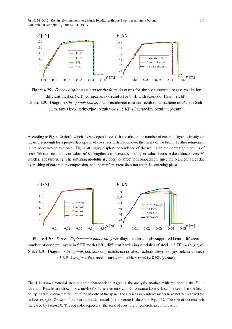
Jukic, M. 2013. Koncni elementi za modeliranje lokaliziranih porusitev v armiranem betonu.
Doktorska disertacija. Ljubljana, UL, FGG.
141
0.00 0.01 0.02 0.03 0.04 0.05v @mD0
20
40
60
80
100
120
F @kND
5 FE
8 FE
10 FE
16 FE
0.01 0.02 0.03 0.04 0.05v @mD0
20
40
60
80
100
120
F @kND
this finite element
Pham, multi-layer
Pham, stress result.
Figure 4.29: Force - displacement under the force diagrams for simply supported beam: results for
different meshes (left), comparison of results for 8 FE with results of Pham (right).
Slika 4.29: Diagram sila - pomik pod silo za prostolezeci nosilec: rezultati za razlicne mreze koncnih
elementov (levo), primerjava rezultatov za 8 KE s Phamovimi rezultati (desno).
According to Fig. 4.30 (left), which shows dependence of the results on the number of concrete layers, already ten
layers are enough for a proper description of the stress distribution over the height of the beam. Further refinement
is not necessary in this case. Fig. 4.30 (right) displays dependence of the results on the hardening modulus of
steel. We can see that lower values of Hs lengthen the plateau, while higher values increase the ultimate force F ,
which is not surprising. The softening modulus Ks does not affect the computation, since the beam collapses due
to crushing of concrete in compression, and the reinforcement does not enter the softening phase.
0.01 0.02 0.03 0.04 0.05v @mD0
20
40
60
80
100
120
F @kND
30 lay. conc.
20 lay. conc.
14 lay. conc.
10 lay. conc.
0.01 0.02 0.03 0.04 0.05v @mD0
20
40
60
80
100
120
F @kND
10 000 000
5 000 000
3 300 000
Hs = 1 000 000
Figure 4.30: Force - displacement under the force diagrams for simply supported beam: different
number of concrete layers in 5 FE mesh (left), different hardening modulus of steel in 8 FE mesh (right).
Slika 4.30: Diagram sila - pomik pod silo za prostolezeci nosilec: razlicno stevilo slojev betona v mrezi
s 5 KE (levo), razlicen modul utrjevanja jekla v mrezi z 8 KE (desno).
Fig. 4.31 shows material state at some characteristic stages in the analysis, marked with red dots in the F − v
diagram. Results are shown for a mesh of 8 finite elements with 20 concrete layers. It can be seen that the beam
collapses due to concrete failure in the middle of the span. The stresses in reinforcements have not yet reached the
failure strength. Growth of the discontinuities (cracks) in concrete is shown in Fig. 4.32. The size of the cracks is
increased by factor 50. The red color represents the zone of crushing of concrete in compression.
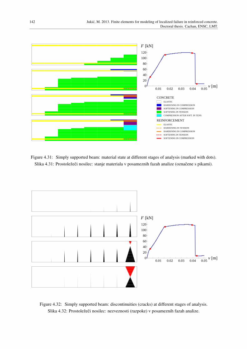
142 Jukic, M. 2013. Finite elements for modeling of localized failure in reinforced concrete.
Doctoral thesis. Cachan, ENSC, LMT.
0.01 0.02 0.03 0.04 0.05v @mD0
20
40
60
80
100
120
F @kND
ELASTIC
HARDENING IN COMPRESSION
SOFTENING IN COMPRESSION
SOFTENING IN TENSION
COMPRESSION AFTER SOFT. IN TENS.
CONCRETE
ELASTIC
HARDENING IN TENSION
HARDENING IN COMPRESSION
SOFTENING IN TENSION
SOFTENING IN COMPRESSION
REINFORCEMENT
Figure 4.31: Simply supported beam: material state at different stages of analysis (marked with dots).
Slika 4.31: Prostolezeci nosilec: stanje materiala v posameznih fazah analize (oznacene s pikami).
0.01 0.02 0.03 0.04 0.05v @mD0
20
40
60
80
100
120
F @kND
Figure 4.32: Simply supported beam: discontinuities (cracks) at different stages of analysis.
Slika 4.32: Prostolezeci nosilec: nezveznosti (razpoke) v posameznih fazah analize.
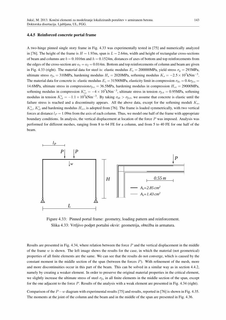
Jukic, M. 2013. Koncni elementi za modeliranje lokaliziranih porusitev v armiranem betonu.
Doktorska disertacija. Ljubljana, UL, FGG.
143
4.4.5 Reinforced concrete portal frame
A two-hinge pinned single story frame in Fig. 4.33 was experimentally tested in [75] and numerically analyzed
in [76]. The height of the frame is H = 1.93m, span is L= 2.64m, width and height of rectangular cross-sections
of beam and columns are b= 0.1016m and h= 0.1524m, distances of axes of bottom and top reinforcements from
the edges of the cross-section are a1 = a2 = 0.014m. Bottom and top reinforcements of column and beam are given
in Fig. 4.33 (right). The material data for steel is: elastic modulus Es = 200000MPa, yield stress σy = 293MPa,
ultimate stress σfs = 310MPa, hardening modulus Hs = 2020MPa, softening modulus Ks = −2.5× 10⁷kNm−3.
The material data for concrete is: elastic modulus Ec = 31500MPa, elasticity limit in compression σdc = 0.4σfcc =
14.6MPa, ultimate stress in compressionσfcc = 36.5MPa, hardening modulus in compression Hcc = 29000MPa,
softening modulus in compression K∗cc = −4× 10⁷kNm−3, ultimate stress in tension σfct = 0.95MPa, softening
modulus in tension K∗ct = −1.1× 10⁷kNm−3. By taking σdt > σfct, we assume that concrete is elastic until the
failure stress is reached and a discontinuity appears. All the above data, except for the softening moduli Ks,
K∗cc, K∗
ct and hardening modulus Hcc, is adopted from [76]. The frame is loaded symmetrically, with two vertical
forces at distance lP = 1.09m from the axis of each column. Thus, we model one half of the frame with appropriate
boundary conditions. In analysis, the vertical displacement at location of the force P was imposed. Analysis was
performed for different meshes, ranging from 8 to 64 FE for a column, and from 5 to 40 FE for one half of the
beam.
L
H
P P
lP
wP
0.55 m
As=2.85 cm2
As=1.43 cm2
Figure 4.33: Pinned portal frame: geometry, loading pattern and reinforcement.
Slika 4.33: Vrtljivo podprt portalni okvir: geometrija, obtezba in armatura.
Results are presented in Fig. 4.34, where relation between the force P and the vertical displacement in the middle
of the frame w is shown. The left image shows the results for the case, in which the material (not geometrical)
properties of all finite elements are the same. We can see that the results do not converge, which is caused by the
constant moment in the middle section of the span (between the forces P ). With refinement of the mesh, more
and more discontinuities occur in this part of the beam. This can be solved in a similar way as in section 4.4.2,
namely by creating a weaker element. In order to preserve the original material properties in the critical element,
we slightly increase the ultimate stress of steel σfs in all finite elements in the middle section of the span, except
for the one adjacent to the force P . Results of the analysis with a weak element are presented in Fig. 4.34 (right).
Comparison of the P −w diagram with experimental results [75] and results, reported in [76] is shown in Fig. 4.35.
The moments at the joint of the column and the beam and in the middle of the span are presented in Fig. 4.36.

144 Jukic, M. 2013. Finite elements for modeling of localized failure in reinforced concrete.
Doctoral thesis. Cachan, ENSC, LMT.
0.02 0.04 0.06 0.08 0.1w @mD
5
10
15
20
P @kND
128C 80B
64C 40B
32C 20B
16C 10B
8C 5B
0.02 0.04 0.06 0.08 0.1w @mD
5
10
15
20
P @kND
128C 80B
64C 40B
32C 20B
16C 10B
8C 5B
Figure 4.34: P −w diagram: results for different meshes of finite elements if all elements to the right
of force P are the same (left) and if reinforcement is weakened in one of them (right).
Slika 4.34: Diagram P −w: rezultati za razlicne mreze koncnih elementov, ce so vsi elementi desno od
sile P enaki (levo) in ce je v enem od njih armatura oslabljena (desno).
0.01 0.02 0.03 0.04 0.05 0.06w @mD
5
10
15
20
P @kND
experiment
Saje et al.
64C 40B
Figure 4.35: P −w diagram: comparison to experiment and results of Saje et al.
Slika 4.35: Diagram P −w: primerjava z eksperimentom in z rezultati Saje et al.
0.01 0.02 0.03 0.04 0.05 0.06w @mD
2
4
6
8
10
12
M @kNmD
experiment
Saje et al.
64C 40B
0.01 0.02 0.03 0.04 0.05 0.06w @mD
2
4
6
8
10
12
M @kNmD
experiment
Saje et al.
64C 40B
Figure 4.36: Moments at the joint of the beam and the column (left) and in the middle of the span
(right): comparison to experiment and results of Saje et al.
Slika 4.36: Moment na stiku stebra in precke (levo) ter na sredini razpona (desno): primerjava z
eksperimentom in z rezultati Saje et al.
Progression of damage, yielding and softening of material is shown in Fig. 4.37, where material state is presented
element-wise and layer-wise for different stages of the analysis, performed on the mesh of 32 FE in the column and
20 FE in the half-beam. If we examine the elements near the inflection point of the beam, where the moments are
close to zero, we can see transition of some layers from compression to tension and vice versa. This happens due
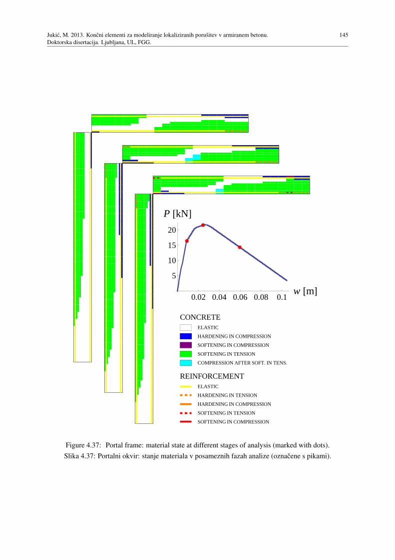
Jukic, M. 2013. Koncni elementi za modeliranje lokaliziranih porusitev v armiranem betonu.
Doktorska disertacija. Ljubljana, UL, FGG.
145
0.02 0.04 0.06 0.08 0.1w @mD
5
10
15
20
P @kND
ELASTIC
HARDENING IN COMPRESSION
SOFTENING IN COMPRESSION
SOFTENING IN TENSION
COMPRESSION AFTER SOFT. IN TENS.
CONCRETE
ELASTIC
HARDENING IN TENSION
HARDENING IN COMPRESSION
SOFTENING IN TENSION
SOFTENING IN COMPRESSION
REINFORCEMENT
Figure 4.37: Portal frame: material state at different stages of analysis (marked with dots).
Slika 4.37: Portalni okvir: stanje materiala v posameznih fazah analize (oznacene s pikami).
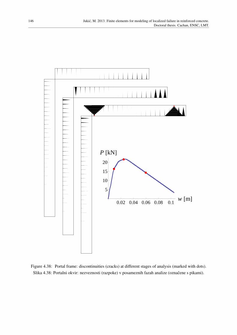
146 Jukic, M. 2013. Finite elements for modeling of localized failure in reinforced concrete.
Doctoral thesis. Cachan, ENSC, LMT.
0.02 0.04 0.06 0.08 0.1w @mD
5
10
15
20
P @kND
Figure 4.38: Portal frame: discontinuities (cracks) at different stages of analysis (marked with dots).
Slika 4.38: Portalni okvir: nezveznosti (razpoke) v posameznih fazah analize (oznacene s pikami).

Jukic, M. 2013. Koncni elementi za modeliranje lokaliziranih porusitev v armiranem betonu.
Doktorska disertacija. Ljubljana, UL, FGG.
147
to shifting of the neutral axis and corresponds to the situation in Fig. 4.18 (left). The cyan color designates a layer
that has developed a discontinuity in tension and was then loaded in compression. In this case, the compressive
stress values are well below σfcc.
Fig. 4.38 shows the discontinuities in concrete, increased by factor 50, for the phases of the analysis, marked with
the red dots. We can see that the greatest part of damage occurs in the middle and at the end of the beam. In the
three rightmost elements (to the right of the load P ) the cracks grow equally at first. But when the ultimate stress
is reached in the tensile reinforcement of the weaker element, the cracks in the remaining elements stop growing.
They do not close because of the plastic deformations in steel.
4.4.6 Two story reinforced concrete frame
Two-story reinforced concrete frame in Fig. 4.39 has been experimentally tested in [71]. Numerical analyses were
done by Pham et al. [52] and Jukic et al. [74], using stress-resultant Timoshenko and Euler-Bernoulli beam finite
elements, respectively, with embedded strong discontinuity in rotation. Analysis with multi-layered Timoshenko
beam element with layer-wise embedded discontinuities in axial displacement and elasto-plastic material models
for both concrete and reinforcement was also done in [52]. Story height of the frame is H = 2m, span is L= 3.5m.
Beam cross-section data is: width b = 0.3m, height h = 0.4m, bottom and top reinforcements As,1 = As,2 =
0.0012m2, distances of reinforcement axes from the edges a1 = a2 = 0.04m. Column cross-section data is the
same, except for a1 = a2 = 0.03m. Material properties of steel are accommodated from data reported in [71]:
elasticity modulus Es = 192500MPa, yield stress σy = 418MPa and ultimate stress σfs = 596MPa are taken directly
from [71], while the hardening modulus Hs = 2790MPa is computed in such way that the ultimate stress is reached
at the same strain as in [71], see Fig. 4.40 (left). The softening modulus is not provided in [71]. We choose
Ks =−4×10⁷kNm−3. Material properties of concrete are also accommodated from data reported in [71]: ultimate
stress in compression σfcc = 30MPa is taken directly from [71], elasticity modulus Ec = 28600MPa and ultimate
stress of concrete in tension σfct = 1.8MPa are taken from Fig. 2 in [71]. Elasticity limit σdc = 8.5MPa and
hardening modulus Hcc = 49000MPa are computed in such way that the ultimate compressive stress is reached at
the same strain as in Fig. 6(a) in [71], see Fig. 4.40 (right). Softening moduli are not provided in [71]. We choose
K∗cc =−2×10⁶kNm−3 for compression and K∗
ct =−107kNm−3 for tension.
L
H
H
700 kN 700 kN
Fu
0.04
0.04
0.32
0.30
0.03
0.03
0.34
0.30
4´3cm2
4´3cm2
4´3cm2
4´3cm2
BEAM
COLUMN
Figure 4.39: Two story frame: geometry, loading pattern and cross-sections.
Slika 4.39: Dvoetazni okvir: geometrija, obtezba in precni prerezi.
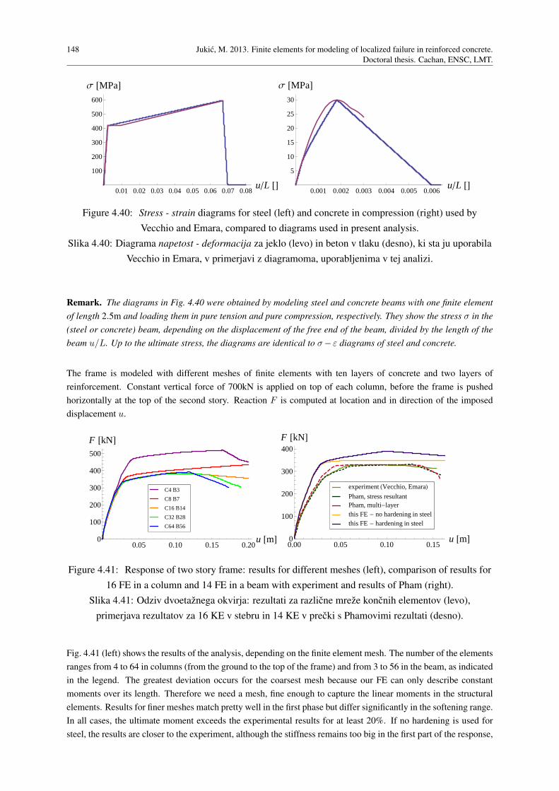
148 Jukic, M. 2013. Finite elements for modeling of localized failure in reinforced concrete.
Doctoral thesis. Cachan, ENSC, LMT.
0.01 0.02 0.03 0.04 0.05 0.06 0.07 0.08uL @D
100
200
300
400
500
600
Σ @MPaD
0.001 0.002 0.003 0.004 0.005 0.006uL @D
5
10
15
20
25
30
Σ @MPaD
Figure 4.40: Stress - strain diagrams for steel (left) and concrete in compression (right) used by
Vecchio and Emara, compared to diagrams used in present analysis.
Slika 4.40: Diagrama napetost - deformacija za jeklo (levo) in beton v tlaku (desno), ki sta ju uporabila
Vecchio in Emara, v primerjavi z diagramoma, uporabljenima v tej analizi.
Remark. The diagrams in Fig. 4.40 were obtained by modeling steel and concrete beams with one finite element
of length 2.5m and loading them in pure tension and pure compression, respectively. They show the stress σ in the
(steel or concrete) beam, depending on the displacement of the free end of the beam, divided by the length of the
beam u/L. Up to the ultimate stress, the diagrams are identical to σ−ε diagrams of steel and concrete.
The frame is modeled with different meshes of finite elements with ten layers of concrete and two layers of
reinforcement. Constant vertical force of 700kN is applied on top of each column, before the frame is pushed
horizontally at the top of the second story. Reaction F is computed at location and in direction of the imposed
displacement u.
0.05 0.10 0.15 0.20u @mD0
100
200
300
400
500
F @kND
C64 B56
C32 B28
C16 B14
C8 B7
C4 B3
0.00 0.05 0.10 0.15u @mD0
100
200
300
400
F @kND
this FE - hardening in steelthis FE - no hardening in steelPham, multi-layerPham, stress resultant
experiment HVecchio, EmaraL
Figure 4.41: Response of two story frame: results for different meshes (left), comparison of results for
16 FE in a column and 14 FE in a beam with experiment and results of Pham (right).
Slika 4.41: Odziv dvoetaznega okvirja: rezultati za razlicne mreze koncnih elementov (levo),
primerjava rezultatov za 16 KE v stebru in 14 KE v precki s Phamovimi rezultati (desno).
Fig. 4.41 (left) shows the results of the analysis, depending on the finite element mesh. The number of the elements
ranges from 4 to 64 in columns (from the ground to the top of the frame) and from 3 to 56 in the beam, as indicated
in the legend. The greatest deviation occurs for the coarsest mesh because our FE can only describe constant
moments over its length. Therefore we need a mesh, fine enough to capture the linear moments in the structural
elements. Results for finer meshes match pretty well in the first phase but differ significantly in the softening range.
In all cases, the ultimate moment exceeds the experimental results for at least 20%. If no hardening is used for
steel, the results are closer to the experiment, although the stiffness remains too big in the first part of the response,

Jukic, M. 2013. Koncni elementi za modeliranje lokaliziranih porusitev v armiranem betonu.
Doktorska disertacija. Ljubljana, UL, FGG.
149
see Fig. 4.41 (right). A case of unloading of the frame is shown in Fig. 4.42. Analysis was performed on a mesh
with 16 FE in columns (8 FE in each story) and 14 FE in beams. Apart from the exceeded ultimate moment,
a difference occurs in the unloading curves which are straight and a little steeper than experimental. Also, the
re-loading follows almost exactly the unloading line.
0.00 0.05 0.10 0.15u @mD0
100
200
300
400
F @kND
Figure 4.42: Response of two story frame: loading and unloading for a mesh of 16 FE in a column and
14 FE in a beam. Comparison to experiment.
Slika 4.42: Odziv dvoetaznega okvirja: obremenjevanje in razbremenjevanje za mrezo s 16 KE v stebru
in s 14 KE v precki. Primerjava z eksperimentom.
Images in Fig. 4.44 show progression of damage and plasticity in the material at several stages of the frame
analysis, performed on a mesh with 16 FE in columns and 14 FE in beams. The stages are marked with red dots
in the response of the frame in Fig. 4.43. The legend for Fig. 4.44 is included in Fig. 4.43. Fig. 4.45 shows the
discontinuities in concrete, corresponding to the same stages of the analysis. Their sizes are increased by factor
50. The red color represents a discontinuity in compression, (zone of crushing of concrete in compression).
0.05 0.1 0.15 0.2u @mD
100
200
300
400
F @kNDELASTIC
HARDENING IN COMPRESSION
SOFTENING IN COMPRESSION
SOFTENING IN TENSION
COMPRESSION AFTER SOFT. IN TENS.
CONCRETE
ELASTIC
HARDENING IN TENSION
HARDENING IN COMPRESSION
SOFTENING IN TENSION
SOFTENING IN COMPRESSION
REINFORCEMENT
Figure 4.43: Two story frame: stages of analysis, corresponding to images in Figs. 4.44 and 4.45.
Slika 4.43: Dvoetazni okvir: faze analize, ki ustrezajo stanjem materiala na slikah 4.44 in 4.45.
4.5 Concluding remarks
We have presented a planar multi-layer Timoshenko beam finite element, composed of several concrete and steel
reinforcement layers. Small deformations are assumed in the beam kinematics. Deformation of an individual layer
is computed from axial deformation of the middle axis of the beam and rotation of the cross-section. Contribution
of the rotation depends on the distance from the middle axis. A discontinuity in axial displacement is introduced
individually into each layer. Axial response of a concrete layer is described with a damage hardening model for
the bulk and a damage softening law at the discontinuity. Axial response of a steel layer is described with isotropic

150 Jukic, M. 2013. Finite elements for modeling of localized failure in reinforced concrete.
Doctoral thesis. Cachan, ENSC, LMT.
Figure 4.44: Two story frame: material state at different stages of analysis, marked in Fig. 4.43.
Slika 4.44: Dvoetazni okvir: stanje materiala v fazah analize, oznacenih na sliki 4.43.
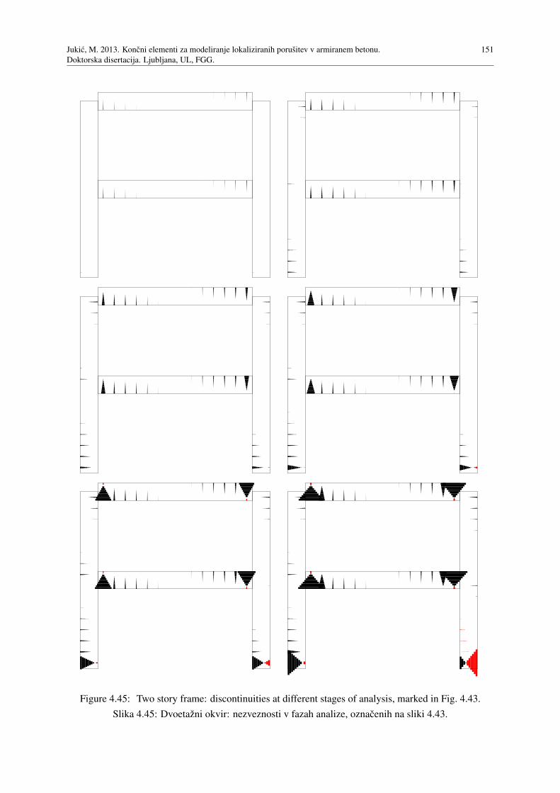
Jukic, M. 2013. Koncni elementi za modeliranje lokaliziranih porusitev v armiranem betonu.
Doktorska disertacija. Ljubljana, UL, FGG.
151
Figure 4.45: Two story frame: discontinuities at different stages of analysis, marked in Fig. 4.43.
Slika 4.45: Dvoetazni okvir: nezveznosti v fazah analize, oznacenih na sliki 4.43.
152 Jukic, M. 2013. Finite elements for modeling of localized failure in reinforced concrete.
Doctoral thesis. Cachan, ENSC, LMT.
hardening plasticity model for the bulk and plastic softening cohesive model at the discontinuity. Shear response
is assumed elastic.
The finite element has been derived for analysis of reinforced concrete beams and frames up to complete failure,
providing a detailed description of material state over the cross-section. It can also be used for computation of
stress-resultant properties of different cross-sections, which are required as an input data in analysis with stress-
resultant beam finite elements, such as the one presented in chapter 2. The derived multi-layer element is not
intended for cyclic loading. Nevertheless, it can handle minor changes of the load sign, which can occur in some
layers due to shifting of the neutral axis even in monotonic loading.
Mesh dependency is observed in the case of cantilever beam under end moment if all finite elements are the same.
The reason lies in simultaneous occurrence of multiple discontinuities along the beam. In a fine mesh a large num-
ber of small discontinuities are formed, while coarse mesh creates a small number of large discontinuities. Since
traction at the discontinuity decreases with its growth, different meshes produce different moment in the beam.
The differences are greatest in the last part of the response, when the moment in the beam begins to drop due to
softening of tensile reinforcement. This can be solved by slightly weakening reinforcement in one of the elements
in the mesh, preventing occurrence of multiple discontinuities in steel along the cantilever beam. If softening of
the beam happens due to crushing of concrete in compression, the problem cannot be solved so effectively, since
there are multiple critical layers of concrete, as opposed to a single critical layer of tensile reinforcement. Minor
deviations appear in the hardening part of the beam response due to cracking of concrete in tension. This cannot be
avoided by weakening one of the elements in the mesh because the moment in the beam is still rising and, sooner
or later, concrete will crack in the remaining elements as well.
Mesh dependency due to cracking of concrete in tension is more evident in the case of cantilever beam under
end transversal force. Since the developed Timoshenko beam finite element can only describe constant state
over its length, a fine mesh is required for adequate description of linear moment along the beam. However,
shortening of the finite elements increases the number and reduces the size of discontinuities in concrete in tension,
resulting in higher traction at the discontinuity and considerably overestimated yield moment of the beam. The
same phenomenon is observed in the cantilever beam under end moment, but to a lesser extent.
Another kinematics issue should be addressed. There is no discontinuity (in rotation or axial displacement) on the
element level, since the embedded discontinuities in axial displacement are defined locally in each layer. Defor-
mation of the beam axis is always interpolated in the same way as for a regular Timoshenko beam. Even when
the element is completely broken, the middle axis is a smooth curve. The bulk of each layer slides along a path,
parallel to the middle axis. In a fine mesh, however, this may not be problematic. The critical finite element ex-
hibits a significantly decreased stiffness and greater curvature than neighboring elements, which can be interpreted
as a jump in rotation, smeared over the length of the critical element. Still, the global kinematics is not completely
accurate.
Several numerical examples and experiments from literature have been modeled with our finite element. Significant
deviation is observed in stiffness and ultimate load of the two-story RC frame. However, the shape of the loading
and unloading diagram is appropriate. Results of the simply supported beam model and the portal frame model
match well the results from the literature. Despite some deficiencies, the finite element allows for quite adequate
modeling of reinforced concrete beams and frames, based on axial responses of concrete and steel, which are easily
obtained from experiments and are independent of the cross-section geometry.
Jukic, M. 2013. Koncni elementi za modeliranje lokaliziranih porusitev v armiranem betonu.
Doktorska disertacija. Ljubljana, UL, FGG.
153
5 VISCOUS REGULARIZATION OF SOFTENING RESPONSE FOR MULTI-LAYER
TIMOSHENKO BEAM FINITE ELEMENT
5.1 Introduction
In this chapter, we upgrade the multi-layer Timoshenko beam finite element, presented in chapter 4, by implement-
ing viscous regularization of the softening response [77]. This method can be used to prevent certain computational
problems, such as alternating between equivalent solutions [78]. In present work, we introduce viscous forces at
discontinuities to help control their development and prevent (physically) erroneous occurrence of multiple dis-
continuities in homogeneous stress field.
When several equivalent finite elements develop a discontinuity simultaneously, the viscous regularization favors
one of them. The preferred element continues to soften, while the others unload. The selection is based on the rate,
at which the discontinuities develop in different elements. The faster a discontinuity grows, the more its growth
is encouraged. Eventually, only the “fastest” element develops a discontinuity and the others unload to satisfy the
equilibrium.
Introduction of viscous regularization into the finite element slightly modifies the equilibrium equations, while the
kinematic and the constitutive equations remain unchanged. This leads to alteration of some expressions, used in
the computational procedure. In this chapter, we only derive the equations that differ from the ones in chapter 4.
The outline of the chapter is as follows. In section 5.2, we introduce the viscous forces into the virtual work
equation, derived in the previous chapter, which produces modified equilibrium equations. In section 5.3, the
modifications to the computation of internal variables are presented. Section 5.4 presents the differences in the
global computation of the nodal degrees of freedom. In section 5.5, the newly developed finite element is tested
on several numerical examples. Conclusions are given in section 5.6.
5.2 Virtual work equation
We have computed the virtual work of internal forces Gint,(e) of the finite element (e) in the previous chapter, see
equation (4.31), and we have obtained expression (5.1).
Gint,(e) =∫
V
(εσ+ γτ)dV = d(e)T f int,(e)+
n(e)CL
∑i=1
α(e),ih(e),i (5.1)
Here, d(e) and f int,(e) are virtual nodal displacements and corresponding internal forces of element (e), α(e),i is the
virtual displacement jump in the i-th layer, and h(e),i is the equivalent of internal force, corresponding to α(e),i.
The number of cracked layers is denoted with n(e)CL. We enrich the standard virtual work of internal forces Gint,(e)
by adding in each discontinuity a viscous term, which depends on the rate of change of the displacement jump
α(e),i and on viscosity parameter ηi.
154 Jukic, M. 2013. Finite elements for modeling of localized failure in reinforced concrete.
Doctoral thesis. Cachan, ENSC, LMT.
Gint,(e)reg =Gint,(e)+
n(e)CL
∑i=1
α(e),i ηiα(e),iAi
︸ ︷︷ ︸
viscous force
= d(e)T f int,(e)+
n(e)CL
∑i=1
α(e),i(
h(e),i+ηiα(e),iAi)
︸ ︷︷ ︸
h(e),ireg
(5.2)
ηi =
ηc for concrete
ηs for steelηc =
ηcc for compression
ηct for tension(5.3)
We refer to the modified expression Gint,(e)reg as the regularized virtual work of internal forces. Expression ηiα(e),iAi
represents the additional viscous force at the discontinuity in the i-th layer. For the sake of clarity, index (e) is
omitted in notations for the viscosity parameter ηi and the cross-section area of the layer Ai. Expression in the
parenthesis is further developed by applying equation (4.39) for h(e),i.
h(e),ireg =Ai
∫
L
Giσidx+ ti
+ ηiαiAi =Ai
∫
L
Giσidx+ ti+ηiαi
(5.4)
Here, Gi = −1/L is the continuous part of the interpolation function for enhanced strain, σi is the stress in the
bulk, and ti is the traction at the discontinuity in the i-th layer. Index (e) is omitted in αi as well.
Equation (5.5) represents the weak equilibrium of the whole structure. Regularized virtual work of internal forces
is computed as a sum of contributions from all finite elements, while the virtual work of external forces is calculated
as a scalar product of the vector of virtual nodal displacements of the structure dstr and the corresponding vector
of external forces f ext,str. The total number of finite elements in the structure is marked with nFE
Gintreg −Gext = 0, Gint
reg =nFE
∑e=1
Gint,(e)reg , Gext = dstrT f ext,str (5.5)
We rearrange equation (5.5) by taking into account the relations between the displacements of the element d(e)
and the displacements of the structure dstr, described in section 4.2.3 of the previous chapter. This brings us to the
following system of global equations.
f int,str − f ext,str = 0
∀e ∈ 1,2, . . . ,nFE , ∀i ∈
1,2, . . . ,n(e)CL
: h(e),ireg = 0
(5.6)
The first equation in (5.6) represents the global equilibrium (equilibrium of each node in the structure) and it is
exactly the same as before, see equation (4.37). The second equation keeps the previous form, only the expression
h(e),i is replaced by h(e),ireg . If expression (5.4) is inserted, the equation can be interpreted as the local equilibrium
between the stress in the bulk σi and the traction at the discontinuity ti.
h(e),ireg = 0 ⇔ ti =−
∫
L
Giσidx−ηiαi = σi−ηiαi (5.7)
We notice that σi and ti are no longer equal. They differ for the viscous term ηiαi. In this aspect, the viscous
regularization can be described as a slight alteration of the considered problem by imposing a small imbalance at
the discontinuity.
Jukic, M. 2013. Koncni elementi za modeliranje lokaliziranih porusitev v armiranem betonu.
Doktorska disertacija. Ljubljana, UL, FGG.
155
5.3 Computation of internal variables
Introduction of viscosity into the finite element changes some equations in the computational procedure as well.
Let us first consider the local phase of the operator-split procedure, in which the internal variables of element (e)
are computed for the k-th iteration at the pseudo-time point τn+1, while the nodal displacements are fixed at the
values from the previous iteration d(e),(k−1)n+1 . Since each internal variable is associated with a single layer of a
single element, the computation is performed separately for each layer i.
For the sake of clarity we will omit in the rest of this section the superscript (e), denoting the finite element, and
the superscript i, denoting the layer.
Computations, described in sections 4.3.1.1, 4.3.1.2 and 4.3.1.4 of the previous chapter remain the same as before.
They concern the shear response and the hardening axial responses of the bulks of concrete and reinforcement
layers, which are described by the original rate independent models. On the other hand, the computations associ-
ated with the discontinuities alter. The approach remains the same as in the element without viscosity, but some
quantities are evaluated by different expressions.
5.3.1 Discontinuity in concrete layer
Here we describe the computational procedure for the softening phase of the concrete layer. The computation is
started by assuming an elastic step, which implies that the softening internal variables ¯D and ¯ξ∗n take the values
from the previous step. The same is true for the hardening internal variables D and ξ.
D(k)n+1 = Dn, ξ
(k)n+1 = ξn,
¯D(k),trialn+1 = ¯Dn,
¯ξ∗(k),trialn+1 = ¯ξ∗n (5.8)
The trial value of traction at the discontinuity is defined by expression (5.9), derived in appendix E. The viscous
term is expressed in the incremental form by introducing the pseudo-time increase ∆τn+1 = τn+1 − τn from the
previous to the current step. The trial value of displacement jump is evaluated according to equation (4.55).
t(k),trialn+1 =
Bd(k−1)n+1 + Dn
ηc∆τn+1
αn
Dn− G ¯Dn+ Dnηc
∆τn+1
¯Dn
, α(k),trialn+1 = ¯Dnt
(k),trialn+1 (5.9)
The local equilibrium (5.7) determines the trial value of the stress in the bulk. The rate of change of the displace-
ment jump α(k),trialn+1 is written in the incremental form, see appendix E for details.
σ(k),trialn+1 = t
(k),trialn+1 +
ηc∆τn+1
(
α(k),trialn+1 −αn
)
(5.10)
The trial value of the failure function ¯φ(k),trialn+1 is computed in the same way as in the previous chapter.
¯φ(k),trialn+1 =
∣∣∣t(k),trialn+1
∣∣∣−(
σfc− ¯q(k),trialn+1
)
, ¯q(k),trialn+1 = min
−K∗c
¯ξ∗(k),trialn+1 ,σfc
= ¯qn (5.11)
156 Jukic, M. 2013. Finite elements for modeling of localized failure in reinforced concrete.
Doctoral thesis. Cachan, ENSC, LMT.
If ¯φ(k),trialn+1 ≤ 0, the trial solution is accepted.
¯D(k)n+1 =
¯D(k),trialn+1 , ¯ξ
∗(k)n+1 =
¯ξ∗(k),trialn+1 , α
(k)n+1 = α
(k),trialn+1
t(k)n+1 = t
(k),trialn+1 , σ
(k)n+1 = σ
(k),trialn+1
(5.12)
If ¯φ(k),trialn+1 > 0, the assumed trial values are inadmissible. We have to compute the softening damage multiplier
¯γ∗(k)n+1 from equation ¯φ
(k)n+1 = 0 in order to compute the new values of internal softening variables, see appendix E.
¯γ∗(k)n+1 =
¯φ(k),trialn+1
(
Dn− G ¯Dn+ Dnηc
∆τn+1
¯Dn
)
K∗c Dn− G+ Dn
ηc∆τn+1
(5.13)
If ¯q(k)n+1 = −K∗
c
(¯ξ∗n+ ¯γ
∗(k)n+1
)
< σfc, the softening internal variables are updated, using the same equations as in
chapter 4, except that ¯γ∗(k)n+1 has a different value.
α(k)n+1 =
(
αmaxn + ¯γ
∗(k)n+1
)
sign(
t(k),trialn+1
)
, ¯ξ∗(k)n+1 =
¯ξ∗n+ ¯γ∗(k)n+1,
¯D(k)n+1 =
α(k)n+1
t(k)n+1
=αmaxn + ¯γ
∗(k)n+1
σfc+K∗c
¯ξ∗(k)n+1
(5.14)
Here, αmaxn = ¯Dnt
maxn = ¯Dn
(
σfc+K∗c
¯ξ∗n
)
is the maximal elastic value of α for the given carrying capacity that
was reached in the last softening step. Traction at the discontinuity and stress in the layer are computed as follows.
t(k)n+1 =
(
σfc− ¯q(k)n+1
)
sign(
t(k),trialn+1
)
, σ(k)n+1 = D−1
n ε(
d(k−1)n+1 ,α
(k)n+1
)
(5.15)
If −K∗c
(¯ξ∗n+ ¯γ
∗(k)n+1
)
>σfc = ¯q(k)n+1, material has lost all carrying capacity and traction at the discontinuity becomes
zero. Note that, due to viscosity, the stress in the bulk is not zero.
t(k)n+1 = σ
(k)n+1 −
ηc∆τn+1
(
α(k)n+1 −αn
)
= 0 (5.16)
From equation (5.16) the displacement jump is computed, see appendix E. The compliance at the discontinuity
becomes infinite because the traction has dropped to zero.
α(k)n+1 =−
Bd(k−1)n+1 + D−1
nηc
∆τn+1αn
G− D−1n
ηc∆τn+1
, ¯D(k)n+1 =
α(k)n+1
t(k)n+1
= ∞ (5.17)
Since the introduction of viscosity does not modify the constitutive relation at the discontinuity, the values of the
tangent modulus (∂t/∂α )(k)n+1 remain the same as in the previous chapter.
5.3.2 Discontinuity in reinforcement layer
In this section we describe the computational procedure for the softening phase of the reinforcement layer. We
start by assuming an elastic trial solution, keeping the softening internal variables α and ¯ξ at the values from the
previous step. The hardening internal variables εp and ξ take the values from the last step as well.
Jukic, M. 2013. Koncni elementi za modeliranje lokaliziranih porusitev v armiranem betonu.
Doktorska disertacija. Ljubljana, UL, FGG.
157
ε(k)p,n+1 = εp,n, ξ
(k)n+1 = ξn, α
(k),trialn+1 = αn,
¯ξ(k),trialn+1 = ¯ξn (5.18)
Stress in the layer and traction at the discontinuity are computed according to equations (4.65) and (5.7), respec-
tively.
σ(k),trialn+1 = Es
(
ε(
d(k−1)n+1 ,α
(k),trialn+1
)
− εp,n
)
t(k),trialn+1 = σ
(k),trialn+1 −
ηs∆τn+1
(
α(k),trialn+1 −αn
)
︸ ︷︷ ︸
=0
= σ(k),trialn+1
(5.19)
The viscous term ηα is written in the incremental form, as defined in appendix E. The difference in the parenthesis
is zero because the displacement jump α is fixed in the trial step (5.18). Next, the trial value of failure function¯φ(k),trialn+1 is computed in the same way as in the previous chapter.
¯φ(k),trialn+1 =
∣∣∣t(k),trialn+1
∣∣∣−(
σfs− ¯q(k),trialn+1
)
, ¯q(k),trialn+1 = min
−Ks¯ξ(k),trialn+1 ,σfs
= ¯qn (5.20)
If ¯φ(k),trialn+1 ≤ 0, the trial solution is accepted.
α(k)n+1 = α
(k),trialn+1 , ¯ξ
(k)n+1 =
¯ξ(k),trialn+1 , σ
(k)n+1 = σ
(k),trialn+1 , t
(k)n+1 = t
(k),trialn+1 (5.21)
If ¯φ(k),trialn+1 > 0, the assumed solution is inadmissible. The plastic softening multiplier ¯γ
(k)n+1 must be computed
from ¯φ(k)n+1 = 0, in order to update the softening internal variables. The procedure is shown in appendix E.
¯γ(k)n+1 =
¯γAn+1 =
¯φ(k),trialn+1
−GEs+Ks+ηs
∆τn+1
; −Ks
(¯ξn+ ¯γA
n+1
)
< σfs
¯γBn+1 =
∣∣∣t(k),trialn+1
∣∣∣
−GEs+ηs
∆τn+1
; −Ks
(¯ξn+ ¯γA
n+1
)
> σfs
(5.22)
The internal variables are updated in the same way as before, except that ¯γ(k)n+1 takes a different value.
α(k)n+1 = αn+ ¯γ
(k)n+1sign
(
t(k),trialn+1
)
, ¯ξ(k)n+1 =
¯ξn+ ¯γ(k)n+1 (5.23)
The stress in the bulk and the traction at the discontinuity can finally be calculated.
σ(k)n+1 = Es
(
ε(
d(k−1)n+1 ,α
(k)n+1
)
− εp,n
)
, t(k)n+1 =
(
σfs− ¯q(k)n+1
)
sign(
t(k),trialn+1
)
(5.24)
Since the introduction of viscosity does not modify the constitutive relation at the discontinuity, the values of the
tangent modulus (∂t/∂α )(k)n+1 remain the same as in the previous chapter.
158 Jukic, M. 2013. Finite elements for modeling of localized failure in reinforced concrete.
Doctoral thesis. Cachan, ENSC, LMT.
5.4 Computation of nodal degrees of freedom
Let us now consider the global phase of the operator-split procedure. Here, the linearized form of global equilib-
rium equations (5.6) is solved to provide the update of the nodal displacements in the k-th iteration at pseudo-time
point τn+1, while the internal variables are fixed at the values, calculated in the local phase of the same iteration.
Introduction of the viscous regularization hardly affects the global phase of the computation. The equilibrium
equations are linearized in exactly the same way as in section 4.3.2.1 of the previous chapter. The only difference
is that the quantity h(e),i,(k)n+1 is replaced by h
(e),i,(k)reg,n+1 , which depends on α
(e),i,(k)n+1 as well.
h(e),i,(k)reg,n+1
(
d(e),(k−1)n+1 ,α
(e),i,(k)n+1 , α
(e),i,(k)n+1
)
= h(e),i,(k)n+1
(
d(e),(k−1)n+1 ,α
(e),i,(k)n+1
)
+ηiα(e),i,(k)n+1 Ai (5.25)
The pseudo-time derivative α(e),i,(k)n+1 is expressed in the incremental form as a function of displacement jump
α(e),i,(k)n+1 , as defined in appendix E.
α(e),i,(k)n+1 =
α(e),i,(k)n+1 −α
(e),in
∆τn+1,
∂α(e),i,(k)n+1
∂α(e),i,(k)n+1
=1
∆τn+1(5.26)
The stiffness matrix K(e),(k)n+1 of finite element (e), defined in equation (4.134), is computed by the same expression.
The term K(e),i,(k)n+1 is defined in equation (4.133).
K(e),(k)n+1 =
n(e)CL
∑i=1
(
Kfd,(e),i,(k)n+1 −K
fα,(e),i,(k)n+1
(
Khα,(e),i,(k)n+1
)−1
Khd,(e),i,(k)n+1
)
+nL
∑i=n
(e)CL
+1
Kfd,(e),i,(k)n+1 (5.27)
However, the components must be computed in accordance with the modified equilibrium equations (5.6). The dif-
ference arises with the components Khd,(e),i,(k)n+1 and K
hα,(e),i,(k)n+1 , which are now defined as derivatives of h
(e),i,(k)reg,n+1
over the nodal displacements of the element d(e),(k−1)n+1 and the displacement jump in the i-th layer α
(e),i,(k)n+1 , re-
spectively.
Khd,(e),i,(k)n+1 =
∂h(e),i,(k)reg,n+1
∂d(e),(k−1)n+1
=∂h
(e),i,(k)n+1
∂d(e),(k−1)n+1
+∂α
(e),i,(k)n+1
∂d(e),(k−1)n+1
︸ ︷︷ ︸
=0
ηiAi =∂h
(e),i,(k)n+1
∂d(e),(k−1)n+1
(5.28)
The additional viscous term in (5.25) does not depend on the nodal displacements, so Khd,(e),i,(k)n+1 is computed in
exactly the same way as in chapter 4. The only modified term of the stiffness matrix is therefore Khα,(e),i,(k)n+1 .
Khα,(e),i,(k)n+1 =
∂h(e),i,(k)reg,n+1
∂α(e),i,(k)n+1
=∂h
(e),i,(k)n+1
∂α(e),i,(k)n+1
+∂α
(e),i,(k)n+1
∂α(e),i,(k)n+1
︸ ︷︷ ︸
=1/∆τn+1
ηiAi =∂h
(e),i,(k)n+1
∂α(e),i,(k)n+1
+ηi
∆τn+1Ai (5.29)
Let us rewrite the components of the element stiffness matrix, defined in equation (4.136), taking into account the
corrected term (5.29).
Jukic, M. 2013. Koncni elementi za modeliranje lokaliziranih porusitev v armiranem betonu.
Doktorska disertacija. Ljubljana, UL, FGG.
159
Kfd,(e),i,(k)n+1 =
∂fint,(e),i,(k)n+1
∂d(e),(k−1)n+1
=
BiT ∂σ
∂ε
∣∣∣∣
(e),i,(k)
n+1
Bi︸︷︷︸
∂ε/∂d
+ B∗T ∂τ
∂γ
∣∣∣∣
(e),i,(k)
n+1
B∗︸︷︷︸
∂γ/∂d
AiL
Kfα,(e),i,(k)n+1 =
∂fint,(e),i,(k)n+1
∂α(e),i,(k)n+1
=
BiT ∂σ
∂ε
∣∣∣∣
(e),i,(k)
n+1
Gi︸︷︷︸
∂ε/∂α
AiL
Khd,(e),i,(k)n+1 =
∂h(e),i,(k)reg,n+1
∂d(e),(k−1)n+1
=
−∂σ
∂ε
∣∣∣∣
(e),i,(k)
n+1
Bi︸︷︷︸
∂ε/∂d
Ai
Khα,(e),i,(k)n+1 =
∂h(e),i,(k)reg,n+1
∂α(e),i,(k)n+1
=
−∂σ
∂ε
∣∣∣∣
(e),i,(k)
n+1
Gi︸︷︷︸
∂ε/∂α
+∂t
∂α
∣∣∣∣
(e),i,(k)
n+1
Ai+ηi
∆τn+1Ai
(5.30)
As we have already mentioned in previous sections, introduction of viscosity does not affect the constitutive equa-
tions, so the tangent moduli in equations (5.30) stay unchanged. The remaining operations of the global computa-
tion are performed identically to the previous chapter.
Remark. Even though the internal forces of the finite element are computed by exactly the same equations, they
evaluate to a (slightly) different value than in the case without viscosity. This is due to the modified computation
of stress in the local phase of the operator-split procedure.
5.5 Numerical examples
Performance of the modified multi-layer Timoshenko beam element is tested on basic numerical examples – pure
tension/compression and pure bending. The computer code of the element has been implemented in the finite
element program AceFEM [69].
5.5.1 One element tension and compression tests
In this section we consider a beam clamped at one end. At the free end, axial displacement is imposed to produce
either pure tension or pure compression. The beam is modeled with a single finite element, therefore no benefits of
viscous regularization are expected. The purpose of this test is to examine the influence of viscosity on the results.
5.5.1.1 Concrete beam
We consider the concrete beam of rectangular cross-section, described in section 4.4.1.1 of the previous chap-
ter. We model it with one finite element with two layers. The geometry and the material data are: beam
length is L = 2.5m, cross-section width is b = 0.2m, cross-section height is h = 0.5m, elastic modulus is Ec =
4× 10⁷kNm−2, elasticity limit in compression is σdc = 40820kNm−2, limit strength in compression is σfcc =
44902kNm−2, hardening modulus in compression is Hcc = 2×10⁶kNm−2, softening modulus in compression is
K∗cc = −5.2× 10⁶kNm−3, limit strength in tension is σfct = 4000kNm−2, and softening modulus in tension is
K∗ct = −8× 10⁶kNm−3. By setting σdt > σfct we assume no damage of the bulk in tension before crack forma-
tion. The additional viscosity parameters for concrete in compression and tension are marked with ηcc and ηct,
respectively. They have units[kNm−3s
].
We impose the axial displacement u at the free end of the beam and compute the resulting axial force F for
different values of the viscosity parameters ηcc and ηct. Since the model is rate dependent, the loading speed must
be prescribed. We impose a unit displacement in a unit of pseudo-time (meter/second).
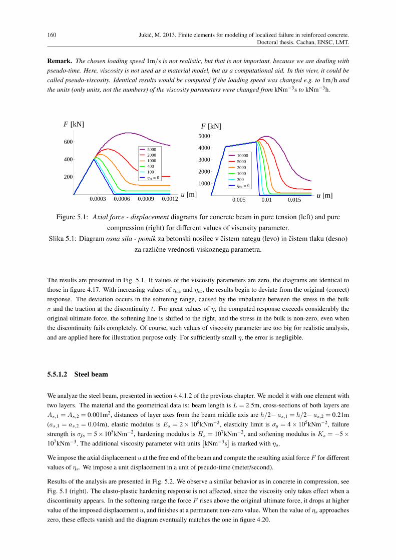
160 Jukic, M. 2013. Finite elements for modeling of localized failure in reinforced concrete.
Doctoral thesis. Cachan, ENSC, LMT.
Remark. The chosen loading speed 1m/s is not realistic, but that is not important, because we are dealing with
pseudo-time. Here, viscosity is not used as a material model, but as a computational aid. In this view, it could be
called pseudo-viscosity. Identical results would be computed if the loading speed was changed e.g. to 1m/h and
the units (only units, not the numbers) of the viscosity parameters were changed from kNm−3s to kNm−3h.
0.0003 0.0006 0.0009 0.0012u @mD
200
400
600
F @kND
Ηct = 0100400100020005000
0.005 0.01 0.015u @mD
1000
2000
3000
4000
5000
F @kND
Ηcc = 030010002000500010000
Figure 5.1: Axial force - displacement diagrams for concrete beam in pure tension (left) and pure
compression (right) for different values of viscosity parameter.
Slika 5.1: Diagram osna sila - pomik za betonski nosilec v cistem nategu (levo) in cistem tlaku (desno)
za razlicne vrednosti viskoznega parametra.
The results are presented in Fig. 5.1. If values of the viscosity parameters are zero, the diagrams are identical to
those in figure 4.17. With increasing values of ηcc and ηct, the results begin to deviate from the original (correct)
response. The deviation occurs in the softening range, caused by the imbalance between the stress in the bulk
σ and the traction at the discontinuity t. For great values of η, the computed response exceeds considerably the
original ultimate force, the softening line is shifted to the right, and the stress in the bulk is non-zero, even when
the discontinuity fails completely. Of course, such values of viscosity parameter are too big for realistic analysis,
and are applied here for illustration purpose only. For sufficiently small η, the error is negligible.
5.5.1.2 Steel beam
We analyze the steel beam, presented in section 4.4.1.2 of the previous chapter. We model it with one element with
two layers. The material and the geometrical data is: beam length is L = 2.5m, cross-sections of both layers are
As,1 = As,2 = 0.001m2, distances of layer axes from the beam middle axis are h/2− as,1 = h/2− as,2 = 0.21m
(as,1 = as,2 = 0.04m), elastic modulus is Es = 2× 10⁸kNm−2, elasticity limit is σy = 4× 10⁵kNm−2, failure
strength is σfs = 5× 10⁵kNm−2, hardening modulus is Hs = 107kNm−2, and softening modulus is Ks = −5×
107kNm−3. The additional viscosity parameter with units[kNm−3s
]is marked with ηs.
We impose the axial displacement u at the free end of the beam and compute the resulting axial force F for different
values of ηs. We impose a unit displacement in a unit of pseudo-time (meter/second).
Results of the analysis are presented in Fig. 5.2. We observe a similar behavior as in concrete in compression, see
Fig. 5.1 (right). The elasto-plastic hardening response is not affected, since the viscosity only takes effect when a
discontinuity appears. In the softening range the force F rises above the original ultimate force, it drops at higher
value of the imposed displacement u, and finishes at a permanent non-zero value. When the value of ηs approaches
zero, these effects vanish and the diagram eventually matches the one in figure 4.20.
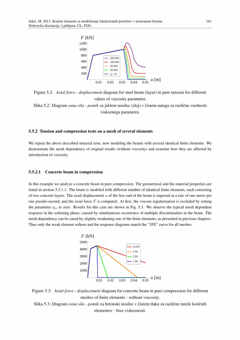
Jukic, M. 2013. Koncni elementi za modeliranje lokaliziranih porusitev v armiranem betonu.
Doktorska disertacija. Ljubljana, UL, FGG.
161
0.01 0.02 0.03 0.04 0.05u @mD
200
400
600
800
1000
1200
F @kND
Ηs = 0
20 000
50 000
100 000
200 000
Figure 5.2: Axial force - displacement diagram for steel beam (layer) in pure tension for different
values of viscosity parameter.
Slika 5.2: Diagram osna sila - pomik za jekleni nosilec (sloj) v cistem nategu za razlicne vrednosti
viskoznega parametra.
5.5.2 Tension and compression tests on a mesh of several elements
We repeat the above described uniaxial tests, now modeling the beams with several identical finite elements. We
demonstrate the mesh dependency of original results (without viscosity) and examine how they are affected by
introduction of viscosity.
5.5.2.1 Concrete beam in compression
In this example we analyze a concrete beam in pure compression. The geometrical and the material properties are
listed in section 5.5.1.1. The beam is modeled with different number of identical finite elements, each consisting
of two concrete layers. The axial displacement u of the free end of the beam is imposed at a rate of one meter per
one pseudo-second, and the axial force F is computed. At first, the viscous regularization is excluded by setting
the parameter ηcc to zero. Results for this case are shown in Fig. 5.3. We observe the typical mesh dependent
response in the softening phase, caused by simultaneous occurrence of multiple discontinuities in the beam. The
mesh dependency can be cured by slightly weakening one of the finite elements, as presented in previous chapters.
Thus only the weak element softens and the response diagrams match the “1FE” curve for all meshes.
0.01 0.02 0.03 0.04 0.05u @mD
1000
2000
3000
4000
5000
F @kND
1 FE
2 FE
5 FE
10 FE
Figure 5.3: Axial force - displacement diagram for concrete beam in pure compression for different
meshes of finite elements - without viscosity.
Slika 5.3: Diagram osna sila - pomik za betonski nosilec v cistem tlaku za razlicne mreze koncnih
elementov - brez viskoznosti.
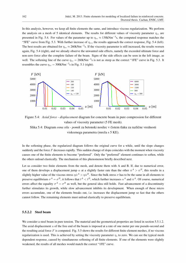
162 Jukic, M. 2013. Finite elements for modeling of localized failure in reinforced concrete.
Doctoral thesis. Cachan, ENSC, LMT.
In this analysis, however, we keep all finite elements the same, and introduce viscous regularization. We perform
the analysis on a mesh of 5 identical elements. The results for different values of viscosity parameter ηcc are
presented in Fig. 5.4. For values of the parameter up to ηcc ≈ 130kNm−3s, the computed response matches the
“5FE” curve from Fig. 5.3. With further increase of ηcc, the results approach the correct response, Fig. 5.4 (left).
The best results are obtained for ηcc ≈ 260kNm−3s. If the viscosity parameter is still increased, the results worsen
again, Fig. 5.4 (right), and we already observe the unwanted side effects, namely the exceeded ultimate force and
non-zero force after the complete failure of the beam. Signs of the side effects can be seen in the left image, as
well. The softening line of the curve ηcc = 260kNm−3s is not as steep as the correct “1FE” curve in Fig. 5.3. It
resembles the curve ηcc = 300kNm−3s in Fig. 5.1 (right).
0.01 0.02 0.03 0.04 0.05u @mD
1000
2000
3000
4000
5000
F @kND
Ηcc = 130
140
150
180
260
0.01 0.02 0.03 0.04 0.05u @mD
1000
2000
3000
4000
5000
F @kND
Ηcc = 300
800
1500
3000
6000
Figure 5.4: Axial force - displacement diagram for concrete beam in pure compression for different
values of viscosity parameter (5 FE mesh).
Slika 5.4: Diagram osna sila - pomik za betonski nosilec v cistem tlaku za razlicne vrednosti
viskoznega parametra (mreza s 5 KE).
In the softening phase, the regularized diagram follows the original curve for a while, until the slope changes
suddenly and the force F decreases rapidly. This sudden change of slope coincides with the moment when viscosity
causes one of the finite elements to become “preferred”. Only the “preferred” element continues to soften, while
the others unload elastically. The mechanism of this phenomenon briefly described next.
Let us consider two finite elements from the mesh, and denote them with A and B. If, due to numerical error,
one of them develops a displacement jump α at a slightly faster rate than the other αA > αB , this results in a
slightly higher value of the viscous stress ηαA > ηαB . Since the bulk stress σ has to be the same in all elements to
preserve equilibrium σA = σB , it follows that tA < tB , which further increases αA and αA. Of course, numerical
errors affect the equality σA = σB as well, but the general idea still holds. Fast advancement of a discontinuity
further stimulates its growth, while slow advancement inhibits its development. When enough of these micro
errors accumulate, one of the elements breaks out, i.e. increases the displacement jump so fast that the others
cannot follow. The remaining elements must unload elastically to preserve equilibrium.
5.5.2.2 Steel beam
We consider a steel beam in pure tension. The material and the geometrical properties are listed in section 5.5.1.2.
The axial displacement u of the free end of the beam is imposed at a rate of one meter per one pseudo-second and
the resulting axial force F is computed. Fig. 5.5 shows the results for different finite element meshes, if no viscous
regularization is used. This is achieved by setting the viscosity parameter ηs to zero. We can see the typical mesh
dependent response, caused by simultaneous softening of all finite elements. If one of the elements were slightly
weakened, the results of all meshes would match the correct “1FE” curve.
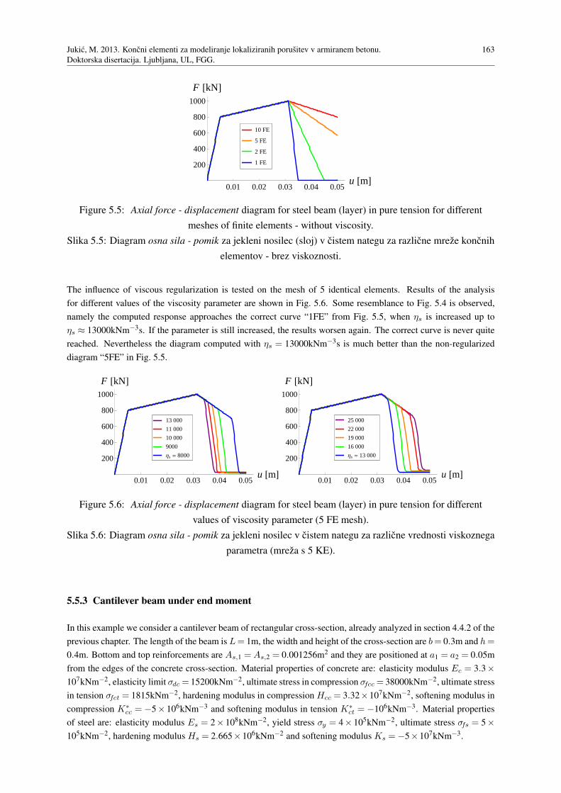
Jukic, M. 2013. Koncni elementi za modeliranje lokaliziranih porusitev v armiranem betonu.
Doktorska disertacija. Ljubljana, UL, FGG.
163
0.01 0.02 0.03 0.04 0.05u @mD
200
400
600
800
1000
F @kND
1 FE
2 FE
5 FE
10 FE
Figure 5.5: Axial force - displacement diagram for steel beam (layer) in pure tension for different
meshes of finite elements - without viscosity.
Slika 5.5: Diagram osna sila - pomik za jekleni nosilec (sloj) v cistem nategu za razlicne mreze koncnih
elementov - brez viskoznosti.
The influence of viscous regularization is tested on the mesh of 5 identical elements. Results of the analysis
for different values of the viscosity parameter are shown in Fig. 5.6. Some resemblance to Fig. 5.4 is observed,
namely the computed response approaches the correct curve “1FE” from Fig. 5.5, when ηs is increased up to
ηs ≈ 13000kNm−3s. If the parameter is still increased, the results worsen again. The correct curve is never quite
reached. Nevertheless the diagram computed with ηs = 13000kNm−3s is much better than the non-regularized
diagram “5FE” in Fig. 5.5.
0.01 0.02 0.03 0.04 0.05u @mD
200
400
600
800
1000
F @kND
Ηs = 8000
9000
10 000
11 000
13 000
0.01 0.02 0.03 0.04 0.05u @mD
200
400
600
800
1000
F @kND
Ηs = 13 000
16 000
19 000
22 000
25 000
Figure 5.6: Axial force - displacement diagram for steel beam (layer) in pure tension for different
values of viscosity parameter (5 FE mesh).
Slika 5.6: Diagram osna sila - pomik za jekleni nosilec v cistem nategu za razlicne vrednosti viskoznega
parametra (mreza s 5 KE).
5.5.3 Cantilever beam under end moment
In this example we consider a cantilever beam of rectangular cross-section, already analyzed in section 4.4.2 of the
previous chapter. The length of the beam is L= 1m, the width and height of the cross-section are b= 0.3m and h=
0.4m. Bottom and top reinforcements are As,1 =As,2 = 0.001256m2 and they are positioned at a1 = a2 = 0.05m
from the edges of the concrete cross-section. Material properties of concrete are: elasticity modulus Ec = 3.3×
107kNm−2, elasticity limit σdc = 15200kNm−2, ultimate stress in compression σfcc = 38000kNm−2, ultimate stress
in tension σfct = 1815kNm−2, hardening modulus in compression Hcc = 3.32×10⁷kNm−2, softening modulus in
compression K∗cc = −5× 10⁶kNm−3 and softening modulus in tension K∗
ct = −106kNm−3. Material properties
of steel are: elasticity modulus Es = 2× 10⁸kNm−2, yield stress σy = 4× 10⁵kNm−2, ultimate stress σfs = 5×
105kNm−2, hardening modulus Hs = 2.665×10⁶kNm−2 and softening modulus Ks =−5×10⁷kNm−3.
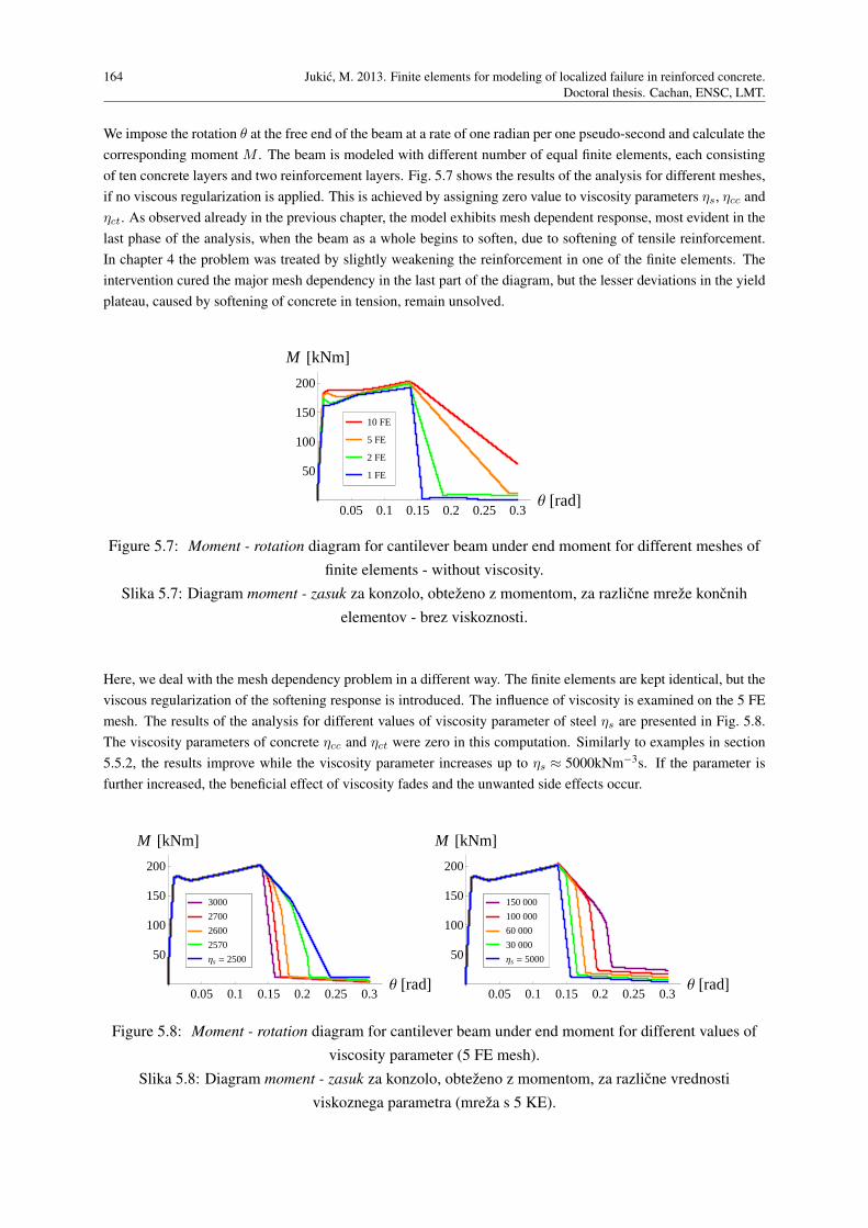
164 Jukic, M. 2013. Finite elements for modeling of localized failure in reinforced concrete.
Doctoral thesis. Cachan, ENSC, LMT.
We impose the rotation θ at the free end of the beam at a rate of one radian per one pseudo-second and calculate the
corresponding moment M . The beam is modeled with different number of equal finite elements, each consisting
of ten concrete layers and two reinforcement layers. Fig. 5.7 shows the results of the analysis for different meshes,
if no viscous regularization is applied. This is achieved by assigning zero value to viscosity parameters ηs, ηcc and
ηct. As observed already in the previous chapter, the model exhibits mesh dependent response, most evident in the
last phase of the analysis, when the beam as a whole begins to soften, due to softening of tensile reinforcement.
In chapter 4 the problem was treated by slightly weakening the reinforcement in one of the finite elements. The
intervention cured the major mesh dependency in the last part of the diagram, but the lesser deviations in the yield
plateau, caused by softening of concrete in tension, remain unsolved.
0.05 0.1 0.15 0.2 0.25 0.3Θ @radD
50
100
150
200
M @kNmD
1 FE
2 FE
5 FE
10 FE
Figure 5.7: Moment - rotation diagram for cantilever beam under end moment for different meshes of
finite elements - without viscosity.
Slika 5.7: Diagram moment - zasuk za konzolo, obtezeno z momentom, za razlicne mreze koncnih
elementov - brez viskoznosti.
Here, we deal with the mesh dependency problem in a different way. The finite elements are kept identical, but the
viscous regularization of the softening response is introduced. The influence of viscosity is examined on the 5 FE
mesh. The results of the analysis for different values of viscosity parameter of steel ηs are presented in Fig. 5.8.
The viscosity parameters of concrete ηcc and ηct were zero in this computation. Similarly to examples in section
5.5.2, the results improve while the viscosity parameter increases up to ηs ≈ 5000kNm−3s. If the parameter is
further increased, the beneficial effect of viscosity fades and the unwanted side effects occur.
0.05 0.1 0.15 0.2 0.25 0.3Θ @radD
50
100
150
200
M @kNmD
Ηs = 2500
2570
2600
2700
3000
0.05 0.1 0.15 0.2 0.25 0.3Θ @radD
50
100
150
200
M @kNmD
Ηs = 5000
30 000
60 000
100 000
150 000
Figure 5.8: Moment - rotation diagram for cantilever beam under end moment for different values of
viscosity parameter (5 FE mesh).
Slika 5.8: Diagram moment - zasuk za konzolo, obtezeno z momentom, za razlicne vrednosti
viskoznega parametra (mreza s 5 KE).
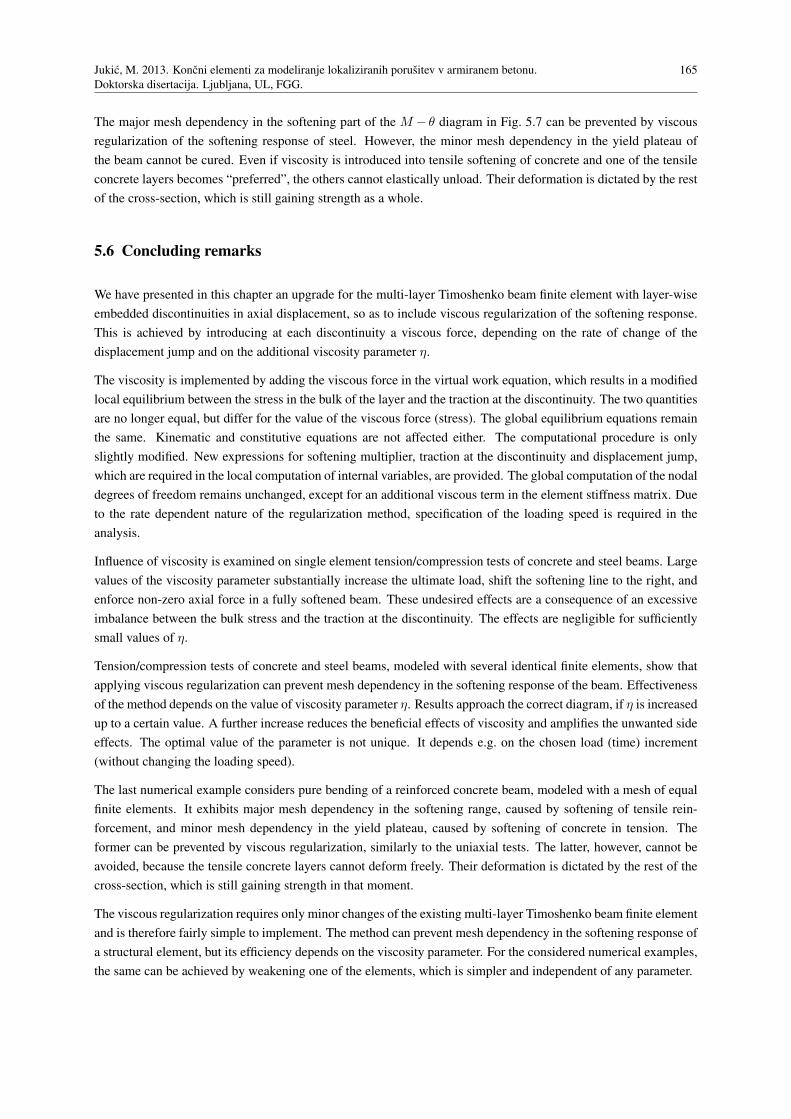
Jukic, M. 2013. Koncni elementi za modeliranje lokaliziranih porusitev v armiranem betonu.
Doktorska disertacija. Ljubljana, UL, FGG.
165
The major mesh dependency in the softening part of the M − θ diagram in Fig. 5.7 can be prevented by viscous
regularization of the softening response of steel. However, the minor mesh dependency in the yield plateau of
the beam cannot be cured. Even if viscosity is introduced into tensile softening of concrete and one of the tensile
concrete layers becomes “preferred”, the others cannot elastically unload. Their deformation is dictated by the rest
of the cross-section, which is still gaining strength as a whole.
5.6 Concluding remarks
We have presented in this chapter an upgrade for the multi-layer Timoshenko beam finite element with layer-wise
embedded discontinuities in axial displacement, so as to include viscous regularization of the softening response.
This is achieved by introducing at each discontinuity a viscous force, depending on the rate of change of the
displacement jump and on the additional viscosity parameter η.
The viscosity is implemented by adding the viscous force in the virtual work equation, which results in a modified
local equilibrium between the stress in the bulk of the layer and the traction at the discontinuity. The two quantities
are no longer equal, but differ for the value of the viscous force (stress). The global equilibrium equations remain
the same. Kinematic and constitutive equations are not affected either. The computational procedure is only
slightly modified. New expressions for softening multiplier, traction at the discontinuity and displacement jump,
which are required in the local computation of internal variables, are provided. The global computation of the nodal
degrees of freedom remains unchanged, except for an additional viscous term in the element stiffness matrix. Due
to the rate dependent nature of the regularization method, specification of the loading speed is required in the
analysis.
Influence of viscosity is examined on single element tension/compression tests of concrete and steel beams. Large
values of the viscosity parameter substantially increase the ultimate load, shift the softening line to the right, and
enforce non-zero axial force in a fully softened beam. These undesired effects are a consequence of an excessive
imbalance between the bulk stress and the traction at the discontinuity. The effects are negligible for sufficiently
small values of η.
Tension/compression tests of concrete and steel beams, modeled with several identical finite elements, show that
applying viscous regularization can prevent mesh dependency in the softening response of the beam. Effectiveness
of the method depends on the value of viscosity parameter η. Results approach the correct diagram, if η is increased
up to a certain value. A further increase reduces the beneficial effects of viscosity and amplifies the unwanted side
effects. The optimal value of the parameter is not unique. It depends e.g. on the chosen load (time) increment
(without changing the loading speed).
The last numerical example considers pure bending of a reinforced concrete beam, modeled with a mesh of equal
finite elements. It exhibits major mesh dependency in the softening range, caused by softening of tensile rein-
forcement, and minor mesh dependency in the yield plateau, caused by softening of concrete in tension. The
former can be prevented by viscous regularization, similarly to the uniaxial tests. The latter, however, cannot be
avoided, because the tensile concrete layers cannot deform freely. Their deformation is dictated by the rest of the
cross-section, which is still gaining strength in that moment.
The viscous regularization requires only minor changes of the existing multi-layer Timoshenko beam finite element
and is therefore fairly simple to implement. The method can prevent mesh dependency in the softening response of
a structural element, but its efficiency depends on the viscosity parameter. For the considered numerical examples,
the same can be achieved by weakening one of the elements, which is simpler and independent of any parameter.
166 Jukic, M. 2013. Finite elements for modeling of localized failure in reinforced concrete.
Doctoral thesis. Cachan, ENSC, LMT.
6 CONCLUSIONS
The aim of the dissertation was to develop finite elements capable of modeling localized failure in reinforced
concrete, for numerical analysis of reinforced concrete beams and frames up to complete collapse. The localized
failure was modeled in accordance with the embedded strong discontinuity approach, in which a discontinuity
in displacement (or rotation) is incorporated into the finite element, resulting in discontinuous displacement (or
rotation) field.
We have derived a stress-resultant Euler-Bernoulli beam finite element with embedded discontinuity in rotation,
based on small deformation kinematics, elastoplastic model with bilinear hardening for the bulk of the element,
and rigid plastic linear softening model for the discontinuity.
• Despite its simplicity, the finite element is capable of describing the major phenomena in reinforced concrete
beam behavior - reduction of stiffness due to cracking of concrete, yielding of reinforcement and localized
failure of the beam.
• The finite element allows for analysis of reinforced concrete beams and frames up to complete failure, which
provides information not only about the ultimate load, but also about ductility and post-peak response of the
structure.
• The obtained results compare reasonably well to other results available in literature and to experimental
results.
• The finite element provides mesh independent softening response of the modeled structure.
• Moment vs. curvature diagram for the bulk and moment vs. rotational jump diagram for the discontinuity
are required as an input for the analysis. They can be determined from an experiment or computed with a
more refined finite element.
• The finite element could be further upgraded by implementing a coupled damage-plasticity model for the
bulk or by including a discontinuity in axial displacements, but for the common reinforced concrete struc-
tures, improvement of the results should not be substantial.
We have derived a multi-layer Euler-Bernoulli beam finite element with layer-wise embedded discontinuities in
axial displacement, based on small deformation kinematics. The reinforced concrete beam is divided into concrete
and reinforcement layers, and a jump in axial displacement is introduced separately into each of them. Behavior of
a concrete layer is controlled by an elasto-damage hardening law in the bulk and by a rigid damage softening law
at the discontinuity. Behavior of a steel layer is controlled by an elastoplastic hardening law in the bulk and by a
rigid plastic softening law at the discontinuity.
• The finite element was intended for detailed analysis of reinforced concrete beams and frames, and for
computation of stress-resultant properties, required as an input in the stress-resultant analysis. However, the
element does not perform as expected. Several issues have been identified.
• The interpolation function for enhanced layer strain has been derived on an isolated layer, under assumption
that it can deform freely. This is not true because the layer is bound to other layers through common
nodal displacements. Consequently, the additional stress caused by enhanced kinematics cannot redistribute
correctly. The stress is only controlled at the discontinuity, where it has to be equal to the traction at the
discontinuity and therefore has to decrease with increasing displacement jump. Elsewhere in the layer, the
stress may even grow above the ultimate stress.
Jukic, M. 2013. Koncni elementi za modeliranje lokaliziranih porusitev v armiranem betonu.
Doktorska disertacija. Ljubljana, UL, FGG.
167
• Equilibrium is only required on the finite element level, but not for each individual layer. We have seen an
example of a beam in pure tension, where stress was linear (not constant) over the length of each layer. If a
layer were singled out, it would not be in equilibrium, but the finite element as a whole is in balance because
the imbalances of individual layers neutralize each other.
• The displacement jumps of individual layers are independent of each other. In a specific case of a can-
tilever beam in pure tension, the values of displacement jumps changed linearly over the height of the beam
(negative on the bottom edge, positive on the top edge and zero in the middle), resulting in a non-zero lat-
eral displacement of the free end of the beam, without disrupting equilibrium (the internal shear forces and
internal moments were zero).
• There is no discontinuity (in rotation) on the element level. The middle axis of the beam always deforms
according to standard Euler-Bernoulli kinematics and is therefore smooth, even if the beam is completely
broken. The bulk of each layer slides along a path, parallel to the middle axis. This may not be problematic
if a fine mesh is used, since the broken finite element exhibits a greater curvature than the neighboring
elements, which can be interpreted as a discontinuity smeared over the whole element.
• Mesh dependency has been observed in numerical tests, most clearly in the case of a cantilever beam under
end moment. Due to constant stress state over the length of the beam, discontinuities appear simultaneously
in all finite elements of the mesh. At the same imposed rotation of the free end of the beam, a fine mesh
produces a great number of small discontinuities and a coarse mesh produces a small number of great
discontinuities. According to the softening material law, the traction at the discontinuity drops with its
increasing size. Therefore, the fine mesh produces a greater moment then the coarse mesh at the same value
of imposed rotation. The greatest deviations appear when the beam as a whole enters the softening phase,
which usually happens due to softening of tensile reinforcement. This can be cured by slightly weakening
reinforcement in one of the finite elements and thus preventing multiple discontinuities. If the beam fails
due to crushing of concrete in compression, the problem cannot be solved so effectively. Also, the (lesser)
mesh dependency due to cracking of concrete in tension cannot be avoided.
• Considering all the deficiencies, the considered multi-layer Euler-Bernoulli beam finite element cannot be
recommended for general use. The only viable application is in case of constant strain/stress state over
the length of the beam, which can occur either in pure tension/compression or in pure bending. In case of
bending, mesh dependency cannot be completely avoided.
We have derived a multi-layer Timoshenko beam finite element with layer-wise embedded discontinuities in axial
displacement, based on small deformation kinematics. The reinforced concrete beam is divided into concrete and
reinforcement layers, and a jump in axial displacement is introduced separately into each of them. Behavior of a
concrete layer is controlled by an elasto-damage hardening law in the bulk and by a rigid damage softening law
at the discontinuity. Behavior of a steel layer is controlled by an elastoplastic hardening law in the bulk and by a
rigid plastic softening law at the discontinuity. Shear response is assumed elastic.
• The finite element allows for detailed analysis of reinforced concrete beams and frames up to complete
failure, which provides information not only about the ultimate load, but also about ductility and post-peak
response of the structure. A detailed description of material state (progression of damage, plasticity and
localized failures) is provided at any stage of the analysis.
• The finite element is not intended for cyclic loading. Nevertheless, it can handle minor changes of the load
sign, which can occur due to shifting of the neutral axis even in monotonic loading.
• Two material laws are required for each material - stress vs. strain for the bulk of the layer and traction
vs. displacement jump for the discontinuity. They can be determined from tension/compression tests. This
makes the finite element appropriate for computation of stress-resultant (material-geometrical) properties
of beams, required as an input in the analysis with a stress-resultant finite element.
168 Jukic, M. 2013. Finite elements for modeling of localized failure in reinforced concrete.
Doctoral thesis. Cachan, ENSC, LMT.
• Mesh dependency has been observed in numerical tests, most clearly in the case of a cantilever beam under
end moment. Due to constant stress state over the length of the beam, discontinuities appear simultaneously
in all finite elements of the mesh. At the same imposed rotation of the free end of the beam, a fine mesh
produces a great number of small discontinuities and a coarse mesh produces a small number of great
discontinuities. According to the softening material law, the traction at the discontinuity drops with its
increasing size. Therefore, the fine mesh produces a greater moment then the coarse mesh at the same value
of imposed rotation. The greatest deviations appear when the beam as a whole enters the softening phase,
which usually happens due to softening of tensile reinforcement. This can be cured by slightly weakening
reinforcement in one of the finite elements and thus preventing multiple discontinuities. If the beam fails
due to crushing of concrete in compression, the problem cannot be solved so effectively. Also, the mesh
dependency due to cracking of concrete in tension cannot be avoided.
• Mesh dependency due to cracking of concrete in tension is more evident in the case of a cantilever beam
under end transversal force. Since the finite element can only describe constant state over the length, a fine
mesh is required for adequate description of the linear moment. However, shortening of the finite elements
increases the number and reduces the size of discontinuities, resulting in a higher traction in tensile concrete
and considerably overestimated yield moment of the beam.
• There is no discontinuity (in rotation) on the element level. The middle axis of the beam always deforms
according to standard Euler-Bernoulli kinematics and is therefore smooth, even if the beam is completely
broken. The bulk of each layer slides along a path, parallel to the middle axis. This may not be problematic
if a fine mesh is used, since the broken finite element exhibits a greater curvature than the neighboring
elements, which can be interpreted as a discontinuity smeared over the whole element.
• Performance of the finite element has been tested on several numerical examples. In some cases, the com-
puted results compare well to other results available in literature and to experimental results. In some cases,
however, the difference was considerable.
• Before the finite element is put to general use, the mesh dependency, caused by softening of concrete in
tension, should be examined carefully. In the specific case of a cantilever under end force, the influence was
substantial. However, in some more complex structures, the mesh dependency was less noticeable.
• The finite element could be modified so as to allow cyclic loading. For that purpose, separate sets of
softening internal variables should be introduced. However, softening responses in tension and compression
are not independent, neither is their relation trivial to describe.
We have upgraded the multi-layer Timoshenko beam finite element, so as to include viscous regularization of the
softening response. This is performed by introducing at each discontinuity a viscous force, depending on the rate
of change of the displacement jump and an additional viscosity parameter. The viscous forces are added in the
virtual work equation, resulting in slightly modified equilibrium equations and consequent minor alterations of the
computational procedure.
• Viscous regularization is relatively simple to implement, as it only requires minor changes of the existing
multi-layer Timoshenko beam finite element.
• Great values of the viscosity parameter can corrupt the results of the analysis by increasing the ultimate
load, shifting the softening line (delaying the softening) and producing a non-zero stress state in a beam
with a fully softened discontinuity. The effects are negligible for sufficiently small values of the parameter.
• Viscous regularization can prevent mesh dependent softening response of a beam, caused by physically
erroneous occurrence of multiple discontinuities in a homogeneous stress field. However, effectiveness of
the regularization depends on the value of the viscosity parameter. The optimal value is not unique, as it
depends e.g. on the chosen load (time) increment.
Jukic, M. 2013. Koncni elementi za modeliranje lokaliziranih porusitev v armiranem betonu.
Doktorska disertacija. Ljubljana, UL, FGG.
169
• Mesh dependency, caused by softening of concrete in tension when the beam as a whole is still gaining
strength, cannot be prevented by this method because the softening concrete layers cannot deform freely.
Their deformation is dictated by the rest of the cross-section.

170 Jukic, M. 2013. Finite elements for modeling of localized failure in reinforced concrete.
Doctoral thesis. Cachan, ENSC, LMT.
RAZSIRJENI POVZETEK
V gradbenistvu se uporablja mnogo materialov, ki ob doloceni obremenitvi lokalno odpovejo. Za lokalizirano
porusitev je znacilno, da je vecji del deformacij zgoscenih na relativno majhnih obmocjih v okolici kriticnih mest
konstrukcije. Z njihovim narascanjem se napetosti v materialu zmanjsujejo, cemur pravimo mehcanje materiala.
Pravilen opis tega pojava je bistvenega pomena v porusni analizi konstrukcij.
V disertaciji se osredotocimo na armiranobetonske nosilce in okvirje, ki so ena prevladujocih konstrukcijskih oblik
pri nas in po svetu. V armiranem betonu se lokalizirana porusitev pojavi kot posledica pokanja betona v nategu
in krusenja v tlaku, tecenja armature, medsebojnega zdrsa obeh komponent in njune lokalne odpovedi. Te lo-
kalizirane poskodbe materiala, ki jih opazimo npr. na vrhu in na dnu stebrov stavb, poskodovanih v potresih,
obicajno opisemo s plasticnim clenkom. V klasicni analizi mejne nosilnosti moment v posameznem clenku ohra-
nja isto vrednost, medtem ko se z narascanjem obremenitve oblikujejo novi clenki drugod po konstrukciji. Tak
pristop omejuje natancnost dolocene mejne nosilnosti ter preprecuje analizo duktilnosti konstrukcije in njenega
post-kriticnega obnasanja. V staticno nedolocenih konstrukcijah porusitev posameznega kriticnega elementa se ne
ogrozi celotne konstrukcije, zato je za njeno natancno analizo potrebno poznati tudi odziv elementa v mehcanju.
V zadnjem casu smo prica znatnemu napredku na podrocju modeliranja mehcanja v numericni analizi konstruk-
cij, vendar precej problemov se vedno ostaja odprtih. Pregled zgodovinskega razvoja in trenutnega stanja na tem
podrocju najdemo npr. v [12–14]. V prvih modelih je bilo mehcanje materiala opisano lokalno, s padajoco kri-
vuljo v diagramu napetost-deformacija. Pristop je sicer enostaven, vendar ga pestijo stevilne tezave, ki jih lahko
opredelimo kot matematicne, fizikalne in numericne. Z matematicnega vidika postanejo parcialne diferencialne
enacbe robnega problema slabo pogojene zaradi negativnega elasticnega modula v obmocju mehcanja [12,15,16].
V konstrukcijskem elementu, diskretiziranem z mrezo koncnih elementov, odpove le kriticni element. Ker je sipa-
nje energije vezano na prostornino materiala, kjer poteka mehcanje, se kolicina disipirane energije z zgoscevanjem
mreze koncnih elementov priblizuje vrednosti nic. V limitni situaciji to pomeni porusitev brez disipacije energije,
kar fizikalno ni sprejemljivo. Z vidika numericnega modeliranja tak pristop ocitno vodi do izrazite odvisnosti
rezultatov od izbrane diskretizacije [17, 18].
Za resitev opisanih tezav je bilo predlaganih vec pristopov. Nekaj zgodnejsih je predstavljenih v [19]. Zelo eno-
stavni so t.i. “crack-band” modeli [20–22], v katerih je lokalizirana porusitev razmazana na celoten koncni element
in porusitev brez disipacije energije preprecena z omejitvijo minimalne velikosti elementov. Ker je volumen, v ka-
terem se material mehca, se vedno odvisen od diskretizacije, je potrebno vrednost modula mehcanja prilagoditi
izbrani mrezi. Sorodno resitev predstavljajo modeli, pri katerih je znotraj elementa predpisan pas fiksne sirine
(materialna karakteristika), v katerem se material mehca [23, 24]. Omenjene metode ne resijo matematicne plati
problema.
Kot alternativa je bilo predstavljenih vec ne-lokalnih metod [19,25–27], pri katerih je napetost v neki tocki funkcija
povprecne (ne-lokalne) deformacije v nekem koncnem volumnu okoli te tocke. Bolj splosno je napetost v posame-
zni tocki funkcija celotnega deformacijskega polja, pri cemer je vplivno obmocje doloceno z uteznimi funkcijami.
Z matematicnega vidika ne-lokalne metode popolnoma regularizirajo obravnavani problem [12]. Zelo sorodna je
gradientna metoda [28, 29], pri kateri za opis napetosti v neki tocki poleg vrednosti deformacij uporabimo tudi
njihov gradient v tisti tocki. Uporabimo lahko tudi gradiente visjega reda [30].
Predlaganih je bilo se vec pristopov, kot sta na primer model Cosseratovega kontinuuma [31, 32], ki poleg tran-
slatornega pomika uposteva tudi lokalno rotacijo posameznega delca (tocke) materiala, in viskoplasticna regulari-
zacija [33], ki obravnava problem kot casovno odvisen. Skupno vsem nastetim metodam je, da se lotevajo opisa
lokalizirane porusitve in mehcanja na nivoju materiala. Koncni elementi so zasnovani tako, da cim natancneje
Jukic, M. 2013. Koncni elementi za modeliranje lokaliziranih porusitev v armiranem betonu.
Doktorska disertacija. Ljubljana, UL, FGG.
171
opisejo obnasanje materiala na mikro nivoju, vkljucno s samodejnim generiranjem nezveznosti na kriticnih me-
stih, in tako zagotovijo primeren odziv konstrukcijskega elementa na makro nivoju.
Pri razvoju koncnih elementov za uporabo v potresnem inzenirstvu se pogosto uporablja popolnoma drugacen
pristop. Numericna analiza velikih konstrukcij pod kompleksno obtezbo, lahko kaj hitro postane racunsko pre-
zahtevna in casovno potratna, zato so koncni elementi zasnovani na najenostavnejsi nacin, ki se zagotavlja pri-
meren makro-odziv konstrukcijskega elementa. Obnasanje armiranobetonskih stebrov, ki izkazujejo lokalizirane
poskodbe na dnu in na vrhu, lahko zadovoljivo opisemo z zelo enostavnim “lumped plasticity” modelom [34, 35],
pri katerem so vse neelasticne deformacije zdruzene v plasticnih clenkih nicelne dolzine na obeh koncih elementa,
medtem ko se vmesni del obnasa elasticno. To seveda ne ustreza dejanskemu stanju materiala, kljub temu pa model
zajame vse bistvene lastnosti odziva stebra.
Diskretni pristop, uporabljen v “lumped plasticity” in sorodnih modelih je alternativa predhodno predstavljenim
zveznim modelom. Obe strani imata svoje prednosti in slabosti. Glavna prednost modelov razmazane nezveznosti
je, da so razviti na mikro nivoju, zato so sposobni opisati katerikoli koscek materiala, ne glede na velikost in polozaj
v konstrukciji, nezveznost pa generirajo samodejno. Slaba stran je ta, da zahtevajo precej gosto mrezo koncnih
elementov v obmocju nezveznosti, kar je lahko problematicno pri analizi vecjih konstrukcij [12, 36]. Nekateri
imajo tudi tezave z blokiranjem [13, 36]. Pomembna prednost diskretnega pristopa je, da se izogne tezavam z
velikostjo obmocja mehcanja, tako da ga skrci v tocko in vpelje lokalni disipativni mehanizem. Poleg tega so
elementi sposobni opisati nezveznosti v pomikih in zasukih, kar omogoca opis konstrukcije z dokaj grobo mrezo
koncnih elementov. Glavna slabost je ta, da se nezveznosti lahko pojavijo le na predhodno dolocenih lokacijah.
V zadnjem casu se je v modeliranju lokalizirane porusitve uveljavil nov pristop, katerega glavna znacilnost je
vkljucitev nezveznih deformacij ali pomikov v standardne koncne elemente. Skoke v deformacijskem polju ime-
nujemo tudi sibke nezveznosti, skoke v polju pomikov pa mocne nezveznosti. V skladu z metodo vgrajene mocne
nezveznosti, ki jo uporabimo tudi v tej disertaciji, je bilo razvitih mnogo razlicnih modelov, npr. [39–48]. Za nas
je posebej zanimiva aplikacija metode na linijske koncne elemente [49–54]. Vsem modelom je skupno, da koncni
volumen lokaliziranih deformacij, ki je predstavljal obmocje disipiranja energije pri modelih razmazane nezve-
znosti, nadomestijo z nezveznostjo v pomikih in s pripadajocim lokalnim disipativnim mehanizmom. To dosezejo
z vpeljavo dodatnih, nezveznih interpolacijskih funkcij. Vsaka oblikovna funkcija je povezana z dodatnim para-
metrom, ki predstavlja velikost nezveznosti. Z vpeljavo kohezivnega materialnega zakona mehcanja, ki skok v
pomiku poveze s konjugirano silo v nezveznosti, se oblikuje lokalni disipativni mehanizem. Dodatne enacbe za
nove parametre so zapisane v obliki lokalnega ravnotezja med napetostmi po elementu in silo (ali napetostjo) v
nezveznosti [1, 14].
Metoda vgrajene mocne nezveznosti zdruzuje dobre lastnosti tako diskretnih, kot zveznih metod. Disipacija ener-
gije ob porusitvi je vezana na nezveznost, ki nima volumna, zato zgoscevanje mreze koncnih elementov ne vpliva
na velikost obmocja mehcanja in na kolicino disipirane energije. S tem sta prepreceni odvisnost rezultatov od dis-
kretizacije in fizikalno nerealna porusitev brez disipacije energije. Tudi z matematicnega vidika je problem mejnih
vrednosti dobro pogojen, kar pomeni, da pristop uspesno resi na zacetku predstavljene fizikalne, numericne in
matematicne tezave. Izboljsana kinematika omogoca korekten opis nezveznega polja pomikov v blizini nezve-
znosti, kar omogoca razvoj koncnih elementov, ki nimajo tezav z blokiranjem. Dodatne interpolacijske oblike so
namrec zasnovane tako, da omogocajo opis breznapetostnega stanja v elementu v primeru popolnoma zmehcane
nezveznosti [14]. Poleg tega vgraditev lokalne kinematike, ki opisuje porusitev materiala na mikro nivoju, v ma-
terialni makro-model popolnoma ustreza vec-nivojski naravi obravnavnega fizikalnega problema [1, 12, 14, 36, 40]
in omogoca modeliranje nezveznosti z relativno grobo mrezo koncnih elementov. Ker je vsak posamezen element
sposoben opisa nezveznosti, ni potrebe po vnaprejsnjem dolocanju njene lokacije. Nastane samodejno in napreduje
po konstrukciji brez spreminjanja osnovne mreze koncnih elementov. Zaradi nastetih lastnosti je metoda primerna
tudi za analizo vecjih konstrukcij.

172 Jukic, M. 2013. Finite elements for modeling of localized failure in reinforced concrete.
Doctoral thesis. Cachan, ENSC, LMT.
Glede na nacin implementacije nezveznosti locimo dva glavna pristopa – extended finite element method (X-
FEM) [39,40,42,57–59] in embedded discontinuity finite element method (ED-FEM) [41,60–63]. Pri X-FEM me-
todah so dodatni parametri, ki se nanasajo na nezvezne interpolacijske funkcije, vezani na vozlisca mreze koncnih
elementov in se jih obravnava kot globalne neznanke. Pri ED-FEM metodah pa so dodatni parametri na posamezen
koncni element in se jih obravnava kot lokalne (elementu lastne) neznanke. Prednosti in slabosti obeh pristopov so
predstavljene v vec studijah [14, 64]. Glavna prednost ED-FEM je v tem, da lahko dodatne neznanke izlocimo iz
globalnih enacb s staticno kondenzacijo na nivoju elementa, medtem ko pri X-FEM vsaka nova nezveznost razsiri
globalni sistem enacb. V disertaciji sledimo ED-FEM pristopu.
Naloga temelji predvsem na predhodnem delu nase raziskovalne skupine, zlasti na linijskih koncnih elementih, ki
so jih razvili Dujc et al. [54] in Pham et al. [52]. V prvem clanku je predstavljen koncni element na nivoju rezultant
napetosti za Euler-Bernoullijev nosilec, ki ima vgrajeni nezveznosti v zasuku in v osnem pomiku in je namenjen
analizi metalnih nosilcev in okvirjev. V drugem clanku je opisan koncni element na nivoju rezultant napetosti za
Timosenkov nosilec, ki ima vgrajeno nezveznost v zasuku in je namenjen analizi armiranobetonskih konstrukcij.
Prvi cilj disertacije je zdruziti oba koncepta in razviti podoben koncni element, ki temelji na Euler-Bernoullijevi
kinematiki in uporablja materialne zakone, primerne za modeliranje armiranega betona. Naslednji cilj je razsiriti
ta koncept na vecslojni model nosilca, podobno kot v [51]. Bolj konkretno lahko nase cilje opredelimo kot:
• razviti raven koncni element na nivoju rezultant napetosti za ravninski Euler-Bernoullijev nosilec z vgra-
jeno nezveznostjo v zasuku, namenjen enostavni robustni in ucinkoviti porusni analizi armiranobetonskih
nosilcev in okvirjev,
• razviti raven vecslojni koncni element za ravninski Euler-Bernoullijev nosilec, ki ima po slojih vgrajene
nezveznosti v osnem pomiku, namenjen detajlni porusni analizi armiranobetonskih nosilcev in okvirjev
ter racunu rezultantnih (materialno-geometrijskih) lastnosti prerezov, potrebnih pri analizi z rezultantnimi
koncnimi elementi,
• razviti raven vecslojni koncni element za ravninski Timosenkov nosilec, ki ima po slojih vgrajene nezvezno-
sti v osnem pomiku, namenjen detajlni porusni analizi armiranobetonskih nosilcev in okvirjev ter racunu
rezultantnih (materialno-geometrijskih) lastnosti prerezov, potrebnih pri analizi z rezultantnimi koncnimi
elementi,
• nadgraditi vecslojni element za Timosenkov nosilec z viskozno regularizacijo odziva v mehcanju.
KONCNI ELEMENT NA NIVOJU REZULTANT NAPETOSTI ZA EULER-BERNOULLIJEV
NOSILEC Z VGRAJENO NEZVEZNOSTJO V ZASUKU
V poglavju 2 razvijemo koncni element na nivoju rezultant napetosti z vgrajeno nezveznostjo v zasuku za rav-
ninski Euler-Bernoullijev nosilec. Element je namenjen za enostavno, robustno in ucinkovito numericno analizo
armiranobetonskih nosilcev in okvirjev do popolne porusitve. Element omogoca samodejno generiranje plasticnih
clenkov z mehcanjem, ki predstavljajo lokalizirano porusitev materiala na kriticnih mestih v konstrukciji. Element
temelji na dveh podobnih koncnih elementih, predstavljenih v [54] in [52]. V prvem clanku je izpeljan koncni
element za Euler-Bernoullijev nosilec z vgrajenima nezveznostma v zasuku in osnem pomiku za analizo metalnih
nosilcev in okvirjev. V drugem clanku je predstavljen element za Timosenkov nosilec z vgrajeno nezveznostjo v
zasuku, v katerem je uporabljen konstitutivni zakon z bilinearnim utrjevanjem, ki omogoca natancnejsi opis ne-
linearnega obnasanja nosilca zaradi razpokanja betona in tecenja armature. Element je zato primeren za analizo
armiranobetonskih konstrukcij, vendar zaradi izbrane kinematike omogoca le opis konstantnega momenta. Tu raz-
vijemo koncni element, ki zdruzuje lastnosti obeh navedenih elementov - konstitutivni zakon, primeren za armirani
beton, in kinematiko, ki omogoca opis linearnih momentov vzdolz elementa.
Jukic, M. 2013. Koncni elementi za modeliranje lokaliziranih porusitev v armiranem betonu.
Doktorska disertacija. Ljubljana, UL, FGG.
173
Koncni element temelji na teoriji majhnih deformacij. Vsebuje vgrajeno nezveznost v zasuku (skok v zasuku),
ki se pojavi na kriticnem mestu v elementu, ko je presezena mejna nosilnost. Obnasanje materiala je opisano z
elastoplasticnim materialnim zakonom z bilinearnim izotropnim utrjevanjem, obnasanje nezveznosti (plasticnega
clenka) pa z materialnim zakonom linearnega mehcanja.
Kinematika
Ravninski Euler-Bernoullijev nosilec modeliramo z ravnim dvovozliscnim koncnim elementom. Vsako vozlisce
ime tri prostostne stopnje, dva pomika in zasuk. V primeru prekoracene nosilnosti se pojavi nezveznost v zasukih
pri koordinati xd in aktivira se dodatna (lokalna) prostostna stopnja - skok v zasuku α. Osni pomik u(x) interpo-
liramo med vozliscne osne pomike u s standardnimi linearnimi oblikovnimi funkcijami Nu (x). Osno deformacijo
ε(x) izracunamo kot odvod osnega pomika.
u(x) = Nu (x)u, ε(x) =∂u
∂x= Bu (x)u
Precni pomik v (x) interpoliramo med vozliscne precne pomike v in zasuke θ s Hermitovimi polinomi Nv (x)
in Nθ (x). Standardni interpolaciji dodamo clen vadd (x,xd), ki opisuje dodatne pomike zaradi skoka v zasuku.
Odvod interpolacijske funkcije M (x,xd) ima enotski skok pri xd, vozliscne vrednosti funkcije in njenega odvoda
pa so enake nic.
v (x,xd) = Nv (x)v+Nθ (x)θ+
vadd︷ ︸︸ ︷
M (x,xd)α
Ukrivljenost κ(x,xd) izracunamo kot drugi odvod precnega pomika.
κ(x,xd) =∂2v
∂x2=
˜κ︷ ︸︸ ︷
Bv (x)v+Bθ (x)θ+
κadd
︷ ︸︸ ︷
G(x,xd)α
Operator G(x,xd) je drugi odvod interpolacijske funkcije M (x,xd). Zaradi nezveznosti prvega odvoda M ′ je G
sestavljen iz zveznega dela G in Dirac-delta funkcije, ki ima neskoncno vrednost na mestu nezveznosti in vrednost
nic drugje. Izraz za G izpeljemo iz zahteve, da mora biti v primeru popolne izgube nosilnosti koncni element
sposoben opisati breznapetostno stanje v nosilcu. V tem primeru se element deformira kot kinematicna veriga
dveh togih teles.
G= M ′′ = G+ ¯G, G=−1+3
(
1− 2xdL
)(1− 2x
L
)
L, ¯G= δxd =
∞; x= xd
0; sicer
Interpolacijo osne deformacije in standardnega dela ukrivljenosti lahko zapisemo tudi krajse.
ε=[
Bu 0 0]
d = Bεd, ˜κ=[
0 Bv Bθ]
d = Bκd, dT =
uT ,vT ,θT
174 Jukic, M. 2013. Finite elements for modeling of localized failure in reinforced concrete.
Doctoral thesis. Cachan, ENSC, LMT.
Princip virtualnega dela
Virtualno osno deformacijo ε in virtualno ukrivljenost κ interpoliramo na enak nacin kot pravi kolicini, med virtu-
alne vozliscne pomike u, v in θ ter virtualni skok v zasuku α. To pripelje do dodatnega clena v izrazu za virtualno
delo notranjih sil Gint,(e) elementa (e).
ε= Buu, κ= Bv v+Bθθ+ Gα︸︷︷︸
κadd
, G int,(e) =∫
L
(εN + κM)dx= d(e)T f int,(e)︸ ︷︷ ︸
standardno
+ α(e)h(e)︸ ︷︷ ︸
dodatno
Vektor posplosenih virtualnih pomikov d(e) zdruzuje vse virtualne prostostne stopnje elementa (e), vektor f int,(e)
pa ustrezno urejene notranje sile. Kolicina h(e) ustreza virtualnemu skoku v zasuku α(e).
d(e)T =
uT , vT , θT
, f int,(e) =∫
L
BεTNdx+∫
L
BκT
Mdx, h(e) =∫
L
GMdx
Z upostevanjem prej izpeljanega izraza za operator G in pravila za integriranje Dirac-delta funkcije razvijemo
izraz za h(e). Moment M (x) je funkcija koordinate x. Njeno vrednost na mestu nezveznosti M |xd oznacimo s t
in definiramo kot moment v nezveznosti, ki je konjugirana kolicina skoku v zasuku α.
∫
L
g (x)δxddx= g (xd) , h(e) =∫
L
(G+ δxd
)Mdx=
∫
L
GMdx+ M |xd =∫
L
GMdx+ t
Iz principa virtualnega dela Gint−Gext = 0 izpeljemo ravnotezne enacbe konstrukcije. Poleg klasicnega globalnega
ravnotezja zunanjih in notranjih sil dobimo dodatno ravnotezno enacbo za vsak element, v katerem je bila nosilnost
prekoracena in se je oblikovala nezveznost v zasukih.
nFE
Ae=1
[
f int,(e)− f ext,(e)]
= 0, ∀e ∈ 1,2, . . . ,nα : h(e) = 0
Tu je A tako imenovani “assembly” operator, nFE stevilo koncnih elementov v celotni konstrukciji, nα pa stevilo
koncnih elementov z aktivirano nezveznostjo. Pomen dodatne enacbe se razjasni, ce vanjo vstavimo izpeljani izraz
za h(e). Ugotovimo, da predstavlja ravnotezje med momentom v nezveznosti t in momenti po elementu M v sibki
(integralski) obliki. Ker se nanasa le na posamezen koncni element, ji pravimo tudi enacba lokalnega ravnotezja.
h(e) = 0 ⇔ t=−∫
L
GMdx
Materialni modeli
Predpostavimo, da je osna sila ves cas elasticna N = EAε. Za upogibni odziv nosilca uporabimo elastoplasticni
model z bilinearnim utrjevanjem. Po dosezeni meji elasticnosti togost nekoliko pade zaradi poskodb v betonu,
bistven padec togosti pa se zgodi zaradi tecenja natezne armature. Krivulja razbremenjevanja ima elasticni naklon.
Osnovne enacbe materialnega modela so izpeljane iz termodinamike (princip maksimalne plasticne disipacije),
glej npr. [73]. Moment izracunamo iz elasticne ukrivljenosti, ki je razlika med skupno ukrivljenostjo κ in plasticno
ukrivljenostjo κp. V izrazu za skupno ukrivljenost nastopa tudi prispevek zaradi skoka v zasuku α.

Jukic, M. 2013. Koncni elementi za modeliranje lokaliziranih porusitev v armiranem betonu.
Doktorska disertacija. Ljubljana, UL, FGG.
175
M = EI (κ− κp) , κ= Bvv+Bθθ+ Gα
Funkcija tecenja φ nadzira prehod iz elasticnega v plasticno obnasanje in obratno. Konstanta Mc > 0 predstavlja
absolutno vrednost momenta, pri katerem se prvic pojavijo neelasticne deformacije. Momentu podobna kolicina
q ≤ 0 predstavlja spremembo meje elasticnosti zaradi utrjevanja materiala in je bilinearna funkcija ukrivljenosti
podobne spremenljivke ξ.
φ(M,q) = |M |− (Mc− q) , q = q(ξ)
Potrebujemo se evolucijski enacbi za notranji spremenljivki κp in ξ ter Kuhn-Tuckerjeve pogoje obremenjevanja
in razbremenjevanja. Tu je ˙γ plasticni mnozitelj, ki izhaja iz izpeljave enacb s principom maksimalne plasticne
disipacije.
˙κp = ˙γ sign(M) , ˙ξ = ˙γ, ˙γ ≥ 0, φ≤ 0, ˙γ φ= 0, ˙γ ˙φ= 0
Podobne enacbe dolocajo togo-plasticen materialni model, ki povezuje moment v nezveznosti t in skok v zasuku
α. Po dosezeni meji nosilnosti Mu > 0 se zacne moment t linearno zmanjsevati z narascanjem α, dokler ne pade
na nic (ob tem mu morajo slediti tudi momenti po elementu M ). V primeru razbremenjevanja vrednost α miruje.
¯φ(t, ¯q) = |t|− (Mu− ¯q) , ¯q = ¯q(
¯ξ)
Funkcija ¯φ nadzira prehod iz elasticnega obnasanja v mehcanje in obratno. Momentu podobna kolicina ¯q ∈ [0,Mu]
predstavlja zmanjsanje nosilnosti zaradi mehcanja materiala in je linearna funkcija zasuku podobne spremenljivke¯ξ. Materialni model zaokrozimo z evolucijskima enacbama za notranji spremenljivki α in ¯ξ ter s pogoji obre-
menjevanja in razbremenjevanja, kjer je ˙γ plasticni mnozitelj mehcanja, ki izhaja iz izpeljave enacb s principom
maksimalne plasticne disipacije.
α= ˙γ sign(t) ,˙ξ = ˙γ, ˙γ ≥ 0, ¯φ≤ 0, ˙γ ¯φ= 0, ˙γ
˙φ= 0
Racunski postopek
Odziv konstrukcije izracunamo tako, da pri posameznih psevdo-casih, ki predstavljajo postopno nanasanje obtezbe,
resimo sistem ravnoteznih enacb, pri cemer moramo zadostiti tudi kinematicnim in konstitutivnim enacbam. Ker
so enacbe izrazito nelinearne, jih v vsakem psevdo-casovnem koraku n+ 1 lineariziramo in resujemo iterativno.
Vsaka Newtonova iteracija k sestoji iz faze (A), v kateri zamrznemo trenutne vrednosti vozliscnih pomikov in po-
sodobimo vrednosti notranjih spremenljivk, in faze (B), v kateri zamrznemo pravkar izracunane vrednosti notranjih
spremenljivk in izracunamo nove prirastke vozliscnih pomikov.
Pri znanih
d(e)n ; κ
(e)p,n, ξ
(e)n , α
(e)n , ¯ξ
(e)n
iscemo
d(e)n+1; κ
(e)p,n+1, ξ
(e)n+1, α
(e)n+1,
¯ξ(e)n+1
.
176 Jukic, M. 2013. Finite elements for modeling of localized failure in reinforced concrete.
Doctoral thesis. Cachan, ENSC, LMT.
Faza (A) je lokalnega znacaja, in jo izvajamo na nivoju koncnega elementa. Pri zamrznjenih vrednostih pomikov
d(e),(k−1)n+1 iz prejsnje iteracije iscemo pripadajoce iterativne vrednosti notranjih spremenljivk in momentov, ki jih
potrebujemo za racun v fazi (B). Dokler element ne doseze meje nosilnosti, sta notranji spremenljivki mehcanja
α in ¯ξ enaki nic in iscemo samo notranji spremenljivki utrjevanja κ in ξ. Ko se nezveznost enkrat aktivira, se
κ in ξ ne spreminjata vec, racunamo pa α in ¯ξ. V vsakem primeru je postopek enak. Najprej predpostavimo
elasticen testni korak, kar pomeni, da notranje spremenljivke obdrzijo vrednosti iz prejsnjega koraka. Izracunamo
testni vrednosti momenta in funkcije tecenja. Ce je le-ta negativna, je bila predpostavka pravilna in obdrzimo
testne rezultate. V nasprotnem primeru notranje spremenljivke posodobimo skladno z evolucijskimi enacbami in
pogoji obremenjevanja in razbremenjevanja. Izracunamo koncno vrednost momenta, ki ga potrebujemo za izracun
notranjih sil koncnega elementa.
Kstr,(k)n+1 ∆d
str,(k)n+1 = ∆f
str,(k)n+1 , K
str,(k)n+1 =
nFE
Ae=1
[
K(e),(k)n+1
]
, ∆fstr,(k)n+1 =
nFE
Ae=1
[
fext,(e)n+1 − f
int,(e),(k)n+1
]
V fazi (B) resimo zgornji linearizirani sistem ravnoteznih enacb, v katerem iscemo prirastke pomikov konstrukcije
∆dstr,(k)n+1 . Operator A sestavi prispevke posameznih elementov v togostno matriko K
str,(k)n+1 in rezidual ∆f
str,(k)n+1
celotne konstrukcije. Togostne matrike posameznih elementov izracunamo z naslednjima izrazoma.
e ∈ 1,2, . . . ,nPα : K(e),(k)n+1 = K
fd,(e),(k)n+1 −K
fα,(e),(k)n+1
(
Khα,(e),(k)n+1
)−1
Khd,(e),(k)n+1
e ∈ nPα+1, . . . ,nFE : K(e),(k)n+1 = K
fd,(e),(k)n+1
Tu je nFE stevilo vseh koncnih elementov v konstrukciji, nPα pa stevilo elementov, ki so ze prekoracili nosilnost
in so trenutno v plasticnem koraku mehcanja. Pri elementih, ki so ze vstopili v mehcanje opazimo dodaten clen,
ki nastopi zaradi izlocitve spremenljivk α(e),(k)n+1 iz globalnega sistema enacb s kondenzacijo lokalnih ravnoteznih
enacb h(e),(k)n+1 = 0. Pri elementih, ki so ze aktivirali nezveznost, vendar se trenutno elasticno razbremenjujejo
(∆α= 0), je dodatni clen enak nic. Posamezni cleni togostne matrike koncnega elementa so definirani s spodnjimi
enacbami.
Kfd,(e),(k)n+1 =
∂fint,(e),(k)n+1
∂d(e),(k−1)n+1
, Kfα,(e),(k)n+1 =
∂fint,(e),(k)n+1
∂α(e),(k)n+1
Khd,(e),(k)n+1 =
∂h(e),(k)n+1
∂d(e),(k−1)n+1
, Khα,(e),(k)n+1 =
∂h(e),(k)n+1
∂α(e),(k)n+1
Ko izracunamo prirastke pomikov in posodobimo vrednosti prostostnih stopenj, vstopimo v naslednjo iteracijo.
∆dstr,(k)n+1 =
(
Kstr,(k)n+1
)−1
∆fstr,(k)n+1 , d
str,(k)n+1 = d
str,(k−1)n+1 +∆d
str,(k)n+1
Iteriranje ponavljamo, dokler ne dosezemo zahtevane konvergence
∥∥∥∆f
str,(k)n+1
∥∥∥< tol,
∥∥∥∆d
str,(k)n+1
∥∥∥< tol, nato stopimo
v naslednji psevdo-casovni korak.
VECSLOJNI KONCNI ELEMENT ZA EULER-BERNOULLIJEV NOSILEC S PO SLOJIH
VGRAJENIMI NEZVEZNOSTMI V OSNEM POMIKU
V poglavju 3 razvijemo vecslojni koncni element za Euler-Bernoullijev nosilec, ki ima vgrajene nezveznosti v
osnem pomiku po posameznih slojih. Element je namenjen za detajlno analizo armiranobetonskih okvirjev in

Jukic, M. 2013. Koncni elementi za modeliranje lokaliziranih porusitev v armiranem betonu.
Doktorska disertacija. Ljubljana, UL, FGG.
177
nosilcev do popolne izgube nosilnosti. Poleg samodejnega pozicioniranja obmocij lokaliziranih deformacij (pla-
sticnih clenkov) vecslojna zasnova koncnega elementa ponuja vpogled v sirjenje poskodb materiala in napredo-
vanje razpok po visini elementa. Za razliko od rezultantnega koncnega elementa, predstavljenega v poglavju 2,
so materialne karakteristike elementa locene od geometrijskih. Z znanimi materialnimi lastnostmi (napetost - de-
formacije), lahko za poljuben prerez izracunamo upogibni odziv (moment - ukrivljenost), ki ga potrebujemo kot
vhodni podatek pri analizi z rezultantnim koncnim elementom.
Vecslojni koncni element je zasnovan na teoriji majhnih deformacij. Razdeljen je na vec slojev betona in armature,
ki jih obravnavamo loceno, kot posebno vrsto palic (z linearnim potekom napetosti po dolzini). Vsak sloj ima
vgrajeno nezveznost v osnem pomiku, ki se razvija neodvisno od drugih slojev. Osni odziv betonskega sloja je
opisan z modelom poskodovanosti z utrjevanjem zvezno po sloju in z modelom poskodovanosti v mehcanju za
nezveznost. Osni odziv sloja armature je opisan z elastoplasticnim modelom z utrjevanjem materiala zvezno po
sloju in s plasticnim modelom mehcanja na mestu nezveznosti.
Kinematika
Obravnavamo raven koncni element s tremi vozlisci za ravninski Euler-Bernoullijev nosilec. Koncni vozlisci
imata po tri prostostne stopnje - dva pomika in zasuk. Dodatno vozlisce na sredini elementa ima le eno prostostno
stopnjo - osni pomik, katerega namen je dvigniti red interpolacije osnega pomika in s tem zagotoviti kompatibilnost
prispevkov upogibnega in osnega odziva k osnim deformacijam. Osni pomik u(x) srednje osi nosilca interpoliramo
med vozliscne osne pomike u s kvadraticnimi interpolacijskimi funkcijami Nu (x).
u(x) = Nu (x)u, Nu (x) =
1−3x
L+
2x2
L2,−
x
L+
2x2
L2,
4x
L−
4x2
L2
, u = u1,u2,u3T
Precni pomik v (x) srednje osi interpoliramo med vozliscne precne pomike v in zasuke θ s Hermitovimi polinomi
Nv (x) in Nθ (x), zasuk θ (x) pa izracunamo kot odvod precnega pomika.
v (x) = Nv (x)v+Nθ (x)θ, θ (x) =∂v
∂x=
∂Nv
∂xv+
∂Nθ
∂xθ
Nosilec razdelimo po visini na poljubno stevilo slojev. Za dovolj fino razdelitev lahko predpostavimo konstantno
napetostno stanje po debelini sloja. Osni pomik ui (x) i-tega sloja izracunamo v njegovi srednji osi, oddaljeni za
yi od srednje osi nosilca.
ui(x,xi
d
)=
ui
︷ ︸︸ ︷
u(x)−yiθ (x)+
ui,add
︷ ︸︸ ︷
M i(x,xi
d
)αi
Sprva pomik opisemo le s standardnim delom ui (x), ki ga sestavljata prispevka zaradi osnega pomika in zaradi
zasuka srednje osi nosilca. Ko napetosti v sloju presezejo mejo nosilnosti, se na kriticnem mestu (pri koordinati xid)
oblikuje nezveznost v osnem pomiku. Dodatni osni pomik ui,add(x,xi
d
)zaradi nezveznosti je opisan z velikostjo
skoka v pomiku αi in z oblikovno funkcijo M i(x,xi
d
). Osno deformacijo sloja εi
(x,xi
d
)izracunamo kot prvi
odvod osnega pomika.
εi(x,xi
d
)=
∂ui
∂x=
˜εi
︷ ︸︸ ︷
Bu (x)u−yi(Bv (x)v+Bθ (x)θ
)+
εi,add︷ ︸︸ ︷
GiR
(x,xi
d
)αi
178 Jukic, M. 2013. Finite elements for modeling of localized failure in reinforced concrete.
Doctoral thesis. Cachan, ENSC, LMT.
Zaradi dodatnega vozlisca na sredini elementa in kvadraticne interpolacije osnega pomika so vsi cleni v standar-
dnem delu osne deformacije ˜εi linearno odvisni od x. Interpolacijske funkcije Bu so namrec prvi odvod kva-
draticnih funkcij Nu, funkcije Bv in Bθ pa drugi odvod kubicnih Hermitovih polinomov Nv in Nθ. Operator GiR
je odvod interpolacijske funkcije M i in ga bomo opisali v nadaljevanju. Indeks R se nanasa na prave (oz. realne)
deformacije. Dodatni del εi,add se aktivira le v slojih, kjer je bila presezena nosilnost in se je oblikovala razpoka.
Bu (x) =∂Nu (x)
∂x, Bv (x) =
∂2Nv (x)
∂x2, Bθ (x) =
∂2Nθ (x)
∂x2
Standardni del osne deformacije i-tega sloja lahko zapisemo tudi krajse.
˜εi =[
Bu −yiBv −yiBθ]
d = Bid, dT =
uT ,vT ,θT
Za pomoc pri dolocanju oblikovne funkcije M i(x,xi
d
), ki opisuje dodatne osne pomike zaradi pojava nezveznosti
v sloju, definiramo “vozliscne pomike sloja” ui =ui
1,ui2,u
i3
Tkot vrednosti standardnega pomika ui (x) na
mestih vozlisc koncnega elementa.
ui =
ui∣∣x=0
, ui∣∣x=L
, ui∣∣x=L/2
T=
u1 −yiθ1,u2 −yiθ2,u3 −yi(
−3(v1 −v2)
2L−
θ1 +θ2
4
)T
Ker je pomik ui kvadraticen, lahko njegovo interpolacijo opisemo s kvadraticnimi interpolacijskimi funkcijami Nu
za osne pomike in z vozliscnimi pomiki sloja. Nato mu pristejemo dodatni pomik zaradi nastanka nezveznosti.
ui (x) = u(x)−yiθ (x) = Nu (x)ui, ui(x,xi
d
)= ui (x)+M i
(x,xi
d
)αi
Da bi celotni pomik sloja ui ohranil vozliscne vrednosti ui, mora imeti funkcija M i v vozliscih (pri x = 0, L
in L/2 ) vrednost nic, za opis nezveznosti pa potrebuje enotski skok pri koordinati xid. Tem pogojem najlaze
zadostimo tako, da za M i uporabimo Heaviside-ovo funkcijo Hxid, od katere odstejemo interpolacijske funkcije
Nuj tistih vozlisc j, pri katerih je x > xi
d.
Hxid=
0; x < xid
1; x≥ xid
M i =
Hxid− (Nu
2 +Nu3 ) ; 0 < xi
d < L/2
Hxid−Nu
2 ; L/2 < xid < L
Ce upostevamo, da je odvod Heaviside-ove funkcije Dirac-delta, lahko zapisemo izraz za operator GiR.
∂Hxid
∂x= δxi
d=
∞; x= xid
0; sicerGiR =
∂M i
∂x=
δxid− (Bu
2 +Bu3 ) ; 0 < xi
d < L/2
δxid−Bu
2 ; L/2 < xid < L
V primeru konstantnih deformacij vzdolz sloja (v primeru cistega upogiba ali cistega natega/tlaka) zgornji izraz
za GiR ni primeren, saj je linearen. Za ta primer izpeljemo M i in Gi
R z naslednjim razmislekom. Konstantne
deformacije ustrezajo linearnemu poteku pomikov, ki jih lahko interpoliramo med dva vozliscna pomika (namesto
treh) z linearnimi oblikovnimi funkcijami Nu∗.

Jukic, M. 2013. Koncni elementi za modeliranje lokaliziranih porusitev v armiranem betonu.
Doktorska disertacija. Ljubljana, UL, FGG.
179
ui (x) = Nu∗ (x)ui∗, Nu∗ (x) = Nu∗1 ,Nu∗
2 =
1−x
L,x
L
, ui∗ =ui
1,ui2
T
Oblikovni funkciji M i in GiR dobimo na enak nacin kot prej.
M i =Hxid−Nu∗
2 =Hxid−
x
L, Gi
R =∂M i
∂x= δxi
d−
1
L
Glede na linearen potek osnih deformacij po posameznem sloju se nezveznost lahko pojavi v enem od koncnih
vozlisc. V posebnem primeru, ko so deformacije sloja konstantne po dolzini nezveznost postavimo v sredino
elementa. Zgornje izraze za operator GiR torej lahko zdruzimo v naslednjem zapisu.
GiR
(x,xi
d
)= Gi
R+ ¯GiR,
¯GiR = δxi
d, Gi
R =
−1
L; xi
d = L/2
−1
L
(
3−4x
L
)
; xid = 0
1
L
(
1−4x
L
)
; xid = L
Lokacijo nezveznosti dolocimo glede na vrednosti napetosti v sloju v trenutku, ko je dosezena meja nosilnosti. V
sloju armature jo postavimo na mesto najvecje napetosti po absolutni vrednosti, saj je obnasanje jekla simetricno
v tlaku in nategu. V primeru konstantnega napetostnega stanja nezveznost postavimo v sredino sloja.
σ1 = σ2 = σ3 ⇒ xid = L/2
|σ1|> |σ2| ⇒ xid = 0
|σ1|< |σ2| ⇒ xid = L
kjer je
σ1 = σ|x=0
σ2 = σ|x=L
σ3 = σ|x=L/2
Pri betonu je lociranje razpoke manj enostavno, saj moramo upostevati razlicni nosilnosti betona v tlaku σfcc in
nategu σfct. Ce je vec kot polovica sloja v nategu σ3 ≥ 0, se pojavi nezveznost v nategu na bolj tegnjenem koncu
sloja. Ce je ves sloj v tlaku, se pojavi tlacna nezveznost na bolj tlacenem koncu. V vmesni situaciji primerjamo
nosilnosti betona v tlaku in nategu, da ugotovimo, katera obremenitev je bolj kriticna.
σ1 = σ2 = σ3 ⇒ xid = L/2
σ1 > σ2 ⇒
σ3 ≥ 0 ⇒ xid = 0
σ3 < 0 ⇒
σ1 ≤ 0 ⇒ xid = L
σ1 > 0 ⇒
|σ2/σ1 | ≤ (σfcc/σfct ) ⇒ xid = 0
|σ2/σ1 |> (σfcc/σfct ) ⇒ xid = L
σ1 < σ2 ⇒ analogno kot pri σ1 > σ2
Princip virtualnega dela
Virtualno osno deformacijo εi v i-tem sloju interpoliramo na enak nacin kot pravo deformacijo, le da operator
GiR zamenjamo z operatorjem Gi
V , kar nam omogoca prilagodljivo interpolacijo virtualne kolicine. Tako kot pri
180 Jukic, M. 2013. Finite elements for modeling of localized failure in reinforced concrete.
Doctoral thesis. Cachan, ENSC, LMT.
pravi deformaciji, dodatni del εi,add nastopa le v n(e)CL slojih, ki so presegli mejo nosilnosti in aktivirali nezveznost.
Izboljsana interpolacija virtualne deformacije prinese dodaten clen v virtualno delo notranjih sil Gint,(e).
εi = Bid+GiV α
i
︸ ︷︷ ︸
εi,add
, Gint,(e) =∫
V
εσdV =∫
L
∑i
εiσiAidx= d(e)T f int,(e)︸ ︷︷ ︸
standardno
+
n(e)CL
∑i=1
α(e),ih(e),i
︸ ︷︷ ︸
dodatno
Vektor posplosenih virtualnih pomikov d(e) zdruzuje vse virtualne prostostne stopnje elementa (e), vektor f int,(e)
pa ustrezno urejene notranje sile. Izracunamo jih kot vsoto prispevkov posameznih slojev f int,(e),i. Kolicina h(e),i
je ekvivalent notranje sile, ki ustreza virtualnemu skoku v osnem pomiku α(e),i.
d(e)T =
uT , vT , θT
, f int,(e) =nL
∑i=1
Ai∫
L
BiTσidx
︸ ︷︷ ︸
f int,(e),i
, h(e),i =∫
L
GiV σ
iAidx
Za operator GiV obdrzimo obliko operatorja Gi
R. Zapisemo ga kot vsoto zveznega dela GiV in Dirac-delta funkcije.
GiV = Gi
V + δxid,∫
L
g (x)δxiddx= g
(xid
)
Z upostevanjem pravila za integriranje Dirac-delta funkcije razvijemo izraz za h(e),i. Napetost v sloju σi je funkcija
koordinate x. Njeno vrednost na mestu nezveznosti σi∣∣xid
oznacimo s ti in definiramo kot napetost v nezveznosti,
ki je konjugirana kolicina skoka v osnem pomiku αi.
h(e),i =∫
L
(
GiV + δxi
d
)
σiAidx=Ai∫
L
GiV σ
idx+Aiσi∣∣xid=Ai
∫
L
GiV σ
idx+ ti
Iz principa virtualnega dela Gint −Gext = 0 izpeljemo ravnotezne enacbe konstrukcije. Poleg standardne enacbe
globalnega ravnotezja zunanjih in notranjih sil dobimo dodatno ravnotezno enacbo za vsak sloj vsakega elementa,
v katerem je bila presezena meja nosilnosti in se je v njem pojavila nezveznost.
nFE
Ae=1
[
f int,(e)− f ext,(e)]
= 0, ∀e ∈ 1,2, . . . ,nFE , ∀i ∈
1,2, . . . ,n(e)CL
: h(e),i = 0
Tu je A “assembly” operator, nFE stevilo koncnih elementov v konstrukciji, n(e)CL pa stevilo slojev z aktivirano
nezveznostjo v koncnem elementu (e). Ce v dodatno enacbo vstavimo zgoraj izpeljani izraz za h(e),i, jo lahko
jasneje interpretiramo. Predstavlja ravnotezje med napetostmi po sloju σi in napetostjo v nezveznosti ti posame-
znega sloja v sibki (integralski) obliki. Ker se nanasa le na posamezen sloj, jo imenujemo tudi enacba lokalnega
ravnotezja.
h(e),i = 0 ⇔ ti =−∫
L
GiV σ
idx

Jukic, M. 2013. Koncni elementi za modeliranje lokaliziranih porusitev v armiranem betonu.
Doktorska disertacija. Ljubljana, UL, FGG.
181
Zvezni del operatorja GiV , oznacen z Gi
V , izpeljemo na tak nacin, da ohranimo fizikalni pomen napetosti v ne-
zveznosti, ki smo jo definirali kot ti = σi∣∣xid. Ce se drzimo spodnje enacbe, zgornji izraz za ti vedno zavzame
vrednost funkcije σi(x= xi
d
)za poljubno linearno funkcijo σi.
GiV
(x,xi
d
)= Gi
V + ¯GiV ,
¯GiV = δxi
d, Gi
V =
−1
L; xi
d = L/2
−2
L
(
2−3x
L
)
; xid = 0
2
L
(
1−3x
L
)
; xid = L
Ce bi namesto tega uporabili kar izraze, ki smo jih izpeljali za GiR, bi npr. v primeru xi
d = 0 za ti dobili vrednost
ti = σi∣∣L/6
6= σi∣∣xid=0
.
Materialni modeli
Lastnosti materiala opisemo s po dvema konstitutivnima zakonoma za vsak sloj. Prvi opisuje zvezo med napetostjo
in deformacijo po sloju, drugi pa zvezo med napetostjo v nezveznosti in skokom v osnem pomiku. Za betonski
sloj uporabimo model poskodovanosti z utrjevanjem. Osni odziv je sprva linearno elasticen. Ko dosezemo mejo
elasticnosti, se zacnejo zvezno po materialu pojavljati mikro poskodbe, kar se odraza v zmanjsani togosti. Ob
razbremenjevanju se deformacije zmanjsujejo premo sorazmerno z napetostjo - crta razbremenjevanja se vraca
proti izhodiscu diagrama. Osnovne enacbe modela so izpeljane iz zakonov termodinamike, glej npr. [73].
σi = Di−1
εi, Di ∈[E−1
c ,∞), εi = Bid+ Gi
Rαi
Tu je Di podajnost sloja, ki je na zacetku enaka inverzni vrednosti elasticnega modula Ec in narasca s pojavom
mikro poskodb. Funkcija poskodovanosti φi nadzira prehajanje iz elasticnega obnasanja v poskodovanost in obra-
tno. Konstanta σd > 0 predstavlja absolutno vrednost napetosti, pri kateri se prvic pojavijo mikro razpoke v nategu
oz. mikro drobljenje materiala v tlaku. Napetosti podobna kolicina qi ≤ 0 predstavlja povecanje meje elasticnosti
zaradi utrjevanja materiala. Odvisna je od deformaciji podobne spremenljivke ξi in modula utrjevanja Hc > 0.
Vrednosti konstant σd in Hc dolocimo posebej za tlak in nateg.
φi(σi, qi
)=∣∣σi∣∣−(σd− qi
), qi =−Hcξ
i
Materialni model obsega se evolucijski enacbi za notranji spremenljivki Di in ξi ter pogoje obremenjevanja in
razbremenjevanja. Tu je ˙γiLagrangev mnozitelj, ki izhaja iz izpeljave enacb po principu maksimalne disipacije
energije.
˙Di=
˙γisign(σi)
σi, ˙ξ
i= ˙γi, ˙γi ≥ 0, φi ≤ 0, ˙γiφi = 0, ˙γi ˙φ
i= 0
Obnasanje nezveznosti v betonskem sloju opisemo z modelom mehcanja, ki povezuje spremenljivki ti in αi. Skok
v osnem pomiku je enak nic, dokler ne dosezemo meje nosilnosti. Od tu dalje se ti zmanjsuje z narascanjem
αi, dokler ne pade na vrednost nic (zaradi enacbe lokalnega ravnotezja mu sledijo tudi napetosti v sloju σi).
182 Jukic, M. 2013. Finite elements for modeling of localized failure in reinforced concrete.
Doctoral thesis. Cachan, ENSC, LMT.
Ob razbremenjevanju skok v pomiku αi linearno pada proti nic (razpoka se zapira), kar ustreza znacaju betona.
Materialni model nezveznosti je definiran z naslednjim kompletom enacb.
ti = ¯Di−1
αi, ¯Di∈ [0,∞) , ¯φ
i(
ti, ¯qi)
=∣∣ti∣∣−(
σfc− ¯qi)
, ¯qi = σfc
(
1−eKc¯ξi)
Tu je ¯Di
podajnost nezveznosti, ¯φi
je funkcija mehcanja, ki nadzoruje prehod iz elasticnega obnasanja v mehcanje
in obratno, σfc > 0 je absolutna vrednost napetosti, pri kateri se aktivira nezveznost, ¯qi ∈ [0,σfc) je napetosti
podobna spremenljivka, ki opisuje zmanjsanje nosilnosti zaradi mehcanja materiala, in je odvisna od pomiku
podobne spremenljivke ¯ξi
in modula mehcanja Kc < 0. Vrednosti konstant σfc in Kc sta razlicni za tlak in nateg.
Opis modela zakljucimo z evolucijskima enacbama za notranji spremenljivki ¯Di
in ¯ξi
ter s pogoji obremenjevanja
in razbremenjevanja, v katerih je ˙γi
Lagrangev mnozitelj, ki izvira iz termodinamicne izpeljave enacb.
˙D
i
=˙γisign
(ti)
ti,
˙ξi
= ˙γi, ˙γ
i≥ 0, ¯φ
i≤ 0, ˙γ
i ¯φi= 0, ˙γ
i ˙φi
= 0
Za izbrani zakon mehcanja (enacba za ¯qi) se izkaze, da je zveza med ti in αi linearna. Resevanje enacb lahko
poenostavimo tako, da vpeljemo novo spremenljivko ¯ξi∗
. Enacba za ¯qi tako dobi linearno obliko.
¯ξi∗=−
1
Kc
(
1−eKc¯ξi)
, ¯qi = σfc
(
1−eKc¯ξi)
=−Kcσfc¯ξi∗=−K∗
c¯ξi∗
V izvirnem zapisu se je kolicina ¯qi asimptoticno priblizevala vrednosti σfc, ko je ¯ξi
narascal prek vseh meja.
Posledicno betonski sloj nikoli ni mogel popolnoma izgubiti nosilnosti , velikost nezveznosti αi pa je bila navzgor
omejena. V novem, linearnem zapisu ¯qi doseze vrednost σfc pri neki koncni vrednosti nadomestne spremenljivke
¯ξi∗
. Ob njenem nadaljnjem narascanju kolicina ¯qi ohranja isto vrednost (nosilnost sloja je enaka nic).
¯qi = min
−K∗c
¯ξi∗,σfc
, K∗c =Kcσfc
Ustrezno prilagodimo tudi evolucijski enacbi, ki ju izrazimo z nadomestnim Lagrangevim mnoziteljem ˙γi∗
. To
omogoca, da skok v pomiku αi narasca tudi po tem, ko je sloj popolnoma izgubil nosilnost. Za obravnavo samo-
stojnega betonskega sloja to sicer ne bi imelo pomena, saj bi ob popolni izgubi nosilnosti postal nestabilen. Za
sloj, ki predstavlja le del nosilca, pa je zmoznost prostega spreminjanja αi potrebna, zato da poruseni sloj ne ovira
deformiranja preostalih slojev.
¯γi∗ =−1
Kc
(
1−eKc ¯γi)
, αi = ˙γi∗sign
(ti),
˙ξi∗= ˙γ
i∗
Obnasanje sloja armature opisemo z elastoplasticnim materialnim modelom z linearnim izotropnim utrjevanjem,
katerega osnovne enacbe so izpeljane iz zakonov termodinamike [73]. Napetost v sloju izracunamo iz elasticne
deformacije, ki je razlika med skupno deformacijo εi in plasticno deformacijo εip.
σi = Es
(εi− εip
), εi = Bid+ Gi
Rαi

Jukic, M. 2013. Koncni elementi za modeliranje lokaliziranih porusitev v armiranem betonu.
Doktorska disertacija. Ljubljana, UL, FGG.
183
Funkcija tecenja φi kontrolira prehod iz elasticnega v plasticno obnasanje in obratno. Tu je σy > 0 napetost na meji
tecenja, qi < 0 pa napetosti podobna kolicina, ki predstavlja povisanje meje elasticnosti zaradi utrjevanja materiala.
Odvisna je od modula utrjevanja Hs > 0 in oddeformaciji podobne spremenljivke ξi.
φi(σi, qi
)=∣∣σi∣∣−(σy − qi
), qi =−Hsξ
i
Potrebujemo se evolucijski enacbi za notranji spremenljivki utrjevanja εip in ξi ter pogoje obremenjevanja in razbre-
menjevanja. Tu je ˙γiplasticni mnozitelj, ki izhaja iz izpeljave enacb s principom maksimalne plasticne disipacije.
˙εip = ˙γisign(σi)
, ˙ξi= ˙γi, ˙γi ≥ 0, φi ≤ 0, ˙γiφi = 0, ˙γi ˙φ
i= 0
Obnasanje nezveznosti v sloju armature opisemo s togo-plasticnim modelom mehcanja. Do prekoracitve meje
nosilnosti σfs je skok v osnem pomiku αi enak nic. Nato se ob povecevanju αi napetost v nezveznosti ti linearno
zmanjsuje, dokler ne doseze vrednosti nic. V primeru razbremenjevanja se vrednost αi ne spreminja.
¯φi(
ti, ¯qi)
=∣∣ti∣∣−(
σfs− ¯qi)
, ¯qi = min
−Ks¯ξi,σfs
Funkcija ¯φi
nadzira prehajanje med elasticnim obnasanjem in mehcanjem. Napetosti podobna kolicina ¯qi ∈ [0,σfs]
predstavlja zmanjsanje nosilnosti zaradi mehcanja materiala. Odvisna je od pomiku podobne spremenljivke ¯ξi
in
modula mehcanja Ks < 0. Potrebujemo se evolucijski enacbi za notranji spremenljivki mehcanja αi in ¯ξi
ter
pogoje obremenjevanja in razbremenjevanja. Tu je ˙γi
plasticni mnozitelj, ki izhaja iz izpeljave enacb po principu
maksimalne disipacije energije.
αi = ˙γisign
(ti)
,˙ξi
= ˙γi, ˙γ
i≥ 0, ¯φ
i≤ 0, ˙γ
i ¯φi= 0, ˙γ
i ˙φi
= 0
Racunski postopek
Konstrukcijo obremenjujemo v psevdo-casovnih korakih. V vsakem koraku resimo sistem ravnoteznih enacb, pri
cemer mora biti zadosceno tudi kinematicnim in konstitutivnim enacbam. Ker so enacbe nelinearne, jih linea-
riziramo in resujemo iterativno po Newtonovi metodi. Vsaka iteracija k je sestavljena iz dveh faz. V fazi (A)
zamrznemo trenutne vrednosti vozliscnih pomikov in posodobimo vrednosti notranjih spremenljivk, v fazi (B) pa
zamrznemo izracunane vrednosti notranjih spremenljivk in izracunamo nove vozliscne pomike.
Pri znanih d(e)n in
D(e),in , ξ(e),in , ¯D(e),i
n , ¯ξ(e),in
ε(e),ip,n , ξ(e),in ,α(e),in , ¯ξ(e),in
iscemo d(e)n+1 in
D(e),in+1 , ξ
(e),in+1 ,
¯D(e),in+1 ,
¯ξ(e),in+1
ε(e),ip,n+1, ξ
(e),in+1 ,α
(e),in+1 ,
¯ξ(e),in+1
.
Fazo (A) izvajamo na nivoju posameznega sloja koncnega elementa. Pri fiksiranih vrednostih pomikov d(e),(k−1)n+1
iz prejsnje iteracije iscemo pripadajoce vrednosti notranjih spremenljivk in napetosti po sloju, ki jih potrebujemo
za racun v fazi (B). Dokler sloj ne preseze meje nosilnosti, sta notranji spremenljivki mehcanja ( ¯Di
in ¯ξi
za beton
oz. αi in ¯ξi
za jeklo) enaki nic in racunamo samo vrednosti spremenljivk utrjevanja (Di in ξi za beton oz. εip in ξi
za jeklo). Ko se nezveznost aktivira, se spremenljivke utrjevanja ne spreminjajo vec in iscemo samo spremenljivke
184 Jukic, M. 2013. Finite elements for modeling of localized failure in reinforced concrete.
Doctoral thesis. Cachan, ENSC, LMT.
mehcanja. V vsakem primeru je postopek enak. Predpostavimo elasticen testni korak, kar pomeni, da notranje
spremenljivke ohranijo vrednosti iz prejsnjega koraka, nato izracunamo testni vrednosti napetosti v sloju funkcije
tecenja. Ce je slednja negativna, je bila predpostavka pravilna in obdrzimo testno resitev. V nasprotnem primeru
posodobimo notranje spremenljivke skladno z evolucijskimi enacbami, pri cemer moramo zadostiti tudi pogo-
jem obremenjevanja in razbremenjevanja. Izracunamo koncno vrednost napetosti, ki jo potrebujemo za izracun
notranjih sil koncnega elementa (prispevek tega sloja).
Kstr,(k)n+1 ∆d
str,(k)n+1 = ∆f
str,(k)n+1 , K
str,(k)n+1 =
nFE
Ae=1
[
K(e),(k)n+1
]
, ∆fstr,(k)n+1 =
nFE
Ae=1
[
fext,(e)n+1 − f
int,(e),(k)n+1
]
V fazi (B) resimo linearizirani sistem ravnoteznih enacb, v katerem so neznanke prirastki pomikov konstrukcije
∆dstr,(k)n+1 . Operator A sestavi prispevke posameznih elementov v togostno matriko K
str,(k)n+1 in rezidual ∆f
str,(k)n+1
celotne konstrukcije. Togostne matrike in notranje sile posameznih elementov izracunamo kot vsoto prispevkov
posameznih slojev.
K(e),(k)n+1 = ∑
i
K(e),i,(k)n+1 , f
int,(e),(k)n+1 = ∑
i
fint,(e),i,(k)n+1
Prispevke K(e),i,(k)n+1 posameznih slojev k togostni matriki elementa izracunamo z naslednjima izrazoma.
i ∈
1,2, . . . ,n(e)CL
: K(e),i,(k)n+1 = K
fd,(e),i,(k)n+1 −K
fα,(e),i,(k)n+1
(
Khα,(e),i,(k)n+1
)−1
Khd,(e),i,(k)n+1
i ∈
n(e)CL+1, . . . ,nL
: K(e),i,(k)n+1 = K
fd,(e),i,(k)n+1
Tu je nL stevilo slojev v koncnih elementih, n(e)CL stevilo slojev v elementu (e), ki so prekoracili mejo nosilnost.
Dodatni clen v prvem izrazu je posledica izlocitve neznank α(e),i,(k)n+1 iz globalnega sistema enacb s kondenzacijo
lokalnih ravnoteznih enacb h(e),i,(k)n+1 = 0. Opomba: v slojih armature, ki so ze aktivirali nezveznost, vendar se
trenutno elasticno razbremenjujejo (∆αi = 0), je dodatni clen zaradi kondenzacije enak nic.
Kfd,(e),i,(k)n+1 =
∂fint,(e),i,(k)n+1
∂d(e),(k−1)n+1
, Kfα,(e),i,(k)n+1 =
∂fint,(e),i,(k)n+1
∂α(e),i,(k)n+1
Khd,(e),i,(k)n+1 =
∂h(e),i,(k)n+1
∂d(e),(k−1)n+1
, Khα,(e),i,(k)n+1 =
∂h(e),i,(k)n+1
∂α(e),i,(k)n+1
V zgornjih enacbah so definirane vse komponente, potrebne za izracun K(e),i,(k)n+1 . Ko izracunamo nove vrednosti
vozliscnih pomikov konstrukcije, jih zamrznemo in vstopimo v fazo (A) naslednje iteracije.
∆dstr,(k)n+1 =
(
Kstr,(k)n+1
)−1
∆fstr,(k)n+1 , d
str,(k)n+1 = d
str,(k−1)n+1 +∆d
str,(k)n+1
Z iteriranjem nadaljujemo, dokler ne dosezemo zahtevane konvergence
∥∥∥∆f
str,(k)n+1
∥∥∥< tol,
∥∥∥∆d
str,(k)n+1
∥∥∥< tol, potem
stopimo v naslednji psevdo-casovni korak.
Jukic, M. 2013. Koncni elementi za modeliranje lokaliziranih porusitev v armiranem betonu.
Doktorska disertacija. Ljubljana, UL, FGG.
185
VECSLOJNI KONCNI ELEMENT ZA TIMOSENKOV NOSILEC S PO SLOJIH VGRAJENIMI
NEZVEZNOSTMI V OSNEM POMIKU
V poglavju 4 izpeljemo vecslojni koncni element za Timosenkov nosilec, ki ima vgrajene nezveznosti v osnem
pomiku po posameznih slojih. Element omogoca detajlno porusno analizo armiranobetonskih nosilcev in okvirjev
s samodejno identifikacijo kriticnih mest v konstrukciji, na katerih pride do lokaliziranih deformacij (plasticnih
clenkov). Vecslojna zasnova elementa omogoca pregled nad nastankom in razvojem poskodb materiala v posa-
meznih slojih ter nad napredovanjem nezveznosti (razpok) po visini nosilca. Materialne karakteristike elementa
so definirane loceno od geometrijskih in jih je moc dolociti z enostavnimi tlacnimi ali nateznimi testi betona in
jekla. Vecslojni element lahko zato uporabimo za izracun rezultantnih materialno-geometrijskih lastnosti (diagram
moment-ukrivljenost), ki so znacilne za posamezen prerez in jih potrebujemo kot vhodni podatek pri analizi z
enostavnejsimi, rezultantnimi koncnimi elementi. V primerjavi z vecslojnim elementom za Euler-Bernoullijev no-
silec, je tu izpeljani element enostavnejsi, saj je napetostno stanje konstantno po njegovi dolzini. To se odraza v
preprostejsi aplikaciji in odsotnosti nekaterih tezav, ki spremljajo element iz prejsnjega poglavja.
Vecslojni koncni element je zasnovan na teoriji majhnih deformacij. Razdeljen je na vec slojev betona in armature,
ki jih obravnavamo loceno, kot palice. Vsak sloj ima vgrajeno nezveznost v osnem pomiku, ki se razvija neodvisno
od drugih slojev. Osni odziv betonskega sloja je opisan z modelom poskodovanosti z utrjevanjem zvezno po sloju
in z modelom poskodovanosti v mehcanju za nezveznost. Osni odziv sloja armature je opisan z elastoplasticnim
modelom z utrjevanjem materiala zvezno po sloju in s plasticnim modelom mehcanja na mestu nezveznosti. Pred-
postavimo linearno elasticen strizni odziv.
Kinematika
Obravnavamo raven dvovozliscni koncni element za ravninski Timosenkov nosilec. Vsako vozlisce ima tri prosto-
stne stopnje - dva pomika in zasuk. Osni pomik u(x) srednje osi nosilca interpoliramo med vozliscna osna pomika
u z linearnimi interpolacijskimi funkcijami N(x). Enako interpoliramo zasuk θ (x) med vozliscna zasuka θ.
u(x) = N(x)u, θ (x) = N(x)θ, N(x) = N1,N2=
1−x
L,x
L
Linearna interpolacija precnega pomika v (x) srednje osi nosilca bi privedla do striznega blokiranja koncnega
elementa, cemur se izognemo z dodatno kvadraticno interpolacijsko funkcijo N3 (x). Parameter v3 dolocimo tako,
da je koncni element sposoben opisati napetostno stanje brez striznih napetosti v primeru konstantnega momenta.
v (x) = N(x)v+N3 (x)v3, N3 (x) =4(L−x)x
L2, v3 =
L
8(θ1 −θ2)
Strizno deformacijo γ izracunamo s spodnjo enacbo. Opazimo, da je konstantna tako po dolzini, kot tudi po visini
koncnega elementa.
γ =∂v
∂x− θ = Bv+B∗θ, B = B1,B2=
−1
L,
1
L
, B∗ = B∗,B∗=
−1
2,−
1
2
Nosilec razdelimo na poljubno stevilo slojev po visini. Za dovolj fino razdelitev lahko predpostavimo konstantno
napetostno stanje po debelini posameznega sloja. Osni pomik ui (x) i-tega sloja izracunamo v njegovi srednji osi,
ki je za yi oddaljena od srednje osi nosilca.

186 Jukic, M. 2013. Finite elements for modeling of localized failure in reinforced concrete.
Doctoral thesis. Cachan, ENSC, LMT.
ui(x,xi
d
)=
ui
︷ ︸︸ ︷
u(x)−yiθ (x)+
ui,add
︷ ︸︸ ︷
M i(x,xi
d
)αi
Na zacetku pomik opisemo le s standardnim delom ui (x) zaradi osnega pomika in zasuka srednje osi nosilca.
Ko napetost v sloju prekoraci mejo nosilnosti, se v sloju (pri koordinati xid) pojavi nezveznost v osnem pomiku.
Dodatni osni pomik ui,add(x,xi
d
)zaradi nezveznosti opisemo z interpolacijsko funkcijo M i
(x,xi
d
)in z velikostjo
skoka v pomiku αi. Osno deformacijo i-tega sloja izracunamo kot odvod osnega pomika.
εi(x,xi
d
)=
∂ui
∂x=
˜εi
︷ ︸︸ ︷
Bu−yiBθ+
εi,add︷ ︸︸ ︷
Gi(x,xi
d
)αi
Standardni del osne deformacije ˜εi je konstanten po posameznem sloju. Operator Gi je odvod oblikovne funkcije
M i in ga bomo opisali v nadaljevanju. Standardno osno deformacijo ˜εi in strizno deformacijo γ lahko zapisemo
tudi krajse.
˜εi =[
B 0 −yiB]
d = Bid, γ =[
0 B B∗]
d = B∗d, dT =
uT ,vT ,θT
Za pomoc pri izpeljavi funkcije M i definiramo “vozliscne pomike sloja” ui =ui
1,ui2
Tkot vrednosti standar-
dnega pomika sloja ui (x) v vozliscih koncnega elementa.
ui =ui∣∣x=0
, ui∣∣x=L
T=u1 −yiθ1, u2 −yiθ2
T
Ker je pomik ui linearen, lahko njegovo interpolacijo zapisemo tudi drugace - z linearnimi interpolacijskimi funk-
cijami N(x) in vozliscnimi pomiki sloja. Pristejemo mu dodatni pomik zaradi nezveznosti ui,add.
ui (x) = u(x)−yiθ (x) = N(x)ui, ui(x,xi
d
)= ui (x)+M i
(x,xi
d
)αi
Da bi celotni pomik sloja ui ohranil vozliscne vrednosti ui, mora imeti funkcija M i v vozliscih (pri x = 0 in L)
vrednost nic, za opis nezveznosti pa potrebuje enotski skok pri koordinati xid. Pogojem najlaze zadostimo tako, da
za M i uporabimo Heaviside-ovo funkcijo Hxid, od katere odstejemo interpolacijsko funkcijo N2.
M i(x,xi
d
)αi =Hxi
d
(x,xi
d
)−N2 (x)
Upostevamo, da je odvod Heaviside-ove funkcije Dirac-delta (obe funkciji sta definirani v prejsnjem razdelku), in
zapisemo izraz za operator Gi.
Gi(x,xi
d
)=
∂
∂xM i(x,xi
d
)= Gi+ ¯Gi, ¯Gi = δxi
d, Gi =−B2 =−
1
L
Glede na konstantno napetostno stanje vzdolz sloja, se lahko nezveznost pojavi kjerkoli. Brez izgube splosnosti jo
lahko postavimo v sredino sloja xid = L/2 .
Jukic, M. 2013. Koncni elementi za modeliranje lokaliziranih porusitev v armiranem betonu.
Doktorska disertacija. Ljubljana, UL, FGG.
187
Princip virtualnega dela
Virtualno osno deformacijo εi i-tega sloja in virtualno strizno deformacijo γ interpoliramo na enak nacin kot pravi
kolicini. Dodatni del virtualne deformacije εi,add nastopa le v slojih, kjer je napetost presegla mejo nosilnosti in
se je oblikovala nezveznost v pomiku. Izboljsana interpolacija prinese dodaten clen v virtualnem delu notranjih sil
Gint,(e) elementa (e).
εi = Bid+Giαi︸ ︷︷ ︸
εi,add
, γ = B∗d, Gint,(e) =∫
V
(εσ+ γτ)dV = d(e)T f int,(e)︸ ︷︷ ︸
standardno
+
n(e)CL
∑i=1
α(e),ih(e),i
︸ ︷︷ ︸
dodatno
Vektor d(e) zdruzuje vse virtualne prostostne stopnje elementa (e), vektor f int,(e) pa ustrezno urejene notranje sile.
Izracunamo jih kot vsoto prispevkov posameznih slojev f int,(e),i. Kolicina h(e),i je ekvivalent notranje sile, ki
ustreza virtualnemu skoku v osnem pomiku α(e),i.
d(e)T =
uT , vT , θT
, f int,(e) =nL
∑i=1
(
BiTσi+ B∗Tτ i)
AiL︸ ︷︷ ︸
f int,(e),i
, h(e),i =∫
L
GiσiAidx
Z upostevanjem prej izpeljanega izraza za operator Gi in pravila za integriranje Dirac-delta funkcije (zapisano v
prejsnjem razdelku) razvijemo izraz za h(e),i. Vrednost napetosti na mestu nezveznosti σi∣∣xid
oznacimo s ti in
definiramo kot napetost v nezveznosti, ki je konjugirana kolicina skoka v osnem pomiku αi.
h(e),i =∫
L
(
Gi+ δxid
)
σiAidx=Ai∫
L
Giσidx+Aiσi∣∣xid=Ai
∫
L
Giσidx+ ti
Princip virtualnega dela Gint−Gext = 0 nas pripelje do ravnoteznih enacb konstrukcije. Poleg standardnega global-
nega ravnotezja notranjih in zunanjih sil dobimo dodatno ravnotezno enacbo za vsak sloj posameznega elementa,
v katerem je bila prekoracena meja nosilnosti in se je v njem pojavila nezveznost.
nFE
Ae=1
[
f int,(e)− f ext,(e)]
= 0, ∀e ∈ 1,2, . . . ,nFE , ∀i ∈
1,2, . . . ,n(e)CL
: h(e),i = 0
Tu je A “assembly” operator, nFE stevilo koncnih elementov v konstrukciji, n(e)CL pa stevilo slojev z aktivirano
nezveznostjo v koncnem elementu (e). Dodatno enacbo lahko jasneje interpretiramo, ce vanjo vstavimo prej
izpeljana izraza za h(e),i in Gi. Vidimo, da zahteva enakost napetosti v sloju σi in napetosti v nezveznosti ti. Ker
se nanasa le na posamezen sloj, jo imenujemo enacba lokalnega ravnotezja.
h(e),i = 0 ⇔ ti =−∫
L
Giσidx= σi
Materialni modeli
Predpostavimo linearno elasticen strizni odziv, ki ga opisemo s spodnjo enacbo, v kateri je c strizni korekcijski
faktor za pravokotni prerez, µi pa strizni modul betonskega ali jeklenega sloja, ki ga izracunamo iz ustreznega

188 Jukic, M. 2013. Finite elements for modeling of localized failure in reinforced concrete.
Doctoral thesis. Cachan, ENSC, LMT.
elasticnega modula in Poissonovega kolicnika.
τ i = cµiγ, c= 5/6, µi =Ei
2(1+νi)
Osni odziv sloja opisemo popolnoma enako kot pri vecslojnem elementu za Euler-Bernoullijev nosilec v prejsnjem
razdelku, torej z dvema materialnima zakonoma za betonski sloj in z dvema za sloj armature.
Racunski postopek
Racunski algoritem je enak tistemu pri Euler-Bernoullijevem nosilcu v prejsnjem razdelku, le da se za racun
notranjih spremenljivk, napetosti, notranjih sil itd. uporabljajo malce drugacni (enostavnejsi) izrazi. Poleg tega se
pri Timosenkovem nosilcu ni potrebno ukvarjati z dolocanjem lokacije nezveznosti.
NADGRADNJA VECSLOJNEGA KONCNEGA ELEMENTA ZA TIMOSENKOV NOSILEC
Z VISKOZNO REGULARIZACIJO ODZIVA V MEHCANJU
V poglavju 5 nadgradimo vecslojni koncni element za Timosenkov nosilec iz prejsnjega poglavja z viskozno re-
gularizacijo odziva v mehcanju. Pri tej metodi vpeljemo dodatno viskozno silo v nezveznosti, katere namen je
prepreciti hkraten pojav vec nezveznosti v homogenem napetostnem polju. Ce se nezveznost pojavi v vec koncnih
elementih hkrati, viskozna regularizacija da prednost enemu izmed njih. Izbrani element se mehca naprej, ostali pa
se elasticno razbremenjujejo. Izbira prednostnega elementa se izvede na podlagi hitrosti napredovanja nezveznosti.
Hitreje kot nezveznost raste, bolj se njena rast vzpodbuja, tako da v koncni fazi samo “najhitrejsi” element razvije
nezveznost. Z vpeljavo viskozne sile malenkostno spremenimo ravnotezne enacbe, medtem ko kinematicne in
konstitutivne enacbe ostanejo nespremenjene. Posledicno se rahlo spremenijo doloceni izrazi, ki jih uporabljamo
v racunskem postopku.
Princip virtualnega dela
V vecslojnem elementu vpeljemo viskozne sile v vsak sloj posebej in jih upostevamo pri racunu virtualnega dela
notranjih sil elementa (e). Izrazu Gint,(e), ki smo ga izpeljali v poglavju 4, pristejemo dodaten clen zaradi viskoznih
sil, ki delujejo na virtualnih skokih v pomiku α(e),i in katerih velikost je odvisna od hitrosti narascanja (pravega)
skoka v pomiku α(e),i in od viskoznega parametra ηi posameznega sloja.
Gint,(e)reg =Gint,(e)+
n(e)CL
∑i=1
α(e),i ηiα(e),iAi
︸ ︷︷ ︸
viskozna sila
= d(e)T f int,(e)+
n(e)CL
∑i=1
α(e),i(
h(e),i+ηiα(e),iAi)
︸ ︷︷ ︸
h(e),ireg
Dobljeni izraz Gint,(e)reg imenujemo regularizirano virtualno delo notranjih sil. Spremenjeni izraz ob virtualnem
skoku v osnem pomiku α(e),i oznacimo s h(e),ireg . Dodatno ga lahko razvijemo, ce upostevamo znani izraz za h(e),i.
h(e),ireg =Ai
∫
L
Giσidx+ ti
+ ηiαiAi =Ai
∫
L
Giσidx+ ti+ηiαi
Jukic, M. 2013. Koncni elementi za modeliranje lokaliziranih porusitev v armiranem betonu.
Doktorska disertacija. Ljubljana, UL, FGG.
189
Tu je Gi = −1/L oblikovna funkcija za interpoliranje dodatnih napetosti zaradi nezveznosti, σi je napetost v
sloju, ti napetost v nezveznosti in Ai prerez i-tega sloja. Iz principa virtualnega dela Gintreg −Gext = 0 izpeljemo
ravnotezne enacbe konstrukcije.
nFE
Ae=1
[
f int,(e)− f ext,(e)]
= 0, ∀e ∈ 1,2, . . . ,nFE , ∀i ∈
1,2, . . . ,n(e)CL
: h(e),ireg = 0
Enacbe globalnega ravnotezja konstrukcije so popolnoma enake kot pri elementu brez viskozne regularizacije,
enacbe lokalnega ravnotezja pa obdrzijo isto obliko, le izraz h(e),i je nadomescen s h(e),ireg . Ce razvijemo lokalno
ravnotezno enacbo i-tega sloja, opazimo, da σi in ti nista vec enaka. Z vpeljavo viskozne sile torej v sloj vnesemo
(majhno) neravnotezje med napetostmi v sloju in v nezveznosti.
h(e),ireg = 0 ⇔ ti =−
∫
L
Giσidx−ηiαi = σi−ηiαi
Racun notranjih spremenljivk
Vsiljeno neravnotezje v sloju se odraza v nekoliko spremenjenih izrazih, ki jih uporabljamo pri racunu notranjih
spremenljivk v fazi (A) posamezne iteracije. V betonskem sloju se izraz za testno vrednost napetosti v nezveznosti
t(k),trialn+1 spremeni na naslednji nacin.
t(k),trialn+1 =
Bd(k−1)n+1
Dn− G ¯Dn
→ t(k),trialn+1 =
Bd(k−1)n+1 + Dn
η∆τn+1
αn
Dn− G ¯Dn+ Dnη
∆τn+1
¯Dn
Tu je ∆τn+1 = τn+1−τn prirastek psevdo-casa, ki izhaja iz zapisa psevdo-casovnega odvoda α(e),i v inkrementalni
obliki. Podobno se spremenita izraz za ¯γ∗(k)n+1, s katerim posodobimo vrednosti notranjih spremenljivk v primeru
prekoracene nosilnosti (ko je ¯φ(k),trialn+1 > 0), in izraz za skok v pomiku v primeru popolne izgube nosilnosti (ko je
t(k)n+1 = 0).
¯γ∗(k)n+1 =
¯φ(k),trialn+1
(
Dn− G ¯Dn+ Dnη
∆τn+1
¯Dn
)
K∗c Dn− G+ Dn
η∆τn+1
, α(k)n+1 =−
Bd(k−1)n+1 + D−1
nη
∆τn+1αn
G− D−1n
η∆τn+1
V sloju armature dobita izraza za ¯γ(k)n+1, s katerima posodobimo vrednosti notranjih spremenljivk (v primeru, da je
¯φ(k),trialn+1 > 0), naslednjo obliko.
¯γ(k)n+1 =
¯γAn+1 =
¯φ(k),trialn+1
−GEs+Ks+η
∆τn+1
; −Ks
(¯ξn+ ¯γA
n+1
)
< σfs
¯γBn+1 =
∣∣∣t(k),trialn+1
∣∣∣
−GEs+η
∆τn+1
; −Ks
(¯ξn+ ¯γA
n+1
)
> σfs
Vsi navedeni izrazi prevzamejo prvotno obliko (kot v koncnem elementu brez viskoznosti), ce vanje vstavimo
vrednost viskoznega parametra η = 0. Opomba: v izrazih sta opuscena indeksa (e) in i.
190 Jukic, M. 2013. Finite elements for modeling of localized failure in reinforced concrete.
Doctoral thesis. Cachan, ENSC, LMT.
Racun vozliscnih pomikov
Pri resevanju ravnoteznih enacb moramo upostevati, da je h(e),ireg odvisen ne le od vozliscnih pomikov elementa d(e)
in skoka v osnem pomiku i-tega sloja α(e),i, temvec tudi od njegovega psevdo-casovnega odvoda α(e),i.
h(e),i,(k)reg,n+1
(
d(e),(k−1)n+1 ,α
(e),i,(k)n+1 , α
(e),i,(k)n+1
)
= h(e),i,(k)n+1
(
d(e),(k−1)n+1 ,α
(e),i,(k)n+1
)
+ηiα(e),i,(k)n+1 Ai
Odvod α(e),i zapisemo v inkrementalni obliki, kjer je α(e),i,(k)n+1 trenutna vrednost skoka, α
(e),in vrednost iz prejsnje-
ga koraka in ∆τn+1 = τn+1 − τn prirastek psevdo-casa od prejsnjega do trenutnega koraka. Izracunamo lahko tudi
odvod ∂α(e),i,(k)n+1 /∂α
(e),i,(k)n+1 , ki ga potrebujemo pri racunu togostne matrike elementa.
α(e),i,(k)n+1 =
α(e),i,(k)n+1 −α
(e),in
∆τn+1,
∂α(e),i,(k)n+1
∂α(e),i,(k)n+1
=1
∆τn+1
Togostna matrika elementa je dolocena z enakim izrazom kot prej, le pri racunu posameznih komponent moramo
upostevati odvisnost izrazov od α(e),i.
K(e),(k)n+1 =
n(e)CL
∑i=1
(
Kfd,(e),i,(k)n+1 −K
fα,(e),i,(k)n+1
(
Khα,(e),i,(k)n+1
)−1
Khd,(e),i,(k)n+1
)
+nL
∑i=n
(e)CL
+1
Kfd,(e),i,(k)n+1
Komponenti Kfd,(e),i,(k)n+1 in K
fα,(e),i,(k)n+1 ostaneta nespremenjeni, saj so izrazi za notranje sile f
int,(e),i,(k)n+1 enaki kot
pri elementu brez viskoznosti. Komponenti Khd,(e),i,(k)n+1 in K
hα,(e),i,(k)n+1 pa sta sedaj definirani kot odvoda h
(e),ireg ,
namesto h(e),i.
Kfd,(e),i,(k)n+1 =
∂fint,(e),i,(k)n+1
∂d(e),(k−1)n+1
, Kfα,(e),i,(k)n+1 =
∂fint,(e),i,(k)n+1
∂α(e),i,(k)n+1
Khd,(e),i,(k)n+1 =
∂h(e),i,(k)reg,n+1
∂d(e),(k−1)n+1
, Khα,(e),i,(k)n+1 =
∂h(e),i,(k)reg,n+1
∂α(e),i,(k)n+1
Izkaze se, da je tudi komponenta Khd,(e),i,(k)n+1 enaka kot prej, saj psevdo-casovni odvod α(e),i ni funkcija vozliscnih
pomikov d(e).
Khd,(e),i,(k)n+1 =
∂h(e),i,(k)reg,n+1
∂d(e),(k−1)n+1
=
od prej︷ ︸︸ ︷
∂h(e),i,(k)n+1
∂d(e),(k−1)n+1
+
dodatno︷ ︸︸ ︷
∂α(e),i,(k)n+1
∂d(e),(k−1)n+1
︸ ︷︷ ︸
=0
ηiAi =∂h
(e),i,(k)n+1
∂d(e),(k−1)n+1
Spremeni se torej samo komponenta Khα,(e),i,(k)n+1 .

Jukic, M. 2013. Koncni elementi za modeliranje lokaliziranih porusitev v armiranem betonu.
Doktorska disertacija. Ljubljana, UL, FGG.
191
Khα,(e),i,(k)n+1 =
∂h(e),i,(k)reg,n+1
∂α(e),i,(k)n+1
=
od prej︷ ︸︸ ︷
∂h(e),i,(k)n+1
∂α(e),i,(k)n+1
+
dodatno︷ ︸︸ ︷
∂α(e),i,(k)n+1
∂α(e),i,(k)n+1
︸ ︷︷ ︸
=1/∆τn+1
ηiAi =∂h
(e),i,(k)n+1
∂α(e),i,(k)n+1
+ηi
∆τn+1Ai
Zdruzevanje togostnih matrik in rezidualov posameznih elementov v togostno matriko in rezidual celotne kon-
strukcije izvedemo enako kot prej. Nato izracunamo prirastke vozliscnih pomikov in stopimo v naslednjo iteracijo.
Ko dosezemo zahtevano konvergenco rezultatov, nadaljujemo z analizo pri naslednjem psevdo-casovnem koraku.
ZAKLJUCKI
Cilj doktorske naloge je bil razviti koncne elemente, sposobne verodostojnega modeliranja lokaliziranih porusitev
v armiranem betonu, za numericno analizo armiranobetonskih nosilcev in okvirjev do popolne porusitve. Za mo-
deliranje lokalizirane porusitve smo uporabili metodo vgrajene nezveznosti, pri kateri se interpolacijo pomikov v
standardnem koncnem elementu nadgradi z nezvezno funkcijo, ki omogoca opis skoka v pomiku znotraj elementa.
Izpeljali smo koncni element na nivoju rezultant napetosti z vgrajeno nezveznostjo v zasuku za ravninski Euler-
Bernoullijev nosilec. Element temelji na teoriji majhnih deformacij, elastoplasticnem materialnem modelu z bili-
nearnim utrjevanjem in zakonu linearnega plasticnega mehcanja v nezveznosti.
• Kljub enostavnosti je koncni element sposoben opisati vse bistvene znacilnosti odziva armiranobetonskih
nosilcev - razpokanje betona, tecenje armature in lokalizirano porusitev nosilca.
• Koncni element omogoca analizo konstrukcij do popolne izgube nosilnosti, zato lahko poleg mejne nosil-
nosti analiziramo tudi duktilnost in post-kriticno obnasanje konstrukcije.
• Rezultati numericnih primerov se razmeroma dobro ujemajo z drugimi rezultati, dostopnimi v literaturi, in
z eksperimentalnimi rezultati.
• Koncni element zagotavlja odziv v mehcanju, neodvisen od mreze koncnih elementov.
• Kot vhodni podatek potrebujemo diagram moment - ukrivljenost in diagram moment v nezveznosti - skok
v zasuku. Lahko ju dolocimo z eksperimentom ali izracunamo z natancnejsim koncnim elementom.
• Element bi lahko nadgradili z mesanim materialnim modelom, ki bi poleg plasticnih deformacij znal opi-
sati tudi zmanjsano togost betonskega prereza zaradi mikro-razpok, ali z vpeljavo skoka v osnem pomiku,
vendar za obicajne armiranobetonske nosilce ni pricakovati bistveno drugacni rezultatov.
Izpeljali smo vecslojni koncni element za Euler-Bernoullijev nosilec, ki ima po slojih vgrajene nezveznosti v
osnem pomiku. Zasnovan je na teoriji majhnih deformacij. Nosilec razdelimo na vec slojev betona in armature.
Obnasanje betonskega sloja je opisano z modelom poskodovanosti z utrjevanjem zvezno po sloju in z modelom
mehcanja v nezveznosti. Sloj armature je opisan z elastoplasticnim modelom z linearnim utrjevanjem zvezno po
sloju in z modelom plasticnega linearnega mehcanja v nezveznosti.
• Koncni element je bil namenjen za natancno analizo armiranobetonskih okvirjev in nosilcev ter za racun
rezultantnih (materialno-geometrijskih) karakteristik poljubnih armiranobetonskih prerezov, potrebnih pri
analizi z rezultantnimi koncnim elementi, vendar element ne deluje, kot je bilo zamisljeno. Nasli smo vec
nepravilnosti.
192 Jukic, M. 2013. Finite elements for modeling of localized failure in reinforced concrete.
Doctoral thesis. Cachan, ENSC, LMT.
• Interpolacijsko funkcijo za dodatne napetosti zaradi nezveznosti smo izpeljali na izoliranem sloju ob pred-
postavki, da se lahko prosto deformira. To ne drzi, saj je sloj povezan z ostalimi sloji preko vozliscnih
pomikov. Posledicno se dodatne napetosti, ki so posledica nezveznosti, ne morejo pravilno razporediti. Na-
petost v sloju nadziramo samo na mestu nezveznosti, kjer mora biti enaka napetosti v razpoki, torej pada z
rastjo nezveznosti. Drugod po sloju lahko napetosti celo presezejo mejo nosilnosti.
• Ravnotezje se zagotavlja samo na nivoju koncnega elementa, ne pa tudi na nivoju posameznega sloja. V
disertaciji smo predstavili numericni primer armiranobetonskega nosilca v cistem nategu, v katerem se je
napetost spreminjala linearno (!) po dolzini posameznega sloja. Ce bi posamezen sloj osamili, ne bi bil v
ravnotezju, nosilec kot celota pa je, saj se neravnotezja posameznih slojev medsebojno iznicijo.
• Skoki v osnem pomiku v posameznih slojih so popolnoma neodvisni med seboj. V enem od numericnih
primerov nosilca (s simetricnim prerezom) v cistem nategu smo opazili linearno spreminjanje velikosti
nezveznosti po visini nosilca (negativna na spodnjem robu, pozitivna na zgornjem robu in nic v sredini).
Kot posledica se je pojavil precni pomik prostega konca nosilca brez kakrsne koli precne obtezbe.
• V kinematiki na nivoju elementa ni nezveznosti (v zasuku). Srednja os elementa se vedno deformira skladno
s standardno Euler-Bernoullijevo kinematiko, torej je gladka, tudi ce nosilec izgubi vso nosilnost. Vsak
sloj zdrsne po tirnici, ki je vzporedna s srednjo osjo elementa. To ne bi smelo povzrocati vecjih tezav,
ce uporabimo dovolj fino mrezo koncnih elementov. Poskodovani koncni element ima namrec povecano
ukrivljenost v primerjavi s sosednjimi elementi, kar lahko interpretiramo kot skok v zasuku, razmazan na
celoten element.
• Opazili smo odvisnost rezultatov od mreze koncnih elementov, ki je bila najlepse vidna v primeru konzole
v cistem upogibu. Zaradi konstantnega napetostnega stanja vzdolz nosilca se nezveznosti pojavijo hkrati v
vseh koncnih elementih. Ob isti vrednosti vsiljenega zasuka na prostem koncu konzole v fini mrezi nastane
vecje stevilo manjsih nezveznosti, v grobi mrezi pa manjse stevilo vecjih nezveznosti. Skladno z zakonom
mehcanja, napetost v nezveznosti pada z narascanjem njene velikosti. Ob istem vsiljenem zasuku torej s
fino mrezo izracunamo vecji moment kot z grobo. Do najvecjih odstopanj pride v zadnjem delu odziva,
ko se element kot celota zacne mehcati, obicajno zaradi odpovedi natezne armature. Tezavo resimo tako,
da malce oslabimo armaturo v enem od koncnih elementov, s cimer preprecimo hkratno odpove armature
v vseh elementih. Ce konzola odpove zaradi drobljenja betona v tlaku, problema ne moremo resiti tako
elegantno. Poleg tega se ne moremo izogniti (manjsi) odvisnosti od diskretizacije zaradi mehcanja betona v
nategu, preden element kot celota doseze mejno nosilnost.
• Glede na nastete pomanjkljivosti obravnavanega vecslojnega elementa za Euler-Bernoullijev nosilec ne mo-
remo priporociti za splosno uporabo. Edina sprejemljiva aplikacija elementa je za primere s konstantnim
napetostnim stanjem vzdolz nosilca (cisti upogib ali cisti tlak/nateg). Ob tem je treba poskrbeti za pra-
vilno lociranje nezveznosti znotraj elementa. V primeru cistega upogiba se ne moremo popolnoma izogniti
odvisnosti od diskretizacije.
Izpeljali smo vecslojni koncni element za Timosenkov nosilec, ki ima po slojih vgrajene nezveznosti v osnem
pomiku. Zasnovan je na teoriji majhnih deformacij. Nosilec razdelimo na vec slojev betona in armature. Obnasanje
betonskega sloja je opisano z modelom poskodovanosti z utrjevanjem zvezno po sloju in z modelom mehcanja v
nezveznosti. Sloj armature je opisan z elastoplasticnim modelom z linearnim utrjevanjem zvezno po sloju in z
modelom plasticnega linearnega mehcanja v nezveznosti.
• Koncni element omogoca detajlno analizo armiranobetonskih nosilcev in okvirjev do popolne porusitve, za-
radi cesar lahko poleg dolocitve mejne nosilnosti konstrukcije dolocimo tudi njeno duktilnost in analiziramo
njeno post-kriticno obnasanje. V vsaki fazi analize je na voljo podroben opis stanja materiala v konstrukciji
(sirjenje poskodovanosti betona, plastificiranja jekla in lokalizirane odpovedi obeh materialov).

Jukic, M. 2013. Koncni elementi za modeliranje lokaliziranih porusitev v armiranem betonu.
Doktorska disertacija. Ljubljana, UL, FGG.
193
• Koncni element ni namenjen ciklicnemu obremenjevanju, vendar kljub temu prenese manjse spremembe
predznaka napetosti, ki se v nekaterih slojih lahko pojavi zaradi premika nevtralne osi tudi pri monotonem
obremenjevanju.
• Potrebujemo dva materialna zakona za vsak material - zvezo med napetostmi in deformacijami po sloju ter
zvezo med napetostjo in skokom v pomiku v nezveznosti. Lahko jih dolocimo z nateznim/tlacnim preiz-
kusom. Zaradi tega je element primeren za racunanje rezultantnih (materialno-geometrijskih) karakteristik
poljubnih armiranobetonskih prerezov, potrebnih pri analizi z rezultantnimi koncnim elementi.
• Pri numericnih primerih smo opazili odvisnost rezultatov od mreze koncnih elementov, ki je bila najlepse
vidna pri konzoli v cistem upogibu. Zaradi konstantnega napetostnega stanja vzdolz konzole se nezveznosti
pojavijo v vseh koncnih elementih hkrati. Ob isti vrednosti vsiljenega zasuka na prostem koncu konzole
v fini mrezi nastane vecje stevilo manjsih nezveznosti, v grobi mrezi pa manjse stevilo vecjih nezveznosti.
Skladno z zakonom mehcanja, napetost v nezveznosti pada z narascanjem njene velikosti. Ob istem vsi-
ljenem zasuku torej s fino mrezo izracunamo vecji moment kot z grobo. Do najvecjih odstopanj pride v
zadnjem delu odziva, ko se element kot celota zacne mehcati, obicajno zaradi odpovedi natezne armature.
Tezavo resimo tako, da malce oslabimo armaturo v enem od koncnih elementov, s cimer preprecimo hkra-
tno odpove armature v vseh elementih. Ce konzola odpove zaradi drobljenja betona v tlaku, problema ne
moremo resiti tako elegantno. Poleg tega se ne moremo izogniti (manjsi) odvisnosti od diskretizacije zaradi
mehcanja betona v nategu, preden element kot celota doseze mejno nosilnost.
• Odvisnost rezultatov od diskretizacije zaradi mehcanja betona v nategu je bila bolj ocitna v primeru konzole
s precno silo na prostem koncu. Ker je element sposoben opisati samo konstantno napetostno stanje po
svoji dolzini, je za zadovoljiv opis linearnega momenta potrebna precej fina mreza koncnih elementov.
Drobljenje mreze poveca stevilo in zmanjsa velikost razpok ter tako povzroci vecje napetosti v tegnjenem
betonu. Posledica tega je obcutno precenjena vrednost momenta na meji tecenja.
• V kinematiki na nivoju elementa ni nezveznosti (v zasuku). Srednja os elementa se vedno deformira skladno
s standardno Euler-Bernoullijevo kinematiko, torej je gladka, tudi ce nosilec izgubi vso nosilnost. Vsak
sloj zdrsne po tirnici, ki je vzporedna s srednjo osjo elementa. To ne bi smelo povzrocati vecjih tezav,
ce uporabimo dovolj fino mrezo koncnih elementov. Poskodovani koncni element ima namrec povecano
ukrivljenost v primerjavi s sosednjimi elementi, kar lahko interpretiramo kot skok v zasuku, razmazan na
celoten element.
• Koncni element smo testirali na vec numericnih primerih. V nekaterih primerih so se rezultati analize dobro
ujemali z drugimi rezultati, dostopnimi v literaturi, in z rezultati eksperimentov. V nekaterih primerih pa je
prislo do vecjih odstopanj.
• Preden lahko element priporocimo za splosno rabo, je treba natancno preuciti tezave z odvisnostjo rezultatov
od mreze koncnih elementov, ki jo povzroci mehcanje betona v nategu. V primeru konzole z linearnim
potekom momentov je bil vpliv pojava obcuten, medtem ko v nekaterih kompleksnejsih primerih odstopanje
ni bilo tako opazno. Morda je vredno razmisliti o drugacnem materialnem modelu za beton v nategu (npr.
princip razmazane nezveznosti, zanemarjena nosilnost betona v nategu, ipd.).
• Koncni element bi lahko nadgradili, tako da bi dovoljeval ciklicno nanasanje obtezbe. V ta namen bi morali
vpeljati locena kompleta notranjih spremenljivk za beton v tlaku in nategu, vendar to ni enostavna naloga.
Tlacni in natezni odziv betona namrec nista neodvisna, njuna povezava pa ni cisto preprosta.
Vecslojni koncni element za Timosenkov nosilec smo nadgradili, tako da vkljucuje viskozno regularizacijo od-
ziva v mehcanju. V nezveznost vsakega posameznega sloja smo vpeljali dodatno viskozno silo, odvisno hitrosti
povecevanja nezveznosti in dodatnega viskoznega parametra. Dodatne sile smo upostevali v zapisu virtualnega
dela, kar je pripeljalo do rahlo spremenjenega sistema ravnoteznih enacb in posledicno do manjsih sprememb v
racunskem postopku.
194 Jukic, M. 2013. Finite elements for modeling of localized failure in reinforced concrete.
Doctoral thesis. Cachan, ENSC, LMT.
• Vpeljava viskozne regularizacije je dokaj enostavna, saj zahteva le manjse spremembe obstojecega vecsloj-
nega elementa za Timosenkov nosilec.
• Velike vrednosti viskoznega parametra lahko vplivajo na pravilnost rezultatov. Povecajo lahko mejno no-
silnost, zamaknejo krivuljo mehcanja (zakasnitev mehcanja) in povzrocijo nenicelno napetostno stanje v
elementu, tudi ko napetost v razpoki pade na vrednost nic. Za majhne vrednosti viskoznega parametra so ti
vplivi zanemarljivi.
• Viskozna regularizacija lahko prepreci odvisnost rezultatov od mreze koncnih elementov, ki jo povzroci (fi-
zikalno nepravilen) hkraten pojav vec nezveznosti v homogenem napetostnem polju, vendar je ucinkovitost
metode odvisna od vrednosti viskoznega parametra. Optimalna vrednost parametra ni enolicna, saj je npr.
odvisna od izbrane velikosti obteznega (casovnega) koraka.
• Z viskozno regularizacijo ne moremo prepreciti odvisnosti rezultatov od mreze koncnih elementov, ki jo
povzroci mehcanje betona v nategu, ko element kot celota se pridobiva nosilnost. Sloji betona se namrec ne
morejo prosto deformirati, ker preostali del prereza diktira njihovo obnasanje.
Jukic, M. 2013. Koncni elementi za modeliranje lokaliziranih porusitev v armiranem betonu.
Doktorska disertacija. Ljubljana, UL, FGG.
195
BIBLIOGRAPHY
[1] Armero, F. 1999. Large-scale modeling of localized dissipative mechanisms in a local continuum: appli-
cations to the numerical simulation of strain localization in rate-dependent inelastic solids. Mechanics of
Cohesive-frictional Materials 4, 2: 101–131.
[2] Lubliner, J. 1990. Plasticity theory. New York, MacMillan: 495 p.
[3] Moy, S. S. J. 1996. Plastic methods for steel and concrete structures. London, MacMillan: 271 p.
[4] Nielsen, M. P. 1984. Limit analysis and concrete plasticity. Englewood Cliffs, Prentice Hall: 420 p.
[5] De Borst, R., Bicanic, N., Mang, H., Meschke, G. (editors). 1998. Computational modelling of concrete
structures: Proceedings of EURO-C 1998, Badgastain, Austria, March-April 1998. Rotterdam, Balkema:
1022 p.
[6] Bicanic, N., De Borst, R., Mang, H., Meschke, G. (editors). 2011. Computational modelling of concrete
structures: Proceedings of EURO-C 2010, Schladming, Austria, March 2010. Leiden, CRC Press/Balkema:
836 p.
[7] Dolsek, M. 2010. Development of computing environment for the seismic performance assessment of re-
inforced concrete frames by using simplified nonlinear models. Bulletin of Earthquake Engineering 8, 6:
1309–1329.
[8] Fajfar, P., Dolsek, M., Marusic, D., Stratan, A. 2006. Pre- and post-test mathematical modelling of a plan-
asymmetric reinforced concrete frame building. Earthquake Engineering and Structural Dynamics 35, 11:
1359–1379.
[9] Markovic, M., Saje, M., Planinc, I., Bratina, S. 2012. On strain softening in finite element analysis of RC
planar frames subjected to fire. Engineering Structures 45: 349–361.
[10] Markovic, M., Krauberger, N., Saje, M., Planinc, I., Bratina, S. 2013. Non-linear analysis of pre-tensioned
concrete planar beams. Engineering Structures 46: 279–293.
[11] Bratina, S., Saje, M., Planinc, I. 2004. On materially and geometrically non-linear analysis of reinforced
concrete planar frames. International Journal of Solids and Structures 41, 24–25: 7181–7207.
[12] Mosler, J. 2004. On the modeling of highly localized deformations induced by material failure: The strong
discontinuity approach. Archives of Computational Methods in Engineering 11, 4: 389–446.
[13] Jirasek, M. 2000. Comparative study on finite elements with embedded discontinuities. Computer Methods
in Applied Mechanics and Engineering 188, 1–3: 307–330.
[14] Linder, C., Armero, F. 2007. Finite elements with embedded strong discontinuities for the modeling of failure
in solids. International Journal for Numerical Methods in Engineering 72, 12: 1391–1433.
[15] Bazant, Z. P. 1976. Instability ductility and size effect in strain - softening concrete. Journal of the Engineer-
ing Mechanics Division 102, 2: 331–344.
[16] Hill, R. 1958. A general theory of uniqueness and stability in elastic-plastic solids. Journal of the Mechanics
and Physics of Solids 6, 3: 236–249.
[17] Tvergaard, V., Needleman, A., Lo, K. K. 1981. Flow localization in the plane-strain tensile test. Journal of
the Mechanics and Physics of Solids 29, 2: 115–142.

196 Jukic, M. 2013. Finite elements for modeling of localized failure in reinforced concrete.
Doctoral thesis. Cachan, ENSC, LMT.
[18] De Borst, R. 2001. Some recent issues in computational failure mechanics. Internationl Journal for Numerical
Methods in Engineering 52, 1–2: 63–95.
[19] Pijaudier-Cabot, G., Bazant, Z. P. 1987. Nonlocal damage theory. Journal of Engineering Mechanics 113,
10: 1512–1533.
[20] Bazant, Z. P., Oh, B. H. 1983. Crack band theory for fracture of concrete. Materials and Structures 16, 3:
155–177.
[21] Rots, J. G., Nauta, P., Kuster, G. M. A., Blaauwendraad, J. 1985. Smeared Crack Approach and Fracture
Localization in Concrete. HERON 30, 1: 1–48.
[22] Bicanic, N., Pramono, E., Sture, S., Willam, K. J. 1985. On numerical prediction of concrete fracture local-
izations. In: Proceedings of NUMETA ’85, Swansea, UK, January 1985. Rotterdam, Balkema: p. 385-392.
[23] Pietruszczak, S., Mroz, Z. 1981. Finite element analysis of deformation of strain-softening materials. Inter-
national Journal for Numerical Methods in Engineering 17, 3: 327–334.
[24] Oliver, J. 1989. A consistent characteristic length for smeared cracking models. International Journal for
Numerical Methods in Engineering 28, 2: 461–474.
[25] Eringen, A. C. 1981. On nonlocal plasticity. International Journal of Engineering Science 19, 12: 1461–1474.
[26] Eringen, A. C. 1983. Theories of nonlocal plasticity. International Journal of Engineering Science 21, 7:
741–751.
[27] Bazant, Z. P., Belytschko, T. B., Chang, T. P. 1984. Continuum theory for strain-softening. Journal of
Engineering Mechanics 110, 12: 1666–1692.
[28] Aifantis, E. C. 1984. On the microstructural origin of certain inelastic models. Journal of Engineering
Materials and Technology 106, 4: 326–330.
[29] De Borst, R., Muhlhaus, H. B. 1992. Gradient-dependent plasticity: Formulation and algorithmic aspects.
International Journal for Numerical Methods in Engineering 35, 3: 521–539.
[30] Coleman, B. D., Hodgdon, M. L. 1985. On shear bands in ductile materials. Archive for Rational Mechanics
and Analysis 90, 3: 219–247.
[31] De Borst, R., Sluys, L. J. 1991. Localization in a Cosserat continuum under static and dynamic loading
conditions. Computer Methods in Applied Mechanics and Engineering 90, 1–3: 805–827.
[32] De Borst, R. 1991. Simulation of strain localization: A reappraisal of the Cosserat continuum. Engineering
Computations 8, 4: 317–332.
[33] Needleman, A. 1988. Material rate dependence and mesh sensitivity in localization problems. Computer
Methods in Applied Mechanics and Engineering 67, 1: 69–85.
[34] Ricles, J. M., Yang, Y. S., Priestley, M. J. N. 1998. Modeling nonductile R/C columns for seismic analysis of
bridges. Journal of Structural Engineering 124, 4: 415–425.
[35] Ricles, J. M., Popov, E. P. 1994. Inelastic link element for EBF seismic analysis. Journal of Structural
Engineering 120, 2: 441–463.
[36] Wells, G. N., Sluys, L. J. 2000. Application of embedded discontinuities for softening solids. Engineering
Fracture Mechanics 65, 2–3: 263–281.
[37] Belytschko, T., Fish, J., Engelmann, B. E. 1988. A finite element with embedded localization zones. Com-
puter Methods in Applied Mechanics and Engineering 70, 1: 59–89.
[38] Sluys, L., Berends, A. 1998. Discontinuous failure analysis for mode-I and mode-II localization problems.
International Journal of Solids and Structures 35, 31–32: 4257–4274.
Jukic, M. 2013. Koncni elementi za modeliranje lokaliziranih porusitev v armiranem betonu.
Doktorska disertacija. Ljubljana, UL, FGG.
197
[39] Simo, J., Oliver, J., Armero, F. 1993. An analysis of strong discontinuities induced by strain-softening in
rate-independent inelastic solids. Computational Mechanics 12, 5: 277–296.
[40] Garikipati, K., Hughes, T. J. R. 1998. A study of strain localization in a multiple scale framework – The
one-dimensional problem. Computer Methods in Applied Mechanics and Engineering 159, 3: 193–222.
[41] Moes, N., Dolbow, J., Belytschko, T. 1999. A finite element method for crack growth without remeshing.
International Journal for Numerical Methods in Engineering 46, 1: 131–150.
[42] Dvorkin, E. N., Cuitino, A. M., Gioia, G. 1990. Finite elements with displacement interpolated embedded
localization lines insensitive to mesh size and distortions. International Journal for Numerical Methods in
Engineering 30, 3: 541–564.
[43] Klisinski, M., Runesson, K., Sture, S. 1991. Finite element with inner softening band. Journal of Engineering
Mechanics 117, 3: 575–587.
[44] Larsson, R., Runesson, K. 1996. Element-embedded localization band based on regularized displacement
discontinuity. Journal of Engineering Mechanics 122, 5: 402–411.
[45] Oliver, J., Linero, D., Huespe, A., Manzoli, O. 2008. Two-dimensional modeling of material failure in
reinforced concrete by means of a continuum strong discontinuity approach. Computer Methods in Applied
Mechanics and Engineering 197, 5: 332–348.
[46] Dujc, J., Brank, B., Ibrahimbegovic, A., Brancherie, D. 2010. An embedded crack model for failure analysis
of concrete solids. Computers and Concrete 7, 4: 331–346.
[47] Brancherie, D., Ibrahimbegovic, A. 2009. Novel anisotropic continuum-discrete damage model capable of
representing localized failure of massive structures: Part I: theoretical formulation and numerical implemen-
tation. Engineering Computations 26, 1–2: 100–127.
[48] Ibrahimbegovic, A., Brancherie, D. 2003. Combined hardening and softening constitutive model of plasticity:
precursor to shear slip line failure. Computational Mechanics 31, 1–2: 88–100.
[49] Armero, F., Ehrlich, D. 2006. Numerical modeling of softening hinges in thin Euler-Bernoulli beams. Com-
puters and Structures 84, 10–11: 641–656.
[50] Ehrlich, D., Armero, F. 2005. Finite element methods for the analysis of softening plastic hinges in beams
and frames. Computational Mechanics 35, 4: 237–264.
[51] Pham, B. H. 2009. Stress-resultant models for optimal design of reinforced-concrete frames. Doctoral thesis.
Cachan, Ecole Normale Superieure de Cachan: 101 p.
[52] Pham, B. H., Davenne, L., Brancherie, D., Ibrahimbegovic, A. 2010. Stress resultant model for ultimate load
design of reinforced-concrete frames: combined axial force and bending moment. Computers and Concrete
7, 4: 303–315.
[53] Wackerfuss, J. 2008. Efficient finite element formulation for the analysis of localized failure in beam struc-
tures. International Journal for Numerical Methods in Engineering 73, 9: 1217–1250.
[54] Dujc, J., Brank, B., Ibrahimbegovic, A. 2010. Multi-scale computational model for failure analysis of metal
frames that includes softening and local buckling. Computer Methods in Applied Mechanics and Engineering
199, 21–22: 1371–1385.
[55] Jelenic, G., Sculac, P., Skec, L. 2012. Plain- and reinforced-concrete planar beam finite elements with
embedded transversal cracking. In: Proceedings of ECCOMAS 2012, Vienna, Austria, September 2012.
[56] Skec, L., Jelenic, G. 2013. Analysis of a geometrically exact multi-layer beam with a rigid interlayer con-
nection. Acta Mechanica. DOI: 10.1007/s00707-013-0972-5 .
198 Jukic, M. 2013. Finite elements for modeling of localized failure in reinforced concrete.
Doctoral thesis. Cachan, ENSC, LMT.
[57] Oliver, J. 1996. Modelling strong discontinuities in solid mechanics via strain softening constitutive equa-
tions. Part 1: Fundamentals. International Journal for Numerical Methods in Engineering 39, 21: 3575–3600.
[58] Oliver, J. 1996. Modelling strong discontinuities in solid mechanics via strain softening constitutive equa-
tions. Part 2: Numerical simulation. International Journal for Numerical Methods in Engineering 39, 21:
3601–3623.
[59] Armero, F., Garikipati, K. 1996. An analysis of strong discontinuities in multiplicative finite strain plasticity
and their relation with the numerical simulation of strain localization in solids. International Journal of Solids
and Structures 33, 20–22: 2863–2885.
[60] Belytschko, T., Black, T. 1999. Elastic crack growth in finite elements with minimal remeshing. International
Journal for Numerical Methods in Engineering 45, 5: 601–620.
[61] Wells, G. N., Sluys, L. J. 2001. A new method for modelling cohesive cracks using finite elements. Interna-
tional Journal for Numerical Methods in Engineering 50, 12: 2667–2682.
[62] Hansbo, A., Hansbo, P. 2004. A finite element method for the simulation of strong and weak discontinuities
in solid mechanics. Computer Methods in Applied Mechanics and Engineering 193, 33–35: 3523–3540.
[63] Mariani, S., Perego, U. 2003. Extended finite element method for quasi-brittle fracture. International Journal
for Numerical Methods in Engineering 58, 1: 103–126.
[64] Oliver, J., Huespe, A. E., Sanchez, P. J. 2006. A comparative study on finite elements for capturing strong
discontinuities: E-FEM vs X-FEM. Computer Methods in Applied Mechanics and Engineering 195, 37–40:
4732–4752.
[65] Dujc, J. 2010. Finite element analysis of limit load and localized failure of structures. Doctoral thesis.
Ljubljana, University of Ljubljana, Faculty of Civil and Geodetic Engineering: 211 p.
[66] Dujc, J., Brank, B., Ibrahimbegovic, A. 2010. Quadrilateral finite element with embedded strong discontinu-
ity for failure analysis of solids. Computer Modeling in Engineering and Sciences 69, 3: 223–259.
[67] Dujc, J., Brank, B., Ibrahimbegovic, A. 2013. Stress-hybrid quadrilateral finite element with embedded
strong discontinuity for failure analysis of plane stress solids. International Journal for Numerical Methods
in Engineering 94, 12: 1075–1098.
[68] AceGen. <http://www.fgg.uni-lj.si/Symech>.
[69] AceFEM. <http://www.fgg.uni-lj.si/Symech>.
[70] Lane, G. E. 1972. Behavior of reinforced concrete beams under combined axial and lateral loading. Air force
weapons laboratory. Kirtland air force base. New Mexico, AFWL-TR-76-130.
[71] Vecchio, F. J., Emara, M. B. 1992. Shear deformations in reinforced concrete frames. ACI Structural Journal
89, 1: 46–56.
[72] OpenSees. <http://opensees.berkeley.edu>.
[73] Ibrahimbegovic, A. 2009. Nonlinear solid mechanics: Theoretical formulations and finite element solution
methods. Dordrecht, Springer: 574 p.
[74] Jukic, M., Brank, B., Ibrahimbegovic, A. 2013. Embedded discontinuity finite element formulation for failure
analysis of planar reinforced concrete beams and frames. Engineering Structures 50: 115–125.
[75] Cranston, W. B. 1965. Tests on reinforced concrete frames, 1: Pinned portal frames. Technical report
TRA/392, Cement and concrete association, London, England.
[76] Saje, M., Planinc, I., Bratina, S. 2005. Large displacements and instability of beam-like structural systems.
In: Engineering structures under extreme conditions: Multi-physics and multi-scale computer models in
nonlinear analysis and optimal design. Amsterdam, IOS Press: p. 329-350.

Jukic, M. 2013. Koncni elementi za modeliranje lokaliziranih porusitev v armiranem betonu.
Doktorska disertacija. Ljubljana, UL, FGG.
199
[77] Oliver, J., Huespe, A. E. 2004. Theoretical and computational issues in modelling material failure in strong
discontinuity scenarios. Computer Methods in Applied Mechanics and Engineering 193, 27–29: 2987–3014.
[78] Li, L., Brancherie, D., Favergeon, J., Roelandt, J. M. 2010. Numerical approach for the description of
different fracture modes for Zr/ZrO2 system - deterministic and probabilistic aspects. Surface and Coatings
Technology 205, 5: 1475–1480.
200 Jukic, M. 2013. Finite elements for modeling of localized failure in reinforced concrete.
Doctoral thesis. Cachan, ENSC, LMT.
LIST OF APPENDICES
APPENDIX A: EQUAL SIGNS OF TRIAL AND FINAL VALUES OF VARIABLES
APPENDIX B: LINEAR RELATION BETWEEN t AND α IN CONCRETE LAYER
APPENDIX C: EXPRESSIONS FOR ttrialn+1 AND ¯γ ∗n+1 IN CONCRETE LAYER
APPENDIX D: INFLUENCE OF xid ON COMPUTATION OF INTERNAL FORCES
APPENDIX E: EXPRESSIONS FOR ttrialn+1 , ¯γ ∗n+1, αn+1 AND ¯γn+1 IN VISCOSITY
Jukic, M. 2013. Koncni elementi za modeliranje lokaliziranih porusitev v armiranem betonu.
Doktorska disertacija. Ljubljana, UL, FGG.
A1
APPENDIX A: EQUAL SIGNS OF TRIAL AND FINAL VALUES OF VARIABLES
We show in this appendix that the signs of trial and final values of certain variables, appearing in computational
procedure, are equal. We demonstrate this equality for the moment in the bulk of the element M and the moment
at the softening hinge t of the stress resultant finite element, and for the stress in the bulk of the layer σ and the
traction at the discontinuity t of the multi-layer finite elements.
STRESS RESULTANT FINITE ELEMENT
Moment in the bulk of the element
Here we show that sign(M trial
n+1
)= sign(Mn+1). Index k, referring to the Newton iteration, is omitted. Behavior
of the bulk of the element is described by plasticity model with bilinear isotropic hardening, for which the following
equations hold.
M trialn+1 = EI (κn+1 − κp,n) , φtrial
n+1 =∣∣M trial
n+1
∣∣− (Mc− qn) (A.1)
If trial value of yield function φtrialn+1 is positive, internal variables are corrected to satisfy φn+1 = 0. We can also
write the updated value of the moment Mn+1 and connect it to the trial value M trialn+1 .
κp,n+1 = κp,n+ γn+1sign(Mn+1) , ξn+1 = ξn+ γn+1
Mn+1 = EI (κn+1 − κp,n+1) = EI (κn+1 − κp,n− γn+1sign(Mn+1)) =
=M trialn+1 −EIγn+1sign(Mn+1)
(A.2)
Above expressions are inserted into equation φn+1 = 0. We consider both options for the hardening variable q.
qn+1 =
−H1ξn+1; ξn+1 ≤ ξ∆H
− (My −Mc)−H2
(ξn+1 − ξ∆H
); ξn+1 > ξ∆H
(A.3)
When ξn+1 ≤ ξ∆H , we obtain:
φn+1 = |Mn+1|− (Mc− qn+1) =
=(M trial
n+1 −EIγn+1sign(Mn+1))sign(Mn+1)−
(Mc+H1ξn+1
)=
=M trialn+1 sign(Mn+1)−EIγn+1 −
(Mc+H1ξn+1
)= 0
(A.4)
It follows that:
M trialn+1 sign(Mn+1) = EIγn+1
︸ ︷︷ ︸
>0
+ Mc︸︷︷︸
>0
+H1ξn+1︸ ︷︷ ︸
>0
> 0 ⇒ sign(M trial
n+1
)= sign(Mn+1) (A.5)
A2 Jukic, M. 2013. Finite elements for modeling of localized failure in reinforced concrete.
Doctoral thesis. Cachan, ENSC, LMT.
When ξn+1 > ξ∆H , we get:
φn+1 = |Mn+1|− (Mc− qn+1) =
=(M trial
n+1 −EIγn+1sign(Mn+1))sign(Mn+1)−
(Mc+(My −Mc)+H2
(ξn+1 − ξ∆H
))=
=M trialn+1 sign(Mn+1)−EIγn+1 −
(My +H2
(ξn+1 − ξ∆H
))= 0
(A.6)
Again, it follows that:
M trialn+1 sign(Mn+1) =EIγn+1
︸ ︷︷ ︸
>0
+ My︸︷︷︸
>0
+H2
(ξn+1 − ξ∆H
)
︸ ︷︷ ︸
>0
> 0 ⇒ sign(M trial
n+1
)= sign(Mn+1) (A.7)
Moment in the softening hinge
Similarly, we can show that sign(ttrialn+1
)= sign(tn+1). For the softening hinge it holds:
ttrialn+1 = M trialn+1
∣∣xd
=[EIκn+1 + Gαn− κp,n
]
x=xd, ¯φtrial
n+1 =∣∣ttrialn+1
∣∣− (Mu− ¯qn) (A.8)
If ¯φtrialn+1 is positive, internal variables are corrected. Let us write the expression for the traction at the discontinuity
tn+1 and express it with the trial value ttrialn+1 .
αn+1 = αn+ ¯γn+1sign(tn+1) ,¯ξn+1 =
¯ξn+ ¯γn+1
tn+1 = Mn+1|xd = EI[κn+1 + Gαn+1 − κp,n
]
x=xd= ttrialn+1 +EI G
∣∣xd
¯γn+1sign(tn+1)(A.9)
Above expressions are inserted into equation ¯φn+1 = 0.
¯φn+1 = |tn+1|− (Mu− ¯qn+1) =
=(
ttrialn+1 +EI G∣∣xd
¯γn+1sign(tn+1))
sign(tn+1)− (Mu− ¯qn+1) =
= ttrialn+1 sign(tn+1)+EI G∣∣xd
¯γn+1 − (Mu− ¯qn+1) = 0
(A.10)
It follows that:
ttrialn+1 sign(tn+1) =−EI G∣∣xd
¯γn+1︸ ︷︷ ︸
>0
+(Mu− ¯qn+1)︸ ︷︷ ︸
≥0
> 0 ⇒ sign(ttrialn+1
)= sign(tn+1) (A.11)
MULTI-LAYER FINITE ELEMENTS
Stress in the bulk of a reinforcement layer
We show in this section that sign(σtrialn+1
)= sign(σn+1). Indices i and k, referring to a certain layer and the
Newton iteration, are omitted. The bulk of a reinforcement layer is described by plasticity model with isotropic
hardening, for which the following equations hold.

Jukic, M. 2013. Koncni elementi za modeliranje lokaliziranih porusitev v armiranem betonu.
Doktorska disertacija. Ljubljana, UL, FGG.
A3
σtrialn+1 = Es (εn+1 − εp,n) , φtrial
n+1 =∣∣σtrial
n+1
∣∣− (σy − qn) (A.12)
If trial value of yield function φtrialn+1 is positive, internal variables are corrected to satisfy φn+1 = 0. We write the
expression for the final value of stress σn+1 and connect it to the trial value σtrialn+1 .
εp,n+1 = εp,n+ γn+1sign(σn+1) , ξn+1 = ξn+ γn+1
σn+1 = Es (εn+1 − εp,n+1) = Es (εn+1 − εp,n− γn+1sign(σn+1)) =
= σtrialn+1 −Esγn+1sign(σn+1)
(A.13)
Above expressions are inserted into equation φn+1 = 0.
φn+1 = |σn+1|− (σy − qn+1) =
=(σtrialn+1 −Esγn+1sign(σn+1)
)sign(σn+1)−
(σy +Hsξn+1
)=
= σtrialn+1 sign(σn+1)−Esγn+1 −
(σy +Hsξn+1
)= 0
(A.14)
It follows that:
σtrialn+1 sign(σn+1) = Esγn+1
︸ ︷︷ ︸
>0
+ σy︸︷︷︸
>0
+Hsξn+1︸ ︷︷ ︸
>0
> 0 ⇒ sign(σtrialn+1
)= sign(σn+1) (A.15)
Stress in the bulk of a concrete layer
We use a similar procedure for the bulk of a concrete layer. First, we write expressions for the trial values of stress
and damage function.
σtrialn+1 = D−1
n εn+1 ⇔ Dnσtrialn+1 = εn+1, φtrial
n+1 =∣∣σtrial
n+1
∣∣− (σd− qn) (A.16)
Just like before, internal variables are corrected if the trial value of yield function φtrialn+1 is positive. We express the
final stress σn+1 with the trial value σtrialn+1 and insert it into equation φn+1 = 0.
σn+1 = D−1n+1εn+1 = D−1
n+1Dnσtrialn+1
φn+1 = |σn+1|− (σd− qn+1) = D−1n+1Dnσ
trialn+1 sign(σn+1)−
(σd+Hcξn+1
)= 0
(A.17)
From here, we can conclude:
σtrialn+1 sign(σn+1) = Dn+1
︸ ︷︷ ︸
>0
D−1n
︸︷︷︸
>0
(σd+Hcξn+1
)
︸ ︷︷ ︸
>0
> 0 ⇒ sign(σtrialn+1
)= sign(σn+1) (A.18)
A4 Jukic, M. 2013. Finite elements for modeling of localized failure in reinforced concrete.
Doctoral thesis. Cachan, ENSC, LMT.
Traction at the discontinuity of a reinforcement layer
This section refers to the Timoshenko beam element. The only difference in the procedure for the Euler-Bernoulli
beam element is that the traction at the discontinuity is equal to the stress evaluated at the location of the disconti-
nuity t= σ|xd , instead of just t= σ. As a consequence, certain quantities are evaluated at xd, in the same way as
for the stress resultant element above. This does not affect the procedure, nor the results.
We show in this section that sign(ttrialn+1
)= sign(tn+1). For the discontinuity in a layer of reinforcement it holds:
ttrialn+1 = σtrialn+1 = Es
(˜εn+1 + Gαn− εp,n
), ¯φtrial
n+1 =∣∣ttrialn+1
∣∣− (σfs− ¯qn) (A.19)
If ¯φtrialn+1 is positive, internal variables are corrected. We express the final value of traction at the discontinuity tn+1
with the trial value ttrialn+1 .
αn+1 = αn+ ¯γn+1sign(tn+1) ,¯ξn+1 =
¯ξn+ ¯γn+1
tn+1 = σn+1 = Es
(˜εn+1 + Gαn+1 − εp,n
)= ttrialn+1 +EsG ¯γn+1sign(tn+1)
(A.20)
Above expressions are inserted into equation ¯φn+1 = 0.
¯φn+1 = |tn+1|− (σfs− ¯qn+1) =
=(ttrialn+1 +EsG ¯γn+1sign(tn+1)
)sign(tn+1)− (σfs− ¯qn+1) =
= ttrialn+1 sign(tn+1)+EsG ¯γn+1 − (σfs− ¯qn+1) = 0
(A.21)
It follows that:
ttrialn+1 sign(tn+1) =−EsG ¯γn+1︸ ︷︷ ︸
>0
+(σfs− ¯qn+1)︸ ︷︷ ︸
≥0
> 0 ⇒ sign(ttrialn+1
)= sign(tn+1) (A.22)
Traction at the discontinuity of a concrete layer
This section refers to the Timoshenko beam element. The only difference in the procedure for the Euler-Bernoulli
beam element is that the traction at the discontinuity is equal to the stress evaluated at the location of the disconti-
nuity t= σ|xd , instead of just t= σ. As a consequence, certain quantities are evaluated at xd, in the same way as
for the stress resultant element above. This does not affect the procedure, nor the results.
First, we write the expression for the trial value of traction at the discontinuity ttrialn+1 . In this expression appears
the displacement jump αtrialn+1 , which is directly dependent on ttrialn+1 . Therefore, we have to rearrange the equation
to express the trial value of traction with known quantities.
ttrialn+1 = σtrialn+1 = D−1
n
(˜εn+1 + Gαtrial
n+1
), αtrial
n+1 = ¯Dnttrialn+1 (A.23)
Jukic, M. 2013. Koncni elementi za modeliranje lokaliziranih porusitev v armiranem betonu.
Doktorska disertacija. Ljubljana, UL, FGG.
A5
ttrialn+1 = D−1n
(
˜εn+1 + G ¯Dnttrialn+1
)
Dnttrialn+1 = ˜εn+1 + G ¯Dnt
trialn+1
ttrialn+1
(
Dn− G ¯Dn
)
= ˜εn+1
(A.24)
From here we can conclude:
ttrialn+1 =(
Dn− G ¯Dn
)
︸ ︷︷ ︸
>0
−1˜εn+1 ⇒ sign
(ttrialn+1
)= sign( ˜εn+1) (A.25)
Exactly the same operation is performed on tn+1, only αtrialn+1 and ¯Dn are replaced by αn+1 and ¯Dn+1.
tn+1 = σn+1 = D−1n
(˜εn+1 + Gαn+1
), αn+1 =
¯Dn+1tn+1 (A.26)
We come to an equivalent conclusion:
tn+1 =(
Dn− G ¯Dn+1
)
︸ ︷︷ ︸
>0
−1˜εn+1 ⇒ sign(tn+1) = sign( ˜εn+1) (A.27)
From (A.25) and (A.27) it is obvious that:
sign(ttrialn+1
)= sign(tn+1) (A.28)
Since ¯Dn+1 is positive, we can also conclude from the second of equations (A.26):
sign(αn+1) = sign(tn+1) (A.29)

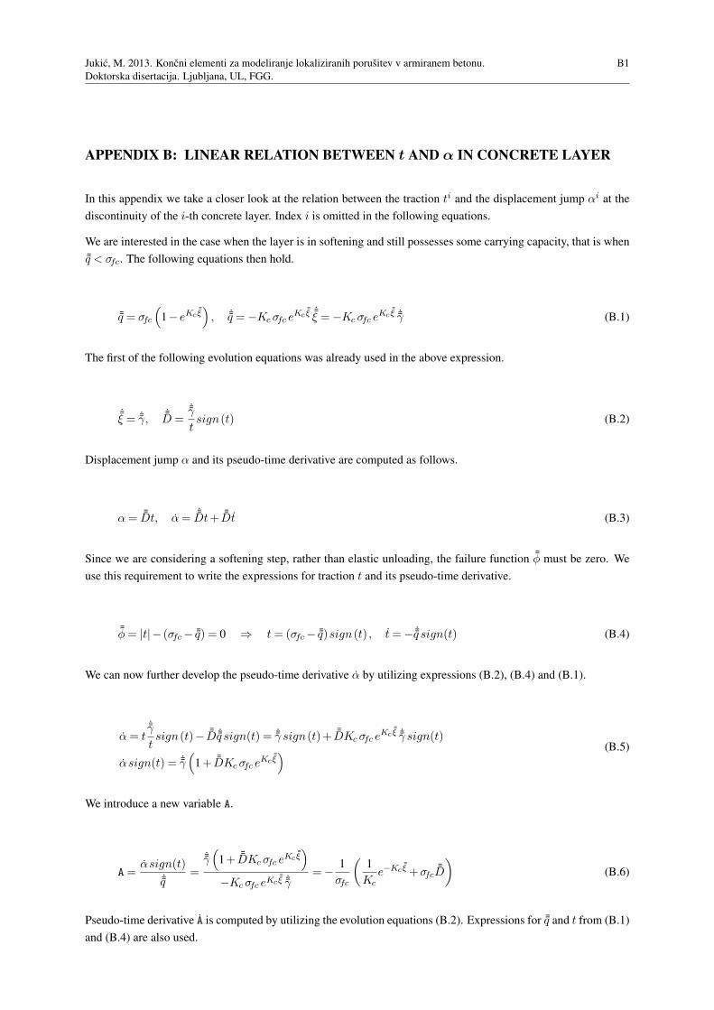
Jukic, M. 2013. Koncni elementi za modeliranje lokaliziranih porusitev v armiranem betonu.
Doktorska disertacija. Ljubljana, UL, FGG.
B1
APPENDIX B: LINEAR RELATION BETWEEN t AND α IN CONCRETE LAYER
In this appendix we take a closer look at the relation between the traction ti and the displacement jump αi at the
discontinuity of the i-th concrete layer. Index i is omitted in the following equations.
We are interested in the case when the layer is in softening and still possesses some carrying capacity, that is when
¯q < σfc. The following equations then hold.
¯q = σfc
(
1−eKc¯ξ)
, ˙q =−Kcσfc eKc
¯ξ ˙ξ =−Kcσfc e
Kc¯ξ ˙γ (B.1)
The first of the following evolution equations was already used in the above expression.
˙ξ = ˙γ,
˙D =
˙γ
tsign(t) (B.2)
Displacement jump α and its pseudo-time derivative are computed as follows.
α= ¯Dt, α=˙Dt+ ¯Dt (B.3)
Since we are considering a softening step, rather than elastic unloading, the failure function ¯φ must be zero. We
use this requirement to write the expressions for traction t and its pseudo-time derivative.
¯φ= |t|− (σfc− ¯q) = 0 ⇒ t= (σfc− ¯q)sign(t) , t=− ˙q sign(t) (B.4)
We can now further develop the pseudo-time derivative α by utilizing expressions (B.2), (B.4) and (B.1).
α= t˙γ
tsign(t)− ¯D ˙q sign(t) = ˙γ sign(t)+ ¯DKcσfc e
Kc¯ξ ˙γ sign(t)
αsign(t) = ˙γ(
1+ ¯DKcσfc eKc
¯ξ) (B.5)
We introduce a new variable A.
A=αsign(t)
˙q=
˙γ(
1+ ¯DKcσfc eKc
¯ξ)
−Kcσfc eKc¯ξ ˙γ
=−1
σfc
(1
Kce−Kc
¯ξ +σfc¯D
)
(B.6)
Pseudo-time derivative A is computed by utilizing the evolution equations (B.2). Expressions for ¯q and t from (B.1)
and (B.4) are also used.
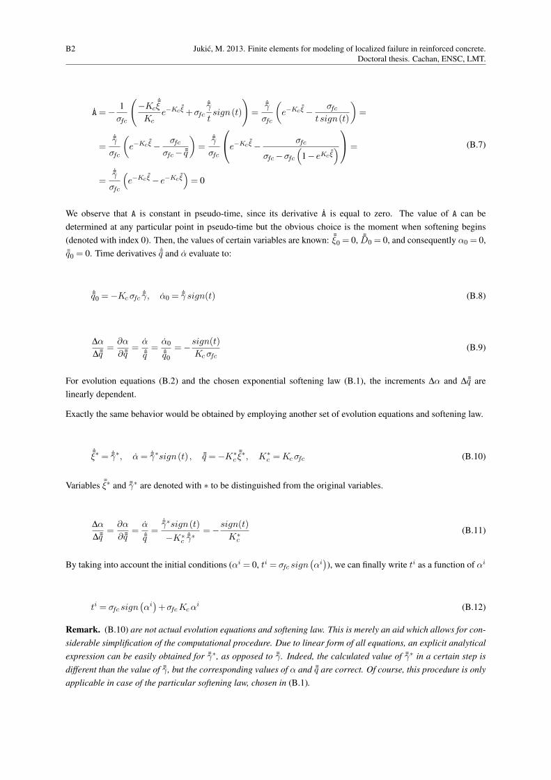
B2 Jukic, M. 2013. Finite elements for modeling of localized failure in reinforced concrete.
Doctoral thesis. Cachan, ENSC, LMT.
A=−1
σfc
(
−Kc˙ξ
Kce−Kc
¯ξ +σfc˙γ
tsign(t)
)
=˙γ
σfc
(
e−Kc¯ξ −
σfct sign(t)
)
=
=˙γ
σfc
(
e−Kc¯ξ −
σfcσfc− ¯q
)
=˙γ
σfc
e−Kc¯ξ −
σfc
σfc−σfc
(
1−eKc¯ξ)
=
=˙γ
σfc
(
e−Kc¯ξ −e−Kc
¯ξ)
= 0
(B.7)
We observe that A is constant in pseudo-time, since its derivative A is equal to zero. The value of A can be
determined at any particular point in pseudo-time but the obvious choice is the moment when softening begins
(denoted with index 0). Then, the values of certain variables are known: ¯ξ0 = 0, ¯D0 = 0, and consequently α0 = 0,
¯q0 = 0. Time derivatives ˙q and α evaluate to:
˙q0 =−Kcσfc ˙γ, α0 = ˙γ sign(t) (B.8)
∆α
∆ ¯q=
∂α
∂ ¯q=
α˙q=
α0
˙q0
=−sign(t)
Kcσfc(B.9)
For evolution equations (B.2) and the chosen exponential softening law (B.1), the increments ∆α and ∆ ¯q are
linearly dependent.
Exactly the same behavior would be obtained by employing another set of evolution equations and softening law.
˙ξ∗ = ˙γ∗, α= ˙γ∗sign(t) , ¯q =−K∗
c¯ξ∗, K∗
c =Kcσfc (B.10)
Variables ¯ξ∗ and ¯γ∗ are denoted with ∗ to be distinguished from the original variables.
∆α
∆ ¯q=
∂α
∂ ¯q=
α˙q=
˙γ∗sign(t)
−K∗c
˙γ∗=−
sign(t)
K∗c
(B.11)
By taking into account the initial conditions (αi = 0, ti = σfc sign(αi)), we can finally write ti as a function of αi
ti = σfc sign(αi)+σfcKcα
i (B.12)
Remark. (B.10) are not actual evolution equations and softening law. This is merely an aid which allows for con-
siderable simplification of the computational procedure. Due to linear form of all equations, an explicit analytical
expression can be easily obtained for ¯γ∗, as opposed to ¯γ. Indeed, the calculated value of ¯γ∗ in a certain step is
different than the value of ¯γ, but the corresponding values of α and ¯q are correct. Of course, this procedure is only
applicable in case of the particular softening law, chosen in (B.1).
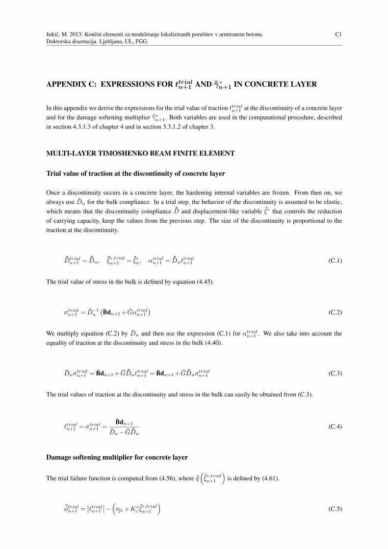
Jukic, M. 2013. Koncni elementi za modeliranje lokaliziranih porusitev v armiranem betonu.
Doktorska disertacija. Ljubljana, UL, FGG.
C1
APPENDIX C: EXPRESSIONS FOR ttrialn+1 AND ¯γ ∗
n+1 IN CONCRETE LAYER
In this appendix we derive the expressions for the trial value of traction ttrialn+1 at the discontinuity of a concrete layer
and for the damage softening multiplier ¯γ∗n+1. Both variables are used in the computational procedure, described
in section 4.3.1.3 of chapter 4 and in section 3.3.1.2 of chapter 3.
MULTI-LAYER TIMOSHENKO BEAM FINITE ELEMENT
Trial value of traction at the discontinuity of concrete layer
Once a discontinuity occurs in a concrete layer, the hardening internal variables are frozen. From then on, we
always use Dn for the bulk compliance. In a trial step, the behavior of the discontinuity is assumed to be elastic,
which means that the discontinuity compliance ¯D and displacement-like variable ¯ξ∗ that controls the reduction
of carrying capacity, keep the values from the previous step. The size of the discontinuity is proportional to the
traction at the discontinuity.
¯Dtrialn+1 = ¯Dn,
¯ξ∗,trialn+1 = ¯ξ∗n, αtrialn+1 = ¯Dnt
trialn+1 (C.1)
The trial value of stress in the bulk is defined by equation (4.45).
σtrialn+1 = D−1
n
(Bdn+1 + Gαtrial
n+1
)(C.2)
We multiply equation (C.2) by Dn and then use the expression (C.1) for αtrialn+1 . We also take into account the
equality of traction at the discontinuity and stress in the bulk (4.40).
Dnσtrialn+1 = Bdn+1 + G ¯Dnt
trialn+1 = Bdn+1 + G ¯Dnσ
trialn+1 (C.3)
The trial values of traction at the discontinuity and stress in the bulk can easily be obtained from (C.3).
ttrialn+1 = σtrialn+1 =
Bdn+1
Dn− G ¯Dn
(C.4)
Damage softening multiplier for concrete layer
The trial failure function is computed from (4.56), where ¯q(
¯ξ∗,trialn+1
)
is defined by (4.61).
¯φtrialn+1 =
∣∣ttrialn+1
∣∣−(
σfc+K∗c
¯ξ∗,trialn+1
)
(C.5)
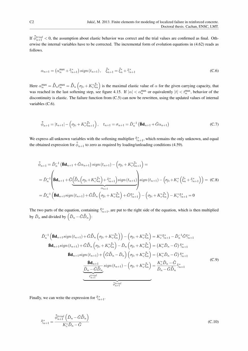
C2 Jukic, M. 2013. Finite elements for modeling of localized failure in reinforced concrete.
Doctoral thesis. Cachan, ENSC, LMT.
If ¯φtrialn+1 < 0, the assumption about elastic behavior was correct and the trial values are confirmed as final. Oth-
erwise the internal variables have to be corrected. The incremental form of evolution equations in (4.62) reads as
follows.
αn+1 =(αmaxn + ¯γ∗n+1
)sign(tn+1) ,
¯ξ∗n+1 =¯ξ∗n+ ¯γ∗n+1 (C.6)
Here αmaxn = ¯Dnt
maxn = ¯Dn
(
σfc+K∗c
¯ξ∗n
)
is the maximal elastic value of α for the given carrying capacity, that
was reached in the last softening step, see figure 4.15. If |α| < αmaxn or equivalently |t| < tmax
n , behavior of the
discontinuity is elastic. The failure function from (C.5) can now be rewritten, using the updated values of internal
variables (C.6).
¯φn+1 = |tn+1|−(
σfc+K∗c
¯ξ∗n+1
)
, tn+1 = σn+1 = D−1n
(Bdn+1 + Gαn+1
)(C.7)
We express all unknown variables with the softening multiplier ¯γ∗n+1, which remains the only unknown, and equal
the obtained expression for ¯φn+1 to zero as required by loading/unloading conditions (4.59).
¯φn+1 = D−1n
(Bdn+1 + Gαn+1
)sign(tn+1)−
(
σfc+K∗c
¯ξ∗n+1
)
=
= D−1n
Bdn+1 + G(
¯Dn
(
σfc+K∗c
¯ξ∗n
)
+ ¯γ∗n+1
)
sign(tn+1)︸ ︷︷ ︸
αn+1
sign(tn+1)−
(
σfc+K∗c
(¯ξ∗n+ ¯γ∗n+1
))
=
= D−1n
(
Bdn+1sign(tn+1)+ G ¯Dn
(
σfc+K∗c
¯ξ∗n
)
+ G ¯γ∗n+1
)
−(
σfc+K∗c
¯ξ∗n
)
−K∗c
¯γ∗n+1 = 0
(C.8)
The two parts of the equation, containing ¯γ∗n+1, are put to the right side of the equation, which is then multiplied
by Dn and divided by(
Dn− G ¯Dn
)
:
D−1n
(
Bdn+1sign(tn+1)+ G ¯Dn
(
σfc+K∗c
¯ξ∗n
))
−(
σfc+K∗c
¯ξ∗n
)
=K∗c
¯γ∗n+1 − D−1n G ¯γ∗n+1
Bdn+1sign(tn+1)+ G ¯Dn
(
σfc+K∗c
¯ξ∗n
)
− Dn
(
σfc+K∗c
¯ξ∗n
)
=(K∗
c Dn− G)
¯γ∗n+1
Bdn+1sign(tn+1)+(
G ¯Dn− Dn
)(
σfc+K∗c
¯ξ∗n
)
=(K∗
c Dn− G)
¯γ∗n+1
Bdn+1
Dn− G ¯Dn︸ ︷︷ ︸
ttrialn+1
sign(tn+1)−(
σfc+K∗c
¯ξ∗n
)
︸ ︷︷ ︸¯φtrialn+1
=K∗
c Dn− G
Dn− G ¯Dn
¯γ∗n+1
(C.9)
Finally, we can write the expression for ¯γ∗n+1.
¯γ∗n+1 =
¯φtrialn+1
(
Dn− G ¯Dn
)
K∗c Dn− G
(C.10)

Jukic, M. 2013. Koncni elementi za modeliranje lokaliziranih porusitev v armiranem betonu.
Doktorska disertacija. Ljubljana, UL, FGG.
C3
MULTI-LAYER EULER-BERNOULLI BEAM FINITE ELEMENT
Derivation of expressions for ttrialn+1 and ¯γ∗n+1 for the Euler-Bernoulli beam is performed in the same way as for the
Timoshenko beam element.The only difference is that stress in no longer constant over the layer and the traction at
the discontinuity is equal to the stress, evaluated at the location of the discontinuity t= σ|xd , instead of just t= σ.
Some other non-constant quantities are evaluated at xd as well, which reflects in the resulting expressions.
ttrialn+1 =
[Bdn+1
Dn− GR¯Dn
]
x=xd
, ¯γ∗n+1 =
¯φtrialn+1
(
Dn− GR¯Dn
)
K∗c Dn− GR
x=xd
(C.11)

Jukic, M. 2013. Koncni elementi za modeliranje lokaliziranih porusitev v armiranem betonu.
Doktorska disertacija. Ljubljana, UL, FGG.
D1
APPENDIX D: INFLUENCE OF xi
dON COMPUTATION OF INTERNAL FORCES
In this appendix we demonstrate how the location of the discontinuity xid in a layer affects the computation in case
of constant strain/stress, resulting in incorrect response of the finite element. The problem was encountered in pure
tension/compression numerical examples in section 3.4.1 and pure bending numerical examples in section 3.4.2.
Pure tension or pure compression
Here, we examine the reasons for the incorrect response of the reinforced concrete beam, computed in section
3.4.1.3. According to section 3.2.4.1, in case of constant stress the discontinuity is placed in the middle of the
layer and the constant operator GiR is chosen from (3.46). The strain in the bulk is computed, as shown in equation
(3.54). Interpolation functions Bi are defined by (3.7) and (3.8).
εi = Bid+ GiRαi = C1x+C2, C1,C2 = const. (D.1)
If the strain is to remain constant over the layer, which is required for the equilibrium, the linear part of expression
(D.1) must be zero. Since GiR is constant, it makes no contribution to the constant C1. For a single-layer finite
element, the coordinate yi is zero and we can conclude
C1 =4
L2(u1 +u2 −2u3) = 0 ⇒ u3 =
u1 +u2
2(D.2)
Expression (D.2) for u3 is inserted in (D.1) to obtain
εi =1
L
(u2 −u1 −αi
)(D.3)
The jump in displacements can be computed from equation (3.35), which reduces to ti = σi for the constant GiV .
In case of monotonic softening, αi = ¯ξ∗i. For concrete one gets
ti =(
σfc+K∗c
¯ξ∗i)
sign(ti), σi = Di−1
εi ⇒ αi =u2 −u1 − DiLσfc sign
(ti)
1+ DiLK∗c sign(t
i)(D.4)
For a steel layer, the only difference would be in the constitutive equation for σi, leading to a slightly different
expression for αi. These equations have been developed for a single-layer finite element and a constant operator
GiR, but they also hold for each layer of a multi-layer element if the transversal displacements v and rotations θ of
the nodes are zero, as in pure tension/compression. Such tests were modeled in section 3.4.1.4. Since expression
for αi depends on material parameters, the displacement jumps are different in concrete and reinforcement.
A different scenario unfolds in sections 3.4.1.1, 3.4.1.2 and 3.4.1.3, however. Despite the linear stress in a layer,
the algorithm detects even the smallest difference between the values at both ends of the finite element, arising
from the numerical procedure. The discontinuity is positioned at the “critical” node and one of the linear operators
D2 Jukic, M. 2013. Finite elements for modeling of localized failure in reinforced concrete.
Doctoral thesis. Cachan, ENSC, LMT.
GiR is chosen from (3.46). The constant C1 from (D.1) is now affected by Gi
R, but it still has to be zero to provide
constant strain over the layer.
C1 =4
L2
(u1 +u2 −2u3 −αi
)= 0 ⇒ u3 =
u1 +u2 −αi
2(D.5)
Inserting expression (D.5) for u3 into (D.1) returns exactly the equation (D.3). The strain is therefore computed
in the same manner as in the case with constant GiR. However, the displacement u3 is no longer independent of
αi, which means that the middle node has to move out of the middle of the element to preserve the equilibrium.
By itself, this is not problematic. In a single-layer finite element or an element composed of equal layers, like the
beams in sections 3.4.1.1 and 3.4.1.2, all displacement jumps αi are equal and require the same u3 to “balance”
them. An issue arises in a finite element, composed of different layers, like the reinforced concrete beam in section
3.4.1.3. Since the displacement jumps are different in steel and concrete, they would each require a different
middle node displacement u3 (computed from (D.5)), which is not possible. A constant strain state is therefore not
possible in such case!
Nevertheless, equilibrium is achievable. For any u3, different from the value in (D.5), stress is linear over the
length of the layer. Contributions of the layer to the internal forces are computed as integrals of the stress, and the
components are different at both ends of the layer fint,(e),iu1 6=−f
int,(e),iu2 , see Fig. 3.26. The layer by itself is out of
balance, but equilibrium of the finite element is satisfied by finding the exact value of u3, at which the imbalance
of internal forces in steel and the imbalance of the internal forces in concrete neutralize each other, see Fig. 3.27,
where fint,(e)u1 = −f
int,(e)u2 . This is possible, because the equilibrium is only required on the element level, and not
on the layer level. Of course, this solution is incorrect, see the comparison in Fig. 3.28.
f int,(e),iu1
6=−f int,(e),iu2
→ ∑i
f int,(e),iu1
︸ ︷︷ ︸
fint,(e)u1
=−∑i
f int,(e),iu2
︸ ︷︷ ︸
fint,(e)u2
(D.6)
Remark. Fig. 3.26 and Fig. 3.27 only show the contributions of the i-th layer to the axial internal forces at the
end nodes. Contributions to the axial internal force at the middle node and contributions to transversal forces and
moments exist also, but their resultants are zero on the element level.
Pure tension or pure compression, non-zero transversal displacement
Another incorrect solution of equilibrium equations exists. So far, we have assumed that the transversal displace-
ments v and rotations θ of the nodes are zero, but this is never explicitly requested. The degrees of freedom change
so as to satisfy the equilibrium equations and it turns out that equilibrium is also possible in pure tension or pure
compression if transversal displacement at the free end of the beam is different from zero. Such situation arises
in a beam with symmetrical cross-section, if the layer discontinuities are positioned at x= 0 in the bottom half of
the beam (yi < 0) and at x= L in the top half of the beam (yi > 0), or vice versa. In the particular example from
section 3.4.1.5, the only difference from section 3.4.1.3 was the reversed orientation of the local axis x, which
sufficed for a slightly different numerical evaluations of stress in the layers and different positioning of the discon-
tinuities. Results in Fig. 3.31 and Fig. 3.32 state that the transversal displacement at the end of the beam increases
with the loading (imposed axial displacement), while the rotation, shear force and moment remain zero. Although
physically not sensible, these results are mathematically possible which is easily verified.
Let us inspect two symmetrically positioned concrete layers of a beam in pure tension. We will show that their
contributions to internal shear forces and moments neutralize each other. Quantities, related to the layer above
Jukic, M. 2013. Koncni elementi za modeliranje lokaliziranih porusitev v armiranem betonu.
Doktorska disertacija. Ljubljana, UL, FGG.
D3
the neutral axis, are denoted with +, and the quantities, related to the layer below the neutral axis, with −. The
elasticity limit is defined higher than the failure stress so there is no damage in the bulk of the layer (Di = E−1c ).
Strain and stress in the layers are computed according to equation (3.54), with zero values for nodal rotations θ.
The operator GiR takes the appropriate value from (3.46), depending on the location of the discontinuity. We choose
xd = 0 for yi−< 0, and xd = L for yi+> 0.
σi = Ec εi, εi+ = Bid+ Gi+
R αi+, εi− = Bid+ Gi−R αi− (D.7)
Contributions of the two layers to shear force fint,(e)v1 in node 1 are defined in equation (3.28). Symmetry of the
layers is taken into account: −yi− = yi+ = yi and Ai− =Ai+ =Ai.
f int,(e),i+v1
=−∫
L
Bv1 y
i+σi+Ai+dx=−∫
L
Bv1 y
iσi+Aidx
f int,(e),i−v1
=−∫
L
Bv1 y
i−σi−Ai−dx=∫
L
Bv1 y
iσi−Aidx(D.8)
After some straightforward manipulation we obtain the expression for their sum. Procedure is repeated for the
remaining shear force fint,(e)v2 and moments f
int,(e)θ1
and fint,(e)θ2
.
f int,(e),i+v1
+f int,(e),i−v1
=4AiEc y
i(6yi (v1 −v2)+L
(αi−+αi+
))
L3
f int,(e),i+v2
+f int,(e),i−v2
=−4AiEc y
i(6yi (v1 −v2)+L
(αi−+αi+
))
L3
fint,(e),i+θ1
+fint,(e),i−θ1
=AiEc y
i(12yi (v1 −v2)+L
(3αi−+αi+
))
L2
fint,(e),i+θ2
+fint,(e),i−θ2
=AiEc y
i(12yi (v1 −v2)+L
(αi−+3αi+
))
L2
(D.9)
If the displacement jumps αi− and αi+ take the value from (D.10), all four expressions in (D.9) are zero. Since the
beam has a symmetrical cross-section, all layers can be arranged into symmetrical pairs and their contributions to
internal shear forces and moments neutralize each other.
αi−= αi+ =−3(v1 −v2)y
i
L⇒ f int,(e)
v1= f int,(e)
v2= f
int,(e)θ1
= fint,(e)θ2
= 0 (D.10)
Therefore, the results from section 3.4.1.5 do not contradict the equations, used in our finite element. Equilibrium
of a beam in “pure tension” (with imposed axial displacement) is indeed possible, even if transversal displacement
at the free end is not zero. The solution is incorrect, but mathematically possible. One of the reasons for existence
of such solution is the absence of any regulation to correlate the displacement jumps in different layers. Each αi
is free to follow equation (D.10). Since the expression depends on the distance of the layer from the middle axis,
the sizes of the discontinuities grow linearly from the middle toward the edge of the beam, which is not physically
reasonable.
Pure bending
Here, we examine the effect of incorrect automatic positioning of the discontinuity in case of pure bending, when
only one layer of concrete exceeds the ultimate tensile stress. Such situation was encountered in sections 3.4.2.1
D4 Jukic, M. 2013. Finite elements for modeling of localized failure in reinforced concrete.
Doctoral thesis. Cachan, ENSC, LMT.
and 3.4.2.2. The first discontinuity appears in the bottom layer of concrete in tension. The rest of the element is
still elastic at that point. Even though the stress is constant over the layer when the ultimate stress is reached, the
discontinuity is placed at either of the two end nodes, rather than in the middle of the element, due to numerical
error. One of the linear functions from (3.46) is chosen for operator GiR. We can see from Fig. 3.13 that the
additional strain in the bulk GiRα
i is negative at the discontinuity and positive at the other end of the layer, which
means that the stress is decreased at xid and increased at the opposite end. Of course, this is not the converged
state, but even when equilibrium is reached, the stress in the layer is not physically logical. At the discontinuity,
the value of σi is equal to the traction ti and smaller than the ultimate tensile stress σfct, which is correct. On the
other end, however, the value of σi is higher than σfct. This happens because GiR was derived on an isolated layer.
If the layer was a self standing three-node bar, as assumed for the derivation, it would deform in such way that the
stress in it would be constant and equal to ti. In truth, the layer is bound to the remaining layers through common
nodal displacements and cannot deform freely. The imbalance, produced by additional strain, is not neutralized
within the cracked layer, but on the level of the finite element. The cracked layer makes only a part of the “required
deformation” and the stress at the non-cracked end of the layer remains too high. Eventually, the traction at the
discontinuity ti and the value of stress σi at the discontinuity xid would drop to zero, but at the opposite end of the
layer the stress would stay positive. The layer would contribute to internal forces, computed as an integral of σi
over the length of the element, even when it is supposed to be completely broken.
Almost constant strain/stress state in a layer
In all previous cases, described in this appendix, the stress in the layer was constant at the moment when the
carrying capacity was reached. The algorithm wrongly positioned the discontinuity at one of the end nodes, due to
numerical error. However, the problem was avoided by manually imposing the location of the discontinuity at the
middle of the element.
This trick cannot be used if the stress state in the layer is linear. In that case, the discontinuity must be placed at the
location of highest stress. If the stress is almost constant (but not quite), for instance in a cantilever beam, loaded
with a great axial force and very small transversal force at the free end, the situation is virtually identical to the one
described above, only without the remedy. Incorrect computation cannot be avoided here. We conclude that, for a
general stress state, the operator GiR, derived in section 3.2.4.1, is inappropriate.
Jukic, M. 2013. Koncni elementi za modeliranje lokaliziranih porusitev v armiranem betonu.
Doktorska disertacija. Ljubljana, UL, FGG.
E1
APPENDIX E: EXPRESSIONS FOR ttrialn+1 , ¯γ ∗
n+1, αn+1 AND ¯γn+1 IN VISCOSITY
In this appendix we derive expressions, required for the computation of softening internal variables in multi-layer
Timoshenko beam finite element with viscous regularization of softening response, presented in chapter 5. Ex-
pressions for the trial value of traction at the discontinuity ttrialn+1 , the damage softening multiplier ¯γ ∗n+1 and the
displacement jump αn+1 are required in the computation of internal variables of a concrete layer, while the expres-
sions for plastic softening multiplier ¯γn+1 is required in the computation of internal variables of a reinforcement
layer.
Discontinuity in concrete layer when ¯q < σfc
Here, we derive the expressions for the trial value of traction at the discontinuity t(k),trialn+1 and the damage soften-
ing multiplier ¯γ∗(k)n+1, which are used in the computation of internal variables in a concrete layer in section 5.3.1.
The following derivation is valid while ¯q < σfc, i.e. until the traction at the discontinuity drops to zero and the
discontinuity compliance ¯D becomes infinite.
Once a discontinuity occurs in the layer, the bulk internal variables are frozen. Therefore, the value Dn is used as
the bulk compliance. In the trial step, the behavior of the discontinuity is assumed to be elastic, which means that
the discontinuity compliance ¯D and displacement-like softening variable ¯ξ∗ that controls the reduction of carrying
capacity, keep the values from the previous step. The size of the discontinuity is computed in accordance with
equation (4.55).
¯D(k),trialn+1 = ¯Dn,
¯ξ∗(k),trialn+1 = ¯ξ∗n, α
(k),trialn+1 = ¯Dn t
(k),trialn+1 (E.1)
The trial value of stress in the bulk is defined by equation (4.45).
σ(k),trialn+1 = D−1
n
(
Bd(k−1)n+1 + Gα
(k),trialn+1
)
(E.2)
Relation between ttrialn+1 and σtrialn+1 is described in equation (5.7). It depends on the pseudo-time derivative α,
which is here defined in incremental form, as the difference between the current value of α and the value from the
previous step, divided by the corresponding increase of time ∆τn+1 = τn+1 − τn.
α(k)n+1 =
α(k)n+1 −αn
∆τn+1, α
(k),trialn+1 =
α(k),trialn+1 −αn
∆τn+1(E.3)
Equation (5.7) can now be rewritten.
t(k),trialn+1 = σ
(k),trialn+1 −
η
∆τn+1
(
α(k),trialn+1 −αn
)
(E.4)
After using the expression (E.1) for α(k),trialn+1 in equation (E.4) we can express σ
(k),trialn+1 with t
(k),trialn+1 .
E2 Jukic, M. 2013. Finite elements for modeling of localized failure in reinforced concrete.
Doctoral thesis. Cachan, ENSC, LMT.
σ(k),trialn+1 = t
(k),trialn+1 +
η
∆τn+1
(
α(k),trialn+1 −αn
)
= t(k),trialn+1 +
η
∆τn+1
¯Dn t(k),trialn+1 −
η
∆τn+1αn (E.5)
We multiply equation (E.2) with Dn and substitute σ(k),trialn+1 with (E.5) and α
(k),trialn+1 with (E.1).
Dn
(
t(k),trialn+1 +
η
∆τn+1
¯Dn t(k),trialn+1 −
η
∆τn+1αn
)
= Bd(k−1)n+1 + G ¯Dn t
(k),trialn+1 (E.6)
After some straightforward manipulation, the trial value of traction at the discontinuity is obtained from (E.6).
t(k),trialn+1 =
Bd(k−1)n+1 + Dn
η∆τn+1
αn
Dn− G ¯Dn+ Dnη
∆τn+1
¯Dn
(E.7)
Next, the trial value of failure function is computed from (4.56), where ¯q(
¯ξ∗(k),trialn+1
)
is defined by (4.61).
¯φ(k),trialn+1 =
∣∣∣t(k),trialn+1
∣∣∣−(
σfc+K∗c
¯ξ∗(k),trialn+1
)
(E.8)
If ¯φ(k),trialn+1 < 0, the assumption about elastic behavior was correct and the trial values are confirmed as final.
Otherwise the internal variables have to be corrected. The incremental form of evolution equations (4.62) reads as
follows.
α(k)n+1 =
(
αmaxn + ¯γ
∗(k)n+1
)
sign(
t(k)n+1
)
, ¯ξ∗(k)n+1 =
¯ξ∗n+ ¯γ∗(k)n+1 (E.9)
where αmaxn = ¯Dnt
maxn = ¯Dn
(
σfc+K∗c
¯ξ∗n
)
is the maximal elastic value of α for the given carrying capacity, that
was reached in the last softening step. If |α| < αmaxn , or equivalently |t| < tmax
n , behavior of the discontinuity is
elastic. The failure function is now written, using the updated values of internal variables (E.9).
¯φ(k)n+1 =
∣∣∣t(k)n+1
∣∣∣−(
σfc+K∗c
¯ξ∗(k)n+1
)
t(k)n+1 = σ
(k)n+1 −
η
∆τn+1
(
α(k)n+1 −αn
)
, σ(k)n+1 = D−1
n
(
Bd(k−1)n+1 + Gα
(k)n+1
) (E.10)
We express all unknown variables with the softening multiplier ¯γ∗(k)n+1, which remains the only unknown, and equal
the obtained expression for ¯φ(k)n+1 to zero as required by loading/unloading conditions (4.59).
¯φ(k)n+1=
(
D−1n
(
Bd(k−1)n+1 + Gα
(k)n+1
)
−η
∆τn+1
(
α(k)n+1 −αn
))
sign(
t(k)n+1
)
−(
σfc+K∗c
¯ξ∗(k)n+1
)
=
=D−1n
(
Bd(k−1)n+1 +
(
G− Dnη
∆τn+1
)
α(k)n+1 + Dn
η
∆τn+1αn
)
sign(
t(k)n+1
)
−(
σfc+K∗c
¯ξ∗(k)n+1
)
=
=D−1n
Bd(k−1)n+1 +
(
G−Dnη
∆τn+1
)(¯Dn
(
σfc+K∗c
¯ξ∗n
)
+ ¯γ∗(k)n+1
)
sign(
t(k)n+1
)
︸ ︷︷ ︸
α(k)n+1
+Dnη
∆τn+1αn
sign(
t(k)n+1
)
−(
σfc+K∗c
(¯ξ∗n+ ¯γ
∗(k)n+1
))
=
=D−1n
((
Bd(k−1)n+1 +Dn
η
∆τn+1αn
)
sign(
t(k)n+1
)
+
(
G−Dnη
∆τn+1
)
¯Dn
(
σfc+K∗c
¯ξ∗n
)
+
(
G−Dnη
∆τn+1
)
¯γ∗(k)n+1
)
−(
σfc+K∗c
¯ξ∗n
)
−K∗c
¯γ∗(k)n+1 = 0
(E.11)

Jukic, M. 2013. Koncni elementi za modeliranje lokaliziranih porusitev v armiranem betonu.
Doktorska disertacija. Ljubljana, UL, FGG.
E3
The two parts of the equation, which contain ¯γ∗(k)n+1, are put to the right side of the equation, which is then multiplied
by Dn and divided by(
Dn− G ¯Dn+ Dnη
∆τn+1
¯Dn
)
:
D−1n
((
Bd(k−1)n+1 +Dn
η
∆τn+1αn
)
sign(
t(k)n+1
)
+
(
G−Dnη
∆τn+1
)
¯Dn
(
σfc+K∗c
¯ξ∗n
))
−(
σfc+K∗c
¯ξ∗n
)
=K∗c
¯γ∗(k)n+1 −D−1
n
(
G−Dnη
∆τn+1
)
¯γ∗(k)n+1
(
Bd(k−1)n+1 +Dn
η
∆τn+1αn
)
sign(
t(k)n+1
)
+
(
G−Dnη
∆τn+1
)
¯Dn
(
σfc+K∗c
¯ξ∗n
)
−Dn
(
σfc+K∗c
¯ξ∗n
)
=K∗c Dn ¯γ
∗(k)n+1−
(
G−Dnη
∆τn+1
)
¯γ∗(k)n+1
(
Bd(k−1)n+1 +Dn
η
∆τn+1αn
)
sign(
t(k)n+1
)
+
((
G−Dnη
∆τn+1
)
¯Dn−Dn
)(
σfc+K∗c
¯ξ∗n
)
=
(
K∗c Dn− G+Dn
η
∆τn+1
)
¯γ∗(k)n+1
Bd(k−1)n+1 + Dn
η∆τn+1
αn
Dn− G ¯Dn+ Dnη
∆τn+1
¯Dn︸ ︷︷ ︸
t(k),trialn+1
sign(
t(k)n+1
)
−(
σfc+K∗c
¯ξ∗n
)
︸ ︷︷ ︸
¯φ(k),trialn+1
=K∗
c Dn− G+ Dnη
∆τn+1
Dn− G ¯Dn+ Dnη
∆τn+1
¯Dn
¯γ∗(k)n+1
(E.12)
Finally, we can write the expression for ¯γ∗(k)n+1.
¯γ∗(k)n+1 =
¯φ(k),trialn+1
(
Dn− G ¯Dn+ Dnη
∆τn+1
¯Dn
)
KcDn− G+ Dnη
∆τn+1
(E.13)
Discontinuity in concrete layer when ¯q = σfc
Here we consider the situation, when the concrete layer loses all carrying capacity. When the stress-like softening
variable reaches the value ¯q= σfc, the traction at the discontinuity t drops to zero (at a non-zero displacement jump
α) and the discontinuity compliance ¯D becomes infinite, so the above derivation does not apply any more. Instead,
the displacement jump α(k)n+1 is computed from equation t
(k)n+1 = 0.
We start by inserting expressions (5.15) for σ(k)n+1 and (E.3) for α
(k)n+1 into equation (5.7).
t(k)n+1 = σ
(k)n+1 −η α
(k)n+1 = D−1
n
(
Bd(k−1)n+1 + Gα
(k)n+1
)
−η
∆τn+1
(
α(k)n+1 −αn
)
(E.14)
The obtained expression for t(k)n+1 is equaled to zero. The equation is then multiplied with Dn and rearranged to
collect the terms containing α(k)n+1.
D−1n
(
Bd(k−1)n+1 + Gα
(k)n+1
)
−η
∆τn+1
(
α(k)n+1 −αn
)
= 0
Bd(k−1)n+1 + Gα
(k)n+1 − Dn
η
∆τn+1α(k)n+1 + Dn
η
∆τn+1αn = 0
(
G− Dnη
∆τn+1
)
α(k)n+1 =−
(
Bd(k−1)n+1 + Dn
η
∆τn+1αn
)
(E.15)
We can now write the expression for the displacement jump α(k)n+1.
α(k)n+1 =−
Bd(k−1)n+1 + Dn
η∆τn+1
αn
G− Dnη
∆τn+1
(E.16)
E4 Jukic, M. 2013. Finite elements for modeling of localized failure in reinforced concrete.
Doctoral thesis. Cachan, ENSC, LMT.
Discontinuity in reinforcement layer when ¯q < σfs
In this section we derive the expression for the plastic softening multiplier ¯γ(k)n+1, required for the computation of
internal variables in the reinforcement layer in section 5.3.2 of chapter 5, in case that the layer still possesses some
carrying capacity, i.e. ¯q < σfs.
We begin by expressing the traction at the discontinuity t(k)n+1 with its trial value t
(k),trialn+1 . To achieve this, we insert
expressions (5.24) for σ(k)n+1 and (E.3) for α
(k)n+1 into equation (5.7).
t(k)n+1 = σ
(k)n+1 −η α
(k)n+1 = Es
(
Bd(k−1)n+1 + Gα
(k)n+1 − εp,n
)
−η
∆τn+1
(
α(k)n+1 −αn
)
(E.17)
The displacement jump is expressed with the softening multiplier by using the evolution equation (5.23). The
applied equality sign(
t(k)n+1
)
=sign(
t(k),trialn+1
)
is justified in appendix A.
t(k)n+1 = Es
(
Bd(k−1)n+1 + G
(
αn+ ¯γ(k)n+1 sign
(
t(k)n+1
))
− εp,n
)
−η
∆τn+1
(
αn+ ¯γ(k)n+1sign
(
t(k)n+1
)
−αn
)
=
= Es
(
Bd(k−1)n+1 + Gαn− εp,n
)
︸ ︷︷ ︸
=σ(k),trialn+1 =t
(k),trialn+1
+EsG ¯γ(k)n+1 sign
(
t(k)n+1
)
−η
∆τn+1
¯γ(k)n+1 sign
(
t(k)n+1
)
=
= t(k),trialn+1 +
(
EsG−η
∆τn+1
)
¯γ(k)n+1 sign
(
t(k)n+1
)
(E.18)
Equation (5.19) has been applied as well, stating that the trial values of traction at the discontinuity and the stress
in the bulk are equal. The stress-like softening variable ¯q is determined by equation (4.76). We are considering the
case when ¯q < σfs. This value is designated with ¯qAn+1.
¯q(k)n+1 =−Ks
¯ξ(k)n+1 =−Ks
(¯ξn+ ¯γ
(k)n+1
)
= ¯q(k),trialn+1 −Ks ¯γ
(k)n+1 → ¯qAn+1 (E.19)
Expressions (E.18) and (E.19) are inserted in the failure function ¯φ(k)n+1, determined by equation (4.75). The
obtained expression has to be zero to fulfill the loading/unloading conditions (4.78).
¯φ(k)n+1 =
∣∣∣t(k)n+1
∣∣∣−(
σfs− ¯q(k)n+1
)
= 0 (E.20)
(
t(k),trialn+1 +
(
EsG−η
∆τn+1
)
¯γ(k)n+1sign
(
t(k)n+1
))
sign(
t(k)n+1
)
−(
σfs− ¯q(k),trialn+1 +Ks ¯γ
(k)n+1
)
= 0
t(k),trialn+1 sign
(
t(k)n+1
)
+
(
EsG−η
∆τn+1
)
¯γ(k)n+1 −
(
σfs− ¯q(k),trialn+1
)
−Ks ¯γ(k)n+1 = 0
∣∣∣t(k),trialn+1
∣∣∣−(
σfs− ¯q(k),trialn+1
)
︸ ︷︷ ︸
¯φ(k),trialn+1
−
(
Ks−EsG+η
∆τn+1
)
¯γ(k)n+1 = 0
(E.21)
From (E.21), the expression for the plastic softening multiplier ¯γ(k)n+1 is obtained. It is denoted with ¯γA
n+1 to
associate it with the stress-like softening variable ¯qAn+1< σfs.
Jukic, M. 2013. Koncni elementi za modeliranje lokaliziranih porusitev v armiranem betonu.
Doktorska disertacija. Ljubljana, UL, FGG.
E5
¯γAn+1 =
¯φ(k),trialn+1
−GEs+Ks+η
∆τn+1
(E.22)
We have derived expression (E.22) under assumption that ¯q < σfs, which has to be verified. ¯qAn+1 has to be
computed from equation (E.19), using expression (E.22) for ¯γ(k)n+1. If the calculated value is indeed smaller than
σfs, the assumption was correct. Otherwise, the carrying capacity at the discontinuity has dropped to zero and
¯q = σfs.
Discontinuity in reinforcement layer when ¯q = σfs
In this section we derive the expression for the plastic softening multiplier ¯γ(k)n+1 for the case when the layer has
lost all carrying capacity at the discontinuity (the stress in the bulk may be different from zero). The stress-like
softening variable is denoted with ¯qBn+1= σfs in order to be distinguished from ¯qAn+1< σfs above.
By inserting ¯qBn+1 in equation (E.20), we conclude that t(k)n+1 = 0. Expression (E.18) for the traction at the discon-
tinuity is equaled to zero. The equality sign(
t(k)n+1
)
=sign(
t(k),trialn+1
)
is applied again.
t(k),trialn+1 +
(
EsG−η
∆τn+1
)
¯γ(k)n+1sign
(
t(k)n+1
)
= 0
t(k),trialn+1 sign
(
t(k),trialn+1
)
+
(
EsG−η
∆τn+1
)
¯γ(k)n+1 = 0
(E.23)
Expression for ¯γ(k)n+1 is acquired from (E.23). It is marked with ¯γB
n+1 to be associated with ¯qBn+1 = σfs.
¯γBn+1 =
∣∣∣t(k),trialn+1
∣∣∣
−GEs+η
∆τn+1
(E.24)
During the computational procedure in section 5.3.2, ¯γ(k)n+1 is first evaluated according to equation (E.22), then the
stress-like variable is computed according to (E.19): ¯qAn+1 =−Ks
(¯ξn+ ¯γA
n+1
)
. If the value is indeed ¯qAn+1 < σfs,
the value ¯γAn+1 is stored. Otherwise the value ¯γB
n+1 from (E.24) is taken.


![Probabilistic Upscaling of Material Failure Using Random ... · spectral stochastic finite element method to plasticity and failure [4]. To solve multiscale failure problems such](https://static.fdocuments.us/doc/165x107/5edc0184ad6a402d66667c35/probabilistic-upscaling-of-material-failure-using-random-spectral-stochastic.jpg)
