1

Finite Element Modelling of Viscosity-Dominated Hydraulic Fractures

Zuorong Chen

CSIRO Earth Science and Resource Engineering

Ian Wark Laboratory, Bayview Avenue, Clayton, VIC 3168, Australia

Abstract

Hydraulic fracturing is a highly effective technology used to stimulate fluid

production from reservoirs. The fully 3-D numerical simulation of the hydraulic

fracturing process is of great importance to developing more efficient application of

this technology, and also presents a significant technical challenge because of the

strong nonlinear coupling between the viscous flow of fluid and fracture propagation.

By taking advantage of a cohesive zone method to simulate the fracture process, a

finite element model based on existing pore pressure cohesive finite elements has

been established to simulate the propagation of a viscosity-dominated hydraulic

fracture in an infinite, impermeable elastic medium. Selected results of the finite

element modelling and comparisons with analytical solutions are presented for

viscosity-dominated plane strain and penny-shaped hydraulic fractures, respectively.

Some important issues such as mesh transition and far-field boundary approximation

in the cohesive finite element model have been investigated. Excellent agreement

between the finite element results and analytical solutions for the limiting case where

the fracture process is dominated by fluid viscosity demonstrates the capability of the

cohesive zone finite element model in simulating the hydraulic fracture growth.

Keywords: hydraulic fracture; cohesive zone model; three dimensional; finite element

method

2

Introduction

Hydraulic fracturing is a powerful technology mainly used in the petroleum industry

to stimulate reservoirs to enhance oil and/or gas production. Other important and

successful applications include determination of in situ stress in rock (Haimson and

Fairhurst, 1970), preconditioning rock for caving or inducing rock to cave in mining

(Jeffrey et al., 2001; van As and Jeffrey, 2000), creation of geothermal energy

reservoirs, and underground disposal of toxic or radioactive waste (Sun, 1969). The

recent global fast growing development of unconventional gas also requires novel

methods of hydraulic fracturing. Furthermore, natural hydraulic fractures are manifest

as kilometre-long volcanic dykes that bring magma from deep underground chambers

to the earth’s surface, or as sub-horizontal fractures known as sills diverting magma

from dykes (Lister and Kerr, 1991; Rubin, 1995; Spence and Turcotte, 1985).

During a standard industrial treatment, the appropriate amounts of fracturing fluid and

proppant are blended and pumped into the rock mass at high enough injection rates

and pressures to open and extend a fracture hydraulically. Minimizing the energy

required for propagation dictates that the hydraulic fracture tends to develop in a

direction perpendicular to the direction of the minimum principal in situ compressive

stress. Typically hydraulic fracturing involves four important coupling processes

(Adachi et al., 2007; Bunger et al., 2005): (i) the rock deformation induced by the

fluid pressure on the fracture faces; (ii) the flow of viscous fluid within the fracture;

(iii) the fracture propagation in rock; and (iv) the leak-off of fluid from the fracture

into the rock formation. Therefore, fully modelling the hydraulic fracturing process

requires solving a coupled system of governing equations consisting of (Bunger and

Detournay, 2008; Bunger et al., 2005; Clifton, 1989; Detournay, 2004) (1) elasticity

equations that determine the relationship between the fracture opening and the fluid

pressure, (2) non-linear partial differential equations for fluid flow (usually obtained

from lubrication theory) that relate the fluid flow in the fracture to the fracture

opening and the fluid pressure gradient, (3) a fracture propagation criterion (usually

given by assuming linear elastic fracture mechanics is valid) that allows for quasi-

static fracture growth when the stress intensity factor is equal to the rock toughness,

and (4) diffusion of fracturing fluid into the rock formation.

3

The problem associated with modelling hydraulic fractures has been addressed by a

large number of papers, starting with the pioneering work by Kristianovitch and

Zheltov (Khristianovic and Zheltov, 1955). The early research efforts concentrated on

obtaining analytical solutions for the complex fluid-solid interaction problems by

assuming a simple fracture geometry, resulting in the well-known 2-D plane strain

PKN and KGD models, and the axisymmetric penny-shaped model (Abe et al., 1976;

Geertsma and de Klerk, 1969; Perkins and Kern, 1961; Sun, 1969). These approaches

typically rely on simplification of the problem either with respect to the fracture

opening profile or the fluid pressure distribution. Because of the geometric limitations

of analytical models, a good deal of effort has been applied to the development of

numerical models to simulate the propagation of hydraulic fractures for more complex

and realistic geometries, with the first such so-called pseudo-3D model developed in

the late 1970s (Settari and Cleary, 1984). Significant progress has been made in

developing 2-D and 3-D numerical hydraulic fracture models (Adachi et al., 2007;

Lecamplon and Detournay, 2007; Zhang et al., 2002; Zhang and Jeffrey, 2006; Zhang

et al., 2007). In recent years, some newly developed numerical methods, such as the

extended finite element method (XFEM), have been applied to investigating hydraulic

fracture problems (Lecampion, 2009). However, because of the difficulty posed by

modelling a fully 3-D hydraulic fracture, numerical simulation still remains a

particularly challenging problem (Peirce and Detournay, 2008).

The cohesive zone finite element method, which has its origin in the concepts of a

cohesive zone model for fracture originally proposed by Barrenblatt (Barenblatt, 1962)

and Dugdale (Dugdale, 1960), has been extensively used with great success to

simulate fracture and fragmentation processes in concrete, rock, ceramics, metals,

polymers, and their composites. Rather than an elastic crack tip region as presumed in

classic linear elastic fracture mechanics with its associated infinite stress at the crack

tip, the cohesive zone model assumes the existence of a simplified fracture process

zone characterized by a traction-separation law. In this way, the cohesive zone model

avoids the singularity in the crack tip stress field that is present in classic fracture

mechanics. In addition, the cohesive zone model fits naturally into the conventional

finite element method, and thus can be easily implemented. So the cohesive finite

element method provides an alternate, effective approach for quantitative analysis of

fracture behaviour through explicit simulation of the fracture processes.

4

Compared to the conventional fracture mechanics method, the cohesive element

method has the following advantages in modelling hydraulic fracturing. Firstly, the

cohesive zone model effectively avoids the singularity at the crack tip region, which

poses considerable challenges for numerical modelling in classic fracture mechanics.

The lubrication equation, governing the flow of viscous fluid in the fracture, involves

a degenerate non-linear partial differential equation (Peirce and Detournay, 2008).

The coefficients (permeability) in the principal part of this equation vanish as a power

of the unknown fracture width (opening). The fracture opening tends to zero near the

tip of an elastic crack as described by classic fracture mechanics. This non-linear

degeneracy poses a considerable challenge for numerical modelling. While, in a

cohesive zone model, fracture opening is not zero but finite at the cohesive crack tip,

which naturally avoids the non-linear degeneracy problem associated with the

singularity in fluid pressure that otherwise must be handled at the crack tip. Secondly,

the hydraulic fracture propagation is a moving boundary value problem in which the

unknown footprint of the fracture and its encompassing boundary need to be found

while specifying an additional fracture propagation criterion in the classic fracture

mechanics method. While in the cohesive zone finite element model, the location of

the crack tip is not an input parameter but a natural, direct outcome of the solution,

which increases the computation efficiency. In addition, the cohesive zone model has

the interesting capability of modelling microstructural damage mechanisms inherent

in hydraulic fracturing such as initiation of micro cracking and coalescence, and the

initiation of a hydraulic fracture from a borehole. Sarris and Papanastasiou (Sarris and

Papanastasiou, 2011) investigated the influence of cohesive process zone in hydraulic

fracture modelling. Chen et al. (Chen et al., 2009) have applied the cohesive element

method to modelling a toughness dominated penny-shaped hydraulic fracture. In this

paper, the cohesive element method has been used to simulate the propagation of a

hydraulic fracture in viscosity-dominated regime.

1. Cohesive Model of Hydraulic Fracture

Figure 1

5

As illustrated in Figure 1, a fracture is hydraulically driven with the injection of a

fluid from the wellbore into the fracture channel. In this model, a pre-defined surface

made up of elements that support the cohesive zone traction-separation calculation is

embedded in the rock and the hydraulic fracture grows along this surface. The fracture

process zone (unbroken cohesive zone) is defined within the separating surfaces

where the surface tractions are nonzero. The fracture is fully filled with fluid in the

broken cohesive zone where no traction from rock fracture exists, but where fluid

pressure is acting on the open fracture surfaces. The definition of the crack tip as used

in reference (Shet and Chandra, 2002) is adopted here, the mathematic crack tip refers

to the point which is yet to separate; the cohesive crack tip corresponds to the damage

initiation point where the traction reaches the cohesive strength maxT and the

separation reaches the critical value 0δ ; the material crack tip is the complete failure

point where the separation reaches the critical value fδ and the traction or cohesive

strength acting across the surfaces are equal to zero. The fracturing fluid can permeate

the cohesive damage zone. Thus the fluid front is taken to coincide with the cohesive

crack tip.

1.1 The cohesive law

The cohesive law defines the relationship between the traction tensor T and the

displacement jump δ across a pair of cohesive surfaces. A cohesive potential function

φ is defined so that the traction is given by

φ∂=∂

Tδ

. (1)

Various types of traction-separation relations (potential functions) for cohesive

surfaces have been proposed to simulate the fracture process in different types of

material systems. The irreversible bilinear cohesive law (Tomar et al., 2004), as

shown in Fig.2, is adopted in this study. This bilinear law is a special case of

trapezoidal model. It can also be regarded as a generalized version of the initial rigid,

linear-decaying irreversible cohesive law. It has been widely used to simulate the

fracture or fragmentation processes in brittle materials. This law assumes that the

6

cohesive surfaces are intact without any relative displacement, and exhibit reversible

linear elastic behaviour until the traction reaches the cohesive strength or equivalently

the separation exceeds 0δ . Beyond 0δ , the traction reduces linearly to zero up to fδ

and any unloading takes place irreversibly.

Figure 2.

1.2 Fluid flow within broken cohesive zone

The flow pattern of the fluid within the gap between the cohesive surfaces is shown in

Figure 2. The fluid is assumed to be incompressible with Newtonian rheology. The

tangential flow within the gap is governed by the lubrication equations (Batchelor,

1967), which is formulated from Poiseulle’s law

3

12 f

wp

µ= − ∇q (2)

and the continuity equation of mass conservation

( ) ( ) ( ),t b

wq q Q t x y

tδ∂ + ∇ ⋅ + + =

∂q (3)

where ( ), ,x y tq is the fluid flux of the tangential flow, ( ), ,fp x y t∇ is the fluid

pressure gradient along the cohesive zone, ( ), ,w x y t is the crack opening, µ is the

fluid viscosity, and ( )Q t is the injection rate. ( ), ,tq x y t and ( ), ,bq x y t , are the

normal flow rates into the top and bottom surfaces of the cohesive elements,

respectively, which reflect the leakoff through the fracture surfaces into the adjacent

material. For an impermeable fracture, there is no leakoff and

( ) ( ), , , , 0t bq x y t q x y t= = .

The normal flow is defined as

( )( )

t t f t

b b f b

q c p p

q c p p

= −

= −

, (4)

7

where tp and bp are the pore pressures in the adjacent poroelastic material on the

top and bottom surfaces of the fracture, respectively, and tc and bc define the

corresponding fluid leakoff coefficients. Here the leakoff coefficients with the unit of

( )sPam ⋅ are input as constants or functions of field variables by the user and can be

interpreted as the effective permeability of a finite layer of permeable material on the

cohesive element surfaces. The leakoff coefficients allow the fluid pressure to act

through the otherwise impermeable cohesive element on the surrounding permeable

material in the main finite element model.

Substituting Eqs. (2) and (4) into Eq. (3) results in Reynolds lubrication equation

( ) ( ) ( ) ( ) ( )31,

12t f t b f b f

wc p p c p p w p Q t x y

tδ

µ∂ + − + − = ∇ ⋅ ∇ +∂

. (5)

The fluid pressure fp is considered as traction acting on the open surfaces of the

fracture. As complete failure eventually occurs within the cohesive zone, there will be

no contribution from the cohesive traction in the open part of the fracture channel.

The fluid pressure, which opens the hydraulic fracture, is balanced by the far-field

stress acting across the cohesive zone and by the cohesive tractions acting across that

zone. So a coupled fluid pressure-traction-separation relationship exists between the

cohesive zone defined by the traction-separation law and the pressurised fracture as

found from solving the lubrication equation (Eq. (5)) with the constraint that all

tractions acting on the entire fracture and cohesive zone must be in equilibrium.

2. Finite Element Simulation

The finite element code ABAQUS/Standard (ABAQUS, 2011) is used for the analysis.

The plane strain KGD and axisymmetric penny-shaped fluid-driven fractures in an

infinite impermeable rock are simulated. The initially unopened fracture is

represented by an embedded array of cohesive zone elements without initial

separation along the entire fracture path. An incompressible Newtonian fluid is

injected at the centre of the fracture at constant injection rate, 0Q . The fracture is

opened and extended hydraulically by the fluid injection. There is no fluid leak-off

8

through the impermeable surfaces of the fracture, so only flow in the fracture radius

direction is modelled. The cohesive elements at the injection point are defined as

initially open to allow entry of fluid, and so that the initial flow and fracture growth is

possible. Since a purely tensile fracture is modelled here, the cohesive zone undergoes

damage and fails under pure normal deformation conditions rather than the mixed

mode that would result from combined normal and shear deformation. Therefore, only

those material parameters related to the pure normal deformation mode will have an

effect in determining the damage initiation criterion and damage evolution behaviour.

2.1 Cohesive element size

In order to guarantee solution convergence, and to properly capture the details of the

deformation field in the vicinity of the crack tip and the traction distribution within

the cohesive zone, the cohesive element size must be smaller than the cohesive zone

length. The cohesive zone length is an inherent length scale determined by material

properties. For mode-I crack growth under plane strain conditions, the cohesive zone

length zd is determined by (Rice, 1980)

( )2

2 22max max

9 9

32 32 1Ic c

z

K GEd

T T

π πν

= =−

(6)

where IcK is the mode-I fracture toughness, E is the Young’s modulus, and ν

Poisson’s ratio. Eq. (6) has been used here as an element size criterion in the cohesive

finite element modelling of the hydraulic fracture.

For a pure normal deformation mode, the critical parameters that are needed to

specify the irreversible bilinear cohesive law include the cohesive energy, cG , the

cohesive strength maxT , the initial cohesive stiffness K , the critical separation at

complete failure fδ , and the critical separation at damage initiation 0δ . But only three

of these parameters are independent, and the following relationship among them can

be defined

2max

max max 0

1 1

2 2 2c f

TG T T

Kδ δ

α α= = = (7)

where 0 fα δ δ= .

9

For comparison, in the hydraulic fracture models based on linear elastic fracture

mechanics, the only parameter involved in defining the fracture propagation criterion

is fracture toughness, IcK .

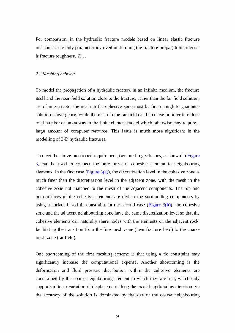
2.2 Meshing Scheme

To model the propagation of a hydraulic fracture in an infinite medium, the fracture

itself and the near-field solution close to the fracture, rather than the far-field solution,

are of interest. So, the mesh in the cohesive zone must be fine enough to guarantee

solution convergence, while the mesh in the far field can be coarse in order to reduce

total number of unknowns in the finite element model which otherwise may require a

large amount of computer resource. This issue is much more significant in the

modelling of 3-D hydraulic fractures.

To meet the above-mentioned requirement, two meshing schemes, as shown in Figure

3, can be used to connect the pore pressure cohesive element to neighbouring

elements. In the first case (Figure 3(a)), the discretization level in the cohesive zone is

much finer than the discretization level in the adjacent zone, with the mesh in the

cohesive zone not matched to the mesh of the adjacent components. The top and

bottom faces of the cohesive elements are tied to the surrounding components by

using a surface-based tie constraint. In the second case (Figure 3(b)), the cohesive

zone and the adjacent neighbouring zone have the same discretization level so that the

cohesive elements can naturally share nodes with the elements on the adjacent rock,

facilitating the transition from the fine mesh zone (near fracture field) to the coarse

mesh zone (far field).

One shortcoming of the first meshing scheme is that using a tie constraint may

significantly increase the computational expense. Another shortcoming is the

deformation and fluid pressure distribution within the cohesive elements are

constrained by the coarse neighbouring element to which they are tied, which only

supports a linear variation of displacement along the crack length/radius direction. So

the accuracy of the solution is dominated by the size of the coarse neighbouring

10

elements rather than the size of cohesive elements. This is a disadvantage in

modelling the pressure distribution close the injection point and near the crack tip for

a viscosity-dominated hydraulic fracture where the fluid pressure varies rapidly at

these sites. The second meshing scheme is much more efficient in matching the fluid

pressure singularity at the crack tip of a viscosity-dominated hydraulic fracture, and

so is used in this work.

Figure 3.

2.3 Far-field boundary conditions

Appropriate boundary conditions on the boundary of the finite region must be applied

to correctly model the propagation of a hydraulic fracture in an infinite medium. The

far-field solution in the infinite medium can be modelled by using infinite elements.

As implemented in Abaqus, the solution in the far field is assumed to be linear, so

only linear behaviour is provided in the infinite elements. In addition, the use of

infinite elements requires that each infinite element edge that stretches to infinity is

centred about an origin, called the “pole”, and the second node along each edge

pointing in the infinite direction must be positioned so that it is twice as far from the

pole as the node on the same edge at the boundary between the finite and the infinite

elements.

Another way of modelling the far-field boundary in dealing with infinite domain

problems is utilising the analytical solution for a displacement discontinuity (DD). It

has been shown that the far-field displacement induced by a finite dislocation (a

fracture) is equivalent to that induced by an infinitesimal DD of equivalent intensity

(Lecampion et al., 2005). This enables us to predict an appropriate displacement to be

applied on the boundary of the finite region.

The displacement field induced by an infinitesimal dislocation loop around an

element Sδ of strength Sbδ (a normal infinitesimal DD) in the z direction located at

11

( ), ,x y z′ ′ ′ in a three-dimensional infinite medium can be expressed in the form (Hills,

1996)

( ) ( ) ( ) ( ) ( )2

3 2

31 2

8 1x

z zb Su x x

r r

δ νπ ν

′−′= − − + −

−

x

( ) ( ) ( ) ( ) ( )2

3 2

31 2

8 1y

z zb Su y y

r r

δ νπ ν

′−′= − − + −

−

x

( ) ( ) ( ) ( ) ( )2

3 2

31 2

8 1z

z zb Su z z

r r

δ νπ ν

′−′= − − + −

−

x

(8)

where ( ) ( ) ( )222 zzyyxxr ′−+′−+′−= is the distance from the field point x to

the centre of the dislocation loop. This displacement can be applied on the boundary

of the finite region via the user subroutine to model the far-field solution for a penny-

shaped fracture in an infinite elastic body.

In a much similar way, the far-field displacement for a plane strain KGD fracture in

an infinite elastic body can be modelled by a normal infinitesimal displacement

discontinuity of strength s in the z direction. Under plane strain conditions for the y

coordinate direction, the x − and z − components of displacement in a homogeneous,

isotropic, linear elastic body with the plane 0z = free from shear traction can be

expressed in terms of a single harmonic function φ as (Crouch, 1976)

( ) ( )2

, 1 2xu x z zx x z

φ φν ∂ ∂= − − −∂ ∂ ∂

( ) ( )2

2, 2 1zu x z z

z z

φ φν ∂ ∂= − −∂ ∂

(9)

And the corresponding harmonic function φ can be obtained as

( ) ( )2 2, ln

4 1o s

x z x zφπ ν

= +−

(10)

Substitution of the harmonic function into Eq. (9) produces the displacements

12

( ) ( )2

2 2 2 2

21 2

4 1x

s x zu

x z x zν

π ν

= − − − − + +

( ) ( )2

2 2 2 2

23 2

4 1z

s z xu

x z x zν

π ν

= − − − + +

(11)

As will be shown later, the use of analytical solutions of an equivalent DD singularity

provides nearly the same prediction for displacement at the far-field boundary in an

infinite domain as the infinite elements, but is much more computationally efficient.

3. Results and Discussions: Comparison with analytical solution

In case of zero lag and zero leakoff, the propagation of a hydraulic fracture in an

impermeable medium is governed by two competing dissipative mechanisms

(Detournay, 2004): one is the flow process characterised by fluid viscosity and

injection rate; and the other is the fracture process characterised by rock toughness.

For toughness-dominated hydraulic fracture propagation, the viscous dissipation is so

small that it is negligible compared to the energy consumed in fracturing the rock.

The ability of a cohesive zone model in simulating the toughness-dominated hydraulic

fracture has been demonstrated in Reference (Chen et al., 2009). We now extend that

result to consider the ability of a cohesive zone model to simulate a viscosity-

dominated hydraulic fracture and compare the numerical results obtained with an

available analytical solution (Appendix).

Unless otherwise specified, the material parameters 30E GPa= , 0.2ν = , and

5.0Pa sµ = ⋅ have been used in the simulation. The fractures are driven under the

action of a constant injection rate 30 0.001Q m s= and 2

0 0.001Q m s= for penny-

shaped and plane strain KGD hydraulic fracture, respectively. The injection point is

located at the origin. Selected results of the simulations and comparisons with an

analytical solution available in the literature are presented for viscosity-dominated

plane strain KGD and penny-shaped hydraulic fractures, respectively.

13

3.1 The plane strain KGD hydraulic fracture

Figure 4.

The simulation results for a plane strain KGD are shown in Figure 4. The

corresponding results predicted by the so-called the M-vertex solution, i.e. the zero

toughness solution (see Appendix), are also shown for comparison. The evolution

parameter 0.0698κ = is far less than 1 throughout the fracture propagation, which

indicates that the simulated hydraulic fracture propagates in the viscosity-dominated

regime and thus can be approximated by the zero toughness solution. The crack length

and crack opening profiles at different times are shown in Figure 4(a) and 4(b),

respectively. The profiles of dimensionless crack opening and dimensionless net fluid

pressure at different times are shown in Figure 4(c) and 4(d), respectively. It can be

seen that the cohesive finite element model is able to produce satisfactory predictions

of the crack length, crack opening profile, and net fluid pressure, and thus to model

the viscosity-dominated plane strain KGD hydraulic fracture. The logarithmic scale

plot of the dimensionless crack opening provides further detail on the effect of the

cohesive zone. Away from the crack tip, the predictions from the cohesive finite

element mode show close agreement with the analytical zero toughness solution. For

example, 0.98ξ = for an relative difference less than 5%. While, due to the effect of

the cohesive process zone, the cohesive finite element prediction is not able to match

the analytical solution in the close vicinity of the crack tip. But the mismatch

decreases with time because the cohesive zone becomes relatively small as the crack

length growths and so its effect on the crack becomes weaker.

3.2 The penny-shaped hydraulic fracture

Figure 5.

14

The evolution of the dimensionless toughness κ with time for a penny-shaped

hydraulic fracture is shown in Figure 5. It can be seen that the evolution parameter is

far less than 1 in the duration of the simulation, which indicates that the simulated

hydraulic fracture propagates in the viscosity-dominated regime throughout the

simulation and thus can be approximated by the zero toughness solution. The

simulation results for the penny-shaped hydraulic fracture are shown in Figure 6.

Figure 6.

The crack radius and crack opening profiles at different times are shown in Figure 6(a)

and 6(b), respectively. The profiles of dimensionless crack opening and dimensionless

net fluid pressure at different times are shown in Figure 6(c) and 6(d), respectively.

The corresponding results by the so-called M-vertex solution i.e. the zero toughness

solution (see Appendix) are also shown for comparison. It can be seen that the

cohesive finite element model is able to produce satisfactory predictions of the crack

radius, crack opening profile, and net fluid pressure, and thus to model the viscosity-

dominated penny-shaped hydraulic fracture. The logarithmic scale plot of the

dimensionless crack opening provides further close examination on the effect of the

cohesive zone. Away from the crack front, the predictions by the cohesive finite

element mode show close agreement with the analytical zero toughness solution. For

example, 0.98ξ = results in a relative difference of less than 5%. While, due to the

effect of the cohesive process zone, the cohesive finite element prediction is not able

to match the analytical solution very near the crack tip. But the mismatch decreases

with time because the cohesive zone becomes relatively small as the crack radius

growths and so its effect on the crack becomes weak.

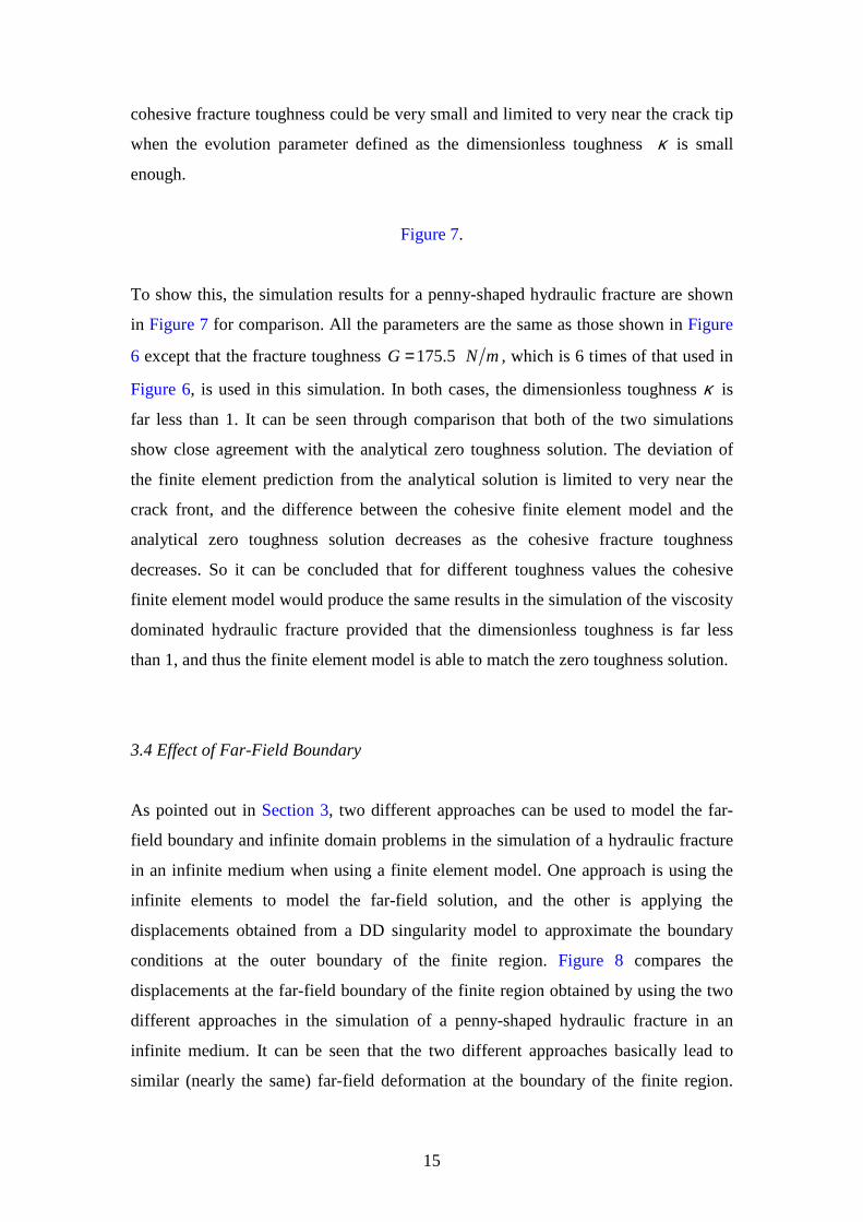
3.3 Fracture Toughness Independent

The zero toughness solution is toughness independent. While, the fracture toughness

is an important material parameter in the cohesive finite element model because it

governs the cohesive damage evolution and fracture propagation. But the effect of

15

cohesive fracture toughness could be very small and limited to very near the crack tip

when the evolution parameter defined as the dimensionless toughness κ is small

enough.

Figure 7.

To show this, the simulation results for a penny-shaped hydraulic fracture are shown

in Figure 7 for comparison. All the parameters are the same as those shown in Figure

6 except that the fracture toughness 175.5G = N m , which is 6 times of that used in

Figure 6, is used in this simulation. In both cases, the dimensionless toughness κ is

far less than 1. It can be seen through comparison that both of the two simulations

show close agreement with the analytical zero toughness solution. The deviation of

the finite element prediction from the analytical solution is limited to very near the

crack front, and the difference between the cohesive finite element model and the

analytical zero toughness solution decreases as the cohesive fracture toughness

decreases. So it can be concluded that for different toughness values the cohesive

finite element model would produce the same results in the simulation of the viscosity

dominated hydraulic fracture provided that the dimensionless toughness is far less

than 1, and thus the finite element model is able to match the zero toughness solution.

3.4 Effect of Far-Field Boundary

As pointed out in Section 3, two different approaches can be used to model the far-

field boundary and infinite domain problems in the simulation of a hydraulic fracture

in an infinite medium when using a finite element model. One approach is using the

infinite elements to model the far-field solution, and the other is applying the

displacements obtained from a DD singularity model to approximate the boundary

conditions at the outer boundary of the finite region. Figure 8 compares the

displacements at the far-field boundary of the finite region obtained by using the two

different approaches in the simulation of a penny-shaped hydraulic fracture in an

infinite medium. It can be seen that the two different approaches basically lead to

similar (nearly the same) far-field deformation at the boundary of the finite region.

16

The slight difference in the outer boundary deformations associated with using the

two different approaches do not result in any change in the predictions of the near-

field solution such as the crack radius, opening profile, and the net fluid pressure

throughout the simulation, which thus are not shown here.

Figure 8.

It is worth of noting that the displacements at the boundary of the finite region

obtained using the DD singularity solution will somewhat deviate from those

modelled by using infinite elements as the fracture radius growths with time. This is

due to the fact that the difference in the far-field solution between a DD singularity

model and a penny-shaped fracture model increases as the ratio of the fracture radius

to the finite domain extent increases. So it is necessary to ensure that the boundary is

located in the far-field at late time in the simulation so that the DD singularity

solution can be applied to the far-field boundary in the simulation of infinite domain.

This is similar to the requirement when using infinite element in Abaqus that the

length of the infinite element edge pointing in the infinite direction should be at least

one or more times the finite region extent.

4. Concluding Remarks

A fluid pressure cohesive zone finite element model has been proposed to simulate

hydraulic fracture propagation in viscosity dominated regimes. The issues of solution

convergence, meshing scheme, and far-field approximation of infinite domain in the

simulation of plane strain KGD and axisymmetric penny-shaped hydraulic fractures in

an infinite elastic body have been addressed. The meshing scheme using mesh

transition and node sharing techniques provides a higher solution accuracy and

efficiency. The transition between the coarse mesh in the far-field and the very fine

mesh in the vicinity of the fracture enables an accurate characterization of the near

field deformation and stresses in the vicinity of a crack tip with less computational

costs. While the node sharing technique, between the cohesive elements and the

adjacent elements, enables an accurate description of the fluid flow within the crack

with high solution efficiency. These issues are critical in the simulation of more

17

complex 3-D hydraulic fractures. In addition, compared to the infinite elements, the

use of the analytical solution of an equivalent DD singularity is computationally

efficient and provides an accurate method to determine the deformation at the far-field

boundary for fractures embedded in an infinite domain.

Excellent agreement between the cohesive finite element results and analytical M-

vertex solutions for the plane strain KGD and penny-shaped hydraulic fractures

demonstrates the ability of a cohesive finite element model to simulate viscosity-

dominated hydraulic fracture propagation. Moreover, the cohesive finite element

model has advantages in dealing with more complex 3-D and T-shaped hydraulic

fractures in multilayer non-homogeneous formations that may exhibit poroelastic

deformation.

Acknowledgements

The author thanks CSIRO for supporting and granting permission to publish this work.

The author is indebted to the following individuals: Rob Jeffrey for his continuing

support and discussions of this work, Andy Bunger, Xi Zhang, Emmanuel Detournay

and John Napier for their helpful comments and discussions of this work.

18

Appendix: Zero toughness solutions for plane strain Kristianovic-Geertsma-de

Klerk and penny-shaped fractures

The solution of a plane strain KGD or a penny-shaped hydraulic fracture in an infinite

elastic body depends on the injection rate 0Q and on the three material parameters E′ ,

K ′ , and µ′ , which are defined as

21

EE

ν′ =

−,

1 232

ICK Kπ

′ =

, 12µ µ′ = (A1)

For the plane strain KGD hydraulic fracture, the crack opening ( ),w x t , crack length

(half length) ( )l t , and net fluid pressure ( ),p x t can be expressed as (Adachi, 2001)

( ) ( ) ( ) ( ) ( ) ( ) ( ) ( ), ,w x t t L t P t t L t P tε ξ ε γ ξ= Ω = Ω

( ) ( ) ( ), ,p x t t E P tε ξ′= Π

( ) ( ) ( )l t P t L tγ=

(A2)

where ( )x l tξ = is the scaled coordinate (0 1ξ≤ ≤ ), ( )tε is a small dimensionless

parameter, ( )L t denotes a length scale of the same order as the fracture length ( )l t ,

( )P t is the dimensionless evolution parameter, and ( )P tγ is the dimensionless

fracture length.

In the viscosity scaling, the evolution parameter ( )P t can be interpreted as a

dimensionless toughness κ

( )1 430

K

E Qκ

µ

′=

′ ′ (A3)

For the viscosity scaling, denoted by a subscript m , the small parameter ( )tε and the

length scale ( )L t take the explicit forms (Adachi, 2001)

1 3

m E t

µε ′ = ′ ,

1 63 40

m

E Q tL

µ′

= ′ (A4)

19

The first order approximation of the zero toughness solution is (Adachi, 2001;

Detournay, 2004)

( ) ( ) ( ) ( ) ( )2

2 3 5 31 1 12 2 2 20 0 1 2

1 11 1 4 1 2 ln

1 1m A A B

ξξ ξ ξ ξξ

− − Ω = − + − + − + + −

( ) ( ) ( ) ( )1 1 12 20 0 1 1 1

1 1 2 1 1 10 7 1, ,1; ; ,1; ; 2

3 2 3 6 2 7 6 2m B A F A F Bξ ξ π ξπ

Π = − + − + −

(A5)

where 1 20 3A = , ( )1

1 0.156A ≅ − , and ( )1 0.0663B ≅ ; B is Euler beta function, and 1F is

hypergeometric function. Thus, ( ) ( )10 0 1.84mΩ ≅ and ( )1

0 0.616mγ = .

For the penny-shaped hydraulic fracture, the crack opening ( ),w r t , crack radius

( )R t , and net fluid pressure ( ),p r t can be expressed as (Savitski and Detournay,

2002)

( ) ( ) ( ) ( ), ,w r t t L t P tε ρ= Ω

( ) ( ) ( ), ,p r t t E P tε ρ′= Π

( ) ( ) ( )R t P t L tγ=

(A6)

where ( )r R tρ = is the scaled radius (0 1ρ≤ ≤ ), ( )tε is the small dimensionless

parameter, ( )L t denotes a length scale of the same order as the fracture radius ( )R t ,

( )P t is the dimensionless evolution parameter, and ( )P tγ is the dimensionless

fracture radius.

In the viscosity scaling, the evolution parameter ( )P t can be interpreted as a

dimensionless toughness κ

1 182

5 3 130

tK

Q Eκ

µ ′= ′ ′

(A7)

20

For the viscosity scaling, denoted by a subscript m , the small parameter ( )tε and the

length scale ( )L t take the explicit forms (Detournay, 2004; Savitski and Detournay,

2002)

1 3

m E t

µε ′ = ′ ,

1 93 40

m

E Q tL

µ′

= ′ (A8)

The first order approximation of the zero toughness solution is (Detournay, 2004;

Savitski and Detournay, 2002)

0.6955moγ =

( ) ( )1 22 3 21 2 1( ) 1 1 arccosmo C C Bρ ρ ρ ρ ρ Ω = + − + − −

(A9)

where 1 0.3581A = , 1 0.1642B = , 2 0.09269B = , 1 1.034C = , 2 0.6378C = , 1 2.479ω = .

( )1 1 21 3

2ln 1

23 1mo A B

ρωρ

Π = − − + −

21

References ABAQUS, 2011. ABAQUS Documentation, Version 6.10-2. Abe, H., Keer, L.M. and Mura, T., 1976. Growth-Rate of a Penny-Shaped Crack in

Hydraulic Fracturing of Rocks .2. Journal of Geophysical Research, 81(35): 6292-6298.

Adachi, A., Siebrits, E., Peirce, A. and Desroches, J., 2007. Computer simulation of hydraulic fractures. International Journal of Rock Mechanics and Mining Sciences, 44(5): 739-757.

Adachi, J.I., 2001. Fluid-driven fracture in permeable rock, University of Minnesota, Minneapolis.

Barenblatt, G.I., 1962. The mathematical theory of equilibrium of cracks in brittle fracture. Advances in Applied Mechanics(7): 55-129.

Batchelor, G.K., 1967. An introduction to fluid dynamics. Cambridge University Press, London, xviii, 615 p. pp.

Bunger, A.P. and Detournay, E., 2008. Experimental validation of the tip asymptotics for a fluid-driven crack. Journal of the Mechanics and Physics of Solids, 56(11): 3101-3115.

Bunger, A.P., Detournay, E. and Garagash, D.I., 2005. Toughness-dominated hydraulic fracture with leak-off. International Journal of Fracture, 134(2): 175-190.

Chen, Z.R., Bunger, A.P., Zhang, X. and Jeffrey, R.G., 2009. COHESIVE ZONE FINITE ELEMENT-BASED MODELING OF HYDRAULIC FRACTURES. Acta Mechanica Solida Sinica, 22(5): 443-452.

Clifton, R.J., 1989. Three-Dimensional Fracture-Propagation Model. In: J.L. Gidley (Editor), Recent Advances in Hydraulic Fracturing - SPE Monograph, pp. 95-108.

Crouch, S.L., 1976. SOLUTION OF PLANE ELASTICITY PROBLEMS BY DISPLACEMENT DISCONTINUITY METHOD .1. INFINITE BODY SOLUTION. International Journal for Numerical Methods in Engineering, 10(2): 301-343.

Detournay, E., 2004. Propagation Regimes of Fluid-Driven Fractures in Impermeable Rocks. International Journal of Geomechanics, 4(1): 35-45.

Dugdale, D.S., 1960. Yielding of Steel Sheets Containing Slits. Journal of the Mechanics and Physics of Solids, 8(2): 100-104.

Geertsma, J. and de Klerk, F.D., 1969. A Rapid Method of Predicting Width and Extent of Hydraulically Induced Fractures. Journal of Petroleum Technology, 21: 1571-1581.

Haimson, B.C. and Fairhurst, C., 1970. In situ stress determination at great depth by means of hydraulic fracturing. In: W.H. Somerton (Editor), Rock Mechanics—Theory and Practice. Am. Inst. Mining Engrg., pp. 559–584.

Hills, D.A., 1996. Solution of crack problems : the distributed dislocation technique. Solid mechanics and its applications ; v. 44. Kluwer Academic Publishers, Dordrecht ; Boston, xii, 297 p. pp.

Jeffrey, R.G., Settari, A., Mills, K.W., Zhang, X. and Detournay, E., 2001. Hydraulic fracturing to induce caving: fracture model development and comparison to field data. Rock Mechanics in the National Interest, 1-2: 251-259.

Khristianovic, S.A. and Zheltov, Y.P., 1955. Formation of vertical fractures by means of highly viscous liquid, Proceedings of the fourth world petroleum congress, Rome, pp. 579-586.

22

Lecampion, B., 2009. An extended finite element method for hydraulic fracture problems. Communications in Numerical Methods in Engineering, 25(2): 121-133.

Lecampion, B., Jeffrey, R. and Detournay, E., 2005. Resolving the geometry of hydraulic fractures from tilt measurements. Pure and Applied Geophysics, 162(12): 2433-2452.

Lecamplon, B. and Detournay, E., 2007. An implicit algorithm for the propagation of a hydraulic fracture with a fluid lag. Computer Methods in Applied Mechanics and Engineering, 196: 4863-4880.

Lister, J.R. and Kerr, R.C., 1991. Fluid-Mechanical Models of Crack-Propagation and Their Application to Magma Transport in Dykes. Journal of Geophysical Research-Solid Earth and Planets, 96(B6): 10049-10077.

Peirce, A. and Detournay, E., 2008. An implicit level set method for modeling hydraulically driven fractures. Computer Methods in Applied Mechanics and Engineering, 197(33-40): 2858-2885.

Perkins, T.K. and Kern, L.R., 1961. Widths of Hydraulic Fractures. Transactions of the Society of Petroleum Engineers of AIME, 222(9): 937-949.

Rice, J.R., 1980. The mechanics of earthquake rupture. In: A.M. Dziewonski (Editor), Physics of the Earth's Interior. North-Holland Publishing Company, Amsterdam.

Rubin, A.M., 1995. Propagation of Magma-Filled Cracks. Annual Review of Earth and Planetary Sciences, 23: 287-336.

Sarris, E. and Papanastasiou, P., 2011. The influence of the cohesive process zone in hydraulic fracturing modelling. International Journal of Fracture, 167(1): 33-45.

Savitski, A.A. and Detournay, E., 2002. Propagation of a penny-shaped fluid-driven fracture in an impermeable rock: asymptotic solutions. International Journal of Solids and Structures, 39(26): 6311-6337.

Settari, A. and Cleary, M.P., 1984. 3-DIMENSIONAL SIMULATION OF HYDRAULIC FRACTURING. Journal of Petroleum Technology, 36(8): 1177-1190.

Shet, C. and Chandra, N., 2002. Analysis of energy balance when using cohesive zone models to simulate fracture processes. Journal of Engineering Materials and Technology-Transactions of the ASME, 124(4): 440-450.

Spence, D.A. and Turcotte, D.L., 1985. Magma-Driven Propagation of Cracks. Journal of Geophysical Research-Solid Earth and Planets, 90(NB1): 575-580.

Sun, R.J., 1969. Theoretical size of hydraulically induced horizontal fractures and corresponding surface uplift in an idealized medium. Journal of Geophysical Research, 74(25): 5995-6011.

Tomar, V., Zhai, J. and Zhou, M., 2004. Bounds for element size in a variable stiffness cohesive finite element model. International Journal for Numerical Methods in Engineering, 61(11): 1894-1920.

van As, A. and Jeffrey, R.G., 2000. Hydraulic fracturing as a cave inducement technique at Northparkes mines, Proceedings of MASSMIN 2000, pp. 165-172.

Zhang, X., Detournay, E. and Jeffrey, R., 2002. Propagation of a penny-shaped hydraulic fracture parallel to the free-surface of an elastic half-space. International Journal of Fracture, 115(2): 125-158.

23

Zhang, X. and Jeffrey, R.G., 2006. The role of friction and secondary flaws on deflection and re-initiation of hydraulic fractures at orthogonal pre-existing fractures. Geophysical Journal International, 166(3): 1454-1465.

Zhang, X., Jeffrey, R.G. and Thiercelin, M., 2007. Deflection and propagation of fluid-driven fractures at frictional bedding interfaces: A numerical investigation. Journal of Structural Geology, 29(3): 396-410.

24

Captions of figures

Figure 1. Embedded cohesive zone in a hydraulic fracture.

Figure 2. Irreversible bilinear cohesive law and fluid flow pattern.

Figure 3. Connecting the cohesive elements to the neighbouring components: (a) by

using surface-based tie constraint; and (b) by sharing nodes.

Figure 4. Comparison of results from FEM and analytical solution for the plane strain

KGD hydraulic fracture: (a) evolution of crack half-length; (b) crack

opening; (c) dimensionless crack opening; and (d) dimensionless net fluid

pressure.

Figure 5. Evolution of the dimensionless toughness with time.

Figure 6. Comparison of results from FEM and analytical solution for a penny-shaped

hydraulic fracture: (a) evolution of crack radius; (b) crack opening; (c)

dimensionless crack opening; and (d) dimensionless net fluid pressure.

Figure 7. Comparison of results from FEM and analytical solution for a penny-shaped

hydraulic fracture: (a) evolution of the dimensionless toughness; (b)

dimensionless crack opening; and (c) dimensionless net fluid pressure.

Figure 8. Comparison of displacements at the boundary of the finite region: (a) ru ;

and (b) zu

25

Figure 1. Embedded cohesive zone in a hydraulic fracture.

Figure 2. Irreversible bilinear cohesive law and fluid flow pattern.

Normal Flow

Tangential Flow

Crack Opening

T

δ

Tmax

K

δ0 δf

Gc

δ0 δf

Mathematical Crack Tip

T(δ)

Material Crack Tip

Cohesive Crack Tip

Fracture Process Zone (Unbroken Cohesive Zone)

Fluid Flow

Wellbore

Injection

Crack Opening

Fluid Pressure

Fluid-Filled Fracture (Broken Cohesive Zone)

26

(a) surface-based tie constraint (b) sharing nodes

Figure 3. Connecting the cohesive elements to the neighbouring components: (a) by

using surface-based tie constraint; and (b) by sharing nodes.

Cohesive elements

Adjacent elements Adjacent zone

Cohesive zone

Adjacent zone

Cohesive zone

27

(a) evolution of crack half-length.

(b) crack opening.

28

(c) dimensionless crack opening.

(d) dimensionless net fluid pressure.

Figure 4 Comparison of results from FEM and analytical solution for the plane strain

KGD hydraulic fracture: (a) evolution of crack half-length; (b) crack opening; (c)

dimensionless crack opening; and (d) dimensionless net fluid pressure.

29

Figure 5 Evolution of the dimensionless toughness with time.

30

(a) evolution of crack radius.

(b) crack opening.

31

(c) dimensionless crack opening.

(d) dimensionless net fluid pressure.

Figure 6 Comparison of results from FEM and analytical solution for a penny-shaped

hydraulic fracture: (a) evolution of crack radius; (b) crack opening; (c) dimensionless

crack opening; and (d) dimensionless net fluid pressure.

32

(a) evolution of the dimensionless toughness.

(b) dimensionless crack opening.

33

(c) dimensionless net fluid pressure.

Figure 7 Comparison of results from FEM and analytical solution for a penny-shaped

hydraulic fracture: (a) evolution of the dimensionless toughness; (b) dimensionless

crack opening; and (c) dimensionless net fluid pressure.

34

(a) ru .

(b) zu .

Figure 8. Comparison of displacements at the boundary of the finite region: (a) ru ;

and (b) zu .