1

Finite Element Modelling For Civil Engineering Fernando Alonso-Marroquin

2017

2

3

TABLE OF CONTENTS

PREFACE __________________________________________________________________________ 6

CHAPTER 1: INTERPOLATION ______________________________________________________ 8

1.1 One-dimensional interpolation __________________________________________________________ 8

1.2 General procedure for derivation of shape functions ________________________________________ 11

1.3 Two-dimensional interpolation ________________________________________________________ 13

Problems ________________________________________________________________________________ 21

CHAPTER 2: MATHEMATICAL FOUNDATION OF FINITE ELEMENT ANALYSIS _______ 23

2.1 Governing equations: strong formulation ________________________________________________ 23

2.2 Weak formulation ___________________________________________________________________ 26

2.3 Finite Difference Method _____________________________________________________________ 27

2.4 Finite Element Method _______________________________________________________________ 29

2.5 Variational principle: minimal form ____________________________________________________ 32

Problems ________________________________________________________________________________ 34

CHAPTER 3: FINITE ELEMENT CONCEPT __________________________________________ 37

3.1 The principle of virtual work __________________________________________________________ 37

3.2 General procedure in Finite Element Analysis_____________________________________________ 37

3.3 Element stiffness matrix of the one-dimensional bar element _________________________________ 38

3.4 Calculation of the stiffness matrix of a two-dimensional bar element ___________________________ 39

3.5 Calculation of the stiffness matrix of flexural beam elements _________________________________ 42

3.6 Two-dimensional flexural members _____________________________________________________ 43

HAPTER 4: BAR AND BEAM FRAMES _______________________________________________ 45

4.1 Assembly of global stiffness matrix _____________________________________________________ 45

4.2 Global matrix equation of a two-bar structure _____________________________________________ 46

4.3 Restrained global stiffness matrix of a simple one-dimensional structure ________________________ 47

4.4 Two-dimensional trusses _____________________________________________________________ 49

4.5 Two-dimensional flexural frames ______________________________________________________ 54

4.6 Suitable node numbering system _______________________________________________________ 55

Problems ________________________________________________________________________________ 58

CHAPTER 5: STRAIN AND STRESS IN CONTINUA ___________________________________ 61

5.1 Kinematic equation: Definition of strain _________________________________________________ 61

5.2 Transformation of strain ______________________________________________________________ 63

4

5.3 Balance equation: Definition of stress ___________________________________________________ 65

5.4 Stress-strain relations ________________________________________________________________ 70

5.5 Plane elasticity _____________________________________________________________________ 75

5.6 Material non-linearity ________________________________________________________________ 78

Problems ________________________________________________________________________________ 82

CHAPTER 6: FINITE ELEMENT FORMULATION OF ELASTIC CONTINUA _____________ 85

6.1 Derivation of the weak form __________________________________________________________ 85

6.2 Derivation of the stiffness matrix _______________________________________________________ 86

6.3 Triangular elements in plane elasticity (T3)_______________________________________________ 87

6.4 Linear rectangular element in plane elasticity (Q4) _________________________________________ 90

Problems ________________________________________________________________________________ 95

CHAPTER 7: FINITE ELEMENT MODELLING OF SCALAR FIELDS ____________________ 98

7.1 Formulation of heat equation __________________________________________________________ 98

7.2 Weak formulation of the heat equation __________________________________________________ 99

7.3 Finite element formulation ___________________________________________________________ 100

7.4 Boundary conditions _______________________________________________________________ 101

7.5 Transient heat transfer analysis _______________________________________________________ 101

Problems _______________________________________________________________________________ 103

CHAPTER 8: FINITE ELEMENT MODELLING OF STRUCTURAL PROBLEMS _________ 105

8.1 Euler Bernoulli beam theory _________________________________________________________ 105

8.2 Calculation of the stiffness matrix of flexural beam elements ________________________________ 107

8.3 Plate bending theory ________________________________________________________________ 111

8.4 Finite element formulation of plates ___________________________________________________ 113

Problems _______________________________________________________________________________ 116

CHAPTER 9: ACCURACY AND EFFICIENCY IN FINITE ELEMENT MODELLING ______ 118

9.1 Accuracy and efficiency of linear triangular elements ______________________________________ 118

9.2 Higher order triangular elements ______________________________________________________ 119

9.3 Accuracy and efficiency of linear rectangular elements ____________________________________ 120

9.4 High order rectangular elements ______________________________________________________ 121

9.5 Coordinate transformation and numerical integration ______________________________________ 122

9.6 Numerical error in the isoparametric formulation _________________________________________ 128

Problems _______________________________________________________________________________ 131

CHAPTER 10: VIBRATION OF STRUCTURES _______________________________________ 134

10.1 Vibration of one degree of freedom ____________________________________________________ 134

5

10.2 Vibration of multiple degree of freedom structures ________________________________________ 135

10.3 Vibration of a continuum structure ____________________________________________________ 136

10.4 Determining the natural frequencies of the structure _______________________________________ 136

10.5 Response Spectrum Method __________________________________________________________ 139

Problems _______________________________________________________________________________ 142

APPENDIX A _____________________________________________________________________ 143

APPENDIX B _____________________________________________________________________ 146

APPENDIX C _____________________________________________________________________ 152

APPENDIX D _____________________________________________________________________ 157

SOLUTIONS TO SELECTED PROBLEMS ___________________________________________ 172

6

PREFACE

This course aims to provide a modern formulation of finite element analysis for modelling engineering systems. The main idea of modelling is to use physical principles and mathematics to arrive at an approximate description of phenomena. These phenomena span a wide range of situations in civil engineering that demand predictive capabilities. A few examples: material behaviour of human-made materials, stability of structures, and transport of heat, water, or contaminants. In structural engineering, one of the responsibilities of the design engineer is to use predictive tools to devise arrangements and establish proportions of members – to withstand, economically and efficiently, the conditions anticipated over the lifetime of a structure. In environmental engineering the description of phenomena is used to improve the natural environment, to provide healthy water, air, and soil for humans and ecosystems, and to remediate pollution produced by human activities. Mathematical modelling complements methods based on empirical experience. Empiricists base their formulae and design decisions on experimental analysis, and this approach can be very competitive and effective if the analysis is carried out properly. Repeatability, rapidity, and reliable accuracy are among its strengths; but the major disadvantage of the empirical method is that it usually yields only one data point of information in the spectrum of the physics involved. If the system is changed from the originally tested specimen (perhaps in dimensions, materials, or loading conditions), the experiment needs to be repeated on the new structure. The costs can be prohibitive. Experiments should be used as the starting point of any investigation. Results of experimental tests provide a window of insight, and hence clues to the behaviour of the structure and the phenomenon governing it. The best engineering approach to a problem is to evolve mathematical methods based on mechanical principles and experimental insight, and to use empirical methods for the ultimate verification of any theoretical or numerical solutions obtained through modelling. Development of mathematical models leads to a set of differential equations called governing equations. In just a few cases it is possible to solve these equations analytically. With analytical expressions we achieve explicit derivation of unknown variables in terms of the known parameters using well-known mathematical functions. These expressions are closed form solutions, and often they make strong assumptions – such as perfect elasticity, and extremely simplified geometry. But real engineering problems often require a detailed description of the geometry of systems, like the cross section of a beam or a retaining wall; or they may be insoluble without a complex specification of material behaviour, perhaps with non-linearity or irreversibility. In these cases elegant analytical solutions are not available. We use numerical analysis instead, which involves the use of algorithms implemented on computers to arrive at approximate solutions of the governing equations, to the necessary degree of precision. Thanks to the rapid increase of computer power, numerical analysis is one of the fastest-growing areas in engineering. Finite element modelling is among the most popular methods of numerical analysis for engineering, as it allows modelling of physical processes in domains with complex geometry and a wide range of constraints. The basic idea of finite element modelling is to divide the system into parts and apply the governing equations at each one of them. The analysis for each part leads to a set of algebraical equations. Equations for all of the parts are assembled to create a global matrix equation, which is solved using numerical methods. The beauty of finite element modelling is that it has a strong mathematical basis in variational methods pioneered by mathematicians such as Courant, Ritz, and Galerkin. The people who

7

actually elaborated the method were engineers working toward greater stability for fuselages and wings of aircraft. In 1943 Richard Courant (in the United States, having left Germany early in World War II) came up with the first finite element modelling using nothing more than high-school mathematics. In 1960, John Argyris (University of Stuttgart) leaded a large group of mathematicians and engineering that established the mathematical basis of the method to allow its application to problems beyond structures, such as seepage analysis, heat transfer, and long-time settlement. In the sixties, the golden age of finite element modelling, scientists and engineers pushed the boundaries of its application, and developed ever more efficient algorithms. Nowadays, finite element analysis is a well-established method available in several commercial codes. But numerical analysis research has not stopped there! In the area of fluid mechanics mesh-free methods have been proposed, which do not require the mesh used in finite elements. Discrete element methods have been developed with the aim of investigating systems of many parts interacting via contact forces. Enthusiasm for these models has spilled beyond the borders of science and engineering. We are entering in a new era of virtual reality (VR), where it is difficult to distinguish reality from simulations. VR are now used in computer games, have inspired movies such as Matrix, and has suggested that we may actually be part of an interactive computer simulation. Such fascinating advances in computer modelling would be impossible without the exploitation of our infinite analytical capabilities to reshape the vision of the word using computers. Welcome to the fascinating world of the numerical modelling!

8

CHAPTER 1: INTERPOLATION

INTERPOLATION

In the finite element method the structure to be analysed is divided into a number of elements that join with each other at a discrete number of points or nodes. The method assumes that the displacement at any point inside the element is a given as a function of the displacement at the nodes. In fact, the displacement is only evaluated at a number of nodes and the displacement at any other point is inferred from these nodal values by interpolation. In this Chapter we will introduce the shape functions. These functions provide an polynomial interpolation of the nodal displacement to any other point of the domain. Expressing the displacement in term of shape functions and nodal displacement will be very used to calculate the strains and stress from the derivatives of the displacement field. We will introduce a general method for derivation of the shape function with different polynomial orders.

1.1 One-dimensional interpolation A polynomial interpolation is used in derivation of the stiffness matrix for most of the finite elements. The use of polynomial functions allows high order elements to be formulated. In this section linear and quadratic interpolation functions are discussed. Linear interpolation

Consider that a continuous function w(x) is to be approximated over the interval x1≤x≤x2 using a linear function (Figure 1-1). The values of the function at point 1 and 2 are W1 and W2, respectively. Assume that the function w(x) can be approximated by a linear function such as:

1 2 w(x) a a x= + (1.1)

where a1 and a2 are unknown coefficients of the function. The coefficients can be determined from the known values at points 1 and 2.

1 1 1 2 1

2 2 1 2 2

W w(x ) a a xW w(x ) a a x

= = += = +

(1.2)

This set of equations can be solved for the unknown coefficients:

1 2 2 1 2 11 2

2 1 2 1

W x W x W Wa , ax x x x

− −= =

− − (1.3)

Therefore the value of the function w at any point x within the interval x1≤x≤x2 can be expressed as:

1 2 2 1 2 1

2 1 2 1

W x W x W Ww(x) xx x x x

− −= +

− − (1.4)

9

1

2

x

1

x1 x2

W1

W2

w

Figure 1-1 Linear interpolation

Rearranging the above equation results in:

2 11 2

2 1 2 1

x x x xw(x) W Wx x x x

− −= +

− − (1.5)

or:

1 1 2 2w(x) N (x) W N (x) W= + (1.6)

where 21

2 1

x xN (x)x x

−=

− and 1

22 1

x xN (x)x x

−=

− are called the shape functions.

The shape functions depend only on the geometry of the nodal points and the type of the interpolation function used. The shape functions N1(x) and N2(x) vary linearly between x1 and x2 as shown in Figure 1-2. Note that the value of the shape function N1(x) is 1 at point 1 and zero at point 2. Similarly the value of the shape function N2(x) is 1 at point 2 and zero at point 1.

1 2

xx1 x2

N(x)

1N1 N2

0

Figure 1-2 Linear shape functions

Quadratic interpolation

Consider that the value of a continuous function w(x) is to be approximated over the interval x1≤x≤x3 using a quadratic function (Figure 1-3). The values of the function at point 1, 2 and 3 are W1, W2 and W3, respectively.

10

1

3

x x1 x3

W1

W3

w

W2 2

x2 Figure 1-3 Quadratic interpolation

The function w(x) can be approximated by a polynomial quadratic function such as:

21 2 3 w(x) a a x a x= + + (1.7)

where a1 to a3 are unknown coefficients of the function. The coefficients can be determined from the known values at points 1, 2 and 3.

21 1 1 2 1 3 1

22 2 1 2 2 3 2

23 3 1 2 3 3 3

W w(x ) a a x a xW w(x ) a a x a xW w(x ) a a x a x

= = + +

= = + +

= = + +

(1.8)

This set of equations can be solved for the unknown coefficients:

( )( )( )

( )( )( )

( )( )( )

2 3 2 3 1 3 1 3 1 2 1 2 1 2 31

1 2 2 3 3 1

2 2 2 2 2 22 3 1 3 1 2 1 2 3

21 2 2 3 3 1

2 3 1 3 1 2 1 2 33

1 2 2 3 3 1

(x x )x x W (x x )x x W (x x )x x Wax x x x x x

(x x )W (x x )W (x x )Wax x x x x x

(x x )W (x x )W (x x )Wax x x x x x

− + − + −= −

− − −

− + − + −=

− − −

− + − + −= −

− − −

(1.9)

Substituting a1, a2 and a3 into Eq. (1.7) results in a quadratic interpolation as a function of nodal values:

1 1 2 2 3 3w(x) N (x) W N (x) W N (x) W= + + (1.10)

where ( ) ( )( ) ( )

2 31

1 2 1 3

x x x xN (x)

x x x x− −

=− −

, ( ) ( )( ) ( )

1 32

2 1 2 3

x x x xN (x)

x x x x− −

=− −

, ( ) ( )( )( )

1 23

3 1 3 2

x x x xN (x)

x x x x− −

=− −

are the

quadratic shape functions. The quadratic shape functions vary quadratically between x1 and x3 as shown in Figure 1-4. The value of the shape function N1(x) is1 at point 1 and zero at points 2 and 3. Similarly the value of the shape function N2(x) is 1 at point 2 and zero at points 1 and 3, and the value of the shape function N3(x) is 1 at point 3 and zero at points 1 and 2.

11

1 2

xx1 x2

N(x)

1

N1

N2

N3

3

x30

Figure 1-4 Quadratic shape functions

The method used above for calculation of the linear of quadratic shape functions can be applied to calculate higher order interpolation functions. However, for higher order polynomials it is difficult to find the unknown coefficients. An alternative method is presented in the next section that is applicable to all types of one or two-dimensional interpolation functions.

1.2 General procedure for derivation of shape functions Suppose an element has m nodes and the values of some quantity of interest (w), such as displacement, head, temperature, are known at each of the nodes. It is assumed that within the element the variation of w at position x can be approximated by a polynomial expression:

1 1 2 2 k k m mw(x) a f (x) a f (x) . a f (x) . a f (x)= + + … + + … + (1.11)

where ak are polynomial coefficients and fk are known functions of the position x. Eq. (1.11) can be written in matrix format as:

T Tw(x) a . f(x) f (x) . a= = (1.12)

where a=[a1, a2, …. , ak, .. am]T and f(x) = [f1(x) , f2(x) , …., fk(x) , …. , fm(x)] T. Suppose that the element nodes are located at the points x1, x2, .…, xm. At the ‘kth’ node the value of the quantity w is:

k 1 1 k 2 2 k k k k m m kW a f (x ) a f (x ) . a f (x ) . a f (x )= + + … + … + (1.13)

Eq. (1.13) holds at each of the m nodes. These equations may be written in matrix form as follows:

W C . a= (1.14)

where 1

2

k

m

aa:

aa:

a

=

,

1

2

k

m

WW:

WW

:W

=

,

1 1 2 1 K 1 m 1

1 2 2 2 k 2 m 2

1 k 2 k k k m k

1 m 2 m k m m m

f (x ) f (x ) . , , f (x ) . . . f (x )f (x ) f (x ) . . . f (x ) . . . f (x ). . . . . . .. . .. . . . . . . . . .

Cf (x ) f (x ) . . . f (x ) . . . f (x ). . . . . . . . . . . . . . . . . .

f (x ) f (x ) . . . f (x ) . . . f (x )

=

The solution of Eq. (1.14) is:

12

-1a C W= (1.15)

When a from Eq. (1.15) is substituted into Eq. (1.12) it is found that the quantity of interest can be expressed in the form of:

T -1 Tw(x) f (x).C .W N (x) W= = (1.16)

where NT(x)= fT(x).C-1 = [ N1(x), N2(x), …., Nk(x), …. Nm(x) ] is the vector of shape functions. If Eq. (1.16) for w(x) is written out in full it takes the form of:

1 1 2 2 k k m mw(x) W N (x) W N (x) . W N (x), . W N (x)= + + … + … + (1.17)

The above equation expresses the value of the quantity w at any position x in terms of the m nodal values W1 to Wm and the shape functions N1(x) to Nm(x) which can be determined from Eq. (1.16). Assume that the inverse of the matrix C is:

11 1m

1

m1 mm

γ γC

γ γ

−

=

(1.18)

where the coefficients γij are known values. Thus the vector of shape functions is:

T1 11 m m1

T T 1

1 1m m mm

f (x)γ f (x)γN (x) f (x)C

f (x)γ f (x)γ

−

+ + = = + +

(1.19)

Therefore each of the shape functions Nk is given by:

k 1 1k 2 2k k kk m mkN f (x)γ f (x)γ f (x)γ . f (x)γ= + + … + + … + (1.20)

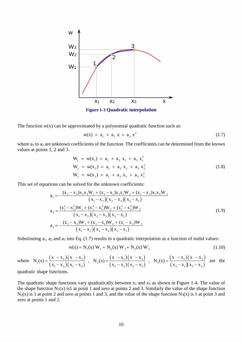
Example 1.1 The linear shape functions for a one-dimensional two-noded element can be found using the generalized method. The function used for approximation of w at position x is:

[ ] [ ]T T1 2 1 2w(x) a a x 1, x . a , a f (x) . a= + = =

where fT(x) = [f1(x), f2(x)] = [1, x] and a=[a1, a2]T. Then matrix C can be written as:

1

2

1 xC

1 x

=

2 1

2 1 2 11

2 1 2 1

x xx x x x

C1 1

x x x x

−

− − − = − − −

Therefore the vector of the shape functions is calculated as:

13

[ ]2 1

2 1 2 1T T 1 2 1

2 1 2 1 2 1 2 1

2 1 2 1

x xx x x x x xx xN (x) f (x) . C 1, x ,

1 1 x x x x x x x xx x x x

−

− − − = = = − − + − − − − − − −

And the shape functions for linear one-dimensional elements are:

2 11 1

2 1 2 1

x x x xN (x) and N (x)x x x x

− −= =

− −

Example 1.2 The quadratic shape functions for a one-dimensional three-noded element can be found as follows.

[ ]T2 2 T1 2 3 1 2 3 w(x) a a x a x 1, x, x . a , a , a f (x) . a = + + = =

where fT(x) = [f1(x), f2(x), f3(x)] = [1, x, x2] and a=[a1, a2, a3]T. Then matrix C is:

21 1

22 2

23 3

1 x xC 1 x x

1 x x

=

( ) ( ) ( ) ( ) ( ) ( )

( ) ( ) ( ) ( ) ( ) ( )

( ) ( ) ( ) ( ) ( ) ( )

2 3 1 3 1 2

1 2 1 3 2 1 2 3 3 1 3 2

1 2 3 1 3 1 2

1 2 1 3 2 1 2 3 3 1 3 2

1 2 1 3 2 1 2 3 3 1 3 2

x x x x x xx x x x x x x x x x x x

x x x x x xCx x x x x x x x x x x x

1 1 1x x x x x x x x x x x x

−

− − − − − − + + +

= − − − − − − − − −

− − − − − −

Therefore the vector of the shape functions for quadratic one-dimensional elements is calculated as:

( ) ( )( ) ( )

( ) ( )( ) ( )

( ) ( )( ) ( )

2 3 1 3 1 2T T 1

1 2 1 3 2 1 2 3 3 1 3 2

x x x x x x x x x x x xN (x) f (x)C , ,

x x x x x x x x x x x x−

− − − − − −= = − − − − − −

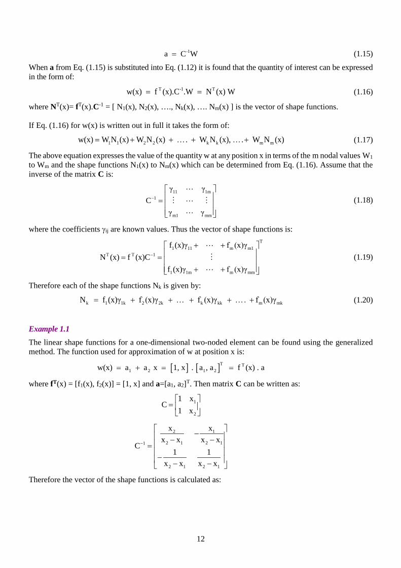
1.3 Two-dimensional interpolation The general method explained in the previous section can be used to derive the shape functions for two-dimensional elements. The shape functions for linear triangles and rectangles are calculated here. The quadratic shape functions for a triangular element are also derived for a specific case. Linear triangles Consider the quantity w is known at 3 nodes of a triangular element having its vertices at nodes 1, 2 and 3 as shown in Figure 1-5 The coordinates of nodes 1 to 3 are (x1,y1), (x2,y2), and (x3,y3) respectively and the values of w at nodes are W1, W2 and W3. If it is assumed that within the element the variation of w is linear with respect to x and y, then the value of w at position (x, y) can be approximated by a simple polynomial expression such as:

14

1 2 3w(x, y) a a x a y= + + (1.21)

or

[ ] [ ]T T1 2 3w(x, y) 1, x, y . a , a , a f (x, y) . a= =

Figure 1-5 Linear triangular element

The values of w are known at the nodes. Therefore, Eq. (1.21) can be written for all the nodes by substituting the coordinates of the nodes into Eq. (1.21):

1 1 2 1 3 1

2 1 2 2 3 2

3 1 2 3 3 3

W a a x a yW a a x a yW a a x a y

= + += + += + +

(1.22)

or

1 1 1 1

2 2 2 2

3 3 3 3

W 1 x y aW 1 x y a or W C . aW 1 x y a

= =

The quantity w(x, y) can now be expressed in the form of:

T -1 T

1 1 2 2 3 3

w(x, y) f (x, y).C .W N (x, y) W N (x, y).W N (x, y).W N (x, y).W

= == + +

(1.23)

with

and 2∆=det [C]= (x2y3 –x3y2)- (x1y3–x3y1)+ (x1y2–x2y1) =2×area of triangle. The shape functions can be found as:

−−−−−−−−−

=−

123123

211332

1221311323321

xxxxxxyyyyyy

yxyxyxyxyxyx

2Δ1C

15

[ ]2 3 3 2 3 1 1 3 1 2 2 1

T T 12 3 3 1 1 2

3 2 1 3 2 1

x y x y x y x y x y x y1N (x,y) f (x,y)C 1, x, y y y y y y y

2Δx x x x x x

−

− − − = = − − − − − −

(1.24)

2 3 3 2 2 3 3 2

13 1 1 3 3 1 1 3

2

31 2 2 1 1 2 2 1

(x y x y ) x(y y ) y(x x )2ΔN (x, y)

(x y x y ) x(y y ) y(x x )N(x,y) N (x, y)2Δ

N (x, y) (x y x y ) x(y y ) y(x x )2Δ

− + − + −

− + − + − = =

− + − + −

(1.25)

The correctness of the shape functions may be verified by checking the following conditions: 1) iN (x, y) 1=∑ at every point within the element

2) i i i

i

N (x, y) 1 at node i where x x and y yN (x, y) 0 at all nodes k where k i

= = == ≠

It can be shown that the sum of all the shape functions is equal to 1, so that condition 1 is satisfied. Condition 2 is also true for all the shape functions. For example, at node 1, x = x1 and y = y1:

2 3 3 2 1 2 3 1 3 21 1 1

2 3 3 2 1 3 3 1 1 2 2 1

(x y x y ) x (y y ) y (x x )N (x , y ) 1(x y x y ) (x y x y ) (x y x y )

− + − + −= =

− − − + −

At node 2, x = x2 and y = y2:

2 3 3 2 2 2 3 2 3 21 2 2

(x y x y ) x (y y ) y (x x )N (x , y ) 02Δ

− + − + −= =

At node 3, x = x3 and y = y3:

2 3 3 2 3 2 3 3 3 21 3 3

(x y x y ) x (y y ) y (x x )N (x , y ) 02Δ

− + − + −= =

Example 1.3 Consider a seepage analysis and suppose that the head has been determined at 3 vertices (nodes) of a triangular element. The coordinates (x, y) of the nodes and the value of the head (h) are shown in the table below:

Node x (m) y (m) H (m) 1 0.4 0.6 1.832 2 4.0 1.4 66.76 3 1.4 3.0 - 8.968

If it is assumed that the head may be approximated linearly throughout the element by the simple expression:

1 2 3h(x,y) a a x a y= + +

Determine the head at point xo = 2.0, yo = 1.5.

16

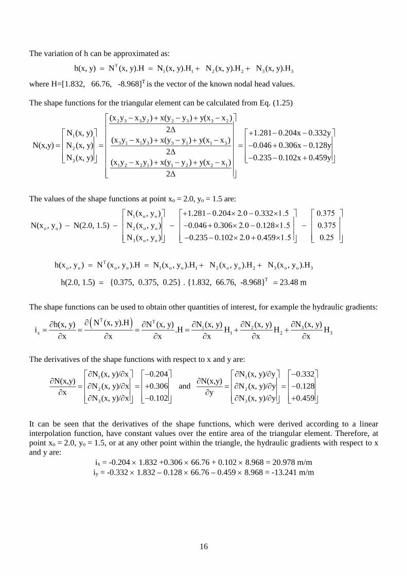
The variation of h can be approximated as:

T1 1 2 2 3 3h(x, y) N (x, y).H N (x, y).H N (x, y).H N (x, y).H= = + +

where H=[1.832, 66.76, -8.968]T is the vector of the known nodal head values. The shape functions for the triangular element can be calculated from Eq. (1.25)

2 3 3 2 2 3 3 2

13 1 1 3 3 1 1 3

2

31 2 2 1 1 2 2 1

(x y x y ) x(y y ) y(x x )2ΔN (x, y) 1.281 0.204x 0.332y

(x y x y ) x(y y ) y(x x )N(x,y) N (x, y) 0.046 0.306x 0.128y2Δ

N (x, y) 0.235 0.(x y x y ) x(y y ) y(x x )2Δ

− + − + −

+ − − − + − + − = = = − + −

− − − + − + −

102x 0.459y

+

The values of the shape functions at point xo = 2.0, yo = 1.5 are:

1 o o

o o 2 o o

3 o o

N (x , y ) 1.281 0.204 0.332 N(x , y ) N(2.0, 1.5) N (x , y ) 0.046 0.306 0.128

N (x , y ) 0.235 0.102 0.459

+ − × 2.0 − × 1.5 0.375 − − − − + × 2.0 − × 1.5 − 0.375 − − × 2.0 + × 1.5 0.25

To o o o 1 o o 1 2 o o 2 3 o o 3h(x , y ) N (x , y ).H N (x , y ).H N (x , y ).H N (x , y ).H= = + +

Th(2.0, 1.5) {0.375, 0.375, 0.25} . {1.832, 66.76, -8.968} 23.48 m= =

The shape functions can be used to obtain other quantities of interest, for example the hydraulic gradients:

( )T T

31 2x 1 2 3

N (x, y).H N (x, y)N (x, y) N (x, y)h(x, y) N (x, y)i .H H H Hx x x x x x

∂ ∂∂ ∂∂ ∂= = = = + +

∂ ∂ ∂ ∂ ∂ ∂

The derivatives of the shape functions with respect to x and y are:

1 1

2 2

3 3

N (x, y)/ x 0.204 N (x, y)/ y 0.332N(x,y) N(x,y)N (x, y)/ x 0.306 and N (x, y)/ y 0.128

x yN (x, y)/ x 0.102 N (x, y)/ y 0.459

∂ ∂ − ∂ ∂ − ∂ ∂ = ∂ ∂ = + = ∂ ∂ = − ∂ ∂

∂ ∂ − ∂ ∂ +

It can be seen that the derivatives of the shape functions, which were derived according to a linear interpolation function, have constant values over the entire area of the triangular element. Therefore, at point xo = 2.0, yo = 1.5, or at any other point within the triangle, the hydraulic gradients with respect to x and y are:

ix = -0.204 × 1.832 +0.306 × 66.76 + 0.102 × 8.968 = 20.978 m/m

iy = -0.332 × 1.832 – 0.128 × 66.76 – 0.459 × 8.968 = -13.241 m/m

17

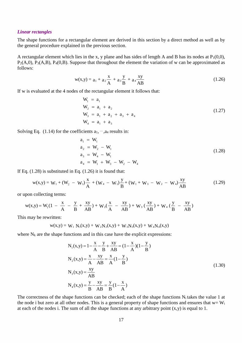
Linear rectangles The shape functions for a rectangular element are derived in this section by a direct method as well as by the general procedure explained in the previous section. A rectangular element which lies in the x, y plane and has sides of length A and B has its nodes at P1(0,0), P2(A,0), P3(A,B), P4(0,B). Suppose that throughout the element the variation of w can be approximated as follows:

1 2 3 4x y xyw(x,y) = + + + a a a aA B AB

(1.26)

If w is evaluated at the 4 nodes of the rectangular element it follows that:

1 1

2 1 2

3 1 2 3 4

4 1 3

W aW a aW a a a aW a a

== += + + += +

(1.27)

Solving Eq. (1.14) for the coefficients a1, …,a4 results in:

1 1

2 2 1

3 4 1

4 1 3 2 4

a Wa W Wa W W a W W W W

== −= −= + − −

(1.28)

If Eq. (1.28) is substituted in Eq. (1.26) it is found that:

1 1 4 1 1 3 2 42x y xyw(x,y) = + (W ) + ( ) + ( + )W W W W W W W WA B AB

− − − − (1.29)

or upon collecting terms:

2 3 41x y xy x xy xy y xyw(x,y) W (1 + ) + ( ) + ( ) + ( )W W WA B AB A AB AB B AB

= − − − −

This may be rewritten: 1 1 2 2 3 3 4 4w(x,y) = (x,y) + (x,y) + (x,y) + (x,y)W N W N W N W N

where Nk are the shape functions and in this case have the explicit expressions:

1

2

3

4

x y xy x yN (x,y) 1 (1 )(1 )A B AB A B

x xy x yN (x,y) (1 )A AB A BxyN (x,y)ABy xy y xN (x,y) (1 )B AB B A

= − − + = − −

= − = −

=

= − = −

(1.30)

The correctness of the shape functions can be checked; each of the shape functions Ni takes the value 1 at the node i but zero at all other nodes. This is a general property of shape functions and ensures that w= Wi at each of the nodes i. The sum of all the shape functions at any arbitrary point (x,y) is equal to 1.

18

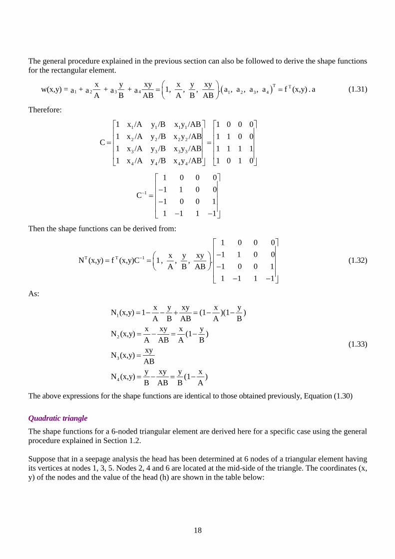
The general procedure explained in the previous section can also be followed to derive the shape functions for the rectangular element.

( )T T1 2 3 4 1 2 3 4

x y xy x y xyw(x,y) = + + + 1, , , . a , a , a , a f (x,y) . aa a a aA B AB A B AB = =

(1.31)

Therefore:

1 1 1 1

2 2 2 2

3 3 3 3

4 4 4 4

1 x /A y /B x y /AB 1 0 0 01 x /A y /B x y /AB 1 1 0 0

C1 x /A y /B x y /AB 1 1 1 11 x /A y /B x y /AB 1 0 1 0

= =

1

1 0 0 01 1 0 0

C1 0 0 11 1 1 1

−

− = − − −

Then the shape functions can be derived from:

T T 1

1 0 0 01 1 0 0x y xyN (x,y) f (x,y)C 1, , , .1 0 0 1A B AB1 1 1 1

−

− = = − − −

(1.32)

As:

1

2

3

4

x y xy x yN (x,y) 1 (1 )(1 )A B AB A B

x xy x yN (x,y) (1 )A AB A BxyN (x,y)ABy xy y xN (x,y) (1 )B AB B A

= − − + = − −

= − = −

=

= − = −

(1.33)

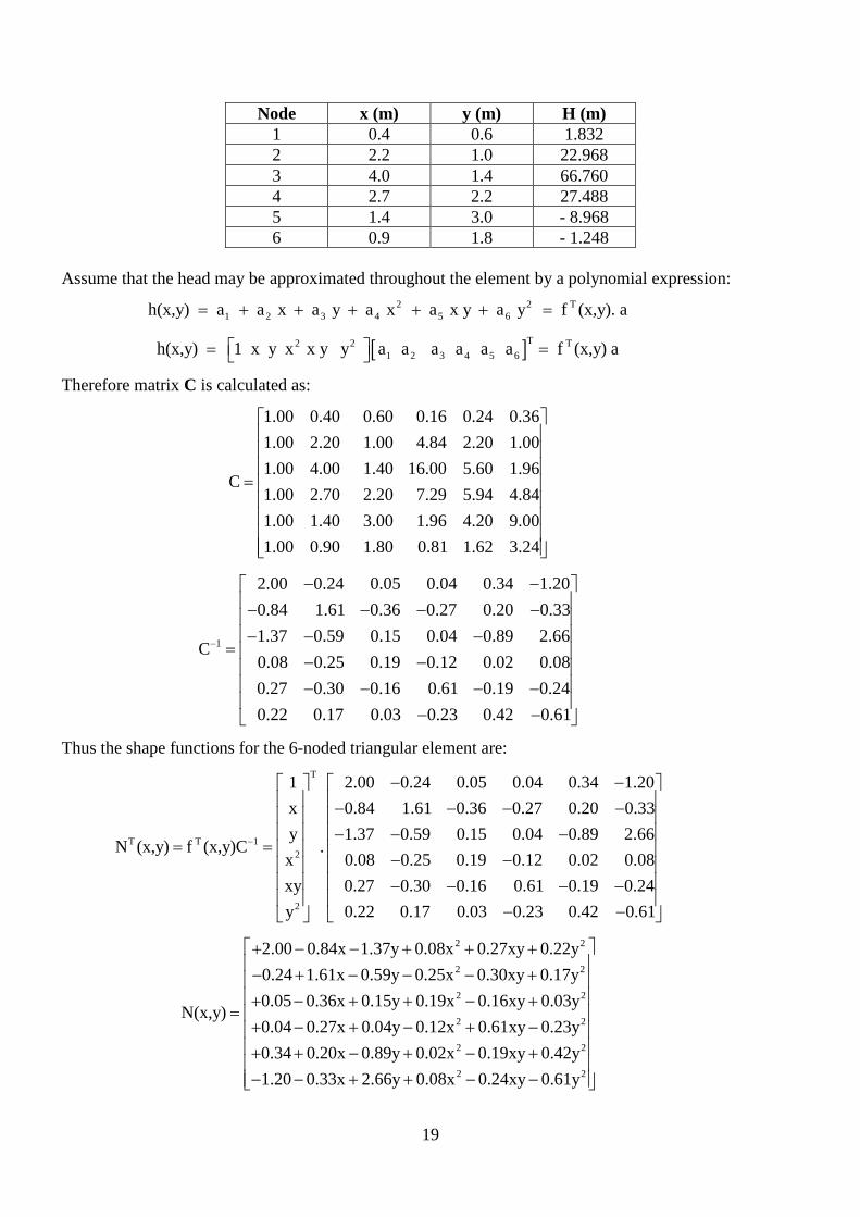
The above expressions for the shape functions are identical to those obtained previously, Equation (1.30) Quadratic triangle The shape functions for a 6-noded triangular element are derived here for a specific case using the general procedure explained in Section 1.2. Suppose that in a seepage analysis the head has been determined at 6 nodes of a triangular element having its vertices at nodes 1, 3, 5. Nodes 2, 4 and 6 are located at the mid-side of the triangle. The coordinates (x, y) of the nodes and the value of the head (h) are shown in the table below:

19

Node x (m) y (m) H (m) 1 0.4 0.6 1.832 2 2.2 1.0 22.968 3 4.0 1.4 66.760 4 2.7 2.2 27.488 5 1.4 3.0 - 8.968 6 0.9 1.8 - 1.248

Assume that the head may be approximated throughout the element by a polynomial expression:

2 2 T1 2 3 4 5 6h(x,y) a a x a y a x a x y a y f (x,y). a= + + + + + =

[ ]T2 2 T1 2 3 4 5 6h(x,y) 1 x y x x y y a a a a a a f (x,y) a = =

Therefore matrix C is calculated as:

1.00 0.40 0.60 0.16 0.24 0.361.00 2.20 1.00 4.84 2.20 1.001.00 4.00 1.40 16.00 5.60 1.96

C1.00 2.70 2.20 7.29 5.94 4.841.00 1.40 3.00 1.96 4.20 9.001.00 0.90 1.80 0.81 1.62 3.24

=

1

2.00 0.24 0.05 0.04 0.34 1.200.84 1.61 0.36 0.27 0.20 0.331.37 0.59 0.15 0.04 0.89 2.66

C0.08 0.25 0.19 0.12 0.02 0.080.27 0.30 0.16 0.61 0.19 0.240.22 0.17 0.03 0.23 0.42 0.61

−

− − − − − − − − −

= − − − − − −

− −

Thus the shape functions for the 6-noded triangular element are:

T

T T 12

2

1 2.00 0.24 0.05 0.04 0.34 1.20x 0.84 1.61 0.36 0.27 0.20 0.33y 1.37 0.59 0.15 0.04 0.89 2.66

N (x,y) f (x,y)C .x 0.08 0.25 0.19 0.12 0.02 0.08xy 0.27 0.30 0.16 0.61 0.19 0.24y 0.22 0.17 0.03 0.23

−

− − − − − − − − −

= = − − − − − −

− 0.42 0.61

−

2 2

2 2

2 2

2 2

2 2

2.00 0.84x 1.37y 0.08x 0.27xy 0.22y0.24 1.61x 0.59y 0.25x 0.30xy 0.17y0.05 0.36x 0.15y 0.19x 0.16xy 0.03y

N(x,y)0.04 0.27x 0.04y 0.12x 0.61xy 0.23y0.34 0.20x 0.89y 0.02x 0.19xy 0.42y1.

+ − − + + +− + − − − ++ − + + − +

=+ − + − + −+ + − + − +− 2 220 0.33x 2.66y 0.08x 0.24xy 0.61y

− + + − −

20

The head at point xo = 2.0, yo = 1.5 can be calculated as:

T T -1o o o o o oh(x , y ) N (x , y ).H f (x , y ). C . H= =

[ ]T To of (x , y ) 1 , 2 , 1.5 , 4.0 , 3.0 , 2.25=

T

T T 1

1.00 2.00 0.24 0.05 0.04 0.34 1.202.00 0.84 1.61 0.36 0.27 0.20 0.331.50 1.37 0.59 0.15 0.04 0.89 2.66

N (2,1.5) f (2,1.5).C .4.00 0.08 0.25 0.19 0.12 0.02 0.083.00 0.27 0.30 0.16 0.61 0.19 02.25

−

− − − − − − − − −

= = − − − − − −

.240.22 0.17 0.03 0.23 0.42 0.61

− −

[ ]TN (2, 1.5) 0.094 , 0.563 , 0.094 , 0.375 , 0.125 , 0.375= − − −

Th(2, 1.5) N (2, 1.5).H 17.45 m= =

The hydraulic gradient with respect to x can be calculated as follows:

( ) ( )T T 1T T

1x

N (x, y).H f (x, y).Ch(x, y) N (x, y) f (x, y)i .H H C Hx x x x x

−−

∂ ∂∂ ∂ ∂= = = = =

∂ ∂ ∂ ∂ ∂

where ∂fT(x,y)/ ∂x =[0 , 1 , 0 , 2x , y , 0]. At point xo=2.0, yo=1.5: ∂fT(xo, yo)/ ∂x =[0 , 1 , 0 , 4 , 1.5 , 0]. The hydraulic gradient at xo=2.0, yo=1.5 is calculated as ix=18.2m/m. The hydraulic gradient with respect to y can also be calculated in the same way as iy= −5.4m/m. The hydraulic gradient is a function of x and y since the variation of the head is no longer linear but quadratic throughout the element. For example the hydraulic gradients at point xo=2.0, yo=2.0 are ix=19.2m/m and iy= −8.4m/m.

21

Problems Problem 1.1. beam deflection It is observed that a beam, which lies in the interval 0< x <2m, undergoing flexural distortion has deflections v1 = 10mm when x = 0 and v2 = 12mm when x = 2m and rotations θ1 = 0.01 when x = 0 and θ2 = −0.02 when x = 2m where θ = ∂v/∂x. Assuming that v = a1 + a2 x + a3 x2 + a4 x3 calculate the deflection, rotation and curvature (∂2v/∂x2) at x = 1.5m. (Answer: v=18.25 mm, θ=-0.0057, ∂2v/∂x2=-0.024 m-1) Problem 1.2. T6 element For the 6-noded triangular element considered in Example 1.4, assume that the vector of nodal head is:

[ ]TH 1.832 , 34.296 , 66.76 , 28.896 , 8.968 , 3.568= − −

Calculate the hydraulic gradients, ix and iy, at points xo=2.0, yo=1.5 and xo=2.0, yo=2.0. Compare the results with those obtained in Example 1.3. Explain a reason for similarity between the results obtained here with those obtained from a 3-noded element in Example 1.3. Problem 1.3. Rectangular element A rectangular element bounded by the lines x = 0, x = 2a, y = 0, y = 2b has nodes at its vertices and the midpoints of its sides. Assume an appropriate polynomial function for variation of quantities within the element and show that the shape functions for node 4 (x = 2a, y = b) and node 5 (x = 2a, y = 2b) are:

4 2

xy(2b y)N2ab

−=

53xy(x/3a y/3b 1)N

4ab+ −

=

Problem 1.4. Triangular element A triangular plane element has 6 nodes at the points (xi, yi ); i = 1, ..., 6. Assuming the temperature T can be approximated in the form:

2 21 2 3 4 5 6T a a x a y a x a xy a y= + + + + +

Determine the shape functions for the element in the global coordinate system and in a local coordinate system which has its origin at the centroid and the X axis parallel to the side joining nodes 1-3 (vector 13 should run in the positive X-direction). Use these to calculate the temperature at the centroid and the temperature gradients ∂T/∂x, ∂T/∂y and ∂T/∂X, ∂T/∂Y Your particular values of (xi, yi Ti ) i = 1, ..., 6 will be given to you. Temperatures are in oc and coordinates in meters. Make sure you show the units of your answers. Your solution should have: (a) Data (xi, yi Ti )

22

(b) Shape function N4 in global coordinates (x,y) (c) Shape function N4 in local coordinates (X,Y) (d) The temperature at the centroid of the element (e) The temperature gradients ∂T/∂x, ∂T/∂X at the centroid

23

CHAPTER 2: MATHEMATICAL FOUNDATION OF FINITE ELEMENT ANALYSIS

MATHEMATICAL FOUNDATION OF FINITE ELEMENT ANALYSIS

In this Chapter we introduce the key concepts of finite element analysis by considering few one-dimensional problems. The formulation includes three steps. The first step is the derivation of the governing equations of the problem along with the identification of its boundary conditions. The second step involves the conversion of the governing equations into a weak form that allows the formulation of the finite element theory. In the third step we subdivide the domain of the system into a set of discrete sub-domains that are called elements, and we define the shape functions in each element. By expressing the seeking solution in terms of those shape functions, the governing equations are converted into a global matrix equation that is solved numerically. This is the essence of all finite element methods.

2.1 Governing equations: strong formulation The first step towards the mathematical modelling of any problem in science or engineering is the derivation of the differential equations of the quantity that needs to be solved. This quantity can be the displacement on a building under wind load, the temperature in an electrical circuit, the distribution of pore pressure in a dam, or the electro-magnetic field produced by an antenna. In most cases these equations can be assembled using four different components.

1) Kinematic equations, describing the gradient (derivative) of the variable we want to solve. For example: the gradient of the displacement is the strain, and the gradient of the head is the hydraulic gradient.

2) Balance equations, which are the mathematical expression of the conservation laws in physics.

Conserved quantities are usually mass, momentum, and energy. For example, for structures in equilibrium, the conservation of momentum lead to the so-called static equations; The Naiver-Stokes equations in fluid mechanics involve conservation of mass and momentum.

3) Constitutive equations, which represent the material properties of the system of study. These

properties are usually derived from experimental tests. In structural mechanics the constitutive model is the stress-strain relation which is given in terms of a stiffness tensor. In transport of heat, radiation or pollutants the constitutive models consist on transport coefficients, such as permeability in seepage flow, or conductivity in heat transfer.

4) Boundary conditions, which are given in the boundary of the domain of the problem. These are required to find a unique solution to the differential equation of the problem

24

(a) (b)

(c) (d)

Figure 2-1 From left to right: (a) the Leaning Tower of St Moritz; (b) the landslide displacements in the lower 200 m, (c) the mathematical model to predicting landslide displacement; and (d) free body diagram of

a slide (Puzrin, A. M. & Sterba, I. (2006). Geotechnique 56, No. 7, 483–489)

To illustrate the derivation of the governing equations, let us consider a simple mathematical model for a complex engineering problem, as shown in Figure 2-1. This example is a simplification of the powerful mathematical formulation of Puzrin and coworkers that has capabilities to predict landslides. Our example is related to a landslide displacement in Switzerland, which have led to the leaning of the St Moritz Tower: the displacement of the inclined slope is constrained by a rock outcrop along the Via Maistra, as shown in the Figure 2-1. Geological survey has shown that the deformation occurs above a sliding layer, and it is constrained by a rock outcrop at the bottom. For simplicity, we assume that the deformation u(x) only occurs in the direction of the slope. We want to derive the governing equations of “u” using the method of infinitesimals. First we divide the slope in slides perpendicular to the slope direction. Let u(x) and u(x+Δx) be the displacement at both side of the slide initially placed at the position x. The width of the slide, Δx, is assumed to be infinitesimally small, which means, very small. The kinematic equation is nothing more than the definition of strain:

u(x+Δx) u(x)ε.=

Δx−

(2.1)

25

where ‘.=’ means that the expression is valid when Δx is infinitesimally small. Thus the equation can be converted into a differential equation using the definition of derivative

duε=dx

(2.2)

This corresponds to the kinematic equation of the problem. Now we will construct the balance equation assuming that the system is in equilibrium. Since the problem is one-dimensional, the equation of conservation of momentum corresponds to the balance of forces in the x-direction:

gσ(x)h σ(x+Δx)h+τΔx τ Δx=0− − (2.3)

where σ is the stress acting on the x-direction, also known as earth pressure, τ is the shear stress acting on the sliding layer, and gτ =γhsinα is the gravity force, and γ is the unit weight of the soil. Eq. (2.3) can be rearranged as

gτ τσ(x+Δx) σ(x) = Δx h

−−− (2.4)

Since Δx is infinitesimal, the equation above can be converted into

dσ = f(x)dx

− (2.5)

where f(x) is the external loads apply to the system that in this case consists of a gravitational load minus the shear stress at the bottom of the boundary. This equation corresponds to the static equation of the problem. We notice that Eq. (2.2) and (2.5) are not sufficient to obtain the displacement profile of the slope. We still need an equation that relates stress and strain that is precisely the constitutive equation of the problem:

σ=Eε (2.6)

E is the Young’s modulus that gives the material property of the soil. It can depend on the position for non-homogenous soil, or on the stress for non-linear materials. Now we can combine Eq. (2.2), (2.5) and (2.6) to obtain the governing equation of our problem:

d duE = f(x)

dx dx −

(2.7)

If the soil behaviour is not lineal, (i.e. E does not depend on σ) this equation can be directly integrated to obtain the displacement along the landslide. We should not forget that every time we integrate we obtain an integration constant, which lead us to an indeterminate solution of our problem. In order to obtain a single solution we need to complete Eq. (2.7) with the so-called boundary conditions. They correspond to the condition of the unknown variable u at the boundary of the domain. Since our slope is constrained by a rock outcrop at the bottom, and free to move at the top, the boundary conditions are

x=L

duu(0)=0 and =0dx

(2.8)

where L is the length of the landslide. The first condition is called essential or fixed boundary condition. It states that the displacement at the bottom of the slope is always zero. The latter one is called natural, or free boundary condition, and it comes after using Eq. (2.2) and (2.6), and the fact that σ=0 at the top of the

26

landslide. If the soil is homogeneous and linear (E= cte) and the top boundary is at the critical state n(τ=σ tan(φ) , where nσ =γhcosα is the normal stress φ is the angle of friction of the soil), an analytical

solution exists for Eq. (2.7) with boundary condition given by Eq. (2.8)

( )γ sin(α) cos(α)tan(φ)u(x)= x(2L x)

2E−

− (2.9)

Note that to obtain this analytical solution we require several strong assumptions, such as one-dimensional deformation, linear elastic soil, and a sliding layer of zero thickness at the critical state. In practice we cannot always depend on too strong assumptions. If we relax the assumptions the resulting governing equation does not have analytical solution. That is where numerical solutions take place. Eq. (2.7) for non-linear material behaviour could in solved replacing the derivatives by finite differences. This leads to a set of algebraic equations that can be resolved numerically. This is the essence of the finite differences method that is useful for systems with simple domains. Yet several real-world problems involve complex domains and the finite different method become problem dependent. The boundary conditions are much simpler to plug in finite element modelling. Here is where the power of the finite element modelling appears, as it provides a unified framework for solving the governing equation of a wide range of problems for any kind of domains and boundary conditions. We will present below the key concepts of finite element modelling which will allow us to understand the general idea of this method.

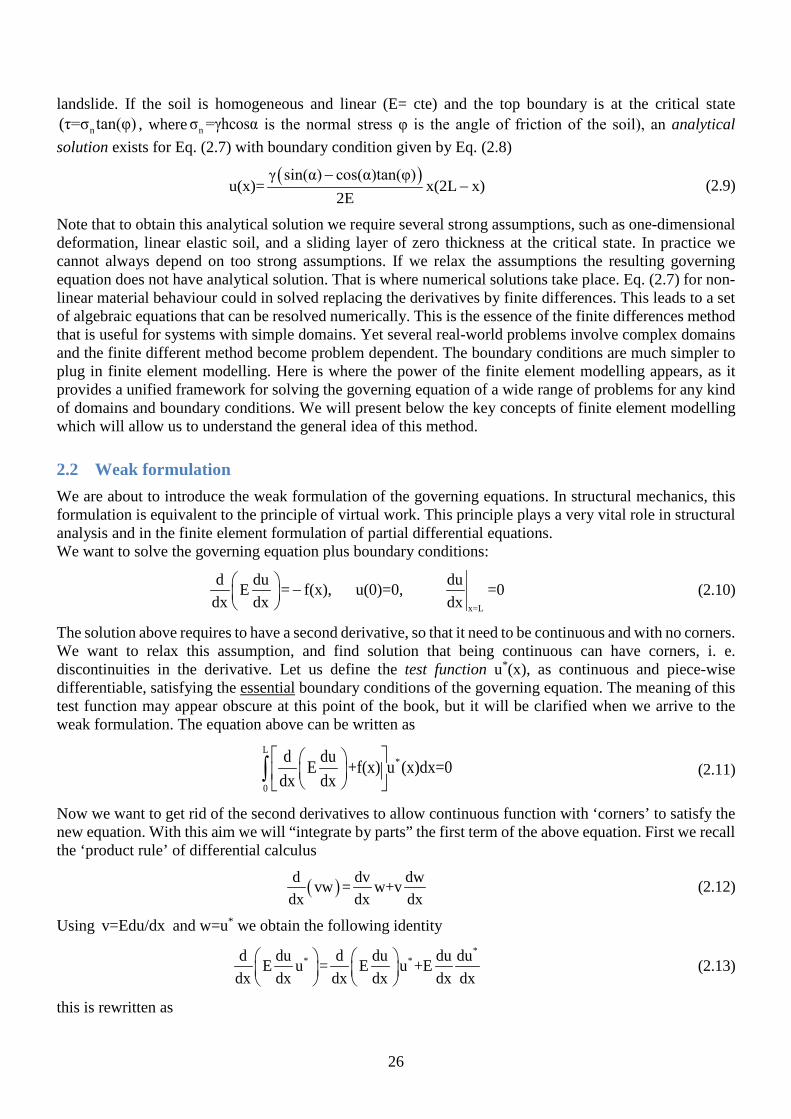
2.2 Weak formulation We are about to introduce the weak formulation of the governing equations. In structural mechanics, this formulation is equivalent to the principle of virtual work. This principle plays a very vital role in structural analysis and in the finite element formulation of partial differential equations. We want to solve the governing equation plus boundary conditions:

x=L

d du duE = f(x), u(0)=0, =0dx dx dx

−

(2.10)

The solution above requires to have a second derivative, so that it need to be continuous and with no corners. We want to relax this assumption, and find solution that being continuous can have corners, i. e. discontinuities in the derivative. Let us define the test function u*(x), as continuous and piece-wise differentiable, satisfying the essential boundary conditions of the governing equation. The meaning of this test function may appear obscure at this point of the book, but it will be clarified when we arrive to the weak formulation. The equation above can be written as

L

*

0

d duE +f(x) u (x)dx=0dx dx

∫ (2.11)

Now we want to get rid of the second derivatives to allow continuous function with ‘corners’ to satisfy the new equation. With this aim we will “integrate by parts” the first term of the above equation. First we recall the ‘product rule’ of differential calculus

( )d dv dwvw = w+vdx dx dx

(2.12)

Using v=Edu/dx and w=u* we obtain the following identity

*

* *d du d du du duE u = E u +Edx dx dx dx dx dx

(2.13)

this is rewritten as

27

*

* *d du d du du duE u = E u Edx dx dx dx dx dx

−

(2.14)

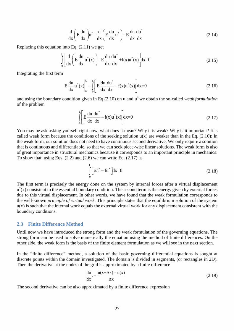
Replacing this equation into Eq. (2.11) we get

L *

* *

0

d du du duE u (x) E +f(x)u (x) dx=0dx dx dx dx

−

∫ (2.15)

Integrating the first term

L L *

* *

0 0

du du duE u (x) E f(x)u (x) dx=0dx dx dx

− −

∫ (2.16)

and using the boundary condition given in Eq (2.10) on u and u* we obtain the so-called weak formulation of the problem

L *

*

0

du duE f(x)u (x) dx=0dx dx

−

∫ (2.17)

You may be ask asking yourself right now, what does it mean? Why it is weak? Why is it important? It is called weak form because the conditions of the seeking solution u(x) are weaker than in the Eq. (2.10): In the weak form, our solution does not need to have continuous second derivative. We only require a solution that is continuous and differentiable, so that we can seek piece-wise linear solutions. The weak form is also of great importance in structural mechanics because it corresponds to an important principle in mechanics: To show that, using Eqs. (2.2) and (2.6) we can write Eq. (2.17) as

L

* *

0

σε fu dx=0 − ∫ (2.18)

The first term is precisely the energy done on the system by internal forces after a virtual displacement u*(x) consistent to the essential boundary condition. The second term is the energy given by external forces due to this virtual displacement. In other words, we have found that the weak formulation corresponds to the well-known principle of virtual work. This principle states that the equilibrium solution of the system u(x) is such that the internal work equals the external virtual work for any displacement consistent with the boundary conditions.

2.3 Finite Difference Method Until now we have introduced the strong form and the weak formulation of the governing equations. The strong form can be used to solve numerically the equation using the method of finite differences. On the other side, the weak form is the basis of the finite element formulation as we will see in the next section. In the “finite difference” method, a solution of the basic governing differential equations is sought at discrete points within the domain investigated. The domain is divided in segments, (or rectangles in 2D). Then the derivative at the nodes of the grid is approximated by a finite difference

du u(x+Δx) u(x).dx Δx

−= (2.19)

The second derivative can be also approximated by a finite difference expression

28

2

x x-Δx2

du du d u dx dx.dx Δx

−= (2.20)

Using both equations above, we obtain a finite difference expression for the second derivative

2

2 2

d u u(x+Δx) 2u(x)+u(x Δx).dx Δx

− −= (2.21)

We can replace the above equation into Eq. (2.7) to obtain

2Δx f(x)u(x+Δx)+2u(x) u(x Δx) F(x), F(x)=

E(x)− − − = (2.22)

Lets assume, for example that the domain is the interval [0, L] and it is divided into four subintervals with nodes 0 1 2 3 4x =0, x =Δx, x =2Δx, x =3Δx, x =4Δx=L . If we calculate Eq. (2.22) in each node the following equations are obtained:

2 1 0 1

3 2 1 2

4 3 2 3

5 4 3 4

x=Δx u +2u u F x=2Δx u +2u u Fx=3Δx u +2u u Fx=4Δx u +2u u F

⇒ − − =⇒ − − =⇒ − − =⇒ − − =

(2.23)

Then the governing equations are converted into algebraical equations, which are completed using the boundary conditions. Thus a pointwise numerical approximation is obtained. The beauty of this method is there is that the derivation of the algebraical equation is straightforward. Unfortunately, this feature often cannot outweigh its main disadvantage, namely that the method is not very tolerant of irregular boundary conditions as shown in Figure 2-2 for 2D grids. The other problem is that the conversion of the boundary conditions into algebraical equations is not always easy and it needs special treatment in each case.

Figure 2-2 Discretization of a turbine blade using (a) finite difference method and (b) finite element method [after Hubner, 1942]

29

2.4 Finite Element Method A more flexible technique to handle boundary condition is the “finite element method”. This method was born from the family of spectral methods, in which the solution is sought as a linear combination of well-known, elementary function –the Fourier analysis is a sister of the finite element method, but the later one proved to be much more computationally efficient. Similar to the finite difference method, the domain of the problem is discretised into smaller sub-regions that are commonly known as finite elements, see Figure 2-2b. Then we define a shape function sitting in each node, and vanishing in all elements that do not contain the node. Untimately the shape function will allow us to interpolate the nodal displacements at any point between the nodes. The simplest option is to assume that each shape function is what we call a ‘hat function’, i.e. a function that is one in the node and decreases linearly to zero in the neighbour nodes. Then we seek a solution as a linear combination of the shape functions

( ) ( )dofn

i 1i iu u N=

=∑x x (2.24)

where the sum goes over all “degrees of freedom” (dof) of the system. As a final result a piecewise linear approximation to the governing equation is arrived at, whose solution is obtained by finding the coefficients

iu . Very complex domains can be modelled with relative ease (Figure 2-2b) using triangles as finite elements. However, we should notice that if we plug Eq. (2.24) into the governing equation Eq. (2.10) and immediate problem is encounter: our shape functions has corners at the node, and we try to differenciate them twice, our equation will produce infinites at each nodes that rules out a solution in the form of Eq. (2.24). Historically many mathematicians encountered the same difficulty until the brilliant idea of Galerkin (Russian Mathematician and Engineer) came. The idea of Galerkin was to use Eq. (2.24) to find an approximate solution of the weak form of the governing equations instead. We will introduce the Galerkin method by formulating the finite element method in one dimension. The basic procedure is essentially the same for two and three-dimensional problems:

1. Decompose the domain into a set finite elements;

2. Define a set of shape functions, each one sitting in what are called nodes of the finite elements;

3. Unknown field variable u(x) is expressed as a linear combination of the shape functions; and

4. The governing equation is transformed into a matrix equation that is solved to obtain coefficient of the linear combination.

Domain Discretisation The domain of the slope problem is the interval [0,L]. Let us divide the interval into four elements (e1, e2, e3, e4). These elements will be joined by five nodes (x0, x1, x2, x3, x4). We seek and approximate solutions at the nodes given by ui=u(xi), i=0,1,..4. The natural question is how many element we need to use. The general rule is that as more elements we use more accurate will be the solution but more calculations need to be done. But in the practice we need to use smaller element in those part of the domain where we expect the solution will change more abruptly. In analysis of structures this happens near to the holes or the interfaces where different bodies interact.

30

x

x1

1 N1(x)

0 x2 x3 x4 x0 e1

e2

e3

e4

x4

x x1

dN1/dx

0 x3

x0 e1

e2

e3

e4

1/Δx

-1/Δx

x2

x

x1

1

0 x2 x3 x4 x0 e1

e2

e3

e4

N2(x)

x4

x x1

dN2/dx

0 x3

x0 e1

e2

e3

e4

1/Δx

-1/Δx

x2

x

x1

1

0 x2 x3 x4 x0 e1

e2

e3

e4

N3(x)

x4

x x1

dN3/dx

0 x3

x0 e1

e2

e3

e4

1/Δx

-1/Δx

x2

x

x1

1

0 x2 x3 x4 x0 e1

e2

e3

e4

N4(x)

x4

x x1

dN4/dx

0 x3

x0 e1

e2

e3

e4

1/Δx

-1/Δx

x2

Figure 2-3 Left: hat shape function in finite element analysis Right: derivatives of the hat functions

Global shape function After discretisation we seek for a solution of the Eq. (2.17) on the domain. The main idea is to sit a shape function in each one of the nodes, (Figure 2-3) and then express the virtual displacement as a linear combination of them. Each shape function will account for deformation at one node, and the total deformation is expressed as a linear combination of the shape functions. In particular, Eq. (2.17) will be valid for u*(x)=Ni(x) (i=1,2,3,4). Thus Eq. (2.17) is written as:

L

ii

0

dNdu(E fN )dx=0 where i 1, 2,3, 4dx d

xx

( ) =−∫ (2.25)

Linear combination The function u(x) is expressed also as a combination of the shape functions:

( ) ( ) ( ) ( ) ( ) ( )4

2 2 3 3 4 4i=1

1 1 i iu x = x + x + x + u N u N u N N N xux =u ∑ (2.26)

If we use shape function as the hat shown in Figure 2-3, it is easy to show that ui is the deformation at the ith-node.

31

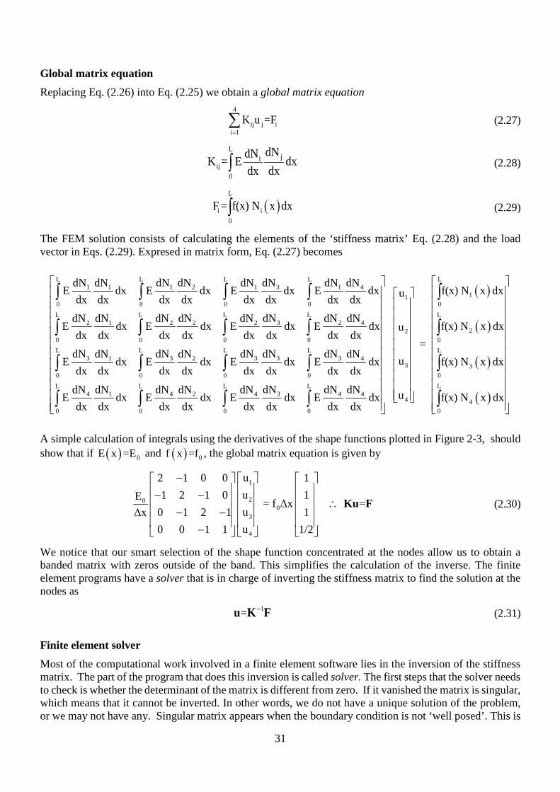
Global matrix equation Replacing Eq. (2.26) into Eq. (2.25) we obtain a global matrix equation

4

ij j ii 1

K Fu ==∑ (2.27)

L

iij

0

jdNdNK = E dx dx dx∫ (2.28)

( )L

i i0

= f(xF ) N x dx∫ (2.29)

The FEM solution consists of calculating the elements of the ‘stiffness matrix’ Eq. (2.28) and the load vector in Eqs. (2.29). Expresed in matrix form, Eq. (2.27) becomes

L L L L

0 0 0 0L L L L

0 0 0 0L L L L

31 1 1 2 1 1 4

32 1 2 2 2 2 4

3 3 3 3 3

0 0 0 0

1 2 4

4

dNdN dN dN dN dN dN dNE dx E dx E dx E dx

dx dx dx dx dx dx dx dxdNdN dN dN dN dN dN dN

E dx E dx E dx E dxdx dx dx dx dx dx dx dx

dN dN dN dN dNdN dN dNE dx E dx E dx E dx

dx dx dx dx dx dx dx dx

dN dNE

dx

∫ ∫ ∫ ∫

∫ ∫ ∫ ∫

∫ ∫ ∫ ∫

( )

( )

( )

( )

L

0L

0L

0L L L L L

11

22

3 3

31 4 2 4 4 4

0 0 0 0

4 40

f(x) N x dx

f(x) N x dx

f(x) N x dx

dNdN dN dN dN dNdx E dx E dx E dx f(x) N x dx

dx dx dx dx d

u

u

x dx d

u

ux

=

∫

∫

∫

∫ ∫ ∫ ∫ ∫

A simple calculation of integrals using the derivatives of the shape functions plotted in Figure 2-3, should show that if ( ) 0E x =E and ( ) 0f x =f , the global matrix equation is given by

1

200

3

4

u2 1 0 0 1u1 2 1 0 1E = f Δx =u0 1 2 1 1Δxu0 0 1 1 1/2

− − − ∴ − − −

Ku F (2.30)

We notice that our smart selection of the shape function concentrated at the nodes allow us to obtain a banded matrix with zeros outside of the band. This simplifies the calculation of the inverse. The finite element programs have a solver that is in charge of inverting the stiffness matrix to find the solution at the nodes as

1= −u K F (2.31)

Finite element solver Most of the computational work involved in a finite element software lies in the inversion of the stiffness matrix. The part of the program that does this inversion is called solver. The first steps that the solver needs to check is whether the determinant of the matrix is different from zero. If it vanished the matrix is singular, which means that it cannot be inverted. In other words, we do not have a unique solution of the problem, or we may not have any. Singular matrix appears when the boundary condition is not ‘well posed’. This is

32

the case for example, when the boundary conditions are free at both ends of the domain. Singular matrices appear also when the material properties of the materials such as Young modulus of thickness of the materials are entered with zero values. This is a common mistake of beginners. The second problem that may be encounter by the solver in problems with large matrices is that the computer needs too much time to invert the matrix. This usually happen when the elements are not properly indexed, leading to sparse matrices. Ideally we want that the elements of the stiffness matrix vanish above a certain distance from the diagonal that is called bandwidth. A typical finite element program consists of three basic units: pre-processor, processor and post-processor. In the pre-processor the geometry of the problem, the boundary conditions and material parameters are entered into the program. The processor generates the elements, assembles the stiffness matrix, and inverts it using the solver. The last component of the program is the post-processor that computes the solution and its derivatives and print or plot the results. In this book we will focus on the theoretical aspects of the implementation of the finite elements within the processor. We focus not only on structural problems, but also in non-structural cases such as seepage analysis and thermal conduction problems. We will focus the so-called static solvers that give solutions of static problems. However, you shall bear in mind that there are solvers for many situations, such as buckling analysis and dynamics systems.

2.5 Variational principle: minimal form The principle of virtual work can be derived from a variational formulation. This formulation leads to a wide range of numerical methods to find equilibrium configuration of complex systems, such as the configuration of DNA molecules. One of these is the finite element method that we have derived from the virtual work principle. Here we present an alternative to derive the weak formulation which is based on energetic principles. The method calculates the energy E(u) of the system in a configuration given by the displacement function u(x). Then the equilibrium of the solution is assumed to be that one that minimizes the energy. This formulation is useful when we are interested in the equilibrium of the system, which is the case of most structural analysis problem. If we want to investigate the transient dynamics we need other methods. The variational formulation defines the ‘energy’ as a ‘functional’ –it means, a function whose argument is a function, and whose value is a real number, which in this case represents the energy:

( )2L

0

1 duE = ( E + fu)dx2 dx

u ∫ (2.32)

We seek for the function u(x) that minimizes the energy. This can be done by using the ‘variational derivative’.

*E(u+εu ) E(u) 0E'(u).ε

−== (2.33)

Where u*(x) is a ‘test function’ that satisfies the essential boundary conditions of the problem. Replacing Eq. (2.32) in Eq. (2.33) we obtain:

L *

*

0

du du(E fu )dx 0dx dx

− =∫ (2.34)

33

This corresponds to the weak form. We can also derive the strong formulation for Eq. (2.34). By integrating this equation by parts,

( )L L* 2 L

* * * *

00 0

udu du d du0 (E fu )dx E u +fu dx+u xdx dx dx dx

= =−−

∫ ∫ (2.35)

Using the boundary condition it leads to

L

*

0

d duE +f(x) u (x)dx 0 dx dx

=∫ (2.36)

Since this equation is valid for any virtual displacement we can assume that the integrand vanish in all points

d duE +f(x)=0

dx dx

(2.37)

This corresponds to the strong formulation. We can conclude that the governing equation of an engineering problem can be written in three different forms: the strong form that is used in the finite differences method to achieve a point-wise approximation; the weak form that allows the finite element formulation and a piecewise linear approximation; and the minimal form, which allow numerical solutions using a wide range of variational methods that are not covered in this book.

34

Problems Problem 2.1. Finite different solution This question is related to the governing equation of the constrained landslide problem

2

0 02d uE = fdx

− x=L

duu(0)=0 and =0dx

Where E0 is the Young modulus of the soils, f0 is the external forces per unit of length, and u(x) is the displacement we want to obtain. Find the analytical solution of this equation. Here we will compare this result with the numerical solutions from the finite difference method and the finite element method. Divide the space domain of the landslide in four equally-spaced intervals with nodes

0 1 2 4x =0, x = x, x =2 x, ,x =L ∆ ∆ Show that the finite different method (FDM) matrix equation of the governing equation is given by

12

2 0

3 0

4

u2 1 0 0 1u1 2 1 0 1f Δx=u0 1 2 1 1Eu0 0 1 1 1

− − − − − −

Solve this equation by inverting the matrix, and find the displacement at the nodes. Problem 2.2. Finite element solution For the differential equation in Problem 2.1, construct the global matrix equation using the finite element method (FEM). You have to do the following 1) Calculate the integrals for K11, K12, K13, K44, F1, and F4. 2) Using these calculations to show that the matrix equation is given by

12

2 0

3 0

4

u2 1 0 0 1u1 2 1 0 1f Δx=u0 1 2 1 1Eu0 0 1 1 1/2

− − − − − −

Invert the matrix to solve the displacement of the nodes. Problem 2.3. Numerical errors Compare the numerical solutions of both FDM and FEM with the analytical solution. What is the numerical error of the solution in each case? How does the numerical error change if the number of elements is duplicated? The numerical error is the difference between the exact solution and the numerical solution. Hint: to compare the numerical solutions, you can work with dimensionless variables by assuming that

20 0f L /E =1 and L=1

35

Problem 2.4. Settlement of soils A soil layer of depth H [m] over a rock bed has a uniform unit weight γ [kN/m3] and a Young modulus E(x) [kN/m2] that varies with depth, see figure. A uniform load P [kN/m2] is applied on the surface. The soil deforms due to the combined action of its weight and the surface load. The deformation due to the surface load is called settlement.

L>>H

H

P

E(x) γ

x

0 Rigid bedrock

Soil layer

1) Derive the kinematic equation of the problem 2) Write down the constitutive equation of the problem 3) Derive the balance equation of the problem, Assume that settlement and compression stresses are

positive. 4) Derive the governing equations along with the boundary conditions. 5) Obtain the analytical solution for the soil deformation, settlement, total strain, and total stress, in the

case of homogeneous soil E(x) = E0. Problem 2.5. Steel bar with variable area A steel bar (E=200 GPa) is fixed to a wall as shown the figure. The bar is pulled by a horizontal force P=1000 N applied at the right. The area changes linearly from 0.01 m2 to 0.0064 m2. The length of the bar is 1m. This problem is about finding the horizontal displacement along the bar. It is assumed that displacements in the right direction are positive.

1) Derive the governing equations of the deformation of the bar. 2) Derive the weak form of the governing equations. 3) Find the global matrix equation with three linear elements. 4) Find the finite element solution of the problem 5) Derive the analytical solution for the problem.

0A LA

L

EP

36

Problem 2.6. Analytical modelling of constrained landslides The governing equation for the displacement of the landslide in Section 2.1 is

gτ τd duE =dx dx h

− − x=L

duu(0)=0 and =0dx

Where E is the Young modulus of the soil, τ the shear stress acting on the sliding layer; h the depth of the sliding layer; and gτ =γhsinα the gravity force; γ is the unit weight of the soil and α is the angle of the slope. 1) Show that if the soil is homogeneous and linear (E= cte) and the soil at the sliding surface is at the critical state ( τ=γhcos(α)tan(φ) , where φ is the angle of friction of the soil), an analytical solution exists for the boundary condition. 0u (x)=γ(sin(α)-tanφcos(α))x(x-2L) 2) Use the Matlab function spdiags to construct the stiffness matrix for 10, 100 and 1000 elements in both FEM and FDM formulation. Solve numerically the global matrix equation. Compare the analytical solution to the numerical solutions, and determine the error of the approximation as a function of the number of elements. 3) Assuming a viscoelastic constitutive relation between earth pressure and the strain

up=Eε+ηε ε=t

∂∂

show that the displacement is a the following function of position and time

-Et/η

ou(x,t)=u (x)(1-e ) 4) Sketch the displacement versus time of the landslide, and earth pressure p along the landslide. Discuss whether the landslide will remain stable in the future.

37

CHAPTER 3: FINITE ELEMENT CONCEPT

FINITE ELEMENT CONCEPT

In the previous Chapter the basic concept of the finite element formulation was introduced, and the stiffness matrix was derived using global shape functions. Although the stiffness matrices of a few more element types may be obtained using similar procedures, for other types of finite elements, such as continuum triangular or rectangular elements, the derivation is not straightforward. Therefore, it is necessary to develop a general procedure that can be used for derivation of the stiffness matrices of all element types. The general method consists of constructing the stiffness matrix of individual elements, and then assembly them into a global stiffness matrix of the complete structure. The aim of this chapter is to introduce this general formulation of the finite element method. The procedure will used to form the stiffness matrix of two different element types, bar element and a flexural beams element.

3.1 The principle of virtual work We recall the principle of virtual work for a single element of the structure. The principle of virtual work states that during any virtual displacement imposed on the boundary of an element, the total work done by the external loads Wext must be equal to the total internal work done Wint by the internal stresses σ(x) .

e

e

int ext

*int V

*ext V

W =W

W = ε (x)σ(x)dV

W = u (x)f(x)dV

∫∫

(3.1)

where f(x) are the external load, and ε*(x) is the virtual strains produced by the virtual displacement *u (x).The integral goes over the volume of the element Ve = AL, where A is the cross section area and L the length of the element. The virtual work principle can be written in matrix form as:

e e

*T *T

V V( ) ( )dV= ( ) ( )dV∫ ∫ε x σ x u x f x (3.2)

This notation is convenient since stress and strains are generally vector quantities that will be defined in 0. He will use this expression since it is more convenient to derive the finite element formulation.

3.2 General procedure in Finite Element Analysis Most finite element computations in numerical analysis comprise the following steps that will be explained in detail along this textbook: 1. Chose a suitable coordinate system. While for many of the geometries a Cartesian coordinate is suitable, a

cylindrical coordinate system may be used for problems with axial symmetry.

38

2. Divide the geometry of the problem into a number of finite elements. Different types of elements may be used to represent differences in physical properties. In structural mechanics, these can be beams, cables, plates, bricks, etc.

3. Use a suitable node numbering system for the elements of the structure. 4. Derive the element matrix equations for all finite elements using the principle of virtual work (or the

principle of minimum potential energy). These equations are typically in the form of:

e e e = k u f (3.3)

where ke is the element stiffness matrix, ue is the vector of element nodal displacements, and ef is the vector of element nodal forces.

5. Assemble the global stiffness matrix for the complete structure from the stiffness matrices of the individual finite elements, and the global force vector to form the element nodal forces:

Ku = F (3.4)

where ee

= ∑K K is the global stiffness matrix, u is the vector of global nodal displacements, and

ee

= ∑F F is the vector of global nodal forces. The matrices eK and eF are ‘inflated’ versions of ke and

ef , as we learn in the next chapter.

6. Apply boundary conditions by eliminating equations related to nodes with zero displacements. The method will be explained in the next chapter.

7. Solve the global stiffness equations to obtain the unknown nodal displacements:

-1= u K F (3.5)

8. Compute the relevant physical quantities in all elements: stresses, strains, curvature and moments. The calculation of the element stiffness matrix, ke, is an important step in the finite element computations and therefore is dealt with in detail in the next section.

3.3 Element stiffness matrix of the one-dimensional bar element A general procedure is presented here that can be used for derivation of the stiffness matrix of various finite elements. The aim is to relate the nodal loads to the nodal displacements, and thereby define the element stiffness matrix. Different types of elements have different numbers of nodes and different numbers of degrees of freedom per node. Therefore, the size of the stiffness matrix is generally different for different element types. In most structural analyses the term degree of freedom may be regarded as the different modes of displacement at each node. However, in general, the term "degree-of-freedom" is applied to any nodal quantity such as displacement, rotation, temperature, hydraulic head, etc. If the number of nodes in the chosen finite element is nne and the number of degree of freedom per node is dof, then the total degrees of freedom for the element is ndof = nne × dof. The size of the element displacement vector, ue, and the element force vector, fe, is equal to ndof and the size of the element stiffness matrix, ke, is equal to ndof × ndof. The element stiffness equations are defined by:

e e e =k u f (3.6)

39

The specific case considered here is a two-node bar element shown in Figure 3-2 Similar to the element of the constrained landslide, we assume that this element can only carry axial loads. The rotation and the deflection normal to the element axis are assumed to be zero. For this element nne=2, dof=1, ndof=2, and therefore the size of the stiffness matrix is 2×2. The linear shape functions for this element are plotted in Figure 3-2.

1 2 u2, p2 u1, p1

x L 0

x1 x2

Figure 3-1 Two-node bar element

1 2

xx1 x2

N(x)

1N1 N2

0

Figure 3-2 Two-node bar element

The matrix equation of this element can be calculated in the same way then in Chapter 2

1 1 1 21 1

2 1 2 22 2

L L

0 0L L

0 0

dN dN dN dNE dV E dVdx dx dx dx

dN dN dN dNE dV E dVd

u p =

x dx dxp

du

x

∫ ∫

∫ ∫ (3.7)

Here the dV=Adx, where A is the area of the bar. If the young modulus and the body forces are uniform, Eq. (3.7) becomes

1 1

2 2

u p1 1EAu p

=1 1L

− −

(3.8)

This is the element matrix equation of the one dimensional bar problem.

3.4 Calculation of the stiffness matrix of a two-dimensional bar element The aim of this section is to present an approach to the construction of the element stiffness matrices of two-dimensional structures through transformation of coordinates. A structural frame usually consists of members set at various angles to one another. Therefore, it is more convenient to set up the stiffness matrix in terms of the local member coordinates and then transform each of the local coordinate system to the global coordinate system adopted for the complete structure. A two-dimensional bar element which is inclined at an angle θ to the global system is shown in Figure 3-3. Axes X and Y refer to the local member system and axes x and y to the global coordinate system. In a framed structure each end of the bar could be displaced in both directions. The displacements U and V, u and v, and the forces P and Q, p and q are related to the local and the global systems, as shown in Figure 3-3.

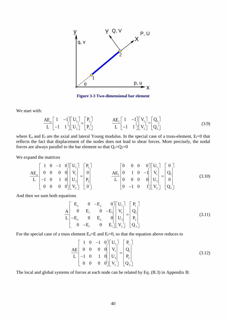
40

XY P, U

x

y

θ1

2

Q, V

p, u

q, v

Figure 3-3 Two-dimensional bar element

We start with:

1 1 1 1a

2 2 2 2

U P V Q1 1 1 1AE AE =U P V Q1 1 1 1L L

l− − = − −

(3.9)

where Ea and El are the axial and lateral Young modulus. In the special case of a truss-element, El=0 that reflects the fact that displacement of the nodes does not lead to shear forces. More precisely, the nodal forces are always parallel to the bar element so that Q1=Q2=0 We expand the matrices

1 11

1 1 1

2 22

2 2 2

U U 01 0 1 0 P 0 0 0 0V V Q0 0 0 0 0 0 1 0 1AE AEU U 01 0 1 0 P 0 0 0 0L LV V Q0 0 0 0 0 0 1 0 1

a l

− − = = − −

(3.10)

And then we sum both equations

a a 1 1

l l 1 1

a a 2 2

l l 2 2

E 0 E 0 U P0 E 0 E V QA

E 0 E 0 U PL0 E 0 E V Q

− − = − −

(3.11)

For the special case of a truss element Ea=E and El=0, so that the equation above reduces to

1 1

1 1

2 2

2 2

U P1 0 1 0V Q0 0 0 0AEU P1 0 1 0LV Q0 0 0 0

− = −

(3.12)

The local and global systems of forces at each node can be related by Eq. (B.3) in Appendix B:

41

( ) ( )( ) ( )

+cos θ sin θP psin θ cos θQ q

= −

(3.13)

Thus the relationship between the applied forces in the local and global systems is:

( ) ( )( ) ( )

( ) ( )( ) ( )

1 1

1 1

2 2

2 2

cos θ sin θ 0 0P psin θ cos θ 0 0Q q

0 0 cos θ sin θP p0 0 sin θ cos θQ q

− = −

(3.14)

or simply:

T =F T f (3.15)

where F and f are the force vectors in the local and global systems, respectively. A similar relationship also exists between the two sets of displacements in the local and global systems:

T =Δ T u (3.16)

Δ and u are the displacement vectors in the local and global systems The stiffness matrix for a member in the global system can now be established. The basic force-displacement relationship for the bar element, given in Eq. (3.12), states that:

e =F K Δ (3.17)

Ke refers to the element stiffness matrix in the local coordinate system. Substituting F and Δ from Eq. (3.15) and Eq. (3.16) into Eq. (3.17) results in:

T Te =T f K T u (3.18)

Both sides of the above equation are multiplied by T.

T Te =TT f T K T u (3.19)

One useful property of the T matrix is that its transpose is equal to its inverse, i.e,

T -1 T -1 , = = =T T T T T T 1 (3.20)

Therefore;

Te e = =f TK T u k u (3.21)

whereby ke is the stiffness matrix of the element in the global system.

Te e =k TK T (3.22)

It can be seen that the global stiffness matrix for a member, ek , can be obtained from the stiffness matrix of the member in the local member coordinate system. So that the stiffness matrix of the bar elements can be written in the global system as shown below.

2 2

2 2

2 2

2 2

c cs c cscs s cs sAE c=cos(θ) ,s=sin(θ)

L c cs c cscs s cs s

− − − − = − − − −

k (3.23)

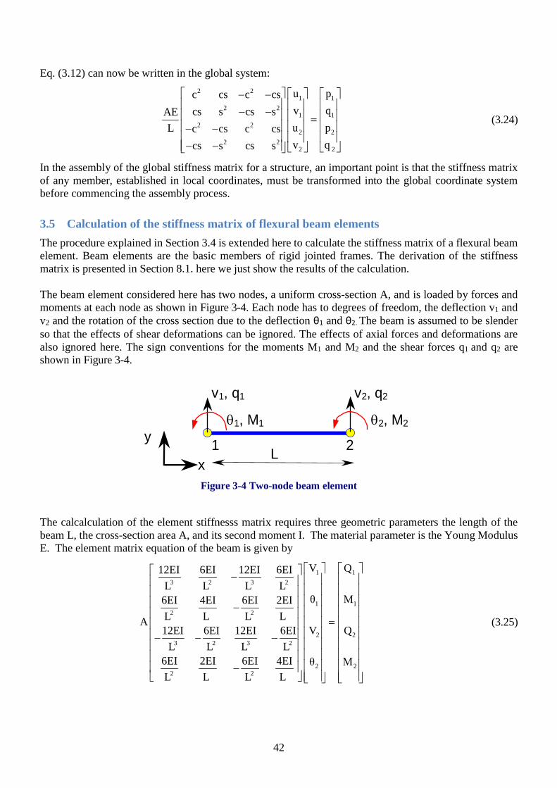
42

Eq. (3.12) can now be written in the global system:

2 21 1

2 21 1

2 22 2

2 22 2

u pc cs c csv qcs s cs sAEu pL c cs c csv qcs s cs s

− − − − = − − − −

(3.24)

In the assembly of the global stiffness matrix for a structure, an important point is that the stiffness matrix of any member, established in local coordinates, must be transformed into the global coordinate system before commencing the assembly process.

3.5 Calculation of the stiffness matrix of flexural beam elements The procedure explained in Section 3.4 is extended here to calculate the stiffness matrix of a flexural beam element. Beam elements are the basic members of rigid jointed frames. The derivation of the stiffness matrix is presented in Section 8.1. here we just show the results of the calculation. The beam element considered here has two nodes, a uniform cross-section A, and is loaded by forces and moments at each node as shown in Figure 3-4. Each node has to degrees of freedom, the deflection v1 and v2 and the rotation of the cross section due to the deflection θ1 and θ2. The beam is assumed to be slender so that the effects of shear deformations can be ignored. The effects of axial forces and deformations are also ignored here. The sign conventions for the moments M1 and M2 and the shear forces q1 and q2 are shown in Figure 3-4.

1 2

v2, q2v1, q1

L

θ2, M2 θ1, M1

x

y

Figure 3-4 Two-node beam element

The calcalculation of the element stiffnesss matrix requires three geometric parameters the length of the beam L, the cross-section area A, and its second moment I. The material parameter is the Young Modulus E. The element matrix equation of the beam is given by

1 13 2 3 2

1 12 2

2 23 2 3 2

2 22 2

V Q12EI 6EI 12EI 6EIL L L L

θ M6EI 4EI 6EI 2EIL L L LA12EI 6EI 12EI 6EI V Q

L L L L6EI 2EI 6EI 4EI θ ML L L L

− −

= − − − −

(3.25)

43

3.6 Two-dimensional flexural members Flexural frames are structures with rigid jointed members that resist loads primarily by flexural action. The stiffness relation is first derived in a local coordinate system, defined by the member axes, and is then transformed to the global system (Figure 3-5). The stress resultants at any point of such members consist of a moment, a transverse shear force, and an axial force. Thus the number of degrees-of-freedom at each node is dof=3. The total degrees-of-freedom for the two-noded flexural element shown in Figure 3-5 is therefore ndof=6. The size of the element stiffness matrix is 6×6.

1

2

V2, Q2

V1, Q1

L

θ2, M2

θ1, M1

x, u, p

y,v,q

U1, P1

U2, P2

θ

X Y

Figure 3-5 Two-node beam element

The stiffness equation of a beam element in its local coordinate system is given by Eq. (3.25). This equation can be expanded to include the effects of axial forces, P1 and P2:

1

1

3 2 3 2

12 2

2

23 2 3 2

22 2

U PEA EA0 0 0 0L L

V12EI 6EI 12EI 6EI0 0L L L L

θ6EI 4EI 6EI 2EI0 0L L L L

EA EA U0 0 0 0L L

12EI 6EI 12EI 6EI V0 0L L L L

6EI 2EI 6EI 4EI θ0 0L L L L

− − − = − − − − −

1

1

1

2

2

2

Q

M

P

Q

M

(3.26)

For an arbitrarily oriented beam element, inclined at an angle θ, it is necessary to express the stiffness matrix in the global coordinate system. The local and global systems of forces and displacements at each node can be related by:

( ) ( )( ) ( )

P cos θ sin θ 0 pQ sin θ cos θ 0 qM 0 0 1 M

= −

(3.27)

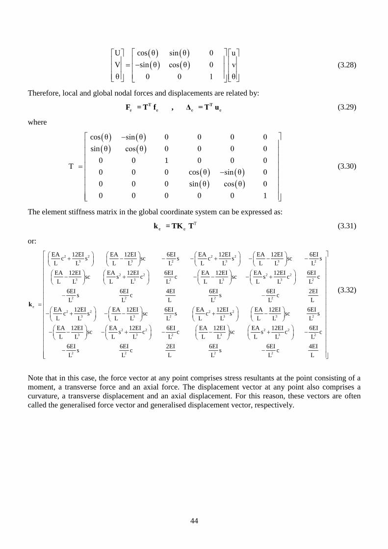
44

( ) ( )( ) ( )

U cos θ sin θ 0 uV sin θ cos θ 0 vθ 0 0 1 θ

= −

(3.28)

Therefore, local and global nodal forces and displacements are related by:

e e e e T TF = T f , Δ = T u (3.29)

where

( ) ( )( ) ( )

( ) ( )( ) ( )

cos θ sin θ 0 0 0 0sin θ cos θ 0 0 0 0

0 0 1 0 0 0T

0 0 0 cos θ sin θ 00 0 0 sin θ cos θ 00 0 0 0 0 1

−

= −

(3.30)

The element stiffness matrix in the global coordinate system can be expressed as:

Te e k = TK T (3.31)

or:

2 2 2 23 3 2 3 3 2

2 2 2 23 3 2 3 3 2

2 2

e

EA 12EI EA 12EI 6EI EA 12EI EA 12EI 6EIc s sc s c s sc sL L L L L L L L L LEA 12EI EA 12EI 6EI EA 12EI EA 12EI 6EIsc s c c sc s c cL L L L L L L L L L

6EI 6EI 4s cL L

+ − − − + − − − − + − − − +

−=k

2 2

2 2 2 23 3 2 3 3 2

2 2 2 23 3 2 3 3

EI 6EI 6EI 2EIs cL L L L

EA 12EI EA 12EI 6EI EA 12EI EA 12EI 6EIc s sc s c s sc sL L L L L L L L L LEA 12EI EA 12EI 6EI EA 12EI EA 12EI 6EIsc s c c sc s cL L L L L L L L L L

−

− + − − + − − − − + − − + − 2

2 2 2 2

c

6EI 6EI 2EI 6EI 6EI 4EIs c s cL L L L L L

− −

(3.32)

Note that in this case, the force vector at any point comprises stress resultants at the point consisting of a moment, a transverse force and an axial force. The displacement vector at any point also comprises a curvature, a transverse displacement and an axial displacement. For this reason, these vectors are often called the generalised force vector and generalised displacement vector, respectively.

45

HAPTER 4: BAR AND BEAM FRAMES

BAR AND BEAM FRAMES

The behaviour of frames structures consisting of bar and beam elements is considered in this chapter. Simple forms of these structures may be analysed using a variety of manual techniques. However, a complex structure like the frame structure in Figure 4-1 consisting of many thousands of these elements, or a structure combining these elements with continuum elements as shown in Figure 4-2, is best suited to analysis by the finite element method. The stiffness of the complete structure can be constructed using the stiffness of each individual element. This matrix represents the relationship between the forces applied to any particular node to the displacement of all the nodes in the structure. But since one node may be shared by different elements, the assembly of the global stiffness matrix is not straighforward. In this chapter we will deal with this important step of the finite element analysis: given the stiffness matrices of all individual elements in a structure. How can these matrices be combined to form the stiffness matrix of the complete structure?

P

Nodes

Element

Figure 4-1 Framed structure Figure 4-2 Continuum structure and finite element

4.1 Assembly of global stiffness matrix In this section we will learn how to assemble the global matrices from the corresponding element matrices. For a complex structure consisting of beams and columns and braces (Figure 4-1), the global stiffness matrix defines the relationship between the load applied at any point to the deformation of any other point in the structure. (The distinct points in a structure where the loads are applied or where the displacements are required are termed “nodes”). The stiffness matrix of individual element is given by

e e e = , e=1,...,nf k u (4.1)

In the first step of the assembly, the element matrices fe and ke of size n x n are expanded to Fe and Ke of size ndof x ndof so that the equation above results in

46

e e = F K u (4.2)

The expanded stiffness matrices have the dimensions ndof x ndof of the global matrix equations. The column vector u contains the degrees of freedom of the whole structure. The column vector Fe and the matrix Ke is completed with zeros for all nodes that do not belong to the element. In the second step of the assembly, the global matrix equation is created by summing all the expanded equations, leading to

n

ee=1n

ee=1

=

=

=

∑

∑

F Ku

K K

F F

(4.3)

4.2 Global matrix equation of a two-bar structure First we present the procedure for the assembly of the stiffness matrix of a simple structure consisting of two bar elements. Consider the two-bar-structure in Figure 4-3. The structure has 3 nodes, each of which may deform and to each of which a force may be applied. Therefore, the force vector or displacement vector has 3 components and the stiffness matrix is of order 3×3.

1 11 12 13 1

2 21 22 23 2

3 31 32 33 3

p k k k up k k k up k k k u

=

(4.4)

p3, u3p2, u2p1, u1

- x +1 ka 2 kb 3

Figure 4-3 Two-bar-structure

By examining the stiffness matrix of the structure more closely, it may be visualized that the stiffness matrix of the complete structure can be formed by the stiffness matrices of the individual elements. The stiffness matrices, the load vectors and the displacement vectors of each of the elements can be written as:

a

a a 11a

a a 22

k k upElement a:

k k up−

= − (4.5)

b

b b 22b

b b 33

k k upElement b:

k k up−

= − (4.6)

Although the two stiffness matrices are of the same order they may not be added directly since they relate to different sets of nodes. However, by adding rows and columns of zeros, both of the element stiffness matrices may be expanded in such a way that each row and column relates to the three nodes:

47

a1 a a 1a2 a a 2

3

p k k 0 uElement a: p k k 0 u

0 0 0 0 u

− = −

(4.7)

1

b2 b b 2b

b b 33

0 0 0 0 uElement b: p 0 k k u

0 k k up

= − −

(4.8)

The above matrices can now be added together to assemble the stiffness matrix of the complete structure.

a11 a a 1

a b2 2 2 a a b b 2

b3 b b 33

pp k k 0 uTwo-bar structure: p p +p k k k k u

p 0 k k up

− = = − + − −

(4.9)

The simple procedure for the assembly of the global stiffness matrix for the two-bar-element structure can be extended for more complex structures.

4.3 Restrained global stiffness matrix of a simple one-dimensional structure We will present here a simple example of how to construct the global matrix equation of the Section 2.4 from the element matrix equations. We start expanding and summing the element matrix equation and then we apply the pertinent boundary conditions. Consider an example similar to the one in Secion 2.4. The structure consists on an elastic material with a fixed displacement 0u(0)=u at x=0 and a force P at x=L. The system is subjected to a uniform force per unit of volume f. The domain of the problem was divided in four elements as

x1=Δx x0=0 x2=2Δx x3=3Δx x4=L

u0 u1 u2 u3 u4 e1 e2 e3 e4 P

Figure 4-4 One-dimensional structure divided in four elements

The element matrix equations are:

i,i 1i 1

i,i+1i

1f xA + i=1,2,3,41

Pu1 1EAPu1 21Δx

−− ∆

− = −

(4.10)

Were i,jP is the load acting on the i-element due to the j-element. We expand the matrix in each one of the elements

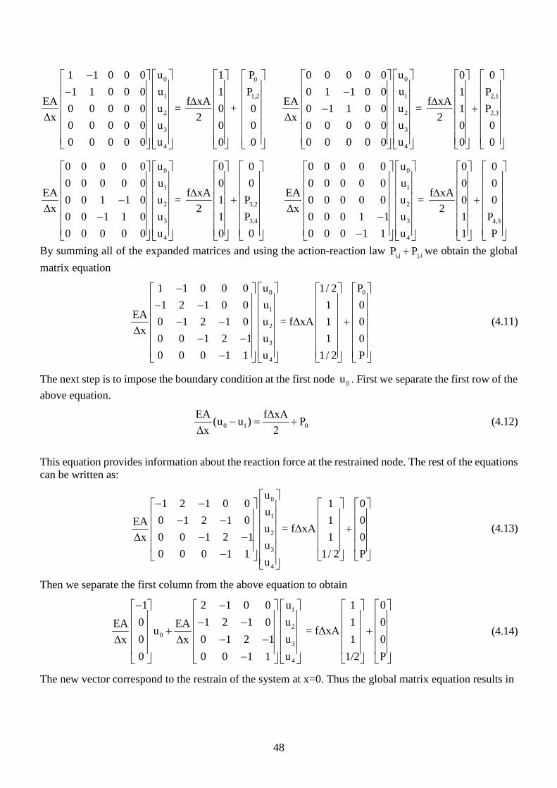
48

0 0

1 1,2

2

3

4

u1 1 0 0 0 1 Pu1 1 0 0 0 1 P

EA = + u0 0 0 0 0 0 0Δx

u0 0 0 0 0 0 0u0 0 0 0 0 0 0

f xA2

− −

∆

0

1 2,1

2 2,3

3

4

u0 0 0 0 0 0 0u0 1 1 0 0 1 P

EA = u0 1 1 0 0 1 PΔx

u0 0 0 0 0 0 0u0 0 0 0 0 0 0

f xA2

− +−

∆

0

1

2 3,2

3 3,4

4

u0 0 0 0 0 0 0u0 0 0 0 0 0 0

EA = u0 0 1 1 0 1 PΔx

u0 0 1

f xA2

1 0 1 Pu0 0 0 0 0 0 0

+− −

∆

0

1

2

3 4,3

4

u0 0 0 0 0 0 0u0 0 0 0 0 0 0

EA = u0 0 0 0 0 0 0Δx

u0 0 0 1 1 1 Pu0

f xA

0 0 1 1 1 P

2

+ − −

∆

By summing all of the expanded matrices and using the action-reaction law i,j j,iP P+ we obtain the global matrix equation

0 0

1

2

3

4

u1 1 0 0 0 1/ 2 Pu1 2 1 0 0 1 0

EA = fΔxAu0 1 2 1 0 1 0Δx

u0 0 1 2 1 1 0u0 0 0 1 1 1/ 2 P

− − − +− − − − −

(4.11)

The next step is to impose the boundary condition at the first node 0u . First we separate the first row of the above equation.

0 1 0EA fΔxA(u u ) PΔx 2

− = + (4.12)

This equation provides information about the reaction force at the restrained node. The rest of the equations can be written as:

0

1

2

3

4

u1 2 1 0 0 1 0

u0 1 2 1 0 1 0EA = fΔxAu0 0 1 2 1 1 0Δx

u0 0 0 1 1 1/ 2 P

u

− −

− − + − − −

(4.13)

Then we separate the first column from the above equation to obtain

1

20

3

4

u1 2 1 0 0 1 0u0 1 2 1 0 1 0EA EAu = fΔxAu0 0 1 2 1 1 0Δx Δxu0 0 0 1 1 1/2 P

− − − − + + − − −

(4.14)

The new vector correspond to the restrain of the system at x=0. Thus the global matrix equation results in

49

1

2

3

4

u2 1 0 0 1 0u1 2 1 0 1 0EA = fΔxAu0 1 2 1 1 0Δxu0 0 1 1 1/2 P

− − − + − − −

(4.15)

In particular, imposing the boundary condition at the first node 0u =0 we obtain

1

2

3

4

u2 1 0 0 1 0u1 2 1 0 1 0EA = fΔxAu0 1 2 1 1 0Δxu0 0 1 1 1/2 P

− − − + − − −

(4.16)

If we take P=0 the results is the same result as derived in Section 2.4 but using a different method: In Section 2.4 we obtained the global matrix equation using the global shape function; here we calculate first the element matrix equations and then assembled all matrices and apply boundary conditions. Note that the essential boundary condition (nodes with zero displacement) was applied by eliminating the row and column of the corresponding node.

4.4 Two-dimensional trusses Plane trusses consist of a pin-jointed assembly of bar elements, each of which is in a state of pure tension or compression. A simple truss structure is shown in Figure 4-5, which is the subject of the analysis in this section. The general procedure explained in the previous section is employed here for the analysis of the truss structure. The general procedure for finite element analyses depends very little on the type of the structure and whether the structure is a truss, a frame, or a discretised continuum.

1. Coordinate system A cartesian coordinate system is best suited to any type of truss. 2. Discretisation The truss structure consists of 10 members. Each of the members is chosen as a pin-jointed finite element. No further discretisation is required for a simple truss structure. The finite elements are numbered from 1 to 10 (in circles) as shown in Figure 4-5. A linear bar element has two nodes, and each node has 2 degrees-of-freedom.

4213H

x

y

53

6

HA, E

1 2 3

4 5 6 7 8 9

10

Figure 4-5 Truss structure

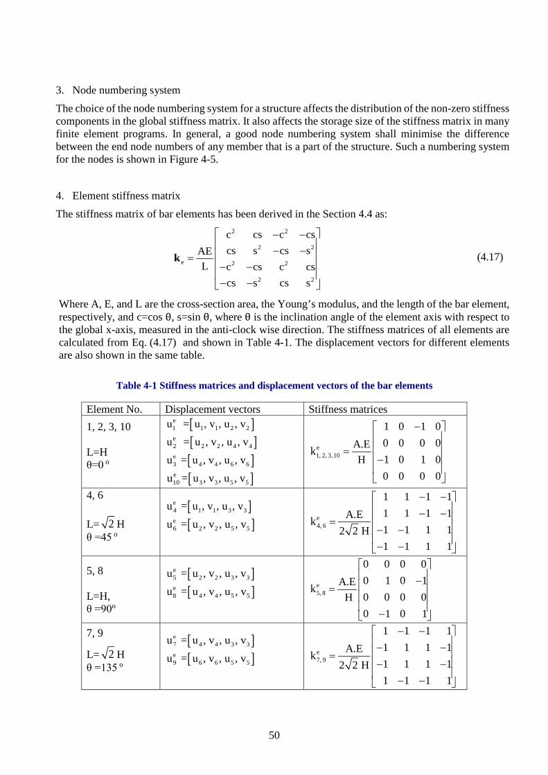
50

3. Node numbering system The choice of the node numbering system for a structure affects the distribution of the non-zero stiffness components in the global stiffness matrix. It also affects the storage size of the stiffness matrix in many finite element programs. In general, a good node numbering system shall minimise the difference between the end node numbers of any member that is a part of the structure. Such a numbering system for the nodes is shown in Figure 4-5.

4. Element stiffness matrix The stiffness matrix of bar elements has been derived in the Section 4.4 as:

2 2

2 2

e 2 2

2 2

c cs c cscs s cs sAE

L c cs c cscs s cs s

− − − − = − − − −

k (4.17)

Where A, E, and L are the cross-section area, the Young’s modulus, and the length of the bar element, respectively, and c=cos θ, s=sin θ, where θ is the inclination angle of the element axis with respect to the global x-axis, measured in the anti-clock wise direction. The stiffness matrices of all elements are calculated from Eq. (4.17) and shown in Table 4-1. The displacement vectors for different elements are also shown in the same table.

Table 4-1 Stiffness matrices and displacement vectors of the bar elements

Element No. Displacement vectors Stiffness matrices 1, 2, 3, 10 L=H θ=0 o

[ ]e1 1 1 2 2u = u , v , u , v

[ ]e2 2 2 4 4u = u , v , u , v e3u =[ ]4 4 6 6u , v , u , v e10u =[ ]3 3 5 5u , v , u , v

e1, 2, 3,10

1 0 1 00 0 0 0A.Ek1 0 1 0H0 0 0 0

− = −

4, 6 L= 2 H θ =45 o

e4u =[ ]1 1 3 3u , v , u , v e6u =[ ]2 2 5 5u , v , u , v

e4, 6

1 1 1 11 1 1 1A.Ek1 1 1 12 2 H1 1 1 1

− − − − = − − − −

5, 8 L=H, θ =90o

e5u =[ ]2 2 3 3u , v , u , v e8u =[ ]4 4 5 5u , v , u , v

e5, 8

0 0 0 00 1 0 1A.Ek0 0 0 0H0 1 0 1

− = −

7, 9

L= 2 H θ =135 o

e7u =[ ]4 4 3 3u , v , u , v e9u =[ ]6 6 5 5u , v , u , v

e7, 9

1 1 1 11 1 1 1A.Ek1 1 1 12 2 H1 1 1 1

− − − − = − − − −

51

5. Global stiffness matrix The element stiffness matrices can be enlarged to full structure size and added together to assemble the global stiffness matrix for the complete structure. An example of this type of assembly has been given in Chapter 1. Since each node has two degrees-of-freedom, the unrestrained global stiffness matrix for the 6-noded structure is of the order 12×12:

1 1 1 11 1 0 0 0 0 0 0 02 2 2 2 2 2 2 21 1 1 10 0 0 0 0 0 0 0

2 2 2 2 2 2 2 21 1 1 11 0 2 0 0 1 0 0 0

2 2 2 2 2 2 2 21 1 1 10 0 1 0 1 0 0 0 0

2 2 2 2 2 2 2 21 1 1 1 10 0 1 0 1 0 0 0

2 2 2 2 2 2 2 2 21 1 1 1 10 1 0 1 0 0 0 0

EA 2 2 2 2 2 2 2 2 2K1 1 1 1H 0 0 1 0 2 0 0 1 0

2 2 2 2 2 2 2 21 1 10 0 0 0 1

2 2 2 2 2 2

+ − − −

− −

− + − − −

+ − − −

− − + − −

− − − + −=

− − + − −

− − +1 0 1 0 0

2 21 1 1 1 10 0 1 0 0 0 1 0

2 2 2 2 2 2 2 2 21 1 1 1 10 0 0 0 0 1 0 1

2 2 2 2 2 2 2 2 21 1 1 10 0 0 0 0 0 1 0 1

2 2 2 2 2 2 2 21 1 1 10 0 0 0 0 0 0 0

2 2 2 2 2 2 2 2

− − − − + − − − − + − − − + − − −

(4.18)

6. Boundary conditions The boundary conditions shall be applied by eliminating rows and columns of the global stiffness matrix associated with the fixed degrees-of-freedom. Four of the degrees-of-freedom are restrained, i.e., u1, v1, u6, v6. Therefore, columns 1, 2, 11, 12 and rows 1, 2, 11,12 of the global stiffness matrix are eliminated and the size of the restrained stiffness matrix reduces to 8×8:

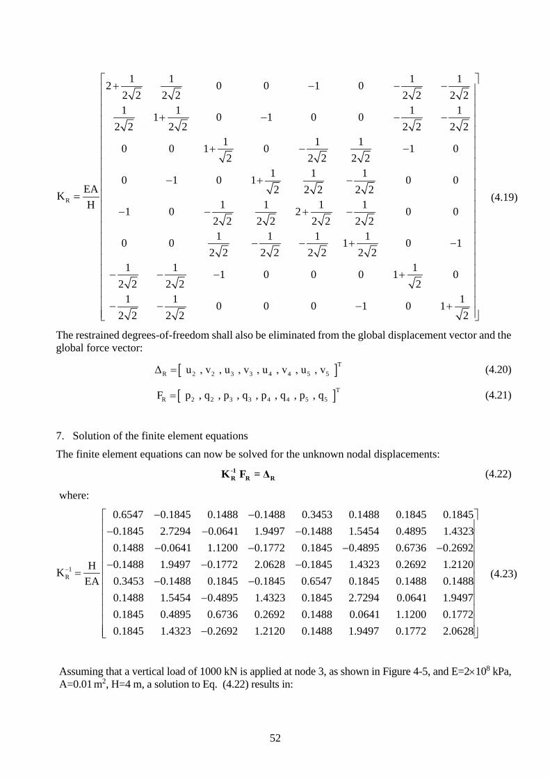
52

R

1 1 1 12 0 0 1 02 2 2 2 2 2 2 21 1 1 11 0 1 0 0

2 2 2 2 2 2 2 21 1 10 0 1 0 1 02 2 2 2 2

1 1 10 1 0 1 0 0EA 2 2 2 2 2K

1 1 1 1H 1 0 2 0 02 2 2 2 2 2 2 21 1 1 10 0 1 0 1

2 2 2 2 2 2 2 21 1 11 0 0 0 1 0

2 2 2 2 21 1 10 0 0 1 0 1

2 2 2 2 2

+ − − − + − − − + − − − + −

= − − + − − − + − − − − + − − − +

(4.19)

The restrained degrees-of-freedom shall also be eliminated from the global displacement vector and the global force vector:

[ ]TR 2 2 3 3 4 4 5 5Δ u , v , u , v , u , v , u , v = (4.20)

[ ]TR 2 2 3 3 4 4 5 5F p , q , p , q , p , q , p , q = (4.21)

7. Solution of the finite element equations The finite element equations can now be solved for the unknown nodal displacements:

-1R R RK F = Δ (4.22)

where:

1R

0.6547 0.1845 0.1488 0.1488 0.3453 0.1488 0.1845 0.18450.1845 2.7294 0.0641 1.9497 0.1488 1.5454 0.4895 1.43230.1488 0.0641 1.1200 0.1772 0.1845 0.4895 0.6736 0.26920.1488 1.9497 0.1772 2.0628 0.1845 1.4323HK

EA−

− −− − −

− − − −− − −

=0.2692 1.2120

0.3453 0.1488 0.1845 0.1845 0.6547 0.1845 0.1488 0.14880.1488 1.5454 0.4895 1.4323 0.1845 2.7294 0.0641 1.94970.1845 0.4895 0.6736 0.2692 0.1488 0.0641 1.1200 0.17720.1845 1.4323 0.2692 1.2120 0.1488 1.9497 0.17

− −−

− 72 2.0628

(4.23)

Assuming that a vertical load of 1000 kN is applied at node 3, as shown in Figure 4-5, and E=2×108 kPa, A=0.01 m2, H=4 m, a solution to Eq. (4.22) results in:

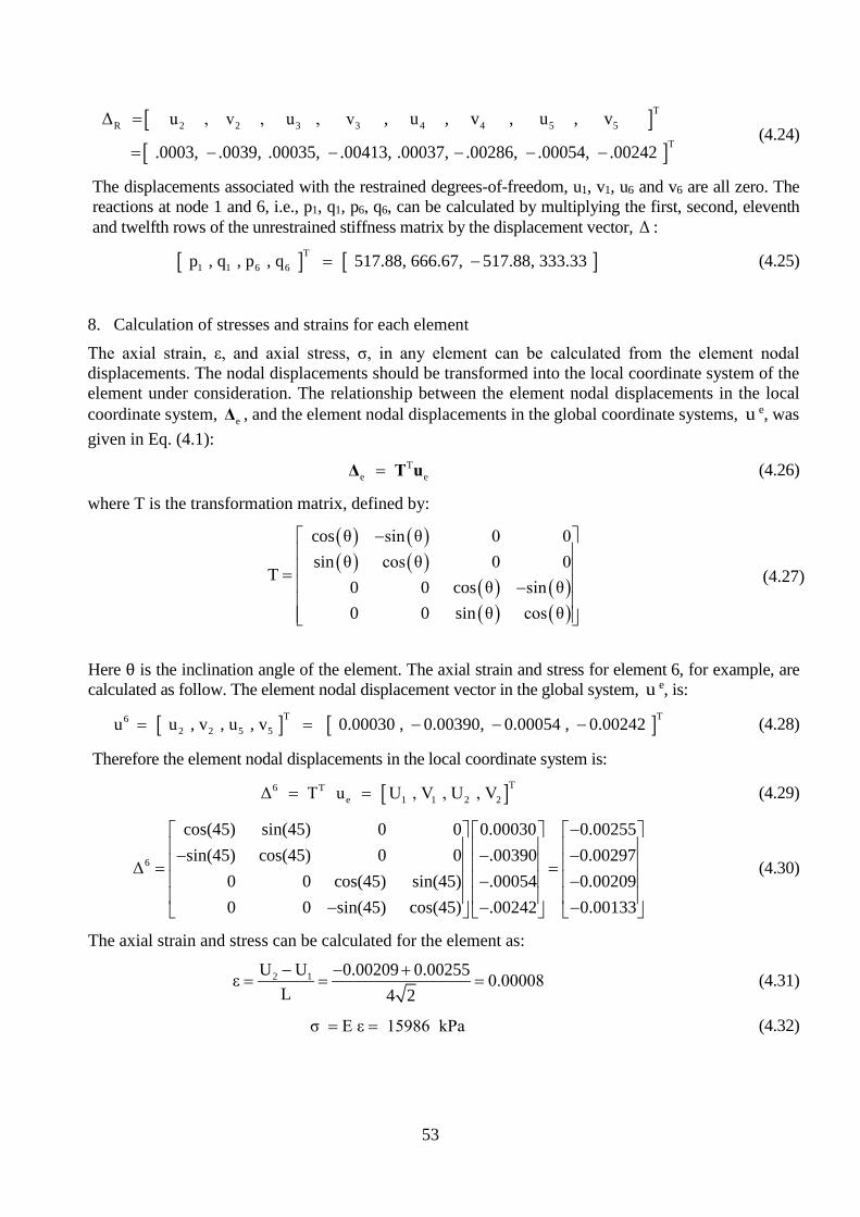
53

[ ][ ]

TR 2 2 3 3 4 4 5 5

T

Δ u , v , u , v , u , v , u , v

.0003, .0039, .00035, .00413, .00037, .00286, .00054, .00242

=

= − − − − − (4.24)

The displacements associated with the restrained degrees-of-freedom, u1, v1, u6 and v6 are all zero. The reactions at node 1 and 6, i.e., p1, q1, p6, q6, can be calculated by multiplying the first, second, eleventh and twelfth rows of the unrestrained stiffness matrix by the displacement vector, Δ :

[ ] [ ]T1 1 6 6 p , q , p , q 517.88, 666.67, 517.88, 333.33 = − (4.25)

8. Calculation of stresses and strains for each element The axial strain, ε, and axial stress, σ, in any element can be calculated from the element nodal displacements. The nodal displacements should be transformed into the local coordinate system of the element under consideration. The relationship between the element nodal displacements in the local coordinate system, eΔ , and the element nodal displacements in the global coordinate systems, u e, was given in Eq. (4.1):

Te e =Δ T u (4.26)

where T is the transformation matrix, defined by: ( ) ( )

( ) ( )( ) ( )( ) ( )

cos θ sin θ 0 0sin θ cos θ 0 0

T0 0 cos θ sin θ0 0 sin θ cos θ

− = −

(4.27)

Here θ is the inclination angle of the element. The axial strain and stress for element 6, for example, are calculated as follow. The element nodal displacement vector in the global system, u e, is:

[ ] [ ]T T6 2 2 5 5 u u , v , u , v 0.00030 , 0.00390, 0.00054 , 0.00242 = = − − − (4.28)

Therefore the element nodal displacements in the local coordinate system is:

[ ]T6 Te 1 1 2 2Δ T u U , V , U , V= = (4.29)

6

cos(45) sin(45) 0 0 0.00030 0.00255sin(45) cos(45) 0 0 .00390 0.00297

Δ0 0 cos(45) sin(45) .00054 0.002090 0 sin(45) cos(45) .00242 0.00133

− − − − = = − − − − −

(4.30)

The axial strain and stress can be calculated for the element as:

2 1U U 0.00209 0.00255ε 0.00008L 4 2− − +

= = = (4.31)

σ E ε 15986 kPa= = (4.32)

54

4.5 Two-dimensional flexural frames The Figure 4-6 shows a plane frame consists of 5 elements that are rigidly connected together. The supports are also fully fixed. The properties of the elements are: Elements 1, 2, 3: A=0.0025m2, I=0.00005m4, E=2×108 kPa Elements 4, 5: A=0.0010m2, I=0.00025m4, E=2×108 kPa If a horizontal load of p2=1000kN is applied at node 2, we want to calculate the rotations of node 2.

42

1

x

y 53

6

10m

5m1 2 3

4 5

Figure 4-6 Frame structure

The general procedure for finite element analyses, explained in the previous section, is employed here for the analysis of the frame. The coordinate system, discretisation (element numbering) and node numbering system used for the analysis of the frame is shown in Figure 4-6. 1. Element stiffness matrix

The stiffness matrices of all elements are calculated using Eq. (3.32) and shown in Figure 3-5, together with the element displacement vectors.

2. Global stiffness matrix The global stiffness matrix is assembled using the direct method explained in the previous section. The restrained global stiffness matrix for the complete structure is given as:

R

40960 0 2400 40000 0 0 0 0 00 104800 12000 0 4800 12000 0 0 0

2400 12000 48000 0 12000 20000 0 0 040000 0 0 80960 0 2400 40000 0 0

K 0 4800 12000 0 109600 0 0 4800 120000 12000 20000 2400 0 88000 0 12000 200000 0 0 40000 0 0 40960 0 24000 0 0 0 480

−−−

− −= − − −

−−

− 0 12000 0 104800 120000 0 0 0 12000 20000 2400 12000 48000

− − −

(4.33)

55

Table 4-2 Stiffness matrices and displacement vectors of the flexural elements

Element No. Displacement vectors Stiffness matrices

1, 2, 3

e1u =[ ]1 1 1 2 2 2u ,v , θ , u , v , θ

e2u =[ ]3 3 3 4 4 4u , v , θ , u , v , θ e3u =[ ]5 5 5 6 6 6u , v , θ , u , v , θ

e1, 2, 3

960 0 2400 960 0 24000 100000 0 0 100000 0

2400 0 8000 2400 0 4000k

960 0 2400 960 0 24000 100000 0 0 100000 0

2400 0 4000 2400 0 8000

− − − − −

= − − −

4, 5 e4u =[ ]2 2 2 4 4 4u , v , θ , u , v , θ

5ue =[ ]4 4 4 6 6 6u , v , θ , u , v , θ e4, 5

40000 0 0 40000 0 00 4800 12000 0 4800 120000 12000 40000 0 12000 20000

k40000 0 0 40000 0 0

0 4800 12000 0 4800 120000 12000 20000 0 12000 40000

− − −

= − − − −

−

3. Boundary conditions

The boundary conditions have been applied to stiffness matrix by the direct assembly method. The vectors of the restrained global degree-of-freedom and the global force vector for the structure are:

[ ] [ ]T TR 2 2 2 4 4 4 6 6 6 1 2 3 4 5 6 7 8 9Δ u , v , θ , u , v , θ , u , v , θ a , a , a , a , a , a , a , a , a= = (4.34)

[ ] [ ]T TR 2 2 2 4 4 4 6 6 6F p , q , M , p , q , M , p , q , M 1000, 0, 0, 0, 0, 0, 0, 0, 0= = (4.35)

4. Solution of the finite element equation

The finite element equations can now be solved which result in the unknown nodal displacements:

[ ]TRΔ 0.394 , 0.002 , 0.019 , 0.377 , 0.000 , 0.002 , 0.370 , 0.002 , 0.018= − − − − (4.36)

Therefore the rotation of node2 is θ2= − 0.019 radians; the negative sign indicates a clockwise rotation.

4.6 Suitable node numbering system A suitable node numbering system is needed to minimise of non-zero elements in the stiffness matrix. This will help in optimizing computer storage and will reduce the number of calculations required to invert the stiffness matrix. This section provides simple instructions for a suitable node numbering system. If the nodes are suitably numbered so that the maximum difference between nodal numbers in any one member is kept small, the stiffness matrix consists of a narrow band of non-zero numbers clustered about the main diagonal. Figure 4-7(a) shows diagrammatically such a banded stiffness matrix. In this figure Ndof is the order of the full square stiffness matrix and B is the “bandwidth”, defined as:

( )of i j maxB d 1 ( Node Node )= × + − (4.37)

56

where dof is the number of degrees-of-freedom at each node and i j max( Node - Node ) is the difference between end node numbers in the member that has the maximum difference in end node numbers. The stiffness matrices are also symmetric. Therefore, for the purpose of efficient storage, the compact storage of Figure 4-7(b) should be adopted, in which only the upper half of the band of the whole stiffness matrix is stored. The diagonal of the whole stiffness matrix becomes the first column of the compact matrix. In large problems B may be only a few percent of Ndof. Thus very large savings in storage can be made by the compact storage of global stiffness matrix. A large portion of the computational time in a finite element analysis is spent on solving the stiffness equations, i.e., finding the inverse of the stiffness matrix. The computational time required for solving the stiffness equations is approximately proportional to the square of the bandwidth of the stiffness matrix. Therefore, a suitable node numbering system allows considerable reductions in computational time by reducing the bandwidth. To demonstrate the effectiveness of a suitable node numbering system in reducing the bandwidth of a structure, consider a five-story frame structure consisting of 10 nodes, each with three degrees-of-freedom. The restrained structure has 30 degrees-of-freedom, thus Ndof=30. Three different node-numbering systems are shown in Figure 4-8, together with the stiffness matrices resulting from each of the systems.

XXXXooooooooooooooooXXXXXoooooooooooooooXXXXXXooooooooooooooXXXXXXXooooooooooooooXXXXXXXooooooooooooooXXXXXXXooooooooooooooXXXXXXXooooooooooooooXXXXXXXooooooooooooooXXXXXXXooooooooooooooXXXXXXXooooooooooooooXXXXXXXooooooooooooooXXXXXXXooooooooooooooXXXXXXXooooooooooooooXXXXXXXooooooooooooooXXXXXXXooooooooooooooXXXXXXXooooooooooooooXXXXXXXooooooooooooooXXXXXXoooooooooooooooXXXXXooooooooooooooooXXXX

Ndof

Ndof B

oooXooXXoXXXXXXXXXXXXXXXXXXXXXXXXXXXXXXXXXXXXXXXXXXXXXXXXXXXXXXXXXXXXXXXXXXXXXXX

B

(a) (b)

Ndof

Figure 4-7 The banded system and compact storage of the stiffness matrix

Each (x) in the stiffness matrices represents a 3×3 matrix containing the stiffness coefficients associated with a node. For system (a) the bandwidth B is equal to 9, and for systems (b) and (c), B=18 and B=30, respectively. Obviously for this structure the most suitable node numbering system is the one presented in Figure 4-8(a). The worst node numbering system is case (c) in Figure 4-8.

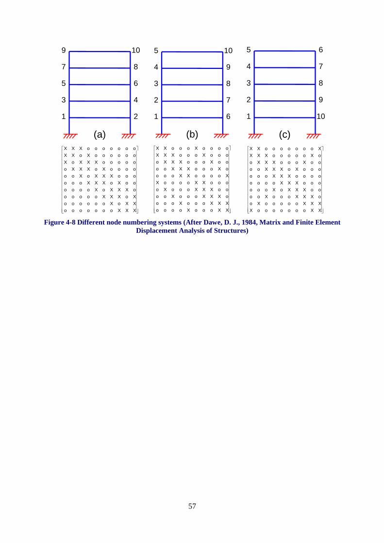
57

5

3

1 2

9

7

4

6

8

10

XXXoooooooXXoXooooooXoXXXooooooXXXoXooooooXoXXXooooooXXXoXooooooXoXXXooooooXXXoXooooooXoXXoooooooXXX

(a)

3

2

1 6

5

4

7

8

9

10

XXoooXooooXXXoooXooooXXXoooXooooXXXoooXooooXXooooXXooooXXooooXoooXXXooooXoooXXXooooXoooXXXooooXoooXX

(b)

3

2

1 10

5

4

9

8

7

6

XXoooooooXXXXoooooXooXXXoooXooooXXXoXooooooXXXooooooooXXXooooooXoXXXooooXoooXXXooXoooooXXXXoooooooXX

(c)

Figure 4-8 Different node numbering systems (After Dawe, D. J., 1984, Matrix and Finite Element

Displacement Analysis of Structures)

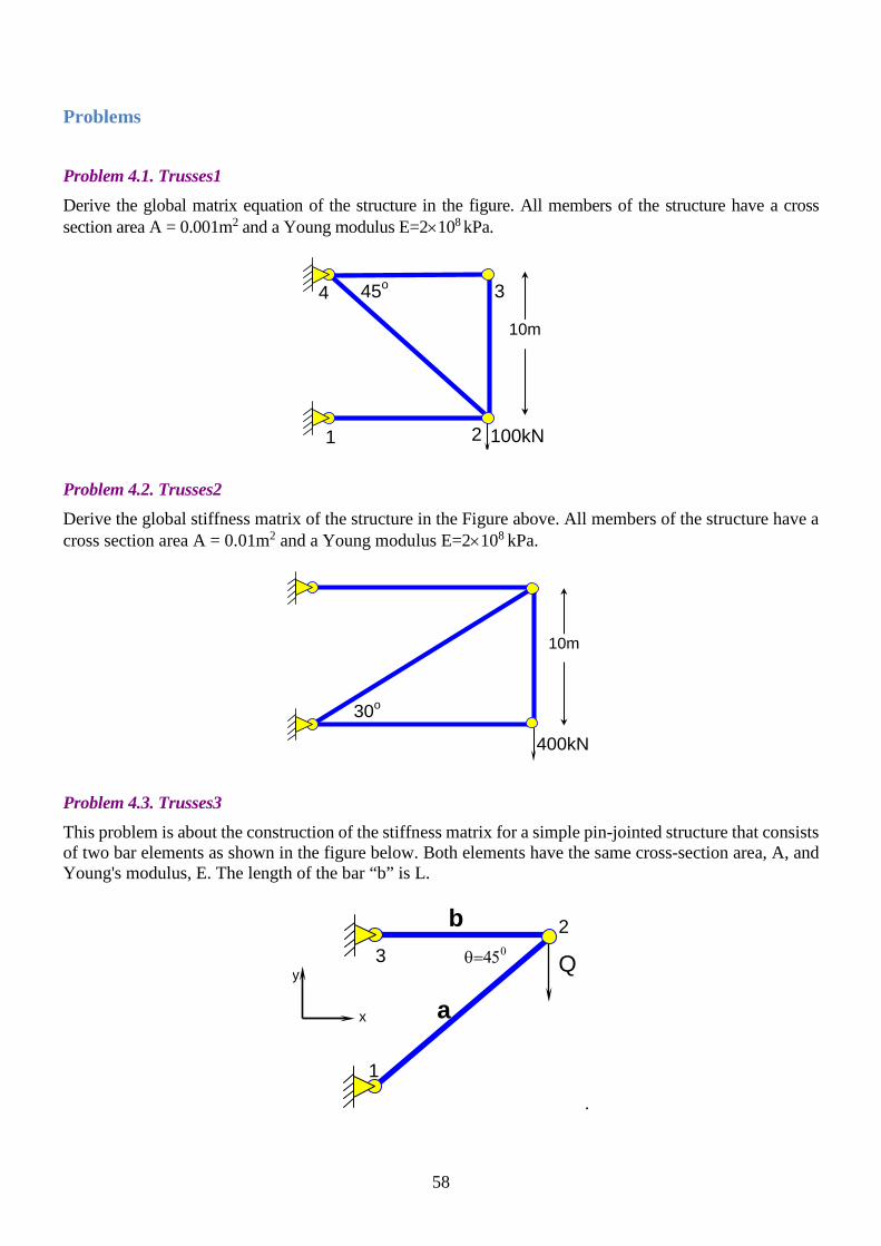
58

Problems Problem 4.1. Trusses1 Derive the global matrix equation of the structure in the figure. All members of the structure have a cross section area A = 0.001m2 and a Young modulus E=2×108 kPa.

100kN

10m

45o

1 2

3 4

Problem 4.2. Trusses2 Derive the global stiffness matrix of the structure in the Figure above. All members of the structure have a cross section area A = 0.01m2 and a Young modulus E=2×108 kPa.

400kN

10m

30o

Problem 4.3. Trusses3 This problem is about the construction of the stiffness matrix for a simple pin-jointed structure that consists of two bar elements as shown in the figure below. Both elements have the same cross-section area, A, and Young's modulus, E. The length of the bar “b” is L.

Q θ=450

1

2

a

3

b

y

x

.

59

1) Find the element matrix equation e e e = f k u for each bar. 2) Find the expanded element matrix equation e e e = F K U for each bar

3) Find the unrestrained global matrix equation 2 2

e ee 1 e 1

, = , == =

= ∑ ∑F KU K K F F

4) Find the global matrix equation after applying the boundary conditions. 5) Find the displacement of the unrestrained nodes Problem 4.4. Trusses 4 1) Calculate the nodal displacements and reactions for the pin-jointed structure shown below.

(All members of the structure have a cross section area A = 0.001m2 and a Young’s modulus E=2×108 kPa.) 2) Evaluate the results, are they reasonable? 3) If the cross section area of the vertical member is increased by 1000 times, how does this change affect the results?

100kN

10m

30o

Problem 4.5. Solver and pre- and post-processing This question is about finding the structure of the finite element analysis using the steps listed below. Most of these steps belong to the three main components of the analysis: pre-processing, processing, and post-processing. Few of the steps are not necessary. Find the steps for each component and sort them in the order they should be executed during the analysis. a) calculate displacement at the

domain b) assembly unrestrained global

matrix equation c) input boundary conditions d) calculate stress at the domain e) input material properties

f) invert global stiffness matrix

g) apply boundary conditions

h) calculate nodal loads i) create element matrix

equations j) invert element stiffness

matrices

k) input nodes l) invert unrestrained global matrix

equation m) calculate stress at the nodes n) input elements o) calculate nodal displacement

Write your solution in the table below. (Note: Not all boxes have to be filled.)

60

Component include the letters a–o of the steps, in the order they should be executed Pre-processor

Solver Post-processor

Problem 4.6. Two bar elements This problem is about the construction of the stiffness matrix for a simple structure that consists of two bar elements as shown in the figure below. Both elements have the same cross-section area A=0.01m2 and the same length L=1m. A load P=10N is applied at the right node. Write your solutions in the boxes below.

.

Eb=100MPa

P Ea=50MPa - x +

u1 u2 u3

1) Write down the element matrix equation e e e = f k u for each bar.

2) Find the expanded element matrix equation e e = F K u for each bar

3) Find the unrestrained global matrix equation 2 2

e ee 1 e 1

, = , == =

= ∑ ∑F Ku K K F F

4) Find the global matrix equation after applying the boundary conditions. 5) Find the displacement of the unrestrained nodes.

61

CHAPTER 5: STRAIN AND STRESS IN CONTINUA

STRAIN AND STRESS IN CONTINUA

The general equations for derivation of the finite element relationships have been established in the previous chapters through consideration of simple one-dimensional elements such as bars and beams. The extension of the general equations to two or three-dimensional elements differs from the unidirectional case only in the degree of complexity involved and not in the basic concepts. The remainder of the textbook will be focussed with two-dimensional elements, but before such elements can be studied in detail, a review of the relevant concepts and the governing relations of continuum mechanics will be presented. To carry out a stress analysis of a structure using the finite element method, it is first necessary to understand the matrix formulation of stress and strain. If you intend to use the method you should also need a good comprehension of constitutive modelling. The reason for this is obvious. Human lives will depend on how well you model the structure and interprets the results. Ultimately, it is a stress analysis problem you will be investigating when analysing a bridge or a foundation – not a computer analysis problem as often depicted in glossy FEM commercial package sales brochures. No matter how sophisticated the computer method may be, experience and knowledgeable engineering judgement should always be the absolute criterion for a correct engineering design decision. In this chapter, the strains and stresses in continua are presented followed by the stress-strain relationships. Consideration on constitutive modelling is focused to linear isotropic elasticity. A brief review on the theory of elasto-plasticity is provided in the last section.

5.1 Kinematic equation: Definition of strain In this section the concept of normal strain and shear strain in a solid continuum will be reviewed. Expressions for transformation of strains from one coordinate system to another are also provided. When a body is subjected to applied loads it will distort. A small element which is subject to in-plane loading may deform in the manner shown schematically in Figure 5-1.

x

y ∆x εxx∆x

x

y

∆y

εyy ∆y

x

y π/2 −γxy

Normal strain in the x-direction

Normal strain in the y-direction

Shear strain in the x-y plane

Figure 5-1 Normal and shear strain in x-y plane

In general a small planar distortion can be broken up into:

62

(a) a rigid body translation in the x direction (b) a rigid body translation in the y direction (c) a rigid body rotation about the z axis (d) a normal strain εxx in the x direction (e) a normal strain εyy in the y direction (f) a shear strain γxy in the xy plane. The rigid body components (a, b, c) involve no change in shape and hence no strain. The axial extensions (d,e) involve a change in area while the shear strain (f) involves no change in area. Relation of strains to displacements An examination of the displacements for the element shown in Figure 5-1 shows that for small deformations and changes of shape, the strains can be expressed in terms of the displacement components as follows:

xxx

yyy

yxxy

uεx

uε

yuuγ

y x

∂=

∂∂

=∂

∂∂= +

∂ ∂

(5.1)

These equations can be written in matrix form

xx

xyy

yxy

0xε

uε 0

uyγ

y x

∂ ∂

∂ = ∂ ∂ ∂ ∂ ∂

(5.2)

It is clear that by examining the deformation of elements in the yz and zx planes it is possible to identify similarly the strains in these planes:

zzz

y zyz

x zzx

uεzu uγz y

u uγz x

∂=

∂∂ ∂

= +∂ ∂

∂ ∂= +

∂ ∂

(5.3)

The full three-dimensional kinematic relation can be written in a compact for as

[ ]( )=ε L u x (5.4)

where:

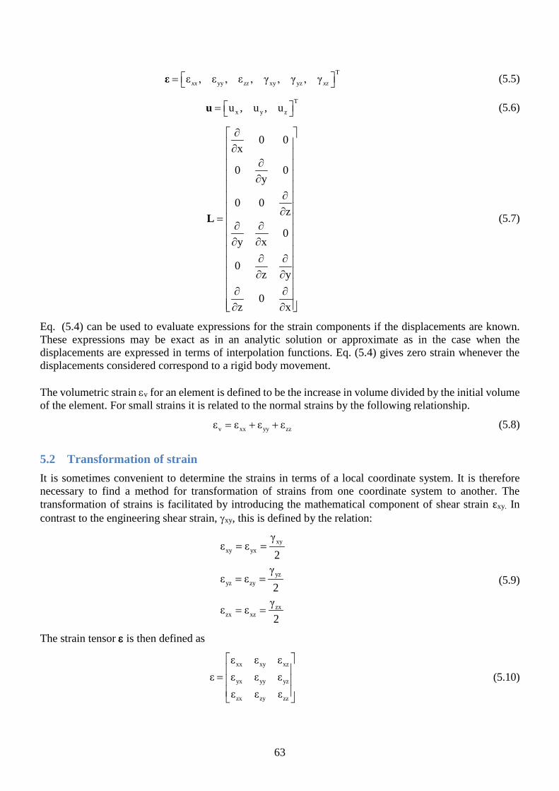
63

T

yy xy yzε , ε , ε , γ , γ , γxx zz xz = ε (5.5)

T

x y zu , u , u = u (5.6)

0 0x

0 0y

0 0z

0y x

0z y

0z x

∂ ∂

∂ ∂

∂ ∂

= ∂ ∂ ∂ ∂ ∂ ∂ ∂ ∂ ∂ ∂ ∂ ∂

L (5.7)

Eq. (5.4) can be used to evaluate expressions for the strain components if the displacements are known. These expressions may be exact as in an analytic solution or approximate as in the case when the displacements are expressed in terms of interpolation functions. Eq. (5.4) gives zero strain whenever the displacements considered correspond to a rigid body movement. The volumetric strain εv for an element is defined to be the increase in volume divided by the initial volume of the element. For small strains it is related to the normal strains by the following relationship.

v xx yy zzε ε ε ε= + + (5.8)

5.2 Transformation of strain It is sometimes convenient to determine the strains in terms of a local coordinate system. It is therefore necessary to find a method for transformation of strains from one coordinate system to another. The transformation of strains is facilitated by introducing the mathematical component of shear strain εxy. In contrast to the engineering shear strain, γxy, this is defined by the relation:

xyxy yx

yzyz zy

zxzx xz

γε ε

2γ

ε ε2

γε ε2

= =

= =

= =

(5.9)

The strain tensor ε is then defined as

xx xy xz

yx yy yz

zx zy zz

ε ε εε ε ε ε

ε ε ε

=

(5.10)

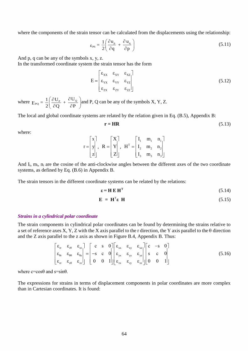
64

where the components of the strain tensor can be calculated from the displacements using the relationship:

p qpq

u u1 = + ε 2 q p∂ ∂

∂ ∂ (5.11)

And p, q can be any of the symbols x, y, z. In the transformed coordinate system the strain tensor has the form

XX XY XZ

YX YY YZ

ZX ZY ZZ

ε ε εΕ ε ε ε

ε ε ε

=

(5.12)

where QPPQ

UU1 = + Ε 2 Q P∂ ∂

∂ ∂ and P, Q can be any of the symbols X, Y, Z.

The local and global coordinate systems are related by the relation given in Eq. (B.5), Appendix B:

r = HR (5.13) where:

xr y

z

=

, X

R YZ

=

, 1 1 1

T2 2 2

3 3 3

I m nH I m n

I m n

=

And Ii, mi, ni are the cosine of the anti-clockwise angles between the different axes of the two coordinate systems, as defined by Eq. (B.6) in Appendix B. The strain tensors in the different coordinate systems can be related by the relations:

Tε = H E H (5.14)

T E = H ε H (5.15)

Strains in a cylindrical polar coordinate The strain components in cylindrical polar coordinates can be found by determining the strains relative to a set of reference axes X, Y, Z with the X axis parallel to the r direction, the Y axis parallel to the θ direction and the Z axis parallel to the z axis as shown in Figure B.4, Appendix B. Thus:

rr rθ rz xx xy xz

θr θθ θz yx yy yz

zr zθ zz zx zy zz

ε ε ε c s 0 ε ε ε c s 0ε ε ε s c 0 ε ε ε s c 0ε ε ε 0 0 1 ε ε ε 0 0 1

− = −

(5.16)

where c=cosθ and s=sinθ. The expressions for strains in terms of displacement components in polar coordinates are more complex than in Cartesian coordinates. It is found:

65

rrr

θ rθθ

θ zzθ zθ

θ θrrθ rθ

uεr

u u1εr θ r

u u1γ 2εz r θ

u uu1γ 2εr θ r r

∂=

∂∂

= +∂

∂ ∂= + =

∂ ∂∂∂

= + − =∂ ∂

(5.17)

5.3 Balance equation: Definition of stress The previous section has been concerned with deformation of a continuous body. In this section the forces within the body that cause this deformation will be examined, stress components under three-dimensional conditions will be defined, and the concept of a stress tensor (matrix) will be introduced together with transformation of stresses in different coordinate systems.

Figure 5-2 Infinitesimal cube used to define the stress

Consider a small rectangular box, having sides of length ∆x, ∆y, ∆z parallel to the x, y, z axes respectively see Figure 5-2. The material outside the boxes will exert a force on each of the six sides of the box. As the dimensions of the box approach zero, the forces on the sides of the box also approach zero. However the force per unit area approaches a limiting value that is called the traction. Consider the positive x face (the face having the x axis as its outward normal) and assume the x, y, z components of the force acting on this face are denoted ∆Fxx, ∆Fxy, ∆Fxz respectively. The stress components (σxx, σxy, σxz) at point P inside the face are defined by the relationships:

xyxx xzxx xy xz

x x x

ΔFΔF ΔFσ . σ . σ .ΔA ΔA ΔA

= = = (5.18)

y

x

z

∆y

∆z

∆Fxy

∆Fxx

∆Fxz

∆x

66

where ∆Ax = ∆y.∆z is the area of the x face. It is similarly possible, by considering the force acting on the y, z faces, to define the stress components (σyx, σyy, σyz) acting on the y face and those acting on the z face (σzx, σzy, σzz). In general

pqpq

p

ΔFσ .

ΔA= (5.19)

where ΔFpq is the force acting on the p-face along the q-direction and ΔAp is the area of the p-face. The collection of stress components σpq (where the indices p, q can take any of the values x, y, z) is called the stress tensor at point P, and is defined below:

xx xy xz

yx yy yz

zx zy zz

σ σ σσ σ σ σ

σ σ σ

=

(5.20)

The stress components σxx, σyy, σzz are called normal or direct stresses. The components σxy, σyz, σzx,, σyx, σzy, σxz are called shear stresses. In structural mechanics a tensile normal stress are assumed to have a positive value. In soil mechanics compressive stresses are assumed to be positive. Traction acting on a plane The stress tensor defined in the previous section can be used to calculate the force per unit area acting on any plane passing through P. Suppose that a plane passing through point P has an outward unit normal n as shown in Figure 5-3.

x

y

z

Traction τ Normal n

Ty

Tz

Tx

Figure 5-3 Traction acting on a plane

By considering the equilibrium of the tetrahedron shown in Figure 5-3 it can be shown that the traction τ (force per unit area) acting on the plane is given by: τ = σ n (5.21)

x xx x xy y xz z

y yx x yy y yz z

z zx x zy y zz z

τ σ n σ n σ nτ σ n σ n σ nτ σ n σ n σ n

= + +

= + +

= + +

67

A simple demonstration of this is found by considering the x-y plane system of stresses in which there are no shear stresses acting on the z face, so that σxz=0 and σyz = 0. The situation is shown schematically in Figure 5-4.

x

y

τ x

τ τ y

σxx

σyx

σyy σxy O

B

A α

n

α

Figure 5-4 Relation of stress and traction

Equilibrium of the forces in x and y directions reveal that:

x xx xyτ AB σ OB σ OA= +

y yx yyτ AB σ OB σ OA = +

OA cosα AB=

OB sinα AB=

The normal to AB is given by:

T T

x y[n n ] [sinα cosα]= =n

So that:

x xx x xy yτ σ n σ n= +

y yx x yy yτ σ n σ n= + Static equations for the stress Under most cases the stress distribution will vary from point to point. In most civil engineering analyses it can be assumed that processes are quasi static, i.e., the effects of acceleration can be neglected. In this case consider the equilibrium of rectangular box shown in Figure 5-5.

68

x

z

y O C

B A

O* C*

B* A*

σxy

σxz

σzz

σzy

σzx σyz

σyy

σyx

σxx ∆x

∆y

∆z

x

y σyy

σyy

σxx σxy

σxx σxy

σyx

σyx

Figure 5-5 Left: equilibrium in a rectangular box whose center is the point (x,y,z). Right: stress components

seen from the top.

The force in the z direction acting on the face A*B*C*0* is: ( )zzσ x,y,z+Δz/2 ΔxΔy+

The force in the z direction acting on the face A B C O is: ( )zzσ x,y,z Δz/2 ΔxΔy− −

The force in the z direction acting on the face A B B*A* is: ( )xzσ x+Δx/2,y,z ΔyΔz+

The force in the z direction acting on the face O C C*O* is: ( )xzσ x x/2,y,z ΔyΔz− − ∆

The force in the z direction acting on the face B C C*B* is: ( )yzσ x,y+Δy/2,z ΔzΔx+

The force in the z direction acting on the face A O O*A* is: ( )yzσ x,y y/2,z ΔzΔx− − ∆ The force in the z direction due to the self-weight of the material is: Zw ΔxΔyΔz In the above relations, the quantities in brackets “()” indicate the coordinates of the point at which the stress is taken. The sum of these 7 force components must vanish. By dividing the resulting equation by the volume of the box and letting ∆x,∆y,∆z→0 it is found that:

yz yzxz xz zz zzz

σ (x,y+Δy/2,z) σ (x,y Δy/2,z)σ (x+Δx/2,y,z) σ (x Δx/2,y,z) σ (x,y,z+Δz/2) σ (x,y,z Δz/2)+ +w = 0x y z

− −− − − −+

∆ ∆ ∆ (5.22)

Now we use the concept of the partial derivative to obtain

yzxz zzz

σσ σ w 0x y z

∂∂ ∂+ + + =

∂ ∂ ∂ (5.23)

The complete set of equilibrium equations can be derived in similar fashion and it is found that:

yxxx xzx

xy yy yzy

zyxz zzz

σσ σ w 0x y z

σ σ σw 0

x y zσσ σ w 0

x y z

∂∂ ∂+ + + =

∂ ∂ ∂∂ ∂ ∂

+ + + =∂ ∂ ∂

∂∂ ∂+ + + =

∂ ∂ ∂

(5.24)

69

where wx, wy, wz are the components of the unit weight of the material in the x, y z directions respectively. It can be written in a compact form

T + =L σ w 0 (5.25)

where L is the differential operator defined above, and

T

yy xy yz

T

x y z

σ , σ , σ , σ , σ , σ

w , w , w

xx zz xz =

=

σ

w

The equation above is also called the strong form of the equilibrium equation. For the finite element analyis, it better to formulate equilibrium using the weak form that will be presented in Chapter 6. Stress components in different coordinate systems The stress components defined by Eq. (5.20) were based on the x, y, z coordinate system. The coordinate system X, Y, Z could also have been used to define the stress tensor Σ and in that case it would have been found that:

XX XY XZ

YX YY YZ

ZX ZY ZZ

σ σ σΣ σ σ σ

σ σ σ

=

(5.26)

If Eq. (5.13) is applied to the three planes having the X, Y, Z directions as outward normal respectively, the stress tensors are related by the following equations:

T=

T

σ HΣHΣ = H σH

(5.27)

where H is the transformation matrix which relates two coordinate systems and defined by Eq. (B.6). Example 5.1 In example 5.1 the stress state was given relative to the x, y, z coordinate system. However, when examining the stress state in the silt seam it is more appropriate to use a local (X, Y, Z) axes in which the Y axis is normal to the seam and the X, Z axes are in the plane of the seam. Thus

0.9397 0.3420 0 250 0 0 0.9397 0.3420 00.3420 0.9397 0 0 300 0 0.3420 0.9397 0

0 0 1 0 0 250 0 0 1

XX XY XZ

YX YY YZ

ZX ZY ZZ

σ σ σσ σ σσ σ σ

+ − − + + = = + + − − + −

Σ

255.85 16.07 016.07 294.15 0 kPa

0 0 250

− = − −

Σ

Symmetry of the stress tensor

The convention adopted in defining the stress components is that σpq defines the "p" component of traction (force per unit area) acting on the plane having the "q" axis as the outward normal. By considering the moment equilibrium of the rectangular box shown in Figure 5-5, it can be shown that:

70

pq qpσ σ= (5.28)

Stress components in cylindrical polar coordinates The stress components for a set of cylindrical polar coordinates correspond to those for a set of Cartesian axes having an X axis parallel to the r direction, a Y axis parallel to the θ direction and a Z axis parallel to the z direction.

rr rθ rz xx xy xz

θr θθ θz yx yy yz

zr zθ zz zx zy zz

σ σ σ c s 0 σ σ σ c s 0σ σ σ s c 0 σ σ σ s c 0σ σ σ 0 0 1 σ σ σ 0 0 1

− = −

(5.29)

where c = cosθ and s = sinθ. The conditions of equilibrium expressed in terms of polar coordinates are:

rθ rr θθrr zrr

rθ θθ θz rθθ

θzzr zz zrz

σ σ σσ σ1 w 0r r θ z r

σ σ σ 2σ1 w 0r r θ z r

σσ σ σ1 w 0r r θ z r

∂ −∂ ∂+ + + + =

∂ ∂ ∂∂ ∂ ∂

+ + + + =∂ ∂ ∂

∂∂ ∂+ + + + =

∂ ∂ ∂

(5.30)

where wr, wθ, wz denote the components of body force acting in the r, θ, z directions respectively so that:

r x y

θ x y

z z

cosθ + sinθw w wsinθ cosθw w w

w w

= +−

(5.31)

5.4 Stress-strain relations The concepts and relationships developed in the previous sections are applicable to any material. Different materials respond to application of forces in different ways and are said to have different constitutive behaviours. In this section the linear relationship between strains and stresses under three-dimensional conditions will be introduced. We assume that the material is isotropic and it behaves elastically. The relationships for the special cases of plane strain, plane stress, and axi-symmetric conditions will be derived from the general relationship. Consider a simple element in a structure. In general the element will not be in a state of zero stress. It will almost certainly be subjected to atmospheric pressure; however, it may also be subjected to additional stresses. For example an element of concrete in a gravity dam, shown in Figure 5-6, will be subjected to stresses due to the self-weight of the material, or an element in a steel section may be stressed because of the rolling process or heat treatment used in its production.

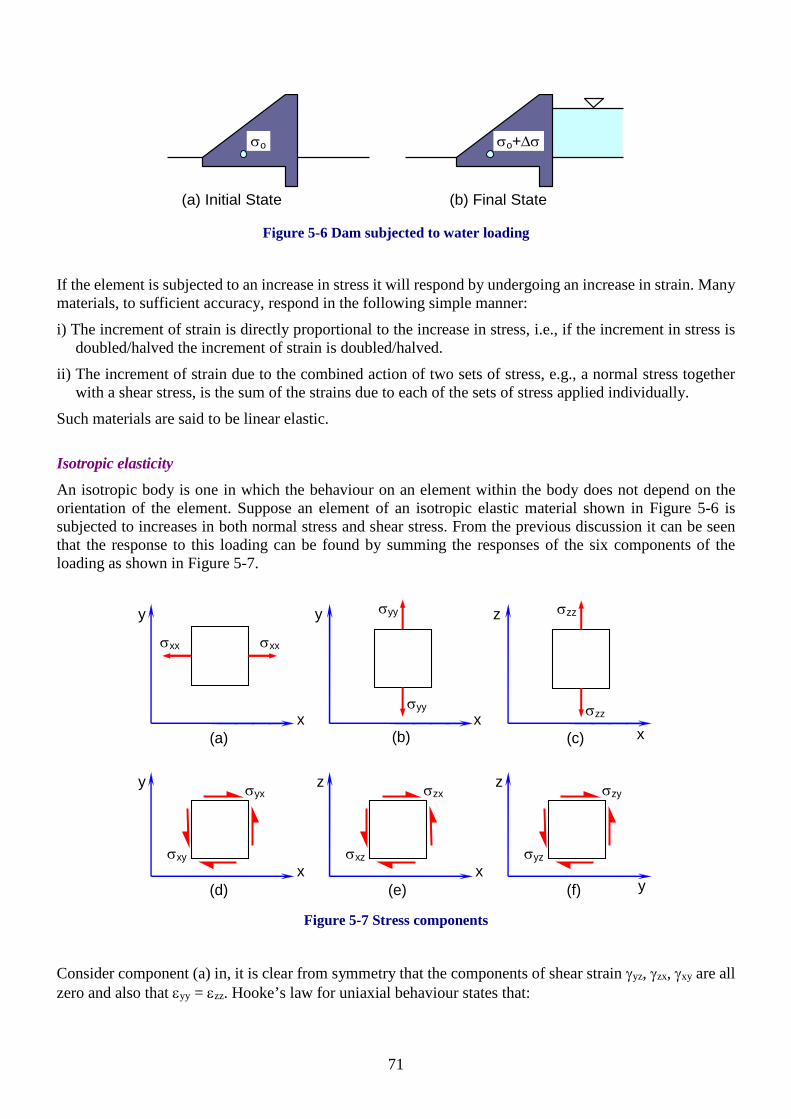
71

(a) Initial State (b) Final State

σo σo+∆σ

Figure 5-6 Dam subjected to water loading

If the element is subjected to an increase in stress it will respond by undergoing an increase in strain. Many materials, to sufficient accuracy, respond in the following simple manner: i) The increment of strain is directly proportional to the increase in stress, i.e., if the increment in stress is

doubled/halved the increment of strain is doubled/halved. ii) The increment of strain due to the combined action of two sets of stress, e.g., a normal stress together

with a shear stress, is the sum of the strains due to each of the sets of stress applied individually. Such materials are said to be linear elastic. Isotropic elasticity An isotropic body is one in which the behaviour on an element within the body does not depend on the orientation of the element. Suppose an element of an isotropic elastic material shown in Figure 5-6 is subjected to increases in both normal stress and shear stress. From the previous discussion it can be seen that the response to this loading can be found by summing the responses of the six components of the loading as shown in Figure 5-7.

x

z σzz

σzz

(c)

σyy

σyy

(b) x

y

(a)

σxx σxx

x

y

(d) x

y

σxy

σyx

(e) x

z

σxz

σzx

(f) y

z

σyz

σzy

Figure 5-7 Stress components

Consider component (a) in, it is clear from symmetry that the components of shear strain γyz, γzx, γxy are all zero and also that εyy = εzz. Hooke’s law for uniaxial behaviour states that:

72

xxxx

xxyy

xxzz

σεEσε νE

σε νE

=

= −

= −

(5.32)

where E and ν are material constants called Young's modulus and Poisson's ratio, respectively. A consideration of the component (b) leads to the conclusion that the only non-zero strain components are:

yyxx

yyyy

yyzz

σε ν

Eσ

εE

σε ν

E

= −

=

= −

(5.33)

Similarly it is found that the response to the component (c) leads to the non-zero strains:

zzxx

zzyy

zzzz

σε νE

σε νE

σεE

= −

= −

=

(5.34)

The response to the combined normal stresses is thus:

xx yy zzxx

yy xx zzyy

zz xx yyzz

σ ν(σ σ )ε

Eσ ν(σ σ )

εE

σ ν(σ σ )ε

E

− +=

− +=

− +=

(5.35)

The shear strain increment, γxy occurs due to an increment of shear stress σxy, as shown in Figure 5-7(d), can be calculated by the following relation:

xy

xy

σγ

G= (5.36)(a)

where G is a material property called the shear modulus. Similarly, the responses to the stress changes (e) and (f) are:

yz

yz

σγ

G= (5.36)(b)

zxzx

σγG

= (5.36)(c)

73

The complete set of stress strain equations is given by Eq. (5.35) and Eq. (5.36). Because of the isotropy of the material the stress-strain relations expressed in terms of another set of coordinate axes (X, Y, Z) should have precisely the same form as Eq. (5.35) and Eq. (5.36). This implies that the shear modulus must be related to Young's modulus and Poisson's ratio. The relationship between the shear modulus, Young’s modulus and Poisson’s ratio for an isotropic elastic material is:

EG2(1 ν)

=+

(5.37)

The complete expression for strain in terms of stress can be presented in a matrix format as:

xx xx

yy yy

zz zz

xy xy

yz yz

zx zx

ε σ1/E ν/E ν/E 0 0 0ε σν/E 1/E ν/E 0 0 0ε σν/E ν/E 1/E 0 0 0γ σ0 0 0 1/G 0 0γ σ0 0 0 0 1/G 0γ σ0 0 0 0 0 1/G

− − − − − −

=

(5.38)

It is often useful to be able to determine the volumetric strain and it is found that:

mv

σεK

= (5.39)

where v xx yy zzε ε ε ε= + + is the volumetric strain, ( )m xx yy zzσ σ σ σ /3= + + is called the mean stress and

( )EK

3 1 2ν=

− is the bulk modulus.

Expression for stress in terms of strain In many cases it is necessary to calculate the stresses resulting from application of a set of strains to an element. Clearly in such cases it is much more convenient to have an expression for stress in terms of strain. There is no difficulty in developing an expression for shear stress in terms of shear strain from Eq. (5.36).

xy xy

yz yz

zx zx

σ G . γσ G . γσ G . γ

=

=

=

(5.40)

An expression for the increase in normal stress caused by the increase in normal strain may be found by writing the first of the relations in Eq. (5.32) to Eq. (5.34) in the form:

( )xx xx xx yy zz1 ν νε σ σ σ σ

E E+ = − + +

(5.41)

and then using Eq. (5.39) to show that:

xx v xxσ λ ε 2G ε= + (5.42)

( )( )

Eνλ1 ν 1 2ν

=+ −

(5.43)

74

The quantity λ is called the Lamé modulus. Similar expressions can be found for σyy and σzz. Thus the complete expression for an increment of stress in terms of an increment of strain is:

xx xx

yy yy

zz zz

xy xy

yz yz

zx zx

σ ελ 2G λ λ 0 0 0σ ελ λ 2G λ 0 0 0σ ελ λ λ 2G 0 0 0σ γ0 0 0 G 0 0σ γ0 0 0 0 G 0σ γ0 0 0 0 0 G

+ + +

=

(5.44)

or in a familiar matrix notation:

σ = D ε (5.45)

where

xx xx

yy yy

zz zz

xy xy

yz yz

zx zx

σ ε λ 2G λ λ 0 0 0σ ε λ λ 2G λ 0 0 0σ ε λ λ λ 2G 0 0 0

, ,σ γ 0 0 0 G 0 0σ γ 0 0 0 0 G 0σ γ 0 0 0 0 0 G

+ + +

= = =

σ ε D (5.46)

D is called the matrix of elastic moduli. It is perhaps worth observing at this stage that the matrix D in Eq. (5.45) is symmetric and positive definite. This is a general characteristic of elastic material and leads to the reciprocal theorem used in the boundary element methods. As stated before, in an isotropic material the form of the stress-strain relation is independent of the particular choice of coordinate system. Therefore, the relationships given in Eq. (5.38) and Eq. (5.44) can be written for cylindrical polar coordinates as:

rr rr

θθ θθ

zz zz

rθ rθ

θz θz

zr zr

ε σ1/E ν/E ν/E 0 0 0ε σν/E 1/E ν/E 0 0 0ε σν/E ν/E 1/E 0 0 0γ σ0 0 0 1/G 0 0γ σ0 0 0 0 1/G 0γ σ0 0 0 0 0 1/G

− − − − − −

=

(5.47)

rr rr

θθ θθ

zz zz

rθ rθ

θz θz

zr zr

σ ελ 2G λ λ 0 0 0σ ελ λ 2G λ 0 0 0σ ελ λ λ 2G 0 0 0

,σ γ0 0 0 G 0 0σ γ0 0 0 0 G 0σ γ0 0 0 0 0 G

+ + +

=

(5.48)

75

5.5 Plane elasticity In this section we discuss three different situation where is not necessary to carry out a full three-dimensional analysis. The three cases are plane stress, plane strain, and axial symmetry conditions. Unders these condition it is possible to reduce the problem to a two-dimensional problem as follows: Plane stress The plane stress case is shown schematically in Figure 5-8, where a uniform thin plate with uniform cross section along the z direction is subjected to edge loads parallel to the plane of the plate. Clearly the increments of stresses σzz, σyz, σxz are all zero on both faces of the plate. It is found that to sufficient accuracy these are zero throughout the entire thickness of the plate. It thus follows that the stresses within the body are completely specified by σxx, σyy, σxy. It can also be shown that to sufficient accuracy these stresses do not vary throughout the thickness of the plate and hence depend only on x, y but not on z.

x

y

Figure 5-8 Plane stress of a thin plate

The stress strain relationship can then be written in the form:

xx xx

yy yy

zz

xy xy

yz

zx

ε 1/E ν/E ν/E 0 0 0 σε ν/E 1/E ν/E 0 0 0 σε ν/E ν/E 1/E 0 0 0

=γ 0 0 0 1/G 0 0 σγ 0 0 0 0 1/G 0γ 0 0 0 0 0

0

1/G00

− − − − − −

From this matrix equation we derive the following three equations.

( )

( )

( )

xx yyxx

yy xxyy

zz xx yy

σ νσε

Eσ νσ

εE

νε ε ε1 ν

−=

−=

= − +−

(5.49)

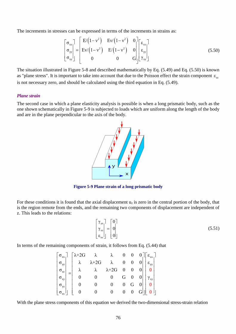
76

The increments in stresses can be expressed in terms of the increments in strains as:

( ) ( )( ) ( )

2 2

xx xx2 2

yy yy

xy xy

E/ 1 ν Eν/ 1 ν 0σ εσ Ev/ 1 ν E/ 1 ν 0 εσ γ0 0 G

− − = − −

(5.50)

The situation illustrated in Figure 5-8 and described mathematically by Eq. (5.49) and Eq. (5.50) is known as "plane stress". It is important to take into account that due to the Poisson effect the strain component zzεis not necessary zero, and should be calculated using the third equation in Eq. (5.49). Plane strain The second case in which a plane elasticity analysis is possible is when a long prismatic body, such as the one shown schematically in Figure 5-9 is subjected to loads which are uniform along the length of the body and are in the plane perpendicular to the axis of the body.

x

y

Figure 5-9 Plane strain of a long prismatic body

For these conditions it is found that the axial displacement uz is zero in the central portion of the body, that is the region remote from the ends, and the remaining two components of displacement are independent of z. This leads to the relations:

yz

xz

zz

γ 0γ 0ε 0

=

(5.51)

In terms of the remaining components of strain, it follows from Eq. (5.44) that

xx xx

yy yy

zz

xy xy

yz

zx

σ λ+2G λ λ 0 0 0 εσ λ λ+2G λ 0 0 0 εσ λ λ λ+2G 0 0 0

=σ 0 0 0 G 0 0 γσ 0 0 0 0 G 0σ 0 0 0 0

0

000G

With the plane stress components of this equation we derived the two-dimensional stress-strain relation

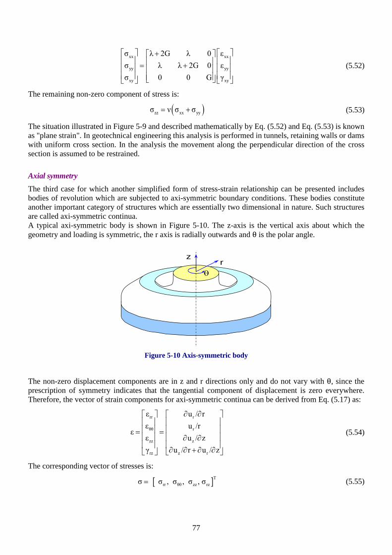
77

xx xx

yy yy

xy xy

σ λ 2G λ 0 εσ λ λ 2G 0 εσ 0 0 G γ

+ = +

(5.52)

The remaining non-zero component of stress is:

( )zz xx yyσ ν σ σ= + (5.53)

The situation illustrated in Figure 5-9 and described mathematically by Eq. (5.52) and Eq. (5.53) is known as "plane strain". In geotechnical engineering this analysis is performed in tunnels, retaining walls or dams with uniform cross section. In the analysis the movement along the perpendicular direction of the cross section is assumed to be restrained. Axial symmetry The third case for which another simplified form of stress-strain relationship can be presented includes bodies of revolution which are subjected to axi-symmetric boundary conditions. These bodies constitute another important category of structures which are essentially two dimensional in nature. Such structures are called axi-symmetric continua. A typical axi-symmetric body is shown in Figure 5-10. The z-axis is the vertical axis about which the geometry and loading is symmetric, the r axis is radially outwards and θ is the polar angle.

r z

θ

Figure 5-10 Axis-symmetric body

The non-zero displacement components are in z and r directions only and do not vary with θ, since the prescription of symmetry indicates that the tangential component of displacement is zero everywhere. Therefore, the vector of strain components for axi-symmetric continua can be derived from Eq. (5.17) as:

rr r

θθ r

zz z

rz z r

ε u / rε u /r

εε u / zγ u / r u / z

∂ ∂ = = ∂ ∂ ∂ ∂ + ∂ ∂

(5.54)

The corresponding vector of stresses is:

[ ]Trr θθ zz rzσ σ , σ , σ , σ= (5.55)

78

The stress-strain relationship for axi-symmetric continua consisting of isotropic materials can be found from Eq. (5.48) as:

( )

rr rr

zz zz

rz rz

θθ rr zz

σ λ+2G λ 0 εσ = λ λ+2G 0 εσ 0 0 G γ

σ =ν σ +σ

(5.56)

The situation illustrated in Figure 5-10 and described by Eq. (5.56) is known as "axial symmetry".

5.6 Material non-linearity Linear, isotropic elasticity is a safe ground for finite element analysis. However, there are sophisticated situations where these assumptions are not valid. This is the case of analysis of soils or materials near to yielding point of failure, or problems where the deformation cannot be assumed to be small in comparison with the length scales of the system. In these cases a non-linear analysis will be the next step after a linear analysis. In the non-linear analysis, we formulate the problem as a set of load increments; each one using the incremental stress-strain relation ∆ ∆σ = D ε (5.57)

Then the non-linear analysis will consist two main extensions: geometric and material non-linearity. In the geometric non-linearity, the deformation of the structure is tracked in each increment by updating the position of their nodes. Then the stiffness matrix is calculated in terms of each new configuration. The load path and load increments need to be specified in this analysis. If you expect that your system will experience large deformation, a geometric non-linearity analysis is highly recommended. An additional assumption in the non-linear analysis is the material non-linearity. It states that the stress-strain relation D in Eq. (5.57) depends on stress and probably on the load history. One of the most widely used non-linear models is the elasto-plastic model. In this model we define a yield surface in the space of stress, which enclosed a region where only elastic deformations are possible. Plastic yielding results in the stress point pushing the yield surface in the stress space, so that the stress state is never outside the yield surface. When the stress is on the yield surface, the strain increment is decomposed into an elastic and a plastic part

Δε=Δε +Δεel pl (5.58)

where the elastic part satisfies

el∆ ∆σ = D ε (5.59)

And the plastic part is given by the so-called non-associated flow rule

pl1Δ = Δh

ε φ σ ψ (5.60)

The new material parameters are h= hardening modulus, φ=yield direction, and ψ=flow direction. Eq. (5.60) also introduces the step function:

79

0 if x 0x if x>0

x≤

=

(5.61)

Note that the yield surface is defined in the stress space that has six independent components. It is possible to reduce this space to three dimensions by using the principal component of the stress. We first note that the stress tensor is symmetric. From linear algebra we learn that this stress in the reference system of its eigenvectors is diagonal, and that the diagonal element are its eigenvalues, here called principal components of stresses. Thus, the stress in the reference systems of its eigenvectors is:

1

2

2

σ 0 0= 0 σ 0

0 0 σ

σ (5.62)

Now it is more convenient to define the yield function in the 3D space of the principal components of the stress tensor. Before to do that, we will define the stress invariants: Mean (hydrostatic) stress:

( )1 2 3p= σ + σ + σ /3 (5.63)

Deviatoric (Von Mises) stress:

( ) ( ) ( )2 2 2VM 1 2 2 3 3 1σ σ –σ + σ –σ + σ –σ / 2 = (5.64)

Lode’s angle:

2 3

1 3

σ σ1tanθ 2 1 σ σ3

30 θ 30

−= − −

− ° ≤ ≤ °

(5.65)

These three quantities are called “invariants” because they do not change when the stress is expressed in a different coordinate system. The geometrical meaning of this stress invariant is depicted in Figure 5-11. The stress state defines a unique point in the 3D space with its principal components. Let us project this point on the so-called hydrostatic line given by the equation 1 2 3σ =σ =σ . The distance from the origin of coordinate to this projection load is the mean (hydrostatic) stress defined by Eq. (5.63). The distance from the stress point to the hydrostatic line is the deviatoric stress, see Eq. (5.64). Now we define the deviatoric plane as the plane perpendicular to the hydrostatic line containing the stress point. Finally, the orientation angle of the stress point in the deviatoric plane is the Lode angle.

80

σ2

σ1

σ3 σ1 = σ2 = σ3

Inside the surface: elastic deformation

On the surface: plastic deformation

σ2 σ1

σ3

A deviatoric plane σ1 + σ2 + σ3 = constant

θ

Figure 5-11 geometrical representation of the stress invariants

For simplicity one would assume that the yielding of a material depends only on the hydrostatic and deviatoric stress. In some cases it is further assumed that the yielding depends on the deviatoric stress only. In other circumstances, such as in cohesive-frictional materials or composites, the yield depends not only on the deviatoric stress but also on the hydrostatic loads. Moreover, some yielding models have been constructed from extension of 2D analysis, such as the Mohr-Coulomb model, leading to yield function that depends on the Lode angle too. In the Table 5-1 below we present a summary of the most used models to represent the yield function.

81

Table 5-1 Four main models of yield surfaces

Ductile materials (steel): Yield independent on hydrostatic pressure

Brittle materials (concrete): Yield dependent on hydrostatic pressure

Tresca’s Yield criterion

1 2 2 3 3 11 1 1max( | |, | |, | |)2 2 2

kσ σ σ σ σ σ− − − =

0 / 2k σ=

Mohr Coulomb Yield criterion

tanncτ σ φ= + cohesionangle of internal friction

cφ

==

Von Misses yield criterion ( ) ( ) ( )2 2 2 2

1 2 2 3 3 1

2 20

– – – 6

3 / 3VM

k

k k

σ σ σ σ σ σ

σ σ

+ + =

∴ = =

Drucker-Prager

33

VMp kσα + =

2sin 6 cos 3(3 sin ) 3(3 sin )

ckϕ φαφ φ

= =+ +

82

Problems Problem 5.1. Poisson Ratio A cubic sample of steel as of side L=1m as shown in green in figure below is axially stretched by a quantity ∆L=1mm. The sample gets contracted in the y and z direction as shown the red cube in the figure. Determine the compression of the sample ∆L’. The Poisson ratio of the sample is ν=0.3.

Problem 5.2. Biaxial Test A long rectangular block is subjected to a biaxial stress as shown in figure below. The Young modulus is E=56MPa and the Poisson ratio is ν=0.4. Assuming that the stress is distributed uniformly inside the sample, determine the horizontal, vertical and shear deformation of the sample.

Problem 5.3. Thin Steel Plate A rectangular plate shown in the following figure is subjected to uniform tractions at two edges in the x coordinate direction. The plate dimensions are 800×400×1 mm. The Young’s modulus of the material is 200,000MPa and the Poisson ratio is 0.3. The edge pressure is 1 MPa tensile on short sides. Assuming that the stress is constant in the plate, calculate all components of the strain

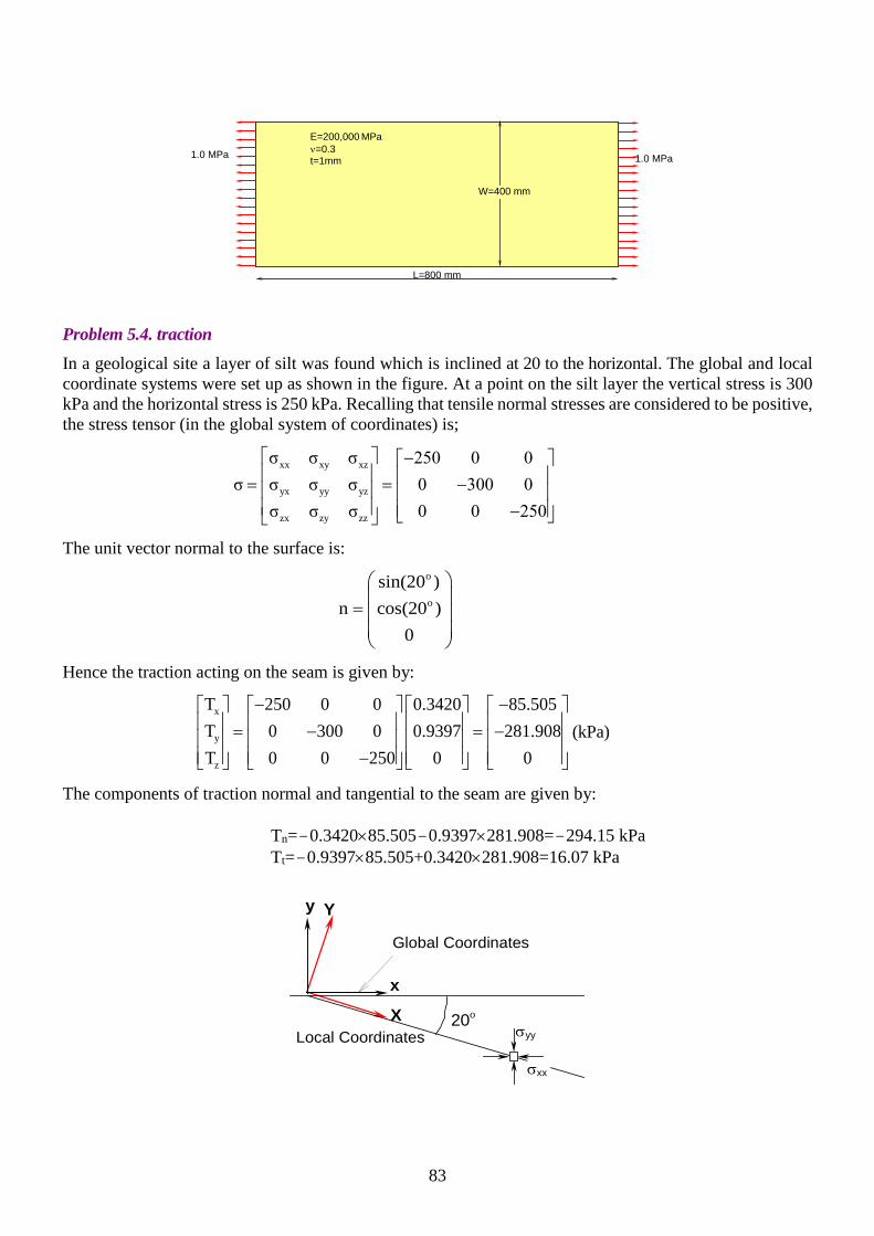
83

E=200,000 MPa

ν=0.3 t=1mm 1.0 MPa 1.0 MPa

L=800 mm

W=400 mm

Problem 5.4. traction In a geological site a layer of silt was found which is inclined at 20 to the horizontal. The global and local coordinate systems were set up as shown in the figure. At a point on the silt layer the vertical stress is 300 kPa and the horizontal stress is 250 kPa. Recalling that tensile normal stresses are considered to be positive, the stress tensor (in the global system of coordinates) is;

xx xy xz

yx yy yz

zx zy zz

σ σ σ 250 0 0σ σ σ σ 0 300 0

σ σ σ 0 0 250

− = = − −

The unit vector normal to the surface is:

o

o

sin(20 )n cos(20 )

0

=

Hence the traction acting on the seam is given by:

x

y

z

T 250 0 0 0.3420 85.505T 0 300 0 0.9397 281.908T 0 0 250 0 0

− − = − = − −

(kPa)

The components of traction normal and tangential to the seam are given by: Tn= −0.3420×85.505 −0.9397×281.908= −294.15 kPa Tt= −0.9397×85.505+0.3420×281.908=16.07 kPa

X

Y

x

y

20o

Local Coordinates

Global Coordinates

σxx

σyy

84

Problem 5.5. rotation of stress In a plane system the stress in global coordinates is:

80.0000 34.641034.6410 40.000

=

σ (MPa)

Calculate the traction on a plane making an angle of 120° with the x-axis. (Answer :Tx = 86.6025 MPa and Ty=50MPa) Problem 5.6. A local set of coordinates with the X axis inclined at 30° to the axis and the Y axis inclined at 120° to the x axis. If the stresses in the global (x, y) system are given by equation in Problem 5.5, show that the stress components in the local (X, Y) coordinate system can be given by

100 00 20

=

Σ (Mpa)

85

CHAPTER 6: FINITE ELEMENT FORMULATION OF ELASTIC CONTINUA

FINITE ELEMENT FORMULATION OF ELASTIC CONTINUA

In the finite element analysis of a problem, the system is idealised as a number of finite elements interconnected only at their nodes. In the analysis of structures consisting of bars and beams, the elements making up the complete structure usually correspond to well-defined parts of the structure. However, when a two- or three-dimensional structure such as a concrete slab or a soil foundation is analysed, there may not clear discrete parts. Rather the continuum is divided into finite elements by making imaginary cuts. There is generally no unique way of idealising a continuum structure with finite elements because such elements provide only approximate mathematical relationships of the continuum structure. The accuracy of the finite element solution of a continuum problem is dependent on the number, type, and arrangement of the finite elements from which the structure is assembled. Considerable choices are available for the basic shape of the elements, the function used to approximate the displacement field for the elements, and the arrangement of the elements. This chapter will cover only the classical two-dimensional finite elements that are used in plane elasticity. Plane elasticity encompasses continuum problems of plane stress, plane strain and axial symmetry. The formulation of each type of problem is almost the same, and the computer code for solving plane stress problems can be adopted with only minor modifications to plane strain and axial symmetry. In plane stress problems the forces normal to the plane are zero. In plane strain analysis the “out-of-plane” displacements are zero. Problems of this kind can basically be treated as two-dimensional problems. In the first section we will convert the strong formulation of the continuum mechanics of the previous chapter in the weak form, which is better known as principle of virtual work. Then we introduce the general method to formulate the equations of the finite element analysis. Next we illustrate some simplest formulations by introducing one of the simplest yet most versatile family of finite elements, the triangular elements. Then we introduce the linear rectangular element, which is the basis of more sophisticated, high order, rectangular elements used in most commercial codes.

6.1 Derivation of the weak form Here we present the derivation of the weak form, or principle of virtual work, for a general continuum mechanics problem we assume that in the domain V the continuum structure satisfies the differential equation:

[ ]T ( ) ( )+ =L σ x w x 0 (6.1)

( )= ( )σ x Dε x (6.2)

[ ]( ) ( )=ε x L u x (6.3)

Where L is the differential operator corresponding to the governing equations. Let us consider a problem without essential boundary conditions. The only boundary condition is given by the flux at the boundary

86

( ). ( ) S= ∈σ x n τ x x (6.4)

where τ(x) is the traction applied at the boundary surface S of the domain. The vector n is a unit vector perpendicular to the surface at point x. We introduce here a virtual displacement *( )u x . Eq. (6.1) is multiplied by a virtual displacement and integrated over the domain

( )*T T

V

( ) ( ) dV + =∫u L σ x w x 0 (6.5)

The next step is to use a generalized rule to integrate by part the first terms of this equations. This integration involve a quite large amount of mathematical steps that we will not include here. The final result will correspond to a generalized principle of virtual work:

*T *T *T

V S V

dV dA+ dV =∫ ∫ ∫ε σ u τ u w (6.6)

This principle stares that the virtual work done by the internal stresses equals the work done by the boundary tractions plus the work done by the external actions.

6.2 Derivation of the stiffness matrix Using the principle of virtual work, the finite element formulation can be derived as follows:

1) The displacement function is connected to the displacement at the nodes using the shape function

e e=u N u (6.7)

2) Strains [ ]=ε L u are connected to nodal displacement

[ ]e e e e ==ε B u B L N (6.8)

3) Using constitutive equation =σ Dε , the stress is related to displacement

e e=σ DB u (6.9)

4) Replace the above equation of stress and strain in the principle of virtual work Eq. (6.6), with * *

e=u Nu as the virtual displacement, and * *e=ε Bu satisfying the corresponding virtual strain:

e e e

*T T *T T *T Te e e e e

V V S

dV dV da = +∫ ∫ ∫u B DB u u N w u N τ (6.10)

where Ve is the volume of the element and Se is the surface of the element where the traction is applied. Since the equation is valid for any virtual displacement satisfying the boundary condition, the equation above becomes:

e e ek u = f (6.11)

e

Te e e

V

dV= ∫k B DB (6.12)

e

T Te e e

V

dV daeS

= +∫ ∫f N w N τ (6.13)

Here we conclude that the calculation of the element stiffness matrix requires three steps:

87

1) Calculate Ne 2) Calculate B by applying the derivative operator to Ne as Be=L[Ne] 3) Use Eq. (6.12) to get the stiffness matrix and Eq. (6.13) To get the load vector

In the next sections we will illustrate the method using linear triangular elements and linear rectangular elements.

6.3 Triangular elements in plane elasticity (T3) A general procedure is given to calculate the stiffness matrix of a simple 3-noded triangular element. The simple triangular element has nodal points at its vertices only. A range of higher-order triangular elements having additional nodes and consequently a more refined representation of displacement and stress fields has been proposed to increase accuracy. Some of the higher-order triangular elements will also be introduced in the next chapter. The 3-noded triangular element shown in Figure 6-1 is the simplest possible planar element and one of the earliest finite elements. It has nodes at the vertices of the triangle only. For a plane elasticity problem, where all displacements are in the plane, the element has two degrees-of-freedom at each node, u and v, corresponding to the displacements in x and y directions respectively. Thus the element has a total of 6 degrees-of-freedom. The displacement vector and the force vector are:

T

e 1 1 2 2 3 3u v u v u v = u

T

e 1 1 2 2 3 3p q p q p q = f

Since each of these vectors contains 6 components, the size of the element stiffness matrix, ke, is 6×6.

u1, p1

v1, q1

x, u, p

y, v, q

1

3

2u2, p2

v2, q2

u3, p3

v3, q3

Figure 6-1 Three-noded triangular element

Stiffness matrix of linear triangular finite element The general procedure explained in Section 6.2 employed here to calculate the stiffness matrix of the 3-noded triangular element. The node numbering and the Cartesian coordinate system shown in Figure 6-1are used for the element. The nodes are numbered in increasing order anti-clockwise. The coordinates of the nodes are (x1,y1), (x2,y2) and (x3,y3). It is noted that the orientation of the element with respect to the xy

88

coordinate system is completely arbitrary. Therefore the element stiffness matrix will be directly expressed in the xy global coordinate system. Here we perform the three steps mentioned in Section 6.2 to calculate the stiffness matrix:

1. Derivation of the shape function N The variation of the displacement components, u and v, within the element can be expressed as complete linear polynomials of x and y:

T

1 2 3T

1 2 3

u(x,y) a a x a y= (x,y)

v(x,y) b b x b y= (x,y)

= + +

= + +

g a

g b (6.14)

where [ ]T(x,y) 1 x y=g , [ ]T1 2 3a a a=a and [ ]T

1 2 3b b b=b . The values of u and v are known at the nodes. Therefore, Eq. (6.14) can be written for all the nodes by substituting the coordinates of the nodes into these equations:

1 1 2 1 3 1 1 1 1 1

2 1 2 2 3 2 2 2 2 2

3 1 2 3 3 3 3 3 3 3

u a a x a y u 1 x y au a a x a y or u 1 x y au a a x a y u 1 x y a

= + + = + + = = + +

1 1 2 1 3 1 1 1 1 1

2 1 2 2 3 2 2 2 2 2

3 1 2 3 3 3 3 3 3 3

v b b x b y v 1 x y bv b b x b y or v = 1 x y bv b b x b y v 1 x y b

= + + = + + = + +

We rewrite these equations as

e e and = =u Ca v Cb (6.15)

where

1 1

2 2

3 3

1 x y1 x y1 x y

=

C (6.16)

Using Eqs. (6.14) and (6.16) the displacement fields u(x, y) and v(x,y) can now be expressed in the form of:

T -1 T

e eT -1 T

e e

u(x, y) (x, y) (x, y)

v(x, y) (x, y) (x, y)

= =

= =

g C u N u

g C v N v (6.17)

with

2 3 3 2 3 1 1 3 1 2 2 1

12 3 3 1 1 2

3 2 1 3 2 1

x y x y x y x y x y x y1 y y y y y y

2Ax x x x x x

−

− − − = − − − − − −

C

where 2A=det [C]= (x2 y3 –x3 y2)- (x1 y3 –x3 y1)+ (x1 y2 –x2 y1) =2 × area of triangle. The shape functions can be found as:

89

[ ]2 3 3 2 3 1 1 3 1 2 2 1

T T 12 3 3 1 1 2

3 2 1 3 2 1

x y x y x y x y x y x y1(x,y) (x,y) 1, x, y y y y y y y

2Ax x x x x x

−

− − − = = − − − − − −

N g C (6.18)

2 3 3 2 2 3 3 2

13 1 1 3 3 1 1 3

2

31 2 2 1 1 2 2 1

(x y x y ) x(y y ) y(x x )2AN (x, y)

(x y x y ) x(y y ) y(x x )(x,y) N (x, y)2A

N (x, y) (x y x y ) x(y y ) y(x x )2A

− + − + −

− + − + − = =

− + − + −

N (6.19)

The general displacements within the element can be related to the nodal displacements using shape functions:

T

1 1 2 2 3 3 eT

1 1 2 2 3 3 e

u N u N u N u =

v N v N v N v =

= + +

= + +

N u

N v (6.20)

Eq. (6.20) can now be written in matrix format as:

1

1

1 2 3 2e e

1 2 3 2

3

3

uv

N 0 N 0 N 0 uuor u(x,y)

0 N 0 N 0 N vvuv

= =

N u (6.21)

2. Derivation of the matrix B The matrix Be has been defined for a general case in Eq. (6.8) and contains derivatives of the shape functions.

[ ] 1 2 3e e

1 2 3

1x 2x 3x

e 1y 2y 3y

1y 1x 2y 2x 3y 3x

0x

N 0 N 0 N 00

0 N 0 N 0 Ny

y x

N 0 N 0 N 00 N 0 N 0 N

N N N N N N

∂ ∂

∂= = ∂

∂ ∂ ∂ ∂ =

B L N

B

(6.22)

The derivatives of the shape functions for the triangular element can be obtained as:

90

1x 2 3

1y 3 2

2x 3 1

2y 1 3

3x 1 2

3y 2 1

N (y y )N (x x )N (y y )1N (x x )2AN (y y )N (x x )

− − −

= − −

−

(6.23)

Therefore the matrix Be is obtained for the linear triangular element as:

2 3 3 1 1 2

e 3 2 1 3 2 1

3 2 2 3 1 3 3 1 2 1 1 2

(y y ) 0 (y y ) 0 (y y ) 01 0 (x x ) 0 (x x ) 0 (x x )

2A(x x ) (y y ) (x x ) (y y ) (x x ) (y y )

− − − = − − − − − − − − −

B (6.24)

It can be seen that Be and therefore strains within the linear triangular element are independent of x and y. For this reason, this element is often called the “constant strain triangle”. 3. Calculating the element stiffness matrix The internal stress can be related to the external loads using the principle of virtual work for the element. This leads to the equation for calculation of the element stiffness matrix.

e

T Te e e e e

V

dV At= =∫k B DB B DB (6.25)

where A and t are the area and the thickness of the element, respectively. Note that because Be and D are independent of coordinate location (x, y), the integration over this element can be performed easily and exactly.

6.4 Linear rectangular element in plane elasticity (Q4) The linear rectangular element is the simplest rectangular element for planar analysis. The interpolation function used to approximate variation of displacements within the element is linear with respect to x and y. For simplicity, a Cartesian coordinate system is adopted where the axes x and y run along two of the element edges, as shown in Figure 6-2. Therefore this coordinate system is the local one. The origin of the x-y axes is chosen for convenience to be at a corner of the rectangle, but could be located at some other points without affecting the procedure for calculation of the element properties. The element has nodes at the four corner points, each node has 2 degrees-of-freedom u and v, corresponding to the displacements in x and y directions respectively Figure 6-2. Thus the element has a total of 8 degrees-of-freedom. The displacement vector and the force vector are:

T

e 1 1 2 2 3 3 4 4u v u v u v u v = u

T

e 1 1 2 2 3 3 4 4p q p q p q p q = f

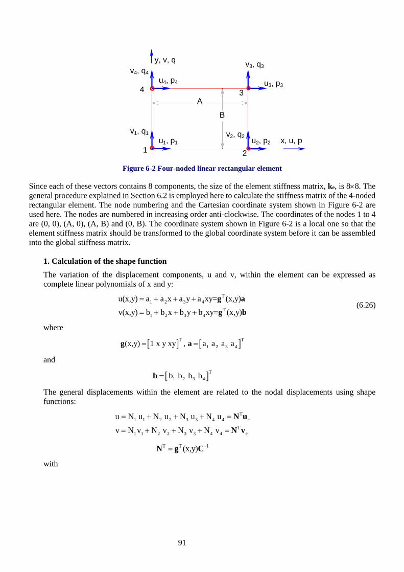
91

x, u, p

y, v, q

1

3

2u1, p1

v1, q1

u3, p3

v3, q3

u2, p2v2, q2

u4, p4

v4, q4

4A

B

Figure 6-2 Four-noded linear rectangular element

Since each of these vectors contains 8 components, the size of the element stiffness matrix, ke, is 8×8. The general procedure explained in Section 6.2 is employed here to calculate the stiffness matrix of the 4-noded rectangular element. The node numbering and the Cartesian coordinate system shown in Figure 6-2 are used here. The nodes are numbered in increasing order anti-clockwise. The coordinates of the nodes 1 to 4 are (0, 0), (A, 0), (A, B) and (0, B). The coordinate system shown in Figure 6-2 is a local one so that the element stiffness matrix should be transformed to the global coordinate system before it can be assembled into the global stiffness matrix.

1. Calculation of the shape function The variation of the displacement components, u and v, within the element can be expressed as complete linear polynomials of x and y:

T

1 2 3 4T

1 2 3 4

u(x,y) a a x a y a xy= (x,y)

v(x,y) b b x b y b xy= (x,y)

= + + +

= + + +

g a

g b (6.26)

where

[ ] [ ]T T1 2 3 4(x,y) 1 x y xy , a a a a= =g a

and

[ ]T1 2 3 4b b b b=b

The general displacements within the element are related to the nodal displacements using shape functions:

T

1 1 2 2 3 3 4 4 eT

1 1 2 2 3 3 4 4 e

u N u N u N u N uv N v N v N v N v

= + + + =

= + + + =

N uN v

T T 1(x,y) −=N g C

with

92

1 1 1 1

2 2 2 2

3 3 3 3

4 4 4 4

1 x y x y1 x y x y1 x y x y1 x y x y

=

C

Therefore the shape functions are:

1

2 T 1

3

4

N 1 x/A y/B xy/ABN x/A xy/AB

(x,y)N xy/ABN y/B xy/AB

−

− − + − = = = −

N g C (6.27)

The equation above can now be written in matrix format as:

1

1

2

1 2 3 4 2e e

1 2 3 4 3

3

4

4

uvu

N 0 N 0 N 0 N 0u vor (x,y)

0 N 0 N 0 N 0 Nv uvuv

= =

u N u

2. Calculation of the B matrix The matrix Be can be obtained from Ne (equation above) as:

1x 2x 3x 4x

e 1y 2y 3y 4y

1y 1x 2y 2x 3y 3x 4y 4x

N 0 N 0 N 0 N 00 N 0 N 0 N 0 N

N N N N N N N N

=

B (6.28)

where Nix, Niy are the derivatives of the shape functions with respect to x, and y, respectively. The derivatives of the shape functions for the 4-noded rectangular element can be obtained as:

1x

1y

2x

2y

3x

3y

4x

4y

N 1/A y/ABN 1/B x/ABN 1/A y/ABN x/ABN y/ABN x/ABN y/ABN 1/B x/AB

− + − + − − = −

−

(6.29)

Therefore the matrix Be is obtained for the linear rectangular element as:

93

e

y 1 1 y y y0 0 0 0AB A A AB AB AB

x 1 x x 1 x0 0 0 0AB B AB AB B AB

x 1 y 1 x 1 y x y 1 x yAB B AB A AB A AB AB AB B AB AB

− − − = − − − − − − − − −

B (6.30)

It can be seen that Be and therefore the strains within the element are a function of x and y. The normal strain εxx varies linearly with y but not with x, while εyy varies linearly with x but not with y. The shear strain varies linearly with x and y throughout the element, as can be seen from the form of the strain-displacement matrix, Be, in Eq. (6.30) 3. Calculation of the stiffness matrix In general, for plane stress or plane strain problems, the matrix D can be written in the form of:

11 12

12 22

33

d d 0d d 00 0 d

=

D (6.31)

This leads to the equation for calculation of the element stiffness matrix in the local coordinate system.

T Te e e e edV t dx dy

eV

= =∫ ∫∫k B D B B D B (6.32)

whereby (t) is the thickness of the element. The product of T

e eB D B has to be evaluated first and the components of the resulting matrix have to be integrated over the area of the element. The final value of the stiffness matrix obtained from these calculations is given by:

11 33 12 33 11 33 12 33 11 33 12 33 11 33 12 33

11 33 12 33 11 33 12 33 11 33 12 33 11 33

11 33 12

e

B A B A B A B A4d 4d 3d 3d 4d 2d 3d 3d 2d 2d 3d 3d 2d 4d 3d 3dA B A B A B A B

A B A B A B A B4d 4d 3d 3d 2d 4d 3d 3d 2d 2d 3d 3d 4d 2dB A B A B A B A

B A4d 4d 3dA B

t12

+ + − + − − − − − − − +

+ − + − − − − − − − +

+ − −

=k

33 11 33 12 33 11 33 12 33

11 33 12 33 11 33 12 33 11 33

11 33 12 33 11 33 12 33

11 33 12 33 11 33

B A B A3d 2d 4d 3d 3d 2d 2d 3d 3dA B A B

A B A B A B4d 4d 3d 3d 4d 2d 3d 3d 2d 2dB A B A B A

B A B A4d 4d 3d 3d 4d 2d 3d 3dA B A B

A B A BSymmetric 4d 4d 3d 3d 2d 4dB A B A

4

− − − − +

+ − + − + + − −

+ + − + −

+ − + −

11 33 12 33

11 33

B Ad 4d 3d 3dA B

A B4d 4dB A

+ − − +

Now the stiffness matrix needs to be converted into the global coordinate system. We note here that this step was not required for triangular element, where we used the global coordinate system to calculate the matrix. Here we used a local coordinate system oriented with the rectangle.

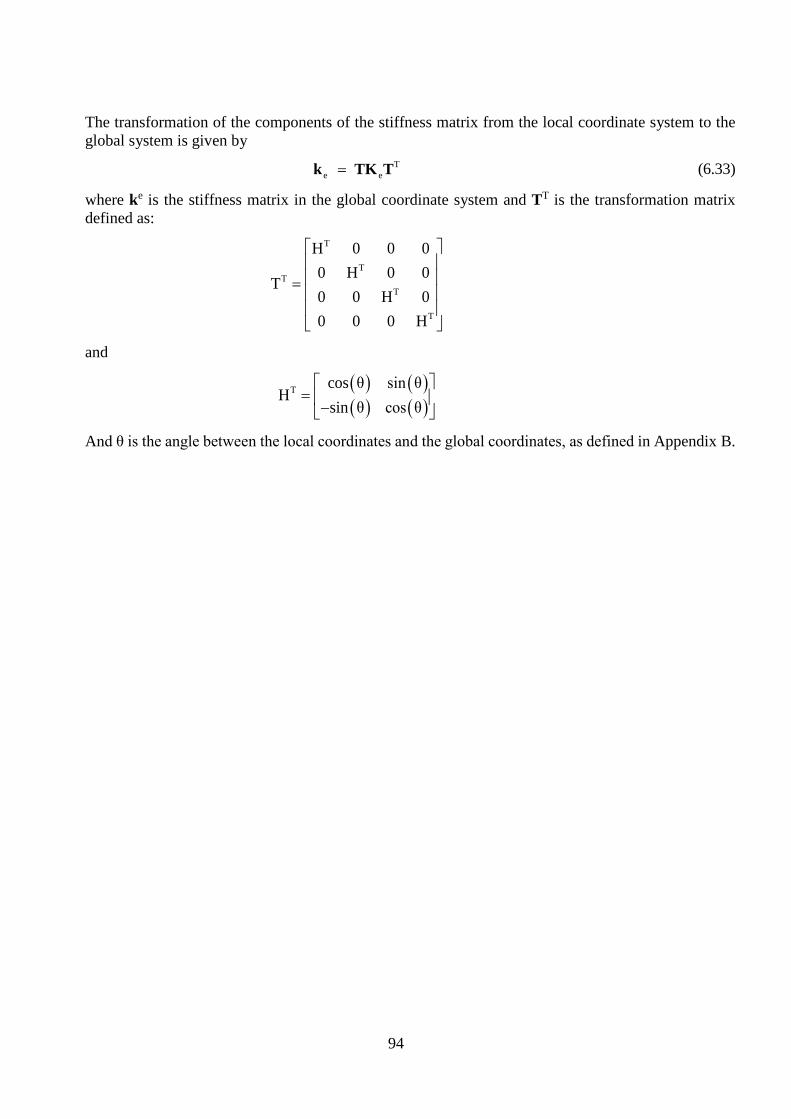
94

The transformation of the components of the stiffness matrix from the local coordinate system to the global system is given by

Te e =k TK T (6.33)

where ke is the stiffness matrix in the global coordinate system and TT is the transformation matrix defined as:

T

TT

T

T

H 0 0 00 H 0 0

T0 0 H 00 0 0 H

=

and

( ) ( )( ) ( )

T cos θ sin θH

sin θ cos θ

= −

And θ is the angle between the local coordinates and the global coordinates, as defined in Appendix B.

95

Problems Problem 6.1. Bar element This problem is about the calculation of the stiffness matrix and the load vector of the simplest element in Finite Element Modelling: the one-dimensional bar. The element consists of two nodes. The displacement along the node occurs in the direction connecting the two nodes only:

x1 x2 u2 u1

Δx The displacement in any position of the node is given by

( ) ( ) ( ) ( ) ( ) e e11 121 2

22

uN N Nu x =u x + u x x (x)N

ux

=

=

⋅ N U

The shape functions are given by the figure below

1 1

x x1 x2

N(x)

1 N1 N2

0

1) Find the shape function Ni(x) as a function of x, x1, and x2 and then construct the row vector Ne

( ) ( )1 2N N= x x eN

2) Calculate d=dx

ee NB

3) Calculate the element stiffness matrix 2

1

e eT e. E . .dxx

x

= ∫k B B

4) Calculate the load vector ( )2

1

eT= x f(x)dxx

x∫e NF

5) Write down the element matrix equation ⋅ =e e ek U F Problem 6.2. Element stiffness matrix of a second order 1D bar Calculate the element stiffness matrix of the 1D element with three nodes with a uniform load f along the element.

L

u1=0, x1=0 u2, x2=L/2 u3, x3=L

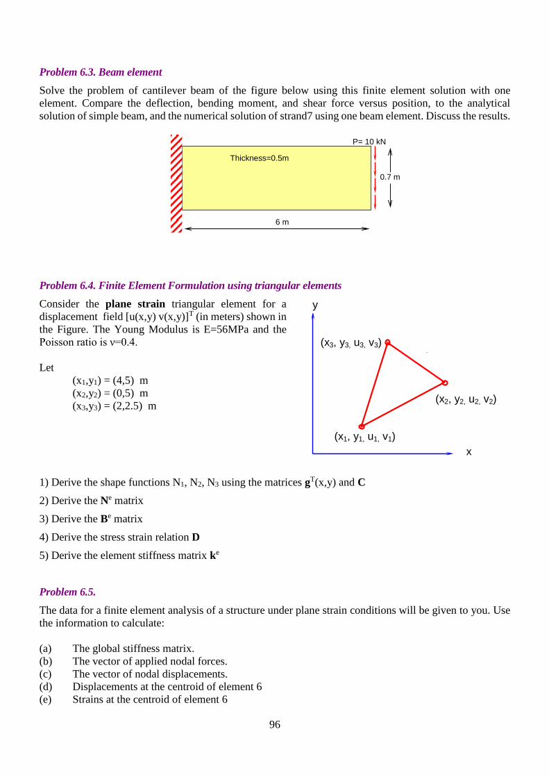
96

Problem 6.3. Beam element Solve the problem of cantilever beam of the figure below using this finite element solution with one element. Compare the deflection, bending moment, and shear force versus position, to the analytical solution of simple beam, and the numerical solution of strand7 using one beam element. Discuss the results.

6 m

0.7 m

P= 10 kN

Thickness=0.5m

Problem 6.4. Finite Element Formulation using triangular elements Consider the plane strain triangular element for a displacement field [u(x,y) v(x,y)]T (in meters) shown in the Figure. The Young Modulus is E=56MPa and the Poisson ratio is ν=0.4. Let

(x1,y1) = (4,5) m (x2,y2) = (0,5) m (x3,y3) = (2,2.5) m

1) Derive the shape functions N1, N2, N3 using the matrices gT(x,y) and C 2) Derive the Ne matrix 3) Derive the Be matrix 4) Derive the stress strain relation D 5) Derive the element stiffness matrix ke Problem 6.5. The data for a finite element analysis of a structure under plane strain conditions will be given to you. Use the information to calculate: (a) The global stiffness matrix. (b) The vector of applied nodal forces. (c) The vector of nodal displacements. (d) Displacements at the centroid of element 6 (e) Strains at the centroid of element 6

x

y

(x3, y3, u3, v3)

(x1, y1, u1, v1)

(x2, y2, u2, v2)

97

(f) Stresses at the centroid of element 6 Problem 6.6. A deep cantilever beam is subjected to a uniformly distributed traction at its free end. The dimension of the beam is shown in the figure below, The Young's modulus, E (MN/m2), is equal to the sum of the numerals of your SID and the Poisson's ratio, is equal to the last two numerals in your SID divided by 200.

1) Calculate the maximum vertical deflection of the beam using the constant strain triangular finite elements. Use 2x6, 4x12 and 8x24 subdivisions to generate different finite element meshes to approximate the deflection of the beam.

2) Compare the performances of the constant strain and the linear strain triangular finite elements on the basis of the number of nodes (or degrees-of-freedom) used in a finite element mesh. For example, use 1x3, 2x6, 4x12 and 8x24 subdivisions to generate finite element meshes of linear strain triangular elements and compare the results with those obtained in section 2.

3) Comment on the distribution of stresses (in particular, normal stress, σxx, close to the beam support) predicted by the finite element analyses using different element types and different number of nodes.

98

CHAPTER 7: FINITE ELEMENT MODELLING OF SCALAR FIELDS

FINITE ELEMENT MODELLING OF SCALAR FIELDS

In the previous chapter we presented the finite element solution of vector fields. In these kinds of problems the variable we want to solve is a vector in the three-dimensional space. This vector usually corresponds to the displacement of the structure. In this chapter we will concentrate in scalar fields. For these problems the unknown variable is a scalar that can represent temperature, excess of pore pressure, hydraulic head, torsion, etc. Likely for us, all these problems share the same mathematical structure, and the corresponding governing equations are the so-called heat equation. We will formulate the heat equation in its strong and weak form and provide finite element solutions for static and transient problems.

7.1 Formulation of heat equation Let us start with the strong formulation of a heat conduction problem. Here the unknown variable is the temperature, which is given in terms of the position. The kinematic equation corresponds to the temperature gradient, for 3D flow it is given by

T T TT= , ,x y z

∂ ∂ ∂∇ ∂ ∂ ∂

(7.1)

We are introducing here the nabla differential operator (nabla = arrow in Arabic) which is useful to formulate partial differential equations in complex form

T[ , , ]x y z∂ ∂ ∂

∇ =∂ ∂ ∂

(7.2)

The constitutive equation corresponds to the Fourier law, which states that the flow of heat is proportional to the gradient of temperature by a factor k that is the conductivity:

= k T− ∇q (7.3)

Then the balance equation corresponds to the principle of conservation of energy. In 1D, It states that the heat generated in an infinitesimal element Q(x)ΔxA equals to the heat that flow in the boundaries of the element A(q(x+Δx) – q(x)), written in differential form for 3D flow:

y Tx zqq q+ + = Q(x,y,z) Qx y z

∂∂ ∂∴ ∇

∂ ∂ ∂q = (7.4)

Putting all equation together we get the same equation as before

T T Tk + k + k = Q(x,y,z)

x x y y z z ∂ ∂ ∂ ∂ ∂ ∂ − ∂ ∂ ∂ ∂ ∂ ∂

(7.5)

Similar equations are derived for seepage flow by changed temperature by hydraulic head, and Q(x) by the amount of water generated inside the elementary volume. In both case the fixed boundary condition correspond to a fixed heat/temperature at the extreme, and the free boundary condition correspond to impermeable/isolated boundaries.

99

Using the nabla operator in Eq. (7.2), the above equation can be simplified as:

( )T k T = Q(x)∇ ∇ − (7.6)

All problems that satisfy this differential equation are known as scalar problems, since the unknown variable “T” is a scalar. There is a wide range of scalar problems in engineering, such as heat flow, conductibility, pore pressure, and torsion. The most general form of the scalar problems is

T ( T) Q=0∇ ∇ +k (7.7)

where k is a matrix in the most general case. Since the unknown field T(x) of these problem is a scalar function, we will refer to these problems as scalar field. The Table 7-1 below shows a list of problems that can be solved using scalar field formulations.

Table 7-1 Variables involved in the heat equation

Field Problem Unknown (T) Material parameter (k) Known (Q) Heat Conduction Temperature Thermal conductivity Internal heat source

Seepage flow Hydraulic head Permeability Zero Incompressible flow Stream function Unity Twice the vorticity

Elastic torsion Stress function (Shear Modulus)- 1 Twice the rate of

twist Electric conduction Voltage Electric conductivity Zero

Gas diffusion Concentration Diffusivity Zero Electrostatics Permittivity Charge density Zero

Magnetostatics Magnetic potential Reluctivity Charge density Incompressible

lubrication Pressure (Film thickness )3/viscosity Lubricant supply

7.2 Weak formulation of the heat equation We aim here to formulate the finite element equation of the heat equation. Let us assume that V is the domain of the problem. The conservation equation of the problem is

T =Q in V ∇ q (7.8)

The boundary of the domain is split as 1 2A=A A∪ , where A1 is the part of the boundary with essential boundary conditions, and A2 is the boundary with free boundary conditions

T T1 2=Q in V T = 0 in A and =g( ) in A∇ q q n x (7.9)

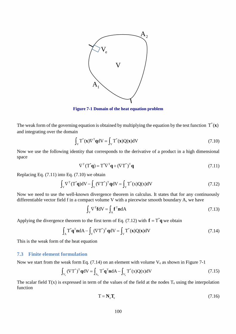
100

Figure 7-1 Domain of the heat equation problem

The weak form of the governing equation is obtained by multiplying the equation by the test function *T ( )xand integrating over the domain

* T *

V VT ( ) dV T ( )Q( )dV∇ =∫ ∫x q x x (7.10)

Now we use the following identity that corresponds to the derivative of a product in a high dimensional space

T * * T * T(T ) T ( T )∇ = ∇ + ∇q q q (7.11)

Replacing Eq. (7.11) into Eq. (7.10) we obtain

T * * T *

V V V(T )dV ( T ) dV T (x)Q(x)dV∇ − ∇ =∫ ∫ ∫q q (7.12)

Now we need to use the well-known divergence theorem in calculus. It states that for any continuously differentiable vector field f in a compact volume V with a piecewise smooth boundary A, we have

T T

V AdV dA∇ =∫ ∫f f n (7.13)

Applying the divergence theorem to the first term of Eq. (7.12) with *T=f q we obtain

* T * T *

A V VT dA ( T ) dV T ( )Q( )dV− ∇ =∫ ∫ ∫q n q x x (7.14)

This is the weak form of the heat equation

7.3 Finite element formulation Now we start from the weak form Eq. (7.14) on an element with volume Ve as shown in Figure 7-1

e e e

* T * T *

V A V( T ) dV T dA T (x)Q(x)dV∇ = −∫ ∫ ∫q q n (7.15)

The scalar field T(x) is expressed in term of the values of the field at the nodes Te using the interpolation function

e eT = N T (7.16)

V

1A

2A

eV

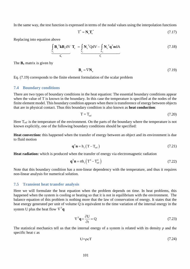
101

In the same way, the test function is expressed in terms of the nodal values using the interpolation functions

* *e eT = N T (7.17)

Replacing into equation above

e 2

e e

T T T Te e e e e

V V A

dV QdV dAe

= −∫ ∫ ∫k f

B kB T N N q n

(7.18)

The Be matrix is given by

e e= ∇B N (7.19)

Eq. (7.19) corresponds to the finite element formulation of the scalar problem

7.4 Boundary conditions There are two types of boundary conditions in the heat equation: The essential boundary conditions appear when the value of T is known in the boundary. In this case the temperature is specified at the nodes of the finite element model. This boundary condition appears when there is transference of energy between objects that are in physical contact. Thus this boundary condition is also known as heat conduction:

refT = T (7.20)

Here Tref is the temperature of the environment. On the parts of the boundary where the temperature is not known explicitly, one of the following boundary conditions should be specified: Heat convection: this happened when the transfer of energy between an object and its environment is due to fluid motion

( )Tc refh T T= −q n (7.21)

Heat radiation: which is produced when the transfer of energy via electromagnetic radiation

( )T 4 4r refσh T T= −q n (7.22)

Note that this boundary condition has a non-linear dependency with the temperature, and thus it requires non-linear analysis for numerical solution.

7.5 Transient heat transfer analysis Here we will formulate the heat equation when the problem depends on time. In heat problems, this happened when the system is cooling or heating so that it is not in equilibrium with the environment. The balance equation of this problem is nothing more that the law of conservation of energy. It states that the heat energy generated per unit of volume Q is equivalent to the time variation of the internal energy in the system U plus the heat flow T∇ q

T U Qt

∂∇ + =

∂q (7.23)

The statistical mechanics tell us that the internal energy of a system is related with its density ρ and the specific heat c as U=ρcT (7.24)

102

Replacing this equation into Eq. (7.23) we obtain

T TρC Qt

∂∇ + =

∂q (7.25)

The weak form can be formulated similar to the static analysis in the previous Chapter. First we multiply by the test function T* and then integrate over the domain,

e e

T * *

V V

TρC T dV T dVt

Q∂ ∇ + = ∂ ∫ ∫q (7.26)

Integrating by parts

e e

T* * *

V V

TT qdV T ρC dV T QdVt E

∂ − ∇ + = ∂∫ ∫ ∫ (7.27)

and using the interpolation function to relate the field variable with its values at the modes

e eT = N T (7.28)

We derive the element matrix equation

e e

ee e e e

T T Te e e e e e e e

V V V

d+ρ dt

dV dV QdVe

=∫ ∫ ∫

Tk T = f C

C = N N k = B kB f N (7.29)

The transient heat solver solves this problem given the initial conditions, using a time sequence algorithm.

103

Problems Problem 7.1. Thermal load A glass window of an Australian house consists of a single layer of glass of 4 mm thick with thermal conductivity k =0.80 W/moC. Determine the temperature at the inside and outside surface of the glass and the steady rate of heat transfer (in W/m2) through the window. Assume that the inside temperature is 20o with coefficient of thermal convection hin= 10 W/m2 oC, and the outside temperature is T =0 o with hout = 30 W/ m2 oC

Problem 7.2. Thermal load 2 The Figure shows the cross section of a plate with temperature T(x) heated from the top with a solar radiation of 500 watts/m2 (watts=J/s). The thermal conductivity k=54 watts/m0C. The temperature is kept constant (T0=300C) at the left boundary, and the right boundary is insulated. The length of the steel plate is L=2m, its wide is W=5m and its thickness is δ= 0.01m

1) Calculate the heat produced in the plate (Q) in watts/m3 2) Derive the governing equations for the temperature in the steady state. Neglect heat loss at the bottom

of the plate 3) Find the analytical solution of the temperature in the steady state. 4) Find the governing equations the temperature by assuming that the right boundary exchanges heat with

the environment of Tr=100C with a convection coefficient of h=11 W/m2 C. 5) Solve the governing equations of question 4.

Problem 7.3. Thermal triangular element Consider the triangular element for a temperature field T(x) (in oC) shown in the figure. The conductivity is k=40 W/(m oC). Let

(x1,y1) = (2,1) m (x2,y2) = (5,3) m (x3,y3) = (3,4) m

oinT =20

ooutT =0

1T

2T

0T

L

Isolated

δ

x

y

(x1, y1, T1)

(x3, y3, T3)

(x2, y2, T2)

104

1) Derive the shape functions 2) Derive the B matrix 3) Derive the element stiffness matrix ke

Problem 7.4. Finite different solution of the transient heat equation Find the finite different equation of the heat Equation

2

2

u uc = F(x,t)tx

∂ ∂−

∂ ∂

Problem 7.5. Finite element solution of the transient heat equation Find the finite element solution of the transient heat equation

2

2

u uc = F(x,t)tx

∂ ∂−

∂ ∂

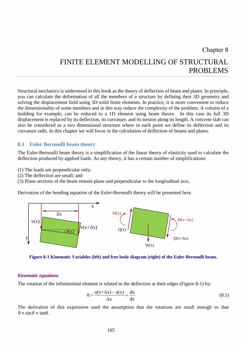
105

CHAPTER 8: FINITE ELEMENT MODELLING OF STRUCTURAL PROBLEMS

FINITE ELEMENT MODELLING OF STRUCTURAL PROBLEMS

Structural mechanics is understood in this book as the theory of deflection of beam and plates. In principle, you can calculate the deformation of all the members of a structure by defining their 3D geometry and solving the displacement field using 3D solid finite elements. In practice, it is more convenient to reduce the dimensionality of some members and in this way reduce the complexity of the problem. A column of a building for example, can be reduced to a 1D element using beam theory. In this case its full 3D displacement is replaced by its deflection, its curvature, and its torsion along its length. A concrete slab can also be considered as a two dimensional structure where in each point we define its deflection and its curvature radii. In this chapter we will focus in the calculation of deflection of beams and plates.

8.1 Euler Bernoulli beam theory The Euler-Bernoulli beam theory is a simplification of the linear theory of elasticity used to calculate the deflection produced by applied loads. As any theory, it has a certain number of simplifications: (1) The loads are perpendicular only; (2) The deflection are small; and (3) Plane sections of the beam remain plane and perpendicular to the longitudinal axis. Derivation of the bending equation of the Euler-Bernoulli theory will be presented here.

x

v(x) v(x+Δx)

Δx

y θ(x)

M(x) M(x+Δx)

Q(x)

Q(x+Δx)

W(x)

Figure 8-1 Kinematic Variables (left) and free body diagram (right) of the Euler-Bernoulli beam.

Kinematic equations The rotation of the infinitesimal element is related to the deflection at their edges (Figure 8-1) by:

u(x+Δx) u(x) duθ.=Δx dx

−= (8.1)

The derivation of this expression used the assumption that the rotations are small enough so thatθ sin tanθθ≈ ≈ .

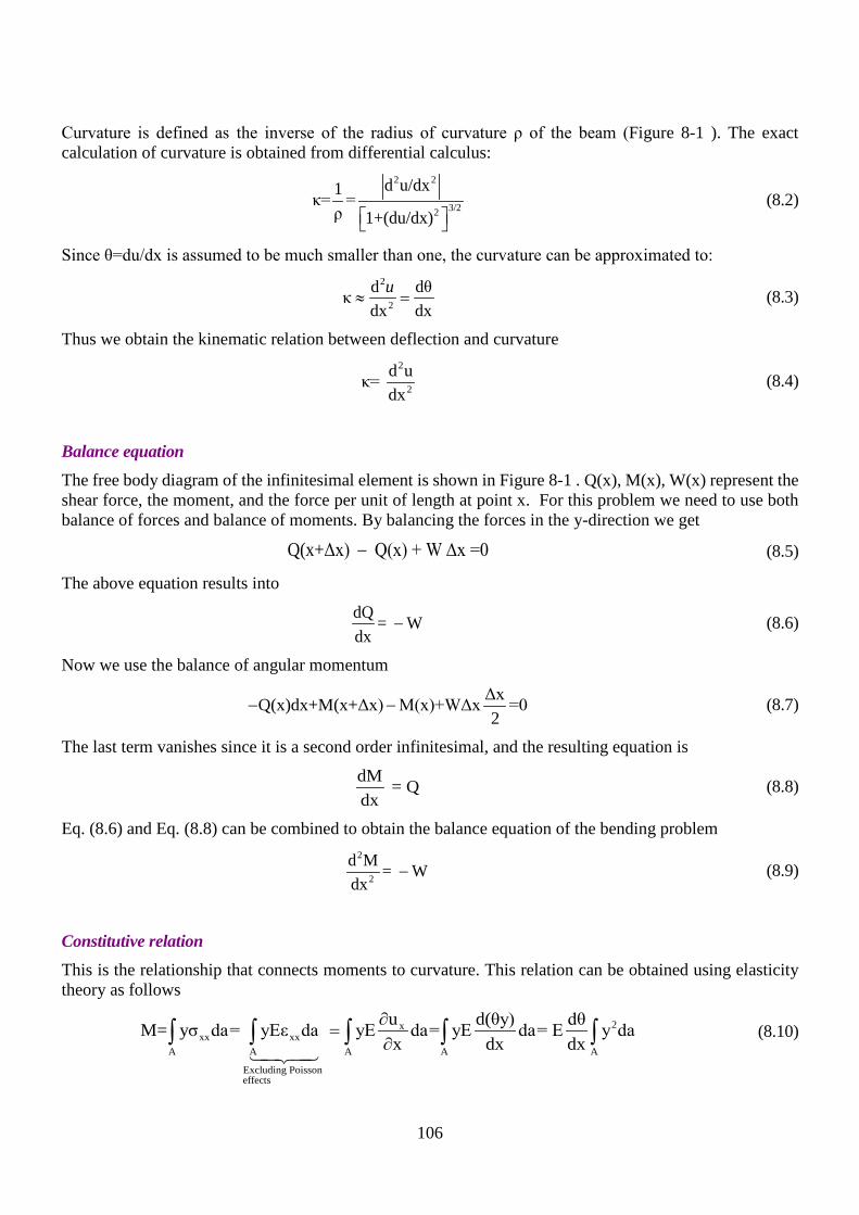
106

Curvature is defined as the inverse of the radius of curvature ρ of the beam (Figure 8-1 ). The exact calculation of curvature is obtained from differential calculus:

2 2

3/22

d u/dx1κ= =ρ 1+(du/dx)

(8.2)

Since θ=du/dx is assumed to be much smaller than one, the curvature can be approximated to:

2

2d dθκdx dx

u≈ = (8.3)

Thus we obtain the kinematic relation between deflection and curvature

2

2d uκ= dx

(8.4)

Balance equation The free body diagram of the infinitesimal element is shown in Figure 8-1 . Q(x), M(x), W(x) represent the shear force, the moment, and the force per unit of length at point x. For this problem we need to use both balance of forces and balance of moments. By balancing the forces in the y-direction we get

Q(x+Δx) Q(x) + W x =0− ∆ (8.5)

The above equation results into

dQ = Wdx

− (8.6)

Now we use the balance of angular momentum

ΔxQ(x)dx+M(x+Δx) M(x)+WΔx =02

− − (8.7)

The last term vanishes since it is a second order infinitesimal, and the resulting equation is

dM = Qdx

(8.8)

Eq. (8.6) and Eq. (8.8) can be combined to obtain the balance equation of the bending problem

2

2

d M = Wdx

− (8.9)

Constitutive relation This is the relationship that connects moments to curvature. This relation can be obtained using elasticity theory as follows

2xxx xx

A A A A A

Excluding Poisson effects

u d(θy) dθM= yσ da= yEε da yE da= yE da= E y dax dx dx

∂=

∂∫ ∫ ∫ ∫ ∫

(8.10)

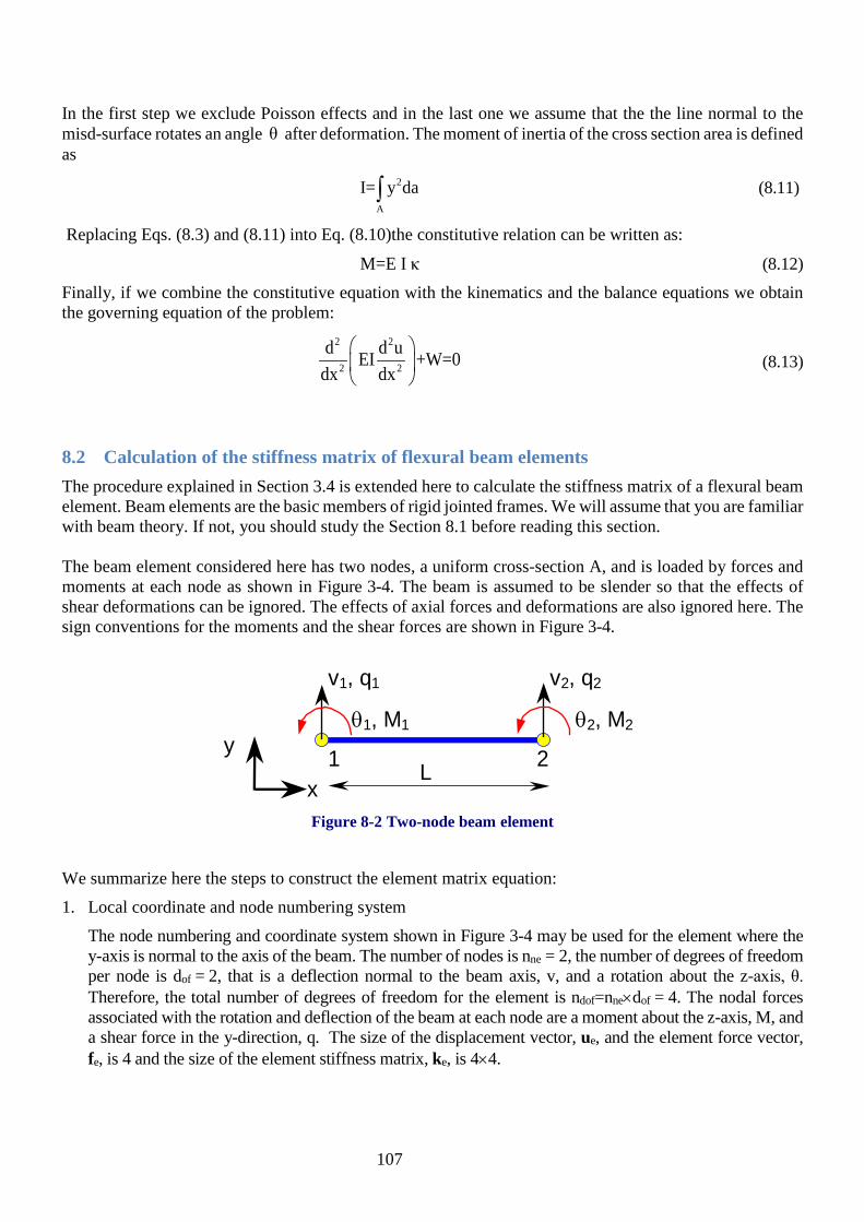
107

In the first step we exclude Poisson effects and in the last one we assume that the the line normal to the misd-surface rotates an angle θ after deformation. The moment of inertia of the cross section area is defined as

2

A

I= y da∫ (8.11)

Replacing Eqs. (8.3) and (8.11) into Eq. (8.10)the constitutive relation can be written as:

M=E I κ (8.12) Finally, if we combine the constitutive equation with the kinematics and the balance equations we obtain the governing equation of the problem:

2 2

2 2

d d uEI +W=0dx dx

(8.13)

8.2 Calculation of the stiffness matrix of flexural beam elements The procedure explained in Section 3.4 is extended here to calculate the stiffness matrix of a flexural beam element. Beam elements are the basic members of rigid jointed frames. We will assume that you are familiar with beam theory. If not, you should study the Section 8.1 before reading this section. The beam element considered here has two nodes, a uniform cross-section A, and is loaded by forces and moments at each node as shown in Figure 3-4. The beam is assumed to be slender so that the effects of shear deformations can be ignored. The effects of axial forces and deformations are also ignored here. The sign conventions for the moments and the shear forces are shown in Figure 3-4.

1 2

v2, q2v1, q1

L

θ2, M2 θ1, M1

x

y

Figure 8-2 Two-node beam element

We summarize here the steps to construct the element matrix equation: 1. Local coordinate and node numbering system

The node numbering and coordinate system shown in Figure 3-4 may be used for the element where the y-axis is normal to the axis of the beam. The number of nodes is nne = 2, the number of degrees of freedom per node is dof = 2, that is a deflection normal to the beam axis, v, and a rotation about the z-axis, θ. Therefore, the total number of degrees of freedom for the element is ndof=nne×dof = 4. The nodal forces associated with the rotation and deflection of the beam at each node are a moment about the z-axis, M, and a shear force in the y-direction, q. The size of the displacement vector, ue, and the element force vector, fe, is 4 and the size of the element stiffness matrix, ke, is 4×4.

108

11 12 13 141 1

21 22 23 241 1

31 32 33 342 2

41 42 43 442 2

k k k kq vk k k kM θk k k kq vk k k kM θ

=

(8.14)

2. Displacement function

The variation of the transverse displacement can be approximated by a polynomial function. The polynomial function must contain one unknown coefficient for each degree of freedom:

2 3

1 2 3 42 3 T

1 2 3 4

v(x) a a x a x a xv(x) [1 x x x ] [a a a a ]

= + + +

= (8.15)

where a1 to a4 are the unknown coefficients. The rotation at any point can be expressed as θ=dv/dx, thus:

2

2 3 42 T

1 2 3 4

θ(x) dv/dx a 2a x 3a xθ(x) [0 1 2x 3x ][a a a a ]

= = + +

= (8.16)

Therefore, the "displacements" at any point along the beam can be obtained from Eq. (8.15) and Eq. (8.16) as:

12 3

22

3

4

aav 1 x x xaθ 0 1 2x 3xa

=

(8.17)

The matrix f(x) and the vector a can be defined for the beam element by:

[ ]vT 2 3

TT1 2 3 4T 2

(x) 1 x x x(x) , a a a a

(x) 0 1 2x 3xθ

= = =

gg a

g (8.18)

3. Relate displacements within the element to the nodal displacements

The general displacements within the element can be related to the nodal displacements as:

T -1ev( ) (x) =x g C u (8.19)

T

12 3T

22

1 0 0 00 1 0 0(x )1 L L L(x )0 1 2L 3L

= =

gC

g (8.20)

109

1

2 2

3 2 3 2

1 0 0 0

0 1 0 0

3 2 3 1L L L L2 1 2 1L L L L

−

= − − −

−

C (8.21)

Thus the shape functions can then be calculated by:

T -1 2 3

2 2

3 2 3 2

1 0 0 00 1 0 0-3 -2 3 -1(x) (x) 1 x x xL L L L2 1 -2 1L L L L

= =

N g C (8.22)

This results in

3 2 3

2 3 2 2 32 3 2 2 3 2

3 2 2 x 3 2 x x(x) 1 x + x , x x + , x x , +L L L L L L L L

= − − − −

N (8.23)

4. Strain-displacement relationship:

The "strains" ε(x) at any point within the element can be related to the nodal displacements ue as follows:

eε(x) = Bu (8.24)

The only strain that need to be considered is the curvature about the z-axis. For the beam considered here, all other strains such as shear strain and axial strain are assumed to be zero. The curvature at any point is defined as: ε(x)=–d2v/dx2. Therefore, the matrix B in Eq. (8.24) is defined as:

θ2 T 2 -1 -1[ d (x)/dx ] [0, 0, 2, 6x] = − = − −B g C C (8.25)

2 3 2 2 3 26 12x 4 6x 6 12x 2 6x, , ,L L L L L L L L

= − − − + − B (8.26)

5. Stress-strain relationship

The “stress” for the beam element, which corresponds to the “strain” or curvature of the beam, is the internal moment. The moment at any point within the beam can be related to the curvature as:

2

2

d vM(x) EIdx

= − (8.27)

Therefore, the stress-strain relationship is:

e(x) (x) = =σ Dε EIBu (8.28)

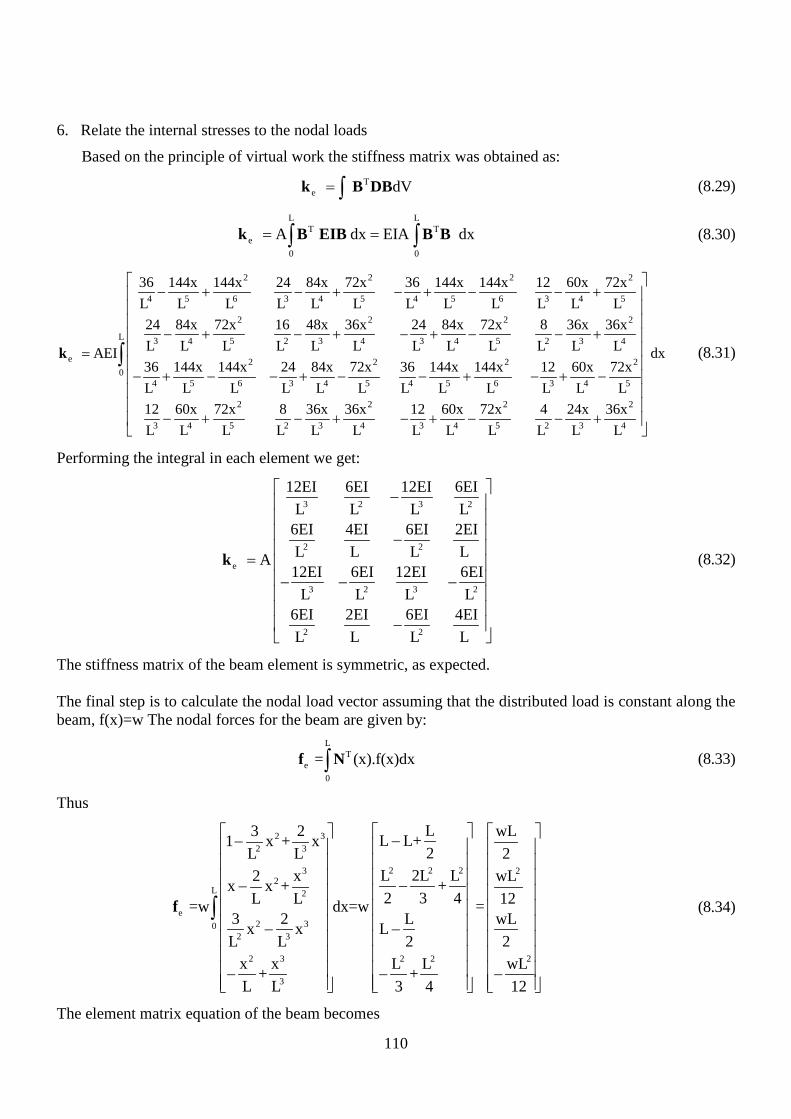
110

6. Relate the internal stresses to the nodal loads

Based on the principle of virtual work the stiffness matrix was obtained as:

Te dV= ∫k B DB (8.29)

L L

T Te

0 0

A dx EIA dx= =∫ ∫k B EIB B B (8.30)

2 2 2 2

4 5 6 3 4 5 4 5 6 3 4 5

2 2 2 2

3 4 5 2 3 4 3 4 5 2 3 4

e 2 2

4 5 6 3 4 5 4 5

36 144x 144x 24 84x 72x 36 144x 144x 12 60x 72xL L L L L L L L L L L L24 84x 72x 16 48x 36x 24 84x 72x 8 36x 36xL L L L L L L L L L L L AEI36 144x 144x 24 84x 72x 36 144x 14L L L L L L L L

− + − + − + − − +

− + − + − + − − +=

− + − − + − − +

kL

2 20

6 3 4 5

2 2 2 2

3 4 5 2 3 4 3 4 5 2 3 4

dx4x 12 60x 72xL L L L

12 60x 72x 8 36x 36x 12 60x 72x 4 24x 36xL L L L L L L L L L L L

− + −

− + − + − + − − +

∫ (8.31)

Performing the integral in each element we get:

3 2 3 2

2 2

e

3 2 3 2

2 2

12EI 6EI 12EI 6EIL L L L

6EI 4EI 6EI 2EIL L L L A12EI 6EI 12EI 6EI

L L L L6EI 2EI 6EI 4EIL L L L

− −

= − − −

−

k (8.32)

The stiffness matrix of the beam element is symmetric, as expected. The final step is to calculate the nodal load vector assuming that the distributed load is constant along the beam, f(x)=w The nodal forces for the beam are given by:

L

Te

0

= (x).f(x)dx∫f N (8.33)

Thus

2 32 3

2 2 23 22

L 2

e2 30

2 3

2 3 2 2 2

3

L3 2 wLL L+1 x + x2L L 2

L 2L L2 x wL+x x +2 3 4L L 12 =w dx=w =

3 2 L wLx x LL L 2 2

x x L L wL+ +L L 3 4 12

−− −− − − − − −

∫f (8.34)

The element matrix equation of the beam becomes

111

3 2 3 2

21

2 21

23 2 3 2

22

2 2

12EI 6EI 12EI 6EI2L L L L

v6EI 4EI 6EI 2EIθL L L L 12Av12EI 6EI 12EI 6EI

L L L L 2θ6EI 2EI 6EI 4EIL L L L 12

wL

wL

wL

wL

− − = − − − − −

(8.35)

8.3 Plate bending theory Plate bending theory, as well as beam theory, is a degeneration of the 3D classical continuum theory. It is assumed that lines normal to the mid-surface of the plate before deformation remain straight and normal to the mid-surface after deformation. This assumption reduces the problem from 3D to 2D, but the rotation of the line involves additional degrees of freedom

Figure 8-3 Formulation of the bending of a plate compressed by a loading force from the top.

The book of Timoshenko (Plates and Shells, McGraw-Hill) provides an excellent introduction to the theory of plates and shell. The book of Logan (first Course in the Finite Element Modelling, Cengage Learning) provides also a simple and detailed introduction. Here we just summarise the main concepts. We define a shell element (Figure 8-3) as a combination of a plate element and a plane stress element. The plane stress element can be deformed only in the parallel direction to the plate. The deformation of the plane stress is defined by u and v. Each point of the plate element has a perpendicular deflection w and two rotation θx and θy. We assume that the moments per unit length, Mx, and My, are positive if the plate is compressed from the top. The curvature κx and κy are positive if the plate is convex downward. The thickness t, Young's modulus E and Poisson's ratio ν of the plate are constant. The variable w is the transverse (z-direction) deflection of the plate mid-surface.

112

Figure 8-4 The shell element is a combination of a plate element and a plane stress element

The kinematic equation of the plate element corresponds to a 2D generalization of the beam theory in Section 8.1. The curvatures are defined by

2 2 2

x y xy2 2

w w wκ κ κ 2x y xy

∂ ∂ ∂= = =

∂ ∂ ∂ (8.36)

which can be written in the matrix form

2

2

x 2

y 2

xy 2

κ κ = w w

κ2

x

y

xy

∂

∂ ∂ ∴ = ∂ ∂

∂

κ L (8.37)

The constitutive equation comes from the elastic analysis of the plate. The final result is

x x3

y y21

2xy xy

M 1 ν 0 κEtM ν 1 0 κ

12(1 ν )M 0 0 (1 ν) κ

= ∴ = − −

M Dκ (8.38)

The combination of the balance of linear and angular moment equation leads to

2 22

xy Tx2 2

M MM +2 + = Q =Qx x y y

y∂ ∂∂− ∴−

∂ ∂ ∂ ∂L M (8.39)

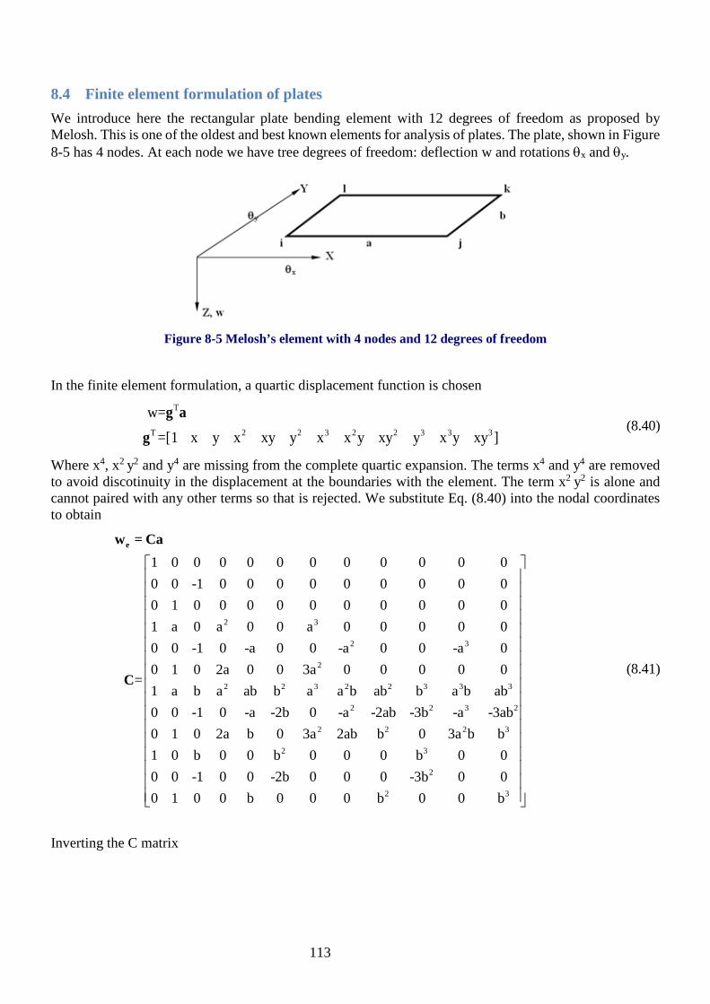
113

8.4 Finite element formulation of plates We introduce here the rectangular plate bending element with 12 degrees of freedom as proposed by Melosh. This is one of the oldest and best known elements for analysis of plates. The plate, shown in Figure 8-5 has 4 nodes. At each node we have tree degrees of freedom: deflection w and rotations θx and θy.

Figure 8-5 Melosh’s element with 4 nodes and 12 degrees of freedom

In the finite element formulation, a quartic displacement function is chosen

T

T 2 2 3 2 2 3 3 3

w==[1 x y x xy y x x y xy y x y xy ]

g ag

(8.40)

Where x4, x2 y2 and y4 are missing from the complete quartic expansion. The terms x4 and y4 are removed to avoid discotinuity in the displacement at the boundaries with the element. The term x2 y2 is alone and cannot paired with any other terms so that is rejected. We substitute Eq. (8.40) into the nodal coordinates to obtain

2 3

2 3

2

2 2 3 2 2 3 3 3

2 2 3 2

2 2 2 3

2 3

2

1 0 0 0 0 0 0 0 0 0 0 00 0 -1 0 0 0 0 0 0 0 0 00 1 0 0 0 0 0 0 0 0 0 01 a 0 a 0 0 a 0 0 0 0 00 0 -1 0 -a 0 0 -a 0 0 -a 00 1 0 2a 0 0 3a 0 0 0 0 0

=1 a b a ab b a a b ab b a b ab0 0 -1 0 -a -2b 0 -a -2ab -3b -a -3ab0 1 0 2a b 0 3a 2ab b 0 3a b b1 0 b 0 0 b 0 0 0 b 0 00 0 -1 0 0 -2b 0 0 0 -3b 0 0

ew = Ca

C

2 30 1 0 0 b 0 0 0 b 0 0 b

(8.41)

Inverting the C matrix

114

2 2

2 2

-13 2 3 2

2 2 2 2

2 2 2 2

1 0 0 0 0 0 0 0 0 0 0 00 0 -1 0 0 0 0 0 0 0 0 00 1 0 0 0 0 0 0 0 0 0 03 2 3 1- 0 0 0 0 0 0 0 0a a a a1 1 1 1 1 1 1 1- - 0 - 0 0 0 -ab a b ab a ab ab b3 2 3 1- - 0 0 0 0 0 0 0 - 0b b b b2 1 2 10 - - 0 - 0 0 0 0 0 0= a a a a3 2 3 1 3 1 3 20 - - 0 - 0 - 0

a b ab a b ab a b ab a b ab3 2 3 2 3 1 30 - - 0 - 0 -

ab ab ab ab ab ab ab

C

3 2 3 2

3 2 3 2 3 2 3 2

3 2 3 2 3 2 3 2

1 0ab

2 1 2 10 0 0 0 0 0 0 - 0b b b b2 1 2 1 2 1 2 1- 0 0 - 0 - 0 -

a b a b a b a b a b a b a b a b2 1 2 1 -2 1 2 1- - 0 0 0 - 0

ab ab ab ab ab ab ab ab

(8.42)

The stiffness matrix is calculating using the operator T -1

e e= = { }B LN L g C , where L is given by Eq. (8.37)

2

2

2

2

2

=

2

x

y

xy

∂−

∂ ∂−

∂ ∂

∂

L (8.43)

The stiffness matrix becomes

e

a bT -1 T T -1

e e eV 0 0

= dV=t ( { (x,y)}. ) ( { (x,y)} )dxdy∫ ∫ ∫Tk B DB L g C D L g C (8.44)

115

3

1 1e 2

0 0

0 0 00 0 00 0 0

1 0 0 0 0 2 . . .2 0 0

{ 1 0 0 0 0 0 . . . }. . .12(1 )

1 0 0 0 0 . . .0 0. . . 2. . .. . .

Ta bEt C dxdy C

νν

νν

− −

− − = − −

∫ ∫k (8.45)

The rest of the steps, including assembling the global matrix equation, applying boundary conditions, and constructing the load vector, follow the standard procedures in previous chapters. In our formulation we assume that the shell can be described as a superposition of a plate element and a plane strain element. Numerous other shell elements have been developed over the years. In some formulations, it is assumed that each element of the shell has six degrees of freedom u, v, w, θx, θy and θz. The last one is the so-called drilling degree of freedom. An artificially stiffness is incorporated to this fictitious degrees of freedom, leading to a formulation that is interesting form the theoretical and practical point of view.

116

Problems Problem 8.1. Structural mechanics: bending of beams A beam fully supported at its two ends has dimensions 2.5m x 0.25m x 0.12m. The material properties are: Young’s modulus: 30,000MPa, Poisson’s ratio 0.2, and density 2,400kg/m3. The load is a combination of the dead load (self-weight) and the live load. The later consists of a load of 1 kN/m distributed along the beam.

w =1kN/ m

0.25m

2.5m

a) Solve the deflection along the beam using simple bending theory.

b) Will the finite element solution with one beam element give the exact solution? Justify your response

Problem 8.2. Structural Mechanics: bending of cantilever beams A cantilever beam has dimensions 2.5m, height 0.25m and thickness (out of plane) 0.12m. The material properties are: Young’s modulus: 30,000MPa, Poisson’s ratio 0.2, and density 2,400kg/m3. The load is a combination of the dead load (self-weight) and the live load. The latter one is a concentrated load at the tip of 4kN.

2.5 m

P= 4 kN

Thickness=0.12m 0.25 m

1) Write the governing equations of the problem

2) Find the analytical solution of the governing equations

3) Using the analytical solution to plot the deflection, bending moment, and shear force versus position

117

Problem 8.3. Rotational stiffness of bended beams The figure below shows the end rotations and the end moments of a beam, along to its total deflection Δ. Solve the equilibrium equation of the beam to obtain a solution for the rotations 1θ and 2θ in terms of the end moments 1M , 2M and the deflection Δ.

1 2 L

θ2, M2

θ1, M1

Δ

Problem 8.4. Frame buckling using beam elements This problem is related to the buckling of a plane frame that has beam and column lengths each of L, pinned at the column bases and fixed against vertical deflection (only) at the 2 extreme beam ends. The loading consists of an equal downward load of P at the top of each column. The beams have an area A, moment of inertia I, Young modulus E, and Poisson ration. The first (sideway) and second (symmetric) buckling modes are shown in the following figures.

(a) First mode of buckling (sideway)

(b) Second mode of buckling (symmetric)

1. Find the critical buckling load as a function of E, I, L, and the buckling factor k. 2. For the sway mode, find the rotational stiffness of the top node of the vertical column, the rotational

stiffness of the node is defined by AA

α α= ∑ where /Mα θ= is the stiffness of any adjacent member

connected to the end of the compression member. The same definition applies to node B. 3. Find the buckling factor of the sway mode using the equation provided below 4. For the symmetric mode, find the rotational stiffness of the top node of the vertical column. 5. Find the buckling factor of the symmetric mode

Hint for the use of the Newton-Raphson method:2(cot ) cosd x ec x

dx= −

118

CHAPTER 9: ACCURACY AND EFFICIENCY IN FINITE ELEMENT MODELLING

ACCURACY AND EFFICIENCY IN FINITE ELEMENT MODELLING

In this chapter we will introduce the isoparametric formulation. This is probably the most important contribution to the field of finite element analysis during the past 40 years. It includes higher-order elements of arbitrary shape (included curved shapes) that are relatively easy to implement into a computer program. The isoparametric formulation is actually used in most commercial packages. The term isoparametric (same parameters) is derived from the use of the same interpolation functions to define the element’s geometric shape as are used to define the displacements within the element. In this chapter, we introduce the basics of this formulation and its implication in accuracy in modelling.

9.1 Accuracy and efficiency of linear triangular elements The linear element is the basic planar element and one of the first elements developed and used in practice. As noted previously, the strains and stresses are constant over the entire area of one element. Therefore a high degree of mesh refinement is required where significant strain gradients exist. Consider two constant strain triangular finite elements shown in Figure 9-1. Assume that only one node of element b is displaced while other nodes are fixed. Then element b is subjected to non-zero strains and stresses, which are constant over the area of the element, while strains and stresses within element “a” are all zero. An infinitesimal element at the boundary of the two finite elements, the shaded area in Figure 9-1, is not in equilibrium. There are obviously discontinuities in strains and stresses at the boundary of the two elements. In view of this fact, it is necessary to use a fine mesh of these elements where high stress or strain gradients are expected.

Figure 9-1 Discontinuity of stress and strain

The linear triangular element has the advantages of simplicity in its formulation. The strain-displacement matrix B is independent of the coordinates. Therefore, the integration of the stiffness matrix T dV∫B DB imposes no difficulty. The main limitation is in accuracy that can be overcome using high-order, isoparametric elements.

119

9.2 Higher order triangular elements Higher order elements have more degrees-of-freedom and usually give a more accurate representation of the actual behaviour. Application of these elements ensures more accurate solutions to be achieved with fewer elements. It was shown in the previous section that the constant strain triangular element has a certain disadvantage, particularly in regions of high stress gradients. One method of dealing with this problem is to use a very fine mesh while still using the basic linear elements. However, an alternative approach is to use higher order elements, elements for which higher order polynomials are used to approximate their displacement functions. This can be done by specifying additional nodes for the elements, thus giving it more degrees-of-freedom. The resulting elements have the advantage that fewer of them are required to achieve certain accuracy. This is at the expense of greater computational complexity that can be easily handled in modern computers. Some of the higher-order triangular elements are shown in Table 9-1 together with the interpolation functions used to derive the stiffness matrices of the elements.

Table 9-1 Planar triangular element types

Shape

Name of

the Element

T3 T6 T9 T10

Shape function Linear Parabolic

Cubic (Non-standard)

Cubic (Standard)

There are substantial advantages on using high-order element in finite element modelling Consider for example the problem of a plate with a hole, See Figure 9-2. If one uses T3 elements, the hole is approximated by a polygon, which produced a substantial error in the modelling of the boundary. The T6 element offers a great improvement in the representation of the boundary. This is because the isoparametric formulation will fit a parabola passing to the three nodes of each side of the T6 element. As a result of that, the circular hole will be replaced to a spline curve (piecewise curve consisting of parabolas) which corresponds to an excellent approximation of the circular hole.

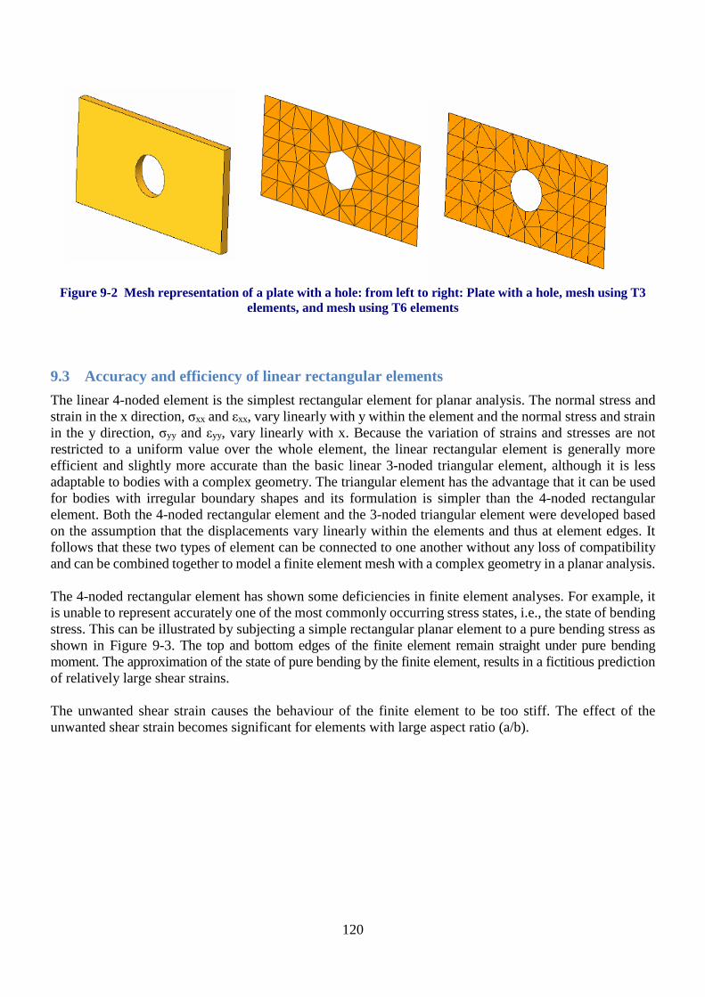
120

Figure 9-2 Mesh representation of a plate with a hole: from left to right: Plate with a hole, mesh using T3 elements, and mesh using T6 elements

9.3 Accuracy and efficiency of linear rectangular elements The linear 4-noded element is the simplest rectangular element for planar analysis. The normal stress and strain in the x direction, σxx and εxx, vary linearly with y within the element and the normal stress and strain in the y direction, σyy and εyy, vary linearly with x. Because the variation of strains and stresses are not restricted to a uniform value over the whole element, the linear rectangular element is generally more efficient and slightly more accurate than the basic linear 3-noded triangular element, although it is less adaptable to bodies with a complex geometry. The triangular element has the advantage that it can be used for bodies with irregular boundary shapes and its formulation is simpler than the 4-noded rectangular element. Both the 4-noded rectangular element and the 3-noded triangular element were developed based on the assumption that the displacements vary linearly within the elements and thus at element edges. It follows that these two types of element can be connected to one another without any loss of compatibility and can be combined together to model a finite element mesh with a complex geometry in a planar analysis. The 4-noded rectangular element has shown some deficiencies in finite element analyses. For example, it is unable to represent accurately one of the most commonly occurring stress states, i.e., the state of bending stress. This can be illustrated by subjecting a simple rectangular planar element to a pure bending stress as shown in Figure 9-3. The top and bottom edges of the finite element remain straight under pure bending moment. The approximation of the state of pure bending by the finite element, results in a fictitious prediction of relatively large shear strains. The unwanted shear strain causes the behaviour of the finite element to be too stiff. The effect of the unwanted shear strain becomes significant for elements with large aspect ratio (a/b).

121

Exact Displacement

M M

Finite Element Displacement

M M

Pure Bending Stress a

b x

y

Figure 9-3 Deformation under pure bending

A large number of these elements have to be used in order to achieve an acceptable accuracy in problems where bending action is important or where a high stress gradient is expected. The use of a greater number of elements in a finite element analysis usually means a longer computation time. Therefore, it is desirable to use higher order elements in many practical analyses.

9.4 High order rectangular elements Higher order elements have more degrees-of-freedom and usually represent a more accurate displacement field, and therefore stress and strain field. Application of fewer elements of this kind in a finite element analysis usually results in a more accurate solution compared with the results of an analysis obtained using lower order elements. To develop higher order elements, higher order polynomials are required in order to approximate displacement functions for the elements. This requires additional nodes which results in more degrees-of-freedom for the elements. Some of the higher order rectangular elements are shown in Table 9-2. The functions used to interpolate the displacements of these elements are usually of the same order in the x and y directions. However, this is not a strict requirement in developing the higher order elements, since it is trivial to generate shape functions for rectangular elements using a different order of interpolation in the x direction to that used in the y direction. This will result in a series of elements which have different numbers of nodal points in the x direction to those in the y direction. It should be noted that as the number of nodes in a finite element increases, calculation of the stiffness matrix of the element becomes more complex. Some of the complexities arise from the parametric multiplication of large matrices and the high number of integration operations. It is also possible increase the accuracy of an element without increasing the nodes. For example, some commercial packages modify the four nodes Q4 element to improve the performance. The modification consists in introducing an additional bubble shape function that considerably decreases the numerical error during bending. As user of commercial packages, you should be aware that there are many improvements of the formulation that affect the calculations, and whose details are hidden to the user.

122

Table 9-2 Higher order rectangular elements

Shape

Name of the

element Q8 Q9 Q12 Q16

Disp. function in x/y direction

Parabolic (Non-standard)

Parabolic (Standard)

Cubic (Non-standard) Cubic (Standard)

9.5 Coordinate transformation and numerical integration The derivation of the stiffness matrix for any high-order element requires integrations of a high number of functions over the area of the element. As the order of the interpolation function for the element increases, integration operations become more complex if they are to be performed analytically. However, analytical integrations may be avoided using coordinate transformation and numerical integration. One of the advantages of numerical integration, as opposed to analytical integration, is that it can all be carried out by the computer. Elements with curved boundaries, or non-rectangular quadrilateral elements can also be easily developed and their stiffness matrices can be integrated without additional difficulty. Summary of numerical integration The term "Quadrature" is the name applied to evaluating an integral numerically rather than analytically. There are a number of methods available for numerical integration. However, the Gauss quadrature rule is the one most often used in finite element analyses and is therefore introduced here. Gauss quadrature rules are written for a finite integral over the interval [ −1, 1] in each coordinate direction. Integration of a function, f(η) in one dimension is expressed as:

( ) ( )1 n

i ii 11

f η dη f η w=−

= ∑∫ (9.1)

where n is the number of integration points (or Gauss points) selected for the integration, ηi is the coordinate for Gauss point i, and wi is the weight for Gauss points. The coordinates of the Gauss points and their weights are well known and some are given in Table 9-3 for various orders of numerical integration.

Table 9-3 Gauss points and weights for one-dimensional integration

Number of Gauss points, n

Coordinate ηi

Weight wi

1 0 2

2 +1/ 3 − 1/ 3

1 1

3 0.6 0

− 0.6

5/9 8/9 5/9

123

The Gauss quadrature rules are designed for cases where f(η) is a polynomial. A rule with n Gauss points is exact for a one-dimensional polynomial integrand of degree up to 2n-1. For example, an integral with 2 Gauss points gives no error for linear, parabolic and cubic polynomials. Gauss quadrature rules may also be used for cases where the integrand is not a polynomial, but the result will only be an approximate one. Integration of a function, f(η,μ) in two dimensions over the area of a quadrilateral, i.e. over the interval [1,1] for both η and μ, can be expressed as:

( ) ( )1 1 n

i i ii 11 1

f η,μ dη dμ f η ,μ w=− −

= ∑∫ ∫ (9.2)

where η i and μ i are the coordinates for Gauss point i. The coordinates of the Gauss points and their weights for two dimensions are given in Table 9-4. The two-dimensional quadrature rules are a simple generalization of the one-dimensional rules where f(η, μ) is a polynomial. A rule with n Gauss points is exact for a two-dimensional polynomial integrand of degree up to 2 1n − . For example, a one-Gauss point rule is valid for a constant or linear function, a 4-Gauss point rule gives no integration error for a polynomial up to and including a cubic.

Table 9-4 Gauss points and weights for two-dimensional integration

Number of Gauss points, n

Coordinate ηi

Coordinate µi

Weight wi

1 0 0 4

4

− 1/ 3 +1/ 3 − 1/ 3 +1/ 3

− 1/ 3 − 1/ 3 +1/ 3 +1/ 3

1 1 1 1

9

− 0.6 0

+ 0.6 − 0.6

+0 + 0.6 − 0.6

0 + 0.6

− 0.6 − 0.6 − 0.6

0 0 0

+ 0.6 + 0.6 + 0.6

25/81 40/81 25/81 40/81 64/81 40/81 25/81 40/81 25/81

Integration schemes for two-dimensional triangular elements can be found in most of the finite element textbooks. It is recommended that an integration rule with 3 Gauss points is used for all triangular elements and an integration rule with at least 4 Gauss points is used for quadrilateral elements. Natural coordinates In order to evaluate an integral over the area or volume of an arbitrary-oriented element, it is necessary to transform the coordinates, as shown the Figure 9-4. In this procedure it is convenient to introduce a system

124

of natural coordinates. A model element is chosen in the interval of [ −1,1] in each direction, so that all of the integrations required to form the element stiffness matrix can be performed using a quadrature rule. Then the real finite element, in the coordinate system x and y, can be mapped onto the model element, in the natural coordinate system, using a standard transformation.

Figure 9-4 Finite element in the natural coordinates (left) and in the Cartesian coordinates (right) the elements shown are: Q4,Q9, T3, and T6.

To transform the variables and the region with respect to which the integration is made a standard process in integral calculus will be used which involves the determinant of the Jacobian matrix, detJ. For example The integration of a function f over the volume eV of the element e becomes:

e

1 1 1

V 1 1 1

f(x,y,z)dx dy dz f(η, μ,ζ)det dη dμ dζ− − −

=∫ ∫ ∫ ∫ J (9.3)

where η, μ and ζ are the natural coordinates corresponding to the actual coordinates of x, y and z, and the Jacobian matrix is calculated as

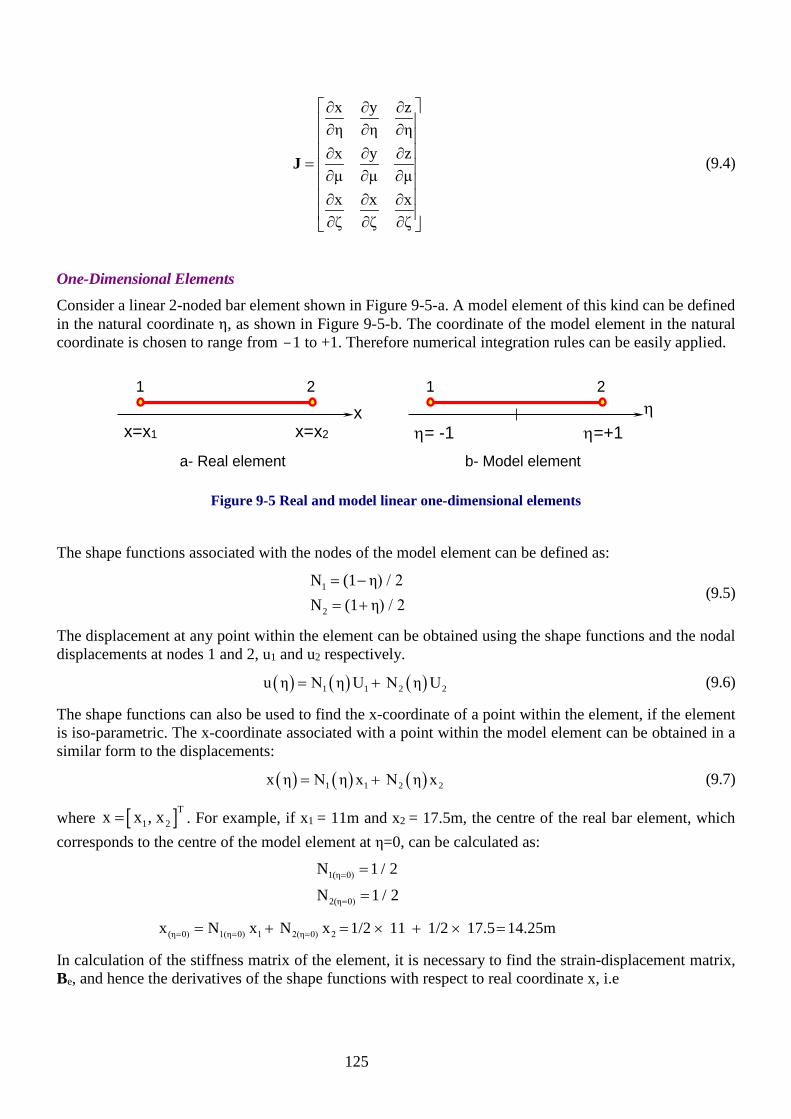
125

x y zη η ηx y zμ μ μx x xζ ζ ζ

∂ ∂ ∂ ∂ ∂ ∂ ∂ ∂ ∂

= ∂ ∂ ∂ ∂ ∂ ∂ ∂ ∂ ∂

J (9.4)

One-Dimensional Elements Consider a linear 2-noded bar element shown in Figure 9-5-a. A model element of this kind can be defined in the natural coordinate η, as shown in Figure 9-5-b. The coordinate of the model element in the natural coordinate is chosen to range from −1 to +1. Therefore numerical integration rules can be easily applied.

x=x1 x=x2

1 2 1 2

η= -1 η=+1 η x

a- Real element b- Model element

Figure 9-5 Real and model linear one-dimensional elements

The shape functions associated with the nodes of the model element can be defined as:

1

2

N (1 η) / 2N (1 η) / 2

= −= +

(9.5)

The displacement at any point within the element can be obtained using the shape functions and the nodal displacements at nodes 1 and 2, u1 and u2 respectively.

( ) ( ) ( )1 1 2 2u η N η U N η U= + (9.6)

The shape functions can also be used to find the x-coordinate of a point within the element, if the element is iso-parametric. The x-coordinate associated with a point within the model element can be obtained in a similar form to the displacements:

( ) ( ) ( )1 1 2 2x η N η x N η x= + (9.7)

where [ ]T1 2x x , x= . For example, if x1 = 11m and x2 = 17.5m, the centre of the real bar element, which

corresponds to the centre of the model element at η=0, can be calculated as:

1(η 0)

2(η 0)

N 1 / 2N 1 / 2

=

=

=

=

(η 0) 1(η 0) 1 2(η 0) 2x N x N x 1/2 11 1/2 17.5 14.25m= = == + = × + × =

In calculation of the stiffness matrix of the element, it is necessary to find the strain-displacement matrix, Be, and hence the derivatives of the shape functions with respect to real coordinate x, i.e

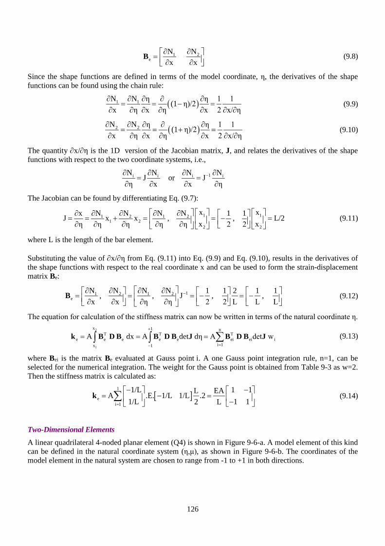
126

1 2e

N Nx x

∂ ∂ = ∂ ∂ B (9.8)

Since the shape functions are defined in terms of the model coordinate, η, the derivatives of the shape functions can be found using the chain rule:

( )1 1N N η η 1 1(1 η)/2x η x η x 2 x/ η

∂ ∂ ∂ ∂ ∂= = − =

∂ ∂ ∂ ∂ ∂ ∂ ∂ (9.9)

( )2 2N N η η 1 1(1 η)/2x η x η x 2 x/ η

∂ ∂ ∂ ∂ ∂= = + =

∂ ∂ ∂ ∂ ∂ ∂ ∂ (9.10)

The quantity ∂x/∂η is the 1D version of the Jacobian matrix, J, and relates the derivatives of the shape functions with respect to the two coordinate systems, i.e.,

1i i i iN N N NJ or Jη x x η

−∂ ∂ ∂ ∂= =

∂ ∂ ∂ ∂

The Jacobian can be found by differentiating Eq. (9.7):

1 11 2 1 21 2

2 2

x xN N N Nx 1 1J x x , , L/2x xη η η η η 2 2

∂ ∂ ∂ ∂∂ = = + = = − = ∂ ∂ ∂ ∂ ∂ (9.11)

where L is the length of the bar element. Substituting the value of ∂x/∂η from Eq. (9.11) into Eq. (9.9) and Eq. (9.10), results in the derivatives of the shape functions with respect to the real coordinate x and can be used to form the strain-displacement matrix Be:

11 2 1 2e

N N N N 1 1 2 1 1, , J , ,x x η η 2 2 L L L

− ∂ ∂ ∂ ∂ = = = − = − ∂ ∂ ∂ ∂ B (9.12)

The equation for calculation of the stiffness matrix can now be written in terms of the natural coordinate η.

2

1

x 1 nT T T

e e e e e ei ei ii 1x 1

A dx A det dη A det w+

=−

= = = ∑∫ ∫k B D B B D B J B D B J (9.13)

where Bei is the matrix Be evaluated at Gauss point i. A one Gauss point integration rule, n=1, can be selected for the numerical integration. The weight for the Gauss point is obtained from Table 9-3 as w=2. Then the stiffness matrix is calculated as:

[ ]1

ei 1

1/L 1 1L EAA .E. 1/L 1/L .21/L 1 12 L=

− − = − = −

∑k (9.14)

Two-Dimensional Elements A linear quadrilateral 4-noded planar element (Q4) is shown in Figure 9-6-a. A model element of this kind can be defined in the natural coordinate system (η,μ), as shown in Figure 9-6-b. The coordinates of the model element in the natural system are chosen to range from -1 to +1 in both directions.

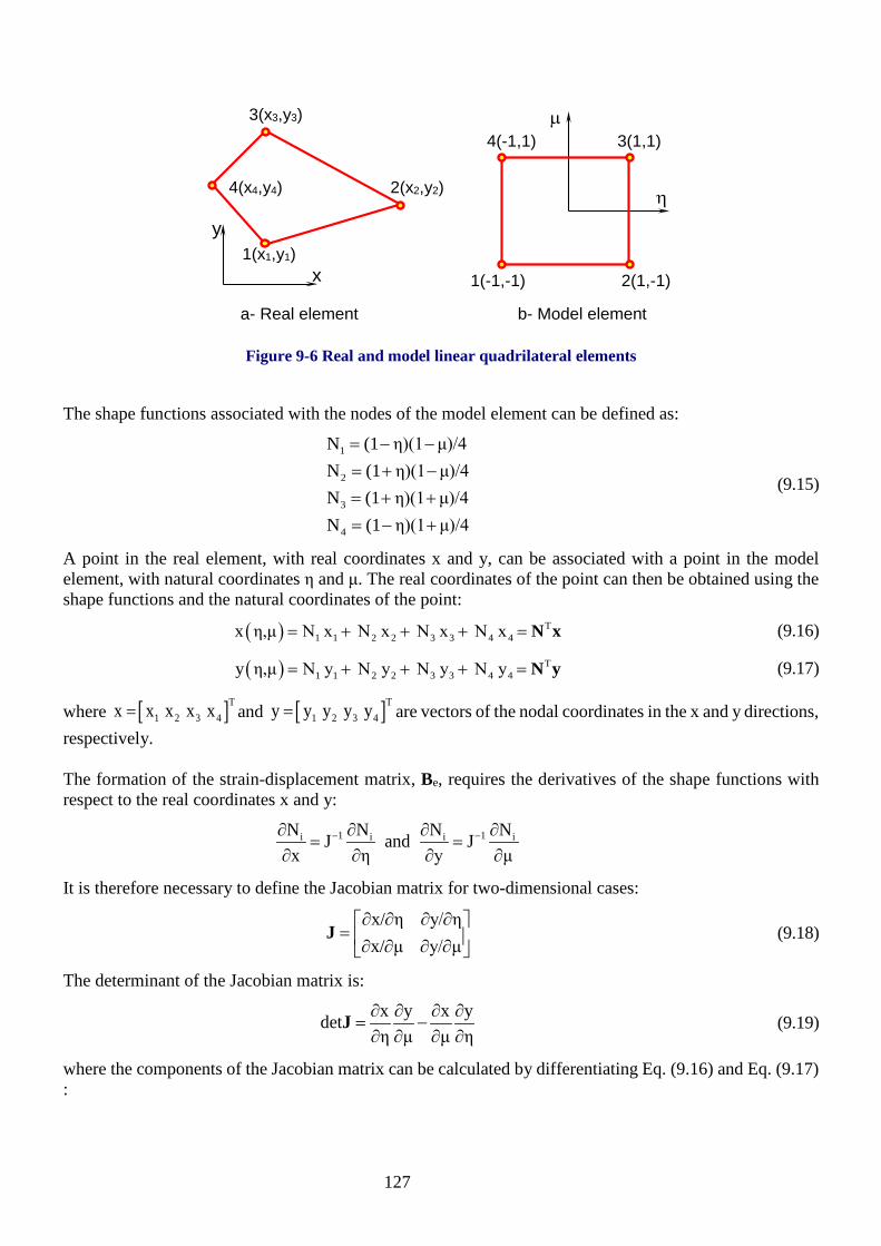
127

1(-1,-1) 2(1,-1)

3(1,1) 4(-1,1)

1(x1,y1)

a- Real element b- Model element

2(x2,y2)

3(x3,y3)

4(x4,y4)

x

y η

µ

Figure 9-6 Real and model linear quadrilateral elements

The shape functions associated with the nodes of the model element can be defined as:

1

2

3

4

N (1 η)(1 μ)/4N (1 η)(1 μ)/4N (1 η)(1 μ)/4N (1 η)(1 μ)/4

= − −= + −= + += − +

(9.15)

A point in the real element, with real coordinates x and y, can be associated with a point in the model element, with natural coordinates η and μ. The real coordinates of the point can then be obtained using the shape functions and the natural coordinates of the point:

( ) T1 1 2 2 3 3 4 4x η,μ N x N x N x N x= + + + = N x (9.16)

( ) T1 1 2 2 3 3 4 4y η,μ N y N y N y N y= + + + = N y (9.17)

where [ ]T1 2 3 4x x x x x= and [ ]T

1 2 3 4y y y y y= are vectors of the nodal coordinates in the x and y directions, respectively. The formation of the strain-displacement matrix, Be, requires the derivatives of the shape functions with respect to the real coordinates x and y:

1 1i i i iN N N NJ and Jx η y μ

− −∂ ∂ ∂ ∂= =

∂ ∂ ∂ ∂

It is therefore necessary to define the Jacobian matrix for two-dimensional cases:

x/ η y/ ηx/ μ y/ μ

∂ ∂ ∂ ∂ = ∂ ∂ ∂ ∂

J (9.18)

The determinant of the Jacobian matrix is:

x y x ydetη μ μ η

∂ ∂ ∂ ∂= −

∂ ∂ ∂ ∂J (9.19)

where the components of the Jacobian matrix can be calculated by differentiating Eq. (9.16) and Eq. (9.17):

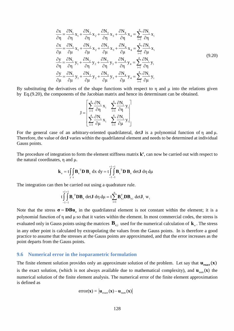
128

431 2 4 i

1 2 3 4 ii 1

431 2 4 i

1 2 3 4 ii 1

431 2 4 i

1 2 3 4 ii 1

431 2 4 i

1 2 3 4 ii 1

NN N N Nx x x x x xη η η η η η

NN N N Nx x x x x xμ μ μ μ μ μ

NN N N Ny y y y y yη η η η η η

NN N N Ny y y y y yμ μ μ μ μ μ

=

=

=

=

∂∂ ∂ ∂ ∂∂= + + + =

∂ ∂ ∂ ∂ ∂ ∂

∂∂ ∂ ∂ ∂∂= + + + =

∂ ∂ ∂ ∂ ∂ ∂

∂∂ ∂ ∂ ∂∂= + + + =

∂ ∂ ∂ ∂ ∂ ∂

∂∂ ∂ ∂ ∂∂= + + + =

∂ ∂ ∂ ∂ ∂ ∂

∑

∑

∑

∑

(9.20)

By substituting the derivatives of the shape functions with respect to η and μ into the relations given by Eq.(9.20), the components of the Jacobian matrix and hence its determinant can be obtained.

4 4i i

i ii 1 i 1

4 4i i

i ii 1 i 1

N Nx yη η

JN Nx yμ μ

= =

= =

∂ ∂ ∂ ∂ = ∂ ∂ ∂ ∂

∑ ∑

∑ ∑

For the general case of an arbitrary-oriented quadrilateral, detJ is a polynomial function of η and μ. Therefore, the value of detJ varies within the quadrilateral element and needs to be determined at individual Gauss points. The procedure of integration to form the element stiffness matrix ke, can now be carried out with respect to the natural coordinates, η and μ.

1 1

T Te e e e e

y x 1 1

t dx dy t det dη dμ+ +

− −

= =∫ ∫ ∫ ∫k B D B B D B J

The integration can then be carried out using a quadrature rule.

1 1 n

T Te e e,i e,i i i

i 11 1

t det dη dμ t det w+ +

=− −

= ∑∫ ∫ B DB J B DB J

Note that the stress e=σ DBu in the quadrilateral element is not constant within the element; it is a polynomial function of η and μ so that it varies within the element. In most commercial codes, the stress is evaluated only in Gauss points using the matrices e,iB used for the numerical calculation of ek . The stress in any other point is calculated by extrapolating the values from the Gauss points. In is therefore a good practice to assume that the stresses at the Gauss points are approximated, and that the error increases as the point departs from the Gauss points.

9.6 Numerical error in the isoparametric formulation The finite element solution provides only an approximate solution of the problem. Let say that ( )exactu x is the exact solution, (which is not always available due to mathematical complexity), and num ( )u x the numerical solution of the finite element analysis. The numerical error of the finite element approximation is defined as

exact numerror( ) = ( ) ( )−x u x u x

129

Since the isoparametric formulation involves few approximations, there is a numerical error that you need to be aware when taking conclusions from the numerical results. From this numerical error we can distinguish three different sources:

1. Domain approximation error, due to approximation of the boundary of the domain by a linear (T3,Q4), quadratic (T6, Q8), or higher order polynomials.

2. Approximation error, due to approximation of the solution by piecewise polynomials (shape functions). This error is decreased when the order of the element is higher.

3. Computational error, due to the use of quadratures in the calculation of the integrals to evaluate the stiffness matrix and the load vectors.

Figure 9-2 shows an example of the domain approximation error: the mesh with T3 elements approximate the circular boundary by a polygon, leading to a large domain approximation error. Replacing the element from T3 to T6 leads to a considerable decrease of this error, since the circular boundary is well approximated by a spline curve. The advantage of the use of higher-order elements is that curved boundaries of irregularly shaped bodies can be approximated more closely than by the use of simple straight-sided linear elements. The approximation error, due to approximation of the solution by piecewise polynomials (shape functions), can be decreased when the order of the element is higher. In general, higher-order element shape functions can be developed by adding additional nodes to the sides of the linear element. These elements result in higher-order strain variations within each element, and convergence to the exact solution thus occurs at a faster rate using fewer elements. The computational error, resulting from approximating the integral by quadratures, is produced by the coordinate transformation from the actual element to the natural element. Elements that are heavily distorted from its natural element usually produce large computational error. Some finite element codes allow measuring this distortion by using a normalized Jacobian eJ which ranged from one for perfectly shaped element to 0 for heavily distorted element. As finite element user, you should avoid element whose normalized Jacobian is too small. The Figure 9-7 below, for example shows two different meshes of a circular area. The left one has very elongated element at the centre that produces large computational error. In the right one the elements are close to squares, which minimized the numerical error of the calculation of stiffness matrix.

Figure 9-7 Real and model linear quadrilateral elements. The arrow at the left figure shows one of the

heavily distorted elements.

130

Basically the quality of the mesh will define the accuracy of the finite element calculation. The mesh can be coarse (have few elements) or refined (have many elements). It is not a general rule that refining the mesh will reduce the numerical error, and in some cases it is better to increase the order of the elements. Refining a region of the domain can be dangerous, since it can lead to incompatibilities: it means, nodes in one element that are not connected to the neighbour element. In these cases we observe spurious discontinuities in the finite element solutions. To avoid discontinuities, it is recommended to use transition elements that connect the coarse region with the refined one, see Figure 9-8.

Figure 9-8 Transition elements using Q4 elements allow to connect a coarse mesh (top) with a fine one

(bottom)

The way we impose boundary conditions can also lead to sources of errors. Stress singularities appear when a load is concentrated in a single node, and it is recommended to distribute the load in few nodes before mesh refining. Finally, unrealistic concentration of stresses can appear in corners of the mesh and it may be necessary to smooth the boundaries or the boundary conditions to reduce the numerical error.

131

Problems Problem 9.1. Isoparametric formulation of high-order 1D element Derive the shape functions of the thermally loaded, master, one-dimensional element with three nodes and a scalar variable T(η)

Problem 9.2. Numerical error in isoparametric formulation A mesh of T3 elements are proposed for calculation of the stress in a plate with a hole. Discuss the three possible causes of numerical error in the finite element analysis using this mesh. Problem 9.3. Thin plate with a hole For the finite element analysis of the plate with a hole, three different meshes are generated, see Figure 2. The symmetry has been considered and thus only a quarter of the model is needed. All the elements are Quad8.

E=200,000 MPa

ν=0.3 1.0 MPa 1.0 MPa

800 mm

40 mm

400 mm

-1 1 η

T 0

132

1) Determine all boundary conditions of the quarter domain. 2) What of the three meshes of Figure 2 will produce the most accurate stress calculation around its

peak value? 1. Justify the response listing the errors produced in each mesh. *Mesh 1 has small squared element at the zone of stress concentration. Mesh 2 is not a good option due to mesh incompatibilities; Quality of Mesh 3 is low.

Mesh 1: 232 Quad8 elements Detail of mesh 1

Mesh 2: 849 Quad8 elements Detail of mesh 2

Mesh 3: 576 Quad8 elements Detail of mesh 3

133

Problem 9.4 Pre-stressed concrete beam A part of a pre-stressed concrete beam is shown in the figure below. The beam has a cross section area of 1m × 2m and a total length of 25 m. The pre-stressing cables apply a total end force of 24000 kN over an area of 0.8m×0.4m. The Young’s modulus and Poisson’s ratio for the concrete material is 30 GPa and 0.25, respectively. You are required to find regions of high transverse tensile stress in the concrete beam due to the external compressive force of the cables. Prepare a suitable mesh to model the beam for a finite element analysis. The maximum number of nodes that you may use is limited to 2000. Solve the problem and answer the following questions: 1- Is a plane stress or plane strain analysis more appropriate? Give reasons. 2- Discuss the degree of mesh refinement that is desirable in the several zones of the beam. Do you need

to model the whole beam in order to find the tensile stresses? 3- Discuss the advantages of the finite element type that you have used in the analysis. Give the total

number of nodes and elements used in your final analysis. 4- At what distance from the ends may the compressive stresses be expected to become approximately

uniform? 5- Draw (or plot) the region where the transverse tensile stress is greater than 1000 kPa. Give the extent

of the region from one end.

0.8m

0.8m

0.4m0.8m

1.0 m

25 m

134

CHAPTER 10: VIBRATION OF STRUCTURES

VIBRATION OF STRUCTURES

The study dynamics of a structure, whether produced by wind load, truck or pedestrian load, or earthquake load, is one of the most important aspects of numerical modelling. Most of the analysis done in engineering assumes that the structure is static. Yet there are many situations where the load changes in time and therefore inertia and damping effects become important. In high-rise buildings, wind loads activate its natural frequencies and may produce uncomfortable oscillations that need to be damped. The 101 Tower in Taiwan incorporates a giant mass damper at its top to effectively damp oscillations. Earthquakes produces a wide spectrum of frequencies in the ground motion. When these frequencies match the natural oscillation of the building, the whole structure may collapse. In bridges there is also unprecedented dynamical phenomena, like the constant sawing of the Millennium Bridge in London due to pedestrian traffic, or the complete collapse of the Tacoma Narrow Bridge due to wind load. The mathematical modelling of these processes requires a clear understanding of the natural frequencies of the structures, and how these frequencies respond to external time-dependent loads.

10.1 Vibration of one degree of freedom If a force is suddenly applied to a structure and then released (a transient excitation), the structure will vibrate at a unique frequency determined by its stiffness, called the natural frequency. If a structure is subject to sustained excitation, the vibration response of the structure will vary depending on the frequency of the sustained excitation. As the exciting frequency approaches the natural frequency of the structure, the movement of the structure will become magnified, because each application of the exciting force will add to the existing vibration of the structure. This is the phenomenon of resonance.

k

c

m

Figure 10-1 Harmonic oscillator with mass m, spring constant k, and damping constant c.

In the dynamic analysis, the structure can be represented as a collection of independent harmonic oscillators that responds independently to the external actions. A harmonic oscillator, Figure 10-1, is an idealised structure consisting of a mass m attached to a spring with spring constant k and a damping constant c . The spring constant accounts to an elastic force applied to the mass given by

elasticF = ku− (10.1)

where u is the displacement of the mass from its resting position. The damping constant accounts for dissipation of energy that reduces the duration and amplitude of vibrations. As the mass moves the force due to damping is proportional to its velocity, and acts in the opposite direction

dampingF = cu− (10.2)

135

where u represents the time derivative of the position, which is the velocity. If F(t) is the time dependent external force acting on the mass, the second Newton’s laws states that

elastic dampingmu=F +F +F(t) (10.3)

Replacing Eqs. (10.1) and (10.2) in (10.3) we derive the equation of motion of the harmonic oscillator ku+cu+mu=F(t) (10.4)

10.2 Vibration of multiple degree of freedom structures Consider, for example, the two storey building frame drawn below.

mass 1

mass 2 L1

L2

Figure 10-2 Lumped mass model of a two storey building

It is assumed that the beams are rigid, so the beam/column connection cannot rotate. The shape of the structure can therefore be defined by the horizontal translation of the upper storey and the horizontal translation of the lower storey (degrees of freedom 1 and 2 respectively). Consistent with this assumption, the mass of each beam can be lumped at its centroid. This is known as lumped mass model. The model of a multi degree of freedom structure is often more generally represented by springs and masses as below,

m2 m1

Figure 10-3 Idealised model of two lumped masses

The Newton’s second law for a system of two undamped mass is given by

1m 1 1 1 2 1 1F = k u +k u +F (t)=mu−∑ (10.5)

( )2m 1 1 1 2 2 2 2F =k u k +k u +F (t)=mu−∑ (10.6)

which can be written in matrix form as,

1 1 1 1 1 1

2 2 1 1 2 2 2

m 0 u k k u F (t)+

0 m u k k +k u F (t)−

= −

(10.7)

This matrix equation can be expressed in a compact matrix form as follows

136

+ = (t)MU KU F (10.8)

where the mass matrix, stiffness matrix, displacement vector, and force vector are given by

1 1 1 1 1

2 1 1 2 2 2

m 0 k k u F (t) = (t)

0 m k k +k u F (t)−

= = = − M K U F (10.9)

10.3 Vibration of a continuum structure Using finite element analysis it is possible to analyse dynamics of a continuous structure as a system of finite degrees of freedom. The governing equation of the structure is given by

2

T2[ ] , t ρ

t∂∂

uL σ + w(x ) = (10.10)

where the last term account for the inertial forces acting on the structure, and ρ is the density of the material. The weak form of this equation is obtained by multiplying it by a virtual displacement and integrating it over its domain.

( )2

*T T *T2

V V

( ) ( ) dV ρ dV t

∂+ =

∂∫ ∫uu L σ x w x u (10.11)

The integration by part convert this equation into

1

2*T *T *T *T

2A V V

dV dA+ dV+ ρ dV tV

∂=

∂∫ ∫ ∫ ∫uε σ u T u w u (10.12)

where 1A is the area were the traction is applied. The next step is to adapt a mesh to the domain of the system, and to introduce a set of interpolation function that connects the displacement of the nodes with the continuous displacement of the structure:

=u NU (10.13)

Replacing Eq. (9.18) and (9.19) into Eq. (9.17) the matrix element equation becomes

+ = (t)MU KU F (10.14)

T Tρ dV dVV V∫ ∫M = N N K = B DB (10.15)

T T

V

dV daS

= +∫ ∫F N w N T (10.16)

10.4 Determining the natural frequencies of the structure The goal of a dynamics analysis of a structure is to find the solution of the matrix equation

+ = (t)MU KU F (10.17)

where the matrices M, K, and F(t) are given. We also request initial conditions, which corresponds to the initial displacement and velocities of the structure. The Eq. (10.17) can be numerical solved using the so-called transient solver. This is time stepping algorithm that tracks the position of each node of the structure in a sequence of discrete timeframes. In practice, this method is not used very often because it involves large amount of calculations.

137

The spectral solvers provide an alternative to the transient solvers that is computationally much more favourable. The principle of this solver is to find the natural vibrations of the structure, which are the vibration experienced due to an initial disturbance in the system. This part of the analysis is called natural frequency solver. Once the vibrational modes are found, we will find the response of each natural mode to any external load (wind, earthquake, or pedestrian motion). The numerical solution is then assumed to be a linear combination of the response of each individual mode. We will start explaining the way to find the natural frequencies of the structure, and then we will introduce the equations of the spectral solution. Natural frequency solver To find the natural frequencies and the vibrational modes of the structure we remove the damping forces and external forces from the governing equation Eq. (10.17)

+ =MU KU 0 (10.18)

We seek as a solution a simple oscillatory function with frequency ω

jωt(t) e= 0U U (10.19)

Replacing Eq. (10.19) into Eq. (10.18) we obtain

20( ω ) 0− =K M U (10.20)

To find a non-trivial solution of this equation, we required the matrix accompanying 0U in Eq. (10.20) to be singular. In other words, its determinant should be zero

ω 0− 2K M = (10.21)

The evaluation of this determinant leads to a polynomial function of ω2. The order of the polynomial is the same as the number of degrees of freedom dofn , and hence we obtain dofn independent values of the natural frequencies. Therefore, a structure has the same number of natural frequencies as there are degrees of freedom to describe the displacements of the masses. The frequencies are usually sorted in ascending order, and the smallest one is called the fundamental frequency of the structure. Each frequency will correspond to a mode shape according to the Eq. (10.20). The modes shapes correspond to an excellent set of base functions to express the general solution of a dynamic probem, as we will see in the next section. Finding the mode shapes

To find themode shapes of the natural frequency iω , we replace into the Eq. (10.20).

2i i( ω ) 0− =K M U (10.22)

The corresponding vibrational modes is given by the ijω tieU . The mode shapes has a special ortogonality

property that is derived as follows: Lets consider the Eq. (10.22) For two different natural frequencies iωand kω

2i i2k k

( ω ) 0( ω ) 0

− =

− =

K M UK M U

(10.23)

138

Lets multiply the first equation by the transpose of a mode shape kU , and the second equation by the

transpose of iU corresponding to the natural frequency kω

T 2 Tk i i k iω 0− =U KU U MU (10.24)

T 2 Ti k k i kω 0− =U KU U MU (10.25)

Now we use an important property of the mode shapes taht can be deduced from the structure of the matrices: The stiffness matrix K is symmetric and mass matrix M is diagonal, so that we can transpose the Eq. (10.25) is given by

T 2 Tk i k k iω 0− =U KU U MU (10.26)

Now if we substract this equation from Eq. (10.24) we get 2 2 T

i k k i(ω ω ) 0− =U MU (10.27) or,

Ti k k iω ω =0≠ ⇒ U MU (10.28)

This equation states that the mode shapes of different natural frequencies are orthogonal with respect to the mass matrix M . Substituting Eq. (10.28) we obtain that

Ti k k iω ω =0≠ ⇒ U KU (10.29)

so that the mode shapes are also orthogonal with respect to the stiffmess matrix K . Since the modes shapes correspond to an orthogonal basis in the dofn –dimensional space, any displacement of the structure can be expressed as a linear combination of these eigenvectors. Let us assume that r is an arbitrary vector in the dofn –dimensional space. We express this vector as a superposition of mode shapes

dofn

k kk=1

= c∑r U (10.30)

Each coefficient ic of this superposition can be calculated by multiplying this equation by TiU M and using

the orthgonality property

Ti

i Ti i

c = U MrU MU

(10.31)

These coefficient are known as mass participation factor of the vector r . Finding the mode shapes

The absolute value or norm of of any dofn –dimensional vector can be defined as

T=r r Mr (10.32)

139

In most cases it is convenient to convert the mode shapes in orthonormal base by dividing each mode shape by its norm. After normalization of the mode shapes, the norm of any vector can be calculated by replacing Eq. (10.32) into Eq. (10.30). This results in:

dofn

2i

i=1r = c∑ (10.33)

This equation is nothing more that the generalization of the Pythagoras’ theorem in the high dofndimensional space, which is useful for the response spectrum method introduced in the next section.

10.5 Response Spectrum Method To perform an analysis of a structure under time variable loads, it is necessary to have a precise information on the evolution of the load with time. In some cases, such as in earthquake analysis, this information is not available. Instead we have only the peak responses of harmonic oscillators as a function of their frequency. The response spectrum method allows us to calculate the peak response of a structure from using the natural frequency analysis (natural frequencies and mode shapes) and the response spectrum to the external load. Response spectrum A response spectrum is a plot of the peak response (displacement, velocity of acceleration) of a harmonic oscillator subjected to a specified acceleration. Let us start writing the equation for a harmonic oscillator

m (t) c (t) k (t)=mg(t)φ φ φ+ + (10.34)

Before solving the ordinary differential equation Eq. (10.34), we write them in a convenient form:

20 i 0(t) 2ξω (t) ω (t)=g(t)φ φ φ+ + (10.35)

where 0ω = k/m is the natural frequencies, and 0c / (2m ω )ξ = is the so-called damping ratio. Duhamel’s integral provides a solution to Eq. (10.35)

it -ξω (t τ)

2i d d i

d0

e(t) g(t) sin(ω (t τ))dτ ω =ω 1 ξω

φ−

= − −∫ (10.36)

The relative displacement spectra is defined as the maximal displacement of the harmonic oscillation due to this ground motion

0 i maxS (ξ,ω )= (t) d φ (10.37)

In similar way, the velocity response spectrum, and the acceleration response spectrum are given by

v 0 maxS (ξ,ω )= (t)φ (10.38)

a 0 maxS (ξ,ω )= (t)φ (10.39)

In the case of earthquake response, the response spectral is calculated from the ground acceleration and the damping on the system. For the analysis of a structure, a history data of earthquake is analysed and the response spectral can be found in the tables and standards.

140

Spectral response solver The spectral response analysis provides a solution to the following equation:

g(t)=MU + CU + KU Mr (10.40)

where the external force is written as (t)= g(t)F Mr , being g(t) the imposed acceleration and the influence coefficient factor r an dofn -dimensional vector accounting to the participation the external load in each one of the nodes. We proposed solution to Eq. (10.25) as a time-modulated combination of modes

dofn

k kk=1

(t)= (t)φ∑U U (10.41)

where kU the vibrational models which are assumed to be normalized k 1=U as Inserting Eq. (10.41) into Eq. (10.40) we obtain

( )dofn

k k k k k kk=1

(t) (t) (t) g(t)φ φ φ =∑ MU + CU + KU Mr (10.42)

Now we assume that the matrices M and C are diagonal, which is valid to classically mass-damped systems. Multiplying by T

iU and using the orthogonality of the modes given by Eq. (10.28)

T T T Ti i i i i i i i i i(t) (t) (t) g(t)φ φ φ =U MU + U CU + U KU U Mr (10.43)

Simplifying

i i i i i i i im (t) c (t) k (t)=m g(t)φ φ φ Γ+ + (10.44)

T

T T T ii i i i i i i i i i T

i i

m c k = = = Γ =U MrU MU U CU X KX

U MU (10.45)

Before solving the ordinary differential equations Eq. (10.44), we write them in a convenient form:

2i i i i i(t) 2 (t) (t) = g(t)iφ ξω φ ω φ Γ+ + (10.46)

where i i iω =k /m are the natural frequencies, and i ic / (2m ω )ξ = are the damping ratios. Duhamel’s integral provides a solution to Eq. (10.46).

i i( ) Γ ( ,ω , )i t S tφ ξ= (10.47)

where

i-ξω (t τ)

2i d d i

d0

eS(ξ,ω ,t) g(t) sinω (t τ)dτ ω =ω 1 ξω

t −

= − −∫ (10.48)

Note that the function iS(ξ,ω ,t) is the response of a harmonic oscillator with natural frequency ω and damping ratio ξ to a imposed acceleration g(t). Replacing Eq. (10.48) into Eq. (10.47) and into Eq. (10.41) gives the spectral solution of the problem. In practice, the calculation dofn ordinary differential equation may result cumbersome. Thus the problem is further simplified by truncating the sum in Eq. (10.41) to keep only the modes that mostly contribute to the dynamical response of the system. First we consider the maximal modal displacement of each mode:

141

i,max i i imax= (t) = Γ S(ξ,ω )φ φ (10.49)

Then the total response can be calculated by summing the individual responses of each degree of freedom. The simplest superposition method is the absolute sum that assumes all modals peaks at the same time. The maximum response is given by

max i,max i i1 1

Γ S(ξ,ω )dof dofn n

i iU φ

= =

= =∑ ∑ (10.50)

In the SRSS method the maximal response is obtained from Euclidian norm of individual response

[ ]22max i,max i i

1 1Γ S(ξ,ω )

dof dofn n

i iU φ

= =

= =∑ ∑ (10.51)

There are more alternatives to superpose the modes, but the most important point is that modes of high frequencies may be removed from the sum as they do not contribute much to the sum.

142

Problems Problem 10.1. Spectral Response A two storey frame building has the mass described in the following figures. The upper columns have a stiffness k and the lower one 2k, where k=200kN/m.

(a) Two-storey building

(b) Spectral acceleration response

1. Determine the matrices K and M

2. Calculate the natural frequencies

3. Calculate the mode shapes

4. Calculate the mass participation factor of each mode

5. Obtain the acceleration of each node using the spectral response given in Figure 2

mass 12t

mass 24t

143

APPENDIX A

A SUMMARY OF MATRIX ALGEBRA A matrix is a set of numbers arranged in rows and columns. An r by c matrix A (rxc) is a matrix which has a total of r rows and c columns. The following rules and definitions apply:

• A square matrix A(nxn) is a matrix which has as many rows as columns. • An identity matrix I of dimensions nxn is a square matrix. • A matrix A(rxc) can be multiplied by a scalar number p, by multiplying each of its elements by that

number. The result is a matrix B=pA of the same dimensions, rxc, as A. • Two matrices A (raxca) and B(rbxcb) can be added together or subtracted from each other if and only if

ra=rb and ca=cb. The result is a matrix C with the same dimension as A and B. • Two matrices A (raxca) and B(rbxcb) can be multiplied by each other (AxB) if and only if ca=rb. The

result is a matrix C with dimensions raxcb. A SUMMARY OF MATRIX OPERATIONS BY MICROSOFT EXCEL To multiply matrix M1 (mxn) by M2 (nxp) using Microsoft-Excel, do the following: 1. Enter values of matrices M1 (mxn). Select the matrix with the mouse (the area becomes black as you

select it). Give the matrix a name (say, mat1) in the “name box” in the top left-hand corner of the sheet. Do the same for M2 (mat2)

2. Select a blank area the size of the resulting multiplication matrix (mxp) with the mouse 3. Type in: =MMULT(mat1,mat2).

(If, for any reason, you haven’t given the matrices names, you can always select them as you are typing the function)

4. Press Ctrl-Shift-Enter, Results are then displayed in the selected area. A similar procedure applies to other matrix functions. Other useful MICROSOFT-EXCEL functions are: TRANSPOSE(mat1), transpose of a matrix MDETERM(mat1), determinant of a matrix (result is a scalar, no need to select area of resulting matrix and no need to type Ctrl-Shift-Enter, only Enter) MINVERSE(mat1): inverse of a matrix MMULT(mat1,mat2): multiplication of 2 matrices

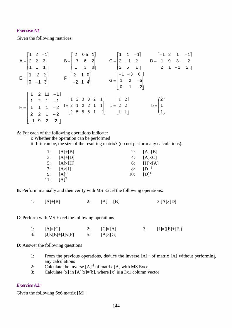
144

Exercise A1 Given the following matrices:

−=

111322121

A

−=

83126710.52

B

−

−=

152212111

C

−−−−

=221223911121

D

−

=310221

E

−

=412012

F

−−

−−=

210521

831G

−−−−−

=

229121222111112111121

H

−=

115552112212123321

I

=

112221

J

=

112

b

A: For each of the following operations indicate:

i: Whether the operation can be performed ii: If it can be, the size of the resulting matrix? (do not perform any calculations).

1: [A]+[B] 2: [A]-[B] 3: [A]+[D] 4: [A]×C] 5: [A]×[H] 6: [H]×[A] 7: [A×[I] 8: [D]-1 9: [A]-1 10: [D]T 11: [A]T

B: Perform manually and then verify with MS Excel the following operations:

1: [A]+[B] 2: [A] − [B] 3:[A]×[D] C: Perform with MS Excel the following operations

1: [A]×[C] 2: [C]×[A] 3: [J]×([E]+[F]) 4: [J]×[E]+[J]×[F] 5: [A]×[G]

D: Answer the following questions

1: From the previous operations, deduce the inverse [A]-1 of matrix [A] without performing any calculations

2: Calculate the inverse [A]-1 of matrix [A] with MS Excel 3: Calculate [x] in [A][x]=[b], where [x] is a 3x1 column vector

Exercise A2: Given the following 6x6 matrix [M]:

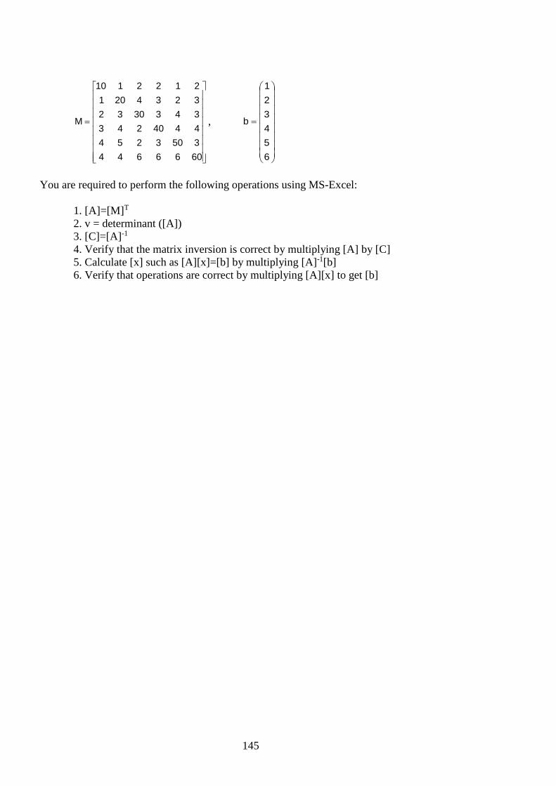
145

=

606664435032544440243343303232342012122110

M ,

=

654321

b

You are required to perform the following operations using MS-Excel: 1. [A]=[M]T 2. v = determinant ([A]) 3. [C]=[A]-1 4. Verify that the matrix inversion is correct by multiplying [A] by [C] 5. Calculate [x] such as [A][x]=[b] by multiplying [A]-1[b] 6. Verify that operations are correct by multiplying [A][x] to get [b]

146

APPENDIX B

B.1: Local and Global Coordinate Systems The position of a point in space is usually defined by nominating its coordinates (x, y, z) relative to a fixed set of reference axes. These coordinates are sometimes called the global coordinates. In the course of analysis it may be more convenient to introduce a local set of coordinates. For example, it may be decided to measure x in the east direction, y in the north direction and z vertically. However in examining the behaviour of a particular piece of bracing it may be much more convenient to adopt a local set of axes with one of the coordinate axes directed along the centroid of bracing. If a local set of coordinate axes is introduced it is desirable to be able to express the local coordinates in terms of the global coordinates and vice versa. For simplicity of presentation only the two dimensional situation will be considered here. A set of local axes derived from translation is shown in Figure B.

X

Y

(x0,y0)

x

y

X

Y

x

y

Figure B. 1 Translation of axes

It can be seen that X = x − x0 (B.1)

Y = y − y0 A set of local axes generated by anti-clockwise rotation through the angle θ is shown in Figure B. . It follows that for this case:

cos( ) sin( )

sin( ) cos( )

X x y

Y x y

θ θ

θ θ

= + +

= − + (B.2)

or in matrix notation:

X +cos( ) sin( ) xY sin( ) cos( ) y

θ θθ θ

= −

(B. 3)

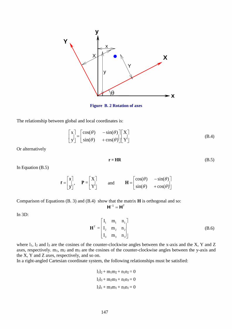
147

X

Y

x

y

X

Y

x

y

θ

Figure B. 2 Rotation of axes

The relationship between global and local coordinates is:

x cos( ) sin( ) Xy sin( ) cos( ) Y

θ θθ θ

− = +

(B.4)

Or alternatively r = HR (B.5)

In Equation (B.5)

=

yx

r , X

=Y

Ρ and cos( ) sin( )sin( ) cos( )

θ θθ θ

− = +

H

Comparison of Equations (B. 3) and (B.4) show that the matrix H is orthogonal and so:

T1 HH =− In 3D:

1 1 1

T2 2 2

3 3 3

I m n= I m n

I m n

H (B.6)

where l1, l2 and l3 are the cosines of the counter-clockwise angles between the x-axis and the X, Y and Z axes, respectively. m1, m2 and m3 are the cosines of the counter-clockwise angles between the y-axis and the X, Y and Z axes, respectively, and so on. In a right-angled Cartesian coordinate system, the following relationships must be satisfied:

l1l2 + m1m2 + n1n2 = 0 l2l3 + m2m3 + n2n3 = 0 l3l1 + m3m1 + n3n1 = 0

148

Example B.1 To illustrate the introduction of local axes, suppose that on a particular site a set of global axes has been set up with the x-axis being in the horizontal plane and the y-axis vertically up. Bore hole data from the site shows the presence of a narrow layer of silt inclined at 20° to the horizontal. In examining the behaviour of the seam it is decided to introduce a local set of axes with its origin 10 m below the surface and with the X-axis directed along the seam (in a downwards direction) and the Y-axis perpendicular to the seam. The global coordinates have their origin at the point of intersection of the seam with the surface.

10 m

X

Yx

y

20o

(a)X

Yx

y

20o

(b) X*

Y*

Global Coordinates

Local Coordinates

Figure B. 3 Rotation and Translation of axes

The calculation is best performed in two stages. First consider the intermediate local coordinates (X*,Y*) shown in Figure B.(b). These coordinates are located at x0=27.4748, y0=-10. Thus

X*= x − 27.4748 Y*= y +10

The relationship between (X,Y) and (X*,Y*) can be found by rotation of axes (notice if you use Equation (B.2) that θ = -20°) and it is found that:

X = 0.9397X* − 0.3402Y* Y = 0.3420X* + 0.9397Y*

This finally leads to the expression for local coordinate in terms of global coordinates:

X = 0.9397x − 0.3402y − 29.2380 Y = 0.3420x + 0.9397y

and to the expression of global coordinate in terms of local coordinates:

x = 0.9397X + 0.3402Y + 27.4748 y = -0.3420X + 0.9397Y − 10

B.2: Cylindrical Polar Coordinates The treatment given in the previous sections has been expressed in terms of cartesian coordinates. In many applications it is more convenient to employ curvilinear coordinates. Typical of these are the cylindrical polar coordinates r, θ, z, which are related to cartesian coordinates by the relation x = r cos θ， y = r sin θ

149

The coordinates are illustrated in Figure B.4

x

z

θ

y

Z

X

Y

r

Figure B. 4: Polar coordinates

Exercise B.1 A rectangular element ABCD has vertices with coordinates as given below.

x(m) y(m) A 2.0000 0.5000 B 6.3879 2.8971 C 1.5937 11.6730

-2.7943 9.2758 The coordinates of the point P is:

x(P)=1.2768 m y(P)=8.0814m If the origin of local coordinates is taken at A and thex-axis is directed along AB and the y-axis is directed along AD find the local coordinates of the point P. Answer: X(P) = 3m Y(P) = 7m B.1: Transformation of Displacement If forces are applied to a body it will deform as shown in Figure B. and thus a point originally at positionP will move to an adjacent position Q. The point is said to be displaced and the displacement is defined by: u=r(Q) − r(P) (B.7)

Thus the displacement components are given by:

x

y

u x(Q) - x(P)=

u y(Q) - y(P)

(B.8)

150

P(x0,y0)

x

y

Q(x,y)

Figure B. 5 Displacement of a point

These displacements are expressed in terms of the global coordinate system. It is often convenient to determine what the displacements are in a local coordinate system. Clearly a translation of axes does not change the displacement components, however a rotation of axes does induce a change. Therefore, it can be seen that:

X x y

Y x y

u = u cos(q) + u sin(q)

u = -u sin(q) + u cos(q) (B.9)

and conversely

x X Y

y X Y

u = u cos(q) - u sin(q)

u = u sin(q) + u cos(q) (B.10)

These equations may be written in matrix form as follows:

== T

u H UU H u

(B.11)

where

uu

=y

x

u is the displacement vector in the global coordinates

uu

=Y

X

U is the displacement vector in the local coordinates

cos(q) -sin(q)

=sin(q) +cos(q)

H

Example B.2 In the situation described in example 1.1 the following movements are recorded:

ux = 18 mm uy = − 5 mm

151

The local coordinate system can be used to assess if this movement corresponds to movement along the seam. It is found that:

0.9397 0.3420 18 18.62 0.3420 0.9397 5 1.46

X

Y

u mmu mm

− = = + −

and thus there is a substantial movement along the seam. B.2: Rigid Body Displacement A body may undergo modes of movement in which there is no change of shape. Figure B. illustrates such a movement in the xy plane.

Initial position

x

y

Final position

O

Figure B. 6 Rigid body movement

It can be seen that the rigid body can be broken up into three distinct movements, a translation in the x direction, a translation in the y direction and a rotation about a line parallel to the z-axis through the point O. It can be shown that for small rotations

ux = xf – xi = uxo − (yi − yo) wz uy = yf – yi = uyo + (xi − xo) wz

where uxo is the rigid body translation in the x direction uyo is the rigid body translation in the y direction wz is the rotation about the z axis and xo, yo are the coordinates of the reference point O.

Exercise B. 2 The centre of a 5m radius silo (a cylindrical container) is located at a pointx=25m, y=10m, z=0m. The following deflections:

ux = 10mm uy = 5mm uz = 2mm

are detected at the point x=29m, y=13m, z=10m. Calculate the radial component of deflection. (Answer: 11mm)

152

APPENDIX C

C.1: Direct Assembly of the Global Stiffness Matrix It is not necessary to assemble the global stiffness matrix of the unrestrained structure. Instead, a system containing only the unrestrained degrees-of-freedom can be assembled to form the restrained stiffness matrix. There are several different strategies that can be adopted to incorporate boundary conditions while assembling the global stiffness matrix. Here an approach based on transformation of the local degrees-of-freedom to the global degrees-of-freedom is discussed in detail.

4 2 1 3H

x

y

5 3

6

H A, E

1 2 3

4 5 6 7 8 9

10

Figure C. 1 Truss structure

Each bar element has ndof=4 local degrees-of-freedom, which is equal to the number of nodes in the element times the number of degrees-of-freedom per node. The structure has also Ndof global degrees-of-freedom, which is equal to the number of nodes in the structure times the number of degrees-of-freedom per node less the number of restrained degrees-of-freedom. The number of the global degrees-of-freedom for the truss structure shown in Figure C. is Ndof =6 × 2 - 4 = 8. Assume that the unrestrained degrees-of-freedom can be rearranged as:

R 1 2 3 4 5 6 7 8Δ { a , a , a , a , a , a , a , a }=

By convention, the rearrangement of the global degrees-of-freedom is formed by going through all the nodes in ascending sequence and allocating an index number i to each degree of freedom that is unrestrained, ai. The restrained degrees-of-freedom have a value of zero and do not contribute to the vector of the global degrees-of-freedom. For example the restrained and unrestrained degrees-of-freedom for the truss are:

Unrestrained DOF u1 v1 u2 v2 u3 v3 u4 v4 u5 v5 u6 v6 Global DOF 0 0 a1 a2 a3 a4 a5 a6 a7 a8 0 0

where a1, for example, is the global label for u2 and a2 is the global label for v2 etc. Therefore, the local degrees-of-freedom for each element can be related to the global degrees-of-freedom. For example for element 6:

Local DOF for element 6 u2 v2 u5 v5 Global DOF a1 a2 a7 a8

The vector of the local degrees-of-freedom can be related to the vector of the global degrees-of-freedom for the restrained structure by a transformation matrix, Q.

Ree Δ . Q δ = (C.1)

153

The size of the transformation matrix is (ndof×Ndof). The component qij of matrix Qe is1 if the ith degree-of-freedom of the element e (the local degrees-of-freedom) is equal to jth global degree-of-freedom, otherwise qij is zero. For element 6, for example, Q6 is:

62

62

61

61

5

5

2

2

6

65443322

87654321

vuvu

vuvu

10000000010000000000001000000001

Q

vuvuvuvuaaaaaaaa

=

The transformation matrices Q for all elements are given in Application of the principle of virtual work eliminates the virtual displacement vector from Equation (C.7) and the element stiffness matrix is obtained in terms of the global degrees-of-freedom which is suitable to be used in the global stiffness matrix for the complete structure directly:

∫= dVQ.B.D.B.QK eTT

eeR (C.8)

The unrestrained element stiffness matrix in terms of the local degrees-of-freedom was given in Equation (2.18) as:

∫= dVB.D.Bk Te (C.9)

Therefore, the relationship between the unrestrained element stiffness matrix, ke, and the restrained element stiffness matrix in terms of the global degrees-of-freedom, e

RK can be obtained by comparing Equation (C.8) with Equation (C.9):

eeT

eeR Q.k.QK = (C.10)

Table C. 1Substituting Equation(C.1) into Equations (2.8) and (2.10) results in:

Ree Δ . Q . B δ . B ε == (C.5)

Ree Δ . Q . B . D δ . B . D σ == (C.6)

where ε and σ are the stress and strain vectors, B is the matrix of strain-displacement relationship. Thus the equation of internal virtual work at the element level becomes:

dVΔ.Q.B.D.B.Q.ΔdVσ.ε ReTT

e*TR

*T∫ ∫= (C.7)

Application of the principle of virtual work eliminates the virtual displacement vector from Equation (C.7) and the element stiffness matrix is obtained in terms of the global degrees-of-freedom which is suitable to be used in the global stiffness matrix for the complete structure directly:

∫= dVQ.B.D.B.QK eTT

eeR (C.8)

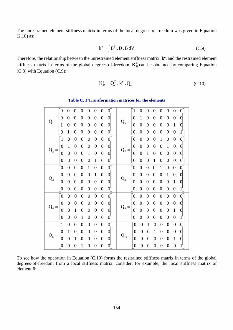
154

The unrestrained element stiffness matrix in terms of the local degrees-of-freedom was given in Equation (2.18) as:

∫= dVB.D.Bk Te (C.9)

Therefore, the relationship between the unrestrained element stiffness matrix, ke, and the restrained element stiffness matrix in terms of the global degrees-of-freedom, e

RK can be obtained by comparing Equation (C.8) with Equation (C.9):

eeT

eeR Q.k.QK = (C.10)

Table C. 1 Transformation matrices for the elements

=

00000010000000010000000000000000

Q1

=

10000000010000000000001000000001

Q6

=

00100000000100000000001000000001

Q2

=

00001000000001000010000000010000

Q7

=

00000000000000000010000000010000

Q3

=

10000000010000000010000000010000

Q8

=

00001000000001000000000000000000

Q4

=

10000000010000000000000000000000

Q9

=

00001000000001000000001000000001

Q5

=

10000000010000000000100000000100

Q10

To see how the operation in Equation (C.10) forms the restrained stiffness matrix in terms of the global degrees-of-freedom from a local stiffness matrix, consider, for example, the local stiffness matrix of element 6:

155

8

7

2

1

5

5

2

2

644

643

642

641

634

633

632

631

624

623

622

621

614

613

612

611

6

5522

8721

aaaa

vuvu

kkkkkkkkkkkkkkkk

k

vuvuaaaa

=

Each component of the stiffness matrix, 6ijk , is tagged with one ar (a global degree-of-freedom associated

with row i of the stiffness matrix) and one ac (a global degree-of-freedom associated with column j of the local stiffness matrix). The tags ar and ac show that kij shall be assembled in row r and column c of the global stiffness matrix. For example, the operation in Equation (C.10) transforms component 6

23k into a position at the second row (due to a2) and the seventh column (due to a7) of the global stiffness matrix. The restrained stiffness matrix for element 6 in the global system is:

=

644

643

642

641

634

633

632

631

624

623

622

621

614

613

612

611

6R

kk0000kkkk0000kk00000000000000000000000000000000

kk0000kkkk0000kk

K

The stiffness matrices of all the elements in the global system are presented in Table C. 2.

156

Table C. 2 Element stiffness matrices in the global system

+

=

0000000000000000000000000000000000000000000000000000000000000001

HEAK1

R

++−−++−−

−−++−−++

=

1100001111000011

000000000000000000000000000000001100001111000011

H22EAK6

R

+−

−+

=

0000000000000000000000000001000100000000000000000000000000010001

HEAK2

R

+−−+−++−−++−+−−+

=

0000000000000000001111000011110000111100001111000000000000000000

H22EAK7

R

+=

0000000000000000000000000001000000000000000000000000000000000000

HEAK3

R

+−

−+

=

101000000000000010100000

0000000000000000000000000000000000000000

HEAK8

R

++++

=

0000000000000000000000000000000000001100000011000000000000000000

H22EAK4

R

+−−+

=

1100000011000000

000000000000000000000000000000000000000000000000

H22EAK9

R

+−

−+

=

0000000000000000000000000000000000001010000000000000101000000000

HEAK5

R

+−

−+

=

0000000001000100000000000000000000000000010001000000000000000000

HEAK10

R

157

APPENDIX D

D.1: Linear Triangular Elements From the Section 6.1, the 3-noded triangular element shown in Fig.D.1 is the simplest possible planar element and one of the earliest finite elements. It has nodes at the vertices of the triangle only. For a plane elasticity problem, where all displacements are in the plane, the element has two degrees-of-freedom at each node, u and v, corresponding to the displacements in x and y directions respectively. Thus the element --has a total of 6 degrees-of-freedom. The displacement vector and the force vector are:

Te 1 1 2 2 3 3[u , v , u , v , u , v ]=u

Te 1 1 2 2 3 3[ p , q , p , q , p , q ]=f

Since each of these vectors contains 6 components, the size of the element stiffness matrix, ke, is 6×6.

u1, p1

v1, q1

x, u, p

y, v, q

1

3

2u2, p2

v2, q2

u3, p3

v3, q3

Fig. D.1: 3-noded triangular element

Stiffness matrix of linear triangular finite element The general procedure explained in Section 2.3 is employed here to calculate the stiffness matrix of the 3-noded triangular element. 1. Local coordinate and node numbering system.

The node numbering and the Cartesian coordinate system shown in Fig. D.1 may be used for the element. The nodes are numbered in increasing order anti-clockwise. The coordinates of the nodes are (x1, y1), (x2, y2) and (x3, y3). It is noted that the orientation of the element with respect to the xy coordinate system is completely arbitrary. Therefore the element stiffness matrix will be directly expressed in the xy global coordinate system.

2. Displacement function The variation of the displacement components, u and v, within the element can be expressed as complete linear polynomials of x and y:

158

yaxaau 321 ++= = a.y)f(x, (D.1)

ybxbbv 321 ++= = b.y)f(x,

where y} x,{1,y)f(x, = , T321 }a ,a ,{aa = and T

321 }b ,b ,{bb = .

3. Relating displacements within the element to the nodal displacements

The general displacements within the element can be related to the nodal displacements using shape functions:

332211 uNuNuNu ++= = eT u.N (D.2)

332211 vNvNvNv ++= = eT v.N

where ui and vi are the nodal displacements in x and y directions, respectively, and Ni are the linear shape functions for the element, as obtained in Chapter 3:

1T y).Cf(x,N −=

=

33

22

11

yx1yx1yx1

C and

−−−−−−−−−

=−

123123

211332

1221311323321

xxxxxxyyyyyy

yxyxyxyxyxyx

2A1C

where A is the area of the triangular element, x1,2,3 and y1,2,3 are the x and y coordinates of the first, the second and the third node of the element. Therefore the shape functions are:

{ }

−−−−−−−−−

== −

123123

211332

1221311323321TT

xxxxxxyyyyyy

yxyxyxyxyxyxyx,1,

2A1y)C(x,fN

−+−+−

−+−+−

−+−+−

=

=

2A)xy(x)yx(y)yxy(x

2A)xy(x)yx(y)yxy(x

2A)xy(x)yx(y)yxy(x

NNN

N

12211221

31133113

23322332

3

2

1

Equation (C.1) can now be written in matrix format as:

=

3

3

2

2

1

1

321

321

vuvuvu

N0N0N00N0N0N

vu or eδ.Ny)δ(x, =

159

4. Strain-displacement relationship

The strains at any point within the element, ε(x,y), can be related to the nodal displacements, δe, by the strain-displacement matrix, Be.

ee δ.By)ε(x, = (D.3)

The matrix Be has been defined for a general case in Section 5.1.2 and contains derivatives of the shape functions. For the general case of a three-dimensional element with m nodes, the strain vector has 6 components and the matrix Be can be defined as:

=

mxmz2x2z1x1z

mymz2y2z1y1z

mxmy2x2y1x1y

mz2z1z

my2y1y

mx2x1x

e

N0NN0NN0NNN0NN0NN0

0NN0NN0NNN00N00N00

0N00N00N000N00N00N

B

(D.4)

where Nix, Niy and Niz are derivatives of shape function i with respect to x, y and z, respectively. Each row of the matrix Be refers to one component of the strain vector. For planar problems, where some components of the strain vector are zero, the size of the matrix Be can be reduced. For example, the strain vector under plane stress and plane strain conditions can be written as:

∂∂+∂∂∂∂∂∂

=

=yu/xv/

yv/xu/

γεε

ε

xy

yy

xxe (D.12)

Therefore, the matrix Be for these conditions can be obtained as:

=

mxmy2x2y1x1y

my2y1y

mx2x1x

e

NNNNNNN0N0N0

0N0N0NB

(D.6)

For the triangular element with three nodes, the matrix Be is:

=

3x3y2x2y1x1y

3y2y1y

3x2x1x

e

NNNNNNN0N0N00N0N0N

B (D.7)

The derivatives of the shape functions for the triangular element can be obtained as:

160

−−−−−−

=

)x(x)y(y)x(x)y(y)x(x)y(y

2A1

NNNNNN

12

21

31

13

23

32

3y

3x

2y

2x

1y

1x

(D.8)

Therefore the matrix Be is obtained for the linear triangular element as:

−−−−−−−−−

−−−=

)y(y)x(x)y(y)x(x)y(y)x(x)x(x0)x(x0)x(x0

0)y(y0)y(y0)y(y

2A1B

211213313223

123123

211332

e (D.9)

It can be seen that Be and therefore strains within the linear triangular element are independent of x and y. For this reason, this element is often called the “constant strain triangle”.

5. Stress-strain relationship The stress-strain relationships for continuum problems have been defined in Section 5.3 as:

εD.σ = (D.11)

where D is the matrix of elastic moduli. Expressions for D have been given for cases of general three-dimensional problems as well as plane strain, plane stress and axial symmetry problems. For example, D for plane strain problems is:

-

+

+=

xy

yy

xx

xy

yy

xx

γεε

G0002Gλλ0λ2Gλ

σσσ

(D.13)

where λ and G are Lamé modulus and shear modulus, respectively.

6. Relating the internal stress to the external loads The internal stress can be related to the external loads using the principle of virtual work for the element. This leads to the equation for calculation of the element stiffness matrix.

∫= dvB.D.Bk eTe

e = t.AB.D.B eTe (D.14)

where A and t are the area and the thickness of the element, respectively. Note that because Be and D are independent of coordinate location (x, y), the integration over this element can be performed easily and exactly.

161

Application of linear triangular elements in analysis of a continuum A simple example is given here to demonstrate application of the linear triangular finite elements in the analysis of a continuum problem. The elastic body to be analysed is a simple homogeneous long block, a cross section of which is shown in Fig. D.2(a). It is constrained by a smooth rigid horizontal boundary and a smooth rigid vertical boundary along its two sides. The block is subjected to normal stresses applied to the other two sides. The Young’s modulus, E, and the Poisson’s ratio, ν, for the block are 56 MPa and 0.4, respectively. The general procedure in finite element analysis, explained in Section 2.2, will be used here for the analysis of the problem.

- Fig. D.2: Elastic block subjected to uniform loads

1. Chose a suitable coordinate system

The Cartesian coordinate system shown in Fig.B(b) is suitable for the problem. 2. Divide the geometry of the problem into a number of finite elements.

The geometry is divided into 4 triangular elements as shown in Fig.B.2(b). 3. Use a suitable node numbering system.

The node numbering system shown in Fig. D.2(b) is chosen. As explained in section 4.5, a good node numbering system should minimise the difference between the node numbers of any member that is a part of the structure. The nodal co-ordinates are shown in Table D. . The data defining each of the elements is given in Table D..

Table D.1: Nodal coordinates

Node x (m) y (m) 1 4.0 5.0 2 0.0 5.0 3 2.0 2.5 4 4.0 0.0 5 0.0- 0.0

162

Table D.2: Element data

Element Node 1 Node 2 Node 3 1 1 2 3

2 2 5 3

3 5 4 3

4 4 1 3

4. Calculate the stiffness matrices of all elements The stiffness matrix of each element can be calculated using Equation (D.14), assuming a unit thickness for the element.

∫= dvB.D.Bk eTe

e = AB.D.B eTe (D.15)

where Be and D can be calculated using Eqs.(6.24) and (D.13). Note that in Equations, x1,2,3 and y1,2,3 are the x and y coordinates of the first node, the second node and the third node of the element. For example, the matrix Be for element 2 is calculated as follows.

−−−−−−−−−

−−−=

)y(y)x(x)y(y)x(x)y(y)x(x)x(x0)x(x0)x(x0

0)y(y0)y(y0)y(y

2A1B

522523323553

253253

522335

2

and )y x- y (x )y x- y (x -)y x- y (x 2A 255223325335 += Substituting -the x and y coordinates of the three nodes in the above relations results in:

2A=(0×2.5 –2× 0) - (0×2.5 –2×5) + (0×0 –0×5) =10 m2

−−−−−−−−−

−−−=

0)(50)(05)(2.52)(02.5)(00)(20)(002)(000)(20

00)(505)(2.502.5)(0

101B2

−−−−

−−=

0.5000.250.200.250.20000.2000.20000.5000.2500.25

B2

163

The matrices Be for all elements are given in Table D..

Table D.3: Strain-displacement matrices

−−−

−=

00.400.250.200.250.200.4000.2000.200

0000.2500.25B1

−−−−

−−=

0.5000.250.200.250.20000.2000.20000.5000.2500.25

B2

−−−−−

−=

00.400.250.200.250.200.4000.2000.200

0000.2500.25B3

−−−

−=

0.5000.250.200.250.20000.2000.20000.5000.2500.25

B4

The matrix of elastic moduli, D, for plane strain analysis is:

+

+=

G0002Gλλ0λ2Gλ

D

where ( )ν12

EG+

= =20000 kPa and ( )2ν1

2Gνλ−

= =80000 kPa. Therefore:

=

2000000012000080000080000120000

D

In this problem the material is assumed to be homogeneous and therefore the matrix of elastic moduli, D, is the same for all elements.

164

The stiffness matrices for all elements are calculated based on Equation (D.15) and presented in Table D..

Table D.4: Element stiffness matrices

−−−

−−−−−−

=

96000016000Sym.

4800010000302504000080002500041500480001000017750150003025040000800015000335002500041500

k1

−−−−−−−

−−

=

25000015000Sym.

125004000030250100007500025000415001250040000177501500020250100007500015000335002500041500

k2

−−−

−−−−−−

=

96000016000Sym.

4800010000302504000080002500041500480001000017750150003025040000800015000335002500041500

k3

−−−−−−−

−−

=

25000015000Sym.

125004000030250100007500025000415001250040000177501500030250100007500015000335002500041500

k4

5. Assemble the global stiffness matrix

The global stiffness matrix is assembled using the direct method of assembly explained in section 4.2. The unrestrained degrees-of-freedom and the global degrees-of-freedom for the whole structure are:

Unrestrained DOF u1 v1 u2 v2 u3 v3 u4 v4 u5 v5 Global DOF a1 a2 0 a3 a4 a5 a6 0 0 0

Therefore the unknown displacements, or the global variables, have six components:

T654321R } a , a , a , a , a , a { Δ =

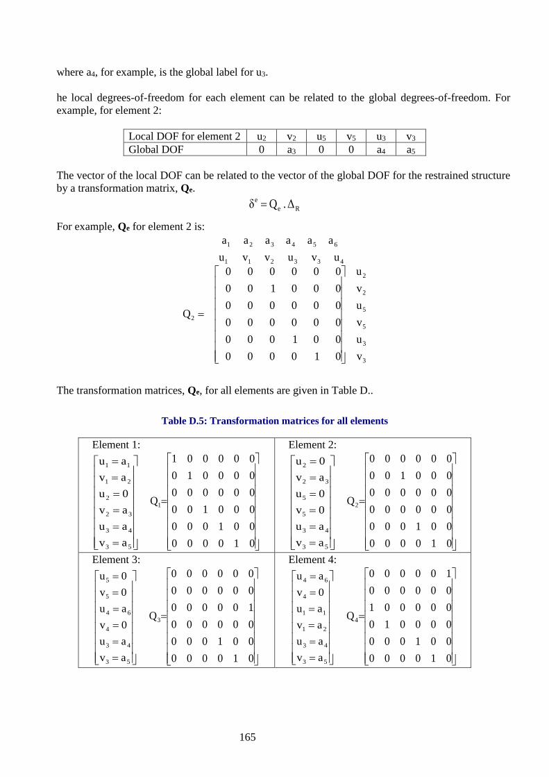
165

where a4, for example, is the global label for u3. he local degrees-of-freedom for each element can be related to the global degrees-of-freedom. For example, for element 2:

Local DOF for element 2 u2 v2 u5 v5 u3 v3 Global DOF 0 a3 0 0 a4 a5

The vector of the local DOF can be related to the vector of the global DOF for the restrained structure by a transformation matrix, Qe.

Ree Δ . Q δ =

For example, Qe for element 2 is:

3

3

5

5

2

2

2

433211

654321

vuvuvu

010000001000000000000000000100000000

Q

uvuvvuaaaaaa

=

The transformation matrices, Qe, for all elements are given in Table D..

Table D.5: Transformation matrices for all elements

Element 1:

======

53

43

32

2

21

11

avauav0uavau

=

010000001000000100000000000010000001

Q1

Element 2:

======

53

43

5

5

32

2

avau0v0uav0u

=

010000001000000000000000000100000000

Q2

Element 3:

======

53

43

4

64

5

5

avau0vau0v0u

=

010000001000000000100000000000000000

Q3

Element 4:

======

53

43

21

11

4

64

avauavau0vau

=

010000001000000010000001000000100000

Q4

166

The restrained stiffness matrix for an element, expressed in terms of global variables, eRK , can be

obtained from the element transformation matrix and the element stiffness matrix, expressed in terms of local variables, using the relationship given in Equation (4.10):

eeT

eeR Q.k.QK =

The restrained element stiffness matrices for all elements are given in Table D..

Table D.6: Restrained element stiffness matrices

−−−−−

=

0096000sym.001600004800010000302500480001000017750302500400008000150002500041500

k1R

−=

0025000sym.00150000012500400003025000000000000

k2R

−=

415004000096000sym.8000016000

000000000000000

k3R

−

−−−−

=

415001000025000sym.75000015000

000015000125004000003025033500100007500002500041500

k4R

The Global stiffness matrix for the whole structure, expressed in terms of the global variables, is obtained by summing the element stiffness matrices.

167

−−−−

−−−−−−−−

=

83000500008300001500033500500002420000605006050050000830000332000500005000083000

06050050000605001775015000150006050050000177506050050000335005000083000150005000083000

KR

6. Assemble the force vector

The finite element equation was obtained in Chapter 2 using the principle of virtual work for the case where the external forces were applied at nodal points only. The finite element equation can be expanded to include the effects of any traction, T, applied on the surface of an element or any body force, F, acting within the body of an element. To make the nodal forces statically equivalent to the actual boundary tractions or body forces, the principle of virtual work is employed. An arbitrary virtual nodal displacement is imposed to the body and the external work done by the various forces and tractions during that displacement are calculated and equated to the internal virtual work. Lets assume that the virtual displacement u*e is applied at the nodes of an element. This results in virtual displacements, u*, and virtual strains, ε*, within the element:

e*δ.Ny)(x,*δ = and e*δ.By)(x,*ε =

The work done by the nodal forces is equal to the sum of the products of the individual force at each node and the corresponding displacement.

eeT1ext .f*δ)(W =

where fe is the vector of nodal forces. The external virtual work done by tractions per unit area and the external virtual work done by distributed body forces per unit volume are:

T*δ)(W T2ext = = .TN*δ TeT

.γ*ε)(W T3ext = = .γB*δ TeT

Equating the total external work with the total internal work obtained by integrating over the volume of the element results in a more general finite element equation:

dvγ.Bds.TNf.δk TTeee ∫∫ ++= (B.16)

The expression on the right-hand-side of Equation (B.16) may be used to calculate the “consistent nodal forces” for the element. For the problem of the long block, the external tractions are applied at elements 1 and 4. The equivalent nodal forces due to the tractions are calculated for each of the elements and then included into the global force vector. Element 1 is subjected to an external uniform traction in the y-direction, Ty=-100kPa.

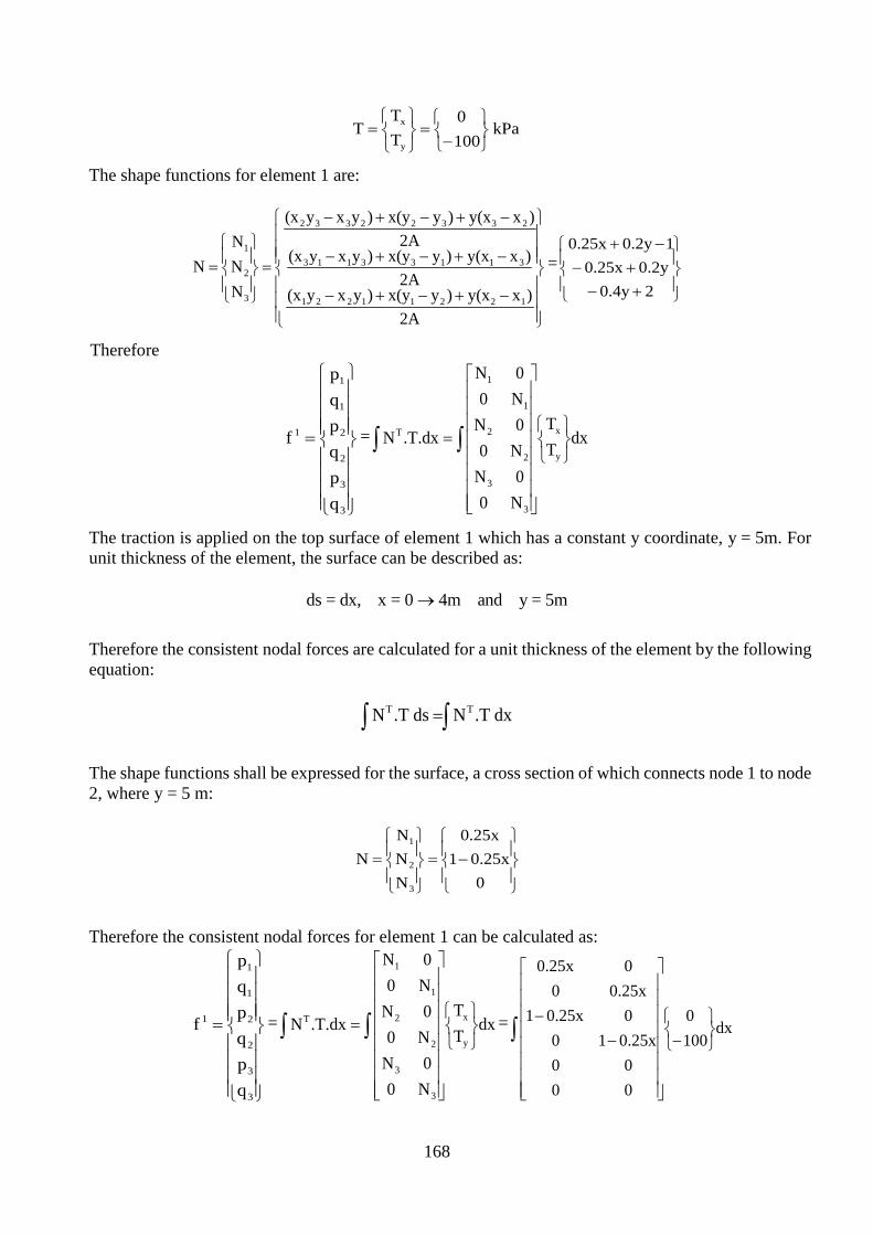
168

kPa1000

TT

Ty

x

−=

=

The shape functions for element 1 are:

−+−+−

−+−+−

−+−+−

=

=

2A)xy(x)yx(y)yxy(x

2A)xy(x)yx(y)yxy(x

2A)xy(x)yx(y)yxy(x

NNN

N

12211221

31133113

23322332

3

2

1

=

+−+−

−+

20.4y0.2y0.25x

10.2y0.25x

Therefore

=

3

3

2

2

1

1

1

qpqpqp

f = ∫∫

= dxTT

N00N

N00N

N00N

.T.dxNy

x

3

3

2

2

1

1

T

The traction is applied on the top surface of element 1 which has a constant y coordinate, y = 5m. For unit thickness of the element, the surface can be described as:

ds = dx, x = 0 → 4m and y = 5m

Therefore the consistent nodal forces are calculated for a unit thickness of the element by the following equation:

dx.TNds.TN TT ∫∫ =

The shape functions shall be expressed for the surface, a cross section of which connects node 1 to node 2, where y = 5 m:

−=

=

00.25x1

0.25x

NNN

N

3

2

1

Therefore the consistent nodal forces for element 1 can be calculated as:

=

3

3

2

2

1

1

1

qpqpqp

f = ∫∫

= dxTT

N00N

N00N

N00N

.T.dxNy

x

3

3

2

2

1

1

T = ∫

−

−−

dx1000

0000

0.25x1000.25x1

0.25x000.25x

169

−

×

−−

=

=

→=

1000

0000

0.125xx000.125xx

0.125x000.125x

qpqpqp

f

40x

2

2

2

2

3

3

2

2

1

1

1 = kN/m

0020002000

−

−

The nodal forces applied on element 1 can be written in terms of the global degrees-of-freedom as:

kN/m

0002002000

ffffff

.fQf

1a6

1a5

1a4

1a3

1a2

1a1

1T1

1R

−−

=

==

Similarly, the consistent nodal forces for element 4 can also be obtained:

kN/m

0005000500

qpqpqp

f

3

3

1

1

4

4

4

−

−

=

= and kN/m

5000000500

ffffff

fQf

4a6

4a5

4a4

4a3

4a2

4a1

4T4

4R

−

−

=

==

The nodal forces applied on elements and expressed in terms of global degrees-of-freedom can now be added together directly to form the global force vector.

−

−−−

=

=

50000200200500

ffffff

F

a6

a5

a4

a3

a2

a1

R

7. Solve the global equations to obtain the unknown nodal displacements The finite element equations can now be solved for the unknown nodal displacements

RRR FΔ.K =

or

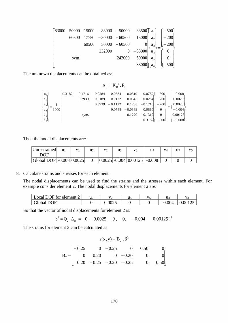
170

−

−−−

=

−−−−−−

50000200200500

aaaaaa

8300050000242000sym.830000332000

06050050000605001500060500500001775060500335005000083000150005000083000

6

5

4

3

2

1

The unknown displacements can be obtained as:

R1

RR F.KΔ −=

−

−

−

=

−

−−−

−−

−−−−−−−

=

0.0080.00125

0.0040.00250.0025

0.008

50000200200500

0.31820.13190.1220sym.0.08160.03390.07880.17160.12330.11220.39390.02840.06420.01220.01890.39390.07820.03190.03840.02840.17160.3182

10001

aaaaaa

6

5

4

3

2

1

Then the nodal displacements are:

Unrestrained DOF

u1 v1 u2 v2 u3 v3 u4 v4 u5 v5

Global DOF -0.008 0.0025 0 0.0025 -0.004 0.00125 -0.008 0 0 0

8. Calculate strains and stresses for each element The nodal displacements can be used to find the strains and the stresses within each element. For example consider element 2. The nodal displacements for element 2 are:

Local DOF for element 2 u2 v2 u5 v5 u3 v3 Global DOF 0 0.0025 0 0 -0.004 0.00125

So that the vector of nodal displacements for element 2 is:

R22 Δ.Qδ = { 0 , 0.0025 , 0 , 0, 0.004 , 0.00125 }T= −

The strains for element 2 can be calculated as:

22 δ.By)ε(x, =

−−−−

−−=

0.5000.250.200.250.20000.2000.20000.5000.2500.25

B2

171

−=

−

−−−−

−−=

00.0005

0.002

0.001250.004

00

0.00250

0.5000.250.200.250.20000.2000.20000.5000.2500.25

γεε

xy

yy

xx

Note that the strains are independent of the coordinates, i.e., the strains are constant within the element. Once the strains are known the stresses can be found as:

y)ε(x,D.y)σ(x, =

=

2000000012000080000080000120000

D

kPa0100200

00.0005

0.002.

2000000012000080000080000120000

σσσ

xy

yy

xx

−−

=

−

=

Similar calculations can be made for all elements.

172

SOLUTIONS TO SELECTED PROBLEMS

Problem 2.4. Settlement of soils

1) ( ) ( )u x x u x dux dx

ε+ ∆ −

= =∆

2) ( )E x εσ =

3) 0ddx

γσ+ =

4) ( ) ( ) ( )d duE x +γ=0 u 0 =0 σ H =Pdx dx

5) ( )2

0 02x P Hu x x

E Eγ γ+

= − +

( )0

Pxs xE

⇒ =

( )

( )0 0

x P HxE E

x x P H

γ γε

γ γ

+⇒ = − +

⇒ σ = − + +

Problem 2.5. Steel bar with variable area

1) d duAE 0d dx x

= ( )u 0 =0 ( )

L

Pσ L =A

2) *L *

0

du duAE d Pu (L)d d

xx x

=∫

3)

1 21

11 2 2 L

2 2

32 L 2 L

A +A2A 02 u 0

A +A A +AE 2A u 0Δx 2 2

u PA +A A +A02 2

− − − =

−

4) A1= 0.0088 m2 A2 = 0.0076 m2 AL= 0.0064 m2

173

16

2

3

1 1 2 2 2 2

u 0.1773u 0.33806 10 mu 0.6187

u(x) = u N (x)+u N (x)+u N (x)

−

= ×

5) ( ) 0

0

A +αpu lnEα A

xx

=

L 0A Aα=L−

Problem 3.1. Bar element

1) 2 1

2 1 2 1

x x x xx x x x

= − − − −eN

2) 1 1

Δx Δx = −

eB

3) Assuming E constant

1 1E1 1Δx

− == −

ek

4) Assuming f(x) constant

e

1fΔx=12

=

F

5) From 3) and 4)

1

2

1fΔx12

u1 1Eu1 1Δx

− −

=

Problem 3.2. Element stiffness matrix of a second order 1D bar The shape function of the element are given by the figure

174

1 2

xx1 x2

N(x)

1

N1

N2

N3

3

x30

The restricted stiffness matrix is given by

22 23 2 2

32 33 3 3

k k u pk k u p

=

Calculation of the shape function ( ) ( )( ) ( )

2 21 3

2 2 22 1 2 3

x x x x x(x L) x Lx x +LxN (x) = x x x x (L/2)(L/2) L /4 L /4

− − − − −= = =

− − − −,

( ) ( )( )( )

2 21 2

3 2 23 1 3 2

x x x x x(x L/2) x Lx/2 2x LxN (x) =x x x x L(L/ 2) L /2 L

− − − − −= = =

− −

Calculation of the B function from the derivatives of the shape function

2 32 2

2x+L 4x LB = B =L /4 L

− −

Calculation of the elements of the stiffness matrix L 2

22 20

16Ek = B Edx=3L∫

L 233 30

7Ek = B Edx=3L∫

L

23 2 30

8Ek = B B Edx=3L

−∫

Calculation of the load vectors L

2 20

2p = N fdx= fL3∫

L

3 30

fLp = N fdx=6∫

Problem 3.3. Beam element *The analytical solution for the deflection of the cantilever with uniform distributed load (Dead Load Case) is:

24 3 21( )

24 6 4w wL wLv x x x x

EI

= − +

Consequently, the moment can then be calculated as:

2 22

2

22

( )2 2

( )2 2

d v w wL wLM x EI x xdx EI EI EI

w wLM x x wLx

= κ ⇒ κ = = − +

∴ = − +

And shear as a function of the position is calculated by:

( )( ) dM xS x wx wLdx

∴ = = −

175

The numerical solution can be calculated by:

e eF = k v Where v1=0 and θ1=0 (restrained):

3 2 3 2

2 2

3 2 3 2

2 2

1 1 1 112 6 12 618 6 18 61 2 1 16 4 6 26 3 6 3

12 6 12 6 1 1 1 118 6 18 6

6 2 6 4 1 1 1 26 3 6 3

e

L L L L

L L L Lk EI EI

L L L L

L L L L

−− −−

= = − − − − − −

− −

For the boundary conditions of the propped cantilever, the matrix has been partitioned to find v2 and θ2:

2

2

1 124.7 18 6

24.7 1 26 3

vEI

θ

− − =

−

2

2

72 18 24.72 0.00311118 6 24.72 0.00069

vEIθ

− − ∴ = = −

Now using the shape functions already calculated from before the deflection for the numerical solution can now be calculated.

( )1 1 1 2 2 3 2 4( ) ( ) ( ) ( )v x v N x N x v N x N xθ θ= + + +

2 3 2 4( ) ( ) ( )v x v N x N xθ= + 2 3

2 32 3 2 4 2 3 2

3 2( ) ( ) ( ) ( ) 0.00311( ) 0.00069( )x xv x v x v N x N x x xL L L L

θ∴ = = + = − − − − +

Now the bending moment can be calculated by:

2

2 22 2 3 2

( ) 6 12 2 6( ) ( )d v x x xvdx L L L L

θ= − + − +

1

2

24.7224.72

24.7224.72

RR

F

− − = −

2

2

00

vvθ

=

176

2

2

( )( ) d v xM x EIdx

= −

2

2 22 2 3 2

( ) 6 12 2 6( ) ( ) ( )d v x x xM x EI EIv EIdx L L L L

θ= − = − − − − +

Consequently shear is thus given by:

2 23 2

12 6( )( ) EIv EIdM xS xdx L L

θ= = +

Thus, the plots for deflection, moment and shear can be produced as a function of position along the beam. For ease of comparison the analytical and finite solutions have been plotted on the same graphs. This is shown in Figures 4, 5, 6 respectively

For the problem above, the numerical solution approximates the displacement along the beam using a

polynomial. There a four degrees of freedom (and thus four unknown coefficients) for the beam element.

Thus, a cubic curve is used to approximate the strains and displacements. However, from the analytical

solution (derived from the strong form) the deflection curve obtained is quartic. Both methods will produce

the same calculated values at the nodes as demonstrated in Figures 4 and 5, yet the values in between nodes

will be different because the curves are not the same within their respective domains. This correlation is

clear from all the plots and calculated results.

Problem 4.1. Trusses1

9

1 1 / 2 2 1 / 2 2 0 0 1.3536 -0.3536 0 0-0.3536 1.3536 0 11 / 2 2 1 1 / 2 2 0 1 2 10

0 0 1 00 0 1 00 1 0 10 1 0 1

EA NL m

+ − −− + − = × − −

177

Problem 4.2. Trusses2

8

1 / 3 0 0 0 0.5774 0 0 00 1 0 1 0 1 0 1

2 10 0 0 0.9524 0.21650 0 1 / 3 3 / 8 3 / 80 1 0.2165 1.12500 1 3 / 8 9 / 8

EA NL m

− − = × + − −

Problem 4.3. Trusses3

1) Element a connects node 1 and node 2 with θ = 45o. Element b connects node 2 to node 3, thus θ = 180o

ba21 21

ba21 21

ba32 32

ba32 32

uu0.5 0.5 0.5 0.5 1 0 1 0 ppvv0.5 0.5 0.5 0.5 0 0 0 0 qqA.E A.E ; uu0.5 0.5 0.5 0.5 1 0 1 0L pp2 Lvv0.5 0.5 0.5 0.5 0 0 0 0 qq

− − − − − = = − − − − −

2)

Element (a):

a1 1

a1 1

q2 2

a2 2

3

4

u p0.5 0.5 0.5 0.5 0 0v q0.5 0.5 0.5 0.5 0 0u p0.5 0.5 0.5 0.5 0 0A.Ev0,5 0.5 0.5 0.5 0 02 L qu0 0 0 0 0 0 0

0 0 0 0 0 0 u 0

− − − − − −

= − −

Element (b):

1

1b

2 2b

2 2b

3 3b

3 3

0u0 0 0 0 0 00v0 0 0 0 0 0

u0 0 1 0 1 0 pA.E 0 0 0 0 0 0L v q0 0 1 0 1 0 u p0 0 0 0 0 0 v q

−

= −

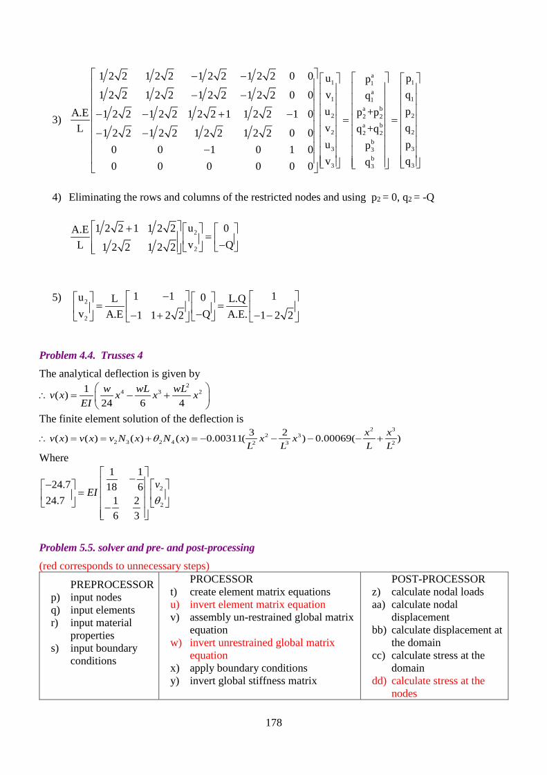
178

3)

a1 11

a1 11

a b2 22 2

a b2 22 2

b3 33

b3 33

1 2 2 1 2 2 1 2 2 1 2 2 0 0 u ppv q1 2 2 1 2 2 1 2 2 1 2 2 0 0 qu pp +pA.E 1 2 2 1 2 2 1 2 2 1 1 2 2 1 0v qL q +q1 2 2 1 2 2 1 2 2 1 2 2 0 0u pp0 0 1 0 1 0v qq0 0 0 0 0 0

− − − − − − + − = = − − −

4) Eliminating the rows and columns of the restricted nodes and using p2 = 0, q2 = -Q

2

2

u1 2 2 1 1 2 2 0A.Ev QL 1 2 2 1 2 2

+ = −

5) 2

2

1 1 1u 0L L.Qv QA.E A.E.1 1 2 2 1 2 2

− = = −− + − −

Problem 4.4. Trusses 4 The analytical deflection is given by

24 3 21( )

24 6 4w wL wLv x x x x

EI

∴ = − +

The finite element solution of the deflection is 2 3

2 32 3 2 4 2 3 2

3 2( ) ( ) ( ) ( ) 0.00311( ) 0.00069( )x xv x v x v N x N x x xL L L L

θ∴ = = + = − − − − +

Where

2

2

1 124.7 18 6

24.7 1 26 3

vEI

θ

− − =

−

Problem 5.5. solver and pre- and post-processing (red corresponds to unnecessary steps)

PREPROCESSOR p) input nodes q) input elements r) input material

properties s) input boundary

conditions

PROCESSOR t) create element matrix equations u) invert element matrix equation v) assembly un-restrained global matrix

equation w) invert unrestrained global matrix

equation x) apply boundary conditions y) invert global stiffness matrix

POST-PROCESSOR z) calculate nodal loads aa) calculate nodal

displacement bb) calculate displacement at

the domain cc) calculate stress at the

domain dd) calculate stress at the

nodes

179

Problem 4.6. two bar elements

1) a

1 1aa

2 2

u1 1 pAE =u1 1L p

− −

b

2 2bb

3 3

u1 1 pAEu1 1L p

− = −

2)

a1 1

aa2 2

3

1 1 0 u pAE 1 1 0 u = p

L0 0 0 u 0

− −

1

bb2 2

b3 3

0 0 0 u 0AE 0 1 1 u p

L0 1 1 u p

− = −

3)

aa a 1 1

a ba a b b 2 2 2

bb b 3 3

E E 0 u pA E E +E E u p +pL

0 E E u p

− − − = −

4) a b b 2

b b 3

E +E E u 0AE E u PL

− = −

5) B aE =cE2a

3

u1+c c 0AEuc c PL

− ⇒ = −

12

3 a

u 1 c c 0PLu c c 1AE

−+ − = − a

1 1 0PLc 1 1AE 1

c

= + a

1PL

c 1AEc

− = +

Problem 5.1.Poisson Ratio

xxσ 0≠ yy zzσ =σ =0

xxσε =E

xx , yy xx yy xxε = σ ε = εEν ν− ⇒ −

ΔL' ΔL L' ΔL L' 0.3mmL L

ν ν⇒ = − ⇒ ∆ = − ⇒ ∆ = −

Problem 5.2.Biaxial Test

xxσ 200kPa= −

yyσ 100kPa= −

zz xx yyσ = (σ +σ )= 120kPav − -3

xx xx-4

yy yy αβ

zz zz

ε 1 σ 2 101ε 1 σ 5 10 γ =0E

ε 1 σ 0

vv vv v

ν − − − × = − − = × − −

xxΔL=ε 4m= 8mm× −

yyΔW=ε 5m=2.5mm× Δt=0

180

Problem 5.3. Thin Steel Plate 6

xx6

yy αβ6

zz

ε 1 1MPa 5 101ε 1 0 1.5 10 γ =0E

ε 1 0 1.5 10

vv vv v

ν −

−

−

− − × = − − = − × − − − ×

6ΔL=5×10 ×800 mm=0.004 mm− 6ΔW= 1.5×10 ×400mm= 0.0006mm−− −

6 6Δt= 1.5×10 ×1 mm = 1.5 10 mm− −− − × Problem 5.5. rotation of stress

Tx = 86.6025 MPa Ty = 50 MPa Problem 6.1. Finite Element Formulation using triangular elements

1) T (x,y)=[1 x y ]g

1 4 5C= 1 0 5

1 2 2.5

T 11 2 3

1

[N (x,y) N (x,y) N (x,y)] (x,y)

1 4 5 10 0 201[1 x y ] 1 0 5 [1 x y ] 2.5 2.5 0

101 2 2.5 2 2 4

[ 1+0.25x+0.2y 0.25x+0.2y 2 0.4y]

−

−

=

− = = − −

= − − −

g C

2)

e

1 1 2 2 3 3

1 1 2 2 3 3

1

1

1 2 3 2

1 2 3 2

( ) ( ) 3

3

u(x, y) N (x, y)u N (x, y)u N (x, y)uv(x, y) N (x, y)v N (x, y)v N (x, y)v

uv

N 0 N 0 N 0 uu(x, y)0 N 0 N 0 N vv(x, y)

uv

= + += + +

⇒ =

u x N x

u

e 3)

181

1 2 3e e

1 2 3

0x 0.25 0 0.25 0 0 0

N 0 N 0 N 00 0 0.20 0 0.20 0 0.40

0 N 0 N 0 Ny0.20 0.25 0.20 0.25 0.40 0

y x

∂ ∂ −

∂ = = = − ∂ − − ∂ ∂ ∂ ∂

B LN

4)

λ 2G λ 0 120 80 0λ λ 2G 0 80 120 0 MPa0 0 G 0 0 20

+ = + =

D

5)

e eT e eT e

V

dV At

41.5 25 33.5 15 8 4030.25 15 17.75 10 48

41.5 25 8 40 MPa=30.25 10 48 m

Sym. 16 096

e

= =

− − − − − − − − −

∫k B DB B DB

Problem 7.1. Thermal load

( )1 2 inin 1

T T h= T T

L k−

−

( )out1 22 out

hT T= T T

L k−

−

1T =5.54°C⇒

2T =4.82°C =

1 22

T T Wq=k =144.6L m−

Problem 7.2. Thermal load 2

1) 3Q=50 kwatts/m

2) 2

02x=L

d T Q dT= T(0)=T =0dx k dx

−

182

3) 0QT(x)= x(2L x)+T2k

−

4) 2

0 c2x=L

d T Q dT= T(0)=T k =h (T(L) T )dx k dx ref− − −

2c 0 ref c

20

c

Q L h (T T )h + QLQ 2kT(x)= x x+T2k k + h L

− −− +

Problem 7.4. Finite different solution of the transient heat equation Finite different solution

j j j j+1 j 1 j 2

j j j+1

cΔ tu (t+Δt)=q (t+Δt) F (t)+ + β [u (t)+ u (t) 2u (t)] where β =Δz

The solution is numerically stable w

= +(t+Δt) (t) =

Δt(t

in β 1/2. If β

+Δt)= (t)+( )Δ

1/21(t+Δt)=F (t)+ [u (t)+

t

2u u

−− −

−⇒ −

⇒

⇒

=

⇒ −

≤

Ku u Fu u Ku F

u u Ku F

j 1(t) ] −

Problem 7.5. Finite element solution of the transient heat equation Weak form L L*

*v

0 0

u u uc dx= u ( F(x,t)dx x x t

∂ ∂ ∂−

∂ ∂ ∂∫ ∫

( ) ( )j j

n

j=1u x = xu N∑

Replacing in the weak form L L

ji j i

0 01F(x,t)

duN N dx N dx

dt

n

j=

−

∑∫ ∫

-1

= +(t+Δt) (t) =

Δt(t+Δt)= (t) ( )Δt

∴−

⇒ −

⇒ + −

Ku Cu Fu uC Ku F

u u C Ku F

Problem 8.1. Structural mechanics: bending of beams

a) ( ) ( )22dead livew +wv x x x24EI

L= −

183

b)

Only approximate: • Exact solution is a fourth order polynomial. • Approximated finite element solution is a third-order polynomial.

Problem 8.2. Structural Mechanics: bending of cantilever beams

1) 2 2 2 3

2 2 2 3x=0 x=L x=L

d d v dv d v d vEI =w v(0)=0, θ(0) =0, M(L)= EI =0, Q(L)= EI =P dxdx dx dx dx

= − −

2)

4

4

3

13

22

1 22

3 212 3

4 3 21 23 4

d v w=EIdx

d v w= x+CEIdx

d v w= x +C x+C2EIdx

Cdv w= x + x +C x+Cdx 6EI 2

C Cwv(x)= x + x + x +C x+C24EI 6 2

Applying boundary conditions

4

3

1 1

2 2 2 2 2

1 2 2 1

(0)=0 C =0θ(0)=0 C =0

P wL P+wLv'''(L)= +C = C =EI EI EI

wL wL PL+wL wL 2PL+wLv''(L)=0 +C L+C =0 C =2EI 2EI EI 2EI 2EI

v

PEI

C L

⇒⇒

− ⇒ − ⇒ −

⇒ ⇒ − − = − =

Replacing the constant into v(x) 2

4 3 2w P+wL 2PL+wLv(x)= x x + x24EI 6EI 4EI

−

3)

Deflection

24 3 2w P+wL 2PL+wLv(x)= x x + x

24EI 6EI 4EI−

Rotation 2

3 2dv w P+wL 2PL+wLθ(x)= = x x + xdx 6EI 2EI 2EI

−

Curvature

184

22dθ w P+wL 2PL+wLκ(x)= = x x

dx 2EI EI 2EI− − + −

Moment 2

2w 2PL+wLM=EIκ= x (P+wL)x2 2

− + −

Shear force dMQ= = w(L x) Pdx

− +

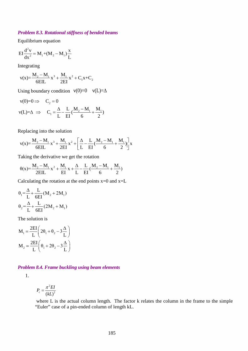
185

Problem 8.3. Rotational stiffness of bended beams Equilibrium equation

2

1 2 12

d v xEI M +(M M )dx L

= −

Integrating

3 22 1 11 2

M M M v(x)= x x C x+C6EIL 2EI

−+ +

Using boundary condition v(0)=0 v(L)=∆

2

2 1 11

v(0)=0 C 0 M M MLv(L)= C ( )

L EI 6 2

⇒ =−∆

∆ ⇒ = − +

Replacing into the solution

3 22 1 1 2 1 1M M M M M ML v(x)= x x ( ) x6EIL 2EI L EI 6 2

− −∆ + + − +

Taking the derivative we get the rotation

22 1 1 2 1 1M M M M M ML θ(x)= x x ( )2EIL EI L EI 6 2

− −∆+ + − +

Calculating the rotation at the end points x=0 and x=L

1 2 1

2 2 1

Lθ = (M 2M )L 6EI

Lθ = (2M M )L 6EI

∆+ +

∆+ +

The solution is

1 1 2

2 1 2

2EIM 2θ θ 3L L

2EIM θ 2θ 3L L

∆ = + −

∆ = + −

Problem 8.4. Frame buckling using beam elements

1.

2

2( )cEIP

kLπ

= where L is the actual column length. The factor k relates the column in the frame to the simple “Euler” case of a pin-ended column of length kL.

186

2.

Using the slope-deflection equations (below) LEI9

LEI6

LEI3

B =+=α

3.

Considering one column, stiffness at base is zero, at top:

LEI9

LEI6

LEI3

B =+=α ,

k is the column effective length factor. Also, 0 A B cM M P= ∆ = − ∆ .

The second equation

(1 cosec ) ( 1 cot ) 0cA B c

B

P LM M Pk k k kπ π π π

α− + + − + ∆ =

Reduced to

cot 0c

B

P Lk kπ π

α− =

We obtain

)k

cot(9k

π=

π

Which is solved using Newton-Rapson or graphically. The result is k = 2.22 4.

Using the slope-deflection equations (below) B3EI 2EI 5EIα = + =L L L

5.

Considering one column, stiffness at base is zero, at top:

B3EI 2EI 5EIα = + =L L L ,

k is the column effective length factor. Also, 0 and 0AM = ∆ = .

Using the second equation

(1 cosec ) ( 1 cot ) 0cA B c

B

P LM M Pk k k kπ π π π

α− + + − + ∆ =

We obtain

1 cot 0c

B

P Lk kπ π

α+ − =

thus

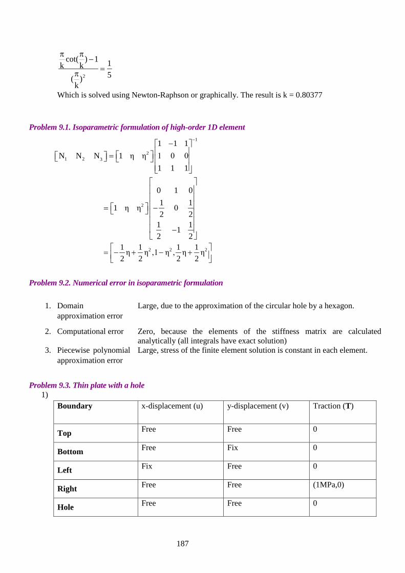
187

51

)k

(

1)k

cot(k

2=

π

−ππ

Which is solved using Newton-Raphson or graphically. The result is k = 0.80377

Problem 9.1. Isoparametric formulation of high-order 1D element

1

21 2 3

1 1 1N N N 1 η η 1 0 0

1 1 1

−− =

2

0 1 01 11 η η 02 2

1 112 2

= − −

2 2 21 1 1 1η η ,1 η , η η2 2 2 2

= − + − +

Problem 9.2. Numerical error in isoparametric formulation

1. Domain approximation error

Large, due to the approximation of the circular hole by a hexagon.

2. Computational error Zero, because the elements of the stiffness matrix are calculated analytically (all integrals have exact solution)

3. Piecewise polynomial approximation error

Large, stress of the finite element solution is constant in each element.

Problem 9.3. Thin plate with a hole

1) Boundary x-displacement (u) y-displacement (v) Traction (T)

Top Free Free 0

Bottom Free Fix 0

Left Fix Free 0

Right Free Free (1MPa,0)

Hole Free Free 0

188

2)

Mesh Domain approximation

error Computational error Piecewise polynomial

approximation error

1

Small: Due to the approximation of the hole by a reasonable number of quadratic

functions

Large in the transition elements which is outside of the region of interest. Small

in the other elements.

Relatively small near to the maximal stress. The error is

due to the exponential change of stress that needs to be fitted

by linear relations.

2

Very small: Due to the approximation of the

hole by a large number quadratic functions

Small due to the low

distortion of the elements but large at the transition zone

due to mesh incompatibility.

Relatively small near to the maximal stress. The error is

due to the exponential change of stress that need to be fitted

by linear relations.

3

Very small: Due to the approximation of the

hole by a large number quadratic functions

High in the domain of interest, due to the high

aspect ratio of the elements

Large near to the maximal stress, due to the relatively large size of the elements.

Problem 10.1. Spectral Response

1. For the top mass:

1 1 2 1 1 1 1 2 1 1( )k x x mx k x k x m x− − = ∴− + = For the bottom mass:

( )1 1 2 2 2 2 1 1 1 2 2 2 2( )k x x k x mx k x k k x m x− − = ∴ − + =

Writing these equation in a matrix form

1 1 1 1 1

2 2 1 1 2 2

0 00 0m x k k x

m x k k k x−

+ = − +

The matrices can be calculated using the given values 312 0 200 200 kN10 kg

0 24 200 300 m−

= × = − m K

2.

We solve the characteristic equation

189

( )

( )( )

2

22

2

2 2 2 2 2 4 2

det 0

0det det 0

3 0 2 3 2

3 2 2 5 0

k k m k m kk k m k k m

k m k m k k mk m

ω

ωω

ω

ω ω ω ω

− =

− − − ⇒ − = = − − −

⇒ − − − = − + =

K m

11 1

1

12 2

1

2 25.77 1.09

22.89 2.182

k s T sm

k s T sm

πωω

πωω

−

−

= = ⇒ = =

= = ⇒ = =

3. Mode 1

21 1 1

1

0

0 0 12 03 0 2 0 1

k k m a k k a ak a b ak k m b k k b am

ω− =

− − − − = ⇒ = ⇒ = − ⇒ = = − − − − −

KX MX

X

Mode 2

21 1 1

2

0

0 / 2 10 0 2

3 0 2 2 2 22k k m a k k a ak a b ak k m b k k b am

ω− =

− − − = ⇒ = ⇒ = ⇒ = = − −

KX MX

X

You are free to choose any value of a, here we choose a=1.

4.

[ ]

[ ]

[ ]

[ ]1

0 11 1 1 1

0 2 1 2 10 1 3 3

1 1 1 10 2 1 2

m mm m m

m m mm m

− − − Γ = = = = −

− − − −

[ ]

[ ]

[ ]

[ ]2

0 11 2 1 2

0 2 1 2 5 50 1 9 9

1 2 1 20 2 2 4

m mm m m

m m mm m

Γ = = = = −

190

5. Maximal response of each mode

( )

( )

1,max 1 1

2,max 2 2

1 113 35 70.79 18

a

a

S T g g

S T g g

φ

φ

= Γ = − × =

= Γ ≈ − × =

Combination of the mode using the absolute sum

max 1,max 1 2,max 2max1 72 53 18

g g

φ φ= +

= +

X X X

You can check that your answer does not depend on a

191