Finite element methods for acoustic scattering

S Langdon1 & S N Chandler-Wilde2

Department of MathematicsUniversity of Reading

Whiteknights PO Box 220Berkshire RG6 6AX

UK

July 18, 2007

1email address: s.langdon@reading.ac.uk2email address: s.n.chandler-wilde@reading.ac.uk

Abstract

In these lecture notes we introduce the finite element method and describehow it can be used to approximate the solution to certain problems of acousticscattering. We also highlight some of the difficulties involved, and brieflysummarise some current research aimed at resolving these issues.

Contents

1 Introduction 2

2 The finite element method 52.1 Some function space definitions . . . . . . . . . . . . . . . . . 52.2 One dimensional model problem . . . . . . . . . . . . . . . . . 52.3 Error estimates . . . . . . . . . . . . . . . . . . . . . . . . . . 102.4 Higher dimensions . . . . . . . . . . . . . . . . . . . . . . . . 11

2.4.1 Size of the linear system . . . . . . . . . . . . . . . . . 142.4.2 Mesh generation . . . . . . . . . . . . . . . . . . . . . 152.4.3 Design of the approximation space . . . . . . . . . . . 16

3 Current research on finite element methods for acoustics 183.1 Unbounded domains . . . . . . . . . . . . . . . . . . . . . . . 183.2 Large wavenumbers . . . . . . . . . . . . . . . . . . . . . . . . 20

4 Conclusions and further reading 22

1

Chapter 1

Introduction

Many physicists and engineers are interested in the reliable simulation ofprocesses in which acoustic waves are scattered by obstacles, with applica-tions arising in areas as diverse as sonar, (see figure 1.1), road, rail or aircraftnoise, or building acoustics. Unless the geometry of the scattering object is

Figure 1.1: Typical acoustic scattering problem

particularly simple, the analytical solution of scattering problems is usuallyimpossible, and hence numerical schemes are required.

Acoustic pressure P (x, t) in a homogeneous media is modelled by the

2

wave equation

∆P − 1

c2

∂2P

∂t2= 0, (1.1)

where c is the speed of sound. Considering for simplicity only the problemof time harmonic acoustic scattering, the pressure is given by

P (x, t) = u(x)e−iωt, (1.2)

where ω is the frequency. Substituting (1.2) into (1.1), we have to solve theHelmholtz equation

∆u + k2u = 0, in D ⊂ Rd, d = 1, 2, 3, (1.3)

where the wavenumber k := ω/c is a physical parameter, proportional tothe frequency of the incident wave. We supplement (1.3) with appropriateboundary conditions, for example the impedance boundary condition

∂u

∂n+ iku = g, on ∂D, (1.4)

where ∂D is the boundary of D and ∂/∂n is the normal derivative. Thesimplest situation to model occurs when the computational domain D isbounded and simply connected (the extra complications arising in the casethat D is an unbounded domain are discussed in §3.1).

In these notes we describe the numerical solution of (1.3) by the finiteelement method, which is renowned both for its versatility, being applicableto a wide range of problems on difficult geometries in one, two and threedimensions, and for its mathematical rigour. In particular, the finite elementmethod lends itself easily to a rigorous error analysis, allowing one to es-tablish a degree of definiteness about the accuracy of the numerical solutionbefore the calculations begin, and also easing the development of adaptivealgorithms, which can be used to achieve a high degree of accuracy with aminimal computational cost.

An outline of the notes is as follows. In chapter 2 we present the finiteelement method for the solution of (1.3)–(1.4). We begin by making somedefinitions in §2.1 and then proceed in §2.2 by demonstrating the implemen-tation of the Galerkin finite element method via a simple one dimensionalexample. In §2.3 we present some error estimates for the method, as appliedto this simple problem, allowing us to discuss the relationship between ac-curacy and computational cost, and in §2.4 we demonstrate in broad termshow this approach can be extended to two and three dimensional problems.

In chapter 3 we discuss some difficulties in applying the finite elementmethod to the solution of acoustic scattering problems. In §3.1 we consider

3

the case that the computational domain D is an unbounded domain, in whichcase one needs to consider with great care the question of what happens atinfinity. In §3.2 we consider the case that the wavenumber k is large, in whichcase standard schemes deteriorate in accuracy.

Finally, in chapter 4 we present some conclusions, and give some ideasfor further reading.

4

Chapter 2

The finite element method

2.1 Some function space definitions

For a domain Ω ∈ Rd, d = 1, 2, 3, we define the function space L2(Ω) ofsquare integrable functions on Ω by saying that f ∈ L2(Ω) if and only if

‖f‖ :=

(∫Ω

|f(x)|2dx

)1/2

< ∞.

For example, x ∈ L2(0, 1), but 1/x /∈ L2(0, 1).The function ‖ · ‖ is a norm, and has the properties that

‖f‖ = 0 if and only if f = 0,

‖f + g‖ ≤ ‖f‖+ ‖g‖, for all f, g ∈ L2(Ω),

‖αf‖ = α‖f‖, for all α ∈ R, f ∈ L2(Ω).

We define further the Sobolev space H1(Ω) by saying that f ∈ H1(Ω) ifand only if

‖∇f‖2 + ‖f‖2 < ∞.

Finally, we say that f ∈ H1(0(Ω) if f ∈ H1(Ω) and f(0) = 0.

These function spaces will be very useful when setting up our finite ele-ment method.

2.2 One dimensional model problem

In order to illustrate the ideas behind the finite element method, we begin byapplying it to the solution of a simple one dimensional model problem. Thisappears as example 4.2.1 in [14, p.107], where a more rigorous mathematicaltreatment can be found.

5

The problem we consider is that of propagation of a time-harmonic planewave along the x-axis;

−d2u

dx2− k2u = f, in Ω := (0, 1), (2.1)

u(0) = 0, (2.2)

du

dx(1)− iku(1) = 0. (2.3)

where f ∈ L2(Ω). We will consider a more realistic two dimensional scatter-ing problem in §2.4.

It is straightforward to show that the exact solution to (2.1)–(2.3) is givenby

u(x) =eikx

k

∫ x

0

sin(ks)f(s) ds +sin(kx)

k

∫ 1

x

eiksf(s) ds, (2.4)

(see problem sheet) which is periodic with period λ := 2π/k, the wave-length. For more complicated problems, and particularly for higher dimen-sional problems, it will not be possible to determine the exact solution inthis way.

The first step to setting up the finite element method is to rewrite theproblem (2.1)–(2.3) in its weak form. We begin by multiplying (2.1) by atest function v ∈ H1

(0(Ω) and integrating to get

−∫ 1

0

u′′(x)v(x)− k2u(x)v(x) dx =

∫ 1

0

f(x)v(x) dx.

Integrating the first term by parts,

[−u′(x)v(x)]10 +

∫ 1

0

u′(x)v′(x) dx− k2

∫ 1

0

u(x)v(x) dx =

∫ 1

0

f(x)v(x) dx.

Now using the boundary condition (2.3) and the fact that v(0) = 0, we haveour weak formulation;Find u ∈ H1

(0(Ω) such that∫ 1

0

u′(x)v′(x) dx− k2

∫ 1

0

u(x)v(x) dx− iku(1)v(1) =

∫ 1

0

f(x)v(x) dx, (2.5)

holds for all v ∈ H1(0(Ω).

To solve (2.5), we begin by defining the finite element mesh

Xh := xi : 0 = x0 < x1 < x2 < . . . < xN = 1,

6

on Ω = (0, 1), and we define the mesh size

h := max1≤i≤N

(xi − xi−1).

The intervals τi = (xi−1, xi) are called the finite elements, and we say thatthe mesh is uniform if all of the elements have the same size h = 1/N .

Next, we define the basis functions. We denote by Sh(0, 1) ⊂ H1(0(0, 1)

the space of continuous piecewise linear functions, with nodal values at thepoints of Xh, satisfying the boundary condition (2.2) at x = 0. Then a setof basis functions for the space Sh(0, 1) is the set of hat functions defined forj = 1, . . . , N − 1 by

χj(x) =

1h(x− xj−1), x ∈ [xj−1, xj],

1h(xj+1 − x), x ∈ [xj, xj+1],

0 elsewhere,

and for j = N by

χN(x) =

1h(x− xN−1), x ∈ [xN−1, 1],

0 elsewhere,

where xj = jh, j = 0, . . . , N , with h = 1/N . Some of these are illustrated infigure 2.1.

To construct our approximate solution for (2.5) we then proceed by re-placing the requirement that u, v ∈ H1

(0(0, 1) with the requirement that

U, v ∈ Sh(0, 1) ⊂ H1(0(0, 1), where U is our approximation to u. This is

our Galerkin finite element method;Find U ∈ Sh(0, 1) such that∫ 1

0

U ′(x)v′(x) dx−k2

∫ 1

0

U(x)v(x) dx−ikU(1)v(1) =

∫ 1

0

f(x)v(x) dx, (2.6)

holds for all v ∈ Sh(0, 1).We are now looking for a function that lies in a finite dimensional vector

space, so we can write U as a linear sum of the basis functions,

U(x) =N∑

j=1

ujχj(x), (2.7)

where uj are unknown coefficients which we must find. Substituting into (2.6)we have

N∑j=1

[∫ 1

0

χ′j(x)v′(x) dx− k2

∫ 1

0

χj(x)v(x) dx

]uj−ikuNv(1) =

∫ 1

0

f(x)v(x) dx,

(2.8)

7

Figure 2.1: Some hat functions

which holds for all v ∈ Sh(0, 1). In particular, (2.8) must hold for eachv = χm, the basis functions for Sh(0, 1). Substituting v = χm, m = 1, . . . , N ,into (2.8) gives us our linear system, a set of N equations for the N unknowncoefficients uj, j = 1, . . . , N ;

N∑j=1

[∫ 1

0

χ′j(x)χ′m(x) dx− k2

∫ 1

0

χj(x)χm(x) dx

]uj−ikuNχm(1)=

∫ 1

0

f(x)χm(x) dx,

(2.9)for m = 1, . . . , N .

In order to set up the linear system to solve on a computer, we then needto determine the coefficient matrix, by evaluating for all j, m = 1, . . . , N eachterm in (2.9). It is a simple exercise in integration (see problem sheet) toshow that

∫ 1

0

χ′j(x)χ′m(x) dx =

0, if |j −m| > 1,−1/h, if |j −m| = 1,2/h, if j = m 6= N,1/h, if j = m = N,

8

∫ 1

0

χj(x)χm(x) dx =

0, if |j −m| > 1,h/6, if |j −m| = 1,2h/3, if j = m 6= N,h/3, if j = m = N.

Noting also that

χm(1) =

0, if m 6= N,1, if m = N,

the linear system is then

(A− k2B − ikC)u = f , (2.10)

where

A :=

2h

− 1h

0. . . 0

− 1h

2h

− 1h

. . . 0

0 − 1h

2h

. . . 0. . . . . . . . . . . . − 1

h

0 0 0 − 1h

1h

, B :=

2h3

h6

0. . . 0

h6

2h3

h6

. . . 0

0 h6

2h3

. . . 0. . . . . . . . . . . . h

6

0 0 0 h6

h3

,

C :=

0 0 0. . . 0

0 0 0. . . 0

0 0 0. . . 0

. . . . . . . . . . . . 00 0 0 0 1

, u :=

u1

u2

u3...

uN

f :=

∫ 1

0f(x)χ1(x) dx∫ 1

0f(x)χ2(x) dx∫ 1

0f(x)χ3(x) dx

...∫ 1

0f(x)χN(x) dx

.

Immediately we see that the matrix to be inverted is sparse - almost all entriesare zero. This is in marked contrast to the boundary element method, forwhich the matrix to be inverted is smaller in size, but dense, i.e. most entriesare nonzero. We also remark that the finite element matrix A− k2B − ikCis tridiagonal - all entries are zero except for those on the main diagonal,and on the diagonal either side of the main diagonal. The bandwidth of thematrix, defined as the width of the band of nonzero entries, is equal to three.Very efficient schemes exist for inverting sparse matrices, and in particularmatrices with a small bandwidth.

To compute our approximation U to u all that remains is to solve thelinear system (2.10), and then having computed the coefficients uj, j =1, . . . , N we can use the formula (2.7).

9

2.3 Error estimates

When solving second order elliptic partial differential equations such as (2.1)using a Galerkin finite element method, such as (2.6), it is often possible toprove an error estimate of the form

‖u− U‖‖u‖

≤ Ch2, (2.11)

for h sufficiently small, where the constant C is independent of h (see [14,p.137] for the derivation of such an estimate for the problem (2.1)–(2.3)).This is known as an asymptotic error estimate because of the condition thatit holds only for h sufficiently small (equivalently for N sufficiently large).We know that if we keep taking N to be larger and larger then eventuallywe will achieve a small error, but the question of exactly how large N has tobe to achieve a certain prescribed error (e.g. 1%) is not always clear.

However, for the Helmholtz problem this is not the whole story. Theconstant C in (2.11) will depend on a number of factors - it may dependon f , and it may depend on the exact solution u, but most importantly itwill depend on the wavenumber k. The wavenumber k is proportional to thefrequency of the incident wave, and thus represents the oscillatory nature ofthe exact solution. The larger k is, the bigger the oscillations in the exactsolution. Note that eikx is an elementary solution of the Helmholtz equationin one dimension, and is periodic with period λ := 2π/k, thus the perioddecreases as k increases.

This has to be resolved by the numerical model by using a fixed numberof elements per wavelength. If an insufficient number of elements is used,the wave will not be well modelled (see figure 2.2), and the “rule of thumb”in the literature (see e.g. [14, 24]) is that ten elements per wavelength arerequired. As k →∞, the number of elements required to maintain accuracythus grows at least linearly with respect to k in one dimension, with the costgrowing at a faster rate in higher dimensions, and this leads to prohibitivecomputational cost for large values of k.

However, when k is very large this approach alone is not sufficient, dueto pollution errors (see e.g. [14, 4]). These arise due to the wavelength notbeing modelled exactly, and propagate through the numerical solution (seefigure 2.3).

In particular, for the exact problem we have discussed here (2.1)–(2.3),Ihlenburg shows [14, p.127] that the relative error satisfies the bound

‖(u− U)′‖‖u′‖

≤ C1hk + C2k3h2, (2.12)

10

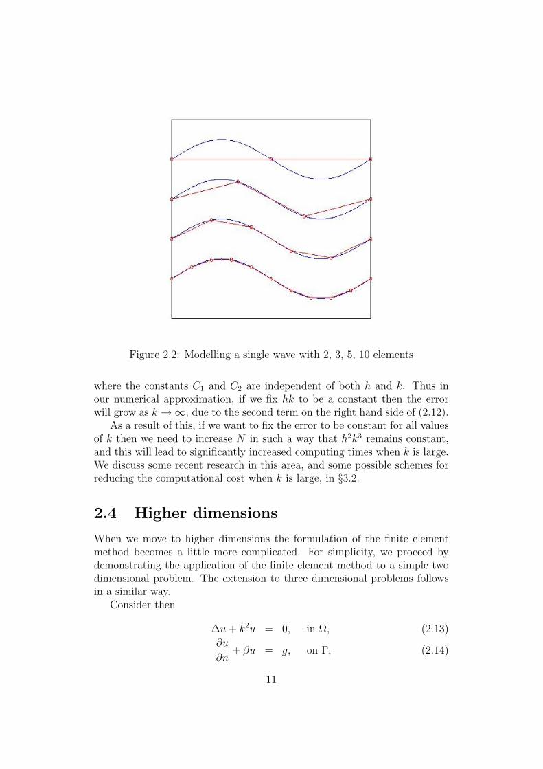
Figure 2.2: Modelling a single wave with 2, 3, 5, 10 elements

where the constants C1 and C2 are independent of both h and k. Thus inour numerical approximation, if we fix hk to be a constant then the errorwill grow as k →∞, due to the second term on the right hand side of (2.12).

As a result of this, if we want to fix the error to be constant for all valuesof k then we need to increase N in such a way that h2k3 remains constant,and this will lead to significantly increased computing times when k is large.We discuss some recent research in this area, and some possible schemes forreducing the computational cost when k is large, in §3.2.

2.4 Higher dimensions

When we move to higher dimensions the formulation of the finite elementmethod becomes a little more complicated. For simplicity, we proceed bydemonstrating the application of the finite element method to a simple twodimensional problem. The extension to three dimensional problems followsin a similar way.

Consider then

∆u + k2u = 0, in Ω, (2.13)

∂u

∂n+ βu = g, on Γ, (2.14)

11

Figure 2.3: Pollution error

where k ∈ R, β ∈ C are constants, ∂/∂n denotes the outward normal deriva-tive, and Ω ∈ R2 is a bounded domain with boundary Γ. Multiplying (2.13)by a test function v ∈ H1(Ω) and integrating we get∫

Ω

v∆u dx +

∫Ω

k2uv dx = 0. (2.15)

Applying the divergence theorem (see e.g. [19, p.26]) we get∫Ω

v∆u dx =

∫Γ

v∂u

∂nds−

∫Ω

∇v.∇u dx,

where dx is the element of area in R2 and ds is the element of arc length onΓ. Substituting into (2.15) and recalling the boundary conditions (2.14) wehave the weak formulation;find u ∈ H1(Ω) such that∫

Ω

∇u.∇v − k2uv dx + β

∫Γ

uv ds =

∫Γ

vg ds, for all v ∈ H1(Ω). (2.16)

As for the one dimensional problem the Galerkin finite element methodthen consists of replacing the space H1(Ω) in (2.16) with a finite dimensional

12

approximation space V ⊂ H1(Ω), and our approximation U ∈ V to u ∈H1(Ω) is then defined by;∫

Ω

∇U.∇v − k2Uv dx + β

∫Γ

Uv ds =

∫Γ

vg ds, for all v ∈ V. (2.17)

Defining V to be the linear span of the basis functions χj, j = 1, . . . , N ,we can then write U ∈ V as

U(x) :=N∑

j=1

ujχj(x),

where the coefficients uj are to be determined, and substituting into (2.17)we have

N∑j=1

[∫Ω

∇χj.∇v − k2χjv dx + β

∫Γ

χjv ds

]uj =

∫Γ

vg ds, for all v ∈ V.

(2.18)Since this equation holds for all v ∈ V it must hold in particular for v = χm,m = 1, . . . , N , and thus we have the linear system

N∑j=1

[∫Ω

∇χj.∇χm − k2χjχm dx + β

∫Γ

χjχm ds

]uj =

∫Γ

χmg ds, (2.19)

for m = 1, . . . , N , or equivalently

Au = f ,

where

A :=

a11 a12 a13... a1N

a21 a22 a23... a2N

a31 a32 a33... a3N

. . . . . . . . .. . . . . .

aN1 aN2 aN3... aNN

, u :=

u1

u2

u3...

uN

f :=

∫Γχ1g ds∫

Γχ2g ds∫

Γχ3g ds...∫

ΓχNg ds

,

with the matrix entries ajm defined by

ajm :=

∫Ω

∇χj.∇χm − k2χjχm dx + β

∫Γ

χjχm ds.

As for the one dimensional problem we can then compute U in three steps;

13

1. Compute each of the matrix entries ajm and each of the right hand sideentries

∫Γχmg ds.

2. Solve the linear system Au = f .

3. Form our approximation U(x) =∑N

j=1 ujχj(x).

There are three main difficulties associated with moving to higher dimen-sions.

2.4.1 Size of the linear system

As the dimension grows, so does the size of the linear system needed toachieve a prescribed level of accuracy. For example, suppose we seek a so-lution accurate to 1%, and we know that the error is bounded by h2, withh := 1/N and N the number of degrees of freedom in each direction. Toachieve 1% accuracy we would thus need to choose N = 10, giving an errorof 1/N2 = 1%. So in one dimension, we would need 10 elements, giving amatrix of size 10×10. However, in two dimensions choosing N = 10 gives 100elements, and the matrix is then of size 100 × 100. In three dimensions thematrix would be of size 1000×1000. So the size of the linear system grows asthe dimension increases. In practice, for practical problems we would needto take N to be a great deal larger than 10 in order to achieve 1% accu-racy and this often leads to impractically large systems. Often it is not justthe solution of these systems that causes problems, even storing them canbecome impossible.

In order to solve the very large systems, it will not usually be possibleto do a direct solve - iterative approaches are needed. These will be faster ifthe bandwidth of the system is smaller - the bandwidth is the width of theband of nonzero diagonals. As we saw in §2.2, in one dimension the matrixhas a bandwidth equal to 3 - this is no problem. However, in two dimensionsthe bandwidth is of order N - although there are only maybe 5 or 9 nonzerodiagonals, the furthest of these from the main diagonal will be a distance Naway. In three dimensions, the bandwidth is of order N2. This means thatthe cost of achieving an accurate iterative solve grows with dimension, andeverything becomes more expensive.

For further details on iterative solution of large sparse linear systems, werefer to [26, 13] and the references therein.

14

2.4.2 Mesh generation

In 1D mesh generation is very easy, as it is just a case of dividing a line upinto sections.

In 2D things becomes a lot more difficult, especially if the geometry ofthe computational domain is complicated. However, for 2D mesh generationmany good codes, both commercial and publicly available, can be used togenerate meshes. A lot of these are based on the Delaunay triangulationalgorithm, which has been shown to be very effective in 2D. For example, amesh generation algorithm is available fromhttp://www.cs.cmu.edu/∼quake/triangle.htmlwhich can be used to generate meshes for a wide range of geometries in2D, including the “snail’s shell” type geometry shown in figure 2.4. This

Figure 2.4: 2D mesh on a complicated geometry

type of geometry would be very hard to model by any means other than atriangulation of the type shown, and demonstrates the versatility of the finiteelement method.

In 3D, things get much more difficult again. The Delaunay triangulationis not particularly effective for 3D mesh generation, and in fact the success ofmost 3D algorithms is measured not by their good performance but rather bythe percentage of elements generated that have big problems, e.g. negativevolume. However, some excellent codes are available, such as NETGEN,

15

downloadable fromhttp://www.hpfem.jku.at/netgen,which was used to generate the meshes in figure 2.5 and 2.6.

There are many resources on the web dealing with mesh generation. Linksto many of the people working in this area, and many publicly available andcommercial codes for mesh generation can be found on some of the followingwebpages;http://www-users.informatik.rwth-aachen.de/. . .∼roberts/meshgeneration.htmlhttp://www.engr.usask.ca/∼macphed/finite/fe resources/mesh.html

http://www.andrew.cmu.edu/user/sowen/mesh.html

2.4.3 Design of the approximation space

Rather than using piecewise polynomial basis functions, many schemes suchas the generalised finite element method (see e.g. [2]) use basis functionschosen specifically to model the behaviour of the solution.

For one dimensional problems it is straightforward to get a good handle onthe behaviour of the solution. Plane waves can only travel in two directions,so they can easily be incorporated into the approximation space in order toimprove the accuracy of the scheme at large wavenumbers (see also §3.2).

In two dimensions, plane waves can travel in all directions on a plane,making the behaviour much harder to model, and in three dimensions thenumber of possible directions increases again. Thus the design of an appro-priate approximation space becomes much more difficult as the dimension ofthe problem increases.

16

Figure 2.5: 3D mesh

Figure 2.6: 3D mesh

17

Chapter 3

Current research on finiteelement methods for acoustics

Although finite element methods have been around for a considerable time,there is still much work to be done on their application to acoustic scat-tering problems, which present a unique set of difficulties. Here, we focusparticularly on two of these.

Firstly, we remark that the finite element method was originally devel-oped for the numerical solution of problems on bounded domains. However,often in acoustic scattering applications the computational domain may beunbounded. In this case, there is an immediate difficulty - how do we discre-tise an infinite domain? This question is addressed in §3.1.

A second difficulty is that when the wavenumber k becomes large, theaccuracy of the “standard” finite element method deteriorates, as alluded toalready in §2.3. Various techniques have been developed to get around thisdifficulty, and these are discussed in §3.2.

3.1 Unbounded domains

In the event that D is an unbounded domain, as is often the case for scatteringproblems, we also need to supplement (1.3) with a Sommerfeld radiationcondition to ensure uniqueness of solution. This corresponds to imposing acondition that no waves are reflected from ∞. So that standing waves cannotoccur, we force

1

R(d−1)/2

(∂u

∂R− iku

)→ 0, as R →∞, d = 1, 2, 3. (3.1)

Solutions of exterior Helmholtz problems that also satisfy (3.1) are known asradiating solutions.

18

There is though a further difficulty. Clearly we cannot discretise anunbounded domain with finite elements. To get around this, many cleverschemes have been suggested for the application of finite element methods tounbounded domains, with the big question being “what to do at infinity”?

One approach is to replace the unbounded domain with a bounded one,by introducing an artificial boundary as shown in figure 3.1. The finite

Figure 3.1: Artificial boundary to replace a problem on an unbounded domainwith one on a bounded domain

element discretisation of the region exterior to the scatterer is then carriedout only in the (small) annular domain enclosing the scatterer. In this case aproblem on an unbounded domain has been replaced with one on a boundeddomain, the difficulty comes in choosing the boundary conditions on theartificial boundary in such a way that the solution of the modified problemis a sufficiently close approximation to the solution of the original problem.

The main tool in the choice of this boundary condition is a coupling ofthe finite element solution to some discrete representation of the analyticalsolution, with the absorbing boundary condition (ABC) chosen in such a waythat there is no reflection of scattered waves (see for example [14, chapter 3]).

To find the behaviour in the region exterior to the artificial boundary,one can either use integral representations (see e.g. [10, 11]), or separationof variables, looking for solutions in the form of plane wave solutions (seee.g. [14, §2.1]).

19

For example, consider again the one dimensional problem (2.1) of §2.2,and suppose now that we wish to solve this problem on an unbounded do-main. The exact solution of (2.1) is given by

u(x) = Aeikx + Be−ikx,

with the constants A and B to be determined by the boundary data. Thecorresponding time-dependent solution is then

P (x, t) = Aei(kx−ωt) + Be−i(kx+ωt),

where the first term on the right hand side represents the outgoing wave,travelling from 0 to ∞, and the second term on the right hand side representsthe incoming wave, travelling from ∞ to 0. Applying at any point x = x0

the boundary condition

ω

k

∂P

∂x(x0) +

∂P

∂t(x0) = 0

eliminates the incoming wave. This is thus a nonreflecting boundary condition(NRBC) at x0 (see problem sheet).

In higher dimensions, the plane waves eikx.d are particular solutions ofthe two or three dimensional Helmholtz equation, where the direction vec-tor d represents a particular direction in which the plane wave is travelling.For example, for d = 3 the plane wave eik(αx+βy+γz) solves (1.3) providedα2 + β2 + γ2 = k2. The difficulty here comes in determining α, β, γ; if weknow the directions of the plane waves in the exact solution then a NRBCcan be deduced for the higher order problem. However, in general the direc-tions are not known, and thus instead one has to construct an ABC as anapproximation to the NRBC.

Other techniques for solving problems on exterior domains include theuse of Perfectly Matched Layers (see e.g. [5]), or infinite elements (see e.g. [1,6, 12]). For a full review of the many schemes available we refer to [14,chapter 3].

3.2 Large wavenumbers

We have already discussed some of the difficulties encountered when k islarge in §2.3.

Various approaches have recently been developed to get around thesedifficulties. Rather than using piecewise linear basis functions, using higherorder piecewise polynomials (the hp approach) can lead to a big improvement

20

in the accuracy of the method (see e.g. [15, 16, 25]). In particular, if theapproximation space consists of piecewise polynomials of order p, then wecan replace the error estimate (2.12) with an estimate of the form

‖(u− U)′‖‖u′‖

≤ C1

(hk

2p

)p

+ C2k

(hk

2p

)2p

, (3.2)

(see [14, p.154]). As for the h-version of this estimate, the first term repre-sents the approximation error and the second term the pollution error. Notethat taking p = 1 gives (2.12) again. Using an hp approach thus significantlyimproves the accuracy of the finite element method - increasing p can leadto a dramatic reduction in the pollution error without needing to decrease has significantly as for the h version.

Another approach is to use basis functions that are specifically tailoredto the problem of high frequency acoustic scattering. This is the idea behindthe generalised finite element method and the partition of unity method (seee.g. [3, 22]), and has been applied to great effect by Bettess et. al. [21, 24,20] using plane wave basis functions. These basis functions take the formeikx.d, where d is a unit vector. Including many such basis functions in theapproximation space, with many direction vectors d, can lead to dramaticallyimproved performance of the method, with a reduction in the number ofelements required per wavelength from ten to two.

A further difficulty in the case that k is large is that the integrals to beevaluated in order to set up the linear system will be highly oscillatory. Com-puting these integrals may become more expensive as k increases. Variousschemes have recently been developed for the efficient evaluation of highlyoscillatory integrals (see e.g. [17, 18]), but this issue is still not fully resolved.

21

Chapter 4

Conclusions and furtherreading

In these notes we have attempted to provide a brief introduction to the finiteelement method, and its use in problems of acoustic scattering. The partic-ular difficulties inherent in this problem, chief amongst them the oscillatorynature of the solution, mean that a naive application of standard schemesmay give poor results. We have thus attempted also to explain why using astandard scheme with a piecewise linear approximation space may performpoorly when the frequency is large, and to give a short summary of somealternative approaches which may lead to improved performance.

The main reference we have used in writing these lecture notes is theexcellent book by Ihlenburg [14], who deals specifically with the applicationof the finite element method to problems of acoustic scattering. In [23], Monkdeals with the application and analysis of finite element methods to problemsof electromagnetic scattering, which share many features and difficulties withacoustic problems.

In addition, there are many excellent books such as [19, 9, 25, 7, 8] pro-viding a clear introduction to the finite element method and its analysis,treating the subject with a far greater mathematical rigour than we haveattempted here.

22

Bibliography

[1] R.J. Astley. Infinite elements for wave problems: A review of currentformulations and an assessment of accuracy. Int. Journ. Num. Meth.Engng., 49:951–976, 2000.

[2] I. Babuska, U. Banerjee, and J.E. Osborn. Generalized finite elementmethods - main ideas, results and perspective. International Journla ofComputational Methods, 1:67–103, 2004.

[3] I Babuska and J.M. Melenk. The partition of unity method. Int. J.Numer. Meth. Eng., 40:727–758, 1997.

[4] I Babuska and S Sauter. Is the pollution effect of the FEM avoidablefor the Helmholtz equation considering high wave numbers. SIAM J.Numer. Anal., 34:2392–2423, 1997. Reprinted in SIAM Rev. 42 (3),451-484, 2000.

[5] J. Berenger. A perfectly matched layer for the absorption of electromag-netic waves. J. Comput. Phys., 114:185–200, 1994.

[6] P. Bettess. Infinite elements. Penshaw Pres, Cleadon, 1992.

[7] D. Braess. Finite Elements. Cambridge University Press, Cambridge,2nd edition, 2001.

[8] S.C. Brenner and L.R. Scott. The Mathematical Theory of Finite Ele-ment Methods. Springer, New York, 1994.

[9] P.G. Ciarlet. The Finite Element Method for Elliptic Problems. North-Holland Publishing Company, 1978.

[10] D Colton and R Kress. Integral Equation Methods in Scattering Theory.Wiley, 1983.

[11] D Colton and R Kress. Inverse Acoustic and Electromagnetic ScatteringTheory. Springer Verlag, 1992.

23

[12] L. Demkowicz and K. Gerdes. Convergence of the infinite element meth-ods for the Helmholtz equation in separable domains. Numer. Math.,79:11–42, 1998.

[13] G.H. Golub and C.F. Van Loan. Matrix Computations. Johns HopkinsUniversity Press, 3rd edition, 1996.

[14] F Ihlenburg. Finite Element Analysis of Acoustic Scattering. Springer-Verlag, New York, 1998.

[15] F Ihlenburg and I Babuska. Finite element solution of the Helmholtzequation with high wavenumber. 1. the h version of the FEM. Comput.Math. Appl., 30(9):9–37, 1995.

[16] F Ihlenburg and I Babuska. Finite element solution of the Helmholtzequation with high wavenumber. 2. the h−p version of the FEM. SIAMJ. Numer. Anal., 34(1):315–358, 1997.

[17] A. Iserles. On the numerical quadrature of highly-oscillating integrals I:Fourier transforms. IMA J. Numer. Anal., 24:365–391, 2004.

[18] A. Iserles. On the numerical quadrature of highly-oscillating integralsII: Irregular oscillations. IMA J. Numer. Anal., 25:25–44, 2005.

[19] C. Johnson. Numerical Solution of Partial Differential Equations by theFinite Element Method. Cambridge University Press, 1987.

[20] O Laghrouche, P Bettess, and R.J. Astley. Modelling of short wavediffraction problems using approximating systems of plane waves. Int.J. Numer. Meth. Eng., 54:1501–1533, 2002.

[21] O. Laghrouche, P. Bettess, E. Perrey-Debain, and J. Trevelyan. Waveinterpolation finite elements for Helmholtz problems with jumps in thewave speed. Comp. Meth. Appl. Mech. Eng., 194:367–381, 2005.

[22] J.M. Melenk and I Babuska. The partition of unity finite elementmethod: Basic theory and applications. Comput. Method Appl. M.,139:289–314, 1996.

[23] P. Monk. Finite Element Methods for Maxwell’s Equations. OxfordScience Publications, 2003.

[24] E. Perrey-Debain, O. Lagrouche, P. Bettess, and J. Trevelyan. Plane-wave basis finite elements and boundary elements for three-dimensionalwave scattering. Phil. Trans. R. Soc. Lond. A, 362:561–577, 2004.

24

[25] B.S. Szabo and I. Babuska. Finite Element Analysis. J. Wiley, 1991.

[26] L.N. Trefethen and D. Bau. Numerical Linear Algebra. SIAM, 1997.

25