Finite element formulation for modeling nonlinear viscoelastic

Comput. Methods Appl. Mech. Engrg. 197 (2008) 4702–4717

Contents lists available at ScienceDirect

Comput. Methods Appl. Mech. Engrg.

journal homepage: www.elsevier .com/locate /cma

Finite element formulation for modeling nonlinear viscoelastic elastomers

Pedro Areias a,1, Karel Matouš a,b,*,1

a Computational Science and Engineering, University of Illinois at Urbana-Champaign, Urbana, IL 61801, USAb Department of Aerospace Engineering, University of Illinois at Urbana-Champaign, Urbana, IL 61801, USA

a r t i c l e i n f o

Article history:Received 10 November 2007Received in revised form 22 February 2008Accepted 17 June 2008Available online 5 July 2008

Keywords:Stabilized elementImplicit gradientIntegration algorithmViscoelasticityPropellant unit cell

0045-7825/$ - see front matter � 2008 Elsevier B.V. Adoi:10.1016/j.cma.2008.06.015

* Corresponding author. Address: Computational Sversity of Illinois at Urbana-Champaign, Urbana, IL 68448.

E-mail address: [email protected] (K. Matouš).URL: http://www.csar.uiuc.edu/~matous/ (K. Mato

1 US Department of Energy, B341494. Alliant Techsy

a b s t r a c t

Nonlinear viscoelastic response of reinforced elastomers is modeled using a three-dimensional mixedfinite element method with a nonlocal pressure field. A general second-order unconditionally stableexponential integrator based on a diagonal Padé approximation is developed and the Bergström–Boycenonlinear viscoelastic law is employed as a prototype model. An implicit finite element scheme with con-sistent linearization is used and the novel integrator is successfully implemented. Finally, several visco-elastic examples, including a study of the unit cell for a solid propellant, are solved to demonstrate thecomputational algorithm and relevant underlying physics.

� 2008 Elsevier B.V. All rights reserved.

1. Introduction

Particle-reinforced elastomers are used in variety of applica-tions, such as solid propellants and automobile tires. The constitu-tive description of this important category of materials is achallenging research topic. The interacting physical processes tak-ing place at various length and time scales make the modeling dif-ficult: there is a large mismatch in stiffness between the matrix andthe reinforcing particles, and large deformations of the quasi-incompressible nonlinear viscoelastic matrix, particle debonding,void growth, matrix tearing, Mullins hysteretic effect under cyclicloading, and other complex phenomena are also present.

Homogenized continuum models are usually used to capturesome of these phenomena. Drozdov and Dorfmann [12], for exam-ple, used the network theory of rubber elasticity to capture thenonlinear equilibrium response of filled and unfilled elastomers.A similar approach was taken by Bergström and Boyce [6,7], whoproposed a dual network model to predict the nonlinear viscoelas-tic response of carbon-black reinforced rubbers, with emphasis oncapturing the large deformations and Mullins effects. Miehe andGöktepe [27] introduced a micromechanics-based micro-spheremodel to represent viscoelasticity of elastomers. Purely phenome-nological continuum laws of varying complexity are also often em-

ll rights reserved.

cience and Engineering, Uni-1801, USA. Tel.: +1 217 333

uš).stems, ATK-21316.

ployed. Examples include Dorfmann and Ogden’s analysis of theMullins effect [11] and Simo’s work on the finite-strain viscoelasticdamage model [35]. One of the most comprehensive studies focus-ing on viscoelasticity and its numerical aspects is that of Reese andGovindjee [34].

Another issue is associated with the numerical analysis of thesematerials. The matrix material is highly nonlinear and nearlyincompressible, so a special numerical framework must be em-ployed. In principle, stable methods for the Stokes equation (see,e.g., Zienkiewicz and Wu [39]) can be adapted, with minor modifi-cations, to finite strain problems. For incompressible bulk deforma-tion, relatively high performance mixed elements were proposed,among others, by Hughes et al. [17], Chiumenti et al. [10] andRamesh and Maniatty [33]. Recently, Puso and Solberg [32] pro-posed an element involving a convex combination with nodalquadrature, Tian et al. [38] developed a general purpose tetrahe-dral element with a good balance of properties, and Hauret et al.[15] introduced a diamond element based on discrete mechanics.In this work, we use the nonlocal pressure element developed byAreias and Matouš [1].

A related challenge is integrating the constitutive equations(ODEs), which are usually stiff and highly nonlinear. An implicitexponential integrator, for example, which is well suited for stiffand highly oscillatory problems has been used in elasto- and visco-plasticity [5]. For classical viscoelasticity, Fancello et al. [13] usedthis integrator in the context of the variational update.

In a series of recent papers, we have focused on decohesion of par-ticles from a matrix [24–26]. In this work, the highly nonlinear visco-elastic response of a binder is investigated, with emphasis on theefficient integration algorithm. The highly nonlinear dependence

mailto:[email protected]

http://www.csar.uiuc.edu/~matous/

http://www.sciencedirect.com/science/journal/00457825

http://www.elsevier.com/locate/cma

P. Areias, K. Matouš / Comput. Methods Appl. Mech. Engrg. 197 (2008) 4702–4717 4703

of the stress in the flow law and the plasticity-like idealization can-not, in general, make use of the Prony series method. Thus, we usethe viscoelastic model proposed by Bergström and Boyce [6,7] anddevelop a new exponential integrator based on a diagonal Padé ra-tional approximation, which has a number of advantages such asA-stability [19] and simplified calculation of derivatives. The exactpreservation of a unit determinant by the Padé approximation in2D and the supremum and infimum of determinant in 3D are alsodemonstrated. This result, which to the authors’ knowledge is new,may have some practical importance.

We propose here a special numerical scheme, which was foundto be required for two reasons:

1. The Bergström–Boyce constitutive equations could not be inte-grated effectively in the general case with traditional exponen-tial integrator.

2. The proposed scheme can be applied to finite strain inelasticanisotropic materials.

Direct application to anisotropic materials results from a spe-cific, anisotropic, flow law and its integration. This is not possiblewith classical integration schemes for nonlinear viscous laws;examples for linear viscous laws are well known in the literature[16].

The paper is organized as follows: in Section 2, we briefly de-scribe the governing equations and highlight our mixed formula-tion with nonlocal pressure [1]. Section 3 details the constitutivemodel including the new Padé integrator and consistent lineariza-tion, and a particularization is constructed for the Bergström–Boyce model. Section 4 is devoted to numerical examples withemphasis on the numerical integration. Several viscoelastic exam-ples are solved to demonstrate the computational algorithm andcomplexity of the underlying physics.

2. Mixed finite element method

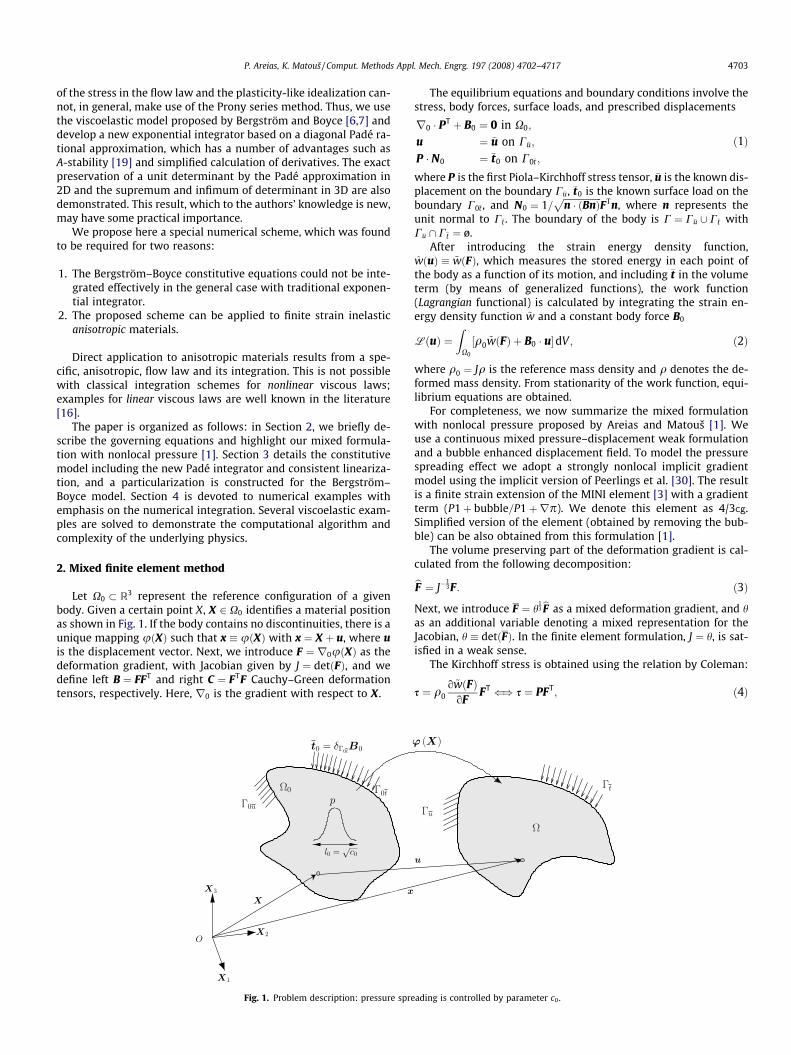
Let X0 � R3 represent the reference configuration of a givenbody. Given a certain point X, X 2 X0 identifies a material positionas shown in Fig. 1. If the body contains no discontinuities, there is aunique mapping uðXÞ such that x � uðXÞ with x ¼ X þ u, where uis the displacement vector. Next, we introduce F ¼ r0uðXÞ as thedeformation gradient, with Jacobian given by J ¼ detðFÞ, and wedefine left B ¼ FFT and right C ¼ FTF Cauchy–Green deformationtensors, respectively. Here, r0 is the gradient with respect to X.

Fig. 1. Problem description: pressure spre

The equilibrium equations and boundary conditions involve thestress, body forces, surface loads, and prescribed displacements

r0 � PT þ B0 ¼ 0 in X0;

u ¼ �u on C�u;

P � N0 ¼ �t0 on C0�t ;

ð1Þ

where P is the first Piola–Kirchhoff stress tensor, �u is the known dis-placement on the boundary C�u, �t0 is the known surface load on theboundary C0�t , and N0 ¼ 1=

ffiffiffiffiffiffiffiffiffiffiffiffiffiffiffiffiffin � ðBnÞ

pFTn, where n represents the

unit normal to C�t . The boundary of the body is C ¼ C�u [ C�t withC�u \ C�t ¼ ø.

After introducing the strain energy density function,wðuÞ � ~wðFÞ, which measures the stored energy in each point ofthe body as a function of its motion, and including �t in the volumeterm (by means of generalized functions), the work function(Lagrangian functional) is calculated by integrating the strain en-ergy density function ~w and a constant body force B0

LðuÞ ¼Z

X0

½q0 ~wðFÞ þ B0 � u�dV ; ð2Þ

where q0 ¼ Jq is the reference mass density and q denotes the de-formed mass density. From stationarity of the work function, equi-librium equations are obtained.

For completeness, we now summarize the mixed formulationwith nonlocal pressure proposed by Areias and Matouš [1]. Weuse a continuous mixed pressure–displacement weak formulationand a bubble enhanced displacement field. To model the pressurespreading effect we adopt a strongly nonlocal implicit gradientmodel using the implicit version of Peerlings et al. [30]. The resultis a finite strain extension of the MINI element [3] with a gradientterm (P1þ bubble=P1þrp). We denote this element as 4/3cg.Simplified version of the element (obtained by removing the bub-ble) can be also obtained from this formulation [1].

The volume preserving part of the deformation gradient is cal-culated from the following decomposition:bF ¼ J�

13F: ð3Þ

Next, we introduce F ¼ h13bF as a mixed deformation gradient, and h

as an additional variable denoting a mixed representation for theJacobian, h � detðFÞ. In the finite element formulation, J ¼ h, is sat-isfied in a weak sense.

The Kirchhoff stress is obtained using the relation by Coleman:

s ¼ q0o ~wðFÞ

oFFT () s ¼ PFT; ð4Þ

ading is controlled by parameter c0.

4704 P. Areias, K. Matouš / Comput. Methods Appl. Mech. Engrg. 197 (2008) 4702–4717

and its deviatoric part reads

T ¼ s� ~p1; ð5Þ

where ~p ¼ 1=3trðsÞ represents the Kirchhoff hydrostatic pressureand 1 is the second-order identity tensor. Satisfaction of poly-con-vexity requires a convex volumetric energy, UðJÞ, such that~p ¼ JdUðJÞ=dJ.

The following equations are provided for ~p and p:

~p � gðJÞ ¼ j½J2 � J þ lnðJÞ�;p � gðhÞ ¼ j½h2 � hþ lnðhÞ�;

ð6Þ

and

h ¼ g�1ðpÞ: ð7Þ

The bulk modulus is j, p and h are pressure-like and dilatation-likequantities, respectively. The function g�1 is obtained only implicitly,since there is no closed-form inverse of g. Due to direct applicationof the Galerkin method, the relationship between volumetric energyUðJÞ, which would enter the functional L mentioned bellow, andgðJÞ is not needed.

To force pressure spreading, the pressure field p obeys the fol-lowing inhomogeneous form of the Helmholtz equation:

p� c0D0p� ~p ¼ 0; ð8Þ

where D0 is the Laplace operator with respect to the material coor-dinates. Here, the area parameter c0 controls the degree of nonlocal-ity of the pressure field. Please note that Eq. (8) will introduce anapproximation of the same order of magnitude as the one inducedby the explicit gradient model

p ¼ ~pþ c0r~p; ð9Þ

which would require C1-continuity of the pressure field, whereasimplicit approach enables a straightforward C0 finite element inter-polation. A weak form of (8) is obtained by using the test function 1Z

X0

1ðp� ~pÞdV0 þ c0

ZX0

r01 � r0pdV0 ¼ 0 ð10Þ

81 2 ½H1ðX0Þ1�, where ½H1ðX0Þnsd � denotes the Sobolev space ofsquare-integrable functions with weak derivatives up to first orderwith range in Rnsd . We make use of the Lasry–Belytschko boundaryconditions for the pressure [20].

After applying standard variational methods and using (10), westate the equilibrium condition and its first variation using a mixedform: Find uðXÞ and pðXÞ such that

dLðu; pÞ ¼Z

X0

(½sþ ðp� ~pÞ1|fflfflfflfflfflfflfflfflfflffl{zfflfflfflfflfflfflfflfflfflffl}

�s

: rv

þ1½p� gðJÞ� þ c0r01 � r0pþ B0 � v)

dV0 ¼ 0

DdLðu; pÞ ¼Z

X0

rv : CTL : rDu� 13rv : ½1� ð1 : CTL : rDuÞ�

�� s : ðrvrDuÞ þ Dp1 : rv þ 1Dp

�J1dgdJ

1 : rDuþ c0r01 � r0Dp�

dV0;

ð11Þfor all v and 1 satisfying

v 2 ½H1ðX0Þ3� ^ 1 2 ½H1ðX0Þ1�; v ¼ 0 on C0�u: ð12Þ

Here, r� ¼ r0 � F�1 is a gradient with respect to the spatial config-uration. Note that both the Kirchhoff stress tensor s ¼ PFT and thegradient of the test function rv ¼ dFF�1 are independent of h, andthat we can determine an instantaneous bulk modulusj0 ¼ 1=hðg0 � p=hÞ. Note that, the functional Lðu; pÞ is not explicitly

defined, since we directly use the Galerkin method leading tounsymmetric stiffness. The equilibrium stress �s is obtained as

�s ¼ T þ p1 ¼ sþ ðp� ~pÞ1: ð13Þ

The term CTL is the tangent modulus, related to the velocity gradi-ent. If the constitutive stress is trace-free, then the time-derivativeof T is given by _T ¼ CTL : L, with L ¼ _FF�1. In our implementation,the initial stress term (third term in (11)) is preceded by a minussign, which is distinct from the usual Lie derivative (or Oldroyd)modulus. Both the tangent and Oldroyd moduli are introduced inSection 3.2. It is worth noting that exact calculation of (11) is nec-essary to obtain quadratic convergence rate of Newton’s methodas demonstrated in Section 4.

3. Constitutive laws

Although the constitutive update scheme developed in thiswork is applicable to a wide range of nonlinear material models,we focus on the nonlinear viscoelastic response suitable for analy-sis of reinforced elastomers, such as solid propellants. We employ aviscoelastic constitutive law, without thermal effects, that is fullynonlinear (both the flow law and the elastic law are nonlinear) inthe sense of Lion [22]. But we will maintain generality of the algo-rithm, which, with minor modifications, can be particularized toother problems such as finite strain plasticity with an arbitraryhyperelastic behavior (not only the traditional Hencky or St. Ve-nant elastoplasticity). Here, we describe the general algorithm,and its particularization for the Bergström–Boyce model is pre-sented in Section 3.3.

First, we introduce the multiplicative decomposition of thedeformation gradient (see [21])

F ¼ FeFv; ð14Þ

where Fe is the reversible (elastic) deformation gradient and Fv de-notes the viscous deformation gradient. The viscous deformationgradient satisfies

detðFvÞ ¼ 1: ð15Þ

The kinematic quantities, such as the viscous right Cauchy–Greentensor and the elastic left Cauchy–Green tensor, are given by

Cv ¼ FTvFv;

Be ¼ FeFTe ¼ FC�1

v FT;ð16Þ

and the relation between the deviatoric stress and the hyperelasticstrain tensors reads

T ¼ TðBeÞ; ð17Þ

where elastic isotropy is assumed (cf. eq. 31, page 142 of [9]). It iseasy to show that there exists a �wðBeÞ such that ~wðFÞ ¼ �wðBeÞ andthe Kirchhoff stress is given by

s ¼ q0o ~wðFÞ

oFFT ¼ 2q0

o�wðBeÞoBe

Be: ð18Þ

For an anisotropy one could use the second Piola–Kirchhoff stress,which is dependent on both C and Cv (see [2]).

The flow law follows the usual definition

_FvF�1v � Dv ¼ _cN; ð19Þ

and the flow vector is given by

N ¼ T=kTkF: ð20Þ

Note that N is a symmetric tensor, and hence the viscous strain rateDv is the complete viscous velocity gradient. The form of the flowlaw also allows pre-existing anisotropy. The notation k � kF is usedhere for the Frobenius norm of a given linear operator �. Next, the


equivalent strain rate, expressed as a nonlinear function of thestress and the viscous right Cauchy–Green tensor, yields

_c ¼ _cðCv;TÞ; ð21Þ

where the relation

_c ¼ kDvkF ð22Þ

holds by construction. The dependence of _c upon Cv and T is ef-fected by means of the two scalar functions fv and T such that

_c ¼ _c½fvðCvÞ; TðTÞ�; ð23Þ

and, although not strictly required, the inverse relation

T ¼ T½ _c; fvðCvÞ� � kTkF ð24Þ

is assumed to be explicit. To inspect the interdependencies in (24),we rewrite it as

_Cv ¼ 2FTv _c½fvðCvÞ; TðFC�1

v FTÞ� TðFC�1v FTÞ

kTðFC�1v FTÞkF|fflfflfflfflfflfflfflfflfflfflfflfflfflfflfflfflfflfflfflfflfflfflfflfflfflfflfflfflfflfflfflffl{zfflfflfflfflfflfflfflfflfflfflfflfflfflfflfflfflfflfflfflfflfflfflfflfflfflfflfflfflfflfflfflffl}

Dv

Fv; ð25Þ

along with the initial condition Cvjt¼0 ¼ 1 in the absence of pre-existing flow. Note that Cv is the only unknown in this system, sinceF is imposed. Also, Fv is a function of _c, and therefore, it is also afunction of Cv. This is a consequence of the evolution law’sdependence on a symmetric vector, leaving a zero spin tensorWv0. Note about anisotropy is made when the integration algorithmis introduced. The determination of Cv is described below.

3.1. Integration algorithm

For a prescribed deformation path, the stress response and theviscous multiplier evolution can be obtained by integrating theconstitutive Eqs. (17) and (25). Since no closed form is available,the ODE system, which consists of the flow law after replacementof the elasticity relation must be solved numerically. The problemis a first-order ODE whose nonlinearity suggests the use of an im-plicit integrator. Although the eigenvalues of the flow matrix arebounded, the scaling parameter _c often induces a stiff system.Thus, the choice of integrator is usually dictated by the particularrequirements of the constitutive update. From the numericalmethods available in the literature, we focus on a class of exponen-tial integrators that are unconditionally stable, and thus areappealing for application in the finite element method.

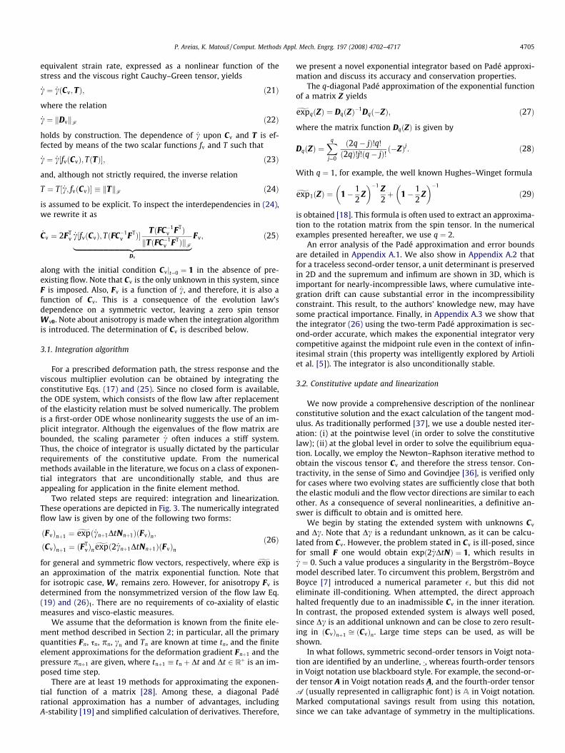
Two related steps are required: integration and linearization.These operations are depicted in Fig. 3. The numerically integratedflow law is given by one of the following two forms:

ðFvÞnþ1 ¼ gexpð _cnþ1DtNnþ1ÞðFvÞn;ðCvÞnþ1 ¼ ðF

TvÞngexpð2 _cnþ1DtNnþ1ÞðFvÞn

ð26Þ

for general and symmetric flow vectors, respectively, where gexp isan approximation of the matrix exponential function. Note thatfor isotropic case, Wv remains zero. However, for anisotropy Fv isdetermined from the nonsymmetrized version of the flow law Eq.(19) and (26)1. There are no requirements of co-axiality of elasticmeasures and visco-elastic measures.

We assume that the deformation is known from the finite ele-ment method described in Section 2; in particular, all the primaryquantities Fn, sn, pn, cn and Tn are known at time tn, and the finiteelement approximations for the deformation gradient Fnþ1 and thepressure pnþ1 are given, where tnþ1 � tn þ Dt and Dt 2 Rþ is an im-posed time step.

There are at least 19 methods for approximating the exponen-tial function of a matrix [28]. Among these, a diagonal Padérational approximation has a number of advantages, includingA-stability [19] and simplified calculation of derivatives. Therefore,

we present a novel exponential integrator based on Padé approxi-mation and discuss its accuracy and conservation properties.

The q-diagonal Padé approximation of the exponential functionof a matrix Z yields

gexpqðZÞ ¼ DqðZÞ�1Dqð�ZÞ; ð27Þ

where the matrix function DqðZÞ is given by

DqðZÞ ¼Xq

j¼0

ð2q� jÞ!q!

ð2qÞ!j!ðq� jÞ! ð�ZÞj: ð28Þ

With q ¼ 1, for example, the well known Hughes–Winget formula

gexp1ðZÞ ¼ 1� 12

Z� ��1 Z

2þ 1� 1

2Z

� ��1

ð29Þ

is obtained [18]. This formula is often used to extract an approxima-tion to the rotation matrix from the spin tensor. In the numericalexamples presented hereafter, we use q ¼ 2.

An error analysis of the Padé approximation and error boundsare detailed in Appendix A.1. We also show in Appendix A.2 thatfor a traceless second-order tensor, a unit determinant is preservedin 2D and the supremum and infimum are shown in 3D, which isimportant for nearly-incompressible laws, where cumulative inte-gration drift can cause substantial error in the incompressibilityconstraint. This result, to the authors’ knowledge new, may havesome practical importance. Finally, in Appendix A.3 we show thatthe integrator (26) using the two-term Padé approximation is sec-ond-order accurate, which makes the exponential integrator verycompetitive against the midpoint rule even in the context of infin-itesimal strain (this property was intelligently explored by Artioliet al. [5]). The integrator is also unconditionally stable.

3.2. Constitutive update and linearization

We now provide a comprehensive description of the nonlinearconstitutive solution and the exact calculation of the tangent mod-ulus. As traditionally performed [37], we use a double nested iter-ation: (i) at the pointwise level (in order to solve the constitutivelaw); (ii) at the global level in order to solve the equilibrium equa-tion. Locally, we employ the Newton–Raphson iterative method toobtain the viscous tensor Cv and therefore the stress tensor. Con-tractivity, in the sense of Simo and Govindjee [36], is verified onlyfor cases where two evolving states are sufficiently close that boththe elastic moduli and the flow vector directions are similar to eachother. As a consequence of several nonlinearities, a definitive an-swer is difficult to obtain and is omitted here.

We begin by stating the extended system with unknowns Cv

and Dc. Note that Dc is a redundant unknown, as it can be calcu-lated from Cv. However, the problem stated in Cv is ill-posed, sincefor small F one would obtain expð2 _cDtNÞ ¼ 1, which results in_c ¼ 0. Such a value produces a singularity in the Bergström–Boycemodel described later. To circumvent this problem, Bergström andBoyce [7] introduced a numerical parameter �, but this did noteliminate ill-conditioning. When attempted, the direct approachhalted frequently due to an inadmissible Cv in the inner iteration.In contrast, the proposed extended system is always well posed,since Dc is an additional unknown and can be close to zero result-ing in ðCvÞnþ1 ffi ðCvÞn. Large time steps can be used, as will beshown.

In what follows, symmetric second-order tensors in Voigt nota-tion are identified by an underline, �, whereas fourth-order tensorsin Voigt notation use blackboard style. For example, the second-or-der tensor A in Voigt notation reads A, and the fourth-order tensorA (usually represented in calligraphic font) is A in Voigt notation.Marked computational savings result from using this notation,since we can take advantage of symmetry in the multiplications.


Typically, the moduli calculated in Voigt notation must have thelast three columns scaled so that the correct values are recovered.Note that in the literature some divergence in Voigt notation oc-curs, resulting in misleading versions of the flow vector. For exam-ple, if the gradient of a yield function is calculated after thereplacement Tij ¼ Tji is performed, then the flow vector is compat-ible with engineering notation for shear strains. Caution must betaken in calculating the derivatives and the consistent modulus;contractions of fourth-order tensors cannot be directly replacedby simple matrix products in Voigt notation. Moreover, to facilitatethe derivations and take advantage of minor symmetry, two oper-ators A and B, valid for general symmetric second-order tensors,are introduced. If A is a given second-order tensor (not necessarilysymmetric), then

AðAÞ� ¼ ½AT � A� ) AðAÞ ¼ d½AT � A�d� ð30Þ

and

BðAÞ� ¼ AðATÞ� ¼ A � AT; ð31Þ

where � is a symmetric second-order tensor. With these operators,we use the compact notation

Be ¼ BðFÞC�1v ð32Þ

and

dC�1v

dt¼ �AðC�1

v ÞdCv

dt: ð33Þ

Employing this nomenclature, the system (26)2 and (24) can bewritten in the form

eq1 � ðCvÞnþ1 �AðFvÞngexpðZnþ1Þ ¼ 0;

eq2 � Tnþ1 : Tnþ1 � T2nþ1ðDc;CvÞ ¼ 0;

ð34Þ

with

Znþ1 ¼ 2 _cnþ1Dt|fflfflffl{zfflfflffl}Dc

Nnþ1: ð35Þ

Note that complementarity problems, such as rate-dependent elas-toplasticity, can be solved in nearly the same form but with a pre-dictor–corrector methodology. It can be seen that our noveltreatment of viscoelasticity is a degenerate case of rate-dependentelastoplasticity with a collapsed elastic region for which (34)2 is al-ways satisfied. Different, more traditional techniques are shown inthe book by Simo and Hughes [37].

At each iteration k of the Newton–Raphson method for solvingthe system (34), the linear system

Mpp � I Mpc

MTp MTc

" #kDCv

DðDcÞ

� �¼

eq1

eq2

� �k

ð36Þ

is solved, and then the viscous right Cauchy–Green tensor and theviscous multiplier are updated as Cv

kþ1 ¼ Cvk þ DCv and Dckþ1 ¼

Dck þ DðDcÞ, respectively. Note that the subscripts n and nþ 1 havebeen dropped for clarity. The linearized terms on the left-hand sideof (36) are given by

Mpp ¼MpTMTp; Mpc ¼MZN;

MTp ¼ 2oToCv

T �MTpT� �

; MTc ¼ 2ToToDc

;ð37Þ

where

MpT ¼ DcMZdNdT

; MTp ¼ �MeBðFÞAðC�1v Þ; MZ ¼ 2AðFvÞNz;

Me ¼dTdBe

; Nz ¼dgexpðZÞ

dZ

ð38Þ

and I represents the fourth-order identity tensor. Fewer than 10iterations are usually required to reach the tolerance kDCvkF 6tol ¼ 1 10�8. The accuracy of this solution affects the exactnessof the tangent modulus.

Once the solution of (36) is obtained, the increment in the vis-cous multiplier is related to the increment in the viscous right Cau-chy–Green tensor by

DðDcÞ ¼ �M�1Tc MTp|fflfflfflfflfflfflffl{zfflfflfflfflfflfflffl}Mcp

DCv; ð39Þ

and the time-derivative of Cv (taken with respect to the imposed F)yields

dCv

dt¼ IM�1

pp MpTMTL|fflfflfflfflfflfflfflfflfflfflffl{zfflfflfflfflfflfflfflfflfflfflffl}MpL

: L; ð40Þ

where

HMpp ¼ I�Mpp �Mpc �Mcp; Me ¼dTdBe

; ð41aÞ

MTL ¼ 2MeBe: ð41bÞ

Here, � denotes the tensor product. Note that MTL is not minor-symmetric in the last two indices, and that the tensor multiplicationin (41b) is made in the last index of Me and the first of Be. Finally,the tangent modulus CTL used in (11), which relates the time deriv-ative of T with the velocity gradient L, is given by

CTL ¼MTL þMTpMpL ¼ ðIþMTpHM�1

pp MpTÞ|fflfflfflfflfflfflfflfflfflfflfflfflfflfflfflfflffl{zfflfflfflfflfflfflfflfflfflfflfflfflfflfflfflfflffl}HCTL

MTL ð42Þ

and satisfies

_T ¼ CTL : L ¼ ð2MeBeÞ : Le ¼MTL : Le; ð43Þ

where Le is the elastic velocity gradient. The Oldroyd modulus, em-ployed in typical finite element implementations (in particular bySimo and Govindjee [14]), which can make use of the Lie derivative,is given by

CLijkl ¼ CTL

ijkl � Tjldik � Tildjk; ð44Þ

where the minor-symmetry of CLijkl is preserved by definition. For

the hyperelastic isotropic case, we can use the strain energy densityfunction �wðBÞ to calculate the tangent modulus

CTLijrs ¼ 4q0Bik

o2 �woBkjoBrm

Bms þ Tijdrs þ Tisdjr : ð45Þ

Here, we use indicial notation for convenience, e.g., ½B�ik ¼ Bik;

½CTL�ijrs ¼ CTLijkl.

Since we approximate the exponential function of a matrixnumerically by Padé series, its derivative is of less cumbersomecalculation. Specifically, we need to calculate NZ ¼ dgexpðZÞ=dZ.For the general case this is done by symbolic software, but in thesimplest case it becomes

NZ ¼ �D�1q

dDq

dZ½gexpðZÞ þ 1�; ð46Þ

where

dDr

dZ¼Xr

j¼0

ð2r � jÞ!r!

ð2rÞ!j!ðr � jÞ! ð�1ÞjP: ð47Þ

The term P in (47) is the derivative of a matrix power, for which arelatively simple formula can be obtained

Prq ¼dZt

dZrq¼Xt�1

s¼0

ZsJrqZt�s�1; ð48Þ

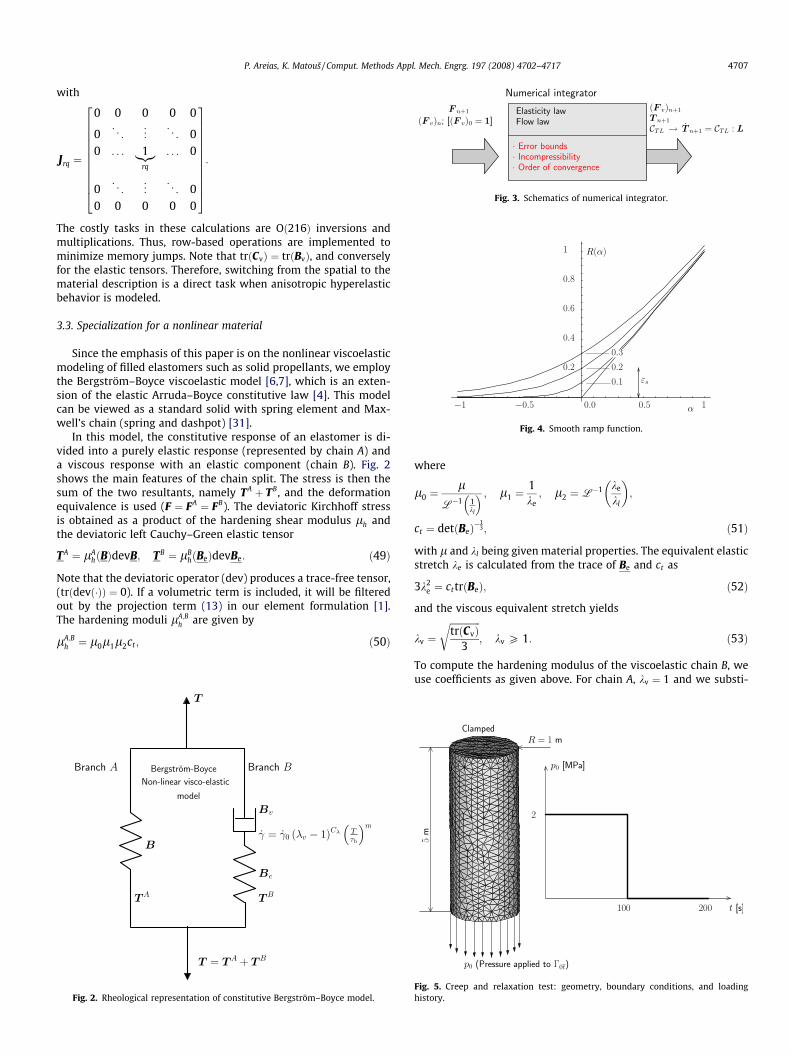
Fig. 3. Schematics of numerical integrator.

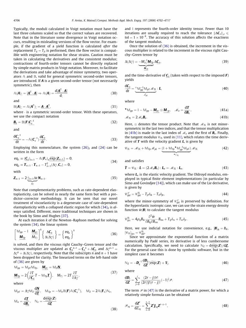
Fig. 4. Smooth ramp function.


with

Jrq ¼

0 0 0 0 0

0 . .. ..

. . ..

00 . . . 1|{z}

rq

. . . 0

0 . .. ..

. . ..

00 0 0 0 0

266666666664

377777777775:

The costly tasks in these calculations are Oð216Þ inversions andmultiplications. Thus, row-based operations are implemented tominimize memory jumps. Note that trðCvÞ ¼ trðBvÞ, and converselyfor the elastic tensors. Therefore, switching from the spatial to thematerial description is a direct task when anisotropic hyperelasticbehavior is modeled.

3.3. Specialization for a nonlinear material

Since the emphasis of this paper is on the nonlinear viscoelasticmodeling of filled elastomers such as solid propellants, we employthe Bergström–Boyce viscoelastic model [6,7], which is an exten-sion of the elastic Arruda–Boyce constitutive law [4]. This modelcan be viewed as a standard solid with spring element and Max-well’s chain (spring and dashpot) [31].

In this model, the constitutive response of an elastomer is di-vided into a purely elastic response (represented by chain A) anda viscous response with an elastic component (chain B). Fig. 2shows the main features of the chain split. The stress is then thesum of the two resultants, namely TA þ TB, and the deformationequivalence is used (F ¼ FA ¼ FB). The deviatoric Kirchhoff stressis obtained as a product of the hardening shear modulus lh andthe deviatoric left Cauchy–Green elastic tensor

TA ¼ lAhðBÞdevB; TB ¼ lB

hðBeÞdevBe: ð49Þ

Note that the deviatoric operator (dev) produces a trace-free tensor,(trðdevð�ÞÞ ¼ 0). If a volumetric term is included, it will be filteredout by the projection term (13) in our element formulation [1].The hardening moduli lA;B

h are given by

lA;Bh ¼ l0l1l2ct ; ð50Þ

Fig. 2. Rheological representation of constitutive Bergström–Boyce model.

where

l0 ¼l

L�1 1kl

� ; l1 ¼1ke; l2 ¼L�1 ke

kl

� �;

ct ¼ detðBeÞ�13; ð51Þ

with l and kl being given material properties. The equivalent elasticstretch ke is calculated from the trace of Be and ct as

3k2e ¼ cttrðBeÞ; ð52Þ

and the viscous equivalent stretch yields

kv ¼ffiffiffiffiffiffiffiffiffiffiffiffiffitrðCvÞ

3

r; kv P 1: ð53Þ

To compute the hardening modulus of the viscoelastic chain B, weuse coefficients as given above. For chain A, kv ¼ 1 and we substi-

Fig. 5. Creep and relaxation test: geometry, boundary conditions, and loadinghistory.

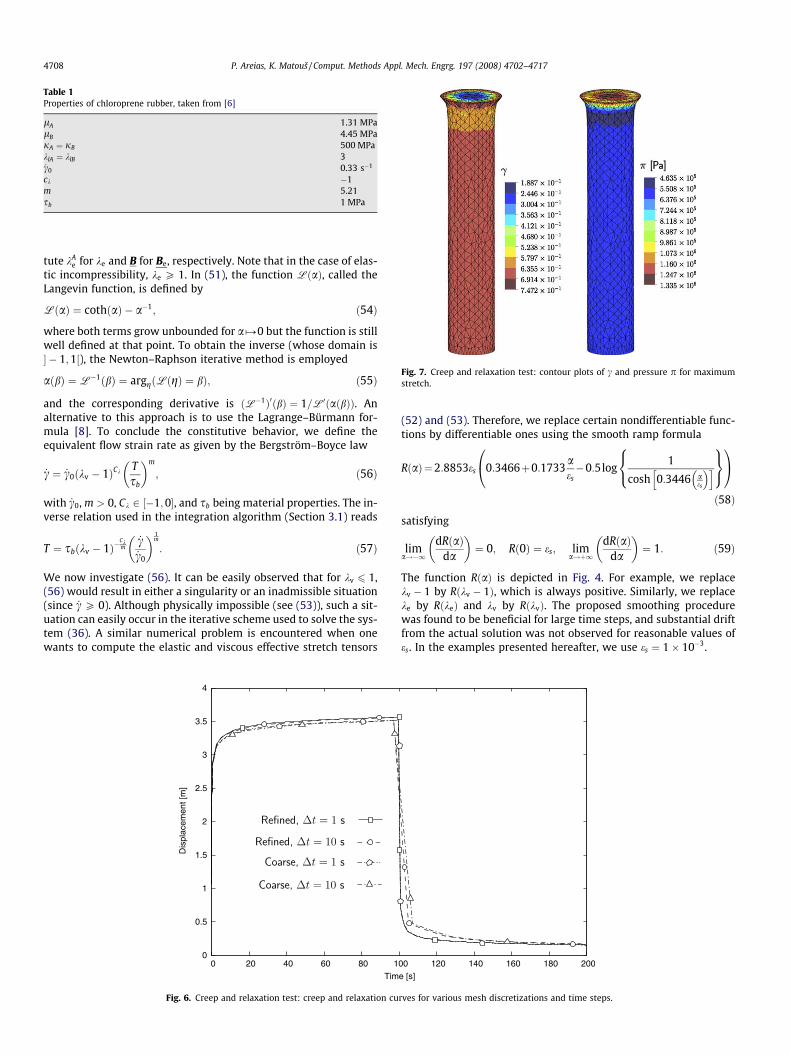
Table 1Properties of chloroprene rubber, taken from [6]

lA 1.31 MPalB 4.45 MPajA ¼ jB 500 MPaklA ¼ klB 3_c0 0.33 s�1

ck �1m 5.21sb 1 MPa

Fig. 7. Creep and relaxation test: contour plots of c and pressure p for maximumstretch.


tute kAe for ke and B for Be, respectively. Note that in the case of elas-

tic incompressibility, ke P 1. In (51), the function LðaÞ, called theLangevin function, is defined by

LðaÞ ¼ cothðaÞ � a�1; ð54Þ

where both terms grow unbounded for a#0 but the function is stillwell defined at that point. To obtain the inverse (whose domain is� � 1;1½), the Newton–Raphson iterative method is employed

aðbÞ ¼L�1ðbÞ ¼ arggðLðgÞ ¼ bÞ; ð55Þ

and the corresponding derivative is ðL�1Þ0ðbÞ ¼ 1=L0ðaðbÞÞ. Analternative to this approach is to use the Lagrange–Bürmann for-mula [8]. To conclude the constitutive behavior, we define theequivalent flow strain rate as given by the Bergström–Boyce law

_c ¼ _c0ðkv � 1ÞCkTsb

� �m

; ð56Þ

with _c0, m > 0, Ck 2 ½�1;0�, and sb being material properties. The in-verse relation used in the integration algorithm (Section 3.1) reads

T ¼ sbðkv � 1Þ�Ckm

_c_c0

� �1m

: ð57Þ

We now investigate (56). It can be easily observed that for kv 6 1,(56) would result in either a singularity or an inadmissible situation(since _c P 0). Although physically impossible (see (53)), such a sit-uation can easily occur in the iterative scheme used to solve the sys-tem (36). A similar numerical problem is encountered when onewants to compute the elastic and viscous effective stretch tensors

Fig. 6. Creep and relaxation test: creep and relaxation cu

(52) and (53). Therefore, we replace certain nondifferentiable func-tions by differentiable ones using the smooth ramp formula

RðaÞ¼2:8853es 0:3466þ0:1733aes�0:5log

1

cosh 0:3446 aes

� h i8<:

9=;0@ 1A

ð58Þ

satisfying

lima!�1

dRðaÞda

� �¼ 0; Rð0Þ ¼ es; lim

a!þ1

dRðaÞda

� �¼ 1: ð59Þ

The function RðaÞ is depicted in Fig. 4. For example, we replacekv � 1 by Rðkv � 1Þ, which is always positive. Similarly, we replaceke by RðkeÞ and kv by RðkvÞ. The proposed smoothing procedurewas found to be beneficial for large time steps, and substantial driftfrom the actual solution was not observed for reasonable values ofes. In the examples presented hereafter, we use es ¼ 1 10�3.

rves for various mesh discretizations and time steps.


To obtain the tangent modulus, we follow the formulation de-rived in Section 3.2 and apply it to either of the branches (A andB). We write_TA ¼MA

TL : L; _TB ¼ CBTL : L; ð60Þ

since by construction, L ¼ LA ¼ LAe . Here, the hyperelastic tangent

modulus of chain A is obtained from (41b) and the viscoelastic tan-gent modulus of chain B is given by (42). To compute the tangentmoduli (41b) and (42), one needs to evaluate several derivatives.For the elastic part, we have

Fig. 8. Creep and relaxation test:

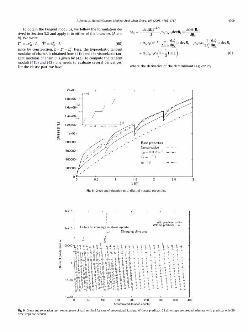
Fig. 9. Creep and relaxation test: convergence of load residual for case of proportional lotime steps are needed.

Me ¼ �detðBeÞ�4=3

3l0l1l2devBe �

d detðBeÞdBe

þ l0l1ðL�1Þ0 ct

2kekl

dk2e

dBe� devBe � l0l2ct

12k3

e

dk2e

dBe� devBe

þ l0l1l2ct I� 13

1� 1� �

; ð61Þ

where the derivative of the determinant is given by

effect of material properties.

ading. Without predictor, 28 time steps are needed, whereas with predictor only 20


d detðBeÞdBe

¼

B22eB33e � B223e

B11eB33e � B213e

B11eB22e � B212e

2ðB13eB23e � B12eB33eÞ2ðB12eB23e � B13eB22eÞ2ðB13eB12e � B23eB11eÞ

8>>>>>>>>><>>>>>>>>>:

9>>>>>>>>>=>>>>>>>>>;: ð62Þ

Note the coefficient 2 in the shear terms, which is required to obtaina correct product and follows from symmetry replacement invokedbefore calculating the derivative. We use the conventionð11;22;33;12;13;23Þ to order the components of symmetric ten-sors. The viscous components are then given by

oToCv¼ � sbCk

3m_c_c0

� �1m

ðkv � 1Þ�Ckþm

m 1;

oToDc¼ sb

Dtm _c0

_c_c0

� �1�mm

ðkv � 1Þ�Ckm ;

ð63Þ

where 1 ¼ f1;1;1;0; 0;0gT and the geometric term yields

Fig. 11. Hollow sphere compression test: load versus displacement diagrams for threeshown.

Fig. 10. Hollow sphere compression test: geomet

dNdT¼ 1kTkF

I� N � N½ �: ð64Þ

4. Numerical tests

To demonstrate the capabilities of the proposed integrationalgorithm using the finite element scheme, we solve several visco-elastic examples. The first part is focused on viscoelastic parameterinfluence, general model capability and a validation study. The lastexample is devoted to analysis of the unit cell for a solid propellant.

4.1. Creep and relaxation test

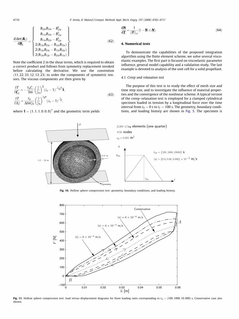
The purpose of this test is to study the effect of mesh size andtime step size, and to investigate the influence of material proper-ties and the convergence of the nonlinear scheme. A typical versionof the creep–relaxation test is employed for a clamped cylindricalspecimen loaded in tension by a longitudinal force over the timeinterval from t0 ¼ 0 s to tf ¼ 100 s. The geometry, boundary condi-tions, and loading history are shown in Fig. 5. The specimen is

loading rates corresponding to tm ¼ f100;1000;10; 000g s. Conservative case also

ry, boundary conditions, and loading history.

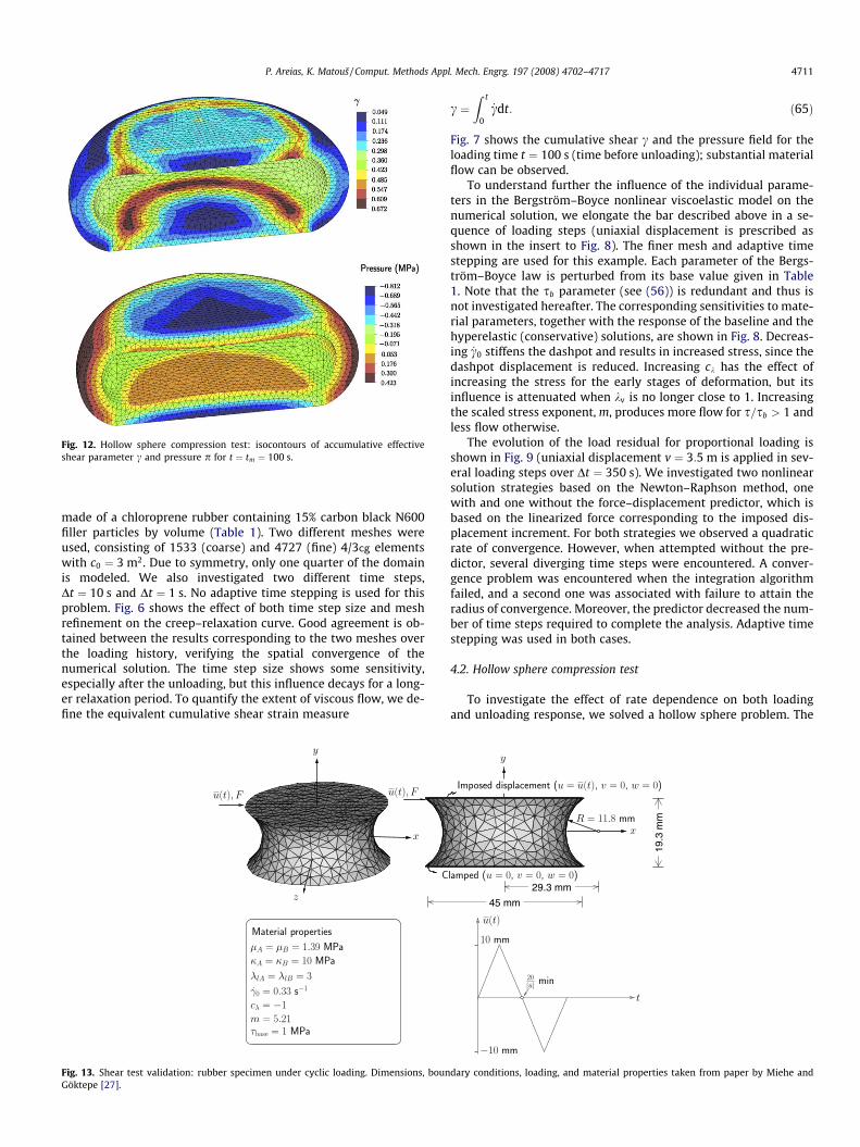
Fig. 12. Hollow sphere compression test: isocontours of accumulative effectiveshear parameter c and pressure p for t ¼ tm ¼ 100 s.


made of a chloroprene rubber containing 15% carbon black N600filler particles by volume (Table 1). Two different meshes wereused, consisting of 1533 (coarse) and 4727 (fine) 4/3cg elementswith c0 ¼ 3 m2. Due to symmetry, only one quarter of the domainis modeled. We also investigated two different time steps,Dt ¼ 10 s and Dt ¼ 1 s. No adaptive time stepping is used for thisproblem. Fig. 6 shows the effect of both time step size and meshrefinement on the creep–relaxation curve. Good agreement is ob-tained between the results corresponding to the two meshes overthe loading history, verifying the spatial convergence of thenumerical solution. The time step size shows some sensitivity,especially after the unloading, but this influence decays for a long-er relaxation period. To quantify the extent of viscous flow, we de-fine the equivalent cumulative shear strain measure

Fig. 13. Shear test validation: rubber specimen under cyclic loading. Dimensions, bounGöktepe [27].

c ¼Z t

0

_cdt: ð65Þ

Fig. 7 shows the cumulative shear c and the pressure field for theloading time t ¼ 100 s (time before unloading); substantial materialflow can be observed.

To understand further the influence of the individual parame-ters in the Bergström–Boyce nonlinear viscoelastic model on thenumerical solution, we elongate the bar described above in a se-quence of loading steps (uniaxial displacement is prescribed asshown in the insert to Fig. 8). The finer mesh and adaptive timestepping are used for this example. Each parameter of the Bergs-tröm–Boyce law is perturbed from its base value given in Table1. Note that the sb parameter (see (56)) is redundant and thus isnot investigated hereafter. The corresponding sensitivities to mate-rial parameters, together with the response of the baseline and thehyperelastic (conservative) solutions, are shown in Fig. 8. Decreas-ing _c0 stiffens the dashpot and results in increased stress, since thedashpot displacement is reduced. Increasing ck has the effect ofincreasing the stress for the early stages of deformation, but itsinfluence is attenuated when kv is no longer close to 1. Increasingthe scaled stress exponent, m, produces more flow for s=sb > 1 andless flow otherwise.

The evolution of the load residual for proportional loading isshown in Fig. 9 (uniaxial displacement v ¼ 3:5 m is applied in sev-eral loading steps over Dt ¼ 350 s). We investigated two nonlinearsolution strategies based on the Newton–Raphson method, onewith and one without the force–displacement predictor, which isbased on the linearized force corresponding to the imposed dis-placement increment. For both strategies we observed a quadraticrate of convergence. However, when attempted without the pre-dictor, several diverging time steps were encountered. A conver-gence problem was encountered when the integration algorithmfailed, and a second one was associated with failure to attain theradius of convergence. Moreover, the predictor decreased the num-ber of time steps required to complete the analysis. Adaptive timestepping was used in both cases.

4.2. Hollow sphere compression test

To investigate the effect of rate dependence on both loadingand unloading response, we solved a hollow sphere problem. The

dary conditions, loading, and material properties taken from paper by Miehe and

Fig. 14. Shear test validation: force–displacement curves (left) and distribution of pressure for both loading rates at points A and B (right). Experimental results, representedby symbols, are taken from [27].

Table 2Estimated mechanical properties of individual constituents

AP particles Blend � small particles + binder

l 132.34 GPa lA 2.9566 MPaj 213.35 GPa jA 163 MPakl 3 lB 2.9566 MPa

jB 163 MPaklA 3klB 3_c0 0.33 s�1

ck �1m 5.21sb 1 Pa


relevant data for this test are shown in Fig. 10. The material prop-erties correspond to chloroprene rubber and are the same as thoseused in the previous example. Two planes compress the spherewith a certain velocity, which is a function of time, and the load-ing/unloading response is monitored.

Fig. 11 shows marked growth in energy dissipation, with therate dependent material stiffening as a function of the displace-ment �u, for different loading velocities. Note that the displacement

Fig. 15. Solid propellant unit cell: geometry, b

in the abscissa corresponds to plane motion, and when the loadingprocess is reversed to unloading at time tm, the loading planemoves away from the sphere, but the sphere in contact does not re-act instantaneously due to its viscoelastic nature. This leads to asudden drop in the transmitted force (region A in Fig. 11), whichis a function of the loading rate and the material relaxation time.Faster loading leads to a larger decline as the material does nothave time to relax. A similar situation appears after the completeunloading (region B in Fig. 11). As one can see, the reaction is zeroand a noticeable gap develops before the sphere regains its originalshape. Note that the volume remains constant throughout thewhole loading history.

The pressure and effective shear strain distributions are shownin Fig. 12. We observe that the distribution of p is smoother thanthe distribution of c due to the smoothing introduced by (8).

4.3. Shear test validation

In order to validate our computational scheme, we compare itwith results presented by Miehe and Göktepe [27], who introduceda micromechanics based microsphere model to represent visco-elasticity of elastomers. Relevant geometry, boundary and loadingconditions, and material properties are shown in Fig. 13. The spec-

oundary conditions, and loading history.

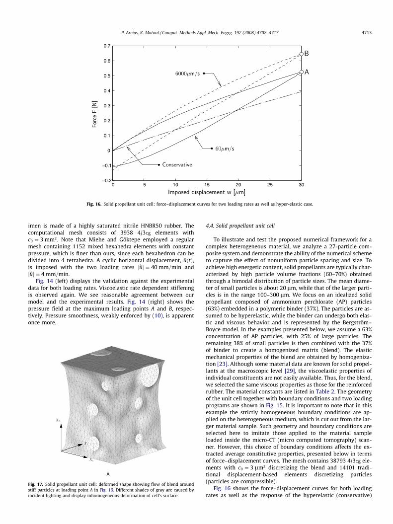
Fig. 16. Solid propellant unit cell: force–displacement curves for two loading rates as well as hyper-elastic case.


imen is made of a highly saturated nitrile HNBR50 rubber. Thecomputational mesh consists of 3938 4/3cg elements withc0 ¼ 3 mm2. Note that Miehe and Göktepe employed a regularmesh containing 1152 mixed hexahedra elements with constantpressure, which is finer than ours, since each hexahedron can bedivided into 4 tetrahedra. A cyclic horizontal displacement, �uðtÞ,is imposed with the two loading rates j _�uj ¼ 40 mm=min andj _�uj ¼ 4 mm=min.

Fig. 14 (left) displays the validation against the experimentaldata for both loading rates. Viscoelastic rate dependent stiffeningis observed again. We see reasonable agreement between ourmodel and the experimental results. Fig. 14 (right) shows thepressure field at the maximum loading points A and B, respec-tively. Pressure smoothness, weakly enforced by (10), is apparentonce more.

Fig. 17. Solid propellant unit cell: deformed shape showing flow of blend aroundstiff particles at loading point A in Fig. 16. Different shades of gray are caused byincident lighting and display inhomogeneous deformation of cell’s surface.

4.4. Solid propellant unit cell

To illustrate and test the proposed numerical framework for acomplex heterogeneous material, we analyze a 27-particle com-posite system and demonstrate the ability of the numerical schemeto capture the effect of nonuniform particle spacing and size. Toachieve high energetic content, solid propellants are typically char-acterized by high particle volume fractions (60–70%) obtainedthrough a bimodal distribution of particle sizes. The mean diame-ter of small particles is about 20 lm, while that of the larger parti-cles is in the range 100–300 lm. We focus on an idealized solidpropellant composed of ammonium perchlorate (AP) particles(63%) embedded in a polymeric binder (37%). The particles are as-sumed to be hyperelastic, while the binder can undergo both elas-tic and viscous behavior and is represented by the Bergström–Boyce model. In the examples presented below, we assume a 63%concentration of AP particles, with 25% of large particles. Theremaining 38% of small particles is then combined with the 37%of binder to create a homogenized matrix (blend). The elasticmechanical properties of the blend are obtained by homogeniza-tion [23]. Although some material data are known for solid propel-lants at the macroscopic level [29], the viscoelastic properties ofindividual constituents are not easily available. Thus, for the blend,we selected the same viscous properties as those for the reinforcedrubber. The material constants are listed in Table 2. The geometryof the unit cell together with boundary conditions and two loadingprograms are shown in Fig. 15. It is important to note that in thisexample the strictly homogeneous boundary conditions are ap-plied on the heterogeneous medium, which is cut out from the lar-ger material sample. Such geometry and boundary conditions areselected here to imitate those applied to the material sampleloaded inside the micro-CT (micro computed tomography) scan-ner. However, this choice of boundary conditions affects the ex-tracted average constitutive properties, presented below in termsof force–displacement curves. The mesh contains 38793 4/3cg ele-ments with c0 ¼ 3 lm2 discretizing the blend and 14101 tradi-tional displacement-based elements discretizing particles(particles are compressible).

Fig. 16 shows the force–displacement curves for both loadingrates as well as the response of the hyperelastic (conservative)

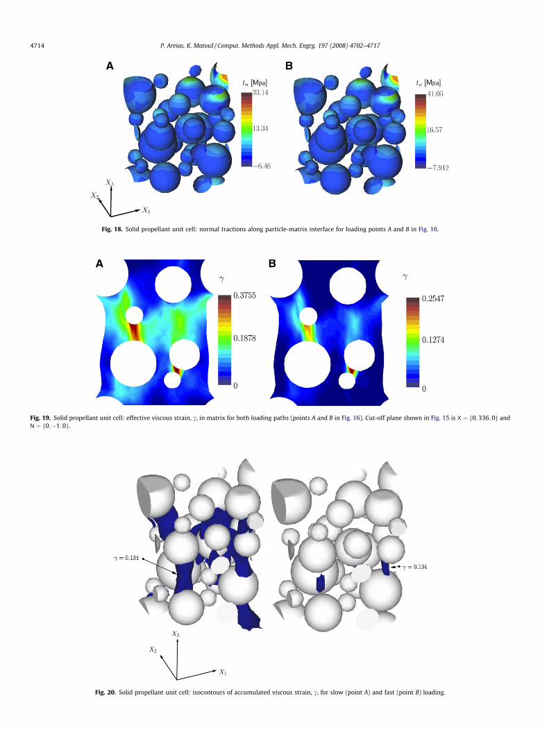
Fig. 18. Solid propellant unit cell: normal tractions along particle-matrix interface for loading points A and B in Fig. 16.

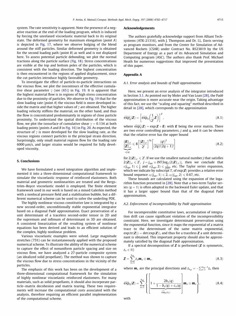
Fig. 19. Solid propellant unit cell: effective viscous strain, c, in matrix for both loading paths (points A and B in Fig. 16). Cut-off plane shown in Fig. 15 is X ¼ f0;336;0g andN ¼ f0;�1;0g.

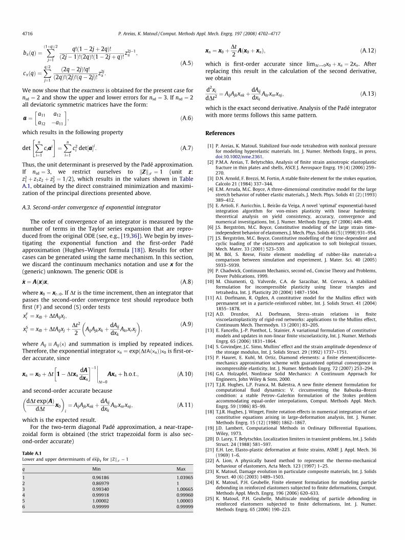
Fig. 20. Solid propellant unit cell: isocontours of accumulated viscous strain, c, for slow (point A) and fast (point B) loading.



system. The rate sensitivity is apparent. Note the presence of a neg-ative reaction at the end of the loading program, which is inducedby forcing the unrelaxed viscoelastic material back to its originalstate. The deformed geometry for maximum elongation (point A)is depicted in Fig. 17, where we observe bulging of the blendaround the stiff particles. Similar deformed geometry is obtainedfor the second loading path (point B) as well and is not displayedhere. To assess potential particle debonding, we plot the normaltractions along the particle surface (Fig. 18). Stress concentrationsare visible at the top and bottom poles of the particles, which isconsistent with the loading direction. The highest concentrationis then encountered in the regions of applied displacement, sincethe cut particles introduce highly favorable geometry.

To investigate the effect of particle-to-particle interactions onthe viscous flow, we plot the isocontours of the effective cumula-tive shear parameter c (see (65)) in Fig. 19. It is apparent thatthe highest material flow is in regions of high stress concentrationdue to the proximity of particles. We observe in Fig. 19 that for theslow loading rate (point A) the viscous field is more developed in-side the matrix and that higher values of c are obtained. The higherloading velocity stiffens the material, on the other hand, and thusthe flow is concentrated predominately in regions of close particleproximity. To understand the spatial distribution of the viscousflow, we plot the isosurface of cumulative shear c ¼ 0:134 at bothloading points (points A and B in Fig. 16) in Fig. 20. As expected, thestructure of c is more developed for the slow loading rate, as theviscous regions connect particles in the principal strain direction.Surprisingly, only small material regions flow for the loading rate6000 lm/s, and larger strains would be required for fully devel-oped viscosity.

5. Conclusions

We have formulated a novel integration algorithm and imple-mented it into a three-dimensional computational framework tosimulate the viscoelastic response of reinforced elastomers. Bothmaterial and geometric nonlinearities are treated and the Bergs-tröm–Boyce viscoelastic model is employed. The finite elementframework used in our work is based on a mixed Galerkin methodwith a nonlocal pressure field and a stabilization bubble, but a dif-ferent numerical scheme can be used to solve the underling PDE.

The highly nonlinear viscous constitutive law is integrated by anew second-order, unconditionally stable exponential integratorbased on a diagonal Padé approximation. Exact preservation of aunit determinant of a traceless second-order tensor in 2D andthe supremum and infimum of determinant in 3D are obtained.A consistent linearization of the resulting system of nonlinearequations has been derived and leads to an efficient solution ofthe complex, highly nonlinear problem.

Various viscoelastic examples were solved. Large magnitudestretches (75%) can be instantaneously applied with the proposednumerical scheme. To illustrate the ability of the numerical schemeto capture the effect of nonuniform particle spacing and size onviscous flow, we have analyzed a 27-particle composite system(an idealized solid propellant). The method was shown to capturethe viscous flow due to stress concentrations in the vicinity of theparticles.

The emphasis of this work has been on the development of athree-dimensional computational framework for the simulationof highly nonlinear viscoelastic reinforced elastomers. For manymaterials, such as solid propellants, it should also incorporate par-ticle–matrix decohesion and matrix tearing. These two require-ments will increase the computational costs associated with theanalysis, therefore requiring an efficient parallel implementationof the computational scheme.

Acknowledgements

The authors gratefully acknowledge support from Alliant Tech-systems (ATK-21316), with J. Thompson and Dr. I.L. Davis servingas program monitors, and from the Center for Simulation of Ad-vanced Rockets (CSAR) under Contract No. B523819 by the USDepartment of Energy as a part of its Advanced Simulation andComputing program (ASC). The authors also thank Prof. MichaelHeath for numerous suggestions that improved the presentationof this paper.

Appendix A

A.1. Error analysis and bounds of Padé approximation

Here, we present an error analysis of the integrator introducedin Section 3.1. As pointed out by Moler and Van Loan [28], the Padéapproximation is more accurate near the origin. Taking advantageof this fact, we use the ‘‘scaling and squaring” method described indetail in [28], which corresponds to the approximation

gexpjqðZÞ ¼ gexpq

1

2j Z� � �2j

; ðA:1Þ

where gexpjqðZÞ ¼ expðZ þ EÞ with E being the error matrix. There

are two error controlling parameters, j and q, and it can be shownthat the relative error has the upper bound

kEkFkZkF|fflffl{zfflffl}

eðj;qÞ

6 8kZkF

2j

�2q ðq!Þ2

ð2qÞ!ð2qþ 1Þ!

" #ðA:2Þ

for 2kZkF 6 2j. If we use the smallest natural number j that satisfies2kZkF 6 2j, j ¼ jopt � INT½log2ð2kZkFÞ�, then we conclude thateðjopt;1Þ 6 1

6 and eðjopt;2Þ 6 12880, etc. The Taylor series expansion,

which we indicate by subscript T , of expðZÞ provides a relative errorbound sequence eTðjopt ;1Þ 6 2, eTðjopt;2Þ 6 0:67, etc.

These bounds are calculated using the expansion of the loga-rithm function presented in [28]. Note that a two-term Taylor ser-ies ðq ¼ 1Þ is often adopted in the backward Euler update, and thatit has a larger upper bound than that of the diagonal Padéapproximation.

A.2. Enforcement of incompressibility by Padé approximation

For incompressible constitutive laws, accumulation of integra-tion drift can cause significant violation of the incompressibilityconstraint. Here, we investigate determinant preservation usingthe exponential function, since it maps the exponential of a matrixtrace to the determinant of the same matrix exponential,expðtrðZÞÞ ¼ detðexpðZÞÞ, and thus for a traceless Z a unit determi-nant is obtained. This important property should also be approxi-mately satisfied by the diagonal Padé approximation.

If a spectral decomposition of Z is performed (Z is symmetric,za 2 R)

Z ¼Xnsd

a¼1

zama �ma; ðA:3Þ

where ma are the principal directions and znsd¼ �

Pnsd�1i¼1 zi, then

gexpqðZÞ ¼Xnsd

a¼1

1þ 2baðqÞ1� baðqÞ þ caðqÞ|fflfflfflfflfflfflfflfflfflfflfflfflfflfflfflfflfflfflffl{zfflfflfflfflfflfflfflfflfflfflfflfflfflfflfflfflfflfflffl}fexpqðzaÞ

266664377775ma �ma

8>>>><>>>>:

9>>>>=>>>>;; ðA:4Þ

with


baðqÞ ¼Xð1þqÞ=2

j¼1

q!ð1� 2jþ 2qÞ!ð2j� 1Þ!ð2qÞ!ð1� 2jþ qÞ! z2j�1

a ;

caðqÞ ¼Xq=2

j¼1

ð2q� 2jÞ!q!

ð2qÞ!ð2jÞ!ðq� 2jÞ! z2ja :

ðA:5Þ

We now show that the exactness is obtained for the present case fornsd ¼ 2 and show the upper and lower errors for nsd ¼ 3. If nsd ¼ 2all deviatoric symmetric matrices have the form:

a ¼a11 a12

a12 �a11

�; ðA:6Þ

which results in the following property

detXn

i¼1

ciai

" #¼Xn

i¼1

c2i det½a�i: ðA:7Þ

Thus, the unit determinant is preserved by the Padé approximation.If nsd ¼ 3, we restrict ourselves to kZkF ¼ 1 (unit z:z2

1 þ z1z2 þ z22 ¼ 1=2), which results in the values shown in Table

A.1, obtained by the direct constrained minimization and maximi-zation of the principal directions presented above.

A.3. Second-order convergence of exponential integrator

The order of convergence of an integrator is measured by thenumber of terms in the Taylor series expansion that are repro-duced from the original ODE (see, e.g., [19,36]). We begin by inves-tigating the exponential function and the first-order Padéapproximation (Hughes–Winget formula [18]). Results for othercases can be generated using the same mechanism. In this section,we discard the continuum mechanics notation and use x for the(generic) unknown. The generic ODE is

_x ¼ AðxÞx; ðA:8Þ

where x0 ¼ xt¼0. If Dt is the time increment, then an integrator thatpasses the second-order convergence test should reproduce bothfirst (F) and second (S) order tests

xFi ¼ xi0 þ DtAijxj;

xSi ¼ xi0 þ DtAijxj þ

Dt2

2AijAjkxk þ

dAij

dxkAkrxrxj

� �;

ðA:9Þ

where Aij � AijðxÞ and summation is implied by repeated indices.Therefore, the exponential integrator xn ¼ expðDtAðxnÞÞx0 is first-or-der accurate, since

xn ¼ x0 þ Dt 1� DtxndAdxn

��1��Dt¼0

Axn þ h:o:t:; ðA:10Þ

and second-order accurate because

dDt expðAÞdDt

x0

� �i

¼ AijAjkxnk þdAij

dxkAkrxnrxnj; ðA:11Þ

which is the expected result.For the two-term diagonal Padé approximation, a near-trape-

zoidal form is obtained (the strict trapezoidal form is also sec-ond-order accurate)

Table A.1Lower and upper determinants of gexpq for kZkF ¼ 1

q Min Max

1 0.96186 1.039652 0.86979 13 0.99340 1.006654 0.99918 0.999605 1.00002 1.000036 0.99999 0.99999

xn ¼ x0 þDt2

Aðx0 þ xnÞ; ðA:12Þ

which is first-order accurate since limDt # 0x0 þ xn ¼ 2xn. Afterreplacing this result in the calculation of the second derivative,we obtain

d2xi

dDt2 ¼ AijAjkxnk þdAij

dxkAkrxnrxnj; ðA:13Þ

which is the exact second derivative. Analysis of the Padé integratorwith more terms follows this same pattern.

References

[1] P. Areias, K. Matouš. Stabilized four-node tetrahedron with nonlocal pressurefor modeling hyperelastic materials. Int. J. Numer. Methods Engrg., in press,doi:10.1002/nme.2361.

[2] P.M.A. Areias, T. Belytschko, Analysis of finite strain anisotropic elastoplasticfracture in thin plates and shells, ASCE J. Aerospace Engrg. 19 (4) (2006) 259–270.

[3] D.N. Arnold, F. Brezzi, M. Fortin, A stable finite element for the stokes equation,Calcolo 21 (1984) 337–344.

[4] E.M. Arruda, M.C. Boyce, A three-dimensional constitutive model for the largestretch behavior of rubber elastic materials, J. Mech. Phys. Solids 41 (2) (1993)389–412.

[5] E. Artioli, F. Auricchio, L. Beirão da Veiga, A novel ’optimal’ exponential-basedintegration algorithm for von-mises plasticity with linear hardening:theoretical analysis on yield consistency, accuracy, convergence andnumerical investigations, Int. J. Numer. Methods Engrg. 67 (2006) 449–498.

[6] J.S. Bergström, M.C. Boyce, Constitutive modeling of the large strain time-independent behavior of elastomers, J. Mech. Phys. Solids 46 (5) (1998) 931–954.

[7] J.S. Bergström, M.C. Boyce, Constitutive modelling of the time-dependent andcyclic loading of the elastomers and application to soft biological tissues,Mech. Mater. 33 (2001) 523–530.

[8] M. Böl, S. Reese, Finite element modelling of rubber-like materials-acomparison between simulation and experiment, J. Mater. Sci. 40 (2005)5933–5939.

[9] P. Chadwick, Continuum Mechanics, second ed., Concise Theory and Problems,Dover Publications, 1999.

[10] M. Chiumenti, Q. Valverde, C.A. de Saracibar, M. Cervera, A stabilizedformulation for incompressible plasticity using linear triangles andtetrahedra, Int. J. Plasticity 20 (2004) 1487–1504.

[11] A.I. Dorfmann, R. Ogden, A constitutive model for the Mullins effect withpermanent set in a particle-reinforced rubber, Int. J. Solids Struct. 41 (2004)1855–1878.

[12] A.D. Drozdov, A.I. Dorfmann, Stress–strain relations in finiteviscoelastoplasticity of rigid-rod networks: applications to the Mullins effect,Continuum Mech. Thermodyn. 13 (2001) 83–205.

[13] E. Fancello, J.-P. Ponthot, L. Stainier, A variational formulation of constitutivemodels and updates in non-linear finite viscoelasticity, Int. J. Numer. MethodsEngrg. 65 (2006) 1831–1864.

[14] S. Govindjee, J.C. Simo, Mullins’ effect and the strain amplitude dependence ofthe storage modulus, Int. J. Solids Struct. 29 (1992) 1737–1751.

[15] P. Hauret, E. Kuhl, M. Ortiz, Diamond elements: a finite element/discrete-mechanics approximation scheme with guaranteed optimal convergence inincompressible elasticity, Int. J. Numer. Methods Engrg. 72 (2007) 253–294.

[16] G.A. Holzapfel, Nonlinear Solid Mechanics: A Continuum Approach forEngineers, John Wiley & Sons, 2000.

[17] T.J.R. Hughes, L.P. Franca, M. Balestra, A new finite element formulation forcomputational fluid dynamics: V. circumventing the Babuska–Brezzicondition: a stable Petrov–Galerkin formulation of the Stokes problemaccommodating equal-order interpolations, Comput. Methods Appl. Mech.Engrg. 59 (1986) 85–99.

[18] T.J.R. Hughes, J. Winget, Finite rotation effects in numerical integration of rateconstitutive equations arising in large-deformation analysis, Int. J. Numer.Methods Engrg. 15 (12) (1980) 1862–1867.

[19] J.D. Lambert, Computational Methods in Ordinary Differential Equations,Wiley, 1973.

[20] D. Lasry, T. Belytschko, Localization limiters in transient problems, Int. J. SolidsStruct. 24 (1988) 581–597.

[21] E.H. Lee, Elasto-plastic deformation at finite strains, ASME J. Appl. Mech. 36(1969) 1–6.

[22] A. Lion, A physically based method to represent the thermo-mechanicalbehaviour of elastomers, Acta Mech. 123 (1997) 1–25.

[23] K. Matouš, Damage evolution in particulate composite materials, Int. J. SolidsStruct. 40 (6) (2003) 1489–1503.

[24] K. Matouš, P.H. Geubelle, Finite element formulation for modeling particledebonding in reinforced elastomers subjected to finite deformations, Comput.Methods Appl. Mech. Engrg. 196 (2006) 620–633.

[25] K. Matouš, P.H. Geubelle, Multiscale modeling of particle debonding inreinforced elastomers subjected to finite deformations, Int. J. Numer.Methods Engrg. 65 (2006) 190–223.

http://dx.doi.org/10.1002/nme.2361


[26] K. Matouš, H.M. Inglis, X. Gu, D. Rypl, T.L. Jackson, P.H. Geubelle, Multiscalemodeling of solid propellants: from particle packing to failure, Compos. Sci.Technol. 67 (2007) 1694–1708.

[27] C. Miehe, S. Göktepe, A micro–macro approach to rubber-like materials. Part II:the micro-sphere model of finite rubber viscoelasticity, J. Mech. Phys. Solids 53(2005) 2231–2258.

[28] C. Moler, C. Van Loan, Nineteen dubious ways to compute the exponential of amatrix, twenty-five years later, SIAM Rev. 45 (1) (2003) 1–46.

[29] S. Ozüpek, E.B. Becker, Constitutive modeling of high-elongation solidpropellants, J. Engrg. Mater. Technol. 114 (1992) 111–115.

[30] R.H.J. Peerlings, R. de Borst, W.A.M. Brekelmans, J.H.P. de Vree, Gradientenhanced damage for quasi-brittle materials, Int. J. Numer. Methods Engrg. 39(1996) 3391–3403.

[31] A.C. Pipkin, Lectures on Viscoelasticity Theory, second ed., Springer-Verlag,1986.

[32] M.A. Puso, J. Solberg, A stabilized nodeally integrated tetrahedral, Int. J. Numer.Methods Engrg. 67 (2006) 841–867.

[33] B. Ramesh, A.M. Maniatty, Stabilized finite element formulation for elastic–plastic finite deformations, Comput. Methods Appl. Mech. Engrg. 194 (2005)775–800.

[34] S. Reese, S. Govindjee, A theory of finite viscoelasticity and numerical aspects,Int. J. Solids Struct. 35 (1998) 3455–3482.

[35] J.C. Simo, On a fully three-dimensional finite-strain viscoelastic damagemodel: formulation and computational aspects, Comput. Methods Appl.Mech. Engrg. 60 (1987) 153–173.

[36] J.C. Simo, S. Govindjee, Non-linear B-stability and symmetry preserving returnmapping algorithms for plasticity and viscoplasticity, Int. J. Numer. MethodsEngrg. 31 (1991) 151–176.

[37] J.C. Simo, T.J.R. Hughes, Computational Inelasticity, corrected second printingedition., Springer, 2000.

[38] R. Tian, H. Matsubara, G. Yagawa, Advanced 4-node tetrahedrons, Int. J. Numer.Methods Engrg. 68 (2006) 1209–1231.

[39] O.C. Zienkiewicz, J. Wu, Incompressibility without tears – how to avoidrestrictions of mixed formulation, Int. J. Numer. Methods Engrg. 32 (1991)1189–1203.

Finite element formulation for modeling nonlinear viscoelastic

Documents

Transcript of Finite element formulation for modeling nonlinear viscoelastic