Finite Element Design of Orthotropic Steel Bridge Decks -...
204
Department of Civil and Environmental Engineering Division of Structural Engineering Steel and Timber Structures CHALMERS UNIVERSITY OF TECHNOLOGY Gothenburg, Sweden 2015 Master’s Thesis 2015:112 Finite Element Design of Orthotropic Steel Bridge Decks Master’s Thesis in the Master’s Programme Structural Engineering and Building Technology JENS HÅKANSSON HENRIK WALLERMAN
Transcript of Finite Element Design of Orthotropic Steel Bridge Decks -...

Department of Civil and Environmental Engineering Division of Structural Engineering Steel and Timber Structures CHALMERS UNIVERSITY OF TECHNOLOGY Gothenburg, Sweden 2015 Master’s Thesis 2015:112
Finite Element Design of Orthotropic Steel Bridge Decks Master’s Thesis in the Master’s Programme Structural Engineering and Building Technology JENS HÅKANSSON HENRIK WALLERMAN


MASTER’S THESIS 2015:112
Finite Element Design of Orthotropic Steel Bridge Decks Master’s Thesis in the Master’s Programme Structural Engineering and Building Technology
JENS HÅKANSSON
HENRIK WALLERMAN
Department of Civil and Environmental Engineering Division of Structural Engineering
Steel and Timber Structures CHALMERS UNIVERSITY OF TECHNOLOGY
Göteborg, Sweden 2015

Finite Element Design of Orthotropic Steel Bridge Decks Master’s Thesis in the Master’s Programme Structural Engineering and Building Technology JENS HÅKANSSON
HENRIK WALLERMAN
© JENS HÅKANSSON, HENRIK WALLERMAN, 2015
Examensarbete 2015:112/ Institutionen för bygg- och miljöteknik, Chalmers tekniska högskola 2015 Department of Civil and Environmental Engineering Division of Structural Engineering Steel and Timber Structures Chalmers University of Technology SE-412 96 Göteborg Sweden Telephone: + 46 (0)31-772 1000 Cover: A screen shot from Brigade Plus showing the orthotropic steel deck bridge in a deformed state. Chalmers Reproservice Göteborg, Sweden, 2015

I
Finite Element Design of Orthotropic Steel Bridge Decks Master’s thesis in the Master’s Programme Structural Engineering and Building Technology JENS HÅKANSSON HENRIK WALLERMAN Department of Civil and Environmental Engineering Division of Structural Engineering Steel and Timber Structures Chalmers University of Technology
ABSTRACT
Orthotropic steel deck bridges consist of a thin deck plate, supported by longitudinal stiffeners, main girders and transversal stiffeners. The system is commonly used because it has several advantages in bridge design. Most bridges today are designed using Finite element software, however the complexity of orthotropic steel deck bridges implies some challenges when it comes to FE-modelling.
The purpose of this thesis was to investigate suitable ways of approaching the complexity of orthotropic steel decks using FE-software, and to find simple, yet accurate modelling techniques. To achieve this, two different approaches were used to model an orthotropic steel deck bridge, one which is a detailed shell model, and one which smears out the stiffness of the longitudinal stiffeners and uses a much less demanding equivalent plate.
An equivalent 2D orthotropic plate was created by calculating membrane, flexural and shear rigidities of the deck plate, together with its longitudinal stiffeners. These rigidities were implied in the FE software Brigade Plus using the option General shell stiffness, which allows the user to create a plate without thickness, but using only rigidities. Section forces and normal stresses from this method were compared with the ones extracted from the detailed shell model, and found to correspond well in many cases, which means that the 2D orthotropic plate is a promising model to use in design.
A parallel study investigated whether it is possible to model slender structural parts by reducing elements in cross section class 4, within the FE-model. Slender parts were modelled by using lamina material in the parts to be reduced, which have reduced stiffness in the buckling direction.
Using lamina material to reduce parts in cross section class 4 was proved to be possible, and a theoretically correct behaviour was shown. However, the method was very time consuming and not practical to use in bridge design.
Key words: Orthotropic steel deck bridges, Bridage Plus, Abaqus, Equivalent plate, Finite element modelling, Trapezoidal ribs

II
Finit elementdimensionering av stålbroar med ortotropa däck
Examensarbete inom masterprogrammet Structural Engineering and Building Technology
JENS HÅKANSSON HENRIK WALLERMAN Institutionen för bygg- och miljöteknik Avdelningen för Konstruktionsteknik Stål- och träbyggnad Chalmers tekniska högskola
SAMMANFATTNING
Stålbroar med ortotropa däck består av en tunn däckplatta, uppstyvad med longitudinella avstyvare, huvudbalkar och transversella avstyvare. Systemet används ofta eftersom det har många fördelar i brodimensionering. De flesta broar idag dimensioneras med hjälp av finit elementmodellering, men komplexiteten i stålbroar med ortotropa däck medför vissa problem i FE-modelleringen.
Syftet med denna rapport var att undersöka lämpliga sätt att angripa kompexiteten hos stålbroar med ortotropa däck i FE-program, och att hitta enkla men samtidigt noggranna modelleringstekniker. För att uppnå detta studerades två olika angreppssätt för att modellera stålbron. Det första är en detaljerad skalmodell, och det andra smetar ut de longitudinella avstyvarnas styvhet och använder en mindre datakrävande ekvivalentplatta.
En ekvivalentplatta skapades genom att beräkna drag-, böj- och skjuvstyvhet för däckplattan tillsammans med de longitudinella avstyvarna. Dessa styvheter användes i FE-programet Brigade Plus med hjälp av alternativet General shell stiffness, vilket tillåter användaren att skapa en platta genom att bara ange styvheter och ingen tjocklek. Sektionskrafter och normalspänning från denna modell jämfördes med de som togs från den detaljerade skalmodellen, och de överensstämde väl i många fall, vilket betyder att den ekvivalenta plattan är en lovande modell för att använda i design.
En parallell studie undersökte om det är möjligt att modellera slanka stålelement genom att reducera element i tvärsnittsklass 4 i FE-modellen. De slanka elementen modellerades med materialegenskapen ”Lamina” i den delen som ska reduceras bort, med reducerad styvhet i bucklingsriktningen.
Att använda materialegenskapen ”Lamina” för att reducera element i tvärsnitsklass 4 visade sig vara möjligt och ett teoretiskt korrekt beteende uppvisades. Metoden visade sig dock vara mycket tidsödande och inte praktisk i brodimensionering.
Nyckelord: Stålbroar, ortotropa däck, Brigade Plus, Abaqus, ekvivalentplatta, Finit elementmodellering, avstyvande kanal

CHALMERS Civil and Environmental Engineering, Master’s Thesis 2015:112 III
Contents ABSTRACT I
SAMMANFATTNING II
CONTENTS III
PREFACE V
NOTATIONS VI
1 INTRODUCTION 1
1.1 Purpose and aim 1
1.2 Limitations 2
1.3 Method 2
2 ORTHOTROPIC STEEL DECK BRIDGES 3
2.1 Structural components of OSDs 5 2.1.1 Wearing surface 5 2.1.2 Deck plate 5 2.1.3 Longitudinal stiffeners 5 2.1.4 Transversal stiffeners 7
2.2 Structural behaviour of OSDs 8 2.2.1 Subsystem 1, local deck plate deformation 8 2.2.2 Subsystem 2, panel deformation 9 2.2.3 Subsystem 3, longitudinal flexure of the ribs 9 2.2.4 Subsystem 4, cross beam in-plane bending 10 2.2.5 Subsystem 5, cross beam distortion 10 2.2.6 Subsystem 6, rib distortion 12 2.2.7 Subsystem 7, global behaviour 12
2.3 Examples of design praxis and their limitations 13 2.3.1 Deck plate 13 2.3.2 Longitudinal stiffeners 13 2.3.3 Transversal stiffeners 14 2.3.4 Main girders 14
2.4 Design of OSD bridges according to Eurocode 15 2.4.1 Phenomena in plated steel structures 16 2.4.2 Effective width method 18 2.4.3 Reduced stress method 20 2.4.4 Finite element modelling 20
3 DESIGN WITH LINEAR FINITE ELEMENTS 24
3.1 Introduction to FEM 24 3.1.1 Element types 24 3.1.2 Mesh sizing 25
3.2 Alternative modelling techniques for OSDs 26

CHALMERS, Civil and Environmental Engineering, Master’s Thesis 2015:112 IV
3.2.1 Alternative 1: Equivalent plate using lamina material 27 3.2.2 Alternative 2: Equivalent 2D orthotropic plate 28
4 CASE STUDY OF AN OSD BRIDGE 34
4.1 Geometry of the bridge 34
4.2 Finite element modelling 35 4.2.1 Boundary conditions 36 4.2.2 Loads 37 4.2.3 Free Body Cut 39
4.3 Detailed shell model 39 4.3.1 Mesh 39 4.3.2 Verification of model 40
4.4 Equivalent 2D orthotropic plate 43 4.4.1 Verification of the equivalent plate 44 4.4.2 Bridge with equivalent plate 47
4.5 Reduced Cross Section 48 4.5.1 Reduced I-beam 49 4.5.2 Redistribution of moment 52 4.5.3 Reduced bridge section 53
4.6 Hand calculations 55
5 RESULTS 57
5.1 Equivalent plate approach 58 5.1.1 Results for equivalent plate approach 59 5.1.2 Evaluation of equivalent plate approach 65
5.2 Reduced cross section 70 5.2.1 Results for reduced cross section 71 5.2.2 Evaluation of reduced cross section 74
6 DISCUSSION 80
7 CONCLUSIONS 82
8 REFERENCES 84
APPENDIX A – RESULTS
APPENDIX B – HAND CALCULATIONS, CASE STUDY
APPENDIX C – HAND CALCULATIONS, I-BEAM STUDY

CHALMERS Civil and Environmental Engineering, Master’s Thesis 2015:112 V
Preface This Master’s Thesis deals with different ways of modelling orthotropic steel bridges using finite element methods. The work was carried out between January and June of 2015 at the office of structural design at ELU in Gothenburg and at the Division of Structural Engineering at Chalmers University of Technology.
We would like to thank ELU for the opportunity to write this thesis, and for giving us access to their office and to necessary software. We also like to thank the employees of ELU for making us feel welcome at their office and for sharing their knowledge. Thanks also to our examiner Associate Professor Mohammad Al-Emrani for inspiration and guidance. We would also like to thank Tim Svensson and Filip Tell for valuable insights during the course of the project. Finally, a special thanks to our supervisor Poja Shams Hakimi whose door was always open, and who spent many hours helping us completing this thesis.
Jens Håkansson and Henrik Wallerman
Göteborg, June 2015

CHALMERS, Civil and Environmental Engineering, Master’s Thesis 2015:112 VI
Notations Roman upper case letters
𝐴 Area
𝐴𝑎 Area of stiffener
𝐴𝑏 Area of stiffener
𝐴𝑒𝑒𝑒 Effective area of stiffener
𝐴𝑠𝑠 Area of stiffener, reduced due to shear effects
𝐷 Rigidity
𝑫 Rigidity matrix
𝐷𝑎𝑎 Average torsional rigidity
𝐷𝑖𝑖 Entries in the rigidity matrix
𝑫𝑠ℎ𝑒𝑎𝑒 Shear rigidity matrix
𝐷𝑠𝑠 Shear rigidity in x-direction
𝐷𝑠𝑠 Shear rigidity in y-direction
𝐷𝑠𝑠 Flexural rigidity in x-direction
𝐷𝑠𝑠,𝑒𝑒𝑟 Reduced flexural rigidity in x-direction
𝐷𝑠𝑠 Torsional rigidity
𝐷𝑠𝑠 Torsional rigidity
𝐷𝑠𝑠 Flexural rigidity in y-direction
𝐷𝑎 Flexural rigidity
𝐸 Young’s modulus
𝐸𝑠 Young’s modulus in x-direction
𝐸𝑠 Young’s modulus in y-direction
𝐺 Shear modulus
𝐺𝑠𝑠 Shear modulus in xy-plane
𝐺𝑠𝑥 Shear modulus in xz-plane
𝐺𝑠𝑥 Shear modulus in yz-plane
𝐼 Second moment of area
𝐼𝑡 Polar moment of inertia
𝐼𝑠 Second moment of area around x-axis
𝐾𝑖𝑖 Shear rigidity
𝐾𝑠𝑠 Shear stiffness
𝐿 Length of beam

CHALMERS Civil and Environmental Engineering, Master’s Thesis 2015:112 VII
𝑀 Bending moment
𝑀𝑚𝑎𝑠 Maximum bending moment
𝑁 Normal force
𝑁𝑚𝑖𝑚 Minimum normal force
𝑃 Point load
𝑃𝐴 Point load
𝑃𝐵 Point load
𝑃𝑐𝑒 Critical buckling load
𝑄 Distributed load
𝑉ℎ Horizontal shear force
𝑉𝑚𝑎𝑠 Maximum magnitude of shear force
𝑉𝑎 Vertical shear force
𝑌 Initial scaling modulus
Roman lower case letters
𝑎 Critical length of column
𝑎 Width of stiffener
𝑏 Width of plate
𝑏 Width of stiffener
𝑏0 Distance between longitudinal stiffeners
𝑏1 Distance between webs of longitudinal stiffener
𝑏𝑏𝑏𝑡 Width of bottom flange of longitudinal stiffener
𝑏𝑒 Effective width of a plate
𝑏𝑖 Width of component of longitudinal stiffener
𝑏𝑤𝑒𝑏 Height of web of longitudinal stiffener
𝑑𝑠𝑠 Membrane rigidity x-direction
𝑑𝑎 Membrane rigidity
𝑑𝑠𝑠 Membrane rigidity y-direction
𝑑𝑠𝑠 Membrane rigidity xy-plane
𝑓𝑠 Yield strength
ℎ𝑤 Height web
ℎ𝑤,𝑒𝑒𝑒 Height web, effective
𝑖𝑎𝑎 Average torsional moment of inertia
𝑖𝑠𝑠 Torsional moment of inertia

CHALMERS, Civil and Environmental Engineering, Master’s Thesis 2015:112 VIII
𝑖𝑠𝑠 Torsional moment of inertia
𝑘 Boundary condition factor for plate
𝑚𝑠𝑠 Bending moment in x-direction
𝑚𝑠𝑠,1 Reduced bending moment in x-direction
𝑚𝑠𝑠 Twisting moment
𝑚𝑠𝑠 Twisting moment
𝑚𝑠𝑠 Bending moment in y-direction
𝑛𝑠𝑠 Membrane force in x -direction
𝑛𝑠𝑠 Membrane force in xy -plane
𝑛𝑠𝑠 Membrane force in yx -plane
𝑛𝑠𝑠 Membrane force in y -direction
𝑡 Thickness of plate
𝑡𝑏𝑏𝑡 Thickness of bottom flange of longitudinal stiffeners
𝑡𝑒𝑒 Thickness of equivalent plate
𝑡𝑖 Thickness of component of longitudinal stiffeners
𝑡𝑡𝑏𝑡 Thickness of top flange of longitudinal stiffeners
𝑡𝑤𝑒𝑏 Thickness of web of longitudinal stiffeners
𝑣𝑠 Vertical force
𝑤 Lateral deflection
𝑥 Length variable
𝑦 Length variable
𝑧 Length variable
Greek letters
𝛼𝑐𝑒 Minimum load amplifier
𝛼𝑢𝑢𝑡,𝑘 Minimum load amplifier
𝛽 Reduction factor for shear lag
𝛾𝑖𝑖 Shear strain in ij-direction
𝛾𝑀1 Partial safety factor
𝛾𝑠𝑠 Shear angle
𝛿 Deflection
𝜖 Strain
𝜖𝑖𝑖 Strain in ij-direction
𝜖𝑠𝑠 Strain in x-direction

CHALMERS Civil and Environmental Engineering, Master’s Thesis 2015:112 IX
𝜖𝑠𝑠 Strain in y-direction
𝜅𝑠𝑠 Curvature in x-direction
𝜅𝑠𝑠 Curvature in y-direction
𝜈 Poisson’s ratio
𝜌 Reduction factor for buckling
𝜌𝑠 Reduction factor in x-direction
𝜌𝑠𝑠 Torsional curvature
𝜌𝑥 Reduction factor in z-direction
𝜎 Normal stress
𝜎𝑐𝑒 Critical normal stress
𝜎𝑔𝑢𝑏𝑏𝑎𝑢 Normal stress from global effects
𝜎𝑖𝑖 Normal stress in ij-direction
𝜎𝑢𝑏𝑐𝑎𝑢 Normal stress from local effects
𝜎𝑚𝑎𝑠 Maximum normal stress
𝜎𝑡𝑏𝑡𝑎𝑢 Total normal stress from global and local effects
𝜎𝑠,𝐸𝑟 Design normal stress in x-direction
𝜎𝑠,𝐸𝑟 Design normal stress in y-direction
𝜏𝐸𝑟 Design shear stress
Φ Rotational angle
𝜒𝑤 Reduction factor due to shear

CHALMERS, Civil and Environmental Engineering, Master’s Thesis 2015:112 X
CHALMERS Civil and Environmental Engineering, Master’s Thesis 2015:112 1
1 Introduction In the 1930s in Germany a new bridge deck system was invented. This new system had many advantages such as low self-weigh and a slender structure. The system is today called orthotropic steel deck, shortened OSD, and it generally consists of a steel plate stiffened by longitudinal stiffeners. This means that the bridge deck will have different properties in the longitudinal and the transverse direction, hence the name, which is a combination of the words orthogonal and anisotropic (US Department of Transportation, 2012).
OSD bridges are frequently used today and the system is especially favourable in movable bridges and bridges with long spans. The system is for instance employed in the Akashi Kaikyō Bridge, which has the longest main span of any suspension bridge in the world (Chatterjee, 2003).
In moveable bridges the system is favourable mainly because of its lightweight, which means that less power is needed to lift and lower the bridge deck and that smaller ballast counterweights are needed. Another considerable advantage is that the orthotropic bridge deck has a good load carrying capacity also in an upright position (US Department of Transportation, 2012).
In OSD bridges structural elements have more than one purpose, which makes the structure complex to analyse. For example, the deck plate is both transferring the wheel loads to the longitudinal stiffeners and working as a top flange for all longitudinal and transversal stiffeners, as well as for the main girders (US Department of Transportation, 2012). This makes all structural elements work together in a complex way.
Today, bridges are usually designed with the help of the finite element method with the intention to capture the behaviour of the structure as a whole. The complexity of steel bridges with orthotropic decks however, implies some challenges when it comes to the FE-modelling. This has led to different models being used for different design purposes, and complementary hand calculations are needed. By doing so, the accuracy of the design might be compromised, and the initial purpose of using the finite element method is lost.
The questions that arise are, which models are the most suitable and accurate for different applications, in which ways can design rules be considered within the FE-model to avoid hand calculations, and whether it is possible to consider all aspects in one unifying model and achieve reasonable results?
1.1 Purpose and aim The purpose of this Master’s thesis is to study some of the problems that can be encountered when modelling OSD bridges with finite element method and investigate suitable ways of approaching these problems. The purpose is also to find simple, yet accurate modelling techniques to facilitate engineering work.
The aim of the Master’s thesis project is to find an approach on how orthotropic steel deck bridges can be modelled with linear finite element method. Another aim is to investigate cases with very slender structural parts, and how this may be considered when performing design on the basis of linear finite element modelling, in order to save computational time.
CHALMERS, Civil and Environmental Engineering, Master’s Thesis 2015:112 2
1.2 Limitations The thesis work is limited to performing FE-analyses of only one OSD bridge and for the purpose of design in the ultimate limit state. Also, the investigation of alternative modelling techniques is limited to the bridge deck and to some extent, the transversal stiffeners. Thus, the rest of the structure is kept more or less similar in comparisons.
The load cases examined are based on traffic loads in Eurocode but are simplified by isolating a single wheel load. The structure will only be analysed with reference to static behaviour which means that no dynamic effects will be treated.
1.3 Method The project consists of two parts. A literature study is performed to investigate the structural behaviour of orthotropic steel deck bridges including regulations and demands according to Eurocode FE-analyses of an OSD bridge is then made to compare different modelling techniques and their adequacy. To perform FE-modelling, different handbooks are examined explaining different aspects in modelling, both generally and for OSD bridges. Master theses, scientific reports and design codes are some of the literature that has been studied.
The FE-analyses are carried out in the FE-software Brigade Plus (Abaqus). In order to compare the two methods, different models are created and analysed. In the first model the geometry will be modelled with correct dimensions and high detail level using shell elements. In the second, more simplified analysis, shell elements will also be used but with an equivalent orthotropic shell for the deck. The stiffness of this equivalent plate corresponds to the actual steel plate itself, together with the stiffness of the longitudinal stiffeners smeared out. For these two different models stresses and sectional forces will be compared to find out if the simplified model can be justified in order to save computational time.
The comparison will be used to state recommendations in design for orthotropic steel bridge decks that could be used in practice when designing new bridges.

CHALMERS Civil and Environmental Engineering, Master’s Thesis 2015:112 3
2 Orthotropic Steel Deck Bridges An orthotropic steel deck generally consists of a steel plate with welded stiffeners in two mutually perpendicular directions. The longitudinal stiffeners are sometimes referred to as ribs, and the transversal stiffeners as cross beams, or floor beams. Main girders in the longitudinal direction support the entire deck. The principal layout of an OSD bridge can be seen in Figure 2.1. Different structural members in the two orthogonal directions mean that the deck has anisotropic stiffness, i.e. the system is orthogonal-anisotropic which is shortened ‘orthotropic’.
Figure 2.1 Principal layout of an orthotropic bridge deck (Karlsson, 2015).
The OSD is an efficient and economic system because the deck acts as top flange for the longitudinal and the transversal stiffeners as well as for the main girders (US Department of Transportation, 2012). This means that material is saved and it also increases the rigidity of the deck.
There are two main types of OSD bridges; Plate girder bridges and box girder bridges (US Department of Transportation, 2012). The original OSD bridges, constructed in the 1930s, where of the former type and were called “battledeck floor”, see Figure 2.2.

CHALMERS, Civil and Environmental Engineering, Master’s Thesis 2015:112 4
Figure 2.2 Plate girder deck.
Box girder bridges provide a bottom lateral bracing system for the bridge cross section, which gives the deck more torsional stiffness (US Department of Transportation, 2012). The box girder represents a simple way to handle horizontal wind loads. The box girder also reduces asymmetrical deflections of the deck, caused by asymmetrical loads. Another advantage of the box girder is that it provides a natural platform from where routine inspections can take place without disturbing the traffic. A box girder can be divided into three categories: the single-cell box, see Figure 2.3, the multi-cell box, see Figure 2.4, and a box with struts that support a cantilever deck, see Figure 2.5 (Mangus, 2000).
Figure 2.3 Single-cell box girder deck.
Figure 2.4 Multi-cell box girder bridge.
Figure 2.5 Box girder deck with struts supporting cantilever deck.

CHALMERS Civil and Environmental Engineering, Master’s Thesis 2015:112 5
2.1 Structural components of OSDs 2.1.1 Wearing surface The wearing surface on the OSD deck can be made from concrete, bitumen or polymer material (US Department of Transportation, 2012). The main purpose of the wearing surface is to provide a skid resistant surface that gives a good ride quality. The wearing surface, however, also protects the deck from corrosion. The wheel pressure on the deck is often assumed to disperse at an angle of 45º in all directions through a bituminous layer. To be on the safe side, this dispersion is sometimes neglected, because it may be lost in higher temperatures when the wearing surface softens (US Department of Transportation, 2012). It is also possible that the wearing surface will be replaced by a thinner one in the future which means that the pressure area from the wheel loads will be smaller, hence the pressure gets higher.
2.1.2 Deck plate The deck plate of an OSD consists of a thin steel plate, which transfers the load to the ribs. As mentioned, the plate often acts as a common top flange for the stiffeners and for the main girders. The minimum thickness of the deck plate today is 14-16 mm; this is mainly due to the sensitivity to fatigue (US Department of Transportation, 2012).
2.1.3 Longitudinal stiffeners Longitudinal stiffeners, also known as ribs, are mainly needed to provide supports for the slender deck plate. Two other functions of the longitudinal stiffeners are to increase the flexural rigidity of the cross section, and to help distribute the load to the transversal cross beams (US Department of Transportation, 2012). The most common practice is that they are continuous over the length of the deck, which means that cut-outs need to be made in the cross beams. The ribs can be either open or closed, as seen in Figure 2.6.

CHALMERS, Civil and Environmental Engineering, Master’s Thesis 2015:112 6
Figure 2.6 Types of longitudinal stiffeners.
The open ribs are simple to fabricate and are easily spliced in the field (AISC, 1963). They are also accessible for inspection and maintenance. Because of their simple geometry they provide a simpler analysis, therefore they were popular in the pre-computer era. The main disadvantage of the open longitudinal stiffeners is that they have essentially no torsional capacity (Mangus, 2000). The open ribs also have very little load distribution capacity in the transverse direction, which means that more longitudinal stiffeners are needed (AISC, 1963). Since no load is transferred transversally all load will go to the cross beams which then will be subjected to a greater load if the span is not reduced, this means that the cross beams need to be spaced much closer. Thus, a solution with open ribs requires a great deal of material.
The closed ribs are advantageous to use because of their high torsional rigidity (AISC, 1963). They also possess a good load distribution capacity in the transverse direction, which in turn means that fewer longitudinal stiffeners are needed, and the spacing between the transversal cross beams can be longer. This also reduces the dead weight of the structure. The main disadvantages of the closed ribs are that they are more difficult to fabricate and that the deck becomes more complex to analyse because of more interaction between the parts of the deck (AISC, 1963).
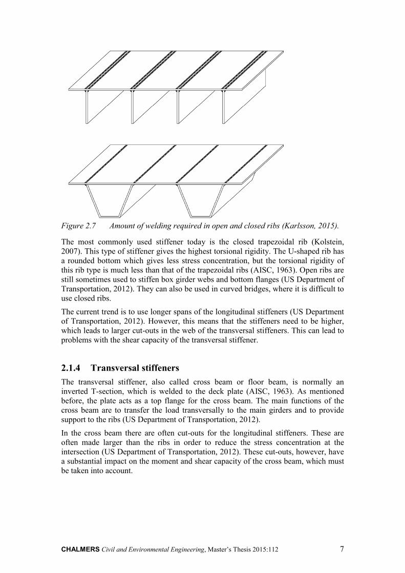
Another advantage with closed ribs is that there is less surface area that needs to be protected against corrosion, than in a system with open stiffeners (Mangus, 2000). Furthermore, fewer welds are needed in closed ribs than in open ones, as illustrated in Figure 2.7. The weld between the longitudinal stiffeners and the deck plate is of great interest because, depending on the number of stiffeners, the total length of this weld can be as much as 50 times the length of the deck (US Department of Transportation, 2012).
CHALMERS Civil and Environmental Engineering, Master’s Thesis 2015:112 7
Figure 2.7 Amount of welding required in open and closed ribs (Karlsson, 2015).
The most commonly used stiffener today is the closed trapezoidal rib (Kolstein, 2007). This type of stiffener gives the highest torsional rigidity. The U-shaped rib has a rounded bottom which gives less stress concentration, but the torsional rigidity of this rib type is much less than that of the trapezoidal ribs (AISC, 1963). Open ribs are still sometimes used to stiffen box girder webs and bottom flanges (US Department of Transportation, 2012). They can also be used in curved bridges, where it is difficult to use closed ribs.
The current trend is to use longer spans of the longitudinal stiffeners (US Department of Transportation, 2012). However, this means that the stiffeners need to be higher, which leads to larger cut-outs in the web of the transversal stiffeners. This can lead to problems with the shear capacity of the transversal stiffener.
2.1.4 Transversal stiffeners The transversal stiffener, also called cross beam or floor beam, is normally an inverted T-section, which is welded to the deck plate (AISC, 1963). As mentioned before, the plate acts as a top flange for the cross beam. The main functions of the cross beam are to transfer the load transversally to the main girders and to provide support to the ribs (US Department of Transportation, 2012).
In the cross beam there are often cut-outs for the longitudinal stiffeners. These are often made larger than the ribs in order to reduce the stress concentration at the intersection (US Department of Transportation, 2012). These cut-outs, however, have a substantial impact on the moment and shear capacity of the cross beam, which must be taken into account.

CHALMERS, Civil and Environmental Engineering, Master’s Thesis 2015:112 8
2.2 Structural behaviour of OSDs More or less all structures that exist are an assembly of different structural element such as beams, columns and plates. Those elements contribute to the complete behaviour of the whole structure in a complex way. For most applications it has been shown that it is conservative in design (on the safe side) to treat each element as independent of each other and therefore be able to design all elements individually (US Department of Transportation, 2012). This approach is simple and often used in design.
For OSD bridges the elements are linked together in a more complex way, and the same structural elements can fulfil more than one function. As mentioned before, the plate serves as load distributer between the ribs as well as top flange for ribs, cross beams and main girders. Due to this complex interaction the approach above is not accurate and the structural elements cannot be treated individually for true response.
Figure 2.8 illustrates how a concentrated load is transferred to the main girders. The load is applied at the deck plate which transfers the load between the ribs. The ribs transfer the load to the cross beams which distribute the load between the main girders.
Figure 2.8 Load path through the OSD bridge (Karlsson, 2015).
To be able to perform accurate hand calculations and describe the complex structural behaviour of OSDs it has been proposed that the whole system is divided into subsystems. These subsystems are assumed to act independent of each other and therefore the effects of the different subsystems are possible to add by superposition (US Department of Transportation, 2012). The possibility to use superposition is based on the assumption that the linear relation between the load and stresses are not affected by the interaction of the single systems (AISC, 1963).
In Section 2.2.1 to Section 2.2.7 follows an explanation of the seven subsystems that are presented and used by US Department of Transportation, (2012).
2.2.1 Subsystem 1, local deck plate deformation The deck plate should, in this subsystem, only transfer the applied wheel load to the adjacent rib walls (US Department of Transportation, 2012). The load is transferred through deck plate bending. Figure 2.9 illustrates how the deck plate is deforming when a concentrated load is applied over a rib.

CHALMERS Civil and Environmental Engineering, Master’s Thesis 2015:112 9
Figure 2.9 Local deformation of deck plate (Karlsson, 2015).
2.2.2 Subsystem 2, panel deformation Panel deformation is a phenomenon that occurs due to the fact that ribs share the same top flange and therefore they cannot act independently. A concentrated load that is applied at the deck plate will be distributed to the nearby ribs, as described in previous section, but due to the common top flange also ribs that are not loaded will deflect. This effect reduces stresses in the loaded ribs but add stresses to the unloaded ones (US Department of Transportation, 2012). The panel deformation is illustrated in Figure 2.10 where it can be seen how all ribs deflect together.
Figure 2.10 Panel deformation of deck plate (Karlsson, 2015).
2.2.3 Subsystem 3, longitudinal flexure of the ribs Ribs are constructed continuous over cross beams and the fact that cross beams deflect when loaded must be considered. To take this flexure into consideration the ribs are modelled as continues over discrete flexible supports. In this model it is assumed that cross beams are simply supported between rigid main girders and will deflect when loaded (US Department of Transportation, 2012). Ribs close to main girders will have almost rigid supports since the cross beams have smaller deflection close to its supports. Contrariwise, ribs close to the mid span of the cross beam will be supported by springs. These two different cases are shown in Figure 2.11, where the deformed shapes of the ribs are illustrated. The effect of the cross beam flexure will increase the positive span moments and decrease the negative support moments compared to the ideal case where the cross beams are rigid (US Department of Transportation, 2012).

CHALMERS, Civil and Environmental Engineering, Master’s Thesis 2015:112 10
Figure 2.11 Support conditions for longitudinal stiffeners at different location
(Karlsson, 2015).
2.2.4 Subsystem 4, cross beam in-plane bending As mentioned before, the ribs are constructed as continuous over the cross beams. This will generate cut-outs in the cross beam cross-section where the rib is passing through. Because of this the geometry of the cross beam will vary, which complicates hand-calculations of in-plane stresses from bending and shear. US Department of Transportation (2012) state that it is recommended to model the whole cross beam using FE-analysis. Figure 2.12 shows the deformed shape of a cross beam subjected to in-plane stresses.
Figure 2.12 In-plane bending of cross beam (Karlsson, 2015).
2.2.5 Subsystem 5, cross beam distortion At cross beam and rib intersection, three different effects occur that affect the local stresses in the cross beam. The local mechanisms at these intersections are: Out-of-plane distortion from bending of ribs, distortion of rib walls due to shear forces and distortion of ribs due to uneven deflection.

CHALMERS Civil and Environmental Engineering, Master’s Thesis 2015:112 11
In Figure 2.13, it is illustrated how the cross beam will distort out-of-plane due to bending of the ribs that passes through. As can be seen by the dashed lines, the distortion is highest at the intersection between the cross beam and the ribs, which causes the cross beam to twist (US Department of Transportation, 2012).
Figure 2.13 Effects on cross beam from bending of ribs (Karlsson, 2015).
The second effect is causing a horizontal distortion of the rib walls, which is illustrated in Figure 2.14, since horizontal shear forces are acting on the walls. These horizontal shear forces are always present when a structure is loaded vertically (US Department of Transportation, 2012). The stress concentrations that appear are dependent on whether the cut-outs are larger or equal in size than the rib passing through. According to US Department of Transportation (2012) the highest stress concentration in the cross beam is generated in this case since the tooth, i.e. the part of the cross beam between the cut-outs, is weaker in plane.
Figure 2.14 Horizontal distortion of cross beam due to horizontal shear forces.
There will also be a vertical distortion in the rib walls in the case when a wheel load is applied eccentrically over the rib as illustrated in Figure 2.15. This distortion is due to the uneven vertical displacement of the deck plate and will cause stress concentrations at the point where the deck plate connects to the rib wall (US Department of Transportation, 2012).

CHALMERS, Civil and Environmental Engineering, Master’s Thesis 2015:112 12
Figure 2.15 Vertical distortion of cross beam due to wheel load.
2.2.6 Subsystem 6, rib distortion If a concentrated load is applied in the mid-span between two cross beams and is eccentric about the axis of the rib, the rib will twist around its rotational centre (US Department of transportation, 2012). Since the intersection between rib and cross beam will be a fixed or partially fixed boundary, depending on how large cut-outs are used, there will be high stress concentrations in the welds where the twisting is restrained. Figure 2.16 illustrates how the ribs are distorted when loaded.
Figure 2.16 Distortion of ribs when loaded (Karlsson, 2015).
2.2.7 Subsystem 7, global behaviour The global system describes the displacement of the main girders as well as the behaviour as a whole when no local effect is taking place. In this system it is possible to use conventional methods to determine stresses and strains in the structure (US Department of Transportation, 2012). Figure 2.17 shows global bending of the OSD bridge.

CHALMERS Civil and Environmental Engineering, Master’s Thesis 2015:112 13
Figure 2.17 Global bending of the OSD (Karlsson, 2015).
2.3 Examples of design praxis and their limitations In conventional bridge design most of the local effects described above are disregarded, and the bridge is designed with regard to global effects. In the design of OSDs the global behaviour can be simplified and the load can be followed from top to bottom through the different components. Each component is analysed separately with regards to its loads and structural capacity.
2.3.1 Deck plate The main load that needs to be taken into account when designing the deck plate is the vertical component of the wheel load. This load can be converted into a transversal line load over the width of the load, and the plate is then analysed as a beam. The webs of the longitudinal stiffeners are in this model seen as rigid supports.
2.3.2 Longitudinal stiffeners The longitudinal stiffeners are modelled as continuous beams, with an effective part of the plate as top flange. The governing load is, as for the deck plate, the traffic load from a single wheel, which is usually placed centrically over the rib. In reality the load will distribute to adjacent ribs, but in hand calculations this effect is disregarded, which is a simplification on the safe side.
The ribs are supported by the cross beams and, as mentioned before, the cross beams can be modelled either as rigid supports or as springs. The spring stiffness is calculated by looking at the deflection in the mid span of the cross beam when the beam is loaded by a unit force, P=1 N. This is a simplification on the safe side, as this does not take into account the position of the rib. The closer the ribs are to the main girders the less the deflection will be and thus the higher the stiffness of the cross beam is, see Figure 2.18.

CHALMERS, Civil and Environmental Engineering, Master’s Thesis 2015:112 14
Figure 2.18 Model to calculate stiffness of the cross beams.
2.3.3 Transversal stiffeners The main load acting on the transversal stiffeners is the reaction force coming from the longitudinal stiffeners, which should be transferred to the main girders. However, load applied on the deck plate close to the cross beams will go directly to the cross beams, and not through the ribs.
The cross section of the cross beam will include an effective part of the deck plate as top flange. The cut outs are taken into account by removing a section corresponding to the height of the cut out from the cross section, see Figure 2.19.
Figure 2.19 Effective height of the web of the cross beam.
The cross beam will have different boundary conditions depending on what type of OSD bridge is used (plate girder bridge, box girder bridge, etc.). For the case of a plate girder bridge the cross beam may be studied in two different parts. The first is the cantilever part, outside the main girders, which is modelled as a cantilever beam with a fixed support at the connection to the main girder. The second part of the cross beam is the internal part between the main girders. This can be modelled as a frame in three parts with the cross beam as the horizontal top part and the two main girders as vertical sections of the frame. The boundary conditions used at the bottom of the main girders are one pinned support and one roller support.
2.3.4 Main girders All the load acting on the bridge will be transferred to the main girders. As most of the load will be transferred to the main girders through the cross beams the reaction force from the cross beams may be applied as point loads on the main girder. However, to simplify calculations a distributed load may be used instead of calculating reaction forces from the cross beams. As seen in Figure 2.20 and Figure 2.21, the difference in bending moment will be small between the two cases, especially when there are many cross beams present.

CHALMERS Civil and Environmental Engineering, Master’s Thesis 2015:112 15
Figure 2.20 Bending moment in a beam on three supports, loaded with distributed
load (solid line) and point loads (dashed line).
Figure 2.21 Bending moment in a beam on seven supports, loaded with distributed
load (solid line) and point loads (dashed line).
2.4 Design of OSD bridges according to Eurocode Eurocode presents two different approaches for designing slender plated structures in steel, using analytical methods, in ULS. The first is the effective width method, where the cross sectional area is reduced, and the second is the reduced stress method, where the strength is reduced instead. Eurocode also gives guidelines for FE-modelling considering different types of analysis, which will be presented in Section 2.4.4.
In Eurocode two major phenomena are taken into consideration: shear lag and buckling. These phenomena will be explained below.

CHALMERS, Civil and Environmental Engineering, Master’s Thesis 2015:112 16
2.4.1 Phenomena in plated steel structures 2.4.1.1 Shear Lag In-plane shear flexibility leads to a non-uniform distribution of bending stress across the width of the flange. This means that the stress in the flange just above the web is greater than expected from gross section analysis, and that the stress in the remote part of the flange is lower than expected (Hendy, 2007). This is illustrated in Figure 2.22. Analysing the exact state of stress is a complex problem, which depends on several factors, such as the loading configuration, the stiffening to the flanges, and plasticity that might occur. In SLS the state of stress can be analysed using a linear FE-analysis, but in ULS a non-linear analysis is required since plasticity usually occurs.
Figure 2.22 Effect of shear lag for normal stress distribution.
2.4.1.2 Buckling One of the main issues when designing steel structures is buckling. When a plate is slender, there is a risk of buckling to occur.
The post-buckling or post-critical behaviour of a plate differs from a column. When a column reach the buckling load it will collapse but a plate will still have a considerable load carrying capacity after buckling (Åkesson, 2005). Figure 2.23 illustrates the post-critical behaviour for both plates and columns. A plate needs to be supported on three or more edges to show post-critical capacity.

CHALMERS Civil and Environmental Engineering, Master’s Thesis 2015:112 17
Figure 2.23 Post-critical stress-deflection curves for plates and columns.
A rectangular plate with post-critical capacity will, after buckling, restrain the out-of-plane deformation by membrane action (Åkesson, 2005). This membrane action will cause transversal tension forces, which limit the magnitude of the deformation. The plate will still be able to carry load through the stiffer edge strips while the mid part loses most of its stiffness. Figure 2.24 illustrates how stresses are transferred through the plate before and after buckling.
Figure 2.24 Stress transfer before and after buckling, negative signs are
compression, positive are tension.
According to Euler the buckling load for a column is described by equation 2.1 where the last part is a correction factor for if the column is wide, like a plate, and 𝑎 is the critical length of the column.

CHALMERS, Civil and Environmental Engineering, Master’s Thesis 2015:112 18
𝑃𝑐𝑒 = 𝜋2∙𝐸∙𝐼𝑎2
∙ 1(1−𝜈2)
(2.1)
If the second moment of area is inserted into equation 2.1, the critical buckling stress can be expressed as shown in equation 2.2. This equation can be used for a plate that is supported on two edges since it will act as a column.
𝜎𝑐𝑒 = 𝜋2∙𝐸
12∙(1−𝜈2)∙�𝑎𝑡�2 (2.2)
However, for a plate with post critical capacity the critical buckling stress is expressed according to equation 2.3, where 𝑏 is the width of the plate.
𝜎𝑐𝑒 = 𝑘 ∙ 𝜋2∙𝐸
12∙(1−𝜈2)∙�𝑏𝑡�2 (2.3)
The difference between the column-like plate (equation 2.2) and a plate supported on three or more edges (equation 2.3) is that the buckling stress is dependent on the width and not the length for a plate-like plate. The factor k takes the boundary conditions for the plate into consideration.
2.4.2 Effective width method The effective width method is the most commonly used method today. It accounts for the capacity of the cross section after a normal stress buckle has occurred (also referred to as post-critical capacity), by removing parts of the cross section where the buckle is assumed to occur. The capacity is then given by a linear stress distribution across the reduced cross section, with the maximum stress equal to the yield strength. The method is presented in EN1993-1-5, Section 4.
In the effective width method, the bending moment and shear forces are mainly carried by one part of the cross section (flange or web), which means that the stress distribution over the cross section is not linear. After buckling there will be a redistribution of stresses to the stiffer edges which will buckle when the stress in those edge stripes reach the yield strength (Al-Emrani, 2013). Thus, the critical buckling stress equation (equation 2.3) is set equal to the yield strength and equation 2.4 is received.
𝑓𝑠 = 𝑘 ∙ 𝜋2∙𝐸
12∙(1−𝜈2)∙�𝑏𝑒𝑡 �2 (2.4)
From this equation the effective width can be solved and by using Poisson’s ratio equal to 0.3, which is normal for steel, equation 2.5 is received.
𝑏𝑒 = 0.95 ∙ �𝐸∙𝑘𝑒𝑦∙ 𝑡 (2.5)
By studying equation 2.5 it can be seen that the effective width is inversely proportional to the yield strength, which means that the higher the quality of the steel is, the lower the effective width becomes. This means that when the yield strength is increased the effective width must be reduced to compensate this, otherwise there will not be higher stresses in the edges. Another aspect is that the effective width is not dependant on the actual width of the plate. This means that it is no use of increasing the width of the plate to get a higher ultimate capacity (Åkesson, 2005).

CHALMERS Civil and Environmental Engineering, Master’s Thesis 2015:112 19
In Eurocode the effective width is calculated by dividing the cross section into subpanels, which are individually analysed for cross section class. If a sub panel is found to be in cross section class 4, which means that the panel is slender and there is a risk of buckling, an effective width is calculated by applying the reduction factor 𝜌 to the width of the subpanel.
As was discussed in Section 2.4.1.2 plates can have a significant post critical strength. Therefore the structural members may be checked for both plate-like and column-like buckling. Because of the post critical strength, the critical stress for plate-like behaviour is always higher than that for column-like behaviour (Beg, 2010). Since the actual behaviour often is somewhere between those behaviours, EN1993-1-5 suggests a formula for a reduction factor due to buckling which is an interpolation between the plate-like and column-like buckling (Johansson, 2007).
2.4.2.1 Main girder The main girder uses the stiffened plate as its top flange. However due to the effect of shear lag the whole plate cannot be utilized as flange. EN1993-1-5 takes this into account by calculating an effective width of the top plate due to shear lag. The effective width is calculated by multiplying the reduction factor 𝛽 with the width of the plate.
Having established the effective cross section of the main girder, the main girder can be analysed for bending and shear (Beg, 2010). For bending, the normal stress is calculated using Navier’s equation, which is compared to the yield strength.
For shear, the capacity may need reduction due to shear buckling depending on the web slenderness. If shear buckling needs to be considered the shear resistance of the web is reduced by the reduction factor 𝜒𝑤. To obtain the reduction factor the critical buckling stress and the slenderness need to be calculated. Shear resistance contribution from the flanges may be added to the shear resistance from the web, this is however often neglected in bridge design as the contribution is very small and extra checks for the welds between the flange and web need to be performed (Beg, 2010). Finally an interaction check between shear force and bending moment needs to be performed.
2.4.2.2 Stiffeners As for the main girders the stiffeners needs to be checked for buckling. However, the stiffeners should also be checked for torsional buckling. EN1993-1-5 proposes two simplified checks, one when warping stiffness is neglected (open flat or bulb cross sections), and one when warping stiffness is considered (open T and L sections, and closed sections). Eurocode states however that a more advanced method of analysis may be used.
As mentioned before the top plate acts as top flange not only for the main girder, but also for the stiffeners. EN1993-1-5 states how the effective cross section of the stiffener should be calculated, where the width of the top plate depends on the thickness of the top plate and the yield strength of the steel.

CHALMERS, Civil and Environmental Engineering, Master’s Thesis 2015:112 20
2.4.3 Reduced stress method EN 1993-1-5 Section 10 gives an alternative design approach - the reduced stress method. This method assumes a linear stress distribution over the whole cross section, up to the stress limit of the panel that buckles first. Until this limit is reached the cross section is fully effective with regard to buckling (Beg, 2010). This means that the weakest element governs the whole cross section capacity, and usually the cross section has to be strengthened, which often makes this method less economic.
The method is based on an approach found in the German standard and it is advantageous since it correlates well with linear FE-analysis (Braun, 2012). However, Johansson (2009) recognises that the method needs to be improved to allow stress redistribution between panels, and that the verification format should be revised because it only is valid for stocky plates. Braun (2012) suggests an improvement for the verification format, which is less conservative than the original method in EN 1993-1-5. In the Swedish national Annex, the reduced stress method is not recommended to be used today.
2.4.3.1 Calculation approach The first step when using this method is to calculate the equivalent design stress, according to von Mises (Beg, 2010). Based on the equivalent stress the minimum load amplifier, 𝛼𝑢𝑢𝑡,𝑘, for the design loads to reach the resistance in the most critical point of the plate, can be calculated. The load amplifier for the design loads to reach the elastic critical load of the plate, 𝛼𝑐𝑒, may be calculated using either hand-calculations or appropriate software. The value of 𝛼𝑐𝑒 corresponds to a certain eigenmode, and it has to be evaluated which eigenmode (and thus which value of 𝛼𝑐𝑒) corresponds to global buckling and which correspond to local buckling. The slenderness can then be calculated from the load amplifiers, with respect to both global and local buckling.
Having established the slenderness, the reduction factor for buckling 𝜌 is determined in the same way as for the effective width method. A reduction factor for local buckling and a reduction factor for global buckling, which takes into account column like and plate like behaviour, is calculated, and the lower of the two may be chosen as the final reduction factor. A reduction factor with respect to shear buckling resistance 𝜒𝑤 is calculated for both local and global behaviour, and the smallest one of the two is chosen. If transverse stress is present, reduction factors has to be calculated in this direction as well.
Finally the resistance is verified according to EN 1993-1-5 Section 10 using a formula based on the von Mises criteria:
� 𝜎𝑥,𝐸𝐸𝜌𝑥𝑒𝑦 𝛾𝑀1⁄ �
2+ � 𝜎𝑧,𝐸𝐸
𝜌𝑧𝑒𝑦 𝛾𝑀1⁄ �2− � 𝜎𝑥,𝐸𝐸
𝜌𝑥𝑒𝑦 𝛾𝑀1⁄ � � 𝜎𝑧,𝐸𝐸𝜌𝑧𝑒𝑦 𝛾𝑀1⁄ � + 3 � 𝜏𝐸𝐸
𝜒𝑤𝑒𝑦 𝛾𝑀1⁄ �2≤ 1 (2.6)
2.4.4 Finite element modelling This section presents and describes the recommendations of Eurocode for FE-analysis, which are given in EN 1993-1-5 Annex C. Today FE-analysis of steel structures has become widely used by designers since FE-software have become more user–friendly (Beg, 2010). However, FE-modelling is still a new method compared to

CHALMERS Civil and Environmental Engineering, Master’s Thesis 2015:112 21
conventional approaches of designing and that is the reason why Eurocode only present recommendations and not fully developed guidelines (Johansson, 2007).
FE-analysis can be used for different purposes and problems. It is important to choose an appropriate detail level to avoid unnecessary complexity and computer effort. The model should give accurate results with the smallest amount of computer power used.
The most common applications of FEM for plated structures are listed in Table 2.1 and these are the one presented in Eurocode. Among these the first one is the most commonly used today by civil engineers.
Table 2.1 Assumptions for FEM modified from Table C.1 in EN 1993-1-5.
Analysis Material behaviour
Geometric behaviour
Initial imperfections Example of use
First order linear elastic Linear Linear No
Elastic shear lag effect, elastic resistance
First order linear plastic Non-linear Linear No
Plastic resistance in ULS
Critical buckling modes
Linear Non-linear No Critical plate buckling load, buckling modes
Second order linear-elastic Linear Non-linear Yes
Elastic plate buckling resistance
Non-linear Non-linear Non-linear Yes Elastic-plastic resistance in ULS
If a non-linear response is to be used the designer needs to consider if and how initial imperfection should be treated in the model. The designer must also decide how the material non-linearity is to be modelled. These two aspects will be described below.
2.4.4.1 Initial Imperfections In some non-linear analysis it is important to take initial imperfections into consideration since these will strongly affect the result due to second order effects.
There are two different types of initial imperfections: geometric imperfections and residual stresses. Geometric imperfection is a result from tolerances in both fabrication and construction. In FE analysis these imperfections are modelled as an initial deformation (Beg, 2010). Annex C of EN 1993-1-5 recommends that the initial deformation should be based on the critical buckling mode with amplitude equal to 80 % of the fabrication tolerances. To get the critical buckling mode a linear buckling analysis can be used in an FE-software, which gives the shape of the buckling mode. This shape can then be scaled to proper amplitude according to Eurocode (Johansson, 2007).
For simple cases, the critical buckling mode is easy to determine, but for complicated problems, the critical buckling mode may not be clear. In those cases it might be more useful to use, instead of numerical solutions, previous knowledge of which buckling modes that are possible and critical (Johansson, 2007).

CHALMERS, Civil and Environmental Engineering, Master’s Thesis 2015:112 22
Residual stresses are self-equilibrated stresses that exist in all plates of the structure (Beg, 2010). These stresses come from the fabrication process when the plate is subjected to rolling or welding. It is difficult to model residual stresses since they vary both systematically and randomly (Johansson, 2007). For example, residual stresses from welding depends on both heat input and weld size, and investigations have shown that the resulting residual stresses vary considerably (Johansson, 2007).
Annex C of EN 1993-1-5 propose that an equivalent imperfection is used where additional amplitude is added to the geometrical imperfection, to take the residual stresses in consideration. This simplified approach works well for buckling of columns but for plate buckling this method has been proved to be over-conservative (Johansson, 2007). Modern FE-software have built in tools to add residual stresses in each part of the structure. This method is recommended since the effects of residual stresses and geometrical imperfections in many cases are different (Beg, 2010).
It is not obvious how the magnitude of the initial imperfections should be chosen to give reliable results. The recommendations in Eurocode tend to be rather conservative and the resistance have been shown to be more than 15 % smaller compared to analytical solutions (Johansson, 2007). It is therefore likely that further studies will lead to improved recommendations.
2.4.4.2 Material Properties The easiest and mostly used material model is a linear-elastic relationship where the material is assumed to be linear-elastic independent of the state of stress. Linear-elastic material properties are illustrated in Figure 2.25. This model can be used for linear problems where yielding is not of interest.
Figure 2.25 Linear-elastic material behaviour.
For non-linear material properties, Eurocode presents four different uniaxial stress-strain relations that can be used in design:
• a1) Neglected strain hardening and horizontal yielding plateau. • a2) Neglected strain hardening and slightly inclined yielding plateau. • b1) Strain hardening and inclined yielding plateau. • b2) Non-linear strain hardening
These four options are visualized in Figure 2.26.

CHALMERS Civil and Environmental Engineering, Master’s Thesis 2015:112 23
Figure 2.26 Different material models for non-linear analysis modified from Figure C.2 in EN 1993-1-5.
Among these, option a1) is the easiest model where strain hardening is neglected and the yield plateau is horizontal. However, this approach can cause numerical problems when modelling with FEM (Beg, 2010). To get numerical stability it is possible to use option a2) where the yield plateau has a very small slope. Both option a1) and a2) are modelled with more or less horizontal yield plateaus, which means continuous strains. This is of course a simplification of the real behaviour, which is discontinuous at the plateau.
When the yield plateau is modelled continuous the bending stiffness, after yielding starts, will be underestimated (Johansson, 2007). This will lead to a prediction where local buckling occurs too early. One way to solve this problem is to use option b1), where the yield plateau is neglected. With this method, correct resistance will be received but the deformation capacity will be underestimated (Johansson, 2007).
The most accurate model is option b2) where the real stress-strain behaviour from tests is used. The difference between the two curves is that the solid curve includes the reduction of area that takes place when the specimen is elongated but the dashed curve calculates stresses for the initial area (Beg, 2010).
Modell (1) (2)
With yielding plateau
(a)
With strain-
hardening
(b)

CHALMERS, Civil and Environmental Engineering, Master’s Thesis 2015:112 24
3 Design with Linear Finite Elements 3.1 Introduction to FEM This section will describe some aspects that are important to take in consideration when creating a FE model. These aspects will strongly affect the accuracy of the result.
3.1.1 Element types When using FE software it is important to choose an element type that is appropriate to describe the specific problem. There are three categories of elements that can be used in the analysis: structural elements, continuum elements and special elements. These element types are illustrated in Figure 3.1. Structural elements resemble actual fabricated members such as cables, bars, beams and shells (Broo, 2008). Continuum elements are a decomposition of a continuum structure and can be used in two or three dimensions. Continuum elements have three degrees of freedom per node, which are all translations, while structural elements such as shells have six degrees of freedom which include both rotations and translations (Austrell, 2004). The last category is special elements which are used for modelling connections between elements. Spring elements, contact elements and interface elements are examples of special elements (Broo, 2008).
Figure 3.1 a) Structural elements e.g. beam elements and shell elements. b)
Continuum elements in two or three dimensions. c) Special elements e.g. springs and dampers.

CHALMERS Civil and Environmental Engineering, Master’s Thesis 2015:112 25
Some element types can have different accuracy depending on if results are interpolated linearly or with higher order between the nodes of the elements. The difference is what kind of shape functions that are used to describe the elements, linear or higher order (Ottosen, 1992). Figure 3.2 illustrates these different shape functions. By using higher order functions the computation time could be reduced since the number of elements required to describe the structural behaviour may be less. But, if the same number of elements is used the computation time will increase since more complex shape functions are used.
Figure 3.2 Difference between linear and higher order elements for a four node
element.
One way to reduce the running time is to use reduced numerical integration, which uses lower-order integration when establishing the stiffness matrix (Ellobody, 2014). The mass and load matrices are still integrated exactly. Figure 3.3 illustrates the difference between full and reduced integration.
Figure 3.3 Difference between full and reduced integration.
3.1.2 Mesh sizing The choice of mesh size is a very important aspect in the FE-analysis. The mesh should be chosen so that the result is sufficiently accurate with the shortest possible running time. To start with, the designer needs to define if the analysis should be carried out for the whole bridge or for individual bridge components. If the whole bridge is modelled with the exact geometry of each detail, the model will become very large and it might be impossible to run the analysis (Ellobody, 2014). One

CHALMERS, Civil and Environmental Engineering, Master’s Thesis 2015:112 26
possibility is to create one main model that describes the global behaviour of the bridge and then local sub-models can be created to study the behaviour of individual details (Ellobody, 2014).
3.2 Alternative modelling techniques for OSDs When creating a detailed shell model all the structural elements are modelled as in reality. This method requires little pre-processing work, but it is time consuming to create and to run. To simplify the FE-modelling, the deck plate with its longitudinal stiffeners may be replaced by an equivalent orthotropic plate by smearing out the stiffness of the longitudinal stiffeners over the whole plate. This method can reduce the running time considerably for the FE-model since the mesh can be coarser when the level of detail is lower. The equivalent plates, however, requires more pre-processing work to calculate the equivalent stiffness of the plate.
The orthotropic properties may be implemented either in the geometry or in the rigidity of the plate. Both these methods will be evaluated in this thesis. Alternative 1 implements the e orthotropic properties in the geometry, and is an equivalent plate using lamina material. Alternative 2 is an equivalent 2D orthotropic plate, which implements the orthotropic properties in the rigidities instead.
For the calculations of the equivalent stiffness the directions of the axes and width and area of the stiffeners are defined as in Figure 3.4.
Figure 3.4 Parameters used in calculations for equivalent stiffness.

CHALMERS Civil and Environmental Engineering, Master’s Thesis 2015:112 27
3.2.1 Alternative 1: Equivalent plate using lamina material One approach to model the bridge is to create a plate with orthotropic material properties, called lamina. In the longitudinal direction this can be done by keeping Young’s modulus, 𝐸𝑠 , at the original value and calculating a thickness of an equivalent plate, 𝑡𝑒𝑒, which gives the same second moment of area as the original plate together with its longitudinal stiffeners.
Since the thickness of the plate now is decided, Young’s modulus needs to be changed to a fictive value in the transverse direction in order to keep the flexural rigidity at the correct value. To calculate the rigidity in the transverse direction, the stiffener with its part of the top plate is modelled as a simply supported beam in the transverse direction. The beam is loaded with equal bending moments in each end, see Figure 3.5.
Figure 3.5 Model used to calculate the transverse rigidity.
The rotation at the edge, 𝜙, can be calculated using simple 2D beam software. From elementary cases the transverse flexural rigidity, 𝐷𝑠𝑠 , can for a simply supported beam be obtained by:
𝜙 = 𝐿3∙𝐷𝑥𝑥
∙ 𝑚𝑠𝑠 + 𝐿6∙𝐷𝑥𝑥
∙ 𝑚𝑠𝑠 (3.1)
In this equation, the first term represents the rotation caused by a bending moment at the support of interest, and the second term represents the rotation caused by a bending moment at the other support. From equation (3.1) an equation for the flexural rigidity is obtained:
𝐷𝑠𝑠 = 𝐿2∙𝜙
∙ 𝑚𝑠𝑠 (3.2)
Since the thickness of the equivalent plate is the same in both directions, a fictive Young’s modulus in the transverse direction can now be calculated:
𝐸𝑠 = 𝐷𝑥𝑥𝐼
(3.3)

CHALMERS, Civil and Environmental Engineering, Master’s Thesis 2015:112 28
This method, however, only works if an isolated plate is studied and if only bending is of interest. Consequently, for a case where the equivalent plate represents the top flange of a bridge, this method is not valid. The second moment of area is kept constant with regard to the local centre of gravity of the plate, but since the cross sectional area of the plate changes, the second moment of area with regard to a global centre of gravity would also change, e.g., in the case of a flange resting on girders.
3.2.2 Alternative 2: Equivalent 2D orthotropic plate To avoid the problems described above, of using equivalent thickness and fictive values of Young’s Modulus, is to define different cross section properties in the two directions. In Brigade Plus it is possible to choose “General shell stiffness” when creating sections. Using this option means that no thickness of the member needs to be chosen, but instead the rigidity of the member is chosen according to equation 3.4:
⎣⎢⎢⎢⎢⎡𝜎𝟏𝟏𝜎𝟐𝟐𝜎𝟑𝟑𝜎𝟏𝟐𝜎𝟏𝟑𝜎𝟐𝟑⎦
⎥⎥⎥⎥⎤
=
⎣⎢⎢⎢⎢⎡𝐷11 𝐷12 𝐷13 𝐷14 𝐷15 𝐷16
𝐷22 𝐷23 𝐷24 𝐷25 𝐷26 𝐷33 𝐷34 𝐷35 𝐷36 𝐷44 𝐷45 𝐷46 𝑠𝑦𝑚 𝐷55 𝐷56 𝐷66⎦
⎥⎥⎥⎥⎤
⎣⎢⎢⎢⎢⎡𝜖𝟏𝟏𝜖𝟐𝟐𝜖𝟑𝟑𝛾𝟏𝟐𝛾𝟏𝟑𝛾𝟐𝟑⎦
⎥⎥⎥⎥⎤
(3.4)
The top left corner of the rigidity matrix in equation 3.4 (enclosed by a solid box) represents membrane rigidity, and the bottom right corner (enclosed by a dashed box) represents flexural rigidity. Since there is no direct relation between membrane and flexural action the top right corner (as well as the bottom left corner, due to symmetry) contains zeroes. Thus, the rigidity matrix becomes:
𝑫 =
⎣⎢⎢⎢⎢⎡𝐷11 𝐷12 𝐷13 0 0 0
𝐷22 𝐷23 0 0 0 𝐷33 0 0 0 𝐷44 𝐷45 𝐷46 𝑠𝑦𝑚 𝐷55 𝐷56 𝐷66⎦
⎥⎥⎥⎥⎤
(3.5)
It is also possible to add transverse shear stiffness, 𝐾11, 𝐾12 and 𝐾22. If these are not specified by the user, they are calculated automatically by Brigade Plus as (Dassault Systèmes, 2007):
𝐾11 = 𝐾22 = �16
(𝐷11 + 𝐷22) + 13𝐷33� 𝑌, 𝐾12 = 0 (3.6)
Here, Y is the initial scaling modulus used in Brigade Plus (Dassault Systèmes, 2007).
The stiffness matrix is divided into two parts, one for membrane action (axial rigidity), and one for flexural action (bending rigidity). The stiffness matrix for membrane action is defined as:
�𝑛𝑠𝑠𝑛𝑠𝑠𝑛𝑠𝑠
� = �𝑑𝑠𝑠 𝑑𝑎 𝑑𝑎 𝑑𝑠𝑠 𝑑𝑠𝑠
� �𝜖𝑠𝑠𝜖𝑠𝑠𝛾𝑠𝑠
� (3.7)

CHALMERS Civil and Environmental Engineering, Master’s Thesis 2015:112 29
Membrane forces in equation (3.6) are described below in Figure 3.6.
Figure 3.6 Direction of membrane forces. The stiffness matrix for bending is defined as:
�𝑚𝑠𝑠𝑚𝑠𝑠𝑚𝑠𝑠
� = �𝐷𝑠𝑠 𝐷𝑎 𝐷𝑎 𝐷𝑠𝑠
𝐷𝑠𝑠� �𝜅𝑠𝑠𝜅𝑠𝑠𝜌𝑠𝑠
� (3.8)
Moments above are defined as in Figure 3.7.
Figure 3.7 Direction of the moments.
However, since the torsional rigidity in an orthotropic deck differs in the x- and y- direction, 𝐷𝑠𝑠 ≠ 𝐷𝑠𝑠, the term 𝐷𝑠𝑠 is replaced by 𝐷𝑎𝑎 representing the average of the two terms, which gives the stiffness matrix for bending of an orthotropic plate as:
�𝑚𝑠𝑠𝑚𝑠𝑠𝑚𝑠𝑠
� = �𝐷𝑠𝑠 𝐷𝑎 𝐷𝑎 𝐷𝑠𝑠 𝐷𝑎𝑎
� �𝜅𝑠𝑠𝜅𝑠𝑠𝜌𝑠𝑠
� (3.9)
Putting equation (3.7) and equation (3.9) together means that the input matrix from equation (3.5) to use in General shell stiffness in Brigade Plus will be:

CHALMERS, Civil and Environmental Engineering, Master’s Thesis 2015:112 30
𝑫 =
⎣⎢⎢⎢⎢⎢⎡𝑑𝑠𝑠 𝑑𝑎 0 0 0 0
𝑑𝑠𝑠 0 0 0 0 𝑑𝑠𝑠 0 0 0 𝐷𝑠𝑠 𝐷𝑎 0 𝑠𝑦𝑚 𝐷𝑠𝑠 0 𝐷𝑎𝑎⎦
⎥⎥⎥⎥⎥⎤
(3.10)
3.2.2.1 Membrane rigidity For a homogenous isotropic plate, the membrane rigidity is defined as:
𝑫 = 𝐸∙𝑡1−𝜈2
�1 𝜈 0𝜈 1 00 0 1
2(1 − 𝜈)
� (3.11)
In the case of an orthotropic plate, the effect of the stiffeners needs to be added to the rigidity (Blaauwendraad, 2010):
𝑫 = 𝐸∙𝑡1−𝜈2
�1 𝜈 0𝜈 1 00 0 1
2(1 − 𝜈)
� + �𝐸 ∙ 𝐴𝑎 𝑎⁄ 0 0
0 𝐸 ∙ 𝐴𝑏 𝑏⁄ 00 0 0
� (3.12)
Here, 𝐴𝑎 and 𝐴𝑏 represent the area of the stiffeners in the x- and y-directions, and a and b represents the width of the stiffeners including its part of the top plate, see Figure 3.4. In this case, only the stiffeners in the y-direction will be included in the equivalent plate, since the stiffeners in the x-direction (the cross beams) are situated to far apart, which means that it is not reasonable to smear out their stiffness. Thus, the final membrane rigidity matrix will be:
𝑫 = 𝐸∙𝑡1−𝜈2
�1 𝜈 0𝜈 1 00 0 1
2(1 − 𝜈)
� + �0 0 00 𝐸 ∙ 𝐴𝑏 𝑏⁄ 00 0 0
� (3.13)
3.2.2.2 Flexural rigidity The flexural rigidity for an orthotropic plate is considerably more complicated to calculate than the membrane rigidity. As seen in equation (3.12) the effect of the stiffeners is simply added to the rigidity of a homogenous plate for membrane rigidity. However, for flexural rigidity each entry in the rigidity matrix (equation 3.9) needs to be calculated separately.
The transverse flexural rigidity, 𝐷𝑠𝑠, is calculated as described in Section 3.2.1 and the flexural rigidity in the longitudinal direction, 𝐷𝑠𝑠, is calculated by looking at the second moment of area of a stiffener:
𝐷𝑠𝑠 = 𝐸∙𝐼𝑦𝑏
(3.14)
In this equation, 𝐼𝑠 is the second moment of area of one longitudinal stiffener together with its part of the top plate, and b is the width of the same structure.
The term 𝐷𝑎 in the flexural rigidity matrix represents rigidity due to lateral contraction. To calculate this term, a bending moment is applied to a stiffener as; the

CHALMERS Civil and Environmental Engineering, Master’s Thesis 2015:112 31
same method used in Figure 3.5. Application of this bending moment leads to a smaller sectional moment, mxx,1, in the top flange between the webs of the stiffener. By calculating an average bending moment, a reduced rigidity in the x-direction can be calculated (Blaauwendraad, 2010):
𝐷𝑠𝑠,𝑒𝑒𝑟 = 𝑏0∙𝑚𝑥𝑥+𝑏1∙𝑚𝑥𝑥,1𝑏∙𝑚𝑥𝑥
∙ 𝐷𝑠𝑠 (3.15)
Here, the widths are as in Figure 3.8.
Figure 3.8 Model used to calculate the reduced transverse rigidity.
Having established the reduced rigidity, the effect of lateral contraction can be calculated:
𝐷𝑎 = 𝜈 ∙ 𝐷𝑠𝑠,𝑒𝑒𝑟 (3.16)
The final term, 𝐷𝑎𝑎, is calculated using the average torsional moment of inertia, 𝑖𝑎𝑎 (Blaauwendraad, 2010):
𝐷𝑎𝑎 = 𝐺 ∙ 𝑖𝑎𝑎2
(3.17)
The average torsional moment of inertia, 𝑖𝑎𝑎 , is defined by the equation (Blaauwendraad, 2010):
𝑖𝑎𝑎 = 12∙ �𝑖𝑠𝑠 + 𝑖𝑠𝑠� (3.18)
The torsional moments of inertia may be calculated by the equations:
𝑖𝑠𝑠 = 16∙ 𝑡𝑡𝑏𝑡3 (3.19)
𝑖𝑠𝑠 = 1𝑏∙ �𝐼𝑡 + 𝑡𝑡𝑡𝑡3∙𝑏
6+ 𝑡𝑏𝑡𝑡3∙𝑏𝑏𝑡𝑡
3+ 2 ∙ 𝑡𝑤𝑒𝑏
3∙𝑏𝑤𝑒𝑏3
� (3.20)
Here, 𝐼𝑡 is the polar moment of inertia, which is defined by:
𝐼𝑡 = 4∙𝐴2
∑𝑏𝑖𝑡𝑖
, 𝑖 = 1,2,3,4 (3.21)
In this equation, 𝑏𝑖 is the length of the four walls of the stiffener, 𝑡𝑖 their thickness, and A is the area enclosed by the four walls, see Figure 3.9.

CHALMERS, Civil and Environmental Engineering, Master’s Thesis 2015:112 32
Figure 3.9 Geometry for calculating polar moment of inertia.
3.2.2.3 Shear rigidity To calculate the shear rigidity in the x-direction, one longitudinal stiffener is modelled as a beam loaded by a vertical force 𝑣𝑠 at each end, see Figure 3.10. The deflection δ is analysed using simple 2D beam software.
Figure 3.10 Model to calculate shear stiffness.
Having established the deflection, the shear stiffness of the stiffener can be calculated using the equation:
𝐾𝑠𝑠 = 𝑎𝑥𝛿
(3.22)
The shear rigidity, 𝐷𝑠𝑠, is obtained from: 𝑏3
12𝐷𝑥𝑥+ 𝑏
𝐷𝑠𝑥= 1
𝐾𝑠𝑥 (3.23)
In the y-direction the shear rigidity is calculated with the formula:
𝐷𝑠𝑠 = 𝐺 ∙ 𝐴𝑠𝑦𝑏
(3.24)
Here, b is as before, and 𝐴𝑠𝑠 is the cross sectional area of the stiffener reduced by a shear factor (Blaauwendraad, 2010). The shear factor is chosen according to

CHALMERS Civil and Environmental Engineering, Master’s Thesis 2015:112 33
Cowper (1966) and simplified to a thin-walled box section. This means that the outstanding parts of the top flange and the inclination of the webs are neglected.

CHALMERS, Civil and Environmental Engineering, Master’s Thesis 2015:112 34
4 Case Study of an OSD bridge In the case study two approaches for modelling an OSD bridge are investigated. In the first approach – the detailed shell model – the bridge will be modelled with highest level of detail possible, using shell elements. For the second approach – the equivalent 2D orthotropic plate – the stiffness of the longitudinal stiffeners will be smeared out and an equivalent plate, resting on transversal stiffeners and main girders is investigated. For these two different models stresses and sectional forces will be compared to find out if the equivalent plate can be used in bridge design.
The case study will also investigate the possibility to reduce parts in cross section class 4 within the FE model. The hypothesis investigated is whether it is possible to extract stresses directly from the FE model, since the model has already been reduced according to Eurocode. This study also serves to compare the method of extracting normal stresses directly from FEM and the method of extracting sectional forces to calculate the normal stresses.
4.1 Geometry of the bridge By studying different bridge designs, the geometry for the case study is chosen according to Figure 4.1. A reasonably simple geometry is sought for, which means that a plate girder deck is chosen. The length of the bridge is chosen to 30 meters, which will give realistic proportions in relation to the chosen cross-section. The span between the cross beams is set to 3 m.
Figure 4.1 Cross-section for case study. Measurements given in mm.

CHALMERS Civil and Environmental Engineering, Master’s Thesis 2015:112 35
The dimensions of the ribs are shown in Figure 4.2.
Figure 4.2 Dimensions of the ribs.
Member thicknesses are given in Table 4.1 and these are chosen to give desirable slenderness for all parts.
Table 4.1 Member thicknesses for all structural elements.
Member Thickness [mm] Deck plate 16 Ribs 4 Main girder web 12 Main girder flange 25 Cross beam web 10 Cross beam flange 20
The geometry of the longitudinal stiffener is chosen to be in cross section class 4 which will cause a reduction of the cross section according to Eurocode. To avoid extensive calculations other parts are designed to not be in cross section class 4. Cross section classes for the structural parts of interest are reported in Table 4.2.
Table 4.2 Cross section classes for structural members.
Part Type Cross Section Class Deck plate between stiffener Internal compression part 1 Web of longitudinal stiffener Internal compression part 4 Bottom flange of longitudinal stiffener Internal compression part 4
Web of main girder Internal compression and bending part 3
4.2 Finite element modelling The FE model is established by creating different parts that are assembled together to form the bridge model. All parts are connected with the assumption that they are perfectly fixed to each other. The FE model of the bridge is illustrated in Figure 4.3. The marked section of the bridge is where the loads, which are described in Section 4.2.2, are placed.

CHALMERS, Civil and Environmental Engineering, Master’s Thesis 2015:112 36
Figure 4.3 Bridge geometry in FE-model. The marked section is where the wheel
loads are placed.
All parts are assigned isotropic material properties, for the detailed shell model, with Young’s modulus 210 GPa and Poisson’s ratio 0.3. All analyses performed are linear elastic which means that yielding and other non-linear effects are not of interest. Therefore, no other material parameters are needed to describe the material. For the alternative modelling techniques described in Section 3.2 properties and rigidities will be chosen according to the theories of that section.
4.2.1 Boundary conditions Creating boundary conditions is an important part in FE-modelling where mistakes are sometimes made. The case study is a simply supported bridge which should be supported at the bottom flange of the main girders. If the support is applied in only one node the stresses at that node will be large and there is a risk that some elements show an unrealistic behaviour due to these high forces. Figure 4.4 illustrates how elements located close to the supported node will distort and deflect unrealistically.

CHALMERS Civil and Environmental Engineering, Master’s Thesis 2015:112 37
Figure 4.4 Unrealistic deflection of elements at support.
One way around this effect is to include parts outside the theoretical span of 30 meters. In this case the bridge is extended by 150 mm in each direction which will create supports at each side with the assumed area of 300x400 mm at the bottom flange, where 400 mm is the width of the flange. Boundaries are placed at a reference node below the support which is connected to the supported area in order to lock the whole surface. The coupling condition used is that the surface is not allowed to move vertically in relation to the reference node. With this measure, local unrealistic deflection of elements is avoided. Figure 4.5 illustrates how the surface is connected to the reference node.
Figure 4.5 Coupling condition at each support.
4.2.2 Loads In the case study, wheel loads are applied according to Eurocode as a concentrated load of 300 kN distributed over a square of 400x400 mm. This results in a uniform pressure of 1 875 kN/m2 which is used in the FE-model. For the case study, seven different load cases will be considered which are described below. Six load cases represent a single wheel load, which in all cases are placed at or between the cross

CHALMERS, Civil and Environmental Engineering, Master’s Thesis 2015:112 38
beams in the middle of the bridge. Load case 5 is not pictured but represents a uniform load of 10 kN/m2 over the whole deck plate, which is approximately the distributed traffic load used in bridge design.
Load case 1 and 2 represent a wheel load placed centrically over the rib closest to the middle of the main girders, see Figure 4.6.
Figure 4.6 Load case 1 and 2. The thick lines parallel to the ribs represent the
main girders. Note that the figure only shows one span between two cross beams.
Load case 3 and 4 represent a wheel load placed eccentrically over the rib closest to the middle of the main girders, see Figure 4.7.
Figure 4.7 Load case 2 and 3. The thick lines parallel to the ribs represent the
main girders. Note that the figure only shows one span between two cross beams.
Load case 6 and 7 represent a wheel load placed centrically over the rib closest to the main girder, see Figure 4.8.

CHALMERS Civil and Environmental Engineering, Master’s Thesis 2015:112 39
Figure 4.8 Load case 6 and 7. The thick lines parallel to the ribs represent the
main girders. Note that the figure only shows one span between two cross beams.
A gravity force is also applied at all members with the steel density of 7 850 kg/m3.
4.2.3 Free Body Cut Free Body Cut is a feature in Brigade Plus which makes it possible to receive sectional forces for solid and shell elements for a combination of structural parts, e.g. a bridge cross section. For a specific state of stress, the software translates the stresses into a combination of moments, normal forces and shear forces.
Free Body Cuts are created by choosing the section which should be included in the calculation by picking the faces or edges, depending on if the section is modelled by solids or shells. A maximum number of cuts should be chosen and also how many elements that should be skipped between each cut. Worth mentioning is that the Free Body Cuts are mesh dependent which means that if the mesh is changed the Free Body Cuts must be redefined.
4.3 Detailed shell model The first approach involves a detailed shell model. In this approach no geometrical simplifications are made, and the bridge is modelled as close to reality as possible. From this model sectional forces will be extracted using the Brigade Plus option Free Body Cut, described in Section 4.2.3. The sectional forces are used to calculate normal stresses, which are used in reduction of the cross section, and in comparison with other approaches.
4.3.1 Mesh To verify that the density of the mesh is adequate a convergence study is performed by changing the mesh size and examining how this affects the result of the analysis, see Figure 4.10. For each mesh size, stresses are extracted from the bridge. It is important that it is the same point that results are extracted from and therefore the intersection between main girder and flange is chosen in mid span, see Figure 4.9.

CHALMERS, Civil and Environmental Engineering, Master’s Thesis 2015:112 40
Figure 4.9 Point where normal stress is extracted for the convergence study.
By this study it is decided that the number of elements should be at least 120 000, which gives an approximate global mesh size of 70 mm. However, to ensure that every component have enough elements a smaller mesh size needs to be chosen. A global size of 25 mm is chosen to ensure that there are enough elements in the web of the ribs. This mesh size also gives an evenly distributed mesh which is required when extracting results in a later stage.
Figure 4.10 Convergence study for detailed shell model. Numbers next to a dot in
the graph represent number of elements.
4.3.2 Verification of model For verification of the model hand calculations are made and stresses compared with FE-results. A uniform pressure of 10 kN/m2 is applied over the whole deck plate.

CHALMERS Civil and Environmental Engineering, Master’s Thesis 2015:112 41
Verification is an important topic since the model needs to have a realistic behaviour. To verify the model, the deflection in mid span is compared with hand calculations. The model for hand calculations is illustrated in Figure 4.11.
Figure 4.11 Model for hand calculations for deflection and stress analysis.
To calculate the global deflection by hand one main girder is analysed with its effective width of the top flange. The load is thus equal to the distributed load on half the bridge, and the self-weight of half of the bridge. The effective width is due to the shear lag effect and is calculated according to EN-1993-1-5. The final cross section is presented in Figure 4.12, see Appendix B2.1 for calculations.
Figure 4.12 Effective width for main girder due to shear lag. Measurements given
in mm.
The deflection from hand calculations is then compared to the FE-model, the comparison is presented in Table 4.3.

CHALMERS, Civil and Environmental Engineering, Master’s Thesis 2015:112 42
Table 4.3 Deflections in midspan, comparison.
Hand Calculations FE-model
Deflection 𝛿 = 71.67 𝑚𝑚 𝛿 = 74.76 𝑚𝑚
Difference 4.3 %
This error is quite large, which can depend on many parameters, such as shear deformations. To be able to draw conclusion a small study on an I-beam, with geometry as in Figure 4.13 (same geometry as the main girder of the case study), is performed.
Figure 4.13 I-beam cross section for deflection study. Measurements given in mm.
Hand calculations used in the verification step rely on Euler-Bernoulli beam theory which works well for beams with a high span to height ratio. For the main girder in the bridge, the ratio is quite good, but there could be some shear deformation which is not accounted for in the Euler-Bernoulli theory. Timoshenko’s beam theory, which takes shear deformations into consideration, is tested to see if the results can be improved, see Appendix C for calculations of the Timoshenko beam. In Table 4.4, different ways of calculating the deflection is compared and it can be seen that the best agreement is achieved when Timoshenko theory is used with beam elements (FEM). When Timoshenko theory is used in hand calculations, the results also get closer to the shell elements model.

CHALMERS Civil and Environmental Engineering, Master’s Thesis 2015:112 43
Table 4.4 Deflection study for I-beam
Method Deflection [mm] Difference from Shell elements
Shell elements (FEM) 13.71 - Beam elements, Timoshenko (FEM) 13.73 0.2 % Beam elements, Euler-Bernoulli (FEM) 13.39 2.4 %
Hand calculation, Euler-Bernoulli 13.39 2.4 % Hand calculation, Timoshenko 13.54 1.3 %
From the I-beam study, it is concluded that it is the shear deformations which give rise to the observed difference in deflection according to Table 4.3. Therefore, instead of deflection, normal stresses in the main girders are used to verify the model. The results are presented in Table 4.5. Here, the difference is quite small, and therefore it is verified that the model behaves correctly.
Table 4.5 Maximum normal stress in main girder for I-beam and full bridge section.
Hand calculations FE model Difference
Bridge section 185.96 MPa 182.22 MPa 2.0 % I-beam (Shell elements) 22.49 MPa 22.20 MPa 1.3 %
4.4 Equivalent 2D orthotropic plate The equivalent plate is created using “General shell stiffness” in Brigade Plus. This option allows the user to define shell elements stiffness directly, instead of defining engineering material constants and a shell thickness.
The rigidity for the plate used in the case study, including the longitudinal stiffeners, is calculated according to Section 3.2.2, see Appendix B4 for calculations. The input rigidity matrix becomes:
𝑫 =
⎣⎢⎢⎢⎢⎡3.692 ∙ 109 1.108 ∙ 109 0 0 0 0
4.602 ∙ 109 0 0 0 0 1.292 ∙ 109 0 0 0 7.317 ∙ 104 2.151 ∙ 104 0 𝑆𝑦𝑚 1.945 ∙ 107 0 2.275 ∙ 106⎦
⎥⎥⎥⎥⎤
The input for shear used is:
𝑫𝒔𝒔𝒔𝒔𝒔 = �7.706 ∙ 105 00 2.351 ∙ 108
�
Brigade Plus does not use units, but here the unit for the membrane rigidity (top left part of D) and the shear rigidity is 𝑃𝑎 ∙ 𝑚2 𝑚⁄ , and the units for the flexural rigidity (bottom right part of D) is 𝑃𝑎 ∙ 𝑚4 𝑚⁄ .

CHALMERS, Civil and Environmental Engineering, Master’s Thesis 2015:112 44
4.4.1 Verification of the equivalent plate To verify the equivalent plate, tests are conducted. The deck plate from the detailed shell model with its longitudinal stiffeners is compared with the equivalent plate using lamina, see Section 3.2.1 and the equivalent 2D orthotropic plate introduced in Section 3.2.2, both with the calculated values for the shear rigidity and with the default values from Brigade Plus, see equation 3.6.
To test the axial rigidity the plates are subjected to a line load first on the short side to test the longitudinal rigidity and then on the long side to test the transverse rigidity, see Figure 4.14.
Figure 4.14 Models used to test the axial rigidity of the plates.
The in plane deflections can be seen in Table 4.6.
Table 4.6 In plane deflection for the four different plates.
Longitudinal deflection, load on short side
Transverse deflection, load on long side
Detailed deck plate 0.064 mm 0.016 mm Equivalent plate 0.065 mm 0.016 mm Equivalent plate, default shear rigidity 0.065 mm 0.016 mm
Equivalent plate using lamina 0.014 mm 0.733 mm
As was discussed in Section 3.2.1 it is clear that the equivalent plate using lamina does not preserve its membrane rigidity, and the plate is thus not studied further.
To test the bending rigidities in the two directions, the plates are subjected to a uniform load and supported on the short and long sides respectively. The plate is tested both simply supported and fully fixed, see Figure 4.15.
Figure 4.15 Boundary conditions used to test the bending rigidity of the plates.

CHALMERS Civil and Environmental Engineering, Master’s Thesis 2015:112 45
The maximum deflection for the different cases is compared, see Table 4.7.
Table 4.7 Out of plane deflection for the three remaining plates.
Supported on short side Supported on long side
Fully fixed Simply supported Fully fixed Simply supported
Detailed deck plate 1.087 m 5.437 m 0.423 m 2.110 m Equivalent plate 1.091 m 5.440 m 0.521 m 2.372 m Equivalent plate, default shear rigidity 1.087 m 5.433 m 0.462 m 2.311 m
In the longitudinal direction (plate supported on the short side) the deflections are very similar. This is expected since in this direction the calculation for the rigidities is a straight forward cross section analysis. However, in the transverse direction (supported on the long side) the deflections differ a bit. In this direction the calculation for the rigidities involves separate beam analysis, which means that the margin of error is larger.
To examine how the equivalent plates distribute the load in comparison with the plate with longitudinal stiffeners, a point load is placed on the plates and the reaction forces are extracted at the supported edge. Because of the longitudinal stiffeners in the detailed plate, the stiffness of this plate varies locally, which means that the reaction forces vary locally. This makes the reaction forces hard to compare with the equivalent plates, which have homogenous stiffness, see Figure 4.16.
Figure 4.16 Reaction forces on the short side for the detailed plate and an
equivalent plate.
To be able to see a global behaviour, the extracted reaction forces are summed over the lengths of the long and short supports respectively and then compared, see Figure 4.17 and Figure 4.18. This will show how the plates distribute the load transversally.

CHALMERS, Civil and Environmental Engineering, Master’s Thesis 2015:112 46
Figure 4.17 Summed reaction forces along short side.
Figure 4.18 Summed reaction forces along long side
The tests show that the 2D orthotropic plate shows behaviour very similar to that of the detailed deck plate, and is a reasonable model to test on the full bridge.
From the tests it is difficult to determine which of the two ways to calculate the shear rigidity is the most appropriate. However, because the load distribution behaviour of the model with hand calculated shear rigidity is slightly closer to the detailed deck plate, this first option is chosen for the case study.

CHALMERS Civil and Environmental Engineering, Master’s Thesis 2015:112 47
4.4.2 Bridge with equivalent plate The bridge with equivalent plate is modelled using shell elements for the main girders and the transverse stiffeners, and General shell stiffness for the deck plate, using the rigidity data presented in Section 4.4. Since the plate now lacks the longitudinal stiffeners, the transverse stiffeners are modelled without cut outs so that it will provide continuous support for the plate, as in reality. The height of the transverse stiffeners is chosen to the original height minus the height of the longitudinal stiffeners (see Figure 2.19).
The equivalent plate is placed at the centre of gravity of the original bridge deck with its longitudinal stiffeners, in order to preserve the neutral axis. This means that the main girder will go above the equivalent plate. However, the part of the main girder above the equivalent plate is very small, and thus neglected, see Figure 4.19.
Figure 4.19 The equivalent plate is place in the centre of gravity of the original
plate, and the outstanding part of the main girder is neglected.
Because the equivalent bridge model is much less detailed a coarser mesh is chosen. A convergence study, according to the same procedure as in Section 4.3.1 is performed, see Figure 4.20, which shows that approximately 35 000 elements are sufficient. This gives a global mesh size of 100 mm, which is used for the whole bridge.
Figure 4.20 Convergence study of bridge with equivalent plate. Numbers next to a
dot in the graph represent number of elements.

CHALMERS, Civil and Environmental Engineering, Master’s Thesis 2015:112 48
4.5 Reduced Cross Section Normally, design of members in cross section class 4 with FEM, is based on the moment distribution with the unreduced cross section. This moment distribution is then used to calculate the state of stress, which in turn is used to reduce the compressed parts of the cross section, in accordance with the effective width method (described in Section 2.4.2). The same moment distribution is used to verify that the reduced cross section withstands the loads. This procedure demands both FE-modelling and hand calculations. If the cross section could be reduced in the FE-model directly, the extra hand calculations would not be necessary.
The reduced section should be able to transfer shear but the normal stress capacity should be zero in the reduced area. In the FE-model this is achieved by changing the material data for the reduced area. To be able to have different properties in different direction lamina material properties is used, see Table 4.8. Young’s modulus in the longitudinal direction should be close to zero (equal to zero is not allowed in Brigade Plus) to avoid normal stress distribution into the reduced part. Poisson’s ratio is equal to zero because otherwise the expansion in perpendicular direction will be infinitely large due to the low stiffness. Since the desire is not to change the material in any other way than to reduce it due to buckling, it is assumed that the shear modulus of the reduced parts remains at the original value.
Table 4.8 Material properties for reduced members.
Ex Ey υ Gxy Gxz Gyz 210 GPa 1 Pa 0 81 GPa 81 GPa 81 GPa
The material directions used in Table 4.8 are explained by Figure 4.21. The y-axis is located along the length of the bridge while the x-axis is along the width.
Figure 4.21 Material orientation for bridge deck.

CHALMERS Civil and Environmental Engineering, Master’s Thesis 2015:112 49
4.5.1 Reduced I-beam To verify the reducing method a simple I-beam is studied which has geometry according to Figure 4.22 with the web in cross section class four. The section is reduced according to Eurocode’s effective width method, see Appendix C for detailed calculations. The reduced cross section is presented in Figure 4.22.
Figure 4.22 I-beam before reduction and after reduction. Dimensions given in mm.
To verify this method both normal stress distributions before and after reduction is compared with each other as well as with hand calculations. Figure 4.23 and Figure 4.24 shows how the normal stress distribution is affected by the reduction made in the FE-model. It is clear that the reduced part does not take any load in the longitudinal direction since the normal stress here is zero, and the stress distribution in the unreduced parts is linear. This behaviour is theoretically correct, and therefore the method seems to be promising to try on the full case study.

CHALMERS, Civil and Environmental Engineering, Master’s Thesis 2015:112 50
Figure 4.23 Normal stress for unreduced I-beam.
Figure 4.24 Normal stress for reduced I-beam.

CHALMERS Civil and Environmental Engineering, Master’s Thesis 2015:112 51
In addition to the theoretically correct behaviour, seen in Figure 4.24, the magnitude of the stresses from FE-model, both before and after reduction, correlates well with the hand calculated values. A comparison between stresses can be seen in Table 4.9.
Table 4.9 Comparison of stresses from hand calculation and FE model.
Hand calculations FE model Difference
Unreduced Top=Bottom -22.49 MPa -22.26 MPa 1.0 %
Reduced Top -23.63 MPa -23.39 MPa 1.0 % Bottom 22.39 MPa 22.10 MPa 1.3 %
A small difference can be seen in Table 4.9, which could be explained by the slight deviation at the edges, which can be seen in Figure 4.23 and Figure 4.24. This could be explained by the fact that the extracted normal stress for each node is averaged by the FE software.
The shear stress is also compared for the unreduced and reduced I-beam. In theory the shear stress distribution should be the same for the two I-beams. However, Figure 4.25 shows that the shear stress distribution changes when adding the reduced part to the I-beam.
Figure 4.25 Shear stress comparison between unreduced and reduced I-beam.

CHALMERS, Civil and Environmental Engineering, Master’s Thesis 2015:112 52
It can be observed that the shear stress does not increase over the reduced part, which is an unwanted effect. However, the shear stress distribution is still similar compared to the unreduced I-beam, even though the behaviour has a small difference.
4.5.2 Redistribution of moment As mentioned before, the design of a member in cross section class 4 is made based on the moment distribution acquired with unreduced cross sections. For more accurate calculations the change of moment distribution due to the reduction of cross sections is investigated, and a second reduction is made based on the new moment distribution. The cross section chosen for this study differs from the case study, since high slenderness, and thus large reduction, is sought for. The cross section for the study is illustrated in Figure 4.26 together with the reduced sections. The cross section in the middle is used in the spans and the right one over the supports.
Figure 4.26 Cross section for rib in stress redistribution study (CS for Cross
Section).
The rib is continuous with three spans of 3 meters, which is illustrated in Figure 4.27. The figure also shows in which regions the reduced sections are used in the second analysis.
Figure 4.27 Calculation model for rib on four supports.
Figure 4.28 shows the two cases of moment distributions for unreduced and reduced cross sections. The difference between them is not distinguishable in the diagram. Therefore, Figure 4.29 is used to quantify the difference between them along the span. It is clear that the difference is very small and that it is reasonable to use the unreduced moment distribution for analysis.

CHALMERS Civil and Environmental Engineering, Master’s Thesis 2015:112 53
Figure 4.28 Moment distribution before and after that the section has been
reduced.
Figure 4.29 Difference in moment distribution between unreduced and reduced
cross section.
4.5.3 Reduced bridge section The procedure with reducing the cross section of the bridge within the FE-model is illustrated in Figure 4.30. First, the bridge is modelled with a gross cross section. A linear finite element analysis gives bending moments and normal forces. These sectional forces are used to calculate an effective area according to Eurocode which is inserted back into the FE-model and a new analysis is made. This will result in a model where stresses can be extracted directly.
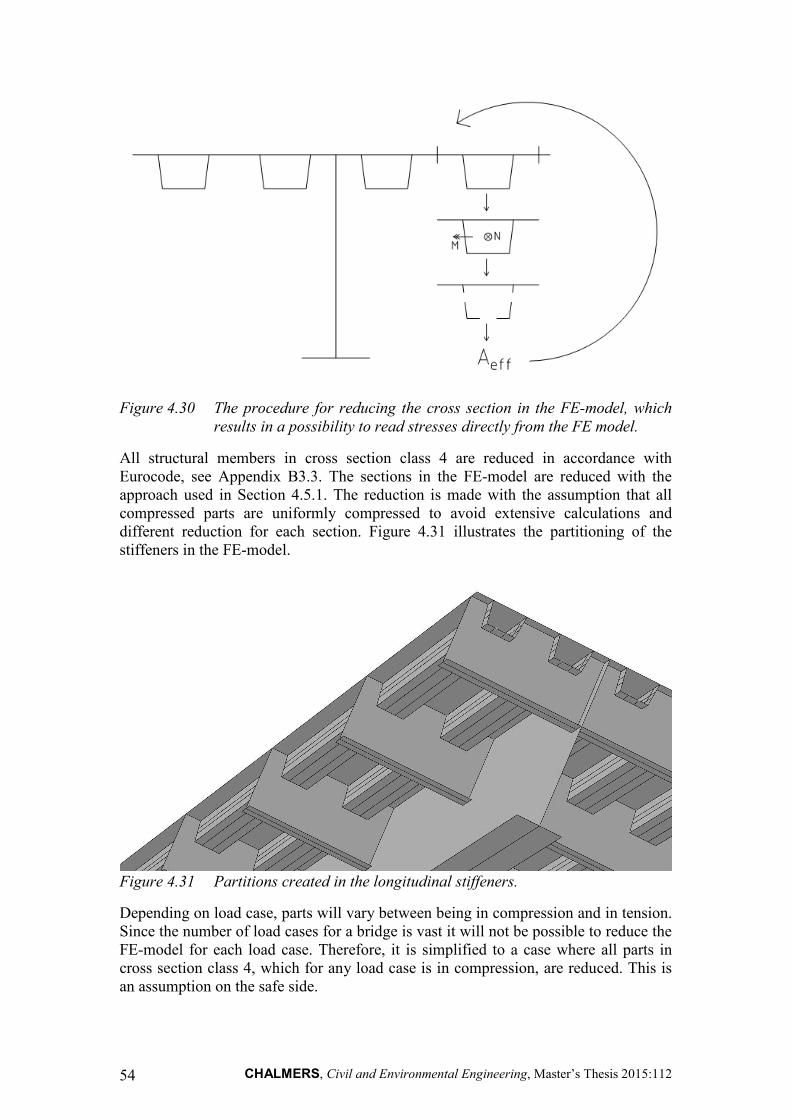
CHALMERS, Civil and Environmental Engineering, Master’s Thesis 2015:112 54
Figure 4.30 The procedure for reducing the cross section in the FE-model, which
results in a possibility to read stresses directly from the FE model.
All structural members in cross section class 4 are reduced in accordance with Eurocode, see Appendix B3.3. The sections in the FE-model are reduced with the approach used in Section 4.5.1. The reduction is made with the assumption that all compressed parts are uniformly compressed to avoid extensive calculations and different reduction for each section. Figure 4.31 illustrates the partitioning of the stiffeners in the FE-model.
Figure 4.31 Partitions created in the longitudinal stiffeners.
Depending on load case, parts will vary between being in compression and in tension. Since the number of load cases for a bridge is vast it will not be possible to reduce the FE-model for each load case. Therefore, it is simplified to a case where all parts in cross section class 4, which for any load case is in compression, are reduced. This is an assumption on the safe side.

CHALMERS Civil and Environmental Engineering, Master’s Thesis 2015:112 55
The mesh used for the reduced bridge section is the same as used in the unreduced detailed shell model, since the geometry is the same, see Section 4.3.1.
It should be noted that, unlike the I-beam example, the deck experience biaxial stresses from bending in both directions and that the reduced web is also loaded in bending out of plane. The effect of this is not examined in this thesis.
4.6 Hand calculations Having extracted the bending moment, M, and the normal force, N, from the unreduced FE-models, the normal stresses in the longitudinal stiffeners are calculated, using Navier’s formula:
𝜎 = 𝑀𝐼∙ 𝑧 + 𝑁
𝐴 (4.1)
Since the sectional forces are extracted for a longitudinal stiffener with associated deck plate, the neutral axis is situated at the local centre of gravity of the stiffeners. This means that, z, is the distance from the neutral axis to the point of interest for stress calculation within the stiffener, see Figure 4.32. The second moment of area, I, and the cross section area, A, are also for the stiffener locally. The global normal stress is calculated for the top and bottom of the longitudinal stiffener by using sectional forces extracted from the unreduced FE models of the detailed shell model, and the equivalent plate.
For some load cases, the normal stresses in the longitudinal stiffeners are also calculated without the use of the FE-models. To receive the global normal stress the bending moment is calculated along the bridge, and the stress is calculated according to Navier’s formula, see equation 4.1. This time, the second moment of area is for the full bridge cross section. The distance to the neutral axis is now the distance from the top and bottom of the longitudinal stiffener to the centre of gravity for the whole bridge. This is done in order to verify the results from the FE models.
As discussed in Section 2.2.3, the transverse stiffeners can be represented either as rigid supports or as spring supports, in hand calculations. Thus, the local bending moments are calculated by modelling one longitudinal stiffener in both ways, and then the normal stress is calculated using Navier’s formula. The stiffness of the springs is calculated according to the method described in Section 2.3.2. The total normal stress for the longitudinal stiffener is finally calculated by adding the global effects to the local effects, see Figure 4.32.

CHALMERS, Civil and Environmental Engineering, Master’s Thesis 2015:112 56
Figure 4.32 Stress calculation from local and global effects.

CHALMERS Civil and Environmental Engineering, Master’s Thesis 2015:112 57
5 Results For designing longitudinal stiffeners, sectional forces needs to be extracted from the unreduced FE model. Section 5.1 presents a comparison between the sectional forces that are received, both from the detailed shell model and the equivalent plate model.
Section 5.2 presents normal stresses for a reduced cross section of the longitudinal stiffeners. The normal stresses are extracted in two different ways. For the unreduced detailed shell model the extracted sectional forces are used in hand calculations on a reduced cross section to obtain the normal stresses. In the reduced detailed shell model, where the cross section has been reduced within the model, the normal stresses are extracted directly from the model.
The comparisons made in Section 5.1 and Section 5.2 are illustrated in Figure 5.1 below.
Figure 5.1 Flow chart for comparisons made in Chapter 5.
The stresses and sectional forces are, for load case 1-5, extracted for the loaded rib closest to the middle of the main girders. For load case 6-7, the stresses and sectional forces are extracted for the loaded rib closest to the main girder. The wheel loads presented in Section 4.2.2 are presented again in Figure 5.2.
Figure 5.2 Load cases presented in Section 4.2.2.

CHALMERS, Civil and Environmental Engineering, Master’s Thesis 2015:112 58
5.1 Equivalent plate approach For the equivalent plate model, nodal sectional forces are extracted and integrated over the width of a longitudinal stiffener to obtain the sectional forces that act over a fictive stiffener, see Figure 5.3.
Figure 5.3 Schematic figure of how the sectional forces are extracted using Free
Body Cut for the detailed shell model (top), and using nodal forces and integration for the equivalent plate (bottom).

CHALMERS Civil and Environmental Engineering, Master’s Thesis 2015:112 59
5.1.1 Results for equivalent plate approach Bending moment The bending moments, obtained by integration of nodal moments, for the six load cases with wheel loads are presented in Figure 5.4. The wheel loads are the most interesting to study in terms of local effects on the rib.
Figure 5.4 Moment distributions for load cases with wheel load. Solid line
represents the detailed shell model, and dashed line represents the equivalent plate model.
The resulting maximum moments are presented in Table 5.1. The difference between the two approaches varies depending on the load position. The maximum moment for the first five load cases differ between 3-11 %. However, for load case 6 and 7, where

CHALMERS, Civil and Environmental Engineering, Master’s Thesis 2015:112 60
the wheel load is applied over the rib closest to the main girder, the difference becomes larger. This higher difference might be because the rib at the main girder distorts and twists a lot more, giving rise to a different behaviour, whereas the rib in the middle mostly deflects vertically.
Table 5.1 Maximum moments. Moments are given in kNm. The calculated difference is how much the equivalent plate model differs from the detailed shell model.
Load case
Detailed shell model Equivalent plate model Difference Mmax Mmax Mmax
1 13.6 14.2 +4.3 % 2 113.4 105.7 -7.3 % 3 11.1 12.4 +10.6 % 4 74.8 70.7 -5.8 % 5 11.9 11.6 -3.3 % 6 12.3 9.5 -29.1 % 7 79.9 90.3 +11.4 %

CHALMERS Civil and Environmental Engineering, Master’s Thesis 2015:112 61
Normal force The normal force distribution for the six load cases with wheel loads are presented in Figure 5.5.
Figure 5.5 Normal force distributions for load cases with wheel load. Solid line
represents the detailed shell model, and dashed line represents the equivalent plate model.
The resulting highest compressive normal forces are presented in Table 5.2. The normal forces correlate well for load cases where the load is applied on the cross beams, and there are less local effects from the rib. When load is applied in a span the normal force in the detailed shell model is much higher than for the equivalent plate model. These deviations will be evaluated in Section 5.1.2.

CHALMERS, Civil and Environmental Engineering, Master’s Thesis 2015:112 62
Table 5.2 Highest compressive normal forces. Normal forces are given in kN. The calculated difference is how much the equivalent plate model differs from the detailed shell model.
Load case
Detailed shell model Equivalent plate model Difference Nmin Nmin Nmin
1 -271.7 -280.6 -3.2 % 2 -355.5 -282.2 +26.0 % 3 -274.0 -283.2 +3.2 % 4 -308.1 -285.1 +8.1 % 5 -602.7 -604.3 -0.3 % 6 -354.9 -353.9 +0.3 % 7 -407.3 -335.8 +21.3 %

CHALMERS Civil and Environmental Engineering, Master’s Thesis 2015:112 63
Shear force The shear force distribution for the six load cases with wheel loads are presented in Figure 5.6.
Figure 5.6 Shear force distributions for load cases with wheel load. Solid line
represents the detailed shell model, and dashed line represents the equivalent plate model.
The general behaviour of the shear force correlates well between the equivalent plate and the detailed shell model for all load cases, which can be seen in Figure 5.6. However in Table 5.3, it can be seen that the difference between the maximum values varies from load case to load case.

CHALMERS, Civil and Environmental Engineering, Master’s Thesis 2015:112 64
Table 5.3 Maximum absolute values of shear force. Shear forces are given in kN. The calculated difference is how much the equivalent plate model differs from the detailed shell model.
Load case
Detailed shell model Equivalent plate model Difference Vmax Vmax Vmax
1 140.1 125.4 -11.7 % 2 143.1 139.5 -2.6 % 3 68.4 39.9 -71.4 % 4 77.3 73.9 -4.6 % 5 13.3 11.0 -20.9 % 6 139.4 137.6 -1.3 % 7 131.0 139.8 +6.3 %
The correlation is not so good for load case 1 and 3 were the load is applied over a cross beam and also for load case 5 which is a uniform load. To examine the difference in the shear force, the three load cases with the wheel load placed at the cross beam are zoomed in, see Figure 5.7.
Figure 5.7 Zoomed in shear distribution curves for load cases with wheel load at
cross beam. Solid line represents the detailed shell model, and dashed line represents the equivalent plate model.
It should be noted that at loads and reaction forces there should be two values for the shear force, since the shear force will shift the same amount as the load or reaction force. This is not the case for the detailed shell model, since the shear force is extracted using Free Body Cut, which only gives one value for each cut. This means that the shifts in the shear force for the detailed shell model are spread out over a few elements. In Figure 5.7 this can be seen in the mismatch of the top values between the two methods.
The reasons for the deviation in shear force, seen in Figure 5.6, can be either that some local effects are missing in the equivalent model, since the stiffness is smeared out, or that the shear rigidity is wrong. The shear factor, which is used to calculate shear rigidity, is a shape factor that is not straight forward to calculate and different scientists have published different approaches (Cowper, 1966). However, since the other values correlate well it might not be this factor that causes the error.

CHALMERS Civil and Environmental Engineering, Master’s Thesis 2015:112 65
Moment, normal force and shear distributions for all load cases are presented in a larger scale in Appendix A.
5.1.2 Evaluation of equivalent plate approach The results in Section 5.1.1 show an expected behaviour for the bending moment and the shear force for all load cases. Both methods give the same behaviour, and most maximum values correlate well, however for the normal force a greater deviation is observed.
The normal force for the rib comes from global bending of the bridge, thus the theoretical behaviour is a parabolic shape which follows the bending moment distribution of the main girders. Figure 5.8 shows a closer view of the normal force distribution for load case 1, for the detailed shell model, the equivalent plate model and hand calculation, which are based on global bending moment.
Figure 5.8 Normal force distribution for load case 1.
It can be seen in Figure 5.8 that the extracted normal force from the two FE models (detailed shell model and equivalent plate model), deviate in behaviour from the theoretical behaviour represented by the hand calculations.
It can be observed that the deviations in behaviour occur at the cross beams. This is due to two effects. The first one is the rotation of the cross beams. The cross beams can be seen as fixed at the main girders, and will, because of the global deflection of the plate, rotate rather than just deflect vertically, see Figure 5.9.

CHALMERS, Civil and Environmental Engineering, Master’s Thesis 2015:112 66
Figure 5.9 The cross beams are seen as fixed at the main girders, and will thus
rotate around its axis, causing extra normal force. The figure on the top shows a case where load is applied between two cross beams and the bottom figure shows a case where load is applied to the cross beam in the middle of the bridge.
This effect causes extra normal force in the plate, since the centre of gravity of the cross beams is not placed at the centre of gravity of the plate. If this would have been the case, the rotation would not cause the cross beams to compress the plate, see Figure 5.10.
Figure 5.10 The rotation of the cross beam, which gives rise to extra normal force.
The figure on the left shows a case where the centre of gravity of the plate and of the cross beam coincide, and no extra normal force is created. In the figure on the right the centres of gravity do not coincide, and an extra normal force is created.

CHALMERS Civil and Environmental Engineering, Master’s Thesis 2015:112 67
The second effect causing local variation of the normal force, is the in plane deflection of the cross beams. This causes the plate to deflect transversally, which can be seen in Figure 5.11.
Figure 5.11 The deck plate, with cross beams seen from above. The cross beams
deflect, which causes a transversal contraction of the plate, causing extra normal force in the plate.
The transversal deflection causes stresses in the transverse direction. Due to the effect of lateral contraction, the transversal stresses cause stresses in the longitudinal direction. This effect causes tension in the plate over the cross beams, which in turn causes the reduction of the compressive normal force.
The effects described above, explain the behaviour of the normal force, when the load is placed at a cross beam. However, when the load is applied between two cross beams a greater deviation of the behaviour between the detailed shell mode and the equivalent plate model can be observed. Load case 2, which shows the greatest deviation, is shown again in Figure 5.12, together with a hand calculated normal force distribution.
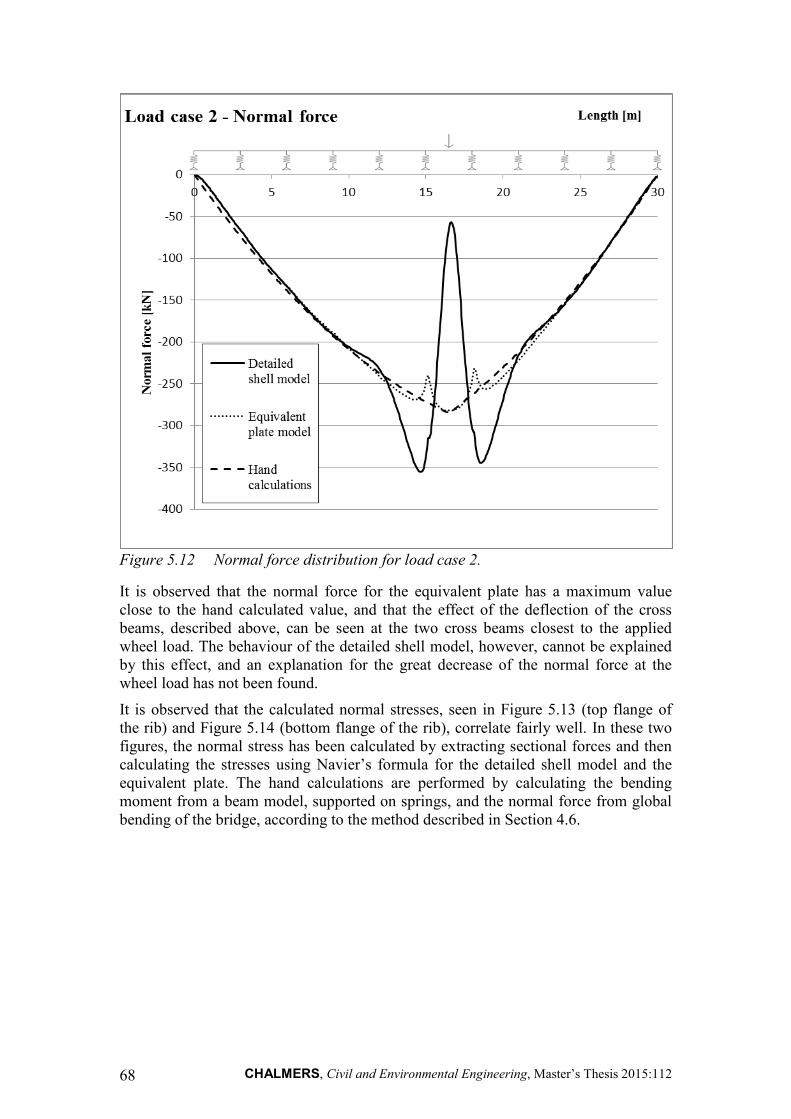
CHALMERS, Civil and Environmental Engineering, Master’s Thesis 2015:112 68
Figure 5.12 Normal force distribution for load case 2.
It is observed that the normal force for the equivalent plate has a maximum value close to the hand calculated value, and that the effect of the deflection of the cross beams, described above, can be seen at the two cross beams closest to the applied wheel load. The behaviour of the detailed shell model, however, cannot be explained by this effect, and an explanation for the great decrease of the normal force at the wheel load has not been found.
It is observed that the calculated normal stresses, seen in Figure 5.13 (top flange of the rib) and Figure 5.14 (bottom flange of the rib), correlate fairly well. In these two figures, the normal stress has been calculated by extracting sectional forces and then calculating the stresses using Navier’s formula for the detailed shell model and the equivalent plate. The hand calculations are performed by calculating the bending moment from a beam model, supported on springs, and the normal force from global bending of the bridge, according to the method described in Section 4.6.

CHALMERS Civil and Environmental Engineering, Master’s Thesis 2015:112 69
Figure 5.13 Normal stress distribution in the top plate of the loaded rib for load
case 2.
Figure 5.14 Normal stress distribution in the bottom plate of the loaded rib for load
case 2.

CHALMERS, Civil and Environmental Engineering, Master’s Thesis 2015:112 70
The difference between the two models probably comes from the erratic behaviour of the normal force from the detailed shell model. Hand calculated normal stresses are also added to compare with these two approaches. It can be observed that the hand calculated stress is higher than both the detailed shell model and the equivalent plate model. This is expected since hand calculations do not take any transverse load distribution into account. In the hand calculations the loaded rib is seen as an isolated beam which takes the whole wheel load. It can be observed that the equivalent plate is much closer to the detailed shell model than the simplified hand calculations.
The approach to simplify the deck plate to an equivalent plate seems to have potential. Even though the amplitudes vary between the models depending on load position, the overall structural behaviour of the equivalent plate follows the behaviour of the detailed shell model.
5.2 Reduced cross section In this section, the reduced section will be analysed using two different approaches. In the first approach, sectional forces have been extracted from the detailed shell model by the Brigade Plus tool Free Body Cut. Free Body Cut provides sectional forces which are used to calculate stresses for a reduced cross section of a rib. This approach means that the normal stresses will be uniform over the width of the rib, thus the transversal variation of the normal stresses is lost. This is an approach used in design, which is why these normal stresses are compared with normal stresses extracted directly from a model with reduced cross section, i.e. the second approach. In the second approach, the cross section has been reduced within the FE model, with the assumption of uniform compression. A linear finite element analysis in then executed with the reduced cross section and maximum stresses are extracted for the top and bottom of the rib, directly from the model.

CHALMERS Civil and Environmental Engineering, Master’s Thesis 2015:112 71
5.2.1 Results for reduced cross section Normal stress in top flange of the loaded rib For the load cases with a wheel load, the normal stress distributions in the top of the loaded rib are presented in Figure 5.15. The calculated normal stresses in the top of the rib from sectional forces extracted from the detailed shell model, using Free Body Cut, are compared with the stresses extracted directly from the reduced cross section model.
Figure 5.15 Normal stress distributions in the top of the rib for load cases with
wheel load. Solid line represents the calculated stress from sectional forces extracted from the unreduced detailed shell model, and dashed line represents stresses extracted directly from the reduced detailed shell model.
Table 5.4 presents the greatest normal stresses for both approaches. For all load cases the stresses extracted from the reduced detailed shell model corresponds well with the calculated values from the unreduced model, which can be seen in Table 5.4.

CHALMERS, Civil and Environmental Engineering, Master’s Thesis 2015:112 72
Table 5.4 Highest compressive normal stresses in the top plate of the loaded rib. The calculated difference is how much the reduced detailed shell model differs from the unreduced detailed shell model.
[MPa] Unreduced detailed shell model
Reduced detailed shell model Difference
Load case Top (Min) Top (Min) 1 -30.4 -29.2 +3.9% 2 -68.4 -66.5 +2.8% 3 -29.6 -28.4 +4.1% 4 -59.2 -56.8 +4.1% 5 -59.3 -57.5 +3.0% 6 -42.4 -40.0 +5.7% 7 -65.2 -61.1 +6.3%

CHALMERS Civil and Environmental Engineering, Master’s Thesis 2015:112 73
Normal stress in bottom flange of the loaded rib The normal stresses in the bottom of the loaded rib for both approaches are presented in Figure 5.16.
Figure 5.16 Normal stress distributions in the bottom of the rib for load cases with
wheel load. Solid line represents the calculated stress from sectional forces extracted from the unreduced detailed shell model, and dashed line represents stresses extracted directly from the reduced detailed shell model.
Table 5.5 presents the highest compressive and tensile normal stresses in the bottom flange of a rib. The correlation between the two approaches for the top of the rib is much better than the correlation in the bottom of the rib, where the reduction is. The behaviour and the extreme values are in many cases comparable.

CHALMERS, Civil and Environmental Engineering, Master’s Thesis 2015:112 74
Table 5.5 Highest compressive and tensile normal stresses in the bottom plate of the loaded rib. The calculated difference is how much the reduced detailed shell model differs from the unreduced detailed shell model.
[MPa] Unreduced detailed shell model
Reduced detailed shell model Difference
Load case
Bottom (Max)
Bottom (Min)
Bottom (Max)
Bottom (Min) Max Min
1 40.6 -29.6 26.3 -29.9 -35.2% +1.0% 2 523.2 -239.1 481.0 -231.9 -8.1% -3.0% 3 28.8 -27.2 20.8 -28.0 -27.8% +2.9% 4 331.0 -157.1 410.6 -194.9 +24.0% +24.1% 5 23.1 -33.2 20.8 -44.6 -10.0% +34.3% 6 21.9 -27.4 11.4 -28.3 -47.9% +3.3% 7 353.8 -159.7 313.4 -151.7 -11.4% -5.0%
The normal stresses can be seen in a larger scale in Appendix A.
5.2.2 Evaluation of reduced cross section It can be seen from Figure 5.15 and Figure 5.16 that the stresses in the top of the rib correspond very well, but differ in the bottom. In the top of the cross section the rib has not been reduced, which might explain that the approaches correspond well there.
To investigate the deviation, the extraction of the normal stresses from the reduced detailed shell model is examined. The normal stresses extracted, are taken along a path in the middle of the top plate of the stiffener, and in the middle of the unreduced part of the bottom flange of the stiffener, see Figure 5.17.
Figure 5.17 Stress extraction points for reduced cross section.
The normal stresses should vary transversally across the longitudinal stiffener, mainly because of the effects of shear lag, see Section 2.4.1.1. Figure 5.18 and Figure 5.19 show how the normal stress varies across the width of the top of the rib, for load cases 1 and 2 respectively. In these figures the longitudinal normal stress is plotted over the width of the rib at the section under the wheel load.

CHALMERS Civil and Environmental Engineering, Master’s Thesis 2015:112 75
Figure 5.18 Normal stress variation across the width of the top plate of the loaded
rib for load case 1, from the reduced model. Values extracted at the centre of the wheel load.
Figure 5.19 Normal stress variation across the width of the top plate of the loaded
rib for load case 2, from the reduced model. Values extracted at the centre of the wheel load.
The behaviour seen above is an expected shear lag behaviour. In Figure 5.18 the normal stresses decrease at the webs of the rib. The compression comes from global effects, but locally over the cross beam, which acts as a support, the top plate is in tension. This means that a decrease in compression represents an increase in tension, which explains the behaviour.
As seen in Figure 5.17 the stresses for the top plate are extracted from a path in the middle of the cross section. In Figure 5.18 and Figure 5.19 it can be seen that extracting these values means that the extracted value is close to an average value over the width of the rib. Free Body Cut calculates the resultant forces and moments over the whole cross section, which means that the stresses calculated from these

CHALMERS, Civil and Environmental Engineering, Master’s Thesis 2015:112 76
sectional forces will represent a case where the stress is uniform across the rib. This means that the value from Free Body Cut also should represent an average value over the rib. This explains why the normal stresses in the top of the cross section are very similar.
In the bottom of the cross section the stresses cannot be extracted in the middle of the cross section, because of the reduction, and is therefore extracted along a path near the edge of the bottom flange (see Figure 5.17). To examine the difference in the normal stresses in the bottom of the cross section, the transversal variation of the normal stresses for the bottom of the rib are plotted in Figure 5.20, Figure 5.21, Figure 5.22 and Figure 5.23.
As can be seen in Figure 5.16 the stresses for load case 2 correspond well even for the bottom flange of the cross section, and Figure 5.20 shows that the transversal normal stress variation is very small, which again means that the extracted value is reasonable.
Figure 5.20 Normal stress distribution across the width of the bottom flange of a
rib for a reduced cross section, load case 2, from the reduced model. Values extracted at the centre of the wheel load.
In Figure 5.16 it was observed that, for load case 4, normal stresses extracted directly from the reduced detailed shell model were larger than the ones calculated from Free Body Cut. In Figure 5.21 below, it can be seen that the transverse distribution of the normal stresses vary greatly. Load case 4 represents a case where the load is placed eccentrically over the rib, which explains this behaviour. The stresses have been extracted along a path to the right of the reduced part. This explains the over estimation of the stresses seen for load case 4.

CHALMERS Civil and Environmental Engineering, Master’s Thesis 2015:112 77
Figure 5.21 Normal stress distribution across the width of the bottom flange of a
rib for a reduced cross section, load case 4, from the reduced model. Values extracted at the centre of the wheel load.
It can be observed that the normal stress for load cases where the wheel load is placed at a cross beam varies more between the calculated normal stress and the directly extracted normal stress in the bottom flange of the rib. To examine this, the transversal distribution of the normal stress is plotted for load case 3 and 6, see Figure 5.22 and Figure 5.23.
Figure 5.22 Normal stress distribution across the width of the bottom flange of a
rib for a reduced cross section, load case 3, from the reduced model. Values extracted at the centre of the wheel load.

CHALMERS, Civil and Environmental Engineering, Master’s Thesis 2015:112 78
Figure 5.23 Normal stress distribution across the width of the bottom flange of a
rib for a reduced cross section, load case 6, from the reduced model. Values extracted at the centre of the wheel load.
As was observed for load case 4, it can again be seen that the transversal distribution of the normal stress varies, and that the normal stresses extracted to the right of the reduced part, might not be representative, which explains the difference in the normal stress distribution observed in Figure 5.16.
To examine whether the reduced rib has a similar behaviour as the unreduced rib, deformation figures for reduced and unreduced ribs are compared. Figure 5.24 shows the deformed rib for load case 2, under the wheel load, and Figure 5.25 shows the deformed rib for load case 4, under the wheel load.
Figure 5.24 Deformed rib for load case 2, under the wheel load (magnified 50
times). Figure on the left shows the unreduced cross section and figure on the right shows the reduced cross section.

CHALMERS Civil and Environmental Engineering, Master’s Thesis 2015:112 79
Figure 5.25 Deformed rib for load case 4, under the wheel load (magnified 30
times). Figure on the left shows the unreduced cross section and figure on the right shows the reduced cross section.
Figure 5.24 and Figure 5.25 implies that the behaviour of the rib is the same for both the reduced and unreduced case, although the reduced rib deforms slightly more than the unreduced. This means that the reduction of the cross section does not greatly affect the distortion of the cross section, which is a desirable property.

CHALMERS, Civil and Environmental Engineering, Master’s Thesis 2015:112 80
6 Discussion Equivalent plate The calculations of different stiffness used for General Shell Stiffness is executed according to one specific method and some smaller simplifications have been made. There is room for refinement which might affect the result and bring the two approaches closer. The representation of other structural elements such as cross beams has in this case study been simplified. Further studies on how this affects the results might lead to improved correlation between amplitudes.
For the case study used in this thesis it was observed that the shear rigidity calculated by Brigade Plus gave results which in some cases were slightly better, and in other cases slightly worse than the hand calculated shear rigidity. It might therefore not be necessary to hand calculate the shear rigidity, but instead use the default values in Brigade Plus. However, it should be noted that only one specific geometry was investigated, and that for other geometries the shear rigidity might matter more.
It was surprising that the normal force behaviour, which often is easy to capture, was the most deviating behaviour. The normal force comes from global bending of the bridge, which should result in a parabolic shape of the normal force distribution. The small local effects at cross beams can be explained, but the great deviation in the span between two cross beams for the detailed shell model cannot. It is possible that Free Body Cut, which is used to extract the sectional forces for the detailed model, has misinterpreted the state of stress, or that this is a local effect which is not captured by the equivalent plate method.
Reduced Plate The intention of reducing the detailed shell model within the FE model was to enable the possibility to extract stresses directly from the reduced FE model and be able to compare it to the yield stress to decide the utilization. However, as mentioned in Section 5.2.2, it has been shown that comparing hand calculated stresses with stresses extracted directly from the FE models might be problematic, because of transverse stress deviations.
In order to draw definite conclusions on the modelling of slender parts it is necessary to investigate the effects of the reduction further. It was shown that the desired behaviour for the longitudinal normal stress was found when examining an I-beam. However, other effects of the reduction were in this thesis not thoroughly investigated before the method was employed in the full bridge model, which means that the deviation in stress observed is difficult to interpret. It should be noted that other effects, such as the biaxial state of stress should be investigated on a smaller scale to verify the method, before using it on a full scale bridge.
Extracting stresses and sectional forces When extracting stresses and sectional forces from the FE model it is very important to consider the material direction, and to be aware of the different element direction in the different parts. In the case study, the top plate and the transversal stiffeners have element directions perpendicular to each other. This means that when extracting stresses or sectional forces along a path, two values will be given at the intersection between the two parts, one which is the desired value and one which is a value for the transversal stiffener in the perpendicular direction. This problem is especially present

CHALMERS Civil and Environmental Engineering, Master’s Thesis 2015:112 81
when extracting shear forces, since in some cases as many as five values were given in an intersection between the plate and a transverse stiffener. This means that some post-processing work is needed to analyse which values need to be excluded. This problem could be avoided if it would be possible to choose element directions so that they correlate with each other in all structural elements in the bridge.
It is important to note that when extracting stresses form shell elements in FE software, the stresses are extracted from either the integration point at the top of the shell, or the one at the bottom of the shell. This will include unwanted local effects of bending stresses. In order to obtain the membrane stress, an average value of the stress at the bottom of the shell and the stress at the top of the shell needs to be calculated.
Free Body Cut Using the Free Body But option in Brigade Plus entails some difficulties. To be able to extract values along the bridge, a section is chosen, and a direction in which the cuts are taken is also chosen. It is vital that the mesh in this direction is even, because otherwise the path might deviate from the desired path. In the case study this meant that a very fine mesh had to be used, which prolonged the running time considerably. The Free Body Cuts themselves also significantly increased the running time of the analysis, so to be able to use this method in practice, it is important to use fairly large intervals between the cuts, but small enough intervals to capture the behaviour.

CHALMERS, Civil and Environmental Engineering, Master’s Thesis 2015:112 82
7 Conclusions Equivalent plate It has been shown that the equivalent plate using lamina material is not a good method. The flexural rigidity of the equivalent plate is kept constant, but the membrane rigidity is changed so the overall behaviour of this plate is not realistic.
The equivalent 2D orthotropic plate, which uses General shell stiffness, is however a promising model to use in design. It has been seen that the behaviour of this plate follows the behaviour of the detailed shell model reasonably well. It is also a much less time consuming method and a much coarser mesh can be used.
When modelling the OSD bridge using an equivalent plate, the moment distribution, the deflection, and the global behaviour are captured well, but some local effects are missed. These effects are for instance the shear lag of the ribs, and the decrease in normal force when the load is placed between two cross beams. The results are however sufficiently close to the detailed shell model that it is reasonable to use this method in preliminary design of an OSD bridge, and, with further research, use in detailed design.
Slender Parts By using lamina material it is possible to model slender steel parts that need to be reduced in the FE software. The normal stress behaviour of an individual part in cross section class 4 follows the theoretical normal stress behaviour of a part which has been reduced according Eurocode.
However, no definite conclusions can be drawn about the behaviour of the reduced bridge model. The normal stress distribution differs a bit from the calculated normal stress, but it is difficult to interpret because of the complexity of a full OSD bridge model.
Even if this method is further investigated and found to give good results, it is still a very time consuming task to partition all the cross section class 4 parts in an orthotropic steel deck bridge. Moreover, because numerous load cases need to be considered in bridge design, the parts to be reduced are not always in compression. When the parts are in bending or tension they should be reduced differently, or not at all.
The factors mentioned above mean that this method is not realistic in bridge design, but it could be interesting to look at in research or when few parts of the structure will be reduced, or if the procedure in the future is included in the software.
Further studies In the case study, seven different load cases were used, each of which contained isolated wheel loads or a uniform load, and thus no combinations of traffic loads were looked at. This means that the actual design of the OSD bridge was not considered in this thesis, but only the specific behaviour of the chosen load cases was studied. In a further study the equivalent plate could be looked at from a design point of view, to investigate the behaviour when subjected to load cases used in design of bridges.
When using the equivalent plate the geometry of the plate is changed. This means that the main girders and the transversal stiffeners also need to be changed. In a further study it could be investigated the best way to model the main girders and the transversal stiffeners and also how to model the connection to the plate.

CHALMERS Civil and Environmental Engineering, Master’s Thesis 2015:112 83
The effects of the shear rigidity for the equivalent plate have not been thoroughly investigated in this thesis. The effects of the shear factor, which in this thesis has been simplified, should be investigated further.
For the normal force behaviour, some of the local deviations from the hand calculated distribution has been explained. However, the great decrease in normal force seen in the detailed shell model in the span between cross beams has not been explained. In order to find out if this behaviour comes from errors in the extraction of the normal force, or from local effects of the detailed shell model, further research is needed.
One of the most important aspects in bride design is fatigue analysis. A further investigation regarding the equivalent plate is to see if it could be used in fatigue analysis. One of the main problems to tackle when it comes to fatigue design using an equivalent plate is that the rib closest to the main girder often is the deciding rib in fatigue analysis, and in the equivalent plate method used in this thesis, this is the rib which deviates the most from the detailed shell model.
The method of reducing slender parts within the FE model seems to have promise. However, only a few effects of the reduction were in this thesis examined before the method was performed on the full bridge model. In order to verify that this method works it is necessary to look at other effects of the method, such as the effect of biaxial stress. It is advisable to study these effects further on a smaller scale in order to isolate specific effects and draw definite conclusions.

CHALMERS, Civil and Environmental Engineering, Master’s Thesis 2015:112 84
8 References AISC (1963): Design Manual for Orthotropic Steel Plate Deck Bridges. American
Institute of Steel Construction, New York, USA
Al-Emrani, M., Åkesson, B. (2013): STEEL STRUCTURES: Course Literature – VSM 191. Chalmers University of Technology, Gothenburg, Sweden
Austrell, P-E. et al. (2004): CALFEM: A Finite Element Toolbox: Version 3.4. The Division of Structural Mechanics, LTH, Lund
Beg, D. et al. (2010): Design of Plated Structures: Eurocode 3: Design of steel structures Part 1-5: Design of plated structures. Wilhelm Ernst & Sohn Verlag, Berlin, Germany
Blaauwendraad, J. (2010): Plates and FEM: Surprises and Pitfalls. Springer, Dordrecht, Netherlands
Braun, B., Kuhlmann, U. (2012): Reduced stress design of plates under biaxial compression. Steel Construction, vol. 5, no 1, pp. 33-40.
Broo, H., Lundgren, K., Plos, M. (2008): A guide to non-linear finite element modelling of shear and torsion in concrete bridges. Chalmers University of Technology, Gothenburg, Sweden
CEN, 2008a. Eurocode 3: Design of steel structures - Part 1-1: General rules and rules for buildings, SIS Förlag AB, Stockholm
CEN, 2008b. Eurocode 3: Design of steel structures - Part 1-5: Plated structural elements, SIS Förlag AB, Stockholm
Chatterjee, S. (2003): The Design of Modern Steel Bridges. Second edition. Blackwell Science Ltd, Oxford, UK
Cowper, G.R. (1966): The Shear Coefficient in Timoshenko’s Beam Theory. Journal of Applied Mechanics, Vol. 33, No.2, pp. 335-340.
Cullimore M.S.G., Smith J.W. (1981): Local Stresses in Orthotropic Steel Bridge Decks Caused by Wheel Loads. Journal of Constructional Steel Research, Vol. 1, No.2, pp. 17-26.
Dassault Systèmes (2007) Abaqus Analysis User’s Manual. http://www.egr.msu.edu/ software/abaqus/Documentation/docs/v6.7/ (2015-04-20).
Ellobody, E. (2014): Finite Element Analysis and Design of Steel and Steel-Concrete Composite Bridges. Elsevier, Amsterdam, Netherlands
Hendy, C.R. and Murphy, C.J. (2007): Designer’s Guide to EN1993-2. Thomas Telford, London, UK
Johansson, B. et al. (2007): Commentary and Worked Examples to EN 1993-1-1 “Plated Structural Elements”, ECCS-JRC Report No. EUR 22898 EN
Johansson, B., Veljkovic, M. (2009) Review of plate buckling rules in EN 1993-1-5. Steel Construction, vol. 2, no 4, pp. 228-234.
Karlsson, A., Wesley, C. (2015) Necessity of Advanced Fatigue Analysis for Orthotropic Steel Deck Bridges. Chalmers University of Technology, Göteborg, Sweden

CHALMERS Civil and Environmental Engineering, Master’s Thesis 2015:112 85
Kolstein M. H. (2007): Fatigue Classification of Welded Joints in Orthotropic Steel Bridge Decks. Ph. D. Thesis. Department of Design and Construction, Delft University of Technology, the Netherlands
Mangus, A.R., Sun, S. (2000): Orthotropic Deck Bridges. In Bridge Engineering Handbook, Chapter 14, edited by Chen, W-F and Duan, L. CRC Press LLC, Boca Raton, Florida, USA
Ottosen, N., Petersson, H. (1992): Introduction to the Finite Element Method. Prentice Hall, London, UK
US Department of Transportation (2012): Manual for Design, Construction, and Maintenance of Orthotropic Steel Deck Bridge. US Department of Transportation, Federal Highway Administration, Publication no. FHWA-IF-12-027. USA
Åkesson, B. (2005): Buckling: ett instabilitetsfenomen att räkna med. Studentlitteratur, Lund, Sweden


Appendix A – Results In this Appendix, all the results from the tests and calculations are presented. For each load case normal force, bending moment, shear force and normal stresses are presented. The stresses and sectional forces are extracted both from the detailed shell model, the reduced detailed shell model and the equivalent shape orthotropic plate.
Contents
A1 LOAD CASE 1 A-1
A2 LOAD CASE 2 A-6
A3 LOAD CASE 3 A-11
A4 LOAD CASE 4 A-16
A5 LOAD CASE 5 A-21
A6 LOAD CASE 6 A-30
A7 LOAD CASE 7 A-35

A-1
A1 Load Case 1 Load case 1 is a wheel load applied centrically over the mid rib at a cross beam, see Figure A.1
Figure A.1 Load case 1. The thick lines parallel to the ribs represent main girders.
Sectional forces from detailed shell model are extracted using Free Body Cut and for the equivalent plate model nodal forces are integrated to receive the sectional forces.
Figure A.2 Moment distribution for load case 1 for the middle rib.

A-2
Figure A.3 Normal force distribution for load case 1 for the middle rib.

A-3
Figure A.4 Shear force distribution for load case 1 for the middle rib.
For the detailed shell model and the equivalent plate model normal stresses are received by extracting moments and normal forces which are used to calculate the normal stress in the reduced cross section. For the reduced detailed model the cross section is reduced within the model. Normal stresses are therefore extracted directly from the FE model.

A-4
Figure A.5 Normal stress distribution for load case 1 at top plate of middle rib (reduced cross section).

A-5
Figure A.6 Normal stress distribution for load case 1 at bottom plate of middle rib (reduced cross section).

A-6
A2 Load Case 2 Load case 2 is a wheel load applied centrically over the mid rib at the span between the mid cross beams, see Figure A.7.
Figure A.7 Load case 2. The thick lines parallel to the ribs represent main girders.
Sectional forces from detailed shell model are extracted using Free Body Cut and for the equivalent plate model nodal forces are integrated to receive the sectional forces.
Figure A.8 Moment distribution for load case 2 for the middle rib.

A-7
Figure A.9 Normal force distribution for load case 2 for the middle rib.

A-8
Figure A.10 Shear force distribution for load case 2 for the middle rib.
For the detailed shell model and the equivalent plate model normal stresses are received by extracting moments and normal forces which are used to calculate the normal stress in the reduced cross section. For the reduced detailed model the cross section is reduced within the model. Normal stresses are therefore extracted directly from the FE model.

A-9
Figure A.11 Normal stress distribution for load case 2 at top plate of middle rib (reduced cross section).

A-10
Figure A.12 Normal stress distribution for load case 2 at bottom plate of middle rib (reduced cross section).

A-11
A3 Load Case 3 Load case 3 is a wheel load applied eccentrically between two ribs at the mid cross beams, see Figure A.13.
Figure A.13 Load case 3. The thick lines parallel to the ribs represent main girders.
Sectional forces from detailed shell model are extracted using Free Body Cut and for the equivalent plate model nodal forces are integrated to receive the sectional forces.
Figure A.14 Moment distribution for load case 3 for the middle rib.

A-12
Figure A.15 Normal force distribution for load case 3 for the middle rib.

A-13
Figure A.16 Shear force distribution for load case 3 for the middle rib.
For the detailed shell model and the equivalent plate model normal stresses are received by extracting moments and normal forces which are used to calculate the normal stress in the reduced cross section. For the reduced detailed model the cross section is reduced within the model. Normal stresses are therefore extracted directly from the FE model.

A-14
Figure A.17 Normal stress distribution for load case 3 at top plate of middle rib (reduced cross section).

A-15
Figure A.18 Normal stress distribution for load case 3 at bottom plate of middle rib (reduced cross section).

A-16
A4 Load Case 4 Load case 4 is a wheel load applied eccentrically between two ribs at the span between the two mid cross beams, see Figure A.19.
Figure A.19 Load case 4. The thick lines parallel to the ribs represent main girders.
Sectional forces from detailed shell model are extracted using Free Body Cut and for the equivalent plate model nodal forces are integrated to receive the sectional forces.
Figure A.20 Moment distribution for load case 4 for the middle rib.

A-17
Figure A.21 Normal force distribution for load case 4 for the middle rib.

A-18
Figure A.22 Shear force distribution for load case 4 for the middle rib.
For the detailed shell model and the equivalent plate model normal stresses are received by extracting moments and normal forces which are used to calculate the normal stress in the reduced cross section. For the reduced detailed model the cross section is reduced within the model. Normal stresses are therefore extracted directly from the FE model.

A-19
Figure A.23 Normal stress distribution for load case 4 at top plate of middle rib (reduced cross section).

A-20
Figure A.24 Normal stress distribution for load case 4 at bottom plate of middle rib (reduced cross section).

A-21
A5 Load Case 5 Load case 5 is a uniformly distributed load which is applied over the whole deck plate. Sectional forces from detailed shell model are extracted using Free Body Cut and for the equivalent plate model nodal forces are integrated to receive the sectional forces.
Figure A.25 Moment distribution for load case 5 for the middle rib.

A-22
Figure A.26 Normal force distribution for load case 5 for the middle rib.

A-23
Figure A.27 Shear force distribution for load case 5 for the middle rib.
For the detailed shell model and the equivalent plate model normal stresses are received by extracting moments and normal forces which are used to calculate the normal stress in the reduced cross section. For the reduced detailed model the cross section is reduced within the model. Normal stresses are therefore extracted directly from the FE model.

A-24
Figure A.28 Normal stress distribution for load case 5 at top plate of middle rib (reduced cross section).

A-25
Figure A.29 Normal stress distribution for load case 5 at bottom plate of middle rib (reduced cross section).
For load case 5 normal stresses are also calculated with hand calculations both for the top plate and the bottom plate. The hand calculated values are compared to the detailed shell model. Hand calculated stresses are preformed both with the assumption that the cross beams work as rigid supports and the assumption that the cross beams deflect and act as springs.

A-26
Figure A.30 Normal stress distribution for load case 5 at top plate of middle rib (reduced cross section).

A-27
Figure A.31 Normal stress distribution for load case 5 at top plate of middle rib (reduced cross section).

A-28
Figure A.32 Normal stress distribution for load case 5 at bottom plate of middle rib (reduced cross section).

A-29
Figure A.33 Normal stress distribution for load case 5 at bottom plate of middle rib (reduced cross section).

A-30
A6 Load Case 6 Load case 6 is a wheel load applied centrically over the rib closest to the main girder. The load is applied at the mid cross beam, see Figure A.34.
Figure A.34 Load case 6. The thick lines parallel to the ribs represent main girders.
Sectional forces from detailed shell model are extracted using Free Body Cut and for the equivalent plate model nodal forces are integrated to receive the sectional forces.
Figure A.35 Moment distribution for load case 6 for the rib closest to the main girder.
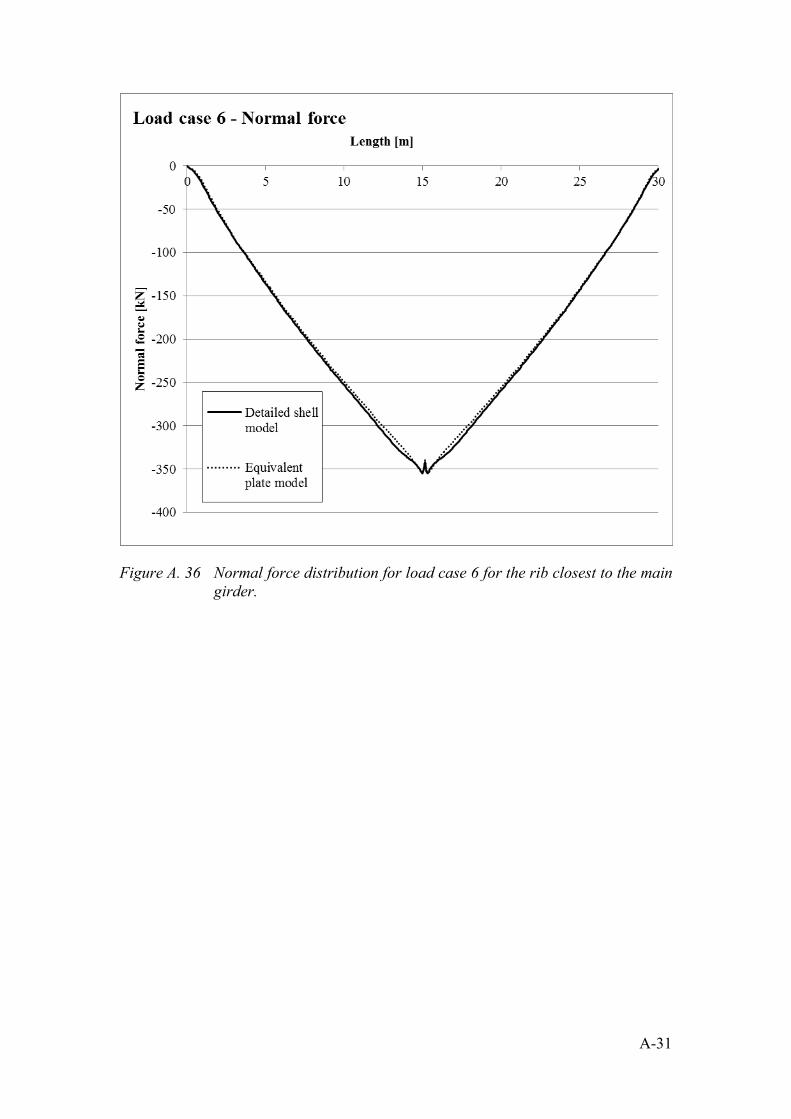
A-31
Figure A. 36 Normal force distribution for load case 6 for the rib closest to the main girder.

A-32
Figure A.37 Shear force distribution for load case 6 for the rib closest to the main girder.
For the detailed shell model and the equivalent plate model normal stresses are received by extracting moments and normal forces which are used to calculate the normal stress in the reduced cross section. For the reduced detailed model the cross section is reduced within the model. Normal stresses are therefore extracted directly from the FE model.

A-33
Figure A.38 Normal stress distribution for load case 6 at top plate of the rib closest to the main girder (reduced cross section).

A-34
Figure A.39 Normal stress distribution for load case 6 at bottom plate of the rib closest to the main girder (reduced cross section).

A-35
A7 Load Case 7 Load case 7 is a wheel load applied centrically over the rib closest to the main girder. The load is applied in the span between the two mid cross beams, see Figure A.40.
Figure A.40 Load case 7. The thick lines parallel to the ribs represent main girders.
Sectional forces from detailed shell model are extracted using Free Body Cut and for the equivalent plate model nodal forces are integrated to receive the sectional forces.
Figure A.41 Moment distribution for load case 7 for the rib closest to the main girder.

A-36
Figure A.42 Normal force distribution for load case 7 for the rib closest to the main girder.

A-37
Figure A.43 Shear force distribution for load case 7 for the rib closest to the main girder.
For the detailed shell model and the equivalent plate model normal stresses are received by extracting moments and normal forces which are used to calculate the normal stress in the reduced cross section. For the reduced detailed model the cross section is reduced within the model. Normal stresses are therefore extracted directly from the FE model.

A-38
Figure A.44 Normal stress distribution for load case 7 at top plate of the rib closest to the main girder (reduced cross section).

A-39
Figure A.45 Normal stress distribution for load case 7 at bottom plate of the rib closest to the main girder (reduced cross section).

Appendix B – Hand Calculations, Case Study In this Appendix the hand calculations connected with the case study are presented. Calculations presented include verification of the model, reduction of the cross section according to Eurocode, as well as normal stress calculations. The normal stress calculations are performed both using only hand calculations and using the sectional forces extracted using the FE software.
Contents
B1 INDATA B-1
B2 VERIFICATION B-4
B2.1 Effective width of main girder with respect to shear lag B-4
B2.2 Global behaviour B-6
B2.3 Effective width, transversal stiffeners B-6
B2.4 Stress in longitudinal stiffener B-9 B.2.4.1 Stress from global effects B-10 B.2.4.2 Longitudinal stiffener with spring support B-11 B.2.4.3 Longitudinal stiffener, simply supported B-12 B.2.4.4 Difference between simply supported and spring supports B-13
B2.5 Deflection for longitudinal stiffener B-14
B3 DETAILED SHELL MODEL B-17
B3.1 Section forces from Free Body Cut B-17
B3.2 Stress in longitudinal stiffener B-23
B3.3 Check of cross section class B-26 B.3.3.1 Web of main girder B-26 B.3.3.2 Plate B-28 B.3.3.3 Longitudinal stiffener B-28 B.3.3.4 Reduction of bottom flange of stiffener B-29 B.3.3.5 Reduction of web of stiffener B-30
B3.4 Stress in reduced longitudinal stiffener B-31 B.3.4.1 Hand calculations B-32 B.3.4.2 Section forces from FEM B-33
B3.5 Normal force and stress in longitudinal stiffener, LC2 B-35
B4 EQUIVALENT PLATE B-39
B4.1 Alternative 1: Equivalent thickness B-40
B4.2 Alternative 2: Equivalent shape orthotropic plate B-42 B.4.2.1 Membrane rigidity B-42 B.4.2.2 Flexural rigidity B-43

B.4.2.3 Shear rigidity B-45 B.4.2.4 Stiffness matrices B-46
B4.3 Section forces for equivalent plate B-47
B4.4 Stress in longitudinal stiffener, equivalent plate B-51
B4.5 Stress in reduced longitudinal stiffener, equivalent plate B-52

B1 IndataMaterial Properties
fy 355MPa Yield strength
E 210GPa Young's modulus
ν 0.3 Poisson's ratio
ρ 7850kg
m3
Density
Geometry
Figure B1.1 Cross section of the case study.
ltot 30m Length of bridge
hw 1500mm Height main girder, web
tw 12mm Thickness main girder, web
tf 25mm Thickness bottom flange of main girder
bf 400mm Width bottom flange of main girder
tp 16mm Thickness plate
hs 200mm Height stiffener, web
B-1

bs.top 300mm Width stiffener, top
bs.bot 250mm Width stiffener, bottom
ts 4mm Thickness stiffener
Length stiffener, webls hs
2 bs.top bs.bot
2
2
0.202 m
ds 300mm Distance between stiffeners
nstiff 10 Number of longitudinal stiffeners
nCB 11 Number of transversal stiffeners
btot nstiff bs.top ds 6 m Width of deck
Figure B1.2 Cross section of the transversal stiffener.
hw.CB 600mm Height cross beam, web
tw.CB 10mm Thickness cross beam, web
tf.CB 20mm Thickness bottom flange of cross beam
B-2

bf.CB 250mm Width bottom flange of cross beam
dcross 3m Distance between cross beams
zCG 353.54mm Centre of gravity for full cross section(from top), calculated using AutoCAD
Second moment of area for full crosssection, calculated using AutoCADIy 53095627213.07mm
4
Area for full cross section, calculatedusing AutoCADA 178000.00mm
2
Loads
gself ρ A g 13.703kN
m Self weight of cross section
Area of web of cross beam, excludingthe cut-outs, calculated usingAutoCAD
ACB.w.real 3036925mm2
Figure B1.3 Area of cross beam web.
VCB ACB.w.real tw.CB bf.CB tf.CB btot Volume of cross beam
Gself.CB nCB VCB ρ g 51.121 kN Weight of cross beam
Smeared out self weight of the crossbeamsgself.CB.smeared
Gself.CB
ltot1.704
kN
m
Q 10kN
m2
Load acting on bridge
Total distributed load on bridgeq Q btot gself gself.CB.smeared 75.407
kN
m
B-3
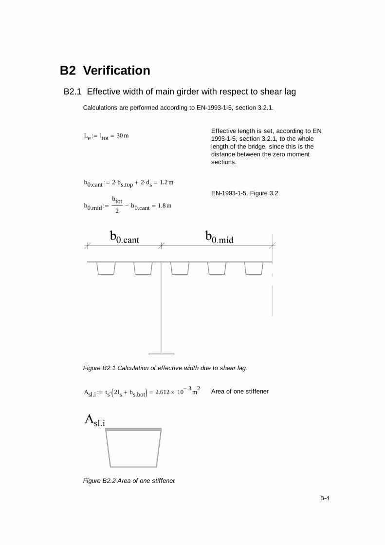
B2 Verification
B2.1 Effective width of main girder with respect to shear lag
Calculations are performed according to EN-1993-1-5, section 3.2.1.
Effective length is set, according to EN1993-1-5, section 3.2.1, to the wholelength of the bridge, since this is thedistance between the zero momentsections.
Le ltot 30 m
b0.cant 2 bs.top 2 ds 1.2 m
EN-1993-1-5, Figure 3.2
b0.mid
btot
2b0.cant 1.8 m
Figure B2.1 Calculation of effective width due to shear lag.
Asl.i ts 2ls bs.bot 2.612 103
m2
Area of one stiffener
Figure B2.2 Area of one stiffener.
B-4
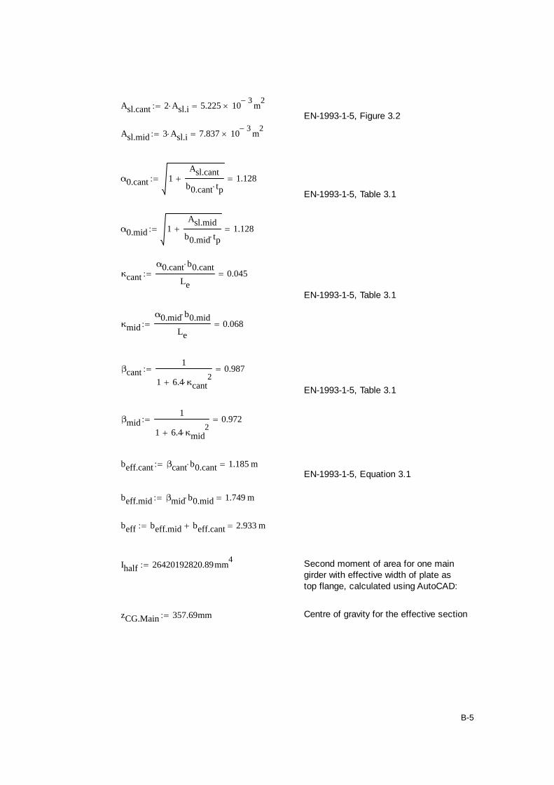
Asl.cant 2 Asl.i 5.225 103
m2
EN-1993-1-5, Figure 3.2
Asl.mid 3 Asl.i 7.837 103
m2
α0.cant 1Asl.cant
b0.cant tp 1.128
EN-1993-1-5, Table 3.1
α0.mid 1Asl.mid
b0.mid tp 1.128
κcant
α0.cant b0.cant
Le0.045
EN-1993-1-5, Table 3.1
κmid
α0.mid b0.mid
Le0.068
βcant1
1 6.4 κcant2
0.987
EN-1993-1-5, Table 3.1
βmid1
1 6.4 κmid2
0.972
beff.cant βcant b0.cant 1.185 mEN-1993-1-5, Equation 3.1
beff.mid βmid b0.mid 1.749 m
beff beff.mid beff.cant 2.933 m
Ihalf 26420192820.89mm4
Second moment of area for one maingirder with effective width of plate astop flange, calculated using AutoCAD:
zCG.Main 357.69mm Centre of gravity for the effective section
B-5

B2.2 Global behaviour
Maximum global deflection for the bridgeδmax.half
5q
2 ltot
4
384 E Ihalf71.672 mm
Maximum global moment in half thebridgeMmax.half
q
2ltot
2
84.242 10
3 kN m
σtop.half
Mmax.half
IhalfzCG.Main tp
Maximum tensile stress at the top of themain girder.
σtop.half 54.857 MPa
σbot.half
Mmax.half
Ihalftp hw zCG.Main
Maximum compressive stress at thebottom of the main girder.
σbot.half 185.961 MPa
B2.3 Effective width, transversal stiffeners
ε235MPa
fy0.814 EN1993-1-1 Table 5.2
beff.CB
tw.CB
215 ε tp 0.2 m EN-1993-1-5, Section 9.1
Figure B2.3 Effective width for transversal stiffener.
B-6

LCB 6 bs.top 6 ds 3.6 m
Figure B2.4 Effective length for transversal stiffener.
Height of effective web of cross beam (removing the cut-outs):
hCB.av hw.CB hs 0.4 m
Figure B2.5 Effective height for transversal stiffener.
Centre of gravity for the cross beam with its effective part of the top flange as web:
zCG.CB
2beff.CB tptp
2 hCB.av tw.CB tp hw.CB hCB.av
hCB.av
2
bf.CB tf.CB tp hw.CBtf.CB
2
2beff.CB tp hCB.av tw.CB bf.CB tf.CB
zCG.CB 0.314 m
B-7

Figure B2.6 Transversal stiffener.
Second moment of area for the effective cross beam:
ICB
2beff.CB tp3
122 beff.CB tp zCG.CB
tp
2
2
tw.CB hCB.av3
12tw.CB hCB.av tp hw.CB hCB.av
hCB.av
2 zCG.CB
2
bf.CB tf.CB3
12bf.CB tf.CB tp hw.CB
tf.CB
2 zCG.CB
2
ICB 1.182 109
mm4
Deflection per unit force, when applying point load centrically:
FCB
LCB3
48 E ICB3.916 10
9
m
N
Stiffness of the cross beam:
KCB1
FCB2.554 10
5
kN
m
B-8

B2.4 Stress in longitudinal stiffener
In hand calculations for the longitudinal stiffeners two cases are compared. One wherethe cross beams are modelled as rigid supports and one where the cross beams aremodelled as spring supports. Bending moment is analysed using the softwareGOBeam.
Top flange of the longitudinal stiffener, accoring to EN1993-1-5, clause 9.1:
beff.stiff 15 ε tpts
2 0.197 m >
bs.top
20.15 m
=> Top flange of longitudinal stiffener taken as cc-distance between stiffeners.
Cross sectional data calculated using AutoCAD
zstiff.CG 39.21mm Centre of gravity for longitudinal stiffener
Second moment of area for longitudinalstiffenerIstiff.y 55585098.53mm
4
Astiff 12200.00mm2
Area of longitudinal stiffener
For load case 6 and 7, only half the outstanding top flange on the side of themain girder is included.
Centre of gravity for longitudinal stiffenerzstiff.CG.LC67 42.57mm
Second moment of area for longitudinalstiffenerIstiff.y.LC67 54282238.60mm
4
Astiff.LC67 11016.00mm2
Area of longitudinal stiffener
Figure B2.7 Width and area for longitudinal stiffener.
B-9

gstiff Astiff ρ g 0.939kN
m Self weight of one longitudinal stiffener
Centre-to-centre distance of thelongitudinal stiffenerssrib ds bs.top 0.6 m
qrib Q srib gstiff 6.939kN
m Total load acting on the longitudinal
stiffener
B2.4.1 Stress from global effects
R1
q ltot
21.131 10
3 kN Reaction force, whole bridge
R2 R1 1.131 103
kN
Figure B2.8 Calculation model for whole bridge.
xGoBeam0
0,000001
0,15
0,3
0,45
0,6
0,75
0,9
1,05
1,2
x-values used by GoBeam.
x xGoBeam m
Total bending moment for half crosssectionMglobal
R1
2x
q
2x
2
2
B-10

Stress in bottom of the longitudinal stiffener due to global effects:
σbot.global
Mglobal
Ihalftp hs zCG.Main
Stress in top of the longitudinal stiffener due to global effects:
σtop.global
Mglobal
IhalfzCG.Main
B2.4.2 Longitudinal stiffener with spring support
Figure B2.9 Calculation model for longitudinal stiffener, with spring supports.
Mspring.GoBeam0,00
0,00
1,16
2,17
3,02
3,71
4,25
4,63
4,85
4,92
Bending moment calculated usingGoBeam.
Mspring Mspring.GoBeam kN m
Stress at the top of the longitudinal stiffener due to local effects.
σtop.spring
Mspring
Istiff.yzstiff.CG
Stress at the bottom of the longitudinal stiffener due to local effects:
σbot.spring
Mspring
Istiff.yhs tp zstiff.CG
B-11

Total stress in the longitudinal stiffener (global and local effects):
σbot.tot.spring σbot.spring σbot.global
σtop.tot.spring σtop.spring σtop.global
B2.4.3 Longitudinal stiffener, simply supported
Figure B2.10 Calculation model for longitudinal stiffener, simply supported.
Msimply.GoBeam0,00
0,00
1,15
2,15
2,99
3,68
4,21
4,58
4,79
4,85
Bending moment calculated usingGoBeam.
Msimply Msimply.GoBeam kN m
Stress at the top of the longitudinal stiffener due to local effects.
σtop.simply
Msimply
Istiff.yzstiff.CG
Stress at the bottom of the longitudinal stiffener due to local effects.
σbot.simply
Msimply
Istiff.yhs tp zstiff.CG
B-12

Total stress in the longitudinal stiffener (global and local effects):
σbot.tot.simply σbot.simply σbot.global
σtop.tot.simply σtop.simply σtop.global
B2.4.4 Difference between simply supported and spring supports
σdiff.top σtop.tot.spring σtop.tot.simply
σdiff.bot σbot.tot.spring σbot.tot.simply
0 10 20 304 10
5
2 105
0
2 105
4 105
6 105
σdiff.top
σdiff.bot
x
Figure B2.11 Difference in normal stress when modelling the supports assprings and non-yielding.
B-13

B2.5 Deflection for longitudinal stiffener
Deflection for a longitudinal stiffener (local effects) calculated using GoBeam, for boththe case with rigid supports and the case with spring supports.
Figure B2.12 Calculation models for longitudinal stiffener.
δsimply.GoBeam0,000
0,000
-0,058
-0,113
-0,164
-0,210
-0,248
-0,278
-0,300
-0,312
δspring.GoBeam-0,032
-0,032
-0,094
-0,153
-0,208
-0,258
-0,300
-0,334
-0,359
-0,375
δsimply δsimply.GoBeam mm δspring δspring.GoBeam mm
0 10 20 304 10
4
3 104
2 104
1 104
0
1 104
δsimply
xFigure B2.13 Deflection for the longitudinal stiffener, transversal stiffenersmodelled as non-yielding supports.
B-14

0 10 20 304 10
4
3 104
2 104
1 104
0
δspring
x
Figure B2.14 Deflection for the longitudinal stiffener, transversal stiffenersmodelled as spring supports.
Deflection of the bridge due to global effects.
δglobal.half
ltot4 q
2
24 E Ihalf
x
ltot2
x3
ltot3
x
4
ltot4
min δglobal.half 71.672 mm
0 10 20 300.08
0.06
0.04
0.02
0
δglobal.half
xFigure B2.15 Global deflection for the bridge.
B-15

Total deflection of a longitudinal stiffener due to local and global effects.
δtot.spring δspring δglobal.half
δtot.simply δsimply δglobal.half
0 10 20 300.08
0.06
0.04
0.02
0
δtot.simply
xFigure B2.16 Deflection for a longitudinal stiffener including global effects,transversal stiffeners modelled as non-yielding supports.
0 10 20 300.08
0.06
0.04
0.02
0
δtot.spring
xFigure B2.17 Deflection for a longitudinal stiffener including global effects,transversal stiffeners modelled as springs.
min δtot.spring 0.071754 m
min δtot.simply 0.071672 m
B-16

B3 Detailed Shell Model
B3.1 Section forces from Free Body Cut
Bending moment and normal force for one longitudinal stiffener are calculated usingthe Free Body Cut tool in Brigade.
Figure B3.1 Extraction of sectional forces for the detailed shell model.
Wheel load placed centrally over rib, at cross beam (Load case 1):
Figure B3.2 Load case 1.
xrib.in
Mrib.CB.in
Nrib.CB.in
0 0,287308 ‐7,48924
0,075 0,799168 ‐173,61
0,15 11,172 ‐650,878
0,225 ‐77,2068 ‐1591,31
0,3 ‐163,713 ‐2645,58
0,375 ‐248,946 ‐3844,33
0,45 ‐332,83 ‐5183,43
0,525 ‐414,877 ‐6645,01
0,6 ‐494,579 ‐8210,76
0,675 ‐571,449 ‐9863,39
B-17

Wheel load placed centrally over rib, between cross beams (Load case 2):
Figure B3.3 Load case 2.
Mrib.span.in
Nrib.span.in
0,28924 ‐7,12383
1,00525 ‐165,078
10,371 ‐620,792
‐77,7187 ‐1529,22
‐163,695 ‐2543,8
‐248,171 ‐3695,25
‐331,095 ‐4980,31
‐412,006 ‐6382,04
‐490,421 ‐7883,02
‐565,879 ‐9466,77
B-18
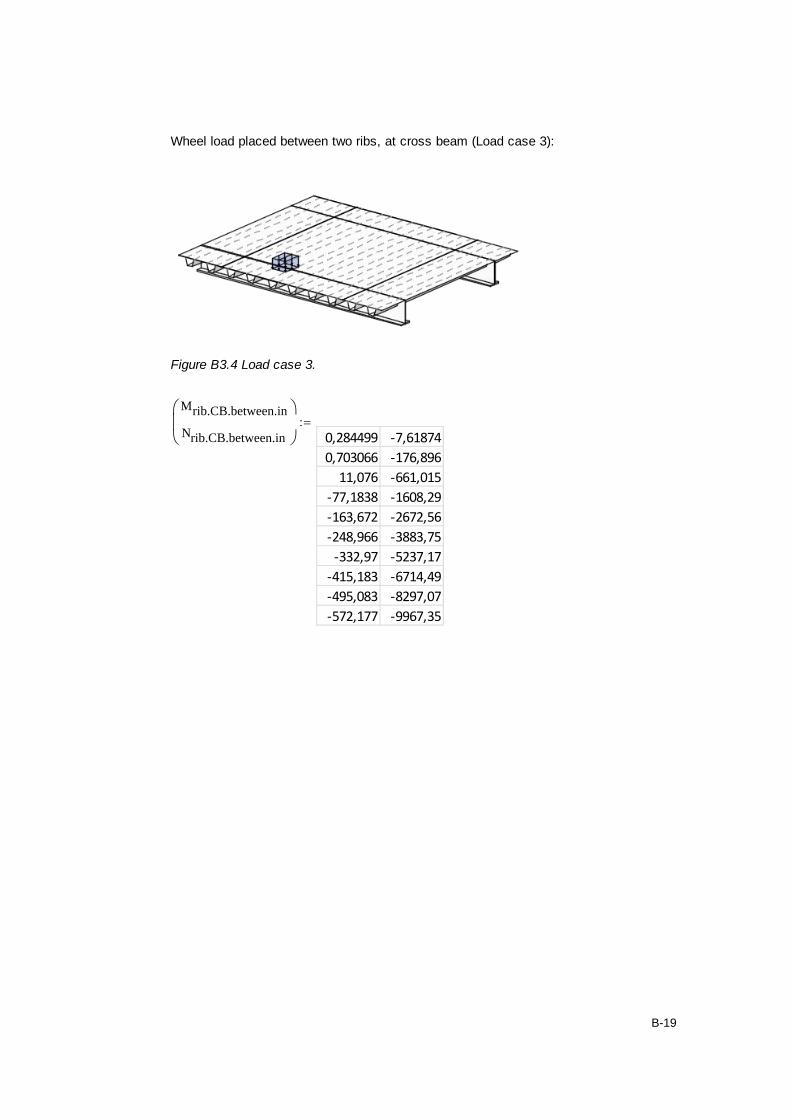
Wheel load placed between two ribs, at cross beam (Load case 3):
Figure B3.4 Load case 3.
Mrib.CB.between.in
Nrib.CB.between.in
0,284499 ‐7,61874
0,703066 ‐176,896
11,076 ‐661,015
‐77,1838 ‐1608,29
‐163,672 ‐2672,56
‐248,966 ‐3883,75
‐332,97 ‐5237,17
‐415,183 ‐6714,49
‐495,083 ‐8297,07
‐572,177 ‐9967,35
B-19

Wheel load placed between two ribs, between cross beams (Load case 4).
Figure B3.5 Load case 4.
Mrib.span.between.in
Nrib.span.between.in
0,287551 ‐7,23506
0,92623 ‐167,925
10,2951 ‐629,559
‐77,696 ‐1543,57
‐163,664 ‐2566,52
‐248,201 ‐3728,49
‐331,239 ‐5025,69
‐412,305 ‐6440,82
‐490,908 ‐7956,17
‐566,577 ‐9555,01
Uniform load acting on the whole deck (Load case 5):
Mrib.uniform.in
Nrib.uniform.in
0,569452 ‐18,2114
‐2,63247 ‐417,188
‐73,8728 ‐1723,55
‐718,22 ‐4824,19
‐1327,46 ‐8072,83
‐1905,6 ‐11638,7
‐2453,73 ‐15548,9
‐2970,99 ‐19765,9
‐3456,25 ‐24245
‐3908,37 ‐28941,8
B-20

Wheel load placed centrally over edge rib, at cross beams (Load case 6):
Figure B3.6 Load case 6.
Medgerib.CB.in
Nedgerib.CB.in
0,925598 ‐62,8477
‐14,5544 ‐1117,89
24,8679 ‐2907,71
43,7848 ‐3346,59
51,042 ‐4196,81
49,6068 ‐5341,53
40,8511 ‐6709,43
24,315 ‐8285,89
‐0,18114 ‐10058,5
‐32,4937 ‐12013,9
B-21
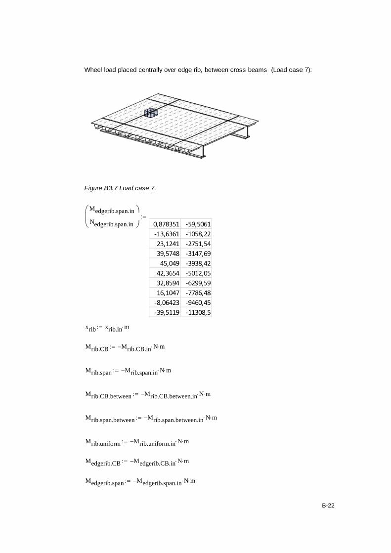
Wheel load placed centrally over edge rib, between cross beams (Load case 7):
Figure B3.7 Load case 7.
Medgerib.span.in
Nedgerib.span.in
0,878351 ‐59,5061
‐13,6361 ‐1058,22
23,1241 ‐2751,54
39,5748 ‐3147,69
45,049 ‐3938,42
42,3654 ‐5012,05
32,8594 ‐6299,59
16,1047 ‐7786,48
‐8,06423 ‐9460,45
‐39,5119 ‐11308,5
xrib xrib.in m
Mrib.CB Mrib.CB.in N m
Mrib.span Mrib.span.in N m
Mrib.CB.between Mrib.CB.between.in N m
Mrib.span.between Mrib.span.between.in N m
Mrib.uniform Mrib.uniform.in N m
Medgerib.CB Medgerib.CB.in N m
Medgerib.span Medgerib.span.in N m
B-22

Nrib.CB Nrib.CB.in N
Nrib.span Nrib.span.in N
Nrib.CB.between Nrib.CB.between.in N
Nrib.span.between Nrib.span.between.in N
Nrib.uniform Nrib.uniform.in N
Nedgerib.CB Nedgerib.CB.in N
Nedgerib.span Nedgerib.span.in N
B3.2 Stress in longitudinal stiffener
Distance from top of the plate to bottomof the longitudinal stiffener. zbot tp hs
ts
2 0.218 m
Figure B3.8 Points where normal stress is calculated.
Stress in rib, load placed centrally over rib, at CB (Load case 1)
σrib.CB.top
Mrib.CB
Istiff.y
tp
2zstiff.CG
Nrib.CB
Astiff
σrib.CB.bot
Mrib.CB
Istiff.yzbot zstiff.CG
Nrib.CB
Astiff
B-23

Stress in rib, load placed centrally over rib, between CBs (Load case 2)
σrib.span.top
Mrib.span
Istiff.y
tp
2zstiff.CG
Nrib.span
Astiff
σrib.span.bot
Mrib.span
Istiff.yzbot zstiff.CG
Nrib.span
Astiff
Stress in rib, load placed between two ribs, at CB (Load case 3)
σrib.CB.between.top
Mrib.CB.between
Istiff.y
tp
2zstiff.CG
Nrib.CB.between
Astiff
σrib.CB.between.bot
Mrib.CB.between
Istiff.yzbot zstiff.CG
Nrib.CB.between
Astiff
Stress in rib, load placed between two ribs, between CB (Load case 4)
σrib.span.between.top
Mrib.span.between
Istiff.y
tp
2zstiff.CG
Nrib.span.between
Astiff
σrib.span.between.bot
Mrib.span.between
Istiff.yzbot zstiff.CG
Nrib.span.between
Astiff
Stress in rib, uniformly distributed load (Load case 5)
σrib.uniform.top
Mrib.uniform
Istiff.y
tp
2zstiff.CG
Nrib.uniform
Astiff
σrib.uniform.bot
Mrib.uniform
Istiff.yzbot zstiff.CG
Nrib.uniform
Astiff
B-24

Stress in rib, load placed centrally over edge rib, at cross beams (Load case 6)
σedgerib.CB.top
Medgerib.CB
Istiff.y.LC67
tp
2zstiff.CG.LC67
Nedgerib.CB
Astiff.LC67
σedgerib.CB.bot
Medgerib.CB
Istiff.y.LC67zbot zstiff.CG.LC67
Nedgerib.CB
Astiff.LC67
Stress in rib, load placed centrally over edge rib, between cross beams (Load case 7)
σedgerib.span.top
Medgerib.span
Istiff.y.LC67
tp
2zstiff.CG.LC67
Nedgerib.span
Astiff.LC67
σedgerib.span.bot
Medgerib.span
Istiff.y.LC67zbot zstiff.CG.LC67
Nedgerib.span
Astiff.LC67
B-25

B3.3 Check of cross section class
Cross section class is checked for the different components according to EN1993-1-1
EN1993-1-1 Table 5.2ε
235MPa
fy0.814
B3.3.1 Web of main girder
Figure B3.9 Normal stress distribution in main girder.
Subjected to bending
Load 1: Stress in main girder, load placed centrally over rib, at CB
σ1.1 28.00MPa
σ2.1 80.03 MPa
ψ1
σ2.1
σ1.12.858
Load 2: Stress in main girder, load placed centrally over rib, between CBs
σ1.2 25.68MPa
σ2.2 77.35 MPa
ψ2
σ2.2
σ1.23.012
B-26

Load 3: Stress in main girder, load placed between two ribs, at CB
σ1.3 24.91MPa
σ2.3 72.79 MPa
ψ3
σ2.3
σ1.32.922
Load 4: Stress in main girder, load placed between two ribs, between CB
σ1.4 24.91MPa
σ2.4 72.79 MPa
ψ4
σ2.4
σ1.42.922
Load 5: Stress in main girder, uinformly distributed load
σ1.5 56.61MPa
σ2.5 186.51 MPa
ψ5
σ2.5
σ1.53.295
Load 6: Stress in rib, load placed centrally over edge rib, at cross beams
σ1.6 54.26MPa
σ2.6 121.58 MPa
ψ6
σ2.6
σ1.62.241
Load 7: Stress in rib, load placed centrally over edge rib, between crossbeams
σ1.7 36.37MPa
σ2.7 116.13 MPa
ψ7
σ2.7
σ1.73.193
B-27

Worst case:
ψw max ψ1 ψ2 ψ3 ψ4 ψ5 ψ6 ψ7 2.241
hw
tw
ε 1 ψw ψw31.671 < 62
Not in class 4.
B3.3.2 Plate
Subjected to compression
Internal part
ds
tp ε23.045 < 33 Cross section class 1
External part
ds
2
tp ε11.523 < 14 Cross section class 3
B3.3.3 Longitudinal stiffener
Assumed to be subjected to uniform compression
Web
ls
ts ε61.932 > 42 Cross section class 4
Bottom flange
bs.bot
ts ε76.818 > 42 Cross section class 4
B-28

B3.3.4 Reduction of bottom flange of stiffener
ψ 1
EN1993-1-5, Table 4.1Assumed to be uniformely compressed.
kσ 4.0
λp.bot
bs.bot
ts
28.4 ε kσ1.352 EN1993-1-5, Section 4.4
ρbot
λp.bot 0.055 3 ψ( )
λp.bot2
0.619
EN1993-1-5, Equation 4.2
beff.bot ρbot bs.bot 0.155 m
be1.bot 0.5 beff.bot 0.077 m EN1993-1-5, Table 4.1
be2.bot 0.5 beff.bot 0.077 m
Figure B3.10 Reduction of bottom flange of longitudinal stiffener.
B-29

B3.3.5 Reduction of web of stiffener
ψ 1EN1993-1-5, Table 4.1Assumed to be uniformely compressed.
kσ 4
λp.web
ls
ts
28.4 ε kσ1.09 EN1993-1-5, Section 4.4
ρweb
λp.web 0.055 3 ψ( )
λp.web2
0.732
EN1993-1-5, Equation 4.2
beff.web ρweb ls 0.148 m
be1.web 0.5 beff.web 0.074 m EN1993-1-5, Table 4.1
be2.web 0.5 beff.web 0.074 m
Figure B3.11 Reduction of web of longitudinal stiffener.
B-30

B3.4 Stress in reduced longitudinal stiffener
Cross sectional data calculated using AutoCAD
Second moment of area for reducedlongitudinal stiffener.Istiff.y.red 40256214.72mm
4
Centre of gravity for reduced longitudinalstiffener.zstiff.CG.red 30.52mm
Area of reduced longitudinal stiffener.Astiff.red 11402.92mm
2
Figure B3.12 Area and centre of gravity of longitudinal stiffener.
For load case 6 and 7, only half the outstanding top flange on the side of themain girder is included.
Second moment of area for reducedlongitudinal stiffener.Istiff.y.red.LC67 40057609.56mm
4
Centre of gravity for reduced longitudinalstiffener.zstiff.CG.red.LC67 33.41mm
Astiff.red.LC67 10236.86mm2
Area of reduced longitudinal stiffener.
B-31

B3.4.1 Hand calculations
Hand calculations are performed both with the assumption that the cross beamsare spring supports and rigid supports.
Figure B3.13 Calculation models for longitudinal stiffener.
σtop.spring.red
Mspring
Istiff.y.redzstiff.CG.red
σbot.spring.red
Mspring
Istiff.y.redhs tp zstiff.CG.red
σtop.simply.red
Msimply
Istiff.y.redzstiff.CG.red
σbot.simply.red
Msimply
Istiff.y.redhs tp zstiff.CG.red
σtop.spring.red.tot σtop.spring.red σtop.global
σbot.spring.red.tot σbot.spring.red σbot.global
σtop.simply.red.tot σtop.simply.red σtop.global
σbot.simply.red.tot σbot.simply.red σbot.global
B-32

B3.4.2 Section forces from FEM
Figure B3.14 Extraction of sectional forces for the detailed shell model.
Stress in rib, load placed centrally over rib, at CB (Load case 1):
σrib.CB.top.red
Mrib.CB
Istiff.y.red
tp
2zstiff.CG.red
Nrib.CB
Astiff.red
σrib.CB.bot.red
Mrib.CB
Istiff.y.redzbot zstiff.CG.red
Nrib.CB
Astiff.red
Stress in rib, load placed centrally over rib, between CBs (Load case 2):
σrib.span.top.red
Mrib.span
Istiff.y.red
tp
2zstiff.CG.red
Nrib.span
Astiff.red
σrib.span.bot.red
Mrib.span
Istiff.y.redzbot zstiff.CG.red
Nrib.span
Astiff.red
Stress in rib, load placed between two ribs, at CB (Load case 3):
σrib.CB.between.top.red
Mrib.CB.between
Istiff.y.red
tp
2zstiff.CG.red
Nrib.CB.between
Astiff.red
σrib.CB.between.bot.red
Mrib.CB.between
Istiff.y.redzbot zstiff.CG.red
Nrib.CB.between
Astiff.red
B-33

Stress in rib, load placed between two ribs, between CB (Load case 4):
σrib.span.between.top.red
Mrib.span.between
Istiff.y.red
tp
2zstiff.CG.red
Nrib.span.between
Astiff.red
σrib.span.between.bot.red
Mrib.span.between
Istiff.y.redzbot zstiff.CG.red
Nrib.span.between
Astiff.red
Stress in rib, uniformly distributed load (Load case 5):
σrib.uniform.top.red
Mrib.uniform
Istiff.y.red
tp
2zstiff.CG.red
Nrib.uniform
Astiff.red
σrib.uniform.bot.red
Mrib.uniform
Istiff.y.redzbot zstiff.CG.red
Nrib.uniform
Astiff.red
Stress in rib, load placed centrally over edge rib, at cross beams(Load case 6):
σedgerib.CB.top.red
Medgerib.CB
Istiff.y.red.LC67
tp
2zstiff.CG.red.LC67
Nedgerib.CB
Astiff.red.LC67
σedgerib.CB.bot.red
Medgerib.CB
Istiff.y.red.LC67zbot zstiff.CG.red.LC67
Nedgerib.CB
Astiff.red.LC67
B-34

Stress in rib, load placed centrally over edge rib, between cross beams(Load case 7):
σedgerib.span.top.red
Medgerib.span
Istiff.y.red.LC67
tp
2zstiff.CG.red.LC67
Nedgerib.span
Astiff.red.LC67
σedgerib.span.bot.red
Medgerib.span
Istiff.y.red.LC67zbot zstiff.CG.red.LC67
Nedgerib.span
Astiff.red.LC67
B3.5 Normal force and stress in longitudinal stiffener, LC2
Load case 2 is singled out as an interesting load case, and hand calculations for thisload case are performed.
lP 16.5m Position of point load
Point loadP 300kN
qself gself gself.CB.smeared 15.407kN
m Self weight for the bridge
RA
P ltot lP qself
ltot2
2
ltot366.103 kN Reaction force
Figure B3.15 Calculation model for load case 2.
B-35

x-values used by GoBeam.
xP1.GoBeam0
0,000001
0,15
0,3
0,45
0,6
0,75
0,9
1,05
1,2
xP2.GoBeam16,5
16,65
16,8
16,95
17,1
17,25
17,4
17,55
17,7
17,85
xP1 xP1.GoBeam m xP2 xP2.GoBeam m
MP1 xP1 RA xP1 qself
xP12
2
Bending moment in the bridge
MP2 xP2 RA xP2 qself
xP22
2 P xP2 lP
σP1 xP1 MP1 xP1
IyzCG zstiff.CG
Normal stress at the centre of gravity ofthe longitudinal stiffener.
σP2 xP2 MP2 xP2
IyzCG zstiff.CG
NP1 xP1 σP1 xP1 Astiff
Normal force at the centre of gravity ofthe longitudinal stiffener.
NP2 xP2 σP2 xP2 Astiff
σP1.top xP1 MP1 xP1
Iy
tp
2zCG
Normal stress at the top of thelongitudinal stiffener.
σP2.top xP2 MP2 xP2
Iy
tp
2zCG
B-36

σP1.bot xP1 MP1 xP1
IyzCG tp hs
ts
2
Normal stress at the bottom of thelongitudinal stiffener.
σP2.bot xP2 MP2 xP2
IyzCG tp hs
ts
2
NP1.top xP1 σP1 xP1 Astiff
Normal force at the top of thelongitudinal stiffener.
NP2.top xP2 σP2 xP2 Astiff
NP1.bot xP1 σP1 xP1 Astiff
Normal force at the bottom of thelongitudinal stiffener.
NP2.bot xP2 σP2 xP2 Astiff
Bending moments calculated using GoBeam.
MLC2.1.GoBeam0,00
0,00
1,15
2,15
2,98
3,67
4,19
4,56
4,78
4,83
MLC2.2.GoBeam158,13
135,56
112,83
89,94
66,89
43,69
20,33
-3,18
-26,85
-50,68
MLC2.1 MLC2.1.GoBeam kN m
MLC2.2 MLC2.2.GoBeam kN m
σtop.LC2.1
MLC2.1
Istiff.y
tp
2zstiff.CG
NP1.top xP1
Astiff
σtop.LC2.2
MLC2.2
Istiff.y
tp
2zstiff.CG
NP2.top xP2
Astiff
B-37

σbot.LC2.1
MLC2.1
Istiff.yhs tp
ts
2 zstiff.CG
NP1.bot xP1
Astiff
σbot.LC2.2
MLC2.2
Istiff.yhs tp
ts
2 zstiff.CG
NP2.bot xP2
Astiff
B-38

B4 Equivalent Plate
Figure B4.1 Direction of the axis for the equivalent plate.
Calculations in this chapter are described in Section 3.2 in the main report, and equationshere are referenced to that section.
B-39

B4.1 Alternative 1: Equivalent thickness
brib bs.top ds 0.6 m Width of one stiffener with its part of thetop plate.
Figure B4.2 Width of longitudinal stiffener.
Dyy
E Istiff.y
brib1.95 10
7
N m2
m Equation 3.14
E1 E 210 GPa
Ieq
Dyy
E19.26 10
7
mm4
m Equivalent secend mometn of area
teq3
12 Ieq 103.59 mm Equivalent thickness
G12
E1
2 1 ν( )80.769 GPa Shear modulus
G13 G12 80.769 GPa
B-40

Rotational angle calculated using Strusoft Frame analysis.
Figure B4.3 Model to calculate rotational angle.
mxx 10kN m
m Bending moment used in Strusoft
φ 0.041rad From Strusoft
Dxx
mxx
2 φbrib 7.3171 10
4
N m2
m Equation 3.2
E2
Dxx
Ieq0.79 GPa Equation 3.3
G23
E2
2 1 ν( )0.304 GPa Shear modulus
B-41

B4.2 Alternative 2: Equivalent shape orthotropic plate
Ab Astiff tp brib 2.6 103
mm2
Area of stiffener without oustanding partof top flange.
Figure B4.4 Area of stiffener.
B4.2.1 Membrane rigidity
dyy
E tp
1 ν2
E
Ab
bs.top ds Equation 3.11
dyy 4.602GPa m
2
m
dv
E tp
1 ν2
ν 1.108
GPa m2
m Equation 3.11
dxx
E tp
1 ν2
3.692
GPa m2
m Equation 3.11
dxy
E tp
1 ν2
1
2 1 ν( ) Equation 3.11
dxy 1.292GPa m
2
m
B-42

B4.2.2 Flexural rigidity
Dxx 0.073MPa m
4
m
Rotational angle calculated using Strusoft Frame analysis.
Figure B4.5 Model to calculate reduced bending moment between webs.
mxx 10kN m
m Bending moment used in Strusoft
Reduced bending moment from Strusoftmxx.1 9.6
kN m
m
Dv νds mxx bs.top mxx.1
brib mxxDxx 0.022
MPa m4
m
Equation 3.15
Dyy 19.455MPa m
4
m
ixy1
6tp
3 6.827 10
7
m4
m Equation 3.19
bav
bs.top bs.bot
20.275 m Average width of stiffener
As hs bav 0.055 m2
Area enclosed by stiffener
B-43

It
4 As2
bs.top
tp
bs.bot
ts 2
hs
ts
6.676 105
m4
Equation 3.21
iyx1
bs.top ds It
tp3
bs.top ds
6
ts3
bs.bot
32
ts3
hs
3
1.12 104
m
4
m
Equation 3.20
Equation 3.18iav
iyx ixy
25.633 10
5
m4
m
Equation 3.17Dav
E
2 1 ν( )
iav
2 2.275
MPa m4
m
D
dxx
Pa m2
m
dv
Pa m2
m
0
0
0
0
dv
Pa m2
m
dyy
Pa m2
m
0
0
0
0
0
0
dxy
Pa m2
m
0
0
0
0
0
0
Dxx
Pa m4
m
Dv
Pa m4
m
0
0
0
0
Dv
Pa m4
m
Dyy
Pa m4
m
0
0
0
0
0
0
Dav
Pa m4
m
B-44

B4.2.3 Shear rigidity
Deflection calculated using Strusoft Frame analysis.
vx 10kN
m Force used in Strusoft
δshear 10.246mm From Strusoft
Figure B4.6 Model to calculate shear stiffness.
Ksx
vx
δshear975.991
kN
m2
Equation 3.22
Dsx
brib
1
Ksx
brib3
12 Dxx
0.771MPa m
2
m
Equation 3.23
Shear factor calculated according to Cowper (1966):
mbox
bav tp
hs ts5.5
nbox
bav
hs1.375
κbox
10 1 ν( ) 1 3 mbox 2
12 72 mbox 150 mbox2
90 mbox3
ν 11 66 mbox 135 mbox2
90 mbox3
10 nbox2
3 ν( ) mbox 3 mbox2
0.143
B-45

Asy Astiff κbox 1.747 103
m2
Reduced area due to shear effects
Equation 3.24Dsy G12
Asy
brib 235.131
MPa m2
m
B4.2.4 Stiffness matrices
D
3.692 109
1.108 109
0
0
0
0
1.108 109
4.602 109
0
0
0
0
0
0
1.292 109
0
0
0
0
0
0
7.317 104
2.151 104
0
0
0
0
2.151 104
1.945 107
0
0
0
0
0
0
2.275 106
Dshear
Dsx
0
0
Dsy
7.706 105
0
0
2.351 108
Pa m2
m
B-46

B4.3 Section forces for equivalent plate
Figure B4.7 Schematic figure showing how the sectional forces were extracted.
Wheel load placed centrally over rib, at cross beam (Load case 1):
xeq.in
Meq.CB.in
Neq.CB.in
0 ‐5,4652 ‐180,521
0,15 16,67887 ‐667,536
0,25 111,8779 ‐1939,31
0,35 253,2259 ‐3629,67
0,45 385,0663 ‐5540,71
0,55 507,4281 ‐7632,08
0,65 620,3345 ‐9867,18
0,75 723,7965 ‐12214,3
0,85 817,838 ‐14647,1
0,95 902,484 ‐17144,1
Wheel load placed centrally over rib, between cross beams (Load case 2):
Meq.span.in
Neq.span.in
‐5,45337 ‐171,068
16,70659 ‐639,397
111,0167 ‐1863,88
250,5583 ‐3490,63
380,5958 ‐5326,31
501,1559 ‐7332,62
612,2575 ‐9474,88
713,9175 ‐11723
806,148 ‐14051,9
888,9735 ‐16441,6
B-47

Wheel load placed between two ribs, at cross beam (Load case 3):
Meq.CB.between.in
Neq.CB.between.in
‐5,46797 ‐183,785
16,82196 ‐676,244
112,381 ‐1962,56
254,153 ‐3672,86
386,4114 ‐5606,74
509,1915 ‐7722,95
622,5165 ‐9984,17
726,3945 ‐12358,1
820,845 ‐14818,2
905,897 ‐17342,8
Wheel load placed between two ribs, between cross beams (Load case 4).
Meq.span.between.in
Neq.span.between.in
‐5,45753 ‐173,93
16,83355 ‐646,985
111,4534 ‐1884,15
251,347 ‐3528,36
381,7301 ‐5384,04
502,636 ‐7412,08
614,086 ‐9577,2
716,086 ‐11848,9
808,653 ‐14201,9
891,8185 ‐16615,8
Uniform load acting on the whole deck (Load case 5):
Meq.uniform.in
Neq.uniform.in
‐6,47732 ‐419,447
175,209 ‐1968,85
807,7565 ‐6070,94
1674,326 ‐11451,3
2470,662 ‐17330,6
3196,896 ‐23611,6
3853,162 ‐30207,7
4439,587 ‐37045,1
4956,291 ‐44062,9
5403,391 ‐51212,9
B-48

xedge.in0
0,025
0,05
0,075
0,1
0,125
0,15
0,175
0,2
0,225
Different x-values for the edge stiffener,because of finer mesh.
Wheel load placed centrally over edge rib, at cross beams (Load case 6):
Meq.edge.CB.in
Neq.edge.CB.in
‐0,11856 ‐65,7519
‐0,28775 ‐181,763
‐0,74984 ‐493,928
‐1,56531 ‐925,936
‐2,98313 ‐1391,93
‐5,14972 ‐1821,38
‐15,0475 ‐2237,01
‐12,0695 ‐2574,46
10,92609 ‐2787,57
33,56169 ‐2956,34
Wheel load placed centrally over edge rib, between cross beams (Load case 7):
Meq.edge.span.in
Neq.edge.span.in
‐0,12152 ‐62,3359
‐0,2999 ‐171,399
‐0,79144 ‐465,587
‐1,65292 ‐872,555
‐3,12032 ‐1310,72
‐5,33223 ‐1713,22
‐14,661 ‐2102,41
‐11,1831 ‐2418,3
11,62638 ‐2615,97
34,06291 ‐2770,84
B-49

xeq xeq.in m
xedge xedge.in m
Meq.CB Meq.CB.in N m
Meq.span Meq.span.in N m
Meq.CB.between Meq.CB.between.in N m
Meq.span.between Meq.span.between.in N m
Meq.uniform Meq.uniform.in N m
Meq.edge.CB Meq.edge.CB.in N m
Meq.edge.span Meq.edge.span.in N m
Neq.CB Neq.CB.in N
Neq.span Neq.span.in N
Neq.CB.between Neq.CB.between.in N
Neq.span.between Neq.span.between.in N
Neq.uniform Neq.uniform.in N
Neq.edge.CB Neq.edge.CB.in N
Neq.edge.span Neq.edge.span.in N
B-50

B4.4 Stress in longitudinal stiffener, equivalent plate
Distance from top of the plate to bottomof the longitudinal stiffener. zbot 0.218 m
Stress in rib, load placed centrally over rib, at CB (Load case 1)
σeq.CB.top
Meq.CB
Istiff.y
tp
2zstiff.CG
Neq.CB
Astiff
σeq.CB.bot
Meq.CB
Istiff.yzbot zstiff.CG
Neq.CB
Astiff
Stress in rib, load placed centrally over rib, between CBs (Load case 2)
σeq.span.top
Meq.span
Istiff.y
tp
2zstiff.CG
Neq.span
Astiff
σeq.span.bot
Meq.span
Istiff.yzbot zstiff.CG
Neq.span
Astiff
Stress in rib, load placed between two ribs, at CB (Load case 3)
σeq.CB.between.top
Meq.CB.between
Istiff.y
tp
2zstiff.CG
Neq.CB.between
Astiff
σeq.CB.between.bot
Meq.CB.between
Istiff.yzbot zstiff.CG
Neq.CB.between
Astiff
Stress in rib, load placed between two ribs, between CB (Load case 4)
σeq.span.between.top
Meq.span.between
Istiff.y
tp
2zstiff.CG
Neq.span.between
Astiff
σeq.span.between.bot
Meq.span.between
Istiff.yzbot zstiff.CG
Neq.span.between
Astiff
B-51

Stress in rib, uinformly distributed load (Load case 5)
σeq.uniform.top
Meq.uniform
Istiff.y
tp
2zstiff.CG
Neq.uniform
Astiff
σeq.uniform.bot
Meq.uniform
Istiff.yzbot zstiff.CG
Neq.uniform
Astiff
Stress in rib, load placed centrally over edge rib, at cross beams (Load case 6):
σeq.edge.CB.top
Meq.edge.CB
Istiff.y.LC67
tp
2zstiff.CG.LC67
Neq.edge.CB
Astiff.LC67
σeq.edge.CB.bot
Meq.edge.CB
Istiff.y.LC67zbot zstiff.CG.LC67
Neq.edge.CB
Astiff.LC67
Stress in rib, load placed centrally over edge rib, between cross beams (Load case 7):
σeq.edge.span.top
Meq.edge.span
Istiff.y.LC67
tp
2zstiff.CG.LC67
Neq.edge.span
Astiff.LC67
σeq.edge.span.bot
Meq.edge.span
Istiff.y.LC67zbot zstiff.CG.LC67
Neq.edge.span
Astiff.LC67
B4.5 Stress in reduced longitudinal stiffener, equivalent plate
Distance from top of the plate to bottomof the longitudinal stiffener. zbot 0.218 m
Stress in rib, load placed centrally over rib, at CB (Load case 1)
σeq.CB.top.red
Meq.CB
Istiff.y.red
tp
2zstiff.CG.red
Neq.CB
Astiff.red
σeq.CB.bot.red
Meq.CB
Istiff.y.redzbot zstiff.CG.red
Neq.CB
Astiff.red
B-52

Stress in rib, load placed centrally over rib, between CBs (Load case 2)
σeq.span.top.red
Meq.span
Istiff.y.red
tp
2zstiff.CG.red
Neq.span
Astiff.red
σeq.span.bot.red
Meq.span
Istiff.y.redzbot zstiff.CG.red
Neq.span
Astiff.red
Stress in rib, load placed between two ribs, at CB (Load case 3)
σeq.CB.between.top.red
Meq.CB.between
Istiff.y.red
tp
2zstiff.CG.red
Neq.CB.between
Astiff.red
σeq.CB.between.bot.red
Meq.CB.between
Istiff.y.redzbot zstiff.CG.red
Neq.CB.between
Astiff.red
Stress in rib, load placed between two ribs, between CB (Load case 4)
σeq.span.between.top.red
Meq.span.between
Istiff.y.red
tp
2zstiff.CG.red
Neq.span.between
Astiff.red
σeq.span.between.bot.red
Meq.span.between
Istiff.y.redzbot zstiff.CG.red
Neq.span.between
Astiff.red
Stress in rib, uniformly distributed load (Load case 5)
σeq.uniform.top.red
Meq.uniform
Istiff.y.red
tp
2zstiff.CG.red
Neq.uniform
Astiff.red
σeq.uniform.bot.red
Meq.uniform
Istiff.y.redzbot zstiff.CG.red
Neq.uniform
Astiff.red
B-53

Stress in rib, load placed centrally over edge rib, at cross beams (Load case 6):
σeq.edge.CB.top.red
Meq.edge.CB
Istiff.y.red.LC67
tp
2zstiff.CG.red.LC67
Neq.edge.CB
Astiff.red.LC67
σeq.edge.CB.bot.red
Meq.edge.CB
Istiff.y.red.LC67zbot zstiff.CG.red.LC67
Neq.edge.CB
Astiff.red.LC67
Stress in rib, load placed centrally over edge rib, between cross beams (Load case 7):
σeq.edge.span.top.red
Meq.edge.span
Istiff.y.red.LC67
tp
2zstiff.CG.red.LC67
Neq.edge.span
Astiff.red.LC67
σeq.edge.span.bot.red
Meq.edge.span
Istiff.y.red.LC67zbot zstiff.CG.red.LC67
Neq.edge.span
Astiff.red.LC67
B-54

Appendix C – Hand Calculations, I-beam Study In this Appendix, hand calculations are presented for an I-beam study, the purpose of which is to justify the difference in deflection for hand calculations and FE modelling. The I-beam study also serves to investigate whether it is possible to reduce the cross section within the FE model.
Contents
C1 INDATA C-1
C2 GROSS CROSS SECTION C-2
C3 REDUCED CROSS SECTION C-5

C1 Indatafy 355MPa Yield strength
hw 1500mm Height of the web
tw 12mm Thickness of the web
bf 400mm Width of the flange
tf 25mm Thickness of the flange
lb 30m Length of the beam
E 210GPa Young's modulus
Load:
Q 10kN
m2
q Q bf 4kN
m
C-1

C2 Gross Cross Section
Second moment of area for the gross section:
Itw hw
3
122
bf tf3
12bf tf
tf
2
hw
2
2
0.015 m4
Maximum moment:
Mmax
q lb2
8450 kN m Middle of the beam
Maximum moment from Abaqus, using free body cut:
Mabaqus 450kN m Middle of the beam
Ratio for moment:
Mmax
Mabaqus1
Maximum stress:
σmax
Mmax
I
hw
2 22.494 MPa
σabaqus 22.2MPa
σmax
σabaqus1.013
Maximum deflection of the beam:
Euler-Bernoulli beam theory:
δEB
5 q lb4
384 E I13.389 mm
C-2

Timoshenko beam theory:
From the differential equation for a beam:
EId
4w x( )
dx4
q x( )EI
κAG
d2
q x( )
dx2
=
EId
3w x( )
dx3
q x( ) xEI
κAG
d q x( )
dx C1=
EId
2w x( )
dx2
q x( )x
2
2
EI
κAGq x( ) C1 x C2=
EId w x( )
dx q x( )
x3
6
EI
κAGq x( ) x C1
x2
2 C2 x C3=
EI w x( ) q x( )x
4
24
EI
κAG
q x( ) x2
2 C1
x3
6 C2
x2
2 C3 x C4=
Boundary conditions:
Moment is zero at 0 and L
EId
2w x( )
dx2
M x( )=
C2 0=
C1EI
κAGLq x( )
q x( ) L
2=
Deflection is zero at 0 and L
C4 0=
C3EI
κAG
q x( ) L
2 q x( )
L3
24 C1
L2
6=
So,
w x( )1
EIq x( )
x4
24
EI
κAG
q x( ) x2
2 C1
x3
6 C3 x
=
ν 0.3
C-3

Agross 2 bf tf hw tw 0.038 m2
Shear coefficient for I-beam (Cowper, 1966):
mκ
2 bf tf
hw tf tw1.093
nκ
bf
hw tf
κ10 1 ν( ) 1 3mκ 2
12 72mκ 150 mκ2
90 mκ3
ν 11 66 mκ 135 mκ
2 90 mκ
3
30 nκ2
mκ mκ2
5 ν nκ
2 8 mκ 9 mκ
2
0.473
GE
2 1 ν( )80.769 GPa
Deflection derived from the differential equation for beams, see above.
C1E I q
κ Agross G lb
q lb
2 5.971 10
4 N
C2E I
κ Agross Gq
lb
2
q lb3
24 C1
lb2
6 4.587 10
6 N m
2
δmid.tim1
E I
qlb
2
4
24
E I
κ Agross Gq
lb
2
2
2 C1
lb
2
3
6 C2
lb
2
13.544 mm
Abaqus:
δabaqus 13.71mm
δEB
δabaqus0.977
δmid.tim
δabaqus0.988
C-4

C3 Reduced Cross Section
Check of cross section class according to EN 1993-1-1 Table 5.2
ε235MPa
fy0.814
Web, internal compression part subjected to bending
hw
tw ε153.635 > 124 Cross section class 4
Top flange, outstand flange, subjected to compression
Cross section class 2
bf tw
2
tf ε9.538 < 10
Calculation of reduced cross section, according to EN1993-1-5, section 4.4.
From table 4.1(assuming pure bending)
ψ 1
kσ 23.9
λp.w
hw
tw
28.4 ε kσ1.107 Equation 4.2
ρw 1 λp.w 0.673if
λp.w 0.055 3 ψ( )
λp.w2
λp.w 0.673if
Equation 4.2
C-5

ρw 0.814
bc
hw
20.75 m
beff1 0.4 ρw bc 0.244 m From table 4.1
beff2 0.6 ρw bc 0.366 m
bgap
hw
2beff1 beff2 0.14 m
Area of reduced cross section:
Aef 2 bf tf beff1 beff2hw
2
tw 0.036 m2
Centre of gravity for the reduced cross section:
zeff
bf tftf
2 beff1 tw tf
beff1
2
beff2
hw
2
tw tf beff1 bgap
beff2
hw
2
2
bf tf tf hwtf
2
Aef0.795 m
C-6

Second moment of area for the reduced cross section:
Ieff
bf tf3
12bf tf zeff
tf
2
2
tw beff1
3
12
tw beff1 zeff tfbeff1
2
2
beff2
hw
2
3
12tw
beff2
hw
2
tw tf beff1 bgap
beff2
hw
2
2 zeff
2
bf tf3
12bf tf tf hw
tf
2 zeff
2
0.015 m4
Deflection for the reduced cross section:
δred
5 q lb4
384 E Ieff13.696 mm
δred.abaqus 14.02mm
δred
δred.abaqus0.977
Maximum stress for reduced cross section:
σtop
Mmax
Ieffzeff tf 23.626 MPa
σbot
Mmax
Ieffhw tf zeff 22.392 MPa
σtop.abaqus 23.39 MPa
σbot.abaqus 22.10MPa
σtop
σtop.abaqus1.01
σbot
σbot.abaqus1.013
C-7