Computer Science Department

TECHNICAL REPORT

"Finite Element Capacitance Matrix Methods"

by

Christoph Borgerst

and

Olof B. Widlundt

Technical Report #261

November, 1986

NEW YORK UNIVERSITY

Ics

<-)

c(04J

IrH £ CUltx> Cu (0

IcN O OJ 1 ^ CO

Ip:^ U) 4-) 'OEh -H COIm x; e J

low

_ i-1 (U

cn-H

O -H

Department of Computer Science

Courant Institute of Mathematical Sciences

251 MERCER STREET, NEW YORK, N.Y. 10012

u-p(0

e

r

V

"Finite Element Capacitance Matrix Methods"

by

Christoph Bbrgerst

and

Olof B. Widlundt

Technical Report #261

November, 1986

t Department of Mathematics, University of California at Berkeley. This work was

supported at the Lawrence Berkeley Laboratory by the Applied Mathematical Sciences

Subprograms of the Office of Energy Research, U.S. Department of Energy under Contract

DE-ACO3-76SF00098.This report will also be issued as a LBL Technical Report #22583.

:{: Department of Computer Science, Courant Institute of Mathematical Sciences. This work

was supported by the National Science Foundation under Grant NSF-DCR-8405506, and by

the U.S. Department of Energy, under Contract DE-ACO2-76ER03077-V, at the Courant

Institute of Mathematics and Computing Laboratory.

Abstract

The purpose of this paper is to further develop and compare finite elenaent capacitance

matTLX methods. We consider in particular the solution of Helmholtz's equation with

Neumann and Dirichlet boundary conditions approximated by piecewise linear and piecewise

quadratic, isoparametric finite elements. Questions concerning the reliable triangulation of

general regions are discussed in detail. A new triangulation algorithm is introduced for

which it is possible to establish uniform upper bounds on the degeneracy of the triangles.

Reports on extensive numerical experiments with a variety of iterative methods are given.

•;;i v;-:fi-

.( "I-!:; ;,nuU/

Finite Element Capacitance Matrix Methods

1. Introduction

In this paper, we will discuss finite element imbedding methods, in particular capaci-

tance matrix methods, for the solution of Neumann and Dirichlet problems on general

bounded domains in the plane. We will give a survey of such methods, discuss details of

implementation, and present numerical results. We have implemented these methods for the

Helmholtz equation. We note that they are also applicable to certain other elliptic equations

without any significant change.

In section 3, we describe a new triangulation algorithm particularly useful in connec-

tion with finite element imbedding methods, where all the triangles away from the boundary

should have their vertices on a regular mesh. For the performance of finite element imbed-

ding methods, it is important to avoid small triangles; see Proskurowski and Widlund (1980).

We give a quantitative definition of non-degeneracy of a triangulation, motivated by the con-

vergence theory of imbedding methods, and prove a bound on the degeneracy of the triangu-

lations generated by our algorithm which is uniform in h and in the region Q.

In section 4, we describe imbedding methods from a linear algebra point of view.

These considerations also apply to domain decomposition methods; see, e.g., Bjj9rstad and

Widlund (1984), Widlund (1986).

For Neumann problems, an efficient finite element imbedding method was introduced

by Proskurowski and Widlund {1980). Related finite difi'erence methods had previously been

studied by Astrakhantsev (1978), Kuznetsov and Matsokin (1974), O'Leary and Widlund

(1979), Proskurowski (1979), Proskurowski and Widlund (1976) and Shieh (1978). A similar

finite element method was also proposed by Korneev (1977). In section 5, we describe an

improved implementation of the method proposed by Proskurowski and Widlund (1980) and

study several variations, including versions using quadratic isoparametric finite elements.

- 2-

The construction of good imbedding techniques is significantly harder for Dirichlel

problems; see sections 6 and 7. One known method makes use of the connection between

interior Dirichlet problems and exterior Neumann problems; see Dr>'ja (1983), VVidlund

(1984). A second method is motivated by the Fredholm integral equation of the second kind

used to establish existence for Dirichlet problems; see, e.g., Garabedian (1964). In this con-

struction, the solution is obtained as the potential generated by a dipole layer located on the

boundary of the domain. The solution of discrete Dirichlet problems can similarly be

obtained as a discrete dipole layer potential. Imbedding methods of this kind have been stu-

died in a finite difference context by Astrakhantsev (1977), O'Leary and Widlund (1979),

Proskurowski and Widlund (1976), Shieh (1979). A finite element dipole method is described

in section 6. A third possibility is to use a single layer Ansatz and precondition the capaci-

tance matrix with an appropriate operator, e.g., with the square root of a discrete Helmholtz

operator on the boundary. We have not carried out numerical experiments with this

method. See, e.g., Bj^rstad and Widlund (1984) for a closely related domain decomposition

algorithm.

- 3-

2. Notation and the form of the finite element systems

Let n be a domain in R'^ such that fi is contained in (0;!)^. We will consider the Neu-

mann problem

-A« + cu = f on n (-^>

^ g on aU,dn

and the Dirichlet problem

-Aa + c« = / on n '-•-'

u ^ g on 9n.

— denotes the exterior normal derivative, and c is a real constant. We restrict c to values

dn .q

such that the problem is, at least, positive semi-definite. _ .

We use finite element discretizations based on triangles ^i,• • .r^t and rj^^i, •

• ,r„^2

such that (rj,)j^^^2N= '^ ^ '^"^2"'^'^'°'^ °^ '^'^^^ ^°*^ -

n* := (Jr. (2.3)

approximates fi; see section 3 for our triangulation algorithm. We use linear elements, i.e.

piecewise linear Lagrangian finite elements, and quadratic isoparametric triangles of type (2);

see Ciarlet (1978), p. 228. In the isoparametric quadratic case, the edges of the triangles

which intersect the boundary can be parabolic curves.

The degrees of freedom are the values of the finite element functions at the vertices of

the triangles, and, in the case of quadratic elements, in addition the values in the midpoints

of the sides of those triangles. We shall make use of an auxiliary boundary value problem on

the entire square (0;l)", with boundary conditions on 5(0;1)^ specified later.

The finite element discretization of the problems on (0;1)^ results in a system of linear

equations

K{c)x_ = r, (2.4)

with

K{c) = K+cM, (2.5)

where K is the stiffness matrix and M is the mass matrix. The entries in K and A/ are of

the form

/ 2.</>^-SZ.V' dx,

\oaf

|0;1|2

respectively, where (i),xl) are canonical basis functions of the finite element space.

We order the unknowns such that K and M take the following form.

K =

M =

Kn A',3^

K 22 A' 23

A' 13 ^'^ 23 '^ 33

iV/j, Mi3

A/o2 A/23

A/ 13 A/ 03 A/ 33

(2.6)

(2.71

where the subscripts 1,2,3 correspond to nodes in the interior of fi* , the exterior and on the

boundary, respectively. We split the matrices /v 33 and A/ 33 as follows.

^33 = ^3'3" +A-j|l, (2.8)

M33 = A/i," + A/j|). (2.9)

Here Kj^' and A/3'3'' are constructed from the contributions of fi* to the integrals defining

the elements of /sTss, M33, and A';^' = A' 33 - A'^'' and A/^"' = A/ 33 - A/3'3'' are the

corresponding contributions from the exterior.

We shall use the notation

G{c

G'h(c) G,2(c) G',3(Ol

Gi2(c)'^ Gr^{c) G 2s,{c

Gi3(0^ Go3(c)^ G33(C

:=A'(c)- (2.10)

and

G :=G(0), G,; :=G,;(0). (2.11)

Vectors such as x and r in (2.4) will often be called mesh functions in the following

sections. Similarly, matrices such as /v (c ) will be called operators.

- 5-

3. A triangulation algorithm

Let CI be an open set in i?^ whose closure CI is contained in (0;1)'. Let P be a finite

set of points in (0;1)^. In our numerical tests, Ci has been a curvilinear polygon, and P the

set of corners of dCl. Let A'^ >1 be an integer and h ==-—. Define— N

f* := {(i^h ,i^h):0<ti,i2<N}. (3.1)

Assumptions on h: h is assumed to be so small that the following two conditions are

satisfied.

(i) If (ji,«o) e{0;...;iV}2, i6P, y.eP , xj^y., and if

i. e \{iy-\)hiix+\)hM(io-^)hii2+\_)h\, then (3.2)

a^ l('i-f)/t;(«-i+f)/«]x[(eo-|)A;(«o+|)A]. (3.3)

(ii) n is contained in [2h ;I-2/i ]'."' ''

We shall construct triangles t^, ,7-4 and r^^i, • • • ,Tn\]2 such that ( 'i/)i<y<o^2 is a

triangulation of (0;!)- and

n* := IJr, (3.4)

approximates Cl. Fig. 1 shows the triangulation of a region CI , and Fig. 2 the corresponding

triangulation of (O;!)*. The algorithm will attempt to construct the triangulation in such a

way that all points in P become vertices of f2 . P can be prescribed in an arbitrary way; in

particular, some of its points can be far from Cl. Such points are detected and removed from

P by our code.

We first define a function

<A: f* -^ {-1;0;1} (3.5)

by the following algorithm.

-6-

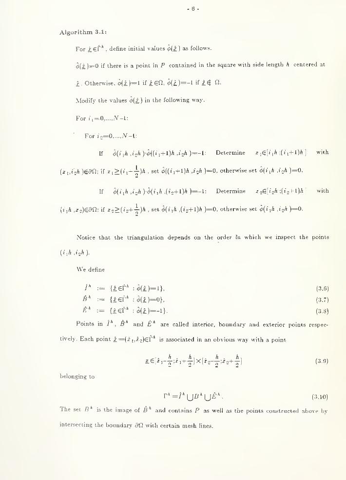
Algorithm 3.1:

For i ef* , define initial values 4>{i.) as follows.

0(f )=0 if there is a point in P contained in the square with side length h centered at

i. Otherwise, <^(i)=l if iefi. 0(1)=-! if 1^ ^

Modify the values 0(i) in the following way.

For ii=0,....iV-l:

For io=0 N-l:

If ^{iih ,inh)-^({i^+ l)h ,ir,h)=-l: Determine x ^€[1 ^h -,{1i+ l)h] with

{xi,i2h )edQ; if ii>(« i+-r)'« , set (^((ji+l)A ,ioA )=0, otherwise set 4>(i ih ,1-2^ )=0.

If .^(i,A ,ioA )<^(j,A ,(i2+l)A )=-l: Determine x^El^^h ,{i2+l)h] with

(«iA ,Z2)€5f2; if X2>(!2H )'» . set 4>(' ih ,(!2+l)A )=0, otherwise set 4>(i ih .'2^ )^0-

Notice that the triangulation depends on the order fn which we inspect the points

We define

/* := {ief :^(i)=l}, (3.6)

S* := {ief : 0(i)=O}, (3.7)

E' := {iet' :^(i)=-l}. (3.8)

Points in / , S and E are called interior, boundary and exterior points respec-

tively. Each point i={xi,X2)Er is associated in an obvious way with a point

^i. h.h, f. h.h, ,,,^e[^i-2-:^i+Tl^(^2-7'-'2+yJ (3.9)

belonging to

r*=/*|JB''|j£'V (3.10)

The set B is the image of B and contains P as well as the points constructed above by

intersecting the boundary dU with certain mesh Unes.

- 7 -

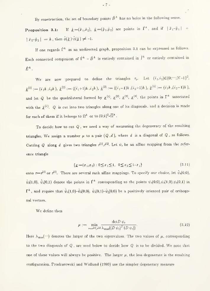
By construction, the set of boundary points B^ has no holes in the following sense.

Proposition 3.1: If x=(ii,i2), £=(^1.2/2) are points in f\ and if \x^-y\\ +

I

i2-y2I

= ^ .then 0(i )-^(i) 7^ -1-

If one regards f * as an undirected graph, proposition 3.1 can be expressed as follows.

Each connected component of f * - B* is entirely contained in /" or entirely contained in

We are now prepared to define the triangles r^. Let (« ,,!2)€{0;-;N-l} ,

id) := (^,h ,i.h ), i(=' := ((m + IJA ,..A ), i'" := {{' i+i)h ,(«o+l)A ), i'^' := (m^ ,(«2+1)/' ).

and let Q be the quadrilateral formed by i*", x.''', x'^', x'^', the points in T" associated

with the x'"'. Q is cut into two triangles along one of its diagonals, and a decision is made

for each of them if it belongs to fi* or to (0;l)--n .

To decide how to cut Q , we need a way of measuring the degeneracy of the resulting

triangles. We assign a number ^ to a pair (Q ,(/), where </ is a diagonal of Q ,as follows.

Cutting Q along d gives two triangles t^'',?*^'. Let t/>r be an affine mapping from the refer-

ence triangle

{x=(x,,X2) : 0<x,<l, 0<X2<1-Xi} (3.11)

onto 7-^r'' or r^"'. There are several such affine mappings. To specify our choice, let \p^0,0),

ip,{l,0), i'J,0,l) denote the points in f* corresponding to the points ipj{0,0),ipj^l,0),xt>j_0,l) in

r* , and require that T/'r(l,0)-V'^0,0), V'r(0,l)-)/'j{0,0) be a positively oriented pair of orthogo-

nal vectors.

fi := rain^^ ^ _ r'r. , ,x i^-^-)

We define then

detZ) i/v

Here Xm3j((-) denotes the larger of the two eigenvalues. The two values of /i, corresponding

to the two diagonals of Q , are used below to decide how Q is to be divided. We note that

one of these values will always be positive. The larger /i, the less degenerate is the resulting

configuration. Proskurowski and Widlund (1980) use the simpler degeneracy measure

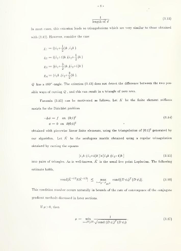
1 . (3.13)length of d

In most cases, this criterion leads to triangulations which are very similar to those obtained

with (3.12). However, consider the case

£3 = (('l + f)''-('2+l)M

3

Li = (uh -(«2+— )/> )

g has a 180" -angle. The criterion (3.13) does not detect the difference between the two pos-

sible ways of cutting Q , and this can result in a triangle of zero area.

Formula (3.12) can be motivated as follows. Let K be the finite element stiffness

matrix for the Dirichlet problem

-A4> = / on (0;1)2 (3.14)

<?i = on a(0;l)2

obtained with piecewise linear finite elements, using the triangulation of (0;1)^ generated by

our algorithm. Let K be the analogous matrix obtained using a regular triangulation

obtained by cutting the squares

[iihiii+l)h]x\ioh;{i2+l)h] (3.15)

into pairs of triangles. As is well-known, K is the usual five point Laplacian. The following

estimate holds,

cond[A'-'''2/vA'-'/^] < max cond[(£> i/v)^(^ Vv)l- (316)

This condition number occurs naturally in bounds of the rate of convergence of the conjugate

gradient methods discussed in later sections.

U fi>0, then

^l = min —;. (3.17)

r=r<",r<=) v/cond (D4'rf{Di',)

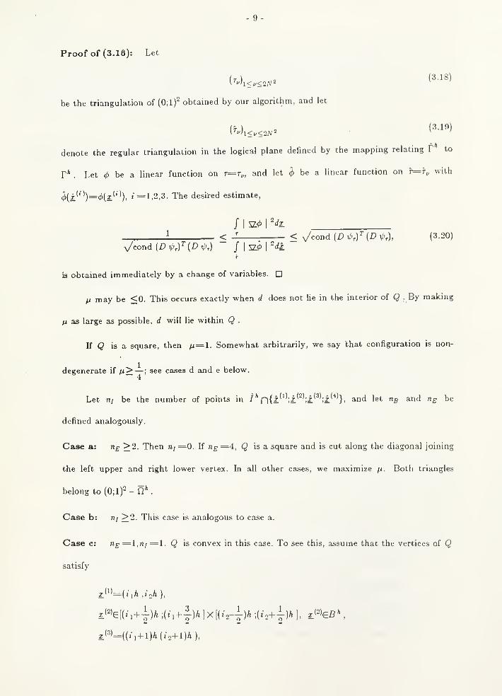
Proof of (3.16): Let

It) > (3-18)

be the triangulation of (0;1)- obtained by our algorithm, and let

It) o (3.19)

denote the regular triangulation in the logical plane defined by the mapping relating T to

r* . Let be a linear function on r=r„, and let ^ be a linear function on r=r„ with

^(i('))=0(^('))^ 2=1,2,3. The desired estimate,

/ IS.0 I

"dx.

< : < x/cond {D i'^f (D Vv), (320)

f

is obtained immediately by a change of variables. D

fx may be <0. This occurs exactly when d does not he in the interior of Q By making

fi as large as possible, d will lie within Q .

U Q is a square, then n=l. Somewhat arbitrarily, we say that configuration is non-

degenerate if /i> — ; see cases d and e below.

Let nj be the number of points in /* n{i''';i''^'''i'^';i.'^'}. ^""^ '^"^ "s ^""^ "r t>e

defined analogously.

Case a: rig >2. Then n, ^0. If ng =4, Q is a square and is cut along the diagonal joining

the left upper and right lower vertex. In all other cases, we maximize fx. Both triangles

belong to (0;!)" - fi* .

Case b: nj >2. This case is analogous to case a.

Case c: rig ^l,ni ^l. Q is convex in this case. To see this, assume that the vertices of Q

satisfy

i(')=(,|/i ,/„/,),

^'''e[('.+|)A;('i+f)/«]x[(.-2-|)A;(«o+y)M. x'^s*,

x(^)= (('l +l)M'2+l)M-

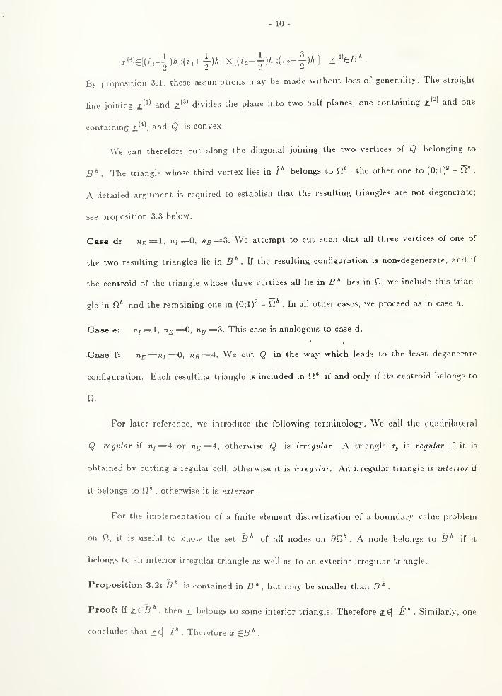
- 10 -

By proposition 3.1, these assumptions may be made without loss of generaUty. The straight

line joining z''* and z'^' divides the plane into two half planes, one containing j'-' and one

containing j'''', and Q is convex.

We can therefore cut along the diagonal joining the two vertices of Q belonging to

5*. The triangle whose third vertex lies in /* belongs to C* ,

the other one to (0:1)'^ - Q .

A detailed argument is required to establish that the resulting triangles are not degenerate;

see proposition 3.3 below.

Case d: n^^l, n, =0, 715=8. We attempt to cut such that all three vertices of one of

the two resulting triangles lie in 5*. If the resulting configuration is non-degenerate, and if

the centroid of the triangle whose three vertices all lie in 5* lies in Q, we include this trian-

gle in n* and the remaining one in (0;l)' - fi* . In all other cases, we proceed as in case a.

Case e: n; =1, n^ =0, ng ^3. This case is analogous to case d.

Case f: n^ =ni ^0, ng^-i- We cut Q in the way which leads to the least degenerate

configuration. Each resulting triangle is included in fi* if and only if its centroid belongs to

n.

For later reference, we introduce the following terminology. We call the quadrilateral

Q regular if n/ =4 or n^ ^4, otherwise Q is irregular. A triangle r^, is regular if it is

obtained by cutting a regular cell, otherwise it is irregular. An irregular triangle is interior if

it belongs to n* , otherwise it is exterior.

For the implementation of a finite element discretization of a boundary value problem

on n, it is useful to know the set B* of all nodes on dQ'' . A node belongs to B ^if it

belongs to an interior irregular triangle as well as to an exterior irregular triangle.

Proposition 3.2: S * is contained in B* , but may be smaller than S* .

Proof: If x_eD, then i belongs to some interior triangle. Therefore i^ £"*

. Similarly, one

concludes that i^ ^^ Therefore i gB* .

- 11 -

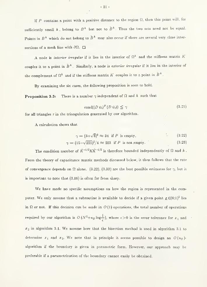
If P contains a point with a positive distance to the region fi, then this point will, for

sufficiently small h , belong to S* but not to S* . Thus the two sets need not be equal.

Points in S* which do not belong to B * may also occur if there are several very close inter-

sections of a mesh line with 50. D

A node is interior irregular if it lies in the interior of Q* and the stiffness matrix K

couples it to a point in fi* . Similarly, a node is exterior irregular if it lies in the interior of

the complement of fi* and if the stiffness matrix K couples it to a point in B .

By examining the six cases, the following proposition is seen to hold.

Proposition 3.3: There is a number 7 independent of Q and h such that

cond((D Af {D A)) < 1 (3-21)

for all triangles t in the triangulation generated by our algorithm.

A calculation shows that

^ = (3+v/8)2 « 34 if P is empty, '- (3.22)

1 = (15+7221)2/4 ~ 223 if P is not empty. ' (3.23)

The condition number of K'^^^'KK'^^'^ is therefore bounded independently of Q and h .

From the theory of capacitance matrix methods discussed below, it then follows that the rate

of convergence depends on Cl alone. (3.22), (3.33) are the best possible estimates for 7, but it

is important to note that (3.16) is often far from sharp.

We have made no specific assumptions on how the region is represented in the com-

puter. We only assume that a subroutine is available to decide if a given point x €(0;1)" lies

in n or not. If this decision can be made in O (1) operations, the total number of operations

required by our algorithm is O {N"+ng\o^— ), where €>0 is the error tolerance for x, and

X2 in algorithm 3.1. We assume here that the bisection method is used in algorithm 3.1 to

determine Xi and X2- We note that in principle it seems possible to design an Olng)-

algorithm if the boundary is given in parametric form. However, our approach may be

preferable if a parametrization of the boundary cannot easily be obtained.

12-

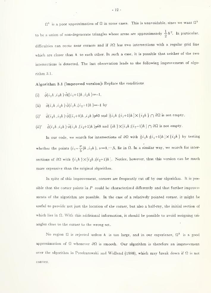
n* is a poor approximation of Q in some cases. This is unavoidable, since we want Q

to be a union of non-degenerate triangles whose areas are approximately —h'. In particular,

difficulties can occur near corners and if dQ has two intersections with a regular grid line

which are closer than h to each other. In such a case, it is possible that neither of the two

intersections is detected. The last observation leads to the following improvement of algo-

rithm 3.1.

Algorithm 3.1 (improved version): Replace the conditions

(1) 0(j,/! ,inh y^{{ii+l)h ,inh )=-l,

(ii) ^{jiA .j'sA ykuli ,('2+1)/' )=-l by

(i)' ^iih ,i.hyk(ii+ l)h ,ioh)f^O and [{i ^h ;(j i+ l)A] X {j'oA } fl 50 is not empty,

(ii)' ct){iih ,t.h y4>(iih ,(^2+i-)h )7^0 and {ih }x[iih ;(j2+1)'' ] fl oifi is not empty.

In our code, we search for intersections of dQ with [(jjA ;{{ i+ l)h jXJziA } by testing

whether the points (« i+— )A .J^A ), 1^=1, 'j5, lie in O. In a similar way, we search for inter-

5

sections of dQ with {i ^h }x[tnh ;(«2+l)/i]. Notice, however, that this version can be much

more expensive than the original algorithm.

In spite of this improvement, corners are frequently cut off by our algorithm. It is pos-

sible that the corner points in P could be characterized differently and that further improve-

ments of the algorithm are possible. In the case of a relatively pointed corner, it- might be

useful to provide not just the location of the corner, but also a half-ray, the initial section of

which lies in Q. With this additional information, it should be possible to avoid assigning tri-

angles close to the corner to the wrong set.

No region CI is rejected unless h is too large, and in our experience, fi* is a good

approximation of Q whenever dCl is smooth. Our algorithm is therefore an improvement

over the algorithm in Proskurowski and Widlund (1980), which may break down if Q is not

convex.

- 13-

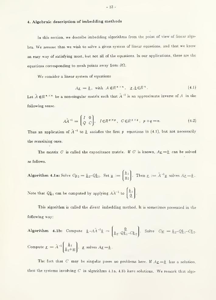
4. Algebraic description of imbedding methods

In this section, we describe imbedding algorithnis from the point of view of Unear alge-

bra. We assume that we wish to solve a given system of linear equations, and that we know

an easy way of satisfying most, but not all of the equations. In our applications, these are the

equations corresponding to mesh points away from dQ.

We consider a linear system of equations

Ax = b_, with AeR"-", x,ie/?v (4.1)

Let A ER" ^" be a non-singular matrix such that A'^ is an approximate inverse of A in the

following sense.

aA-'= g^, leR''", CeR''" , P+q=n. (4.2)

Thus an application of A"' to 6. satisfies the first p equations in (4.1), but not necessarily

the remaining ones.

The matrix C is called the capacitance matrix. If C is known, Ax_= b_ can be solved

as follows.

Algorithm 4.1a: Solve C^o = b_2-Qb_i- Set a1.

y.2Then x :== .4 a solves Ax_= b_.

Note that Qb_i can be computed by applying AA ' to

This algorithm is called the direct imbedding method. It is sometimes presented in the

following way:

Algorithm 4.1b: Compute 6. -.4^4 '6. Solve Cw = b_2''Qi.[-Cb_n.

Compute x_ = A ^ii

bn+W X solves Ax =6

The fact that C may be singular poses no problems here. If Ax_= b_ has a solution,

then the systems involving C in algorithms 4.1a, 4.1b have solutions. We remark that algo-

- 14-

rithm 4.1a is slightly more efficient than algorithm 4.1b.

The direct imbedding method can be an efficient technique if g «p and if a sequence

of problems Ax_=b_ with different right-hand sides b_ is to be solved.

Next we describe iterative imbedding methods. Here the system involving the matrix

C is solved iteratively. For this purpose, we use the conjugate gradient algorithm, written in

the following form.

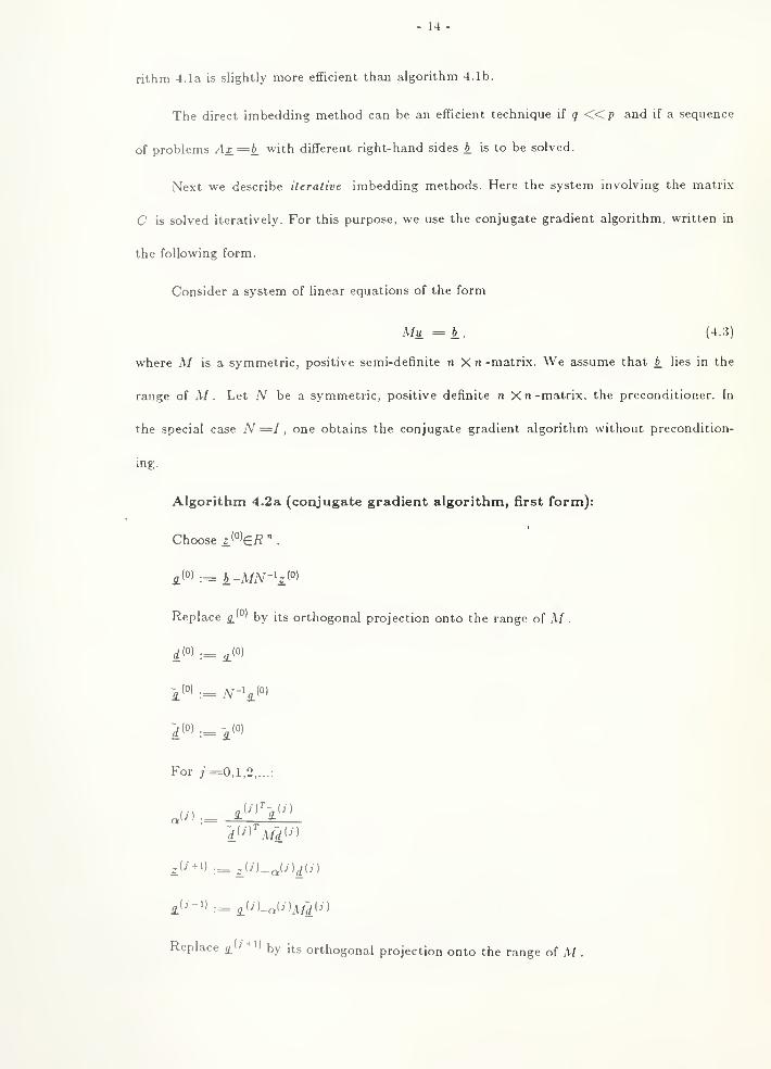
Consider a system of linear equations of the form

Mu = b_. (4.3)

where M is a symmetric, positive semi-definite n X n -matrix. We assume that b_ lies in the

range of M . Let N he a, symmetric, positive definite n Xn -matrix, the preconditioner. In

the special case N =1 , one obtains the conjugate gradient algorithm without precondition-

ing.

Algorithm 4.2a (conjugate gradient algorithm, first form):

Choose 2 '°'e/? " .

^(0) := 6.-A//V-'i.'°)

Replace <j.'°' by its orthogonal projection onto the range of A/

.

i"" := 7V-i<z.<°'

rf(°' := i(°)

For; =0,1,2,...:

Replace £''+'> by its orthogonal projection onto the range of M

.

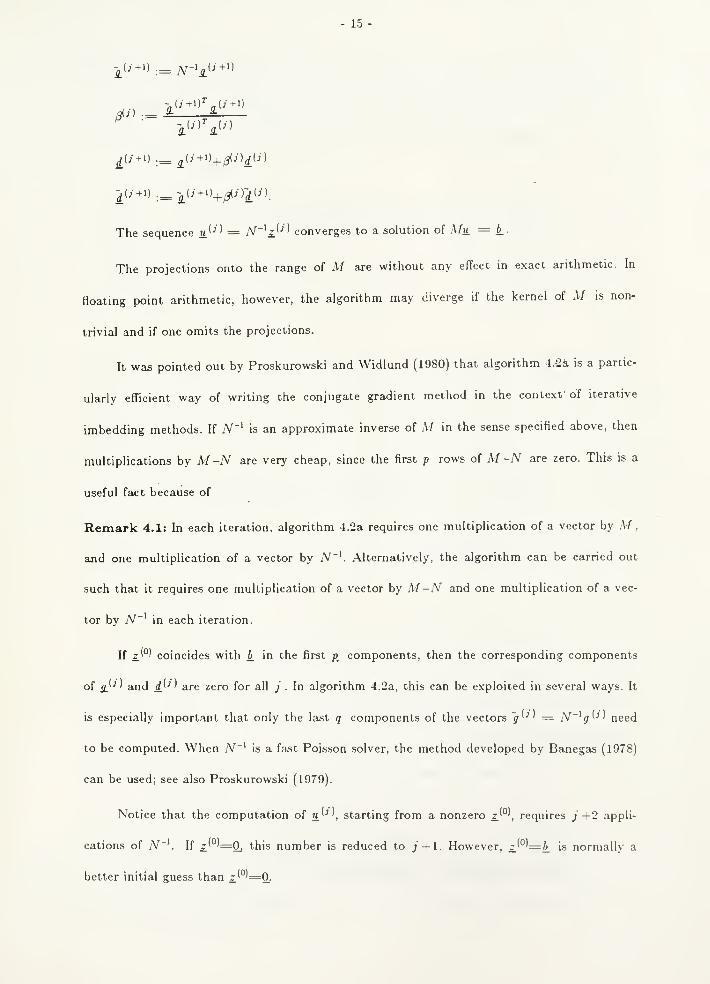
- 15 -

The sequence u '•'' = N~^z}^ ' converges to a solution of A/u = b_-

The projections onto the range of M are without any effect in exact arithmetic. In

floating point arithmetic, however, the algorithm may diverge if the kernel of M is non-

trivial and if one omits the projections.

It was pointed out by Proskurowski and Widlund (1980) that algorithm 4.2i is a partic-

ularly efficient way of writing the conjugate gradient method in the context of iterative

imbedding methods. If jV"' is an approximate inverse of M in the sense specified above, then

multiplications by M-N are very cheap, since the first p rows of M -N are zero. This is a

useful fact because of

Remark 4.1: In each iteration, algorithm 4.2a requires one multiplication of a vector by M,

and one multiplication of a vector by N'^. Alternatively, the algorithm can be carried out

such that it requires one multiplication of a vector by M-N and one multiplication of a vec-

tor by A'^"' in each iteration.

If z.'°' coincides with b_ in the first p. components, then the corresponding components

of g}^ ' and rf'-' ' are zero for all j . In algorithm 4.2a, this can be exploited in several ways. It

is especially important that only the last q components of the vectors ~g^^' = N'^g''^' need

to be computed. When A'^"' is a fast Poisson solver, the method developed by Banegas (1978)

can be used; see also Proskurowski (1979).

Notice that the computation of u''' , starting from a nonzero 5.'°', requires j +2 appli-

cations of N'^. If i'°—0, this number is reduced to j +1. However, ±}°^=b_ is normally a

better initial guess than i.'°'=0.

- 16-

For later reference, we also state the second commonly used form of the algorithm.

Algorithm 4.2b (conjugate gradient algorithm, second form):

Choose u'^'efl".

Replace (z.'°' by its orthogonal projection onto the range of M

.

1(0) ,^ -^(0)

For y =0,1,2,...:

Replace ij.'-'"^'^ by its orthogonal projection onto the range of M

.

The sequence ?t converges to a solution of A/u = 6..

Notice that the vectors </'•'' are not needed here. One easily sees that the two algo-

rithms are equivalent. Here the computation of u '•'', starting with any u.'°', requires only j

applications of A'^"'.

We now consider using the conjugate gradient method for the equation

Ca.2 = Aa-Qii-

The difficulty is that C is virtually never symmetric and positive definite with respect to the

euclidean inner product. To see this, note that C is a principal minor of .AA~\ which is

non-symmetric in general even if A and .4 are symmetric and positive definite. However, C

- 17 -

is often symmetric and positive definite with respect to an appropriately chosen inner pro-

duct. We shall now demonstrate this fact and show how to exploit it. We note that a similar

result holds in the continuous case; see Proskurowski and Widlund (1980).

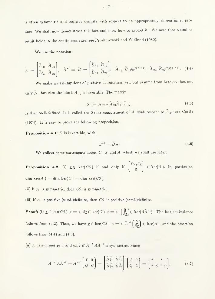
We use the notation

A =An A 12

A 21 A 22

A"' =: S =•fill -^12

, A,„B,,eR'''' ,A22, 522ei?'^'. (4.4)

We make no assumptions of positive definiteness yet, but assume from here on that not

only A , but also the block A u is invertible. The matrix

S := A 22 - A 21A h'A ,2, (4-5)

is then well-defined. It is called the Schur complement of A with respect to An; see Cottle

(1974). It is easy to prove the following proposition.

Proposition 4.1: 5 is invertible, with

S = 522-

We collect some statements about C , S and A which we shall use later:

(4.6)

B 12'SkjProposition 4.2: (i) xS ker(C5) if and only if |

" '^"'*| € ker(A ). In particular,

dim ker(A )= dim ker(C) = dim ker( C5 ).

(ii) If A is symmetric, then CS is symmetric.

(iii) If A is positive (semi-)definite, then CS is positive (semi-)definite.

Proof: (i) xG ker( CS) <= > SiG ker(C) <= > f|;.]e ker(AA"'). The last equivalence

follows from (4.2). Thus, we have xG ker( C5) <= > A~'j ^T 1 € ker(A ), and the assertion

follows from (4.4) and (4.6).

(ii) A is symmetric if and only if A" AA~^ is symmetric. Since

A-'^ AA-^ = A-I

Q C^11 -^21

£5J 2 tj nn

I

Q C S'^C (4.7)

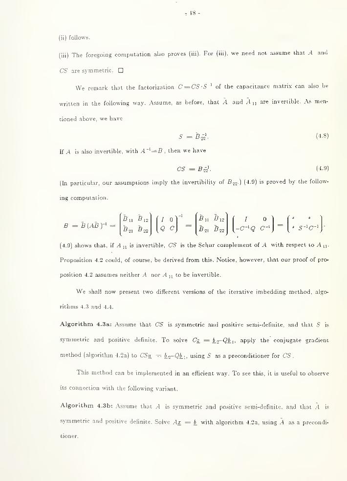
- 18-

(ii) follows.

(iii) The foregoing computation also proves (iii). For (iii), we need not assume that .4 and

CS are symmetric. D

We remark that the factorization C^CS-S'"^ of the capacitance matrix can also be

written in the following way. Assume, as before, that A and An are invertible. .\s men-

tioned above, we have

5 = Soo'. (4.8)

If A is also invertible, with ,4''=B ,then we have

CS = B^\ (4.9)

(In particular, our assumptions imply the invertibility of Soo.) (4.9) is proved by the follow-

ing computation.

B = B (AB )-' =B ny B 22

. 1

/

Q c

B II B 12

B 21 B 22

(4.9) shows that, if A n is invertible, CS is the Schur complement of A with respect to A n-

Proposition 4.2 could, of course, be derived from this. Notice, however, that our proof of pro-

position 4.2 assumes neither A nor .4 n to be invertible.

We shall now present two different versions of the iterative imbedding method, algo-

rithms 4.3 and 4.4.

Algorithm 4.3a: Assume that CS is symmetric and positive semi-definite, and that 5 is

symmetric and positive definite. To solve Cz_ = b_2-Qh.\, apply the conjugate gradient

method (algorithm 4.2a) to CSu = io-Qib using 5 as a preconditioner for CS .

This method can be implemented in an efficient way. To see this, it is useful to observe

its connection with the following variant.

Algorithm 4.3b: Assume that A is symmetric and positive semi-definite, and that A is

symmetric and positive definite. Solve Ax_ = b_ with algorithm 4.2a. using A as a precondi-

tioner.

- 19 -

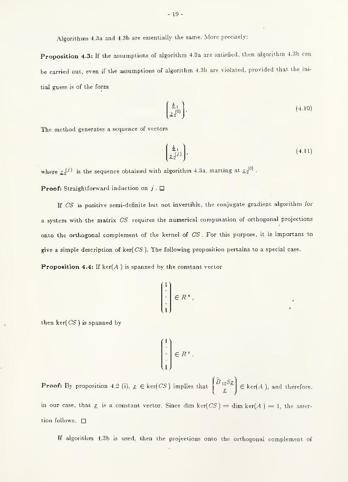
Algorithms 4.3a and 4.3b are essentially the same. More precisely:

Proposition 4.3: If the assumptions of algorithm 4.3a are satisfied, then algorithm 4.3b can

be carried out, even if the assumptions of algorithm 4.3b are violated, provided that the mi-

tial guess is of the form

The method generates a sequence of vectors

(4.10)

(4.11)

where 1.2'•'

' is the sequence obtained with algorithm 4.3a, starting at 2.J,(0)

Proof: Straightforward induction on y . D

If CS is positive semi-definite but not invertible, the conjugate gradient algorithm for

a system with the matrix CS requires the numerical computation of orthogonal projections

onto the orthogonal complement of the kernel of CS . For this purpose, it is important to

give a simple description of ker( C5 ). The following proposition pertains to a special case.

Proposition 4.4: If ker(A ) is spanned by the constant vector

€ R\

then ker(C5 ) is spanned by

U

ER'

Proof: By proposition 4.2 (i), j G ker(C5') implies that3 [oSx_

€ ker(.4 ), and therefore,

in our case, that x is a constant vector. Since dim ker( C5) = dim ker(.4 )= 1, the asser-

tion follows, n

If algorithm 4.3b is used, then the projections onto the orthogonal complement of

- 20-

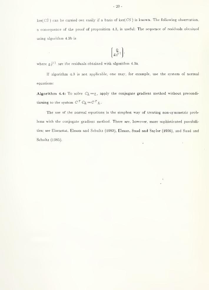
ker(C'5) can be carried out easily if a basis of ker( C'5 ) is known. The following observation,

a consequence of the proof of proposition 4.3, is useful: The sequence of residuals obtained

using algorithm 4.3b is

where g_j' ' are the residuals obtained with algorithm 4.3a.

If algorithm 4.3 is not applicable, one may, for example, use the system of normal

equations:

Algorithm 4.4: To solve Cz_^r_, apply the conjugate gradient method without precondi-

tioning to the system C Cz_^=C l.

The use of the normal equations is the simplest way of treating non-symmetric prob-

lems with the conjugate gradient method. There are, however, more sophisticated possibili-

ties; see Eisenstat, Elman and Schultz (1983), Elman, Saad and Saylor (1986), and Saad and

Schultz (1985).

- 21 -

5. Neumann problems

5.1. Description of the algorithms

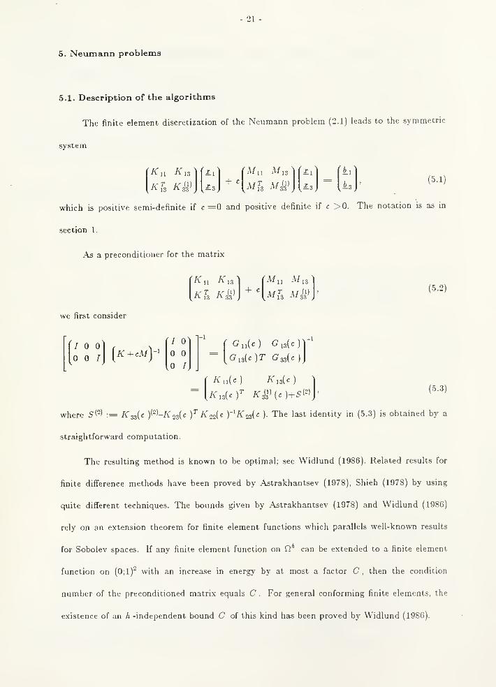
The finite element discretization of the Neumann problem (2.1) leads to the symmetric

system

•^13 -^33 Li

'A/ii Mis'

^fL Mis" i3

(b

(5.1)

which is positive semi-definite if c =0 and positive definite if c >0. The notation is as in

section 1.

.\s a preconditioner for the matrix

Kn A'i3^ (Mu Mi3(5.2)

we first consider

(o /)(^+'^^^)-'

/ 01

/

-1

r G„(e) G,3(or'

(5.3)

( KJc) K,s(c)

where S'=' := AT 33(0 )'-'-/v23(c )^ ^ 22{<: )"'^23(<; )• The last identity in (5.3) is obtained by a

straightforward computation.

The resulting method is known to be optimal; see Widlund (1986). Related results for

finite difference methods have been proved by Astrakhantsev (1978), Shieh (1978) by using

quite different techniques. The bounds given by Astrakhantsev (1978) and Widlund (1986)

rely on an extension theorem for finite element functions which parallels well-known results

for Sobolev spaces. If any finite element function on 17 can be extended to a finite element

function on (0;1)^ with an increase in energy by at most a factor C, then the condition

number of the preconditioned matrix equals C . For general conforming finite elements, the

existence of an h -independent bound C of this kind hzis been proved by Widlund (1986).

- 22 -

Because of the triangles near dQ, M does not have the same stencil everywhere, and

K +cM cannot be inverted using a fast solver on (0;1)". In (5.3), we therefore replace this

matrix by a more convenient spectrally equivalent matrix. A first possibility is

K + ch-I. (5.4)

As in section 3, K is the matrix defined in the same way as A' , but on the regular triangula-

tion('•^)i<^<2jv2;

se^ (319)-

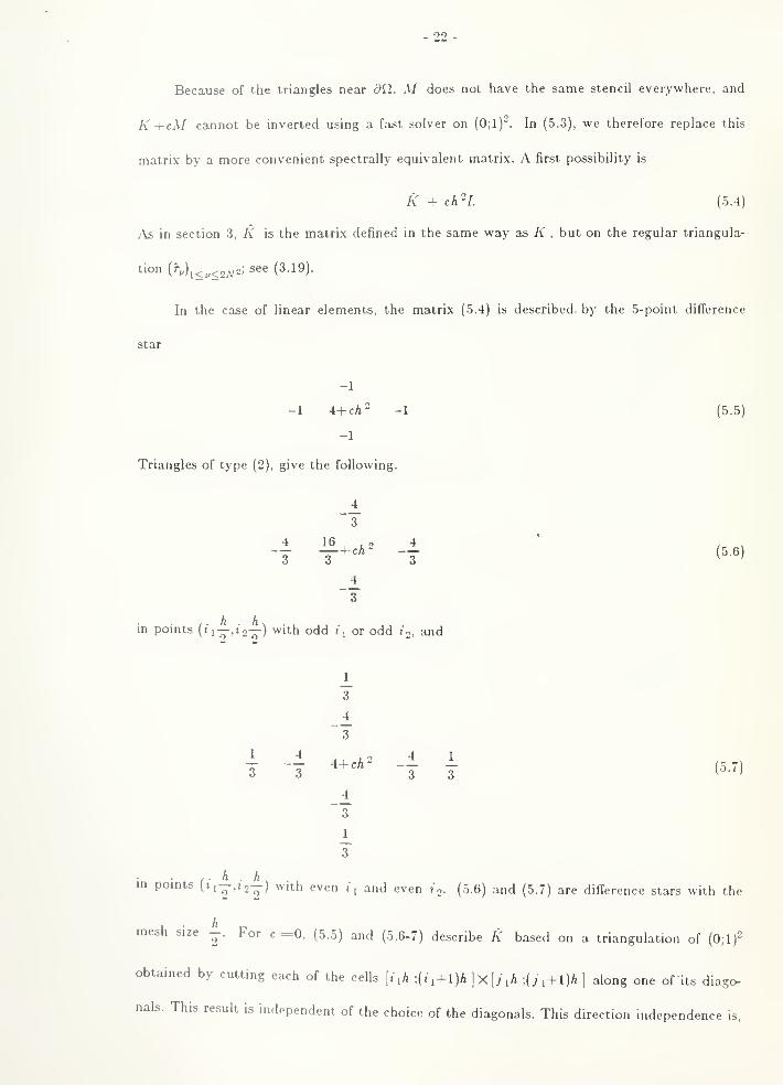
In the case of linear elements, the matrix (5.4) is described, by the 5-point difference

star

(5.5)

23

however, accidental. For triangles of type (3), the direction in which the cells are cut will

effect the stencils.

As an alternative to (5.6-7) we could also use the operator (5.5) on the grid T - as a.

preconditioner in the case of quadratic elements. It can easily be shown that (5.5) and (5.6-7)

are spectrally equivalent operators, by comparing the corresponding quadratic forms, element

by element.

In addition to (5.5) or (5.6-7), we must specify boundary conditions for j: i=0, Xi= l,

X2=0, J 2=1. They should be chosen such that the resulting discrete Helmholtz problems can

be treated by a fast solver. The choice of the boundary conditions on 5(0;1)- will be dis-

cussed further in section 5.2.

We report now on numerical experiments illustrating the performance of several

different versions of the method for the following test regions; compare Figures 1-6.

{(x„Zo) : [(z,-0.5)2+(x2-0.5)2]'/2 < 0.4} (5.8)

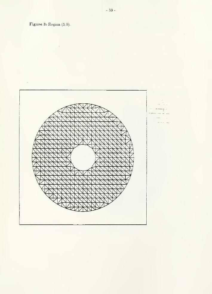
{(xi,X2) : [(x,-0.5)V(x2-0.5)Y/' E (0.1;0.4)} (5.9)

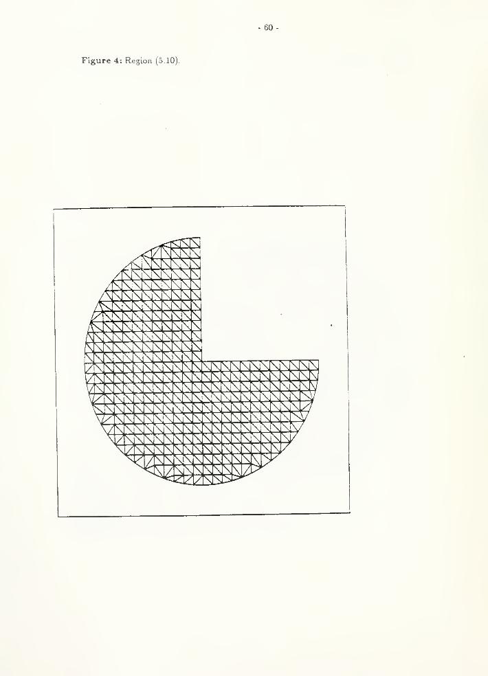
{(xi,Xn):[{xi-0.5f+(x2-O.5fY^^<0A, ii<0.5 or Z2<0.5} (5,10)

(0.2;0.8)* (5.11)

(0.2;0.8)- - [0.475;0.525]X[0.2;0.5] (5.12)

5.2. The choice of boundary conditions for the auxiliary Helmholtz problems

We shall present numerical comparisons of the following boundary conditions on

a(0;l)2:

(i) Periodicity conditions at Xi=0, Xi^l and homogeneous Dirichlet conditions at X2=0.

X2=l.

(ii) Homogeneous Dirichlet conditions on the entire boundary 5(0;1)^.

- 24 -

(iii) Homogeneous Neumann conditions on the entire boundary 9(0;1)-.

The condition number of the preconditioned matrix is minimized when homogeneous

Neumann boundary conditions are chosen, since the minimum energy extension to (O;l)-of a

finite element function on fi* satisfies, in the discrete sense, homogeneous Neumann boun-

dary conditions on d(0;lf. If the constant c in eq. (2.1) is zero, the solution of the auxiliary

problem is unique only up to an additive constant. We then require the solution to have

zero average in fi .

We use algorithm 2.2a and count the number of calls to the fast solver on (9(0il)-

required to reduce the euclidean norm of the residual by a factor < 10"^ Here the word resi-

dual refers to the quantity which is denoted by g_ in algorithm 2.2a. In the notation of algo-

rithm 2.2a, the initial approximation z_o is taken to be the right-hand side A.. One could also

use 2.0=0. The resulting condition number estimates are equal to those obtained with r.o=ft.

,

but the number of iterations needed to reach the desired accuracy is often by 1 or 2 larger.

We apply the method to the problem

-Au +CU = const. + sin(xi4-X2) on Cl (513)

-?^ = on an, (5.14)on

where the constant is chosen such that the discrete compatibility condition is satisfied.

Some nunjerical results for c =0, using linear elements, are shown in Table I. Note

that the number of calls to the fast solver is the number of iterations plus two. Our results

confirm that Neumann conditions on 517 are the best choice, but also suggest that the choice

of boundary conditions on 5(0;1)" is of no great importance.

5.3. The choice of the discrete Helmholtz operator in the case of quadratic ele-

ments

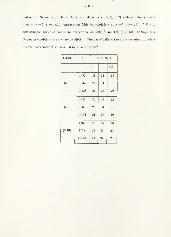
Table II shows results analogous to those in Table I, but using piecewise quadratic ele-

ments. We use (i) (5.6-7) with periodicity conditions in the a:,-direction and homogeneous

25-

Dirichlet conditions in the jo-direction, (ii) (5.5) with mesh width — and homogeneous Neu-

mann conditions on ^(O;!)^, and (iii) (5.5) with mesh width — and homogeneous Dirichlet

conditions on 3(0;1)^. We conclude that the use of (5.5) instead of (5.6-7) leads to a slight

increase in the number of calls to the fast solver. (5.5) may, however, be preferable, since the

implementation of a fast solver is more difficult for (5.6-7) than for (5.5).

We briefly indicate a way of constructing an FFT-based fast solver for problems involv-

ing the operator (5.6-7). We confine ourselves to the case of periodicity conditions at Xi=0,

Zi= l and homogeneous Dirichlet conditions at io=0, io=l, and assume that iV is even.

Any grid function u * (j i,jo) on

{ix„X2)=(ix-^.i2j)-0<i,<2N-l, l<i2<2N-l} (5.15)

has a unique expansion of the form

a*(x„Xo) =

-i-Ao(x2) + Y]^k{x2)<:os(2nkxi)+Y]B,{x2)sin(^^'^Xi)+^Ap,(xn)cos{2KNx,). (5.16)

Using the Fast Fourier Transform, such expansions can be computed and evaluated in

O [N'^logN ) operations.

To develop a fast solver for (5.6-7) based on (5.16), we must consider the result

'* ('^11^2) of applying (5.6-7) to a function of the form (5.16). r* (^1,12) ^^ the expansion

r'{xuX2) =I

N-l N-l .

-Co(x2) + T, Ck{x2)cos{27rkXi)+J^Di,(xn)sm{27:kxi)+-CN{x2)cos{2KNxi). (5.17)"^ *=i k=i ^

A straightforward computation shows that the coefficient C^{x2\, for a fixed index k and a

given Xo, depends only ou. A^.[y] and .4^/ [\j ), where

V = N-k (5.18)

andI

y-X2|<2h . Similarly, /^^(jro) depends only on Bi, {y ) and 5^- {y ). The derivation

of these results, and of the systems of linear equations which describe the relations between

Ak , Bk , C). and D). , use the formulae

- 26-

cos(27ryt' i^) = cos(2nki—) Hi is even, (5.19)

cos(27rA-' t^) = -cos(2nki^) ifi is odd, (5.20)

and similar formulae for the sine.

For each pair (k ,k' ), one obtains a system of linear equations relating the .4^ ,.4^- to

the Ck,Ci,> , and a system relating the B), ,5^' to the D^ ,!>*' . These systems are block pen-

tadiagonal, with blocks of size 2X2. Within the nonzero blocks, there is considerable addi-

tional sparsity.

An different solver can be derived as follows. Consider the four variables associated

with the pomts (2.-.A 2z,A), ^[Oi,+ l]^r~i2^), (2m|,(2^'2-1)|). ((2/,+l)|.(2.c-l)|) as a

four-vector-valued variable. Then the operator (5.6-7) is a five-point operator, operating on

four-vector-valued grid functions. We can then use the Fast Fourier Transform with respect

to one variable to reduce the linear system to block tridiagonal systems, with blocks of size

4X4. Alternatively, if the problem is doubly periodic on [0;lp, then the Fast Fourier

Transform with respect to both variables can be used. This results in N~ 4X4 linear systems

of equations. We note that this systematic technique has been used by Bjprstad and Widlund

(1981) to develop a fast solver for a conforming finite element approximation of the bihar-

monic equation on regular hexagonal meshes.

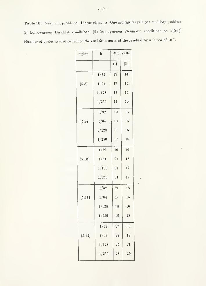
5.4. Inexact solution of the auxiliary problems on the square

Instead of using a direct fast solver, one can attempt to use an approximate solver to

increase the efficiency of the method. We use (5.5) with homogeneous Dirichlet conditions on

5(0;1) . As an approximate solver, we use a multigrid cycle constructed such that the

effective preconditioner is symmetric and positive definite and is spectrally equivalent with

the exact preconditioner. A cycle satisfying these conditions can easily be found. We use a

V-cycle (see Stiiben and Trottenberg (1982)), with red-black Gauss-Seidel sweeps arranged in

a symmetric way relative to the coarse grid correction step. The total amount of work

- 27 -

required for the cycle corresponds to 5-6 Gauss-Seidel iteration steps. Results with this

method are shown in Table III.

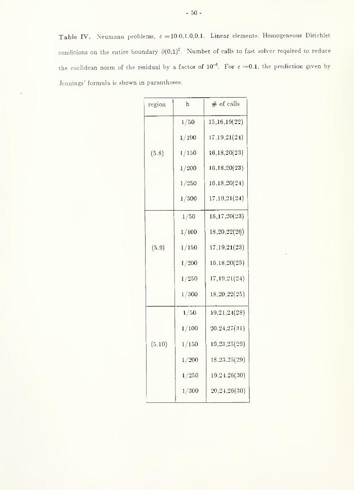
5.5. The case c >0

If n, h and f ,g are fixed, the number of iterations required to reduce the residual by

a prescribed factor increases as c —0, and it is significantly larger for c >0, c «0 than for

c =0. This fact will prove useful in the following section, where exterior Neumann problems

for the Helmholtz equation will be used as auxiliary problems in a Dirichlet solver.

If c =0, then G [e f^^K (c )G (c )'/' is uniformly well-conditioned in the sense that the

quotient of the largest and the smallest nonzero eigenvalue is bounded uniformly in h .

Notice, however, that G (e y^"K {c )G (c Y^'^ has a simple zero eigenvalue. If c >0, c ~0,

then the condition number of G (c )'/-/! (c )G [c )'/" is large, by the continuity of the eigen-

values. There is only one outlying eigenvalue, namely one near 0. For the conjugate gradient

method, a small outlying eigenvalue is more harmful than a large one; see Jennings (1977).

•Denote the eigenvalues of G {c Y^^K {c )G {c Y^^ by 0<X, <X2<-- <X„ . Following Jen-

nings, the number of conjugate gradient iterations needed to achieve a fixed accuracy e may

increase by at most

in comparison with the case of c ^0. This estimate is independent of e.

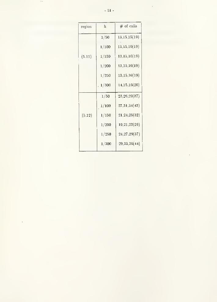
Table IV contains results with c >0. For c ^0.1, the table also contains the prediction

based on Jennings' formula (5.21), i.e. the (rounded) sum of (5.21) and the number of calls to

the fast solver needed for c =0. The results show that (5.21) is a good, even though not

quite sharp, prediction of the true behaviour.

- 28 -

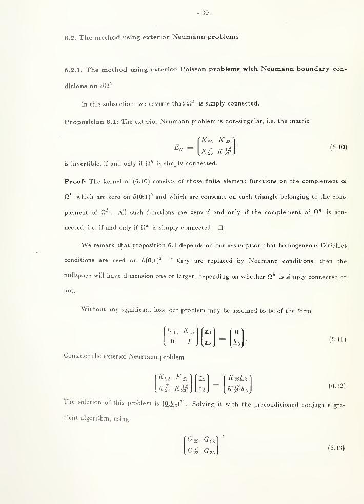
6. Dirichlet problems on grid-aligned regions

In this section, we assume that all boundary nodes lie on the regular grid. For regions

which are not grid-aligned, additional considerations are needed; see section 7. We shall res-

trict our discussion to the case c =0, i.e. to the Poisson equation. This is, in a certain

respect, the hardest case, since the difficulty with a related Neumann problem described in

section 6.2.1 and resolved in section 6.2.2 does not occur if c >0 or if the Neumann problem

otherwise is known to be non-singular. We only use homogeneous Dirichlet boundary condi-

tions on 5(0;!)^ in this section.

6.1. A non-optimal method

The simplest approach to the Dirichlet problem is to treat it as if it were a Neumann

problem, i.e. to solve a problem of the form

A'ii2.i = ii • (6.1)

using the conjugate gradient method with the preconditioner G fi . This method is non-

optimal, i.e. the condition number of the preconditioned matrix is not bounded as h —>-0, but

grows like 0(-— ). To see this, we consider, without loss of generality, the Dirichlet problema

on a region enlarged by one layer of mesh points, i.e. the problem described by

(6.2)

^11 ^13

13 '^ 33A'T. K

We use the preconditioner

1

(6.3)

Cii '^ \z

^ \Z '-'33,

As is shown in section 5, (6.3) is spectrally equivalent with

We can therefore compare (6.4) with (6.2). The generalized Rayleigh quotient can be written

as

- 29

is is+ xiK:^^x_s

'A'u /vis"

yvfs A'ii' is

Our problem can easily be reduced to one of the form

KiiXi + A' isis = 0.

The Rayleigh quotient then takes the form

(6.5)

1 +is AT 3*3 is

is^'^^'is

(6.6)

(6.71

where

S(" = A-3'3" -ATsA'fi'A^s. (6.8)

It can easily be shown that K ^' is diagonally dominant and that all its eigenvalues

are in a fixed interval bounded away from zero. 5''', on the other hand, has some eigenvalues

on the order of h . Therefore the condition number grows linearly with —

.

n

. Nevertheless, our experiments have lead to the conclusion that the method is more

efficient than one might expect. Unlike the methods of sections 6.2 and 6.3, it requires no

modifications on regions which are not grid-aligned. In addition, it has the advantage of per-

mitting the incomplete solution of the auxiliary problems on (0;1)^, while the method of sec-

tion 6.2 requires the exact solution of those problems.

Table V shows some of our numerical results, using the grid-aligned L-shaped region

(0.2;0.8)2-[0.5;0.8]2 (6.9)

as well as regions (5.8), (5.9), which are not grid-aligned. The right-hand side is sin(ii+ i.i),

the boundary condition is homogeneous.

- 30-

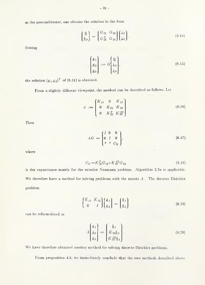
8.2. The method using exterior Neumann problems

6.2.1. The method using exterior Poisson problems with Neumann boundary con-

ditions on dC*

hi this subsection, we assume that Q'' is simply connected.

Proposition 6.1: The exterior Neumann problem is non-singular, i.e. the matrix

A 22 K 23

(6.10)

is invertible, if and only if fi* is simply connected.

Proof: The kernel of (6.10) consists of those finite element functions on the complement of

fi* which are zero on 5(0;1)^ and which are constant on each triangle belonging to the com-

plement of n* . All such functions are zero if and only if the complement of U is con-

nected, i.e. if and only if Cl is simply connected. D

We remark that proposition 6.1 depends on our assumption that homogeneous Dirichlet

conditions are used on 5(0;1)^. If they are replaced by Neumann conditions, then the

nullspace will have dimension one or larger, depending on whether 17* is simply connected or

not.

Without any significant loss, our problem may be assumed to be of the form

11 Kn) (li

!L3(6.11)

Consider the exterior Neumann problem

K 22 A 23

£.3 /vil'As(6.12)

The solution of this problem is [O^kzV . Solving it with the preconditioned conjugate gra-

dient algorithm, using

(j no Cj

23 G^33

22 ^23

(6.13)

31-

as the preconditioner, one obtains the solution in the form

'\ (Gnz G23^

(6.14)

Setting

^1

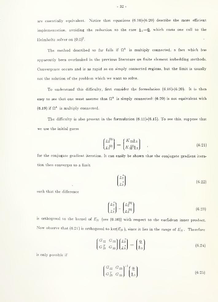
32

are essentially equivalent. Notice that equations (6.16)-(6.20) describe the more efficient

implementation, avoiding the reduction to the case 6.i=Q, which costs one call to the

Helmholtz solver on (0;!)'.

The method described so far fails if Q* is multiply connected, a fact which has

apparently been overlooked in the previous literature on finite element imbedding methods.

Convergence occurs and is as rapid as on simply connected regions, but the limit is usually

not the solution of the problem which we want to solve.

To understand this difficulty, first consider the formulation (6.16)-(6.20). It is then

easy to see that one must assume that f2* is simply connected: (6.20) is not equivalent with

(6.19) if Q* is multiply connected.

The difficulty is also present in the formulation (6.1l)-(6.15). To see this, suppose that

we use the initial guess

'j°t

k^i°'(6.21)

for the conjugate gradient iteration. It can easily be shown that the conjugate gradient itera-

tion then converges to a limit

^3(6.22)

such that the difference

i3 23'°' (6.23)

IS orthogonal to the kernel of E^ (see (6.10)) with respect to the euclidean inner product.

Now observe that (6.21) is orthogonal to ker(£'yv ), since it lies in the range of E^ Therefore

G'23

23 '-'33G o^-i G m (6.24)

is only possible if

'-'23 '^ 33(6.2.5)

- 33-

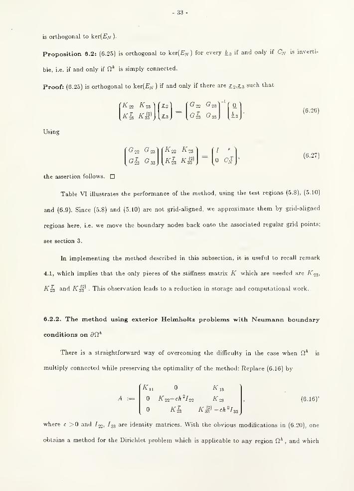
is orthogonal to ker(£'/\/ ).

Proposition 6.2: (6.25) is ortliogonal to ker(£';v ) for every is if and only if Cjv is inverti-

ble, i.e. if and only if fi* is simply connected.

Proof: (6.25) is orthogonal to ker(£'jv ) if and only if there are X2,£3 such that

/Y 22 *^ 23 X_2

S.3.

'22 '-'23

G 23 G' 33

(6.26)

Using

Goo G

:)(

/\no K'

G^z G^][Kl Kjl^ CJ''(6.27)

the assertion follows. Q

Table VI illustrates the performance of the method, using the test regions (5.8), (5.10)

and (6.9). Since (5.8) and (5.10) are not grid-aligned, we approximate them by grid-aligned

regions here, i.e. we move the boundary nodes back onto the associated regular grid points;

see section 3.

In implementing the method described in this subsection, it is useful to recall remark

4.1, which implies that the only pieces of the stiffness matrix K which are needed are /v23>

Kns and A'JI' . This observation leads to a reduction in storage and computational work.

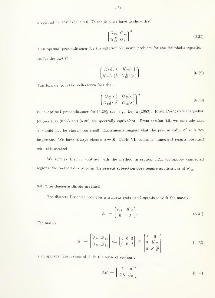
6.2.2. The method using exterior Helmholtz problems with Neumann boundary

conditions on 50*

There is a straightforward way of overcoming the difficulty in the case when fi* is

multiply connected while preserving the optimality of the method: Replace (6.16) by

(K

A :=

Kl3

Ko2+<:h'^l22 A' 23

Kl Kg^+ch-l3

(6.16)'

23 '^33 T-c" ^33J

where c >0 and /20, 733 are identity matrices. With the obvious modifications in (6.20), one

obtains a method for the Dirichlet problem which is applicable to any region Q*, and which

34

is optimal for any fixed c >0. To see this, we have to show that

. (6.28)

O 22 ^23

'23 'j 33

,

is an optimal preconditioner for the exterior Neumann problem for the Helmholtz equation,

i.e. for the matrix

/(roo(r ) Kns(c )

(6.29)

(6.30)

This follows from the well-known fact that

^22(0 Onjc)y'

is an optimal preconditioner for (6.29); see, e.g., Dryja (1983). From Poincare's inequality

follows that (6.28) and (6.30) are spectrally equivalent. From section 4.5, we conclude that

c should not be chosen too small. Experiments suggest that the precise value of c is not

important. We have always chosen c ^10. Table VII contains numerical results obtained

with this method.

We remark that in contrast with the method in section 6.2.1 for simply connected

regions, the method described in the present subsection does require applications of A' 22.

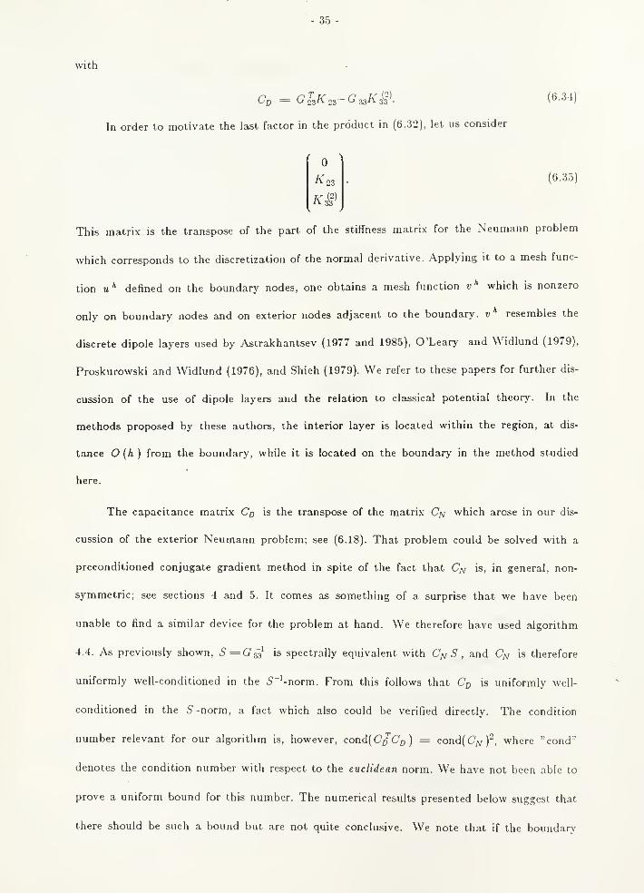
8.3. The discrete dipole method

The discrete Dirichlet problems is a linear systems of equations with the matrix

A :=A" 11 A' 13

(6.31)

The matrix

B^11 -Sis

5 31 -633

35

with

Co = Gl^K,^+G^Ki\ (6.34)

In order to motivate the Icist factor in the product in (6.32), let us consider

(6.35)

This matrix is the transpose of the part of the stiffness matrix for the Neumann problem

which corresponds to the discretization of the normal derivative. Applying it to a mesh func-

tion u * defined on the boundary nodes, one obtains a mesh function v * which is nonzero

only on boundary nodes sind on exterior nodes adjacent to the boundary, v * resembles the

discrete dipole layers used by Astrakhantsev (1977 and 1985), O'Leary and Widlund (1979),

Proskurowski and Widlund (1976), and Shieh (1979). We refer to these papers for further dis-

cussion of the use of dipole layers and the relation to classical potential theory. In the

methods proposed by these authors, the interior layer is located within the region, at dis-

tance O {h ) from the boundary, while it is located on the boundary in the method studied

here.

The capacitance matrix C^ is the transpose of the matrix C;v which arose in our dis-

cussion of the exterior Neumann problem; see (6.18). That problem could be solved with a

preconditioned conjugate gradient method in spite of the fact that Cyv is, in general, non-

symmetric; see sections 4 and 5. It comes as something of a surprise that we have been

unable to find a similar device for the problem at hand. We therefore have used algorithm

4.4. As previously shown, S=G^ is spectrally equivalent with Cyv? , and Cf^ is therefore

uniformly well-conditioned in the 5''-norm. From this follows that C^ is uniformly well-

conditioned in the 5 -norm, a fact which also could be verified directly. The condition

number relevant for our algorithm is, however, cond( C'/Cp) ^ cond(C;v)^, where "cond"

denotes the condition number with respect to the eucltdean norm. We have not been able to

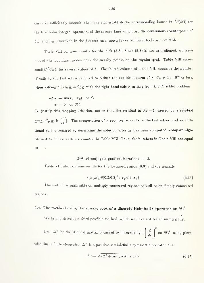
prove a uniform bound for this number. The numerical results presented below suggest that

there should be such a bound but are not quite conclusive. We note that if the boundary

- 36-

curve is sufficiently smooth, then one can establish the corresponding bound in L-(dQ) for

the Fredholm integral operators of the second kind which are the continuous counterparts of

Cn and Cp . However, in the discrete case, much fewer technical tools are available.

Table VIII contains results for the disk (5.8). Since (5.8) is not grid-aligned, we have

moved the boundary nodes onto the nearby points on the regular grid. Table VlII shows

cond( C/Cd ), for several values of h . The fourth column of Table VIII contains the number

of calls to the fast solver required to reduce the euclidean norm of r-C'o iH by 10'* or less,

when solving CjCc w=Cpr_ with the right-hand side r. arising from the Dirichlet problem

-Au = sin(xi-l-x2) on n

u ^ on dQ.

To justify this stopping criterion, notice that the residual in Ax_= b_ caused by a residual

Q^=ri~CQ u; isI

1 . The computation of r. requires two calls to the fast solver, and an addi-

tional call is required to determine the solution after w_ has been computed; compare algo-

rithm 4.1a. These calls are counted in Table VIII. Thus, the 'numbers in Table VTII are equal

to

2# of conjugate gradient iterations + 3.

Table VIII also contains results for the L-shaped region (6.9) and the triangle

{(jri,j:o)e(0.2;0.8)2 : X2<l-Xi}. (6.36)

The method is applicable on multiply connected regions as well as on simply connected

regions.

6.4. The method using the square root of a discrete Helmholtz operator on SC*

We briefly describe a third possible method, which we have not tested numerically.

Let -A be the stiffness matrix obtained by discretizing - J_(is

on dn using piece-

wise hnear finite elements. -A* is a positive semi-definite symmetric operator. Set

/ := V-A* +chl , with c >0. (6.37)

37

The discrete Dirichlet problem can be written in the form

A' 11 A' 13

/ is

i,

/is

If one uses the matrix

as an approximate inverse of

<J 13 ^33

A a A' 13

J

then one obtains the capacitance matrix

C = JG 33-

(6.38)

(6.39)

(6.40)

(6.41)

Algorithm 4.3 is applicable, but requires knowledge of J . The resulting method is known to

be optimal in the sense that the matrix C is uniformly well conditioned in the S"'-norm;

compare Bj^rstad and Widlund (1984) for the proof of a closely related theorem on domain

decomposition methods.

We remark that for 6.3^0, algorithm 4.4 can be used applying /' only. However, we

have the same theoretical difficulties with this least squares algorithm as with the method of

section 6.3.

<J22

- 39 -

We partition this matrix in the following way,

•^00 -^01

L = \ . TJ-t^Ol '^ 11

(7.3)

Here the subscript refers to interior regular nodes, while 1 refers to interior irregular nodes;

see section 3.

Dryja shows that L is spectrally equivalent with

'Loo

L=/J-

^'-'^

He then proposes to use L to precondition L, solving problems involving Lqo with the

method discussed in section 6.2.

As a modification of this method, we consider the following method, which we call

DIRGG [6] (5e[0;l)).

Algorithm 7.1 {DIRGG (6) ): Solve the problem K nX.i=L\ using the conjugate gradient

method in the form of algorithm 4.2b, with preconditioner /^n- Whenever a problem of the

form ATiiiti = r.i is to be solved, perform an iteration which reduces the euclidean norm of

the residual by the factor 6.

As before, the word residual refers to the quantity denoted by q_ in algorithm 4.2b.

For the outer iteration, we use algorithm 4.2b rather than algorithm 4.2a, for the fol-

lowing reason. If one replaces N~'^ by any linear or nonlinear approximation, possibly depen-

dent on y , and if g_j—> for ;' —>• oo, then «y still converges to a solution of Mu_ ^ 6. in

algorithm 4.2b. Even if the g_j converge to zero in algorithm 4.2a, it is not clear how to

obtain a convergent approximation for A/"' 6. .•

We use the method of section 6.2 in the inner iteration, i.e. for the approximate solu-

tion of problems involving the matrix K i\. We denote by DIRGG (1) the method obtained if

(7 fi rather than A'n is used as the preconditioner.

It follows from our results in section 3 that DIRGG (0) requires a number of (outer)

iterations which is independent of the region as well as of the mesh size. This is confirmed by

- 40-

Table X, which shows the number of outer iterations required to reduce the euclidean norm

of the initial residual by lO"" with the method DIRCG (10'^°). The right-hand side is

sinlxi+jo). and the boundary conditions are homogeneous. DIRCG (lQ-^°) is, of course,

quite inefficient, since the number of inner iterations is large.

There appears to be no known convergence theory for (5G(0;1). We have tested

DIRCG (6) for A =1/150, using (5=0.05,0.10,0.15, •,0.95, 1.0, using test regions (5.8) and

(5.10). Since (5.8), (5.10) are simply connected, we used the method of section 6.2.1 for the

inner iteration. For both regions, a residual reduction by the factor 10''^ was accomplished

fastest with <5=1.0, requiring 26 calls to the fast solver for region (5.8), and 27 calls for

region (5.10). For region (5.8), the second best choice was (5=0.1, requiring 44 calls to the

fast solver. For region (5.10), the second best choice was (5=0.05, with 56 calls. Some addi-

tional experiments also indicated that 6=1.0 is indeed the best 5€[0;ll in the cases con-

sidered here.

Instead of the conjugate gradient method, one may use a different iterative method for

the outer iteration. We have conducted some numerical experiments with the preconditioned

two stage Richardson method; see Young (1971). For this case, a theory has been developed

by Golub and Overton (1981). However, our experiments suggest that for our application, the

conjugate gradient method is superior to the two stage Richardson method. We note that

other outer iteration methods have been considered more recently by Golub and Overton

(1986).

- 41 -

8. Summary and discussion of results

For Neumann problems on relatively simple domains, we have found that the finite ele-

ment imbedding method is quite efficient. Counting the number of operations needed to

achieve a prescribed accuracy, it is clear that the method in section 5.4 is the most efficient

one among those considered here. The only methods we know of which could be more

efficient are multigrid methods. A well-chosen multigrid algorithm, applied to the problem

on the irregular region directly, would require substantially less work than the method in sec-

tion 5.4, especially if the Full Multigrid method were used to solve to truncation error accu-

racy; compare, e.g., Chan and Saied (1985), Hackbusch (1985), p. 94, and Stiiben (1982).

However, imbedding methods have certain advantages. Their implementation is very much

simpler, in particular for higher order finite elements. A useful feature is the complete

separation of issues concerning the geometry of the region from those of the solution of the

boundary value problems. In section 4, we have described a quite general way of handling

the geometry. An additional attractive feature is the delegation of almost all work to a fast

Helmholtz solver on a rectangle, which makes it possible to use highly efficient, specialized

software, such as the multigrid program MGOO by Foerster and VVitsch (1982), or possibly

even special hardware.

For Dirichlet problems, the methods have the advantages discussed above but are less

efficient, unless the region is grid-aligned. The method using the exterior Neumann problem

seems preferable to the one using discrete dipoles.

An alternative domain imbedding method has been described by Dendy (1982). In this

method, artificial equations of the form u''(x)=0 corresponding to mesh points x_ outside

the region Cl are added to obtain a problem on the unit square. This problem is solved with a

multigrid solver capable of treating equations with strongly discontinuous coefficients. The

numerical results presented by Dendy, for a Dirichlet problem on a disk, are very encourag-

ing. Work on a comparison between the two approaches, and possibly the use of our triangu-

lation algorithm in combination with Dendy's method, has begun.

- 42 -

References

Astrakhantsev, G. P., On the Numerical Solution of Dirichlet's Problem in an Arbitrary

Region, "Methods of Computational and Applied Mathematics," vol. 2, P.I. Marchuk,

ed., Novosibirsk (1977).

Astrakhantsev, G. P., Methods of Fictitious Domains for a Second-Order Elliptic Equation

with Natural Boundary Conditions, U.S.S.R. Computational Math, and Math. Phys.

18, No. 1, 114 (1978).

Astrakhantsev, G. P., Numerical Solution of Mixed Boundary Value Problems for Second-

Order Elliptic Equations in an Arbitrary Domain, U.S.S.R. Computational Math, and

Math. Phys. 25, No. 1, 129 (1985).

Bjprstad, P. E. and O, B. Widlund, unpublished (1981).

Bjprstad, P. E. and O. B. Widlund, Iterative Methods for the Solution of Elliptic Problems

on Regions Partitioned into Substructures, Technical Report #136, Computer Science

Department, New York University, New York (1984), to af)pear in SIAVI J. Numer.

.Ajial., 1986.

Chan, T. F. and F. Saied, A Comparison of Elliptic Solvers for General Two-Dimensional

Regions, SIAM J. Sci. Stat. Comput. 6, No. 3 (1985).

Ciarlet, P. G., "The Finite Element Method for Elliptic Problems," North-Holland, Amster-

dam (1978).

Cottle, R., Manifestations of the Schur Complement, Lin. Alg. Appl. 8, 189 (1974).

Dendy, J. E., Black Box Multigrid, J. Comp. Phys. 48, 366 (1982).

Dryja, M., A Finite Element-Capacitance Matrix Method for the Elliptic Problem, SIAM J.

Numer. Anal. 20, 671 (1983).

Dryja, M., manuscript (1986)

- 43-

Eisenstat, S. C, H. C. Elman and M. H. Schultz, Variational Iterative Methods for Nonsym-

metric Systems of Linear Equations, SIAM J. Numer. Anal. 20, 345 (1983).

Elman, H. C, Y. Saad and P. E. Saylor, A Hybrid Chebyshev Krylov Subspace Algorithm

for Solving Nonsymmetric Systems of Linear Equations, SL\M J. Sci. Stat. Comput. 7,

840 (1986).

Foerster, H. and K. Witsch, Multigrid Software for the Solution of Elliptic Problems on

Rectangular Domains: MGOO (Release 1), in "Lecture Notes in Mathematics," vol. 960,

Springer-Verlag, Berlin (1982).

Garabedian, P., "Partial Differential Equations," John Wiley, New York (1964).

Golub, G. and M. Overton, Convergence of a Two-Stage Richardson Iterative Procedure for

Solving Systems of Linear Equations, in "Lecture Notes in Mathematics," vol. 912,

Springer-Verlag (1982).

Golub, G. and M. Overton, The Convergence of Inexact Richardson and Chebyshev Itera-

tive Methods for Solving Linear Systems, in preparation (1986).

Hackbusch, W., "Multigrid Methods and Applications," Springer-Verlag (1985).

Jennings, A., Influence of the Eigenvalue Spectrum on the Convergence Rate of the Conju-

gate Gradient Method, J. Inst. Math. Appl. 20, 61 (1977).

Korneev,-V. G., Iterative Methods of Solving Systems of Equations for the Finite Element

Method, USSR Computational Math, and Math. Phys. 17, no. 5, 109 (1977).

Kuznetsov, J. A. and A. M. Matsokin, A Matrix Analog of the Method of Fictitious

Domains, preprint, Novosibirsk Computing Center (1974).

O'Leary, D. P. and O. B. Widlund, Capacitance Matrix Methods for the Helmholtz Equa-

tion on General Three-Dimensional Regions, Math. Comp. 33, 849 (1979).

Proskurowski, W., Numerical Solution of Helmholtz's Equation by Implicit Capacitance

Matrix Methods, ACM Trans. Math. Software 5, 36 (1979).

- 44 -

Proskurowski, W. and O. B. Widlund, On the Numerical Solution of Helmholtz's Equation

by the Capacitance Matrix Method, Math. Comp. 30, 433 (1976).

Proskurowski, W. and O. B. Widlund, A Finite Element-Capacitance Matrix Method for the

Neumann Problem for Laplace's Equation, SIAM J. Sci. Stat. Comput. 1, 410 (1980).

Saad, Y. and M. H. Schultz, Conjugate Gradient-Like Algorithms for Solving Nonsymmetric

Linear Systems, Math. Comp. 44, 417 (1985).

Shieh, A., On the Convergence of the Conjugate Gradient Method for Singular Capacitance

Matrix Equations from the Neumann Problem of the Poisson Equation, Numer. Math.

29, 307 (1978).

Shieh, A., Fast Poisson Solvers on General Two-Dimensional Regions for the Dirichlet Prob-

lem, Numer. Math. 31,405(1979).

Stiiben, K., MGOl: A Multi-Grid Program to Solve AU - c{x ,y)U = f (x,y] (on U),

U =g {x ,y )

(on dQ), on Nonrectangular Bounded Domains Q, IMA-Report 82.02.02,

GMD, St. Augustin (1982).

Stiiben, K. and U. Trottenberg, Multigrid methods: fundamental algorithms, model problem

analysis and applications, in "Lecture Notes in Mathematics," vol. 960, Springer-

Verlag, Berlin (1982).

Widlund, O. B., Iterative Methods for Elliptic Problems on Regions Partitioned into Sub-

structures and the Biharmonic Dirichlet Problem, in Proceedings of the Sixth Interna-

tional Conference on Computing Methods in Science and Engineering, Versailles,

France, December 1983.

\oung, D. M., "Iterative Solution of Large Linear Systems," Academic Press, New York

(1971).

- 45-

Table I. Neumann problems. Linear elements, (i) Periodicity conditions at xi=0. Xi= l

and homogeneous Dirichlet conditions at ^2=0. 2^2=1. (») homogeneous Dirichlet conditions,

(iii) homogeneous Neumann conditions. Number of calls to fast solver required to reduce the

euclidean norm of the residual by a factor of 10" .

region

46

region

- 47-

Table EI. Neumann problems. Quadratic elements, (i) (5.6), (5.7) with periodicity condi-

tions at 1 1^0, Xi=:l and homogeneous Dirichlet conditions at jto^O, jo^I' (i') (5-5) with

homogeneous Dirichlet conditions everywhere on (9(0;1)"', and (iii) (5.5) with homogeneous

Neumann conditions everywhere on c)(0;l)'. Number of calls to fast solver required to reduce

the euclidean norm of the residual by a factor of 10"'.

region

48

region

- 49 -

Table in. Neumann problems. Linear elements. One multigrid cycle per auxiliary problem;

(i) homogeneous Dirichlet conditions, (ii) homogeneous Neumann conditions on a(0;l)-.

Number of cycles needed to reduce the eucUdean norm of the residual by a factor of 10" .

region

- 50-

Table IV. Neumann problems, c =10.0.1.0,0.1. Linear elements. Homogeneous Dirichlet

conditions on the entire boundary 5(0;!)". Number of calls to fast solver required to reduce

the euclidean norm of the residual by a factor of 10"^ For c =0.1, the prediction given by

Jennings' formula is shown in parantheses.

region

- 51

region

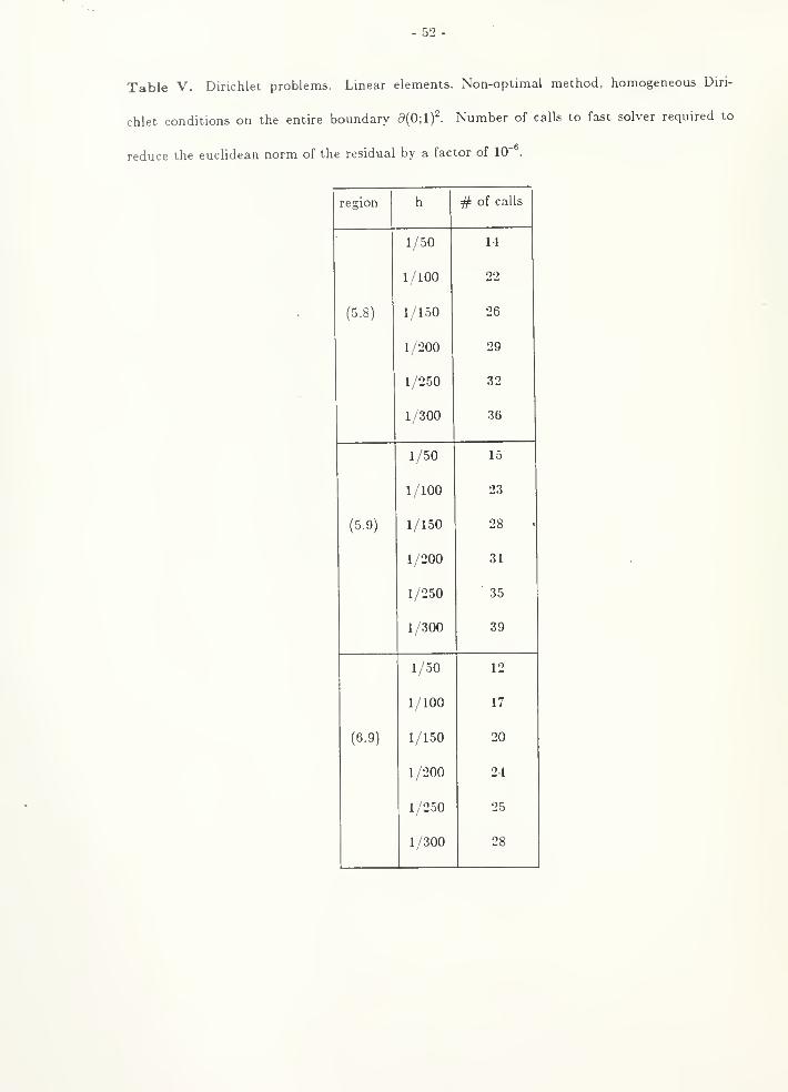
- 52 -

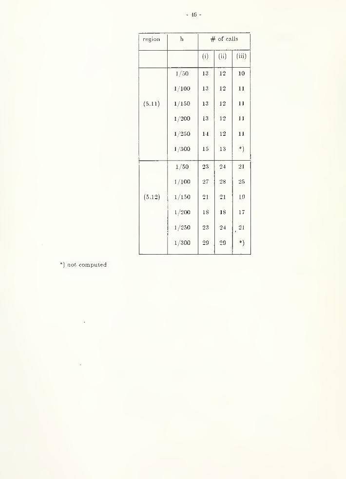
Table V. Dirichlet problems. Linear elements. Non-optimal method, homogeneous Diri-

chlet conditions on the entire boundary a(0;l)-. Number of calls to fast solver required to

reduce the euclidean norm of the residual by a factor of 10' .

region

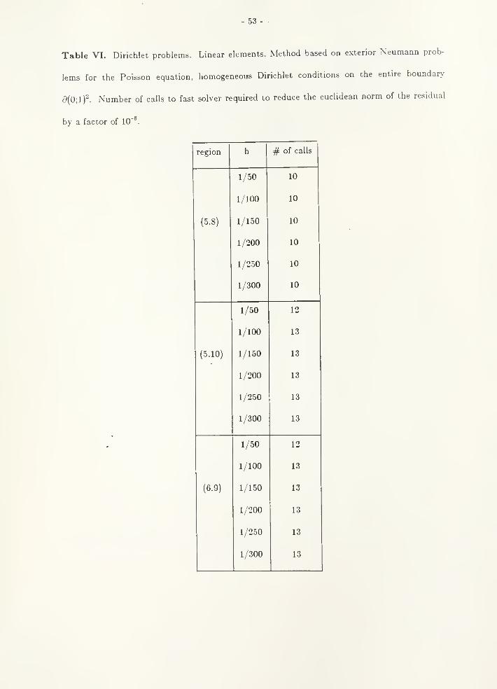
- 53-

Table VI. Dirichlet problems. Linear elements. Method based on exterior Neumann prob-

lems for the Poisson equation, homogeneous Dirichlet conditions on the entire boundary

a(0;l)^. Number of calls to fast solver required to reduce the euclidean norm of the residual

by a factor of 10".

region

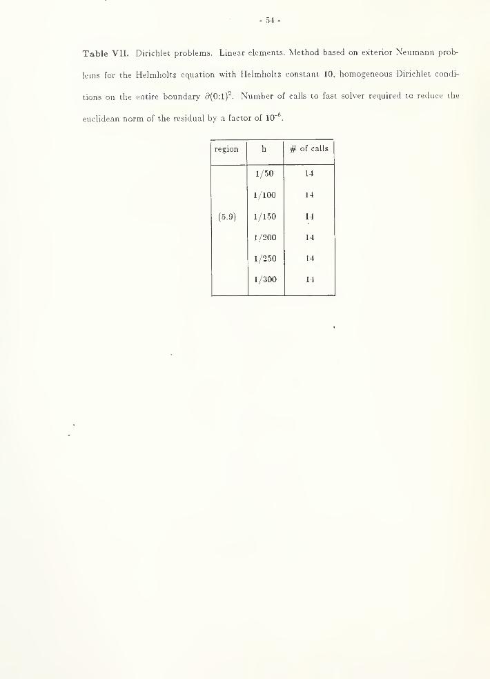
- 54 -

Table VII. Dirichlet problems. Linear elements. Method based on exterior Neumann prob-

lems for the Helmholtz equation with Helmholtz constant 10, homogeneous Dirichlet condi-

tions on the entire boundary 9(0;1)^. Number of calls to fast solver required to reduce the

euclidean norm of the residual by a factor of 10".

region

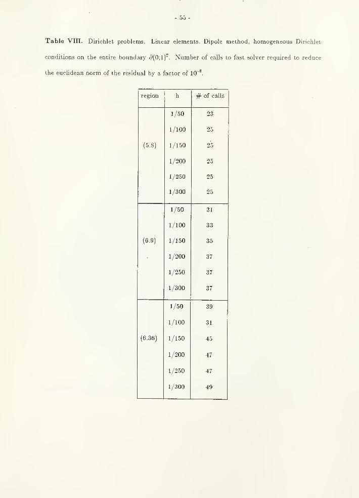
- 55 -

Table Vin. Dirichlet problems. Linear elements. Dipole method, homogeneous Dirichlet

conditions on the entire boundary 5(0;1)'. Number of calls to fast solver required to reduce

the eucUdean norm of the residual bv a factor of 10"^.

region

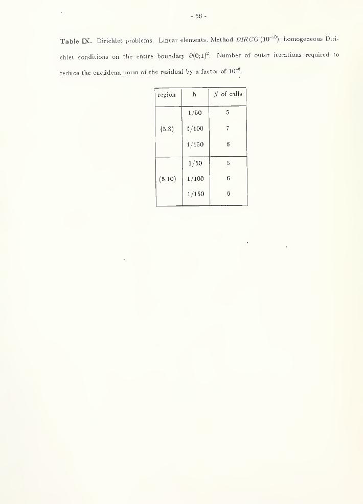
- 56 -

Table DC. Dirichlet problems. Linear elements. Method DIRCG (lO"'"), homogeneous Diri-

chlet conditions on the entire boundary d{0;lf. Number of outer iterations required to

reduce the euchdean norm of the residual by a factor of 10" .

region

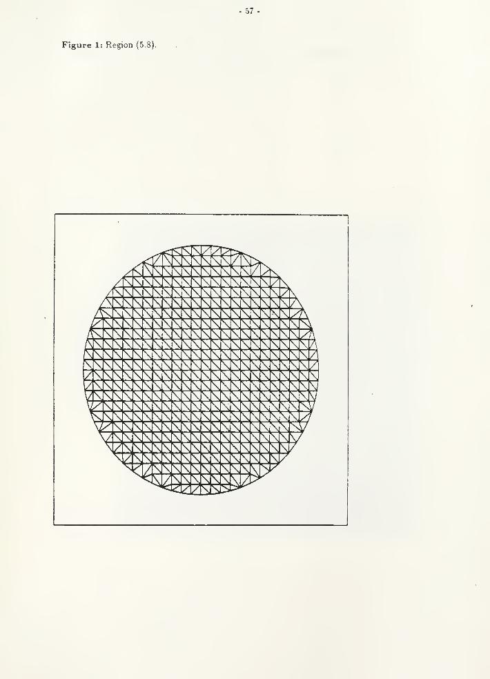
Figure 1: Region (5.8).

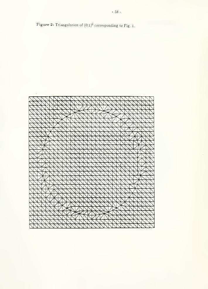
58-

Figure 2: Triangulation of (0;1)- corresponding to Fig. 1.

^^ ^^^^^^^ "^N^^^^^t

59

Figure 3: Region (5.9).

60

Figure 4: Region (5.10).

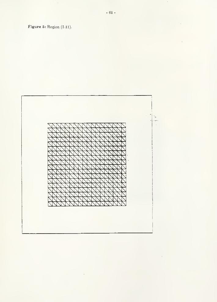
Figure 5: Region (5.11).

-61-

..-.

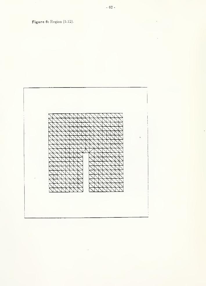
Figure 6: Region (5.12).

- 62-

NYU COMPSCI TR-261 C.2Borgers, ChristophFinite element capacitancematrix methods

-NYU COMPSCI TR-261 c.2 —Borgers, ChristophFinite element capacitance _matrix methods

7^,St»'

DATE DUE

^niNTCo mu. s.A.

.^'^m¥^mm\mm