Louisiana State UniversityLSU Digital Commons

LSU Historical Dissertations and Theses Graduate School

1968

Finite Element Analysis of Salt Pillar Models.William Joseph BergeronLouisiana State University and Agricultural & Mechanical College

Follow this and additional works at: https://digitalcommons.lsu.edu/gradschool_disstheses

This Dissertation is brought to you for free and open access by the Graduate School at LSU Digital Commons. It has been accepted for inclusion inLSU Historical Dissertations and Theses by an authorized administrator of LSU Digital Commons. For more information, please contactgradetd@lsu.edu.

Recommended CitationBergeron, William Joseph, "Finite Element Analysis of Salt Pillar Models." (1968). LSU Historical Dissertations and Theses. 1466.https://digitalcommons.lsu.edu/gradschool_disstheses/1466

This dissertation has been microiilmed exactly as received 69-4449

BERGERON, William Joseph, 1934- FINITE ELEMENT ANALYSIS OF SALT PILLAR MODELS.

Louisiana State University and Agricultural and Mechanical College, Ph.D., 1968 Engineering Mechanics

University Microfilms, Inc., Ann Arbor, Michigan

FINITE ELEMENT ANALYSIS OF SALT PILLAR MODELS

A Dissertation

Submitted to the Graduate Faculty of the Louisiana State University and

Agricultural and Mechanical College in partial fulfillment of the

requirements for the degree of Doctor of Philosophy

inThe Department of Engineering Mechanics

byWilliam Joseph Bergeron

.S., University of Southwestern Louisiana, 1959 M.S., Louisiana State University, 1961

August, 1968

ACKNOWLEDGEMENT

The author wishes to express his gratitude to Dr.Robert L. Thoms for having suggested the problem presented herein and for his quidance, assistance, and encouragement throughout its solution. He also wishes to express his thanks to the rest o f his committee and to the staff of the Engineering Mechanics Department for making his stay at L.S.U. not only a beneficial one, but also a pleasant one.

Special acknowledgement is also due his wife Rena and children Stephanie, Renee, Angelle, and Bryan for their understanding and patience while he completed his education.

ii

TABLE OF CONTENTS

Page

ACKNOWLEDGEMENT i i

LIST OF FIGURES viNOMENCLATURE V i ii

ABSTRACT xiiiCHAPTER I - INTRODUCTION 1

THE WASTE DISPOSAL PROBLEM 1' DISPOSAL IN SALT MINES 2"PROJECT SALT VAULT" 6THE SALT PILLAR MODEL 10THE MECHANICAL BEHAVIOR OF SALT 11THE FINITE ELEMENT METHOD 11

CHAPTER II - THE SALT PILLAR MODEL 12INTRODUCTION 12DEVELOPMENT OF THE PILLAR MODEL 13DESCRIPTION OF THE PILLAR MODEL 20VALUE OF THE PILLAR MODEL 22

CHAPTER III - THE MECHANICAL BEHAVIOR OFROCK SALT 25

INTRODUCTION 25

Page

PREVIOUS WORK: GENERAL 27PREVIOUS WORK: "PROJECT DRIBBLE" 30RECENT WORK: SALT PILLAR MODELS AND

"PROJECT SALT VAULT" 31CHAPTER IV - THE FINITE ELEMENT METHOD 41

INTRODUCTION 41REVIEW OF LITERATURE 42ADVANTAGES OF THE FINITE ELEMENT METHOD 43 CONCEPT OF ANALYSIS 45THE FINITE^ELEMENT 46THE AXI-SYMMETRIC 1 TWO-DIMENSIONAL'

PROBLEM 48THE COMPUTER PROGRAM 51CONVERGENCE CRITERIA 53ALTERNATE ENERGY APPROACH 55

METHOD OF ANALYSIS 57GENERAL STEPS 57MATHEMATICAL PROCEDURE 58

CHAPTER V - PROBLEM SOLUTION 81INTRODUCTION 81THE CREEP LAW ADOPTED FOR SALT 82CREEP EFFECTS MODIFICATIONS 91THE APPLICATION OF THE FINITE ELEMENT METHOD 94

iv

Page

CHAPTER VI - CONCLUSIONS H IBIBLIOGRAPHY 115APPENDIX A - DERIVATION OF THE STIFFNESS MATRIX 122APPENDIX B - PROGRAM LISTING FOR CREEP RATE

ANALYSIS 126APPENDIX C - PROGRAM LISTING FOR SALT PILLAR MODEL

ANALYSIS (LINEAR ELASTICITY) 128APPENDIX D - PROGRAM LISTING FOR SALT PILLAR MODEL

ANALYSIS (CREEP EFFECTS MODIFICATION) 144APPENDIX E - PROGRAM LISTING FOR PLOT OF NODAL POINTS 161VITA 164

v

LIST OF FIGURES

Figure Page1.1 Layout of Experimental Area 82.1 Behavior of Pillar Models under Various

Loading Conditions 152.2 Development of Lateral Stress for Various

W/H Ratios of the Pillar Models 182.3 Salt Pillar Model (3/4 Section) 213.1 Mechanical Model of Rock Salt (By Serata) 343.2 Mechanical Model of Rock Salt (By Obert) 374.1 A Plane Stress Region Divided into

Triangular Shaped Elements 474.2 Axi-Symmetric Idealization 494.3 Axi-Symmetric Elements 504.4 Strains and Stresses in Axi-Symmetric

Solids 645.1 Mechanical Model Proposed for Rock Salt 855.2 Strain Rate at-Constant Temperature 875.3 Strain Rate at Constant Stress 885.4 Sample of Results From Creep Rate Analysis 895.5 Flow Chart of Elastic Analysis Program 975.6 Flow Chart of Creep Modifications Program 985.7 Results of Creep Analysis 99

vi

Figure page

5.8 Results of Creep Analysis 1005.9 Results of Creep Analysis 1015.10 Results of Creep Analysis 1025.11 Pillar Load Distribution 1055.12 Plot of Original Nodal Points 1075.13 Plot of Nodal points After Elastic and

Creep Displacements (Two Days) 108

kJ* 1—1 *in Tracing of a photograph of Salt pillar

a Deformed

109

NOMENCLATURE

A = area; constanta = inner diameter of steel rings; constantB = constantb = outer diameter of steel ring; constant[B] = matrix function used to obtain strainsC = constantc = constantD = constant; diameter of circular pillar model[D] = elasticity matrix

= that part of [D] which depends only on v

j*DecJ = 1 elasto-creep1 matrixE = elastic modulusE = Maxwell elastic modulus (instantaneousm

elastic modulus)E^ = Kelvin elastic modulus (delayed or retarded

elastic modulus)e = 2.7183; general element

e-|pj- = nodal forces on e[f] - displacement field

fl' ^2 = functionsG^ = elastic shear modulusG 2 = retarded shear modulus

v m

distributed external load per unit area height of pillar model identity matrix integralsnodal points of element eoctahedral shearing strengthstiffness matrix of entire structurestiffness matrix of element econstant; slope of 5 vs t on log-log plot(negative)matrix function used in obtaining displace­ment fieldconstant; slope of e vs a on log-log plot (positive); number of nodes distributed body force per unit volume of materialinternal pressure applied to steel rings radial component of body force radial force per unit length of the circum­ference of a nodeexternal forces applied at the nodes r-coordinate of centroid of element e stress matrix absolute temperature (°K)

ix

t = timeU = component of nodal force in r-directionu = component of displacement in r-directionV = component of nodal force in z-directionv = component of displacement in z-directionW = width of square pillar modelZ = axial component of body forceZ = axial force per unit length of the circum­

ference of a node z = z-coordinate of centroid of element e

a = coefficient of thermal expansion; constant0 = constanty = shear strainv = octahedral shear strain' oA = area of triangle e-jj- = displacement vectore = straine = pillar cumulative deformation (in. in.'*')z oe = pillar strain rate

oC, = viscoelastic constant*1

— viscoplastic constant

^k' ^1' ^2 = Kelv:*-n viscosity

x

n = Maxwell viscosityMm©0 = temperature rise m element e

v = Poisson's ratioit = 3.1416a = stressa = effective stresscj = average applied axial pillar stress

or = shear stressT = octahedral shear stress0t . = t at t = 01 o

Supercriptse = element eT = transposed

= evaluated at r, z ' = corrective term

Subscriptsb = boundary forcec = creepe = elastici, j, k = 1st, 2nd, 3rd nodes respectively of element e

xi

LA = laterally appliedo = initialp = body forcepi = plasticr = radialt = thermalz = axialI,II,...,V = partition numberse = initial straino6 = tangential

xii t

ABSTRACT

The creep characteristics of rock salt were studied in an application of the finite element method. A creep law was proposed for rock salt and creep and large dis­placement modifications proposed for the finite element method. The scope of this study was limited to £he use of physical constants of rock salt available from other investigators. ,

An analysis was made of the proposed creep law and the proposed creep modifications and these were shown to com­plement each other. A computer program was written to solve the problem and was shown to produce small errors.

The actual problem solved was the determination of stresses and displacements in an axi-symmetric salt pillar model when it was subjected to a pillar load of 6,000 psi at 300°K for total times of two, five, and ten days. Included with the results were computer obtained plots of the original finite element salt pillar model and the deformed finite element salt pillar model.

Deformations obtained for the finite element salt pillar model correlated very well with deformations observed in recent publications showing actual deformed salt pillar models.

CHAPTER I

INTRODUCTION

THE WASTE DISPOSAL PROBLEMConcern for the hazards created by radioactive fallout

from weapon testing programs prompted an investigation by Parker et al. (1)* into the source, magnitude, and disposi­tion of the other radioactive debris generated in our nuclear age. It was noted that the major source of radio­active wastes from peacetime uses of nuclear energy will be that produced by the irradiation of fissionable fuel in stationary power reactors. According to predictions by Lane (2), this radioactive waste per year produced will be over five hundred times as much as that produced in

.-rai*bomb tests, and by the year 2000, over a thousand times as much. Therefore, it is imperative that a safe means be found to handle the radioactive waste products from nuclear reactors.

This high-level radioactive waste which is separated from the reuseable unconsumed uranium in the reprocessing of spent reactor fuel has far too much radioactivity to

*Numbers in parentheses pertain to references appended to this paper.

1

2

allow disposal to the living environment. With the growth of the nuclear power industry, this disposal problem is becoming increasingly serious and thus necessitates the development of a total and safe containment procedure. At the present time, the majority of the wastes produced in all countries are stored either as acid liquors in stain­less steel tanks or as alkaline liquors in mild steel tanks in underground locations at the processing plants (3). However, as the nuclear power industry expands throughout the world, storage of hundred of millions of gallons of liquid wastes with obvious hazards and with the cost of monitoring and tank replacement over-~the centuries becomes less attractive. Therefore, considerable research has been in progress for the past ten years to devise methods for- the conversion of these high-level liquid wastes into solids. These processes are only treatment steps, however, and they must be followed by a disposal operation. Thus, an ultimate disposal operation is required that will insure that the fission products are safely contained for centuries without further attention or need for monitoring.

DISPOSAL IN SALT MINESThe Earth Science Division of the National Research

Council organized in 1955 at Princeton University a

3

meeting (4) of sixty-five geologist, engineers, and personnel from other related disciplines to propose and discuss the disposal of radioactive wastes in geologic formations.

The storage of radioactive wastes in salt formations aroused considerable interest at this conference and in 1957, the report of the committee on Waste disposal (5) suggested disposal of solid form wastes in cavities mined in salt beds and salt domes as the possibility promising the most practical immediate solution, of the problem.

Some of the advantages cited for salt were:(1) Rock salt is widely distributed and abundant: United

13States reserves are estimated at greater than 6 x 10 tons (1,6).(2) The thermal conductivity of rock salt (2.5 Btu/hr- ft-F° at 200°F) is higher than most rocks and will enable larger quantities of heat to be dissipated (7).(3) Rock salt has a compressive strength similar to that of concrete, but unlike concrete and most other rocks, salt will flow plastically and relieve stress concentration pro­duced by mining and heating. Under normal mining condi- ' tions, the stress concentrations and temperatures are sufficiently low that supports are not needed.

4

(4) Salt formations in the United States are located in areas of low seismicity.(5) Salt is essentially impermeable due to its plastic nature when under pressure. Any cracks which might develop in the salt formation would be expected to be self-healing, as indicated by the lack of solution caverns similar to those found in limestone formations.(6) The cost of mining salt is less than most other rocks. In reference to the first advantage; if the estimated waste solution through the year 2000 A.D. is converted to solids and ultimately stored in salt mines, an area of about 1200 acres will be required (3). This is not considered unrea­sonable for the size of the nuclear economy involved and for the quantity of rock salt available.

As a result of the above reports, the ORNL initiated studies on the disposal of high-level radioactive wastes in salt cavities. The economics of-an actual disposal facility in a salt mine, the heat transfer from the waste to the salt, and the effects of heat and radiation on the properties of salt were considered. The following major conclusions drawn from these studies were (8,9,10):

(1) The "in situ" heat-transfer properties of rock salt are sufficiently close to the values determined in the laboratory on single crystals so that confidence can

5

be placed on theoretical heat-transfer calculations.(2) Elevated temperatures will cause accelerated

creep, but the exact effect on structural stability of the mine cannot be predicted from the present studies with sufficient accuracy to allow the design of a disposal facility making the optimum use of mine space.

(3) Most bedded-salt deposits contain trapped moisture which is released by shattering of the salt at temperatures above 250°C. By limiting the maximum salt temperature ina disposal operation to 200°C, this problem can be avoided.

(4) Rock salt is comparable to concrete for gamma radiation shielding.

g(5) A radiation dose of 5 x 10 R produces some changes in the structural properties of rock salt (i.e., about a 10% reduction in compressive strength) however, becauseof the shielding characteristics of salt, the effect pro­duced will be limited to the salt near the radiation source.

(6) Gamma radiation may produce some free chlorine within the salt structure; however, the amount released is expected to be negligible.

(7) The relative stability at ambient temperature of a salt mine used for waste disposal can be predicted from observed conditions in existing mines.

6

(8) The economics of a salt mine facility for disposal of future high-level power reactor wastes indicate that costs will be of the order of 0.01-0-02 mils/kwh of electricity generated.

"PROJECT SALT VAULT"These studies were only in preparation for the actual

final goal of the ORNL program on radioactive waste dis­posal in underground salt formations. This goal was to demonstrate the equipment and operations necessary to carry out safe and economical disposal of high-level solidified wastes in a typical disposal operation in the Carey Salt Mine at Lyons, Kansas. Considerable emphasis in the United States has been placed on this demonstration project which is called "Project Salt Vault" (11,12,13,14,15,16). The objectives of this salt mine study werei.

(1) to confirm the feasibility of disposal in salt mines;

(2) to demonstrate the required waste-handling equip­ment and techniques;

(3) to determine the possible gross effects of radia­tion on hole closure, floor uplift, salt-shattering temperatures, etc., in an area where the salt temperature is in a range of 100-200°C;

7

(4) to determine the possible release of radiolytically produced chlorine; and

(5) to collect information on creep and plastic flow of salt at elevated temperatures which can be used later in the design of an actual disposal facility.

The last objective of the study is the one with which this report is concerned.

A newly mined experimental area was created at the periphery of the mine at a higher level than the existing abandoned mine and of the most desirable geometry, so as to have the purest salt strata in the floor where the radioactive source was to be located. Four experimental rooms (Figure 1.1) were mined and in November, 1965, fourteen irradiated fuel assemblies (10^ curi) from the Engineering Test Reactor, contained in seven cans, were placed in the floor in the first room. A series of elec­trical heaters in the same geometric array as the main radioactive array was placed in the fourth room as a con­trol to determine the effect of heat only. The final portion of the demonstration was a pillar heating experi­ment where a large mass of salt underlying a mine pillar was heated by electrical heaters to about 100°C beneath the pillar. This portion of the project was set up to obtain information on mine stability as a result of

8

Feet0 50 100 150 vI— 1------1----- 1

T Electrical „ >/Heaters Array

200 „M a m u v Radioactive Array

100 -• *

From

Ramp Up

Existing Mine Workings

Figure 1.1. Layout of Experimental Area

increased salt temperatures. However, it was delayed until the end of 1966 since it was assumed that extreme salt movement would take place. The temperature, flow rate, and overburden load transfer in the center pillar were monitored by means of thermocouples, strain gages, and strain change meters located in and around the experimental area and throughout the mine. Experiments were also performed in the laboratory on models of the salt pillars to complement the data obtained from the mine.

The following conclusions were presented by Bradshaw and associates to the First Congress of the International Society of Rock Mechanics, Lisbon, Portugal in September and October of 1966 (15).

(1) The pillar-model tests have proven themselves to be useful for understanding the way in which salt movement take^ place, and it is reasonable to expect that predic­tions based on the elevated temperature models will also be valid.

(2) No measurable effects of radiation on the flow of salt were expected or observed.

(3) Thermal expansion of the floor and increased transverse expansion rates in the pillars adjacent to the array rooms have been about as expected with acceleration of movement in the ceiling exceeding expectation. However,

10

these movements should not cause trouble during the time when a room is still being filled with radioactive wastes.

Considerable laboratory tests (8,9,10,15,17,18,19,20, 21,22,23,24) were carried out to measure the effects of temperature and radiation on plastic flow and on the stabi­lity of salt, and the test area in the mine was well instru­mented to compare the actual conditictfis with theoretical predictions. Thus, the salt-flow data obtained in this experiment should, when combined with the results of labo­ratory and theoretical studies on the structural stability of rock salt at elevated temperatures and pressures, allow the establishment of a basis for the design of an actual disposal facility for optimum use of salt mine space.

THE SALT PILLAR MODELThe study of this report is a theoretical one in which

the salt pillar model is analyzed by numerical procedures. This model is the one proposed by Obert (19) and is the one which has evolved as the standard test model in all the many recent laboratory tests. However, as of this date, there is no evidence of any theoretical creep studies performed on the salt pillars or on this salt pillar model. This model, its development, its description, and its value are discussed in detail in Chapter II.

11

THE MECHANICAL BEHAVIOR OF ROCK SALTin order to study the creep behavior of the salt pillar

model, information on rock salt's mechanical behavior is necessary. A review of the laboratory experiments conducted in this area is presented in Chapter III and the relative merits of the various experiments are discussed. The mechan­ical models of salt presented by investigators who worked with the salt pillar models are discussed in Chapter V and a new mechanical model is proposed and fitted to the data obtained by Bradshaw and his associates (21) .

THE FINITE ELEMENT METHODThe numerical procedure used in studying the creep of

the salt pillar model is the 'Finite Element Method1. A general discussion of the method and the actual mathematical analysis of an axi-symmetric elastic problem is presented in Chapter IV. In order to account for creep behavior, the analysis is then extended into the nonlinear range by the introduction of a "variable elasticity1 procedure. The application of this procedure to the creep law adopted for this analysis is discussed in Chapter V.

CHAPTER II

THE SALT PILLAR MODEL

INTRODUCTIONSalt pillars are the unexcavated areas of salt left

within the limits of a salt mine and, as such, they are the most important element in stabilizing the underground structure. in the salt mines, these pillars undergo con­tinuous deformation (creep), The creep rate of the pillar depends on the average pillar stress (which in turn depends on the extraction ratio and the depth of the mine), the shape and height of the pillars, the temperature of the salt and the time since creation of the pillars.

Sufficient data on existing salt mines were available to enable predictions to be made on the stability of mines at ambient temperatures, but no data or experience were available which were directly applicable at elevated tem­peratures. Studies performed by Serata (18) and obert (14) [1964] at ambient temperatures have shown that creep in rock salt mines may be approximated by testing scale-model specimens uniaxially by providing proper horizontal restraints over the floor and roof portions of the model. These horizontal restraints produced triaxial stress

13

conditions similar to those found in the pillars in the salt mines. Lomenick and Bradshaw [1965] (20) studied the behavior of these scale model pillars (D/H = 4) at tempera­tures up to 200°C and stresses up to 10,000 psi for time periods of several thousand hours.

DEVELOPMENT OF THE PILLAR MODELSerata and Obert in their developments of a model

pillar each investigated the effects of specimen shape and

end constraints on the strength and deformational behavior

of salt. Following is a general discussion of these

investigations.

The most important difference of a mine pillar from a

laboratory specimen is the continuous medium of the upper

and lower formations over and under the exposed pillar por­

tion. Thus, they each insisted that a pillar model should

reflect the proper relation of the pillar to the surrounding

medium of an infinite extent since the pillar in the mine

is actually a part of a continuous medium. Furthermore,

the medium is subjected to both the lateral earth pressure

and strain-confinement in addition to the overburden load.

The influence of the continuous medium on the behavior of

the pillar portion is manifold. It adds to the axially

14

loaded pillars the following effects which virtually change its behavior:

1. Friction and cohesive forces acting on both ends

of the pillar.2. Room for elastic and time dependent deformations

to reduce localized stress developed in the pillar.3. Transfer of the formation's lateral pressure onto

the pillar.4. Confinement against lateral expansion of the

pillar at both ends,Serata demonstrated in the laboratory these effects

of the continuous medium by testing specimens with various degrees of confinement. His experimental results are sum­marized in Figure 2.1 in which the stress-strain curves of

— four types of specimens are compared. All the specimens have similar square pillars, but different friction and confinement conditions on the ends. The Type A specimen is a 3-inch cube uniaxially loaded with a friction reducer attached to each end of the specimen. The Type B specimen is an identical 3-inch cube uniaxially loaded with the loading ends directly exposed to the steel surface of the loading plungers. Thus, the only difference between the two is the degree of friction created on the specimens in the process of loading. However, the failure strength of

15

20ID04 16 o o o

1— 1

COCOo4JCO

20 30 40 6010 50

Strain (%)

Type AUJmW/H = 1

Type BUrr

Type C

UW/H = 1

nW/H = 2

Type DLiJ;:pmW/H = 2

Figure 2.1. Behavior of pillar Models Under Various Loading Conditions

16

the Type B specimen was twice as large as the other. This

strength increase was credited to the larger lateral fric­

tion developed over the steel contact surfaces of the Type

B specimen. The Type C specimen is identical to the Type

B specimen except for its height which is only half as

great. This reduction in the height increased the failure

strength of the same material to approximately three times

the true uniaxial strength. The Type D specimen has a

pillar located in the center of the specimen exactly the

same as Type C but has in addition a confined continuous

medium at each end of the pillar. This medium at the top

and at the bottom of the specimen represents, respectively,

the roof and floor of the mine. This simulates closely

the natural conditions of a mine pillar.

Experiments performed by Obert produced the same

results, i.e., (1) the end constraints strongly affect the

specimen strength with confined conditions at the ends of

the pillar increasing the strength, and (2) as the ratio

W/H was increased, the specimens lost their brittle

characteristics and tended to flow rather than fracture.

The stress-strain curves for the different specimens illustrated in Figure 2.1 show the effects of the medium confinement. Due to the difference in degree of end- confinement conditions and to the addition of media at

each end to simulate the continuous medium, a significant increase of the failure strength and in the time dependent creep was observed for the Type D specimen. This is graphically illustrated in Figure 2.2. In this figure, the distribution of axial stress and lateral stress in the pillar section is considered in the three different pillar models. These pillar models have the same width but dif­ferent heights. Serata indicates that very little or no lateral stress appears in the middle portion of the tall pillar, in which = 2W, since he assumed that the end effects would not reach this far. This condition is similar to the Type A specimen of Figure 2.1.

Serata, assuming the octahedral shearing stress criterion, proposed the following general equation for the maximum pillar stress.

He applied Equation 2.1 to the tall pillar of Figure 2.2, in which the average lateral stress is nearly zero, and

a z omax

3 (2.1)av

18

Predominantly

Partially Triaxial

Uniaxial

JO

Figure 2.2. Development of Lateral Stress for Various W/H Ratios of the Pillar Model

19

obtained the value of ctmax, = 3,200 psi. This was fairlyT

close to the laboratory strength which he obtained for the Type A pillar of Figure 2.1.

The medium pillar resembles Types B and C specimens of Figure 2.1, since a considerable amount of the lateral stress reaches the middle part of this pillar. The maxi­mum strength of the medium pillar is calculated by EquationA in which a_ > 0 as:L

Thus, the medium pillar should be stronger than the tall pillar by the amount of the average lateral stress qL»avexisting at the middle of the pillar.

The short pillar of Figure 2.2 with its secure con­finement and reduced height gives a greatly increased lateral stress magnitude. This is the condition for the Type D specimen of Figure 2.1.

Obert arrived at similar results in his laboratory, i.e., as the W/H ratio of the pillar model was increased, the compressive strength also increased and there was an increase also in the tendency for the models to flow rather than fracture.

3 (2.2)CTmax,M av

20

DESCRIPTION OF THE PILLAR MODELSince the deformational behavior of salt was so

strongly dependent on the end constraints, model pillars made from salt had to provide some means of controlling and determining the magnitude of this factor. Obert found the model shown in Figure 2.3 to satisfy these requirements. The model is cylindrical* in shape with a portion of the center ground out to form the pillar and surrounding rooms. To supply the confining pressures to the roof and floor portions, steel rings (3/4 inch thick by 1 inch height) were cemented to the ends of the model with an epoxy cement that completely filled the gap between the salt and the rings. The ends of the model were allowed to extend past the steel rings 1/8 inch so that when it was loaded no axial force was applied to the steel rings. Two dial gages were mounted 180° apart on the steel rings to provide means of measuring the cavity closure of the pillar model. Three resistance strain gages, oriented to respond to tangential strain, were cemented to the periphery of each ring at 120° intervals. The internal pressure applied to the ring was

*Cross section of mine pillars are not circular, but model studies by Obert show that the relation between compressive strength and diameter/height or width/height ratio are vir­tually identical if the width of a pillar is taken as its smaller lateral dimension.

I

Epoxy Cement

Steel Ring Roof-

V V n/ V

v v w/ / /

---- ' V r - " - - I|J

Pillar Salt Specimen-Floor /// VV V v

^ - 1

///, v „ v vJ-J-L V \ l V I. — — ----— 1—

TH

Figure 2.3. Salt Pillar Model (3/4 Section)

22

determined by the equation for thick wall rings,

2 2 E eQ (b - a )e (2.3)

Under the assumption that the lubricant on the bearing plates reduced the end constraints to a negligible value,

Bradshaw (15) and associates found from pillar model tests that the radial stress was equal to about 50% of the aver­age vertical pillar stress. It should be observed, however, that this stress is actually not in the pillar portion it­self as was assumed, but, in the floor and roof sections at the interface between the salt and the steel rings.

VALUE OF THE PILLAR MODELObert found through laboratory experimentation with

rock salt that the mode of failure and the strength of the above model pillars were virtually the same as that for the conventional compression specimen having the same pillar D/H ratio tested without end lubricants. However, the above pillar model was considered a much better model since there was no discontinuity in the model material at the roof and

the radial stress a in the pillar model was obtained from

a (2.4)r

23

floor and since the steel rings permitted a means of determining and controlling the magnitude of the end con­straints. Bradshaw (21) and associates performed a corre­lation of convergence measurement in salt mines with laboratory creep-test data and found a reasonable agreement with the rates measured in the Kansas mines. They also observed that the horizontal expansions of the pillars did not seem to be great enough to account for the apparent shortening of the pillars. A plausible explanation accepted by them at that time was that part of the pillar volume expanded into the room via the floor and roof. Again the pillar model proved valuable, for in a later paper (15), this was shown to actually take place in the testing of pillar models.

Bradshaw and associates (15) performed research in the laboratory with model pillars (at temperatures up to 200°C and stresses up to 14,000 psi) and in a 1,000 feet deep salt mine ("Project Salt Vault") using reactor fuel and electrical heaters. Measurements of convergence, strain, strain rates and stress changes were obtained. Again, the model.tests were found to correlate well with underground measurements and observations. Also, these pillar model tests, since they indicate the radial stress developed,

24

have shown in a qualitative way why roof-sags and floor- heaves take place in the salt mines.

Thus, the pillar model test performed have shown that these salt pillar models can give useful information about salt movement in the mines both at ambient and at elevated temperatures.

CHAPTER III

THE MECHANICAL BEHAVIOR OF ROCK SALT

INTRODUCTIONThe problem of accurately determining the stress,

strain, and creep in a rock structure in the earth's crust is a rather complex one. Theoretical studies differ widely in many of the basic assumptions about the physical pro­perties of the rock itself. Some solutions of problems in underground stress analysis assume that rock is elastic, homogeneous and isotropic in character, and that its physi­cal properties are neither time nor temperature dependent; others assume that rocks are nonhomogeneous, anisotropic, plastic, viscoplastic, viscoelastic, time and temperature dependent, or a combination thereof.

The study of the physical properties of rock salt, the member of the rock family considered here, is especially complicated by its viscoplastic, viscoelastic, time, tempe­rature, and pressure dependent characteristics. in the underground structure, the pressure involved is a function of the depth, stratigraphy, the percentage of salt exca­vated, and the configuration of the excavation. The temperature is a function of the depth, the size and shape

26

of the structure, the rate of heat production of the stored material and the thermal conduction in the surrounding salt. Although rock salt is somewhat nonhomogeneous and anisotro­pic (because of impurities in the salt such as anhydrites and shale, and more so in the bedded salt than in the dome salt, and because of flow bands in dome salt which formed as the salt crept from a deeper source to its present posi­tion) , the rock salt of the salt pillar model considered in this study will be assumed to be homogeneous and isotropic. The time, temperature, and pressure dependent characteris­tics will, however, be considered in this analysis.

Another complication is that the physical properties of rock salt depend upon the testing method. The major factors which affect the testing results are the size of the test specimen, cross-sectional form of the specimen, ratio of specimen width (or diameter) to height, degree of friction on the loading surface of the specimen, confining pressure, geometry of loading, rate of loading and size of crystalline grains. In this analysis, the results of the testing procedure which are consistent with the salt pillar model's material, size, shape, and loading conditions will be used.

Experiments to describe the creep phenomena and to determine the physical properties of rock salt were rather

27

limited before 1959. Since that time, investigators such as Bradshaw, Serata, obert, LeCompte, Boresi, Deere, and others have performed a number of varied experiments under different test conditions.

PREVIOUS WORK: GENERALStocke and Borchert [1936] (25) performed a few two-

hour test on natural polycrystalline rock salt. These test were conducted at room temperature and atmospheric pressure with axial stresses ranging from 372 psi to 3,900 psi.

Griggs [1939] (26) conducted a creep test of 42 dayson a prism of a single crystal of halite loaded in uniaxial compression to 900 psi at room temperature and atmospheric pressure.

Kendall [1958] (27) carried out creep experiments oncylinders of a single crystal of halite at room temperature under confining pressures of 0 psi and 2,000 psi and with stress differences ranging from 500 psi to 4,000 psi.

Gunter and Parker [1959] (28) made some uniaxial creeptests at room temperature and with an axial stress of 2,500 psi on natural dome salt and bedded salt to determine the effects of radiation on the creep behavior of rock salt. Some structural properties at room temperature and at 200°C

28

for irradiated and unirradiated natural dome salt and bedded salt were also determined.

Brown and Jessen [1959] (29) studied the effects ofpressure and temperature on a 2 inch, cylindrical cavity contained in a 6 inch long by 6 inch diameter salt core under triaxial pressure conditions. They determined rates of closure of these cavities under axial stresses of 1,000 psi to 8,000 psi and temperatures of 32°C to 204°C.

Serata and Gloyna's work [1959] (30) on the mechanicalproperties of rock salt was the most extensive up to that time. Except for a few runs with synthetic single crystals, most of their work was carried out on fine-grained natural polycrystalline rock salt. They presented a theoretical analysis of stress distribution around various forms of cavities. Experiments were conducted in the laboratory and in a salt mine to investigate the strength of these cavi­ties. Using uniaxial compression, they investigated the following properties of rock salt: strength, Young'sModulus, Poisson's ratio, and strain-hardening. They also studied the effects of triaxial compression on the strength of rock salt from various test data and the effects of temperature and pressure on the creep rates.

Serata and Gloyna [I960] (31) followed their earlierwork with a discussion of the theoretical principles of

29

structural stability of underground salt cavities and of the significance of the principles as they relate to other cavities. They applied the theory of plasticity to the evaluation of stress and strain conditions of salt cavities. The concept of a yielded zone which develops around the cavities was introduced, and a theoretical development of the extent and stress distribution of the zone was illus­trated through the use of ideal spherical and cylindrical cavities under uniform triaxial compression. Application of the concept to actual conditions such as cavity irregu­larities, brittleness of formation, and nonhydrostatic loading was also discussed.

LeCompte [1964] (24) investigated the effects oftemperature to 300°C, confining pressures to 14,500 psi, stress difference to 2,000 psi, and different grain sizes on the creep behavior of rock salt. These creep test were carried out on artificial polycrystalline rock salt speci­mens and on one single crystal. In this study and in an earlier one [1960] (34), he fitted the equation e = A + Btnto his creep data and experimentally evaluated the constants A, B, and n for different temperatures and confining pressures.

30

PREVIOUS WORK: "PROJECT DRIBBLE"With Deere as consultant to Holmes and Narver, Inc,,

who represented the AEC, a comprehensive test program, "Project Dribhle," was outlined for determining the signi­ficant physical properties of rock salt. The Engineering Laboratories, Bureau of Reclamation, United States Depart­ment of the Interior, Denver, Colorado, performed some of the triaxial test [1962] (22) at 73°F with lateral pres­sures ranging from zero to 5,000 psi on a series of 4 15/16 inch diameter rock salt cores from Tatum Dome near Jackson, Mississippi. The purpose of these tests was to determine shear strength characteristics in terms of the equation of Mohr's envelope. The majority of the tests [1963] (32)were performed at the United States Army Engineer Waterways Experimental Station, Corps of Engineers, Vicksburg, Mississippi. These test, on the same type core as above, included petrographic examination of cores, uniaxial com­pressive cyclic loading test, specific gravity, porosity, permeability and interstitial fluid determinations, non­destructive dynamic tests, and creep test of uniaxial compressive and triaxial extensive types.

Boresi and Deere [1963] (23) presented a report inwhich the triaxial compression tests (Bureau of Reclamation) and the creep tests (Corps of Engineers) were used in

31

assessing the probable behavior of the cavity to be exca­vated at Tatum Dome, Mississippi. By a curve fitting process, thoy obtained and presented the following equation relating strain, stress and time:

e = K a t (3.1)

RECENT WORK: SALT PILLAR MODELS AND "PROJECT SALT VAULT"Serata [1964] (18) studied the triaxial properties of

rocks and the underground stress field in order to establish a theoretical basis for mathematical analysis of underground openings and support systems. Rock salt of uniform quality was used as the model material in the various models of the structures to test his theoretical conclusions on the behavior of these systems. A new testing method designated the "transition test" was developed in the Michigan State University Laboratory in order to supplement the shortcom­ings of the conventional triaxial testing method and to provide a condition similar to an infinite continuous medium. It was used to determine the triaxial properties of the rock salt. Using a single specimen, all the follow­ing material property coefficients of a continuous rock salt medium were determined:

6Young's modulus, E = 0.86 x 10 psx

Poisson's ratio, v = 0.16Octahedral shearing strength, Kq = 1,500 psi

0Elastic shear modulus, = 0.39 x 10 psi

gRetarded elastic shear modulus, = 0.0042 x 10 psi

0Viscoelastic constant, = 150 x 10 psi-minutes

0Viscoplastic constant, = 2,000 x 10 psi-minutes

Assuming five fundamental property coefficients for rocks,

Gf, G2, C=2 ' and V 3 flve"e!ement time-dependentmechanical model of the triaxial behavior of the material was presented.

The effects of the individual factors which'influence the physical properties of rock salt in testing procedures were investigated in order to design laboratory models of underground structures which were free from these influences. A model of an underground cylindrical opening was developed, and its behavior was in good agreement with the proposed theory and with field observations conducted in various salt mines. This led to the development of models for underground supporting systems. A square pillar model with confined continuous medium on both ends of the pillar (Type D specimen of Chapter II) was thus developed to simulate the natural conditions of a mine pillar. Its behavior was also in good agreement with the proposed theory and with field observations.

33

Serata concluded that the deformation of the pillar consisted of three independent components of elastic, vis­coelastic, and viscoplastic deformations, and that the individual deformations associated with each component could be analyzed by the theory developed with theJproperty coefficients obtained and with the initial underground stress field. The model pillar was also used for studying the long-term behavior of a mine pillar in which the time- dependent deformation was expressed by

dSzo ^ zo " ^ rT i - Ko - ( h /Cl)— = ■ - I—CT"’ •(3.2)

To ■ CG2/{2) -1+ c2 ■ e J •Equation (3.2) is thus a separation into two exponential components of the effects of viscoplasticity and visco­elasticity.

Serata also proposed a mechanical model for rock salt and is shown in Figure 3.1.

Obert [1964] (19) investigated the effects of specimenshape and end constraints on the strength and deformational behavior of salt and trona specimens. From these prelimi­nary tests, he developed a pillar model that has proven

34

OctahedralStress

OctahedralStrain

o 4“ V\AA/—

2W W VK

• c.■ > Y o

Elastic Viscoelastic ViscoplasticUnit | unit I Unit

Figure 3.1. Mechanical Model of Rock Salt(by Serata)

to be realistically related to its prototype in the mine and which has been adopted as the standard test pillar model (15,16,20,21). He then studied the strength and deformational behavior of pillar models made from salt, potash, and trona tested under constant applied loads at ambient temperature. This pillar model was the one used by Bradshaw and associates in their model studies connected with "Project Salt Vault" and is the one considered in this study (Figure 2.3).

Obert also performed creep tests with this pillar model in which he used a D/H ratio of 4 and a constraining ring thickness of 3/4 inch. He fitted to the data from the creep tests a general expression of the form

e = A + Bt + Cf (t) , (3.3)zo c — -zwhere: A = - -° , elastic strainEm

ctz qB = —-- , steady-state creep

“ \ t / 3Tlf(t) = (1 - e ), initial or transient-

creep/C.

36

The mechanical model corresponding to this expression is presented in Figure 3.2. He found that although Equation 3.3 could be fitted to any given creep data by proper selection of the constants, no set of constants would pro­vide a fit for the family of curves for any rock type,primarily because 3n was not constant for different'mvalues of cr • For a family of curves, he found that the

osteady-state strain rate e could be expressed by

om

K = D ^ n (3‘4>z zo om

where for Kansas salt, n = 3.0 for o = 4,000 psi tozo10,000 psi and where the "in situ" pillar stress can be reasonably approximated from the depth and extraction ratio.

Bradshaw and associates [1964] (21) at the request ofthe Oak Ridge National Laboratory were furnished data by L. Obert of the Applied Physics Laboratory of the United States Bureau of Mines on a series of creep test on Obert's salt pillar model. The results of these tests were com­pared with actual measurements in salt mines in order to gain more information on the design parameters involved in "Project Salt Vault". Obert performed 1,000 hour creep tests at ambient temperature on the salt pillar models of

37

E 3nm

az < 'VVVV-o

m

Ek■vww

3n CT.k

Elastic Steady-Creep Transient-CreepUnit | Unit | Unit

Figure 3.2. Mechanical Model of Rock Salt(by Obert)

38

D/H ratio of 4 and with average pillar stresses of 4,5,6, 7,8,10, and 12,000 psi. Vertical shortening of the pillars, as a function of time and stress, was measured by means of the two dial gauges attached to the steel restraining rings of the pillar model. Bradshaw and associates plotted creep rate vs. time from Obert's cumulative deformation curves by taking their tangents. They then fitted to these curves an equation of the form

They observed that the value of m was in reasonable agree­ment with those obtained by the USBM using salt samples from other mines, but that the value of n differed signifi­cantly. However, the use of the above equation to extra­polate the creep rate out to 70 years produced predicted creep rates which were in good agreement with those actually measured in the mine from which the samples came. Therefore, they concluded that salt from one mine may have different mechanical properties from salt in other mines.

Bradshaw and associates [1965-1967] (15,16,20) afterhaving obtained predicted creep rates, which were in good

B a (3.5)ezo oIt was found that a reasonable fit was obtained with

ez 9 x 10”8 az3.1 t-0.6 in.in. ^ day ^(3.6)

o o

39

agreement with the creep-closure rates measured in the Kansas mines since 1959, extended the model test to elevated temperatures. They studied the behavior of the salt pillar models at temperatures ranging up to 200°C and stresses up to 10,000 psi. A sizeable increase in the deformation of the pillars was observed with increasing load, but, even more significant was the greatly accele­rated creep rates of the salt at the elevated temperatures. Cavity closure vs. time curves at 22.5°C, 60°C, and 100°C for loads of 4,000 psi and 6,000 psi were plotted. All curves were in general similar in shape, exhibiting an initial high creep rate that decreased with time and con­tinued to do so in tests of duration in excess of 5,000 hours. These curves gave support to a previously developed hypothesis (33) that the effect of elevating the temperature is effectively the same as that of increasing the average pillar stress and that the relationship between creep rate and axial stress follows the same power law regardless of temperature. However, it was observed that at temperatures of 100°C and above, the deformational behavior of the models departs somewhat from that produced by increased stress.

To the data obtained by Bradshaw and associates at the Oak Ridge National Laboratory, the following approximate

empirical equations were fitted for times from 10 hours on

CHAPTER IV

THE FINITE ELEMENT METHOD

INTRODUCTIONThe stress analysis of some of the present day complex

structures of arbitrary shape, subject to thermal and mechanical loads, is not only of considerable academic in­terest, but in some cases, practical and necessary. In some of these problems, the governing differential equa­tions have been known for many years, but closed form solutions have been obtained for only a limited number of severely idealized situations. Thus, the stress analyst must rely on experimental and/or numerical techniques.With the rapid development of digital computers and with the associated advance in numerical procedures, such as the one considered here, the expensive experimental models now often used in design of structures are rapidly becoming replaced by more economic computation.

Before numerical, computer-based solutions of real problems dealing with complex continua can be solved, it is necessary to limit their infinite degrees of freedom to a finite, although sometimes large, number of unknowns.The most popular of the numerical techniques using this

process of discretization has been the finite difference method. However, for some problems such as structures of composite materials or of arbitrary geometry, this proce­dure is difficult to apply. An alternative approach, that of finite elements, appears to offer considerable advantages and its relatively simple logic makes it ideally suited for the computer. Thus, this will be the numerical solution used in the analysis of the salt core and restrain­ing steel ring of the axi-symmetric salt pillar model con­sidered in this study.

Review of LiteratureThe finite-element method was originally developed in

the aircraft industry and was introduced as a method of direct structural analysis (35). Since that time, it has been the subject of investigation by many workers interested in approximate solutions of elasto-static boundary value problems. The method has proven to be extremely effective for the treatment of problems in plane stress and plane strain (36^41), and several computer programs for solutions of plane elasticity problems are now in existence (38-40).

On a smaller scale, the applicability of the method to plate and shell bending problems has been demonstrated (42-45) and impressive results were obtained in the analysis

43

of axi-symmetric shells approximated by a series of trun­cated cone elements (45,46). Recently, this procedure was recognized to be equivalent to the well known Rayleigh- Ritz procedure which when applied to the same problem resulted in exactly the same formulation as that achieved previously by the structural approach (41,47,48). Thus, this procedure was extended to a variety of physical pro­blems in which an 'extremum' principle exists (48-52). Although the general concept is clearly applicable to the analysis of three-dimensional solids, only preliminary investigations of this type have been reported (37,53-55).

Recently, the finite element method was applied to the structural analysis of axi-symmetric solids with con­siderable success (56-58). Another recent extension of the method has been in the area of non-linear problems, where plasticity, creep, and large deformations are considered (37,48,59,60).

Advantages of the Finite Element MethodThe advantages of the finite element method in com-

parison to other numerical approaches are numerous.Unlike the finite difference method which is difficult to apply for structures of arbitrary geometry or of composite materials, the finite element method is completely general

with respect to geometry and material properties. Complex bodies composed of many different materials are easily represented. Since anisotropic materials are automatically included in the formulation, filament structures are readily handled. The shape of the element can be chosen to best fit the particular problem considered and the size of these elements can be varied in accordance with the anticipated stress gradients. Displacement or stress boundary condi­tions may be specified at any node (or nodal circle) within the finite element system. Arbitrary thermal, mechanical, and acceleration loads are possible. Mathematically, it can be shown that the method converges to the exact solution as the number of elements is increased (44,61); therefore, any desired degree of accuracy may be theoretically obtained, in addition, the finite element approach generates equili­brium equations which produce a symmetric, positive-definite matrix which may be placed in band form and solved with a minimum of computer storage and time. With the recent recognition of this procedure as an equivalent Rayleigh- Ritz procedure, the method now has a much broader basis which permits applications to be extended to almost all problems where a variational formulation is possible. In addition, procedures have been suggested for this method which allows extension into the area of non-linear problems, thereby including plasticity, creep, and large deformations.

45

Concept of AnalysisThe numerical analysis is based upon finding an

alternative form of the governing equations which is easier to solve than the governing differential equations of the continuous solid. The discretization process re­duces the problem from solving a system of differential equations to solving an equivalent set of algebraic equa­tions. Therefore, the ultimate goal is to derive the governing equations of the idealized solid.

The concept of finite elements, as originally intro­duced by Turner et al. (35), handles the problem of dis­cretization by assuming that the real continuum is divided into a finite number of discrete structural elements interconnected only at a finite number of joints or nodal points at which some fictious forces, representative of the distributed stresses acting on the element boundaries,, are introduced. The finite elements are formed by figura­tively cutting the original continuum into a number of appropriately shaped pieces, retaining in the elements the properties of the original material. In the analysis, these assumed structural elements are entirely equivalent to the components of an ordinary framed structure. Thus, the analysis process consists merely in the normal opera­tions of satisfying compatibility and equilibrium conditions

46

at the nodal points, using any standard structural analysis procedure.

In practice, the displacement formulation (36,41) of structural analysis generally has been found most convenient for treating finite element idealizations of elastic con- tinua, and this will be the method used in this analysis. Thus, in summary, the finite element analysis may be viewed as a generalization of structural analysis theory that makes possible the analysis of two- and three-dimensional elastic continua by the same procedure used in the analysis of ordinary framed structures.

The Finite ElementSeveral types of elements may be used in the represen­

tation of a structure. In the plane stress analysis of a thin slice, the most frequently used element is the triangu­lar shape element, e, as defined by the nodes i, j, and m numbered in .counter-clockwise order and by the straight line boundaries as indicated by Figure 4.1. In the finite element approximation of axi-symmetric solids, the con­tinuous structure is replaced by a system of axi-symmetric elements which are interconnected at circumferential joints or nodal circles. In the axi-symmetric stress analysis, which is mathematically two-dimensional in nature, the

47

>*X

Figure 4.1. A Plane Stress Region Divided Into Triangular Shaped Elements

48

triangular shaped element of the plane stress analysis becomes the cross section of the ring elements. (See Figure 4.2 and Figure 4.3.) It should be recognized that the finite elements that are shown here are actually com­plete rings in the third dimension (extending through the angle 0 = 2tt) , and that the nodal 'points' at which they are connected are in reality circular lines in plan view. Otherwise, the system shown is entirely equivalent to a finite element plane stress or plane strain problem.

The Axi-Symmetric 'Two-Dimensional' problemThe axi-symmetric structure to be considered in this

analysis is shown in Figure 4.2-A. Because of the sym­metry of the structure and its loading about the vertical Z axis, the two components of displacement in any plane sectioning the body along its axis of symmetry define com­pletely the state of strain and therefore, the state of stress. Thus, displacements of the system will be deve­loped only in the radial and vertical directions; tangential displacements do not exist. Furthermore, stresses and strains do not vary in the tangential direction.

From a mathematical point of view, this class of system is two-dimensional in nature and may be represented as shown in Figure 4.2-B. An appropriate idealization of

49

A; 'Axi-Symmetric Solid

B. Two-Dimensional View of Axi- Symmetric Continuum

A Z

pa-**r

C. Two-Dimensional View of Finite Element Idealization of Axi- Symmetric Continuum

Figure 4.2. Axi-Symmetric Idealization

50

X

A. Typical Triangular Axi-Symmetric Element

Z

r

B. Two-Dimension View of Axi-SymmetricElement

Figure 4.3. Axi-Symmetric Elements

51

this 'two-dimensional' system, using triangular finite elements, is shown in Figure 4 . 2 - c . Thus, the system shown is entirely equivalent in degree of mathematical complexity to a finite element plane stress or plane strain problem, and standard plane stress computer programs may be adapted to the solution of this class of system. It is necessary merely to develop stiffness and load matrices appropriate to the 'ring type' finite elements, taking proper account of the fact that tangential stresses and strains result from radial displacements in the axi-symmetric system.

The Computer ProgramFinite element plane stress computer programs provide

a significant contribution to the analysis of axi-symmetric solids by finite elements since these programs can be modi­fied to solve the latter problems. Thus, some of the pro­gramming efforts represented by existing plane stress programs can be incorporated into an axi-symmetric analysis program.

The general finite element analysis program can be divided into three phases:1. The element stiffnesses and the element loads are

computed.2. The stiffness matrix and the load matrix for the

52

complete structure are formed (by superposingindividual element effects) and the resultingnodal displacements are computed.

3. The element stresses are evaluated.In the axi-symmetric analysis, the plane stress program

must be modified by substituting into phase one the appro­priate axi-symmetric element stiffness and load subroutines in place of the corresponding plane stress routines. The assembly and solution of the 'two-dimensional' equilibrium equations of phase two are left unchanged. Phase three is unchanged in principle; the stresses in each element, e,are still calculated as in the plane stress program. How­ever, the displacement matrix now represents the nodal displacements associated with the axi-symmetric element. Thus, it is necessary to refer to the appropriate axi- symmetric expressions for each of these matrices, but no modification of the program is required.

The input data required for the axi-symmetric analysis and for the plane stress analysis is identical. The physi­cal property data concerning each finite element, the geometric co-ordinates of each nodal point, the loading associated with each element, and certain miscellaneous items concerning boundary conditions, etc., must be supplied in both computer programs.

53

The output data is equivalent to that obtained from the plane stress program except that one additional item is obtained; the stress in the 9-direction.

Convergence CriteriaThe dependability of the finite element method is

strongly controlled by the assumed shape functions since they limit the infinite degrees of freedom of the system. Thus, the exact solution may never be reached, irrespec­tive of the fineness of the mesh. To insure convergence to the correct result, certain simple requirements have to be satisfied (44,48,56,57).

1. The assumed displacements must be continuous over the elements and must be continuously differentiable up to and including the highest derivative required in the formu­lation of the element strains.

2. The deformation between adjacent elements must be compatible since no gaps or overlaps are permitted in the deformed finite element system. With nodal displacements selected as generalized displacements, this requirement is easily satisfied. The displacements along any side of the element are selected so that they depend only on the dis­placements at the nodes bounding the side. For triangular two-dimepsional elements, this boundary compatibility

54

condition is satisfied by assuming displacements that vary linearly in each direction. The edges of each element will then displace as straight lines, and no gaps can develop between them as long as nodal continuity is maintained.If complete compatibility can be maintained (internally and on the boundary), then the finite element method can be demonstrated to converge to these exact results as the mesh size is reduced (44,61).

3. The displacement function must be a linear function of the generalized displacements. This is necessary so that the load-displacement equation will be linear. In the dis­placement expression, as a consequence, the coefficient of the nodal displacement must be non-dimensional so as to satisfy dimensional requirements.

4. The displacement function must be of such a form that if nodal displacements are compatible with a constant strain condition, such constant strain will, in fact, be obtained. This incorporates the requirement that it does not permit straining of an element to occur when the nodal displacements are caused by a rigid body displacement, since rigid body displacements are a particular case of constant strain - with a value of zero.

It should be noted that all of the above stipulations are independent of element shape, material characteristics, and the smallness of strains and displacements.

55

Alternate Energy ApproachAlthough the 'structural analysis' approach is direct

and physically interpretable, the concept of replacing the distributed stresses on the element boundaries by 'equiva­lent' static loads raised some questions of the exact physical conditions that were being imposed and what approxi mations were, in fact, made by the process. Recently, this problem was approached via an alternate route which led to the recognition of the equivalence of the finite element- structural analysis approach with a minimization process(41,47,48). Thus was shown the similarity of the formula­tion with the well-known Rayleigh-Ritz methods.

The finite element method based on energy principles differs from the usual Rayleigh-Ritz procedure in the choice of displacement functions. Instead of the smooth displace­ment function of the Rayleigh-Ritz method, extending over the entire solid, the finite element method uses many dis­placement functions, each restricted to a small part of the solid. Also, contrary to the Rayleigh-Ritz procedure, quantities with obvious physical meaning are chosen as the variable parameters. This allows the analyst to maintain at all times a direct physical 'contact' with the real

problem being examined.

56

In the minimization process, it was shown that if the system of displacements was defined throughout the struc­ture by the element displacement functions, with the nodal displacements acting as undetermined parameters, then the procedure of minimization of the total potential energy of the system results in precisely the same formulation as that achieved by the 'structural analysis' approach. Therefore, there now exist two equivalent, alternate form­ulations. In the first, an equation is written and its direct solution attempted. In the second, the problem is to find a function minimizing a certain specified func=** " tional over the field involved.

A list of but a few of the many problems encountered in engineering practice which can be solved by finite element-energy method is:

heat conduction, bending of prismatic beams, seepage through porous media, irrotational flow of ideal fluids, distribution of electric (or magnetic) potential, torsion of prismatic shafts, etc.

Thus was opened the door of application of finite elements beyond that of structural analysis to the much wider range of almost all problems where a variational formulation is possible.

57

METHOD OF ANALYSIS

General StepsUsing the displacement method of the • 1 structural

analysis' procedure,. the finite element analysis proce­dure can be summarized as follows:

1. Idealization. The axi-symmetric elastic con­tinuum is separated by imaginary surfaces into a system of triangular shape ring elements which are then reduced to equivalent triangular plane elements for the mathematical analysis.

2. Element Analysis. Assuming that the triangular elements are interconnected at their three vertex nodal points, a displacement function is used to define uniquely the state of displacement within each finite element in terms of its three nodal displacements. Thus, the state of strain within each element is defined in terms of its nodal displacements by the displacement functions, and together with any initial strain and the elastic properties of the material, so is the state of stress throughout the element and, hence, also on its boundaries, A system of forces concentrated at the nodes and equilibrating the boundary stresses and any distributed loads is determined. This results in the stiffness matrices which relate the forces developed at the element nodal points to the

58

corresponding element displacements.3. Assembly of Elements. The nodal stiffness matrix

for the complete structure is evaluated by superposition of the individual element stiffnesses contributing to each nodal point force. This involves only simple matrix addi­tion when all element stiffnesses have been expressed in the same co-ordinate system.

4. Displacement Analysis. The nodal equilibrium equations, expressed by means of the structural stiffness matrix, are solved for the nodal displacements which re­sulted from the applied nodal forces.

5. Stress Analysis. The element stresses resulting from the computed nodal displacements are evaluated by means of element stress matrices.

6 . Non-linear Creep Analysis. The above procedure is extended into the non-linear range by iterative and step-by-step procedures modified to include creep strains.

Mathematical ProcedureThe finite element analysis, which was summarized in

general terms will now be presented in more detailed mathe­matical form. Using the method presented by Zienkiewicz (48), the direct formulation of the finite element charac­teristics will be undertaken first. A general solution of

59

a linear axi-symmetric elastic problem will be presented, which will then be extended into the non-linear range and modified to include creep strains.

1. Displacement Function. Using a typical 'plane' finite element, e, defined as shown in Figure 4.3-B, with nodes i, j, and m numbered in an counter-clockwise order, the nodal displacement at node i is defined by its two components as

iand the six components of element displacements by the vector

The displacements within an element have to be uniquely defined by these six values (one value for each of the two degrees of freedom for each of the three nodal points). The simplest representation is given by two linear poly­nomials

The six constants a are evaluated by solving the two sets

(4.1)

(4.2)

u = a. + a2r + ouz(4.3)

v = a4 + a5r + a^z

60

of three simultaneous equations which arise when the nodal co-ordinates are inserted and the displacements equated to the appropriate nodal displacements. Writing, for example, for the radial displacements

u.X ll P H + a 2ri + a3Ziu .

3 = aL + a2rj + a3Zjum = a l + a 2rm + a3Zm '

(4.4)

a,/ a9, and a, are solved for in terms of displacements u.,u ., and u to obtain 1 m

u = [Y"a. + b.r + c . z } u. + C a . + b . r + c . z' ) u .2A L\ i x x J x K 3 3 3 J j

+ ( a + b r + c z ) u l , (4.5)\. m m m J mj

in which

a , = r . z x 3 m - r z . m 3

b . — z . - i 3z = z . m jm (4.5a)

c . = r - x m r . = r . . 3 m3

The other coefficients are obtained by a cyclic permutationof subscripts in the order i, j , m, and

1 r . z .X X2a = det 1 r . z . 3 3 = 2 (area of triangle ijm)

1 r z m m (4.6)

61

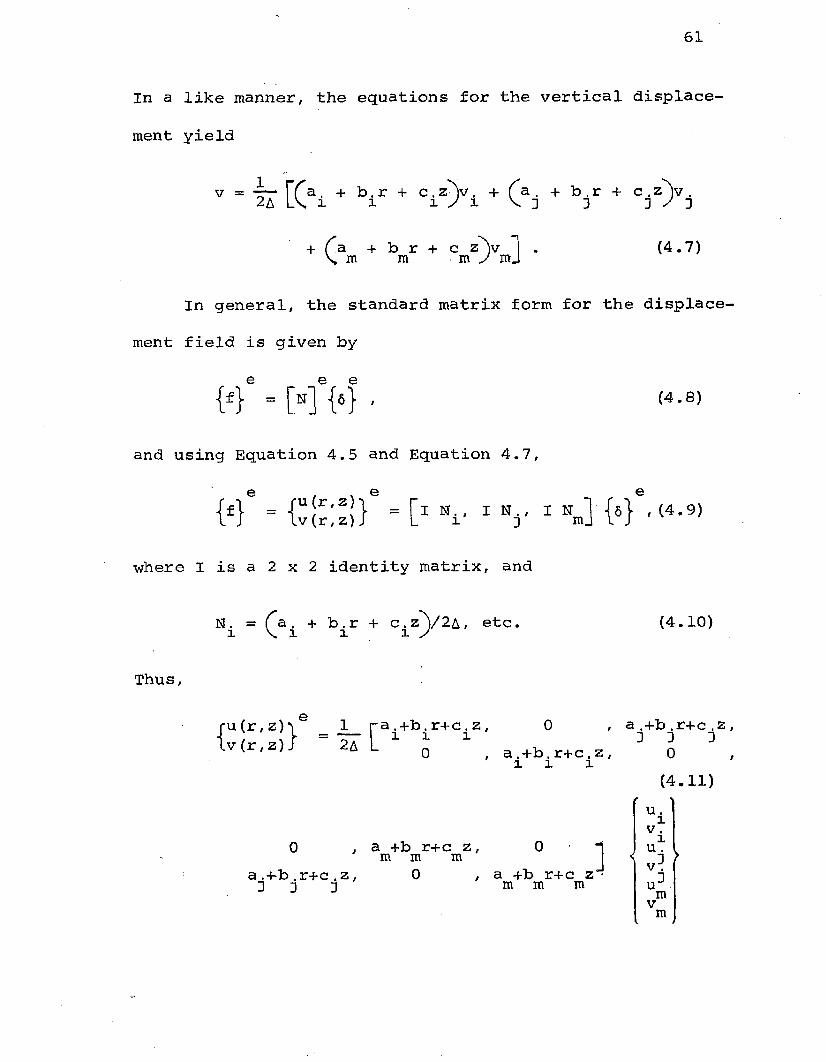
In a like manner, the equations for the vertical displace­

ment yield

v = rra . + b.r + c. z'V. + (a . + b . r + c, z'V .2 a L \ i l V.D 3 3 y 3

+ C a + b r + c z )v \ m m m J mj (4.7)

In general, the standard matrix form for the displace­ment field is given by

e e{*} - m { , } , (4.8)

and using Equation 4.5 and Equation 4.7,

{ £} * " { . M i } ' - t 1 Nr 1 V 1 Nm] {« }

where I is a 2 x 2 identity matrix, and

N. = ( a. + b . r + c.z )/2A, etc. i V i i x J (4.10)

Thus,

ru(r,z)'ie _ JL_ ra.+b,r+c,z,lv(r,z)J 2a L 1 q 1 , a.+b.r+c.z, x i x

, a +b r+c z, m m ma.+b.r+c.z, 0

3 3 D , a +b r+c z m m m]

a .+b .r+c ,z , 3 3 3

0(4.11)

u .xV . X< ujV.u3 mvm

62

To verify that this choice of displacement function satisfies the basic requirements listed in an earlier sec­tion on convergence criteria, the displacements u and v are first investigated in their original form,

u = a, + a9r + ouz1 (4.3)

v = a4 + a5r + a6Z '

where a,/ <x, are constant. These linear polynomials1 oare obviously continuous as are their first partial deriva­tives. Thus, the first requirement is satisfied. The second requirement, for the special case of triangular two- dimensional elements, is that the displacement vary linearly in each direction. Again, this requirement is satisfied by these two linear polynomials. The third requirement is therefore also satisfied since, as required, the displace­ment function was chosen as linear functions of the displacements.

The fourth requirement is discussed in the next section on strains, where it is illustrated that constant strains are in fact obtained with a constant condition.

2. Strain. The total strain at any point within the element can be defined by the components which contribute to internal work. For the axi-symmetric system, these are the four non-zero components which are illustrated along

63

with the associated stresses in Figure 4.4. In terms of displacements, these strains are given by

ts{•} ■

eeze< ef ► = <

^ r zi. <

dv/dzdu/dru/r

du/dz + dv/dr(4.12)

Using the displacement function defined by Equation 4.10, Equation 4.12 can be written in general as

e eB " [B1 B •and for the axi-symmetric problem as

. W" “ [Bi‘ V Bm] W ■in which

0 , cb. , 0 :

a./r + b^ + c.z/r, 01 X I b.x , etc,

Thus,

(4.13)

(4.14)

(4.15)

rz12A

0b ia . /r+b.+c.z/r, x x xCi

0

a /r+b +c z/r, m m mc ,m

c . ,o1 , 0 ,

bi'

0b.

a ./r+b^+c,z/r, 3 c 3 3j

m

m

c ., 0 3, 0 ,V

f u -XV .Xu .< v 3 \3umVmV

(4.16)

64

Z

- -I

rz rze j o j r r

Figure 4.4. Strains and Stresses in Axi-Symmetric Solids

Since the matrix [B]e involves the co-ordinates r andz, the strains are not constant within the element as in the plane stress or plane strain case. This is due to the

then the strains will he constant. As this is the only state of displacement coincident with a constant strain condition, it is clear that the displacement function satisfies the fourth convergence requirement.

3. Initial Strain (thermal strain). Initial strains are those that are independent of stress, and may be due to many causes. In general, for the axi-symmetric problem, four independent components of initial strain can result and are given by

Although these initial strains may, in general, depend on the position within the element, they are usually defined by average, constant values, and this procedure will be used in this analysis.

The most frequently encountered case of initial strain is that due to a thermal expansion, which for the isotropic material considered here yields

e term. Note, however, that if u is proportional to r, 0

eezoe e(4.17)

0where 0 is the average temperature rise in the element and a is the coefficient of thermal expansion.

In the generalization of the finite element method to account for creep in non-linear elastic problems, this ini­tial strain in the 'incremental-initial strain' procedure is assumed to be composed of two parts. For each increment of time, the initial strain increment is assumed to be com­posed of both a thermal and a creep component, i.e.,

4 K}= A k)+ 4 k) • <4-19)4. Elasticity Matrix. Assuming general elastic be­

haviour, the relationship between stresses and strains will be linear and of the general form

R e - [D]e CM* - kf ) - (4-20>0where [D] is an elasticity matrix containing the appro­

priate material properties of the general element, e.For the axi-symmetric problem, this becomes

67

The elasticity matrix [D] is derived by writing for the isotropic three-dimensional case considered here (ignoring the initial strains for convenience)

rz

' v O r + QCD

- £ 0 . - V 0 e + O )

= ■ 1 0 * - v 0 z + O )2 ( 1 +

; E ^ Ozr)' 1

(4.22)

and then solving for the stresses. This yields

E(l-y)(1+v) (l-2v)

VV ____l-v 1-V

1 -r-l—V

0

(4.23)

(symmetric) ~(i^v)

where, in general, each element may have different values for the material values E and

5. The Stiffness Matrix. The stiffness matrix of the element ijm can now be computed according to the general relationship*

♦Derivation of stiffness matrix in Appendix.

68

T[k]e = ^ t B ] e [D]0[B]0d(vol) . (4.24)

For the axi-symmetric problem, this becomesT

[k]® = 2tt ^ [B]e [D]®[B]er dr dz . (4.25)

6Since the matrix [B] depends on the co-ordinates,the integration cannot be performed as easily as in thecase of the plane stress problem. The simplest approximate

0procedure is to evaluate [B] for a centroidal point

= ( ri + r j + rnD/3

" (zi + zi + v )/3 '(4.26)

3

which gives as a first approximationT*

[k]e « 2tt [B]e [D]®[B3e r A, (4.27)

where A is the triangle area.0With the matrix [B] of Equation 4.13 written as

[B]S = [Ei. B., -Bj (4.28)

and with ky Equation 4.15, the stiffness matrix,for computational convenience, can be written in a parti­tioned form as

69

k. .11 k. .13 k .lm

1—1 1_1 (D II k . .31 k. . 33 k.3m (4.29)k . mi k . m 3 kmm

in which the 2 by 2 submatrices are built up as

[krs] " 2" S [ ® r f H M r dr dZ ' (4.30)

At this stage, it is also useful to split up the submatrices into constant and variable parts

[BJ = [5i]+ [V] (4'31)in which ■*-s the- value of £B^ at the centroid as inEquation 4.27 and accounts for the variation fromthis value. Thus ^s given by

[V] - 0 0 0 0 1 0 0 0

{(ai+ciZ)/r r ( a: +c Ja^/rj-/2A. (4.32)

Substituting the above expression into Equation 4.30 and noting that

^ [Bi/] r dr dz ~ CO] ,

the following is obtained

[\s] = fra] + [krs']

(4.33)

(4.34)

70

in which the first term is given by

[Ers] ■ 2" [5r f [D]e [5s] E (4.35)

and the second term is a corrective term which is obtained

from

(2A)

001

000

0 0

( ar+crZ)/r ' C ar+Cr5> ' } ' { (as+Csz)/r

' (VV)7*}W J / r J - r dr dz J . (4.36)

If the various integrands are written in abbreviated nota­tion

s — dr dz = AI, r 1

dr dz = AI,

s dr dz = AI,,r 3

(4.37)

then the corrective term becomes

tkrs'] - 2 l L 33 0] K as ( h ' -) (4.38) -2

+ O W V r ) CI2 - 5 + CrCs C h “ !")} '

71

where the integrals I , I2# and I3 are evaluated explicitlyin terms of the nodal co-ordinates.„

6. External Nodal Forces. In the general axi-symmetric analysis, the nodal forces resulting from external loadsrepresent a combined effect of the forces acting along thewhole circumference of the circle forming the element 'node1. Thus, if R represents the radial component force per unit length of the circumference of a node (or a radius r), theexternal 'force1 which will be introduced in the computationis

Similarly, in the axial direction, the combined effect of the axial forces is represented by

7. Nodal Forces Due to Initial Strain. The general expression for the nodal forces due to initial strain* is

2tt r R . (4.39a)

2tt r z . (4.39b)

Thus, in general for the axi-symmetric analysis,2rr r , R .

(4.40)

*See derivation of stiffness matrix in Appendix.

72

Te e ek - r $ [ B] [ D] k ) d ‘v o l > - ' (4-4 1 >

eo

For the axi-symmetric analysis, this becomes

Te e e= _ 2tt ^ [b] r dr dz, (4.42)

e Oe e

and partitioning (noting that constant overthe element),

k} - -2" C S [Bifr dr dz) M k f • (4-43)eo

As in the stiffness matrix determination, the approximate expression

T © ©ki = -2n csi] [°] k> z (4-*4>eo

together with a 'corrective1 term can be used. This yields

{p.} = {f .} + {F.'} . (4.45)e e eo o o

However, the corrective term is now zero sincee

= 2tt Q ^ [Bi'] r dr d50 [D] {e0} = °* (4 -46>eo

Therefore, this gives exactly

.73

{f .} = - 2rr [I.] [d ] {eo} 5 A .eo

T e e(4.47)

8. Nodal Forces Due to Distributed Body Forces. The only distributed body forces (those acting on a unit volume of material within the element) in this specific axi- symmetric analysis will be that due to gravity, and in this analysis, it is insignificant and therefore, will be neg­lected. However, in a general problem, this contribution is written as

per unit volume of material in the r and z directions. The general expression for the nodal force due to distri buted body forces* is

(4.48)

Te e eP

d(vol) . (4.49)

For the axi-symmetric analysis, this becomesT

(4.50)

and partitioning,

(4.51)

*See derivation of stiffness matrix in Appendix.

74

Using a co-ordinate shift to the centroid of the triangular area and assuming the body forces are constant over this area,

Pi}p = = (%}p = - ( 4 - 5 2 )

9. Nodal Forces Due to Boundary Forces. Boundary elements, in general, are subjected to specified displace­ments and specified distributed external loading. The first presents no problem, but, a loading term has to be added to the nodes of the element which has a boundaryface. By the virtual work consideration, this results in

Te e^ |gj- d (area) , (4.53)

where is the distributed external load per unit areaand where the integration is taken over the boundary areaof the element. For the axi-symmetric case and constant load this becomes

Te e-jVj- = - 2rr ^ £n J r dr -jjgj- . (4.54)

For the expression to be valid, -|gj- must have the same number of components as . Thus, for this particularanalyses,

T. e e-jF. = - 2tt ^ r dr | , (4.55)

75

and partitioning,

{Fil = -2,1 S Nir dr C) • ( 4 - 5 6 )D 2In practice, an integration of this type is seldom

explicitly carried out. This boundary loading is usually considered by the analyst to be represented simply by concentrated loads acting on the boundary nodes and are calculated by direct static procedures.

10. Assembly and Analysis. With the above formulae derived, the solution for nodal displacements and stresses now follows a standard structural routine. Assuming elas­tic behaviour of the element, the characteristic relation for the element is of the form

{ f } S = [ k ] { 6 } + { f } + { f } + { f } , ( 4 . 5 7 )€ P i )o

ewhere -FJ- is a matrix giving all the forces acting on theelement, [k]e is defined by Equations 4.24 through 4.38,

e eis defined by Equations 4.1 through 4.11, |Fj- re-6O

presents the nodal forces required to balance any initialstrain and is defined by Equations 4.41 through 4.47,

erepresents the nodal forces required to balance any

Pdistributed loads acting on the element and is defined by

eEquations 4.48 through 4.52, and represents the nodal

b

76

forces required to balance distributed boundary loads and is defined by Equations 4.53 through 4.56. The first

ments of the nodes.A preliminary analysis is performed and this permits

a unique definition of stresses or internal reactions at any specified point or points of the element in terms of the nodal displacements. Defining such stresses by a

is obtained in which the last three terms are the stresses due to initial stresses, distributed element loads, and boundary loads respectively when no nodal displacement occurs.

To obtain a complete solution, the conditions of displacement compatibility and of equilibrium have to be satisfied throughout.

Any system of nodal displacements

eterm, , represents the forces induced by displace-

ematrix , a relationship of the form

e e . e e e e(4.58)

o

6 1(4.59)

77

listed now for the whole structure in which all the elements participate, automatically satisfies the first condition.

As the conditions of overall equilibrium have already been satisfied within an element, all that is necessary is to establish equilibrium conditions at the nodes of the structure. The resulting equations contains the displace­ments as unknowns, and once these have been solved, the 'structural' problem is determined.

In a general analysis, the structure is loaded by external forces

H -Rn

(4.60)

applied at the nodes in addition to the distributed loads applied to the individual elements. To establish the equilibrium conditions at a typical node, i, each component of has, in turn, to be equated to the sum of the compo­nent forces contributed by the elements meeting at the nodes. Considering all the force components, this gives

K} -1 {hi" • (4-61>where the summation, \ , is taken over all the elements of

e ethe structure. Substitution of Equation 4.57 for

78

and using the submatrices of the stiffness matrix of Equa>e

tion 4.29 to involve only the appropriate forces >

Equation 4.61 becomes

t o - \ l t o j ’t o * X t o ‘ * X t o ) *m-1 e e e e Po

I K}‘ • ( 4 - 6 2 )e bIf a particular element does not include the node in question, it will contain no submatrices with an i suffix and, therefore, its contribution will simply be zero. Once all nodes have been considered, the overall system of equations is established.

This system of equations can be written in matrix form as

[K] {6} = {r}.- {F}e - {f} - {f} , (4.63)o

in which the submatrices are

[K im] = I [k i j e

K t ‘ I {Fi}e e

K>b-xw: -b e bwith the summations including all the elements,

So 0 eo (4.64)ePe

79

The system of equations resulting from Equation 4.63 can be solved once the prescribed support, displacements have been substituted. Without substitution of a minimum number of prescribed displacements to prevent rigid body movement of the structure, it is impossible to solve this system, because the displacements cannot be uniquely deter­mined by the forces in such a situation. This physically obvious fact will result in the matrix [K] being singular,i.e., not possessing an inverse.

Once the solution of the unknown displacements has been obtained, the stresses at any part of the element can be found from its stress matrix. Substitution of Equation 4.13 into Equation 4.20 yields

0 0 ' 0 ^ 0' 0 W - HHW - M W - (4-65)6 6where by comparing with Equation 4.58, [D] [B] is recog-

e enized to be [S]e and - j e j is recognized to be

e„ To account for the effect of the distributed body

eoforces and the distributed boundary loads, these stress effects have to be added to Equation 4.65. This yields for the general analysis

w - hMw* - M W + Hpe + •

(4.66)

80

This is just Equation 4.58 which established 'a prior' the characteristics for each element and is applied to each element in turn.

Due to the matrix [B] being a function of position in the element, the stresses, unlike the plane problem where the stresses are constant in the element, vary throughout the element. It is convenient now to evaluate the average stress at the centroid of the element. Thus, Equation 4„66 becomes

■ mWw’ - MV + + {< •(4.67)

Zienkiewicz (48) indicates that this procedure causes a certain amount of oscillation of stress values between elements to occur and that a better approximation can be achieved by averaging nodal stresses. -

CHAPTER V

PROBLEM SOLUTION

INTRODUCTIONThe creep laws and corresponding mechanical models for

the salt pillar models which were presented in Chapter III neither satisfied this author nor did they meet the require­ments of this analysis. Thus, in this section, an 'improved' creep law and its corresponding mechanical model is presented and justification for its adoption given.

The finite element analysis for axi-symmetric bodies which was developed in Chapter IV was modified to handle creep effects and was applied to the salt pillar model and programmed in Fortran IV for the IBM 7040 computer. The program followed the general format of an existing two- dimensional program (48), but with many modifications in order to apply it to this problem. Because of limited com­puter space, two sets of programs were run; one for the elastic analysis and one for the creep analysis.

A thorough series of checks of the main programs and of the subroutines were performed before any attempt was made to run the entire program. Included in the output of each of the two analyses were the displacements of the

81

82

nodal points, the new nodal point co-ordinates, and the stresses in each element. A program was then written to plot the nodal points in the salt pillar model at different stages of the analysis.

THE CREEP LAW ADOPTED FOR SALTThe creep laws proposed by Serata and Obert in their

work with salt pillar models do not in either case truly represent the mechanical behaviour of salt.

Serata in his creep law and corresponding mechanicalmodel fitted his constants to the creep data so that theflow of his viscoplastic unit (Bingham model) diminishedwithin a relatively short period of time with the flow ofhis viscoelastic unit (Kelvin model) continuing for. a verylong or infinite length of time. This is rather confusingsince this is just opposite to what one would expect fromthese two units. Also, his strain rate equation (Equation3.2) involves a lateral stress (aT7V) which he, in severalLAplaces in his paper (18), implies is the lateral stress in the pillar, but, which actually is only the stress applied laterally at the roof and floor sections of his model.In the present analysis, this lateral stress at these two positions, in the interior, and in the pillar itself is one of the unknowns of the problem that is eventually solved for.

83

Obert's creep Law and corresponding mechanical model

{Burger's model) is a rather common one in rock mechanicsand has been used by several other investigators (62,63,64). Although it was used as the model for rock salt, itdoes not provide an exact representation of rock salt fortwo reasons. The first was indicated by Obert when heobserved that no set of constants for his creep law(Equation 3.3) would provide a fit for a family of curvesfor rock salt primarily because 3*r\ was not constant fordifferent values of a . The second becomes obvious

zo

after reviewing the literature on rock salt. Several in­vestigators (15,18,20,21,23,24) have observed that rock salt's creep rate continues to decrease with time, a characteristic which can be classified as the 'age harden­ing' property. Obert's steady state creep rate, however, remains constant with time.

Since Bradshaw's data on creep with the salt pillar models appears to be the best documented and the most com­plete, involving also the temperature as one of the vari­ables, a study was made of it in an attempt to use it to propose an approximate creep law for rock salt. In this process, the creep rate curve which he fitted to his data was separated into two components, a transient creep rate component and a steady creep rate component. The steady

84

creep rate component, unlike Obert's, was required to exhibit the 'age hardening' property of salt by having it fit the actual creep rate curve after the transient creep rate was no longer effective. Success was finally achieved with the following creep law for the salt pillar model which is proposed at this time:

The first term on the right represents the elastic strain, the second represents the transient creep, and the third represents the steady state creep.

The mechanical model corresponding to this creep law is presented in Figure 5.1. It consists of a Hookean unit and two Kelvin units, with the steady creep Kelvin-unit possessing a more viscous dashpot but a much weaker spring than the transient creep Kelvin unit. The following relations are implied:

azezo o

(5.1)

where: ^ ( ^ = T10.9

o o

85

E. E,

Et A W —

— v y v v ' —

z o ^i-H7<

- V W V ^ y ^ A A A A A

f]'

Elastic Transient-Creep | Unit | Unit |

Steady-CreepUnit

Figure 5.1. Mechanical Model Proposed for Rock Salt

The strain rate was obtained by taking a time deriva­tive of Equation (5.2) to give

*z - (Cla> l ' T)fi >z > " at + ( ca 0 fl<T)£/ > z > " Bt-o 7 o o(5.3)

The four constants, C , C , a and @ were obtained by curveJ. £fitting to Equation (3.7) which represents Bradshaw’s data. These constants are independent of time, stress and temperature.

The results of the curve fitting are presented in Figures 5.2 through 5.4. The first is a plot at constant temperature and various pillar stresses of the transient creep rate, the steady creep rate, the sum of these two components and also the creep rate as obtained by Bradshaw. The second is a plot at constant pillar stress and various temperatures of the same quantities. The third is a sample

87

Strain Rate vs Time Temperature = 27° C 0 = Bradshaw's Creep Rate A = Transient Creep Rate

+ Steady Creep Rate

8,000

50 100 150Figure 5.2. Strain Rate at Constant Temperature

88

o10

Strain Rate vs Time 6,000 psi

Bradshaw’s Creep Curve Transient Creep Rate + Steady Creep Rate

Stress

110

200'

210

310

Figure 5.3. Strain Rate at Constant Stress

89

CREEP PATE CI-ECK EEFCERCN, W. PARCH 6 8 L S t

DELTA = 5 . CAVSSTRESS = 6 C C 0 . P S ITEPF = 3 C 0 . CEG. KEL,

CI AALPHAC2BBETACTR

0 . 4 1 7 C E - 2 1 - 0 . 1 0 ACE CC

0 . 9 7 4 0 E - 2 2 - C . 6 7 0 C E - 0 2

C . 7 6 8 C E - 2 C

IRE TCR SCR TR TESTR

5 . 3 . C 5 4 9 7 9 8 6 - C 3 1 . 1 6 0 6 8 8 0 E - C 3 4 . 2 1 5 6 6 7 8 E - C 3 4 . 2 1 3 0 7 1 6 E - C 31 C. 1 . 8 1 6 24 83 E- C 3 1 . 1 2 2 4 4 9 1 E - C 3 2 . 9 3 8 6 9 7 3 E - C 3 2 . 6 8 4 9 C 7 6 E - C 31 5 . 1 . C1 9 79 6 9 E - 0 3 1 . 0 8 5 4 6 9 9 E - C 3 2 . 16 5 2 6 6 8 E - C 3 2 . 0 6 2 8 6 1 2 E - C 32 C . 6 . 4 1 9 6 1 4 6 E - C 4 1 • 0 4 5 7 0 9 0 E - C 3 1 . 6 5 1 6 7 C 4 E - 0 3 1 . 7 1 1 0 3 8 8 E - C 32 5 . 3 . 8 1 6 5 9 2 7 E - C 4 1 . 0 1 5 1 2 6 2 E - C 3 1 . 3 5 6 7 8 5 5 E - C 3 1 . 4 8 0 0 2 2 6 E - C 33 C . 2 . 2 6 9 C 4 2 8 E - C4 5 . E 1 6 8 2 7 9 E - 0 4 I . 2 C e 5 8 7 1 E - C 3 1 . 3 1 4 6 2 0 8 E - C 33 5 . 1 . 3 4 8 9 9 2 6 E - 0 4 9 • 4 9 3 4 1 1 7 E - C 4 1 . 0 £ 4 2 4 0 4 E - C 3 1 • 1 8 9 2 8 2 7 E - C 3AC. 8 . C 2 C 0 3 8 2 E - 0 5 5 . 1 8 0 6 5 0 3 E - C 4 9 . 5 8 2 6 54 I E - 0 4 I . 0 9 0 4 1 1 3 E - C 34 5 . 4 . 7 6 8 0 7 7 3 E - 0 5 f i . 8 7 8 1 9 2 9 E - C 4 9 . 3 5 5 C 0 0 7 E - 0 4 1 . C 10 C 4 6 1 E - C 35 0 . 2 . 8 3 4 7 2 0 0 E - 0 5 £ . 5 8 5 7 0 0 1 E —0 4 8 . 8 6 5 1 7 2 1 E - 0 4 9 . 4 3 1 8 9 2 5 E - C 45 5 . 1 . 6 £ 5 2 9 9 3 E - C 5 8 , 3 0 2 8 4 3 5 E - 0 4 8 . 4 7 1 3 7 3 4 E - 0 4 8 . 8 6 5 3 0 3 0 E - C 46 0 . 1 . C C 1 9 4 5 0 E - 0 5 E . 0 2 9 3 0 5 6 E - C 4 8 . 1 2 9 5 C C 0 E - 0 4 8 . 3 7 7 8 1 9 8 E - C 46 5 . 5 . 9 5 6 76 9 3 E - C 6 7 . 7 6 4 7 7 9 4 E - C 4 7■8 2 4 3 4 7 0 E - 0 4 7 . 9 5 3 0 B 5 3 E - C 47C . 3 . 5 4 1 4 2 1 8 6 - 0 6 7 . 5 0 8 9 6 8 I E - 0 4 7 . 5 4 4 3 82 2 E - 0 4 7 . 5 7 9 0 6 4 8 E - C 47 5 . 2 . 1 C 5 4 4 7 9 E - 0 6 7 . 2 6 1 5 8 4 4 E - C 4 7 . 2 8 2 6 3 E 8 E - 0 4 7 . 2 4 6 6 8 7 4 E - C 48 0 . 1 . 2 5 1 7 32 2 E - C 6 7 . 0 2 2 3 5 0 9 E - C 4 7 . C 3 4 8 6 8 2 E - 0 4 6 . 9 4 8 9 7 6 6 E - C 48 5 . 7 . 4 4 1 8 0 4 9 E - 0 7 £ , 7 9 0 5 9 8 9 E - 0 4 6 . 7 5 8 4 4 C 6 E - C 4 6 . 6 B 0 4 7 0 0 E - C 49 0 . 4 . 4 2 4 3 0 5 6 E - 0 7 £ . 5 6 7 2 6 8 9 E - C 4 6 . 5 7 1 6 9 3 2 E - 0 4 6 . 4 3 6 8 2 50 E - C 49 5 . 2 . 6 3 0 3 4 C 6 E - 0 7 6 . 3 5 0 9 0 9 6 E - C 4 6 . 3 5 35 4 C 0 E - C 4 6 . 2 1 4 5 4 0 2 E - C 4

I O C . 1 . 5 6 3 7 9 1 6 E - 0 7 6 . 1 4 1 6 7 8 2 E - C 4 6 . 1 4 3 2 4 2 0 E - 0 4 6 . 0 1 0 7 5 9 4 E - C 41 0 5 . 9 . 2 5 7 0 6 2 3 E - C 8 5 . 9 3 9 3 4 0 I E - 0 4 5 . 5 4 C 2 6 9 8 E - 0 4 5 . 8 2 3 1 2 7 6 E - C 41 1 0 . 5 . 5 2 7 2 9 4 7 E - C 8 5 . 7 4 3 6 6 8 1 E - C 4 5 . 7 4 4 2 2 0 8 E - 0 4 5 . 6 4 9 6 8 3 1 E - C 41 1 5 . 3 . 2 8 6 0 9 0 3 E - 0 8 5 . 5 5 4 4 4 2 4 E - C 4 5 . 5 5 4 7 7 1 1 E - C 4 5 . 4 0 8 7 7 8 9 E - C 41 2 0 , 1 . 9 5 3 6 4 8 0 E - C 8 5 . 3 7 1 4 50 9 E - C 4 5 . 3 7 1 6 4 6 2 E - C 4 5 . 3 3 9 0 1 9 7 E - C 41 2 5 . 1 . 1 6 1 4 E 3 9 E - 0 8 5 . 1 9 4 4 8 7 9 E - C 4 5 . 1 5 4 6 0 4 C E - C 4 5 . 1 9 9 2 1 5 7 E - C 41 3 C . 6 . 5 C 5 2 6 0 7 E - 0 5 5 . 0 2 3 3 5 5 0 E - C 4 5 . 0 2 34 2 4 0 E - 0 4 5 . 0 6 8 3 4 50 E - C41 3 5 . 4 . 1 C 5 3 1 5 5 E - 0 5 4 . 8 5 7 8 6 0 2 E - C 4 4 . 8 5 7 9 0 1 2 E - 0 4 4 . 9 4 5 5 2 4 8 E - C 41 AC. 2 . 4 40 6 5 6 8 E - C 5 4 . 6 9 7 8 1 7 6 E - C 4 4 . 6 5 7 8 4 1 9 E - 0 4 4 . 8 2 9 9 8 8 8 E - 0 41 4 5 • 1 . 4 5 1 0 4 4 4 E - 0 5 4 . 5 4 3 0 4 7 5 E - C 4 4 . 5 4 3 C 6 2 0 E - 0 4 4 . 7 2 1 0 6 6 8 E - C 41 5 C . 8 . 6 2 6 7 5 6 5 E - 10 4 . 3 9 3 3 7 6 4 E - 0 4 4 . 3 5 3 3 8 5 1 E - C 4 4 . 6 1 8 1 7 1 3 E - C 4

Figure 5.4. Sample of Results From Creep Rate Analysis

90

of the results obtained from the program which is included in the Appendix. As can be noted, a relatively good and consistent matching was obtained with the sum of the two creep rate components and Bradshaw's creep rate.

Assuming that the creep strain occurs without volume change, i.e., in a similar manner to the usual plastic strain assumption, the 'uniaxial1 strain rate of Equation 5.3 is generalized to give

which depends on Poisson's ratio alone.

If Bradshaw's creep rate' curve (Equation 3.7) had been obtained in axial tests of salt samples, then the five con­stants C^, , a, (3, and K would in Equation 5.4 give thecorrect strain rate. His creep rate curve, however, was an expression for the creep rate of the pillar model in the

ez

It C*10-9)Y T rT rz

(5.4)

where the effective stress, a, is given by

and where fD 1 is that part of the elasticity matrixL oj

91

■axial direction in terms of the average applied pillar stress. Since there are no data at this time from which to obtain the correct values of these constants, the values as obtained from Equation 3.7 will be used. Additional comments regarding the use of the above equations will appear in a later chapter.

CREEP EFFECTS MODIFICATIONS

In order to account for the time dependent strain (creep), the general format of the 'incremental-variable elasticity' procedure as suggested by Zienkiewicz (48) is followed, but with some additional modifications to fit the conditions of this analysis, i.e., instantaneous applied, constant pillar load, no separate component of plastic strain, and time dependent strain. The pillar load is instantaneously applied and maintained constant for a given increment of time with the nodal point displacements at the end of this increment found, by the use of a suit­ably modified elasticity matrix, as if the material was elastic.

For the elastic strain,1e e e

(5.6)

92

For the creep strain,

k}e = ce[Do] W*« <5-7)where

Ce = Ce (t, T, 0)- (5.8)

Thus,-1 -1e e

{ • . } = C [ De] ♦ c» [ do] ) H ■(5.9)

or,-1 -1 -1e eH -CM +ceK] ) ({«•}* W ) •

(5.10)This defines an 1elasto-creep1 value of an elasticity

matrix as-1 -1 -1

[V] -CM *'•[”.] 5 'In general, the complete problem is solved in an

iterative way as described by the following steps:1. The full load is applied to the structure and

the elastic displacements.,.. , and stresses,e i,based on E = .Ee and t = 0 are determined

respectively for each nodal point and eachelement.

93

2. For a fixed At > 0 (i.e., at a particular instant),a new value of E = E is determined for eachecelement depending on the state of stress reachedin that element in the preceeding step. The total

edisplacement, / an<a the stress, , for

iAt is then determined. This stress is now usedin the first step of iteration in this particular

etime interval to find a better estimate of 46 V .I ecjThe iteration procedure is used until reasonable convergence has occurred.

3. The new co-ordinates of each nodal point is foundby an<3 used to calculate

new. old.i i

a new stiffness matrix for the next time interval.4. Step 1 is repeated with the new stiffness matrix.5. Step 2 is repeated.6. Step 3 is repeated, etc.

In reference to the iteration of the second step; Argyris (59) in a problem similar to this one, but involving plas­tic deformations with the 'incremental initial strain' method, suggested that it is sometimes not really necessary to perform this iteration procedure if the time interval is small enough, but that an improvement can be achieved

94

by specifying a limited number (two. or three) iterations to be carried out in each time interval.

THE APPLICATION OF THE FINITE ELEMENT METHODThe general finite element method presented in Chapter

IV with the creep modifications developed in this chapter was adapted to the solution of displacements and stresses in the salt pillar model. The solution was carried out with a pillar stress of 6,000 psi and a temperature of 300°K using step 1 and step 2, with no iterations, com­pletely through the first time interval of two days.

The assumptions which were discussed earlier in pre­vious chapters and used in the application of this method to the axi-symmetric salt pillar model were:

1. Rock salt was homogeneous and isotropic.2. The elastic properties measured by Serata

(see Chapter III) were the ones which are most applicable to this problem and were used in the elastic analysis.

3. The creep curves of Bradshaw (see 'The Creep Law Adopted for Salt’ in this chapter) are the most general and the best documented and were the ones used for the creep analysis.

95

4. The applied pillar load was instantaneously applied and maintained constant.

5. The only nodal forces were those due to the applied pillar loads.

6. The salt pillar model was maintained at constant temperature.

7. The initial strain was zero.8. There was no separate component of plastic

strain.9. The stress in each element was evaluated at

its centroidal point and was assumed constant over the element.

The axi-symmetric salt pillar model was divided into 'two-dimensional' elements as discussed in Chapter IV and illustrated in the top part of Figure 4.2-C. The division used produced 77 nodal points and 117 elements. (See plot of original nodal points by Calcomp 553 Plotter, Figure 5.12.) With two degrees of freedom associated with each nodal point, the solution of 154 simultaneous equations was required.

The linear elastic solution of these simultaneous equations for the displacements and then the stresses was accomplished by a program which followed the format of the one proposed by Zienkiewicz and Cheung (48) for plane stress

96

or plane strain triangular elements. The program was studied in detail and then altered to convert it to an axi-symmetric program, to account for the time dependent strain, and to implement it on the IBM 7040. Major changes were required in the main program and in all subroutines except 'Solve1 and .'Matinv'. Because of limited space re­maining in the computer, a separate program similar to the linear elasticity one, but with a few changes and additions, was written to include the effects of the time dependent strain. Flow charts of these two programs appear in Figure 5.5 and Figure 5.6, with the programs appearing in the Appendix. (See Appendix C and Appendix D.) Figures 5.7 through 5.10 contain the printed output of the creep analy­sis program for a 6,000 psi applied pillar load, 300°K constant temperature and for the first time increment of 2 days.

An important feature of these programs was the sub­division of the stiffness matrix into parts which were then written in a tridiagonalized manner. This allowed for the solution of the equations in steps by inverting only a small part of the overall stiffness matrix and not the entire matrix at one time. This was accomplished by dividing the idealized structure into segments called 'partitions'. In this analysis, five partitions were used

97

START

y t

(1) Read input data.

(2).. .. .................................. ____________________________________________________________

Loop: 1 = 1 , number of partitions.’ f _ .

(3) Loop: J = first element, last element.1

(4) Call subroutine for calculation of nodal forces.

> *(5) Call subroutine for formation of element

stiffness and stress matrices.

(6) Assemblage of overall stiffness*matrix.

(7) Introduction of prescribed displacements.--------------------- — i __ .

(8) Call subroutine for solution of equationsand calculation of residuals.

............... . . .... . .. . - ........ .(9) call subroutine for calculation of displace­

ments, co-ordinates of displaced nodal points, and stresses and printing (punching) of output.

STOP

Figure 5.5. Flow Chart of Elastic Analysis Program.

98

START

(1) Read input data.

(7) Assemblage of overall stiffness matrix.

(8) Introduction of prescribed displacements.

(2) Loop: I = 1, number of partitions.

(3) Loop: J = first element, last element.

(9) call subroutine for solution of equations and calculation of residuals.

(5) Introduction of time, temperature, and stress dependent creep effects.

(6) Call subroutine for formation of element stiffness and stress matrices.

(4) call subroutine for calculation of nodal forces.

(10) Call subroutine for calculation of displace­ments, co-ordinates of displaced nodal points, and stresses and printing (punching) of output.

STOP

Figure 5.6. Flow Chart of Creep Modifications program.

99

F I N I T E E L E f E M ANALYSIS CF SALT PI LL AR PODELS CREEP PCC IF I CATI CNS

BERCEPCN, k. APRIL,1S66 L.S.U.

AVERAGE PILLAR STRESS = 6 C C 0 . PSINOCE P - C I S P l AC E P E M S Z - D I S P L A C E P E N T S NEk R CC-•CRD. NEW Z CC-•CFG.

1 1 . 2 2 3 1 8 5 4 E - 1 4 - 7 . 4 1 0 7 4 4 1 E - 0 3 1 . 2 3 3 1 8 5 4 E - 14 1 . 4 9 2 5 8 9 3 E CO2 - S . 6 1 7 9 3 7 3 E - 1 6 - 1 . 4 3 6 1 3 9 7 E - C 2 - 9 . 6 1 7 9 3 7 3 E - 16 1 . 1 8 5 6 3 8 6 E CO3 - 4 . S 6 3 7 8 9 1 E - 1 5 - 1 . 9 0 3 9 2 4 2 E- C 2 - 4 . 9 6 3 7 8 9 1 E- 15 8 . 8 C 5 6 C7 6 E -C 14 - 8 . S 7 3 C 2 6 5 E - 1 6 - 1 . 4 6 7 8 5 1 4 E - C 2 - 8 . S 7 3 C 2 6 5 E- 16 5 . 8 5 3 2 1 4 5 E - C 15 - 9 . 7 6 6 8 1 2 0 E - 1 6 - 9 . 0 6 1 9 3 8 4 E -C 3 - S . 7 6 6 8 1 2 C E- 16 2 . 9 0 9 3 8 0 6 E - C l6 - 1 . 6 0 4 8 5 5 1 E - 2 2 - 1 . 3 8 7 8 1 7 3 E - 1 5 - 1 . 6 C 4 8 5 5 1 E- 2 2 - 1 . 3 8 7 6 1 7 3 E - 1 57 1 . 4 7 7 6 4 6 5 E- C 2 - 2 . 2 1 2 7 2 2 6 E - C 2 3 . 1 4 7 7 6 4 7 E- 0 1 1 . 4 7 7 8 7 2 8 E COe - 3 . 6 1 1 9 9 2 7 E-C 2 - 3 . 3 C 6 3 3 6 4 E - C 3 2 . 9 6 3 e e C l E - 0 1 . 1 . 1 9 6 6 9 3 7 E CC5 - 2 . 4 E E 8 8 S 2 E-C 2 - 9 . 5 7 7 3 1 4 1 E - 0 3 2 . 9 7 5 4 1 1 1 E- 0 1 8 . 9 0 4 2 2 6 8 E - C 1

1C 2 . C S 6 9 C 8 0 E-C 3 - 1 . 1 3 2 1 1 7 5 E- C 2 3 . C 2 0 9 6 S 1 E- 0 1 5 . 8 8 6 7 8 8 2 E - C 1l i 2 . 7 5 3 7 2 6 6 E- C 3 - 6 . 5 6 4 6 2 7 3 E - 0 3 3 . 0 2 7 5 3 7 3 E- 0 1 2 . 9 3 4 3 5 3 8 E - C 112 4 . EC 9 3 0 4 3 E-C 2 - 1 . 7 8 8 1 2 3 1 E - 1 5 3 . 0 4 5 C 9 3 1 6 - 01 - 1 . 7 8 8 1 2 3 1 E - 1 512 1 . 8 2 6 1 2 1 4 E - 0 2 - 2 . 4 8 8 3 3 6 1 E - G 2 6 . 1 8 2 6 1 2 1 E - 0 1 1 . 4 7 5 1 1 6 6 E CC14 9 . 1 5 8 4 5 3 0 E - 0 2 - 1 . 3 8 5 8 C 3 C £ - 0 2 6 . C S 1 5 8 4 5 E-•01 1 . 1 8 6 1C2C E CO15 - 5 . 8 4 6 6 0 0 1 E - C 2 - 1 . 7 7 9 4 8 3 8 6 - C 3 5 . 9 4 1 5 3 4 C E- 0 1 8 . 5 8 2 2 C 5 1 E - C 116 5 . C 2 6 7 1 0 0 E- C 4 - 5 . 9 6 5 9 6 0 4 E - C 3 6 . OC 50 26 7 E-■01 5 . 5 4 C 3 4 C 2 E -C 117 4 . 5 8 1 2 1 9 4 E- C 2 - 5 . 4 5 5 7 3 4 4 E- C 3 6 . 0 4 9 8 1 2 1 E- ■01 2 . 9 4 5 4 4 2 7 E -C 1I E 7 . 3 5 6 9 5 1 2 E - C ? - 1 . 8 3 1 0 0 8 2 E - 1 5 6 . 0 7 3 5 6 9 5 E- 0 1 - 1 . B 3 1 C C 8 2 E - 1 5I S 2 . 1 2 8 2 3 3 6 E-C 2 - 2 . 6 1 1 4 4 5 4 E-C 2 9 . 2 1 3 8 3 3 3 E- 0 1 1 . 4 7 3 E 8 5 5 E CC2C 1 . 3 2 8 5 9 6 9 E-C 2 - 1 . 7 0 5 1 6 7 1 E-C 2 9 . 1 3 3 8 9 5 7 E- 01 1 . 1 8 2 5 4 8 3 E CC21 4 . 5 1 1 2 7 5 3 E - 0 2 - 1 . 0 1 1 8 7 4 2 E - C 2 5 . 0 4 5 1 1 2 7 E -■01 8 . 8 9 8 8 1 2 5 E - C 122 - 2 . 3 6 7 2 1 6 0 E - 0 2 - 3 . 7 5 1 4 1 3 8 E - C 5 8 . 9 7 6 3 2 7 8 6 - ■01 5 . 5 9 9 6 2 4 8 E - C 12 3 4 . 2 2 3 0 0 8 2 E- C 2 - 1 . 9 9 1 1 8 8 7 E - C 3 5 . 0 4 2 3 3 C C E- 0 1 2 . 9 8 C C 8 8 1 E- C 124 9 . 6 2 0 5 6 8 5 E-C 2 - 2 . 0 8 9 1 6 4 E E - 1 5 9 . C S 6 2 C 5 6 E- 01 - 2 . C 8 5 1 6 4 8 E - 1 52 5 3 . 3 7 3 2 3 3 5 E- C 2 - 3 . 9 3 0 3 6 4 6 E - C 2 1 . 2 3 3 7 3 2 3 E 0 0 1 . 4 6 0 6 9 6 3 E CO26 1 . 6 5 1 0 5 8 8 E- C 2 - 2 . 0 9 7 2 6 6 6 E - C 2 1 . 2 1 6 5 1 C 6 E OC 1 . 1 7 9 C 2 7 3 E CO2 7 8 . C A 7 4 9 5 1 E - 0 2 - 1 . 5 C 0 7 3 1 1 E - C 2 1 . 2 C 8 0 4 7 5 E CO 8 . 8 4 5 5 2 6 8 E - C 12 e 6 . 7 6 5 8 2 4 1 E - 0 2 - 9 . 8 2 8 7 7 8 2 E - 0 3 1 . 2 C 6 7 6 5 8 E OC 5 . 9 C 1 7 1 2 2 E-C 12S 2 . C 2 4 0 0 5 9 E - 0 2 3 . 9 1 5 3 4 7 0 E - C 4 1 . 2 C 2 C 2 4 0 E OC 3 . 0 0 3 5 1 5 4 E - C 13C 9 . 2 E 1 4 8 1 4 E - 0 3 - 1 . 7 4 1 5 7 4 0 E - 1 5 1 . 2 0 9 2 8 1 5 E 0 0 - 1 . 7 4 1 5 7 4 0 E - 1 53 1 3 . 7 C 9 2 3 2 1 E-C 2 - 4 . 5 7 1 5 0 0 9 E - C 2 1 . 5 3 7 0 5 2 3 E OC 1 . 4 5 4 2 8 5 0 E CO32 2 . 8 1 5 8 9 2 2 E - 0 2 - 3 . 5 7 4 7 6 9 C E - C 2 1 . 5 2 8 1 5 8 5 E OG 1 . 1 6 4 2 5 2 3 E CO33 1 . 0 5 5 4 0 3 8 E - 0 2 - 2 . 0 5 6 6 0 0 8 E - 0 2 1 . 5 1 0 5 5 4 0 E OC 8 . 7 9 4 3 3 9 5 E - C 13 4 9 . 7 2 4 8 8 8 0 E-C 2 - 1 . 6 1 5 8 6 7 5 E- C 2 1 . 5 0 9 7 2 4 5 E 0 0 5 . 8 3 8 4 1 3 2 E - C 135 1 .C 5 8 3 2 8 0 E-C 2 - 1 . 1 1 0 5 2 3 5 E - 0 2 1 . 5 1 0 9 8 3 3 E 0 0 2 . 8 8 8 5 4 7 7 E - C 136 7 . 4 6 4 6 3 5 1 E - C 2 - 2 . 9 3 5 3 3 8 4 E - 1 5 1 . 5 0 7 4 6 4 6 E 0 0 - 2 . 9 3 5 3 3 8 4 E - 1 53 7 3 . 4 3 0 8 6 7 7 E-C 2 - 6 . 3 6 3 0 3 2 0 E - C 2 1 . 8 3 4 3 0 8 7 E OG 1 . 4 3 6 3 6 9 7 E CO38 3 . 1 4 4 7 9 3 7 E - C 2 - 6 . 0 7 5 6 5 7 3 E - 0 2 1 . 8 3 1 4 4 7 9 E OC 1 . 1 3 9 2 4 3 4 E CO3S 2 . 1 3 8 7 9 2 2 E - 0 2 - 5 . 3 1 3 9 9 9 6 E - 0 2 1 . 8 2 1 3 8 7 9 E OC 8 . 4 6 8 6 C 0 C E - C 14C 1 . 2 C 5 7 4 4 6 E - 0 2 - 4 . 6 5 7 1 9 4 C E - C 2 1 . 8 1 2 C 5 7 4 e 00 7 . 0 3 4 2 8 0 6 E - C 14 1 1 . 2 5 8 3 8 3 0 E - 0 2 - 4 . 3 9 2 7 2 7 5 E - C 2 1 . 8 1 2 5 8 3 8 E 0 0 5 . 5 6 0 7 2 7 3 E - 0 14 2 1 . 2 9 6 5 0 2 2 E - 0 2 - 4 . 1 5 6 9 6 6 1 E - 0 2 1 . 8 1 2 9 6 5 C E OC 4 . 0 8 4 3 0 3 4 E - C 14 3 3 . 4 2 3 7 6 9 5 E - 0 2 - 2 . 8 1 2 0 4 7 3 E - 0 2 1 . 8 3 4 2 3 7 7 E 0 0 2 . 7 1 8 7 9 5 3 E - C 14 4 1 . 8 1 6 8 6 8 6 E- C 2 - 1 . 4 5 1 7 8 1 1 E - C 2 1 . 8 1 8 1 6 E 7 E OC 1 . 3 5 4 8 2 1 9 E - C 14 5 3 . 2 8 4 6 6 4 7 E -C 2 - 1 . 1 2 6 5 6 3 5 E - 1 5 1 . 8 3 2 8 4 6 6 E OC - 1 . 1 2 6 5 6 3 5 E - 1 54 6 3 . 2 5 9 5 8 4 2 E - 0 2 - 8 . 5 7 0 7 0 2 0 E - C 2 2 . 1 3 2 5 9 5 8 E OC 1 . 4 1 4 2 9 3 0 E 0 04 7 2 . E 7 7 5 9 0 2 E-C 2 - 8 . 2 9 3 0 5 5 4 E - C 2 2 . 1 2 8 7 7 5 9 E 0 0 1 . 1 1 7 C 6 9 0 E CO4 8 2 . 4 3 1 6 9 5 9 E - C 2 - 8 . 1 7 9 2 2 C 2 E - C 2 2 . 1 2 4 3 1 7 0 E OC B . 1 8 2 C 7 7 S E - C 14 S 1 . 5 4 1 1 5 2 5 E - 0 2 - 6 . 8 3 3 8 4 0 5 E - 0 2 2 . 0 1 5 4 1 1 5 E 0 0 6 . 3 1 6 6 1 5 9 E-C 1

Figure 5.7. Results of Creep Analysis

100

5C 1 . 4 C 2 6 3 9 4 e - c : - 6 . 4 C 2 0 9 8 4 E - C 2 2 . C 1 4 C 2 6 4 E CC 4 . 3 5 5 7 5 C 2 E - C l51 1 . 3 5 7 5 2 9 0 E - 0 2 - 5 . 5 5 8 2 0 4 2 E- C 2 1 . 9 1 3 5 7 5 3 E OC 5 . 8 4 4 1 7 8 5 E - C l5Z 4 . 6 6 9 6 2 4 5 E -C 2 - 5 . 1 6 2 9 1 6 3 E - C 2 2 . 0 4 8 6 9 6 2 E CC 2 . 4 8 3 7C84 E-C 153 4 . 6 5 6 1 2 3 7 E -C 2 - 4 . 4 2 3 8 4 1 2 E - 1 6 2 . 0 4 8 5 6 1 2 E OC - 4 . 4 2 3 8 4 1 3 e -1854 3 . 1 1 6 8 1 6 8 E -C 2 - 5 . 6 3 2 7 1 8 6 E - C 2 2 . 4 3 1 1 6 6 2 E OC 1 . 4 C 3 6 7 2 8 E CC55 2 . 7 1 4 C 3 8 0 E- C 2 - 9 . 4 C 1 8 9 C 7 E - C 2 2 . 4 2 7 1 4 C 4 E OC 1 . 1 0 5 5 8 1 1 E CC56 2 . 1 5 5 4 3 6 6 E-C 2 - 9 . 2 5 3 4 3 6 4 E - C 2 2 . 4 2 1 5 5 4 4 E OC 8 . 0 7 4 6 5 6 3 E - C l57 l . e i 5 3 1 9 1 E-C 2 - 8 . 5 4 2 4 9 3 4 E -C 2 2 . 2 1 8 1 5 3 2 E OC 6 . 1 4 5 7 5 C 7 E - C l58 1 . 1 6 7 5 7 4 6 E-C 2 - 8 . 6 C 7 9 8 7 9 E - C 2 2 . 2 1 1 6 7 5 8 E OC 4 . 1 3 5 2 C 1 2 E - C l55 1 . 6 4 C C 9 3 7 E-C 2 - 9 . 2 2 3 6 7 3 9 E- C 2 2 . 4 1 6 4 C 1 C E OC 6 . 0 7 6 6 3 2 6 E - C l6C 1 . C 7 6 3 7 9 0 E-C 2 - 9 . 2 2 1 4 5 3 1 E - C 2 2 . 4 1 0 7 6 3 8 E OC 4 . 0 7 7 8 5 4 7 E - C l61 2 . 5 6 0 4 9 1 9 E-C 2 - 1 . 0 3 4 5 C 3 4 E - C 1 2 . 7 2 9 6 0 4 8 E OC 1 . 3 9 6 5 4 5 6 E CO6 2 2 . 5 6 2 7 3 8 5 6 - C 2 - 1 . 0 1 8 5 0 1 5 E - C 1 2 . 7 2 5 8 2 7 4 E OC 1 . 0 8 8 1 4 5 5 E CC63 2 . C C 2 4 7 9 6 E-C 2 - 1 . 0 0 4 9 9 5 2 E - C 1 2 . 7 2 C C 2 4 8 E OC 7 . 5 5 5 C 0 4 6 E-C 164 1 . 5 2 5 5 2 6 5 E- C 2 - 9 . 7 4 5 9 6 5 2 E - C 2 2 . 6 1 5 3 5 5 3 E OC 6 . 0 2 5 4 0 3 4 E - C l6 5 1 . 0 * 3 3 7 5 4 E-C 2 - 9 . 7 2 1 8 2 6 1 E- C 2 2 . 6 1 0 4 3 3 7 E OC 4 . 0 2 7 E 1 7 4 E - C l6 6 2 . 6 C 5 5 6 2 B E- C 2 - 1 . 0 9 2 0 5 7 6 E - C 1 3 . 0 2 8 0 5 5 6 E OC 1 . 3 5 C 7 5 4 2 E CC67 2 . 4 4 0 5 7 6 2 E-C 2 - 1 . 0 8 0 4 9 C 5 E - C 1 3 . 0 2 4 4 0 5 8 E OC 1 . C 8 1 5 5 C 5 E CC66 1 . 6 5 8 7 2 4 1 E-C 2 - 1 . 0 7 2 1 9 2 8 E - C 1 3 . 0 1 8 5 8 7 3 E OC 7 . 9 2 7 8 0 7 1 E - C l65 1 . 4 6 5 7 6 9 4 E - 0 2 - 1 . 0 2 2 5 6 8 8 E - 0 1 2 . 8 1 4 8 5 7 7 E OC 5 . 9 7 7 4 3 1 1 E - C l7C 1 . C 1 5 6 6 0 5 E-C 2 - 1 . 0 2 0 1 3 9 1 E - C 1 2 . 8 1 C 1 5 6 9 E CC 3 . 5 7 5 8 6 0 5 E - C l71 1 . 4 4 6 5 6 9 8 E-C 2 - 1 . C 6 7 8 4 5 C E - C 1 3 . 0 1 4 4 6 5 7 E OC 5 . 5 3 2 1 5 5 0 E - C l72 9 . 5 6 4 0 9 8 4 E-C 2 - 1 . C 6 5 6 7 2 1 E - C 1 3 . 0 0 5 5 6 4 1 E OC 3 . 9 3 4 3 2 7 9 E - C l73 2 . 7 3 5 1 9 1 1 E - 0 2 - 1 . 2 1 1 8 7 4 9 E - 0 1 3 . 7 7 7 3 5 1 5 E CC 1 . 3 7 8 8 1 2 5 E CC74 2 . 2 7 7 6 5 7 1 E-C 2 - 1 . 2 0 8 5 2 6 2 E - 0 1 3 . 7 7 2 7 7 6 6 E OC 1 . 0 7 5 1 4 7 4 E CO75 1 . 7 6 1 2 2 2 3 E-C 2 - 1 . 2 0 8 8 6 6 1 £ - 0 1 3 . 7 6 7 6 1 2 2 E OC 7 . 7 5 1 1 3 3 9 E - C l76 1 . 3 8 1 6 0 6 6 E-C 2 - 1 . 2 0 9 3 6 4 1 E - C 1 3 . 7 6 3 8 1 6 1 E OC 5 . 7 9 0 6 3 5 9 E - C l77 9 . 9 2 2 6 9 4 6 E-C 2 - 1 . 2 0 9 0 2 3 6 E - 0 1 3 . 7 5 9 9 3 2 7 E OC 3 . 7 5 0 5 7 6 4 E - C l

Figure 5.8. Results of Creep Analysis

101

ELEEEM NLR EER12345678 910

11121314151617181920 21 22232425262 72 82 9303132333 43 5363738394 04 14 2434 44 5464 74 84 9505 15 2535 45 55 6

2 - S T R E S S R- ST R E S S

9 . S 7 5 6 7 6 S E 0 4 1 . C 4 5 5 8 5 0 E 0 5- 1 . 7 4 7 5 1 5 6 E 0 4 - 1 . 8 5 5 5 5 4 3 E 0 4- 2 . 3 S 2 1 2 4 C E 0 4 - 2 . E 7 3 2 1 5 1 E 0 4- 1 . 5 0 E 4 4 7 6 E 0 4 - 1 . 6 4 5 C S 1 0 E 04- 5 • 9 1 C 83 4 4 E 0 4 -6 . 0 3 5 6 7 9 7E C 4- 1 . 2 6 7 4 5 5 4 E 0 4 - 1 . 0 3 5 3 8 9 1 E 04- 1 . 8 0 6 8 7 6 6 E 0 4 - 1 . 4 4 8 3 6 6 4 E 0 4- 1 . C 6 5 G E 5 5 E 0 4 - 5 . 5 8 2 8 2 8 1 E 0 3- 1 . 6 6 3 8 1 7 2 E 0 4 - 9 . 5 3 E 1 1 7 2 E 0 3- 9 . 3 6 6 0 3 5 1 E 0 3 3 . 5 1 C 4 6 88E 02

6 . 0 5 5 7 5 2 1 E 0 4 6 . 3 C 3 C 0 6 3 E 0 4- 6 . 7 4 4 1 5 1 6 E 0 4 - 6 . 2 6 6 9 2 5 0 E 0 4

3 . 6 5 1 6 2 5 C E 0 4 4 . 1 5 5 1 3 98 E 0 4- 5 . C 5 C 3 8 6 T E 0 3 - 7 . 1 2 5 C 7 0 3 E 0 3- 4 . 9 3 * 3 E 6 5 E 0 4 - 5 . 1 8 C 2 3 2 2 E 0 4

1 . 2 5 M 4 6 5 E 0 4 1 . 1 7 C 4 7 9 3 E 0 4- 3 . 9 3 E S 7 0 3E 0 4 - 3 . 5 9 7 0 0 8 6 E 0 4- 7 . 6 3 T 7 C 7 C E 0 3 - 3 . 3 6 C 7 5 3 0 E 0 3- 1 . 7 8 S 5 1 4 5 E 0 4 - 1 . 2 3 2 3 6 0 9 E 0 4- 9 . 1 1 1 8 1 2 5 E 0 3 - 1 . 5 4 5 7 2 6 6 E 0 3

4 . 4 5 E 8 1 7 2 E 0 4 4 . 6 3 2 1 2 5 0 E 0 4- 6 . 3 2 * 4 7 5 C E 0 4 -6 . 0 8 £ 75 55E 0 4

4 . 3 9 2 2 4 2 2 E 0 4 4 . 6 2 2 5 3 4 4 E 0 4- 4 . 5 6 3 6 7 1 5 E 0 4 - 4 . C 4 1 6 2 0 7 E 0 4- 1 . 5 7 2 3 7 6 6 6 0 4 -8 . 9 6 6 4 6 87E 0 3

1 . 5 5 4 2 1 6 4 E 0 4 1 . 3 I E 5 1 84E 0 4- 4 . 0 2 1 2 23 5 E 0 4 - 4 . 2 7 3 E 1 5 5 E 0 4

8 . 2 9 6 4 1 0 IE 0 3 8 . 1 4 6 6 4 0 7 E 0 3- 2 . 6 5 4 C 7 5 4 E 0 4 - 2 . 6 0 S 2 8 3 6 E 0 4- 7 . 8 7 3 6 172E 0 3 - 1 . 9 1 5 6 3 2 8 E C 3

3 . 2 6 8 2 S 6 5 E 0 4 3 . 7 C 2 C S Q 0 E 0 4- 5 . 5 6 2 2 1 2 5 E 0 4 - 5 . 3 7 1 8 6 7 2 E 0 4

3 . 9 0 7 17 C3 E 0 4 4 . C 9 2 8 3 2 8 E 0 4- 5 . 5 C 6 6 9 3 7 E 0 4 - 5 . 2 5 3 5 7 8 1 E 0 4

5 . 5 5 1 3 3 6 0 E 0 3 8 . 7 5 7 6 1 7 2 6 0 3- 7 . 8 4 7 2 4 2 2 E 0 3 - 1 . 4 4 2 3 0 4 7 E 02- 3 . 8 1 5 5 0 4 7 E 0 4 - 2 . 9 2 7 1 3 2 8 E 0 4

1 . 0 0 7 7 4 5 5 E 0 4 7 . S 3 2 2 1 4 8 E 0 3- 2 . 6 7 0 5 53 3 E 0 4 - 2 . 8 1 1 9 2 7 3 E 0 4- 2 . 5 3 8 6 5 6 3 E 0 3 - 1 . 3 5 6 6 0 1 6 E 0 3

2 . 9 3 5 3 8 1 3 E 0 4 3 . 1 3 2 5 9 6 9 E 0 4- 4 . 6 3 5 1 4 6 5 E 0 4 - 4 . 1 5 2 C 5 3 8 E 0 4

2 . 4 2 E 0 8 7 5 E 0 4 - 2 - . S 7 6 5 8 4 4 E 0 4- 5 . 1 9 2 79 29 E 0 4 - 4 . 5 8 4 7 3 4 4 E 0 4

6 . 9 4 1 3 4 3 8 E 0 3 8 . 8 4 8 5 6 2 5 E 0 3- 2 . 4 1 2 E 4 6 1 E 0 4 -2 . 0 9 1 5 6 e 8E 0 4- 1 . 0 7 1 3 9 8 4 E 0 4 —7 . 6 4 7 0 9 3 8 E 0 3

1 . 2 1 C C C 6 2 E 0 4 2 . 1 8 3 4 5 2 4 E 0 4- 4 . 8 5 4 7 1 3 3 E 0 4 - 4 . 2 7 3 3 5 2 4 E 0 4

1 . 4 4 6 4 2 1 5 E 0 3 2 . 4 2 C 7 0 3 1 E 022 . 5 6 4 5 5 0 C E 0 4 2 . 5 6 6 5 0 6 3 E 0 4

- 4 . 4 0 2 7 4 3 8 E 0 4 - 4 . 1 6 6 9 6 25E 0 42 . 7 4 2 4 4 3 8 E 0 4 2 . 5 8 C 9 7 8 2 E 0 4

- 4 . 3 1 2 1 4 3 8 E 0 4 - 3 . 6 7 1 7 1 5 6 E 0 41 . 5 8 1 6 5 6 2 6 0 4 2 . 1 7 C 0 8 1 3 E 0 4

- 3 . 2 5 2 6 9 C 6 E 0 4 - 3 . 0 5 E C C C 0 E 0 4

7 - S T R E S S P 2 - S T R E S S

1 . C 3 2 4 4 4 5 E 0 5 2 . 6 2 3 5 5 2 C E 02- 1 . 8 5 5 5 5 4 7 E 0 4 5 . 8 6 2 9 54 5E 02- 2 . 5 6 2 7 0 8 2 E 04 5 . C 2 1 8 4 7 3E 02- 1 . 6 4 5 0 9 1 8 E 04 9 . 0 5 8 2 3 2 7E 02- 5 . 5 6 5 8 4 5 3 E 0 4 7 . 5 2 0 3 9 5 4 E 02- 1 . C 3 5 3 5 0 2 E 0 4 6 . C 3 2 6 8 7 6 6 02- 1 . 4 3 1 1 8 9 1 6 0 4 7 . C 6 3 3 0 1 I E 02- 5 . 5 8 2 8 4 3 7 E 0 3 7 . 5 7 2 2 3 8 C E 02- 5 . 3 0 3 6 5 5 3 E 0 3 2 . 6 6 7 7 8 7 3 E 02

3 . 5 1 0 4 6 6 8 E 02 - 4 . 9 3 0 6 7 6 C E --106 . 3 7 3 9 7 1 8 E 0 4 4 • 3 4 5 1 5 6 6 E 02

- 6 . 3 8 3 0 8 6 7 E 0 4 5 . 8 8 9 0 1 3 7E 023 . 5 4 0 6 0 5 5 6 0 4 4 . 4 4 6 4 7 7 IE 02

- 7 . 0 4 1 1 8 7 5 E 0 3 7 . 1 5 0 1 8 5 IE 02- 5 . 1 2 0 9 2 6 3 E 0 4 2 . 3 5 0 8 86 2 E 02

1 . 2 3 0 9 9 1 C E 0 4 1 . 4 8 4 3 7 3 6 E 02- 3 . 8 3 0 4 7 3 8 E 0 4 2 . 3 4 6 8 3 3 5 E 02- 3 . 2 1 9 6 4 4 5 E 0 3 1 . 3 8 4 2 1 6 5 E 02- 1 . 1 7 4 9 6 7 6 E 0 4 —4 . 5 5 6 5 8 5 5 E 02- 1 . 3 3 5 3 5 8 4E 0 3 - 6 . 6 7 5 3 5 3 4 E 02

4 . 6 8 2 0 C 9 4 E 0 4 4 . e c s c e e s E 02- 6 . C 6 3 5 9 5 3 E 04 4 . 6 0 7 7 5 8 C E 02

4 . 6 0 5 0 5 6 5 E 0 4 5 . E 7 8 9 7 1 4 E 02- 4 . 2 5 6 2 4 14E 04 7 . 7 4 1 1 8 2 4 E 02- 1 . 2 5 4 3 8 5 2 E 0 4 - 2 . 4 1 4 6 5 6 6 E 02

1 . 3 8 7 6 0 7 2 E 0 4 - 8 . 2 2 0 5 8 0 C E 01- 4 . 1 0 8 C 2 7 1 E 0 4 - 1 . 7 5 8 8 6 7 5 E 029 . 4 5 1 2 0 7 0 E 0 3 - 3 . 1 9 0 9 5 7 1 E 02- 2 . 3 9 7 6 3 8 1 E 0 4 - 6 • 5 5 9 0 6 7 7 E 02- 1 . 2 4 1 5 5 4 7 E 03 - 5 . 1 6 8 2 5 4 C E 02

3 . 6 1 9 5 1 8 6 E 0 4 2 . 8 5 0 6 2 9 3 E 02- 5 . 3 4 C 3 3 1 3 E 0 4 3 . 1 5 7 5 3 3 8 E 02

4 . 1 C C 5 9 8 5 E 0 4 4 . 6 6 5 6 7 2 3 E 02- 5 . 2 7 6 3 3 7 5 E 0 4 4 • 8 2 3 5 1 8 1 E 028. 1 8 4 6 C 9 3 E 0 3 - 5 . 6 C 7 3 8 5 2 E 02- 3 . 4 4 8 4 8 0 5 E 0 3 - 5 . 8 3 8 6 7 2 1 E 02- 3 . 3 2 1 3 2 9 7 E 0 4 - 1 . 1 6 4 1 3 8 2 E 0 3

9 . 1 2 0 7 3 8 3 E 0 3 - 1 . 2 8 9 3 8 0 4 E 0 3- 2 . 6 1 5 0 4 5 C E 0 4 - 1 . 3 2 5 0 4 0 5 E 0 3

5 . 4 1 2 8 9 0 6 E 02 - 1 . 5 2 7 3 5 9 2 E 0 33 • 1 8 6 3 6 7 5 E 0 4 1 . 8 2 8 2 0 0 1 E 02

- 4 . 2 4 3 3 5 4 7 E 0 4 1 . 5 8 7 5 0 9 8 E 022 . 8 1 5 C 9 3 6 E 0 4 2 . 8 5 2 6 0 2 6 E 02

- 4 . 9 7 5 9 6 0 2 E 0 4 3 . 5 6 6 4 1 3 6 6 028. 7 1 5 2 5 0 C E 0 3 - 6 • 5 2 3 3 2 6 C E 02- 2 . 1 3 3 8 7 3 5 E 0 4 - 9 . 5 6 5 3 6 6 2 E 02- 8 . 0 2 8 5 7 8 2 E 0 3 - 1 . 4 5 2 2 5 6 IE 0 3

1 • 8 0 5 9 2 9 7 E 0 4 - 1 . 7 1 4 2 1 5 1 6 0 3- 4 . 5 0 5 5 1 9 5 E 0 4 - 1 . 2 3 5 3 3 7 5 E 0 3

2 . C 2 0 3 1 2 5 E 0 3 - 1 . 9 7 8 9 5 1 3 E 0 32 . 7 1 5 4 3 7 5 E 0 4 - 1 . 3 C 3 C 5 1 6 E 0 3

- 4 . 1 2 0 3 8 4 4 E 0 4 - 1 . 4 1 7 4 5 2 5 E 0 33 . C 1 3 2 4 6 5 E 0 4 - 1 . 6 3 4 8 5 1 2 E 0 3

- 3 . 8 4 5 5 4 2 2 E 0 4 - 1 . 8 4 2 4 8 1 2 E 0 31 . 5 6 7 6 6 88 E 0 4 - 1 . 7 0 7 7 1 8 I E 0 3

- 3 . C 5 4 8 1 2 5E 0 4 - 4 . 2 3 5 4 C 7 4 E 0 3

Figure 5.9. Results of Creep Analysis

102

57 -2.68C1C62E 04 -2 .6355CCOE 04 -2.661CCCCE 04 -4.3185C14E 0358 1.3299625E 04 1.5318687E 04 1.51C5687E 04 -3.8C26671E 0359 -2.4ECE552E 04 -2.1271406E 04 -2.15C510 2E 04 -6.7375411E 0360 -1.S740562E 04 -1.1272212E 04 -1.42251E8E 04 -4.4387521E 0361 -1.866CC62E 04 -1.1492625E 04 -1.4266715E 04 1.C738771E 0362 5.6G42C21E 03 1 .087 6COOE 04 9.1258594E 03 -7. 16C373 IE 0263 -1.76C2578E 04 -1 .1286375E 04 -1.2833156E 04 -1.7C36562E 0364 1.EE3752EE 04 1.51*74385 04 2. 1C3875CE 04 -2.657327EE 0365 -3.8648S62E 04 -3.66C1703E 04 -3.6826406E 04 -2.2416556E 03<6 2.72IC6EEE 04 2.6562250E 04 2.54 7625CE 04 -3.7400247E 0367 -4.3760964E 04 -4.C556078E 04 -4.C655C78E 04 -2.4725493E 0368 1.075C937E 04 1 .280 S875E 04 1.2E51875E 04 -1.5642442E 0369 -5.8225656E 04 -5.21C5344E 04 -5.40 38265E 04 -2.358128CE 0370 -1.14C825CE 04 -8.53C3750E 03 -9. 2 1725GCE 03 -3, E474575E 0371 1.051E565E 04 2.1575157E 04 2.1 144125E 04 -5.C354256E 0372 -1.C35512EE 04 -8 .C671250E 03 -8.212125CE C 3 -5 .CCC7325E 0373 -5.55SE452E 04 -5.35C2141E 04 -5.2353203E 04 -5.2655C72E 0374 -6.4256875E 03 -4.4 2 2 2 5C0E 03 -5.C65000CE 03 -2.4426381E 0375 -8.37 29375E 03 -2.C465C00E 03 -4.2015625E C 3 -5.C657C47E 0376 -1.C125437E 04 -4 .04 7 8750E 03 -6.C73750CE 03 -1. 54 54 52 5E 027 7 -1.561CCCCE 03 5.3C53750E 03 2.5C3CCOCE 03 -5.52024C6E 0278 -1.1E82C62E 04 -6.2042125E 03 -8.C6E625CE 03 -1 -5CC4565E 0379 9.67C625CE 03 1 .234 5 750E 04 1•175025CE 04 -4.C312356E 0380 1.2963187E 04 1.35C4812E 04 1,681353eE 04 -2.C273555E 0381 -2.6975797E 04 -2.65C66E8E 04 -2.4175141E 04 -1.4546597E 0382 1-4521CCCE 04 1 .42 25750E 04 2.C757613E 04 -3.5582124E 0383 -3.4464547E 04 -3*54-3813E 04 -3.175550CE 04 -1.E752141E 0384 1.217 328 IE 04 7 .749C938E 03 1.651653 IE 04 -2.2410 045 E 0385 -3.e423812E 04 -2.5586500E 04 -3.C58450CE 04 -5. 272246 IE 0386 -5.76C5CCCE 03 -2.96 51406E 03 -3.4428281E C 3 -3.1C88 84 5E 0367 -3.iececccE 04 -3.4621125E 04 — -3.1 13825CE 04 -7.292035EE 03ea -3.512C275E 04 -4 .35C6125E 04 -2.54C725CE 04 -4.742377CE 0389 3.llC 1762E 04 1.G476781E 04 3.7135585E 04 -1.E6C8CCE E 0390 2.925875CE 03 -2.182C125E 04 4.1553125E 04 -7.7975 74 2E 0391 5.2KCCCCE 03 9.35125C0E 03 1•4EC7C62E 04 -1 . E648392E 0392 -1.884C797E 04 -1.80 41719E 04 -1.4285234E 04 -1.5269214E 0393 5.764625CE 03 5.E674375E 03 1.7127313E 04 -2.7718632E 0394 -2-009 4 719 E 04 -2.C172313E 0 4 -1.2755C94E 04 -2.C5C1G84E 0395 1.927062SE 03 -6.5995625E 03 2•695550CE 04 -8.7783202E 0296 1.6974485E 04 6.O31CC0OE 03 3.4253360E 04 1.6C9C625E 0297 -5.22E2438E 03 -3.1945157E 04 3.1567016E 04 7.440593 E E 0398 -4.3C975CCE 03 -1.46I4250E 04 1.3611G37E 05 -4•7973355E 0399 6.2945CCCE 03 5 -7826250E 03 1.2557812E 04 -1.638167CE 03ICO -1.3503E12E 04 -1 .3256172E C 4 -7.2312812E 03 -1.6787135E 03101 5.23E4375E 03 2.83E5C00E C 3 1.E525438E 04 -1-6481387E 03102 -9.655e554E 03 -8 .52C2656E 03 3.6853281E 03 -1.6691973E 03103 -1.8737187E 03 -6.4 371563E 03 3.6291215E 04 3.7229 531E 03104 -1.5695CCCE 03 9.2712 5C0E 02 3.1123813E 04 1.C518125E 03105 4.4452656E 03 -1.3411031E 04 9.212 35 65E 04 4.3319 375 E 03106 -1.684CCCCE 03 -5 .107 75C0E 03 1.1C21537E 05 -4.781023 5E 03107 5.931625CE 03 7.65775C0E 03 6.7767E75E 04 -1.223789 IE 0210B 1.6721875E 02 -1.2267031E 04 5.7051641E 04 7.22 5 8750 E 03109 -2.91225CCE 02 -1.6062 500E 01 1.15724 65E 05 -3.C566 563E 03no 1.13C03S1E 02 2.4485746E 02 6.460514 IE 03 -2•E255664 E 02111 -2.5629144E 03 -1.3158696E 03 6.0156088E 03 -1.5130327E 03112 B.G126172E 02 -8 .531 7 188E 02 5.2522773E 03 5.577578 5 E 01113 -1.7614170E 03 -1.07CC308E 03 4.527S437E 03 -6.2933105 E 01114 7.45E0469E 02 -7.979 87C7E 02 4.12C9215E 03 2.555170 5 E 02115 -1.296 29 2CE 03 -3.2676953E 02 3.5056797E 03 1.458C161E 03116 3.2764375E 02 -1.8E08496E 02 3.1523086E 02 2 . 135800 E E 02117 -3.874851 IE 02 3 .8692871E 02 3.C3CE586E 03 1.3236437E 03

Figure 5-10. Results of Creep Analysis

103

with twelve to eighteen nodal points per partition. Thus, for this division, the largest to be inverted was a 36 x 36 matrix.

The main program and each subroutine was thoroughly

checked out before any attempt was made to run the entire

program. Many additional 'Write' statements were added

{for checking analysis only) to check the formation of the

matrices and the mathematical computation at different

stages in the programs. Hand calculations were made to

verify these checks. The final check was the introduction

of a zero applied pillar stress which produced as expected:

zero displacements, zero stress, and no change in nodal

point co-ordinates.

Included in the programs was a calculation of resi­

duals. These residuals were the difference between the

original nodal forces and the nodal forces calculated from

the newly solved displacements. As an example, in the

second partition, the residuals were found from the matrix

equation

TK x } = h x } - [ c x] K } - [ Kxx] K x }

(5,12)

104

where: = residuals for second partition,= nodal forces for second partition,

[C], [K] = parts of overall tridiagonalized stiffness matrix, and

= newly solved displacements.

For this analysis, the loads on the nodal rings due to theapplied pillar load with the load distribution indicatedin Figure 5.11 ranged'from a low of 2,827.4 pounds to ahigh of 41,987 pounds. The residuals on the nodal ringsfor the elastic analysis ranged from a high of 0.07

— 3 8pounds to a low of 10 pounds. The residuals for thecreep analysis was somewhat larger, ranging in values from

“38a high of 6.5 pourids to a low of 10 pounds. These resi duals in relation to the magnitudes of the nodal forces were quite small and well within the range of accuracy expected in this analysis.

The final analysis of the results of this problem was performed by means of a plot program written for the Cal- comp 563 Plotter. Plots of the original nodal points, the nodal points afljer elastic displacements, and the nodal points after elastic and creep displacements for total times of 10 days, 5 days, and 2 days were performed. This plot routine included the drawing of lines to represent

105

St2.0a 1.9 a

L

1.8cr 1. 6a

1.4a1.1a

£U 7 a0. 5a

_Q,.3537538a

Figure 5„11. Pillar Load Distribution

106

the finite element, axi-symmetric body idealization, and was run in order to obtain a visual analysis of the de­formations. Very little displacement occurred in the elastic analysis alone. in the creep analysis, however, the plots indicated, as expected, a rapid creep at first which decreased with time. Thus, only plots of the origi­nal nodal points and of the nodal points after elastic and creep displacements for the two days run were included.(See Figure 5.12 and Figure 5.13.) Included for comparison is Figure 5.14, which is a tracing of a photograph of a deformed salt pillar which appeared in Lomenick's Ph.D. Thesis (65) of March, 1968. Although the pillar load dis­tributions were different, several significant similarities in the deformations of the physical pillar model and the finite element pillar model should be noted. These are:

1. The pillar section of each tended to flow up in a similar fashion into the roof portion of the model.

2. The pillar section of each bulged out in a similar fashion into the room area of the model.

3. The corner of the room area representing the pillar-roof joint in each deformed in a similar manner.

FINITE ELEMENT ANALYSIS OF SALT PILLAR MODELSBERGERON. W. J. RPRJL I960 L. S. U.

B t » u u _ ______ ______r _ n________________at m________________«________________to__________ ■__________________________ t*

Figure 5.12. Plot of Original Nodal Points

FINITE ELEMENT ANALYSIS OF SALT PILLAR MODELSBERGERON. W. J. APRIL, i960 L. S. U.

Figure 5.13. Plot of Nodal Points After Elastic and Creep Displacement (Two Days)

109

Z

I T" i I | I ”1 T" |0 1 2

Figure 5.14. Tracing of a Photograph of a Deformed Salt Pillar Model

(AA' Represents Original Top of Pillar Section of Model.)

110

Thus, the small residuals when combined with the excellent correlation between the actual deformed, .pillar model and the deformed finite element pillar model pro­vided strong support to the validity of the proposed creep law, to the proposed creep modifications, to the basic assumptions made, and to the method of analysis used in this study.

CHAPTER VI

CONCLUSIONS

This was the initial study in this particular research program and no attempt was made to carry any one question to its final and absolute solution. Instead, much effort was spent in gathering background material for this program and in raising questions which this author felt could be at least partially answered by proposing new approaches and by using the existing data from other investigators. It is felt that the additional data required in future studies on any particular question can be obtained by the investigator at that time.

It should be noted that although the proposed creep modifications for the finite element technique and the pro­posed creep law with its corresponding mechanical model were developed independently of each other, they actually complement each other. This can be observed by consider­ing the mechanical model by its two major components, the elastic component with it's elastic coefficient, D^, con­nected in series with the creep component with its response coefficient, D^. Two such components, by elemen­tary analysis, combine to give the overall coefficient,

111

112

-1 -1 -1(D + D . But, this is just D , the 'elasto-creep'V e c y eccoefficient as defined by the proposed creep modifications.

Lomenick (65) stated that a theoretical approach to the solution of the problem of creep in rock salt does not appear practical at the present time and also that the mechanisms of deformation within salt pillars are not fully understood. it is felt that this study not only clearly indicates that theoretical solutions are indeed practical, but also that it presents the method which will be used to analyze in detail the deformational mechanisms in the interior of these salt pillars.

Following are several projects which this author be­lieves are within the realm of this research program and which he feels should be carried out by future investi­gators:

1. A study of the elastic behavior of salt with physical experiments to determine the elastic modulus and Poisson's ratio as functions of temperature. With these values, the original study could be extended into the temperature range expected in the mines.

2. A study of the heat conduction properties of salt and the temperature distribution in the

113

pillars. This should allow for the method of the original study to be used to account for variations of temperature with position and time in the model. Thus, it would be possible to account for thermal strains and strain rates which vary not only with time but also with temperature.

3. A study of the creep properties of salt which would include the obtaining of more accurate estimates of the uniaxial constants for Equation 5.3, the equation generalized to give the creep law used here.

4. An extension to the original analysis which would include introducing a flat steel plate on top and bottom of the pillar to give a constant displace­ment there and thus more closely simulate the actual model testing.

5. An extension to the original analysis which wouldcarry it through a number of time steps with iterations in each time step and which would thus account for large displacements. (See out­line of these steps in Chapter IV.)

6. An extension to the original analysis which wouldaccount for the fact that the hoop component of

114

stress is not constant through the element but, in fact, actually varies with position in the element.

7. A study with some or all of the above improve­ments which would include careful measurements of surface displacements of the physical salt pillar model and comparison to computed surface displacements of the finite element model under identical loads and at identical times.

8. A study using the methods indicated above, but with shale layers in the finite element model to determine the effect of shale partings in the mine pillars.

An extension to this work outside of this research program would be the study of other geologic materials which behave in a similar manner to rock salt. This was first proposed by Serata (18) when he observed that rock salt possessed all the important characteristics of rocks, and that the much more pronounced creep characteristics of rock salt should make possible an accurate study of the time dependent properties of the other rock.

BIBLIOGRAPHY

1. Parker, F. L., Hemphill, L., and Crowell, J., Status Report on Waste Disposal in Natural Salt Formations, ORNL - 2560, September, 1958.

2. Lane, J. A., "Determining Nuclear Fuel Requirements for Large-Scale Industrial Power," Nucleonics 12 10, 1954.

3. Regan, W. H. (ed.), Proceedings of the Symposium on the Solidification and Long-Term Storage of Highly Radioactive wastes, Richland, Washington, CONF 660208, February, 1966.

4. Proceedings of the Princeton Conference on Disposal of Radioactive wastes Products, Princeton University, Princeton, New Jersey, September 10-12, 1955.

5. Report of the Committee on waste Disposal of the Division of Earth Sciences, "The Disposal of Radio­active Waste on Land," National Academy of Sciences - National Research Council Publication 519, Washington, D.C., September, 1957.Mineral Resources of the United States, Public Affairs Press, 1958.

7. Birch, F., "Generation of Heat in Radioactive Wastes in Deep Reservoirs," Report for Committee on Waste Disposal of the Division of Earth Sciences, NAC - NRC, 1958.

8. Bradshaw, R. L., Empson, F. M., Boegly, W. J., Jr., Kubota, H., Parker, F. L., Struxhess, E. G., "Pro­perties of Salt Important.in Radioactive waste Dis­posal, " Proceedings of the Internationa1 Conference on Saline Deposits, Houston, Texas, November 12-17, 1962, in press.

9. Bradshaw, R. L., et al., "Ultimate Storage of High- Level Waste Solids and Liquids in Salt Formations," Treatment and Storage of High-Level Radioactive Wastes, IAEA, Vienna, 1963.

115

116

10. Bradshaw, R. L., et al., "Ultimate Storage of High- level Waste Solids and Liquids in Salt Formations,” Retention and Migration of Radioactive Ions in Soils, French University Press, Paris, 1963.

11. Boegly, W. J., Jr., Bradshaw, R. L., Empson, F. M.,et al., "Project Salt Vault: Radioactive waste Dis­posal in a Salt Mine," ORNL-P-1479, 1964.

12. Bradshaw, R. L., Blanche, J. 0., Boegly, W. J., Jr., Empson, F. M., et al., "Deposits of High Activity Power Reactor Waste in Salt Mines: A Concept and Field Scale Demonstration," Nuclear Structure Engi­neering 2, October, 1965.

13. Empson, F. M., Boegly, W. J., Jr., McClain, W. C.,et al., "Project Salt Vault: Design and Operation,"Proceedings of Internationa1 Symposium on the Solidi­fication and Long-Term Storage of Highly Radioactive Wastes, Richland, Washington, February 14-18, 1966.

14. Boegly, W. J., Bradshaw, R. L., et al., "Project SaltVault: A Demonstration Disposal of High-Level Radio­active Solids in Lyons, Kansas Salt Mines," Health Physics 12, March, 1966.

15. Bradshaw, R. L., Lomenick, T. F., McClain, W. C., Empson, F. M., et al., "Model and Underground Studies of the influence of Stress, Temperature, and Radia­tion on Flow and Stability in Rock Salt Mines," Proceedings of the First Congress of the International Society of Rock Mechanics, Lisbon, Portugal, September 25 - October 2, 1966.

16. McClain, W. C., Bradshaw, R. L., Empson, F. M., "Dis­posal of High-Level Solidified Wastes in Salt Mines," ORNL-P-3053, 1967.

17. Morgan, K. Z., et al., Health Physics Division Annual Report, for period ending 31 July 1964, ORNL-3697,1964.

18. Serata, S., "Theory and Model of Underground Opening and Support System," Proceedings of the Sixth Symposium on Rock Mechanics, Rolla, Missouri, pp. 260-292, Octo­ber , 1964.

117

19. Obert, L., "Deformation Behavior of Model Pillars Made from Salt, Trona, and Potash Ore," Proceedings of the Sixth Symposium on Rock Mechanics, Rolla, Missouri, pp. 339-560, October, 1964.

20. Lomenick, T. F., Bradshaw, R. L., "Accelerated Deforma­tion of Rock Salt at Elevated Temperature," Nature 207, pp. 158-159, July 10, 1965.

21. Bradshaw, R. L., Boegly, W. J., Jr., Empson, F. M., "Correlation of Convergence Measurements in Salt Mines with Laboratory Creep-test Data," Proceedings of the Sixth Symposium of Rock Mechanics, Rolla, Missouri, pp. 501-514, October, 1964.

22. Division of Engineering Laboratories, Bureau of Recla­mation, Department of Interior, "Triaxial compression Tests of Salt Rock Cores for the United States AtomicEnergy Commission Project Dribble," Laboratory ReportNo. C-1043, October, 1962.

23. Boresi, A. P., Deere, D. U., "Creep Closure of a Spheri­cal cavity in an Infinite Medium," report for Holmes and Narver, Inc., Las Vegas Division, May, 1963.

24. LeCompte, Paul, "Creep in Rock Salt," Journal of Geology 73, pp. 469-484, May, 1965.

25. Stocke, K., Borchert, H., "Fliessgrenzen von salzge- steinen und Salztektonik," Kali, Vol. 20, 1936.

26. Griggs, David T., "Deformation of Rocks Under High Confining Pressures," Journal of Geology, Vol. 44, pp. 541-77, 1936.

27. Kendall, M. A., "An investigation of the Creep Pheno­mena Exhibited by Solenhoten Limestone, Halite, and Cement Under Medium Confining Pressures," Master's Thesis, Agriculture and Mechanical College of Texas, p. 54, 1958.

28. Gunter, B. D., Parker, F. L., "Structural Propertiesof Rock Salt: Status Report on waste Disposal inNatural Salt Formations; II," ORNL-2700, Radioactive Waste, p. 14-25, 1959.

118

29. Brown, K. E., Jessen, F. W., "Effect of Pressure and Temperature on Cavities in Salt," Journal of Petroleum Technology, pp. 341-345, 1959.

30. Serata, S., Gloyna, E. F., "Development of Design Prin­ciple for Disposal of Reactor Fuel Waste Into Under­ground salt Cavities," Technical Report of University of Texas to Atomic Energy Commission, TID 6317, 1959.

31. Serata, S., Gloyna, E. F., "Principles of Structural Stability of Underground salt cavities," Journal of Geophysical Research, Volume 65, No. 9, pp. 2979-2987, September, 1960.

32. Corps of Engineers, "Project Dribble, Petrographic Examination and Physical Tests of Cores, Tatum Salt Dome, Mississippi," Technical Report No. 6-614,January, 1963.

33. Bradshaw, R. L., "Waste Treatment and Disposal, Quar­terly Progress Report, May-October 1963," ORNL-TM- 757, edit, by Blanco, R. E., and Parker, F. L., 132, 1964.

34. LeCompte, Paul, "Creep and Internal Friction in Rock Salt," Harvard University Doctoral Dissertation, 1960.

35. Turner, M. J., Clough, R. W., Martin, H. C., and Topp, L. J., "Stiffness and Deflection Analysis of Complex Structures," Journal of the Aeronautical Sciences,Vol. 23, No. 9, September, 1956.

36. Clough, R. W., "The Finite Element Method in Plane Stress Analysis," Proceedings, 2nd ASCE Conference on Electronic Computation, Pittsburgh, Pa., September, 1960.

37. Gallagher, R. H., Padlog, J., and Bijlaard, P. P., "Stress Analysis of Heated Complex Shapes," ARS J.,32, 700-707, 1962.

38. Wilson, F. L., "Finite Element Analysis of Two- Dimensional Structures," Structural Engineering Labo­ratory Report 63-2, University of California, Berkeley, California, June, 1963.

119

39. Clough, R. W., and Wilson, E. L., "Stress Analysis of a Gravity Dam by the Finite Element Method," RILEM Bulletin, No. 19, June, 1963.

40. Clough, R. W., and Raphael, J. M., "Stress Analysisin Non-Uniform Media by the Finite Element Method,"Report No. SESM-63-2, Inst, of Engineering Research, University of California, Berkeley, California.

41. Clough, R. W., "The Finite Element in Structural Mechanics," in: Stress Analysis, Zienkiewicz, 0. C.and Holister, G. S., eds., John Wiley, 1965.

42. Adini, A., and Clough, R. W., "Analysis of PlateBending by the Finite Element Method," Report sub­mitted to the National Science Foundation, Grant G7337, March, 1960.

43. Melosh, R. J., "A Stiffness Matrix for the Analysisof Thin Plates in Bending," Journal of the Aero­nautical Sciences, Vol. 28, pp. 34-42, 1961.

44. Melosh, R. J., "Basis for Derivation of Matrices for the Direct Stiffness Method," Journal of the American Institute for Aeronautics and Astronautics, Vol. 1, pp. 1631—1636, July, 1963.

45. Grafton, P. E. and Strome, D. R., "Analysis of Axi-symmetrical Shells by the Direct Stiffness Method," Journal of the American Institute for Aeronautics and Astronautics, Vol. 1, pp. 2342-2347, October,1963.

46. Popov, E. P., Penzien, J., and Lu, Z. A., "Finite Element Solution of Axi-symmetric Shells," Proceed­ings of American Society of Civil Engineers, Engi­neering Mechanics Division, pp. 119-145, 1964.

47. Fraeijs de Veubeke, B., "Displacement and Equilibrium Models in the Finite Element Method," in: Stress Analysis, Zienkiewicz, 0. C. and Holister, G. S., eds., John Wiley, 1965.

48. Zienkiewicz, 0. C., The Finite Element Method in Structural and Continuum Mechanics, McGraw-Hill, 1967.

120

49. Zienkiewicz, O. C. and Cheung, Y. K., "Finite Elements in the Solution of Field Problems," The Engineer, pp. 507-510, September 24, 1965.

50. Visser, W., "A Finite Element Method for the Determina­tion of Non-Stationary Temperature Distribution and Thermal Deformations," Prof. Conference on Matrix Methods in Structural Mechanics, Air Force Inst, of Techn., Ohio, October, 1965.

51. Zienkiewicz, 0. C., Mayer, P., and Cheung, Y. K., "Solution of Anisotropic Seepage problems by Finite Elements," Proceedings of the American Society of Civil Engineering, 92, EMI, pp. 111-120, 1966.

52. Wilson, E. L. and Nickell, R. E., "Application of the Finite Element Method to Heat Conduction Analysis," Nuclear Engineering and Design 4, pp. 276-286, 1966.

53. Melosh, R. J., "Structural Analysis of Solids," Journal of the Structural Division, ASCE, Vol. 89, No. ST4,Proc. paper 3593, August, 1963.

54. Argyris, J. H., "Matrix Analysis of Three-Dimensional Elastic Media - Small and Large Displacement," Journal of American Institute of Aeronautics and Astronautics 3_, pp. 45-51, January, 1965.

55. Argyris, J. H., "Three-Dimensional Anisotropic and In- homogeneous Media - Matrix Analysis for Small and Large Displacements," Ingenious Archives,34, pp. 33055, 1965.

56. Clough, R. W. and Rashid, Y., "Finite Element Analysis of Axi-symmetric.Solids," Journal of the Engineering Mechanics Division 91, pp. 71-85, February, 1965.

57. Rashid, Y., "Analysis of Axi-symmetric Composite Struc­tures by the Finite Element Method," Nuclear Engineering and Design 3, pp. 163-182, 1966.

58. Wilson, E. L., "Structural Analysis of Axi-symmetric Solids," Journal of American Institute of Aeronautics and Astronautics 3, pp. 2269-2274, December, 1965.

59. Argyris, J. H., "Elasto-lastic Matrix Displacement Analysis of Three-Dimensional Continua," Journal of the Royal Aeronautical Society 69, pp. 633-635, Septem­ber, 1965.

121

60. Marcal, p. V. and King, I. P., "Elastic-plastic Analysis of Two-Dimensional Stress Systems by the Finite Element Method," international Journal of Mechanical Sciences 9, 3, pp. 143-155, March 1967.

61. Fraeijs de Veubeke, B., "Duality Between Displacement and Equilibrium Method with a View to Obtaining Upper and Lower Bounds to Static Influence Coefficients," Proceedings, 14th Meeting of AGARD Structures and Materials panel, Paris, July, 1962.

62. Shoua, Ezra D., "Effects of Confining Pressure on Polycrystalline Rock Behavior Analysed by Rheological Theory," Proceedings of the First Congress of the inter­national Society of Rock Mechanics, Lisbon, Portugal, September 25-Oetober 1, 1966.

63. Hardy, H. R., Jr., "Analysis of the Inelastic Deforma­tion of Geologic Materials in Terms of Mechanical Models," Proceedings of the Society for Experimental Stress Analysis 1967 Spring Meeting, Ottawa, Ontario, Canada, May 16-19, 1967.

64. Duvall, W. I. and Obert, L., Rock Mechanics and the Design of Structures in Rocks, John Wiley and Sons,Inc., 1967.

65. Lomenick, T. F., "Accelerated Deformation of Rock Salt at Elevated Temperature and Pressure and its Implica­tions for High Level Radioactive Waste Disposal,-u- - Ph.D. Thesis, University of Tennessee, March, 1968.

APPENDIX A

DERIVATION OF THE STIFFNESS MATRIX

122

123

APPENDIX A DERIVATION OP THE STIFFNESS MATRIX

In order to make the nodal forces,

{ f } & = Jpjl , (A.l)I m.

statically equivalent to the actual boundary stresses anddistributed loads, an arbitrary (virtual) nodal displace-

ement, ^6*^ > is imposed and the external and internal work done by the various forces during that displacement are equated.

Equation 4.8 and Equation 4.13 for the displacementsand strains within the element yield respectively

e e e{f*} = [nJ , and

e e e{g *} = [b] |6*]- . (A. 2)

The external work done by the nodal forces is givenby

Te e{6*} {f} . (A.3)

The internal work per unit volume done by the stressesand distributed forces is given by

T T6 6 6{e*j -[ct} - {f*} {p} , (A.4)

124

and using Equations A.2, this becomes

MeT( [B]eTRe - M*TH) -Similarly, the internal work per unit area done by theboundary forces is given by

T T e ' e“ {6*} M {9J ' ( A ' 6 )

Equating the external work and the total internal work yields

T T Te e e e e{6*} {f} = {§*} ( .$ [B] {a}, d(vol) (A.7)

T Te e-■$ M W d(vol> - S' M|gj- d(area)^ .

For arbitrary virtual displacements and with Equation 4.13and Equation 4.20 substituted intb Equation A.7,

W - ( - U * ] eT H

T Te ek)d(vol) - S W {p}d(vol) - S M/gj. d(area). (A.8)

Comparison of Equation A.8 with the general character­istic relation of a structural element (Equation 4.57)

allows the following terms to be defined:

[K]*“Sl:B] H H d(vol)'T{F} = - $ M H K) d ( v o l ) '

5 oTe

{F} = “ ^ [N ] {P} d (v o 1 )' andPTe e{F} = " S darea '

APPENDIX B

PROGRAM LISTING FOR CREEP RATE ANALYSIS

126

127

tJCE BERGERCNi V. .tEXECLTE HATFCRt : c o o o a n e t 5 3 0 2 9 b e r g e r c n , w.

~ C BERGERCN W 1306-53C29C TRAh SI EM CREEP RATE AND STEADY CREEP RATE CHECK2C1 50 REAC(S»2C)DELTAfSTRESSrTEPP>ClAfALPHAfC2B»BETA*CTR2 2C FDRPATI 3F 7.0 , 5E 10 .A )3 IFISTRESS)9C,90,51A 51 HRlTE(fc,tO)5 60 FGRPAT {1H»A8HCREEP RATE CHECK BERGERCN, W. PARCH 68 LSU//It WRITE(t,t11CELTA,STRESS,TEPP,C1A,ALPHA ,C2B,BETA ,CTP7 61 FCRPAT11X,9FCELTA = ,F7.0,6H DAYS/IX , 9FSTRESS = ,F7.0,EH PSIV1 lXi SET EPP = ,F7.C,UH DEG. KEL.//1X,2 9FC1A = .En.A./lXTgHALPHA = , E15. A,/l X , 9HC2 B = ,E15.A,/3 1X.9FEETA = , E15.A,/IX,9HCTR = ,E15.A,///I X ,AHT IPE ,BX,A AFTCR ,13X,3HSCR,13X,3HTR ,12X.5HTESTR/f I1C T IPE = CELT A11 32 TCR = C1A*TEPP*»1C.9«STRESS**3.2»EXP{ALPFA«TIPEI*IC.C**(-2C)12 SCR=E2E«TEMP«*10.9«STRESS«*3.2*EXP(BETA*TIPE)«10.0*«t-2Q)13 TR = TCR-»SCR1A TESTP = CTR*TEPP»»1C.9«STRESS»»3.2*(TIPE«2A.)**(-0.6 5)* 10.C««(-20)15 WRITE(6,62)T1ME,TCR,SCR,TR,TESTR16 62 FCPPATIlXfF5.0tIP£E1£.7)17 TIPE = TIP E +DELTA20 IFIT1PE-150. 132,32,5C21 9C STCP22 ENC 1 ENTRY

APPENDIX C

PROGRAM LISTING FOR SALT PILLAR MODEL ANALYSIS(Linear Elasticity)

128

129

EERGERCN, V,. PREPRCCESSCR - JOB CCCCCC

$F I L E BERGFN • FTCC2 . • , L J 6 , Li 16 , BLCCK = 2 6 35 , S INGLE , LR L = 2 635 , RCT = 1 »$ETC REEL»EFP=PERRX.,EOF=RECFX.»ECR=REORX.$FILE EERCFN 'FTCC3.S L 13,U 13,BLCCK*28,DOL8LE,LRL=36,RCT=1.$ETC R E E L t E F P = P E P R X . , E O F = R E C F X . , E C R = R E O R X .

130

F O R T R A N S O U R C E L I S TI S N S O U R C E S T A T E M E N T

0 SIEFTCC BERGERON W 13C6-5302SC FINITE ELEMENT ANALYSIS CF SALT PILLAR MODELSC ELASTIC ANALYSISCC MAIN PROGRAMC

1 DIMENSION X(10C,2),XE(3,2),NF(15),NB(15,2),BV(15,2)»NEP(150 ), 1NCC(150,3),E(2),P(2),GE(2),NLBE(10),FPL(1C),NSTART<10>,2NENCI10>»NFIRST110>#NLAST(1C)

C2 CCMMCN C(fc,fc),CBAt4,6>,DB(4,6),A<6,6),B<4,6),ST(5C,lC0)tU (200*4)*

1XNEWIICO * 8)C

3 CALL FPTRAP (— 3 )4 PEVIND15 PEMINC4

CC READING AND PRINTING OF DATACC READ CONSTANTS

6 REAC(5,10)NPART,NPOIN,NELEM,NBCUN,NCCLN,NYM,NFREE,NEEL17 10 FCPMAT(1014 )

C READ NODAL FCINT CO-ORDINATES20 CC301* 1»NPO IN'21 30 PEACI5,35)X(I,]),X(I,2)

C X (1«1)=R CC-CRCINATE OF NODAL PCINT IC X (I *2)=Z CO-ORCINATE OF NODAL PCINT I

23 35 FORMAT{5F14•€)C READ ELEMENT NODAL NUMBER AND ELEMENT PROPERTY NUMBER

24 CC40I*1,NELEM25 40 REAC(5*10)(NOD( I * J )» J=1,3)*NEP(I)

C NCC (I * J )*NOCAL NUMBER CF J NODE OF ELEMENT IC NEF11> =1 IF ELEMENT IS SALT CR =2 IF STEELC READ PRESCRIBED DISPLACEMENTS

33 CC£OI*1»NBOUN34 50 R£AC(5,45)NF( I )*NB<1,1) * N B (I * 2)* B V (I*1)»BVl I *2)

C N F (1)*NODAL POINT NUMBER GF FIRST NODAL POINT N1TF FRESC. CISP.36 45 FCPMAT(3I4,2F16.8)

C READ FIRST AND LAST ELEMENTS AND NODAL POINTS IN EACH PARTITION37 C06C1*1,NPA RT40 60 READ(5f10)NSTART(I)»NEND(I)»NFIRSTtI)*NLAST(I)

C READ ELASTICITY VALUES42 CC61I=1,NYM43 61 REAC(5*35)E(I)*P(I1.GE(I)

C READ LOADED BOUNDARY ELEMENT NUMBERS AND FPL ON EACH45 READ(5,10)(NLBE(I>,I*1,NBEL)

C NLGE(1 )*ELEMENT NUMBER OF FIRST LOADED BOUNDARY ELEMENT52 READ(5,11MFPL(I)«I*1*NBEL)57 11 FCPMAT(9F6.4,F12.8)

CC AECVE DATA REMAINS CONSTANT FOR ALL PILLAR LCACS

60 hR!TE(6«2>61 2 FORMAT(1H1* 45FFINITE ELEMENT ANALYSIS CF SALT PILLAR MODELS//,IX,

1 3 5HBERGERCN, M. APRIL, 196e L.S.U.//)

131

F O R T R A N S O U R C E L I S TISN

CC

62 163 626465 63

CC

66 80C67

C7071727374 7577

ICO101102103104105106107110111 85113114115116

CC

117120121122123 131124 132125126127130131 9CC132133134135136137 5142 80144 801146 8CCC

SCLRCE STATEMENT

R/V> PILLAR LCAC REACf 5,62 )PILLC FCPRATtFlO.CJ hRITE(6,63)PILLCFORMAT(1H ,20HAV. PILLAR STRESS = ,F10.C,5F PS I/1CALCULATION CF NCDAL LCACS ELE TC PILLAR LCAC NCCLN=NCOLN+lCALL LCPILI>»XE,NDD,NCCLN,NPCIN,NBEL,NLBE,FPL,PILLCI FORMATION OF MATRICES INTERaOCC70II=ltNPART CC75I=1,5Q CC 7 5J = 1 * IOO ST ( I» J )=0»NST=N5TART( II)N EN =NENDI II )K»NFIRST(II)L*NLAST( I1 )RINUS=K-1CC 8000 LK = NST ,NEN R M* LK- INTER CCE5I=1,3 JJ = NOC C LKiI )X E (I, 1 ) = X (JJ, 1 )X E I I,2)=X(JJ,2>J-NEP(LK)YR=E(J)PR=P(J )G = GE(J >CALCULATION OF ELEMENT STIFFNESS AND STRESS RATR ICES CALL FERI(XE,YM,PR,G,RM)CC 801 LL=1» 3 CC£CKK*1,3IF(NOD(LK,KK)-K)80»131»131 IF{N O B(LK,K K )— L )132,132,80 R*NFREE*(NOC(LK,KK)-K)N*NFREE*!NOD(LK,LL)-K1 I=NFREE*(KK-1)J = N FREE*ILL-1)1F(N)80,900,SCC CC 5 N J=» I» NFREE COSMI*l»NFR EE RRI»M*WI NNJ-N+NJ IRI-I+MI JNJ=J+NJST!MMI,NNJl=ST!RMI,NNJ)+C(INI,JNJ)CONTINUE CONTINUE

5CCC CONTINUE CC INTRODUCTION CF PRESCRIBED DISPLACEMENTS

ISN1501511521531541551561571601611621631651671711721731741751761772C020120 2203235236237240

241242243244245246

132

F C R T R A N S O U R C E L I S TS C L R C E S T A T E M E N T

CC2 90I = 1» NBCUN R =N F (I )-K RR=NFII >-1 IF ( H )290,242,242

242 IF(NF{I)-L)243,243,250243 CC2 30J = 1» NFREE

IF CNBCItJ))23Ci 345. 230 345 NRI=NFREE*M4J

ST I NR T,NM I > “ST (NR I» NR I )*.1E*12 CC233JJ=1,NC£LN JNJ=NFREE*RR+J

233 U(JNJ,JJ]=ST<NRI,NMI1*BV<I,J)230 CONTINUE 290 C C M I N U E

I M ER=NEN RI = NFREE*MINUS-f 1 NJ=NFREE*L R=NJ-RI+1I F { II-NPART )115,116,115

115 NA=NFREE*(NLAST( 11+1 I-RINUS)GC TO 117

116 NA=R+1117 N=NA-R

RR=R+170 h R I T E t 4 ) R, N , H ST U , J ) ,I = l,R),J = l,R),<<STtI»J),I = l,R >,J=RR,NA) ,

1 ( (I ( I , J ) , I=MI,NJ) ,J=1,NCGLN)R Eh INC 1 REh INC2 R Eh INC3 REV.1NC4

CC SOLUTION OF TR IC I AGONAL RATRICES AND CALCULA T ICN CF RESICUALS

CALL SCLVE (NPARTtNCCLN1 8CC5 REhINC 3CALL STRESS<NPART,NFIRST,NILAST,NCCLN,NELER,NCC,NFREE,NPCIN,

1PUL0,X)NCCLN=NC0LN-1

20 STCP ENC

133

F O R T R A N S O U R C E L I S TISN SCIRCE STATEMENT

0 $ IBFTC LCPIL1 SLEROUTINE LCP IL(X ,X E ,NCD»NCCLN»NPCIN,KBEL,NLeE,FFL*PILLC)C EEP6ERON W 1306-53025C SUBROUTINE FOR CALCULATION CF LOADS DUE TC PILLAR LCAO

2 C IRENS ION XllCCf2),XEI3t2)tNCD(15Ct3),NLBEIlC)tFFL(lC)3 CCNFCN C I 6 ffc),CeAl4t6),DB(4t6).AI6t6),B(4,6),ST(50,ICO).L(200,4)»

1XNEWIICO,81C

4 N PC IN23NP01 M 25 CC10I»1.NPC IN26 1C U! I,NCCLN) = C.

10 CC20II*1,N8EL11 CCN*FPLI I I)«PILLC12 IJXNLBE(11J13 £C£5I* 1» 314 JJ = NOC(IJ 11 IC IJ IS THE ELEKENT NC. AND JJ IS THE NCCAL NC. CF I NCDE CF IJ15 85 XEtl,l>*X(JJfl )17 ELH*-1.57075632*(XE(3»1)«*2-XE(1,1>**2)*CCN20 CC £ 6 13 1» 3, 221 JJ=NOC(IJ, I )22 86 U(2*JJ ,N CC L M = H2*JJ,NCOLN) + ELH24 20 CONTINUE26 RETURN27 ENC

134

FCRTRAN SOURCE LISTI S N S C L R C E S T A T E M E N T

0 lieFIC FEM1 SLEROUTINE FEM<XE , YM , PR ,G , M M >

C EERGERON W 13C6-5302SC SLEROUTINE FCR FORMATION CF ELEMENT STIFFNESS ANC STRESS MATRICESC FCR AXI-SYMETRIC PROBLEM

2 CIMENSION D(4*4)»XE(3«2)*Zta(3l»ZX(3),ZYl3)3 CCMMCN C(6,6),CEA(4,6),DB(A,6 >,A(6,6>,B<4,6),S7(5C.100),0(200,4) *

1 XN E I* (ICO » 8)C

4 CC2QJ*1•65 CC21I*1,46 e u »j > = o .7 C B ( I , J 1 =0 .

10 21 CBAII,J)=0.12 CC20I=1,613 A ( I *J )=0•14 20 C|I,J)=0.17 CC22J=1*420 CC221=1,421 22 E U , J ) = 0 .24 T HRD»l./3.25 CRX=(XE(1*1)+XE(2*1)+XE(3*1))*THIRD26 CRY = ( X E < l , 2 H X E ( Z , 2 M X E ( 3 , 2 n « T H I R C27 Z M 1 ) = XE{2*1)*>E(3»2)-XE(3»1)*XE(2*2)30 ZM2)*XE<3,n«XE(l,2)-XE(l,l)«XE(3,2)31 Z M 3)* XE I I, 1)*XE(2,2)-XE(2,1)*XE(1,2>32 CCS 1=1*333 X E (I*1) =XEI 1,1 )-CRX34 5 X E ( 1,2 > = XE< I,21-CRY36 2X11)=XE(2,2)-XE(3*2)37 2X(2)=XE(3,2)-XE(1,2)40 2XI3)=XE(1,2)-XEI2,2)41 Z Y (1) »XE I 3, 1 )-XE(2,1)42 Z Y 12)=XEI1*1)-XE(3,1)43 ZY(3)*XE(2«l)-XE(l,l)44 2K=XE(2,1)«XEI3,2)-XE(3»1)*XE{2,2)45 Z = 3 .*ZKC

C ELASTICITY MATRIX FCR A XI-SYMMETRIC CASE46 CCCN*(YM*<1 .-PR) I/I <1. + PR)M1.-2.«PR))47 CCCN2=PR/< l .-pp )5C C U ,1 > = 0 C GN51 C<1,2»=DC0N«CCCN252 Cfl,3)*Dll,2)53 C U , 4 ) * 0 .54 C(2,l) =0(1*2)55 C ( 2 * 2)*0C0N56 CC2,3>-0(1,2>57 C(2,4>=0.60 G(3il)*D(It3)61 C(3*2)»D(2,3)62 EI3,3)=DC0N63 C(2,4)«0.64 C(4,1)*DI1*4)65 C(4,2)=0<2»4)

135

F C P 7 R A N S C L R C E L I S T F E FI S N S C L R C E S T A T E M E N T

6 6 .Cl A, 3 1=0(3, A)67 C(A,4)=G

CC e M T R I X FOR A>I-SYRRETR IC CASE

70 E ( 1 » 2 1 =ZY I 1 171 E(1,41=ZY(2172 E(1,6)=ZY(3173 EI2,l)=ZXll)7A E(2,3)=ZX(2)75 B12,51=ZXI3>76 CL C =QRY/ORX77 E (2,1)=ZW(1 J/CRX+ZXI1 l + ZY(1>*CLC

ICC El 3 ,3 >=ZW(2)/CRX+ZX(2 > + Z Y (2 )*CLC101 E(3»5)=ZW(3)/CRX+ZX(31+ZYI3)»CUC102 E(4,1)=ZYI1)103 B<4,2)=ZXI1)10A EIAt3I=ZYI2)105 E(A,4I=ZX(2) “ -106 EI A ,51=ZY(3 1107 E(A,6)=ZX(3I110 CCA0I=1,4111 CC4GJ=1,6112 CCACK=1 * A113 AC CE(I,J)=DB( I,J)+C(I,K)*B(K,JI/Z117 VCl=3.14159265*Z«0RX120 CC6CI=1,6121 CC6CJ=1»6122 CC60K=1,4123 60 CI I,J)=C(1,Jl + EIK,I1«DB(K,J )*VCL/Z127 IF! PM 1128,126,127130 127 ViB ITEI 1) I (CE( I , J 1 , 1*1, A 1 , J=i,6 1 ,CRX,CRY1A 1 126 RETURN142 ENC

136

ISN01

2

3

456 7

11121516

515253545657 62 63

114115116 117 120 121 122 123 127130131132133 137140141 144146147 160 161 162163164165220221

FORTRAN SCLRCE LISTSCLRCE STATEMENT

IIEFTC SCLVESIER0LT1NE - SCLVEINPART,NCCLN)

C EEPGERCN W 1306-5302SC SLEROUTINE FCR SOLUTION CF ECLATICNSC IRENS ION AH(5C,50),BH( 50, 50 ),YHI5C.50),TF(5C.4),RS(50,4 ) ,F(50 ,4),

1CIS<50,4)CCHHON C(6,6),CEA(4,6),DB(4,6),A(6,6),B(4,6),ST(5G,1C0),L(200.4)*

1XNEW(ICO,8)C

C C 140 I = 1,50 CC141J=1»NCCLN T F (I.J )=0.

141 PS I Ir J 1 =0 .CC140J=1.50

14C YH(I,J)=0.CC144LL=1,NPARTREAC(4)R»N»((AMI»J)»I*1»N),J=1»H),((BMI»J),I = 1»F)»J = 1 , M «

1(<F( I, J) , 1=1,H ),J = 1,NCCLN)15C CC424I=1,H

CC425J=1,NCCLN F ( I , J )=F< I,J)-TF(I,J )

425 CIS(I,J)=F< I * J )CC4 24J=1»N

424 A N <I,J)=ANI I,J )-YM(I,J)CALL NATINV(AN ,N,DIS,NCCLN)V»PITE(2)N»N*t(ANlI,J),I=l,N),J = l,N),((BN(I,J)*I = l,N),J=l»N)»

1<(F<I,J),I*1,N ),J=1,NCCLN)IFINPART-LLJ4 37 ,437,432

432 CALL NATH(AN»F»CIS,N,N,NCOLN)CALL MATTNIEH,CIS,TF,N,N,NCCLN)CC110J=1,N C C 110 I = 1,K Y MI , J ) = 0 .CC110K=1,N

11C YN < I, J)*YN< I, J ) +AM ( I ,K)*BN(K,J)CC 111 J = 1,N C C U 1 I = 1,N AN( I, J )=0.CC1 11K=1,H

111 A H ( I,J)=AN( I,J>+BH<K,I)*YH(K,J)CC1121=1,NCC112J=1,N

112 YN(I,J)=AN( I,J)144 CONTINUE437 PEVIND4

HP ITE(3)1 <DIS< I,J),I=1,N),J=1,NCCLN)IF(NPART-1)tCO ,6C0,6C1

601 NA=NPART-1CC441LL=1,NA E ACKSPACE2 EACKSPACE2READt2)N,N»((AN(I*J),I=l,N),J=l,N)»((BN(I,J),I=l»N)»J=l*N)»

X ( F < I,J),1 = 1,H ),J»1,NCCLN)CALL NATM(BN,CIS»TF,N»N,NCCLN)CC444J=1,NCCLN

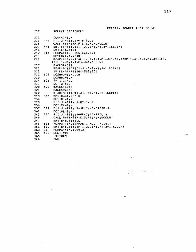
ISN

2 2 22232262272412422432442773CC311312313314317320321322i t - i

334335336337341342346347350351363364365366

137

F O R T R A N S O U R C E L I S T S O L V ES C L R C E S T A T E M E N T

CC 4 4 4I= 1,F 444 FI I,J )= F I I , J I - T F I I , J )

CALL M T M A F t F f C I S f F . N . N C C L M 441 f c R I T E ( 3 ) U C l S M » J ) , I = l,P),J = l f N C C L M

bP ITE(6,515)515 F C P N A T U O H RES ICOALS/ )

C C 5 C 0 L L = 1 , N P A R TP E A C < 4 I N tN , < ( A M I , J ) , I = l , M ) , J = l , K > , I I B M I , J ) , I = l,F),J = l , M ,

II ( F I I tJ > , I = ] » M > J = l » N C C L M EAC KSPA CE3R E A C l 3 ) ( ( D I S U t J ) t I = l,R),J = l , N C C L M I F ( L L - N P A R T ) 5 0 E , 5 0 5 , 5 C 5

5C5 C C 5 0 6 J = l t N C 0 L N C C 5 0 6 I = 1 , N

5C6 TF 1 I» J ) =*0 .GC TO 509

5CE EA C K S P A C E 3 E A C K SPA CE3REACI3)I I TF'I I , J ) , I = 1,N ) ,J = 1,NCCLN )

50 5 C C 5 1 0 J = 1 , N C C L N CC5 10I* 1«NFI I ,J »= F I I t J ) - P S ( I t J )CC S 1 2K* lfM

512 F I I tJ ) * F ( I » J ) - A M l f K > * C I S l K , J )CCS 10L = 1.N

51C F U , J ) * F I I , J ) - E M I , L J * T F ( L , J >- CALL R A T T F I e F , C I S , R S f N , F fNCCLN) hF I TE t 6 » 516 ILL

516 F C R N A T I 1 X » 1 2 F P A R T . NC. = t I4,)5C0 b R I T E ( 6 t31)I(F(I *J ) , I = 1»RItJ = 1 *N C O L M 31 F C P F A T ( 1 X , 1 2 E 5 . 2 I 6CC C C M I N U E

RETURN ENC

IS*01

23

4567

1C1415

r> o o r>

r> n

138

F C B T R A A S C L P C E L I S TS C L R C E S T A T E M E N T

$ I6FTC RATMS L E R O U T I N E RATR I X M A T ,V P A T ,P R A T ,R ,N ,N C C L N )EEP GERC N U 13CC-5302S MAT RIX MULT 1PLICATICAD I M E N S I O N X M A T < 5 C , 5 0 > , Y M A T ( 5 C , 4 1 , P R A T ( 5 C . 4 »C C R R C N C ( 6 . 6 ) , C e A ( 4 , 6 ) » O B { 4 , 6 ) , A ( 6 , 6 U B ( 4 , 6 ) , S T ( 5 C i l G O ) , U 2 G 0 » 4 ) »

1XA E W (1 C O » 8)X R A 7 IS M BY A LEFT MAT RIX TC BE M L L TIPL IEC YRAT IS N BY NC C L N R I G H T MATRIX TO BE M U L T IPL IED PRAT IS M BY NCCLN P P C CUCT MATRIXCCl C I = l f M CC 10J=1,N C0LN PRA T(I,J)*0 .CC1 0 K = l j N

1C F R A T ( I ,J)=PRAT11,J) + X R A T ( I , K ) « Y R A T ( K , J )RETURNEAC

139

FORTRAN SOURCE LISTISN SCIRCE STATEMENT

0 $ IEFTC MATTM1 SUBROUTINE MA T TM ( XMAT, YMAT t PM A T t N»M .NCCLN )

C BERGERON W 1306-53025C MATRIX MUL T I P L I C A T I O N hITH XMAT TRANSPOSED

2 DIMENSI ON XMAT(50.50)tYMAT(5C,4),PMAT<50,4)3 COMMON CIf c»6) ,CEA( 4,6), DB(4 ,6),A I6,6) ,BI4 ,6),S T(50, lC0) .U(20 O,4>,

1XNEW(1C0,8)C XMAT IS M BY N LEFT MATRIXC YMAT IS M BY NCC LN RIGHT MATRIXC PMAT IS N BY NCCLN PPOCUCT OF XMAT TRA NSPOSED AND YMATC

4 DC 10I = 1»N5 DC 10J*1fNCOLN6 PMAT(I,J)=0.7 DC 10K*1»M

10 1C FMA T I I , J ) = P M A T ( I , J ) + X M A T ( K , I ) « Y M A T ( K , J )1 4 RETURN15 END

ISNa1

23

4567

10222324253031

32333435364750616263

64657677

100101102105106107110111115126127140141143154

140

F O R T R A N S O U R C E L I S TSCLRCE S T A TEME NT

1 IEFTC STRESSSUE ROUTINE S T R E S S ( N P A R T ,NFIPST ,N L A S T , N C C L N ,N E L E R , N C C ,N F R E E ,NPC IN,

lPILLO.X)C E E P G E R C N K 13C 6-5302SC S L E R O L T I N E FOR C A L C U L A T I O N CF STRESSES

CIRENS ION N C C I 1 5 0 , 3 ) , N F I R S T ( 15) , N L A S T ( 1 5 ) ,X(1C0,2)C CR RON C I 6 , 6 ) , C E A ( 4 , 6 ) , D 8 ( 4 , 6 ) , A I 6 , 6 ) , B ( 4 , 6 ) , S T ( 5 C , 1 0 0 > ,1(200,4) ,

1 XN E W I I C O , 8)C

CC6C0I I=1,NPART JJ = N P A R T+1 -II R = N F R E E * ( N F IRST(JJ)-l ) + l N * N F R E E * N L A S T U J >

6CC R£AC(3)((UII»J),I=RI,N), J=l, NCCLN )C C 5 0 1 = 1 , NPOIN C C E O J = 1,NCOLNX N E W I I , 2 * J - 1 )=X (1 , 1 ) + L ( 2 * 1 - 1 , J)

SC XNEWI I , 2 * J)= X(I,2 ) + U(2*I,J)W R I T E { 6 , 6 1 3 )

613 F C R R A T ( 1 F I , 4 5 F F I M T E E L E RENT ANA L Y S I S CF SALT PILLAR RtCCELS/,lX,1 16HE LAST IC A N A L Y S I S / / , I X , 2 6 H B E R G E R C N , W. APRIL, 1 9 6 8 , 3X,2 6 FL .S.U .//)W PITEI 6,6 1 4 JPILLE

614 FCPRATI I X,2 4 H A V E R A G E PILLAR STRESS = ,F10.0,5F FSI/) h P I T E { 6 , 6 1 5 )

615 F C R R A T I 1 H . 4 C RNCD E R-01 S P L A C E R E N T S Z - D I S P L A C E R E N T S ,5 X ,I 3 1 H NEW R CO-CRC. NEW Z CC-CRC./)WRI TE I 6,32) (I I,LI 2 * 1 - 1 , J ) , L ( 2 * I , J ) ,X N E W I I , 2 « J - 1 ) , X N E W I I , 2 » J ) ,

II = 1,N P 0 I N ) , J = 1 , N C C L N )32 F C P R A T I I X , 1 4 , 1 F 4 E 1 8 . E )

WRITE 17,33) (IUI 2 * 1 - 1 , J ) , U ( 2 « I , J ) , I = 1,N P C I N ),J=l,NCCLN)33 F C R R A T ( 2 E 1 6 .8)

W R I T E ( 6 , 6 3 5 )635 F O F H A T I 1 H 1 , 1 5 F E L E M E N T N U R BER ,16F Z - S TRES S ,

1 16H R - S T R E S S ,16H T - S TRES S ,16F R Z - S T R E S S /)C

C C 2 0 L L = 1 , N E L E RR E A C H ) I I C B I I , J ) , I * 1 , 4 ) , J = 1 , 6 ) , C R X , C R Y CC 6 2 0 J = 1 , N C C L N TTC620I = 1,3 J J = N O C I L L , I )C ( 2 * I - 1 , J ) = L 1 2 * J J - 1 * J )

620 C ( 2 « I , J ) = U ( 2 * J J , J )C.C 6 3 0 J = l , N C C L N CC6 30I=1,4 C E A ( I ,J )=0.C C 6 3 0 K * 1 , 6

630 C B A ( I , J > = D B A I I , J J + D B I I , K ) * C ! K , J )W R I T E ( 6 , 3 1 ) L L , I I C B A I I , J ) , 1 = 1 , 4 ) , J = l , N C C L N )

31 F C R H A T I 6 X , 1 4 , 5 X , 1 P 4 E 16.7)WRI TE I 7,46) (ICBAI I ,J ) , I = 1,4 ) , J = 1,N C C L N )

46 F C P R A T ( 4 E 1 6 *8 )20 C O N T I N U E

W R 1 T E I 7 , 4 5 ) I ( X N E W 1 I , 2 * J - 1 ) , X N E W ( I , 2 * J ) , I = 1 , N F C I N ) , J = 1 , N C C L N )45 F C P R A T I 2 F 14 .6 )

141

ISN155156

SCLRCE S T/ iTEH EMRETURN

ENE

FCRTRAN SCLRCE LIST STFESS

142

I S N

C1

2345 7

101112131415 lfi 17 20 21 23 25

262730313233353637404143444546

4750515354555760616263

F O R T R A N S C L R C E L I S TS C L R C E S T A T E M E N T

IIEFTC NAT INVSLE ROUTINE NAT I N V (A ,N ,BtN )

C M AT RIX INVERSICN WITH A C C O M P A N Y I N G SCL LTICN CF LINEAR ECL A T I C N SCC I NI TIAL IZATI ON

CINENSION IF JVC T(50),A (50.50),BI 50t4>,INDEXI 50>2),FIVOT I 50>10 CET ERN= 1.015 C C2 CJ=1 ,N2C I F I V O T (J )=C3C CCS 5 0 1 = 1»N

CC SEARCH FOR FIVCT ELE NENT40 ANA X=G.O45 C C 1 05J= l,N50 IF(IPIV OT(J) -I ) 60 * 1C 5 * 6060 C C 1 C 0 K = 1 , N70 I F ( I P I V O T I K > - l ) E C t l O C , 7 4 C80 IF <ABS(ANAX >-AES(A(J,K)))8 5,ICC, IOC85 IRCh=J40 ICCLUM=K45 ANAX*A(JtK)ICC C C M I N U E105 C C M I N U E11C IP I V O T ( I C C L U N ) * I P I V C T ( I C C L U N ) + l

CC INT ERC H A N G E RCHS TO PUT PIVCT ELE MENT ON DIA GONAL130 IF ( IROV.-ICOLUN 1140,260 .140140 CET ERN =-DET ERN15C CC 2 C 0 L * 1 , N16C SV»AP=A(IROW,L)170 A ( I R O H * L ) = A ( I C C L L M f L )2CC A ( I C O L U M vL )"SNAP205 I F ( M ) 2 6 0 , 2 6 C , 2 1C21C C C 2 5 0 L = 1 , M220 S hA P = B (IROW » L )230 B(IROh,L)=*B(ICCLLM,L)25C E ( ICCLUM.L ) = SKAP260 INC E X ( 1,1) = IROW270 I N C E X I 1 * 2 1 = 1 CCLUN21C PIVCTI I)= A( I C C L L N , I C C L U N )32C C E T E R M = D E T E R M « P I V O T ( I) __

CC CIVILE PIVOT RCVi BY PIVOT ELENENT330 A I I C G L U M ,ICCL UN >*1.0340 CC 3 50L=1» N350 A ( 1 C C L U M , L ) » A I I C C L U N , L )/ P I V C T (I )355 I F ( M ) 3 8 0 , 380*360360 CC 3 7 0 L * 1 1M370 B ( I C O L U M , L ) * B ( I C C L U M , L ) / P I V C T ( I )

C PECUCE N C N - P I V C T RONS38C CC545 L 1 = 1 » N351 I F { L l - I C 0 L U N ) 4 C C » 5 4 5 » 4 C C

4CC T * A (L 1 * ICOLLM )420 A(L1>IC0LUM)>0.0430 CC4 5 0 L * 1 f N

143

FOR TRAN SCORCE LIST FAT IKVISN SCLRCE STATEMENT

64 45C A t L l * L ) = A I L l , L ) - A ( I C C L L K , L ) « T66 456 I F (0)545,545,46067 460 CCS C O L = l , K70 5CC G ( L l , L > * B < l l , L > - B ( I C C L U 0 fL)*T72 545 C C M I N U E74 5 50 C C M I N U E. C

C INTERCH ANGE C C L UFNS76 600 C C 7 1 0 1 = 1 , N77 61C L*N+1-1

ICO 62C I F ( I N C E X ( L , 1 ) - I N C E X ( L , 2)1 63 0 , 7 1 0 , 6 3 0101 630 J R C N = I N D E X ( L* 1 )102 640 JCCLUN=INCEXILt2>103 650 E C 7 0 5 K = 1 , N104 660 S hA P = A (K * J R C h )105 67C A(K,JRQW)=A(K,JCCLUFJ1C6 7CC A(N*JCCLUP) *SVt/P107 7C5 C C M I N U E111 710 C C M I N U E113 740 RETURN114 750 ENC

APPENDIX D

PROGRAM LISTING FOR SALT PILLAR ANALYSIS (Creep Effects Modification)

144

145

EER G E P C N , W. P R E F R C C E S S C R - J C e CCCCCO

SFILE BERGFN •F T C O 2 . • , L 1 6,U 1 6 , BLCCK = 2 £ 3 5 , S I N G L E ,LRL = 2 6 3 5 . R C T * 1,tETC R E E L , E F P = P E P R X . , E O F = R E C F X . fECR =RED RX.SFILE P ER GFN ' F T C 0 3 . •, U 1 3 . U 1 3 , B L C C K = 2 8 , D O U B L E »LRL = 3 6 ,R C T = 1,SETC REEL.EF P = P E R R X . t E 0 F = R E C F X .,ECR=RECRX.

146

F O R T R A N S O U R C E L I S TI S N S C U R C E S T A T E M E N T

0 IIEFTCC EEP G E R C N W 13C 6-53025C FINITE ELEMENT A N A L Y S I S CF SALT PILLAR MODELSC CRE EP M O D I F I C A T I O N SCC MAIN PROGRAMC

1 D I M E N S I O N X ( 1 C C , 2 ) , X E ( 3 , 2 ) , N F ( 1 5 ) , N B < 1 5 , 2 ) , B V 115,2 ) .NEP 1150 ) , 1 N C C U 5 0 , 3 ) , E C 2 ) , P C 2 ) ,G E <2),N L B E 1 1 0) ,F P L (10>,NST ART 110) , 2 N E N C { 1 0 ) , N F I R S T ( 1 0 ) , N L A S T ( 1 0 ) , S T R E S S ( 1 5 0 , 3 )

C2 C C M M O N Cl 6 , 6 ) , C B A ( 4 , 6 ) , D B I A , 6 ) , A ( 6 , 6 ) , B < 4 , 6 ) , S T I 5 C , 1 0 0 ) ,U(200,4),

1 X N E H 1 I C O , 8)C

3 CALL F P T R API -3)4 REM INC 15 REM INC4

CC R E A DING AND P R I NTIN G OF DATACC READ CON S T A N T S

fc R E A C ( 5 » 1 0 J N P A R T » N P 0 I N , N E L E M . N B C L N , N C C L N , N Y M , N F R E £ , N 6 E L17 1C F C P M A T 1 1014 )

C READ NOD AL PCINT C O - C R D I N A T E S20 - C C 3 0 I * 1 » N P O IN21 30 R E A C ( 5 , 3 5 ) X ( 1 , 1 ) , X I 1,2)

C X (I,1) *R C O - O R D I N A T E CF NODAL PCINT IC X ( I ,2)=Z C O - O R D I N A T E OF NODAL PCINT I

23 35 F C P M A T I 5 F 1 4 .6)C R EA D E L E M E N T NCC AL N U M B E R ANC ELEMENT PROPERTY NLMEEP

24 0 0 4 0 1 * 1 , NELEM25 40 R E A C I 5 , 1 0 ) ( N C D ( I , J ) , J * 1 , 3 ) , N E P ( I )

C NODI I,J )*NCCAL N UM BER CF J NCCE CF E L E M E N T IC NEP 11 )*1 IF ELEMENT IS SALT CR =2 IF STEELC READ P R E S C R I B E D D I S P L A C E M E N T S

33 D C 5 0 1 * 1,NB O I N34 50 R E A C ( 5 , 4 5 ) N F ( I ), N B ( I , 1 ) , N 8 ( 1 , 2 ) , B V ( I , 1 ) , B V ( I ,2)

C NFI 1) =NODAL PCINT N U M B E R OF FIRST NCCAL PCINT MITF FRESC. CISP.36 45 F C P M A T ( 3 I 4 , 2 F 1 6 . 8 )

C READ FIRST AND LAST E L E M E N T S AND NCD AL POINTS IN EACH PAR T I T I O N37 CCfcO I*1»NPART40 60 R E A C ( 5 » 1 0 ) N S T A P T I I ) ,NEN'D| I ) ,NFIRST (I ) , NLAST ( I)

C REAC E L A S T I C I T Y V A L UES42 C C 6 11* 1,NYM43 61 R E A C ( 5 , 3 5 ) E ( I ) , P ( I ) , G E ( I )

C REAC L OA DED B O U NDAR Y E L E M E N T N U M BERS AND FPL CN EACH45 R E A D | 5 , 1 0 ) ( N L B E I I ) , I » l , N B £ L )

C N L E E (1)“ ELEMENT N U M B E R OF FIR ST L OA DED B O U NDAR Y ELEMENT52 R E A C C 5 . 1 1 ) ( FPL !I>, I * 1 , N B E L )57 11 F C P M A T < 9 F 6 . 4 , F I 2 . 8 )

CC ABOVE DATA R E M AINS C O N S T A N T FOR ALL PILLAR LOADS

60 MR 1TEI 6,2 )61 2 F C P M A T I 1 H 1 , 4 5 H F I N I T E E L E M E N T A N A L Y S I S CF SALT PILLAR M O D E L S / / , I X ,

1 2 5 H 6 E R G E R C N , M. APRIL, 1966 L.S.U.//)

147

I S N

CC

62 16 3 6 26 465 63

Ccc6667 6475 657677 66

CC

100 60C101

c102103104105106 75 111112113114115116 117 120 121 122123 85125126 127130131132133

CC

134135136137140 131141 132142143144145146 900

F G R T R A N S O U R C E L I S TS C L R C E S T A T E M E N T

R/N P I L LAR LCAC R E A C (5 ,62)P ILLC F C P P A T ( F 1 0 . C ) t,PITEI6,63)PILLCF C P P A T l l H ,iOHAV. P I L LAR STRESS = ,F10.Q,5H P S I /)R EA C STRESS FRCP P R O GRAM NC. 1, S T R E S S ( I ,JJ t=ELEME NT NC., J-1,2,3 FOR Z,R,T STRESS CC 64 I=1,NELEP RE A C (5,65)( S T R E S S ! I , J >,J=l,3)F C R P A T ( 3 E 1 6 . 8 >R E A C ( 5,66 )T I RE ,CTI ME,TE MP F C R P A T ( 3 F 8 . C )C A L C U L A T I O N CF NCDAL LCA CS CUE TC PILLAR LCAC N CC L N = N C O L N + 1C AL L LDPILt X , X E , N O D , N C C L N , N P O I N , N B E L , N L B E , F P L , P I L L C ) FCP PAT ION OF PATR ICES IN T ER*0C C 7 0 I 1=1,NPART C C 7 5 I = 1 * 50 C C 7 5J* I,100 S T ( I,J)*0.N ST *NST A R T ( II )N E N * N E N D { 1 1 )K*N F I R S T { II 1 l*N LAST( 1 1 )PIN U S * K - 1CC 8000 LK= N S T ,NEN P P = L K - I N T E R C C 651 *1,3 J J * N O D ( L K , I )X E ( I , 1 ) * X ( J J , 1 )X E ( I,2 >*X(JJ,2)J * N EP(L K)YP = E(J )P R * P (J )G * C E ( J )S Z * S T R E S S ( L K , 1 >S P* STR E S S (L X ,2 )S T A N * S T R E S S ( L K , 3 )C A L C U L A T I O N CF ELE MENT STIFFNE SS ANC STRESS PATRICES CAL L F E M I X E , Y M , P R , G , P M , T I M E , O T I P E , T E M P , J , S Z , S R , S T A N ) CC 801 L L * 1,3 C C 8 0 K K * 1 , 3I F ( N O D ( L K , K K ) — K >80 ,131,131 I F ( N O C I L K , K K ) - L >132,13 2,80 P * N F R E E * ( N O C ( L P , K K ) - K )N * N F R E E * ( N O O I L P , L L > - K )I * N F R E E * ( K K — 1)J * N F R E E * ( L L - 1 >I F ( N ) 8 0 , 900 ,900 C C S N J * 1,NFR EE

148

F C P T R A N S O U R C E L I S TISN SCLRCE STATENENT

147 CCER I * 1,NFR EE150 NPI*M4FI151 N N J =N+N J152 IN 1 * I+H I153 JNJ =J+N J154 5 ST(NMI,NNJ) =ST(NNI,NNJ )+C(IK I,J N J )157 80 CONTINUE161 801 CONTINUE - -163 80CC CONTINUE

CC I M R C C U C T ICN CF P R E S C R I B E D CI S P L A CEH ENT S

165 C C 2 9 0 I * 1 , N B C U N166 N = N F ( I > - K167 N N = N F ( I )— 1170 I F( M)29 0,242 ,242171 242 I F ( N F ( I 1 - L ) 2 4 3 , 2 4 3 , 2 9 G172 243 CC2 30vlx 1, NFREE173 I F ( N B ( I , J ) ) 2 3 C , 345,230174 345 NN1=»NFREE*H+J175 STI NMI , N M I ) * S T (N K I , NN I )*« 1E+12176 CC2 3 3 J J = 1 , N C C L N177 J N J * N F R E E * P N 4 J200 233 Li (JN J , J J IKS T (N M , NMI ) *B V ( I , J )202 230 C O N T I N U E204 290 CON T I N U E206 I NT ER-N EN207 NI*NFREE«MINUS-*1210 N J = N F R E E * L211 N * N J - M 1+1212 IF(II-N PART 1115,116,115213 115 NA = N F R E E « ( N L A S T ( II+1I-NINUSI214 GC TO 117215 116 NA=M+1216 117 N»N A-N217 NK*N-H220 70 W R I T E ( 4 ) N , N , ( ( S T ( I , J ) » I * l f K ) » J = l » M ) » I (S T (I ,J ) , 1 = 1,N ),J*NN,NA) ,

1 ( < L ( I , J ) , I = N 1 , N J ) , J = 1 , N C 0 L N )252 REW INC1253 REI* INC2254 RES,1NC3255 R E H N C 4

CC S O L U T I O N OF TRIC I AGONAL MAT RICE S AND C A L C U L A T I C N CF R E S I D U A L S

256 CALL SOLVE ( N P A R T ,N C C L N )257 8005 REN INC 3260 CA L L T C T D I S ( N P A R T ,N F I R S T , N L A S T ,N C C L N , N E L E N ,N C C ,N F R E E , N P C I N ,

1PILLD.X)261 N C C L N * N C 0 L N - 1262 20 STCP263 ENC

149

FORTRAN SOURCE LISTISN SCLRCE STATEME NT

0 *ieFTC LCPIL1 SUBROUTINE LCPIL(X,XE.NOD,NCOLN,NPC1N»NBEL,NLBE,FPL,PILLC I

C BERGERON W 1306-53025C S L E R O U T I N E FCR C A L C U L A T I O N CF LCADS CUE TC PILLAR LCAD

2 C I R E N S I O N X 1 1 0 C , 2 ) , X E ( 3 , 2 ) , N C C ( 1 5 0 , 3 ) ,NLBE( 1C> , F P L <10>3 CORRON C (6,6)»CB A <4,6 ), D8 (4,6),A (6,6),B (4,6),S T (50,100),Uf200,4 ) ,

lXN EUIlCO.S)C

4 NPC I N 2 * N P C I M 25 C C 1 0 I * 1 , N P 0 IN26 1C L ( I,N C C L N ) =C.

10 C C 2 0 I 1*1 ,NBEL11 CCN=FPL< II)«PILLC12 IJ’ NLBEl II)13 C C E 5 1*1,314 J J = N 0 D ( I J , I )

C IJ IS THE ELENENT NO. AND JJ IS THE NCD AL NC. OF I NCDE CF IJ15 85 X E < 1 , 1 ) = X < J J , 1 )17 ELF — 1 . 5 7 0 7 9 6 3 2 * ( X E I 3 , 1 ) * * 2 - X E ! 1 , 1 ) * * 2 M C C N20 C C 6 6 I » 1 , 3 , 221 J J * N O C < I J , I >22 86 U ( 2 * J J , N C O L N ) * L ( 2 * J J » N C 0 L N ) + E L F24 20 C O N T I N U E26 RETURN27 ENC

150

F O R T R A N S C L R C E L I S TI S N S C L R C E S T A T E M E N T

0 IIEFTC FEM1 S L E R Q U T I N E F E M (X E ,Y M ,P R ,G »MMt TIKE *C T I M E ,T E M P J * S Z .S R ,S T A N )

C EEP GERC N W 13C 6-5302S -C S L E R O U T I N E FCR F O R M A T I C N OF E L E MENT S T I FFNE SS ANC STRESS MAT RICESC FCR A X I - S Y M E T R I C P R O B L E M

2 C I M E N S I O N D ( 5 0 , 5 C ), X E ( 3 , 2 > , Z M 3 ) , Z X ( 3 1 , Z Y ( 3 ) , C E I ( A , A ) tD C I (4,4). 1 C L M 5 0 » 1 >3 C C M MON C < 6 , 6 ) , C B A { A , 6 ) , 0 B ( A , 6 ) , A ( 6 , 6 > , B < A , 6 J tS T { 5 0 , 1 0 0 > ,L( 200,4), 1 X N E W J 100,8)

C4 CC2CJ*1?65 CC2 1 I = 1 , A6 E ( I ( J ) =0 .7 C E ( I * J ) =0 .

10 21 CE A f I t J > » 0 .12 CC2 0 I = 1 , 613 A t 11J ) -0 •1A 20 CI1,J)= 0.17 T M R D = l . / 3 .20 CPX = ( X E ( l , n + XE(2,l)4XE(3»lJ I-THIRD21 C P Y * I X E ( 1 , 2 ) + X E { 2 , 2 ) + X E ( 3 , 2 ) I *THIRD22 ZV»(l) = X E t 2 . 1 ) * X E ( 3 . 2 ) ' X E ( 3 , l ) * X E ( 2 , 2 )23 Z M 2 ) * X E ( 3 , 1 ) « X E ( 1 , 2 ) - X E { 1 , I J * X E < 3 . 2 )2 4 ZM3)=*XEI l , l ) * X E I 2 t 2 ) - X E ( 2 , l ) * X E < 1 . 2 )25 CC 51=1 * 326 XEII,1) = XE( If D - C R X27 5 XEI I,2 > = X E ( 1,21-CRY31 ZX< 1> = X E ( 2 , 2 ) - X E 1 3 , 2 ) -32 Z X ( 2 ) * X E ( 3 , 2 1 - X E ( 1.2)33 Z X ( 3 ) = X E l l , 2 ) - X E I 2 . 2 )34 Z Y ( l ) * X E ( 3 t ] ) - X E ( 2 f l )35 Z Y ( 2 ) m X E ( l t l ) - X E ( 3 t l l36 Z Y < 3 ) » X E | 2 t l ) - X E ( l f l )37 Z K = X E ( 2 » l ) * > E ( 3 » 2 ) — X E ( 3 * l ) * X E t 2 * 2 IAC Z = 3 .»ZK4 1 IF t J J - 2 )1? 2 f2

CC INVERTED ELA S T I C I T Y M AT RIX FCR AXI-SYM. CASE

A2 1 P E * - PR/Y M A3 CE II1,11 = 1. ZYMAA C E I ( l t2)=PEA 5 C E I I 1 , 3 ) = P EA6 C E I ( l , A ) * O . CA 7 CE I (2* 1)*PE50 C E l ( 2 f 2 ) = 0 E l ( l , U51 C E I ( 2 t 3 ) = P E52 C E I ( 2 , A > * 0 . C53 C E I ( 3 f l ) » P E5A C E I (31 2 ) “ PE55 C E I ( 3 t 3 ) = C E I < l t l )56 C E I ( 3 # A ) = 0 « C57 C E 1 ( A . 1 ) = 0 . C60 CEI(At2)=0-.C61 CE 1 (At 3 )S G« C62 C E I I A f A ) ® ! . / G

151

F O R T R A N S O U R C E L I S T F E NI S N S C L R C E S T A T E M E N T

CC INVERTED CREEP N A T RIX FOR AXI -SYP . CASE

63 FES = ( l . / 2 . * * l . l ) • ( { (SZ-SR)**2+< S R - S T A N I * * 2 + ( STAN-S2 »**2 I * * 1 •1>64 T N 7 = 1 0 . * * < - 2 0 >65 C C * . 7 6 8 * T F T *TE NP«* 10.9* (TIPE-»24. ) ■» « ( - 0 . 6 5 ) * F E S * C T I N E « T P T66 C F = - C C /2.67 C C I ( 1 , 1 ) = C C7 0 CC I ( 1 , 2 ) = C P71 C C I ( 1 , 3 ) = C P72 C C I ( 1 , 4 ) = 0 . C73 C C I ( 2 , 1 ) = C P74 C C 1 ( 2 , 2 ) =CC75 C C I ( 2 , 3 ) = C P76 C C 1 ( 2 , 4 ) = 0 . C77 C C I ( 3 , 1 ) = C P

ICO C C I (3 » 2 ) =CP101 CC I (3 , 3 ) =CC102 C C 1 (3 » 4)=0 » C1 0 3 C C I ( 4 , 1 ) = 0 . C104 C C I ( 4 , 2 ) = 0 . C105 CC I < 4, 3 ) =0 . C106 C C I ( 4 t4)= 3.*C C107 CC 3 J = 1 , 4110 CC 3 1=1,4111 3 C( I,J)=DEI< I,J) + C C I U , J J114 CALL K A T I N V ( C » 4 ,C U M ,C I115 GC TO 4

CC EL A S T I C I T Y FATPIX FCR A X I - S Y N F E T R I C CASE

1 1 6 2 C C C N = ( Y M * t 1 . - P R ) ) / ( ( 1 • + P R I * { 1 » - 2 . * P R I >117 C C C N 2 * P R / ( l . - P P )120 C (1,1)=CCON; 1 2 1 C ( I , 2 ) = 0 C G N « C C C N 21 2 2 C ( 1 , 3 ) = D ( 1 , 2 )123 C (1»4)=0.124 C ( 2 , 1 ) = D ( 1 , 2 )125 CI 2 , 2 ) =DCON1 2 6 C ( 2 , 3 > = 0 ( 1 , 2 >1 2 7 C ( 2 , 4 ) = 0 .130 C ( 3 , 11=0(1,3)131 C ( 3 , 2 > = D ( 2 » 3 )132 C (3,3)=OCCN133 C (3,4)=0.134 C ( 4 * 1 ) = D ( 1 » 4 )135 C(4 ,2 } = D ( 2 , 4 )136 C ( 4 , 31=0(3,4}137 C ( 4 , 4 }=G

CC e F A T R I X FOP A X I - i Y F F E T R I C CASE

140 4 G (1, 2)= Z Y (1 )141 B(1 ,4) = Z Y ( 2 )142 B ( 1 , 6 ) = Z Y ( 3 )1 4 3 e ( 2 , l > * Z X t l >144 e < 2 , 3 ) = Z X ( 2 )145 B (2,5) = Z X (3 )

152

F C R T R 4 N SCARCE LIST FEPISN S CL RCE S T M E H E M146 C L C = O R Y / O R X147 fi< 3.1 ) = Z W ( 1 )/CP X + Z X (1 ) + Z Y (1) * CLC150 B ( 2 » 3 ) S Z W 1 2 ) / C R X + Z X ( 2 J + Z Y ( 2 ) « C L C151 e(3»5I = ZW(3)/CPX-fZX(2I + ZY( 3 > « C L C152 B ( 4 1 1 J *2 Y C 1)153 B 14 » 2 ) - Z X (1 )154 B ( 4 ,3)= ZY<2)155 B ( 4 t4)= Z X ( 2 )156 E ( 4 , 5 ) = Z Y ( 3 )157 B ( 4 ,6)= ZX(3)160 CC 4 0 Ix 1» 4161 CC4 C J = 1 , 6162 C C 4 0 K = 1»4163 40 C E (Ir J )= D B ( I , J ) + C ( 1 , K ) * B ( K , J ) / Z167 V C L = 3 . 1 4 1 5 9 2 6 5 « Z « 0 R X170 CC6 G I = 1 » 6171 C C 6 0 J = 1 , 6172 CC 6 0 K X 1*4173 60 C I I , J > XC ( I , J ) * E ( K , I ) * D B ( K tJl* V C L / Z177 IF ( R M M 2 9 » 1 2 f i » 1 2 72C0 127 H P I T E I D I (DE(l»J)fI = l»4)*J=l,6) ,0RX,CRY211 128 RETURN212 ENC

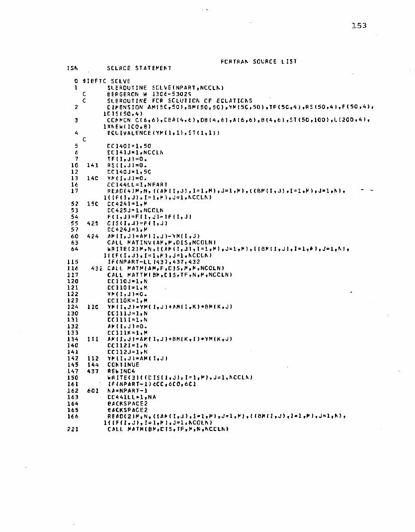
ISN01

2

34

56710

12131617

5253545557606364

115116117120121122123124130131132133134140141142145147150161162163164165166

221

153

F O R T R A N S O U R C E L I S TS C L R C E S T A T E M E N T

tIEFTC SCLVESLE ROUTINE S C L V E (N P A R T ,N C C L N )

C BERGERON U 13C6-5302SC SLE R O U T I N E FCR SOL UTIO N CF ECLATIC NS

C IRENS ION A M I 5 C , 5 0 ) , B M ( 5 0 , 5 C ), Y M ( 5 C , 5 0 ) , T F ( 5 C , 4 ) , R S 1 50 ,4), F (50,4), 1C I S (50,4)COMMON C ( 6 , 6 ) , C e A ( 4 , 6 ) , D B ( 4 , 6 ) , A ( 6 , 6 ) , B ( 4 , 6 ) , S T (50 ,100) , L (200,4 ) ,

1XN E W ( I C O , 8)EC L-l VALENCE (Y M (1,1),ST(1,1)J

CC C 1 4 0 I = 1 » 5 0 E C I 4 1 J = 1 , N C C L N TF ( I,J)=0.

141 RSI I,J )=0.CC 140J = 1,5C

14C Y M ( I, J )=0•C C 1 4 4 L L = 1 , N P A R TREA0I4) M,N, (( A M I ,J) , 1 = 1,M ) ,J = 1 , M ) , ( ( B N (I ,J ) ,I*1,M ) ,J*1.N> , * ~

1 ( (F (1,J ) , 1 = 1 , M ),J = 1,NCCLN)15C CC4 24I= 1,M

C C 4 2 5 J = 1 , N C C L N F( I , J ) = F ( I , J ) - T F ( l , J )

425 C IS (I,J )=F( I,J)C C 4 2 4J= 1,M

424 AM ( I,J ) = AN( I,J ) - Y M ( I , J >CALL M A T I N V ( A M , M , D I S , N C O L N )K P I T E ( 2 ) M , N , ( ( A M ( I , J ) , I = l t M ) f J = l , K ),(( BM(I, J),I* l,l|),J = l,N),

1 ( C F ( I,J), 1=1,M ),J = 1,NCCLN)IF(NPAR T-LL 1437 ,437,432

432 CALL M A T M ( A M , F , C I S , M , M , N C O L N )CALL N A T T M C B M , C I S , T F , N , M , N C C L N )C C 110J = 1» N C C 1 1 0 Is 1, K YM( I,J) =0.C C 1 1 0 K = 1,M

U C YM(I, J >»YM( I,J )+AM( I , K ) *BM ( K , J )CC111J=*1,N CC1 1 1 I = 1 , N AM ( I,J)=0.CC1 UK=*1,M

111 A M( I*J) =AM( I,J) + B M ( K , I )* Y M (K » J )C C 1 1 2 1 = 1 , NC C 1 12J = 1 ,N

112 Y M (I,J )=A M ( 1,J )144 CON TINU E437 RENINC4

N R I T E ( 3 ) ( ( C I S ( I , J ) , 1 =1 ,M ) , J =1, NCCLN )IFI NPART— 1)6 CC, 6 C 0 , 6 C 1

601 N A = N P A R T — 1CC4 41LL=.l ,NABAC K S P A C E 2BAC K S P A C E 2R E A C ( 2 ) M , N , ( ( A M C I , J ) , I = 1 , M I , J * 1 , M ) , ( ( B M ( I , J ) , I » 1 , M ) , J = 1 , N ) ,

H ( F ( I , J ) , 1=1,M 1,J*1,NCOLN)CALL M A T M ( B M , C I S , T F , M , N , N C C L N )

154

F C R T R A N S O U R C E L I S T S C L V EISN SCLRCE STATEMENT222 CC444J= 1,NCC LN223 CC4 44 I = 1, H224 444 Ft J,J )= F ( I»J)-TF(I,J)227 CALL H A T H t A M , F ,C I S , H , R , N C C L N )230 441 KRI7EC3)!tDISt I ,J )»1 = 1,H ),J = 1,NCCLN)242 WRITE(6,515)243 515 FCPMAT 110H R E S I C U A L S / )244 CC500LL=1,NP AR7245 R E A C { 4 ) M , N , ( ( A M I , J ) , I - = l , M ) * J = l,H),t(BM(I»J)

1 1 (Ft I ,J ), I=1,R ),J=l,NCCLN)300 EACKSFACE3301 R E A C ( 3 H ( D I S t I , J ) , I = 1 , M ) ,J=l, NCCLN)312 IFtLL-NPART ) 506,505, 50 5313 505 CCS 06J=1,NCCLN314 CCSC6I*L,N315 5C6 7 F (1,J )*0•320 C-C TO 509321 5CE EAC KSPACE3322 EAC KSPACE3323 PE A D < 3 ) t ( T F t I , J ) , I-1,N) , J*l, NCCLN)334 5CS ECS 10J * 1 »NCCLN335 CCS10I=*1,M3 36 Ft I,J ) = F ( I,Jl-PStl,J)337 C C S 1 2 K * 1 ,M340 512 F U , J)*F( I, J)-AM (1,K >*CIS(K, J)342 CCS 10L = I ,N343 5 1C Ft I, J )* F { I, J ) - E M I,L)*TFtL,J)347 CALL H A T T H t E H , C I S , R S , N , H , N C C L N )3 50 VtRITE<6,516 ILL351 516 FCB MAT( 1X,12 FPART . NC. *,14,)352 5CC ViRITE(fc,31) (( F ( I , J ) , 1*1,M),J*1,NCOLN)364 31 FCPMATtlX,12E9.2)365 6C0 CONTINUE366 RETURN363- ENC

155

FORTRAN SOURCE LISTISN SCL RCE STATEME NT

0 JIEFTC MATM1 S L E R O U T I N E M A T M (X M A T ,Y M A T ,P M A T ,M ,N fN C O L N )

C B E R G E R O N M 130C-5302SC M A T RIX M U L T I P L I C A T I O N

2 D I M E N S I O N X M A T ( 5 0 , 5 C ) , Y M A T ( 5 C , A ) , P M A T 1 5 0 , A I3 C C M M C N C ( 6 , 6 ) , C E A ( 4 , 6 ) , D 8 < A , 6 ) fA(6,6),BlA,fc) ,ST ( 5C , ICO » ,1 ( 200 , A ) »

1 X N E W I I C O . 8)C XMAT IS M BV N LEFT M A T RIX TC BE M U L TIPL IEDC YMAT IS N BY N C C L N RIG HT M AT RIX TO BE MUL T I P L I E DC PM AT IS M BY N C C L N P R C CUCT MATRIXC

A C C I 0 I * 1 » M5 C C 1 0 J = 1 , N C O L N6 PMA T(I , J ! = C .7 C C 1 0 K = 1 * N

10 IC P M A T ( I , J » = P M A T ( I , J ) + X M A T ( I , K I * Y M A T I K , J )1A RETURN15 END

156

F O R TRAN SOURCE LISTISN SCLRCE STATEMENT

0 $ IEFTC RATTR1 SLE R O U T I N E R A T T R I X M A T ,Y R A T ,P R A T ,N ,R ,N C O L N )

C E E R GERC N W 13Ce-5302SC RATRIX M U L T I P L I C A T I O N Vi ITH XR AT TRA NSPC SEC

2 C IRENS ION XRA T(50 »50),YRIAT<5C,4),PRAT<5C,4)3 CCR RCN C ( 6 , 6 ) , C E A ( 4 Tt ) . D B ( A , E ) » A ( 6 , 6 ) t B ( A , 6 ) , S T ( 5 C t l C 0 ) , L I 200,4 ) ,

1XN E to I ICO » 8 )C XRAT IS R! BY N LEFT RATRIXC YRAT IS M BY NCCLN RIG HT RATRIXC PRAT IS N BY NCCLN P R O D U C T CF XRAT T R A N S P C S E C ANC YRATC

4 CC10I=1 ,N5 C C 10J = 1,NCO LNfc PRATI I » J )=0 .7 CC1 0 K = 1 » M

10 1C P R A T I I » J I = P R A T ( I t J l + X R A T I K , I )■■ YR AT < K , J )14 RETURN15 ENC

. 157

I S N

01

23

456 7

1C222324253031

32333435

36

4750616263

64657677 100

101 102105106 1C7 110 11 1 115 126 127140141 143154155

F O R T R A N S C L R C E L I S TSCLRCE STATEMENT

JIEFTC TCTOISSLEROUTINE TCTC1S(NPART,NFIRST,NLAST,NCCLN,NELEM ,NCC,NFREE,NPC IN,

IP ILLD t X )C BERGERON M 13C6-5302SC SLE RCUTINE FCR C A L C U L A T I O N CF TCTAL D I S PLAC EMENT S

DIMENSION N C C ( 1 E C , 3 ) , N F I R S T < 1 5 ) , N L A S T ( 1 5 ) , X ( 1 C 0 , 2 >COMMON Cl 6 , 6 ) , C B A (4,6 >, D B ( 4 , 6 ) ,A(6,6),B(4,6) , S T (50 ,100) , U (200 , 4 ) ,

1 X N E U I I C O , 8)C

CC6 C0II =1,NP ART J J = N P A R T + 1— II M = NFREE*(NF I R S T (J J ) - 1 ) + l N= N F R E E *NLAS T(.J)

6CC R E A C I B K I U I I , J ) , I =M,N ) , J= 1 .NCCLN )C C 5 0 I=1 ,NPOI N CC5 0J = 1 , N C C L NX N E W I 1,2*J-l) = XI 1,1)+UI 2*1-1, J)

5C XNEWI1, 2*J)= X( I , 2 ) + L ( 2 * I , J »WP ITEI6,613 )

613 F C B M A T I 1 H 1 ,45HF1NITE ELE MENT ANA LYSIS CF SALT PILLAR MODELS/,IX,1 15FCREEP M 0 C I F I C A T I C N S / / , 1 X , 3 2 F B E R G E R C N , N. APRIL, 1960 L.S.U.//IWRI TEI 6 . 6 1 4 1PILLC

614 FOR MAT! IX , 2 4 H A V E R A G E PILLAR STRESS = ,F10.0,5P PSI/1 WP I TE(6,615 )

615 FCPMAT11H , 4CFNCCE R - D I S P L A C E M E N T S Z-DISFLAC E M E N T S ,5 X ,1 3 1HNEW R CC-CRC. NEW Z CC-CRB./)W R I T E ! 6,32) ((I,UI 2 * I - 1 , J ),U 1 2 * 1 , J ) , X N E W 1 1 , 2*J - 1) ,XN EW( 1 , 2 * J 1,

1 I3 1»N PC INI, J=1,N CCLNI32 FCPMATI IX,I4.1P4E18.E)

W R I T E ! 7,3 3 ) 11UI 2 * 1 - 1 , J ) , L (2 * I , J !,1 = 1, N P C I N ),J = l , N C C L N )33 F CP MATI 2E16 .8 )

WR ITEC6.635 )635 FCPMAT I lflV, 15F E LEMENT NUM BER ,16H Z-STRESS ,

1 16H R-STRESS ,16F T-STRESS ,16F RZ-STRESS /)C

CC 2 0 L L = 1,NEL EMR E A D ! 1 ) IICB 11, J ),1 = 1 , 4 ) , J = l,61,CRX,CRY C C 6 2 0 J - 1,NCC LN CC 6 2 0 13 1,3 J J 3N 0 C (L L , I )C ( 2 * I - 1 , J ) = l ( 2 « J J - l , J )

62C C(2«I,J )=U(2 *J^,J )CC6 30J * 1,NCCLN C C6 30I=1,4 CBAII,J )=0.CC6 30K = 1 ,6

630 D B A ( I , J ) = D B A < I ,J J + D B (I ,K > * C (K ,J )WRITE!6,31)LL,I(CBA(I,J ),I*1,4),J=1,NCOLN)

31 FCPMATI6X,I 4 , 5 X , 1P4E16.7)WRITE I 7,46) !(D EA ( I , J ) , I * 1 , 4 ) , J 3 1,NCCLN)

46 F O R M A T C 4 E 16 .8)20 CON TINUE

WRITE (7, 45) t C X N E W d , 2*J-1) , XNEW I I,2*J) ,1*1,N F C I N > ,-»l»NCCLN)45 F C P M A T (2 F 14 .6 )

RETURN

158

ISN1 5 6

SCLRCE STATEMENT

ENE

FORTRAN SOURCE LIST TCTCIS

159

F G R T R A N S C L i R C E L I S TI S N S C L R C E S T A T E M E N T

0 $ IE F1C RATINV1 S L E R OUT INE R A T I N V (A ,N ,B ,RI

C RATRIX INVERSION WITh A C C O M P A N Y I N G SCL LTIC N CF LINEAR EQUATIONSCC INITIAL IZAT ICN

2 C IRENS ICN I F I V C T ( 5 0 ) , A { 5 C , 5 0 ) , B ( 5 0 , A ) , I N D E X ( 5 C , 2 ) , F I V C T ( 5 0 )3 IC CET ERR = 1.0 A 15 C C 2 0 J = 1 , N5 2C I P I VOT ( J ) =0 7 3C CC 5 5 0 1 = 1 * N

CC SEARCH FOR PIVCT ELEMENT

10 AO ARA X = 0 .011 A 5 C C 1 C 5J= 1,N12 5C IFIIPIVOTIJ )-I I 6 C , 105,6013 60 CCI C 0 K = 1 , N1A 7C IF( IPIV0T1K )— 1 )£C*lCCt7AC15 80 I F I A B $ ( A M A X ) ~ A E S ( A < J , K ) ) ) 8 5 , 1 C G , 1 0 C16 85 IRCW=J17 50 ICC LUM = K20 95 ARA X = A (J , K )21 ICC C O N TINU E 23 1C5 C O N TINU E25 11C IP IVOT ( ICOLUR )= I P I V C H ICCLUR ) + l

CC I NT ERCH ANGE RCV.S TO PUT PIVCT ELEMENT ON DIA GONAL

26 130 IFl I R O W - I C O L U R ) 1 A O , 2 6 0 » 1 A O27 1 AC D E T E R M = - DETERM30 150 CC2 C 0 L = 1 , N31 160 SVAP=A( IRCW,L)32 170 A(I ROW,L )*A ( ICC L L M , L )33 2CC A (I C O L U M , L)-SW AP35 205 IF(R)260,26C,21C36 210 CC 2 5 0 L = 1 » M37 220 SW A P = B ( I R O W , L )AO 230 E ( 1 R 0 W » L ) - B ( I C C LU H ,L )A 1 250 E ( I CO LUM, L)-SW APA3 260 INC E X ( 1,1) = IRCW AA 270 INCEXI I,2) = IC0LUR A5 310 PIVCTI IJ = A CICCLUR,ICCLUR)A6 320 C E T E R R = C E T E R R « P I V O T ( I)

CC DIVIDE PIVOT RCW BY PIVOT ELERENT

A 7 330 A ( I C O L U M , I C C L U R 1 = 1.050 3 AO C C 3 5 0 L * 1 , N51 350 A( I C O L U M , L ) = A ( I C O L U R , L ) / P I V C T (I )53 355 IF C M ) 3 8 0 , 3 8 0 , 3 6 05A 360 C C 2 7 0 L “ 1»M55 370 B ( I C O L U M , L T - B C I C C L U R ,L )/ P I V C T (I )

C R E C U C E N O N - F I V C T . R O W S 57 38C CCSA5 Ll= l*N60 391 I F I L l - I C O L U M J A C C , 5 A 5 ,ACC61 AOO T - A I L 1 , ICOLU M)62 A2C A (L1,ICOLUM) = C »063 A3C CCA 50L = 1,N

160

F O R TRAN SOURCE LIST RAT INVISN SCLRCE S T A TEME NT64 450 A ( l l , L ) = A ( L l , L »-A (ICCLUR,L ) *T66 456 IF(M)545,545,46067 460 C C E 0 Q L = l » M70 5CC e ( L l , L ) = B ( L l , L ) - B ( I C C L L R , l ) » T72 54 5 CON T I N U E74 550 CON TINU E

CC INTERCH ANGE C G L UHNS

76 6CC C C 7 1 0 I * 1 » N77 6 IC L = N + 1— I

100 620 IF( I N C E X ( L t l ) - I N C E X ( L , 2 ) 163 0,710,630101 620 J R C H - I N D E X ! L , 1)102 640 J C C L U H a INCEX(L«2)103 650 C C 7 0 5 K a l,N104 660 SV A P=A (K, JRCVi )105 670 A ( K , J R C W ) * A ( K , J C C L U H )106 7CC A I K , J C C L U H ) * S H A P107 705 C O N TINU E111 710 C O N TINU E113 740 RETURN114 750 ENC

APPENDIX E

PROGRAM LISTING FOR PLOT OF NODAL POINTS

161

162

F C R T R A N S O U R C E L I S TI S N S C L R C E S T A T E M E N T

C tIEFTC FLCTNPC PLCT CF NOD AL FCINTS

1 DIM E N S I O N B U F F E R ! 6 0 C C ) » X A R ! 1 C 2 ) , Y A R ( 1 0 2 ) « N C C I 1 5 C « 3 1 » A ( 5 1 * B ( 5 )2 C IF ENS ION H E A C i m , H E A C 2 < 8 )3 D I M ENSI ON X E P I 1 4 1 , Y B P ! 1 4 ) fNCBP!12)4 NCEP ( 1 ) -15 N C E P ! 2 1 = 76 NCEPI3)=137 N C E P (A 1 = 19

10 N C E P !51*2511 N C 6 P (6) =3112 NCE P (7 1*3713 N C E P (6) *4614 NC E P (91 = 5415 N C E P ! 101=6116 N C E F I 111=6617 N C E P ! 121=7320 R E A D ( 5 , 1 0 J N F A R T , N P O I N , N E L E M24 1C F C P M A T (1014 125 CATA H E A D 2 / 4 5 F E E R G E R C N , V. J. A P R I L 1968 L. S. U. /26 CC4GI=1»NEL EM27 40 R E A C I 5 , 1 0 > I N C C ! I » J ) , J = 1 , 3 )35 REAC!5»45) (X A R i l l ,Y A R ( 1 1, 1 = 1,NPC I M42 45 FCPMAT !2F14.6>43 CALL P L O T S ! B U F F E R , 6 C C C 144 X A R !N P C I N + 1 )=C .45 X A R ( N P C I N + 2 )«1C .46 CATA T I T L E X /6i* R /47 CATA T I T L E Y / 6 F Z /50 CATA HEADl/*5»-F INITE ELEMENT A N A L Y S I S CF S AL T PILLAR M O D E L S /51 CALL A X I S I O .,0 .»T ITLE X,-6, 3e.0 ,0. ,0.,.1,10* )52 CALL A X I S ! 0 . , 0 . , T I T L E Y t6 , 1 5.,5 C.,0. ,.l,1 0.)

^53 E (4 ) = 0 .54 CALL S Y M B O L ( 8 . , 1 7 . » . 5 , H E A D 1 , C . ,45155 CALL S Y M B O L ! 8 . , 1 6 . , . 2 5 , H E A D 2 ,C .,45156 A !4 1 =C •57 A (£)=•160 E 1E 1 = . 161 CC6 0I = 1 , N E L E M62 CC£0J*1,363 K*N CD(I,J)64 A (J )= X A R !K 165 5C E(J)=YA R!K)

C JCIN 3 NO C A L PTS FOR AN ELEMENT67 60 CALL L I N E (A ,B , 3 , 1 , 0 , C 1

C NEXT N U M B E R EACF POI NT _71 C C 7 C I * 1 » N P C IN72 X*XAR1 I 1 M C . + .12573 Y = Y A R ( 11*10.4. 12574 FPN=I75 CALL N U M B E R ( X , V , . 1 2 5 , FPN , 0 . 1 176 70 CON TINUE

100 _ EC 500 1=1,12101 J = N G B P ! 1 1102 X E F 1 1 1* X A R ( J 1

163

FORTRAN SOURCE LIST FLC1NPISN S'LRCE STATEMENT103 YEF (I )*VARIJ)104 5CC C O N T I N U E106 XEF(13)*0.107 XEF(14)*.l110 YEF ( 1 3 ) - 0 .111 YEF(1A)*.1112 CALL L I N E ( X B P , Y E P , 1 2 , l t C , 0 )113 CALL P L O T (3 E ■» 5 • » — 3(114 CALL PLO T I O . t C . f S 9 9 )115 STCP116 ENC

VITA

William Joseph Bergeron was born in Eunice, Louisiana on June 9, 1934. He attended public school in Eunice and graduated from Eunice High School in May, 1952. He entered Southwestern Louisiana Institute in Lafayette, Louisiana, completed his freshman year there, and then joined the U.S. Air Force. In June, 1954, he married a girl from Eunice and at present is the father of three girls and a boy.Upon completion of his service obligation, he returned to Southwestern Louisiana Institute and in June, 1959, he received the degree of Bachelor of Science in Petroleum Engineering. He then worked as an engineer with Hallibur­ton until January, 1960, at which time he enrolled in the Graduate School of Louisiana state University. He com­pleted the requirements for the degree of Master of Science in Engineering Mechanics in August, 1961. He then joined the staff in the Physics Department at the Univer­sity of Southwestern Louisiana and remained there until August, 1965 when he re-entered the Graduate School at Louisiana State University. He is now a candidate for the degree of Doctor of Philosophy in the Department of Engineering Mechanics.

164

EXAMINATION AND THESIS REPORT

Candidate: William Joseph Bergeron

Major Field: Engineering Mechanics

Title of Thesis: "Finite Element Analysis of Salt Pillar Models"

Approved:

S. ~~fhtr>rwMajor Professor and Chairman

Dean of the Graduate School

EXAMINING COMMITTEE:

Date of Examination:

June 6, 1968