Finite Element- 2 Dimensional Model for Thermal Distribution · Finite Element- 2 Dimensional Model...

Finite Element- 2 Dimensional Model for ThermalDistribution

Vinh The Nguyen

August 4, 2010

Abstract

Computerized thermal modeling is vital in engineering designs nowadays. Finite element method has beenapplied to give highly accurate approximate results. In this paper we will discuss about using finite elementmethod, specifically triangular elements, with Matlab to generate a 2 dimensional model for thermal distri-bution. We will also compute the maximum error of the model as the number of elements increases, discussabout temperature on side of the model, and observe the change in temperature distribution if there is adefect in the model.

0.1 Introduction

Finite element method is a numerical technique to find approximate results of partial differential equations(PDE). This method uses a complex system of points called nodes which make a grid called a mesh. Thismesh is programmed to contain the material and structural properties which define how the structure willreact to certain loading conditions. [2]The challenge of this method is to create equations to approximate the equations to be studied. The FiniteElement Method is a good choice for solving partial differential equations over complicated domains (likecars and oil pipelines), when the domain changes (as during a solid state reaction with a moving boundary),when the desired precision varies over the entire domain, or when the solution lacks smoothness. [1]In our problem, we want to construct a two dimensional plate model (at steady state) for thermal distributionusing finite element method. We also use finite element to construct a defected model and study temperaturedistribution throughout it. The temperature distribution is a PDE problem as following:

δ2ϑ

δx2+δ2ϑ

δy2= 0, Ω = 0 < x < 5; 0 < y < 10 (1)

With boundary conditions:

ϑ(x, 0) = 0 0 < x < 5 (2)ϑ(y, 0) = 0 0 < y < 10 (3)

ϑ(x, 10) = 100 sin(πx

10) 0 < x < 5 (4)

δϑ

δx(5, y) = 0 0 < y < 10 (5)

This PDE problem is approached by using Matlab to build triangular mesh as shown in figure 1. Also theexact solution of this problem is given as:

ϑ(x, y) =100 sinh(πy10 ) sin(πx10 )

sinh(π)(6)

In this problem we also need to compare the numerical solution generated by Matlab and the exact analyticalsolution.

0.2 2D Plate Model

We started up using 2D model in order to generate new understanding and improve computer method forcalculating temperature distribution along the model. 2D model has great advantages because it is cheap,fast to process, give accurate numerical result, and could be processed more efficient and faster with parallelmethod.

1

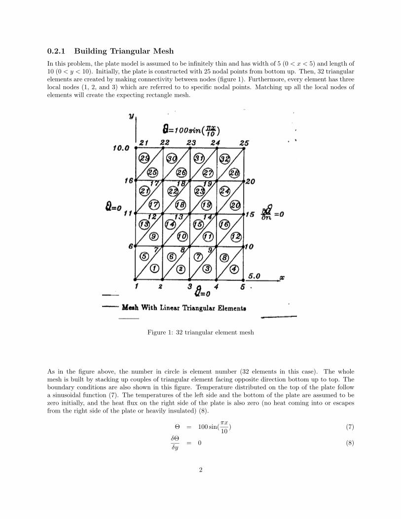
0.2.1 Building Triangular Mesh

In this problem, the plate model is assumed to be infinitely thin and has width of 5 (0 < x < 5) and length of10 (0 < y < 10). Initially, the plate is constructed with 25 nodal points from bottom up. Then, 32 triangularelements are created by making connectivity between nodes (figure 1). Furthermore, every element has threelocal nodes (1, 2, and 3) which are referred to to specific nodal points. Matching up all the local nodes ofelements will create the expecting rectangle mesh.

!

!

!

!

Figure 1: 32 triangular element mesh

As in the figure above, the number in circle is element number (32 elements in this case). The wholemesh is built by stacking up couples of triangular element facing opposite direction bottom up to top. Theboundary conditions are also shown in this figure. Temperature distributed on the top of the plate followa sinusoidal function (7). The temperatures of the left side and the bottom of the plate are assumed to bezero initially, and the heat flux on the right side of the plate is also zero (no heat coming into or escapesfrom the right side of the plate or heavily insulated) (8).

Θ = 100 sin(πx

10) (7)

δΘδy

= 0 (8)

2

The mesh can be reconstructed with the same length and width but with more elements by increasing thenumber of nodal points which will be discussed later.

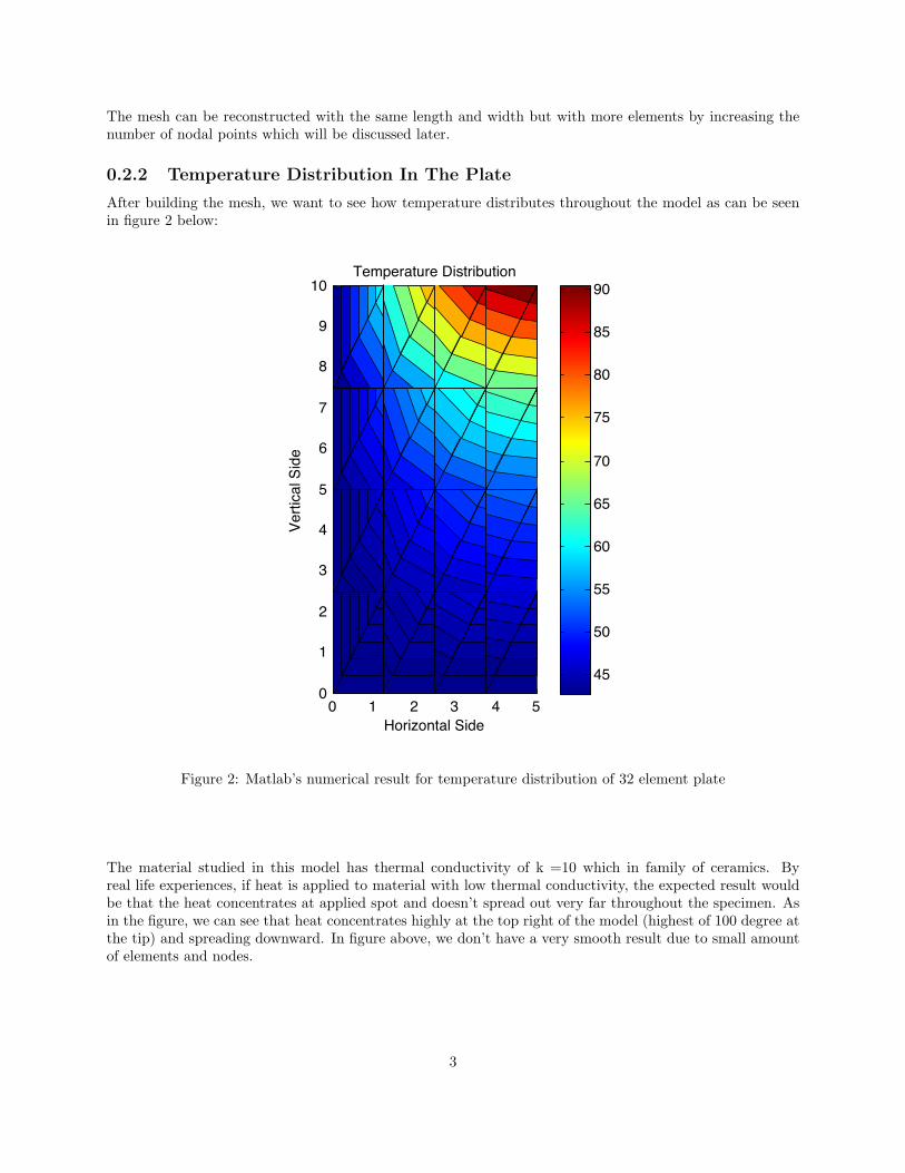
0.2.2 Temperature Distribution In The Plate

After building the mesh, we want to see how temperature distributes throughout the model as can be seenin figure 2 below:

0 1 2 3 4 50

1

2

3

4

5

6

7

8

9

10Temperature Distribution

Horizontal Side

Vert

ical S

ide

45

50

55

60

65

70

75

80

85

90

Student Version of MATLAB

Figure 2: Matlab’s numerical result for temperature distribution of 32 element plate

The material studied in this model has thermal conductivity of k =10 which in family of ceramics. Byreal life experiences, if heat is applied to material with low thermal conductivity, the expected result wouldbe that the heat concentrates at applied spot and doesn’t spread out very far throughout the specimen. Asin the figure, we can see that heat concentrates highly at the top right of the model (highest of 100 degree atthe tip) and spreading downward. In figure above, we don’t have a very smooth result due to small amountof elements and nodes.

3

0.2.3 Matlab Code for 25 Nodes and 32 Elements

This is our first approach to build 32 elements. This way of approach is not really efficient and we willintroduce the alternative after this. Here we create connectivity between local nodes of elements in order toconstruct the mesh

%%zeros matrix (2 by 25)xn=zeros ( nsd , nnp ) ;%%Using repmat to r e p l i c a t e matr icesA= [ 0 : 1 . 2 5 : 5 ] ;B=repmat (A, 1 , 5 ) ;%% Input ing x and y va lue f o r nodal po in t sxn (1 , : )=B; xn ( 2 , 1 : 1 : 5 ) = 0 ;xn ( 2 , 6 : 1 : 1 0 ) = 2 . 5 ; xn ( 2 , 1 1 : 1 : 1 5 ) = 5 ;xn ( 2 , 1 6 : 1 : 2 0 ) = 7 . 5 ; xn (2 , 21 : 1 : 25 )=10 ;%%Connec t i v i t y between nodes%%Local nodes are matched up wi th g l o b a l nodes

%%Row 1 of matrix− LOCAL NODE 1i en ( 1 , 1 : 1 : 4 ) = [ 1 : 1 : 4 ] ; %l o c a l node 1 o f e lements 1 to 4i en ( 1 , 5 : 1 : 8 ) = [ 7 : 1 : 1 0 ] ; %l o c a l node 1 o f e lements 7 to 10i en ( 1 , 9 : 1 : 1 2 ) = [ 6 : 1 : 9 ] ; %l o c a l node 1 o f e lements 6 to 9i en ( 1 , 1 3 : 1 : 1 6 ) = [ 1 2 : 1 : 1 5 ] ; %l o c a l node 1 o f e lements 13 to 16i en ( 1 , 1 7 : 1 : 2 0 ) = [ 1 1 : 1 : 1 4 ] ; %l o c a l node 1 o f e lements 17 to 20i en ( 1 , 2 1 : 1 : 2 4 ) = [ 1 7 : 1 : 2 0 ] ; %l o c a l node 1 o f e lements 21 to 24i en ( 1 , 2 5 : 1 : 2 8 ) = [ 1 6 : 1 : 1 9 ] ; %l o c a l node 1 o f e lements 25 to 28i en ( 1 , 2 9 : 1 : 3 2 ) = [ 2 2 : 1 : 2 5 ] ; %l o c a l node 1 o f e lements 29 to 32

%%Row 2 of matrix− LOCAL NODE 2i en ( 2 , 1 : 1 : 8 ) = [ 2 : 1 : 9 ] ; %l o c a l node 2 o f e lements 1 to 8i en ( 2 , 9 : 1 : 1 6 ) = [ 7 : 1 : 1 4 ] ; %l o c a l node 2 o f e lements 9 to 16i en ( 2 , 1 7 : 1 : 2 4 ) = [ 1 2 : 1 : 1 9 ] ; %l o c a l node 2 o f e lements 17 to 24i en ( 2 , 2 5 : 1 : 3 2 ) = [ 1 7 : 1 : 2 4 ] ; %l o c a l node 2 o f e lements 25 to 32

%%Row 3 of matrix− LOCAL NODE 3i en (3 , 1 : 1 : 4 )= ien ( 1 , 5 : 1 : 8 ) ; %l o c a l node 3 o f e lements 1 to 4i en (3 , 5 : 1 : 8 )= ien ( 1 , 1 : 1 : 4 ) ; %l o c a l node 3 o f e lements 5 to 8i en (3 , 9 : 1 : 12 )= ien ( 1 , 1 3 : 1 : 1 6 ) ; %l o c a l node 3 o f e lements 9 to 12i en (3 ,13 :1 : 16 )= ien ( 1 , 9 : 1 : 1 2 ) ; %l o c a l node 3 o f e lements 13 to 16i en (3 ,17 :1 : 20 )= ien ( 1 , 2 1 : 1 : 2 4 ) ; %l o c a l node 3 o f e lements 17 to 20i en (3 ,21 :1 : 24 )= ien ( 1 , 1 7 : 1 : 2 0 ) ; %l o c a l node 3 o f e lements 21 to 24i en (3 ,25 :1 : 28 )= ien ( 1 , 2 9 : 1 : 3 2 ) ; %l o c a l node 3 o f e lements 25 to 28i en (3 ,29 :1 : 32 )= ien ( 1 , 2 5 : 1 : 2 8 ) ; % l o c a l node 3 o f e lements 29 to 32

0.2.4 Numerical Results as Number of Elements Increases

What would we expect for the numerical results of temperature distribution as the number of elements andnodal points increase? The answer will be shown in figure 3 below. As the number of elements increasesfrom 128 to 1682, the result gets smoother and smoothers because there is less gap between data as in theoriginal plate of 32 elements.

4

0 1 2 3 4 50

1

2

3

4

5

6

7

8

9


Horizontal side

Ve

rtic

al sid

e

70

75

80

85

90


(a) 128 elements

0 1 2 3 4 50

1

2

3

4

5

6

7

8

9


Horizontal side

Vert

ical sid

e

82

84

86

88

90

92

94

96


(b) 512 elements

0 1 2 3 4 50

1

2

3

4

5

6

7

8

9


Horizontal Side

Ve

rtic

al S

ide

90

91

92

93

94

95

96

97

98


(c) 1682 elements

Figure 3: Matlab’s numerical results as number of elements increases from left to right (a), (b), and (c)

0.2.5 Matlab Code for Increasing Elements and Nodal Points

As we revised the code again and again, we finally come up with the final efficient code to increase numberof nodal points and elements as shown below:

nsd=2; % number o f space dimensionndf =1; % number o f degree o f freedom per nodenen=3; % number o f e lement nodesnxd = 5 ; % number o f po in t s in x d i r e c t i o nnyd = 5 ; % number o f po in t s in y d i r e c t i o nxinc = 5/(nxd−1); % Increment in x d i r e c t i o nyinc = 10/(nyd−1); % Increment in y d i r e c t i o nne l =(nxd−1)∗(2∗(nyd−1))−2; % number o f e lementsnnp=nxd∗nyd ; % number o f nodal po in t s

%−−−−−−−−−−−−−−−−−−−−−−−−−%% Nodal coord ina t e s%%−−−−−−−−−−−−−−−−−−−−−−−−−−%% xn ( i ,N):= coord ina te i f o r node N% N=1 , . . . , nnp% i =1 , . . . , nsdxn=zeros ( nsd , nnp ) ; %2 by nnp matrixpnumb = 0 ;for j = 1 : nyd

for i = 1 : nxdpnumb = pnumb + 1 ;%%inpu t ing x and y va lue f o r nodal po in t s %%xn (1 ,pnumb) = ( i −1)∗ xinc ;xn (2 ,pnumb) = ( j −1)∗ yinc ;

5

endend

0.2.6 Temperature Distribution on Right Side of The Model

As we already succeed in thermal distribution throughout the plate model, we want to analyze the temper-ature distribution on the right side of the model, where flux is assumed to be zero. The result is expectedto match with the exactly solution:


sinh(π)(9)

Holding x = 5 for all y, will give us the temperature distribution on the right side of the plate. Then,equation (9) become:

ϑ(5, y) =100 sinh(πy10 ) sin( 5π

10 )sinh(π)

; 0 < y < 10 (10)

Back to our 2D model, we want to see how our result would match up with the exact solution above (10).Starting with 32 elements, the temperature at the bottom is zero and rises up to 100 at the top. However,because there are big gaps between data of nodal points on the side of the model, the result shown in figurebelow is not very smooth. But, again as we start to increase the number of elements, we observe the samephenomenon as in the above section, the result start to get smoother and smoother due to less and less datagap.

0 2 4 6 8 100

20

40

60

80

10032 elements

Y!axis

Tem

pera

ture

0 2 4 6 8 100

20

40

60

80

100128 elements

Y!axis

Tem

pera

ture

0 2 4 6 8 100

20

40

60

80

100512 elements

Y!axis

Tem

pera

ture

0 2 4 6 8 100

20

40

60

80

1001682 elements

Y!axis

Tem

pera

ture


Figure 4: Temperature distribution as number of elements increases

As we observe that the result get smoother and smoother, we also want to see if they converge to theexact solution. To do that, we plot all the result in one graph as in figure below:

6

0 1 2 3 4 5 6 7 8 9 100

10

20

30

40

50

60

70

80

90

100

Y!Axis

Tem

pera

ture

32 elements

128 elements

512 elements

1682 elements

Temperature at TheRight Side of ThePlate

The temperature linesconverge to a smooth lineasthe number of elementsincreases


Figure 5: Convergence of results

0.2.7 Matlab Code for Plotting Side Temperature

A = load ( ’ 32 e lements . mat ’ ) ; %Load temperature o f nodal po in t s in 32 element p l a t eB = load ( ’ 128 e lements . mat ’ ) ; %Load temperature o f nodal po in t s in 128 element p l a t eC = load ( ’ 512 e lements . mat ’ ) ; %Load temperature o f nodal po in t s in 512 element p l a t eD = load ( ’ 1682 e lements . mat ’ ) ; %Load temperature o f nodal po in t s in 1682 element p l a t ex=5; %ho ld ing x cons tanty=linspace ( 0 , 1 0 ) ; %Creat ing domain f o r yg=100∗(sinh ( pi∗y ./10 )∗ sin ( pi∗x /10))/ sinh ( pi ) ; %exac t s o l u t i o n

Ucomp1 = A. Ucomp ( 5 : 5 : 2 5 ) ;%Reading temperature on the r i g h t s i d e o f 32 element p l a t eUcomp2 = B. Ucomp ( 9 : 9 : 8 1 ) ;%Reading temperature on the r i g h t s i d e o f 128 element p l a t eUcomp3 = C. Ucomp ( 1 7 : 1 7 : 2 8 9 ) ;%Reading temperature on the r i g h t s i d e o f 512 element p l a t eUcomp4 = D. Ucomp ( 3 0 : 3 0 : 9 0 0 ) ;%Reading temperature on the r i g h t s i d e o f 1682 element p l a t eX1 = A. xn ( 2 , 5 : 5 : 2 5 ) ; X2 = B. xn ( 2 , 9 : 9 : 8 1 ) ;X3 = C. xn ( 2 , 1 7 : 1 7 : 2 8 9 ) ; X4 = D. xn ( 2 , 3 0 : 3 0 : 9 0 0 ) ;%%PLOT RESULTSplot (X1 , Ucomp1 , ’p− ’ ) ;% 32 elementshold onplot (X2 , Ucomp2 , ’mv− ’ ) ;% 128 e lementshold onplot (X3 , Ucomp3 , ’h−k ’ ) ;% 512 e lementshold onplot (X4 , Ucomp4 , ’ r∗− ’ ) ;% 1682 e lements

7

0.2.8 Computing Error in The Model

Finite element method gives approximate results, so the model we built definitely has error compared tothe exact numerical result. Before computing the error (in percentage) of the model, we used Matlab toconstruct the exact result base on the function below:


sinh(π)(11)

Next, we construct a parameter to calculate temperature at every nodal point. After we have the exactsolution and the nodal point temperature, the error at each nodal point is computed by this equation (12):

Error =Exact Solution−NodalPoint temperature

Exact Solution.100 (12)

After calculating the error, we observe a phenomenon in which, the maximum percentage error dramaticallydrops as the number of elements increases. This phenomenon is shown in figure below.

0 1 2 3 4 50

1

2

3

4

5

6

732 elements

X!axis

Pe

rce

nta

ge

Err

or

0 1 2 3 4 50

0.5

1

1.5

2128 elements

X!axis

Pe

rce

nta

ge

Err

or

0 1 2 3 4 50

0.05

0.1

0.15

0.2

0.25

0.3

0.35

0.4

0.45512 elements

X!axis

Pe

rce

nta

ge

Err

or

0 1 2 3 4 50

0.02

0.04

0.06

0.08

0.1

0.12

0.141682 elements

X!axis

Pe

rce

nta

ge

Err

or


Figure 6: Matlab’s numerical result for maximum percentage error as number of elements increases. Maxi-mum percentage error drop from 6 (32 elements) to 1.6 (128 elements) to 0.43 (512 elements) to 0.13 (1682elements)

8

0.2.9 Matlab Code for Error Computing

%%Exact So lu t i on %%for i= 1 : nnp

Exact ( i )= 100∗ sinh ( pi∗xn (2 , i )/10)∗ sin ( pi∗xn (1 , i )/10)/ sinh ( pi ) ;end%%Error Computing %%Error=abs ( ( Exact−Ucomp ) ) . / ( Exact )∗100 ;

for i =1:nnpi f Exact ( i )+Ucomp( i )==0

i f Exact ( i )−Ucomp( i )==0Error ( i )=0;

elseError ( i )=100;

endend

end

0.3 Temperature Distribution In a Defected Plate Model

After computing the error in the model, we want to move forward to another important part in the project,temperature distribution of the model with a hole. What the temperature distribution would be like if thereis a hole in the model? To approach this problem, we start with building the mesh.

0.3.1 Building the Mesh

The mesh is built in Matlab nearly the same way as with the original mesh, except for the middle part of it.8 elements are taken out leaving an empty space in the mesh. In order to take away the elements, the num-ber of nodal points and elements has to be reduced. Figure below shows the mesh with a hole in the middle.

0 1 2 3 4 50

1

2

3

4

5

6

7

8

9

10Mesh

1 2 3 4 5

6 7 8 9 10

11 12 13 14

15 16 17 18 19

20 21 22 23 24

(1) (2) (3) (4)

(5) (6) (7) (8)

(9) (10)

(11) (12)

(13) (14)

(15) (16)

(17) (18) (19) (20)

(21) (22) (23) (24)

X!axis

Y!axis


Figure 7: Mesh of the defected plate model

9

As in figure 7 above, the nodal point is built in the same pattern from left to right and from bottomup. The hole is built by building the nodes so that they surround certain areas and by setting up noconnectivity between nodes there.

0.3.2 Matlab Code of The Mesh With Hole

Since we haven’t figured out the relationship of nodes at the hole, the whole mesh is built manually and thisis not an efficient way to study the model when the number of elements increases.

%Bui ld ing Nodal Pointsxn ( 1 , 1 : 1 : 5 ) = 0 : 1 . 2 5 : 5 ; %X va lue o f e lements 1 to 5xn ( 1 , 6 : 1 : 1 0 ) = 0 : 1 . 2 5 : 5 ; %X va lue o f e lements 6 to 10xn (1 ,11)=0; xn (1 ,12 )=1 .25 ; %X va lue o f e lements at the ho l e (11 , 12)xn (1 ,13 )=3 .75 ; xn (1 ,14)=5; %X va lue o f e lements at the ho l e (13 , 14)xn ( 1 , 1 5 : 1 : 1 9 ) = 0 : 1 . 2 5 : 5 ; %X va lue o f e lements 15 to 19xn ( 1 , 2 0 : 1 : 2 4 ) = 0 : 1 . 2 5 : 5 ; %X va lue o f e lements 20 to 24xn ( 2 , 6 : 1 : 1 0 ) = 2 . 5 ; %Y va lue o f e lements 6 to 10xn ( 2 , 1 : 1 : 5 ) = 0 ; %Y va lue o f e lements 1 to 5xn ( 2 , 1 1 : 1 : 1 2 ) = 5 ; %Y va lue o f e lements at the ho l e (11 , 12)xn ( 2 , 1 3 : 1 : 1 4 ) = 5 ; %Y va lue o f e lements at the ho l e (13 , 14)xn ( 2 , 1 5 : 1 : 1 9 ) = 7 . 5 ; %Y va lue o f e lements 15 to 19xn (2 , 20 : 1 : 24 )=10 ; %Y va lue o f e lements 20 to 24%Bui ld ing Local Nodal Pointsi en ( 1 , 1 : 1 : 4 ) = 1 : 1 : 4 ;i en ( 1 , 5 : 1 : 8 ) = 7 : 1 : 1 0 ;%Local nodes 1 and 2 at ho l ei en (1 ,9)=6; i en (1 ,10)=9; i en (2 ,9)=7; i en (2 ,10)=10;i en (1 ,11)=12; i en (1 ,12)=14; i en (2 ,11)=11; i en (2 ,12)=13;i en (1 ,13)=11; i en (1 ,14)=13; i en (2 ,13)=12; i en (2 ,14)=14;i en (1 ,15)=16; i en (1 ,16)=19; i en (2 ,15)=15; i en (2 ,16)=18;i en ( 1 , 1 7 : 1 : 2 0 ) = 1 5 : 1 8 ; i en (2 , 17 : 20 )=16 :19 ;i en (1 , 21 : 24 )=21 :24 ; i en ( 2 , 2 1 : 1 : 2 4 ) = 2 0 : 2 3 ;i en ( 2 , 1 : 1 : 4 ) = 2 : 5 ;i en ( 2 , 5 : 1 : 8 ) = 6 : 9 ;

i en ( 3 , 1 : 4 ) = 7 : 1 0 ;i en ( 3 , 5 : 8 ) = 1 : 4 ;%Local node 3 at ho l ei en (3 ,9)=12; i en (3 ,10)=14;i en (3 ,11)=6; i en (3 ,12)=9;i en (3 ,13)=16; i en (3 ,14)=19;i en (3 ,15)=11; i en (3 ,16)=13;i en ( 3 , 1 7 : 1 : 2 0 ) = 2 1 : 2 4 ;i en ( 3 , 2 1 : 1 : 2 4 ) = 1 5 : 1 8 ;

After constructing the mesh, we want to set up boundary conditions for the model and observe its steadystate temperature distribution.

0.3.3 Temperature Distribution in The Defected Model

The boundary conditions for this plate stays the same for all the sides as in the original plate. Heat isapplied on the top of the plate as a sinusoidal function (7). There is no heat being applied to the left side

10

and the bottom side, the temperature at these places is considered to be absolute zero. There is no heat fluxthrough the right side of the plate because it’s heavily insulated. The only difference in this model is thatthere is boundary condition at the hole and the temperature there is also considered to be zero.After setting up all the boundary conditions, we have been able to make a thermal distribution graph forthe model with Matlab as in figure 8 below.

0 1 2 3 4 50

1

2

3

4

5

6

7

8

9


X!axis

Y!

axis

55

60

65

70

75

80

85

90

95


Figure 8: Temperature distribution of a defected plate model

As in figure 8 above, temperature spreading to almost everywhere on the upper part and the right side ofthe plate. The highest heat concentration is still at the top right corner. Because there is no heat fluxthrough the hole, thermal energy has to be spread in different direction. In this case, heat is forced to spreadthroughout the top part and the right side part of the model.

Comparing Temperature Distribution of Original Plate Model and Defected Plate Model

After finishing the temperature distribution of the defected model, we want to compare the result to that ofthe original plate.

11

0 1 2 3 4 50

1

2

3

4

5

6

7

8

9


X!axis

Y!

axis

55

60

65

70

75

80

85

90

95


(a) Hole model

0 1 2 3 4 50

1

2

3

4

5

6

7

8

9


X!axis

Y!

axis

45

50

55

60

65

70

75

80

85

90

95


(b) Original model

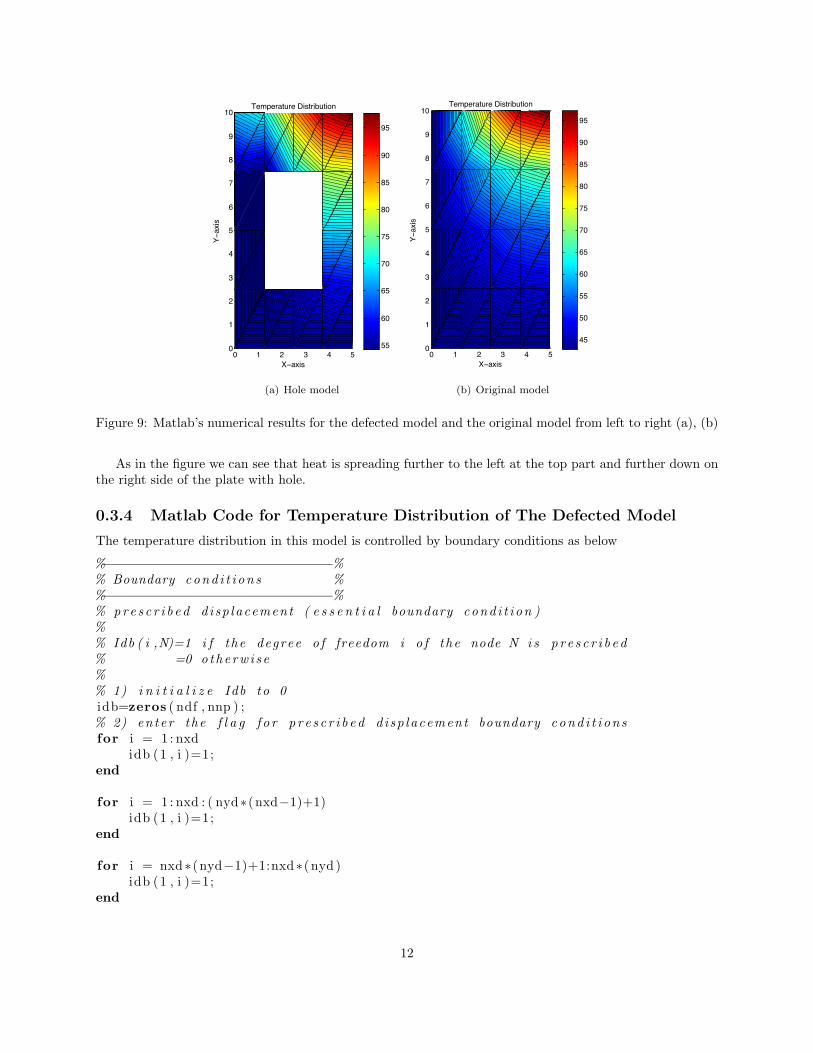
Figure 9: Matlab’s numerical results for the defected model and the original model from left to right (a), (b)

As in the figure we can see that heat is spreading further to the left at the top part and further down onthe right side of the plate with hole.

0.3.4 Matlab Code for Temperature Distribution of The Defected Model

The temperature distribution in this model is controlled by boundary conditions as below

%−−−−−−−−−−−−−−−−−−−−−−−−−−−−−%% Boundary cond i t i on s %%−−−−−−−−−−−−−−−−−−−−−−−−−−−−−%% pre s c r i b e d d i sp lacement ( e s s e n t i a l boundary cond i t i on )%% Idb ( i ,N)=1 i f the degree o f freedom i o f the node N i s p r e s c r i b e d% =0 otherw i s e%% 1) i n i t i a l i z e Idb to 0idb=zeros ( ndf , nnp ) ;% 2) enter the f l a g f o r p r e s c r i b e d d i sp lacement boundary cond i t i on sfor i = 1 : nxd

idb (1 , i )=1;end

for i = 1 : nxd : ( nyd∗(nxd−1)+1)idb (1 , i )=1;

end

for i = nxd∗(nyd−1)+1:nxd∗( nyd )idb (1 , i )=1;

end

12

%−−−−−−−−−−−−−−−−−−−−−−−−−−−−−−−−−−−−−−−−−−−−−−−−−−−−−−−−−−−−−−−−−−−−−−−%% pre s c r i b e d nodal temperature boundary cond i t i on s %%−−−−−−−−−−−−−−−−−−−−−−−−−−−−−−−−−−−−−−−−−−−−−−−−−−−−−−−−−−−−−−−−−−−−−−−%% g ( i ,N) : p r e s c r i b e d temperature f o r the dof i o f node N% i n i t i a l i z e gg=zeros ( ndf , nnp ) ;% enter the va l u e sfor i=nxd∗(nyd−1):nxd∗nyd−1

g (1 , i )=100∗ sin ( pi∗xn (1 , i ) / 1 0 ) ; %heat equat ion on top o f the p l a t eend%Temperature at the ho l e%g ( 1 , 7 : 1 : 9 ) = 0 ;g (1 ,12 :1 :13 )=0g ( 1 , 1 6 : 1 : 1 8 ) = 0 ;

0.4 conclusion

Overall, finite element method gives very good approximate results for the PDE problem in this projectas the number of elements increases. The maximum percentage of error also drop dramatically at very bigamount of elements. Furthermore, this method is a useful tool to study the temperature distribution of adefected model, especially the plate model with a hole in the middle, where we have no exact solution tocompare to. Clearly, using this method in Matlab give lots of advantages in numerical approximation.

0.5 Acknowledgements

I would like to thank Professor Nima Rahbar who guided us throughout the project, from proposing thisproject to providing us the background we need in finite element method. I also want to thank ProfessorGottlieb, Professor Kim and Csums staff for their encouragement and support throughout the program.

13

Bibliography

[1] Peter Widas. Introduction to finite element analysis. http://www.sv.vt.edu/classes/MSE2094_NoteBook/97ClassProj/num/widas/history.html, April 1997.

[2] Wikipedia. Finite element method. http://en.wikipedia.org/wiki/Finite_element_method, August2010.

14

Finite Element- 2 Dimensional Model for Thermal Distribution · Finite Element- 2 Dimensional Model...

Documents

Transcript of Finite Element- 2 Dimensional Model for Thermal Distribution · Finite Element- 2 Dimensional Model...