THE MANUAL OF

CONSTRUCTION PRODUCTIVITY MEASUREMENT

AND PERFORMANCE EVALUATION

CONSTRUCTION

INDUSTRY

INSTITUTE

Page | 1

CHAPTER 1

INSTRODUCTION

Productivity is one the most of frequently discussed topics in the construction

industry. The reason is that productivity translates directly into costs and ultimately in

to contractor profits made or lost on the job. In most projects, productivity is the most

difficult cost component to estimate. It is also the most difficult one to control [7, 14,

17]. Indeed, productivity can be affected by many things, both major and minor. Some

factors are within the control of the contractor may be unaware that adverse factors are

present.

Considering the importance of construction productivity to project cost and

schedule control, one would expected to find a large body of well-codified knowledge

describing how to recognize productivity problems and offering known, sure – to-

successful remedies. In reality, little such information exists on what affects

productivity and, more important, by how much [13]. The range of opinions on factors

is extensive. Some blame global issues such as the economy, union politics, or

government regulations. Others argue that the work ethic is the problem. However, a

growing majority of those closely associated with the construction industry look to the

project itself for the factors affecting productivity. The focus on the way in which

projects are planned, organized, and managed. Fortunately, the implication is that most

of the factors affecting productivity can be identified and controlled to the large

degree. One thing seems relatively certain: Before it can be improves, productivity

must be measured [13].

PURPOSE

The objective of this manual is to describe an approach to construction

productivity measurement that can be used by general and specialty contractors and

owners on small – to medium – sized commercial and industrial projects. Perform

evaluation, which is an extension of productivity measurement, is also discussed. The

concepts are equally applicable to contractors and owners who do not have

productivity measurement system or who need a simple , inexpensive measurement

approach. The approach emphasizes measurements for selected labor-intensive

construction activity at the screw level. The important factors considered I developing

the approach include the size and duration of project; the value of measuring a few

activities instead of the total effort; the relationship to other control systems that may

or may not be used; the need for little or no additional staff or overhead expense; the

need for easy – to – understand, timely, and accurate information; and, last, the needs

of the user.

APPLICATION

The approach described in this manual is not restricted to any particular project

size or type. Appropriate areas of application have been identified on commercial and

industrial project alike. Certain Activities on highway projects and maintenance or

outage work on process, petrochemical, and power plant can be measured using these

techniques. The techniques can be applied equally well to lump sum, unit price, or cost

reimbursable contracts and can be used by owners, contractors, and special

contractors.

Page | 2

This manual is unique in that is a comprehensive guide to measuring

construction productivity. It offer an encouraging and appealing approach to the

measurement task by stating from the outset that productivity measurement is simple,

effective and can be done for little overhead expense. The contractor who implements

the procedures presented in this manual will develop almost immediately an increased

awareness and sensitivity to productivity issues. By following up with corrective

action on the problem that surface, a contractor may easily save 10 percent or more on

the labor cost of the major construction activities that impact total project cost and

schedule.

DEFINITIONS

In this manual, the following terms and definitions are used:

Account – A record or identification scheme used to categorize information about

a specific work item or activity, an account represents a discrete part or category of the

work to be performed. For example, an account may contain the work-hours used in

the erection if formwork for elevated slabs.

Control account – a control account consist of a grouping of related accounts or

activities where each account has a unique degree of difficulty or level effort required.

For example, the account for wall, column, and slabs formwork may be grouped into a

single control account titled formwork.

Control budget – The base estimate of work-hour, quantities, and productivity for

an activity or account, the control budget is used for comparative purposes to evaluate

performance.

Earned value – This technique is used for calculating the percent complete of a

control account. It uses a weighted average approach in which the weight assigned to

each individual account in the control account is based on the initial work-hour

estimate for the account compared to the sum of the initial estimated work-hour for all

accounts included in the control account [5].

Forecasting – The process of projecting the total work-hour required to complete

an account or activity is called forecasting [3].

Performance evaluation – This process involves the comparison of the actual

progress and productivity to the control budget. It includes the comparison of quantity

installation rates and work-hour consumption rates. Forecasting is a part of

performance evaluation.

Performance factor – A measure of construction efficiency, it is the planed

productivity divided by the actual productivity. This ratio is sometimes called a PF

value or a rate ratio. A ratio greater than 1.0 signified better -than – planned

performance.

Productivity – The work-hour require per unit of work, productivity is the input

divided by the output and is calculated for a finite time interval. It is commonly called

the unit rate [17].

Productivity measurement – This process of quantifying the work-hour and

quantities associated with an activity or account provides the measurements used in

productivity calculations and performance evaluations [7].

Page | 3

BARRIER TO MONITORING PRODUCTIVITY

Many contractors do not measure or monitor construction productivity. The most

common reasons for not doing so are:

- I’ve never monitored productivity before.

- I don’t know how to measure productivity.

- Productivity control is a part of a cost control system, which is too complicated

to understand and too expensive to implement

- Productivity cannot be controlled.

- Productivity measurement will not tell me something about my project that o

don’t really know.

The first two reasons cited are really a reflection of past practices where

productivity measurement was not an absolute necessity. Keen competitions for

projects, high inflation rates, increased project complexity, and greater exposure to

unforeseen risks have changed this situation. Productivity measurement has emerged

as an inexpensive way to control one of the more important contractor risks,

specifically the craft work-hours.

Historically, the most widely publicized productivity measurement systems have

emerged from the heavy industrial and power plant construction sectors of the

industry. Here, productivity control has always been treated as subset of the cost

control system. Understandably, many contractors have been discouraged by apparent

complexity and the prohibitive expense of operating a large, complex cost control

system. Until now, the prevailing attitude seems to have been that productivity

measurement must be tied to these types of system [1]. In reality, however, the two

functions of productivity control and cost control can be separated, and, in doing so,

productivity measurement and control can be made simple, inexpensive, effective, and

timely. This manual is the first known comprehensive document that recognizes the

two functions as separable.

The last two challenges to productivity measurement can be considered together.

A growing body of knowledge says that productivity can be controlled [4]. This

assertion is supported by the conclusion that work ethic, labor union, and poorly

motivated workers are not the primary root causes of productivity problems. Studies

have consistently shown that that problems result from the way project are designed,

organized, planned, and managed, and that these conditions exist whether the project is

large or small, commercial or industrial, or union or merit shop [4,144]. The following

are a few of the more commonly reoccurring causes of poor productivity that are

within the exclusive control of the contractor:

- Crews are too large, especially at the beginning and end of and activity.

- Stockpile and storage areas are poorly organized.

- Materials are inadequately marked or not sorted fro easy retrieval.

- Delays result from waiting for tools and equipment.

- Housekeeping practices are poor.

- Inability to maintain continuity or momentum results because screws are

reassigned to different to work or locations.

- Work of one screw interferes with that of another.

- Sequencing and control of the work are poor.

- Material deliveries are untimely.

Page | 4

This list could easily be expanded, but the important point is that many of these

causes exist to varying degrees on all construction projects.

If these causes occur repeatedly, why aren’t they corrected? Actually, many of

them are subtle and appear gradually. Although, they may never be noticed, they are

still there. Often, by the time a problem is noticed, the damage has already been done.

In many other cases, corrective action is perceived to cost more than it would save.

What then is the role of productivity measurement and performance evaluation?

They should provide early warning signals, long before the problem is obvious. They

should answer the question: How serious is the problem? They should be the basis for

measuring the economic impact of alternatives and should be the basis measuring the

economic impact of alternatives and should provide an easy means for quantifying the

results.

ORGANIZATION OF THE MANUAL

This manual is organized into four main parts. The first part, which includes

chapter 2 and 3, describes the framework for productivity measurement. Chapter 2

explains the basic concepts of cost control, cost accounting, and productivity control.

Chapter 3 defines the system criteria and then develops the framework for productivity

measurement and control. Productivity accounts are presented, and the relationship to

other account and control system is described.

Part II of the manual explains the basic concepts of productivity measurement,

reporting, and devaluation. Chapter 4 describes how to measure work-hour and

quantities. Five methods of quantity measurement are described. Chapter 5 shows four

types of productivity calculations and graphically illustrates each. The advantages of

tabular and graphical output are described. Chapter 6 describes performance

evaluation, which is the process of comparing the productivity calculations with the

project estimate. Analytical and graphical forecasting techniques are illustrated.

More advanced concepts are addressed in part III. Rues of credit for complex tasks

and the earned value technique for control accounts are coveted in chapter 7. The

technique the forecasting using standard productivity curves is also detail. Chapter 8

addresses concepts that integrate productivity and schedule parameters.

Part IV presents several case studies and summarizes the results. Chapter 9

describes case studies of three contractors involved primarily in commercial and light

industrial construction. Their long – range objectives in measuring productivities are

describes along with lesions learned during the implementation process. The case

studies illustrate how productivity can be used to understand the factors that affect

productivity, to monitor and control important activities, and to develop labor units for

estimating. Chapter 10 summarizes the case study finding and conclusion.

USE OF THE MANUAL

The manual explains concepts in a general way, which means the techniques can

be applied regardless of the type of control system already in-place, nature of work,

sophistication of the contractors, and so forth. Part I explains the framework for

productivity measurement, and readers who have an understanding of productivity

control using a cost control system may wish to begin directly with chapter 3. For the

experienced user, chapter 2 and 3 describe the context in which measurements are

made. These two chapters will ease apprehension that contractor must implement a

cost control system to used the techniques; no significant changes in current modes if

Page | 5

operation are required. An experienced user should first concentrate on the basic

concepts in part II. As one becomes familiar with these, the first step beyond manual

tracking will probably be to computerize the process, which can be done relatively

easily on a spreadsheet program such as LOTUS 1-2-3 or on an integrated system like

framework II or SYMPHONY. After mastering the basic concepts on several projects,

the contractor may be ready to try some of the advance concepts in part III. The

experienced users may want to review part II before proceeding to part III, or may be

feel comfortable about implementing some of the advanced concepts from the outset.

All reader will find the case studies in part IV to be valuable, as they describe some

specific about implementation and details of lessons learned. The examples illustrate a

wide range of applications.

Page | 6

PART I - FRAMEWORK FOR PRODUCTIVITY CONTROL

An outgrowth of defense systems acquisition and large , cost reimburse

construction projects such as for nuclear power plants, refineries and coal gasification

facilities was the development of sophisticated cost control systems. These systems are

characterized by the breakdown of project expenditures according to code of accounts

Each account can be monitored for excessive costs, and these can be traced to the

source, e.g. , labor, construction equipment, construction materials, permanent plant

equipment, etc. [11].

Cost control systems have also been used to monitor labor productivity but

whether they are the most effective way of monitoring productivity questionable. This

section of the manual will develop the framework around which productivity can be

monitored in a simple and timely manner. Chapter shows that the cost control system

can be used for two purposes, and that the system is used affects the level of detail.

The most detailed form is needed for control purposes. The code of account structure

is designed to isolate problem areas. With this system, all project activities are tracked

in considerable detail, there is a feedback loop, and a support staff is needed. The

second form of the costing model is used only for accounting purposes. This simple

system, which supports the need to develop historical estimating data, concentrates on

accumulating costs at the end of the project. Many contractors use this type of model

because it is easy to understand and inexpensive to carry out. Unfortunately, the need

for controlling the rationale for simplifying the cost control system is then developed.

Chapter 3, the criteria for a productivity measurement and control system presented.

Using these criteria, the code of accounts for petrochemical facility and general

commercial construction are revised to be consistent productivity control needs. A

framework is developed in which productivity control operates separately from the

cost control system.

Page | 7

CHAPTER 2

FRAMEWORK FOR PRODUCTIVITY MEASUREMENT

AND PERFORMANCE EVALUATION

INTRODUCTION

A successful project is generally considered to be one that meets certain technical

objectives, is completed on or ahead of schedule, within the owner’s or contractor’s

budget, and results in a reasonable profit for the contractor. To ensure success, an

effective project control system must be implemented to provide managers and

superintendents with timely and accurate feedback on the consumption of resources.

Historically, this has meant the implementation of a cost control system. Prior to the

development of the productivity measurement system presented in Chapter 3, it is

worthwhile to review the differences in detail and usages of costing systems.

CHARACTERISTICS OF COSTING SYSTEMS

Usages

Costing system are designed to track and account for project costs. The reasons for

doing so are two-fold. First, the tracking function can be used during construction to

control project costs. Tracking highlights activities or areas that deviate significantly

from planned expenditures so that corrective action can be taken. How the system will

be used generally establishes the level of detail and degree of sophistication [11].

Costing system to Support Cost control

The more detailed and sophisticated systems are used to monitor and control cost

during construction. While these systems also support the estimating of future projects,

the requirement for considerable detail and sophistication arises to satisfy three

essential needs related to the control function: 1) to develop comparisons to project

estimates during construction, 2) to provide timely feedback, and 3) to isolate

particular problem areas where cost deviations are significant. Figure 1 shows the

overall cost control process. During construction, the contractor must account for costs

and work-hours and measure progress. Comparisons to the control budget are made

periodically, and corrective action is taken when required.

The framework for cost control is a standard code of accounts which defines how

costs will be categorized. Since costs and work-hours are used to estimate future work,

they must be consistently charged to each account from project to project [10]. Thus,

codes of accounts are typically standardized, and the accounts used for each project are

uniquely selected from the standard codes. The term “standard” should not be

misinterpreted, as there are no standards of practice. In reality, most contractors

develop their own standard codes that are uniquely tailored to their own mode of

operation.

Page | 8

Figure 1: Costing system to Support Cost Control

The hierarchical nature of cost codes is illustrated in Figure 2, which shows an

example of a code structure for a grass roots petrochemical facility [6]. Because the

emphasis is on isolating problem areas, the cost indicators allow for the charging of

expenditures to more narrowly defined areas such as direct costs, indirect costs,

subcontract costs, or home office costs. A four-digit activity code is divided into three

levels of detail. The first two digits define major activities or types of work and are

illustrated in Table 1. Table 2 shows the detailed subdivision of account 17xx, which is

aboveground non-racked piping. The cost classification code is used to further divide

the costs into direct labor, construction materials, construction equipment, and so

forth. In a comprehensive cost control system, numerous cost classification codes are

used.

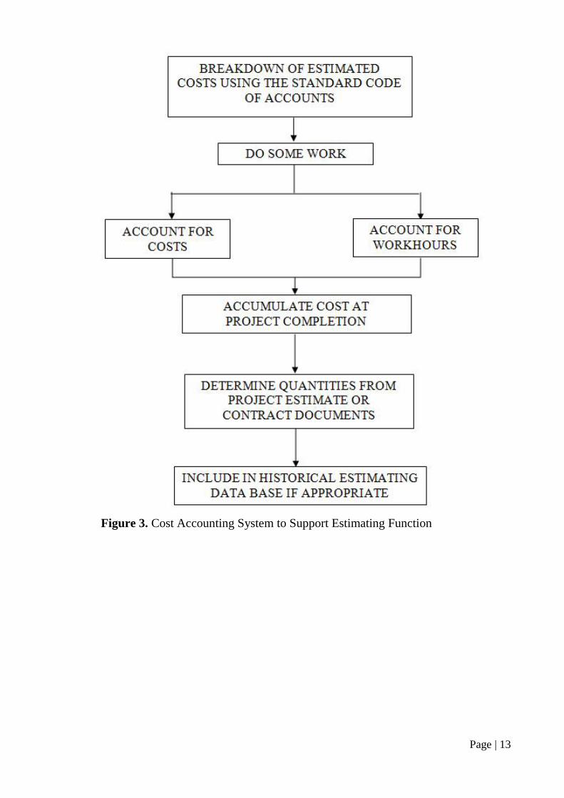
Costing Systems to Support Estimating

The costing systems used only to support the estimating function are less

sophisticated and not as detailed as those required for cost control. Figure 3 illustrates

the reason. As can be seen, there are no comparisons to projects estimates, no variance

analyses, and no feedback loop. The main emphasis is on accumulating costs at the

end of the job, so timeliness is not an issue, and minimal or no support staff is needed.

Also, quantities or progress are often not measured but rather are summarized at

project completion. These data may be extracted from the project estimate or contract

documents.

Page | 9

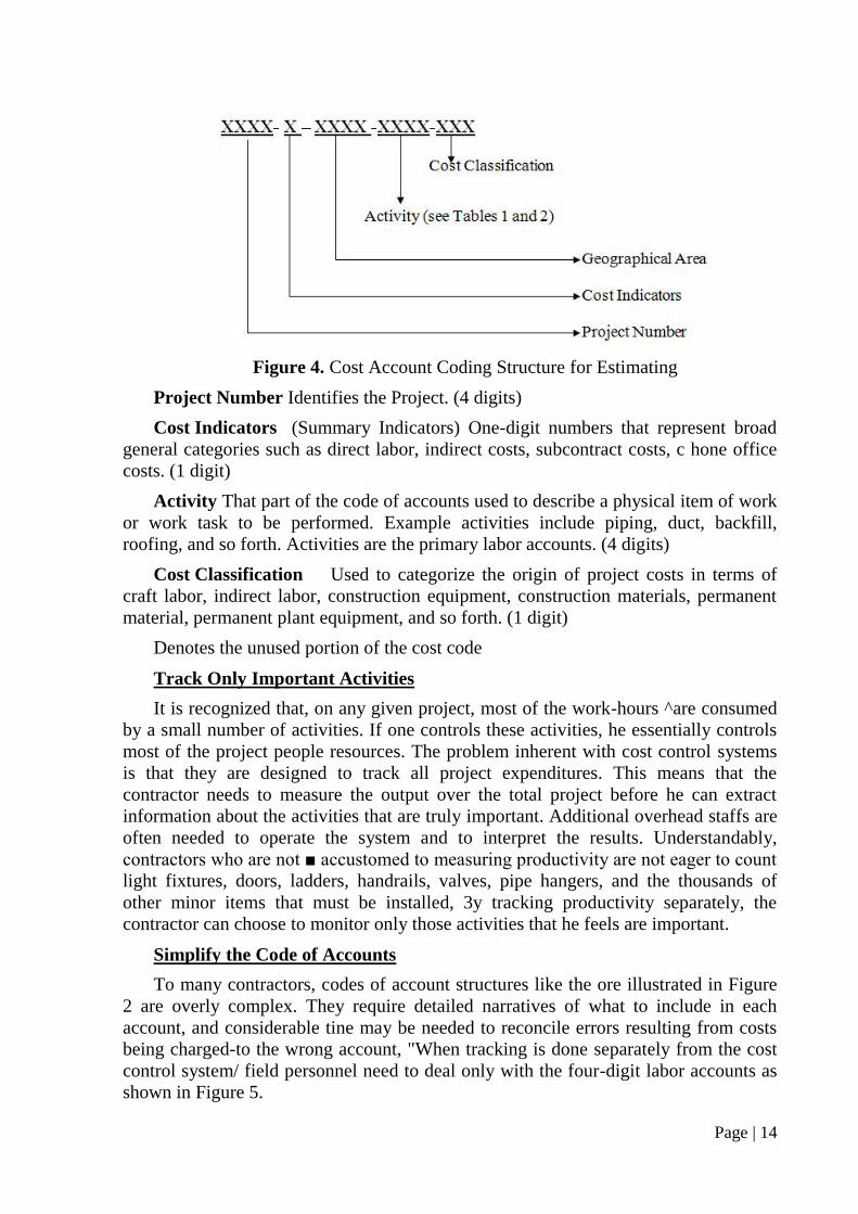
The code of accounts need not be as detailed as that required for cost control two

reasons. First, it is not necessary to divide the project into areas since the code of

accounts is not being used to isolate problem areas. Second, a contractor would prefer

to have certain components of work grouped into a single account. An example would

be piping plus related scaffolding and material handling. Groupings that include

similar work plus the manual direct and indirect support effort facilitate the need to

develop accurate estimates in a relatively short period of time.

The net result is that only part of the code of accounts shown in Figure 2 is

needed. The applicable portion is shown in Figure 4, where the 16 digit code used for

cost control has been reduced to 10 digits. The number of possible entries for the cost

classification part of the code would be greatly reduced, from 50 or more to probably

four or five. The number of cost indicators would probably be reduced as well.

PRODUCTIVITY CONTROL

Historically, productivity measurement and control have been done almost

exclusively as a subset of the larger, more detailed cost control systems. The literature

abounds with articles and advertisements that show how to monitor costs and

productivity using the cost control system [3, 5, 15, 19].

Ironically, the fact that these two control systems are typically viewed as one is

probably a main reason why many contractors do not measure productivity. To these

contractors, cost control systems are too large and complicated, require a support staff

dedicated to measuring and quantifying site activities, and result in an intolerable

overhead expense [5]. Alternatively, these contractors rely on the much simpler

accounting-type systems such as the one shown in Figures 3 and 4. However, these

provide little in the way of control.

Fortunately, productivity measurement can be greatly simplified while still

providing control. If comparisons are to be made with the project estimate, then

productivity control must originate from the same code of accounts as does the cost

control system. Thereafter, productivity measurement and control can be done

separately from the cost control system. This separation allows the freedom necessary

to tailor the system to perform a specific function. The result is a system that is simple,

timely, and inexpensive» The remainder of the chapter develops this concept through

an explanation of the desired goals needed to achieve the cost-effectiveness of the

system.

Page | 10

Figure 2: Cost Account Coding Structure for Cost Control [6]

Project Number: Identifies the Project. (4 digits)

Cost Indicator: (Summary Indicators) One – digit numbers that represent broad

general categories such as direct labor, indirect costs, subcontract costs, or home office

cost. (1 digit)

Area: Designation is reserved for project numbers which relate to geographical

area, process unit, and so forth. (4 digits)

Activity: That part of the code of accounts used to describe a physical item of

work task to be performed. Example activities include piping, duct, backfill, roofing,

and so forth. Activities are the primary labor accounts. (4 digits)

Cost Clarification: Used to categorize the origin of project costs in terms of craft

labor, indirect labor, construction equipment, construction materials, permanent

material, permanent plant equipment, and so forth. (3 digits)

Page | 11

Table 1. List of Major Activity Accounts for the Model Plant Petrochemical

Facility [6]

Account No. Description

01XX Site Preparation/Demolition/Salvage/Removal for Relocation

02XX Site Improvements

03XX Underground Electrical

04XX Underground Piping

07XX Piling

08XX Concrete and Excavation

12XX Structural Steel

15XX Building Construction (Petroleum & Chemical Projects).

16XX Aboveground (Racked Outside Overhead) Piping

17XX Aboveground Non-racked Piping

18XX Aboveground Electrical

19XX Instrumentation

20XX Insulation

21XX Painting

23XX Paving

24XX Ducts

4XXX Major Equipment

Page | 12

Table 2. Detailed Subdivision for Aboveground Non-racked Piping Activities [6]

Account

Number Description

Unit of

Measure

17XX ABOVE GROUND NONRAKED PIPING

170X Material for aboveground non-racked piping -

1711 Prefab pipe outside shops Lump Sum

172X Spool Fabrication

1721 Spool fabrication - carbon steel 2 in- and under Linear Feet

1722 Spool fabrication - carbon steel 2 1/2 to 12 in. Linear Feet

1723 Spool fabrication - carbon steel 14 in. and above Linear Feet

1724 Spool fabrication - alloy 2 in, and under Linear Feet

1725 Spool fabrication - alloy 2 ½ to 12 in. Linear Feet

1726 Spool fabrication ~ alloy 14 in. and above Linear Feet

1727 Spool fabrication - other than carbon steel and alloy Linear Feet

1728 Hanger and support fabrication Lump Sum

173X Spool Erection and Field Run Pipe

1731 Spool erection - carbon steel and alloy 2 in. and under Linear Feet

1732 Spool erection - carbon steel and alloy 2 1/2 to 12 in Linear Feet

1733 Spool erection - carbon steel and alloy 14 in. and above Linear Feet

1734 Spool erection - other than carbon steel and alloy Linear Feet

1735 Field run pipe - 2 in. and under Linear Feet

1736 Field run pipe - above 2 in. Linear Feet

1737 Hangers and supports Linear Feet

1738 Testing x-ray, cleaning and pickling and stress relieving Lump Sum

1795 Sketching and material takeoff Lump Sum

1796 Piping materials Lump Sum

1797 Scaffolding Lump Sum

Page | 13

Figure 3. Cost Accounting System to Support Estimating Function

Page | 14

Figure 4. Cost Account Coding Structure for Estimating

Project Number Identifies the Project. (4 digits)

Cost Indicators (Summary Indicators) One-digit numbers that represent broad

general categories such as direct labor, indirect costs, subcontract costs, c hone office

costs. (1 digit)

Activity That part of the code of accounts used to describe a physical item of work

or work task to be performed. Example activities include piping, duct, backfill,

roofing, and so forth. Activities are the primary labor accounts. (4 digits)

Cost Classification Used to categorize the origin of project costs in terms of

craft labor, indirect labor, construction equipment, construction materials, permanent

material, permanent plant equipment, and so forth. (1 digit)

Denotes the unused portion of the cost code

Track Only Important Activities

It is recognized that, on any given project, most of the work-hours ^are consumed

by a small number of activities. If one controls these activities, he essentially controls

most of the project people resources. The problem inherent with cost control systems

is that they are designed to track all project expenditures. This means that the

contractor needs to measure the output over the total project before he can extract

information about the activities that are truly important. Additional overhead staffs are

often needed to operate the system and to interpret the results. Understandably,

contractors who are not ■ accustomed to measuring productivity are not eager to count

light fixtures, doors, ladders, handrails, valves, pipe hangers, and the thousands of

other minor items that must be installed, 3y tracking productivity separately, the

contractor can choose to monitor only those activities that he feels are important.

Simplify the Code of Accounts

To many contractors, codes of account structures like the ore illustrated in Figure

2 are overly complex. They require detailed narratives of what to include in each

account, and considerable tine may be needed to reconcile errors resulting from costs

being charged-to the wrong account, "When tracking is done separately from the cost

control system/ field personnel need to deal only with the four-digit labor accounts as

shown in Figure 5.

Page | 15

Tailor the Level of Detail

The level of detail in the code of accounts is typically established on the basis of

costs and does not always fully support the productivity control needs. Two examples

illustrate this point. The cost of 6-inch-KHameter stainless steel pipe is different from

that of 2 1/2-inch-diameter carbon steel pipe. In the cost control system, these

commodities are tracked separately. But, from the productivity measurement

viewpoint, the two may be nearly identical. Furthermore, a crew may install several

types of pipe in a single day, thus requiring that the quantities and work-hours be

reported by type. Thus, the costing system places an added burden on a reporting

system that contains more information than may be required for productivity control.

Figure 5. Codes for Productivity Measurement

Activity That part of the code of accounts used to describe a physical item of

work or work task to be performed. Example activities include piping, duct, backfill,

roofing, and so forth. Activities are the primary labor accounts and are thus the

productivity codes. (4 digits)

Denotes the unused portion of the cost code

In the second example, the unit cost difference of structural steel for commercial

multistory and structural steel for warehouse-type buildings may be sufficiently minor

to allow the two to be included in the same cost account. However, the units work-

hours for erection maybe very different. In this case, productivity control requires a

level of detail not available in the costing system. As illustrated in these two examples,

cost control and productivity measurement sometimes require different levels of detail.

Separate tracking allows the flexibility to meet the particular, needs at hand.

Simplify Units of Measure

The units of measure are established by a cost engineer or estimator for his own

particular need* Structural steel is purchased by the ton, so the measurement of

installed quantities is also by the ton. A foreman or superintendent can easily

determine how many pieces of structural steel have been erected and bolted, but to

convert these pieces to tons requires considerable time to study the drawings and to

make calculations. Likewise, an estimator determines the number of pipe hangers on

the basis of so many hangers per linear foot of pipe. Field personnel may know how

many hangers were installed, but, without measuring or studying the isometric

drawing, they will not readily know the footage. Thus, the units of measure used to

Page | 16

support estimating or cost control can sometimes place added burdens on field

personnel by requiring excessive measurement and quantification of the work.

Reduce the Amount of Data

Cost control systems handle sizeable amounts of data. The output generated is

typically in the form of summary statistics or numerical-data. Field supervisors who

would normally make use of productivity data have limited time or enthusiasm for

studying the numbers to make inferences about the progress of their work. Graphical

analyses enhance the ability to quickly interpret information, but, in some cost control

systems, the main emphasis is on generating numerical data, not graphs. The

timeliness of feedback is another concern. Consequently, some cost-control systems

provide information to field personnel in a form that is difficult to interpret, and which

may arrive too late to be of value.

SUMMARY

This chapter has shown that the level of detail in a costing system is related to how

the system is used. Many small- and medium-sized contractors want to collect only

historical estimating data. Their systems are simple and can be used with minimal

overhead expense. However, a system used for cost control purposes is far more

complex and expensive to operate.

Most contractors associate productivity measurement with cost control, but

productivity can be monitored and controlled separately from the cost control system,

and this means of measurement is recommended. Cost-control systems track

everything? Productivity control monitors only a few items controlling the work. The

level of detail needed for productivity control is not always the same as for cost

control. The units of measure are established by cost engineers and estimators, and

these often place unnecessary demands on field personnel for measuring and

quantifying their work. The feedback in cost control systems is sometimes in the form

of numerical data, whereas many field personnel having minimal experience with

measuring productivity prefer graphical output.

Page | 17

CHAPTER 3

CONCEPTUAL DESIGN OF THE PRODUCTIVITY

MEASUREMENT SYSTEM

The productivity measurement and performance evaluation system developed

herein for: 1- Small and medium-sized contractors who do not routinely measure

productivity and 2 - The larger and more sophisticated contractors who are

constructing projects for which the project budget prevents the use of a detailed and

expensive cost control system. Project can be commercial or industrial, or other types

which include labor-intensive activities. Maintenance and outage-type work are also

ideally suited for the productivity measurement system.

BASIS FOR SYSTEM DEVELOPMENT

Project Characteristics

On most commercial projects, the overhead expenses must be kept to a minimum.

The same situation prevails in the heavy industrial sector of the industry. The mega

projects of the 1970s are no longer being built, and shorter and smaller projects place

special demands on cost-control systems such as the one described in Chapter 2. The

structure of the code of accounts makes it difficult to reduce project overhead by

simply reducing the scope of the cost control system. While the support staff can be

trimmed, the need for some support will always exist. Activity durations today are

shorter then they have been in the past. Important controlling activities sometimes last

only 30-60 days. If effective control is to be exercised, feedback must occur quickly.

Even a two-week reporting cycle (most projects function on a monthly reporting cycle)

provides reporting probably too infrequently.

The need to reduce overhead means that quantity tracking must be provided by

those who are responsible for doing the work. Lower level supervisors are neither

accustomed to working with intricate cost codes like the one shown in Figure 2, nor

are they anxious to spend the time necessary to perform anything more than

elementary measurements. Unfortunately, these are the elements needed to drive the

cost control system.

Assumptions

The design of the productivity measurement system must consider the essential

features of cost control system as described in Chapter 2 and relate these to the

environment in which it must function. Therefore, the following assumptions are

presented as the basis for developing the productivity measurement system.

1. The productivity measurement system must be structured around the code of

accounts if comparisons to the project estimate are to be made. However, the tracking

and feedback can be done separately from the costing system.

2. A contractor’s code of account establishes the basis for deciding which activities to monitor. If the codes are too broad to support effective monitoring, the

system can still function as a stand-alone system. However, comparisons to project

estimates may not be possible.

3. Systems presently used by contractors to track or control costs are which

unaffected by the productivity measurement system.

Page | 18

4. The contractor is not required to install a cost control system in order to

measure and control productivity.

5. The productivity measurement system can operate independently from the

estimating or schedule control system. Productivity measurement can yield worthwhile

results, even if one do not have a work-hour, quantity or schedule estimate. However,

performance cannot be evaluated without these estimates.

6. Only direct labor accounts are of interest. The most cost-effective which

approaches to productivity control is to concentrate on the labor-intensive activities.

Such activities are a small percentage of the total number of activities, yet they have

the greatest effort on the project.

7. The focus of the measurement effort is at the crew level.

8. The system is implementable at the job site and able to be done manually.

However, if a microcomputer is available, it will facilitate this task.

System criteria

The assumptions listed provide guidance for developing the productivity

measurement system. The system should satisfy the following criteria:

1. Inexpensive - The system should be easy to implement, require little overhead

to operate, and have the capability to be manually driven

2. Simple – The data requirements should be minimal. Reporting should be done

by foremen using easy-to-comprehend units of measure; output should make liberal

use of graphics.

3. Flexibility – The system should be easily tailored to the operational needs and

objectives of the contractor. Rigid, inflexible systems, which require the contractor

instead, to adjust his mode of operation to the system, are undesirable.

4. Accuracy – The output must reflect what actually occurs at the site. The level of

detail should help to isolate problem areas.

5. Timeliness – Feedback must be given quickly so that corrective action can be

taken on short-duration activities. End-of-the-day feedback is possible, if it is

desirable, thus summaries can be produced weekly. Otherwise, feedback can be

provided at a frequency consistent with the scope and magnitude of the project.

6. Support Performance Evaluation – Labor comparisons to the project estimate

should be possible. This includes comparisons to the estimated work-hours, quantities,

unit rate, and planned duration for labor-intensive activities.

Page | 19

FRAMEWORK FOR PRODUCTIVITY MEASUREMENT

The above criteria have been used in developing the productivity measurement

system that is described throughout the remainder of this manual.

Reporting Requirements

The reporting system relies upon the input of two data items namely work-hours

and quantities (progress) for selected labor-intensive activities. The data collection and

analysis process are shown in Figure 6.

The foreman, on a daily basis, records the work-hours spent by a crew in

performing the particular task in question and the quantities installed or progress made

by the crew that day. Generally, the reporting of work-hours is done for payroll

purpose, so productivity measurement imposes no new work-hour reporting

requirement. The only possible change in reporting work-hours maybe reported

separately those work-hours spent on the activity being-monitored.

The reporting of quantities, or progress, is not routinely done by many contractors.

However, the knowledge of how much work has been done which is a fundamental

requirement for monitoring and control. The quantity-reporting scheme developed

herein, and described in detail in Chapter 4, is simple, is done for only a small number

of labor-intensive activities, is characterized be easy-to-use units of measure, and can

be easily and quickly summarized by the foreman at the end of the day.

As shown in Figure 6, productivity calculations are made using the reported work-

hours and quantities. These calculations can be done manually, but the most efficient

approach is to use a microcomputer. Input can be done by a clerk or time keeper.

Because the amount of data input is miniscule, the entire entry and analysis process

involves minimal effort and time. Feedback should be almost instantaneous, and

computer programmers, systems operators. Quantity surveyors or data entry personnel

are unnecessary.

Relationship to Other Accounting or Control Systems

Productivity measurement is designed to be a stand-alone system that is

implemented entirely at the job site. Nevertheless, it is related to several other control

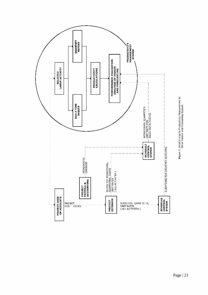
and accounting systems. As shown in Figure 7, the productivity measurement system

utilizes information available from other systems but does not provide feedback to

these systems.

The selection of activities to monitor should be made according to the breakdown

of project activities established by the costing system. The reason for this is quite

simple work-hour reporting will be done this way for both payroll and cost-accounting

purposes. Productivity measurement then can rely on the same work-hour data that is

necessary if comparisons to the project estimate are needed. Where cost accounting

and monitoring systems are already in place, a definition already exists of the items

included in each account, and dual reporting would merely increase the confusion and

amount of paperwork.

Page | 20

Page | 21

Page | 22

Data from the cost accounting and control system are used to prepare project

estimates. Several important pieces of data from the estimate can be used to enhance

the productivity measurement system. These items are the estimated total work-hours

and quantities. The estimated unit rate can also be calculated. These parameters

provide important baselines for comparing current performance.

Although schedule control is generally viewed as separate from cost or

productivity control, productivity and quantity installation rates are an integral part of

predicting completion dates. Therefore, if available, the planned completion date or

estimated duration can be used to evaluate performance.

Selection of activities to monitor

The activities that should be monitored are the ones which affect the success of the

project. To maintain simplicity and minimize project overhead, only those activities

that affect the success of the project should be tracked, those that are labor-intensive.

The labor-intensive activities tend to have the longest durations and therefore are

critical form the schedule point of view.

Often, activities to monitor can be selected on the basis of experience. An

alternative approach is to calculate the total project work-hours and to divide this sum

by the number of line items or accounts. This calculation yields the average work-

hours per line item. Those items or accounts for which the estimated work-hours are

greater than this average can be designated as labor-intensive. This method usually

results in less than one-fourth of the line items or accounts being significant. This list

can be further modified at the prerogative of the manager.

Development of productivity codes

The project code of accounts is structured to support the cost control or accounting

function. However, productivity control is comparatively simple and narrower in

scope. Thus, productivity code structures for industrial and commercial construction

are discussed below.

Figure 5 shows how a 16-digit cost code used for the construction of

petrochemical facilities can be reduced to four digits. The four-digit activity code is

ideally suited for productivity control. This four-digit productivity code defines three

levels of detail. The broadest level, represented by the first two digits, denotes major

construction activities such as aboveground electrical, aboveground non-racked piping,

and so forth. Table 1 provides a complete listing of the 17 major activities. The third

and fourth digits further subdivide each major activity. Figure 8 illustrates the

productivity code for the erection of aboveground conduit. A fifth digit (not shown)

can be added at the user’s discretion to further define the conduit by size or type.

Figure 8. Structure of Productivity Measurement Codes for Industrial

Construction

18 1 2

SUBFEATURE LEVEL

1. Aboveground Conduit

FEATURE LEVEL

2. Electrical Raceways

MAJOR ACTIVITY OR FUNCTION LEVEL

2. Electrical Raceways

Page | 23

The structure of example of productivity measurement code for commercial

constructions is shown in figure 9 to be a five-digit code. The code number represents

structural formwork for concrete columns. The code structure is based upon the master

format published by the construction specifications institute (CSI) [12]. The major

activity or function level is denoted by the first two digits. Among the major activities

is concrete, masonry, metals, mechanical, and electrical work. The remaining three

levels further subdivide the major activities by size and type of work.

Once the code structure has been established, it is necessary to develop the

various project accounts, which is accomplished by examining the complete code of

accounts and identifying likely labor-intensive accounts and identifying likely labor-

intensive activities. The non-labor-intensive accounts and others involving incidental

work can be deleted. The remaining accounts form the productivity measurement

codes. Representative codes are listed in appendices A and B for industrial and

commercial construction, respectively. The total number of accounts has been reduced

by a factor of more than four or five.

Unit of measure

The units of measure should be simple and easy to apply and should not burden

field personnel with unnecessary or time-consuming measurements. Convenient

counting schemes are desirable, and the units of measure must be selected so that

results are accurate.

In most instances, the same units used in the costing system can be used in the

productivity measurement system. However, there are exceptions. The following

partial list shows some of the accounts where the units of measure may be different:

Alternative Units of measure

Item of

work Cost Control Productivity measurement

Structural Steel Ton Piece, level, or tons

Pipe Hangers Linear feet Each

HVAC Duct Ton Linear feet

Sheet Piling Ton Linear feet

Column

Formwork

Square feet of

contract area

Linear feet, each, or square feet of

contract area

Obviously, the units in the costing system reflect how materials are purchased,

whereas, in the productivity system, they should relate to how components are

installed, units can vary from project to project.

Page | 24

Figure 8. Structure of Productivity Measurement Codes for Commercial

Construction

SUMMARY

This chapter has presented the framework for the productivity measurement

system that satisfies five criteria determined by the characteristics of the project and

the field supervisors who must rely upon the system. Crew level reporting is required

on a daily basis, and only labor –intensive activities are monitored. The productivity

measurement codes originate from the code of accounts designed for cost control

purposes, but the number of accounts is greatly reduced by eliminating non-labor-

intensive codes. In some instances, the units of measure have been changed to more

closely reflect how components are installed. Because the productivity measurement

system is not needed to provide feedback to other control systems, it is flexible and

can be tailored to suit particular project needs.

1 1 3

TYPE

1 Slab on grade

2 Elevated Slab

3 Colums4 Footers7 Beams

FEATURE LEVEL

1 Formwork

MAJOR ACTIVITY OR FUNCTION LEVEL03 Concrete

FEATURE LEVEL

1 Structural

03

Page | 25

PART II – BASIC CONCEPTS OFPRODUCTIVITY MEASUREMENT

AND PERFORMANCE EVALUATION

Productivity measurement and performance evaluation are two separate functions.

Productivity measurement involves the collection of information about various

activities. Specifically, production and the corresponding work-hours over o given

period of time are assigned to their respective activities or accounts, and these data can

be examined to determine if productivity is improving or declining.

Performance evaluation, on the other hand, involves a comparative analysis.

Work-hours, quantities, and productivity are evaluated against the planned values used

in the original project estimate. Activity durations can be projected and compared with

the planned or required completion dates of the activities.

Part II of this manual introduces the simplified concepts of productivity

measurement and performance evaluation. Chapter 4 describes five simple concepts of

measuring quantities and provides guidelines for selecting an appropriate measurement

method. The tracking of work-hours is also addressed. Chapter 5 shows how

productivity can be reported. Various calculations and formats are giving, and their

interpretations are illustrated. Principles of performance evaluation are given in

chapter 6, which also explains how to develop work-hour and productivity forecasts.

Page | 26

CHAPTER 4

MEASUREMENT OF QUANTITIES AND WORK-HOURS

INTRODUCTION

The tracking of work-hours alone is inadequate as a monitoring or control measure

because work-hours must be evaluated in the context of the amount of completed

physical work. It follows that effective project monitoring requires the measurement

of both the quantities and the work-hours needed to install these quantities (2, 13, 15,

16) The first part of this two-part chapter describes the basic principles of quantity

measurement (surveying), and the last part addresses the measurement of work-hours.

SIMPLICITY: THE CORNER STONE OF EFFECTIVE MEASUREMENT

Simplicity and effectiveness may at first seem to involve trade-offs, but, in reality,

the two features support each other. When concepts are simple, they are readily

understood. If a technique is simple, and therefore readily understood, it will be easy

to use, and its acceptance and application in a variety of situations will be more likely.

This simplicity encourages users to tailor the technique to their particular needs,

resulting in effective measurement.

Throughout this manual, simplicity has been integrated into the conceptual design

of the system. The most important advancement toward simplicity is the separation of

the productivity measurement system from the cost control system, making possible a

substantial reduction in the number a complexity of cost accounts and the use of

simple and convenient units of measure. These principles were described in Chapter 3

and were used to develop the productivity codes in Appendices A and B.

Freedom from the costing system also means that monitoring can be done the job

site without a need for support personnel. Feedback can be obtaining daily rather than

weekly or monthly. The conciseness of the data means it can be readily digested by the

project superintendent or foreman. Each these aspects are illustrated throughout the

remaining chapters in this manual

PRELIMINARY CONSIDERATIONS

When designing productivity control system for a Specific project, two

preliminary considerations must be made: the selection of the activities the will be

monitored and the level of detail in reporting.

Not all productivity codes are needed to establish effective project control; only

the codes important to the particular project should be used. While no conclusive rules

can be established, consideration should be given activities that are labor-intensive,

last long enough for corrective action be taken, and are interrelated with other

activities. If available, a CPM schedule can be used to identify activities with little or

no float time. Activities should be selected after considering the scope, complexity,

and duration of the work.

The level of detail relates to the scope of work for a particular activity and can

vary from project to project. Three illustrations of labor-intensive activities are given

below. The first involves pipe spool erection and field run pipe on a process facility,

and the second activity is structural steel erection on an office building. The last

Page | 27

activity is cable pulling on a refinery project. The following levels of detail selected

from Appendices A and B are possible:

1. Pipe spool erection on a process plant

17XX ABOVEGROUND NONRACKED PIPING

1730 Spool Erection and Field Run Pipe

1732 Spool Erection, 2 1/2 to 12 in.

1735 Field Run, 2 in. and under

2. Structural steel erection on an office building

05XXX METALS

05100 Structural Framing

05120 Structural Steel

05121 Multistory Type

05122 Warehouse Type

3. Cable pulling on a refinery project

18XX ABOVEGROUND ELECTRICAL

1830 Wire and Cable Installation

1831 Wire and Cable in Conduit

1832 Wire and Cable in Tray

As can be seen, several levels of detail can be used for each activity. The choice is

a matter of selecting the lowest level of detail that is consistent with the needed level

of control over the work. Obviously, not all activities will be monitored at the same

level of detail. Each of the three activities listed above will be used to illustrate

measurement concepts in subsequent discussions.

Page | 28

MEASURING THE AMOUNT OF WORK COMPLETED

How the amount of work completed is determined for a particular activity depends

upon the nature of the work and the particular control needs of the project. The

principal methods available for measuring quantities are

1. Units completed - Quantity surveys or physical measurement of work items are

involved in this method, which is best suited for situations where items can be easily

and quickly measured or counted, like cubic yards of excavation or number of ceiling

tiles in place.

2. Percent complete - A subjective evaluation is made by the foreman or

supervisor.

3. Level of effort - This method relies on predetermined rules to give appropriate

credit for partially completed work that must evolve through several stages. For

example, the stages of formwork are erection, alignment, tightening, stripping, and

cleaning. This method often used for bulk commodity items.

4. Incremental milestones - This variation of the level of effort method is used

where specific milestones can be identified, but quantities of output cannot be easily

measured. An example application is for equipment installation, alignment, and

testing.

5. Start/finish percentages - In this method, another variation of the level of

effort method, the only milestone or phases are starting and finishing.

Each of these methods is described in detail in subsequent paragraphs, and

examples illustrate the type of work for which each method is best suited.

Units Completed (Physical Measurement)

The simplest method of measuring output is to actually measure or count the units

of work completed. For example, one can physically measure how man feet of cable,

cubic yards of excavation, inches of weld, square feet of concrete block wall, or

number of plumbing fixtures which have been completed In a typical commercial or

industrial facility, there are numerous items or activities for which this simple but

effective method can be applied.

Several criteria exist for the proper application of the unit complete method.

These are summarized in Table 3. The scope of the work must be well defined and

relatively straightforward so that the number of output unit and their status can be

quickly ascertained. The units completed method is best applied where the work does

not include a mix of subtasks or where, if i does include a mix, these subtasks are few

in number and can be accomplished in a relatively short time frame.

For example, cable pulling is measured in terms of linear feet of cable pulled. The

scope of work is well defined, and the quantities installed can be quickly determined

from the pull ticket or pulling schedule. Cable pull is straightforward because the work

does not involve subtasks.

The placement of concrete for a slab on grade is a task which involves the subtasks

of placing, vibrating, and finishing- Although three subtasks are involved, all are

measured against cubic yards of concrete in place since the three are executed

simultaneously. The units completed method can be applied to concrete placement

because the quantity is readily measurable.

Page | 29

Table 3. Comparison of Various Methods of Quantity Measurement

Method Criteria Advantages Disadvantages

Units completed

Well-defined scope

Output determined quickly by counting or elementary math

Relatively few subtasks- Short duration for completing each unit of output Single craft or trade

Most detailed and accurate Does not rely on subjective opinions or evaluations Claimed output can be readily verified

Cost and accuracy of data

collection if misapplied

Percent complete

(Supervisor opinion)

Relatively minor tasks where reasonably accurate estimates can be made

Simple

Inexpensive

Quick

Can be very inaccurate and misleading

Level of Effort

Activities involving overlapping subtasks. Subtasks must be measurable or their status easily defined. Best suited where there is a large number of similar items, and the work will be ongoing for an extended period of time.

Greater detail and objectivity than simply estimating how work was done and less expensive than counting or measuring the units completed

More involved than simply estimating the percent complete

Incremental Milestone

Best suited where there are only a few item each subtask is difficult to measure, and the work may lost for an extended period of time

Easy to use

Simple to understand

Long periods may elapse before an intermediate milestone is reached

Start/ Finish

Percentages

Activity lacks intermediate milestone Activity of item of work should be of short duration

Work best for a large number of item

Simple

May be inaccurate, especially if there are few item of if the activity duration is length.

Page | 30

Another criterion for using the units completed method is that the time needed to

perform the completed installation of an individual unit of output should be relatively

short, say a day or less. Trench excavation and the hanging of doors would qualify,

whereas the testing of a piping system or the installation and alignment of equipment

probably would not. Also, work involving multiple crafts is often not well suited to the

units completed method because it can seldom be completed in a day.

The primary advantage of the units completed method is that, when properly

applied, it is the most accurate and therefore reliable method available. It is a

relatively objective method because it does not require a subjective opinion to

determine what has been completed. A third advantage of this method is that an audit

of the reported production is easily accommodated. The main problem with the units

completed method is the cost of data collection when the method is improperly

applied.

It is worth noting that pipe fabrication shops can use this method of measuring

output because there is commonality among many items. Since the fabrication shop is

responsible for a relatively narrow scope of work (bulk quantity items), the breadth of

the reporting system could be reduced without significant increases in manpower or

cost requirements.

Percent Complete (Supervisor Opinion) Method

A simple subjective approach is to ask the supervisor's opinion of the percentage

of the task which is completed. It is useful for relatively minor tasks, usually of short

duration, where development of a more complicated intermediate milestone or level of

effort formula is not justified. Painting, dewatering, architectural trimming, and

landscaping are candidates for this approach.

Level of Effort

A control system requiring the physical measurement of numerous items of work

would too burdensome and costly. One way to simplify the measurement process is to

assign a predetermined percent complete to a task on the basis of the completion of

various subtasks. The percentage is based upon the relative work-hours required to

complete each subtask.

To illustrate the level of effort method, the following example is considered in

which a contractor must install 1,708 small-bore pipe hangers. The following list of

subtasks involved shows the relative level of effort required for each. The relative

level of effort, or weighted completion status, is defined as rules of credit.

Subtask Unit of measure Rules of Credit

Fabricate each 0.40

Install each 0.50

Pre-service inspection each 0.10

Total task each 1.00

Page | 31

If, at sore point in time, 366 hangers have been fabricated, 185 installed, and 41

inspected, then the cumulative number of hangers completed is calculated as follows:

Cumulative Quantity (each) = 366 (0.40) + 185 (0.50) + 41 (0.10) (1)

= 243.0

The subtasks are selected so that the status can be easily determined by the

foreman, and no credit is given until the subtask is finished. The rules of credit remain

the same for all items of work within a given category or account. In this example,

they would be the same for all small-bore hangers, irrespective of the type or size of

hanger.

In another example, a contractor installs modular formwork for a reinforced

concrete basement wall. First, the outside form is erected, braced, and aligned. The

inside form is erected next. Thereafter, the two forms are braced, shored, and plumbed

as a unit. After the concrete placement, the form are stripped, cleaned, and oiled.

Example rules of credit for this task are given below·

Subtask Unit of Measure Rule of credit

Erect initial wall form ft2 0.90

Erect second wall form ft2 0.70

Final bracing and plumbing ft2 0.10

Strip and clean ft2 0.10

Total tasks ft2

The crew cannot take full credit for the work until after the forms have been

removed and cleaned. Notice that the sum of the rules does not add to l.00. This is

because the first = subtasks are applied to only half the total wall area.

A somewhat more detailed example involves the erection of piping isometrics.

Figure 10 shows the daily quantity report in which the Forman reports the status of

four isometrics. The rules of credit for pipe erection are presented below:

Page | 32

Daily quantity report

Pipe erection 163X and 173X

Foreman: Smith Page: 1 of 1

Date: Project: 8609

Office code: 2-0007

Status of work: List quantity installed and check appropriate column 1, 2, or 3.

(1) Erected Count pipe erected in place but not bolted/welded completely.

(2) End connections complete count pipe end connections completed bolted/welded

in place.

(3) Trimmed and complete Count Pipe completed and ready for test.

Isometric

drawing # Account #

Status of work Total

quantity

to be

installed

(ft)

Pipe

size

(in.)

Cumulative

quantity

installed to

date

(ft) (1) (2) (3)

A-267-30 Spool 1732 X 20 10 20

A-267-32 Spool 1732 X X 36 3 36

0-527-43 Field run

1735 X 231 1/2 200

0-527-43 Field run

1735 X X 231 1/2 147

0-819-02 Field run

1735 X X X 10 1-1/2 10

Figure 10: Daily quantity report

Page | 33

Subtask Unit of measure Rules of credit

Erected ft 0.30

Connections complete ft 0.50

Trimmed ft 0.20

Total task ft 1.00

Figure 10 shows that, for isometric drawing #A-267-30, the entire 20 feet have

been erected. The end connections on isometric #A-267-32 have been completed for

entire 36 feet. The last isometric, #0-819-02, has been entirely finished. However, for

the third isometric (drawing #0-527-43), 200 of 231 feet have been erected, but only

147 feet of the system have the connections completely bolted. The cumulative

footage is calculated as:

Cumulative quantity = 20 (0.30) + 36 (0.30 +0.50) + 200 (0.30) + 147 (0.50) +

10(0.30 + 0.50 + 0.20)

= 178.3 feet (2)

In the above example, the quantities for each of the subtasks are counted the same

way. This will not always be the case, as is illustrated by structural steel building:

Subtask Unit of measure Rules of credit

Erecting Individual pieces 0.50

Bolting (bolt-up) Individual pieces 0.25

Plumbing Pieces grouped by tier 0.15

Tightening (torque bolts) Pieces grouped by tier 0.10

Total task piece 1.00

In this example, output is measured by the number of pieces, i.e. , beams and

columns. Incidental pieces like gusset plates, tie rods, etc., are not counted. Plumbing

is done by tier, and as each tier is completed, the crew is credited for 15 percent of the

pieces associated with that particular tier. Likewise, tightening of high-strength bolts is

tracked according to the pieces per tier.

Importance of rules of credit

Rules of credit are used to specify the installation status of many commodity items

or components. The rules recognize partially completed work and provide an accurate

completion status without the added expense of detailed physical measurements. To

illustrate the influence of rules of credit on the accuracy of output measurements, the

situation represented in Figure 11 shows the cumulative work-hours per piece of

structural steel as a function of time. The task involved the structural steel erection of a

Page | 34

six-story building. As can be seen, when rules of credit are not applied, the manager

receives an overly optimistic view of the work. In this particular project, the last eight

work days were devoted exclusively to plumbing and tightening. Once all of the steel

was erected, the activity took almost 50 percent more time to finish, and the work-

hours per piece increased by about 40 percent. It should be obvious that, for some

items, progress and productivity cannot be accurately measured without the

application of rules of credit.

Fortunately, rules of credit are not complicated. Table 4 shows example rules for

various commodity items. In general, no more than three to five subtasks should be

considered. Each contractor develops a unique set of rules, which can remain

unchanged from project to project.

0

DAY

Figure 11. Implication of not using rules of credit,

structural steel erection (Account 05121)

CU

MU

LA

TIV

E Q

UA

NT

ITIE

S (

PIE

CE

S)

10 20 300

200

400

600

800 WITHOUT RULES OF CREDIT

WITH RULES OF CREDIT

RULES OF CREDITSTRUCTURAL STEEL ERECTION

ERECTING 50%BOLTING 25%PLUMBING 15%TIGHTENING 10%

Page | 35

Criteria

The level of effort method should be used when the manner in which credit is

awarded for partially completed work can lead to misleading interpretation of

progress, productivity, and performance. From the previous examples, it should be

readily apparent that the level of effort method is best suited for those activities that

involve a number of overlapping subtasks. These subtasks may include more than one

craft, but, obviously, each subtask must be measurable. As illustrated by the structural

steel example, measurement concepts can be simplified. To be used effectively, the

status of subtasks must be easy to determine: e.g., a valve has been accepted; a cable,

terminated; or a piece of pipe, aligned. Finally, the level of effort method is well suited

for tasks where there is a large number of similar commodity items and for task that

may be in progress for an extended period of time.

Advantages and Disadvantages

The principle advantage of the level of effort method is that it allows one to obtain

greater objectivity and accuracy than by merely estimating the percent complete, yet it

is not as detailed (and, consequently, time-consuming and costly) as the units

completed method. The main disadvantage is that it can increase the complexity of the

reporting system for some items.

Incremental Milestone

The incremental milestone method of measurement is a variation of the level of

effort method and is characterized by the identification of a series of intermediate

milestones. A predetermined percent complete is associated with each milestone, as is

illustrated in Figure 12, with shows the sequence of installation of a major vessel in a

power plant. This method can be used when only a few items must be considered or

when the subtasks are difficult to measure and the task will take an extended period of

time to complete. In Figure 12, the subtasks are sequential rather than concurrent.

Start/Finish percentages

This method is applicable to task which lack readily definable intermediate

milestones or for which the effort in terms of work-hours required is very difficult to

estimate. It is best suited to short-duration tasks like valve installations. With the

start/finish method, one arbitrarily assigns a percent complete to the start of a task.

Zero is often used, but it can be 20 percent or even 50 percent. When the item is

complete, 100 percent completion is credited. No intermediate percentages are used

because subtasks cannot be identified.

Millwright or mechanical work is sometimes monitored in this way. For example,

alignment of a major fan and motor may take from a few hours to a few weeks,

depending upon the complexity. All one knows for certain is when the work starts and

when it is finished.

Other examples include flushing and cleaning, testing, and major rig operations.

To effectively use this method, the activities or items of work should be of relatively

short duration. Also, a large number of items will tend to reduce the inaccuracies

apparent in the approach.

Page | 36

Task or

commodity

Unit of

measure Rules of credit Description

Mechanical

equipment each

15% set

45% installed

40% accepted

On or near location in building

Bolted, welded, or released for grout

QC accepted after final alignment

and complete hookup

Pipe spool

or field run

pipe

spool or

feet

60% erected

30% welded/bolted

10% accepted

in place to rough line and grade with

fit-up lugs at all welds

all field welds/bolted completed and

accepted

tested and accepted by QC

Electrical

termination each

70% terminated

30% accepted

Terminations completed cable on

both ends and accepted by QC

Tested and accepted by QC

HVAC feet

40% erected

40% connected

20% accepted

In place on permanent hangers

All flanges connected and sealed

Testing and balancing completed;

installation accepted by QC

Pipe hanger

(small-bore) each

40% fabricated

50% installed

10% accepted

Shakeout; shop or field assembly

Attached to support and completely

secured to pipe

Accepted by QC

Masonry

(foundation

wall,

reinforced,

grouted)

square

feet of

wall

70% block

placement

20%grouting

10% paging

Placement of concrete masonry units

Placement of reinforcement and

grouting

Paging of the outside wall

Structural

steel (bolted

connections)

pieces

50% erection

25% bolting

15% plumbing

10% tightening of

bolts

Beam and columns in place

All bolts installed in joints and

connections

Each floor or tier plumbed and

aligned

Final tightening of bolts with impact

wrench

Page | 37

Figure 12. Large equipment installation – incremental milestone

Selection of an appropriate method

The selection of an appropriate method of measurement is relatively simple. For

instance, the incremental milestone and the start/finish percentages methods are

applied in situations where the subtasks are difficult to define or measure. Equipment

installation, alignment, and testing were cited as examples of tasks for which these

methods can be tracked more accurately using other methods. Thus, there are three

primary methods remaining from which to choose: the units completed, level of effort,

and percent completed methods.

In developing a measurement system, the overriding concern is that the system

works for the manager, and not that the manager works for the system. In selecting a

method, four criteria should be considered: Simplicity, degree of control needed,

project complexity, and project scope. The simplest method always be selected. It is

important that quantity measurements and, ultimately, productivity calculations reflect

what actually occurs on the project. The installation and calibration of instruments,

hanging of doors, and electrical terminations can be accomplished with little effort by

simply counting the units completed. On the other hand, it would be foolish to measure

the square footage of painted surface to determine progress. Estimating the percent

complete of painting provides equally useful information with much less effort.

The civil and bulk commodity items are usually labor-intensive and must be

closely monitored. Typically, these items require a significant number of work-hours,

involve the completion of several or more subtasks, utilize multiple crafts, and include

sub commodities of varying complexity. For example, an underground gravity flow

piping system contains pipe, catch basins, manholes, and valve boxes. Also, an

aboveground non racked piping system contains several sizes of pipes, valves, and

hangers. Actual measurement would be impractical and simple estimation of the

RECEIVED AT SITE

0%

50%

100%

SET

ALIGNED

INTERNALS INSTALLED

TESTED

ACCEPTED

Page | 38

percent complete would probably be inaccurate. Therefore, the level of effort method

is appropriate for many of the more important items.

Project complexity and scope are important considerations in selecting a method.

On small projects, or larger ones where the item in question is relatively minor, there

is little justification for establishing control measures based on the level of effort

method. Thus, instrument raceways might be tracked by the percent complete method

on a small job, whereas, on a larger one, the level of effort method may be used. If, on

the smaller job, the runs are straight and not particularly complex, for example, if clip

supports are used, then the units’ complete method can be easily applied.

The measurement methods and units of measure for the activities identified earlier

are:

1732 spool erection, 2 ½ to 12 in. (lin ft) level of effort

1735 field run pipe, 2 in and under (lin ft) level of effort

05121 multistory structural steel erection (piece) level of effort

1830 wire and cable in conduit and tray (lin ft) unit complete or start/finish

percentage

For pipe and steel erection, the level of effort method is chosen because each

involves several easy-to-define subtasks. Several days may elapse before a pipe

isometric is finished. The bolt tightening on structural steel may not occur until the end

of the task. Conversely, in cable pulling, each pull can normally be completed in a

single shift. The routing of cable from raceway to the termination or device will be

through short conduit runs that are already in place. The tracking of progress by

subtasks is not worth the effort. The unit of measure, linear feet, can be obtained from

the pull ticket. If the pulls are long and it is likely that many pulls will be incomplete at

the end of a shift, then the start/finish percentages method is suitable. If the conduit is

not installed and the cable must be coiled until later, then another approach, for

instance, the increment milestone method can be used.

Table 5 summarizes suggested methods of measurement for selected commercial

and industrial work.

REPORTING WORK-HOURS

Importance of Consistency

The reporting of work-hours is simpler than the measurement of quantities. All

that is needed is to assure that the work-hours are properly associated with the work

that is being performed. On a single project, the same coding system and level of detail

used to record quantities must be applied to the charging of work-hours as well. For

instance, if quantities of pipe are differentiated by size, then the work-hours must be

tracked in the same way. Thorough understanding of the productivity codes is

essential. If comparisons incorporated into the historical data file, then consistency is a

must. While the level of detail may vary from project to project, the definitions and

contents of the codes must be the same.

Page | 39

Reporting Work-hours to support Project Control

The total work-hours needed to construct a particular component can be divided

into seven categories. Figure 13 illustrates this concept for the spool erection and

installation of field run pipe. While this work normally is thought of as being mainly

part of the pipefitter craft, the figure shows that other workers also contribute to piping

activities. In some cost systems used primarily for estimating purpose, all of the work-

hours represented in.

Table 5. Suggested Methods of Quantity Measurement for Selected Items

Method of

Measurement General/Civil Mechanical Electrical

Units

Completed

Masonry partitions

excavation concrete

placement site

preparation piling

paving roofing siding

Plumbing fixture

pipe hangers

underground piping

shop fabrication of

bulk commodity

items insulation

Cable pulling

terminations lighting

fixtures underground

electrical

instrumentation

Percent

Complete

Painting backfill

architectural trim

landscaping and seeding

flooring scaffolding

special finishes

Plumbing systems

piping

Lighting systems

control wiring

Level of

effort

Structural steel concrete

formwork major

concrete pours masonry

systems

Piping isometrics

HVAC duct Cable tray conduit

Incremental

Milestone Cabinet and millwork

Equipment

installations

complex HVAC

systems

Control panels

transformers

Start/finish

percentages

Demolition salvage

major rigging operations

short duration activities

Flush, clean, and

tests of systems

short duration

millwright

alignment valve

installation

Start-up and testing

instrumentation

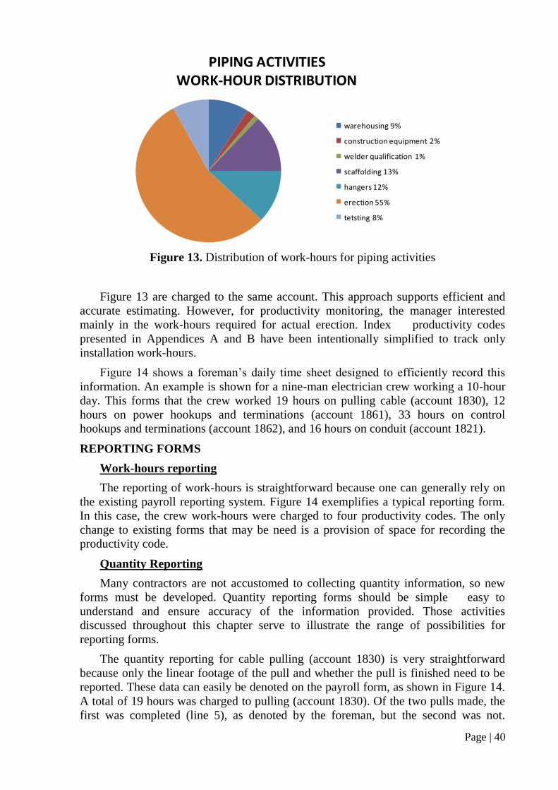
Page | 40

Figure 13. Distribution of work-hours for piping activities

Figure 13 are charged to the same account. This approach supports efficient and

accurate estimating. However, for productivity monitoring, the manager interested

mainly in the work-hours required for actual erection. Index productivity codes

presented in Appendices A and B have been intentionally simplified to track only

installation work-hours.

Figure 14 shows a foreman’s daily time sheet designed to efficiently record this

information. An example is shown for a nine-man electrician crew working a 10-hour

day. This forms that the crew worked 19 hours on pulling cable (account 1830), 12

hours on power hookups and terminations (account 1861), 33 hours on control

hookups and terminations (account 1862), and 16 hours on conduit (account 1821).

REPORTING FORMS

Work-hours reporting

The reporting of work-hours is straightforward because one can generally rely on

the existing payroll reporting system. Figure 14 exemplifies a typical reporting form.

In this case, the crew work-hours were charged to four productivity codes. The only

change to existing forms that may be need is a provision of space for recording the

productivity code.

Quantity Reporting

Many contractors are not accustomed to collecting quantity information, so new

forms must be developed. Quantity reporting forms should be simple easy to

understand and ensure accuracy of the information provided. Those activities

discussed throughout this chapter serve to illustrate the range of possibilities for

reporting forms.

The quantity reporting for cable pulling (account 1830) is very straightforward

because only the linear footage of the pull and whether the pull is finished need to be

reported. These data can easily be denoted on the payroll form, as shown in Figure 14.

A total of 19 hours was charged to pulling (account 1830). Of the two pulls made, the

first was completed (line 5), as denoted by the foreman, but the second was not.

PIPING ACTIVITIES WORK-HOUR DISTRIBUTION

warehousing 9%

construction equipment 2%

welder qualification 1%

scaffolding 13%

hangers 12%

erection 55%

tetsting 8%

Page | 41

Therefore, the crew credited with having pulled 175 linear feet, which is the length of

the first pull.

Quantity reporting for spool erection and field run pipe can be done on form such

as the one shown in Figure 10. This generic form can be used for racked and non-

racked pipe. All that is required of the foreman is to record the total quantity and pipe

size, as given on the isometric drawing, and to report the completion status and linear

footage. To minimize the chance for mistakes, the completion status is described on

the form.

Because the layout of structural steel is unique from project to project a generic

data collection form cannot be developed. However, all that is needed is a convenient

way for the foreman to report when a piece has been erected, bolted, or tightened and

when a floor has been plumbed. A graphical layout such as the one shown in Figure 15

is desirable. The foreman simply

Page | 42

DATE: 7-30-86

CRAFT:……Electrician……… BADGE NO

FOREMAN:……J. Barker……………… 173

(SIGNATURE)

SUPT: ……………………………..

(SIGNATURE)

START:…6:30….AM

PM STOP:…5:00… AM

PM

WO

RK

DE

SC

RIP

TIO

N

Lig

hti

ng l

ine

5,

Lin

e 5 L

UU

S

,175’-

Com

ple

ted

Ter

m &

Pan

el C

able

s L

ine

5

GIG

,LU

US

Ter

m

J.B

, L

ine

5 G

IG,

LU

US

Ter

m P

anel

s &

Dev

ices

, L

ine

5,

LU

US

, U

G

Conduit

for

Sta

r-w

hee

l L

ine

5

FI

Ter

m B

MI

Pan

el,

Lin

e 5 L

UU

S

Route

Cab

le &

25 P

in R

ecpt.

to

MCC FI Line 260’-

Inco

mple

te

Conduit

for

Dust

Contr

ol

Lin

e 5

,

LU

US

FOREMAN INSTRUCTOR

1. List Badge Numbers in

Numerical Order

2. Write in “Work Description”

columns in order. Do not skip

columns

3. Make sure description hours

equal total hours worked

4. Fill in Start &Stop Time

5. Sign Your Card

AC

CO

UN

T N

O

18

30

18

61

18

62

18

62

18

21

18

62

18

30

18

21

ANY INJURIES TODAY?

IF SO. EXPLAIN BELOW IN REMARK

BADGE

NO

NAME

CL

AS

S

DE

SC

RIP

TIO

N HOURS WORKED

REG

01

1.5

2.0

TOTAL REMARKS

(ABSENT LATE/EARLY START

STAYED LATE, INJURED, ECT)

75 G.Fisher S 10 10 < 10

76 D.Lewis S 10 10 < 10

173 J.Barker SF 10 10 < 1 2 2 1 1 1 1 1

174 C.Brooks S 10 10 < 5 3 2

478 D.Davis S 10 10 < 10

533 R.Lowes S 10 10 < - - - - - - - - Absent (Personal)

630 M.Balley S 10 10 < 6 4

660 S.Tanck II-1 0 0 < 1 3 3 3

661 J.Pierce S 10 10 < 2 3 5

<

TOTAL HOURS 80 80 < 12 12 8 18 7 7 7 9

Figure 14. Example of Foreman’s Daily Time Sheet

Page | 43

Marks the erected pieces and circles the joints that have been bolted or tightened.

The possibility of mistakes is greatly reduced because the form can be completed

quickly and easily.

SUMMARY

This chapter has presented five methods of measuring progress. The primary

methods are the units completed, percent complete, and the level of effort. Examples

of when each method can be used were cited. The measurement of work-hours was

also discussed, and a sample time sheet was given

Date FloorErection

Bolting

Tightening

Plumbing

Figure 15. Data Colletion Form for structural steel erection (Account 05121)

25'- 0" 25'- 0" 25'- 0" 26'- 0"

26

'- 0

"2

6'-

0"

26

'- 0

"2

6'-

0"

B C D E F

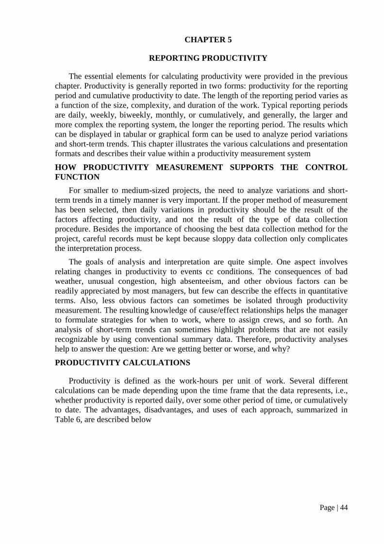
Page | 44

CHAPTER 5

REPORTING PRODUCTIVITY

The essential elements for calculating productivity were provided in the previous

chapter. Productivity is generally reported in two forms: productivity for the reporting

period and cumulative productivity to date. The length of the reporting period varies as

a function of the size, complexity, and duration of the work. Typical reporting periods

are daily, weekly, biweekly, monthly, or cumulatively, and generally, the larger and

more complex the reporting system, the longer the reporting period. The results which

can be displayed in tabular or graphical form can be used to analyze period variations

and short-term trends. This chapter illustrates the various calculations and presentation

formats and describes their value within a productivity measurement system

HOW PRODUCTIVITY MEASUREMENT SUPPORTS THE CONTROL

FUNCTION

For smaller to medium-sized projects, the need to analyze variations and short-

term trends in a timely manner is very important. If the proper method of measurement

has been selected, then daily variations in productivity should be the result of the

factors affecting productivity, and not the result of the type of data collection

procedure. Besides the importance of choosing the best data collection method for the

project, careful records must be kept because sloppy data collection only complicates

the interpretation process.

The goals of analysis and interpretation are quite simple. One aspect involves

relating changes in productivity to events cc conditions. The consequences of bad

weather, unusual congestion, high absenteeism, and other obvious factors can be

readily appreciated by most managers, but few can describe the effects in quantitative

terms. Also, less obvious factors can sometimes be isolated through productivity

measurement. The resulting knowledge of cause/effect relationships helps the manager

to formulate strategies for when to work, where to assign crews, and so forth. An

analysis of short-term trends can sometimes highlight problems that are not easily

recognizable by using conventional summary data. Therefore, productivity analyses

help to answer the question: Are we getting better or worse, and why?

PRODUCTIVITY CALCULATIONS

Productivity is defined as the work-hours per unit of work. Several different

calculations can be made depending upon the time frame that the data represents, i.e.,

whether productivity is reported daily, over some other period of time, or cumulatively

to date. The advantages, disadvantages, and uses of each approach, summarized in

Table 6, are described below

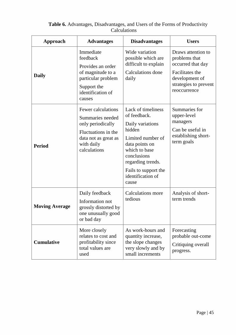
Page | 45

Table 6. Advantages, Disadvantages, and Users of the Forms of Productivity

Calculations

Approach Advantages Disadvantages Users

Daily

Immediate

feedback

Provides an order

of magnitude to a

particular problem

Support the

identification of

causes

Wide variation

possible which are

difficult to explain

Calculations done

daily

Draws attention to

problems that

occurred that day

Facilitates the

development of

strategies to prevent

reoccurrence

Period

Fewer calculations

Summaries needed

only periodically

Fluctuations in the

data not as great as

with daily

calculations

Lack of timeliness

of feedback.

Daily variations

hidden

Limited number of

data points on

which to base

conclusions

regarding trends.

Fails to support the

identification of

cause

Summaries for

upper-level

managers

Can be useful in

establishing short-

term goals

Moving Average

Daily feedback

Information not

grossly distorted by

one unusually good

or bad day

Calculations more

tedious

Analysis of short-

term trends

Cumulative

More closely

relates to cost and

profitability since

total values are

used

As work-hours and

quantity increase,

the slope changes

very slowly and by

small increments

Forecasting

probable out-come

Critiquing overall

progress.

Page | 46

Daily Productivity

The daily productivity or the unit rate is defined simply as:

Daily Productivity

( )

Both work-hours and quantities must be changed to the same account. In Figure

14, as an example, the electrician crew worked 80 total work-hours on that day, but

only 19 of these were charged to cable pulling. They completed one pull of 175 feet. In

this instance; the daily productivity for cable pulling is calculated only for completed

work as:

Daily Productivity

( )

)1830_(Code

Much information can be gained by studying the daily productivity of a crew.

Some causes of productivity decline can be readily identified, whereas others are some

subtle and require further investigation. To illustrate the usefulness of daily

productivity statistics, three examples are given using the activities developed in

Chapter 4.

Structural steel

Figure 16 shows a plot of the daily productivity of an ironworker crew erecting

structural steel on a six-story office building. Six days are of particular interest,

namely, days 4, 12, 15, 18, 21, and 24. The poor productivity on days 15 and 18 can be

explained by cold temperatures, 20’P and 12'F, respectively. On day 4, the weather

was bad, and the crew was sent hale after having worked for about 3 hours. With this

knowledge, the manager could better decide whether to work or send the crew home

on subsequent clays. Day 12 is more difficult to explain. The temperature was 27'F,

but the real problem may have been in the coordination of the work among the four

subtasks. Much of the effort was spent for plumbing, and few pieces of steel were

erected. On days 21 and 24, much of the work involved bolting

The role of daily productivity data is to focus attention and create awareness and

sensitivity. Later in this chapter, it will be shown how other data can be used in

conjunction with daily productivity to help isolate other productivity problems.

Pipe Erection

The daily productivity of a pipe erection crew installing six-inch-diameter pipe

spools (account 1732) is shown in Figure 17. The crew was working a 58-hour/week

schedule. During the first nine days, the daily crew productivity worsened at a steady

rate. Thereafter, erratic variations are observed. Given this information, a foreman or

superintendent should investigate the causes. Perhaps work assignments or

interferences with other crews· are the problems.

Cable Pulling

The analysis of cable pulling (account 1830) is similar to that of pipe erection. As

can be seen in Figure 18, steady increases in unit rates occurred after day 118.

Page | 47

0 5 10 15 20 25 30

0

2

4

6

8

DAY

WO

RK

HO

UR

S P

ER

PIE

CE

Difficulties in Plumbing Coordination

Bad Weather

Bolting Only

Figure 16. Unit Productivity for Structural Steel Erection

(Account 05121)

4 8 12 16 200

0

2

4

6

8

10

12

DAY

DA

ILY

WO

RK

HO

UR

S P

ER

LIN

EA

R F

OO

T

Figure 17. Unit Productivity for Pipe Erection (Account 1732)

Page | 48

Period Productivity

Calculating productivity for a given period of time is similar to calculating daily

productivity. Typical reporting periods are weekly, biweekly, and monthly. Only the

work-hours charged and the quantities installed during the period are consider. Period

productivity is calculated as follows:

Period Productivity

( )

Period productivity data are useful for upper- and middle level managers because

of their summary nature. For lower-level managers, the data can serve as a report card

and can help in establishing -short-term targets for example a goal may be to improve

productivity the next week by 10 percent compare with the previous week.

The limitations of period summaries are two-fold. First, if the duration of an

activity is short, then period productivity calculations do not provide adequate time for

problem evaluation and corrective action. Also, there are too few data points to

provide confidence in reaching conclusions. Period summaries are more appropriate

for longer duration activities. Second, period calculations tend to hide the effects of

various factors on productivity. For instance, the erratic character of the data in Figure

17 after day nine probably would not appear in weekly summaries.

14213212211210292

0.2

0.1

0.3

0.4

0.5

0

DAY

DA

ILY

WO

RK

HO

UR

S P

ER

LIN

EA

R F

OO

T

Figure 18. Unit Productivity for Cable Pulling (Account 1830)

Page | 49

Moving-average

Moving-average calculations are a compromise between daily and period

calculations. A time frame, n, is selected, and productivity over that period is

calculated using Equation 4. As the data for another day are collected, they are added

to the existing data, and the data from the oldest or least current day are deleted. Thus,

the calculation always includes the data from the previous n days. The advantage over

the simple period approach is that, because a new value is calculated each day, short-

term trend can be identified. The value of n is often selected to cover a work week

(n=5) that productivity from each day of the week is always included.

The value of the moving average is the early recognition of short-term trends.

These are often difficult to recognize using daily productivity data because it is subject

to considerable variability. Moving averages dampen the variability, as is shown in

Figure 19 which is the first 12 days of the structural steel erection example previously

discussed.

The data used in calculating the moving average in Figure 19 are summarized in

Table 7. By using a five-day moving average, it can be seen that the short-term

assessment is that productivity shows early signs of becoming worse. While the

upward trend in the last six days is small, it deserves careful monitoring. This trend is

not necessarily evident from studying the daily productivity data alone.

Page | 50

Table 7. Moving Average Calculations for Structural Steel Erection (Figure 19)

Day

Unit

Work-

hours

(1)

Work-hour

Total

(Last 5 days)

(2)

Unit

Quantities

(3)

Quantity

Total

(Last 5 days)

(4)

Unit

Productivity

(5)

Productivity

5-Day

Moving

Average (6)

1 38 38 18.5 18.5 2.027

2 40 78 30.6 41.9 1.307

3 56 134 39.1 88.2 1.432

4 20 154 6.0 94.2 3.333

5 56 210 53.3 147.5 1.051

6 56 228 35.5 164.5 1.578

7 56 244 27.8 161.7 2.014

8 40 228 28.5 151.1 1.404

9 54 262 48.3 193.4 1.118

10 46 252 21.6 161.7 2.130

11 41 237 47.1 173.3 0.870

12 53 234 19.6 165.1 2.704

5 10 15 20 25 30

DAY

0

0

1

2

3

4

WO

RK

HO

UR

S P

ER

PIE

CE

DAILY PRODUCTIVITY

5-DAY MOVING AVERAGE

Figure 19. Unit and Moving Average Productivity for the First

12 Days of Strutural Steel Erection (Account 05121)

Page | 51

Cumulative Productivity

Cumulative productivity is a compilation of all of the work-hours charged to an

account divided by the total quantities installed to date. It is calculated using the

following equation:

Cumulative Productivity

( )

The primary use of cumulative productivity calculations is to assess how the work

is progressing on the whole and to predict the' final productivity rate upon completion

of the activity, comparisons against the budgeted work-hours can be made in order to

evaluate potential profitability, figures 20 through 22 show the cumulative

productivity for the three example activities. The cumulative productivity curve for

structural steel in figure 20 shows that after the initial startup phase, the cumulative

productivity hovered at; just under 1.5 work-hours per piece until the last eight days.

Thereafter, the cumulative productivity declined by approximately 20 percent. Figures

21 and 22 clearly show steady losses in productivity for both cable pulling and pipe

erection.

As the work progresses, the number of work-hours and quantities will become

increasingly larger. Beyond, for example, ten reporting periods (days), even large

changes in daily product1vity will have a small effect on the cumulative productivity

calculation. Therefore, cumulative productivity calculations are of limited use in

detecting daily variations or short-term trends.

REPORTING FORMAT

The advantages of reporting productivity data in either graphical or tabular form

are described below.

Graphical Format

Graphical representations of productivity data are highly desirable because large

amounts of data can be quickly absorbed and understood. Graphs are especially

desirable for foremen and superintendents because the visual image allows them to

evaluate trends and make predictions without the need to manipulate data. Graphs also

create an element of confidence. Because they can be easily and quickly

comprehended, graphs support the criteria of simplicity, accuracy, and timeliness as

outlined in Chapter 3.

Graphical formats are especially suited for situations where updates to the data are

done on a daily basis. These include daily and cumulative productivity and moving

average calculations. A number of examples were presented earlier in this chapter.

Graphs are also well suited for comparing or reconciling two parameters, for example

productivity versus schedule considerations (see Chapter 8).

One limitation of graphics is that, if scales are improperly selected, it is more difficult

to put things into proper perspective. Graphs are not well suited to the presentation of

summary data.

Page | 52

0.7

0.9

1.1

1.3

1.5

1.7

91 101 111 121 131 141

DAY

CU

MU

LA

TIV

E W

OR

KH

OU

RS

PE

R L

INE

AR

FO

OT

Figure 21. Culmulative Productivity for Cable Pulling (Account 1830)

0.7

0.7

0.7

0.7

0.7

0.7

0.7 0.7 0.7 0.7 0.7 0.7

DAY

CU

MU

LA

TIV

E W

OR

KH

OU

RS

PE

R L

INE

AR

FO

OT

Figure 22. Culmulative Productivity for Large-Bore Pipe Erection (Account

1732)

Page | 53

Tabular Format

Tables of data are useful for summary statistics because there is little interpretation

required relative to the order of magnitude. Summary data on a weekly basis for a

crew installing small-bore pipe (account 1735) are given in Table 8. Summary data in

this form support the development of rules of thumb. For example, one can suppose

that it has been determined that the crew should be able to install 450 linear feet of

small-bore pipe per week. It can be seen that, after a slow start, the crew was able to

maintain this pace through week. 15. This is followed by six weeks of below-par

production. Weeks 15 through 17 are particular in revealing. The data show reduced

work-hours and output, but, at the same time; productivity decreased. This situation

suggests that the problem is related more to the nature of the work than to the number

of craftsmen assigned to the work. Over the last six weeks, the work-hours increased

significantly. The weekly output eventually increased, but it did so at the expense of

significant work-hour increases.

ANALYSIS OF WORK HOUR AND QUANTITY RATES

So far, this chapter has concentrated on studying the different forms of

productivity calculations. It follows, however, that, as suggested in Table 8; added

insight can be gained by individually reviewing the work-hour and quantity trends and

relating them to productivity trends.

Figures 23 and 24 show cumulative and daily work-hours and quantities,

respectively, for the small-bore pipe erection activity described at the beginning of the

chapter (account 1735). In figure 22, the productivity steadily worsened throughout the

activity duration. In Figure 23, both the cumulative and daily curves show that,

through weekday 15, the number of work-hours assigned to the work was very

consistent. Relative to the quantities", figure 24 shows a different picture. Four distinct

phases are seen; each with successively lower daily output. Only phase 4 can be

associated with the number of craftsmen assigned to the work.

The study of quantities helps to develop a sensitivity that can be applied to many

projects. For example, figure 25 shows the cumulative quantity curves for three similar

steel erection projects. Project A has been developed throughout this chapter. Project B

proceeded satisfactorily until a change in methods on day 13 forced the crew to

integrate its week with that of another. On Project C, the fact that steel deliveries

occurred very slowly from the beginning is clearly reflected.

Where the level of effort method of measurement is used, it is often possible to

review quantities installed for each subtask. Figure 26 illustrates the usefulness of this

type of analysis. The figure shows the cumulative pieces of steel that have been

erected, bolted, plumbed, and tightened. The completion rates should be reviewed

concurrently with the unit and cumulative productivity curves, shown in Figures 16

and 20, respectively. In figure 26, the relationship between plumbing and bolting is of

particular interest. The four-day delay in plumbing from day 15 through day 18

ultimately affected the bolting operation. The result of this breakdown in coordination

of the work is a loss of productivity, as shown by both figures 16 and 20.

Page | 54

Table 8. Typical Weekly Productivity Summary for Small-Bore Pipe (Account 1735)

Small - Bore Pipe (Account 1735)

Week

Quantity Work-hours Productivity

Weekly

lin ft

installed

(1)

Cumulative

fin ft

installed (2)

Weekly

Work-hours

(3)

Cumulative

Work-hours

(4)

Weekly

work-hours

lin ft

(5)

Cumulative

work-hour

lin ft

(6)

1 351 351 460 460 1.31 1.31

2 350 701 500 960 1.43 1.37

3 232 933 440 1400 1.9 1.5

4 587 1520 500 1900 0.85 1.25

5 438 1958 450 2350 1.03 1.2

6 453 2411 350 2700 0.77 1.12

7 532 2943 390 3090 0.73 1.05

8 557 3500 515 3605 0.92 1.03

9 500 4000 315 3920 0.63 0.98

10 453 4453 310 4230 0.68 0.95

11 450 4903 330 4560 0.73 0.93

12 532 5435 440 5000 0.83 0.92

13 326 5761 300 5300 0.92 0.92

14 467 6228 430 5730 0.92 0.92

15 449 6677 480 6210 1.07 0.93

16 334 7011 310 6520 0.93 0.93

17 255 7266 310 6830 1.22 0.94

18 418 7684 470 7300 1.12 0.95

19 377 8061 570 7870 1.51 0.98

20 243 8304 600 8470 2.47 1.02

21 262 8566 610 9080 2.33 1.06

22 513 9079 725 9805 1.41 1.08

23 521 9600 645 10450 1.24 1.09

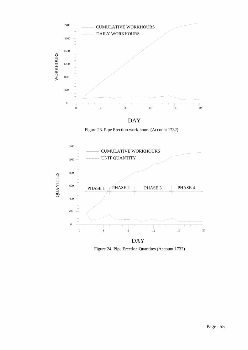
Page | 55

0

400

800

1200

1500

2000

2400

0 4 8 12 16 20

DAY

Figure 23. Pipe Erection work-hours (Account 1732)

WO

RK

HO

UR

S

CUMULATIVE WORKHOURS

DAILY WORKHOURS

0

200

400

600

800

1000

1200

0 4 8 12 16 20

DAY

Figure 24. Pipe Erection Quantites (Account 1732)

QU

AN

TIT

ES

PHASE 1 PHASE 2 PHASE 3 PHASE 4

CUMULATIVE WORKHOURS

UNIT QUANTITY

Page | 56

SUMMARY

This chapter has demonstrated four important, methods of calculating productivity.

These calculations can be done apart from any knowledge of budgeted work-hours,

total quantities, or schedule considerations. Tabular and graphical formats were

illustrated. The use 'of work-hour and quantity rates in conjunction with productivity

curves to detect some of the cause of productivity losses was demonstrated. Each

graphical and tabular illustration showed how the information contained therein' could

provide insight to the manager relative to productivity. The emphasis throughout the

chapter has been on creating awareness and sensitivity.

0

200

400

600

800

0 10 20 30 40

DAY

Figure 25. Cumulative Quantity Curves for Three steel Erection Projects (Account 05121)

CU

MU

LA

TIV

E Q

UA

NT

ITIE

S (

PIE

CE

S) PROJECT A

PROJECT B

PROJECT C

0

200

400

600

800

0 5 10 15 20 25

DAY

Figure 26. Cumulative Quantities for the Subtasks in Structural Steel Erection

(Account 05121)

CU

MU

LA

TIV

E Q

UA

NT

ITIE

S

ERECT

BOLT

PLUMB

TIGHTEN

Page | 57

CHAPTER 6

PERFORMANCE EVALUATION

The analysis of daily productivity variations and short-term trends is very useful,

but Lt represents only a part of the overall control process. To strengthen perceptions

about productivity problems and to provide insight into potential profitability, it is

necessary to compare current productivity with the estimated or planned rates [91. The

process of making comparisons between actual and estimated productivity "is called

performance evaluation [181. As illustrated in Figure 7, the needed information for

comparative purposes includes the estimated work-hours, quantities, and productivity

(unit rate) from the project estimate and the planned duration or required completion

date from the project schedule. This chapter describes several ways of comparing

work-hours, quantities, and productivity using performance factors. Forecasting

techniques are also discussed.

CONTROL BUDGET

The control budget is the baseline against which comparisons are made. For

productivity control, a control budget is established for each activity which consists of

the total estimated work-hours, total quantities to be installed based on the quantity

take off, and the estimated productivity upon completion. If no estimate for the activity

is available, then the project manager can use realistic target values. Table 9 shows the

control budget for the pipe erection, structural steel, and cable pulling activities

presented in Chapter 4.

Performance Factors

The simplest form of performance evaluation is to compare the actual and planned

productivity values. This is done using a performance factor, which is a measure of

construction efficiency. The performance factor (PF) is calculated as follows:

Perform

( )

A performance factor is greater than unity indicates better-than-estimated

performance. Improvements in productivity are reflected by smaller productivity

values or reductions in the unit rate and larger or increasing PF values.

Numerical Comparisons

Typical numerical comparisons are made on a period and cumulative basis. Table

10 shows an example of a performance evaluation report in which actual work-hours,

quantities, and unit rates are compared to the control budget. The period calculations

are a summary of the previous five days.

Page | 58

Table 9. Example of an Initial Control Budget

Activity Description Account Units

Estimated

Work-

hours

(1)

Quantities

to be

installed

(2)

Planned

Unit Rate

(3)

Aboveground Non-racked

Piping, Spool Erection, 2

1/2 to 12 in

1732 lin ft 1,350 1,069 1.27

Aboveground Non-racked

Piping, Field Run, 2 in. and

Under

1735 lin ft 10,200 10,000 1.02

Structural Steel Erection,

Multistory Type 5121 pieces 963 642 1.5

Wire and Cable Pulling in

Conduit and Tray 1830 lin ft 6,228 69,202 0.09

Page | 59

Table 10. Example Performance Evaluation Report

Account Activity Units of

Measure

Work-hours Quantities

Budgeted

Unit Rate

Performance

Factor Total

Forecasted

Work-hours Budget Period To Date Percent Budget Period

To

Date Percent Period

To

Date

(1) (2) (3) (4) (5) (6) (7) (8) (9) (10) (11) (12)

1732 Piping lin ft 1,350 658 1,824 135 1,063 197 917 86 1 0 1 2,114

1735 Piping lin ft 10,200 450 2,350 23 10,000 438 1,95

8 20 1 1 1 12,002

5121 Structural

Steel piece 963 228 782 81 642 158 517 81 1 1 1 971

1830 Cable lin ft 6,228 730 1,060 17 69,202 9,612 14,3

27 21 0 1 1 5,020

Column (4) = Column (3) : Column (1) x 100

Column (8) = Column (7) : Column (5) x 100

Column (10) = Column (9) : [Column (2) : Column (6)]

Column (11) = Column (9) : [Column (3) : Column (7)]

Column (12) = Column (3) x Column (5) : Column (7)

Page | 60

In this example, the large-bore piping work (account 1732) is preceded very

ineffectively. Progress during the previous week was especially poor. Eighty-six

percent of the quantities had been installed, but there was a significant overrun in

work-hours. The small-bore piping (account.1735) was projected to overrun. Steel

erection proceeded as had been planned. The cable pulling productivity was about 20

percent better than the budgeted but only 21 percent of the cable had been pulled.

Column (8) of Table 10 shows the percentage of budgeted quantities that were

installed. This is the true representation of the percent complete of an activity. It has

been observed that some contractors use the percentage of work-hours as a measure of

percent complete. For this approach to be correct, the budgeted unit rate and the

quantity takeoff must be accurate, and the actual unit rate must equal the budgeted unit

rate. The large-bore piping activity in Table 10 illustrates the danger in relying on the

consumed work-hours for ·this purpose.

Graphical Analyses of the PF

It is often helpful to review a graphical plot of the to-date performance factors.

Figure 27 show a graphical plot of cumulative performance factors that is typical for

many industrial construction activities. At the outset, performance is usually worse

than expected because the crews are not yet familiar with the work, because of

overstaffing in anticipation of an accelerated pace of work, or for other reasons. Before

long, performance improves and is actually better than planned. This trend may remain

until near the end of the activity, when congestion and difficulties with the final

completion of systems cause productivity to decline. The shape of the curve is

important because it represents an expectation. The shape varies with the type of work

(and the level of detail used in tracking the work.

Figure 28 show the cumulative performance factors for the first 13 days of the

large-bore piping activity and can be compared with Figure 27. Essentially, from the

beginning, the work as performed at below-par performance and the trend continued to

work. In this instance, the unit rate as probably underestimated, since planned

performance as never achieved. Because the PFs did not stabilize, below-par

productivity may also be a problem.

Figure 29, which give the cumulative PF values for cable pulling, show instability

that is the opposite of the piping activity. However, the PF trended toward a PF of 1.0,

so the activity may have proceeded as planned. Although a degree of instability is

expected at the outset, the PF values should eventually stabilize. If not changes in

methods or requirements, increasingly difficult work, or increased congestion are

among the possible causes. Dramatic or sharp changes in PF values may result for a

variety of reasons, but these should be relatively easy to identify.

Page | 61

FORECASTING

Numerical Approach

A second dimension of performance evaluation is forecasting the total work-hours

used in completing an activity. The ability to forecast is valuable for projecting work-

hour variances and assessing cost impacts. The simplest method of forecasting is to

divide the to-date work-hours by the per-cent complete of the activity. The following

equation can be used:

Work hour forecast at activity completion

( )

Column 12 in Table 10 shows the work-hour-s forecasts using this equation.

Sometimes it is helpful to have additional information related to forecasts. Table 11

shows a sample forecast report that provides relative and actual variances.

Graphical Approach

The numerical approach to forecasting using Equation 7 assumes that the

productivity will remain constant until the activity is completed. This approach is

subject to err-or if the cumulative productivity changes appreciably. A simpler and

often more accurate approach is to manually forecast using graphs.

Graphical forecasts can combine to-date trends, knowledge of what lies ahead, and

intuition of a manager who has had similar experiences on other projects. Also, the

manager must under-stand what has occurred on the activity until that point in time.

To forecast using graphs, a learning curve plot is needed. A learning curve is simply

the cumulative unit productivity. On they-axis plotted against the cumulative

quantities on the x-axis. Figures 30 through 32 illustrate productivity forecasts for

large-bore pipe erection, structural steel, and cable pulling, respectively. As can be

seen, some subjectivity is involved. These productivity forecasts can be compared with

those in Table 10 and with the actual productivity at completion as follows:

10 20 300 40 50 60 70 80 90 100

1.0

PERCENT COMPLETE

Figure 27. Plots of Typical Cumulative Performance Factors for Many

Industrial Construction Activities

CU

MU

LA

TIV

E P

ER

FO

RM

AN

CE

FA

CT

OR

S

Page | 62

Activity Unit

Calculated

Forecast

(Table 10)

Graphical Forecast

(Figures 30-32) Actual

Large-bore pipe

erection work-hours/lin ft 1.99 2.25 2.23

Structural steel work-hours/piece 1.51 1.41 1.73

Cable pulling work-hours/lin ft 0.074 0.088 0.103

Table 11. Example Forecast Report

Account Activity

Work-hours Percent

Completed Budgete

d To Date Forecast Overrun Variance

(1) (2) (3) (4) (5) (6)

1732 Piping 1350 1824 2114 764 1.57 86

5121 Structural

steel 963 782 971 8 1.01 81

1830 Cable 6228 1060 5000 -1208 0.81 21

0

CUMULATIVE QUANTITIES (LINEAR FOOT)

Figure 30. Productivity Forecasr for Pipe Erection (Account 1732)

CU

MU

LA

TIV

E P

RO

DU

CT

IVIT

Y

300 15000

0.75

1.5

2.25

3.00

600 900 1200

ES

TIM

AT

E 1

,063 L

F

FORECAST: 2.25 WH/LF

Page | 63

This comparison shows that the graphical forecast can be more accurate than the

analytical ones. The projected work-hours to complete can be readily calculated from

the productivity forecast.

RELIABILITY OF ESTIMATES

In preparing the project estimate, managers and estimators make the best use of

available data. Unfortunately, the time available for preparing the estimate is usually

200 10000

1.25

1.5

1.75

2.00

400 600 800

ES

TIM

AT

E642

PC

S

FORECAST: 1.41 WH/PC

0

CUMULATIVE QUANTITIES (PIECE)

Figure 31. Productivity Forecasr for Structural Steel (Account 05121)

CU

MU

LA

TIV

E P

RO

DU

CT

IVIT

Y

0

CUMULATIVE QUANTITIES (LINEAR FOOT)

Figure 32. Productivity Forecasr for Cable Pulling (Account 1830)

CU

MU

LA

TIV

E P

RO

DU

CT

IVIT

Y

14,000

.050

.075

1.00

.125

ES

TIM

AT

E6

92

02

LF

FORECAST: 0.088 WH/LF

28,000 42,000 56,000 70,000 84,400

1.75

2.00

Page | 64

limited, and the information may be incomplete. As a result, quantity takeoffs may be

in error, or, in some cases, a work task may be completely overlooked. Productivity

data is subject to wide variation, so the assumptions made in the estimating phase will

seldom exactly coincide with reality. Accordingly, the estimate should not be

considered a document without fault, and, when variances develop during the control

phase of a project, analysis of results should always consider estimating errors as a

possible reason.

To illustrate, it is assumed that the work-hours for .a given activity are projected to

overrun. Some of the possible explanations for the overrun are listed below.

- The total quantity of work may have been underestimated, requiring more labor

and material than budgeted.

- The estimated work-hours per unit of work may have been unrealistically low.

- Crew productivity may have been lower than what should reasonably be

expected for a variety of reasons.

Next, it is assumed that the projected work-hours for another activity are expected

to be right on target. This does not necessarily mean that everything was correct. In

fact, either of the following could be the situation:

- A low quantity estimate may be offset by better-than-budgeted productivity.

- Worse-than-budgeted productivity may be compensated for by fewer quantities

than budgeted.

Thus, productivity control is much more than simp11 watching for negative total

variances with and among activities or amounts. The status of an account is the

composite status of a number of parts, and each of those parts should be watched, even

if productivity appears favorable.

SUMMARY

This chapter has illustrated simple analytical and graphical techniques for

comparing actual performance to the control budget and for making work-hour

forecasts. Minimal information is required, and the output is in a concise and easy-to-

understand form.

Page | 65

PART III – ADVANCED CONCEPTS OF PRODUCTIVITY

MEASUREMENT AND PERFORMANCE EVALUATION

Chapters 4 through 6 covered the basic concepts that must be mastered en order to

effectively measure productivity. Persons who have previous experience with cost-

control systems will be familiar with most of these. However, there is much more to be

gained from productivity measurement and performance evaluation than can be

provided by the basic concepts. Therefore, Part III presents advanced concepts that can

be applied by the more experienced user,

Cumulative productivity changes as activities progress. Chapter 7 begins with a

presentation of standard productivity performance curves and shows how they can be

used to improve the accuracy of work-hour forecasts. Comparison of the shape of an

actual cumulative performance curve to the shape of the standard curve is also useful.

The earned value concept, a method for calculating the percent complete of a control

account, is described. The chapter concludes by describing five indices that may

suggest the cause of productivity problems.

Chapter 8 shows how productivity data and schedule information can be

integrated; The emphasis is on graphical presentations and indices that permit a very

quick assessment of overall performance.

Page | 66

CHAPTER 7

ADVANCED MEASUREMENT AND FORECASTING CONCEPTS

Chapter 4 through 6 presented the basic concepts of productivity measurement,

analysis, and forecasting which can be effectively applied to many construction

activities. However, situations occasionally arise where details several modifications

and extensions that will allow one to measure complex construction activities and to

more accurately forecast the total work-hours using standard productivity curves. The

earned value technique for monitoring control accounts is also described.

Measuring complex construction activities

Chapter 4 described how the level of effort method could be used to measure the

quantities (progress) for activities involving subtasks. The method is particularly well

suited to measuring bulk commodity items. However, the level of effort method can

also be used to monitor complex, one-off-a-kind items, as is illustrated by the example

for the erection of an absorber tower on a process plant.

For this work, it is estimated that 520 tons of structural steel are involved. Table

12 shows the status of the work at an early stage of completion. Different units of

measure are used for the various subtasks. Several items, such as shakeout, plumb, and

punch-list, are associated with the entire absorber tower and cannot be conveniently

related to a particular tier or bay. These subtasks are measured on the basis of percent

complete. Girts and sag rods are measured according to the number of bays finished.

The columns, beams, braces, and connections are measured by the piece. The overall

progress of the erection operation is determined by multiplying the percent complete

of each subtask by the respective rule of credit. The table shows that the work is 15.6

percent complete. The equivalent tonnage erected is 15.6 percent of the 520 tons, or

80.5 tons.

Forecasting using standard productivity performance curves

A characteristic problem with construction productivity is that it is continually

changing. This variability can result in significant analysis and forecasting

inaccuracies when using the linear approach defined by Equation 7 in chapter 6. The

need to develop accurate forecasts is particularly acute during the early stages of an

activity.

To overcome the problem of variations in cumulative unit rates, some contractors

have developed standard productivity performance curves for key commodity items.

The curves reflect the contractor’s expectations, on the basic of his experience, of how

productivity performance should change during the installation process. An example

of a standard productivity performance curve for small-bore pipe installation (account

1735) is shown in Figure 33.

Table 12. Quantities for the Erection of a 520-Ton Absorber Tower

Subtask Units of

Measure

Rule of

Credit

Total

Quantity

Quan-

tity to

Date

Percent

Comp-

lete

Relative

Percent

Complete

Total

Equiv-

alent

Tons

Equiv-

alent Tons

to Date

(1) (2) (3) (4) (5) (6) (7)

Run

foundation EA 0.02 200 200 100.0 2.0 10.4 10.4

Page | 67

bolts

Shim % 0.02 100 100 100.0 2.0 10.4 10.4

Shake out % 0.05 100 100 100.0 5.0 26 26.0

Columns EA 0.06 84 74 88.1 5.3 31.2 27.5

Beams EA 0.1 859 52

Cross braces EA 0.11 837 57.2

Girts & sag

rods BAY 0.2 38 104

Plum & align % 0.09 100 5 5.0 0.5 46.8 2.3

Connections EA 0.3 2977 74 2.5 0.7 156 3.9

Punch-list % 0.03 100 15.6 0.0

TOTAL

CONTROL TON 1 520 520 0.0

Column (4) = Column (3) x Column (2) x 100

Column (5) = Column (4) x Column (1)

Column (6) = Column (1) x total estimate quantity, ie. in this case, 520 tons

Column (7) = Column (4) x Column (6) : 100

0

PERCENT COMPLETE

Figure 33. Standard Productivity Performance Curve

for Pipe Erection (Account 1735)

CU

MU

LA

TIV

E P

ER

FO

RM

AN

CE

FA

CT

OR

20 1000.7

40 60 80

0.8

0.9

1.0

1.1

1.2

1.3

Page | 68

The use of the standard productivity performance curve is illustrated by the small-

bore piping (account 1975) example shown in Table 10. The installation is 20 percent

complete. From the performance evaluation report (Table 10), the to-date productivity

is calculated as:

To-date Productivity

(account 1735) =

2,350

1,958

= 1.20 work-hours/lin ft

This compares to the budgeted unit rate at completion of 1.02 work-hours/lin ft,

which would indicate an 18 percent overrun. However, from the standard productivity

performance curve (Figure 33), it is expected that the unit rate should be higher at 20

percent complete than it will be at completion. To calculate the forecasted work-hours

using the standard curve, the date from Table 10 are substituted into the following

equation to yield forecast work-hours.

Forecast

Work-hours =

Actual

Unit

Rate

X

Expected

Performance

Factor

X

Current

Quantity

Estimate

=

=

1.20 x (0.93) x (10,000) = 11,160 work-hours

This forecast is 842 work-hours less than the 12,002 work-hours calculated in

Table 10. The resulting forecast unit rate at completion is 1.12 work-hours/lin ft.

The standard productivity performance curve can be applied also when quantity

estimates are revised. This situation is demonstrated in Table 13, which is a typical

productivity report for a pipe-filter crew installing small-bore pipe. The work-hour

forecast in column 5 is calculated using Equation 9.

Sometimes it is useful to compare actual performance to the standard productivity

performance curve. A comparison of the actual performance factor (PF) values in

Table 13, column 10 with values in Figure 33 is shown in Figure 34. In this

comparison, the crew never performed as well as expected for extended periods of

time, even though the performance factor was greater than 1.0 for half of the time.

Thus, where unit rates are known to vary appreciably, the performance factor should

always be compared with the standard productivity performance curve.

MONITORING PROGRESS USING CONTROL ACCOUNTS

Many times it is advantageous to monitor constructions progress by grouping

similar activities into a single larger category called a control account. For example,

small-bore (account 1735) and large-bore (account 1732) piping can be combined into

an aboveground non-racked piping control account (account 1730). Similarly, wall

forms (account 03117), and elevated slab forms (account 03112) can be combined into

one category, the structural formwork control account (account 03110).

Page | 69

Table 13. Productivity Report for Small-bore pipe (Account 1735) – Showing Revised Quantity Estimates

Week

Quantiy Work-hours Productivity

Initial Budget: 10,000 linear feet (lf) Initial Budget: 10,200 work-hours Initial Budget: 1.02 work-hours/linear feet (wh/lf)

Takeoff lf Install

Cumulative %

Complete

Work-hours

Expended

Work-hours

Forecast

% Complete

Actual wh/lf

Expected Performance

Factor

Forecast wh/lf

Actual Performance

Factor

(1) (2) (3) (4) (5) (6) (7) (8) (9) (10)

1 10,000 351 3.5 460 10484 0.04 1.31 0.8 1.05 0.78

2 701 7.0 960 11504 0.08 1.37 0.84 1.15 0.74

3 9,800 933 9.5 1400 12647 0.11 1.50 0.86 1.29 0.68

4 1,520 15.5 1900 11025 0.17 1.25 0.9 1.13 0.82

5 1,958 20.0 2350 10939 0.21 1.20 0.93 1.12 0.85

6 2,411 24.6 2700 10645 0.25 1.12 0.97 1.09 0.91

7 2,943 30.0 3090 10290 0.30 1.05 1 1.05 0.97

8 3,500 35.7 3605 10397 0.35 1.03 1.03 1.06 0.99

9 4,000 40.8 3920 10276 0.38 0.98 1.07 1.05 1.04

10 4,453 45.4 4230 10054 0.42 0.95 1.08 1.03 1.07

11 9,600 4,903 51.1 4560 9911 0.46 0.93 1.11 1.03 1.10

12 5,435 56.6 5000 9980 0.50 0.92 1.13 1.04 1.11

13 5,761 60.0 5300 9980 0.53 0.92 1.13 1.04 1.11

14 6,228 64.9 5730 10157 0.56 0.92 1.15 1.06 1.11

15 6,677 69.6 6210 10268 0.60 0.93 1.15 1.07 1.10

16 7,011 73.0 6520 10267 0.64 0.93 1.15 1.07 1.10

17 7,266 75.7 6830 10378 0.66 0.94 1.15 1.08 1.09

18 7,684 80.0 7300 10488 0.70 0.95 1.15 1.09 1.07

19 8,061 84.0 7870 10497 0.75 0.98 1.12 1.09 1.04

20 8,304 86.5 8470 10869 0.78 1.02 1.11 1.13 1.00

21 8,566 89.2 9080 11092 0.82 1.06 1.09 1.16 0.96

22 9,079 94.6 9805 10990 0.89 1.08 1.06 1.14 0.94

23 9,600 9,600 100.0 10450 10450 1.00 1.09 1 1.09 0.94

Page | 70

Column (3) = Column (2) : Column (1) x 100

Column (5) = Column (1) x Column (9)

Column (6) = Column (4) : Column (5)

Column (8) Determined from standard productivity performance curve

Column (9) = Column (7) x Column (8)

Column (10) = 1.02 : Column (7)

Column (7) = Column (4) : Column (2)

In the above example, the relationship between the control account and the

individual activities is defined by the framework of the productivity codes or the code

of accounts. Fortunately, the measurement concepts developed here do not require

such a rigorous formulation. In fact, the control account need not be a recognizable

code selected from the code of account. For instance, a commercial contractor may be

interested primarily in the timely construction of floor space so that other trades can

begin erecting partitions, fixtures, etc. The floor area control account may be defined

as followed:

0

PERCENT COMPLETE

20 100

0.7

40 60 80

0.8

0.9

1.0

1.1

1.2

0.6

EXPECTED PERFORMANCE

ACTUAL PERFORMANCE

Page | 71

Floor Area (Control account)

05121 Structural steel erection

05210 Web joist

05300 Metal decking

03312 Concrete elevated slabs

As can be seen, a contractor can readily adapt the productivity measurement to fit

his own special needs.

The use of control accounts often makes it easier to evaluate progress because a

single broad-scope account is studied rather than a collection of several narrow-scope

accounts. However, the difficulty in using this approach arises because the effort

required for each of the various narrow-scope accounts is not the same. For instance,

in Table 9, the budgeted quantities, work-hours, and unit rates for small- and large-

bore pipe differ greatly. For this reason, the narrow-scope accounts cannot be

combined without appropriate adjustments. Fortunately, the earned value concept can

be used to eliminate this problem in order to facilitate the combination of narrow-

scope accounts to form a single control account.

THE EARNED VALUE CONCEPT

The earned value concept is a technique for calculating the percent complete of a

control account. It is a weighted-average technique in which each account is assigned a

weight that accounts for the degree of difficulty of that part of the work and the

estimated quantities to be installed. With the earned value concept, each account is

assigned a fixed amount of resources that can be earned. The resources earned can be

either work-hours or dollars, since these are the only two types of resources to which

the many units of measure in a project (cubic yards, linear feet, each, ect.) can be

converted. If the resources are work-hours, then the total work-hours that can be

earned are calculated as follows:

Total Earnable

Work-hours

(each Account)

= Initial Estimated

Unit Rate

x Current Quantity

Estimate

Figure 35 illustrates the concept using the data from Table 9 for small- and large-

bore pipe. Using the initial estimate, the maximum work-hours that can be earned in

completing the piping control account is 11,550.

Page | 72

As the work is accomplished, work-hours in each account are earned at the unit

rate specified in this initial control estimate. The quantities installed are converted to

earned work-hours by using Equation 11, and the sum of the earned work-hours

represents the earned work-hours for the control account. The following equations are

used to determine these values:

Earned Value

(Work-hours)

for the

Control Account

= ∑ Initial Estimated

Unit Rate X

Quantities Installed

to Date (11)

Percent

Complete of

the Control

Account

= Earned Work-hours to Date

x 100 (12)

Initial Estimated

Unit Rate x

Current Quantity

Estimate

Prior to the start of an account, nothing is earned; when it is complete, 100 percent

of the work-hour has been earned. No more than 100 percent can ever be earned. The

percentage of the work-hours earned also represents the percent complete of the

control account.

The earned value technique is demonstrated by the following example using the

small- and large-bore piping data in Table 9. The budgeted unit rates are 1.02 and 1.27

work-hours/lin ft, respectively. Table 14 shows how the percent complete for the

control account (1730) is calculated using the initial estimate, the current quantity

estimate, unit rate, and the quantities installed to date.

A second sample shows how revised quantity estimates affect the earned value and

percent complete calculations. Here, the estimated quantities for small-bore piping are

revised downward from the original 10,000 lin ft (Table 9) to 9,600 lin ft. the

estimated quantity of large-bore pipe remains the same. The change for small-bore

piping is reflected in the productivity report (Table 13) after week 11. Table 15 shows

the quantities to date and the percent complete calculation.

Several points relative to the earned value concept are important. The total work-

hours that can be earned in an account changes only if the current forecasted quantities

change, as is illustrated in Table 15, Column 3. The total is revised upward or

downward according to the initial estimated unit rate, which never changes (The initial

Figure 35. Illustration of Earned Work-hours for Piping Control Account

SMALLBORE PILEACCOUNT

(1735)

TOTALWORKHOURS

TO BEEARNED

10,200

LARGEBORE PILEACCOUNT

(1732)

PILECONTROLACCOUNT

(1730)

TOTALWORKHOURS

TO BEEARNED

1,350

TOTALWORKHOURS

TO BEEARNED,CONTROLACCOUNT

11,550

PE

RC

EN

T

0

40

20

60

80

100

ACCOUNT/WORK HOUR EQUIVALENTS

Page | 73

estimated unit rate should not be confused with the forecasted or actual unit rate).

Since the initial estimated unit rate is always used, it provides a permanent datum from

which to measure performance. Thus, the work-hours earned in installing a given

quantity of materials are independent from the actual work-hours used. The quantities

to date are determined using rules of credit and are actual contract quantities, as

opposed to purchased quantities, which may include allowances for waste. Quantities

do not change if work must be redone because of interior quantity or a design change.

Table 14. Calculation of Percent Complete Using Earned Work-hours, Example 1

Account

Initial Unit

Rate

Estimate

Current

Quantity

Estimate

Total

Work-hours

to be earned

Quantities

to Date

Earned

Work-

hours

to Date

Percent

Complete

(1) (2) (3) (4) (5) (6)

1732 1.27 1,063 1,350 197 250 18.5

1735 1.02 10,000 10,200 701 715 7

1730

(control) 11,550

956 8.4

Column (3) = Column (1) x Column (2)

Column (5) = Column (1) x Column (4)

Column (6) = Column (5) : Column (3) x 100

Table 15. Calculation of Percent Complete Using Earned Work-hours, Example 2

Account

Initial Unit

Rate

Estimate

Current

Quantity

Estimate

Total

Work-hours

to be earned

Quantities

to Date

Earned

Work-

hours

to Date

Percent

Complete

(1) (2) (3) (4) (5) (6)

1732 1.27 1,063 1,350 957 1,215 90

1735 1.02 9,600 9.792 4,903 5,001 51.1

1730

(control) 11,142

6,216 55.8

Column (3) = Column (1) x Column (2)

Column (5) = Column (1) x Column (4)

Column (6) = Column (5) : Column (3) x 100

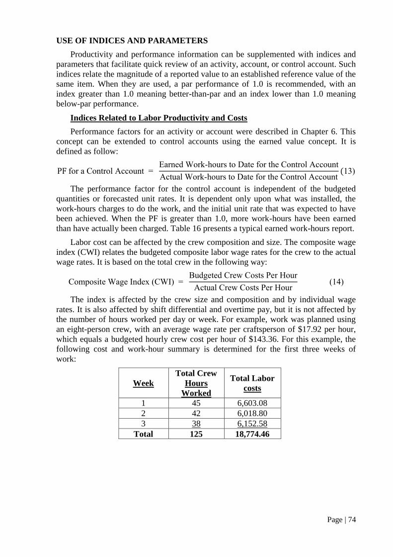
Page | 74

USE OF INDICES AND PARAMETERS

Productivity and performance information can be supplemented with indices and

parameters that facilitate quick review of an activity, account, or control account. Such

indices relate the magnitude of a reported value to an established reference value of the

same item. When they are used, a par performance of 1.0 is recommended, with an

index greater than 1.0 meaning better-than-par and an index lower than 1.0 meaning

below-par performance.

Indices Related to Labor Productivity and Costs

Performance factors for an activity or account were described in Chapter 6. This

concept can be extended to control accounts using the earned value concept. It is

defined as follow:

for a Control Account Earned Work hours to Date for the Control Account

Actual Work hours to Date for the Control Account 13)

The performance factor for the control account is independent of the budgeted

quantities or forecasted unit rates. It is dependent only upon what was installed, the

work-hours charges to do the work, and the initial unit rate that was expected to have

been achieved. When the PF is greater than 1.0, more work-hours have been earned

than have actually been charged. Table 16 presents a typical earned work-hours report.

Labor cost can be affected by the crew composition and size. The composite wage

index (CWI) relates the budgeted composite labor wage rates for the crew to the actual

wage rates. It is based on the total crew in the following way:

Composite Wage Index (CWI) Budgeted Crew Costs Per our

Actual Crew Costs Per our (14)

The index is affected by the crew size and composition and by individual wage

rates. It is also affected by shift differential and overtime pay, but it is not affected by

the number of hours worked per day or week. For example, work was planned using

an eight-person crew, with an average wage rate per craftsperson of $17.92 per hour,

which equals a budgeted hourly crew cost per hour of $143.36. For this example, the

following cost and work-hour summary is determined for the first three weeks of

work:

Week

Total Crew

Hours

Worked

Total Labor

costs

1 45 6,603.08

2 42 6,018.80

3 38 6,152.58

Total 125 18,774.46

Page | 75

Table 16. Typical Earned Work-hour Report

Account

Initial

Unit Rate

Estimate

Current

Quantity

Estimate

Total

Work-

hours to be

earned

Quant-

ities to

Date

Actual

Work-

hours to

Date

Earned

Work-

hours to

Date

Percent

Complete

Perfor-

mance

Factor

Percent

Com-plete

(1) (2) (3) (4) (5) (6) (7) (8) (9)

1732 1.27 1,063 1,350 957 1,597 1,215 90.0 0.76 90

1735 1.02 9,600 9.792 4,903 4,560 5,001 51.5 1.10 51.1

1730

(control) 11,142

6,157 6,216 56.8 1.01 55.8

Column (3) = Column (1) x Column (2)

Column (6) = Column (1) x Column (4)

Column (7) = Column (6) : Column (3) x 100

Column (8) = Column (6) : Column (5)

The actual crew cost per hour can be calculated as follow:

Actual Crew Cost Per our Total Labor Costs

Total Crew ours Worked (15)

18,774.46

125

= $150.2

The composite wage index (CWI) can then be calculated by using Equation (14):

An index of less than 1.0 reflects the combined influence of overtime pay, crew

size and composition, individual wages, and the average crew size, the index is also

affected by absenteeism.

A labor budget performance index, which combined the performance factor and

the composite wage index, is sometimes calculated:

Labor Budget Performance Index (LBPI) Performance Factor Composite Wage Index(16)

This index gives a clearer picture of labor cost trends.

Indices Related to Estimating Accuracy

Obviously, the accuracy of a quantity estimate can have considerable influence on

the work-hours required to complete the work. An inaccurate estimate can actually

hinder the analysis of other indices and parameters. The estimating quantity variance

factor (EQVF) is intended to catalogue variances between the actual and estimated

quantity of work. It is calculated as follows:

EQVF Initial Estimated Quantity Revised Estimate Quantity

Revised Quantity Estimate (17)

A positive EQVF indicates that fewer quantities will be installed than were

initially estimated. A negative EQVF means that the initial quantity estimate was low.

Page | 76

A variance factor for a control account can be calculated also in the following

way:

EQVF for Control Account ∑ ( EQVF Total Earned Work hours)

Total Earned Work hours for Control Account (18)

Typical estimating quantity variance factors are shown in Table 16.

SUMMARY

This chapter has described how advanced concepts can be used to improve the

accuracy of analysis and forecasting technique. Complex construction activities can be

monitored using the level of effort method. If different units of measure are used for

the various subtasks, then the estimated quantities must be used. Standard

productivities curve allow one to reply on prior knowledge of how productivity varies

in order to improve forecasts. Performance factors can also be compared to standard

curves. Quantity estimates are needed in order to use standard productivity curve. The

earned value concept has been described as a technique for calculating the percent

complete of a control account. Several indices have been presented which can help in

isolating the cause of productivity problems.

Page | 77

CHAPTER 8

PRODUCTIVITY AND SCHEDULE PERFORMANCE

Satisfactory productivity performance and schedule performance do not always

occur simultaneously. Productivity can be good, but the work may be behind schedule.

Likewise, schedules are often met at the expense of significant productivity losses.

Thus, to have a more complete picture of project performance, productivity and

schedule performance must be viewed together. This chapter illustrates how these two

aspects can be integrated. The type of scheduling system used is irrelevant. It can be in

the form of a bar chart, a CPM schedule, a required activity completion date, or simply

an allocation of a certain number of working days.

ESTABLISHING PLANNED PROGRESS

The progress of an activity is measured on the basis of the percentage of the total

quantities that have been installed. To evaluate schedule performance, a planned

progress curve is needed which shows the scheduled cumulative percentage of the

quantities installed versus time. The simplest progress curve assumes that the same

number of quantities will be installed each day or week. This assumption yields a

straight line curve from 0 to 100 percent, with the project finishing at the required

time. Throughout this manual, however, cumulative unit rate curves have been shown

to be typically nonlinear. Therefore, one would expect the planned progress curve also

to be nonlinear.

Planned progress curves can be drawn subjectively or they can be developed from

a standard productivity performance curve such as the one shown in Figure 33. The

following example illustrates how they can be developed using a standard productivity

performance curve.

The control budget data for structural steel erection can be determined from Table 9:

Estimated quantities 642 pieces

Estimated work-hours 963 work-hours

Estimated unit rate 1.50 work-hours/piece

To complete the steel erection, the plan is to work eight hours a day, five days per

week, using a maximum crew size of eight. Five ironworkers will be hired for the first

week to perform shakeout and to erect the first and second floor columns. Three more

Page | 78

crew members will be hired beginning the second week, bringing the crew to the

required size. When the progress of the work reaches 85 percent, which roughly

coincides with the completion of the erection subtask, the crew will be reduced to four

ironworkers and will remain at four until the work is completed. The planned manning

level is shown in Figure 36, and Figure 37 shows the standard productivity

performance curve for structural steel erection.

Figure 36. Planned manning level, structural Steel erection ( Account 05121)

At the outset, the performance factor is expected to be considerably below (par.

From Figure 37, the expected PF value is 0.70. The output and percent complete for

the first day can be calculated:

Cumulative First Day Output = 0.4x 0.70 / 1.50 = 18.67 pieces

Percent Complete = 18.67 x 100 / 642 = 2.9 percent

The following day, the expected performance factor is 0.73, which yields:

Cumulative Second Day Output = 80 x 0.73 / 1.50 = 38.83 pieces

Percent Complete = 38.93 x 100 /642 = 6.1 percent

Output for subsequent days is calculated by repeating the procedure until all

estimated quantities are installed. Table 17 summarizes the calculations for this

example, and Figure 38 shows the planned progress curve as a function of the

10 20 30 40 50 60 70 80 90 100

1

2

3

4

5

6

7

8

PERCENT COMPLETE

CR

EW

SIZ

E

Page | 79

percentage of time. The curve has the characteristic S-shape. For instance, when 20

percent of the time has elapsed, one would expect that 14 percent of the work would

be done. At the 80 percent milestone, about 90 percent of the work should be

completed. As can be seen in Table 17, the projected duration is 19 working days.

A second example is for the small-bore piping operation (account 1735). The

standard productivity performance curve shown in Figure 33 is used. The cumulative

percent complete calculations are shown in Table 18 and Figure 39. As in the

previous example, expected progress is less at the beginning and end of the activity.

The slowest progress shown in Figure 39 occurs during the first 25 percent of time.

INDICES RELATED TO THE SCHEDULE

One, of the simplest forms of schedule evaluation is to compare wnat was actually

done with what was planned. This evaluation can be represented by a schedule

performance index. The index is calculated as shown:

Schedule Performance Index (SPI)

Scheduled Quantities to Date (19)

Figure 37. Standard productivity performance curve for structural Steel erection

( Account 05121)

20 40 60 80 100

0.7

0.8

0.9

1.0

1.1

0

CU

MU

LA

TIV

E P

ER

FO

RM

AN

CE

FA

CT

OR

PERCENT COMPLETE

Page | 80

0

PERCENT TIME

Figure 38. Planned Progress Curve for Structural Steel

Erection (Account 05121)

20 10040 60 800

PE

RC

EN

T C

OM

PL

ET

E

20

40

60

80

100

0

PE

RC

EN

T C

OM

PL

ET

E

20

40

60

80

100

0

PERCENT TIME

Figure 39. Planned Progress for Small-Bore Piping

(Account 1735)

20 10040 60 80

Page | 81

Table 17: Planned progress calculations for structural Steel erection ( Account 05121)

Estimate

642 pieces

Assumption

8 Crew members

963 work-hours 8-hours workday

1.5 work-hours/piece 5 days per week

Day Daily work-

hours

Cumulative

work hours

Expected

cumulative

performance

factor

(figure 37)

Expected

Cumulative

unit rate

Cumulative

daily

output

Cumulative

percent

complete

(1) (2) (3) (4) (5) (6) (7)

1 40 40 0.7 2.14 18.67 2.9

2 40 80 0.73 2.05 38.39 6.1

3 40 120 0.81 1.85 64.8 10.1

4 40 160 0.85 1.76 90.67 14.1

5 40 200 0.89 1.69 118.67 18.5

6 64 264 0.92 1.63 161.92 25.2

7 64 328 0.95 1.58 207.73 32.4

8 64 392 0.97 1.55 253.49 39.5

9 64 456 0.99 1.52 300.96 46.9

10 64 520 1.01 1.49 350.13 54.5

11 64 584 1.01 1.49 393.23 61.3

12 64 648 1.02 1.47 440.64 68.6

13 64 712 1.02 1.47 484.16 75.4

14 64 776 1.02 1.47 527.68 82.2

15 64 840 1.03 1.46 576.8 89.8

16 32 872 1.02 1.47 592.96 92.4

17 32 904 1.02 1.47 614.72 95.8

18 32 936 1.01 1.49 630.24 98.2

19 32 968 1.01 1.49 651.79 100

Column (5) = Estimated unit rate + column (4)

Column (6) = Column (3) x Column (4) + Estimated unit rate

Column (7) = [Column (6) + Estimated quantity ] x 100%

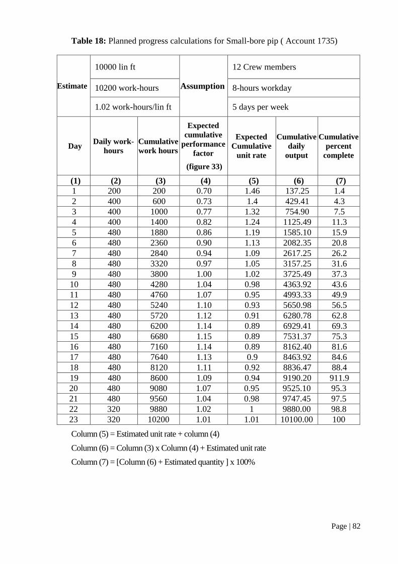
Page | 82

Table 18: Planned progress calculations for Small-bore pip ( Account 1735)

Estimate

10000 lin ft

Assumption

12 Crew members

10200 work-hours 8-hours workday

1.02 work-hours/lin ft 5 days per week

Day Daily work-

hours

Cumulative

work hours

Expected

cumulative

performance

factor

(figure 33)

Expected

Cumulative

unit rate

Cumulative

daily

output

Cumulative

percent

complete

(1) (2) (3) (4) (5) (6) (7)

1 200 200 0.70 1.46 137.25 1.4

2 400 600 0.73 1.4 429.41 4.3

3 400 1000 0.77 1.32 754.90 7.5

4 400 1400 0.82 1.24 1125.49 11.3

5 480 1880 0.86 1.19 1585.10 15.9

6 480 2360 0.90 1.13 2082.35 20.8

7 480 2840 0.94 1.09 2617.25 26.2

8 480 3320 0.97 1.05 3157.25 31.6

9 480 3800 1.00 1.02 3725.49 37.3

10 480 4280 1.04 0.98 4363.92 43.6

11 480 4760 1.07 0.95 4993.33 49.9

12 480 5240 1.10 0.93 5650.98 56.5

13 480 5720 1.12 0.91 6280.78 62.8

14 480 6200 1.14 0.89 6929.41 69.3

15 480 6680 1.15 0.89 7531.37 75.3

16 480 7160 1.14 0.89 8162.40 81.6

17 480 7640 1.13 0.9 8463.92 84.6

18 480 8120 1.11 0.92 8836.47 88.4

19 480 8600 1.09 0.94 9190.20 911.9

20 480 9080 1.07 0.95 9525.10 95.3

21 480 9560 1.04 0.98 9747.45 97.5

22 320 9880 1.02 1 9880.00 98.8

23 320 10200 1.01 1.01 10100.00 100

Column (5) = Estimated unit rate + column (4)

Column (6) = Column (3) x Column (4) + Estimated unit rate

Column (7) = [Column (6) + Estimated quantity ] x 100%

Page | 83

Similarly, the schedule performance index for a control account can be expressed as:

S for a Control Account

Scheduled Work hours to Date ( )

An SPI greater than 1.0 indicates that the work is ahead of schedule. The work is

behind schedule if the index is less than 1.0.

INTEGRATING PRODUCTIVITY AND SCHEDULE PERFORMANCE

Productivity and schedule performance are closely related, and it is advantageous

to study the two simultaneously. For an activity, this can be easily done graphically

by plotting the performance factor (Equation 6) against the schedule performance

index (Equation 19). For a control account, Equations 13 and 20 are used.

Figure 40 shows how to interpret the results. Data points in the first quadrant

indicate that both productivity and schedule performance are better than planned. If

both are worse than planned, then the data point will be in the third quadrant. Figure

40 includes possible reasons why a data point will fall in a particular quadrant.

Figure 41 shows the schedule and productivity performance history for the

structural steel operation. For this example, the work began ahead of schedule, and

productivity was better than planned. However, beginning with day 7, there was a

steady and pronounced deterioration in the schedule. Productivity remained at the

planned level through day 17. Thereafter, a continued loss in productivity occurred.

Figure 42 shows a similar curve for the small-bcre piping operation. While the

progress was ahead of schedule for the first three weeks, productivity was

considerably worse than planned by the end of the period. This was followed by a

seven-week period in which the work remained ahead of schedule and productivity

performance steadily improved. After week 10, both schedule and productivity levels

deteriorated.

MONITORING OVERALL PROJECT PERFORMANCE

Thus far, the concepts described have been applied to the evaluation of activities

or control accounts. Yet, these concepts can be extended for the monitoring of the

performance of the overall project or a portion thereof. In doing so, it is unnecessary

to monitor all project activities.

The following example illustrates the performance monitoring of a total project.

While the work may involve thousands of activities, only a few accounts have been

Page | 84

isolated as being the controlling or significant items of work. These items can be

combined into a relatively small number of control accounts, shown by Figure 43 in

bar chart format. The columns in figure 43 are explained by Table 19. Control of

these nine control accounts should result in the control of the overall project.

Figure 40. Schedule performance index Venus performance factor

possible weather delays

undermanding of the work

later than planned start

overly optimistic schedule

0.5 1.0 2.0 3.0 4.00.0 5.0

SCHEDULE

PREFORMANCE INDEX(SPI)

AHEAD OF SCHEDULE, BETTER

THAN ESTIMATED PRODUCTIVITY

BEHIND SCHEDULE, BETTER THAN

PLANNED PRODUCTIVITY

2.0

3.0

4.0

5.0

0.5

0.0

BEHIND SCHEDULE LOWER THAN

PLANNED PRODUCTIVITY

AHEAD OF SCHEDULE,WORSE

THAN ESTIMATED PRODUCTIVITY

earlier than planned start

poor productivity offset by fewer than plan quantities

over manning

low productivity estimates

saving in work-hours

overly optimistic schedule

fewer quantities than estimated

very favorable working conditions

PERFORMANCE FACTOR (PF)

many possible causes including

inaccurate estimatea

later than planed start

dfficult and disoranized work, etc

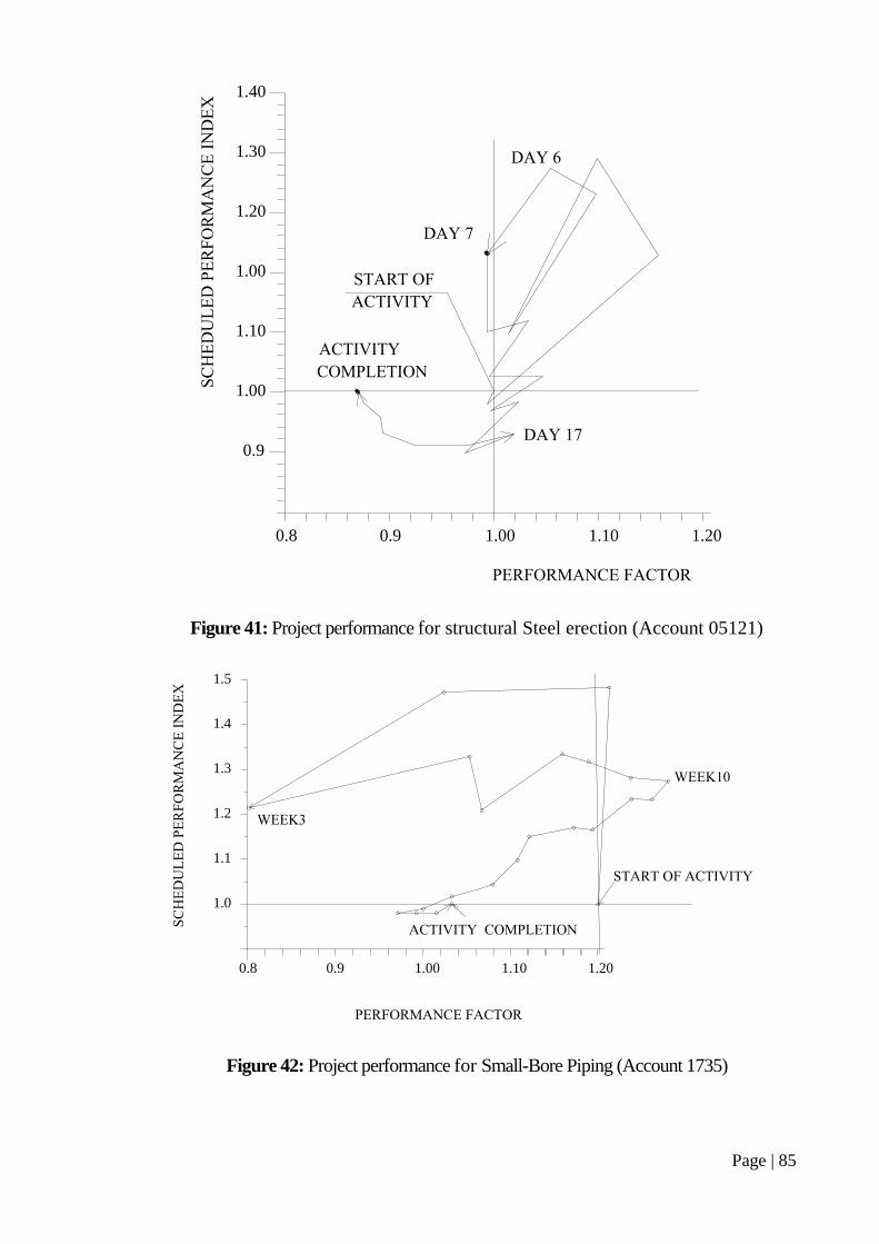
Page | 85

Figure 41: Project performance for structural Steel erection (Account 05121)

Figure 42: Project performance for Small-Bore Piping (Account 1735)

START OF

ACTIVITY

0.90.8 1.00 1.10 1.20

0.9

1.00

1.10

1.00

1.20

1.30

1.40

PERFORMANCE FACTOR

DAY 17

DAY 6

DAY 7

SC

HE

DU

LE

D P

ER

FO

RM

AN

CE

IN

DE

X

ACTIVITY

COMPLETION

0.90.8 1.00 1.10 1.20

1.0

1.1

1.2

1.3

1.4

1.5

PERFORMANCE FACTOR

SC

HE

DU

LE

D P

ER

FO

RM

AN

CE

IN

DE

X

WEEK3

WEEK10

START OF ACTIVITY

ACTIVITY COMPLETION

Page | 86

30 60 85 90 95100

15 45 85100

35 55 75 90 9510015

50 65 75 85 9510030155

50 65 80 90 971003520103

30 50 75 90 97100155

30 50 75 90 97100155

15 40 75100

15 40 75100

86 92 9710044 54 65 7619 24 29 353 6 11 151

S: SCHEDULE PROGRESSA: ACTUAL PROGRESS

PROGRESS OF PRODUCTIVTY REPORTING

Figure 43. Progress Chart Based on Earned Value Concepts

PROJECT:

CUSTOMER:

ControlAccount

COSTCODE

SCHEDULE

MONTHS

EARTHWORK

S

A

FOUNDATION

STRUCTURAL STEEL

EQUIPMENT SETTING

PIPING

ELECTRICAL

INSTRUMENTATION

INSULATION

PAINTING

TOTAL CONSTRUCTION

1 2 3 4 5 6 7 8 9 10 11 12 13 14 15 16 17 18

S

A

S

A

S

A

S

A

S

A

S

A

S

A

S

A

S

A

Earned Value

REL.WEIGHT

IWHRS

PERCENTCOMPLETE

I

EARNEDWHRS

ACTUALWHRS

EXPENDED

PerformanceFactor

Sch.

Perf.

Index

(1) (2) (3) (4) (5) (6) (7)

TO DATE (-/-/-) PF Trends

MONTHS

3 6 9 12 15

10,000 32

25,000 82

30,000 102

25,000 82

95,000 322

50,000 172

40,000 142

12,500 42

12,500 41

300,000 1002

Page | 87

Figure 43 shows the planned monthly progress for each control account. Column 1 contains the

maximum earned work-hours. This column will change only if the quantities are revised. The relative

weight in column 2 indicates the degree of difficulty of each control account relative to the total. Because

these weights are determined by the earned work-hours and the percent complete calculations are

determined by rules of credit and earned work-hours in individual accounts, an accurate assessment of

percent complete should be possible.

Figure 44 provides a- progress schedule prepared at the end of the eighth month. It shows late

completion of the earthwork, foundation, structural steel, and equipment setting subtasks. The piping and

electrical work are shown to be ahead of schedule. This progress is reflected by the schedule

performance index (SPI), which, when an activity is completed, becomes 1.0. The SPI cannot be

calculated for an activity that begins early, as is the case for the electrical work. Overall, the work in this

example is ahead of schedule (SPI = 1.05) because of the influence of the piping and electrical work,

which have the largest relative weights. Using the earned work-hours, the percent complete can be

calculated as 30.3 percent. If the actual work-hours were used, the percent complete would be 32

percent, or about 6 percent higher than the actual amount. Productivity is better than planned on the

earthwork, structural steel, and piping. However, overall productivity is lower than planned, since the

actual work-hours are more than the earned work-hours.

USE OF EARLY AND LATE START DATES

If the scheduling system used provides early and late start times, these times can be combined

graphically with quantity arc progress information to produce commodity curves. An example is shown

in Figure 45 for small-bore pipe on a power plant project. The planned progress based on early and late

start dates yields an envelope in which actual progress must fall if the project schedule is to be

maintained. As can be seen in Figure 45, schedule slippage occurred, and a recovery plan was

successfully initiated. The small-bore pipe is currently progressing according to the late-start schedule.

SUMMARY

This chapter has described how schedule and productivity performance can be viewed

simultaneously to better understand how the job is progressing. To access actual progress, there must be

a plan. A planned progress curve was developed using a standard productivity curve and a variable

manning level. This was also used to determine the activity duration. Overall monitoring of an activity or

control account was done graphically. The performance factor was plotted against a schedule

performance index. The concepts of earned value were then used to show how the progress and

productivity of a total project effort can be monitored.

Table 19. Definition of Terms in Figures 43 and 44

Earned Value Work-hours - Indicates the estimated work-hours required to complete this control

account. This number remains unchanged unless the quantities are revised.

Relative Weight - Defines the relative value of this control account compared to the total construction

effort for this project. It is determined on the basis of the distribution of earned work-hours.

Percent Complete - Indicates the physical measurement of work completed in the specific control

account.

Earned Work-hours to Date - Defines the work-hour that should have been spent for the equivalent

work progress. It is determined by multiplying the quantities installed times the budgeted unit rate.

Actual Work-hours Expended - Indicates the actual work-hours expended to date. It is usually

obtained from the time sheet.

Performance Factor - Indicates the relative productivity as compared to the pre-established budget

(1.0 being the budgeted productivity). Anything less than 1.0 indicates the expenditure of more work-

hours to accomplish equivalent units of work than originally budgeted.

Schedule Performance Index - A comparison of actual earned work-hours to the planned earned

work-hours. An index greater than 1.0 indicates that the work is ahead of schedule.

Page | 88

1983 1984

JAN FEB MAR APR MAY JUN JUL AUG SEP OCT NOV DEC JAN FEB MAR APR MAY JUN JUL

ACT. MONTH 32 559 761 818 909 587 837 300 787 1339 600 104 148 146 321

SCHED. MONTH 480 730 940 880 860 810 760 760 700 650 440 200 140 120 120 120 100 100 90

ACT. CUM. 582 1141 1902 2720 3629 4216 5063 5353 6140 7474 8079 8183 8331 8477 8798

SCHED. CUM. 1030 1760 2700 3580 4440 5250 6010 6770 7470 8120 8560 8760 8900 9020 9140 9200 9360 9460 9550

J F M A M J J A S O N D J F M A M J J A S O N D4.0

13.6

23.2

32.8

42.4

52.0

61.6

71.2

80.8

90.4

100

1983 1984

PE

RC

EN

T C

OM

PL

ET

E

BASE ON EARLY START

SMALL BORE-PILE

BASE ON LATE START

BASE ON ACTUAL

Page | 89

1 2 3 4 5 6 7 8 9 10 11 12 13 14 15 16 17 18

S

A

S

A

S

A

S

A

S

A

S

A

S

A

S

A

S

A

Earned Value

REL.WEIGHT

IWHRS

PERCENTCOMPLETE

I

EARNEDWHRS

ACTUALWHRS

EXPENDED

PerformanceFactor

Sch.

Perf.

Index

(1) (2) (3) (4) (5) (6) (7)

TO DATE (-/-/-) PF Trends

MONTHS

3 6 9 12 15

10,000 32

25,000 82

30,000 102

25,000 82

95,000 322

50,000 172

40,000 142

12,500 42

12,500 41

300,000 1002

30 60 85 90 95100

15 45 85100

35 55 75 90 9510015

50 65 75 85 9510030155

50 65 80 90 971003520103

30 50 75 90 97100155

30 50 75 90 97100155

15 40 75100

15 40 75100

86 92 9710044 54 65 7619 24 29 353 6 11 151

S: SCHEDULE PROGRESSA: ACTUAL PROGRESS

PROGRESS OF PRODUCTIVTY REPORTING

Figure 44. Progress Report Showing Status as of the Eight Month

95 9880

96 10050

50 85

6020

15

3

18 306

PROJECT:

CUSTOMER:

ControlAccount

COSTCODE

SCHEDULE

MONTHS

EARTHWORK

S

A

FOUNDATION

STRUCTURAL STEEL

EQUIPMENT SETTING

PIPING

ELECTRICAL

INSTRUMENTATION

INSULATION

PAINTING

TOTAL CONSTRUCTION

Page | 90

PART IV - LESSONS LEARNED AND FINDINGS

Chapters 9 and 10 cover the case studies. The goal of the case studies was to test the basic

concepts presented in Part II and report any needed modification. None were found to be

necessary. Mother goal was to describe experiences with implementing the measurement

system. Generally, these experiences were positive.

In Chapter 9, profiles of the three contractors are presented, and the 13 activities that

were studied are described. The diverse backgrounds and interests of the contractors and the

range of conditions and project types encountered in the case study activities add to the

credibility of the results. The chapter documents examples of haw productivity measurement

can be used to develop labor units for estimating, to understand factors that affect

productivity, and to monitor and control important activities. These examples show the

versatility of productivity measurement. Several situations are shown where labor units for

estimating can be developed. In these situations, summarizing work-hours and quantities at

project completion would have been inappropriate. For another activity, work-hours rather

than quantities were recorded for each subtask. In other examples, the effects of various

disruptions on productivity are shown. The disruptions documented include quality problems,

drawing errors, bad weather, crew reassignments, equipment breakdown, and several others.

The case study data are, also used to forecast the work-hours and workdays needed to

complete several activities. Earned value calculations are used on another activity to show

that there were difficulties in maintaining momentum. Performance factor curves were used to

isolate activities with the greatest opportunity f0c improvement and, to compare actual

productivity to expectations.

The case study findings are summarized in Chapter 10. These are organized according to

the six system criteria stated in Chapter 3. Other relevant findings are' also presented.