Finescale Vertical Structure of a Cold Front as Revealed ...geerts/bart/coldfront.pdf · Finescale...

Finescale Vertical Structure of a Cold Front as Revealed by anAirborne Doppler Radar

BART GEERTS, RICK DAMIANI, AND SAMUEL HAIMOV

University of Wyoming, Laramie, Wyoming

(Manuscript received 30 July 2004, in final form 11 November 2004)

ABSTRACT

In the afternoon of 24 May 2002, a well-defined and frontogenetic cold front moved through the Texaspanhandle. Detailed observations from a series of platforms were collected near the triple point betweenthis cold front and a dryline boundary.

This paper primarily uses reflectivity and Doppler velocity data from an airborne 95-GHz radar, as wellas flight-level thermodynamic data, to describe the vertical structure of the cold front as it intersected withthe dryline. The prefrontal convective boundary layer was weakly capped, weakly sheared, and about 2.5times deeper than the cold-frontal density current.

The radar data depict the cold front as a fine example of an atmospheric density current at unprecedenteddetail (�40 m). The echo structure and dual-Doppler-inferred airflow in the vertical plane reveal typicalfeatures such as a nose, a head, a rear-inflow current, and a broad current of rising prefrontal air that feedsthe accelerating front-to-rear current over the head. The 2D cross-frontal structure, including the frontalslope, is highly variable in time or alongfront distance. Along this slope horizontal vorticity, averaging �0.05s�1, is generated baroclinically, and the associated strong cross-front shear triggers Kelvin–Helmholtz (KH)billows at the density interface. Some KH billows occupy much of the depth of the density current, possiblyeven temporarily cutting off the head from its trailing body.

1. Introduction

In the afternoon of 24 May 2002, a cold front–drylineintersection was intercepted over the southern GreatPlains by an armada of mobile observing platforms aspart of the International H2O Project (IHOP_2002;Weckwerth et al. 2004). The objective of the missionwas to capture the initiation of thunderstorms in thevicinity of these boundaries. In the region of detailedobservations, the cold front penetrated under the moistair east of the dryline. Deep convection broke out a fewtens of kilometers east of this region, clearly ahead ofthe well-defined surface cold front. This paper does notattempt to explain the timing or location of this con-vective initiation. Rather, it describes the meso-� andmicroscale structure of this cold front, with an emphasison the vertical airflow structure, as documented by air-borne radar data.

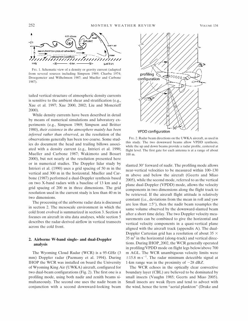
It has long been postulated that on the meso-� scalethe cold air associated with a cold front may assume thevertical structure of a density (or gravity) current (Fig.1). Such a current results when two fluids of differentdensity are juxtaposed. Because of negative buoyancy,the denser fluid will penetrate below the less densefluid in the form of a shallow current with an elevatedhead and a turbulent wake (Benjamin 1968). Atmo-spheric density currents have received a great deal ofattention (e.g., Simpson 1987), and they have been in-voked in the interpretation of a range of mesoscalephenomena, including thunderstorm-generated gustfronts (Charba 1974; Wakimoto 1982; Mueller and Car-bone 1987; Mahoney 1988), sea breezes (Abbs andPhysick 1992), land breezes (Schoenberger 1984), ka-tabatic winds spreading over level terrain (Bromwich etal. 1992), and also cold fronts (Clarke 1961; Carbone1982; Hobbs and Persson 1982; Shapiro 1984; Shapiroet al. 1985; Bond and Fleagle 1985; Garratt 1988; Le-maitre et al. 1989; Nielsen and Neilley 1990; Trier et al.1990; Bond and Shapiro 1991; Hakim 1992; Roux et al.1993; Koch and Clark 1999; Wakimoto and Bosart2000). Numerical experiments have shown that the de-

Corresponding author address: Dr. Bart Geerts, Dept. of At-mospheric Sciences, University of Wyoming, Laramie, WY 82071.E-mail: [email protected]

JANUARY 2006 G E E R T S E T A L . 251

© 2006 American Meteorological Society

MWR3056

tailed vertical structure of atmospheric density currentsis sensitive to the ambient shear and stratification (e.g.,Xue et al. 1997; Xue 2000, 2002; Liu and Moncrieff2000).

While density currents have been described in detailby means of numerical simulations and laboratory ex-periments (e.g., Simpson 1969; Simpson and Britter1980), their existence in the atmosphere mainly has beeninferred rather than observed, as the resolution of theobservations generally has been too coarse. Some stud-ies do document the head and trailing billows associ-ated with a density current (e.g., Intrieri et al. 1990;Mueller and Carbone 1987; Wakimoto and Bosart2000), but not nearly at the resolution presented hereor in numerical studies. The Doppler lidar study byIntrieri et al. (1990) uses a grid spacing of 50 m in thevertical and 300 m in the horizontal. Mueller and Car-bone (1987) performed a dual-Doppler synthesis basedon two X-band radars with a baseline of 13 km and agrid spacing of 200 m in three dimensions. The gridresolution used in the current study is less than 40 m intwo dimensions.

The processing of the airborne radar data is discussedin section 2. The mesoscale environment in which thecold front evolved is summarized in section 3. Section 4focuses on aircraft in situ data analyses, while section 5describes the radar-derived airflow in vertical transectsacross the cold front.

2. Airborne W-band single- and dual-Doppleranalysis

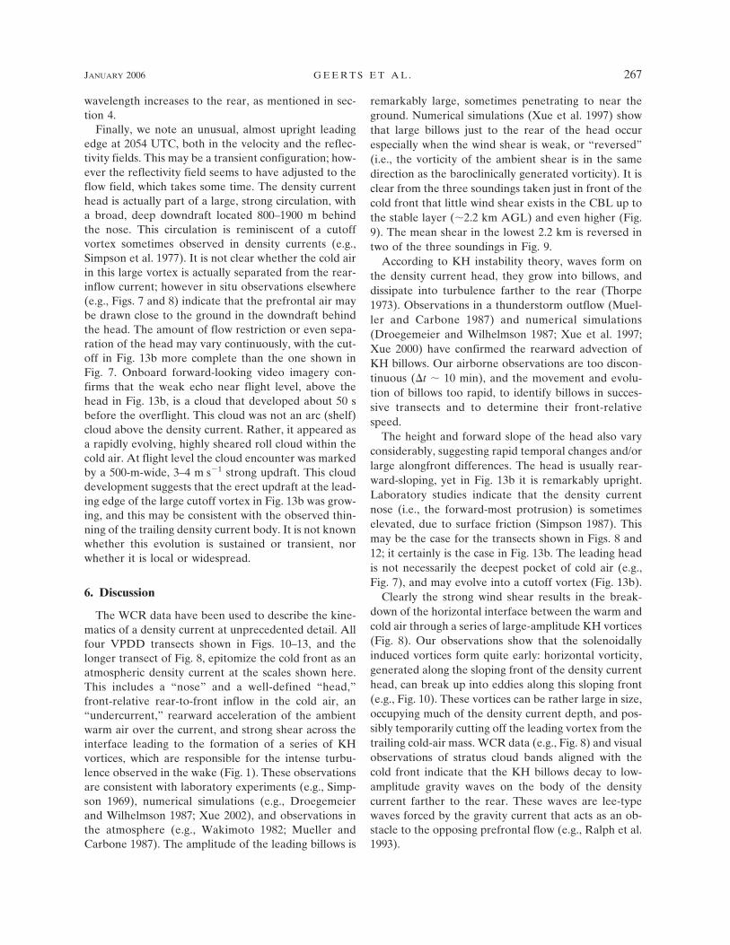
The Wyoming Cloud Radar (WCR) is a 95-GHz (3mm) Doppler radar (Pazmany et al. 1994). DuringIHOP the WCR was installed on board the Universityof Wyoming King Air (UWKA) aircraft, configured fortwo dual-beam configurations (Fig. 2). The first one is aprofiling mode, using both nadir and zenith beams si-multaneously. The second one uses the nadir beam inconjunction with a second downward-looking beam

slanted 30° forward of nadir. The profiling mode allowsnear-vertical velocities to be measured within 100–130m above and below the aircraft (Geerts and Miao2005), while the second mode, referred to as the verticalplane dual-Doppler (VPDD) mode, allows the velocitycomponents in two dimensions along the flight track tobe retrieved. If the aircraft flight attitude is relativelyconstant (i.e., deviations from the mean in roll and yaware less than �5°), then the nadir beam resamples thesame volume observed by the downward-slanted beamafter a short time delay. The two Doppler velocity mea-surements can be combined to give the horizontal andvertical velocity components in a quasi-vertical planealigned with the aircraft track (appendix A). The dual-Doppler Cartesian grid has a resolution of about 35 �35 m2 in the horizontal (along-track) and vertical direc-tions. During IHOP_2002, the WCR generally operatedin profiling/VPDD mode on flight legs below/above 700m AGL. The WCR unambiguous velocity limits were�15.8 m s�1. The radar minimum detectible signal at1-km range was in the proximity of �28 dBZ.

The WCR echoes in the optically clear convectiveboundary layer (CBL) are believed to be dominated bysmall insects (Vaughn 1985; Geerts and Miao 2005).Small insects are weak flyers and tend to advect withthe wind, hence the term “aerial plankton” (Drake and

FIG. 1. Schematic view of a density or gravity current (adaptedfrom several sources including Simpson 1969; Charba 1974;Droegemeier and Wilhelmson 1987; and Mueller and Carbone1987).

FIG. 2. Radar beam directions on the UWKA aircraft, as used inthis study. The two downward beams allow VPDD synthesis,while the up and down beams provide a radar profile, centered atflight level. The first gate for each antenna is at a range of about100 m.

252 M O N T H L Y W E A T H E R R E V I E W VOLUME 134

Farrow 1988; Russell and Wilson 1997). Thus the re-trieved horizontal velocity should be unbiased. It is notclear how well the retrieved vertical echo motion rep-resents vertical air motion. Small insects tend to opposethe updraft in which they become embedded (Geertsand Miao 2005). This seems to be the only viable ex-planation for the existence and persistence of fine lines,where the echo strength is some 10–30 dBZ above val-ues observed elsewhere in the fair-weather CBL (Wil-son et al. 1994; Russell and Wilson 1997), implying in-sect concentrations of one to three orders of magnitudehigher than background values. Passive tracers wouldsimply diverge near the top of the CBL and disperse.Hence the CBL is known as the “mixed” layer. A seriesof IHOP_2002 flight legs in the fair-weather CBL (i.e.,far away from fine lines) suggest that small insectsmove down relative to the ambient vertical air motionat 0.5 � 0.2 m s�1 on average, and that this downwardmotion increases in updrafts, at nearly half the updraftspeed itself (Geerts and Miao 2005). Small insects maymove down either actively, or by folding their wingsand falling down at their “terminal velocity.” Which ofthese two methods is the fastest depends on the Reyn-olds number acting on the insect, but it is probablylimited to �2 m s�1 (Pedgley 1982). Thus it is conceiv-able that the rate of opposition of microinsects to up-drafts has a ceiling. Geerts and Miao (2005) did not findsuch ceiling, but their assessment of insect vertical mo-tion applies to the fair-weather CBL. The updraftsalong a cold front may be stronger and more sustainedthan those associated with thermals. In short, in orderto obtain the best-guess vertical air motion (wwcr,air), weadjust the echo vertical motion (wwcr,insects) for insectmotion by means of Eq. (2) in Geerts and Miao (2005):

wwcr,air � min�1.96wwcr,insects � 0.82, wwcr,insects

� 1.5 m s�1. 1�

The first term is a linear regression based on verticalvelocity comparisons between the UWKA gust probeand first-gate WCR data above and below the aircraft.The second term constrains this correction (i.e., the in-cremental upward motion) to 1.5 m s�1. Here wwcr,insects

is the scatterer vertical motion (appendix A), wwcr,air isthe best-guess air vertical motion, and min() takes theminimum of its arguments.

How accurate are the resulting air velocities? Onesource of uncertainty is the temporal evolution of thescattering features (at a resolution of �35 m) betweenthe two radar illuminations. The airborne dual-Dopplervelocity retrieval method is feasible as long as the vol-ume scanned by one of the beams is observed by theother in a time interval shorter than the characteristic

evolution time scale of the scattering volume. With abeam-to-beam time difference of 6 s per 1 km from theaircraft, this condition should be satisfied at typicalWCR ranges (usually no more than 3 km). But clearlythis error increases with range. Other error sources in-clude both rapid aircraft attitude variations and thecross-track wind. The first results in an irregular spac-ing and alignment between adjacent beams, with con-sequent degradation of the vertical resolution. The sec-ond plays a role in the removal of the horizontal windcomponent from the near-vertical radial wind; the best-guess horizontal wind profile is used in the solution ofthe velocity decomposition problem (see appendix A).The roll and yaw (sideslip) standard deviations for theflight segments used here were within 2°. The overalluncertainty in the calculated velocities for the 24 Maydata is estimated to be in the order of 1 m s�1 at a rangeof 1 km and for WCR signal-to-noise ratios greater than0 dB.

3. Mesoscale evolution

In the afternoon of 24 May 2002, a SW–NE-orientedcold front approached a nearly stationary, north–south-oriented dryline near Shamrock, near the eastern mar-gin of the Texas panhandle (Weckwerth et al. 2004;Wakimoto et al. 2006). This front was weak in themorning hours, but frontogenesis occurred during thedaytime as the cold sector remained covered by a vaststratus cloud deck (Fig. 3), a process that has been ob-served elsewhere (e.g., Miller et al. 1996). A sharp con-trast in equivalent potential temperature (�e) waspresent at 1800 UTC mainly near the Oklahoma pan-handle (Fig. 4). Differential horizontal advection of �e

during 0600–1800 UTC clearly contributed to thesharpening �e gradient. The center of the low-level cy-clonic circulation was in the northern Texas panhandle,just north of the intensive observations, and a 1.2 �10�4 s�1 center of positive relative vorticity was foundover eastern Colorado at 300 mb, associated with awell-defined short-wave trough (Fig. 4).

The front was mostly stationary in the morning hours(1000–1400 UTC), but it accelerated thereafter. Theconvergence along the cold front was weak between1500 and 1900 UTC, at least around the Amarillo Next-Generation Weather Radar (NEXRAD; 143 km westof Shamrock): a clearly defined fine line did not de-velop there until 2000 UTC, about 4 h after frontalpassage at the radar site. Similarly, radar and surfacestation data do not reveal a dryline until about 1930UTC, but this may be due to the remoteness of thesurrounding radars and the paucity of operationalweather stations in the Texas panhandle: mobile meso-


net and mobile ground-based radars confirm the pres-ence of a weak dryline boundary from about 1840 UTC,and the Naval Research Laboratory (NRL) P-3 withElectra Doppler Radar (ELDORA) manages to trackthis dryline from about 1900 UTC (Wakimoto et al.2006).

A 1906 UTC Mobile GPS/Loran AtmosphericSounding System (M-GLASS) sounding on the moistside of the dryline (not shown) shows a well-mixedCBL, with a well-defined top around 2.0 km AGL. TheCBL wind is weak, from 160° to 190°, and the windveers to �220° just above the CBL, with speeds increas-ing to 12 m s�1. The sounding does not reach saturationin the CBL, but UWKA observations at this time indi-cate several cumulus clouds in the upper �400 m of theCBL, at 7, 15, and 19 km east of the dryline. Eightdropsondes were released by a Learjet aircraft around2030 UTC from 4700 m MSL along an east–westflight leg located just south of the UWKA flight tracks(Fig. 5). The CBL in the eastern half of this leg hasmixing ratio (q) values around 12 g kg�1. This layer isweakly capped at about 1.4 km AGL. The cap has apotential temperature jump � of 1–2 K, a q of about�3 g kg�1, and a winds veering from southeasterly tosouthwesterly. This shallow cap becomes better definedtoward the east, where it caps abundant stratocumulusclouds, according to UWKA forward camera footage.

The low-level moisture gradient and confluence be-

tween sondes 3 and 4 (2032–2035 UTC) suggests thepresence of a dryline at the surface. Dropsonde 3 has aremarkably deep mixed layer (about 2.6 km deep),which is drier (8 � q � 9 g kg�1) than that in sonde 4.Also, the near-surface wind has a westerly component(Fig. 5). The (q, �) of the air in this CBL is similar tothat in the southwesterly current above the dryline;thus presumably this is one air mass advected over thedryline.

A second, stronger stable layer ( � of �3 K) ispresent near 2.4 km AGL above this air mass. This capextends west of the dryline and is better defined atsounding 3 than on the moist side of the dryline, be-cause of surface-driven convective mixing and/or me-soscale frontogenetical forcing. Near the top of thedeep mixed layer just west of the dryline (sounding 3),the relative humidity peaks at 91%.

A marked humidity gradient is present farther west,above the cold-frontal surface between dropsonde 2 (q� 2 g kg�1) and the Mobile Cross-Chain Loran Atmo-spheric Sounding System (M-CLASS) sounding (q � 8g kg�1), between 1.4 and 2.2 km AGL. This boundaryalso separates warmer air to the west from �2 K coolerair to the east and is convergent in the east–west direc-tion. It is marked as an “elevated dryline” in Fig. 5.Remotely sensed humidity data from the Lidar Atmo-spheric Sensing Experiment (LASE) instrument,aboard an aircraft following exactly the same track asthe dropsonde aircraft, confirm the existence of thissharp humidity boundary above the cold front(Wakimoto et al. 2006). The UWKA never traveled farenough west to sample it. This boundary may be due tofrontogenetical vertical motion, with subsidence to theNW and uplift to the SE. Because just east of this el-evated dryline potential instability exists [(d�e/dz) � 0]and the air is close to saturation, such uplift would leadto deep convection. In fact �e decreases some 14 Kbetween 2.5 and 3.5 km AGL in sonde 3 (Fig. 5).

We calculate the convective available potential en-ergy (CAPE) and convective inhibition (CIN) of thesoundings assuming adiabatic mixing in the lowest 50mb. The 1906 UTC sounding (east of the dryline) has aCAPE of 1627 J kg�1 and a CIN of �45 J kg�1. AnM-GLASS sounding was released at 1917 UTC be-tween the surface cold front and the surface dryline.This sounding, the last one released before the cold-frontal passage, only extends up to 340 mb, but it cap-tures the same deep, dry CBL as sonde 3, with a clearcap near 2.5 km AGL. Its CIN is �5 J kg�1 and itsCAPE is estimated at 1806 J kg�1. Sonde 3, released inthe same sector some 30 km farther south at 2032 UTC,has a CIN of �12 J kg�1 and a CAPE estimated at 1983J kg�1. These estimates assume an upper atmosphere

FIG. 3. Change of temperature gradient ( T/ x) over time dur-ing 24 May 2002 in the Texas panhandle and western Oklahoma.Temperatures are obtained from the Oklahoma Mesonet and theNational Weather Service network. Here x is computed as theshortest distance between a station in the cold air and the coldfront. The location of the latter is fine-tuned based on a fine lineobserved in the displays of the Amarillo and Vance, TX,NEXRAD radars and S-band dual-polarization Doppler radar(S-Pol), although between 1600 and 1800 UTC none of the radarsclearly locates this fine line. The value of T is obtained from thestation in the cold air, and the closest station in the warm air.Mobile mesonet temperatures are not included.


(above the highest level with data) from the 1906 UTCfull sounding. In short, the triple-point environmentwas poised for convective initiation.

Shared Mobile Atmospheric Research and TeachingRadar (SMART-R) and mobile mesonet data showthat the circulation near the dryline is confluent, andthat the dryline echo strength intensifies between 1900UTC and the time that it is lifted over the cold front.During that period the dryline also moved to the east atabout 3 m s�1. The cold front, propagating toward thesoutheast at a speed of about 7 m s�1, and the devel-oping dryline intersect about 25 km west of theSMART-R located at Shamrock at 2000 UTC (Fig. 6).Mesonet surface observations confirm the presence ofthree air masses near the “triple point”: the postfrontalcool air mass; the warm, moist air east of the dryline,advected from the south; and the warmest and driest airmass, wedged between the cold front and the dryline.Note the elevated dewpoint values in the postfrontalair; in fact they are higher than those east of the dryline(Fig. 6). The high moisture content of the postfrontal

air is confirmed by UWKA measurements (e.g., Fig. 8of Weckwerth et al. 2004) and is consistent with thestratus cloud deck, whose edge trailed the cold front byabout 10 km during UWKA observations. The synopticflow (Fig. 4) suggests that this moisture is drawn fromthe east and is wrapped around by the cyclonic flow.

The triple point was the focus of intensive observa-tions. ELDORA Doppler wind syntheses indicate thatthe triple point was the center of a cyclonic circulationand rising air currents (Wakimoto et al. 2006). TheUWKA flew multiple legs, 30–50 km long at levels be-tween 150 and 2440 m AGL, crossing both the surfacedryline and cold front. The cold front protruded underthe dryline, upon which the latter becomes elevatedand smeared out, as shown further by radar data.

Deep convection did not break out at the cold front,nor did it break out along the triple point as that point“zipped” southward. Rather, deep convection devel-oped east of the cold front, and the development zippednorthward. The first towering cumuli developed around2010 UTC, just east of the SSW–NNE-oriented dryline,

FIG. 4. Synoptic situation at 1800 UTC on 24 May 2002, based on the initial fields of the Eta Model. Shown are the 900-mb equivalentpotential temperature (color field), the 900-mb wind barbs (a full barb equals 5 m s�1), the sea level pressure (thin yellow contours),and the 300-mb geopotential height (thick red contours).


Fig 4 live 4/C

FIG. 5. Cross section across the cold front and dryline, based on a series of sondes dropped between 2022 and 2047 UTC along awest-to-east transect at 35°N, starting near the center of the Texas panhandle. Also included is an M-CLASS sounding released at2056 UTC. The top transect shows mixing ratio q (g kg�1) and potential temperature � (K), and the bottom one relative humidity

→


Fig 5 live 4/C

near Childress, about 90 km south of Shamrock (Xueand Martin 2006). Later the deep convection pro-gressed northward, with the first towering cumulusalong the final UWKA flight leg at 2113 UTC, some30 min after the dropsonde data were collected there(Fig. 5). The echo from this first cumulus was weak(��5 dBZ), indicating that precipitation-size particleshad not yet formed. The UWKA forward-looking cam-era indicates that the congestus penetrated well abovethe flight level, which was 2.6 km AGL, that is, justabove the second stable layer, with even taller cumulijust south of the flight track. This indicates that at thislocation and time an undiluted parcel rising to 2.5 kmwas positively buoyant, or at least penetrated throughwhat CIN may have remained. By 2130 UTC a solidline of thunderstorms was present from Childress to theTexas–Oklahoma border east of Shamrock. This linewas aligned with the dryline, but as it continued toexpand toward the northeast, it became aligned withthe cold front.

4. Finescale aircraft and cloud radar observations

A vertical transect of WCR reflectivity and corre-sponding in situ measurements across the cold frontand primary dryline is shown in Fig. 7. Note that theWCR reflectivity values are much lower than those fora C-band radar (Fig. 6). That is because reflectivity isinferred from power assuming Rayleigh scattering, yetthe bulk of the W-band scatterers in the CBL are be-lieved to be in the Mie regime (Geerts and Miao 2005)where the scattering efficiency oscillates with size. At Cband, a larger fraction of scatterers are in the Rayleighregime.

A transect similar to the one in Fig. 7, but about 13min later, is shown in Fig. 8 of Weckwerth et al. (2004).In both transects the cold-frontal surface clearly slopestoward the cold air, while the dryline echo is upright.Both show a clear discontinuity of � and q at the coldfront. The dryline is marked by sudden moistening ( q� 2 g kg�1) and some cooling ( � � 1 K). In terms ofbuoyancy, the moistening and cooling roughly canceleach other [ �� 0 (Fig. 7b)]. In both transects thedryline echo is weaker than the cold front echo, possi-bly because the �10 m s�1 surface winds behind thecold front pick up and mix more insects and nonbiotic

scatterers. The most remarkable difference betweenthe 1935 UTC transect (Fig. 7) and the 1948 UTCtransect (Fig. 8 of Weckwerth et al. 2004) regards thedepth and shape of the leading edge of the cold-frontaldensity current. Clearly the morphology of the densitycurrent head (Fig. 1) changes rapidly. The WCR datamay also witness alongfront variations: laboratorysimulations have demonstrated that the leading edge ofdensity currents is marked by a series of clefts and lobes(e.g., Simpson and Britter 1980).

The rapid changes in echo structure are consistentwith the variability of vertical air velocity structure. InFig. 7 an updraft of up to 7 m s�1 occurs at the head ofthe cold front, and several strong up- and downdraftsfollow behind. Behind the first, shallow head at x � 0(horizontal axis in Fig. 7), warm, dry air is entrainedfrom above, down to flight level (360 m AGL). This issuggested by the q depression and � spike at 1.5 � x �2 km (Fig. 7a), and the coincident low WCR reflectivityabove flight level. This buoyant parcel (Fig. 7b) is aboutto be propelled upward again by the observed updraft.

FIG. 6. SMART-R 0.5° elevation reflectivity (dBZ ) scan, plusmobile mesonet observations, at 2000 UTC. Also shown are theUWKA track, nearly intersecting the triple point, with flight-levelwinds at 725 mb, and the Learjet track, with the location of somedropsondes shown in Fig. 5.

←

RH (%) and equivalent potential temperature �e (K). Wind vectors are plotted, with a full barb representing 5 m s�1. The cold frontand the dryline are shown. The moist air below the dryline (solid red line) is weakly capped near 1.4 km AGL, and a second stable layeris found near 2.4 km AGL (dashed red line). This appears to be the upper limit of an elevated moist layer, whose western limit is quiteapparent above the cold-frontal surface.


Fig 6 live 4/C

FIG. 7. (a) Mixing ratio and potential temperature, and (b) virtual potential temperature and gust probe vertical velocity, along a flighttrack at 360 m AGL across the cold front and dryline, around 1935 UTC, displayed at an aspect ratio (height:length) of 21⁄2:1. This crosssection cuts across the cold front at an angle of about 35° from the cold-front normal direction. (c), (d) Corresponding WCR verticalvelocity and reflectivity above flight level.


Fig 7 live 4/C

It is not clear whether the strong postfrontal echo at2 � x � 4 km in Fig. 7d, up to 1.5 km AGL, containscold air, in other words whether the head tops at 1.5 kmAGL. A flight leg at about 1200 m AGL crosses thecold front at 2025 UTC and encounters two brief surgesof cooler, moister air, coincident with WCR plumes upto flight level, but � � 1 K, suggesting that this plumehas been much diluted. Another flight leg at this level,crossing the cold front at 2054 UTC, does not interceptthe cold-frontal surface at all. Other WCR reflectivitytransects and photography from aboard the UWKA in-dicate that the deep cold-frontal plume shown in Fig. 7is rather rare. The head of the cold front was not deepenough to saturate the air and yield a cloud. Severaldownward intrusions of ambient air can be seen in thereflectivity transect behind the cold front, and the highvariability of � behind the cold front is an indication ofintense mixing between the two different air masses.

The intense mixing behind the cold-frontal head isapparent also in a transect around 2028 UTC (Fig. 8),after the cold front has penetrated under the dryline(the one shown at x � �12 km in Fig. 7). A �700 mwide updraft peaking at 9 m s�1 is found at the cold-frontal head. This broad updraft is strongest near thetop of the strongest echoes (700–800 m AGL accordingto Fig. 8d), but it extends to the top of the mixed layer

near 2.0 km AGL; that is, it is much deeper than thecold-frontal surface. The updraft peak is trailed by a 5m s�1 downdraft. The curling of the reflectivity in thedirection of the wind shear across the cold-frontal sur-face is indicative of large, breaking Kelvin–Helmholtz(KH) waves.

One of the KH billows, at x � 2.6 km, brings drier,warmer air down to flight level, merely 170 m AGL(Fig. 8). Downward curls of low reflectivity tend to cor-respond with downdrafts. The amplitude of the KHbillows and the strength of the updraft/downdrafts nearthe cold-frontal surface quickly dampen toward therear. The sloping echo bands above the cold front inFig. 8d may be detrained echo-rich cool air, or else theymay be sheared-out remnants of plumes in the prefron-tal CBL. The trailing narrow strip of higher reflectivityaround 600–700 m AGL (x � 8 km in Fig. 8) is at leastpartially due to cloud droplets: stratus clouds werepresent starting at about x � 8 km. Video from a for-ward-facing camera on the UWKA shows a series oflow-amplitude cloud bands aligned with the front, pre-sumably due to gravity waves on the cold-frontal sur-face. The bands merge into a continuous stratus deckfarther rearward. WCR reflectivity transects such asthat in Fig. 8 indicate that the depth of the trailing bodyof the density current (h in Fig. 1) is about 800 m. This

FIG. 8. (a) Mixing ratio and potential temperature, and (b) wind speed and direction along a flight track at 170 m AGL across thecold front, around 2029 UTC. (c), (d) The corresponding WCR vertical velocity and reflectivity fields above flight level. The aspect ratioof the cross sections is exactly 1:1. The angle between this cross section and the cold-front normal direction is less than 20°.


Fig 8 live 4/C

agrees with lidar backscatter observations (Wakimotoet al. 2006), and a high-resolution numerical simulation(Xue and Martin 2006).

We now compare some of the observed density cur-rent characteristics to theory. Kelvin–Helmholtz insta-bility occurs when the Richardson number Ri is lessthan 0.25 (Britter and Simpson 1978; Mueller and Car-bone 1987). The Ri is the ratio of the stability (N2) tothe shear between two fluids; in other words it com-pares the potential energy needed to overturn two lay-ers, to the kinetic energy available for it (Holton 2004,p. 283). The Ri for an interfacial layer is

Ri �N2

|�v|2, 2�

where is v the wind vector. Because Ri involves gradi-ents, it is very scale-dependent. Near-surface flight-level data [Figs. 7 and 8, as well as Fig. 8 in Weckwerthet al. (2004)] suggest that the horizontal temperaturegradient ( �/ x) at the cold front is about 3 K over adistance of 100 m along the flight track. If we assumethat this gradient is tilted into the vertical, then N2 ≅10�3 s�2. An M-GLASS sounding was released about 2min after the passage of the cold front, at 2006 UTC.The cold-frontal surface is encountered at about 800 mAGL. Potential temperature and the horizontal windnormal to the cold front are filtered to a height incre-ment of 100 m. Under these conditions, we obtain amaximum stability ( �/ z) of 3.6 K (100 m)�1 at 800 mAGL, that is, about the same gradient as in the hori-zontal direction across the front. At the same level andover the same depth, the front-normal shear |�v| is 0.12s�1. Thus the minimum Ri is 0.08; that is, the densityinterface at 800 m AGL is unstable to KH overturning.

The wavelength L of KH billows depends on thedepth of the mixed layer h and also on Ri. For Ri � 0.1,the ratio h/L � 0.4 (Thorpe 1973). Assuming a post-frontal mixed-layer depth h of 800 m, the wavelength Lshould be about 2 km. Figure 8d, and flow field analysespresented in section 5 below, indicate that the wave-length is quite irregular, starting at about 1 km andincreasing rearward of the head. Most theoretical andlaboratory work on KH billows has focused on linearwave development along a horizontal, sheared densityinterface, not along the leading edge of a density cur-rent. The irregularity of the KH wavelength is consis-tent with the variable structure of the head and thenonlinear behavior of high-amplitude breaking waves.

The intense mixing can only be sustained by contin-ued front-relative rear-to-front inflow of cool air. Thefrontal passage is associated with a veering of the windfrom southwesterly to northwesterly (Fig. 8), with wind

speeds at 170 m between 10 and 13 m s�1, clearly ex-ceeding the speed of the cold front (7 m s�1). Suchfront-to-rear current is characteristic of a density cur-rent (Simpson 1987), and laboratory experiments sug-gest that it is 40%–50% stronger than the density cur-rent speed (Simpson and Britter 1980; Goff 1976), thatis, about 9.8–10.5 m s�1 in our case, in a fixed referenceframe.

Finally, we compare the observed speed of the coldfront to the density current speed Udc as inferred fromtheory and laboratory experiments (Simpson 1987):

Udc � Fr�gh��

��

� 0.62U. 3�

Here Fr is the Froude number of the prefrontal air, ��

the difference in virtual potential temperature acrossthe density current, and U the prefrontal flow, normalto the density current. In our case, �� 4K [Figs. 7and 8, and Fig. 8 in Weckwerth et al. (2004)], and U ��4 m s�1 (Fig. 9). Thus to yield Udc � 7 m s�1, Frshould be about 0.9, which compares well to the valuesof Fr used in the literature (e.g., Wakimoto 1982; Smithand Reeder 1988).

5. Vertical kinematic structure of the cold front

Four sections of VPDD-derived air motion across thecold front are presented. Two of them are from a lowflight level (about 1200 m AGL) and two from a higheraltitude (about 2300 m AGL). The former ones clip offparts of the circulation above the density current, butthey tend to be more accurate due to the shorter radarrange (section 2). The vectors will be shown in a front-relative frame of reference. Also shown are selectstreamlines and the “horizontal” vorticity field, that is,the component of the vorticity vector normal to theWCR transect. More details on the derivation of thevelocity fields are given in appendix B.

The cold front is merely 1.5 km northwest of theprimary dryline (Fig. 6) in the cross section shown inFig. 10. The peak reflectivity values are unusually high(�5 dBZ) near the ground, possibly due to debris anddust that could be seen blowing over some bare fieldsfrom the air. The tilt of the warm current rising over thedensity current, and that of the echo plume associatedwith it, is close to 45°. Just behind the deep slantedupdraft is a pronounced downdraft. At flight level q issome 2 g kg�1 higher above the head (x � 2200 m), and� some 4 K lower. Also, the maximum q and minimum� are about the same values as those encountered at lowlevels in the prefrontal dry-side CBL. This suggests thatair from the prefrontal CBL below is lifted to a height


of 2.3 km AGL, into the stable layer between 2.0 and2.4 km AGL (section 3). A similar air mass (high q, low�) is encountered again farther upstream at 2.3 kmAGL, above the front (between 3050 � x � 3600 m inFig. 10). This appears to be another perturbation in thestable layer, this time not associated with an updraft inthe close-range VPDD velocities. Farther to the WNW(x � 3800 m), q decreases to 2 g kg�1 and � returns to�310 K, and several other, weaker high-q, low-�anomalies follow. These anomalies are negativelybuoyant and should subside, as they are not sustainedby uplift. Apparently the density current head triggersa trailing gravity wave in the stable layer well abovethat current. Numerical simulations confirm that astable layer tends to cap the maximum amplitude ofKH billows and that gravity waves can be generated inthis layer by an underlying density current [e.g. the“LID1” experiment in Xue (2002)].

The retrieved vector field in Fig. 10 displays muchlocal variability, but in general it appears quite smoothand continuous between grid points, especially in echo-rich areas. The horizontal vorticity of the flow field inFig. 10 (not shown) peaks in a sloping belt that is nearlycoincident with the high-echo belt. The vorticity peaksnear the top of the ascent, consistent with the bend in

the streamlines. Also note the acceleration of the flowover the density current head, and the merger, justahead of the head, of the descending upper-CBL airwith ascending lower-CBL air.

A second pass over the front, about 10 min later,precisely transects the triple point (Fig. 11), accordingto SMART-R reflectivity imagery (not shown) and Fig.4d in Wakimoto et al. (2006). The remnants of thedryline, being lifted over the cold front, may be seen inthe reflectivity field (Fig. 11a) and the flow field (Fig.11b), but not in the in situ observations at 2.3 km AGL.The dryline circulation is most apparent in the verticalvelocity field (Fig. 11b), with rising motion to the west,and sinking motion to the east. This circulation is alsoresolved by a stepped traverse of UWKA gust probedata (C. Ziegler 2004, personal communication).

When a strong density current (i.e., one with a largenegative buoyancy or virtual potential temperaturedeficit) collides with a weaker one, it penetrates underthe weaker one, and the remnants of the latter may beseen as a propagating bore on the surface of the strongcurrent (Kingsmill and Crook 2003). In our case theintersection of cold front and dryline can hardly be con-sidered a collision between density currents, becausethe dryline lacks a substantial buoyancy gradient (Fig.

FIG. 9. Wind speed profile normal to the cold front, as inferred from three sondes. Drop 4was released about 36 km ahead of the cold front, the two others within 15 km of the front.The frame of reference is fixed. Negative values imply flow toward the front.


7). Thus the dryline boundary is simply stretched outand diffused in the front-to-rear flow, with no dynamiceffect on the cold-frontal surface.

The tilt of the leading edge of the front in Fig. 11 ismerely 30°, notwithstanding the orientation of thistransect, just �16° off the normal across the cold front.Near the ground, the edge of the density current ap-pears sharper (stronger reflectivity gradient) and aslightly elevated “nose” appears (Fig. 1). In the upperlayers of the cross section the flow is less turbulent, atleast at the scales resolved by the VPDD analysis. Thisis the prefrontal air mass uplifted and accelerated to therear by the advancing density current.

A remarkably continuous, sloping belt of ascendingmotion is found at the leading edge of the density cur-

rent (Fig. 11b). This belt is broad (�500–800 m) andreaches across the full depth of the CBL (nearly 2.0km). The updrafts average (peak) about 4 m s�1 (12m s�1) in this belt. The maximum downward velocityreaches �10 m s�1 at 4500 m behind the density currentnose. The vertical velocity field shows some undula-tions in the top layer (between 2.0 and 2.2 km) abovethe density current. This, together with flight-level data,is consistent with the stable layer found near 2.0–2.3 kmAGL.

The leading edge of the front corresponds with asloping zone of strong wind shear. The correspondingvalues of horizontal vorticity are as high as 0.20 s�1

(Fig. 11c). In a narrow sloping belt about 1200 m deepthat separates updrafts from downdrafts (Fig. 11b) and

FIG. 10. (a) Flight-level (�2.3 km AGL) mixing ratio and potential temperature for a 290°–110° transect over the cold front at 1958UTC. (b) Front-relative airflow field below the aircraft (white vectors). The airflow is synthesized from the slant forward and nadirWCR beam radial velocities. The aspect ratio is 1:1; i.e., the vertical axis or vertical component of the vectors are not exaggerated. Thegrid resolution 35 m � 33 m. The solid green lines with arrows are select streamlines, shown to aid the visualization of the flow. Thebackground color field is nadir beam radar reflectivity. The solid red stripe at the bottom is the ground.


Fig 10 live 4/C

FIG. 11. (a)–(c) As in Fig. 10, but at 2009 UTC, with a flight leg orientation of 344°–164°; (b) and (c) have thesame vector field as in (a), except that the background color field in (b) is vertical air motion (m s�1) and in (c)is horizontal vorticity (s�1). Flight-level data are not shown.


Fig 11 live 4/C

in which insects are concentrated (Fig. 11a), the vortic-ity averages 0.05 s�1 (Fig. 11c). These vorticity valuesare 5–10 times larger than previously reported for anatmospheric density current (Mueller and Carbone1987) and comparable to the highest radar-measuredvalues in tornadoes (Wurman and Gill 2000). Clearlythis vorticity cannot be advected from the warm or coldsides, so it must be locally generated by the buoyancygradient: ignoring variations in the third dimension(along the cold front), the Lagrangian change in hori-zontal vorticity � is proportional to the horizontal gra-dient of buoyancy B (e.g., Rotunno et al. 1988):

D�

Dt≅ �

�B

�x≅ �

g

��

��

�x. 4�

UWKA data (e.g., Fig. 7) indicate that �� 3K on thescale of �100 m, and thus 0.06 s�1 of vorticity, can begenerated in one minute. The vorticity generated alongthe sloping density current head is shed rearward and is“collected into nodes by the KH instability and the[shear] layer is rolled up into billows . . .” (Scorer 1997).Little vorticity exists on average to the right of the den-sity current head in Fig. 11 (only partly shown). Behindthe head, the vorticity variability is much larger, andnumerous small, mainly positive cores are present.(Here positive vorticity means that the vector pointsout of the page.) These cores are the result of KH wavebreaking; however turbulent kinetic energy (mostly atsmaller scales) is probably also generated by the largesurface heat fluxes as cold air moves over a soil heatedby a high sun. A �500 m large positive vortex is presentnear x � 2200 m, z � 1000 m in Fig. 11c. Smallervortices appear to be shed from this main vortex, andappear to be advected toward the surface and then for-ward by the rear inflow. Some vortex structures arestrong enough to affect the scatterers’ distribution (e.g.,at x � 1600 m, x � 2500 m, both near z � 1100 m in Fig.11a).

The �100 m deep layer of negative vorticity valuesnear the bottom of Fig. 11c is no artifact; in fact itoccurs in the cold air only. This vorticity is generated bysurface friction. Clearly the WCR resolution suffices tocapture the aerodynamic boundary layer in which, rela-tive to the front, the flow is reversed (the “undercur-rent”; Fig. 1).

A low-level VPDD transect across the cold front,about 15 min after it collided with the dryline, is shownin Fig. 12. The remnants of the dryline are believed tobe near x � 3500 m, with some enhanced reflectivityand an updraft/downdraft couplet just below flight levela moisture gradient at flight level, 1.1 km AGL. Thedensity current head is just tall enough that some cooler

air is sampled at flight level, near 1000 � x � 1300 m(Fig. 12a). That cooler air also contains more watervapor, as documented before (Figs. 7 and 8). The den-sity current nose is well defined, and above it the lead-ing edge slopes back at about 55°, which is muchsteeper than 15 min earlier (Fig. 11), even though theflight leg orientation is the same.

Unlike previous transects, a second reflectivity maxi-mum is found in the updraft region (near x � 1500 m,z � 600 m) of a large vortex to the rear, marked as “A”in Fig. 12b. In fact reflectivity values in this updraftinside the gravity current body are higher than thosealong the sloping head, suggesting that the updraft issustained (Geerts and Miao 2005). The diameter of vor-tex A is about 1000 m, and on that scale the horizontalvorticity �, 0.04 s�1, is nearly as large as at the leadingedge. Fine streaks in the vorticity field (Fig. 12d), as-sociated with curved cores of stronger ascent (Fig. 12c),appear to be wrapping around vortex A. The circula-tion around A and the resulting entrainment/detrain-ment are strong enough that the rear-inflow currentbecomes much weaker ahead of A. The downdraft tothe left of vortex A penetrates to very low levels, whichhas been observed in other transects (e.g., Fig. 8) and inother studies (e.g., Mahoney 1988).

Pressure variations in KH billows are largely dynami-cally induced (e.g., Houze 1993, p. 315), and the pres-sure perturbation (p�) in the center of the billows canbe estimated from a cyclostrophic balance:

1�

�p�

�n� Rs�

2, 5�

where Rs is the mean radius of curvature of the stream-lines around the vortex, n the distance coordinate in theradial direction (positive outward), and � the air den-sity. With � � 0.04 s�1 and Rs � 500 m, the pressuredeficit within circulation A is 4 mb. Pressure deficitscan also result from the acceleration of the front-to-rearflow over the head (e.g., Wakimoto 1982): if we assumesteady flow and apply the Bernoulli equation along astreamline from the stagnation point (x � 0, z � 0) tothe head of the density current (the bold streamline inFig. 12b), then the perturbation pressure p� can be es-timated as

p� � ��V2

2, 6�

where V is the wind speed in the front-relative frame ofreference. The broad updraft to the right of vortex A(Fig. 12c) may be due to the Bernoulli pressure deficitabove the head. Here V is relatively weak along thestreamline near x � 1500 m, but farther downstream


FIG. 12. (a)–(d) As in Fig. 10, but the flight level is �1.1 km, the flight leg orientation is 344°–164°, and the time is 2024 UTC; (c)and (d) show the same flow field as (b), except that the background color field in (c) is vertical air motion (m s�1) and in (d) is horizontalvorticity (s�1).


Fig 12 live 4/C

this streamline encounters V values up to 18 m s�1; thusthe pressure deficit there is 2 mb according to (6). Dy-namically induced pressure deficits of this magnitudehave been numerically simulated, both in strong KHvortices and in the density current head (Xue et al.1997). In IHOP flight-level pressure perturbationscould not be measured accurately because the exactaltitude of the aircraft was unknown, but at x � 1200 mthe difference between pressure altitude (MSL) and at-titude-corrected radar altitude (AGL) suddenly in-creased by �15 m. This can be attributed to the non-hydrostatic pressure deficit, if the local terrain is level.

A continuous, broad (�500–800 m wide) updraftslopes over the incoming density current (Fig. 12c), asin Fig. 11. The updraft speed averages 4 m s�1 andincreases upward, which implies convergent flow ac-cording to airmass continuity. To the rear of the updraftbelt is an equally continuous, sloping downdraft aver-aging �1 m s�1. This vertical velocity couplet is consis-tent with a narrow belt of positive vorticity with mean(peak) values similar to those obtained for Fig. 11,namely 0.05 s�1 (0.17 s�1). The vorticity data in Figs.11c and 12d yield an average shear |�v| of 0.1 s�1 alongthe sloping frontal boundary, over a distance x of 100m. Thus Ri ≅ 0.1. This compares well with the sounding-estimated value (section 4), confirming that KH insta-bility is expected.

The three transects shown so far have focused on thedensity current head and the major vortex behind it.We now look farther behind the leading edge to exam-ine how the KH billows evolve. These billows clearlyplay a major role in the mixing and entrainment of thegravity current with the lifted prefrontal CBL. The flow

field transects of Fig. 13, as well as the echo struc-ture shown in Fig. 8, indicate that rearward of the headthe amplitude of the KH billows decreases, and thusthe entrainment/detrainment along the density inter-face decreases. Figure 13a is the same transect as Fig.12. The transect in Fig. 13b was flown about 30 minlater.

Several breaking KH waves are evident in the reflec-tivity pattern in Fig. 8. Such waves are associated withrotating flow, as can be seen for instance at x � 3600 mand x � 6200 m in Fig. 13b. The wave-breaking processappears complex, with small vortices superimposed onlarge ones, many of them sheared out by the wind shearat the density interface. The circulations in the 2024UTC transect (Fig. 13a) are 300–600 m deeper than the2054 UTC transect, suggesting that the density currentdepth decreases during this interval. In fact downdraftsdominate in the later transect, at least to the rear of thehead (not shown), indicating a subsidence of the gravitycurrent top at this stage. The echo strength also de-creases substantially (Fig. 13).

At the largest scale, both transects in Fig. 13 can beviewed as an amplitude-ordered series of three largeecho protrusions sloping upward in the direction of theshear vector (toward the northwest, i.e., from right toleft), each associated with a closed circulation in afront-relative frame of reference. A similar imageemerges in the field horizontal vorticity field (notshown), when one ignores the small-scale features:three sloping swaths of positive vorticity are present,some 1500–2000 m apart along the flight track. A simi-lar wavelength can be seen in Fig. 8: the dominant vor-tices near the head may be shorter (�1000 m), but the

FIG. 13. As in Fig. 10, but the flight level is �1.1 km and at (a) 2000:24 UTC (the flight leg orientation is 344°–164°) and (b)2000:54 UTC (the flight leg orientation is 300°–120°).


Fig 13 live 4/C

wavelength increases to the rear, as mentioned in sec-tion 4.

Finally, we note an unusual, almost upright leadingedge at 2054 UTC, both in the velocity and the reflec-tivity fields. This may be a transient configuration; how-ever the reflectivity field seems to have adjusted to theflow field, which takes some time. The density currenthead is actually part of a large, strong circulation, witha broad, deep downdraft located 800–1900 m behindthe nose. This circulation is reminiscent of a cutoffvortex sometimes observed in density currents (e.g.,Simpson et al. 1977). It is not clear whether the cold airin this large vortex is actually separated from the rear-inflow current; however in situ observations elsewhere(e.g., Figs. 7 and 8) indicate that the prefrontal air maybe drawn close to the ground in the downdraft behindthe head. The amount of flow restriction or even sepa-ration of the head may vary continuously, with the cut-off in Fig. 13b more complete than the one shown inFig. 7. Onboard forward-looking video imagery con-firms that the weak echo near flight level, above thehead in Fig. 13b, is a cloud that developed about 50 sbefore the overflight. This cloud was not an arc (shelf)cloud above the density current. Rather, it appeared asa rapidly evolving, highly sheared roll cloud within thecold air. At flight level the cloud encounter was markedby a 500-m-wide, 3–4 m s�1 strong updraft. This clouddevelopment suggests that the erect updraft at the lead-ing edge of the large cutoff vortex in Fig. 13b was grow-ing, and this may be consistent with the observed thin-ning of the trailing density current body. It is not knownwhether this evolution is sustained or transient, norwhether it is local or widespread.

6. Discussion

The WCR data have been used to describe the kine-matics of a density current at unprecedented detail. Allfour VPDD transects shown in Figs. 10–13, and thelonger transect of Fig. 8, epitomize the cold front as anatmospheric density current at the scales shown here.This includes a “nose” and a well-defined “head,”front-relative rear-to-front inflow in the cold air, an“undercurrent,” rearward acceleration of the ambientwarm air over the current, and strong shear across theinterface leading to the formation of a series of KHvortices, which are responsible for the intense turbu-lence observed in the wake (Fig. 1). These observationsare consistent with laboratory experiments (e.g., Simp-son 1969), numerical simulations (e.g., Droegemeierand Wilhelmson 1987; Xue 2002), and observations inthe atmosphere (e.g., Wakimoto 1982; Mueller andCarbone 1987). The amplitude of the leading billows is

remarkably large, sometimes penetrating to near theground. Numerical simulations (Xue et al. 1997) showthat large billows just to the rear of the head occurespecially when the wind shear is weak, or “reversed”(i.e., the vorticity of the ambient shear is in the samedirection as the baroclinically generated vorticity). It isclear from the three soundings taken just in front of thecold front that little wind shear exists in the CBL up tothe stable layer (�2.2 km AGL) and even higher (Fig.9). The mean shear in the lowest 2.2 km is reversed intwo of the three soundings in Fig. 9.

According to KH instability theory, waves form onthe density current head, they grow into billows, anddissipate into turbulence farther to the rear (Thorpe1973). Observations in a thunderstorm outflow (Muel-ler and Carbone 1987) and numerical simulations(Droegemeier and Wilhelmson 1987; Xue et al. 1997;Xue 2000) have confirmed the rearward advection ofKH billows. Our airborne observations are too discon-tinuous ( t � 10 min), and the movement and evolu-tion of billows too rapid, to identify billows in succes-sive transects and to determine their front-relativespeed.

The height and forward slope of the head also varyconsiderably, suggesting rapid temporal changes and/orlarge alongfront differences. The head is usually rear-ward-sloping, yet in Fig. 13b it is remarkably upright.Laboratory studies indicate that the density currentnose (i.e., the forward-most protrusion) is sometimeselevated, due to surface friction (Simpson 1987). Thismay be the case for the transects shown in Figs. 8 and12; it certainly is the case in Fig. 13b. The leading headis not necessarily the deepest pocket of cold air (e.g.,Fig. 7), and may evolve into a cutoff vortex (Fig. 13b).

Clearly the strong wind shear results in the break-down of the horizontal interface between the warm andcold air through a series of large-amplitude KH vortices(Fig. 8). Our observations show that the solenoidallyinduced vortices form quite early: horizontal vorticity,generated along the sloping front of the density currenthead, can break up into eddies along this sloping front(e.g., Fig. 10). These vortices can be rather large in size,occupying much of the density current depth, and pos-sibly temporarily cutting off the leading vortex from thetrailing cold-air mass. WCR data (e.g., Fig. 8) and visualobservations of stratus cloud bands aligned with thecold front indicate that the KH billows decay to low-amplitude gravity waves on the body of the densitycurrent farther to the rear. These waves are lee-typewaves forced by the gravity current that acts as an ob-stacle to the opposing prefrontal flow (e.g., Ralph et al.1993).


7. Conclusions

Airborne Doppler radar data, as well as coincidentaircraft data, have been used to describe the verticalstructure of a cold front intersecting with a dryline andpenetrating into a relatively deep, weakly capped, andweakly sheared convective boundary layer. Frontogen-esis due to differential surface heating over the centralGreat Plains resulted in a well-defined cold front, whichwas shallow compared to the prefrontal CBL. Becausethe dryline was not associated with a buoyancy gradi-ent, its collision with the cold front had no significantdynamic impact on the cold front. Deep convection didbreak out, but clearly ahead of the cold front, at least inthe region of detailed observations.

The radar data depict the cold front as an atmo-spheric density current at unprecedented detail (�40m). The echo structure and dual-Doppler-inferred air-flow in the vertical plane reveal typical features such asa nose, a head, a rear-inflow current, an undercurrent,and a current of rising prefrontal air that acceleratesinto a rearward flow over the head. The width of thisupdraft is nearly the same as the depth of the densitycurrent body, �800 m, and over this width it is �4m s�1 strong. The two-dimensional cross-frontal struc-ture, including the frontal slope and the elevation of thenose, is highly variable in time and/or alongfront dis-tance. Along a sloping zone marking the leading edgeof the head, horizontal vorticity is baroclinically gener-ated, averaging �0.05 s�1. The associated wind sheartriggers Kelvin–Helmholtz waves that rapidly amplifyand break. The KH billows behind the head have alarge diameter, sometimes occupying much of thedepth of the density current, leading to strong entrain-ment of prefrontal air deep down into the density cur-rent. On one occasion the head even seems to becomecut off from the density current body. Lee-type gravitywaves occur on the cold-frontal surface to the rear ofthe KH billows. The density current also triggers undu-lations in the cap near 2.0–2.4 km AGL, a layer stableenough to prevent deep convection, notwithstandingthe strong updraft over the cold front.

This study describes the kinematic structure of thecold-frontal density current and its mesoscale environ-ment. It does not quantitatively assess dynamical pro-cesses, especially those of vorticity generation andbreakup. This requires knowledge of the pressure andbuoyancy distribution. Further plans include a retrievalof these fields assuming dynamical consistency with theobserved flow field, subject to lateral boundary condi-tions provided by soundings. This technique has beenused before (e.g., Roux et al. 1984; Lin et al. 1986;Geerts and Hobbs 1991), but not at this resolution.

Acknowledgments. This work is support by the Na-tional Science Foundation, Grant ATMS0129374.David Leon provided the initial WCR dual-Dopplersyntheses of the cold front. Larry Oolman processedthe King Air and sounding data. Roger Wakimoto pro-vided us with an early version of the Wakimoto et al.(2006) paper. While this study focuses on WCR andKing Air data, it relies on data collected by allIHOP_2002 participants, especially the Learjet,SMART-R, ELDORA, and mobile mesonet crews.

APPENDIX A

Dual-Doppler Analysis Technique

A total of four antennas are mounted on the UWKA:two point down along the vertical plane normal to thatof the wings (Fig. 1); the other two point sideways tothe starboard side of the aircraft. The first pair allowsfor the retrieval of velocities on a vertical plane alignedwith the aircraft track (VPDD); the second scans a hori-zontal plane (side and forward-side antennas, yieldinghorizontal-beam dual-Doppler, which was not used inIHOP_2002). One of the horizontal beams can be re-directed upward, thus allowing for the up/down profil-ing mode (Fig. 1). Obviously, the effective plane of scanwill also depend on the aircraft attitude.

The conceptual basis of the airborne dual-Dopplersynthesis is well established (Jorgensen et al. 1983; Rayet al. 1985; Heymsfield et al. 1996). The radar radialvelocities from one pair of beams (antennas) are cor-rected for aircraft motion and synthesized to provideorthogonal components of the scatterers’ mean velocityin a given illuminated volume (Fig. A1). The synthesisrequires a merging of the radial velocities onto a com-mon grid. This can be carried out in two different waysaccording to the type of flight pattern adopted. In caseof large attitude Kelvin–Helmholtz variations produc-ing a curved aircraft track, three-dimensional (3D) ra-dar-scanned surfaces are computed. The grid layout, inthis case, consists of a complex undulating surface gen-erated by following the aircraft trajectory and attitudein a 3D space. For sufficiently straight and level flightlegs, the dual-Doppler analysis can be simplified byprojecting the 3D data from the two beams onto a meangeometrical plane, which approximates a vertical (orhorizontal) plane. The latter method can be used for 24May, because all cold-front transects were straight andlevel by design. A full description of the gridding meth-odology is beyond the scope of this paper; here it willsuffice to state that the grid is constructed based on theaircraft track relative to a reference frame advectingwith the mean wind (Gal-Chen 1982) and on the de-sired grid-cell dimensions. Data points coming from the


two beams are then assigned to the grid cells based ontheir spatial position and weighted according to se-lected criteria. Doppler velocity data are unfolded toresolve frequency aliasing, if any, before proceedingwith the dual-Doppler calculations.

These calculations are based on a velocity inverse de-composition problem, consisting of the retrieval of thevelocity vector that decomposes in the radar-measuredcomponents for every grid cell. Since the true scatterervelocity is a 3D vector, but there are only two indepen-dently measured components (one per beam direction),one may hope to resolve with sufficient accuracy justthe velocity on the plane determined by the beam di-rections. However, in order to achieve a good determi-nation of this 2D vector, an estimate of the cross-planecomponent, the vector normal to the solution plane(see below), is necessary (Fig. A1). For instance, whenthe aircraft rolls 3° under a 10 m s�1 cross-track wind,then this wind causes a 0.5 m s�1 error in the verticalvelocity that is obtained by projecting the slant-verticalvector onto the vertical plane. For this purpose an ex-ternal guess of the 3D (or at least horizontal) wind vec-tor is also employed. This can be inferred from in situgust probe measurements, or a proximity sounding. Thesought velocity v associated with any given grid cell iscalculated by solving a linear system of equations:

�v � b1 � c1

v � b2 � c2

···

v � bn � cn

, A1�

where bk represent the beam unit vectors associatedwith n data points belonging to a grid cell, ck are thecorresponding measured Doppler radial velocities(positive away from the radar), and · stands for a dotproduct. The unknown vector v is the mean absolute(ground relative) velocity of the scatterers in the vol-ume. A prescribed mean wind velocity can be sub-tracted at a later stage, for example, to investigate thefront-relative kinematic field (appendix B). Weightingcan be applied to each equation in (A1) based on dif-ferent criteria, for example, known measured Dopplervelocity error. All the vector fields presented in thispaper are calculated using a uniform weighting.

Given that the data points are from two independentmeasurements (two beams) and that the radar resolu-tion volume is normally only a fraction of the selectedgrid resolution, the set of Eqs. (A1) can be described asoverdetermined but rank deficient. This type of prob-lem can be solved with a generalized weighted leastsquares method, such as the singular value matrix de-composition (SVD) (Golub and Van Loan 1989, 241–248; Nash 1990, 19–42). The SVD solution of system(A1) can be expressed as follows:

v � �V��W��1�U�T �c�, A2�

where {c} is the vector of the measured radial velocitiesand the product [V][W]�1[U]T is the pseudoinverse ma-trix of [B] (the system matrix of the beam unit vectorcoefficients): [U] is a (n � 3) matrix whose columns areorthogonal, [W] is a (3 � 3) diagonal matrix of singularvalues wjj, and [V] is a (3 � 3) orthonormal matrix. Animportant property of the SVD is that the columns of[U], whose same numbered elements wii are nonzero,represent an orthonormal set of basis vectors that spanthe solution space, that is, the range of [B]. Further-more, the columns of [V], whose same numbered ele-ments wii are zero, represent an orthonormal set ofbasis vectors that span the null space. This propertymay be used to add the external wind information tothe solution and thus improve its accuracy. The nullspace, in the dual-Doppler analysis, can be representedby the unit vector normal to the solution plane. Thesolution plane, from a geometrical point of view, is thebest fit, in the least squares sense, of all the planesdetermined by the beam unit vector pairs.

APPENDIX B

Display of Velocity Fields

The flow fields shown in the VPDD transects (Figs.10–13) are relative to the cold front. We assume a fron-tal motion of 6.9 m s�1 toward 148°, based on a time

FIG. A1. Dual-Doppler concept: a given scatterer’s volume isilluminated nearly simultaneously by two beams of different inci-dence. Here V1 and V2 are the Doppler mean radial velocitiesdeprived of aircraft motion; Vxp denotes the unmeasured “crossplane” component normal to the plane of the beams.


series of SMART-R reflectivity images, ELDORAdata shown in Wakimoto et al. (2006), and UWKA/WCR transects. This corresponds well with the theo-retical speed of a density current (Simpson and Britter1980),

uDC � Fr�gh��

�� Ua, B1�

where Ua is the ambient mean flow (positive when di-rected away from cold air), h is defined in Fig. 1, � isthe air density difference, and Fr is the Froude numberFr � Ua /Nh, and N the Brunt–Väisälä frequency. UsingUa � �3.5 m s�1 (the average prefrontal flow normal tothe front, in the lowest 2 km, according to three sound-ings shown in Fig. 9), N � 0.005 s�1 (from the samethree prefrontal soundings, in the lowest 2 km), h � 800m (section 4), and � � � T� � 4 K (Fig. 8 and othertransects, estimated over a distance of �10 km behindthe cold front), we obtain UDC � 6.7 m s�1.

The streamlines shown in the VPDD transects (Figs.10–13) are, by definition, locally tangent to the instan-taneous vectors in the frame of reference moving withthe cold front. These streamlines are initiated at arbi-trary points, and then integrated through the field.

The vectors shown are undersampled, to enhancelegibility of the wind field. They are not filtered norsmoothed; however the streamlines are obtained basedon a smoothed velocity field. Smoothing is used also inthe calculation of the horizontal vorticity. A Laplacesmoothing technique is used, with a dampening factorof 0.3. This technique minimizes the sum of the squaresof the velocity component partial derivatives. This re-sults in a 2D weighted moving average that dampenswithout completely removing the peaks in the originalfield. Four smoothing passes are applied in the twodeep transects (Figs. 10 and 11), and two passes in thetwo shallow transects (Figs. 12 and 13).

REFERENCES

Abbs, D. J., and W. L. Physick, 1992: Sea-breeze observations andmodelling: A review. Aust. Meteor. Mag., 41, 7–19.

Benjamin, T. B., 1968: Gravity currents and related phenomena. J.Fluid Mech., 31, 209–248.

Bond, N. A., and R. G. Fleagle, 1985: Structure of a cold frontover the ocean. Quart. J. Roy. Meteor. Soc., 111, 739–759.

——, and M. A. Shapiro, 1991: Research aircraft observations ofthe mesoscale and microscale structure of a cold front overthe eastern Pacific Ocean. Mon. Wea. Rev., 119, 3080–3094.

Britter, R. E., and J. E. Simpson, 1978: Experiments on the dy-namics of a gravity current head. J. Fluid Mech., 88, 223–240.

Bromwich, D. H., J. F. Carrasco, and C. R. Stearns, 1992: Satelliteobservations of katabatic-wind propagation for great dis-tances across the Ross Ice Shelf. Mon. Wea. Rev., 120, 1940–1949.

Carbone, R. E., 1982: A severe frontal rainband. Part I. Storm-wide hydrodynamic structure. J. Atmos. Sci., 39, 258–279.

Charba, J., 1974: Application of gravity current model to analysisof squall-line gust front. Mon. Wea. Rev., 102, 140–156.

Clarke, R. H., 1961: Mesostructure of dry cold fronts over fea-tureless terrain. J. Atmos. Sci., 18, 715–735.

Drake, V. A., and R. A. Farrow, 1988: The influence of atmo-spheric structure and motions on insect migration. Annu.Rev. Entomol., 33, 183–210.

Droegemeier, K. K., and R. B. Wilhelmson, 1987: Numericalsimulation of thunderstorm outflow dynamics. Part I: Out-flow sensitivity experiments and turbulence dynamics. J. At-mos. Sci., 44, 1180–1210.

Gal-Chen, T., 1982: Errors in fixed and moving frame of refer-ences: Applications for conventional and Doppler radaranalysis. J. Atmos. Sci., 39, 2279–2300.

Garratt, J. R., 1988: Summertime cold fronts in Southeast Aus-tralia—Behavior and low-level structure of main frontaltypes. Mon. Wea. Rev., 116, 636–649.

Geerts, B., and P. V. Hobbs, 1991: The organization and structureof clouds and precipitation on the mid-Atlantic coast of theUnited States. Part IV: Retrieval of thermodynamic andcloud microphysical structures of a frontal rainband fromDoppler radar data. J. Atmos. Sci., 48, 1287–1305.

—— and Q. Miao, 2005: The use of millimeter Doppler radarechoes to estimate vertical air velocities in the fair-weatherconvective boundary layer. J. Atmos. Oceanic Technol., 22,225–246.

Goff, C. R., 1976: Vertical structure of thunderstorm outflows.Mon. Wea. Rev., 104, 1429–1440.

Golub, G. H., and C. F. Van Loan, 1989. Matrix Computations. 2ded. The John Hopkins University Press, 623 pp.

Hakim, G. J., 1992: The eastern United States side-door cold frontof 22 April 1987: A case study of an intense atmosphericdensity current. Mon. Wea. Rev., 120, 2738–2762.

Heymsfield, G. M., and Coauthors, 1996: The EDOP radar systemon the high-altitude NASA ER-2 aircraft. J. Atmos. OceanicTechnol., 13, 795–809.

Hobbs, P. V., and P. O. G. Persson, 1982: The mesoscale andmicroscale structure and organization of clouds and precipi-tation in midlatitude cyclones. Part V: The substructure ofnarrow cold-frontal rainbands. J. Atmos. Sci., 39, 280–295.

Holton, J. R., 2004: An Introduction to Dynamic Meteorology. 4thed. Academic Press, 535 pp.

Houze, R. A., 1993: Cloud Dynamics. Academic Press, 573 pp.Intrieri, J. M., A. J. Bedard, and R. M. Hardesty, 1990: Details of

colliding thunderstorm outflows as observed by Doppler li-dar. J. Atmos. Sci., 47, 1081–1099.

Kingsmill, D. E., and A. Crook, 2003: An observational study ofatmospheric bore formation from colliding density currents.Mon. Wea. Rev., 131, 2985–3002.

Koch, S. E., and W. L. Clark, 1999: A non-classical cold frontobserved during COPS-91: Frontal structure and the processof severe storm initiation. J. Atmos. Sci., 56, 2862–2890.

Jorgensen, D. P., P. H. Hildebrand, and C. L. Frush, 1983: Feasi-bility test of an airborne pulse-Doppler meteorological radar.J. Appl. Meteor., 22, 744–757.

Lemaitre, Y., G. Scialom, and P. Amayenc, 1989: A cold frontalrainband observed during the LANDES-FRONTS 84 experi-ment: Mesoscale and small-scale structure inferred fromdual-Doppler radar analysis. J. Atmos. Sci., 46, 2215–2235.

Lin, Y. J., T. C. Wang, and J. H. Lin, 1986: Pressure and tempera-ture perturbations within a squall-line thunderstorm derived


from SESAME dual-Doppler data. J. Atmos. Sci., 43, 2302–2327.

Liu, C. H., and M. W. Moncrieff, 2000: Simulated density currentsin idealized stratified environments. Mon. Wea. Rev., 128,1420–1437.

Mahoney, W. P., 1988: Gust front characteristics and the kinemat-ics associated with interacting thunderstorm outflows. Mon.Wea. Rev., 116, 1474–1492.

Miller, L. J., M. A. LeMone, W. Blumen, R. L. Grossman, N.Gamage, and R. J. Zamora, 1996: The low-level structure andevolution of a dry arctic front over the central United States.Part I: Mesoscale observations. Mon. Wea. Rev., 124, 1648–1675.

Mueller, C. K., and R. E. Carbone, 1987: Dynamics of a thunder-storm outflow. J. Atmos. Sci., 44, 1879–1898.

Nash, J. C., 1990: Compact Numerical Methods for Computers:Linear Algebra and Function Minimisation. 2d ed. AdamHilger, 498 pp.

Nielsen, J. W., and P. P. Neilley, 1990: The vertical structure ofNew England coastal fronts. Mon. Wea. Rev., 118, 1793–1807.

Pazmany, A., R. McIntosh, R. Kelly, and G. Vali, 1994: An air-borne 95 GHz dual-polarized radar for cloud studies. IEEETrans. Geosci. Remote Sens., 32, 731–739.

Pedgley, D. E., 1982: Windborne Pest and Diseases: Meteorologyof Airborne Organisms. Wiley, 284 pp.

Ralph, F. M., C. Mazaudier, M. Crochet, and S. V. Venkateswa-ran, 1993: Doppler sodar and radar wind-profiler observa-tions of gravity-wave activity associated with a gravity cur-rent. Mon. Wea. Rev., 121, 444–463.

Ray, P. S., D. P. Jorgensen, and S.-L. Wang, 1985: AirborneDoppler radar observations of a convective storm. J. ClimateAppl. Meteor., 24, 688–698.

Rotunno, R., J. B. Klemp, and M. L. Weisman, 1988: A theory forstrong, long-lived squall lines. J. Atmos. Sci., 45, 463–485.

Roux, F., J. Testud, M. Payen, and B. Pinty, 1984: West Africansquall-line thermodynamic structure retrieved from dual-Doppler radar observations. J. Atmos. Sci., 41, 3104–3121.

——, V. Marécal, and D. Hauser, 1993: The 12/13 January 1988narrow cold-frontal rainband observed during MFDP/FRONTS 87. Part I: Kinematics and thermodynamics. J. At-mos. Sci., 50, 951–974.

Russell, R. W., and J. W. Wilson, 1997: Radar-observed “finelines” in the optically clear boundary layer. Reflectivity con-tributions from aerial plankton and its predators. Bound.-Layer Meteor., 82, 235–262.

Schoenberger, L. M., 1984: Doppler radar observation of a land-breeze cold front. Mon. Wea. Rev., 112, 2455–2464.

Scorer, R. S., 1997. Dynamics of Meteorology and Climate. Wiley,686 pp.

Shapiro, M. A., 1984: Meteorological tower measurements of asurface cold front. Mon. Wea. Rev., 112, 1634–1639.

——, T. Hampel, D. Rotzoll, and F. Mosher, 1985: The frontalhydraulic head: A micro-� scale (�1 km) triggering mecha-

nism for mesoconvective weather systems. Mon. Wea. Rev.,113, 1166–1183.

Simpson, J. E., 1969: A comparison between laboratory and at-mospheric density currents. Quart. J. Roy. Meteor. Soc., 95,758–765.

——, 1987: Gravity Currents: In the Environment and the Labo-ratory. Ellis Horwood, 244 pp.

——, and R. E. Britter, 1980: A laboratory model of an atmo-spheric mesofront. Quart. J. Roy. Meteor. Soc., 106, 485–500.

——, D. A. Mansfield, and J. R. Milford, 1977: Inland penetrationof sea-breeze fronts. Quart. J. Roy. Meteor. Soc., 103, 47–76.

Smith, R. K., and M. J. Reeder, 1988: On the movement and low-level structure of cold fronts. Mon. Wea. Rev., 116, 1927–1944.

Thorpe, S. A., 1973: Experiments on instability and turbulence ina stratified shear flow. J. Fluid Mech., 61, 731–751.

Trier, S. B., D. B. Parsons, and T. J. Matejka, 1990: Observationsof a subtropical cold front in a region of complex terrain.Mon. Wea. Rev., 118, 2449–2470.

Vaughn, C. R., 1985: Birds and insects as radar targets: A review.Proc. IEEE, 73, 205–227.

Wakimoto, R. M., 1982: The life cycle of thunderstorm gust frontsas viewed with Doppler radar and rawinsonde data. Mon.Wea. Rev., 110, 1060–1082.

——, and B. L. Bosart, 2000: Airborne radar observations of acold front during FASTEX. Mon. Wea. Rev., 128, 2447–2470.

——, H. V. Murphey, E. V. Browell, and S. Ismail, 2006: The“triple point” on 24 May 2002 during IHOP. Part I: AirborneDoppler and LASE analyses of the frontal boundaries andconvection initiation. Mon. Wea. Rev., 134, 231–250.

Weckwerth, T. M., and Coauthors, 2004: An overview of the In-ternational H2O Project (IHOP_2002) and some preliminaryhighlights. Bull. Amer. Meteor. Soc., 85, 253–277.

Wilson, J. W., T. M. Weckwerth, J. Vivekanandan, R. M.Wakimoto, and R. W. Russell, 1994: Boundary-layer clear-airradar echoes: Origin of echoes and accuracy of derived winds.J. Atmos. Oceanic Technol., 11, 1184–1206.

Wurman, J., and S. Gill, 2000: Finescale radar observations of theDimmitt, Texas (2 June 1995), tornado. Mon. Wea. Rev., 128,2135–2164.

Xue, M., 2000: Density current in two-layer shear flows. Quart. J.Roy. Meteor. Soc., 126, 1301–1320.

——, 2002: Density currents in shear flows: Effects of rigid lid andcold-pool internal circulation, and application to squall linedynamics. Quart. J. Roy. Meteor. Soc., 128, 47–74.

——, and W. J. Martin, 2006: A high-resolution modeling study ofthe 24 May 2002 dryline case during IHOP. Part I: Numericalsimulation and general evolution of the dryline and convec-tion. Mon. Wea. Rev., 134, 149–171.

——, Q. Xu, and K. K. Droegemeier, 1997: A theoretical andnumerical study of density currents in nonconstant shearflows. J. Atmos. Sci., 54, 1998–2019.


Finescale Vertical Structure of a Cold Front as Revealed ...geerts/bart/coldfront.pdf · Finescale...

Documents

Transcript of Finescale Vertical Structure of a Cold Front as Revealed ...geerts/bart/coldfront.pdf · Finescale...