Finding Shortest Path on Land Surface

Lian Liu, Raymond Chi-Wing Wong

Hong Kong University of Science and Technology

June 14th, 2011

Introduction

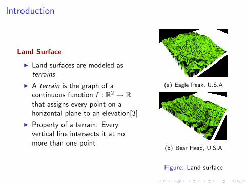
Land Surface

◮ Land surfaces are modeled asterrains

◮ A terrain is the graph of acontinuous function f : R

2 → R

that assigns every point on ahorizontal plane to an elevation[3]

◮ Property of a terrain: Everyvertical line intersects it at nomore than one point

(a) Eagle Peak, U.S.A

(b) Bear Head, U.S.A

Figure: Land surface

Introduction

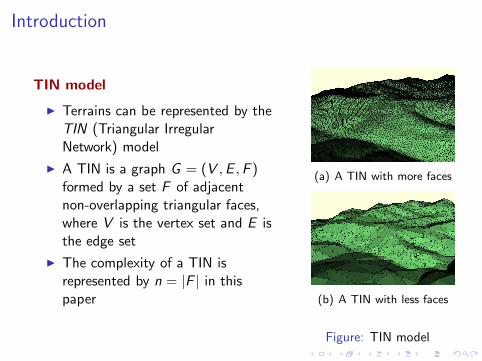
TIN model

◮ Terrains can be represented by theTIN (Triangular IrregularNetwork) model

◮ A TIN is a graph G = (V ,E ,F )formed by a set F of adjacentnon-overlapping triangular faces,where V is the vertex set and E isthe edge set

◮ The complexity of a TIN isrepresented by n = |F | in thispaper

(a) A TIN with more faces

(b) A TIN with less faces

Figure: TIN model

Introduction

Different Types of Shortest Paths

◮ Euclidean shortest path (pe)

◮ Surface shortest path (ps)

◮ As indicated in previouspapers[7], there is|ps | ≥ |pe |

St

peps

s

Figure: Euclidean shortest pathvs. Surface shortest path

Introduction

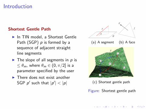
Shortest Gentle Path

◮ In TIN model, a Shortest GentlePath (SGP) p is formed by asequence of adjacent straightline segments

◮ The slope of all segments in p is≤ θm, where θm ∈ (0, π/2] is aparameter specified by the user

◮ There does not exist anotherSGP p′ such that |p′| < |p|

p

Hθ

(a) A segment

~n

f

(b) A face

St

p2

p1

p3

s

(c) Shortest gentle path

Figure: Shortest gentle path

Introduction

Problem Definition

Given a source point s, a destination point t on a terrain surfaceS , maximum slope value θm and approximation factor ǫ. Our goalis to find a path p between s and t such that p satisfies thefollowing two requirements:

◮ Slope requirement: p is a gentle path with maximum slope θm

◮ Distance requirement: |p| ≤ (1 + ǫ)|po |, where po is the SGPbetween s and t

When θm = π/2, there is no slope constraint, so our problemdegenerates to the conventional approximate surface shortest pathproblem

Introduction

Motivation

◮ High complexity

◮ O(n2) complexity[2] if the slopeconstraint is not considered

◮ At least as hard as the surfaceshortest path problem

Applications

◮ Application to the industry◮ Navigation◮ Path planning

◮ Application to the academia◮ Surface k-nearest neighbor

search◮ Natural sciences

Figure: Shahabi et al.,“Indexing land surface forefficient kNN query”,PVLDB ’08[7]

Related Work

Finding Shortest Paths

◮ Exact algorithms

Ref Author Time Technique

[5] Mitchell etal.

O(n2 log n) Continuous Dijk-stra

[2] Chen, Han O(n2) One angle one split

◮ Approximation algorithms

Ref Author Time Technique

[1] Aleksandrovet al.

O( n√ǫlog n

ǫlog 1

ǫ) Steiner point inser-

tion

[8] Xing et al. − Shortest path ora-cle

Related Work

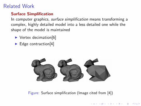
Surface Simplification

In computer graphics, surface simplification means transforming acomplex, highly detailed model into a less detailed one while theshape of the model is maintained

◮ Vertex decimation[6]

◮ Edge contraction[4]

Figure: Surface simplification (Image cited from [4])

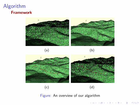
AlgorithmFramework

s

t

S

(a)

S̃

s̃

t̃

(b)

S̃

p̃

s̃

t̃

(c)

s

t

p

S

(d)

Figure: An overview of our algorithm

Algorithm

Path Mapping

◮ Step 1: Shadowing◮ Compute the projective path

of p̃ on S◮ From the property of a

terrain, any path p̃ on S̃ hasexactly one correspondingprojective path p on S

◮ Step 2: Adjusting◮ For each path segment

pi = ab, if its slope is largerthan θm, then we apply thepath finding algorithm A tofind the SGP p̃i between a

and b, and replace pi with p̃i

S̃

S

p̃

p

(a)

f

θ

p′

(b)

f

θ

p p′

(c)

Figure: Path mapping

Algorithm

Distance Bound

Though the slope requirement is satisfied, the distance bound,|p| ≤ (1 + ǫ)|po |, is requiredThe distance error is determined by the difference between S̃ andS , denoted by ∆(S , S̃)

◮ If S̃ is exactly the same as S , that is ∆(S , S̃) = 0, no errorwill be caused, but the computation is slow

◮ If S̃ is over-simplified, S̃ contains much less faces than S , thecomputation is fast, but the error may be too large

Given a TIN terrain S , find a simplified surface S̃ such that

◮ For any pair of po and the mapped path p found by ouralgorithm, |p| ≤ (1 + ǫ)|po |

◮ The number of faces in S̃ is minimized

Algorithm

Distance Bound

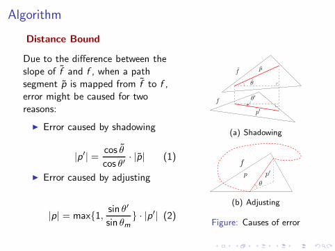
Due to the difference between theslope of f̃ and f , when a pathsegment p̃ is mapped from f̃ to f ,error might be caused for tworeasons:

◮ Error caused by shadowing

|p′| =cos θ̃

cos θ′· |p̃| (1)

◮ Error caused by adjusting

|p| = max{1,sin θ′

sin θm

} · |p′| (2)

f̃

f

p̃

p′

θ̃

θ′

(a) Shadowing

f

θ

p p′

(b) Adjusting

Figure: Causes of error

Algorithm

Distance Bound

We define ∆(S , S̃), the difference between S and S̃ as follows:

∆(S , S̃) = λ × λ′ (3)

◮ λ: the largest possible mapping error from S to S̃

◮ λ’: the largest possible mapping error from S̃ to S

λ and λ′ are extracted from the geometric parameters of S and S̃

Theorem (Distance Bound)

Let po be the SGP between a given pair of points on S and p be

the path found by our algorithm. And let S̃ be the simplified

surface. If ∆(S , S̃) ≤ 1 + ǫ, then |p| ≤ (1 + ǫ)|po |.

AlgorithmSurface Simplifier

Given a terrain surface S , maximum slope θm and approximationratio ǫ, the algorithm Simplifier simplifies S based on a greedyapproach such that Theorem 1 is satisfied:

1: Sort the vertices of S by an error metric[6]2: for all vertices v do

3: Check whether v can be removed according to Theorem 14: if yes then

5: Removed v from S

6: Triangulate the hole left by v ’s removal

remove

(a) (b) (c)

Figure: Triangulation

ExperimentSettings

We did experiments on both real data sets and synthetic data sets.The real data set is available to the public for free at Geo

Community, which was also used by previous research[7, 9, 8]

◮ CPU: 2xQuad Core 3GHz

◮ Memory: 32GB RAM

◮ Language: C++

(a) Eagle Peak (b) Bear Head

Figure: Real data sets

ExperimentIllustration of the Results

(a) Original surface (b) ǫ = 0.1

(c) ǫ = 0.25 (d) ǫ = 0.5

Figure: Result of surface simplification (Eagle Peak where θm = 0.3)

ExperimentEffect of θm

0

2

4

6

8

10

12

14

16

0 0.1 0.2 0.3 0.4 0.5 0.6 0.7 0.8

Prep

roce

ssin

g tim

e (1

03 s)

θm

(a)

0

500

1000

1500

2000

2500

3000

3500

4000

0 0.1 0.3 0.5 0.7 0

100

200

300

400

500

600

700

Num

ber

of f

aces

(10

3 )

Stor

age

(MB

)

θm

No. of faces in orig. sufaceNo. of faces remained

(b)

0

500

1000

1500

2000

2500

3000

3500

4000

0.1 0.2 0.3 0.4 0.5 0.6 0.7

Tim

e fo

r pa

th f

indi

ng (

s)

θm

Time for finding poTime for finding p

Time for finding pc

(c)

20

30

40

50

60

70

80

90

0.1 0.2 0.3 0.4 0.5 0.6 0.7

Path

leng

th (

m)

θm

The length of poThe length of p

The length of pcWorst-case bound

(d)

Figure: Effect of θm (Eagle Peak where ǫ = 0.1)

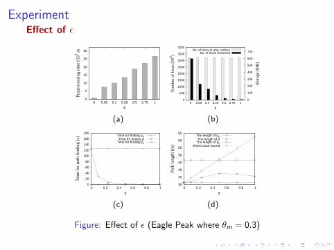
ExperimentEffect of ǫ

0

5

10

15

20

25

30

10.750.50.250.10.050

Prep

roce

ssin

g tim

e (1

03 s)

ε

(a)

0

500

1000

1500

2000

2500

3000

3500

4000

10.750.50.250.10.050 0

100

200

300

400

500

600

700

Num

ber

of f

aces

(10

3 )

Stor

age

(MB

)

ε

No. of faces in orig. surfaceNo. of faces remained

(b)

0

20

40

60

80

100

120

140

160

180

0 0.2 0.4 0.6 0.8 1

Tim

e fo

r pa

th f

indi

ng (

s)

ε

Time for finding poTime for finding p

Time for finding pc

(c)

30

35

40

45

50

55

60

65

0 0.2 0.4 0.6 0.8 1

Path

leng

th (

m)

ε

The length of poThe length of p

The length of pcWorst-case bound

(d)

Figure: Effect of ǫ (Eagle Peak where θm = 0.3)

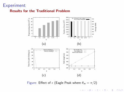
ExperimentResults for the Traditional Problem

0

5

10

15

20

25

30

10.750.50.250.10

Prep

roce

ssin

g tim

e (1

03 s)

ε

(a)

0

500

1000

1500

2000

2500

3000

3500

4000

10.750.50.250.10 0

100

200

300

400

500

600

700

Num

ber

of f

aces

(10

3 )

Stor

age

(MB

)

ε

No. of faces in orig. sufaceNo. of faces remained

(b)

0

20

40

60

80

100

120

0 0.2 0.4 0.6 0.8 1

Tim

e fo

r pa

th f

indi

ng (

s)

ε

Time for finding poTime for finding p

(c)

200

250

300

350

400

450

500

0 0.2 0.4 0.6 0.8 1

Path

leng

th (

m)

ε

The length of poThe length of p

Worst-case bound

(d)

Figure: Effect of ǫ (Eagle Peak where θm = π/2)

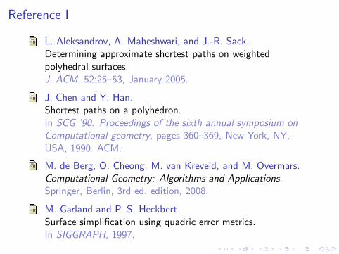
Reference I

L. Aleksandrov, A. Maheshwari, and J.-R. Sack.Determining approximate shortest paths on weightedpolyhedral surfaces.J. ACM, 52:25–53, January 2005.

J. Chen and Y. Han.Shortest paths on a polyhedron.In SCG ’90: Proceedings of the sixth annual symposium on

Computational geometry, pages 360–369, New York, NY,USA, 1990. ACM.

M. de Berg, O. Cheong, M. van Kreveld, and M. Overmars.Computational Geometry: Algorithms and Applications.Springer, Berlin, 3rd ed. edition, 2008.

M. Garland and P. S. Heckbert.Surface simplification using quadric error metrics.In SIGGRAPH, 1997.

Reference II

J. S. B. Mitchell, D. M. Mount, and C. H. Papadimitriou.The discrete geodesic problem.SIAM J. Comput., 16(4):647–668, 1987.

W. J. Schroeder, J. A. Zarge, and W. E. Lorensen.Decimation of triangle meshes.In SIGGRAPH, 1992.

C. Shahabi, L.-A. Tang, and S. Xing.Indexing land surface for efficient knn query.PVLDB, 1(1):1020–1031, 2008.

S. Xing and C. Shahabi.Scalable shortest paths browsing on land surface.In Proceedings of the 18th SIGSPATIAL International

Conference on Advances in Geographic Information Systems,GIS ’10, pages 89–98, New York, NY, USA, 2010. ACM.

Reference III

S. Xing, C. Shahabi, and B. Pan.Continuous monitoring of nearest neighbors on land surface.PVLDB, 2(1):1114–1125, 2009.

Q & A

Frequently Asked Questions

◮ Q1: The details of distance bound?

Q & A I

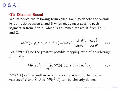
Q1: Distance Bound

We introduce the following term called MRS to denote the overalllength ratio between p and p̃ when mapping a specific pathsegment p̃ from f̃ to f , which is an immediate result from Eq. 1and 2:

MRS(< p, f >,< p̃, f̃ >) = max{1,sin θ′

sin θm

} ·cos θ̃

cos θ′(4)

Let MR(f , f̃ ) be the greatest possible mapping ratio of an arbitraryp̃. That is,

MR(f , f̃ ) = max∀p̃∈f̃

MRS(< p, f >,< p̃, f̃ >) (5)

MR(f , f̃ ) can be written as a function of ~n and ~̃n, the normalvectors of f and f̃ . And MR(f̃ , f ) can be similarly defined

Q & A II

We say that face f overlaps f̃ if there exists a vertical line thatintersects both f and f̃

We then define a face pair set CS(S , S̃) that contains alloverlapping face pairs from S and S̃ as follows:

CS(S , S̃) = {(f , f̃ )|f ∈ F , f̃ ∈ F̃ and f overlaps f̃ } (6)

Let λ be the largest possible MR(f , f̃ ) for all face pairs inCS(S , S̃), so

λ = max(f ,f̃ )∈CS(S,S̃)

MR(f , f̃ ) (7)

And λ′ is similarly defined as

λ′ = max(f ,f̃ )∈CS(S,S̃)

MR(f̃ , f ) (8)