![Link Prediction for Annotation Graphs using Graph ...samir/grant/lppdabw.pdfLink Prediction for Annotation Graphs using Graph Summarization 5 and dense subgraphs [27]. To the best](https://static.fdocuments.us/doc/165x107/5f6908beeca6434d616aa425/link-prediction-for-annotation-graphs-using-graph-samirgrant-link-prediction.jpg)
Finding Dense Subgraphs via Low-Rank Bilinear …users.ece.utexas.edu/~dimakis/DKS_ICML.pdfFinding...
28
Finding Dense Subgraphs via Low-Rank Bilinear Optimization Dimitris S. Papailiopoulos DIMITRIS@UTEXAS. EDU Ioannis Mitliagkas IOANNIS@UTEXAS. EDU Alexandros G. Dimakis DIMAKIS@AUSTIN. UTEXAS. EDU Constantine Caramanis CONSTANTINE@UTEXAS. EDU The University of Texas at Austin Abstract Given a graph, the Densest k-Subgraph (DkS) problem asks for the subgraph on k vertices that contains the largest number of edges. In this work, we develop a new algorithm for DkS that searches a low-dimensional space for provably dense subgraphs. Our algorithm comes with novel performance bounds that depend on the graph spectrum. Our graph-dependent bounds are surprisingly tight for real-world graphs where we find subgraphs with density provably within 70% of the optimum. These guarantees are sig- nificantly tighter than the best available worst case a priori bounds. Our algorithm runs in nearly linear time, un- der spectral assumptions satisfied by most graphs found in applications. Moreover, it is highly scalable and parallelizable. We demonstrate this by implementing it in MapReduce and execut- ing numerous experiments on massive real-world graphs that have up to billions of edges. We em- pirically show that our algorithm can find sub- graphs of significantly higher density compared to the previous state of the art. 1. Introduction Given a graph G on n vertices with m edges and a parame- ter k, we are interested in finding an induced subgraph on k vertices with the largest average degree, also known as the maximum density. This is the Densest k-Subgraph (DkS)– a fundamental problem in combinatorial optimization with applications in numerous fields including social sciences, communication networks, and biology (see e.g. (Hu et al., 2005; Gibson et al., 2005; Dourisboure et al., 2007; Saha et al., 2010; Miller et al., 2010; Bahmani et al., 2012)). DkS is a notoriously hard problem. It is NP-hard by reduc- Proceedings of the 31 st International Conference on Machine Learning, Beijing, China, 2014. JMLR: W&CP volume 32. Copy- right 2014 by the author(s). tion to MAXCLIQUE. Moreover, Khot showed in (Khot, 2004) that, under widely believed complexity-theoretic as- sumptions, DkS cannot be approximated within an arbi- trary constant factor. 1 The best known approximation ratio was n 1/3+✏ (for some small ✏) due to (Feige et al., 2001). Recently, (Bhaskara et al., 2010) introduced an algorithm with approximation ratio n 1/4+✏ , that runs in time n O(1/✏) . Such results, where the approximation factor scales as a polynomial in the number of vertices, are too pessimistic for real-world applications. This resistance to better ap- proximations, despite the long history of the problem, sug- gests that DkS is probably very hard in the worst case. Our Contributions. In this work we move beyond the worst case framework. We present a novel DkS algorithm that has two key features: i) it comes with approximation guarantees that are surprisingly tight on real-world graphs and ii) it is fully parallelizable and can scale up to graphs with billions of edges. Our algorithm combines spectral and combinatorial tech- niques; it relies on examining candidate subgraphs ob- tained from vectors lying in a low-dimensional subspace of the adjacency matrix of the graph. This is accomplished through a framework called the Spannogram, which we de- fine below. Our approximation guarantees are graph-dependent: they are related to the spectrum of the adjacency matrix of the graph. Let opt denote the average degree (i.e., the density) of the densest k-subgraph, where 0 opt k - 1. Our algorithm takes as input the graph, the subgraph size k, and an accuracy parameter d 2 {1,...,n}. The output is a subgraph on k vertices with density opt d , for which we obtain the following approximation result: Theorem 1. For any unweighted graph, our algorithm out- puts in time O ⇣ n d+2 ·log n δ ⌘ a k-subgraph that has density opt d ≥ 0.5 · (1 - δ) · opt - 2 ·|λ d+1 |, with probability 1 - 1 n , where λ i is the ith largest, in mag- 1 approximation ratio ⇢ means that there exists an algorithm that produces in polynomial time a number A, such that 1 opt A ⇢, where opt is the optimal density.
Transcript of Finding Dense Subgraphs via Low-Rank Bilinear …users.ece.utexas.edu/~dimakis/DKS_ICML.pdfFinding...
Finding Dense Subgraphs via Low-Rank Bilinear Optimization
Dimitris S. Papailiopoulos [email protected] Mitliagkas [email protected] G. Dimakis [email protected] Caramanis [email protected]
The University of Texas at Austin
AbstractGiven a graph, the Densest k-Subgraph (DkS)problem asks for the subgraph on k vertices thatcontains the largest number of edges. In thiswork, we develop a new algorithm for DkS thatsearches a low-dimensional space for provablydense subgraphs. Our algorithm comes withnovel performance bounds that depend on thegraph spectrum. Our graph-dependent boundsare surprisingly tight for real-world graphs wherewe find subgraphs with density provably within70% of the optimum. These guarantees are sig-nificantly tighter than the best available worstcase a priori bounds.
Our algorithm runs in nearly linear time, un-der spectral assumptions satisfied by most graphsfound in applications. Moreover, it is highlyscalable and parallelizable. We demonstrate thisby implementing it in MapReduce and execut-ing numerous experiments on massive real-worldgraphs that have up to billions of edges. We em-pirically show that our algorithm can find sub-graphs of significantly higher density comparedto the previous state of the art.
1. IntroductionGiven a graph G on n vertices with m edges and a parame-ter k, we are interested in finding an induced subgraph on kvertices with the largest average degree, also known as themaximum density. This is the Densest k-Subgraph (DkS) –a fundamental problem in combinatorial optimization withapplications in numerous fields including social sciences,communication networks, and biology (see e.g. (Hu et al.,2005; Gibson et al., 2005; Dourisboure et al., 2007; Sahaet al., 2010; Miller et al., 2010; Bahmani et al., 2012)).
DkS is a notoriously hard problem. It is NP-hard by reduc-
Proceedings of the 31 st International Conference on MachineLearning, Beijing, China, 2014. JMLR: W&CP volume 32. Copy-right 2014 by the author(s).
tion to MAXCLIQUE. Moreover, Khot showed in (Khot,2004) that, under widely believed complexity-theoretic as-sumptions, DkS cannot be approximated within an arbi-trary constant factor.1 The best known approximation ratiowas n1/3+✏ (for some small ✏) due to (Feige et al., 2001).Recently, (Bhaskara et al., 2010) introduced an algorithmwith approximation ratio n1/4+✏, that runs in time nO(1/✏).Such results, where the approximation factor scales as apolynomial in the number of vertices, are too pessimisticfor real-world applications. This resistance to better ap-proximations, despite the long history of the problem, sug-gests that DkS is probably very hard in the worst case.
Our Contributions. In this work we move beyond theworst case framework. We present a novel DkS algorithmthat has two key features: i) it comes with approximationguarantees that are surprisingly tight on real-world graphsand ii) it is fully parallelizable and can scale up to graphswith billions of edges.
Our algorithm combines spectral and combinatorial tech-niques; it relies on examining candidate subgraphs ob-tained from vectors lying in a low-dimensional subspaceof the adjacency matrix of the graph. This is accomplishedthrough a framework called the Spannogram, which we de-fine below.
Our approximation guarantees are graph-dependent: theyare related to the spectrum of the adjacency matrix of thegraph. Let opt denote the average degree (i.e., the density)of the densest k-subgraph, where 0 opt k � 1. Ouralgorithm takes as input the graph, the subgraph size k, andan accuracy parameter d 2 {1, . . . , n}. The output is asubgraph on k vertices with density optd, for which weobtain the following approximation result:Theorem 1. For any unweighted graph, our algorithm out-puts in time O
⇣nd+2·logn
�
⌘a k-subgraph that has density
optd � 0.5 · (1� �) · opt� 2 · |�d+1
|,
with probability 1� 1
n , where �i is the ith largest, in mag-
1approximation ratio ⇢ means that there exists an algorithmthat produces in polynomial time a number A, such that 1 opt
A
⇢, where opt is the optimal density.
Finding Dense Subgraphs via Low-Rank Bilinear Optimization
nitude, eigenvalue of the adjacency matrix of the graph.If the graph is bipartite, or if the largest d eigenvaluesof the graph are positive, then our algorithm runs in timeO�nd+1
+ Td
�, and outputs a k-subgraph with density
optd � opt� 2 · |�d+1
|,
where Td is the time to compute the d leading eigenvectorsof the adjacency matrix of the graph.
Our bounds come close to 2+✏ and 1+✏ factor approxima-tions, when �d+1
is significantly smaller than the density ofthe densest k-subgraph. In the following theorem, we givesuch an example. However, we would like to note that inthe worst case our bounds might not yield something mean-ingful.Theorem 2. If the densest-k-subgraph contains a constantfraction of all the edges, and k = ⇥(
pE), then we can
approximate DkS within a factor of 2+ ✏, in time nO(1/✏2).If additionally the graph is bipartite, we can approximateDkS within a factor of 1 + ✏.
The above result is similar to the 1 + ✏ approximation ratioof (Arora et al., 1995) for dense graphs, where the densest-k-subgraph contains a constant fraction of the ⌦(n2
) edges,where k = ⌦(n). The innovation here is that our ratio alsoapplies to sparse graphs with sublinear number of edges.
Computable upper bounds. In addition to these theoret-ical guarantees, our analysis allows us to obtain a graph-dependent upper bound for the optimal subgraph density.This is shown in Fig. 3 in our experimental section, wherefor many graphs our algorithm is provably within 70% fromthe upper bound of opt. These are far stronger guaranteesthan the best available a priori bounds. This illustrates thepotential power of graph-dependent guarantees that, how-ever, require the execution of an algorithm.
Nearly-linear time approximation. Our algorithm has aworst-case running time of O
⇣nd+2·logn
�
⌘. Under some
mild spectral assumptions, a randomized version of our al-gorithm runs in nearly-linear time.Theorem 3. Let the d largest eigenvalues of the graph bepositive, and let the d-th,(d + 1)-st largest have constant
ratio:��� �d�d+1
��� � C. Then, we can modify our algorithmto output, with probability 1 � �, a k-subgraph with den-sity (1� ✏)
2 · optd, in time O�m · log n+
n✏d
· log�
1
✏·���
,where m is the number of edges.
We found that the above spectral condition holds for alld 5, in many real-world graphs that we tested.
Scalability. We develop two key scalability features thatallow us to scale up efficiently on massive graphs.
Vertex sparsification: We introduce a pre-processing stepthat eliminates vertices that are unlikely to be part of
the densest k-subgraph. The elimination is based on thevertices’ weighted leverage scores (Mahoney & Drineas,2009; Boutsidis et al., 2009) and admits a provable boundon the introduced error. We empirically found that evenwith a negligible additional error, the elimination dramati-cally reduced problem sizes in all tested datasets.
MapReduce implementation: We show that our algorithmis fully-parallelizable and tailor it for the MapReduceframework. We use our MapReduce implementation torun experiments on Elastic MapReduce (EMR) on Ama-zon. In our large-scale experiments, we were able to scaleout to thousands of mappers and reducers in parallel over800 cores, and find large dense subgraphs in graphs withbillions of edges.
1.1. Related workDkS algorithms: One of the few positive results for DkS isa 1+ ✏ approximation for dense graphs where m = ⌦(n2
),and in the linear subgraph setting k = ⌦(n) (Arora et al.,1995). For some values of m = o(n2
) a 2 + ✏ approx-imation was established by (Suzuki & Tokuyama, 2005).Moreover, for any k = ⌦(n) a constant factor approx-imation is possible via a greedy approach by (Asahiroet al., 2000), or via semidefinite relaxations by (Srivastav& Wolf, 1998) and (Feige & Langberg, 2001). Recently,(Alon et al., 2013) established new approximation resultsfor graphs with small “✏-rank,” using an approximate solverfor low-rank perturbed versions of the adjacency matrix.
There is a vast literature on algorithms for detect-ing communities and well-connected subgraphs:greedy schemes (Ravi et al., 1994), optimization ap-proaches (Jethava et al., 2012; d’Aspremont et al., 2010;Ames, 2011), and the truncated power method (Yuan& Zhang, 2011). We compare with various of thesealgorithms in our evaluation section.
The Spannogram framework: We present an exact solverfor bilinear optimization problems on matrices of constantrank, under {0, 1} and sparsity constraints on the variables.Our theory is a generalization of the Spannogram frame-work, originally introduced in the foundational work of(Karystinos & Liavas, 2010) and further developed in (As-teris et al., 2014; Papailiopoulos et al., 2013), that obtainsexact solvers for low-rank quadratic optimization problemswith combinatorial constraints, such as sparse PCA.
MapReduce algorithms for graphs: The design of MapRe-duce algorithms for massive graphs is an active researcharea as Hadoop becomes one of the standards for storinglarge data sets. The related work by Bahmani et al. (Bah-mani et al., 2012) designs a novel MapReduce algorithmfor the densest subgraph problem. This densest subgraphproblem requires finding a subgraph of highest normal-ized density without enforcing a specific subgraph size k.
Finding Dense Subgraphs via Low-Rank Bilinear Optimization
Surprisingly, without a subgraph size restriction, the dens-est subgraph becomes polynomially solvable and thereforefundamentally different from what we consider in this pa-per.
2. Proposed AlgorithmThe density of a subgraph indexed by a vertex set S ✓{1, . . . , n} is equal to the average degree of the verticeswithin S:
den(S) = 1TSA1S|S|
where A is the adjacency matrix (Ai,j = 1 if (i, j) is anedge, else Ai,j = 0) and the indicator vector 1S has 1sin the entries indexed by S and 0 otherwise. Observe that1TSA1S =
Pi,j2S Ai,j is twice the number of edges in the
subgraph with vertices in S .
For a fixed subgraph size |S| = k, we can express DkS asa quadratic optimization:
DkS : opt = (
1/k) · max
|S|=k1TSA1S
where |S| = k denotes that the optimization variable is ak-vertex subset of {1, . . . , n}.
The bilinear relaxation of DkS. We approximate DkS viaapproximating its bipartite version. This problem can beexpressed as a bilinear maximization:
DBkS : opt
B= (
1/k) · max
|X |=kmax
|Y|=k1TXA1Y .
As we see in the following lemma, the two problems arefundamentally related: a good solution for the bipartite ver-sion of the problem maps to a “half as good” solution forDkS. The proof is given in the Supplemental Material.
Lemma 1. A ⇢-approximation algorithm for DBkS impliesa 2⇢-approximation algorithm for DkS.
2.1. DkS through low rank approximations
At the core of our approximation lies a constant ranksolver: we show that DBkS can be solved in polynomialtime on constant rank matrices. We solve constant rankinstances of DBkS instead of DkS due to an important im-plication: DkS is NP-hard even for rank-1 matrices with 1
negative eigenvalue, as we show in the Supplemental Ma-terial.
The exact steps of our algorithm are given in the pseudo-code tables referred to as Algorithms 1-3.2 The output ofour algorithm is a k-subgraph Zd that has density optd that
2In the pseudocode of Algorithm 2, topk(v), denotes the in-dices of the k largest signed elements of v.
comes with provable guarantees. We present our theoreti-cal guarantees in the next subsection.
Our main algorithmic innovation, the constant rank solverfor DBkS (Algorithms 2-3), is called many times: in lines5, 8, and 15 of our general DkS approximation, shown asAlgorithm 1. We describe its steps subsequently.
Algorithm 1 low-rank approximations for DkS
1: [Vd,⇤d] = EVD(A, d)2: if G is bipartite then3: B = bi-adjacency of G4: [Vd,⌃d,Ud] = SVD(B, d)5: {Xd,Yd} = argmax|X|+|Y|=k 1
TXVd⌃dU
Td 1Y .
6: Zd = Xd [ Yd
7: else if The first d eigenvalues of A are positive then8: {Xd,Xd} = argmax|X|=|Y|=k 1
TXVd⇤dV
Td 1Y .
9: Zd = Xd
10: else11: for i = 1 :
logn� do
12: draw n fair coins and assign them to vertices13: L = vertices with heads; R = {1, . . . , n}� L14: Bi
d = [Vd⇤dVTd ]L,R
15: {X i,Yi} = argmax|X|+|Y|=k 1TXBi
d1Y .16: end for17: {X i,Yi} = argmax
1in 1TX iB
id1Yi
18: Zd = Xd [ Yd
19: end if20: Output: Zd
Constant rank solver for DBkS. In the following wepresent an exact solver for DBkS on constant rank approxi-mations of A. Our DkS algorithm makes a number of callsto the DBkS low-rank solver on slightly different (sometimes rectangular) matrices. The details of the general low-rank solver are in the Supplemental Material.
Step 1: Obtain Ad =
Pdi=1
�ivivTi , a rank-d approxima-
tion of A. Here, �i is the i-th largest in magnitude eigen-value and vi the corresponding eigenvector.
Step 2: Use Ad to obtain O(nd) candidate subgraphs. For
any matrix A we can solve DBkS by exhaustively checkingall
�nk
�2 pairs (X ,Y) of k-subsets of vertices. Surprisingly,
if we want to find the X ,Y pairs that maximize 1TXAd1Y ,
i.e., the bilinear problem on the rank-d matrix Ad, then weshow that only O(nd
) candidate pairs need to be examined.
Step 3: Check all k-set pairs {X ,Y} obtained by Step 2,and output the one with the largest density on the low-rankweighted adjacency Ad.
In the next section, we derive the constant rank-solver us-ing two key facts. First, for each fixed vertex set Y , weshow that it is easy to find the optimal set X that maximizes1TXAd1Y for that Y . Since this turns out to be easy, then
the challenge is to find the number of different vertex setsY that we need to check. Do we need to exhaustively checkall
�nk
�k-sets Y? We show that this question is equivalent
Finding Dense Subgraphs via Low-Rank Bilinear Optimization
to searching the span of the first d eigenvectors of A, andcollecting in a set Sd the top-k coordinates of all vectorsin that d-dimensional space. By modifying the Spanno-gram theory of (Karystinos & Liavas, 2010; Asteris et al.,2014), we show how this set has size O(nd
) and can beconstructed in time O(nd+1
). This will imply that DBkS
can be solved in time O(nd+1
) on Ad.
Computational Complexity. The worst-case time com-plexity of the constant-rank DBkS solver on Ad is O(Td+
nd+1
), where Td is the time to compute the first d eigenvec-tors of A. Under conditions satisfied by many real worldgraphs, we show that we can modify our algorithm and ob-tain a randomized one that succeeds with probability � andis ✏ far from the optimal rank-d solver, while its complex-ity reduces to nearly linear in the number of edges m of thegraph G: O
�m · log n+
n✏d
· log�
1
✏·���
.
Algorithm 2 lowrankDBkS(k, d, A)1: [Vd,⇤d] = EVD(A, d)2: Sd = Spannogram(k,Vd)
3: {Xd,Yd} = argmax|X|=k maxY2Sd 1TXVd⇤dV
Td 1Y
4: Output: {Xd,Yd}1: Spannogram(k, Vd)
2: Sd = {topk(v) : v 2 span(v1
, . . . ,vd)}3: Output: Sd.
2.2. Approximation Guarantees
We approximate DBkS by finding a solution to the constantrank problem
max
|X |=kmax
|Y|=k1TXAd1Y .
We output a pair of vertex sets, Xd,Yd, which we refer toas the rank-d optimal solution, that has density
opt
Bd = (
1/k) · 1TXd
A1Yd .
Our approximation guarantees measure how far opt
Bd is
from opt
B, the optimal density for DBkS. Our boundscapture a simple core idea: the loss in our approximationcomes due to solving the problem on Ad instead of solvingit on the full rank matrix A. This loss is quantified in thenext lemma. The detailed proofs of the following resultsare in the supplemental material.Lemma 2. For any matrix A: opt
Bd � opt
B � 2 · |�d+1
|,where �i is the ith largest eigenvalue of A.
Using an appropriate pre-processing step and then runningAlgorithm 2 as a subroutine on a sub-sampled and low-rankversion of A, we output a k-subgraph Zd that has densityoptd. By essentially combining Lemmata 1 and 2 we obtainthe following bounds.
Theorem 1. Algorithm 1 outputs in time O⇣
nd+2·logn�
⌘a
k-subgraph that has density
optd = den(Zd) � 0.5 · (1� �) · opt� 2 · |�d+1
|,
with probability 1� 1
n , where �i is the ith largest, in mag-nitude, eigenvalue of the adjacency matrix of the graph.If the graph is bipartite, or if the largest d eigenvalues ofthe graph are positive, then our algorithm runs in timeO�nd+1
+ Td
�, and outputs a k-subgraph with density
optd � opt � 2 · |�d+1
|, where Td is the time to com-pute the d leading eigenvectors of the adjacency matrix ofthe graph.
Using bounds on eigenvalues of graphs, Theorem 1 trans-lates to the following approximation guarantees.
Theorem 2. If the densest-k-subgraph contains a constantfraction of all the edges, and k = ⇥(
pE), then we can
approximate DkS within a factor of 2+ ✏, in time nO(1/✏2).If additionally the graph is bipartite, then we can approxi-mate DkS within a factor of 1 + ✏.
Remark 1. The above results are similar to the 1+ ✏ ratioof (Arora et al., 1995), which holds for graphs where thedensest-k-subgraph contains ⌦(n2
) edges.
Graph dependent bounds. For any given graph, afterrunning our constant rank solver on Ad, we can computean upper bound to the optimal density opt via bounds onopt
B, since it is easy to see that optB � opt. Our graph-dependent bound is the minimum of three upper bounds onthe unknown optimal density:
Lemma 3. The optimal density of DkS can be bounded as
opt min
�(
1/k) · 1TXd
Ad1Yd + |�d+1
|, k � 1, �1
.
In our experimental section, we plot the above upperbounds, and show that for most tested graphs our algorithmperforms provably within 70% from the upper bound on theoptimal density. These are far stronger guarantees than thebest available a priori bounds.
3. The Spannogram FrameworkIn this section, we describe how our constant ranksolver operates by examining candidate vectors in a low-dimensional span of A.
Here, we work on a rank-d matrix Ad = v1
uT1
+ . . . +vduT
d where ui = �ivi, and we wish to solve:
max
|X |=|Y|=k1TX�v1
uT1
+ . . .+ vduTd
�1Y . (1)
Observe that we can rewrite (1) in the following way
max
|X|=|Y|=k1TX
v1
· (uT1
1Y)| {z }c1
+ . . .+ vd · (uTd 1Y)| {z }cd
�
= max
|Y|=k
✓max
|X|=k1TXvY
◆, (2)

Finding Dense Subgraphs via Low-Rank Bilinear Optimization
where vY = v1
· c1
+ . . . + vd · cd is an n-dimensionalvector generated by the d-dimensional subspace spannedby v
1
, . . . ,vd.
We will now make a key observation: for every fixed vectorvY in (2), the index set X that maximizes 1T
XvY can be eas-ily computed. It is not hard to see that for any fixed vectorvY , the k-subset X that maximizes 1T
XvY =
Pi2X [vY ]i
corresponds the set of k largest signed coordinates of vY .That is, the locally optimal k-set is topk(vY).
We now wish to find all possible locally optimal sets X . Ifwe could possibly check all vectors vY , then we could findall locally optimal index sets topk(vY).
Let us denote as Sd the set of all k-subsets X that are theoptimal solutions of the inner maximization of (2) for anyvector v in the span of v
1
, . . . ,vd
Sd = {topk([v1
· c1
+ . . .+ vd · cd]) : c1, . . . , cd 2 R}.
Clearly, this set contains all possible locally optimal X setsof the form topk(vY). Therefore, we can rewrite DBkS onAd as
max
|Y|=kmax
X2Sd
1TXAd1Y . (3)
The above problem can now be solved in the followingway: for every set X 2 Sd find the locally optimal set Ythat maximizes 1T
XAd1Y , that is, this will be topk(Ad1X ).Then, we simply need to test all such X ,Y pairs on Ad andkeep the optimizer.
Due to the above, the problem of solving DBkS on Ad
is equivalent to constructing the set of k-supports Sd, andthen finding the optimal solution in that set. How large canSd be and can we construct it in polynomial time? Ini-tially one could expect that the set Sd could have size asbig as
�nk
�. Instead, we show that the set Sd will be tremen-
dously smaller, as in (Karystinos & Liavas, 2010) and (As-teris et al., 2014).Lemma 4. The set Sd has size at most O(nd
) and can bebuilt in time O(nd+1
) using Algorithm 2.
3.1. Constructing the set Sd
We build up to the general rank-d algorithm by explainingspecial cases that are easier to understand.
Rank-1 case. We start with the d = 1 case, where wehave S
1
= {topk(c1 · v1
) : c1
2 R}. It is not hard to seethat there are only two supports to include in S
1
: topk(v1
)
and topk(�v1
). These two sets can be constructed in timein time O(n), via a partial sorting and selection algorithm(Cormen et al., 2001). Hence, S
1
has size 2 and can beconstructed in time O(n).
Rank-2 case. This is the first non-trivial d which exhibitsthe details of the Spannogram algorithm.
Let an auxiliary angle � 2 � = [0, ⇡) and let
c = [
c1c2 ] =
hsin�cos�
i.3
Then, we re-express c1
· v1
+ c2
· v2
in terms of � as
v(�) = sin� · v1
+ cos� · v2
. (4)
This means that we can rewrite the set S2
as:
S2
= {topk(±(v(�)),� 2 [0,⇡)}.
Observe that each element of v(�) is a continuous spec-tral curve in �: [v(�)]i = [v
1
]i sin(�) + [v2
]i cos(�).
Consequently, the top/bottom-k supports of v(�) (i.e.,topk(±v(�))) are themselves a function of �. How canwe find all possible supports?
0 0.5 1 1.5 2 2.5 3−10
−8
−6
−4
−2
0
2
4
6
8
!
[v(!)]1[v(!)]2[v(!)]3[v(!)]4[v(!)]5
Figure 1. A rank d = 2 spannogram for n = 5 and two randomvectors v
1
,v2
. Observe that every two curves intersect in exactlyone point. These intersection points define intervals in which atop-k set is invariant.
The Spannogram. In Fig. 1, we draw an example plotof five curves [v(�)]i, i = 1, . . . , 5, which we call aspannogram. From the spannogram in Fig. 1, we cansee that the continuity of these sinusoidal curves impliesa “local invariance” property of the top/bottom k supportstopk(±v(�)), in a small neighborhood around a fixed �.So, when does a top/bottom-k support change? The indexsets topk(±v(�)) change if and only if two curves cross,i.e., when the ordering of two elements [v(�)]i,[v(�)]jchanges.
Finding all supports: There are n curves and each pair in-tersects at exactly one point in the � domain4. Therefore,there are exactly
�n2
�intersection points. These
�n2
�inter-
section points define�n2
�+ 1 intervals. Within an interval
the top/bottom k supports topk(±v(�)) remain the same.Hence, it is now clear that |S
2
| 2
�n2
�= O(n2
).
A way to find all supports in S2
is to compute the v(�i,j)
vectors on the intersection points of two curves i, j, and3Observe that when we scan �, the vectors c,�c express all
possible unit norm vectors on the circle.4Here we assume that the curves are in general position. This
can be always accomplished by infinitesimally perturbing thecurves as in (Papailiopoulos et al., 2013).
Finding Dense Subgraphs via Low-Rank Bilinear Optimization
then the supports in the two adjacent intervals of such in-tersection point. The v(�i,j) vector on an intersection pointof two curves i and j can be easily computed by first solv-ing a set of linear equations [v(�i,j)]i = [v(�i,j)]j )(ei � ej)T [v1
v2
]ci,j = 02⇥1
for the unknown vectorci,j , where ei is the i-th column of the n ⇥ n identity ma-trix, i.e., ci,j = nullspace((ei � ej)T [v1
v2
]). Then, wecompute v(�i,j) = [v
1
v2
]ci,j . Further details on break-ing ties in topk(v(�i,j)) can be found in the supplementalmaterial.
Computational cost: We have�n2
�intersection points,
where we calculate the top/bottom k supports for eachv(�i,j). The top/bottom k elements of every v(�i,j) canbe computed in time O(n) using a partial sorting and se-lection algorithm (Cormen et al., 2001). Since we performthis routine a total of O(
�n2
�) times, the total complexity of
our rank-2 algorithm is O(n3
).General Rank-d case. The algorithm generalizes to arbi-trary dimension d, as we show in the supplemental mate-rial; its pseudo-code is given as Algorithm 3.Remark 2. Observe that the computation of each loop un-der line 2 of Algorithm 3 can be computed in parallel. Thiswill allow us to parallelize the Spannogram.
Algorithm 3 Spannogram(k,Vd)1: Sd = ;2: for all (i
1
, . . . , id) 2 {1, . . . , n}d and s 2 {�1, 1} do
3: c = s · nullspace
0
@
2
4[(Vd]i1,:�[Vd]i2,:
...[Vd]i1,:�[Vd]id,:
3
5
1
A
4: v = VTd c
5: S = topk(v)6: T = S � {i
1
, . . . , id}7: for all
�d
k�|T |�
subsets J of (i1
, . . . , id) do8: Sd = Sd
S(T [ J )
9: end for10: end for11: Output: Sd.
3.2. An approximate Sd in nearly-linear time
In our exact solver, we solve DBkS on Ad in timeO(nd+1
). Surprisingly, when Ad has only positive eigen-values, then we can tightly approximate DBkS on Ad innearly linear time.Theorem 3. Let the d largest eigenvalues of the graph bepositive, and let the d-th,(d + 1)-st largest have constant
ratio:��� �d�d+1
��� � C. Then, we can output, with probability
1 � �, a k-subgraph with density (1� ✏)2 · optd, in time
O�m · log n+
n✏d
· log�
1
✏·���
.The main idea is that instead of checking all O(nd
) possi-ble k sets in Sd, we can approximately solve the problemby randomly sampling M = O
�✏�d · log
�1
✏·���
vectorsin the span of v
1
, . . . ,vd. Our proof is based on the factthat we can “approximate” the surface of the d-dimensional
sphere with M randomly sampled vectors from the span ofv1
, . . . ,vd. This allows us to identify, probability 1 � �,near-optimal candidates in Sd. The modified algorithm isvery simple and is given below; its analysis can be found inthe supplemental material.
Algorithm 4 Spannogram approx(k, Vd,⇤d)
1: for i = 1 : O�✏�d · log
�1
✏·���
do2: v = (⇤1/2
d ·Vd)T · randn(d, 1)
3: Sd = Sd [ topk(v) [ topk(�v)4: end for5: Output: Sd.
4. Scaling upIn this section, we present the two key scalability featuresthat allow us to scale up to graphs with billions of edges.
4.1. Vertex SparsificationWe introduce a very simple and efficient pre-processingstep for discarding vertices that are unlikely to appear ina top k set in Sd. This step runs after we compute Ad anduses the leverage score, `i =
Pdj=1
[Vd]2
i,j |�j |, of the i-thvertex to decide whether we will discard it or not. We showin the supplemental material, that by appropriately setting athreshold, we can guarantee a provable bound on the errorintroduced. In our experimental results, the above elimina-tion is able to reduce n to approximately n̂ ⇡ 10 · k fora provably small additive error, even for data sets wheren = 10
8.
4.2. MapReduce ImplementationA MapReduce implementation allows scaling out to a largenumber of compute nodes that can work in parallel. Thereader can refer to (Meng & Mahoney, 2013; Bahmaniet al., 2012)) for a comprehensive treatment of the MapRe-duce paradigm. In short, the Hadoop/MapReduce infras-tructure stores the input graph as a distributed file spreadacross multiple machines; it provides a tuple streaming ab-straction, where each map and reduce function receivesand emits tuples as (key, value) pairs. The role of the keysis to ensure information aggregation: all the tuples with thesame key are processed by the same reducer.
For the spectral decomposition step of our scheme wedesign a simple implementation of the power method inMapReduce. The details are beyond the scope of this work;high-performance implementations are already available inthe literature, e.g. (Lin & Schatz, 2010). We instead focuson the novel implementation of the Spannogram.
Our MapReduce implementation of the rank-2 Spanno-gram is outlined in Algorithm 4. The Mapper is responsiblefor the duplication and dissemination of the eigenvectors,V
2
,U2
= V2
⇤2
, to all reducers. Line 3 emits the j-throw of V
2
and U2
once for every node i. Since i is used asthe key, this ensures that every reducer receives V
2
,U2
in
Finding Dense Subgraphs via Low-Rank Bilinear Optimization
their entirety.
From the breakdown of the Spannogram in Section 3, it isunderstood that, for the rank-2 case, it suffices to solve asimple system of equations for every pair of nodes. TheReducer for node i receives the full eigenvectors V
2
,U2
and is responsible for solving the problem for every pair(i, j), where j > i. Then, Line 6 emits the best candidatecomputed at Reducer i. A trivial final step, not outlinedhere, collects all n2 candidate sets and keeps the best oneas the final solution.
The basic outline in Algorithm 4 comes with heavy com-munication needs and was chosen here for ease of exposi-tion. The more efficient version that we implement, doesnot replicate V
2
,U2
n times. Instead, the number of re-ducers – say R = n↵ – is fine-tuned to the capabilities ofthe cluster. The mappers emit V
2
,U2
R times, once forevery reducer. Then, reducer r is responsible for solvingfor node pairs (i, j), where i ⌘ r (mod R) and j > i. De-pending on the performance bottleneck, different choicesfor ↵ are more appropriate. We divide the construction ofthe O(n2
) candidate sets in S2
to O(n↵) reducers and each
of them computes O(n2�↵) candidate subgraphs. The to-
tal communication cost for this parallelization scheme isO(n1+↵
): n↵ reducers need to have access to the entireV
2
,U2
that has 2 · 2 · n entries. Moreover, the total com-putation cost for each reducer is O(n3�↵
).
Algorithm 5 SpannogramMR(V2
,U2
)1: Map({[V
2
]j,:, [U2
]j,:, j}):2: for i = 1 : n do3: emit: hi, {[V
2
]j,1, [V2
]j,2, [U2
]j,1, [U2
]j,2, j}i4: end for1: Reducei(hi, {[V2
]j,1, [V2
]j,2, [U2
]j,1, [U2
]j,2, j}i , 8j):2: for each j � i+ 1 do3: c = nullspace([V]i,: � [V]j,:)
4: [denj , {Xj ,Yj}] = max
|Y|=k,X2topk(±V2c)1XV
2
UT2
1Y
5: end for6: emit:
⌦i, {Xi,Yi} = maxj 1XjV2
UT2
1Yj
↵
5. Experimental EvaluationWe experimentally evaluate the performance of our al-gorithm and compare it to the truncated power method(TPower) of (Yuan & Zhang, 2011), a greedy algorithm by(Feige et al., 2001) (GFeige) and another greedy algorithmby (Ravi et al., 1994) (GRavi). We performed experimentson synthetic dense subgraphs and also massive real graphsfrom multiple sources. In all experiments we compare thedensity of the subgraph obtained by the Spannogram to thedensity of the output subgraphs given by the other algo-rithms.
Our experiments illustrate three key points: (1) for alltested graphs, our method outperforms – some times signif-icantly – all other algorithms compared; (2) our method is
104 106 108 10100
200
400
600
800
1000G
!
n, 12 , k = 3
!n"
Subgra
phden
sity
|E |
G-FeigeG-RaviTPowerSpannogram
(a) Densities of the recoveredsubgraph v.s. the expectednumber of edges.
0 100 200 300 400 500 600
240
400
800
Total time in minutes
Number
ofco
res
Running times on 2.5 Billion Edges
Power methodSpannogram
(b) Running times of theSpannogram and power itera-tion for two top eigenvectors.
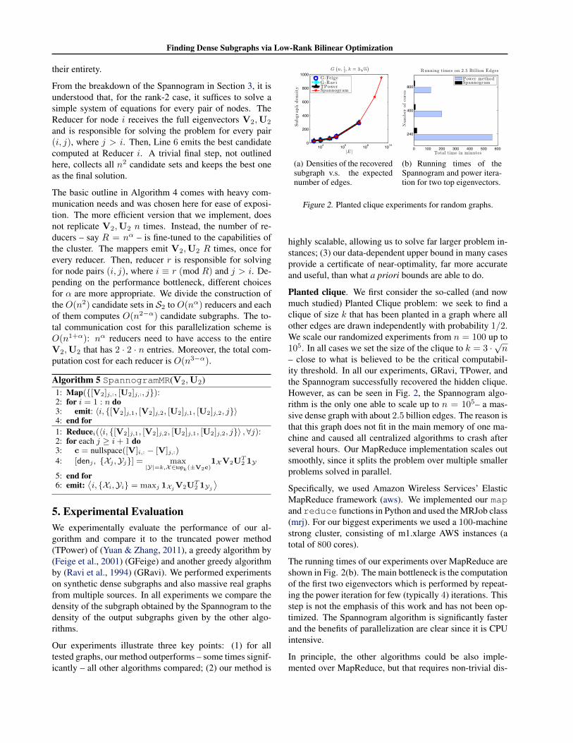
Figure 2. Planted clique experiments for random graphs.
highly scalable, allowing us to solve far larger problem in-stances; (3) our data-dependent upper bound in many casesprovide a certificate of near-optimality, far more accurateand useful, than what a priori bounds are able to do.
Planted clique. We first consider the so-called (and nowmuch studied) Planted Clique problem: we seek to find aclique of size k that has been planted in a graph where allother edges are drawn independently with probability 1/2.We scale our randomized experiments from n = 100 up to10
5. In all cases we set the size of the clique to k = 3 ·pn
– close to what is believed to be the critical computabil-ity threshold. In all our experiments, GRavi, TPower, andthe Spannogram successfully recovered the hidden clique.However, as can be seen in Fig. 2, the Spannogram algo-rithm is the only one able to scale up to n = 10
5– a mas-sive dense graph with about 2.5 billion edges. The reason isthat this graph does not fit in the main memory of one ma-chine and caused all centralized algorithms to crash afterseveral hours. Our MapReduce implementation scales outsmoothly, since it splits the problem over multiple smallerproblems solved in parallel.
Specifically, we used Amazon Wireless Services’ ElasticMapReduce framework (aws). We implemented our mapand reduce functions in Python and used the MRJob class(mrj). For our biggest experiments we used a 100-machinestrong cluster, consisting of m1.xlarge AWS instances (atotal of 800 cores).
The running times of our experiments over MapReduce areshown in Fig. 2(b). The main bottleneck is the computationof the first two eigenvectors which is performed by repeat-ing the power iteration for few (typically 4) iterations. Thisstep is not the emphasis of this work and has not been op-timized. The Spannogram algorithm is significantly fasterand the benefits of parallelization are clear since it is CPUintensive.
In principle, the other algorithms could be also imple-mented over MapReduce, but that requires non-trivial dis-

Finding Dense Subgraphs via Low-Rank Bilinear Optimization
Figure 3. Subgraph density vs. subgraph size (k). We compare our DkS Spannogram algorithm with the algorithms from (Feige et al.,2001) (GFeige), (Ravi et al., 1994) (GRavi), and (Yuan & Zhang, 2011) (tPM). Across all subgraph sizes k, we obtain higher subgraphdensities using Spannograms of rank d = 2 or 5. We also obtain a provable data-dependent upper bound (solid black line) on theobjective. This proves that for these data sets, our algorithm is typically within 80% from optimality, for all sizes up to k = 250, andindeed for small subgraph sizes we find a clique which is clearly optimal. Further experiments on multiple other data sets are shown inthe supplemental material.
tributed algorithm design. As is well-known, e.g., (Meng& Mahoney, 2013), implementing iterative machine learn-ing algorithms over MapReduce can be a significant taskand schemes which perform worse in standard metrics canbe highly preferable for this parallel framework. Care-ful MapReduce algorithmic design is needed especially fordense graphs like the one in the hidden clique problem.
Real Datasets. Next, we demonstrate our method’s per-formance in real datasets and also illustrate the power ofour data-dependent bounds. We run experiments on largegraphs from different applications and our findings are pre-sented in Fig. 3. The figure compares the density achievedby the Spannogram algorithm for rank 1, 2 and 5 to theperformance of GFeige, GRavi and TPower. The figureshows that the rank-2 and rank-5 versions of our algorithm,improve – sometimes significantly – over the other tech-niques. Our novel data-dependent upper-bound shows thatour results on these data sets are provably near-optimal.
The experiments are performed for two community graphs(com-LiveJournal and com-DBLP), a web graph (web-NotreDame), and a subset of the Facebook graph. A largerset of experiments is included in the supplemental material.
Note that the largest graph in Figure 3 contains no morethan 35 million edges; these cases fit in the main memoryof a single machine and the running times are presentedin the supplemental material, all performed on a standardMacbook Pro laptop using Matlab. In summary, rank-2took less than one second for all these graphs while priorwork methods took approximately the same time, up to afew seconds. Rank-1 was significantly faster than all othermethods in all tested graphs and took fractions of a sec-ond. Rank-5 took up to 1000 seconds for the largest graph(LiveJournal).
We conclude that our algorithm is an efficient option forfinding dense subgraphs. Different rank choices give atradeoff between accuracy and performance while the par-allel nature allows scalability when needed. Further, ourtheoretical upper-bound can be useful for practitioners in-vestigating dense structures in large graphs.
6. AcknowledgmentsThe authors would like to acknowledge support from NSFgrants CCF 1344364, CCF 1344179, DARPA XDATA, andresearch gifts by Google, Docomo and Microsoft.

Finding Dense Subgraphs via Low-Rank Bilinear Optimization
ReferencesAmazon Web Services, Elastic Map Reduce. URL http://
aws.amazon.com/elasticmapreduce/.
MRJob. URL http://pythonhosted.org/mrjob/.
Alon, Noga, Lee, Troy, Shraibman, Adi, and Vempala, Santosh.The approximate rank of a matrix and its algorithmic applica-tions: approximate rank. In Proceedings of the 45th annualACM symposium on Symposium on theory of computing, pp.675–684. ACM, 2013.
Ames, Brendan PW. Convex relaxation for the planted clique,biclique, and clustering problems. PhD thesis, University ofWaterloo, 2011.
Arora, Sanjeev, Karger, David, and Karpinski, Marek. Polyno-mial time approximation schemes for dense instances of np-hard problems. In STOC, 1995.
Asahiro, Yuichi, Iwama, Kazuo, Tamaki, Hisao, and Tokuyama,Takeshi. Greedily finding a dense subgraph. Journal of Algo-rithms, 34(2):203–221, 2000.
Asteris, Megasthenis, Papailiopoulos, Dimitris S, and Karystinos,George N. The sparse principal component of a constant-rankmatrix. IEEE Trans. IT, 60(4):228–2290, 2014.
Bahmani, Bahman, Kumar, Ravi, and Vassilvitskii, Sergei. Dens-est subgraph in streaming and mapreduce. Proceedings of theVLDB Endowment, 5(5):454–465, 2012.
Bhaskara, Aditya, Charikar, Moses, Chlamtac, Eden, Feige, Uriel,and Vijayaraghavan, Aravindan. Detecting high log-densities:an O(n1/4
) approximation for densest k-subgraph. In STOC,2010.
Boutsidis, Christos, Mahoney, Michael W, and Drineas, Petros.An improved approximation algorithm for the column subsetselection problem. In Proceedings of the twentieth AnnualACM-SIAM Symposium on Discrete Algorithms, pp. 968–977.Society for Industrial and Applied Mathematics, 2009.
Cormen, Thomas H, Leiserson, Charles E, Rivest, Ronald L, andStein, Clifford. Introduction to algorithms. MIT press, 2001.
d’Aspremont, Alexandre et al. Weak recovery conditions usinggraph partitioning bounds. 2010.
Dourisboure, Yon, Geraci, Filippo, and Pellegrini, Marco. Ex-traction and classification of dense communities in the web. InWWW, 2007.
Feige, Uriel and Langberg, Michael. Approximation algorithmsfor maximization problems arising in graph partitioning. Jour-nal of Algorithms, 41(2):174–211, 2001.
Feige, Uriel, Peleg, David, and Kortsarz, Guy. The dense k-subgraph problem. Algorithmica, 29(3):410–421, 2001.
Gibson, David, Kumar, Ravi, and Tomkins, Andrew. Discoveringlarge dense subgraphs in massive graphs. In PVLDB, 2005.
Hu, Haiyan, Yan, Xifeng, Huang, Yu, Han, Jiawei, and Zhou,Xianghong Jasmine. Mining coherent dense subgraphs acrossmassive biological networks for functional discovery. Bioin-formatics, 21(suppl 1):i213–i221, 2005.
Jethava, Vinay, Martinsson, Anders, Bhattacharyya, Chiranjib,and Dubhashi, Devdatt. The lovasz theta function, svms andfinding large dense subgraphs. In NIPS, 2012.
Karystinos, George N and Liavas, Athanasios P. Efficient com-putation of the binary vector that maximizes a rank-deficientquadratic form. IEEE Trans. IT, 56(7):3581–3593, 2010.
Khot, Subhash. Ruling out ptas for graph min-bisection, densestsubgraph and bipartite clique. In FOCS, 2004.
Lin, Jimmy and Schatz, Michael. Design patterns for efficientgraph algorithms in mapreduce. In Proceedings of the EighthWorkshop on Mining and Learning with Graphs, pp. 78–85.ACM, 2010.
Mahoney, Michael W and Drineas, Petros. Cur matrix decompo-sitions for improved data analysis. Proceedings of the NationalAcademy of Sciences, 106(3):697–702, 2009.
Meng, Xiangrui and Mahoney, Michael. Robust regression onmapreduce. In Proceedings of The 30th International Confer-ence on Machine Learning, pp. 888–896, 2013.
Miller, B, Bliss, N, and Wolfe, P. Subgraph detection using eigen-vector l1 norms. In NIPS, 2010.
Papailiopoulos, Dimitris, Dimakis, Alexandros, and Ko-rokythakis, Stavros. Sparse pca through low-rank approxima-tions. In Proceedings of the 30th International Conference onMachine Learning (ICML-13), pp. 747–755, 2013.
Ravi, Sekharipuram S, Rosenkrantz, Daniel J, and Tayi, Giri K.Heuristic and special case algorithms for dispersion problems.Operations Research, 42(2):299–310, 1994.
Saha, Barna, Hoch, Allison, Khuller, Samir, Raschid, Louiqa, andZhang, Xiao-Ning. Dense subgraphs with restrictions and ap-plications to gene annotation graphs. In Research in Computa-tional Molecular Biology, pp. 456–472. Springer, 2010.
Srivastav, Anand and Wolf, Katja. Finding dense subgraphs withsemidefinite programming. Springer, 1998.
Suzuki, Akiko and Tokuyama, Takeshi. Dense subgraph problemswith output-density conditions. In Algorithms and Computa-tion, pp. 266–276. Springer, 2005.
Yuan, Xiao-Tong and Zhang, Tong. Truncated power method forsparse eigenvalue problems. arXiv preprint arXiv:1112.2679,2011.
Supplemental Material for:Finding Dense Subgraphs via Low-Rank Bilinear Optimization
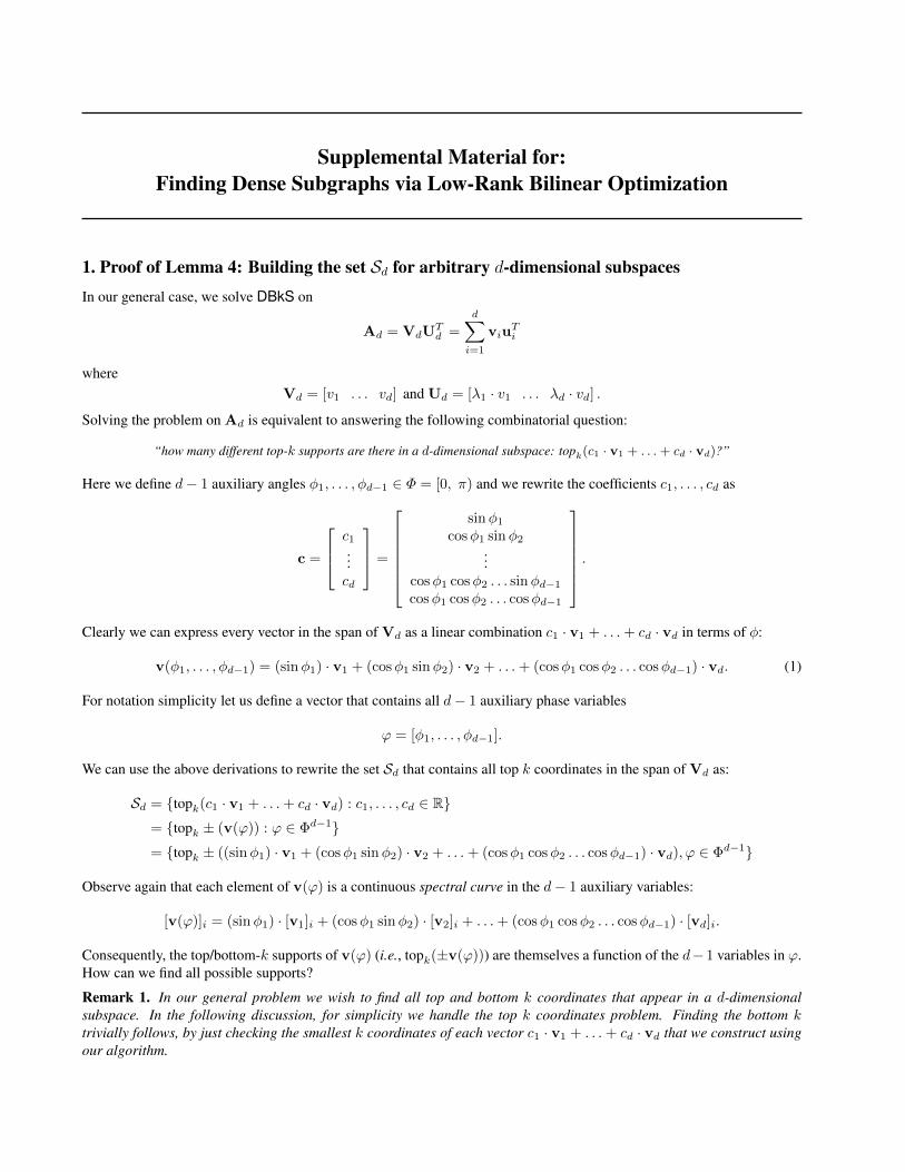
1. Proof of Lemma 4: Building the set Sd for arbitrary d-dimensional subspacesIn our general case, we solve DBkS on
Ad = VdUTd =
dX
i=1
viuTi
whereVd = [v
1
. . . vd] and Ud = [�1
· v1
. . . �d · vd] .
Solving the problem on Ad is equivalent to answering the following combinatorial question:
“how many different top-k supports are there in a d-dimensional subspace: topk(c1 · v1 + . . .+ cd · vd)?”
Here we define d� 1 auxiliary angles �1
, . . . ,�d�1
2 � = [0, ⇡) and we rewrite the coefficients c1
, . . . , cd as
c =
2
6
4
c1
...cd
3
7
5
=
2
6
6
6
6
6
4
sin�1
cos�1
sin�2
...cos�
1
cos�2
. . . sin�d�1
cos�1
cos�2
. . . cos�d�1
3
7
7
7
7
7
5
.
Clearly we can express every vector in the span of Vd as a linear combination c1
· v1
+ . . .+ cd · vd in terms of �:
v(�1
, . . . ,�d�1
) = (sin�1
) · v1
+ (cos�1
sin�2
) · v2
+ . . .+ (cos�1
cos�2
. . . cos�d�1
) · vd. (1)
For notation simplicity let us define a vector that contains all d� 1 auxiliary phase variables
' = [�1
, . . . ,�d�1
].
We can use the above derivations to rewrite the set Sd that contains all top k coordinates in the span of Vd as:
Sd = {topk(c1 · v1
+ . . .+ cd · vd) : c1, . . . , cd 2 R}= {topk ± (v(')) : ' 2 �
d�1}= {topk ± ((sin�
1
) · v1
+ (cos�1
sin�2
) · v2
+ . . .+ (cos�1
cos�2
. . . cos�d�1
) · vd),' 2 �
d�1}
Observe again that each element of v(') is a continuous spectral curve in the d� 1 auxiliary variables:
[v(')]i = (sin�1
) · [v1
]i + (cos�1
sin�2
) · [v2
]i + . . .+ (cos�1
cos�2
. . . cos�d�1
) · [vd]i.
Consequently, the top/bottom-k supports of v(') (i.e., topk(±v('))) are themselves a function of the d� 1 variables in '.How can we find all possible supports?
Remark 1. In our general problem we wish to find all top and bottom k coordinates that appear in a d-dimensional
subspace. In the following discussion, for simplicity we handle the top k coordinates problem. Finding the bottom ktrivially follows, by just checking the smallest k coordinates of each vector c
1
· v1
+ . . .+ cd · vd that we construct using
our algorithm.
Title Suppressed Due to Excessive Size
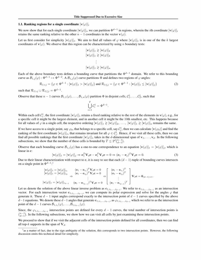
1.1. Ranking regions for a single coordinate [v(')]i
We now show that for each single coordinate [v(')]i, we can partition �
d�1 in regions, wherein the ith coordinate [v(')]iretains the same ranking relative to the other n� 1 coordinates in the vector v(').
Let us first consider for simplicity [v(')]1
. We aim to find all values of ' where [v(')]1
is in one of the the k largestcoordinates of v('). We observe that this region can be characterized by using n boundary tests:
[v(')]1
? [v(')]2
[v(')]1
? [v(')]3
...[v(')]
1
? [v(')]n
Each of the above boundary tests defines a bounding curve that partitions the �
d�1 domain. We refer to this boundingcurve as B
1,j(') : �d�1 7! �
d�2. A B1,j(') curve partitions � and defines two regions of ' angles:
R1>j = {' 2 �
d�1
: [v(')]1
> [v(')]j} and R1j = {' 2 �
d�1
: [v(')]1
[v(')]j} (2)
such that R1>j [R
1j = �
d�1.
Observe that these n� 1 curves B1,1('), . . . ,B1,n(') partition � in disjoint cells, C1
1
, . . . , C1
T , such that
T[
i=1
C1
i = �
d�1.
Within each cell C1
i , the first coordinate [v(')]1
retains a fixed ranking relative to the rest of the elements in v('), e.g., fora specific cell it might be the largest element, and in another cell it might be the 10th smallest, etc. This happens becausefor all values of ' in a single cell, the respective ordering [v(')]
1
? [v(')]2
, . . . , [v(')]1
? [v(')]n remains the same.
If we have access to a single point, say '0
, that belongs to a specific cell, say C1
j , then we can calculate [v('0
)] and find theranking of the first coordinate [v(')]
1
, that remains invariant for all ' 2 C1
j . Hence, if we visit all these cells, then we canfind all possible rankings that the first coordinate [v(')]
1
takes in the d-dimensional span of v1
, . . . ,vd. In the followingsubsections, we show that the number of these cells is bounded by T 2
d�
n�1
d�1
�
.
Observe that each bounding curve B1,i(') has a one-to-one correspondence to an equation [v(')]
1
= [v(')]j , which islinear in c:
[v(')]1
= [v(')]j ) eT1
Vdc� eTi Vdc = 0 ) (e1
� ej)TVdc = 0. (3)
Due to their linear characterization with respect to c, it is easy to see that each (d� 1)-tuple of bounding curves intersectson a single point in �
d�1:1
[v(')]1 = [v(')]i1[v(')]1 = [v(')]i2
...[v(')]1 = [v(')]id�1
)
(e1 � ei1)TVdc = 0
(e1 � ei2)TVdc = 0
...(e1 � eid�1)
TVdc = 0
)
2
6664
(e1 � ei1)T
(e1 � ei2)T
...(e1 � eid�1)
T
3
7775Vdc = 0(d�1)⇥1.
Let us denote the solution of the above linear inverse problem as c1,i1,...,id�1 . We refer to c
1,i1,...,id�1 as an intersectionvector. For each intersection vector c
1,i1,...,id�1 , we can compute its polar expression and solve for the angles ' thatgenerate it. These d � 1 input angles correspond exactly to the intersection point of d � 1 curves specified by the aboved�1 equations. We denote these d�1 angles that generate c
1,i1,...,id�1 , as '1,i1,...,id�1 which we refer to as the intersection
point of the d� 1 curves B1,i1('), . . . ,B1,id�1(').
Since, the '1,i1,...,id�1 intersection points are defined for every d � 1 curves, the total number of intersection points is
�
n�1
d�1
�
. In the following subsections, we show how we can visit all cells by just examining these intersection points.
We proceed to show that if we visit the adjacent cells of the intersection points defined for all coordinates, then we can findall top-k supports in the span of Vd.
1as a matter of fact, due to the sign ambiguity of the solution, this corresponds to two intersection points. However, the followingdiscussion omits this technical detail for simplicity.

Title Suppressed Due to Excessive Size
1.2. Visiting all cells = finding all top k supports
Our goal is to find all top-k supports that can appear in the span of Vd. To do so, it is sufficient to visit the cells where[v(')]
1
is the k-th largest coordinate, then the cells where [v(')]2
is the k-largest, and so on. Within such cells, onecoordinate (say [v(')]i) remains always the k-th largest, while the identities of the bottom n � k coordinates remain thesame. This means that in such a cell, we have that
[v(')]i � [v(')]j1 , . . . , [v(')]i � [v(')]jn�k
for all ' in that cell and some scecific n� k other coordinates indexed by j1
, . . . , jn�k. Hence, although the sorting of thetop k�1 elements might change in that cell (i.e., the first might become the second largest, and vice versa), the coordinatesthat participate in the top k � 1 support will be the same, while at the same time the k-th largest will be [v(')]i.
Hence, for each coordinate [v(')]i, we need to visit the cells wherein it is the k-th largest. We do this by examining all cellswherein [v(')]i retains a fixed ranking. Visiting all these cells (T for each coordinate), is possible by visiting all n ·
�
n�1
d�1
�
intersection points of Bi,j(') curves as defined earlier. Since we know that each cell is adjacent to at least 1 intersectionpoint, then at each of these points we visit all adjacent cells. For each cell that we visit, we compute the support of thelargest k coordinates of a vector v('
0
) with a '0
that lies in that cell. We include this top k index set in Sd and carry thesame procedure for all cells. Since we visit all coordinates and all their adjacent cells, this means that we visit all cells Ci
j .This means that this procedure will construct all possible supports in
Sd = {topk(c1 · v1
+ . . .+ cd · vd) : c1, . . . , cd 2 R}
1.3. Constructing the set Sd
To visit all possible cells Cij , we now have to check the intersection points, which are obtained by solving the system of
d� 1 equations
[v(')]i1 = [v(')]i2 = . . . = [v(')]id,[v(')]i1 = [v(')]i2 , . . . , [v(')]i1 = [v(')]id . (4)
We can rewrite the above as2
6
4
eTi1 � eTi2...
eTi1 � eTid
3
7
5
Vdc = 0(d�1)⇥1
(5)
where the solution is the nullspace of the matrix, which has dimension 1.
To explore all possible candidate vectors, we need to visit all cells. To do so, we compute all possible�
nd
�
solutionintersection vectors ci1,...,id . On each intersection vector we need to compute the locally optimal support set
topk (Vdci1,...,id) .
Then observe that the coordinates i1
, . . . , id of Vdci1,...,id have the same value, since they all satisfy equation (5). Letus assume that t of them appear in the set topk (Vdci1,...,id). The, finding the top k supports of all neighboring cell isequivalent to checking all different supports that can be generated by taking all
�
dt
�
possible t-subsets of the i1
, . . . , idcoordinates with respect to Vdci1,...,id , while keeping the rest of the elements in Vdci1,...,id in their original ranking, ascomputed in topk (Vdci1,...,id) . This, induces at most O(
�
dd/2
�
) local sortings, i.e., top k supports. All these sortings willeventually be the elements of the Sd set. The number of all candidate support sets will now be O(
�
dd/2
��
n�1
d
�
) = O(nd)
and the total computation complexity is O�
nd+1
�
, since for each point we compute the top-k support in linear time O(n).
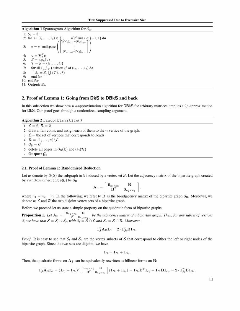
For completeness the algorithm of the spannogram framework that generates Sd is given below.
1.4. Resolution of singularities
In our proofs, we assumed that the curves in v(�) are in general position. This is needed so that no more than d� 1 curvesintersect at a single point. This assumption is equivalent to requiring that every d ⇥ d submatrix of Vd is full rank. This“general position” requirement can be handled by introducing infinitesimal perturbations in Vd. The details of the analysisof this method can be found in (Papailiopoulos et al., 2013).
Title Suppressed Due to Excessive Size
Algorithm 1 Spannogram Algorithm for Sd.1: Sd = ;2: for all (i1, . . . , id) 2 {1, . . . , n}d and s 2 {�1, 1} do
3: c = s · nullspace
0
@
2
4[(Vd]i1,:�[Vd]i2,:
...[Vd]i1,:�[Vd]id,:
3
5
1
A
4: v = VTd c
5: S = topk(v)6: T = S � {i1, . . . , id}7: for all
�d
k�|T |�
subsets J of (i1, . . . , id) do8: Sd = Sd
S(T [ J )
9: end for10: end for11: Output: Sd.
2. Proof of Lemma 1: Going from DkS to DBkS and backIn this subsection we show how a ⇢-approximation algorithm for DBkS for arbitrary matrices, implies a 2⇢-approximationfor DkS. Our proof goes through a randomized sampling argument.
Algorithm 2 randombipartite(G)1: L = ;, R = ;2: draw n fair coins, and assign each of them to the n vertice of the graph.3: L = the set of vertices that corresponds to heads4: R = {1, . . . , n}\L5: G
B
= G6: delete all edges in G
B
(L) and GB
(R)
7: Output: GB
2.1. Proof of Lemma 1: Randomized Reduction
Let us denote by G(S) the subgraph in G induced by a vertex set S . Let the adjacency matrix of the bipartite graph createdby randombipartite(G) be G
B
AB
=
0n1⇥n2 BBT 0n2⇥n1
�
,
where n1
+ n2
= n. In the following, we refer to B as the bi-adjacency matrix of the bipartite graph GB
. Moreover, wedenote as L and R the two disjoint vertex sets of a bipartite graph.
Before we proceed let us state a simple property on the quadratic form of bipartite graphs.
Proposition 1. Let AB
=
h
0n1⇥n2 B
BT 0n2⇥n1
i
be the adjacency matrix of a bipartite graph. Then, for any subset of vertices
S , we have that S = Sl [ Sr, with Sl = S \ L and Sr = S \R. Moreover,
1TSAB
1S = 2 · 1TSlB1Sr .
Proof. It is easy to see that Sl and Sr are the vertex subsets of S that correspond to either the left or right nodes of thebipartite graph. Since the two sets are disjoint, we have
1S = 1Sl + 1Sr .
Then, the quadratic forms on AB
can be equivalently rewritten as bilinear forms on B:
1TSAB
1S = (1Sl + 1Sr )Th
0n1⇥n2 B
BT 0n2⇥n1
i
(1Sl + 1Sr ) = 1SrBT1Sl + 1SlB1Sr = 2 · 1T
SlB1Sr .
Title Suppressed Due to Excessive Size
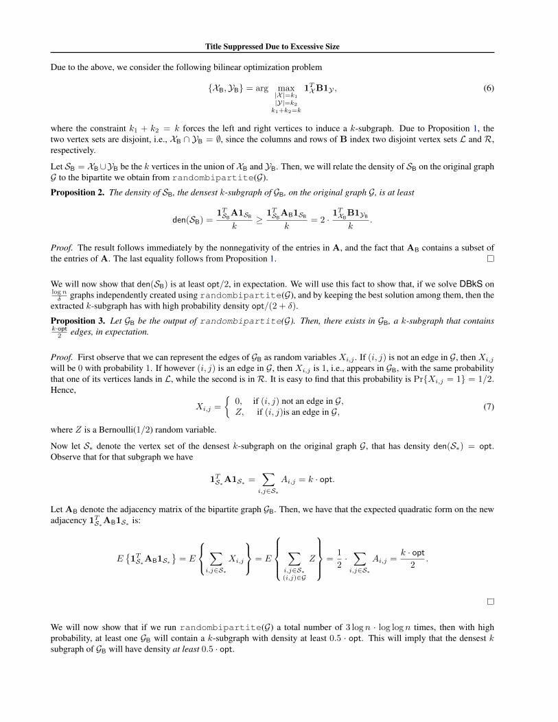
Due to the above, we consider the following bilinear optimization problem
{XB
,YB
} = arg max
|X |=k1
|Y|=k2
k1+k2=k
1TXB1Y , (6)
where the constraint k1
+ k2
= k forces the left and right vertices to induce a k-subgraph. Due to Proposition 1, thetwo vertex sets are disjoint, i.e., X
B
\ YB
= ;, since the columns and rows of B index two disjoint vertex sets L and R,respectively.
Let SB
= XB
[YB
be the k vertices in the union of XB
and YB
. Then, we will relate the density of SB
on the original graphG to the bipartite we obtain from randombipartite(G).
Proposition 2. The density of SB
, the densest k-subgraph of GB
, on the original graph G, is at least
den(SB
) =
1TSB
A1SB
k�
1TSB
AB
1SB
k= 2 ·
1TX
B
B1YB
k.
Proof. The result follows immediately by the nonnegativity of the entries in A, and the fact that AB
contains a subset ofthe entries of A. The last equality follows from Proposition 1.
We will now show that den(SB
) is at least opt/2, in expectation. We will use this fact to show that, if we solve DBkS onlogn� graphs independently created using randombipartite(G), and by keeping the best solution among them, then the
extracted k-subgraph has with high probability density opt/(2 + �).
Proposition 3. Let GB
be the output of randombipartite(G). Then, there exists in GB
, a k-subgraph that contains
k·opt2
edges, in expectation.
Proof. First observe that we can represent the edges of GB
as random variables Xi,j . If (i, j) is not an edge in G, then Xi,j
will be 0 with probability 1. If however (i, j) is an edge in G, then Xi,j is 1, i.e., appears in GB
, with the same probabilitythat one of its vertices lands in L, while the second is in R. It is easy to find that this probability is Pr{Xi,j = 1} = 1/2.Hence,
Xi,j =
⇢
0, if (i, j) not an edge in G,Z, if (i, j)is an edge in G, (7)
where Z is a Bernoulli(1/2) random variable.
Now let S⇤ denote the vertex set of the densest k-subgraph on the original graph G, that has density den(S⇤) = opt.Observe that for that subgraph we have
1TS⇤A1S⇤ =
X
i,j2S⇤
Ai,j = k · opt.
Let AB
denote the adjacency matrix of the bipartite graph GB
. Then, we have that the expected quadratic form on the newadjacency 1T
S⇤A
B
1S⇤ is:
E�
1TS⇤AB
1S⇤
= E
8
<
:
X
i,j2S⇤
Xi,j
9
=
;
= E
8
>
>
<
>
>
:
X
i,j2S⇤(i,j)2G
Z
9
>
>
=
>
>
;
=
1
2
·X
i,j2S⇤
Ai,j =k · opt
2
.
We will now show that if we run randombipartite(G) a total number of 3 log n · log log n times, then with highprobability, at least one G
B
will contain a k-subgraph with density at least 0.5 · opt. This will imply that the densest ksubgraph of G
B
will have density at least 0.5 · opt.
Title Suppressed Due to Excessive Size
Algorithm 3 DkS 2 approx(G, �)1: for i = 1 :
logn� do
2: GB
i= randombipartite(G)
3: Bi= biadjacency of G
B
i
4: {X i,Yi} = argmax|X |=k1,|Y|=k2,k1+k2=k 1TXBi1Y
5: end for6: {X
B
,YB
} = argmaxi 1TX i[YiA1X i[Yi
7: Output: SB
= XB
[ YB
Proposition 4. Then, with probability at least 1� 1
n , we have
1TSB
A1SB
� 1� �
2
· opt.
Proof. In this proof we will use the reverse Markov Inequality which states that for any random variable X , such thatX m, then, for any a E{X}, we have
Pr{X a} m� E{X}m� a
.
Let S⇤ denote the densest k-subgraph for G. Here, our random variable will be the the quadratic form
X = 1TS⇤A
iB
1S⇤ .
Due to Proposition 3, we have that E{X} = 0.5 · k · opt. Hence, set m = k · opt and ↵ =
k·opt2
� � · k·opt2
to obtain:
Pr
⇢
X k · opt2
� � · k · opt2
�
k · opt� k · opt/2k · opt� k·opt
2
+ � · k·opt2
=
1
1 + �
Now, observe that if we want to have with probability 1� 1
n at least one graph GBi where
1TS⇤A
iB
1S⇤ >1� �
2
· k · opt,
we need to draw l graphs, such that✓
1
1 + �
◆l
1
n
which yields l = lognlog(1+�) . Since � 2 (0, 1), we have that a number of
log n
�
draws suffices (assuming the base-2 logarithm), so that
max
i1TX i[YiAi
B
1X i[Yi � max
i1TS⇤A
iB
1S⇤ � 1� �
2
1TS⇤A1S⇤ .
Proposition 4 establishes Lemma 2. What we show in our approximation results is that we can compute a solution withdensity at least
1� �
2
· opt� 2|�d+1
|,
where �d+1
is the d+ 1 absolutely largest eigenvalue of the adjacency matrix A.
Title Suppressed Due to Excessive Size
3. Proof of Theorem 13.1. Low-rank DBkS on bipartite graphs and rectangular matrices
The first important technical proposition that we show, is that we can solve DBkS for any constant rank rectangular matrixB of dimensions n
1
⇥ n2
.
Proposition 5. Let B be any matrix of size n1
⇥ n2
and let
Bd =
dX
i=1
�iviuTi
be its singular value decomposition, where vi and ui is the left and right singular vectors corresponding to the ith largest
singular value �i(B). Then, we can solve the following problem
{Xd,Yd} = arg max
|X |=k1,|Y|=k2
1TXBd1Y .
in time O(min{n1
, n2
}d+1
).
Proof. For simplicity we assume that the left singular vectors are scaled by their singular values, hence
Bd = v1
uT1
+ . . .+ vduTd .
Let us without loss of generality assume that n1
n2
.
We wish to solve:
max
|X |=k1,|Y|=k2
1TX�
v1
uT1
+ . . .+ vduTd
�
1Y . (8)
Observe that we can rewrite (8) in the following way
max
|X|=k1,|Y|=k2
1TX
v1 · (uT
1 1Y)| {z }c1
+ . . .+ vd · (uTd 1Y)| {z }cd
�= max
|Y|=k2
✓max
|X|=k1
1TXvY
◆,
where vY = v1
· c1
+ . . . + vd · cd is an n1
-dimensional vector generated by the d-dimensional subspace spanned byv1
, . . . ,vd.
We will now make a key observation: for every fixed vector vY , the index set X that maximizes 1TXvY can be easily
computed. It is not hard to see that for any fixed vector vY , the k1
-subset X that maximizes
1TXvY =
X
i2X[vY ]i
corresponds to either the set of k1
largest or k1
smallest signed coordinates of vY . That is, the locally optimal sets areeither topk1
(vY) or topk1(�vY).
We now wish to find all possible locally optimal sets X . If we could possibly check all vectors vY , then we could find alllocally optimal index sets topk1
(±vY).
Let us denote as Sd the set of all k1
-sized sets X that are the optimal solutions of the inner maximization of in the above,for any vector v in the span of v
1
, . . . ,vd
Sd = {topk1(±[v
1
· c1
+ . . .+ vd · cd]) : c1, . . . , cd 2 R}.
Clearly, this set contains all possible locally optimal X sets of the form topk1(vY). Therefore, we can rewrite DBkS on
Bd asmax
|Y|=k2
max
X2Sd
1TXBd1Y . (9)
Title Suppressed Due to Excessive Size
The above problem can now be solved in the following way: for every set X 2 Sd find the locally optimal set Y thatmaximizes 1T
XBd1Y . Again, this will either be topk2(�Bd1X ) or topk2
(Bd1X ). Then, we simply need to test all suchX ,Y pairs on Bd and keep the optimizer.
Due to the above, the problem of solving DBkS on the rectangular matrix Bd is equivalent to constructing the set of k1
-supports Sd, and then finding the optimal solution in that set. How large can Sd be and can we construct it in polynomialtime? As we showed in the first section of the supplemental material this set has size O(
�
n1
d
�
) and can be constructed intime O(nd+1
1
).
Observe that in the above we could have equivalently solved the problem by finding all the top k2
sets in the span ofu1
, . . . ,ud, say that they belong in set S 0d. Then, we could solve the problem by finding for each k
2
sized set Y 2 S 0d the
optimal k1
sized set X . Both approaches are the same, and the one with the smallest dimension is selected to reduce thecomputational complexity.
The algorithm that solves the problem for rectangular matrices is given below.
Algorithm 4 low-rank approximations for DBkS1: lowrankDBkS(k
1
, k2
, d, B)
2: [Vd,⌃d,Ud] = SVD(B, d)3: Sd = Spannogram(k
1
,Vd)
4: {Xd,Yd} = argmax|Y|=k2maxX2Sd 1T
XVd⌃dUTd 1Y
5: Output: {Xd,Yd}
1: Spannogram(k1
, Vd)
2: Sd = {topk(v) : v 2 span(v1
, . . . ,vd)}3: Output: Sd.
3.2. Bipartite graphs part of Theorem 1
In our following derivations, for both cases of a rectangular and square symmetric matrices, we consider the same notationof the output solution and output density for simplicity:
{Xd,Yd} = arg max
|X |=k,|Y|=k1TXAd1Y and opt
B
d =
1TXd
A1Yd
k,
{Xd,Yd} = arg max
k1,k2:k1+k2=kmax
|X |=k1,|Y|=k2
1TXBd1Y and opt
B
d = 2
1TXd
B1Yd
k.
Moreover, as a reminder the optimal solutions and densities for the problems of interest (DkS, DBkS on A, and DBkS onB) are
S⇤ = arg max
|S|=k1TSA1S and opt =
1TS⇤A1S⇤
k,
{X⇤,Y⇤} = arg max
|X |=k,|Y|=k1TXA1Y and opt
B
=
1TX⇤
A1Y⇤
k,
{X⇤,Y⇤} = arg max
k1,k2:k1+k2=kmax
|X |=k1,|Y|=k2
1TXB1Y and opt
B
= 2
1TX⇤
B1Y⇤
k.
We continue with bounding the distance between the optimal solution for DBkS and rank-d optimal solution pair {Xd,Yd}.We have the following result, which is essentially Lemma 2 of our main paper.Proposition 6. For any matrix A, we have
opt
B
d � opt
B � 2 · |�d+1
|. (10)
Title Suppressed Due to Excessive Size
Moreover, for any rectangular matrix B, we have
opt
B
d � opt
B � 2 · �d+1
. (11)
Proof. Let X⇤,Y⇤ be the optimal solution of DBkS on A and let Xd,Yd be the optimal solution of DBkS on the rank-dmatrix Ad. Then, we have
opt
B
d =
1TXd
A1Yd
k=
1TXd
(Ad +A�Ad)1Yd
k=
1TXd
Ad1Yd
k+
1TXd
(A�Ad)1Yd
k
�1TXd
Ad1Yd
k�
k1Xdk2 · k(A�Ad)1Ydk2
k�
1TXd
Ad1Yd
k� |�d+1
|, (12)
where the first inequality comes due to Cauchy-Schwarz and the second due to the fact that the norm of the indicator vectoris k and the operator norm of A�Ad is equal to the d+ 1 largest eigenvalue of A.
Moreover, we have that
opt
B
=
1TX⇤
A1Y⇤
k=
1TX⇤
(Ad +A�Ad)1Y⇤
k=
1TX⇤
Ad1Y⇤
k+
1TX⇤
(A�Ad)1Y⇤
k
1TXd
Ad1Yd
k+
1TX⇤
(A�Ad)1Y⇤
k
1TXd
Ad1Yd
k+
k1X⇤k2 k(A�Ad)1Y⇤k2
k
1TXd
Ad1Yd
k+ |�d+1
| (13)
where the first inequality comes due to the fact that 1TXd
Ad1Yd � 1TX⇤
Ad1Y⇤ and the second and third are similar to theprevious bound. We can now combine the above two bound to obtain:
opt
B
d � opt
B � 2 · |�d+1
|. (14)
In the exact same way, we can obtain the result for rectangular matrices.
The above proposition, combined with Proposition 1 give us the bipartite part of Theorem 1, where opt
B
= opt, that is
opt
B
d � opt
B � 2 · |�d+1
| = opt� 2 · |�d+1
|.
3.3. Graphs with their first d eigenvalues positive part of Theorem 1
To establish the part about graphs with the d largest eigenvalues being positive, we use the following result.Proposition 7. If Ad is positive semidefinite, then
max
|X |=k
1TXAd1X
k= max
|X |=kmax
|Y|=k
1TXAd1Y
k
Proof. This is easy to see by the fact that for any two sets X ,Y we have
max
|S|=k1TXAd1Y max
|X |=k,|Y|=k1TXAd1Y = max
|X |=k,|Y|=k1TXVd⇤
1/2d ⇤1/2
d VTd 1Y
max
|X |=k,|Y|=kmax
n
k⇤1/2d Vd1X k2, k⇤1/2
d Vd1Yko
max
|X |=k,|Y|=kmax
�
1TXAd1X , 1T
YAd1Y
max
|S|=k1TSAd1S
where the second inequality comes due to the Cauchy-Schwarz inequality.
We can combine the above proposition with the first part of Proposition 6 to obtain that
optd = opt
B
d � opt� 2|�d+1
(A)|
when Ad is positive semidefinite.
Title Suppressed Due to Excessive Size
3.4. Arbitrary graphs part of Theorem 1
In the next proposition, we show how to translate a low-rank approximation of A after we used the random sampling ofrandombipartite(G). We need this result to to establish the general result of Theorem 1, by connecting the previousspectral bound, with the 2 loss in approximation between DBkS and DkS.
Proposition 8. Let A be the adjacency matrix of a graph. Moreover, let the matrices P1
and P2
be such that B = P1
AP2
is the bi-adjecency created by each loop of randombipartite(G), where P1
is an n1
⇥n matrix indexing the left vertices
of the graph, and P2
is an n⇥ n2
sampling matrix that indexes the right vertices of the sub-sampled graph. Then,
opt
B
d � opt
B � 2|�d+1
(A)|,
where opt
B is the maximum density on B = P1
AP2
.
Proof. Let without loss of generality assume that B will be the bipartite subgraph between the first n1
and the remainingn2
= n� n1
vertices, such that
A =
C BBT D
�
(15)
Then there are two sampling matrices that pick the corresponding columns and rows
P1
= [In1⇥n1 0n1⇥n2 ] and P2
=
0n1⇥n2
In2⇥n2
�
Then, instead of working on the matrix that is the rank-d best fit for B, we work on
Bd = P1
AdP2
.
Now, we use the bounding techniques of our previous derivations:
optd =
1TXd
B1Yd
k=
1TXd
P1
(Ad +A�Ad)P2
1Yd
k=
1TXd
P1
AdP2
1Yd
k+
1TXd
P1
(A�Ad)P2
1Yd
k
�1TXd
P1
AdP2
1Yd
k�
k1Xdk2 · kP1
(A�Ad)P2
1Ydk2
k�
1TXd
P1
AdP2
1Yd
k� |�d+1
|, (16)
where the last step comes due to the fact that P1
,P2
their singular values are 1. We can use a similar bound to obtain
opt
B 1TXd
P1
AdP2
1Yd
k+ |�d+1
|,
where opt
B is the density of the densest k-subgraph on the graph with bi-adjacency matrix P1
AP2
. and combine theabove to establish the result.
We can now use our random sampling Proposition 4 and combine that with Propositions 8, and 6, to establish Theorem 1for arbitrary graphs.
4. Proof of Theorem 2: graphs with highly dense k-subgraphsWe now establish the following a priori spectral bound that holds for any graph.
Lemma 1. For any unweighted graph G, we have that
|�d| r
2 ·md
(17)
where m is the number of edges in G.
Title Suppressed Due to Excessive Size
Proof. Observe that
d · �2
d dX
i=1
�2
i nX
i=1
�2
i = kAk2F =
X
i,j
A2
i,j =
X
i,j
Ai,j = 2 ·m, .
where the second to last equality comes due to the fact that A2
i,j can only be 1 or 0.
We use this bound and Theorem 1, to obtain a the following result, which is a restatement of Theorem 2.
Proposition 9. If the densest-k-subgraph contains a constant fraction of all the edges, and k = ⇥(
pE), then we can
approximate DkS within a factor of 2+ ✏, in time nO(1/✏2). If additionally the graph is bipartite, then we can approximate
DkS within a factor of 1 + ✏.
Proof. For any arbitrary graph, due to Theorem 1, we have
optd �✓
1� �
2
◆
· opt� 2 · |�d+1
|.
Since, we assumed that the densest k-subgraph contains a constrant fraction of the edges, this means that k · opt = c1
·mfor some constant c > 0. Moreover, we assumed that k = c
2
·pm, for some constant c
2
> 0. Hence,
c2
·pm · opt = c
1
·m ) opt =
c1
c2
·pm.
Using Lemma 1, we also get
|�d| r
2m
d=
r
2
d· c2c1
· opt.
Combining the above gives us
optd �✓
1� �
2
◆
· opt� 2|�d+1
| �
1� �
2
�r
2
d· c2c1
!
· opt
Hence, if we wantq
2
d · c2c1
=
�2
, we need to set d =
l
1
2
· c22c21
· 1
�2
m
= O(
1
�2 ). Setting � =
✏2
establishes the result. In asimilar way, we obtain the 1 + ✏ approximation for bipartite graphs, by using the second bound of Theorem 1.
5. Proof of Lemma 3: Data Dependent BoundsProof. Let X⇤,Y⇤ be the optimal solution of DBkS on A and let Let Xd,Yd be the optimal solution of DBkS on the rank-dmatrix Ad. Then, for the first bound we have
opt
B
=
1TX⇤
A1Y⇤
k=
1TX⇤
(Ad +A�Ad)1Y⇤
k=
1TX⇤
Ad1Y⇤
k+
1TX⇤
(A�Ad)1Y⇤
k
1TXd
Ad1Yd
k+
1TX⇤
(A�Ad)1Y⇤
k
1TXd
Ad1Yd
k+
k1X⇤k2 k(A�Ad)1Y⇤k2
k
1TXd
Ad1Yd
k+ |�d+1
|. (18)
The upper bound k � 1 is trivial by the fact that for any X and Y we have
1TXA1Yk
1TX (11T � In)1Y
k k(k � 1)
k= k � 1.
The last bound is simply due to the spectral bound on the bilinear form 1TXA1Y
k k1X k2·kA1Yk2k �
1
.
Title Suppressed Due to Excessive Size
6. Proof of Theorem 3: Nearly-linear Time AlgorithmWhen the matrix Ad has mixed signs of eigenvalues, then we have to go through the route of DBkS. However, when Ad
has only positive eigenvalues, then it is easy to show that solving the bilinear problem on Ad is equivalent to solving
max
|X |=k
1TXAd1X
k.
This is the DkS low-rank problem, that now can be solved by our algorithm. We show that when this spectral scenarioholds, we can speed up computations tremendously, by the use of a simple randomization.
Let us first remind the fact that DBkS and DkS are equivalent for positive semidefinite matrices. We will show here howmax|S|=k 1
TSAd1S can be approximately in time nearly-linear in n, by only introducing a small relative approximation
error. Our approximation will use ✏-nets.Definition 1. (✏-net) Let Sd = {c 2 Rd
: kck2 = 1} be the surface of the d-dimensional sphere. An ✏-net of Sd is a finite
set N d✏ ⇢ Sd such that
8c 2 Sd 9 bc 2 N d✏ : kc� bck
2
✏.
We now show that we can solve our optimization, via the use of ✏-nets, which we construct in the next subsection.Proposition 10. Let N d
✏ be an ✏-net of Sd. Then,
(1� ✏)2 · max
|S|=k1TSAd1S max
c2Nd✏
max
|S|=k
⇣cT⇤1/2
d VTd 1S
⌘2 max
|S|=k1TSAd1S . (19)
Proof. Let c be a d⇥ 1 unit length vector, i.e., kck2
= 1. Then, by the Cauchy-Schwartz inequality we have
(cT⇤1/2d VT
d 1S)2 k⇤1/2d VT
d 1Sk22
.
We can get equality in the previous bound for a unit norm c co-linear to ⇤1/2d VT
d 1S . Therefore, we have
k⇤1/2d VT
d 1Sk22
= max
kck2=1
(cT⇤1/2d VT
d 1S)2. (20)
Hence,max
|S|=k1TSAd1S = max
|S|=kk⇤1/2
d VTd 1Sk2
2
= max
|S|=kmax
kck2=1
(cT⇤1/2d VT
d 1S)2. (21)
We can now obtain the upper bound of the proposition, since N d✏ ✓ Sd. Now for the lower bound, let (1Sd , cd) denote the
optimal solution of the above maximization, such that
max
|S|=k1TSAd1S = (cdVd
T1Sd)2.
Then, there exists a vector bc in the ✏-net N d✏ , such that cd =
bc+ r, with krk ✏. Then,
rmax
|S|=k1TSAd1S = cd
TVTd 1Sd = (
bc+ r)TVTd 1Sd
(↵)
bcTVTd 1Sd + ✏ · kVT
d 1Sdk =
bcTVTd 1Sd + ✏ ·
rmax
|S|=k1TSAd1S ,
where (↵) is due to the triangle inequality, then the Cauchy-Schwartz inequality, and then the fact that krk ✏. From theabove inequality we get
(1� ✏)2 max
|S|=k1TSAd1S
�
bcTVTd 1Sd
�
2 max
c2Nd✏
max
|S|=k
�
cTVTd 1S
�
2
which concludes the proof.
The importance of the above proposition lies in the fact that for a fixed c we can easily solve the problem
max
|S|=k
�
cTVTd 1S
�
2
.
Title Suppressed Due to Excessive Size
Observe that the above optimization is the same problem that we had to solve for a fixed Y in Section 3. This inner productis maximized when S picks the largest, or smallest k elements of the n-dimensional vector cTVT
d . The complexity to dothat is linear O(n) (Cormen et al., 2001).
It is now obvious that the number of elements, and the complexity to construct N d✏ is important. In the next subsection, we
show how to build such a net, using similar random coding arguments to (Wyner, 1967). Let N d✏ be a set of vectors drawn
uniformly on the sphere (the cardinality is determined in the next subsection and will be O(
1
✏d· log( 1
✏·� )). Our algorithmoperates as follows: First we draw a set of |N d
✏ | random vectors, and then we find the corresponding optimal S , by solving
max
c2M✏
max
|S|=k
⇣
cT⇤1/2d VT
d 1S⌘
2
.
This can be done in time O(|N d✏ | · n). Then, among all these solutions, with probability 1 � �, the best solution satisfies
the bound of the proposition. The randomized algorithm is given below for completeness.
Algorithm 5 Randomized Spannogram1: Spannogram approx(k, Vd,⇤d)2: Sd = ;3: for i = 1 : |N d
✏ | do4: v = (⇤1/2
d ·Vd)T · randn(d, 1)
5: Sd = Sd [ topk(v) [ topk(�v)6: end for7: Output: argmaxS2Sd
�
�
�
⇤1/2d VT
d 1S�
�
�
.
Computing Ad in the first step of the algorithm, can also be done in nearly linear-time in the size of the input A. Thereis extensive literature on approximating Ad by a rank-d matrix bAd such that kAd � bAdk2 �, in time proportional tothe nonzero entries of A times a logarithmic term, as long as |�d/�d+1
| is at least a constant (Rokhlin et al., 2009; Halkoet al., 2011; Gittens et al., 2013).
6.1. A simple ✏-net construction via random coding principles
We construct an ✏-net of the d-dimensional sphere by randomly and independently drawing a sufficient number of uniformlydistributed points. This construction is essentially studied by Wyner (Wyner, 1967) in the asymptotic d ! 1 regime, undera different question: how many random spherical caps are needed to cover a sphere?
The idea behind our construction is simple, and uses to ingredients. First, by a lemma of (Vershynin, 2010) (p.8, Lemma5.2) we know that there exist an ✏-net on the d-dimensional sphere of size at most
|N d✏ |
✓
1 +
2
✏
◆d
.
Then, we use an elementary balls-and-bin arguments to find the number of vectors that we need to draw at random, sothat each point of the net N d
✏ , is ✏-close to at least one of the vectors that we drew. This set of random vectors will thencorrespond to a 2 · ✏-net.
More formally, letCd
(c0
, ✏) =�
c 2 Sd : kc� c0
k ✏
,
be a spherical cap of Sd centered at c0
, that includes all vectors within distance ✏ from c0
. Let us now define a set of m✏,d
spherical caps for each point c0
of the set N d✏ . Then, by the definition of an ✏-net, the caps centered at the vectors of N d
✏
cover the sphere:[
c02Nd✏
Cd(c
0
, ✏) =�
c 2 Sd : kc� c0
k ✏
= Sd.
Title Suppressed Due to Excessive Size
Now, consider an arbitrary point bc0
in some spherical cap Cd(c
0
, ✏). By the triangle inequality, any other point c inCd
(c0
, ✏), satisfieskc� bc
0
k kc� c0
k+ kc0
� bc0
k 2✏.
The above implies that if we construct a set that contains at least one point from each of the m✏,d caps centered on thevectors of N d
✏ , then this set of points forms a 2✏-net. In the following, we do this by randomly drawing a sufficient numberof vectors on the sphere.
Let us draw random points uniformly distributed over Sd, by normalizing randomly generated Gaussian vectors distributedaccording to N(0, Id). A random point falls in one particular cap with probability at least 1
m✏,d. This is true, since m✏,d
spherical caps suffice to cover the surface of the sphere. The probability that some of the caps is empty after we throw mvectors is
Pr
8
<
:
|Nd✏ |
[
i=1
{cap i is empty after m vector draws}
9
=
;
|N d✏ | ·
✓
1� 1
|N d✏ |
◆m
. (22)
If we wish the probability of this “bad event” to be �, then we get that the number of m vectors that we need to throw hasto satisfy
|N d✏ | ·
✓
1� 1
|N d✏ |
◆m
� ) log(|N d✏ |) +m · log
✓
1� 1
|N d✏ |
◆
log(�)
)m � log(�)� log(|N d✏ |)
log
⇣
1� 1
|Nd✏ |⌘
=
log(|N d✏ |/�)
� log
⇣
1� 1
|Nd✏ |⌘ �
d log�
1+2✏�
�
1
|Nd✏ |
)m �✓
1 +
2
✏
◆d
·✓
d · log✓
1 +
2
✏
◆
+ log �
◆
Hence, we get the following lemma.Lemma 2. Let us draw uniformly at random
✓
1 +
2
✏
◆d
·✓
d · log✓
1 +
2
✏
◆
+ log �
◆
= O
✓
1
✏dlog
✓
1
✏ · �
◆◆
vectors on the d-dimensional sphere. Then, with probability at least 1� �, this set is a 2 · ✏-net of the sphere.
7. Vertex Sparsification via Simple Leverage Score SamplingOur algorithm comes together with a vertex elimination step: after we compute the low-rank approximation matrix Ad,we discard rows and columns of Ad, i.e., vertices, depending on their weighted leverage scores. Leverage score samplinghas been extensively studied in the literature, for many different applications, where it can provably provide small errorbounds, while keeping a small number of features from the original matrix (Mahoney & Drineas, 2009; Boutsidis et al.,2009).
As we see in the following, this pre-processing step comes with an error guarantee. We show that by throwing awayvertices with small leverage scores, can only introduce a provably small error.
Let us define as
`i =
�
�
�
�
h
Vd|⇤|1/2i
i,:
�
�
�
�
=
v
u
u
t
dX
j=1
[Vd]2
i,j |�j |,
the weighted leverage score of a vertex i. Then, our elimination step is simple. Let ˆAd be a subset of Ad, where we haveeliminated all vertices with `i ⌘
3k`1. Let PH be a diagonal matrix of 1s and 0s, with a 1 only in the (i, i) indices such
that `i > ⌘3k`1
. Then,ˆAd = PHAdPH.
We can now guarantee the following upper bound on the error introduced by the elimination.
Title Suppressed Due to Excessive Size
Proposition 11. Let
ˆAd be created as above,
ˆAd = PHAdPH.
where PH is a diagonal matrix of 1s and 0s, with a 1 on (i, i) indices such that `i >⌘
3k`1. Then,
1TXAd1Y
k� ⌘ 1T
X ˆAd1Yk
1TXAd1Y
k+ ⌘, (23)
for all subsets of k vertices X ,Y .
Proof. Let for brevity ✓ be a user tuned threshold. Moreover, let PH be a diagonal matrix of 1s and 0s, with a 1 on (i, i)indices such that `i > ✓, and let PL be a diagonal matrix of 1s and 0s, with a 1 on (i, i) indices such that `i ✓. Clearly,
PH +PL = In⇥n.
Then, we can rewrite Ad as:
Ad = (PH +PL)Ad(PH +PL) = PHAdPH +PLAdPL +PHAdPL +PLAdPH.
Then, we have the following
|1TX (Ad � ˆAd)1Y | = |1T
X (PLAdPL +PHAdPL +PLAdPH)1Y | (24)
|1TXPLAdPL1Y |+ |1T
XPHAdPL1Y |+ |1TXPLAdPH1Y | (25)
(26)
Observe that for the first error term we have
|1TXPLAdPL1Y | = |1T
XPLVd⇤1/2d S⇤1/2
d VTd PL1Y | (27)
k1TXPLVd⇤
1/2d k · kS⇤1/2
d VTd PL1Yk k1T
XPLVd⇤1/2d k · kSk · k⇤1/2
d VTd PL1Yk (28)
= k1TXPLVd⇤
1/2d k · 1 · k⇤1/2
d VTd PL1Yk
pk · ✓ ·
pk · ✓ = k · ✓2. (29)
where the second and third inequalities come due to the Cauchy-Schwarz inequality. In the above S denotes the diagonalmatrix that contains the signs of the eigenvalues. Clearly, its operator norm is 1. Hence, the last inequality in the aboveis due to the fact that 1X ,1Y have k entries with 1, and each picks the rows of Vd⇤
1/2d with the highest leverage score.
Then, due to the triangle inequality on the k-largest row norms (i.e., leverage scores) of Vd⇤1/2d we get the final result.
Similarly, we can bound the remaining two error terms
|1TXPLAdPH1Y | = |1T
XPLVd⇤1/2d S⇤1/2
d VTd PH1Y | (30)
k1TXPLVd⇤
1/2d k · kS⇤1/2
d VTd PH1Yk k1T
XPLVd⇤1/2d k · kSk · k⇤1/2
d VTd PH1Yk (31)
= k1TXPLVd⇤
1/2d k · 1 · k⇤1/2
d VTd PH1Yk
pk · ✓ ·
pk · `
1
= k · ✓ · `1
. (32)
Since, ✓ `1
, we conclude that the above error can be bounded as
|1TX (Ad � ˆAd)1Y |
k 3 · k · ✓ · `
1
= ⌘.
Hence, we obtain the proposition.
8. NP-hardness of DkS on rank-1 matricesIn this section, we establish the hardness of the quadratic formulation of DkS, even for rank-1 matrices. Interestingly theproblem is not hard when we relax it to its bilinear form as we showed in our main result. The claim follows.
Claim 1. DkS is NP-hard for rank-1 matrices A with one negative eigenvalue.
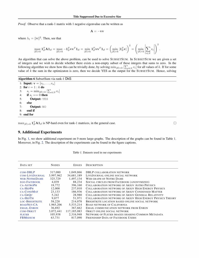
Title Suppressed Due to Excessive Size
Proof. Observe that a rank-1 matrix with 1 negative eigenvalue can be written as
A = �vv
where �1
= kvk2. Then, see that
max
|S|=k1TSA1S = max
|S|=k�1T
SvvT1S = min
|S|=k1TSvv
T1S =
✓
min
|S|=k|1T
Sv|◆
2
=
min
|S|=k
�
�
�
�
�
X
i2S
vi
�
�
�
�
�
!
2
.
An algorithm that can solve the above problem, can be used to solve SUBSETSUM. In SUBSETSUM we are given a setof integers and we wish to decide whether there exists a non-empty subset of these integers that sums to zero. In thefollowing algorithm we show how this can be trivially done, by solving min|S|=k
�
�
P
i2S vi�
� for all values of k. If for somevalue of k the sum in the optimizaton is zero, then we decide YES as the output for the SUBSETSUM. Hence, solving
Algorithm 6 SubsetSum via rank-1 DkS1: Input: v = [v
1
, . . . , vn]2: for i = 1 : k do3: si = min|S|=k
�
�
P
i2S vi�
�
4: if si == 0 then5: Output: YES6: else7: Output: NO8: end if9: end for
max|S|=k 1TSA1S is NP-hard even for rank-1 matrices, in the general case.
9. Additional ExperimentsIn Fig. 1, we show additional experiment on 9 more large-graphs. The description of the graphs can be found in Table 1.Moreover, in Fig. 2. The description of the experiments can be found in the figure captions.
Table 1. Datasets used in our experiments
DATA SET NODES EDGES DESCRIPTION
COM-DBLP 317,080 1,049,866 DBLP COLLABORATION NETWORKCOM-LIVEJOURNAL 3,997,962 34,681,189 LIVEJOURNAL ONLINE SOCIAL NETWORKWEB-NOTREDAME 325,729 1,497,134 WEB GRAPH OF NOTRE DAMEEGO-FACEBOOK 4,039 88,234 SOCIAL CIRCLES FROM FACEBOOK (ANONYMIZED)CA-ASTROPH 18,772 396,160 COLLABORATION NETWORK OF ARXIV ASTRO PHYSICSCA-HEPPH 12,008 237,010 COLLABORATION NETWORK OF ARXIV HIGH ENERGY PHYSICSCA-CONDMAT 23,133 186,936 COLLABORATION NETWORK OF ARXIV CONDENSED MATTERCA-GRQC 5,242 28,980 COLLABORATION NETWORK OF ARXIV GENERAL RELATIVITYCA-HEPTH 9,877 51,971 COLLABORATION NETWORK OF ARXIV HIGH ENERGY PHYSICS THEORYLOC-BRIGHTKITE 58,228 214,078 BRIGHTKITE LOCATION BASED ONLINE SOCIAL NETWORKROADNET-CA 1,965,206 5,533,214 ROAD NETWORK OF CALIFORNIAEMAIL-ENRON 36,692 367,662 EMAIL COMMUNICATION NETWORK FROM ENRONCOM-ORKUT 3,072,441 117,185,083 ORKUT ONLINE SOCIAL NETWORKFLICKR 105,938 2,316,948 NETWORK OF FLICKR IMAGES SHARING COMMON METADATAFBMEDIUM 63,731 817,090 FRIENDSHIP DATA OF FACEBOOK USERS
Title Suppressed Due to Excessive Size
ReferencesBoutsidis, Christos, Mahoney, Michael W, and Drineas, Petros. An improved approximation algorithm for the column
subset selection problem. In Proceedings of the twentieth Annual ACM-SIAM Symposium on Discrete Algorithms, pp.968–977. Society for Industrial and Applied Mathematics, 2009.
Cormen, Thomas H, Leiserson, Charles E, Rivest, Ronald L, and Stein, Clifford. Introduction to algorithms. MIT press,2001.
Gittens, Alex, Kambadur, Prabhanjan, and Boutsidis, Christos. Approximate spectral clustering via randomized sketching.arXiv preprint arXiv:1311.2854, 2013.
Halko, Nathan, Martinsson, Per-Gunnar, and Tropp, Joel A. Finding structure with randomness: Probabilistic algorithmsfor constructing approximate matrix decompositions. SIAM review, 53(2):217–288, 2011.
Mahoney, Michael W and Drineas, Petros. Cur matrix decompositions for improved data analysis. Proceedings of the
National Academy of Sciences, 106(3):697–702, 2009.
Papailiopoulos, Dimitris S, Dimakis, Alexandros G, and Korokythakis, Stavros. Sparse pca through low-rank approxima-tions. arXiv preprint arXiv:1303.0551, 2013.
Rokhlin, Vladimir, Szlam, Arthur, and Tygert, Mark. A randomized algorithm for principal component analysis. SIAM
Journal on Matrix Analysis and Applications, 31(3):1100–1124, 2009.
Vershynin, Roman. Introduction to the non-asymptotic analysis of random matrices. arXiv preprint arXiv:1011.3027,2010.
Wyner, Aaron D. Random packings and coverings of the unit n-sphere. Bell System Technical Journal, 46(9):2111–2118,1967.
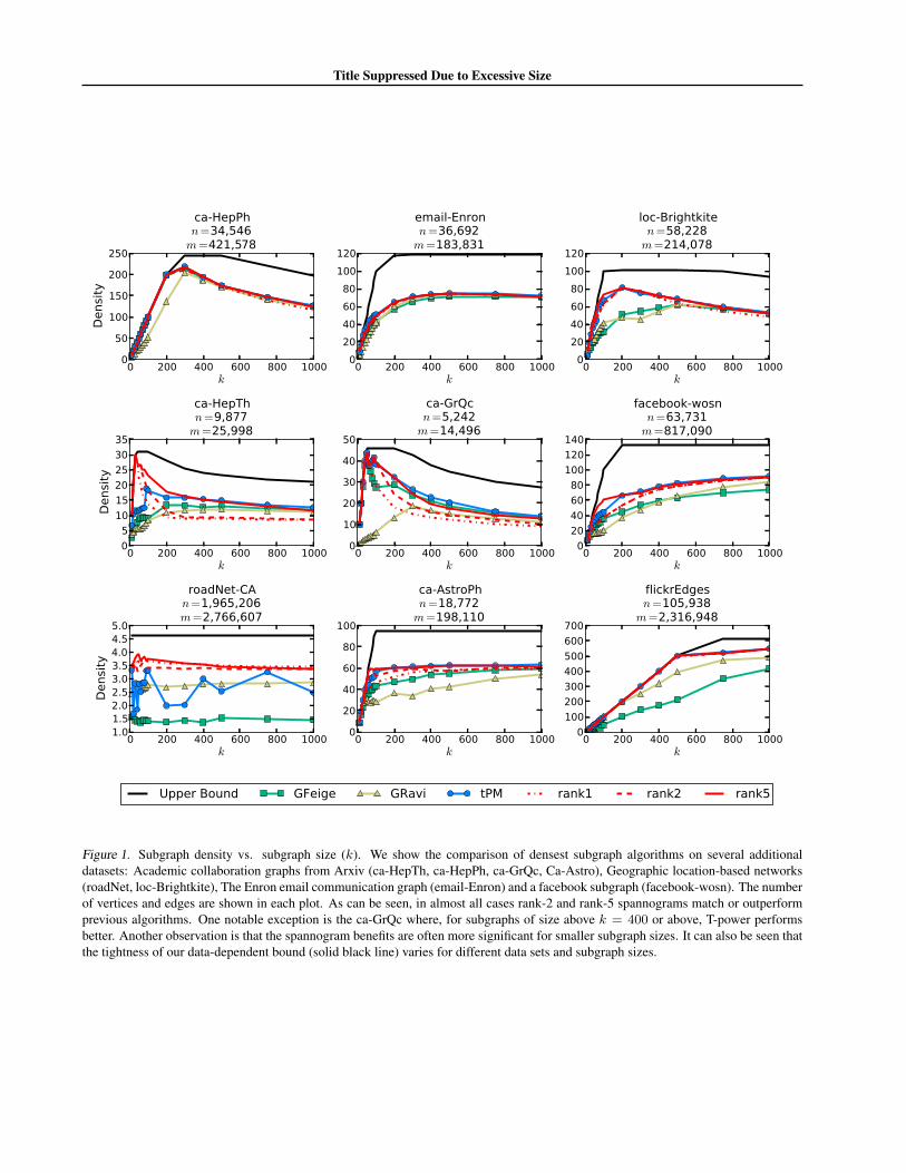
Title Suppressed Due to Excessive Size
Figure 1. Subgraph density vs. subgraph size (k). We show the comparison of densest subgraph algorithms on several additionaldatasets: Academic collaboration graphs from Arxiv (ca-HepTh, ca-HepPh, ca-GrQc, Ca-Astro), Geographic location-based networks(roadNet, loc-Brightkite), The Enron email communication graph (email-Enron) and a facebook subgraph (facebook-wosn). The numberof vertices and edges are shown in each plot. As can be seen, in almost all cases rank-2 and rank-5 spannograms match or outperformprevious algorithms. One notable exception is the ca-GrQc where, for subgraphs of size above k = 400 or above, T-power performsbetter. Another observation is that the spannogram benefits are often more significant for smaller subgraph sizes. It can also be seen thatthe tightness of our data-dependent bound (solid black line) varies for different data sets and subgraph sizes.
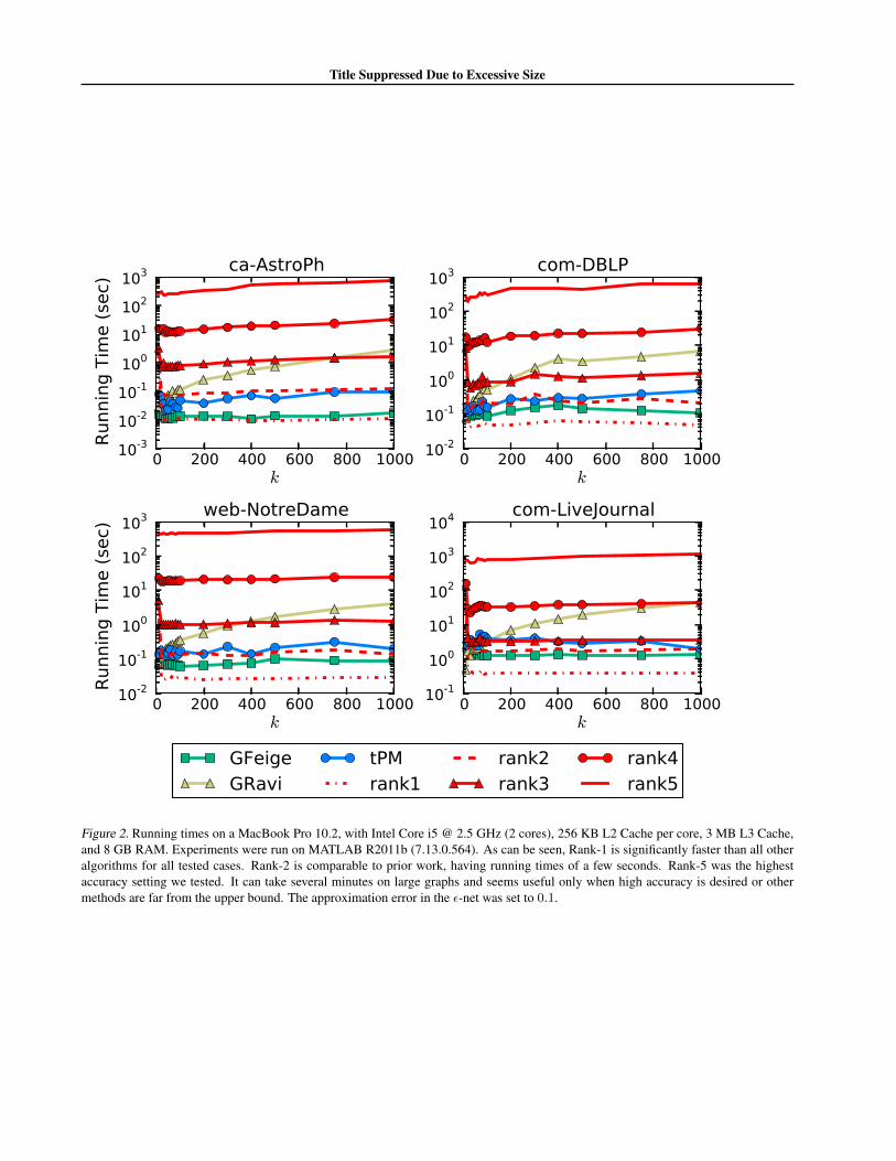
Title Suppressed Due to Excessive Size
Figure 2. Running times on a MacBook Pro 10.2, with Intel Core i5 @ 2.5 GHz (2 cores), 256 KB L2 Cache per core, 3 MB L3 Cache,and 8 GB RAM. Experiments were run on MATLAB R2011b (7.13.0.564). As can be seen, Rank-1 is significantly faster than all otheralgorithms for all tested cases. Rank-2 is comparable to prior work, having running times of a few seconds. Rank-5 was the highestaccuracy setting we tested. It can take several minutes on large graphs and seems useful only when high accuracy is desired or othermethods are far from the upper bound. The approximation error in the ✏-net was set to 0.1.