Work Productivity Analysis of Conventional Floor Structure ...

Financial Structure, Production and Productivity Growth in U.S. Food Manufacturing Industry
Ferdaus Hossain and Ruchi Jain * Department of Agricultural, Food & Resource Economics
Rutgers University, New Brunswick, New Jersey
A paper prepared for presentation at the Annual Meetings of the AAEA, August 5-8, 2001, Chicago.
______________________________ * Assistant Professor and Graduate Student, respectively, Dept. of Agricultural, Food & Resource Economics,
Rutgers University, 55 Dudley Road, New Brunswick, NJ 08901-8520.

Financial Structure, Production and Productivity Growth in U.S. Food Manufacturing Industry
Abstract
This paper examines how financing decision by firms affect production, input demands,
profitability, and productivity. A model that integrates production technology with financing
decision is applied to the U.S. food manufacturing industry. Empirical results shows that
output supply, variable input demands, profitability and productivity are affected by agency
costs of debt and signaling benefits of dividend payments. A one percent increase in dividend
payment leads to a 0.11 percent increase in post-tax variable profit, while a one percent
increase in outstanding debt causes the variable profit to decline by 0.04 percent. Every $1.00
raised through bond issue is associated with $.076 in debt adjustment cost. Average annual
total factor productivity growth was 0.8 percent in U.S. food manufacturing industry.
Signaling benefit contributed for about 3.75 percent of the growth in productivity, while
agency cost accounted for about 11.25 percent reduction in growth. Thus, positive signaling
benefits of dividend payment was more than offset by the agency cost of debt in the
productivity growth in the U.S. food manufacturing industry.

Financial Structure, Production and Productivity Growth in U.S. Food Manufacturing Industry
Major changes in the structure and performance of manufacturing industries over the
recent decades have generated considerable interest among researchers to understand the
implications of these changes. Although the increased interest in changes in market structure,
technology, and globalization have led many researchers to explore the issue in various
contexts, U.S. food manufacturing sector has received far less attention than either the more
high-tech manufacturing sectors or the agricultural sector. The food-manufacturing sector is
clearly important in terms of its size and welfare implications relative to many sectors that
have received far more attention. Food and fiber industries account for about 20 percent of
the U.S. manufacturing output of which about 85 percent comes from the food industry. The
U.S. food-manufacturing sector is nearly as large as the farm sector, and is greater than the
12 percent share of the food industry in U.K. and 3 percent share in Canada (Paul 1999a).
Although generally perceived as less technology oriented than other manufacturing
sectors, the average capital intensity of the food manufacturing industry is about as high as
that for the remaining non-durable manufacturing sector, and is close to that of transportation
equipment and fabricated metals industries (Paul 1999a). The average high-tech component
in capital in the food industry increased considerably over the years, from 1.5 percent in 1961
to 10 percent in 1991. Further, the ratio of high-tech capital to “other capital” increased from
3 percent in 1958 to 25 percent in 1991. The increase in the average high-tech capital in the
food industry between 1976 and 1991 (from 4 percent to 10 percent) is close to that for the
overall non-durable industry. (Paul 1999a, and Berndt and Morrison 1995).

2
The U.S. food-manufacturing industry has been affected by several factors including
consolidation and concentration. Major structural changes took place in the industry via
mergers and acquisition, especially during 1965-70 and 1979-89. The average four-firm
concentration ratio increased from about 59 percent in 1987 to about 65 percent in 1992. At
4-digit SIC level, during the 1972-92 period, this concentration ratio increased at least 25
percent in 14 food industries while it increased more than 100 percent in case of soft drinks,
meat packing, macaroni and spaghetti, and poultry slaughtering and processing industries.
Another development in the U.S. food manufacturing industry relates to changing
financial structure of the sector. Over the years the industry has significantly increased its
dependence on debt financing as is evident from Figure 1, which shows the debt/asset ratio of
the industry (SIC 20) for the 1960-98 period. The rising debt/asset ratio in Figure 1 imply
that the industry has significantly increased its debt use over the years, from about 25 percent
in 1960 to 26 percent in 1964, and reaching to 39 percent in 1974. After falling to 34 percent
by 1976 and remaining stable, the ratio increased from 35 percent in 1984 to 56 percent in
1990. The ratio remained above 50 percent during the entire 1990s. Also note that the sharp
increases in the debt/asset ratio during 1964-74 and 1984-90 periods almost mirrors the
periods when this industry experienced increased pace of consolidation and concentration.
Despite these developments and the importance of the industry, few studies have
focused on the performance of the food industries. Previous research on the performance of
the food and fiber industries includes Heien (1983), Huang (1991), Goodwin and Brester
(1995), Morrison (1997), Morrison and Seigel (1998) and Paul (1999a, 1999b). Heien (1983)
computes the Törnqvist-Theil multifactor productivity index for the aggregate and selected
disaggregated industries. However, his study suffers from some major drawbacks for not

3
including capital and problems with input definitions. Morrison (1997) analyzes the impacts
of capital investment and asset fixity on cost structure and productivity of the food industry
while Paul (1999a) focuses on scale economy, mark-up behavior, trade, investment and cost
structure in the aggregate food and fiber industry. Morrison and Siegel (1998) explore the
existence and extent of scale economies arising from “knowledge capital”, high-tech capital,
and human capital. Paul (1999b) explores the impacts of technical change and trade on costs,
scale economies, pricing behavior and input demand, but focuses only on the meat sector.
None of the studies mentioned above addresses the interlinkages between financial
decisions and production, input demand and dynamic efficiency. This follows the past
tradition of analyzing production and performance where decisions on real economic
variables are kept separate from financial decisions. However, recent research has shown that
real and financial decisions of firms may be interconnected due to the existence of
asymmetric information, information costs and the consequent frictions in capital markets1.
Incentive conflicts due to information asymmetry generate agency costs of bond
financing and signaling benefits of dividend payments, and thereby affect production and
investment decisions. Debt levels are determined through a trade-off between agency costs
and tax benefits of debt financing, while dividend payments are decided based on the trade-
off between tax disadvantages and signaling benefits. The recognition of the potential effects
of financial variables on many aspects of real economic decisions needs to be incorporated in
the empirical analyses of production, technological change and productivity growth.
1 See Hubbard (1998) for comprehensive surveys on the issue.

4
Despite the recognition of the effects of financial decisions on real economic
variables, empirical evidence on the effects of financial variables, especially of agency costs
of debt and signaling benefits of dividends, on production, profitability, technological change
and productivity growth is still limited. Few studies in the area include Kim and Maksimovic
(1990) and Greenwald, Kohn and Stiglitz (1990) and Bernstein and Nadiri (1993). Kim and
Maksimovic (1990) analyze the effects of agency costs on the productivity of U.S. airline
industry. Greenwald, Kohn and Stiglitz (1990) study investigates the effect of agency costs
on the productivity of the overall U.S. manufacturing sector while Bernstein and Nadiri
(1993) examine the effects of both agency costs of debt and signaling benefits of dividend
payments on production, technological change and total factor productivity (TFP) growth for
the U.S. manufacturing sector. They decompose the TFP growth that allows quantitative
estimation of the contribution of debt and dividend payments on TFP growth. However, these
issues have not been addressed in the context of U.S. food manufacturing industry.
The objective of this study is to provide empirical evidence on the impacts of agency
costs of debt and signaling benefits of dividend payments on output supply, input demands,
profitability, technological progress, and the dynamic efficiency, measured by total factor
productivity (TFP) growth in the U.S. food manufacturing industry. The paper is organized
as follows: Section 2 describes the conceptual framework and empirical model used in the
study. Section 3 describes the variables used, data sources, and estimation method utilized in
the analysis. Section 4 presents the empirical results, followed by the Conclusions section.

5
Conceptual Framework and Empirical Model
The conceptual framework that underlies the empirical analysis integrates production
technology with agency costs of debt and signaling benefits of dividend payments, where
production and financial decisions are simultaneously modeled. In this setting, tax costs of
dividends and agency costs of debt affect output supply, while output and input prices affect
dividend payments. The model incorporates adjustment costs to long-run equilibrium due to
capital installation costs as well as costs associated with new debt issue. The decomposition
of TFP in this framework allows evaluation of the impacts of agency costs of debt and
signaling benefits of dividend on the dynamic efficiency of the food manufacturing industry.
The production process is described by the following function
( )1, , , ,mt t t t ty F x K K tx −= ∆ , (1)
where, F is the production function, y denotes output, x is an n-dimensional vector of
variable inputs, mtx is the managerial input, K denotes capital, ∆K denotes change in capital,
and t is a technology indicator captured by time trend. Subscript t refers to time period.
The managerial input represents the services of planning, organizing, and monitoring
input use to ensure technologically efficient production2. There are capital adjustment costs
in the production process in the form of foregone output due to resource allocation for capital
installation, which are represented in the production function by changes in capital input.
The monitoring of managerial decisions by shareholders and creditors cannot be done
without costs. The asymmetric information between managers and shareholders and creditors
2 See Brander and Spencer (1989) for discussions on managerial inputs and financial structure.

6
may lead to incentive divergence between the agents. Dividend payments and new shares
issues by firms serve as signaling devices (Leland and Pyle 1977, Ross 1977, Myers and
Majluf 1984, and Bernheim 1991). Management’s decision to pay dividends signals that the
firm is in good financial position with adequate net flow of funds. However, the signaling
benefits of dividends have a trade-off in the form of higher tax obligations associated with
dividend payments (King 1977, Auerbach 1979, and Poterba and Summers 1985).
Asymmetric information between managers and creditors is a source of agency costs.
Jensen and Meckling (1976), Stiglitz and Weiss (1981), and Greenwald, Kohn and Stiglitz
(1990) show that, in the presence of asymmetric information, firms can undertake relatively
risky investments that increase the risk exposure of the creditors. Myers (1977) suggests that
debt financing involves costs to firms because they may have to forego profitable investment
opportunities. Part of the benefit of debt-financed investments accrue to creditors while
shareholder bear the costs. The agency cost of debt is traded off against tax reductions
associated with interest payments on debt.
The signaling benefits of dividend and agency costs of debt are incorporated into the
model by defining the following managerial cost function,
( )1, ,mt t t tc G D B Bµ −= ∆ , (2)
where mtc is managerial cost, µ is the price of managerial input, D is dividend payment, B is
the value of outstanding bonds and ∆B is the value of new bonds issue. The function G may
be interpreted as the firm’s financing ability function, which is decreasing in debt and
increasing in dividends. The agency costs are associated with both outstanding debt and new
bond issues, the latter defines the debt adjustment cost. The managerial cost function is

7
connected with the G function in the sense that an increase (decrease) in financing ability
increases (decreases) the demand for managerial services, and the managerial input cost rises
(falls). A formal link between managerial input demand and the G-function can be obtained
by applying the Shephard’s Lemma on (2) to obtain 1( , , )mt t t t
mtdc
dx G D B Bµ −= = ∆ . Thus, the
G-function represents the managerial input demand. Substituting mtx into the production
function (1) yields an augmented production function that includes financial variables,
( )1 1, , , , , ,t t t t t t ty x D B K K B t− −= ℑ ∆ ∆ (3)
The production cum managerial, equation (3), shows that debt and dividend levels
affect output supply and input use. An increase (decrease) in outstanding debt lowers
(increases) managerial input demand, which in turn decreases (increases) output with given
non-managerial inputs. Thus, changes in outstanding debt affect both capital and non-capital
inputs. Similarly, changes in new debt issue and dividends generate output and input effects.
Capital is a quasi-fixed input whose stock follows the process
( ) 11t t tK I Kδ −= + − (4)
where 0 < δ < 1 is the fixed depreciation rate, and It is the investment in time t. The flow of
funds relating the production and financing decision can be described as
1, 1 , 0Tt t t t t t t t t n t tP y Q I R B B S D−− − − + ∆ + ∆ − =P x , (5)
where, P1,t is the post-tax price of output, TtP is a vector of post-tax variable input prices, Qt
represents the post-tax purchase price of capital, Rt is the post-tax interest rate on debt, and
∆Sn,t is the value of share issue in time t.

8
Production and financing decisions are made to maximize the expected discounted value of
equity. The optimization problem is
( ),
, , , ,1, , , , ,
(1 )/(1 ){ }
max
t t t t n t t
t t p g ny x I D S BE D u u Sτ τ τ τ τ
τ
α∞
=∆ ∆− − − ∆∑ (6)
subject to equations (3) - (5), given initial capital stock and debt level. In the above equation,
the discount factor is 1, , 1 1 , 1 , 11, [(1 (1 )/(1 ))]t t t t t p t g tu ua a r −
+ + + += = + − − where ρ is the discount
rate, up is the personal income tax rate, and ug is the capital gains tax rate with 0 < ug <up < 1.
Shareholders are subject to dividend tax at the same rate as personal income tax rate.
In this setting, the intertemporal production and financing problem can be solved in
two stages. The first stage determines the short-run equilibrium, which is obtained from
1, 2,{ , , }
max
t t t
Tt t t t t t
y x DP y P D P x− − (7)
subject to equations (3) and (5), conditional on the capital stock and debt levels. In equation
(7) above, 2 , ( )/(1 ) 0t p g gP u u u= − − > can be considered as the price of dividend, which is the
additional tax shareholders have to pay per dollar of dividends relative to receiving a dollar
of capital gains. In the short-run the firm chooses output, variable inputs, and dividend to
maximize the post-tax variable profit net of dividends. In the short-run equilibrium the tax
cost associated with dividends is offset at the margin by the signaling benefits through higher
managerial ability to finance production. Conditional on capital stock and debt, dividend
payments are determined simultaneously with output supply and variable factor demands.
Thus, under this framework, output supply and variable input demands are affected
by changes in dividend price while dividend payments are affected by output and variable
input prices. Debt level affects output and input decisions through the marginal productivity

9
of managerial input and the rate of substitution between managerial input and variable inputs.
Further, changes in debt level affect dividend payments through the effects of agency costs
on signaling ability. In the short-run, capital accumulation and technological change affect
the relative marginal product of the managerial input, and thereby the dividend payments.
The solution to the optimization problem in equation (6) generates a post-tax variable
profit function (net of dividend payments) given by
( )1, 2, 1 1, , , , , , ,v Tt t t t t t t tP P P K B K B t− −Φ = Φ ∆ ∆ (8)
In order to empirically implement the model, a translog functional form is assumed.
Thus the variable profit (net of dividend payments) function is given by3
( )
( ) ( )
( ) ( )
1 1
2 21 1
1 1
2 2
1 1
1
0 22 1
2ln ln ln ln
ln ln ln ln
ln ln ln
0.5n n B B
ij i n j n ks k si j k K s K
n B n B
ik i n it i n kt
i k K i k K
n Bv
i i n k k tn i k K
tt
k k
P P P P K K
P P K P P K
P P K tP
t
t t
b b
b b b
b b b b
b+ +
+ += = = =
+ +
+ += = = =
+
++ = =
Φ = + + + + + +
+ + +
∑∑ ∑ ∑∑∑ ∑ ∑
∑ ∑ (9)
where, P1 is post-tax price of output, P2 is the post-tax price of dividend, Pi denotes post-tax
price of variable inputs for i (i = 3, …n+2), Kk = capital input, and KB = Debt level. In
equation (9) the symmetry condition is imposed by assuming βij = βji, and βks = βsk. Further,
marginal capital and debt adjustment costs are assumed to be zero when net investment and
new bond issues are zero. This assumption allows separation of adjustment costs from other
components of net variable profit. The adjustment cost is given by
3 The homogeneity of degree one of the variable profit function in prices is imposed by normalizing
Φv and prices by a variable input price. Henceforth, time subscript is omitted to simplify notation.

10
0.5 , B B
aks k s ks sk
k K s K
c K Kα α α= =
= ∆ ∆ =∑∑ . (10)
Both new debt and capital expansion affect the marginal adjustment costs of both capital and
debt, and this interaction reflects that often new debt are issued to finance capital expansion.
Using the net variable profit function (9), the short-run equilibrium conditions are
obtained by applying the Hotelling’s Lemma to obtain
( )1
21
i = 1, 2, , n+1ln ln , n B
i i ij j n ik k itj k K
s P P K tβ β β β+
+= =
= + + +∑ ∑ … (11)
where s1 = P1y / Φv is output’s share in (net) variable profit, s2 = -P2D/Φv is dividend share in
Φv, and si = -Pixi/Φv is variable input i’s share in Φv (i = 3, …,n+1). Equation (11) above
shows that in the short-run equilibrium output, dividends and variable factor components of
Φv are functions of relative output and input prices, capital stock, debt level, and technology.
The intertemporal productions and financing decisions are solved in the second stage.
In this stage firms choose the optimal debt and share issue. Substituting equations (4) and (8)
into equation (6), the intertemporal production and financing problem can be expressed as
, 1 1 11{ , }
[ ( (1 ) )]max v
t tK B
E R B B B Q K Kτ τ
τ τ τ τ τ τ τ ττ
α δ∞
− − −=
Φ − + − − − −∑ (12)
where Q and R denote the post-tax purchase price of investment and interest rate on debt.
Solution to the optimization problem in equation (12) results in the determination of
optimal capital and debt level for the firm. Once the new (optimal) levels of capital and debt
are determined, the investment and new debt issues are determined which in turn allows the
determination of the share issue. Substituting the solutions for capital and debt from equation
(12) into equation (11) allows the determination of output supply, dividend payments and

11
variable factor demands. New share issues are then determined by plugging-in the solutions
for output, inputs, dividend payments, new investment, and debt into equation (5).
Substituting the post-tax net variable profit function defined in equation (9) and the
adjustment cost function defined in equation (10) into equation (12), and solving the
intertemporal optimization problem leads to the following two Euler equations
( )
1
, 1 , 1 2, 11
1 2, 1 1 1 1
([ ln ln ln
( 1)]( ) / (1 )) 0
n
KK t KB t t t t t K KK t KB t iK i t n ti
vkt t n t t KK t KB t t
K B Q E K B P P
t P K K B Q
α α α β β β β
β α α δ
+
+ + + +=
+ + + + + +
− ∆ − ∆ − + + + +
+ + Φ + ∆ + ∆ − − =
∑ (13)
( )
1
, 1 , 1 2, 11
1 2, 1 1 1 1
1 ([ ln ln ln
( 1)]( ) / 1) 0
n
BB t KB t t t t B BB t KB t iB i t n ti
vBt t n t t BB t KB t t
B K E B K P P
t P B B K R
α α α β β β β
β α α
+
+ + + +=
+ + + + + +
− ∆ − ∆ + + + + +
+ + Φ + ∆ + ∆ − − =
∑ (14)
Equation (13) shows that at optimal capital level the expected marginal post-tax profit of
capital in period t+1 inclusive of expected adjustment cost and post-tax purchase price
savings from previous period’s undepreciated capital stock is offset against the post-tax
contemporary purchase of capital inclusive adjustment cost. Equation (14) implies that at
equilibrium the expected marginal reduction in post-tax profit in period t+1 due to the agency
costs of debt inclusive of interest payments net of expected debt adjustment cost savings
from previous period’s debt issue is offset against the current additional funds from a dollar
of debt net of marginal debt adjustment costs. These two equations reveal that capital
expansion and debt increases have opposite effects on variable profit. The benefit of capital
is the profit it generates, while that of debt is the extra fund that flows to the firm while profit
is reduced due to agency costs.

12
Data and Estimation
Data used in the study relates to the food manufacturing industry (SIC 20) and cover
the 1960-96 period. Data on quantities and implicit price indices of outputs and inputs are
from NBER Manufacturing Productivity Database. The input and output quantities and price
data in the NBER database (at 4-digit SIC level) are first converted to real values at 1987
prices and then aggregated to 2-digit SIC level. Real output and input quantities are obtained
by simply adding up across industries. Aggregate price indices are obtained as weighted
averages of the price indices with revenue/cost share of each of the 4-digit industry used as
weights.
Output is measured by the real value of shipments. There are two variable factors,
labor and material (including energy), and a quasi-fixed input, capital. Quantity of labor input
is defined in millions of hours and includes only the production workers. Nominal wage rate
per hour is obtained by dividing total production wage bill by the total hours worked. Real
wage rate is obtained by deflating the nominal wage rate with the GDP deflator.
The dollar value of Cash Dividends Charged to Retained Earnings (for SIC 20)
obtained from Quarterly Financial Report (QFR) is used as total dividend payment. The real
values of the dividend payments are obtained by deflating the nominal dividend payments by
the GDP deflator, obtained from the Bureau of Labor Statistics. The price of dividend is
defined as ( ) ( )2 / 1p g p pP u u P u= − − where up is the effective personal tax rate on dividend
income, ug is the effective tax rate on capital gains and Pp is the GDP deflator. Data on tax
rates on dividend income and capital gains for 1960-84 are from Feldstein and Jun (1987),
which was updated for other years using information obtained from the Statistics of Income.

13
Real value of capital, in 1987 dollars, and implicit deflator for new investment are
from the NBER database, which includes both equipment capital, and structures and
building. Using the investment deflator the post-tax purchase price of investment is
calculated as: Qt = PI (1 – ωk – ucz) where PI is investment deflator, ωk is investment tax
credit, uc is corporate income tax rate, and z is present value of capital consumption
allowance. Investment tax credit was first instituted in 1962 so that the value of ωk for 1960
and 1961 are set equal to zero. Data on the investment tax credit for the years 1962 to 1981
are from Jorgenson and Sullivan (1981). For other years, we follow Bernstein and Nadiri
(1993) and use 8% rate for 1981 and 7.5% for the remaining years. Corporate income tax rate
for 1960- 85 are from Pechman (1987), which was updated using information obtained from
the office of tax analysts at the U.S. department of treasury. The present value of capital
consumption allowances is calculated as z = λ(1 - ηωk)(r + λ) where λ is the ratio of capital
consumption allowance to capital stock less treasury stock (both obtained from QFR) at cost,
η is 0.5 for 1962 and 1963 and zero elsewhere, and r is the yield on 10-year U.S. T-bonds.
The stock of debt is defined as the sum of installments due in more than one year on
long-term loans from banks, and other long-term debt. Both are end of the period values for
the fourth quarter and are obtained from the QFR. Interest rate on debt is measured by the
yield on 10-year Treasury bonds. Discount rate is given by ρ(1 -up)/(1 –ug), where ρ is the
annual rate of return on equity in the food industry (SIC 20) obtained from QFR.
The empirical model consists of equations (9), (11), (13) and (14). The adjustment
cost function (equation (10) is not estimated because the parameters are contained in the
capital and debt equations. The endogenous variables in the model are post-tax net variable

14
profit, output, labor, dividend variable profit components, capital and debt. For empirical
estimation of the system of equations, error terms with zero expected value are added to
equations (9) and (11). Error terms are introduced in equations (13) and (14) by removing the
conditional expectations operator and substituting realized values of the variables. It is
assumed that the error structure forms a positive definite symmetric covariance matrix.
Since the empirical model contains expected future values of the variables, the
equations are estimated using Hansen and Singleton’s (1982) GMM estimator. Equivalent to
non-linear 3SLS estimator, it is consistent and efficient for the set of instruments used
(Pindyck and Rotemberg 1983). Lagged values of relative prices, interest rate, post-tax
purchase price of capital, post-tax variable profit, capital and debt are used as instruments.
Empirical Results
The estimated model coefficients and the associated standard errors are presented in
Table 1. The model coefficients are well determined and most coefficients are statistically
significant. The J-statistics for testing the validity of the overidentifying restrictions of the
model yield an estimated value of 53.26. For our empirical model, the J-statistic is distributed
as χ2 with degrees of freedom equal to 47. The 95% critical value of 2
47÷ is 64.00, which is
greater than the computed value of the statistic. Thus we conclude that the null hypothesis
that the model is correctly specified cannot be rejected.
Financial Consideration, Production and Profitability
First, we present the results relating to the effects of financing strategy on allocation
decisions relating to output supply, input demands, and profitability of aggregate U.S. food
industry. The effects of financing decisions on output, inputs and profitability work through

15
two channels. One channel relates to the effects on production and profitability when price of
dividend is altered via changes in tax code, while the other relates to the effects of changes in
outstanding debt that has been determined by the financing decision in the previous period.
First we consider the effects of changes in prices of output and variable inputs as well
as dividend. In the empirical model output and input prices affect dividend payments, which
in turn affect output supply and input demand. The short-run price elasticities are given by
( ) /ij ij i j ij i ie s s s sβ δ= + − i, j = output, dividend, labor,
where eij = elasticity of the ith quantity with respect to the jth price, δij = 1 if i = j, and δij = 0
if i ≠ j. Recall that si > 0 for output and si < 0 for dividend and variable inputs. Price
elasticities associated with material input are calculated by obtaining the relevant coefficients
form the homogeneity restriction. Share of material input is obtained as s4 = 1 – s1 – s2 – s3.
The estimated price elasticities and associated standard errors are presented in Table 2
which shows that increases in output prices increase output supply, dividend payments and
demand for both variable inputs. Increase in dividend price has negative effects on output,
dividend payments and variable input demands. Further, increases in both variable input
prices have negative impacts on output (as expected), dividend payment and demand for both
inputs. Estimated elasticities suggest that dividend is relatively more responsive to changes in
output and input prices than its own price. Changes in dividend price generate only inelastic
responses from output supply and input demands while changes in other prices bring elastic
responses. A one percent increase in dividend price leads to reductions in output supply and
input demands, with magnitudes ranging from 0.013 to 0.352.

16
Changes in dividend price also affect variable profit via its effects on output supply
and input demands. Since post-tax variable profit (before dividend payments) is given by
( )21v v sπ = Φ − where s2 = - P2D/Φv, the elasticity of πv with respect to dividend price is
[ ]2 2 2 22 2(1 ) /(1 )e s s sπ β= − − −
The estimated value for eπ2 is -0.018 (with a S.E. = 0.004) implying that a one percent
increase in dividend price causes only about 0.02 percent decrease in πv. The signaling
benefit of dividend (in higher profitability) is the percentage change in πv relative to
percentage change in dividends resulting from a one percent increase in dividend price. In
terms of the model parameters, this is given by 2 22De e eπ π= , where eπ2 and e22 are as
defined earlier. The estimated eπD is 0.11 implying that a one percent increase in dividend
causes about 0.11 percent increase in the variable profit of U.S. food manufacturing industry.
The level of debt also affects output supply and variable input demands. Based on
model coefficients, we estimate the effects of outstanding debt on production, dividend
payments, and profitability. Also, we compare these results with the effects of increases in
capital stock and technological change. The effects of technological change, capital, and debt
on output supply, variable input demands, and dividend payments can be computed as
i = output, dividend, labor and materials, j = K, B, t ij ij i je s eφβ= +
where eφj is the effect of j on post-tax variable profit.
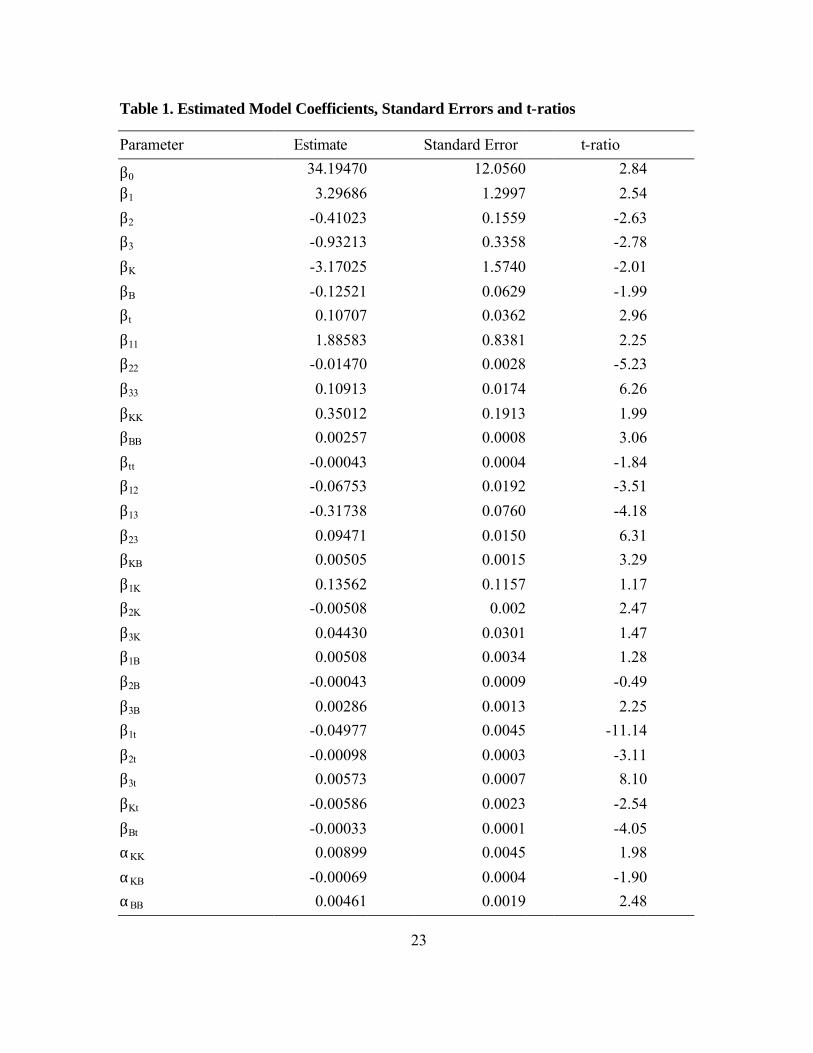
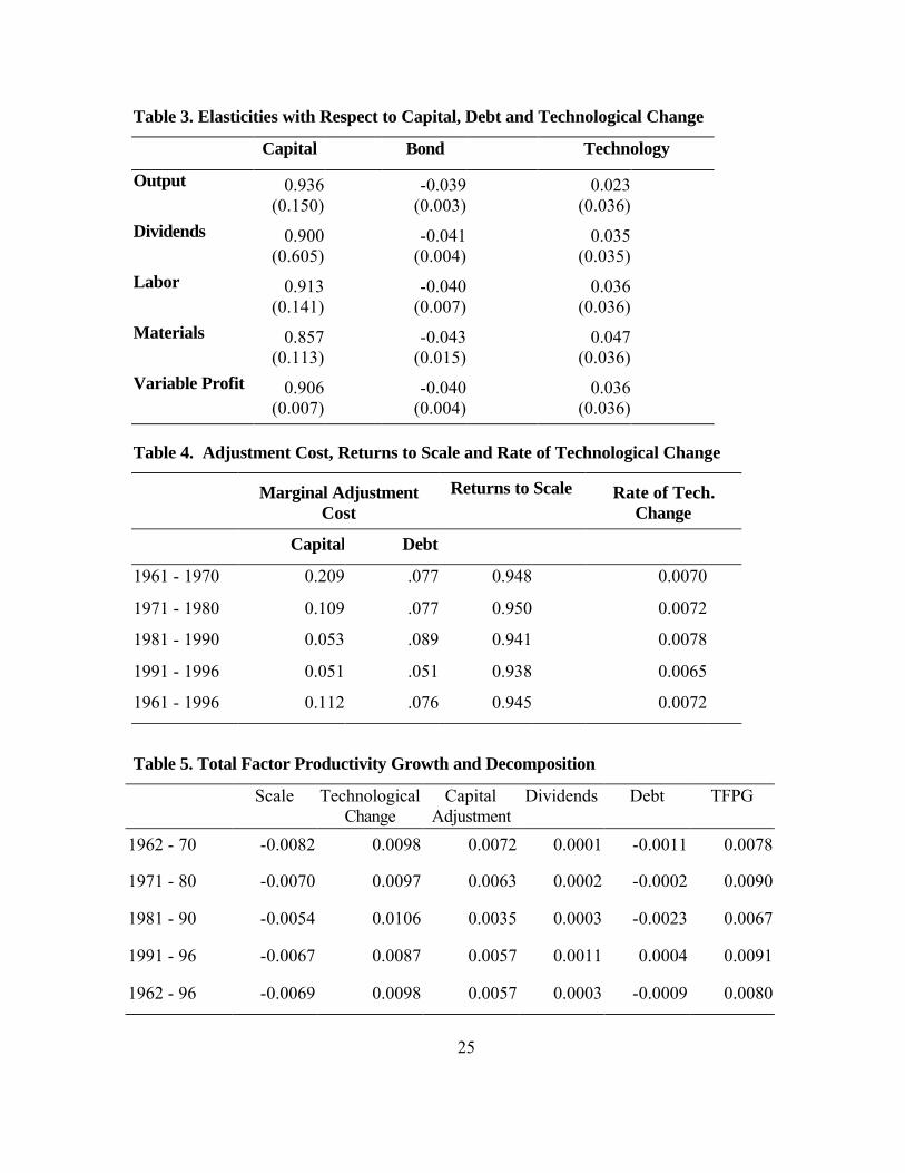
The estimated values of the elasticities and their associated standard errors are
presented in Table 3, which clearly shows that increases in debt have negative impacts on
output, input demands, and profitability. Point estimates of the elasticities with respect to
debt suggest that a one-percent increase in debt leads to about 0.04 percent decline in output,

17
dividend payments, and variable input demands. The agency cost associated with outstanding
debt can be defined in terms of foregone profitability. Expressed in elasticity form, the effect
of debt on post-tax variable profit is given by 2 2 2(1 ) /(1 )B B Be e s sπ φ β = − − − , the point
estimate of which is –0.040 with S.E. of 0.004. The finding that profitability falls with higher
debt levels is consistent with the notion that higher debt levels cause agency costs to rise.
These elasticities are comparable to those obtained by Kim and Maksimovic (1990) for U.S.
airline industry, and Bernstein and Nadiri (1993) for U.S. manufacturing sector as a whole.
Effects of capital expansion and technological change on output, input demands, and
dividend payments are also given in Table 3. Capital expansion and technological change
have positive effects on production, dividends and profitability, and therefore works to
mitigate the negative effects on these variables. Estimated elasticities suggest that capital is
the driving factor affecting output, input demands, dividend payments and variable profits.
Adjustment Costs
The adjustment costs in our model are reflected in the costs associated with capital
expansion and debt issue. The estimated adjustment cost parameters, αKK, αKB and αBB in
equations (13) and (14), reported in Table 1, show that own adjustment costs coefficients are
positive (as expected) while the interaction term αKB is negative. The signs αKK and αBB
imply that net capital expansion via investment increases marginal installation cost while
additional debt issue increases the marginal agency costs. Negative αKB implies that capital
investment and debt issues are adjustment complements in the sense that increases in net
capital stock lower the marginal agency cost. That is, agency costs are reduced when capital

18
expansion is financed through debt. Estimated coefficients yield (αKKαBB - 2
KBα )> 0 implying
convexity of adjustment costs in net capital investment and new debt issue.
The agency costs of debt affect the adjustment towards long run equilibrium and
create a wedge between the contemporaneous and long run effects of debt on profitability. In
long-run equilibrium the marginal debt adjustment cost is zero and the reduction in variable
profit due to agency costs is the difference between post-tax rate of return to shareholders
and the post-tax interest rate on debt, which is given by , , , ,(1 )/(1 ) (1 )B t t p t g t t c tW u u r uρ= − − − − ,
where rt(1-uc,t) = Rt, rt is the interest rate on debt in period t and uc,t is corporate income tax
rate in period t. In the long run, the ratio between the marginal agency cost and the net
opportunity cost of funds (WB) has to equal to unity. Therefore, the relative importance of
marginal adjustment costs of debt (the system deviates from long-run equilibrium) can be
obtained as the ratio of marginal adjustment cost (i.e., adjustment cost per dollar of new debt)
to the rate of return to shareholders. This is given by [ ] ,( ) / /BB t KB t t B tB K B Wα α∆ + ∆ ∆ . The
computed marginal adjustment costs of capital increase and new debt are reported in Table 4.
The average marginal debt adjustment cost was found to be about 0.076 for the 1961-96
period implying that for $1.00 cost of debt there is an additional adjustment cost of about
$0.076. This adjustment cost was highest in the 1980s and lowest during 1991-96 period.
Similarly in long-run equilibrium when marginal adjustment cost is zero, marginal
profit associated with capital expansion equals the after-tax rental rate (or the opportunity
cost of capital serves) of capital given by , , ,[ (1 )/(1 ) ]K t t t p t g tW Q u uρ δ= − − + . Therefore, the
marginal adjustment cost of capital is [ ] ,( ) / /BB t KB t t K tK B K Wα α∆ + ∆ ∆ . Estimated marginal
adjustment cost of capital (reported in Table 4) yield an average adjustment cost of 0.112 for

19
1961-96 period, implying that that for $1.00 rental of capital services, there is an additional
adjustment cost of $0.118 of which $0.112 is the capital installation cost and $0.076 is debt
adjustment cost. These findings are similar to those of Berndt and Morrison (1981), Pindyck
and Rotemberg (1983), Mohnem, Nadiri and Prucha (1986), Bernstein and Nadiri (1993).
Returns to Scale, Technological Change and Productivity Growth
Returns to scale in production, given by the proportional change in output in response
to changes in variable inputs and quasi-fixed factor (capital), and the rate of technological
change are also affected by debt and dividend price. It is assumed that managerial inputs and
technology do not change. Under this assumption, the post-tax variable profit function can be
used to obtain a measure of the degree of returns to scale as
2
1 13
/ ( ln ln ) /n
vi
i
RRS s s K s+
=
= − + ∂ Φ ∂∑ (15)
where i = 3 represents labor and i = n+2 = 4 represents material input. The rate of
technological change can also be obtained from the variable profit function as
1( ln ) /vRTC t s= ∂ Φ ∂ (16)
Table 4 contains the results relating to returns to scale (RRS) and the rate of technical
change (RTC) for the U.S. food manufacturing industry. These results suggest that the U.S.
food manufacturing industry is essentially a constant returns to scale industry. The estimated
rate of technical change in this industry fluctuated between 0.70 and 078 percent for most of
the years except the 1991-96 period when this rate was found to be 0.65 percent. The
estimated average rate of RTC was 0.72 percent for the 1961-96 period. Thus, the U.S. food
industry experienced a slower rate of technical progress relative to the overall manufacturing
sector. For instance, both Bernstein and Nadiri (1993) and Gullickson (1995) estimated a 1.3

20
percent annual rate of technological change for the aggregate manufacturing industry. A
noticeable aspect of our result is that the RTC in the food manufacturing industry was slower
in the first half of 1990s when U.S. economy experienced widespread technological progress.
The dynamic efficiency of the food industry is investigated by analyzing the total
TFP growth over the 1961-96 period. Traditional sources of TFP growth are technological
change and scale effects. Recent extensions in the literature have included factors such as
efficiency, market power, asset fixity, etc. as additional sources of TFP change. We do not
focus on market power or efficiency, but obtain an expanded TFPG decomposition to include
the effects of agency costs of debt and signaling benefits of dividend payments. Total factor
productivity growth is defined by
ln ( ) ( / ) lnM
i i ki L
TFPG d y Px C W K C d K=
= − −∑ (17)
where L = labor input, and M is the material inputM
i i Ki L
C Px W K=
= +∑ is the total cost. Taking a
total differential of equation (8) and 1 2
Mv
i ii L
P y Px P D=
Φ = − −∑ , the Hotelling’s Lemma yields
( )( )
1 2lnln ln ln lnln
ln ln lnln
M v
i ii L
v v
s d y s d x s d D d KK
d B tB
=
∂ Φ+ + = ∂
∂ Φ+ + ∂ Φ ∂∂
∑ (18)
where s1 = P1y/Φv > 0, s2 = - P2D/Φv, and si = - Pixi/Φv < 0 (i = L, M) are output, dividend,
and variable input components in net variable profit. Multiplying both sides of (18) by
(Φv/C) and adding (17) to both sides of (18) gives
( )1
2
1 ( / ) ln ( / ) ln ( / )( ln ln
( / ) ln ) ( / ) ln ( / )( ln ln ) ln
v v v v v
v v vk
TFPG C s d y C t C K
W K C d K C s d D C B d B
= − Φ + Φ ∂ Φ ∂ + Φ ∂ Φ ∂
− + Φ + Φ ∂ Φ ∂ (19)

21
The TFP decomposition in equation (19) shows that there are five components of TFP
growth. The first term is the scale effect, the second term reflects technological change, the
third term denotes the capital adjustment effect, the fourth term reflects the signaling benefits
of dividends, and the fifth term is the effect of agency costs of debt financing. Thus, TFP
growth in the food industry, in addition to being affected by the traditional factors, is also
impacted by financing decision of firms.
In this decomposition of TFP growth, increases in dividend payments make positive
contribution while increases in debt make negative contribution TFP growth. Results of TFP
decomposition are presented in Table 5. Table 5 shows that in the U.S. food manufacturing
industry, TFP experienced an average annual growth rate of 0.8 percent during the 1961-96
period. The signaling benefits of dividend payments contributed to the average annual rate of
TFP growth by 0.0003 or 3.75 percent, compared to a 4.2% contribution calculated by
Bernstein and Nadiri (1993) for the overall U.S. manufacturing industry. Agency cost of debt
made a negative contribution to the TFP growth in the food manufacturing industry. For the
1961-96 period, agency cost associated with debt reduced TFP growth by 0.0009 or by 11.25
percent. This is about three and a half times the negative contribution of debt to TFP growth
in the overall manufacturing sector computed by Bernstein and Nadiri (1993) and about 4
times that computed by Kim and Maksimovic (1990) for U.S. airline industry. Thus, for the
U.S. food manufacturing industry, we find that the dynamic efficiency effects associated with
agency costs of debt are much higher than the signaling benefits associated with dividend
payments. Adjustment of capital to long-run equilibrium made had positive effects on TFP
growth, implying that the positive effects of capital outweighed the installation costs and
adjustment costs associated with bond financing of capital. Growth in TFP came mainly from

22
technological progress and capital expansion, while scale effects and agency costs of debt
were a drag on the TFP growth in the U.S. food manufacturing industry.
Conclusion
In this study, we examine how financing decision by firms affect production, input
demands, profitability, and productivity. In particular, we estimate the impacts of agency
costs of associated with debt financing and signaling benefits of dividend payments on output
supply, input demands, profitability, and productivity growth in U.S. food manufacturing
industry. We find that a one percent increase in dividend payment leads to a 0.11 percent
increase in post-tax variable profit, while a one percent increase in outstanding debt causes
the variable profit to decline by 0.04 percent. The average adjustment cost in the U.S. food
industry was about $0.118 of which $0.112 was capital installation cost and $.076 was
attributable to the agency cost from bond issue.
Output supply and variable input demand are affected by dividend payments and
outstanding debt. Dividend payments have positive effects on output supply and variable
input demands through positive signaling benefits, while outstanding debt level have
negative via agency costs. Agency costs and signaling benefits also affected the TFP growth
in U.S. food manufacturing industry. Overall, annual total factor productivity growth was 0.8
percent in U.S. food manufacturing industry. Signaling benefit contributed for about 3.75
percent of the growth in productivity, while agency cost accounted for about 11.25 percent
reduction in growth. Thus, positive signaling benefits of dividend payment was more than
offset by the agency cost of debt in the productivity growth in the U.S. food manufacturing
industry.
23
Table 1. Estimated Model Coefficients, Standard Errors and t-ratios
Parameter Estimate Standard Error t-ratio
β0 34.19470 12.0560 2.84
β1 3.29686 1.2997 2.54
β2 -0.41023 0.1559 -2.63
β3 -0.93213 0.3358 -2.78
βK -3.17025 1.5740 -2.01
βB -0.12521 0.0629 -1.99
βt 0.10707 0.0362 2.96
β11 1.88583 0.8381 2.25
β22 -0.01470 0.0028 -5.23
β33 0.10913 0.0174 6.26
βKK 0.35012 0.1913 1.99
βBB 0.00257 0.0008 3.06
βtt -0.00043 0.0004 -1.84
β12 -0.06753 0.0192 -3.51
β13 -0.31738 0.0760 -4.18
β23 0.09471 0.0150 6.31
βKB 0.00505 0.0015 3.29
β1K 0.13562 0.1157 1.17
β2K -0.00508 0.002 2.47
β3K 0.04430 0.0301 1.47
β1B 0.00508 0.0034 1.28
β2B -0.00043 0.0009 -0.49
β3B 0.00286 0.0013 2.25
β1t -0.04977 0.0045 -11.14
β2t -0.00098 0.0003 -3.11
β3t 0.00573 0.0007 8.10
βKt -0.00586 0.0023 -2.54
βBt -0.00033 0.0001 -4.05
αKK 0.00899 0.0045 1.98
αKB -0.00069 0.0004 -1.90
αBB 0.00461 0.0019 2.48

24
Figure 1. Debt/Asset Ratio in U.S. Food Manufacturing Industry: 1960-98
0.20
0.25
0.30
0.35
0.40
0.45
0.50
0.55
0.60
1955 1960 1965 1970 1975 1980 1985 1990 1995 2000Year
Deb
t R
atio
Table 2. Short-run Price Elasticities
Materials
4.496
(0.359)
-0.013
(0.008)
-0.327
(0.061)
-4.156
(0.473)
Quantity Price
Output Dividends Labor Materials
Output
3.404
(0.214)
-0.034
(0.008)
-0.364
(0.041)
-3.05
(0.194)
Dividends
7.847
(1.117)
-0.163
(0.016)
-5.786
(0.591)
-1.898
(0.983)
Labor
5.043
(0.268)
-0.352
(0.027)
-1.669
(0.234)
-3.023
(0.242)
Note: Elasticities are computed at mean values, and standard errors are in parentheses.
25
Table 3. Elasticities with Respect to Capital, Debt and Technological Change
Capital Bond Technology
Output
0.936 (0.150)
-0.039 (0.003)
0.023 (0.036)
Dividends
0.900 (0.605)
-0.041 (0.004)
0.035 (0.035)
Labor
0.913 (0.141)
-0.040 (0.007)
0.036 (0.036)
Materials
0.857 (0.113)
-0.043 (0.015)
0.047 (0.036)
Variable Profit
0.906 (0.007)
-0.040 (0.004)
0.036 (0.036)
Table 4. Adjustment Cost, Returns to Scale and Rate of Technological Change
Marginal Adjustment
Cost Returns to Scale
Rate of Tech.
Change
Capital Debt
1961 - 1970 0.209 .077 0.948 0.0070
1971 - 1980 0.109 .077 0.950 0.0072
1981 - 1990 0.053 .089 0.941 0.0078
1991 - 1996 0.051 .051 0.938 0.0065
1961 - 1996 0.112 .076 0.945 0.0072
Table 5. Total Factor Productivity Growth and Decomposition
Scale
Technological
Change Capital
Adjustment Dividends
Debt
TFPG
1962 - 70 -0.0082 0.0098 0.0072 0.0001 -0.0011 0.0078
1971 - 80 -0.0070 0.0097 0.0063 0.0002 -0.0002 0.0090
1981 - 90 -0.0054 0.0106 0.0035 0.0003 -0.0023 0.0067
1991 - 96 -0.0067 0.0087 0.0057 0.0011 0.0004 0.0091
1962 - 96 -0.0069 0.0098 0.0057 0.0003 -0.0009 0.0080

26
References
Auerbach, A.J. “Wealth Maximization and the cost of capital.” Quart. J. Econ. 93(August
1979): 433-446
Berndt, E.R., and C. J. Morrison. “Short-run Labor Productivity in a dynamic Model.” J.
Econometrics 16(August 1981): 339-365.
Berndt, E. R., and C. J. Morrison. “High-Tech Capital Formation and Economic Performance
in U.S. Manufacturing Industries: An Exploratory Analysis.” J. Econometrics
65(January 1995): 9-43.
Bernheim, B.D. “Tax Policy and the Dividend Puzzle.” Rand J. Econ. 22(Winter 1991): 445-
476.
Bernstein, J.I., and M. I. Nadiri. “Corporate Taxes and Incentives and the Structure of
Production: A Selected Survey,” The Impact of Taxation on Business Activity. J.M.
Mintz and D.D. Purvis, eds., Kingston, Ontario: John Deutsch Institute for the Study
of Economic Policy, 1988.
Bernstein, J.I., and M. I. Nadiri. “Production, Financial Structure and Productivity Growth in
U.S. Manufacturing Industry.” NBER Working Paper No. 4309, 1993.
Brander, J.A., and B.J. Spencer. “Moral Hazard and Limited Liability: Implications for the
Theory of the Firm.” Int. Econ. Rev. 30(November 1989):833-851.
Feldstein, M., and J. Jun. “The Effects of Tax Rules on Non-Residential Fixed Investment:
Some Preliminary Evidence for the 1980s.” The Effects of Taxation on Capital
Accumulation. M. Feldstein, ed., Chicago: University of Chicago Press, 1987.

27
Goodwin, B.K., and G. W. Brester. “Structural Changes in Factor Demand Relationships in
the U.S. Food and Kindred Products Industry.” Amer. J. Agr. Econ. 77(February
1995):69-79.
Gullickson, W. “Measurement of Productivity Growth in U.S. Manufacturing.” Monthly
Labor Review. Washington, D.C.: U.S. Dept. of Labor, Bureau of Labor Statistics,
118(July 1995):13-28.
Hansen, L. P., and K. J. Singleton. “Generalized Instrumental Variables Estimation of
Nonlinear Rational Expectations Models.” Econometrica 50(September 1982): 1269-
1286.
Heien, D. M. “Productivity in U.S. Food Processing and Distribution.” Am. J. Agr. Econ.
65(May 1983):297-302.
Huang, K. S. “Factor Demands in the US Food Manufacturing Industry.” Am. J. Agr.
Econ.73(August 1991):615-620.
Hubbard, G. R. “Capital-Market Imperfections and Investment.” J. Econ. Lit. 36(January
1998): 193-225.
Greenwald, B.C., M. Kohn, and J.E. Stiglitz. 1990, “Financial Market Imperfections and
productivity Growth.” J. Econ. Behav. Org. 13(June 1990):321-345.
Jensen, M.C., and W. Meckling. 1976, “Theory of the firm: Managerial Behavior, Agency
Costs and Capital Structure.” J. Fin. Econ. 3(March 1976):305-360.
Jorgenson, D.W., and M.A. Sullivan. “Inflation and Corporate Capital Recovery.”
Depreciation, Inflation, and Taxation of Income from Capital. C. R. Hulten, ed.,
Washington D.C.: The Urban Institute, 1981.

28
Kim, M. and V. Maksimovic. “Technology, Debt, and the Exploitation of Growth Options,”
J. Banking. 14(December 1990):1113-30.
King, M.A. Public Policy and the Corporation, London: Chapman and Hall, 1977.
Leland, H.E., and D.H. Pyle. “Informational Asymmetries, Financial Structure, and Financial
Intermediation.” J. Finance. 32(May 1977):371-387.
Mohnen, P., M.I. Nadiri, and I. Prucha.1986, “R&D, Production Structure and Productivity
Growth in the U.S., Japanese, and German Manufacturing Sectors.” Eur. Econ. Rev.
30(1986):749-772.
Morrsion, C. J. “Assessing the Productivity of Information Technology Equipment in US
Manufacturing Industries.” Rev. Econ. Stat. 79(August 1997):471-481.
Morrison, C. J., and D. Siegel. “External Capital Factors and Increasing Returns in US
Manufacturing.” Rev. Econ. Stat. 80(February 1998):30-45.
Myers, S.C. “Determinants of Corporate Borrowing.” J. Fin. Econ. 5(1977):147-175.
Myers, S.C., and N.S. Majluf. “Corporate Financing and Investment Decisions when Firms
have Information Investors Do Not Have.” J. Fin. Econ. 13(June 1984):187-221.
Paul, C. J. M. “Production Structure and Trends in U.S. Meat and Poultry Products
Industries.” J. Agr. Res. Econ. 24(December 1999a):281-298.
Paul, C. J. M. “Scale effects and mark-ups in the US Food and Fibre Industries: Capital
Investments and Import Penetration Impacts.” J. Agr. Econ. 50(January 1999b):64-
82.
Pechman, J. A. Federal Tax Policy, Washington, D.C.: Brookings Institution, 1987.
Pindyck, R.S., and J.J. Rotemberg. “Dynamic Factor Demands and the Effects of Energy
Price Shocks.” Amer. Econ. Rev. 73(December 1983):1066-79.

29
Porterba, J., and L.H. Summers. “The Economic Effects of Dividend Taxation,” Recent
Advances in Corporate Finance. E.I. Altman and M.G. Subrahmanyam, eds.,
Homewood, IL: Richard D. Irwin, 1985.
Ross, S.A. “The Determination of Financial Structure: The Incentive Signaling Approach.”
Bell J. Econ. 8(Spring 1977):23-40.
Stiglitz, J.E. and A.M. Weiss. “Credit Rationing in Markets with Imperfect Formation.”
Amer. Econ. Rev. 101(June 1981):393-410.